FULLTEXT01.pdf - https ://uu.diva-portal.org

ACTA UNIVERSITATIS UPSALIENSISUppsala Studies in Economic History, 107

Tony Kenttä

When Belongings Secure Credit…

Pawning and Pawners in Interwar Borås

Dissertation presented at Uppsala University to be publicly examined in Hörsal 2,Ekonomikum, Kyrkogårdsgatan 10, Uppsala, Friday, 4 November 2016 at 13:15 for thedegree of Doctor of Philosophy. The examination will be conducted in Swedish. Facultyexaminer: Professor Mats Olsson (Ekonomisk-historiska institutionen, Lunds universitetet).

AbstractKenttä, T. 2016. When Belongings Secure Credit…. Pawning and Pawners in Interwar Borås.Uppsala Studies in Economic History 107. 279 pp. Uppsala: Acta Universitatis Upsaliensis.ISBN 978-91-554-9695-1.

This dissertation deals with pawning primarily from the perspective of the pawners. It utilisestwo samples from the ledgers of a municipal pawnshop in Borås in western Sweden, from1922/23 and 1932/33. Its aim is to deal with the relation between the material and financial sideof pawning as well as the causes behind pawning. One of the results of the study is that mostpawn loans were very small, which means that pawning probably was connected to incomeinsufficiency. It showed that weekly repeated pawning, which has been proposed in previousresearch as a common pattern, was nearly non-existent. Instead, most pawners were occasionalcustomers at the pawnshop.

It was shown that certain collateral (such as clothes and decorative objects) affected the lengthof the redemption time. This meant that pawners had the ability to redeem a pledge quickly – ifthey had a need for the item. However, at the same time, pawns could remain for a long time inthe pawnshop, which indicates that repaying the loan was difficult for the pawner. Otherwise,they should have acted to minimise the interest they had to pay for the loan. For the pawner thepayment of the loan likely meant foregoing much needed consumption in the present.

According to this study, variability of income was a more important cause for pawning thanthe size of income. Pawn loans likely countered short-term variation in income or expenditures.However, it could not help against long-term unemployment. The study also investigated ifpawning was affected by the life cycle, but found no clear relationship. The study showed thatmost of the customers at the pawnshop were male, which goes against most of the previousresearch. Another of the study’s result was that women’s pawning, but not men’s pawning, wasconnected to the presence of children in the household, and women had also more children thanmen did. Having many children had also an effect on women’s pawning, but not on men’s. Thestudy considers that it seems like women pawned more due to family needs than men did.

Keywords: Pawning, Pawners, Pawnshops, Credit, Consumption Credit, Debt, Working class,Workers, Life Cycle, Gender, Borås, interwar

Tony Kenttä, Department of Economic History, Box 513, Uppsala University, SE-75120Uppsala, Sweden.

© Tony Kenttä 2016

ISSN 0346-6493ISBN 978-91-554-9695-1urn:nbn:se:uu:diva-303601 (http://urn.kb.se/resolve?urn=urn:nbn:se:uu:diva-303601)

Innehåll

List of Tables and Figures ................................................................................ 9

Acknowledgments .......................................................................................... 15

CHAPTER 1 Introduction .............................................................................. 17Previous Research ..................................................................................... 21

Working-class Finances and the Life Cycle of the Family .................. 21Family and Individual .......................................................................... 29Consumption Credits ........................................................................... 31Studies on Pawning ............................................................................. 33Collateral ............................................................................................. 35The Demand for Pawn Loans .............................................................. 39Income and Pawning ........................................................................... 41

Aim ........................................................................................................... 43The Setting of the Dissertation ................................................................. 44Limitations ................................................................................................ 46The Merits and Contribution of this Dissertation ..................................... 47A Short Background of Pawnshops in Sweden ........................................ 48Outline of the Dissertation ........................................................................ 51

CHAPTER 2 Theory ...................................................................................... 53The Reproduction of the Wage-labouring Household .............................. 53The Financial Role of Pawn Loans in the Household .............................. 56Pawns – Material and Financial ................................................................ 58Income and Pawning ................................................................................. 60Expenditures and Pawning........................................................................ 61Who Pawned and for Whom? ................................................................... 62Summary ................................................................................................... 65

CHAPTER 3 Method and sources ................................................................. 66The Method in General ............................................................................. 66Approach to the Financial Side of Pawning ............................................. 67Approach to the Material Side of Pawning ............................................... 67Approach to Questions of the Need for Pawning ..................................... 68The Sources .............................................................................................. 69The Sampling Method of the Database..................................................... 76The Structure of the Database ................................................................... 78

The Reconstruction of Pawners ................................................................ 81The Household Database .......................................................................... 82Summary ................................................................................................... 84

CHAPTER 4 Borås – the Town and its Pawnshop ........................................ 85Economy of Borås circa 1870–1933 ......................................................... 85Population 1870–1933 .............................................................................. 90The Setting in 1922/23 and 1932/33 ......................................................... 92Borås Pawnshop ........................................................................................ 92

Institutional Framework ...................................................................... 93Lending at Borås Pawnshop ................................................................ 95

Summary ................................................................................................... 99

CHAPTER 5 The Level and Variability of Income ..................................... 101Development of Wages ........................................................................... 103Occupations ........................................................................................... 104

Textile and Clothing Workers ............................................................ 105Workers in the Mechanical Engineering Industry ............................. 107Construction Workers ........................................................................ 108Commerce .......................................................................................... 110Craftsmen ............................................................................................111Paid Domestic Labour ....................................................................... 112Hotel and Restaurant ......................................................................... 115Office and Technical Employees ....................................................... 116Public Officials .................................................................................. 118Public Workers ................................................................................... 120Unskilled Workers ............................................................................. 123Finer Categorization .......................................................................... 123

Unemployment ....................................................................................... 124The Categorization by Occupation ........................................................ 128

CHAPTER 6 The Household Economy....................................................... 130Income .................................................................................................... 130Income Structure of the Household ........................................................ 136Unemployment, Pensions and Assistance ............................................... 142Balance and Loans .................................................................................. 147Expenditures ........................................................................................... 150Summary ................................................................................................. 154

CHAPTER 7 The Two Sides of Pawning: Material and Financial .............. 156The Use of Pawn Loans .......................................................................... 156The Collateral and its Redemption ......................................................... 164Seasonal Pawning ................................................................................... 184Summary ................................................................................................. 189

CHAPTER 8 The Need for Pawning ........................................................... 191Size and Variability of Income ................................................................ 191Children and the Life Cycle .................................................................... 201Pawning for Whom? ............................................................................... 218Summary ................................................................................................. 227

CHAPTER 9 Summary and Concluding Discussion ................................... 230Summary ................................................................................................. 230Concluding Discussion ........................................................................... 237

APPENDIX I Occupational Categorisation in Detail .................................. 243

APPENDIX II Occupational Categories in Relation to the Income Categorization .............................................................................................. 263

APPENDIX III Expenditures from the Cost of Living Surveys .................. 267

APPENDIX IV Regression Analysis ........................................................... 270

Sources and Literature ................................................................................. 272

9

List of Tables and Figures

Tables

Table 3.1. Categorization of pawns ............................................................. 80

Table 4.1. Employment in the textile and clothing industries in Borås 1930.............................................................................................................. 88

Table 4.2 Occupations in Borås at the end of 1920 and at the end of 1930.............................................................................................................. 90

Table 4.3 Average number of loans and number of loans per person in different towns in 1901–1905 ....................................................................... 97

Table 5.1 Model of categorization of occupation ...................................... 102

Table 5.2 Average wages (SEK) in various branches of the textile and clothing industry in Sweden 1932 .............................................................. 106

Table 5.3 Average wages (SEK) in mechanical engineering workshops, relevant branches, in Sweden 1932 ............................................................ 108

Table 5.4 Average wages (SEK) in construction work, relevant trades, in Sweden 1932 .......................................................................................... 109

Table 5.5 Average wages (SEK) in commerce and warehouses, in Sweden 1932 ...............................................................................................111

Table 5.6 Average wages (SEK) among (relevant) craftsmen in Sweden 1932 ...............................................................................................112

Table 5.7 Median annual salaries (SEK) for office and technical employees in Sweden 1920 (1925 inquiry) and average salaries (SEK) in 1932 (wage statistics) .................................................................................117

Table 5.8 Average wages (SEK) in municipal industries and construction in Sweden 1932 .................................................................................... 122

Table 5.9 The broad categorization of occupations. .................................. 129

10

Table 6.1 Per cent of Swedish households by annual household expenses in 1922/23 and annual household income in 1932/33; divided by social class. Limits in current prices ......................................................... 132

Table 6.2 Assessed income (SEK) in Borås 1920 ...................................... 135

Table 6.3 Annual rent cost (SEK) in Borås in 1933/1934 (in constant prices, 1923) .........................................................................................................153

Table 7.1 Size of loans (SEK) in samples 1922/23 and 1932/33 (only new loans) .................................................................................................. 157

Table 7.2 Figures on average income in Borås during the 1920s and 1930s (constant prices, 1923). ................................................................... 158

Table 7.3 Prices (nominal, SEK) of various commodities in 1920s and 1930s .......................................................................................................... 161

Table 7.4 Frequency of loans per person in samples 1922/23 and 1932/33 ...................................................................................................... 162

Table 7.5 Average borrowed sum (nominal, SEK) by number of loans per pawner from samples 1922/23 and 1932/33 ........................................ 164

Table 7.6 Numbers and percentages of new loans by category of pawn, with mean borrowed sums (SEK) for each category, in samples 1922/23 and 1932/33, constant prices (1923) ......................................................... 165

Table 7.7 Number and per cent of renewed loans, with percentage of loans renewals in each category of pawn, for samples 1922/23 and 1932/33 ...................................................................................................... 167

Table 7.8 Number of days between borrowing and redemption (or renewal) for only new loans in samples 1922/23 and 1932/33 ..................... 168

Table 7.9 Median number of days between borrowing and redemption (or renewal) by borrowed sum in samples 1922/23 and 1932/33 (only new loans) .................................................................................................. 170

Table 7.10 Regression analyses of days between borrowing and redemption (or renewal), in two panels for samples 1922/23 and 1932/33 (only new loans) .................................................................................................. 172

Table 7.11 Clothes and shoes, sub-categories, number and percentage of new loans and number of days between borrowing and redemption (or renewal; by quartiles) in pawnshops in two panels for samples 1922/23 and 1932/33 (only new loans) ...................................................... 174

11

Table 7.12 Weekday of borrowing and redemption (or renewal) for loans on suits and for all other loans, in samples 1922/23 and 1932/33 (only new loans) ......................................................................................... 175

Table 7.13 Medians and quartiles for days between borrowing and redemption (or renewal) for rings, watches and other jewellery in samples 1922/23 and 1932/33 (only new loans) .............................................. 177

Table 7.14 Regression analysis of days between borrowing and payment or renewal, including sub-categories of clothes and shoes. In two panels for samples 1922/23 and 1932/33 (only new loans) .................................. 178

Table 7.15 Number and per cent of public and private pawns in respectively samples 1922/23 and 1932/33 (only new loans) .............................. 181

Table 7.16 Number of days between borrowing and payment or renewal for respectively public and private pawns in samples 1922/23 and 1932/33 (new loans) ................................................................................... 181

Table 7.17 Regression analysis of days between borrowing and payment or renewal with private-public dimension as the independent variable (along with borrowed sum), in two panels for samples 1922/23 and 1932/33 (only new loans) ........................................................................... 182

Table 7.18 Per cent of loans by month of pawning for three categories of pawns and one for all loans for samples 1922/23 and 1932/33 (only new loans) .................................................................................................. 185

Table 7.19 Actual and expected distribution of clothes and shoes by months from sample 1932/33 and the actual per cent distribution for the same kind of pawns in sample 1922/23 with residuals (only new loans).......................................................................................................... 186

Table 7.20 Distribution of coats by months in samples 1922/23 and 1932/33 along with expected distribution for 1932/33 based on the per cent distribution in 1922/23 (only new loans) ........................................... 187

Table 7.21 Days between borrowing and payment (or renewal) in quartiles for coats by month of pawning in samples 1922/23 and 1932/33 (only new loans) ......................................................................................... 188

Table 7.22 ANOVA test for sub-categories in clothes and shoes and jewellery and watches for the days between borrowing and payment or renewal by each month of pawning mean for samples 1922/23 and 1932/33 (only new loans) ........................................................................... 189

12

Table 8.1 Occupational categorization of pawners in samples 1922/23 and 1932/33 compared to the working population in Borås in census 1930 ........................................................................................................... 192

Table 8.2 The distribution of pawners in the category of workers for samples 1922/23 and 1932/33 and general population of Borås from census 1930 ................................................................................................ 193

Table 8.3 The occupation of partners of pawners designated as wives in loan journals in sample 1922/23 ........................................................... 195

Table 8.4 The distribution of pawners in samples 1922/23 and 1932/33 and in the general working population of Borås from census 1930 by the dimensions of income (two panels) ...................................................... 197

Table 8.5 Loans per group (excluding renewals), the group sum of loans and the group mean number of loans for samples 1922/23 and 1932/33 ...................................................................................................... 199

Table 8.6 Pawning wives – their partners’ distribution along dimensions of income in sample 1922/23 .................................................................... 200

Table 8.7 Comparison between the household size (by pawner) in the 1922/23 sample and the household size in Borås from the census of 1920............................................................................................................ 203

Table 8.8 Number of new loans by number of own children in 1922/23 sample ........................................................................................................ 203

Table 8.9 Regression analysis of (new) loans per person in sample 1922/23, with number of own children ...................................................... 205

Table 8.10 Pawners in sample 1922/23 by age group compared to general population of Borås in census 1920 ................................................... 206

Table 8.11 Age group and marriage status among pawners in the sample 1922/23 and general population of Borås in census 1920 ........................ 208

Table 8.12 Percentage of male and female pawners over the age groups and the percentage of men in the whole age group of pawners in sample 1922/23 ...................................................................................................... 210

Table 8.13 Married pawners by age group with only their own children (or no children) living in their household in sample 1922/23 .................. 212

13

Table 8.14 Married pawners by age group and divided into those with less than five children and those with five or more children, with exclusively their own children (or no children) in their household from sample 1922/23 .......................................................................................... 214

Table 8.15 Regression analysis of (new) loans per married pawners with exclusively own children with age variables and number of own children in sample 1922/23 ...................................................................................... 216

Table 8.16 Gender among pawners (incl. only renewers) samples 1922/23 and 1932/33 compared to the general population of Borås from censuses 1920 and 1930 .................................................................... 219

Table 8.17 Pawners (above 19 years old) by gender and marital status in the sample 1922/23 compared to the general population of Borås from census 1920 ....................................................................................... 219

Table 8.18 Per cent and number of pawners with children of their own in their own household by gender and marriage status in the sample 1922/23 ...................................................................................................... 221

Table 8.19 Frequency of household size among married pawners by gender in the sample 1922/23 and a comparison to general population (restricted to those living in two person households) of Borås from census 1920 ................................................................................................ 223

Table 8.20 Number and per cent of pawners, by gender, divided into number of pawner’s own children in their household in the sample 1922/23 ...................................................................................................... 224

Table 8.21 Average number of new loans (less than 20 loans per person) by number of own children in household and by gender in the 1922/23 sample ........................................................................................................ 225

Table I.1 Categorisation of occupations into upper and sub-categories as well as income categories (level and variability) .................................. 243

Table I.2 Wage statistics ............................................................................. 256

Table I.3 Occupation, number of employed with an income, total income for whole group and per person for Sweden from census 1930 ....... 260

Table II.1 The distribution of occupational categories in size and variation of income. In three panels: level of income, variation of income and number of observations in occupational groups ........................................ 264

14

Figures

Figure 3.1 The percentage of entries per month in the pawn loan ledger and in the database in 1922/23 ..................................................................... 77

Figure 3.2 The percentage of entries per weekday in the pawn loan ledger and in the database in 1922/23 ............................................................... 78

Figure 4.1 Annual numbers of loans in Borås pawnshop (left axis) and number of loans per person in Borås 1904–1939 (right axis) ...................... 96

Figure 4.2 Capital lent annually (left axis) and average lent sum per loan (right axis) in Borås pawnshop, constant prices, SEK ................................. 98

Figure 5.1 Real annual wage developments (index) for workers and officials divided into men, women and minors (only for workers) in Sweden 1918-1932 (1913=100) ................................................................. 104

Figure 5.2 Unemployment in unions in manufacturing in Sweden, June 30 1922–June 30 1923 and September 30 1932–October 31 1933 ... 126

Figure 5.3 Unemployment in unions in services and crafts in Sweden, June 30 1922–June 30 1923 and September 30 1932–October 31 1933 .. 126

Figure 5.4 Unemployment in unions in construction in Sweden, June 30 1922–June 30 1923 and September 30 1932–October 31 1933 .. 127

Table III.1 The distribution of costs (annually, weekly, relatively) for normal households in Borås and Sweden in the living cost survey of 1922/23 ..................................................................................................... 267

Table III.2 The distribution of costs (annually, weekly, relatively) for normal households in Borås and Sweden in the living cost survey of 1932/33 ..................................................................................................... 268

Table IV.1 Regression analysis of (new) loans per person in sample 1922/23, with number of own children, and exclusively for married pawners (in connection with table 8.10) .................................................... 270

Table IV.2 Regression analysis of (new) loans per person 1922/23 with dummy variable for pawners with large families (in connection with table 8.10) .......................................................................................... 271

15

Acknowledgments

First of all, I would like to thank my PhD supervisors for all the help and advice throughout the writing of this dissertation. Sofia Murhem and Göran Ulväng were with me from the start of this project, and provided much help and support to me, when they assisted me in setting the foundation of this dissertation. I am grateful to them and they have my deepest thanks. Due to unfortunate circumstances, Sofia Murhem, could not be my supervisor during the last year. Dan Bäcklund volunteered to help me during these last months, and for that I am very grateful. He has provided me with much helpful advice, and he has made a large contribution to the finished version of the dissertation. He was also my opponent during the finished manuscript seminar. Without all three of them, this dissertation would not be what it is today. It might not even have become a dissertation.

A special thanks goes to Göran Salmonsson, as he was the second oppo-nent during the finished manuscript seminar and he also read several versions of many chapters in this dissertation. Our discussions on film and similarly important topics have also been delightful. Maths Isacson receives also a spe-cial thanks from me, as he read the last version of my manuscript (together with Bäcklund), and provided me with many helpful and thoughtful com-ments. I would also like to thank Anders Perlinge for being the opponent on my licentiate essay. I would like also to thank Olle Jansson, Magnus Eklund, Linn Spross, Lisa Ramqvist for having read and commented on various parts of the dissertation. I also extend thanks to Kristina Lilja for providing me with various tips and for taking an interest in my work. Another special thanks goes to Göran Rydén, who helped me get into the doctoral programme in the first place, with general tips as well as being a great supervisor to my masters’ essay. A very special thanks goes to Lynn Karlsson, for her great help with both the proofreading and the typesetting of this dissertation, as well as for her great patience with my work on this dissertation in its last phase.

I would like also thank the teachers (Magnus Eklund, Karin Ågren, Henric Häggqvist) of the B-course for good cooperation and fine team-work. They have also provided me with advice and discussions about teaching, and they have made me a better teacher. Teaching has provided me with many welcome breaks from working with the dissertation. I would like also to thank Fredrik Sandgren, for giving me the privilege of teaching on various courses, primar-ily within the B-course.

16

Here, I would like also to thank my friends, for providing pleasant distrac-tions from work and intelligent discussions. Finally, I would like to thank my family for support and help not just during the project, but all throughout my life: my mother, Ing-marie Kenttä, my father, Roger Kummu, and my sister, Tina Kenttä.

All the errors in this dissertation are my own.

Tony Kenttä

17

CHAPTER 1

Introduction

In a monetarized market economy, households always run the risk of either income shortfalls or unexpected expenditures that threaten to throw off their financial balance, and therefore possibly also their access to the means of living.1 This was especially true in the early industrial society, where the in-comes were low and the welfare system quite undeveloped. In this society, the margins of the household economy were small. A household can counter imbalances in its finances through either savings or credit.2 Savings consists of accumulated past income and can either be connected to certain risks (in-surance3) or to (more) liquid holdings (savings accounts). Savings ensure a buffer for the household. However, many households cannot today accumu-late sufficient savings, especially in the working class, and this was even more so in the era of the early industrial society. They had to rely on credit in case of unexpected shortages.

This is not a matter of credit for investment, but for consumption. There is not an extensive literature on consumption credit in Sweden.4 There were a few credit options open to working-class people in early industrial society. Borrowing money through family, relatives and friends’ networks was perhaps the most common, although it is problematic to say anything conclusive due to the lack of research and the difficulty of researching small, informal loans. Credit through these networks likely could have been obtained on easier terms than other forms of credit. On the other hand, it was probably a limited source of credit, where the supply of credit did not match the demand for credit from borrowers. Another option for consumption credit open to the working class

1 Johnson makes the point of balance (although extended to all societies); Johnson, Paul, Saving and Spending – The Working-class Economy in Britain 1870–1939, 1985, p. 1.2 It is assumed here, in order to clarify the reasoning, that the income of the household, includ-ing aid from other households, is constant in the short term.3 For example health insurance, burial insurance and life insurance.4 For instance, the relatively recent ed. Ögren, Anders, The Swedish Financial Revolution, 2010, does not really discuss consumption credit at all. There has been research on credit between persons (which to some extent might include loans mainly for consumption), for instance ru-ral personal credit in Isacson, Maths, Ekonomisk tillväxt och social differentiering 1680–1860 – Bondeklassen i By socken, Kopparbergs län, 1979, pp. 157–162. Hellgren, Hilda, Fasta Förbindelser – En studie av låntagare hos sparbanken och informella kreditgivare i Sala 1860–1910, 2003, has studied the credit from private persons and from the savings bank in the town of Sala. Most of those who borrowed were, however, from the upper reaches of society or the middle class, and not workers; Hellgren, 2003, pp. 83–84, 116–122, 131–132.

18

was retail credit (commodities provided by retailers on the promise of paying later). Borrowing from moneylenders (i.e. a private lender who lends money for profit) has also existed as an option in some places.5 It is however difficult to say anything concrete about the prevalence of moneylending in a profes-sional sense.

There was also a formalised credit option for the working class, which involved the accumulated real assets of their households – pawning. Pawn-ing is a credit transaction that creates an inflow of money for the pawning household in exchange of an outflow of material wealth from that household. The need for a pawn excludes the most destitute and pawning existed also in the middle-class, but usually to a smaller extent.6 This requirement of a pawn did, however, lower the risk of lending to low-income households, and it sets pawning apart from many other forms of credit.7 Pawning is consequently suited to an urban environment, especially one where there is extensive urban migration, because cities are places where strangers live together and credit information is lacking. Potential lenders often lacked information about po-tential borrowers in a city, with the result that no trust could emerge between them.

Unlike retail credit, which brought in consumer goods for the borrower, pawning meant that material objects (often consumer durables) flowed out from the household. Borrowing from family, relatives and friends or mon-eylenders did not (usually) mean losing access to material objects in one’s possession. Moneylending was also likely more expensive than pawning, as there was no collateral, which increased the risk for the lender.8 On the other hand, pawning did not put tension on the borrower’s social relations, which asking for loans among family, relatives or friends might have done. However, pawning could be stigmatizing for the pawner, which is one explanation why some people used agents to pawn for them.9

On a social scale, pawnshops are credit institutions, which means that they direct a flow of money from savings (regardless of whether the savings come from the pawnbroker or if he, in turn, has borrowed them) to borrowers. In other words, the pawnshop, as an institution of credit, redistributes money from sources with excess money in the present to individuals in need of mon-ey in the present. The (private) pawnshop performs these exchanges in order

5 See Tebbutt, Melanie, Making Ends Meet – Pawnbroking and Working-class Credit, 1983, pp. 50–57; Johnson, 1985, pp. 188–192. 6 Tebbutt, 1983, pp. 4–6, 13–14; Johnson, 1985, p. 188; Francois, 2006, pp. 3–5, 7–8.7 Johnson, 1985, p. 188, assumes this in relation to non-collateralized moneylending; Bouman, F.J.A. and Houtman, R., “Pawnbroking as an Instrument of Rural Banking in the Third World”, Economic Development and Cultural Change, vol. 37, no. 1, Oct. 1988, pp. 72, 74–76, argue that collateral reduces risks and transactions costs.8 Johnson, 1985, p. 188.9 Roberts, Elizabeth, A Woman’s Place – An Oral History of Working-class Women 1890–1940, 1984, p. 149 and Tebbutt, 1983, pp. 43–44.

19

to garner profits from either the future repayments with interest from borrow-ers or from auctioning forfeited collateral.

Auctions carry of course a risk, as it is possible that the cost of the loan (for the pawnbroker) will not be compensated in full by the price brought in at the auction, and it is also possible that the pawn will remain unsold. The loan value can be specified as being based on the value of the pawn as a potential commodity at the future date of an eventual auction. However, if the pawn had qualities that would make the pawner likely to redeem the pawn, this could play a role in valuation.10

Pawnbrokers usually lent in small sums, which necessitated a high vol-ume of loans in order for the pawnshop to make profits.11 F. J. A. Bouman and R. Houtman note that the ratio between transaction costs and small loans is large, thus overhead costs must be low if small loans are to be profitable for the lender.12 Lending to low-income households is also generally riskier and may require a thorough assessment and different measures to collect the loan.13 That it might also be easier, and therefore cheaper, to assess the value of a pawn than to assess the financial status of a household is an advantage for the pawnbroker in terms of transaction costs (we may add that this is es-pecially valid in times which lack the information infrastructure of the present day). Another advantage is that the pawnbroker has no need for various forms of collection, as he already holds the pawn, which he can sell if the pawner defaults.14 We can assume that the location of the pawnshop is usually urban, due to the need of a large volume of loans. However, its business may reach beyond its city as evidenced by the article of Bouman and Houtman.15

Thus, the material wealth used to back the pawn loan makes trust unnec-essary, but not worthless, in this credit form. Trust can still engender better conditions for pawners and safer loans for pawnbrokers.16 Nonetheless, it is not the pawner’s good name, reputation or credit record that secures the loan, but only a material object in the possession of the pawner. This feature makes pawning a pre-eminent credit channel for poor people without a credit re-cord or with a deficient one, but who possess some form of valuable material wealth.

The special feature about pawn loans is thus the collateral. There are of course other forms of credit that utilise collateral to secure the loan, mortgages

10 Tebbutt, 1983, pp. 75–77.11 Minkes, A.L., “The Decline of Pawnbroking”, Economica, New Series, vol. 20, no. 77, Feb. 1953, pp. 13–15. Bouman and Houtman, 1988, pp. 72, 74–75. 12 Bouman and Houtman, 1988, pp. 71–72, 77, 84.13 Collard, Sharon, “Affordable Credit for Low-income Households”, in Glendinning, Caroline and Kemp, Peter, eds., Cash and Care: Policy Challenges in the Welfare State, 2006, pp. 99–100.14 Bouman and Houtman, 1988, pp. 74–76.15 Bouman and Houtman, 1988, pp. 75.16 There is also evidence from Woloson that an American pawnshop registered some people as bad credit risks. Woloson, 2009, pp. 81–82.

20

being perhaps the most prominent example. However, the material object for a mortgage, the real estate, remains under the control and use of the borrowing household, while pawning separates the material object from the pawner, for as long as she or he has not paid back the loan.

Herein lies also the danger early industrial society perceived in pawning. It was feared that households would pawn more and more of their material wealth, and gradually become more and more dispossessed as they could not repay the growing number of loans. Thus, the households would be dragged down into a cycle of increasing debt, leading to their destitution. Wendy Wo-loson has pointed out that this was a quite terrifying fate in the USA, where possession and the use of material objects often played an important part in defining one’s identity.17 Most likely this fear was not confined to America. However, this dissertation will show that the relation between pawning and destitution through a debt cycle is exaggerated, at least for the current object of study, a municipal pawnshop in the interwar years in Borås, a town in west-ern Sweden with a large sector of textile and clothing industries.

The relationship between the material side (the pawn) and the financial side (the debt) of pawning will be a part of the foundation of this dissertation. The relation between the financial and material side of pawning is highlighted by the fact that pawning requires a material object from the material wealth of the household. This object might, however, be involved in several pro-cesses of consumption and labour in the household. Pawning thus requires the interruption of the consumption of consumer durables in order to satisfy other present, recurring needs. The aim of the dissertation is to study the role of pawn loans for the finances of working-class families, as well as the re-lationship between the financial side and the material side of pawning. The dissertation will also investigate the causes behind pawning. The source ma-terial will be based on two samples from pawn loan ledgers in 1922/23 and 1932/33 from Borås pawnshop.

This introduction will continue by discussing previous research on work-ing-class finances, as well as pawning. Thereafter the aim and the research questions of the dissertation will be presented. The merits of the dissertation and its limitations will also be discussed. A short historical background of pawning in Sweden will also be presented. The introduction will conclude with an outline of the dissertation.

17 Woloson, Wendy A., In Hock – Pawning in America from Independence through the Great Depression, 2009, pp. 115–118. Tebbutt discusses that the “cult of possession” in Victorian Britain made pawning shameful, at least for the poor aiming for more respectability, due to the alienation of personal property. Tebbutt, 1983, pp. 43–44.

21

Previous Research In order to understand pawning, it will have to be related to the general con-ditions of the working-class economy. The focus will be on the customers, as this dissertation is primarily about them and their relation to pawning. The discussion on working-class finances will also bring up the importance of the life cycle. The section will then proceed to consider the tension between fam-ily and individuals regarding the distribution of resources within the family. Thereafter, it will turn to the subject of consumption credits and from there move on the field of pawning.

Working-class Finances and the Life Cycle of the FamilyHistorian Paul Johnson considers the working class to be a rational agent and that workers lacked the income to buy all that they needed and wanted. Therefore, the working class would prefer to derive actual advantages from borrowing or saving, as their incomes otherwise could have gone to con-sumption in the present. However, for Johnson, the working-class family was not singularly utility maximizing nor evidenced absolute rationality. Instead, many of their wants originated in their community and in their search for re-spectability within the community.18 One of the main conclusions of Johnson’s book on the working-class economy is that the instability of the working-class economy, due to low and irregular incomes, generally prevented long-term saving.19 Thus, saving for old age and the like was generally too costly for workers, and it was also not demanded by them, according to Johnson, as the possible benefits lay far in the future and there was a risk that death occurred before the worker had a chance to enjoy the benefits of this form of saving.20 Benjamin Seebohm Rowntree likewise thought the labourer’s income likely could not provide enough savings for old age.21

The working class had, according to Johnson, also a preference for accu-mulating real assets rather than saving money, as they lacked so many material goods. These real assets could be liquidated at pawnshops, which partly might explain the popularity of pawnshops. Material goods were also valued for their value of display in the working-class community.22 Historian Gareth St-edman Jones argues that the aim of saving among the poorer sections of the working class in late 19th century was precisely for specific expenses, either commodities used for display in the community or for traditions and holidays, and not to insure oneself or aimlessly accumulate a reserve fund. For instance, death or burial insurance was common, which provided for the funeral of a 18 Johnson, 1985, pp. 5–6, 224, 226, 231.19 Johnson, 1985, pp. 8–9, 219–220.20 Johnson, 1985, pp. 82–85.21 Rowntree, B. Seebohm, Poverty: A Study of Town Life, [1901] 2000, pp. 136–137.22 Johnson, 1985, pp. 179–183, 222–223.

22

person, but not for the livelihood of the descendants of the deceased. This was related to the need for self-respect and respectability, and outweighed con-cerns of utility.23 Johnson agrees in part with this view, but claims that workers also saved in insurance that benefitted the living as well.24

The working class saved in a different way compared to the middle class. The middle class saved a residual of their income, which was regularly larger than their expenses, while saving for the working class was a planned ex-pense, which required foregoing consumption in the present. The savings of the working class usually went to some short-term expenditure, such as pledgeable consumer durables or some form of precautionary insurance (paid on a regularly basis).25 In their research on savings banks, economic historians Kristina Lilja and Dan Bäcklund found that, despite a rapid growth of net savings in the late 19th century, less than half of all Swedish workers in the probate sample of 1900–1905 had net savings, and many had little in their savings accounts. Withdrawals were also rather common, although many ac-counts had inactive savers as owners.26 This lends credence to Johnson, as this pattern of saving indicates short-term saving for specific expenses. Only unmarried women had most of their savings in savings banks in 1900–1905.27

This Lilja and Bäcklund attribute to unmarried women usually receiving board and lodging from their employer (usually as servants). Savings banks provided flexibility. Unmarried men seem to have had smaller accounts in savings banks than unmarried women had, although they had a larger share of their savings in savings account than did married men (who, on the other hand, had larger accounts and more savings in general). Lilja and Bäcklund explain the gender difference among the unmarried by the fact that unmarried men led a more monetarized life, experienced more seasonal unemployment, and were likely less thrifty than unmarried women.28 They also found a mar-ital difference among male workers regarding saving, as married men saved more in different kinds of insurance (such as life insurance, sickness and burial funds), which would protect their families in case they became unable to work. For unmarried men this did not matter quite as much, as they instead utilised the individual deposits of the savings banks for precautionary savings (that is, if they saved at all).29

23 Stedman Jones, Gareth, “Working-Class Culture and Working-Class Politics in London, 1870-1900; Notes on the Remaking of a Working Class”, Journal of Social History, vol. 7, no. 4, 1974, pp. 473–475.24 Johnson, 1985, pp. 43–47 (in his chapter on burial and life insurance), 84–86.25 Johnson, 1985, pp. 99–100, 177–179 (regarding pledgeability as a factor in acquiring goods), 220–221.26 Lilja, Kristina and Bäcklund, Dan, “Savings Banks and Working-Class Saving During the Swedish Industrialisation”, Financial History Review, vol. 23, no. 1, 2016, pp. 120–122.27 Lilja and Bäcklund, 2016, pp. 122–128.28 Lilja and Bäcklund, 2016, pp. 120–124, 126–128.29 Lilja and Bäcklund, 2016, pp. 122–128.

23

The economy of the working-class individual was thus not constant, but varied depending on his or hers relationship with others, especially familial relationships. The conditions for the working-class economy, and therefore also its financial balance, shifted throughout the life of a worker, which usu-ally was connected to two families: her/his parents’ family and her/his own family, and their respective life cycles. Rowntree was one of the first to dis-cuss the life cycle of working-class families. Rowntree divided poverty into primary and secondary, where primary poverty meant that the household earned too little income to pay for the bare essentials, while secondary pover-ty was caused by improvident living and spending (which could be caused by an irregularity of income). It is, however, notable that Rowntree considered that secondary poverty could also to some extent be explained by the squalid living conditions in the working class. He also thought that irregular income could lead to careless spending.30

Rowntree argues that the life cycle meant that the lifetime experience of poverty was much more common than a measure of poverty at any point in time showed, because people moved in and out of poverty.31 Rowntree said that a (male) labourer during his lifetime would move in and out of potential (primary) poverty during five periods, each of which was marked by compar-ative poverty or prosperity. The first period of poverty was early childhood, when the children of the household yet could not supplement the income of the father. The next period would appear when the labourer had grown up and found himself in the position of being a father with young children. Finally, Rowntree considered old age as a period of poverty, when the children of the labourer had left his household and he no longer could work. A period of comparative prosperity would arise first when he had started working and was living in his parents’ household, until the time his marriage had led to children, and secondly when his own children had started working.32 It can also be not-ed that Rowntree considered that many women would live in poverty during most of their pregnancies.33

Several researchers have pointed out the importance of providers other than the husband (especially children) for the working-class family (as Rown-tree did as well), and thus also the importance of the life cycle. Historians Sara Horrell and Jane Humphries have pointed out that the rise of male breadwin-ning families cannot solely be explained by real wage increases among males, as employment opportunities of women and children were also important factors. Their study is based on household budgets accumulated from many sources from the time period 1787–1865. Real wage increases for males were connected to a possibility of affording more leisure for women and children,

30 Rowntree, [1901] 2000, pp. 140–142, 144–14531 Rowntree, [1901] 2000, pp. 137–138.32 Rowntree, [1901] 2000, pp. 136–138.33 Rowntree, [1901] 2000, p. 137

24

while limited opportunities of employment (sometimes due to legislation) for women and children were connected to poverty.34

It can also be added that even though male breadwinning was on the rise, the man rarely could provide for his family throughout the life cycle. Most male workers (except factory workers) could not keep their income growing at the same rate as the growing needs of their families, as the number of children grew while the fathers aged. Still the income per adult equivalent remained stable, which was due to the labour of the wife and primarily the children. The children were found to usually be a bigger contributor of labour income than the mother was. Some groups of workers, such as miners and tradesmen, made progress regarding the male breadwinner’s ability to provide for the family (as measured by the percentage of the male income spent on necessities) during Horrell’s and Humphries’ time period, but for many the switch to the male breadwinning family meant a worsening of the family economy.35

Like Horrell and Humphries, economist Michael R. Haines found that chil-dren (and to a lesser extent wives) increasingly added to the family income as the man grew older. In his classic article on the life cycle of industrial working-class households (in the US and five European countries) in the late 19th century, he showed that family income and family expenditures continued to increase until the parents reached the age of 60 years or until the children had left the family. The family then became an “empty nest”, defined as childless households where the wife was above the age of childbearing (around the age of 45). This concept can also include families which never had had children. Family expenditure and income either peaked at the same age or the same life cycle stage (US), or the expenditures peaked one life cycle stage before income (Europe). This happened despite the fact that the income of husbands peaked in the age of 30–39.36 In life cycle terms, the husband’s income peaked in the US when his youngest child was 0–4 years and in Europe at the latter stage of the youngest being between 5–14 years. This means that the composition of family income was changed and larger shares of the income came from the wife (for instance incomes from boarding lodgers) and particularly from the children, as Horrell and Humphries also had argued. This was a strategy to combat the life cycle “squeeze” of increasing expenditure and falling income for the male household head.37

Haines also found that the families in his research had a positive savings rate seen as a group and regardless of life cycle stage (except for families with 34 Horrell, Sara and Humphries, Jane, “The Origins and Expansion of the Male Breadwinner Family: The Case of Nineteenth-Century Britain”, International Review of Social History, vol. 42, Supplement S5, Sept. 1997, pp. 26–27, 30–33, 40–42, 46–50, 52–54, 56–59, 63–64.35 Horrell and Humphries, 1997, pp. 31–33, 36–42.36 Haines, Michael R., “Industrial Work and the Family Life Cycle, 1889–1890”, in ed. Useld-ing, Paul, Research in Economic History – A Research Annual, vol. 4, 1979, 293, 297–305. Haines’ study is not based on a cohort, but on a cross section from the US Labor Survey 1889–1890. Haines, 1979, pp. 292–293, 295.37 Haines, 1979, pp. 291–292 (life cycle squeeze), 297–305 and Horrell and Humphries, 1997, p. 32.

25

household heads below 20 years of age). There was, however, a quite large minority of families with deficits (around a third for the US and nearly a fourth for the European countries). He explains the lack of dissaving at younger and likely more expensive life cycle stages with the lack of consumer credit. The savings rate increased in higher life cycle stages and with an aging household head, which is explained by Haines by retirement savings. Also, it is implied that savings to pay for mortgages could explain this pattern (there were more homeowners as household heads aged and had to save to pay mortgages due to the methods of payment).38

Haines later expanded his research on these sources by taking savings behaviour directly into account.39 He argued that working-class households in-vested both in human capital for their children, as well as in real assets (mainly housing). Home ownership had a positive effect on saving, as it required sav-ing for lump-sum payments on the mortgages (in those times). Children, on the other hand, had both a negative and positive effect on savings, as they first increased expenditures for consumption (and thus lessened the “surplus” from current income minus current expenditures), but started to generate income through market work when they grew up. The households accumulated human capital in the form of children (and thus had a better chance to manage the life cycle squeeze when the male household head’s income started to decrease). This was valid especially for the European countries, where home ownership was much less common than in the United States.40 In a regression analysis, the number of children (in different ages) as well as number of school children had a negative impact on saving, yet the number of working children had a positive impact, but was only significant for one coefficient (for Europe and savings rate).41

Lilja and Bäcklund have studied the choice between two strategies for pro-viding for old age in Sweden, either investing in children, who will provide for the parent at old age, or financial saving. These strategies are somewhat simi-lar to the proposed choice by Haines between children and real assets (above all homes). Lilja and Bäcklund found an incomplete transition from investing in children towards financial savings during the 19th century (two samples from 1820–1825 and 1900–1905), as the net costs of children grew (due to compulsory education, child labour legislation and worse opportunities on the labour market) during this century.42 In 1900–05, adolescents had a significant

38 Haines, 1979, pp. 304–305.39 Haines, Michael R., “The Life Cycle, Savings, and Demographic Adaptation: Some Histor-ical Evidence for the United States and Europe”, in Rossi, Alice S., ed., Gender and the Life Course, 1985.40 Haines, 1985, pp. 43–44 (life cycle squeeze), 51–55, 61.41 Haines, 1985, pp. 57–60.42 Lilja, Kristina and Bäcklund, Dan, “To Depend on One’s Children or to Depend on Oneself: Savings for Old-age and Children’s Impact on Wealth”, The History of the Family, vol. 18, no. 4, 2013, pp. 510–511, 516, 522–525, 527–528. They utilised probate records from three Swed-

26

negative effect (in a multiple regression) on the wealth of both skilled and unskilled workers, while adult children had only a significant negative effect for skilled workers. Similar effects had not occurred in the 1820–25 sample.43

This, however, did not mean that most workers could accumulate sufficient wealth to survive their old age (even though median wealth had increased four times). At most one out of eight could save so much wealth, that they could fully provide for old age (calculated as ten years at a poor relief subsistence standard).44 In essence, Rowntree’s observation that old age possibly meant poverty was still valid for Sweden. Lilja and Bäcklund conclude that the two strategies came into conflict during the 19th century, yet support from children remained important for those with very limited assets also at the turn of the 20th century.45

The need for credit likely depended in part on the balance between incomes and expenditures in working-class families, likely more so than acquiring new material wealth. The relation between balances and debts has been studied by economic historians Elyce Rotella and George Alter in late 19th century USA. Based on the American 1889/1890 Cost of Living Survey, they found that around a third of the households ran deficits (among renters, home owners not included). They separated the families with deficits into those with voluntary and involuntary deficits (with around three-fourths of the families with defi-cits categorized as involuntary). Families with voluntary deficits were defined as those whose estimated potential family income (i.e. by sending all children to work) would cover expenditures. Families with involuntary deficits were those who could not.46 Those with voluntary deficits were on average large families, where the husbands were past their income peak. Rotella and Alter argue that these families invested in their children (in education) and expected future family income to rise enough (by more children working) to cover any debt incurred.47

Involuntary debtors did not have this option. Younger males usually headed these families and they had rather young children. These families were thus in the most financially sensitive phase of the life cycle.48 Yet these families were found to spend more than the estimated predictions on consumption (based on family income, age and number of children), which Rotella and Alter in-terpreted as consumption smoothing.49 The source that Rotella and Alter used

ish cities, Uppsala, Falun and Eskilstuna, in two cross-section samples from 1820–1825 (for master artisans and workers) and 1900–1905 (for skilled and unskilled workers), pp. 513–515.43 Lilja and Bäcklund, 2013, pp. 524–525.44 Lilja and Bäcklund, 2013, pp. 522–524 and 528.45 Lilja and Bäcklund, 2013, pp. 524–528.46 Rotella, Elyce and Alter, George, “Working Class Debt in the Late Nineteenth Century United States”, Journal of Family History, vol. 18, no. 2, 1993, pp. 112–115.47 Rotella and Alter, 1993, pp. 113, 117–118.48 Rotella and Alter, 1993, pp. 113, 117–118.49 Rotella and Alter, 1993, pp. 119–121.

27

does not include any information of assets and debts, except for homeowner-ship. However, by estimating accumulated savings, they could point to when and under what conditions it was likely that families incurred debts (although an upward bias is found, as the survey only included employed families). They estimated for occupational groups in three industries: bar iron, iron ore and cotton textiles. Those most at risk for incurring debts (instead of covering deficits with dissaving) had low wages and worked in industries that lacked opportunities for child labour, or the parents wanted to educate their children. This meant that despite the low wages in the cotton textile industry, families could avoid (most) debts by sending their children out to work.50

Business historians Peter Scott and James Walker have studied expenditure smoothing in Britain during the 1930s using a household expenditure survey made in 1937/38. They point out that the financial management of households has to solve two large problems, namely volatility of income and volatility of expenditure (primarily of “‘lumpy’ purchases” such as clothes and coal). Their view is that during the interwar period in Britain people started to smooth expenditure by using various forms of credit and savings arrangements cou-pled to regular payments (for instance hire-purchase and insurances), and left the expensive services of pawnbrokers and moneylenders.51 They found that most household had smoothed household expenditure (during the four weeks of the survey), though around a fifth experienced volatility and a tenth high expenditure. Services (often medically related) and, above all, clothing and footwear created volatility in expenditures (less important were durables and fuel).52 They found that a quite large share of the household expenditure was committed to expenditure smoothing, and was slowly decreasing with ris-ing income.53 In addition, life cycle events, primarily the formation of a new household, increased the risk of expenditure crises and encouraged the use of more hire-purchase and clothing clubs (which were also used more by those families who had children aged 14–17).54

Economic historian Sakari Saaritsa has studied income smoothing, es-pecially the difference between informal and formal means of transfers, by utilising a cost-of-living study (among workers) in quarterly summaries for Helsinki in Finland made in 1928. Saaritsa found that both gifts and assis-tance, as well as credit, had a significant negative correlation with household income, which means that they were associated with low and fluctuating in-come. Credit was interpreted by Saaritsa as mostly informal, short-term and

50 Rotella and Alter, 1993, pp. 113, 121–126.51 Scott, Peter M., and Walker, James, “Working-Class Household Consumption Smoothing in Interwar Britain”, The Journal of Economic History, vol. 72, no. 3, Sept. 2012, pp. 797–799. Quote on p. 798. They use smoothing of consumption and expenditure interchangeably. They discuss hire-purchase as a credit form on pp. 802–803 and insurance on pp. 803–805.52 Scott and Walker, 2012, pp. 808–810.53 Scott and Walker, 2012, pp. 814–816, 821–822.54 Scott and Walker, 2012, pp. 819–822.

28

interest-free loans within the community; only in two cases did credit originate from the pawnshop.55 Gifts and assistance had a small effect in the regressions, which Saaritsa interpreted to mean that informal solidarity could be used for smoothing income, but did not help that much. Credit had the largest effect, followed by dissaving. Gifts and assistance were also associated with deeper and longer shocks to the household economy or permanently low incomes, while credit and dissaving were more coupled to short-term variations.56

Smoothing was less prevalent among those with the lowest income and those with the highest in comparison to the middle layer. Those with the low-est income had likely less access to various means of smoothing, while the highest did not need to smooth their income to the same degree. This was also coupled to income, as those with the lowest income relied more on gifts and assistance for income smoothing, while those with the highest income instead dissaved, and those with incomes in the middle used credit. The infor-mal loans, Saaritsa concluded, demanded a reciprocity that put them beyond the reach of the poorest.57 This indicates that there were different strategies for smoothing income available at different level of incomes.

Paul Johnson has also studied data on defaults on small debts, based on county court data on debt recovery in the United Kingdom.58 The debtors in these cases were usually working-class men, while the creditors were gener-ally various traders of goods and services (but also doctors were a noticeable group).59 Johnson generally wanted to use this as an index for working-class economic distress in Britain, as debt defaults indicate financial problems, while debt in itself can both be connected to better and worse financial conditions. This is of lesser relevance for the purposes of this dissertation, but he also achieves results regarding real wages and economic instability, as debt de-fault indicates a more instable economic situation for the working class. More instability should not be an indication of lower living standards, as northern Britain had more defaults than southern, but also had higher real wages than the rural south.60 Debt failure was therefore not necessarily connected to the level of income, but could also be an effect of unstable incomes.

In conclusion, the incomes of the working-class family were both low and irregular in the 19th and early 20th centuries, which complicated financial plan-55 Credit only correlated to quarterly income, not annual income, (which might therefore be more associated with fluctuating income rather than low income per se from my understanding), while gifts and assistance were correlated on both annual and quarterly income. Saaritsa, Saka-ri, “The Poverty of Solidarity: The Size and Structure of Informal Income Smoothing among Worker Households in Helsinki, 1928”, Scandinavian Economic History Review, vol. 59, no. 2, June 2011, pp. 105–107.56 Saaritsa, 2011, pp. 116–119.57 Saaritsa, 2011, pp. 118–121.58 Johnson, Paul, “Small Debts and Economic Distress in England and Wales, 1857–1913”, The Economic History Review, vol. 46, no. 1, Feb. 1993, pp. 65–66.59 Johnson, 1993, p. 68.60 Johnson, 1993, pp. 69–72, 76–78, 85–86.

29

ning. Workers usually saved money in the short term, with a set objective. For instance, this saving could take the form of insurance, to guard workers from various threats: unemployment, sickness and death. However, they had difficulties saving for the long term, especially old age. All this points to the life cycle of the working class as being important. It had great effects on the financial balance between income and expenditures. This could be countered by expanding the family’s supply of labour. However, in the 20th century it seems that this had become a more costly strategy, as the costs for education of children had increased, while their opportunities on the labour market had decreased.

The strategy to substitute the income of children for the falling income of the husband, rather than engaging in some form of financial saving, might have been prevalent among pawners, as pawning indicates some form of mon-etary shortage. This strategy choice would thus mean that pawners had larger than average families, as they would still pursue the strategy of investing in children. It might also imply that pawning was uncommon in households where the children were adults and still living at home and the households were in the successful phase of the life cycle. Many pawners should have also been in the more financially sensitive phase of the life cycle, when the chil-dren were young or when they had left their parental home. It is also likely that the pawning households would be among those with the involuntary deficits of Rotella and Alter, and that it would be common with young families at the pawnshop. The life cycle likely played a role in causing pawning, which has not been studied earlier.

Family and IndividualHouseholds were, however, not only units experiencing a common life cy-cle, but consisted of individuals with different roles and different claims on the resources of the household. For instance, Tebbutt considers working-class women to be the primary clients of the pawnshop. Women were the majority of customers at the pawnshops, according to Tebbutt, as they managed the financial funds of the family (she even considers the pawnshop central to how women made ends meet).61

Saaritsa has further utilised the Finnish cost-of-living study by investigat-ing gender differences in informal transfers. Saaritsa argues that there is a difference between receiving gifts and assistance in cash or in kind, where the former is associated with the male sphere of the household economy and the latter with the female counterpart. He argues that cash assistance follows a mutual insurance model, which demands reciprocity to insure losses in house-hold head’s income. Assistance in kind was instead negatively related to the income of the wife. Wives predominantly engaged in domestic activities like-

61 Tebbutt, 1983, p. 1–2, 35–38, 47–48.

30

ly had a bigger chance to build networks, which could provide aid in kind. However, giving cash aid and loans were positively related to receiving aid in kind, which Saaritsa interprets as a connection to the male sphere.62

Based on the US Labor Survey, historian Daniel Scott Smith has shown that the father’s consumption of clothes was less affected than that of the mother by the birth of another child. If the wife had income from work out-side of the home, that lessened the differential as well.63 Peter Scott and James Walker, along with business historian Peter Miskell, have also shown in their study of working-class leisure expenditure in Britain 1937/38 that dual-earner households participated more in leisure and had a more diversified consump-tion of leisure than male breadwinner households had, even when factoring in the number of employed in the family, the number of male and female family members and total household expenditure.64 They also found variations based on the age and gender composition of the household; for instance the number of adolescent girls had a positive effect on expenditure dedicated to going to the cinema. Leisure was also affected by the life cycle, with small children restricting the consumption of leisure, while adolescents and young adults increased it. However, regarding the diversity of leisure there was a negative effect, at least for boys.65 Their main conclusion is that whether or not a mem-ber of the household did paid labour (which underlay much of the inequalities of power in a household) would affect the allocation of leisure consumption.66

Economic historian Per Simonsson has studied the influence of the income of the wife (among other things) on household consumption. He utilises the cost of living survey of 1913/1914, where he finds that the wife only earned a small share of the household’s total income. Her income increased the con-sumption of certain goods, mostly what one could categorize as necessary goods (such as food and housing), which Simonsson interprets as the wife en-tering the labour market when the man earned too little. He does not find that her income was negatively correlated with some goods, which would have indicated more clearly that she had an influence on the man’s income due to incomes of her own. However, he does note that the magnitude of change outweighed the wife’s share of the total income, which still indicates some influence on the man’s income. He does not find indications of conflict over consumption in 1913. One of the explanations he suggests is that this could be 62 Saaritsa, Sakari, “Informal transfers, men, women and children: Family economy and in-formal social security in early 20th century Finnish households”, The History of the Family, vol. 13, no. 3, 2008, pp. 327–329.63 Scott Smith, Daniel, “A Higher Quality of Life For Whom? Mouths to Feed and Clothes to Wear in the Families of Late Nineteenth-Century American Workers”, Journal of Family His-tory, vol. 19, no. 1, 1994, pp. 8, 13, 17–18.64 Scott, Peter, Walker, James T. and Miskell, Peter, “British Working-Class Household Compo-sition, Labour Supply, and Commercial Leisure Participation During the 1930s”, The Economic History Review, vol. 68, no. 2, 2015, pp. 657 and 675–679.65 Scott, Walker and Miskell, 2015, pp. 668, 675–678.66 Scott, Walker and Miskell, 2015, pp. 678–679.

31

due to the low living standards, which made it quite obvious what was needed in the household.67

In a study of Ghent, social historian Patricia Van den Eeckhout showed that female labour participation (at least in the early years of the family) could be a way for families, where the husband received a relatively low wage, to equalize family income in relation to families with higher-waged male house-hold heads. Ghent was somewhat similar to Borås, as it was a textile town (with an engineering sector). The husband’s share of the total family income increased with the wage, even when age was factored in, until the children started to substitute for the male wage. It is also to be noted that the families experienced a U-shaped family income, with a high income when the husband was young, which fell and did not catch up until the husband was in his forties. This was due to the exit of the wife from the labour market, which occurred before the children could substitute for her. Van den Eeckhout notes that this was quite unlike what Haines found in his study, where family income was continuously growing. However, having a child did not necessarily stop a woman from working; rather women stopped working in a larger degree when their children could start to replace them.68

In summary, it has been shown that the working-class household hard-ly can be seen solely as a unit; rather it was composed of individuals with different needs. Men and women could act in different spheres of the house-hold economy, although these spheres were usually interconnected. A case of U-shaped family income (unlike Haines’ continuously rising one) has also been pointed out above. It was shown that wage labourers likely had more influence over the family expenditures than non-labourers and that this was beneficial for men.

Consumption CreditsWorking-class debt has been studied and there were many forms of credit, some coming into existence or prominence in the interwar period. Howev-er, the most common alternatives to pawning for consumption credit for the working class should have been loans made through networks of family, kin and friends69 along with retail credit70. The meaning of retail credit is an ex-change of consumer goods or services for a promise of payment. In Britain, Johnson considers shop credit to have been the most common form of retail 67 Simonsson, Per, Bidrag till familjens ekonomiska historia – Inflytande över konsumtion inom svenska hushåll under 1900-talet, 2005, p. 110, 118–119, 160.68 Van den Eeckhout, Patricia, ”Family Income of Ghent Working-Class Families ca. 1900”, Journal of Family History, vol. 18, no. 2, 1993, pp. 87–91, 95–98, 101–106, 108. The families’ household heads worked as cotton, linen and metal workers and as artisan (wood workers, printers, cabinet makers). The household head was also married. Van den Eeckhout’s material comes from Ghent in 1900; van den Eeckhout, pp. 88 and 90.69 Saaritsa, 2011, discusses this to some extent as has been seen.70 Johnson, 1985, p. 144–149 has a discussion on shop credit.

32

credit.71 Hire-purchase, another form of retail credit, is for financing consumer durables, and therefore the credit motive is likely different from pawning.72

Martin Fritz has discussed People’s bank of Gothenburg (Göteborgs Folk-bank, founded in 1871), which intended to lend to poorer clients and also to be an alternative to the (private) pawnshop. It offered a variety of loans (some collateralized). However, the loans seemed to have been much larger than the pawnshop loans and very much fewer, if they are compared to the pawnbro-kers of Gothenburg (which Fritz does not do).73 The loans from the People’s bank seem to have been the matter of a quite different form of credit than pawn loans.

Historian Elizabeth Roberts has discussed shop credit and similar forms of credit in her oral history of British working-class women in 1890–1940. She connects shop credit to low and irregular income. According to her, many forms of credit were shameful (note the discussion of her view on pawning below). However, the shame could vary based on the commodity financed by credit and the avenue of credit. Only the very poorest families, according to Roberts, tried to get credit from common shopkeepers. On the other hand, getting credit from local shops or door-to-door salesmen (called the Scotch-men) who arranged clubs in order to buy clothes or household linens was no problem for respectability (unlike credit from shopkeepers for food), and this was the most acceptable form of credit. Roberts argues that getting credit was the woman’s responsibility, as she had to make ends meet. Borrowing might, speculates Roberts, also have been damaging to the reputation of a man, as it would negate his ability to provide for his family.74

According to historian Avram Taylor, new forms of credit such as check trading (buying on instalment checks that could be exchanged in stores for goods) could also be as socially disrespectable as pawning, though this is a point of controversy (one interviewee considered that there were no shame in ticket agencies, as opposed to pawning). For instance, stores in the neighbour-hoods of the respectable and skilled working class were reported to not give credit (in Newcastle). Taylor suggests also that these areas lacked pawnshops as well.75 On the other hand, historians Sean O’Connell and Chris Reid have

71 Johnson, 1985, p. 144–145.72 Johnson, 1985, p. 144–145 and Tebbutt, 1983, pp. 193–195 discuss hire-purchase at some length.73 Fritz, Martin, “Formella kreditgivare – banker och bankliknande institut på Göteborgs kredit-marknad 1820–1900”, in eds. Hallén, Per, Aldman, Lili-Annè and Fritz, Martin, Krona eller klave – utvecklingen av kreditmarknaden i Göteborg under 1800-talet, 2015, pp. 104–105, 106–108, 154–155.74 Roberts, 1984, p. 148–149 and Roberts, Elizabeth, “Working-Class Standards of Living in Barrow and Lancaster, 1890–1914”, The Economic History Review, New Series, Vol. 30, no. 2, May 1977, pp. 315–317. The latter is also based on interviews (as well as documents); see pp. 306–307.75 Taylor, Avram, “‘Funny Money’, Hidden Charges and Repossession: Working Class Expe-riences of Consumption and Credit in the Inter-war Years”, in eds. Benson, John and Ugolini,

33

suggested that check trading might have been a source of respectability among at least parts of the working class. They also suggest that checks could have worked together with pawning, as they allowed the purchasing of goods that could be immediately pawned.76

Taylor notices a tension between the desire for respectability and solidarity and mutuality (for instance help in the case of repossession), which according to him structured the experiences of the working class with credit and con-sumption.77 In a book by O’Connell, based on interviews, he points out that women tended in their narration to present a respectable image of themselves, where respectability included not taking any loans. The book concerns pri-marily forms of credit that utilised the working-class community networks to gather financial information about (potential) debtors.78 Nevertheless, the interviewees did not see every credit form as a debt (for instance, mail order). However, hire purchase was associated with credit and “one was only in debt when unable to make payments”.79 He also mentions that the female inter-viewees had more financial problems if they did not know their husbands’ wage, especially in comparison with the wives who had husbands who handed over an unopened pay packet.80 This might mean that the willingness of the male to hand over the wage could play a role in the financial security of the family.

Studies on PawningAny general overview of pawning and pawnshops as a field of research would say that this is a rather small field. Even internationally there have only been a few monographs published on the subject. Perhaps the most important of these is historian Melanie Tebbutt’s Making Ends Meet, which was published in 1983. It is a history of British pawnbroking during the 19th and early 20th centuries.81 Apart from Tebbutt’s book, there is also historian Wendy Wolo-son’s In Hock – Pawning in America from Independence through the Great Depression82, which is a history of pawnshops and pawning in America, and

Laura, Cultures of Selling: Perspectives on Consumption and Society Since 1700, 2006, pp. 170–171, 177–178. 76 O’Connell, Sean and Reid, Chris, “Working-Class Consumer Credit in the UK, 1925–1960: The Role of the Check Trader”, The Economic History Review, vol. 58, no. 2, May 2005, pp. 384–385, 391 and 398–399.77 Taylor, 2006, pp. 164, 177–178, 180–181.78 O’Connell, Sean, Credit and Community – Working-Class Debt in the UK since 1880, 2009, pp. 6, 19–20.79 O’Connell, 2009, pp. 19–20.80 O’Connell, 2009, pp. 20–21.81 Tebbutt, 1983.82 Woloson, 2009.

34

historian Marie-Ellen Francois A Culture of Everyday Credit83, where the subject is the pawnshops of Mexico City and especially the publicly-owned pawnshop Monte de Piedad. Beyond the historical literature on pawning, there is also economist John Caskey’s Fringe Banking, which is about the economics and the contemporary situation of pawning (along with payday loans) in the 1990s.84

There has been some research on pawning in Sweden, although no histor-ical monographs have been produced. A dissertation in law has been written by legal scholar Per Ellsberger on the subject of the legalities of pawning. It recounts some of the institutional history behind pawnbroking in Swe-den.85 It also contains a shorter international comparison on the regulations of pawnbroking.86 Ellsberger relates as well to the history of Stockholm’s pub-lic pawnshop, the Generalassistanskontor.87 Economic historian Sven Fritz has written about the Generalassistanskontor’s earlier history, because it was founded as one of new credit facilities of the late 17th century in Sweden.88 Martin Fritz has written shortly on pawnshops in Gothenburg in the late 19th century, in his chapter on formal creditors in the book on Gothenburg’s credit market. He finds that the loans were small (and that the lent capital in total was also small), but that the number of loans was large (about five loans per person around 1900). However, the number of loans per person was falling during the late 19th century.89 Research on contemporary pawning and pawnbroking will normally not be discussed in this dissertation, as the conditions for pawning have changed fundamentally.90 However, some results of general significance will be noted.83 Francois, Marie Eileen, A Culture of Everyday Credit – Housekeeping, Pawnbroking, and Governance in Mexico City, 1750–1920, 2006.84 Caskey, John, Fringe Banking – Check-Cashing Outlets, Pawnshops, and the Poor, 1994.85 Ellsberger, Per, Pantlån – Om ränta och värdepappersrättsliga konflikter i pantbankernas kreditgivning, 2004, pp. 43–97.86 Ellsberger, 2004, pp. 99–140.87 Ellsberger, 2004, pp. 67–70.88 Fritz, Sven, Studier i Svenskt Bankväsen 1772–1789, 1967, pp. 9 and 99.89 Fritz, 2015, pp. 154–155.90 Some notable examples of research on contemporary pawning and pawnbroking, beyond those already mentioned, are Bos, Marieke, Carter, Susan Payne and Skiba, Paige Marta, “The Pawn Industry and Its Customers: The United States and Europe”, Law & Economics Work-ing Paper No 12 – 26, Vanderbilt University Law School, available online: http://papers.ssrn.com/sol3/papers.cfm?abstract_id=2149575 (last accessed: 2014-11-13); Schrader, Heiko, Lom-bard Houses in St. Petersburg – Pawning as a Survival Strategy of Low-income Households, 2000; and Raccanello, Kristiano, Anand, Jayant and Dolores, Eder Gibran Bielma, “Pawning for Financing Health Expenditures: Do Health Shocks Increase the Probability of Losing the Pledge?”, The Economics of Health and Wellness: Anthropological perspectives, Research in Economic Anthropology, vol. 26. Jothee Sinnakkannu and Payal Bhatt have written about Islamic pawnshops. Sinnakkannu, Jothee and Bhatt, Payal, “Ar-Rahnu (Islamic Pawning Brok-ing) Opportunities and Challenges in Malaysia”, 6th International Islamic Finance Conference 2008, 2008, available online: http://www.kantakji.com/media/165561/file656.pdf (last ac-cessed: 2014-11-10).

35

CollateralWhat kind of material objects could and would be pledged? According to Tebbutt, clothing, particularly women’s clothing, was the most pawned item, based on a source material from 1836. Far behind comes bedding, which how-ever was more common than “metal goods (watches, rings and medals)” and Bibles, the only good of any noteworthy quantity among miscellaneous goods according to Tebbutt. She also claims that pawnbrokers did not like to lend on jewellery (mostly wedding rings), because, as one pawnbroker said, it was considered to be a last resort for the customers.91 However, Tebbutt also men-tions that the division of pawnshops into “industrial” (for the working-class) and “city” pawnshops (for the middle class and upwards) meant that the in-dustrial dealt with “soft goods… (clothing, bedding and household items)”, while the city pawnshop traded on jewellery and plate.92 Johnson also consid-ers most of the pawns to have been clothes and soft goods in the household (based on information from 1870) and usually of low value.93

Economic historians Sofia Murhem and Göran Ulväng also found that clothing was the largest category of pawns in Karlskrona until 1930, when jewellery and watches took over that position. The pawns also became more diversified towards the later part of in their period (1872–1950). They note that pawning clothes could indicate destitution on the part of the customers, as they had to part with a good with an important use value for their living standard.94

Ethnologist Birgitta Skarin Frykman has discussed pawning in her book about working-class culture in Gothenburg in the late 19th century. Her ma-terial (regarding pawning) is based on previously collected interviews with workers based on their memories of this time.95 One of her sources mentions that one of the institutional pawnshops (Majorna AB) restricted pawns to clothing, shoes, watches and rings, though this was not typical of the small-er pawnshops.96 Social historian Karl Christian Führer found that Germans mostly borrowed on jewellery, watches and to a lesser extent clothes based on evidence from the early 1900s. He says that collateral was connected to their function of public display, and that pledges were material objects that in-creased or preserved the wearer’s social status.97 Respectability was of general

91 Tebbutt, 1983, pp. 26–27, 33–3492 Tebbutt, 1983, p. 5 (quote on the same page).93 Johnson, 1985, p. 167–168.94 Murhem, Sofia and Ulväng, Göran, “Pawning Inequality as Business? – Pawn-broking in Sweden 1872–1950”, unpublished conference paper, Business History Conference – European Business History Association, Miami, USA, 22-25/6 2015, pp. 2, 5–6, 9–10.95 Skarin Frykman, Birgitta, Arbetarkultur – Göteborg 1890, 1990, pp. 36 and 135–136.96 Skarin Frykman, 1990, p. 135.97 Führer, Karl Christian, “Pawning in German Working-Class Life Before the First World War”, International Review of Social History, vol. 46, no. 1, 2001, pp. 37–38 and 40.

36

importance in the working-class community (of Britain) according to John-son, and pawning was considered shameful.98

Previous research is in agreement that most pawns were redeemed in the end.99 Tebbutt finds that quick redemption was rather common, although it could vary based on the clientele of the pawnshop (where the pawnshop with a better-off clientele actually had more pawns with longer redemption times).100 Führer notes that most loans were redeemed two to three months after they had been incurred. He also says that economic downturns did not affect the rate of forfeitures that much, but rather increased the rate of renewals (unlike Johnson, who argued that forfeitures increased in downturns). 101 Woloson expresses the same view as Führer regarding the relationship between re-demption and economic downturns.102 The redemption rate was very high in Germany (although the practice of selling the pawn ticket meant that it was not always the pawner who redeemed the pawn).103 The redemption rate has also been shown to have been high for Swedish pawnshops. For Karlskrona pawnshop the share of pawns left for auction was between 5–10 per cent.104

Woloson finds a change in pawns in the late 19th century towards collateral with enduring value like jewellery, from the earlier predominance of collat-eral such as clothes (although Woloson also points out that this was not just a change in customer behaviour, but that pawnshops also stopped accepting certain pawns,). This is in accordance with Tebbutt’s British perspective on the small and falling role of women’s clothes as collateral during the 1920s and 1930s (which to a lesser degree concerned almost all sorts of soft goods); many pawnbrokers had started to refuse women’s clothing. They both attri-bute this to the fact that buying new clothes (on credit in Tebbutt’s case) had almost become as cheap as redeeming the old clothes from the pawnshop (the price being a little above the borrowed amount according to Tebbutt), as the value of clothes had been destabilized by mass production and changing fashions.105 Führer mentions that the average pawn value tended to fall in Ger-many due to mass production and that especially clothes and watches were affected.106 In Sweden mass production had also started to emerge, and for instance, ready-made clothing was also spreading since the late 19th century.

98 Johnson, 1985, pp. 43–47 (in relation to burial insurance), 183–187, 225–227.99 Johnson, 1985, p. 173; Woloson, 2009, pp. 119–120; Francois, pp. 8 and 211; Minkes, 1953, pp. 16–17.100 Tebbutt, 1983, p. 9 (based on figures from two liverpudlian pawnbrokers in the 1860s).101 Führer, 2001, pp. 40–42 and Johnson, 1985, p. 173.102 Wolson, 2009, p. 119.103 Führer, 2001, pp. 40–42 (based on a Munich municipal pawnshop 1905–1908 and a Hamburg private pawnshop, with no specific date, although the source is from 1911).104 Murhem and Ulväng, 2015, p. 14.105 Woloson, 2009,pp. 82–83; Tebbutt, 1983, pp. 156–159.106 Führer, 2001, p. 36.

37

It has already been mentioned, in Murhem and Ulväng’s study of Karlskrona, that this shift in type of collateral had taken place by the 1930s.107

Seasons have been argued to exist in pawning, as pawners borrowed on their winter clothes in spring and redeemed them in autumn.108 Johnson also brings up seasonal differences, such as the pawning habits of the seasonally unem-ployed, like dockworkers in winter.109 Führer finds an increase in pawning in April and May, which is met by an increase in redemptions in October, which he connects to the seasonal pawning of things that were useless in summer (primarily clothes). This freed storage space at home for workers.110

One of the most discussed features of pawning in the 19th and early 20th centuries, which relates to poverty and the possibility of pawnshops being a poverty trap, was weekly pawning. Tebbutt points to the weekly pawning cycles, wherein pawners borrowed on Monday and redeemed the loans on Saturdays. She claims (based on qualitative sources) this was a prominent pat-tern of pawning among habitual pawners and that pawnshops actually made most of their profits on this weekly cycle.111 The weekly pawn cycle was also found among American working-class women according to Woloson, which she bases on qualitative sources.112 Francois notes that there were customers with regularities in their pawning habits, usually women, and that some visited the pawnshop almost daily in the middle of the 19th century. She bases this on pawnshop records, but on the pawning habits of individual customers, without any estimation of how common this pattern was among the clientele.113

The most detailed discussion of weekly pawning is found in Johnson, and one of the most interesting analyses in Johnson’s book concerns the rather expensive weekly pawning of Sunday suits. Stedman Jones mentions that the Sunday suit was an integral part of self-respect and respectability (he also mentions the weekly pattern of pawning the suit).114 Johnson explains the pat-tern as based on the social importance of the Sunday suit, which use however was limited to Sundays and therefore could be pawned during the weekdays. Johnson bases his discussion of the weekly pawning cycle on qualitative sources (and literature), like the other authors (with the exception of Fran-cois).115 The problem with these sources is that it is hard to get an appreciation

107 Murhem and Ulväng, 2015, p. 9. The Karlskrona study is based on samples for every tenth year, p. 5.108 Tebbutt, 1983, p. 31. (However, she mentions that some pawnshops refused overcoats in the summer months.) 109 Johnson, 1985, pp. 177–179.110 Führer, 2001, p. 40.111 Tebbutt, 1983, pp. 6–8, 12–13, 31.112 Woloson, 2009, pp. 93–94.113 Francois, 2006, pp. 101–102.114 Stedman Jones, 1974, p. 475 and Johnson, 1985 pp. 180–183.115 Johnson, 1985, pp. 181–184.

38

of the extent of this practice. For example, interviewed pawnbrokers might have an outsized estimation of the occurrence of regulars.

Tebbutt considers the weekly pawning cycle to be on the wane in the interwar period; however in many inner city slums the practice lived on. Oc-casional pawning also maintained its position and might have even increased, according to Tebbutt, and the pawns became of a better quality. After the Sec-ond World War, the weekly pawning cycle died out.116

In Sweden, Skarin Frykman found in an interview material references to the weekly cycle of pawning Sunday clothes for Gothenburg, where it was reported that it was usually done by wives. This source also recounts other practices of pawnshops. Skarin Frykman attributes alcoholism as a common cause to become involved in a “circle of indebtedness”, which she considers to have been difficult to exit.117 Skarin Frykman quotes a source, an eval-uation on poor people applying for aid, where it is told in a case that the people in the case file had pawned their Sunday clothes and had been unable to redeem them, which made them stay home at Sundays.118 Björn Horgby thinks, through an estimation of the total volume of loans in the pawnbroking market in Norrköping in the 1880s, that about 2,000–3,000 of the families in Norrköping followed a weekly pawning cycle. This would be a majori-ty of the working-class families in Norrköping.119 Mats Franzén, in his book on the working-class culture in Stockholm during the interwar period, writes that one of his interviewees refers to that it was common to be in such a cy-cle (although the memory concerned the 1910s than the 1920s or the 1930s). Franzén is sceptical to prevalence of the weekly pawning cycle in the interwar period, at least for larger groups among the poorer parts of the population (he, however, notes that the pawnbroking industry still was quite big).120

In contrast to Johnson, Woloson, Tebbutt and Francois, Elyce Rotella has argued that long-term weekly pawning would be financially unsustainable.121 However, according to Johnson, the basic uncertainty of working-class financ-es and the social value of certain goods (like the Sunday suit which could be borrowed on during the week) explain the acceptance of the costs of this prac-tice. Future pawning or other forms of borrowing was not considered by the working class as certain, as times could (and likely would) become better and thereby break the indefinite weekly cycle of pawning. Regularity might thus

116 Tebbutt, 1983, pp. 157–158, 161–162, 164–165, 196–197.117 Skarin Frykman, 1990, pp. 135–136. Quote on p. 136. My translation of “cirkel av skuldsättning”.118 Skarin Frykman, 1990, pp. 155–157.119 Horgby, Björn, Egensinne och skötsamhet – Arbetarkulturen i Norrköping 1850–1940, 1993, pp. 186–187.120 Franzén, Mats, Den Folkliga Staden – Söderkvarter i Stockholm mellan krigen, 1992, pp. 177–178.121 Rotella, Elyce J., “Visiting Uncle – Pawnshop Activity and the Business Cycle in the Late Nineteenth Century”, unpublished paper, 1989, pp. 7–8.

39

not mean continual pawning throughout the year, but rather it could be con-centrated to certain slumps in the family economy of pawners.122 Führer thinks that weekly pawning was uncommon in Germany, but the source material he uses is only reports from public pawnshops and not based on a material actu-ally accounting for pawning.123 Murhem and Ulväng join Rotella and Führer, finding little evidence for weekly pawning (the average time that a pawn re-mained in the Karlskrona pawnshop was four months).124

Previous research has indicated that it was common to pawn clothes, which is interesting as clothes are things that usually are used continuously by their owners. Clothes quite neatly highlight the trade-off between the money bor-rowed in a pawn loan and the loss of property, which is actually used by the pawning household. The pawning of Sunday suits for a week indicates that use value (and when things could be used) might affect how the loan was handled by the pawner. The existence of the weekly pawn cycle has been dis-cussed, where the proponents have mainly relied on qualitative sources, while opponents have pointed to the costliness of the practice.

In order to gain money for living costs and bills by pawning, the household had to lose access to a useful thing. This seems to change over time as clothes were replaced by jewellery and the like, which might have had a symbolic and public value rather than actual usefulness (although watches could tell time). It could for instance have been sensitive to lend on wedding rings. Although one must point out that clothes were things that were used in public and could have strong symbolic values, too, as in the case of the Sunday suit.

The Demand for Pawn LoansIn Woloson’s view, time is a factor in maintaining or not maintaining financial stability, especially regarding the recurrence of costs. Those with few resourc-es often had to pay more for credit and had to pay recurring costs more often and at higher rates (such as paying rent every two weeks instead of every month). Through pawn loans, one could buy time.125 Another reason given by researchers for the demand of pawn loans is that there might be a lack of other credit (or saving) options. Tebbutt, for instance, considers the development of new forms of credit as one of the causes behind the decline of pawnshops in Britain, although one could ask whether pawning and these new forms of credits competed with each other, as many of the new forms of credit financed access to consumer durables.126 Another advantage of pawnshops could be liquidity, in relation to the then contemporary institutions of savings facili-

122 Johnson, 1985, pp. 180–183 and 222.123 Führer, 2001, p. 40.124 Murhem and Ulväng, 2015, pp. 12–13, 16–17.125 Woloson, 2009, pp. 88–89.126 Tebbutt, 1983, p. 137.

40

ties (for example savings banks). Pawnshops had longer opening hours and pawning meant immediate money, according to Johnson, until the Post Of-fice Savings Bank introduced withdrawal-on-demand for smaller sums in the United Kingdom 1905.127

However, pawning was not just considered as another form of credit; it could also present a threat. We have already discussed Woloson’s observation that there existed a bourgeois criticism of pawning based on the idea that per-sonal possessions could be considered as a part of the owner’s self. Pawning risked thus one’s own self, especially if the pawned items had a sentimental history.128 Taylor observes that pawning was a threat to respectability.129 Rob-erts notes that the men and women she interviewed had a negative attitude towards pawnbrokers. She points out that visiting the pawnbroker did seem more like a last resort than a common strategy for balancing the household economy.130

A common idea concerning the demand for pawn loans has been that eco-nomic depression benefits pawnbrokers by increasing the volume of pawning. Downturns would thus increase the demand for pawn loans. As income falls due to unemployment in various forms, the need for consumption credit should certainly increase, and thereby pawning should likewise increase. Economist A.L. Minkes have argued against such a relationship. His conclusion is that the longer a depression continues, the more unlikely it becomes that the de-pression benefits pawnbrokers. He notes that an increase in pawning in the context of depression has the consequence that pawners run out of valuable collateral at the same time as they are unable to redeem previous pawn loans. According to Minkes, the pawnbroker becomes short on liquid assets, as he is lending money for pawns that might never be redeemed and furthermore might be hard to sell. A pawn must also remain with the pawnbroker for quite a while (Minkes points to the British regulation of twelve months and seven days) before he can sell it at an auction. There are also space restraints, as pawnbrokers store physical things.131

However, Minkes also nuances the idea that depression is actually bad for pawnbrokers. As the pawnbroker has the ability to sell his unredeemed pawns below market price, he need not have been hit as hard as other retailers would have been. The redemptions will not shrink to nothing, which provides some income. He might also use a form of capital rationing by lowering the propor-tion of the loan in relation to its (future) market value, or in other words, he

127 Johnson, 1985, p. 114–116, 179.128 Woloson, 2009, pp. 115–118.129 Taylor, 2006, pp. 177–178. 130 Roberts, 1984, pp. 149–150.131 Minkes, 1953, p. 17–18.

41

will lend less for the same pawn. Finally, when the depression ends, he will have a large stock of cheap goods to sell off.132

Tebbutt also argues that the Great Depression hurt pawnbrokers as the financial distress of their customers became too great and their customers be-came unable to redeem their pawn(s).133 Like Tebbutt, Führer considers that when the economy improved, the pawning business improved as well, while downturns led to less pawning. This was due to pawning being primarily a means to handle minor unexpected costs. However, pawn loans could not cover a situation of deep or prolonged financial crisis in the family (as for instance, if the main wage-earner became chronically ill or unemployed for a long time), as families had, as mentioned above, little of value and the size of the loans were small.134

In summary, previous research has argued that most of the pawners were likely low-income earners. It does not seem like depressions necessarily in-creased pawning in the medium to long run, as many customers ran out of property to pawn. Pawning was found to garner small loans, and Führer argued that most were used to handle unexpected costs. The meagre earlier research indicates that most pawn loans were connected to insufficient income and maintaining a standard of living, rather than an expansion of material wealth.

Income and PawningPawning has traditionally been connected to low income, but the poorest do not seem to have been the most common customers in the pawnshop, ac-cording to previous research, likely because many of them did not own any valuable property.135 It is also reasonable, from my point of view, that many of the poorest were supported by poor relief, instead of debts. Führer notes that the loans were usually for small sums, not more than a few days of wages for a skilled worker, which likely meant that pawners came from the lower reaches of German society, although he does not think that they used the pawnshop when they suffered deeper financial crises, as the loans were so small.136 Wo-loson observes that pawnshops needed a large enough group of working poor who needed cash loans, while, on the other hand, owning property of suf-ficient value to pawn, as well as having incomes that would allow them to redeem the pawn.137

132 Minkes, 1953, p. 17–18.133 Tebbutt, 1983, pp. 151–152, 155–156.134 Führer, 2001, pp. 40–41, 42–44. Like Führer and Tebbutt, Woloson contends that (long) depressions are not favourable to pawnshops. Woloson, 2009, pp. 81–83, 85 and Tebbutt, 1983, pp. 23–26, 155–156, 159–160.135 Tebbutt, 1983. pp. 11–14 (at least not in licensed pawnshops).136 See Führer, 2001, pp. 36, 42.137 Woloson, 2009, p. 15.

42

However, not only low income has been discussed, but also the effect of employment on pawning.138 Sofia Murhem tested six hypotheses concerning the cause of the decline of the pawnshop in Karlskrona, a port city in Sweden. Her material covers the period 1880–1930. In Karlskrona pawning started to decline in the early 1910s.139 The first hypothesis, that regular banks replaced the pawnshops, is rejected, as the size of personal (bank) loans was much larger than pawn loans and loans based on a personal guarantee declined after the First World War. The second hypothesis, that other forms of consumption credit would have substituted pawn loans, is dismissed, as shop credit was on the wane and Sweden was rather undeveloped regarding newer forms of con-sumption credit. The third hypothesis, that welfare reforms lessened the need for pawn loans, was also rejected, as public welfare was rather undeveloped at the time of the decline of pawning.140 Using a multiple regression analysis, Murhem rejected the fourth hypothesis, that diminishing prices (on food and other living costs) made pawning decline. On the other hand, the fifth (real wage increases) and the sixth hypotheses (general welfare, measured by em-ployment at an important industry in Karlskrona) had significant results in the short-term period (1901–1930). However, real wage increases were not significant at the 5 %-level for the long-term period (1880–1930).141

Murhem’s research indicated that increasing real wages and above all in-creasing employment might explain the decline of the Karlskrona pawnshop. Pawning would thus be connected to poverty and unemployment, which have been traditional explanations for pawning. Tebbutt connects pawning to low incomes, but also to irregular incomes, which made planning difficult. She mentions that in most cases small savings were not amassed by workers, but by domestic servants and shop assistants, who had lower, but more regular incomes.142 Also Franzén thinks that pawning is mainly due to irregularity of income.143

Murhem, together with Ulväng, also maintain in another paper that the cus-tomers of the pawnshop were primarily the working poor and not the destitute or very poor. They reach this conclusion because (among other things) even though the loans were small, they represented (on average) more than a day’s wage for a day labourer, although the ratio was decreasing, and the pawns stayed in the pawnshop much longer than what the weekly cycle proposes. 144

Führer has also reached this conclusion, by comparing pawnbroking in Germany and Britain in the period before the First World War. He notes that 138 Tebbutt, 1983, pp. 9–10, 11–13, 19.139 Murhem, Sofia, “Credit for the Poor: The Decline of Pawnbroking 1880–1930”, European Review of Economic History, vol. 20, no. 2, 2016, pp. 199, 202–203 (hypotheses) and 205–206.140 Murhem, 2016, pp. 206–209, 210–212.141 Murhem, 2016, pp. 209–213.142 Tebbutt, 1983, pp. 11–13.143 Franzén, 1992, pp. 177–178.144 Murhem and Ulväng, 2015, pp. 7–8, 12–13, 16–17.

43

there were fewer pawnshops in Germany than in Britain. This was not only due to institutional differences, such as that public pawnshops were a common occurrence in Germany and that municipal authorities could stop the estab-lishment of new pawnshops. He also points towards a possible lower standard of living in the German working class compared to the British (which in the latter case would lead to a more secure economic situation and more valuable pawns). He thinks that the German welfare institutions, though better than the British, were still too narrow and small to have a negative effect on pawn-ing.145 Woloson connects the rise of pawnshops to industrial capitalism, which both provided the working poor (as discussed in the beginning of this section), as well as the consumer goods that could become pawns.146 Thus, to a certain extent, a higher standard of living among their customers might be beneficial for the business of pawnbrokers, but the living standard can be neither too low nor too high for a large amount of pawning (as the middle classes were not the most common customers).

It has been shown in earlier research that pawners belonged to the poorer strata of society, however not the poorest. As Woloson pointed out, pawn-shops needed rather a clientele of working poor, who could actually redeem the pawns. This makes it likely that pawning was to some extent influenced by the level of income earned. As Führer argued, pawning was likely restrained by too low living standards, but, as Murhem has shown, pawning was also negatively affected by real wage increases. Variability of income has also been considered a factor behind borrowing, as the ability to plan ahead is stymied by variabilities in income.

AimPawning is a credit transaction with the intention to alleviate the financial needs of a household, at the cost of not only the loan and the principal, but also of the removal of a use value from the material wealth of a household. As we have seen above, the effect of a pawn’s use has been discussed in previous research, but only for particular use values (especially Sunday clothes), not in general. This relates to the problem of how households balanced their finan-cial economies, by for instance using short-term consumption credits, such as pawning. Pawning connects the financial economy of the household to the management of its material possessions. How could these material posses-sions be used to borrow money while the households at the same time needed to use them in their everyday lives? The dissertation is structured around these two sides of pawning, the material (the collateral in the consumption of the household) and the financial (the monetary need).

145 Führer, 2001, pp. 30–35, 44.146 Woloson, 2009, pp. 15–16.

44

The aim of the dissertation is to investigate the possible roles of pawning in the household economy, both in its material side and its financial side. The material side of pawning will be able to tell us about the relation between the use value of the pawn and its loan value. The financial side will concentrate on the role of pawning in working-class finances. This will show how households used the loans to finance their lives.

This includes also trying to explain which conditions caused the monetary need for pawning among the pawners. This will primarily be connected with occupation (the income side of the family economy) and the structure of the household, primarily the relation between dependents and income earners (the expense side) and the change brought upon this relationship by the life cycle of the household. Scholars have put forth a number of assumptions and state-ments regarding in particular the economic status of pawners and the causes behind pawning on an individual and a household scale, but none have really been tested. The life cycle, on the other hand, has not been discussed at all in relation to pawning. These two factors should have caused differences both between the general population and the population of pawners, as well as dif-ferences within the population of pawners. A further point of inquiry will be if pawners used pawn loans as a part of a common household economy or for their own individual economies. This will be primarily investigated as a gender difference. No researcher has discussed whether men and women used pawn loans to finance different things, or for different spheres (the individual against the household), even though pawning has been considered to have a special connection to women and their roles as household managers.

The questions:

1. What role could pawn loans play in the finances of a working-class household? What relation was there between the use value of the collateral and the pawner’s handling of the pawn loan?

2. What caused the need of pawning, and would thus explain the differences between pawners and the general population, as well as differences within in the group of pawners? Were there gender differences with regard to whose needs were satisfied by the pawn loan?

The Setting of the DissertationThe time period of the dissertation is the interwar period. This was a time of ambiguity, in one sense, and in another sense, a time of transition. Politi-cally, Sweden was unstable in the 1920s, but in 1932 the Social Democratic

45

Party ascended to power and remained there until 1976.147 The party initiated the (long-term) construction of a comprehensive welfare state upon their ac-cession (the famed Folkhemmet). Moves had been taken previously towards some form of welfare state, for instance rudimentary state pensions and vari-ous forms of unemployment aid (for instance, providing emergency labour to the unemployed), but they were usually insufficient and sometimes provided in a means-tested form, for example emergency labour (nödhjälpsarbete). Un-employment insurance was instituted in 1934 (just after the last survey year in the dissertation), which was the third system of unemployment aid in this pe-riod, complementing unemployment aid (cash grants and emergency labour) and poor relief.148

The interwar period was also a period of slow economic growth and high unemployment. Two depressions took place during the period, the post-war depression 1921–23 and the Great Depression 1929–1933, while at same time society lacked adequate institutions to handle social problems. This might have exacerbated the need for credit. On the other hand, earlier research has been skeptical to the ability of downturns to increase pawning, and a period of growth also took place in Sweden in the late 1930s and for the period as a whole there was a moderate growth in real hourly earnings (measured for male manufacturing workers), even though there were rather long periods of stagnation, especially in the 1930s. Economic historian Svante Prado gives the figure of an average annual growth rate of 2.1 per cent for real hourly earnings 1913–1950. The 1940s were a period of quite good growth in wages (except for a fall in the beginning of the period) and better than many years in the 1920s and 1930s. It is also notable that working hours were restricted to a 48-hour work week in 1920 for several sectors (including manufacturing), which means that the increase in hourly wages was larger than the increase in annual wages.149 New consumer products also entered the market, for instance ready-made clothing (although mostly for men)150 and new consumer durables (such as radios, vacuum cleaners and cars).151

Finally, for pawnshops the interwar era could also be seen as a period of ambiguity and transition. There had been a growth of institutional pawnshops in the late 19th century and early 20th centuries, but by the post-war era the

147 Except for a short break in the summer of 1936, when the Agrarian Party sat alone in gov-ernment.148 For the three systems, see Wegerman, Leif, Försörjd av sin hustru – Genus, Folklig praktik och medborgarskap i arbetslöshetshjälpen 1921–1939, 2008, in particular, pp. 83–90.149 Prado, Svante, “Nominal and Real Wages of Manufacturing Workers, 1860–2007”, in eds. Edvinsson, Rodney, Jacobson, Tor, and Waldenström, Daniel, Exchange Rates, Prices, and Wages, 1277–2008, 2010, pp. 494–497.150 Söderberg, Johan, “Consumption, gender and preferences in Sweden, 1920–1965”, Scandi-navian Economic History Review, vol. 46, no. 1, 1998, pp. 73–74.151 Kuuse, Jan, Varaktiga konsumtionsvarors spridning 1910–1965 – en indikator på välstånd-sutvecklingen i Sverige, 1969, pp. 27, 29–42, 46–48.

46

pawnshop industry had declined.152 There existed 69 companies in 32 towns in Sweden in 1936 (37 owned by private persons, 21 incorporated and 11 munic-ipal), which had decreased to 56 companies by 1949. In 1993 there were only 17 companies (with 29 offices).153 This decline is also evident international-ly.154 That the interwar era is a period of ambiguity and transition makes it an interesting object for study, especially since one could argue that pawnbroking had grown together with the industrial society that was now changing.

The investigated city will be Borås, a well-known town of the textile indus-try in Sweden during the interwar period. The municipality in Borås owned, as noted, the studied pawnshop. Borås has several interesting features. It was one of the fastest growing towns in Sweden during the late 19th century and early 20th century, largely because of the expansive textile and garment indus-try in the city. It was also one of the most industrialized cities in Sweden, with a largely homogenous industrial structure.

LimitationsThe dissertation will not involve itself in the business operations of the pawn-shop, as this is not relevant to the economy of the pawners. The dissertation will not discuss the effect of depression upon pawning, whether it increased or decreased pawning, despite being set partly during depressions in both the studied periods. To fully discuss the effect of the crises, another approach would be needed (for instance the inclusion of a non-depressed period); more-over the effects of depression have already been discussed quite extensively in the rather limited literature on pawning. At the time of the earlier sample, in 1922/23, the post-war depression had waned, and there are some signs that the Great Depression may not have hit Borås as hard as other towns of Swe-den (see chapter 4). Other credit facilities and welfare state measures (such as unemployment insurance) will only be discussed in order to provide context.

152 See below, in the section “A Short Background of Pawnshops in Sweden”.153 SOU 1994:61, Pantbankernas Kreditgivning, pp. 42–43. Figures comes from various inquir-ies by the National Board of Health and Welfare (Socialstyrelsen), except for 1993, where the figures were collected by the Swedish Association of Pawnshops (Svenska Pantbanksförenin-gen). The industry seems to have rebounded (the inquiry led to a liberalisation of regulations for pawning in 1995), as the Swedish Association of Pawnshops states that there exists 21 com-panies with 57 offices in Sweden today (see http://www.pantbankerna.com/index.php?id=53, accessed 2016-04-15).154 Tebbutt, 1983, pp. 137, 159–162, 196–197 (where she notes that above all the “city” pawn-shops have survived; these served middle-class customers, who were occasionally in debt). Johnson, 1985, pp. 168–170 locates the decline to after 1914 in Britain.

47

The Merits and Contribution of this DissertationIn each of its three aspects (material, financial and the causes of pawning) the dissertation will add to our knowledge of working-class finances. No one has investigated the role of the use value of the pawn in general in the handling of the loan, although some discussions on specific pawns (like Sunday suits) have been undertaken, for instance by Tebbutt and Johnson. There has not been a consistent effort to connect the pawn loans taken and the household consumption needs, especially concerning household characteristics (such as the size of the household). The causes behind pawning on a household level have not been investigated thoroughly in the interwar period (or for any pe-riod), especially using quantitative source material coupled with household data. This will be done by utilising actual pawn loan ledgers from the mu-nicipal pawnshop of Borås, a source material that is not so common in the literature (Woloson has used such material to some extent and Francois has used inventories155). Previous research has relied more on qualitative evidence (historical research) and surveys (contemporary research).

The causes behind pawning on a household level have been studied for contemporary times, but no one has really studied the causes in a wider per-spective (the economic situation of the household) before contemporary times, which cannot really be compared to the period before the Second World War. Above all, mass production had changed what could be pawned156 and there-fore also likely changed the composition of customers to some degree. The dissertation will also question some previous results. The dissertation will go against the claim, made for instance by Tebbutt, that females were predom-inant among the clients of the pawnshop. The dissertation will thus discuss the role of gender for pawning, especially whether pawning practices differed between men and women. It will also question the existence of the habitual pawner following a weekly cycle, at least for the interwar era.

The contribution of the dissertation lies thus in its investigation of the eco-nomic patterns of pawners, especially the relationship between the material economy and the monetary economy of the household. It will discuss the re-lationship between the uses of real assets and their monetary value as pawns. The most important social group investigated by this dissertation will be the working class. The dissertation will add knowledge about the working-class economy in the interwar era, and to some extent, also for the industrial era as a whole (1870–1939) before the Second World War. It will do this by looking at a consumption credit option among others, perhaps not the most common, but still an option that was utilised quite extensively.

Moreover, pawning gives us a view into the relation between the demand for money and the usefulness of real assets among the working class. What 155 Woloson, 2009, pp. 91, 94, 105 (she mentions the Simpsons pawn loan ledger, but never discusses it fully) and Francois, 2006, pp. 13–14.156 Tebbutt, 1983, pp. 156–157.

48

kinds of things could be given up to the pawnshop and for how long? It will also tell us to some extent about how much credit the working class was able to gain from pawning and how often they sought out this credit alternative. The dissertation will investigate the relationship between pawning and the life cycle. It will also look into how the size and variability of income affected pawning.

A Short Background of Pawnshops in SwedenThe history of pawning starts in a hazy ancient past. Whether its origin lay in China or Tibet does not concern us here, nor if it was 3,000 years ago or later.157 However, this does tell us that pawning is a simple credit relationship, readily invented where credit might be needed. The act of handing over a pawn, a tangible thing, as collateral for a money loan is not in itself a particu-lar complicated procedure. This simplicity has proliferated pawning all over the world. Pawning was regulated early in Sweden, already in its medieval laws.158 There were probably people who quite early on specialized (at least partly) in pawning. However, the rise of the trade known as private pawnbro-king is buried in a rather opaque past. When the Generalassistanskontor in Stockholm, one of the most important institutions in the history of pawnshops in Sweden, was created in 1772159, it is not unlikely that there were some private pawnshops. According to the regulations of 1832 and 1863, the Gen-eralassistanskontor was supposed to provide loans to (above all) the poor in Stockholm. It lived on until 1892 as an institution open for the public.160

In 1884, came a regulation which demanded a license for pawnbroking. Its intentions were to counteract that pawnbrokers helped thieves unload stolen goods, as well as diminish the industry of pawnbroking. The pawnbroker was supposed to have trust among the citizenry and be of sound finances.161 An-other qualification was added in 1910, as the need for pawnbroking in the area was now to be assessed by authorities, before a new license was handed out. Once more was the object to restrict the growth of the private pawnbrokers.162 The state also tried to stop thieves from using pawnbrokers, by demanding that names and addresses were recorded, which was extended to all pawn-shops in 1918. The regulations of 1918 also brought an age limit to pawning, where the pawner has to be 18 years old. 163

157 Ellsberger, 2004, pp. 36–37.158 Ellsberger, 2004, pp. 39–40.159 Ellsberger, 2004, p. 68.160 Ellsberger, 2004, pp. 69–70.161 Elllsberger, 2004, pp. 70–71, 76–77.162 Ellsberger, 2004, p. 78.163 Ellsberger, 2004, p. 72, 85–86, 87.

49

Whether or not these private pawnbrokers were shadowy figures intent on exploiting those who had fallen into desperate straits, they are however quite shadowy in the archives. The archives do not divulge much about the private pawnbrokers. However, some facts can be made clear. The archives of an inquiry made by the city of Stockholm in 1870 contain a list on pawnbroking obtained from the police. It lists 42 pawnbroker offices in the city. With the licensing requirement of 1884, new source materials were generated. It seems that the police in at least some cities kept a register of pawnbrokers.164 Another list made by the police in Stockholm for the years 1884–1887 contains statis-tics on 29 pawnbroking offices in 1884 to 42 offices in 1887. In average these private pawnbrokers lent around 570,000 loans annually. Carl Albin Bergman was the largest owner measured in number of offices (he owned five offices). Interestingly female pawnbrokers comprised a sizeable minority: eight offices were owned by women during these years. They operated between 10–20 per cent of the offices and made up close to a quarter of the pawnbrokers during the whole of this period.165 In Gothenburg 1886–1905 there were between 12–18 private pawnbrokers with an approximate average of 440,000 annual loans in total.166

For Borås, the 1880s population census mentions a pawnbroker, one Johan Alfred Persson, living close to the centre of Borås. There is, however, no men-tion of him as a pawnbroker in the later censuses, but it is probably the same man who appears in 1890 as a market trader (torghandlande) and in 1900 as a fish trader. There was also a Linus Axel Andersson, whose occupation was recorded as a pawnbroker in the 1910 census.167 Of course, it is not impossible that Persson continued pawnbroking as a side activity, but no evidence of such remains. There is also a report of a private pawnshop in Borås in the 1920s, although solely that it closed in 1925.168

Some fragments of information exist concerning the incomes of pawnbro-kers. In County Governor’s Report (Femårsberättelserna), which were reports made from all counties of Sweden, there is some mention of pawnshops. This 164 Such registries have been found in Malmö (Malmö Stadsarkiv, Centralpolisen i Malmö 1874–1964, ser. D3E, Förteckningar över pantlånare) and Stockholm (Stockholms stadsarkiv, Överståthållarämbetet för polisärenden 3 (ÖÄ), ser. D.XI, Rullor över pantlånare).165 Stockholms stadsarkiv, Överståthållarämbetet för polisärenden 3 (ÖÄ), ser. F VIII, Handl-ingar angående pantlånerörelsen.166 BiSOS H, Kungl. Maj:ts befallningshavandes femårsberättelse, Göteborgs och Bohus län 1886–1890, p. 39; Göteborgs och Bohus län 1891–1895, p. 39; Göteborgs och Bohus län 1896–1900, p. 59; Göteborgs och Bohus län 1901–1905, p. 66. Note that these sources are different volumes in the same series.167 The man has the same birthplace and year of birth and his wife has a similar name (Johan Alfred Persson, birthplace Brämhult, b. 1848, Augusta Andreasdotter, b. 1851 in Borgstena/Bergstena Älvsborgs/Elfsborgs län). Search for: “Johan Alfred”, “Persson”, “1848”, “Bräm-hult”. Axel Linus Andersson, birthplace Nårunga, b. 1864 in the 1910 census and Borås as home parish. Search for: “Axel Linus”, “Andersson”, “1864” and “Nårunga”. Online source: https://sok.riksarkivet.se/folkrakningar.168 Borås Kommunalblad, 1933, B164.

50

source is not comprehensive. The reports were not standardized and therefore the standard of the data alternates between different provinces. Certain prov-inces did not mention the subject of pawnshops, while others did, but without any statistical records.169 Of course, the data also varied with the passing of time. The Five-Year Report of Sörmland 1896–1900 mentions that there were two private pawnbrokers in Eskilstuna during the period.170 These two were apparently taxed for a yearly income of 9,000 SEK and 5,000 SEK respective-ly.171 They had thus quite considerable incomes and might illustrate an upper level, rather than something representative of pawnbrokers as a whole. The Five-Year Reports were discontinued after 1905.

In the second half of the 19th century, there were also signs of a movement to create municipal and incorporated pawnshops, often with some beneficial purpose for the poor. The private pawnbrokers were actively targeted by the evolving municipal and incorporated pawnshops, and the plans behind a mu-nicipal or privately incorporated charity pawnshop usually combined cheap loans to the poor with a commitment to combat the private pawnshops. These pawnshops had certain similarities with the Generalassistanskontor, at least in connection to their purpose. Gothenburg seems to have been one of the first cities outside of Stockholm to acquire a municipal or public pawnshop, as one was started in 1856. The intention behind this pawnshop was to provide cheap loans in order to fight the “pernicious effects of private lenders’ secret usury”.172

Experiments with municipal or incorporated pawnshops were dispersed over the country. In the southernmost county of Sweden, Malmöhus län, there were incorporated pawnshops in Ystad, Helsingborg and Landskrona accord-ing to the report of 1886–1890 (they are not mentioned in later reports).173

In 1891, an incorporated pawnshop was founded in Malmö.174 Gothenburg had three incorporated pawnshops by 1901.175 Stockholm also had several, the dominating one being the Stockholms pantaktiebank, founded in 1874, and 169 For instance, BiSOS H, Kungl. Maj:ts befallningshavandes femårsberättelse, Malmöhus 1886–1890, p. 34, just mentions three pawnshops. 170 However, one pawnbroker quit during this period, so in 1896 there had been three pawnbro-kers. BiSOS H, Kungl. Maj:ts befallningshavandes femårsberättelse, Sörmland 1896–1900, p. 66.171 BiSOS H, Kungl. Maj:ts befallningshavandes femårsberättelse, Sörmland 1896–1900, pp. 66–67.172 BiSOS H, Kungl. Maj:ts befallningshavandes femårsberättelse, Göteborgs och Bohus län 1856–1860, p. 45.173 BiSOS H, Kungl. Maj:ts befallningshavandes femårsberättelse, Malmöhus 1886–1890, p. 34.174 BiSOS H, Kungl. Maj:ts befallningshavandes femårsberättelse, Malmöhus län 1891–1895, p. 32, where we are told also of its purpose (to provide cheap loans and make private pawnbro-kers more humane towards their customers through competition) and a regulation in the articles of association regarding profits (not more than five per cent in dividends).175 BiSOS H, Kungl. Maj:ts befallningshavandes femårsberättelse, Göteborgs och Bohus län 1901–1905, pp. 66–67.

51

with up to seven offices in the capital. The average number of loans provided by this company was circa 350,000 annually in 1874–1938, but it peaked at 470,000 loans in 1891.176

In northern Sweden, Sundsvall’s incorporated pawnshop was proba-bly the largest with an average of around 22,000 loans (for 1893–1895 and 1901–1905)177, but there was also one municipal pawnshop in Luleå and one incorporated in Gällivare (formed in 1900, but closed by 1905). In 1905, apart from the already mentioned cities, there were incorporated pawnshops in Es-kilstuna, Norrköping, Kalmar, Karlshamn, Halmstad, Örebro, Västerås and Östersund. There was also one that was about to start in Enköping. In total, the official summary of the Five-Year Reports lists 18 incorporated pawnshops. The municipal pawnshops were fewer, but not insignificant. Apart from in Luleå, they existed in Uppsala, Nyköping, Jönköping and Falun.178 The sum-mary also mentioned pawnshops termed “philanthropic” in Kristianstad and Karlskrona. Thus, nearly every county in Sweden in 1905 had an incorporated or municipal pawnshop.179

Outline of the DissertationThe next chapter will discuss the theory of the dissertation and will present hypotheses related to the questions of the dissertation. The third chapter will explain the methodology of the dissertation. The fourth chapter will give a context of Borås and will relate the business history of the Borås pawnshop. Then there will be two chapters that provide context to occupations (Sources of income) and households (The Household Economy). The intention of the first of these two chapters (chapter 5) is to create a categorization of occupa-tions, while chapter 6 will portray the functioning of the economy within the household as well as provide context on the living standard of families in the interwar period. Especially Sources of income will deepen the discussion in chapter 3 on method, by discussing in detail the construction of the categori-zation of occupations.

The empirical part is divided into two chapters. Chapter 7 will deal with the material and the financial side of pawning. In that chapter primarily the 176 Berättelse angående Stockholms kommunalförvaltning, Stadsfullmäktiges beredning-sutskott, Stockholm, various volumes, and Statistisk årsbok för Stockholms Stad, Stockholms Stads Statistiska Kontor, various volumes. With missing values for 1916, 1918, 1919 and 1934. 177 My calculation for Sundsvall, based on 49,521 loans 1893–1895 and 127,952 loans 1901–1905. BiSOS H, Kungl. Maj:ts Befallningshavande femårsberättelser, Sammandrag 1891–1895, p. 144 and BiSOS H, Kungl. Maj:ts Befallningshavande femårsberättelser, Sammandrag 1901–1905, p. 207. No statistics were published for the Sundsvall pawnshop in 1896–1900, BiSOS H, Kungl. Maj:ts Befallningshavande femårsberättelser, Sammandrag 1896–1900, p. 163.178 The Borås pawnshop is not mentioned, despite having been founded in 1892.179 BiSOS H, Kungl. Maj:ts Befallningshavande femårsberättelser, Sammandrag 1901–1905, p. 207.

52

first question will be answered. The material side of pawning will try to infer the relation of the use value of the pawn to the handling of the loan by the pawners. The financial part on pawns will bring up the characteristics of the size of the loans. The final empirical chapter (8) of the dissertation will try to explain the causes behind pawning in households, primarily by relating this to family and occupation. It will also discuss if pawning was for individual needs or for the family. The ninth and last chapter of the dissertation will be a summary and a concluding discussion.

53

CHAPTER 2

Theory

This chapter will begin with a general survey of the reproduction of labour power as well as the family under capitalism. After this the two questions of the financial and material side of pawning – the management of pawn loans and the relation of the use value of the pawn to pawning, respectively – as well as the causes of pawning will be dealt with theoretically. This will lead to a number of hypotheses that will form the basis for the following inquiries.

The Reproduction of the Wage-labouring HouseholdProduction in every society is dependent on the production of three necessary categories – the production of the means of production, means of consump-tion and labour power.1 The means of production are used for production (raw materials, capital goods and other inputs), and are of less consequence for this dissertation. The means of consumption are the products that satisfy the diverse needs and desires of the human population. These means include both the pawns and the products that are needed and desired by the pawner and which he or she aims to buy with the money borrowed from the pawnshop (perhaps supplemented with his or her own money). The difference between the latter and the earlier set of products is that pawns usually have to be “du-rable” (consumption does not immediately destroy the product and it does not deteriorate in a short time), while the desired products tend to be means of consumption that are destroyed by consumption (such as food) or products with repeating payments (rented housing).

The last category is the production of labour power, which renders hu-mans, according to Seccombe, able to co-operate in complex and flexible ways through the division of labour.2 The means of consumption are the input prod-ucts of this production, and various forms of labour such as caring, upbringing and education are part of the production of labour power.3 These are the two 1 Seecombe, Wally, Millenium of Family Change: Feudalism to Capitalism in Northwestern Europe, 1992, p. 11. Seccombe talks about the production of the means of subsistence instead of the means of consumption, but I prefer the latter as it suggests a standard of living that is beyond mere subsistence. 2 Seccombe, 1992, p. 15.3 Seccombe, 1992, discusses the origin and some general features of so-called domestic labour; see pp. 11, 13–16, 18–22. See also Seccombe, Wally, “The Housewife and her Labour Under Capitalism”, New Left Review, series I, vol. 83, January-February 1974 and Seccombe, Wally,

54

categories of main interest for the dissertation, as pawn loans are essentially about turning (durable) input products into collateral at the pawnshop, most likely in order to acquire other input products necessary for the production of labour power (more on that below), which is the essential function of the wage-labouring household, as its continued existence is conditioned on the continuation of this production.

The use of the term wage-labouring households above indicates that we are talking about capitalist societies. In a capitalist mode of production, most of the production of the means of consumption and production can be orga-nized in a capitalist fashion. This is, however, not possible for the production of labour power.4 A capitalist-organized production of labour power would entail that the worker himself or herself would be a commodity, and not a free person. If workers are to be owners of a commodity, their labour power, then they themselves cannot be products of a capitalist organised production, but must be the products of another organisation and process of production. This necessary other organisation of production is the working-class family.

As the capitalist mode of production separates the production of the means of consumption from the production of labour power or “reproduction”, a new uncertainty enters the lives of workers. No longer are harvest failures the main problem for the production of labour power, but instead the risk of no lon-ger being able to sell the commodity of labour power, due to unemployment, sickness, a body no longer fit for work and similar problems.5 This of course also affects the dependents of a working-class family, those who are yet not able to engage in wage labour and those who are too old or too sick to do so. The uncertainty of selling wage labour might cause financial imbalances and subsequently a need for credit. Therefore, both the size and the variability of income, as well as the life cycle of the family, will likely matter for the de-mand for credit and will be discussed further below.

This uncertainty has to be solved in some way in a capitalist society, as it needs a continuous reproduction of a working-class. The welfare state has been one such solution.6 However, in the time period of the dissertation, the working-class family itself plays a large role in ensuring the reproduction of its labour power through its own capacity to make ends meet. For example, the working-class family can try to save in good times (for instance through insurance) to be able to smooth consumption in bad times.7 Weathering the Storm – Working-class Families from the Industrial Revolution to the Fertility Decline, 1993, pp. 5–14 for his discussion of domestic labour in general under capitalism. 4 Polanyi, Karl, The Great Transformation: The Political and Economic Origins of Our Time, 2001, pp. 136–137; Uno, Kōzō, Principles of Political Economy – Theory of a Purely Capitalist Society, 1980, pp. 16, 21, 54; Marx, Karl, Kapitalet – Kritik av den politiska ekonomin, [1867] 1997, pp. 144–152. Seccombe, 1993, pp. 5–6, discusses this relation as a general feature of capitalism, but does not emphasis its necessity.5 Seccombe, 1993, pp. 14–16. 6 Seccombe, 1993, pp. 16–17.7 Seccombe, 1993, p. 16. Johnson, 1985, pp. 85–86, 99–100, 124–125.

55

The uncertainty of reproduction, on the other hand, also means that the future is open for the worker. The worker’s means of consumptions are no lon-ger decided by the worker’s own production, but are bought on a market. The consumption of the worker thus takes on an abstract form through the wage, as philosopher Jason Read points out, due to this separation of the production of the means of consumption (and production) and the production of labour power.8 The worker is not connected to a specific work process (unlike a peas-ant bound to his soil), but might need to change work process, sometimes even frequently (as for instance in the case of casual labour). The wage-labouring household has to continuously make consumption decisions and allocate the wage for different inputs of means of consumption.

There is, however, both a financial and material side to the production of labour power in the household, as reproduction requires both domestic labour and durable inputs. Nonetheless, the financial side plays a large role in the working-class household, as the household usually has no capacity to produce the necessary means of consumption. The financial side of the working-class family is about making ends meet; or as the historian Paul Johnson pointed out, it is a balancing act between income and expenditure.9 Pawn loans and other forms of consumption credit are a way to keep the balance in the present, while either reserving future income or losing part of the (durable) means of consumption.

The wage is, however, a divisible quantity, as it can be distributed in vari-ous ways among the members of the household. As the wage is both divisible and stands for an abstract form of consumption, there is a potential for tension between the individual needs of the members of the family and the needs of the family as a whole. This can be illustrated by a husband who is withholding too much of his wage for his own individual needs to the detriment of the rest of the family.10 In a family whose access to the means of consumption is pri-marily based on money, or abstract purchasing power, it is also easier to erect individual economic spheres apart from the rest of the family or household. A wage labourer with a (sufficient) wage can also leave his or hers current household at will.11 Therefore, the family is no longer a necessity for wage labourers in order to gain access to the means of consumption for wage la-bourers. This is not the case for dependents. This likely led to a power balance within the working-class household, which favoured the household’s wage 8 Read, Jason, The Micro-politics of Capital – Marx and the Prehistory of the Present, 2003, pp. 57–59, 80–83. Read bases his conclusions on readings of Antonio Negri and Marx.9 Johnson, 1985, p. 1. This does not exclude that some workers during industrialisation could, on a small scale, produce various goods. However, Lars-Olov Johansson, in his study of the in-formal economy in Dalarna 1933, came to the conclusion that production within the household was quite unimportant, especially in urbanised areas. Johansson, Lars-Olov, Levebrödet – Den informella ekonomin i 1930-talets Dalarna, 1996, pp. 221–223.10 Seccombe, 1993, pp. 11–12.11 Seccombe, 1993, pp. 18–19, points out that capitalism gives workers individual incentives to form temporary liaisons and that it does not sustain life-long commitments.

56

labourers.12 It will be theorized below that this will have effects on pawning, especially in a functional divide between the genders.

The Financial Role of Pawn Loans in the HouseholdCredit could be used to acquire new material wealth, as a mortgage for in-stance allows the borrower to buy property. Johnson calls this premeditated credit (although he does not talk about real property, but rather credit for du-rables).13 In this case, it is the wish for something that cannot be covered by current income and that is not considered to be necessary. It is usually an addition to the family’s material wealth. However, credit could also be a response to imbalances between incomes14 and expenditures (which Johnson calls spontaneous credit15). Imbalances in the economy of the working-class household could of course happen due to a multitude of causes as mentioned above.

Causes behind imbalances can be separated into two categories – whether they arise on the income or the expenditures side. Of course, in an abstract sense, expenditures can always be adjusted to income. There is a given sum of income, a budget constraint, which can be used to finance the same sum of ex-penditures – unless we factor in that humans have needs. It is only in relation to needs that we can talk about insufficiency of income, as needs preclude the total flexibility of the sum of expenditures. In other words, without needs, one would not have to spend any of one’s income. Expenditures for necessities are also usually inelastic in relation to income.

Beyond some absolute needs of the body (for instance, a certain amount of food, protection from cold, water, etc.), needs have to be understood as partly a cultural product. There are also usually different conceptions of needs in different stratums of any given society. For example, Francois argues that the pawning middle-class households of Mexico City had different standards of luxury and needs than lower-class households.16 Needs can also change with a growing economy.17 For the social scientist, it is hard to draw a distinction between the necessary and the nonessential. In this dissertation, the problem is avoided by utilising a subjective conceptualization of need, which theoreti-12 Scott, Walker, and Miskell, 2015, pp. 658, 672–679, who look at the relation of labour partic-ipation of different household members, household composition and the composition of leisure consumption. Simonsson, 2005, pp. 108, 118–119, 160–161 finds ambiguous and limited sup-port for the influence of the wife’s income on the composition of consumption of households based on the 1913 living cost survey (he also uses sources from 1952 and 2000).13 Johnson, 1985, p. 150.14 Incomes refer of course to the total incomes of a household, not just its labour incomes.15 Johnson, 1985, pp. 148–149.16 Francois, 2006, pp. 261.17 As also Marx thought, Marx, [1867] 1973, pp. 147–148 och Marx, Karl, Grundrisse –Foun-dations of the Critique of Political Economy (rough draft), 1973, pp. 408–409.

57

cally equates needs to the consuming subject’s perception of needs. Therefore this conceptualization of necessary expenditures does not rule out what could be called “problematic” necessities, like alcohol addiction.

The collateral used in pawning in the interwar era were usually some second-hand durable consumer goods, and the pawn loan was at a discount in comparison to the second-hand sales value (which was already at a discount to the sales value of a new product) of the collateral. These two factors should have ensured that the pawn loan would be of rather low value and could not be used to finance the accumulation of material wealth (new durables) or expensive services. Instead, this form of credit would be connected to income insufficiency, or problems of buying the inputs needed for reproduction of labour power in the working-class family. Pawn loans would thus differ from, for instance, hire and purchase loans, which usually were a means to acquire new material wealth in the present. It is also unlikely that someone would use pawn loans to increase the quality of lesser-priced goods – beyond the standard of these goods that they considered as necessary or of a “decent” standard. One would likely not have pawned to better one’s food consumption, unless one’s current income could not uphold what was considered the necessary quality of food consumption.

However, pawn loans would probably not be a common occurrence among the working-class family. Pawners visiting the pawnshop weekly would likely be a minority. As Johnson, Führer and Rotella have pointed out, weekly pawn-ing throughout the year would be very expensive (even though Johnson still believes that pawners could use the pawnshop weekly in periods lesser than a year).18 The annual interest rate, and correspondingly the annual amount paid in interest, would have become very high. Real wages had also increased from the 19th century to the interwar era, which Murhem has shown to be an im-portant factor (although stable employment might have been a more important one) in the decline of pawn loans for another Swedish city, Karlskrona.19 For most people the visit to the pawnshop would be an occasional and not a regular occurrence, even in the early 20th century. Pawning would be occasioned by some sudden fall in income or a sudden rise in expenditures, where pawning would be used to maintain some standard of living considered as necessary and balance the household economy to this sudden shock. Examples of such shocks could be unemployment, sickness, possibly the death of the main in-come earner and unexpected expenditures.20

In essence, we can formulate a hypothesis concerning what kind of mon-etary need pawn loans were used to satisfy. The hypothesis proposes that pawners borrowed at the pawnshop due to income insufficiency, either be-

18 Johnson, 1985, pp. 180–181; Führer, 2001, p. 40; Rotella, unpublished paper, pp. 7–8.19 Murhem, Sofia, 2016, pp. 209–213.20 Führer, 2001, pp. 42–43 points especially to unexpected expenditures, as pawn loans would not be able to finance long-term unemployment.

58

cause of unexpected drops in income or unexpected expenditures, and not in order to expand their current material wealth.

Pawns – Material and FinancialPawn loans are not just a financial contract, where the pawner cedes future in-come in order to gain a monetary loan in the present. In fact, the pawner is not even bound to the pawn loan, as he or she could just let the loan pass maturity without paying back – if he or she is willing to let go off their property: the pawn. This is also the crux of the matter of pawn loans – they always include a pledge. This collateral has of course some form of use value for the pawner, which is lost during the duration of the loan. Therefore, pawn loans will not only have a financial side, but also a material side, as a pawn loan basically diminishes the material wealth of a household so that it, in exchange, can get hold of liquid means. Further, it also means that with pawn loans, a durable means of consumption (or in rarer cases, a means of production) is turned into money, which will most likely be used for regular expenditure for recurring non-durable necessities (given that the hypothesis of income insufficiency is correct).

The use value of the pawn should play a role in the pawner’s handling of the loan. This would primarily affect the duration of the loan, where the importance of the use value should have had a negative effect on the dura-tion. The duration might, however, be prolonged by the size of the loan. Of course, for the decision to redeem the pawn, the loan value will also matter. It is the relation between these two values, the use value and the loan value, which is important for the redemption of the pawn. The concept of utility (in a neo-classical sense) might have been used instead. However, by using this dual structure, it is made clear that the pawn had both a monetary value and a use value. In other words, the collateral could engender money to the house-hold, but the household still had some “use”21 for it – otherwise the household would sell the collateral rather than pawn it (which would also give the house-hold more money). Pawning meant that the household would like to retain ownership of the pawn.

The interest and the principal is paid by deductions from future income, which is in a sense similar to saving, except one does not accumulate mone-tary or material wealth, as in saving. Johnson has pointed out that there was a difference between the working-class and the middle-class in regards to sav-ing. Johnson considers that the difference between the working-class and the middle-class is that the latter had (usually, but not always) higher and more regular income as well as more wealth. Middle-class saving concerned pri-marily the remainder of the salary at the end of the month after the monthly 21 Use in the widest possible sense: even if it was only an aesthetic or sentimental value, it would count as “use”.

59

expenses had been paid (the middle class also preferred individual solutions instead of collective ones, such as co-ops and friendly societies). Savings were made up of a natural excess or surplus of income. Savings were thus not accumulated for any specific goal, but rather an accumulation of varying surpluses.22

For the working-class, on the other hand, savings were based on achieving a short- or medium-term goal or insuring oneself against certain risks, and saving always meant foregoing something else in the present. At the level of income of the working-class, there were usually needs and desires in the pres-ent for which all of the present income could be used.23 Paying for a pawn loan demanded in this regard the same as saving: an indebted working-class family would likely have to forego consumption of a “normal standard” in order to pay for the pawn loan, while a middle-class family would likely be able to use their frequently occurring surplus to pay for the loan.

As stated, the monetary value of the loan was not the only factor regulating the duration of the loan. The use value acted like a pull effect towards paying the loan, as then the use value could once more be used in the household, while the borrowed sum acted like deterrent, as paying the loan meant giving up consumption in the present. There are several features of the use value that might affect the duration of the loan. The first interesting feature would be the frequency of use. Johnson has pointed out that it matters if the household (otherwise) has a constant use of the item that they pawn. His example is the Sunday suit, which was only used on Sundays and for which the family had no use during the rest of the week. However, on Sundays it was an essential part of keeping up a respectable appearance. Therefore, the Sunday suit could be pawned during the week, as long as it was redeemed before Sunday.24

Another example of a possible effect of discontinuous use would be the pawning of seasonal clothing, where the use is connected to the seasons.25 Constant usefulness would of course mean that the pawn was in some respect always missed in the household and there would thus be a constant pull to redeem it. Discontinuous use, on the other hand, would lead to a periodical interest in the pawn, exercising pull when time for usage approached. An ex-ample could be seasonal clothing, such as winter coats. Pawns that were used in public spaces would be noticeable by others than family members – and therefore the absence of a pawn would be noticeable to the community. This could affect one’s respectability. One could once more compare the Sunday suit, the public and respectable clothing, to for example (fine) cutlery, which was primarily for display in the home, where the pawners had the ability to regulate quite closely who could see the cutlery and when they could see it.22 Johnson, 1985, pp. 8–9, 99–100, 219–221.23 Johnson, 1985, pp. 8–9, 85, 99–100, 219–221.24 Johnson, 1985, pp. 181–183.25 Tebbutt, 1983, p. 31, mentions blankets, sets of bowls (sporting equipment) and, implicitly, overcoats (she says that some pawnshops refused to take them in for the summer).

60

Previous research on pawning has suggested a decline in the frequency of clothing as a pawn sometime during the late 19th and especially the first half of the 20th century.26 Woloson points out that pawnshops limited themselves to pawns of a higher and more stable value after the arrival of mass-produced consumer goods, such as watches and jewellery (as well as music instruments and cameras) at the start of the 20th century.27 Francois attributes a falling value for clothes due to among other things the appearance of ready-made clothing produced in factories, but does say that clothes retained a value as collateral. Tebbutt emphasises that it was above all (used) women’s clothes that were negatively affected by a falling value because of changing fashions.28

This would mean a shift in the type of use value of the pawns, from clothes, which could simultaneously have a “functional” use value (to keep warm etc.) and a representative or symbolic use value (respectability in a Sunday suit for instance), to perhaps mostly jewellery and watches, where watches had the functional use value of timekeeping, but where both watches and jewellery had perhaps mostly symbolic use values (for instance, the wedding ring as an indication of marriage). Jewellery and watches, at least as long as they were made of precious metals, were also more able to retain their monetary value, unlike clothes, which had become an item of fashion and thus usually lost much of their monetary value in a quite short time (although Tebbutt points out that watches experienced a fall in pawn value due to mass production29). This would likely also mean a difference in the redemption time for clothes and jewellery including watches, where clothes should have had a lower re-demption time.

In conclusion, one hypothesis can be formulated. This hypothesis on use value is that apart from the monetary value of the pawn, the use value of the pawn also played a role for the management of the loan, in the matter of the length of the loan.

Income and PawningPawning was theorized to be mostly arise from income insufficiency or the problem of buying inputs for the reproduction of labour power in the working-class family. Consumption credit due to income insufficiency was considered to be used for maintaining a standard of living or a way of life. If pawning is due to income insufficiency, in which situations does this shortfall arise? Johnson brings up old age, unemployment and sickness as common 26 Tebbutt, pp. 156–159 describes it as a move away from soft goods, such as clothing.27 Woloson, 2009, pp. 82–83.28 Tebbutt, 1983, pp. 34, 84, 157–159. Francois, 2006, pp. 177, 182–185, 187–188 says that, based on inventories of pawnshops, household goods (such as “household decoration items” and “modern amenities”) overtook clothing in the late 19th century, although pawning clothes did not disappear. Clocks and watches also increased as collateral. 29 Tebbutt, 1983, p. 84.

61

threats to the financial situation of the working-class, which lead to a low and precarious income. The irregularity of income also made it difficult to plan one’s economy.30 The fall in income can thus be due to unemployment (both full-time and part-time), wage rate cuts or less demand for labour services (informal incomes). It can also be due to a too small wage, even in full-time employment, in relation to the standard of living needed. Finally, the nature of the specific wage labour could be such that it naturally comes with ei-ther regular, seasonal unemployment or irregular unemployment (and usually short-term employment).

Thus, we can say that there are three ways income insufficiency may arise due to income: conjunctural unemployment, work incapacity (due to sickness or disability), low wages and structural variation in employment in certain types of jobs (seasonal or irregular). There is no good source on possible dis-ability or sickness among pawners, therefore work incapacity cannot be tested. This is also the case for unemployment. A general hypothesis on the relation of size and the variability of income to pawning can however be tested. The size and the variability of the income should have had two effects on pawning. Lower-income individuals should have been more common among pawners and they should have pawned more often than did pawners with higher in-comes. Those with more variable incomes, especially irregular variations, should have had the same relation to pawning as those with regular incomes.

However, not only incomes could vary, but also expenditures. The most obvious variation is the number of persons to be provided for by the income.

Expenditures and PawningExtraordinary and/or unexpected expenditures, such as journeys, weddings, medical costs due to illness and funerals, could lead to pawning. However, the occurrence of these extraordinary expenditures is usually random in relation to occupation, income and (mostly) age or life cycle position. As they can appear for anyone and at any time, they will not tell us anything about the spe-cific economic situation of pawners. There is also no source material for most of these expenditures. The relation between pawning and extraordinary ex-penditures would thus not say that much nor could it be studied. However, the ability of household to handle these extraordinary expenditures is important. This ability is also related to the economic situation of the pawner’s house-hold, for example through the size and variability of its income (as discussed above).

However, the structure of the household could affect the ability to handle these costs, for instance through changing the balance between income and 30 Johnson, 1985, pp. 1–3, 8–9, 193. Death is also mentioned, due to incurring burial costs. He discusses various forms of insurance against sickness, unemployment and old age in chapter 3 (pp. 48–87).

62

expenditures. Children are and were likely one of the more important causes behind expanding costs. This, however, may depend on the age distribution of the children. In the interwar period, children were still to some extent a possible source of income for families, even though the occupational debut had been pushed forward to the early teens (after compulsory schooling). In this dissertation, it has been assumed that 14 years is the cut-off point (the last year for attending the compulsory Folkskola was at the age of 12/13), when children might start earning income for the family.

This points to the importance of the life cycle. As Rowntree remarked, families started out as a childless couple that enjoyed a “good” living standard as both persons could work.31 When the family started growing, the young children usually (before childcare was common) forced the mother out of the labour market (it was however somewhat common with women performing very low-waged, informal service jobs such as taking in laundry). Thus, the family had both more “mouths to feed” as well as losing one of its wage earn-ers. As the children grew up, they became more likely to start working. This replaced the lost income of the wife and decreasing labour income of the man (whose income usually peaked in his middle age32). Finally, as the children moved out of the household, the remaining old couple may have become poor, due to the loss of the labour power of both the man and the woman.

We are dealing here with a hypothesis on the relation between pawning and the life cycle, which proposes that the position in the life cycle affected the demand for pawn loans, by changing the balance between incomes and expenditures. When incomes decreased or when expenditures expanded be-cause of the life cycle, then the demand for pawn loans should have increased (and vice versa). This suggest that pawners should primarily have come from young families, when children caused new expenditures for the family and also likely occupy one of the parent’s time, and from pensioners, whose chil-dren had moved out, leaving the remaining parents to survive on one or two small pensions. Pawners should also have had more children in comparison to the general population.

Who Pawned and for Whom?Expenditures were, however, also connected to who did the pawning, and es-pecially, for whose needs pawning was undertaken. As discussed above, there was potentially a conflict over the distribution of resources within the work-ing-class family, where the wage-labouring members had an advantage, as they provided the household with incomes. This boils down to the question: did pawners pawn for themselves or for their family? It cannot be assumed that every pawner pawned in order to buy public goods for the whole house-31 Rowntree, [1901] 2001, pp. 136–138.32 Haines, 1979, pp. 298–301.

63

hold or distribute individual goods bought by the pawn loan in the family. Rather it might be so that some pawners, despite being part of a household, used pawn loans to finance individual expenses.

It is a given that some pawners would have pawned for themselves, be-cause they resided within a single household. Pawners in single households were likely not the only ones pawning for themselves exclusively. It has been pointed out that in the working-class family the wife was usually the financial manager of the household.33 Several systems for dividing the wage between the male (primary, but perhaps not the sole) wage-earner and the wife have been found.34 It is also, at least, a reasonable assumption that for most fami-lies the wife should have had more time to devote to market transactions than other (adult) family members. Pawning was also a fast way to borrow money. One would get the money after the pawnshop had assessed the value of one’s pawn and some administrative information had been recorded. In pawning there was no lengthy loan application or inquiry into the borrower’s financial status, as all loans were collateralized and based on the value of the pawn. The pawnshop in Borås was open at least all weekdays according to the regula-tions (as many other pawnshops).35

All this should mean that pawning and shopping would be relatively easy to combine time-wise. If the wife was the financial manager of the family, then it is likely that married female pawners, at least to some degree, pawned for their family. Of course, small personal incomes could also have led the wife to pawn for her own needs.

For married males, on the other hand, it was likely that more of the pawn-ing was made for their own needs than for family needs. Tebbutt suggests also that men in general pawned “more for treats than necessities”.36 If a man had already given part of his income (and retained an individual share) to the manager of the family economy (the wife), why would he pawn for his family – other than in the rather few cases where it would be more opportune 33 Several authors have referred to this situation: Johnson, 1985, pp. 87; Tebbutt, 1983, p. 37–38; Roberts, E., 1984, pp. 125, 135–136, 148–152, 161–164; Ross, Ellen, “Survival Networks: Women’s Neighbourhood Sharing in London before World War I”, History Workshop, no. 15 (Spring), 1983, p. 7; Pahl, Jan, Money and Marriage, 1989, pp. 36–37, 40. An inquiry made by the Swedish state in 1947 tells us that the purchases of food and goods directed to the household were usually made by the housewife, and she played a large role in purchasing clothes; SOU 1947:46, Betänkande angående familjeliv och hemarbete, p. 24. It also provides some figures on the prevalence of determined amounts of households money as well as non-determined (40 per cent received a determined amount and 56 per cent a non-determined; SOU 1947:46, pp. 35–36). 34 Pahl, 1989, pp. 49–58 discusses research and her own theory.35 See also Borås stadsarkiv, Borås pantlånekontor, ser. F1. Reglementen, Instruktion för Borås Stads Pantlånekontor, approved by the city council (stadsfullmäktige) 1891, printed in 1892 (henceforth Instructions 1892), §9, p. 4 and Reglemente (av år 1921 och 1938) för Borås stads pantlånekontor, printed in 1939 (henceforth Regulations 1939), §5, p. 5. Johnson, 1985, p. 179, argues that the opening hours were one of the great advantages of pawnshops as this meant they provided more liquidity than, for example, savings banks (before 1905).36 Tebbutt, 1983, pp. 34–35.

64

for him (the full-time wage worker) to go to the pawnshop rather than his wife (whose domestic work likely included shopping)? It is important to note that this does not mean that men acted solely for individual goals, but that they might contribute financially to family goals primarily by seceding part of their wages to the financial manager of the family (and thereafter they had done “their part”).37 Any independent financial action undertaken by the man should above all have been directed to individual goals, if the woman took care of the pooled funds of the family.38

It is possible that the man could pawn as a favour to the wife, but as men-tioned above the man (if he was employed) likely had less time for market transactions than his wife, and it is quite likely that one pawned when one needed money for immediate purchases, since pawn loans were likely small loans. The wife would probably have taken care of most of the pawning for family needs as she took care of the family finances and as the husband had already contributed to the family by giving the wife part of the wage, even though this of course does not mean that it was impossible for men to pawn for family needs. Rather, it is a matter of degree, where women should have pawned more for family needs, while men should have pawned more for their individual needs.

How can this be tested with the current data of the dissertation, which has no data on the pawners’ reasons for pawning? If married women pawned for family needs, they would likely react to the presence of children. As will be discussed in more detail below, children should mean more income insuffi-ciency for families, as young children cannot support themselves, while at the same time they increase expenditures. Families’ incomes were usually nega-tively affected by the arrival of children, as the family would likely have lost the income of the wife, if and when she exited the labour market in order to provide domestic labour for the children. For men, on the other hand, given that they mostly pawned due to their individual needs, the presence of chil-dren should have had less effect. A child could negatively affect the amount of the wage that was allocated to the individual needs of the man, but the man may have had enough bargaining power to counter these appropriations of his wage to some extent. An increasing number of children could also increase the frequency of income insufficiency in family finances. This should once more have less effect on men. Women should therefore more often have had children and should also have had more children than men. Women should also have experienced an effect on pawning from having more children, which should not have been a concern for men (in the same degree).

The ongoing concern of this section is who the benefactors of a pawn loan were. Were the loans primarily made for the pawning individual or were they 37 In combination with perhaps financing various types of insurance of value to the family.38 Obviously, that the woman was the financial manager of the family does not mean that she was the sole decision-maker regarding the family finances, just that she took care of most of the day-to-day transactions.

65

made for the family of the pawner? The concern can be formulated as the hy-pothesis that women pawned relatively more due to family needs, while men pawned relatively more due to individual needs. This should also be valid for married pawners. We are thus proposing that gender in general decided for whose benefit the pawn loan was made.

SummaryThis chapter had the working-class family in a capitalist economy as its point of origin. It was deemed that under capitalism the family needed to balance monetary income and expenditures. When the family experienced imbalances, pawn loans could be a way to restore the balance. In the chapter, five hypoth-eses were formulated.

1. Pawners borrowed at the pawnshop due to income insufficiency, either because of unexpected drops in income or unexpected expenditures, and not in order to expand their current material wealth.

2. Apart from the monetary value of the pawn, the use value of the pawn also played a role for the management of the loan, in the matter of the length of the loan.

3. The size and the variability of the income should have had two effects on pawning. Lower-income individuals should have been more com-mon among pawners and they should have pawned more often than did pawners with higher incomes. Those with more variable incomes, espe-cially irregular variations, should have had the same relation to pawning as those with regular incomes.

4. The position in the life cycle affected the demand for pawn loans, by changing the balance between incomes and expenditures. When incomes decreased or when expenditures expanded because of the life cycle then the demand for pawn loans should have increased (and vice versa).

5. Women pawned relatively more due to family needs, while men pawned relatively more due to individual needs. This should also be valid for married pawners.

66

CHAPTER 3

Method and sources

This chapter describes and discusses the method applied in the dissertation. The chapter will also examine the sources used in the dissertation. It will be-gin by discussing the question that is part of every discussion on method: how is the dissertation going to answer its own questions?

The Method in GeneralThis dissertation wants above all to study the practices of pawners. How of-ten did they pawn? What did they pawn? How did the fact that the collateral was a part of their property and likely used in some way affect the way they managed the loan? And perhaps, most importantly: why did they pawn? These questions concern mostly matters of frequency, timing and causality, which makes quantitative methods suitable for the dissertation. The quantitative methods used range from simple frequency tables to linear regression. The latter will be used to investigate questions of causality, when the data allows such methods (more on that below).

This method, coupled with the material at hand (mainly pawn loan led-gers and household data), will, however, not be able to establish the reason behind pawners’ actions. It will only try to investigate if there are correlations or other quantitative relationships in line with the proposed hypotheses (see the previous chapter). It cannot say anything about what the pawners them-selves considered as the reason behind their pawning and their management of pawn loans. In order to do quantitative study of the reasons behind pawning, some sort of (quantifiable) material covering the attitudes of pawners towards pawning would have been needed, but such sources would likely have been impossible to find. A qualitative method would maybe have garnered more on the reasoning of pawners, as well as the meaning of pawn loans for them. However, most of the qualitative material is likely based on the opinions of others (social welfare workers, writers, philanthropists and the like) regarding pawners, rather than on pawners’ own reasoning. Besides, there is also an advantage to studying the causes rather than the reasons of the pawners, as a quantitative causal study opens up the possibility of causal relationships be-yond the pawner’s own view.

67

Approach to the Financial Side of PawningWhat role could pawn loans play in the finances of working class households? The first hypothesis on income insufficiency can be broken down into smaller questions. What kind of expenditures could pawn loans finance? How much could pawners get from a pawn loan? An important variable will be borrowed sums. Once the distribution of the sums is known, then it is possible to com-pare these sums with incomes for workers and prices for different articles of consumption. It is to be noted that the time of the thesis’ databases based on the pawn loan ledgers coincide (approximately) with the cost of living surveys, in order to optimise such comparisons. An important measure will be average borrowed sums for different categories of pawns, which will tie together this part with the material side of pawning.

Another important question is: how often did pawners turn to pawning to solve financial problems? However, it is only possible to answer how often pawners took a loan at the pawnshop, not how often they choose pawning as the solution to their financial problems, as there existed other credit options (and dissaving, if the household in the past had had the possibility to save). For most pawners, the number of times they pawned is likely fewer than the times they experienced a need for credit. This question also relates to the prev-alence of habitual pawning, as it will be possible to infer whether this practice was common or not. Finally, only a sample of the pawn loan ledger has been taken, during what amounts to two years at the pawnshop, which means that many of the individual pawners will have taken more loans during this time. Even if this means that an individual pawner might have taken more loans than the sample shows, the average number of times a pawner went to the pawnshop should be approximately correct, as the sample misses other one-time pawners.

Approach to the Material Side of PawningThe primary question of the material side in the aim of the thesis is the re-lationship between the use value of the collateral in the pawner’s household economy and the loan value (the second hypothesis). If the second hypothesis is true, then redemption time should be inversely related to use value. This was more extensively discussed in the theory chapter. However, the disserta-tion needs to begin by finding out what kind of material things pawners used as collateral. Much of the second hypothesis will then be answered by measur-ing redemption times for different type of collateral, as well as by using linear regressions (with redemption time as the dependent variable). Pawns might also have certain patterns in redemption time; for instance, earlier research has considered that pawnshop customers pawned their Sunday suits on weekdays, and redeemed them on Saturday, so they could use their suits on Sunday (see

68

chapter 1). Seasons might also have played a role in the patterns of redemption for some collateral, as the importance of use value can vary depending on the season. The method used will primarily be to measure differences in pawning for different times of the year, but whether there was any variation in average redemption time based on seasons will also be investigated. The reasoning behind the latter method is that if a pledge was pawned during its off-season, it would likely have remained a longer period of time in the pawnshop, than if it was pawned in season.

Approach to Questions of the Need for PawningThe question here concerns the causes behind pawning – or what generated a need for pawning? Moreover, to whom was this need connected – the individ-ual pawner or the household? This was expressed in the theory chapter by the third, fourth and the fifth hypotheses.

Preferably we would have had access to a sample from the population of Borås that could give us a group that pawned and another that did not. There-after, we could compare these two groups based on a number of background variables. This is of course not possible, as there is no such registry of who pawned and who did not pawn in Borås. Instead, we have to make do with only having access to pawners, and comparing this group with general sta-tistics on the Borås population, mostly from the censuses of 1920 and 1930. What needs to be made is a comparison between the characteristics (for in-stance the household size) of the general population and the pawners. The differences within the group of pawners must also be examined.

Another limitation in this study is that the pawn loan ledgers have only recorded the occupational titles of pawners, and thus do give not any infor-mation on incomes. Unemployment is difficult to measure as well, as most unemployed likely gave their occupational title. Hence, there is no way of measuring unemployment’s effect on pawning. Neither is there any easy way of measuring the effect of illness or other forms of work incapability, which likely explain part of the pawning. Possibly wage lists and the like from com-panies could have been used in order to find out more about work absences, but this would have required (among other things) identifying a sufficient number of pawners in different companies archives, which would have been a very time-consuming task.

The number of dependents and providers will vary in accordance with the life cycle and is measured by the number of children living in the household (whether they belong to the pawner or not) under 14 years of age (this is the age when they had exited elementary school). Children who were 14 years or older could earn income on the labour market for the family. It is assumed that children who had moved out of the household would have no important relation to the economy of the household. Another measure of dependency

69

that will be utilised is household size. Both variables, for income from wage labour and dependency, will thus be rather crude approximations of what they are supposed to measure, but at the same time the validity of these variables should not be too far off. This approach with a comparison and a correla-tion will likely answer the question of whether income (third hypothesis) and the life cycle (fourth hypothesis) were causal factors in generating a need for pawning.

There is also the question of the fifth hypothesis. It will be somewhat dif-ficult to answer if pawners pledged as individuals or as a part of a household, as most direct information regarding the household economy of pawners is unknown (such as its total income and the composition of its consumption). One way around this is to make indirect propositions based on how a pawner would act if he or she pawned for him-/herself or if he or she pawned for their household. This has been done extensively in the theoretical discussion of the dissertation (chapter 2). This difference would then be noticeable as female pawners would more often have had children (and also have had more chil-dren) and the number of children would have had an effect on their pawning – if the fifth hypothesis is correct. This is an indirect method, so the results should be interpreted carefully. However, it is difficult to think of another cause (than the proposed gender difference) that would lead to the discussed propositions, especially if they are all shown to be correct.

After this general explanation of the methods used to answer the questions, it is now time to turn to the foundation for the methodological inquiry, namely the sources of this dissertation.

The SourcesThe foremost sources used in this dissertation are the pawn loan ledgers of the Borås pawnshop for July–June 1922/23 and October–September 1932/33. The relatively short length of the survey period is due to the depth of the in-quiry. The pawns loans will be connected to individual pawners, and, for the 1922/23 sample, household statistics will be added. Loans practices and the composition of pawners probably changed slowly. It can also be noted that pawners were similarly distributed in the same occupations and over the gen-ders in 1922/23 and in 1932/33 (see chapter 8).

A reconstruction of the pawners and their pawning history has been under-taken based on the sample, in order to gather pawning records on individual pawners. These will of course not be complete as they are based on a sample. For 1922/23, household data has also been collected. The ledgers were used to note loans and renewals in the daily operations of the pawnshop. An entry in the ledger includes information on the unique identification number for the loan, the borrowed sum, a description of the pawn, an end date for payment or renewal and the name, occupation and address of the pawner. The material

70

is ordered by day and month, which makes it possible to know which date the loan was given. The loan ledger was likely used to keep track of the loans in the daily service of the customers, inventory and bookkeeping. It is also pos-sible to see if the entry involved a renewal, which would be indicated by an additional loan number in the description of the collateral.

One problem with the pawn loan ledgers is that it is not possible to differ-entiate between payment and renewal in connection with the end date for the entry, except by utilising the redemption books1, which has not been possible due to time restrictions. The ordering of information in this source was also a complicating factor. The loans are ordered after the month of redemption, not after loan number which would have been much easier to process. Besides that, renewed loans would get a new loan number, and therefore the original loan number would (likely) not appear in the redemption book. The original loans are the interesting ones, as we would like to know whether they were redeemed or not (in the end) and how long it took.

However, the problem of not differentiating between renewal and redemp-tion is a limited one, as most renewals would likely occur at the end of the loan period. The loans that were renewed instead of redeemed, had likely already been in the pawnshop for a long time. Therefore, it is likely that most of the underestimation of the redemption time is for pawns that had already been a long time in the pawnshop. Most likely knowing the “true” redemption time would strengthen the results regarding which pawns were in the pawnshop for a long time. This would have also required quite a lot of tracing for the last loan number (which would be only written in the redemption book) for some loans.

Sometimes the writer of the loan ledgers has noted things regarding the loan, most often concerning pawners who had lost their pawn note (pantsedel), which were used as a mean of identification of the pawn for the pawner. As they were not personalized2, pawn notes could be exchanged between the original pawner and a customer willing to buy the pawned collateral by pur-chasing the note from the original pawner and paying the loan.

It is likely that the source does not distort the image of the daily opera-tions of the pawnshop to any greater degree than perhaps the existence of inadvertent faults in writing and calculation. It is very unlikely that anyone would intentionally misrepresent the daily operations of the pawnshop (with the exception of committing a crime). Accountants also checked the ledgers annually. The source is trustworthy concerning its display of the daily oper-ations of the pawnshop. A final word on the quality of this source is that it 1 Borås stadsarkiv, Borås pantlånekontor, ser. D2-D4, Inlösta lån, volumes 1922, 1923, 1932, 1933.2 Borås stadsarkiv, Borås pantlånekontor, ser. F1, Instructions 1892, §13, p. 5 and Regulations 1939, §13, p. 6. See also Borås Kommunalblad, 1938, B418 (which shows that §13 was not changed in this regard in 1938). In 1921 and 1938, the pawn notes had to include the loan number, the day of borrowing, the borrowed sum, and the terms of the loan and a description of the pawn.

71

sometimes can be hard to read, although this is rare, but as this problem none-theless exists, it should be mentioned.

However, this source does not account for all pawning in Borås in 1922/23, as there was as mentioned another pawnshop co-existent with the Borås Pawn-shop (until 1925, when the private pawnshop closed). Therefore, this source does not cover the whole of the market. The other pawnshop has only been mentioned, unnamed, in a commentary on the daily operation of the Borås municipal pawnshop, which makes it problematic to find any information re-garding this pawnshop.3 It is difficult to say if this affects anything other than the number of loans (which is considerable higher in 1932/33 than 1922/23). The private pawnshop was likely as big as the municipal one, as the number of loans doubles in 1926 (see chapter 4). It could affect patterns of pawning if these two pawnshops had different groups of customers.

However, the two samples lead to approximately similar results, even though there are a few differences. One such difference is that the redemption time is somewhat longer in 1932/33. The loan size is also quite similar before and after the private pawnshop’s demise, at least compared to the situation before the war and the 1920s crisis. This suggests that the customers were liv-ing under roughly the same circumstances. This leads me to conclude that the shutdown of the private pawnshop probably mostly just increased the number of loans at the municipal pawnshop. Renewals are, however, more common in 1932/33 than in 1922/23. This might, however, have been caused by the Great Depression, which was ongoing in 1932/33 (in 1922/23, we were moving out of the post-war depression). In both samples there was a considerable time lag for certain categories of pawns that were redeemed quite long after the crises in both samples (in 1924 and 1934). The second and last difference is that there were some changes in what was used as collateral, primarily more jewellery and watches and somewhat less clothes in 1932/33. This might, however, be more adequately explained by moderately increasing incomes during the interwar period and that the value of second-hand clothes had fallen quite considerably, rather than that there was a different clientele at the private pawnshop.4

The pawn loan ledgers are the prime source of this dissertation and will provide the bulk of the material for the empirical chapters. There are however, other sources used in this dissertation. An important one is the demographical source material in the (digitalized) parish registers of the Swedish Church5 (kyrkoböckerna), have been used along with the pawn loan ledgers to create the household database. Primarily, the parish registers (församlingsbok) have been used, but also the registers of banns and weddings (lysnings- och vigsel-bok), birth and baptism registers (födelse- och dopböcker), death and burial

3 Borås Kommunalblad, 1933, B164.4 Tebbutt, 1983, pp. 156–159 (for clothes).5 Landsarkivet i Göteborg, Borås församlingsarkiv. See online: http://www.arkivdigital.net/.

72

registers (död- och begravningsböcker), registers of immigration and emigra-tion into parish (in- och utflyttningslängder), the registers for “non-existing persons” (obefintlighetsbok, for persons whose whereabouts were unknown to the priests) have been used to supplement and check information in the par-ish registers. In these records, priests registered the households of the parish and their changes. The priest recorded changes in the household (birth and deaths for example, as well as the movements of individual household mem-bers quite closely. This source has been utilised to find data on the households of the pawners. An alternative source would have been the assessment book, a registry of taxpayers, (taxeringslängderna), which might have given income figures, but since they are in Gothenburg and not digitalized, this meant that it would have taken too much time to use these sources.

The property tax assessment rolls (fastighetslängden) has been used in conjunction with the parish registers. They follow above all household heads (with summary statistics on the household and a referral to the parish regis-ters) continuously. The processes of finding a pawner started by identifying whether the address provided in the pawn loan ledger was a neighbourhood address (kvartersaddress), so I would be able to find the pawner in the prop-erty tax assessment roll. Sometimes it has been possible to use the address given in the pawn loan ledger directly in the registry to the property tax assess-ment roll. Other times, if the address provided was a street address, a registry of street addresses, which list the corresponding neighbourhood address, has been used.6 The Ortnamnsregister7 (Eng. place name registry) has also been of use.

From the property tax assessment roll it is possible to identify a pawner. If a pawner has not been found at the particular entry in the property tax assess-ment roll, then entries close to the original one have been searched (in the case of street addresses, the closest street numbers, which could have a different neighbourhood address). If there are several entries that each could be the ad-dress given in the loan ledger (for example because of incomplete addresses), all have been searched, except in cases where the address was very vague or would allow for a large number of potential addresses. Only households of pawners living within the municipality of Borås have been excerpted, in order to decrease the excerption time. Including other municipalities would have also increased the risk of an erroneous connection of a pawner to a household.

Another important source is the Cost of Living surveys (Levnadskost-nadsundersökningarna) for 1922/23 and 1932/33, although its importance has mainly been to provide context for the household economy. As has been already pointed out, the period of the samples from the loan ledgers has been fitted to these surveys, in order to be able to use them optimally for back-6 A copy of the “roteregister” from Borås addresskalender, 1943, was provided by the Borås Stadsarkiv.7 Institutet för språk och folkminnen, online resource: http://www2.sofi.se/SOFIU/topo1951/_cdweb/.

73

ground on the household economy. This fit is somewhat loose, as the inquiry had different starting dates for the surveys for respondents, and the starting dates were somewhat differently distributed among the classes of families. On their own the cost of living surveys give a view of the financial life of workers, lower officials and middle class families in cities and industrial towns. Work-ers and lower officials were the prime target groups of the surveys, which specifically looked at families, in other words households consisting of hus-band, wife and under-aged children.8

The survey gave families an accounting book for their incomes and ex-penditures, where they were to provide details concerning the kind of goods bought and their costs. Quantities were to be registered for food, lightning and fuel. This information was to be noted daily in the book. The largest problem with the survey is the sampling technique, which was not randomized. They found people through committees.9

The non-randomized sample might have given a bias to so-called “respect-able” working class families, with better incomes and perhaps better skills to manage the family economy (as they would likely be more interested in the task), which is pointed out in the 1932/33 survey. Lars-Olov Johansson, who has studied the cost of living survey 1932/33, objects to the proposition that these household generally managed their economy better than other house-holds did.10 They might be somewhat unrepresentative of the normal pawners’ economic circumstances, as the survey’s respondents were likely better off. The average income of male household heads in the 1932 survey was around 2,900 SEK for industrial workers, while the wage statistics of the National Board of Health and Welfare show an average of 2,600 SEK for male work-ers. The latter figure of course include younger workers, who would have had lower wages than the household heads of the survey due to their age, but it is questionable if that can explain all of the difference (even though the survey report seems quite convinced of it).11

Another problem is that the survey in itself likely improved the survey re-spondents’ ability to manage their household economy, as the respondent was able to learn much information on the incomes and above all expenditures of his or hers family. Therefore, the survey must be seen as the survey respon-

8 SOS, Levnadskostnaderna i städer och industriorter omkring år 1923, 1929, p. 8 (henceforth SOS, Levnadskostnaderna 1923, 1929) and SOS, Levnadsvillkor och hushållsvanor i städer och industriorter omkring år 1933, 1938, pp. 11–12 (henceforth SOS, Levnadsvillkor 1933, 1938). 1932/33 included also farm workers’, woodsmen’s and farmer’s households, but the results from these groups were to be published separately.9 SOS, Levnadskostnaderna 1923, 1929, p. 8 and SOS, Levnadsvillkor 1933, 1938, p. 12.10 SOS, Levnadsvillkor 1933, 1938, p. 21; Johansson, 1996, p. 58.11 SOS, Levnadsvillkor 1933, 1938, pp.19, 44 and SOS, Lönestatistisk årsbok 1932, 1933, p. 64. The wage used from the wage statistics included overtime, benefits in kind etc., in order to show the labour income rather than a wage rate. The figure in the cost of living survey does not include benefits in kind, but the average is only about 55 SEK for workers. Nor is male extra income (average: 88 SEK) included.

74

dent’s handling his or hers economy in the most rational way possible for him or her. The third problem of the survey is that there are rather few observations for most towns. For Borås 1922/23 there were 53 finished books, but only 36 were processed for the survey. For 1932/33, the corresponding figures from Borås were 55 finished books, of which 42 were included in the survey.12 Despite these problems, the surveys still give the most detailed picture, of the available material, of the economies in the working class and lower middle class of the interwar era – the two groups which were the most common as clients in the pawnshop.

The wage material gathered by the National Board of Health and Welfare has also been used, primarily for categorising occupations after level and vari-ability of income (see chapter 5 for more on the categorisation). In general the wage statistics from 1932 have been used to provide one homogenous source. Working hours from this source have also been used to determine variability in uncertain cases (often in favour of regular income). Around 2,000 hours per year have been deemed as a normal work year and therefore as a regular income. The material from 1932 has been complemented by the wage statistic from 1935, to avoid low points in the business cycle.

The National Board of Health and Welfare gathered wage information through surveys to employers in most cases. However, information from for example craftsmen, seamen and maids was gathered from public employment agencies. Some state agencies also handed over wage data. The information gathered included various figures on the number of workers and the total wage sum, with ordinary working hours, overtime, hourly wage and piece wage being specified. The total wage sum also included cash benefits apart from the wage and the value of benefits in kind. The Board received answers from 8,611 employers, which represented about two-thirds of the respondents asked.13

The biggest problem is that this is not individual wage data, but rather cal-culations of averages based on the total wage sum and the (average) number of workers. This matters most for the annual wage (due to the calculation of the average number of workers), the most important variable for our purposes.14 This hides individual differences among workers (which the wage report also notices) and as usual outliers can distort the average. The wage report also mentions that it becomes difficult to calculate yearly wages for seasonal work-ers based on this method. The lack of individual difference in wages among workers may make it difficult to compare industries, as they can have differ-ent proportions of high-waged and low-waged workers.15 However, this is the best source available due to its homogenous method of gathering information and its comprehensiveness (although in this dissertation the figures for some

12 SOS, Levnadskostnaderna 1923, 1929, p. 11 and SOS, Levnadsvillkor 1933, 1938 p. 16.13 SOS, Lönestatistisk årsbok 1932, 1933, pp. 35–36.14 SOS, Lönestatistisk årsbok 1932, 1933, p. 39.15 SOS, Lönestatistisk årsbok 1932, 1933, pp. 39–40.

75

minor occupations have been complemented with information from censuses on income in these occupations). The rough categorisation (into low, middle-, and high-waged workers) does not require so much detail and can withstand some errors in the source it is based on. For many occupations, as seen in chapter 5, literature has complemented this source.

The censuses of 1920 and 1930 have also been used, primarily for data regarding the number of households in Borås and the occupational structure of the town. Regarding the occupational structure, the census for Borås in 1930 has been used (as it has the most detailed occupational statistics of the two censuses for Borås16) to compare the pawners’ occupational structure with the whole town of Borås. A complicating factor is that some of the pawners are from places outside of Borås. The occupational structure of Borås have been also re-categorised into level and variability of income, based on the same categorisation (as well as this can be followed in the censuses).

A problem here is that the 1930 census underestimates the number of unskilled workers, as the census figures on employment are mainly divid-ed by industry, supplemented by an occupational division, that for Borås, only divides into business owners (large and small), functionaries (office and technical) and workers.17 There is thus no way of differentiating skilled and unskilled workers in each industry for Borås. The 1920 census has been used for households, as it is closest to the household database based on the pawn loan ledgers of 1922/23. In the 1920 census, the household is based on persons who live together (whether they were family members, relatives, or employ-ees) and get their daily board from the head of the family.18 This might mean that the census’ definition of a household is quite similar to the one used for the pawners’ household database, which primarily relies on persons living together (the parish registers do not really show who shares daily board). Military personnel living in barracks, prisoners, those living in poor relief institutions (or similar institutions) were counted as not living in a household in the census.19

In the thesis, various reports, testimonies and news items from the Borås Kommunalblad (Borås Municipal Paper) are used. It was a newspaper that focused mainly on the operations of the municipality in a wide sense. For instance, it printed the minutes of the city council. Some parts of this source should be regarded as being very reliable. This concerns primarily the annual accounting reports of the Borås pawnshop, which have been the main materi-al for information about the finances of Borås pawnshop, where the primary

16 The most detailed occupational structure of Borås in the census of 1920 is SOS, Folkräkningen 1920, IV, table 4, pp. 134–141, which however does not differentiate between workers, functionaries and business-owners.17 SOS, Folkräkningen 1930, III, pp. 8*–-10*. Table 10 have been used for the re-categorisation, see pp. 420ff.18 SOS, Folkräkningen 1920, I, pp. 37*–38*.19 SOS, Folkräkningen 1920, I, p. 38*.

76

interest has been the number of loans as well as capital lent some years before the First World War until the end of the 1930s. In some cases, news items in the Borås Kommunalblad concerning finances have been used, when the ac-counting reports have not been available in Borås Kommunalblad. These have probably been directly drawn from the accounting reports, though of course reprinting allows for another round of possible errors.

Testimonies most often come from the manager (föreståndare) of the pawnshop, the accountant Samuel Frantzich, and sometimes explanations probably emanated from someone on the staff of the pawnshop, but who were not presented by name in the Borås Kommunalblad. Although Frantzich must be considered knowledgeable about the pawnshop, his knowledge might be lacking, especially in precision, compared to actual investigations. A rather minor inquiry was actually undertaken in 1933, when the existence of the municipal pawnshop was questioned in a bill to the municipal council (the bill was later defeated).20

The Sampling Method of the DatabaseThe method used in the dissertation to create the samples is a systematic sam-pling based on the pages of the pawn loan ledgers for the specific time periods. Every third page in the ledger has been recorded in the database and every page contains thirty loans, unless it is at the beginning or at the end of a month. In that case the page contains than thirty loans or less. Only the loans on the actual page in those cases have been recorded. An alternative would have been to record 30 loans at the end and beginning of a month, but this method was not chosen as it would break the page progression and the sample would not include every third page.

In systematic sampling the source material must be ordered in such a way as to not interfere with the question at hand. There can be no cyclical varia-tion, which could create a bias.21 There is likely no such variation in the ledger. Possibly, there could be a variation in days or months, so that some week-days or months are more represented on every third page. The loan ledgers from 1 July 1922 to 26 June 192322 contain 4,489 entries, whereof 3,703 are loans and 786 renewals. Of those, 1,470 have been entered into the database, divided into 1,222 new loans and 248 renewals. New loans have been predom-inantly used in the analysis. The loans are thus 82 per cent of the observations

20 Borås Kommunalblad, 1933, B163-B166 (the inquiry) and Borås Kommunalblad, 1933, A48-A49 (the decision on the bill).21 Newbold, Paul, Carlson, William L. and Thorne, Betty M., Statistics for Business and Eco-nomics, 2003 (1995) pp. 707–708.22 Note that the earlier end date of 26 June, rather than 30 June 1923 is simply because the last loan on the last page sampled was on that date. If one were to continue the sample, the next page sampled would thus have been in July.

77

in the source, while the comparable statistic for the database is 83 per cent. There is hardly any difference between population and sample in this regard for the sample 1922/23. The sample of 1932/33 contains 3,024 observations, divided into 2,248 new loans and 776 renewed (there are thus somewhat more renewals than in 1922/23).

For 1922/23 the entries in the sample have been compared to the number of entries in the whole journal for months and weekdays. This has been only done for 1922/23, because the 1922/23 sample has been used more frequently than the 1932/33 sample due to the household database, and it is sufficient to do this comparison once. The number of entries (thus including both new loans and renewals) in the ledger in comparison to the number of observations in the database for 1922/23 shows them to be quite similar (figure 3.1). The largest differences are in September (+0.88 per cent in the database) and Oc-tober (-1.01 per cent), but none seem to indicate a large bias. It is also quite natural that there is some variation between the source and sample. There are however larger differences when one compare weekdays between the source and the database for 1922/23 (figure 3.2).

The pawnshop was closed on Sundays23 (see the next chapter for more in-formation). Regarding the other weekdays, as noted the differences are larger

23 Some loans have been marked as having been redeemed on Sundays. This concerns twelve loans for 1922/23, whereof eight had been redeemed on the last day of 1922, and two for 1932/33. It is uncertain whether this is due to error on my part or the pawnshop’s, or if the pawnshop actually was open on some Sundays.

Figure 3.1 The percentage of entries per month in the pawn loan ledger and in the database in 1922/23

0,00%

2,00%

4,00%

6,00%

8,00%

10,00%

12,00%

Entries % per month LEDGER Entries % per month DATABASE

Source: Pawn Loan Ledgers 1922/23.

78

than for months, most markedly on Mondays, Tuesdays and Fridays (-5.41 per cent, -5.31 per cent and 5.27 per cent). I do not think, however, they are large enough to conclude that there is some bias in the database. The differences be-tween the days also seem to move in the same direction. For example, there is an increase on Mondays and then a slight fall on Tuesday both in the ledger as well as in the sample. It is nonetheless possible that there is some non-random variation in the sample, but in my opinion this is not likely.

The Structure of the DatabaseThe 1922/23 database contains as noted 1,470 observations and the cor-responding figure for 1932/33 is 3,024 observations. There was a slight inconsistency in the excerption process between both datasets. In the 1922/23 dataset, observations that appeared to be for the same pawner were registered under the same name, while in the 1932/33 dataset the names were registered strictly according to what was written in the journal. This probably has not affected the results very much because, among other things, there were only a few pawners with a larger number of loans. The data for 1922/23 was later rechecked, but it is not likely that this might have led to some wrong connec-tions in the reconstruction of pawners.

Figure 3.2 The percentage of entries per weekday in the pawn loan ledger and in the database in 1922/23

0,00%

5,00%

10,00%

15,00%

20,00%

25,00%

30,00%

Sunday Monday Tuesday Wednesday Thursday Friday Saturday

Entries % Weekdays, LEDGER Entires % Weekdays, DATABASE

Source: Pawn Loan Ledgers 1922/23.

79

The database contains several time variables detailing the time of the loan and the time of payment, renewal or auction, and especially the time between borrowing and repayment (or renewal). The borrowed sum is its own variable.

The description of the collateral in the loan ledger is categorised as several variables. The categorisation is based on the function or the use of the pawn. As a loan can contain several pawns of different kinds, three variables (for each level of categorisation) have been used for categorising each pawn. A pawn loan containing a suit and a watch would thus be categorised in two variables – one for the suit and one for the watch. That has been proven suit-able for recording almost every pawn loan, as very few included more than four categories of pawns. Each pawn has then been categorised into two lev-els, which can be seen in table 3.1. Thus, the previous example, suits, have been categorized as the sub-category “suits”, which also belongs to the upper category of “Clothes and Shoes”, while the watch would be categorised in the sub-category “watches”, which belongs to the upper category of “Jewellery and watches”. This categorisation has been made in order to provide both detail and an overview. This means, however, that the number of pawns is greater than the number of loans. The frequencies of categories will reflect the number of loans that contain at least one pawn from the category in question. Subsequently there is a certain overlap of categories among loans.

The occupation of the pawner has also been categorized into three levels according to the kind of work performed (see chapter 5 and appendix I for the occupational categorisation). For example, a weaver is first categorized as a textile worker, then as an industrial worker and finally as a worker. Since a large majority of the women have been recorded in the ledgers only as wives, the category of wives exists, even if being a wife is not an occupation in the sense of being a remunerated job. The upper categories of occupations, apart from the aforementioned wives, include workers, entrepreneurs, officers or soldiers in the military, white collar workers (and students), unemployed and a category for loans with two pawners registered. Workers include those work-ing in industry, construction, service, transport and agriculture, craftsmen and those working in civil service jobs (such as firemen and policemen). The last piece of information on the person regards the address of the pawner, which has been primarily used to reconstruct the pawners throughout the database and also to identify the pawner’s household. Finally, there are variables for loans that were auctioned off (based on the lack of redemption date) or were renewals (the identification number of the loan renewed has also been record-ed in a variable for identification reasons).

Finally, an important note on the data on loans displayed in the empirical chapters (7 and 8) is that it does not include renewed loans (unless otherwise noted). The renewals were 17 per cent of the 1922/23 sample and 26 per cent of the 1932/33 sample. It might give a more distorted picture to include renew-als with new loans, as renewals mean the re-registrations of old loans. There is for example a difference in the distribution of pawns among new and renewed

80

Table 3.1. Categorization of pawns

Upper categories Lower categories Examples

Clothes and shoes Dresses DressesSuits and similar Suits, uniform, tuxedoSkirts and similar SkirtsMen’s and Women’s Coats Coats, raincoats, overcoatPants PantsShoes Shoes, galoshes, slippersOther Shirt, umbrella, cane, boa, vest.

Textiles Bedclothes and similar Sheets, blanket, pillowDecoration Rugs, curtains, table clothesUtility textiles TowelsCloth (raw material) Fabrics, lining

Bicycles Bicycles BicycleDecorative home objects

Cutlery Knives, forks, spoons, fruit knivesOther dinnerware Cake slicer, coffee pot, traysPrecious metals Gold, silverOther Chromium, goblet, alarm clock,

vaseFinancial instruments/Bonds

Bonds Bonds

Jewellery and watches

Watches Clock, pocket watches, wristwatches

Rings Golden ring, ringsOther jewellery Necklaces, bracelets, golden coins

Work and hobby objects

Tools Sewing machine Products Eyeglasses1

Music instruments Guitar, violin, accordionWork clothes and shoes Pole climbersOther means of production Camera, tripod

Utility objects2 Kitchen objects Saucepan, baking dishWeapons Rifle, revolvers Bags and similar Bags, briefcase, portmanteauOther utility objects Flatiron, needle, magnet, wringer

Leisure objects3 Books BooksGramophone records Gramophone recordsOther Ice skates

Diverse Diverse Packages, bags, lunch box1 The pawn description indicated that there were several (ett parti) from a watchmaker, which is a likely occupation to deal with eyeglasses.2 In the 1932/33 database this category also includes the under-category of household applianc-es, including such things as vacuum cleaners and electric coffee makers.

3 In the 1932/33 database this category also includes the under-category of gramophones, in-cluding such things as gramophones and portable gramophones.

81

loans. Therefore the measurement avoids including loans that were taken be-fore the start of the period. It also avoids “doubles”, or loans that have been both registered in the sample as a new loan and then once again as a renewal. These “double” loans are, however, few (8 observations in 1922/23 sample and 38 observations in 1932/33), as this required, apart from the loan and the renewal happening under the same period, also that they were included in the sample (which as mentioned did not record approximately 2/3 of the entries in the loan ledger). They have also been identified and have been filtered from the rest of the survey. The number of loan entries for pawners have also been reduced by the number of times they have renewed a loan.

The Reconstruction of PawnersIn order to be able to study pawners’ loan practices during the sample peri-od, pawn loans need to be connected to their pawner. The pawners had to be “reconstructed” with their loan history during the sample period. This recon-struction was done by aggregating the database on the basis of the pawner’s name, occupation and residence (split into two variables, one with street names/neighbourhood addresses and the other with street numbers).

The pawners had to then be manually reconstructed on basis of similarities in these variables. This is not a simple process that can be performed mechan-ically by a computer. As the data is accumulated over a year there are often differences in the same pawner’s personal information recorded at each loan. These differences can arise from actual changes in the life of the pawner, for instance a change of work or a move to another residence.24

However, differences could also be engendered from divergent record-ing of personal information for different loans. A pawner’s name, occupation and residence could be recorded differently (it does not seem to have been the pawner who wrote in the loan ledger, due to the similarities in the hand-written entries). Particularly residence can cause difficulties, as the entries could switch between recording street names and neighbourhood addresses. To solve these cases, a registry of the administrative unit termed a rote (from 1943) was used as well as the Ortnamnsregister. Names could either be differ-ently spelled or be shortened to initials. Occupations could shift between more general designations (such as factory worker) and more specific (like weaver). Members of the military posed a particular problem as their service number seems to have been changed quite quickly.

As the differences in the entries could be quite diverse, the process of reconstructing a pawner’s loan history had to be done by using my own judge-ment to a certain extent. It is also difficult to construct any general principles concerning the merging of loans into a pawner. Names are of course the most 24 Of course surnames could be changed because of marriage, but I do not think I have found any such cases.

82

distinctive and constant feature25 of a person. However, a very common name (like Carl Johansson) does not provide much guidance as to whether two or more loans belong to the same or different pawners. On the other hand, a rare name might point to a specific pawner despite changes in work and residence. Occupation and residence are hardly constant features of a person, but do still provide guidance for merging records. Usually they are quite distinctly recorded, at least in the case of residence. Work titles can be quite generally described (such as factory worker) and therefore provide less guidance. The reconstruction is of course subject to the problems of interpretation and should be taken as such. However, I believe that it is a matter of quite minor errors, as the reconstruction has been based on three variables, which should give dis-tinctive information for many pawners, making it easier to reconstruct them, while on the other hand providing checks against combining different pawners into one. The database 1922/23 contains 744 pawners and 1932/33 1,626.

The Household DatabaseFinally, work has been done to identify pawners’ households in the parish registers. This has only been done for the 1922/23 sample as many parish reg-isters for 1932/33 were at the time of my data collection still confidential and they had not been digitalized (though the process seems to have reached 1941 at the time of writing26). This means also, beyond the question of confidenti-ality, that they are archived in Gothenburg. Therefore, in order to save time, I decided to only work with 1922/23. It is difficult to imagine that there were any larger differences in the household structure between the two periods. The unemployment of minors, which might have effects on the relation between pawning and the life cycle, might have been somewhat worse in 1932/33, but it was also bad in 1922/23. The fertility rates were continuously low through-out the interwar era. Maybe the number of children per household became a bit lower in 1932/33 as the children in older households (when the fertility was higher) had moved out. The smaller 1922/23 sample was nonetheless quite time consuming. This has generated an extended database, built on the reconstruction of pawners. It contains 331 observations (of 744 pawners); however ca. 100 soldiers were excluded, as well as 84, who lived outside of Borås

The parish registers need some interpretative work. The registers for Borås have also used a categorisation that seems to diverge from other parish reg-isters. They were usually organized topographically, by location. The Borås parish registers, on the other hand, follow a chronological registration (where the registration order is organized according to when people moved into the parish or when they changed families). This was done especially for mobile 25 Names are mostly changed, as noted, because of marriage, which only concerns surnames.26 See ArkivDigital, online: http://www.arkivdigital.se/, where the digitalization of Church books for Älvsborg county has reached 1941.

83

population, which moved frequently.27 Borås had only one parish until 1939, when the parish was split into a western and an eastern parish.28

That means that if a person moved out of a family somewhere in Borås, this person was still recorded as being a member of the family and registered on the same page as the rest of the family. Instead, the move is noted by a number (in the housing column) referring to a page in the property tax assess-ment rolls, containing the new address and where one can usually see when this person moved out. However, within the parish only the year of the move had to be registered29, which of course gives rise to some uncertainty regard-ing people moving in 1922 or 1923 (those moving in 1923 have been usually registered as part of the household, but have also been marked as moving out).

Another problem is that when people moved back to their families from some place outside of Borås, they might have been registered as a separate entry in the parish register and the property tax assessment rolls, even though they likely lived with their families (as they lived on the same address). I have usually registered them as living with the family, if they are registered at the same neighbourhood address, especially if they followed the family, when it moved to a new address. My reasoning is that it is unlikely that persons would find a different apartment at the same neighbourhood address, where their old family lived. There might have been some persons I have missed due to separate registration. The reason is that they were not mentioned on the house-hold page and I did not connect them to the household from the property tax assessment rolls. There might also be some who should not have been regis-tered with their families, as they actually lived separately from the family, in another household.

The same problem exists with couples that lived together, but were not married. They were then usually registered separately in the property tax as-sessment rolls and the parish register. However, if their moves in earlier or later years were similar (they moved at the same time to the same place), then it is likely that they were a couple and usually I have registered them as shar-ing a household. The likelihood of this is also augmented if they had a child or if they got married after 1922/23.

Both these occurrences, separate entries for certain family members and couples, might overestimate the household size, but not taking them into ac-count would likely have underestimated the actual size of the households even more. It is hard to give a good estimate of the prevalence of this problem, but it should still be rather minor.

27 Lext, Gösta, Studier i Svensk Kyrkobokföring 1600–1946, 1984, pp. 185–186 for general principles of registration. Alphabetical was another possible order of registration.28 Berglund, Bengt et al., Borås Stads Historia III – Omstrukturering och anpassning 1920–2000, 2005, p. 260 (henceforth Borås Stads Historia III). The united parish was shared with Brämhult, which is today a part of the municipality and the city of Borås. In 1920 the united parish had 28,863 members, of which 28,459 lived in Borås and 404 in Brämhult.29 Lext, 1984, pp. 205–206.

84

The principle variables that I have recorded are the date of birth of the pawner and other people in the household, birthplace, core size (if the house-hold head was single or in some form of relationship), the occupation of the household head, his partner, and information on the pawner (note that the pawner could be a household head as well as the wife of a household head). Variables are also the number of children in the household, as well as the number of children the pawner might have had, the average age of all children (anyone, including pawners, of any age living with their parents in the house-hold are defined as children30 in the household) above and under age 14 along with the gender of the children and finally any lodgers.

Most of these variables will be quite evident from the description of the approach to causes behind pawning, but some comments may be warranted. It is to be noted that the pawner can be the household head, the wife, a child, live in a single household or be a lodger within a household. It has been deemed that it will be more concise and to the point to utilise an average measure of the age of the children and to separate the children into those over (or equal to) and under 14 years, which is deemed the age when they can enter the labour market (because they had graduated from the Swedish elementary school at the time, the Folkskola).

SummaryThis dissertation has two sets of questions concerning the material and finan-cial factors of pawning, along with the causes of pawning. Primarily the first set of questions (the role of pawn loans in household finances and the relation of the use value to the management of the pawn loan) will be answered by looking at redemption time while factoring in the borrowed sum. The bor-rowed sum on loans is also important in answering questions regarding the financial side of pawning. The second set of questions (the cause of the need for pawning and if pawning was related to the individual or family economies) will be answered by comparisons within the group of pawners (by frequency), comparisons with the general population and the correlation between pawning (per person) and occupation and dependency within the household. Whether the pawn loan was taken by men and women for the whole household econ-omy or if they were connected to an individual sphere is also studied, by for instance looking at the correlation of the pawning with the number of children.

The dissertation uses primarily pawn loan ledgers and parish registers as its primary source material. These are used to create three databases, one for the loans, one for the reconstructed pawners and one for the households of the pawners. Other materials that are used in a supplementary role are for example the Borås Kommunalblad, the censuses of 1920 and 1930, the wage statistics from the National Board of Health and Welfare and Costs of Living Surveys. 30 A person can therefore both be a parent as well as a child, if he or she lived in a household, which included both his or her parent(s) and his or her children.

85

CHAPTER 4

Borås – the Town and its Pawnshop

This chapter is about the town of Borås, its economy and the lending at the municipal pawnshop. The population development of Borås will also be dis-cussed. The pawnshop will primarily be viewed from the perspective of the annual number of loans given and its institutional regulations. The chapter will begin by giving an account of the history of Borås from the late 19th cen-tury to the early 1930s, focusing on the points mentioned above.

Economy of Borås circa 1870–1933The economy of Borås was intimately connected to its hinterland, Sjuhärads-bygden, where the most important industries in Borås, the textile and clothing industries, emerged.1 Sjuhäradsbygden was one of the prime areas with a proto-industrial dynamic in Sweden, especially, but not exclusively, in textile production.2 Early on, this also stimulated the construction of factories, where Rydboholm cotton mill of 1834 (in Mark) was the pioneer.3

Borås had had a symbiotic relationship with the cottage industry, whereby the cloth produced in the rural cottage industry was dyed in Borås. However, this relationship depended on the prohibition against dyeing textiles in the countryside, which was abolished with “The Freedom of Trade” act 4 in 1864.

However, cotton mills arose in Borås in the middle of the 19th century.5 The growth of the cotton weaving mills became rapid after the 1860s. The produc-tion value of the cotton mills is reported to have grown very rapidly, from ca 380,000 SEK in 1870 to ca 7.5 million SEK in 1912.6 The textile industry7 in 1 Berglund, Bengt et al., Borås Stads Historia II – Industrins och industrisamhällets framväxt 1860-1920, 2005, pp. 30-38 (henceforth Borås Stads Historia II) and Borås festskrift utgiven av Tekniska förbundet i Borås vid dess 25-årsjubileum den 4/4 1933, Tekniska förbundet i Borås, 1933, pp. 88-95 (henceforth Borås festskrift 1933)..2 Isacson, Maths and Magnusson, Lars, Proto-industrialisation in Scandinavia – Craft Skills in the Industrial Revolution, 1987, pp. 25–26.3 Borås Stads Historia II, pp. 33–36.4 My translation of Näringsfriheten.5 Borås Stads Historia II, pp. 36–38.6 Borås Stads Historia II, pp. 106–108 and 153–154. Figures presented on pp. 106 and 154. These numbers are in current prices, not real prices. There are small discrepancies between the table published on p. 154 and the one on p. 153.7 The clothing and tricot industries are included in the following numbers.

86

Borås made up the greater part of the industrial economy of the city. In 1870, around two thirds of all the industrial production value in Borås came from the textile industry. This increased to around 90 per cent already in 1880 and remained around this level until 1919 (86 per cent).8 The First World War, which had hit the industry quite hard9, might explain the somewhat smaller percentage in 1919.

The cotton weaving mills within the textile industry did lose some of their importance during this period. From representing around 83 per cent of all production value in the textile industry in 1875, they made up only 29 per cent in 1912. Other steps in the production process of textiles expanded, and the Borås textile industry became diversified. However, the cotton weaving mills did not stop expanding. For example, the number of looms kept increasing until 1912.10 Spinning was a smaller industry than weaving in Borås. Cotton yarn was also bought outside of Borås, for example from Sjuhäradsbygden, but foreign yarn was also imported.11 Spinning mills for wool were founded in Borås in the 1880s. The woollen mills were the new addition to the industrial fauna of Borås in the 1890s.12

The step after spinning yarn and weaving cloth in the textile production process, dye-works and other processing facilities for cloth, had been the tra-ditional industry of Borås. The first dye-works was founded in the 1690s.13 In the second half of the 19th century, they had moved from an artisanal form to a more industrialized form of production. The textile printing facilities in Borås were also being industrialized. The production value of the dye works was rather small in comparison to the weaving and spinning mills, but most of their production value came from value added by the dye-works, as much of their business was based on dyeing cloth on commission14. Dyeing on com-mission meant that dye-works, unlike weaving and spinning mills, did not own their raw materials and thus the raw materials were not included in the production value of the dye-works.15 However, they did not have many work-ers. In 1913, bleacheries, dye-works and textile finishing works16 had only 300 workers, as opposed to close to 1,800 workers in the cotton weaving mills.17

The textile industry, as mentioned, ran into problems during the First World War, especially because of the raw material shortages that had arisen as the war closed off Sweden from much of its foreign trade. Almost a third 8 Borås Stads Historia II, pp. 105–107 and 151–153. My calculations for 1880 and 1919.9 Olsson, K.J., Textilarna – Svenska Textilarbetareförbundet 1898-1938, 1938, pp. 180–181.10 Borås Stads Historia II, pp. 105–107, 151–154 and 158.11 Borås Stads Historia II, pp. 33, 108–109, 152–153, 162–163 and 166.12 Borås Stads Historia II, pp. 153–155, 162–164 and 166.13 Borås festskrift 1933, pp. 78, 82–83 and Borås Stads Historia II, pp. 24–26 and 28.14 My translation of lönefärgning.15 Borås Stads Historia II, pp. 110–111.16 appreteringsverk.17 Borås Stads Historia II, p. 110 and Nilsson, K.G., Borås statistik, 1921, p. 21.

87

of the members in Textile Workers’ Union (on a national scale) were unem-ployed in early 1918. The material shortages forced the cotton industry to shut down production almost completely. The next year brought improvements to the textile industry, although this came late in the year for the woollen indus-try.18 The 1920s meant increasing problems with foreign competition, but the post-war depression in the beginning of the 1920s became less severe for the textile industries than for other industrial sectors, as the raw material shortag-es during the war had also meant less investment. The fall in prices after the war also de-facto increased the tolls (which were based on weight, not value, which meant that they had not reacted to the preceding war-time inflation).19 The textile industry, measured in number of employees, continued to grow during the 1920s and had almost double the number of employed in 1930 in comparison to 1920. The growth continued in the 1930s, but at a quite dimin-ished rate. Especially the clothing industry became an important employer.20

The tricot and clothing producers were the ones who used the textile cloth. Even though they hardly existed before the 1890s, they were particularly dy-namic branches of the Borås textile industry from 1890 into and during the interwar period.21 At first it was tricot that grew, but especially in the 1910s the clothing industry expanded rapidly. In 1920, the clothing industry over-took the leading position of the tricot industry.22 They co-existed in a rather symbiotic relationship with the cottage industry, unlike weaving and spinning, whose cottage industry had essentially died out in the 19th century. The rela-tionship between the clothing and cottage industries had emerged in the late 19th century when the domestic production of clothes (whether knitting or sewing) started to replaced home weaving.23 Thus, both industries employed many home workers and became therefore a source of income for many wom-en.24 In 1919, the production value of the clothing and tricot industries was 27 per cent of the production value of the whole textile industry and a little less for the total industrial production value.25

Detailed information on the distribution of employees in the textile and clothing industries in 1930 is displayed in table 4.1. According to the cen-suses, around 40 per cent of total employment was in the textile and clothing

18 Olsson, K.J, 1938, p. 180–181, 184 and 188.19 Borås Stads Historia III, pp. 98–100.20 Borås Stads Historia III, pp. 102–103 and SOS, Folkräkningen 1920, IV – Yrkesräkning I, pp. 136–137, SOS, Folkräkningen 1930, III, p. 438, SOS, Folkräkningen 1940, III, pp.105, 265 (12,140 employed).21 Borås Stads Historia II, pp. 111–112, 151–152 and 173; Borås Stads Historia III, pp. 115–116 and 119.22 Borås Stads Historia II, pp. 152–153, 173 and 175.23 Sterner, Björn, Textil Hemindustri i Sjuhäradsbygden under 1900-talets första hälft, 1973, pp. 17–19.24 Borås Stads Historia II, pp. 170–173 and 175–176.25 Borås Stads Historia II, pp. 152–153.

88

industry26 (see also Table 4.2). The table shows that employment in the sew-ing and tricot production, combined, was marginally greater than in the older industries of spinning and weaving mills (although both sewing and tricot production might have had considerable number of smaller establishments or self-employed, unlike the more thoroughly industrialized weaving and spin-ning mills). Except for dyeing and bleaching, the other industries were quite negligible in terms of employment. It can also be noted that the textile indus-try had a majority of women employed (58 per cent). Most women worked in tricot and sewing (62 per cent of the women employed in the textile and clothing industries), while men in the textile and clothing industries worked mostly in weaving (51 per cent of the men). However, no gender was margin-alized in these industries (among those with substantial employment), except for dyeing and bleaching (dominated by men) and hat-making (dominated by women).

Although the textile industry dominated, there existed also other kinds of industries in Borås. There was an engineering industry in the town, although it was not large. In 1919, the branch comprised only 3 per cent of the total industrial production value in Borås. The most prominent company was Borås Mekaniska Verkstad (eng. Borås Mechanical Works), an older form of work-shop as it manufactured many different products. Repairs were a common form of business in this industry in Borås.27 Borås also had two breweries, 26 SOS, Folkräkningen 1920, IV, pp. 134 and 137; SOS, Folkräkningen 1930, III, pp. 181 and 191 The figure refers to the F sub-group textile and clothing industry (textil- och beklädnadsin-dustri) in the II. Industry and crafts in the census. SOS, Folkräkningen 1920, IV, p. 14 and SOS, Folkräkningen 1930, III, p. 12*.27 Borås Stads Historia II, pp. 152–153 and 178; Borås Stads Historia III, p. 126.

Table 4.1. Employment in the textile and clothing industries in Borås 1930Employed % of textile and clothing

industriesSpinning mills 1,196 12.3Weaving mills 3,345 34.4Tricot production and knitwear 2,052 21.1Rope making, string making, twine making and net making 2 0.0

Sewing 2,535 26.1Making of hats and caps (also milliners) 150 1.5Dyeing, bleaching and similar 313 3.2Laundry and ironing 67 0.7Other relevant industries (flax processing and umbrella making etc.) 53 0.5

Total 9,713 99.8Note: Includes business owners and functionaries. Source: SOS, Folkräkningen 1930, III, p. 438.

89

which were the large companies in the food and beverages industry, which stood for circa 2 per cent of the total industrial production value in 1919.28

According to Kent Olsson, there were also some smaller slaughterhouses, meat plants and bakeries.29 Newspapers had existed in Borås from 1838, the year when the newspaper Borås Tidning was founded. Besides Borås Tidning, there existed several other newspapers, such as Västgöten (1890) and Väst-göta-Demokraten (1926), in the vicinity of Borås in the 1920s and 1930s.30 There were also some leather industries, carpentry factories, paper and card-board factories, printers, chemical-technical industries, power stations and glazed tile factories in 1919.31

Nevertheless, the labour market was largely concentrated to the textile in-dustry and overall industrial employment was large in Borås. The censuses of 1920 and 1930 classified around 60 per cent of the working population in Borås as industrial workers or craftsmen (Table 4.2).32 The next largest group after industrial workers or craftsmen (including construction workers), was those who worked in trade and transport, which were common urban occupa-tions. The retail sector had grown, and had especially after the 1890s become more specialized.33 The trade sector was not restricted to Borås; for example mail order (of especially textiles and clothes) had become a business of some importance in Borås during the 1920s, primarily targeting Sweden’s rural ar-eas, such as Upper Norrland, where Borås had a dominating market position.34

Other forms of employment were in comparison rather insignificant in this predominantly industrial town. However, there is one feature of Borås’ em-ployment structure that should be mentioned, and this may have been more pronounced there than in many other Swedish towns. Borås had a rather large domestic industry (for textiles and clothing) for a quite long time. This sector, as mentioned, provided employment for many women and integrated them into the labour market (although also men were employed in the domestic industry of clothing).35 Especially married women could remain employed in wage labour because of the domestic industry, as it provided the flexibility they needed.

28 Borås Stads Historia II, pp. 153 and 178–180; Borås Stads Historia III, p. 128.29 Borås Stads Historia III, pp. 127–128.30 Borås Stads Historia II, pp. 130–131 and 182; Borås Stads Historia III, pp. 141–143.31 Borås Stads Historia II, p. 153. All had 3 per cent or less of the production value 1919.32 SOS, Folkräkningen 1920 IV, p. 29.33 Borås Stads Historia II, pp. 185–190.34 Borås Stads Historia III, pp. 132–135.35 Sterner, 1973, pp. 92, 94, 96, 98.

90

Population 1870–1933The population development of Borås followed the rapid pace set by industri-alization. Borås had the fastest growing population among towns in Sweden between 1860 and 1920.36 The population growth really started sometime after the beginning of the industrialization process in the 1880s. In 1880, Borås 36 Borås Stads Historia II, p. 59.

Table 4.2 Occupations in Borås at the end of 1920 and at the end of 19301920 1930

Employed % Employed %

Agriculture and subsidiaries 680 4.6 608 2.7

Industrial workers and craftsman:

Mining, mineral, metal and machine industries 475 3.2 590 2.6

Earth and stone industries1 45 0.3 86 0.4Wood industry 380 2.6 274 1.2Paper and printing industries 200 1.4 344 1.5Food and luxuries industries2 286 2.0 492 2.2Textile and clothing industries 5,805 39.7 9,713 43.0Leather, hair and rubber goods industries 289 2.0 354 1.6Chemical-technical industries 23 0.2 37 0.2Construction, lightning, water mains, etc. 894 6.1 1,585 7.0Non-specified industries 24 0.2 52 0.2Total for industrial workers and craftsman 8,421 57.5 13,527 59.9

Trade and transport3 2,617 17.9 4,370 19.4General service and professionals4 933 6.4 1,323 5.9Domestic work 695 4.7 1,074 4.8Formerly employed and others 1,288 8.8 1,673 7.4Total 14,634 100.0 22,575 100.0

1 Jord- och stenindustri2 Närings- och njutningsmedelstillverkning3 Handel och samfärdsel.4 Allmän tjänst och fria yrken for 1920, Allmän förvaltningstjänst och fria yrken for 1930.Sources: SOS, Folkräkningen 1920 IV – Yrkesräkningen 1: Folkmängden, Inkomsten och Förmögenheten efter grupper av yrken inom varje härad och stad, 1926, pp. 134–141 and SOS, Folkräkningen 1930 III – Folkmängden efter yrke, inkomst och förmögenhet: 1 avd., 1936, pp. 178–183, 186-187 and 190–191.

91

had a population of 4,754 according to the population registers (Mantalsläng-der).37 In 1922, this had grown to 29,524 persons, which means an increase by more than five times.38 This was a rapid growth rate, at 4.4 per cent an-nually. Migration to Borås, as well as the young population of Borås (which increased nativity), lay behind the population increase. Borås was firmly in the first stage of demographic transition, which meant a high birth rate and a falling death rate, although the late 19th century meant also falling birth rates.39

The population growth continued in the 1920s, although the post-war crisis and the Great Depression slowed it down and the rapid growth reappeared first in the second half of the 1920s. Despite slow-downs, there was no pop-ulation decrease during the period 1920–1939.40 The immigration, a clearer indicator of short-run economic fluctuations than the natural changes in the population, had a positive net effect during the interwar years (from 1920).41 By 1933 Borås had grown further, which meant that the population was then 40,580 persons and had increased by more than a third since 1922.42 Thus, Borås in 1922–1933 had a slower growth rate (2.9 per cent annually)43 than in 1880–1922, but it was still a matter of a quite rapid increase.

In conjunction with the population growth, the town grew also spatially. New areas were built and after the 1890s much of the agriculture in the town disappeared.44 The surrounding municipality of Torpa was incorporated with the Borås municipality in 1920.45 Another interesting demographic feature is that Borås had many women among industrial workers and craftsmen, and before the turn of century there were years when they were in the majority.46 According to the census of 1930, around 44 per cent of those occupied in industry and crafts were women, and in the textile and clothing industries a majority were women (58 per cent).47

The new industrial workers from the 1870s and onwards mostly moved into the periphery of Borås, usually outside of the town limits and town plans, where there was cheap housing.48 Borås was a quite heavily segregated town. The mean annual income in 1915 was somewhat below 1,500 SEK. The town was divided into ten areas known as rotes (in 1915). In rote 1, which was ap-37 BiSOS H, Kungl. Maj:ts befallningshavandes femårsberättelse, Älvsborgs län 1876–1880, p. 9.38 SOS, Statistisk årsbok för Sverige 1923, 1923, p. 9.39 Borås Stads Historia II, pp. 60-65 and Borås Stads Historia III, pp. 39–42.40 Borås Stads Historia III, pp. 37–38.41 Borås Stads Historia III, p. 39.42 SOS, Statistisk årsbok för Sverige 1934, 1934, p. 5.43 My calculation. 44 Borås Stads Historia II, pp. 373–374.45 Borås Stads Historia II, pp. 55–59.46 Jungen, Rune, Vävarstad i uppror – Arbetarrörelsen i Borås 1880–1920, 1978, pp. 18–19.47 SOS, Folkräkningen 1930, III, pp. 438 and 450.48 Borås Stads historia II, pp. 364–365.

92

proximately the inner town, the mean income was above 3,500 SEK. Along with rote 4, the eastern Villastaden, this was where most high and middle income earners lived. The rote 2 (north-eastern parts of the town), rote 5 (southern areas Daltorp and Elisedal), rote 8 (the western areas Norrby and Kronäng), rote 9 (north-western areas Landala and Kilsund), rote 10 and rote 3 had a mean income below or equal to 1,000 SEK.49

The Setting in 1922/23 and 1932/33Let us finish this part by giving an account of the economic situation in 1922/23 and 1932/33. The crisis after the First World War had come primarily in 1920–1921. In 1921, national unemployment in the textile union had in-creased to 32 per cent in July (yearly mean around 20 per cent).50 The worst of the post-war crisis was however over by 1922, though unemployment at the national level remained large (around 10 per cent) throughout the decade.51 The national textile union recorded figures quite below 10 per cent. At the end of June 1922, the national unemployment recorded by the union was around 6.4 per cent, with a yearly high of 7.0 per cent at the end of January and a low at the end of September of 2.5 per cent. The annual average for 1922 was 4.6 per cent, which fell to 1.9 per cent in 1923.52 Borås might thus have had fewer problems with unemployment during the crisis and had also smaller costs than comparative towns for 1921. According to Olsson, during the interwar years, Borås became the most industrialized town in Sweden, measured in industrial workers per thousand inhabitants.53 The 1920s ended with the Great Depres-sion, but the remaining years of the 1930s nonetheless became a period of relatively rapid growth in Sweden.54

Borås PawnshopThe municipal pawnshop in Borås was opened in 1892. The full name was “The town of Borås pawn loan office”, although it is simply called the Borås pawnshop in this dissertation.55 The population of Borås was as mentioned growing rapidly during the period, which might have increased the need for relief in the form of a pawnshop. The pawnshop was instituted in order to 49 Borås Stads historia II, pp. 383–385.50 Magnusson, Lars, Sveriges ekonomiska historia, 2010, pp. 334–337; Sociala meddelanden, 1922, p. 267.51 Magnusson, 2010, p. 336.52 Sociala meddelanden, 1924, pp. 90–91.53 Borås Stads Historia III, p. 10454 Magnusson, 2010, pp. 276–277 (growth series), 337–340 and Borås Stads Historia III, p. 99.55 Instructions 1892.

93

alleviate poverty within Borås.56 Beginning in 1904 statistics of the pawnshop were published in the Borås Kommunalblad. This source contains information on loans per year, a most important statistics for measuring the intensity of pawning.

Institutional FrameworkThe lending at the Borås pawnshop was quite thoroughly regulated. Two sourc-es of regulations have been found, one document from 1891 (but printed in 1892) and the other a document of the updated regulations from 1938, which changed the regulations from 1921 in some instances. A proposal that details the (proposed) changes in 1938 to the 1921 regulations has also been found in the Borås Kommunalblad.57 The exposition of the institutional framework will primarily relate to regulations that affected pawners directly and which might have had effects on their pawning habits. Thus regulations regarding, for instance, the organization of governance within the pawnshop will be ex-cluded. Nevertheless it can be noted that the pawnshop was administered by a board, which employed a manager58, in charge of the daily operations of the pawnshop. This structure did not change between the regulations of 1892 and the updated regulations of 1921 and 1938.59

The opening paragraph of these regulations stated that the general purpose of the pawnshop was to relieve those in monetary need by providing “minor money loans for a short period of time for as small fees and otherwise inex-pensive terms as the maintenance of the business allows”60. The pawnshop was thus a form social assistance. According to the regulations (1891 along with 1921 and 1938), pawners could borrow money at the pawnshop every non-holiday61, in other words Monday until Saturday.62

In the regulations the loans expired after six months; however a “grace period” of two months was accorded to the pawner who was late in redeeming his pawn (although it seems as though in practice loans could remain in effect for a longer period of time; see chapter 7). Thus only after eight months would

56 Instructions 1892, §1, p. 3.57 Borås Kommunalblad, 1938, B416-B419. The proposed changes concerned §8, §13, §14, §15, §19 and §21.58 verkställande direktör in 1892 and föreståndare in 1921/38. 59 Regulations 1939, §2, §7 and §8 pp. 3–5. See also Instructions 1892, §2–3, p. 3.60 Regulations 1939, §1, p. 3 and Instructions 1892, §1, p. 3. Author’s translation.61 Although a few loans have been found that were recorded as being redeemed on Sundays, it is unclear if this is a recording error on my part or in the source, or if the pawnshop had actually been open on Sundays.62 The pawnshop was also closed at auctions and for taking stock and during the closing of the yearly accounts (1921 and 1938 excluded accounts). Instructions 1892, §9, p. 4, and Regula-tions 1939, §11, p. 5.

94

a pawn be sold at a public auction according to the regulations. Any surplus generated by the auction was to be passed on to the pawner.63

Certain kinds of collateral were not allowed. Things that were either bulky, difficult to store (and move) or deteriorated during storage could not be pawned (1921 mentions also fragile pawns).64 Interestingly the regulations from 1891 and 1921 also listed approved kinds of collateral (along with a general category), which might tell us something about what kind of goods the pawnshop expected (or preferred) as collateral. These categories were “gold, silver and other metals, bedclothes, wearing apparel and linens, smaller household utensils or loose property in general.”65 In the regulations of 1921 “furniture, tools and machines and smaller household utensils” and also secu-rities were added to the aforementioned items.66 In the regulations of 1921 and 1938 it was specified that the pawnshop would not lend on children’s clothes or used bedclothes. Bedclothes (although it is not specified if they were used) were, however, lent on in 1922/23, but no clothes specified as being for chil-dren have been found.67 The pawner could not be a minor68 and the regulations of 1921 and 1938 added that the pawner should not be drunk (and specified the age to 18).69 In the updated regulations of 1921 and 1938, a pawn could be fetched by anyone above 15 years paying the loan with the pawn bill.70

The regulations also specified the monetary conditions of the loan. They stated that the loan would only be in full SEK and thus that the minimum loan would be at 1 SEK.71 The older regulations of 1892 also contained a maximum loan of 50 SEK, which had been raised to 200 SEK in 1921, but this disap-peared in 1938.72 There was thus a loan limit during the periods covered by the samples. The interest rate was simple and non-compounded. Both regulations contained a maximum interest rate on 2.5 per cent monthly (30 per cent annu-ally), though they formulated the restriction differently. The older regulations of 1892 said that this was the starting rate of the pawnshop, but that the board could later on lower the rate if it was shown in the daily operations that this

63 Instructions 1892, §10 and §16, pp. 4, 6; Regulations 1939, §13 and §15, pp. 5–7 and Borås Kommunalblad, 1938, B417 and B419.64 Instructions 1892, §10, pp. 4–5; Regulations 1939, §13, pp. 5–6 and Borås Kommunalblad, 1938, B417-B418.65 Instructions 1892, §10, pp. 4–5. Author’s translation.66 Borås Kommunalblad, 1938, B417-B418. 67 Regulations 1939, §13, p. 6, and Borås Kommunalblad, 1938, B418.68 Instructions 1892, §13, p. 5.69 Regulations 1939, §13, p. 6 and Borås Kommunalblad, 1938, B418.70 Regulations 1939, §13, p. 6 and Borås Kommunalblad, 1938, B418.71 Instructions 1892, §10, p. 4, Regulations 1939, §13, p. 6 and Borås Kommunalblad, 1938, B418.72 Instructions 1892, §10, p. 4, and Borås Kommunalblad, 1938, B418.

95

could be done without endangering the pawnshop.73 The 1921 and 1938 regu-lations laid the decision of the interest rate (and administration costs) with the board, but said that the maximum would be 2.5 per cent monthly.74

The regulations of 1892, 1921 and 1938 also detailed a minimum amount for the interest rate – at least the amount corresponding to one month had to be paid, and at least 10 öre (1892) and later 25 öre (1921 and 1938).75 In the 1921 and 1938 regulations, it was also stated that as long as the loan was not paid, the beginning of each month would be counted as a full month76; a loan paid off one month and a day from the date of the loan would thus incur two months of interest. In the 1938 regulations, it was added that a “smaller” en-rolment fee77 could also be levied if the board decided so, but this was not the case in the 1921 regulations.78

The valuation of the pawn was also regulated. The 1892 regulations said that no more than half of the value of the pawn should be lent on the pawn.79 The later regulations were changed so that no greater amount was allowed than the future sales value (after eight months) subtracted by interest and sales costs.80

In conclusion, the aim of the pawnshop was to alleviate poverty, hence its non-profit motive. It was usually open Monday to Saturday. A pawner was to be an adult and could pawn anything that did not deteriorate, was not bulky or caused storage difficulties. There were valuation restrictions, so that the pawnshop would secure its reimbursement in case the pawn had to be sold. The collateral was kept for at most six months along with a two months grace period. After that it could be sold at an auction. There was a maximum interest rate of 2.5 per cent per month (with a minimum amount of interest). The min-imum loan was for 1 SEK and the maximum 200 SEK. These were the most important rules of the pawnshop.

Lending at Borås PawnshopThe pawnshop underwent a period of decline during 1905–1910, followed by a long period of stagnation with about 4,000 loans annually (see figure 4.1). Then suddenly the number of loans rose precipitously in the middle of

73 Instructions 1892, §12, p. 5. It has been checked in the redemption book that the interest rate is straight.74 Regulations 1939, §14, p. 6, and Borås Kommunalblad, 1938, B418.75 Instructions 1892, §12, p. 5; Regulations 1939, §14, p. 6 and Borås Kommunalblad, 1938, B418. In the later regulations it is just stated that when a new month had started it counted as a full month.76 Regulations 1939, §14, p. 6 and Borås Kommunalblad, 1938, B418.77 inskrivningsavgift.78 Regulations 1939, §14, p. 6 (also for quote) and Borås Kommunalblad, 1938, B418.79 Instructions 1892, §11, p. 5.80 Regulations 1939, §13, p. 6 and Borås Kommunalblad, 1938, B418.

96

the 1920s. From 1924 to 1926, the volume of loans doubled. The reason for this extreme increase was that a private pawnshop closed in 1925.81 Thus, the explanation to the surge lay within the market, rather than in any change in demand for loans in general. This was well before the Great Depression of 1929, and the situation during the depression seems to have been a plateau rather than an increase in the loan volume. Thus, the depression years do not seem to be connected to this increase in loan volume. Actually the volume of loans neither increased nor decreased during these years.

Another interesting observation is that neither did the large post-war crisis circa 1920–1922 seem to have increased borrowing in a fundamental way. After 1932 there was a smaller slump in borrowing (16 per cent fewer loans 1932–1935), which may have been related to the crisis. It seems probable that the crisis led to more pawners losing much of their valuable assets. There had also been a spike in the number of auctions in the preceding year, 1931 (1,152 forfeited loans), and the number of auctions had been larger in 1929–1933 than the average for 1926–1939 (708 forfeited loans).82

81 Borås Stadsfullmäktiges handlingar den 11 maj 1933, B164.82 Borås Kommunalblad, volumes 1904–1940. I chose the number of auctioned loans, rather than any proportional measure, as there was no good way to measure the latter. The source published the number of loans given in a year, but an auctioned loan might not necessarily have been incurred in the same year as it was auctioned. Rather there should have been a num-ber of loans incurred in (above all) the previous year that went to auction. I chose the range

Figure 4.1 Annual numbers of loans in Borås pawnshop (left axis) and number of loans per person in Borås 1904–1939 (right axis)

0,00

0,05

0,10

0,15

0,20

0,25

0,30

0,35

0,40

0,45

0

2 000

4 000

6 000

8 000

10 000

12 000

1904 1906 1908 1910 1912 1914 1916 1918 1920 1922 1924 1926 1928 1930 1932 1934 1936 1938

Number of loans given annual Loans per person

Source: Borås Kommunalblad, volumes 1904–1940, Nilsson, K.G., Borås statistik, 1921 for population 1904–1913 and SOS, Statistisk årsbok för Sverige 1914–1939.

97

Another piece of information seen in the diagram is that the Borås pawn-shop did not attract as many loans relative to the size of the population as other pawnshops (table 4.3). In comparison with cities of roughly similar size, such as Eskilstuna, Nyköping, Sundsvall, Västerås, Kalmar, Uppsala and Falun, with municipal or incorporated pawnshops during 1901–1905, Borås pawn-shop was one of the smaller in terms of loans per person, although not the smallest. The data comes from the Femårsberättelserna (Five-Year Reports). Due to their termination in 1905, only the earliest data for Borås pawnshop can be presented here. The data only involves one pawnshop in each city, usually either an incorporated or a municipal one, which means that other pawnshops were excluded. Differences within in the structure of the market between towns are thus not accounted for.

of 1926–1939 for comparability, as the number of loans grew a lot after the private pawnshop closed in 1925. The average number of forfeited loans includes the years 1929–1933. Without these years the average would be 617 auctioned-off loans (for 1926–1928 and 1934–1939).

Table 4.3 Average number of loans and number of loans per person in different towns in 1901–1905Pawnshop Average number of loans

annuallyNumber of loans per

inhabitant 1901–19051

Sundsvall 25,590 1.63Eskilstuna (1902-1905) 18,996 1.41Kalmar 14,915 1.112

Uppsala (1905) 17,822 0.73Falun (1905)3 5,837 0.55Borås (1904-1905) 6,800 0.37Nyköping 2,244 0.29Västerås 3,200 0.242

Kristianstad 1,597 0.15

Total average 10,261 0.721 Population according to priesthood’s calculations in Five-Year Reports.2 Only the total number of loans, not loans per year, was published for pawnshop in Kalmar and Västerås during 1901–1905; therefore an average of the population in 1901–1905 is used to calculate loans per person. Västerås calculated from an average capital lent per year and the average loan value.3 For Falun, there was only figures for 1900 and 1905. Only 1905 is shown above, as there was such a long lack of figures. There was 2,414 loans in 1900. Sources: Data from BiSOS H, Kungl. Maj:ts befallningshavandes femårsberättelse 1901–1905: in Västernorrlands län 1901–1905, pp. 59, 67; Södermanlands län 1901–1905, pp. 54, 63; Kalmar län 1901–1905, pp. 34, 39; Uppsala län 1901–1905, pp. 36, 47; Kopparbergs län 1901–1905, pp. 71, 79; Kristianstads län 1901–1905, pp. 78, 85, Västmanlands län 1901–1905, pp. 27, 29 and Älvsborgs län 1901–1905, p. 45 along with Borås Kommunalblad, volumes 1904–1906.

98

The pawnshops with most loans per person were located in towns, such as Sundsvall and Eskilstuna, with large industries and a large working class (table 4.3). These conditions may, however, not completely explain the differ-ences, as Västerås (another large industrial town) and Borås had a rather low number of average loans per person, even though loans per person were higher between 1884 and 1900 in Västerås, around one loan per person. It is notice-able that loans per persons decreased after 1905 in Borås, although a smaller increase came in the middle of the 1920s when the loan volume doubled. The volume of loans did not keep up with the population growth in Borås.

If we turn our attention to the actual capital lent at the pawnshop, there are two trends depending on whether it is total lent capital or the average capital per loan that is observed. The total lent capital fell somewhat before the war (figure 4.2). During the war it fell to its lowest point during the time period studied. After the war the pawnshop lent as much capital as it did before the war. In 1925, when the private pawnshop shut down, the capital sum started to grow until it reached a new plateau, around 70,000 SEK annually, in 1929. There seems to have been a little growth between 1926 and 1929, as lent cap-ital was around 65,000 SEK in 1926 (which is the year when most business should have transferred from the defunct private pawnshop). Otherwise, the Great Depression is associated with a rather stagnant sum of lent capital, until

Figure 4.2 Capital lent annually (left axis) and average lent sum per loan (right axis) in Borås pawnshop, constant prices, SEK

0,00

1,00

2,00

3,00

4,00

5,00

6,00

7,00

8,00

9,00

10,00

0

10 000

20 000

30 000

40 000

50 000

60 000

70 000

80 000

90 000

190419061908191019121914191619181920192219241926192819301932193419361938

Lent real capital total (1914) Average real lent sum (1914)

Note: Price index KPI from SCB, index year 1914. Source: Borås Kommunalblad, 1904–1940.

99

1933–1934 when it started to fall (however it recovered towards the end of the 1930s).

The lent capital mimics the number of loans, which means that the average lent capital per loan was quite stable. The figure increased somewhat before the war, but seems to have fallen during it. In the post-war period of 1918–1923, the real average loan increased by about 50 per cent. It fell somewhat from this level in the subsequent years and was quite stagnant until the end of the 1930s. It is to be noted that average loan value increased only marginally above the average value of 1908–1911. There seems to have been a normal-ization of the average lent sum. The average lent sum does not seem to have been affected by the end of the private pawnshop. If the old pawnshop had a negative effect on the average lent sum (by taking pawns of lower value than the municipal), then this effect should have been most notable in 1926. The level of the average lent sum in 1926 was around the same figure as before the war, which suggests a normalization. From 1929 there was a slow increase in the average lent sum, which became more rapid at the end of the 1930s. Thus, the Great Depression does not seem to have led to lower-valued pawns. The stagnant real average value of a pawn loan meant that the monetary gains of a pawn loan were stable and calculable.

The pawnshop had naturally quite slim profits due to the aim of providing cheap loans to the poor and the temporarily distressed. During the period, the (net) profits were never above 4,700 SEK and on average less than 1,900 SEK. In relation to the yearly lent capital, the net profit was on average less than 3 per cent and at most close to 5 per cent.

SummaryThis chapter is divided into two parts. The first part concerned the town of Borås, and provided the setting of the study. The second part showed the de-velopment of the Borås pawnshop.

Borås was a town in rapid development during the late 19th and early 20th centuries, with some of the fastest population growth in Sweden. The economy of Borås was primarily geared towards the textile industry in the second half of the 19th century. Especially the weaving mills were important, while spin-ning was more common in Sjuhäradsbygden, the hinterlands of Borås. The weaving mills replaced the traditional craft industry in dyeing and printing textiles as the main industries in Borås, although printing and dyeing survived and developed. In the late 19th and particularly during the early 20th centuries, the clothing and tricot industries developed quickly. Although usually por-trayed as a town primarily engaged in textile and clothing production, there were other industries in Borås, such as mechanical engineering workshops, breweries and newspapers/printing. Also retail and wholesale trade developed in the 20th century, especially with the advent of mail order. On the other hand,

100

most people relied on industrial work for their main income (60 per cent ac-cording to the census of 1920). Borås was a town segregated between rich and poor, where the rich lived in the old centre, while the poor lived in the surrounding peripheries.

The Borås pawnshop gave around 4,000 loans annually between ca 1910–1925; after that the number of loans doubled in the middle of the 1920s. This was due to changed market conditions as a private pawnshop closed at the time. The number of loans did not seem to be markedly affected by either the post-war crisis or the depression. The volume remained quite stable during the Great Depression, until the late stages of that crisis when the volume dropped somewhat. The value of the average loan decreased somewhat during the period after 1923. The Borås pawnshop did not attract as many pawners as other municipal or incorporated pawnshops in Sweden 1901–1905, although it was not the smallest in relation to population. The pawnshop was open Monday through to Saturday. Certain goods were not allowed as collateral, for instance bulky goods or things that would deteriorate during the length of the loan. The maximum interest rate was 2.5 per cent monthly and the interest was non-compounded. The aim of the pawnshop was to alleviate poverty.

101

CHAPTER 5

The Level and Variability of Income

The purpose of this chapter is to map out income differences between occu-pations in Borås relevant for pawning, in order to create a categorisation of occupations. However, many of the figures and descriptions in this chapter concern Sweden as a whole, as it is usually difficult to find specific infor-mation on Borås. The chapter will begin by discussing the general real wage development and then proceed to give a survey of the conditions of wage earning in relevant occupations. After the survey, the chapter will discuss un-employment for different occupations. At the end, the categorisation will be summarized.

It is the financial side of an occupation, or the stream of income it en-genders, that may have an effect on pawning. The level of income attained from one’s occupation might obviously have had an effect. Larger incomes means less incentive to pawn, particularly since pawn loans likely were “con-sumption” loans. However, the variability of the income stream can also likely affect the need for pawning.1 Variability can exhibit itself in various ways. Did the income disappear completely in periods (i.e. unemployment) or did the level of income vary (due to part-time unemployment)? Is the variability regular or irregular? For example, construction workers experienced seasonal unemployment, where they completely lost income in regular intervals. Reg-ular variability makes planning possible, while irregular does not. Therefore, it might be necessary to separate between regular and irregular forms of vari-ability in the income stream.

How can a categorization into these two dimensions, the level and vari-ability of income, be constructed based upon occupational titles from pawn loan journals and parish registers? In essence occupational title is used as an instrumental variable for the two unknown variables, the size and variability of the income stream. In order for it to become an instrument, it needs to be categorized. Note that this categorization will be based on the situation in gen-eral in the occupation, not on the individual pawner’s particular situation. The only thing connecting the pawner to a specific occupation is the occupational

1 Franzén, 1986, Mats, “Familjeliv och löneberoende”, Arkiv för studier i arbetarrörelsens his-toria, no. 34–35, pp. 32–33, 37–38 has pointed towards the importance of the level of income, but above all, the regularity of income. See also his discussion on class structure in Franzén, 1992, pp. 123–127 which combines regularity of unemployment with exchangeability.

102

title; subsequently the size and variability of an individual pawner’s income remain unknown.

This means that the general or typical situation in an occupation is utilized in order to connect the individual pawner to the likely financial risks he or she faced from the income stream derived from his or hers occupation. However, this approach also means that an unknown amount of error is introduced in the categorization. For instance, even though bricklayers experienced season-al unemployment, some bricklayers may not have been unemployed during winter, and it might even have been so that some bricklayers pawned during winter despite being employed. Thus, it is a much less precise method than utilizing individual data on pawners’ income, but it is necessary due to the lack of information on individual pawners.

The level of income is suitably categorised in an ordinal scale with three categories: higher-middle-low income. A simpler division into two catego-ries will also be used, which will simply merge the categories of higher and middle income, while the category of low income remains untouched. These two divisions are not too complicated, which gives a beneficial simplicity in relation to the lacking source material, at the same time as the divisions allow appropriate variation.

The second dimension, variability, is categorized in regular income (small variations in employment and level of income over the year), seasonal varia-tions (seasonal unemployment and changes in level of income) and irregular variations (casual labour or day wages, with income and employment fluc-tuating irregularly). The second dimension really combines two possible variables, variation in the level of income and variation in employment. There would likely be no benefits from separating these two variables, at the same time as a separation would increase errors in the categorisation. Otherwise, the categorisation is quite clear, as it pertains to the ability to plan and the effect of variability upon that ability. A regular income simplifies planning, while seasonal variation requires more planning, and an irregular income is very problematic for planning. The model of the final two instrumental variables is sketched out in table 5.1.

Table 5.1 Model of categorization of occupation

Categories Regular income Seasonal variation Irregular variation

Low income Low and regular Low and seasonal Low and irregular

Middle income Middle and regular Middle and seasonal Middle and irregular

High income High and regular High and seasonal High and irregular

103

The general hypothesis behind the instrumental variables is that the need for pawn loans increased with less income and/or more irregular variation. In-teraction between the dimensions is not theorized, but they should not cancel each other out. Thus, it is hypothesized that an occupation with low income and irregular variability would generate the most incentive to pawn, while an occupation with high and regular income would generate the least incentive to pawn. This, however, does not mean that a continuous increase in incentive to pawn over the two dimensions is hypothesized. It is not, for instance, nec-essarily certain that a high and irregular income would give less incentive to pawn than a middle and seasonal income. Finally, female wages will also be discussed, even though female pawners with an occupation were quite rare, as most were designated as wives. However, the female wages is important in order to gain an understanding as to why working women were uncommon at the pawnshop. On the other hand, male wages are more important for the categorisation of an occupation.

Development of WagesIn this section we will discuss the development of wages in general, before the conditions in various occupations are discussed. Svante Prado has built a series of real and nominal wages (in manufacturing) from 1860–2007, which has shown that the interwar era gave rather modest real wage increases.2 Dur-ing the First World War, there was a fall in real wages (measured in hourly earnings) for manufacturing workers by 11 per cent. The real wages then in-creased rapidly during the years after the war, 1918–1921, and even though they fell in the deflation crisis, they were still higher than before the war. The rest of the interwar era brought modest increases, especially due to the slow wage growth in the 1930s. For the whole period of 1913–1950, the real wage (for hourly earnings) increased by 2.1 per cent annually in Sweden, which is somewhat slower than the mean for 1860–2007 (2.3 per cent). However, hour-ly earnings increased more than annual earnings during the period, due to the restriction of working hours to 48 hours weekly in 1919.3

In figure 5.1, the wage statistics index for real (annual) wages is shown for workers and officials. That there are figures for officials’ salaries as well as annual wages makes it an important supplement to the figures calculated by Prado. According to this index, the real wages of female workers grew the most during the period, and thereafter those of male and minor workers with a bit of a gap. The officials’ salaries had, however, almost stagnated after the cri-sis in the 1920s, although the salaries of females had grown most in the period 2 Prado, 2010, pp. 480, 495–496. Prado has created the series by utilising both the series in Gös-ta Bagge’s (et al.) Wages in Sweden for 1860–1913 and the official wage statistics from 1913 based on nine industries in the manufacturing sector, pp. 483–485, 490–491.3 Prado, 2010, pp. 495–496.

104

before the crisis. The figures have been “standardized” (i.e. the figures have been re-calculated so that the distribution for the variables in question is the same during the time period) for gender and occupational groups for officials, and only gender for workers.4

Thus, the 1922/23 sample of pawn loans and pawners came after a rapid increase in real wages, which had ended, however, with a downturn. However, the fall left the real wages noticeably higher than before the war. Thereafter, a period of more modest wage growth started, which lasted until the Great Depression. The second sample, 1932/33, is from the end of the depression. Between 1922 and 1933 wages increased for female and male workers by cir-ca 30 per cent (minors around 35 per cent), while the change for officials was only around 5 per cent.

Occupations The occupations discussed in this chapter are textile workers, mechanical engineering workers, construction workers, employees in the commerce sector, craftsmen, domestic labour, hotel and restaurant workers, private of-4 SOS, Lönestatistisk årsbok 1935, 1936, pp. 38 and 46.

Figure 5.1 Real annual wage developments (index) for workers and officials divided into men, women and minors (only for workers) in Sweden 1918-1932 (1913=100)

0

20

40

60

80

100

120

140

160

180

1918 1919 1920 1921 1922 1923 1924 1925 1926 1927 1928 1929 1930 1931 1932 1933 1934 1935

Male workers Female workers Minor workers

Male officials Female officials

Note: Officials include technical, office and shop personnel.Source: SOS, Lönestatistisk årsbok för Sverige 1935, 1936, pp. 40 and 48.

105

ficials, public officials and workers. The selection has been made based on the frequency of occupations found in the loan journals and in order to give a general overview of the occupational structure of pawners. Occupations with a large number of women, but few observations (domestic labour and hotel and restaurant workers), have been selected for discussion despite the few ob-servations in general on employed female pawners. The level and regularity of incomes within these occupations will be the main subjects of this discussion. I have preferred to mostly use income instead of wages or salaries in the fol-lowing discussion of occupations, as it is reasonable that most of the income comes from labour incomes for pawners, and the term income puts the focus on the pawner’s whole economic situation.

Textile and Clothing WorkersThe most common form of industrial employment in Borås was in the tex-tile and clothing industries. Only factory workers will be touched upon in this section. The textile and clothing industries employed many women. Anita Göransson differentiated the labour force into three hierarchal catego-ries (based on a mechanized wool factory in the 1870s in Norrköping). The upper category included foremen and the like, the middle was comprised of spinners, repairmen, raisers (ruggare), fullers (valkare) and rinsers (sköl-jare) among others, and finally, the lower consisted of weavers, cloth cutters (överskärerskor) and twisters (tvinnerskor). Male workers dominated in the two upper categories, while women were mostly in the lowest category.5

Kent Olsson published some figures on the income of textile workers in Borås, based on taxation records for about hundred female and male factory workers living in the town districts Kilsund and Norrby, which showed low wages, on average about 1,800 SEK for a male textile worker (many obser-vations in the range of 1,500 SEK to 2,500 SEK) and 1,400 SEK for a female textile worker (1,000 SEK to 2,000 SEK) in 1935.6 Jan Kuuse has shown that textile workers had consistently lower wages than the average for all manu-facturing workers.7

According to the statistics gathered by the National Board of Health and Welfare, the differences in average wages between various branches of the textile industries (cotton, wool, dye works) were not large, although the cloth-ing industry seems to have had somewhat higher wages (see table 5.2).8 On the other hand, the wages in knitwear mills, the tricot industry, seem to have

5 Göransson, Anita, Från familj till fabrik: teknik, arbetsdelning och skiktning i svenska fabriker 1830–1877, 1988, p. 180.6 Borås Stads Historia III, pp. 423 and 511 (footnote 20).7 Kuuse, Jan, Inkomstutveckling och förmögenhetsbildning – En undersökning av vissa yrkes-grupper 1924–1959, 1970, pp. 62–64.8 These statistics include tailor workshops, which should have had more of an artisanal kind of labour force, employing more skilled labour.

106

been only marginally higher. The relationship between the textile and clothing industry regarding wages is also confirmed by the conflicts in industrial rela-tions of the time, where the Swedish Clothing Industry Association (Sveriges Konfektionsindustriförbund) fought to lower the wages to the same level as in the textile industry in the 1920s.9

There was of course a considerable gender wage gap, as the average fe-male wage was only 67 per cent of the average male wage. These wages were calculated by the National Board of Health and Welfare by dividing the total wage sum by the number of employed persons, and are not based on wage data for individuals. It might be prudent to point out the weaknesses of aver-age wages, especially since there is no measure of variation provided. These industries (as all industries) included a variety of jobs, likely differently paid. There were some smaller groups who had considerably higher wages than the average (like dyers).10 Kuuse notes that there was little seasonal unemploy-ment for textile workers and that the (registered) unemployment was lower than in other industries. However, short-time work and short-time employ-ment existed in the textile industry.11

9 Nerman, Ture, Svenska Beklädnadsarbetareförbundets historik 1889–1939, 1939, p. 282.10 Hesselgren, Eva, Vi äro tusenden – Arbets- och levnadsförhållanden inom svensk textilin-dustri med särskilt avseende på Gamlestadens Fabrikers AB 1890–1935, 1992, pp. 127–129. Dyers at Gamlestaden Fabrikers AB in 1900 had still considerably higher wages than female weavers and spinners. Eva Hesselgren shows, however, that nationally (figures from Bagge et al., Wages in Sweden, 1933) the wages of dyers were equalized with especially female weavers in the 1920s. 11 Kuuse, 1970, p. 64.

Table 5.2 Average wages (SEK) in various branches of the textile and clothing industry in Sweden 1932

Gender Weekly Wage Annual Wage

Cotton industry Men 41.74 2,086

Women 28.28 1,412

Wool industry Men 42.56 2,105Women 29.40 1,419

Knitwear mills Men 42.62 2,215

Women 28.96 1,440

Dye works, bleach works and impregnation factories

Men 41.52 2,046Women 23.49 1,405

Tailor shops and needlecraft factories Men 55.56 2,989

Women 32.94 1,658

Textile and clothing industry, (total) Men 44.19 2,240Women 30.05 1,498

Note: Wages include overtime, benefits in kind and similar. Source: SOS, Lönestatistisk årsbok för Sverige 1932, 1933, pp. 60–61.

107

Workers in the textile and clothing industry had relatively low wages (see table 5.2). On the other hand, employment in the sector was steady. In conclu-sion, textile and clothing workers should be categorized as having low-income jobs, but with a regular income stream.

Workers in the Mechanical Engineering IndustryThere was a larger engineering workshop in Borås, the Borås Mekaniska Verk-stad, which was, as previously mentioned (see chapter 4), an older type of workshop.12 This set it apart from the newer and more modern companies, which produced a limited line of products in long series.13 The older and dif-ferentiated kind of production needed qualified workers, who were better paid than the average worker was, although Magnusson, in his study of Munk-tells in Eskilstuna, finds a trend towards equalization during 1900–1920.14 At the same time, these workshops also demanded unskilled labour, for exam-ple different kinds of transport workers and helpers, who aided the skilled workers with transportation and simple tasks. Usually a mechanical workshop consisted of a forge (although this became increasingly uncommon after the introduction of welding in the 1930s), a machine workshop, plate works and a foundry as well. Common occupations in the mechanical engineering indus-try were machine workers (such as lathe operators), filers, founders, platers, smiths, helpers and transport workers.15

Workers in this industry were usually paid hourly wages or by different types of piece wages. Ulf Olsson found in his dissertation on the wage struc-ture in the mechanical engineering industry, that there were in the interwar period a certain move to piece wages in Gothenburg, especially among wom-en.16 In 1932, 57 per cent of the average working hours were paid in piece wages.17

The workers in the mechanical engineering industry had a somewhat high-er average wage (table 5.3) than their counterparts in the textile industry (table 5.2), although the difference was not great. The difference between female wages in these industries was even less. This is, however, a somewhat compli-cated industry to draw conclusions about based on average wages, due to the structure of occupations in the industry. A large part of the labour force was

12 Borås Stads historia II, p. 178.13 Magnusson, Lars, Arbetet vid en svensk verkstad: Munktells 1900–1920, 1987, pp. 82–88.14 See for instance Magnusson, 1987, pp. 136–139 and Isacson, Maths, Verkstadsarbete under 1900-talet: Hedemora Verkstäder före 1950, 1987, p. 372.15 See for example Magnusson, 1987, pp. 138–139, 153–159; Isacson, 1987, p. 372 and Isacson, Maths and Magnusson, Lars, Vägen till fabrikerna – industriell tradition & yrkeskunnande i Sverige under 1800-talet, 1983, pp. 31–32, 35–36, 42, 47–48.16 Olsson, Ulf, Lönepolitik och lönestruktur – Göteborgs verkstadsarbetare 1920–1949, 1970, pp. 120–121.17 SOS, Lönestatistisk årsbok för Sverige 1932, 1933, p. 56.

108

quite or even very skilled, while another part consisted of unskilled labour. Ulf Olsson examined for 1920–1949 in Gothenburg the wage relations between skilled workers, assembly-line or semi-skilled workers and unskilled workers for male workers aged 21–59 years old. Unskilled workers had about 81–90 per cent of the wage of a skilled worker in Gothenburg during 1920–1949 ac-cording to Olsson.18 There were likely no assembly-line workers in Borås, due to the small size of this sector in Borås, and because the predominant company belonged to the older type of mechanical workshop, which is why they will not be discussed here.

Another difference in Gothenburg between skilled and unskilled workers in this industry was that the former primarily worked for piece rates, while the wages of the latter were divided between time and piece rates during this pe-riod.19 Borås had also somewhat lower wages than the average for the country (Gothenburg was above average).20

As the workers in the mechanical engineering industry only had somewhat higher wages than the workers in the textile industry, this group of occupations should therefore also be denoted as low-income jobs. The work, however, was steady, just as in the textile industry, and therefore the income should be con-sidered as regular.

Construction WorkersConstruction workers consisted of a diverse group of occupations, ranging from trained craftsmen to completely unskilled workers.21 There was thus a wide range of wages and employment conditions within the group. Construc-tion workers also often changed workplaces.22 The normal labour process 18 Olsson, U., 1970, pp. 64–66.19 In 1920 and 1930, 76 per cent and 84 per cent of the skilled workers worked for piece rates, in comparison to 50 and 56 per cent among the unskilled workers. Olsson, U., 1970, pp. 73–74.20 Olsson, Ulf, Regionala löneskillnader inom svensk verkstadsindustri 1913–1963, 1971, pp. 12–18.21 Åmark, Klas, Maktkamp i byggbransch – Avtalsrörelser och konflikter i byggbranschen 1914–1920, 1989, pp. 52–53, 60–63.22 Åmark, 1989, pp. 53–56.

Table 5.3 Average wages (SEK) in mechanical engineering workshops, rele-vant branches, in Sweden 1932

Gender Weekly Wage Annual Wage

Mechanical engineering workshops, other workshops

Men 51.74 2,477Women 30.97 1,534

Note: Wages include overtime, benefits in kind and the like. Engineering workshops were di-vided into shipyards and other workshops. As shipyards, for natural reasons, were not present in Borås, only the figures for other workshops are presented.Source: SOS, Lönestatistisk årsbok för Sverige 1932, 1933, p. 56.

109

behind erecting a new building can be separated into earthwork combined with foundation work, bricklaying and woodworking. Work on interior fittings was completed by several specialists (such as electricians and pipe fitters). The main groups involved in the construction of new buildings, according to Klas Åmark, were bricklayers and hodmen, woodworkers and the diverse set of workers involved in laying the foundation of the building. The woodworkers were divided into two basic groups. The first group made floors and ceilings and the second made various interior details (doors, windows, etc.)23 Some carpenters were employed in construction during the summer, and worked in factories during the winter, when construction was in its low winter season.24

However, the seasonal character of construction work was perhaps the most important factor behind the need for credit among construction workers. For some groups, seasonal unemployment could be extremely high. A temperature of a few degrees below freezing hindered bricklaying and cement casting in construction. The unemployment for bricklayers in the winter months could reach 60 per cent and was at least 30–40 per cent. For woodworkers these figures were about 10–20 per cent.25

The seasonal feature of employment in construction work made credit or dissaving a necessity in the winter months, unless other forms of work could be found. Thus, the income of construction workers varied within a regular pattern. They had a possibility to save to counter the shortage of work during winter. Their wages were in between the low and the middle range as they were calculated to earn approximately between 2,000 SEK to 3,000 SEK annually (see table 5.4). They can therefore be categorised as having a middle-sized income with seasonal variations.23 Åmark, 1989, pp. 60–62.24 Åmark, 1989, p. 60.25 Åmark, 1989, pp. 66–70.

Table 5.4 Average wages (SEK) in construction work, relevant trades, in Swe-den 1932

Weekly wage Annual wage, calculated (36 weeks)

House construction 85.21 3,068Road and water construction 60.44 2,176Electric installations 76.95 2,770Pipework 76.72 2,762Painting and glaziery 80.34 2,892Construction (total) 81.11 2,920

Note: Annual wages are not available. Very few females were employed in this industry, there-fore there is no division based on gender is in the table and the total wage (including both men and minors) is presented in the table. Calculations for annual wages are my own. The annual wage is based on 36 weeks employment, which calculates for 16 weeks of winter. Source: SOS, Lönestatistisk årsbok för Sverige 1932, 1933, p. 63.

110

CommerceThis was a somewhat heterogeneous group of workers, with likewise heter-ogeneous working conditions. Broadly, the sector can be said to consist of the wholesale and retail trade, and the employees can be divided into shop personnel, warehouse workers and office employees. Office (and technical) employees will be considered in another section below. The Swedish state published a statistical report on the conditions of work and salaries for the commercially employed in private companies in 1925.26 In this report com-mercially employed is a wider concept than the one utilized in this section. It includes managers (except those with salaries above 25,000 SEK), office clerks (except travelling salesmen), shop personnel, technical personnel and warehouse personnel (except those performing heavier manual work) dis-tributed in the branches of wholesale, retail, bank, insurance, industry and transport (with some exceptions).27 In this section, the focus will be on the wholesale and retail trade.

The salaries in the commerce sector were generally in the form of a fixed salary, and for a minority this salary could be combined with a commission or a similar arrangement. Most employees were paid on a monthly basis, but a considerable minority were paid semi-monthly. Performance-based elements of the salary could for instance be a bonus, paid for example at Christmas or Midsummer, or a commission based on the individual’s or the firm’s per-formance. During the war years and some years afterwards, a cost-of-living index supplement could be paid out because of the wartime inflation. The above-mentioned report does give estimates of the yearly sum derived from sales commissions, for a “normal” shop assistant “at certain larger companies in Stockholm”, which were approximately 700 SEK in 1919 and 500 SEK 1924 (current prices) – quite large sums. 28

Few commerce workers worked overtime regularly, although quite many worked some overtime. There was also some seasonal overtime based on commercial seasons and the balancing of the books.29 According to the survey from the employers, about 12 per cent in wholesale and 25 per cent in retail received payments in kind. These benefits were usually only free lunch, ex-cept in country shops, where the employee could be provided with free board and lodging.30

26 Three surveys were made for the report, two in 1920, directed both to employers and employ-ee, but there was also an additional one in 1924, directed to the employees due to the turbulence associated with the crisis in the early 1920s. SOS, Arbets- och Löneförhållandena för Affärsan-ställda i Sverige, 1925, pp. 13–15.27 SOS, Arbets- och Löneförhållandena för Affärsanställda i Sverige, 1925, pp. 12–13.28 In 1920 and 1924 about a sixth received a bonus, commission and the like in wholesale and retail. SOS, Arbets- och Löneförhållandena för Affärsanställda i Sverige, 1925, pp. 97–98. Quote on page 98.29 SOS, Arbets- och Löneförhållandena för Affärsanställda i Sverige, 1925, pp. 77–80.30 SOS, Arbets- och Löneförhållandena för Affärsanställda i Sverige, 1925, pp. 95–97.

111

As can be seen, there was quite a wide spectrum of wages, but still quite high wages and the figure for the wage statistics in 1932 was above 3,000 SEK. Therefore, more qualified personnel are categorised as having a high income, while less qualified are placed in the middle income category. As commerce workers usually had a stable employment with a monthly wage, they should be considered to have had regular incomes, despite the fact that some had varying remuneration (caused for instance by commissions). The benefits in kind were usually not important outside of rural commerce.

CraftsmenThis was a rather diverse group of occupations, primarily defined by the tra-ditional form of production, namely small-scale crafts production, although by 1920s and 1930s certain groups would likely have been incorporated in an industrial factory system. Workshops were, moreover, not independent from the factory system. Rather, they were integrated into it as complementary sites of production (as subcontractors), facilities for the repair of factory goods or

Table 5.5 Average wages (SEK) in commerce and warehouses, in Sweden 1932Wage statistics 19231 Gender Weekly wage2 Annual WageShop employee Men 51.87 2,697Shop employee Women 37.12 1,930

Inquiry, figures for 1923 and from staff Gender Weekly wage2 Annual Wage

Shop and warehouse employees, with more qualified work Men 87.85 4,568

Shop and warehouse employees, with more qualified work Women 52.98 2,755

Shop and warehouse employees, with simpler work Men 52.33 2,721

Shop and warehouse employees, with simpler work Women 38.50 2,002

Wage statistics 1932 Gender Weekly wage Annual Wage3

Commerce and warehousesMen 61.60 3,069Women 37.79 1,808

1 See inquiry for figures (SOS, Arbets- och Löneförhållandena för Affärsanställda i Sverige, 1925).2 Weekly wage calculated through dividing annual wage with 52 weeks.3 Includes overtime, benefits in kind and the like.Source: SOS, Lönestatistisk årsbok för Sverige 1932, 1933, p. 64 and SOS, Arbets- och Löne-förhållandena för Affärsanställda i Sverige, 1925, p. 99–100, 102.

112

older craft goods and as shops for factory production.31 Some occupations considered as craft occupations belonged to groups of occupations and are considered in other sections (although not always discussed explicitly), main-ly construction workers (see above), smiths (mechanical engineering industry) and dye workers (the textile and clothing workers). In the databases based on the pawn loan ledgers, there are several persons with occupations that can be considered to at least have had traditions in craft production. There are vari-ous kinds of bakers, cork cutters, shoemakers, tailors, watchmakers, saddlers, sieve-makers, makers of tile stoves, cabinetmakers and goldsmiths.

Craftsmen are a somewhat difficult group to find information on regard-ing wages, due to the small scale of the operations. In the wage survey, there was an over-representation of larger companies, while smaller industries and handicrafts were under-represented.32 The figures found display a picture of rather large wage differences among craftsmen, although they are somewhat similar to the wages in the industrial sector (see table 5.6), and they have been categorised as having middle or low incomes with mostly regular incomes (see Appendix I for full categorisation).

Paid Domestic LabourDomestic services include a wide range of jobs, from maids living with their employers to more temporary forms such as laundresses, charwomen and

31 Ericsson, Tom, Mellan kapital och arbete – Småborgerligheten i Sverige 1850-1914, 1988, pp. 72–73, 76–78.32 SOS, Lönestatistisk årsbok för Sverige 1932, 1933, pp. 37–38. See also Appendix I for some estimations regarding wages for these groups.

Table 5.6 Average wages (SEK) among (relevant) craftsmen in Sweden 1932Occupation Average hourly pay Annual wageBakeries (men) 1.53 3,538Shoe factories (men) 1.20 2,248Tailor workshops and clothing factories (men) 1.31 2,989Tailor shops and clothing factories1 (women) 0.77 1,658Carpentry and furniture factories (men) 0.98 1,983Glassworks (men) 0.99 1,627Gold and silverware factories (men) 1.50 3,244Quarries and stone masonries (men) 0.81 -

Note: Average hourly pay is average wage income including overtime, payments in kind, etc. Only figures for bakeries as a general category are included (sub-categories soft bread bakeries, crispbread bakeries and biscuit factories). Only figures for glassworks as a general category are included (sub-categories crystal and small glass works, window glassworks and bottle glass-works). Some occupations lack average yearly wages, as they were seasonal occupations. Source: SOS, Lönestatistisk årsbok för Sverige 1932, 1933, table 10, pp. 56–59, 61–62.

113

cleaning help, who were hired for specific tasks. Therese Nordlund Edvins-son and Johan Söderberg note that in the urban parts of Sweden a majority of “bourgeois” families employed domestic servants.33 However, by the 1930s the recruitment of maids was in a state of crisis in large parts of the developed Western world. The demand for maids was continually larger than the supply. This was termed the “servant crisis” or “servant problem”.34

During the 1920s and 1930s, the maid servant (hembiträde), or the so-called the lone housemaid (ensamjungfru), became more important. This was a servant who performed a general and a diverse set of domestic tasks.35 More specialized forms of jobs in domestic labour appeared mostly in households with several servants. There were also an upper category of housekeepers, who took care of economic matters in addition to domestic tasks, and they were employed in households without a mistress. They were at the top of the status hierarchy of domestic paid workers. According to Kerstin Moberg, the remaining positions in order of status were cooks, maids and housemaids.36

The working hours for maids were not fixed, and maids were generally to be on hand for their employer (although there was a move towards fixed working hours). Many domestic servants at the time worked only until they married.37 Many maids also changed their workplace quite frequently. Around two-fifths had been less than a year at their current workplace.38The maid usu-ally lived with her employer.

The maid also received considerable payments in kind and was usually provided with necessities such as housing, food and doing their laundry. The inquiry asked several organizations and institutions connected to domestic work to estimate the value of these payments in kind. These estimates had a median value stretching from 40 SEK to 70 SEK per month. In western Swe-den in towns with 30,000–100,000 inhabitants (similar in size and geography to Borås), the estimated median payments in kind was 55 SEK per month.39 In the wage statistics, (mostly) public employment agencies estimated the value of benefits in kind for female servants to have been around 40–50 SEK month-ly (except for Stockholm, where the value was 75 SEK).40

33 Nordlund Edvinsson, Therese and Söderberg, Johan, “Servants and Bourgeois Life in Urban Sweden in the Early 20th Century”, Scandinavian Journal of History, vol. 35, no. 4, 2010, p. 428.34 Nordlund Edvinsson and Söderberg, 2010, pp. 430, 432–436 and Moberg, Kerstin, Från Tjänstehjon till hembiträde, 1978, p. 25.35 Moberg, 1978, pp. 12–13, 25.36 Moberg, 1978, pp. 12–13. 37 Nordlund Edvinsson and Söderberg, 2010, pp. 427 and 430 and SOS, Arbetsförhållandena inom det husliga arbetets område, 1936, pp. 44–46, 67–69, 83–84.38 SOS, Arbetsförhållandena inom det husliga arbetets område, 1936, pp. 58–61. If they were unemployed, it was the employment time at their last workplace that was counted.39 SOS, Arbetsförhållandena inom det husliga arbetets område, 1936, pp. 31, 40–41, 104–105.40 SOS, Lönestatistisk årsbok för Sverige 1932, 1933, p. 79.

114

Regarding the monetary part of compensation for domestic labour, the cooks had the highest average wages with a mean of around 58 SEK per month (for towns under 100,000 inhabitants, like Borås), then housemaids (husjungfru) who received 46 SEK, nannies 43 SEK and the lone housemaid 41 SEK, according to the employers’ survey in the inquiry.41 Moberg gives information concerning earlier wage data from a small inquiry made by the Maids’ Association (Hembiträdesföreningen) 1919 based on 60 members in Stockholm (which seems for Moberg to be more valid for wages in the upper reaches), where wages varied between 50–70 SEK per month.42 More modest figures (perhaps explained partly by the stabilization of money value) come from the National Board of Health and Welfare’s wage statistics, compiled by Moberg for 1914–1940. For a housemaid, the lone housemaid and kitchen maids the wages were 34–36 SEK 1922 and 33–34 SEK 1932 (28 SEK–29 SEK in 1922 prices).43 In 1932, a housekeeper had a wage rate of 43 SEK ac-cording to the wage statistics (estimated by the public employment agencies, which also include the previously mentioned figures for 1932 from Moberg).44

Regarding part-time domestic labour, where the goal was primarily to earn a complementary wage for the family income, it is difficult to find literature and data that deal directly with wages, both their level and variability. For instance, it is quite likely that many of those registered as wives in the loan ledgers received a small income from this sector, for instance from laundry and cleaning services, but these kind of jobs were never registered in the led-ger (at least not in a way makes clear whether the pawner’s occupation was of the more temporary kind) and likely not the parish registers either. This type of work was likely more casual, and clients hired these women for short-term tasks, for instance helping the maid with the spring or autumn laundry. These positions were usually for one or a couple of days.45 The estimates in the wage statistics say that the day wage for a laundry and cleaning (female) worker was 3.65 SEK (and free board) and for temporary assistance with work 3.46 SEK.46

The domestic workers had low wages and should thus be categorized in the low-income group. The large benefits in kind, however, likely diminished the need of pawning among maids, at least for necessities. Also their little spare time might have both complicated pawning as an act and diminished their consumption (as they had little time to use purchased items). Their income should thus be categorized as regular but low.41 SOS, Arbetsförhållandena inom det husliga arbetets område, 1936, pp. 92–93. The figure on the lone housemaid concerns towns between 100,000 to 10,000 inhabitants.42 Moberg, 1978, p. 34.43 Moberg, 1978, p. 37. 1923 is missing. For 1932, see also SOS, Lönestatistisk årsbok för Sverige 1932, 1933, p. 7744 SOS, Lönestatistisk årsbok för Sverige 1932, 1933, pp. 74–77.45 SOS, Arbetsförhållandena inom det husliga arbetets område, 1936, p. 39.46 SOS, Lönestatistisk årsbok för Sverige 1932, 1933, pp. 75–77 and 79.

115

Hotel and RestaurantEmployment in this sector spanned from small cafés to large hotels and work-ers generally performed various tasks of reproduction (such as cleaning, preparation of meals, serving food, etc.) in a marketised form. A large struc-tural divide in this group of workers existed between those who had direct contact with customers, and therefore received tips, and those who performed their work in the “background” (for instance, workers in kitchens).47 In gen-eral, payment was partly in kind. In the inquiries made by the National Board of Health and Welfare in 1914 and 1915, 78 per cent received both free board and lodging and another 20 per cent only board.48 However, in a supplemen-tary inquiry in 1920 (in Stockholm), the Board found a diminishing trend of free lodging (primarily among females in various catering functions)49, which might have increased the cash component of the wages.

For the cash component, there existed two systems and a hybrid between these systems. The first system was based on a fixed monthly wage, while the second system was based exclusively on tipping. The hybrid between the two extremes was common among waiters or other workers who had direct contact with customers. Overall in 1914/15 somewhat more than a third had a tipping component in some form, but, for instance, among waiters, about 70 per cent were paid partly or wholly by tips.50 Tipping, of course, introduced uncertainty concerning the size of the wage and therefore made planning difficult for the individual and perhaps also for his or her family economy . This uncertainty was, however, balanced by a large share of workers who, like maids, had the benefits of free board and lodging. There were also large numbers of workers in the sector who had a fixed wage. Like domestic help, there seemed to be a large group who changed their workplace frequently, especially women, as few had stayed at their workplace for a long time.51 The wage statistics pub-lished estimates from (mostly) the public employment agencies of 64 SEK monthly for low-level hotel employees (hotelldrängar) and others, and 40 SEK for (female) dishwashers and kitchen maids at hotels.52

This group likely had low wages due to being in the service sector and hav-ing a large component of benefits in kind. They should thus be categorized as having a low income. It is, however, more difficult to categorize the stability of their income stream, as some relied primarily on tipping for their income, while others had no tipping component, and thus had a fixed monthly income. The most reasonable solution is to differentiate between those occupations that likely had a tipping component, which is considered as an irregular form 47 SOS, Arbetsförhållandena för Hotell- och Restaurangpersonalen i Sverige, 1922, p. 51.48 SOS, Arbetsförhållandena för Hotell- och Restaurangpersonalen i Sverige, 1922, p. 48.49 SOS, Arbetsförhållandena för Hotell- och Restaurangpersonalen i Sverige, 1922, p. 63.50 SOS, Arbetsförhållandena för Hotell- och Restaurangpersonalen i Sverige, 1922, pp. 50–51.51 SOS, Arbetsförhållandena för Hotell- och Restaurangpersonalen i Sverige, 1922, pp. 29–30.52 SOS, Lönestatistisk årsbok för Sverige 1932, 1933, p. 77-79.

116

of income, and those without a tipping component, which is considered as having a regular income stream.

Office and Technical EmployeesThis group can be divided into office workers, working primarily with com-mercial tasks, technical workers, working primarily with the technical aspects of production, and managers, who led the workforce of the company. The focus will be on office and technical workers, as there are only a few cases of pawners with an occupation title hinting at a management position. The office as a workplace was in a state of transformation in the early 1900s and the interwar period. Mats Greiff has proposed that the office, in at least some workplaces, became more similar to a factory, with a pronounced division of labour and some mechanization of the labour process.53 This division of labour led to the stratification of the office clerk, from multi-tasking clerks, who each had their own area of competence even though they were situated in a hierarchy, to a division of labour.54

Many lower clerks had lesser career prospects than clerks in management positions, who were usually recruited from outside the office (for instance, from higher education). Especially female clerks wound up in routine jobs with no prospects of a career. This was part of the feminization of office work, where women took up these new positions.55 The number of officials (includ-ing those in the public sector) in Sweden grew continually from the middle of the 19th century to the interwar era (and after). In 1880, the privately employed officials became more numerous than the publicly employed officials.56

The employment conditions of the office and technical employees were quite steady. They were usually permanently employed, although they could lose their jobs in times of crisis.57 Most received a monthly salary, while a much smaller minority received their salary every other week according to the previously mentioned inquiry, Arbets- och löneförhållandena för affärs-anställda i Sverige, from 1925. It should be noted that this inquiry includes commerce workers (which already have been discussed above) apart from management, technical and office employees. A somewhat large minority (a sixth in 1919) could have a variable part of their salary, for instance gratuities, commissions or bonuses (this includes commerce employees). For this mi-53 Greiff, Mats, Kontoristen – Från chefens högra hand till proletär – proletarisering, femini-sering och facklig organisering bland svenska industritjänstemän 1840–1950, 1992, pp. 167, 173–174, 239–241, 315–318, 398–399.54 Greiff, 1992, pp. 99–100, 103–104, 217–219, 239–240.55 Greiff, 1992, pp. 217–219, 223–224, 233, 240, 317, 400–404.56 Greiff, 1992, pp. 87–90. Greiff gets his figures from Carlsson, Sten, Yrken och samhällsgrup-per – den sociala omgrupperingen i Sverige efter 1866, 1968.57 Greiff points out that salaried employees could experience unemployment due to crises could happen in the late 19th century, although it was rarer than for workers. Greiff, 1992, pp. 131–132, 142.

117

nority the variable part was quite significant for the salary. According to the inquiry, it accounted for around 25 per cent of the remuneration. This share might, however, have been less common among technical and office employ-ees than among commerce employees.58

The differences in salaries between different occupations among office and technical employees could be very large. For office employees with simpler work (which likely was the most common occupation for those who called themselves clerks at the pawnshop), 69 per cent had an annual salary for males between 2,000 SEK to 4,999 SEK in 1920. However, around 31 per cent was in the low salary group of 1,000–2,999 SEK. Technical male personnel with simpler work were approximately distributed somewhat above office employ-ees with simpler work. Among technical personnel with simpler work, 78 per cent were paid between 3,000 SEK to 6,999 SEK. Female office employees (with simpler work) had a more compressed and lower salary distribution,

58 SOS, Arbets- och Löneförhållandena för Affärsanställda i Sverige, 1925, pp. 97–98.

Table 5.7 Median annual salaries (SEK) for office and technical employees in Sweden 1920 (1925 inquiry) and average salaries (SEK) in 1932 (wage statistics)Occupation Median annual salary according

to 1925 Inquiry (1932 prices)1

Office employee, with qualified work, male 4,607Office employee, with qualified work, female 2,873Office employee, with simpler work, male 2,117Office employee, with simpler work, female 1,625Technical employee, with qualified work, male 5,033Technical employee, with simpler work, male 2,709Technical employee, with simpler work, female2 1,577

Occupation Average salaries 1932 , according to the Wage statistics

Technical staff, men 5,416Technical staff, women 2,580Office staff, proper (b-group3), men 4,682Office staff, proper (b-group3), women 2,579

1 1925 inquiry is Arbets- och Löneförhållandena för Affärsanställda i Sverige, SOS, 1925, pp. 108–109. Data from the inquiry to employers (covers more employees).2 No figures on salaries published for women with qualified technical work.3 The wage statistics are divided into four groups (a-d) for office staff, and b refers to proper office staff.Source: SOS, Arbets- och Löneförhållandena för Affärsanställda i Sverige, 1925, pp. 108–109 and SOS, Lönestatistisk årsbok för Sverige 1932, 1933, p. 53.

118

where 82 per cent were within 1,000 SEK to 3,999 SEK.59 The figures in the published wage statistics from 1932 were an annual salary for male technical staff of 5,416 SEK and for male office staff of 4,196 SEK. Female counter-parts earned 2,580 SEK (technical) and 2,533 SEK (office) according to the wage statistics.60 In table 5.7 there are figures from the inquiry concerning wages from 1920.

These large wage differentials makes it somewhat complicated to catego-rize office and technical employees, but generally they tend, at least among males (which were almost all of office and technical employees among the pawners), to have rather high salaries. Subsequently, they should be put in the category high or middle-income earners depending on their qualifications. They were permanently employed and, although not as well protected as state officials (see below) in regard to unemployment, they had quite stable jobs that paid a monthly salary. Therefore, they should be categorized as having a regular income.

Public OfficialsThis section will deal with public officials, primarily those employed by the state and the municipalities. Municipal officials will likely be more important than state officials among the clientele of Borås pawnshop. There were proba-bly not many state officials in Borås, particularly considering that the railroads in Borås were private.61

There was an inquiry made about public officials in the interwar period. Anställnings- och avlöningsförhållandena för lägre personal i allmän tjänst62

investigated the conditions for (lower) public employees, whether they were workers or officials. This inquiry included most state employees, but only a part of the employees in the municipalities.63 There was a selection made among smaller municipalities.64 For investigated state workers came from the state agencies (and the like), which had a larger number of employees who mostly did manual labour.65 These limitations of the survey do of course in-troduce biases, but the survey nonetheless ought to include the most relevant 59 SOS, Arbets- och Löneförhållandena för Affärsanställda i Sverige, 1925, pp. 107–110 (em-ployer figures).60 SOS, Lönestatistisk årsbok för Sverige 1932, 1933, p. 42. This does not include groups added in 1931, whose inclusion lowers the average salary for male office staff to 3,866 SEK.61 Borås Stads Historia II, p. 136.62 The collection of answered surveys were completed in 1928–29; see SOS, Anställnings- och avlöningsförhållandena för lägre personal i allmän tjänst, 1931, p. 33*.63 SOS, Anställnings- och avlöningsförhållandena för lägre personal i allmän tjänst, 1931, p. 14*.64 SOS, Anställnings- och avlöningsförhållandena för lägre personal i allmän tjänst, 1931, pp. 33*–34*. 65 SOS, Anställnings- och avlöningsförhållandena för lägre personal i allmän tjänst, 1931, pp. 17*–19*.

119

groups of public officials (and workers) that were potential clients at the Borås pawnshop.

The basic division among state officials was between established and non-established employees. The established official (ordinarie) was em-ployed on a certificate of appointment (konstitutorial) and was thus ensured employment for life, provided that he was not guilty of any type of serious misconduct.66 The inquiry found that 74 per cent of the state officials included were established and thus had a secure position. There were however large variations among the state agencies.67 The non-established official (extraordi-narie) were not employed on these terms, but was usually better off than the reserves or extra officials (extrabetjänter), which were temporarily employed either as substitutes for the established officials or due to seasonal hikes in the demand of labour from the state.68

The municipal officials did not usually have the same formal terms of employment, but it was concluded in the inquiry that few more permanently employed municipal officials had been made to leave their employment unless they had committed a criminal offense or had been proven to be “completely incompetent”. This seemed to be the case despite their rather loose formal employment terms, where they were employed until further notice, sometimes combined with a period of notice.69 These two categories of officials thus had certain employment, at least if the employee had advanced somewhat in his career.

The working conditions for the public official changed quite a bit in the beginning of the interwar period. The terms of employment for officials changed fundamentally for some state agencies in 1919 and remained largely in place until 1939.70 The structure of these regulations spread and influenced both other state agencies and municipalities.71 The system of salaries in these regulations was gradated by type of occupation and position. There were 20 gradations. Each gradation included five classes based on years of employment (women could however not reach beyond the seven lowest gradations and were also restricted to four age classes). The system also included salary additions based on local differences in cost of living. The salary classes

66 Kvarnström, Lars, Män i staten – Stationskarlar och brevbärare i statens tjänst 1897–1937, 1998, p. 23.67 SOS, Anställnings- och avlöningsförhållandena för lägre personal i allmän tjänst, 1931, p. 77*.68 Kvarnström, 1998, pp. 23–24.69 SOS, Anställnings- och avlöningsförhållandena för lägre personal i allmän tjänst, 1931, pp. 49*–50*.70 Kvarnström, 1998, pp. 96, 99 and 106.71 SOS, Anställnings- och avlöningsförhållandena för lägre personal i allmän tjänst, 1931, pp. 45* and 50*.

120

created automatic salary increases and the top salary within each gradation was reached after twelve years.72

The average annual salary in 1927 was 3,123 SEK (in 1932 prices, as the rest of the figures in this paragraph) for all lower state officials. In the county councils or secondary municipalities (landsting), the lower officials earned on average annually 1,727 SEK; however this was due to a large contingent of females and because many enjoyed large payments in kind, such as free board and lodging (calculated to the value of 509 SEK annually). The average established male official’s salary was 2,462 SEK, compared to 1,656 SEK for the established female official.73 The officials in the municipalities in the cost-of-living index areas (dyrortsgrupper) D, E, F (Borås was in E74) made on average annually 3,244 SEK and the average for all municipal officials was 3,308 SEK.75 There is also some information regarding certain groups of municipal officials in Borås in 1927. Policemen (poliskonstapel) made annu-ally on average 3,363 SEK, firemen 3,269 SEK, male and female elementary school teachers (total with supplementary incomes) 5,079 SEK and 4,440 SEK respectively in Borås.76

The public official was thus paid above average and had access to great security of employment. This made them, in a purely economic perspective, one of the groups with the least likelihood to take pawn loans. The public officials should be categorized as having a high or middle income depending on the particular occupation. They also had very stable employment, which is categorised as a regular income.

Public WorkersThe public sector also had employees who were characterised as workers. They were concentrated to some groups, with a substantial gender divide. Males were by far the majority of workers found by the inquiry; circa 85 per cent of all public workers were males between 18 and 60 years old, while only 4 per cent were female in the same age group (there was also a minority of younger and older workers, as well as a small group of foremen).77 As munic-ipal workers were likely the larger part of the public workers in Borås, only the distribution of occupation among municipal workers will be discussed. Male municipal workers were, however, concentrated in some similar groups

72 Kvarnström, 1998, pp. 96–97.73 SOS, Anställnings- och avlöningsförhållandena för lägre personal i allmän tjänst, 1931, pp. 78*, 80*-81*.74 SOS, Anställnings- och avlöningsförhållandena för lägre personal i allmän tjänst, 1931, pp. 83* and 138*.75 SOS, Anställnings- och avlöningsförhållandena för lägre personal i allmän tjänst, 1931, p. 83*.76 SOS, Anställnings- och avlöningsförhållandena för lägre personal i allmän tjänst, 1931, p. 138*.77 SOS, Anställnings- och avlöningsförhållandena för lägre personal i allmän tjänst, 1931, p. 86* and Table F., p. 90*.

121

as male workers employed by the state, such as infrastructural workers78 (32 per cent) as well as engineering workers and metalworkers (9 per cent). Along with workers at tramways (21 per cent), machinists (12 per cent) and sanita-tion workers (10 per cent), these five groups made up 84 per cent of the male workers in municipal employment. This depends of course on what kind of services a municipality provided (quite few municipalities had tramways for instance). The female workers in the municipalities were found primarily in only one occupation, park and cemetery work (91 per cent).79

One of the most significant differences between public workers and officials was that many of the workers were employed under collective bar-gaining agreements. In 1920, the bargaining organisation for Swedish cities80 was founded, and negotiations between this organization and the municipal workers’ union provided rules concerning negotiations on agreements and general points (such as vacation and sick pay) for the collective bargaining agreements. The overall situation for public workers did, nonetheless, seem to consist of rather heterogeneous working conditions.81

Did the public workers enjoy the same security as public officials? They did not have the formal employment security of the white-collar employees. There was more temporary employment among public workers than among officials. The inquiry found that only 51 per cent of the state workers could be categorized as annually employed82, with a somewhat larger share among municipal workers (65 per cent). This share varied a lot among the different branches of workers and occupations.83 The period of employment for many municipal workers was long. In Malmö, Stockholm and Gothenburg (where calculations had been undertaken), 72 per cent had been employed for five years or more and 42 per cent for more than ten years.84

The workers also usually enjoyed some social protections, although these could vary among municipalities. Municipal workers had protection regarding sick leave, and health care was usually paid by the municipality for the worker and in some cases even for family members. Compensation for work-related accidents was usually regulated by the municipal sick benefits (which could be above the legal requirements), and funeral aid was given in many munic-78 Workers working with streets, tracks, road and hydraulics.79 SOS, Anställnings- och avlöningsförhållandena för lägre personal i allmän tjänst, 1931, p. 87*.80 39 municipalities (almost all of the larger municipalities according to the inquiry) were part of the organization at the time of SOS, Anställnings- och avlöningsförhållandena för lägre personal i allmän tjänst, 1931, p. 51*.81 SOS, Anställnings- och avlöningsförhållandena för lägre personal i allmän tjänst, 1931, pp. 46*–47*, 51*–53*.82 Annual working hours at least 2,100 hours per year or 44 weeks per year. SOS, Anställnings- och avlöningsförhållandena för lägre personal i allmän tjänst, 1931, p. 87* and 90*.83 SOS, Anställnings- och avlöningsförhållandena för lägre personal i allmän tjänst, 1931, pp. 87*, 90*–91* and Table H., p. 92*.84 SOS, Anställnings- och avlöningsförhållandena för lägre personal i allmän tjänst, 1931, p. 92* and Table I., 93*.

122

ipalities. Workers’ pensions were becoming more common by the end of the 1920s, although they were hardly the rule.85

The wage model for municipal workers was somewhat different from the state’s wage model, as many state workers worked for piece wages, while hourly wages were more common among municipal workers.86 The average annual wage (including benefits) for an adult male municipal worker in the cost-of-living index areas D–F was 2,970 SEK (in 1932 prices, for the rest of the paragraph).87 This was quite similar to the wage for the average for state workers (2,911 SEK). However, both these groups of workers consisted of several trades, with quite varying wages. The highest paid municipal workers were tramway personnel, sheet-metal workers, painters, machinists, bricklay-ers, electric linesmen and installation workers. Their annual wages ranged between 3,048 SEK to 3,303 SEK. The worst paid were infrastructural work-ers (as in the case of state-employed workers) and farm and forest workers, with 2,722 SEK and 1,829 SEK, respectively.88 However, within the occupa-tions the wages could vary quite a lot. According to SOS 1931, this variation seemed larger for employees of the state than for the municipality.89 There are also some figures on wages from municipal industries in the wage statistics, displayed in table 5.8.

85 SOS, Anställnings- och avlöningsförhållandena för lägre personal i allmän tjänst, 1931, pp. 52*–53*.86 SOS, Anställnings- och avlöningsförhållandena för lägre personal i allmän tjänst, 1931, pp. 116*–118.87 SOS, Anställnings- och avlöningsförhållandena för lägre personal i allmän tjänst, 1931, p. 104*.88 SOS, Anställnings- och avlöningsförhållandena för lägre personal i allmän tjänst, 1931, Ta-ble O., p. 109*.89 SOS, Anställnings- och avlöningsförhållandena för lägre personal i allmän tjänst, 1931, pp. 128*–129*.

Table 5.8 Average wages (SEK) in municipal industries and construction in Sweden 1932

Weekly wage Annual Wage

Power, lightning and water purification plants, men 69.11 3,483

Construction, men 77.91 3,864Total for Municipal works and construction etc., men 75.73 3,761

Note: Wages include overtime, benefits in kind and the like. Only municipal industries are presented; none were state-owned. This is because none of the categories for state industries fit Borås (mechanical and electrical engineering and shipyards; electric line work and pow-er plants; sawmills etc.; track and construction work, supply service and storage etc.). SOS, Lönestatistisk årsbok för Sverige 1932, 1933, p. 63). Not all sub-categories are presented, as streetcar operations have not been included. Source: SOS, Lönestatistisk årsbok för Sverige 1932, 1933, p. 64.

123

As public workers had an income that lies in the middle of the scale, they will be categorized as middle-income earners. The groups with lower wages, forest and farm workers, were not generally part of the Borås labour market, although a few pawners were designated as state foresters. They have been coded as having a low, but regular income. Despite the fact that some in this group had piece wages, and there were some temporary jobs, most seem to have enjoyed a regular income.

Unskilled WorkersMany pawners were only called oddjobbers or unskilled workers in the pawn loan ledgers. Not much can be said about these, as there is no information about the businesses where they were employed. Likely they had low wages, since only physical labour without much skill or education was demanded of them. However, Kent Olsson states that they could earn up to 3,000 SEK (more than textile workers), which was a rather high wage. On the other hand, it is not clear how he reaches this conclusion (although he has used the tax-ation records for other occupations).90 The unskilled workers will, however, still be categorized as low income earners. They likely also had irregular em-ployment and an irregular income stream. This is not a certainty, as many unskilled labourers could have permanent employment. However, without any more information than occupational title, it is more reasonable to assume irregularity. Thus, the group will be considered to have had an irregular stream of income, as well as low incomes.

Finer CategorizationBeyond the overall categorization done in this chapter, there is a finer categori-zation in the appendix. There, a relatively homogenous source (Lönestatistisk årsbok 1932) has been utilised to gain actual figures on the occupations. How-ever, the Lönestatistisk årsbok combines several sources on wages and does not cover all occupations. The best figures it presents are based on employers reporting total wage sums for the branch (including everything, such as over-time) and dividing that sum with the number of workers in this branch, which is a rather approximate method. The worst figures are just estimations from public employment agencies. In cases where I have not found an occupation in the Lönestatistisk årsbok, I have supplemented with figures on income from the census of 1930, which are very approximate as they include the total in-come of an occupational group divided by the number of workers in each field. As noted, these are all quite approximate figures and I have used them more as guidelines rather than as definite measures that can decide the cate-gorisation of occupations. Sometimes I have had to guess based on an overall

90 Borås Stads Historia III, p. 423

124

knowledge about the occupation. However, these occupations do not usually have many pawners. The finer categorization follows of course the broader categorization laid out in this chapter.

UnemploymentUnemployment during the interwar era was generally large, with two peaks during the deflation crisis 1921–1922 and the Great Depression 1929–1933. It is, however, quite hard to find an accurate measure of the extent of unemploy-ment during this period due to lacking data. Union statistics have been most commonly used. According to these, the pattern of total unemployment was marked by a peak in the deflation crisis in 1921–22, from a rather low unem-ployment in 1920 to the spike of 25 per cent unemployment in 1921, which abates somewhat in 1922. In 1923, unemployment fell rapidly and remained at around 10 per cent for the rest of the decade until the second year of the Great Depression, 1931, when it started to rise again. It continued to rise in 1932 and 1933. After that peak, unemployment started to fall once more.91

This source is of course coupled with several difficulties. The union mem-bers were a minority of the labour force. This would not be so problematic, as long as union members were not different from non-unionized workers in regard to unemployment. This might, however, not have been the case, as it is possible that union members were more experienced than non-union workers, since it is likely that those with stable and long-term employment more fre-quently chose to unionize than newer employees with unstable employment. Union members would then have been less affected by unemployment than non-unionized workers. This pattern might also have been more pronounced among unions with many skilled workers. That the statistics were gathered from many different sources, also complicates the accuracy of the statistics.

Hans Wallentin has thoroughly criticised the union data as source material on unemployment primarily during the 1920s. For instance, for Gothenburg (Wallentin’s case), the frequency of reporting and the number of unions that reported to the National Board of Health and Welfare varied, and during the 1920s, the material consists more and more of unions in occupations and in-dustries with low unemployment. Thus, the reports might not really record a change on the labour market, but rather a change regarding which unions reported and which did not.92 Wallentin bases his own method of calculating unemployment on a sample from the population registers in Gothenburg for workers. This is an indirect method that aims to calculate the maximum annu-al income given an hourly wage rate and particular number of working hours 91 Svensson, Rebecca, När järnarbetare hanterar spaden och målaren knackar makadam – Om arbetslöshetspolitik i en arbetarstyrd kommun, Västerås, under 1920-talets krisår, 2004, pp. 36–38.92 Wallentin, Hans, Arbetslöshet och levnadsförhållanden i Göteborg under 1920-talet, 1978, pp. 1, 65–66 and 69, 72–73.

125

for a year (2,400 hours), then comparing this maximum figure with the actual income. He also makes deductions for work conflicts, emergency labour and an overall deduction for such things as sickness, studies and conscription. He likewise excluded some groups, such as women with underage children from the labour force.93

Using this method, he finds that unemployment in Gothenburg was higher than the union data shows and that it did not really fall after the deflation crisis of 1922. Wallentin does, however, consider that the unemployment in Gothen-burg caused by the deflation crisis was cyclical and that it affected adult males and minors, while the unemployment during the latter part of the 1920s was structural and above all affected minors.94 Regardless of whether Wallentin or the union statistics are correct regarding whether unemployment did or did not continue at the same level after the crisis, one conclusion is that the unemployment was continuously large throughout the interwar era, although how large is the question.

However, the union figures are likely the best available for the different occupational groups, and we are interested in which occupational groups ex-perienced most unemployment during the interwar era. Let us therefore look at unemployment differentiated by union (on a national scale) starting in 1922/23 and then proceeding to 1932/33. Of course, it is problematic that the statistics are on a national scale rather than pertaining to Borås specifically, but these are the best figures available without extensive research. Do note that the periods in the diagrams (figures 5.2–5.4) on unemployment start at different dates (6/30 1922–6/30 1923 and 9/30 1932–9/30 1933) due to the sample periods for the pawn loan databases. However, each period is one year long.

The textile workers’ union had very low unemployment with a mostly downward trend in 1922/23. The garment workers’ union also showed rel-atively low unemployment figures, except for the winter months, which was likely due to seasonal unemployment among at least tailors. It is more doubt-ful if this seasonal pattern concerns those working in the clothing industry.95 They followed approximately the same pattern in 1932/1933. The shoe and leather industry workers’ union and the typographers’ union showed relative-ly low unemployment figures after September 1922, which was repeated in 1932/1933 (figure 5.2).

Among service-related unions (figure 5.3), the municipal workers’ union presented very low unemployment figures, while the commercial employees’ union had a somewhat higher unemployment, but it was still low in relation to general unemployment. This situation continues in 1932/33, but at a high-93 Wallentin, 1978, pp. 12–15, 75–77.94 Wallentin, 1978, pp. 79 and 84–88. Although it is to be noted that Wallentin does not produce a continuous series, but takes samples from 1920, 1922, 1924, 1928 and 1930, Wallentin, 1978, p. 25.95 Nerman, 1939, pp. 21 and 24.

126

Figure 5.2 Unemployment in unions in manufacturing in Sweden, June 30 1922–June 30 1923 and September 30 1932–October 31 1933

0,00%

10,00%

20,00%

30,00%

40,00%

50,00%

60,00%

Tailor workers' union/Clothing workers' union Textile workers' union

Metal industry workers' union - mechanical engineering Founders' union

Shoe and leather industry workers' union All unions

Unskilled and factory workers' union

Source: Socialstyrelsen, Sociala meddelande 1924, nr 2, 1924, pp. 90–91; Socialstyrelsen, So-ciala meddelanden 1933, nr 3, 1933, p. 148; Socialstyrelsen, Sociala meddelanden 1934, nr 3, 1934, p. 164.

Figure 5.3 Unemployment in unions in services and crafts in Sweden, June 30 1922–June 30 1923 and September 30 1932–October 31 1933

0,00%

5,00%

10,00%

15,00%

20,00%

25,00%

30,00%

35,00%

40,00%

45,00%

Commerce workers' union Municipal workers' union Saddlers' and upholsterers' union

Transport workers' union Typographers' union All unions

Source: Socialstyrelsen, Sociala meddelande 1924, nr 2, 1924, pp. 90–91; Socialstyrelsen, So-ciala meddelanden 1933, nr 3, 1933, p. 148; Socialstyrelsen, Sociala meddelanden 1934, nr 3, 1934, p. 164.

127

er level, especially for municipal workers. Unemployment among transport workers, which had mostly mirrored the general development in 1922/23, was much higher as the second period progressed.

The statistics from the various unions of construction workers (figure 5.4) might be somewhat difficult to interpret due to the immense seasonal unem-ployment. It is, however, noticeable that the bricklayers’ union, tin and sheet metal workers’ union and painters’ union reported levels below the average unemployment rate both in the summer and autumn months (until November 1922) and in the spring months (April to June 1923). Among construction workers, it is noticeable that the woodworkers had higher rates of unemploy-ment than the average. In 1932/33, the two unions that replaced the wood workers’ union (the wood industry workers’ union and wood-building work-ers’ union) had once again higher rates than the general trend of average unemployment. The seasonal character of construction work was of course one cause of the unemployment for the construction workers, but more unions seem to have been at relatively higher levels of unemployment in season in 1932/33, especially in 1933 (granted that the season of 1932 was almost over by October 1932). Thus, it seems that for construction workers the unemploy-ment in season in 1932/33 was relative worse compared to the general trend, than in 1922/23, where the construction workers had had relatively better un-employment figures than the general trend.

Figure 5.4 Unemployment in unions in construction in Sweden, June 30 1922–June 30 1923 and September 30 1932–October 31 1933

0,00%

10,00%

20,00%

30,00%

40,00%

50,00%

60,00%

70,00%

Tinsmith and sheet metal workers' union Electrical workers' union

Bricklayers' union Painters' union

Woodworkers' union 1922-23 Wood construction workers' union

Wood industry workers' union Road and hydraulics construction workers' union

All unions

Source: Socialstyrelsen, Sociala meddelande 1924, nr 2, 1924, pp. 90-91; Socialstyrelsen, So-ciala meddelanden 1933, nr 3, 1933, p. 148; Socialstyrelsen, Sociala meddelanden 1934, nr 3, 1934, p. 164.

128

Those unions with above average unemployment in 1922/23 were in the industrial sector (figure 5.2), and primarily within the mechanical engineering industry. The metalworkers’ union (only mechanical engineering is presented due to the occupational structure in Borås), the unskilled and factory workers’ union and the foundry workers’ union all had higher rates of unemployment than the average, although they had a downward trend (however the gener-al and factory workers’ union followed the general development’s trend). In 1932/33, the mechanical engineering industry followed the level of the gen-eral development more closely. Unlike in 1922/23, the unskilled and factory workers’ union experienced markedly higher levels of unemployment than the average.

The Categorization by Occupation As mentioned in the beginning of the chapter, the categorization of the oc-cupations is based on two dimensions, level of income and variability of income. Occupations are placed into categories through qualitative assess-ment. Quantitative measures would have to be assembled from many sources, and especially for the second dimension, variability of income, it is not certain that there are any suitable measures. Qualitative assessment means that the oc-cupations are placed in categories on reasoning based on the context presented in this chapter.

The categorization (see also table 5.9) will mostly be based on larger oc-cupational groups, incorporating several occupational titles. For instance, construction workers will be placed in the middle income with seasonal variation group, due to their large weekly wages and pattern of seasonal unemployment. Textile workers will be placed in the low and regular income group, where also workers in the mechanical engineering industry will be placed. Pawners titled as factory workers, due to the ubiquity of textile work-ers in Borås, will be categorized in the same group as textile workers, i.e. low and regular income. Pawners titled as unskilled workers will be placed in the low and irregular income category. Public officials will be placed in the regu-lar income group, combined either with high or middle income, while public workers will be placed in the middle and regular group. Unemployed (found by lack of occupational title) will be placed in the low income with irregular variation group. Pawners with the occupational title of wife (and suchlike) will not be included in the categorization.

129

Table 5.9 The broad categorization of occupations.Categories Regular income Seasonal variation Irregular variation

High income

Public officials (higher), Office and technical employees (higher), Commerce (higher), business owners

Middle income

Public workers, public officials (lower), office and technical employees (middle), commerce (lower)

Construction workers

Low income

Textile and clothing workers, factory workers, mechanical engineering workers, paid domestic labour, hotel and restaurant (non-tipping), militaries, students

Unskilled workers, hotel and restaurant (tipping), unemployed

130

CHAPTER 6

The Household Economy

The purpose of this chapter is to provide context on the household economy in relation to pawning. The average income, as well as average expenditures of households, are discussed, as are possible sources of income other than labour (unemployment aid, sick benefits and pensions). The chapter will try to show what kind of problems could lead to income insufficiency and a need for con-sumption credits, which might have been solved by pawning. This is done in order to provide a sense of the incomes of working-class households, as well as the kind and level of costs these households faced. The chapter will also discuss the structure of income – which members provided the income of the households and how much did they provide? Regarding expenditures, special attention is given to food, housing and clothing expenditures.

The chapter will start by examining incomes (both their level and structure) and then move on to the expenditures of households. Thereafter unemploy-ment is discussed – what were the effects of unemployment on the household economy and what kinds of unemployment relief existed in the interwar era? The focus will be mainly on workers’ and lower officials’ households, which were also the focus of the cost of living surveys, which this chapter uses ex-tensively. The chapter uses data on the whole of Sweden from the survey, unless otherwise is noted (and then mostly from Borås). Generally throughout the chapter have money values have been re-calculated into constant prices (1923), unless otherwise is noted.1

IncomeOne hypothesis of the theory chapter was that pawnshop customers pawned due to income insufficiency, in order to maintain their standard of living. An-other hypothesis was that the size and variability of income played a role in the demand for pawn loans. In order to be able to test these hypotheses, we need an understanding of the level of and distribution of income in Borås. We have discussed the wages of particular occupations and the development of wages in general in the preceding chapter. We now go on to discuss the level of income for the household as a whole, and not just the individual wages. We 1 The calculation of the cost of living survey 1932/33 has been based on 1933. The price index has been taken from the Consumer Price Index (Konsumentprisindex), which is available on-line: http://www.scb.se/.

131

will also need to understand the level and structure of expenditures as well as the balance of income and expenditures, but these issues will be discussed in sections further below.

The cost of living surveys are one source for retrieving information about household income rather than the incomes or wages of individual workers, at least for the households which had an employed husband. The surveys excluded households where the husband had been unemployed for a longer time during the survey period, although some separate statistics on this group of unemployed were presented in both surveys. Singles were excluded, as the surveys were restricted to family households.2 The surveys divided the households into three “classes”: industrial workers (in 1932/33 only called workers), lower officials (lägre tjänstemän) and middle class, where the fig-ures for industrial workers and lower officials are the most interesting for the purposes of this dissertation.3

The surveys made in 1922/23 and 1932/33 included Borås. The surveys in Borås consisted of 36 working-class and lower officials’ families in 1922/23 and 42 families in 1932/33 (whereof 36 were categorized as working-class or lower officials).4

In the survey of 1922/23, the mean annual family income for participating industrial workers from the whole of Sweden was around 3,547 SEK and for lower officials 4,424 SEK.5 The household incomes for 1932/33 were 4,026 SEK for workers’ and 4,853 SEK for lower officials’ households.6 It should be noted that the figures include estimates on the monetary value of incomes in kind, but this was a quite small share of the total income (more on this below). The surveys also give the distribution around the mean for these groups.

Many industrial workers and lower officials belonged to the middle in-come category (table 6.1). The difference lay, however, in the bottom and the top groups. A substantial share of the workers’ households had low incomes (or expenses), while only a slim minority of the households of lower offi-cials had similarly low incomes. Do note that the limits differ upwards for the different survey years due to appreciation of monetary value during the period between the surveys. There was also a substantial minority of lower officials in the top category, along with some workers. Due to the problem of 2 SOS, Levnadskostnaderna 1923, 1929, pp. 8 and 115; SOS, Levnadsvillkor 1933, 1938, pp. 12 and 14 (in 1932/33 it is noted that unemployment for more than four weeks or part-time work during a longer time lead to the exclusion of the household, unless it was a matter of seasonal variations, as for instance in construction).3 SOS, Levnadskostnaderna 1923, 1929, pp. 15 and 17–19 and SOS, Levnadsvillkor 1933, 1938, pp. 26 and 30–32.4 SOS, Levnadskostnaderna 1923, 1929, p. 11 and SOS, Levnadsvillkor 1933, 1938, pp. 16 and 194 (for number of workers’ and lower official’s households). For further methodological notes, see the preceding methodological chapter. 5 SOS, Levnadskostnaderna 1923, 1929, p. 16.6 SOS, Levnadsvillkor 1933, 1938, p. 30. Recalculated into 1923 prices, based on index 1933=151 and index 1923=174.

132

comparing the two surveys in this case (different sets of figures and different categories), it will only be noted that in comparison between the two surveys the share of lower officials may have decreased in the top end of the income/expense distribution. The wage statistics also show that the real (annual) wage growth 1913–1932 was larger for workers (index 137) than for administrative employees (115).7

The survey investigated the representativeness of the figures, at least for workers (the most data), by checking male wages (and not total household income). In 1922/23 the mean male wage for the households of industrial workers was 3,006 SEK in the survey, which was 14 per cent higher than the average wage for male workers (in industry, commerce and transportation) 1923 to be 2,632 SEK.8 The ratio was about the same in 1932/33 (about 13 per cent).9 The comparability is, however, somewhat off, as the male workers in 7 SOS, Lönestatistisk årsbok för Sverige 1932, 1933, pp. 42–43 and 49. 1913=100. The figure that was chosen for administrative employees does not include new groups added in 1931, for comparability with earlier figures.8 SOS, Levnadskostnaderna 1923, 1929, pp. 37–40.9 SOS, Levnadsvillkor 1933, 1938, p. 19. It seems as if the survey added the main male wage (2,891.1 SEK) and benefits in kind (54.6 SEK) to reach the estimate on average wage income; SOS, Levnadsvillkor 1933, 1938, p. 44. I have chosen nominal prices because this is a matter

Table 6.1 Per cent of Swedish households by annual household expenses in 1922/23 and annual household income in 1932/33; divided by social class. Limits in current pricesSurvey Group Up to 3000

SEK3000–4500

SEK4500 SEK and above Total

1922/23Industrial workers (%) 25 63 12 100Lower officials (%) 3 60 36 100Middle class (%) 0 7 93 100Group Up to 3000

SEK3000–5000

SEK5000 SEK and above Total

1932/33Workers (%) 35 58 7 100Lower officials (%) 8 73 19 100Middle class (%) 0 7 93 100

Notes: The limits for 1932/33 in 1923 prices are: up to 3,457 SEK; 3,457–5,762 SEK; 5,762 SEK and above. The figures are based on compiled calculations in the reports on the surveys; therefore the categories are fixed. The table shows annual household expenses from the cost of living survey 1922/23 and annual household income from 1932/33. The figures are thus not completely comparable, but were the ones available from the reports of the surveys. It should be noted that the difference between mean income and expenses in 1922/23 was only about -18 SEK for industrial workers and -25 SEK for lower officials and -63 SEK for middle class households. Do note that the categories are not the same as there was only information on 3,000 to 4,500 SEK in 1922/23 and 3,000–5,000 SEK in 1932/33. Sources: SOS, Levnadskostnaderna 1923, 1929, pp. 16 and 25; SOS, Levnadsvillkor 1933, 1938, pp. 30–31.

133

the cost of living surveys were married men (and presumably older), while the wage statistics included workers from a broader age spectrum.

The 1932/33 survey compares itself also (regarding families with two adults and children) with the Housing Census of 1933 (Allmänna bostadsräkningen år 1933), which had also gathered information on income. Although the cost of living surveys had no families with top family incomes (above 15,000 SEK), household with higher incomes (up to 10,000 SEK) were still over-represent-ed compared to the Housing Census. Especially over-represented in relation to the Housing Census were families with incomes between 4,000–7,000 SEK (35 per cent in the cost of living survey, while 16 per cent in the Housing Census). There were also close to no families with the lowest incomes (below 2,000 SEK) in the cost of living surveys, even though they made up a little more than a fifth of all families in the Housing Census (current prices). 10

This over-representation of households with relatively high incomes in the cost of living survey existed despite the fact that the Housing Census was geared to overestimate income in relation to the cost of living surveys. The Housing Census measured the full income of all family members (based, how-ever, on their own income tax returns), while the cost of living survey only counted the contribution of children to the household economy (not their full incomes).11

The workers in the survey were thus better paid than a Swedish worker in general and low income households are likely underrepresented in the survey. This might mean that there is a chance that the survey does not quite capture the groups that formed the customers of the pawnshop. That, however, de-pends on how important low income was as cause for pawning.

Historical studies of income for the interwar era have shown a somewhat similar picture as in the previous discussion. Olsson studied the change in living standards for households in Gothenburg and whether living standards became more equal during the period 1919–1960. He utilized the income data in population registers and the census for 1960, from which he took samples from several years (1919, 1925, 1929, 1938, 1945 and 1960), to create figures for household income.12 Looking at the absolute income of some of the more relevant occupational groups for 1925, we find similar figures as in the cost of living survey, possibly somewhat higher. Households headed by male clerks had a household median income (in 1923 prices, before taxes) of 4,031 SEK, mailmen 3,932 SEK, turners 3,047 SEK, carpenters 3,539 SEK, construction

of representability (the difference between the figures is the important thing), and therefore it is better to retain the actual wages from the sources, so it is easier for the interested reader to check the original source.10 SOS, Levnadsvillkor 1933, 1938, pp.18–21. Once more, the figures in current prices have been retained for the sake of representability.11 SOS, Levnadsvillkor 1933, 1938, pp.18–21.12 Olsson, Kent, Hushållsinkomst, Inkomstfördelning och försörjningsbörda. En undersökning av vissa yrkesgrupper i Göteborg 1919–1960, 1972, pp. 57 and 61–66.

134

(unskilled) workers 2,949 SEK and male textile workers 2,949 SEK in 1925.13 Household income (pre-tax, calculated by consumption units) increased for some (construction workers, textile workers, mailmen and turners) during the interwar era in Gothenburg according to Olsson, but at a slower pace in com-parison to post-war developments (1945–1960).14

In the Taxeringen till inkomst- och förmögenhetsskatt år 1920 (a special inquiry into on the tax records from 1920) there is some interesting data for Borås on incomes (table 6.2). Taxation reviews did not concern everyone in the interwar years and quite many actually avoided submitting tax return forms. The limit was set to 600 SEK.15 The tax agencies assessed 38 per cent of the population for taxes in the town of Borås in 1920.16 The figures are somewhat shaky due to large movements in prices and wages during the early 1920s. Although the assessment did not include the majority of the population in Borås, likely most adult men were assessed and most of them were also probably the main income earners in the households. This makes the tax re-cords a good source for at least the income of the males, or in other words, the most important providers of income in families.17

The assessed income was calculated as the estimated income plus one six-tieth of the wealth of the assessed.18 As can be seen in table 6.2, most had an assessed income above 1,200 SEK or about 15 SEK weekly in 1923 prices.19 On the other hand, nearly a fifth had very low incomes. However, the as-sessed income was based on individuals, where for instance many of the low income earners (usually children) could have been part of households, where the household head earned considerably higher incomes.20 However, based on the same source (taxation records), the Housing Census 1920 (Allmänna bo -stadsräkningen år 1920) not only published figures for individuals, but also for families. In the Housing Census from 1920, an income calculation had been undertaken in order to find the ratio between rent and income. This in-come calculation shows that Borås workers had low wages (1,962 SEK for the family income of tenant contract holders) in comparison to workers in the rest of the country (2,258 SEK for the family income of tenant contract holders).21

13 Olsson, 1972, pp. 116–120, 132–141, 14* (exact figures on 14*) and 228 (commentary to tables, for information on real prices).14 Olsson, 1972, pp. 143–147. 15 SOS, Taxeringen till inkomst- och förmögenhetsskatt år 1920, 1923, p. 6*. See also Johans-son, 1996, p. 48 concerning the situation in 1933, where the same limit was applied.16 SOS, Taxering till inkomst- och förmögenhetsskatt år 1920, 1923, p. 25*.17 SOS, Taxering till inkomst- och förmögenhetsskatt år 1920, 1923, pp.6–7*, 25*.18 SOS, Taxering till inkomst- och förmögenhetsskatt år 1920, 1923, pp.6–7*, 25*.19 Index 1920=271 and Index 1923=174.Calculated for 52 weeks.20 Olsson draws the same conclusion regarding the taxation records for 1935 in Borås Stads Historia III, p. 420.21 SOS, Allmänna bostadsräkningen år 1920, 1924, p. 138*, 86–89 (Table 12). Recalculated into 1923 prices, based on index 1919=266 and index 1923=174.

135

Borås was thus a low income town, which is not surprising due to the pre-ponderance of the textile industry. The average household income in Borås in the cost of living survey 1922/23, on the other hand, was 3,819 SEK (which includes all sources of income for the family).22 This is, however, for a so-called “normal household”, which is a standardization to 3.3 consumption units (the average size of households in the survey) or a husband, a wife and 2 or 3 children (consumption units vary based on gender and age).23 Also in Borås, there seems to have been an over-representation of households with better incomes in the cost of living surveys.

In 1935 the average income, according to the taxation records, was 2,668 SEK and that only 3,000 out of about 26,500 income earners had more than 3,368 SEK in income. However, this includes young people with low incomes (who might still have belonged to their parental household).24 The Housing Census of 1933 showed a median family income of 3,357 SEK for families of two adults with one or two children.25 The ordinary family income thus compared more to the higher individual incomes in Borås. However, the total income in the cost of living survey of 1932/33 was 4,235 SEK for a normal household in Borås, which would mean a weekly income of 81 SEK.26 In the 22 SOS, Levnadskostnaderna 1923, 1929, p. 178.23 SOS, Levnadskostnaderna 1923, 1929, p. 14 and SOS, Levnadsvillkor 1933, 1938, p. 28.24 Borås Stads Historia III, pp. 420–421. Recalculated into 1923 prices, based on index 1935=155 and index 1923=174. Note that the summaries of the taxation records were usually not published, and it would require much work to assemble summaries on my own.25 SOS, Allmänna bostadsräkningen år 1933 och därmed sammanhängande undersökningar, 1936, p. 123. 26 SOS, Levnadsvillkor 1933, 1938, p. 194. Weekly income is calculated for 52 weeks here.

Table 6.2 Assessed income (SEK) in Borås 1920

Assessed amount (current, SEK)

Mean assessed income (in

1923 prices)

Mean assessed weekly income (in 1923 prices)

Number of taxed

Percentage of taxed (%)

Up to 600 259 4.98 27 0.3610–1,200 703 13.51 1,855 17.71,210–2,500 1,154 22.20 4,795 45.72,510–4,000 2,018 38.81 2,275 21.74,010–5,000 2,841 54.63 572 5.5Above 5 010 11,864 228.15 973 9.3Total 2,344 45.08 10,497 100.0

Assessed amount comes from both wealth and labour income. Categories in 1923 prices: up to 385 SEK; 392–770 SEK; 1612–2,568 SEK; 2,575–3,210 SEK; 3,217 SEK and above. Mean in-come calculated from the total assessed amount for a specific category (not displayed) divided with the number of taxed of that specific category. Mean assessed weekly income calculated by dividing mean assessed income with 52 (number of weeks). Source: SOS, Taxeringen till inkomst- och förmögenhetsskatt år 1920, 1923, p. 33.

136

survey households with better incomes were thus still over-represented, also in Borås.

However, in comparison with the individual data, discussed above, we can conclude that the households participating in the survey did have considerably higher incomes than the average in Borås. Many of the men likely had similar incomes to the 3,000 income earners with the highest incomes in Borås 1935 according to Olsson’s figures from the taxation records. On the other hand, figures on individuals might not always display the actual standard of living, as an individual with low income might be a part of a household with quite high income. However, the housing censuses showed that income figures in the cost of living surveys were high in relation to the ordinary population. Therefore, it is best to carefully interpret the data presented here from the cost of living surveys. The Housing Census of 1933 also showed that around 3,000 SEK (in 1923 prices) was likely a quite common family income.

Income Structure of the HouseholdFor the subject matter of the dissertation, not only the level of the income matters, but also the structure of income in the household. The hypothesis, that there was a gender difference regarding for whose needs the pawner bor-rowed, requires context on the structure of income, especially since it was indicated in previous research that wage earners had a greater possibility to affect the structure of expenditures than members without incomes.27 Here it will also be shown how much income the members earned and potentially had access to. This will matter for the life cycle hypothesis, by giving some context regarding the contributions of children. However, let us start with the wage differences between men and women, which above all tell us of the potential income of single females, who ought to have earned less than single men and therefore should have been a primary customer of the pawnshop, if the hypothesis correlating low income and pawning is correct.

In 1913, a Swedish female worker in the manufacturing sector had an aver-age relative wage of 58 per cent of the average male wage in the same sector, according to economic historian Maria Stanfors.28 This made for a consider-able gender difference in incomes among single households, as well as for female-headed households in comparison to male-headed. Nevertheless, the relative wage of women improved after the First World War (or 1919–192229). After the initial increase in the early 1920s, the female relative wage was quite stable for workers during the rest of the period; however for female salaried

27 See for instance Scott, Walker and Miskell, 2015 and Scott Smith, 1994. 28 Stanfors, Maria, Mellan arbete och familj – Ett dilemma för kvinnor i 1900-talets Sverige, 2007, p. 134.29 Prado, 2010, pp. 498–499.

137

employees the wage gap relative to men increased during the 1930s (they al-ready had a lower ratio than female workers).30

According to the official wage statistics from the National board of Health and Welfare, the average female worker’s annual real wage was approxi-mately 1,490 SEK in 1923 and 1,777 SEK in 1932, while a female salaried employee (in the private sector) had on average an annual wage of 2,627 SEK in 1923 and 2,586 SEK in 1932. The average male worker’s annual wage was correspondingly 2,482 SEK in 1923 and 2,915 SEK in 1932, while the male salaried employee had an average annual wage31 of 4,699 SEK in 1923 and 4,873 SEK in 1932.32 Note that the wage statistics did not indicate an increas-ing wage gap. Despite lower wages, women might, on the other hand, have had on average safer employment, with little or no seasonal unemployment.33 The ones working in the domestic work also had many benefits in kind (board and lodging)34, which might have made pawning unnecessary. The textile in-dustry in Borås and domestic work comprised around 65 per cent of employed women (another 10 per cent of the women were in the category of former em-ployed and others, which included widows), who did not experience seasonal unemployment.35

According to the cost of living surveys, most of the families’ income de-rived from the husband’s main wage. In 1922/23 the average proportion of the husband’s main wage varied little between social groups. Among workers’ households, the husband’s main wage comprised 83 per cent of the total in-come (including incomes in kind) and 87 per cent among households of lower officials. The husband could also have had extra incomes and they were on average 3 per cent of total income in workers’ and lower officials’ households. Finally, a large part of the incomes in kind derived from benefits acquired through the husband’s job (in total, incomes in kind were around 3–4 per cent of the total income).36 The figures for the husband’s main wage 1932/33 were

30 Stanfors, 2007, pp. 137–138.31 The figure does not include groups that were added in 1931 (such as line staff (linjepersonal) at the private railroads), in order to gain comparability between 1922 and 1932.32 Among officials, there were, however, quite large differentials between technical, office and shop staff. For instance in 1922, the average annual wage for a female technician was 2,847 kronor, for a female clerk it was 3,032 kronor, while a female shop employee had 2,274 kronor. For males the differential was even larger. Male technicians had an average annual wage of 6,105 kronor, male clerks 4,802 kronor and male shop employees 3,134 kronor. For 1932, the wages of officials do not include groups added in 1931. SOS, Lönestatistisk årsbok för Sverige 1932, 1933, pp. 42 and 48. Recalculated into 1923 prices, based on index 1932=155 and index 1923=174.33 Lilja and Bäcklund, 2016, p. 122. See also chapter 5.34 SOS, Arbetsförhållandena inom det husliga arbetets område, 1936, pp. 40–41, 104–105.35 SOS, Folkräkningen 1930, III, 1936, Table 10.36 SOS, Levnadskostnaderna 1923, 1929, pp. 28–30 and 36–37.

138

similar. Figures for extra income and incomes in kind were also approximate-ly the same.37

The mean male wage in a normal household in Borås was 3,180.9 SEK in 1922/23. This translates to a mean weekly pay of 61.17 SEK.38 The main male wage thus comprised most of the family’s income (around 80 per cent), which was also the overall pattern in the study for working-class and lower official’s households, where the average male wage made up 85 per cent of family in-come in 1922/23.39 The proportion between the male wage and the household income was not published for Borås in 1932/33.

This heavy reliance on one provider made the family income sensitive to changes in the business cycle. There was also the problem that income did not continuously increase with age, but peaked somewhere in middle age. The 1920 census showed that male workers generally peaked at the age of 40–50, while administrative personnel and official peaked later, at 50–60.40

Only a minority of wives in the surveys had an income of their own, around 35 per cent in workers’ households and 24 per cent among lower officials’ households for 1922/23. The corresponding figures for 1932/33 were simi-lar. Among the households where the wife had an income, it was annually a little above 190 SEK for both groups in 1922/23 and 253 SEK (workers’) to 318 SEK (lower officials’ households) in 1932/33. Both surveys state that the incomes of the wives in workers’ and lower officials’ households generally came from paid domestic labour.41 For most, this was likely not a full-time position (they were not maids).

It is quite notable for Borås that the wife’s income was somewhat higher in the working class and lower officials’ families, averaging 189 SEK or cir-ca 5 per cent of the family income (in a normal household) in 1922/23 (this includes all households, not only those with incomes from the wife).42 For the overall figures for industrial workers (2 per cent and 65 SEK) and lower officials (1 per cent and 45 SEK), the figures for wages of wives in Borås was above normal.43 The relative figures are probably more comparable than the absolute ones, as we do not know if there is any difference in household size between Borås and the rest of the country (which would affect the conversion to a normal household in the cost of living surveys). This disparity on the part

37 SOS, Levnadsvillkor 1933, 1938, pp. 43–45 and 49–51.38 SOS, Levnadskostnaderna 1923, 1929, p. 178. Mean yearly income divided by 52 weeks.39 SOS, Levnadskostnaderna 1923, 1929, p. 157.40 SOS, Folkräkning 1920, V, 1927, pp. 106–109.41 SOS, Levnadskostnaderna 1923, 1929, pp. 30–31 and SOS, Levnadsvillkor 1933, 1938, pp. 45–47. 42 SOS, Levnadskostnaderna 1923, 1929, p. 178.43 SOS, Levnadskostnaderna 1923, 1929 pp. 156–157, 161. Figures not available in 1933 report. SOS, Levnadsvillkor 1933, 1938, pp. 194–195.

139

of Borås can probably be explained by the large home industry in Borås and the fact that the textile industry employed relatively many married women.44

Kent Olsson also provided figures for the percentage of total (monetary) income for the wife (with male household head). In 1925, the wife provided on average 8 per cent of the income in workers’ households (among low-in-come earners, a separate category, the figure was 6 per cent). Depending on the structure of the household, the wife provided at most 15 per cent on aver-age among workers’ households (this was among childless households). The corresponding figures for lower officials’ were 6 per cent (in total) and 15 per cent (at most, among childless households).45 Martin Järnek in his study on Malmö reached the figure of 4 per cent in 1925 on average for the wife’s contribution to the total (monetary) income.46

Therefore we can conclude that the wife’s income contribution in general was small and that far from every wife provided to the incomes of the house-hold. Rather it was a minority in families with an employed husband. That Järnek and Olsson gives higher figures might be due to the fact that the cost of living surveys excluded households with unemployed husbands, low-income households and generally was focused on families (as seen in Olsson, the biggest contribution from the wife was among childless households). Nev-ertheless, in general the income of the wife made up only a small part of the family’s income, if indeed she had any income of her own. The wife is usually described as the manager of the family’s income, in that she bought most of what the family consumed, but she remained highly dependent on the income of her husband.

Contributions from children were somewhat common among workers and they more frequently had incomes from children than the households of lower officials and the middle class, likely due to greater needs and the fact that workers’ children usually ended their education earlier than those from lower officials’ and middle class households (which is brought up in the surveys). The surveys, however, also note that workers and lower officials had more adult children living at home.47

The 1922/23 survey notes that errand boy was one of most common oc-cupations for children, although there were also (adult) children with more qualified occupations.48 Franzén, in his study of workers in interwar Stock-44 Sterner, 1973, p. 94, 96 on the size of work force of domestic workers employed by Borås companies (these workers could of course live outside of Borås) in the 1930s and Borås Stads Historia III, pp. 429–433, mainly on the situation in the textile industry in the 1930s.45 Olsson, 1972, pp. 108–109.46 Järnek, Martin, Studier i hushållens inkomstförhållanden 1925-1964 – En undersökning av Malmö mot bakgrund av den svenska inkomstdebatten, 1971, p. 102. Järnek used the taxation material, p. 50.47 The survey 1922/23 only says that workers had more children than either of the other two groups. SOS, Levnadskostnaderna 1923, 1929, pp. 31–32 and SOS, Levnadsvillkor 1933, 1938 pp. 47–48.48 SOS, Levnadskostnaderna 1923, 1929, p. 31.

140

holm, has noted that for an errand boy the norm was a weekly pay of 15 SEK, of which 12 SEK went to the family, though there were variations).49 The 1922/23 survey mentions that most children handed over most of their income, while a minority paid for board and lodging.50

Nationally, 25 per cent of the workers’ households and 17 per cent among lower officials had income from children’s contributions in 1922/23. These percentages had fallen in 1932/33 to 17 per cent for workers’ and 14 per cent for lower officials’ households. Children’s contributions were much larger than incomes from the labour of wives for workers’ and lower officials’ house-holds. Among those households nationally that had incomes from children’s contributions, the average sum amounted to 613 SEK in workers’ households and 512 SEK in lower officials’ in 1922/23. The sum of contributions had also fallen in the 1932/33 survey, to 463 SEK among workers and 395 SEK among lower officials.51

This meant that the income contribution of wives and children (on aver-age, among households with the respective income) had become more equal, although the contribution of children still was larger. This seems, however, not to have been the case in Borås. Children’s contributions in Borås were much smaller (for a normal household) than the income of wives, 92 SEK and circa 2 per cent, which is somewhat lower than the overall amount (125 SEK and 3 per cent, for a normal household among workers and lower officials’) in 1922/23.52 Thus, the relation between the incomes of wives and children was reversed in Borås in comparison to Sweden in general. It is, however, no-ticeable that both the income of wives and the contributions of children were rather small in comparison to the incomes of the fathers, although they could provide an important, albeit small, share of total household income, especially children’s contributions (for Sweden as a whole).

The term children’s contributions already suggests the individual econo-mies of children, whereby they contribute to family’s total economy. From the questionnaires, one finds out that most families had some sort of agreement regarding the older children’s participation in the family economy. One such agreement is that the family provides everything except clothes for the child.53 This particular agreement might also be an effect of the increasing fashion consumption of clothes, which increased the costs of clothes and presumably 49 Franzén, 1992, pp. 218–219. There is no specific year given and therefore the figure is in current prices.50 SOS, Levnadskostnaderna 1923, 1929, pp. 30–32 and SOS, Levnadsvillkor 1933, 1938, pp. 45 and 47–48.51 SOS, Levnadskostnaderna 1923, 1929, pp. 30–32 and SOS, Levnadsvillkor 1933, 1938, pp. 45 and 47–48. 52 SOS, Levnadskostnaderna 1923, 1929, pp. 157 and 178.53 Material gathered from the primary material of the Cost of Living Survey 1922/23. Socialstyrelsen 4:e byrån, byrån för pris- och socialvårdsstatistik 1913–1961, SE/RA/420267/420267.05, H6e Allmän levnadskostnadsundersökning 1922–1923 (hushållsböck-er). One such example is found in volume 14, no. 591.

141

was present more among the youth rather than married adults or small chil-dren. It is quite uncertain if the contribution of children really covered their expenses. The incomes and the expenditures of older children might have been on the whole a net loss for the household. The wages of minors emulated the wage growth of males, but was somewhat slower. Hans Wallentin has pointed out that the incomes of minors decreased relative to the incomes of adult men during the 1920s in Gothenburg.54

Other cash incomes (sick benefits, unemployment aid, gifts, interest, lodg-ing incomes, sold products, dividends from cooperatives, lottery winnings and the like) amounted to quite a large amount in Borås (228 SEK for a nor-mal household and circa 6 per cent of the income) in 1922/23.55 In general in Sweden, these incomes comprised on average around 5 per cent of the total income of workers’ households and 4 per cent of lower officials’ in 1922/23.56

In 1932/33 this had marginally increased among workers to 8 per cent and lower officials to 6 per cent. The most important source of income here were lodging incomes, which can be said to be an income usually derived from do-mestic work by wives. Around 19 per cent in 1922/23 in all social groups had this form of income, and earned on average (among those households that had the income), between 395 SEK to 460 SEK (it was thus quite equal, as the sur-vey also noted). This was much larger than the other incomes in this category, although for example sick benefits and other forms of assistance were quite important for workers’ household. However, in the 1932/33 survey report it is said that the surveyors had tried to avoid households with lodgers, which should underestimate the prevalence and perhaps also the income gained (al-though lodging had a larger share of total household income 1932/33 for all groups). We will therefore not discuss the figures from 1932/33.57 This leaves only incomes in kind. Except for benefits, which have already been discussed above, most incomes in kind were very small. 58

We can therefore conclude that most of the income was earned by the hus-band, and that most of the income came from his primary job, although he could also have had supplementary sources of income. The woman usual-ly did not usually provide income; however this was more common among working-class households, and might have been even more common among the lower income households, which the surveys did not cover as thoroughly. Borås was also a special case regarding female incomes, as the surveys indi-

54 Wallentin, 1978, pp. 120–121.55 My calculation. SOS, Levnadskostnaderna 1923, 1929, pp. 29 and 178. These figures for Borås are not available in the 1932/33 survey; SOS, Levnadsvillkor 1933, 1938, p. 194.56 SOS, Levnadskostnaderna 1923, 1929, pp. 29 and 32–33. 57 SOS, Levnadskostnaderna 1923, 1929, pp. 29–30 and 32; SOS, Levnadsvillkor 1933, 1938, pp. 44 and 48–49. Lodging incomes had been split into incomes from lodgers belonging to the family (like children paying for board and lodging) and lodgers outside of the family.58 SOS, Levnadskostnaderna 1923, 1929, pp. 29–30 and 33-37 and SOS, Levnadsvillkor 1933, 1938, pp. 44–45 and 49–52.

142

cated that women provided more than children did to the household economy. This was not surprising as towns with large textile and clothing industries usually had larger shares of women participating in the labour market. How-ever, both groups provided quite little to the overall household income. There existed also small contributions of non-labour related income or benefits for loss of labour income.

Unemployment, Pensions and AssistanceLittle has been written on how unemployment affected the economy of a household in this period in Sweden. There is some information in the cost of living surveys. In the survey of 1922/23, there is an investigation into a particular locality, Stora Tuna, where many were unemployed due to a la-bour conflict at the Domnarvets ironworks. The survey has data on twelve households from this locality, where the period of unemployment for the male household heads was on average somewhat more than 27 weeks. The sur-vey had compared these twelve households with unemployed heads to twelve households in employment from the same locality. 59

The income was of course lower among the unemployed, almost 23 per cent less on average, and expenditures were 19 per cent less than among the employed. The expenditures were thus still 3 per cent larger (or circa -71 SEK) than the incomes among the unemployed, while there was a small sur-plus on average among the employed. Purchases on credit and withdrawals from bank accounts covered this deficit, according to the survey report (it did not mention any pawn loans). The structure of income changed in households with unemployed heads. The most obvious change was that the income from the father’s main occupation was only around 51 per cent, quite a good deal lower than for the rest of those surveyed (among the employed it was 86 per cent). However, the extra incomes of the father increased to 10 per cent and he had large incomes from unemployment aid (14 per cent of the household’s incomes). It is also worth noting that the wife in the households with an un-employed head contributed a larger share of the household income. The wives in households with unemployed heads had also larger incomes than in the em-ployed households (from 0.1 per cent to 5.5 per cent and from 2 SEK to 127 SEK). The children also contributed a larger share (5.7 per cent compared to 4.3 per cent), but this was only a small increase in absolute terms.60

There was much more data on unemployment in the cost of living survey of 1932/33 (109 households) than in the survey of 1922/23, but the house-holds were not from the same town, and thus had somewhat different income and expenditures. Many of the male household heads were workers, and about

59 SOS, Levnadskostnaderna 1923, 1929, pp. 115–117. 60 SOS, Levnadskostnaderna 1923, 1929, pp. 115–117.

143

one-third were in the metal industry and a fourth in the wood industry.61 The average total combined length of unemployment for all families was 21 weeks, which included part-time unemployment (employment was less than a full week’s working hours). Unemployment of some length affected the house-holds on average for 34 weeks. For around 12 per cent of the households, the husband’s unemployment had been longer than 40 weeks (five households had no income from the household head).62

Household income of all households experiencing unemployment was 2,959 SEK compared to 4,026 SEK among workers’ households from the cost of living survey (among whom there were some households that had experi-enced shorter periods of unemployment during the year).63 The households of the unemployed had on average a deficit of 74 SEK (or 2 per cent of house-hold income), while employed workers’ had a surplus of 63 SEK (2 per cent of household income).64 The husband provided most of the income, although the share of income from his main employment fell with the length of unemploy-ment (for all households of the unemployed around 62 per cent of the income came from this source). Instead, income from the husband came increasingly, as in the previous survey, in the form of extra income and, of course, income from unemployment relief and emergency labour. These three sources of in-come, together, made up on average 14 per cent of total income among the unemployed, as opposed to 3 per cent in employed workers’ households.65

The wives’ income was somewhat larger in the households of unemployed in comparison to employed workers’ households, but not by much (circa 5 per cent compared to 2 per cent). However, the survey also reports that it seems that many wives of unemployed husbands would have been employed, regardless of whether the husband had been unemployed or not. It also seems as though the income of the wife fell when the husband was unemployed. Therefore, the wives did not or were not able to expand their supply of market labour, when the husband lost his job. Possibly they too were affected by un-employment. The children’s contributions were also somewhat larger among the unemployed (4 per cent compared to 2 per cent), but did not seem to be affected by the unemployment of the household head. In addition, income from gifts, sick aid and poor relief were a bit larger among the households of

61 SOS, Levnadsvillkor 1933, 1938, pp. 250–251.62 SOS, Levnadsvillkor 1933, 1938, pp. 250–253. Unemployment length was calculated by di-viding the actual wage with an estimated “normal” wage. Thus if the actual wage was only two-thirds of the normal wage, than the person had been unemployed for one-third of the year. For seven households the wife’s income has also been added to the calculation, due to the fact that it seems like the wife in “normal” times (i.e. when the husband was employed) also worked and the household was based on two providers of income.63 SOS, Levnadsvillkor 1933, 1938, pp. 256–257. 64 SOS, Levnadsvillkor 1933, 1938, pp. 259–260. The household income is the “income” on the asset side and does not include for instance loans.65 SOS, Levnadsvillkor 1933, 1938, pp. 254–255 and 258.

144

the unemployed.66 It should be mentioned that the households with unemploy-ment had an estimated normal wage (for the male head) that was somewhat less than the average actual male wage in the employed workers’ households (circa 3,123 SEK compared to 3,331 SEK).67 Thus, even if the unemployed men had been in full employment during the year, they would have earned a smaller income than the average worker would, according to the survey. The unemployed belonged to a poorer group of workers.

An interesting fact is that, although the households of the unemployed had a larger gross borrowing than the employed workers’ households (about 109 SEK compared to 69 SEK annually)68, this borrowing in no way covered the fall in income. It can also be noted that the unemployed households added to their debts, as their net borrowing (borrowing minus repayments) was 31 SEK (the survey says, however, that discounting an outlier would bring down the net to 10 SEK). The employed households, on the other hand, decreased their debts by 54 SEK on average. This suggests that those households affected by unemployment had little ability to smooth their income through credit, due to limited options. It can also be noted that gross borrowing was less among households with longer periods of unemployment. The survey points out that even in the cases where the unemployed workers had used their savings and credit options to the utmost, this only increased their annual income by a few per cent.69

During the interwar era, several systems of unemployment relief existed. From 1914 to 1918, there was mostly a means-tested cash grant for unem-ployed who could not find a job on the free market. However, in 1918 the state decided to supply more jobs for the unemployed, also means-tested and at a lower wage than the market wage. There was also, in some cases municipal emergency labour, where the regulation of wages was not the same as in state jobs. The municipalities could also provide unemployment relief in cash or in kind.70

Cash grants started, however, to disappear in 1922 and 1923 (replaced by emergency labour), as the state cut down its contribution to the municipalities for cash grants (the municipalities administered much of the unemployment aid). Cash grants were virtually abolished until 1927, although some munic-ipalities received an exemption in this matter, and then paid the cash grants through the poor relief. This could be administered without means-testing, as well as without requiring repayment.71 Cash grants started to increase again at the time of the Great Depression. In 1933, more than 30 per cent of the (assis-

66 SOS, Levnadsvillkor 1933, 1938, pp.255–256 and 258.67 SOS, Levnadsvillkor 1933, 1938, pp. 254–255 and 259–260.68 SOS, Levnadsvillkor 1933, 1938, p. 259.69 SOS, Levnadsvillkor 1933, 1938, p. 259 70 Svensson, 2004, pp. 40–41 and 44.71 Svensson, 2004, pp. 43, 46–48 and 50.

145

tance-seeking) unemployed received cash grants, slightly more than the ones that were offered emergency labour, although this relationship was reversed the next year.72

These unemployment measures did not help all the unemployed. Rebecca Svensson states, in her study of municipal unemployment policies, that in 1918–1924 between 53–60 per cent of those who sought relief received it and in 1925–1934 the figure was between 40–67 per cent. Union unemployment relief or the poor relief might have helped the remaining unemployed.73 In addition, the unemployment relief began to exclude certain groups. The state cut all relief to unemployed women on 12 September 1921, on April 1922 sea-sonal workers suffered the same fate and in the same month, the state stopped granting relief to new applicants without dependents. After 15 May 1922 there was to be no more relief for single workers, but some municipalities were given exemptions.74 The Borås municipality arranged for instance emergency labour beginning with the post-war crisis.75

Sick benefits were in a transitional phase during the interwar period. Be-fore 1931, they had been organised through voluntary health insurance funds (sjukkassor), and they continued to be so after 1931, although they became regulated and financially supported by the state. According to Åke Elmér, in his book on Swedish social politics, the funds never covered the whole popu-lation (at most two thirds) and, due to the voluntariness of the funds, the loss of income was for most people not covered sufficiently by the benefits. The insured could choose the level of benefits, which was between 1–6 SEK per day. Elmér states that even in 1952 (when the maximum had been raised to 14 SEK), most insured only got 2–3 SEK per day.76 This meant that a week of sickness, even at the highest level of insurance (i.e. 36 SEK), a person with 3,000 SEK of annual income (circa 58 SEK weekly) would lose a substantial part of his or her income.77 The funds also covered medical treatment, al-though not its full cost.78 There existed also a state insurance for occupational injuries from 1901.79

Those who had become too old to work were another, special group that could likely have used the pawnshop due to their low incomes. In 1913, Swe-den instituted a universal pension system, which consisted of two parts, one part financed by fees paid by the future pensioner (an insurance model) and an additional pension, for those pensioners with little or no pension from their fee-based pension. The taxpayers financed the additional pension. It would 72 Svensson, 2004, pp. 45–47.73 Svensson, 2004, pp. 45–46.74 Wallentin, 1978, pp. 103–104.75 Borås Stads Historia III, pp. 274–275.76 Elmér, Åke, Svensk Socialpolitik, 1954, pp. 221–223.77 My calculation, based on benefits for six days and that there were 52 weeks in a year.78 Elmér, 1954, p. 223.79 See Elmér, 1954, pp. 243–256.

146

take many years, even decades, before the fee-based pension could provide an acceptable standard of living to most pensioners; therefore, the additional pension was of much importance. The pension was paid out to those who ei-ther were 67 years old or unable to work (due to invalidity). The pension was usually small and many pensioners had to supplement it with poor relief. This concerned especially pensioners in towns and cities. Men had higher pensions than women had. Even despite the pension reform in 1935 (thus after my pe-riod), a quite large minority of pensioners (30 per cent 1939–1947) received help from poor relief.80

This pension system thus had the effect that many pensioners had very low (although stable) incomes and might therefore be in need of pawning. There was also an expansion of institutional elder care in the early 1900s and the interwar period, although the deflation crisis slowed this down in the 1920s.81 The institutional elder care is, however, of less importance to the dissertation, as it is quite unlikely that any larger number of pawnshop customers lived in institutional care.

Finally, there was also the poor relief as an institution of assistance. There was a legal obligation to provide for, as mentioned above, old people, but also ill or injured and minors, who could not provide for themselves. Poor relief was generally not supposed to provide for the unemployed, although it did so to a certain extent, and the poor relief could provide for an unemployed house-hold head’s family, even though he was not supposed to receive any support.

Poor relief gave assistance to recipients either living in their own households or at an institution (or boarded out to other private households).82

For those who lived in their own households, Wallentin, in a study of poor relief, says that the poor relief could pay for rent, some firewood or provide cash allowances. The most common reasons for receiving poor relief were unemployment, illness and insufficient work capacity (including old age in my understanding). Wallentin says that these reasons were behind 80 per cent of cases of poor relief in towns. From 1923 to 1930 the share of recipients of poor relief in Sweden grew slowly and was around 5 per cent (a bit higher in the cities, at 6 per cent). This share grew rapidly during the 1930s crisis to cir-ca 10 per cent for the whole country and 12 per cent in the towns in 1933 and then tapered off.83 The real costs of poor relief decreased somewhat during the 1920s, but started to increase with the Depression; however the (real) average cost per recipient fell from 1923–1933.84

80 Edebalk, Per Gunnar, ”Folkpension och åldringsvård – om svensk socialpolitik 1903-1950”, Socialvetenskaplig tidskrift, no. 2-3, available online: http://svt.forsa.nu, 2003, pp. 135 and 140–141.81 Edebalk, 2003, pp. 138, 140 and 142–146.82 Wallentin, Hans, Svensk fattigvård under mellankrigstiden, 1990, pp. 5–7, 52 and 55.83 Wallentin, 1990, pp. 50–55. Figures on reasons and per cent of recipients are based on the official statistics for poor relief.84 Wallentin, 1990, pp. 33–34.

147

In Borås 1919, around 440 persons (not accounting for those who were fully provided) were given poor relief amounting from 5 SEK to 20 SEK monthly from the town (3 SEK to 13 SEK in 1923 prices). The poor relief in Borås supported a majority of women at the turn of the century and in the be-ginning of the 20th century. In the beginning of the 20th century, the number of relief recipients increased.85 There was also a closed institution, a workhouse, which housed for instance 95 persons from 17 December 1914 to 25 Novem-ber 1915 according to Berglund.86

Balance and LoansBefore I consider expenditures, I will discuss the balance between income and expenditures, which is important for the hypothesis of income insufficiency and also the hypothesis on the size and variability of income. This order has been chosen as we start with the imbalances and then move on to what may have caused imbalances (expenditures). This section will discuss the balance between income and expenditures primarily based on the findings in the cost of living surveys. It is, however, important to note that borrowing neither au-tomatically rose due to an annual deficit, nor did an annual surplus preclude borrowing.87 Therefore, also the amount borrowed by these households will be discussed. This section will mainly deal with the national level.

In general there was a slight deficiency in 1922/23 of about 20 SEK for lower officials’ and workers’ households. The proportion of the deficits to income was small, less than 1 per cent for both groups, and 53 per cent, a slight majority, among the workers’ and the lower officials’ had deficits. The survey found that most covered these deficits through dissaving. Among the households of lower officials and workers, the deficit was related to the annual income per consumption unit, as those with a lower income per consumption unit had larger deficits. This is quite unsurprising; however it must be noted that the deficits arose mainly due to growing households and not to lower incomes, according to the survey. This reversed the relation of deficits to total income – higher total incomes meant larger deficits. Thus, the question was if income could keep up with the expanding families. The surveys also noted

85 Borås Stads Historia II, pp. 232–234.86 Borås Stads Historia II, pp. 234–236.87 The cost of living survey 1922/23 show balance accounts with the following categories in assets: cash at the beginning of the accounting year, incomes, loans taken, repaid loans from others (whom the household had lent money to), withdrawals from the bank; and liabilities: cash at the end of the accounting year, expenditures, repayment of loans (undertaken by the household), sums lent from the household, purchases of premium bonds (premieobligationer), bank deposits. SOS, Levnadskostnaderna 1923, 1929, p. 25. 1932/33 adds a balance of stor-age of goods at the beginning and the end of the accounting year on the asset side and has exchanged the category of premium bonds with purchases of securities on the liabilities side. SOS, Levnadsvillkor 1933, 1938, p. 53.

148

that many families in the survey were experiencing a financially difficult pe-riod (in the life cycle), which could explain part of the general deficit in the survey of 1922/23.88

Interestingly, the survey points out that there was a limit to the deficits, as workers had neither large savings nor access to much credit. Most expenditures were also covered by incomes rather than dissaving, borrowing, repayment of loans given or money available at the start of the accounting year89 (the sur-veys did not, however, investigate the wealth of the families, just the monetary change of the wealth of the household during the accounting year90). However, the proportion of income to balance amount differed between the two groups: for workers the proportion was 93 per cent and for lower officials 90 per cent. This means that most relied mainly on income earned during the year, while having rather little savings or access to credit (and lent rather little to other persons). However, the access to savings or credit differed, likely due to dif-fering incomes.91

Times were better in 1932/33 regarding the result for the year. Both groups made, on average, a surplus (workers: 63 SEK, lower officials: 47 SEK). In-terestingly, the surplus was also larger in relation to income for workers (1.6 per cent) than for lower officials (1.0 per cent). The 1932/33 survey attributes these better results to the economic growth of the past decade and possibly due to better management of the family finances due to information spread by state agencies and other organisations. It can, however, be noted that 45 per cent of lower officials’ and workers’ households still had a deficit. The average among those who ran a deficit was 141 SEK in deficit for workers’ households (3.5 per cent of average group income) and 244 SEK for lower officials’ (5.0 per cent).92

The increasing proportion of deficits in relation to income does indicate, as the 1922/23 survey brought up, that households with higher incomes could ac-cumulate larger deficits due to more savings or greater access to credit, which also the survey report noticed. The proportion of income to the whole balance amount, decreased only very slightly in 1932/33 in comparison to 1922/23 (the proportion was, for instance, 91 per cent for workers). The 1932/33 sur-vey does not publish any results based on income per consumption unit, but it is to be noted that total income was now in a positive relation to surpluses, or in other words, the larger the total household income, the larger surplus.93 This is obviously a reversal of the pattern of 1922/23. It therefore seems as 88 SOS, Levnadskostnaderna 1923, 1929, pp. 25–28 and 108–110.89 SOS, Levnadskostnaderna 1923, 1929, pp. 25–28 and 108–110.90 SOS, Levnadskostnaderna 1923, 1929, p. 25 and SOS, Levnadsvillkor 1933, 1938, p. 52.91 SOS, Levnadskostnaderna 1923, 1929, pp. 25–28.92 SOS, Levnadsvillkor 1933, 1938, pp. 52–55. In 1923 prices (index figure for 1933 (=151) used for 1932/33 prices).93 SOS, Levnadskostnaderna 1923, 1929, pp. 26–28; and SOS, Levnadsvillkor 1933, 1938, pp. 53–55.

149

though income could better keep up with the size of the family in 1932/33 than in 1922/23.

The loans are perhaps the most important for the dissertation in the balance sheet for these households. Unfortunately, there seems to be no figures for the incidence of loans among households, only the borrowed amount. On average, a workers’ household had taken loans for 107 SEK during the accounting year, for which it had repaid 102 SEK in 1922/23, while a lower officials’ house-hold had borrowed 184 SEK and repaid 193 SEK. The workers and the lower officials paid negligent amounts in interest (however, the survey was quite certain that interest payments were underestimated).94

The figures for borrowing shrank in the 1932/33 survey, to 69 SEK for workers’ households and 116 SEK for lower officials’ households. The work-ers increased repayments somewhat (123 SEK), while for lower officials’ households the figure fell to 182 SEK. The households also lent money (likely to friends, family and relatives), but these were rather insignificant sums for workers (on average about 9 SEK in 1922/23 and 11 SEK in 1932/33) and lower officials (about 15 SEK in 1922/23 and 19 SEK in 1932/33).95

These figures suggest that credit was quite restricted for these households, especially for the workers and the lower officials. The households of workers, for instance, only borrowed about 3.0 per cent of their income and 2.8 per cent of the total asset side (incomes, loans, withdrawals from bank accounts, etc. added together) in 1922/23.96 Total saving or dissaving cannot be calculated from the published figures on balances (a fact they also discuss97), as some savings were accounted for among expenditures, while saving in a bank was separately accounted for on the asset side. However, in 1922/23 they made withdrawals from their savings accounts. For workers’ households, this figure was about -17 SEK, and it was slightly higher for lower officials, about -21 SEK.98 For 1932/33, workers’ households broke about even at the savings bank, while lower officials (at -18 SEK) continued to withdraw funds from their savings accounts.99 However, if one adds for example insurance (which is among the expenditures) to savings (which were on average above 100 SEK for all groups), then one would get a positive net wealth formation (which was noted by both survey reports).100

94 SOS, Levnadskostnaderna 1923, 1929, pp. 25 and 81. Interest is separately accounted for among expenditures. SOS, Levnadskostnaderna 1923, 1929, p. 81.95 SOS, Levnadsvillkor 1933, 1938, pp. 52–53 and SOS, Levnadskostnaderna 1923, 1929, p. 25. 1932/33 figures in 1923 prices.96 SOS, Levnadskostnaderna 1923, 1929, p. 25. 97 SOS, Levnadskostnaderna 1923, 1929, p. 26 and SOS, Levnadsvillkor 1933, 1938, p. 53.98 SOS, Levnadskostnaderna 1923, 1929, p. 25. Net savings calculated by subtracting with-drawals from deposits. 99 SOS, Levnadsvillkor 1933, 1938, p. 53. 1932/33 figures in 1923 prices.100 SOS, Levnadskostnaderna 1923, 1929, pp. 26, 71–77 and SOS, Levnadsvillkor 1933, 1938, pp. 53, 83–87.

150

There were many households in both surveys that had deficits at the end of the cost of living surveys, although many deficits were quite small. This might, however, have been a consequence of limited access to credit and sav-ings. Borrowing was also relatively small among households, though the size was dependent on which group (and likely also income). Borrowing was also coupled with “dissaving” from bank accounts, which might indicate that both strategies were used due to the limitations of both credit and savings. How-ever, no figures could be provided for total dissaving. Higher incomes led to greater borrowing. A household with larger incomes might acquire more material wealth on credit (due to a more secure economic situation), but it might also have more expenditures that it considered necessary (as it had got-ten used to a certain standard in its household and also from its community). The 1932/33 survey proved also to have fewer households with deficits than in 1922/23, which might be somewhat surprising considering the Great De-pression, but in 1922/23 the post-war depression ended. However, it seems as though the kind of households that were represented in the survey (family households with a head employed most of the year) fared better in 1932/33 than in 1922/23.101 This is also suggested by the wage development (discussed in the previous chapter), which showed modest increases in real wages.

ExpendituresThe questions in this section are what kind of expenditures did a common household have and how large were they? Food, clothes, and housing will be discussed. The figures are based on a normal household and can be found in Appendix III.

HistorianYvonne Hirdman, in her study of the politics, culture and con-sumption of food in Stockholm 1870–1920, has pointed out that between 1907 and 1922 (the source material based on various cost of living surveys), the food’s share of expenditures had fallen for all social groups (workers, lower officials and higher officials or middle class) in Stockholm, although most for higher officials. However, the absolute cost of food per day and consumption unit had become more equal.102

In the 1922/23 survey, food, tobacco, alcohol, etc. (among the normal household and on a national level) comprised 46 per cent of the industrial workers’ household income (1,578 SEK annually) and 40 per cent of the lower officials’ household income (1,733 SEK). This share had fallen for all groups in the 1932/33 survey, to 37 per cent for workers’ and 33 per cent among 101 This is also the survey’s conclusion (in relation to income) and its authors also concluded that the development had been better among the included households than in general (based on a comparison with the wage statistics). SOS, Levnadsvillkor 1933, 1938, pp. 154–155.102 Hirdman, Yvonne, Magfrågan – mat som mål och medel Stockholm 1870–1920, 1983, pp. 34–36.

151

lower officials’.103 This indicates that the groups surveyed (remember though that the surveys excluded many groups) had achieved some advances in liv-ing standard. The share of food, tobacco, alcohol, etc. in the budget usually fell with increasing income (per consumption unit) in both surveys. However, some sub-items might increase along with increasing income (thus were nor-mal or luxury goods), as eating outside of the home, tobacco and alcohol did in the 1932/33 survey.104 The falling share of food with increasing incomes is an example, of course, of the famous “law” by the statistician Ernst Engel.105

Of course, in times of falling income, households tried to cut down on expenditures. However, they did not cut down so much on food, which was rather income inelastic. This can be shown in the comparison of employed (workers’ households) and unemployed households in the surveys, where foodstuffs (a sub-category in food, tobacco, alcohol, etc.) was 10 per cent lower among the unemployed households, while expenditures in general were 23 per cent lower.106

The unemployed households would have had, as mentioned earlier, some-what lower male wages than the average for workers’ households107, which likely would have meant a bit lower expenditures. However, the survey also calculated the difference between periods of employment and unemployment within the unemployed households for 55 households, who had at least had one quarter with normal employment. Between the quarter with no unemployment and the quarter when it was the largest, the differences in expenditures were 21 per cent (for households with less than three months of unemployment) and 34 per cent (for households with more than three months of unemployment).108 This would mean that cutting down on expenditures, rather than taking loans, was the way of dealing with most of the deficit incurred from losing labour income.

The second largest category, clothes and shoes, differed from this daily shopping for food, with purchases made on a yearly basis and obviously re-quiring a rather large financial effort considering that almost 14 per cent in 1922/23 and 12 per cent in 1932/33 of the yearly expenses for workers went to clothes.109

103 SOS, Levnadskostnaderna 1923, 1929, pp. 40–41 and SOS, Levnadsvillkor 1933, 1938, p. 57.104 SOS, Levnadskostnaderna 1923, 1929, pp. 40–42 and SOS, Levnadsvillkor 1933, 1938, pp. 59–62 and 65 (the report only mentions the Swedish term njutningsämnen, which has been interpreted here to mean tobacco and alcohol).105 Hirdman, 1983, p. 32 (although Hirdman formulates the law, via a quote, in the opposite way: the poorer a family was, the larger share of their income went to food).106 SOS, Levnadsvillkor 1933, 1938, pp. 261–264.107 SOS, Levnadsvillkor 1933, 1938, p. 254.108 SOS, Levnadsvillkor 1933, 1938, pp. 264–265.109 SOS, Levnadskostnaderna 1923, 1929, pp. 65 and 67, and SOS, Levnadsvillkor 1933, 1938, pp. 80–81. Do note that the category includes various kinds of repairs and maintenance.

152

Rent was important to pay on time, as the law on renting housing allowed a respite of only two days (excepting Sundays). In 1923, a further period was added of twelve day respite, after an eviction application had been submitted by the landlord.110 The landlord had also a right to keep the property of the tenant (who was the contract holder) until the rent debt was paid (the value of the property kept was to be equal to the amount of the debt, however at most six months of rent).111

Housing did not make up as large a share of the budget as one could ex-pect. Only 10–11 per cent of the expenditures were dedicated to housing in 1922/23. This is attributable to the fact that the state had regulated rent during the war (1917–1923) and this regulation had just ended during the survey pe-riod.112 The share of rent did increase in the living cost survey of 1932/33, but not by very much. It was around 13–15 per cent of the household income for households in all social groups.113 The share of housing increased in 1932/33 with increasing income, but not in 1922/23. However the increasing share of housing in 1932/33 was likely (at least partly), according to the survey, an effect of the uneven geographical representation. There were quite large local differences in the cost of housing (which also the survey 1922/23 pointed out).114

In the interwar era inquiries were made specifically on housing and rent.115 The General Housing Count 1933 (Allmänna bostadsräkningen 1933) was an inquiry into the housing conditions of some 243 municipalities (where property owners were required to answer two questionnaires on their housing property and the apartments belonging to this property, which in part had to be signed by tenants).116 There are figures for Borås, especially for the smaller apartments (which were likely more prevalent among pawners).

As can be seen, there were quite large variations for the same type of apart-ment (in the same city), and the quality of the apartment obviously mattered (table 6.3). Yet housing costs cannot be seen as exorbitant in Borås, as only the median for new two room apartments with central heating was a fourth of the average annual income in a normal household in Borås (4,235 SEK) in the

110 Wallengren, Hans, Hyresvärlden – Maktrelationer på hyresmarknaden i Malmö ca.1880–1925, 1994, p. 151.111 Wallengren, 1994, pp. 152 and 154.112 SOS, Levnadskostnaderna 1923, 1929, p. 61. On the effects of the rent regulation in the survey, see SOS, Levnadsvillkor 1933, 1938, pp. 156–157. Wallengren discusses the rent regu-lation and its application; Wallengren, 1994, pp. 93–98.113 SOS, Levnadsvillkor 1933, 1938, p. 76.114 SOS, Levnadskostnaderna 1923, 1929, p. 62 and SOS, Levnadsvillkor 1933, 1938, pp. 77–78.115 For instance, SOS, Hyresräkningen år 1924, part I (”Hyresförhållandena m.m.”) and II (”Boendeförhållandena”), 1925 and 1926, and SOS, Allmänna bostadsräkningen år 1933 och därmed sammanhängande undersökningar, 1936.116 SOS, Allmänna bostadsräkningen år 1933 och därmed sammanhängande undersökningar, 1936, pp. 18–20.

153

living cost survey 1932/33.117 The General Housing Count provided also their own figures for the share of housing costs in relation to family income, which for Borås was 17 per cent of family income. In general it was 16 per cent.118 The share was somewhat higher in the 1933 General Housing Count than the 117 For the income figure, see SOS, Levnadsvillkor 1933, 1938, p. 194.118 SOS, Allmänna bostadsräkningen år 1933 och därmed sammanhängande undersökningar, 1936, pp. 18, 118 and 133–134. The figures are from the taxation registers (taxeringslängder-na) 1933, which refer to incomes in 1932. Family income is defined as the total income of all family members (which likely gives a higher figure for income than household income, as the full income of adult children is included). Servants and lodgers have not been included in this measure. 45 towns were included in this inquiry, SOS, Allmänna bostadsräkningen år 1933 och därmed sammanhängande undersökningar, 1936, pp. 26–28.

Table 6.3 Annual rent cost (SEK) in Borås in 1933/1934 (in constant prices, 1923)Apartment type Lower quartile Upper quartile Median rentOne room and a kitchen

Without central heating379 495 441

Without central heating, built before 1924 373 485 433

With central heating 540 721 624

With central heating, built after 1924 584 734 683

Two rooms and a kitchen

Without central heating 607 797 733

Without central heating, built before 1924 594 799 730

With central heating 864 1,097 956

With central heating, built after 1924 881 1,130 1,038

Note: Rent figures concern the rent year of October 1 1933 to September 30 1934 (which ex-plains why 1934 is used). Includes apartments on the free market (excluded: apartments owned by employers rented to employees, apartments in which relatives of the owner lived, apartments belonging to housing foundations (bostadsstiftelse), non-profit housing corporations (allmän-nyttiga bostadsaktiebolag), cooperative housing associations, municipal apartments, furnished rooms, and vacant apartments. See SOS, Allmänna Bostadsräkningen år 1933 och därmed sammanhängande undersökningar, 1936, pp. 25, 33–34. Heating costs included in the rent for apartments with central heating (if paid separately, then the apartment have been excluded).Source: SOS, Allmänna bostadsräkningen år 1933 och därmed sammanhängande undersöknin-gar, 1936, pp. 106 and 270–271.

154

average (for Sweden) in the cost of living surveys, but the difference was not large.

The 1920 General Housing Count does note that the proportion paid for rent in relation to income had become depressed during the war due to rent lagging behind other living costs in price increases. This was mainly because of the aforementioned rent regulation. In 1912–1914 (figures originally from the 1912–1914 inquiry), the proportion of rent had been around 17 per cent of family income, while it was only 9 per cent in 1920. The 1912–14 figures were quite close to the 1933 figures. Workers generally used a lower proportion of their income for rent (7 per cent of family income in 1920) than officials (10 per cent), and particularly business owners (13 per cent of family income) or pensioners and relief recipients (12 per cent).119 Borås had a somewhat lower share for rent, around 8 per cent of family income for all households in 1920.120

SummaryThe household income for most families during the interwar era likely ranged between 2,000 SEK and 4,500 SEK. There was, however, a substantial mi-nority with very low incomes in Borås. Most income came from the husband (if there was one), even when he was unemployed. However, children and to a lesser extent wives could be important sources of income for the house-hold. The contribution of children might lessen the need for pawning in later stages of the life cycle (before the children left the household). It seems that at least workers had quite limited credit. It is also likely that cutting down on expenditures was more important than credit in times of crisis (for instance unemployment).

There were several relief systems for unemployment, although cash grants disappeared during 1922 and 1923, replaced by emergency labour. Cash grants came back during the Great Depression. A universal pension system existed from 1913, but many pensioners had very low incomes and had to turn to poor relief as well. Their low incomes might make pawning an alternative for pen-sioners. Food was by far the largest component of expenditures. Clothes and shoes were the second largest, with housing the third (in the 1920s). The share

119 SOS, Allmänna bostadsräkningen år 1920, 1924, pp.165*–166*. For an explanation of social groups, see pp. 84*ff. Do note that the incomes are based on the taxed income, and thus are from the preceding year, 1919. Wages were increasing still in 1919, then they peaked in 1920 and started to fall, and therefore the difference between 1919 and 1920 should not be so large, according to the inquiry. See p. 133*. The proportion of rent also excludes households without known income (where all family members most likely had too small incomes to need to file tax-es), as well as tenants in “mixed apartments” where the tenant used the apartment in his work or enterprise (see p. 45*), tenants with lodgers and others renters outside of the household, where there is no possibility to calculate a net rent for the family. See p. 134*.120 SOS, Allmänna bostadsräkningen år 1920, 1924, p. 143*.

155

of housing costs grew somewhat during the period, due to the fact that rents had been controlled during the war and sometime afterwards. This has set the context of the household economy, and it is time to look into the material and financial relations in the households created by pawn loans.

156

CHAPTER 7

The Two Sides of Pawning: Material and Financial

This chapter deals with the first set of questions of the dissertation, the material and the financial side of pawning. The two predominant research questions in this chapter focus on the relation of the pawn loan to the household economy of the working class (the financial side) and the importance of the use value of the collateral for the household’s management of the pawn loan (the material side). This has been expressed in the first two hypotheses in the theory chapter. The first hypothesis says that the reason for pawning was insufficient income rather than that the pawner wanted to increase his or hers material wealth (his or hers collection of durable use values). The chapter will start with this hypothesis in the first section. The second hypothesis stated that the use value of the pawn mattered for the handling of the loan, especially for how long the pawner waited before redeeming the pawn. In regard to the second hypothesis, the chapter will also treat the question of whether there were seasonal move-ments in pawning. The second and third section of this chapter deals with the second hypothesis.

The Use of Pawn LoansIt is of course impossible to know exactly what pawners did with the money they gained from their pawn loans. There are no quantitative data. Possibly one could find some qualitative data in the form of newspaper articles, inter-views, etc., but these are likely rather uncertain sources and it is quite hard to arrive at generalizable conclusion from such materials. However, the size of the loan might say something, at least about the limits of financing through pawn loans, especially if compared to the household’s expenditures and the prices of various goods.

In the theory chapter, it was proposed that pawning was driven by income insufficiency, or in other words, that these loans were used to maintain some standard of living, rather than financing the accumulation of new material wealth or purchases of expensive nonessential services. This would also mean that pawners tried primarily to maintain a current and decent standard of liv-ing, rather than to make it better. If pawn loans are small in relation to the expenditures of the household and especially the prices of consumer durables,

157

then it is likely that the financing capability of pawn loans was restricted to ba-sic necessities. This would strengthen the case that income insufficiency was the motive for pawning and that pawn loans were primarily used for maintain-ing a standard of living (by satisfying needs).

The distribution of the sizes of loans is unsurprisingly quite skewed by some large outliers. It is thus more prudent to look at the median, which was 10 SEK for 1922/23 and 1932/33 (in 1923 prices, table 7.1). This is a quite low sum, and also the third quartile was low, only 15 SEK in 1922/23 and 17 SEK 1932/33 (in 1922/23 prices). The rather large maximums were outliers and, as we shall see below, and the amount borrowed represented only a small monthly wage.

The mean was around 45 SEK weekly income from the tax assessment 1920, (all prices deflated to 1923 monetary value, table 7.2). This was, howev-er, distorted by a minority with high incomes. Therefore it is better to restrict oneself to the large majority that made equal or below 5,000 SEK annual-ly (or 26 SEK weekly). This way we also avoid people with large fortunes (which had an effect on assessed income). The median pawn loan would thus be around 40 per cent of the weekly income. There was, however, a quite large group of low-income individuals (around 18 per cent) with assessed annual incomes of between 392–770 SEK and a mean of 702 SEK. Yet the median pawn loan 1922/23 was less than their average weekly income (14 SEK).1 Also, those who earned this little might have been part of a household (for instance, a child to the household head), rather than heading a household of their own.

1 There is also a group with even smaller incomes (up to 600 SEK in current prices), but they were just 0.26 per cent of those assessed for taxes, and likely had other non-taxed incomes or someone in their family with larger incomes, even though the median pawn loan was bigger than their average weekly income.

Table 7.1 Size of loans (SEK) in samples 1922/23 and 1932/33 (only new loans)

1922/23 1932/33

Mean loan 12.33 11.06Median loan 10.00 9.00First quartile 5.00 5.00Third quartile 15.00 15.00Minimum loan 1.00 1.00Maximum loan 120.00 125.00Median loan (1923 prices)1 10.00 11.52N 1,222 2,248

1 Calculated with 1933 figures for 1932/33 and using the KPI index from SCB. 1933=151 and 1923=174. Source: Databases on pawn loans.

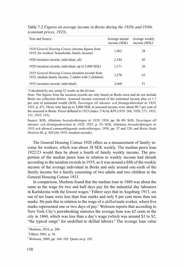
158

The General Housing Census 1920 offers us a measurement of family in-come for workers, which was about 38 SEK weekly. The median pawn loan 1922/23 would then be about a fourth of family weekly income. The pro-portion of the median pawn loan in relation to weekly income had shrunk according to the taxation records in 1935, as it was around a fifth of the weekly income of the average individual in Borås and only around one-sixth of the family income for a family consisting of two adults and two children in the General Housing Census 1933.

In comparison, Murhem found that the median loan in 1880 was about the same as the wage for two and half days pay for the industrial day labourers in Karlskrona with the lowest wages.2 Führer says that in Augsburg 1913, six out of ten loans were less than four marks and only 8 per cent more than ten marks. He puts this in relation to the wage of a skilled male worker, where five marks represented one or two days of pay.3 Woloson reports that according to New York City’s pawnbroking statistics the average loan was 62 cents in the city in 1860, which was less than a day’s wage (which was around $1 to $2, “the typical range” for unskilled to skilled labour).4 The average loan value 2 Murhem, 2016, p. 206.3 Führer, 2001, p. 36.4 Woloson, 2009, pp. 104–105. Quote on p. 105.

Table 7.2 Figures on average income in Borås during the 1920s and 1930s (constant prices, 1923).Year and Source Average annual

income (SEK)Average weekly income (SEK)1

1920 General Housing Census (income figures from 1919, for workers’ households, family income) 1,962 38

1920 (taxation records; individual, all) 2,344 45

1920 (taxation records; individual, up to 5,000 SEK) 1,371 26

1933 General Housing Census (taxation records from 1932, median family income, 2 adults with 2 children) 3,270 63

1935 (taxation records; individual) 2,668 51

1 Calculated by me, using 52 weeks as the divisor.Note: The figures from the taxation records are only based on Borås town and do not include Borås tax collection district. Assessed income consisted of the estimated income plus ca 1.7 per cent of estimated wealth (SOS, Taxeringen till inkomst- och förmögenhetsskatt år 1920, 1923, p. 6*). Those who had up to 5,000 SEK in assessed income were about 90.7 per cent of the assessed in Borås. Prices deflated to 1923 (index 174) by KPI (1919: 266, 1920, 271; 1933, 151; 1935, 155).Source: SOS, Allmänna bostadsräkningen år 1920, 1924, pp. 86–89; SOS, Taxeringen till inkomst- och förmögenhetsskatt år 1920, 1923, p. 33; SOS, Allmänna bostadsräkningen år 1933 och därmed sammanhängande undersökningar, 1936, pp. 37 and 128; and Borås Stads Historia III, p. 420 (for 1935, taxation records).

159

was much higher in Stockholm in 1923, where the Stockholm Pantaktiebank lent on average 29 SEK per loan.5 However, Stockholm was a much more expensive city than Borås and even though the loan values were much larger, they were not enormously so.

We can say that the loans in Borås seem to be approximately in the range of other pawnshops loans. Perhaps the figures for the 1920s were a bit on the high side regarding the relation between loan value and incomes, as it seems as the loan value represented a larger share of income than found by Führer and Woloson, but, on the other hand, was quite similar to what Murhem found. The income figures from 1920 are, however, somewhat uncertain due to the instability of the value of money in the years after the First World War. The figures for the 1930s seem to be more in line with previous research. It can also be mentioned that the loans were way below many other credit institu-tions. Fritz found that the smallest loans at the People’s bank of Gothenburg (which deemed itself as a competitor to pawnshops), was below 200 SEK.6 Kristina Lilja showed that loans from Falun savings banks were in several hundreds of SEK at the turn of the century for the group with the lowest av-erage, while the average for workers was quite much above a thousand SEK.7

The matter could also be put in this way: only a small minority of the new loans (7 per cent) in 1922/23 were equal or larger than 26 SEK (the weekly income for those with less than 5,000 SEK in annual income 1920). In the case of average weekly incomes of 45 SEK (the average of all incomes in the taxation assessment 1920), there were only very few new loans (2 per cent) that were equal or larger. Even the maximum (of all loans) could only have replaced the monthly pay of a rather small annual wage. Hence pawners could not use pawn loans to replace wages for longer periods without labour income (due to unemployment, sickness, etc.), but perhaps pawn loans could supplement unemployment aid or other forms of support. This is also Führer’s conclusion.8

Most loans were thus quite small in relation to the weekly income of most families. How did they relate to different kinds of weekly expenditures? From the cost of living survey 1922/23 (in Borås, normal household among workers and lower officials), it is clear that pawn loans could take care of most costs (such as heating, lighting, insurance and association fees) on a weekly basis.9 A median pawn loan in 1932/33 might be able to pay a week’s rent (based on figures for 1933/34) for a one-room apartment with a kitchen, but without

5 Stockholms Stads statistiska kontor, Statistisk årsbok för Stockholms Stad, 1926, p. 106. Cal-culated through dividing the annual number of loans given with the annual sum of lent capital.6 Fritz, 2015, pp. 104–105, 107–108.7 Lilja, Kristina, Marknad och hushåll – Sparande och krediter i Falun 1820–1910 utifrån ett livscykelperspektiv, 2004, pp. 145–146 (in 1861–1870 prices).8 Führer, 2001, p. 43.9 See appendix II for figures from the cost of living surveys.

160

central heating (see table 7.3).10 The pawn loan would likely have been able to finance most of the running weekly costs, except for food, where it none-theless could be a supplement. However, households did not pay all of their budget items in small repeating weekly costs, as some were paid in larger lump sums. Clothes and hospital care are such examples. Hospital care varied much between households, as many households would not have any outlays for hospital care, while others had large costs. Nor, does it seem likely that pawn loans could finance much of consumer durables, which also required payment in larger lump sums.

The prices of most consumer durables made it also unlikely that pawn loans could finance the accumulation of material wealth (in the form of con-sumer durables). It was also in the nature of pawning that financing durables would be difficult. Take the simple example of bicycles, which were pawned in both 1922/23 and 1932/33. The median loan given on a bicycle was 25 SEK in 1922/23 and 15 SEK in 1932/33 (current prices). The median bicycle loan was above the ninetieth percentile in 1922/23 and larger than seventy percent of the loans in 1932/33. Bicycles were thus one of the categories with the larg-est loans. This quite common consumer durable would thus secure a relatively large loan, but one must remember that the pawn loan was always less than the potential sales price (given that there were no misappreciation on the part of the pawnbroker). Pawned bicycles were also second-hand items and thus of less value than new bicycles. Just this example shows how quite unreasonable it is to assume that pawn loans could finance the purchase of consumer dura-bles in most cases.

As table 7.3 shows, this seems to be true for most of the durable commod-ities, with sewing machines, (new) bicycles, gramophones, radios, vacuum cleaners, men’s suits, etc. being far out of reach for the average pawn loan. There were, however, some forms of clothes (like cotton shirts and under-wear) that could be financed through a pawn loan.

Pawning was something that could provide rather small supplements to the family economy, when the family was in need of money due to some form of income insufficiency, either because of some loss of income (caused by for ex-ample sickness) or an increase in expenditures, both regular (such as food and rent) and extraordinary (such as weddings, journeys, medicine, etc.) It might be likelier that this insufficiency was generated by some necessary expendi-ture out of the ordinary, as pawning was no alternative for replacing labour income for any substantial period. Pawn loans could likely finance one week of rent or make a large contribution to it, as well as pay heating bills, various insurance subscriptions and a substantial part of the food bill. However, most consumer durables could not be financed with a pawn loan. In general, the data thus supports the hypothesis of income insufficiency. 10 Based on the median (new) loan being 9 SEK (based on current prices), which enables the payment of one week of an annual rent of 468 SEK (9 SEK median loan times 52 weeks). See chapter 6 for figures on annual rent.

161

Table 7.3 Prices (nominal, SEK) of various commodities in 1920s and 1930sCommodity Price 1923 Price 19307

Sewing machine, Husqvarna Freja A11 180.00a 175.008,c

Bicycle (men), Husqvarna Vapenfabriks AB, P18171 160.00b 145.00c

Gramophone, Silverton with crank2 50.88 50.00c

Radio, Concerton II/Radiola RC (extrapolated 1924)2 218.00b 58.00d

Radio, Silverton2 - 190.00c

Vacuum cleaner, Electrolux model 253 - 225.00e

Men’s suit, ready-made4 98.00 90.00

Winter overcoat (men’s), ready-made4 93.00 85.00

Cotton shirt (men’s) 4 3.45 3.00

Men’s underwear4 3.95 3.20

Cotton fabric for ladies’ dress; per meter4 0.95 0.80

Boots, stout grained-leather4 13.75 13.75

Milk, whole; per liter5 0.24 0.22

Butter, table (dairy); per kilogram5 3.73 2.93

Potatoes, old; per 5 litres5 0.55 0.38

Salted pork, Swedish (pork belly); per kilogram5 2.20 2.16

Salted herring, first-rate; per kilogram5 0.53 0.69

Coffee, not roasted (obränt), first-rate Santos; per kilogram5 2.45 2.42

Sugar, cube; per kilogram5 1.07 0.45

Apartment: one room and a kitchen, without central heating, weekly rent6 5.56b 7.13c

a 1922; b 1924; c 1933; d 1931; e 19351 Ljungberg, 1990, price lists from companies.2 Ljungberg, 1990, prices from post order firm Åhlens and Holm.3 Ljungberg, 1990, producer price index (partiprisindex), PPI.4 SOS, Detaljpriser och indexberäkningar åren 1913–1930, retail prices.5 SOS, Detaljpriser och indexberäkningar åren 1913–1930, retail prices, average annual price for Borås.6 For Borås, based on average annual rent. Calculated for 52 weeks.7 Many commodities lacked a figure for 1932 or 1933, and 1930 was the most common figure.8 Extrapolated figure from another model of the product; see Ljungberg, 1990, p. 309.Note: Commodity names have been shortened in some cases. The cheapest examples have been chosen. Cotton fabric for ladies’ dresses has been chosen in lieu of figures on ready-made cloth-ing for women. Some prices are producer prices, but mostly for durables and the retail prices should be higher, which strengthens the conclusion on pawning’s (non-)financing of durable. Source: Ljungberg, 1990, pp. 310, 339, 323 and 327; SOS, Detaljpriser och indexberäkningar åren 1913–1930, 1933, pp. 48 and 104–134 (table 1); SOS, Hyresräkningen år 1924 – del 1. Hyresförhållandena m.m., 1925, p. 56 and SOS, Allmänna bostadsräkningen år 1933 och därmed sammanhängande undersökningar, 1936, pp. 270–271.

162

How often did pawners in general take pawn loans? In earlier research, many have suggested that some form of weekly pawning existed, or at least that pawners had periods during a year when they repeatedly pawned week-ly.11 Others have suggested that weekly pawning would be too costly for the family economy.12 In the theory chapter, this dissertation supported the latter argument. Real wages had also increased between the 19th century and the in-terwar period. Income variability had likely also decreased during this period. Both these trends likely made instances of income insufficiency less frequent, as most needs would be inelastic in relation to income. Therefore, one can as-sume that most pawners should only visit the pawnshop occasionally or even rarely, while few would visit the pawnshop regularly.

Table 7.4 reveals that the proposition is largely true. For most pawners, pawning was an occasional activity in the interwar era, although there was a very small group of very active pawners, who pawned approximately weekly or came close to this. These, however, do not account for more than around 1 per cent of all pawners.13 For two of these, it is unlikely that they took out all their loans for themselves, due to their very large number of loans. Probably they rather acted as agents for others. The majority of pawners were found to only have taken one loan at the pawnshop during the period of the sample. 11 See for example Tebbutt, 1983, pp. 6–8, 12–13 and Johnson, 1985, pp. 180–183.12 Rotella, 1989, pp. 7–8.13 If one looks only at new loans and limits the loans to those with more than 12 loans.

Table 7.4 Frequency of loans per person in samples 1922/23 and 1932/331922/23 1932/33

All loans Only new loans All loans Only new loans

No. % No. % No. % No. %

1 504 67.7 460 71.7 1,088 66.9 953 73.52–6 218 29.3 167 26.0 491 30.2 307 23.77–12 15 2.0 9 1.4 25 1.5 18 1.413–24 2 0.3 3 0.5 20 1.2 17 1.3>24 5 0.7 3 0.5 2 0.1 1 0.1

Total 744 100.0 642 100.1 1,626 99.9 1,296 100.0

Mean number of loans per person

1.98 1.64 1.86 1.38

Note: The sum of pawners is smaller among new loans, because people who were found to have taken out no new loans were subtracted (these measured 102 persons in 1922/23 and 330 persons in 1932/33). Loan intervals set after number of months.Source: Databases on pawn loans.

163

There is a quite large minority for both years that had only renewed loans at the pawnshop without taking out any new loans in the samples.

This is only a sample of two time periods corresponding each to one year in time, so it is quite possible that many of the one-time borrowers (and zero new borrowers) actually took out more new loans. This, however, should not change the distribution of the number of loans per pawner that much. Even though some individual pawners had taken more loans than in the sample, there would be an inflow of new persons, who would have only borrowed once. Therefore the distribution of the number of loans would remain quite stable. The pawnshop also did a very short inquiry (for a discussion in the town council about the pawnshop) for the month of January in 1933, which showed fairly similar results. They found that 85 per cent had visited the pawnshop once, 10 per cent two times and 5 per cent more than two times.14

It should be noted, as is evident in table 7.4, that 75 per cent of the pawn-ers only took out one new loan or only renewed loans for both 1922/23 and 1932/33. Almost all (95 per cent) took only four new loans at most in both samples. This shows quite conclusively that for the large majority of pawners visiting the pawnshop was not a regular activity, even though there was a small group that had many loans. This would mean that for the large majority of pawners there were quite few situations of income insufficiency, where the pawnshop was a good alternative. It is, however, difficult to say if they had few instances of income insufficiency in general, as they could also choose to solve these instances by other means than pawning. There were also oth-er options for obtaining credit. Family members, relatives and friends likely gave each other small loans. Retail credit is another alternative. Moneylenders might have also existed in Borås, although this is difficult to know.15

The number of loans a pawner has made at the pawnshop should be neg-atively correlated with the average borrowed sum. As discussed in the theory chapter, more instances of income insufficiency would likely mean that those who pawned multiple times had less valuable material wealth, as it would be difficult to accumulate that material wealth, and their economic status should likely have been worse off with more frequent instances of income insuffi-ciency (unless those with fewer pawn loans also relied on different forms of credit as opposed to those with more pawn loans).

There seems to be a trend towards lower values with more loans (table 7.5), but the correlations (which does not include those who only renewed loans) are not significant.16 Therefore, we have to assume that the groups were quite similar in terms of their average borrowed sum (which however includes renewals as well). 14 Borås Kommunalblad, 1933, p. B165.15 Possibly there is some information on moneylending in police records, but that is far from the subject of this dissertation.16 The correlations are not significant. 1922/23: correlation is -.050 and p= .210. 1932/33: cor-relation is -.044 and p= .111.

164

The Collateral and its RedemptionThus far, the discussion has only concerned the financial side of pawning. The hypothesis that income insufficiency mainly drove pawning has been shown to have support, above all due to the finding that pawn loans were small. Pawnshops offered also a quite limited amount of credit, which suggests by itself that the material wealth of pawners was not that valuable. However, what kinds of material wealth were used as collateral? Earlier research has found a predominance of clothing, but also a shift during the late 19th and early 20th centuries from clothes, due to their falling value, to pawns with a higher and steadier value such as jewellery and watches.17 Had workers in Borås ex-perienced the shift from clothes and shoes, which was indicated by previous research to have happened in the 20th century?

This question also touches upon the use values that were lost during the loan period. The loss of a use value is something that separates pawning from many other forms of credit. This leads to the second hypothesis, which stated that the importance of the use value should have affected the time between the date of pawning and the date of redemption at the pawnshop. If the pawn had an important use value (in relation to the loan value), then this would have lessened the time at the pawnshop. The dimension of public and private in the 17 Tebbutt, 1983, pp. 156–159, Woloson, 2009, pp. 82–83, Francois, 2006, pp. 177, 182–185 and 187–188.

Table 7.5 Average borrowed sum (nominal, SEK) by number of loans per pawner from samples 1922/23 and 1932/33

1922/23 1932/33

One loan 14.51 12.30

2–6 loans 12.64 10.36

7–12 loans 9.27 11.83

13–24 loans 6.34 9.71

More than 24 loans 9.95 6.731

Total mean 14.80 12.441 Only one observation.Note: The calculation in this table has been done by taking the total borrowed sum for each pawner and dividing it with the number of loans for the pawner. The table then presents the average of each pawner’s average borrowed sum for each interval of the number of loans. The mean borrowed sum includes the value of renewed loans. Those with zero new loans have a higher mean borrowed sum (20.53 SEK in 1922/23 and 14.99 SEK in 1932/33, current prices) than the rest, which explains why the total mean is larger than the group means displayed in the table. Loan intervals set after number of months.Source: Databases on pawners.

165

use of the pawn should also matter, as pawns ordinarily used in public would have remained less time at the pawnshop as they were visible to the commu-nity. This is not the only factor behind the duration of the loan. The borrowed sum would likely also play a role, as a larger loan should have required a longer time for the pawner to accumulate the payment of the principal and the interest. A working-class family would likely have had to “save” or forgo current consumption in order to pay for the pawn loan. Bigger loans should thus take a longer time to pay off.

Table 7.6 shows the various categories of material wealth used as pawns in new loans (renewals are not included). There is a clear dominance in both samples of clothes, shoes, jewellery and watches. It is, however, important to note in table 7.6 that the total of the per cent and frequency distribution will be larger than both the total number of loans and a hundred per cent. This is due to some overlap between categories, as a pawn loan could consist of several pawns. Therefore, the percentage should be interpreted as meaning that 54 per

Table 7.6 Numbers and percentages of new loans by category of pawn, with mean borrowed sums (SEK) for each category, in samples 1922/23 and 1932/33, constant prices (1923)

1922/23 1932/33

No. %Mean

borrowed sum

No. %Mean

borrowed sum

Mean borrowed sum (1923

prices)Clothes and Shoes 662 54.2 11.15 921 41.0 11.70 13.48

Textiles 73 6.0 7.75 61 2.7 8.67 9.99Bicycles 31 2.5 25.13 24 1.1 22.14 25.51Decorative home objects 46 3.8 12.63 91 4.0 8.58 9.89

Bonds 45 3.7 32.40 30 1.3 34.92 39.41Jewellery and watches 305 25.0 11.89 948 42.2 12.64 14.57

Work and hobby objects 34 2.8 14.12 127 5.6 17.50 20.17

Utility objects 21 1.7 9.71 60 2.7 15.98 18.41Leisure objects 4 0.3 9.75 44 2.0 15.66 18.05Miscellaneous 22 1.8 7.77 2 0.1 5.76 6.64Total new loans 1,222 - 12.33 2,248 - 11.06 12.74

Note: As one loan can belong to multiple categories, the sum of the frequencies of the catego-ries will not add up to the total number of new loans. KPI used as a deflator (index 1923=174 and index 1933=151).Source: Databases on pawn loans.

166

cent of the loans included either clothes or shoes (the most important catego-ry), while 46 per cent did not. However, one cannot add together categories, due to the possible overlap. Clothes, shoes and textiles were not part of 60.2 per cent of the loans, but rather 59.4 per cent in 1922/23. However, this over-lap does not affect the fact that clothes, shoes, jewellery and watches were the most common types of pawns. There are also two missing cases in 1922/23, but they are not shown in table 7.6 as they are renewals.

In 1922/23, 79 per cent of the new loans had clothes, shoes, jewellery or watches as a pawn (although, as mentioned, the loans were not exclusively restricted to these categories). The same measure was 82 per cent in 1932/33. This is similar to what has been found in previous research. Tebbutt found that clothes were a large part of the pawns.18 However, Führer found in Germany that more jewellery and watches were pawned than clothes in the early 1900s. Clothes were however still a large category. There were also quite large shares of bicycles and bed-sheets.19 There was little overlap between the two cate-gories. Only five new loans in 1922/23 (0.4 per cent) and 18 in 1932/33 (0.8 per cent) had a pawn from both categories. From 1922/23 to 1932/33 the cat-egory of jewellery and watches grow, while that of clothes and shoes shrank. Murhem and Ulväng found a similar, more complete shift from clothes to jew-ellery and watches in Karlskrona during the interwar period.20 The shift from clothes and shoes to jewellery and watches was nonetheless not completed by 1932/33, as the two categories were instead of equal size. Clothes and shoes remained an important category in 1932/33.

Before we move on to the redemption time, let us shortly discuss the dif-ferences in collateral between new and renewed loans. The share of renewed loans among all loans increased in 1932/33 to around a fourth, from somewhat more than 15 per cent in 1922/23. In the loan journal, renewals were registered again mixed in with new pawn loans. A renewed loan was thus registered at least two times – one time when it was a new loan and then for every time it was renewed. Therefore, the statistics shown in table 7.7 on renewed loans do not say anything directly about how many loans of the new loans in the sample that would be renewed.

The distribution of renewed loans was quite different from the distribution of new loans or all loans in both samples. The most remarkable difference is that clothes and shoes were a part of the collateral in many fewer renewed loans than in new loans, only 18 per cent in 1922/23 and 13 per cent in 1932/33 (table 7.7). This could be interpreted as that their use value kept clothes and shoes from being left in the pawnshop for a long time. The two categories that were much more common among renewed loans, than in new loans, were bonds and decorative home objects. This is not so surprising, as they lack an

18 Tebbutt, 1983, pp. 33–34; 19 Führer, 2001, p. 37.20 Murhem and Ulväng, 2015, pp. 9–10.

167

important use value and were shown above to have been left for a long time in the pawnshop among new loans. Even though the share of bonds had fallen quite a bit in the 1932/33 distribution of renewed loans, this is still a valid con-clusion.21 The renewals do give some indication that the use value, in relation to the loan value, might matter for the decision to redeem the collateral.

It is important to note that it is impossible to know from the current source material whether the loan was paid or renewed.22 The first thing that can be 21 Except for the very small category of leisure objects, which can be disregarded.22 In general, renewals should have happened at the end limit of the loan, thus after about six to eight months (see chapter 4 on the Borås pawnshop) in the pawnshop, as there was really no point in paying a loan to be extended except at the end of the loan. This ought to mean that the categories are somewhat underestimated in relation to the actual redemption date. This should,

Table 7.7 Number and per cent of renewed loans, with percentage of loans renewals in each category of pawn, for samples 1922/23 and 1932/33

1922/23 1932/33

Number % of renewals

% of loans within

categoryNumber % of

renewals

% of loans within

categoryClothes and Shoes 45 18.1 6.4 100 12.9 9.8

Textiles 39 15.7 34.8 73 9.4 54.5Bicycles 13 5.2 29.5 4 0.5 14.3Decorative home objects 36 14.5 43.9 107 13.8 54.0

Bonds 30 12.1 40.0 31 4.0 50.8Jewellery and watches 72 29.0 19.1 401 51.7 29.7

Work and hobby objects 7 2.8 17.1 36 4.6 22.1

Utility objects 7 2.8 25.0 27 3.5 31.0Leisure objects 2 0.8 33.3 33 4.3 42.9Miscellaneous 2 0.8 8.3 0 0.0 0.0

Total number of renewed loans 248 - 16.9 776 - 25.7

Number of missing 2 - - 0 - -

Note: As one loan can belong to multiple categories, the sum of the frequencies of the catego-ries will not add up to the total number of renewed loans. That a loan is missing, means that nothing of the pawn description could be interpreted and the loan could not be placed in any category. Note that the per cent within the category does not say anything about what happened to new loans, it just says what the share of renewed loans of all loans was within a category (the remainder would thus be the share of new loans of all loans).Source: Databases on pawn loan databases.

168

noticed about table 7.8 is that half of the loans were paid (or renewed) within about a month in 1922/23, but also that the time spent in the pawnshop grew very fast in the upper half – the third quartile is almost five times larger than the median. There were also a quite large number of new loans that seem to have been paid within a week: 27 per cent were paid within this time period and the first quartile is only 5 days in 1922/23. That means that if the pawn was not redeemed rather rapidly, it was left in the pawnshop for a long time. In 1932/33, the time between borrowing and paying (or renewing) had increased and the median had doubled. However, the proportion of new loans that was redeemed within a week had only fallen to 22 per cent. The longer periods of redemption time might be explained by the crisis of the 1930s (the early 1920s was also a time of crisis, but recovery was on its way in 1922 and 1923).

It can also be noted that the redemption times seem quite long in compari-son with the figures Tebbutt found on two Liverpool pawnbrokers in the 1860s,

however, strengthen the conclusions as it would prolong the redemption time most for those categories that already had the longest redemption time.

Table 7.8 Number of days between borrowing and redemption (or renewal) for only new loans in samples 1922/23 and 1932/33

1922/23 1932/33

First quartile Median Third

quartileFirst

quartile Median Third quartile

Clothes and Shoes 5 14 79 5 22 136

Textiles 13 50 185 61 151 259 Bicycles 28 72 190 40 130 238 Decorative home objects 54 179 257 65 190 256

Bonds 122 182 239 58 152 196 Jewellery and watches 11 54 171 19 96 212

Work and hobby objects 45 104 212 5 35 181

Utility objects 17 80 262 24 136 217 Leisure objects 105 122 -1 42 165 256 Miscellaneous 5 17 179 1 68 -1

Total 5 32 151 9 64 185 1 No figure presented due to very few observations.Note: A loan is counted into a specific category if at least one pawn belongs to said category. Observations regarding redemption only concern pawn loans which have a redemption date. Loans without such dates – i.e. loans that have been auctioned off, are not counted among observations.Source: Databases on pawn loans.

169

where the “low” establishment had two-thirds of its pawns redeemed within a week and the other pawnshop, with a better-off clientele, had about a third redeemed with a week, and above 60 per cent within a month. A pawnshop near Salford, according to Tebbutt, had quite a number of loans redeemed very quickly: 5 per cent of the loans were redeemed the same day and 8 per cent the next.23 It can be noted here that the pawnshop with the better-off clientele ac-tually had longer redemption times. It might be that better finances also leads to more material wealth, which subsequently means that pawners had less need of their collateral, and could leave it at the pawnshop for a longer time.

There were many differences between the categories. Primarily we can see that clothes and shoes had a particularly low median redemption time. This is valid for the whole distribution of clothes and shoes. For example, its third quartile is smaller than the third quartile of the other categories. Clothes and shoes had of course important use values, especially as people at this time did not have a large collection of clothes and shoes.

The opposite to the categories of clothes and shoes in this regard were bonds and decorative home objects. Bonds lacked a use value, as they were a financial means of saving, and thus only had a monetary value. Decorative home objects could have use values, for instance cutlery, but here it is reason-able to assume that many times the pawners had some other set of cutlery for everyday use, and the pawned cutlery was the better set.24 Neither decorative home objects nor bonds were used in public space, but in the private space of the home. Hence, the pawner could keep such objects easily from pub-lic view. Unless someone saw you pawn the silver cutlery, it is unlikely that someone would find out (without your permission) that your cutlery was at the pawnshop, and not in your home. Both categories had the largest medians in 1922/23, and the first quartile was likewise the largest. 25

Jewellery and watches also had a quite low median even though they had less obvious use value (watches tell time and wedding rings might be of sym-bolic value). They had nonetheless a much larger median in both samples than clothes and shoes, which is interesting in the perspective of the possible shift between these two categories. Clearly, jewellery and watches could remain much longer in the pawnshop than clothes and shoes. If the quite similar loan values are factored in, this suggests that pawners let jewellery and watches remain at the pawnshop much longer than clothes and shoes by their own choice. Bicycles had a low median in 1922/23, and did have an important use value, but the median increased quite markedly in 1932/33. They did, however, provide quite large loans, which might prolong the time spent in the pawnshop, especially in the crisis years of the 1930s (even though the real value of the loans on bicycles was lower in 1932/33 than in 1922/23).23 Tebbutt, 1983, pp. 9 and 13.24 Some pawned objects in this category were specified as silver spoons. 25 In 1932/33 bonds had a smaller median than leisure objects and the first quartile of textiles was slightly larger than for bonds.

170

There was a clear trend showing a rising number of days spent in the pawnshop for pawns with a greater loan value, although there are some irregu-larities (table 7.9). The overall trend is, however, quite obvious. Consequently, it seems as though both the use value and the monetary value of the loan were factors in the decision regarding how long a pawn remained in the pawnshop.

It seems obvious that this was a decision for the pawner, and not forced upon him or her by economic circumstances, because categories with simi-lar values could have quite different distributions of redemption time. This is evident for the categories of jewellery and watches together with clothes and shoes, where the first quartile, median and third quartile of jewellery and watches were at least the double those of the category of clothes and shoes (except the third quartile in 1932/33; see table 7.8). The category of deco-rative home objects, despite having a mean just about 1.5 SEK higher than clothes and shoes in 1922/23 and being quite less valuable in 1932/33 (see table 7.6), had a first quartile and median that was more than ten times larg-er than for clothes and shoes. Textiles, which provided clearly less valuable loans, remained much longer in the pawnshop. It is also unlikely that clothes and shoes belonged primarily to some group of better-off pawners (which would be an alternative explanation to the quicker redemption). Clothes and shoes were rather something that everybody owned, unlike many other kinds of pawns. They also had a clear use value, which would make it preferable to

Table 7.9 Median number of days between borrowing and redemption (or re-newal) by borrowed sum in samples 1922/23 and 1932/33 (only new loans)

1922/23 1932/33

Borrowed sum (SEK, nominal prices)

Median (days)

Number of new loans

Share of new

loans (%)

Median (days)

Number of new loans

Share of new

loans (%)0–5 19 319 26.1 47 637 28.36–10 21 452 37.0 65 853 37.911–15 24 191 15.6 82 393 17.516–20 46 100 8.2 63 189 8.421–25 112 72 5.9 41 70 3.126–30 89 47 3.8 104 40 1.831– 180 41 3.4 159 66 2.9Total 32 1,222 100.0 64 2,248 100.01

1 When percentage sums (which is supposed to become 100) have become smaller due to round-ing errors, I have chosen to put the sum at 100.0, to avoid confusion.Note: In nominal prices, as it is the trend due to rising loan value that is important, not com-parability between the samples. The number of new loans with a redemption time was 1,153 loans in 1922/23 and 2,084 loans in 1932/33. Observations regarding redemption only concern pawn loans which have a redemption date. Loans without such dates – i.e. loans that have been auctioned off, are not counted among observations.Source: Databases on pawn loans.

171

avoid pawning clothes and shoes. It seems as though pawners had a choice in the matter of letting a pawn remain in the pawnshop, and that some pawns were more important to reintegrate into the household due to their use value.

Let us see if a regression analysis strengthens these results. The following predictions seem to be appropriate based on the results presented above. The borrowed sum should have had a positive effect on the number of days be-tween borrowing and payment or renewal. The category of clothes and shoes should have had a negative effect. Decorative home objects and bonds should, on the other hand, have had a positive effect. Bicycles might be negative, due to the important use-value. All other categories should have had no effect.

The regression analysis for 1922/23 shows that the predictions for bor-rowed sum, clothes and shoes and decorative home objects were correct (table 7.10). They have their predicted signs and they are significant. Bonds are sig-nificant at the 90 %-level with the correct sign. The categories of jewellery and watches, textiles, work and hobby objects, utility objects, leisure objects and miscellaneous had, as predicted, no effect. Bicycles, although of the right sign, is far from significant and the prediction was not correct.

There are some differences for the regression analyses based on the data from 1932/33 in comparison to 1922/23 (table 7.10). Bonds have no signifi-cant effect at all and the predicated sign was wrong. Work and hobby objects have become significant and have a negative sign. This might be due to the rel-atively useful items in this category.26 Otherwise the results are quite similar to the ones for 1922/23; for instance decorative home objects have the same sign and are highly significant, but have a somewhat smaller coefficient. Also clothes and shoes was significant again.

The two most important types of pawns in the category of clothes and shoes in 1922/23 and 1932/33 were suits and coats (of various kinds; raincoats are included for instance), which were rather large and expensive types of clothes. The category of coats likely included a large number of winter clothes, but it is impossible to differentiate between winter coats and more year-round coats, as many pawns in this category were simply described as “coat”. In the chap-ter on theory, coats were proposed to have a seasonal pattern, which will be investigated below. The Sunday suit has been considered as having a weekly pattern in previous research, as discussed in the theory chapter. This does not mean that this type of clothes necessarily was part of repeated weekly pawn-ing, but that when pawners used Sunday suits as collateral, they usually stayed in the pawnshop for a week or less, as the pawner (or someone in the family of the pawner) had to use them on Sunday. This weekly pattern ought to have been present also in Borås.

Other important sub-categories of clothes and shoes were pants. There were also some female clothes, such as dresses and skirts. In 1932/33 the whole category had become less diverse. In 87 per cent of the loans in the clothes 26 Although there are many music instruments, which might have been used mostly in hobbies, but they could also be used for working if the pawner made money by playing music.

172

and shoes category in 1932/33, at least one pawn was either a suit or a coat of some kind.27 The female-specific sub-categories (but likely not all female-specific clothes) had disappeared, but for one pawned dress. Tebbutt says that the pawning of women’s clothing declined more than for male clothing as mass fashion lessened the value of women’s clothing faster.28 This might partly explain the small number of female-specific clothes in the samples although some female-specific clothes are hidden in the categorisation; for instance the subcategory of coats includes women’s coats.

Shoes had become a remarkably smaller category in 1932/33. Pants and other types of clothes had also shrunk as categories. This might be a part of a shift in pawning, although it is still the case of quite useful pawns replac-ing other useful pawns (unlike jewellery and watches replacing clothes and

27 Note that the overlap, i.e. the number of loans with both a coat and suit, has been subtracted from the total figure of the sub-categories coats and suits, to prevent double-counting. The loans could of course include some other type of pawn too, due to the possibility of one loan consisting of several pawns.28 Tebbutt, 1983, pp. 156–159.

Table 7.10 Regression analyses of days between borrowing and redemption (or renewal), in two panels for samples 1922/23 and 1932/33 (only new loans)Panel I. 1922/23 (N=1,153)Dependent variable: Number of days between borrowing and payment/renewalIndependent Variables: Borrowed sum (SEK) and dummy variables for types of

pawns (Clothes and shoes; Textiles; Bicycles; Decorative home objects; Bonds; Jewellery and watches; Work and hobby objects; Utility objects; Leisure objects; Miscellaneous)

Adjusted R2 .118F-value and significance 16.346 .000

Independents: B coefficients

Standard error Standardized Beta Significance

Constant 93.524 16.791 .000

Borrowed sum 1.255 .286 .135 .000Clothes and shoes -49.200 16.586 -.247 .003Textiles -1.129 18.105 -.003 .950Bicycles -19.920 24.509 -.031 .417Decorative home objects 61.271 21.307 .109 .004Bonds 41.936 22.459 .082 .062Jewellery and watches -10.313 17.053 -.045 .545Work and hobby objects 25.014 23.705 .040 .292Leisure objects 13.547 67.812 .006 .842Miscellaneous -1.275 26.181 -.002 .961

(cont.)

173

shoes). Coats and suits were also the most valuable pawns among clothes and shoes.29

The sub-categories that remained the shortest time in the pawnshop were skirts, pants and shoes in 1922/23 (table 7.11). Dresses (in 1922/23) and coats remained the longest time. The redemption time of coats might be explained by seasonal loans, where the coat was left for the off-season in the pawnshops (see next section). Dresses have rather few observations, so it is hard to say anything conclusive about the patterns for that category. Suits were in the mid-dle regarding the distribution of time, which is interesting as suits did not have the weekly pattern (redeemed within a week) that the category should have according to previous research.30 The median is two weeks or above, even 29 Median value of new loan (in constant 1923 prices) for: dresses 5 SEK (1922/23) and 2 SEK (1932/33, only one loan); skirts 5 SEK (1922/23) and no loans in 1932/33; pants 8 SEK (1922/23) and 5 SEK (1932/33); suits 15 SEK (1922/23) and 14 SEK (1932/33); shoes 6 SEK (1922/23) and 5 SEK (1932/33); coats 10 SEK (1922/23) and 9 SEK (1932/33); other clothes 10 SEK (1922/23) and 6 SEK (1932/33). 30 Johnson, 1985, pp. 180–183.

Table 7.10 (continued)

Panel II. 1932/33 (N=2,084)

Dependent variable: Number of days between borrowing and payment/renewalIndependent Variables: Borrowed sum (SEK) and dummy variables for types of

pawns (Clothes and shoes; Textiles; Bicycles; Decorative home objects; Bonds; Jewellery and watches; Work and hobby objects; Utility objects; Leisure objects; Miscellaneous)



Standard error

Standardized Beta Significance

Constant 123.512 11.075 .000

Borrowed sum .824 .226 .080 .000Clothes and shoes -59.919 10.984 -.297 .000Textiles 23.459 16.496 .036 .155Bicycles 6.818 22.253 .007 .759Decorative home objects 42.796 14.243 .080 .003Bonds -7.902 21.147 -.009 .709Jewellery and watches -13.210 10.928 -.066 .227Work and hobby objects -44.828 13.788 -.101 .001Leisure objects 20.959 18.834 .028 .266Miscellaneous -60.134 68.059 -.019 .377

Note: The category of utility objects was excluded, in order to provide a baseline for the dummy variables for the pawn categories. Source: Databases on pawn loans.

174

though there was a large share of suits that were redeemed within a week. Did pawners own several suits or were Sunday clothes no longer that important? Still, pawners would not usually leave a suit for a very long time in the pawn-shop. The third quartile was only a little longer than two and a half months. That is much less than the third quartiles of other (upper) categories of pawns (except for suits’ own upper category of clothes and shoes). The pattern of weekly pawning could also be investigated by looking at the distribution of weekdays when suits were pawned and redeemed.

Table 7.11 Clothes and shoes, sub-categories, number and percentage of new loans and number of days between borrowing and redemption (or renewal; by quartiles) in pawnshops in two panels for samples 1922/23 and 1932/33 (only new loans)

Panel I. 1922/23

Number (new loans)

% (of new

loans)

% (of new loans on

clothes and shoes)


quartile

Dress (female) 16 1.3 2.4 9 77 195Skirts 20 1.6 3.0 4 5 38Pants 50 4.1 7.6 3 5 19Suits 164 13.4 24.8 5 18 60Shoes 134 11.0 20.2 4 5 18Coats 261 21.4 39.4 5 31 151Clothes, other 89 7.3 13.4 4 10 65

Panel II. 1932/33

Number (new loans)

% (of new

loans)

% (of new loans on

clothes and shoes)


quartile

Dress (female) 1 <0.1 0.1 - - -Skirts 0 0.0 0.0 - - -Pants 52 2.3 5.6 3 5 34Suits 413 18.4 44.8 5 14 81Shoes 59 2.6 6.4 4 11 50Coats 409 18.2 44.4 7 56 166Clothes, other 66 2.9 7.2 4 7 86

Note: As loans can include several pawns, there is an overlap among the categories, and there-fore the percentage of new clothes and shoes loan does not add up to 100 per cent. Observations regarding redemption only concern pawn loans which have a redemption date. Loans without such dates – i.e. loans that have been auctioned off, are not counted among observations. Source: Databases on pawn loans.

175

Suits had quite opposite distributions of weekdays for borrowing and re-deeming (table 7.12). Suits were generally pawned in the beginning of the week, with more than half being pawned on Monday and Tuesday. However, the weekdays of redemption were even clearer. On Saturday, 85 per cent of all suits were redeemed in 1922/23 and 51 per cent in 1932/33. It can be not-ed that for suits, which were redeemed within seven days, the weekly pattern

Table 7.12 Weekday of borrowing and redemption (or renewal) for loans on suits and for all other loans, in samples 1922/23 and 1932/33 (only new loans)

Loans on suits

1922/23 1932/33

Weekday % pawned on % redeemed on % pawned on % redeemed onMonday 33.5 1.9 37.5 4.8Tuesday 25.0 3.7 18.4 5.3Wednesday 8.5 1.2 15.3 9.0Thursday 7.9 7.5 6.5 8.3Friday 9.1 1.2 10.2 22.3Saturday 15.9 84.5 12.1 50.5Total 100.0 100.0 100.0 100.0

Obs. 164 161 413 400

All other loans1922/23 1932/33

Weekday % pawned on % redeemed on % pawned on % redeemed onMonday 25.0 4.3 20.8 11.1Tuesday 23.3 3.9 16.2 9.3Wdnesday 14.7 2.6 17.5 13.2Thusday 13.1 6.8 12.4 11.5Friday 7.8 3.7 14.0 21.7Saturday 15.9 77.5 19.0 33.1Total 100.0 98.81 100.0 100.0

Obs 1,058 992 1,835 1,6841 This sum does not fully add up from the values in the table, as about 1 per cent or eleven of the pawn loans were listed as being redeemed on Sunday. It is uncertain whether there has been some error in my registration of these redemption dates, or if the pawnshop was actual open on some Sundays or if the pawnshop itself had filled out the wrong date in the loan journal. Noteworthy is that seven loans were recorded as being redeemed on the 31st of December 1922.Note: All other loans does not include suits. Source: Databases on pawn loans.

176

of pawning Monday and redeeming Saturday was even stronger than for all suits.31 In 1922/23, 80 per cent of the suits redeemed within seven days were pawned on Monday or Tuesday, which decreased to 70 per cent in 1932/33. The weekday for redemption was Saturday for 83 per cent of these loans in 1922/23 (which is about the same as for suits in general) and 67 per cent in 1932/33 (however, if Friday is added, this share increases to 92 per cent).

It can also be noted that, especially regarding the weekday of pawning, that the other pawns differed from suits. Although Monday was the largest weekday for pawning for all other pawns, this was less so than for suits. Re-garding redemption, other pawns had a pattern more similar to suits, at least for 1922/23. Most pawns were redeemed or renewed on Saturday in 1922/23, even though Saturday was even more common for suits. This is not so surpris-ing, as many would receive their pay on Saturday.

However, in 1932/33, some interesting things happened. Suits are now more dissimilar in comparison to all other pawns, but above all Saturday has drastically diminished as the day for redemption (or renewal) for all other pawns. In 1932/33, the redemptions or renewals are more spread out over the week, even though Saturday is still the day when most renewals or redemp-tions are carried out.

This could perhaps be explained by the fact that renewals seem to be more common in 1932/33 (which might be less connected to the payday). For the pawns redeemed or renewed within a week, 44 per cent took place on a Sat-urday. If the redemption time is increased to within 180 days, the share falls somewhat to 38 per cent done on Sunday. However, if we only take the loans that had a redemption time above 180 days, then only 23 per cent of the loans were redeemed or renewed on Saturday.

It seems very likely that most of the renewals took place after a long re-demption time and therefore the renewal day might not be connected to a pay-day. Therefore, the likely increased proportion of renewals might have made Saturday a less common day for redemption. It seems as though suits to a certain extent followed a weekly pattern, with pawning in the beginning of the week and redemption in the end of the week. There were also many short-term loans in the category. However, even though many loans in the category of suits remained in the pawnshop only a short time, there was not a majority that was pawned and redeemed within a week (table 7.11). A weekly pattern was therefore not the predominant pattern, which is not the same result that previous research (see chapter 1 and 2) has concluded based on qualitative research. People perhaps owned several suits, yet they still redeemed the suit quickly, which indicates a need for it.

There is also another category, for which it might be beneficial to break down into its sub-categories, namely the category for jewellery and watches. It can be argued that watches have a more important use value than jewellery, 31 59 suits out of 164 (36 per cent) in 1922/23 were redeemed or renewed in one to seven days. 166 suits out of 413 (40 per cent) in 1932/33 followed the same pattern.

177

as they tell time. The category of jewellery and watches consists mostly of rings and watches, which each is a sub-category (there is also a third sub-cat-egory for other jewellery).

Except for the category of other jewellery, there does not seem to be partic-ularly large differences between the sub-categories regarding redemption time (table 7.13). Between the samples, there are also changes regarding which category that has the greatest number of days in the pawnshop. Possibly there is a difference in 1932/33 in favour of watches having the lower number of days. Let us use regression analysis to decide if there is any influence on the number of days in the pawnshop for these two variables.

This new regression model (for each sample) will also incorporate dummy variables for the sub-categories of clothes and shoes: dresses, skirts32, shoes, pants, suits, coats, and other clothes, as well as rings, watches and other jewel-lery. Otherwise, the regression includes the previously used upper categories. The predictions are the same as before for the upper categories, although work and hobby objects are expected to be significant and negative, while bonds are expected to be non-significant for 1932/33 (based on previous regressions). Rings, watches and other jewellery are expected to have no significance, be-cause their redemption time was quite similar to the redemption time of all pawns. All sub-categories of clothes and shoes are expected to have a negative sign, except for dresses.

Rings and watches are not significant in either regression (table 7.14). Oth-erwise, most of the previously used variables (borrowed sum and the upper 32 Except for 1932/33, where there are no observations for skirts.

Table 7.13 Medians and quartiles for days between borrowing and redemption (or renewal) for rings, watches and other jewellery in samples 1922/23 and 1932/33 (only new loans)

1st Quartile (days)

Median (days)

3rd Quartile (days)

Observations

1922/23

Watches 9 52 152 211Rings 11 40 205 71Other jewellery 248 262 298 6

1932/33

Watches 21 90 196 570Rings 16 120 238 310Other jewellery 42 193 251 31

Note: Observations only concern pawn loans in the specified categories, which have a redemp-tion date. Loans without such dates – i.e. loans that have been auctioned off, are not counted among observations. Source: Databases on pawn loans.

178

categories for type of pawn) keep their signs and significance in these models. For 1922/23 the significances for these variables are the same (bonds, even at the 95 %-level, decorative and borrowed sum). They have retained the same signs for the coefficient (positive for all three). This is also the case for the new model of 1932/33, where the borrowed sum, decorative home objects and work and hobby objects are significant in both this new and the previous model (table 7.10, panel II). They have also retained their signs.

Table 7.14 Regression analysis of days between borrowing and payment or renewal, including sub-categories of clothes and shoes. In two panels for samples 1922/23 and 1932/33 (only new loans)Panel I. 1922/23 (N=1,153)Dependent variable: Number of days between borrowing and payment/renewalIndependent Variables: Borrowed sum (SEK) and dummy variables for types of pawns

(Dresses; Skirts; Pants; Shoes; Suits; Coats; Other clothes; Textiles; Bicycles; Decorative home objects; Bonds; Jewellery and watches; Work and hobby objects; Utility objects; Leisure objects; Miscellaneous)


Independents: B coefficients Standard error Standardized

Beta Significance

Constant 96.081 11.411 .000

Borrowed sum 1.221 .300 .132 .000Dresses 4.338 24.712 .005 .861Skirts -52.065 21.217 -.069 .014Pants -70.533 15.977 -.144 .000Suits -71.686 13.056 -.251 .000Shoes -67.231 13.004 -.211 .000Coats -23.059 11.438 -.096 .044Other clothes -29.276 11.348 -.079 .010Watches -17.847 12.538 -.070 .155Rings -11.567 14.984 -.028 .440Other jewellery 146.342 39.241 .106 .000Textiles -2.084 14.738 -.005 .888Bicycles -21.626 21.089 -.034 .305Decorative home objects 59.857 17.996 .107 .001Bonds 40.453 18.949 .079 .033Work and hobby objects 22.899 20.005 .037 .253Leisure objects 11.371 65.062 .005 .861Miscellaneous -3.573 22.700 -.005 .875

(cont.)

179

How did the sub-categories of clothes and shoes fare? Dresses were the only category with a positive coefficient in 1922/23, as predicted; however it was far from significant and it had a negative sign in 1932/33. The largest absolute coefficient were shown by pants, suits and shoes, which all had co-efficients of quite similar size. Coats were also significant in both regressions, but with a smaller absolute coefficient. Suits were, however, clearly the vari-able with most impact (according to the standardized coefficients) followed

Table 7.14 (continued)

Panel II. 1932/33 (N=2,084)Dependent variable: Number of days between borrowing and payment/renewalIndependent Variables: Borrowed sum and dummy variables for types of pawns

(Dresses; Skirts; Pants; Shoes; Suits; Coats; Other clothes; Watches; Rings; Other jewellery; Textiles; Bicycles; Decorative home objects; Bonds; Work and hobby objects; Utility objects; Leisure objects; Miscellaneous)



Beta Significance

Constant 116.002 8.245 .000

Borrowed sum .858 .236 .083 .000Dresses -58.718 94.146 -.013 .533Pants -70.409 14.883 -.108 .000Suits -66.803 8.796 -.264 .000Shoes -79.284 14.851 -.125 .000Coats -27.529 8.673 -.107 .002Other clothes -24.263 12.666 -.042 .056Watches -10.545 8.498 -.047 .215Rings 1.833 9.167 .007 .842Other jewellery 29.027 18.731 .034 .121Textiles 30.301 15.143 .046 .046Bicycles 13.689 20.948 .015 .514Decorative home objects 48.809 12.870 .091 .000Bonds -1.430 19.975 -.002 .943Work and hobby objects -37.838 11.958 -.085 .002Leisure objects 27.084 17.400 .036 .120Miscellaneous -52.791 66.811 -.016 .430

Note: Utility objects have not been included, and stands as baseline. Skirts have not been in-cluded in 1932/33, because there is no observation of skirts in 1932/33.Source: Databases on pawn loans.

180

by shoes, pants and then borrowed sum (except for in 1932/33, where coats come before borrowed sum). There are differences in 1932/33, as skirts are no longer part of the model due to lack of observations.

It is clear from these two models and previous statistics that there were dif-ferences between different types of clothes concerning the redemption time. Suits, pants and shoes seemed to have remained fewer days in the pawnshop (or at least until renewal) compared to other types of clothes. Coats had a smaller, but significant effect in the regression model. Possibly skirts too, while dress-es seem to have had no effect on redemption or renewal behaviours. Suits, pants and shoes had larger standardized coefficients than borrowed sum (the case for coats as well in 1932/33), which means that they had a larger effect than the size of the loan.

Clothes and shoes were used in public spaces, and their absence was to a certain degree visible to the community. Even though clothes and shoes had obvious functions, it has already been mentioned that they could be status objects as well. The theory chapter discussed whether a pawn that was used in public spaces and therefore evident to the pawner’s community could have an effect on loan behaviour, as creating and maintaining a respectable image of oneself was important. This means that an object with a use value, which was used to construct respectability and had a public function (which of course many respectable things had), would likely either not be pawned or would be redeemed faster than things that were used in private spaces.

The most important pawns, clothes, shoes, jewellery, and watches, have been categorised as public. However, this might argue against the idea that publicly used pawns would remain for less time in the pawnshop than those used in private, as that should also mean that pawners, if they had the choice, would choose not to pawn possessions used in public, which they obviously did. This is likely due to (too) little choice in collateral for the pawners and thus the pawners were forced to pawn collateral used in public spaces.

For this section, the pawns have been categorised as either used in public or in private spaces. Pawns used in public spaces are primarily used there, while pawns used in private spaces may be more ambiguous as they might also be usable in public spaces. Any loan that contains at least one pawn that is categorised as public is categorised as a loan with public pawns, regardless of the categorisation of possible other pawns in the loan. A loan with private pawns has therefore no pawns that were used primarily in public spaces, while a loan categorised as public pawns may also have pawns used primarily in pri-vate spaces too. Usually, it is the upper categories that have been categorised as either public or private, but sometimes the categorisation has been made at the sub-category level. The categorisation is thus not that detailed.

As can be seen in table 7.15, the vast majority of (new) loans had pawns that were primarily used in public spaces. This is similar to what Führer noted regarding Germany in the early 1900s (that many pawns were public, status

181

objects).33 The proportion was quite stable for both samples; there were only slightly more loans with a public pawn in 1932/33 than in 1922/23. Was there any difference in the distribution of time between borrowing and redemption (or renewal)?

It is obvious that the loans made with pawns used primarily in public spac-es remained less time in the pawnshop before being paid or renewed. The difference nevertheless decreases in 1932/33 (table 7.16). In 1922/23 the third quartile of the loans with public pawns is smaller than the median of loans with pawns used in private spaces. The quartiles for public pawns were still smaller in 1932/33, but the difference had become less. The median of public loans was no longer smaller than the first quartile of private pawns. Nonethe-less, the overall conclusion still holds: pawns used in public seemed to have been redeemed much faster than private pawns in general.

The regression models show that the difference between public and private space is significant (table 7.17). This also has a larger effect than the borrowed sum according to the standardized coefficients. The 95th percentile of the bor-rowed sum (30 SEK in 1922/23 and 25 SEK in 1932/33, current prices) would thus have a smaller effect (45 days in 1922/23 and 19 days in 1932/33) than

33 Führer, 2001, pp. 37–38.

Table 7.15 Number and per cent of public and private pawns in respectively samples 1922/23 and 1932/33 (only new loans)

Public pawns Private pawns Total

Sample No of loans % of loans No of loans % of loans No of loans % of loans1922/23 1003 82.1 219 17.9 1,222 100.01932/33 1880 83.6 368 16.4 2,248 100.0

Note: Public pawn loans have at least one pawn used in public spaces, while private pawn loans have no pawns used in public spaces. Source: Databases on pawn loans.

Table 7.16 Number of days between borrowing and payment or renewal for respectively public and private pawns in samples 1922/23 and 1932/33 (new loans)

1922/23 1932/33

First Quartile Median

Third Quartile N

First Quartile Median

Third Quartile N

Public 5 21 116 956 7 55 179 1,763Private 34 138 226 197 25 134 240 321Total 5 32 151 1,153 9 64 185 2,084

Note: The reason that N is less than the total number of new loans is due to some loans lacking renewal or payment date, i.e. they were auctioned. Source: Databases on pawn loans.

182

the dummy of public loans. The determination coefficient is, however, very low for both models.

One conclusion of this section is that use values played a definite role in re-lation to the borrowed sum in the pawner’s decision regarding the redemption time. This part of the use value hypothesis has been upheld by the data. It is also important to point out that redemption was a decision, as pawns securing smaller loans could stay in the pawnshop for a longer time than more valu-ables pawns. The regression models also suggest that some use values (for instance, certain sub-categories among clothes and shoes) had a larger effect than the borrowed sum.

Table 7.17 Regression analysis of days between borrowing and payment or renewal with private-public dimension as the independent variable (along with borrowed sum), in two panels for samples 1922/23 and 1932/33 (only new loans)Panel I. 1922/23 (N=1,153)Dependent variable: Number of days between borrowing and payment/renewalIndependent Variables: Borrowed sum (SEK) and dummy variables for loans with

pawns used in public spaces (where zero equals loans with only pawns used primarily in private spaces)



Beta Significance

Constant 117.317 7.844 .000

Borrowed sum 1.490 .262 .161 .000Loans with public pawns -63.665 7.439 -.242 .000

Panel II. 1932/33 (N=2,084)Dependent variable: Number of days between borrowing and payment/renewalIndependent Variables: Borrowed sum (SEK) and dummy variables for loans with

pawns used in public spaces (where zero equals loans with only pawns used primarily in private spaces)



Beta Significance

Constant 122.388 6.369 .000

Borrowed sum .752 .225 .073 .001Loans with public pawns -33.961 6.028 -.123 .000

Note: “Loans with public pawns” is a dummy variable, where value one equals a public loan.Source: Databases on pawn loans.

183

This means that pawners could decide (to a certain extent) when to redeem a pawn, even though borrowed sum also affected redemption time. Redemp-tion time was not regulated only by the borrowed sum, which would be the case if redemption was only a matter of waiting until one had accumulated sufficient amounts of future income to pay the loan. The most important cate-gory, where use value played a role in decreasing time, was clothes and shoes. For decorative home objects, the lack of a use value led to the pawns being left for a long time in the pawnshop. Bonds, which also lacked use value, had a more ambiguous effect, with only a significant effect in 1922/23.

This also means that the payment of interest was of lesser concern for the pawner, as the variation in redemption time dependent on use value suggests that the pawner did not necessarily prioritise quickly redeeming the loan in order to minimise interest. They did not seem to act primarily to restrict the cost of the loan. Redemption time was affected by the size of the loan, but the pawner could let a loan accrue interest if the use value of the pawn lacked im-portance. Rather than the interest, it was probably paying the principal that was the difficult part (which would have caused the biggest loss of consumption in the present) for the pawner. Therefore, they would not act to minimise the in-terest they had to pay. Also Johnson pointed out that the absolute sum (due to the low discretionary income of workers) was more important for the working class than the interest rate.34 This could make him or her care somewhat less about a pawn without an important use value, even if they could likely pay the loan quite quickly (as they obviously redeemed important pawns) – given that they cut down on present consumption (as they likely had no natural surplus in their weekly budget like in the middle-class as Johnson argued).

There was also a burgeoning mass culture, which might have made cer-tain pawns less important. The samples seemed to indicate that a shift from clothes and shoes, with important use values, to jewellery and watches, with less important use values (except for social significance) was underway. Final-ly, it was shown that loans made with pawns primarily used in public spaces remained for a shorter period in the pawnshop until they were redeemed (or renewed) than loans made with pawns used in private spaces. This suggests that the social and symbolic significance of a pawn was important and that whether pawns could be observed by others (outside of the family) played a role in the decision regarding when to redeem. Pawns used for constructing a respectable image in public life were thus more important to redeem than the ones the pawners used in his or hers own home, where the pawner had the ability to regulate others’ access to the pawn.

34 Johnson, 1985, p. 222.

184

Seasonal PawningIn the theoretical chapter, as a part of the use value hypothesis, it was theo-rised that seasonal pawning would be a part of the pawning practices in Borås. Seasonal pawning would be particularly relevant for clothes, as the difference between the seasons is considerable in Sweden and thus would render some clothes (such as winter coats) useless in the off-season. These things could be left in the pawnshop without incurring any loss of a use value for the pawner during the off-season. Bicycles might also have had a season (with the off-season being winter). Other possible seasonal pawns are things used in various leisure activities, but these were rather few in the samples. In the table 7.18 have also jewellery and watches been added, as it was a large category.

There does not, however, seem to be any pronounced seasonal patterns. Although there are significant chi-square tests for the categories, most notably for the category of clothes and shoes, where both samples have significant chi-square tests, there were no obvious patterns. The top months for pawning clothes and shoes in 1922/23 were January, April, May, July and October, while in 1932/33 they were May and July, October (table 7.18). The bottom months were February, March and December in 1922/23 and February, March, September and December in 1932/33.

There were thus months that recurred in the top and the bottom. May, July and October were in the top for both samples, while February, March and December were in the bottom. However, this is rather spread out, especially for the top, even though it seems likely that the winter months saw somewhat less pawning of clothes and shoes, although in January the pawning of clothes and shoes increased. It may be the case that in spring and summer there was seasonal pawning of winter clothes, but it is a rather unclear trend.

For the other pawns, there does not seem to be a pronounced pattern jewel-lery and watches, even though the category has a significant chi-square test for 1922/23. The most important pattern for bicycles was that many were pawned in October, which was likely connected to the winter season. However, there were few observations for bicycles, which probably explains why the chi-square tests were not significant. There were also many bicycles pawned in the summer, when they should have had a clear use value.

It is also instructive that a chi-square goodness-of-fit test for 1932/33, which utilizes expected values derived from the percentage distribution in 1922/23 multiplied by the total number of loans in the category in 1932/33, was significant (table 7.19). Thus the null hypothesis, that there was no popu-lation difference between the actual distribution for 1932/33 and the expected distribution, where the same percentage distribution as in 1922/23 had been used to calculate an expected distribution, is rejected. If there had been a clear seasonal pattern in pawning for the whole category, then the null hypothesis should have been retained, as the seasonal pattern should, roughly, have been repeated in both samples.

185

However, there might be specific types of clothes that had a seasonal pat-tern, which might be hidden in the upper category by other clothes and shoes without seasonal patterns. Coats seem to be the obvious candidate, due to the existence of winter coats. It is not possible to separate winter coats from year-round coats, as most coats is just noted as “coats” in the pawn loan journals. Therefore only coats in general can be examined.

There seems to be certain patterns. The chi-square tests (assuming equal-ity) for both samples’ frequency distributions are significant and the null hypothesis that there were no population differences between the months in the frequency of pawned coats should be rejected. The most obvious pattern is

Table 7.18 Per cent of loans by month of pawning for three categories of pawns and one for all loans for samples 1922/23 and 1932/33 (only new loans).

Clothes and shoes

Jewellery and watches

Bicycles All loans

1922

/23

(%)

1932

/33

(%)

1922

/23

(%)

1932

/33

(%)

1922

/23

(%)

1932

/33

(%)

1922

/23

(%)

1932

/33

(%)

January 10.1 8.5 10.8 9.6 0.0 0.0 9.7 8.7February 5.3 6.9 7.2 8.4 3.2 0.0 6.4 8.1March 5.3 6.8 6.9 7.7 0.0 4.2 6.1 7.3April 10.0 8.8 8.5 8.8 6.5 8.3 9.2 9.4May 10.1 10.5 7.5 9.2 16.1 12.5 9.2 9.5June 7.9 9.7 13.8 8.9 9.7 20.8 9.2 9.6July 12.2 9.9 7.2 7.2 3.2 8.3 11.1 8.2August 8.2 6.9 9.8 9.2 16.1 4.2 8.8 8.1September 7.4 5.6 8.2 7.6 3.2 12.5 7.3 6.8October 11.2 10.2 8.5 7.9 25.8 25.0 10.5 8.9November 6.5 9.3 5.6 6.9 6.5 4.2 5.9 8.0December 5.9 6.7 5.9 8.8 9.7 0.0 6.5 7.6

Total 100.0 100.0 100.0 100.0 100.0 100.0 100.0 100.0N (obs.) 662 921 305 948 31 24 1,222 2,248

Chi-square, p-value .000 .001 .035 .579 .087 .283 .000 .012

Note: Chi-square tests assume an equal number of observations as the null hypothesis. The tests have been carried out for each category in each sample. They are thus goodness-of-fit tests which pertain only to the columns (and for number of observations of course), and not the whole table. Source: Databases on pawn loans.

186

that there was more pawning of coats in April and May than in the first three months of the year, which seems natural if there was a seasonal pawning of winter coats (table 7.20). April is usually one of the first months when winter clothes likely are not needed anymore, which would make it an appropriate time to pawn winter coats for the off-season.

The pawning of coats in the winter seems to be less, which might be natural due to winter coats being in use. However, the fall period of October and No-vember (which borders on winter) saw a rise in the pawning of coats in both samples. This might be explained by the pawning of summer or year-round coats, when pawners were more likely to have started to use winter coats. Nonetheless, it is noticeable that the chi-square between the actual distribution in 1932/33 and the expected distribution, given the percentage distribution in 1922/23, is significant. If coats had a seasonal pattern, this should repeat itself in both samples. Thus, there should not be any difference between the sam-ple’s distributions. The null hypothesis that there were no differences between

Table 7.19 Actual and expected distribution of clothes and shoes by months from sample 1932/33 and the actual per cent distribution for the same kind of pawns in sample 1922/23 with residuals (only new loans)

Actual distribution

1932/33

Expected distribution

1932/33

Residuals The per cent distribution of 1922/23 (%)

January 78 93 -14.9 10.1February 64 49 15.3 5.3March 63 49 14.3 5.3April 81 92 -11.0 10.0May 97 93 4.1 10.1June 89 73 16.3 7.9July 91 112 -21.3 12.2August 64 76 -11.4 8.2September 52 68 -16.1 7.4October 94 103 -9.1 11.2November 86 60 26.2 6.5December 62 54 7.8 5.9

Total 921 100.0

Chi-square, p-value .000

Note: The expected distribution for 1932/33 is based on the percent distribution of 1922/23. Source: Databases on pawn loans.

187

the distributions of the two samples is rejected. This holds true also if one groups the months into quarters for 1932/33.35

However, there is still a chance that the hypothesis is true, if we focus on changes in the redemption time. In the previous section of this chapter on the distribution of redemption time, it was shown that coats had a large interquar-tile range, 146 days in 1922/23 and 160 days36 in 1932/33. The first quartile was very low, only 5 days in 1922/23 and 7 days in 1932/33, while the third quartile was 151 days in 1922/23 and 166 days in 1932/33 (see table 7.11). Only dresses among clothes and shoes had a larger third quartile in 1922/23, 35 Quarters January–March (actual 96, expected 74), April–June (actual 135, expected 132), July–September (actual 77, expected 107) and October–December (actual 101, expected 97). Chi-square: p-value: .002.36 Due to rounding it does not quite match with the first quartile (which was 6.5 days more ac-curately) and third quartile just below.

Table 7.20 Distribution of coats by months in samples 1922/23 and 1932/33 along with expected distribution for 1932/33 based on the per cent distribution in 1922/23 (only new loans)Coats No.

1922/23No.

1932/33Per cent1922/23

Per cent1932/33

Expected distribution 1932/33 (by 1922/23’s per

cent distribution)January 24 35 9.2 8.6 38February 9 30 3.4 7.3 14March 14 31 5.4 7.6 22April 35 42 13.4 10.3 55May 29 53 11.1 13.0 45June 20 40 7.7 9.8 31July 29 36 11.1 8.8 45August 21 23 8.0 5.6 33September 18 18 6.9 4.4 28October 35 37 13.4 9.0 55November 13 37 5.0 9.0 20December 14 27 5.4 6.6 22

Total 261 409 100.0 100.0 4081

Chi-square, p-value .0001 .0042 - - .0003

1 Due to rounding this sum does not become exactly the number of coats in 1932/33 (409).2 Chi-square test is the same as in the column for frequency 1922/23.3 The chi-square test is not for testing if the frequency for the months is equal, but rather if the actual distribution for 1932/33 is different from an expected distribution for 1932/33 generated from the percentage distribution of 1922/23. It is the same test as in the table 7.19.Note: The expected distribution for 1932/33 is based on the percent distribution of 1922/23.Source: Databases on pawn loans.

188

but then the first quartile was 9 days, almost double the size of the first quartile of coats in 1922/23 (and there were few observations).

This means that there were both substantial shares of coats that were re-deemed (or renewed) very quickly as well as coats that remained several months in the pawnshop. If there was seasonal pawning, it would likely stretch over several months, as the pawn would be useless during the off-season. A winter coat pawned in April would not be needed until five or six months later, around October. Therefore redemption time should vary with season, if seasonal pawning existed.

It is quite clear that the median of days between loan and payment (or renewal) increased sharply in April and May to between four months and a little less than six months (table 7.21). This change is pronounced and it seems reasonable that some form of seasonal pawning occurred in the spring with coats, likely winter coats. This is also to some extent shown by the ANOVA tests, which are significant and show that the mean of days spent in the pawn-shop varied by month for both samples. The ANOVA tests if there are any differences in the group mean of the dependent variable (here days between

Table 7.21 Days between borrowing and payment (or renewal) in quartiles for coats by month of pawning in samples 1922/23 and 1932/33 (only new loans)

First quartile Median Third quartile

Coats 1922/23 1932/33 1922/23 1932/33 1922/23 1932/33January 10 5 25 17 199 86February 5 4 12 37 39 238March 5 3 17 22 128 211April 12 111 126 170 205 199May 48 62 148 144 168 181June 7 27 44 80 133 145July 3 11 14 42 91 107August 2 5 16 12 41 48September 2 4 27 8 159 141October 9 3 26 34 117 195November 5 5 19 21 159 90December 5 5 12 10 146 142

Total 5 31 151 7 56 166

ANOVA, days between loan and payment, dependent, by month of loan

1922/23 1932/33

P-value .007 .000

Source: Databases on pawn loans.

189

loan and redemption or renewal) by groups of the independent variable (here the month when the coats were pawned).

From the increase in the median number of days, it is quite clear that, in combination with the increase in pawning during the same months, that there was a seasonal pawning of coats. ANOVA tests were also used in an attempt to try to identify any unknown seasonal pawning within in the two largest upper categories (clothes and shoes; jewellery and watches). The sub-categories that only cover the remainder (other clothes and other jewellery) and those with too few observations have, however, been excluded.

There does not seem to be any irregularities that would indicate some form of seasonal pawning, as the p-value is quite large and thus the null hypothesis would be retained, except for shoes and watches in 1932/33 (table 7.22). As this analysis only concerns one sample out of the two, it is quite uncertain that these differences really were due to seasonal pawning. The conclusion of this section is that seasonal pawning seems to have been somewhat uncommon, but that it existed, at the very least for coats.

SummaryThis chapter has shown that most pawn loans were likely the result of income insufficiency, with the pawners trying to maintain a certain standard of liv-ing, rather than accumulating material goods through pawn loans. The first hypothesis was thus supported by the data. This was primarily shown through comparing the distribution of borrowed sums with income and expenditure

Table 7.22 ANOVA test for sub-categories in clothes and shoes and jewellery and watches for the days between borrowing and payment or renewal by each month of pawning mean for samples 1922/23 and 1932/33 (only new loans)Category Sample p-value Obs.Pants 1922/23 .329 49

1932/33 .192 50

Suits 1922/23 .357 161

1932/33 .488 400

Shoes 1922/23 .111 124

1932/33 .006 53

Rings 1922/23 .172 71

1932/33 .141 310

Watches 1922/23 .142 211

1932/33 .001 570

Source: Databases on pawn loans.

190

statistics. Pawn loans could not really finance much else than expenditures for consumables, and they could not in general finance any longer period of labour income loss. A month of unemployment could hardly be covered by a pawn loan. Most pawners only pawned a few times and weekly pawning was a marginal affair. The most common pawns were clothes, shoes, jewellery and watches. There seemed to be a movement towards the less important use val-ues of jewellery and watches, but it was not finished at the time of the samples.

The data indicated that use value was important for managing the loans, especially for clothes and shoes, which had the shortest redemption time. Use value, for instance for clothes and shoes, could have more impact on the time spent in the pawnshop than the size of the loan, which indicates that pawn-ers had a fair amount of choice in the matter of letting a pawn stay in the pawnshop. There were also large differences between categories of pawns regarding redemption time, despite their having approximately the same bor-rowed sum. This also indicates that interest was not that important, as a pawn without an important use value could be left in the pawnshop to accrue interest – even though the pawners likely could pay the loan if they forewent present consumption. The principal of the loan was the hard part of the loan to pay and therefore it did not really matter if the loan got more expensive.

Redemption time was also affected by whether a pawn was used in public or private spaces, where the first lessened the time spent in the pawnshop. Seasonal pawning was shown to likely have existed, at least in the case of coats, but otherwise there were few categories or sub-categories that showed tendencies of seasonal pawning. In conclusion, both the effect on redemption time of use value and the seasonality of certain pawns were found in the data. The second hypothesis was thus largely supported.

191

CHAPTER 8

The Need for Pawning

In this chapter, we will primarily discuss the causes behind pawning. The theory chapter proposed three hypotheses (numbers 3–5) for the causes of pawning. We will start with the hypothesis relating to income, then move on to the life cycle, and finally discuss gender differences in pawning. The third hypothesis says that the size of and variability of income should have had an effect on who became a pawner, as well as on the number of pawn loans a person took. The lower and the more irregular income was, the likelier it would have been that a person would pawn. Low wages and structural varia-tion in labour incomes should also have been associated with a larger number of loans per person. This is also valid for seasonal incomes, but seasonality should have had a smaller effect, as planning is easier with seasonal incomes than those that are irregular. This hypothesis will be discussed in the first sec-tion of the chapter.

The fourth hypothesis concerns the relation between pawning and the stag-es in the life cycle of the pawner, which should have regulated the household balance between income and expenditures. Pawners should more commonly have had a difficulty in balancing their household finances in the sensitive stages of the life cycle (young parenthood and empty-nest households), and this should have led to a selection effect as well as to more loans per person. It was also stated that pawners should have had more children than the general population of Borås. This hypothesis will be discussed in the second and third section of this chapter.

The fifth hypothesis said that there was a gender difference between men and women regarding the needs satisfied by pawning, where women pawned more due to family needs than men. This hypothesis will be investigated in the fourth section of this chapter. The fifth hypothesis also states that the women’s pawning should have increased with the number of children – which should not be the case for men.

Size and Variability of IncomeBy comparing the distribution of occupations among pawners with the distri-bution of the population in Borås with an occupation according to the census of 1930, it is possible to see how the pawners differed from the general popula-tion in connection to the two proposed factors, size and variability of income.

192

As the databases on pawners include a minority that was living outside Borås, it is not completely comparable with the census of Borås. In a small inquiry made for January 1933 by the pawnshop itself, it was noted that 14 per cent lived outside Borås.1 This might increase rural and textile occupations in the samples, due to the preponderance of the textile industry in Sjuhäradsby-gden.

Note also that the group of wives does not really have any corresponding group among the occupational census. This skews the comparison, as wives were a quite substantial group among pawners. Later on, we will use the house-hold database to gain some idea of the distribution of occupations among the husbands of pawning wives (although this is a rather small sample). Wives might explain the gap in table 8.1 between the proportion of workers in the census and their share among pawners.

Otherwise, it can be noted that the military seems to have been very over-represented in relation to their number in the census, but likely many of the 1 Borås Kommunalblad, 1933, B165.

Table 8.1 Occupational categorization of pawners in samples 1922/23 and 1932/33 compared to the working population in Borås in census 1930

Pawners 1922/23 Pawners 1932/33 Borås 1930 census (detailed)

Number % Number % Number %

Workers 429 57.7 1,110 68.3 16,792 78.5Business owners 44 5.9 136 8.4 1,988 9.3Military 102 13.7 66 4.1 196 0.9Wives 131 17.6 208 12.8 - -White-collar employees and students 28 3.8 54 3.3 2,161 10.1

Unemployed/Unknown 1 0.1 21 1.3 247 1.2Two pawners for the same loan 2 0.3 8 0.5 - -

Romas - - 6 0.4 - -Multiple occupations 5 0.7 9 0.6 - -

Missing 2 0.3 8 0.5 - -

Total 744 100.0 1,626 100.0 21,384 100.0

Note: My calculations based on the census 1930 do not include former workers, pensioners without a former title or widows. It is not possible to recode the published data for the census of 1920, as it lacks information on the distribution of workers, white-collar employees and business owners in each sector for Borås. Some people who were business owners have been categorised as craftsman (thus winding up in the category for workers). Source: Databases on pawners and SOS, Folkräkningen 1930, III, pp. 42–474.

193

military men were not counted in the Borås census (as they had lived, in their civilian lives, in other towns and would later on return). It is therefore dif-ficult to say anything about whether military men were over-represented or not. White-collar employees, and, to a lesser degree, business owners were under-represented among pawners. It should be noticed that business owners are a somewhat ambiguous group. Unemployed and people without titles are too uncertain groups to make possible any real comparison (quite likely there could be a substantial part of pawners who used an occupational title, but were unemployed at the moment of pawning).

This broad categorization of occupations in Borås must be broken down into smaller categories to gain a firmer sense of what kind of occupations were common among pawners. We will look at the category of workers, as it was the largest one (table 8.2).

There were no large differences between the two samples. Craftsmen and transport workers had a somewhat smaller share in 1932/33 than in 1922/23, while service workers increased their share quite considerably. Otherwise, the categories were about the same. In comparison to the census, the biggest dif-ference is that the share of industrial workers was much smaller among paw-ners than among the working population in general. This might be explained

Table 8.2 The distribution of pawners in the category of workers for samples 1922/23 and 1932/33 and general population of Borås from census 1930

Pawners 1922/23 Pawners 1932/33 Borås 1930 census (detailed)

Number % Number % Number %

Construction workers 68 15.9 169 15.2 1,363 8.1

Craftsmen 40 9.3 79 7.1 588 3.5Farmworkers 8 1.9 21 1.9 215 1.3Industrial workers 143 33.3 370 33.3 10,139 60.4Service workers 58 13.5 212 19.1 3,522 21.0Transport workers 46 10.7 77 6.9 707 4.2Other civil service occupations 6 1.4 14 1.3 191 1.1

Other workers 57 13.3 156 14.1 67 0.4Multiple occupations1 3 0.7 12 1.1 - -

Total 429 100.0 1,110 100.0 16,792 100.01 Multiple occupations appear again here, as there were some pawners with multiple occupa-tions, but these occupations all were coded as being within the category for workers.Source: Databases on pawners and SOS, Folkräkningen 1930, III, pp. 422–474.

194

to some extent by the category of other workers, which is much larger in the samples than in the census. The difference might be due to more detailed in-formation on occupations in the census than in the pawn loan ledgers. In the samples, the category of other workers mostly consists of unskilled workers or persons titled “workers”.2 These labels could of course refer to persons who worked for instance in manufacturing, construction or the service sector.

Still, even if all of the category of other workers really were employed in the industrial sector (which is unlikely), there would still be a substantial gap between the samples and the census regarding industrial workers. The category of industrial workers was the only category that was really underrep-resented in the samples. Over-represented categories, on the other hand, were construction workers, craftsmen and transport workers. Service workers were quite substantially under-represented if the 1922/23 sample is compared to the 1930 census. The difference for this group was, on the other hand, quite small between the sample of 1932/33 and the 1930 census. This might be the matter of an actual increase of service workers in Borås in the 1920s, rather than that service workers went from under-representation to having approximately the same proportion among pawners as in the general population.

Let us look at the occupational distribution of husbands of pawning wives, in order to find out the likely main income source in the households of these wives. As this information is from the household database, it only covers a portion of the pawning wives. A quite large number (about a third) are not included in the household database (as they lived outside of Borås or could not be found in the parish registers). Therefore, it is not appropriate to let the partners of these wives, replace their wives in the occupational distributions among all pawners in 1922/23. Including them below in the occupational dis-tributions would also diminish the comparability between the distributions of 1922/23 and 1932/33. Note that table 8.3 does not necessarily show household heads, only partners. Some married pawners still lived with their parents, so there might have been other important income sources in the household, too. In total there were 76 married women in the household database and for 73 of them3 their occupation was designated as wife in the pawn loan ledger. Out of these 73 observations, 13 lacked information on the occupation of the partner (in addition to one observation where the information could not be interpreted, as mentioned in table 8.3).

Nevertheless, the occupational distribution of husbands shows approxima-tely the same pattern as the distribution among pawners in general. Business owners were somewhat more common in comparison to pawners in general as well as to the occupational structure in the census of 1930, but this could be a random effect due to the small sample. White-collar employees were a minority, as among pawners in general. The most noticeable difference is

2 The Swedish titles are grovarbetare for unskilled workers and arbetare for workers.3 The three remaining observations were categorised as workers.

195

that no wife was married to a military man (not even a non-commissioned of-ficer), which were likely due to the fact that most military men were young.4 The large majority of spouses to pawning wives were workers, to a slightly larger extent than among pawners in general. It is rather uncertain though if this reflects an actual population difference. Looking only at spouses that were workers, we can see that even more spouses than among pawning workers were construction workers, while industrial workers had a slightly smaller share. Most remarkable was that spouses in the categories of other workers and service workers were much more uncommon than among pawning workers. Farmworkers were likely non-existent due to the sampling of the household database, which was restricted to the Borås municipality.

4 Remember also that commissioned officers are categorised among white-collar employees.

Table 8.3 The occupation of partners of pawners designated as wives in loan journals in sample 1922/23Occupation of wife’s partner, broad categorisation

Number %

Occupation of wife’s partner, detailed categorisation

Number % % within workers

Worker

45 75.0

Construction workers 15 25.0 33.3

Craftsmen 6 10.0 13.3Industrial workers 16 26.7 35.6Service workers 1 1.7 2.2Transport workers 4 6.7 8.9Other civil service workers 1 1.7 2.2

Other workers 2 3.3 4.4Business owner 7 11.7 Business owner 7 11.7 -White-collar employees and students

2 3.3White-collar employees and students

2 3.3 -

One pawner has multiple occupations

5 8.3One pawner has multiple occupations

5 8.3 -

Uninterpretable 1 1.7 Uninterpretable 1 1.7 -

Total 60 100.0 Total 60 100.0 100.0

Note: Information on partner’s occupation comes from parish registers or property tax as-sessment rolls. That one pawner has multiple occupations means that there was diverging information on occupation from these two sources, which could not be reconciled. Widows designated as wives in the loan ledger have been excluded. Source: Household database.

196

A summary of the comparisons regarding occupations should start by con-cluding that pawners were most commonly some kind of worker or the wife of a worker, quite in line with the general population of Borås. Business owners were somewhat under-represented, but not as much as white-collar employ-ees. Explanations for this might be that white-collar employees received a steady salary, which also was quite large, and were relatively protected against unemployment. Their salaries would likely permit a saving pattern, as pointed out by Johnson, where there was always a (planned) remainder of the salary that they could and would save.5 They would thus likely have enjoyed a natu-ral surplus, without scrimping on consumption. From this surplus they could accumulate a reserve, which made consumption loans quite unnecessary.

Business owners were somewhat under-represented, and it was likely smaller business owners with a less steady income who utilised the pawnshop. Military men were common, even though we cannot say anything about their relation to the general population of Borås (as the census likely did not record many of the conscripts and volunteers from other towns). Military men might have pawned due to low incomes and because many were cut off from their network of family and friends, who could otherwise provide small loans.

Craftsmen, construction workers, transport workers and other workers were over-represented. It is somewhat difficult to say if the category of other workers (mostly unskilled workers) was really over-represented, given the problems mentioned above regarding the categorisation of this group in the census. Craftsmen could be explained by varying incomes, especially if they had some form of small business of their own (which is difficult to say based just on the occupational title). Perhaps irregular variation was more common than assumed in the categorisation of this group (most craftsmen have been coded as having a regular or seasonal variation of income). Construction workers had quite high incomes, but on the other hand suffered from seasonal unemployment. This seasonal variation might be behind most of the borrow-ing by construction workers at the pawnshop. Transport workers and unskilled workers might have been poorly paid and might have had irregular wages (although transport workers mostly have been coded as regular). On the other hand, low pay was also the case for industrial workers as well (especially textile workers), which were a large group that were considerably under-represented. Industrial workers should, on the other hand, have had quite regular incomes.

One of the most striking points to emerge from table 8.4 is that the low-income group was represented to about the same degree as in the total popula-tion. The proportion of low-income pawners was somewhat larger in 1922/23 than in the general population, but it is possible that low-income occupations were actually somewhat more common in the general population in 1922/23 as well. The categorisation needs to be interpreted carefully, as it is built on a general conception of the occupations and not on direct data on the incomes

5 Johnson, 1985, pp. 99–100 and 220–221.

197

Table 8.4 The distribution of pawners in samples 1922/23 and 1932/33 and in the general working population of Borås from census 1930 by the dimensions of income (two panels)Panel I. 1922/23 sample.

1922/23 sample 1930 census

Reg

ular

Seas

onal

Irre

gula

r

Tota

l

Reg

ular

Seas

onal

Irre

gula

r

Tota

l

Low% 57.6 1.3 11.0 69.9 59.9 1.0 2.4 63.3 Obs. 346 8 66 420 12,802 215 519 13,536

Middle% 15.3 11.3 0.0 26.6 21.3 6.4 0.0 27.7 Obs. 92 68 0 160 4,554 1,376 0 5,930

Higher% 3.5 0.0 0.0 3.5 9.0 0.0 0.0 9.0Obs. 21 0 0 21 1,918 0 0 1,918

Total% 76.4 12.6 11.0 100.0 90.1 7.4 2.4 100.0Obs. 459 76 66 601 19,274 1,591 519 21,384

Missing 143 (of 744 obs.) 1,191 (of 22,575 persons)1

Panel II. 1932/33 sample.1932/33 sample 1930 census

Reg

ular

Seas

onal

Irre

gula

r

Tota

l

Reg

ular

Seas

onal

Irre

gula

r

Tota

l

Low% 46.7 1.5 15.2 63.4 59.9 1.0 2.4 63.3Obs. 642 21 209 872 12,802 215 519 13,536

Middle% 18.6 12.4 0.0 31.1 21.3 6.4 0.0 27.7Obs. 256 171 0 427 4,554 1,376 0 5,930

Higher% 5.5 0.0 0.0 5.5 9.0 0.0 0.0 9.0Obs. 76 0 0 76 1,918 0 0 1,918

Total% 70.8 14.0 15.2 100.0 90.2 7.4 2.4 100.0Obs. 974 192 209 1375 19,274 1591 519 21,384

Missing 251 (of 1626 obs.) 1,191 (of 22,575 persons)1

1 Note that this number of missing cannot quite be compared with the missing in the samples (which mainly consists of wives, titles that could not be interpreted or were missing) as this is the figure of excluded employed persons (yrkesutövare). The excluded are people who were not really in any form of occupation, such as pensioners and widows.Percentages calculated against the total number of pawners. Also note that there were pawners living outside of Borås. For the (quantitative) relation of occupational categorisation to this income categorisation, see appendix III. Note that partners of wives are not included.Source: Databases on pawners and SOS, Folkräkningen 1930, III, pp. 422–474.

198

of specific individuals. The categorisation of the census is supposed to be as similar as possible to the categorisation of pawners, even though certain occupations in the census did not occur in the samples from the pawn loan ledgers.

Interestingly, the middle-income group (which includes some work-ing-class occupations, such as construction workers and some craftsmen) was slightly larger in 1932/33 and about the same in 1922/23 as the general pop-ulation. The group with higher incomes was, as expected, under-represent-ed in relation to the general population. Regular occupations were somewhat under-represented in comparison to the census. The unskilled workers were under-counted in the census, as it presents only the number of workers in dif-ferent sectors, without any division into skilled and unskilled workers. There-fore, it is likely there were more workers in the general population who had irregular incomes than is presented in this categorisation of the 1930 census. Nonetheless, it seems clear, especially for seasonal workers (mainly construc-tion workers), that workers with a regular source of income were less common as pawners than in the general population.

If we look at the combination of size and variation of income, we find that low and regular income was the most common source of income for the majority of pawners, but at the same time this category was somewhat under-represented. The low income and irregular variation of employment was quite over-represented, but this is probably due to some extent to the aforementioned measurement problem of irregularly employed in the census. Pawners with low and seasonal income consisted of farm workers, which was a small group and in line with the census (do note that a part of the pawners came from out-side of Borås, and this was likely common among pawning farm workers). Middle-income earners with regular employment were somewhat under-represented, while middle-income earners with seasonal employment were clearly over-represented. There were no middle-income earners categorised in irregular employment. Higher-income earners were categorised exclusively as having a regular income in both the samples and the census.

In relation to the hypothesis at the beginning of this section, it can be said that at least the variation part of the hypothesis seems to be supported by the data. Even though it is somewhat uncertain that there were more irregular em-ployed among pawners than in the general population, there was still a quite large gap between the two groups. The share among pawners 1932/33 was more than six times the share in the general population. It is also clear that seasonal variation had a positive effect on pawning.

The evidence concerning the income size hypothesis is less convincing. The low-income group among pawners seems to be in line with the corresponding share in the general population, which also was the case for the middle-income group. The middle-income group was even somewhat over-represented in 1932/33. There seems, however, to have existed some income effect, as the higher income group was under-represented. Will this change if we factor

199

in possible group differences in number of loans per persons between these groups?

The overall impression of table 8.5 is that there was not a particularly large difference among these groups, which might be explained by it being pri-marily men who have been categorised along the dimensions above and, as will be shown below (table 8.21), females had more loans per persons. As the measure is the average of new loans, there will be pawners that have zero new loans (i.e. only renewals).6 The differences that existed in fact argue against the hypothesis, as pawners with a regular income stream had a somewhat larg-er mean number of loans than the other groups, and middle or higher income earners had a larger mean than low-income earners. Nevertheless, the overall picture is one of largely similar mean number of loans. Would the occupa-tional distribution and the selection effect change if we look at the spouses of pawning wives?

The distribution of size and variation of incomes among spouses (table 8.6) leave us with a somewhat reinforced impression of the conclusions drawn for pawners in general. There are, however, some differences in the distribution of the size and variation of income among the partners to married female pawn ers, even though the figures must be interpreted carefully due to the small sample size. The first thing that can be noticed is that the proportion of low-income earners among partners was somewhat lower than in general for pawners (of which 70 per cent were low-income earners). It is the middle-income earner 6 This explains why low and irregulars in 1922/23 have an average below one.

Table 8.5 Loans per group (excluding renewals), the group sum of loans and the group mean number of loans for samples 1922/23 and 1932/33

1922/23 1932/33

Reg

ular

Seas

onal

Irre

gula

r

Tota

l

Reg

ular

Seas

onal

Irre

gula

r

Tota

l

Low Mean 1.51 1.13 0.98 1.42 1.34 1.24 1.25 1.32

Sum 521 9 65 595 861 26 261 1,148Middle Mean 1.20 1.29 0 1.24 1.65 1.31 0 1.52

Sum 110 88 0 198 423 224 0 647Higher Mean 1.67 0 0 1.67 1.07 0 0 1.07

Sum 35 0 0 35 81 0 0 81

TotalMean 1.45 1.28 0.98 1.38 1.40 1.30 1.25 1.36

Sum 666 97 65 828 1,365 250 261 1,876

Missing 143 (of 744 obs.) 251 (of 1626 obs.)

Note: Partners of wives are not included in the table.Source: Databases on pawners.

200

group that has grown, which also coincides with the fact that seasonal income was more prevalent among married pawners, in comparison both to pawners in general 1922/23 (13 per cent) and restricted to the household database (also 13 per cent).

This is explained by the large proportion of construction workers among the spouses to the married female pawners (see above). The combination of regular variation and middle incomes were about the same as for pawners in general. The number of spouses with higher incomes was smaller than in the census (9 per cent). The occupational groups with middle incomes were im-portant among the clientele of the pawnshop, and among spouses they were over-represented in comparison to the census. Lower income earners were on the other hand under-represented, as well as those with higher incomes. The patterns of variation of income had some differences in comparison to pawn-ers in general. Seasonal variation may even be more over-represented among spouses, while irregular variation was uncommon.

The group average of new loans among married female pawners based on the classification of their spouses’ income will not be discussed in any detail, as the sample groups are too small. Nevertheless, it can be noted that the group averages are generally larger than among pawners in general, but the differ-ences are not large if one restricts the number of loans to below 20 (between 1.8–2.4 new loans among the larger groups).

To summarize this section, workers were the most important clientele of the Borås pawnshop, but their share was about the same as among the gen eral population of Borås. Seasonally employed construction workers were over-

Table 8.6 Pawning wives – their partners’ distribution along dimensions of income in sample 1922/23

Reg

ular

Seas

onal

Irre

gula

r

Tota

l

Low% 50.0 0.0 3.7 53.7Obs. 27 0 2 29

Middle% 14.8 27.8 0.0 42.6Obs. 8 15 0 23

Higher% 3.7 0.0 0.0 3.7Obs. 2 0 0 2

Total% 68.5 27.8 3.7 100.0Obs. 37 15 2 54

Missing 19 (out of 73)

Note: The table excludes widows. The total number of married persons designated as wife in the pawn loan ledgers, who are also included in the household database, is 73.Source: Household database.

201

represented among workers, while industrial workers were largely under-represented. Otherwise, particularly military men were common (although it is difficult to say if they were over-represented or not) and white-collar em-ployees were under-represented. If one looks at the size of the income, then low-income earners were in the majority, but they were not over-represented in relation to the general population of Borås (instead they made up about the same proportion of the population).

Instead, middle-income earners were over-represented, which suggests that rather well-off groups (most of them belonging to better-off parts of the working class) used the pawnshop quite commonly. The categorisation of construction workers (among the middle-income group) might affect this conclusion, where some occupations seem to have had incomes on the border between lower and middle incomes (see chapter 5). Switching construction workers to the low-income category would increase the share of lower-income earners among pawners quite substantially. There seems, however, to have existed an income effect, as higher income earners were rather rare and quite under-represented in relation to their share of Borås population.

On the other hand, it was shown that variation of income mattered for the pawnshop clientele (which was also shown by the share of construction work-ers, the by far most prominent group of those with seasonal incomes). This might also be the case for irregular incomes, which a quite large minority of pawners had, but it is to some degree difficult to compare it with the popula-tion of Borås, due to the likely under-estimation of earners of irregular income in the categorisation of the census material. It seems as variation might have had a more important selection effect than the size of the income in compari-son to the general population of Borås.

However, the dimensions of income, size and variation did not prove to be important within the pawner population, as the average number of loans between the groups were quite similar, and any difference actually pointed to more loans per person in the better-off groups (in the middle-income or even higher income strata and for those with regular incomes). As there were several ways of handling imbalances in the household economy (for instance, one could borrow from family and friends), this might dilute the relationship between pawning and income.

Children and the Life CycleThe size of the household was theorized to have an effect on the expendi-tures, and the size is generally dependent on the number of children in the household. Three claims have been made in the dissertation regarding the relationship between children and pawning. First, pawners should have had more children than the average household in Borås. Second, more children within the population of pawners should have led to more loans. Third, and

202

finally, the families with young children should have been over-represented and have had a greater number of loans, as the balance between incomes and expenditures should have been precarious when the children could not per-form market work. The household was in the most strenuous part of its life cycle, when the woman likely would have stopped working and the children were still too young to work, all of which left the household relying on the sole income of the husband. This last claim is thus especially connected to the hypothesis concerning the relation between the life cycle and pawning, as young children were usually associated with a certain stage of the life cy-cle of a household. In the case of single and/or pawners, where the children had moved out of the household, pensioners should be more common among pawners, due to their low income.

This section will start by comparing the household size of pawners with the general population in Borås, in order to find out if pawners lived in larger households. It will proceed by investigating the relation between number of children and the number of loans. Thereafter, the section will move on to the core of the discussion on the relation between the life cycle and pawning. It will start by discussing the age distribution of pawners, the first age distribu-tion of interest in the life cycle (as it affects the pawners’ income). After that, it will move on to the age distribution of (married) pawners’ children, which is the second age distribution of importance for the life cycle. It will also in-vestigate the relation between the numbers of loans a pawner has taken to the age distribution of the pawner’s children.

The census of 1920 does not provide information on the number of chil-dren per person in Borås, therefore we must use the household size as a proxy for the number of children. The comparison is between households in Borås ordered by size and pawners arranged by the size of the households they lived in, as there were likely only a few persons in each household who could and would pawn (due to age restrictions etc.) However, there were some pawners who came from the same household, so the pawners and the census are not fully comparable in this case.

A pawner’s household was on average quite a bit larger than the average household in Borås (table 8.7). The number of pawners living in households with only one or two persons was underrepresented, while households with 6–10 persons were heavily over-represented and the largest households, those with more than 10 persons, were somewhat over-represented. However, large-ly the same proportion among pawners lived in a normal household size, 3–5 persons, as among the general population. Larger household size had thus a selection effect on the population of pawners. Let us turn to the relationship between the number of loans and the number of children (table 8.8).

There are no large differences regarding the number of new loans between pawners with no children up to those with four children of their own. The big-gest differences were that among those with three children of their own, there were more pawners who had no new loans and that correspondingly fewer had

203

Table 8.7 Comparison between the household size (by pawner) in the 1922/23 sample and the household size in Borås from the census of 1920

1922/23 sample Household size in Borås 1920 (in no. of households, not persons)

Number of persons in household

Number % Number %

1 44 13.3 2,033 25.12 33 10.0 1,306 16.13-5 140 42.3 3,348 41.36-10 104 31.4 1,366 16.8Above 10 10 3.0 62 0.8

Total 331 100.0 8,115 100.0

Mean 4.79 3.441

Median 4.00 31 Calculated by subtracting those who were not counted as living in a household (institutional-ized, etc.) in the statistics from the total population in Borås. Those not counted as living in a household were 261 persons, which gives a total population, counted in households, of 27,965. Note: The sample counts pawners by the size of their household. Some pawners lived in the same household.Source: Household database and SOS, Folkräkningen 1920, I, p. 199.

Table 8.8 Number of new loans by number of own children in 1922/23 sampleNumber of own children

None (%)

One child (%)

Two children

(%)

Three children

(%)

Four children

(%)

Five or more

children (%)

Count

No new loans 13.5 15.2 13.7 29.0 18.5 14.0 52One loan 63.5 58.7 56.9 41.9 59.3 40.0 1852-6 loans 22.2 26.1 29.4 25.8 18.5 32.0 847-12 loans 0.8 0.0 0.0 3.2 3.7 8.0 713-24 loans 0.0 0.0 0.0 0.0 0.0 2.0 1Above 24 loans 0.0 0.0 0.0 0.0 0.0 4.0 2

Total 100.0 100.0 100.0 100.0 100.0 100.0 331Count 126 46 51 31 27 50

Note: No restriction on number of loans.Source: Household database.

204

borrowed once in this group. However, the distribution changes among the largest families. These had a larger number of loans and the share of the group that had only borrowed once, was smaller. This indicates that there might have been large differences between pawners with small families and those with large families. This was the case for all pawners, but should reasonably vary by civil status.

Linear regression will hopefully clarify the relation between number of children and number of pawn loans taken. In the regression analysis present-ed in table 8.9, the number of own children have been included as well as dummies for the dimensions of income (size and variability, except for higher and regular, which functions as a baseline). The pawner’s age and the square of the age have also been included. The theory predicts that having children of one’s own should have had positive effects on pawning; likewise for low, middle, seasonal and irregular income7 (even though it is unlikely that they actually would have an effect, due to results in the previous section). There should be a negative sign for the age of the pawner and a positive sign for the squared age of the pawner, as aging usually means that the income of the person grows (thus fewer pawn loans), while age squared should indicate a peak in income and should therefore have a positive coefficient (in essence, more risk of pawning when young and when old, due to low incomes – a life cycle pattern).

The number of own children has the predicted signs for the coefficients and, as seen in table 8.9, the number of own children is the only variable that is significant at the 95 %-level. The other variables show no significance, except for income-dummies, which are significant at the 90 %-level, but they have negative coefficients. The regression thus supports the proposition that the number of own children mattered for the number of new loans. It should be noted that regressions cannot test for the selection effect, as that would have demanded a source material that includes both pawners and non-pawners in Borås. If restricted to married pawners, the regression shows essentially the same result.8

If the number of children is replaced by a dummy variable for pawners with five or more children, the dummy had both a positive coefficient and was highly significant, just as the variable for number of children.9 No other variable was significant at the 95 %-level. This means that there likely was a positive effect of large families on pawning, while this effect did not seem to appear in the range of one to four children. In essence, it seems to affirm that 7 Note that this include partners to wives, because the data here only concerns the household database, unlike above, in the occupational distributions, where also the databases on pawners 1922/23 and 1932/33 were used.8 Own children have B coefficient=.181, standard error=.063, standardized B coefficient=.232, and significance=.005. No other variable is significant at the 95 %-level. For full regression, see Appendix IV.9 The dummy five or more children has B coefficient=.773, standard error=.267, standardized beta=.176 and significance=.004. For full regression, see Appendix IV.

205

the number of children mattered for the number of loans, but only for pawn-ers with larger families or living in large households. However, it should be pointed out that it has been shown that children still had a selection effect for occasional pawning. For instance, single households were under-represent-ed among pawners. This cannot (once again) be shown by a regression, as this would require a material that included non-pawners as well as pawners. Therefore, we can only compare the pawner population with the Borås popu-lation, as has been done above (see table 8.7).

We now know that the number of own children in the household had effects on pawning, both a selection effect (regarding household size) and the number

Table 8.9 Regression analysis of (new) loans per person in sample 1922/23, with number of own childrenDependent variable: Number of new loans (excluding renewals)Independent Variables: Number of own children; Number of children in the

household; Dummy for low income earners (incl. partners); Dummy for middle income earners (incl. partners)1; Dummy for irregular income (incl. partners); Dummy for seasonal income (incl. partners)2; Age of pawner; Age of pawner, squared

Adjusted R2 .046F-test, value and p 3.038 .004Special conditions Pawners with more than 19 new loans excluded.


Standard error


Constant .902 1.040 .386

Number of own children .132 .045 .191 .003Dummy income for low earners (incl. partners) -1.071 .587 -.336 .069Dummy for middle income earners (incl. partners) -1.127 .608 -.349 .065Dummy for seasonal income (incl. partners) -.001 .303 .000 .997Dummy for irregular income (incl. partners) -.407 .324 -.074 .210Age of pawner .077 .050 .645 .120Age of pawner, squared -.001 .001 -.653 .110

1 Higher income earners taken as a baseline, because they, in theory, ought to have the least number of new loans.2 Regular income earners taken as a baseline, because they, in theory, ought to have the least number of new loans.Note: Includes all pawners, except those with more than 19 loans. Thus, both unmarried and married pawners. N=296.Source: Household database.

206

of loans (although mostly for larger groups of children). Did the ages of chil-dren matter as well? Did children of different ages have different effects on pawning? We will here truly move into the hypothesis on pawning and the life cycle, as this begins the discussion of the connection between pawning and the phase of the life cycle in the household. However, the life cycle includes two important age cycles. We have already mentioned the children, but the age of the parents will also matter, especially that of the husband, as this will affect the household income. The wage of the husband, the most important source of income in most families, should at first rise with age and then fall. We will therefore start by investigating the age distribution of pawners (table 8.10).

There were differences in the age distribution of the pawner population and in the age distribution of adults in Borås. This is also shown by a chi-square test.10 There is one age group that was quite under-represented among the pawners – the oldest (>60). They also have a significant t-test. The result for the oldest group was not expected; rather it was assumed they would be prominent among pawners due to the low incomes of pensioners. However, this perhaps also indicates that low incomes were not a prime cause behind pawning. The under-representation could be the result of pensioners enjoying a relatively financially stable, but poor, standard of living based on the pension system, in combination with poor relief. Another explanation might be that the elderly lacked valuable material wealth, as they might have owned mostly old 10 In the chi-square test, the percentage distribution of the age group from the general population was used for the expected distribution of age groups for the pawner population. The result was p=.000.

Table 8.10 Pawners in sample 1922/23 by age group compared to general population of Borås in census 1920

1922/23 Pawners 1920 census

Age group Number % Number % T-test, p-value1

20–29/20–30 98 30.4 5,175 29.4 .68730–39/30–40 91 28.3 4,144 23.6 .06540–49/40–50 50 15.5 3,317 18.9 .09650–59/50–60 57 17.7 2,312 13.1 .032>=60 26 8.1 2,645 15.0 .000

Total 322 100.0 17,593 100.01 This is one-sample T-tests, where a dummy for the age group has been tested against the value of the age group in the census. The tests excluded pawners, who were below 20 years old.Note: Age calculated at 1923/07/01 (the end date of the database). The first set of age groups in the age group column is the classification in the household database. The second set of age groups comes from the census. Pawners below 20 years of age have been excluded (because most could not legally pawn), due to the difficulties of comparing them with the age group 15–20 in the census. Source: Household database and SOS, Folkräkningen 1920, I, p. 199.

207

things, which had lost their value over the years. They might also have had difficulties repaying loans with their low incomes, which could have deterred pawning. Finally, they likely had few children, which not only diminished household income, but lowered household expenditures as well.

Over-represented age groups were 30–39 and 50–59 year-olds. The first was significant at the 90 %-level and the latter was significant at the 95 %-level. It is possible that 30–39 represents primarily families with young chil dren, while 50–59 represents the period when the children started to leave the household and the earning capabilities of the household head likely had already peaked.11 The age group of 40–49 had a slightly smaller share in the household database than in the 1920 census, and was weakly significant at the 90 %-level t-test. It seems as the 40–49 year-olds were under-represented. The age group 40–49 represented also a small dip in relation to the share of the age groups of 30–39 and 50–59, which both were, as mentioned, over-represented.

If a person had had his or hers first child at the age of thirty12, this child would still turn 18 before his or her parent turned 50. The child could have started working some years before the age of 18. The age group of 40–49 would thus have been in the life cycle phase when children started working, which meant that the household would probably be at the peak of its potential income as the income of the father would also be at its highest. The 1920 census noted that incomes peaked in this age for most occupational groups of (male) workers.13 Therefore, the age distribution of the pawners seems to fit the life cycle quite well. However, the life cycle depends also on the age distribution of the children. The life cycle pattern should also only be present among pawners with a family of their own – therefore married and unmarried pawners should be separated.

The comparison between the distributions becomes a sort of test of the strength of the hypothesis on pawning and the life cycle, because if the un-married and the married followed the same age pattern, then one could suspect that there was another factor causing this pattern, not the life cycle. There is a significant difference in median and mean age for married and unmarried pawners, which is rather unsurprising as this age difference should also be present in the adult population of Borås. There were also significant differenc-es between the distributions of unmarried and married pawners.14

11 See Haines, 1979, pp. 290 and 297–301 and SOS, Folkräkningen 1920, V, 1927, pp. 106–109.12 The marriage age (if we use it as proxy for when men had their first child) for men was 29.4 years in the 1930s. Nilsson, Hans and Tedebrand, Lars-Göran, Familjer i växande städer – Strukturer och strategier vid familjebildning i Sverige 1840–1940, 2005, pp. 74–75.13 SOS, Folkräkningen 1920, V, 1927, pp. 106–109.14 The average age for unmarried pawners was 31 years and for married pawners 41 years. The median age for single pawners was 29 years and 39 years for married pawners. The t-test for average age between single and married pawners has a significant Levene’s test (p=.000), thus equal variances is not assumed (only a marginal difference in significance and in t-value if equal variances had been assumed). p<.000. Pawners below 20 years have been excluded in the

208

The difference between married pawners and the married population of Borås in the age group of 20–29 (table 8.11) was considerably larger than the difference between pawners in general and the Borås population in the same age group (table 8.10). Young married pawners (20–29) were also the second largest age group among married pawners. Married 30–39 year-olds pawners had about the same share as in the married population of Borås. Mar-ried pawners in the age group of 40–49 were under-represented (table 8.11), and the under-representation is more pronounced than the difference between pawners and the Borås population in general in the same age group (table 8.10). Married pawners in the age group of 50–59 year olds were once again over-represented in relation to the married population.

Unmarried pawners deviated to some extent from this pattern. They were concentrated in the younger age groups (77 per cent between 20 and 39 years). The one age group among unmarried that was over-represented in relation to preceding test, just as in the table 8.11. If they had been included, the p-value would have been even lower. The average age for unmarried pawners would also drop to circa 30 years.

Table 8.11 Age group and marriage status among pawners in the sample 1922/23 and general population of Borås in census 1920

Married pawners Unmarried pawners

Age group N

o. S

ampl

e

No.

Cen

sus 1

920

% S

ampl

e

% C

ensu

s 192

0

% o

f tot

al a

ge

grou

p (s

ampl

e)

No.

Sam

ple

No.

Cen

sus 1

920

% S

ampl

e

% C

ensu

s 192

0

% o

f tot

al a

ge

grou

p (s

ampl

e)

20–29/ 20–30 47 1,168 23.2 13.2 48.0 50 3,984 54.3 54.5 51.0

30–39/ 30–40 59 2,522 29.1 28.5 64.8 28 1,497 30.4 20.5 30.8

40–49/ 40–50 35 2,296 17.2 25.9 70.0 8 827 8.7 11.3 16.0

50–59/ 50–60 43 1,537 21.2 17.4 75.4 4 513 4.3 7.0 7.0

>=60 19 1,330 9.4 15.0 73.1 2 485 2.2 6.6 7.7

Total 203 8,853 100.0 100.0 63.0 92 7,306 100.0 100.0 28.6

Note: The first set of age groups in the age group column is the classification in the household database. The second set of age groups comes from the census. Pawners below 20 years of age have been excluded, due to difficulties in comparing them with the age group 15–20 in the cen-sus (because most could not legally pawn). Widowed or divorced pawners are not shown in the above table, as they are quite small groups (in total 27 observations). Per cent of total age group refers to the per cent with the particular civil status of the particular age group; for instance among 20–29 years unmarried pawners made up 47 per cent of the total age group, and thus a little less than half of the pawners between 20–29 years, were unmarried. Source: Household database and SOS, Folkräkningen 1920, III, p. 59.

209

its proportion in the general population was the 30–39 year-olds. However, around eight pawners of that group were also categorised as being in some of relationship (for instance, co-habitating with someone). If those were exclud-ed and the over-representation would be quite smaller. The age groups above 40 were under-represented in relation to the census. It seems as though many unmarried pawners had trouble with their economy when they were young adults (between 20–39 years). Expenditures should not differ so much be-tween younger and older unmarried pawners and could therefore not explain this difference. Low incomes might explain some of the difference between younger and older unmarried persons, although it cannot quite explain why pawning did not increase (in relation to the proportion of the age group in the population) in the latter part of middle age (50–59 years) and after retirement, as income should have fallen by then, and pawning correspondingly should have risen. Another alternative explanation is that unemployment or other forms of income variation were more concentrated to the younger unmarried persons than to the older.15

There was also a similar pattern in the age distribution of married pawners, which is problematic for the hypothesis on pawning and the life cycle. The age group 20–29 is larger among the unmarried, but not over-represented as among the married. The percentage of those aged 30–39 is similar among married and unmarried pawners, but the unmarried pawners are over-repre-sented, unlike the married. According to the hypothesis, it would be relatively easy to explain these young married pawners (they would likely have young children, which made their household unbalanced) – if not the same pattern had existed among the unmarried pawners.

Is there anything in common between these young married and the un-married pawners that can explain this age pattern rather than the hypothesis on pawning and the life cycle? There should not be any great similarities re-garding expenditures; rather it was in expenditures one should find the largest differences, especially since young married pawners likely had more children than unmarried pawners (although they of course could have children). The structure of expenditures should have been different for the young family in comparison to a young unmarried person (regardless if that person lived in someone else’s household or in a household of his or hers own). The fre-quency of unexpected expenditures was probably also higher for the young family. Thus, the similar age pattern cannot be explained by similarities in expenditures.

Nor does the income situation seem to be able to explain common similar-ities. There were dissimilarities between the two groups, where there seems to have been more income variation among the unmarried pawners, but, on the other hand, there were more cases of low income among married pawners. However, the age group 30–39 did seem to have had more pawners with vari-15 Hans Wallentin has pointed out that many young workers were affected by unemployment during the latter part of the 1920s in Sweden. Wallentin, 1978, pp. 79 and 87–88.

210

able incomes than for the average unmarried and married pawners, especially regarding irregular incomes. Around 11 per cent of married and 19 per cent of unmarried pawners who were between 30–39 year old had irregular incomes, while for married and unmarried pawners as a whole the figures were 6 and 12 per cent respectively. Unstable or low incomes do not seem to provide a com-mon explanation for the similarities in the 20–29 age group. Possibly the in-come variations could explain the commonalties in the 30–39 age group. Be-yond expenditures and incomes, there is, however, one commonality among the married and unmarried 20–29 and 30–39 year-olds: they were mostly men.

We can see that men were concentrated to the younger age groups in table 8.12; more than half of all married and unmarried male pawners were around 20–39 years. However, it is not surprising that the unmarried men were also more concentrated to the younger age groups than the married male pawners, who were more equally distributed over the age groups. It is normal that, as a group, unmarried men are younger than married men. The married women were, on the other hand, more concentrated to older age groups (30–59). Due to the small sample size, it is difficult to say anything about the age distribu-tion of unmarried women. It seems that if we want a common explanation to the over-representation of 20–39 years olds among the married, we have to attribute this to some common phenomena among men. Perhaps alcohol consumption among young men, regardless if they were married or not, could explain this pattern? However, this dissertation cannot answer that question.

However, we do not need to have a common explanation for the similari-ties in the age group 20–39 among unmarried and married. There can be two different causes leading to the same result. Possibly one could explain the over-representation among married pawners with the life cycle (unlike for unmarried pawners), although we have to discuss the age distribution among

Table 8.12 Percentage of male and female pawners over the age groups and the percentage of men in the whole age group of pawners in sample 1922/23

Unmarried Married

Age group Men, % Women, % % men of

age group Men, % Women, % % men of age group

20–29 57.8 22.2 96.0 28.1 14.7 76.630–39 28.9 44.4 85.7 28.1 30.7 61.040–49 9.6 0.0 100.0 15.6 20.0 57.150–59 3.6 11.1 75.0 18.8 25.3 55.860+ 0.0 22.2 0.0 9.4 9.3 63.2

Total 100.0 100.0 90.2 100.0 100.0 63.1N 83 9 92 128 75 203

Note: Number of observations for age groups, see preceding table.Source: Household database.

211

children before we can make any final judgement on the hypothesis on pawn-ing and the life cycle. Besides, the similarities in the age pattern among mar-ried and unmarried pawners were restricted to the youngest age groups (29 years and below) and the oldest age group. Otherwise, it was a matter of two diverging age patterns.

How can these diverging age patterns between married and unmarried pawners be explained? The age group of 40–49 was under-represented among married pawners, while among the unmarried the same age group had a sim-ilar proportion as in the census. This under-representation might be due, as already mentioned, to a prevalence of older children, who could earn market incomes, in families of this age group. It is also noteworthy that unmarried pawners aged 40–49 were, unlike married pawners in the same age group, not under-represented in relation to the population of unmarried persons in Borås. This under-representation among 40–49 year olds seems thus to be clearly an effect of marriage (and presumably family).

In the age group 50–59 among the married, this should have changed, as children should have started to leave the family and the income earning power of the father waned. This would explain the age group’s over-representation among the married in accordance with the hypothesis. Up to and including 50–59, changes in the life cycle among the married seem to largely explain the pattern of borrowing. However, we have not yet discussed the age distribution of children among pawners, and the life cycle does not seem to be able to explain the under-representation of pawners above 60 years. This stage in the life cycle should have meant rapidly diminishing incomes, as the last children had left the household and the father had already retired or was close to retir-ing. Yet this was still a small under-represented age group. As we see, much of the reasoning on the distribution of pawners by age groups hinges on the ages of the pawner’s children – the second important age distribution in the family.

Table 8.13 has been restricted to pawners who live in households with only their own children, as it is not possible in the household database to separate the ages of the pawners’ own children from the ages of all children in the household. The figures on the number of children in the household are a maxi-mum for the whole sample year. It is possible that in a few cases the maximum is larger than the number of children actually living in the household any time during the sample year, if for instance a child leaves before another child re-turns to the household. It would also have been preferable if we had been able to compare these figures to the general population, but the census 1920 does not include such data.

It is here that the hypothesis on pawning and the life cycle runs into most trouble. We will start by summarising the results and then discuss each age group by itself. Table 8.13 shows that the age groups 40–49 and 50–59 had the greatest number of children, but the 30–39 and 40–49 year olds had the great-est number of young children, which according to the hypothesis on pawning and the life cycle should have been more of a burden on the household econo-

212

my. On the other hand, the 50–59 age group had the greatest number of older children, followed by the oldest age group. The balance between the averages were towards younger children up to and including age group 40–49, while those aged 50–59 and above had more older children. This would suggest that the age group 30–39 had the toughest balance between young and old children (in view of the averages of younger and older children), as they had the great-est number of younger children, but very few older children.

This should be compared to the expectations based on the hypothesis on pawning and the life cycle. We have already noted that the youngest (married) age groups are over-represented and that the share of the age group 30–39 was about the same as in the census population (see table 8.11). According to the hypothesis, these families should have had a tough economic situation and therefore should have been over-represented among pawners. The eco-nomic situation was supposed to have been caused by young children, who added to the number of dependents, while restricting the labour supply of the household. The number of young children among these pawners seems to support the hypothesis to a certain extent. However, the age group 30–39 was not over-represented, despite having more young children than the age group 20–29, which goes against the hypothesis.

The next age group, 40–49, was expected to be under-represented in com-parison to the general population, which they were. On the other hand, this age group had quite a lot of young children, and even slightly more young children than older children. This does not necessarily go against the hypothesis. If many in the age group 40–49 years in the general population of Borås enjoyed prosperous circumstances due to added income from children, and therefore

Table 8.13 Married pawners by age group with only their own children (or no children) living in their household in sample 1922/23

Age group

% with children under 14

years

Mean number of children under 14

% with children 14

years or older

Mean number of children 14 years or

older

Mean number children in

total

20–29 82 1.55 0 0 1.5530–39 86 2.61 18 0.21 2.8440–49 71 2.14 75 1.71 3.8650–59 59 1.12 85 2.65 3.76>=60 0 0 79 2.14 2.14

Total 70 1.78 42 1.06 2.85

Count 119 71

Note: Number of observations are 170 pawners. Of these pawners, 24 had no children (14 per cent).Source: Household database.

213

did not need to pawn, the remaining group that did pawn in this age group might have found it particularly difficult to balance incomes and expenditures. The added income from children was perhaps not enough for those who still pawned in the age group 40–49 years. One reason might be that they still had many underage children. However, the problem here is that we lack informa-tion on the number and the ages of children in the corresponding age group in the general population in Borås. We cannot say whether the pawners in the age group 40–49 were different regarding the age distribution of their children from the general population in the same age group.

The over-representation of the age group 50–59 among pawners is predict-ed by the hypothesis, as the children of the household should have started to leave the household in this age group. However, this age group had a surplus of older children. A possible explanation can be that the strategy of relying on children worked poorly during the interwar era, among other things due to unemployment among minors. The cost of living surveys recorded a decline from the 1922/23 survey to 1932/33 survey in both the percentage of families that received contributions from the children, as well as in the actual sums they received.16 Therefore households with many older children might have found themselves in a situation where they had to support many older children who could not find employment at the same time as their consumption was more costly than that of younger children. It can be noted that Lilja and Bäck-lund found increasing costs for children during the 19th century, which had a negative effect on the strategy of relying on children in old age.17

This would suggest that the number of children was more important than the age distribution of the children, the core of the hypothesis on pawning and the life cycle. In terms of the age pattern of pawners, this should mean that older pawners should be more common than younger pawners, because it takes time to have a large number of children and the average marital age was quite high in Sweden.18 We have seen indications supporting this explanation, primarily that the age group 50–59 was over-represented. On the other hand, if the number of children was more important than their age distribution, then the (married) age group 20–29 should not have been over-represented (see table 8.11). Neither can the number of children explain why the age group 40–49, who had most children, was under-represented. Even if the corresponding age group in the general population had less children than the pawners among 40–49 year olds had, the pawners in this age group should have had more chil-16 SOS, Levnadskostnaderna 1923, 1929, pp. 30–32 and SOS, Levnadsvillkor 1933, 1938 pp. 45 and 47–48. See also Chapter 6.17 Lilja and Bäcklund, 2013, pp. 527–528; in a conference paper by Lilja and Bäcklund, prelim-inary results based on the budget survey in 1933 indicate that children 13–20 years generally had a significant negative effect on household savings. Bäcklund, Dan and Lilja, Kristina, “Adolescents’ impact on family economy during the first decades of the twentieth century”, Unpublished conference paper, ESHD, Leuven, 2016.18 The marital age was 29.1 years for men and 26.5 years for women 1911–1920 in Sweden. Nilsson and Tedebrand, 2005, p. 74.

214

dren than for instance the (married) 20–29 year olds in the general population, and therefore should at least have been over-represented to the same extent as the 20–29 year olds.

Therefore, neither the life cycle nor the number of children can fully ex-plain the age patterns of pawners. We have noticed that the pawning patterns were somewhat different among large families (more than five children). They had more loans than the smaller families. Could the larger families also have had a different age distribution among pawners, which obscures a life cycle pattern among smaller families?

We see two quite different age patterns for smaller and larger families (ta-ble 8.14). The smaller families follow the common age pattern, with a large number of pawners in the youngest age groups, a dip in the age group 40–49 and a (smaller) rise in the age group 50–59. The larger families, on the other hand, are concentrated evenly to age groups spanning 30–59. As it takes time to have that many children, there were no larger families in the 20–29 age group. Thereafter, the share is constant for the larger families until the oldest group (presumably as their children start to move out of the household).

This can be interpreted as the need for credit was not really changed by the age distribution of children in these larger families. Thus, the age pattern of the pawners with large families seems to be caused by their large number of children. This is also supported by the fact that the age distribution of children changes from a (large) surplus of younger children to a surplus of older chil-dren, yet the share of the age groups are constant. It is, however, somewhat difficult to fully prove that the age pattern of larger families was driven by the (large) number of children, as we do not know the corresponding shares in the general population of Borås for large families in different age groups.

Table 8.14 Married pawners by age group and divided into those with less than five children and those with five or more children, with exclusively their own children (or no children) in their household from sample 1922/23

Less than five children Five or more children

Age group

% pawners

Mean children

under 14

Mean children 14 and above

N % pawners

Mean children

under 14

Mean children 14 and above

N

20–29 28.6 1.55 0.00 38 0.0 - - 030–39 33.1 2.00 0.14 44 32.4 4.83 0.50 1240–49 12.0 0.81 1.06 16 32.4 3.92 2.58 1250–59 16.5 0.59 1.77 22 32.4 2.08 4.25 1260+ 9.8 0.00 1.92 13 2.7 0.00 5.00 1

Total 100.0 1.30 0.65 133 100.0 3.51 2.51 37

Source: Household database.

215

However, it seems likely that pawning among larger families was not caused by the proposed life cycle pattern, where pawning would diminish when the children got older and could earn incomes.

It is more of an open question if the age distribution of pawners with small-er families was driven by the life cycle. They still conformed to the age pattern for pawners, which could have been caused by the life cycle, although it is complicated by the large number of pawners in the younger age groups. Of course, for them there was also a surplus of younger children. This was not the case for the age group 40–49, which had a small surplus of older chil-dren among the smaller families. This surplus, however, grew in the next age group, 50–59, whose share also expanded. This was the same relationship that contradicted the hypothesis on pawning and the life cycle.

Finally, we will also look at the relationship between the age distribution among pawners’ children and the number of new loans, using a regression analysis. The dummy for children younger than 14 years should be positive, while the opposite dummy, for children 14 years and above, should be nega-tive. The number of children and the income dummies have also been includ-ed, and they have the same predictions as above (positive coefficients).

All age-related variables were not significant and the dummy for younger children also had the wrong sign (table 8.15). The only variable that was still significant at the 95 %-level was the number of the pawner’s own children and it had a positive coefficient, which it should have according to the theory. This might point to a conclusion that the number of children was more important for the number of loans than the age distribution of the children. This would indicate that the balance between income providers and those provided for was not that important for the number of new loans, just as the surplus of older children above indicated for the age group 50–59. On the other hand, there are the selection effects that were found for the age group 40–49, where there were fewer pawners. In general, for the hypothesis on pawning and the life cycle, it seems that the life cycle did not have an effect on the number of loans.

To summarize this section, it was first shown that larger household size had a selection effect on pawners, as pawners in average lived in larger households than the general population of Borås. The number of children had also an effect on the number of loans a pawner took, albeit the effect existed mostly among larger families, with five or more children. The section looked at the age distribution of all pawners, which showed a possible life cycle pattern for pawners, as 40–49 year-olds were represented in about the same share in the general population as for all pawners, which broke the expectation of a nega-tive selection effect.

The age distribution of married pawners showed this possible life cycle pattern more clearly, with a concentration in the younger age groups (20–39 years), combined with a dip among 40–49 year olds, when at least some of the children should have been old enough to begin working for wages. One of the young age groups (20–29) and the older age group of 50–59 years among mar-

216

ried pawners were over-represented in relation to the census, while 40–49 year olds were under-represented. There was a small resurgence in the age group 50–59. Pensioners were, however, also under-represented, which goes against the hypothesis on pawning and the life cycle, where older persons should have been more common among pawners due to their low incomes. This might be explained by the fact that pensioners had low, but stable incomes, had few valuables and/or relied on poor relief. They might also have been a part of

Table 8.15 Regression analysis of (new) loans per married pawners with exclusively own children with age variables and number of own children in sample 1922/23Dependent variable: Number of new loans (excluding renewals)Independent Variables: Dummy for pawners with five or more children of their

own; Number of children in household; Dummy for low income earners (incl. partners); Dummy for middle income earners (incl. partners)1; Dummy for irregular income (incl. partners); Dummy for seasonal income (incl. partners)2; Dummy for children under 14 years; Dummy children 14 years and above; Age balance (children 14 years and above subtracted with children under 14 years)

Adjusted R2 .073

F-test, value and p 2.698 .012Special conditions Pawners with more than 19 new loans excluded.


Standard error


Constant 2.428 .899 .008

Number of own children .290 .103 .335 .006Dummy for low income earners (incl. partners)1 -1.562 .915 -.410 .090Dummy for middle income earners (incl. partners) 1 -1.415 .962 -.365 .143Dummy for seasonal income (incl. partners)2 .158 .500 .032 .752Dummy for irregular income (incl. partners) 2 -.519 .621 -.067 .405Dummy for children under 14 years -.225 .412 -.056 .586Dummy children 14 years and above -.047 .404 -.013 .907

1 Higher income earners taken as a baseline, because they, in theory, ought to have the least number of new loans.2 Regular income earners taken as a baseline, because they, in theory, ought to have the least number of new loans. N=152.Source: Household database.

217

their children’s households or received other forms of aid from their children, which could keep them from the pawnshop.

It was also found that the age distribution of married pawners differed from that of unmarried pawners (who did not follow a life cycle pattern). However, there were many married and unmarried pawners among 20–29 year olds, al-though only the married pawners were over-represented. Also in the age group 30–39 there were many married and unmarried, although only the unmarried were over-represented. It was discussed if this concentration among younger age groups could be explained by a common factor among both married and unmarried pawners or if it was a matter of two separate causes for the same results among the two groups.

Income and expenditures were brought up as possible explanations, but neither was common to both married and unmarried, except for the income variation among 30–39 year-olds, and therefore could not explain the com-mon pattern in the 20–29 age groups. There was, however, one common fac-tor: men. It could be that men had some specific pawning pattern which they brought with them into the early years of marriage (it was suggested that this might be explained by male consumption of alcohol). However, it could also be a matter of two causes, where the life cycle could explain the age pattern of the married pawners. The age patterns did also diverge after the age group 30–39 for married and unmarried (except for the oldest group, where they once more were similar). In the end, the results were inconclusive regarding whether this was the matter of two separate explanations or one common one.

The age distribution of children was the most problematic for the hypoth-esis on pawning and the life cycle. The youngest age groups (20–39 for mar-ried pawners) followed the hypothesis concerning the age distribution of their children as they had, not surprisingly, mostly young children. The 40–49 age group still consisted of slightly more young children. This could be due to the observation that the (married) pawners in this age group primarily consisted of those with “unbalanced” life cycles, although this is difficult to prove without knowing the age distribution of the children of the same age group in the gen-eral population in Borås. The group that deviated the most from the hypothesis was the age group 50–59, which had a surplus of older children in relation to younger children, at the same time as they were over-represented in relation to the general population.

It was discussed if an explanation relying on the number of children (where more children would have led to a higher prevalence of pawning) explained the age pattern better than the hypothesis, but the results were ambiguous. The number of children could not explain the over-representation of the youngest group (which had the fewest children) and the under-representation of the age group 40–49 (which had the most children). In relation to this, it was found in the regression analysis that only the variable “number of children” showed a clearly significant effect on the number of loans (table 8.15).

218

It could have been that the life cycle was followed only by a section of the pawners. It was shown that the pawners with large families actually followed an age pattern more in line with that presumably in effect if the number of children drove pawning (and not the life cycle). They had no pawners in the younger age groups and a similar share for 30–59 year-olds, which did not vary with the change in the age distribution of children. However, since we do not know the distribution of larger families in the general population, it is somewhat difficult to say anything conclusive. The smaller families had somewhat of a life cycle pattern, but it was dampened in the dip among the 40–59 year-olds.

Pawning for Whom?Finally, we shall discuss the fifth hypothesis, which suggested that women should have pawned more often due to family needs, while men should have pawned more often due to their individual needs. This does of course not pre-clude that women pawned for individual needs or that men pawned for family needs. The problem was to test these theoretical propositions with the source material at hand. The presence of children was considered to be a diverging factor, if the hypothesis is correct, as children would likely increase the risk of income insufficiency due to family needs.

Therefore, it was stated that if the hypothesis is true, then it would be more common for female pawners to have children living in their households than for male pawners. Female pawners should also have had more children on av-erage than male pawners. Finally, female pawners should have experienced a positive effect on their number of loans with an increasing number of children, which should not have been the case for male pawners. This difference should also have existed among married pawners.

Most pawners were male and this did not change between the years of the samples (as seen in the databases on pawners; table 8.16). This goes against one of the main conclusions in previous research about gender – that the cus-tomers of pawnshops were primarily women.19 Perhaps this is a geographi-cal difference between Sweden and the countries studied in previous research (primarily Britain), although it is somewhat difficult to see what would have caused it. Another possibility is that it is a time difference – most of the previ-ous research focuses on the 19th century and the early 20th century. If that were the case, one might imagine that the economic situation had improved, which made female pawning abate (less income insufficiency in the family).

Female pawners were highly concentrated among the married, more so than men and far above the corresponding figure for the married females in Borås 1920 (table 8.17). Here it can be noted that a chi-square test, with the

19 Tebbutt, 1983, pp. 34–36.

219

same distribution of civil status as among the general population as the null hypothesis, is not significant for men, while there is a significant difference for women.20 Unmarried female pawners were very under-represented in compar-ison to the adult population in Borås 1920, where almost half were unmarried. The share of unmarried among men was about the same as in the population. This clearly suggests that marriage had an effect on female pawning, while it 20 For men: p=.445, for women: p>.000.

Table 8.16 Gender among pawners (incl. only renewers) samples 1922/23 and 1932/33 compared to the general population of Borås from censuses 1920 and 1930

Pawners 1922/23

Pawners 1932/33

Census 1920 (20 years

and above)

Census 1930 (20 years

and above)Male, % (excl. missing etc.) 78 82 43 44Female, % (excl. missing etc.) 22 18 57 56Total % 100 100 100 100

Note: There were 717 observations for 1922/23 and 1,570 observations for 1932/33. Missing observations were 27 in 1922/23 (about 4 per cent of total number of observations, 744) and 56 in 1932/33 (about 3 per cent of total number of observations, 1626).Source: Databases on Pawners and SOS, Folkräkningen 1920, III, p. 59 and SOS, Folkräknin-gen 1930, II, p. 72.

Table 8.17 Pawners (above 19 years old) by gender and marital status in the sample 1922/23 compared to the general population of Borås from census 1920

Female pawners

Male pawners Borås 1920, females (20 years

and above)

Borås 1920, males, (20 years

and above)No. % No. % No. % No. %

Unmarried1 9 9.5 83 36.6 4,542 45.2 2,764 36.6Married2 75 78.9 128 56.4 4,462 44.4 4,391 58.2Widowed or divorced 11 11.6 16 7.0 1,038 10.3 396 5.2

Total 95 100.0 227 100.0 10,042 100.0 7,551 100.01 Among pawners, this category includes those who were in a relationship, but were not yet married.2 Among pawners, this category includes pawners who got married during the period, were remarried or were married, but not cohabitating.Note: The household database does not include men in the military (and the census likely did not record most of these men either, as many came from other towns). Source: Household database, SOS, Folkräkningen, 1920, I, p. 90 and SOS, Folkräkningen 1920, III, p. 59.

220

did not seem to have had an effect on male pawning. The share for previously married pawners was somewhat larger for both genders in comparison to the population, but the difference was small and the groups of pawners were also small, which might mean that this was just random variation in the sample.

That there seems to have been a marriage effect among women supports the theoretical proposition that women pawned mostly for family needs. There were also more unmarried females than males in the population of Borås. Females accounted for 62 per cent of all unmarried persons in the popula-tion of Borås (20 years and above). It is quite likely that unmarried pawners had the largest share pledging for individual needs, as many lived in single households and many living in their parental household should likewise have pawned for their individual needs above all. Unmarried females obviously did not pawn to the same degree as unmarried men; rather it seems that it was after women had formed a family, that they were at most risk of having to visit the pawnshop. This suggests that the needs of the family drove female pawning. However, we have to also discuss the distribution of children.

There seems to be a difference between men and women in regards to children. Male pawning seemed to be less connected to children than female pawning. It was only a small minority of female pawners who used the pawn-shop without having any children of their own (table 8.18). For men, about half still had children, but, of course, half did not have (in their household) any children of their own. This is also a significant difference according to a t-test.21 The distribution was more equal among married female and male pawners, although among male pawners there was a larger share who had no children in their household. A t-test showed a small significant difference between married women and men.22 The difference is, on the other hand, most obvious among unmarried pawners, where a (small) majority of women had children, while the large majority among unmarried men had none (as noted earlier, rather few female pawners were unmarried, while this was a sizable category among men).

There seems to have been a difference between male and female pawn-ers concerning children. Few childless women pawned, while quite many childless men did. It can also be pointed out that the household database does not incorporate military men, which were a quite large group in 1922/23 (for more, see below) and who were likely both single and childless, as many were conscripts or volunteers. Childless and single men should thus have been even more common among pawners than is shown in this sample. The results show that men pawned, even without children, while for women this was quite rare. Even among unmarried female pawners, it seemed to be quite common to have children, which was not the case for men. No comparative statistics on parenthood have been found for Borås, but it would be strange if there 21 Levene’s test is significant (.000), therefore unequal variances assumed. p<.000.22 Levene’s test is significant (.000), therefore unequal variances assumed. p=.047. If equal var-iances had been assumed, then it would only have been significant at the 90 %-level (p=.067).

221

were considerably fewer men (in general) than women in Borås living with children of their own. A larger share of men in the population of Borås was married than women23 (which commonly led to children), and this should per-haps entail that there were more men than women who had children in Borås. Nonetheless, we can know nothing for certain in this matter, except that a large difference between the shares of women and men living with children is naturally quite unlikely.

Thus, in general for women, there seems to have been a connection be-tween pawning and children, which does not seem to have been present for men to the same degree. Even though the difference was significant between married men and women regarding children, it was rather small. The presence of children in marriage would likely have been near universal; therefore it might not be surprising that a similar percentage among married male and female pawners had children.

The second proposition said that more children should increase women’s need to pawn, given that they really pawned for family needs. Thus, female pawners should have had more children on average than male pawners. The number of children should also have had a positive effect on the number of pawn loans made by women, but not for men. This should not have been the case for men to the same degree, assuming that it is correct that they pawned more for their own individual needs, as the number of children should not 23 Although they were slightly fewer in absolute numbers (4,391 married men and 4,474 married women in 1920). SOS, Folkräkningen 1920, III, p. 59.

Table 8.18 Per cent and number of pawners with children of their own in their own household by gender and marriage status in the sample 1922/23Did pawner have children?

Female pawners Male pawners

Yes (%) No (%) No. Yes (%) No (%) No.

Unmarried1 58.3 41.7 12 4.5 95.5 89Married2 92.0 8.0 75 82.8 17.2 128Widowed or divorced 100.0 0.0 11 50.0 50.0 16

Total 88.8 11.2 - 49.4 50.6 -No. 87 11 98 115 118 233

1 Includes those who were in a relationship, but were not yet married. Every female who was in a relationship had children, while 4 out of 10 men in relationships had children.2 Includes pawners who got married during the period, were remarried or were married, but not cohabitating.Note: The Household database does not include military men (and the census likely did not record most of these men either, as many came from other towns). Some of those counted as married got married during the sample period. As the figures come from the household data-base, they originate from the 1922/23 pawn loan ledgers. Includes pawners of all ages.Source: Household database.

222

have increased his personal expenditures (but did perhaps decrease the share of income a man could use for his individual consumption). This would also be the case for married pawners.

In order to achieve a comparison with Borås, we start by comparing the size of the household (the 1920 census, as mentioned, does not provide any statistics on the number of children adults might have had). Therefore, we have to rely on household size as a proxy variable like in the section above on children and the life cycle. The unit of comparison is once more the house-hold, not persons, as in the section on children and the life cycle.

The households among pawners were larger on average, regardless of gender, than the households of Borås were. There are no available detailed statistics on the gender distribution of members by household size in Borås, but there are statistics on single person24 and multiple persons’ households respectively. There were more women who lived in single households than males (58 per cent of single households consisted of a female). In Borås, 8 per cent of all women and 7 per cent of all men lived in single households.25 Here it becomes clear that single women were underrepresented as pawners in comparison to men. While women were a majority of single households in the general population of Borås, among pawners they were a tiny minority of those pawners who lived in single households (only 7 per cent of pawners who lived in single households were women).

Again, this indicates that family needs were connected to female pawn-ing, while males pawned regardless of whether they lived in a family or not. Single women (in the sense that they were living by themselves) should have had smaller incomes than single men (see chapter 6) at the same time as they should not have had much smaller expenditures. Women could, on the oth-er hand, have been located in occupations such as domestic service, where they could have had little spare time, as well as being provided with board and lodging. This would have meant significantly reduced expenditures for single women. Still, many women were employed in the textile and clothing industries of Borås, where board and lodging generally did not exist. On the other hand, textile workers seem to have been under-represented (as they were industrial workers), perhaps due to their regular incomes.

Men should thus in general have had a better income situation, if they were fully employed, and in many cases had a similar situation as women regard-ing expenditures. However, men should have been located to a greater extent than women in employment with income variation, which could have led to a greater need for credit. Of course, women could also have preferred some other form of credit (like moneylending or borrowing from family, relatives or friends). But why would women then start to pawn after they had formed families? Is it because they had owned fewer valuable things when they were 24 Note that an unmarried pawner need not live by themselves. 25 Calculated against the total population of men and women, i.e. including those not belonging to a household (which is 12,851 men and 15,375 women).

223

single or because they married a husband with income variation? The disser-tation cannot answer these questions, as it is beyond its aim and its source material, but it is interesting questions.

Women were not only conspicuously absent as pawners living in single households, they also lived in larger households than males (table 8.19).26 The correlation between household size and female pawners is also significant, although the correlation is not very large.27 This is also valid, if only mar-ried pawners are taken into consideration (the married female pawner lived in households with an average size of 5.81 persons, while the average size of the household of the male married pawner was 4.87). The size of the household is also positively correlated with the pawner being a married woman.28

For pawners of both genders, households of two persons were under-repre-sented (for female pawners, 3–5 person household were also under-represent-

26 A t-test of the averages shows that this was significant above the 95 %-level. Levene’s test is not significant (p=.587), therefore equal variances assumed. p<.000. 27 The correlation is -.191 and significant with p<.000. Women coded as 0, men as 1, thus a negative correlation means that being a woman correlates with household size.28 This is upheld in a t-test. Levene’s test is not significant (p=.364), therefore equal variances assumed, p=.011. The correlation is -.178 (women coded as 0) and significant at p=.011.

Table 8.19 Frequency of household size among married pawners by gender in the sample 1922/23 and a comparison to general population (restricted to those living in two person households) of Borås from census 1920

Number of persons in household

Female pawners Male pawners Household size in Borås 1920 (in no. of households, not persons)

Freq. % Freq. % Freq. %2 6 8.1 11 9.1 1,306 21.53–5 31 41.9 68 56.2 3,348 55.16–10 34 45.9 38 31.4 1,366 22.5Above 10 3 4.1 4 3.3 62 1.0

Total 74 100.0 121 100.0 6,082 100.0

Mean 5.88 5.09 4.261

Median 5.50 5.00 3.001 Calculated by subtracting singles and those who were not counted as living in a household (institutionalized, prisoners, military men living in the regiments; see Folkräkningen 1920, I, p. 37*–38*) in the statistics from the total population in Borås. Those not counted as living in a household were 261 persons and persons in single households amounted to 2,033, which gives a total population, counted in households, of 27,965 (from the total population of 28,226 in Borås). This was divided with the number of households, 8,115. Note that 8 pawners recorded as married lived in one person households. They are not included above (they were around 4 per cent of all married). Source: Household database and SOS, Folkräkningen 1920, I, p. 199.

224

ed), while households of 6–10 persons were very over-represented, especially for female pawners. Very few female pawners lived, as noted, in single house-holds, while many female pawners lived in households of 6–10 members, of which there was a much larger proportion among female pawners than among male pawners. The proportion of pawners of both genders living in house-holds with over 10 members was about the same between the genders, but was quite larger than among the general population. However, there were rather few observations in this category and any results are uncertain. In the end, female pawners lived in larger household than male pawners, but both groups had larger households on average than the general population. Both genders experienced a selection effect of increased household size on pawning, but it seemed to be bigger for women.

It can be noted that while the distribution of the pawner’s own children in male pawners’ household is almost continuously falling (except for the cate-gory of five or more children), the proportion shifts for female pawners (table 8.20). The largest proportion of female pawners was in the category of pawn-ers with five or more children. More than half of the female pawners had three children or more of their own, which can be compared to the 76 per cent of the male pawners who had less than three children. This observation is strength-ened by a significant correlation (although not very large) between women

Table 8.20 Number and per cent of pawners, by gender, divided into number of pawner’s own children in their household in the sample 1922/23

Pawner’s own children

Number of own children in the household

Female pawners Male pawners

Number % Number %0 11 11.2 115 49.41 13 13.3 33 14.22 21 21.4 30 12.93 15 15.3 16 6.94 11 11.2 16 6.95 or more 27 27.6 23 9.9

Total 98 100.0 233 100.0

Mean 3.22 1.49Median 3 1

Note: This table concerns includes all pawners, not just married pawners.Source: Household database.

225

and the number of their own children.29 The correlation becomes smaller if only married men and women are included, but it is still significant.30

This difference between the genders, whether married or not, is upheld in a t-test.31 The difference in the average number of children of their own was quite large, almost two children in favour of female pawners (for the medians, the difference was exactly two). The difference was smaller between married pawners. However, if one restricts this to only married pawners, then one would still find a mean difference in favour of married female pawners and also a significant t-test.32

If women pawned for family needs and the number of children increased the risk of income insufficiency, then women should have had more children than men, who should have pawned regardless of children. This seems to be the case, even though it might be so that male pawners also experienced an effect of children, but smaller than that for women, as the household size of male pawners was larger than the household size among the general popu-lation in Borås. More children could have led to more instances of income insufficiency, which subsequently should have also led to more pawn loans (and not just an increased occurrence of pawning). If women pawned due to family needs, unlike men, then only women should have this increase in loans with more children.

There was not much change or difference between the genders in the first five categories (zero to four children of their own) – the average number of new loans was about the same, moving from an average of one loan to 1.71 (table 8.21).33 This was also the case for married female and male pawners. 29 Correlation -.349 (women coded as 0, men as 1) and p<.000.30 Correlation -.214 (women coded as 0, men as 1) and p=.002.31 T-test: Levene’s test is not significant (.052), equal variances assumed p<.000. 32 For female pawners in general the mean number of own children was 3.22, while it was for men 1.49. For female married pawners it was 3.52, and for male married pawners it was 2.52. T-test: Levene’s test is not significant (.378), equal variances assumed. p=.002. 33 Remember that some pawners only had renewals, which gave them a zero value on new loans.

Table 8.21 Average number of new loans (less than 20 loans per person) by number of own children in household and by gender in the 1922/23 sampleNumber of own children in household

Females, mean new loans

Males, mean new loans

Married females, mean

new loans Married males, mean new loans

0 1.27 1.23 1.17 1.271 1.31 1.36 1.13 1.242 1.38 1.30 1.25 1.363 1.33 1.75 1.00 1.734 1.18 1.50 1.33 1.505 or more 2.92 1.61 3.24 1.61

Source: Household database.

226

However, when we reach the last category (five or more children), where the pawner had a very large family, we see that the average for female pawners in-creased markedly. This was expected, as we have seen partly the same results in the discussion on the life cycle. This does not happen for men. It should be noted that the number of loans per person has been restricted to less than twen-ty loans, which excludes a few pawners, most notably two pawners, who had taken very many loans and who, as previously noted, are suspected of acting as pawning agents for other persons.

It seems that the risk of income insufficiency increased in (and only in) very large families – for women. Several t-tests show significance in this case. The mean difference in new loans between all those with five or more chil-dren and everyone else is significant.34 However, if the genders are separated into two tests, there is a gender difference. For men, there is no significant difference between those with five or more children and everyone else.35 For women, on the other hand, we find a significant difference.36 This quite clearly indicates some effect (although not terribly large37) on female pawning due to being a mother to a large number of children, but not for men. The same results are also achieved for married female and male pawners.38 Although we cannot say anything about the actual intentions among pawners, it seems as there was a connection between female pawning and having children, unlike for men. However, one needs to note that group sizes can become somewhat small here.

To conclude this section, it can be said that female pawners were a minori-ty at the Borås pawnshop. Marriage seems to have had an effect on female pawning, while men did not experience this marriage effect. The share of un-married persons was larger among male pawners in comparison to female pawners. Unmarried pawners consisted also almost only of men. Marriage indicates an effect of having a family, and almost all female pawners had children, while half of the male pawners did not have children. This seems to confirm the first condition for the last hypothesis on the gender difference of pawning: that female pawners should more often have had children, if they 34 Levene’s test significant (p<.000), then equal variances not assumed and p=.013. Includes also those with only renewals, i.e. zero new loans. Less than 20 loans per person. 35 Levene’s test not significant (p=.163), equal variances assumed. p=.297. Includes also those with only renewals, i.e. zero new loans. Less than 20 loans per person. 36 Levene’s test significant (p<.000), equal variances not assumed, p=.023. Includes also those with only renewals, i.e. zero new loans. Less than 20 loans per person.37 Average is just 1.61 loans higher for female pawners with five children or more in comparison to all other female pawners.38 For women: Levene’s test is significant (<.000), equal variances not assumed, p=.010. Aver-age for married female pawners with five or more children is 3.24 new loans (21 observations); for every other married female 1.18 new loans (51 observations). For men: Levene’s test is not significant (.410), equal variances assumed, p=.471. Average for married males with five or more children is 1.61 new loans (23 observations), every other married male 1.38 new loans (105 observations). Both tests includes also those with only renewals and less than 20 loans per person.

227

pawned for family needs. This seems to also be the case for married females, however, the significance was small.

The second condition also seems to be supported, as female pawners lived in larger households and had more children than male pawners (also valid for married females). However, both male and female pawners lived in larger households than the general population of Borås, indicating some effect of large households on pawning among men.

The third and final condition was that the number of children should have had an effect for women within the population of pawners, or more children should have had led to more loans. This seems to not have been the case for smaller and mid-sized household. There was little growth in the number of average loans until the households became large, with five or more children. This effect was only noticeable for women (also when comparing married pawners), once more suggesting that women pawned for family needs, even though it was not a matter of a continuous rise and it only affected a limited group of pawners.

Nevertheless, as men did not experience the same effect, it seems that be-yond a threshold in the number of children, the problem of income insuffi-ciency increased markedly for married female pawners. This was not the case for males. It is also noticeable that the group of single households consisted mostly of men, although their income should have been larger than for wom-en in single households and their expenditures should not have been much higher. However, female employment included jobs, such as domestic service, that afforded little spare time and provided board and lodging. This might have restricted pawning for single women in domestic service (most were un-married39), as they had most of the necessities of life and had little spare time when they could use their wages.40 It seems like the last hypothesis, that wom-en pawned (at least more frequently) for family needs, while men pawned for individual needs, has some support in the data.

SummaryHypothesis 3 stated that the size of the income as well as its variability mat-tered for pawning. Persons with lower and/or variable incomes should have been more common as pawners and should have pawned more. It was shown, however, that middle-sized incomes were over-represented, even though the majority of customers were low-income earners (but in proportion to or slight-ly less in relation to the low-income population of Borås). This went against the proposed effects of level of income. On the other hand, pawners with high-er incomes were under-represented, which indicates some kind of threshold 39 Nordlund and Söderberg, 2010, pp. 427 and 430; SOU 1937:16, Betänkande och förslag i fråga om utbildning av hembiträden, pp. 38–39.40 Lilja and Bäcklund, 2016, p. 122 (on board and lodging) and SOS, Arbetsförhållandena inom det husliga arbetets område, 1936, pp. 75–86 (on spare time and working hours).

228

for income, above which pawning became rarer. However, the variability of income proved to be more relevant, as both persons with seasonal and irreg-ular income were over-represented among pawners. The ability to plan thus seemed more important for pawning than the size of the income. However, the number of loans did not seem to be much affected by either dimension, therefore this was mostly the matter of a selection effect.

The fourth hypothesis concerned the relation between pawning and the life cycle of the household, which said that the position in the life cycle should affect who became a pawner and how much they pawned. It was shown that especially young married pawners (between 20–39 years) were a large pro-portion of the pawners. Married 20–29 and 50–59 year olds were over-repre-sented, while 40–49 years old were under-represented. This seemed to fit the life cycle quite well, as young pawners should have had young children, who could not earn an income, while the wage-working adult children of the 50–59 year olds should have started to leave the household. The 40–49 year olds would thus have been reaping the benefits of adolescents beginning to earn an income and therefore would not need to pawn.

However, the age distribution of children seems to not have been as im-portant as the number of children (especially pawners with many children, five or more), which challenged the hypothesis on pawning and the life cycle. For instance, the age group 50–59 had a surplus of older children. However, the number of children could not fully explain why young married pawners were such a large group nor why the age group 40–49 (which had the most children) was under-represented. Those 60 and above were quite under-repre-sented, which went against the prediction regarding this age group. Possibly this was once more a sign that stability of income was more important than the size of the income. In the end, it seems that the life cycle did not have a selection effect nor an effect on the number of loans a pawner took. However, it seems that the number of children mattered for pawning, both as a selection effect and in increasing the number of loans within the pawner population.

The fifth hypothesis said that women pawned more due to family needs, while men’s pawning was more connected to individual needs. It was shown that more women than men had children (also when comparing married pawners). The large majority of pawners were also male. Nevertheless, fe-male pawners lived in larger households and had also more children than male pawners. Married female pawners also lived in larger household than married male pawners. Large families increased pawning for women (loans per pawn-er), but not for male pawners (also a difference between married pawners), which indicates that women’s pawning at least to some extent was affected by the number of children.

This hypothesis can be considered as supported to some extent by the data. It is also strengthened by the fact that unmarried women are very under-repre-sented in the sample (even though there were more women than men living in one-person households in Borås), while the proportion of single male pawners

229

was much closer to the share of single-person households in Borås. The fact that single women worked in the domestic sector, where they could receive board and lodging (thus lessening the need for pawning), and in the textile and clothing industries, where they could receive regular wages, could mean that single women had less need of pawning. In conclusion, it seems as men pawned regardless of whether they had family or not, while women’s pawning was much more connected to having a family.

230

CHAPTER 9

Summary and Concluding Discussion

This chapter is divided into a summary, which primarily discusses the results of the dissertation, and a concluding discussion of the results, which brings up their wider implications for working-class finances during the interwar era and industrialisation.

SummaryPawning has been deemed in previous research to be mostly for low income earners and pawnshops have been seen as banks for the poor. It was one of the credit options open for the working class in early industrial society; others were credit from retailers, family and friends or moneylenders. As a credit form, pawning is somewhat special, as it demands collateral, which the pawner loses access to during the loan. The pawn loan meant a flow of material things from the household in order to engender a flow of money into the household. In previous research, pawning was considered as an essential aid to the working-class family economy, which is shown by the discussion on the existence of a weekly cycle, where persons continuously would pawn on Monday, redeem on Saturday (pay-day) and once again pawn on Monday (although not likely repeating the cycle throughout the whole year).

The subject of the dissertation was primarily to find out what role pawn loans played in the pawner’s household economy and the causes behind pawn-ing. This was expressed in two questions (chapter 1) and subsequently also five hypotheses (chapter 2). The first question asked about the role of pawning in the finances of the working-class household, as well as the relation of the use value of the pawn to redemption time. This led to the first two hypotheses. Hypothesis 1 stated that pawning was (primarily) due to income insufficiency. Hypothesis 2 concerned the relation between the use value of the collateral and the management of the pawn loan, and stated that not only the borrowed sum, but also the use value of the collateral, would matter for the length of the redemption time.

The second question dealt with the causes of pawning and if there was a gender difference regarding whether family or individual needs were financed by pawning. This was expressed in the remaining three hypotheses. Hypoth-esis 3 stated that both the size and the variability of income mattered for who

231

became a pawner and for how often one pawned. Earlier research has also pointed towards this as an explanation for pawning and other forms of bor-rowing. Though both factors have been considered important for pawning in earlier research, no one has quantitatively tested them. The lower and more variable the income, the likelier it should have been that one would become a pawner and the more often one should have pawned. In this thesis variability has been categorised into seasonal and irregular, where irregular incomes have been considered to be the worst case.

Hypothesis 4 concerned changing expenditures in households caused by changing positions in the life cycle. It focused on children. It said that young families and empty-nest households would have increased the possibility that one would pawn and also increased how often one would pawn. The life cycle has not been discussed in previous research on pawning, but has been a recur-ring theme in studies of working class economy. It was also stated that having more children should have been positively related to pawning.

Hypothesis 5 said that women pawned relatively more for family needs, while men pawned relatively more for their individual needs. This hypothe-sis was motivated by the conception that the woman was the manager of the family economy. The role of women has been discussed in previous research, and they have been considered to have been the most important clients of pawnshops. Tebbutt has said that women pawned due to necessity, while men pawned for pleasures – but she did not test this quantitatively and relied most-ly on qualitative sources.

The studied (municipal) pawnshop was located in Borås, a textile town in western Sweden. Borås was a rather small town of 30,000–40,000 inhabi-tants, but grew quite rapidly both before and during the interwar era. The most important industries by far in Borås were the textile and clothing industries, which also employed many women. It had a large working class and was one of the towns with the largest share of its employed population working in manufacturing (chapter 4). The study concerns the interwar era, which was a transitional period in Sweden. The interwar era was characterised by crises, the post-war crisis and later the Great Depression, but it was also during this period that the foundations for the welfare state was laid. Mass production had emerged, with more and new consumer goods. At the same time had real wages had increased (with a few interruptions) since the late 19th century.

The municipal pawnshop in Borås provided the primary source material for the dissertation: the pawn loan ledgers. These ledgers were used to find information about the loans and, foremost, the borrowers (chapter 3). Quan-titative methods (such as regression analysis) were used to analyse this and other materials in the dissertation. The ledgers included information on the size of the loan, the collateral, the date of renewal or redemption, the name of the pawner, the occupation of the pawner and his or her address. This material was collected into two databases on the loans, based on two cross-section sam-ples from 1922/23 and 1932/33 respectively. They were compared with each

232

other. The loans database was then aggregated into a database on the pawners, based on their names, occupations and addresses. For the 1922/23 sample, this was supplemented with a database on the households of the pawners. For the household database, the source material was the parish registers combined with the database on pawners. Two kinds of pawners were excluded from the household database, military men and pawners living outside of the Borås municipality. The household and pawners’ database were compared with the general population in Borås (based on the censuses of 1920 and 1930). The cost of living surveys were also used for context on the household economy (primarily chapter 6).

As mentioned, the first hypothesis said that pawning arose from income insufficiency. However, the source material gives no information on what pawners financed with pawn loans. Instead an indirect method was used by comparing the borrowed sum with potential income, the common level of expenditures of similar households and the cost of consumer durables. The results showed that pawn loans were small, mostly considerably less than one week of pay for most people in Borås. Thus, pawns loan could not be more than a supplementary help (for instance to unemployment aid) in the case of unemployment of any substantial length. This was similar to Führer’s con-clusions (see chapter 1), regarding Germany in the late 19th and early 20th century, where he found that pawning was used mostly for smaller variations in income and unexpected expenditure, but not for more long-term problems, such as unemployment.

An ordinary pawn loan could finance most of the weekly bills except for food and larger lump sums. Most pawn loans were also quite below the cost of most consumer durables. The conclusion is that pawn loans could mainly finance short-term expenditures for recurring costs (such as rent) and non-durables (such as food), which indicates that the circumstance behind pawning was temporary income insufficiency. Loans could likely also have been taken because of a need to supplement income due to expenditures out of the ordi-nary (weddings, journeys, moving). Pawning was thus a way to turn durables into necessary non-durables (or to rent), while at the same time not losing the durables forever (chapter 7).

It is also important to note that instances of income insufficiency solved by pawning seemed to be quite rare among pawners, as few pawners had sub-stantial numbers of loans. It is, however, not possible to say, with the source material used in the dissertation, if this was due to few instances of income insufficiency in general, or if most people preferred to solve them through other means (such as credit from family and friends, retail credit, etc.) This is also seen in the dissertation’s results on the matter of weekly pawning. In pre-vious research, there has been a debate on the existence of weekly pawning, where the pawner would pawn and redeem an item weekly. The dissertation shows that only very few pawners came even close to weekly pawning, and most pawners took only one loan per year. It is somewhat difficult to know

233

if weekly pawning had never been widespread in Sweden or if it had disap-peared before the interwar period. In the latter case, it would be interesting to find out the cause behind the decline of weekly pawning, which could be a task for future research.

A feature peculiar to pawning is that the borrower loses access to his prop-erty, which usually has a use value for its owner. This was the subject of the discussion of the second hypothesis. The pawn was part of a pawner’s life, where it was used and could often be a part of the construction of her/his identity. It could also play a role in the relation between the pawner and the surrounding community (for instance, the importance of Sunday clothes). A pawn loan also implies that pawners wanted to keep the property. Otherwise, the pawner could have sold it for more money than he or she gained from borrowing on the collateral in the pawnshop.

There was of course variation in the use value of the pawn and different pawns could lead to different management of the pawn loan. Differences in use value mattered above all for how long the collateral remained at the pawn-shop. The redemption time would thus not only be affected by the size of the loan, where larger loans took longer time to pay off, but also by the use value of the collateral (in relation to the loan value).

In earlier research, a shift in collateral from clothes to pawns with steadier value has been proposed for the late 19th and early 20th century. The disser-tation shows that the shift from clothes and shoes to other things, such as jewellery and watches, was not completed in the interwar era at the Borås pawnshop, but was under way. The proportion of loans made on jewellery and watches was growing and in 1932/33 had grown to a similar size as the pro-portion of loans collateralized by clothes and shoes. It was above all clothes, shoes, jewellery and watches that the pawners of Borås pawnshop used as col-lateral. Clothes and shoes had the shortest redemption times of all categories of pawns, while decorative home objects and bonds had some of the longest redemption times.

The difference between these categories of collateral lays in the use value, both in its actual use and where it was used (chapter 7). Clothes and shoes had a very clear use value, especially if the pawner did not own particularly many sets of clothes and shoes, while bonds had only a financial value. Dec-orative home objects had only a decorative use value, which could be spared, and were only used in private spaces, while clothes and shoes mattered per-haps most in the public sphere, and were used to construct the identity of the pawner in the community. Only a minority of suits had the pattern of weekly pawning. Although some were pawned and redeemed within a week, most were not, and even though suits had one of the shortest stays in the pawn-shop, still most suits had a longer redemption time than one week. This speaks against widespread weekly pawning of suits.

Linear regression was used to ascertain the influence of different pawns and borrowed sums on redemption time. It was found that clothes and shoes

234

were significant for both samples with the predicted negative effect on re-demption time. Several sub-categories also proved significant for the 1922/23 sample (pants, suits and shoes, all with a negative effect on redemption time). The borrowed sum had a consistently positive and significant effect. None-theless, it is noteworthy that some sub-categories seem to have had a larger impact than the borrowed sum. Decorative home objects as well as bonds (expect for the 1932/33 sample) were shown to have positive and significant effects. The type of collateral could thus affect redemption time both negative-ly and positively (in relation to the borrowed sum).

Regression also showed that collateral with public use had a negative and significant effect. This effect was larger than the (positive) effect of the size of the loan. This means that the pawners often pledged things that were used in public, where their absence could be known and cause shame for the pawn-er, which increased the importance of redemption. This supports Führer’s conclusions that things that were pawned often provided social status in public (see chapter 1).

It was also considered whether seasons in use value (chapter 7), for instance clothes fitted to certain seasons, might affect the redemption time. Simply put, the pawn could remain during the off-season in the pawnshop. Results showed little evidence for seasonal pawning except for coats, and here it was “hidden”, as it was not the changes in the number of loans that showed the seasonal pattern, but the seasonal increase in redemption time. The pawning of coats changed somewhat between the seasons, and an increase in pawning was noticeable during the spring months of April and May, which might indi-cate seasonal pawning. However, what really showed the seasonal pattern was the redemption time, which increased substantially in May and April (from a few days to a few months). Coats were the only category where seasonality was found. Though seasonal pawning existed, it does not seem to have been of great importance.

Concerning the causes behind pawning, the third hypothesis stated that both the level and the variability of income would cause selections effects on pawners, as well as increase the number of loans per pawner. In order to study this problem, occupational titles were classified along two income dimensions – level and variability (see chapter 5 for an in-depth discussion of the categori-sation). This classification lacks of course precision in comparison to having actual figures on income and employment.

Pawners were compared with the general population of Borås (from the census reports of 1930), which had also been classified according to size and variability of income. The results showed that variability probably was more important than level of income (chapter 8). Most pawners were workers and had low incomes, but in general those with low incomes were represented in about the same proportion as in the general population of Borås. Instead, middle income earners were somewhat over-represented, while higher income earners were under-represented.

235

Thus, possibly one could say that level of income, except for rather high incomes (in the established middle class), was not an important cause of pawning. Low income might, however, have delimited a group of possible customers at the pawnshop (since high income earners were rather rare), but that did not mean that low income was in itself enough to cause pawning. Income variability, on the other hand, showed an over-representation of both seasonal workers (most of whom were construction workers) and irregular incomes. There is, however, a measurement problem with the latter in the census, as likely many workers with irregular incomes cannot be identified and counted in the census reports, whose classifications were (overall) based on branches of industry, and not on types of job. However, they made up quite a large group among pawners who were quite clearly over-represented in comparison to the general population of Borås. There were only selection effects, as the number of loans displayed little difference among the various sub-groups. This indicates that the (lack of) ability to plan one’s economy was a more decisive factor behind pawning than the size of one’s income. How-ever, neither affected the number of loans one took.

The fourth hypothesis related the effect of the life cycle on pawning (chap-ter 8). The life cycle was hypothesised to have selection effects, as well as effects on the number of pawn loans. It was stated that pawn loans should have been more common when the pawner had young children, when the adult chil-dren started to leave the household of the pawner and when the pawner had retired. On the other hand, pawn loans should have been relatively rare when children started to work, but had not yet left the home.

It was shown that for married pawners, 20–29 year-olds were over-repre-sented and 30–39 year-olds were represented at about the same rate as their share in the general population. That these two young age groups had so many pawners fitted well into the hypothesis on the relation between pawning and the life cycle. However, it was problematic for the hypothesis that the 30–39 year-olds were not over-represented, partly due to the predicted role of young pawners with families and partly considering that they had the greatest num-ber of young children. The 40–49 year-olds were under-represented and still had a slight surplus of young children. The 50–59 year-olds were over-repre-sented, which fits once more quite well with the hypothesis. However, in the age group 50–59 there was a surplus of older children, which did not fit the hypothesis.

The age group 60 and above also differed from the predicted results. It was under-represented, which is odd as older workers should have had (con-siderably) lower incomes as many had passed their peak income or even had retired. Most of their children should have left the households. On the other hand, their expenditures should have fallen too, but it is quite uncertain that this would compensate for the fall in income (and many elderly relied on poor relief). This might point once more to the observation that low income was not the most decisive cause behind pawning, as many pensioners had low, but

236

stable incomes (combined possibly with some form of secure minimum stan-dard from the poor relief).

A different explanation than the life cycle for the age pattern was also dis-cussed. It was based on the number of children (more children, more pawning). There is some support that the number of children mattered, as the households of pawners were larger than households in general in Borås. Older pawners should have had more children, if the number of children mattered above all, as it takes time to have many children. However, the number of children could not explain why 20–29 year-olds (who had the smallest number of children) were over-represented, nor why 40–49 year-olds (who had the largest number of children) were under-represented.

By using linear regression, it was shown that the number of own children was in general important, while the age of children did not seem to matter for the number of pawn loans. This effect existed primarily among larger families (five or more children). Pawners with large families were thus more frequent customers at the pawnshop than those with smaller families. However, it was still a matter of fairly occasional visits even for pawners with large families.

In the fifth hypothesis it was assumed that family needs were more im-portant for women’s pawning than for men’s pawning (chapter 8). It was impossible to observe directly who benefitted from pawning, as this would have demanded quite specific data on the family economy of pawners. How-ever, if the hypothesis is correct, this should have had several observable consequences. Women should more often have had children and they should also have had more children, as this should be a factor behind their pawning if the hypothesis is correct. The number of children should also have had a positive effect on the number of loans for women, but not for men. This would also be correct if restricted to married pawners only.

There were considerable more men pawning than women at the Borås pawnshop and they were more evenly divided between unmarried and married men. Women did not seem to be the main customers, as considered by previ-ous research, of the Borås pawnshop. It would be a quite interesting question to pursue, whether this gender difference really existed between Sweden and Britain, or whether it is more of a time difference, and to investigate the cause behind this difference. Did the economic development in the late 19th and early 20th century lead to other alternatives for women? It is, however, beyond this dissertation to answer this question.

There were much fewer unmarried women than unmarried men among pawners. It was somewhat surprising that unmarried women were so absent among pawners as women should have had lower wages than men at the same time as they had about the same expenditures. One explanation might be that unmarried women worked more often than unmarried men in occupations that provided free board and lodging. However, in Borås the textile and clothing industry was a large employer of women, and it did not provide board and lodging. Board and lodging cannot therefore be the only explanation. The tex-

237

tile and clothing industry offered, on the other hand, regular wages. Unmarried men might have been employed in industries with more income variation than unmarried women.

In general, women started pawning when they were married. They expe-rienced a clear marriage effect, as the proportion of married female pawners was much larger than the proportion of married females in the general pop-ulation in Borås. This was unlike the case for men, for whom there was no difference in the distribution of civil status between pawners and the general population. The marriage effect could have been caused by dependence on husbands with variable incomes, but it indicates mostly an effect due to hav-ing a family. Female pawners in general had children more often than men. This was an effect of the larger proportion of unmarried men among the pawn-ers. However, there was also a (small) significant difference between married women and men regarding the presence of children in their own household. There was a significant difference between married men and women regarding the number of own children. It seems hard to find an effect of children on the selection of pawners independent of the marriage effect.

The relation between children and the number of loans per pawner was shown to be restricted to large families (five or more children of their own), as was also found in the discussion on the life cycle. The effect on the number of loans from having a large family happened only to women. The share of fe-male pawners with a large family was also much greater than for men, which indicates a selection effect, and on average they lived in larger households.

Overall, it seems reasonable to conclude that the data supports, to an ex-tent, the hypothesis that women pawned more for family needs than men did. There was a marriage effect for women. They more often had children (also the case among married pawners, although the difference was small). Female pawners also lived in larger households and they experienced an effect of having a large family on the number of pawn loans. This was also the case if one compared only married pawners. Those who borrowed most times at the pawnshop were usually also women.

Concluding DiscussionIn order to commence the concluding discussion, we will begin with a sum-mation of the practice of pawning: pawning was an occasional activity that arose from income insufficiency, which was common with low and above all variable incomes. Weekly pawning did not seem to exist as a widespread practice in interwar Sweden, as only a few pawners seemed to come close to the number of loans required. The loans were small and could finance neither a substantial spell of unemployment, nor most consumer durables except in very rare cases. The pawns, on the other hand, had to be some form of dura-bles, and pawn loans meant the separation of some form of use value from

238

the household economy of the pawner. At the same time, though, as the loans were arguably taken for income insufficiency, there were large variations in the redemption time. The importance of a pawn’s use value, as well as when the pawn was used, could affect when and for how long a pawner waited to redeem the pawn. The importance of the use value could for instance affect the number of days that a pawn remained in the pawnshop, radically lowering it for most types of clothes and shoes; on the other hand, winter coats could stay in the pawnshop until the off-season was over and there was once more a use for them.

This pattern does not merely inform us about the role of the use value, but also about the handling of the loan in general. The pawns could remain for a long time at the pawnshop, but that was not necessarily due to problems with paying off the loan. Similarly valued pawns could have the most varying re-demption times. If a pawner needed his collateral (as was the case with most clothes), he or she could usually redeem it quite quickly. If the collateral was not especially needed in the everyday life of the pawner, then it could stay in the pawnshop for a long time.

This tells us two things: the pawners had a choice regarding when to redeem a pawn, and that the sum of interest did not matter that much. The conclusion that pawners had a choice rests on the preceding reasoning on variations in redemption time. The less importance of the sum of interest is evidenced by the fact that collateral without an important use value could remain for a long while in the pawnshop – even though the pawner likely had the ability to re-deem the collateral. Thus, the pawners did not act to minimize interest, and this tells us two more things about workers’ economy: paying off the loan was doable, but it still hurt the economy of the working-class family, and it was the principal that was the difficult part.

This ties in with Paul Johnson’s reasoning (chapter 2) on the differences between working-class and middle-class finances (and he also considers the absolute sum to be more important than the interest). According to Johnson, the middle class usually had a recurring economic surplus, while the work-ing class did not. This should mean that in order to pay for the principal and the loan, the working-class would have to forgo consumption in the present. Therefore, they would postpone the payment of a loan until it was necessary, or at least for such a long period of time that they would not have to dedicate so much of their weekly income to “save” for the redemption of the collateral. The middle class, on the other hand (in this hypothetical reasoning), would likely pay off a loan when the next salary arrived, instead of accumulating their surplus. They would thus prioritise minimizing the sum of interest they would have to pay (as Johnson argued1), because paying off a loan would not have made them forgo consumption in the present.

1 Johnson, 1985, pp. 222–223.

239

The working class would, on the other hand, likely have to forgo consump-tion in order to pay the loan, and therefore they chose to postpone payment until they needed the pledge. As we see, the redemption times of pawn loans actually fit quite well into Johnson’s reasoning on the working class and its re-lation to credit. It also means that there quite obviously was room for choice in the finances of the working-class household in the interwar era, but that there were also quite tight restraints. The average pawn loan could be paid off in a hurry, if the collateral was much needed, but it likely demanded scrimping on consumption. Therefore, the shift from clothes to other pawns, which seems to have been ongoing in Borås and internationally, indicates an improvement in the living standards of the working class. Credit actually came on easier terms, as it was no longer a matter of having to pawn things that one would need in the near future.

That the principal was difficult to pay leads us to the balance of income and expenditures, where most of the explanations to pawning was sought. The structure of income was of course a part of income insufficiency, which was the circumstance behind pawning. The individual income of the pawner mattered for the occurrence and frequency of pawning, but mostly due to vari-ations in the ability to plan one’s economy. The level of the income seemed to matter less. This indicates that a need for pawn loans in the working class was more affected by variations in the income than by a low income in general. This relation can likely be generalised to all forms of consumption credit that was available to the working class in the interwar era (like pawning, retail credit, borrowing from family and friends, borrowing from a moneylender), as they all likely concerned small loans. It was exactly the smallness of the loans that made them most useful in cases of small fluctuations in income, because a pawn loan could not replace many days of income.

This made pawn loans useless in case of long-term unemployment, or for that matter, an even but low income. In these cases, unemployment and low income, the working class likely tried to match their expenditures to their incomes rather than to increase their income by borrowing. This matching was likely easier to perform if one had a regular income. However, the level of income was not without an effect on pawning, as there seems to have been an income threshold over which people stopped pawning. People with higher incomes avoided pawning, likely because they did not need small loans (even if they had considerably more valuable pawns, the loans would still be quite small) and they likely had other credit options. Lower incomes (if we include middle income as well) were probably a necessary condition for turning to the pawnshop, but it was not a sufficient cause.

The life cycle of the family was supposed to also affect the balance of the household economy and thereby pawning. As we have discussed above, there was no clear selection effect or effect within the pawner population from the life cycle, although the age distribution of pawners did move in such a pattern. It seemed rather that the number of children (with more children increasing

240

selection and frequency) had more effect, although the number of children could not explain the age patterns among pawners. This could be an indica-tion that the strategy of relying on children in old age did not quite work in the interwar era and left the users of this strategy in a difficult balancing act.2 It is also noteworthy that the fertility rates in Sweden had fallen since the late 19th century.3 This also indicates rising net costs for having a child. This would concurrently mean that smaller families had been able to better counter the depths of the life cycle, without turning to pawning.

One could also try to be more precise regarding what it was in the life cycle that could cause pawning. The life cycle could likely bring about changes in the variability of household income, for instance, if the regular income of the father was replaced (to some degree) by irregular income from the children. Otherwise, the life cycle would change the level of household income, but the level of income did not seem to have had much effect on pawning. However, if it meant that the household moved over the “income threshold” or if expen-ditures did not increase as much as income, this could mean that the household would stop pawning due to increased income.

The life cycle also changed the expenditures of the household, where the level should actually increase with the age of the household (as older children are likely more costly than younger children). If older children were not a net gain, this could of course have led to problems with balancing the incomes and expenditures of the household. Here, the variability in children’s income could be a factor. If the household had problems balancing its incomes and expenditures, then even small incomes from the children could matter, and therefore also the variability of their incomes. Possibly, the frequency of un-expected, high expenditures could also increase with the increasing age of the household. One might therefore imagine that older children could not only cause higher costs for the household, but also more often unexpected costs. These changes brought on by the life cycle in both the level and variability of expenditures and incomes could thus point towards older children actually increasing households’ need for credit. However, there might be a difference between adolescent children and adult children (still living at home), where the latter might have been a net gain for the household and therefore have had a negative effect on the need for credit. This claim cannot be tested with the source material used for the dissertation, but it would be an interesting ques-tion for future research.

Pawning varied between the genders, as the women’s pawning seemed to be quite closely connected to their families. Women were a minority at the

2 Preliminary results based on the budget survey in 1933 indicate that children 13–20 years generally had a significantly negative effect on household savings. Bäcklund, Dan and Lilja, Kristina, “Adolescents’ impact on family economy during the first decades of the twentieth century” Unpublished conference paper, ESHD, Leuven, 2016.3 Hofsten, Erland, Svensk befolkningshistoria – Några grunddrag i utvecklingen från 1750, 1986, pp. 49–53.

241

pawnshops, unlike what has been suggested in previous research. A possible interpretation is that the need for credit had shifted from families towards younger men, as the economic development had benefitted older men with families, while younger men had been affected by unemployment during the interwar era. It seems also as though women’s pawning reacted to the presence and the number of children in a different way from men’s pawning.

It seems as pawning in interwar Sweden differed somewhat from the image of pawning given in previous research in other countries during the 19th and early 20th century. There were, of course, similarities: the loans were small, it was mostly the working class that pawned and clothes were commons as pawns (although, like in previous research, they were decreasing in impor-tance). However, one distinct difference is that women were quite few in relation to men, while previous research has pointed towards a majority of female pawners (based mostly on qualitative evidence). It is difficult to say if this was a historical or a geographical difference. However, since it seems quite likely that women’s pawning was more connected to the needs of their families than men’s pawning, this might indicate that the increasing living standards and income security (through more stable employment and wag-es) could explain some of the lesser presence of female pawners in interwar Sweden. Here, we can also note that the unemployment crises of the 1920s and 1930s did not affect pawning. Pawning could not help much against un-employment of any substantial length, as also Führer has argued. Therefore, it is also quite clear that women would not return to the pawnshop due to the unemployment crises.

Another difference compared to the results of previous research is that weekly or more frequent pawning was not found to any larger extent. This can be a matter of an actual difference, or it could be that the existence of weekly pawning was exaggerated in previous research. Führer, for instance, found little evidence of weekly pawning in Germany in the late 19th and early 20th centuries. Of course, one could imagine an explanation that combines both an exaggeration of the presence of frequent pawning, but also that the frequency was lower in interwar Sweden. Pawn loans seemed to be quite occasional for the pawners of Borås, and and a very large part of the working class in Borås does not seem to have pawned at all during the course of a year. Here, the increasing stability of income and higher incomes from the late 19th century to the interwar era might have caused a fall in pawning.

It also seems as though pawns remained longer in the pawnshop in Borås than what was indicated in for example Tebbutt (chapter 1 and 7). There were, however, some loans that were taken and redeemed within a week in the Borås pawnshop. On the other hand, the median redemption time was considerably longer, especially if one does not include clothes and shoes. This could be interpreted as the pawners having come in possession of more “superfluous” things, which they did not have the same immediate need for, as they did clothes and shoes. The increase in incomes from the late 19th century to the

242

interwar era might thus have translated into more material wealth, which had no immediate use value for the pawner. This also meant, as mentioned above, that the pawners got easier credit (as they did not have to lose an important use value).

Finally, we will touch upon the decline in pawning during the first half of the 20th century, even though this was not a part of the subject of the disserta-tion. If pawning was mostly due to variations in income, the stabilisation of income, as employment grew more stable and year-round, while wage rates became increasingly stable, might be one explanation for the decline of pawn-ing. That decreasing income variation for those already employed could have played an important role in the decline of pawning in Sweden is different to Murhem’s conclusion regarding the same matter (see chapter 1), as she point-ed to increasing wages and, above all, increasing employment as the two most important causes.

It should also be noted that variation in expenditures (weddings, journeys, unexpected costs due to illness, death, etc.) should have remained quite con-stant, but the ability to deal with these expenditures grew, for instance through higher incomes and less income variation. The increase in income level and stability should in themselves also have allowed for more types of insurance (for example unemployment benefit funds, sickness, burial, life and endow-ment insurance). Insurance protected against income losses (due to illness, unemployment, death) and against extraordinary expenditures (for instance medical costs). Thus, it was likely the increasing stability in income that ex-plained the decline in pawning, as the extraordinary expenditures remained quite constant during the period and low incomes did not seem to explain that much of pawning (more than the threshold discussed above). Showing the relation of decreasing income variation to the decline of pawning for a longer period of time would be an important contribution to future research.

243

APPENDIX I

Occupational Categorisation in Detail

Apart from what has been written about the occupational categorisation in chapter 5, the wage statistics from 1932 (some figures on working hours have been checked in 1935, to avoid an effect of the depression business cycle) and the census of 1930 have also been used for categorising occupations on the income dimensions. This appendix consists of three tables, where the first (ta-ble I.1) details the categorisation of occupational titles into both occupational categories and income categories. The second (table I.2) shows information from the wage statistics concerning wages and working hours, while the third (table I.3) shows income figures from the census of 1930. Pawners with “for-mer” (före detta) before their occupational title have been coded as having low and regular income.

Table I.1 Categorisation of occupations into upper and sub-categories as well as income categories (level and variability)Occupation Occupational Occupational upper Income Incomedescription Sub-category category level variability(in Swedish) Wife and unmarried women

Hustru Wife Wives and unmarried Missing Missing womenFru/Fr. Wife Wives and unmarried Missing Missing womenI hemmet Wife Wives and unmarried Missing Missing womenFröken Miss Wives and unmarried Missing Missing womenHemmadotter Miss Wives and unmarried Missing Missing womenIndustrial workers

Appreturarbetare Textile worker Industrial workers Low RegularSpinnare/Spinneri- Textile worker Industrial workers Low Regular arbetareFärgeriarbetare/ Textile worker Industrial workers Low RegulaFärgarerFärgmästare Textile worker Industrial workers Low Regular

244

Textilarbetare Textile worker Industrial workers Low RegularVävare Textile worker Industrial workers Low RegularVävmästare Textile worker Industrial workers Low RegularSömmerska/ Textile worker Industrial workers Low Regularsöm. Trikåstickare Textile worker Industrial workers Low RegularStickare Textile worker Industrial workers Low RegularStickerska Textile worker Industrial workers Low RegularTrikåarbetare Textile worker Industrial workers Low RegularPressare Textile worker Industrial workers Low RegularRuggare Textile worker Industrial workers Low RegularDressare Textile worker Industrial workers Low RegularSömnadsarbetare Textile worker Industrial workers Low Regular (arb.)Styckläggare Textile worker Industrial workers Low RegularTextilare Textile worker Industrial workers Low RegularPlåtslagare Metal- and machine Industrial workers Low Regular workerMekaniker Metal- and machine Industrial workers Low Regular workerGjutare Metal- and machine Industrial workers Low Regular workerMaskinarbetare Metal- and machine Industrial workers Low Regular workerMaskinist Metal- and machine Industrial workers Low Regular workerVerkst./ Metal- and machine Industrial workers Low RegularVerkstadsarbetare workerJärnarbetare Metal- and machine Industrial workers Low Regula workerrMontör Metal- and machine Industrial workers Low Regular workerVerkstadssnickare Metal- and machine Industrial workers Low Regular workerMetallarbetare Metal- and machine Industrial workers Low Regular workerMetall-slipare/ Metal- and machine Industrial workers Low RegularMetallslip workerSlipare Metal- and machine Industrial workers Low Regular workerFilare Metal- and machine Industrial workers Low Regular workerSmed Metal- and machine Industrial workers Low Regular workerSmedmästare Metal- and machine Industrial workers Low Regular worker

245

Mekanisk arbetare/ Metal- and machine Industrial workers Low Regular Mek. Arb. workerFabriksarbetare/fab. Factory worker Industrial workers Low Regular arb. Typograf1 Other industrial Industrial workers Middle Regular workersTypografarbetare Other industrial Industrial workers Middle Regula workersrApperaturarbetare Other industrial Industrial workers Low Regular workersBryggeriarbetare2 Other industrial Industrial workers Middle Regular workersGlasarbetare3 Other industrial Industrial workers Low Regular workersGlasmästare Other industrial Industrial workers Low Regular workersMejerist Other industrial Industrial workers Low Regular workersMejeri-elev Other industrial Industrial workers Low Regular workers Stenhuggare4 Other industrial Industrial workers Low Regular workersSågverksarbetare5 Other industrial Industrial workers Low Regular workersSågarbetare/sågare Other industrial Industrial workers Low Regular workersVirkesk. Other industrial Industrial workers Low Regular workersLäderarb. Other industrial Industrial workers Low Regular workersGummiarbetare 6 Other industrial Industrial workers Low Regular workersBokbindare 7 Other industrial Industrial workers Middle Regular workersBokbinderiarbetare8 Other industrial Industrial workers Middle Regular workers

1 Middle income due to relatively high wages for typesetters, see wage statistics in table I.2.2 Middle income due to relatively high wages in brewing industry, see wage statistics in table I.2.3 Includes also glaziers. Few working hours in 1932, but according to 1935 the working hours were above 2,000 (SOS, Lönestatistisk årsbok 1935, 1936, p. 55).4 No number of working hours given and a low hourly wage in the wage statistics. I have chosen to code as low and regular. See wage statistics in table I.2.5 Low wages and about 1900 hours (1932) and 2100 hours (1935); see SOS, Lönestatistisk årsbok 1935, 1936, p. 56).6 Coded the same as leather workers.7 Title assumed to have about the same conditions as typesetters, due to lack of information.8 Title assumed to have about the same conditions as typesetters, due to lack of information.

246

Kemigraf 9 Other industrial Industrial workers Middle Regular workersFormare Other industrial Industrial workers Low Regular workersTillskärare10 Other industrial Industrial workers Low Regular workersSkoarb. Other industrial Industrial workers Low Regular workersSkofabriksarbetare Other industrial Industrial workers Low Regular workersTygskoarb. Other industrial Industrial workers Low Regular workersFörtennare/ Other industrial Industrial workers Low RegularFörtenare11 workers Svarvare12 Other industrial Industrial workers Low Regular workersKolvakt13 Other industrial Industrial workers Low Regular workersMaskinsnickare Other industrial Industrial workers Low Regular workersGarvare/ Other industrial Industrial workers Low Regulargarveriarbetare/ workersgarf. Arb. Tapettryckare14 Other industrial Industrial workers Low Regular workersSlipare av kristall/ Other industrial Industrial workers Low RegularKristallslipare workersKartongarbetare/ Other industrial Industrial workers Low Regularkartong. Arb.15 workers Kopparslagare16 Other industrial Industrial workers Low Regular workersFörman17 Other industrial Industrial workers Middle Regular workers

9 Title coded the same as a typesetter.10 Title assumed to have similar conditions as in the textile industry.11 Assumed to have similar conditions as metal manufacture (metallmanufaktur).12 Assumed to have similar conditions as metal workshops.13 No figures given, have chosen to code as for total industry.14 The title has been interpreted as working in some form of wallpaper factory; otherwise it should be some form of typesetting (which would increase the level of income to middle). 15 The title has been coded after the conditions in paper mills.16 Coded as metal manufacture17 Assumed to better waged then the ordinary industrial worker, therefore income on the middle level, although industry is unknown.

247

Construction workers

Anläggningsarbetare Structural work Construction workers Middle SeasonalAsfaltsläggare/ Structural work Construction workers Middle SeasonalasfaltsarbetareElektriker/ Structural work Construction workers Middle Seasonalelektrik/elektr.Extra/ Linjearb./ Structural work Construction workers Middle SeasonalLinjearbetareTelefonarbetare Structural work Construction workers Middle SeasonalRörarb./ Structural work Construction workers Middle SeasonalRörarbetareRörläggare Structural work Construction workers Middle SeasonalStenarbetare Structural work Construction workers Middle SeasonalStensättare Structural work Construction workers Middle SeasonalVägarbetare Structural work Construction workers Middle SeasonalKabelläggare Structural work Construction workers Middle SeasonalMattläggare Construction Construction workers Middle SeasonalBetongarbetare Construction Construction workers Middle SeasonalCementarbetare Construction Construction workers Middle SeasonalByggnadsarbetare/ Construction Construction workers Middle SeasonalByggnads. Arb.Grundläggare Construction Construction workers Middle SeasonalIsolatör Construction Construction workers Middle SeasonalMurare Construction Construction workers Middle SeasonalMålare/mål. Construction Construction workers Middle SeasonalTapetsör/ Construction Construction workers Middle SeasonalTapetserare/Tapetser.Snickare/ Construction Construction workers Middle SeasonalByggnadssnickare/Snick.Skorstensbyggare Construction Construction workers Middle SeasonalIsolerare/Isoler. Construction Construction workers Middle SeasonalService workers

Lagerbiträde Warehouse Service workers Middle RegularLagerarbetare Warehouse Service workers Middle RegularLagerbokhållare Warehouse Service workers Middle RegularPackare/ Warehouse Service workers Middle RegularPackerska/Packhuskarl/k.Lastare Warehouse Service workers Middle RegularMagasinsarbetare/ Warehouse Service workers Middle Regularmagasins. ArbBiträde Commerce Service workers Middle RegularAffärsbiträde Commerce Service workers Middle RegularButiksbiträde Commerce Service workers Middle Regular

248

Butiksföreståndare18 Commerce Service workers Higher RegularExpeditions- Commerce Service workers Higher Regularföreståndare19

Handelsexpedit Commerce Service workers Higher RegularHandelsbiträde Commerce Service workers Middle RegularHandelsarbetare Commerce Service workers Middle RegularAgent Commerce Service workers Higher RegularExpeditionsförest. Commerce Service workers Higher RegularFörsäljare Commerce Service workers Higher RegularAutomobil- Commerce Service workers Higher Regularförsäljare/förs.Tidningsförsäljare/ Commerce Service workers Middle Regularförs.Platsförsäljare Commerce Service workers Middle RegularFotobiträde Commerce Service workers Middle RegularCharkuterist Commerce Service workers Middle RegularCharkuteriarbetare Commerce Service workers Middle RegularResebiträde Commerce Service workers Middle RegularOmbud Commerce Service workers Middle RegularKassörska Commerce Service workers Middle RegularHushållerska/ Domestic Service workers Low Regularhushåll/ i hushållHembiträde Domestic Service workers Low RegularStrykerska Domestic Service workers Low RegularBarberare20 Body Service workers Middle RegularFrisör21 Body Service workers Middle RegularElev å damfrisering22 Body Service workers Middle RegularMassör23 Body Service workers Middle RegularKallskänka/ Body Service workers Low RegularKalvskänka24

Köksbiträde Body Service workers Low RegularSmörgåsnisse Body Service workers Low IrregularKock Body Service workers Low RegularKokerska Body Service workers Low Regular

18 Titles that sound like they have more responsibility, such as managers or supervisors, have been coded as having a higher level of income.19 Titles that sounds like they have more responsibility, such as managers or supervisors, have been coded as having a higher level of income.20 No information for barbers; I have made the assumption that this might be middle and regular.21 No information for hairdressers, I have made the assumption that this might be middle and regular.22 No information for hairdressers, I have made the assumption that this might be middle and regular.23 No information for masseurs, I have made the assumption that this might be middle and reg-ular (like for hairdressers and barbers).24 “Kalvskänka” is probably a spelling mistake.

249

Stadsbud/stadsb.25 Errands Service workers Low RegularSpringpojk Errands Service workers Low RegularExpresskarl Errands Service workers Low RegularExpressbud Errands Service workers Low RegularSotare26 Maintenance Service workers Middle RegularTrädgårdsarbetare27 Maintenance Service workers Low RegularTrädgårdsmästare/-m. Maintenance Service workers Low RegularVaktmästare28 Maintenance Service workers Low RegularStäderska Maintenance Service workers Low RegularHotellvaktmästare Maintenance Service workers Low RegularReparatör/Rep.29 Maintenance Service workers Low RegularTelefonreparatör/-rep. Maintenance Service workers Low RegularBilreparatör/Bilrep. Maintenance Service workers Low RegularBillacker Maintenance Service workers Low RegularHissmontör Maintenance Service workers Low RegularMotorman Maintenance Service workers Low RegularMusiker30 Entertainment Service workers Low Irregular and leisureArtist Entertainment Service workers Low Irregular and leisurePianist Entertainment Service workers Low Irregular and leisureReseombud31 Entertainment Service workers Low Regular and leisureHovmästare32 Entertainment Service workers Low Irregular and leisureServitör Entertainment Service workers Low Irregular and leisureKällaremästare Entertainment Service workers Low Irregular and leisureRestaurangsarbetare Entertainment Service workers Low Regular and leisure

25 There are only figures for communications (samfärdsel), which suggest a middle income, but the job of messenger seems more likely to have been low waged.26 In the census the occupational specification is categorised as construction work, (see census statistics in table I.3), therefore middle income.27 I have found nothing in the wage statistics 1932. As it is likely a rural occupation, I have assumed that they have low wages.28 I have assumed that they have low wages and regular occupations.29 I have used the average for industry as a whole, therefore they are coded as low wage and regular work.30 No information in wage statistics; I have chosen to code this as an occupation with low and irregular income.31 Coded as lower level shop staff.32 Coded the same as “kallskänkor” in level of income; however, as tipping is likely part of the income, it is considered as irregular work.

250

Skådespelare33 Entertainment Service workers Low Irregular and leisureFotograf34 Entertainment Service workers Low Regular and leisureMaskör35 Entertainment Service workers Low Irregular and leisureNattvakt36 Guard Service workers Low RegularOther workers

Hantlangare Casual labourer Other workers Low IrregularMånadskarl Casual labourer Other workers Low IrregularDiversearbetare Casual labourer Other workers Low IrregularArb./Arbetare Other workers Other workers Low IrregularGrofarb./ Other workers Other workers Low IrregularGrofarbetare/GrovarbetareCraftsmen

Bagare37 Food Craftsmen Middle RegularBagarlärling Food Craftsmen Middle RegularSockerbagare Food Craftsmen Middle RegularKonditor38 Food Craftsmen Middle RegularKorkskärare Food Craftsmen Low RegularSkomakare39 Clothes and shoes Craftsmen Low RegularSkräddare40 Clothes and shoes Craftsmen Low RegularMössmakare Clothes and shoes Craftsmen Low RegularUrmakare41 Watchmaker Craftsmen Middle RegularTaffelmakare Other craftsmen Craftsmen Middle RegularSadelmakare Other craftsmen Craftsmen Low RegularSikt-makare42 Other craftsmen Craftsmen Low RegularKakel(s)ugnsmakare Other craftsmen Craftsmen Midldle Seasonal

33 No information in wage statistics, is assumed to be an occupation with low and irregular income.34 Coded as lower level shop staff.35 No information in wage statistics, is assumed to be an occupation with low and irregular income.36 Coded as janitor.37 This title has quite high wages and large amount of working hours, therefore coded as middle and regular. 38 This title has quite high wages and large amount of working hours, therefore coded as middle and regular. 39 Low-waged in industry, therefore also low-waged here.40 The title has wages on the borderline between low and middle, but I choose to code them as low.41 In the census (table I.3) they were categorised together with goldsmiths and jewellers. Gold- and silver factories have middle and regular income.42 Coded as metal manufacture.

251

Hemvävare 43 Other craftsmen Craftsmen Low IrregularMöbelsnickare Other craftsmen Craftsmen Low RegularGuldsmed Other craftsmen Craftsmen Middle RegularGuldsmedsarbetare Other craftsmen Craftsmen Middle RegularTransport workers

Chaufför/chafför/ Car transport Transport workers Middle Regularschafför44

Kusk Horse transport Transport workers Middle RegularÅkare Horse transport Transport workers Middle RegularKörare45 Horse transport Transport workers Middle RegularLok-eld/Lokeld46 Railroads Transport workers Low RegularLokförare/lokf. Railroads Transport workers Low RegularLok-puts Railroads Transport workers Low RegularStationskarl/k. Railroads Transport workers Low RegularStationskarls- Railroads Transport workers Low Regularförman, -förm. Stationsskriv./ Railroads Transport workers Low Regularstationskriv.Eldare Railroads Transport workers Low RegularJärnvägsarbetare Railroads Transport workers Low RegularJärnvägsman Railroads Transport workers Low RegularBromsare Railroads Transport workers Low RegularSmörjare Railroads Transport workers Low RegularVagnsmörjare Railroads Transport workers Low RegularBanarbetare Railroads Transport workers Low RegularBanmästare Railroads Transport workers Low RegularBanvakt Railroads Transport workers Low RegularSjöman47 Sailor Transport workers Low IrregularTransport- Other transport Transport workers Middle Regulararbetare48 workers

43 The title is assumed to have lower wages than factory workers and more loose connection to the employment, therefore coded as low and irregular.44 Drivers, etc. have been categorised based on the figures for communications in the wage sta-tistics, and therefore coded as middle and regular.45 Drivers, etc. have been categorised as based on the figures for communications in the wage statistics, and therefore coded as middle and regular.46 As there was no state-owned railroad in Borås, I have used figures for private companies, which give low and regular wages.47 Wages estimated to be low. See wage statistics in table I.2. Probably irregular if ashore, which is likely the case in Borås. 48 Figures for communications are used, and therefore it is coded as middle and regular.

252

Farm workers

Dräng Farm workers Farm workers Low SeasonalLadugårdskarl/ Farm workers Farm workers Low SeasonalGårdskarlJordbruksarbetare Farm workers Farm workers Low SeasonalFiskare49 Fisher Farm workers Low SeasonalBusiness owners

Handlande50/handl. Tradesmen Business owners Middle RegularHandelsidkare Tradesmen Business owners Middle RegularFiskhandlande51 Tradesmen Business owners Low RegularGårdfarihandlare Tradesmen Business owners Low RegularHandelsresande52/ Tradesmen Business owners Middle Regularhand. Res.Lumphandlare/ Tradesmen Business owners Low Regularlumpsaml.53

Skorthandlande54 Tradesmen Business owners Low RegularFrukthandlande/ Tradesmen Business owners Low RegularFrukth.Resande55 Tradesmen Business owners Middle RegularResehandlande Tradesmen Business owners Middle RegularKöpman56 Tradesmen Business owners Higher RegularKommissionär57 Tradesmen Business owners Middle RegularBiljardägare58 Tradesmen Business owners Middle RegularAffärsinnehavare/ Tradesmen Business owners Middle Regularinneh.59

Lantbrukare/lantbruk. Farmer Business owners Low Regular/Jordbrukare/lantbr./Jordbr./Jordbruk60

49 No other information, coded as agricultural worker.50 Great variation in income according the census (table I.3), therefore income coded as on middle level.51 Low incomes according to the census (table I.3).52 Above 3,000 SEK, therefore middle level of income, in census statistics (table I.3).53 Coded as pedlar (gårdfarihandlare).54 Coded as pedlar.55 Coded as traveling salesman (handelsresande).56 Judged as a better sort of trader, therefore higher incomes.57 Coded as local salesman (platsförsäljare).58 Judged as owner of, manager, superintendent of hotel, restaurant, café, boarding house (see table I.2) etc., therefore middle-level income.59 Judged as some form of retailer. There were large variation of income, but I have chosen to categorise the title as middle-level income.60 Almost all have low incomes, except for tenants of larger properties. See census statistics in table I.3.

253

Tvättinrättning61 Maintenance, Business owners Low Regular business ownerVerkstadsägare62 Workshop, Business owners Low Regular business ownerLägenhetsäg. Property Business owners Higher RegularFastighetsäg. Property Business owners Higher RegularByggmästare63 Property Business owners Low RegularFabrikant64 Factory owner Business owners Low RegularFabriksidkare Factory owner Business owners Low RegularÅkeriägare65 Transport business Business owners Low RegularDroskägare Transport business Business owners Low RegularMilitary66

Musikfurir/ Non-commissioned Military Low Regulafurir musik officerrSergeant Non-commissioned Military Middle Regular officerFanjunkare Non-commissioned Military Middle Regular officerFurir Non-commissioned Military Low Regular officerKorpral Non-commissioned Military Low Regular officerVice korpral/ Non-commissioned Military Low Regularvice korpr. officerSju.-korpral Non-commissioned Military Low Regular officerMusikkorpral/ Non-commissioned Military Low Regularmusik. Korpr. officerVärnpliktig Private Military Low RegularVolontär/volentär/ Private Military Low Regularvol./votentärKandidat, Private Military Low Regularförmodligen vpl.Musiker (militär) Private Military Low RegularMusikvolontär/ Private Military Low Regularvol. Musik/musik vol./m. vol.

61 Likely a small business-owner, therefore low incomes. 62 Mechanical workshops and smiths, smaller businesses, have low incomes, therefore coded as such.63 For small business-owner, low incomes.64 Estimated from a selection of industries suitable for Borås and for small business-owners.65 Haulage contractor (åkeriägare) and taxi owner (droskägare) have low incomes according to the census (table I.3)66 According to the census (table I.3), for privates low and for non-commissioned officers mid-dle income.

254

Musikelev/Musiker- Private Military Low Regularelev67/M. elevMilitär Private Military Low RegularOther civil service workers

Brandman Fireman Other civil service Middle Regula workersrReservbrandman Fireman Other civil service Middle Regula workersrKonstapel Police Other civil service Middle Regula workersrPolisman/Polis Police Other civil service Middle Regula workersrKommunalarbetare Municipal Other civil service Middle Regular maintenance workersKronojägare68 Other civil service Other civil service Low Regular workers workersPostiljon/brevbärare/ Other civil service Other civil service Low Regularbrefbär. workers workersWhite-collar employees and students69

Bokhållare/Bokförare Office White-collar employees Higher Regular and studentsKontorist Office White-collar employees Middle Regular and studentsSekreterare Office White-collar employees Middle Regular and studentsSkrivbiträde Office White-collar employees Middle Regular and studentsSkrivare Office White-collar employees Middle Regular and studentsStadsbitr. Office White-collar employees Middle Regular and studentsAvdelningschef Manager White-collar employees Higher Regular and studentsStudent/Studerande/ Student White-collar employees Low RegularStud/Studer/fil. Stud./ and studentstekn. Stud. Ingenjör White-collar White-collar employees Higher Regular employees and studentsKandidat70 White-collar White-collar employees Middle Regular employees and students

67 Title seems to belong to the military.68 Low incomes according to the census (table I.3).69 I have used my judgement regarding titles in this category; however, all titles have at least been coded as middle and regular (except for students, who have been coded as low and reg-ular). 70 I have counted this title as having some form of employed position, as bachelor (kandidat) is an exam. Title coded as middle and regular like most in the white-collar employee category.

255

Kemist White-collar White-collar employees Higher Regular employees and studentsTekniker White-collar White-collar employees Higher Regular employees and studentsTeknolog White-collar White-collar employees Higher Regular employees and studentsTrafikchefsassistent White-collar White-collar employees Middle Regular employees and studentsVerkmästare/verkm. White-collar White-collar employees Middle Regular employees and studentsLärarinna White-collar White-collar employees Higher Regular employees and studentsLöjtnant White-collar White-collar employees Higher Regular employees and studentsKapten White-collar White-collar employees Higher Regular employees and studentsLänskanslist, e.o. White-collar White-collar employees Middle Regular employees and studentsLandskanslist White-collar White-collar employees Middle Regular employees and studentsInspektör White-collar White-collar employees Middle Regular employees and studentsFörsäkringsinspektör White-collar White-collar employees Middle Regular employees and studentsRitare White-collar White-collar employees Middle Regular employees and studentsTecknare White-collar White-collar employees Middle Regular employees and studentsDekoratör White-collar White-collar employees Middle Regular employees and studentsRedaktör White-collar White-collar employees Higher Regular employees and studentsReklamtecknare White-collar White-collar employees Middle Regular employees and studentsKontrollör White-collar White-collar employees Higher Regular employees and studentsMusik-direktör White-collar White-collar employees Higher Regular employees and studentsFil. Kand. White-collar White-collar employees Low Regular employees and studentsUnemployed/unknown Unemployed Unemployed/unknown Low IrregularReservarbetare71 In emergency labour Unemployed/unknown Low Irregular

71 Emergency labour was likely temporary, therefore irregular income.

256

Two pawners72

Hustru/Stenarbetare Two pawners Two pawners Missing Missingfärgare/reseombud Two pawners Two pawners Missing Missingstuder./köpman Two pawners Two pawners Missing MissingVillaägare/villaägare Two pawners Two pawners Missing Missingfabr.arb./fabr.arb Two pawners Two pawners Missing Missingsnickare/f.d. Chaufför Two pawners Two pawners Missing Missingfru/chaufför Two pawners Two pawners Missing Missingförsälj./biljardinneh. Two pawners Two pawners Missing Missingkorpral/furir Two pawners Two pawners Missing Missingstadsbud/stadsbuds- Two pawners Two pawners Missing Missingförest. Romanies

Zigenare/Zigen. Romas Romas Missing Missing

Table I.2 Wage statisticsIndustry/occupation Working hours Hourly wage, Annual wage on average per including (including overtime, year and worker overtime benefits in kind, etc. (h) benefits in (SEK) kind etc. (SEK) Textile and clothing industry (male, total) 2,270 0.98 2,240Spinning mills, weaving mills etc. (male) 2,227 0.91 2,086Dye works, bleaching facilities, impregnation (male) 2,231 0.92 2,046Tailor shops and sewing factories (male) 2,240 1.31 2,989/weekly: 55.56)Men’s clothes tailor workers - - (weekly: 51)Ore mining and metal industry (male) 2,013 1.21 2,435Mechanical workshops (total, male) 2,052 1.22 2,512Mechanical workshops, (other than shipyards) (male) 2,038 1.21 2,477Graphic industry (total, male) 2,336 1.55 3,685Book and job printing (accidenstryck) 2,334 1.45 3,376Newspaper printing 2,326 1.70 4,074Breweries and soda factories (male) 2,336 1.51 3,577Glassworks (male) 1,638 0.99 1,627Dairy and margarine factories (male) 2,450 1.19 2,916Quarry and stonemasonry (male) - 0.81 (weekly pay:35.88)Wood industry (male) 2,007 0.96 1,936Sawmills and planing mills 1,927 0.96 1,850

72 This category is taken from loans where two pawners have been mentioned in the loan entry. They have been coded as missing.

257

Leather, hair and rubber products factories (male) 2,046 1.17 2,394Tanneries (male) 2,235 1.14 2,557Shoe factories (male) 1,882 1.20 2,248/weekly: 46.86Shoemaking workers73 - - (weekly pay: 41)Rubber products factories (male) 2,305 1.22 2,817Metal manufactory (male) 2,094 1.14 2,404Carpentry and furniture factories (male) 2,013 0.98 1,983Wallpaper factories (male) 2,324 1.03 2,399Crystal and small glassworks (male) 1,398 0.92 1,295Paper and graphic industry 1,972 1.19 2,385Coarse paper industry 2,143 1.07 2,312Construction (total, including new enterprises, male)74 - 1.80 (weekly pay:82.26)House construction work(incl. new enterprises, male)74 - 1.79 (weekly pay: 82.57)Road and water construction work(incl. new enterprises, male)74 - 1.34 (weekly pay: 60.60) Installation work (male)75 - 1.73 (weekly pay: 77.06)Electrical installation work (male)75 - 1.59 (weekly pay: 77.22)Piping work (male)75 - 1.92 (weekly pay: 84.14)Painting and glaziery (male)74 - 1.94 (weekly pay: 85.85) Commerce and warehouse (male) 2,385 1.31 3,069Office staff: Commerce: all employed (male) [a]76 - - 3,789Office staff: Commerce:proper office and shop staff (male), [b]76 - - 4,221Office staff: Commerce: janitors, errand boys etc. (male), [c]76 - - 1,468Office staff, all employed [except line staff at private railroads such as enginedrivers, conductor, etc.] (male)[a] 77 - - 4,196Office staff, proper office and shop staff[b]77 - - 4,682

73 Data is from table 11 in SOS, Lönestatistisk årsbok 1932, 1933. Estimates of the normal cash wage (without overtime compensation or piece wages) from the public employment agencies, not actual labour income. Based on from figures in all towns (samtliga orter).74 The wage statistiscs have presented two different measures, one with every enterprise, the other disregarding new enterprises (which were a majority of the enterprises).75 Installation is not divided in into including or excluding new companies as construction in general.76 Data is from table 9 in SOS, Lönestatistisk årsbok 1932, 1933, the letter in square brackets is a sign for the division of occupations in commerce. a=all employed, b=proper office and store staff, c=janitors, errand boys etc.77 Data is from table 9 in SOS, Lönestatistisk årsbok 1932, 1933. For office staff, the letter in square brackets is a sign for the division of occupations in office work, a=all employed, b=prop-er office and store staff, c=janitors, errand boys etc.

258

Office staff: janitors, errand boys etc., (male) [c]77 - - 1,768Technical staff, all employees (male) - - 5,416Technical staff, engineers, draughtsman etc - - 6,284Technical staff, overseers, foremen - - 4,653Office staff: Banks: janitors, errand boys etc., (male) [c]78 - - 2,829Shop staff: all employed, (male) [a]79 - - 2,575Shop staff: proper office and shop staff, (male), [b]79 - - 3,359Shop staff: janitors, errand boys etc. (male)79 - - 948Housekeepers80 - - (monthly pay: 43)Housemaids (husjungfrur)80 - - (monthly pay: 33) Lone housemaid (ensamjungfrur)80 - - (monthly pay: 34)Kitchen maids (female)80 - - (monthly pay: 34)Washerwomen and ironing women (strykerskor)80 - - (weekly pay: 25)Laundry- and cleaning female - - (daily pay with free workers80 board: 3.65)Laundry facilities (male)81 Low-level hotel employees (hotelldrängar) etc.80 - - (monthly pay: 64Hotel female dishwashers, cooks etc.80 - - (monthly pay: 40)Communications (male) 2,244 1.56 3,438 Road carriers (male) 2,428 1.41 3,220Rail operators (private) (male) 2,381 0.89 2,107Various kinds of sailors, - - Monthly “rent”82:foreign traffic 51-219; sailor/ able seaman (Sw. matros): 149Various kinds of sailors, - - Monthly “rent”82: domestic traffic 49-209; sailor/ able seaman (Sw. matros): 142

78 Data is from table 9 in SOS, Lönestatistisk årsbok 1932, 1933. The letter in square brackets is a sign for the division of occupations in banks. a=all employed, b=proper office and store staff, c=janitors, errand boys etc. Banks included because they were the only ones with very divergent wages for janitors etc. 79 Data is from table 9 in SOS, Lönestatistisk årsbok 1932, 1933. The letter in square brackets is a sign for the division of occupations in commerce, a=all employed, b=proper office and store staff, c=janitors, errand boys etc.80 Data is from table 11 in SOS, Lönestatistisk årsbok 1932, 1933. Estimates of the normal cash wage (without overtime compensation or piece wages) from the public employment agencies, not actual labour income. Based on figures in all towns.81 Data is from table 10 in SOS, Lönestatistisk årsbok 1932, 1933. Title is likely different from washerwomen according to report.82 Includes free board and lodging on ship.

259

Various kinds of sailors, - - Monthly “rent”82: sailing vessels 45-156; sailor/ able seaman (Sw. matros): 131Bakeries (male) 2,315 1.57 3,663/ weekly (60.02)Biscuit factories (male)83 2,458 1.13 2,767/ weekly (54.39)Bakery workers84 Weekly: 59Chocolate and candy factories (male) 2,295 1.26 2,884/weekly (57.81)Food industry, total, male 2,353 1.37 3,230Gold- and silverware factories (male) 2,169 1.50 3,244/ weekly (65.65)Tile, stone and clayware factories (male) 2,100 1.16 2,440 (weekly: 49.52)Permanent agricultural Own board day labourers (male)85 (summer /winter): 3.93/3.12; employers board - - (summer /winter): 2.77/2.12; for nation and stated wage Temporary agricultural Own board day labourers (male, (summer /winter): without free housing)85 4.43/3.47; - employers board - (summer /winter): 3.15/2.37; for nation and stated wage Municipal works and construction etc. (male) 2,272 1.41 3,198Total industry (male) 2,047 1.15 2,377

Source: SOS, Lönestatistisk årsbok, 1933, usually Table 10 (pp.56ff), but also (see footnotes) Table 2 (pp. 16–17), Table 9 (p. 53), and Table 11 (pp. 77ff).

83 Soft bread and crisp bread bakeries are quite close to bakeries (regarding male wages).84 Data is from table 11 in SOS, Lönestatistisk årsbok 1932, 1933. Estimates of the normal cash wage (without overtime compensation or piece wages) from the public employment agencies, not actual labour income. Based on from figures in all towns.85 Data is from table 2 in SOS, Lönestatistisk årsbok 1932, 1933.

260

Table I.3 Occupation, number of employed with an income, total income for whole group and per person for Sweden from census 1930Occupation Number of Total income Income per employed with for whole person an income group, (SEK) (1,000s SEK) Wholesalers 2,359 39,614.9 16,793Owners of (managers in) trading companies, department stores and similar 3,228 61,454.0 19,038Commercial agent 3,305 16,064.1 4,861Commissioners and brokers etc. 2,520 12,686.3 5,034Retail trade; cereals, fodder, seeds, fertilizer 408 1,794.0 4,397Retail trade; cattle, horses (live animals) 628 1,619.7 2,579Retail trade; meat, charcuterie 2,311 9,209.2 3,985Retail trade; bread (not in combination with other commodities) 182 346.4 1,903Retail trade; milk, butter, cheese, egg (dairy products etc.) 2,111 4,688.2 2,221Retail trade; fruit, vegetables, flowers (garden products) 2,471 5,280.8 2,137Retail trade; fish 2,517 4,832.7 1,920Retail trade; other fresh foodstuffs and other combinations 1,042 2,973.9 2,681Retail trade; coffee, sugar, tea and diverse groceries 4,894 15,890.4 3,247Retail trade; tobacco and cigars 1,965 4,991.8 2,540Retail trade; manufactures, fashion goods, clothing 7,949 29,353.0 3,693Retail trade; footwear, leather, galoshes 1,582 6,040.6 3,818Retail trade; furniture 672 4,846.1 7,211Retail trade; diverse household utensils, household articles 788 2,978.6 3,780Retail trade; hardware, machines 1,538 10,270.3 6,678Retail trade; wooden goods, fuel 2,262 7,011.2 3,100Retail trade; books, paper, art, antiquities and owners of newspaper offices 1,502 6,213.6 4,137Retail trade; other special goods 1,915 8,811.3 4,601Retail trade; not specified goods 1,097 2,725.0 2,484Tradesmen: general stores, rural general stores and ship stores 13,534 34,555.6 2,553Lesser tradesmen, not mentioned above 2,987 4,073.1 1,364Commercial travelers 10,178 31,759.9 3,120Owner of, manager, superintendent of hotel, restaurant, café, boarding house etc. 10,172 31,919.1 3,138

261

Homestead owners86 243,414 281,072.8 1,155Other landowners (also croft owners, taxed crofters) 51,409 24,894.2 484Tenants (of larger properties) 918 2,947.5 3,211Cultivators, country farmers (brukare, landbönder) 46,417 50,838.2 1,095Crofters (jordtorpare (torpare)) 12,264 10,641.4 868Other business owners in agriculture and animal husbandry (poultry farm owners, beekeepers, pig farmers etc.) 1,167 1,364.4 1,169Laundry and ironing, bigger business owners or similar 82 762.4 9,298Laundry and ironing, smaller business owners 2,391 2,497.9 1,045Mechanical workshops and foundries, bigger business owners or similar 848 14,777.5 17,426Mechanical workshops and foundries, smaller business owners 2,996 6,336.1 2,115Smiths (not at ironworks) and blacksmiths, larger business owners or similar 70 462.0 6,600Smiths (not at ironworks) and blacksmiths, smaller business owners 3,916 5,646.9 1,442Capitalists, rentiers 10,016 56,037.8 5,595Owners of larger house (especially in towns and town-like localities) without other occupation 4,110 24,609.6 5,988Owners of smaller house (especially in the countryside) without other occupation 21,139 5,363.5 254House construction enterprises, larger businessowners or similar 1,121 19,016.2 16,964House construction enterprises, smaller businessowners 4,150 10,684.9 2,575Sum of group I. Construction enterprises, lightning, water-pipes etc., larger business owners or similar 2,202 31,112.8 14,129Sum of group I. Construction enterprises, lightning, water-pipes etc., smaller business owners 11,101 26,429.8 2,381Textile and clothing industry, larger business owners or similar 1,229 19,911.6 16,201Textile and clothing industry, smaller business owners 20,546 22,384.7 1,089Food and stimulant production (närings- o. njutningsmedelstillverkning), larger business owners or similar 1,645 28,029.4 17,039

86 Excluded from agricultural business owners here: estate owners (godsägare), horticulturists (including those working on land owned by others), dairymen (owners or tenants) (mejerister (ägare el. arrendatorer)), nomadic Samis (nomadlappar).

262

Food and stimulant production (närings- o. njutningsmedelstillverkning), smaller business owners 10,672 22,400.1 2,099Leather, hair and rubber products industry, larger business owners or similar 753 11,743.7 15,596Leather, hair and rubber products industry, smaller business owners 14,580 22,663.9 1,554Haulage contractors and taxi owners etc. 13,359 29,805.1 2,231Officers and similar 3,139 26,589.3 8,471Non-commissioned officers and similar 3,985 15,803.1 3,966Army and navy men 11,335 15,102.9 1,332Municipal administration not accounted elsewhere: Firemen 1,008 3,502.2 3,474Municipal administration not accounted elsewhere: Police 3,981 15,218.8 3,823Municipal administration not accounted elsewhere: Janitors, debt collectors etc. 1,492 3,983.6 2,670State forester, forest foreman, forester 4,125 10,226.8 2,479Post, telegraph, telephone: Post: Postilions, mailmen, janitors 7,636 15,981.7 2,093Post, telegraph, telephone: Post: Postal assistants, mail clerks, postal station masters, postal station superintendent, office staff 4,992 12,777.1 2,560Education: Teachers at: general secondary schools, higher girl’s schools, junior secondary schools, municipal middle schools, elementary school seminars 5,716 32,957.2 5,766Education: teacher at: elementary schools and junior schools 32,991 105,280.8 3,191State administration outside of customs: higher functionaries 3,803 39,227.0 10,315State administration outside of customs: lower functionaries 3,056 7,539.5 2,467Municipal administration not accounted elsewhere: officials (egentliga tjänstemän) 2,261 21,049.3 9,310Municipal administration not accounted elsewhere: office Staff 2,372 6,070.2 2,559Literary and artistic occupations: Main editors, authors, writers, publicists 659 5,358.1 8,131Literary and artistic occupations: Editors, journalists 2,098 9,313.4 4,439

Source: SOS, Folkräkningen 1930, III, Table 8 (p. 206ff).

263

APPENDIX II

Occupational Categories in Relation to the Income Categorization

Table II.1 shows the distribution of occupational categories over the dimen-sions of level of income and variation of income. The purpose is to give the reader a sense of the relation between these two categorisations. On the di-mension of size, we see that several occupational categories are completely or nearly so in the low income category: industrial workers, farm workers, other workers (mostly unskilled), military, unemployed (or unknown job). Crafts-men are also to a large extent in the low income category. Finally, service and transport workers have a majority (although not in 1932/33 for transport workers) of their observations in the low income category.

The only category that is completely in the middle income category is con-struction workers, but civil service workers, business owners and white-collar employees have a large share of their observations in the middle income category. There are also substantial minorities among craftsman and ser-vice workers in this category. White-collar employees and business owners (in 1932/33) have a large share in the higher income category, while service workers have a small share of its observations in that category. No other oc-cupational categories have any observations in the higher income category.

Regarding variation of income, most occupational categories are concen-trated to regular income. Craftsmen, industrial workers, transport workers, other civil service workers, business owners, military and white-collar em-ployees have all or nearly all their observations in the regular category. Service workers also have a very large share of their observations in the reg-ular category. Only construction workers and farm workers (and a couple of observations in 1932/33 for craftsmen) have any observations in the seasonal category; on the other hand all observations for construction workers and farm workers have been categorised as seasonal. Other workers and unemployed (or unknown) have all their observations in the irregular category. Otherwise, there are some observations from craftsmen (in 1932/33), service workers and transport workers in the irregular category.

264

Table II.1 The distribution of occupational categories in size and variation of income. In three panels: level of income, variation of income and number of observations in occupational groupsPanel I. Level of income.

Level of income

Low Middle High

1922/23 (%)

1932/33 (%)

1922/23 (%)

1932/33 (%)

1922/23 (%)

1932/33 (%)

Construction workers 0 0 100 100 0 0Craftsmen 85 76 15 24 0 0Industrial workers 97 96 3 4 0 0Farm workers 100 100 0 0 0 0Service workers 55 56 31 32 14 12Transport workers 59 38 41 62 0 0Other civil service workers 17 21 83 79 0 0

Other workers 100 100 0 0 0 0Business-owners 46 24 55 50 0 27Military 97 100 3 0 0 0White-collar employees and students

7 19 46 56 46 26

Unemployed/ unknown 100 100 0 0 0 0

N (obs.) 420 872 160 427 21 76

Source: Database on pawners.

265

Panel II. Variation of income.

Variation of income

Regular Seasonal Irregular

1922/23 (%)

1932/33 (%)

1922/23 (%)

1932/33 (%)

1922/23 (%)

1932/33 (%)

Construction workers 0 0 100 100 0 0Craftsmen 100 96 0 3 0 1Industrial workers 100 100 0 0 0 0Farm workers 0 0 100 100 0 0Service workers 88 86 0 0 12 14Transport workers 98 97 0 0 2 3Other civil service workers 100 100 0 0 0 0

Other workers 0 0 0 0 100 100Business-owners 100 100 0 0 0 0Military 100 100 0 0 0 0White-collar employees and students

100 100 0 0 0 0

Unemployed/ unknown 0 0 0 0 100 100

N (Obs.) 459 974 76 192 66 209

Note: The table shows how an occupational category is distributed over the categories in 1) Level of income (low, middle and higher) and 2) Variation of income (regular, seasonal, irreg-ular) for 1922/23 and 1932/33.Source: Database on pawners.

266

Panel III. Number of Observations in occupational groups.

Number of observations

1922/23 1932/33

Construction workers 68 169Craftsmen 40 79Industrial workers 143 370Farm workers 8 21Service workers 58 212Transport workers 46 77Other civil service workers 6 14Other workers 57 156Business-owner 44 136Military 102 66White-collar employees and students 28 54

Unemployed/unknown 1 21

Observations 601 1,375

Note: Observations for workers from table above. Source: Database on pawners.

267

APPENDIX III

Expenditures from the Cost of Living Surveys

The following tables show the expenditures for a normal household in Borås and in Sweden (restricted to workers’ and lower officials’ households) from the cost of living surveys 1922/23 (table III.1) and 1932/33 (table III.2).

Table III.1 The distribution of costs (annually, weekly, relatively) for normal households in Borås and Sweden in the living cost survey of 1922/23

Category of products

Borås for workers’ and lower officials’ families (normal household)

In general for workers’ and lower officials’

families (normal household)

Annually, SEK

Weekly, SEK %

Annually, SEK %

Food, tobacco, alcohol, etc. 1693.9 32.58 44.9 1635.5 42.7

Housing 342.9 6.59 9.1 376.2 9.8Fuel and light 182.8 3.52 4.9 166.0 4.3Clothes and shoes 520.7 10.01 13.8 533.6 13.9Taxes 250.8 4.82 6.7 297.0 7.8Furnishings (inventarier) 185.4 3.57 4.9 170.3 4.5

Association and insurance fees 154.4 2.97 4.1 186.1 4.9

Education of children 20.5 0.39 0.5 30.7 0.8Newspapers 45.9 0.88 1.2 39.3 1.0Books 8.6 0.17 0.2 12.9 0.3Writing materials, postage, phone 14.2 0.27 0.4 21.8 0.6

Washing and ironing outside the home 6.6 0.13 0.2 8.2 0.2

Cleaning products 37.3 0.72 1.0 43.2 1.1Hospital care 46.9 0.90 1.2 59.7 1.6Health care 12.5 0.24 0.3 13.2 0.3Domestic help 5.6 0.11 0.2 15.2 0.4

268

Category of products

Borås for workers’ and lower officials’ families (normal household)

In general for workers’ and lower officials’

families (normal household)

Annually, SEK

Weekly, SEK %

Annually, SEK %

Gifts 91.4 1.76 2.4 63.7 1.7Entertainment and amusements 35.0 0.67 0.9 23.8 0.6

Travels 59.7 1.15 1.6 75.6 2.0Interest on loans 4.6 0.09 0.1 7.9 0.2Remaining expenses 52.5 1.01 1.4 50.8 1.3Sum 3772.2 72.54 100.0 3830.7 100.0

Note: The Cost of Living Survey in Borås for workers’ and lower officials’ households. Normal household. Source: SOS, Levnadskostnaderna 1923, 1929, pp. 157, 159, 178 and 180.

Table III.2 The distribution of costs (annually, weekly, relatively) for normal households in Borås and Sweden in the living cost survey of 1932/33

1932/33Category of products

Borås (normal household) In general for workers’ and lower officials’ families

(normal household)

Annually, SEK1

Weekly, SEK %

Annually, SEK %

Food, tobacco, alcohol, etc. 1572.65 30.24 38.0 1534.31 35.1

Housing 666.30 12.81 16.1 623.17 14.3Fuel and light 194.51 3.74 4.7 174.92 4.0Clothes and shoes 525.60 10.11 12.72 554.03 12.7Taxes 194.51 3.74 4.7 289.81 6.6Furnishings 157.27 3.02 3.8 187.83 4.3Association and insurance fees 227.62 4.38 5.5 310.78 7.1

Education of children 12.41 0.24 0.3 41.60 1.0Newspapers, books, etc.3 53.80 1.03 1.3 63.03 1.4

Writing materials, postage, phone 16.56 0.32 0.4 30.88 0.7

Washing and ironing, cleaning products4 41.39 0.80 1.0 43.79 1.0

Hospital care 70.36 1.35 1.7 88.15 2.0

269

1932/33Category of products

Borås (normal household) In general for workers’ and lower officials’ families

(normal household)Annually,

SEK1Weekly,

SEK %Annually,

SEK %

Bodily care5 41.39 0.80 1.0 42.52 1.0Domestic help 8.27 0.16 0.2 14.52 0.3Gifts 107.60 2.07 2.6 93.34 2.1Entertainment and amusements 53.80 1.03 1.3 63.72 1.5

Travels6 103.46 1.99 2.5 97.95 2.2Own vehicle 24.83 0.48 0.6 40.68 0.9Interest on loans - - - 10.49 0.2Remaining expenses 66.22 1.27 1.6 63.95 1.5Sum 4138.55 79.59 100.0 4369.47 100.0

1 Only percentages given in source, SEK calculated from percentages and the total sum of ex-penditures.2 Sum of percentage for the separate categories: clothes and shoes. My calculation.3 Changed category in 1932/33.4 Changed category in 1932/33.5 Changed category in 1932/33.6 For Borås, the categories work and market place journeys added together with other journeys.Note: Expenditures on a yearly, weekly basis for Borås and for a yearly basis for workers’ and lower officials’ households in general deflated to 1923 prices, based on index1933=151 and index1923=174. Absolute figures from Borås calculated by relative figures for each category multiplied with the total expenditures (absolute figures not included in cost of living survey 1932/33). Interest on loans not included as a separate category for Borås, likely in the category for remaining expenses.Source: SOS, Levnadsvillkor 1933, 1938, pp. 178, 179, 194–195.

270

APPENDIX IV

Regression Analysis

This appendix shows regressions (table IV.1 and table IV.2) referred to in chapter 8, but not showed in their entirety. The title of the table will point out the table, which these alternative regressions are connected to in the disserta-tion.

Table IV.1 Regression analysis of (new) loans per person in sample 1922/23, with number of own children, and exclusively for married pawners (in connection with table 8.10)Dependent variable: Number of new loans (excluding renewals)Independent Variables: Number of own children; Number of children in the household;

Dummy for low income earners (incl. partners); Dummy for middle income earners (incl. partners)1; Dummy for irregular income (incl. partners); Dummy for seasonal income (incl. partners)2; Age of pawner; Age of pawner, squared



Beta Significance

Constant .858 1.886 .650Number of own children .181 .063 .232 .005Dummy income for low earners (incl. partners)1 -1.568 .872 -.435 .074Dummy for middle income earners (incl. partners) 1 -1.463 .907 -.401 .108Dummy for seasonal income (incl. partners) 2 .045 .438 .010 .918Dummy for irregular income (incl. partners) 2 -.498 .563 -.066 .378Age of pawner .089 .085 .632 .300Age of pawner, squared -.001 .001 -.657 .275

1 Higher income earners taken as a baseline, because they, in theory, ought to have the least number of new loans.2 Regular income earners taken as a baseline, because they, in theory, ought to have the least number of new loans.Note: Includes only married pawners (except those with more than 19 loans), unlike table 8.19, which included all pawners. N=178.Source: Household database.

271

Table IV.2 Regression analysis of (new) loans per person 1922/23 with dummy variable for pawners with large families (in connection with table 8.10)Dependent variable: Number of new loans (excluding renewals)Independent Variables: Dummy for pawners with Five or more children of their own;

Number of children in household; Dummy for low income earners (incl. partners); Dummy for middle income earners (incl. partners)1; Dummy for irregular income (incl. partners); Dummy for seasonal income (incl. partners)2



Beta Significance

Constant .691 1.023 .500Dummy for five or more children belonging to pawner .773 .267 .176 .004Dummy for low income earners (incl. partners)1 -1.045 .587 -.328 .076Dummy for middle income earners (incl. partners)1 -1.115 .608 -.345 .068Dummy for seasonal income (incl. partners)2 -.018 .303 -.004 .953Dummy for irregular income (incl. partners)2 -.418 .324 -.076 .197Age of pawner .092 .048 .770 .058Age of pawner, squared -.001 .001 -.752 .061

1 Higher income earners taken as baseline, because they, in theory, ought to have the least num-ber of new loans.2 Regular income earners taken as baseline, because they, in theory, ought to have the least number of new loans.Note: The number of children variable has been exchanged for a dummy of large families (more than five own children). Includes all pawners, except those with more than 19 loans. Thus, both unmarried and married pawners. N=296.Source: Household database.

272

Sources and Literature

Unpublished Sources

RiksarkivetSocialstyrelsen 4:e byrån, Byrån för pris- och socialvårdsstatistik 1913–1961, ser.

H6e Allmän levnadskostnadsundersökning 1922–1923.

Landsarkivet in Gothenburg (digitalized at www.arkivdigital.net/)Fastighetslängder, Borås, ser. AIIb (mainly AIIb:3–5, 1914–1923), various volumes.Församlingsböcker, Borås, ser. AIIa (mainly AIIa:35–43, 1905–1938), various

volumes.Församlingsböcker, Borås Gustav Adolf AIIa:1. In- och utflyttningslängder, Borås, ser. BI and BII, various volumes.Obefintlighetsböcker, Borås, ser. AIII:1–2.Lysnings- och vigselböcker Borås, ser. EI, various volumes.Födelse- och dopböcker, ser. CI, various volumes.Registers to church books and property tax assessment roll, AIIc:1–AIIc:3, 1893–

1934.

Borås StadsarkivBorås pantlånekontor, 1892–1971, ser D1., Lånejournaler 1922, 1923, 1932, 1933.Borås pantlånekontor, 1892–1971, ser. D2–D4, Inlösta lån, volumes 1922, 1923,

1932, 1933.Borås pantlånekontor, 1892–1971, ser. F1, Instruktion för Borås Stads Pantlånekon-

tor, 1891, printed in 1892.Borås pantlånekontor, 1892–1971, ser F1, Reglemente (av år 1921 och 1938) för

Borås stads pantlånekontor, printed in 1939. .

Malmö StadsarkivCentralpolisen i Malmö 1874–1964, ser. D3E, Förteckningar över pantlånare.

Stockholm StadsarkivÖverståthållarämbetet för polisärenden 3 (ÖÄ), ser. D.XI, Rullor över pantlånare.Överståthållarämbetet för polisärenden 3 (ÖÄ), ser. F VIII, Handlingar angående

pantlånerörelsen.

273

Online sources:https://sok.riksarkivet.se/folkrakningar.

Published SourcesBerättelse angående Stockholms kommunalförvaltning, Stadsfullmäktiges beredning-

sutskott, Stockholm, various volumes.Borås Kommunalblad, Borås stadsarkiv, 1904–1940Borås adresskalender, 1943BiSOS H (Bidrag till Sveriges officiella statistik), Kungl. Maj:ts befallningshavandes

femårsberättelser, various volyms, 1856–1905, available online: http://www.scb.se/.

Nilsson, K.G., Borås statistik, Borås 1921 Ortnamnsregistret, Institutet för språk och folkminnen, from 1951 is available online

at: http://www2.sofi.se/ Sociala meddelanden 1924, Kungliga Socialstyrelsen, Stockholm, 1924, available on-

line: http://www.scb.se/.Sociala meddelanden 1933, Kungliga Socialstyrelsen, Stockholm, 1933, available on-

line: http://www.scb.se/.Sociala meddelanden 1934, Kungliga Socialstyrelsen, Stockholm, 1934, available on-

line: http://www.scb.se/.SOS (Sveriges officiella statistik), Allmänna bostadsräkningen år 1920, Stockholm,

1924, available online: http://www.scb.se/.SOS (Sveriges officiella statistik), Allmänna bostadsräkningen år 1933 och därmed

sammanhängande undersökningar, Stockholm, 1936, available online: http://www.scb.se/.

SOS (Sveriges officiella statistik), Detaljpriser och indexberäkningar åren 1913–1930, Sveriges officiella statistik, 1933, available online: http://www.scb.se/.

SOS (Sveriges officiella statistik), Folkräkningen den 31 december 1920, various volumes, Sveriges offentliga statistik, Stockholm, 1923–1927, available online: http://www.scb.se/

SOS (Sveriges officiella statistik), Folkräkning den 31 december 1930, various vol-umes, Sveriges offentliga statistik, Stockholm, 1935–1939 available online: http://www.scb.se/

SOS (Sveriges officiella statistik), Levnadskostnaderna i städer och industriorter om-kring år 1923, Stockholm, 1929.

SOS (Sveriges officiella statistik), Levnadsvillkor och hushållsvanor i städer och in-dustriorter omkring år 1933, Stockholm, 1938.

SOS (Sveriges officiella statistik), Lönestatistisk årsbok för Sverige 1932, Stockholm, 1933.

SOS (Sveriges officiella statistik), Lönestatistisk årsbok för Sverige 1935, Stockholm, 1936, available online: http://www.scb.se/.

SOS (Sveriges officiella statistik), Statistisk årsbok för Sverige, various volumes, Stockholm, 1914–1939, available online: http://www.scb.se/.

SOS, Taxeringen till inkomst- och förmögenhetsskatt år 1920, Stockholm, 1923.

274

Statistisk årsbok för Stockholms Stad, Stockholms Stads Statistiska Kontor, various volumes.

LiteratureBerglund, Bengt, Caldenby, Claes, Johansson, Lars and Olsson, Kent, Borås Stads

Historia II – Industrins och industrisamhällets framväxt 1860–1920, Lund, 2005 (also called Borås Stads Historia II).

Berglund, Bengt, Caldenby, Claes, Johansson, Lars and Olsson, Kent, Borås Stads Historia III – Omstrukturering och anpassning 1920–2000, Lund, 2005 (also called Borås Stads Historia III).

Borås festskrift utgiven av Tekniska förbundet i Borås vid dess 25-årsjubileum den 4/4 1933, Tekniska förbundet i Borås, Stockholm 1933 (also called Borås festskrift 1933).

Bos, Marieke, Carter, Susan Payne and Skiba, Paige Marta, “The Pawn Industry and Its Customers: The United States and Europe”, Law & Economics Working Paper No 12–26, Vanderbilt University Law School, available online: http://papers.ssrn.com/sol3/papers.cfm?abstract_id=2149575.

Bouman, F.J.A. and Houtman, R., “Pawnbroking as an Instrument of Rural Banking in the Third World”, Economic Development and Cultural Change, vol. 37, no. 1, Oct. 1988.

Bäcklund, Dan and Lilja, Kristina, “Adolescents’ impact on family economy during the first decades of the twentieth century”, Unpublished conference paper, ESHD, Leuven, 2016.

Caskey, John, Fringe Banking – Check-Cashing Outlets, Pawnshops, and the Poor, New York, 1994.

Collard, Sharon, “Affordable Credit for Low-income Households”, in Glendinning, Caroline and Kemp, Peter, eds., Cash and Care: Policy Challenges in the Welfare State, Bristol, 2006.

Edebalk, Per Gunnar, “Folkpension och åldringsvård – om svensk socialpolitik 1903–1950”, Socialvetenskaplig tidskrift, no. 2-3, available online: http://svt.forsa.nu, 2003.

Ellsberger, Per, Pantlån – Om ränta och värdepappersrättsliga konflikter i pantbank-ernas kreditgivning, Dissertation: Lund University, Stockholm, 2004.

Elmér, Åke, Svensk Socialpolitik, fifth edition, Malmö, 1954.Ericsson, Tom, Mellan kapital och arbete – Småborgerligheten i Sverige 1850–1914,

Umeå, 1988.Francois, Marie Eileen, A Culture of Everyday Credit – Housekeeping, Pawnbroking,

and Governance in Mexico City, 1750–1920, Lincoln, 2006.Franzén, Mats, “Familjeliv och löneberoende”, Arkiv för studier i arbetarrörelsens

historia, no. 34–35, 1986.Franzén, Mats, Den folkliga staden – Söderkvarter i Stockholm mellan krigen, Lund,

1992.Fritz, Martin, “Formella kreditgivare – banker och bankliknande institut på Göteborgs

kreditmarknad 1820–1900”, in eds. Hallén, Per, Aldman, Lili-Annè and Fritz, Martin, Krona eller klave – utvecklingen av kreditmarknaden i Göteborg under 1800-talet, Malmö, 2015.

275

Fritz, Sven, Studier i Svenskt Bankväsen 1772–1789, Dissertation: Stockholm Univer-sity, Stockholm, 1967.

Führer, Karl Christian, “Pawning in German Working-Class Life Before the First World War”, International Review of Social History, vol. 46, no. 1, 2001.

Greiff, Mats, Kontoristen – Från Chefens Högra Hand till Proletär – proletarisering, feminisering och facklig organisering bland svenska industritjänstemän 1840–1950, Dissertation: Lund University, Lund, 1992.

Göransson, Anita, Från familj till fabrik: teknik, arbetsdelning och skiktning i svenska fabriker 1830–1877, Dissertation: Umeå University, Lund, 1988.

Haines, Michael R., “Industrial Work and the Family Life Cycle, 1889–1890”, in ed. Uselding, Paul, Research in Economic History – A Research Annual, vol. 4, Greenwich, 1979.

Haines, Michael R., “The Life Cycle, Savings, and Demographic Adaptation: Some Historical Evidence for the United States and Europe”, in Rossi, Alice S., ed., Gender and the Life Course, New York, 1985.

Hellgren, Hilda, Fasta Förbindelser – En studie av låntagare hos sparbanken och informella kreditgivare i Sala 1860–1910, Dissertation: Uppsala University, Up-psala, 2003.

Hesselgren, Eva, Vi äro tusenden – Arbets- och levnadsförhållanden inom svensk textilindustri med särskilt avseende på Gamlestadens Fabrikers AB 1890–1935, Dissertation: Stockholm University, Stockholm, 1992.

Hirdman, Yvonne, Magfrågan – mat som mål och medel Stockholm 1870–1920, Stockholm, 1983.

Hofsten, Erland, Svensk befolkningshistoria – Några grunddrag i utvecklingen från 1750, Stockholm, 1986.

Horgby, Björn, Egensinne och skötsamhet – Arbetarkulturen i Norrköping 1850–1940, Stockholm, 1993.

Horrell, Sara and Humphries, Jane, “The Origins and Expansion of the Male Bread-winner Family: The Case of Nineteenth-Century Britain”, International Review of Social History, vol. 42, Supplement S5, September 1997.

Isacson, Maths, Ekonomisk tillväxt och social differentiering 1680–1860 – Bond-eklassen i By socken, Kopparbergs län, Dissertation: Uppsala University, Uppsala, 1979.

Isacson, Maths, Verkstadsarbete under 1900-talet: Hedemora Verkstäder före 1950, Lund, 1987.

Isacson, Maths and Magnusson, Lars, Proto-industrialisation in Scandinavia – Craft Skills in the Industrial Revolution, Leamington Spa, UK, 1987.

Isacson, Maths and Magnusson, Lars, Vägen till fabrikerna – industriell tradition & yrkeskunnande i Sverige under 1800-talet, Stockholm, 1983.

Johansson, Lars-Olov, Levebrödet – Den informella ekonomin i 1930-talets Dalarna, Dissertation: Uppsala University, Uppsala, 1996.

Johnson, Paul, Saving and Spending – The Working-class Economy in Britain 1870–1939, Oxford, 1985.

Johnson, Paul, “Small Debts and Economic Distress in England and Wales, 1857–1913”, The Economic History Review, vol. 46, no. 1, Feb. 1993.

Jungen, Rune, Vävarstad i uppror – Arbetarrörelsen i Borås 1880–1920, Stockholm, 1978.

276

Järnek, Martin, Studier i hushållens inkomstförhållanden 1925–1964 – En un-dersökning av Malmö mot bakgrund av den svenska inkomstdebatten, Dissertation: Lund University, Lund, 1971.

Kuuse, Jan, Varaktiga konsumtionsvarors spridning 1910–1965 – en indikator på väl-ståndsutvecklingen i Sverige, Göteborg, 1969.

Kuuse, Jan, Inkomstutveckling och Förmögenhetsbildning – En undersökning av vis-sa yrkesgrupper 1924–1959, Dissertation: University of Gothenburg, Gothenburg, 1970.

Kvarnström, Lars, Män i staten – Stationskarlar och brevbärare i statens tjänst 1897–1937, Dissertation: Stockholm University, Stockholm, 1998.

Lext, Gösta, Studier i Svensk Kyrkobokföring 1600–1946, Gothenburg, 1984. Lilja, Kristina, Marknad och hushåll – Sparande och krediter i Falun 1820–1910

utifrån ett livscykelperspektiv, Dissertation: Uppsala University, Uppsala, 2004.Lilja, Kristina and Bäcklund, Dan, “To Depend on One’s Children or to Depend on

Oneself: Savings for Old-age and Children’s Impact on Wealth”, The History of the Family, vol. 18, no. 4, 2013.

Lilja, Kristina and Bäcklund, Dan, “Savings Banks and Working-Class Saving During the Swedish Industrialisation”, Financial History Review, vol. 23, no. 1, 2016.

Ljungberg, Jonas, Priser och Marknadskrafter i Sverige 1885–1969, Disseration: Lund University, Lund, 1990.

Magnusson, Lars, Arbetet vid en svensk verkstad: Munktells 1900–1920, Lund, 1987.Magnusson, Lars, Sveriges Ekonomiska Historia, Stockholm, 2010.Marx, Karl, Grundrisse –Foundations of the Critique of Political Economy (rough

draft), London, 1973.Marx, Karl, Kapitalet – Kritik av den politiska ekonomin, Lund, [1867] 1997.Minkes, A.L., “The Decline of Pawnbroking”, Economica, New Series, vol. 20, no.

77, Feb. 1953.Moberg, Kerstin, Från Tjänstehjon till hembiträde, Dissertation: Uppsala University,

Uppsala, 1978.Murhem, Sofia, “Credit for the Poor: The Decline of Pawnbroking 1880–1930”, Eu-

ropean Review of Economic History, vol. 20, no. 2, 2016.Murhem, Sofia and Ulväng, Göran, “Pawning Inequality as Business? – Pawn-bro-

king in Sweden 1872–1950”, unpublished conference paper, Business History Conference, European Business History Association, Miami, USA, 22–25/6 2015.

Nerman, Ture, Svenska Beklädnadsarbetareförbundets historik 1889–1939, Stock-holm, 1939.

Newbold, Paul, Carlson, William L. and Thorne, Betty M., Statistics for Business and Economics, Upper Saddle River, New Jersey, 2003 (1995).

Nilsson, Hans and Tedebrand, Lars-Göran, Familjer i växande städer – Strukturer och strategier vid familjebildning i Sverige 1840–1940, Umeå, 2005.

Nordlund Edvinsson, Therese and Söderberg, Johan, “Servants and Bourgeois Life in Urban Sweden in the Early 20th Century”, Scandinavian Journal of History, vol. 35, no. 4, 2010.

O’Connell, Sean, Credit and Community – Working-Class Debt in the UK since 1880, Oxford 2009.

277

O’Connell, Sean and Reid, Chris, “Working-Class Consumer Credit in the UK, 1925–1960: The Role of the Check Trader”, Economic History Review, vol. 58, no. 2, May 2005.

Olsson, K.J., Textilarna – Svenska Textilarbetareförbundet 1898–1938, Norrköping, 1938.

Olsson, Kent, Hushållsinkomst, Inkomstfördelning och försörjningsbörda. En un-dersökning av vissa yrkesgrupper i Göteborg 1919–1960, Dissertation: University of Gothenburg, Gothenburg, 1972.

Olsson, Ulf, Lönepolitik och lönestruktur – Göteborgs verkstadsarbetare 1920–1949, Dissertation: Gothenburg university, Gothenburg, 1970.

Olsson, Ulf, Regionala löneskillnader inom svensk verkstadsindustri 1913–1963, Go-thenburg, 1971.

Pahl, Jan, Money and Marriage, Basingstoke, 1989.Polanyi, Karl, The Great Transformation – The Political and Economic Origins of

Our Time, Boston, 2001.Prado, Svante, “Nominal and real wages of manufacturing workers, 1860–2007”,

in Edvinsson, Rodney, Jacobson, Tor, and Waldenström, Daniel, eds., Exchange Rates, Prices, and Wages, 1277–2008, Stockholm, 2010.

Raccanello, Kristiano, Anand, Jayant and Dolores, Eder Gibran Bielma, “Pawning for Financing Health Expenditures: Do Health Shocks Increase the Probability of Losing the Pledge?”, The Economics of Health and Wellness: Anthropological perspectives, Research in Economic Anthropology, vol. 26.

Read, Jason, The Micro-politics of Capital – Marx and the Prehistory of the Present, Albany, 2003.

Roberts, Elizabeth, “Working-Class Standards of Living in Barrow and Lancaster, 1890–1914”, The Economic History Review, New Series, Vol. 30, no. 2, May 1977.

Roberts, Elizabeth, A Woman’s Place – An Oral History of Working-Class Women 1890–1940, Oxford and New York, 1984.

Ross, Ellen, “Survival Networks: Women’s Neighbourhood Sharing in London before World War I”, History Workshop, no. 15 (Spring), 1983.

Rotella, Elyce J., “Visiting Uncle – Pawnshop Activity and the Business Cycle in the Late Nineteenth Century”, unpublished paper, Indiana University, 1989.

Rotella, Elyce and Alter, George, “Working Class Debt in the Late Nineteenth Cen-tury United States”, Journal of Family History, vol. 18, no. 2, 1993.

Rowntree, B. Seebohm, Poverty: A study of town life, Bristol, [1901] 2001.Saaritsa, Sakari, “Informal transfers, men, women and children: Family economy and

informal social security in early 20th century Finnish households”, The History of the Family, vol. 13, no. 3, 2008.

Saaritsa, Sakari, “The poverty of solidarity: the size and structure of informal income smoothing among worker households in Helsinki, 1928”, Scandinavian Economic History Review, vol. 59, no. 2, June 2011.

Schrader, Heiko, Lombard Houses in St. Petersburg – Pawning as a Survival Strategy of Low-income Households, Münster, 2000.

Scott Smith, Daniel, “A Higher Quality of Life For Whom? Mouths to Feed and Clothes to Wear in the Families of Late Nineteenth-Century American Workers”, Journal of Family History, vol. 19, no. 1, 1994.

278

Scott, Peter M., and Walker, James, “Working-Class Household Consumption Smoo-thing in Interwar Britain”, The Journal of Economic History, vol. 72, no. 3, Sept. 2012.

Scott, Peter, Walker, James T. and Miskell, Peter, “British Working-Class Household Composition, Labour Supply, and Commercial Leisure Participation During the 1930s”, The Economic History Review, vol. 68, no. 2, 2015.

Seccombe, Wally, “The Housewife and her Labour Under Capitalism”, New Left Re-view, series I, vol. 83, January–February 1974.

Seecombe, Wally, Millenium of Family Change: Feudalism to Capitalism in North-western Europe, London, 1992.

Seccombe, Wally, Weathering the Storm – Working-class Families from the Industrial Revolution to the Fertility Decline, London, 1993.

Simonsson, Per, Bidrag till familjens ekonomiska historia – Inflytande över konsum-tion inom svenska hushåll under 1900-talet, Dissertation: Stockholm University, Stockholm, 2005.

Sinnakkannu, Jothee and Bhatt, Payal, “Ar-Rahnu (Islamic Pawning Broking) Oppor-tunities and Challenges in Malaysia”, 6th International Islamic Finance Conference 2008, 2008, available online: http://www.kantakji.com/media/165561/file656.pdf (last accessed: 2014-11-10).

Skarin Frykman, Birgitta, Arbetarkultur – Göteborg 1890, Gothenburg, 1990.SOS (Sveriges officiella statistik), Anställnings- och avlöningsförhållandena för lägre

personal i allmän tjänst, Stockholm, 1931.SOS (Sveriges officiella statistik), Arbets- och Löneförhållandena för Affärsanställda

i Sverige, Stockholm, 1925.SOS (Sveriges officiella statistik), Arbetsförhållandena inom det husliga arbetets om-

råde, Stockholm, 1936.SOS (Sveriges officiella statistik), Arbetsförhållandena för hotell- och restaurangper-

sonalen i Sverige, Stockholm, 1922.SOS (Sveriges officiella statistik), Hyresräkningen år 1924 – del I Hyresförhållande-

na m.m., Stockholm, 1925.SOS (Sveriges officiella statistik), Hyresräkningen år 1924 – del II Boendeförhållan-

dena, Sveriges Officiella Statistik, Stockholm, 1926.SOU 1937:16, Betänkande och förslag i fråga om utbildning av hembiträden, 1937.SOU 1947:46, Betänkande angående familjeliv och hemarbete, 1947.SOU 1994:61, Pantbankernas kreditgivning, 1994.Stanfors, Maria, Mellan arbete och familj – Ett dilemma för kvinnor i 1900-talets

Sverige, Stockholm, 2007.Stedman Jones, Gareth, “Working-Class Culture and Working-Class Politics in Lon-

don, 1870–1900; Notes on the Remaking of a Working Class”, Journal of Social History, vol. 7, no. 4, 1974.

Sterner, Björn, Textil hemindustri i Sjuhäradsbygden under 1900-talets första hälft, Stockholm, 1973.

Svenska Pantbanksföreningen, website, the history section, http://www.pantbankerna.com/.

Svensson, Rebecca, När järnarbetare hanterar spaden och målaren knackar makadam – Om arbetslöshetspolitik i en arbetarstyrd kommun, Västerås, under 1920-talets krisår, Dissertation: Uppsala University, Uppsala, 2004.

279

Söderberg, Johan, “Consumption, gender and preferences in Sweden, 1920–1965”, Scandinavian Economic History Review, vol. 46, no. 1, 1998.

Taylor, Avram, “‘Funny Money’, Hidden Charges and Repossession: Working Class Experiences of Consumption and Credit in the Inter-war Years”, in eds. Benson, John and Ugolini, Laura, Cultures of Selling: Perspectives on Consumption and Society Since 1700, Aldershot Hants, 2006.

Tebbutt, Melanie, Making Ends Meet – Pawnbroking and Working-Class Credit, Lon-don, 1983.

Uno, Kōzō, Principles of Political Economy – Theory of a Purely Capitalist Society, Brighton, 1980.

Van den Eeckhout, Patricia, “Family Income of Ghent Working-Class Families ca. 1900”, Journal of Family History, vol. 18, no. 2, 1993.

Wallengren, Hans, Hyresvärlden – Maktrelationer på hyresmarknaden i Malmö ca.1880–1925, Dissertation: University of Lund, Ystad, 1994.

Wallentin, Hans, Arbetslöshet och Levnadsförhållanden i Göteborg under 1920-talet, Dissertation: University of Gothenburg, Gothenburg, 1978.

Wallentin, Hans, Svensk Fattigvård under Mellankrigstiden, Östersund, 1990.Wegerman, Leif, Försörjd av sin hustru – Genus, Folklig praktik och medborgarskap

i arbetslöshetshjälpen 1921–1939, Dissertation: Stockholm University, Stock-holm, 2008.

Woloson, Wendy A., In Hock – Pawning in America from Independence through the Great Depression, Chicago, 2009.

Åmark, Klas, Maktkamp i byggbransch – Avtalsrörelser och konflikter i byggbran-schen 1914–1920, Lund, 1989.

Ögren, Anders, ed., The Swedish Financial Revolution, Basingstoke, 2010.

Acta Universitatis Upsaliensis UPPSALA STUDIES IN ECONOMIC HISTORY

Editors: Maths Isacson & Lars Magnusson Volumes 1–9 are part of the series Ekonomisk-historiska studier, Scandinavian Uni-versity Books, which were published in 1965–1973 by Esselte Studium, Stockholm.

Under its new title, the series is included in the publication group Acta Universitatis Upsaliensis and is distributed in the same way as the other series of that group.

1. Bo Gustafsson, Den norrländska sågverksindustrins arbetare 1890–1913.

Arbets- och levndsförhållanden. 1965. Lic avhandl. 2. Nils Gruvberger, Svensk utrikessjöfart 1865–1885. Företagsformer och ägande-

struktur. 1965. Lic.avhandl. 3. Lars Furhoff. Upplagespiralen. 1967. 4. Bo Gustafsson, Marxism och revisionism. Eduard Bernsteins kritik av marxis-

men och dess idéhistoriska förutsättningar. 1969. 5. Kersti Sågvall-Ullenhag, AB Åtvidabergs förenade industrier med föregångare.

1970. 6. Jörgen Ullenhag, Den solidariska lönepolitiken i Sverige. Debatt och verklig-

het. 1971. 7. Ur ekonomisk-historisk synvinkel. Festskrift tillägnad professor Karl-Gustaf

Hildebrand 25.4.1971. 8. Hans Modig, Järnvägarnas efterfrågan och den svenska industrin 1860–1914.

1971. 9. Staffan Sjöberg, Arbetare vid Surahammars järnverk. Löne- och anställnings-

förhållanden 1936–1969. 1973. 10. Ragnhild Lundström, Alfred Nobel som internationell företagare. Den nobelska

sprängämnesindustrin 1864–1886. 1974. 11. Göran Dyverfeldt, Norrbottnisk sågverksindustri 1900–1925. AB Ytterstfors-

Munksund och dess föregångare. 1974. 12. Britta Jonell Ericsson, Skinnare i Malung. Från hemarbete till fabriksindustri.

1975. 13. Karsten Lundequist, Socialhjälpstagande – utveckling och orsaker 1945–1965.

Med en intensivundersökning av hjälptagandet i Uppsala. 1976. 14. Eskil Ekstedt, Utbildningsexpansion. En studie över den högre utbildningens

expansion och ekonomins strukturella omvandling i Sverige under efterkrigs-tiden. 1976.

15. Bertil Jakobsson, Företaget, kommunen och individen. En studie i relationerna mellan Söderfors bruk AB och Söderfors kommun och dess invånare 1895–1925. 1976.

16. Bo Gustafsson (utg.), Den offentliga sektorns expansion. Teori och metod-problem. Bidrag från ett tvärvetenskapligt symposium i Uppsala 9–12 mars 1976 anordnat med stöd av Statens Råd för Samhällsforskning. 1977.

17. Alf Johansson, Den effektiva arbetstiden. Verkstäderna och arbetsintensitetens problem 1900–1920. 1977.

18. Maths Isacson, Ekonomisk tillväxt och social differentiering 1680–1860. Bondeklassen i By socken, Kopparbergslän. 1979.

19. Franklin Chinna Swamy Vivekananda, Unemployment in Karnataka, South India. 1979.

20. Lars Magnusson, Ty som ingenting angelägnare är än mina bönders conserva-tion ... – Godsekonomi i östra Mellansverige vid mitten av 1700-talet. 1980.

21. Howard Simson, The Social Origins of Afrikaner Fascism and its Apartheid Policy. 1980.

22. Anders Forsman, En teori om staten och de offentliga utgifterna. 1980. 23. Kurt Wickman, Makro-ekonomisk planering– orsaker och utveckling. 1980. 24. Jan-Erik Pettersson, Kristidsekonomi och företagsutveckling. Industrin i Upp-

sala län 1939–49. 1980. 25. Lars Magnusson, Kapitalbildning i Sverige 1750–1860: Godsen. 1983. 26. Mats Larsson, Arbete och lön vid Bredsjö bruk. En studie av löneprinciper och

lönenivåer för olika yrkeskategorier vid Bredsjö bruk 1828–1905. 1986. 27. Bob Engelbertsson, Industriarbete i förindustriell arbetsmiljö. Sala gruva och

silververk under 1800-talet. 1987. 28. Peter Gårestad, Industrialisering och beskattning i Sverige 1861–1914. 1987. 29. Mats Morell, Studier i den svenska livsmedelskonsumtionens historia. Hospital-

hjonens livsmedelskonsumtion 1621–1872. 1989. 30. Mats Essemyr, Bruksarbetarnas livsmedelskonsumtion. Forsmarks bruk 1730–1880.

1989. 31. Une Sahlgren, Från mekanisk verkstad till internationell industrikoncern. AB

Scania Vabis 1939–1960. 1989. 32. Irma Irlinger, TCO och kvinnorna. Tidsperioden 1944–1974. Studie av TCOs

och SIFs arbetsmarknadspolitik och behandling av principen lika lön för lika arbete. 1990.

33. Kersti Ullenhag (ed.), “Hundred Flowers Bloom”, Essays in Honour of Bo Gustafsson. 1991.

34. Paulina de los Reyes, The Rural Poor. Agrarian Changes and Survival Strate-gies in Chile 1973–1989. 1992.

35. Inger Jonsson, Linodlare, väverskor och köpmän. Linne som handelsvara och försörjningsmöjlighet i det tidiga 1800-talets Hälsingland. 1994.

36. Bo Hännestrand, Människan, samhälle och ledarhunden. Studier i ledar-hundsarbetets historia. 1995.

37. Torbjörn Lundqvist, Den stora ölkartellen. Branschorganisering och kartell-bildning i bryggeriindustrin 1885–1914. 1995.

38. Ulf Magnusson, Från arbetare till arbetarklass. Klassformering och klass-relationer i Fagersta – ett mellansvenskt brukssamhälle ca 1870–1909. 1996.

39. Lars-Olov Johansson, Levebrödet. Den informella ekonomin i 1930-talets Dalarna. 1996.

40. Juan Bergdahl, Den gemensamma transportpolitiken. Elimineringen av hinder för gränsöverskridande vägtransporter inom den Europeiska Gemenskapen 1958–1992. 1996.

41. Göran Salmonsson, Den förståndiga viljan. Svenska Järn- och metall-arbetareförbundet 1888–1902. 1998.

42. Nighisty Ghezae, Irrigation Water Management. A Performance Study of the Rahad Scheme in Sudan, 1977–1996. 1998.

43. Annika Åkerblom, Arbetarskydd för kvinnor. Kvinnlig yrkesinspektion i Sverige 1913–1948. 1998.

44. Klas Nyberg, Kommersiell kompetens och industrialisering. Norrköpings ylle-industriella tillväxt på Stockholms bekostnad 1780–1846. 1999.

45. Richard Ringmar, Gästriklands bergsmän, Kronan och handelskapitalet. Aktö-rer och institutionella spelregler i bergsmansbruket, 1650–1870. 1999.

46. Mikael Lönnborg, Internationalisering av svenska försäkringsbolag. Driv-krafter, organisering och utveckling 1855–1913. 1999.

47. Fredrik Sandgren, Åt var och en efter behov? En studie av lanthandeln i Rev-sundsregionen i östra Jämtland 1870–1890. 1999.

48. Torbjörn Engdahl, The Exchange of Cotton. Ugandan Peasants, Colonial Market Regulations and the Organisation of the International Cotton Trade, 1904–1918. 1999.

49. Mikael Olsson, Ownership Reform and Corporate Governance. The Slovak Privatisation Process in 1990–1996. 1999.

50. Pernilla Jonsson, Marknadens väv. Svenska mekaniserade bomullsväverier i distribution och försäljning 1850–75. 2000.

51. Alejandro González Arriagada, Surviving in the City. The Urban Poor of Santi-ago de Chile 1930–1970. 2000.

52. Lars Fälting, Småhusfinansiering. En studie av kommunens, statens och en-skilda aktörers riskhantering i Nyköping 1904–1948. 2001.

53. Magnus Carlsson, Det regionala särintresset och staten. En studie av besluts-processerna kring Mälarbanan och Svealandsbanan 1983–1992. 2001.

54. Erik Lindberg, Borgarskap och burskap. Om näringsprivilegier och borger-skapets institutioner i Stockholm 1820–1846. 2001.

55. Carl Jeding, Co-ordination, Co-operation, Competition. The Creation of Com-mon Institutions for Telecommunications. 2001.

56. Tom Petersson, Framväxten av ett lokalt banksystem. Oppunda sparbank, Södermanlands enskilda bank och stationssamhället Katrineholm 1850–1916. 2001.

57. Christer Petersson, Lanthandeln. En studie av den fasta handelns regionala utveckling i Västmanlands län 1864–1890. 2001.

58. Rikard Skårfors, Stockholms trafikledsutbyggnad. Förändrade förutsättningar för beslut och implementering 1960–1975. 2001.

59. Kersti Ullenhag, Delen och helheten. Företags- och industrihistorisk forskning under fyra årtionden. 2001.

60. Henrik Lindberg, Att möte krisen. Politikbyte på lokal nivå under industrikrisen i Söderhamn 1975–1985. 2002.

61. Anna Eriksson-Trenter, Anspråk och argumentation. En studie av användning och uttolkning av lag vid naturresurskonflikter i nordvästra Hälsingland ca 1830–1879. 2002.

62. Annette H. K. Son, Social Policy and Health Insurance in South Korea and Taiwan. A Comparative Historical Approach. 2002.

63. Anders Sjölander, Den naturliga ordningen. Makt och intressen i de svenska sparbankerna 1882–1968. 2003.

64. Peter Hedberg, Handeln och betalningarna mellan Sverige och Tyskland 1934-1945. Den svensk-tyska clearingepoken ur ett kontraktsekonomiskt per-spektiv. 2003.

65. Ylva Hasselberg och Peter Hedberg (red.), I samma båt. Uppsatser i finans- och företagshistoria tillägnade Mats Larsson. 2003.

66. Hilda Hellgren, Fasta förbindelser. En studie av låntagare hos sparbanken och informella kreditgivare i Sala 1860–1910. 2003.

67. Jenny Andersson, Mellan tillväxt och trygghet. Idéer om produktiv socialpolitik i socialdemokratisk socialpolitisk ideologi under efterkrigstiden. 2003.

68. Sofia Murhem, Turning to Europe. A New Swedish Industrial Relations Regime in the 1990s. 2003.

69. Branka Likić Brborić, Democratic Governance in the Transition from Yugoslav Self-Management to a Market Economy. The Case of the Slovenian Priva-tization Debates 1990–1992. 2003.

70. Rebecca Svensson, När järnarbetare hanterar spaden och målaren knackar makadam. Om arbetslöshetspolitik i en arbetarstyrd kommun, Västerås, under 1920-talets krisår. 2004.

71. Kristina Lilja, Marknad och hushåll. Sparande och krediter i Falun 1820–1910 utifrån ett livscykelperspektiv. 2004.

72. Malin Junestav, Arbetslinjer i svensk socialpolitisk debatt och lagstiftning 1930–2001. 2004.

73. Johan Samuelsson, Kommunen gör historia. Museer, identitet och berättelser i Eskilstuna 1959–2000. 2005.

74. Berit Bengtsson, Kampen mot § 23. Facklig makt vid anställning och avsked i Sverige före 1940. 2006.

75. Tomas Matti, Professionella patriarker. Svenska storföretagsledares ideal, praktik och professionaliseringsprocess 1910–1945. 2006.

76. Maria Axelsson, Ifrågasatta företagare. Konkursförvaltares syn på kvinnor och män som företagsgäldenärer under 1900-talet. 2006.

77. Malin Jonsson, Kvinnors arbete och hushållens försörjning. Vävinkomsternas betydelse för hushållsekonomin i Siljansbygden 1938–1955. 2006.

78. Julia Peralta Prieto, Den sjuka arbetslösheten – svensk arbetsmarknadspolitik och dess praxis 1978–2004. 2006.

79. Sara Flygare, The Cooperative Challenge. Farmer Cooperation and the Politics of Agricultural Modernisation in 21st century Uganda. 2006.

80. Pernilla Jonsson, Silke Neunsinger and Joan Sangster (eds.), Crossing Bound-aries: Women’s Organizing in Europe and the Americas, 1880s–1940s. 2007.

81. Magnus Eklund, Adoption of the Innovation System Concept in Sweden. 2007. 82. Karin Ågren, Köpmannen i Stockholm. Grosshandlares ekonomiska och sociala

strategier under 1700-talet. 2007. 83. Anna Brismark, Mellan producent och konsument. Köpmän, kommissionärer

och krediter i det tidiga 1800-talets Hälsingland. 2008. 84. Christopher Lagerqvist, Kvarboende vid vägs ände. Människors försörjning i

det inre av södra Norrland under svensk efterkrigstid. 2008. 85. Lili-Annè Aldman, En merkantilistisk början: Stockholms textila import

1720–1738. 2008. 86. Anders Houltz, Brita Lundström, Lars Magnusson, Mats Morell, Marie Nisser,

Eva Silvén (redaktörer), Arbete pågår – i tankens mönster och kroppens miljöer. 2008.

87. Andreas Dahlkvist, Conflicting Contexts. The Implementation of European Works Councils in Sweden. 2009.

88. Erik Magnusson, Den egna vägen. Sverige och den europeiska integrationen 1961–1971. 2009.

89. Göran Bergström, Från svensk malmexport till utländsk etablering Grängesbergs-bolagets internationalisering 1953–1980. 2009.

90. Maurits Nyström, Att ta spjärn mot glömskan. 2010. 91. Lars Fälting, Mats Larsson, Tom Petersson, Karin Ågren (redaktörer), Aktörer

och marknader i omvandling. Studier i företagandets historia tillägnade Kersti Ullenhag. 2011.

92. Marie Nisser, Maths Isacson, Anders Lundgren, Andis Cinis (eds.), Industrial Heritage Around the Baltic Sea. 2012.

93. Mikael Karlsson, Filantropi under konstruktion. En undersökning av Sällskapet DBW:s samhällsengagemang 1814–1876. 2012.

94. Jan Ottosson, Ylva Hasselberg, Maths Isacson, Mats Larsson och Klas Nyberg (redaktörer), Till ämnets gagn. En festskrift till professor Lars Magnusson i samband med 60-årsdagen. 2012.

95. Lars Magnusson, Klas Nyberg, och Lynn Karlsson (redaktörer), Vetenskap och politik. Bo Gustafsson 1931–2000, en minnesskrift på 80-årsdagan av hans födelse. 2012.

96. Lars Karlsson, The Incentive to Abate. The Swedish Pulp and Paper Industry and the 1969 Environment Protection Act. 2012.

97. Johanna Värlander, A Genealogy of Governing Economic Behaviour. Small-scale credit in Malawi 1930–2010. 2013.

98. Gabriel Söderberg, Constructing Invisible Hands. Market Technocrats in Sweden 1880–2000. 2013.

99. Jan Ottosson och Lynn Karlsson (redaktörer), Professor Mats Larsson 60 år. En dokumentation från ett hyllningsseminarium i oktober 2013. 2013.

100. Olle Jansson, Industriell invandring. Utländsk arbetskraft och metall- och verk-stadsindustrin, i Västmanlands län och på Bulten i Hallstahammar, 1946–1967. 2014.

101. Carlo Edoardo Altamura, European Banks and the Rise of International Fi-nance after Bretton Woods (1973–1982). 2015.

102. Michael Funke, Regulating a Controversy. Inside Stakeholder Strategies and Regime Transition in the Self-Regulation of Swedish Advertising 1950–1971. 2015.

103. Henric Häggqvist, On the Ocean of Protectionism. The Structure of Swedish Tariffs and Trade 1780–1830. 2015.

104. Linn Spross, Ett välfärdsstatligt dilemma. Statens formuleringar av en arbets-tidsfråga 1919–2002. 2016.

105. Åsa Malmström Rognes, Family Matters. Essays on Families, Firms and Funding in the Philippines 1850–2014. 2016.

106. Rosalía Guerrero Cantarell, Images of Work and Love. The Dynamics of Econ-omy and Emotions on the Big Screen in Sweden and Mexico 1930–1955. 2016.

107. Tony Kenttä, When Belongings Secure Credit….Pawning and Pawners in Interwar Borås. 2016.

FULLTEXT01.pdf - https ://uu.diva-portal.org

Documents