Experimental Studies of Wind Turbine Wakes – Power Optimisation and Meandering by Davide Medici December 2005 Technical Reports from KTH Mechanics Royal Institute of Technology S-100 44 Stockholm, Sweden

Welcome message from author
This document is posted to help you gain knowledge. Please leave a comment to let me know what you think about it! Share it to your friends and learn new things together.
Transcript
Experimental Studies of Wind Turbine Wakes
–Power Optimisation and Meandering
by
Davide Medici
December 2005Technical Reports from
KTH MechanicsRoyal Institute of TechnologyS-100 44 Stockholm, Sweden

Akademisk avhandling som med tillstand av Kungliga Tekniska Hogskolan iStockholm framlagges till offentlig granskning for avlaggande av teknologiedoktorsexamen fredagen den 10:e februari 2006 kl 10.15 i Sal D3, Lindstedtsv. 5Entreplan, KTH, Stockholm.
c©Davide Medici 2005
Universitetsservice US AB, Stockholm 2005
D. Medici 2005, Experimental Studies of Wind Turbine Wakes - PowerOptimisation and Meandering
KTH Mechanics, Royal Institute of TechnologyS-100 44 Stockholm, Sweden
Abstract
Wind tunnel studies of the wake behind model wind turbines with one, twoand three blades have been made in order to get a better understanding ofwake development as well as the possibility to predict the power output fromdownstream turbines working in the wake of an upstream one. Both two-component hot-wire anemometry and particle image velocimetry (PIV) havebeen used to map the flow field downstream as well as upstream the turbine.All three velocity components were measured both for the turbine rotor normalto the oncoming flow as well as with the turbine inclined to the free streamdirection (the yaw angle was varied from 0 to 30 degrees). The measurementsshowed, as expected, a wake rotation in the opposite direction to that of theturbine. A yawed turbine is found to clearly deflect the wake flow to the sideshowing the potential of controlling the wake position by yawing the turbine.The power output of a yawed turbine was found to depend strongly on the rotor.The possibility to use active wake control by yawing an upstream turbine wasevaluated and was shown to have a potential to increase the power outputsignificantly for certain configurations.
An unexpected feature of the flow was that spectra from the time signalsshowed the appearance of a low frequency fluctuation both in the wake and inthe flow outside. This fluctuation was found both with and without free streamturbulence and also with a yawed turbine. The non-dimensional frequency(Strouhal number) was independent of the freestream velocity and turbulencelevel but increases with the yaw angle. However the low frequency fluctuationswere only observed when the tip speed ratio was high. Porous discs have beenused to compare the meandering frequencies and the cause in wind turbinesseems to be related to the blade rotational frequency. It is hypothesized thatthe observed meandering of wakes in field measurements is due to this shedding.
Descriptors: Wind Energy, Power Optimisation, Active Control, Yaw, VortexShedding, Wake Meandering
iii

Preface
The first part of this thesis consists of an introduction to utilising wind en-ergy for electricity power production, its principles and a description of wakestability, a review of relevant work, a description of the techniques and equip-ment used in the experiments and a short summary of the results. The secondpart consists of seven research papers that describe the results in detail. Thecontents of the papers have not been changed as compared to the published ver-sions, except for some typographical errors, but they have been adapted to thepresent thesis format. The papers still to be submitted for journal publicationpresent the most recent results.
iv
”Venimmo al pie’ d’un nobile castello,sette volte cerchiato d’alte mura,difeso intorno d’un bel fiumicello.
Dante, Inf., IV, 106-108.
(At foot of a magnificent castle we arrived,seven times with lofty walls begirt,and around defended by a pleasant stream.)”
v

vi
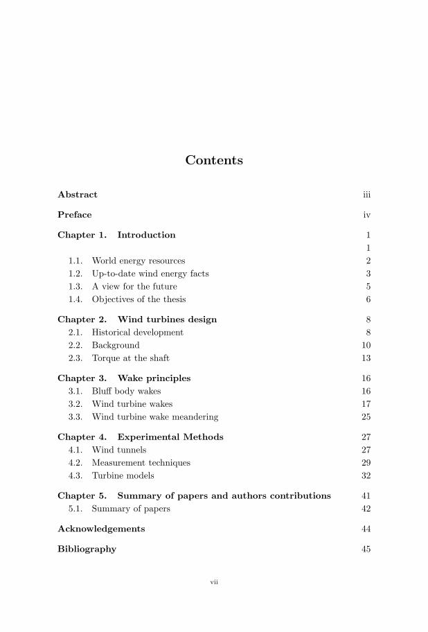
Contents
Abstract iii
Preface iv
Chapter 1. Introduction 11
1.1. World energy resources 21.2. Up-to-date wind energy facts 31.3. A view for the future 51.4. Objectives of the thesis 6
Chapter 2. Wind turbines design 82.1. Historical development 82.2. Background 102.3. Torque at the shaft 13
Chapter 3. Wake principles 163.1. Bluff body wakes 163.2. Wind turbine wakes 173.3. Wind turbine wake meandering 25
Chapter 4. Experimental Methods 274.1. Wind tunnels 274.2. Measurement techniques 294.3. Turbine models 32
Chapter 5. Summary of papers and authors contributions 415.1. Summary of papers 42
Acknowledgements 44
Bibliography 45
vii

Paper 1 51
Paper 2 65
Paper 3 87
Paper 4 103
Paper 5 119
Paper 6 145
Paper 7 165
viii

ix
CHAPTER 1
Introduction
The footnote in my Divina Commedia explained Dante’s words, quote: Thecastle is the human philosophy, i.e. the Knowledge, and its seven walls aremetaphysics, physics, mathematics, ethics, economy, dialectic and politics. Itis interesting that except the first one, all are needed to build a wind farmand I hope that Dante is not too upset about my comparison. Convincing thepublic is today’s real challenge, since the technical problems are easier to solveand sometimes they can be just a matter of convenience and investment. R&Dcan provide many answers and luckily even more questions, since every singlecomponent must be of the top quality to have a good wind turbine. This thesisdeals with only some of the technical aspects, but the first chapter is meant asan introduction for the reader who is unfamiliar with the wide world of windenergy.
In principle, it is easy to install a wind farm: ask where the wind blows,check for some signs like trees bending predominantly in one direction, installa tower with 3-4 anemometers at different heights and a vane to measure thewind direction and measure for at least one year to be sure of capturing theseasonal winds. With these data it is possible to calculate if the wind is strongand constant enough, and if so buy a wind turbine and install it. An on-shorewind turbine costs about 900 euros/kW rated power, but since it can be agood investment the issue is nowadays mainly political. Which are the mostlymentioned problems of wind turbines? A wind turbine is seen as a bird-killerand a source of stress for the animals and people leaving nearby. Anyone whohas visited the wind farms on Gotland must have seen ducks flying happily fewmeters from the 80 m diameter wind turbines, not a slaughter of birds underthe rotor. It will be shown in paper 4 how the flow is affected far upstreamof a wind turbine, and the above mentioned ducks can definitely sense this. Ofcourse some areas should be off-limits (e.g. the migration routes and nationalparks), but this would leave enough resources to develop wind energy to aconsiderably higher level than today. Noise can be a serious issue and forsome old wind turbines it was a problem, but the technology has remarkablyimproved and new solutions are under development.
The visual impact is usually the main approach to oppose wind farms.Wind turbine manufacturers have during the years developed more slender
1
2 1. INTRODUCTION
machines and they have paid more attention to the design, but more can bedone. Of course at the end it all comes down to convenience and the worldsituation in the last years has contributed to increase the attention towardsother energy sources, since oil prices are constantly rising and pollution too.Europe imports 50% of its energy needs and the oil is located primary inpolitically unstable regions, while nuclear power is hardly an option not onlyfor the public opinion aversion, but also for the limited uranium reserves. Theenergy demands coming from China will surely affect the West, and it lookslike green policy is not their primary worry (see Hassan (2005)). Acceptancecomes after knowledge and it is possible to notice an increased attention aboutrenewable energy (Lemonick et al. (2005), Parfit (2005)). The use of renewableenergy sources goes together with energy saving policies, and of course withthe traditional sources. Renewable energy resources can compete with thetraditional and wind energy, although it is not the only answer, can have aleading role.
1.1. World energy resources
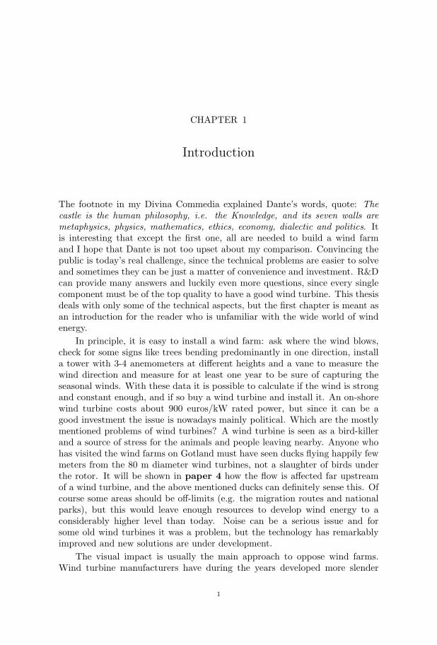
When it comes to the statistics of the actual use of energy supplies, there existsmall discrepancies between different studies due to differences in the defini-tions and methods used to evaluate the resources. Here the general definitionsused by the International Energy Agency (IEA, www.iea.org) will be adopted.It states that renewable energy sources include hydro, geothermal, solar pho-tovoltaics, solar thermal, tide, wave, ocean, wind, solid biomass, gases frombiomass, liquid biofuels, and renewable municipal solid waste. In general energyindependence is probably a dream for most countries, but energy productionis not. A look at the 2003 fuel shares of the world energy production in fig-ure 1.1(a) as from IEA (2005a), shows the strong dependency from few energysources. Crude oil supplies more than one third of the total 1.23 · 105 TWh1.Five countries in Europe are among the first ten importers of oil in the world.If the picture is restricted to the electricity production (figure 1.1(b)), coal isthe most commonly used source. Italy has the first position among the im-porters of electricity (not such a privileged leadership) with 51 TWh in 2003.Accordingly to the Statistiska Centralbyran SCB (statistics Sweden), Swedenhas produced 155.6 TWh of electricity from October 2004 to September 2005,with approximately 91% equally divided between nuclear and water power.
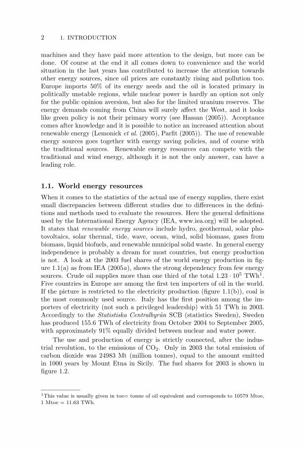
The use and production of energy is strictly connected, after the indus-trial revolution, to the emissions of CO2. Only in 2003 the total emission ofcarbon dioxide was 24983 Mt (million tonnes), equal to the amount emittedin 1000 years by Mount Etna in Sicily. The fuel shares for 2003 is shown infigure 1.2.
1This value is usually given in toe= tonne of oil equivalent and corresponds to 10579 Mtoe,
1 Mtoe = 11.63 TWh.
1.2. UP-TO-DATE WIND ENERGY FACTS 3
Oil
34.4%
Coal
24.4%
Other
0.5%
Renwables and
waste
10.8%
Hydro
2.2%
Nuclear
6.5%
Natural Gas
21.2%
(a) Shares of the world energy supply.
Gas
19.4%
Oil
6.9%
Coal
40.1%
Other
1.9%
Hydro
15.9%
Nuclear
15.8%
(b) Shares of the world electric-
ity production.
Figure 1.1. Source: IEA (2005a), data from 2003.
0
5
10
15
20
25
30
35
40
45
Coal Other Gas Oil
Tota
l, %
Figure 1.2. Fuel shares of the world CO2 emissions in per-centage, the total being 24983 Mt.
1.2. Up-to-date wind energy facts
The rated power from a turbine (i.e. the maximum obtainable power) is onlyobtained if the wind speed is higher than a characteristic value, typically around12 m/s at hub-height. A wind turbine runs below the rated power for approx-imately 75% of its production time. There is also an upper wind speed abovewhich the turbine is shut down in order to avoid damages to the turbine. Theinstalled capacity of wind energy (for a wind turbine park, country or theworld) is the sum of the rated power of all considered turbines. Having theabove analysis in mind, in order to understand if wind energy has a potentialto develop even further, it is essential to understand the world wind resources.Data have been collected during many years in the 30 OECD (Organisation forEconomic Co-operation and Development) countries, which includes Sweden
4 1. INTRODUCTION
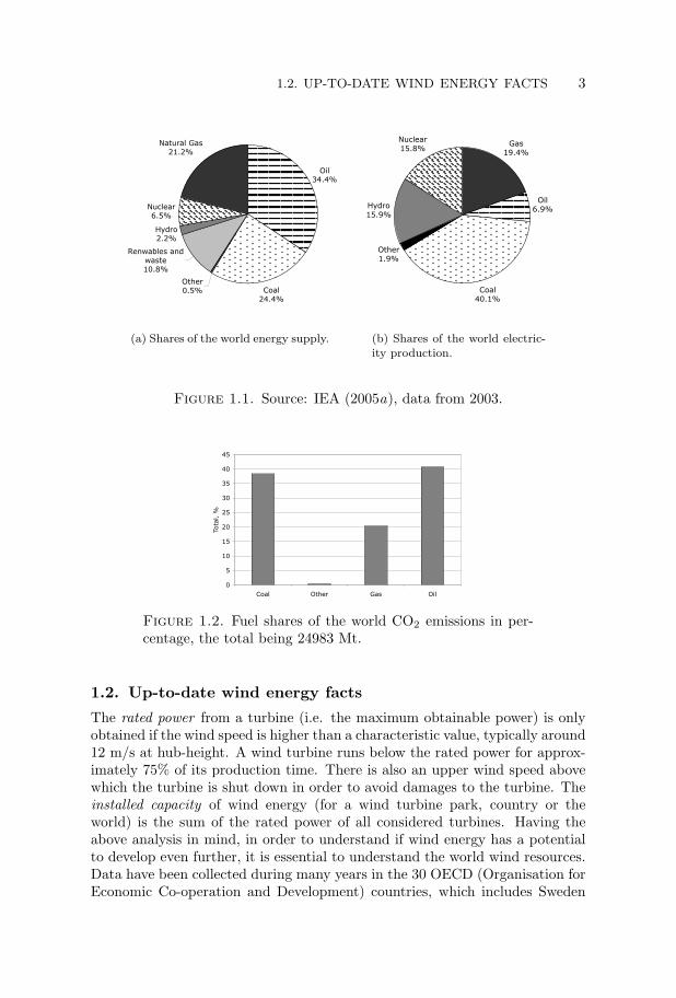
COUNTRY Installed capacity Total by endin 2004 [MW] of 2004 [MW]
China 198 764Denmark 3 3118 (13%)Germany 2020 16629Greece 43 468Italy 357 1265Japan 434 940Netherlands 167 1072New Zealand 132 168Spain 2061 8263Sweden 38 442 (5%)UK 253 900 (14%)USA 359 6740Rest of the world 2397 7095Total 8462 47864 (1.2%)
Table 1.1. Installed capacity, data from IEA (2005b). Be-tween parenthesis is the off-shore share.
since 1961, and in other areas of the world. The methodology, see for exam-ple Grubb & Meyer (1993), is to calculate the available land with an annualaverage wind speed higher than a chosen threshold value (in the cited case,above 5.1 m/s at a height of 10 m from the ground level). The energy outputcalculated from the velocity distribution is reduced by 90% when constraintssuch as high-populated areas, human activities, noise, visual impact, etc. areconsidered. According to this report, the energy available in the wind in theworld is 53000 TWh per year. Furthermore, no off-shore sites were consid-ered by Grubb & Meyer (1993) whereas, today, great attention is focussed alsoon this area. For instance, the amount of energy which can be produced byoff-shore sites in Europe is estimated in the order of 2000 TWh per year.
The statistics for some of the IEA (International Energy Agency) Windmembers are shown in table 1.1. It is evident that wind in Europe is mainlya 3-countries business, with Germany and Spain leading the growth. Denmarkis focussing more on re-powering old wind turbines and on the off-shore de-velopment. The European Union target has been set to 75 GW of installedpower by 2010, of which 10 GW will be off-shore, and an additional 100 GW isthe aim by 2020. In addition, the Kyoto protocol and the premium for greenenergy production have pushed for higher private investment in renewable en-ergies. The price for electricity production is rapidly approaching that fromother sources thanks to more efficient wind turbines and lower costs. The in-stallation cost depends strongly on the location and size of the project, but awind turbine alone is between 600 and 900 euros/kW, increasing between 800and 1100 euros/kW for the complete installation. As an example, Japan has
1.3. A VIEW FOR THE FUTURE 5
slightly higher costs because of the complex terrain and service can become ex-pensive during the typhoon season. The investment is roughly divided betweenthe turbine (75%) and the infrastructures necessary to build the power plant.Off-shore costs are higher because of the more challenging environment.
Wind turbines are designed for a 20 years life (or more) and have provento be very efficient. Some parts (e.g. the brake pads) must be replaced everytwo-three years, but more important and costly components such as the gear-box might need to be replaced once in a lifetime. The overall wind turbineavailability exceeds 98%.
1.3. A view for the future
Regarding my idea for future developments, I hope there will be two mainapproaches: medium wind turbines with a rated power below 1 MW and largerones of the order of several MW. The installation of even a single wind turbinein areas where there is none can help to accept more projects. Countries suchas Italy or Japan have a large percentage of complex terrain (mountains orhills), and therefore smaller wind turbines are easier to transport and install.It must be remembered that good infrastructures in a mountain area may notbe enough: a 750 kW wind turbine blade is approximately 23 m long. Althoughmore costly, the transport of this kind of blade by an helicopter can still be anoption. If the size of the turbines will only increase and these turbines will beoff the market, this method will be unrealistic. On the other hand, the bigger,the better philosophy may be more difficult to accomplish both socially andpolitically, but its pay-back is highly rewarding in terms of produced energy,so that even the few projects which see and end justify today’s efforts in thisdirection. The Danish approach has proven to be the most reliable and efficient:local communities have a share and participate in the wind farm projects. Itis harder to be against wind energy if it helps with the bills.
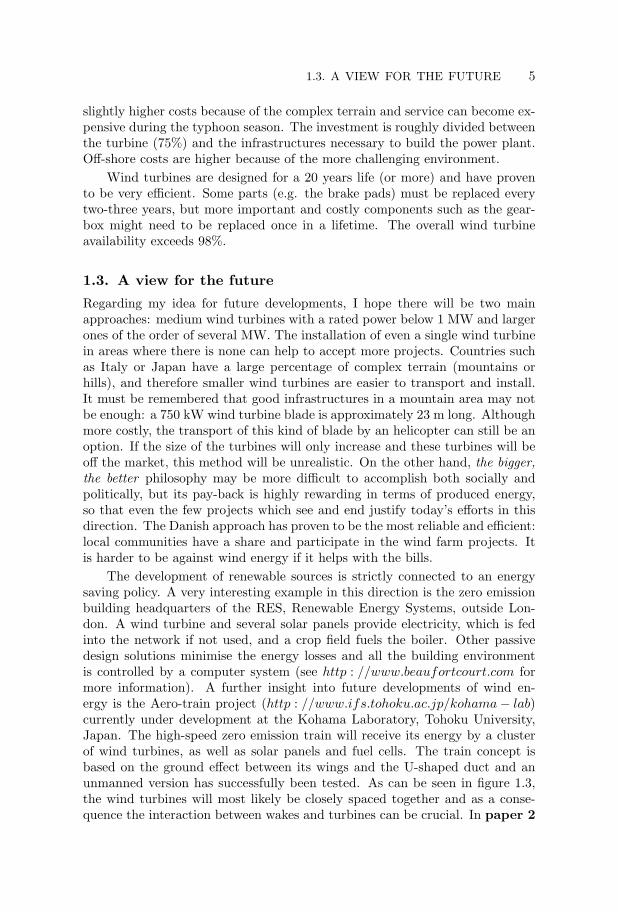
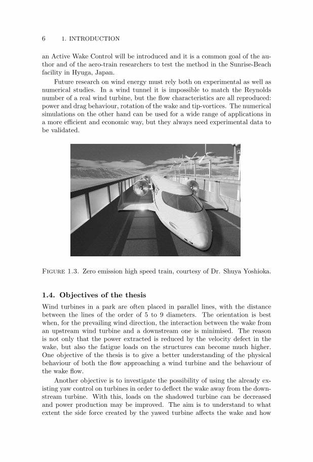
The development of renewable sources is strictly connected to an energysaving policy. A very interesting example in this direction is the zero emissionbuilding headquarters of the RES, Renewable Energy Systems, outside Lon-don. A wind turbine and several solar panels provide electricity, which is fedinto the network if not used, and a crop field fuels the boiler. Other passivedesign solutions minimise the energy losses and all the building environmentis controlled by a computer system (see http : //www.beaufortcourt.com formore information). A further insight into future developments of wind en-ergy is the Aero-train project (http : //www.ifs.tohoku.ac.jp/kohama− lab)currently under development at the Kohama Laboratory, Tohoku University,Japan. The high-speed zero emission train will receive its energy by a clusterof wind turbines, as well as solar panels and fuel cells. The train concept isbased on the ground effect between its wings and the U-shaped duct and anunmanned version has successfully been tested. As can be seen in figure 1.3,the wind turbines will most likely be closely spaced together and as a conse-quence the interaction between wakes and turbines can be crucial. In paper 2
6 1. INTRODUCTION
an Active Wake Control will be introduced and it is a common goal of the au-thor and of the aero-train researchers to test the method in the Sunrise-Beachfacility in Hyuga, Japan.
Future research on wind energy must rely both on experimental as well asnumerical studies. In a wind tunnel it is impossible to match the Reynoldsnumber of a real wind turbine, but the flow characteristics are all reproduced:power and drag behaviour, rotation of the wake and tip-vortices. The numericalsimulations on the other hand can be used for a wide range of applications ina more efficient and economic way, but they always need experimental data tobe validated.
Figure 1.3. Zero emission high speed train, courtesy of Dr. Shuya Yoshioka.
1.4. Objectives of the thesis
Wind turbines in a park are often placed in parallel lines, with the distancebetween the lines of the order of 5 to 9 diameters. The orientation is bestwhen, for the prevailing wind direction, the interaction between the wake froman upstream wind turbine and a downstream one is minimised. The reasonis not only that the power extracted is reduced by the velocity defect in thewake, but also the fatigue loads on the structures can become much higher.One objective of the thesis is to give a better understanding of the physicalbehaviour of both the flow approaching a wind turbine and the behaviour ofthe wake flow.
Another objective is to investigate the possibility of using the already ex-isting yaw control on turbines in order to deflect the wake away from the down-stream turbine. With this, loads on the shadowed turbine can be decreasedand power production may be improved. The aim is to understand to whatextent the side force created by the yawed turbine affects the wake and how
1.4. OBJECTIVES OF THE THESIS 7
the structure of the 3-dimensional wake is changed. An interesting observationis that the turbine model wake meanders in a similar way as a bluff body, suchas observed for example in field measurements in the Alsvik wind farm, on theisland of Gotland. This kind of motion may prove to be very important in windparks, where interactions between several wakes can take place.
To reach the objectives we have used small wind turbine models and mea-sured the velocity field related to the flow behind the turbines in a wind tunnel.We have used both hot-wire anemometry and PIV techniques and made exten-sive measurements for a number of configurations of the wind turbines.
Chapter 2 of the thesis gives some fundamentals of wind turbines, both froma historical and modern perspective, whereas chapter 3 gives some basic resultsfor power extraction related to the flow in the wake. Chapter 4 describes theexperimental techniques and the turbines used in the present study. Chapter 5is a summary of the papers which are appended to the present thesis.
CHAPTER 2
Wind turbines design
2.1. Historical development
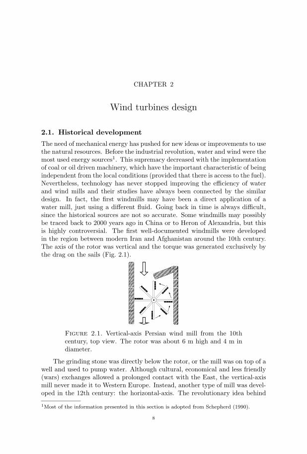
The need of mechanical energy has pushed for new ideas or improvements to usethe natural resources. Before the industrial revolution, water and wind were themost used energy sources1. This supremacy decreased with the implementationof coal or oil driven machinery, which have the important characteristic of beingindependent from the local conditions (provided that there is access to the fuel).Nevertheless, technology has never stopped improving the efficiency of waterand wind mills and their studies have always been connected by the similardesign. In fact, the first windmills may have been a direct application of awater mill, just using a different fluid. Going back in time is always difficult,since the historical sources are not so accurate. Some windmills may possiblybe traced back to 2000 years ago in China or to Heron of Alexandria, but thisis highly controversial. The first well-documented windmills were developedin the region between modern Iran and Afghanistan around the 10th century.The axis of the rotor was vertical and the torque was generated exclusively bythe drag on the sails (Fig. 2.1).
Figure 2.1. Vertical-axis Persian wind mill from the 10thcentury, top view. The rotor was about 6 m high and 4 m indiameter.
The grinding stone was directly below the rotor, or the mill was on top of awell and used to pump water. Although cultural, economical and less friendly(wars) exchanges allowed a prolonged contact with the East, the vertical-axismill never made it to Western Europe. Instead, another type of mill was devel-oped in the 12th century: the horizontal-axis. The revolutionary idea behind
1Most of the information presented in this section is adopted from Schepherd (1990).
8
2.1. HISTORICAL DEVELOPMENT 9
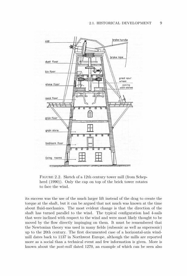
Figure 2.2. Sketch of a 12th century tower mill (from Schep-herd (1990)). Only the cap on top of the brick tower rotatesto face the wind.
its success was the use of the much larger lift instead of the drag to create thetorque at the shaft, but it can be argued that not much was known at the timeabout fluid-mechanics. The most evident change is that the direction of theshaft has turned parallel to the wind. The typical configuration had 4-sailsthat were inclined with respect to the wind and were most likely thought to bemoved by the flow directly impinging on them. It must be remembered thatthe Newtonian theory was used in many fields (subsonic as well as supersonic)up to the 20th century. The first documented case of a horizontal-axis wind-mill dates back to 1137 in Northwest Europe, although the mills are reportedmore as a social than a technical event and few information is given. More isknown about the post-mill dated 1270, an example of which can be seen also
10 2. WIND TURBINES DESIGN
in the Skansen museum, Stockholm. The post-mill was usually a wooden towerstanding on a main post and the entire block was turned accordingly to thewind direction. New engineering problems had to be solved, but many weresuccessfully managed by the Dutch tower-mill shown in figure 2.2. This wind-mill is the natural development of the older post-mill and it is first recordedin the beginning of the 15th century in the Turkish town of Gallipoli. Someinteresting features can be observed in both the post-mill and the Dutch-mill:the shaft is not perpendicular to the tower, but slightly inclined as for themodern wind turbines. This leaves a good clearance between the tower andthe sails. The torque was transmitted to the vertical shaft by a large wheelwith pegs. This wheel was large in order to increase the breaking torque of aband around its circumference, since the speed of the millstones was controlledby the miller setting the friction between the band and the wheel. A bearingat the end of the horizontal shaft sustained all the axial drag. The Dutch-millcap was movable and the platform at the mid-height was used both to activatethe brake and to operate the sails. The largest recorded mill of this kind hada tower of 37 m and a rotor of 30 m.
A lot more could be said about the mill development, but it is not in thescope of this thesis. In the end it can be mentioned that many improvementshave regarded the sails, the materials used in the construction and the controlmethods; the latter are described in the next section. Modern windmills aremainly used to produce electricity and they are called wind turbines, but thephysical principle has not changed over the years. What is considerably differ-ent is the size and the efficiency as compared to wind mills only few decadesago. Off-shore wind turbines have increased up to 120 m in diameter and 5 MWof nominal power. The size of the on-shore wind turbines is generally smallerbecause of the road constraints for transportation.
2.2. Background
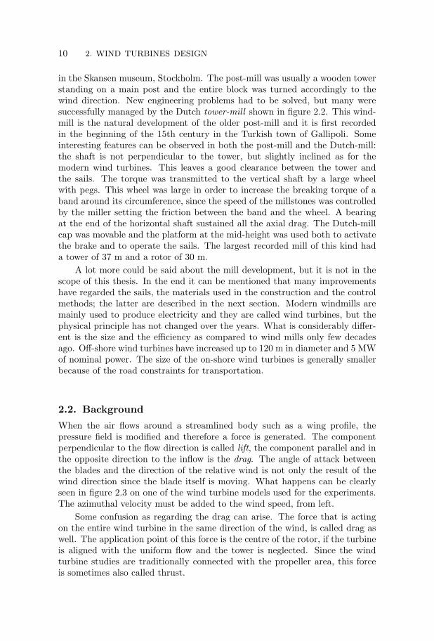
When the air flows around a streamlined body such as a wing profile, thepressure field is modified and therefore a force is generated. The componentperpendicular to the flow direction is called lift, the component parallel and inthe opposite direction to the inflow is the drag. The angle of attack betweenthe blades and the direction of the relative wind is not only the result of thewind direction since the blade itself is moving. What happens can be clearlyseen in figure 2.3 on one of the wind turbine models used for the experiments.The azimuthal velocity must be added to the wind speed, from left.
Some confusion as regarding the drag can arise. The force that is actingon the entire wind turbine in the same direction of the wind, is called drag aswell. The application point of this force is the centre of the rotor, if the turbineis aligned with the uniform flow and the tower is neglected. Since the windturbine studies are traditionally connected with the propeller area, this forceis sometimes also called thrust.
2.2. BACKGROUND 11
Figure 2.3. The angle between the plane of the rotor and thelocal wind direction is decreasing as moving towards the tip,hence the stall starts from the root. The turbine rotates clock-wise.
For good performance of a wing of a wind turbine blade, flow separationon the blade surface should be avoided. This is the reason why wind turbineshave twisted blades: the angle of attack is optimised from tip to root, for themost frequent operational condition, by making the blade to turn out of theplane of rotation when moving towards the root. However the so-called stallcontrol, one of the main aerodynamic controls on wind turbines, makes the stallto occur gradually from the root as the wind speed increases. The reason is toavoid high loads and also high power production which can cause problems tothe electrical components of the wind turbine. This is a passive type of control,since the angle of attack on the blades increases with increasing wind speed.
A second important aerodynamic control present on wind turbines is theyaw control. It will be shown how the power is proportional to the cube of thewind speed normal to the rotor plane. To maximize the power output the windturbine is turned towards the wind by means of electrical motors, which movethe entire nacelle (i.e. the top part of the wind turbine including the shaft,the gearbox if present, the generator and the other systems) around the tower.Both the yaw control and the twist of the blades were well known in the past,when windmills produced not electrical but only mechanical energy. The thirdmostly used control is the pitch control. In this active control, the entire bladeis turned, to optimise the angle of attack with respect to the wind. If the poweroutput from the generator becomes too high, the system decreases the angleof attack of the blades, in order to obtain less power. This mechanism is theopposite of the active stall control, where the blades are instead turned out ofthe wind to increase the stall, thereby ”wasting” the excess energy in the wind.
All the wind turbines have a cut-in wind speed, after which the wind-generated torque is greater than the friction in the system and the rotor starts
12 2. WIND TURBINES DESIGN
to rotate and produce electricity. The cut-off speed is instead the higher limitfor the working conditions, above which the loads produced are considereddangerous for the machine. The range of velocities is typically somewherebetween 3 m/s and 30 m/s, but depends on the type of wind turbine considered.When the conditions exceed the highest velocity limit, the turbine is stoppedfirst by means of aerodynamic controls, e.g. pitching the blade and causing anextended stall, and then the brakes act on the shaft. Tip ailerons are also usedin some models as aerodynamic breaks, or the entire tip itself is tilted.
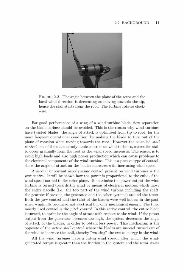
Some wind turbines run at constant rotational speed, giving a constant fre-quency of the current produced. Small fluctuations in the frequency are allowedand adjusted with an electronic converter. The reason is that the turbines areconnected to an electrical grid with a specific frequency of the current (50 Hzin Europe), which has to be matched by the production plant. Two main con-cepts are presently on the market: the most common is connecting the shaftwith an high speed generator through a gearbox which increases the rotationalfrequency. Without the gearbox the stator is a large multi-layer ring, where thelower rotational frequency of the rotor is balanced by a greater number of polesin the stator. In this way the frequency of the produced current is increasedand the machine can be directly connected to the electrical system. The maxi-mum power of wind turbines has increased from 0.4 MW of a decade ago to the5 MW machines, manufactured by e.g. Enercon and General Electrics. Oneexample of a modern wind turbine is the Enercon E66 shown in figure 2.4. Ithas a rated power of 2 MW and a diameter of 70 m.
Figure 2.4. Enercon E66. Courtesy of Enercon GmbH.
2.3. TORQUE AT THE SHAFT 13
For a given power output, the choice is then between a large, low speedrotor such as for the Enercon wind turbine, or a smaller, high speed rotor,although hybrid system have been developed. Ultimately, both have someinconvenience. The weight of the nacelle is of the order of 3-400 tons for thegearless machine, and only about a fifth when the gearbox is present. On theother hand, the gearbox has to stand the large torque from the blades and thefluctuations of the wind speed and direction, which may cause it to break. Alsothe initial cost is generally in favour of a high speed generator, however theabsence of moving parts is a pro-factor for the low speed generator.
In the nacelle a small fixed crane can also be placed to considerably speedup the process of changing internal parts of the wind turbine. When it comesto assembling the machine, some interesting solutions can be seen. On-shorethe process is usually easier: the machine is put together in situ connectingelements of the tower, of the nacelle and of the service parts (shaft, generator,active power controls, etc.). On the ground, in case of a three-bladed turbine,two blades are connected together and then lifted in front of the nacelle. Atthe end also the third blade is raised and bolted to the shaft. Off-shore theenvironment is more challenging. First, the basement of the tower must bebuilt. In a second stage, special-purpose ships with a crane are used andequipped with a number of poles that descend on the sea bottom and anchorthe ship. The turbine is put together on-shore and then loaded on the ship, forexample in only three pieces: the tower, the nacelle with two blades mounted,and a third single blade. The final assembling process of these parts can takeplace at sea in typical eight hours, if the weather conditions are good.
2.3. Torque at the shaft
Most of the wind turbines have a horizontal axis rotor because of their higherenergy production with respect to the vertical axis. The advantage of the hori-zontal axis is that, except for the velocity changes in the atmospheric boundarylayer, the blades operate at a nearly constant angle of attack. The lift on theprofile is always favourable to the rotation. The vertical axis wind turbine hasinstead a cyclical change in the sign of the angle between the wind speed andthe azimuthal velocity, hence the total torque is reduced. Consider a sym-metrical wing profile: with the chord parallel to the wind direction only thedrag acts on the blade and therefore the torque at this position is opposing therotation. For both the vertical and horizontal axis wind turbine, the runningcondition is the balance between the load (breaking torque) on the shaft givenby the generator and the driving torque Q created by the rotor. This is relatedto the mechanical power P by:
P = ΩQ (2.1)
The torque of one of the turbines used in this study is shown in figure 2.5as a function of the rotational speed Ω, with the load depending only on thegenerator. At a constant wind speed, the rotor accelerates until it reaches
14 2. WIND TURBINES DESIGN
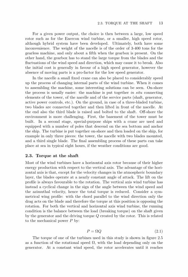
Figure 2.5. Rotor torque as a function of the rotational speedfor the wind turbine model 2 (see Chapter 4). : U∞=5 m/s,: U∞=8 m/s, 4: U∞=11 m/s. The dashed line is for aheavy load from the generator, the solid line for a light load.
the rotational speed that balances the load from the generator. If the rotormoves from the equilibrium point, the load restores the original Ω. Supposethat the rotor speed increases, then the breaking torque from the generator ishigher (figure 2.5) and slows down the rotor. A steep Q-Ω curve can lead toan unstable equilibrium, i.e. a fluctuating Ω, since there is not a well definedcrossing between the torque from the rotor and the load from the generator.The production of current is directly proportional to the torque on the shaftsince a DC generator has been used and the variation of the internal lossescan be neglected. Curves for different wind speed collapse if the followingcoefficients are introduced:
P12ρAdU3
∞=
ΩR
U∞· Q
12ρAdRU2
∞⇔ CP = λCQ (2.2)
where U∞ is the wind speed, R is the rotor radius and Ad is the area swept bythe blades. The tip-speed ratio λ is defined as tip-speed/wind speed.
A high solidity (σ=blade area/Ad) turbine means a lower λ, therefore fromEq. 2.2 at constant CP the torque coefficient is higher. This type of turbine ispreferred for water pumps. On the other hand, the starting torque is higherand high σ turbines may need the application of a torque by e.g. an electricalmotor to start rotating. Many wind turbines for electrical generation have acontrol on the loading in order to change the rotational speed and to keepan optimum tip-speed ratio (as close as possible to CPmax
) for a wide range ofwind speeds. The optimum λ depends strongly on the blade characteristics andon the lift-to-drag ratio, see figure 2.6. When this ratio tends to infinity, thepower coefficient tends to the so-called Glauert limit which will be derived in
2.3. TORQUE AT THE SHAFT 15
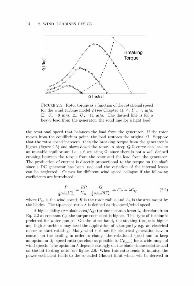
Figure 2.6. Power as a function of the rotational speed fordifferent CL/CD values.
chapter 3. The Betz limit is the maximum theoretical limit which is approachedfor λ → ∞ and this will be discussed as well in the next chapter. As for theeffect of the number of blades on the power coefficient we refer to paper 3. Itmust be mentioned here that the higher efficiency with the increasing number ofblades is referring to an inviscid fluid, while for real wind turbines the increasein lift is counter-balanced by the increased drag and it becomes useless (andcostly) to add more blades to the rotor.
CHAPTER 3
Wake principles
3.1. Bluff body wakes
A wind turbine can be viewed as a bluff body, which is defined as any non-streamlined body, because of the large wake generated behind it. This sectionis aimed at giving a brief summary on bluff body wakes.
A characteristic of bluff body wakes is the self-similarity reached far down-stream, see e.g. Johansson et al. (2003), where the wake development can bedescribed by an appropriate normalisation. This self-similarity state is reachedat a downstream distance of the order of 50 diameters and it is of little in-terest for practical wind farm application. In addition, the tip-vortices shieldthe wind turbine wake and delay the turbulent mixing with the free stream.Nevertheless the near wake of bluff bodies has been extensively studied, e.g. byBevilaqua & Lykoudis (1978). They have compared the wakes of a sphere andof a porous disc with the same drag, finding that the self-similar mechanismdepends on the initial conditions. The wake ”remembers” the shape of thebody in the form of the larger eddies which travel downstream. Connected tothe large scale vortex shedding from the body is a wake meandering with fre-quency f , which is usually normalised with a body length and the free-streamvelocity to give the Strouhal number:
St =fD
U∞(3.1)
The normalisation with a geometrical scale gives a Strouhal number whichis a function of the aspect ratio of the body, as shown by Kiya & Abe (1999)for the wake behind elliptic discs. Miau et al. (1997) found that the wakemeandering behind discs has no preferred rotational pattern and that the fre-quency depends on the Reynolds number. The Strouhal number changes withthe inclination of the disc (see Calvert (1967)) and it was proved by Castro(1971) and Higuchi et al. (1998) that the large scale oscillation (meandering)of the wake behind two-dimensional plates and discs is influenced by the poros-ity. These effects are important for studying a wind turbine wake since a windturbine can be simulated by a porous disc, such as in Sforza et al. (1981), sincemomentum is let through the rotor. The porous disc is largely studied alsotoday as a model for a wind turbine in Sørensen et al. (1998), Sharpe (2004)
16
3.2. WIND TURBINE WAKES 17
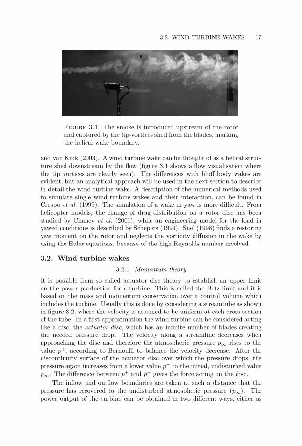
Figure 3.1. The smoke is introduced upstream of the rotorand captured by the tip-vortices shed from the blades, markingthe helical wake boundary.
and van Kuik (2003). A wind turbine wake can be thought of as a helical struc-ture shed downstream by the flow (figure 3.1 shows a flow visualisation wherethe tip vortices are clearly seen). The differences with bluff body wakes areevident, but an analytical approach will be used in the next section to describein detail the wind turbine wake. A description of the numerical methods usedto simulate single wind turbine wakes and their interaction, can be found inCrespo et al. (1999). The simulation of a wake in yaw is more difficult. Fromhelicopter models, the change of drag distribution on a rotor disc has beenstudied by Chaney et al. (2001), while an engineering model for the load inyawed conditions is described by Schepers (1999). Snel (1998) finds a restoringyaw moment on the rotor and neglects the vorticity diffusion in the wake byusing the Euler equations, because of the high Reynolds number involved.
3.2. Wind turbine wakes
3.2.1. Momentum theory
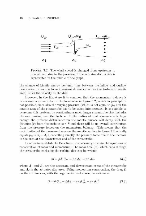
It is possible from so called actuator disc theory to establish an upper limiton the power production for a turbine. This is called the Betz limit and it isbased on the mass and momentum conservation over a control volume whichincludes the turbine. Usually this is done by considering a streamtube as shownin figure 3.2, where the velocity is assumed to be uniform at each cross sectionof the tube. In a first approximation the wind turbine can be considered actinglike a disc, the actuator disc, which has an infinite number of blades creatingthe needed pressure drop. The velocity along a streamline decreases whenapproaching the disc and therefore the atmospheric pressure p∞ rises to thevalue p+, according to Bernoulli to balance the velocity decrease. After thediscontinuity surface of the actuator disc over which the pressure drops, thepressure again increases from a lower value p− to the initial, undisturbed valuep∞. The difference between p+ and p− gives the force acting on the disc.
The inflow and outflow boundaries are taken at such a distance that thepressure has recovered to the undisturbed atmospheric pressure (p∞). Thepower output of the turbine can be obtained in two different ways, either as
18 3. WAKE PRINCIPLES
U -∆uU
PP
A1
p+
p-
Ad A2
U -∆ud
Figure 3.2. The wind speed is changed from upstream todownstream due to the presence of the actuator disc, which isrepresented in the middle of the graph.
the change of kinetic energy per unit time between the inflow and outflowboundaries, or as the force (pressure difference across the turbine times itsarea) times the velocity at the disc.
However, in the literature it is common that the momentum balance istaken over a streamtube of the form seen in figure 3.2, which in principle isnot possible, since also the varying pressure (which is not equal to p∞) on themantle area of the streamtube has to be taken into account. It is possible toovercome this problem by considering a much larger streamtube that includesthe one passing over the turbine. If the radius of that streamtube is largeenough the pressure disturbance on the mantle surface will decay with thedistance (r) from the turbine as r−2 and there will be no overall contributionfrom the pressure forces on the momentum balance. This means that thecontribution of the pressure forces on the mantle surface in figure 3.2 actuallyequals p∞ · (A2−A1), cancelling exactly the pressure force due to the increasein the area at the downstream end of the streamtube.
In order to establish the Betz limit it is necessary to state the equations ofconservation of mass and momentum. The mass flow (m) which runs throughthe streamtube enclosing the turbine disc can be written
m = ρA1U∞ = ρA2U2 = ρAdUd (3.2)
where A1 and A2 are the upstream and downstream areas of the streamtubeand Ad is the actuator disc area. Using momentum conservation, the drag Don the turbine can, with the arguments used above, be written as
D = mU∞ − mU2 = ρA1U2∞ − ρA2U
22 (3.3)
3.2. WIND TURBINE WAKES 19
By using Bernoulli’s equation both upstream and downstream the turbineit is possible to obtain an expression for the pressure difference p+− p− acrossthe turbine such that
p+ − p− =12ρ(U2
∞ − U22 ) (3.4)
and the drag on the turbine hence becomes
D =12ρAd(U2
∞ − U22 ) = ρAd
(U∞ − ∆u∞
2
)·∆u∞ (3.5)
where U2 = U∞ − ∆u∞, i.e. ∆u∞ is the velocity defect in the wake at thedownstream end of the streamtube. Using the same notation, Eq. 3.3 becomes
D = m (U∞)− m (U∞ −∆u∞) = m∆u∞ = ρAd (U∞ −∆ud) ·∆u∞ (3.6)
where ∆ud is the velocity decrease at the turbine plane. A simple comparisonbetween Eq. 3.5 and Eq. 3.6 gives the result known as Froude’s theorem:
∆ud =∆u∞
2(3.7)
The total power in the wind, i.e. the kinetic energy passing through acontrol area A (normal to the wind) per unit time, can be expressed as
PTOT =12ρAU3
∞ (3.8)
The power extracted by the wind turbine on the other hand can be writtenas
PE =12m(U2∞ − U2
2
)=
12m[U2∞ − (U∞ −∆u∞)2
](3.9)
which after some algebra can be rewritten
PE = ρAd (U∞ −∆ud)2 · 2∆ud (3.10)
The maximum power output is found by searching for the maximum in PE
with respect to the velocity defect at the disc ∆ud. From Eq. 3.10 we obtain
∂PE
∂∆ud= 0 → (∆ud)PEmax
=U∞3
(3.11)
The maximum power for the actuator disc with no losses, from Eq. 3.10using Eq. 3.11, can be compared with the energy flux of the wind (Eq. 3.8) inorder to obtain the efficiency of a turbine (Betz limit):
PEmax
PTOT=
827ρAdU
3∞
12ρAdU3
∞=
1627≈ 0.529 (3.12)
20 3. WAKE PRINCIPLES
The power and drag are often expressed in terms of the non-dimensionalpower coefficient CP , already defined in Eq. 2.2, and drag coefficient CD
CD =D
12ρAdU2
∞(3.13)
In the Betz limit we find CD = 89 . A measure of the energy extracted from
the wind is given by the axial interference factor defined as
a =∆ud
U∞(3.14)
Plugging the result of Eq. 3.7 and the definition in Eq. 4 into Eq. 3.6 weobtain:
CD = 4a (1− a) (3.15)
From Eq. 3.10 we have PE=D (U∞ −∆ud) and therefore the power coeffi-cient can be rewritten as
CP = CD (1− a) (3.16)
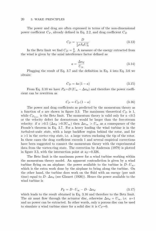
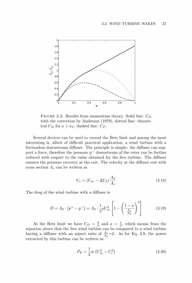
The power and drag coefficients as predicted by the momentum theory asa function of a are shown in figure 3.3. The maximum theoretical CD is 1,while CPmax
is the Betz limit. The momentum theory is valid only for a <0.5or the velocity defect far downstream would be larger than the free-streamvelocity: if a >0.5 (∆ud >0.5U∞) then ∆u∞ > U∞ as a consequence of theFroude’s theorem in Eq. 3.7. For a heavy loading the wind turbine is in theturbulent-wake state, with a large backflow region behind the rotor, and fora >1 in the vortex-ring state, i.e. a large vortex enclosing the tip of the rotor.In these cases the drag coefficient exceeds 1 and several empirical correctionshave been suggested to connect the momentum theory with the experimentaldata from the vortex-ring state. The correction by Anderson (1979) is plottedin figure 3.3, with the intersection point at aT =0.326.
The Betz limit is the maximum power for a wind turbine working withinthe momentum theory model. An apparent contradiction is given by a windturbine flying on an airplane: the power available to the turbine is D · U∞,which is the extra work done by the airplane to bring along the turbine. Onthe other hand, the turbine does work on the fluid with an energy (per unittime) equal to D ·∆ud (see Glauert (1926)). Hence the power available to thewind turbine is
PE = D · U∞ −D ·∆ud (3.17)which leads to the result obtained in Eq. 3.16 and therefore to the Betz limit.The air must flow through the actuator disc, otherwise ∆ud = U∞, i.e. a=1and no power can be extracted. In other words, only a porous disc can be usedto simulate a wind turbine since for a solid disc it is CP =0.
3.2. WIND TURBINE WAKES 21
0 0.2 0.4 0.6 0.8 10
0.2
0.4
0.6
0.8
1
1.2
1.4
1.6
1.8
2
a
CP, C
D
Figure 3.3. Results from momentum theory. Solid line: CD
with the correction by Anderson (1979), dotted line: theoret-ical CD for a > aT , dashed line: CP .
Several devices can be used to exceed the Betz limit and among the mostinteresting is, albeit of difficult practical application, a wind turbine with africtionless downstream diffuser. The principle is simple: the diffuser can sup-port a force, therefore the pressure p− downstream of the rotor can be furtherreduced with respect to the value obtained for the free turbine. The diffuserensures the pressure recovery at the exit. The velocity at the diffuser exit withcross section Ae can be written as
Ue = (U∞ −∆Ud)Ad
Ae(3.18)
The drag of the wind turbine with a diffuser is
D = Ad ·(p+ − p−
)= Ad ·
12ρU2
∞
1−
(1− a
Ae
Ad
)2 (3.19)
At the Betz limit we have CD = 89 and a = 1
3 , which means from theequation above that the free wind turbine can be compared to a wind turbinehaving a diffuser with an aspect ratio of Ae
Ad=2. As for Eq. 3.9, the power
extracted by this turbine can be written as
PE =12m(U2∞ − U2
e
)(3.20)
22 3. WAKE PRINCIPLES
Using Eq. 3.18 and deriving with respect to Ud = (U∞−∆ud) it is possibleafter some algebra to find the maximum power production
PEmax
PTOT=
43√
3≈ 0.769 (3.21)
A second option is to use a shroud, i.e. an axisymmetric lifting surface,around the rotor. This concept is common between propellers (see e.g. the aero-train in figure 1.3), but it is applicable only to small rotors, thus preventingits use for typical wind turbine sizes. The circulation around the annular winginduces a higher velocity through the turbine, but only if the lift is directedtowards the centre of the rotor. A CP up to 2 is possible according to de Vries(1979), while the calculations by Hansen et al. (2000) show that for a shroudwhich only partially recovers the static pressure is
PEmax
PTOT≈ 0.94 (3.22)
There are other means to increase the power production: Hutter (1977)considers a flow deflection through the rotor of an angle ϕ with respect to thesymmetry axis. This gives a higher mass flow, and therefore a higher powercoefficient, since the velocity through the rotor is (U∞ − ∆ud)/ cos(ϕ). Thepower gain is quantified by Landahl (1979) for a deflection of ϕ=35.25 as beingthe double of the Betz limit
PEmax
PTOT=
3227≈ 1.185 (3.23)
although the practical limitation of such a device are acknowledged by theauthor himself.
The state-of-the-art of wind turbine technology has increased the powercoefficient to values close to 0.5. Future studies can most likely fine-tune thewind turbine in order to increase the power production, but the main gainlot more can be done towards the power optimisation from a cluster of windturbines. The already cited work by Hutter (1977) estimates the turbulentexchange between the outer flow and the wake, predicting a faster wake recoveryfor heavily loaded wind turbines and a possible reduction of the downstreamspacing. On the other hand, for the typical distances between wind turbines ina farm (7 to 9 diameters), a more practical idea may be to extract less energyfrom an upstream turbine in order to leave more energy for the downstream ones(see Dahlberg (1998) and Corten et al. (2003)). Another method is the recentlydeveloped Active Wake Control (AWC) by J. A. Dahlberg and described indetail in paper 2. Paper 1 to paper 4 focus on wake measurements and aimat improving the power production from a cluster of wind turbines.
3.2. WIND TURBINE WAKES 23
3.2.2. Effects of wake rotation on the energy extraction
A complication not taken into account by the momentum theory is that thewake will rotate. This is due to the fact that the flow gives a torque on theturbine, which in turn gives an angular momentum to the flow in the wake,hence the energy extraction creates some kinetic energy related to the wakerotation. In the following we will analyze this effect and show how it affectsthe possible amount of energy extracted by the turbine.
In a rotating system (with system rotation Ω), the Bernoulli equation canbe written
p +12ρU2
R −12ρ (Ω× r)2 = const (3.24)
where the third term on the LHS is the centrifugal body force and UR isthe velocity vector in the rotating system. The classical Bernoulli equation,i.e. Eq. 3.24 without the rotation term, can be applied along a streamlinewith r=const. Such a streamline does not exist for a wind turbine, since thestreamtube including the turbine is expanding. A more physical interpretationof this equation can be given by considering an absolute reference system (suchas the earth) for the wind turbine flow, with UR=U + (Ω × r). Substitutinginto Eq. 3.24 gives
p +12ρU2 + ρU · (Ω× r) = const (3.25)
Therefore the energy extraction from the flow, i.e. a change in the totalhead H=p+1
2ρU2, is possible only if U is deflected towards Ω × r during thepassage through the rotor. Equation 3.25 states that the azimuthal velocity inthe wake is a necessary condition to extract energy, i.e. to obtain the reductionin the total head. The only energy extractor in the flow is the rotating blade(s),which is the only solid surface capable of bearing a torque. Upstream of therotor there is no energy extractor, therefore no azimuthal velocity and the flowcan be considered irrotational.
Glauert (1935) showed that by calculating the torque in each blade sectionas functions of the local forces assuming an infinite number of blades and africtionless fluid, it is possible to obtain an expression for the power coefficientwhich includes the effects of the tangential velocity through the tangentialinduction factor a′ = v/Ωr:. The derivation can be found in many text books(see e.g. de Vries (1983)) and it gives the power coefficient as function of thetip-speed ratio λ as
CP =(
2λ
)2 ∫ λ
0
(1− a) a′X3dX (3.26)
where X = λr/R is the local tip-speed ratio.A different approach is to use the momentum equations and Bernoulli
equation (see de Vries (1979)). It gives the power loss due to the rotation ofthe wake and it will be shown that the Betz limit derived in Section 3.2.1 can
24 3. WAKE PRINCIPLES
Betz
A
B
C
D
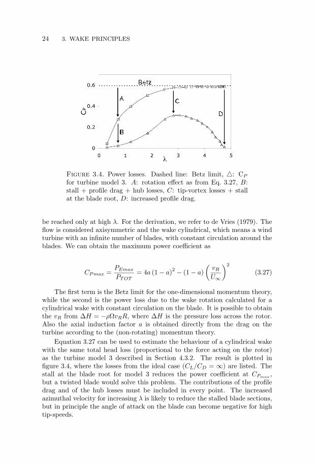
Figure 3.4. Power losses. Dashed line: Betz limit, 4: CP
for turbine model 3. A: rotation effect as from Eq. 3.27, B:stall + profile drag + hub losses, C: tip-vortex losses + stallat the blade root, D: increased profile drag.
be reached only at high λ. For the derivation, we refer to de Vries (1979). Theflow is considered axisymmetric and the wake cylindrical, which means a windturbine with an infinite number of blades, with constant circulation around theblades. We can obtain the maximum power coefficient as
CPmax =PEmax
PTOT= 4a (1− a)2 − (1− a)
(vR
U∞
)2
(3.27)
The first term is the Betz limit for the one-dimensional momentum theory,while the second is the power loss due to the wake rotation calculated for acylindrical wake with constant circulation on the blade. It is possible to obtainthe vR from ∆H = −ρΩvRR, where ∆H is the pressure loss across the rotor.Also the axial induction factor a is obtained directly from the drag on theturbine according to the (non-rotating) momentum theory.
Equation 3.27 can be used to estimate the behaviour of a cylindrical wakewith the same total head loss (proportional to the force acting on the rotor)as the turbine model 3 described in Section 4.3.2. The result is plotted infigure 3.4, where the losses from the ideal case (CL/CD = ∞) are listed. Thestall at the blade root for model 3 reduces the power coefficient at CPmax
,but a twisted blade would solve this problem. The contributions of the profiledrag and of the hub losses must be included in every point. The increasedazimuthal velocity for increasing λ is likely to reduce the stalled blade sections,but in principle the angle of attack on the blade can become negative for hightip-speeds.
3.3. WIND TURBINE WAKE MEANDERING 25
3.3. Wind turbine wake meandering
Section 3.1 gives a general introduction on bluff body wakes, while Section 3.2describes the wind turbine wake from the theoretical point of view. Duringthe measurements described in paper 2, a low frequency meandering of thewake was observed. The large scale vortex shedding is well known for discs andspheres, but relatively little is still known about wind turbine wake meandering.Probably the most known case of vortex-induced absolute instability is theVon Karman vortex street behind a two-dimensional cylinder. The ring vortexshed by the disc edge is responsible for the meandering, and Berger et al.(1990) observed that a disc oscillating around its axis has a helical mode witha preferred twisting direction opposite to the disc.
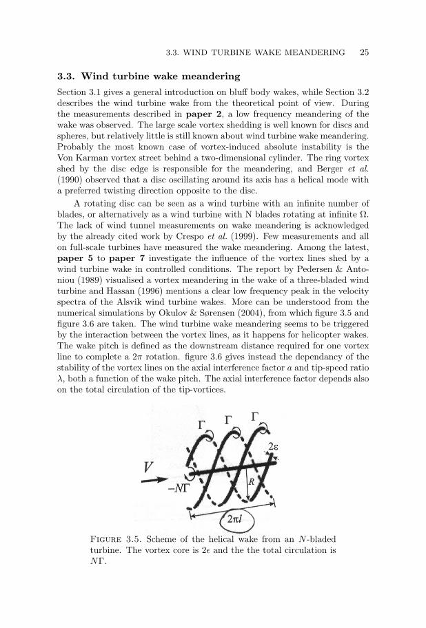
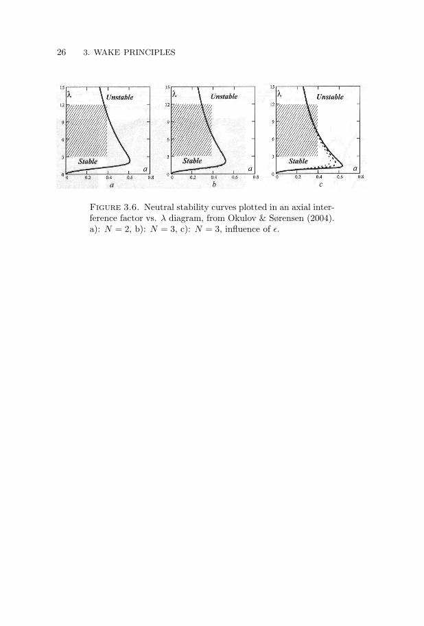
A rotating disc can be seen as a wind turbine with an infinite number ofblades, or alternatively as a wind turbine with N blades rotating at infinite Ω.The lack of wind tunnel measurements on wake meandering is acknowledgedby the already cited work by Crespo et al. (1999). Few measurements and allon full-scale turbines have measured the wake meandering. Among the latest,paper 5 to paper 7 investigate the influence of the vortex lines shed by awind turbine wake in controlled conditions. The report by Pedersen & Anto-niou (1989) visualised a vortex meandering in the wake of a three-bladed windturbine and Hassan (1996) mentions a clear low frequency peak in the velocityspectra of the Alsvik wind turbine wakes. More can be understood from thenumerical simulations by Okulov & Sørensen (2004), from which figure 3.5 andfigure 3.6 are taken. The wind turbine wake meandering seems to be triggeredby the interaction between the vortex lines, as it happens for helicopter wakes.The wake pitch is defined as the downstream distance required for one vortexline to complete a 2π rotation. figure 3.6 gives instead the dependancy of thestability of the vortex lines on the axial interference factor a and tip-speed ratioλ, both a function of the wake pitch. The axial interference factor depends alsoon the total circulation of the tip-vortices.
Figure 3.5. Scheme of the helical wake from an N -bladedturbine. The vortex core is 2ε and the the total circulation isNΓ.
26 3. WAKE PRINCIPLES
Figure 3.6. Neutral stability curves plotted in an axial inter-ference factor vs. λ diagram, from Okulov & Sørensen (2004).a): N = 2, b): N = 3, c): N = 3, influence of ε.
CHAPTER 4
Experimental Methods
This chapter describes the different experimental techniques as well as the windturbine models used in the present work in some more detail than has beenpossible to include in the research papers. Section 4.1 gives a short descriptionof the MTL wind tunnel where most of the experimental work was carried out.Also a short description of LT-5 wind tunnel at FOI is given. The velocitymeasurement techniques used was both Particle Image Velocimetry (PIV) aswell as hot-wire anemometry. Both techniques as they have been implementedin the present work, are described in section 4.2. Several different turbinemodels have been used during the course of this work and they are all describedin section 4.3.
4.1. Wind tunnels
4.1.1. MTL wind tunnel (KTH)
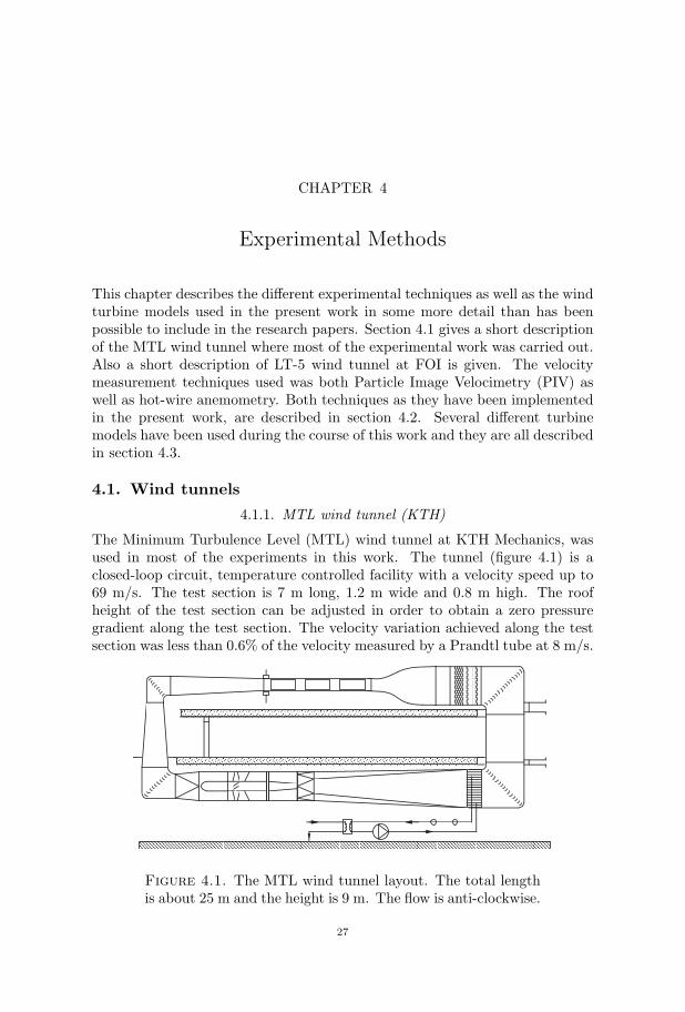
The Minimum Turbulence Level (MTL) wind tunnel at KTH Mechanics, wasused in most of the experiments in this work. The tunnel (figure 4.1) is aclosed-loop circuit, temperature controlled facility with a velocity speed up to69 m/s. The test section is 7 m long, 1.2 m wide and 0.8 m high. The roofheight of the test section can be adjusted in order to obtain a zero pressuregradient along the test section. The velocity variation achieved along the testsection was less than 0.6% of the velocity measured by a Prandtl tube at 8 m/s.
Figure 4.1. The MTL wind tunnel layout. The total lengthis about 25 m and the height is 9 m. The flow is anti-clockwise.
27
28 4. EXPERIMENTAL METHODS
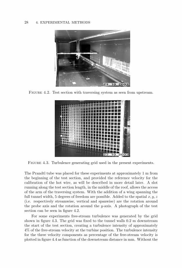
Figure 4.2. Test section with traversing system as seen from upstream.
Figure 4.3. Turbulence generating grid used in the present experiments.
The Prandtl tube was placed for these experiments at approximately 1 m fromthe beginning of the test section, and provided the reference velocity for thecalibration of the hot wire, as will be described in more detail later. A slotrunning along the test section length, in the middle of the roof, allows the accessof the arm of the traversing system. With the addition of a wing spanning thefull tunnel width, 5 degrees of freedom are possible. Added to the spatial x, y, z(i.e. respectively streamwise, vertical and spanwise) are the rotation aroundthe probe axis and the rotation around the y-axis. A photograph of the testsection can be seen in figure 4.2.
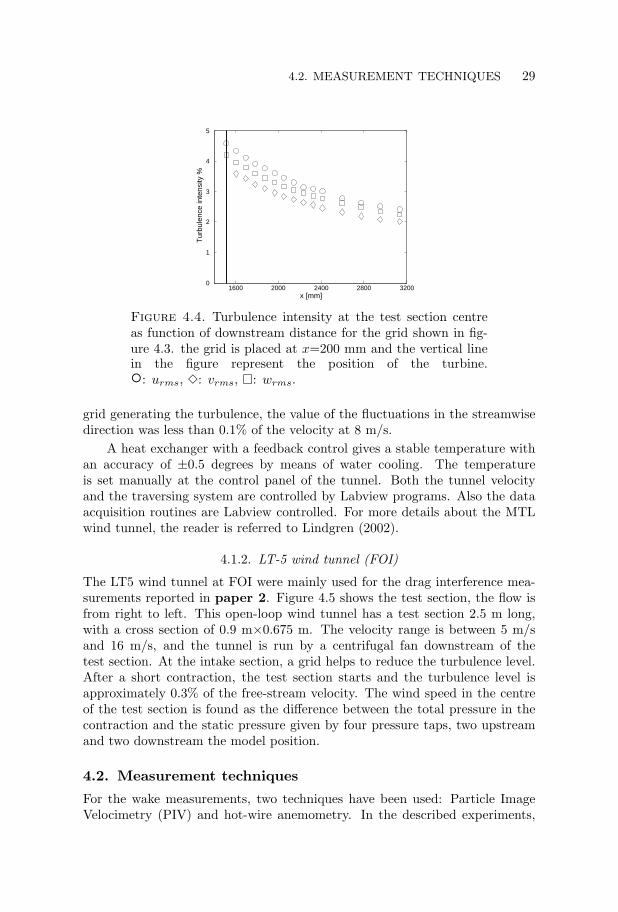
For some experiments free-stream turbulence was generated by the gridshown in figure 4.3. The grid was fixed to the tunnel walls 0.2 m downstreamthe start of the test section, creating a turbulence intensity of approximately4% of the free-stream velocity at the turbine position. The turbulence intensityfor the three velocity components as percentage of the free-stream velocity isplotted in figure 4.4 as function of the downstream distance in mm. Without the
4.2. MEASUREMENT TECHNIQUES 29
1600 2000 2400 2800 32000
1
2
3
4
5
x [mm]
Tur
bule
nce
inte
nsity
%
Figure 4.4. Turbulence intensity at the test section centreas function of downstream distance for the grid shown in fig-ure 4.3. the grid is placed at x=200 mm and the vertical linein the figure represent the position of the turbine.: urms, 3: vrms, : wrms.
grid generating the turbulence, the value of the fluctuations in the streamwisedirection was less than 0.1% of the velocity at 8 m/s.
A heat exchanger with a feedback control gives a stable temperature withan accuracy of ±0.5 degrees by means of water cooling. The temperatureis set manually at the control panel of the tunnel. Both the tunnel velocityand the traversing system are controlled by Labview programs. Also the dataacquisition routines are Labview controlled. For more details about the MTLwind tunnel, the reader is referred to Lindgren (2002).
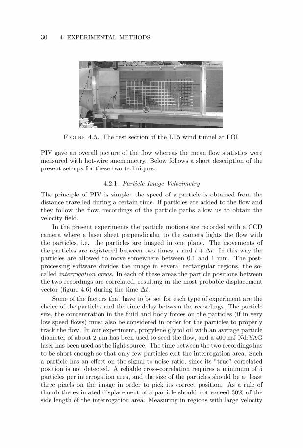
4.1.2. LT-5 wind tunnel (FOI)
The LT5 wind tunnel at FOI were mainly used for the drag interference mea-surements reported in paper 2. Figure 4.5 shows the test section, the flow isfrom right to left. This open-loop wind tunnel has a test section 2.5 m long,with a cross section of 0.9 m×0.675 m. The velocity range is between 5 m/sand 16 m/s, and the tunnel is run by a centrifugal fan downstream of thetest section. At the intake section, a grid helps to reduce the turbulence level.After a short contraction, the test section starts and the turbulence level isapproximately 0.3% of the free-stream velocity. The wind speed in the centreof the test section is found as the difference between the total pressure in thecontraction and the static pressure given by four pressure taps, two upstreamand two downstream the model position.
4.2. Measurement techniques
For the wake measurements, two techniques have been used: Particle ImageVelocimetry (PIV) and hot-wire anemometry. In the described experiments,
30 4. EXPERIMENTAL METHODS
Figure 4.5. The test section of the LT5 wind tunnel at FOI.
PIV gave an overall picture of the flow whereas the mean flow statistics weremeasured with hot-wire anemometry. Below follows a short description of thepresent set-ups for these two techniques.
4.2.1. Particle Image Velocimetry
The principle of PIV is simple: the speed of a particle is obtained from thedistance travelled during a certain time. If particles are added to the flow andthey follow the flow, recordings of the particle paths allow us to obtain thevelocity field.
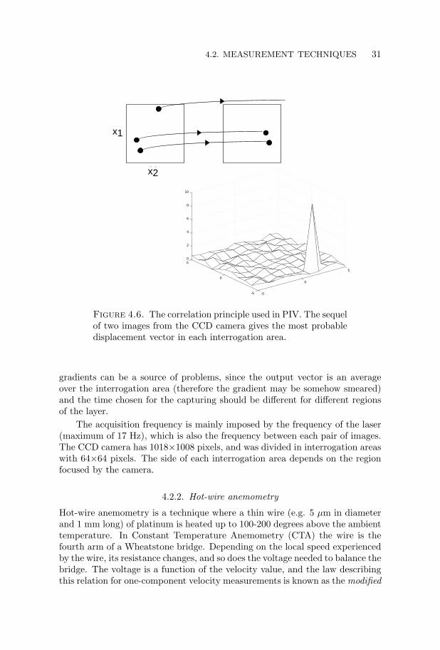
In the present experiments the particle motions are recorded with a CCDcamera where a laser sheet perpendicular to the camera lights the flow withthe particles, i.e. the particles are imaged in one plane. The movements ofthe particles are registered between two times, t and t + ∆t. In this way theparticles are allowed to move somewhere between 0.1 and 1 mm. The post-processing software divides the image in several rectangular regions, the so-called interrogation areas. In each of these areas the particle positions betweenthe two recordings are correlated, resulting in the most probable displacementvector (figure 4.6) during the time ∆t.
Some of the factors that have to be set for each type of experiment are thechoice of the particles and the time delay between the recordings. The particlesize, the concentration in the fluid and body forces on the particles (if in verylow speed flows) must also be considered in order for the particles to properlytrack the flow. In our experiment, propylene glycol oil with an average particlediameter of about 2 µm has been used to seed the flow, and a 400 mJ Nd:YAGlaser has been used as the light source. The time between the two recordings hasto be short enough so that only few particles exit the interrogation area. Sucha particle has an effect on the signal-to-noise ratio, since its ”true” correlatedposition is not detected. A reliable cross-correlation requires a minimum of 5particles per interrogation area, and the size of the particles should be at leastthree pixels on the image in order to pick its correct position. As a rule ofthumb the estimated displacement of a particle should not exceed 30% of theside length of the interrogation area. Measuring in regions with large velocity
4.2. MEASUREMENT TECHNIQUES 31
-5
0
5
-5
0
50
2
4
6
8
10
x2
x1x1
x2
Figure 4.6. The correlation principle used in PIV. The sequelof two images from the CCD camera gives the most probabledisplacement vector in each interrogation area.
gradients can be a source of problems, since the output vector is an averageover the interrogation area (therefore the gradient may be somehow smeared)and the time chosen for the capturing should be different for different regionsof the layer.
The acquisition frequency is mainly imposed by the frequency of the laser(maximum of 17 Hz), which is also the frequency between each pair of images.The CCD camera has 1018×1008 pixels, and was divided in interrogation areaswith 64×64 pixels. The side of each interrogation area depends on the regionfocused by the camera.
4.2.2. Hot-wire anemometry
Hot-wire anemometry is a technique where a thin wire (e.g. 5 µm in diameterand 1 mm long) of platinum is heated up to 100-200 degrees above the ambienttemperature. In Constant Temperature Anemometry (CTA) the wire is thefourth arm of a Wheatstone bridge. Depending on the local speed experiencedby the wire, its resistance changes, and so does the voltage needed to balance thebridge. The voltage is a function of the velocity value, and the law describingthis relation for one-component velocity measurements is known as the modified
32 4. EXPERIMENTAL METHODS
King’s Law, see Johansson & Alfredsson (1982):
U = k1(E2 − E20)
1n + k2
√E − E0 (4.1)
where E is the measured voltage, E0 the voltage at zero velocity, and k1, k2,n are the coefficients from the calibration. The wire is soldered to two prongswhich are shaped in order to reduce their influence on the flow.
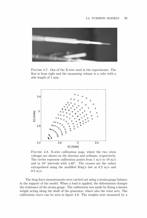
Using two wires placed approximately 45 degrees with respect to the flowdirection, the two velocity components can be calculated as combination ofthe voltages output from the wires. Such a probe is called an X-probe and aphotograph of one of the probes used (and built at KTH Mechanics) is shownin figure 4.7. The size of the measurement volume is 1 mm3 In the calibration,the probe is turned to a known angle (from –40 to +40) with respect tothe free-stream velocity (from 1 m/s to 18 m/s) measured by a Prandtl tube.Two 2-dimensional fifth order polynomials are fitted to the voltages and thecoefficients are calculated with the least square method. A typical calibrationmap is shown in figure 4.8.
Calibration points were taken down to a free-stream velocity of 1 m/s. Iflower velocities need to be measured by the hot-wire, this is not a problemwhen the modified King’s law is used (Eq. 4.1). The polynomials must insteadinclude the velocity range of the measurements. The reason is that the fittingpolynomials are not reliable outside the calibration range, since they can divergeto infinity. A solution was found in order to include also the points for velocitieslower than the allowed minimum of 1 m/s. The voltages from each wire, havingin common the same angle with respect to the wind direction, were fitted to themodified King’s law. In this way, the voltage values for lower velocities (namely0.2 m/s and 0.5 m/s) were extrapolated and inserted in the calibration map ofthe X-wire. Differences were noticeable with the calibration corrected in thisway.
4.3. Turbine models
The main advantage of doing simulation of wind turbines in a wind tunnel,as compared to field measurements, is the controlled flow conditions. On theother hand, the Reynolds number cannot be matched: the difference in chordis evident and wind speed must be kept low to avoid too high rotational speed.The latter may be a source of problem, since the centrifugal forces can modifythe boundary layer on the blades and the development of the wake itself. Onthe other hand, as mentioned by Vermeer et al. (2003), measurements at lowReynolds number are suitable for comparison with numerical models as longas an appropriate wing profile is chosen.
The power output of the turbine can simply be measured from the currentand voltage across the generator. However in this case the internal friction aswell as losses in the generator are not taken into account. By instead calibratingthe generator to obtain the torque from the current its is possible to get theaerodynamic power efficiency.
4.3. TURBINE MODELS 33
Figure 4.7. One of the X-wire used in the experiments. Theflow is from right and the measuring volume is a cube with aside length of 1 mm.
2.6 3 3.42.2
2.6
3
3.4
E1 [Volts]
E2
[Vol
ts]
Figure 4.8. X-wire calibration map, where the two wiresvoltages are shown on the abscissa and ordinate, respectively.The circles represent calibration points from 1 m/s to 18 m/sand in 10 intervals with ±40. The crosses are the valuesextrapolated using the modified King’s law at 0.2 m/s and0.5 m/s.
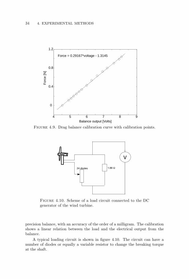
The drag force measurements were carried out using a strain-gauge balancein the support of the model. When a load is applied, the deformation changesthe resistance of the strain-gauge. The calibration was made by fixing a knownweight acting along the shaft of the generator, where also the rotor acts. Thecalibration curve can be seen in figure 4.9. The weights were measured by a
34 4. EXPERIMENTAL METHODS
4 5 6 7 8 9
0
0.4
0.8
1.2
Balance output [Volts]
For
ce [N
]
Force = 0.29167*voltage - 1.3145
Figure 4.9. Drag balance calibration curve with calibration points.
1.66 !24 diodes
V
Figure 4.10. Scheme of a load circuit connected to the DCgenerator of the wind turbine.
precision balance, with an accuracy of the order of a milligram. The calibrationshows a linear relation between the load and the electrical output from thebalance.
A typical loading circuit is shown in figure 4.10. The circuit can have anumber of diodes or equally a variable resistor to change the breaking torqueat the shaft.
4.3. TURBINE MODELS 35
4.3.1. Turbine model 1
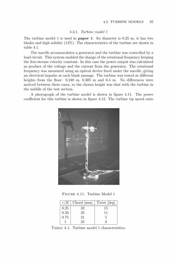
The turbine model 1 is used in paper 1. Its diameter is 0.25 m, it has twoblades and high solidity (14%). The characteristics of the turbine are shown intable 4.1.
The nacelle accommodates a generator and the turbine was controlled by aload circuit. This system enabled the change of the rotational frequency keepingthe free-stream velocity constant. In this case the power output was calculatedas product of the voltage and the current from the generator. The rotationalfrequency was measured using an optical device fixed under the nacelle, givingan electrical impulse at each blade passage. The turbine was tested at differentheights from the floor: 0.248 m, 0.305 m and 0.4 m. No differences werenoticed between these cases, so the chosen height was that with the turbine inthe middle of the test section.
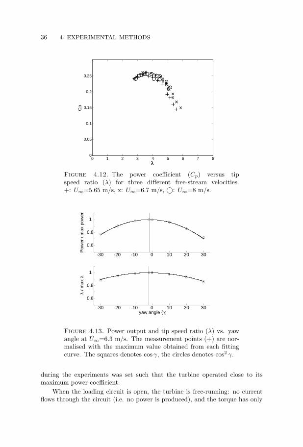
A photograph of the turbine model is shown in figure 4.11. The powercoefficient for this turbine is shown in figure 4.12. The turbine tip speed ratio
Figure 4.11. Turbine Model 1
r/R Chord [mm] Twist [deg]0.25 32 150.50 35 110.75 31 51 25 3
Table 4.1. Turbine model 1 characteristics.
36 4. EXPERIMENTAL METHODS
0 1 2 3 4 5 6 7 80
0.05
0.1
0.15
0.2
0.25
λ
Cp
Figure 4.12. The power coefficient (Cp) versus tipspeed ratio (λ) for three different free-stream velocities.+: U∞=5.65 m/s, x: U∞=6.7 m/s, ©: U∞=8 m/s.
-30 -20 -10 0 10 20 30
0.6
0.8
1
Pow
er /
max
pow
er
-30 -20 -10 0 10 20 30
0.6
0.8
1
λ / m
ax λ
yaw angle (γ)
Figure 4.13. Power output and tip speed ratio (λ) vs. yawangle at U∞=6.3 m/s. The measurement points (+) are nor-malised with the maximum value obtained from each fittingcurve. The squares denotes cos γ, the circles denotes cos2 γ.
during the experiments was set such that the turbine operated close to itsmaximum power coefficient.
When the loading circuit is open, the turbine is free-running: no currentflows through the circuit (i.e. no power is produced), and the torque has only
4.3. TURBINE MODELS 37
to overcome the internal friction of the rotating parts. Therefore the rotationalspeed is at the maximum value. The open circuit can be achieved by alsoincreasing the variable resistance to a value where the generator is unable toproduce a current through the circuit. The opposite situation is when theresistance is zero, or the circuit is short-circuit.
4.3.1.1. Yaw dependence
Another characteristic investigated for this wind turbine is the variation of thepower with respect to the flow angle. In figure 4.13 the variation both of Cp
and the tip speed ratio is shown for turbine model 1 keeping the loading con-stant. Both the power curve and the tip speed ratio as function of the yawangle showed a symmetric behaviour after a small offset was applied. The–1.8 degrees offset may be due to an asymmetry in the turbine behaviour be-cause of the direction of rotation. For this model the variation of the outputpower is nearly proportional to the square of cos γ, whereas the tip speed ratiovaries linearly with cos γ when the loading on the turbine was constant.
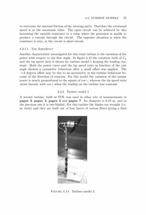
4.3.2. Turbine model 2
A second turbine, built at FOI, was used in other sets of measurements inpaper 2, paper 3, paper 5 and paper 7. Its diameter is 0.18 m, and asthe previous one it is two-bladed. For this turbine the blades are straight (i.e.no twist) and they are built out of four layers of carbon fibres giving a final
Figure 4.14. Turbine model 2.
38 4. EXPERIMENTAL METHODS
thickness of 0.5 mm. The profile is based on the Gottingen 417A airfoil, chosenfor its good performance at low Reynolds number. The chord at the tip is16 mm and the maximum chord is 27 mm, at 12% of the radius. The solidityis 13%. The blades are attached by a screw, 3 mm in diameter, to the 23 mmdiameter nacelle. These screws allow the setting of the pitch angle of the blades,defined as the line connecting the leading edge to the trailing edge at 85% ofthe radius. A designated set-up was built at FOI to fix the pitch angle (seeMontgomerie & Dahlberg (2003)) and allows an accuracy of ±0.05 degrees.
The blade pair is connected to a 24V DC motor that works as a generator.In this case the torque was calibrated versus the output voltage and was shownto be a straight line. Hence the aerodynamic power produced by the turbinecan be calculated by measuring the generator voltage and the rotational speed.
The other important characteristic for a wind turbine is the drag1 coeffi-cient. The results e.g. in paper 3 show how the drag coefficient first increaseswith the tip speed ratio and then tends to level out at a value which is of theorder of 0.9. During the experiments, the running conditions for the turbine,such as power and drag coefficients, were measured and compared before andafter. No change was observed, proving that the model had stable characteris-tics during the maximum 30 hours measurements period. Details on the bladegeometry can be seen in the Appendix of paper 5.
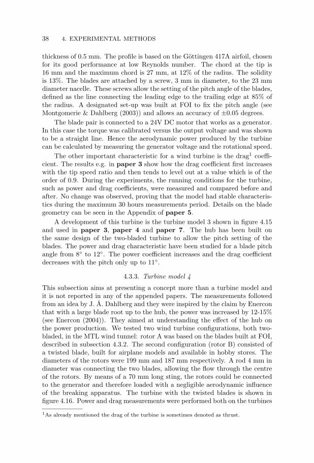
A development of this turbine is the turbine model 3 shown in figure 4.15and used in paper 3, paper 4 and paper 7. The hub has been built onthe same design of the two-bladed turbine to allow the pitch setting of theblades. The power and drag characteristic have been studied for a blade pitchangle from 8 to 12. The power coefficient increases and the drag coefficientdecreases with the pitch only up to 11.
4.3.3. Turbine model 4
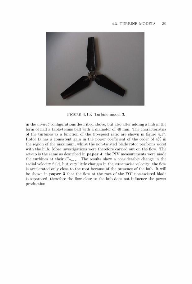
This subsection aims at presenting a concept more than a turbine model andit is not reported in any of the appended papers. The measurements followedfrom an idea by J. A. Dahlberg and they were inspired by the claim by Enerconthat with a large blade root up to the hub, the power was increased by 12-15%(see Enercon (2004)). They aimed at understanding the effect of the hub onthe power production. We tested two wind turbine configurations, both two-bladed, in the MTL wind tunnel: rotor A was based on the blades built at FOI,described in subsection 4.3.2. The second configuration (rotor B) consisted ofa twisted blade, built for airplane models and available in hobby stores. Thediameters of the rotors were 199 mm and 187 mm respectively. A rod 4 mm indiameter was connecting the two blades, allowing the flow through the centreof the rotors. By means of a 70 mm long sting, the rotors could be connectedto the generator and therefore loaded with a negligible aerodynamic influenceof the breaking apparatus. The turbine with the twisted blades is shown infigure 4.16. Power and drag measurements were performed both on the turbines
1As already mentioned the drag of the turbine is sometimes denoted as thrust.
4.3. TURBINE MODELS 39
Figure 4.15. Turbine model 3.
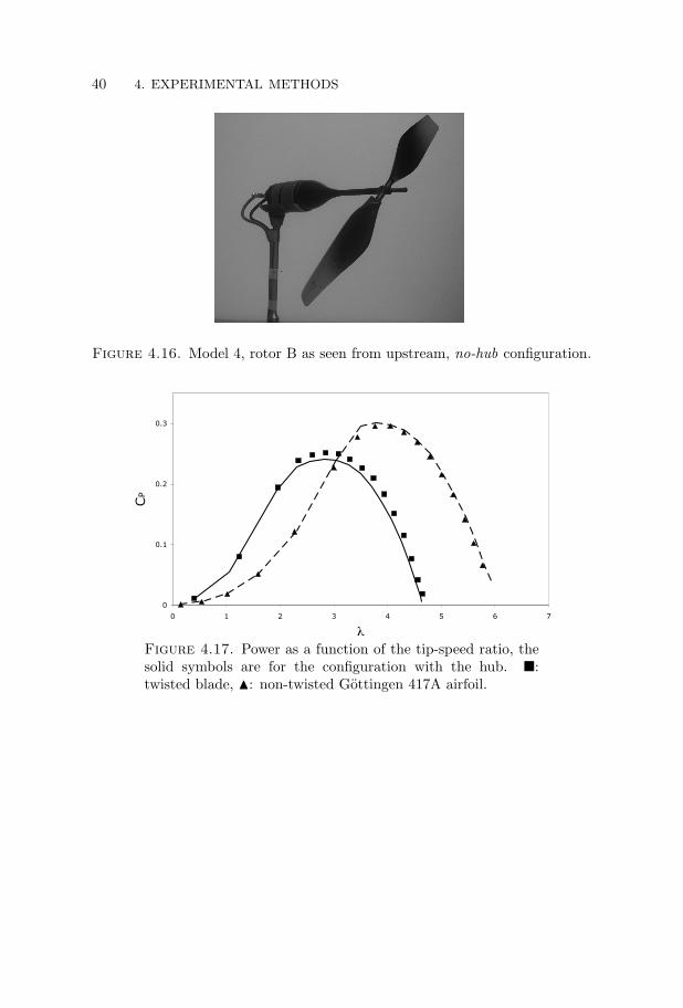
in the no-hub configurations described above, but also after adding a hub in theform of half a table-tennis ball with a diameter of 40 mm. The characteristicsof the turbines as a function of the tip-speed ratio are shown in figure 4.17.Rotor B has a consistent gain in the power coefficient of the order of 4% inthe region of the maximum, whilst the non-twisted blade rotor performs worstwith the hub. More investigations were therefore carried out on the flow. Theset-up is the same as described in paper 4: the PIV measurements were madethe turbines at their CPmax
. The results show a considerable change in theradial velocity field, but very little changes in the streamwise velocity: the flowis accelerated only close to the root because of the presence of the hub. It willbe shown in paper 3 that the flow at the root of the FOI non-twisted bladeis separated, therefore the flow close to the hub does not influence the powerproduction.
40 4. EXPERIMENTAL METHODS
Figure 4.16. Model 4, rotor B as seen from upstream, no-hub configuration.
0
0.1
0.2
0.3
0 1 2 3 4 5 6 7
λ
CP
Figure 4.17. Power as a function of the tip-speed ratio, thesolid symbols are for the configuration with the hub. :twisted blade, N: non-twisted Gottingen 417A airfoil.
CHAPTER 5
Summary of papers and authors contributions
The thesis is based on the following seven papers.
Paper 1Parkin, P., Holm, R. and Medici, D. “The application of PIV to the wake of awind turbine in yaw”, Proc. 4th International Symposium on Particle ImageVelocimetry, Gottingen, 2001.
The experiment was led by PP and RH. The data processing and analysis wasdone by DM supervised by PP. The paper was written by PP and RH, whereasDM analysed the data.
Paper 2Dahlberg, J. A. and Medici, D. “Potential Improvement of wind turbine ar-ray efficiency by active wake control (AWC)”, Proc. European Wind EnergyConference, Madrid, 2003.
The work was equally divided between the authors. The original idea of AWCwas by JAD.
Paper 3Medici, D. “Influence of the number of blades on the wake of a wind turbinemodel”.
Paper 4Medici, D. “The upstream flow of a 3-bladed wind turbine model in yaw”.
Paper 5Medici, D. and Alfredsson, P.H. “Measurements on a wind turbine wake: 3Deffects and bluff-body vortex shedding”, Wind Energy. Published online.
The measurements were performed by DM, as well as the data analysis. Thepaper was written together with HAL.
Paper 6Medici, D. and Alfredsson, P.H. “Wind Turbine Near Wakes and Comparisonsto the Wake Behind a Disc”, AIAA-paper-205-0595.
41
42 5. SUMMARY OF PAPERS AND AUTHORS CONTRIBUTIONS
The measurements were performed by DM, as well as the data analysis. Thepaper was written together with HAL.
Paper 7Medici, D. “A note on the frequency of wind turbine wake meandering”.
5.1. Summary of papers
In paper 1 the near wake downstream a rotating wind turbine model is studiedusing PIV, both with the turbine normal to the free stream direction and underyawed conditions. It is shown that yawing the turbine makes the wake deflecttowards the side of the downstream blade, in response to a force perpendicularto the wind direction. The PIV used in the experiment allowed several instantpictures of the flow, and in specific of the tip vortices. The vortices, togetherwith the rotation of the wake, seem to make the difference with the wakefrom another bluff body, as if the wake can be frozen until these vortices areparticularly strong and easily detectable. The effect of yawing can be seen inthe mean velocity values, which are known every few millimetres thanks to thetechnique used for the measurements. The velocity in a chosen point can evendouble when the wake moves away.
In paper 2 various effects on a single turbine under yaw is studied aswell as the interaction between two turbines by traversing one turbine in thespanwise direction downstream an undisturbed turbine. In this way a directmeasure of the power interference can be obtained, showing itself in terms of”power wakes”. The effect of yaw on the power deficit is studied and a modelfor a wind farm is used to predict the effect of active yaw control. It is shownthat for a six turbine station an increase in power of about 4% can be achieved.
Paper 3 describes in detail the changes in the wake as a consequence ofthe number of blades. Wind turbines with two and three blades have beenstudied in connection with their commercial production, while the one-bladedturbine has a more fundamental importance: the helical wake can be clearlyvisualised since the vortex lines shed by the blade tip are far from each other.The multi-bladed turbine, although with the same pitch, shows on the otherhand a high mixing in the wake. The velocity field has been measured up to 9diameters downstream for some chosen conditions and at x/D = 1 as a functionof the tip-speed ratio. The shape of the wake seems to change dramatically inthe central region and becomes deeper for high λ.
All the previous papers dealt with the near or far wake, while paper 4focus on the flow immediately upstream of the rotor. The 3-bladed turbinehas been yawed and the flow is proved to be two-dimensional up to typically3-4 mm from the blades, where the viscosity induces the rotation of the flow.The reduction of the power with the yaw angle goes with the cube of the windspeed, but this coefficient is highly dependent on the number of blades. Thepaper shows that the momentum theory can be successfully applied upstreamof a rotating wind turbine.
5.1. SUMMARY OF PAPERS 43
In paper 5 the wind turbine wake is studied using two component hot-wire measurements. It is shown that the wake from a single wind turbineexhibits a large degree of non-symmetry with respect to the central axis whenyawed. The effect of free stream turbulence is also studied. An unexpectedand interesting phenomenon was observed during the measurements, namely alarge scale motion of the wake which reflects itself in low frequency variationsas detected by the hot wire measurements. The frequency, if expressed as aStrouhal number, is similar to what one would expect for shedding behind asolid disc and it was concluded that the turbine sheds vortices in a similarway as a disc. It was hypothesized that the meandering of the wake observedbehind full scale turbines is due to such vortex shedding.
Paper 6 compares the meandering frequencies of the two-bladed modelof paper 5 to the meandering behind porous discs. It was observed that theStrouhal number depends on the tip-speed ratio and tends to the values givenby porous discs. A turbine in yaw increases the low-frequency shedding ina similar way as a solid disc. In this respect, the vortex ring behind a disccan be seen as the limit for λ → ∞ of the vortex structures behind a windturbine. The meandering frequency behind a disc disappears for high porosity,as showed also by Castro (1971).
In order to further investigate the parameters influencing the meandering,the measurements presented in paper 7 were performed in the wake of turbineswith different number of blades, blade pitch and tip-speed ratio. The meander-ing frequency was observed to change for the different configurations, althougha connection with the drag coefficient was not established. At the same time,the low frequency showed to be dependent on the number of blades, suggestinga link to the blade passage frequency. This finding is in agreement with thetheory, according to which the wake meandering depends on the wake pitch(a measure of the distance between the vortex lines), on the axial interferencefactor and on the vortex strength.
Acknowledgements
This work was mainly financed under the Vindforsk program of the EnergyAgency of Sweden (STEM) and for the final crucial months by Elforsk, forboth of which I am very grateful.
I want to thank first my supervisor Prof. Henrik Alfredsson for his adviceand help during my course of studies. His contributions have always taught mesomething important.
Jan-Ake Dahlberg has had a crucial role during these years. Thank youfor your help, enthusiasm and friendship. My work would not have been pos-sible without your assistance. Sven-Erik Thor and Bjorn Montgomerie arealso acknowledged for their many fruitful discussions and help. I also want tothank Prof. Jens Sørensen for his comments and for many discussions on wakemeandering.
Prof. Y. Kohama and Dr. S. Yoshioka are acknowledged for the assistanceand the welcome provided during the 21st Century COE internship at theTohoku University, Sendai, Japan.
Marcus Gallstedt and Ulf Landen always made my ideas a reality. Dr. NilsTillmark is acknowledged for his assistance and help with many problems.
Luca F. and Marco have become true and important friends. A specialthanks goes to Leandro for his friendship and for the Wednesdays lunches.
Many other people need to be mentioned: Luca B., Ramis the runner,Mike, Fredrik, Jens and everybody in the Lab and at the Department. Junand Kristian: thank you for the great time in Stockholm and in Tokyo.
My Swedish journey started seven years ago and I will never forget all thefriends that made my time here worthwhile. The months during my Nippo-Kiwi-Aussie journey were unforgettable, thanks to everyone who made it sospecial and sharpened my English listening!
Last but not least, I would like to mention the same people who have beenthere for me over the years. Despite the distance, we are even closer. Thanksto my brother Dario, to Cesare, Luca S. and Guido.
Grazie alla mia famiglia per il supporto durante tutti questi anni.
44
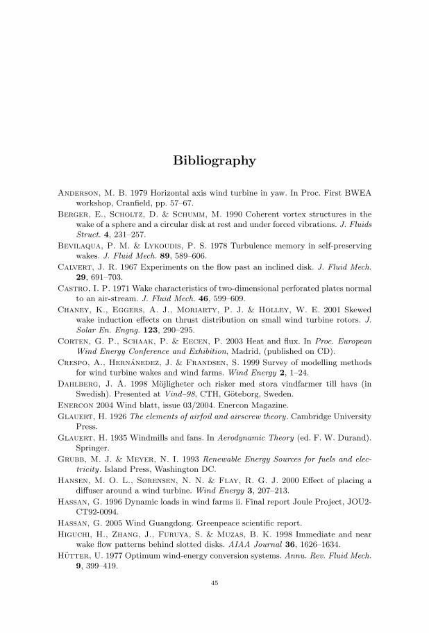
Bibliography
Anderson, M. B. 1979 Horizontal axis wind turbine in yaw. In Proc. First BWEAworkshop, Cranfield, pp. 57–67.
Berger, E., Scholtz, D. & Schumm, M. 1990 Coherent vortex structures in thewake of a sphere and a circular disk at rest and under forced vibrations. J. FluidsStruct. 4, 231–257.
Bevilaqua, P. M. & Lykoudis, P. S. 1978 Turbulence memory in self-preservingwakes. J. Fluid Mech. 89, 589–606.
Calvert, J. R. 1967 Experiments on the flow past an inclined disk. J. Fluid Mech.29, 691–703.
Castro, I. P. 1971 Wake characteristics of two-dimensional perforated plates normalto an air-stream. J. Fluid Mech. 46, 599–609.
Chaney, K., Eggers, A. J., Moriarty, P. J. & Holley, W. E. 2001 Skewedwake induction effects on thrust distribution on small wind turbine rotors. J.Solar En. Engng. 123, 290–295.
Corten, G. P., Schaak, P. & Eecen, P. 2003 Heat and flux. In Proc. EuropeanWind Energy Conference and Exhibition, Madrid, (published on CD).
Crespo, A., Hernanedez, J. & Frandsen, S. 1999 Survey of modelling methodsfor wind turbine wakes and wind farms. Wind Energy 2, 1–24.
Dahlberg, J. A. 1998 Mojligheter och risker med stora vindfarmer till havs (inSwedish). Presented at Vind–98, CTH, Goteborg, Sweden.
Enercon 2004 Wind blatt, issue 03/2004. Enercon Magazine.
Glauert, H. 1926 The elements of airfoil and airscrew theory . Cambridge UniversityPress.
Glauert, H. 1935 Windmills and fans. In Aerodynamic Theory (ed. F. W. Durand).Springer.
Grubb, M. J. & Meyer, N. I. 1993 Renewable Energy Sources for fuels and elec-tricity . Island Press, Washington DC.
Hansen, M. O. L., Sørensen, N. N. & Flay, R. G. J. 2000 Effect of placing adiffuser around a wind turbine. Wind Energy 3, 207–213.
Hassan, G. 1996 Dynamic loads in wind farms ii. Final report Joule Project, JOU2-CT92-0094.
Hassan, G. 2005 Wind Guangdong. Greenpeace scientific report.
Higuchi, H., Zhang, J., Furuya, S. & Muzas, B. K. 1998 Immediate and nearwake flow patterns behind slotted disks. AIAA Journal 36, 1626–1634.
Hutter, U. 1977 Optimum wind-energy conversion systems. Annu. Rev. Fluid Mech.9, 399–419.
45
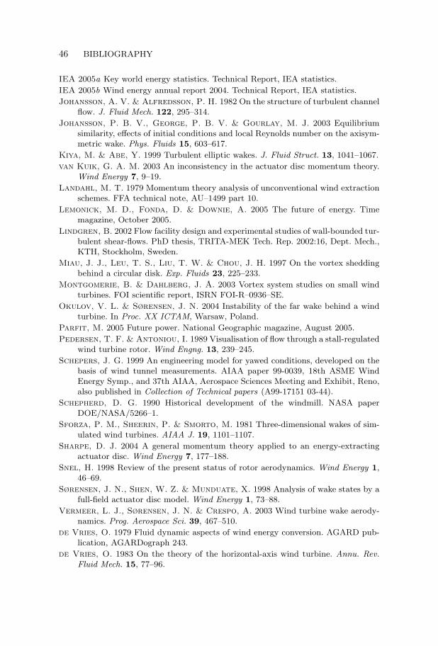
46 BIBLIOGRAPHY
IEA 2005a Key world energy statistics. Technical Report, IEA statistics.
IEA 2005b Wind energy annual report 2004. Technical Report, IEA statistics.
Johansson, A. V. & Alfredsson, P. H. 1982 On the structure of turbulent channelflow. J. Fluid Mech. 122, 295–314.
Johansson, P. B. V., George, P. B. V. & Gourlay, M. J. 2003 Equilibriumsimilarity, effects of initial conditions and local Reynolds number on the axisym-metric wake. Phys. Fluids 15, 603–617.
Kiya, M. & Abe, Y. 1999 Turbulent elliptic wakes. J. Fluid Struct. 13, 1041–1067.
van Kuik, G. A. M. 2003 An inconsistency in the actuator disc momentum theory.Wind Energy 7, 9–19.
Landahl, M. T. 1979 Momentum theory analysis of unconventional wind extractionschemes. FFA technical note, AU–1499 part 10.
Lemonick, M. D., Fonda, D. & Downie, A. 2005 The future of energy. Timemagazine, October 2005.
Lindgren, B. 2002 Flow facility design and experimental studies of wall-bounded tur-bulent shear-flows. PhD thesis, TRITA-MEK Tech. Rep. 2002:16, Dept. Mech.,KTH, Stockholm, Sweden.
Miau, J. J., Leu, T. S., Liu, T. W. & Chou, J. H. 1997 On the vortex sheddingbehind a circular disk. Exp. Fluids 23, 225–233.
Montgomerie, B. & Dahlberg, J. A. 2003 Vortex system studies on small windturbines. FOI scientific report, ISRN FOI-R–0936–SE.
Okulov, V. L. & Sørensen, J. N. 2004 Instability of the far wake behind a windturbine. In Proc. XX ICTAM, Warsaw, Poland.
Parfit, M. 2005 Future power. National Geographic magazine, August 2005.
Pedersen, T. F. & Antoniou, I. 1989 Visualisation of flow through a stall-regulatedwind turbine rotor. Wind Engng. 13, 239–245.
Schepers, J. G. 1999 An engineering model for yawed conditions, developed on thebasis of wind tunnel measurements. AIAA paper 99-0039, 18th ASME WindEnergy Symp., and 37th AIAA, Aerospace Sciences Meeting and Exhibit, Reno,also published in Collection of Technical papers (A99-17151 03-44).
Schepherd, D. G. 1990 Historical development of the windmill. NASA paperDOE/NASA/5266–1.
Sforza, P. M., Sheerin, P. & Smorto, M. 1981 Three-dimensional wakes of sim-ulated wind turbines. AIAA J. 19, 1101–1107.
Sharpe, D. J. 2004 A general momentum theory applied to an energy-extractingactuator disc. Wind Energy 7, 177–188.
Snel, H. 1998 Review of the present status of rotor aerodynamics. Wind Energy 1,46–69.
Sørensen, J. N., Shen, W. Z. & Munduate, X. 1998 Analysis of wake states by afull-field actuator disc model. Wind Energy 1, 73–88.
Vermeer, L. J., Sørensen, J. N. & Crespo, A. 2003 Wind turbine wake aerody-namics. Prog. Aerospace Sci. 39, 467–510.
de Vries, O. 1979 Fluid dynamic aspects of wind energy conversion. AGARD pub-lication, AGARDograph 243.
de Vries, O. 1983 On the theory of the horizontal-axis wind turbine. Annu. Rev.Fluid Mech. 15, 77–96.
Related Documents