Full-Scale Wind Tunnel Study of the Seaglider Underwater Glider Laszlo Techy, Ryan Tomokiyo, Jake Quenzer, Tyler Beauchamp, Kristi Morgansen [email protected] Department of Aeronautics & Astronautics, University of Washington Seattle WA, 98195-2400 UWAA Technical Report Number UWAATR-2010-0002 September 2010 Department of Aeronautics and Astronautics University of Washington Box 352400 Seattle, Washington 98195-2400 PHN: (206) 543-1950 FAX: (206) 543-0217 URL: http://www.aa.washington.edu

Welcome message from author
This document is posted to help you gain knowledge. Please leave a comment to let me know what you think about it! Share it to your friends and learn new things together.
Transcript

Full-Scale Wind Tunnel Study of the Seaglider UnderwaterGlider
Laszlo Techy, Ryan Tomokiyo, Jake Quenzer, Tyler Beauchamp, Kristi [email protected]
Department of Aeronautics & Astronautics, University of WashingtonSeattle WA, 98195-2400
UWAA Technical ReportNumber UWAATR-2010-0002September 2010
Department of Aeronautics and AstronauticsUniversity of WashingtonBox 352400Seattle, Washington 98195-2400PHN: (206) 543-1950FAX: (206) 543-0217URL: http://www.aa.washington.edu
Contents1 Introduction 2
2 Experimental Setup 42.1 Test Configurations . . . . . . . . . . . . . . . . . . . . . . . . . . . . . . . . . . . . . . . . . . . . 42.2 Test Regime . . . . . . . . . . . . . . . . . . . . . . . . . . . . . . . . . . . . . . . . . . . . . . . . 52.3 Conventions and Nomenclature . . . . . . . . . . . . . . . . . . . . . . . . . . . . . . . . . . . . . . 7
3 Results 93.1 Aerodynamic Coefficients for Standard Seaglider . . . . . . . . . . . . . . . . . . . . . . . . . . . . 93.2 Aerodynamic Coefficients for Seaglider with 1.5 m Wings . . . . . . . . . . . . . . . . . . . . . . . 103.3 Effects of the Wings . . . . . . . . . . . . . . . . . . . . . . . . . . . . . . . . . . . . . . . . . . . . 113.4 Drag Comparison of Seaglider Tail Section versus Ogive Tail Section . . . . . . . . . . . . . . . . . 143.5 Parasite Drag and Dynamic Pressure . . . . . . . . . . . . . . . . . . . . . . . . . . . . . . . . . . . 163.6 Drag Contribution from the CT-cell . . . . . . . . . . . . . . . . . . . . . . . . . . . . . . . . . . . 173.7 Static Longitudinal Stability . . . . . . . . . . . . . . . . . . . . . . . . . . . . . . . . . . . . . . . 183.8 Directional Stability . . . . . . . . . . . . . . . . . . . . . . . . . . . . . . . . . . . . . . . . . . . . 19
4 Summary 20
5 Appendix A: Configuration 1 22
6 Appendix B: Configuration 2 25
7 Appendix C: Configuration 3 28
8 Appendix D: Configuration 4 31
9 Appendix E: Parameters 34

Full-Scale Wind Tunnel Study of the Seaglider Underwater Glider
Laszlo Techy, Ryan Tomokiyo, Jake Quenzer, Tyler Beauchamp, Kristi [email protected]
Department of Aeronautics & Astronautics, University of WashingtonSeattle WA, 98195-2400
September 2010
Abstract
This report describes full-scale wind tunnel tests of the Seaglider underwater vehicle that were conducted onJune 30, 2010 in the University of Washington Kirsten Wind Tunnel. The goal of the wind tunnel study was toidentify aerodynamic force-and moment coefficients of the glider. The identified parameters are important for 1) on-line performance calculations; 2) high-fidelity simulations; 3) aiding future glider designs; 4) data post-processing.Several different glider configurations have been tested, including two different tail sections and two different setof wings. The glider’s original concave tail section was interchangeable with a newer design that featured an ogiveprofile. The glider model was also tested both in the presence and in the absence of the conductivity-temperature (CT)cell to measure drag contribution from the CT-cell alone, and to be able to compare results across the tail sections.During the test it was observed that the Seaglider lacks static longitudinal stability at the typical range of operatingReynolds numbers. The lack of static aerodynamic stability is counter-balanced by the moment resulting from theoffset between center of gravity and center of buoyancy. The document presents aerodynamic coefficients for theglider at typical operating speeds.
1 IntroductionThe Seaglider is a buoyancy-driven underwater glider originally developed for oceanographic research. The vehiclewas designed at University of Washington as a collaboration between the Applied Physics Lab and the School ofOceanography [2]. From early design stages significant emphasis has been placed on the aerodynamic properties ofthe vehicle to maximize performance characteristics, such as range and endurance. The streamlined profile of thevehicle outer skin was selected based on hydrodynamic study of axisymmetric bodies in axial flow [5]. The shape thatwas adopted for the vehicle based on this study has the ability to “maintain laminar flow over more than 80% of thesurface area at speeds as high as 7 m/s” [2]. Even though this streamlined shape necessitated a sophisticated pressurehull design, the anticipated performance improvements were large enough to make this design effort worthwhile.
The Deepglider is a variant of the Seaglider currently under development at University of Washington. The Deep-glider’s maximum depth is 6000 m, at which depth extreme stresses are exerted on the pressure hull. This necessitatedthe departure from the tapered Seaglider design, and a technologically simpler and more robust cylindrical shape wasadopted. Drop-tests have been carried out at the saltwater tank facility of the Seaglider Fabrication Center to test dif-ferent outer skin shapes [6]. The drop-tests revealed that the original Seaglider shape had the largest drag-coefficientof all tested models, and that an ogive nose section and tail section performed significantly better. Flow-visualizationstudies conducted in the Low-Speed Wind Tunnel at the University of Washington Aerodynamics Laboratory (UWAL)during early development stages of the glider showed that the flow separates just behind the station of maximum ra-dius on the original Seaglider fairing [2]. It was noted in [6] that the ogive tail prolongs the area of attached flow dueto its convex, gently-tapered shape, explaining some of the performance gain compared to the original Seaglider tailfeaturing a concave profile.
Identification of the aerodynamic force-and moment coefficients of the Seaglider is important for several reasons.1) The parameters can be used in performance studies of the vehicle to help identify optimal flight conditions. Es-timates of these parameters are presently used in on-line guidance calculations on the glider computer to determine
2
desired pitch mass location and buoyancy setting as a function of pilot-specified mission parameters, such as durationof the dive and desired depth. More accurate knowledge of these parameters improves the precision of the glider’s nav-igation algorithm. 2) The aerodynamic parameters are necessary for the development of high-fidelity flight simulationsof the glider. Such simulations can be used to study and validate the efficacy of different motion planning strategies. 3)Comparing the drag coefficient across the different glider configurations helps determine minimum-drag skin profilesand may guide the design of future gliders. 4) The parameters are currently used during post-processing of the glidesand to visualize the glider’s path in the horizontal plane. The paths are reconstructed using dead-reckoning based onthe estimated speed and heading angle. Accurate knowledge of the speed is desired for the accuracy of such plots.
The full-scale wind-tunnel tests described in this document were conducted on June 30, 2010 in the University ofWashington Kirsten Wind Tunnel to accurately measure the aerodynamic properties of the Seaglider. A set of vehicleconfigurations and geometries were tested in the tunnel, including different wings and fairing profiles. In addition tothe identification of the desired force-and moment coefficients, the following observations were made:
• The drag coefficient for the Seaglider with the CT-cell is 47.7 % larger than without the CT-cell.
• The original Seaglider shape (tapered nose-section, concave tail section, 1 m wings) lacks static longitudinalstability in the typical operating regime. It was observed that the aerodynamic center of the vehicle shifts aftwith increasing dynamic pressure, and the glider becomes stable between 0.22 < q < 0.66 psf correspondingto 0.32 < v < 0.56 m/s in water. This speed is currently outside of the glider’s operating regime, although maybe accessible using larger buoyancy engines. The lack of static aerodynamic stability is counter-balanced by themoment couple resulting from the offset between center of gravity and center of buoyancy. This metacentricheight helps recover stability, explaining why the glider performs stable glides in experiments. With the larger,1.5 m, wings the glider is aerodynamically stable in the typical Seaglider operating regime.
• At the glider’s typical operating speed the parasite drag coefficient shows variation with dynamic pressure anddoes not stay constant. The functional dependence suggested in [2] was confirmed in the wind tunnel experi-ments.
• The magnitude of the measured yawing moments is very small, indicating that the glider is marginally direc-tionally stable.
• The drag coefficient for the original Seaglider configuration with the concave tail section is 12.4% larger thanfor the configuration with the newly designed ogive tail section. Although the CT-cell was removed from theSeaglider, the oxygen sensor was left attached by mistake, leaving this test inconclusive as the increased dragmay come from the oxygen sensor.
UWAATR-2010-0002 3
2 Experimental SetupThe full-scale wind-tunnel tests of the Seaglider and modified configurations were conducted in a Reynolds numbermatched test regime at University of Washington Kirsten Wind Tunnel. The tunnel is a subsonic, closed circuit, doublereturn wind tunnel that has a test section with a rectangular 8’ x 12’ cross-section that is 10 feet long. Two sets of 14’9”-diameter seven-bladed propellers move the air up to 200 MPH through the test section. Additional information onthe tunnel can be found in [1].
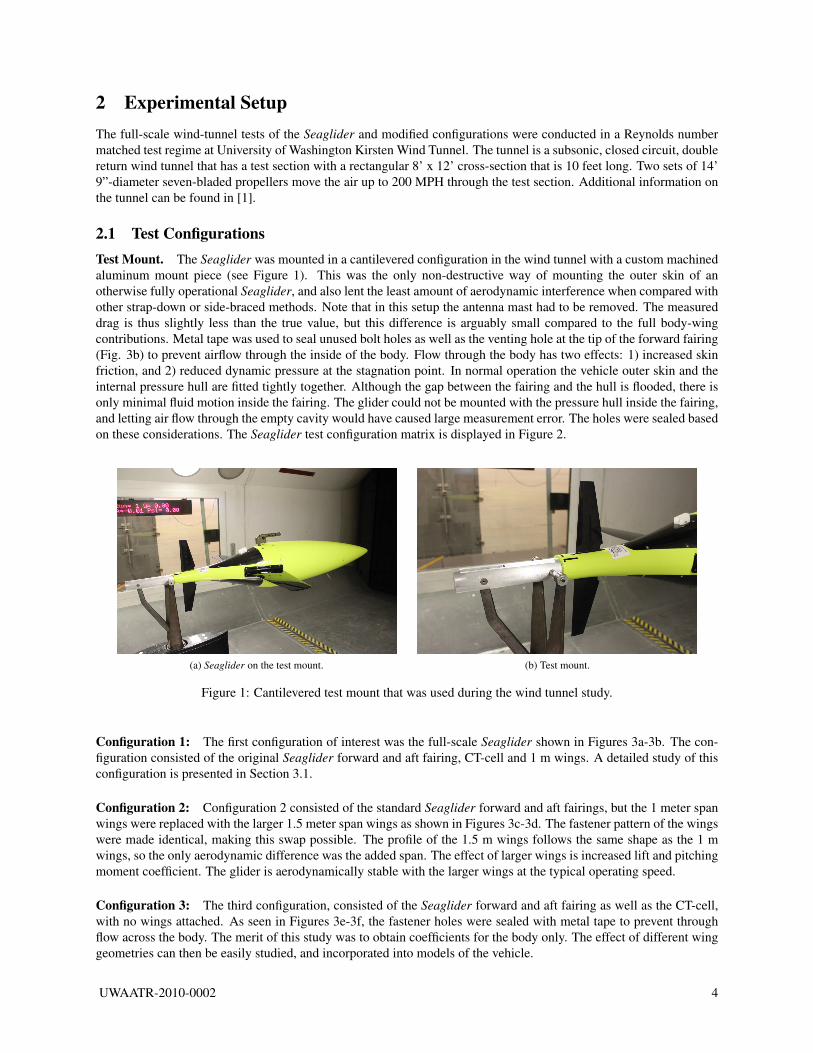
2.1 Test ConfigurationsTest Mount. The Seaglider was mounted in a cantilevered configuration in the wind tunnel with a custom machinedaluminum mount piece (see Figure 1). This was the only non-destructive way of mounting the outer skin of anotherwise fully operational Seaglider, and also lent the least amount of aerodynamic interference when compared withother strap-down or side-braced methods. Note that in this setup the antenna mast had to be removed. The measureddrag is thus slightly less than the true value, but this difference is arguably small compared to the full body-wingcontributions. Metal tape was used to seal unused bolt holes as well as the venting hole at the tip of the forward fairing(Fig. 3b) to prevent airflow through the inside of the body. Flow through the body has two effects: 1) increased skinfriction, and 2) reduced dynamic pressure at the stagnation point. In normal operation the vehicle outer skin and theinternal pressure hull are fitted tightly together. Although the gap between the fairing and the hull is flooded, there isonly minimal fluid motion inside the fairing. The glider could not be mounted with the pressure hull inside the fairing,and letting air flow through the empty cavity would have caused large measurement error. The holes were sealed basedon these considerations. The Seaglider test configuration matrix is displayed in Figure 2.
(a) Seaglider on the test mount. (b) Test mount.
Figure 1: Cantilevered test mount that was used during the wind tunnel study.
Configuration 1: The first configuration of interest was the full-scale Seaglider shown in Figures 3a-3b. The con-figuration consisted of the original Seaglider forward and aft fairing, CT-cell and 1 m wings. A detailed study of thisconfiguration is presented in Section 3.1.
Configuration 2: Configuration 2 consisted of the standard Seaglider forward and aft fairings, but the 1 meter spanwings were replaced with the larger 1.5 meter span wings as shown in Figures 3c-3d. The fastener pattern of the wingswere made identical, making this swap possible. The profile of the 1.5 m wings follows the same shape as the 1 mwings, so the only aerodynamic difference was the added span. The effect of larger wings is increased lift and pitchingmoment coefficient. The glider is aerodynamically stable with the larger wings at the typical operating speed.
Configuration 3: The third configuration, consisted of the Seaglider forward and aft fairing as well as the CT-cell,with no wings attached. As seen in Figures 3e-3f, the fastener holes were sealed with metal tape to prevent throughflow across the body. The merit of this study was to obtain coefficients for the body only. The effect of different winggeometries can then be easily studied, and incorporated into models of the vehicle.
UWAATR-2010-0002 4
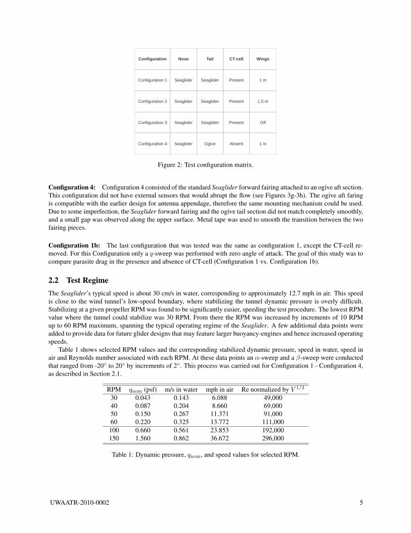
Configuration Nose Tail CT-cell Wings
Configuration 1 Seaglider Seaglider Present 1 m
Configuration 2 Seaglider Seaglider Present 1.5 m
Configuration 3 Seaglider Seaglider Present Off
Configuration 4 Seaglider Ogive Absent 1 m
Figure 2: Test configuration matrix.
Configuration 4: Configuration 4 consisted of the standard Seaglider forward fairing attached to an ogive aft section.This configuration did not have external sensors that would abrupt the flow (see Figures 3g-3h). The ogive aft faringis compatible with the earlier design for antenna appendage, therefore the same mounting mechanism could be used.Due to some imperfection, the Seaglider forward fairing and the ogive tail section did not match completely smoothly,and a small gap was observed along the upper surface. Metal tape was used to smooth the transition between the twofairing pieces.
Configuration 1b: The last configuration that was tested was the same as configuration 1, except the CT-cell re-moved. For this Configuration only a q-sweep was performed with zero angle of attack. The goal of this study was tocompare parasite drag in the presence and absence of CT-cell (Configuration 1 vs. Configuration 1b).
2.2 Test RegimeThe Seaglider’s typical speed is about 30 cm/s in water, corresponding to approximately 12.7 mph in air. This speedis close to the wind tunnel’s low-speed boundary, where stabilizing the tunnel dynamic pressure is overly difficult.Stabilizing at a given propeller RPM was found to be significantly easier, speeding the test procedure. The lowest RPMvalue where the tunnel could stabilize was 30 RPM. From there the RPM was increased by increments of 10 RPMup to 60 RPM maximum, spanning the typical operating regime of the Seaglider. A few additional data points wereadded to provide data for future glider designs that may feature larger buoyancy-engines and hence increased operatingspeeds.
Table 1 shows selected RPM values and the corresponding stabilized dynamic pressure, speed in water, speed inair and Reynolds number associated with each RPM. At these data points an α-sweep and a β-sweep were conductedthat ranged from -20◦ to 20◦ by increments of 2◦. This process was carried out for Configuration 1 - Configuration 4,as described in Section 2.1.
RPM qnom (psf) m/s in water mph in air Re normalized by V 1/3
30 0.043 0.143 6.088 49,00040 0.087 0.204 8.660 69,00050 0.150 0.267 11.371 91,00060 0.220 0.325 13.772 111,000
100 0.660 0.561 23.853 192,000150 1.560 0.862 36.672 296,000
Table 1: Dynamic pressure, qnom, and speed values for selected RPM.
UWAATR-2010-0002 5

(a) Configuration 1. (b) Configuration 1.
(c) Configuration 2. (d) Configuration 2.
(e) Configuration 3. (f) Configuration 3.
(g) Configuration 4. (h) Configuration 4.
Figure 3: Configurations tested during the wind tunnel study.
UWAATR-2010-0002 6
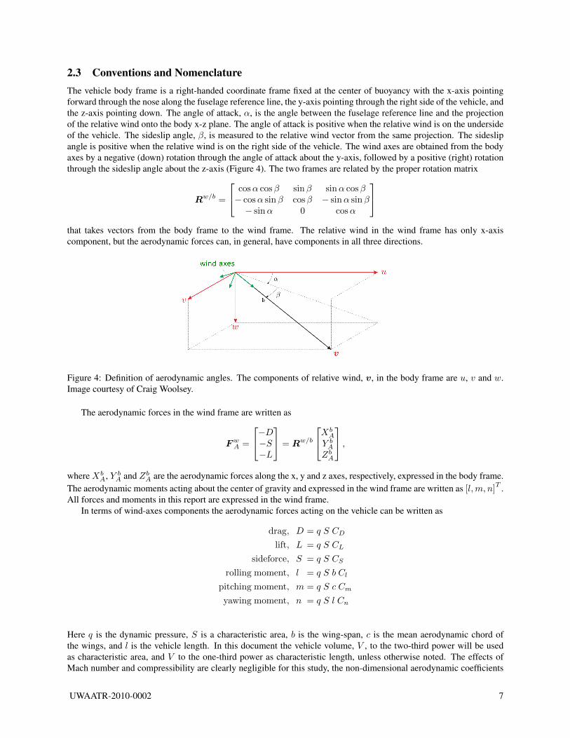
2.3 Conventions and NomenclatureThe vehicle body frame is a right-handed coordinate frame fixed at the center of buoyancy with the x-axis pointingforward through the nose along the fuselage reference line, the y-axis pointing through the right side of the vehicle, andthe z-axis pointing down. The angle of attack, α, is the angle between the fuselage reference line and the projectionof the relative wind onto the body x-z plane. The angle of attack is positive when the relative wind is on the undersideof the vehicle. The sideslip angle, β, is measured to the relative wind vector from the same projection. The sideslipangle is positive when the relative wind is on the right side of the vehicle. The wind axes are obtained from the bodyaxes by a negative (down) rotation through the angle of attack about the y-axis, followed by a positive (right) rotationthrough the sideslip angle about the z-axis (Figure 4). The two frames are related by the proper rotation matrix
Rw/b =
cosα cosβ sinβ sinα cosβ− cosα sinβ cosβ − sinα sinβ
− sinα 0 cosα
that takes vectors from the body frame to the wind frame. The relative wind in the wind frame has only x-axiscomponent, but the aerodynamic forces can, in general, have components in all three directions.
Figure 4: Definition of aerodynamic angles. The components of relative wind, v, in the body frame are u, v and w.Image courtesy of Craig Woolsey.
The aerodynamic forces in the wind frame are written as
FwA =
−D−S−L
= Rw/b
XbA
Y bA
ZbA
,whereXb
A, Y bA and Zb
A are the aerodynamic forces along the x, y and z axes, respectively, expressed in the body frame.The aerodynamic moments acting about the center of gravity and expressed in the wind frame are written as [l,m, n]T .All forces and moments in this report are expressed in the wind frame.
In terms of wind-axes components the aerodynamic forces acting on the vehicle can be written as
drag, D = q S CD
lift, L = q S CL
sideforce, S = q S CS
rolling moment, l = q S b Cl
pitching moment, m = q S c Cm
yawing moment, n = q S l Cn
Here q is the dynamic pressure, S is a characteristic area, b is the wing-span, c is the mean aerodynamic chord ofthe wings, and l is the vehicle length. In this document the vehicle volume, V , to the two-third power will be usedas characteristic area, and V to the one-third power as characteristic length, unless otherwise noted. The effects ofMach number and compressibility are clearly negligible for this study, the non-dimensional aerodynamic coefficients
UWAATR-2010-0002 7

therefore depend on the aerodynamic angles α and β only. The moments are positive when they correspond to apositive right-hand rotation about the corresponding wind frame axis.
We follow standard aircraft convention when assuming quadratic dependence for the drag coefficient, and lineardependence for the rest of the coefficients [3] [4].
Cl(β) = Clββ, CL(α) = CLαα (1)
Cm(α) = Cmαα, CD(α, β) = CD0
+ CDαα2 + CDββ
2 (2)Cn(β) = Cnββ, CS(β) = CSββ. (3)
The glider is symmetric about the x-z plane, hence the rolling moment, yawing moment, and sideforce are zero whenthe sideslip angle is zero. Other than the science sensors, the glider is also symmetric about the x-y plane. Althoughthe forces acting on the CT-cell are significant, we assume zero pitching moment at zero angle of attack.
In the above definition of the forces and moments, the effect of the body, the wings and the rudder are all treatedtogether. The wind-tunnel study was performed for configurations with the standard 1 m wings, with the 1.5 m wingsand in the absence of wings (Configuration 1, 2 and 3, respectively). This allowed to measure the body and the wingcontributions separately. The longitudinal forces and moments can be split into body and wing contributions as:
D = Db +Dw = qV 2/3
[(CDb0 + CDbαα
2 + CDββ2)+
Sw
V 2/3
(CDw0 + CDwαα
2)]
(4)
L = Lb + Lw = qV 2/3
[CLbαα+
Sw
V 2/3CLwαα
](5)
m = mb +mw = qV 2/3c
[Cmbαα− cm
lcb/acwSw
V 2/3cCLwαα
], (6)
where Sw is the planform area of the wings, lcb/acw is the distance between the center of buoyancy and the meanaerodynamic center of the wings, and cm is a non-dimensional coefficient.
Remark 2.1. Note that the wings are symmetric, hence the zero-lift pitching moment is zero. Since the aerodynamiccoefficients for the wing are referenced about the mean aerodynamic center, the pitching moment for the wing is zero.Ideally, the moment contribution then comes from the wing lift force alone, defined by the wing volume ratio
lcb/acwSw
V 2/3c.
The coefficient cm is used to account for the discrepancy in the measured values.
The dependence of these non-dimensional coefficients on the aerodynamic angles are first-order (quadratic forCD) approximations of more complicated functional relationships. In reality, the force-and moment coefficients alsovary as a function of Reynolds number. As pointed out in [2], the parasite drag at such low Reynolds numbers varieswith dynamic pressure to the three-fourth power. Using this alternative functional dependence, one may write
L = ql2Caα (7)
D = ql2(Cbq
−1/4 + Ccα2). (8)
Remark 2.2. Note that in the above equations the vehicle length squared is used as characteristic area to keep withthe notation of [2].
Remark 2.3. Also note that the coefficient Cb is now dimensional.
The wind tunnel tests confirmed this form of functional dependence. Nevertheless, the definitions in equations (1)-(6) are widely accepted, hence we present the non-dimensional coefficients for both equations (1)-(6) and (7)-(8). Thecoefficients for equations (1)-(6) are given at the Seaglider’s typical operating speed, 27 cm/s.
UWAATR-2010-0002 8
3 Results
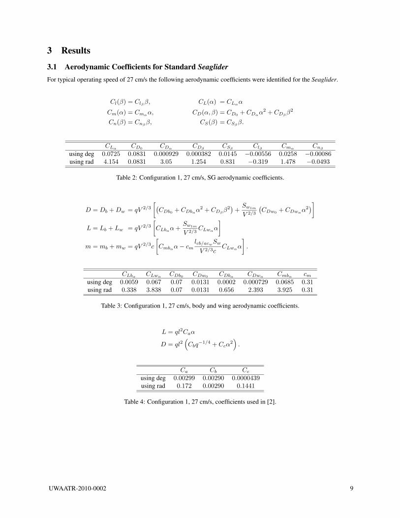
3.1 Aerodynamic Coefficients for Standard SeagliderFor typical operating speed of 27 cm/s the following aerodynamic coefficients were identified for the Seaglider.
Cl(β) = Clββ, CL(α) = CLαα
Cm(α) = Cmαα, CD(α, β) = CD0
+ CDαα2 + CDββ
2
Cn(β) = Cnββ, CS(β) = CSββ.
CLα CD0CDα CDβ CSβ Clβ Cmα
Cnβ
using deg 0.0725 0.0831 0.000929 0.000382 0.0145 −0.00556 0.0258 −0.00086using rad 4.154 0.0831 3.05 1.254 0.831 −0.319 1.478 −0.0493
Table 2: Configuration 1, 27 cm/s, SG aerodynamic coefficients.
D = Db +Dw = qV 2/3
[(CDb0 + CDbαα
2 + CDββ2)+Sw1m
V 2/3
(CDw0 + CDwαα
2)]
L = Lb + Lw = qV 2/3
[CLbαα+
Sw1m
V 2/3CLwαα
]m = mb +mw = qV 2/3c
[Cmbαα− cm
lcb/acwSw
V 2/3cCLwαα
].
CLbα CLwα CDb0 CDw0CDbα CDwα Cmbα cm
using deg 0.0059 0.067 0.07 0.0131 0.0002 0.000729 0.0685 0.31using rad 0.338 3.838 0.07 0.0131 0.656 2.393 3.925 0.31
Table 3: Configuration 1, 27 cm/s, body and wing aerodynamic coefficients.
L = ql2Caα
D = ql2(Cbq
−1/4 + Ccα2).
Ca Cb Cc
using deg 0.00299 0.00290 0.0000439using rad 0.172 0.00290 0.1441
Table 4: Configuration 1, 27 cm/s, coefficients used in [2].
UWAATR-2010-0002 9
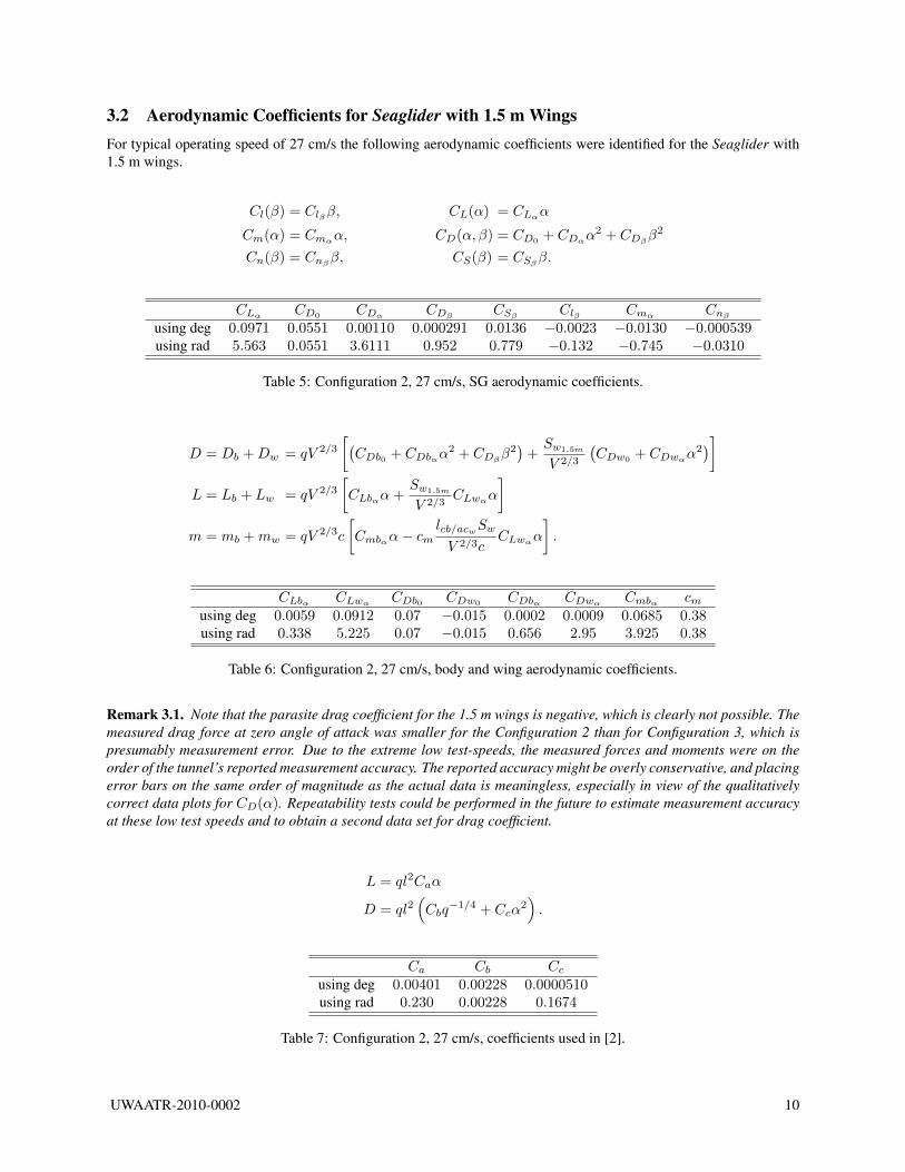
3.2 Aerodynamic Coefficients for Seaglider with 1.5 m WingsFor typical operating speed of 27 cm/s the following aerodynamic coefficients were identified for the Seaglider with1.5 m wings.
Cl(β) = Clββ, CL(α) = CLαα
Cm(α) = Cmαα, CD(α, β) = CD0
+ CDαα2 + CDββ
2
Cn(β) = Cnββ, CS(β) = CSββ.
CLα CD0CDα CDβ CSβ Clβ Cmα
Cnβ
using deg 0.0971 0.0551 0.00110 0.000291 0.0136 −0.0023 −0.0130 −0.000539using rad 5.563 0.0551 3.6111 0.952 0.779 −0.132 −0.745 −0.0310
Table 5: Configuration 2, 27 cm/s, SG aerodynamic coefficients.
D = Db +Dw = qV 2/3
[(CDb0 + CDbαα
2 + CDββ2)+Sw1.5m
V 2/3
(CDw0 + CDwαα
2)]
L = Lb + Lw = qV 2/3
[CLbαα+
Sw1.5m
V 2/3CLwαα
]m = mb +mw = qV 2/3c
[Cmbαα− cm
lcb/acwSw
V 2/3cCLwαα
].
CLbα CLwα CDb0 CDw0 CDbα CDwα Cmbα cmusing deg 0.0059 0.0912 0.07 −0.015 0.0002 0.0009 0.0685 0.38using rad 0.338 5.225 0.07 −0.015 0.656 2.95 3.925 0.38
Table 6: Configuration 2, 27 cm/s, body and wing aerodynamic coefficients.
Remark 3.1. Note that the parasite drag coefficient for the 1.5 m wings is negative, which is clearly not possible. Themeasured drag force at zero angle of attack was smaller for the Configuration 2 than for Configuration 3, which ispresumably measurement error. Due to the extreme low test-speeds, the measured forces and moments were on theorder of the tunnel’s reported measurement accuracy. The reported accuracy might be overly conservative, and placingerror bars on the same order of magnitude as the actual data is meaningless, especially in view of the qualitativelycorrect data plots for CD(α). Repeatability tests could be performed in the future to estimate measurement accuracyat these low test speeds and to obtain a second data set for drag coefficient.
L = ql2Caα
D = ql2(Cbq
−1/4 + Ccα2).
Ca Cb Cc
using deg 0.00401 0.00228 0.0000510using rad 0.230 0.00228 0.1674
Table 7: Configuration 2, 27 cm/s, coefficients used in [2].
UWAATR-2010-0002 10

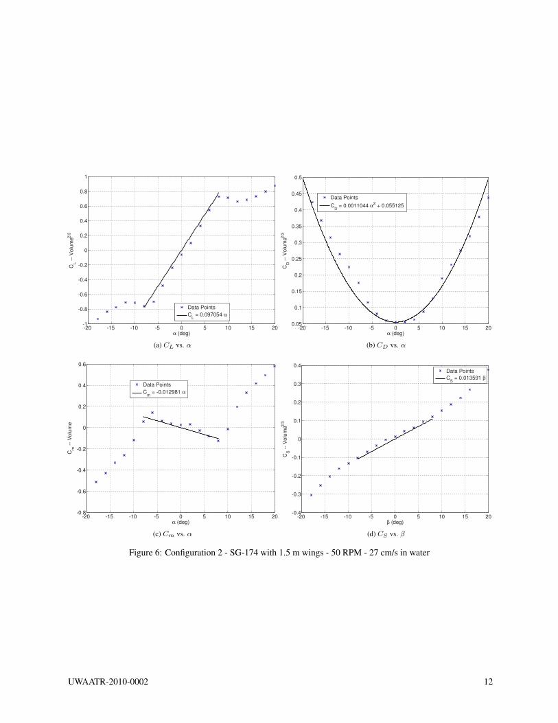
3.3 Effects of the WingsThe first three configurations were tested to determine the effect the wings had on the performance of the Seaglider.Figures 5 - 7 show the plots for CL vs. α, CD vs. α, and Cm vs. α for the Configuration 1 - Configuration 3. Figures 5and 6 show that the main effect of the 1.5 meter wings is increased lift coefficient and that the glider becomes stablein the typical operating regime.
-20 -15 -10 -5 0 5 10 15 20-1
-0.8
-0.6
-0.4
-0.2
0
0.2
0.4
0.6
0.8
α (deg)
CL -
- V
olu
me2
/3
Data Points
CL = 0.072501 α
(a) CL vs. α
-20 -15 -10 -5 0 5 10 15 200.05
0.1
0.15
0.2
0.25
0.3
0.35
0.4
0.45
0.5
α (deg)
CD -
- V
olu
me2
/3
Data Points
CD = 0.0009289 α
2 + 0.083146
(b) CD vs. α
-20 -15 -10 -5 0 5 10 15 20-1.5
-1
-0.5
0
0.5
1
1.5
α (deg)
Cm
--
Vo
lum
e
Data Points
Cm
= 0.025787 α
(c) Cm vs. α
-20 -15 -10 -5 0 5 10 15 20-0.5
-0.4
-0.3
-0.2
-0.1
0
0.1
0.2
0.3
0.4
0.5
β (deg)
CS -
- V
olu
me2
/3
Data Points
CS = 0.014546 β
(d) CS vs. β
Figure 5: Configuration 1 - Seaglider with 1 m wings - 50 RPM - 27 cm/s in water
UWAATR-2010-0002 11
-20 -15 -10 -5 0 5 10 15 20-1
-0.8
-0.6
-0.4
-0.2
0
0.2
0.4
0.6
0.8
1
α (deg)
CL -
- V
olu
me2
/3
Data Points
CL = 0.097054 α
(a) CL vs. α
-20 -15 -10 -5 0 5 10 15 200.05
0.1
0.15
0.2
0.25
0.3
0.35
0.4
0.45
0.5
α (deg)
CD -
- V
olu
me2
/3
Data Points
CD = 0.0011044 α
2 + 0.055125
(b) CD vs. α
-20 -15 -10 -5 0 5 10 15 20-0.8
-0.6
-0.4
-0.2
0
0.2
0.4
0.6
α (deg)
Cm
--
Vo
lum
e
Data Points
Cm
= -0.012981 α
(c) Cm vs. α
-20 -15 -10 -5 0 5 10 15 20-0.4
-0.3
-0.2
-0.1
0
0.1
0.2
0.3
0.4
β (deg)
CS -
- V
olu
me2
/3
Data Points
CS = 0.013591 β
(d) CS vs. β
Figure 6: Configuration 2 - SG-174 with 1.5 m wings - 50 RPM - 27 cm/s in water
UWAATR-2010-0002 12

-20 -15 -10 -5 0 5 10 15 20-0.4
-0.3
-0.2
-0.1
0
0.1
0.2
0.3
α (deg)
CL -
- V
olu
me2
/3
Data Points
CL = 0.0059177 α
(a) CL vs. α
-20 -15 -10 -5 0 5 10 15 200.06
0.08
0.1
0.12
0.14
0.16
0.18
α (deg)
CD -
- V
olu
me2
/3
Data Points
CD = 0.00019958 α
2 + 0.070099
(b) CD vs. α
-20 -15 -10 -5 0 5 10 15 20-1.5
-1
-0.5
0
0.5
1
1.5
α (deg)
Cm
--
Vo
lum
e
Data Points
Cm
= 0.068512 α
(c) Cm vs. α
-20 -15 -10 -5 0 5 10 15 20-0.5
-0.4
-0.3
-0.2
-0.1
0
0.1
0.2
0.3
0.4
0.5
β (deg)
CS -
- V
olu
me2
/3
Data Points
CS = 0.015178 β
(d) CS vs. β
Figure 7: Configuration 3 - Seaglider with no wings - 50 RPM - 27 cm/s in water
UWAATR-2010-0002 13
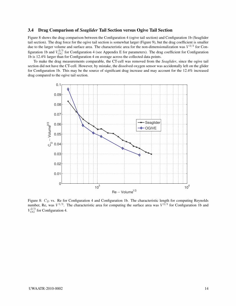
3.4 Drag Comparison of Seaglider Tail Section versus Ogive Tail SectionFigure 8 shows the drag comparison between the Configuration 4 (ogive tail section) and Configuration 1b (Seaglidertail section). The drag force for the ogive tail section is somewhat larger (Figure 9), but the drag coefficient is smallerdue to the larger volume and surface area. The characteristic area for the non-dimensionalization was V 2/3 for Con-figuration 1b and V 2/3
OG for Configuration 4 (see Appendix E for parameters). The drag coefficient for Configuration1b is 12.4% larger than for Configuration 4 on average across the collected data points.
To make the drag measurements comparable, the CT-cell was removed from the Seaglider, since the ogive tailsection did not have the CT-cell. However, by mistake, the dissolved oxygen sensor was accidentally left on the gliderfor Configuration 1b. This may be the source of significant drag increase and may account for the 12.4% increaseddrag compared to the ogive tail section.
105
106
0
0.01
0.02
0.03
0.04
0.05
0.06
0.07
0.08
0.09
0.1
Re -- Volume1/3
CD -
- V
olu
me2
/3
Seaglider
OGIVE
Figure 8: CD vs. Re for Configuration 4 and Configuration 1b. The characteristic length for computing Reynoldsnumber, Re, was V 1/3. The characteristic area for computing the surface area was V 2/3 for Configuration 1b andV
2/3OG for Configuration 4.
UWAATR-2010-0002 14

105
106
10-2
10-1
Re -- Volume1/3
Dra
g (
lb)
Seaglider
OGIVE
Figure 9: Drag vs. Re for Configuration 4 and Configuration 1b. The drag force is 10.4% larger for Configuration 4than Configuration 1b on average. Note that Configuration 4 has larger surface area, however, the oxygen sensor —present in Configuration 1b — is absent in Configuration 4.
UWAATR-2010-0002 15
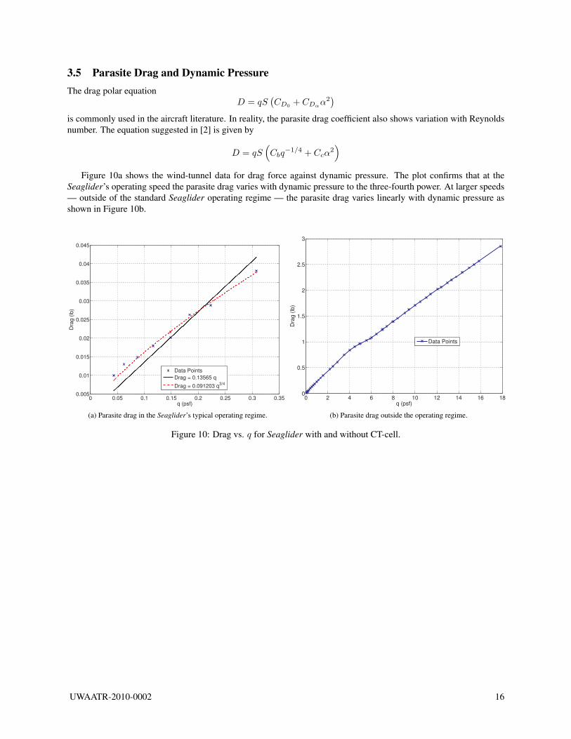
3.5 Parasite Drag and Dynamic PressureThe drag polar equation
D = qS(CD0 + CDαα
2)
is commonly used in the aircraft literature. In reality, the parasite drag coefficient also shows variation with Reynoldsnumber. The equation suggested in [2] is given by
D = qS(Cbq
−1/4 + Ccα2)
Figure 10a shows the wind-tunnel data for drag force against dynamic pressure. The plot confirms that at theSeaglider’s operating speed the parasite drag varies with dynamic pressure to the three-fourth power. At larger speeds— outside of the standard Seaglider operating regime — the parasite drag varies linearly with dynamic pressure asshown in Figure 10b.
0 0.05 0.1 0.15 0.2 0.25 0.3 0.350.005
0.01
0.015
0.02
0.025
0.03
0.035
0.04
0.045
q (psf)
Dra
g (
lb)
Data Points
Drag = 0.13565 q
Drag = 0.091203 q3/4
(a) Parasite drag in the Seaglider’s typical operating regime.
0 2 4 6 8 10 12 14 16 180
0.5
1
1.5
2
2.5
3
q (psf)
Dra
g (
lb)
Data Points
(b) Parasite drag outside the operating regime.
Figure 10: Drag vs. q for Seaglider with and without CT-cell.
UWAATR-2010-0002 16
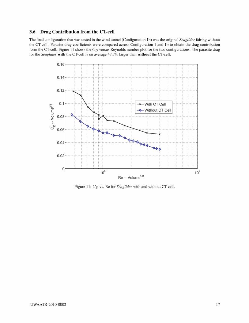
3.6 Drag Contribution from the CT-cellThe final configuration that was tested in the wind tunnel (Configuration 1b) was the original Seaglider fairing withoutthe CT-cell. Parasite drag coefficients were compared across Configuration 1 and 1b to obtain the drag contributionform the CT-cell. Figure 11 shows the CD versus Reynolds number plot for the two configurations. The parasite dragfor the Seaglider with the CT-cell is on average 47.7% larger than without the CT-cell.
105
106
0
0.02
0.04
0.06
0.08
0.1
0.12
0.14
0.16
Re -- Volume1/3
CD -
- V
olu
me
2/3
With CT Cell
Without CT Cell
Figure 11: CD vs. Re for Seaglider with and without CT-cell.
UWAATR-2010-0002 17
3.7 Static Longitudinal StabilityThe wind tunnel tests revealed that the glider lacks static longitudinal stability, indicated by positive pitching momentcoefficient in the typical operating regime. Positive pitching moment coefficient results in a positive (nose-up) momentwhen the angle of attack is positive, which further increases the angle of attack. For positive α, a negative restoringmoment would be required for static longitudinal stability. The moment coefficient plots presented in Figure 14,Figure 20, Figure 26 and Figure 32 show that at the lowest test speed the moment coefficient is a monotonicallyincreasing function of α crossing the abscissa at the origin (no moment at zero angle of attack). As the wind speedincreases the curves shift toward the origin; eventually they cross over the abscissa and lose their monotonic property.Beyond that point the curves have negative slope and an inflexion point at the origin. This indicates that the gliderbecomes stable beyond a certain flow speed, which, however, is currently outside of the operating regime.
The glider is longitudinally stable with the larger, 1.5 m, wings in the current operating regime. Since the wingsare mounted behind the center of gravity, the wing lift force — acting with the moment arm between the wing meanaerodynamic center and vehicle center of gravity — provides a restoring moment. This is also true for the shorterwings, however, since the body itself is aerodynamically unstable, the restoring moment from the short, 1 m span,wings is not sufficient to counter the body effects (observe these trends in Figure 14, Figure 20 and Figure 26). TheSeaglider with the ogive aft fairing and the 1 m wings is also unstable in the current operating regime.
The reason that the Seaglider performs stable glides in experiments is the restoring moment resulting from the off-set between the center of buoyancy and center of gravity. Compared to this moment, the magnitude of the aerodynamicmoment is small. Knowing the vertical CG-CB separation and other vehicle parameters, it is simple matter to performa static equilibrium calculation and estimate the pitch angle variation compared to a stationary case. For example, thedestabilizing aerodynamic moment resulting from 5◦ angle of attack may be easily countered by a gravity torque froma pitch angle increase of less than 1◦.
UWAATR-2010-0002 18
3.8 Directional StabilityThe magnitude of the measured yawing moment was very small compared to other aerodynamic forces and moments.The bare hull is symmetric about any plane containing the fuselage reference line, hence the bare hull is directionallyunstable for the same reasons it is longitudinally unstable. The vertical stabilizer provides the required restoringmoment and ensures stable glides. The yawing moment coefficients presented in Figure 15, Figure 21, Figure 27 andFigure 33 are very small in magnitude, and on occasions not symmetric in sideslip angle. The reason for this is thatthe yawing moments calculated from Cn were on the order of 10−2 in-lb, whereas the measurement accuracies forthe wind tunnel are 0.01 lb for the forces and 0.2 in-lb for yawing moment. The anomalies in the yawing and rollingmoment graphs is likely to be caused by the measurement accuracy of the wind tunnel and the small test speeds.Relatively small yawing moment coefficients imply that there is small restoring capability in the presence of sideslipangle, and hence the glider might be close to being neutrally stable in yaw angle.
UWAATR-2010-0002 19
4 SummaryThis report described full-scale wind tunnel tests for the Seaglider that were conducted in the University of WashingtonKirsten Wind Tunnel. Aerodynamic coefficients were presented for different vehicle geometries at typical operatingspeeds. The following observations were also made:
1. The drag coefficient for the Seaglider with the CT-cell is 47.7 % larger than without the CT-cell. The CT-cellwas known to be a major drag contributor, however the extent of this contribution was unexpected. Housing allthe science sensors inside the fairing could significantly reduce drag and improve efficiency in future gliders.
2. The Seaglider lacks static longitudinal stability in the typical operating regime. The lack of static aerodynamicstability is counter-balanced by the moment couple resulting from the offset between center of gravity and centerof buoyancy. This metacentric height helps recover stability, explaining why the glider performs stable glidesin experiments. Larger wings could help recover aerodynamic stability, and also improve glide performance.
3. The magnitude of the measured yawing moments is very small, indicating that the glider is marginally direc-tionally stable.
4. The measured drag force for the newly designed ogive tail section (Configuration 4) is on average 10.4% largerthan for the original Seaglider configuration (Configuration 1b). By mistake the dissolved oxygen sensor wasleft on the Seaglider for the drag comparison; the ogive tail section of Configuration 4 was completely smoothwithout any obstructions. The drag coefficient for Configuration 1b is 12.4% larger than the drag coefficientfor Configuration 4. The outcome of this test remains inconclusive, as the 12.4% increased drag coefficient forConfiguration 1b versus Configuration 4 may come from the oxygen sensor.
UWAATR-2010-0002 20
References[1] Anon. Technical guide for the Kirsten Wind Tunnel. Technical report, University of Washington Aeronautical
Laboratory, Seattle, WA, 2002.
[2] C. C. Eriksen, T. J. Osse, R. D. Light, T. Wen, T. W. Lehman, P. L. Sabin, J. W. Ballard, and A. M. Chiodi.Seaglider: A long-range autonomous underwater vehicle for oceanographic research. Journal of Oceanic Engi-neering, 26(4):424–436, 2001. Special Issue on Autonomous Ocean-Sampling Networks.
[3] S. F. Hoerner. Fluid-dynamic Lift: practical information on aerodynamic and hydrodynamic lift. Brick Town, NJ,1975.
[4] S. F. Hoerner. Fluid-dynamic Drag: practical information on aerodynamic drag and hydrodynamic resistance.Bakersfield, CA, 1992.
[5] R. M. Hubbard. Hydrodynamics technology for an Advanced Expendable Mobile Target (AEMT). TechnicalReport 8013, University of Washington, Applied Physics Lab, Seattle, WA, 1980.
[6] N. Pelland. Analysis of potential fairing shapes through photography of scale-model freefall. Technical ReportDeepGlider II Technical Report, University of Washington, School of Oceanography, Seattle, WA, 2009.
UWAATR-2010-0002 21
5 Appendix A: Configuration 1
-20 -15 -10 -5 0 5 10 15 200
0.05
0.1
0.15
0.2
0.25
0.3
0.35
0.4
0.45
0.5
α (deg)
CD -
-Vo
lum
e2/3
0.143 m/s
0.204 m/s
0.267 m/s
0.325 m/s
0.561 m/s
0.862 m/s
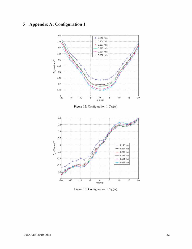
Figure 12: Configuration 1 CD(α).
-20 -15 -10 -5 0 5 10 15 20-1
-0.8
-0.6
-0.4
-0.2
0
0.2
0.4
0.6
0.8
α (deg)
CL -
-Vo
lum
e2/3
0.143 m/s
0.204 m/s
0.267 m/s
0.325 m/s
0.561 m/s
0.862 m/s
Figure 13: Configuration 1 CL(α).
UWAATR-2010-0002 22

-20 -15 -10 -5 0 5 10 15 20-5
-4
-3
-2
-1
0
1
2
3
4
5
α (deg)
Cm
--V
olu
me
0.143 m/s
0.204 m/s
0.267 m/s
0.325 m/s
0.561 m/s
0.862 m/s
Figure 14: Configuration 1 Cm(α).
-20 -15 -10 -5 0 5 10 15 20-0.06
-0.04
-0.02
0
0.02
0.04
0.06
0.08
β (deg)
Cn -
-Vo
lum
e
0.143 m/s
0.204 m/s
0.267 m/s
0.325 m/s
0.561 m/s
0.862 m/s
Figure 15: Configuration 1 Cn(β).
UWAATR-2010-0002 23
-20 -15 -10 -5 0 5 10 15 20-0.3
-0.2
-0.1
0
0.1
0.2
0.3
0.4
0.5
0.6
β (deg)
Cl -
-Volu
me
0.143 m/s
0.204 m/s
0.267 m/s
0.325 m/s
0.561 m/s
0.862 m/s
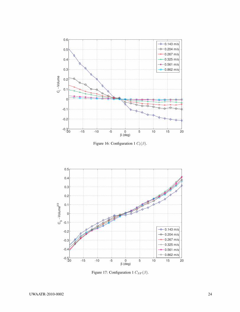
Figure 16: Configuration 1 Cl(β).
-20 -15 -10 -5 0 5 10 15 20-0.5
-0.4
-0.3
-0.2
-0.1
0
0.1
0.2
0.3
0.4
0.5
β (deg)
CS -
-Volu
me2
/3
0.143 m/s
0.204 m/s
0.267 m/s
0.325 m/s
0.561 m/s
0.862 m/s
Figure 17: Configuration 1 CSF (β).
UWAATR-2010-0002 24

6 Appendix B: Configuration 2
-20 -15 -10 -5 0 5 10 15 200
0.1
0.2
0.3
0.4
0.5
0.6
0.7
α (deg)
CD -
-Vo
lum
e2/3
0.143 m/s
0.204 m/s
0.267 m/s
0.325 m/s
0.561 m/s
0.862 m/s
Figure 18: Configuration 2 CD(α).
-20 -15 -10 -5 0 5 10 15 20-1.5
-1
-0.5
0
0.5
1
α (deg)
CL -
-Vo
lum
e2/3
0.143 m/s
0.204 m/s
0.267 m/s
0.325 m/s
0.561 m/s
0.862 m/s
Figure 19: Configuration 2 CL(α).
UWAATR-2010-0002 25
-20 -15 -10 -5 0 5 10 15 20-4
-3
-2
-1
0
1
2
3
4
α (deg)
Cm
--V
olu
me
0.143 m/s
0.204 m/s
0.267 m/s
0.325 m/s
0.561 m/s
0.862 m/s
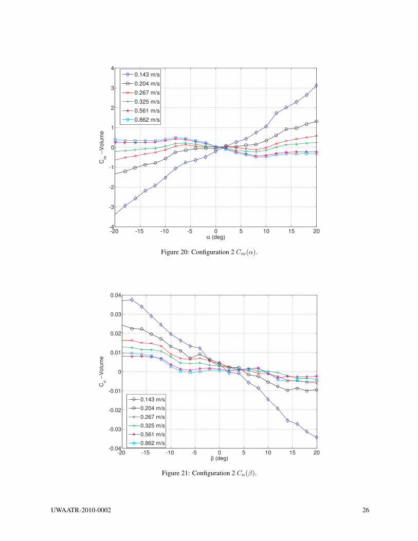
Figure 20: Configuration 2 Cm(α).
-20 -15 -10 -5 0 5 10 15 20-0.04
-0.03
-0.02
-0.01
0
0.01
0.02
0.03
0.04
β (deg)
Cn -
-Vo
lum
e
0.143 m/s
0.204 m/s
0.267 m/s
0.325 m/s
0.561 m/s
0.862 m/s
Figure 21: Configuration 2 Cn(β).
UWAATR-2010-0002 26
-20 -15 -10 -5 0 5 10 15 20-0.1
-0.05
0
0.05
0.1
0.15
0.2
0.25
0.3
β (deg)
Cl -
-Vo
lum
e
0.143 m/s
0.204 m/s
0.267 m/s
0.325 m/s
0.561 m/s
0.862 m/s
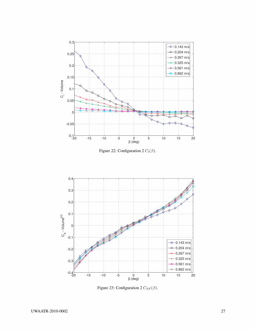
Figure 22: Configuration 2 Cl(β).
-20 -15 -10 -5 0 5 10 15 20-0.4
-0.3
-0.2
-0.1
0
0.1
0.2
0.3
0.4
β (deg)
CS -
-Volu
me2
/3
0.143 m/s
0.204 m/s
0.267 m/s
0.325 m/s
0.561 m/s
0.862 m/s
Figure 23: Configuration 2 CSF (β).
UWAATR-2010-0002 27

7 Appendix C: Configuration 3
-20 -15 -10 -5 0 5 10 15 200.02
0.04
0.06
0.08
0.1
0.12
0.14
0.16
0.18
0.2
α (deg)
CD -
-Vo
lum
e2/3
0.143 m/s
0.204 m/s
0.267 m/s
0.325 m/s
0.561 m/s
0.862 m/s
Figure 24: Configuration 3 CD(α).
-20 -15 -10 -5 0 5 10 15 20-0.5
-0.4
-0.3
-0.2
-0.1
0
0.1
0.2
0.3
α (deg)
CL -
-Vo
lum
e2/3
0.143 m/s
0.204 m/s
0.267 m/s
0.325 m/s
0.561 m/s
0.862 m/s
Figure 25: Configuration 3 CL(α).
UWAATR-2010-0002 28

-20 -15 -10 -5 0 5 10 15 20-5
-4
-3
-2
-1
0
1
2
3
4
α (deg)
Cm
--V
olu
me
0.143 m/s
0.204 m/s
0.267 m/s
0.325 m/s
0.561 m/s
0.862 m/s
Figure 26: Configuration 3 Cm(α).
-20 -15 -10 -5 0 5 10 15 20-0.04
-0.02
0
0.02
0.04
0.06
0.08
β (deg)
Cn -
-Vo
lum
e
0.143 m/s
0.204 m/s
0.267 m/s
0.325 m/s
0.561 m/s
0.862 m/s
Figure 27: Configuration 3 Cn(β).
UWAATR-2010-0002 29

-20 -15 -10 -5 0 5 10 15 20-0.2
-0.1
0
0.1
0.2
0.3
0.4
0.5
β (deg)
Cl -
-Volu
me
0.143 m/s
0.204 m/s
0.267 m/s
0.325 m/s
0.561 m/s
0.862 m/s
Figure 28: Configuration 3 Cl(β).
-20 -15 -10 -5 0 5 10 15 20-0.5
-0.4
-0.3
-0.2
-0.1
0
0.1
0.2
0.3
0.4
0.5
β (deg)
CS -
-Volu
me2
/3
0.143 m/s
0.204 m/s
0.267 m/s
0.325 m/s
0.561 m/s
0.862 m/s
Figure 29: Configuration 3 CSF (β).
UWAATR-2010-0002 30
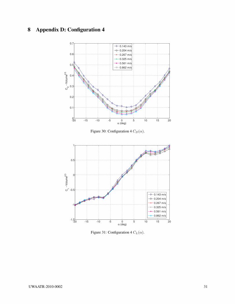
8 Appendix D: Configuration 4
-20 -15 -10 -5 0 5 10 15 200
0.1
0.2
0.3
0.4
0.5
0.6
0.7
α (deg)
CD -
-Vo
lum
e2/3
0.143 m/s
0.204 m/s
0.267 m/s
0.325 m/s
0.561 m/s
0.862 m/s
Figure 30: Configuration 4 CD(α).
-20 -15 -10 -5 0 5 10 15 20-1.5
-1
-0.5
0
0.5
1
α (deg)
CL -
-Vo
lum
e2/3
0.143 m/s
0.204 m/s
0.267 m/s
0.325 m/s
0.561 m/s
0.862 m/s
Figure 31: Configuration 4 CL(α).
UWAATR-2010-0002 31

-20 -15 -10 -5 0 5 10 15 20-5
-4
-3
-2
-1
0
1
2
3
4
5
α (deg)
Cm
--V
olu
me
0.143 m/s
0.204 m/s
0.267 m/s
0.325 m/s
0.561 m/s
0.862 m/s
Figure 32: Configuration 4 Cm(α).
-20 -15 -10 -5 0 5 10 15 20-0.08
-0.06
-0.04
-0.02
0
0.02
0.04
0.06
0.08
0.1
0.12
β (deg)
Cn -
-Vo
lum
e
0.143 m/s
0.204 m/s
0.267 m/s
0.325 m/s
0.561 m/s
0.862 m/s
Figure 33: Configuration 4 Cn(β).
UWAATR-2010-0002 32

-20 -15 -10 -5 0 5 10 15 20-0.3
-0.2
-0.1
0
0.1
0.2
0.3
0.4
0.5
0.6
β (deg)
Cl -
-Volu
me
0.143 m/s
0.204 m/s
0.267 m/s
0.325 m/s
0.561 m/s
0.862 m/s
Figure 34: Configuration 4 Cl(β).
-20 -15 -10 -5 0 5 10 15 20-0.5
-0.4
-0.3
-0.2
-0.1
0
0.1
0.2
0.3
0.4
0.5
β (deg)
CS -
-Volu
me2
/3
0.143 m/s
0.204 m/s
0.267 m/s
0.325 m/s
0.561 m/s
0.862 m/s
Figure 35: Configuration 4 CSF (β).
UWAATR-2010-0002 33
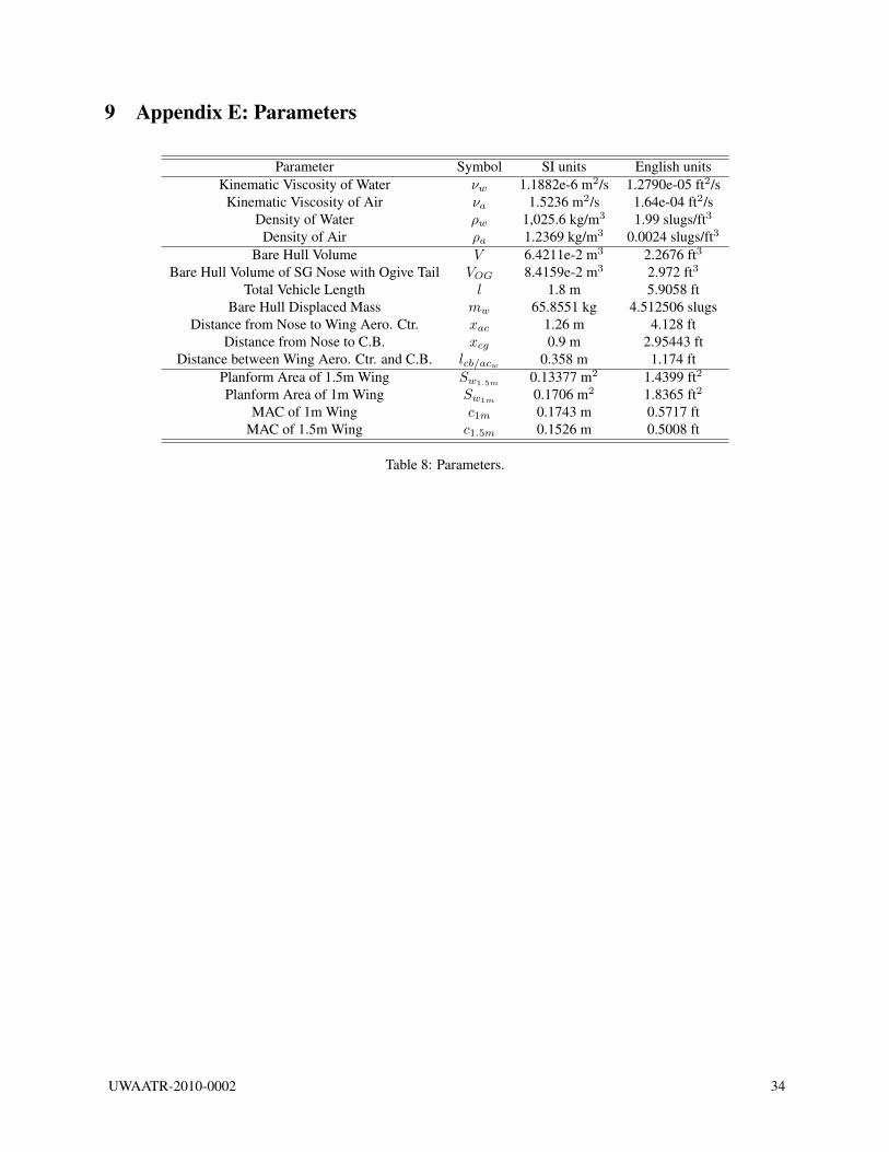
9 Appendix E: Parameters
Parameter Symbol SI units English unitsKinematic Viscosity of Water νw 1.1882e-6 m2/s 1.2790e-05 ft2/s
Kinematic Viscosity of Air νa 1.5236 m2/s 1.64e-04 ft2/sDensity of Water ρw 1,025.6 kg/m3 1.99 slugs/ft3
Density of Air ρa 1.2369 kg/m3 0.0024 slugs/ft3
Bare Hull Volume V 6.4211e-2 m3 2.2676 ft3
Bare Hull Volume of SG Nose with Ogive Tail VOG 8.4159e-2 m3 2.972 ft3
Total Vehicle Length l 1.8 m 5.9058 ftBare Hull Displaced Mass mw 65.8551 kg 4.512506 slugs
Distance from Nose to Wing Aero. Ctr. xac 1.26 m 4.128 ftDistance from Nose to C.B. xcg 0.9 m 2.95443 ft
Distance between Wing Aero. Ctr. and C.B. lcb/acw 0.358 m 1.174 ftPlanform Area of 1.5m Wing Sw1.5m 0.13377 m2 1.4399 ft2
Planform Area of 1m Wing Sw1m 0.1706 m2 1.8365 ft2
MAC of 1m Wing c1m 0.1743 m 0.5717 ftMAC of 1.5m Wing c1.5m 0.1526 m 0.5008 ft
Table 8: Parameters.
UWAATR-2010-0002 34
Related Documents