University of New Hampshire University of New Hampshire University of New Hampshire Scholars' Repository University of New Hampshire Scholars' Repository Doctoral Dissertations Student Scholarship Winter 1996 Full-scale comparative evaluation of two slow sand filter cleaning Full-scale comparative evaluation of two slow sand filter cleaning methods methods Jan A. Kem University of New Hampshire, Durham Follow this and additional works at: https://scholars.unh.edu/dissertation Recommended Citation Recommended Citation Kem, Jan A., "Full-scale comparative evaluation of two slow sand filter cleaning methods" (1996). Doctoral Dissertations. 1929. https://scholars.unh.edu/dissertation/1929 This Dissertation is brought to you for free and open access by the Student Scholarship at University of New Hampshire Scholars' Repository. It has been accepted for inclusion in Doctoral Dissertations by an authorized administrator of University of New Hampshire Scholars' Repository. For more information, please contact [email protected].

Welcome message from author
This document is posted to help you gain knowledge. Please leave a comment to let me know what you think about it! Share it to your friends and learn new things together.
Transcript
University of New Hampshire University of New Hampshire
University of New Hampshire Scholars' Repository University of New Hampshire Scholars' Repository
Doctoral Dissertations Student Scholarship
Winter 1996
Full-scale comparative evaluation of two slow sand filter cleaning Full-scale comparative evaluation of two slow sand filter cleaning
methods methods
Jan A. Kem University of New Hampshire, Durham
Follow this and additional works at: https://scholars.unh.edu/dissertation
Recommended Citation Recommended Citation Kem, Jan A., "Full-scale comparative evaluation of two slow sand filter cleaning methods" (1996). Doctoral Dissertations. 1929. https://scholars.unh.edu/dissertation/1929
This Dissertation is brought to you for free and open access by the Student Scholarship at University of New Hampshire Scholars' Repository. It has been accepted for inclusion in Doctoral Dissertations by an authorized administrator of University of New Hampshire Scholars' Repository. For more information, please contact [email protected].
INFORMATION TO USERS
This manuscript has been reproduced from the microfilm master. UMI
films the text directly from the original or copy submitted. Thus, some
thesis and dissertation copies are in typewriter face, while others may be
from any type of computer printer.
The quality of this reproduction is dependent upon the quality of the
copy submitted. Broken or indistinct print, colored or poor quality
illustrations and photographs, print bleedthrough, substandard margins,
and improper alignment can adversely afreet reproduction.
In the unlikely event that the author did not send UMI a complete
manuscript and there are missing pages, these will be noted. Also, if
unauthorized copyright material had to be removed, a note will indicate
the deletion.
Oversize materials (e.g., maps, drawings, charts) are reproduced by
sectioning the original, beginning at the upper left-hand comer and
continuing from left to right in equal sections with small overlaps. Each
original is also photographed in one exposure and is included in reduced
form at the back of the book.
Photographs included in the original manuscript have been reproduced
xerographically in this copy. Higher quality 6” x 9” black and white
photographic prints are available for any photographs or illustrations
appearing in this copy for an additional charge. Contact UMI directly to
order.
UMIA Bell & Howell Information Company
300 North Zeeb Road, Ann Arbor MI 48106-1346 USA 313/761-4700 800/521-0600
Reproduced with permission of the copyright owner. Further reproduction prohibited without permission.

Reproduced with permission of the copyright owner. Further reproduction prohibited without permission.
FULL-SCALE COMPARATIVE EVALUATION OF TWO SLOW SAND FILTER CLEANING METHODS
BY
JANA.KEM A.B., Eariham College, 1962
B.C.E., Civil Engineering, Rensselaer Polytechnic Institute, 1962 M.S., Environmental Engineering, Rensselaer Polytechnic Institute, 1963
DISSERTATION
Submitted to the University of New Hampshire
in Partial Fulfillment of
the Requirements for the Degree of
Doctor of Philosophy
in
Engineering
December, 1996
Reproduced with permission of the copyright owner. Further reproduction prohibited without permission.
UMI Number: 9717853
UMI Microform 9717853 Copyright 1997, by UMI Company. All rights reserved.
This microform edition is protected against unauthorized copying under Title 17, United States Code.
UMI300 North Zeeb Road Ann Arbor, MI 48103
Reproduced with permission of the copyright owner. Further reproduction prohibited without permission.
This dissertation has been examined and approved.
OilDissertation Director. M. Robin Collins, Ph.D., P.E. Associate Professor of Civil Engineering
IIWilliam Chesbro, Ph.D.Professor Emeritus of Microbiology
:ivii Engineering
Clones P. Malley, Jr., Ph.D. . 'j ' -Associate Professor of Civil Engineering
Monroe L Weber-Shirk, Ph.D.Instructor, School of Civil and Environmental Engineering, Cornell University
Z 7 A ^ v ^996Date
Reproduced with permission of the copyright owner. Further reproduction prohibited without permission.

ACKNOWLEDGEMENTS
Many people were necessary to operate, monitor, and analyze samples for this project
Their help, suggestions, encouragement and support were and are still appreciated. Richard Allen
of the Hartford (CT) Metropolitan District Commission and David Bernier of the Gorham (NH)
Water and Sewer Department were instrumental in the development of the research concept and
in providing the facilities that were first planned to be used for the full-scale plant comparisons.
The operators and staffs of the West Hartford, CT, Gorham, Newport, and Portsmouth, NH; and
Newark, NY plants assisted with the data collection, provided information on their facilities, and,
most importantly, maintain, and operate their plant to provide high quality water to the public.
Laboratory assistants Stephen Dundorf and Holly Clark Gallagher analyzed countless samples of
water and media often when it had to be earned out within restricted storage periods and in spite of
their personal schedules. Several graduate students at the University of New Hampshire also
contributed time, methods, and support; the help of Christopher Vaughan, Peter Dwyer, and
Laurel Flax was appreciated.
I cannot suffientiy express my appreciation to my wife and family for their patience and
support during this period. I also appreciate the many friends and clients who encouraged and
supported me in my effort
iii
Reproduced with permission of the copyright owner. Further reproduction prohibited without permission.
TABLE OF CONTENTS
ACKNOWLEDGMENTS iiiLIST OF FIGURES viUST OF TABLES viiiABBREVIATIONS xiABSTRACT xnCHAPTER
1. INTRODUCTION 11.1 Slow Sand Filter Cleaning Methods 31.2 Project Goals, Objectives and Expected Benefits 7
2. LITERATURE REVIEW 92.1 History 92.2 Operations 122.3 Cleaning Methods 142.4 Performance Factors Affecting Removal of Water Impurities 192.5 Costs 442.6 Slow Sand Filter Limitations 47
3. METHODS AND MATERIALS 493.1 Overview 493.2 Full Scale Studies 493.3 Pilot Plant Studies 603.4 Laboratory Scale Studies 643.5 Laboratory Methods and Materials 683.6 Data Analysis Methods 823.7 Costs 85
4. RESULTS FOR INDIVIDUAL PLANTS 884.1 Gorham, New Hampshire 884.2 Newport, New Hampshire 944.3 Newark, New York 1184.4 West Hartford, Connecticut 1354.5 Pilot Plant Studies 1664.6 Laboratory Scale Studies 182
5. DISCUSSION OF RESULTS BETWEEN PLANTS 2115.1 Influence of Temperature 2115.2 Sand Media Characteristics 2195.3 Influence of Sand Media Age 2355.4 Influence of Filter Biomass 2445.5 Importance of Source Water Quality 2595.6 Influence of Filtration Rate and Empty Bed Contact Time 2625.7 Cleaning Frequency 2675.8 Effectiveness of Cleaning Methods 2705.9 Cleaning Method Costs 276
6. CONCLUSIONS 2827. RECOMMENDATIONS 285
7.1 Comparative Study of the Two Slow Sand Cleaning Methods 2857.2 Ripening 2867.3 Removal of Natural Organic Matter (NOM) 2867.4 Influence of Temperature 2867.5 Rlter Media Size 287
iv
Reproduced with permission of the copyright owner. Further reproduction prohibited without permission.
7.6 Sampling and Analytical Methods 287
REFERENCES 288
APPENDIX A- SUMMARY OF EXPERIMENTAL DESIGN 298
APPENDIX B- QUALITY ASSURANCE AND QUALITY CONTROL 302
APPENDIX C- SAMPLE CALCULATIONS 309
v
Reproduced with permission of the copyright owner. Further reproduction prohibited without permission.
UST OF FIGURES
Number
1 Typical sections of slow sand filters for scraping and harrowing 52 Schematic of Gorham, NH filter 513 Schematic of Newport, NH filter 544 Schematic of Newark, NY filter 565 Schematic of West Hartford, CT filter 586 Pilot plant filter 627 Laboratory filter column 668 Ripening trends as measured by turbidity after hand raking at Newport, NH 1109 Ripening trends as measured by turbidity after scraping and harrowing at Newport, NH111
10 Ripening trends as measured by turbidity and particle count after (a) scraping and(b)harrowing at Newport, NH 112
11 Ripening trends as measured by total coliform after scraping and harrowing atNewport, NH 113
12 Ripening trends as measured by turbidity after scraping at Newark, NY 12813 Ripening trends as measured by turbidity and particle counts after scraping at
Newark, NY 12914 Ripening trends as measured by turbidity after harrowing at West Hartford, CT 14915 Ripening trends as measured by turbidity and particle counts after harrowing at
West Hartford, CT 15016 Ripening trends as measured by total coliform after harrowing at West Hartford, CT 15117 Headloss development as a function of cleaning technique at pilot filters at
Portsmouth, NH 17318 Influence of sand media age and depth in filter on TOC removal 18519 Influence of sand media age and depth in filter on UV absorbance removal 18620 Influence of sand media age and depth in filter on TOC removal from
Glucose/Glutamic add solution 18721 Influence of different water sources on removal of NOM as measured by TOC by
sand from different sources 19522 Influence of different water sources on removal of NOM as measured by
UV absorbance by sand from different sources 19623 Removal of TOC from G/GA solution by sand from different sources 19724 Influence of natural coatings on sand media on removal of NOM as measured
by TOC 20225 Influence of natural coatings on sand media on removal of NOM as measured by UV
absorbance 20326 Influence of natural coatings on sand media on removal of TOC from
Glucose/Glutamic add solution 20427 Influence of flow rate on TOC removal 20828 Influence of flow rate on UV absorbance removal 20929 Mean removals of turbidity, particles, NPDOC, and UV absorbance at plants,
for water temperatures >8°C 21430 NPDOC removal vs temperature 21731 UV absorbance removal vs temperature 21832 Total volatile solids distribution as a function of filter age and depth for harrowed filters
at West Hartford, CT 23633 FRM distribution as a function of filter age and depth for harrowed filters at West
vi
Reproduced with permission of the copyright owner. Further reproduction prohibited without permission.
Hartford, CT 23734 Carbohydrate distribution as a function of filter age and depth for harrowed filters
at West Hartford, CT 23835 AFDC distribution as a function of filter age and depth for harrowed filters at West
Hartford, CT 23936 Iron distribution as a function of filter age and depth for harrowed filters at West
Hartford, CT 24037 Manganese distribution as a function of filter age and depth for harrowed filters
at West Hartford, CT 24138 NPDOC removal vs volatile solids in upper 30 cm of filter media 24639 UV absorbance removal vs volatile solids in upper 30 cm of filter media 24740 NPDOC removal vs FRM in upper 30 cm of filter media of filter media 24841 UV absorbance removal vs FRM in upper 30 cm of filter media 24942 NPDOC removal vs carbohydrates in upper 30 cm of filter media 25043 UV absorbance removal vs carbohydrates in upper 30 cm of filter media 25144 NPDOC removal vs AFDC in upper 30 cm of filter media 25245 UV absorbance removal vs AFDC in upper 30 cm of filter media 25346 NPDOC removal vs iron in upper 30 cm of filter media 25447 UV absorbance removal vs iron in upper 30 cm of filter media 25548 NPDOC removal vs manganese in upper 30 cm of filter media 25649 UV absorbance removal vs manganese in upper 30 cm of filter media 257
vii
Reproduced with permission of the copyright owner. Further reproduction prohibited without permission.
UST OF TABLES
Number Page1 Relationship between filter bacterial biomass as quantified by acriflavine direct count
(AFDC) and Foiin reactive material (FRM) in the top 30 cm of three municipal slow sand filters and organic precursor mass removal rates (after APHA, 1989) 6
2 Recommended design criteria for slow sand filtration 103 Source water criteria for slow sand filtration 114 Typical removals reported for slow sand filters 125 Process variables affecting removal efficiencies in slow sand filters 226 Reported maturation times for slow sand filters (Logsdon, 1991) 327 Reported organism counts and concentrations of biomass indicators in biofilters 40-418 Comparison of reported organism counts and concentrations of biomass indicators
in slow sand filters 429 Comparison of cleaning methods, per 100 sq. meters (after Huisman and Wood,
1974) 4510 Comparison of cleaning methods, per 100 sq. meters (after Renton et al., 1991) 4611 Labor requirements for filters cleaned by scraping (Letterman and Cullen, 1985) 4612 Summary of labor requirements from miscellaneous sources 4713 Filters at West Hartford, CT 5714 Pilot plant media specifications 6315 Summary of laboratory filter columns run by sources of sand and water 6716 Analytical methods used during the study 7017 Particle counting size ranges and maximum counts per size range 7218 Sampling containers, preservation techniques, and holding times 8319 Quality control methods 8620 Summary of plant filter details 8821 Water quality data for Gorham, NH, temperature, turbidity, and UV absorbance 89-9022 Water quality data for Gorham, NH, NPDOC, and BDOC 9123 Summary of water quality at Gorham, NH 9224 Sand media characteristics at Gorham, NH 9525 Water quality data for Newport, NH, temperature, turbidity, and particle counts 9726 Water quality data for Newport, NH, NPDOC, and UV absorbance 9827 Water quality data for Newport, NH, BDOC, and miscellaneous parameters 9928 Summary of water quality at Newport, NH 10029 Filter cleaning schedule at Newport, NH 10130 Work schedule for scraping Newport Filter 1, November 9,1993 10331 Work schedule for harrowing Newport Filter 2, January 10,1994 10432 Analyses on wash water from wet harrowing at Newport, NH, January 10,1994 10533 Summary of data on cleaning filters at Newport, NH 10534 Wash water iron and manganese concentrations from hand raking at Newport, NH,
May 18,1993 10635 Ripening trends after hand raking at Newport, NH 107-10836 Ripening trends after scraping and harrowing at Newport, NH 10937 Sand media characteristics at Newport, NH 115-11638 Filter cleaning schedule at Newark, NY 119-12039 Water quality data for Newark, NY, temperature, turbidity, and particle counts 12140 Water qualjty data for Newark, NY, NPDOC, and BDOC 12241 Water quality data for Newark, NY, UV absorbance, and miscellaneous
parameters 122
viii
Reproduced with permission of the copyright owner. Further reproduction prohibited without permission.
42 Work schedule for Newark, NY, August 17,1993 12543 Work schedule for Newark, NY, October 26,1993 12544 Summary of data on cleaning filters at Newark, NY 12645 Ripening trends after scraping at Newark, NY 12746 Sand media characteristics at Newark, NY 131 -13247 Mean AFDC per unit solids, FRM, and carbohydrate for Newark, NY 13448 History of West Hartford, CT, filters 13549 Water quality data for West Hartford, CT, temperature, turbidity, and particle counts13650 Water quality data for West Hartford, CT, NPDOC, and BDOC 13751 Water quality data for West Hartford, CT, UV absorbance, and miscellaneous
parameters 13852 Summary of water quality parameters at West Hartford, CT 13953 Comparison of 1993 results with 1987 results by Spanos (1989) 14054 Cleaning schedule for West Hartford, CT 14155 Sept 15/Oct 13,1993 work schedule for West Hartford Filter 18 14256 Sept 15/Oct12,1993 work schedule for West Hartford Filter 21 14357 Wash water from West Hartford Filter 1, October 5,1993 14558 Summary of data on cleaning filters at West Hartford, CT 14659 Ripening trends after harrowing at West Hartford, CT 147-14860 Sand media characteristics at West Hartford, CT 152-15561 FRM concentrations, in mg per gram volatile solids at West Hartford, CT 15862 Carbohydrate concentrations, in mg C per gram volatile solids at West Hartford,
CT 15863 Reconditioning records for West Hartford, CT 16164 Summary of West Hartford Filter 19 media analyses, March 21,1994 16365 Water quality data for pilot scale filters during phase 1, temperature, and turbidity 16866 Water quality data for pilot scale filters during phase 2, temperature, and turbidity 16967 Water quality data for pilot scale filters during phase 1 and 2, coliform bacteria 17068 Water quality data for pilot scale filters during phase 1 and 2, NPDOC,and BDOC 17169 Water quality data for pilot scale filters during phase 2, UV absorbance, and particle
counts 17270 Water quality data for pilot scale filters during ripening, temperature, and turbidity 17471 Water quality data for pilot scale filters during ripening, NPDOC, and UV
absorbance 17572 Headlosses for pilot scale filters during ripening 17673 Particle counts for pilot scale filters during ripening, Sept 6-7,1993 177-17874 Sand media characteristics in pilot plant filters 18075 Statistical comparison of media characteristics at end of pilot plant testing 18176 Effects of sieving on media used in columns comparing sand age, depth,
and carbon source 18377 Descriptions of columns comparing sand age, depth, and carbon source 18478 Influence of media age and depth on removal of TOC and UV absorbance 18979 Descriptions of columns comparing different water sources with different sources of
sand media 19180 Characteristics of sand media after comparing performance of differing water
sources and sources of sand media 19281 NOM organic carbon removals comparing water sources and sources of sand
media 19382 G/GA organic carbon removals comparing water sources and sources of sand
media 19483 Descriptions of columns comparing water source and proportion of natural
coatings on sand media 199
ix
Reproduced with permission of the copyright owner. Further reproduction prohibited without permission.
84 NOM organic carbon removals comparing proportion of natural coatings on sandmedia 200
85 G/GA organic carbon removals comparing proportion of natural coatings on sandmedia 201
86 Descriptions of columns comparing filter rate 20587 NOM organic carbon removals comparing filter rate 20788 Summary of plant performance relative to temperature 21289 Comparison of removal efficiency between plants when temperature >8°C
(relative to 90 percent significance) 21590 Regression data for removal of NPDOC and UVA vs temperature 21691 Comparison of media characteristics with previous studies 21992 Comparison of media characteristics with previous studies, water temperatures
greater than 8°C 22093 Comparison of organic characteristics in top 1.2 cm of filters 224-22594 Comparison of organic characteristics between 25-30 cm of filters 226-22795 Comparison of organic characteristics, mean for upper 30 cm of filters 228-22996 Comparison of metal characteristics in top 1.2 cm of filters 230-23197 Comparison of metal characteristics between 25-30 cm of filters 232-23398 Comparison of metal characteristics, mean for upper 30 cm 234-23599 Performance and SUVA from Collins et al. 261100 SUVA from Gorham, NH, Newport, NH, Newark, NY, and West Hartford, CT,
and performance at 15°C from regression curves 261101 Reynolds numbers for flow at facilities in study 263102 First order reaction coefficients, per hour, for removal of NPDOC and UV
absorbance 264103 Mean first order reaction coefficients, per hour, for removal of NPDOC and UVA
between plants which had cleaned with harrowing vs plants which had not 265104 Comparisons of filter run, volume of water filtered, and turbidity loads for
Newark, NY and West Hartford, CT 269105 Volatile solids removed by cleaning filters 271106 Material in upper 30 cm of filters at West Hartford, CT, that would have been
removed by scraping and which were removed by harrowing 275107 Summary of cleaning cost 277108 Equipment used for cleaning 278
x
Reproduced with permission of the copyright owner. Further reproduction prohibited without permission.
UST OF ABBREVIATIONS
AFDC acriflavin direct count
BDOC biodegradable organic carbon
cms cubic meters per second
COD chemical oxygen demand
CFU colony forming units
DO dissolved oxygen
EBCT empty bed contact time
FRM Folin reactive material
gal gallons, U.S.
gpm gallons per minute
h hectare
lb pounds
m meter
mg milligram
m/hr meters per hour
m/s meters per second
M molar
MG million gallons
MGD million gallons per day
mL milliliter
ML million liters
NOM natural organic matter
NTU nephelometric turbidity units
POC particulate organic carbon
RO reverse osmosis
sf square feet
SSF slow sand filter
SUVA specific UV absorbance
sy square yards
THMFP trihalomethane formation potential
TOC total organic carbon
microgram
University of New Hampshire
US Environmental Protection
Agency
Ultraviolet absorbance@ 254 nm,
cm'1
Reproduced with permission of the copyright owner. Further reproduction prohibited without permission.
ABSTRACT
FULL-SCALE COMPARATIVE EVALUATION OF TWO SLOW SAND FILTER CLEANING
METHODS
by
Jan A. Kem
University of New Hampshire, December, 1996
Slow sand filters are an established treatment method for water with low turbidity. They
usually are effective for the removal of turbidity, microorganisms (including cysts of Giardia and
Cryptosporidium), and particles, but they require significant periods of time for cleaning. In the
1950's, West Hartford, CT developed a harrowing process to reduce the time and labor required
for cleaning at that plant A 1988 study observed those filters had higher removal rates for non-
particulate dissolved organic carbon and UV absorbing materials, surrogates for trihalomethane
formation, than did filters at two other plants cleaned by the conventional scraping method.
This study was planned to compare the effectiveness of the two cleaning methods and
their effects on performance of full-scale filters on a side-by-side basis using a new plant at
Gorham, NH. Headlosses through those filters developed very slowly, and the study was
transferred to a similar plant at Newport, NH where operations were studied through the initial
ripening phase and one cycle of cleaning by each cleaning method. This information was
supplemented with data collected from separate plants which had been using the two methods
since the 1950's and from pilot scale filters. The effects of filter application rates, source water,
and filter media characteristics were studied with laboratory scale columns. Removal performance
of the full scale filters were compared for temperature, turbidity, particles, nonpurgeable dissolved
organic carbon, and UV absorbing materials. The upper 30 cm of filter media at each of the plants
was sampled over the study. Concentrations of volatile solids, protein, carbohydrates, bacteria,
iron, manganese, calcium, and aluminum were compared and related to performance. The
differences between filter cleaning methods were compared in relation to labor and time required,
wastes generated, and resultant media characteristics.
Overall performance of the slow sand filters was influenced by water temperature, sand
media age, filter biomass content, source water quality, filtration rate, and empty bed contact time.
Some removal trends suggested filter harrowing resulted in higher removals of organic carbon and
UV absorbing materials but the conclusion must be qualified because the trend was not consistent
and was dependent on other confounding factors, e.g. water source, temperature, and sand age.
xii
Reproduced with permission of the copyright owner. Further reproduction prohibited without permission.
CHAPTER 1
INTRODUCTION
There are three recognized problems smaller water supply systems must overcome in the
production of safe drinking water (AWWA, 1982; Lippy, 1984). The first problem is that small
community water systems generally experience much higher unit water costs than larger systems.
The second problem is that few treatment technologies for common water supply contaminants
have been successfully scaled-down to be operationally and economically applicable to small
water supply systems. The third problem is that few communities are able to afford skilled
operators devoted solely to operating complex treatment processes. In short, low cost treatment
performance reliability, and simplicity of operation and maintenance are all critical elements of
treatment technology in small water supply systems.
Passage of the 1986 Amendments to the Safe Drinking Water Act required the USEPA to
specify where filtration of surface water sources is mandatory. Common filtration methods
applicable for small water systems include the following options (Hansen, 1987):
package conventional or direct filtration treatment plants,
ultrafiltration (membrane or cartridge),
diatomaceous earth (precoat) filtration, and
slow sand filtration.
Under appropriate circumstances, slow sand filtration may be the simplest and the most
efficient method of water treatment According to the World Health Organization (Huisman and
Wood, 1974), slow sand filtration is simple, inexpensive, reliable, and is still the chosen method of
purifying water supplies for some of the major cities of the world. For example, the Thames Water
Authority in London uses slow sand filters to provide drinking water to over 8 million people.
1
Reproduced with permission of the copyright owner. Further reproduction prohibited without permission.
Although more widely used in European countries, a survey of twenty-seven slow sand filtration
plants in the United States (Slezak and Sims, 1984) indicated that most are currently serving small
communities (<10,000 persons), are more than 50 years old, and are effective and inexpensive to
operate. In a more recent study comparing the combined costs of construction and operation of
package water filtration plants and slow sand filters in New Hampshire, the slow sand filter plants
were found to provide finished water at a lower cost (Mann, 1995). A comparative study between
slow sand filtration and direct filtration (Cleasby et al. et al., 1984) concluded that slow sand filters
were superior especially where simple operation is important
The characteristic features of the slow sand filter, besides its slow rate of filtration, are the
lack of chemical pretreatment and the cleaning of filter beds by surface scraping and sand
removal. Other distinguishing characteristics include uniformly sized sand at all bed depths, small
effective size of the sand media, accumulation of source water bacteria and other materials in a
schmutzdecke ("dirty layer") at and near the surface of the bed, no filter media backwashing, and
relative long filter run times between cleaning. A filter ripening period at the start-up of each filter
run is required for optimum treatment performance. A filtered water outlet control structure is
desired to maintain submergence of the media under all conditions to minimize potential air binding
problems.
A significant drawback of slow sand filters is the relative long filter downtime required
during conventional cleaning and the necessity to decide when a filter has "ripened" sufficiently to
be placed back on line following a filter-to-waste period. Use of pristine, cold water supply sources
can lengthen the ripening time. Since filter cleaning, sand handling, and subsequent filter
downtime may represent a significant portion of operating costs (Letterman and Cullen, 1985),
more efficient filter cleaning techniques may need to be developed before slow sand filters can
become more attractive to many small communities.
2
Reproduced with permission of the copyright owner. Further reproduction prohibited without permission.
1.1 SLOW SAND FILTER CLEANING METHODS
Conventional Surface Scraping- Terminal headloss in a slow sand filter is reached when the cake
formed at the surface, i.e. schmutzdecke, and upper sand layers impedes water passage. The
filter is typically restored to design flows by manually or mechanically scraping away the top layers
of the media, usually 1-2 cm (0.5-1.0-in.), after draining the filter supernatant water below the
media surface. Scrapings continue until a minimum sand layer is reached, usually 30 cm to 50 cm
(9-15-in.) when the remaining sand is removed, cleaned together with the stored sand, and placed
back in the filter to the original bed depth. Huisman and Wood (1974) recommend resanding by a
method known as trenching or throwing-over of remaining sand on top of cleaned sand. Trenching
may help to avoid deposit accumulation in the lower parts of the filter bed and is thought to help
"seed" the replacement sand with microorganisms to minimize the biological ripening period.
The classical scraping cleaning technique is considered labor intensive and frequently
requires a ripening period after cleaning. Letterman and Cullen (1985) concluded from a study of
six plants in central New York that filter scraping requires approximately 5 labor hours per 93
square meters (5 lh/1000 sf) of filter surface while the resanding operation requires approximately
50 labor hours per 93 square meters (50 lh/1000 sf). They defined ripening as "the interval of time
immediately after a scraped and/or resanded filter was put back on line in which the turbidity or
particle count results for the scraped/resanded filter are significantly greater than the
corresponding values for a control filter." Ripening periods were evident in slow sand filters with
lengths varying from 6 hours to 2 weeks.
Filter/Schmutzdecke Harrowing- Operators at West Hartford, Connecticut developed a unique
method of cleaning slow sand filters (Minkus, 1954; Collins etal, 1988; Collins etal, 1989; Allen,
1991). When filter headloss approaches the maximum allowable headloss of 1.8 m (5.9-ft), the
supernatant water is drained to a height approximately 30 cm (1-ft) above the sand media. A
rubber-tired tractor equipped with a comb-tooth harrow is placed on the filter to rake the sand
3
Reproduced with permission of the copyright owner. Further reproduction prohibited without permission.
media. Simultaneously, the filter surface sumps are kept open causing a steady discharge of
overlaying water. As the harrow is dragged over the sand, colloidal debris in the top 30 cm (1-ft) of
sand media is loosened and caught by the moving water stream and is eventually discharged at
the filter surface and not down through the filter bed. When the filter supernatant water drops
below 8 cm(3-in), harrowing is suspended until the filter has refilled by reverse flow to a depth of
30 cm (1-ft) when harrowing is resumed. The process is repeated until the entire filter surface has
been wet harrowed. The filter is then drained overnight and, on the following day, the filter is dry
harrowed to loosen the sand and level the surface. The filters are then refilled from below with
filtered water from adjacent filters to a depth of about 30-cm (1-ft) and then to overflow level with
raw water before being returned to service. Filter run lengths generally last 4-8 weeks. The entire
filter sand bed is removed and thoroughly cleaned once every 8-10 years.
Only fine clay colloids and other small particulate debris are removed by filter harrowing
and very little sand is lost Other major treatment advantages also seem apparent The harrowing
method typically requires significantly less time and labor to complete than the usual scraping
method. One driver can usually harrow a 0.13 to 0.2 ha (1/3-1/2 acre) filter surface in less than 2
hours. Moreover, harrowed filters are put back on line within hours, instead of days or weeks. The
method apparently causes a majority of the debris of the surface deposit to be washed away while
a portion of the bacterial population attached to the sand media is raked into the depths of the filter
sand bed. The ability to maintain a high bacterial population after cleaning is believed
(Fenstermacher, 1989; Collins et al., 1988,1989) enables the harrowed filters to be quickly placed
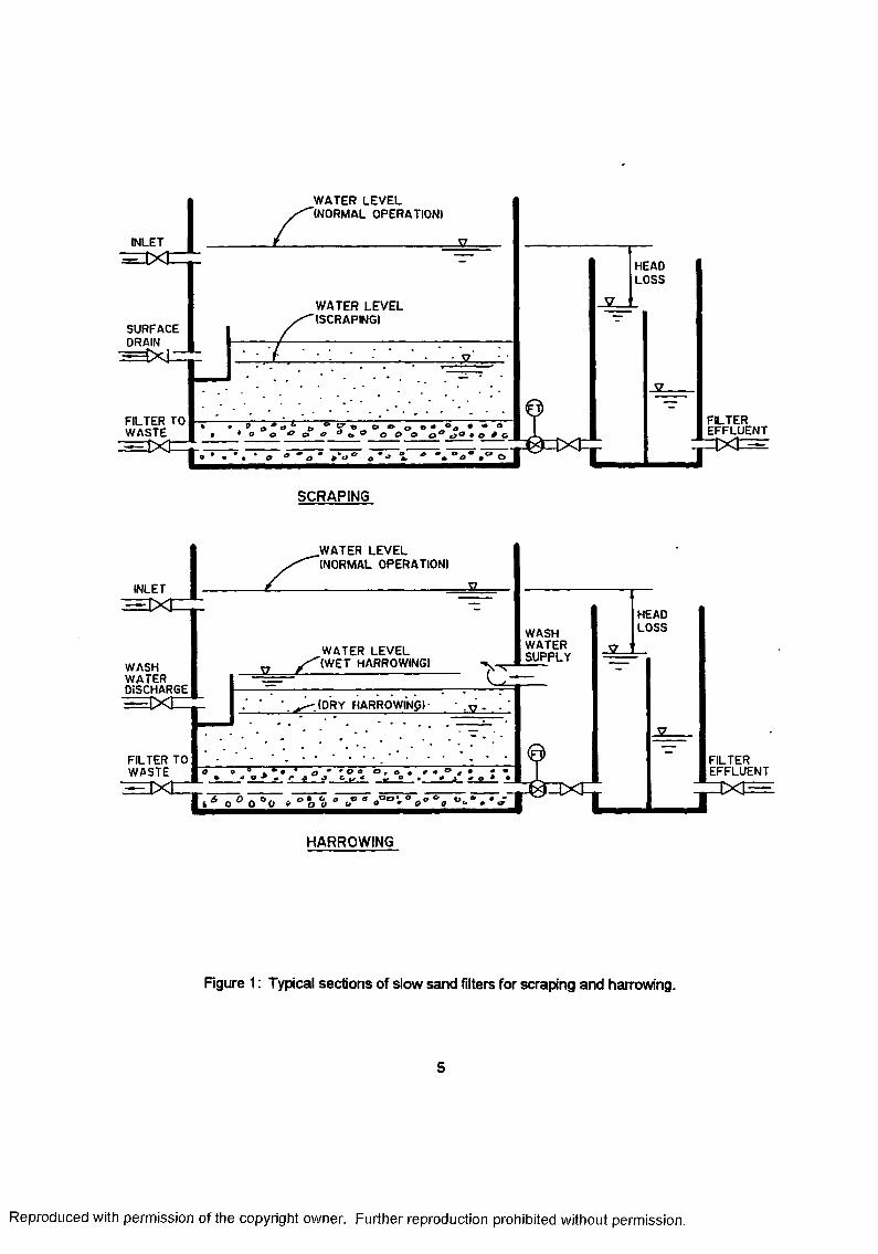
back on line without a deterioration in treatment performance. The process piping requirements for
each of the two filter cleaning methods are shown schematically in Figure 1.
Analyses of cores taken from three mature full-scale slow sand filters revealed a
significant relationship between trihalomethane formation potential mass removal rates (mg/m2*hr)
and filter media biomass as shown in Table 1 (Collins et al., 1988,1989). Filter biomass was
4
Reproduced with permission of the copyright owner. Further reproduction prohibited without permission.
WATER LEVEL (NORMAL OPERATION)
INLET
HEADLOSS
WATER LEVEL (SCRAPING)
SURFACEDRAIN
FILTEREFFLUENT
FILTER TO WASTE j=t>C
SCRAPING
WATER LEVEL (NORMAL OPERATION)
INLET3X1 HEAO
LOSSWASHWATERSUPPLYWATER LEVEL
(WET HARROWING)WASHWATERDISCHARGE3 X 1 = (DRY HARROWINff) •
FILTER TO WASTE
^ ix tzFILTEREFFLUENT
HARROWING
Figure 1: Typical sections of slow sand filters for scraping and harrowing.
Reproduced with permission of the copyright owner. Further reproduction prohibited without permission.
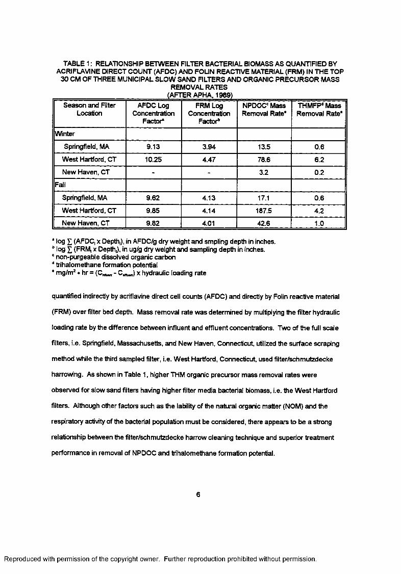
TABLE 1: RELATIONSHIP BETWEEN FILTER BACTERIAL BIOMASS AS QUANTIFIED BY ACRIFLAVINE DIRECT COUNT (AFDC) AND FOUN REACTIVE MATERIAL (FRM) IN THE TOP
30 CM OF THREE MUNICIPAL SLOW SAND FILTERS AND ORGANIC PRECURSOR MASSREMOVAL RATES
Season and Filter Location
AFDC Log Concentration
Factor*
FRM Log Concentration
Factor*1
NPDOC* Mass Removal Rate*
THMFP<* Mass Removal Rate*
Winter
Springfield, MA 9.13 3.94 13.5 0.6
West Hartford, CT 10.25 4.47 78.6 6.2
New Haven, CT - - 3.2 0.2
Fall
Springfield, MA 9.62 4.13 17.1 0.6
West Hartford, CT 9.85 4.14 187.5 4.2
New Haven, CT 9.82 4.01 42.6 1.0
1 log E (AFDC, x Depth,), in AFDC/g dry weight and smpling depth in inches. b log £ (FRM, x Depth,), in ug/g dry weight and sampling depth in inches. c non-purgeable dissolved organic carbon d trihalomethane formation potential * mg/m2 • hr = (C *^ - C— x hydraulic loading rate
quantified indirectly by acriflavine direct cell counts (AFDC) and directly by Folin reactive material
(FRM) over filter bed depth. Mass removal rate was determined by multiplying the filter hydraulic
loading rate by the difference between influent and effluent concentrations. Two of the full scale
filters, i.e. Springfield, Massachusetts, and New Haven, Connecticut, utilized the surface scraping
method while the third sampled filter, i.e. West Hartford, Connecticut, used filter/schmutzdecke
harrowing. As shown in Table 1, higher THM organic precursor mass removal rates were
observed for slow sand filters having higher filter media bacterial biomass, i.e. the West Hartford
filters. Although other factors such as the lability of the natural organic matter (NOM) and the
respiratory activity of the bacterial population must be considered, there appears to be a strong
relationship between the filter/schmutzdecke harrow cleaning technique and superior treatment
performance in removal of NPDOC and trihalomethane formation potential.
6
Reproduced with permission of the copyright owner. Further reproduction prohibited without permission.
Filter/schmutzdecke harrowing of slow sand filters may also be advantageously utilized to
quickly mature slow sand filters after cleaning when the water source is of exceptional quality.
Biological maturation of pilot slow sand filters in Gorham (New Hampshire) was determined to be a
very slow process typically requiring several months to establish a surface deposit over the entire
filter surface. For example, a pilot slow sand filter with an effective sand size of 0.34 mm and
uniformity coefficient of 2.0 operating at a hydraulic flow rate of 0.25 m/hr (0.1 gpm/sf) developed
less than 10 cm (4-in) headloss after 189 days of continuous operation. The raw water turbidity,
dissolved organic carbon, UV absorbance, total coliform, and temperature levels during the pilot
study (May-November 1989) averaged below 0.20 NTU, 2.0 mg/L, 0.06 cm'1, 12 CFU/100 mL, and
10'C, respectively. A filter cleaning method that will minimize removal of biomass and bacterial
population in the mature schmutzdecke and top filter sand layers was desirable at Gorham to
reduce slow sand filter maturation requirements.
1.2 PROJECT GOALS, OBJECTIVES, AND EXPECTED BENEFITS
This research study proposed to evaluate the performance of two slow sand filter cleaning
methods, surface scraping, and filter harrowing, under controlled full-scale conditions at a recently
constructed slow sand filtration facility in Gorham, New Hampshire. The facility went on-line in
February 1991 and appeared to offer a unique opportunity to quantify cleaning effectiveness,
maintenance costs, filter downtime, headloss development rates, and filter-to-waste requirements
for each cleaning method in full-scale filter comparisons. The project goal was to document any
financial savings and treatment effectiveness that a small community could reap by utilizing one
filter cleaning method over another.
The Gorham, NH plant was in operation for over two years before cleaning was necessary
and so the plans to use that facility for comparative operations were suspended. Data on
comparative cleaning operations were obtained at Newport, NH. Data on comparative filter
characteristics was developed from full-scale filters at Gorham and Newport, NH, Newark, NY,
7
Reproduced with permission of the copyright owner. Further reproduction prohibited without permission.
West Hartford, CT, and pilot plants at Portsmouth, NH. Data on filter performance was developed
from each of the previously mentioned facilities and laboratory scale studies at the UNH
environmental engineering laboratories.
The following parameters were used for comparison between the two cleaning methods:
Filter performance
Effectiveness of cleaning operations
Filter-to-waste requirements to achieve an acceptable treatment performance
Headloss development rate after each filter cleaning
Filter downtime required for each cleaning episode
Variation in cleaning frequency rate, and
Yearly maintenance costs associated with operation and cleaning of each filter.
8
Reproduced with permission of the copyright owner. Further reproduction prohibited without permission.
CHAPTER 2
UTERATURE REVIEW
2.1 HISTORY
2.1.1 Slow Sand Filtration
Sand filters have been used to treat water since the early nineteenth century (Hiisman
and Wood, 1974; Slezak and Sims, 1984; Ellis, 1985). Untreated water was filtered through a bed
of sand and the resulting water was used for drinking, washing, and industrial purposes. The
earliest known design of these filters has become known as a "slow sand filter.” This type of
treatment is still used. Seventy-one slow sand filter plants were identified in the United States in
1988 (Logsdon, 1991). That study found that forty-five percent of the plants served populations of
less than 1,000 and seventy-six percent served populations of less than 10,000 persons. A few
larger plants also use slow sand filtration, most notably West Hartford, CT in the US, but also
including Amsterdam, Antwerp, London, Paris, and Zurich in Europe (Huisman and Wood, 1974;
Weber-Shirk, 1992). After 1900, "mechanical filters" (generally of the rapid-sand filter type) gained
in popularity and they have become the prevalent type of filtration. Rapid sand filters are generally
used after chemical coagulation and settling and are able to treat raw water containing
concentrations of turbidity, clays, algae, and other matter that could not be treated or treatted
economically by slow sand filters.
Slow sand filters attracted renewed attention after 1970 for their low costs for operation
and their reliable removal of coliform bacteria and Giardia cysts (Logsdon, 1991). At least 225
slow sand plants had been identified by 1994 in the United States (Brink and Parks, 1996). The
need to remove dissolved organic precursor material also has led to renewed research.
The essential features of a slow sand filter include a tank to maintain a relatively constant
9
Reproduced with permission of the copyright owner. Further reproduction prohibited without permission.
supply of water and pressure over a layer of fine to medium filter sand, a layer of support gravel
and underdrain system to collect the filtered water, and a system of valves and piping to control the
rates of flow, depth of water over the filter sand, and back pressure on the underdrain system
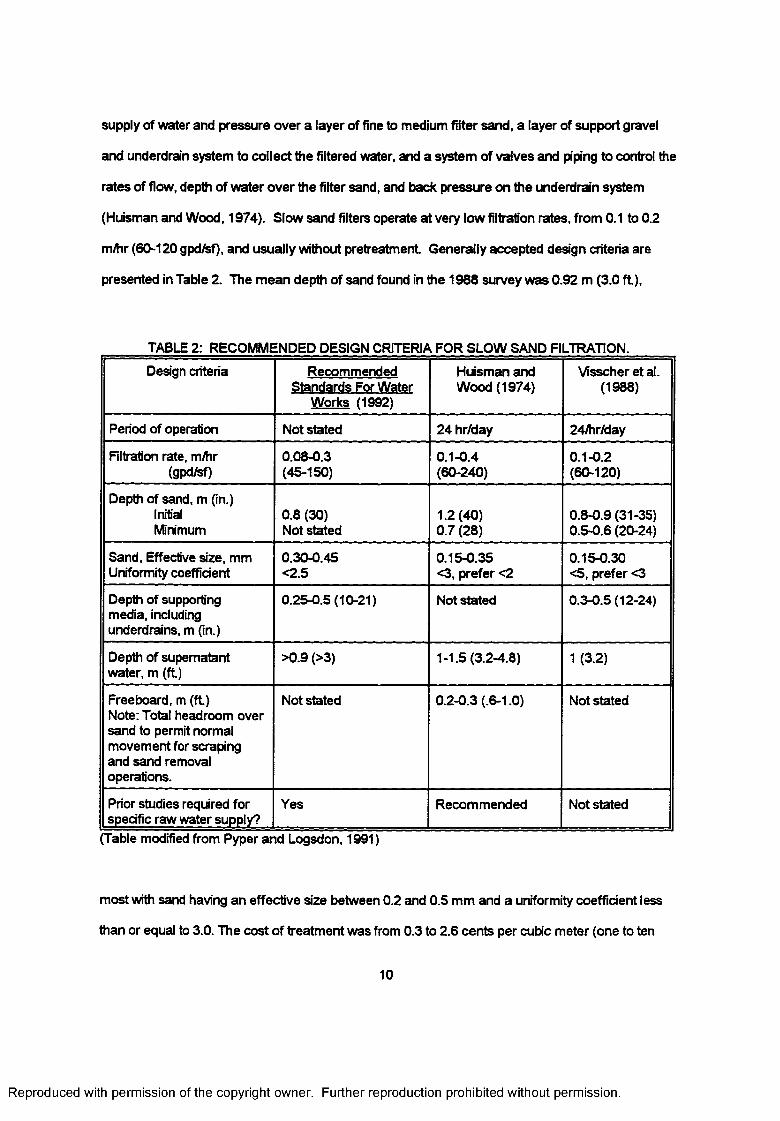
(Huisman and Wood, 1974). Slow sand filters operate at very low filtration rates, from 0.1 to 0.2
m/hr (60-120 gpd/sf), and usually without pretreatment Generally accepted design criteria are
presented in Table 2. The mean depth of sand found in the 1988 survey was 0.92 m (3.0 ft),
TABLE 2: RECOMMENDED DESIGN CRITERIA FOR SLOW SAND FILTRATION.
Design criteria Recommended Standards For Water
Works (1992)
Huisman and Wood (1974)
Visscher et al. (1988)
Period of operation Not stated 24 hr/day 24/hr/day
Filtration rate, m/hr (gpd/sf)
0.08-0.3(45-150)
0.1-0.4 (60-240)
0.1-0.2 (60-120)
Depth of sand, m (in.) Initial Minimum
0.8 (30) Not stated
1.2 (40) 0.7 (28)
0.8-0.9 (31-35) 0.5-0.6 (20-24)
Sand, Effective size, mm Uniformity coefficient
0.30-0.45<2.5
0.15-0.35 <3, prefer <2
0.15-0.30 <5, prefer <3
Depth of supporting media, including underdrains, m (in.)
0.25-0.5 (10-21) Not stated 0.3-0.5 (12-24)
Depth of supernatant water, m (ft)
>0.9 (>3) 1-1.5 (3.2-4.8) 1 (3.2)
Freeboard, m (ft)Note: Total headroom over sand to permit normal movement for scraping and sand removal operations.
Not stated 0.2-0.3 (.6-1.0) Not stated
Prior studies required for specific raw water supply?
Yes Recommended Not stated
Table modified from Pyper and Logsdon, 1991)
most with sand having an effective size between 0.2 and 0.5 mm and a uniformity coefficient less
than or equal to 3.0. The cost of treatment was from 0.3 to 2.6 cents per cubic meter (one to ten
10
Reproduced with permission of the copyright owner. Further reproduction prohibited without permission.
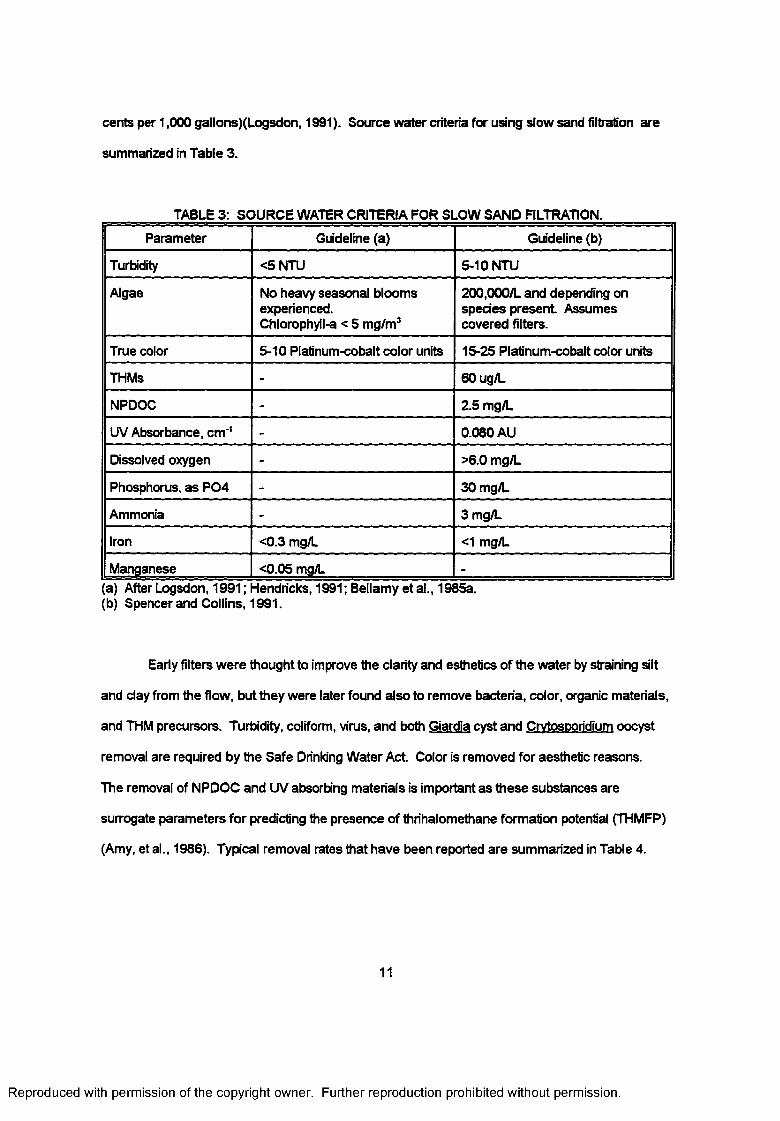
cents per 1,000 gallons)(Logsdon, 1991). Source water criteria for using slow sand filtration are
summarized in Table 3.
TABLE 3: SOURCE WATER CRITERIA FOR SLOW SAND FILTRATION.
Parameter Guideline (a) Guideline (b)
Turbidity <5 NTU 5-10 NTU
Algae No heavy seasonal blooms experienced.Chlorophyll-a < 5 mg/m3
200,000/L and depending on spedes present Assumes covered filters.
True color 5-10 Platinum-cobalt color units 15-25 Platinum-cobalt color units
THMs - 60ug/L
NPDOC - 2.5 mg/L
UV Absorbance, cm'1 - 0.080 AU
Dissolved oxygen - >6.0 mg/L
Phosphorus, as P04 - 30 mg/L
Ammonia - 3 mg/L
Iron <0.3 mg/L <1 mg/L
Manganese <0.05 mg/L -a) After Logsdon, 1991; Hendricks, 1991; Bellamy et al., 1985a.
(b) Spencer and Collins, 1991.
Early filters were thought to improve the clarity and esthetics of the water by straining silt
and clay from the flow, but they were later found also to remove bacteria, color, organic materials,
and THM precursors. Turbidity, coliform, virus, and both Giardia cyst and Crvtosporidium oocyst
removal are required by the Safe Drinking Water Act Color is removed for aesthetic reasons.
The removal of NPDOC and UV absorbing materials is important as these substances are
surrogate parameters for predicting the presence of thrihalomethane formation potential (THMFP)
(Amy, et al., 1986). Typical removal rates that have been reported are summarized in Table 4.
11
Reproduced with permission of the copyright owner. Further reproduction prohibited without permission.
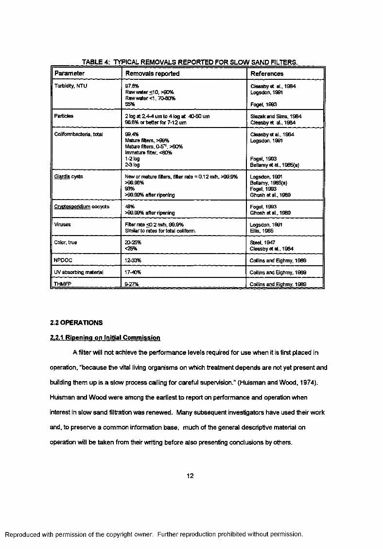
TABLE 4: TYPICAL REMOVALS REPORTED FOR SLOW SAND FILTERS.
Parameter Removals reported References
Turbidity, NTU 97.8%Raw water <10, >90% Raw water <1,7080% 55%
Cleasbyet al., 1984 Logsdon, 1991
Fogel, 1993
Particles 2 log at 2.4-4 um to 4 log at 40-50 um 96.8% or better for 7-12 um
Slezakand Sims, 1984 Cleasbyet al., 1984
Colifbrmbacteria, total 99.4%Mature filters, >99% Mature filters, 0-5^, >90% Immature filter. <80%1-2 log2-3 log
Cleasbyet al., 1964 Logsdon.1991
Fogel, 1993 Bellamy et al., 1985(a)
Giardia cvsts New or mature filters, filter rate = 0.12 m/h, >99.9% >99.98%93%>99.99% after ripening
Logsdon. 1991 Bellamy. 1965(a) Fogel. 1993 Ghosh et al., 1989
CrvDtosDoridium oocvcts 48%>99.99% after npening
Fogel, 1993 Ghosh etal., 1989
Viruses Filter rate <0.2 m/h, 99.9% Similar to rates for total coliform.
Logsdon, 1961 Ellis. 1965
Color, true 20-25%<25%
Steel, 1947 Cleasbyetal., 1964
NPDOC 12-33% Collins and Bghmy, 1989
UV absorbing material 17-40% Collins and Bghmy, 1969
THMFP 9-27% Collins and Bghmy, 1969
2.2 OPERATIONS
2.2.1 Ripening on Initial Commission
A filter will not achieve the performance levels required for use when it is first placed in
operation, "because the vital living organisms on which treatment depends are not yet present and
building them up is a slow process calling for careful supervision." (Huisman and Wood, 1974).
Huisman and Wood were among the earliest to report on performance and operation when
interest in slow sand filtration was renewed. Many subsequent investigators have used their work
and, to preserve a common information base, much of the general descriptive material on
operation will be taken from their writing before also presenting conclusions by others.
12
Reproduced with permission of the copyright owner. Further reproduction prohibited without permission.
"When filters are to be first started, they should be filled from below to expel air bubbles
from the interstices of the sand, and then from above to the normal working depth. The outlet
valve should then be opened and the effluent run to waste at about one quarter of the normal rate,
without interruption, for a period of at least several weeks in tropical climates and longer where
temperatures are low. The time also depends on the nature of the raw water. The flow is
gradually increased until it reaches the designed rate. Formation of a schmutzdecke and an
increase in the head loss are signs that ripening is proceeding satisfactorily, but comparative
chemical and bacteriological analyses of raw and effluent are needed to demonstrate that the filter
is in full working condition and that the water may be diverted to the public supply. Any interruption
longer than the period required to fill the clear well may necessitate another period of ripening to
maintain effluent quality" (Huisman and Wood, 1974). Although there is no consistent definition of
"ripening," filter is said to be ripened when the effluent quality is better than its influent though the
effluent quality must be able to meet regulatory requirements before it may be used. The length of
the time for ripening varies widely, ranging from one week to several months (Hendricks, 1991).
It is essential for the sand to have been washed thoroughly before it is placed in a filter so
that effluent turbidity levels will fall to acceptable levels within a few days or weeks (Logsdon,
1991; Ghosh et al., 1989). One objective of pilot testing is to determine the length of ripening time
needed (Hendricks, 1991).
2.2.2 Cleaning
As water continues to be filtered, impurities are deposited on the surface of the sand
media and in the interstices of the media. This interstitial material includes microorganisms,
allochthonous and autochthonous biodegradable and non-biodegradable oranic materials, and
inorganic matter. These deposits increase resistance to the flow of water and the difference in
pressure, or "headloss", between the surface of the water over the filter and the water leaving the
underdrains increases. Eventually the headloss will approach the available difference between the
13
Reproduced with permission of the copyright owner. Further reproduction prohibited without permission.
elevation of the overlying water surface and the bottom of the filter. If the filter were allowed to
continue operating, the headloss would exceed the available difference and negative pressures
would result just below the schmutzdecke layer. This could cause release of dissolved gases,
resulting in local "air binding" of the spaces between sand grains. Filter air binding could reduce
removal efficiencies by increasing localized hydraulic loading on the remaining filter bed. Filters
are cleaned before the headlosses accumulate to the maximum level to avoid this condition.
2.3 CLEANING METHODS
Cleaning is the chief operating expense at slow sand filter plants and much effort has been
made to simplify this operation and to introduce mechanical processes where possible. Surface
scraping has been used almost universally, but several other processes have been tried. Dry
raking has been used to lengthen the period of service and save time, using 2 or 3 rakings
between scrapings. When the bed is then scraped, a much greater depth of sand must be
removed than otherwise (Tumeaure and Russell, 1924; Letterman and Cullen, 1985). Deep
spading and loosening also have been used, but this process was of doubtful value as it disturbed
the action of the filter much more than surface raking (Tumeaure and Russell, 1924). In a more
recent pilot operation, it was demonstrated that mixing the upper 10 cm (4 in.) of sand after it had
been cleaned by scraping reduces removals as compared with operation following normal
cleaning (Bellamy et al. 1985a).
In-place cleaning by agitation and washing within a travelling box has been used in
Wilmington, Del. (Tumeaure and Russell, 1924); Paris and Ashford Common Works of London
(Renton etal., 1991); Antwerp (Huisman and Wood, 1974; Renton etal., 1991); and Hartford, CT
(Minkus, 1954). Hydraulic movement of the sand to portable cleaning equipment and replacement
has been used in drained filters (Tumeaure and Russell, 1924; Letterman and Cullen, 1985) and in
operating filters (Renton et al., 1991). Removable synthetic geotextile material placed on the
media surface has also been considered (Mbwette and Graham, 1988; Vochten et al., 1988).
14
Reproduced with permission of the copyright owner. Further reproduction prohibited without permission.
Scraping remains the predominating method in use, however.
2.3.1 Scraping
The scraping method of cleaning has been widely described (Huisman and Wood, 1974;
Letterman and Cullen, 1985; Hendricks, 1991; and many others). Scraping involves draining the
filter, removing the upper 1 to 2 cm (0.5 to 1 inch) from the filter to expose a cleaner sand surface,
and returning the filter to service. Because a portion of the sand media has been removed, a
period of re-ripening may be necessary before the filtered water may be used. The depth of the
sand bed is progressively depleted by the amount of sand removed each time it is scraped.
Eventually the remaining sand will have become too shallow to effectively treat the incoming
water. The filter will then need to be "resanded" by adding a layer of new sand over the remaining
sand or by replacing all the sand in the filter, and the new sand ripened as reqiired for a new filter.
Letterman and Cullen (1985) also described the scraping practices at a number of plants in upstate
New York and presented information on the variations practiced within an area under the same
regulatory body. The use of mechanical equipment for scraping has also been described
(Huisman and Wood, 1974; Renton etal., 1991).
2.3.2 Harrowing
Wet raking while maintaining a cross-flow of water to carry away suspended materials to
suitable drains, referred to as the "Brooklyn method”, had been attempted but it was regarded as
difficult to clean a filter to a sufficient depth and did not come into general use (Tumeaure and
Russell, 1924). After several other cleaning methods had been tried without satisfaction, a
modification of this method was adopted in the early 1950's at the West Hartford, CT plant and is
still being used (Minkus, 1954; Allen, 1991). The protocol for harrowing as practiced at West
Hartford is as follows:
1. Between 3 and 5 A.M., close the raw water supply.
2. By 8 A.M., lower a small tractor through the narrow entrance shaft to the sand level.
15
Reproduced with permission of the copyright owner. Further reproduction prohibited without permission.
3. The water level in the filter is maintained at about 5 to 30 cm (2 to 12 inches) above the
sand while the tractor pulls a small spring toothed harrow over the surface for 4 to 5 hours.
This stirs up the top materials and washes them across the sand to an outlet drain. This
water, from the raw water supply, is introduced from a channel along one side of the filter
and flows to a drain channel along the side of the filter opposite the supply channel. The
velocity of the flow across the filter surface is only about 0.1 to 0.25 cm/s (0.05 to 0.1 fps)
but the tractor keeps circling the bed and resuspending the material until most of it reaches
the drain channel. Filtered water is also introduced up through the filter from the
underdrain to prevent debris from further penetrating the filter during wet harrowing. This
upflow is at a rate of approximately 0.02 m/hr (0.008 gpm/sf) and far below the rate
necessary to fluidize the sand media.
4. After about 4 hours, the underdrain is opened, and the water drained to about 30 cm
(12-inches) below the surface of the sand.
5. The next morning, either the same tractor or a larger crawler tractor is used to pull a
larger toothed-harrow for a half day to scarify the bed to a greater depth and break the
deeper crust
6. The filter is then filled from below to above the sand surface with filtered water, then
raw water is added from above the filter to raise the level to about one meter (3- ft) above
the sand. The filter is then opened to the system but at only about a quarter of its capacity
for the first shift
Collins et al. (1989) found a significant relationship between the mass removal rates of
THMFP (mg/m2 *hr) and the filter media biomass as quantified by FRM and AFDC. They found
that the filters cleaned by harrowing outperformed those cleaned by scraping. They also reported
harrowing required less time and labor than did the surface scraping method and that the effluent
quality did not deteriorate due to the cleaning because the bacterial population was maintained.
2.3.3 Ripening after Cleaning
Nearly all investigators report the initial performance of a filter that has just been cleaned
must be carefully monitored because it may exhibit a ripening period. Letterman and Cullen (1985)
16
Reproduced with permission of the copyright owner. Further reproduction prohibited without permission.
defined a ripening period as "occurring when a filter which had Just been put in operation removes
particulates at a lower efficiency than removed by an identical filter which had been operating for a
significant time." The adverse impacts of ripening are reduced by filtering to waste until the desired
performance is again reached (Logsdon, 1991). Not all filters necessarily exhibit ripening
(Letterman and Cullen. 1985).
After cleaning and filling, the filter should be started slowly and gradually. If ripening is
necessary, the effluent is run to waste until analyses demonstrate that it satisfies the normal quality
standards. The process is markedly accelerated as compared to when the bed was initially placed
in service (Huisman and Wood, 1974). This period can range from overnight as at the Newport
NH filters monitored in this investigation, to 24-48 hours (Logsdon, 1991). The development of the
schmutzdecke is sometimes considered to be necessary for full efficiency in removing particles,
especially if Giardia cysts are of concern (Cleasby et al., 1984). This was particularly important
during the first four filter cycles in their pilot plant operation, though not during later operations.
Only four of 10 cleaning operation at plants using the scraping method have shown their ability to
remove turbidity and coliform was affected after cleaning (Letterman and Cullen, 1985), but no
comparable information was reported for removal of OOC or UV absorbing materials. The length
of ripening observed in these four plants ranged from 6 hours to two weeks. Neither
prechlorination nor water temperature appeared to correlate with ripening period duration.
2.3.5 Reconditioning
"During the long operating period, some of the raw water impurities and some of the
products of biodegradation will have been earned into the sand bed to a depth of some 0.3 to 0.5
m, according to the grain size of the sand" (Huisman and Wood, 1974). To prevent cumulative
fouling and increased resistance, this depth of sand should be removed before resanding but it
does not need to be discarded (Logsdon, 1991). A practice known as "throwing-over" the
remaining sand onto cleaned sand laid on the supporting gravel has been described (Huisman and
17
Reproduced with permission of the copyright owner. Further reproduction prohibited without permission.
Wood, 1974; Renton et al., 1991) and would retain the sand without allowing the bed to become
strayed.
Renton et al. (1991) noted that if the lower layers of sand were allowed to reman within
the filter over a prolonged period, an accumulation of silt and organic debris effectively dogged the
bed, thereby redudng subsequent run times and output Thames Water Utilities Ltd. fadlities have
used hand trenching. This method involved hand excavation of a trench across the filter, washing
the excavated sand, and repladng the washed material into the filter in the course of rebuilding the
gravel and sand layers. Sometimes unwashed excavated sand was placed on the surface of the
replacement sand adjacent to the trench. This would build the filter up to approximately normal
operating depths but leave the older layers with their accumulated debris on top where it could
continue to cause head loss. Manual trenching had the advantage that no special tools or skills
were required but it was costly in both time and labor. A "deep skimming" process is now used to
replace the former hand labor method, cutting down to the support gravel layer. Resanding is
required every 12 to 15 filter runs or as necessary when the minimum depth of 0.3 m (1-ft) is
reached. That thickness has been established within their jurisdiction to maintain the adequate
particle removals as an effective barrier against pathogens. The resanding operations take 2 to 3
weeks to complete followed by a one to 3 week conditioning period for "ripening" before the beds
are returned to service. Performance of deep skimmed beds is such that they produce an average
of 24 percent more water than when reconditioned sand is placed on an older layer containing
debris. Resanding by the trenching method also produced a marked improvement but strict
comparisons were not made as to the use of differing sand grades, dean sand criteria, and
operating conditions which may also influence behavior of the beds. Initial head losses for a bed
which had been scraped was 0.59 mm but only 0.28 mm after reconditioning with deep skimming
(Renten et al., 1991).
Various sand washing methods have been reported (Huisman and Wood, 1974: Renton et
18
Reproduced with permission of the copyright owner. Further reproduction prohibited without permission.
al., 1991; Allen, 1991; Whitman, 1992). A completely dean sand is difficult to attain. Washing
rarely removes the strongly adherent organic coating entirely from grains and, after exposure to
air, this material can "become soluble and serve as a substrate for bacterial growth." Under
favorable temperatures and moisture conditions, the sand will contain large numbers of bacteria
and not all will contribute to the treatment process. Resanding should be done in the winter if
washed sand is to be used (Huisman and Wood, 1974). When washed, the sand loses its finer
particles and coarser sand may allow deeper penetration of impurities (Huisman and Wood, 1974).
2.4 PERFORMANCE FACTORS AFFECTING REMOVAL OF WATER IMPURITIES
2.4.1 General Factors
Early reports on slow sand filters considered their ability to remove particles due to the
straining properties of the sand or schmutzdecke layer. Later studies recognized performance was
related to other biological and physical mechanisms present in the filters. Removal mechanisms
for slow sand filters have been described in detail elsewhere (Huisman and Wood, 1974; Ellis,
1985; Hendricks, 1991; Haarhoff and Cleasby, 1991; Weber-Shirk, 1992; Weber-Shirk and Dick,
1997).
Weber-Shirk (1992) summarized the development of theories regarding the performance
of slow sand filters. Simpson, in 1827 prior to building a full-scale filter, stated "the principle of the
action depends upon the strata of filtering material being finest at the top, the interstices being
more minute in the fine sand than the strata below; and the silt, as its progress is arrested, (while
the water passed from it renders the interstices between the particles of sand still more minute,
and the bed generally produces better water when it is pretty well covered with silt than at any
other time." This theory has remained prevalent and much of the literature emphasizes the role of
the formation of a dirty-skin, the "schmutzdecke," as an effective filtering media (Cleasby, et al.,
1984; Letterman and Cullen, 1985). In 1939 Simpson believed the process included something
more than straining. Other investigators also began to look at other mechanisms. Piefke (Fuertes,
19
Reproduced with permission of the copyright owner. Further reproduction prohibited without permission.
1901) concluded that straining could not account for the removal of bacteria and proposed
biological action on the surface and in the sand was responsible for most of their removal. Meek
and Shieh (1984), as well as operating data from numerous plants including those cited by
Letterman and Cullen (1985), noted that reripening was not necessarily required after the removal
of the schmutzdecke by scraping. Studies by Hendricks (Meek and Shieh, 1984) demonstrated
that it was the maturity of the biomass within the filter that was critical to removal of G'ardia cysts,
regardless of the age of the scmutzdecke and the time since resanding over mature support gravel
layers.
Filtration generally has been studied as a clean bed process which traps particles (Camp,
1964; Ives and Sholji, 1965; Yao et al.,1971; O'Melia and Ali, 1978; and numerous others). O'Melia
and co-workers have been particularly notable in their application of collector theory based on
consideration of efficiency of both particle transport to a collector and subsequent particle capture
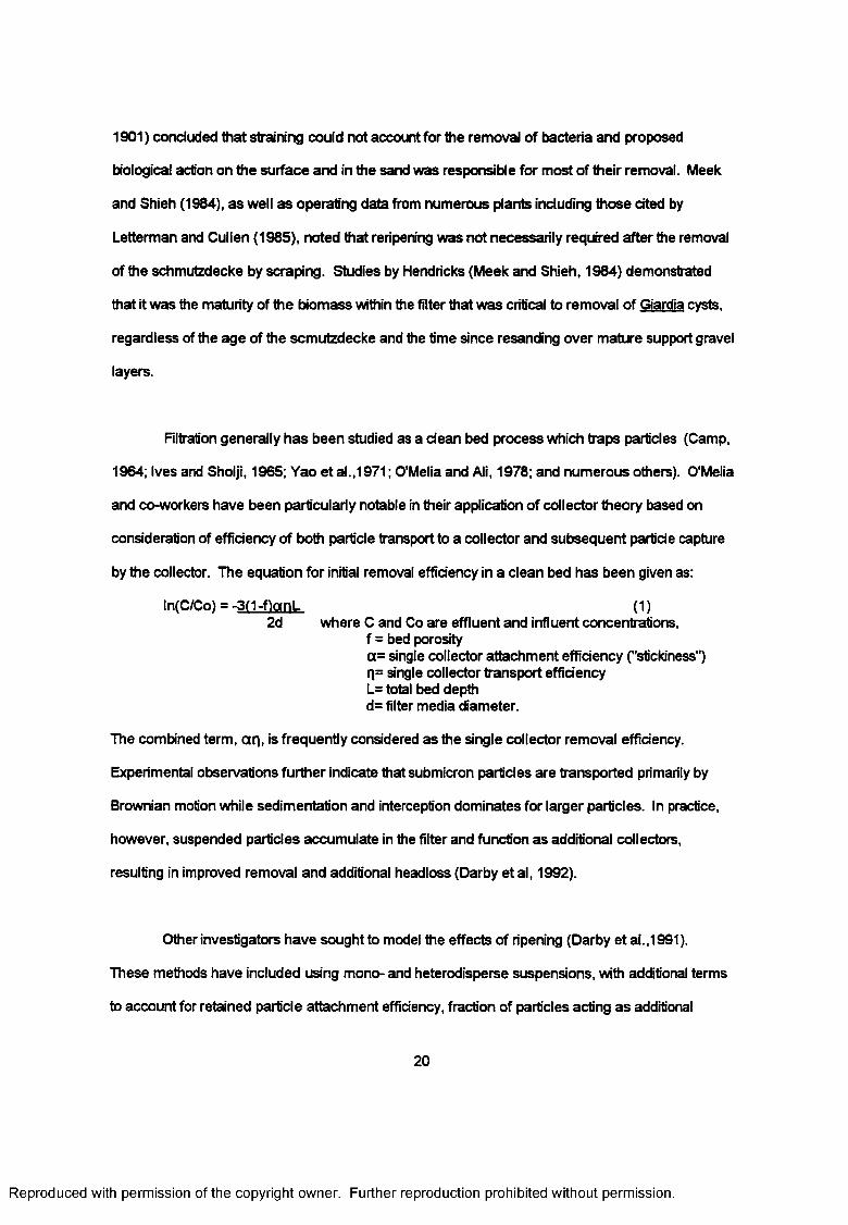
by the collector. The equation for initial removal efficiency in a clean bed has been given as;
InfC/Co) = -3(1-flanL (1)2d where C and Co are effluent and influent concentrations,
f = bed porositya= single collector attachment efficiency ("stickiness") q= single collector transport efficiency L= total bed depth d= filter media diameter.
The combined term, an, is frequently considered as the single collector removal efficiency.
Experimental observations further indicate that submicron particles are transported primarily by
Brownian motion while sedimentation and interception dominates for larger particles. In practice,
however, suspended particles accumulate in the filter and function as additional collectors,
resulting in improved removal and additional headloss (Darby et al, 1992).
Other investigators have sought to model the effects of ripening (Darby et al.,1991).
These methods have included using mono- and heterodisperse suspensions, with additional terms
to account for retained particle attachment efficiency, fraction of particles acting as additional
20
Reproduced with permission of the copyright owner. Further reproduction prohibited without permission.
collectors, fraction of particles contributing to headloss, the transport efficiency of retained
particles, the removal efficiency of collected particles, and the density of additional particles(Darby
et al., 1992). These extensions of the collector theories make the understanding of full-scale filters
more realistic but point out the complexity of ripening even under controlled laboratory conditions.
Huisman and Wood (1974) and Hendricks (1991) viewed the biofilm developing on the
sand grains as increasing the "stickiness" of the media and its ability to capture and hold particulate
matter until it was metabolized. Studies using water from natural sources indicate that
accumulation of matter in filter media is also affected by microbial growth, and the biodegradation
is affected by the form of the nutrient carbon sources, whether particulate or soluble (Hijnen and
Van der Kooij, 1992). The type and amount of carbon present affect the removal potential of a
filter as does the mass and extent of acclimation of the biological population. DOC has been
identified as a potentially important source of particle volume in floe formed using chemical
coagulation, and it has been suggested that 1.6 ppm of particle volume per mg DOC/L should be
added when estimating the final volume of particles resulting from treatment (Wiesner and
Mazounie, 1989). Subsequent metabolism of assimilable organic material would reduce the
volume in a biological filter. Metabolism would also release products to lower portions of the filter
and eventually to the filter underdrains (Bouwer and Crowe, 1988).
Hendricks and Bellamy (1991) listed process variables affecting microorganism removal
efficiencies by field-scale slow sand filters. These variables are listed in Table 5.
These variables also have been identified in relation to the removal efficiency for turbidity, particles,
and organic matter. There has been little discussion of the relationships between these variables
and removal of NPDOC and UV absorbing materials.
A 1988 study of relative performances between three filter plants in New England found
differences in removals of NPDOC, UV absorbing materials, and THMFP (Fenstermacher, 1989;
21
Reproduced with permission of the copyright owner. Further reproduction prohibited without permission.
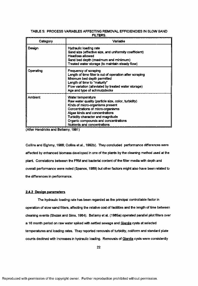
TABLE 5: PROCESS VARIABLES AFFECTING REMOVAL EFFICIENCIES IN SLOW SANDFILTERS.
Category Variable
Design Hydraulic loading rateSand size (effective size, and uniformity coefficient) Headloss allowedSand bed depth (maximum and minimum)Treated water storage (to maintain steady flow)
Operating Frequency of scrapingLength of time filter is out of operation after scraping Minimum bed depth permitted Length of time to "maturity"Flow variation (alleviated by treated water storage) Age and type of schmutzdecke
Ambient Water temperatureRaw water quality (particle size, color, turbidity) Kinds of micro-organisms present Concentrations of micro-organisms Algae kinds and concentrations Turbidity character and magnitude Organic compounds and concentrations Nutrients and concentrations
After Hendricks and Bellamy, 1991)
Collins and Bghmy, 1988; Collins etal., 1992b). They concluded performance differences were
affected by enhanced biomass developed in one of the plants by the cleaning method used at the
plant Correlations between the FRM and bacterial content of the filter media with depth and
overall performance were noted (Spanos, 1989) but other factors might also have been related to
the differences in performance.
2.4.2 Design parameters
The hydraulic loading rate has been regarded as the principal controllable factor in
operation of slow sand filters, affecting the relative cost of facilities and the length of time between
cleaning events (Slezak and Sims, 1984). Bellamy et al. (1985a) operated parallel pilot filters over
a 16 month period on raw water spiked with settled sewage and Giardia cysts at selected
temperatures and loading rates. They reported removals of turbidity, coliform and standard plate
counts declined with increases in hydraulic loading. Removals of Giardia cysts were consistently
22
Reproduced with permission of the copyright owner. Further reproduction prohibited without permission.
above 99.98 percent at all loadings and differences were not significant They concluded that
loading rates should be considered in design due to the unmistaken influence of hydraulic loading
rates on percent removals. This position appears to have continued support in establishing design
criteria for slow sand filters.
Hendricks and Bellamy (1991) reviewed literature on this topic ranging from Hazen (1913),
"the efficiency of removal almost uniformly decreases rapidly with increasing (flow) rate", to more
recent sources. They concluded that the removal of turbidity, coliform bacteria, Giardia cysts, and
standard plate count are uniformly high and loading rates should not be a deciding factor in design.
Taylor (1974) concluded there was no difference in performance for loadings between 0.12-0.25
m/hr to 0.5-0.6 m/hr (0.05-0.1 to 0.2-0.24 gpd/sf). Collins et al. (1992) found differences in
treatment performance which were statistically indistinguishable between the rates of 0.05 m/hr
and 0.10 m/hr (0.02-0.04 gpd/sf). It is generally agreed that the loading rate should not be varied
rapidly (Huisman and Wood, 1974; Haarhoff and Cleasby, 1991; Hendricks, 1991). Ellis (1985)
summarized a number of reports with the conclusion that the appropriate hydraulic loading rate
should be related to raw water quality established from pilot scale investigations.
Haarhoff and Cleasby (1991) reviewed removal of organic carbon and reported studies
with diverse results ranging from "no removal" to as much as 60 to 75 percent removals. They
concluded many of the differences were the results of variations in the composition of organic
materials in the raw water as measured by the tests for TOC, COD, THMFP, etc. Haberer et al.
(1984) related the removal of DOC and permanganate value to filtration rates. Removals of either
DOC or permanganate value declined by approximately 40 percent as the filter rate was increased
from 0.1 to 0.4 m/h (0.04 to 0.16 gpd/sf). Studies by Rechenberg(1965) reported the effluent
permanganate consumption to be a function of filter rate according to the equation;
Ce = ( 0.8vfA0.17) x Ci (2)
where Ce and Ci are the effluent and influent permanganate consumption, and vf is the relative
23
Reproduced with permission of the copyright owner. Further reproduction prohibited without permission.
filtration rate (Huisman and Wood, 1974). Collins etal. (1992) did not find the differences in
NPDOC removal, when expressed in percentage removal, to be significantly different between
rates of 0.05 and 0.10 m/h (0.02 and 0.04 gpd/sf) but the mass of DOC removed was higher at the
higher hydraulic loading.
Most plants are designed to use approximately the same depth of sand. Generally, the
depth of filter sand is relatively constant over the area of each filter and for all filters at a particular
plant after they have been resanded. The depth within a filter varies slowly over time if the filter is
cleaned by scraping 1 -2 cm (0.5 to 1 in) every one to three months. To the extent that the filter
depth approaches one meter (3.2 ft), the empty bed contact time (EBCT), in hours, will be
approximately the reciprocal of the hydraulic loading rate, in meters/hour. The normal range of
EBCT for 1.0 m (3.2-ft) deep filters operating within hydraulic loading rates of 0.1-0.2 m/hr (0.04-
0.08 gpd/sf) would be 10 to 5 hours. The EBCT is a process parameter which also has been
related to filter performance, particularly when relating performance to adsorptive or biological
processes. These processes are time-dependent and higher loading rates reduce the contact
period.
Billen et al. (1992) studied biological filters and concluded that reductions in rapidly
hydrolyzable macromolecular BDOC were essentially completed within 20 to 30 minutes but there
was no significant reduction of slowly hydrolyzable materials within "practical contact times." There
was no definition given for practical contact times, but that study was relating experience with
granular activated carbon (GAC) contactors which would normally have an EBCT of less than one
hour. Wang and Summers (1994) concluded EBCT was "the key parameter for design and
operation of drinking water biofilters” and DOC removal was independent of filter velocities in the
range of 1.5 to 5 m/s (0.6 to 2.0 gpd/sf). Wang and Summers (1993) also concluded that DOC
removal was a function of the product of biomass and contact time, thus mass transfer and
biokinetics must be considered. Their studies found one-third of the biodegradable natural organic
24
Reproduced with permission of the copyright owner. Further reproduction prohibited without permission.
matter (NOM) removed within a 30 minute EBCT was removed within the first 3 minutes.
Attention should also be given to the uniformity of flow across the filter area. Variations in
head loss due to the accumulated materials in or on the surface, possible a'r binding within the
media, the uniformity of the sand, and the construction of the underdrain system cannot be
prevented, but can be minimized (Huisman and Wood, 1974).
2.4.3 Filter sand
Huisman and Wood (1974) considered the quality of the filter effluent to be dependent
primarily on the grain size of the filter sand, and not on hydraulic loading rate so long as the flows
remaned within generally defined limits. Their reasoning, however, related the performance with
available surface area of the sand grains which is related to grain size. They believed the greater
the surface area, the more contact between the "constituents of the raw water, thus speeding up
chemical reactions (surface catalysis)." The total area of sand grain surface is also related to the
depth of the sand media and they equated a depth of 0.6 m (2-ft) of a sand with grains of 0.15 mm
to a depth of 1.4 m (4.6-ft) of a sand with a grain size of 0.35 mm. That relation is also consistent
with the formula for the removal of particulates given by Montgomery (1985):
N/N„ = expf-iy(1-g„) Lrfl (3)dm
where N/N0 = ratio of particles removed i(i = a shape factor e„ = porosity of media L = total depth of the media H = collision factor, and dm = media size.
Their conclusions concerning the importance of grain size were qualified by the affects of raw
water quality, ripening, and cleaning operations.
Most specifications for sand adapt the "Standard for Filtering Material" (AWWA, 1989) by
revising the grain sizes from those specified for rapid sand filters (effective size of 0.35 -0.65 mm,
and uniformity coefficient < 1.7) to those for slow sand filters as shown in Table 2. An additional
25
Reproduced with permission of the copyright owner. Further reproduction prohibited without permission.
modification used in some areas is to allow the use of locally available sand with an add solubility
exceeding 5 percent (Letterman and Cullen, 1985). Studies reported in 1894 by the
Massachusetts Board of Health conduded the use of sand "containing a considerable amount of
lime" would result in increased head losses and increase the hardness of the water from slow
sand filters (Tumeaure and Russell, 1924). Specifications for rapid sand filter media limit the add
solubility so that addic water applied to the filter would not dissolve significant quantities of the filter
material (AWWA, 1989). The raw water supplies in central New York State (Letterman and
Cullen, 1985) have pH, alkalinity, and hardness in ranges compatible with the native sand found in
the area and dissolution has not been reported as a concern. Other variances from specifications,
induding those for uniformity coeffidents, are often allowed to permit the use of locally available
and/or less expensive supplies (Ellis, 1985; Huisman and Wood, 1974).
The effective size of the sand should be based on at least a simple pilot-plant investigation
to ensure satisfactory results for the particular raw water source (Ellis, 1985). A very fine sand
should be more effective in removal of the various raw water constituents, but with more rapid
development of headloss and more frequent cleaning. Coarse sand reduces the frequency of
cleaning, but removals are lower and deep clogging may require scraping to greater than normal
depths of 1-2 cm (0.5-1 in.). Bellamy et al. (1985b) reported that although the removals of
coliform bacteria declined from 99.4 percent to 96.0 percent and standard plate counts increased
from 470 to 1050 colong forming units (CFU)/mL as the effective size was increased from less
than 0.3 mm to 0.615 mm, the removals from filters using both sizes were still high and the
removals of Giardia cysts were complete over both sizes. They concluded that the argument for
using a finer sand was reasonable only on the basis that it would reduce the schmutzdecke
penetration into a coarser sand and thus reduce the volume of sand to scraped during each
cleaning.
It is essential that the sand of all sizes and sources be thoroughly washed to remove the
26
Reproduced with permission of the copyright owner. Further reproduction prohibited without permission.
finest grains, day, organic matter, and other materials that would "wash out" when the filter is first
used, contributing to turbidity, coliform, and otherwise reduce the quality of the filtered water. It is
also essential that the sand be the same throughout the filter area so that the filtration rate is the
same (Tumeaure and Russell, 1924). The porosity of the filter media will remain the same for
grains of the same shape, but historical opinions have stated that the smaller openings between
finer media will clog more quickly if there is a large variation in particle size as represented by a
larger uniformity coeffident and with the development of interstitial biomass(Tumeaure and
Russell, 1924; also as expressed in most specifications for filter media). DiBemardo and Rivera
(1996) concluded, however, that filter runs were longer for sands of the same effective size if the
uniformity coeffident were greater, 4.3 vs 2.2. These authors also reported porosity and hydraulic
conductivity increased with increasing uniformity coeffident
2.4.4 Sand bed depth (maximum and minimum)
Ellis (1985) summarized the action of slow sand filters as "prindpally the result of straining
through the developing filter skin and the top few mm of sand, together with biological activity."
Others have stressed the biological activity extending from a few centimeters to the entire depth of
the bed (Logsdon, 1991; Collins etal., 1992; Weber-Shirk, 1992; Wang. 1995).
The depth of sand to be provided in a filter depends on three factors: First, the thickness
of sand in which the population of purifying bacteria is high, about 0.3 to 0.4 m(1-1.3-ft); second,
the depth below the first in which the degradation byproducts from the first zone are stabilized,
about 0.4 to 0.5 m (1.3-1.6-ft); and third, the allowable thickness of filter that is to be scraped off
before the filter depth is to be restored (Huisman and Wood, 1974). Together, they suggested a
total depth of 1.2-1.4 m (3.9-4.6-ft) be initially provided to allow for 5 years of operation between
resanding operations, with 0.7-0.9 m (2.3-3-ft) minimum thickness when the filter is to be resanded.
Rachwal et al. (1988) reported 0.3 m (1-ft) to be the minimum depth permissible for the Thames
Water Authority system. Bellamy et al (1985b) found coliform bacteria removal decreased from 97
27
Reproduced with permission of the copyright owner. Further reproduction prohibited without permission.
to 95 percent as bed depth was reduced from 0.97 m (3.2-ft) to 0.48 m (1.6-ft), and
recommended allowing filters to be depleted only to this extent before resanding. Ellis (1985)
summarized the available literature and, agreeing with established criteria for the initial filter depth,
concluded that the basis for minimum depth varied with the quality of water to be produced. As
little as 0.3 m (1 -ft) was necessary for turbidity and coliform removal, but 0.6 m (2-ft) was
necessary "to ensure the removal of all viruses, and perhaps to complete the oxidation of
ammonia." Experiments at the Lawrence Experiment Station by the Massachusetts Board of
Health revealed that filters 1.2-1.5 m (4-5 ft) thick were less affected than filters 0.3-0.6 m (1-2 ft)
thick by variations in flow rate or by scraping, though their performance under uniform conditions
was not significantly different (Tumeaure and Russell, 1924).
2.4.5 Headloss allowed
Filtration removes particulate and dissolved materials from the incoming water. The
coarser materials accumulate on the surface while finer materials are trapped both in the
schmutzdecke on the surface and within the filter media. As the materials accumulate within the
filter, deposits reduce the pore space leading to increased resistance to flow, measured as head
loss. The loss is small after filter cleaning but increases more rapidly near the end of a filter cycle.
The length of the filter run will be determined in part by the magnitude of the allowable head loss.
The head loss should not be allowed to closely approach the depth of water over the filter which
might allow the pressure below the schmutzdecke on the filter surface to fall below atmospheric
pressures and result in air-binding. Although the available headloss limits the length of the filter
cycle and is related to the operating costs of slow sand filters, the maximum allowable loss has not
been related to performance except in relation to the extent to which the filter pores have
accumulated materials.
2.4.6 Frequency of cleaning
Slezak and Sims (1984) surveyed 22 slow sand filter plants in the United States and
28
Reproduced with permission of the copyright owner. Further reproduction prohibited without permission.
reported the length of filter cycles to range from 40 to 46 days in the spring, summer, and fall to 60
days in the winter, though the percent coeffident of variation was 63 to 73 percent by season. The
frequency of cleaning was site specific and related to the available head, grain-size distribution,
influent water quality, water temperature, and algae (Letterman and Cullen, 1985; Logsdon, 1991).
Ellis' (1985) summary of literature on slow sand filters also cautioned against applying results of
one application to another site and recommended pilot-scale investigations to determine the
optimum filter rate and whether silt might be earned deeply into the filter requiring greater cleaning
than normal. That literature summary also indicated that higher filter rates would shorten filter
runs, but increase the total production between cleaning.
Collins et al. (1992) found that increased hydraulic loading, from 0.05 to 0.10 m/hr (0.02-
0.04 gpd/sf), significantly increased the frequency that filters needed to be cleaned since the
accumulated particulate and dissolved organic materials contributed to head loss development
The productivity of the filter in that study was strongly affected. One of the filters operating at 0.10
m/hr required cleaning three times over a 132 day period while another using the same water at
0.05 m/hr never reached a terminal headloss of 1.3 m. Other studies and reports also have
attributed the cause of frequent cleaning to higher hydraulic loading rates on filters. No information
was found in comparing cleaning frequency between the scraping and harrowing cleaning
methods.
Tumeaure and Russell (1924) reported the amount of water filtered in the period between
cleaning operations ordinarily ranged from 40 to 80 MG/acre (37-74 cubic meters per square
meter, 920-1800 gal/sf). Letterman and Cullen (1985) reported the frequency of cleaning by
scraping to be between 1 and 1.5 months. The volume of production per filter cycle was 112-650
cubic meters per square meter (3000-16,000 gal/sf). They did not find a clear relationship between
raw water quality, scraping procedures, and cleaning frequency, but found convenience and
tradition were more important determinants. The period of service was also reported to depend
29
Reproduced with permission of the copyright owner. Further reproduction prohibited without permission.
upon the character of the water, upon the fineness of the sand, upon the maximum allowable loss
of head, and for many waters the algal growth season. Renton et al.(1991) found that a filter
usually required cleaning when it had trapped between 1 and 300 grams of carbon per square
meter. At a flow rate of 5 cubic meters per second per 12 hectares of sand, treating water
containing 500 mg of carbon per cubic meter (0.15 m/hr, or 0.06 gpd/sf at 0.5 mg/L), the relative
headloss accumulation rate would be 1 to 5% per day (Steel, 1947). Based on these operating
conditions, using a filter sand of 0.3 mm effective size with a uniformity coeffident between 1.7 and
2.3 and a maximum headloss of one meter, each bed would be expected to require cleaning three
to four times a year. In practice the beds were cleaned before maximum headloss was attained
and the number of cleanings per year averaged between six and seven times. Filter productivity
was not affected by the flow rate and the filters averaged 190 to 195 cubic meters per square
meter of filter between cleaning. Rachwal et al. (1996) reported productivities of from 100 to over
2,000 cubic meters per square meter as typical and from 100 to 200 in studies at the Thames
Water's Kempton Part AWTC demonstration plant
2.4.7 Length of time filter is out of operation after cleaning
"The quicker the cleaning can be completed, the less will be the disturbance to the
bacteria and the shorter the period of re-ripening" has been one glide in plant operations.
"Provided they have not been completely dried out, the microorganisms enmeshed below the
surface will quickly recover and will adjust themselves to their position relative to the new bed
level" (Huisman and Wood, 1974). Destabilization of the biological population by dewatering for a
prolonged period (Pyper and Logsdon 1991; Hendricks and Bellamy, 1991) and the ambient
temperature while the filter is cleaned (Ellis, 1985) has been considered more significant than
removal of the schmutzdecke as the cause for a ripening period. The Thames Authority found that
scraping of slow sand filters and keeping the filter dry for periods in excess of 72 hours requires the
beds to be run to waste to allow ripening (Renton et al., 1991). Visscher (1991), however,
recommended Intermittent operation should not be permitted because an unacceptable
30
Reproduced with permission of the copyright owner. Further reproduction prohibited without permission.
deterioration of bacteriological quality occurs 4 to 5 hours after filters recommence operation. A
pilot filter being cleaned by scraping was tested by intentionally disturbing the media to a depth of
10 cm (4 in). The efficiency of coliform removal following this cleaning decreased by 0.5 -1 log as
compared to a control filter which had been scraped but not disturbed (Bellamy et al., 1985a).
Letterman and Cullen (1985), in their study of plants in central New York State, found evidence of
ripening in only 4 of 10 cleaning events. The need for ripening appeared to be related to the extent
of filter disturbance, depletion of filter depth, and quality of the particulate matter. It did not relate
to temperature, use of prechlorination, scraping methodology, or cleaning frequency. Cleasby
(1984) reported that the removal of particles in the size of 7-12 um was reduced for two days after
cleaning, but still remained over 94 percent in all cases.
2.4.8 Length of time to maturity
New and newly reconditioned filters go through a period of ripening when they are first
operated. Ellis (1985) stated that the schmutzdecke would develop within a few days but maturing
was concerned with changes in depth. He related the rate of maturation to the slow development
of a balance of microorganisms and bacteria taking up to 40 days. During this period, an initial
deposit is laid down on the sand grains by physical processes and subsequent formation of an
adhesive film of bacterial slime (Logsdon, 1991). Galvin (1992), in a study of changes to media in
a rapid sand filtration plant, determined that organic and inorganic coatings developed over a
prolonged period, and recommended sand replacement or reconditioning only after 21 years by
which time the rate of accumulation of organics had slowed. The ability of a filter to remove
particulate and dissolved materials, measured as turbidity, coliform, DOC, or other parameters,
develops at various rates. Higher raw water temperatures and nutrient concentrations were
reported to reduce the time required to achieve targeted removal rates (Huisman and Wood, 1974;
Bellamy etal., 1985b; Ellis, 1985; Hendricks, 1991; Logsdon, 1991). The reported times required
to achieve maturity in slow sand filters are listed in Table 6. Collins (1990) reported 30 to 40
days were necessary before pilot filters at Gorham, NH, began removing turbidity from this
31
Reproduced with permission of the copyright owner. Further reproduction prohibited without permission.
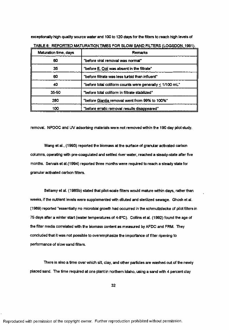
exceptionally high quality source water and 100 to 120 days for the filters to reach high levels of
TABLE 6: REPORTED MATURATION TIMES FOR SLOW SAND FILTERS (LOGSDON. 1991).
Maturation time, days Remarks
60 "before viral removal was normal"
35 "before E. Coli was absent in the filtrate"
60 "before filtrate was less turbid than influent"
40 "before total coliform counts were generally < 1/100 mL"
35-50 "before total coliform in filtrate stabilized"
280 "before Giardia removal went from 99% to 100%"
100 "before erratic removal results disappeared"
removal. NPDOC and UV adsorbing materials were not removed within the 190 day pilot study.
Wang etal., (1993) reported the biomass at the surface of granular activated carbon
columns, operating with pre-coagulated and settled river water, reached a steady-state after five
months. Servais et al.(1994) reported three months were required to reach a steady state for
granular activated carbon filters.
Bellamy et al. (1985b) stated that pilot-scale filters would mature within days, rather than
weeks, if the nutrient levels were supplemented with diluted and sterilized sewage. Ghosh et al.
(1989) reported "essentially no microbial growth had occurred in the schmutzdecke of pilot filters in
75 days after a winter start (water temperatures of 4-8°C). Collins et al. (1992) found the age of
the filter media correlated with the biomass content as measured by AFDC and FRM. They
concluded that it was not possible to overemphasize the importance of filter ripening to
performance of slow sand filters.
There is also a time over which silt, clay, and other particles are washed out of the newly
placed sand. The time required at one plant in northern Idaho, using a sand with 4 percent clay
32
Reproduced with permission of the copyright owner. Further reproduction prohibited without permission.
fines, was over nine months (Tanner, 1990). This process is not a part of filter maturation and its
effects on filtrate quality could be confused.
2.4.9 Aae and type of schmutzdecks
A substantial amount of the literature is related to the development of the schmutzdecke
(Huisman and Wood, 1974; Ellis, 1985; Logsdon, 1991). There is apparently no agreement on the
exact point at which the schmutzdecke is considered to end and the intergranular biomass to
begin. If the schmutzdecke is considered to be the accumulated material at the sand/water
interface (Haarhoff and Cleasby, in Logsdon, 1991), then the age of the schmutzdecke will be
limited by the cleaning cycle. If this layer is also to include the top 1 to 2 cm of the sand layer, the
age will be similarly limited if the filter is cleaned by scraping. Some of this intergranular material
may not be removed by harrowing, however, and could become mixed into the depth penetrated
by the harrow.
Haarhoff and Cleasby (1991) attributed particle removal mainly to the schmutzdecke
layer and considered removal within the bed to be minor. Cleasby (AWWA, 1990) stated the solids
removal occurred as"cake filtration" as the materials entered the face of the granular bed,
becoming even more dominant as the filter cycle progressed. Ellis (1985) also concluded that
purification resulted from straining through the filter skin and through the top few millimeters of
sand and included biological activity as a reason for removals. Bellamy et al., (1985b), however,
did not find the straining theory supported by tests comparing removal of coliform bacteria by filter
media of different sizes and overlaid with 0.5 cm diatomaceous earth (effective size = 0.013 mm).
2.4.10 Water temperature
Logsdon (1991) summarized several studies showing water temperature to be a critical
parameter in removal of particulates. Information was presented demonstrating that the removal of
Giardia cysts was reduced from 99.9 to 99.5 percent when the water temperature declined from 9
33
Reproduced with permission of the copyright owner. Further reproduction prohibited without permission.
to 2 °C. Bellamy et al. (1985b) ran two identical pilot-scale filters in parallel, with the temperatures
of 17°C and 2 °C, and found coliform bacteria removals were 99.6 and 92 percent, respectively.
They concluded slow sand filtration was sensitive to the effects of low temperatures. Huisman and
Wood (1974) and Haarhoff and Cleasby (1991) also related performance to temperature and
temperature related processes such as the ability of the filter to nitrify ammonia.
Van de Vloed (1956) related the reduction in permanganate consumption to water
temperature with the formula:
Permanganate consumption, mg/L = (T+11 )/9 (4)
where T is temperature in °C. It also has been noted that nitrification of ammonia practically
ceases at 6 °C (Huisman and Wood, 1974). Servais et al. (1992), studying biological GAC filtration
with glucose, found the EBCT had to be doubled when the water temperature decreased from 20
°C to 8 °C to maintain the same BDOC removal efficiency, even though the average bacterial
biomass was constant Meek and Shieh (1984) recommended 5 °C as the minimum water
temperature at which a slow sand filter can function. Weltfc and Montriel (Graham and Collins,
1996) concluded that adsorption accounts for the removal of BDOC by slow sand filters at
temperatures of less than 8°C. Substantial biodegradation occurred at higher temperatures. The
temperature threshold was found to be 12°C for the processes removing DOC. Seger and
Rothman (1996) found TOC removal rates directly related to raw water temperatures, ranging
from 5 percent at 2°C to 20 percent at 15°C.
Temperature also physically affects the loss of head through the filter media through its
impact on viscosity of water. As the temperature changes from 20 °C to 4°C, the absolute viscosity
increased from 0.01005 g/cm sec.(2.36 Ib/fthr) to 0.01567 g/cm sec. (4.23 Ib/fthr). This will
increase the headloss, a function of the absolute viscosity and density of water, by approximately
80 percent
34
Reproduced with permission of the copyright owner. Further reproduction prohibited without permission.
2A11 Raw water quality
Letterman and Cullen (1985) found the nature of particulates in raw water was the most
significant factor on filtrate quality as measured by turbidity and particle count Ghosh et al. (1989)
reported poor removals of particles in sizes less that 3 um. The distribution of particle sizes in the
raw water also was important with the presence of larger particles resulting in an increase in
removal of smaller particles (Mackie and Bai, 1993).
The nature of NOM in water and treatment has been discussed elsewhere (Aiken et al.,
1995; Owen etal. 1995; Klevens, 1995). There have been efforts to identify specific classes of
chemical compounds or to relate treatability to a number of parameters, as NPDOC, UV
absorbance, humic and non-humic fractions, molecular weights, and biodegradability. Due to the
complex composition of humic substances which compose much of the NOM, however, it is not
practical to fully analyze such source materials. Most of the organic material is resistant to
microbial degradation, however (Larson, 1978; Dahm, 1981; Meyer et al., 1987; Wang, 1995). A
small portion (about 15 percent of the BDOC), generally consisting of readily available low
molecular weight substances, is rapidly biodegraded within three minutes (Wang, 1995).
NPDOC (and DOC) and UV absorbance at 254 nm have been used to characterize water
supplies as they have been accepted as surrogate parameters for TTHMFP (Amy et al., 1986;
Edzwald et al., 1985). NPDOC and DOC are used in most studies to identify the total available
carbon mass but biodegradable dissolved organic carbon (BDOC, sometimes BOM) and
assimilable organic carbon (AOC) are used in others (Servais et al., 1987; Huck, 1990; Mogren et
al., 1990; Block et al., 1992; Prevost et al., 1992; Collins and Vaughan, 1993). Differences in water
characteristics result from the source of NOM (Aikens and Cotsaris, 1995) and cultural differences
in the watershed (Berner and Berner, 1987), season (Klevens, 1995), and analytical methods
(Collins and Vaughan, 1993). Klevens (1995) found BDOC of raw Croton Reservoir water to be 19
35
Reproduced with permission of the copyright owner. Further reproduction prohibited without permission.
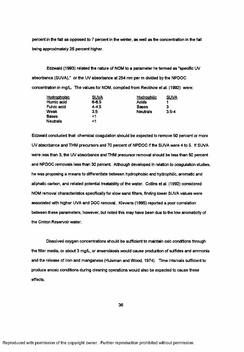
percent in the fall as opposed to 7 percent in the winter, as well as the concentration in the fall
being approximately 25 percent higher.
Edzwald (1993) related the nature of NOM to a parameter he termed as "specific UV
absorbance (SUVA)," or the UV absorbance at 254 nm per m divided by the NPDOC
concentration in mg/L. The values for NOM, compiled from Reckhow et al. (1992) were:
Edzwald concluded that chemical coagulation should be expected to remove 50 percent or more
UV absorbance and THM precursors and 70 percent of NPDOC if the SUVA were 4 to 5. If SUVA
were less than 3, the UV absorbance and THM precursor removal should be less than 50 percent
and NPDOC removals less than 30 percent Although developed in relation to coagulation studies,
he was proposing a means to differentiate between hydrophobic and hydrophilic, aromatic and
aliphatic carbon, and related potential treatability of the water. Collins et al. (1992) considered
NOM removal characteristics specifically for slow sand filters, finding lower SUVA values were
associated with higher UVA and DOC removal. Klevens (1995) reported a poor correlation
between these parameters, however, but noted this may have been due to the low aromatidty of
the Croton Reservoir water.
Dissolved oxygen concentrations should be sufficient to maintain oxic conditions through
the filter media, or about 3 mg/L, or anaerobiosis would cause production of sulfides and ammonia
and the release of iron and manganese (Hu'sman and Wood, 1974). Time intervals sufficient to
produce anoxic conditions during cleaning operations would also be expected to cause these
effects.
Hydrophobic Humic act'd Fulvic acid Weak Bases Neutrals
SUVA6-6.54-4.53.5<1<1
HydrophilicAddsBasesNeutrals
SUVA133.5-4
36
Reproduced with permission of the copyright owner. Further reproduction prohibited without permission.
Prechlorination is used in many plants for algae and zebra mussel control. Logsdon
(1991) summarized reports in which some opposed the practice and others noted positive benefits.
Letterman and Cullen (1985) found turbidity removal was somewhat higher at slow sand filter
plants which prechlorinated at low concentrations, not sufficient to leave a residual in the filter
effluent, but did not believe it was significant Goldgrabe etal., (1993) found prechlorination
sufficient to maintain a residual level of 1.0 mg/L in the dearwell following the filters improved
removals of particles but shortened slow sand filter run by about 10 percent Prechlorination had
no significant effect on the removal of turbidity. Prechlorination at high concentrations does
produce significant changes in filter biomass (Jacobson and Wellington, 1949; Ludwig, 1961, as
reported by Logsdon), resulting in a change in the appearance of the schmutzdecke and
subsurface sand and reducing volatile solids concentrations in the schmutzdecke layer. Wang et
al. (1995) found prechlorination at rates of 2.5-3.0 mg/L virtually eliminated development of
biomass in rapid-rate anthradte-sand media filters.
2.4.12 Microorganisms population and concentrations
Slow sand filters are inhabited by a complex population of organisms (Huisman and
Wood, 1974; Duncan, 1988; Haarhoff and Cleasby, 1991; Weber-Shirk, 1993). The filter surface
becomes coated with a layer of detritus from the supernatant water, particles collected at the
surface by straining and biomass growth. This surface mat contains high numbers of organisms
and volatile matter which decline with depth into the media. Most of the available organic energy
source is in the influent water and is removed as it passes through the surface of the filter. Less
readily degraded compounds and degradation products from the upper layers of the filter are
transported more deeply into the filter. These numbers also vary with the availability of energy
source, seasonal water characteristics, temperature, predation, filter age, flow rate, cleaning
practices, and time since the last cleaning operation. The biomass accumulations are low because
of the low substrate concentrations and do not entirely cover the sand or carbon grains (Wang and
Summers, 1993).
37
Reproduced with permission of the copyright owner. Further reproduction prohibited without permission.
Organisms in slow sand filters have been identified and counted (Duncan, 1988; Harrhoff
and Cleasby, in Logsdon, 1991; Weber-Shirk, 1993; Uoyd, 1996; Wolton et al.,1996). Weber-
Shirk (1993) and Uoyd (1996) showed positive correlation between bacterial removals and the
presence of specific protozoan predators. Vertical profiles for algae, protozoa, invertebrates,
bacteria, and viruses have been presented (Haarhoff and Cleasby, 1991). Seger and Rothman
(1996) reported the biomass, as represented by ATP and total cell count, varied with water
temperature in the top 6 cm of the filter but not at greater depths. Horizontal distributions of
organisms have not generally been considered. Harrhoff and Cleasby (1991) reported an
investigation of algal variations across the filter surface and considered the changes due to
hydraulic and environmental differences. Spanos (1989), using FRM as an indicator of biomass to
compare the density of biomass between cores taken from filters, found no significant difference
between two cores taken within one filter, or between pairs of cores taken from two filters at the
same plant
The purpose of this investigation was not to determine the classifications and numbers of
organisms within the filters but to consider the relative changes to the filter media resulting from the
different cleaning methods. The filter biomass is a complex population and it has been variously
characterized. The selection of an indicator of filter biomass should consider a substance common
to all cells, one not stored but released upon death, easily measured, and widely used (Wang et
al., 1995). Eghmy et al. (1988) related the numbers of microbial population in a filter with Folin-
reactive material (FRM), acriflavine direct counts (AFDC), nutritionally specific heterotrophs, and
with extractable iron and manganese. Spanos (1989) and Eghmy et al. (1992) also compared the
concentrations of organisms in filters relative to other parameters, comparing acriflavin direct
counts (AFDC), with FRM, iron, manganese, and heterotrophic spread plate counts on R2A agar.
Wang et al., (1995) used phospholipid analyses to indicate the presence of active biomass. Liu et
al. (1992) also considered carbohydrates as a biomass indicator based on its presence in bacterial
capsular material. Klevens (1995) used protein, DAPI direct counts, heterotrophic plate counts,
38
Reproduced with permission of the copyright owner. Further reproduction prohibited without permission.
phospholipids, and the incorporation of C-14 L-aminoacetate and C-31 phospholipids. Yordanov et
al. (1996) used heterotrophic plate counts, FRM, total biofilm carbohydrates, and chlorophyll-a.
Total volatile solids historically have been used in sludge analyses to measure the organic content
of heterogenous organic solids. Lazarova and Manem (1995) reviewed analytical methods for
characterization of biofilms. They concluded that further studies were needed, but both total
protein and lipids content were simple assays to give indications of biofiim activity.
Numbers of organisms and concentrations of materials found present in slow sand filters
are summarized in Table 7, and comparisons of mass relative to such concentrations are
summarized in Table 8. All reported declining numbers or concentrations with increasing depth.
Seger and Rothman (1996) found decreasing concentration of ATP in slow sand filters to a depth
of 30 cm, but no further change below that level to the bottom of their sampling at 70 cm. Moll and
Summers (1996) found decreasing concentrations of phospholipids throughout the full 70 cm
range in their study of rapid sand biofilters but with an increasing percentage of the phospholipids
attached to the media surfaces as depth increased, from 60 percent attached at the surface to 90
percent at a depth of 70 cm. Eighmy et al.(1991), Duncan(1988), Collins et al.(1992), and
Yardanov et al. (1996) sampled to depths of 15 cm or less in slow sand filters. Their results also
indicated bacterial counts and FRM declined significantly with increasing depths. Yardanov etal.
(1996) reported carbohydrate concentrations at the schmutzdecke level but not with depth.
The biomass in the filter media has been considered essential to the satisfactory
performance of slow sand filters by most recent researchers( Bellamy, 1985b; Spanos, 1989;
Collins, 1988,1989,1990,1992; Weber-Shirk, 1992; Wang, 1995) although abiotic removal of
particulates has also been shown (Weber-Shirk and Dick, 1997). Higher accumulations of
biomass have also been correlated to higher removals of DOC, UV absorbance, and THMFP
(Collins et al., 1992). The importance of biomass is also implied by a review of the performance
factors listed earlier, most of which can be directly related to the simplified two-film biological
39
Reproduced with permission of the copyright owner. Further reproduction prohibited without permission.
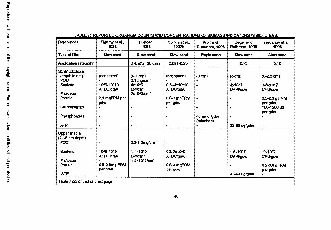
Reproduced
with perm
ission of the
copyright ow
ner. Further
reproduction prohibited
without
permission.
TABLE 7: REPORTED ORGANISM COUNTS AND CONCENTRATIONS OF BIOMASS INDICATORS IN BIOFILTERS.
References Eighmy etal., Duncan, Collins etal., Moll and Seger and Yardanov et a l.,1988 1988 1992b Summers, 1996 Rothman, 1996 1996
Type of filter Slow sand Slow sand Slow sand Rapid sand Slow sand Slow sand
Application rate,m/hr 0.4, after 20 days 0.021-0.25 0.13 0.10
Schmutzdecke(depth in cm) (not stated) (0-1 cm) (not stated) (0 cm) (3 cm) (0-2.5 cm)POC - 2.1 mg/cm3 - - - -
Bacteria 10A9-10A10 4x10A9 0.3-4x10*10 - 4x10*7 3-8x10*7AFDC/gdw EPI/cm3 AFDC/gdw DAPI/gdw CFU/gdw
Protozoa - 2x10*3/cm3 - - - .
Protein 2.1 mgFRM per - 0.5-3 mgFRM - - 0.5-2.3 g FRMgdw per gdw per gdw
Carbohydrate - - - - - 100-1500 ugper gdw
Phospholipids - - - 48 nmol/gdw - -
(attached)ATP - - - - 32-60 ug/gdw -
Uooer media(2-15 cm depth)
POC - 0.2-1.2mg/cm3 - - - -
Bacteria 10A8-10A9 1-4x10*9 0.3-2x10*9 _ 1.5x10*7 -2x10*7AFDC/gdw EPI/cm3 AFDC/gdw DAPI/gdw CFU/gdw
Protozoa - 1 -5x10A3/cm3 - - - -
Protein 0.5-0.8mg FRM - 0.5-3 mgFRM - - 0.2-0.8 gFRMper gdw per gdw per gdw
ATP - - - - 32-43 ug/gdw -
Table 7 continued on next page.
40
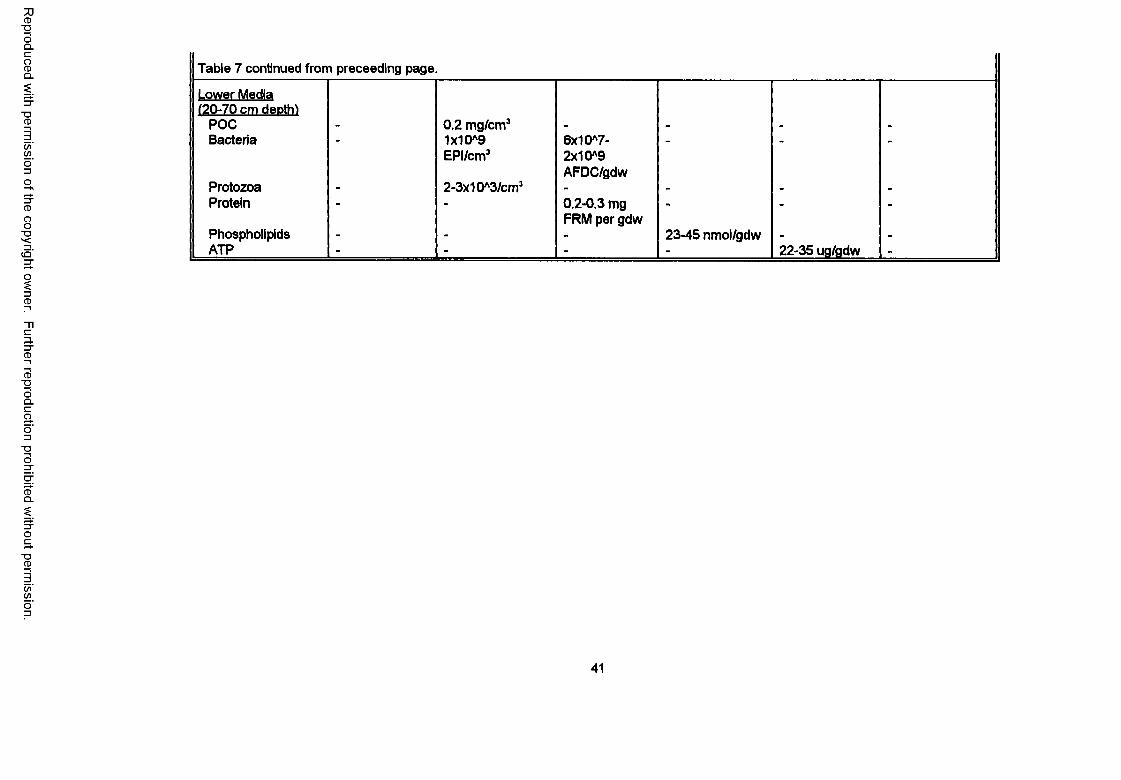
Reproduced
with perm
ission of the
copyright ow
ner. Further
reproduction prohibited
without
permission.
Table 7 continued from preceeding page.
kower Medial /20-70 cm depth)
POC 0.2 mg/cm3Bacteria - 1x10*9 6x10*7- - - -
Protozoa
EPI/cm3
2-3x10*3/cm5
2x10*9AFDC/gdw
Protein - - 0.2-0.3 mg - - -
Phospholipids _FRM per gdw
23-45 nmol/gdw . .ATP - - - - 22-35 ug/gdw -
41
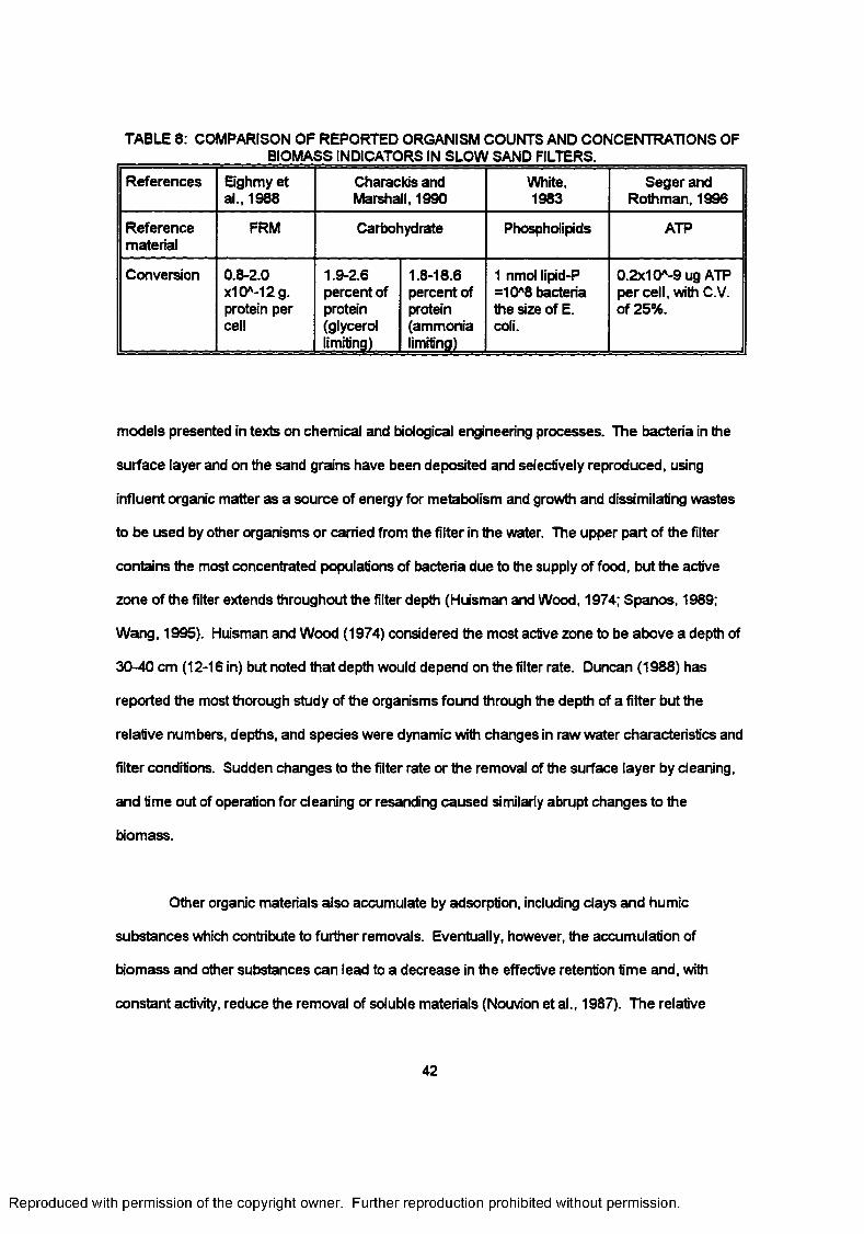
TABLE 8: COMPARISON OF REPORTED ORGANISM COUNTS AND CONCENTRATIONS OF ___________________BIOMASS INDICATORS IN SLOW SAND FILTERS.
References Eighmy et al., 1988
Charackis and Marshall, 1990
White,1983
Seger and Roth man, 1996
Referencematerial
FRM Carbohydrate Phospholipids ATP
Conversion 0.8-2.0 x10M 2g. protein per cell
1.9-2.6 percent of protein (glycerol limiting)
1.8-18.6 percent of protein (ammonia limiting)
1 nmol lipid-P =10A8 bacteria the size of E. coli.
0.2x10A-9 ug ATP per cell, with C.V. of 25%.
models presented in texts on chemical and biological engineering processes. The bacteria in the
surface layer and on the sand grains have been deposited and selectively reproduced, using
influent organic matter as a source of energy for metabolism and growth and dissimilating wastes
to be used by other organisms or earned from the filter in the water. The upper part of the filter
contains the most concentrated populations of bacteria due to the supply of food, but the active
zone of the filter extends throughout the filter depth (Huisman and Wood, 1974; Spanos, 1989;
Wang, 1995). Huisman and Wood (1974) considered the most active zone to be above a depth of
30-40 cm (12-16 in) but noted that depth would depend on the filter rate. Duncan (1988) has
reported the most thorough study of the organisms found through the depth of a filter but the
relative numbers, depths, and species were dynamic with changes in raw water characteristics and
filter conditions. Sudden changes to the filter rate or the removal of the surface layer by cleaning,
and time out of operation for cleaning or resanding caused similarly abrupt changes to the
biomass.
Other organic materials also accumulate by adsorption, including clays and humic
substances which contribute to further removals. Eventually, however, the accumulation of
biomass and other substances can lead to a decrease in the effective retention time and, with
constant activity, reduce the removal of soluble materials (Nouvion et al., 1987). The relative
42
Reproduced with permission of the copyright owner. Further reproduction prohibited without permission.
porosity of discrete particles is estimated as 0.6-0.8 and that of flocculent particles as 0.9-0.95
(Montgomery, 1985).
2.4.13 Alaae
Algae are present in almost all water sources, converting dissolved inorganic carbon,
nitrogen, phosphorus, and other nutrients into biomass. Most algal growth in fresh water is
dependent upon light as an energy source, though some species are also able to use organic
carbon sources for energy. Although algae can be beneficial to the treatment process if they are
an active part of the schmutzdecke, algae can seriously affect filter operations by shortening the
time between cleaning to as little as one sixth of the normal time (Ellis, 1985). Other algal effects
on filter operations include: production of tastes and odors in the water; increases in the
concentration of soluble and biodegradable organics in the water; development of anoxic
conditions in the filters; and increased difficulties with filter cleaning. As most filters are covered
and algae cannot build biomass without light energy, the negative effects of algae predominate on
filter operations. Species, concentrations, and community dynamics vary widely with water
characteristics, temperature, available sunlight, and the nature of the water body (quiescent or
moving, shallow or deep, turbidity, etc.). Algal enumeration was considered essential in Judging
the acceptability of a raw water for treatment with slow sand filters (Cleasby etal., 1984).
The general annual algal cycle begins in the spring and early summer with increasing algal
development as lake or stream water warms, reaching one or more peak concentrations during
warm weather, and dying in the late summer and fall as the sunlight intensity and water
temperatures decline. Sudden changes in the environment such as temperature, sunlight, or
available nutrients, can also result in a sudden die-off of the algal population. The diurnal algal
metabolic cycle uses sunlight during part of the day to produce biomass through photosynthesis
and oxygen during the entire day and to aerobically metabolize the biomass for energy throughout
the 24-hour day. Additional oxygen is necessary to oxidize metabolic wastes and organic materials
43
Reproduced with permission of the copyright owner. Further reproduction prohibited without permission.
released when the cells die and lyse. There is usually a slight excess of oxygen production over
uptake in natural waters, with the balance of the unoxidized biomass removed from the chan by
burial at the bottom of the water body (Bemer and Berner, 1987). The oxidation processes of
respiration and degradation continue in a covered slow sand filter after photosynthesis ceases due
to the lack of sunlight
The algal load on filters will affect filter operation in several ways, yet the dissolved organic
load created by the death and lysis of the cells releases appreciable amounts of materials such as
glycolic add, polypeptides, and carbohydrates that are readily biodegradable (Ellis, 1985).
Huisman and Wood (1974) claimed the organic load contributed by algae to be equivalent to the
organic uptake during growth, yet the predominant source of nutrients for algae are inorganic and
so the load must exceed the original organic mass. The weighted average of the organic load
during a death phase of the algal cyde may be more biodegradable than before growth but that
would have to be due to the prevalence of readily biodegraded compounds released by the cell.
The biodegradability of the NPDOC in the fall of the year is reported to be greater than in the spring
(Prevost, 1991; Klevens, 1995).
2.5 COSTS
The cost of treating water by slow sand filtration has been studied (Slezak and Sims, 1984;
Logsdon et al, 1990; Berg et al., 1991; and others). In their review of 27 plants, Slezak and Sims
(1984) reported filter cleaning to be a major component of the operating costs. The operating
costs ranged from $0,003 to 0.026 per cubic meter ($0.01 to 0.10 per 1,000 gallons) for 59 percent
of the plants to as much as $0.13 per cubic meter ($0.50 per 1,000 gallons) for 5 percent of the
plants in this 1984 study. Cleaning and the handling of sand represented 60-80 percent of the
direct operating costs Ashford Commons works of the Thames Water Authority (Rachwal et al.,
(Graham, 1988) and so reductions in these would have a significant impact on the plant cost In all
cases, labor was the most significant portion of the cleaning cost
44
Reproduced with permission of the copyright owner. Further reproduction prohibited without permission.
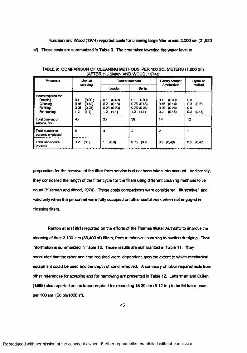
Huisman and Wood (1974) reported costs for cleaning large filter areas, 2,000 sm (21,520
sf). Those costs are summarized in Table 9. The time taken lowering the water level in
TABLE 9: COMPARISON OF CLEANING METHODS, PER 100 SQ. METERS (1.000 SF) (AFTER HUISMAN AND WOOD, 1974):
Parameter Manualscraping
Tractor scrapers Gantry scraper Amsterdam
Hydrauficmethod
London Berlin
Hours required for Draining Cleaning Refilling Re-ripening
0.1 (0.09) 0.45 (0.42) 0.25 (0.23) 1.2 (1.1)
0.1 (0.09) 0.2 (0.18) 0.25 (0.23) 1.2 (1.1)
0.1 (0.09) 0.25 (0.18) 0.25 (0.23) 1.2 (1.1)
0.1 (0.09) 0.15 (0.14) 0.25 (0.23) 0.2 (0.18)
0.00.3 (0.28) 0.0 0.2 (0.18)
Total time out of service, hrs
40 35 36 14 10
Total number of persons employed
8 4 2 2 1
Total labor-riours involved
3.75 (3.5) 1 (0.9) 0.75 (0.7) 0.5 (0.46) 0.5 (0.46)
preparation for the removal of the filter from service had not been taken into account Additionally,
they considered the length of the filter cycle for the filters using different cleaning methods to be
equal (Huisman and Wood, 1974). Those costs comparisons were considered "illustrative" and
valid only when the personnel were fully occupied on other useful work when not engaged in
cleaning filters.
Renton et al (1991) reported on the efforts of the Thames Water Authority to improve tine
cleaning of their 3,100 sm (33,400 sf) filters, from mechanical scraping to suction dredging. Their
information is summarized in Table 10. Those results are summarized in Table 11. They
concluded that the labor and time required were dependent upon the extent to which mechanical
equipment could be used and the depth of sand removed. A summary of labor requirements from
other references for scraping and for harrowing are presented in Table 12. Letterman and Cullen
(1985) also reported on the labor required for resanding 15-30 cm (6-12-in.) to be 54 labor-hours
per 100 sm (50 ph/1000 sf).
45
Reproduced with permission of the copyright owner. Further reproduction prohibited without permission.
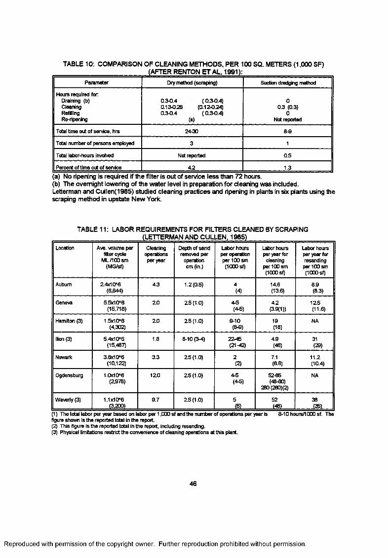
TABLE 10: COMPARISON OF CLEANING METHODS, PER 100 SQ. METERS (1,000 SF)(AFTER RENTON ETAL, 1991):
Parameter Dry method (scraping) Suction dredging method
Hours required forDraining (b) 0.30.4 (0 .30 .4 ) 0Cleaning 0.130.26 (0.120.24) 0.3 (0.3)Refilling 0.30.4 (0 .30 .4 ) 0Re-ripening (a) Not reported
Total time out of service, hrs 2400 8-9
Total number of persons employed 3 1
Total labor-hours involved Not reported 0.5
Percent of time out of service 4.2 1.3
a) No ripening is required if the filter is out of service less than 72 hours.(b) The overnight lowering of the water level in preparation for cleaning was included.Letterman and Cullen(1985) studied cleaning practices and ripening in plants in six plants using the scraping method in upstate New York.
TABLE 11: LABOR REQUIREMENTS FOR FILTERS CLEANED BY SCRAPING ___________________(LETTERMAN AND CULLEN, 1985)__________________
Location Aue. volume per filter cycle
NIL/100 sm (MG/sf)
Cleaning operations per year
Depth of sand removed per
operation cm (in.)
Labor hours per operation per 100 sm (1000 sf)
Labor hours per year for
cleaning per 100 sm (1000 sf)
Labor hours per year for resanding
per 100 sm (1000 sf)
Auburn 24x10*6 4.3 1.2 (0.5) 4 14.6 8.9(6.844) (4) (13.6) (8.3)
Geneva 5.5x10*6 2 0 25(1.0) 4 5 4.2 125(15.718) (45) (3.9(1)) (11.6)
Hamflton (3) 1.5x10*6 2 0 2 5 (1.0) 9-10 19 NA(4,302) (8-9) (18)
llion (3) 5.4x10*6 1.8 8-10(3-4) 22-45 4.9 31(15.487) (21-42) (46) (29)
Newark 3.6x10*6 3.3 25(1.0) 2 7.1 11.2(10,122) (2) (6.6) (10.4)
Ogdensburg 1.0x10*6 120 25(1.0) 4-5 52-65 NA(2,978) (45) (48-60)
280 (260) (2)
Waveriy (3) 1.1x10*6 9.7 25(1.0) 5 52 38(3.200) (5) (48) OS)
1) The total labor per year based on labor per 1,(XX) sf and the number of operations per year is 8-10 hours/1000 sf. Thefigure shown is the reported total in the report.(2) This figure is the reported total in the report, including resanding.(3) Physical limitations restrict the convenience of cleaning operations at this plant
46
Reproduced with permission of the copyright owner. Further reproduction prohibited without permission.
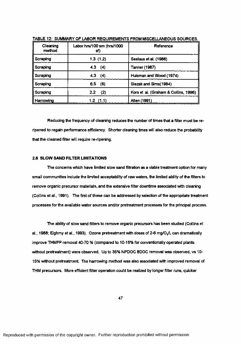
TABLE 12: SUMMARY OF LABOR REQUIREMENTS FROM MISCELLANEOUS SOURCES.
Cleaningmethod
Labor hrs/100 sm (hrs/1000 sf)
Reference
Scraping 1.3 (1.2) Seelausetal. (1986)
Scraping 4.3 (4) Tanner (1987)
Scraping 4.3 (4) Huisman and Wood (1974)
Scraping 6.5 (6) Slezak and Sims(1984)
Scraping 2.2 (2) Kors et al. (Graham & Collins, 1996)
Harrowing 1.2 (1.1) Allen (1991)
Reducing the frequency of cleaning reduces the number of times that a filter must be re
ripened to regain performance efficiency. Shorter cleaning times will also reduce the probability
that the cleaned filter will require re-ripening.
2.6 SLOW SAND FILTER LIMITATIONS
The concerns which have limited slow sand filtration as a viable treatment option for many
small communities include the limited acceptability of raw waters, the limited ability of the filters to
remove organic precursor materials, and the extensive filter downtime associated with cleaning
(Collins et al., 1991). The first of these can be addressed by selection of the appropriate treatment
processes for the available water sources and/or pretreatment processes for the principal process.
The ability of slow sand filters to remove organic precursors has been studied (Collins et
al., 1988; Eighmy et al., 1993). Ozone pretreatment with doses of 2-6 mg/Oa/L can dramatically
improve THMFP removal 40-70 % (compared to 10-15% for conventionally operated plants
without pretreatment) were observed. Up to 35% NPDOC BDOC removal was observed, vs 10-
15% without pretreatment The harrowing method was also associated with improved removal of
THM precursors. More efficient filter operation could be realized by longer filter runs, quicker
47
Reproduced with permission of the copyright owner. Further reproduction prohibited without permission.

cleaning, and shorter ripening periods. Long term improvements would also be achieved by
extending the periods between resanding.
48
Reproduced with permission of the copyright owner. Further reproduction prohibited without permission.
CHAPTER 3
METHODS AND MATERIALS
3.1 OVERVIEW
Investigations were carried out on three separate scales of filters- full scale, pilot plant, and
laboratory scale. Analytical methods and quality control for the various facilities were similar. This
section describes the facilities and the methods used during the investigations. The number of
facilities studied at each scale, the factors considered at that facility, and the process
measurements and parameters analyzed at each facility are summarized in Appendix A.
3.2 FULL SCALE STUDIES
3.2.1 Gorham. New Hampshire
Gorham, New Hampshire (1989 population, 3,173) is located at the intersections of Routes
2 and 16 near the Maine-New Hampshire border 15 kilometers (9 miles) north of M t Washington.
The dty was supplied with unfiltered, chlorinated water from either/or both its Perkins Brook and Icy
Gulch surface water supplies. The 1986 Amendments to the Safe Drinking Water Act required
filtration of surface water sources and studies were undertaken by the city's consulting engineer,
Rist-Frost Associates, P.C. and their subconsultant (Collins, 1990) which recommended the
construction of a slow sand filter plant The completed facility is a 3.8 ML/d (I.O MGD) plant
incorporating three separate filter beds of which only two have been used. The plant began
filtering to waste January 21,1991 and began delivering filtered water to the system February 12,
1991 (Bernier, 1994). Each filter has a design capacity of 1.26 ML/d (0.33 MGD) at a loading of
0.13 m/hr (0.05 GPM/sf).
The individual filters are 20 meters by 23 meters (65 x 75 ft) and contains 0.68 meters
49
Reproduced with permission of the copyright owner. Further reproduction prohibited without permission.
(27-in) of washed sand with an effective size of 0.25 mm and a uniformity coefficient of 1.8 (Rist-
Frost, 1991). The filters are covered and accessible by concrete ramps within the control building
area. The effluent is monitored by a Venturi flow tube for flow and a Hach Model 1720C Low
Range turbidimeter (Hach, Loveland, CO). The schematic details of a single filter are shown in
Figure 2.
The filters incorporate an arrangement that facilitates harrowing. This arrangement
includes an adjustable weir along the entire length of one side of the filter, an inlet header pipe
along the entire length of the wall opposite the adjustable weir, and the ability to supply a reverse
flow of filtered water from the underdrain system up through the filter media. This reverse flow is
below the rate required to suspend the media as in a backwash for a rapid sand filter. Concrete
ramps are provided so that a small tractor has convenient access to the filter surface.
The harrowing process is earned out by closing the influent raw water valve to the
designated filter, and draining the supernatant water level down to approximately the top of the
adjustable weir 30 centimeters above the media surface. This depth of water is sufficiently shallow
that a cross flow provides sufficient velocity to carry colloidal and fine suspended particles across
the filter surface, provided they are periodically resuspended by the passage of the tractor and
harrow. The flushing water supply enters the filter at the water surface level from the header pipe
along the far wall. The upflow through the media during this time is not intended to suspend sand
media but to prevent downward passage of colloidal solids and material removed from the sand
grains during the harrowing operation. The washwater flows to a 0.70 ML (185,000 gal)
wastewater equalization pond where it infiltrates into the sandy soil under the conditions of a state
underground injection well permit (Bernier, 1994). The additional cost of incorporating these
features to facilitate harrow cleaning techniques over the conventional scraping method was
estimated to be approximately 7% of the construction cost (Scott, 1991).
50
Reproduced with permission of the copyright owner. Further reproduction prohibited without permission.
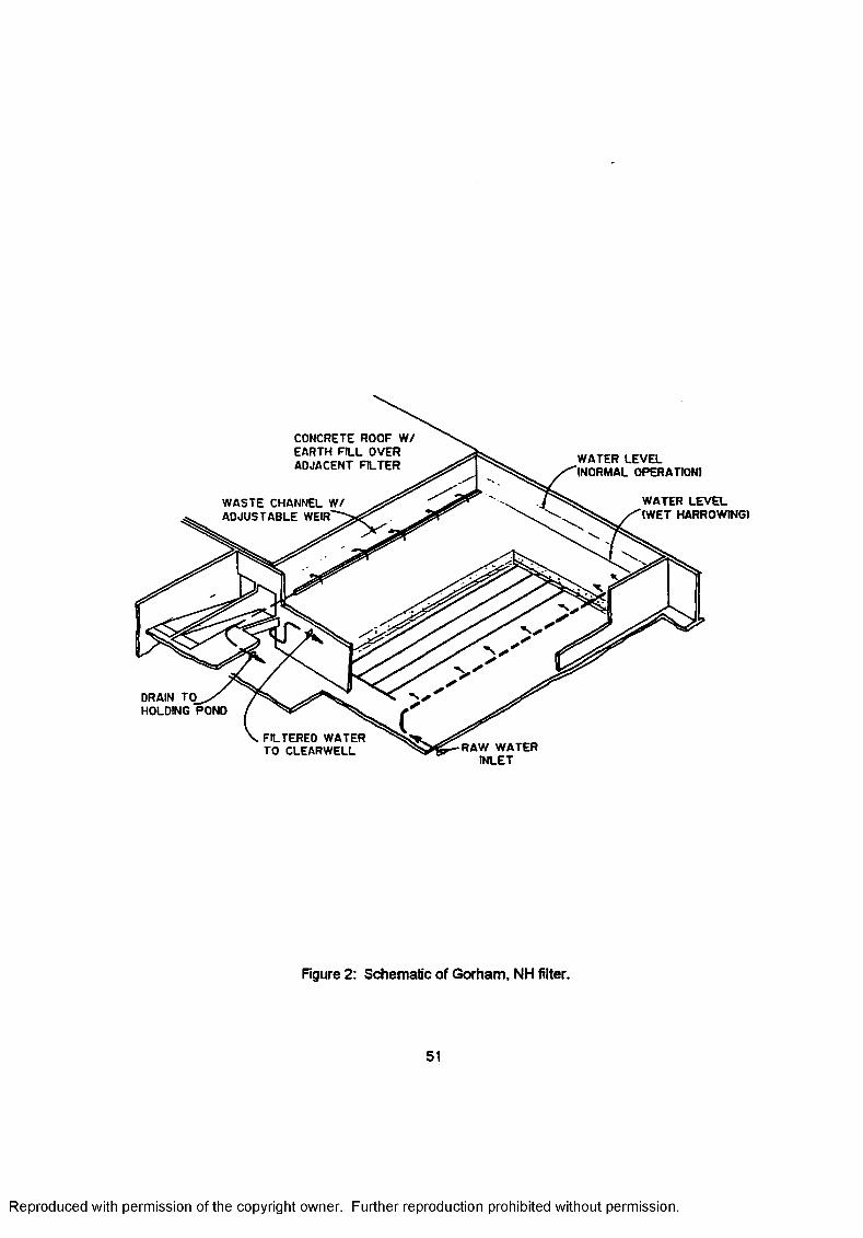
WATER LEVEL (NORMAL OPERATION)
WATER LEVEL (WET HARROWING)
CONCRETE ROOF W / EARTH FILL OVER ADJACENT FILTER
WASTE CHANNEL W / ADJUSTABLE WEIR
DRAIN TO HOLDING POND
FILTERED WATER TO CLEARWELL RAW WATER
INLET
Rgure 2: Schematic of Gorham, NH filter.
51
Reproduced with permission of the copyright owner. Further reproduction prohibited without permission.
Samples of raw and filtered water were taken from sampling taps in the pipe gallery.
Cores of the filter media were taken at three horizontally spaced locations established by random
number selection (Collins, etal., 1992).
This plant was to be used in the investigation to consider the effects of cleaning one filter
by harrowing and the adjacent filter by scraping. In this manner, both filters could be operated with
identical raw water quality and under the same environmental conditions (Collins, 1991). Cleaning
procedures were to be initiated when filters reached a terminal head loss of about 2 m (6-ft) or
when effluent turbidities exceeded 1.0 NTU. A study period of 12 to 18 months was anticipated.
The facility began operation in February 1991 and data collection was begun in May of 1992.
Because no cleaning operation had been necessary through the summer of 1993 and the prospect
of repeated cleaning of the same filter was even more remote, plans to use this facility for
comparative operations were suspended. The operating plans, the study preparation, and the
development of the quality assurance/quality control documents for this facility, however, were
utilized in the data collected for this plant and for the other facilities discussed later.
3.2.2 Newport. New Hampshire
Newport, New Hampshire (1990 population, 6,110) is located at the intersection of Routes
11 and 10 on the southwestern side of the state and about 30 km (20 miles) south of Lebanon,
New Hampshire. Until October 1992, the dty was supplied with unfiltered, chlorinated water from
its upland, high quality, supply from Gilman Pond. There is also a ground water supply at Pollards
Mills for backup. As they had at Gorham, NH, the city's Consulting Engineer, Rist-Frost Associates,
P.O. recommended construction of a slow sand filter plant The completed facility is a 2.6 ML/d
(0.7 MGD) plant incorporating three separate filter beds and all three beds are used. Each filter is
designed for a nominal capacity of 0.88 ML/d (0.23 MGD) at a design application rate of 0.13 m/hr
(0.05 gpm/per sf) (Rist-Frost-Shumway, 1993). This plant was designed by the same engineer as
at Gorham, NH and used the same basis of design and the same sand media specification. This
52
Reproduced with permission of the copyright owner. Further reproduction prohibited without permission.
plant is nearly identical to the Gorham facility except for the location of the access ramps to the
filters and the smaller design flow. Because the head loss developed at a faster rate in Newport
than at Gorham, arrangements were made with the Town of Newport to use filters at their slow-
sand filter plant in place of those at Gorham for the study under the USEPA grant
The facilities are depicted in Figure 3. The individual filters are 21 meters long x 17 meters
wide (68 by 55.7 f t ) and contain 0.68 meters (27 in) of washed sand with an effective size of 0.25
mm at a uniformity coefficient of I.8. (Rist-Frost-Shumway, 1993). The filters are covered and
accessible by 1.8 meter (6 ft) concrete ramps within the control building.
The filter design is also similar to that described for Gorham, providing an influent pipe
along one side of the filter, an adjustable weir along the opposite side, and the ability to supply a
reverse flow from the underdrain system up through the filter media. The ceiling height is
approximately 3 m (10-ft) above the level of the sand. The washwater holding pond was sized for
the estimated volume of water from cleaning two filters consecutively, or 0.75 ML (200,000 gal)
(Scott, 1994). The pond discharges both through the sandy bottom and to a surface stream.
Solids settled rapidly and remain on the pond bottom.
Samples of raw and treated water were taken from taps in the pipe gallery. Samples of
wash water were taken from the drain outlet to the settling pond or creek or, after dark, from
sample taps in the pipe gallery.
3.2.3 Newark. New York
Newark, New York (1990 population, 9,611) is located at the intersection of Routes 31
and 88 in Wayne County, New York, midway between the cities of Syracuse and Rochester, NY.
The Village has been supplied with water from Canandaigua Lake since 1951 through its slow
sand filtration plant located in the Village of Shortsville, midway between Canandaigua Lake and
53
Reproduced with permission of the copyright owner. Further reproduction prohibited without permission.
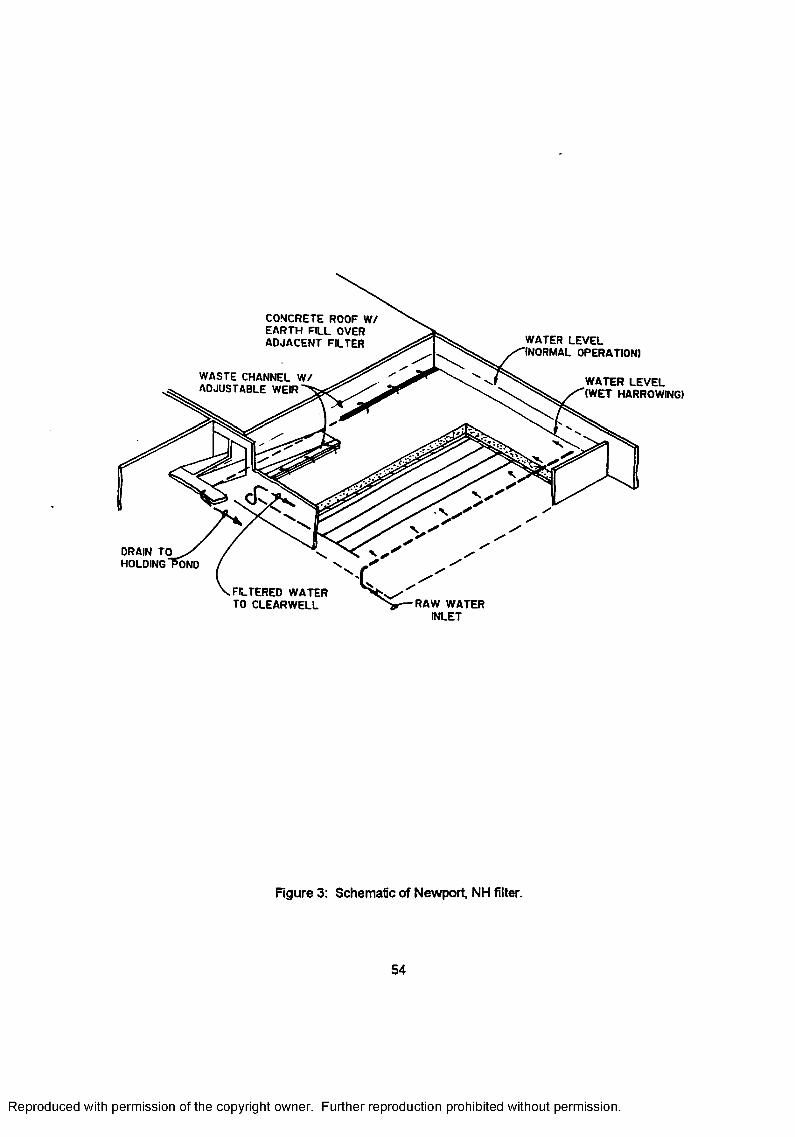
WATER LEVEL (NORMAL OPERATION)
WATER LEVEL (WET HARROWING)
CONCRETE ROOF W / EARTH FILL OVER ADJACENT FILTER
WASTE CHANNEL W / ADJUSTABLE WEIR
DRAIN TO h o ld in g "Pond
. FILTERED WATER TO CLEARWELL RAW WATER
INLET
Figure 3: Schematic of Newport, NH filter.
54
Reproduced with permission of the copyright owner. Further reproduction prohibited without permission.
the Village of Newark. In 1969, pressure diatomaceous filters having a capacity of 2.8 ML/d (0.75
MGD) apiece were added to increase the treatment capacity of the plant The completed facility
has a capacity of 13 ML/d (3.5 MGD) using the four original slow sand filters and the two pressure
diatomaceous earth filters. Each slow sand filter has a nominal capacity of 1.9 ML/d (0.50 MGD)
at loading of 0.16 m/hr (0.064 gpm/sf). The slow sand filters have always been cleaned by
scraping.
The individual filters are 42 meters by 12 meters (139-ft by 39-feet) and contain 0.9
meters (3-ft) of washed sand with an effective size of 0.39 mm and uniformity coefficient of 2.4.
The filters are covered and accessible by 2.8 meter (9.3 ft) wide concrete ramps from outside the
control building. Ceiling height in the filter area is 2.4 m (8-ft). The layout is presented in Figure 4.
When the level of sand reaches a minimum allowable level of approximately 30 cm
(12-inches), the remaining sand is removed and new sand was placed over the gravel around the
pipes. The sand was purchased locally and washed before placement The filter was filled from
the bottom as after a normal cleaning operation, 40 kg (100 lb) of hypochlorite added, and run to
waste until there was satisfactory turbidity and coliform removal. The filters monitored for this
study had been rebuilt in January 1992 (Filter No. 3) and May 1990 (Filter No. 4). Although sand
had been saved for the last two years and washed using a sand washing device constructed by
plant personnel, none had been returned to the filters through January 1994. Before that, filter
sand was used for fill. No wastewater was produced during cleaning.
The raw water is from Canandaigua Lake, one of the Finger Lakes of New York State.
Unlike the waters of New England, the water is very hard and has a high alkalinity and alkaline pH
(Bloomfield, 1978). Samples of raw and filtered water were taken from taps in the pipe galleries.
55
Reproduced with permission of the copyright owner. Further reproduction prohibited without permission.
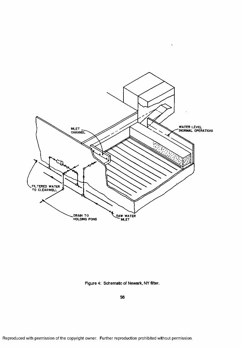
DRAIN TO HOLDING POND
^RAW WATER ‘ NLET
Figure 4: Schematic of Newark, NY filter.
56
Reproduced with permission of the copyright owner. Further reproduction prohibited without permission.
3.2.4 Hartford Metropolitan District Commission. West Hartford. Connecticut
This plant is one of two principal plants serving the Hartford Connecticut metropolitan area
and has a current capacity of 189 ML/d (50 MGD) using raw water from upland reservoirs (Allen,
1991). This facility has 22 slow sand filters with a total surface area of 5.1 hectares (12.5 acres)
with filters constructed over a period of time as outlined in Table 13. The filter capacity is
TABLE 13: FILTERS AT WEST HARTFORD, CT
Filter Numbers Year constructed Surface area hectares (acres)
1-8 1922 0.20 (0.5)
9-10 1927 0.30 (0.75)
11-14 1941 0.20 (0.5)
15-18 1953 0.20 (0.5)
19-22 1960 0.30 (0.75)
based on an application rate of 0.16 m/hr (0.064 gpm/sf). The filter sand ranges in depth from 0.6
to 0.7 meters (24 to 27-inches). The effective sizes of the sand used over the years have ranged
from 0.25 to as high as 0.35 mm and with uniformity coefficients of from 1.4 to 3, but with the
smaller effective size and lower uniformity coefficients required in more recent years
(Fenstermacher, 1988). The filters are covered and accessible from buildings located at the point
at which sets of four filters have comers coming together. The access is by ladder and by
overhead electrically powered hoists on monorails. Manholes provided through the roof structures
can be used for ventilation or delivering sand. The filter layout is shown in Figure 5.
The filters were originally constructed to be cleaned using the scraping method but costs
and the inconveniences of those operations led to the development of alternative methods
(Minkus, 1953). Various alternative methods were used in the years from 1922 to 1950 until the
present method of harrowing was developed which has been used continuously since the mid
57
Reproduced with permission of the copyright owner. Further reproduction prohibited without permission.
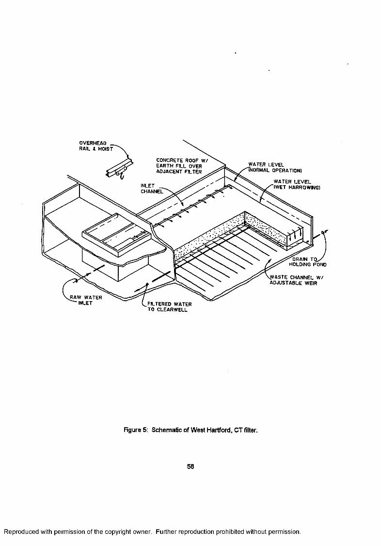
OVERHEAD _ RAIL ( HOIST
CONCRETE ROOF W/ EARTH FILL OVER ADJACENT FILTER
WATER LEVEL TNORMAL OPERATION!
WATER LEVEL (WET HARROWING)INLET _
CHANNEL
DRAIN Toy HOLDING POND
JWASTE CHANNEL W/ ADJUSTABLE WEIR
RAW WATER " INLET FILTERED WATER
TO CLEARWELL
Figure 5: Schematic of West Hartford, CT filter.
58
Reproduced with permission of the copyright owner. Further reproduction prohibited without permission.
1950's. The harrowing method developed at this facility is the one on which the cleaning methods
for both Gorham and Newport plants have been based.
The West Hartford filters are much larger and older than those at Gorham and Newport
and so additional description of the cleaning method will be necessary. The inlet of the filter to be
cleaned is closed at some time between 3 and 5 AM on that day to allow the water surface to fall
to near the weir overflow level. The crew performing the wet harrowing operation opens the drain
to finish lowering the level and lowers the tractor and harrow into the filter with a monorail hoist
The filter is wet harrowed until the early afternoon when the filter underdrain is opened to the drain
to further lower the water surface below the surface of the sand. The first tractor and its spring
toothed harrow is removed and moved to the filter this crew is to wet harrow the following day.
The following day, a second crew moves its tractor and scarifying harrow into the filter and dry
harrows the sand until early afternoon. The surface is inspected, and the underdrain system
partially opened to allow filtered water from the three adjacent filters to begin filling the cleaned
filter from below. After the water level rises above the sand, raw water is introduced through the
regular inlet to complete the filling and the filter is opened to begin flowing to the clear well at a
rate of 1.9 ML/d (0.5 MGD) until the following morning. The flow is then increased in 1.9 ML/d (0.5
MGD) steps until it reaches its full capacity.
The sand in the filters has been removed, washed, and replaced at intervals of from 10 to
over 20 years. New sand is purchased only as necessary to replace losses from the cleaning
operations (Allen, 1991). The filters used in this study were last reconditioned in 1974 (Filter No.1),
1980 (Filter No. 18), and 1993 (Filter No. 21).
Samples of raw water were taken from sampling taps in the pipe galleries of Filter No.1 for
Filters 1-10 and 18-22,andin the pipe gallery of Filter No. 18 for that filter. Filtered water samples
were taken from taps in the pipe galleries for each of the filters sampled. Wastewater samples
59
Reproduced with permission of the copyright owner. Further reproduction prohibited without permission.
were taken in the pipe galleries of those filters. The results of the analyses are presented in
Chapter 4.
Slow sand filters must be reconditioned periodically because filter capacity decreases over
time despite regular harrowing. The filters at the West Hartford plant have been reconditioned
after varying intervals. The goal had been to recondition filters at intervals as short as 7 or 8 years
but filters had gone over 20 years due to budget restrictions in the 1970's and 80's, thus deferring
the financial costs (approximately $95,000 per filter for the past two operations, each on 0.3
hectare (3/4-acre) filters) and time out of service. Instead a filter was selected for reconditioning
based on its reduced capacity. Reconditioning had been accomplished formerly using plant
employees, but the work is done now by outside contractors under public bidding. The contractor
supplies the labor and supervision, and the Metropolitan District Commission (MDC) supplies the
equipment and water. The work procedure is specified by the MDC and inspected periodically by
them. Data on these operations were also collected and analyzed as a part of this report
Wastewater, from harrowing and reconditioning, was discharged to surface channels on
the plant site which flow to a settling pond, then to a off-site river.
3.3 PILOT PLANT STUDIES
Pilot plant studies were carried out from August 19,1992 to September 19,1993 at the
Portsmouth, NH water treatment plant located in Madbury, NH. Three parallel pilot plants were
operated using a common water supply to compare the effects of cleaning methods under
intensive conditions and to record rates of head loss development, filter cycles, and the effects of
aging on the filter media.
The plant's water supply is from the Bellamy Reservoir which is a shallow surface water
supply with high color, relatively high turbidity, and high concentrations of iron, manganese, and
60
Reproduced with permission of the copyright owner. Further reproduction prohibited without permission.
organic carbon. The reservoir and water treatment plant were constructed by the U.S. Army Corps
of Engineers and put into service in 1961. The Portsmouth plant uses conventional alum
coagulation, flocculation, and rapid filtration and has a design capacity of 43 ML/d (5.5 MGO)
(Fenstermacher, 1989).
The pilot filters for this study were constructed from 30 centimeter (12-inch) diameter.
Schedule 80 pipe. A diagram of the plant is presented in Figure 6.
The filters were flanged 60 centimeters (24 in) from the bottom to facilitate installation,
cleaning, and sampling of the filter bed. The flanges were sealed with a rubber gasket and
secured with 8 bolts around the perimeter. The influent line was a 1.3 centimeter (1/2 in) PVC line
extending to the center of the filter just under the surface of the water. An overflow tube located
91 centimeters (36 in) above the sand surface maintained the height of water on the filter. The 0.6
centimeter (1/4 in) diameter PVC rod was cemented around the perimeter of the interior filter wall
7.5 centimeters (3 in) below the sand media surface to reduce sidewall channeling. The ratio of
filter diameter to media effective size was 700 which greatly exceeded the ratio of 50 which should
avoid measurable effects on rates of head buildup and variation in turbidity and particle count
(Lang et al., 1993). An underdrain was provided by a 0.6 centimeter (1/4 in) NPT X I.5 centimeter
(5/8 in) hose-barb adapter threaded into the center of the bottom of the filter base. A piezometer
connection was also made about 2 centimeters (1 in) above the base through the side of the filter
with a similar connection.
Raw water was supplied from the main plant raw water supply to a constant head tank
located above the pilot plant filters. Individual connections from near the bottom of the
constant-head tank were connected by Tygon tubing to a multi-head peristaltic pump
(Cole-Parmer, Chicago, IL) and by tubing to each of the filters. The pump maintained equal flow to
each of the parallel filters at a rate more than sufficient to match the output The excess flow
61
Reproduced with permission of the copyright owner. Further reproduction prohibited without permission.
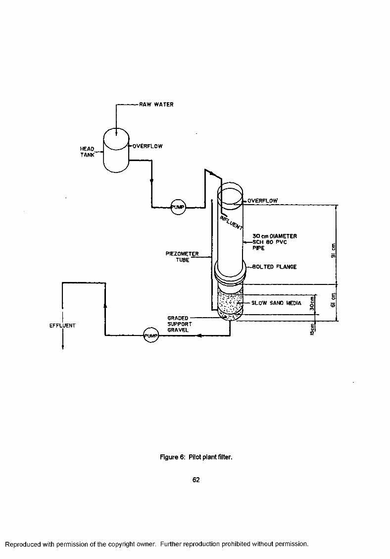
RAW WATER
OVERFLOWHEADTANK
OVERFLOW'UMP
3 0 cm OIAMETER ■SCH 8 0 PVC PIPE
PIEZOMETERTUBE
o>
I—BOLTED FLANGE
SLOW SAND MEDIA
GRADED - SUPPORT GRAVEL
EFFLUENT
'UMPj
Rgure 6: Pilot plant filter.
Reproduced with permission of the copyright owner. Further reproduction prohibited without permission.
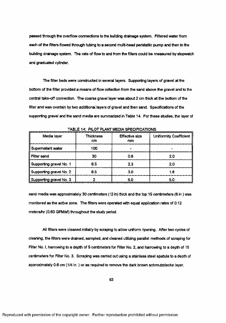
passed through the overflow connections to the building drainage system. Filtered water from
each of the filters flowed through tubing to a second multi-head peristaltic pump and then to the
building drainage system. The rate of flow to and from the filters could be measured by stopwatch
and graduated cylinder.
The filter beds were constructed in several layers. Supporting layers of gravel at the
bottom of the filter provided a means of flow collection from the sand above the gravel and to the
central take-off connection. The coarse gravel layer was about 2 cm thick at the bottom of the
filter and was overlain by two additional layers of gravel and then sand. Specifications of the
supporting gravel and the sand media are summarized in Table 14. For these studies, the layer of
____________ TABLE 14: PILOT PLANT MEDIA SPECIFICATIONS
Media layer Thicknesscm
Effective size mm
Uniformity Coefficient
Supernatant water 100 - -
Filter sand 30 0.6 2.0
Supporting gravel No. 1 6.5 2.3 2.0
Supporting gravel No. 2 6.5 3.0 1.8
Supporting gravel No. 3 2 5.0 5.0
sand media was approximately 30 centimeters (12 in) thick and the top 15 centimeters (6 in ) was
monitored as the active zone. The filters were operated with equal application rates of 0.12
meters/hr (0.63 GPM/sf) throughout the study period.
All filters were cleaned initially by scraping to allow uniform ripening. After two cycles of
cleaning, the filters were drained, sampled, and cleaned utilizing parallel methods of scraping for
Filter No. I, harrowing to a depth of 5 centimeters for Filter No. 2, and harrowing to a depth of 15
centimeters for Filter No. 3. Scraping was carried out using a stainless steel spatula to a depth of
approximately 0.6 cm (1/4 in ) or as required to remove the dark brown schmutzdecke layer.
63
Reproduced with permission of the copyright owner. Further reproduction prohibited without permission.
Harrowing was carried out using a 1.2 cm (1/2-in.) dia. steel rod on which laboratory tape was used
to mark 5 and 15 cm (2 and 6-in), respectively, as maximum depth for penetration. All filters were
drained for cleaning so that the water surface was below the surface of the sand. After scraping or
harrowing, treated water was pumped in reverse through the underdrain zone of each filter and up
through the media until the water level rose above the sand. Raw water was then added through a
side port located 5 cm (2-in) above the surface of the sand. After the level had reached 30 cm (1 -
ft) or more above the sand surface, additional water was added from the top using a hose with a
baffled outlet so that the sand surface would not be disturbed. After the water level reached the
overflow elevation, the system was turned on in the forward direction and the filter cycle started.
The raw water was sampled from the tube discharging to Filter No. I. Filtered water was
sampled from the several discharges of the multi-head peristaltic pump drawing from the
respective filter underdrain connections. Raw water temperatures were determined using a
laboratory thermometer suspended in the constant head tank.
3.4 LABORATORY SCALE STUDIES
Laboratory scale sand filter tests were earned out in the fall and winter of 1993 at the
Environmental Engineering Laboratory at University of New Hampshire to compare filter
characteristics that could not be measured in the field scale plants.
The laboratory filters consisted of glass columns measuring 2.54 cm diameter x 53 cm
long (1-in. x 21-in.), containing approximately 40 cm (16-in.) of a selected sand media. The ratio of
column diameter to media effective size was 50 to avoid measurable variations in turbidity and
particle counts. The ends of the tubes were capped with a valve and connected with tubing to a
laboratory pump (Masterflex, Cole-Parmer, Chicago, IL). The system was arranged so that the
pump would draw water from a stoppered one-liter reservoir on a shelf above the filter column and
discharge at a controlled rate into the bottom of the filter. The filtered water exited the filter at its
64
Reproduced with permission of the copyright owner. Further reproduction prohibited without permission.
upper end and flowed to the reservoir on the shelf above the filter. A schematic view of a single
filter column is presented in Figure 7.
Eight columns were mounted in parallel on a wooden support frame. Each column had its
own reservoir and pump head, but the pump heads were mounted on common variable speed
drive motors to maintain similar flow rates. The entire system was located in a constant
temperature room maintained at 20+ 0.5°C. The filter columns were operated at various flow rates.
Filter media used in the columns was taken from a variety of sources and stored in a
refrigerator. Generally, the sand was screened on the day columns were filled. The sands were
wet screened on a No. 45 sieve (0.014 mm opening)under a flow of RO filtered laboratory water
until the water ran clear. The sand was placed in a column with a stainless steel laboratory
spatula, while maintaining sufficient water depth in the column to cover the settled sand. The
column was filled in layers and vibrated for 5-seconds at each layer with a Maxi-Mixer (Thermolyne
Corp., Dubuque, Iowa) to remove air. The sand was supported at the bottom of the column by a
plastic mesh to prevent its entrance into the valve and tubing below the column. After filling, the
columns were placed on the wooden support frame, connected to the pumped circulation system
which temporarily had general purpose laboratory water in the reservoir flacks, and the pumps
started. Air bubbles were released in part by the upflow of water but more importantly by vibration
of the columns. Pump flow rates were calibrated at this time. When ready, the reservoirs were
emptied and refilled with the designated "raw water" to be used in the tests.
The general purpose, sources of sand, and sources of water used for the individual
laboratory filter column runs are summarized in Table 15. The sand used during Column Run No.
4 received additional preparation. A portion of the sand was screened several days before it was
to be placed in a column to allow it to be cleaned of organic matter by burning in a muffle furnace
overnight This was then cooled, and cleaned by repeated add extraction with 1:1 nitric add until
65
Reproduced with permission of the copyright owner. Further reproduction prohibited without permission.
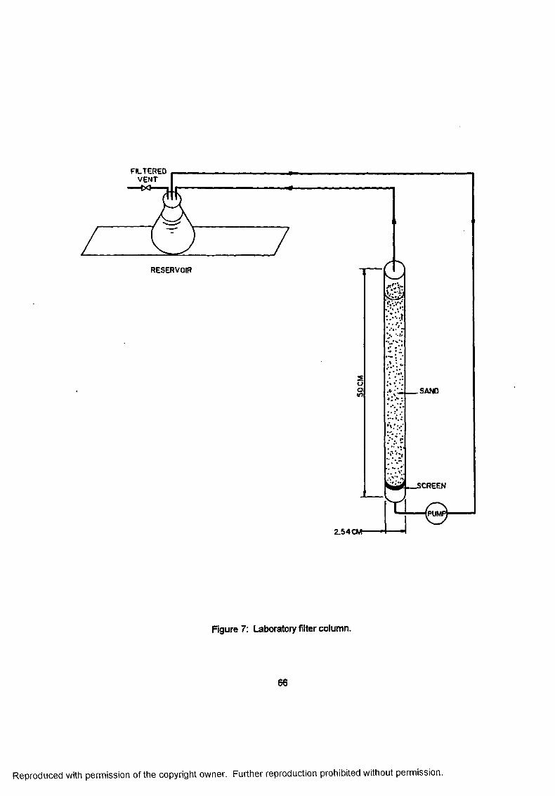
FILTEREDVENT
RESERVOIR
SANDin
iCREEN
[PUMP]
2.54 CM-
Figure 7: Laboratory filter column.
66
Reproduced with permission of the copyright owner. Further reproduction prohibited without permission.
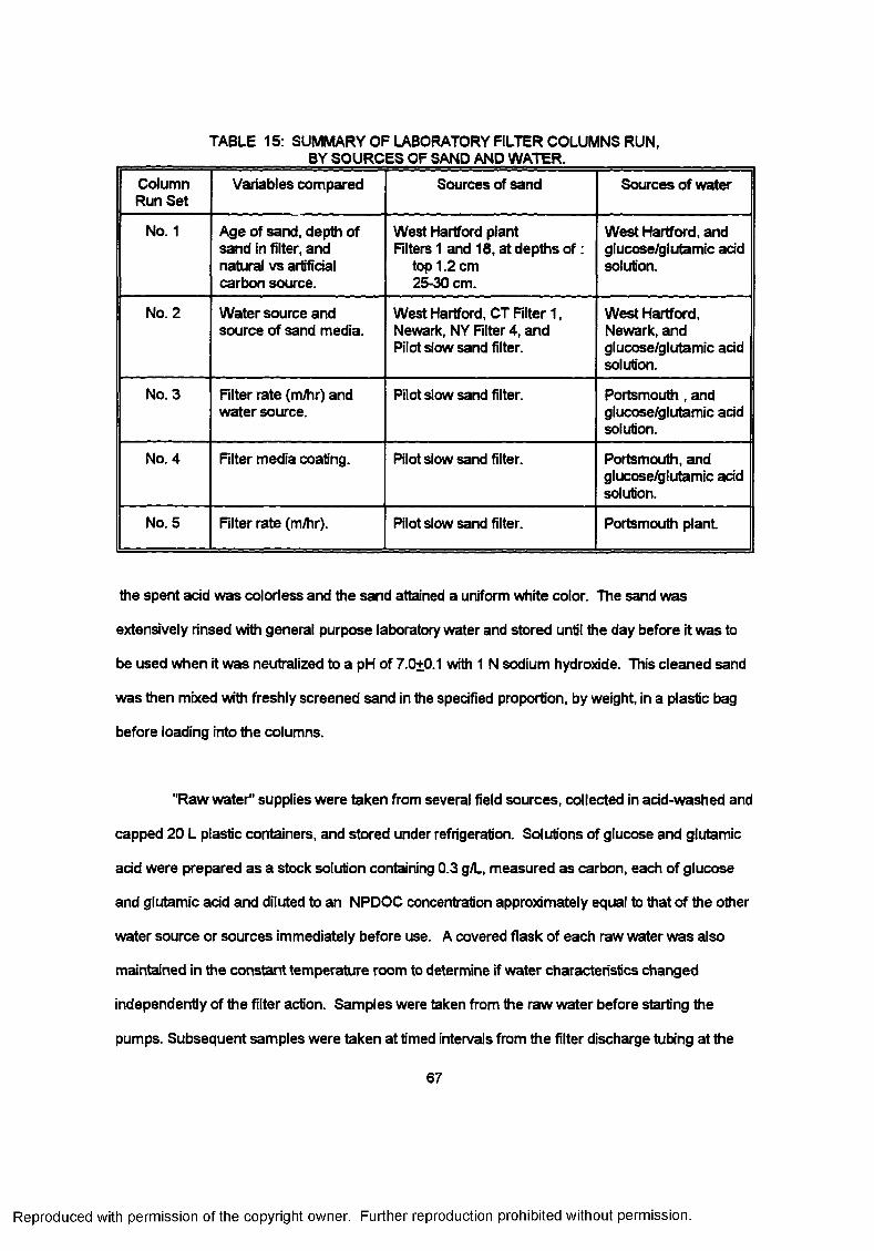
TABLE 15: SUMMARY OF LABORATORY FILTER COLUMNS RUN, BY SOURCES OF SAND AND WATER.
Column Run Set
Variables compared Sources of sand Sources of water
No. 1 Age of sand, depth of sand in filter, and natural vs artifidal carbon source.
West Hartford plant Filters 1 and 18, at depths of :
top 1.2 cm 25-30 cm.
West Hartford, and glucose/glutamic add solution.
No. 2 Water source and source of sand media.
West Hartford, CT Filter 1, Newark, NY Filter 4, and Pilot slow sand filter.
West Hartford, Newark, and glucose/glutamic add solution.
No. 3 Filter rate (m/hr) and water source.
Pilot slow sand filter. Portsmouth, and glucose/glutamic add solution.
No. 4 Filter media coating. Pilot slow sand filter. Portsmouth, and glucose/glutamic add solution.
No. 5 Filter rate (m/hr). Pilot slow sand filter. Portsmouth plant
the spent add was colorless and the sand attained a uniform white color. The sand was
extensively rinsed with general purpose laboratory water and stored until the day before it was to
be used when it was neutralized to a pH of 7.0+0.1 with 1 N sodium hydroxide. This cleaned sand
was then mixed with freshly screened sand in the specified proportion, by weight, in a plastic bag
before loading into the columns.
"Raw water" supplies were taken from several field sources, collected in add-washed and
capped 20 L plastic containers, and stored under refrigeration. Solutions of glucose and glutamic
add were prepared as a stock solution containing 0.3 g/L, measured as carbon, each of glucose
and glutamic add and diluted to an NPDOC concentration approximately equal to that of the other
water source or sources immediately before use. A covered flask of each raw water was also
maintained in the constant temperature room to determine if water characteristics changed
independently of the filter action. Samples were taken from the raw water before starting the
pumps. Subsequent samples were taken at timed intervals from the filter discharge tubing at the
67
Reproduced with permission of the copyright owner. Further reproduction prohibited without permission.
connection to the supply reservoir above the filter. Sampling times and room temperatures were
recorded.
3.5 LABORATORY METHODS AND MATERIALS
3.5.1 General
The various analytical methods used have been listed separately below by the form in
which the sample existed, whether aqueous or solid. It was necessary to use differing equipment
for some aqueous sample methods because the full scale plants were so widely distant fro each
other and reference is accordingly made in those sections. Sources of documentary information
are also listed in this section.
Several grades of water were used in the course of the experiment Ordinary supplies
used to wash glassware with phosphorus free detergent was from the Durham public water
supply. General purpose rinsing water was taken from the RO system installed within the building.
That system typically removes 95 to 99% of the polyvalent ions, greater than 99% of large
molecular weight organics, and over 99% of large bacteria (Gallagher, 1992). Type II laboratory
water was supplied within the laboratory from the reverse osmosis supply by passage through
multi-media ion exchange columns and filtered with 0.22 micron filters. This system, with the
trade name of ’Mlli-Q" (Millipore Rlter Corporation, Bedford, MA) was used for rinsing add washed
glassware, and for preparation of reagents.
Glassware, porcelain, plasticware, and container caps were washed with tap water and
phosphorus-free detergent, rinsed with water from the RO system, and further cleaned as required
for spedal purposes. Chromic add-cleaned glassware and plasticware were filled or immersed
with a chromic add cleaning solution prepared from a commerdal reagent, and allowed to stand
for a minimum of one hour. The chromic add cleaning solution was then returned to a storage
container and the cleaned ware rinsed at least three times with Type II laboratory water, air dried,
68
Reproduced with permission of the copyright owner. Further reproduction prohibited without permission.
covered with aluminum foil, and stored for subsequent use. Glassware and plasticware given a
nitric add wash was filled or immersed in a 1:1 nitric add solution for at least one hour. The nitric
add cleaning solution was returned to its storage container and the cleaned ware washed at least
three times with Type II laboratory water, air dried, and covered with poly-film or a watch glass
before further use.
After March 1993, certain pieces of glass or porcelain ware were cleaned with the muffle
furnace. These pieces were to be used for tests where it was essential that all organic material
had been removed. Furnace cleaning is a derivation of a method (Weber-Shirk, 1992) for deaning
glass beads to remove residual carbon. This method was also used in a study (Kaplan, et al,
1993) of preparation methods for bioassay vessels and other glassware. In that study glassware
cleaning with potassium dichromate-sulfuric add was compared with heating in a muffle furnace
for six hours. It was concluded that high temperature eliminated organic carbon contaminates
from glassware as effectively as potassium dichromate. A furnace time of two hours was suffident
to destroy the organic carbon content and kill organics in the volatile solids test and two hours was
adopted for the use in this project This ware was detergent washed, rinsed with general purpose
laboratory water, dried, and placed in the muffle furnace at a temperature of 550°C for at least two
hours. They were then removed, placed in a desiccator for cooling, and sealed with appropriate
covers before being stored for further use.
Many of the container caps could not be add washed or furnace cleaned. These caps
were detergent washed, rinsed with general purpose laboratory water, and rinsed repeatedly with
Type II laboratory water, allowed to stand overnight in Type II water in a chromic add washed
container, rinsed twice more in the morning, dried in the 60°C oven, and immediately placed on
their matching containers which had received add washing or furnace deaning.
69
Reproduced with permission of the copyright owner. Further reproduction prohibited without permission.
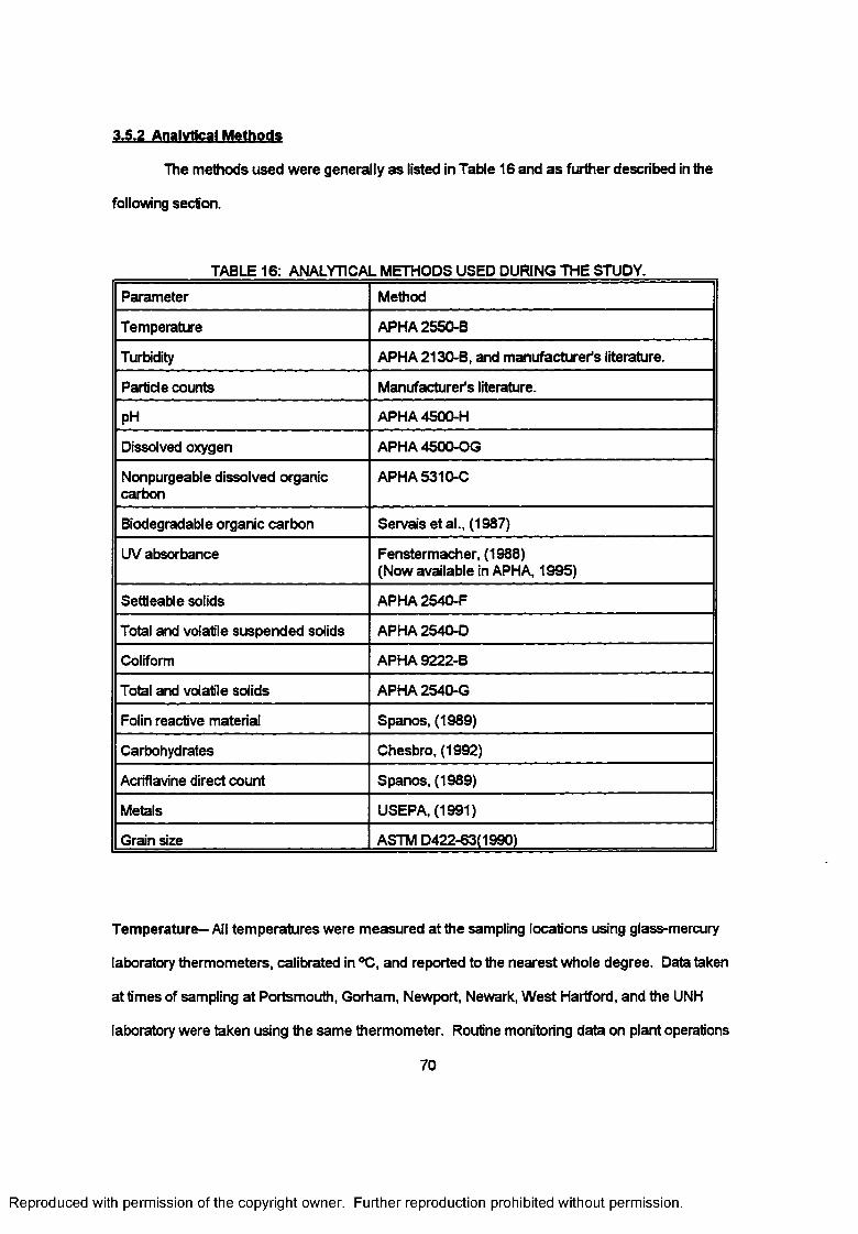
3.5.2 Analytical Methods
The methods used were generally as listed in Table 16 and as further described in the
following section.
TABLE 16: ANALYTICAIL METHODS USED DURING THE STUDY.
Parameter Method
Temperature APHA 2550-B
Turbidity APHA 2130-B, and manufacturer's literature.
Particle counts Manufacturer's literature.
pH APHA 4500-H
Dissolved oxygen APHA 4500-OG
Nonpurgeable dissolved organic carbon
APHA 5310-C
Biodegradable organic carbon Servais etal., (1987)
UV absorbance Fenstermacher, (1988)(Now available in APHA, 1995)
Settleable solids APHA 2540-F
Total and volatile suspended solids APHA 2540-D
Coliform APHA 9222-B
Total and volatile solids APHA 2540-G
Folin reactive material Spanos, (1989)
Carbohydrates Chesbro, (1992)
Acriflavine direct count Spanos, (1989)
Metals USEPA, (1991)
Grain size ASTM D422-63(1990)
Temperature— All temperatures were measured at the sampling locations using glass-mercury
laboratory thermometers, calibrated in °C, and reported to the nearest whole degree. Data taken
at times of sampling at Portsmouth, Gorham, Newport, Newark, West Hartford, and the UNH
laboratory were taken using the same thermometer. Routine monitoring data on plant operations
70
Reproduced with permission of the copyright owner. Further reproduction prohibited without permission.
at the Portsmouth, Gorham, Newport, Newark, and West Hartford facilities were taken from plant
operating reports. Temperatures were measured on grab samples in one liter beakers in which the
thermometer was allowed to stand for not less than one minute to reach equilibrium with the
sample.
Turbidity— Measurements on field samples of water from Newport, Newark, West Hartford, and
the column studies were performed on a laboratory turbidimeter (Hach, Loveland, CO).
Measurements on Gorham samples were performed by Gorham using a Hach Model 2100A.
Samples from the Portsmouth pilot plant were performed using a Hach Ratio Turbidimeter
belonging to the Portsmouth Water Treatment Plant laboratory. Daily turbidity records at all plants
were provided from plant records. The turbidimeters were allowed to warm for not less than I hour
and were tested against secondary standards of formazine in the 0 to 2 NTU range. All samples
were taken by grab sampling and stored in glass or plastic containers which had been
chromic-acid cleaned. Samples were stored, when necessary between point of collection and
laboratory analysis, in cooled containers using ice or frozen "blue-ice" blocks.
Particle Counts— Particle counts were made using a Met-One (Grants Pass, Oregon) Model 250
Particle Counter system with the Model 250 batch sampler, Model 214 single sensor counter, and
LB 1010 light-blocking sensor. Samples were stored in chromic add washed polyethylene
containers or sterile twirl bags. Studies by Flax (1993) indicated that storage in a refrigerator for up
to five days did not cause a significant change in particle count on filtered water samples, but
counting for the present study was generally completed within 24 hours. The particle counter was
set up with a maximum combined count not to exceed 30,000 counts per mL and samples with
counts in excess of this limit were diluted with Type II laboratory water. Particle counts for various
sizes were collected in "bins" as listed in Table 17. Data were saved to the computer disk and
plotted in counts per mL for each size range. Each counting series was performed in triplicate and
the results for the three runs averaged. Background counts of Type II laboratory water were also
performed before and after a series of counts for quality control and to determine the particle
71
Reproduced with permission of the copyright owner. Further reproduction prohibited without permission.
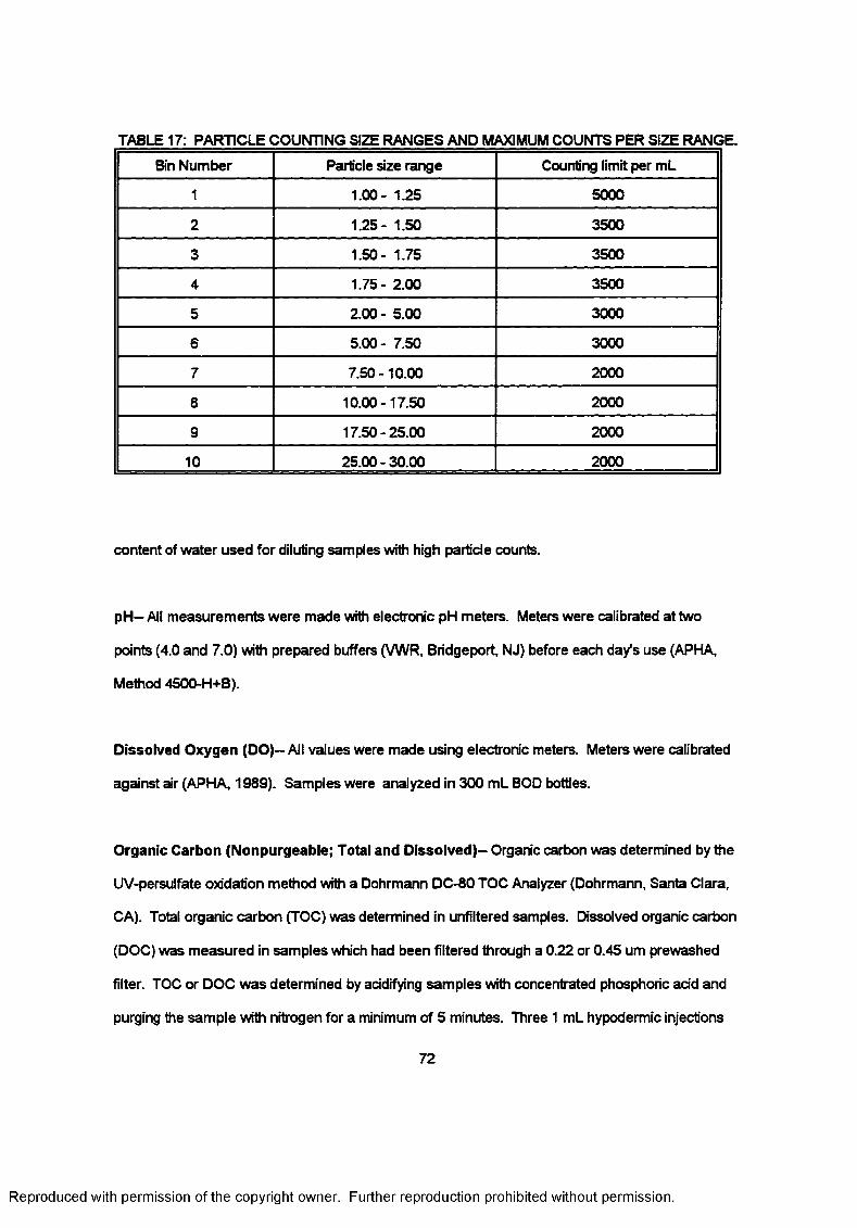
TABLE 17: PARTICLE COUNTING SIZE RANGES AND MAXIMUM COUNTS PER SIZE RANGE.
Bin Number Particle size range Counting limit per mL
1 1.00- 1.25 5000
2 1.25- 1.50 3500
3 1.50- 1.75 3500
4 1.75- 2.00 3500
5 2.00- 5.00 3000
6 5.00- 7.50 3000
7 7.50-10.00 2000
8 10.00-17.50 2000
9 17.50 - 25.00 2000
10 25.00 - 30.00 2000
content of water used for diluting samples with high particle counts.
pH— Ail measurements were made with electronic pH meters. Meters were calibrated at two
points (4.0 and 7.0) with prepared buffers (VWR, Bridgeport NJ) before each day's use (APHA,
Method 4500-H+B).
Dissolved Oxygen (DO)— All values were made using electronic meters. Meters were calibrated
against air (APHA, 1989). Samples were analyzed in 300 mL BOD bottles.
Organic Carbon (Nonpurgeable; Total and Dissolved)— Organic carbon was determined by the
UV-persulfate oxidation method with a Dohrmann DC-80 TOC Analyzer (Dohrmann, Santa Clara,
CA). Total organic carbon (TOC) was determined in unfiltered samples. Dissolved organic carbon
(DOC) was measured in samples which had been filtered through a 0.22 or 0.45 urn prewashed
filter. TOC or DOC was determined by acidifying samples with concentrated phosphoric add and
purging the sample with nitrogen for a minimum of 5 minutes. Three 1 mL hypodermic injections
72
Reproduced with permission of the copyright owner. Further reproduction prohibited without permission.
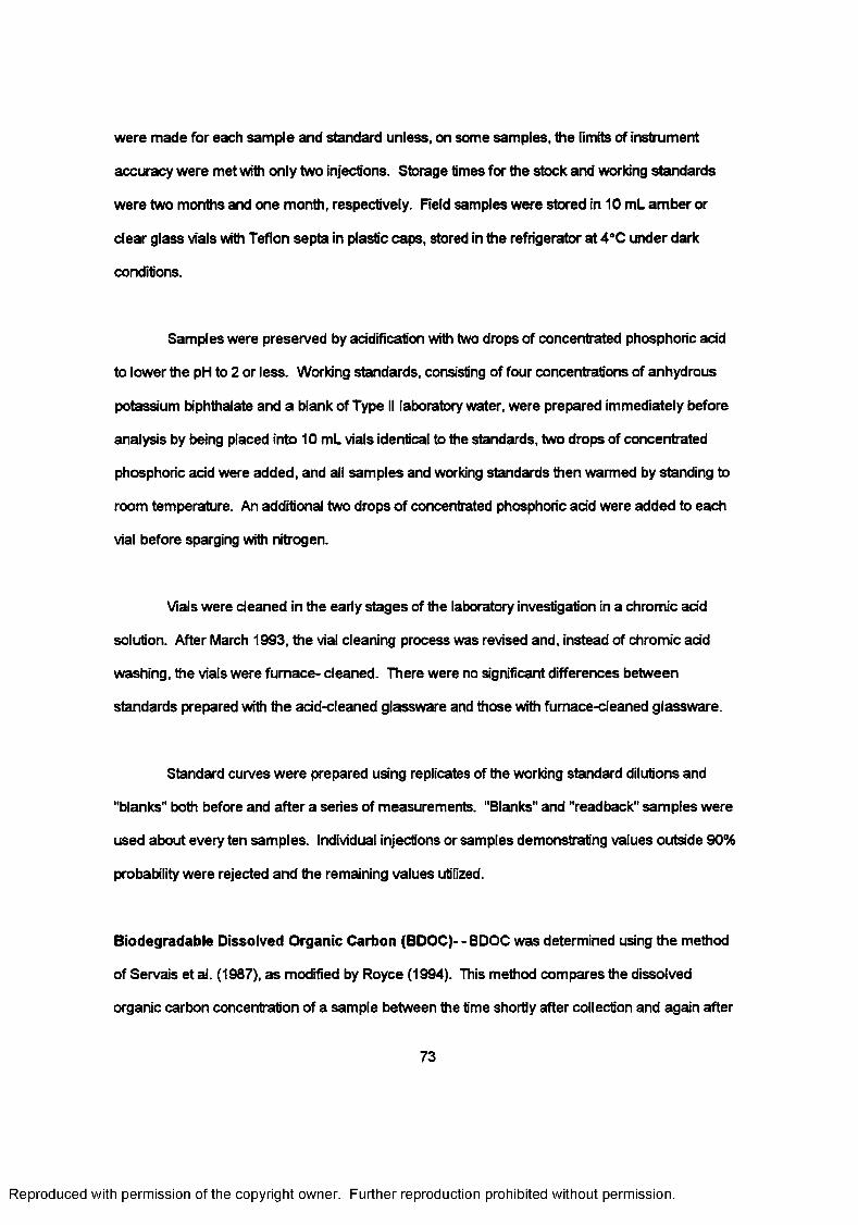
were made for each sample and standard unless, on some samples, the limits of instrument
accuracy were met with only two injections. Storage times for the stock and working standards
were two months and one month, respectively. Reid samples were stored in 10 mL amber or
clear glass vials with Teflon septa in plastic caps, stored in the refrigerator at 4°C under dark
conditions.
Samples were preserved by acidification with two drops of concentrated phosphoric add
to lower the pH to 2 or less. Working standards, consisting of four concentrations of anhydrous
potassium biphthalate and a blank of Type II laboratory water, were prepared immediately before
analysis by being placed into 10 mL vials identical to the standards, two drops of concentrated
phosphoric add were added, and all samples and working standards then warmed by standing to
room temperature. An additional two drops of concentrated phosphoric add were added to each
vial before sparging with nitrogen.
Vials were cleaned in the early stages of the laboratory investigation in a chromic add
solution. After March 1993, the vial cleaning process was revised and, instead of chromic add
washing, the vials were furnace- cleaned. There were no significant differences between
standards prepared with the add-cleaned glassware and those with furnace-cleaned glassware.
Standard curves were prepared using replicates of the working standard dilutions and
"blanks" both before and after a series of measurements. "Blanks" and "readback" samples were
used about every ten samples. Individual injections or samples demonstrating values outside 90%
probability were rejected and the remaining values utilized.
Biodegradable Dissolved Organic Carbon (BDOC)- - BDOC was determined using the method
of Servais et al. (1987), as modified by Royce (1994). This method compares the dissolved
organic carbon concentration of a sample between the time shortly after collection and again after
73
Reproduced with permission of the copyright owner. Further reproduction prohibited without permission.
it has been held at 20°C in the dark for a period of 28 to 30 days. Field samples were preserved by
refrigeration at 4°C before analysis. All glassware was add-cleaned and sterilized by autodaving.
Filters were sterilized by autodaving or purchased in an already sterile condition.
Samples were filtered using a filter apparatus (Kontes, Vineland, NJ) and 0.22 urn filters
(Sartoris, Bohemia, NY) to filter sterilize the sample. At least 250 mL of sterile Type II water was
used to rinse filters of any detergents and then to rinse the flask. The filter was then rinsed with at
least 50 mL of sample to flush the laboratory water from the filter and flask. At least 200 mL of
sample was then filtered and the filtrate collected and transferred to a sterile, covered 250 mL
Eiienmeyer flask. For some samples, more than one filtering operation was necessary to recover
at least 200 ml of filtrate; when required, the same washing operations were performed on the new
filters.
After all samples had been filtered and flasks prepared, 2.0 um filters were then used to
remove organisms larger than bacterial size from the sample. "Seed" water was prepared by
utilizing the above mentioned prewash, rinse, and filtering operation. 10 to 20 ml of seed water
was then transferred to a sterile container. Four mL of the seed water was transferred to each
flask and the flasks mixed by swirling. TOC vials were filled from each flask for the "zero d a /'
sample, acidified with two drops of concentrated phosphoric add, and stored at 4°C for later
analysis. The covered flasks were placed in cardboard boxes and closed to prevent light and
possible algal development, and kept in a constant temperature room at 20°C.
t
The flasks, rather than being held static as in the Servais method, were placed on a shaker
table to ensure complete mixing during the storage period. The flasks were taken from the
constant temperature room at designated periods and aliquates transferred into clean TOC vials as
above. Normally, samples were taken at 0 and 28 days for determination of BDOC, although on
occasion, samples were taken at intermediate times to determine the rate of development
74
Reproduced with permission of the copyright owner. Further reproduction prohibited without permission.
Analyses were normally prepared in duplicate and the results averaged.
Ultraviolet Light Absorbance at 254 nm (UV at 254 n m )- This parameter is a surrogate for
estimating trihalomethane formation potential and depends upon the absorption of ultraviolet light
at 254 nm (Amy, et al., 1986). Reid samples were stored at 4°C before analysis and analyzed
within 7 days of collection . The samples were warmed to room temperature. Samples were
filtered through Whatman GF/F filters (which have been ashed in the muffled furnace for one-half
hour before use), using disposable syringes, and filter holders. Rlters and equipment had been
pre-rinsed with approximately 50 mL of Type II laboratory water and at least 20 mL of sample prior
to use. The filtered sample were discharged directly into clean quartz cuvette, the pH adjusted to
7.0 by the addition of two drops of pH buffer solution, and placed in the spectrophotometer for
reading. Results are reported as absorption per cm.
The spectrophotometer (Bausch & Lomb Spectronic 2000, Rochester NY) was allowed to
warm up for a period of at least 1 hour before analysis. All samples were analyzed using matched
quartz cuvettes. Triplicate analyses were made on each sample with sample blanks of Type II
laboratory water used before and after each series of analyses and as readbacks during the
course of analysis to detect instrument drift
Settleable Solids— This test was performed in the field on aqueous samples of wash water from
the harrowing process. Grab samples were collected on a timed basis from the wash water flow.
One liter of sample was mixed in the sampling container and poured into the Imhoff cone to the I
liter mark. The sample was settled for approximately 45 minutes. The cone was then rotated to
gently dislodge solids which had adhered to the sloping sides of the cone. After an additional 15
minutes of settling, the volume was read at the upper surface of the settled solids.
Total and Volatile Suspended Solids— Suspended solids were measured on aqueous samples
75
Reproduced with permission of the copyright owner. Further reproduction prohibited without permission.
of wash water from the harrowing process as described above. Grab samples were collected on a
timed basis, stored in polyethylene sample containers, and refrigerated until time of analysis in the
laboratory. Settieable solids were removed prior to filtration and the supernatant from the
settieable solids test was used. Whatman GF/F, 47 mL diameter, glass fiber filters were used for
all measurements.
CoHform Bacteria— All coliform bacterial testing was performed by a laboratories certified by the
Department of Environmental Services of the State of New Hampshire or the Connecticut
Department of Health. These laboratories were: Gorham, NH, Wastewater Treatment Plant,
Claremont, NH, Water Treatment Plant, Portsmouth, NH, Water Treatment Plant, and West
Hartford, CT, Water Treatment Plant
Flow— Flow rates at the respective facilities were measured by a variety of methods. Flow
measurements at the Gorham Water Treatment Facility utilized the plant Venturi tube flow meters
which had been calibrated at the start of the testing program. Flow measurements at the Newport
Water Treatment Facility were by insert flow meters (Data Industrial Item 71-000472). The main
meter on the plant output is a Venturi meter. Flow measurements at the Newark Water Treatment
Facility were by Venturi-type flow meters.
Flow measurements at the West Hartford Water Treatment Facility also used Venturi flow
meters. Some of these flow meters were known to be highly inaccurate but a "master" Venturi
flow meter for the combined flow from each section of the plant was used to adjust the estimated
rates for individual filters in that section of the plant Wastewater flows were estimated by
measuring the cross section area of the stream channel carrying the flow and surface velocity
across the width of the flow. The surface velocities of segments across the stream were related to
mean velocities using curves of equal velocity in various channel sections (Chow, 1959).
76
Reproduced with permission of the copyright owner. Further reproduction prohibited without permission.
Flows for the pilot plants and the column studies were measured with a stop watch for the
time to fill graduated cylinders.
Total and Volatile Solids- The procedure was from Spanos, (1989 with Method 2540G (APHA,
1989) as a secondary reference. Duplicate analyses were run on each sample., using
approximately 5 grams, wet weight, of sample.
Folin Reactive Material— Folin reactive material, FRM, was used to estimate the protein content
and, from that, the active microbiological mass within the sand samples. FRM was determined
based on the method by Spanos (1990) and based also on the methods by Lowry (1951) and
Gerhardt et al. (1981). All glassware was washed with chromic add or fumace-cleaned. Pipet tips
and temperature sensitive equipment were washed repeatedly with Type II laboratory water and air
dried.
All tests were performed in duplicate. Approximately 3 grams, wet weight, of samples
were weighed into 50 mL Erlenmeyer flasks. The initial step in the analytical process was to
remove FRM from the sand grains by adding 40 mL of neutralized 0.1 % (wN ) sodium
pyrophosphate to each flask and mixing the sample on a MaxiMixer for 30 seconds, off for 30
seconds, and again for 30 seconds, before being allowed to settle. The FRM was converted from
protein with caustic by adding 3.5 mL of the extract in a clean 12 mL disposable glass vial and 7
mL of 1.0 N sodium hydroxide The samples were heated for 10 minutes in a 90°C water bath to
increase the rate of reaction. Vials with Type II laboratory water as blanks and standard
concentrations prepared with crystalline bovine albumin were prepared as for samples, including
the dilution with 2 volumes of 1.0 n sodium hydroxide and heating in the water bath. One mL
aliquots of all standards, samples, and replicates were then transferred to clean 12 mL disposable
glass vials for analysis. The mixture of the sodium carbonate and potassium tartrate copper
sulfate solution was used the same day it was prepared and not held for other tests. The sodium
77
Reproduced with permission of the copyright owner. Further reproduction prohibited without permission.
carbonate and potassium tartrate solution were prepared in advance. The Folin-Ciocaiteu reagent
was 1.95 normal and was diluted to half strength with Type II laboratory water. This solution was
also diluted daily for testing purposes. The color was allowed to develop for 20 minutes before
being read at a wavelength of 750 nm with the spectrophotometer.
The bovine albumin used for the standard was stored in a tightly closed vial in the
refrigerator until the day before use. Approximately 0.075 grams of the crystalline bovine albumin
serum was placed in an add washed 25 mL volumetric flask to which 2 mL of one normal sodium
hydroxide was added with sufficient Type II laboratory water to bring the volume up to the mark.
The actual weight of albumin was recorded and used for the adjustment of the final standard
curve. Concentrations used to prepare a standard cun/e were 3,30, and 60 ug/L Calculations
were performed using the standard curve and corrected for the actual weight of albumin and the
percent of protein in albumin (97%).
Carbohydrates- Biomass in the sand media samples was also estimated by analyzing for
carbohydrates which are contained in capsular material (Liu, et al., 1992). Carbohydrates were
measured using the phenol-sulfuric add determination (Chesbro, 1992). All glassware was
washed with chromic add or furnace-cleaned. Pipet tips and temperature sensitive equipment
were washed repeatedly with Type II laboratory water and air dried.
The analytical procedure was run in triplicate on each sample. Approximately 0.3 grams
of sand was weighed into the disposable glass 12 mL vials, the weight recorded, and two mL of
Type II laboratory water was added. Blanks and standards were prepared using 2 mL of Type II
laboratory water for appropriate dilution of sucrose as a standard carbohydrate. Standard
solutions were prepared from a stock made of 0.375 grams of sucrose per 100 mL and then
diluted to produce concentrations of I.5 ,15, and 30 mg/L carbon. A concentration of 60 mg C/L
carbon exceeded the range of the spectrophotometer. Blanks and standards were placed into the
78
Reproduced with permission of the copyright owner. Further reproduction prohibited without permission.
disposable vials also using volumes of 2 m L When ready for analysis, the equipment was placed
under a fume hood for safety and then 0.15 mL of analytical grade 89 percent Phenol was added
and followed immediately by 5.0 mL of analytical grade concentration sulfuric add. The vial was
capped, mixed by inversion five times, and allowed a minimum of 15 minutes to develop color.
The vials were then read with the spectrophotometer at the wave length of 489 nm.
Acriflavine Direct Count— Acriflavine Direct Counts (AFDC) were earned out using the method of
Spanos (1989), Balkwill and Ghiorse (1985) and Mooney (1993). Before the organisms were
stained for epifluorescent microscopy, they were removed from the surface of the sand grains.
The organisms and other coatings were removed using the same extraction procedure as for the
Folin reactive material test but using glassware which had also been autodaved for sterilization
and reagents which had been prepared using aseptic techniques and filter sterilized water. Blank
samples of solutions were carried through the extraction, filtration, and counting steps to determine
the background levels of organisms that were present through contamination of materials.
The procedure involved several steps. One mL of extract for each sample, replicate, and a
"blank" was transferred to a sterile dilution tube. The dilution tubes were mixed with a Maxi-Mixer
and held for filtration. The final dilution was fixed with 1 mL of glutaraldehyde solution per 10 mL
of diluted sample. The tube was remixed, recapped, and then stored at 4°C for up to several
weeks.
The organisms in the dilution tubes were filtered so that the organisms were retained on
the black polycarbonate filters for epifluorescent staining and counting. The filter apparatus was
not suitable for sterilization and so it was washed with phosphorus-free detergent and rinsed
thoroughly with Type II water. Backing filters, with 0.45 um openings, were first placed in the filter
apparatus to support the 0.2 um polycarbonate filters and both were washed with 2 mL of citrate
solution which was discarded. One mL of sample was then added, filtered, and an additional 2 mL
79
Reproduced with permission of the copyright owner. Further reproduction prohibited without permission.
of citrate solution was added and filtered, One mL of acriflavine stain was added and allowed to
stand for 10 minutes before filtration. A final 2 mL of citrate solution was added and filtered. The
filters were then removed from the apparatus, placed on laboratory paper towels with the
organism on top so as not to be in contact with contaminated surfaces. After drying, the filters
were transferred to microscope slides, I drop of immersion oil added, and the cover slip placed to
complete the procedure. The slide could then be stored in the dark at 4°C for later counting. The
filtrate was discarded.
Sodium citrate solution was a 0.I M solution, acidified to a pH of 4 with concentrated
hydrochloric add. The glutaraldehyde solution was a 25% solution in Type II laboratory water with
I.99 grams of Cacodyiic add added, and filter sterilized with a disposable syringe and filter. The
acriflavine solution was a 1.0 mM solution. Filters for the test were 0.2 um, 25 mL black
polycarbonate filters (Nuclepore) and placed on a backing support filter which was a 0.45 micron
25 mL (Gilman Sdences) Metricel membrane filter. The black polycarbonate filters were
purchased gas-sterilized while the backing filter was sterilized by autodaving.
The organisms on the filters were counted by students in the Department of Microbiology
at the University of New Hampshire for bacteria, fungal fragments, and protozoa. Bacteria and
protozoa were differentiated by visual size in the experience of the counter. Fungal fragments
were identified as filaments. The counts were expressed in numbers of organisms per field of a
measured diameter microscopic view.
M etals- Metals were analyzed using the USEPA Contract Lab Program Statement of Work for
Inorganic Analyses/Soil/ Sediment Digestion Procedure (USEPA, 1991) as modified by Vaughan
(1993) and by the Inductively Coupled Plasma (ICP) Analytical Technique at the New Hampshire
Materials Testing Laboratory. All samples were run in duplicate, with analytical standards and
blanks included for quality assurance. Blanks were prepared using the same techniques but
80
Reproduced with permission of the copyright owner. Further reproduction prohibited without permission.
without any sand sample being added, and standards were prepared using appropriate laboratory
metal standards. Metal tests were performed on all samples for total iron, total manganese, total
calcium, and total aluminum. All glassware was add washed with 50 percent nitric add for a
minimum of one hour, and then rinsed with Type II laboratory water.
Sand samples were mixed in the plastic storage bags, and approximately one gram by wet
weight was transferred to add washed beakers for analysis (Vaughan, 1993). Ten mL of 1:1 nitric
add was added to each beaker, the beaker covered with a watch glass, and placed on a hot plate
to heat at approximately 95°C for 10 minutes without boiling. At the end of 10 minutes, the
samples were removed, allowed to cool, and 5 mL of concentrated nitric add was added. The
watch glasses were replaced, samples returned to the hot plates, and bdled gently (refluxed) for
30 minutes. Although Type II laboratory water could have been added to maintain the volume at
greater than 5 mL, the step was not necessary. The sample was then cooled, 2 mL of Type II
laboratory water added, and 3 mL of 30 percent hydrogen peroxide added, the watch glasses
replaced, and the beakers returned to the hot plate to be warmed at approximately 95°C until the
effervescence substantially subsided. Additional I mL volumes of 30 percent hydrogen peroxide
were added and the samples continued to be warmed until the effervescence again substantially
subsided. No more than 10 mL of the 30 percent peroxide was used for any of the samples. The
beakers were again cooled, and 5 mL of one to one hydrochloric add and 10 mL of Type II
laboratory water then added to the beaker. The cover glass was replaced and the samples
returned to the hot plate for an additional 10 minutes of warming at 95°C. The beakers were again
cooled, the contents of the beaker (including the sand) was transferred to add washed 100 mL
volumetric flasks, diluted to the mark with Type II laboratory water and allowed to settle overnight
A portion of the flask supernatant was carefully decanted to add washed polyethylene sample
containers without transfer of any sediment These samples in the polyethylene vials were then
sent to the contract laboratory for analysis.
81
Reproduced with permission of the copyright owner. Further reproduction prohibited without permission.
Grain Size Analysis— Samples were prepared for sieve analysis by air drying at 103°C overnight
The sand samples were cooled to room temperature and placed in sealed plastic bags for storage
prior to sieve analysis. Sample sizes were approximately 500 grams minimum. Sieves used were
the 3/8th, No. 8, No. 10, No. 20, No. 40, No. 60, No. 140, No. 200, and pan. Samples were usually
run without duplicates but, because of overlapping analyses and filter runs, there were duplications
for certain samples. These data have been used for determinations of accuracy and precision.
3.6 DATA ANALYSIS METHODS
3.6.1 Analytical Tools
Data analysis was performed using a IBM-Compatible Personal Computer and with the
following programs:
Microsoft Windows Version 3.1 (Microsoft Corporation, Redmond, WA)WordPerfect Version 6.0a for Windows (WordPerfect Corporation, Orem, Utah)Microsoft Excel Version 4.0 Spreadsheet (Microsoft Corporation, Redmond, WA)Jandel Scientific Sigma Plot 5.0 for Windows (San Rafael, CA)
The SigmaPlot program was used for laboratory data conversions and plotting. The Excel
program was used for general spread sheet calculations and basic statistical analyses, such as
means, standard deviation, ANOVA, and t-tests.
3.6.2 Quality Assurance and Quality Control
A quality assurance and control plan (Collins et al., 1992) was used as a guide for
sampling, analysis, and use of data. Sampling locations have been described earlier in this
Section. Sampling containers and storage methods are summarized in Table 18. Samples were
labeled in the field, for location, time, site, and preservation used. Chain of custody forms were
attached and the samples shipped or transported by the sampling personnel in refrigerated foam
chests to the laboratory.
Analytical methods have been described elsewhere in this Chapter, but detailed
82
Reproduced with permission of the copyright owner. Further reproduction prohibited without permission.
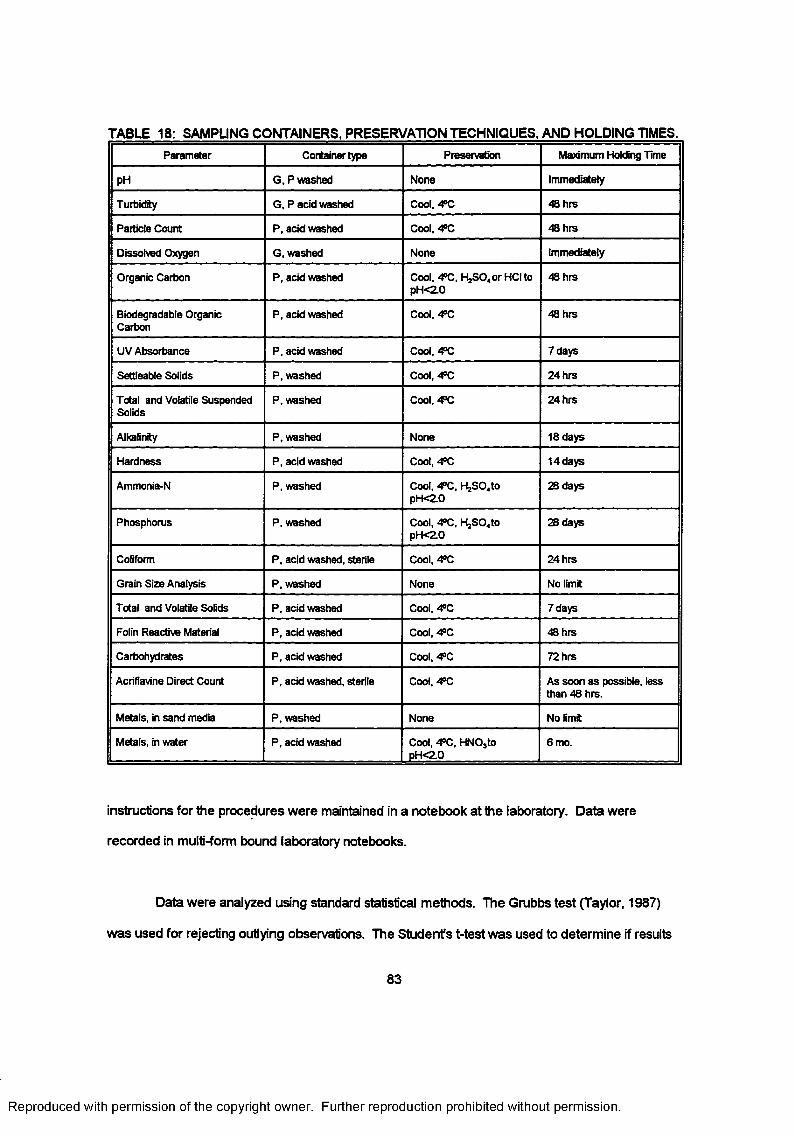
TABLE 18: SAMPLING CONTAINERS. PRESERVATION TECHNIQUES. AND HOLDING TIMES.Parameter Container type Preservation Maximum Holding Time
pH G. P washed None Immediately
Turbidity G, P acid washed Cool, 4°C 48 hrs
Particle Count P, acid washed Cool, *PC 48 hrs
Dissolved Oxygen G, washed None Immediately
Organic Carbon P. acid washed Cool. 4PC, H jS04orHCIto PHK2.0
48 hrs
Biodegradable Organic Carbon
P, acid washed Cool. 4PC 48 hrs
UV Absorbance P, acid washed Cool, 4^C 7 days
Settieable Solids P, washed Cool, 4°C 24 hrs
Total and Volatile Suspended Solids
P, washed Cool, 4>C 24 hrs
Alkalinity P, washed None 18 days
Hardness P, acid washed Cool, 4PC 14 days
Ammonia-N P, washed Cool. 4?C, H jS04to pH<2-0
28 days
Phosphorus P, washed Cool, 4°C, H jS04to pH<2.0
28 days
Coliform P, acid washed, sterile Cool, 4°C 24 hrs
Grain Size Analysis P, washed None No limit
Total and Volatile Solids P, acid washed Cool, <PC 7 days
Folin Reactive Material P, acid washed Cool, 4?C 48 hrs
Carbohydrates P, acid washed Cool, 4>C 72 hrs
Acriflavine Direct Count P, acid washed, sterile Cool. 4°C As soon as possible, less than 48 hrs.
Metals, in sand media P, washed None No limit
Metals, in water P, acid washed Cool. •‘PC, HN03to pH<2.0
6 mo.
instructions for the procedures were maintained in a notebook at the laboratory. Data were
recorded in multi-form bound laboratory notebooks.
Data were analyzed using standard statistical methods. The Grubbs test (Taylor, 1987)
was used for rejecting outlying observations. The Student's t-test was used to determine if results
83
Reproduced with permission of the copyright owner. Further reproduction prohibited without permission.
were significantly different, and a confidence limit of 90 percent was used unless otherwise noted.
The standard deviation of sample populations were compared and pooled (Taylor, 1987; Collins et
al., 1992a). Method Detection Limits were based on "one-tailed" 99 percent confidence level using
the standard deviation estimated on reagent blanks.
Water quality analyses are reported as the mean value of the individual analyses, with
standard deviations when the analyses were performed in replicate on the same sample. Water
quality analyses over extended periods are reported with the mean value and the standard
deviation of the individual analyses over the period.
The filter media was cored using a 3.8 cm (1.5-in.) diameter polyvinyl chloride tube. The
tube was open at both ends with the coring end bevelled on the inside to facilitate insertion into the
sand media. The tube was inserted at predetermined locations (Collins et al., 1992) to depths as
marked on the outside of the tube and the tube withdrawn from the media. The full length of the
sample cores at Gorham, NH were removed from the filter room and extracted, with tapping of the
tube and pressing from the top with a wooden rod, onto a clean plastic sheet for subsampling by
depth intervals. Sample cores at the other plants were taken with the same tube to the bottom of
the individual depth intervals, removed from the media, and the media sample for that depth
removed directly from the open bottom of the tube. All media samples were taken within one cm
(0.5-in.) of the designated sample depth. Samples were deposited directly into sterile 56 gm (2-
ounce) "Whirl-Pak" bags and stored in ice chests until they could be returned to the laboratory for
refrigeration. The analyses were performed in replicate for each subsample. Results of the
analyses for each subsample were compared for statistical outliers, then the resultant mean and
standard deviation for each was compared with those for other cores within the same filter to
determine if there were statistically significant differences at the 90 percent level. All analyses for
the three cores in each filter for the same subsample depth, excluding outliers, were then used to
determine the mean and standard deviation for the sample set representing the filter at this depth.
84
Reproduced with permission of the copyright owner. Further reproduction prohibited without permission.
The media was analyzed for grain size, total and volatile solids, FRM, carbohydrates, AFDC, iron,
manganese, calcium, and aluminum.
Quality control was maintained by: 1) adherence to the written laboratory procedures
based on the referenced methods and instrument manufacturers instruction, 2) use of duplicates
on all filter media and many aqueous samples, 3) use of spikes, replicate analyses, reagent
blanks, analytical "readbacks", and 4) comparison of the results with others from the same source
and with those from the other sources. The methods are summarized in Table 19. Information on
the limits of detection, method detection limits, and distribution of variance between processing
steps is presented in Appendix B.
The laboratories at each plant were visited at the start of the project and again near the
end of the work. Communications were maintained with both plant superintendents and with the
laboratory manager and sampling staff at each plant
3.7 COSTS
3.7.1 Labor
Labor requirements for the various cleaning operations were determined by observation of the
numbers of personnel and the time involved for cleaning.
3.7.2 Equipment
Equipment and personnel time were recorded at the time of the cleaning event It should
be noted that equipment at some plants might be used only for cleaning operations and remain out
of service for long periods. Other plants, specifically the West Hartford plant, use the equipment
daily because of the large number of filters being cleaned on a regular basis.
85
Reproduced with permission of the copyright owner. Further reproduction prohibited without permission.
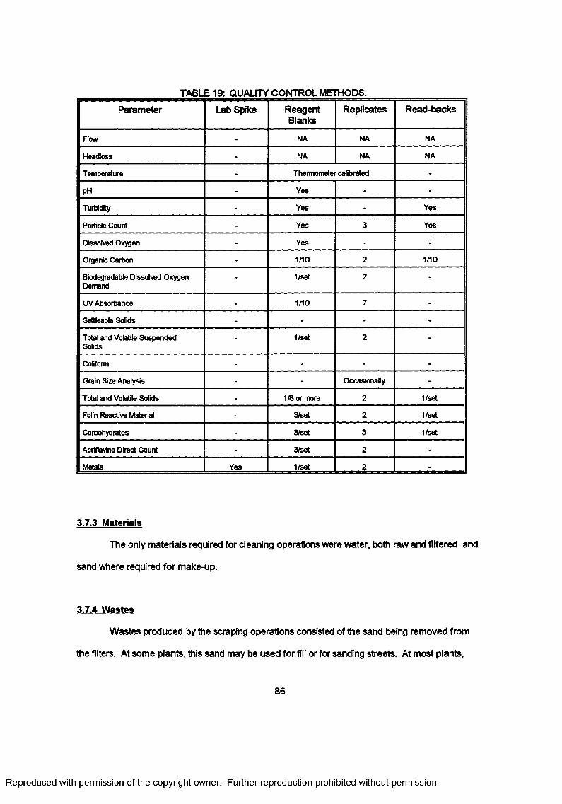
TABLE 19: QUALITY CONTROL ME1rHODS.Parameter Lab Spike Reagent
BlanksReplicates Read-backs
Flow - NA NA NA
Headloss - NA NA NA
Temperature - Thermometer calibrated -
pH - Yes - -
Turbidity - Yes - Yes
Particle Count - Yes 3 Yes
Dissolved Oxygen - Yes - -
Organic Carbon - 1/10 2 1/10
Biodegradable Dissolved Oxygen Demand
- 1/set 2 -
UV Absorbance - 1/10 7 -
Settleable Solids - - - -
Total and Volatile Suspended Solids
- 1/set 2 -
Coliform - - - -
Grain Size Analysis - - Occasionally -
Total and Volatile Solids - 1/8 or more 2 1/set
Folin Reactive Material - 3/set 2 1/set
Carbohydrates - 3/set 3 1/set
Acriflavine Direct Count - 3/set 2 -
Metals Yes 1/set 2 -
3.7.3 Materials
The only materials required for cleaning operations were water, both raw and filtered, and
sand where required for make-up.
3.7.4 Wastes
Wastes produced by the scraping operations consisted of the sand being removed from
the filters. At some plants, this sand may be used for fill or for sanding streets. At most plants,
86
Reproduced with permission of the copyright owner. Further reproduction prohibited without permission.
however, the sand was stockpiled until sufficient sand was in storage to justify hydraulic cleaning
operations after which the sand may be reused for make-up in other filters. It was not possible to
measure the wastes from hydraulic cleaning while the filter was being resanded at West Hartford.
Estimates were made based on the differences in quality between "dirty" sand being removed and
the clean sand which replaced it
Additional wastes are generated from the harrowing operations in the form of wash water.
Measurements of flow volumes during the cleaning operations were made at Newport NH using
the flow meters. Measurements at West Hartford were based on the cross sectional areas and
estimated mean velocity of flow in the drainage channels. Measurements of settleable and
suspended solids in the wastewaters were made as discussed earlier.
3.7.4 Filter Time
Records of filter times and throughput were taken from plant records.
3.7.5 Administration
Estimates of administrative time involved with the cleaning of filters were prepared from
discussions with the plant staff.
87
Reproduced with permission of the copyright owner. Further reproduction prohibited without permission.
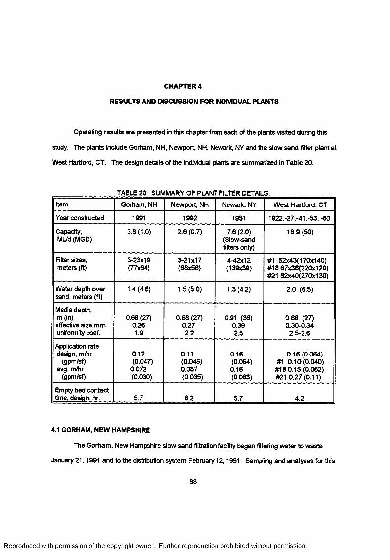
CHAPTER4
RESULTS AND DISCUSSION FOR INDIVIDUAL PLANTS
Operating results are presented in this chapter from each of the plants visited during this
study. The plants indude Gorham, NH, Newport, NH, Newark, NY and the slow sand filter plant at
West Hartford, CT. The design details of the individual plants are summarized in Table 20.
TABLE 20: SUMMARY OF PLANT FILTER DETAILS.
Item Gorham, NH Newport, NH Newark, NY West Hartford, CT
Year constructed 1991 1992 1951 1922,-27,-41,-53, -60
Capacity, ML/d (MGD)
3.8 (1.0) 2.6 (0.7) 7.6 (2.0) (Slow-sand filters only)
18.9 (50)
Filter sizes, meters (ft)
3-23x19(77x64)
3-21x17(68x56)
4-42x12(139x39)
#1 52x43(170x140) #18 67x36(220x120) #21 82x40(270x130)
Water depth over sand, meters (ft)
1.4 (4.6) 1.5 (5.0) 1.3 (4.2) 2.0 (6.5)
Media depth, m (in)effective size,mm uniformity coef.
0.68 (27) 0.26 1.9
0.68 (27) 0.27 2.2
0.91 (36) 0.39 2.5
0.68 (27) 0.30-0.34
2.S-2.6
Application rate design, m/hr
(gpm/sf) avg, m/hr
(gpm/sf)
0.12(0.047)
0.072(0.030)
0.11(0.045)0.087(0.035)
0.16(0.064)0.16(0.063)
0.16 (0.064) #1 0.10(0.040)
#18 0.15(0.062) #21 0.27(0.11)
Empty bed contact time, design, hr. 5.7 6.2 5.7 4.2
4.1 GORHAM, NEW HAMPSHIRE
The Gorham, New Hampshire slow sand filtration facility began filtering water to waste
January 21,1991 and to the distribution system February 12,1991. Sampling and analyses for this
88
Reproduced with permission of the copyright owner. Further reproduction prohibited without permission.
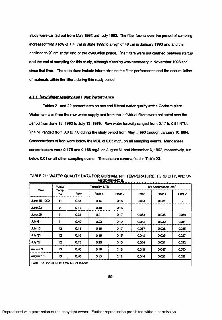
study were earned out from May 1992 until July 1993. The filter losses over the period of sampling
increased from a low of 1.4 cm in June 1992 to a high of 48 cm in January 1993 and and then
declined to 20 cm at the end of the evaluation period. The filters were not cleaned between startup
and the end of sampling for this study, although cleaning was necessary in November 1993 and
since that time. The data does include information on the filter performance and the accumulation
of materials within the filters during this study period.
4.1.1 Raw Water Quality and Filter Performance
Tables 21 and 22 present data on raw and filtered water quality at the Gorham plant
Water samples from the raw water supply and from the individual filters were collected over the
period from June 15,1992 to July 13,1993. Raw water turbidity ranged from 0.17 to 0.84 NTU.
The pH ranged from 6.6 to 7.0 during the study period from May I, I993 through January 10,1994.
Concentrations of iron were below the MDL of 0.03 mg/L on all sampling events. Manganese
concentrations were 0.175 and 0.168 mg/L on August 31 and November 3,1992, respectively, but
below 0.01 on all other sampling events. The data are summarized in Table 23.
TABLE 21: WATER QUALITY DATA FOR GORHAM, NH, TEMPERATURE, TURBIDITY, AND UV ____________ ABSORBANCE.
DateWaterTemp.
°C
Turbidity. NTU UV Absorbance, cm-'
Raw Filter 1 Filter 2 Raw FHterl Filter 2
June 15,1992 11 0.44 0.18 0.18 0.034 0.031 -
June 22 11 0.17 0.18 0.18 - - -
June 29 11 0.31 0.21 0.17 0.034 0.038 0.034
July 6 11 0.48 0.23 0.18 0.042 0.032 0.031
July 13 12 0.16 0.18 0.17 0.037 0.036 0.035
July 20 12 0.16 0.18 0.15 0.040 0.036 0.037
July 27 12 0.13 0.20 0.15 0.034 0.031 0.032
August 3 13 0.40 0.18 0.16 0.048 0.047 0.090
August 10 13 0.40 0.15 0.16 0.044 0.036 0.038
TABLE 21 CONTINUED ON NEXT PAGE
89
Reproduced with permission of the copyright owner. Further reproduction prohibited without permission.
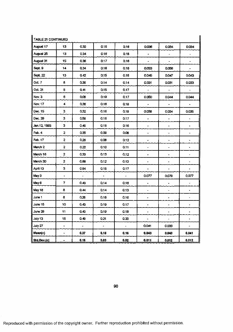
TABLE 21 CONTINUED
August 17 13 0.30 0.16 0.16 0.036 0.034 0.034
August 25 13 0.34 0.16 0.18 - - -
August 31 15 0.36 0.17 0.16 - - -
Sept. 9 14 0.34 0.16 0.16 0.053 0.056 -
Sept 22 13 0.42 0.15 0.16 0.045 0.047 0.043
O ct 7 8 0.36 0.14 0.14 0.031 0.031 0.033
Oct 21 8 0.41 0.15 0.17 - - -
Nov. 3 6 0.06 0.19 0.17 0.050 0.044 0.044
Nov. 17 4 0.36 0.16 0.18 - - -
Dec. 15 3 0.32 0.16 0.18 0.038 0.034 0.035
Dec. 29 3 0.56 0.16 0.17 - - -
Jan. 12,1993 3 0.45 0.16 0.16 - - -
Feb. 4 2 0.35 0.09 0.06 - - -
Feb. 17 2 0.26 0.06 0.12 - - -
March 2 2 0.22 0.10 0.11 - - -
March 16 2 0.33 0.13 0.12 - - -
March 30 2 0.66 0.12 0.13 - - -
April 13 3 0.84 0.15 0.17 - - -
May 3 - - - - 0.077 0.079 0.077
May 6 7 0.43 0.14 0.16 - - -
May 18 8 0.44 0.14 0.13 - - -
Junel 8 0.38 0.16 0.16 - - -
June 15 10 0.43 0.19 0.17 - - -
June 29 11 0.43 0.19 0.18 - - -
July 13 15 0.49 0.21 0.20 - - -
July 27 - - - - 0.041 0.033 -
Mean(c) - 0.37 0.16 0.16 0.043 0.040 0.041
Std.Dev.(c) - 0.15 0.03 0.02 0.011 0.012 0.012
90
Reproduced with permission of the copyright owner. Further reproduction prohibited without permission.
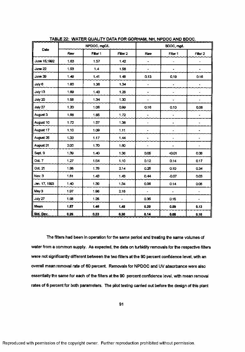
TABLE 22: WATER QUALITY DATA FOR GORHAM, NH, NPDOC AND BDOC.
DateNPDOC. mgC/L BDOC, mg/L
Raw Filter 1 Fi*er2 Raw Filter 1 Filter 2
June 15,1962 1.63 1.57 1.42 - - -
June 22 1.53 1.4 1.56 - - -
June 29 1.46 1.41 1.48 0.13 0.19 0.16
July 6 1.60 1.36 1.34 - - -
July 13 1.69 1.43 1.28 - - -
July 20 1.58 1.34 1.30 - - -
July 27 1.20 1.06 0.99 0.16 0.10 0.06
August 3 1.66 1.85 1.72 - - -
August 10 1.72 1.57 1.36 - - -
August 17 1.10 1.06 1.11 - - -
August 25 1.33 1.17 1.44 - - -
August 31 2.00 1.70 1.60 - - -
Sept 9 1.39 1.40 1.36 0.06 <0.01 0.08
O ct 7 1.27 1.54 1.10 0.12 0.14 0.17
O ct 21 1.96 1.79 2.14 0.25 0.10 0.34
Nov. 3 1.81 1.43 1.43 0.44 -0.07 0.03
Jan. 17,1993 1.40 1.39 1.34 0.06 0.14 0.08
May 3 1.97 1.96 Z16 - - -
July 27 1.68 1.28 - 0.35 0.15 -
Mean 1.57 1.46 1.45 0.20 0.09 0.13
Std. Dev. 0.26 0.23 0.30 0.14 0.08 0.10
The filters had been in operation for the same period and treating the same volumes of
water from a common supply. As expected, the data on turbidity removals for the respective filters
were not significantly different between the two filters at the 90 percent confidence level, with an
overall mean removal rate of 60 percent Removals for NPDOC and UV absorbance were also
essentially the same for each of the filters at the 90 percent confidence level, with mean removal
rates of 6 percent for both parameters. The pilot testing earned out before the design of this plant
91
Reproduced with permission of the copyright owner. Further reproduction prohibited without permission.
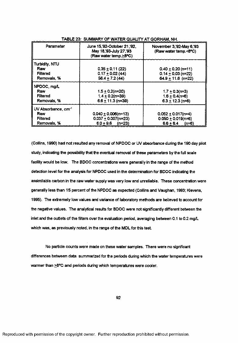
TABLE 23: SUMMARY OF WATER QUALITY AT GORHAM. NH.Parameter June 15,'92-October 21 ,'92,
May 18,'93-July27,,93 (Raw water temp.>8°C)
November 3,'92-May 6/93 (Raw water temp.<8°C)
Turbidity, NTU Raw Filtered Removals, %
0.35 + 0.11 (22) 0.17 + 0.02(44) 56.4 ±7 .2 (44)
0.40 +0.20 (n=11) 0.14 +0.03 (n=22) 64.9 + 11.6 (n=22)
NPDOC, mg/L Raw Filtered Removals, %
1.5 + 0.2(n=20) 1.4 + 0.2(n=39)6.6 + 11.3 (n=39)
1.7 + 0.3(n=3) 1.6 + 0.4(n=6) 6.3 +12.3 (n=6)
UV Absorbance, cm'1 Raw Filtered Removals, %
0.040 + 0.006(n=13) 0.037 + 0.007(n=23)
6.0+ 9.6 in=23)
0.052 + 0.017(n=4) 0.050 + 0.019(n=6)
6.6 + 6.4 (n=6)
(Collins, 1990) had not resulted any removal of NPDOC or UV absorbance during the 190 day pilot
study, indicating the possibility that the eventual removal of these parameters by the full scale
facility would be low. The BDOC concentrations were generally in the range of the method
detection level for the analysis for NPDOC used in the determination for BDOC indicating the
assimilable carbon in the raw water supply was very low and unreliable. These concentration were
generally less than 15 percent of the NPDOC as expected (Collins and Vaughan, 1993; Klevens,
1995). The extremely low values and variance of laboratory methods are believed to account for
the negative values. The analytical results for BDOC were not significantly different between the
inlet and the outlets of the filters over the evaluation period, averaging between 0.1 to 0.2 mg/L
which was, as previously noted, in the range of the MDL for this test
No particle counts were made on these water samples. There were no significant
differences between data summarized for the periods during which the water temperatures were
warmer than >8°C and periods during which temperatures were cooler.
Reproduced with permission of the copyright owner. Further reproduction prohibited without permission.
4.1.2 Filter Media
Although the filters were not cleaned during the evaluation period, samples were taken on
two occasions. Sample cores from this filter were difficult to extract and, while the filter was
flooded, could not be taken at depths into the filter greater than the person taking the samples
could reach to manually cover the lower end of the sample tube after it had been inserted to the
desired depth. At the time of the May 1992 sampling, the media was also apparently "air-bound" in
different locations of the filter and would not support the weight of a person walking on these
isolated pockets. The water level was subsequently lowered and the filter slowly backfilled, and
the media was able to support a person's weight afterward.
The surface of these filters were covered by a thick layer of schmutzdecke material unlike
that observed in the other full-scale filters in this study or in the pilot-scale filters at Portsmouth, NH.
In the other filters, the schmutzdecke layer visible on top of the sand media was thin and
gelatinous. At Gorham, the layer was as much as one to two cm thick but similar in appearance to
moss or lichen growing in a woodland environment This layer easily separated from the surface
of the media if the water above it were disturbed. The information on the media is presented in
Table 24.
The data on the subsample relicates was analyzed using two-factor ANOVA methods to
determine if the variation between replicates exceeded that between core subsamples by depth or
that between cores at the same depth. A statistical probability of 90 percent was used for
determining significance. A sample of this calculation for the July 27,1993 analyses for volatile
solids is attached in Appendix B. The results of such statistical analyses for the Gorham, NH media
samples taken July 27,1993 indicated that the variations between replicates were not significant,
that the variations between cores were not significant, but the variation between depth was
significant for volatile solids and FRM. The variations for carbohydrates were significant between
replicates, depth, and cores, showing this analytical parameter should not be considered further for
93
Reproduced with permission of the copyright owner. Further reproduction prohibited without permission.
this sample event The variations for these factors, as well as AFDC, iron, manganese, calcium,
aluminum, are also summarized in Table 24.
These results were generally consistent with the data collected by Spanos (1989)
indicating AFDC counts of 10* to 10® per gram dry weight in the schmutzdecke and upper 30 cm of
media at the West Hartford, CT plant, Springfield, MA plant, and New Haven, CT plant and ratios
of FRM to AFDC of 0.4 to 2 x 10',z g FRM per cell as counted by AFDC. The comparable results at
the Gorham plant for AFDC counts were also 10s to 10s per gram dry weight in the schmutzdecke
and upper 30 cm of media, but 5 to 6 x 10',z g FRM per cell as counted by AFDC which was more
than twice those indicated. The ration of carbohydrate to protein concentrations were in the range
of 0.2 to 0.3 percent which was low relative to the 2 to 3 percent expected from the literature
(Charackis and Marshall, 1990).
This information should also be considered relative to the history of the filters. The filters
had been in operation only since January, 1991 and had never been cleaned. It is estimated that
the annual flow of water through the filter had been approximately 1.6 ML/sm with an estimated
load of 2.6 kg/sm NPDOC. The estimated NPDOC removal was six percent, or an estimated
removal of less than 0.1 kg/sm. The load of turbidity and UV Absorbing materials, calculated as
the NTU or UVA times the flow in ML, are estimated as 0.66x10*6 NTU units/sm and 0.08x10*6
UVA units/sm, respectively.
4.2 NEWPORT, NEW HAMPSHIRE
The Newport New Hampshire facility was first visited in May I993. At that time, the filters
were ready to be cleaned for the first time since they had been put in operation in October, 1992.
The subsequent cleaning operations were sampled through January, 1994. The filters at this plant
were operated using both of the two principal cleaning methods, scraping and harrowing, to
compare their effects on plant performance and media development The evaluation period ended
94
Reproduced with permission of the copyright owner. Further reproduction prohibited without permission.
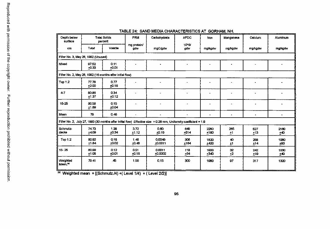
Reproduced
with perm
ission of the
copyright ow
ner. Further
reproduction prohibited
without
permission.
TABLE 24: SAND MEDIA CHARACTERISTICS AT GORHAM. NH.Depth below
surface
cm
Total Solids percent
FRM
mg protein/ gdw
Carbohydrate
mgC/gdw
AFDC
10*6/gdw
Iron
mg/kgdw
Manganese
mg/kgdw
Calcium
mg/kgdw
Aluminum
mg/kgdwTotal Volatile
Filter No. 3, May 28,1982 (Unused)
Mixed 97.52 0.11 _ _ _+0.33 +0.01
Filter No. 2, May 28,1982 (16 months alter initial flow)
Top 1.2 77.78 0.77 _ _ _+2.00 +0.16
4-7 80.86 0.34 _ _ _ .+1.37 ±0.12
15-25 80.58 0.15 _ _ _ m♦1.89 ±0.04
Mean 79 0.46 - - - - - - -
Filter No. 2, July 27,1983 (30 months alter initial flow) Effective size = 0.26 mm, Uniformity coefficient = 1.9
Schmutz 74.73 1.38 3.72 0.60 648 2280 285 527 2160decke +4.08 ±0.34 ±1.12 ±0.15 ±514 ±160 ±1 ±13 ±40
Top 1.2 80.92 0.18 1.48 0.0048 306 1820 40 258 1080+1.84 ±0.02 ±0.48 ±0.0011 ±164 ±420 ±1 ±14 ±80
15-25 80.98 0.12 0.51 0.0011 118 1900 32 242 1030+1.06 ±0.01 ±0.16 ±0.0002 ±64 ±340 ±2 ±19 ±40
Weighted 79.41 .45 1.56 0.15 300 1980 97 317 1320Mean,w
(•) Weighted mean = [(Schmutz./4) + (Level 1/4) + ( Level 2/2)]
95
in January 1994, however, before the filters could be repeatedly cleaned with the respective
cleaning methods. Consequently, long-term comparative treatment performance data were
limited. The data does include comparative information on the costs of the methods and on the
accumulation of materials within the filters during the first year of operation.
4.2.1 RAW WATER QUALITY AND FILTER PERFORMANCE-
Tables 25 through 27 present the collected data on raw and filtered water quality. Water
samples from the raw water supply and from the individual filters were collected over the period
from May 12,1993 to January 10,1994. There were no samples taken from Filter 2 after it had
been harrowed except during the first 17.5 hours of ripening. Raw water turbidity ranged from 0.2
to 0.7 NTU except during the runoff periods when it reached 1.2 to 1.6 (Newport, 1993). The pH
ranged from 6.6 to 7.0 during the study period from May I, I993 through January 10,1994. The data
on turbidity removals for the respective filters were not significantly different between the filters at
the 90 percent confidence level, with an overall mean
removal rate of 80 percent Removals for NPDOC and UV absorbance were also compared and
found to be essentially the same for each of the filters at the 90 percent confidence level, with
mean removal ratesof 22 percent for both parameters. The BDOC concentrations were below the
MDL levels in the raw water and filter discharges.
The data showed differences were significant at the 90 percent condidence level for
removal of UV absorbance between the samples before June and after November 20 which
corresponded with water temperatures in the raw water supply at or above 8°C, or below 8°C.
The data was separated around these dates and reanalyzed with the results presented in Table 28.
The differences between the filters in the removal of all parameters were not significant at
the 90 percent level except between July and November 20 when the mean removal of particles in
the Filter No. 1 were lower than those in the other two filters. None of the data contributing to this
96
Reproduced with permission of the copyright owner. Further reproduction prohibited without permission.
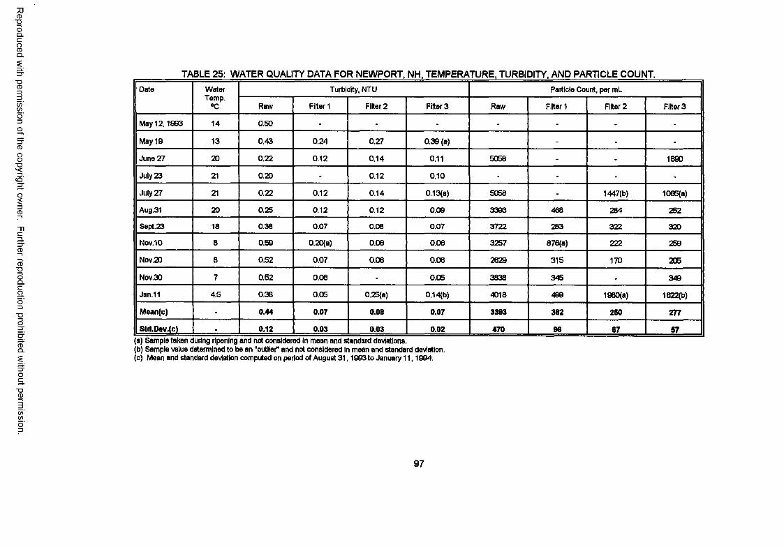
Reproduced
with perm
ission of the
copyright ow
ner. Further
reproduction prohibited
without
permission.
TABLE 25: WATER QUALITY DATA FOR NEWPORT, NH, TEMPERATURE. TURBIDITY, AND PARTICLE COUNT.Date Water
Temp.°C
Turbidity, NTU Particle Count, per mL
Raw Filter 1 Filter 2 Filter 3 Raw Filter 1 Filter 2 Filter 3
May 12,1993 14 0.50 - - - - - - -
May 19 13 0.43 0.24 0.27 0.39(a) - - -
June 27 20 0.22 0.12 0.14 0.11 5068 - - 1890
July 23 21 0.20 - 0.12 0.10 - - - -
July 27 21 0.22 0.12 0.14 0.13(a) 5068 - 1447(b) 1066(a)
Aug.31 20 0.25 0.12 0.12 0.09 3393 468 284 252
Sept.23 18 0.38 0.07 0.06 0.07 3722 283 322 320
Nov.10 8 0.59 0.20(a) 0.06 0.06 3257 876(a) 222 259
Nov.20 8 0.52 0.07 0.06 0.06 2629 315 170 205
Nov.30 7 0.52 0.06 - 0.06 345 - 349
Jan.11 4.5 0.38 0.05 0.25(a) 0.14(b) 4018 499 1660(a) 1622(b)
Mean(c) - 0.44 0.07 0.08 0.07 3393 382 260 277
Std.Dev.(c) - 0.12 0.03 0.03 0.02 470 96 67 57(a) Sample taken during ripening and not considered In mean and standard deviations.(b) Sample value determined to be an "outlier'' and not considered in mean and standard deviation.(c) Mean and standard deviation computed on period of August 31,1963 to January 11,1994.
97
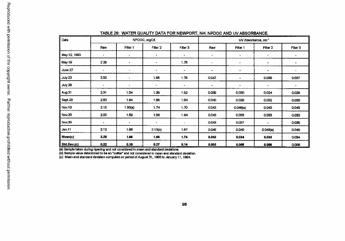
Reproduced
with perm
ission of the
copyright ow
ner. Further
reproduction prohibited
without
permission.
TABLE 26: WATER QUALITY DATA FOR NEWPORT, NH, NPDOC AND UV ABSORBANCE,Date NPDOC, mgC/L UV Absorbance, cm'1
Raw Filter 1 Filter 2 Filter 3 Raw Filter 1 Filter 2 Filter 3
May 12,1903 - - - - - - - -
May 19 2.28 - - 1.78 - - - -
June 27 - - - - - - - -
July 23 2.50 - 1.98 1.78 0.047 - 0.039 0.037
July 26 - - - - - - - -
Aug.31 2.31 1.54 1.35 1.52 0.039 0.030 0.024 0.026
Sept. 23 2.63 1.64 1.96 1.94 0.040 0.029 0.032 0.030
Nov.10 2.15 1.86(a) 1.74 1.70 0.043 0.046(a) 0.043 0.043
Nov.20 2.00 1.59 1.56 1.64 0.043 0.033 0.033 0.033
Nov.30 - - - - 0.043 0.037 - 0.036
Jan. 11 2.12 1.96 2.13(b) 1.87 0.045 0.040 0.043(a) 0.040
Mean(c) 2.28 1.68 1.66 1.74 0.043 0.034 0.033 0.034
Std.Dev.(c) 0.22 0.19 0.27 0.14 0.003 0.006 0.008 0.006a) Sample taken during ripening and not considered in mean and standard deviations.
(b) Sample value determined to be an "outlier" and not considered in mean and standard deviation.(c) Mean and standard deviation computed on period of August 31,1993 to January 11,1994.
98
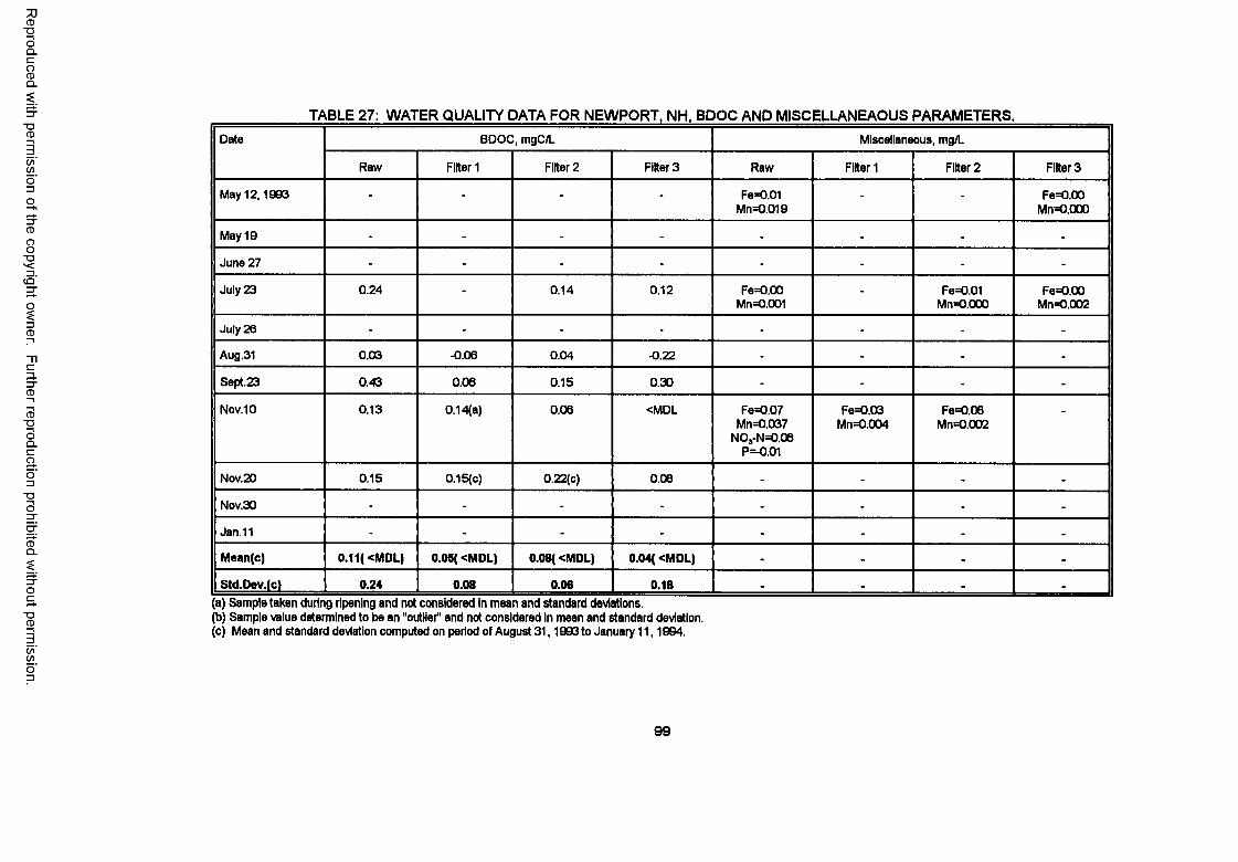
Reproduced
with perm
ission of the
copyright ow
ner. Further
reproduction prohibited
without
permission.
TABLE 27: WATER QUALITY DATA FOR NEWPORT. NH, BDOC AND MISCELLANEAOUS PARAMETERS.Date BDOC, mgC/L Miscellaneous, mg/L
Raw Filter 1 Filter 2 Filter 3 Raw Filter 1 Filter 2 Filter 3
May 12,1993 - - - - Fe=0.01Mn=0.019
- - Fe=0.00Mn=0.000
May 19 - - - - - - - -
June 27 - - - - - - - -
July 23 0.24 - 0.14 0.12 Fe=0.00Mn=0.001
- Fe=0.01Mn=0.000
Fe=0.00Mn=0.002
July 26 - - - - - - - -
Aug .31 0.03 -0.06 0.04 -0.22 - - - -
Sept.23 0.43 0.06 0.15 0.30 - - - -
Nov.10 0.13 0.14(a) 0.06 <MDL Fe=O.07Mn=0.037
N 03-N=0.06P=-0.01
Fe=O,03Mn=0.004
Fe=0.06Mn=0.002
Nov.20 0.15 0.15(c) 0.22(c) 0.06 - - - -
Nov.30 - - - - - - - -
Jan. 11 - - - - - - - -
Mean(c) 0.11( <MDL) 0.05( <MDL) 0.08( <MDL) 0.04( <MDL) - - - -
Std.Dev.(c) 0.24 0.08 0.06 0.18 - - - -
(a) Sample taken during ripening and not considered In mean and standard deviations.(b) Sample value determined to be an "outlier" and not considered in mean and standard deviation.(c) Mean and standard deviation computed on period of August 31,1903 to January 11,1994.
99
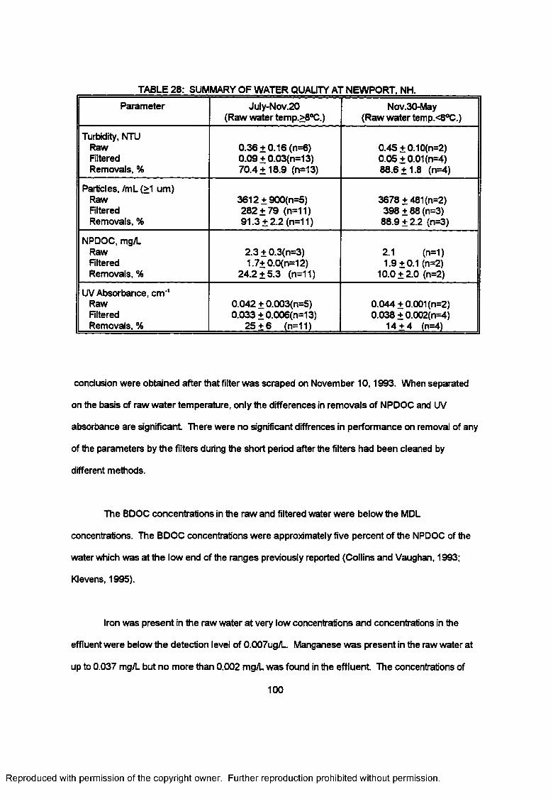
TABLE 28: SUMMARY OF WATER QUALITY AT NEWPORT, NH.
Parameter July-Nov.20 (Raw water temp.>8°C.)
Nov.30-May (Raw water temp.<8°C.)
Turbidity, NTU Raw Filtered Removals, %
0.36 + 0.16 (n=6) 0.09 + 0.03(n=13) 70.4+18.9 (n=13)
0.45 +0.10(n=2) 0.05 +0.01 (n=4) 88.6 ±1 .8 (n=4)
Particles, /mL (>1 um) Raw Filtered Removals, %
3612 + 900(n=5) 282 + 79 (n=11) 91.3 + 2.2 (n=11)
3678 + 481 (n=2) 398 + 88 (n=3)
88.9 + 2.2 (n=3)
NPDOC, mg/L Raw Filtered Removals, %
2.3 + 0.3(n=3) 1.7+0.0(n=12)
24.2 + 5.3 (n=11)
2.1 (n=1) 1.9+ 0.1 (n=2)
10.0 + 2.0 (n=2)
UV Absorbance, cm'1 Raw Filtered Removals, %
0.042 ± 0.003(n=5) 0.033 + 0.006(n=13)
25 + 6 (n=11)
0.044 +0.001 (n=2) 0.038+ 0.002(n=4)
14 + 4 (n=4)
conclusion were obtained after that filter was scraped on November 10,1993. When separated
on the basis of raw water temperature, only the differences in removals of NPDOC and UV
absorbance are significant There were no significant diffrences in performance on removal of any
of the parameters by the filters during the short period after the filters had been cleaned by
different methods.
The BDOC concentrations in the raw and filtered water were below the MDL
concentrations. The BDOC concentrations were approximately five percent of the NPDOC of the
water which was at the low end of the ranges previously reported (Collins and Vaughan, 1993;
Wevens, 1995).
Iron was present in the raw water at very low concentrations and concentrations in the
effluent were below the detection level of 0.007ug/L. Manganese was present in the raw water at
up to 0.037 mg/L but no more than 0.002 mg/L was found in the effluent The concentrations of
100
Reproduced with permission of the copyright owner. Further reproduction prohibited without permission.
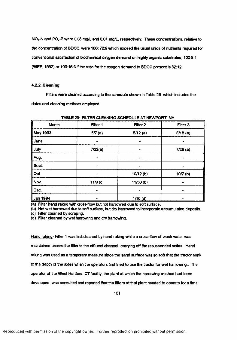
NOj-N and P 04-P were 0.08 mg/L and 0.01 mg/L, respectively. These concentrations, relative to
the concentration of BDOC, were 100:72:9 which exceed the usual ratios of nutrients required for
conventional satisfaction of biochemical oxygen demand on highly organic substrates, 100:5:1
(WEF, 1992) or 100:15:3 if the ratio for the oxygen demand to BDOC present is 32:12.
4.2.2 Cleaning
Filters were cleaned according to the schedule shown in Table 29 which includes the
dates and cleaning methods employed.
TABLE 29: FILTER CLEANING SCHEDULE AT NEWPORT, NH.
Month Filter 1 Rlter 2 Rlter 3
May 1993 5/7 (a) 5/12 (a) 5/18 (a)
June - - -
July 7122(a) - 7/26 (a)
Aug. - - -
Sept - - -
Oct - 10/12 (b) 10/7 (b)
Nov. 11/9 (c) 11/30 (b) -
Dec. - - -
Jan 1994 - 1/10 (d) _
a) Rlter hand raked with cross-flow but not harrowed due to soft surface.(b) Not wet harrowed due to soft surface, but dry harrowed to incorporate accumulated deposits.(c) Filter cleaned by scraping.(d) Filter cleaned by wet harrowing and dry harrowing.
Hand raking- Filter 1 was first cleaned by hand raking while a cross-flow of wash water was
maintained across the filter to the effluent channel, carrying off the resuspended solids. Hand
raking was used as a temporary measure since the sand surface was so soft that the tractor sunk
to the depth of the axles when the operators first tried to use the tractor for wet harrowing,. The
operator of the West Hartford, CT facility, the plant at which the harrowing method had been
developed, was consulted and reported that the filters at that plant needed to operate for a time
101
Reproduced with permission of the copyright owner. Further reproduction prohibited without permission.
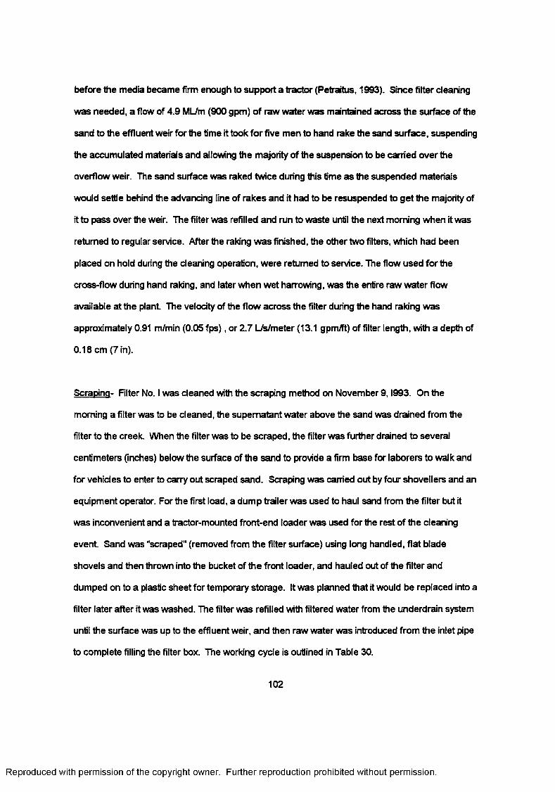
before the media became firm enough to support a tractor (Petraitus, 1993). Since filter cleaning
was needed, a flow of 4.9 ML/m (900 gpm) of raw water was maintained across the surface of the
sand to the effluent weir for the time it took for five men to hand rake the sand surface, suspending
the accumulated materials and allowing the majority of the suspension to be earned over the
overflow weir. The sand surface was raked twice during this time as the suspended materials
would settle behind the advancing line of rakes and it had to be resuspended to get the majority of
it to pass over the weir. The filter was refilled and run to waste until the next morning when it was
returned to regular service. After the raking was finished, the other two filters, which had been
placed on hold during the cleaning operation, were returned to service. The flow used for the
cross-flow during hand raking, and later when wet harrowing, was the entire raw water flow
available at the plant The velocity of the flow across the filter during the hand raking was
approximately 0.91 m/min (0.05 fps), or 2.7 L/s/meter (13.1 gpm/ft) of filter length, with a depth of
0.18 cm (7 in).
Scraping- Rlter No. I was cleaned with the scraping method on November 9 ,1993. On the
morning a filter was to be cleaned, the supernatant water above the sand was drained from the
filter to the creek. When the filter was to be scraped, the filter was further drained to several
centimeters (inches) below the surface of the sand to provide a firm base for laborers to walk and
for vehicles to enter to carry out scraped sand. Scraping was earned out by four shovellers and an
equipment operator. For the first load, a dump trailer was used to haul sand from the filter but it
was inconvenient and a tractor-mounted front-end loader was used for the rest of the cleaning
event Sand was "scraped" (removed from the filter surface) using long handled, flat blade
shovels and then thrown into the bucket of the front loader, and hauled out of the filter and
dumped on to a plastic sheet for temporary storage. It was planned that it would be replaced into a
filter later after it was washed. The filter was refilled with filtered water from the underdrain system
until the surface was up to the effluent weir, and then raw water was introduced from the inlet pipe
to complete filling the filter box. The working cycle is outlined in Table 30.
102
Reproduced with permission of the copyright owner. Further reproduction prohibited without permission.
TABLE 30: WORK SCHEDULE FOR SCRAPING NEWPORT FILTER 1, NOVEMBER 9,1993.
Time interval Activity Labor and Equipment
7:00-8:30 Drain filter 1 person, none
8:30-9:15 Scraping 5 persons, loader
9:15-10:30 Smoothing surface by dragging 4 persons, tractor
10:30-15:30 Refill filter Brief visit by 1 person.
15:30-7:30 Rlter to waste Brief visit by 1 person.
7:30 Return to service
The total volume of sand removed was 3.2 cubic meters (4.2 cy) as measured at the dump site.
No wash water was generated except for the volume of raw water drained from the filter before
cleaning and the water filtered to waste. None of this water required treatment before discharge to
the receiving stream.
Harrowing- Filter No. 2 was cleaned by the wet harrowing method and monitored for this study.
Before the sand would support the tractor, however, the filter had to be cleaned twice without the
wet harrowing step. Dry harrowing the accumulated material into the filter media hastened the rate
at which the filter surface became sufficiently firm to support the tractor and allowing the wet
harrowing method to proceed. The West Hartford plant uses this same procedure after a filter bed
is "reconditioned" (Petraitus, 1993). There was no wastewater or waste sand generated during dry
harrowing operations except while the filter was ripened over night
The final wet harrowing/dry harrowing operation was similar to that of hand raking except a
small rubber-tired tractor pulled a harrow around the filter surface while flow was maintained from
the influent pipe across the filter surface to the overflow weirs. The harrow penetrated
approximately 0.2 m (8 in) below the surface of the sand and suspended the accumulated
materials so they could be earned to the holding pond. After the wet harrowing, the filter water
103
Reproduced with permission of the copyright owner. Further reproduction prohibited without permission.
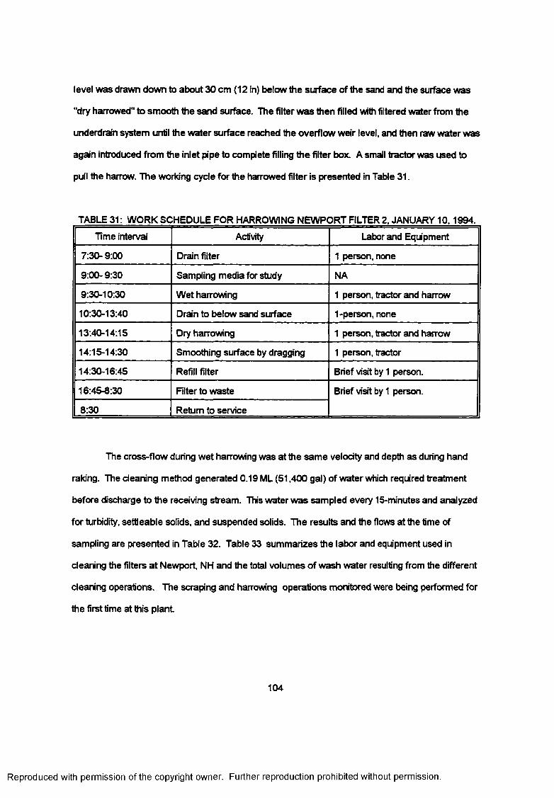
level was drawn down to about 30 cm (12 in) below the surface of the sand and the surface was
"dry harrowed" to smooth the sand surface. The filter was then filled with filtered water from the
underdrain system until the water surface reached the overflow weir level, and then raw water was
again introduced from the inlet pipe to complete filling the filter box. A small tractor was used to
pull the harrow. The working cyde for the harrowed filter is presented in Table 31.
TABLE 31: WORK SCHEDULE FOR HARROWING NEWPORT FILTER 2. JANUARY 10,1994.
Time interval Activity Labor and Equipment
7:30-9:00 Drain filter 1 person, none
9:00-9:30 Sampling media for study NA
9:30-10:30 Wet harrowing 1 person, tractor and harrow
10:30-13:40 Drain to below sand surface 1-person, none
13:40-14:15 Dry harrowing 1 person, tractor and harrow
14:15-14:30 Smoothing surface by dragging 1 person, tractor
14:30-16:45 Refill filter Brief visit by 1 person.
16:45-8:30 Rlter to waste Brief visit by 1 person.
8:30 Return to service
The cross-flow during wet harrowing was at the same velocity and depth as during hand
raking. The cleaning method generated 0.19 ML (51,400 gal) of water which required treatment
before discharge to the receiving stream. This water was sampled every 15-minutes and analyzed
for turbidity, settieable solids, and suspended solids. The results and the flows at the time of
sampling are presented in Table 32. Table 33 summarizes the labor and equipment used in
cleaning the filters at Newport, NH and the total volumes of wash water resulting from the different
cleaning operations. The scraping and harrowing operations monitored were being performed for
the first time at this plant
104
Reproduced with permission of the copyright owner. Further reproduction prohibited without permission.
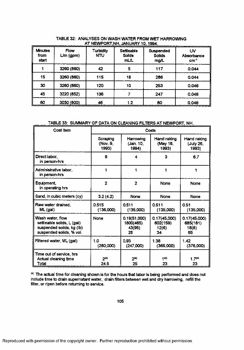
TABLE 32: ANALYSES ON WASH WATER FROM WET HARROWING _____________ AT NEWPORT.NH, JANUARY 10.1994._____________
Minutesfromstart
Flow L/m (gpm)
TurbidityNTU
SetHeableSolidsmL/L
SuspendedSolidsmg/L
UVAbsorbance
cm'1
1 3260(860) 42 5 117 0.044
15 3260(860) 115 16 286 0.044
30 3260 (860) 120 10 253 0.046
45 3220(852) 136 7 247 0.046
60 3030(800) 46 1.2 80 0.046
TABLE 33: SUMMARY OF DATA ON CLEANING FILTERS AT NEWPORT, NH.
Cost Item Costs
Scraping (Nov. 9, 1993)
Harrowing (Jan. 10,
1994)
Hand raking (May 18,
1993)
Hand raking (July 26,
1993)
Direct labor, in person-hrs
9 4 3 6.7
Administrative labor, in person-hrs
1 1 1 1
Equipment, in operating hrs
2 2 None None
Sand, in cubic meters (cy) 3.2 (4.2) None None None
Raw water drained, ML (gal)
0.515(136,000)
0.511(135,000)
0.511(135,000)
0.51(135,000)
Wash water, flow settleable solids, L (gal) suspended solids, kg (lb) suspended solids, % vol.
None 0.19(51,000)1800(465)
43(95)28
0.17(45,000)602(159)
12(6)34
0.17(45,000)685(181)
18(8)65
Filtered water, ML (gal) 1.0(280,000)
0.93(247,000)
1.38(365,000)
1.42(376,000)
Time out of service, hrs Actual cleaning time Total
2<»>24.5
2<*)25
1«23
1.7W23
l,) The actual time for cleaning shown is for the hours that labor is being performed and does not include time to drain supernatant water, drain filters between wet and dry harrowing, refill the filter, or ripen before returning to service.
Reproduced with permission of the copyright owner. Further reproduction prohibited without permission.
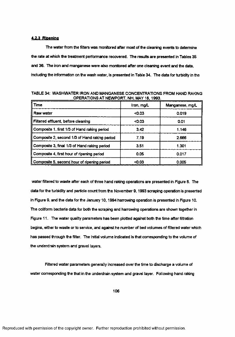
4.2.3 Ripening
The water from the filters was monitored after most of the cleaning events to determine
the rate at which the treatment performance recovered. The results are presented in Tables 35
and 36. The iron and manganese were also monitored after one cleaning event and the data,
including the information on the wash water, is presented in Table 34. The data for turbidity in the
TABLE 34: WASHWATER IRON AND MANGANESE CONCENTRATIONS FROM HAND RAKINGOPERATIONS AT NEWPORT, NH, MAY 18.1993.
Time Iron, mg/L Manganese, mg/L
Raw water <0.03 0.019
Rltered effluent before cleaning <0.03 0.01
Composite 1, first 1/3 of Hand raking period 3.42 1.146
Composite 2, second 1/3 of Hand raking period 7.19 2.666
Composite 3, final 1/3 of Hand raking period 3.51 1.301
Composite 4, first hour of ripening period 0.05 0.017
Composite 5, second hour of ripening period <0.03 0.005
water filtered to waste after each of three hand raking operations are presented in Figure 8. The
data for the turbidity and particle count from the November 9,1993 scraping operation is presented
in Figure 9, and the data for the January 10,1994 harrowing operation is presented in Figure 10.
The coltform bacteria data for both the scraping and harrowing operations are shown together in
Figure 11. The water quality parameters has been plotted against both the time after filtration
begins, either to waste or to service, and against he number of bed volumes of filtered water which
has passed through the filter. The initial volume indicated is that corresponding to the volume of
the underdrain system and gravel layers.
Rltered water parameters generally increased over the time to discharge a volume of
water corresponding the that in the underdrain system and gravel layer. Following hand raking
106
Reproduced with permission of the copyright owner. Further reproduction prohibited without permission.
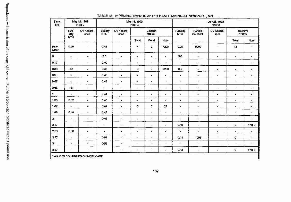
Reproduced
with perm
ission of the
copyright ow
ner. Further
reproduction prohibited
without
permission.
TABLE 35: RIPENING TRENDS AFTER HAND RAKING AT NEWPORT. NH.Time,
hrsMay 12,1993
Filter 2May 18,1993
Filter 3July 26,1993
Filter 3
TurbidityNTU
UV Absorbance
TurbidityNTU
UV Absorbance
Coliform/100mL
TurbidityNTU
ParticleCount/mL
UV Absorbance
Colltorm/100mL
Total Fecal Non- Total Non-
Rawwater
0.26 - 0.43 - 4 2 >200 0.20 5060 - 12 -
0 - - 3.0 - - - - 3.0 - - - -
0.17 - - 0.40 - - - - - - - - -
0.33 40 - 0.45 - 0 0 >200 3.0 - - - -
0.5 - - 0.45 - - - - - - - - -
0.67 - - 0.45 - - - - - - - - -
0.83 43 - - - - - - - - - - -
1 - - 0.44 - - - - - - - - -
1.33 0.52 - 0.46 - - - - - - - - -
1.67 - - 0.44 - 0 0 27 - - - - -
1.83 0.46 - 0.45 - - - - - - - - -
2 - - 0.45 - - - - - - - - -
2.17 - - - - - - - 0.15 - - 0 TNTC
2.33 0.50 - - - - - - - - - - -
2.67 - - 0.63 - - - - 0.14 1066 - 0 -
3 - - 0.55 - - - - - - - - -
3.17 - - - - - - - 0.13 - - 0 TNTC
TABLE 35 CONTINUES ON NEXT PAGE
107
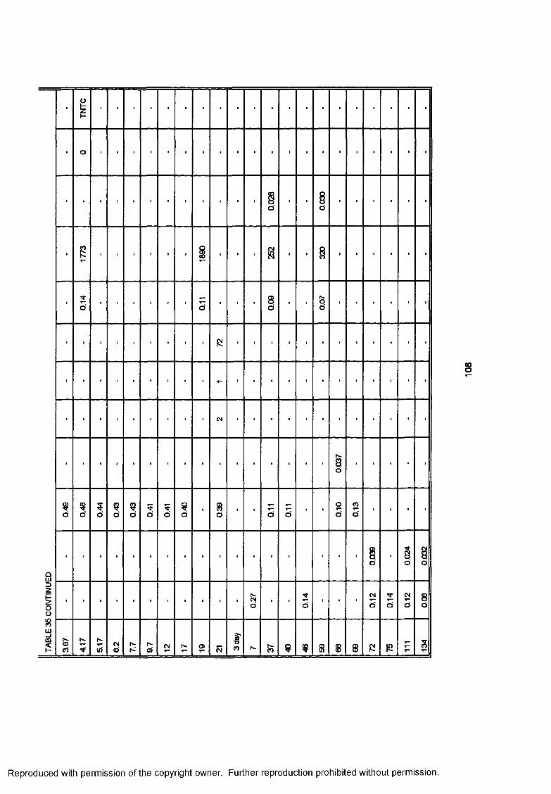
CM
CM
CM
CD
Reproduced with permission of the copyright owner. Further reproduction prohibited without permission.
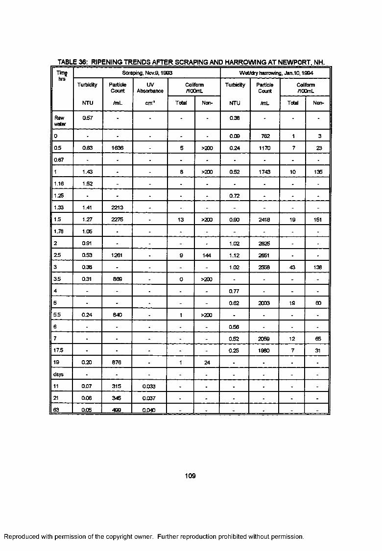
TABLE 36: RIPENING TRENDS AFTER SCRAPING AND HARROWING AT NEWPORT, NH.Timghrs
Scraping, Nov.9,1993 Wet/dry harrowing, Jan.10,1984
Turbidity ParticleCount
UVAbsorbance
CoflformAlOOmL
T urbidity ParticleCount
Conform/IQOmL
NTU /mL cm'1 Total Non- NTU /mL Total Non-
Rawwater
0.57 - - - - 0.38 - - -
0 - - - - - 0.09 762 1 3
0.5 0.83 1636 - 5 >200 0.24 1170 7 23
0.67 - - - - - - - - -
1 1.43 - - 8 >200 0.52 1743 10 135
1.16 1.52 - - - - - - - -
1.25 - - - - - 0.72 - - -
1.33 1.41 2213 - - - - - - -
1.5 1.27 2275 - 13 >200 0.90 2418 19 151
1.78 1.05 - - - - - - - -
2 0.91 - - - - 1.02 2625 - -
2 5 0.53 1261 - 9 144 1.12 2651 - -
3 0.38 - - - - 1.02 43 138
3.5 0.31 869 - 0 >200 - - - -
4 - - - - - 0.77 - - -
5 - - - - - 0.62 2003 19 60
5.5 0.24 840 - 1 >200 - - - -
6 - - - - - 0.56 - - -
7 - - - - - 0.52 2059 12 65
17.5 - - - - - 0.25 1960 7 31
19 0.20 876 - 1 24 - - - -
days - - - - - - - - -
11 0.07 315 0.033 - - - - - -
21 0.06 345 0.037 - - - - - -
63 0.05 499 0.040 - - - - - -
109
Reproduced with permission of the copyright owner. Further reproduction prohibited without permission.
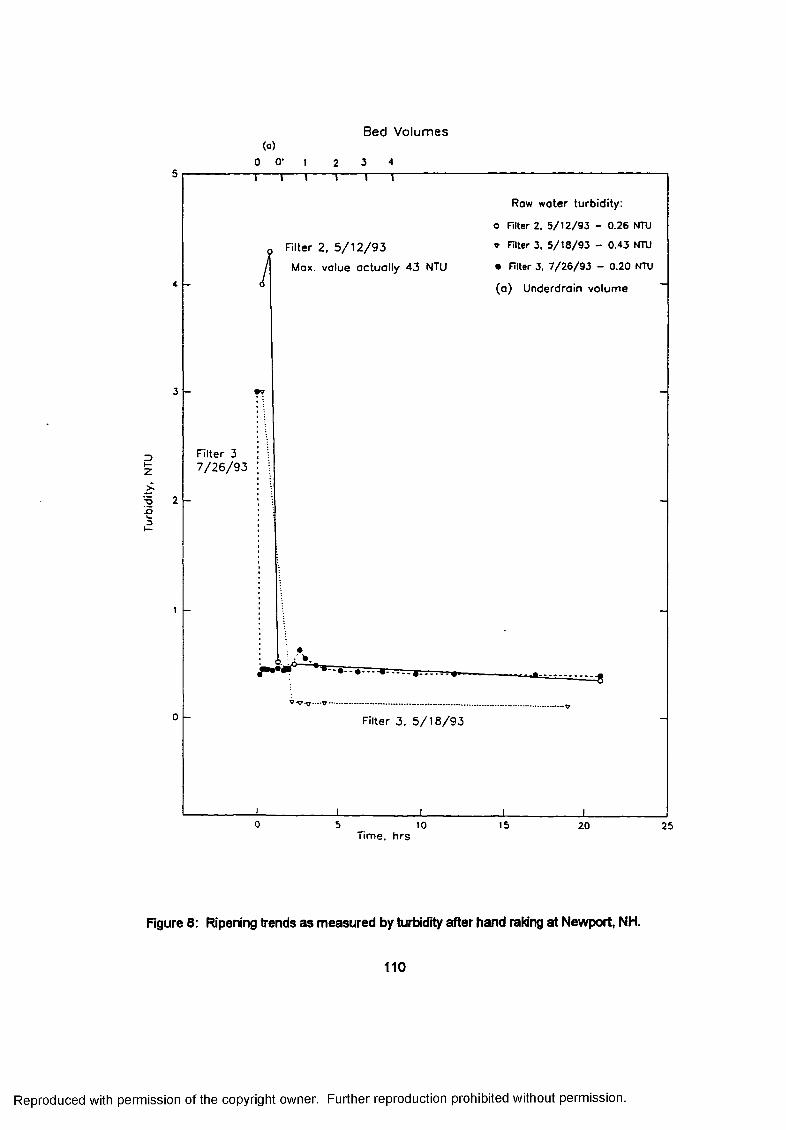
Turb
idity
, N
TUBed Volumes
(0)0 0 - 1 2 3 4
5
Raw water turbidity:
o Rlter 2. 5 /1 2 /9 3 - 0.26 NTU
* Filter 3, 5 /1 8 /9 3 - 0.43 NTU
• niter 3, 7 /2 6 /9 3 - 0.20 NTU
(a ) Underdrain volume
Filter 2, 5 / 1 2 / 9 3
Max. value actually 43 NTU4
3
Filter 3 7 / 2 6 / 9 3
2
l
0 Filter 3. 5 / 1 8 / 9 3
o 5 1510 20 25Time, hrs
Figure 8: Ripening trends as measured by turbidity after hand raking at Newport, NH.
110
Reproduced with permission of the copyright owner. Further reproduction prohibited without permission.
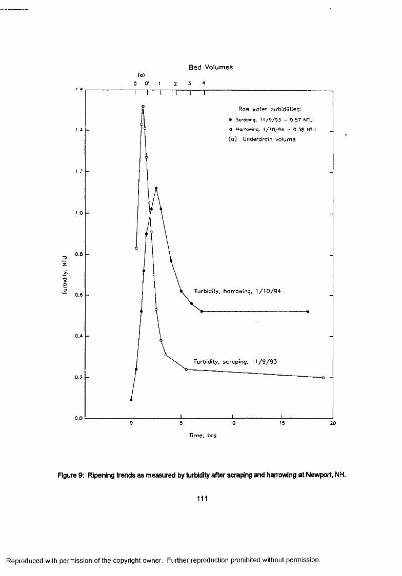
Turb
idity
, NT
UBed Volumes
(o)0 O’ 1 2 3 4
1----- 1----- 1------1----- 1--- 1-------------
Raw water turbidiities:
• Scroping. 11 /9 /9 3 - 0.57 NTU
o Harrowing, 1 /1 0 /9 4 - 0.38 MT'J
(a ) Underdrain volume
Turbidity, harrowing. 1 /1 0 /94 -
Turbidity. scraping, 1 1 /9 /9 3
0 5 10 15 20
Time, hrs
Figure 9: Ripening trends as measured by turbidity after scraping and harrowing at Newport, NH.
111
Reproduced with permission of the copyright owner. Further reproduction prohibited without permission.
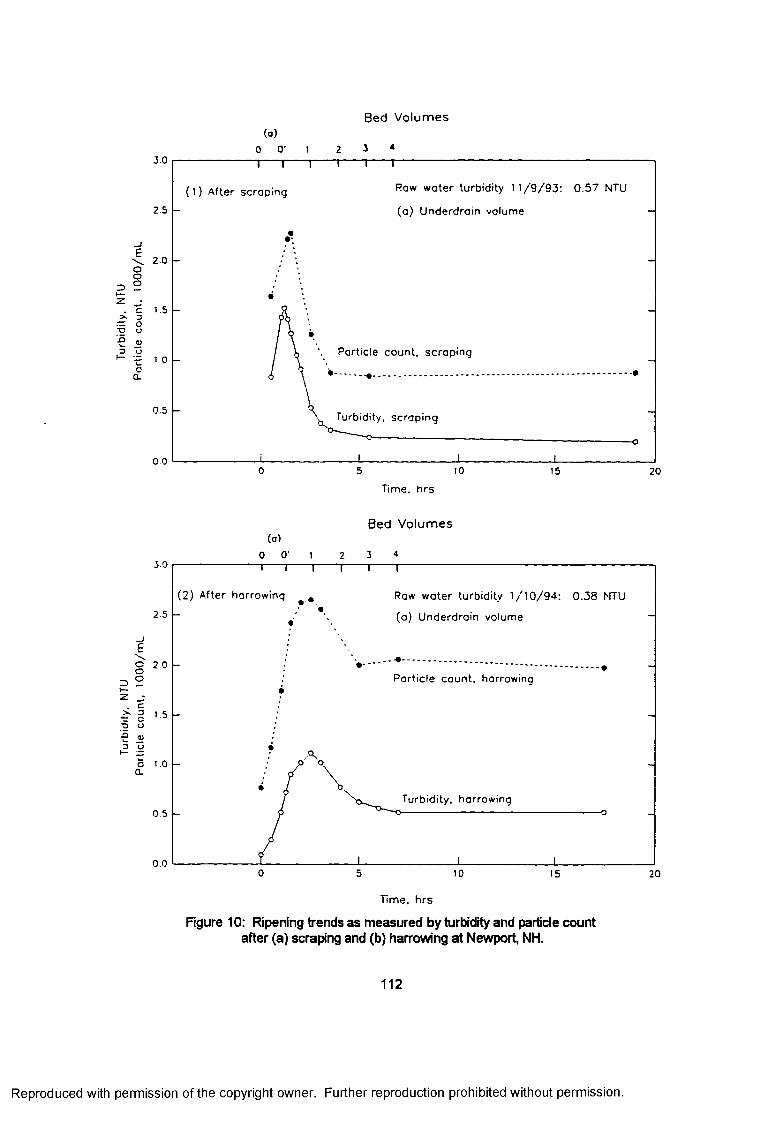
Turb
idity
, NT
U Tu
rbid
ity.
NTU
Pa
rticl
e co
unt,
1000
/mL
Part
icle
co
unt,
1000
/mL
Bed Volumes(a)
0 O' I 2 3 “3.0
Raw water turbidity 1 1 /9 /9 3 : 0 .5 7 NTU
(a ) Underdrain volume
(1 ) After scraping
2 5
2 0
Particle count, scraping
0.5 Turbidity, scraping
0.05 100 15 20
Time, hrs
Bed Volumes(a)
o O' 1 2 3 “3.0
(2 ) After harrowing Raw water turbidity 1 /1 0 /9 4 : 0 .3 8 NTU
(a ) Underdrain volume2.5
Particle count, harrowing
Turbidity, harrowing0.5 —o -
0.00 5 10 15 20
Time, hrs
Figure 10: Ripening trends as measured by turbidity and particle count after (a) scraping and (b) harrowing at Newport, NH.
112
Reproduced with permission of the copyright owner. Further reproduction prohibited without permission.
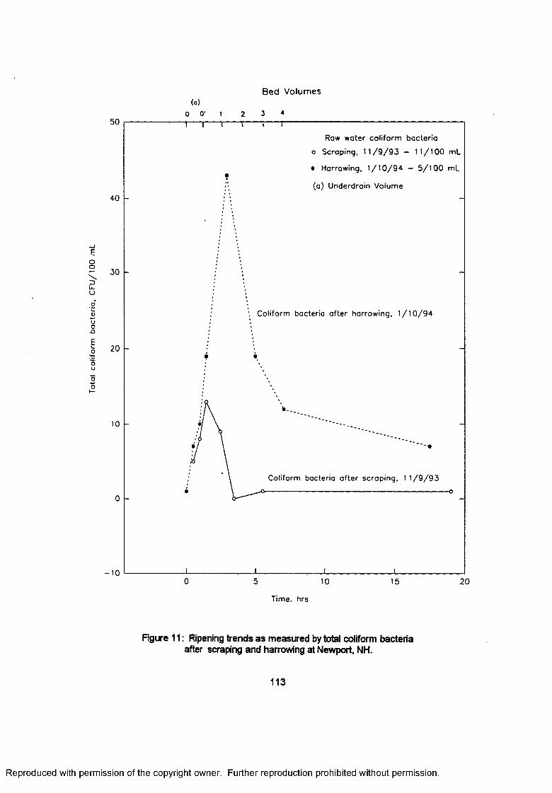
Tota
l co
lifor
m
bact
eria
, C
FU/1
00
mL
Bed Volumes(a)
o O' i 2 3 4......................... I ■ 'I — i— t ■ v r ............. - - - ■— ■ ---------- -
Raw water coliform bacteria
o Scraping, 1 1 / 9 / 9 3 — 1 1 /1 0 0 mL
• Harrowing, 1 / 1 0 / 9 4 — 5 /1 0 0 mL•
-
>• (a) Underdrain Volume
-
Coliform bacteria after harrowing. 1 /1 0 /9 4
t •
\ b'~ --— ij
i \
\ Coliform bacteria after scraping, 1 1 / 9 /9 3
• \ ^ --------------------------------------------------------------------------------o
i 1 . . . 1 _____________1 ............... .................0 5 10 15 20
Time, hrs
Figure 11: Ripening trends as measured by total coliform bacteria after scraping and harrowing at Newport, NH.
113
Reproduced with permission of the copyright owner. Further reproduction prohibited without permission.
the filter surfaces, the turbidity rapidly declined to normal filtered water concentrations. Ripening
trends for particles and coliform bacteria were not monitored following hand raking. This operation
disturbed the filter media to a depth of less than one centimeter and while an reverse flow was
mantained and little impact was expected.
Ripening trends after scraping and harrowing were more pronounced. Filtered water
turbidities had recovered after 8 hours following hand raking or harrowing and after five hours
following raking. Both turbidity and particle count were higher after harrowing than after scraping,
but this data represents only the ripening period following the first time these cleaning operations
were carried out on the filters. Total coliform removal recovered within about four hours after
hand rakingor scraping but coliforms were still present after 17.5 hours following the first time this
filter was harrowed.
4.3.5 Filter Media
Samples of the sand at different depths in the filters were taken immediately before the
filters were cleaned. These data are presented in Table 37 and represent the changes in the upper
30 cm (12 in) of the filter media during the first year of operation.
Media Sampling— The three cores taken from Filter 3 on May 18 and July 26 were separated by
depth, and the subsamples at the same level of the three cores composited before analysis. The
remaining filter sampling events were sampled and the subsamples at the separate depths of each
core analyzed separately.
Volatile Solids— The cores from each filter sampling event show significant differences in volatile
solids concentrations between cores at different locations within the filter but no significant
differences at the respective depths between the events of May 18, July 26, and November 10.
The cores taken January 9,1994 contained significantly less volatile solids at all levels in the sand
114
Reproduced with permission of the copyright owner. Further reproduction prohibited without permission.
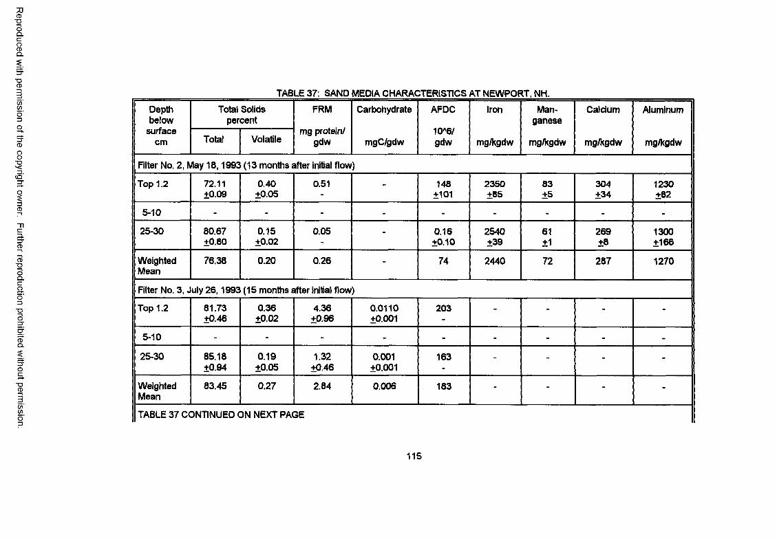
Reproduced
with perm
ission of the
copyright ow
ner. Further
reproduction prohibited
without
permission.
TABLE 37: SAND MEDIA CHARACTERISTICS AT NEWPORT. NH.
Depthbelow
Total Solids percent
FRM Carbohydrate AFDC Iron Manganese
Calcium Aluminum
surfacecm Total Volatile
mg protein/ gdw mgC/gdw
1 0 *6 /gdw mg/kgdw mg/kgdw mg/kgdw mg/kgdw
Filter No. 2, May 18,1993 (13 months after initial flow)
Top 1.2 72.11+0.09
0.40+0.05
0.51 - 148±101
2350±85
83±5
304±34
1230±82
5-10 - - - - - - - - -
25-30 80.67+0.80
0.15+0.02
0.05 - 0.16±0.10
2540±39
61±1
269±8
1300±166
WeightedMean
76.38 0.20 0.26 - 74 2440 72 287 1270
Filter No. 3, July 26,1993 (15 months after initial flow)
Top 1.2 81.73+0.46
0.36±0.02
4.36+0.96
0.0110+0.001
203 - - - -
5-10 - - - - - - - - -
25-30 85.18+0.94
0.19+0.05
1.32+0.46
0.001±0.001
163 - - - -
WeightedMean
83.45 0.27 2.84 0.006 183 - - - -
TABLE 37 CONTINUED ON NEXT PAGE
115
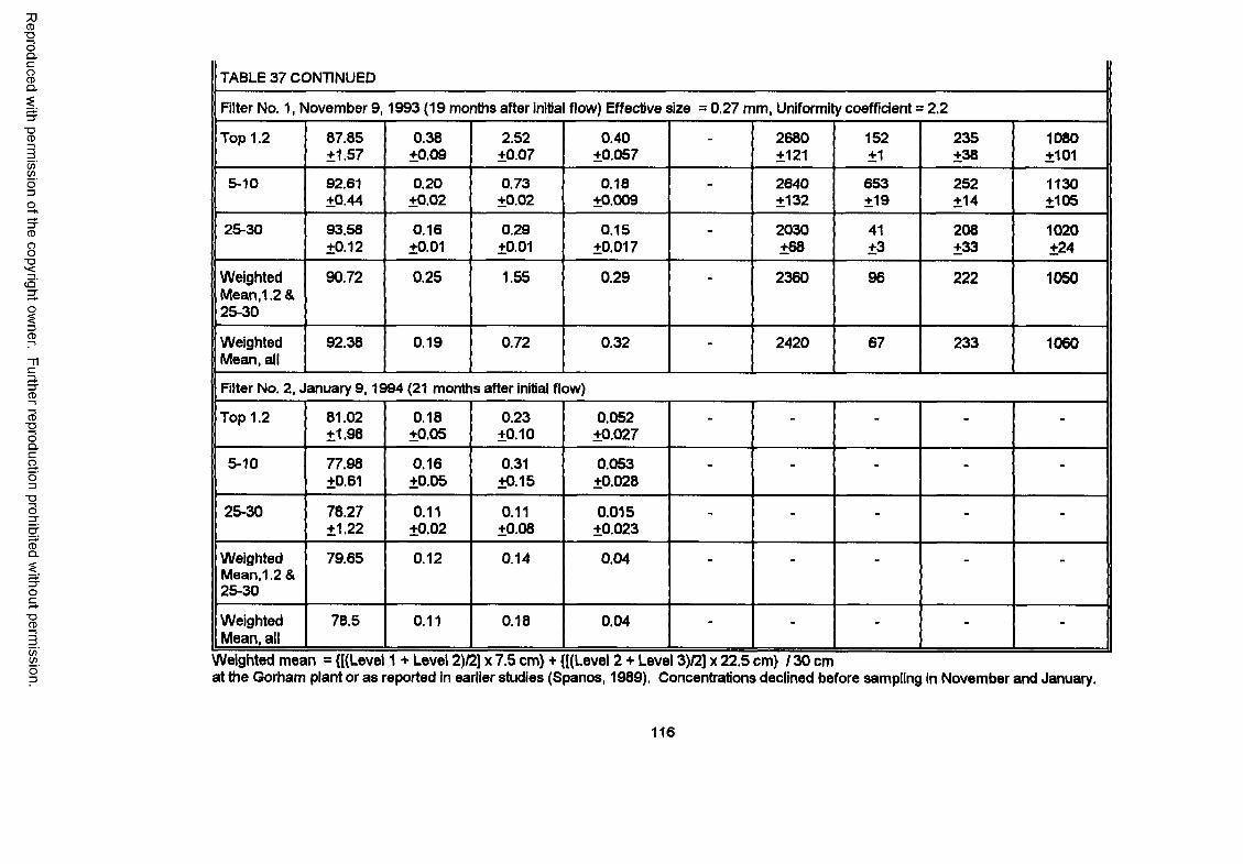
Reproduced
with perm
ission of the
copyright ow
ner. Further
reproduction prohibited
without
permission.
TABLE 37 CONTINUED
Filter No. 1, November 9,1993 (19 months after initial flow) Effective size = 0.27 mm, Uniformity coefficient == 2.2
Top 1.2 87.85±1.57
0.38±0.09
2.52±0.07
0.40±0.057
- 2680±121
152±1
235±38
1080±101
5-10 92.61±0.44
0.20±0.02
0.73±0.02
0.18±0.009
- 2640±132
653±19
252±14
1130±105
25-30 93.58±0.12
0.16±0.01
0.29±0.01
0.15±0.017
- 2030±68
41±3
208±33
1020±24
WeightedMean,1.2&25-30
90.72 0.25 1.55 0.29 - 2360 96 222 1050
Weighted Mean, all
92.38 0.19 0.72 0.32 - 2420 67 233 1060
Filter No. 2, January 9,1994 (21 months after initial flow)
Top 1.2 81.02±1.98
0.18±0.05
0.23±0.10
0.052±0.027
- - - - -
5-10 77.98±0.61
0.16±0.05
0.31±0.15
0.053±0.028
- - - - -
25-30 78.27±1.22
0.11±0.02
0.11±0.08
0.015±0.023
- - - - -
Weighted Mean,1.2 & 25-30
79.65 0.12 0.14 0.04 - - - - -
Weighted Mean, all
78.5 0.11 0.18 0.04 - - - - -
Weighted mean = {[(Level 1 + Level 2)12] x 7.5 cm} + {[(Level 2 + Level 3)/2] x 22.5 cm} 1 30 cmat the Gorham plant or as reported in earlier studies (Spanos, 1989). Concentrations declined before sampling in November and January.
116
filter than at the times of sampling in May, July, and November.
Folin Reactive Material— The proteinaceous material in the media samples varied considerably,
between cores, depths, and with season. The results of the analyses on the samples of May 18,
1993 and January 9,1994 were consistent with each other, but there were not sufficient replicates
of tiie May 18 analyses for statistical evaluation. Both sets of samples had been taken after
several months of treating water under winter conditions, but there is insufficient evidence to
confirm that cold weather operation was the cause of the lower concentrations. The FRM
concentrations in the top 1.2 cm (1/2 in) and in the middle of the harrowing depth at 5-10 cm (2-4
in) were significantly higher than in the lower level just below the harrowed depth, at 25-30 cm (10-
12 in), by a factor of over 4. The concentrations at the top and the mid-level were not significantly
different from each other, however.
The protein content of the samples of July 26 and November 9,1993, at all core locations
and depths are significantly higher than at the time of the other samples of sand collected from
"cold water" conditions. There were significant differences between the cores and between the
different depths of the November 9 sampling. The difference between depths was more
pronounced at the time of the November 9 sampling, by a factor of 12, than at the time of the July
sampling when the top 1.2 cm was 3.4 times higher in concentration than at the 25-30 cm level.
The FRM concentrations detected in the filters were increasing between May and July.
During this period, the filter surfaces were cleaning by hand raking, without scraping or harrowing,
in order to promote the development of interstital material which might consolidate the media so it
would bear the weight of mechanical cleaning equipment The development of such material was
indicated by the increasing FRM. The initial concentrations in May at a depth of 25-30 cm was
approximately one-tenth of the concentrations at the Gorham plant, yet they increased at both this
depth and at the surface to concentrations greater than been previously reported (Spanos, 1989;
117
Reproduced with permission of the copyright owner. Further reproduction prohibited without permission.
Eghmy etal. 1988).
Carbohydrates— Carbohydrate concentrations, like the FRM concentrations, differ between cores,
depths, and with time, but with less variation between them than with the FRM analyses. The
concentration at the 25-30 cm (10-12 in) level did decrease after the November 9 sample as had
the FRM concentration, but by only about one-third instead of the nearly 80 percent for FRM. The
carbohydrate concentration at the top 1.2 cm (1/2 in) decreased by 70 percent in the same period,
relative to the 90 percent reduction in FRM.
Acriflavine Direct Count (AFDC)— The only two sets of AFDC measurements were on the early
samples from May 18 and July 26,1993. The results indicated a bacteria count of 2 x 10* per
gram dry weight and about 0.6 x 10" per gram volatile solids in the top 1.2 cm. The results at the
25-30 cm depth were not consistent, with only 0.2 x 10⁶ in May and 2 x 10* in July, per gram dry
weight of solids, and 10* and 10" per gram volatile solids, respectively. The count per gram
volatile solids at the top for both dates, and at the bottom level for the July sample appear
consistent at about 0.6 to 1 x 10". The counts per gram FRM for the July sample are 5 x 10'° in
the top 1.2 cm and 10" at the 25-30 cm depth. The count per gram carbohydrate (as carbon)
were 2 x 10'3 at the top 1.2 cm and 1 x 10u at the 25-30 cm depth.
Metals— The concentrations of iron, calcium, and aluminum at the top 1.2 cm and the 25-30 cm
depth did not change substantially, but the manganese concentrations increased between May and
November in the top 1.2 cm (1 /2 in) but not at the depth of 25-30 cm (10-12 in).
4.3 NEWARK, NEW YORK
The Newark plant was visited from August 17 to November 16,1993 to record the costs of
cleaning with the scraping method and to monitor water quality. The cleaning and resanding
118
Reproduced with permission of the copyright owner. Further reproduction prohibited without permission.

operations at this plant, and the ripening periods after them, have also been studied by Letterman
(1985). The filters at this plant have only been cleaned by scraping. The cleaning schedule for
each of the filters over the past five years is summarized in Table 38.
TABLE 38: FILTER CLEANING SCHEDULE AT NEWARK, NY.Month Filter 1 Filer 2 Filer 3 Filer 4
Jan. 1981 1/23 - - -
Feb. - 2/26 ms -
Mar. 3/20 - - -
Apr. - - - 4/3
May 5/30 5/29 - -
June 6/27 - - -
July - 7/8 7/11 -
Aug. 8/8 8/20 - 8/22
Sept. - - - -
Oct 10/1 - - -
Nov. - 11/22 - -
Dec. Resanded, 12/3 - - -
Jan. 1992 - - Resanded. 1/6 -
Feb. - 2/14 - 2/6
Mar. - - - -
Apr. - 4/22 - -
May - - - 5/13
June 6/3 6/10 6/18 6/18
July 7/7 7/8 - -
Aug. - - - 8/4
Sept 9/2 - 9/3 -
Oct - - - -
Nov. - - - -
Dec. - 12/9 - -
Jan. 1963 1/19 - - 1/21
Feb. - - 2/19 -
TABLE 38 CONTINUED ON NEXT PAGE
119
Reproduced with permission of the copyright owner. Further reproduction prohibited without permission.
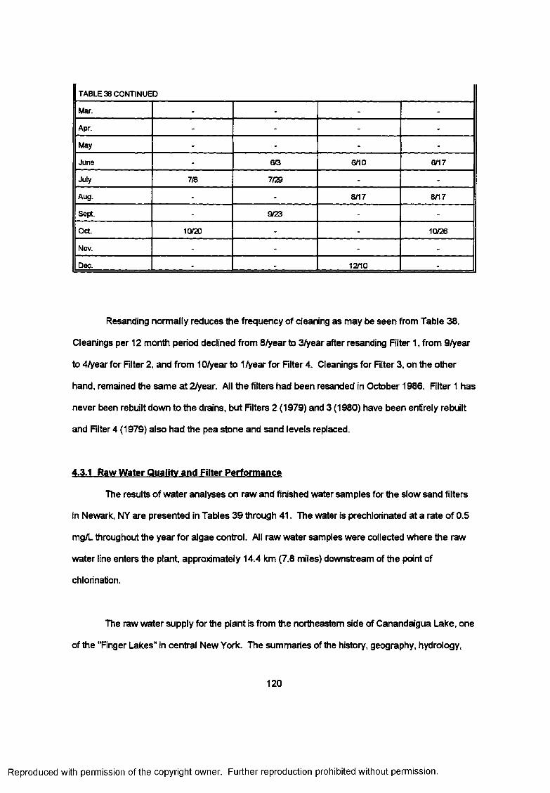
TABLE 38 CONTINUED
Mar. - - - -
Apr. - - - -
May - - - -
June - 6/3 6/10 6/17
July 7/8 7/29 - -
Aug. - - 8/17 8/17
Sept - 9/23 - -
Oct 10/20 - - 10/26
Nov. - - - -
Dec. - - 12/10 -
Resanding normally reduces the frequency of cleaning as may be seen from Table 38.
Cleanings per 12 month period declined from 8/year to 3/year after resanding Filter 1, from 9/year
to 4/year for Filter 2, and from 10/year to 1/year for Filter 4. Cleanings for Filter 3, on the other
hand, remained the same at 2/year. All the filters had been resanded in October 1986. Filter 1 has
never been rebuilt down to the drains, but Filters 2 (1979) and 3 (1980) have been entirely rebuilt
and Filter 4 (1979) also had the pea stone and sand levels replaced.
4.3.1 Raw Water Quality and Filter Performance
The results of water analyses on raw and finished water samples for the slow sand filters
in Newark, NY are presented in Tables 39 through 41. The water is prechlorinated at a rate of 0.5
mg/L throughout the year for algae control. All raw water samples were collected where the raw
water line enters the plant approximately 14.4 km (7.8 miles) downstream of the point of
chlorination.
The raw water supply for the plant is from the northeastern side of Canandaigua Lake, one
of the "Finger Lakes" in central New York. The summaries of the history, geography, hydrology,
120
Reproduced with permission of the copyright owner. Further reproduction prohibited without permission.
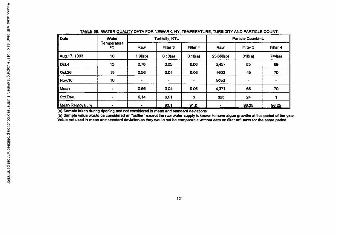
Reproduced
with perm
ission of the
copyright ow
ner. Further
reproduction prohibited
without
permission.
TABLE 39: WATER QUALITY DATA FOR NEWARK, NY, TEMPERATURE, TURBIDITY AND PARTICLE COUNT.
Date WaterTemperature
°C
Turbidity, NTU Particle Count/mL
Raw Filter 3 Filter 4 Raw Filter 3 Filter 4
Aug. 17,1993 10 1.90(b) 0.13(a) 0.16(a) 23.660(b) 318(a) 744(a)
Oct.4 13 0.76 0.05 0.06 3,457 83 69
Oct.26 15 0.56 0.04 0.06 4602 49 70
Nov. 16 10 - - - 5053 - -
Mean - 0.66 0.04 0.06 4,371 66 70
Std.Dev. - 0.14 0.01 0 823 24 1
Mean Removal, % - - 93.1 91.0 - 98.25 98.25a) Sample taken during ripening and not considered in mean and standard deviations.
(b) Sample value would be considered an "outlier" except the raw water supply is known to have algae growths at this period of the year. Value not used in mean and standard deviation as they would not be comparable without data on filter effluents for the same period.
121
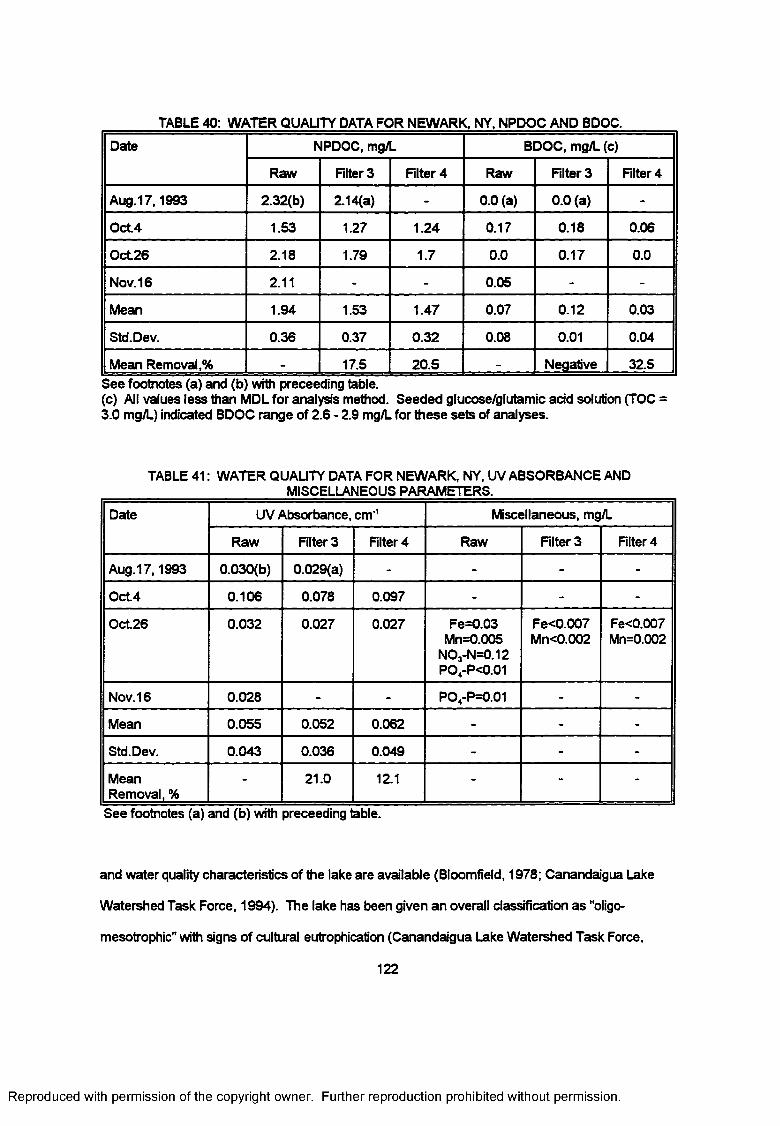
TABLE 40: WATER QUALITY DATA FOR NEWARK, NY, NPDOC AND BDOC.
Date NPDOC, mg/L BDOC, mg/L (c)
Raw Filter 3 Filter 4 Raw Filter 3 Filter 4
Aug.17,1993 2.32(b) 2.14(a) - 0.0 (a) 0.0 (a) -
Oct4 1.53 1.27 1.24 0.17 0.18 0.06
Oct26 2.18 1.79 1.7 0.0 0.17 0.0
Nov.16 2.11 - - 0.05 - -
Mean 1.94 1.53 1.47 0.07 0.12 0.03
Std.Dev. 0.36 0.37 0.32 0.08 0.01 0.04
Mean Removal,% - 17.5 20.5 - Negative 32.5See footnotes (a) and (b) with preceeding table.(c) All values less than MDL for analysis method. Seeded glucose/glutamic add solution (TOC = 3.0 mg/L) indicated BDOC range of 2.6 - 2.9 mg/L for these sets of analyses.
TABLE 41: WATER QUALITY DATA FOR NEWARK, NY, UV ABSORBANCE AND MISCELLANEOUS PARAMETERS.
Date UV Absorbance, cm'1 Miscellaneous, mg/L
Raw Filter 3 Filter 4 Raw Filter 3 Filter 4
Aug.17,1993 0.030(b) 0.029(a) - - - -
Oct4 0.106 0.078 0.097 - - -
Oct.26 0.032 0.027 0.027 Fe=0.03Mn=0.005
NOj-N=0.12PO4-P<0.01
Fe<0.007Mn<0.002
Fe<0.007Mn=0.002
Nov.16 0.028 - - PO4-P=0.01 - -
Mean 0.055 0.052 0.062 - - -
Std.Dev. 0.043 0.036 0.049 - - -
MeanRemoval, %
- 21.0 12.1 - - -
See footnotes (a) and (b) with preceeding table.
and water quality characteristics of the lake are available (Bloomfield, 1978; Canandaigua Lake
Watershed Task Force, 1994). The lake has been given an overall classification as "oligo-
mesotrophic" with signs of cultural eutrophication (Canandaigua Lake Watershed Task Force,
122
Reproduced with permission of the copyright owner. Further reproduction prohibited without permission.
1994). The water has a mean hardness of 128 mg/L with a mean alkalinity of 96 mg/L (both as
CaC03). The nutrient levels in the eplimnion vary seasonally due to algal activities, but those of
the hypolimnion stay relatively constant (Bloomfield, 1978). The nitrate-nitrogen and soluble
reactive phosphorus concentrations of raw water were reported as about 0.3 and 0.01 mg/L,
respectively. Analyses on the raw water sample of October 26,1993 indicated concentrations of
0.12 mg/L N 03-N and less than 0.01 mg/L P04-P. A second analysis showed 0.01 mg/L P04-P, on
the November 16,1993 raw water sample. The intake is at approximately 14 meters (46 ft) (Lozier,
1947) and is within the normal range of 10 to 15 meters for the thermocline.
The only parameter to test different between filters at 90 percent significance by the
Students t-test would have been on the BDOC data but the results were below the MDL of the test
and thus unreliable. It is concluded that there was no significant difference between the
performances of the two filters. The mass ratio of BDOC:NOs-N: P 04-P is 11:10:0.5 which is
sufficient to avoid nitrogen and phosphorus nutrient deficiency from these sources, and confirms
the observation that organic carbon substrate is the rate limiting nutrient (WEF, 1992).
4.3.2 Cleaning Procedures
The flow to a filter was halted the evening before cleaning so that the water
surface could fall to near the level of the sand surface by the next morning without wasting the
supernatant water. The next morning, the filtered water line was closed and the drain opened to
complete the drawdown to 2 to 3 cm (1 in) or more below the sand. The cleaning procedures
used during those visits are summarized below. Filters 3 and 4 were both cleaned on August 17,
1993 and Filter 4 was again cleaned on October 27.
The scraping operation was earned out with a crew of 4 persons using a small truck
refitted locally with a hydraulically operated, low-sided, dump body having a capacity of
approximately 0.8 cubic meter (1.1 cy). The crew proceeded in a line over a width of about 6
123
Reproduced with permission of the copyright owner. Further reproduction prohibited without permission.
meters (20 ft) down one long side of the filter with two men ahead and one on each side of the
truck. The crew removed the top 1 to 2 cm (1/2 to 3/4-in.) of the schmutzdecke/sand using long-
handled, aluminum, flat-blade shovels, and threw it into the dump body of the truck parked behind
them. As the crew advanced, the driver periodically left his shovel, moved the truck back up to the
edge of the area being scraped, and returned to his position scraping. The width of filter scraped
by each crew member varied with the rate of shovelling by each member and the need to keep the
line progressing in an even pattern around the truck, adjusting for the time lost by the driver. When
the truck was filled, at about every 6 meters (20-ft), the truck was driven out of the filter on a
concrete ramp built as part of the original plant design to dump the sand with sand saved from
previous cleanings on a paved area within 30 meters (100-ft) of the ramp. The truck then returned
to the scraping area and the crew resumed scraping. As the work reached the end of the filter, the
work line moved to the other side of the 12 meter wide filter and worked back toward the end
where they had started. When the scraping was finished, the tire marks and ridges left in the sand
were smoothed by dragging a piece of wire mesh fencing with the lawn tractor. The filter was
then refilled, first from the bottom with filtered water until it covers the sand, and then from the top
with raw water. No water was filtered to waste before the filter was returned to service. The
schedules for the cleaning operations monitored on the two occasions are outlined in Tables 42
and 43.
The volume of scraped sand was not measured due to the lack of a storage area at which
the sand could be measured separately from sand from previous cleaning operations. The
number of truck loads was also regarded as unsuitable due to non-uniform loads. The volume
was therefore estimated on the basis of the filter area and the depth to which the sand was to be
removed. No wastewater was generated except when draining the last foot of supernatant water
and the water within the filter media before scraping. The data on the cleaning operations for
each of the 504 sq. meter (5,420 sf) filters are summarized in Table 44.
124
Reproduced with permission of the copyright owner. Further reproduction prohibited without permission.
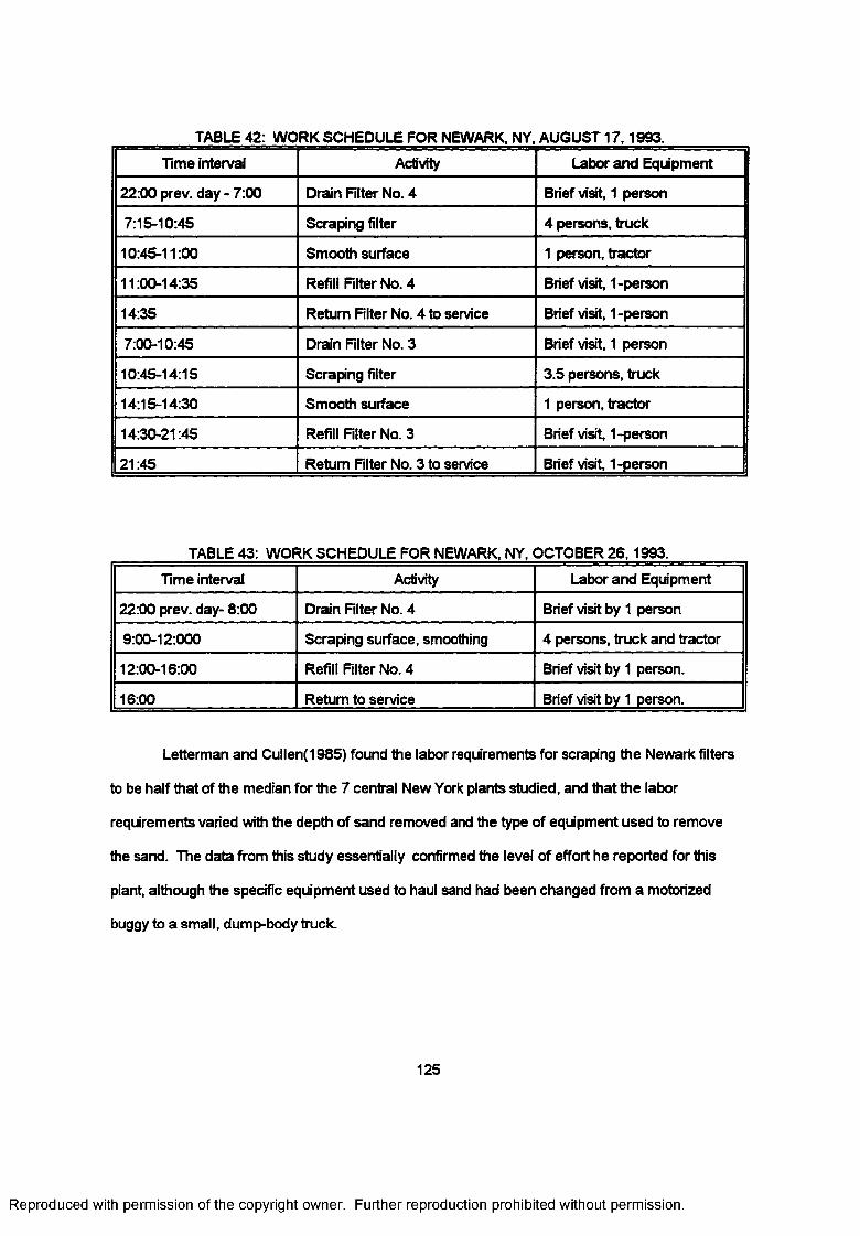
TABLE 42: WORK SCHEDULE FOR NEWARK. NY. AUGUST 1 7 .1993-
Time interval Activity Labor and Equipment
22:00 prev. day - 7:00 Drain Filter No. 4 Brief visit, 1 person
7:15-10:45 Scraping filter 4 persons, truck
10:45-11:00 Smooth surface 1 person, tractor
11:00-14:35 Refill Filter No. 4 Brief visit, 1-person
14:35 Return Filter No. 4 to sen/ice Brief visit, 1-person
7:00-10:45 Drain Filter No. 3 Brief visit, 1 person
10:45-14:15 Scraping filter 3.5 persons, truck
14:15-14:30 Smooth surface 1 person, tractor
14:30-21:45 Refill Filter No. 3 Brief visit, 1-person
21:45 Return Filter No. 3 to service Brief visit, 1-person
TABLE 43: WORK SCHEDULE FOR NEWARK, NY, OCTOBER 26.1993.
Time interval Activity Labor and Equipment
22:00 prev. day- 8:00 Drain Filter No. 4 Brief visit by 1 person
9:00-12:000 Scraping surface, smoothing 4 persons, truck and tractor
12:00-16:00 Refill Filter No. 4 Brief visit by 1 person.
16:00 Return to service Brief visit by 1 person.
Letterman and Cullen(1985) found the labor requirements for scraping the Newark filters
to be half that of the median for the 7 central New York plants studied, and that the labor
requirements varied with the depth of sand removed and the type of equipment used to remove
the sand. The data from this study essentially confirmed the level of effort he reported for this
plant, although the specific equipment used to haul sand had been changed from a motorized
buggy to a small, dump-body truck.
125
Reproduced with permission of the copyright owner. Further reproduction prohibited without permission.
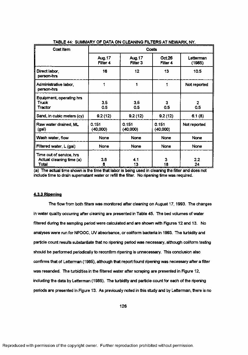
TABLE 44: SUMMARY OF DATA ON CLEANING FILTERS AT NEWARK, NY.
Cost Item Costs
Aug.17 Filter 4
Aug.17 Filter 3
Oct.26 Filter 4
Letterman(1985)
Direct labor, person-hrs
16 12 13 10.5
Administrative labor, person-hrs
1 1 1 Not reported
Equipment, operating hrsTruckTractor
3.50.5
3.50.5
30.5
20.5
Sand, in cubic meters (cy) 9.2 (12) 9.2 (12) 9.2 (12) 6.1 (8)
Raw water drained, ML (gal)
0.151(40,000)
0.151(40,000)
0.151(40,000)
Not reported
Wash water, flow None None None None
Filtered water, L (gal) None None None None
Time out of service, hrs Actual cleaning time (a) Total
3.88
4.113
318
2.224
a ) The actual time shown is the time that labor is being used in cleaning the filter and does not include time to drain supernatant water or refill the filter. No ripening time was required.
4.3.3 Ripening
The flow from both filters was monitored after cleaning on August 17,1993. The changes
in water quality occurring after cleaning are presented in Table 45. The bed volumes of water
filtered during the sampling period were calculated and are shown with Figures 12 and 13. No
analyses were run for NPDOC, UV absorbance, or coliform bacteria in 1993. The turbidity and
particle count results substantiate that no ripening period was necessary, although coliform testing
should be performed periodically to reconfirm ripening is unnecessary. This conclusion also
confirms that of Letterman (1985), although that report found ripening was necessary after a filter
was resanded. The turbidities in the filtered water after scraping are presented in Figure 12,
including the data by Letterman (1985). The turbidity and particle count for each of the ripening
periods are presented in Figure 13. As previously noted in this study and by Letterman, there is no
126
Reproduced with permission of the copyright owner. Further reproduction prohibited without permission.
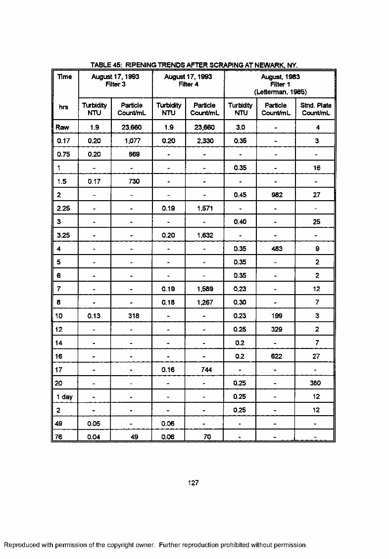
TABLE 45: RIPENING TRENDS AFTER SCRAPING AT NEWARK, NY.
Time August 17,1993 Filter 3
August 17,1993 Filter 4
August, 1983 Filter 1
(Letterman, 1985)
hrs TurbidityNTU
Particle Count/m L
TurbidityNTU
Particle Count/m L
TurbidityNTU
Particle Count/m L
Stnd. Plate Count/mL
Raw 1.9 23,660 1.9 23,660 3.0 - 4
0.17 0.20 1,077 0.20 2,330 0.35 - 3
0.75 0.20 869 - - - - -
1 - - - - 0.35 - 16
1.5 0.17 730 - - - - -
2 - - - - 0.45 982 27
2.25 - - 0.19 1,571 - - -
3 - - - - 0.40 - 25
3.25 - - 0.20 1,632 - - -
4 - - - - 0.35 483 9
5 - - - - 0.35 - 2
6 - - - - 0.35 - 2
7 - - 0.19 1,589 0.23 - 12
8 - - 0.18 1,267 0.30 - 7
10 0.13 318 - - 0.23 199 3
12 - - - - 0.25 329 2
14 - - - - 0.2 - 7
16 - - - - 0.2 622 27
17 - - 0.16 744 - - -
20 - - - - 0.25 - 380
1 day - - - - 0.25 - 12
2 - - - - 0.25 - 12
49 0.05 - 0.06 - - - -
76 0.04 49 0.06 70 - - -
127
Reproduced with permission of the copyright owner. Further reproduction prohibited without permission.
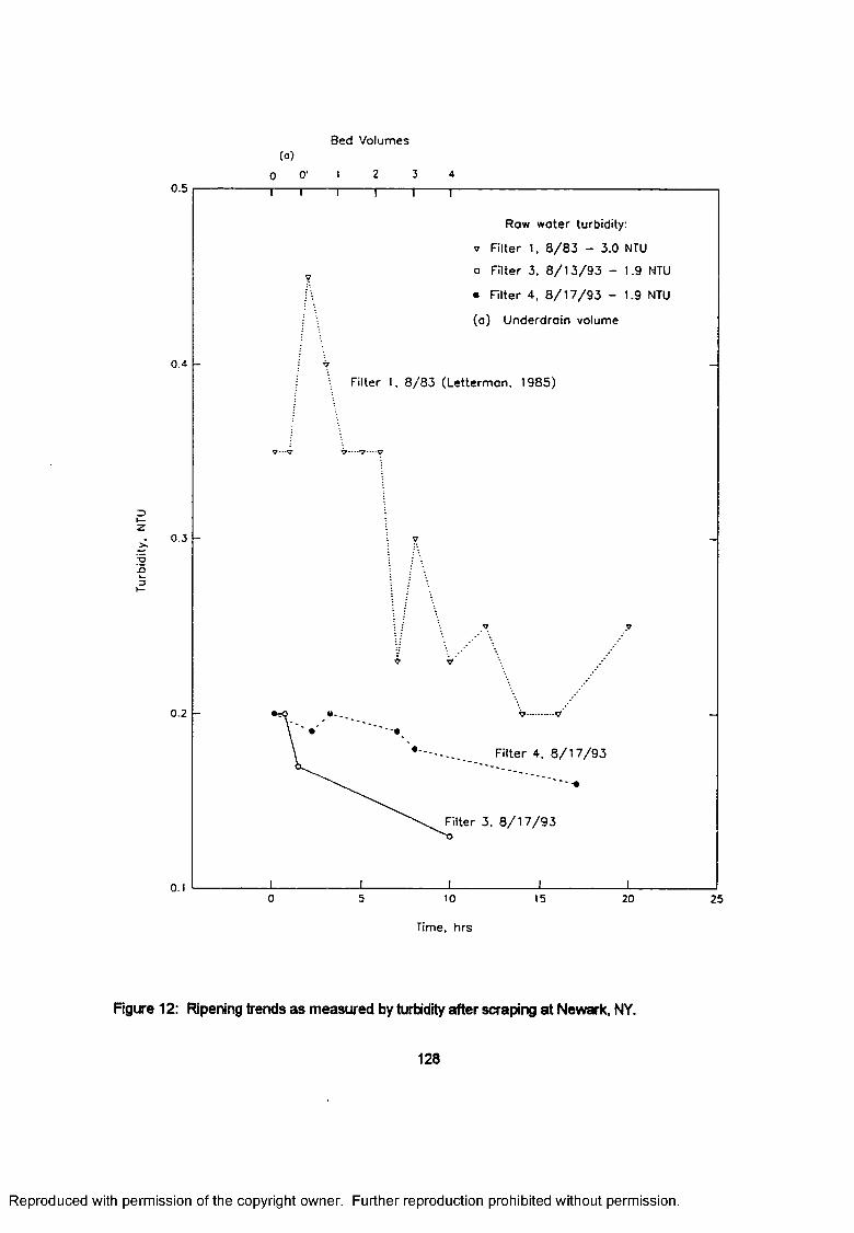
Turb
idity
, NT
U
0.5
Bed Volumes(° )
0 O’ l 2 3
t r
0.4
0.3
0.2
i i r
Raw water turbidity:
* Filter 1, 8 /8 3 - 3 .0 NTU
o Filter 3, 8 / 1 3 / 9 3 - 1.9 NTU
• Filter 4, 8 / 1 7 / 9 3 - 1.9 NTU
(a ) Underdrain volume
Filter 1, 8 /8 3 (Letterm an. 1985)
Filter 4. 8 / 1 7 / 9 3
Filter 3. 8 / 1 7 / 9 3
0.110
Time, hrs
15 20 25
Figure 12: Ripening trends as measured by turbidity after scraping at Newark, NY.
128
Reproduced with permission of the copyright owner. Further reproduction prohibited without permission.
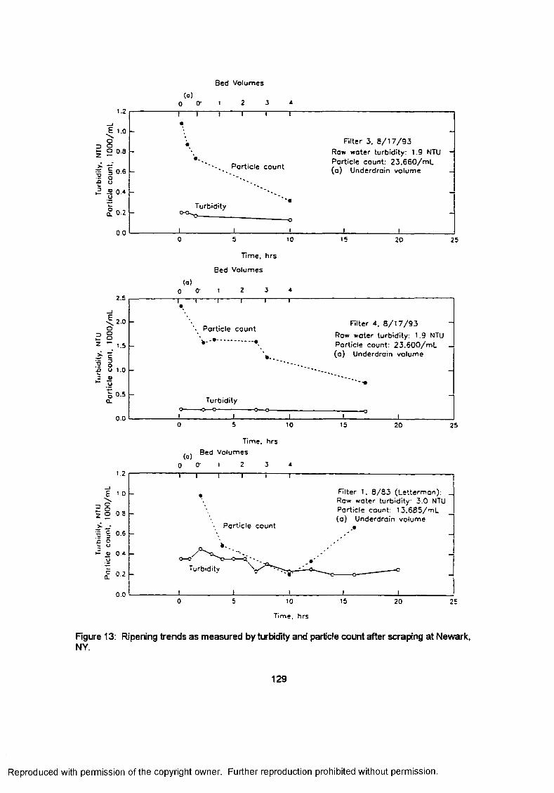
1.2
E 1.0 \ o
D O £ 2 08^ -r1 i 0-6•O u►2 ® o *u
a 0.2
0 0
2.S
< 2 0o
D °2 oz r . 152r c5 o .a u 1.0w3 a
, 0.5
0.0
(o)0 0‘ 1
1-----1-------- r
Bed Volumes
2 3 *
Particle count
Turbidity
_L-o
5 10
Time, hrs
Bed Volumes
(a)0 O' 1
10
(o )0 O'
Time, hrs Bed Volumes
i 2 3
Filter 3, 8 /1 7 /9 3 Raw water turbidity: 1.9 NTU Particle count: 2 3 .6 6 0 /m L (a) Underdrain volume
15 20 25
1 I I 1 I 1 •
-*• Particle count
R te r 4. 8 /1 7 /9 3\ Row water turbidity: 1.9 NTU
-..................... Particle count: 2 3 .6 0 0 /m l _
(a) Underdroin volume
Turbidity
i i i . . . 1 i15 20 25
E Filter 1. 8 /8 3 (Letterman): Row water turbidity- 3.0 NTU Particle count: 13 .685 /m L (a) Underdrain volume
co
Particle countcoueu
= 0.2a.
0.050 1510 20 25
Time, hrs
Figure 13: Ripening trends as measured by turbidity and particle count after scraping at Newark, NY.
129
Reproduced with permission of the copyright owner. Further reproduction prohibited without permission.
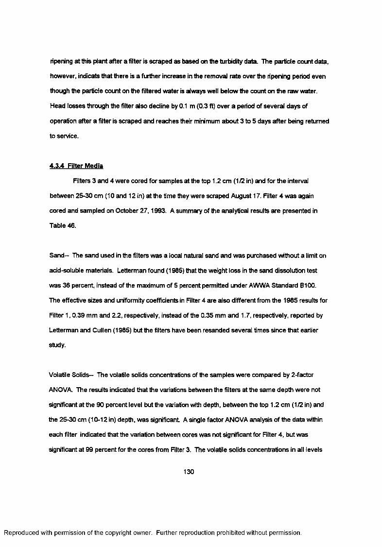
ripening at this plant after a filter is scraped as based on the turbidity data. The particle count data,
however, indicats that there is a further increase in the removal rate over the ripening period even
though the part'de count on the filtered water is always well below the count on the raw water.
Head losses through the filter also decline by 0.1 m (0.3 ft) over a period of several days of
operation after a filter is scraped and reaches their minimum about 3 to 5 days after being returned
to service.
4.3.4 Filter Media
Rlters 3 and 4 were cored for samples at the top 1.2 cm (1 /2 in) and for the interval
between 25-30 cm (10 and 12 in) at the time they were scraped August 17. Filter 4 was again
cored and sampled on Odober 27,1993. A summary of the analytical results are presented in
Table 46.
Sand— The sand used in the filters was a local natural sand and was purchased without a limit on
add-soluble materials. Letterman found (1985) that the weight loss in the sand dissolution test
was 36 percent, instead of the maximum of 5 percent permitted under AWWA Standard B100.
The effective sizes and uniformity coeffidents in Filter 4 are also different from the 1985 results for
Filter 1,0.39 mm and 2.2, respectively, instead of the 0.35 mm and 1.7, respectively, reported by
Letterman and Cullen (1985) but the filters have been resanded several times since that earlier
study.
Volatile Solids— The volatile solids concentrations of the samples were compared by 2-factor
ANOVA. The results indicated that the variations between the filters at the same depth were not
significant at the 90 percent level but the variation with depth, between the top 1.2 cm (1/2 in) and
the 25-30 cm (10-12 in) depth, was significant A single factor ANOVA analysis of the data within
each filter indicated that the variation between cores was not significant for Filter 4, but was
significant at 99 percent for the cores from Filter 3. The volatile solids concentrations in all levels
130
Reproduced with permission of the copyright owner. Further reproduction prohibited without permission.
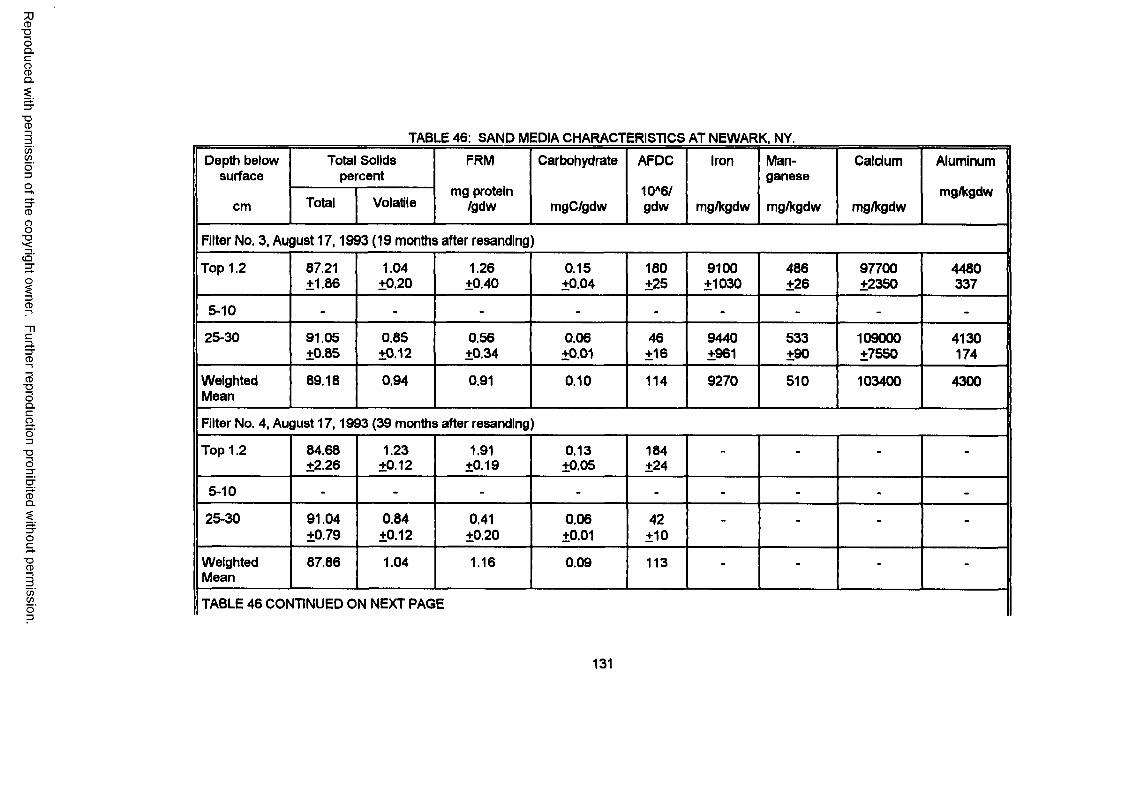
Reproduced
with perm
ission of the
copyright ow
ner. Further
reproduction prohibited
without
permission.
TABLE 46: SAND MEDIA CHARACTERISTICS AT NEWARK. NY.
Depth below surface
Total Solids percent
FRM Carbohydrate AFDC Iron Manganese
Calcium Aluminum
cm Total Volatilemg protein
/gdw mgC/gdw10*6/gdw mg/kgdw mg/kgdw mg/kgdw
mg/kgdw
Filter No. 3, August 17,1993 (19 months after resanding)
Top 1.2 87.21±1.86
1.04±0.20
1.26±0.40
0.15±0.04
180±25
9100±1030
486±26
97700±2350
4480337
5-10 - - - - - - - - -
25-30 91.05±0.85
0.85±0.12
0.56±0.34
0.06±0.01
46±16
9440±961
533±90
109000±7550
4130174
WeightedMean
89.18 0.94 0.91 0.10 114 9270 510 103400 4300
Filter No. 4, August 17,1993 (39 months after resanding
Top 1.2 84.68±2.26
1.23±0.12
1.91±0.19
0.13±0.05
184±24
- - - -
5-10 - - - - - - - - -
25-30 91.04±0.79
0.84±0.12
0.41±0.20
0.06±0.01
42±10
- - - -
WeightedMean
87.86 1.04 1.16 0.09 113 - - - -
TABLE 46 CONTINUED ON NEXT PAGE
131
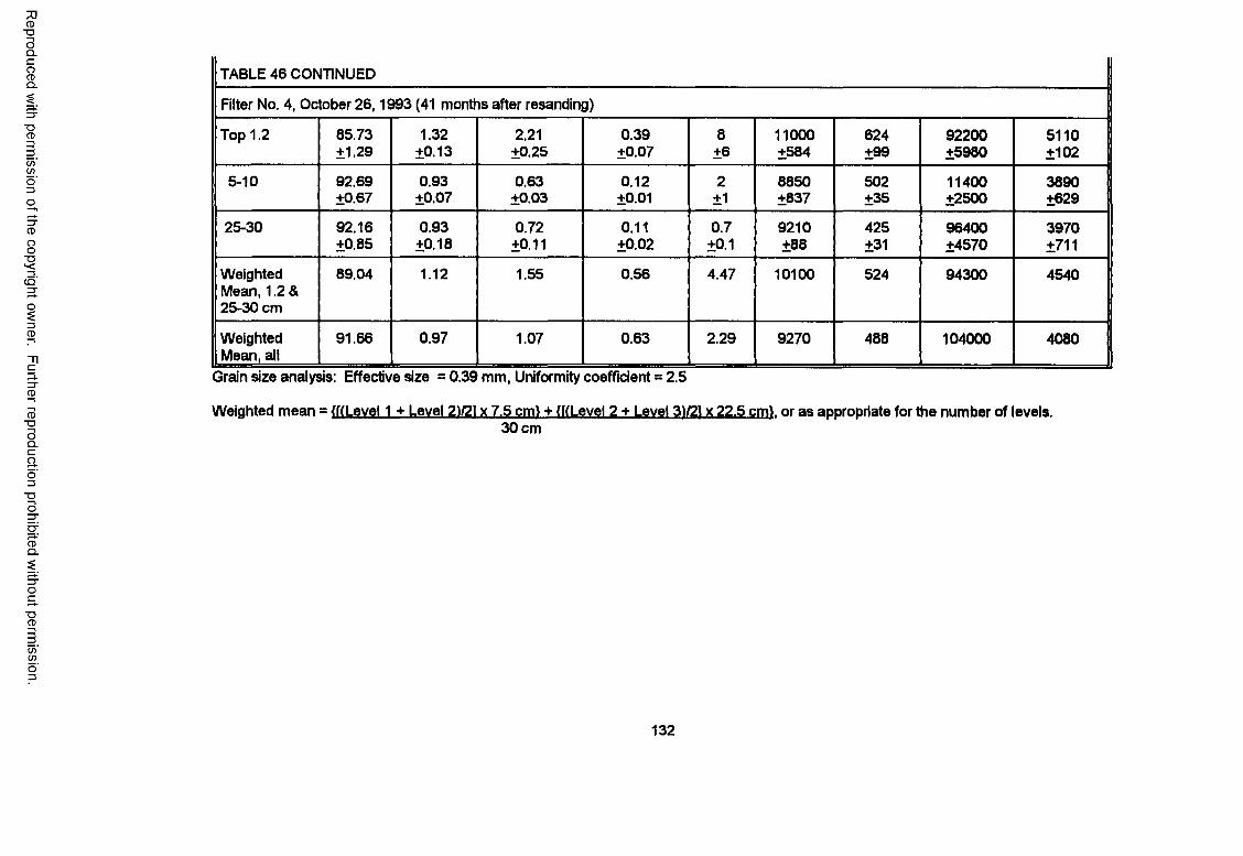
Reproduced
with perm
ission of the
copyright ow
ner. Further
reproduction prohibited
without
permission.
TABLE 46 CONTINUED
Filter No. 4, October 26,1993 (41 months after resandin 3)
Top 1.2 85.73±1.29
1.32±0.13
2.21±0.25
0.39±0.07
8±6
11000±584
624±99
92200±5980
5110±102
5-10 92.69±0.67
0.93±0.07
0.63±0.03
0.12±0.01
2±1
8850±837
502±35
11400±2500
3890±629
25-30 92.16±0.85
0.93±0.18
0.72±0.11
0.11±0.02
0.7±0.1
9210±88
425±31
96400±4570
3970±711
Weighted Mean, 1.2 & 25-30 cm
89.04 1.12 1.55 0.56 4.47 10100 524 94300 4540
Weighted Mean, all
91.66 0.97 1.07 0.63 2.29 9270 488 104000 4080
Grain size analysis: Effective size = 0.39 mm, Uniformity coefficient = 2.5
Weighted mean = fffLevel 1 + Level 21/21 x 7.5 cm) + ffdevel 2 + Level 31/21 x 22.5 cm}, or as appropriate for the number of levels.30 cm
132
of Core 3 from that filter were significantly lower than in Cores 1 and 2. The significant difference
between levels in the cores taken from Filter 4 on October 26 occurred between the top 1.2 cm
(1/2 in) and the 5-10 cm (2-4 in) depth and not between the 5-10 cm (2 to 4 in) and the 25-30 cm
(10 to 12 in) depth.
Folin Reactive Material (FRM)— Results for protein content were similar to that for volatile solids
concentration. The concentration differences were not significant on an overall basis between
filters or between cleaning dates but the variation between levels was significant whether based on
dry weight or volatile solids. Differences in FRM concentrations with depth were predominately in
the change between the top 1.2 cm (1/2 in) and the 5-10 cm (2 to 4 in) level and not between the
5-10 cm (2 to 4 in) and the 25-30 cm (10 to 12 in) levels. FRM concentration increased between
the 5-10 cm (2 to 4 in) level and the 25-30 cm (10 to 12 in) level rather than decreasing as had
volatile solids concentrations. The variation between filters was not significant Variations between
cores within each filter were not significant except in filter 3 where results for Core 2 were atypical,
rather than Core 3 which had been atypical for volatile solids concentrations. The concentration in
the Newark, NY filters were similar to the concentrations determined for the West Hartford, CT
filters by Spanos (1989).
Carbohydrates— The carbohydrates data indicated significant differences in concentrations
between filters and between depths within filters. The differences between filters occurred
between the August and October sampling events for Filter 4 and which indicated the
concentrations of carbohydrate at both top and bottom levels increased over the time period. The
difference between depths was significant in the data from all three samplings but the data from
the October 26 cleaning indicated the predominant change was between the top 1.2 cm (1/2 in)
and the 5-10 cm (2 to 4 in) level and not between the 5-10 cm (2 to 4 in) and the 25-30 cm (10 to
12 in) levels. This agrees with the results for volatile solids and FRM, as the schmutzdecke
material is included in the top 1.2 cm (1/2 in) of material. A comparison between the cores for the
133
Reproduced with permission of the copyright owner. Further reproduction prohibited without permission.
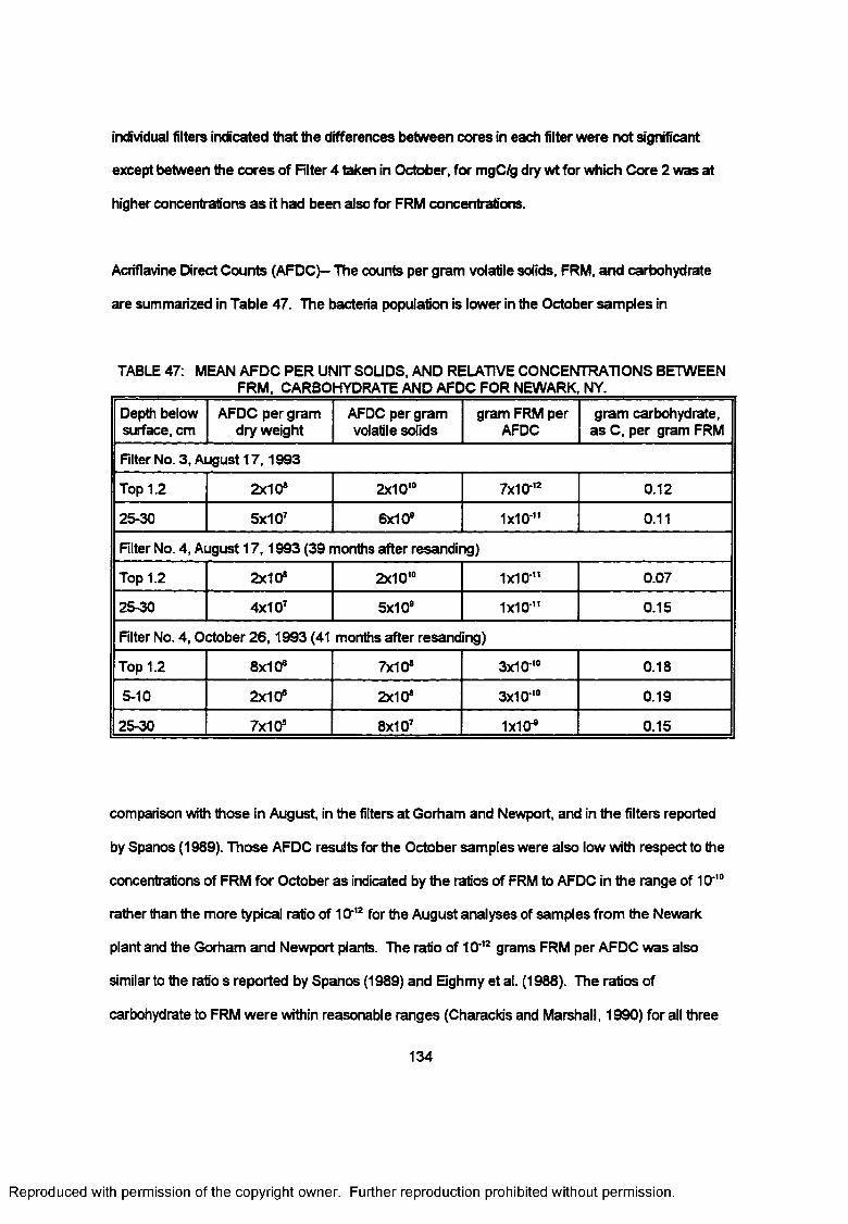
individual filters indicated that the differences between cores in each filter were not significant
except between the cores of Filter 4 taken in October, for mgC/g dry wt for which Core 2 was at
higher concentrations as it had been also for FRM concentrations.
Acriflavine Direct Counts (AFDC)— The counts per gram volatile solids, FRM, and carbohydrate
are summarized in Table 47. The bacteria population is lower in the October samples in
TABLE 47: MEAN AFDC PER UNIT SOUDS, AND RELATIVE CONCENTRATIONS BETWEEN ________________FRM, CARBOHYDRATE AND AFDC FOR NEWARK, NY._______________
Depth below surface, cm
AFDC per gram dry weight
AFDC per gram volatile solids
gram FRM per AFDC
gram carbohydrate, as C, per gram FRM
Filter No. 3, August 17,1993
Top 1.2 2x10* 2x10’° 7x1 O'2 0.12
25-30 5x10⁷ 6x10* 1x10-" 0.11
Filter No. 4, August 17,1993 (39 months after resanding)
Top 1.2 2x10* 2x10,n 1x1 O'" 0.07
25-30 4x10⁷ 5x10* 1x10" 0.15
Filter No. 4, October 26,1993 (41 months after resanding)
Top 1.2 8x10s 7x10* 3x1 O'10 0.18
5-10 2x10* 2x10* 3x10'10 0.19
25-30 7x10s 8x10⁷ 1x10* 0.15
comparison with those in August, in the filters at Gorham and Newport, and in the filters reported
by Spanos (1989). Those AFDC results for the October samples were also low with respect to the
concentrations of FRM for October as indicated by the ratios of FRM to AFDC in the range of 1010
rather than the more typical ratio of 10'12 for the August analyses of samples from the Newark
plant and the Gorham and Newport plants. The ratio of 10 ,z grams FRM per AFDC was also
similar to the ratio s reported by Spanos (1989) and Eghmy et al. (1988). The ratios of
carbohydrate to FRM were within reasonable ranges (Charackis and Marshall, 1990) for all three
134
Reproduced with permission of the copyright owner. Further reproduction prohibited without permission.
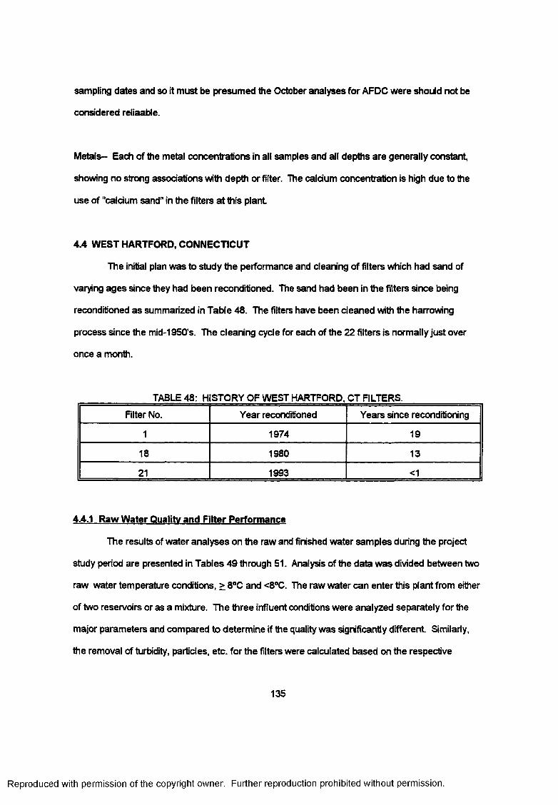
sampling dates and so it must be presumed the October analyses for AFDC were should not be
considered reliaable.
Metals- Each of the metal concentrations in all samples and all depths are generally constant,
showing no strong associations with depth or filter. The calcium concentration is high due to the
use of "calcium sand" in the filters at this plant
4.4 WEST HARTFORD, CONNECTICUT
The initial plan was to study the performance and cleaning of filters which had sand of
varying ages since they had been reconditioned. The sand had been in the filters since being
reconditioned as summarized in Table 48. The filters have been cleaned with the harrowing
process since the mid-1950’s. The cleaning cycle for each of the 22 filters is normally just over
once a month.
TABLE 48: H STORY OF WEST HARTFORD, CT FILTERS.
Filter No. Year reconditioned Years since reconditioning
1 1974 19
18 1980 13
21 1993 <1
4.4.1 Raw Water Quality and Filter Performance
The results of water analyses on the raw and finished water samples during the project
study period are presented in Tables 49 through 51. Analysis of the data was divided between two
raw water temperature conditions, > 8°C and <8°C. The raw water can enter this plant from either
of two reservoirs or as a mixture. The three influent conditions were analyzed separately for the
major parameters and compared to determine if the quality was significantly different Similarly,
the removal of turbidity, particles, etc. for the filters were calculated based on the respective
135
Reproduced with permission of the copyright owner. Further reproduction prohibited without permission.
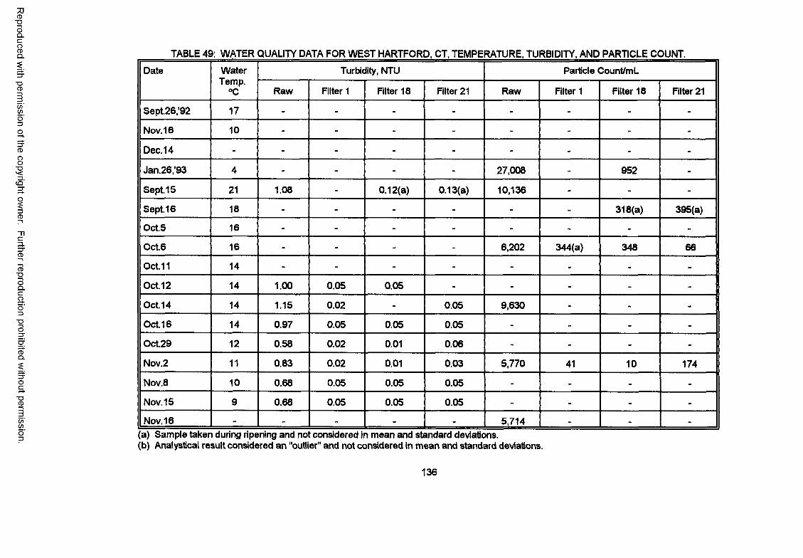
Reproduced
with perm
ission of the
copyright ow
ner. Further
reproduction prohibited
without
permission.
TABLE 49: WATER QUALITY DATA FOR WEST HARTFORD, CT, TEMPERATURE. TURBIDITY, AND PARTICLE COUNT.
Date WaterTemp.
°C
Turbidity, NTU Particle Count/mL
Raw Filter 1 Filter 18 Filter 21 Raw Filter 1 Filter 18 Filter 21
Sept.26/92 17 - - - - - - - -
Nov. 16 10 - - - - - - - -
Dec. 14 - - - - - - - - -
Jan.26/93 4 - - - - 27,008 - 952 -
Sept. 15 21 1.08 - 0.12(a) 0.13(a) 10,136 - - -
Sept. 16 18 - - - - - - 318(a) 395(a)
Oct.5 16 - - - - - - - -
Oct.6 16 - - - - 6,202 344(a) 348 66
Oct. 11 14 - - - - - - - -
Oct. 12 14 1.00 0.05 0.05 - - - - -
Oct. 14 14 1.15 0.02 - 0.05 9,630 - - -
Oct. 16 14 0.97 0.05 0.05 0.05 - - - -
Oct.29 12 0.58 0.02 0.01 0.06 - - - -
Nov.2 11 0.83 0.02 0.01 0.03 5,770 41 10 174
Nov.8 10 0.68 0.05 0.05 0.05 - - - -
Nov. 15 9 0.68 0.05 0.05 0.05 - - - -
Nov. 16 - - - - - 5,714 - - -
(a) Sample taken during ripening and not considered in mean and standard deviations.(b) Analystical result considered an "outlier" and not considered in mean and standard deviations.
136
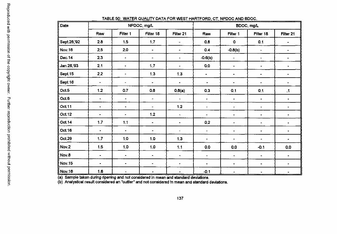
Reproduced
with perm
ission of the
copyright ow
ner. Further
reproduction prohibited
without
permission.
TABLE 50: WATER QUALITY DATA FOR WEST HARTFORD, CT. NPDOC AND BDOC.
Date NPDOC, mg/L BDOC, mg/L
Raw Filter 1 Filter 18 Filter 21 Raw Filter 1 Filter 18 Filter 21
Sept.26/92 2.8 1.5 1.7 - 0.8 0 0.1 -
Nov. 16 2.5 2.0 - - 0.4 -0.8(b) - -
Dec. 14 2.3 - - - -0.6(b) - - -
Jan.26/93 2.1 - 1.7 - 0.0 - - -
Sept. 15 2.2 - 1.3 1.3 - - - -
Sept. 16 - - - - - - - -
Oct.5 1.2 0.7 0.8 0.8(a) 0.3 0.1 0.1 .1
Oct.6 - - - - - - - -
Oct. 11 - - - 1.2 - - - -
Oct. 12 - - 1.2 - - - - -
Oct. 14 1.7 1.1 - - 0.2 - - -
Oct. 16 - - - - - - - -
Oct.29 1.7 1.0 1.0 1.3 - - - -
Nov.2 1.5 1.0 1.0 1.1 0.0 0.0 -0.1 0.0
Nov.8 - - - - - - - -
Nov. 15 - - - - - - - -
Nov. 16 1.6 - - - -0.1 - - -(a) Sample taken during ripening and not considered in mean and standard deviations.(b) Analystical result considered an "outlier" and not considered in mean and standard deviations.
137
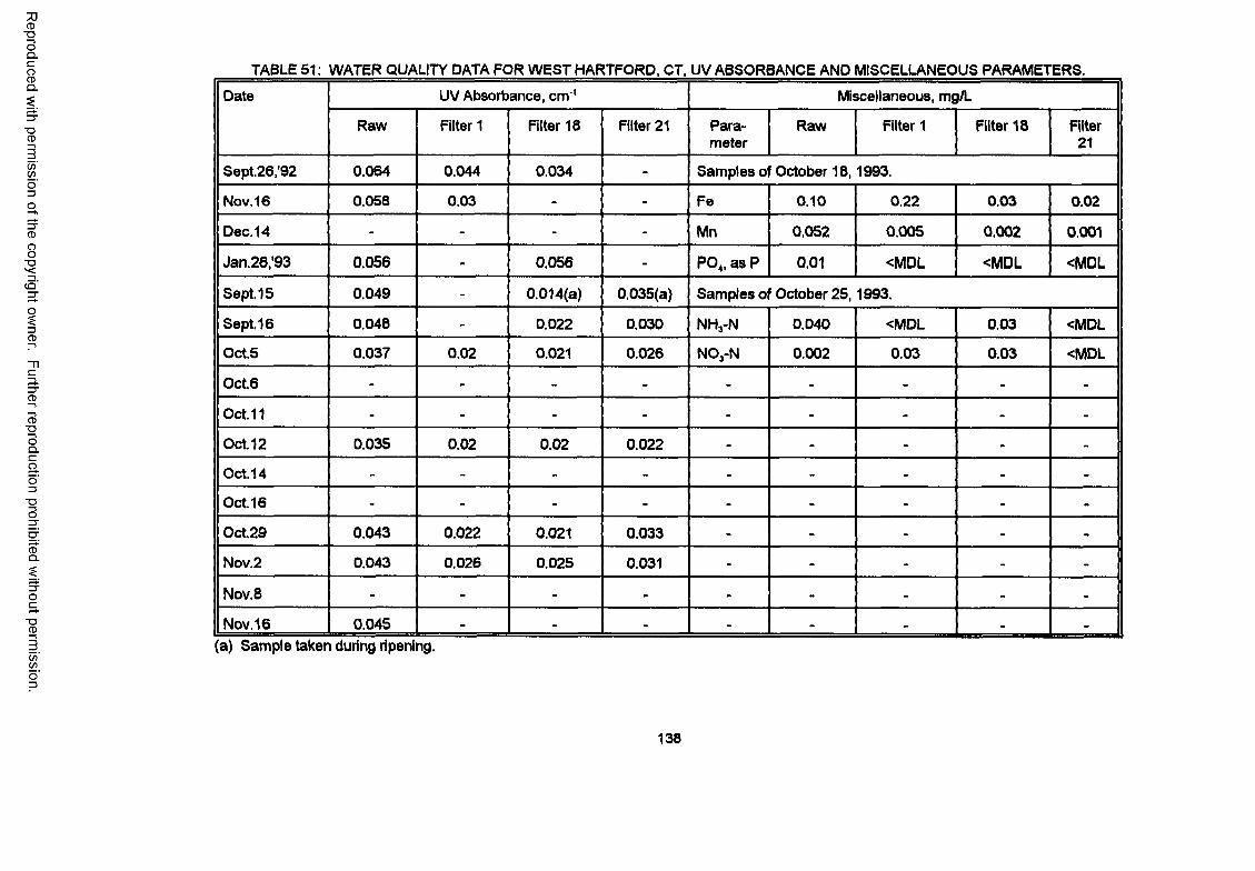
Reproduced
with perm
ission of the
copyright ow
ner. Further
reproduction prohibited
without
permission.
TABLE 51: WATER QUALITY DATA FOR WEST HARTFORD, CT. UV ABSORBANCE AND MISCELLANEOUS PARAMETERS.
Date UV Absorbance, cm ' Miscellaneous, m£I/L
Raw Filter 1 Filter 18 Filter 21 Parameter
Raw Filter 1 Filter 18 Filter21
Sept.26/92 0.064 0.044 0.034 - Samples of October 18,1993.
Nov. 16 0.058 0.03 - - Fe 0.10 0.22 0.03 0.02
Dec. 14 - - - - Mn 0.052 0,005 0.002 0.001
Jan.26/93 0.056 - 0.056 - P 04, as P 0.01 <MDL <MDL <MDL
Sept. 15 0.049 - 0.014(a) 0.035(a) Samples of October 25,1993.
Sept. 16 0.048 - 0.022 0.030 NHj-N 0.040 <MDL 0.03 <MDL
Oct.5 0.037 0.02 0.021 0.026 NOa-N 0.002 0.03 0.03 <MDL
Oct.6 - - - - - - - - -
Oct. 11 - - - - - - - - -
Oct. 12 0.035 0.02 0.02 0.022 - - - - -
Oct.14 - - - - - - - - -
Oct. 16 - - - - - - - - -
Oct.29 0.043 0.022 0.021 0.033 - - - - -
Nov.2 0.043 0.026 0.025 0.031 - - - - -
Nov.8 - - - - - - - - -
Nov. 16 0.045 - - - - - - - -(a) Sample taken during ripening.
138
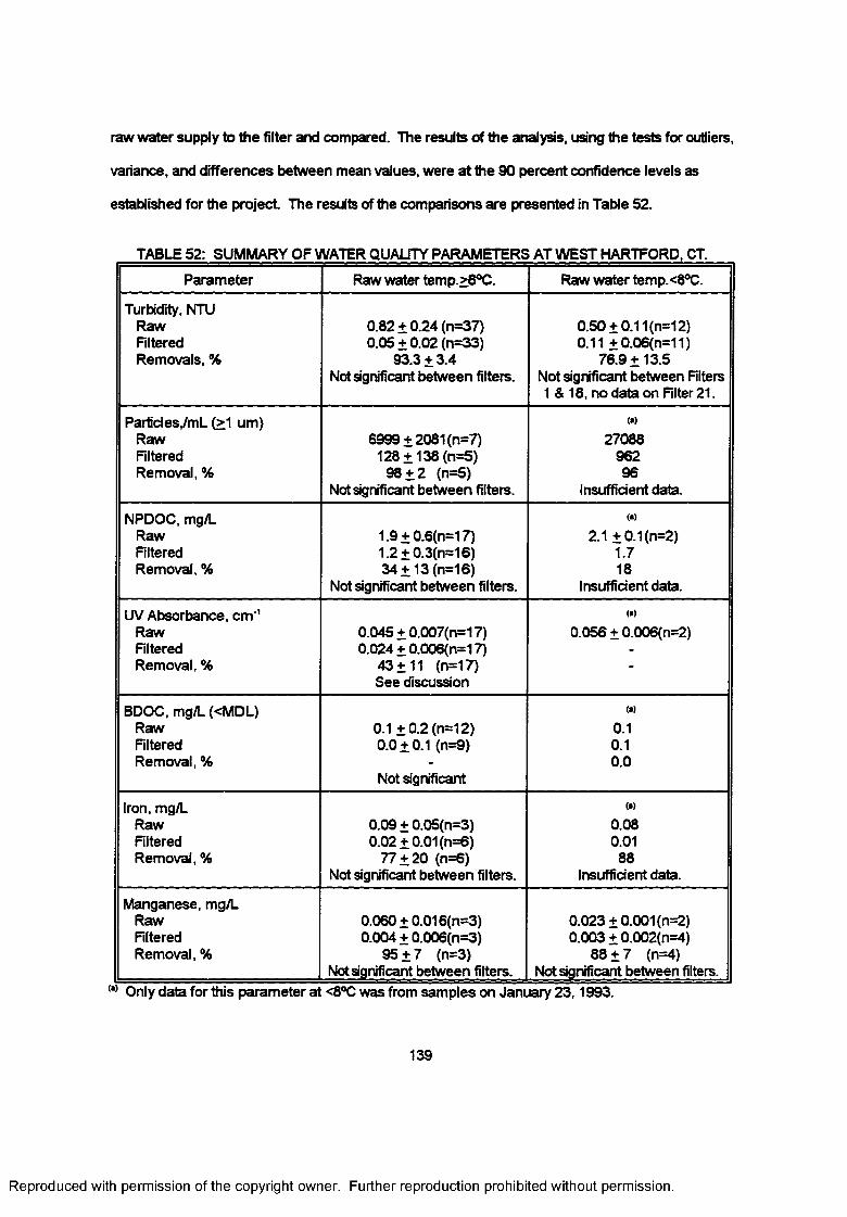
raw water supply to the filter and compared. The results of the analysis, using the tests for outliers,
variance, and differences between mean values, were at the 90 percent confidence levels as
established for the project The results of the comparisons are presented in Table 52.
TABLE 52: SUMMARY OF WATER QUALITY PARAMETERS AT WEST HARTFORD, CT.
Parameter Raw water temp.>8°C. Raw water temp.<8°C.
Turbidity, NTU Raw Filtered Removals, %
0.82 + 0.24 (n=37)0.05 + 0.02 (n=33)
93.3 + 3.4 Not significant between filters.
0.50 + 0.11(n=12)0.11 + 0.06(n=11)
76.9 + 13.5 Not significant between Filters 1 & 18, no data on Filter 21.
Part'des/mL (>1 um) Raw Filtered Removal, %
6999 + 2081 (n=7)128 +138 (n=5)
98 + 2 (n=5)Not significant between filters.
(»)27088
96296
Insufficient data.
NPDOC, mg/L Raw Filtered Removal, %
1.9 + 0.6(n=17)1.2 + 0.3(n=16)34 + 13 (n=16)
Not significant between filters.
w2.1 +0.1(n=2)
1.7 18
Insufficient data.
UV Absorbance, cm'1 Raw Filtered Removal, %
0.045 + 0.007(n=17) 0.024 + 0.006(n=17)
43 + 11 (n=17) See discussion
(*>0.056 + 0.006(n=2)
BDOC, mg/L (<MDL) Raw Filtered Removal, %
0.1 +0.2 (n=12) 0.0+ 0.1 (n=9)
Not significant
(a)0.10.10.0
Iron, mg/L Raw Filtered Removal, %
0.09 + 0.05(n=3)0.02 + 0.01 (n=6)
77 + 20 (n=6)Not significant between filters.
(a)
0.080.01
88Insufficient data.
Manganese, mg/L Raw Filtered Removal, %
0.060 + 0.016(n=3) 0.004 + 0.006(n=3)
95 + 7 (n=3)Not significant between filters.
0.023 + 0.001 (n=2) 0.003 + 0.002(n=4)
88 ± 7 (n=4)Not significant between filters.
(' ’ Only data for this parameter at <8°C was from samples on January 23,1993.
139
Reproduced with permission of the copyright owner. Further reproduction prohibited without permission.
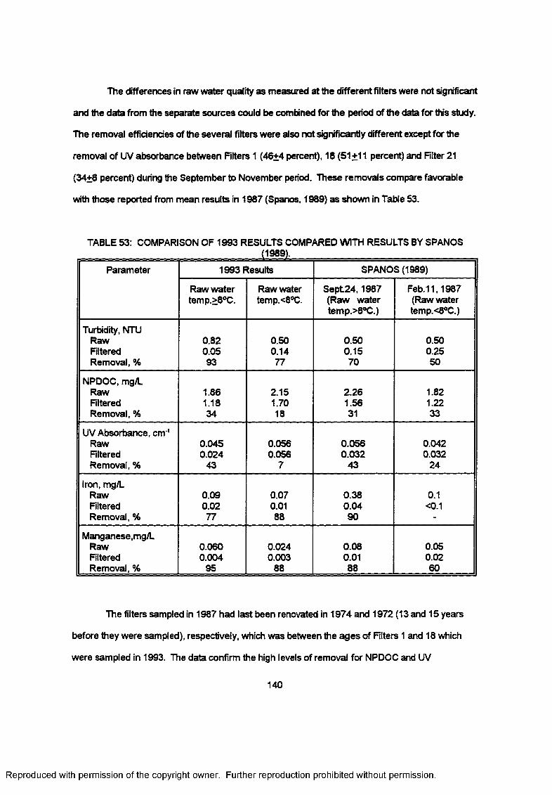
The differences in raw water quality as measured at the different filters were not significant
and the data from the separate sources could be combined for the period of the data for this study.
The removal efficiencies of the several filters were also not significantly different except for the
removal of UV absorbance between Filters 1 (46+4 percent), 18 (51+11 percent) and Filter 21
(34+8 percent) during the September to November period. These removals compare favorable
with those reported from mean results in 1987 (Spanos, 1989) as shown in Table 53.
TABLE 53: COMPARISON OF 1993 RESULTS COMPARED WITH RESULTS BY SPANOS(1989).
Parameter 1993 Results SPANOS (1989)
Raw water temp.>8°C.
Raw water temp.<8°C.
S ept24 ,1987 (Raw water temp.>8°C.)
Feb.11,1987 (Raw water temp.<8°C.)
Turbidity, NTURaw 0.82 0.50 0.50 0.50Filtered 0.05 0.14 0.15 0.25Removal, % 93 77 70 50
NPDOC, mg/LRaw 1.86 2.15 2.26 1.82Filtered 1.18 1.70 1.56 1.22Removal, % 34 18 31 33
UV Absorbance, cnr'Raw 0.045 0.056 0.056 0.042Filtered 0.024 0.056 0.032 0.032Removal, % 43 7 43 24
Iron, mg/LRaw 0.09 0.07 0.38 0.1Filtered 0.02 0.01 0.04 <0.1Removal, % 77 88 90 -
Manganese,mg/L Raw Filtered Removal, %
0.0600.004
95
0.0240.003
88
0.080.0188
0.050.0260
The filters sampled in 1987 had last been renovated in 1974 and 1972 (13 and 15 years
before they were sampled), respectively, which was between the ages of Filters 1 and 18 which
were sampled in 1993. The data confirm the high levels of removal for NPDOC and UV
140
Reproduced with permission of the copyright owner. Further reproduction prohibited without permission.
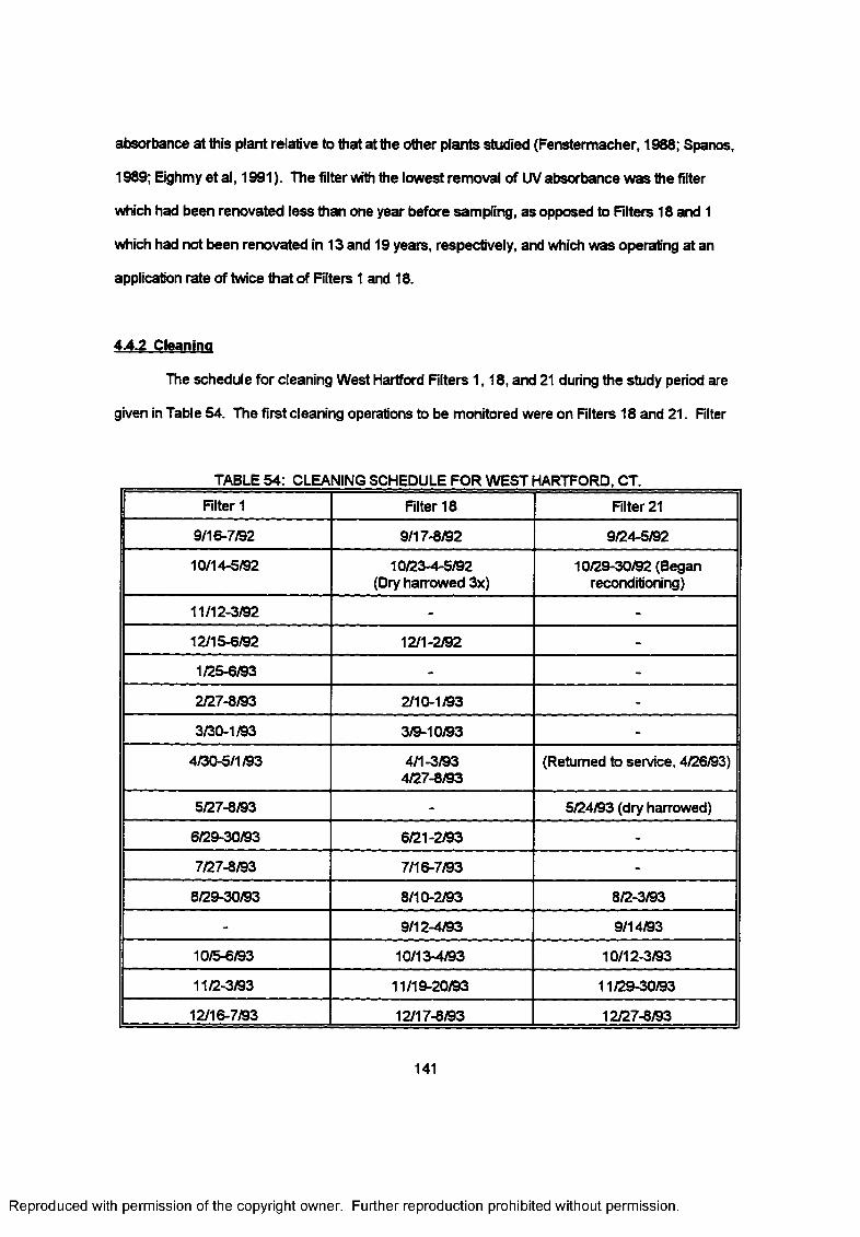
absorbance at this plant relative to that at the other plants studied (Fenstermacher, 1988; Spanos,
1989; Eighmy et al, 1991). The filter with the lowest removal of UV absorbance was the filter
which had been renovated less than one year before sampling, as opposed to Filters 18 and 1
which had not been renovated in 13 and 19 years, respectively, and which was operating at an
application rate of twice that of Filters 1 and 18.
4.4.2 Cleaning
The schedule for cleaning West Hartford Filters 1,18, and 21 during the study period are
given in Table 54. The first cleaning operations to be monitored were on Filters 18 and 21. Filter
TABLE 54: CLEANING SCHEDULE FOR WEST HARTFORD, CT.
Filter 1 Filter 18 Filter 21
9/16-7/92 9/17-8/92 9/24-5/92
10/14-5/92 10/23-4-5/92 10/29-30/92 (Began(Dry harrowed 3x) reconditioning)
11/12-3/92 - -
12/15-6/92 12/1-2/92 -
1/25-6/93 - -
2/27-8/93 2/10-1/93 -
3/30-1/93 3/9-10/93 -
4/30-5/1/93 4/1-3/934/27-8/93
(Returned to service, 4/26/93)
5/27-8/93 - 5/24/93 (dry harrowed)
6/29-30/93 6/21-2/93 -
7/27-8/93 7/16-7/93 -
8/29-30/93 8/10-2/93 8/2-3/93
- 9/12-4/93 9/14/93
10/5-6/93 10/13-4/93 10/12-3/93
11/2-3/93 11/19-20/93 11/29-30/93
12/16-7/93 12/17-8/93 12/27-8/93
141
Reproduced with permission of the copyright owner. Further reproduction prohibited without permission.
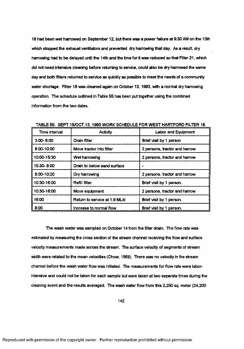
18 had been wet harrowed on September 12, but there was a power failure at 9:30 AM on the 13th
which stopped the exhaust ventilators and prevented dry harrowing that day. As a result, dry
harrowing had to be delayed until the 14th and the time for it was reduced so that Filter 21, which
did not need intensive cleaning before returning to service, could also be dry harrowed the same
day and both filters returned to service as quickly as possible to meet the needs of a community
water shortage. Filter 18 was cleaned again on October 13,1993, with a normal dry harrowing
operation. The schedule outlined in Table 55 has been put together using the combined
information from the two dates.
TABLE 55: SEPT 15/OCT.13,1993 WORK SCHEDULE FOR WEST HARTFORD FILTER 18.
Time interval Activity Labor and Equipment
3:00-8:00 Drain filter Brief visit by 1 person
8:00-10:00 Move tractor into filter 2 persons, tractor and harrow
10:00-15:30 Wet harrowing 2 persons, tractor and harrow
15:30-8:00 Drain to below sand surface -
8:00-10:20 Dry harrowing 2 persons, tractor and harrow
10:30-16:00 Refill filter Brief visit by 1 person.
10:30-16:00 Move equipment 2 persons, tractor and harrow
16:00 Return to service at 1.9 ML/d Brief visit by 1 person.
8:00 Increase to normal flow Brief visit by 1 person.
The wash water was sampled on October 14 from the filter drain. The flow rate was
estimated by measuring the cross section of the stream channel receiving the flow and surface
velocity measurements made across the stream. The surface velocity of segments of stream
width were related to the mean velocities (Chow, 1959). There was no velocity in the stream
channel before the wash water flow was initiated. The measurements for flow rate were labor-
intensive and could not be taken for each sample but were taken at two separate times during the
cleaning event and the results averaged. The wash water flow from this 2,250 sq. meter (24,200
142
Reproduced with permission of the copyright owner. Further reproduction prohibited without permission.
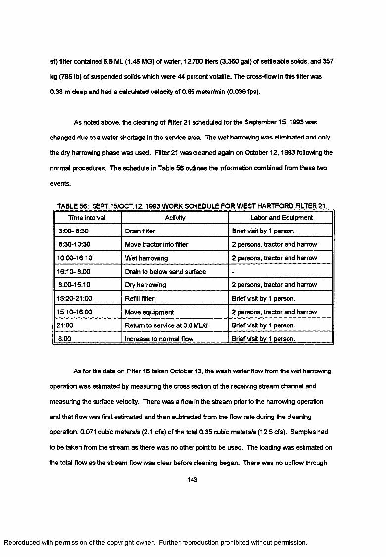
sf) filter contained 5.5 ML (1.45 MG) of water, 12,700 liters (3,360 gal) of settleable solids, and 357
kg (785 lb) of suspended solids which were 44 percent volatile. The cross-flow in this filter was
0.38 m deep and had a calculated velocity of 0.65 meter/min (0.036 fps).
As noted above, the cleaning of Filter 21 scheduled for the September 15,1993 was
changed due to a water shortage in the service area. The wet harrowing was eliminated and only
the dry harrowing phase was used. Filter 21 was cleaned again on October 12,1993 following the
normal procedures. The schedule in Table 56 outlines the information combined from these two
events.
TABLE 56: SEPT. 15/OCT.12,1993 WORK SCHEDULE FOR WEST HARTFORD FILTER 21.
Time interval Activity Labor and Eqiipment
3:00- 8:30 Drain filter Brief visit by 1 person
8:30-10:30 Move tractor into filter 2 persons, tractor and harrow
10:00-16:10 Wet harrowing 2 persons, tractor and harrow
16:10-8:00 Drain to below sand surface -
8:00-15:10 Dry harrowing 2 persons, tractor and harrow
15:20-21:00 Refill filter Brief visit by 1 person.
15:10-16:00 Move equipment 2 persons, tractor and harrow
21:00 Return to service at 3.8 ML/d Brief visit by 1 person.
8:00 Increase to normal flow Brief visit by 1 person.
As for the data on Filter 18 taken October 13, the wash water flow from the wet harrowing
operation was estimated by measuring the cross section of the receiving stream channel and
measuring the surface velocity. There was a flow in the stream prior to the harrowing operation
and that flow was first estimated and then subtracted from the flow rate during the cleaning
operation, 0.071 cubic meters/s (2.1 cfs) of the total 0.35 cubic meters/s (12.5 cfs). Samples had
to be taken from the stream as there was no other point to be used. The loading was estimated on
the total flow as the stream flow was clear before cleaning began. There was no upflow through
143
Reproduced with permission of the copyright owner. Further reproduction prohibited without permission.
the filter during the wet harrowing operation according to the flow meter. The total wash water
load from the six hours of wet harrowing was calculated to be 6.5 ML (1.7 MG) water containing
26,800 liters (7,080 gal) of settleable solids and 612 kg (1,346 pounds) of suspended solids which
were 34 percent volatile. The cross-flow velocity was calculated to be 0.62 meters/min. (0.034
fps) and was about 0.38 m (15 in) deep.
Filter 1 was cleaned October 5,1993 following a schedule similar to those for filters 18
and 21. The wash water produced during the wet harrowing operation was sampled. The flow
was estimated by measuring the cross section area of the flow in the drain channel in the filter
building and its surface velocity as described earlier. Unlike the arrangements for introducing the
wash water during wet harrowing Filters 18 and 21, Filter 1 is an older filter which does not have
flow channels along the long sides for inlet and outlet of the cross-flow. Instead, raw water must
be introduced from the inlet comer of the filter to a depth of about 0.3 m (1 ft), the flow turned off,
and the drain located in the same comer is opened to draw the water back with the resuspended
materials produced while the tractor harrows. This operation results in a continuing variation in the
rate of wash water flow and characteristics. The cross-flow velocity varied from zero to about 1
m/min (3 fps) across the area of the filter and over the time to drain off the surface.
The calculated total wash water load was 0.33 ML (87,000 gal) containing 5,200 liters
(1,380 gal) of settleable solids and 120 kg (260 lb) of suspended solids which were 37 percent
volatile. Filter 1 was again cleaned on 11/2/93 after cores had been collected but the wash water
flow was not monitored. The load and its flow pattern are presented in Table 57. The information
collected on the cleaning operations for the filters is presented in Table 58.
4.4.3 Ripening
The filtered water from the filters was monitored after several of the cleaning events to
determine the rates at which the removal performance recovered. The results of these analyses
144
Reproduced with permission of the copyright owner. Further reproduction prohibited without permission.
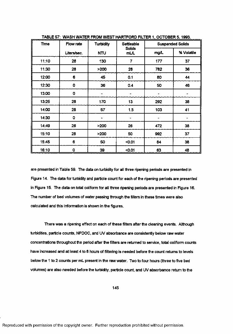
TABLE 57: WASH WATER FROM WEST HARTFORD FILTER 1, OCTOBER 5,1993.
Time Flow rate Turbidity SettleableSolidsmL/L
Suspended Solids
Liters/sec. NTU mg/L % Volatile
11:10 28 130 7 177 37
11:30 28 >200 28 782 36
12:00 6 45 0.1 80 44
12:30 0 36 0.4 50 46
13:00 0 - - - -
13:25 28 170 13 292 38
14:00 28 57 1.5 103 41
14:30 0 - - - -
14:49 26 >200 26 472 38
15:10 28 >200 50 992 37
15:45 6 50 <0.01 84 38
16:10 0 39 <0.01 63 48
are presented in Table 59. The data on turbidity for all three ripening periods are presented in
Figure 14. The data for turbidity and particle count for each of the ripening periods are presented
in Figure 15. The data on total coliform for all three ripening periods are presented in Figure 16.
The number of bed volumes of water passing through the filters in these times were also
calculated and this information is shown in the figures.
There was a ripening effect on each of these filters after the cleaning events. Although
turbidities, particle counts, NPDOC, and UV absorbance are consistently below raw water
concentrations throughout the period after the filters are returned to service, total coliform counts
have increased and at least 4 to 8 hours of filtering is needed before the count returns to levels
below the 1 to 2 counts per mL present in the raw water. Two to four hours (three to five bed
volumes) are also needed before the turbidity, particle count, and UV absorbance return to the
145
Reproduced with permission of the copyright owner. Further reproduction prohibited without permission.
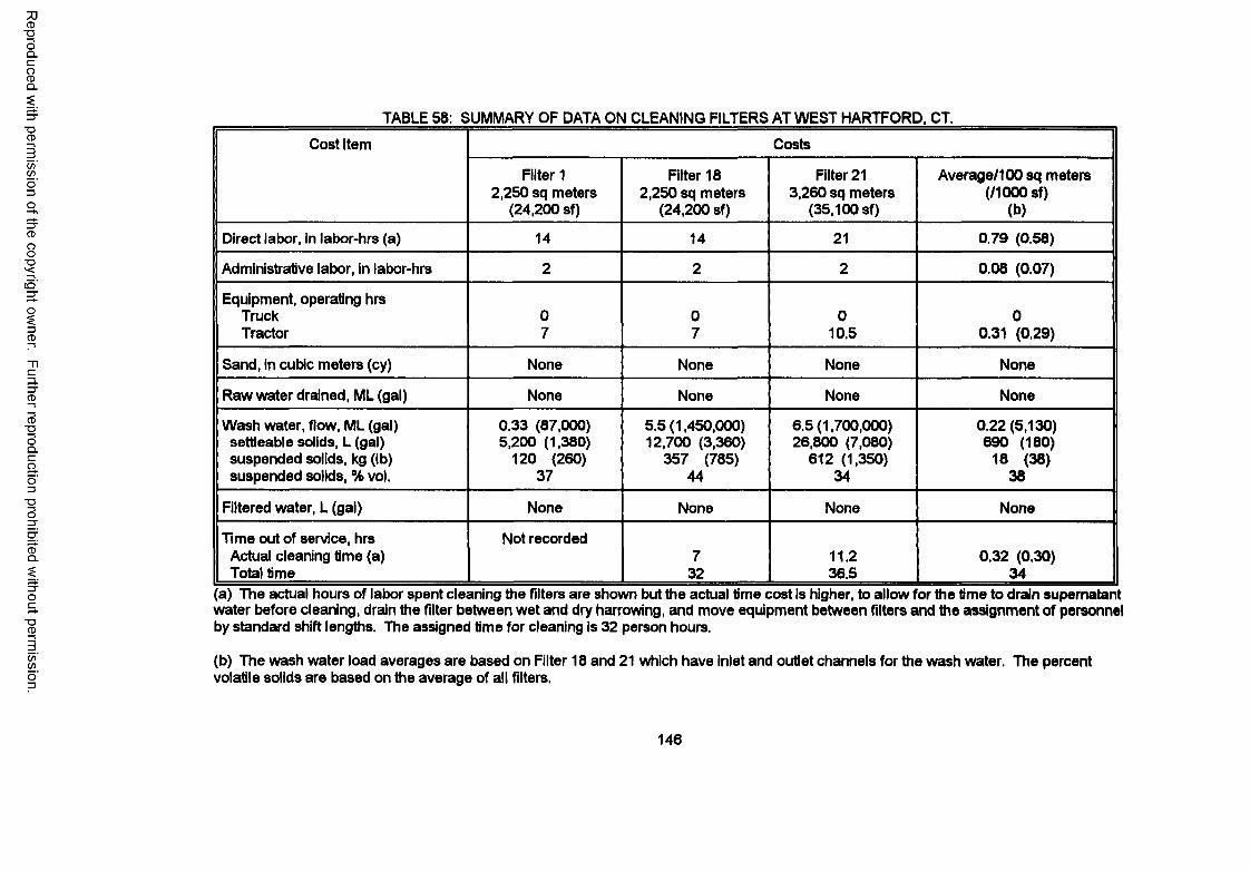
Reproduced
with perm
ission of the
copyright ow
ner. Further
reproduction prohibited
without
permission.
TABLE 58: SUMMARY OF DATA ON CLEANING FILTERS AT WEST HARTFORD. CT.
Cost Item Costs
Filter 1 2,250 sq meters
(24,200 sf)
Filter 18 2,250 sq meters
(24,200 sf)
Filter 21 3,260 sq meters
(35,100 sf)
Average/100 sq meters (/1000sf)
(b)
Direct labor, in labor-hrs (a) 14 14 21 0.79 (0.58)
Administrative labor, in labor-hrs 2 2 2 0.08 (0.07)
Equipment, operating hrsTruck 0 0 0 0Tractor 7 7 10.5 0.31 (0.29)
Sand, in cubic meters (cy) None None None None
Raw water drained, ML (gal) None None None None
Wash water, flow, ML (gal) 0.33 (87,000) 5.5(1,450,000) 6.5(1,700,000) 0.22 (5,130)settleable solids, L (gal) 5,200 (1,380) 12,700 (3,360) 26,800 (7,080) 690 (180)suspended solids, kg (lb) 120 (260) 357 (785) 612 (1,350) 18 (38)suspended solids, % vol. 37 44 34 38
Filtered water, L (gal) None None None None
Time out of service, hrs Actual cleaning time (a)
Not recorded7 11.2 0.32 (0.30)
Total time 32 36.5 34(a) The actual hours of labor spent cleaning the filters are shown but the actual time cost is higher, to allow for the time to drain supernatant water before cleaning, drain the filter between wet and dry harrowing, and move equipment between filters and the assignment of personnel by standard shift lengths. The assigned time for cleaning is 32 person hours.
(b) The wash water load averages are based on Filter 18 and 21 which have inlet and outlet channels for the wash water. The percent volatile solids are based on the average of all filters.
146
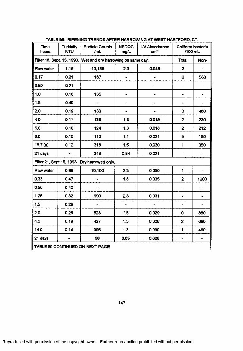
TABLE 59: RIPENING TRENDS AFTER HARROWING AT WEST HARTFORD, CT.
Timehours
TurbidityNTU
Particle Counts /mL
NPDOCmg/L
UV Absorbancecm'1
Coliform bacteria 7100 mL
Filter 18, Sept 15,1993. Wet and dry harrowing on same day. Total Non-
Raw water 1.16 10,136 2.0 0.046 2 -
0.17 0.21 187 - - 0 560
0.50 0.21 - - - - -
1.0 0.16 135 - - - -
1.5 0.40 - - - - -
2.0 0.19 130 - - 3 480
4.0 0.17 138 1.3 0.019 2 230
6.0 0.10 124 1.3 0.018 2 212
8.0 0.10 110 1.1 0.021 5 180
18.7(a) 0.12 318 1.5 0.030 1 350
21 days - 348 0.84 0.021 - -
Filter 21, Sept15,1993. Dry harrowed only.
Raw water 0.99 10,100 2.3 0.050 1 -
0.33 0.47 - 1.8 0.035 2 1200
0.50 0.40 - - - - -
1.25 0.32 690 2.3 0.031 - -
1.5 0.26 - - - - -
2.0 0.26 523 1.5 0.029 0 880
4.0 0.19 427 1.3 0.026 2 660
14.0 0.14 395 1.3 0.030 1 460
21 days - 66 0.85 0.026 - -
TABLE 59 CONTINUED ON NEXT PAGE
147
Reproduced with permission of the copyright owner. Further reproduction prohibited without permission.
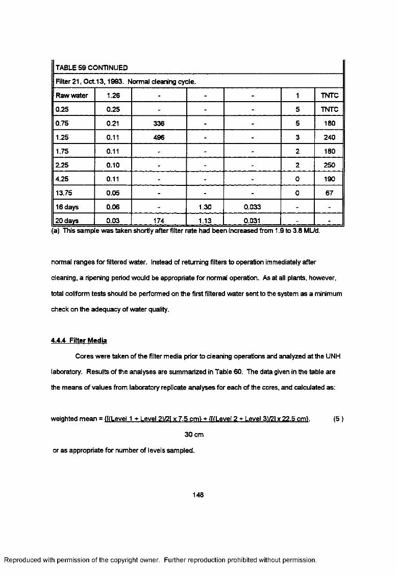
TABLE 59 CONTINUED
Filter 21, O ct13,1993. Normal cleaning cyde.
Raw water 1.26 - - - 1 TNTC
0.25 0.25 - - - 5 TNTC
0.75 0.21 336 - - 5 180
1.25 0.11 496 - - 3 240
1.75 0.11 - - - 2 180
2.25 0.10 - - - 2 250
4.25 0.11 - - - 0 190
13.75 0.05 - - - 0 67
16 days 0.06 - 1.30 0.033 - -
20 days 0.03 174 1.13 0.031 - -
a) This sampl e was taken shortly after filter rate had been increased from 1.9 to 3.8 ML/d.
normal ranges for filtered water. Instead of returning filters to operation immediately after
cleaning, a ripening period would be appropriate for normal operation. As at all plants, however,
total coliform tests should be performed on the first filtered water sent to the system as a minimum
check on the adequacy of water quality.
4.4.4 Filter Media
Cores were taken of the filter media prior to cleaning operations and analyzed at the UNH
laboratory. Results of the analyses are summarized in Table 60. The data given in the table are
the means of values from laboratory replicate analyses for each of the cores, and calculated as:
weighted mean = WLevel 1 + Level 2V2I x 7.5 cm! + fffLevel 2 + Level 31/21 x 22.5 cm). (5 )
30 cm
or as appropriate for number of levels sampled.
148
Reproduced with permission of the copyright owner. Further reproduction prohibited without permission.
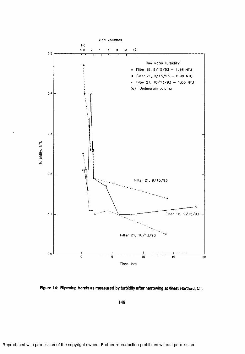
Turb
idity
, NT
U
0.5
Bed Volumes(a)
0 0 - 2 4 6
- n 1— i----r8 10 12"i 1 r
0.*
0.3
0.2
0.1
0.0
Raw water turbidity:
o n ite r 18. 9 / 1 5 / 9 3 - 1 .16 NTU
• Filter 21, 9 / 1 5 / 9 3 - 0 .9 9 NTU
* Filter 21, 1 0 /1 3 /9 3 - 1.00 NTU
(a ) Underdrain volume
Filter 21, 9 /1 5 /9 3
Filter 18. 9 /1 5 /9 3 -
Filter 21 . 1 0 /1 3 /9 3
10 15 20
Time, hrs
Figure 14: Ripening trends as measured by turbidity after harrowing at West Hartford, CT.
149
Reproduced with permission of the copyright owner. Further reproduction prohibited without permission.
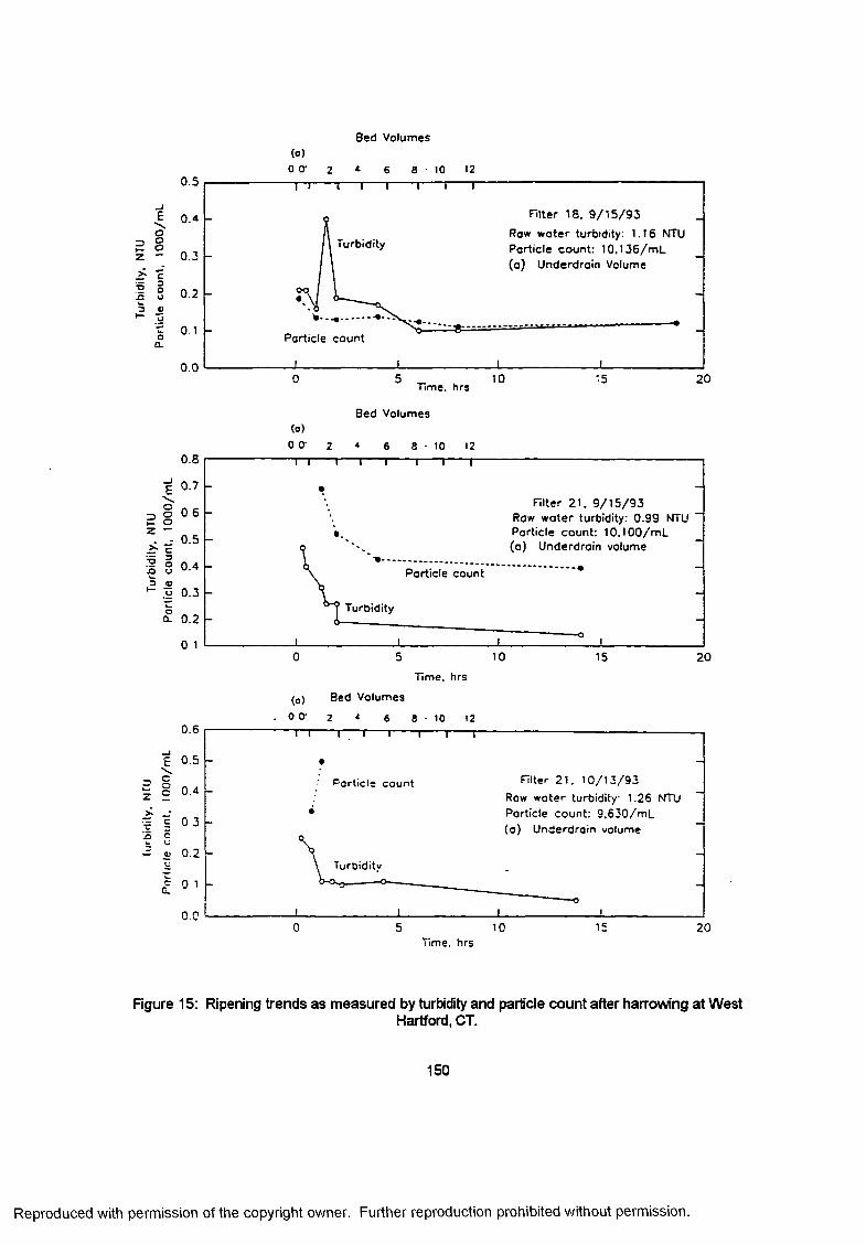
Bed Volumes
Eo
=3 °2 O
_ C
IS o n u
□a
(o) 0 O' 10 12
0.5
Filter 18. 9 /1 5 /9 3
Row water turbidity: 1.16 NTU Particle count: 10 .136/m L (a) Underdrain Volume
Turbidity0.3
0.2
0.1 Particle count
0.05 10 15 200
Time, hrs
Escoo
jo uW3 03
2 § z 2>? § h c
Bed Volumes(a)
0 0 ' 2 * 6 8 - 1 0 120.8
0.7Filter 21. 9 /1 5 /9 3
Raw water turbidity: 0.99 NTU - Particle count: 10.100/m L _(a) Underdrain volume
0.6
0.5
0.4 Particle count
0.3Turbidity
0.2
0 10 5 10 15 20
Time, hrs
(0) Bed Volumes
o O' 2 « 6 8 - 1 0 120.6
0.5
Filter 21. 1 0 /1 3 /9 3 Row water turbidity 1.26 NTU Particle count: 9 .630/m L (a) Underdrain volume
Particle count0.4
0 3
0.2
0 1
0.0150 5 10 20
Time, hrs
Figure 15: Ripening trends as measured by turbidity and particle count after harrowing at WestHartford, CT.
150
Reproduced with permission of the copyright owner. Further reproduction prohibited without permission.
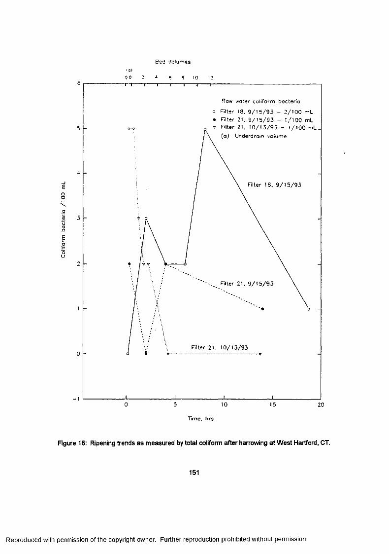
Colif
orm
ba
cter
ia
/100
m
LBed Volumes
10)oo ; •» 6 a io >2
Raw water coliform bacteria
o Filter 18. 9 / 1 5 / 9 3 - 2 /1 0 0 mL • Filter 21. 9 / 1 5 / 9 3 - 1 /1 0 0 mL ^ Filter 21. 1 0 /1 3 /9 3 - 1 /1 0 0 m L_
(a ) Underdrain volume
Filter 18. 9 / 1 5 / 9 3
Filter 21, 9 / 1 5 / 9 3
Filter 21 . 1 0 /1 3 /9 3
- 150 10 15 20
Time, hrs
Figure 16: Ripening trends as measured by total coliform after harrowing at West Hartford, CT.
151
Reproduced with permission of the copyright owner. Further reproduction prohibited without permission.
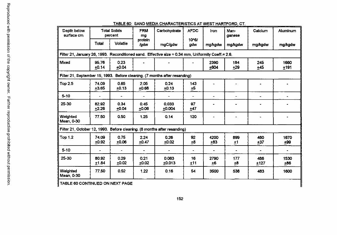
Reproduced
with perm
ission of the
copyright ow
ner. Further
reproduction prohibited
without
permission.
TABLE 60; SAND MEDIA CHARACTERISTICS AT WEST HARTFORD. CT.
Depth below surface cm
Total Solids percent
FRMmg
protein/gdw
Carbohydrate
mgC/gdw
AFDC
10*6/gdw
Iron
mg/kgdw
Manganese
mg/kgdw
Calcium
mg/kgdw
Aluminum
mg/kgdwTotal Volatile
Filter 21, January 26,1993. Reconditioned sand. Effective size = 0.34 mm, Uniformity Coeff,= 2.6.
Mixed 95.76±0.14
0.23±0.04
- - - 2390±604
184±29
245±45
1660±191
Filter 21, September 15,1993. Before cleaning. (7 months after resanding)
Top 2.5 74.09+3.65
0.65±0.13
2.05±0.68
0.24±0.13
143±5
- - - -
5-10 - - - - - - - - -
25-30 82.92±2.26
0.34±0.04
0.45±0.06
0.033±0.004
97±47
- - - -
Weighted Mean, 0-30
77.50 0.50 1.25 0.14 120 - - - -
Filter 21, October 12,1993. Before cleaning. (8 months after resandingJ)
Top 1.2 74.09±0.92
0.75±0.06
2.24±0.47
0.26±0.02
92±8
4200±83
899±1
480±37
1670±99
5-10 - - - - - - - - -
25-30 80.92±1.84
0.29±0.02
0.21±0.02
0.063±0.013
16±11
2790±6
177±8
486±127
1530±86
Weighted Mean, 0-30
77.50 0.52 1.22 0.16 54 3500 538 483 1600
TABLE 60 CONTINUED ON NEXT PAGE
152
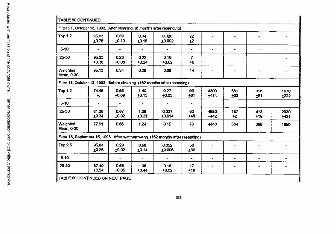
Reproduced
with perm
ission of the
copyright ow
ner. Further
reproduction prohibited
without
permission.
TABLE 60 CONTINUED
Filter 21, October 13,1993, After cleaning. (8 months after resanding)
Top 1.2 95.03±0.76
0.39±0.10
0.34±0.18
0.020±0.002
22±2
- - - -
5-10 - - - - - - - - -
25-30 95.23±0.38
0.28±0.08
0.22±0.24
0.16±0.02
7±6
- - - -
Weighted Mean, 0-30
95.13 0.34 0.28 0.09 14 - - - -
Filter 18, October 13,1993. Before cleaning. (162 months after resanding)
Top 1.2 74.46+,
0.65±0.09
1.40±0.15
0.27±0.05
99±81
4300±414
581±33
318±51
1670±222
5-10 - - - - - - - - -
25-30 81.36±0.34
0.67±0.02
1.08±0.21
0.037±0.014
52±48
4580±442
187±2
413±19
2030±421
Weighted Mean, 0-30
77.91 0.66 1.24 0.15 76 4440 384 366 1850
Filter 18, September 15,1993. After wet harrowing. (162 months after resanding)
Top 2.5 95.84±0.26
0.29±0.02
0.68±0.14
0.052±0.005
56±39
- - - -
5-10 - - - - - - - - -
25-30 87.40±0.54
0.56±0.05
1.38±0.44
0.18±0.02
17±18
- - - -
TABLE 60 CONTINUED ON NEXT PAGE
153
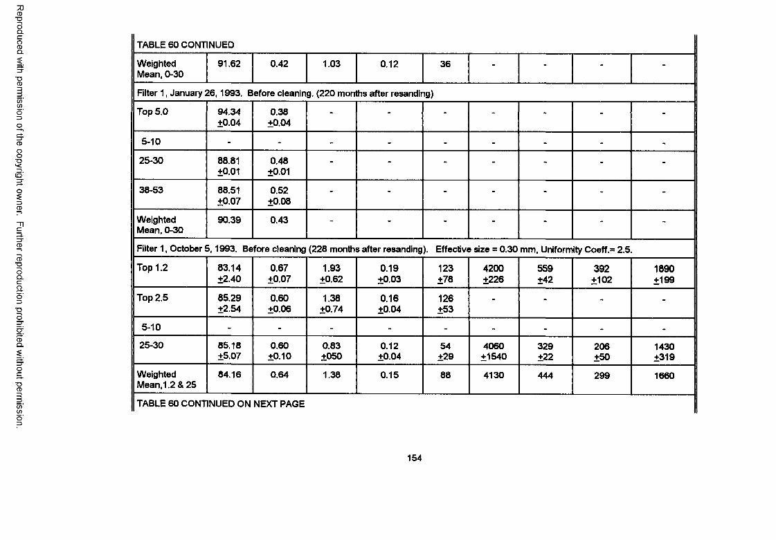
Reproduced
with perm
ission of the
copyright ow
ner. Further
reproduction prohibited
without
permission.
TABLE 60 CONTINUED
Weighted Mean, 0-30
91.62 0.42 1.03 0.12 36 - - - -
Filter 1, January 26,1993. Before cleaning. (220 months after resanding)
Top 5.0 94.34±0.04
0.38±0.04
- - - - - - -
5-10 - - - - - - - - -
25-30 88.81±0.01
0.48±0.01
- - - - - - -
38-53 88.51±0.07
0.52±0.08
- - - - - - -
Weighted Mean, 0-30
90.39 0.43 - - - - - - -
Filter 1, October 5,1993. Before cleaning (228 months after resanding). Effective size = 0.30 mm, Uniformity Coeff.= 2.5.
Top 1.2 83.14±2.40
0.67±0.07
1.93±0.62
0.19±0.03
123±78
4200±226
559±42
392±102
1890±199
Top 2.5 85.29±2.54
0.60±0.06
1.38±0.74
0.16±0.04
126±53
- - - -
5-10 - - - - - - - - -
25-30 85.18±5.07
0.60±0.10
0.83±050
0.12±0.04
54±29
4060±1540
329±22
206±50
1430±319
Weighted Mean,1.2 & 25
84.16 0.64 1.38 0.15 88 4130 444 299 1660
TABLE 60 CONTINUED ON NEXT PAGE
154
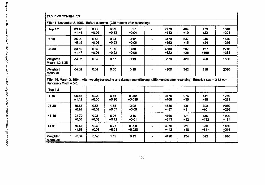
Reproduced
with perm
ission of the
copyright ow
ner. Further
reproduction prohibited
without
permission.
TABLE 60 CONTINUED
Filter 1, November 2,1993. Before cleaning. (229 months after resanding)
Top 1.2 83.16±1.48
0.47±0.09
0.99±0.33
0.17±0.04
- 4270±142
494±10
270±23
1640±204
5-10 85.92 0.43 0.54 0.12 . 3470 347 246 1570±5.19 ±0.06 ±0.23 ±0.06 ±892 ±15 ±24 ±215
25-30 83.10 0.67 1.09 0.30 4880 287 427 2710±1.47 ±0.06 ±0.22 ±0.06 ±622 ±26 ±169 ±338
Weighted 84.06 0.57 0.87 0.19 • 3870 420 258 1600Mean, 1.2 & 25
Weighted 84.52 0.52 0.80 0.19 4100 342 316 2010Mean, all
Filter 19, March 3,1994. After wet/dry harrowing and during reconditioning. (259 months after resanding) Effective size = 0.32 mm,Uniformity Coeff. = 3.0.
Top 1.2 - - - - - - - - -
5-10 95.56 0.36 0.58 0.082 _ 3170 276 411 1260±1.12 ±0.05 ±0.16 ±0.046 ±788 ±30 ±68 ±239
25-30 89.63 0.58 1.68 0.22 4880 98 593 2010±0.92 ±0.02 ±0.07 ±0.05 ±457 ±11 ±101 ±256
41-46 92.79 0.38 0.94 0.10 4660 91 649 1990±0.38 ±0.02 ±0.22 ±0.01 ±543 ±12 ±132 ±154
56-61 89.61 0.37 0.77 0.098 4080 81 670 1850±1.68 ±0.05 ±0.21 ±0.020 ±442 ±10 ±341 ±215
Weighted 90.34 0.52 1.19 0.19 4120 134 592 1810Mean, all
155
Volatile Solids— Analyses for total and volatile solids at different depths in the cores taken from the
respective filters showed significant variance at the 90 percent level between cores, depths, and
filters. The concentrations at the top 1.2 cm of the filters sampled were approximately the same
immediately before the filters were cleaned. This concentration was not related to the length of
time since the filter had been reconditioned. The volatile solids concentrations at the 25-30 cm
depth of the filters did increase over time since the filters had been reconditioned, from a mean of
0.23 percent in the sand after reconditioning to 0.58 to 0.67 percent after 19 to 24 year of
operation. The concentrations in the intermediate depth of 5-10 cm (2-4 in) were lower than in the
top or lower levels.
The concentration differences between the top 1.2 cm (1/2 in) and top 5 cm (1 in) of cores
taken from Filter 1 on October 5,1993 were not significantly different The concentration of
volatile solids in the top 1.2 cm (top 1/2 in) and at the depth of 25-30 cm (10-12 in) in Filter 1,
sampled in January 1993,were lower than at the same depths and in the same filter in October and
in November of the same year. This was evident in Filter 18 media, sampled in October, which
had operated 66 months less than Filter 1. Folin Reactive Material- The concentration of protein
in the separate samples varied significantly between cores within a filter, between depths in the
cores, and between filters. The samples of January 1993 had not been analyzed for FRM so there
was no basis for comparison between seasons. Such differences had been reported by Spanos
(1989), who also found that there were differences relative to media depth in a filter and between
filters at different plants. No differences were reported by Spanos between FRM concentrations in
cores from the same filter or between filters at the same plant Significant differences also were
found in this study in FRM concentrations with the age of sand following reconditioning.
The effects of cleaning were also significantly different in FRM concentration in the upper
30 cm (12 in) of filter media between cores taken before and after harrowing. As indicated in
Table 50, the mean FRM concentration in Filter 21 was reduced from 1.22 mg/g dry wt before
156
Reproduced with permission of the copyright owner. Further reproduction prohibited without permission.
cleaning to 0.92 mg/g dry wt after cleaning in October 1993. The mean concentration in the upper
30 cm (12 in) of Filter 18 was reduced from 1.24 mg/g dry wt to 1.03 mg/g dry wt after wet
harrowing
The FRM concentration, per gram volatile solids, did not vary significantly in the top 1.2 cm
9112 in) of the filter media over the age of the sand in filters, but did increase at the 25-30 cm (10-
12 in) depth over the age of filter sand from 16 + 24 mg/g volatile solids to 292 + 12 mg/g volatile
solids. These data are summarized in Table 61.
Carbohydrates— Carbohydrate concentrations, expressed as elemental carbon per gram volatile
solids, varied between cores, depths, filters, and age of sand. The carbohydrate concentration did
not vary significantly in the top 1.2 cm (1/2 in) of the filter media over the age of the sand in filters,
but did change at the 25-30 cm (10-12 in) depth, increasing over the age of filter sand as
summarized in Table 62.
Acriflavin Direct Count (AFDC)— The bacteria counts variations were significant only with the depth
of the sample in the filter. The results did not significantly change with the age of the sand.
Metals— Iron concentrations did not vary over the age of the sand in the top 1.2 cm (1/2 in) of filter
media, but the concentration for iron and manganese at the lower depths increased with increasing
sand age. The iron concentration at the 25-30 cm (10-12 in) depth increased from 2390 mg/kg
dry wt in the reconditioned sand to 4580 mg/kg dry wt after 162 months of service but did not
increase further. The concentrations at the lower depths were sampled at the beginning avid end
of resanding. The concentration of iron increased significantly over that period.
The manganese concentrations varied widely. The concentration in the top 1.2 cm (1/2 in)
was relatively constant, except for that in Filter 21 after 8 months of operation when it was
157
Reproduced with permission of the copyright owner. Further reproduction prohibited without permission.
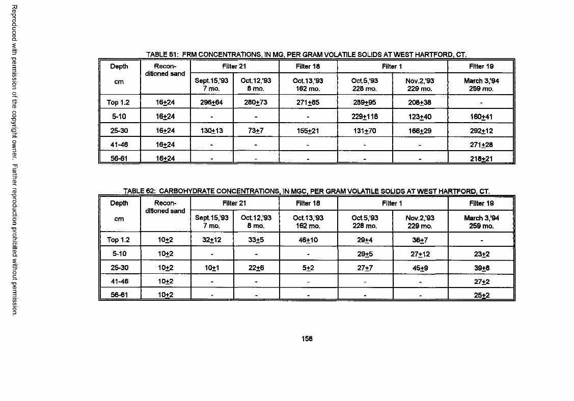
Reproduced
with perm
ission of the
copyright ow
ner. Further
reproduction prohibited
without
permission.
TABLE 61: FRM CONCENTRATIONS, IN MG. PER GRAM VOLATILE SOLIDS AT WEST HARTFOR D.CT.
Depth Reconditioned sand
Filter 21 Filter 18 Filter 1 Filter 19
cm Sept. 15/93 7 mo.
Oct. 12 ,'93 8 mo.
Oct. 13/93 162 mo.
Oct.5/93 228 mo.
Nov.2/93 229 mo.
March 3/94 259 mo.
Top 1.2 16+24 296+64 280+73 271±85 289+95 208+38 -
5-10 16+24 - - - 229+118 123±40 160±41
25-30 16±24 130+13 73+7 155+21 131±70 166+29 292±12
41-46 16+24 - - - - - 271±28
56-61 16+24 • - . . • 218+21
TABLE 62: CARBOHYDRATE CONCENTRATIONS. IN MGC. PER GRAM VOLATILE SOLIDS AT WEST HARTFORD. CT.
Depth Reconditioned sand
Filter 21 Filter 18 Filter 1 Filter 19
cm Sept. 15/93 7 mo.
Oct. 12 ,'93 8 mo.
Oct. 13/93 162 mo.
Oct.5/93 228 mo.
Nov.2/93 229 mo.
March 3/94 259 mo.
Top 1.2 10+2 32+12 33+5 46+10 29±4 36±7 -
5-10 10+2 - - - 29±5 27±12 23±2
25-30 10+2 10+1 22+6 5+2 27±7 45±9 39±8
41-46 10+2 - - - - - 27±2
56-61 10+2 - - - - - 25±2
158
approximately twice that observed during other sampling periods. The manganese
concentrations at the 25-30 cm (10-12 in) depth increased with sand age except in Filter 19 which
had been sampled during reconditioning. Caldum and aluminum concentrations did not change
significantly, with depth or sand age.
4.4.5 Reconditioning
The reconditioning procedure normally begins with the plant operators harrowing the filter,
moving the hydraulic washing equipment and hoses into the appropriate filter building, and draining
the filter. The contractor who is to do the reconditionnning moves the equipment from the building
into the filter and is reinstructed on cleaning procedures. Sand is manually shoveled into ejector
boxes which move the sand hydraulically through hoses to vortex washing tanks. Wash water
from the vortex tanks is discharged to the filter effluent channel and drains to the holding reservoir
used to settle wash water from the harrowing process. Entrained solids settle in the reservoir and
the overflow is discharged to a creek under a discharge permit The sand from the tanks is
dumped onto the surface of the filter nearby. Later the sand is again shoveled into a ejector box,
through another vortex washing tank, and discharged to an area of the filter which has previously
been emptied. The cleaned sand dewaters on the gravel supporting layer and remains. The depth
of sand is built up to the normal operating depth of 0.68 meters (27 in) and, when the entire filter
area has been recovered, the filter is ready to be put back into use.
Although this description outlines the basic procedures, the filter is full of sand when work
begins and no area is available to place the reconditioned sand. During the early stages of the
operations, partially reconditioned sand is conveyed (after the first washing step) onto the surface
of a portion of the bed that will be reconditioned later and stored. When a sufficient area has been
cleared to the gravel supporting layer, fully reconditioned sand is replaced.
Water for the ejectors and washing operations is taken from the raw water supply of the
159
Reproduced with permission of the copyright owner. Further reproduction prohibited without permission.
plant The waste water from the vortex tanks and from the filter underdrains is discharged to a
holding reservoir as previously described. The volumes of water used and solids produced have
never been measured.
The upper few centimeters of the gravel supporting layer is manually shoveled into a
mechanical screening apparatus so that the gravel can be separated from sand which has mixed
with it during filter operation and during the reconditioning procedure. The separated gravel is
replaced as the operations move across the filter and the relatively small volume of sand thrown
back onto uncleaned areas for reconditioning.
Sand losses from successive harrowing operations and the reconditioning procedures are
made up as reconditioning reaches the end of the filter and an area of the supporting gravel layer
remains uncovered with cleaned sand. This portion of the filter is refilled with virgin sand
purchased for that purpose. Replacement sand is currently purchased with an effective size of
from 0.32 to 0.38 mm with uniformity coefficient of less than 2.3 from Holliston Sand & Gravel in
Slatersville, Rhode Island. Makeup sand for the last two 0.2 hectare (1/2 acre) filters cleaned, No.
12 and 14 in 1989-90, was a combined total of 2.7 million kg (620 tons). Make up sand for the last
four 0.3 hectare (3/4 acre) beds. No. 19 through 22, was 1,0 .5 ,2 .4, and 1 million kg (250,120,
544, and 240 tons), respectively.
Reconditioning normally takes from 4 to 6 months: I to 2 weeks during which the sand filter
is awaiting the reconditioning crew, from 9 to 20 weeks while the filter is being reconditioned, and
then 1 to 2.5 months while the filter is run to waste and "ripened." The progress of ripening is
monitored by sampling the filtered water for turbidity, total and fecal coliform, and total plate count
When the total coliform count drops to 0 to 1 colony forming units (CFU) per I00 mL, the filter is
placed back into service. The actual time for filters to be out of service, exclusive of preliminary
time awaiting the reconditioning crew, is summarized in Table 63.
160
Reproduced with permission of the copyright owner. Further reproduction prohibited without permission.
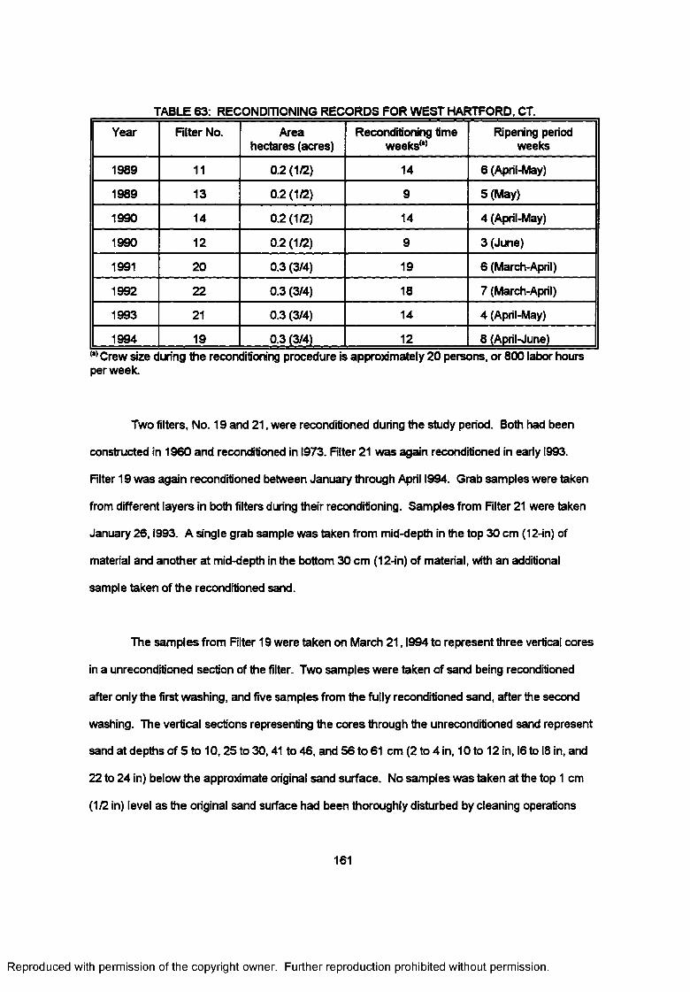
TABLE 63: RECONDITIONING RECORDS FOR WEST HARTFORD, CT.
Year Rlter No. Area hectares (acres)
Reconditioning time weeks(,)
Ripening period weeks
1989 11 0.2 (1/2) 14 6 (April-May)
1989 13 0.2 (1/2) 9 5 (May)
1990 14 0.2 (1/2) 14 4 (April-May)
1990 12 0.2 (1/2) 9 3 (June)
1991 20 0.3 (3/4) 19 6 (March-April)
1992 22 0.3 (3/4) 18 7 (March-April)
1993 21 0.3 (3/4) 14 4 (April-May)
1994 19 0.3 (3/4) 12 8 (April-June)(a)Crew size during the reconditioning procedure is approximately 20 persons, or 800 labor hours per week.
Two filters. No. 19 and 21, were reconditioned during the study period. Both had been
constructed in 1960 and reconditioned in I973. Filter 21 was again reconditioned in early I993.
Rlter 19 was again reconditioned between January through April I994. Grab samples were taken
from different layers in both filters during their reconditioning. Samples from Rlter 21 were taken
January 2 6 ,1993. A single grab sample was taken from mid-depth in the top 30 cm (12-in) of
material and another at mid-depth in the bottom 30 cm (12-in) of material, with an additional
sample taken of the reconditioned sand.
The samples from Rlter 19 were taken on March 2 1 ,1994 to represent three vertical cores
in a unreconditioned section of the filter. Two samples were taken of sand being reconditioned
after only the first washing, and five samples from the fully reconditioned sand, after the second
washing. The vertical sections representing the cores through the unreconditioned sand represent
sand at depths of 5 to 10,25 to 30,41 to 46, and 56 to 61 cm (2 to 4 in, 10 to 12 in, 16 to 18 in, and
22 to 24 in) below the approximate original sand surface. No samples was taken at the top 1 cm
(1/2 in) level as the original sand surface had been thoroughly disturbed by cleaning operations
161
Reproduced with permission of the copyright owner. Further reproduction prohibited without permission.
and mixed with partially reconditioned sand stored on it The results of analyses on the samples
from Rlter 19 are shown in Table 64.
Sieve Analyses- The effective sizes for the sand samples at all levels and for all samples were
not significantly different at the 95% probability level using 2-factor analysis of variance (ANOVA)
calculations. A comparison of the different levels between the different cores in the
unreconditioned sand showed a probability of inequality of only about 40% between levels. A
comparison between the mean effective size of each separate core of unreconditioned sand with
the two samples of once- washed sand and the three samples of reconditioned sand showed only
a 65% probability of inequality. This result was surprising as it had been expected that the vortex
sand washing process would remove very fine materials and result in a larger effective grain size.
This was not true based on mean values of 0.318 mm for the unreconditioned sand, 0.283 mm
after the first wash and 0.306 mm for the reconditioned sand. The variance between samples at
each level for the few samples analyzed overshadowed the relatively small differences in grain
size.
A similar 2-factor ANOVA on the uniformity coefficients from these data demonstrated
greater probabilities for inequality. The analysis indicated a 92 percent probability of inequality
between uniformity coefficients at the different depths for the unreconditioned sand and just under
a 90% probability of inequality between uniformity coefficients of the unreconditioned, once-
washed, and reconditioned sands. The uniformity coefficients of the two grades of reconditioned
sands were not significantly different at the 90 percent confidence level, but the difference
between the unconditioned and reconditioned sands was significant
Since the effective size of the sand was not changed but the uniformity coefficient
decreased, the vortex sand washing and reconditioning process apparently reduced the proportion
162
Reproduced with permission of the copyright owner. Further reproduction prohibited without permission.
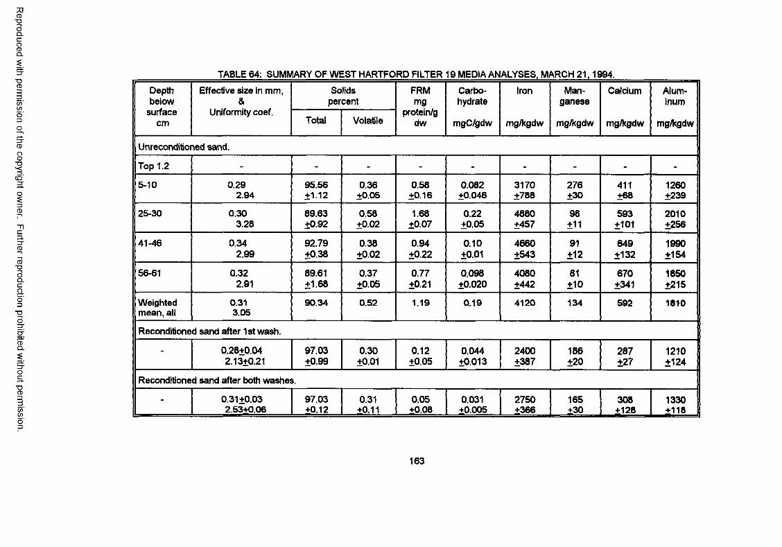
Reproduced
with perm
ission of the
copyright ow
ner. Further
reproduction prohibited
without
permission.
TABLE 64: SUMMARY OF WEST HARTFORD FILTER 19 MEDIA ANALYSES. MARCH 21.1994.
Depthbelow
Effective size in mm, &
Solidspercent
FRMmg
Carbohydrate
Iron Manganese
Calcium Aluminum
surfacecm
Uniformity coef.Total Volatile
protein/gdw mgC/gdw mg/kgdw mg/kgdw mg/kgdw mg/kgdw
Unreconditionecl sand.
Top 1.2 - - - - - - - - -
5-10 0.292.94
95.56+1.12
0.36±0.05
0.58±0.16
0.082±0.046
3170±788
276±30
411±68
1260±239
25-30 0.303.28
89.63+0.92
0.58+0.02
1.68±0.07
0.22±0.05
4880±457
98±11
593±101
2010±256
41-46 0.342.99
92.79+0.38
0.38±0.02
0.94±0.22
0.10±0.01
4660±543
91±12
649±132
1990±154
56-61 0.322.91
89.61+1.68
0.37±0.05
0.77±0.21
0.098±0.020
4080±442
81±10
670±341
1850±215
Weighted mean, all
0.313.05
90.34 0.52 1.19 0.19 4120 134 592 1810
Reconditioned sand after 1st wash.
- 0.28+0.042.13+0.21
97.03+0.99
0.30±0.01
0.12±0.05
0.044±0.013
2400±387
186±20
287±27
1210±124
Reconditioned sand after both washes.
- 0.31+0.032.53+0.06
97.03+0.12
0.31+0.11
0.05+0.08
0.031±0.005
2750+366
165+30
308+128
1330+118
163
of D-60 grain size material in the sand which narrowed the relation between the D-60 and D-10
sizes. This is contrary to expectation but was consistent with the analyses of the five partially or
fully reconditioned samples and the twelve unreconditioned samples.
Volatile Solids— The sample cores were found to be affected by their locations. The sites for the
three cores of the "dirty sand" (before reconditioning) were determined by taking random numbers
between zero and 13 as the length of the exposed sand face available for sampling was 4.0
meters (13 feet). The first number was "one" and resulted in taking the core for D-1 adjacent to a
column where the harrowing equipment could not loosen the sand when it was harrowed just
before starting the reconditioning process. The sample at the 5-10 cm (2 to 4 in) level from this
core was significantly darker and contained more organic material than samples from comparable
levels at cores D-2 and D-3. These latter samples were taken at a distance from columns and had
been regularly traversed with the harrow. The results from the analyses on Core D-1 at the depth
of 5-10 cm (2 to 4 in), and to a lesser extent at the depth of 25-30 cm (10 to 12 in), were statistically
atypical in comparison to the results from Cores D-2 and D-3. The effective sizes and uniformity
coefficients of the respective cores did not show any differences, but those for total and volatile
solids did. Results of analyses on Core D-1 were different from those on Cores D-2 and D-3
because of the location next to the column.
Two-way ANOVA results showed very high probabilities of inequalities between the total
and volatile solids concentrations between the levels, between the different cores, but only 89
percent probable between the unreconditioned and reconditioned sand samples if all three cores
of the "dirty sand" were considered. The volatile solids content of the media adjacent to the
column at depths of 5-10 cm and 25-30 cm were approximately double (0.80 percent vs 0.34
percent, and 0.82 percent vs 0.58 percent) those of samples taken where the media wass
accessible to the harrow. When the results of core D-1 next to the column were omitted, the
probabilities of inequality between the unreconditioned and reconditioned sands increased to
164
Reproduced with permission of the copyright owner. Further reproduction prohibited without permission.
greater than 95%.
One-tailed t-Tests on the mean values for percent volatile solids in each of the
unreconditioned, first wash, and reconditioned samples indicated that differences between means
for the unreconditioned samples (0.483+/-0.007 percent, n=3) and the first wash samples
(0.301 +/-0.000 percent, n=2) is 97 percent probable. The similar test between the first wash
samples and the reconditioned samples (0.315+/-.005 percent, n=3) indicated that, while the mean
percent of volatile solids appeared to be increased by the second washing step and storage in
place, the probability was not significant (P=0.66).
A pattern of accumulation within the filter emerges, beginning with the data on volatile
solids but continuing through the data for protein, carbohydrates, and metals. Generally, the
concentration of volatile solids in the level near the top of the sand filter, 5-10 cm (2-4 in), are
below those at 25-30 cm (10 to 12-inches), the level just below the depth reached by the harrowing.
The characteristics of the sand at the 5-10 cm level (2-4 in) are relatively similar to those at depths
of 41-61 cm (16 to 24-inches). The sample adjacent to the column, on the other hand, indicates
much higher concentrations of volatile solids to the depth just below the depth of harrowing than
for the samples taken where the sand has been harrowed regularly.
Folin Reactive Material (FRM)— Two-factor ANOVA results on the unreconditioned sand samples
showed greater than 99% probability of inequality between the FRM concentrations between
different depths in the filter bed, whether including the results of the high organic layer in core D-1
or not When the results for FRM concentration were corrected from mg of protein per g dry wt of
filter media to gram of protein per gram of volatile solids within the sand filter sample, the ANOVA
results showed less effect from interactions between the selection of the core location and depth of
sample and less variation within these replicate samples.
165
Reproduced with permission of the copyright owner. Further reproduction prohibited without permission.
Results from ANOVA calculations consistently showed over 98% probability of inequality in
or between the FRM concentration in the unreconditioned and reconditioned sands. Whereas
sieve analyses and solids analyses showed almost no improvements in quality of sand before and
after reconditioning, FRM analysis shows very significant removal of protein material by
reconditioning.
Carbohydrates— An ANOVA on the results of the carbohydrate tests, reported as carbon on a dry
weight basis, showed significant differences between all samples, at all depths, and between the
unreconditioned and the reconditioned sands. There is high probabilities of difference (>99.9)
between the different locations of unreconditioned sand cores, between the different depths within
each core, and for interactions between these two factors but with very low variance between
replicate analyses. The data which had been corrected for volatile solids concentration also
showed equally high probabilities of differences between the samples, depths, and interaction
whether the results of core D-1 were included or not
4.5 PILOT PLANT STUDIES
Laboratory scale sand filter tests were earned out to compare filter characteristics that
could not be made in the field. The tests were in three phases, an initial ripening period of three
cycles during which all three parallel filters were cleaned by scraping, the principal study period of
five cycles during which the filters were cleaned by different methods, and a final period during
which the filters ripening was studied after cleaning. The filter media was then sampled to
determine if differences had developed as a result of the respective cleaning methods. These
filters, unlike the field scale plants, were near the UNH laboratory and more extensive testing was
feasible.
4.5.1 Raw Water Quality and Filter Performance
Analytical results of raw and filtered water samples during the first two phases of study are
166
Reproduced with permission of the copyright owner. Further reproduction prohibited without permission.
presented in Tables 65 through 69. Performance was compared between the filters for phase 1,
when all were cleaned by scraping. The only significant differences found in performance were
between turbidity removals when the filtered water was greater than or equal to 8°C and when it
was less than 8°C. Little data was collected for NPDOC and BDOC removal during this period as
the time was intended primarily maturing the filter media.
The cleaning methods were changed for the second phase of this study beginning June,
1993. Scraping continued to be used to clean Filter 1, but a harrowing process was used for Filters
2 and 3 as described in the section on "Methods and Materials." Performance was also compared
between the filters for this phase of the study. The results showed no significant differences
between filter performance except for headlosses. Headlosses for the filters are shown
graphically in Figure 17. The filter cleaned by harrowing showed greater head losses than the filter
cleaned by scraping after the third cleaning cycle, with increasing losses developing in each of the
two subsequent cycles the filters were operated. The harrowing method used in the pilot filters,
however, could not reproduce the full operation of plant scale cleaning. The filers were cleaned
while an upflow was maintained through the media, but no cross flow could be maintained. The
suspended materials were removed by bailing, however. Because the cleaning methods could not
be entirely reproduced in the pilot scale, however, observations from this part of the research
concerning the rate of head loss development are not conclusive.
4.5.2 Ripening
At the end of the second phase, the filters were cleaned and operated for a short period to
compare their ripening characteristics. The results are summarized in Tables 70 to 72.
The quality of the filtered water from Filters 2 and 3 showed increases in turbidity and UV
absorbance in the first 120 minutes after cleaning. NPDOC increased during the first 90 minutes
after cleaning, but at a lower rate. The qualtiy of water from Rlter 1 was also affected during
167
Reproduced with permission of the copyright owner. Further reproduction prohibited without permission.
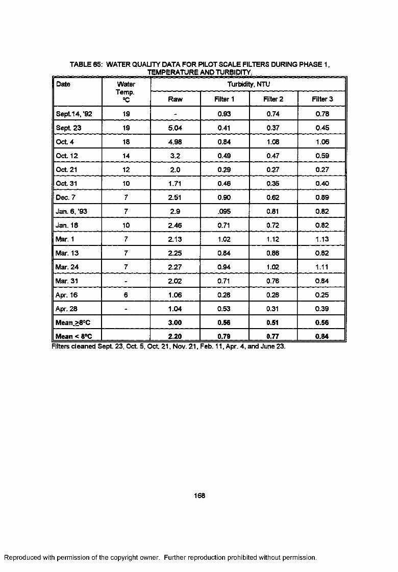
TABLE 65: WATER QUALITY DATA FOR PILOT SCALE FILTERS DURING PHASE 1,TEMPERATURE AND TURBIDITY.
Date WaterTemp.
°C
Turbidity, NTU
Raw Rlter 1 Rlter 2 Rlter 3
Sept14, '92 19 - 0.93 0.74 0.78
Sept 23 19 5.04 0.41 0.37 0.45
Oct 4 18 4.98 0.84 1.08 1.06
Oct 12 14 3.2 0.49 0.47 0.59
Oct 21 12 2.0 0.29 0.27 0.27
Oct 31 10 1.71 0.46 0.35 0.40
Dec. 7 7 2.51 0.90 0.62 0.89
Jan. 6, '93 7 2.9 .095 0.81 0.82
Jan. 18 10 2.46 0.71 0.72 0.82
Mar. 1 7 2.13 1.02 1.12 1.13
Mar. 13 7 2.25 0.84 0.86 0.82
Mar. 24 7 2.27 0.94 1.02 1.11
Mar. 31 - 2.02 0.71 0.76 0.84
Apr. 16 6 1.06 0.28 0.26 0.25
Apr. 28 - 1.04 0.53 0.31 0.39
Meanj>8°C 3.00 0.56 0.51 0.56
Mean < 8°C 2.20 0.79 0.77 0.84Filters cleaned Sept 23, Oct 5, Oct 21, Nov. 21, Feb. 11, Apr. 4, and June 23.
168
Reproduced with permission of the copyright owner. Further reproduction prohibited without permission.
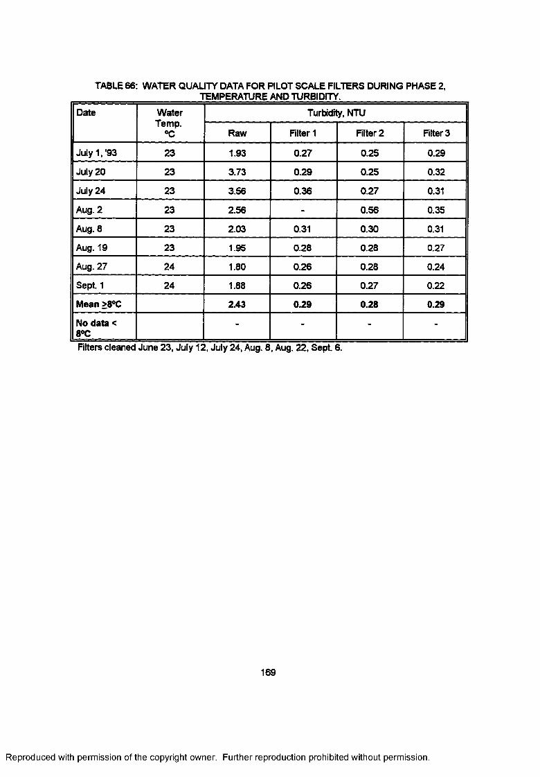
TABLE 66: WATER QUALITY DATA FOR PILOT SCALE FILTERS DURING PHASE 2,TEMPERATURE AND TURBIDITY.
Date WaterTemp.
°C
Turbidity, NTU
Raw Rlter 1 Rlter 2 Rlter 3
July 1, '93 23 1.93 0.27 0.25 0.29
July 20 23 3.73 0.29 0.25 0.32
July 24 23 3.56 0.36 0.27 0.31
Aug. 2 23 2.56 - 0.56 0.35
Aug. 8 23 2.03 0.31 0.30 0.31
Aug. 19 23 1.95 0.28 0.28 0.27
Aug. 27 24 1.80 0.26 0.28 0.24
Sept 1 24 1.88 0.26 0.27 0.22
Mean >8°C 2.43 0.29 0.28 0.29
No data < 8°C
- - - -
Filters cleaned June 23, July 12, July 24, Aug. 8, Aug. 22, Sept 6.
169
Reproduced with permission of the copyright owner. Further reproduction prohibited without permission.
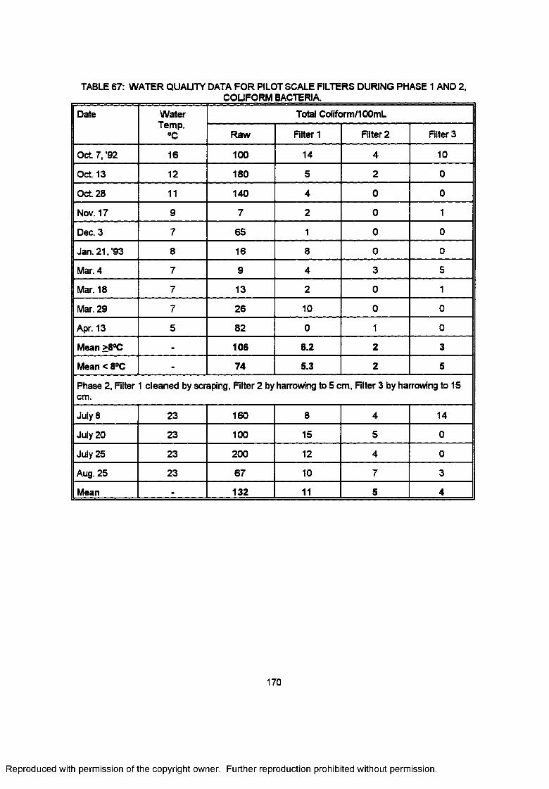
TABLE 67: WATER QUALITY DATA FOR PILOT SCALE FILTERS DURING PHASE 1 AND 2,COUFORM B A C TE R IA .___________________________
Date WaterTemp.
°C
Total Coliform/100mL
Raw Rlter 1 Rlter 2 Rlter 3
Oct 7, '92 16 100 14 4 10
Oct 13 12 180 5 2 0
Oct 28 11 140 4 0 0
Nov. 17 9 7 2 0 1
Dec. 3 7 65 1 0 0
Jan. 21 ,'93 8 16 8 0 0
Mar. 4 7 9 4 3 5
Mar. 18 7 13 2 0 1
Mar. 29 7 26 10 0 0
Apr. 13 5 82 0 1 0
Mean >8°C - 106 6.2 2 3
Mean < 8°C - 74 5.3 2 5
Phase 2, Rlter 1 cleaned by scraping, Rlter 2 by harrowing to 5 cm, Rlter 3 by harrowing to 15 cm.
July 8 23 160 8 4 14
July 20 23 100 15 5 0
July 25 23 200 12 4 0
Aug. 25 23 67 10 7 3
Mean - 132 11 5 4
170
Reproduced with permission of the copyright owner. Further reproduction prohibited without permission.
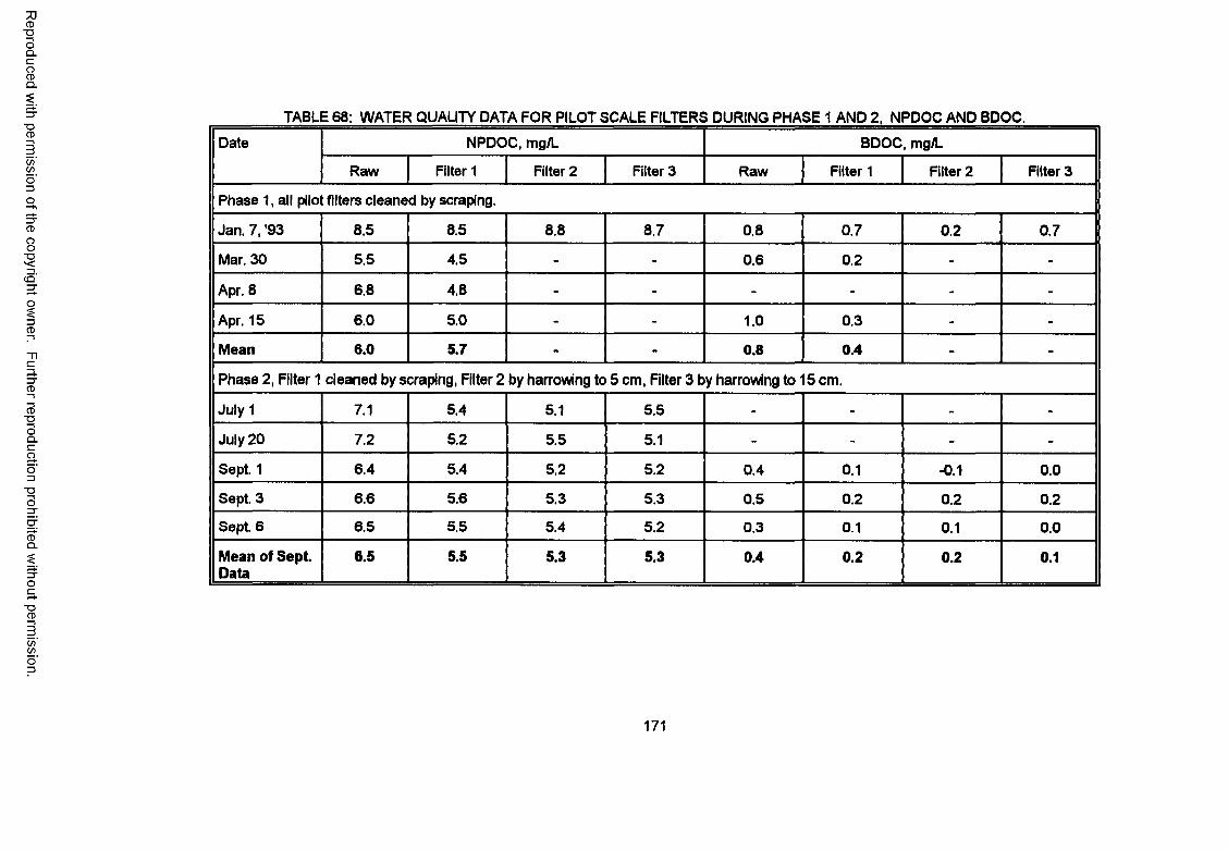
Reproduced
with perm
ission of the
copyright ow
ner. Further
reproduction prohibited
without
permission.
TABLE 68: WATER QUALITY DATA FOR PILOT SCALE FILTERS DURING PHASE 1 AND 2. NPDOC AND BDOC.
Date NPDOC, mg/L BDOC, mg/L
Raw Filter 1 Filter 2 Filter 3 Raw Filter 1 Filter 2 Filter 3
Phase 1, all pilot filters cleaned by scraping.
Jan. 7, '93 8.5 8.5 8.8 8.7 0.8 0.7 0.2 0.7
Mar. 30 5.5 4.5 - - 0.6 0.2 - -
Apr. 8 6.8 4.8 - - - - - -
Apr. 15 6.0 5.0 - - 1.0 0.3 - -
Mean 6.0 5.7 - - 0.8 0.4 - -
Phase 2, Filter 1 cleaned by scraping, Filter 2 by harrowing to 5 cm, Filter 3 by harrowing to 15 cm.
July 1 7.1 5.4 5.1 5.5 - - - -
July 20 7.2 5.2 5.5 5.1 - - - -
Sept. 1 6.4 5.4 5.2 5.2 0.4 0.1 -0.1 0.0
Sept. 3 6.6 5.6 5.3 5.3 0.5 0.2 0.2 0.2
Sept. 6 6.5 5.5 5.4 5.2 0.3 0.1 0.1 0.0
Mean of Sept. Data
6.5 5.5 5.3 5.3 0.4 0.2 0.2 0.1
171
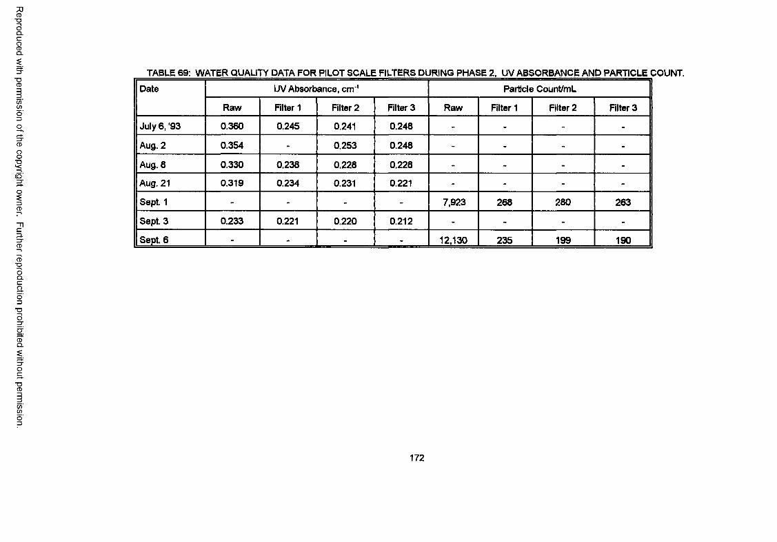
Reproduced
with perm
ission of the
copyright ow
ner. Further
reproduction prohibited
without
permission.
TABLE 69: WATER QUALITY DATA FOR PILOT SCALE FILTERS DURING PHASE 2. UV ABSORBANCE AND PARTICLE COUNT.
Date UV Absorbance, cm"' Particle Count/mL
Raw Filter 1 Filter 2 Filter 3 Raw Filter 1 Filter 2 Filter 3
July 6, '93 0.360 0.245 0.241 0.248 - - - -
Aug. 2 0.354 - 0.253 0.248 - - - -
Aug. 8 0.330 0.238 0.228 0.228 - - - -
Aug. 21 0.319 0.234 0.231 0.221 - - - -
Sept. 1 - - - - 7,923 268 280 263
Sept. 3 0.233 0.221 0.220 0.212 - - - -
Sept. 6 - - - - 12,130 235 199 190
172
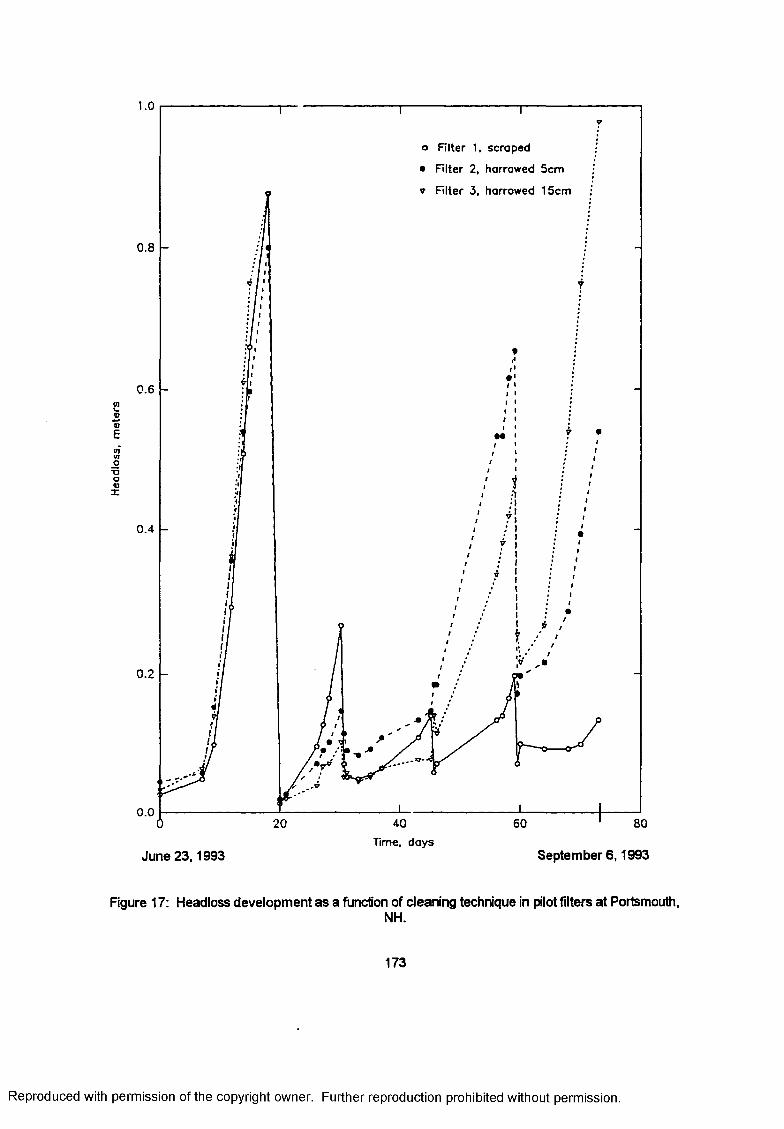
Hea
dlos
s,
met
ers
o niter 1. scraped
• Rlter 2, harrowed
» Rlter 3, harrowed
0.8
0.6
M
0 .4
0.2
0.020
Time, daysJune 23,1993 September 6,1993
Figure 17: Headloss development as a function of cleaning technique in pilot filters at Portsmouth,NH.
173
Reproduced with permission of the copyright owner. Further reproduction prohibited without permission.
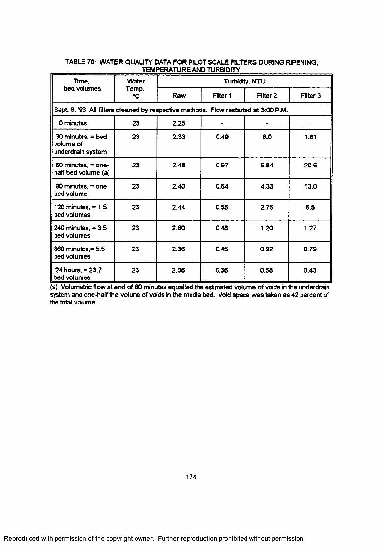
TABLE 70: WATER QUALITY DATA FOR PILOT SCALE FILTERS DURING RIPENING,______________________ TEMPERATURE AND TURBIDITY.
Time, bed volumes
WaterTemp.
°C
Turbidity, NTU
Raw Rlter 1 Rlter 2 Rlter 3
Sept 6, '93 All filters cleaned by respective methods. Flow restarted at 3:00 P.M.
0 minutes 23 2.25 - - -
30 minutes, = bed volume of underdrain system
23 2.33 0.49 6.0 1.61
60 minutes, = one- half bed volume (a)
23 2.48 0.97 6.84 20.6
90 minutes, = one bed volume
23 2.40 0.64 4.33 13.0
120 minutes, = 1.5 bed volumes
23 2.44 0.55 2.75 6.5
240 minutes, = 3.5 bed volumes
23 2.60 0.48 1.20 1.27
360 minutes,= 5.5 bed volumes
23 2.36 0.45 0.92 0.79
24 hours, = 23.7 bed volumes
23 2.06 0.36 0.58 0.43
a) Volumetric flow at end of 60 minutes equalled the estimated volume of voids in the underdrain system and one-half the volune of voids in the media bed. Void space was taken as 42 percent of the total volume.
174
Reproduced with permission of the copyright owner. Further reproduction prohibited without permission.
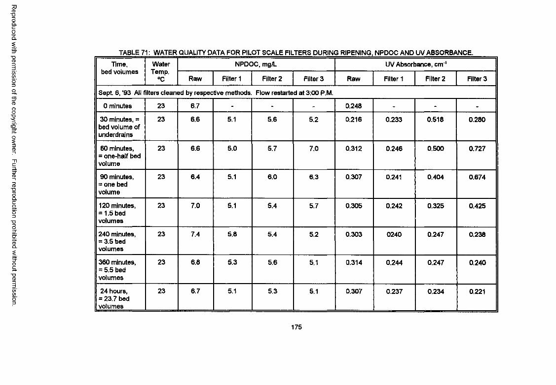
Reproduced
with perm
ission of the
copyright ow
ner. Further
reproduction prohibited
without
permission.
TABLE 71: WATER QUALITY DATA FOR PILOT SCALE FILTERS DURING RIPENING, NPDOC AND UV ABSORBANCE.
Time, bed volumes
WaterTemp.
°C
NPDOC, mg/L UV Absorbance, cm'1
Raw Filter 1 Filter 2 Filter 3 Raw Filter 1 Filter 2 Filter 3
Sept. 6, '93 All filters cleaned by respective methods. Flow restarted at 3:00 P.M.
0 minutes 23 6.7 - - - 0.248 - - -
30 minutes, = bed volume of underdrains
23 6.6 5.1 5.6 5.2 0.216 0.233 0.518 0.280
60 minutes,= one-half bed volume
23 6.6 5.0 5.7 7.0 0.312 0.246 0.500 0.727
90 minutes, = one bed volume
23 6.4 5.1 6.0 6.3 0.307 0.241 0.404 0.674
120 minutes, = 1.5 bed volumes
23 7.0 5.1 5.4 5.7 0.305 0.242 0.325 0.425
240 minutes, = 3.5 bed volumes
23 7.4 5.8 5.4 5.2 0.303 0240 0.247 0.238
360 minutes, = 5.5 bed volumes
23 6.8 5.3 5.6 5.1 0.314 0.244 0.247 0.240
24 hours, = 23.7 bed volumes
23 6.7 5.1 5.3 5.1 0.307 0.237 0.234 0.221
175
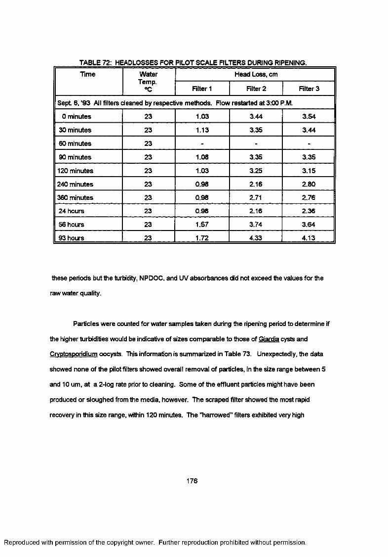
TABLE 72: HEADLOSSES FOR PILOT SCALE FILTERS DURING RIPENING.
Time WaterTemp.
°C
Head Loss, cm
Filter 1 Rlter 2 Rlter 3
Sept 6, '93 All filters cleaned by respective methods. Flow restarted at 3:00 P.M.
0 minutes 23 1.03 3.44 3.54
30 minutes 23 1.13 3.35 3.44
60 minutes 23 - - -
90 minutes 23 1.08 3.35 3.35
120 minutes 23 1.03 3.25 3.15
240 minutes 23 0.98 2.16 2.80
360 minutes 23 0.98 2.71 2.76
24 hours 23 0.98 2.16 2.36
56 hours 23 1.S7 3.74 3.64
93 hours 23 1.72 4.33 4.13
these periods but the turbidity, NPDOC, and UV absorbances did not exceed the values for the
raw water quality.
Particles were counted for water samples taken during the ripening period to determine if
the higher turbidities would be indicative of sizes comparable to those of Giardia cysts and
Cryptosporidium oocysts. This information is summarized in Table 73. Unexpectedly, the data
showed none of the pilot filters showed overall removal of particles, in the size range between 5
and 10 urn, at a 2-log rate prior to cleaning. Some of the effluent particles might have been
produced or sloughed from the media, however. The scraped filter showed the most rapid
recovery in this size range, within 120 minutes. The "harrowed" filters exhibited very high
176
Reproduced with permission of the copyright owner. Further reproduction prohibited without permission.
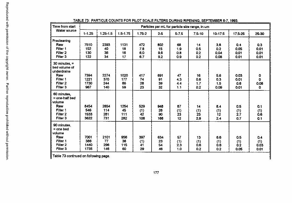
Reproduced
with perm
ission of the
copyright ow
ner. Further
reproduction prohibited
without
permission.
TABLE 73: PARTICLE COUNTS FOR PILOT SCALE FILTERS DURING RIPENING, SEPTEMBER 6-7,1993.
Time from start Water source
Particles per mL for particle size range, in urn
1-1.25 1.25-1.5 1.5-1.75 1.75-2 2-5 5-7.5 7.5-10 10-17.5 17.5-25 25-30
PrecleaningRaw 7510 2393 1131 472 802 68 14 3.8 0.4 0.3Filter 1 152 40 18 7.8 15 1.9 0.5 0.2 0.05 0.01Filter 2 130 36 16 6.0 9.6 0.8 0.2 0.04 0.01 0.01Filter 3 122 34 17 6.7 9.2 0.9 0.2 0.08 0.01 0.01
30 minutes, = bed volume of underdrains
Raw 7394 2274 1020 417 691 47 16 5.6 0.03 0Filter 1 1221 370 177 74 91 4.3 0.6 0.3 0.01 0Filter 2 1730 244 86 28 39 4.4 1.7 1.5 0.6 0.08Filter 3 967 140 59 23 32 1.1 0.2 0.09 0.01 0
60 minutes,= one-half bed
volumeRaw 8454 2654 1254 529 948 87 14 8.4 0.5 0.1Filter 1 546 114 45 (1) 26 (1) (1) (1) (1) (1)Filter 2 1533 281 111 42 90 23 23 12 2.7 0.6Filter 3 3622 731 282 106 168 12 2.9 2.4 0.7 0.1
90 minutes, = one bed
volumeRaw 7001 2101 956 397 634 57 13 6.6 0.5 0.4Filter 1 386 77 36 (1) 23 (1) (1) (1) (1) (1)Filter 2 1440 296 115 41 54 2.3 0.6 0.6 0.2 0.03Filter 3 1735 146 60 29 46 1.0 0.2 0.2 0.05 0.01
Table 73 continued on following page.
177
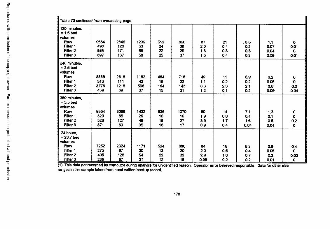
Reproduced
with perm
ission of the
copyright ow
ner. Further
reproduction prohibited
without
permission.
Table 73 continued from proceeding page.
120 minutes, = 1.5 bed
volumes Raw 9564 2846 1239 512 866 87 21 .8.6 1.1 0Filter 1 498 120 53 24 38 2.0 0.4 0.2 0.07 0.01Filter 2 858 171 65 22 29 1.6 0.3 0.3 0.04 0Filter 3 897 137 58 25 37 1.3 0.4 0.2 0.09 0.01
240 minutes, = 3.5 bed
volumes Raw 8886 2616 1182 464 716 49 11 6.9 0.2 0Filter 1 513 111 43 16 22 1.1 0.2 0.2 0.05 0Filter 2 3776 1216 506 164 143 6.6 2.3 2.1 0.6 0.2Filter 3 459 89 37 15 21 1.2 0.1 0.2 0.09 0.04
360 minutes, = 5.5 bed
volumes Raw 9534 3066 1432 636 1070 80 14 7.1 1.3 0Filter 1 320 65 26 10 16 1.9 0.6 0.4 0.1 0Filter 2 526 127 49 18 27 3.9 1.7 1.6 0.5 0.2Filter 3 371 83 35 16 17 0.9 0.4 0.04 0.04 0
24 hours,= 23.7 bed
volumes Raw 7252 2324 1171 524 886 84 16 8.2 0.9 0.4Filter 1 275 67 30 13 20 2.0 0.6 0.4 0.05 0Filter 2 495 126 54 22 32 2.9 1.0 0.7 0.2 0.03Filter 3 286 67 31 12 18 0.99 0.2 0.2 0.01 0
(1) This data not recorded by computer during analysis for unidentified reason. Operator error believed responsible. Data for other sizeranges in this sample taken from hand written backup record.
178
particle releases after cleaning, as also evidenced by the turbidity and color, but the removal had
recovered the precleaning level within 360 minutes for Rlter 3, but not within 24 hours for Rlter 2.
This was surprising as Rlter 3 had been disturbed more deeply than Rlter 2, to 15 cm vs 5 cm.
The greatest increases in particle release after cleaning occurred between 0 and 60
minutes after the flow was restarted in the scraped filter. The rates of increase were approximately
10-fold in the sizes up to 2 urn. The greatest releases for the "harrowed" filters occurred slightly
later, at about 60 minutes after the flow was restarted. Although the highest releases from Rlter 2
were detected 240 minutes after the flow was restarted, this "peak" occured after an earlier peak
had begun to decline and is suspected as atypical in a theoretical hydraulic flow through porous
media. This might occure in a plant scale application, however, due to effects of short-circuiting,
underdrain detention time, and/or intermittent release of deposits. Particle counting showed its
importance to operation control during the ripening period.
4.5.3 Sand Media
After the filters had operated for five cleaning cycles, Phase 2 of the pilot study was ended
and the sand media analyzed as for the plant scale filters. The results are summarized in Table
74. The data on media sample analyses was statistically analyzed. Volatile solids, in a 2-way
ANOVA between the top 2.5 cm and the level between 12-15 cm and between filters, showed
significant differences at the 90 percent confidence level. Differences within samples (interactions)
were not significant in 1-way ANOVA comparions, the differences between the filters were not
significant in the top 2.5 cm (p=0.34) but they were at the 12-15 cm level (p=.05). Similar
comparisons were made for FRM and carbohydrates, with results as summarized in Table 75.
There was no data on AFDC and there were no replicates on the analyses for metals. The
schmutsdecke sample was composited from the surface of all three filters to provide for sufficient
sample for analyses.
179
Reproduced with permission of the copyright owner. Further reproduction prohibited without permission.
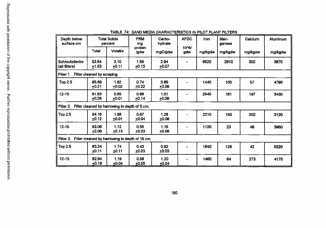
Reproduced
with perm
ission of the
copyright ow
ner. Further
reproduction prohibited
without
permission.
TABLE 74: SAND MEDIA CHARACTE RISTICS IN PILOT PLANT FILTERS
Depth below surface cm
Total Solids percent
FRMmg
Carbohydrate
AFDC Iron Manganese
Calcium Aluminum
Total Volatileprotein/gdw mgC/gdw
10*6/gdw mg/kgdw mg/kgdw mg/kgdw mg/kgdw
Schmutzdecke (all filters)
53.54±1.53
3.10±0.11
1.56±0.10
2.94±0.07
- 6520 2610 302 3870
Filter 1. Filter cleaned by scraping.
Top 2.5 85.89±0.21
1.62±0.02
0.74±0.22
0.85±0.06
- 1440 105 57 4790
12-15 81.63±0.26
0.85±0.01
0.66±0.14
1.01±0.06
- 2540 161 197 3430
Filter 2. Filter cleaned by harrowing to depth of 5 cm.
Top 2.5 84.18±0.12
1.68±0.01
0.67±0.04
1.28±0.08
- 2210 150 202 3120
12-15 83.06±2.09
1.12±0.13
0.55±0.03
1.15±0.06
- 1120 23 46 3950
Filter 3. Filter cleaned by harrowing to depth of 15 cm.
Top 2.5 83.24±0.11
1.74±0.11
0.43±0.03
0.92±0.03
- 1640 128 42 5220
12-15 82.94±0.19
1.19+0.04
0.58±0.05
1.20±0.04
- 1460 64 273 4170
180
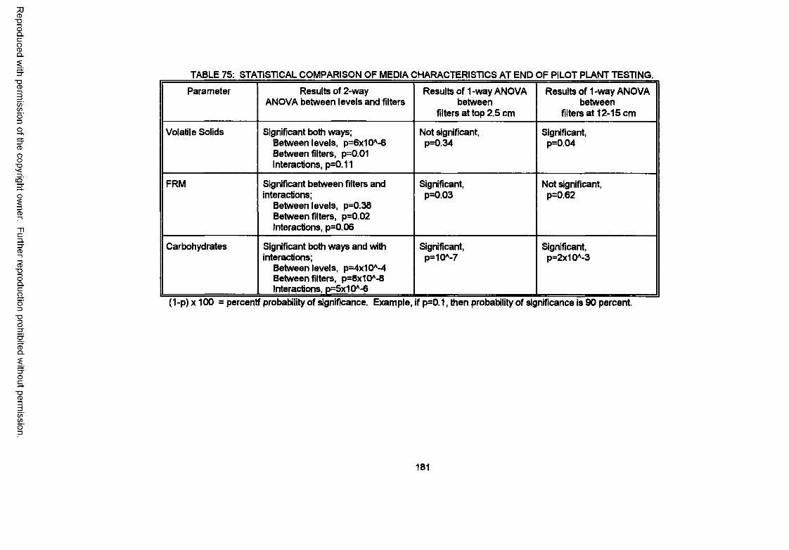
Reproduced
with perm
ission of the
copyright ow
ner. Further
reproduction prohibited
without
permission.
TABLE 75: STATISTICAL COMPARISON OF MEDIA CHARACTERISTICS AT END OF PILOT PLANT TESTING.
Parameter Results of 2-way ANOVA between levels and filters
Results of 1-way ANOVA between
filters at top 2.5 cm
Results of 1-way ANOVA between
filters at 12-15 cm
Volatile Solids Significant both ways; Between levels, psBxlOMS Between filters, p=0.01 Interactions, p=0.11
Not significant, p=0.34
Significant,p=0.04
FRM Significant between filters and interactions;
Between levels, p=0.38 Between filters, p=0.02 Interactions, p=0.06
Significant,p=0.03
Not significant,p=0.62
Carbohydrates Significant both ways and with interactions;
Between levels, p=4x10A-4 Between filters, p=8x10A-8 Interactions, p=5x10A-6
Significant,p=10A-7
Significant,p=2x10A-3
(1-p) x 100 = percent probability of significance. Example, if p=0.1, then probability of significance is 90 percent.
181
The cleaning methods resulted in different media coating characteristics although the
various parameters were not consistent in this conclusion. The differences between filters, shown
by the 2-way ANOVA, were consistenly significant for all parameters at probabilities greater than
for the interaction, demonstrating the filters had established separate characteristics, although they
may need to be operated for additional cleaning cycles for the differences in coating characteristics
to become consistently statistically significant at the respective levels.
4.6 LABORATORY SCALE STUDIES
Laboratory scale sand filter tests were earned out to compare filtration factors that could
not be made in the field. These factors included the influence on filter performance from age of
media and its position within the filter bed (i.e., top vs bottom), the effects of applying raw water
from one plant's source to the sand media from another plant, removing coating on the sand grains
in the media, and changing the rate of flow through the filter. The laboratory-scale tests were able
to compare these factors under constant temperature conditions and, unless intended otherwise, at
equal flow rates.
4.6.1 Influence of Sand Media Aae
The first series of tests were made using filter sand from the West Hartford, CT plant
where it had been determined that there were differences in performance between filters. The
sand was taken from Rlter 1 and Rlter 21 which represented nearly the longest (19 years) and
shortest (less than one year) periods since reconditioning of any of the filters at this plant
Separate samples of the sand were also taken from the selected filters at the top 1 cm (1 /2 in) and
at a depth of 25-30 cm (10-12 in) to compare differences that may be related to depths of media
within filters.
Information on the media characteristics, as collected from the filters and after preparation
for the filter column, is presented in Table 76. The effective sizes were increased from
182
Reproduced with permission of the copyright owner. Further reproduction prohibited without permission.
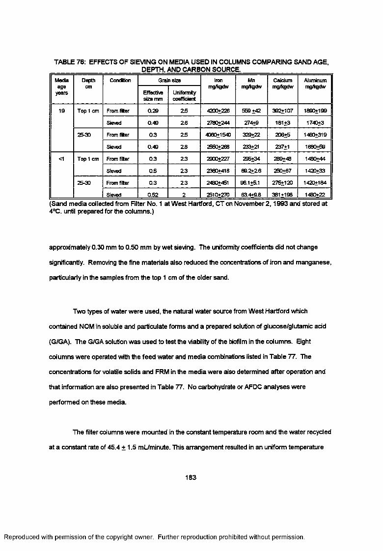
TABLE 76: EFFECTS OF SIEVING ON MEDIA USED IN COLUMNS COMPARING SAND AGE, _________________________ DEPTH, AND CARBON SOURCE.__________________________Mediaage
years
Depthcm
CondKon Gram size Ironmg/kgdw
Mnmg/kgdw
Calciummg/kgdw
Aluminummg/kgdw
Effective size mm
Uniformlycoefficient
19 Top 1 cm FrornfiKer 0.29 2 5 4200+226 559+42 392+107 1890+199
Sieved 0.49 2 6 2780+244 274+9 181+3 1740+3
2530 From fflter 0.3 2 5 4060+1540 329+22 206+5 1460+319
Sieved 0.49 2 8 233+21 237+1 1680+59
<1 Top 1 cm From titer 0.3 2 3 2900+227 295+34 289+48 1480+44
Sieved 0.5 2 3 2360+418 69.2+26 250+67 1420+33
2530 From filter 0.3 2 3 2480+451 96.1+5.1 275+120 1420+184
Sieved 0.52 2 2510+270 63.4+9.8 381+198 1480+22
Sand media collected from Filter No. 1 at West Hartford, CT on November 2,1993 and stored at 4°C. until prepared for the columns.)
approximately 0.30 mm to 0.50 mm by wet sieving. The uniformity coefficients did not change
significantly. Removing the fine materials also reduced the concentrations of iron and manganese,
particularly in the samples from the top 1 cm of the older sand.
Two types of water were used, the natural water source from West Hartford which
contained NOM in soluble and particulate forms and a prepared solution of glucose/glutamic add
(G/GA). The G/GA solution was used to test the viability of the biofilm in the columns. Eight
columns were operated with the feed water and media combinations listed in Table 77. The
concentrations for volatile solids and FRM in the media were also determined after operation and
that information are also presented in Table 77. No carbohydrate or AFDC analyses were
performed on these media.
The filter columns were mounted in the constant temperature room and the water recyded
at a constant rate of 45.4 ± 1.5 mL/minute. This arrangement resulted in an uniform temperature
183
Reproduced with permission of the copyright owner. Further reproduction prohibited without permission.
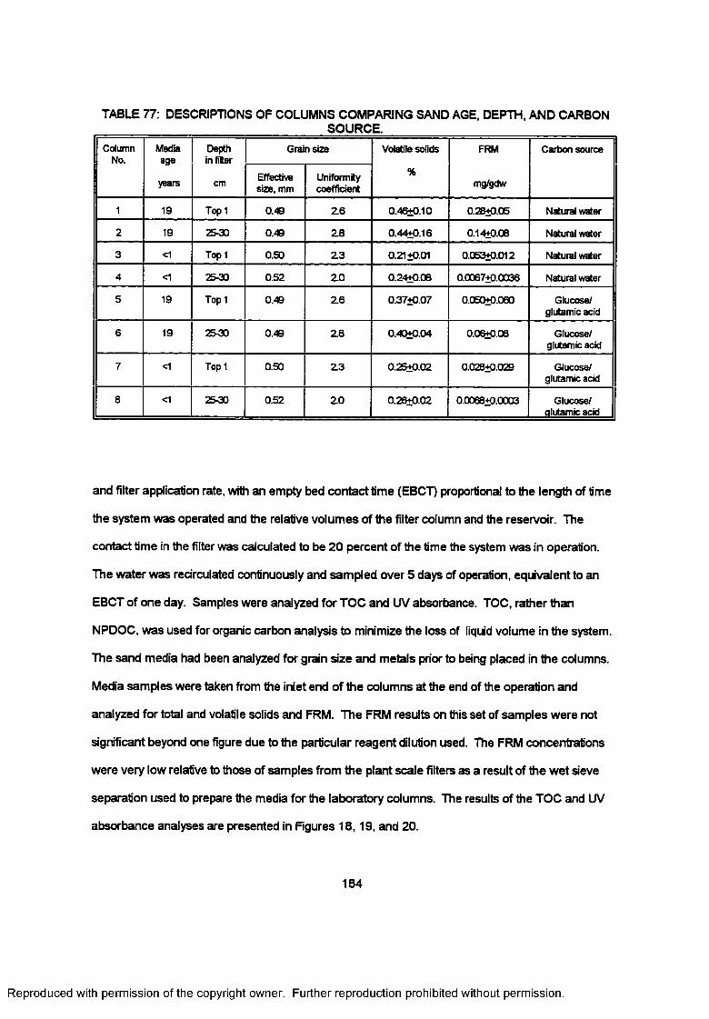
TABLE 77: DESCRIPTIONS OF COLUMNS COMPARING SAND AGE, DEPTH, AND CARBON ________ SOURCE.Column
No.Mediaage
years
Depth in liter
Grain size Volatile solids FRM Carbon source
cm Effective size, mm
Uniformlycoefficient
%mg/gdw
1 19 Top 1 0.49 2 6 0.48+0.10 0.28+0.05 Natural water
2 19 25-30 0.49 2 8 0.44+0.16 0.14+0.08 Natural water
3 <1 Topi 0.50 2 3 0.21+0.01 0.063+0.012 Natural water
4 <1 25-30 0.52 2 0 0.24+0.08 0.0067+0.0036 Natural water
5 19 Top 1 0.49 2 6 0.37+0.07 0.050+0.060 Glucose/ glutamic acid
6 19 2530 0.49 2 8 0.40+0.04 0.06+0.06 Glucose/ glutamic acid
7 <1 Top 1 0.50 2 3 0.25+0.02 0.028+0.029 Glucose/ glutamic acid
8 <1 2530 0.52 2 0 0.26+0.02 0.0068+0.0003 Glucose/ glutamic add
and filter application rate, with an empty bed contact time (EBCT) proportional to the length of time
the system was operated and the relative volumes of the filter column and the reservoir. The
contact time in the filter was calculated to be 20 percent of the time the system was in operation.
The water was recirculated continuously and sampled over 5 days of operation, equivalent to an
EBCT of one day. Samples were analyzed for TOC and UV absorbance. TOC, rather than
NPDOC, was used for organic carbon analysis to minimize the loss of liquid volume in the system.
The sand media had been analyzed for grain size and metals prior to being placed in the columns.
Media samples were taken from the inlet end of the columns at the end of the operation and
analyzed for total and volatile solids and FRM. The FRM results on this set of samples were not
significant beyond one figure due to the particular reagent dilution used. The FRM concentrations
were very low relative to those of samples from the plant scale filters as a result of the wet sieve
separation used to prepare the media for the laboratory columns. The results of the TOC and UV
absorbance analyses are presented in Figures 18,19, and 20.
184
Reproduced with permission of the copyright owner. Further reproduction prohibited without permission.
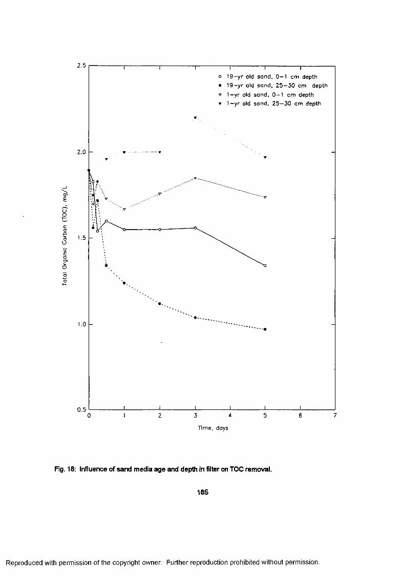
Tota
l O
rgan
ic
Car
bon
(TO
C),
mg
/L2.5
o 1 9 -y r old sand. 0 —1 cm depth
• 19—yr old sand, 2 5 - 3 0 cm depth
1 —yr old sand. 0 - 1 cm depth
▼ 1 - y r old sand, 2 5 —30 cm depth
V.
2.0
' • —
0.55 70 2 3 4 6
Time, days
Fig. 18: Influence of sand media age and depth in filter on TOC removal.
185
Reproduced with permission of the copyright owner. Further reproduction prohibited without permission.
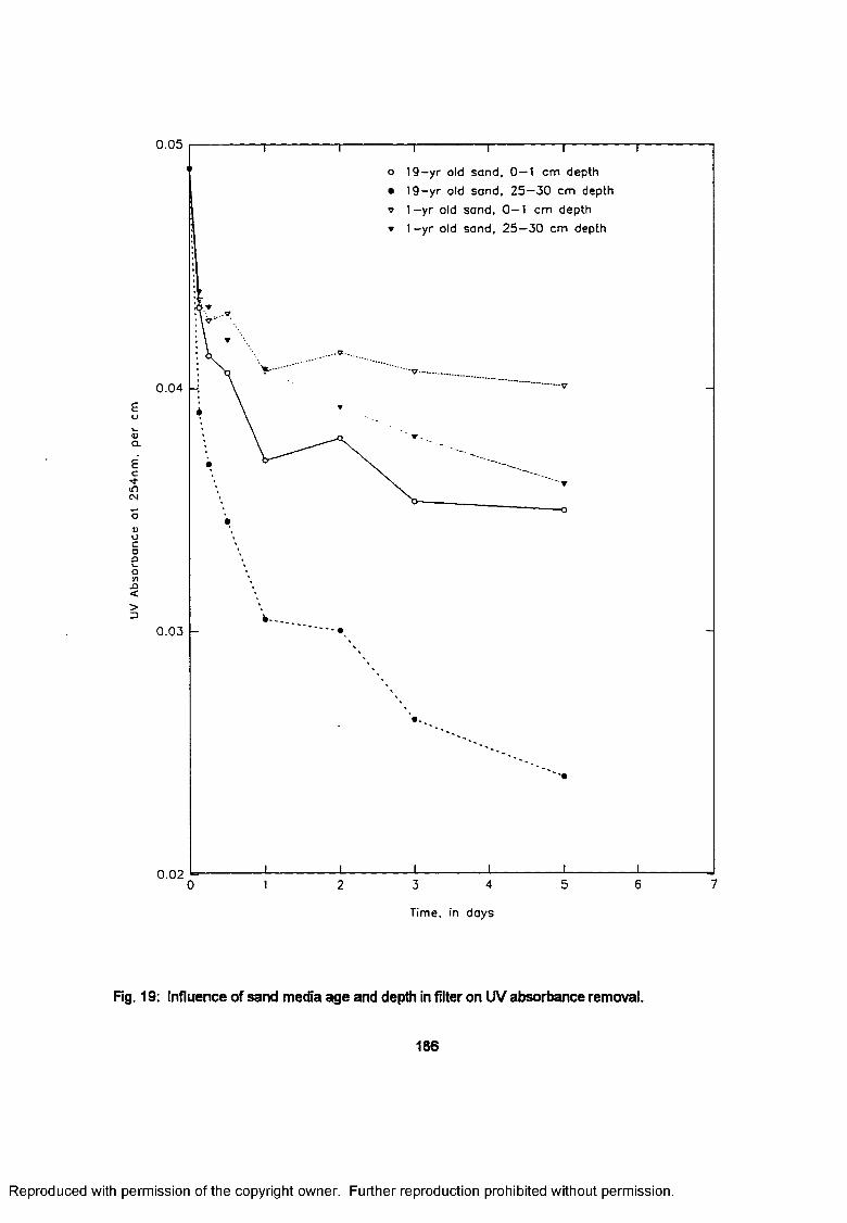
UV
Abs
orba
nce
at
254n
m,
per
cm0.05
1 9 -y r old sand, 0 —1 cm depth
1 9 -y r old sand, 2 5 —30 cm depth
1- y r old sand, 0 —1 cm depth
1 —yr old sand, 2 5 —30 cm depth
0 .0 4
0 .0 3
0.02
Time, in days
Fig. 19: Influence of sand media age and depth in filter on UV absorbance removal.
186
Reproduced with permission of the copyright owner. Further reproduction prohibited without permission.
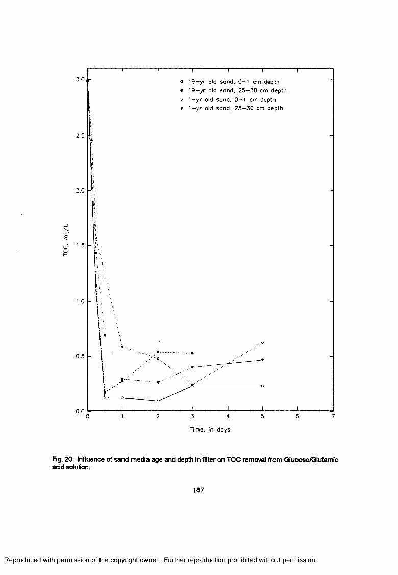
3.0 o 19—yr old sand, 0 —1 cm depth
• 19—yr old sand, 2 5 —30 cm depth
v 1 —yr old sand, 0 - 1 cm depth
* 1—yr old sand, 2 5 - 3 0 cm depth
2.5
2.0
_ i
o>E
oot-
0.5
0.0
Time, in days
Fig. 20: Influence of sand media age and depth in filter on TOC removal from Glucose/Glutamic add solution.
187
Reproduced with permission of the copyright owner. Further reproduction prohibited without permission.
Removals of both TOC and UV absorbance from the natural water source were greater
for the columns containing sand that had been in service for 19 years than for the columns
containing "younger sand", regardless of depth, and greater for the sand taken at a depth of 25-30
cm in the filters than for the sand taken from the top 1 cm of a filter, regardless of age. The
removal rates for TOC were similar to those for UV absorbance except in the column circulating
the natural water and containing sand collected from the top of a filter which had been in operation
less than 1 year. In that column, the TOC concentration initially decreased but, after the first 3
hours of operation (EBCT = 0.6 hours), the TOC concentration increased and then remained
slightly above the concentration in the raw water for the remainder of the 5 days operation. Only
one column showed an increase in UV absorbance after the initial reduction. It appeared that there
was an initial removal of both NOM and G/GA followed by a period when the filters were releasing
material. The released materials also appeared primarily aliphatic as they do not cause UV
absorbance but are detected by the TOC test which detects both aliphatic and aromatic
compounds. A study of the source and significance of these releases should be made, perhaps
using water sources labelled with radiocarbon to determine if the released material has first been
metabolized.
Removal of TOC from the glucose/glutamic add solution was similar in certain respects to
removals from natural water though the rate and percentages removed were higher. The influent
TOC concentration was reduced by 96 percent within 12 hours (EBCT = 2.4 hours) by the 19 year
old sand taken from a filter at a depth of 25-30 cm as compared to a 16 percent reduction in TOC
from the natural water over the same time period by the same sand and depth. Removals of TOC
from the G/GA solution by media in the other columns were less rapid but they each reduced the
TOC to less than 10 percent of the initial concentration in 12 to 76 hours (EBCT = 2.4 to 15 hours).
The relative performances of the individual sand media were in the same order as for removal of
TOC and UV absorbance from natural water.
188
Reproduced with permission of the copyright owner. Further reproduction prohibited without permission.
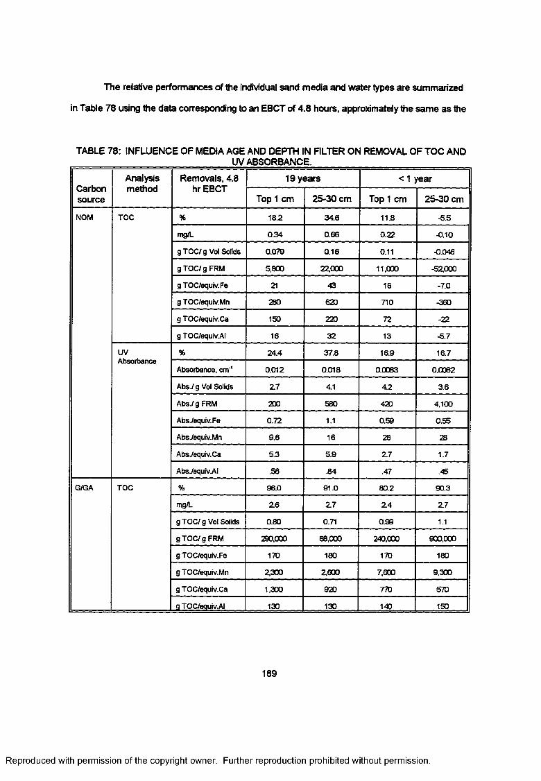
The relative performances of the individual sand media and water types are summarized
in Table 78 using the data corresponding to an EBCT of 4.8 hours, approximately the same as the
TABLE 78: INFLUENCE OF MEDIA AGE AND DEPTH IN FILTER ON REMOVAL OF TOC AND ____________ UV ABSORBANCE.
Carbonsource
Analysismethod
Removals, 4.8 hr EBCT
19 years < 1 year
Top 1 cm 25-30 cm Top 1 cm 25-30 cm
NOM TOC % 18.2 34.6 11.8 -5.5
mg/L 0.34 0.66 0.22 -0.10
g TOC/g Vol Solids 0.079 0.16 0.11 -0.046
gTO C/g FRM 5,800 22000 11,000 -52000
g TOC/equiv.Fe 21 43 16 -7.0
g TOC/equiv.Mn 280 620 710 -360
g TOC/equiv.Ca 150 220 72 -22
g TOC/equiv.AI 16 32 13 -5.7
UVAbsorbance
% 24.4 37.8 16.9 16.7
Absorbance, cnv' 0.012 0.018 0.0063 0.0082
Abs./ g Vol Solids 2 7 4.1 4.2 3.6
AbsigFRM 200 580 420 4.100
AbsJequiv.Fe 0.72 1.1 0.59 0.55
AbsVequiv.Mn 9.6 16 26 28
Abs./equiv.Ca 5.3 5.9 2 7 1.7
Abs./equiv.AI .56 .84 .47 .45
G/GA TOC % 96.0 91.0 80.2 90.3
mg/L 2 6 2 7 2 4 2 7
gTO C/g Vol Solids 0.80 0.71 0.99 1.1
gTO C/g FRM 290.000 68,000 240,000 900,000
g TOC/equiv.Fe 170 180 170 180
g TOC/equiv.Mn 2300 2600 7,600 9,300
g TOC/equiv.Ca 1,300 920 770 570
q TOC/equiv.AI 130 130 140 150
189
Reproduced with permission of the copyright owner. Further reproduction prohibited without permission.
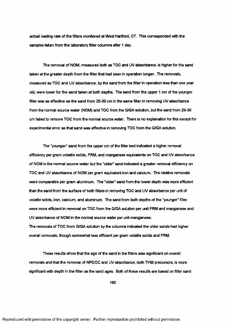
actual loading rate of the filters monitored at West Hartford, CT. This corresponded with the
samples taken from the laboratory filter columns after 1 day.
The removal of NOM, measured both as TOC and UV absorbance, is higher for the sand
taken at the greater depth from the filter that had been in operation longer. The removals,
measured as TOC and UV absorbance, by the sand from the filter in operation less than one year
old, were lower for the sand taken at both depths. The sand from the upper 1 cm of the younger
filter was as effective as the sand from 25-30 cm in the same filter in removing UV absorbance
from the normal source water (NOM) and TOC from the G/GA solution, but the sand from 25-30
cm failed to remove TOC from the normal source water. There is no explanation for this except for
experimental error as that sand was effective in removing TOC from the G/GA solution.
The "younger" sand from the upper cm of the filter bed indicated a higher removal
efficiency per gram volatile solids, FRM, and manganese equivalents on TOC and UV absorbance
of NOM in the normal source water but the "older" sand indicated a greater removal efficiency on
TOC and UV absorbance of NOM per gram equivalent iron and caldum. The relative removals
were comparable per gram aluminum. The "older" sand from the lower depth was more efficient
than the sand from the surface of both filters in removing TOC and UV absorbance per unit of
volatile solids, iron, caldum, and aluminum. The sand from both depths of the "younger” filter
were more effident in removal on TOC from the G/GA solution per unit FRM and manganese and
UV absorbance of NOM in the normal source water per unit manganese.
The removals of TOC from G/GA solution by the columns indicated the older sands had higher
overall removals, though somewhat less effident per gram volatile solids and FRM.
These results show that the age of the sand in the filters was significant on overall
removals and that the removal of NPDOC and UV absorbance, both THM precursors, is more
significant with depth in the filter as the sand ages. Both of these results are based on filter sand
190
Reproduced with permission of the copyright owner. Further reproduction prohibited without permission.
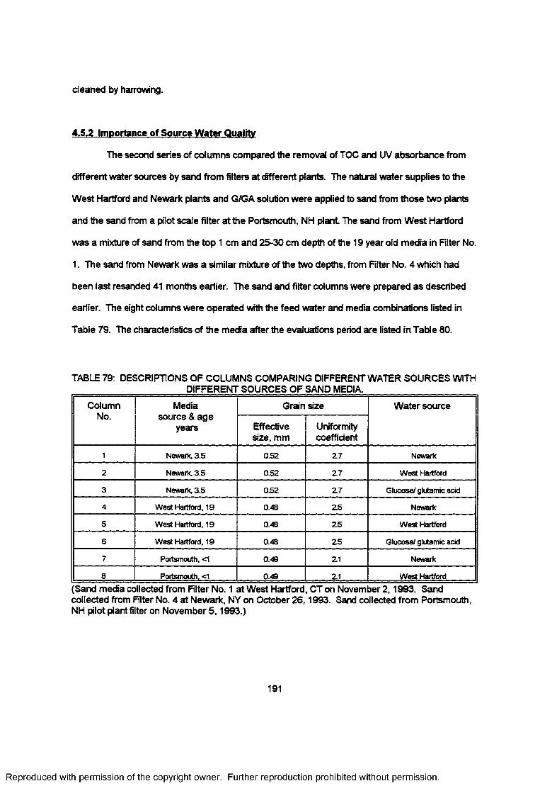
cleaned by harrowing.
4.5.2 Importance of Source Water Quality
The second series of columns compared the removal of TOC and UV absorbance from
different water sources by sand from filters at different plants. The natural water supplies to the
West Hartford and Newark plants and G/GA solution were applied to sand from those two plants
and the sand from a pilot scale filter at the Portsmouth, NH plant The sand from West Hartford
was a mixture of sand from the top 1 cm and 25-30 cm depth of the 19 year old media in Filter No.
1. The sand from Newark was a similar mixture of the two depths, from Filter No. 4 which had
been last resanded 41 months earlier. The sand and filter columns were prepared as described
earlier. The eight columns were operated with the feed water and media combinations listed in
Table 79. The characteristics of the media after the evaluations period are listed in Table 80.
TABLE 79: DESCRIPTIONS OF COLUMNS COMPARING DIFFERENT WATER SOURCES WITHDIFFERENT SOURCES OF SAND MEDIA.
ColumnNo.
Media source & age
years
Grain size Water source
Effective size, mm
Uniformitycoefficient
1 Newark, 3.5 0.52 2 7 Newark
2 Newark, 3.5 0.52 2.7 West Hartford
3 Newark, 3.5 0.52 2.7 Glucose/ glutamic acid
4 West Hartford, 19 0.48 2.5 Newark
5 West Hartford, 19 0.48 2 5 West Hartford
6 West Hartford, 19 0.48 25 Glucose/ glutamic acid
7 Portsmouth. <1 0.49 21 Newark
8 Portsmouth. <1 0.49 21 West Hartford
[Sand media collected from Filter No. 1 at West Hartford, CT on November 2,1993. Sand collected from Filter No. 4 at Newark, NY on October 26,1993. Sand collected from Portsmouth, NH pilot plant filter on November 5,1993.)
191
Reproduced with permission of the copyright owner. Further reproduction prohibited without permission.
Reproduced
with perm
ission of the
copyright ow
ner. Further
reproduction prohibited
without
permission.
TABLE 80: CHARACTERISTICS OF SAND MEDIA AFTER COMPARING PERFORMANCE WITH DIFFERING WATER SOURCE AND ____________________________ DIFFERENT SOURCES OF SAND MEDIA. ___________
Column Media Volatile FRM Carbo AFDC Iron Manganese Calcium AluminumNo. source & solids hydrate
age mgC/gdw 10*6/in years % mg/gdw x 1000 gdw mg/kgdw mg/kgdw mg/kgdw mg/kgdw
1 Newark, 1.19+0.11 0.13+0.04 12.3+1.5 0.9+0.1 9270 540 120000 33603.5 ±488 ±18 ±8580 ±536
2 Newark, 1.29+0.07 0.16+0.02 12.0+1.0 1.1±1.3 9610 544 116000 39003.5 ±370 ±46 ±22800 ±145
3 Newark, 1.15+0.15 0.21+0.11 13.2+1.0 1.5+0.2 8060 497 117000 29903.5 ±620 ±71 ±2280 ±352
4 West 0.34±0.04 0.25+0.01 33.8+4.2 5.7+3.3 2880 281 1010 1870Hartford, 19 ±391 ±34 ±587 ±488
5 West 0.38+0.17 0.23+0.03 29.0+2.5 4.9+0.8 3180 248 298 1880Hartford, 19 ±157 ±2 ±58 ±107
6 West 0.44±0.17 0.19+0.04 34.4+1.3 4.3+0.2 3660 237 377 2020Hartford, 19 ±266 ±12 ±128 ±237
7 Portsmouth, 0.50+0.04 0.24±0.02 31.4+3.7 2.8+0.8 1900 31 217 2230<1 ±713 ±8 ±75 ±246
8 Portsmouth, 0.51+0.01 0.22+0.01 31.3+0.7 4.8+1.3 1920 33 299 2390<1 ±822 ±1 +47 ±76
192
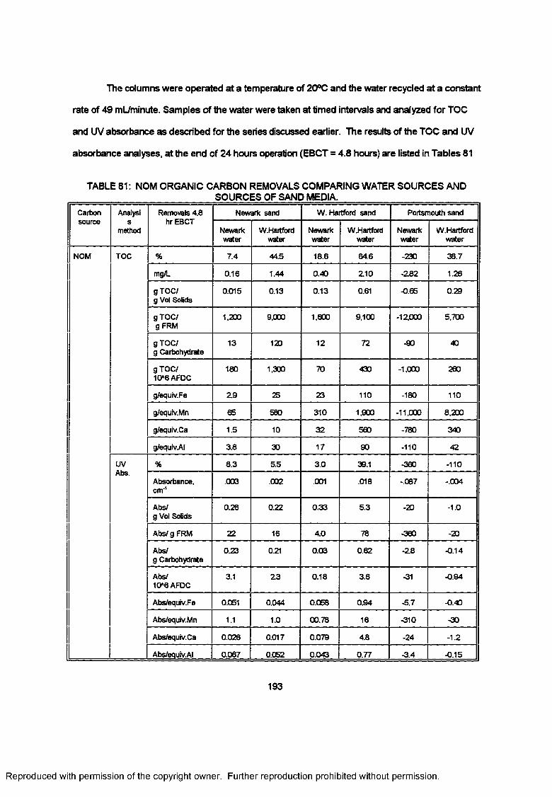
The columns were operated at a temperature of 20°C and the water recycled at a constant
rate of 49 mL/minute. Samples of the water were taken at timed intervals and analyzed for TOC
and UV absorbance as described for the series discussed earlier. The results of the TOC and UV
absorbance analyses, at the end of 24 hours operation (EBCT = 4.8 hours) are listed in Tables 81
TABLE 81: NOM ORGANIC CARBON REMOVALS COMPARING WATER SOURCES ANDSOURCES OF SAND MEDIA.
Carbon Analysi Removals 4.8 hr EBCT
Newark sand W . Hartford sand Portsmouth sandsource s
method Newarkwater
W.Hartfordwater
Newarkwater
W.Hartfordwater
Newarkwater
W.Hartfordwater
NOM TOC % 7.4 44.5 18.6 64.6 -230 38.7
mg/L 0.16 1.44 0.40 210 -282 1.26
gTOC/ g Vol Solids
0.015 0.13 0.13 0.61 -0.65 0.29
gTOC/ g FRM
1,200 9,000 1,600 9,100 -12000 5,700
gTOC/g Carbohydrate
13 120 12 72 -90 40
gTOC/10»6AFDC
180 1,300 70 430 -1,000 260
g/equiv.Fe 2.9 25 23 110 -180 110
g/equiv.Mn 65 580 310 1,900 -11,000 8,200
g/equiv.Ca 1.5 10 32 560 -780 340
g/equiv.AI 3.8 30 17 90 -110 42
UVAbs.
% 8.3 5.5 3.0 39.1 -360 -110
Absorbance,cm'1
.003 .002 .001 .018 -.087 -.004
Abs/g Vol Solids
0.28 0.22 0.33 5.3 -20 -1.0
Abs/g FRM 22 16 4.0 78 -360 -20
Abs/g Carbohydrate
0.23 0.21 0.03 0.62 -28 -0.14
Abs/10*6 AFDC
3.1 23 0.18 3.6 -31 -0.94
Abs/equiv.Fe 0.051 0.044 0.058 0.94 -5.7 -0.40
Abs/equiv.Mn 1.1 1.0 00.78 16 -310 -30
Abs/equiv.Ca 0.026 0.017 0.079 4.8 -24 -1.2
Abs/equiv.AI 0.067 0.052 0.043 0.77 -3.4 -0.15
193
Reproduced with permission of the copyright owner. Further reproduction prohibited without permission.
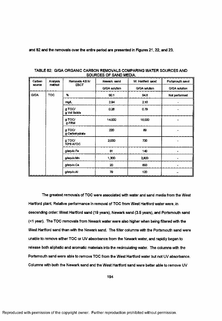
and 82 and the removals over the entire period are presented in Rgures 21,22, and 23.
TABLE 82: G/GA ORGANIC CARBON REMOVALS COMPARING WATER SOURCES AND SOURCES OF SAND MEDIA.
Carbon Analysismethod
Removals 4.8 hr EBCT
Newark sand W.Hartford sand Portsmouth sandsource
G/GA solution G/GA solution G/GA solution
G/GA TOC % 90.1 94.6 Not performed
mg/L 29 4 210 -
gTO C/ g Vol Solids
0.28 0.79 -
gTO C/ g FRM
14.000 16.000 -
gTO C/ g Carbohydrate
220 89 -
gTO C/ 10*6 AFDC
2000 720 -
g/equiv.Fe 61 140 -
g/equiv.Mn 1,300 2800 -
g/equiv.Ca 20 650 -
g/equiv.AI 79 120 -
The greatest removals of TOC were associated with water and sand media from the West
Hartford plant Relative performance in removal of TOC from West Hartford water were, in
descending order: West Hartford sand (19 years), Newark sand (3.5 years), and Portsmouth sand
(<1 year). The TOC removals from Newark water were also higher when being filtered with the
West Hartford sand than with the Newark sand. The filter columns with the Portsmouth sand were
unable to remove either TOC or UV absorbance from the Newark water, and rapidly began to
release both aliphatic and aromatic materials into the recirculating water. The columns with the
Portsmouth sand were able to remove TOC from the West Hartford water but not UV absorbance.
Columns with both the Newark sand and the West Hartford sand were better able to remove UV
194
Reproduced with permission of the copyright owner. Further reproduction prohibited without permission.
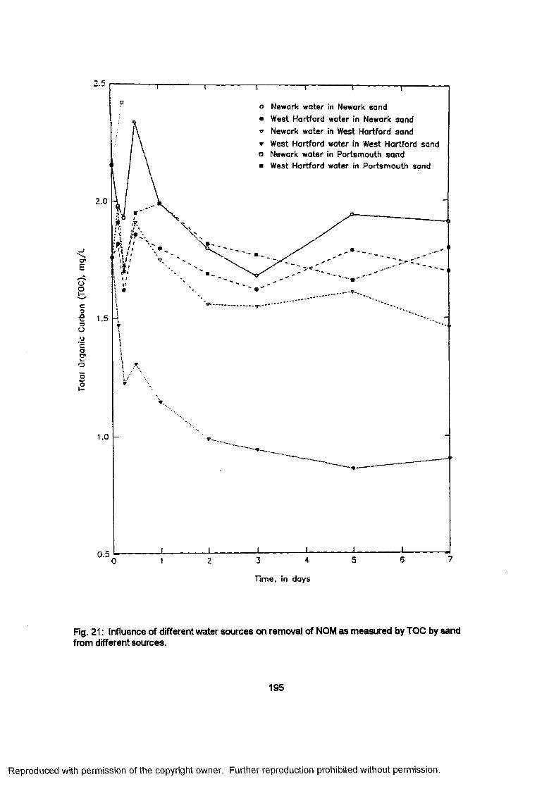
Tota
l O
rgan
ic
Car
bon
(TO
C),
mg
/L
Newark water in Newark sand West Hartford water in Newark sand Newark water in West Hartford sand West Hartford water in West Hartford sand Newark water in Portsmouth sand West Hartford water in Portsmouth sand
2.0
;C.
0.5
Time, in days
Fig. 21: Influence of different water sources on removal of NOM as measured by TOC by sand from different sources.
195
Reproduced with permission of the copyright owner. Further reproduction prohibited without permission.
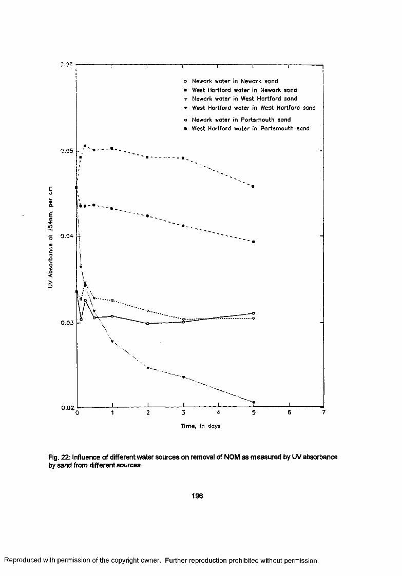
UV A
bsor
banc
e at
254n
m,
per
Newark water in Newark sand
West Hartford w ater in Newark sand
Newark w ater in West Hartford sand
West Hartford w ater in West Hartford sand
Newark water in Portsmouth sand
West Hartford water in Portsmouth sand
0 .0 5
Eo
0 .0 4
■ • 7.- o -
0 .0 3
0.02
Time, in days
Fig. 22: Influence of different water sources on removal of NOM as measured by UV absorbance by sand from different sources.
196
Reproduced with permission of the copyright owner. Further reproduction prohibited without permission.
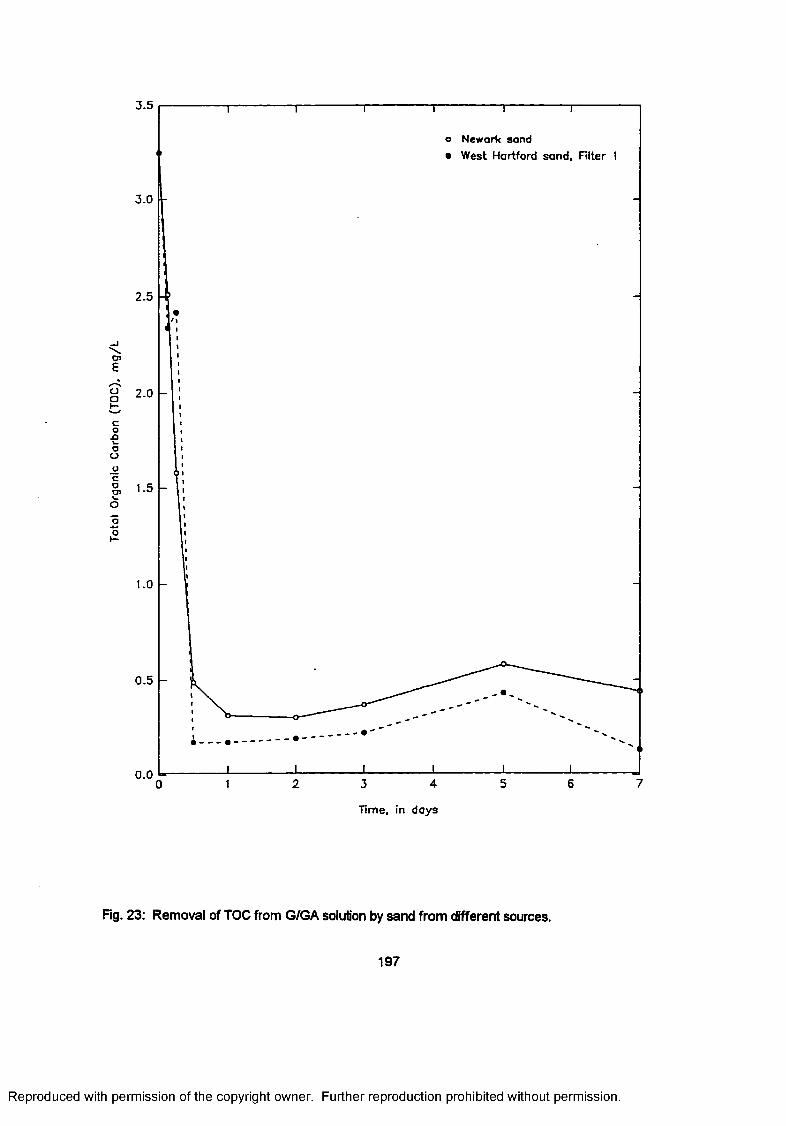
Toto
l O
rgan
ic
Carb
on
(TO
C),
mg
/L3.5
o Newark sand
• West Hartford sand. Filter 1
3 .0
2 .5
2.0
1.5
1.0
0 .5
o -
0.05 73 62 410
Time, in days
Fig. 23: Removal of TOC from G/GA solution by sand from different sources.
197
Reproduced with permission of the copyright owner. Further reproduction prohibited without permission.
absorbing material from the source water normally supplied to these filter media than from the
water from the other source. The West Hartford sand was able to remove 39 percent of the UV
absorbing material from its own source water as compared to the Newark sand removing only 8
percent from its own supply, however. TOC in the water from the West Hartford source was more
readily removed than that in water from the Newark supply or Portsmouth supply. The UV
absorbance also was more readily removed than that in water from the other supplies. Generally
the sand media normally used with a water source, and therefore acclimated to it, was able to
remove a greater percentage of the NOM and UV absorbance from that supply than the sand
media from another plant although the sand media from the West Hartford plant was more
effective in removing TOC from the Newark source than was the Newark sand media. Both
media removed TOC from the G/GA solution at appntimately the same percentage. The removals
per unit of FRM, carbohydrate, and AFDC were higher for the Newark sand media.
4.2.3 Influence of Natural Coating Material on Filter Media
A third set of columns were run to compare removal of TOC and UV absorbance after
removing a portion of natural media coating on the sand. Media preparation was described in
Chapter 3. Four pairs of columns were prepared. Pairs of columns had all, two-thirds, one-third,
or none of the natural coating removed by add and combustion, as described in "Methods and
Materials," and one column of each pair operated water sources as summarized in Table 83. The
results of the analyses for TOC and UV absorbance at the end of the first day of the operating
period (EBCT equal to 4.8 hours) are summarized in Tables 84 and 85 and the removals over the
entire period are presented in Figures 24, 25, and 26.
The respective filters media removed NOM and G/GA, measured both as TOC and UV
absorbance, in relative proportion to the amounts of initial biomass on the sand. The columns
which contained sand which had all organic coating and metallic coating removed still
demonstrated an ability to remove organic carbon. There was no evidence of a lag period before
198
Reproduced with permission of the copyright owner. Further reproduction prohibited without permission.
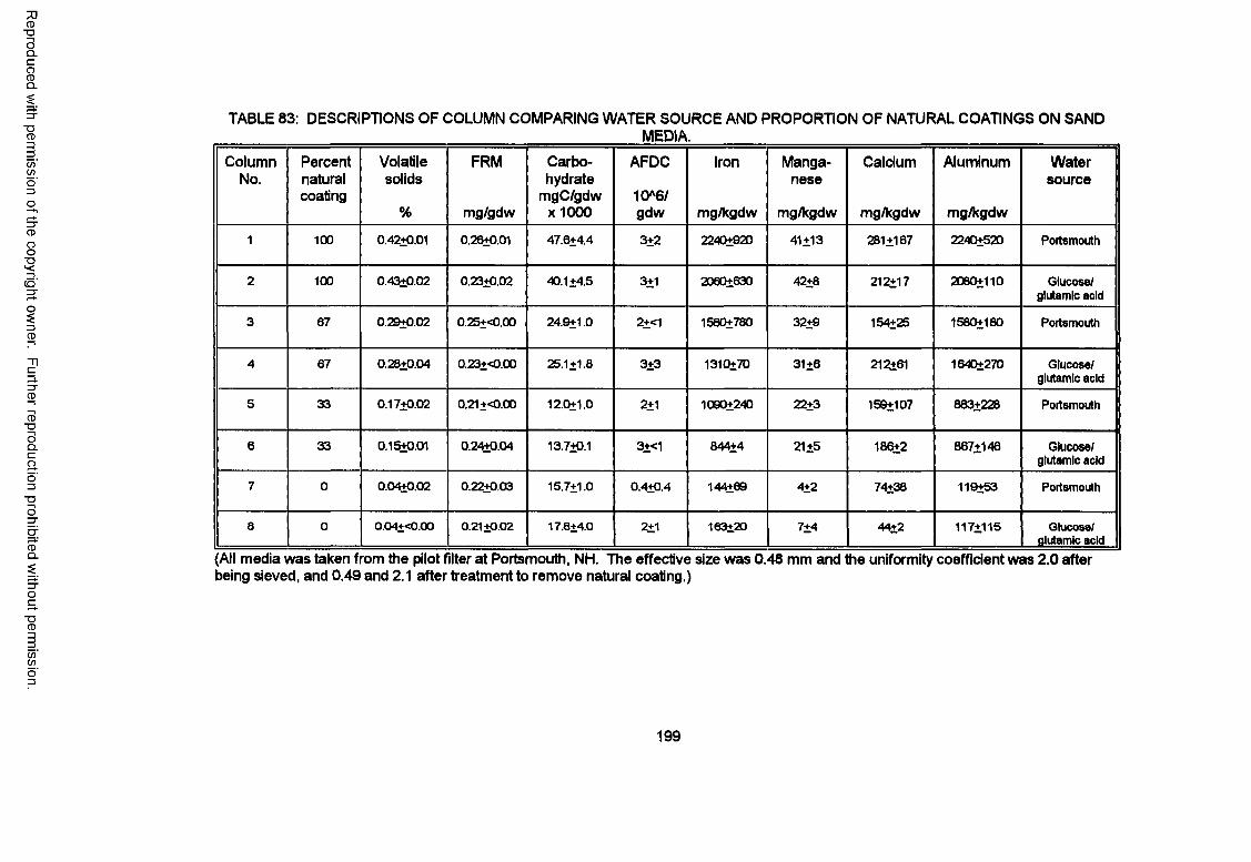
Reproduced
with perm
ission of the
copyright ow
ner. Further
reproduction prohibited
without
permission.
TABLE 83: DESCRIPTIONS OF COLUMN COMPARING WATER SOURCE AND PROPORTION OF NATURAL COATINGS ON SAND _____________________________________________________ MEDIA._____________________________________________________
ColumnNo.
Percentnaturalcoating
Volatilesolids
%
FRM
mg/gdw
Carbohydrate
mgC/gdw x 1000
AFDC
10*6/gdw
Iron
mg/kgdw
Manganese
mg/kgdw
Calcium
mg/kgdw
Aluminum
mg/kgdw
Watersource
1 100 0.42+0.01 0.26+0.01 47.6+4.4 3+2 2240+920 41+13 281+167 2240+520 Portsmouth
2 100 0.43+0.02 0.23+002 40.1+4.5 3+1 206Q+630 42+8 212+17 2060+110 Glucose/ glutamic acid
3 67 0.29+0.02 0.25+0.00 24.9+1.0 2+<1 1580+780 32+9 154+25 1560+180 Portsmouth
4 67 0.28+0.04 0.23+0.00 25.1+1.8 3+3 1310+70 31+6 212+61 1640+270 Glucose/ glutamic acid
5 33 0.17+0.02 0.21+0.00 12.0+1.0 2+1 1090+240 22+3 159+107 883+228 Portsmouth
6 33 0.15+0.01 0.24+0.04 13.7+0.1 3+<1 844+4 21+5 186+2 867+146 Glucose/ glutamic acid
7 0 0.04+0.02 0.22+0.03 15.7+1.0 0.4+0.4 144+69 4+2 74+38 119+53 Portsmouth
8 0 0.04+<0.00 0.21+0.02 17.8+4.0 2+1 163+20 7+4 44+2 117+115 Glucose/ glutamic add
(All media was taken from the pilot filter at Portsmouth, NH. The effective size was 0.48 mm and the uniformity coefficient was 2.0 after being sieved, and 0.49 and 2.1 after treatment to remove natural coating.)
199
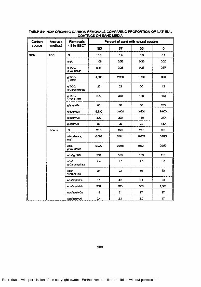
TABLE 84: NOM ORGANIC CARBON REMOVALS COMPARING PROPORTION OF NATURALCOATINGS ON SAND MEDIA.
Carbon Analysis Removals Percent of sand with natural coatingsource method 4.8 hr EBCT
100 67 33 0
NOM TOC % 16.8 8.9 5.6 3.1
mg/L 1.06 0.56 0.36 0.20
gTOC/ g Vol Solids
0.31 0.23 0.23 0.57
gTOC / g FRM
4,000 2,300 1,700 890
gTOC/ g Carbohydrate
22 23 30 12
gTOC / 10*6 AFDC
370 310 180 470
g/equiv.Fe 80 60 55 230
g/equiv.Mn 5,700 3,900 3,500 9,900
g/equiv.Ca 300 290 180 210
g/equiv.AI 38 29 32 130
UVAbs. % 25.8 15.5 12.5 9.5
Absorbance,cm'1
0.068 0.041 0.033 0.025
Abs7g Vol Solids
0.020 0.016 0.021 0.073
Abs/g FRM 260 160 160 110
Abs/g Carbohydrate
1.4 1.6 2.8 1.6
Abs/10*6 AFDC
24 23 16 60
Abs/equiv.Fe 5.1 4.3 5.1 29
Abs/equiv.Mn 360 280 330 1,300
Abs/equiv.Ca 19 21 17 27
Abs/equiv.AI 2.4 Z1 3.0 17
200
Reproduced with permission of the copyright owner. Further reproduction prohibited without permission.
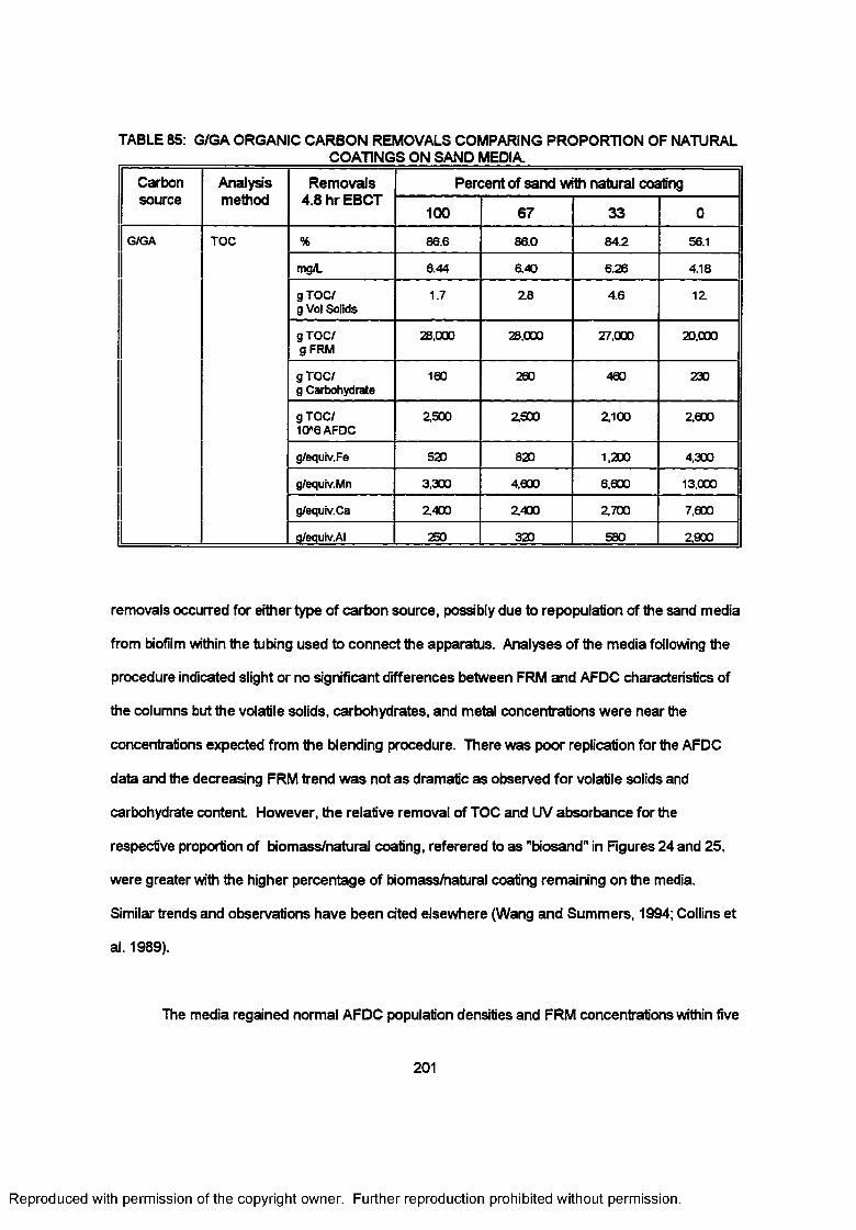
TABLE 85: G/GA ORGANIC CARBON REMOVALS COMPARING PROPORTION OF NATURAL __________________ COATINGS ON SAND MEDIA.
Carbon Analysismethod
Removals 4.8 hr EBCT
Percent of sand with natural coatingsource
100 67 33 0
G/GA TOC % 86.6 86.0 84.2 56.1
mg/L 6.44 6.40 6.26 4.18
gTO C/ g Vol Solids
1.7 2 8 4.6 12
gTO C/ g FRM
28.000 28,000 27,000 20,000
gTOC/g Carbohydrate
160 260 460 230
gTO C/ 10*6 AFDC
2,500 2500 2100 2600
g/equiv.Fe 520 820 1,200 4,300
g/equiv.Mn 3.300 4,600 6,600 13,000
g/equiv.Ca 2,400 2400 2700 7,600
g/equiv.AI 250 320 580 2900
removals occurred for either type of carbon source, possibly due to repopulation of the sand media
from biofiim within the tubing used to connect the apparatus. Analyses of the media following the
procedure indicated slight or no significant differences between FRM and AFDC characteristics of
the columns but the volatile solids, carbohydrates, and metal concentrations were near the
concentrations expected from the blending procedure. There was poor replication for the AFDC
data and the decreasing FRM trend was not as dramatic as observed for volatile solids and
carbohydrate content However, the relative removal of TOC and UV absorbance for the
respective proportion of biomass/natural coating, referered to as "biosand" in Figures 24 and 25,
were greater with the higher percentage of biomass/natural coating remaining on the media.
Similar trends and observations have been cited elsewhere (Wang and Summers, 1994; Collins et
al. 1989).
The media regained normal AFDC population densities and FRM concentrations within five
201
Reproduced with permission of the copyright owner. Further reproduction prohibited without permission.
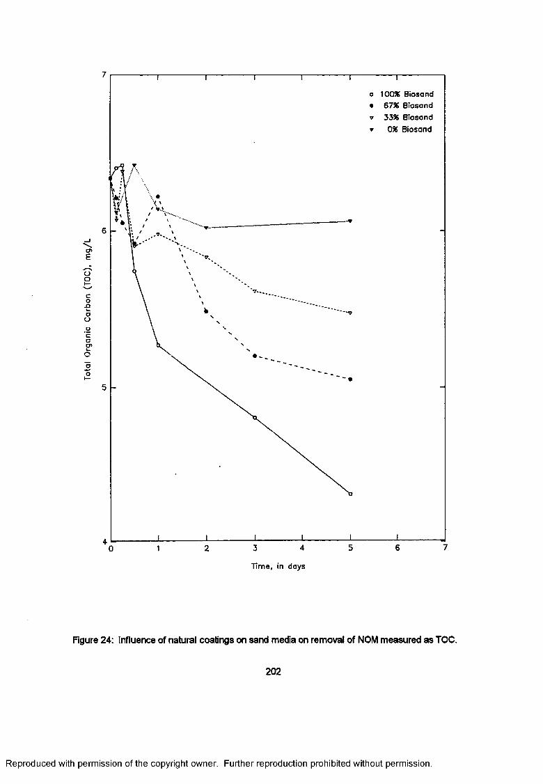
Tota
l O
rgan
ic
Car
bon
(TO
C),
mg
/L7
o 100% Biosand• 67% Biosandv 33SS Biosand* 085 Biosand
6
5
475 63 420
Time, in days
Figure 24: Influence of natural coatings on sand media on removal of NOM measured as TOC.
202
Reproduced with permission of the copyright owner. Further reproduction prohibited without permission.
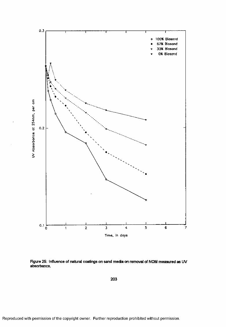
UV
Abs
orba
nce
at
254n
m,
per
cm0.3
o 100% Biosand• 67% Biosandv 33% Biosand
▼ 0% Biosond
0.2
Time, in days
Figure 25: Influence of natural coatings on sand media on removal of NOM measured as UV absorbance.
203
Reproduced with permission of the copyright owner. Further reproduction prohibited without permission.
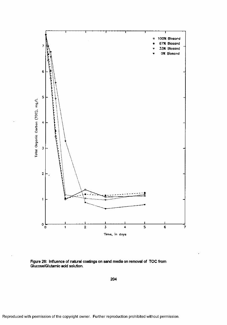
T T
o>E
oo
co•Ok.oo
_o'EoO'
100% Biosand
67% Biosand
33% Biosand
0% Biosand
7
6
5
4
3
2
02 3 5 6 70 1 4
Time, in days
Figure 26: Influence of natural coatings on sand media on removal of TOC from Glucose/Glutamic add solution.
204
Reproduced with permission of the copyright owner. Further reproduction prohibited without permission.
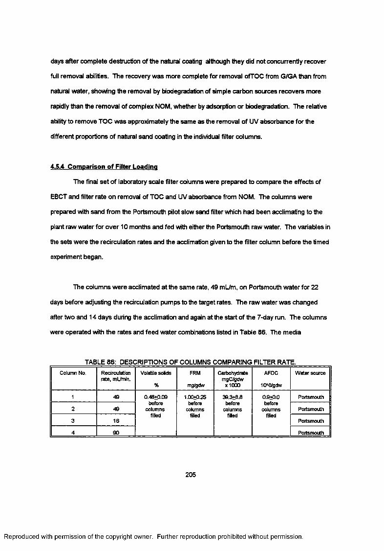
days after complete destruction of the natural coaling although they did not concurrently recover
full removal abilities. The recovery was more complete for removal ofTOC from G/GA than from
natural water, showing the removal by biodegradation of simple carbon sources recovers more
rapidly than the removal of complex NOM, whether by adsorption or biodegradation. The relative
ability to remove TOC was approximately the same as the removal of UV absorbance for the
different proportions of natural sand coating in the individual filter columns.
4.5.4 Comparison of Filter Loading
The final set of laboratory scale filter columns were prepared to compare the effects of
EBCT and filter rate on removal of TOC and UV absorbance from NOM. The columns were
prepared with sand from the Portsmouth pilot slow sand filter which had been acclimating to the
plant raw water for over 10 months and fed with either the Portsmouth raw water. The variables in
the sets were the recirculation rates and the acclimation given to the filter column before the timed
experiment began.
The columns were acclimated at the same rate, 49 mL/m, on Portsmouth water for 22
days before adjusting the recirculation pumps to the target rates. The raw water was changed
after two and 14 days during the acclimation and again at the start of the 7-day run. The columns
were operated with the rates and feed water combinations listed in Table 86. The media
TABLE 86: DESCRIPTIONS OF COLUMNS COMPARING FILTER RATE.Column No. Recirculation
rate, mL/min.Volatile solids
%
FRM
mg/gdw
Carbohydrate mgC/gdw
x 1000
AFDC
10'6/gdw
Water source
1 49 0.48+0.09before
columnsfilled
1.00+0.25before
columnsfilled
39.3+8.8before
columnsfilled
0.9+0.0before
columnsfilled
Portsmouth
2 49 Portsmouth
3 16 Portsmouth
4 90 Portsmouth
205
Reproduced with permission of the copyright owner. Further reproduction prohibited without permission.
characteristics which had been determined are also listed in that table. No metal analyses were
made for these sets of columns but the concentrations would be expected to be similar to those for
the fully coated material reported with the preceding set of columns. The source and preparation
of sand had been the same as discussed previously. All media was taken from the pilot filter at
Portsmouth, NH. The effective size was 0.48 mm and the uniformity coefficient was 2.0 after bang
sieved. As with the preceding sets of columns, the net EBCT was the same for all columns.
The higher removals were associated with the higher flow rates, again for both TOC and
UV absorbance. The data for the removals with time are presented in Table 87 and Rgures 27 and
28. The differences in removal of TOC, between the lower flow rate and the three higher rates,
were proportional to the flow rates yet the differences in removal of UV absorbance was small.
The removal of TOC was more sensitive to velocity than was removal of UV absorbance in these
flow ranges. The UV absorbing materials are more humic in nature and are less biodegradable.
Higher filter rates increase the interstitial velocity within the media and velocity affects the
boundary layer of fluid about sand or other particles within the filter. The pore spaces in a sand
filter vary in size and shape, depending on particle size and distribution of sizes, shape, and the
extent to which the space may be filled with trapped biological or inorganic debris. A relationship
used in the ground water field for flow through porous media is:
V = Q/(A*n) (6)
where A is the cross-section area and n is the porosity of the media. For clean sand the porosity
would be approximately 0.42 (AWWA, 1990). The interstitial velocity for a pumping rate of 49
mL/min in the 2.54 cm diameter laboratory-scale filter column would be 0.36 cm/second. The
condition of the interstitial flow, laminar or turbulent, can then be determined by the equation for
Reynolds number using the equation:
R. = pvd/p (7)
where d is the mean particle diameter, p the density of water, p the specific viscosity, and flow is
206
Reproduced with permission of the copyright owner. Further reproduction prohibited without permission.
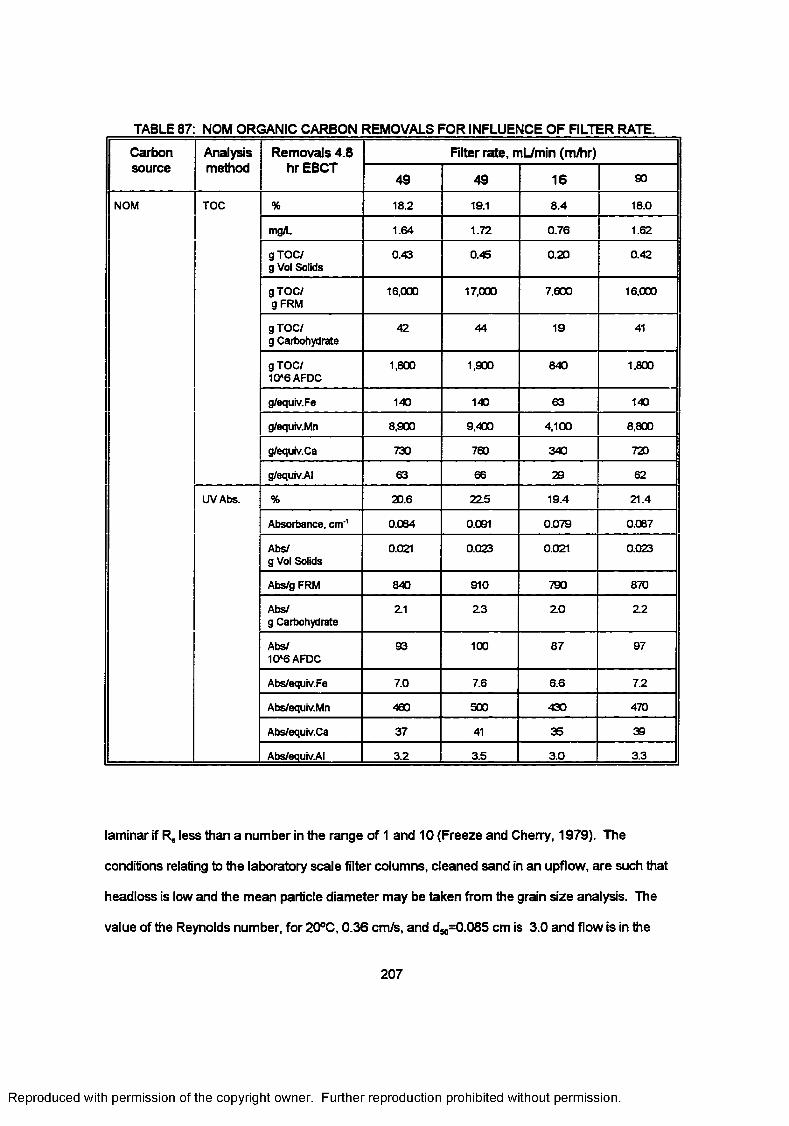
TABLE 87: NOM ORGANIC CARBON REMOVALS FOR INFLUENCE OF FILTER RATE.
Carbon Analysismethod
Removals 4.8 hr EBCT
Filter rate, mL/min (m/hr)source
49 49 16 90
NOM TOC % 18.2 19.1 8.4 18.0
mg/L 1.64 1.72 0.76 1.62
gTO C/ g Vol Solids
0.43 0.45 0.20 0.42
gTOC/ g FRM
16,000 17,000 7,600 16,000
gTOC/g Carbohydrate
42 44 19 41
gTOC/ 10*6 AFDC
1,800 1,900 840 1,800
g/equiv.Fe 140 140 63 140
g/equiv.Mn 8,900 9,400 4,100 8,800
g/equiv.Ca 730 780 340 720
g/equiv.A! 63 66 29 62
UVAbs. % 20.6 225 19.4 21.4
Absorbance, cm'1 0.064 0.091 0.079 0.067
Abs/g Vol Solids
0.021 0.023 0.021 0.023
Abs/g FRM 840 910 790 870
Abs/g Carbohydrate
2.1 2 3 2 0 2 2
Abs/10*6 AFDC
93 100 87 97
Abs/equiv.Fe 7.0 7.6 6.6 7.2
Abs/equiv.Mn 460 500 430 470
Abs/equiv.Ca 37 41 35 39
Abs/equiv.AI 3.2 3.5 3.0 3.3
laminar if R. less than a number in the range of 1 and 10 (Freeze and Cherry, 1979). The
conditions relating to the laboratory scale filter columns, cleaned sand in an upflow, are such that
headloss is low and the mean particle diameter may be taken from the grain size analysis. The
value of the Reynolds number, for 20°C, 0.36 cm/s, and dM=0.085 cm is 3.0 and flow is in the
207
Reproduced with permission of the copyright owner. Further reproduction prohibited without permission.
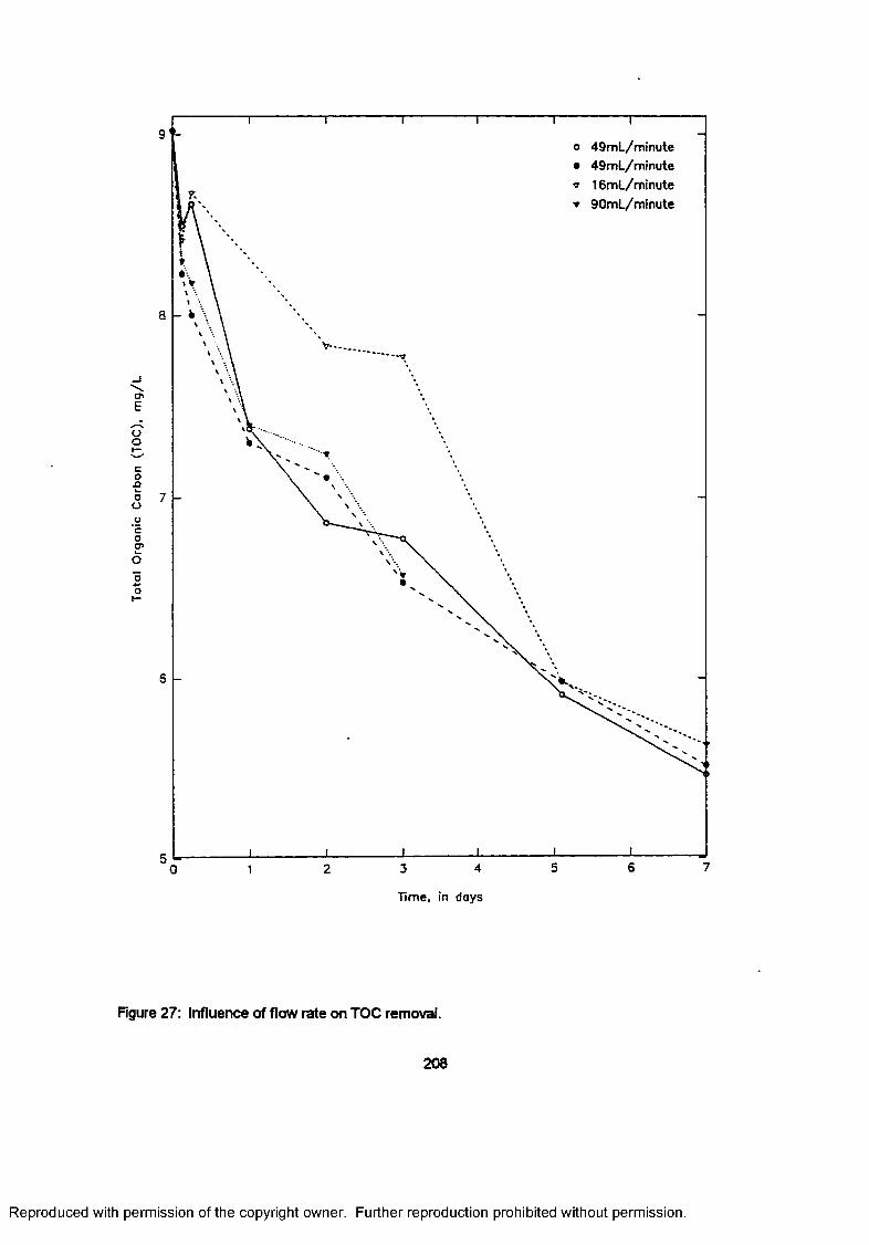
Tota
l O
rgan
ic
Carb
on
(TO
C),
mg
/L9
o 49mL/minute • 49mL/minute <r 16mL/minute ▼ 90mL/minute
8
7
6
5 75 63 420 1
Time, in days
Figure 27: Influence of flow rate on TOC removal.
208
Reproduced with permission of the copyright owner. Further reproduction prohibited without permission.
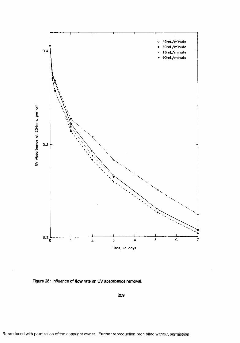
UV
Abs
orba
nce
at
254n
m,
per
cm
o 4 9 m L /m in u te
• 49mL/minute » 16mL/minute* 90mL/minute
0 .4
0 .3
0.2
Time, in days
Figure 28: Influence of flow rate on UV absorbance removal.
209
Reproduced with permission of the copyright owner. Further reproduction prohibited without permission
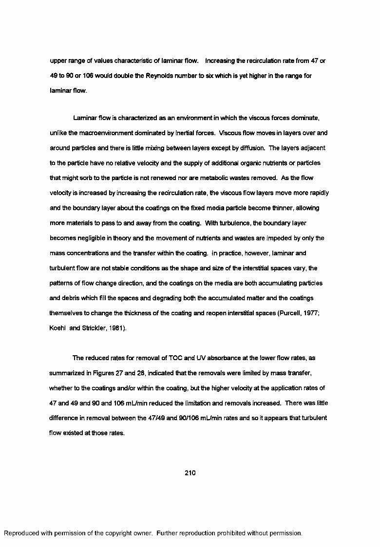
upper range of values characteristic of laminar flow. Increasing the recirculation rate from 47 or
49 to 90 or 106 would double the Reynolds number to six which is yet higher in the range for
laminar flow.
Laminar flow is characterized as an environment in which the viscous forces dominate,
unlike the macroenvironment dominated by inertial forces. Viscous flow moves in layers over and
around particles and there is little mixing between layers except by diffusion. The layers adjacent
to the particle have no relative velocity and the supply of additional organic nutrients or particles
that might sorb to the particle is not renewed nor are metabolic wastes removed. As the flow
velocity is increased by increasing the recirculation rate, the viscous flow layers move more rapidly
and the boundary layer about the coatings on the fixed media particle become thinner, allowing
more materials to pass to and away from the coating. With turbulence, the boundary layer
becomes negligible in theory and the movement of nutrients and wastes are impeded by only the
mass concentrations and the transfer within the coating. In practice, however, laminar and
turbulent flow are not stable conditions as the shape and size of the interstitial spaces vary, the
patterns of flow change direction, and the coatings on the media are both accumulating particles
and debris which fill the spaces and degrading both the accumulated matter and the coatings
themselves to change the thickness of the coating and reopen interstitial spaces (Purcell, 1977;
Koehl and Stickler, 1981).
The reduced rates for removal of TOC and UV absorbance at the lower flow rates, as
summarized in Figures 27 and 28, indicated that the removals were limited by mass transfer,
whether to the coatings and/or within the coating, but the higher velocity at the application rates of
47 and 49 and 90 and 106 mL/min reduced the limitation and removals increased. There was little
difference in removal between the 47/49 and 90/106 mL/min rates and so it appears that turbulent
flow existed at those rates.
210
Reproduced with permission of the copyright owner. Further reproduction prohibited without permission.
CHAPTER 5
d is c u s s io n OF RESULTS BETWEEN PLANTS
The operating results from each full-scale slow sand filtration plant were presented in the
previous chapter. Results of the pilot scale and laboratory scale studies were also presented in
that chapter. The data trends and comparisons demonstrated the importance of temperature,
sand media age, sand media biomass/coating content, source water carbon (nutrients)
characteristics, empty bed contact time (EBCT), and plant facility management/personnel
capabilities on the performance and operation of slow sand filters. Each of these variables will be
discussed in this section along with how each cleaning method may impact their influence on
performance. The section concludes with a discussion on the cleaning frequency, effectiveness,
and costs associated with the scraping and harrowing methods.
5.1 INFLUENCE OF TEMPERATURE
The performance of plant-scale filters relative to temperature, presented earlier by plants,
is summarized together in Table 88. No data was collected on the Newark, NY plant during
periods when the water temperature was less than 8°C and so no comparisons were made for
operation of that plant Similarly, there was no data collected for certain parameters at other
plants and those omissions are indicated in the table. Ail statistical comparisons for this portion of
the study used the two-tailed t-test with a 90 percent confidence limit
Water temperatures have been found by earlier studies to be important to removals of
turbidity, coliform bacteria, and Giardia cysts (Bellamy et al., 1985a, 1985b; Fogel etal., 1993) and
Cryptosporidium oocysts removal (Fogel et al., 1993). The removals of turbidity were significantly
higher, using the two tailed t-test and a confidence limit of 90 percent, with temperatures at or
211
Reproduced with permission of the copyright owner. Further reproduction prohibited without permission.
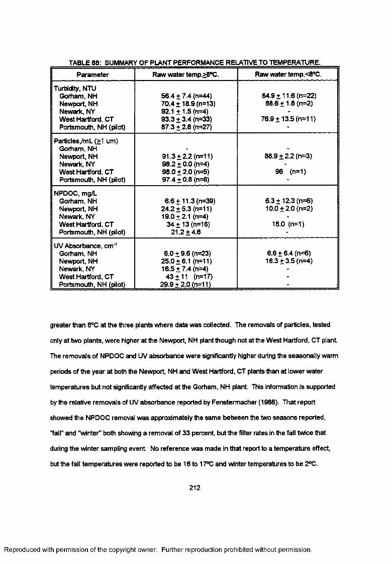
TABLE 88: SUMMARY OF PLANT PERFORMANCE RELATIVE TO TEMPERATURE.
Parameter Raw water temp.>8°C. Raw water temp.<8°C.
Turbidity, NTU Gorham, NH Newport, NH Newark, NY West Hartford, CT Portsmouth, NH (pilot)
56.4 +7 .4 (n=44) 70.4+18.9 (n=13) 92.1 +1.5 (n=4)93.3 + 3.4 (n=33)87.3 +2.8 (n=27)
64.9+11.6 (n=22) 88.6 + 1.8 (n=2)
76.9 + 13.5 (n=11)
Particles/mL (>1 um) Gorham, NH Newport, NH Newark, NY West Hartford, CT Portsmouth, NH (pilot)
91.3 + 2.2 (n=11) 98.2 + 0.0 (n=4) 98.0 + 2.0 (n=5)97.4 ±0 .8 (n=6)
88.9 + 2.2 (n=3)
96 (n=1)
NPDOC, mg/L Gorham, NH Newport, NH Newark, NY West Hartford, CT Portsmouth, NH (pilot)
6 .6+11.3 (n=39) 24.2 + 5.3 (n=11) 19.0 + 2.1 (n=4)
34 + 13 (n=16) 21.2 + 4.6
6.3 +12.3 (n=6) 10.0 + 2.0 (n=2)
18.0 (n=1)
UV Absorbance, cm-' Gorham, NH Newport, NH Newark, NY West Hartford, CT Portsmouth, NH (pilot)
6.0 + 9.6 (n=23) 25.0 + 6.1 (n=11) 16.5 + 7.4 (n=4)
43 + 11 (n=17) 29.9 + 2.0 (n=11)
6.6 + 6.4 (n=6) 16.3 + 3.5 (n=4)
greater than 8°C at the three plants where data was collected. The removals of particles, tested
only at two plants, were higher at the Newport, NH plant though not at the West Hartford, CT plant
The removals of NPDOC and UV absorbance were significantly higher during the seasonally warm
periods of the year at both the Newport, NH and West Hartford, CT plants than at lower water
temperatures but not significantly affected at the Gorham, NH plant This information is supported
by the relative removals of UV absorbance reported by Fenstermacher (1988). That report
showed the NPDOC removal was approximately the same between the two seasons reported,
"fall" and "winter" both showing a removal of 33 percent, but the filter rates in the fall twice that
during the winter sampling event No reference was made in that report to a temperature effect,
but the fall temperatures were reported to be 16 to 17°C and winter temperatures to be 2°C.
212
Reproduced with permission of the copyright owner. Further reproduction prohibited without permission.
Temperature had been previously reported to be significant in the performance of slow sand filters
in permanganate consumption (Van de Vloed, 1956), nitrification (Huisman and Wood, 1974), and
removal of BDOC (Servais et al., 1992; and Welte and Montriel, 1996). The effect at the Gorham,
NH plant appeared to have been present for NPDOC removal, as shown later in Figure 30, but
insufficient to be statistically significant due to the wide standard deviation in the data. The effect of
temperature at the Gorham, NH plant was not noticeable on the removal of UV absorbance.
The removal of turbidity varied with temperature at all plants and removal of particles
varied with temperature at the Newport, NH plant though not at the West Hartford, CT plant There
was no significant difference in removal of either parameter between the two plants which had
used the scraping method (Newark, NY) and the harrowing method (West Hartford, CT) to clean
filters.
The NPDOC and UV absorbance removals at all plants were plotted against temperature
and removals were found higher at temperature at or greater than 8°C. Because of this and
because no comparable removal data had been collected for the Newark, NY plant when water
temperatures were below this level, the data for all the plants was separated according to
temperatures at or above 8°C or below 8°C, Removals at the Gorham plant were not found to be
related to temperature but these data also were separated so the data for comparison between
plants would be on the same temperature base. The removals during periods when the raw water
temperatures equal or exceeded 8°C are summarized in Figure 29. The statistical significance of
the removal efficiencies between the plants and temperature ranges are summarized in Table 89.
There were significant differences between all plants in the percent of NPDOC and UV absorbance
removed.
The data used in Collins et al. (1992) also showed a significant difference in removals of
NPDOC and UV absorbance between samples in the "winter" and "fall" but offered no explanation.
213
Reproduced with permission of the copyright owner. Further reproduction prohibited without permission.
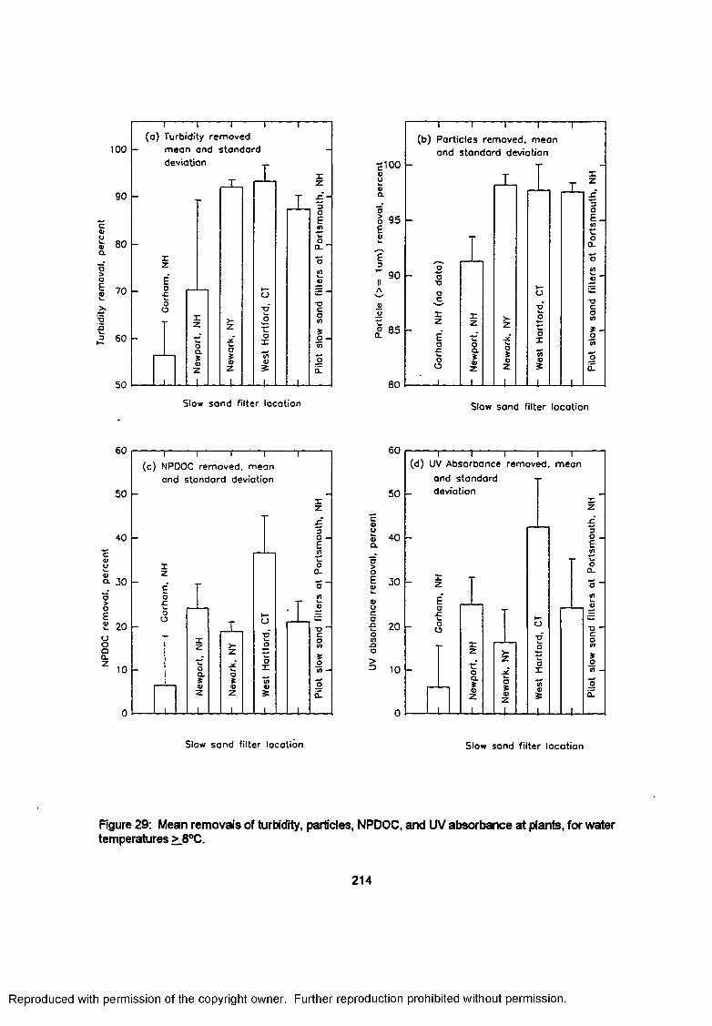
NPDO
C re
mov
al,
perc
ent
Turb
idity
re
mov
al,
per
cen
t
100 -
i 1---------1---------r(o ) Turbidity rem oved
mean and standard deviation
90 -
80 -
70 -
60
Eo.coo
oas©
Z
>z
50
L
o"OwooX
X 3OE<nwOa.'
oa 95 Eu
E3
ItA
OU
~I---------- 1---------- 1---------- 1-----------T(b ) Particles removed, mean
and standard deviation
T
90
80
o*ooc
rz
E*a.cwOo
Slow sand filter location Slow sand filter location
60 1 1 1---------- 1—(c ) NPDOC removed, mean
and standard deviation
50 -
40 -
30 -
20 -
10 -
xzEa.coo
oas©
Z
X ■owo
ax
£ *3 O ■E
oa.
*oco
odi
oEa)u.©Ocon
£XO
60
50
40
30
20
10
T I i i r (d ) UV Absorbance removed, mean
and standard deviation
Ea-Coo
roa.*4)
Xz
3 O .
EtoQ.0 ‘01 V
*o • c o 0»*001 •
£al
Slow sand filter location Slow sand filter location
Figure 29: Mean removals of turbidity, particles, NPDOC, and UV absorbance at plants, for water temperatures >8°C.
214
Reproduced with permission of the copyright owner. Further reproduction prohibited without permission.
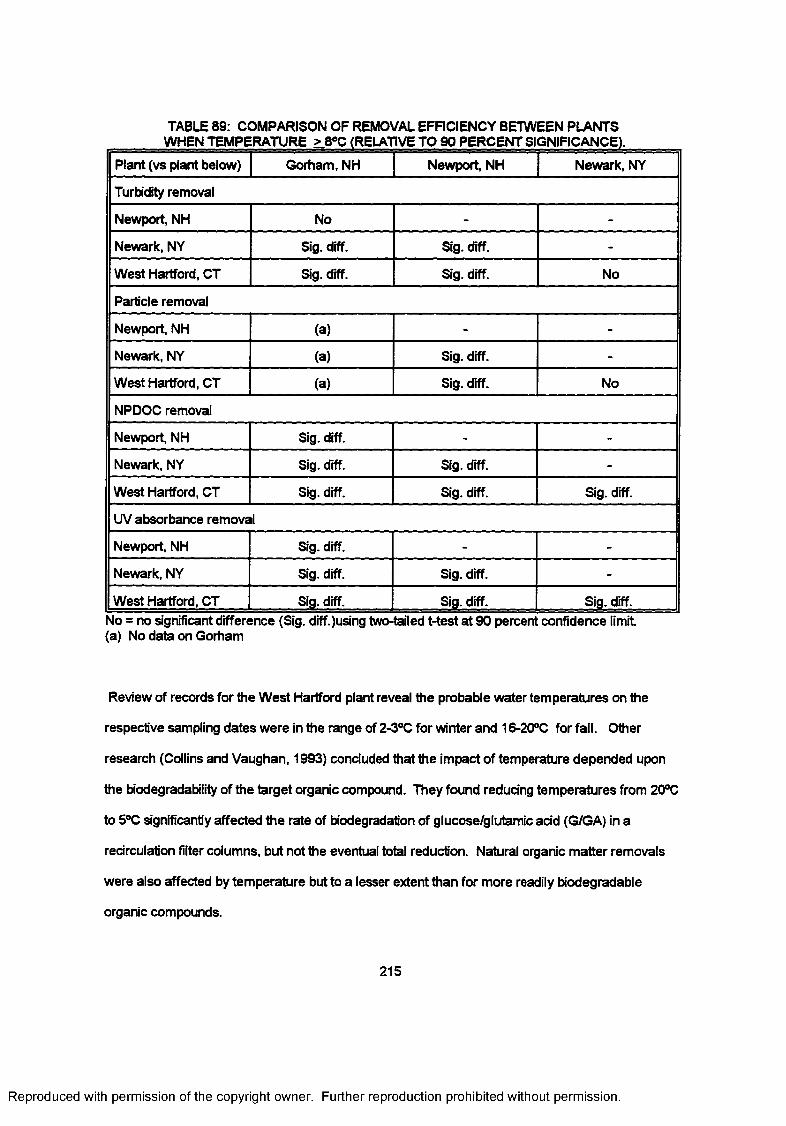
TABLE 89: COMPARISON OF REMOVAL EFFICIENCY BETWEEN PLANTS WHEN TEMPERATURE >_8°C (RELATIVE TO 90 PERCENT SIGNIFICANCE).
Plant (vs plant below) Gorham, NH Newport, NH Newark, NY
Turbidity removal
Newport, NH No - -
Newark, NY Sig. diff. Sig. diff. -
West Hartford, CT Sig. diff. Sig. diff. No
Particle removal
Newport, NH (a) - -
Newark, NY (a) Sig. diff. -
West Hartford, CT (a) Sig. d'rff. No
NPDOC removal
Newport, NH Sig. diff. - -
Newark, NY Sig. diff. Sig. diff. -
West Hartford, CT Sig. diff. Sig. diff. Sig. diff.
UV absorbance removal
Newport, NH Sig. diff. - -
Newark, NY Sig. diff. Sig. diff. -
West Hartford, CT Sig. diff. Sig. diff. Sig. diff.No = no significant difference (Sig. diffusing two-tailed t-test at 90 percent confidence limit(a) No data on Gorham
Review of records for the West Hartford plant reveal the probable water temperatures on the
respective sampling dates were in the range of 2-3°C for winter and 16-20°C for fall. Other
research (Collins and Vaughan, 1993) concluded that the impact of temperature depended upon
the biodegradability of the target organic compound. They found reducing temperatures from 20°C
to 5°C significantly affected the rate of biodegradation of glucose/glutamic add (G/GA) in a
redrculation filter columns, but not the eventual total reduction. Natural organic matter removals
were also affected by temperature but to a lesser extent than for more readily biodegradable
organic compounds.
215
Reproduced with permission of the copyright owner. Further reproduction prohibited without permission.
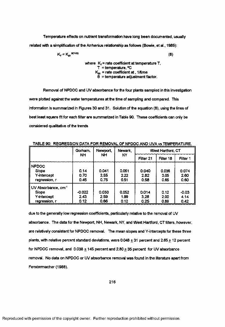
Temperature effects on nutrient transformation have long been documented, usually
related with a simplification of the Arrhenius relationship as follows (Bowie, et al., 1985):
K r=K20̂ (8)
where KT= rate coefficient at temperature T,T = temperature, °C
Ka, = rate coefficient a t, 1/time 8 = temperature adjustment factor.
Removal of NPDOC and UV absorbance for the four plants sampled in this investigation
were plotted against the water temperatures at the time of sampling and compared. This
information is summarized in Figures 30 and 31. Solution of the equation (8), using the lines of
best least square fit for each filter are summarized in Table 90. These coefficients can only be
considered qualitative of the trends
TABLE 90: REGRESSION DATA FOR REMOVAL OF NPDOC AND UVA vs TEMPERATURE.
Gorham, Newport,NH
Newark, West Hartford, CTNH NY
Filter 21 Filter 18 Filter 1
NPDOC Slope Y-intercept regression, r
0.140.700.45
0.0412.550.75
0.0512.220.51
0.0402.820.58
0.0363.050.65
0.0742.600.60
UV Absorbance, cnr1 Slope Y-intercept regression, r
-0.0222.430.12
0.0332.590.66
0.0521.990.12
0.0143.280.25
0.122.000.89
-0.034.140.42
due to the generally low regression coefficients, particularly relative to the removal of UV
absorbance. The data for the Newport, NH, Newark, NY, and West Hartford, CT filters, however,
are relatively consistent for NPDOC removal. The mean slopes and Y-intercepts for these three
plants, with relative percent standard deviations, were 0.048 + 31 percent and 2.65 + 12 percent
for NPDOC removal, and 0.038 + 145 percent and 2.80 + 35 percent for UV absorbance
removal. No data on NPDOC or UV absorbance removal was found in the literature apart from
Fenstermacher (1988).
216
Reproduced with permission of the copyright owner. Further reproduction prohibited without permission.
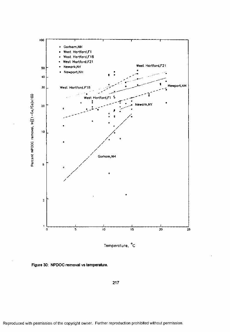
100
oo
aa\i)01
a>o<=5i.
ooQa.zc4)OwVQ-
50
40
30
20
10
,---------------
« Gorham,NH
■ West Hartford.F1
■» West H artford .F l 8♦ West Hartford.F21* Newark.NY• Newport.NH
West H artfo rd .F l 8
West Hartford,F21
I 0
Newport.NH
West Hartford.Fl ° _ -o - "• __ j - ' »* - ' ' ’ * .« Newark,NY
T
90o e
• .. ■ ,► ' i
/ 0
V
//
//
/ ,
Gorham,NH
/
//
10 15 20 25
Temperature, C
Figure 30: NPDOC removal vs temperature.
217
Reproduced with permission of the copyright owner. Further reproduction prohibited without permission.
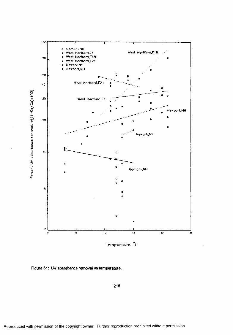
Perc
ent
UV
abso
rban
ce
rem
oval
, ln
[( I -
Ce
/Co
)x1
00
]
ig o
o G o rh a m .N H• West Hartford.Flo West H artfo rd .F l8• West Hartford.F21 v Newark.NY• Newport.NH
Waet H artford.F l8
70
SO
West Hartford,F21*0
30 West Hartford.F1
Newport,NH
20
10
Gorham,NH
2o s 10 IS 2520
Temperature, °C
Figure 31: UV absorbance removal vs temperature.
218
Reproduced with permission of the copyright owner. Further reproduction prohibited without permission.
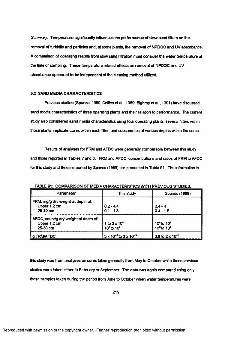
S u m m a ry : Temperature significantly influences the performance of slow sand filters on the
removal of turbidity and particles and, at some plants, the removal of NPDOC and UV absorbance.
A comparison of operating results from slow sand filtration must consider the water temperature at
the time of sampling. These temperature related effects on removal of NPDOC and UV
absorbance appeared to be independent of the cleaning method utilized.
5.2 SAND MEDIA CHARACTERISTICS
Previous studies (Spanos, 1989; Collins et al., 1989; Eghmy et al., 1991) have discussed
sand media characteristics of three operating plants and their relation to performance. The current
study also considered sand media characteristics using four operating plants, several filters within
those plants, replicate cores within each filter, and subsamples at various depths within the cores.
Results of analyses for FRM and AFDC were generally comparable between this study
and those reported in Tables 7 and 8. FRM and AFDC concentrations and ratios of FRM to AFDC
for this study and those reported by Spanos (1989) are presented in Table 91. The information in
TABLE 91: COMPARISON OF MEDIA CHARACTERISTICS WITH PREVIOUS STUDIES.
Parameter This study Spanos (1989)
FRM, mg/g dry weight at depth of:Upper 1.2 cm 0.2 - 4.4 0 .4 -425-30 cm 0.1 -1 .3 0 .4 -1 .5
AFDC, count/g dry weight at depth of:Upper 1.2 cm 1 to3x10* 10* to 10®25-30 cm 107to 10* 10* to 10®
g FRM/AFDC 5x10 ',2to 3 x 1 0 'n 0.8 to 2 x 1 0 -*
this study was from analyses on cores taken generally from May to October while those previous
studies were taken either in February or September. The data was again compared using only
those samples taken during the period from June to October when water temperatures were
219
Reproduced with permission of the copyright owner. Further reproduction prohibited without permission.
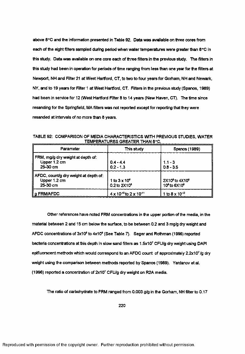
above 8°C and the information presented in Table 92. Data was available on three cores from
each of the eight filters sampled during period when water temperatures were greater than 8°C in
this study. Data was available on one core each of three filters in the previous study. The filters in
this study had been in operation for periods of time ranging from less than one year for the filters at
Newport, NH and Filter 21 at West Hartford, CT, to two to four years for Gorham, NH and Newark,
NY, and to 19 years for Filter 1 at West Hartford, CT. Filters in the previous study (Spanos, 1989)
had been in service for 12 (West Hartford Filter 8 to 14 years (New Haven, CT). The time since
resanding for the Springfield, MA filters was not reported except for reporting that they were
resanded at intervals of no more than 8 years.
TABLE 92: COMPARISON OF MEDIA CHARACTERISTICS WITH PREVIOUS STUDIES, WATER _______________________ TEMPERATURES GREATER THAN 8°C.
Parameter This study Spanos (1989)
FRM, mg/g dry weight at depth of:Upper 1.2 cm 0 .4 -4 .4 1.1 -325-30 cm 0.2 -1 .3 0.8 - 3.5
AFDC, count/g dry weight at depth of:Upper 1.2 cm 1 to 3x10* 2X10* to 4X10*25-30 cm 0.2 to 2X10* 10* to 6X10*
g FRM/AFDC 4 x1 0 ‘12to 2 x 10'" 1 to 8 x 10-’2
Other references have noted FRM concentrations in the upper portion of the media, in the
material between 2 and 15 cm below the surface, to be between 0.2 and 3 mg/g dry weight and
AFDC concentrations of 3x10* to 4x10® (See Table 7). Seger and Rothman (1996) reported
bacteria concentrations at this depth in slow sand filters as 1.5x10⁷ CFU/g dry weight using DAPI
epifluorscent methods which would correspond to an AFDC count of approximately 2.2x10⁷/g dry
weight using the comparison between methods reported by Spanos (1989). Yardanov et al.
(1996) reported a concentration of 2x10⁷ CFU/g dry weight on R2A media.
The ratio of carbohydrate to FRM ranged from 0.003 g/g in the Gorham, NH filter to 0.17
220
Reproduced with permission of the copyright owner. Further reproduction prohibited without permission.
g/g in the West Hartford, CT filters. Carbohydrate materials include cellular polysaccharides at
ratios of approximately 2 to 3 percent, if carbon limited, to 19 percent, if ammonia limited
(Charackis and Marshall, 1990), but also cellulose and other organic degradation organics. The
carbohydrate analyses for the cores in the Gorham, NH filter are at approximately ten percent of
the expected concentration relative to the FRM and AFDC concentrations and may not be valid.
The carbohydrate concentrations in the Newport, NH, Newark, NY, and West Hartford, CT filters
averaged 15, 14, and 17 percent of the FRM concentrations and within the range expected from
the literature (Charackis and Marshall, 1990).
Spanos(1989) had reported from analyses of two cores within the same filter at
Springfield, MA, using an ANOVA analysis with a 95 percent confidence limit, that there were no
significant differences between cores and, from analyses of cores from different filters at that
same plant that there were also no significant differences between the two different filters. He
also did not find any significant differences between the cores taken from a Springfield, MA filter in
the fall and winter. He did report significant differences (FRM, AFDC, iron, manganese) between
depths in cores and between filters at different plants (Springfield, MA, New Haven, CT, and West
Hartford, CT) for FRM, iron, and manganese, but not AFDC.
The current study used a confidence level of 90 percent and 2-way ANOVA methods to
compare the analyses of three cores from each filter and multiple filters at each of the four plants.
Significant differences in volatile solids, FRM, and carbohydrates were found between cores taken
from the same filter at all plants except Gorham. Differences in AFDC were present but were not
consistently related. Few literature references were found relating to variations between samples
at the same depth at different locations within the same filter. Haarhoff and Cleasby (1991)
reported from their literature review that 'Throughout the slow sand literature, the implicit
assumption is made that the vertical biological stratification is the same everywhere in the filter"
and that it "may be a reasonable assumption." One reference was reported (Bellinger, 1979) that
221
Reproduced with permission of the copyright owner. Further reproduction prohibited without permission.
showed significant variations in algal distribution existed on the filter surface, with variations of
about an order of magnitude on two sampling occasions. Factors leading to the variations were
hydraulic turbulence at the influent point which prevented uniform schmutzdecke formation, and
weather condition (wind and light exposure) on the open filters studied. Minkus (1954) reported
that hydraulic permeability of cores from cleaned sand filters varied but did not comment on
possible causes. Tumeaure and Russell (1924) noted that variations in filtering rate would occur
between parts of filters because of scraping, variations in headlosses in the underdrain system,
and possible breakage of the underdrains. Intermittent development of schmutzdecke at Gorham
and Newport, differences cleaning intensity in comers and adjacent to walls and columns when
tractor harrowing was used, variations in cross-flow velocity during wet harrowing, and differences
in the depth of sand removed by scraping between individual laborers, and differences in depths of
filter sand were observed during this study giving qualitative evidence of possible causes. Filter
permeability may also have varied due to localized compaction, deposition, or even blockage of
underdrains but these last factors are hypothesized.
The results of these comparisons between cores and filters within plants have been
presented earlier with results on the specific plants. Few differences were found between the
mean data for the same filter sampled twice within a short time period and within the same season,
such as for Filter 21 at West Hartford, CT. or between filters at the same plant which had been
operating for approximately the same length of time, as for Filters 3 and 4 at Newark, NY (19 and
39 months) sampled on the same day. Significant differences were found between mean data for
the same filter if it were sampled during different seasons, as occurred at all plants, and from
different filters at the same plant if the sand in the filters had been in use for significantly different
time periods, as for Filters 1,18, and 21 (ages of 19 years, 13 years, and less than one year,
respectively since reconditioning) at West Hartford, CT. The filters used by Spanos (1988) at West
Hartford, by comparison, had aged 13 years before the fall sampling and 15 years before the
winter sampling.
222
Reproduced with permission of the copyright owner. Further reproduction prohibited without permission.
All cores taken in the current study, at Gorham, Newport, Newark, and West Hartford,
showed significant differences with depth for volatile solids, FRM, carbohydrates, and AFDC.
Differences in iron, manganese, calcium, and aluminum concentrations seldom occurred except
with depth and between plants. The media characteristics presented in the preceding chapter
were compared between plants, using data on filters sampled during the same general season
and filtering water having similar temperatures. The comparisons were made between filters for
characteristics of the media in the top 1.2 cm and of the media between 25-30 cm. The surface
schmutzdecke was excluded from these comparisons as it could not be collected in a consistent
manner. The surface schmutzdecke readily and unavoidably detached from the sand surface at
the Gorham and Newport plants when attempting to collect it but was firmly attached at the
Newark and West Hartford plants. The surface schmutzdecke was separated from the surface of
the West Hartford filter samples allowing comparison to the samples from Gorham and Newport
The surface schmutzdecke at the Newark, NY filters was very thin and tightly bound to the sand
but was scraped, as well as possible, from the sand core surface before analyzing for the media
characteristics. The statistical comparison between the respective levels for the filters of the
various plants are summarized in Tables 93 and 94. The mean values of the upper and lower
levels were averaged and the standard deviations pooled, and the resultant values compared as
summarized in Table 95. All comparisons were made using the two-tailed t-test with a 90 percent
probability. A separation of variance on the data for the Newark NY plant is presented in Appendix
B.
Volatile solids, FRM, carbohydrates, and AFDC were generally different between the
filters at all plants for the top 1.2 cm and between the 25 and 30 cm depths and for the mean of
the concentrations at those two depths. Volatile solids concentrations were different between
filters at both depths, except between the two older filters at West Hartford. FRM concentrations in
the surface of the Gorham filters were different only from the Newport and youngest West Hartford
223
Reproduced with permission of the copyright owner. Further reproduction prohibited without permission.
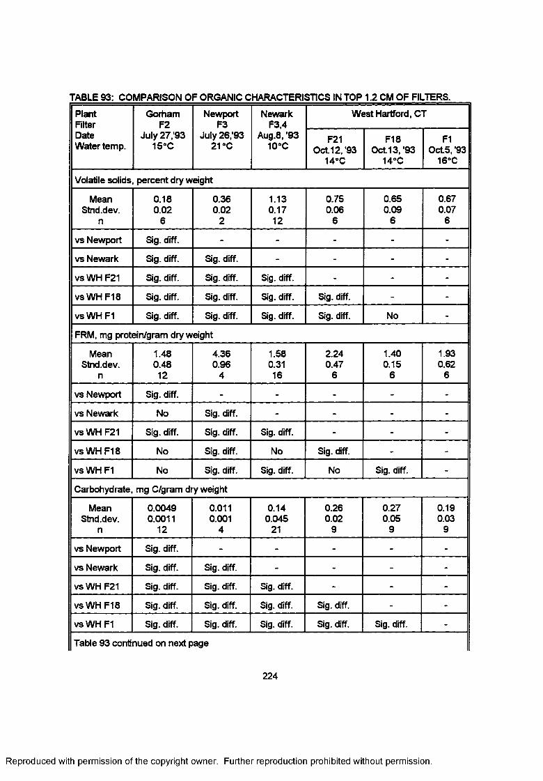
TABLE 93: COMPARISON 0 F ORGANIC CHARACTERISTICS IN TOP 1.2 CM OF FILTERS.
Plant Gorham Newport Newark West Hartford, CTFilter F2 F3 F3.4Date July 27/93 July 26/93 Aug.8,’93 F21 F18 F1Water temp. 15°C 21 °C 10°C Oct 12, '93 Oct 13, '93 Oct5, '93
148C 14°C 16“C
Volatile solids, percent dry weight
Mean 0.18 0.36 1.13 0.75 0.65 0.67Stnd.dev. 0.02 0.02 0.17 0.06 0.09 0.07
n 6 2 12 6 6 6
vs Newport Sig. diff. - - - - -
vs Newark Sig. diff. Sig. diff. - - - -
vsW HF21 Sig. diff. Sig. diff. Sig. diff. - - -
vsW HF18 Sig. diff. Sig. diff. Sig. diff. Sig. diff. - -
vsW H FI Sig. diff. Sig. diff. Sig. diff. Sig. diff. No -
FRM, mg protein/gram dry weight
Mean 1.48 4.36 1.58 2.24 1.40 1.93Stnd.dev. 0.48 0.96 0.31 0.47 0.15 0.62
n 12 4 16 6 6 6
vs Newport Sig. diff. - - - - -
vs Newark No Sig. diff. - - - -
vsW HF21 Sig. diff. Sig. diff. Sig. diff. - - -
vsW HF18 No Sig. diff. No Sig. diff. - -
vs WH F1 No Sig. diff. Sig. diff. No Sig. diff. -
Carbohydrate, mg C/gram dry weight
Mean 0.0049 0.011 0.14 0.26 0.27 0.19Stnd.dev. 0.0011 0.001 0.045 0.02 0.05 0.03
n 12 4 21 9 9 9
vs Newport Sig. diff. - - - - -
vs Newark Sig. diff. Sig. diff. - - - -
vs WH F21 Sig. diff. Sig. diff. Sig. diff. - - -
vsW HF18 Sig. diff. Sig. diff. Sig. diff. Sig. diff. - -
vsW H FI Sig. diff. Sig. diff. Sig. diff. Sig. diff. Sig. diff. -
Table 93 continued on next page
224
Reproduced with permission of the copyright owner. Further reproduction prohibited without permission.
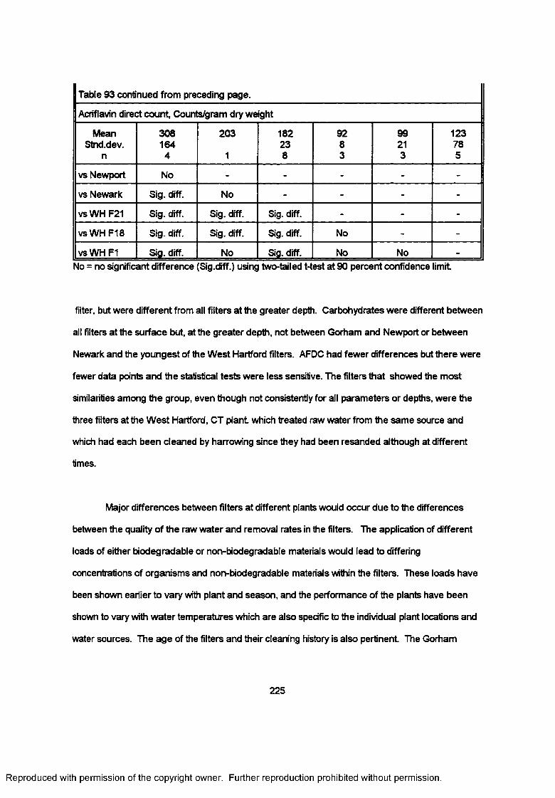
Table 93 continued from preceding page.
Acriflavin direct count Counts/gram dry weight
MeanStnd.dev.
n
308164
4
203
1
182238
9283
99213
123785
vs Newport No - - - - -
vs Newark Sig. diff. No - - - -
vsWHF21 Sig. diff. Sig. diff. Sig. diff. - - -
vsW HF18 Sig. diff. Sig. diff. Sig. diff. No - -
vsW H FI Sig. diff. No Sig. diff. No No -
No = no significant difference ’Sig.diff.) using two-tailed t-test at 90 percent confidence limit
filter, but were different from all filters at the greater depth. Carbohydrates were different between
all filters at the surface but, at the greater depth, not between Gorham and Newport or between
Newark and the youngest of the West Hartford filters. AFDC had fewer differences but there were
fewer data points and the statistical tests were less sensitive. The filters that showed the most
similarities among the group, even though not consistently for all parameters or depths, were the
three filters at the West Hartford, CT plant which treated raw water from the same source and
which had each been cleaned by harrowing since they had been resanded although at different
times.
Major differences between filters at different plants would occur due to the differences
between the quality of the raw water and removal rates in the filters. The application of different
loads of either biodegradable or non-biodegradable materials would lead to differing
concentrations of organisms and non-biodegradable materials within the filters. These loads have
been shown earlier to vary with plant and season, and the performance of the plants have been
shown to vary with water temperatures which are also specific to the individual plant locations and
water sources. The age of the filters and their cleaning history is also pertinent The Gorham
225
Reproduced with permission of the copyright owner. Further reproduction prohibited without permission.
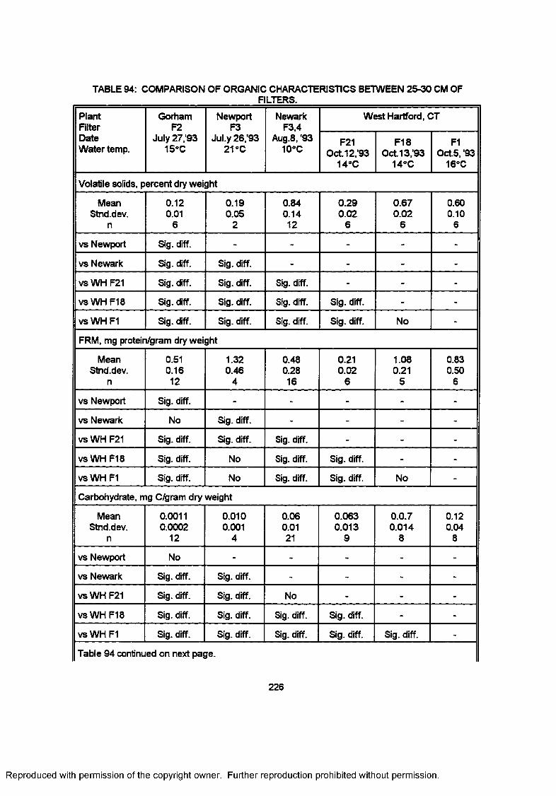
TABLE 94: COMPARISON OF ORGANIC CHARACTERISTICS BETWEEN 25-30 CM OFFILTERS.
PlantFilterDateWater temp.
GorhamF2
July 27/93 15°C
NewportF3
July 26/93 21 °C
Newark F3.4
Aug. 8. '93 10°C
West Hartford, CT
F21 O ct12/93
14°C
F18O ct13/93
14°C
F1Oct5, '93
16"C
Volatile solids, percent dry weight
Mean 0.12 0.19 0.84 0.29 0.67 0.60Stnd.dev. 0.01 0.05 0.14 0.02 0.02 0.10
n 6 2 12 6 6 6
vs Newport Sig. diff. - - - - -
vs Newark Sig. diff. Sig. diff. - - - -
vs WH F21 Sig. diff. Sig. diff. Sig. diff. - - -
vsW HF18 Sig. diff. Sig. diff. Sig. diff. Sig. diff. - -
vsW H FI Sig. diff. Sig. diff. Sig. diff. Sig. diff. No -
FRM, mg protein/gram dry weight
Mean 0.51 1.32 0.48 0.21 1.08 0.83Stnd.dev. 0.16 0.46 0.28 0.02 0.21 0.50
n 12 4 16 6 5 6
vs Newport Sig. diff. - - - - -
vs Newark No Sig. diff. - - - -
vs WH F21 Sig. diff. Sig. diff. Sig. diff. - - -
vsW H FI 8 Sig. diff. No Sig. diff. Sig. diff. - -
vs WH F1 Sig. diff. No Sig. diff. Sig. diff. No -
Carbohydrate, mg C/gram dry weight
Mean 0.0011 0.010 0.06 0.063 0.0.7 0.12Stnd.dev. 0.0002 0.001 0.01 0.013 0.014 0.04
n 12 4 21 9 8 8
vs Newport No - - - - -
vs Newark Sig. diff. Sig. diff. - - - -
vsW HF21 Sig. diff. Sig. diff. No - - -
vs WH F18 Sig. diff. Sig. diff. Sig. diff. Sig. diff. - -
vs WH F1 Sig. diff. Sig. diff. Sig. diff. Sig. diff. Sig. diff. -
Table 94 continued on next page.
226
Reproduced with permission of the copyright owner. Further reproduction prohibited without permission.
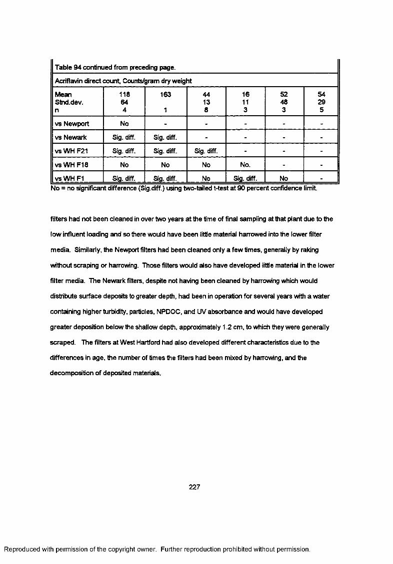
Table 94 continued from preceding page.
Acriflavin direct count. Counts/gram dry weight
MeanStnd.dev.n
118644
163
1
44138
16113
52483
54295
vs Newport No - - - - -
vs Newark Sig. diff. Sig. diff. - - - -
vsW HF21 Sig. diff. Sig. diff. Sig. diff. - - -
vsW H F18 No No No No. - -
vsW H F1 Sig. diff. Sig. diff. No Sig. diff. No -No = no significant difference (Sig.diff.) using two-tailed t-test at 90 percent confidence limit
filters had not been cleaned in over two years at the time of final sampling at that plant due to the
low influent loading and so there would have been little material harrowed into the lower filter
media. Similarly, the Newport filters had been cleaned only a few times, generally by raking
without scraping or harrowing. Those filters would also have developed little material in the lower
filter media. The Newark filters, despite not having been cleaned by harrowing which would
distribute surface deposits to greater depth, had been in operation for several years with a water
containing higher turbidity, particles, NPDOC, and UV absorbance and would have developed
greater deposition below the shallow depth, approximately 1.2 cm, to which they were generally
scraped. The filters at West Hartford had also developed different characteristics due to the
differences in age, the number of times the filters had been mixed by harrowing, and the
decomposition of deposited materials.
227
Reproduced with permission of the copyright owner. Further reproduction prohibited without permission.
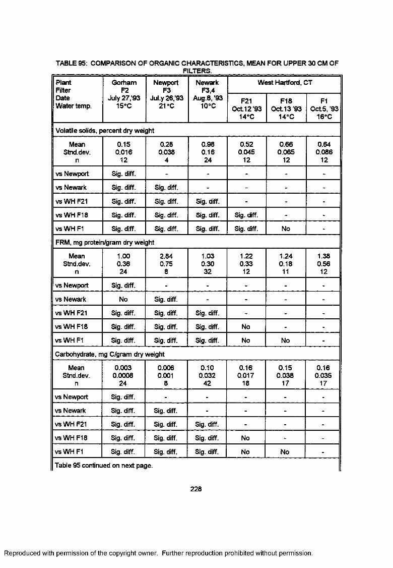
TABLE 95: COMPARISON OF ORGANIC CHARACTERISTICS, MEAN FOR UPPER 30 CM OFFILTERS.
PlantFilterDateWater temp.
GorhamF2
July 27/93 15°C
NewportF3
Jul.y 26/93 21 »C
Newark F3.4
Aug.8, '93 10°C
West Hartford, CT
F21 Oct 12'93
14°C
F18 Oct 13 '93
14“C
F1Oct5, '93
168C
Volatile solids, percent dry weight
Mean 0.15 0.28 0.98 0.52 0.66 0.64Stnd.dev. 0.016 0.038 0.16 0.045 0.065 0.086
n 12 4 24 12 12 12
vs Newport Sig. diff. - - - - -
vs Newark Sig. diff. Sig. diff. - - - -
vsWHF21 Sig. diff. Sig. diff. Sig. diff. - - -
vsW HF18 Sig. diff. Sig. diff. Sig. diff. Sig. diff. - -
vsW H FI Sig. diff. Sig. diff. Sig. diff. Sig. diff. No -
FRM, mg protein/gram dry weight
Mean 1.00 2.84 1.03 1.22 1.24 1.38Stnd.dev. 0.36 0.75 0.30 0.33 0.18 0.56
n 24 8 32 12 11 12
vs Newport Sig. diff. - - - - -
vs Newark No Sig. diff. - - - -
vs WH F21 Sig. diff. Sig. diff. Sig. diff. - - -
vs WH F18 Sig. diff. Sig. diff. Sig. diff. No - -
vsW H FI Sig. diff. Sig. diff. Sig. diff. No No -
Carbohydrate, mg C/gram dry weight
Mean 0.003 0.006 0.10 0.16 0.15 0.16Stnd.dev. 0.0008 0.001 0.032 0.017 0.038 0.035
n 24 8 42 18 17 17
vs Newport Sig. diff. - - - - -
vs Newark Sig. diff. Sig. diff. - - - -
vsWHF21 Sig. diff. Sig. diff. Sig. diff. - - -
vsW HF18 Sig. diff. Sig. diff. Sig. diff. No - -
vsW H FI Sig. diff. Sig. diff. Sig. diff. No No -
Table 95 continued on next page.
228
Reproduced with permission of the copyright owner. Further reproduction prohibited without permission.
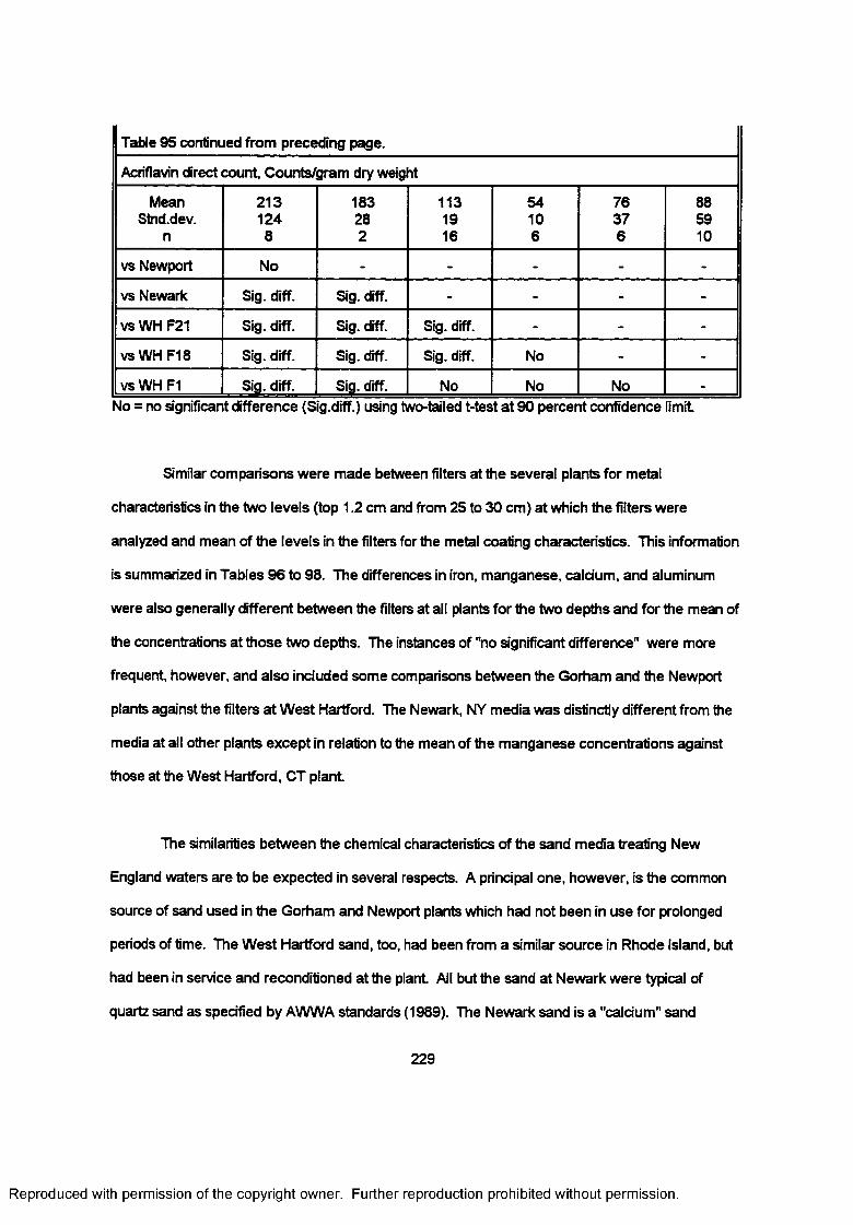
Table 95 continued from preceding page.
Acriflavin direct count Counts/gram dry weight
MeanStnd.dev.
n
2131248
183282
1131916
54106
76376
885910
vs Newport No - - - - -
vs Newark Sig. diff. Sig. diff. - - - -
vs WH F21 Sig. diff. Sig. diff. Sig. diff. - - -
vsW HF18 Sig. diff. Sig. diff. Sig. diff. No - -
vs WH F1 Sig. diff. Sig. diff. No No No -
No = no significant difference (Sig.diff.) using two-tailed t-test at 90 percent confidence imit
Similar comparisons were made between filters at the several plants for metal
characteristics in the two levels (top 1.2 cm and from 25 to 30 cm) at which the filters were
analyzed and mean of the levels in the filters for the metal coating characteristics. This information
is summarized in Tables 96 to 98. The differences in iron, manganese, calcium, and aluminum
were also generally different between the filters at all plants for the two depths and for the mean of
the concentrations at those two depths. The instances of "no significant difference" were more
frequent, however, and also included some comparisons between the Gorham and the Newport
plants against the filters at West Hartford. The Newark, NY media was distinctly different from the
media at all other plants except in relation to the mean of the manganese concentrations against
those at the West Hartford, CT plant
The similarities between the chemical characteristics of the sand media treating New
England waters are to be expected in several respects. A principal one, however, is the common
source of sand used in the Gorham and Newport plants which had not been in use for prolonged
periods of time. The West Hartford sand, too, had been from a similar source in Rhode Island, but
had been in service and reconditioned at the plant All but the sand at Newark were typical of
quartz sand as specified by AWWA standards (1989). The Newark sand is a "calcium" sand
229
Reproduced with permission of the copyright owner. Further reproduction prohibited without permission.
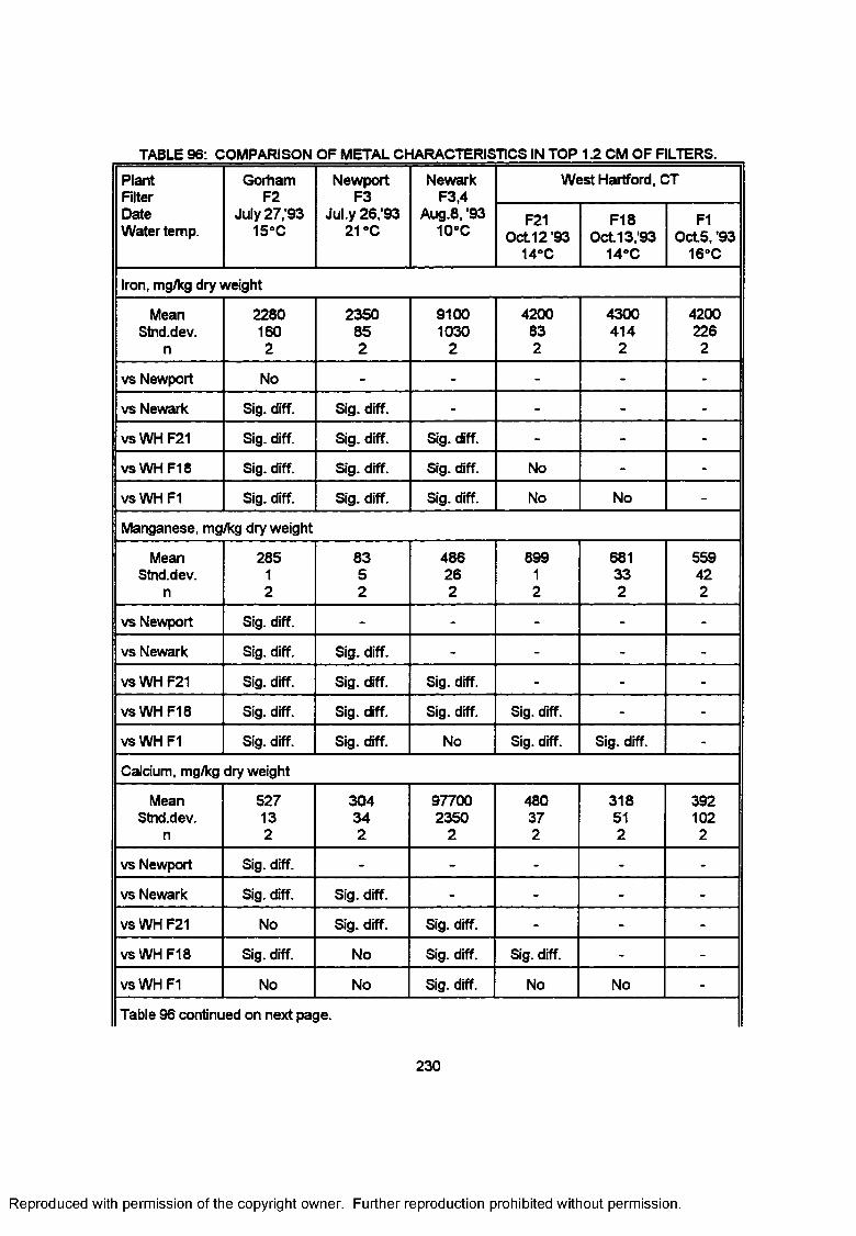
TABLE 96: COMPARISON OF METAL CHARACTERISTICS IN TOP 1.2 CM OF FILTERS.
PlantFilterDateWater temp.
GorhamF2
July 27,'93 158C
NewportF3
Jul.y 26/93 21 °C
Newark F3.4
Aug.8, '93 10°C
West Hartford, CT
F21Oct12'93
14°C
F18Oct 13,'93
14°C
F1Oct5, '93
16°C
Iron, mg/kg dry weight
Mean 2280 2350 9100 4200 4300 4200Stnd.dev. 160 85 1030 83 414 226
n 2 2 2 2 2 2
vs Newport No - - - - -
vs Newark Sig. diff. Sig. diff. - - - -
VSWHF21 Sig. diff. Sig. diff. Sig. diff. - - -
VSWHF18 Sig. diff. Sig. diff. Sig. diff. No - -
vsW H FI Sig. diff. Sig. diff. Sig. diff. No No -
Manganese, mg/kg dry weight
Mean 285 83 486 899 681 559Stnd.dev. 1 5 26 1 33 42
n 2 2 2 2 2 2
vs Newport Sig. diff. - - - - -
vs Newark Sig. diff. Sig. diff. - - - -
vsWHF21 Sig. diff. Sig. diff. Sig. diff. - - -
vs WH F18 Sig. diff. Sig. diff. Sig. diff. Sig. diff. - -
vs WH F1 Sig. diff. Sig. diff. No Sig. diff. Sig. diff. -
Calcium, mg/kg dry weight
Mean 527 304 97700 480 318 392Stnd.dev. 13 34 2350 37 51 102
n 2 2 2 2 2 2
vs Newport Sig. diff. - - - - -
vs Newark Sig. diff. Sig. diff. - - - -
vsWHF21 No Sig. diff. Sig. diff. - - -
vsW HF18 Sig. diff. No Sig. diff. Sig. diff. - -
vsW H FI No No Sig. diff. No No -
Table 96 continued on next page.
230
Reproduced with permission of the copyright owner. Further reproduction prohibited without permission.
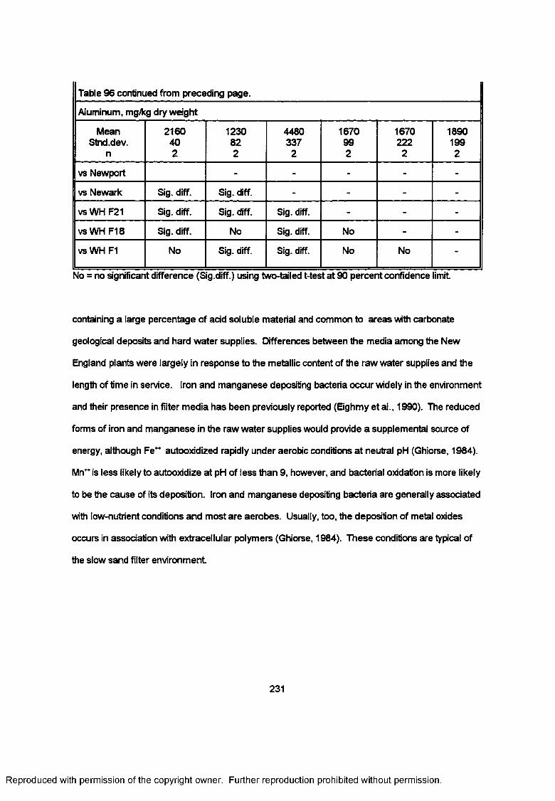
Table 96 continued from preceding page.
Aluminum, mg/kg dry weight
MeanStnd.dev.
n
2160402
1230822
4480337
2
1670992
1670222
2
18901992
vs Newport - - - - -
vs Newark Sig. diff. Sig. diff. - - - -
vsW HF21 Sig. diff. Sig. diff. Sig. diff. - - -
vsW HF18 Sig. diff. No Sig. diff. No - -
vsWH F1 No Sig. diff. Sig. diff. No No -
No = no significant difference (Sig.diff.) using two-tailed t-test at 90 percent confidence limit
containing a large percentage of add soluble material and common to areas with carbonate
geological deposits and hard water supplies. Differences between the media among the New
England plants were largely in response to the metallic content of the raw water supplies and the
length of time in service. Iron and manganese depositing bacteria occur widely in the environment
and their presence in filter media has been previously reported (Eghmy et al., 1990). The reduced
forms of iron and manganese in the raw water supplies would provide a supplemental source of
energy, although Fe~ autooxidized rapidly under aerobic conditions at neutral pH (Ghiorse, 1984).
Mn~is less likely to autooxidize at pH of less than 9, however, and bacterial oxidation is more likely
to be the cause of its deposition. Iron and manganese depositing bacteria are generally associated
with low-nutrient conditions and most are aerobes. Usually, too, the deposition of metal oxides
occurs in association with extracellular polymers (Ghiorse, 1984). These conditions are typical of
the slow sand filter environment
231
Reproduced with permission of the copyright owner. Further reproduction prohibited without permission.
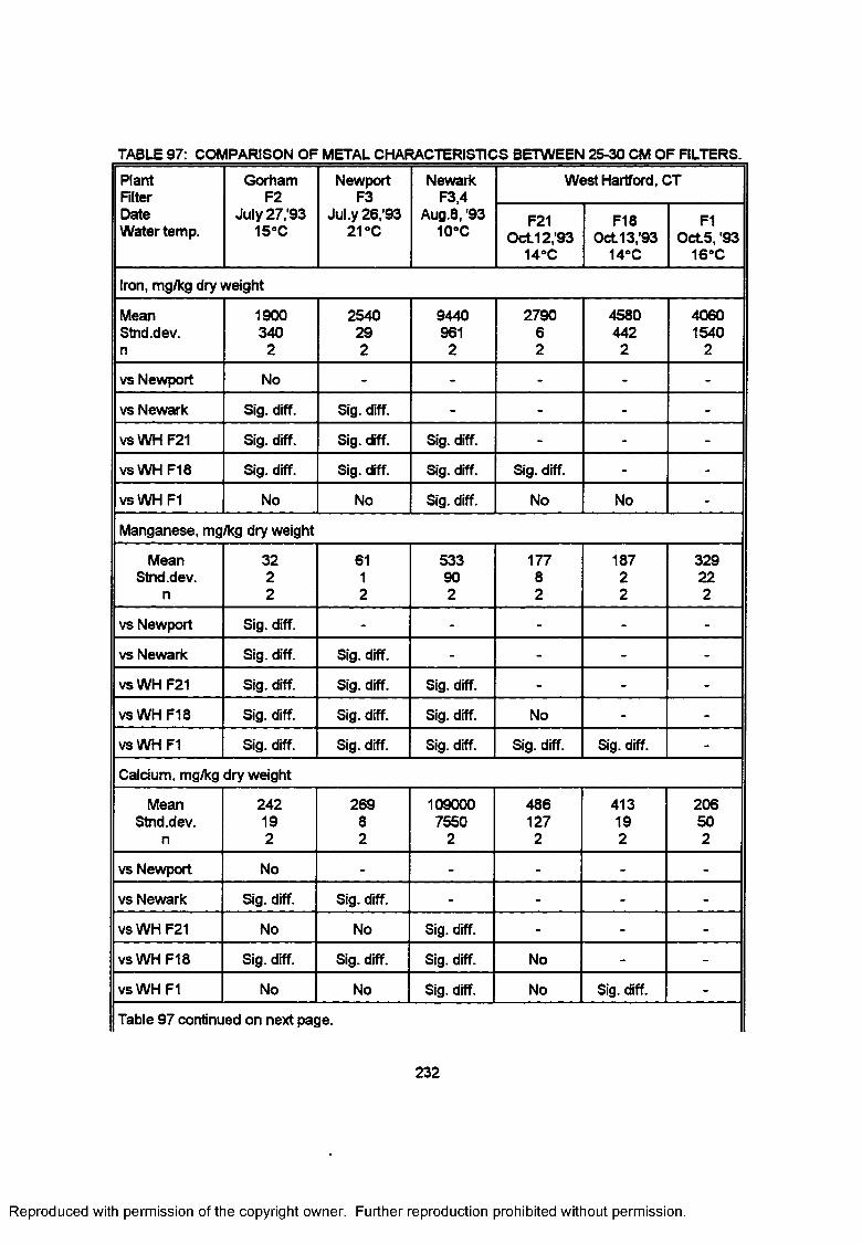
TABLE 97: COMPARISON OF METAL CHARACTERISTICS BETWEEN 25-30 CM OF FILTERS.
PlantFilterDateWater temp.
GorhamF2
July 27/93 15°C
NewportF3
Jul.y 26/93 21-C
Newark F3,4
Aug.8, '93 10°C
West Hartford, CT
F21 O ct12/93
14“C
F18Oct13/93
14“C
F1Oct5, '93
16°C
Iron, mg/kg dry weight
Mean 1900 2540 9440 2790 4580 4060Stnd.dev. 340 29 961 6 442 1540n 2 2 2 2 2 2
vs Newport No - - - - -
vs Newark Sig. diff. Sig. diff. - - - -
vsWHF21 Sig. diff. Sig. diff. Sig. diff. - - -
vsW HF18 Sig. diff. Sig. diff. Sig. diff. Sig. diff. - -
vs WH F1 No No Sig. diff. No No -
Manganese, mg/kg dry weight
Mean 32 61 533 177 187 329Stnd.dev. 2 1 90 8 2 22
n 2 2 2 2 2 2
vs Newport Sig. diff. - - - - -
vs Newark Sig. diff. Sig. diff. - - - -
vsWHF21 Sig. diff. Sig. diff. Sig. diff. - - -
vs WH F18 Sig. diff. Sig. diff. Sig. diff. No - -
vsW H FI Sig. diff. Sig. diff. Sig. diff. Sig. diff. Sig. diff. -
Calcium, mg/kg dry weight
Mean 242 269 109000 486 413 206Stnd.dev. 19 8 7550 127 19 50
n 2 2 2 2 2 2
vs Newport No - - - - -
vs Newark Sig. diff. Sig. diff. - - - -
vs WH F21 No No Sig. diff. - - -
vsW HF18 Sig. diff. Sig. diff. Sig. diff. No - -
vs WH F1 No No Sig. diff. No Sig. diff. -
Table 97 continued on next page.
232
Reproduced with permission of the copyright owner. Further reproduction prohibited without permission.
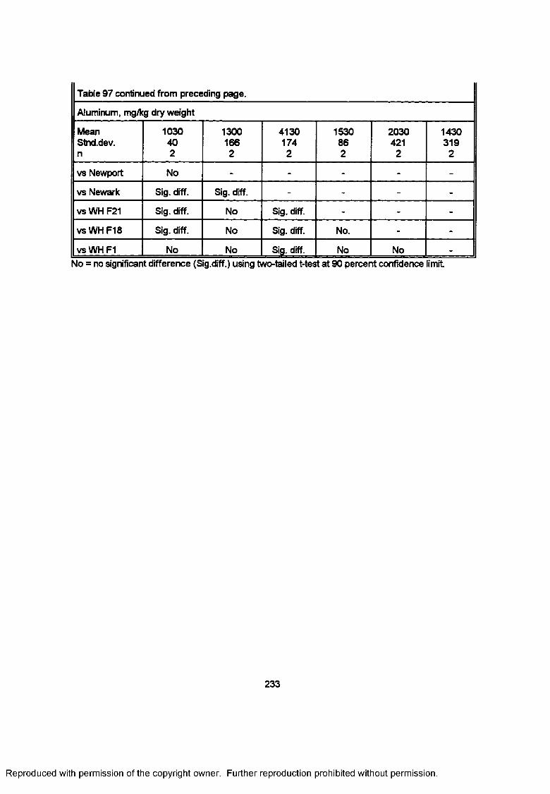
Table 97 continued from preceding page.
Aluminum, mg/kg dry weight
MeanStnd.dev.n
1030402
13001662
41301742
1530862
2030421
2
1430319
2
vs Newport No - - - - -
vs Newark Sig. diff. Sig. diff. - - - -
vsWHF21 Sig. diff. No Sig. diff. - - -
vsW HF18 Sig. diff. No Sig. diff. No. - -
vsW H FI No No Sig. diff. No No -No = no significant difference (Sig.diff.) using two-tailed t-test at 90 percent confidence limit
233
Reproduced with permission of the copyright owner. Further reproduction prohibited without permission.
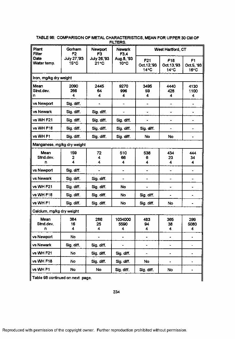
TABLE 98: COMPARISON OF METAL CHARACTERISTICS, MEAN FOR UPPER 30 CM OF ____________ FILTERS.
PlantFilterDateWater temp.
GorhamF2
July 27/93 15°C
NewportF3
July 26/93 21 »C
Newark F3,4
Aug.8, '93 10°C
West Hartford, CT
F21 O ct12/93
14°C
F18Oct13/93
14°C
F1Oct5, '93
16°C
Iron, mg/kg dry weight
Mean 2090 2445 9270 3495 4440 4130Stnd.dev. 266 64 990 59 428 1100n 4 4 4 4 4 4
vs Newport Sig. diff. - - - - -
vs Newark Sig. diff. Sig. diff. - - - -
vsW HF21 Sig. diff. Sig. diff. Sig. diff. - - -
vs WH F18 Sig. diff. Sig. diff. Sig. diff. Sig. diff. - -
vsW H FI Sig. diff. Sig. diff. Sig. diff. No No -
Manganese, mg/kg dry weight
Mean 159 72 510 538 434 444Stnd.dev. 2 4 66 6 23 34
n 4 4 4 4 4 4
vs Newport Sig. diff. - - - - -
vs Newark Sig. diff. Sig. diff. - - - -
vsW HF21 Sig. diff. Sig. diff. No - - -
vs WH F18 Sig. diff. Sig. diff. No Sig. diff. - -
vs WH F1 Sig. diff. Sig. diff. No Sig. diff. No -
Calcium, mg/kg dry weight
Mean 384 286 1034000 483 365 299Stnd.dev. 16 25 5590 94 38 5080
n 4 4 4 4 4 4
vs Newport No - - - - -
vs Newark Sig. diff. Sig. diff. - - - -
vsW HF21 No Sig. diff. Sig. diff. - - -
vs WH F18 No Sig. diff. Sig. diff. No - -
vs WH F1 No No Sig. diff. Sig. diff. No -
Table 98 continued on next page.
234
Reproduced with permission of the copyright owner. Further reproduction prohibited without permission.
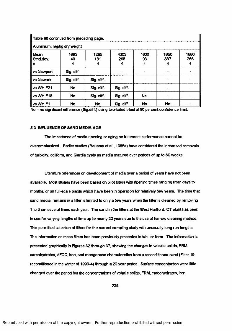
Table 98 continued from preceding page.
Aluminum, mg/kg dry weight
MeanStnd.dev.n
1695404
12651314
4305268
4
1600934
1850337
4
1660266
4
vs Newport Sig. diff. - - - - -
vs Newark Sig. diff. Sig. diff. - - - -
vsW HF21 No Sig. diff. Sig. diff. - - -
vs WH F18 No Sig. diff. Sig. diff. No. - -
vsW H FI No No Sig. diff. No No -No = no significant difference (Sig.diff.) using two-tailed t-test at 90 percent confidence limit
5.3 INFLUENCE OF SAND MEDIA AGE
The importance of media ripening or aging on treatment performance cannot be
overemphasized. Earlier studies (Bellamy et al., 1985a) have considered the increased removals
of turbidity, coliform, and Giardia cysts as media matured over periods of up to 80 weeks.
Literature references on development of media over a period of years have not been
available. Most studies have been based on pilot filters with ripening times ranging from days to
months, or on full-scale plants which have been in operation for relatively few years. The time that
sand media remains in a filter is limited to only a few years when the filter is cleaned by removing
1 to 3 cm several times each year. The sand in the filters at the West Hartford, CT plant has been
in use for varying lengths of time up to nearly 20 years due to the use of harrow cleaning method.
This permitted selection of filters for the current sampling study with unusually long run lengths.
The information on these filters has been previously presented in tabular form. The information is
presented graphically in Figures 32 through 37, showing the changes in volatile solids, FRM,
carbohydrates, AFDC, iron, and manganese characteristics from a reconditioned sand (Filter 19
reconditioned in the winter of 1993-4) through a 20 year period. Surface concentration were little
changed over the period but the concentrations of volatile solids, FRM, carbohydrates, iron,
235
Reproduced with permission of the copyright owner. Further reproduction prohibited without permission.
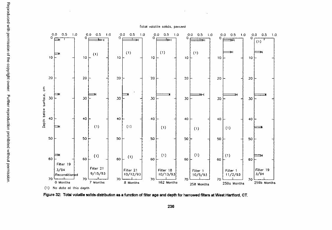
Reproduced
with perm
ission of the
copyright ow
ner. Further
reproduction prohibited
without
permission.
Total volatile solids, percent
3</)so<un
a.CDa
0
10
20
30
40
50
60
70
0 .0 0 .5 1.0 0.0 0.5 1.0 0.0 0 .5 1.0
=31
=w
=31
Filter 19
3 /9 4Recondition
i2d
0
10
20
30
40
50
60
70
S T
(I)
(1)
(1)
Filter 2 !
9 / 1 5 / 9 3
0
10
20
30
40
50
60
70
3 1
(1)
( I)
(1)
Filter 21 1 0 /1 2 /9 3
l
0.0 0
0.5 1.0
(D10 -
20
30 -
40 -
(1)
50 -
60 -( ')
708 Months
Filter 18 1 0 /1 3 /9 3
I____162 Months
0.0 0
0 .5 1.0 0 .0
10
20
30
40
50
60
70
=EH
(1>
3 H
( I)
(D
Filter 1 1 0 /5 /9 3
i
20
30
40
50
60
70
0.5
ESfT.0 0 .0 0 .5 1.0
0
3 1
3 1
(1)
(D
Filter 1 1 1 /2 /9 3
i258 Months0 Months 7 Months
(1 ) No data at this depth
Figure 32: Total volatile solids distribution as a function of filter age and depth for harrowed filters at West Hartford, CT.
10
20
30
40
50
60
70
0 )
31
Filter 19 3 /9 4
259a Months 259b Months
236
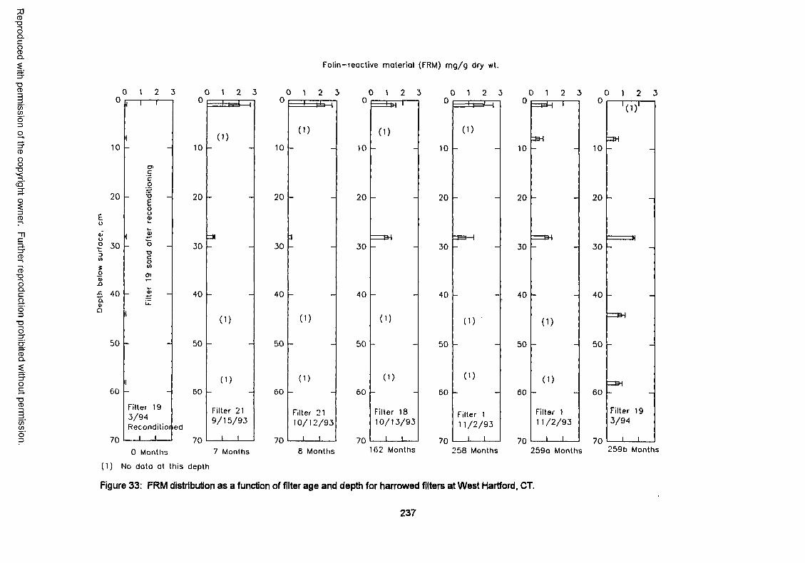
Reproduced
with perm
ission of the
copyright ow
ner. Further
reproduction prohibited
without
permission.
Folin-reactive material (FRM) m g /g dry wt.
0 1 2 3 0 1 2 3 0 1 2 3 0 1 2 3 0 1 2 3 0 1 2 3 0 1 2 3
10
20
£oatoS 30
$oa>A£ 40Clq>Q
50
60
70
n — r
O'cco•6Eoua>
•ocoW
Filter 19 3 /9 4Reconditioned i i
10
20
30
40
50
60
70
d )
(i)
( i)
Filter 21 9 /1 5 /9 3
i i
10
20
30
40
50
60
70
(1)
0 )
(1)
Filter 21 1 0 /1 2 /9 3
10
20
30
40
50
60
70
tJH
(D
(1)
(1)
Filter 18 1 0 /1 3 /9 3
I I__
10
20
30
40
50
60
70
(0
(0 '
( ')
Filter 1 1 1 /2 /9 3
i i
10
20
30
40
50
60
70
S T
(D
(0
Filter 1 1 1 /2 /9 3
I l _
=tH10
20
30
40
50
60
70
'(1)'
=3H
Filter 19 3 /9 4
I I_0 Months 7 Months 8 Months >62 Months 258 Months 259a Months 259b Months
(1) No data at this depth
Figure 33: FRM distribution as a function of filter age and depth for harrowed filters at West Hartford, CT.
237
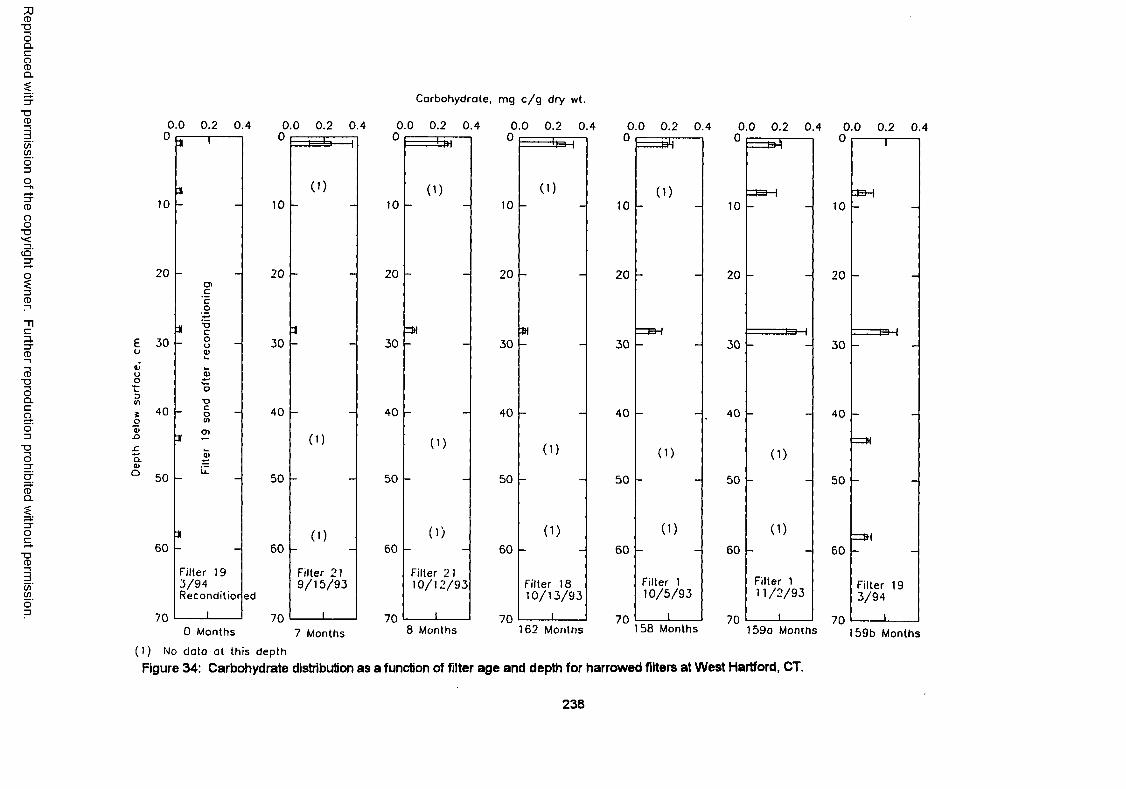
Reproduced
with perm
ission of the
copyright ow
ner. Further
reproduction prohibited
without
permission.
Carbohydrate, mg c /g dry wt.
0 .0 0.2 0 .4 0 .0 0 .2 0.4 0.0 0.2 0 .4 0 .0 0 .2 0 .4 0 .0 0 .2 0 .4 0 .0 0 .2 0.40 , ---------- 0 0 0 0 0
10
* 1
*10
( 010
--------- U h
(1 )10
.......... ‘H H
( D10
t — 3^
(1 )10
----- M
=3=H
20CJ>cco
20 - 20 - 20 - 20 - 20 -
j 12 3H30 o“ U — 0) k_
k.4)O
30 30 30 30 30
40T3 C— o ”CO
a ^0)
40
(1 )
40
(1 )
40
( D
40
(1 )
40
(1 )
50u.
31
50
(1)
50
(1 )
50
(1 )
50
(1 )
50
(1 )60 - 60 60 - 60 - 60 r 60 -
Filter 19 3 /9 4Reconditior ed
Filter 21 9 /1 5 /9 3
Filter 21 1 0 /1 2 /9 3 Filter 18
1 0 /1 3 /9 3Filter 1 1 0 /5 /9 3
Filter 1 11/ 2 / 9 3
70 I 70 i 70 I 70 I 70 1 70 I0 Months 7 Months 8 Months 162 Months 158 Months 1 5 9 0 Months
(1 ) No data at this depthFigure 34: Carbohydrate distribution as a function of filter age and depth for harrowed filters at West Hartford, CT.
0 .0 0.2 0.4
3=H 10 -
20 -
~ ■ H H 30 -
40 -
50 -
=3H 60 -
Filter 19 3 /9 4
70 --------- 1---------159b Months
2 3 8
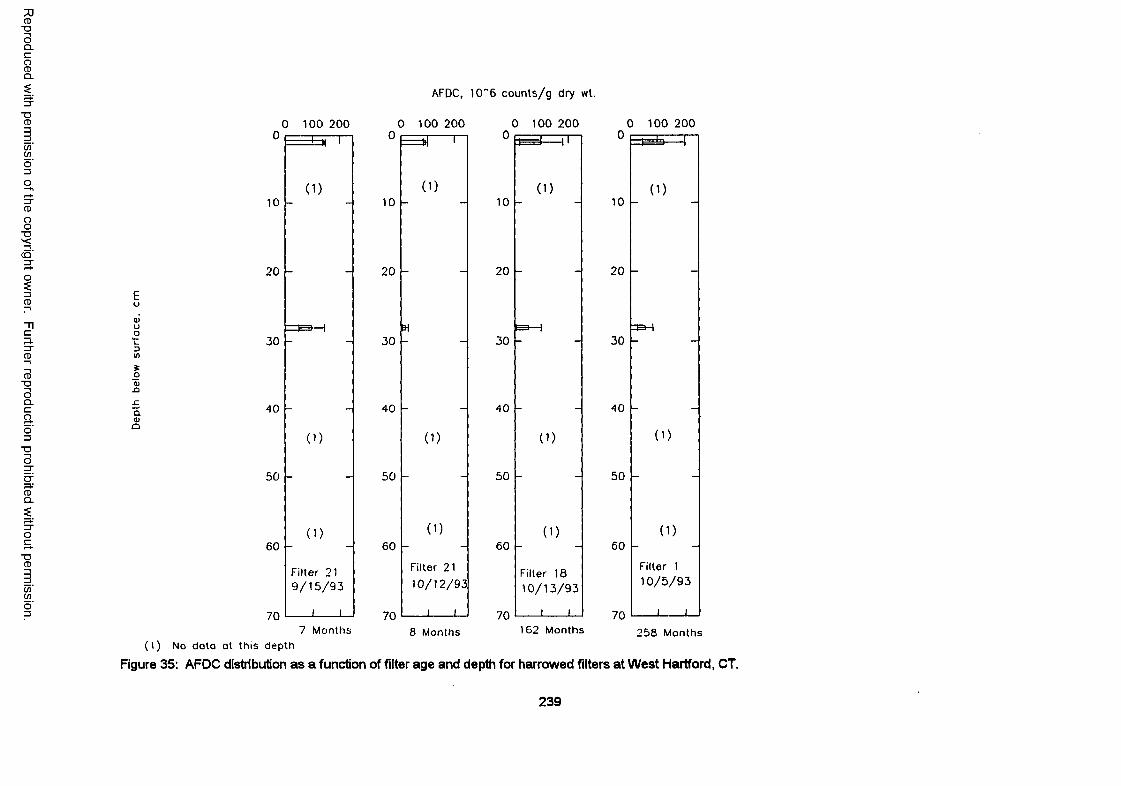
Reproduced
with perm
ission of the
copyright ow
ner. Further
reproduction prohibited
without
permission.
AFDC, 1CT6 c o u n ts /g dry wt.
0 100 200 0 100 200 0 100 200 0 100 2000 ----Hi 1 0 ---ol I 0 1---f 11 0 . I - 1 T ”
10(1 )
10(1 )
10(1 )
10(1 )
20 - 20 - 20 - 20 -
30fctEs—i
3091
30E3—1
303 M
40
( l )
40
(1 )
40
(1)
40
(D
50 - 50 - 50 - 50 -
60(1 )
Filter 21 9 / 1 5 / 9 3
60(0
Filter 21
1 0 /1 2 /9 3
60(1 )
Filter 18 1 0 /1 3 /9 3
60(1 )
Filter 1 1 0 /5 /9 3
70 I i 70 i i 70 .1 1 .. 70 i I
7 Months 8 Months 162 Months 258 Months(1 ) No data at this depth
Figure 35: AFDC distribution as a function of filter age and depth for harrowed filters at West Hartford, CT.
239
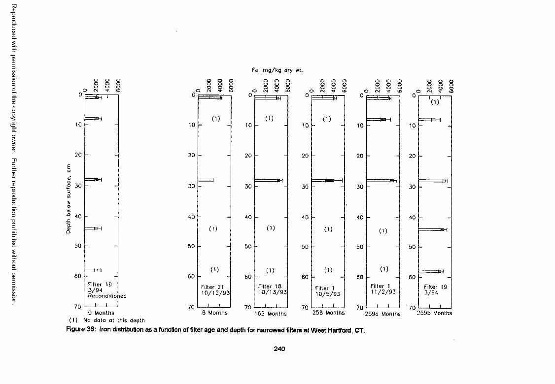
Reproduced
with perm
ission of the
copyright ow
ner. Further
reproduction prohibited
without
permission.
Fe, mg/kg dry wt.
oooo CN
ooooooco
10
20
Eu6uo 30u3CO5 O 0> jD 40Q.ata
50
60
70
oooCN
OoooooCO
o o oo o oo o oCN CO
oooCN
OoooooCO
oooCN
OooN-oooCO
oooooo
ooo0 0 0 0 0— y=H 1 ------1------ ------1----- )H
'( 1 ) '
— f=H (1 ) (1 ) ( D10 10 10 10 10
-------1—* ' \
----- PH
20 - 20 20 20 20
30 30------------- p |
30--— --» 1
30--------------f=»"1
30-------------- (=H
- _ 40 _ _ 40 __ _ 40 _ _ 40 _ _ 40 .
----- F=H (1 ) (1 ) ( D (1 ) H 1
- 50 - 50 - 50 - 50 - 50 -
----- PH (1 ) (1 ) (1 ) (1 )60 60 60 60 60
----- HI
Filter 19 3 /9 4Reconditio
1 1
)ed
70
Filter 21 1 0 /1 2 /9 3
l I 70
Filter 18 1 0 /1 3 /9 3
i . 70
Filter 1 1 0 /5 /9 3
I I 70
Filter 1 1 1 /2 /9 3
I I 70
Filter 19 3 /9 4
l I8 Months 162 Months 258 Months0 Months
(1 ) No data at this depth
Figure 36: Iron distribution as a function of filter age and depth for harrowed filters at West Hartford, CT.
259a Months 259b Months
240
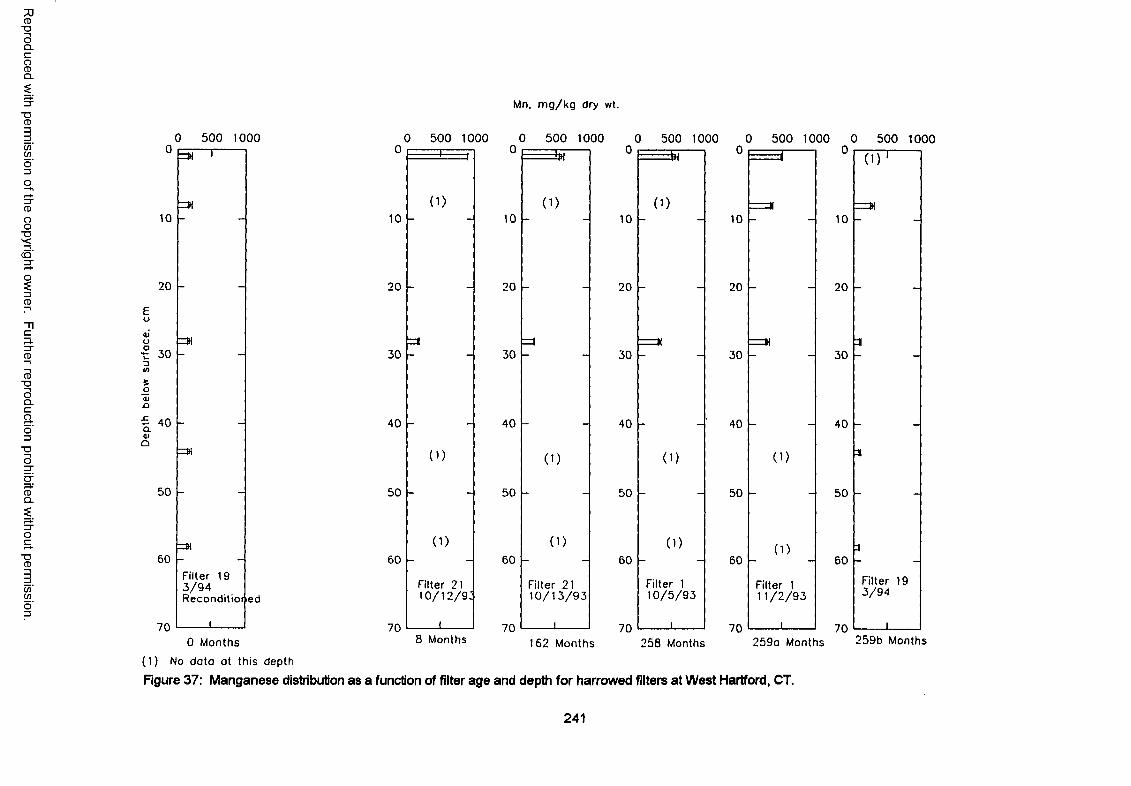
Reproduced
with perm
ission of the
copyright ow
ner. Further
reproduction prohibited
without
permission.
Mn, m g /k g dry wt.
0 50 0 1000 0 50 0 1000 0 5 0 0 1000 0 500 1000 0 50 0 1000 0 500 1000
10
20
Eo4)Or 303105o
=M
aDO
40
50
60
70
=M
Filter 19 3 /9 4 Reconditioi ed
10
20
30
40
50
60
70
(1)
(1)
(1)
Filter 2110/ 12/ 9 :
i8 Months
10
20
30
40
50
60
70
itt
(1)
0 )
(1)
Filter 21 1 0 /1 3 /9 3
I____
10
20
30
40
50
60
70
=ST
(1)
(1)
(0
Filter 1 1 0 /5 /9 3
i162 Months 258 Months
10
20
30
40
50
60
70
(1)
(1)
Filter 1 1 1 /2 /9 3
I___
10
20
30
40
50
60
70
(1) T
Filter 19 3 /9 4
0 Months
(1 ) No data at this depth
Figure 37: Manganese distribution as a function of filter age and depth for harrowed filters at West Hartford, CT.
259a Months 259b Months
241
and manganese increased over the period. AFDC, caldum, and aluminum were not significantly
changed. It would be expected that the surface media would not change greatly as the sampling
was earned out immediately before filters were to be cleaned. At this time, the filters had
accumulated approximately the same mass of organic or inorganic materials as over the preceding
filter cycle, generally four to six weeks at this plant An increase in accumulation would have been
indication that the filter had not been sufficiently deemed over the operating period, yet plant
experience had been that even the oldest filter media was generally able to be cleaned to at least
one-half of the capacity of its rated capacity (Allen, 1991). Since the filters were not showing
increased concentrations of volatile solids, FRM, carbohydrates, iron and manganese in the
surface of the filters, then the cleaning technique was achieving its purpose at this level. The
development of increasing concentrations at the lower levels indicated that harrow was mixing
surface materials into the filter at greater depth than the concentrations developing over a similar
time period at the Newark, NY plant which cleaned filters by scraping.
Past research has demonstrated a positive relationship between schmutzdecke age and
biomass as quantified by cell protein and bacterial counts (Collins et al., 1992b). Elapsed time or
age of a filter media and potential cell growth are considered to be more important in controlling
bacterial population levels than filtration of bacteria from the source water (Ripley and Saleem,
1973; Wood, 1980; and Collins et al., 1992b). Wang et al. (1995) also noted that the removal of
DBP precursors is likely related to microbial activity rather than the amount of biomass. The
growth of the sand media biofilm will be dependent on cell growth potential which, in turn, will be
dependent on the availability of the rate limited nutrient, usually organic substrate, and suitable
growth environment Increased surface scraping will inherently limit the age of the schmutzdecke
material as compared to the harrowing method which maintains schmutzdecke-like bacterial
populations throughout the harrowed portion of filter bed (Collins et al., 1989). The age of sand in
a filter cleaned by scraping is also limited by the eventual removal of the media and resanding of
the filter.
242
Reproduced with permission of the copyright owner. Further reproduction prohibited without permission.
Sand aging may also relate to changes in non-biological parameters such as metal
composition in the sand media coating over time. Biological filters are noted for their exceptional
removals of iron and manganese (Degremont, 1991). The older filters in this study accumulated
higher iron and manganese, but the most significant differences were between the water supplies
to the respective plants. The Newark plant had significantly higher concentrations of iron and
manganese than did any of the other plants, but the media had been in the filters for 1.5 to 3 years
at Newark as compared to the 19 and 13 years that the media had been in Filters 1 and 18,
respectively, at West Hartford. Additional studies have looked more closely at the retention of
NOM by artificially coated iron oxide coated media (Benjamin et al., 1993) and naturally occurring
iron oxides (Gu et al., 1994; Tipping, 1991; Davis, 1982). Each study has demonstrated the
efficacy of NOM adsorption on the metal oxide surface. Consequently, total metal content and
composition in the surface coatings of sand media is considered to contribute to the natural aging
or ripening of filter media.
The laboratory scale column tests, comparing the removal of TOC and UV absorbance
from NOM by sand media of different age (19 years and less than one year) at uniform application
rates, EBCT, temperature, and raw water quality confirmed the higher removals with the sand
having the greater age and surface coating deposition. The laboratory scale column tests,
comparing the removal of TOC and UV absorbance by sand having differing percentages of the
natural coatings removed (none to all), also at uniform conditions of application rates, EBCT,
temperature, and raw water quality, also confirmed the higher removals with sand having the
greater surface coating deposition. In these tests, however, it was also demonstrated that
biological coatings as measured by FRM, carbohydrates, and AFDC were capable of rapid
replacement The FRM and carbohydrate concentrations of the media which had all coatings
removed prior to the tests had coatings at the end of the five days of testing equal to the media
from which two-thirds of the coatings had been removed. The AFDC concentration on the media
filtering the G/GA solution was not significantly different after five days between the media with no
243
Reproduced with permission of the copyright owner. Further reproduction prohibited without permission.
remaining natural coating and the media with one-third natural coating at the start of the five day
test period. The AFDC concentrationon the media filtering the NOM had not recovered, but the
ratio of FRM to AFDC was atypical and the AFDC data may not have been valid. Since the FRM
and carbohydrate values for the several media analyses were consistent and only the one set of
AFDC values were atypical, it was concluded that the media had quickly recovered FRM,
carbohydrate, and AFDC during the five day test period. The innoculation for the regrowth would
have been the internal surfaces of the tubing using to connect the filter columns and reservoirs as
they were not sterilized before the test period.
S u m m a ry : The importance of sand media age and subsequent ripening conditions on the
treatment performance of slow sand filtration should not be underemphasized. Sand media aging
involves the surface accumulation of biological and inorganic constituents that are beneficial to the
treatment process. The extent of sand media aging will be a function of how long the sand can be
used before resanding and whether the filter cleaning method used at the plant will result in early
depletion of the sand in the filter. Filter harrowing appears to accelerate the aging phenomenon
as compared to surface scraping by distributing the biomass deposits remaining after cleaning
throughout the upper filter layers rather than physically removing the material with the uppermost
few centimeters from the filter bed. Furthermore, scraping will limit filter age to four to six years (or
as determined by the media depth and length filter cycles as the particular plant in question) as the
depth is reduced by one-half to one-inch with each cleaning cycle. The harrowing method of
cleaning avoids the reduction in filter depth that is caused by scraping and has allowed filters to
remain in service up to 20 years.
5.4 INFLUENCE OF FILTER BIOMASS
A biological process will be more efficient if, for a given volume of media, the
concentration of biomass is higher (Collins etal., 1992b) or more active (Wang etal., 1995).
Bellamy et al. (1985a and 1985b) found the state of the biological community significantly
244
Reproduced with permission of the copyright owner. Further reproduction prohibited without permission.
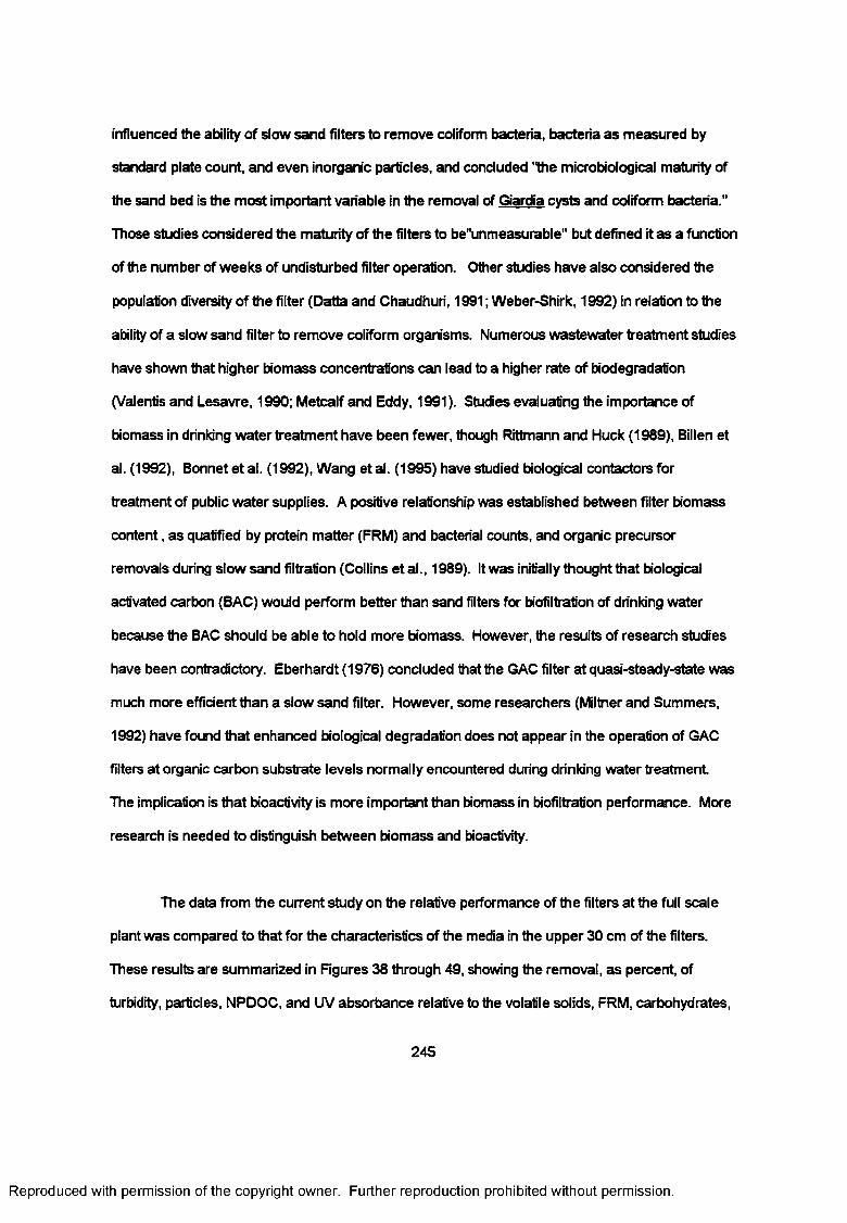
influenced the ability of slow sand filters to remove coliform bacteria, bacteria as measured by
standard plate count, and even inorganic particles, and concluded "the microbiological maturity of
the sand bed is the most important variable in the removal of Giardia cysts and coliform bacteria."
Those studies considered the maturity of the filters to be"unmeasurable" but defined it as a function
of the number of weeks of undisturbed filter operation. Other studies have also considered the
population diversity of the filter (Datta and Chaudhuri, 1991; Weber-Shirk, 1992) in relation to the
ability of a slow sand filter to remove coliform organisms. Numerous wastewater treatment studies
have shown that higher biomass concentrations can lead to a higher rate of biodegradation
(Valentis and Lesavre, 1990; Metcalf and Eddy, 1991). Studies evaluating the importance of
biomass in drinking water treatment have been fewer, though Rittmann and Huck (1989), Billen et
al. (1992), Bonnet et al. (1992), Wang et al. (1995) have studied biological contactors for
treatment of public water supplies. A positive relationship was established between filter biomass
content, as quatified by protein matter (FRM) and bacterial counts, and organic precursor
removals during slow sand filtration (Collins et al., 1989). It was initially thought that biological
activated carbon (BAC) would perform better than sand filters for biofiltration of drinking water
because the BAC should be able to hold more biomass. However, the results of research studies
have been contradictory. Eberhardt (1976) concluded that the GAC filter at quasi-steady-state was
much more efficient than a slow sand filter. However, some researchers (Miltner and Summers,
1992) have found that enhanced biological degradation does not appear in the operation of GAC
filters at organic carbon substrate levels normally encountered during drinking water treatment
The implication is that bioactivity is more important than biomass in biofiltration performance. More
research is needed to distinguish between biomass and bioactivity.
The data from the current study on the relative performance of the filters at the full scale
plant was compared to that for the characteristics of the media in the upper 30 cm of the filters.
These results are summarized in Figures 38 through 49, showing the removal, as percent, of
turbidity, particles, NPDOC, and UV absorbance relative to the volatile solids, FRM, carbohydrates,
245
Reproduced with permission of the copyright owner. Further reproduction prohibited without permission.
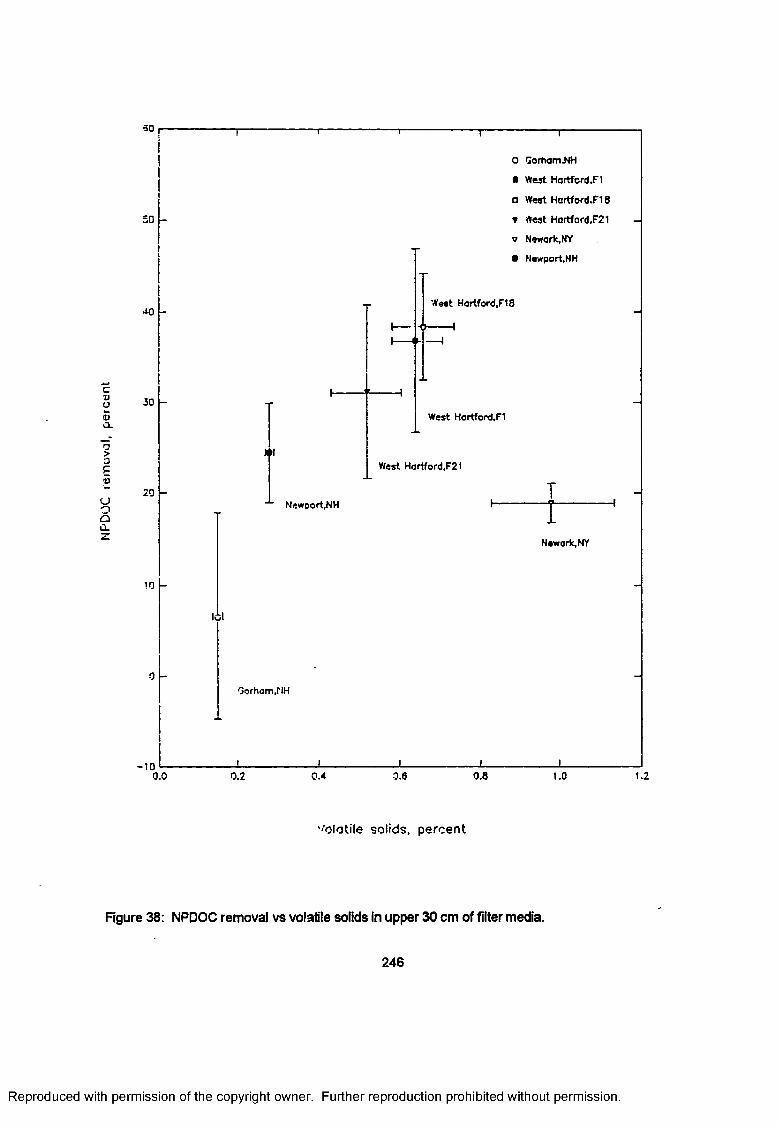
NPDO
C re
mov
al,
perc
ent
60
40
30
20
10
t i l
Newport.NH
Oorhom.NH
O Gortiam.NH
■ West Hortford.Fl
o West Hartford.F18
» West Hartford.F21
■7 Newark, NY
• Newport,HH
W««t Hortford.Fl 8
1
West Hortford.Fl
West Hortford.F21
T
TNewark, NY
-1 00.0 0.2 0.4 0.6 0.8 1.0 1.2
'''olatile solids, percent
Figure 38: NPDOC removal vs volatile solids in upper 30 cm of filter media.
246
Reproduced with permission of the copyright owner. Further reproduction prohibited without permission.
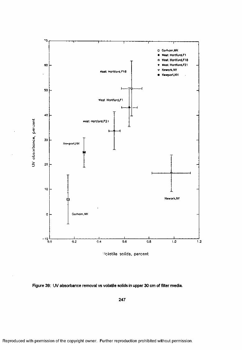
UV
abso
rban
ce,
per
cen
t
60
50
40
30
20
10
west Hortford.Fl 8
West Hartford.F1
(-
ivest Hartford.F21
Me~pcrt.NH
III
£
Gorham,NH
O Gorhom.NH ■ West Hartfcrd.F1
Q West Hortford.Fl 8* West Hortford.F21
v Newark.NY• Newport,NH
Newark.NY
-100.0 0.2 0.4 0.6 0.8 1.0 1.2
'■'olatile solids, percent
Figure 39: UV absorbance removal vs volatile solids in upper 30 cm of filter media.
247
Reproduced with permission of the copyright owner. Further reproduction prohibited without permission.
NPDO
C re
mov
al,
perc
ent
50 T T
West Hortford.F18
40
30
West Hartford,F21
20
to
West Hortford.Fl
-INewark,NY
I $---------1
Gorhom.NH
O Gorhom.NH
■ West Hortford.Fl
Q West Hartford,F10
▼ West Hartford.F21
v Newark,NY
• Newport.NH
Newport.NH
-100.0 0.5 1.0 1.5 2.0 2.5 3.0 3.5 4.0
FRM, mg p ro te in /g dry wt.
Figure 40: NPDOC removal vs FRM in upper 30 cm of filter media.
248
Reproduced with permission of the copyright owner. Further reproduction prohibited without permission.
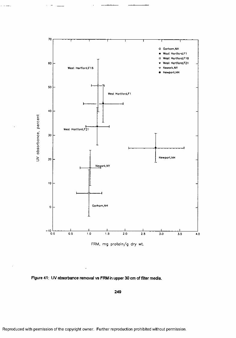
UV ab
sorb
ance
, pe
rcen
t70 r
60
so
40
30
20
10
O Gorhom.NH
■ West Hartford.F1
West Hortford.Fl8
West Hortford,F21 Newark.NY Newport.NH
West Hortford.Fl8
West Hortford.Fl
West Hartford,F21
Newport.NH
Newark.NY
Gorhom.NH
- 1 00 0 0.5 1.0 1.5 2.0 2.5 3.0 3.5 4.0
FRM. mg p ro te in /g dry wt.
Figure 41: UV absorbance removal vs FRM in upper 30 cm of filter media.
249
Reproduced with permission of the copyright owner. Further reproduction prohibited without permission.
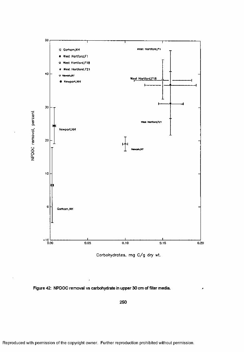
NPDO
C re
mov
al,
perc
ent
=o, i
40
0 Gorham,NH
■ West Hartford,FI
O West Hertford, f718
T West Hartford.F21
7 Newart-NT
• Newport.NH
30
MNewport.NH
20 IT
west H a rtfo ra .n
West Hartford.Fia
west Hartfere.F2l
Nsworfcjrr
10
Gortiom.NH
-1C0.00 0.05 0.10 0.15 0.20
Carbohydrates, mg C /g dry wt.
Rgure 42: NPDOC removal vs carbohydrate in upper 30 cm of filter media.
250
Reproduced with permission of the copyright owner. Further reproduction prohibited without permission.
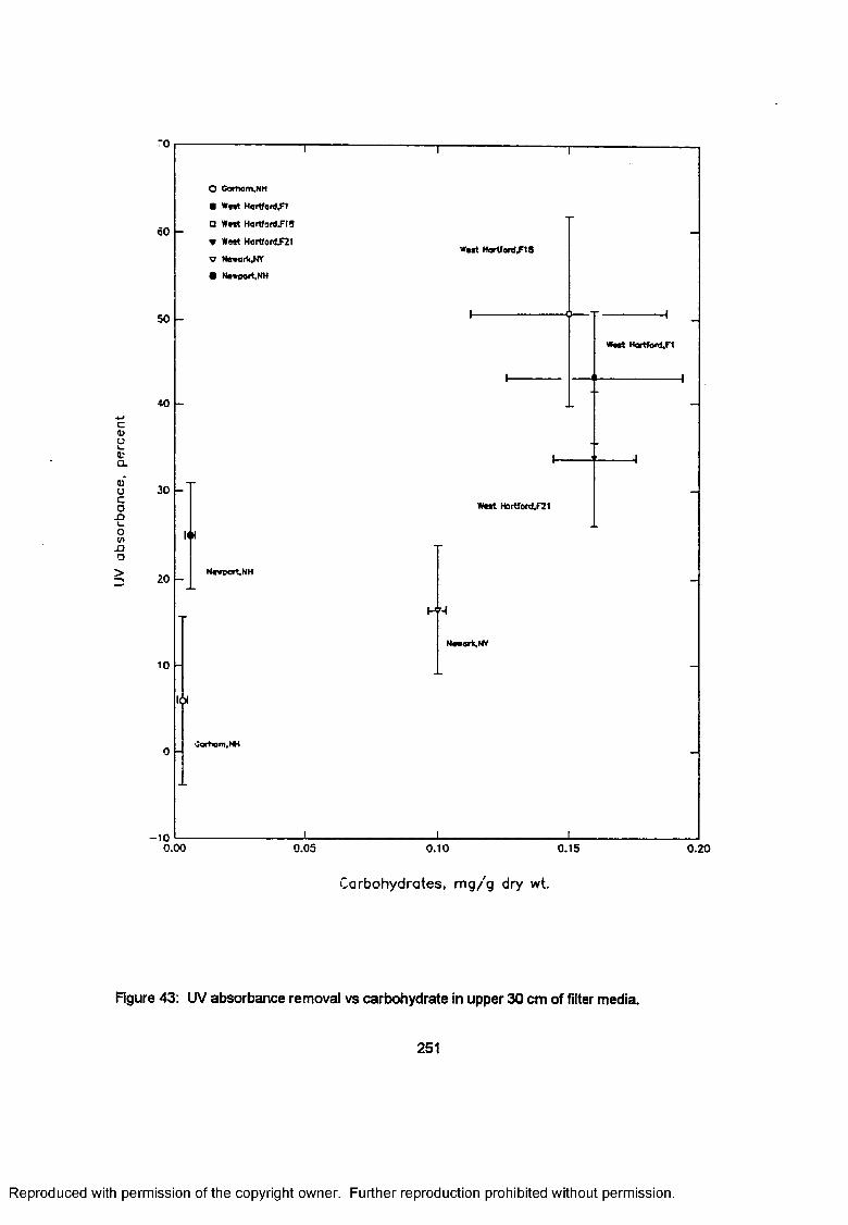
IJV
abso
rban
ce,
per
cent
60
50
40
O Comom,NH
■ Wart HartfoflJ.F1
Q Wort H a r t fo rd ^ ! §
W Wart H a rtfo rd .F21
V HewarV*• Nooport.NH
30
M
20 N « vcart.N H
10
W a t H a rtfo rd .F 1 8
W i r t H o rtfo fd ,F 21
H?-*
N«wark,NY
W at HartfonJ.F1
>0*
- 1 00.00 0.05 0.10 0.15 0.20
Carbohydrates, mg/'g dry wt.
Figure 43: UV absorbance removal vs carbohydrate in upper 30 cm of filter media.
251
Reproduced with permission of the copyright owner. Further reproduction prohibited without permission.
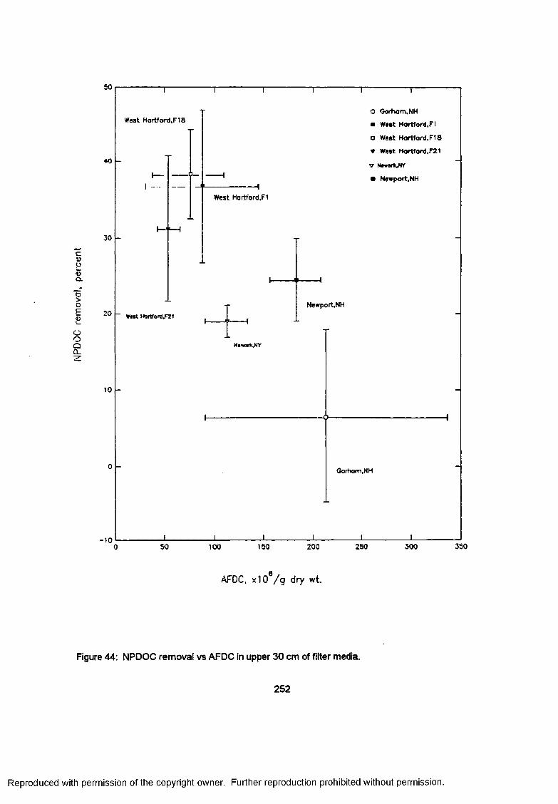
NPDO
C re
mov
al,
perc
ent
50 T
West H o rtfo rd .F IB
♦0
30I—1'—I
O Gorhom.NH
■ West H o rtfo rd .F l
a West H o rtfo rd .F l 8
▼ West H artford ,F21
V Ne*ark,Nr
• Newport.NH
West Hartford,F1
20 West H a rtfo rd .F 2 l
10
Newport.NH
N«worV,MY
Gorhom.NH
-1 050 100 150 200 250 300
AFDC, x10 /g dry wt.
Figure 44: NPDOC removal vs AFDC in upper 30 cm of filter media.
252
350
Reproduced with permission of the copyright owner. Further reproduction prohibited without permission.
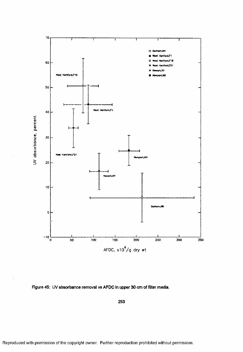
UV
abso
rban
ce,
per
cen
t70
60
w « t t U o r t fo rd . r iB
50
-to
30
O Gorttom,NH
m W M t Kartford .F1
□ W est H o rtfo rd F IB
▼ W cet Hartf6rd.F21
V N**orK .M Y
• H— port NH
w « s t h o n fo r d .n
w est M a rtfo rt,F 2 l
20
10
G arham,NH
-1050 100 150 200 250 300 350
AFDC, xlO /g dry wt
Figure 45: UV absorbance removal vs AFDC in upper 30 cm of filter media.
253
Reproduced with permission of the copyright owner. Further reproduction prohibited without permission.
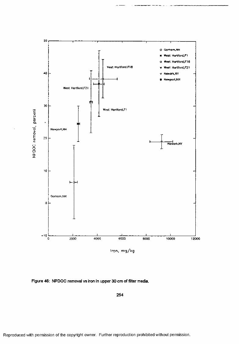
NI-'D
OO
rem
oval
, pe
rcen
t
:a r T
JO
West Hortford.F21
30
Newport.NH
20
Dll
10
I—d-l
Gorhom.NH
n
West Hartford.Ft 8
West Hortford.Fl
O G orhom .N H
■ West Hortford.Fl
a West Hortford.Fl 8
▼ West Hartford,F21
v Newark, NY
• Newport.NH
Nework.NY
-102000
i4000 6000 8000
i10000
iron, m g /k g
Figure 46: NPDOC removal vs iron in upper 30 cm of filter media.
254
12000
Reproduced with permission of the copyright owner. Further reproduction prohibited without permission.
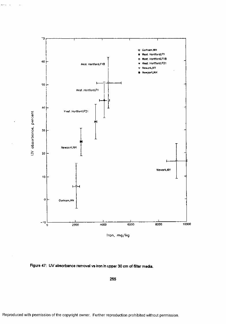
UV
abso
rban
ce,
per
cent
T T T
60
■MbI
40
30
10
iVest Hortford.Fl 8
tfe3t Hartfcrd.F1
r-«st Hartford.F21
Newacrt.NH
-9--------- 1
M
O Gorham .NH ■ West Hortford.Fl
a West Hortford.Fl 8 ▼ West Hartford.F21
t Newark, NY
• Newport,NH
10
Gorhom.NH
Newark.NY
- ' 02000 4000 6000 8000
Iron, m q /k q
Figure 47: UV absorbance removal vs iron in upper 30 cm of filter media.
255
l
10000
Reproduced with permission of the copyright owner. Further reproduction prohibited without permission.
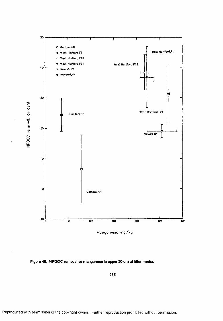
NPDO
C le
mov
ol,
perc
ent
50
♦o
O Gorhom.NH
■ West Hortford.Fl
□ West Hartford.F18
t West Hortford.F21
a Newark,NY
• N ewport,NH
Weat H ortfo rd .F18
30
20
West Hartford.Ft
Nev*port,NH West Hartford,F21
I-
H
10
Newark, NY
Gorhom.NH
- 1 0100 ZOO 300 4 00 5 0 0 800
Manganese, m g /k g
Figure 48: NPDOC removal vs manganese in upper 30 cm of filter media.
256
Reproduced with permission of the copyright owner. Further reproduction prohibited without permission.
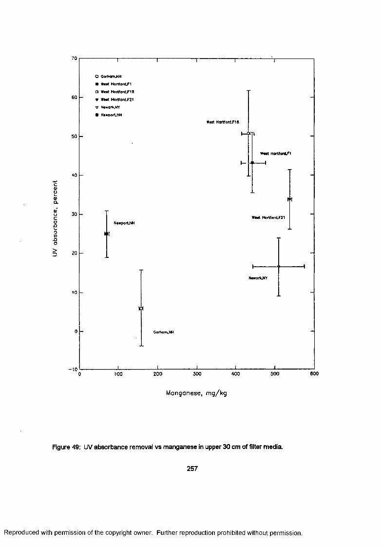
UV
abso
rban
ce,
per
cen
t70
60
O Cortioni.N H
■ West H a rtfard .F1
□ West H a r t fo r d / 'IB
▼ West H a r t fo rd /2 1
w Neworfc.Wr
• Ne«pcrt.M H
Weet H a r t fo r d /1 8
50
40
Weet H artfo rd /1
30
20
W est H a r t fo rd /2 1
NewportNH
M
mi
10
Ipl
N ew arV .H r
'Jct+K jm .N H
-1 0100 200 300 400 500 600
Manganese, m g/kg
Figure 49: UV absorbance removal vs manganese in upper 30 cm of filter media.
257
Reproduced with permission of the copyright owner. Further reproduction prohibited without permission.
AFDC, iron, and manganese characteristics of those filters.
Comparisons between older and newer/fresher sand media in this study, on both full scale
and laboratory scale filters, correlated superior removals of NPDOC and UV absorbance with sand
media having ages up to 19 years. This improved performance appeared to be related to the
biological and inorganic composition of the sand media coatings as discussed earlier and shown in
the preceding figures, 38 to 49.
Neither of the two cleaning methods studied removes such a large proportion of the
natural sand coating biomass that they would affect the ability of the cleaned sand to remove TOC
or UV absorbing materials. Ripening trends following cleaning events indicate the cleaned filters
have substantially recovered pre-event performance levels within a few hours or bed volumes
filtered. Scraping may remove a layer of the media in its entirety, but the sand media which is
newly exposed has already developed a significant microbiological population (Eghmy et al.,
1992). Harrowing removed materials from a greater thickness of the media, agitating, disrupting,
and carrying off deposits down to 15 to 20 cm in the media as opposed to removing only the
upper 1 to 2 cm, but harrowing also redistributes the remaining sand coating material/biomass
throughout this thickness. This generalization is not meant to say that there is no effect from the
cleaning methods. Both cleaning methods impact the surface deposits which are often reported to
provide the greater part of treatment by slow sand filters. Also, as noted in Chapter 2 and
elsewhere, a period of ripening may be necessary after a filter is cleaned to recover the former
levels of filter performance (Letterman and Cullen, 1985). The need for ripening new filter media,
whether following construction of the facility or resanding, was shown by the relative removal of
NPDOC and UV absorbing material. The advantage of trenching and "throwing-over" the lower
part of the filter media during resanding is apparent from both the point of retaining natural sand
coatings within the filter and increasing the mean age of the filter media. An advantage of the
harrowing cleaning method over scraping can also be deduced as it retains the sand within the
258
Reproduced with permission of the copyright owner. Further reproduction prohibited without permission.
filter and avoids the need to replace sand every 5 to 10 years. The sand in a harrowed filter will
eventually require reconditioning, but the filters at West Hartford have been operated for up to 20
years before reconditioning. They plan to reduce this to 10 years (Allen, 1993).
The rapidity with which AFDC and FRM materials recover in the media and the slower
recovery of the removal performance of the media indicates that prolonged ripening of a new sand
involves more than the development of a simple biofilm. The information from the laboratory filter
columns does not explain whether the longer ripening is necessary for the development of a “thick
film'' as suggested by Rittmann (1990), a more heterogeneous population of bacteria or
microfauna (Weber-Shirk, 1992), or other characteristics necessary for removal. A longer study
period and modified experimental design should be used to provide a filter arrangement that could
be sampled during the evaluation period to consider these factors.
S u m m a ry : The evidence presented in this study, especially from the laboratory-scale filters,
support the importance of biomass on slow sand filter performance. Increasing biomass content
resulted in a proportional increase in organic carbon removal. As observed in previous studies,
the harrowing cleaning method can elevate the biomass content of slow sand filters, measured as
protein and carbohydrate, over that in filters cleaned by surface scraping. The scraped filters at the
Newark plant, however, contained higher concentrations of volatile solids than did the harrowed
filters at West Hartford. The reason for this can not be easily explained by the collected data but
may be related to the activity of the materials at the different plants.
5.5 IMPORTANCE OF SOURCE WATER QUALITY
The source of water is also important to biofiltration efficiency. Several studies have
mentioned that the organic carbon substrate is usually the rate-limiting nutrient in the biological
processes (LeChevallier et al., 1990). For a variety of reasons, the biodegradable content of
natural waters will vary from source to source (Aiken and Cotsaris, 1995; Owen et al., 1995).
259
Reproduced with permission of the copyright owner. Further reproduction prohibited without permission.
Nitrogen and phosphorous are not considered rate limiting for established biofilm because the
necessary nutrients for biological activity are considered to be already stored in the surface coating
(Camper, 1994). However, this may not be the case during the initial start-up stages of a
biofiltration process.
Recent research (Wang and Summers, 1993) has proposed that the biodegradable
content of the dissolved organic carbon (NPDOC) may be subdivided into a fast biodegradable
portion which follows Monod kinetics and a much slower biodegradable portion which follows first-
order kinetics. The fast portion would be preferentially removed in an engineered process since
detention times for both are generally measured in minutes or hours. The slower biodegradable
portion is typically measured in days. Consequently, the fast and slow biodegradable kinetic
fractions of natural organic matter in water will be dependent on the relative biodegradability of
NOM which, in turn, will be dependent on the groundwater contribution (and other hydrogeologic
factors) to the surface raw water. The West Hartford water supply, for example, would appear to
be more amenable to biofiltration than the low organic content source waters in New Hampshire.
Another important factor to consider in source water influences is that complex metabolic
interactions within the filter bacterial population may be dependent indirectly on the biological
characteristics of the source water. Past research (Collins et al., 1989) demonstrated that the
greater propensity to metabolize benzoate, and aromatic compound, in the West Hartford filters
correlated to superior NOM removals than observed in other slow sand filtration facilities. In that
study, raw water quality showed SUVA (Edzwald, 1993) characteristics of the West Hartford water
to be more amenable to removal of UV absorbance and THM precursors, and to be more
consistent with seasons. The data for these determinations and results are summarized in Table
99. Comparable data from the current study is presented in Table 100.
260
Reproduced with permission of the copyright owner. Further reproduction prohibited without permission.
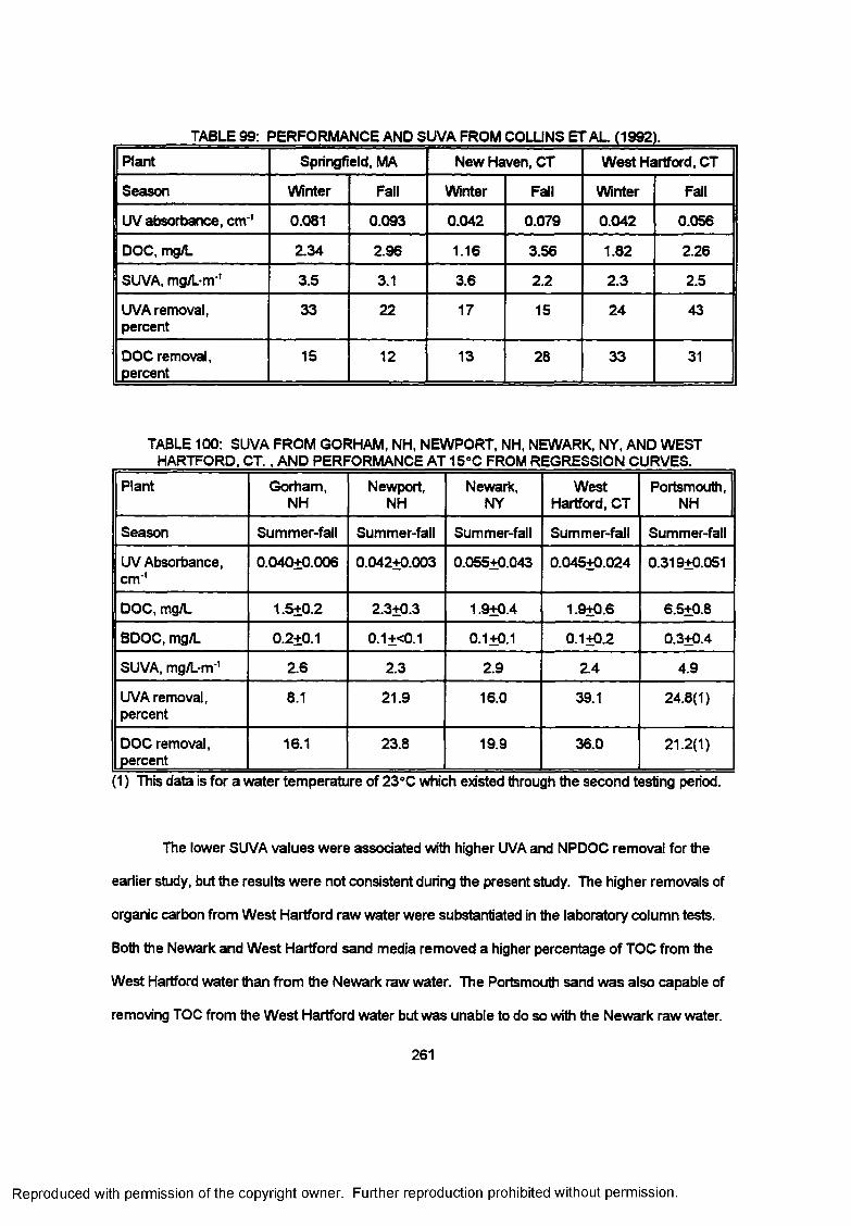
TABLE 99: PERFORMANCE AND SUVA FROM COUJNS ETAL. (1992).
Plant Springfield, MA New Haven, CT West Hartford, CT
Season Winter Fall Winter Fall Winter Fall
UV absorbance, cm'1 0.081 0.093 0.042 0.079 0.042 0.056
DOC, mg/L 2.34 2.96 1.16 3.56 1.82 2.26
SUVA, mg/L-m'1 3.5 3.1 3.6 2.2 2.3 2.5
UVA removal, percent
33 22 17 15 24 43
DOC removal, percent
15 12 13 28 33 31
TABLE 100: SUVA FROM GORHAM, NH, NEWPORT, NH, NEWARK, NY, AND WEST HARTFORD, CT. . AND PERFORMANCE AT 15°C FROM REGRESSION CURVES.
Plant Gorham,NH
Newport,NH
Newark,NY
West Hartford, CT
Portsmouth,NH
Season Summer-fall Summer-fall Summer-fall Summer-fall Summer-fall
UV Absorbance, cm'1
0.040+0.006 0.042+0.003 0.055+0.043 0.045+0.024 0.319+0.051
DOC, mg/L 1.5+0.2 2.3+0.3 1.9+0.4 1.9+0.6 6.5+0.8
BDOC, mg/L 0.2+0-1 0.1+<0.1 0.1±0.1 0.1+0.2 0.3±0.4
SUVA, mg/L-m'1 2.6 2.3 2.9 2.4 4.9
UVA removal, percent
8.1 21.9 16.0 39.1 24.8(1)
DOC removal, percent
16.1 23.8 19.9 36.0 21.2(1)
1) This data is for a water temperature of 23°C which existed through the second testing period.
The lower SUVA values were associated with higher UVA and NPDOC removal for the
earlier study, but the results were not consistent during the present study. The higher removals of
organic carbon from West Hartford raw water were substantiated in the laboratory column tests.
Both the Newark and West Hartford sand media removed a higher percentage of TOC from the
West Hartford water than from the Newark raw water. The Portsmouth sand was also capable of
removing TOC from the West Hartford water but was unable to do so with the Newark raw water.
261
Reproduced with permission of the copyright owner. Further reproduction prohibited without permission.
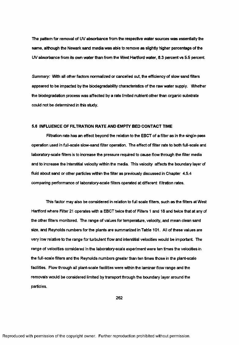
The pattern for removal of UV absorbance from the respective water sources was essentially the
same, although the Newark sand media was able to remove as slightly higher percentage of the
UV absorbance from its own water than from the West Hartford water, 8.3 percent vs 5.5 percent
S u m m a ry : With all other factors normalized or cancelled out, the efficiency of slow sand filters
appeared to be impacted by the biodegradability characteristics of the raw water supply. Whether
the biodegradation process was affected by a rate limited nutrient other than organic substrate
could not be determined in this study.
5.6 INFLUENCE OF FILTRATION RATE AND EMPTY BED CONTACT TIME
Filtration rate has an effect beyond the relation to the EBCT of a filter as in the single-pass
operation used in full-scale slow-sand filter operation. The effect of filter rate to both full-scale and
laboratory-scale filters is to increase the pressure required to cause flow through the filter media
and to increase the interstitial velocity within the media. This velocity affects the boundary layer of
fluid about sand or other particles within the filter as previously discussed in Chapter 4.5.4
comparing performance of laboratory-scale filters operated at different filtration rates.
This factor may also be considered in relation to full scale filters, such as the filters at West
Hartford where Rlter 21 operates with a EBCT twice that of Rlters 1 and 18 and twice that at any of
the other filters monitored. The range of values for temperature, velocity, and mean clean sand
size, and Reynolds numbers for the plants are summarized in Table 101. All of these values are
very low relative to the range for turbulent flow and interstitial velocities would be important The
range of velocities considered in the laboratory-scale experiment were ten times the velocities in
the full-scale filters and the Reynolds numbers greater than ten times those in the plant-scale
facilities. Flow through all plant-scale facilities were within the laminar flow range and the
removals would be considered limited by transport through the boundary layer around the
particles.
262
Reproduced with permission of the copyright owner. Further reproduction prohibited without permission.
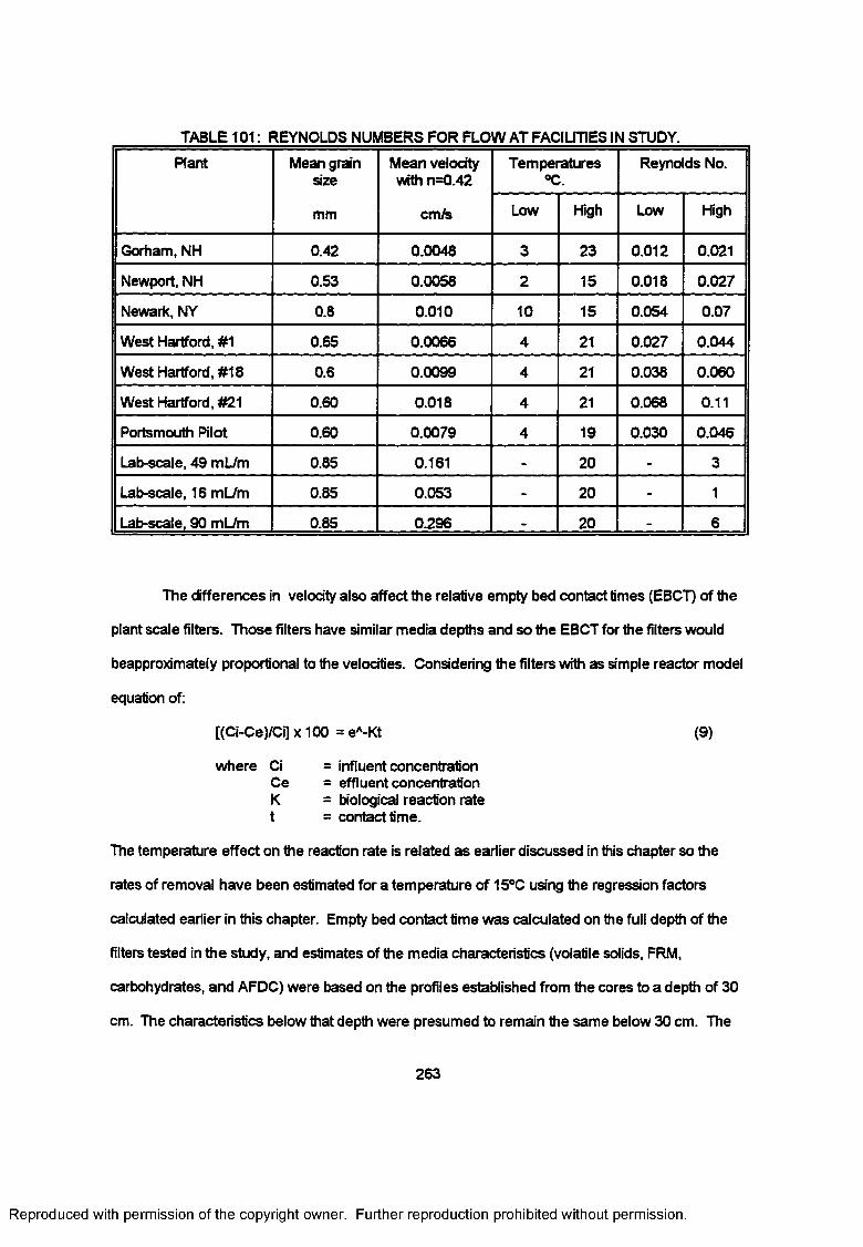
TABLE 101: REYNOLDS NUMBERS FOR FLOW AT FACILITIES IN STUDY.
Plant Mean grain size
Mean velocity with n=0.42
Temperatures°C.
Reynolds No.
mm cm/s Low High Low High
Gorham, NH 0.42 0.0048 3 23 0.012 0.021
Newport, NH 0.53 0.0058 2 15 0.018 0.027
Newark, NY 0.8 0.010 10 15 0.054 0.07
West Hartford, #1 0.65 0.0066 4 21 0.027 0.044
West Hartford, #18 0.6 0.0099 4 21 0.038 0.060
West Hartford, #21 0.60 0.018 4 21 0.068 0.11
Portsmouth Pilot 0.60 0.0079 4 19 0.030 0.046
Lab-scale, 49 mL/m 0.85 0.161 - 20 - 3
Lab-scale, 16 mL/m 0.85 0.053 - 20 - 1
Lab-scale, 90 mL/m 0.85 0.296 - 20 - 6
The differences in velocity also affect the relative empty bed contact times (EBCT) of the
plant scale filters. Those filters have similar media depths and so the EBCT for the filters would
beapproximately proportional to the velocities. Considering the filters with as simple reactor model
equation of:
[(Ci-Ce)/Ci] x 100 = eA-Kt (9)
where Ci = influent concentrationCe = effluent concentrationK = biological reaction ratet = contact time.
The temperature effect on the reaction rate is related as earlier discussed in this chapter so the
rates of removal have been estimated for a temperature of 15°C using the regression factors
calculated earlier in this chapter. Empty bed contact time was calculated on the full depth of the
filters tested in the study, and estimates of the media characteristics (volatile solids, FRM,
carbohydrates, and AFDC) were based on the profiles established from the cores to a depth of 30
cm. The characteristics below that depth were presumed to remain the same below 30 cm. The
263
Reproduced with permission of the copyright owner. Further reproduction prohibited without permission.
relative performance of the plant-scale filters is summarized as shown in Table 102. An example
of the calculation of one set of the values is presented in Appendix C.
TABLE 102: FIRST ORDER REACTION COEFFICIENTS (HR ') FOR REMOVAL OF NPDOC ANDUVA.
Gorham, Newport, Newark, West Hartford, CT
NH NH NY Filter 21 Rlter 18 Filter 1
Loading rate, m/hr 0.072 0.11 0.070 0.14 0.16 0.12
Filter depth, m 0.68 0.68 0.75 0.68 0.68 0.68
Detention time, hr 9.4 6.2 5.4 4.8 4.2 5.7
Temperature, °C 15 21 10 14 14 16
Est NPDOC removal at 15°C,% (a)
16.1 23.8 19.8 30.7 36.4 40.9
Reaction coeff. per unit- Volatile solids FRMCarbohydrateslO ^AFDC
0.300.160.29108
1 ^ -6
0.510.160.18112
2.1A-6
0.550.390.514.7
5.0A-6
0.710.130.774.9
1 ^ -5
0.860.0910.536.8
9.7A-6
0.650.0750.433.4
6 & - 6
Est UV absorbance removal at 15°C, % (a)
8.1 21.9 16.0 32.9 44.4 40.0
Reaction coeff. per unit- Volatile solids FRMCarbohydratesAFDC
0.220.120.2281
9.8A-7
0.500.150.18110
2.0A-6
0.51.0360.474.3
4.6A-6
0.730.130.784.8
1.6^5
0.900.0960.557.2
1.0*-5
0.650.0740.433.4
6.6*6(a) Removal at 15°C calculated using regression factors in Table 90.
Comparisons were made between the data for the three filters which had not been
harrowed before or during the study period against the three at West Hartford which had been
harrowed. The results are summarized in Table 103. The comparisons between the two sets of
filters, differentiated by having been cleaned by harrowing or not, is presented to raise the issue of
possible significance. The three filter plants which had not been harrowed filtered raw waters from
significantly different sources, with sand of different chemical characteristics, and had been in
operation for different lengths of time. One plant had never been cleaned, another cleaned only a
264
Reproduced with permission of the copyright owner. Further reproduction prohibited without permission.
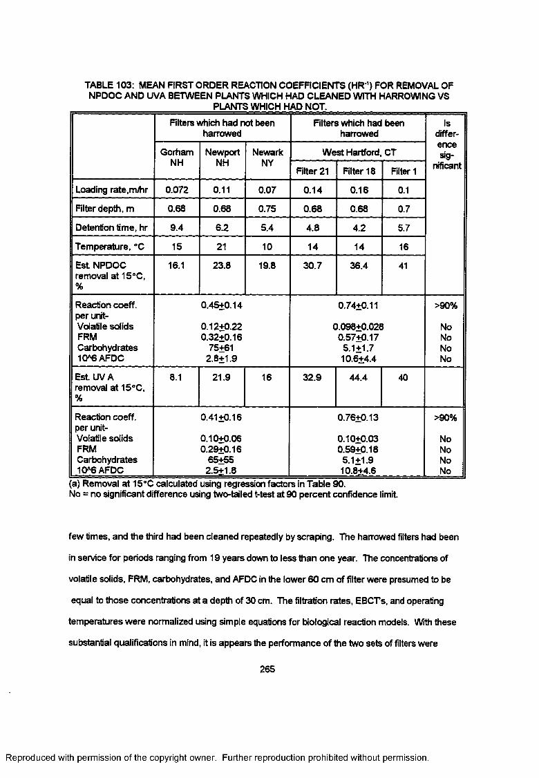
TABLE 103: MEAN FIRST ORDER REACTION COEFFICIENTS (HR ') FOR REMOVAL OF NPDOC AND UVA BETWEEN PLANTS WHICH HAD CLEANED WITH HARROWING VS
PLANTS WHICH HAD NOT.
Filters which had not been harrowed
Filters which had been harrowed
Isdiffer
GorhamNH
NewportNH
NewarkNY
West Hartford, CTencesig
Filter 21 Filter 18 Filter 1 nificant
Loading rate,m/hr 0.072 0.11 0.07 0.14 0.16 0.1
Filter depth, m 0.68 0.68 0.75 0.68 0.68 0.7
Detention time, hr 9.4 6.2 5.4 4.8 4.2 5.7
Temperature, “C 15 21 10 14 14 16
Est NPDOC removal at 15°C, %
16.1 23.8 19.8 30.7 36.4 41
Reaction coeff. per unit- Volatile solids FRMCarbohydrates 10*6 AFDC
0.45+0.14
0.12+0.22 0.32+0.16
75+61 2.8+1.9
0.74+0.11
0.098+0.028 0.57+0.17
5.1+1.7 10.6+4.4
>90%
NoNoNoNo
Est UVA removal at 15°C, %
8.1 21.9 16 32.9 44.4 40
Reaction coeff. per unit- Volatile solids FRMCarbohydrates 10*6 AFDC
0.41+0.16
0.10+0.06 0.29+0.16
65+55 2.5+1.8
0.76+0.13
0.10+0.03 0.59+0.18
5.1+1.9 10.8+4.6
>90%
NoNoNoNo
a) Removal at 15“C calculated using regression factors in Table 90.'Jo = no significant difference using two-tailed t-test at 90 percent confidence limit
few times, and the third had been cleaned repeatedly by scraping. The harrowed filters had been
in service for periods ranging from 19 years down to less than one year. The concentrations of
volatile solids, FRM, carbohydrates, and AFDC in the lower 60 cm of filter were presumed to be
equal to those concentrations at a depth of 30 cm. The filtration rates, EBCTs, and operating
temperatures were normalized using simple equations for biological reaction models. With these
substantial qualifications in mind, it is appears the performance of the two sets of filters were
265
Reproduced with permission of the copyright owner. Further reproduction prohibited without permission.
significantly different, at over 90 percent confidence, in removal of both NPDOC and UV
absorbance. The major differences were, however, between the filters at the Gorham and
Newport plants which had not been cleaned (or cleaned only by surface raking at the time of
media sampling) and the harrowed filters at West Hartford, CT. The characteristics of the scraped
filters at Newark, NY were intermediate between those of the abovementioned sets. The NPDOC
removals, when expressed as removal per unit mass of volatile solids, FRM, carbohydrates, and
AFDC, show the removals of NPDOC per unit of volatile solids, FRM, carbohydrates, and AFDC
not to be statistically different at the 90 percent confidence level. This conclusion was consistent
with the results from the laboratory columns reported in Section 4.2.3 on the influence of natural
coating material on filter media where the removal of NOM varied with the relative natural coating
on the sand media. The major differences in performance were between the filters which had not
been cleaned by either method and those which had been in service longer and cleaned
repeatedly by either method. The unusually high concentration of volatile solids at the Newark, NY
plant make comparisons relating to that paramater unreliable. The Newark, NY plant takes its
supply from a lake with periodic algal blooms and also continuously prechlorinates the flow to the
plant for algal control in intake line. These factors may result in the accumulation of higher
concentrations of inactive volatile solids than at the other plants included in the study.
The UV absorbance removals, when expressed as removal per unit of volatile solids,
FRM, carbohydrates, and AFDC, show the removals of UV absorbance per unit mass of volatile
solids, FRM, carbohydrates, and AFDC also not to be statistically different at the 90 percent
confidence level. This difference may have been a result of the relative activity of the biomass
within the volatile solids at the respective plants. Analyses for the microbial activity or rates of
mineralization (Spanos, 1989) might clarify this difference.
S u m m a ry : The removal information for the two sets of filters, unharrowed vs harrowed, have
similar rates of NPDOC and UV absorbance removal, and it is possible that the unit rates of
266
Reproduced with permission of the copyright owner. Further reproduction prohibited without permission.
removal are the same for volatile solids, FRM, carbohydrates, and AFDC for both NPDOC and UV
absorbance. These similarities, though based on supposition, should be explored by further study.
In particular, filters having longer history of operation and more sampling records. Media
characterization throughout the media depth should be used to test these relationships.
5.7 CLEANING FREQUENCY
It had been planned to compare cleaning methods at either the Gorham or Newport plants
over consecutive cleaning operations. The time required to develop sufficient headloss and
associated filter deposits for cleaning was so long, however, that sampling at that plant was moved
to the Newport plant Cleaning operations were more frequent at that plant, but the field studies
had to be terminated in early 1994 due to personal commitment elsewhere. Consequently, data
could not be obtained directly to compare the frequency that would result from the different
cleaning methods.
The pilot plant operation at Portsmouth, NH, provided a means of estimating the
comparative rates that filter headloss would develop. Three filters were ripened over the period of
February to June 1993 while using the scraping method for cleaning, and then operated in parallel
for five filter cycles between June and September 1993 while using different cleaning methods on
each filter. One filter was cleaned by scraping to the bottom of the darkly colored sand. The other
two filters were cleaned by harrowing, one to a depth of 5 cm (2 in) and the other to a depth of 15
cm (6 in). The development of headlosses were shown in Figure 17. The three filters developed
headloss at similar rates through the first three cycles, and the scraped filter continued to develop
losses at a similar rate through the remaining two cycles of the comparison. The harrowed filters,
however, developed losses at accelerated rates after the third cycle. The media was sampled
between the surface and 2.5 cm and between 25 and 30 cm. The results have been presented
earlier in Table 74 and reviewed on the following page. Media characteristics appeared to have
begun to develop but not sufficiently to differentiate for all parameters. Additional evidence is
267
Reproduced with permission of the copyright owner. Further reproduction prohibited without permission.
needed to support the differences between filters cleaned by the different methods.
The comparative performances of the full-scale plants at Newark, NY and West Hartford
also provide evidence of the greater rate of headloss development in filters cleaned with the
harrowing method. The raw water supplies of the two plants have been discussed earlier, with the
evidence that both are generally high quality and approximately the same particle count, NPDOC,
and UV absorbance, but with higher turbidity and summer algae (Canandaigua Lake Watershed
Task Force, 1994) in the raw water at the Newark plant The length of filter runs over the three
year period of 1991 to 1993, the total volumes of water filtered per run during the evaluation period
in the summer and fall of 1993, and the turbidity and NPDOC loads for the filters are indicated in
Table 104.
The length of the filter cycles at the Newark plant were longer that those at West Hartford,
except for Filter 21 which had been resanded less than one year before the evaluation period. This
data was compared with the records for Filter 19 which had been in service 20 years since it had
been last resanded, and which had averaged 17.0 ML/100 sq. meters (4.17 MG/1000 sf) during its
last two filter runs before reconditioning. The production from Filter 19 was lower than for either
Filter 3 or 4 at Newark and Filter 21 at West Hartford, but still significantly higher than for Filters 1
and 18 at West Hartford. If the length of the filter cycles at the plants were normalized to the same
final headloss, the filter runs of the scraped filters at Newark, NY would have been about three
times those for Filter 21 at West Hartford. The volumes filtered per filter run for all filters was
above the range of "40 to 80 MG/acre", or 3.0 to 6.1 ML/100 sq meters (0.75 to 1.5 MG/1,000 sf)
reported by Tumeaure and Russell (1924).
The turbidity loads on the filters during the cycle were much heavier at the Newark
plant than at West Hartford. Algal development in the supply to the Newark plant causes the
summer filter cycles to be one-third shorter that in the winter. The length of filter cycles at West
268
Reproduced with permission of the copyright owner. Further reproduction prohibited without permission.

TABLE 104: COMPARISONS OF FILTER RUN, VOLUME OF WATER FILTERED, AND _______ TURBIDITY LOADS FOR NEWARK, NY AND WEST HARTFORD, CT._______
ParameterNewark, NY West Hartford, CT
Filter 3 Filter 4 Filter 1 Filter 18 Filter 21
Years since 1.5 3 19 13 <1resanding
Filter run Afterdays resanding:-June-Nov. 93+36, n=3 98+76,n=6 33+6,n=14 35+8,n=13 36+8,n=4-Nov.-June 147+32,n=3 145+35, n=4 42+25,n=7 55+30,n=8 -
Headlosschange over 0.52+.15 0.73+.03 Meter Meter 1.8+.01run, m (ft) (1.7+.5) (2.4+. 1) inoperative inoperative (5.8+.0)
Volume filtered.ML/100 sq.meters 25.6 19.8 6.88 10.7 24.2(MG/1000 sf (6.29) (4.85) (1.69) (2.62) (5.95)
Turbidity load (b),NTU-ML/100 sq.meters 77.4 60.7 6.19 9.62 21.9(NTU.MG/1000 sf) (19.0) (14.9) (1-52) (2.36) (5.37)
NPDOCremoved(c>kg/100 sq. 50 9.3 3.4 5.3 10
meters(lb/1000 sf) (22) (19) (7) . (11) (20)
(>) The filter cycles at the respective plants are ended when the headlosses increase and filter flows decrease to levels the operators decide will not supply the expected water supply requirements of the coming several weeks. There is no precise rule used at either plant
‘•’’The turbidity load was defined as the product of flow and the daily turbidity of the raw water to the plant, over the September to November period.
(c) The estimates of NPDOC removal were made from the volumes of water filtered, the mean NPDOC of the raw and filtered over the September to November period.
Hartford were also shorter during the summer and fall than in the winter, by about one-fifth,
although there is no record of algal growths in their supply. The NPDOC mass removed by the
filters was in the range of 3 to 10 kg/100 sq. meters (7 to 22 lb/1000 sf). These are below the
range of 10 to 30 kg "carbon trapped" /100 sq. meter reported (Renton et al.,1991) at Thames
269
Reproduced with permission of the copyright owner. Further reproduction prohibited without permission.
Water Authority. The basis of their figures was not reported and may have included particulate
carbon as well as the NPDOC monitored in this study. The volume of water filtered per filter cycle
also was not reported (Renton et al„ 1991).
S u m m a ry . The harrowed filters developed headlosses more quickly than the scraped filter before
the end of the fifth cleaning cycle. Narrowing resulted in greater filter resistance in the upper layer
of the filter bed than scraping but harrowing to the depth of 30 cm, instead of 5 cm, can reduce the
impact of harrowing-induced filter resistance.
5.8 EFFECTIVENESS OF CLEANING METHODS
The effectiveness of the cleaning methods is usually measured by the rate at which a filter
builds up "headloss", or the resistance of the filter and its contents to the passage of applied water.
As discussed earlier in this section, the scraped filters at the Newark, NY plant developed
headlosses more slowly than the filters at West Hartford. The headloss of the scraped pilot-scale
filter at Portsmouth, NH also developed more slowly than in either of the harrowed pilot-scale
filters.
The mass of materials removed from a filter by each of the cleaning methods also was
estimated by comparing the mass of volatile solids, biomass, and metals in the filter sand cores
taken before and after several cleaning events. A summary of that information is presented in
Table 105 for the volatile solids component, with the amounts removed by the respective cleaning
methods.
The calculated mass of volatile solids removed from the upper 30 cm of Filters 18 and 21
at West Hartford did not correlate with the loads based on the samples from the washwater and its
estimated flow volumes. The calculated mass values were based on the difference between the
mean volatile solids concentrations in the upper 30 cm before and after harrowing. The
270
Reproduced with permission of the copyright owner. Further reproduction prohibited without permission.
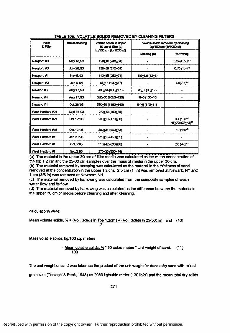
TABLE 105: VOLATILE SOUDS REMOVED BY CLEANING FILTERS.Plant
& FflterDate of cleaning Volatile solids in upper
30 cm of (iKer (a) kg/100 sm(Ib/1000 sf)
Volatile solids removed by cleaning kg/100 sm (lb/1000 sf)
Scraping (b) Harrowing
Newport, #3 May 18,'93 120+16(240+34) - 0/24 (0.50)w
Newport, #3 July 26/93 130+18(270+37) - 0.70 (1.4)**
Newport, #1 Nov.9/93 140+35(280+71) 5.9+1.6 (12+3) -
Newport. #2 Jan.9/94 66+18 (130+37) - 3.6(7.4)w
Newark. #3 Aug.17,'93 480+84(960+170) 43+8 (88+17) -
Newark, #4 Aug.17/93 520+60(1050+120) 49+5(100+10) -
Newark. #4 Oct 26,93 570+79(1160+160) 54+5(110+11) -
West Hartford #21 Sept 15/93 220+43(460+88) - -
West Hartford #21 Oct12/93 230+18(470+38) - 6.4 (13)w 45+20 (92+48)ld|
West Hartford #18 Oct13/93 300+31 (600+63) - 7.0(14)(cB
West Hartford #1 J a n ^ S S 220+15(450+31) - -
West Hartford #1 OctS.93 310+42(630+86) - 2 0 (4.0)w
West Hartford #1 Nov.2/93 270+36 (550+74) - -
a) The material in the upper 30 cm of filter media was calculated as the mean concentration of the top 1.2 cm and the 25-30 cm samples over the mass of media in the upper 30 cm.(b) The material removed by scraping was calculated as the material in the thickness of sand removed at the concentration in the upper 1.2 cm. 2.5 cm (1 in) was removed at Newark, NY and 1 cm (3/8 in) was removed at Newport, NH.(c) The material removed by harrowing was calculated from the composite samples of wash water flow and its flow.(d) The material removed by harrowing was calculated as the difference between the material in the upper 30 cm of media before cleaning and after cleaning.
calculations were:
Mean volatile solids, % = (Vol. Solids in T od 1.2cm) + (Vol. Solids in 25-30cm), and (10)2
Mass volatile solids, kg/100 sq. meters
= Mean volatile solids. % * 30 cubic metes * Unit weight of sand. (11) 100
The unit weight of sand was taken as the product of the unit weight for dense dry sand with mixed
grain size (Terzaghi & Peck, 1948) as 2083 kg/cubic meter (130 Ib/cf) and the mean total dry solids
271
Reproduced with permission of the copyright owner. Further reproduction prohibited without permission.
for the depth of the sample in the filter bed. The mass in the wash water was based on the
composite sampling reported in "Results and Discussion of Results in Individual Plants." The wash
water sampling was earned out according to the methods presented in Methods and Materials and
the results generally follow the estimated weights of volatile solids in the upper 1.2 cm of the filter
media. The mean value of the percent volatile solids at the top 1.2 cm (1 /2 in) and the lower 25-30
cm (10-12 in) layers of the filter, before and after the cleaning process, also appear consistent with
the data on these and other filters in the study. Even though Filters 18 and 21 had not been
cleaned thoroughly at the time of the September 15 cleaning, due to the power failure and water
shortage, the solids that remained in the filters until the next cleaning should have been indicated in
the results of analyses on both the washwater samples and the media cores. Errors from the
washwater sampling would have been expected to have been equally divided between over and
under representing the true mean, or below the mean if solids were settling in the channels and not
collected by mid-depth sampling. Any errors in the sand core sampling might also have been
expected to be equally divided around the mean, yet the samples taken from Filter 19 in March
1994 indicated that there were areas of the filters, adjacent to wall and roof columns, where the
harrow does not reach and the media is not effectively cleaned. The total area represented by
those portions of the filter within approximately 30 cm (12-in) of the walls and columns at West
Hartford amount to only approximately 6.5 percent of the total filter area. That would not account
for the differences, however, even with a liberal allowance for uncleaned areas in comers of the
filter.
The mass of volatile solids removed at Newport by harrowing was approximately equal to
that removed by scraping, but the mass removed by hand raking was only about one-tenth as
much as by either scraping or harrowing. This may have been due to the media being less mature
at the time of the hand raking operations, after only 13 and 15 months of operation as opposed to
18 and 21 months for scraping and harrowing, respectively. The most obvious difference between
the cleaning methods was the extent to which the media was affected, as the surface of the filters
272
Reproduced with permission of the copyright owner. Further reproduction prohibited without permission.
were hand raked to a depth of less than 1.2 cm (1 /2 in) only twice during a cleaning operation,
while harrowing penetrated the filters to a depth of 15-20 cm (6-8 in) during repeated traverses and
scraping entirely removed most or all of the media depth affected by raking. It is concluded that
hand raking is not an effective means of removing volatile solids from the media. Hand raking was
effective in reducing the head loss of the filters over the summer of 1993 and maintained water
production while the filter media compacted to support the weight of the equipment for harrowing.
The method could be used in the future to extend the time before scraping or harrowing is
necessary, but would allow accumulations of organic matter in the filter.
The scraping method removed the greatest mass of volatile solids from the filters at
Newport, but the harrowing method was used only after a prolonged period when the raw water
temperature was low and at a time when the calculated volatile mass in the upper 30 cm (12 in) of
the media was half that at the time of scraping. If the removal by cleaning method were
normalized as a percentage of the original mass in the upper 30 cm, then the harrowing method
would have removed slightly more volatile matter, removing 5.3 percent as compared with
scraping to a depth of 1 cm (3/8 in) which removed 4.3 percent It must be noted, however, that
the measurements on both scraping and harrowing were not replicated and the conclusion needs
to be supported by other evidence. The depth to which the sand was scraped at Newport was also
less than practiced at most plant, 1 cm (3/B in) as compared to 2.5 cm (1 in).
Only the scraping method has been used at Newark, NY and a direct comparison between
cleaning operations at this plant with the results of harrowing these filters is not possible. The
mass of volatile solids removed by scraping operations was complete for the depth of media
scraped. The scraping at this plant was estimated at the time of cleaning to have been 1.9 cm (3/4
in) but the long term mean scraping depth appears to have been 2.5 cm (1 in) based on the
changes in sand levels and the number of cleanings since resanding. If the scraping depth were
2.5 cm (1 in), then 9.0+0.8 percent of the volatile mass in the upper 30 cm (12 in) of filter was
273
Reproduced with permission of the copyright owner. Further reproduction prohibited without permission.
being removed. If the depth were 1.9 cm (3/4 in), then the removal would have been reduced to
about 7 percent There were no measurements taken to further define changes in concentrations
of volatile matter or other parameters with depth in the upper 1.2 cm (1/2 in) of the Newark filters.
Although the filters at West Hartford have been cleaned solely by harrowing for more than
40 years, it is possible to compare the results of harrowing with estimates of the materials would
have been removed with a selected thickness of the upper layers of media. This thickness was
selected to be 2.5 cm (1 in) based on the apparent long-term depth of scraping at Newark, NY and
the wide-spread practice of scraping to this depth (Letterman and Cullen, 1985). The mass of
materials that would have been removed with scraping to a depth of 2.5 cm (1 in) and that were
removed by harrowing are presented in Table 106.
The effectiveness of the harrowing methods at West Hartford were low relative to the
estimated load of volatile solids in the filters, if based only on the washwater sampling, but the
volatile solids in the top 1.2 cm of sand media in the filters (x=11.5 kg, s=4.4, n=5) were maintained
consistently lower, by 46 percent than found in the Newark, NY plant (x=21.2 kg, s=2.5, n=3)over
the same season. The data on cores before and after cleaning West Hartford Filter 21 showed
decreases in all filter media parameters after harrowing. Only the percent total dry solids of the
media increased after harrowing. Relative standard deviations on the mean values generally
decreased also, indicating greater uniformity of the media after harrowing. The data for Filter 18
cannot be used to prepare a similar estimate of the differences in materials in the media before
and after harrowing because the September 15,1993 cores were after an abbreviated cleaning
session, and the October 13,1993 cores were taken at the end of that filter run rather than before
the cleaning of September 15. The harrowing method removed more material from the filter
media than did the scraping method except in Filter 1. Filter 1 does not have inlet and outlet
channels on opposite sides of the filter bed so that washwater can flow continuously across the
filter during the harrowing process.
274
Reproduced with permission of the copyright owner. Further reproduction prohibited without permission.
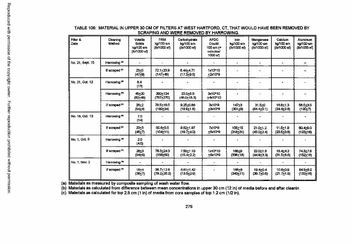
Reproduced
with perm
ission of the
copyright ow
ner. Further
reproduction prohibited
without
permission.
TABLE 106: MATERIAL IN UPPER 30 CM OF FILTERS AT WEST HARTFORD, CT, THAT WOULD HAVE BEEN REMOVED BY ________________________ SCRAPING AND WERE REMOVED BY HARROWING. _________
Filter & Date
CleaningMethod
Volatile Solids
Kg/100 sm (lb/1000 sf)
FRM Kg/100 sm (lb/1000 sf)
Carbohydrate Kg/100 sm (lb/1000 sf)
AFDC Count/
100 sm (= colonies/ 1000 sf)
Iron Kg/100 sm (lb/1000 sf)
Manganese Kg/100 sm (lb/1000 sf)
Calcium Kg/100 sm (lb/1000 sf)
Aluminum Kg/100 sm (lb/1000 sf)
No. 21. Sept. 15 Harrowing w - - - - - - - -
If scraped(c> 23+5(47+9)
72.1+23.9(147+49)
8.44+4.71(17.3+9.6)
1x10*10+2x10*9
- - - -
No. 21. Oct. 12 Harrowing w 6.4(13)
- - - - - - -
Harrowing w 45+20(92+48)
390+134(797+270)
23.5+8.9(48.0+18.3)
3x10*10+4x10*10
- - - -
If scraped w 26+2(54+4)
78.5+16.5(160+34)
9.25+0.86(18.9+1.8)
3x10*9+3x10*8
147+3(301+6)
31.5+0(64.4+0.1)
CO CD
f-, CN ,
58.5+3.5(120+7)
No. 18. Oct. 13 Harrowing w 7.0(14)
- - - - - - -
If scrapedw 23+3(48+7)
50.6+5.5(104+11)
9.62+1.97(19.7+4.0)
7x10*9+6x10*9
155+15(318+31)
21.0+1.2(43.0+2.4)
11.5+1,9(23.5+3.8)
60.4+8.0(123+16)
No. 1, Oct. 5 Harrowing w 2.0(4.0)
- - - - - - -
If scraped w 28+3(54+6)
76.3+24.3(156+50)
7.55+1.10(15.4+2.2)
1x10*10+6x10*9
165+9(338+18)
22.0+1.6(44.9+3.3)
15.4+4.2(31.5+8,6)
74.3+7.8(152+16)
No. 1, Nov. 2 Harrowing w - - - - - - - -
If scraped w 18+4(38+7)
38.7+12.8(79.2+26.2)
6.61+1.42(13.5+2.9)
- 168+6(343+11)
19.4+0.4(39.7+0.8)
10.6+0,9(21.7+1.9)
64.5+8.0(132+16)
(a) Materials as measured by composite sampling of wash water flow.(b) Materials as calculated from difference between mean concentrations in upper 30 cm (12 in) of media before and after cleanin(c) Materials as calculated for top 2.5 cm (1 in) of media from core samples of top 1.2 cm (1/2 in).
275
S u m m a ry . The harrowing method being practiced at West Hartford, except in Filter 1 which has
not been properly equipped, removed more accumulated material than would the scraping
method if only 2.5 cm of sand were removed.
5.9 CLEANING METHOD COSTS
The costs of the scraping and harrowing cleaning techniques at the respective plants are
summarized in Table 107. The directly measured labor costs for the scraping method, in person-
hours per unit of area cleaned, are twice those for harrowing method. The results at the Newport,
NH plant which directly compared the costs of the two cleaning methods, on adjacent filters and by
the same personnel, demonstrated the scraping method used twice the labor required for
harrowing, although the length of time harrowing method at the Gorham plant (Bernier, 1994) are
essentially the same as at Newport The direct labor costs per unit of filter area cleaned at West
Hartford were about one-half this (0.63 persons-hrs/100 sq. meters, vs 1.20 persons-hrs/100 sq.
meters at Newport), but the costs at West Hartford would be about equal to the Newport costs if
the additional time required for moving tractors and ventilation fans between buildings were
included. The tractors and ventilation fans were already located or permanently installed at the
other plants. The time to harrow filters at the Gorham and Newport plants had been based on the
time per unit area used at West Hartford and no studies were made to determine if the time should
be modified.
Larger crews were used for scraping, ranging from 3 to 5 persons at various times at the
two plants monitored in this study. The direct labor used in the Newport, NH and Newark, NY
plants, including the time for removing the sand from the filters and dumping it in storage piles, was
almost identical on the basis of person-hours per unit of area cleaned, and considerably lower than
reported for other plants (Letterman and Cullen, 1985). The labor required at these plants
averaged 2.7 person-hours per 100 sq. meters (2.5 person-hrs/1,000 sf) as opposed to the
average of 8.9 hrs per 100 sq. meters of filter (8.2 hrs/1,000 sf) from the 1983 data (Letterman and
276
Reproduced with permission of the copyright owner. Further reproduction prohibited without permission.
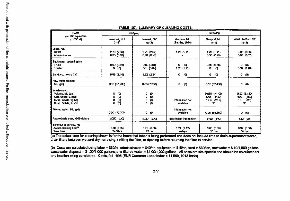
Reproduced
with perm
ission of the
copyright ow
ner. Further
reproduction prohibited
without
permission.
TABLE 107: SUMMARY OF CLEANING COSTS.Costs
per 100sq meters (1.000 sf)
Scraping Harrowing
Newport, NH (n=1)
Newark, NY (n=3)
Gorham, NH (Bemler, 1994)
Newport, NH (n=1)
West Hartford, CT (n=3)
Labor, hrs DirectAdministrative
2.70 (2.50) 0.30 (0.28)
2.71 (2.52) 0.20 (0.18)
1.20 (1.11) 1.20 (1.11) 0.30 (0.28)
0.63 (0.58) 0.06 (0.07)
Equipment, operating hrs Truck Tractor
0.60 (0.56) 0 (0)
0.69(0.61)0.10(0.09)
0 (0) 1.20 (1.11)
0.60 (0.56) 0 (0)
0 (0) 0.31 (0.29)
Sand, cu.meters (cy) 0.96 (1.16) 1.82 (2.21) 0 (0) 0 (0) 0 (0)
Raw water drained, ML (gal) 0.16(37,700) 0.03 (7,380) 0 (0) 0.15(37,450) 0 (0)
Wastewater,Volume, ML (gal) Sett. Solids, L (gal) Susp. Solids, kg (lb) Susp. Solids, % Vol.
0 (0) 0 (0) 0 (0) 0 (0)
0 (0) 0 (0) 0 (0) 0 (0)
Information not available
0.058(14,100) 540 (129) 12.9 (26.4)
28
0.22 (5,130) 690 (180) 18 (38)
38
Filtered water, ML (gal)0.30 (77,700) 0 (0)
Information not available 0.28 (68,500) 0 (0)
Approximate cost, 1908 dollars $250 (230) $220 (200) Insufficient information $150 (140) $32 (29)
Time out of service, hrs Actual cleaning time** Total time
0.60 (0.55) 24.5 hrs
0.71 (0.66) 13 hrs
1.21 (1.12) 4 days
0.60 (0.55) 25 hrs
0.32 (0.30) 34 hrs
a) The actual time for cleaning shown is for the hours that labor is being performed and does not include time to drain supernatant water,drain filters between wet and dry harrowing, refilling the filter, or ripening before returning the filter to service.
(b) Costs are calculated using labor = $30/hr, administration = $40/hr, equipment = $15/hr, sand = $30/ton, raw water = $.10/1,000 gallons, wastewater disposal = $1.00/1,000 gallons, and filtered water = $1.00/1,000 gallons. All costs are site specific and should be calculated for any location being considered. Costs, fall 1996 (ENR Common Labor Index = 11,560,1913 basis).
277
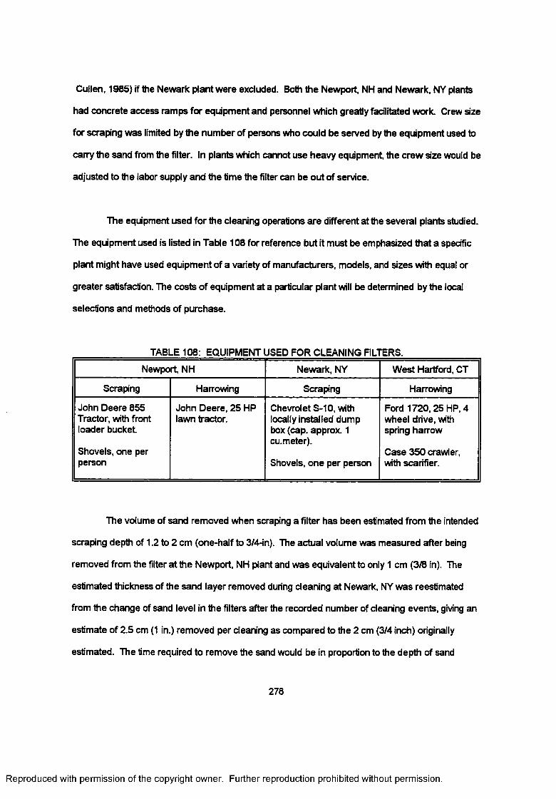
Cullen, 1985) if the Newark plant were excluded. Both the Newport, NH and Newark, NY plants
had concrete access ramps for equipment and personnel which greatly facilitated work. Crew size
for scraping was limited by the number of persons who could be served by the equipment used to
carry the sand from the filter. In plants which cannot use heavy equipment, the crew size would be
adjusted to the labor supply and the time the filter can be out of service.
The equipment used for the cleaning operations are different at the several plants studied.
The equipment used is listed in Table 108 for reference but it must be emphasized that a specific
plant might have used equipment of a variety of manufacturers, models, and sizes with equal or
greater satisfaction. The costs of equipment at a particular plant will be determined by the local
selections and methods of purchase.
TABLE 108: EQUIPMENT USED FOR CLEANING FILIrERS.
Newport, NH Newark, NY West Hartford, CT
Scraping Harrowing Scraping Harrowing
John Deere 855 Tractor, with front loader bucket
Shovels, one per person
John Deere, 25 HP lawn tractor.
Chevrolet S-10, with locally installed dump box (cap. approx. 1 cu.meter).
Shovels, one per person
Ford 1720,25 HP, 4 wheel drive, with spring harrow
Case 350 crawler, with scarifier.
The volume of sand removed when scraping a filter has been estimated from the intended
scraping depth of 1.2 to 2 cm (one-half to 3/4-in). The actual volume was measured after being
removed from the filter at the Newport, NH plant and was equivalent to only 1 cm (3/8 in). The
estimated thickness of the sand layer removed during cleaning at Newark, NY was reestimated
from the change of sand level in the filters after the recorded number of cleaning events, giving an
estimate of 2.5 cm (1 in.) removed per cleaning as compared to the 2 cm (3/4 inch) originally
estimated. The time required to remove the sand would be in proportion to the depth of sand
278
Reproduced with permission of the copyright owner. Further reproduction prohibited without permission.
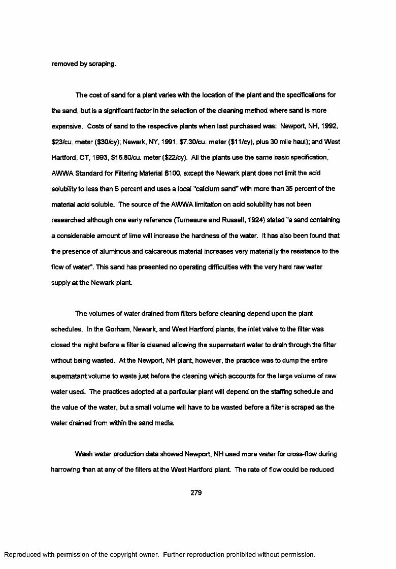
removed by scraping.
The cost of sand for a plant varies with the location of the plant and the specifications for
the sand, but is a significant factor in the selection of the cleaning method where sand is more
expensive. Costs of sand to the respective plants when last purchased was: Newport, NH, 1992,
$23/cu. meter ($30/cy); Newark, NY, 1991, $7.30/cu. meter ($11/cy), plus 30 mile haul); and West
Hartford, CT, 1993, $16.80/cu. meter ($22/cy). All the plants use the same basic specification,
AWWA Standard for Filtering Material B100, except the Newark plant does not limit the add
solubility to less than 5 percent and uses a local "calcium sand” with more than 35 percent of the
material add soluble. The source of the AWWA limitation on add solubility has not been
researched although one early reference (Tumeaure and Russell, 1924) stated "a sand containing
a considerable amount of lime will increase the hardness of the water. It has also been found that
the presence of aluminous and calcareous material increases very materially the resistance to the
flow of water". This sand has presented no operating difficulties with the very hard raw water
supply at the Newark plant
The volumes of water drained from filters before cleaning depend upon the plant
schedules. In the Gorham, Newark, and West Hartford plants, the inlet valve to the filter was
closed the night before a filter is cleaned allowing the supernatant water to drain through the filter
without being wasted. At the Newport, NH plant, however, the practice was to dump the entire
supernatant volume to waste just before the cleaning which accounts for the large volume of raw
water used. The practices adopted at a particular plant will depend on the staffing schedule and
the value of the water, but a small volume will have to be wasted before a filter is scraped as the
water drained from within the sand media.
Wash water production data showed Newport, NH used more water for cross-flow during
harrowing than at any of the filters at the West Hartford plant The rate of flow could be reduced
279
Reproduced with permission of the copyright owner. Further reproduction prohibited without permission.
but it was observed by the personnel that the suspended solids from wet harrowing would rapidly
settle onto the filter surface after the tractor had passed. For this reason, it was not believed that
the volume should be reduced. The cross-flow velocity in the Newport, NH filter was estimated at
0.91 meter/min (0.05 fps) and at 0.64 meter/min. (0.035 fps) in Filters 18 and 21 at West Hartford.
The volumes of settieable solids and mass of suspended solids at the two different plants were
similar even though the West Hartford filters had been in service longer since the sand had been
washed.
Another significant factor determining the volume of water used in the cleaning cycle is the
ripening period. The Newport, NH filter effluent displayed a noticeable improvement during the
overnight period while filters were ripened before being returned to service. The Newark, NY filter
operations in this study, as in the summer of 1983 (Letterman and Cullen, 1985), did not show the
need to ripen the filters to produce filtered water having low turbidity and particle count, yet several
other slow sand filter plants studied in the 1985 report did. The West Hartford filters in this study
were not ripened before being returned to service but the filtered water, as was presented in Figure
16, showed total coliform bacteria were present in numbers that would ordinarily justify a period of
ripening. The decision on whether to return a filter to service without a ripening period will have to
be made on a plant-by-plant basis, using performance information collected after the filter is
cleaned, and with consideration given for the duration of the time the filter has been out of service.
The time that filters monitored in this study were out of service for a cleaning event was
found to be related as much to the scheduling requirements of the staff and whether the filter
needed to ripen before being returned to service as it was to the cleaning method used. The very
short time the Newark, NY filters were out of service was due to the efficiency of the scraping
operation at this plant and the lack of a ripening period. The very long time the filters were out of
service at West Hartford was for the convenience of scheduling separate crews for the two steps
of harrowing, and the overnight period between them. At the time of the September 15,1993
280
Reproduced with permission of the copyright owner. Further reproduction prohibited without permission.
sampling, however, Filter 21 was wet and dry harrowed and returned to service in only about 12
hours which approached the time used at Newark. It has been previously reported that the shorter
the time that the filters are out of service, the more quickly the bacteria will recover and the
ripening period will be shortened (Huisman and Wood, 1974; Ellis, 1985; Bauer, 1994). For this
reason cleaning operations should be scheduled so that the filters are returned to service as soon
after being drained as possible.
Part of the sand is removed each time a filter is cleaned by scraping and eventually the
thickness of the filter sand is reduced to an unacceptable level. The filter must then be taken out
of service and resanded. The frequency depends on the amount of sand initially present the
amount removed per cleaning event and the minimum thickness that is allowable. The Newark
plant used an initial depth of 0.75 to 0.9 meters (30 to 36 in), removed about 2.5 cm (1 in) per
cleaning, and resanded when the thickness is down to about 0.3 m (1 ft). Other factors were also
considered when deciding to resand, such as scheduling, budget surpluses, and general filter
performance which may lead to earlier resanding.
The history of the four filters at the Newark plant since 1986 was for filters to be resanded
after an average of 5.8 years. The time out of service for resanding averaged 26 days, or 1.2
percent of the time, of which 9 days was spent resanding with 4 days for weekends and
interruptions and an average of 11 days ripening the sand. The comparable information on the
four most recent West Hartford filters reconditioned was for them to be reconditioned at about a
twenty year interval, with the filters out of sen/ice for six months, or 2.5 percent of the time. Of that
time, an average of 70 day was spent reconditioning with 30 days for weekends and interruptions
and the balance of the time for ripening the sand. The actual time spent for the resanding or
reconditioning was 1.8 days/100 sq. meters (1.7 day/1000 sf) at Newark and 3 days/100 sq. meters
(2.8 days/1000 sf) at West Hartford. The ripening time at Newark averaged 11 days but about 2
months at West Hartford.
281
Reproduced with permission of the copyright owner. Further reproduction prohibited without permission.
CHAPTER 6
CONCLUSIONS
This project focused on evaluating two slow sand filter cleaning methods, surface scraping
and filter harrowing, for their impact on filter treatment performance and operational and
maintenance requirements. The objective was to assess the effectiveness and limitations of each
filter cleaning method with the goal of assisting small water systems to make an informed decision
as to which cleaning method would be most advantageous to them. Several significant
conclusions were made during the course of this investigation and are summarized as follow:
• Both surface scraping and filter harrowing were effective methods for cleaning slow sand
filters. Each method has been utilized at separate locations in New York and New
England with few complaints or concerns and with minimal disruptions to the filtration
process.
• The choice of the most appropriate filter cleaning method depended on several factors but
one that has been often overlooked is the capability and professionalism of the water utility
personnel. The differences in organizational capability, adaptability, and overall
knowledge of their own treatment process were significant between staff at the filtration
facilities monitored. In many instances, whichever filter cleaning method is easiest to
implement may be the most appropriate. Filters cleaned by either method can produce
satisfactory quality drinking water.
• Assessment of filter cleaning methods involved evaluation of filter treatment performance,
cleaning effectiveness and frequency, filter ripening requirements, and cleaning costs.
Because of the diversity between the treatment facilities and the lack of full-scale side-by-
282
Reproduced with permission of the copyright owner. Further reproduction prohibited without permission.
side comparisons, no filter cleaning procedure emerged as clearly the most efficient based
on the above criteria. In general, filter harrowing increased cleaning frequency but
required fewer hours of labor per cleaning event The actual filter downtime per cleaning
event, based on procedural protocol rather than water quality data, was approximately the
same for both methods.
Some trends in the removal of NPDOC and UV absorbance suggested filter harrowing
resulted in more efficient filter treatment performance but the conclusion must be
tempered because the trend was not consistent and was dependent on other confounding
factors, e.g. water source, temperature, sand age.
Overall slow sand filter performance, on removal of turbidity, particles, NPDOC, and UV
absorbance, was influenced by water temperature. Removal of NPDOC and UV
absorbance was also influenced by sand media age, filter biomass content, source water
quality, and filtration rate/empty bed contact time. Filter media size and sand filter depth
were not evaluated individually in this study. In general, slow sand filter performance was
enhanced with higher temperature, older sand media, higher filter biomass content, and
source water with NOM conducive to adsorption/biodegradation. The influence of filtration
rate depended on the biodegradability of the organic matter. Increasing hydraulic loading
rate improved the kinetic removal of easily biodegradable organic compounds.
Filter biomass was quantified by protein content (FRM), carbohydrate, bacterial counts,
and volatile solids. Each of the testing methods had its advantages and disadvantages but
the easiest and most consistent method was the volatile solids test followed by
carbohydrates. None of these techniques could be correlated with bioactivity since
bioactivity determinations were not directly performed in this study.
283
Reproduced with permission of the copyright owner. Further reproduction prohibited without permission.
Biomass distribution within a filter bed was dependent on filter cleaning method. Surface
scraping resulted in the highest biomass located in the schmutzdecke/upper sand layers
decreasing with depth below the filter surface. Filter harrowing resulted in a more
heterogenous distribution of biomass throughout the filter bed with elevated accumulations
just below the harrowed layers.
The inorganic and biological composition of sand surface coatings varied with sand media
age, filter bed depth, and cleaning method. Although confounding problems occurred, a
direct relationship existed between inorganic accumulations, e.g.. iron and manganese,
and the removal of NOM as measured by NPDOC and UV absorbance.
Filters cleaned by the harrowing method will remain at or near full media depth until
resanding is necessary. The depth of media in filters cleaned by scraping will be
progressively reduced and resanding will be required earlier.
The harrowing method of cleaning uses less labor and sand than the scraping method, but
the water required during wet harrowing results in the use of more water and produces
more wastewater. The use of water and production of wastewater if the filters are cleaned
by scraping results only if the filters must be "ripened" after cleaning. The estimated total
cost for labor, equipment, water, and replacement sand media is lower for filters cleaned
with the harrowing method.
In order to fully evaluate slow sand filter cleaning methods, the assessment period needs
to encompass the handling of sand media from resanding operation to resanding
operation, a period generally measured in 5 to 10 years increments. Filter cleaning
methods may have a profound influence on resanding operations both in frequency of
cleaning and in requirements for material handling.
284
Reproduced with permission of the copyright owner. Further reproduction prohibited without permission.
CHAPTER 7
RECOMMENDATIONS
Several questions arose during the study which could not be resolved because critical
facilities were not available or could not be used during the time the facilities were available. Other
questions were suggested by this study.
7.1 COMPARATIVE STUDY OF THE TWO SLOW SAND FILTER CLEANING METHODS
The present study was unable to use the facilities at Gorham, NH for the full-scale
comparisons of the scraping and harrowing methods. The filters at Gorham did not reach terminal
headloss for cleaning until after it had been necessary to transfer the study to another plant The
Gorham filters operated for a total of 2.75 years before cleaning was required. The filters at the
Newport plant ripened satisfactorily, yet the time remaining for the study did not allow for more
than one cleaning operation with each method.
The high quality raw water supplies for which slow sand filtration is commonly used in
upper New England resulted in prolonged a ripening period. Additionally, as reported during the
evaluation periods at Newport and West Hartford, new or resanded filter may not be able to be
harrowed when first used. During the initial cleaning operations, harrowing operations will have to
be modified until the filter media will bear the weight of harrowing equipment Finally, when the
planned cleaning methods are used, they should be monitored over several seasons to separate
the effects of temperature and seasonal water quality.
A full-scale comparison of the two cleaning methods should still be performed with side-
by-side filters using the same sand source and with the same water source. Such a study should
begin with a new plant and virgin sand, and operate over at least one resanding cycle (four or
285
Reproduced with permission of the copyright owner. Further reproduction prohibited without permission.
more years) for the filter cleaned with the scraping method and possibly over a resanding cycle for
the filter cleaned with the harrowing method (ten to twenty years). A realistic budget will also be
necessary to maintain the sampling, testing, and data analysis over the study period.
7.2 RIPENING
The initial ripening period for slow sand filters should be monitored to define the changes in
both the chemical (organic and inorganic) and biological content of the sand coatings as a function
of depth in the filter, filter run time, and treatment performance. The role of filter ripening and
aging on the performance of the slow sand filters needs to be further defined. The need for re
ripening after a cleaning operation should also be further compared, side-by-side, for several
cycles over a period of years to determine if either cleaning method may have an additional need
to filter to waste before returning to service.
7.3 REMOVAL OF NATURAL ORGANIC MATTER (NOM)
The importance of filter biomass to performance has been shown previously yet biomass
alone is not the reason for higher performance in the West Hartford filters. Emphasis should be
given to developing a relationship between biomass and bioactivity, and distinguishing between
surface removals of NOM and the removals occurring with depth in the media. Performance of
the filter media in removing both particulate and dissolved NOM need to be considered.
7.4 INFLUENCE OF TEMPERATURE
Temperature is one of the most important parameters in performance of slow sand filters
as measured by turbidity, particles, NPDOC, and UV absorbance. Earlier temperature studies
have used the removal of turbidity, coliform, and Giardia cysts but there has been limited data on
the removal of THM or surrogates relative to temperature and raw water characteristics.
Information should be collected and used to estimate the relative seasonal effectiveness of the
biofiltration process.
286
Reproduced with permission of the copyright owner. Further reproduction prohibited without permission.
7.5 FILTER MEDIA SIZE
The rate of headloss development in filters which had been cleaned by harrowing was
greater than for filters which were cleaned by scraping. The filter to be harrowed in the
comparative study might use a larger size (>0.4 mm) or more uniform grain size to reduce
headlosses and extend the length of filter runs.
More detailed studies are needed to relate the influence of media size on headloss development,
before and after each cleaning method.
7.6 SAMPUNG AND ANALYTICAL METHODS
Arrangements are needed to allow sampling to the full depth of the sand filter during filter
operations so that draining is not necessary. The filters sampled during this study could have been
grouped, roughly, into two types: "young" filters into which the sampler could be pressed by hand
but the sand would not remain in the sampling tube while being withdrawn unless the filter had
been drained to below the level of the sample, and "older” filters from which a sample could be
taken but the tube could be driven to a depth of only about 30 cm (12 in). The Gorham and
Newport filters were examples of the former, and the Newark and older West Hartford filters were
of the latter type.
The plant selected for a comparative study should be located near the laboratory to allow
frequent sample collection and analysis, improving the statistical significance of the removal
performance data. The plant should also have instrumentation on the raw water supply to the
filters, and on finished and wash water lines from each filter with flow indicators, recorders, and
totalizers; permanent sampling connections should be installed on all raw, filtered, and wash water
lines; and headloss indicators should be required on each filter. This instrumentation should be
required on larger plants and would also be appropriate on all plants in order to monitor treatment
performance, development of headlosses leading to the cleaning, and wash water discharges.
287
Reproduced with permission of the copyright owner. Further reproduction prohibited without permission.
REFERENCES
Aiken, G., and Cotsaris, E. (1995). "Soil and Hydrology: Their Effect on NOM", JAWWA, 87(1), 36- 45.
Allen, R.B. (1991). "A Method of Cleaning Slow Sand Filters Developed at the West Hartford, CT Water Treatment Plant" Presented to American Water Works Association Slow Sand Filter Workshop, October, 1991. Durham, NH.
Allen, R.B. (1993). Personal communication. West Hartford, CT.
American Public Health Association - APHA (1989). Standard Methods for the Examination of Water and Wastewater. 17th edition. APHA, Washington, DC.
American Society for Testing and Materials - ASTM (1990). "ASTM Standard D422-63 (reapproved 1990), Standard Test Method for Particle-Size Analysis of Soils", Philadelphia, PA.
American Water Works Association - AWWA (1981). Seminar Proceedings: Small Water System Problems. AW W A. Denver, CO.
American Water Works Association - AWWA (1989). AWWA Standard for Filtering Material. ANSI/AWWA B100-89. AWWA. Denver, CO.
American Water Works Association - AWWA (1990). Water Quality and Treatment (ed. F.W. Pontius). AW W A. Denver, CO.
Amy, G.L., Chadik, P A , King, P.A (1986). "A Statistical Analysis of Surrogate Parameter for Predicting Trihalomethane Formation Potential (THMFP). Envir. Technol. Letter, 7:99.
Attenboro, G. (1993-4). Personal communications. Newark, NY.
Balkwill, D .L, Ghiorse.W.C. (1985). "Characterization of Subsurface Bacteria Associated with Two Shallow Aquifers in Oklahoma", Appl. Environ. Microbiol., Vo!.50, No.3, pp.580-588.
Bellamy, W.D., Silverman, G.P., Hendricks, D.W., and Logsdon, G.S. (1985a). "Removing Gardia Cysts with Slow Sand Filtration". JAWWA. 77(2), 52-60.
Bellamy, W.D., Hendricks, D.W., and Logsdon, G.S. (1985b). "Low Sand Filtration: Influences of Selected Process Variables", JAWWA. 77(12), 62-66.
Bellinger, E.G. (1979). "Some biological aspects of slow sand filters.” Journal of the Institute of Water Engineers and Scientists. 33,19-29.
Benjamin, M.M., etal. (1993). NOM adsorption onto iron-oxide-coated sand. AWWARF Final Report AWWARF. Denver, CO.
Berg, P., Tanner, S., and Shieh, C.Y. (1991). "Construction, Operation, and Maintenance Costs."(In Logsdon, 1991).
288
Reproduced with permission of the copyright owner. Further reproduction prohibited without permission.
Bemer, E.K., and Bemer, R.A (1987). The Global Water Cvcle. Prentice-Hall, Englewood Cliffs, NJ.
Bemier, D. (1991-4). Personal communication. Gorham, NH.
Billen, G„ Servais, P., Bouillot, P., and Ventresque, C. (1992). "Functioning of biological filters used in drinking -water treatment-the Chabrol model", J. Water SRT-Aqua, 41(4), 231-241.
Block, J.C., Mathieu, L., Servais, P., Fontvieille, D., Wemer, P. (1992). "Indogenous Bacterial Innocula forMeasuring the Biodegradable Organic Carbon (BDOC) in Water," W at Res. 26(4) 481-486.
Bloomfield, J A , Ed. (1978). Lakes of New York State. Vol. 1: Ecology of the Finger Lakes. Academic Press, Inc. New York.
Bonnet M.C., Welte, B., And Montiel, A. (1992). "Removal of Biodegradable Dissolved Organic Carbon in a Water Treatment Plant", W at Res., 26(12), 1673-1680.
Bouwer, E., and Crowe, P.B. (1988). "Biological Processes in Drinking Water Treatment" JAWWA 80(9), 82-93.
Bowie, F.L, Mills, W.B., Porcella, D.B., Campbell, C.L, Pagenkopf, J.R., Rupp, G.L., Johnson, KM., Chan, P.W.H., Gherini, S. A., Chamberlin, C.E. (1985). Rates. Constants, and Kinetics Formulations in Surface Water Quality Modeling (2nd edt EPA/500/3-85/040. USEPA, Athens, GA.
Brink, D. R. and Parks, S. (1996). "Update on Slow Sand/Advanced Biological Filtration Research." In Graham and Collins, 1996).
Camp, T.R. (1964). 'Throry of Water Filtration," Journal of Sanitary Engineering Division, ASCE, Vol. 90, No. SA2,1-29.
Camper, A (1994). Personal communication. Montana State University.
Canandaigua Lake Watershed Task Force (1994). The State of the Canandaigua Lake Watershed-1994. Canandaigua Lake Watershed Task Force, Canandaigua, NY.
Characklis, W.G. and Marshall, KC. (1990). Biofilms. John Wiley & Sons, New York.
Chesbro, W. (1992). "Phenol-Sulfuric Add Determination of Carbohydrate", Laboratory notes. University of New Hampshire, Durham, NH.
Chow, V.T. (1959). Qpen-Channel Hydraulics. McGraw-Hill. New York.
Cleasby, J.L, Hilmoe, D.J., Dimitracopoulos, C.J. (1984). "Slow Sand and Direct In-Line nitration of a Surface Water". JAWWA, 76(12), 44-55.
Collins, M.R. and Eighmy, T.T. (1988). Modifications to the Slow Rate Filtration Process for Improved Trihalomethane Precursor Removal. In: Slow Sand Filtration: Recent Developments in Water Treatment Technology. N.J.D. Graham (Ed.). Ellis Horwood Ltd., Chichester,UK.
Collins, M.R., Eighmy, T.T., Fenstermacher, J.M. and Spanos, S.K (1989). Modifications to the Slow Sand Filtration Process for Improved Removals of Trihalomethane Precursors. AWWARF Final Report Denver, CO.
289
Reproduced with permission of the copyright owner. Further reproduction prohibited without permission.
Collins, M.R., Eighmy, T.T., Malley, J.P. (1990). "Modifications to Enhance the Performance of Conventional Slow Sand Filtration". Presented to Energy Technologies in Practice Seminar, AWWA National Conference, June 1990. Cincinnati, OH.
Collins, M.R., Eighmy, T.T., Malley, J.P. (1991). "Evaluating Modifications to Slow Sand Filters." JAWWA, 84(9)62-70.
Collins, M.R. (1990). "Pilot Study of Slow Sand Filtration Process in Gorham, New Hampshire”. Engineering Report to Gorham, NH. University of New Hampshire, Durham, NH.
Collins, M.R. (1991). "Grant Application for 'Full-Scale Comparative Evaluation of Two Slow Sand Filter Cleaning Methods'". University of New Hampshire, Durham, NH.
Collins, M.R., Bernier, D.P., Kern, J.A. (1992a). "Quality Assurance Plan Addendum to 'Full-Scale Comparative Evaluation of Two Slow Sand Filter Cleaning Methods'". Report to USEPA. University of New Hampshire, Durham, NH.
Collins, M.R., Eighmy, T.T., Fenstermacher, J.M. and Spanos, S.K. (1992b). "Removing Natural Organic Matter by Conventional Slow Sand Filtration", JAWWA, 84(5)80-90.
Collins, M.R., and Vaughan, C.W. (1993). "Assessing Biofilter Treatability of Natural Organic Matter", AWWA WQTC Conf. Proceedings.
Collins, M.R., and Graham, M.J.D., eds. (1994). Slow Sand Filtration. AWWA, Denver, CO.
Dahm, C.N. (1981). "Pathways and Mechanisms for Removal of Dissolved Organic Cargon from Leaf Leachate in Streams." Can.J.Fish.Aquat Sri. 38:68-72.
Darby, J.L., Lawler, D.F., Wilshusen, T.P. (1991). "Depth Filtration of Wastewater: Particle Size and Ripening," Res. JWPCF, 63(3), 228-238.
Darby, J.L., Altanasio, R.E., Lawler, D. F. (1992). "nitration of Heterodisperse Suspensions: Modeling of Particle Removal and Head Loss," WatRes. 26( )711-726.
Datta, A.K., and Chaudhuri, M. (1991). 'Mcrobial Purification in Slow Sand Filter", Env. Tox. and Water Quality, Vol. 6.239-247.
Davis, J.A. (1981). "Adsorption of natural dissolved organic matter at the oxideA/vater interface", Geochim. Cosmochim. Acta., 46(11)2381-2393.
Degremont (1991). Water Treatment Handbook. Lavoisier Publishing, Paris, France.
DiBemardo, L. and Escobar Rivera, A. (1996). 'Influence of Sand Uniformity Coefficient on Slow Sand Filtration Performance." (In Graham and Collins, 1996).
Dowdy, S.M., and Wearden, S. (1991). Statistics for Research. John Wiley & Sons, New York.
Duncan, A. (1988). 'The Ecology of Slow Sand Filters," Slow Sand Filtration. Ellis Horwood Limited, Chichester, West Sussex, England.
Eberhardt, M. (1976). "Experience with the use of biological effective activated carbon", Translations of Reports on Special Problems of Water Technology. Vol. 9. Adsorption. Ed. H. Sontheimer, EPA-600/9-76-030, p.331.
290
Reproduced with permission of the copyright owner. Further reproduction prohibited without permission.
Edzwald, J.K (1993). "Coagulation in Drinking Water Treatment Particles, Organics and Coagulants." W at Sd.Tech., 27(11)21-35.
Edzwald, J.K, Becker, W.C., and Wattier, K L (1985). "Surrogate Parameters for Monitoring Organic Matter and THM Precursors." JAWWA, 77(4)122-132.
Eighmy, T.T., Collins, M.R., Spanos, S.K, and Fenstermacher, J. (1988). "Microbial Population Distributions and Benzoate Mineralization Kinetics in a Municipal Slow Sand Filter." W at Sd. Technol., 20,293-299.
Eighmy, T.T., Collins, M.R., Spanos, S.K, and Fenstermacher, J. (1992). "Microbial Populations, Activities and Carbon Metabolism ini Slow Sand Filters." W at Res., 26 (10), 1319-1328.
Eighmy, T.T., Collins, M.R., Malley, J.P., Royce, J., Morgan, D. (1991). Biologically Enhanced Slow Sand Filtration for Removal of Natural Organic Matter. AWWARF. Denver, CO.
Ellis, KV. (1985). "Slow Sand Filtration". CRC Critical Reviews in Environmental Control. 15(4), 315-354.
Fenstermacher. J.M. (1988). "Modifications to Slow-rate Filtration to Improve Removal of Trihalomethane Precursors.", Masters Thesis, University of New Hampshire, Durham, NH.
Fogel, D., Isaac-Renton, J., Guasparini, R., Moorehead, W., and Ongerth, J. (1993). "Removing Giardia and Cryptosporidium by Slow Sand nitration", JAWWA, 85(11)77-84.
Fuertes, J.H. (1901). Water Filtration Works. John Wiley and Sons, New York.
Galvin, r.M. (1992). "Ripening of Silica Sand used for Filtration," WatRes., 26(5), 683-688.
Gallagher, B. (1992). "Memorandum to Al Knight regarding Laboratory Water System", University of New Hampshire, Durham, NH.
Gerhardt, P. (1981). Manual of Methods for General Bacteriology. Am. Soc. for Microbiologists, Washington DC.
Ghiorse, W.C. (1984). "Biology of Iron-and Manganese-Depositing Bacteria." (from Ann.Rev.Microbiol., 1984. 38:515-50.
Ghosh, M.M., Schuler, P.F., Gopalan, P. (1989). "Field Study of Giardia and Cryptosporidium Removal from Pennsylvania Surface Waters by Slow Sand and Diatimaceous Earth Filtration," Environmental Resources Research Institute, Pennsylvania State University, University Park, PA
Goldgrabe, J.C., Summers, R.S., and Miltner, R.J. (1993). "Particle Removal and Head Loss Development in Biological Filters," JAWWA, 85(12) 94-106.
Graham, N. and Collins, R. (1996). Advances in Slow Sand and Alternative Biological Filtration. John Wiley & Sons. New York.
Gu, B. er al. (1994). "Adsorption and desorption of natural organic matter on iron oxide: Mechanisms and models", Environ. Sd. Technol., 28(1)38-46.
Haberer, K , Drews, M., and Waltenberg, M. (1984). "Entfemung organischer Wasserinhaltstoffe bei der Langsamsandfiltration." Vom Wasser, 63,121-140.
291
Reproduced with permission of the copyright owner. Further reproduction prohibited without permission.
Hansen, S.P. (1987). Workshop on Emerging Technologies for Drinking Water Treatment Filtration. USEPA, CERI-87-49.
Haarhoff, J. and Cleasby, J.L (1991). "Biological and Physical Mechanism in Slow Sand Filtration." (In Logsdon, 1991).
Hendricks, D. (ed) (1991). Manual of Design for Slow Sand Filtration. AWWARF and AWWA. Denver, CO.
Hendricks, D.W., and Bellamy, W.D. (1991). 'Mcroorganism Removals by Slwo Sand Filtration." (In Logsdon, 1991).
Hijinen, W.A.M., and Van der Kooij, D. (1992). 'The Effect of Low Concentrations of Assimilable Organic Carbon (AOC) in Water on Biological Clogging of Sand Beds," WaLRes. 26(7), 963-972.
Hirsche, S.D., and Sims, R.C. (1994). "Particles and Microorganisms in Slow Sand Filtration." (In Collins and Graham, 1994).
Huck, P.M. (1990). "Measurement of Biodegradable Organic Matter and Bacterial Growth Potential in Drinking Water," JAWWA, 82(7), 78-86.
Huisman, L , and Wood, W. (1974). Slow Sand Filtration. World Health Organization. Geneva, Switzerland.
Ives, K.J. and Sholji, I. (1965). "Research on Variables Affecting Filtration." Journal Sanitary Engineering Division, ASCE, Vol. 91, No. SA4,1-18.
Kaplan, L.A., Bott, T.L., and Reasoner, D.J. (1993). "Evaluation and Simplification of the Assimilable Organic Carbon Nutrient Bioassay for Bacterial Growth in Drinking Water." Appl. Environ. Microbio., Vol. 59, No. 5,1532-39.
Klevens, C.M. (1995). "Natural Organic Matter Characterization and Treatability by Biologically Activated Carbon Filtration of Croton Reservoir Water." MS Thesis , Civil Engineering, UNH, Durham, NH.
Koehl, M.A.R., and Stickler, J.R. (1981). "Copepod Feeding Currents: Food Capture at Low Reynolds Number", Limnology and Oceanography, 26:6,1062-1073.
Lang, J.S., Firon, J.J., Jansen, A.T., Trussed, R.R., and Hodges, Jr., W.E. (1993). "Investigating Filter Performance as a Function of the Ratio of Filter Size to Media Size," JAWWA, 85(10),122- 130.
Larson, R.A. (1978). "Dissolved Organic Matter of a Low Colored Stream," Freshwater Biology, Vol. 8,91-104.
Lazarova, V., and Manem, J. (1995). "Biofilm Characterization and Activity Analysis in Water and Wastewater Treatment" W at Res. 29(10)2227-2245.
LeChevallier, M.W., etal. (1990). Assessing and Controlling Bacterial Rearowth in Distribution Systems. AWWARF Final Report AWWA, Denver, CO.
Letterman, R.D. (1987). "An Overview of Filtration," JAWWA, 79(12), 26-32).
292
Reproduced with permission of the copyright owner. Further reproduction prohibited without permission.
Letterman, R.D., Cullen, R.R., Jr. (1985). Slow Sand Filter Maintenance Costs and Effects on Water Quality. Report No. EPA/600/2-85/056. USEPA. Washington, DC.
Lippy, D.H. and Waltria, S.C. (Feb. 1984). Water Borne Disease Outbreaks -1946-1980: A Thirty-Five Year Perspective. JAWWA, 76:2:60.
Liu, D., Lau, Y .L , Chau, Y.K., and Pacepavidus, G.J. (1992). "A Simple Technique for the Estimation of Biofilm Growth and Biomass". National Water Research Institute, Burlington,Ontario.
Liu, D., Lau, Y.L., Chau, Y.K., and Pacepavidus, G.J. (1993). "Characterization of Biofilm Development on Artifidal Substratum in Natural Water." W at Res., 27(3), 361-367.
Logsdon, G., (ed) (1991). Slow Sand Filtration: Manual of Practice. New York. American Sodety of Civil Engineers.
Logsdon, G.S., Sorg, T.J., and Clark, R.M. (1990). "Capability and Cost of Treatment Technologies for Small Systems." JAWWA, 82:6:60-66.
Lowry, O.H., Rosebrough, N.J., Farr, A .L, and Randall, R.J. (1951). "Protein Measurement with the Folin Phenol Reagent" J. Biol. Chem., No. 193, pp 265-275.
Lozier, W.S., Company (1947). Construction Plans for Canandaigua Lake Water Supply for Newark. New York. Wm. S. Lozier Company, Rochester, NY.
Mann, R. (1995). "Regulatory Perspectives of Slow Sand Filters in New Hampshire." Paper delivered at Slow Sand Filtration Regional Workshop II, Oct 20,1995. Rutland, VT.
Mbwelte, R.S.A., and Graham, N.J.D. (1988). "Pilot Plant Evaluation of Fabric Protected Slow Sand Filters." In: Slow Sand nitration: Recent Developments in Water Treatment Technology. N.J.D. Graham (Ed.). Ellis Horwood Ltd., Chichester,UK.
Meek, C.R., and Shieh C.Y. (1984). "Applications of Slow Sand Filters for Small Community System," Presented at Pasdfic NW Section meeting of AWWA, Eugene Oregan, May 9-11,1984.
Metcalf & Eddy (1991). Wastewater Engineering. (3rd Edl. McGraw-Hill, New York.
Meyer, J.L., Edwards, R.T., and Risley, R. (1987). "Bacterial Growth on DOC from a Blackwater River." Microbial Ecology, Vol. 13,13-29.
Miller, J.C. and Miller, J.N. (1988) Statistics for Analytical Chemistry. 2nd edition. Ellis Horwood Limited. Chichester, England.
Miltner, R.J. and Summers, R. S. (1992). "A pilot-scale study of biological treatment", Proceedings of AWWA Annual Conference.
Minkus, A.J. (1954). " Washing Slow Sand Filters with a Lateral Flow of Water". Jour. NEWWA 68:2: 121-134.
Mogren, E.M., Scarpino, P., Summers, R.S. (1990). "Measurement of Biodegradable Dissolved Organic Carbon in Drinking Water." Presented at AWWA Conference, Cincinnati Ohio, June 18- 21,1990.
293
Reproduced with permission of the copyright owner. Further reproduction prohibited without permission.
Moll, D.M., and Summers, R.S. (1996). "Performance, Biomass and Community Structure Profiles of Biological Rapid Media Filters." (In Graham and Collins, 1996).
Moll, D.M., Wang, J.Z., and Summers, R.S. (1995). "NOM Removal by Distinct Microbial Populations in Biofiltration Processes." Presented at AWWA Annual Conference, June 18-22, 1995. Anneheim, CA
Montgomery, James M., Consulting Engineers, lnc.(1985). Water Treatment Principles and Design. John Wiley & Sons. New York.
Mooney, R. (1993). Personal communication. University of New Hampshire, Durham, NH.
Nouvion, N., Block, J.C.,Faup, G.M. (1987). "Effect of Biomass Quantity and Activity on TOC Removal in a Fixed-BedReactor," WatRes. 21 (1), 35-40.
Prevost, M., Coailier, J., Mailly, J., Desjardins, R., and Duchesne, D. (1992). "Comparison of Biodegradable Organic Carbon (BDOC) Techniques on Process Control,” J. Water SRT-Aqua 4(3) 141-150.
Purcell, E.M. (1977). "Life at Low Reynolds Number," Amer.J. of Physics, 45,1, 3-10.
Pyper, G.R., and Logsdon, G.S. (1991). "Slow Sand Filter Design." (In Logsdon, 1991).
O'Melia & Ali (1978). "The role of retained particles in deep bed filtration," Proc.Wat.Tech., 10, 167-182.
Owen, D.M., Amy, G.L., Chowdgury, Z.H., Paode, R., McCoy, G., and Viscosil, K. (1995). "NOM characterization and treatability", JAWWA, 87(1), 46-63.
Paris, D. (1992). "How to be a Champion Particle Counter”, unpublished paper, University of New Hampshire, Durham, NH.
Pyper, G.R., and Logsdon, G.S. (1991). "Slow Sand Filter Design." (In Logsdon, 1991).
Rachwal, A.J., Bauer, M.J., Chipps, M.J., Colboume, J.S. and Foster, D.M. (1996). "Comparison between Slow Sand and High Rate Biofiltration." (In Graham and Collins, 1996).
Rechenberg, W. (1965). "Attempts to improve the quality of artifically recharged ground water by prefiltration." Hydrological Research Department of the Dortmund Stadtwerke A.G. Dormund, F.D.R.
Reckhow, D A , Bose, P., Bezbura, B., Hesse, E.M., and MacKnight, AP., Transformations of natural organic material during preozonation. EPA Report, USEPA, Drinking Water Research Division, Cincinnati, Ohio.
Recommended Standards For Water Works (1992). A report of the water works committee of the Great Lakes-Upper Mississippi River Board of State Public Health and Environmental Managers of the member states and province of Illinois, Indiana, Iowa, Michigan, Minnesota, Missouri, New York, Ohio, Ontario, Pennsylvania, and Wisconsin. Health Education Services, Albany, NY.
Renton, P.J., Bayley, R.G., and Bauer, M.J. (1991). 'Existing and New Cleaning Techniques for Large Scale Slow Sand Filters". Presented to American Water Works Association slow Sand Filter Workshop, October, 1991. Durham, NH.
294
Reproduced with permission of the copyright owner. Further reproduction prohibited without permission.
Ripley, D.P. and Saleem, Z.A. (1973). "Clogging in Simulated Glacial Aquifers Due to Artificial Recharge”, Water Resources Res., 9(4), 1047.
Rist-Frost Associates, P.C. (1991). Draft Manual of Operation and Maintenance for the 1.0 MGD Slow Sand Water Filtration Facility. Gorham. New Hampshire. Laconia, NH.
Rist-Frost-Shumway Engineering, P.C. (1993). Manual of Operation and Maintenance for the Slow Sand Water Filtration Facility for the Town of Newport New Hampshire. Laconia, NH.
Rittmann, B.E., and Huck, P.M. (1989). "Biological Treatment of Public Water Supplies", CRC Critical Reviews in Environmental Control. 19(2), 119.
Rittmann, B.E. (1990). "Analyzing Biofilm Processes used in Biological Filtration", JAWWA, 74(10), 540.
Royce, J. (1992). Masters Thesis (in preparation), University of New Hampshire, Durham, NH.
Scott, J.L (1991). "Project Costs of Slow Sand Filtration Facilities in Gorham and Newport, New Hampshire." Presented at AWWA/UNH Slow Sand nitration Workshop, Durham, NH.
Scott, J.L. (1994). Personal communication. Laconia, NH.
Seger, A., and Rothman, M. (1996). "Slow Sand Filtration with and without Oxonation in Nordic Climate." (In Graham and Collins, 1996)
Servais, P., Billen, G., and HascoSt, M.C. (1987). "Determination of the Biodegradable Fraction of Dissolved Organic Matter in Waters." W at Res., Vol.21, No.4, pp.445-450.
Servais, P., Billen, G., and Bouillot, P. (1994). "Biological Colonization of Granular Activated Carbon Filters in Drinking Water Treatment," ASCE JEE 120(4), 888-899.
Slezak, L.A. and Sims, R.C. (1984). The Application and Effectiveness of Slow Sand Filtration in the United States. JAWWA, 76(12),38 .
Spanos, S.K (1989). "Slow Sand filter Microbiology". Masters Thesis, University of New Hampshire, Durham, NH
Spencer, C.M., and Collins, M.R. (1991). 'W ater Quality Limitations to the Use of Slow Sand Filters." Presented at AWWA/UNH Slow Sand Filtration Workshop, Durham, NH.
Steel, E.W. (1947). Water SuppIv and Sewerage. (2nd Ed.), McGraw-Hill, New York.
Tanner, S.A. and Ongerth, J.E. (1990). "Evaluating the Performance of Slow Sand Filters in Notrhem Idaho". JAWWA, 76(12), 51.
Taylor, E.W. (1974). Forty-fifth Report on the Results of the Bacteriological, Chemical, and Biological Examination of the London Waters for the Years 1971 -1973, Metropolitan Water Board, London.
Taylor, J.K (1987). Quality Assurance of Chemical Measurements. Lewis Publishers. Chelsea,Ml.
295
Reproduced with permission of the copyright owner. Further reproduction prohibited without permission.
Terzaghi, K„ and Peck, R.B. (1948). Soil Mechanics in Engineering Practice. John Wiley & Sons, New York.
Tipping, E. (1982). "The adsorption of aquatic humic substances by iron oxides", Geochim. Cosmochim. Ada., 45(2),191-199.
Tumeaure, F.E., and Russell, H.L. (1924). Public Water-Supplies (3rd Ed.). John Wiley & Sons, New York.
USEPA Contrad Laboratory Program (1991). "Methods for Chemical Analysis of Water and Wastewater (Total Residual Method 160.3)", Office of Research and Development, Cinannati, Ohio.
Vaughan, C.W. (1993). Masters Thesis (in preparation), University of New Hampshire, Durham, NH.
Valentis, G., and Lesavre, J. (1990). "Wastewater treatment by attached-growth microorganisms on a geotextile support", Water Sd. Tech., 22(1/2), 43-51.
Van de Vloed, A. (1956). "Comparison Between Slow Sand and Rapid Filters,” in International Water Supply Assoc, Third Congress. London, 1955. Int. W at Supply Assoc.
Visscher, J.T. (1988). "Water Treatment by Slow Sand Filtration: Considerations for Design, Operation, and Maintenance." (In Graham, 1988)
Vochten, P., Liesseries, J., and Verstrate, W. (1988). 'The Application of Polyurethane to Improve Slow Sand Filters." (In Graham, 1988).
Wang, J.Z. (1995). "Assessment of Biodegradation and Biodegradation Kinetics of Natural Organic Matter in Drinking Water Biofilters." PhD Thesis, Civil and Environmental Engineering, University of Cinannati, Cindnnati, OH.
Wang, J.Z., and Summers, R.S. (1993). "The Evaluation of Organic Matter and Disinfection Byproduct Control in Biofilters with Biomass and Bioactivity Analyses", AWWA Proceedings Water Quality Technology Conference. Nov. 7-11,1341-1358. Miami, FL.
Wang, J.Z., Summers, R.S., Miltner, R.J. (1995). "Biofiltration Performance: Part 1, Relationship to Biomass," JAWWA, 87(12), 55-63).
Water Environment Federation & American Sodety of Civil Engineers (1992). Design of Munidpal Wastewater Treatment Plants (2nd Ed). Water Environment Federation, Alexandria, VA.
Weber-Shirk, M.L. (1992). "Bacteria Removal Mechanisms in Slow Sand Filters." PhD Dissertation, School of Civil and Environmental Engineering, Cornell University, Ithaca, NY.
Weber-Shirk, M.L. and Dick, R.I. (1997, in press). "Physical-Chemical Ripening Mechanisms in Slow Sand Filters,” JAWWA.
Welte, B., and Montiel, A. (1996). "Removal of BDOC by Slow Sand Filtration: Comparison with Granular Activated Carbon and Effect of Temperature." (In Graham and Collins, 1996).
White, D.C. (1983). "Analysis of microorganisms in terms of quantity and activity in natural environments." (In Slater, R., Whittenbury, and Wimpenny, J.W.T., eds. Microbes in Their Natural Environments. Cambridge University Press, Cambridge, UK).
296
Reproduced with permission of the copyright owner. Further reproduction prohibited without permission.
Whitman and Howard (1992). "Vortex Separator Performance." Presented to New England Waterworks Conference Meeting, September, 1992. West Lebanon, NH.
Wiesner, M.R., and Mazounie, P. (1989). "Raw Water Characteristics and the Selection of Treatment Configuration for Particle Removal," JAWWA, 81(5), 80-89.
Wolton, R.S., Chaloner, D.T., and Armitage, P.D. (1996). 'The Colonisation, Role in Filtration and Potential Nuiscance Value of Midges in Slow Sand Filter Beds." (In Graham and Collins, 1996).
Wood, W.W. (1980). "Criteria for Artificial Recharge, Wastewater Reuse for Groundwater Recharge," Proc. of Svm.. S eot6-7.1979. (T. Asano and P.V. Roberts, Ed). Calif. State Polytechnic Univ., Pomona, CA.
Yao, KM., Habibian, M.T., O'Melia, C.R. (1971). 'Water and Wastewater nitration: Concepts and Applications". ES&T, 5(11), pp.1102-1112.
Yardanov, R.V., Lamb, A.J., Melvin, M.A.L, and Littlejohn, J. (1996). "Biomass Characteristics of Slow Sand Filters Receiving Ozonated Water." (In Graham and Collins, 1996).
297
Reproduced with permission of the copyright owner. Further reproduction prohibited without permission.
APPENDIX A
SUMMARY OF EXPERIMENTAL DESIGN
A.1 GENERAL
This appendix summarizes the number of full-scale water treatment plants, laboratory-
scale column tests, and pilot-plant tests. The summaries list the parameters analyzed and the
individual process measurements at each scale of the investigation.
Reproduced with permission of the copyright owner. Further reproduction prohibited without permission.
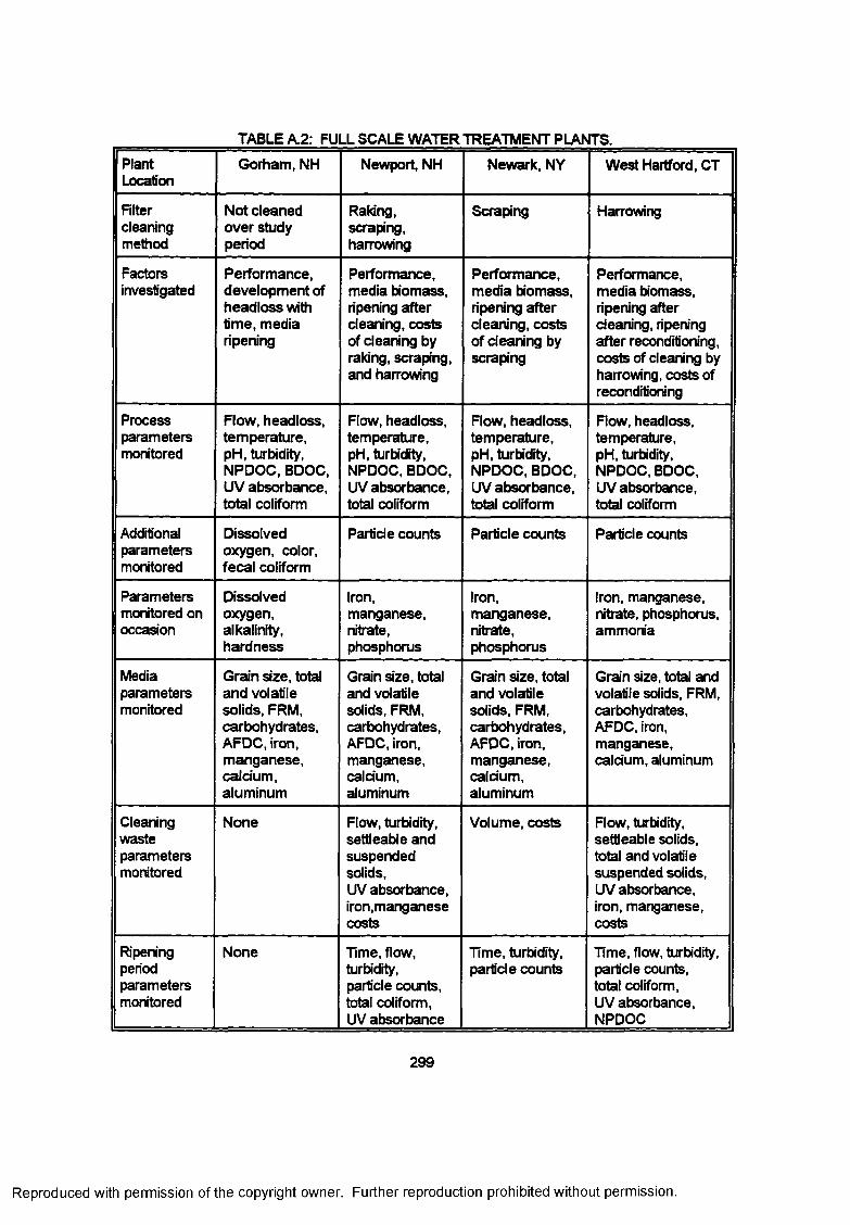
TABLE A.2: FULL SCALE WATER TREATMENT PLANTS.
PlantLocation
Gorham, NH Newport, NH Newark, NY West Hartford, CT
Filtercleaningmethod
Not cleaned over study period
Raking,scraping,harrowing
Scraping Harrowing
Factorsinvestigated
Performance, development of headloss with time, media ripening
Performance, media biomass, ripening after cleaning, costs of cleaning by raking, scraping, and harrowing
Performance, media biomass, ripening after cleaning, costs of cleaning by scraping
Performance, media biomass, ripening after cleaning, ripening after reconditioning, costs of cleaning by harrowing, costs of reconditioning
Processparametersmonitored
Flow, headloss, temperature, pH, turbidity, NPDOC, BDOC, UV absorbance, total coliform
Flow, headloss, temperature, pH, turbidity, NPDOC, BDOC, UV absorbance, total coliform
Flow, headloss, temperature, pH, turbidity, NPDOC, BDOC, UV absorbance, total coliform
Flow, headloss, temperature, pH, turbidity, NPDOC, BDOC, UV absorbance, total coliform
Additionalparametersmonitored
Dissolved oxygen, color, fecal coliform
Particle counts Particle counts Particle counts
Parameters monitored on occasion
Dissolvedoxygen,alkalinity,hardness
Iron,manganese,nitrate,phosphorus
Iron,manganese,nitrate,phosphorus
Iron, manganese, nitrate, phosphorus, ammonia
Mediaparametersmonitored
Grain size, total and volatile solids, FRM, carbohydrates, AFDC, iron, manganese, calcium, aluminum
Grain size, total and volatile solids, FRM, carbohydrates, AFDC, iron, manganese, calcium, aluminum
Grain size, total and volatile solids, FRM, carbohydrates, AFDC, iron, manganese, calcium, aluminum
Grain size, total and volatile solids, FRM, carbohydrates, AFDC, iron, manganese, calcium, aluminum
Cleaningwasteparametersmonitored
None Flow, turbidity, settleable and suspended solids,UV absorbance, iron,manganese costs
Volume, costs Flow, turbidity, settleable solids, total and volatile suspended solids, UV absorbance, iron, manganese, costs
Ripeningperiodparametersmonitored
None Time, flow, turbidity, particle counts, total coliform, UV absorbance
Time, turbidity, particle counts
Time, flow, turbidity, particle counts, total coliform,UV absorbance, NPDOC
299
Reproduced with permission of the copyright owner. Further reproduction prohibited without permission.
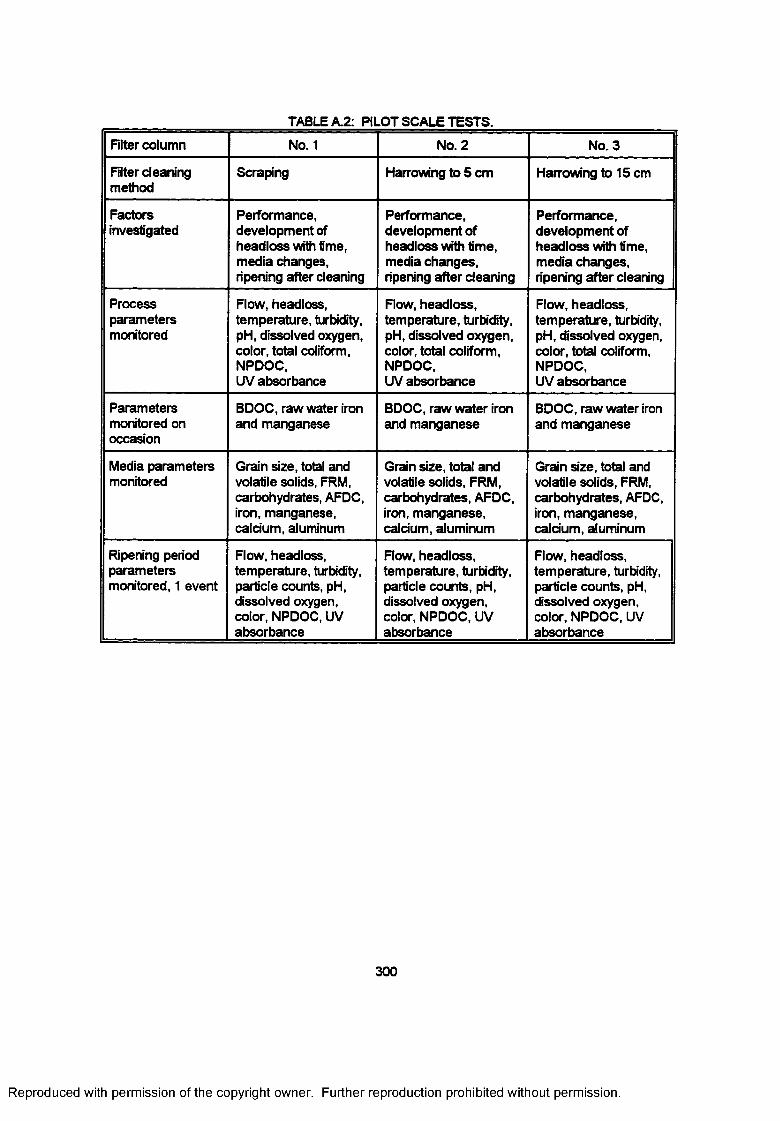
TABLE A.2: PILOT SCALE TESTS.
Filter column No. 1 No. 2 No. 3
Filter cleaning method
Scraping Harrowing to 5 cm Harrowing to 15 cm
Factorsinvestigated
Performance, development of headloss with time, media changes, ripening after cleaning
Performance, development of headloss with time, media changes, ripening after cleaning
Performance, development of headloss with time, media changes, ripening after cleaning
Processparametersmonitored
Flow, headloss, temperature, turbidity, pH, dissolved oxygen, color, total coliform, NPDOC,UV absorbance
Flow, headloss, temperature, turbidity, pH, dissolved oxygen, color, total coliform, NPDOC,UV absorbance
Flow, headloss, temperature, turbidity, pH, dissolved oxygen, color, total coliform, NPDOC,UV absorbance
Parameters monitored on occasion
BDOC, raw water iron and manganese
BDOC, raw water iron and manganese
BDOC, raw water iron and manganese
Media parameters monitored
Grain size, total and volatile solids, FRM, carbohydrates, AFDC, iron, manganese, calcium, aluminum
Grain size, total and volatile solids, FRM, carbohydrates, AFDC, iron, manganese, calcium, aluminum
Grain size, total and volatile solids, FRM, carbohydrates, AFDC, iron, manganese, calcium, aluminum
Ripening period parameters monitored, 1 event
Flow, headloss, temperature, turbidity, particle counts, pH, dissolved oxygen, color, NPDOC, UV absorbance
Flow, headloss, temperature, turbidity, particle counts, pH, dissolved oxygen, color, NPDOC, UV absorbance
Flow, headloss, temperature, turbidity, particle counts, pH, dissolved oxygen, color, NPDOC, UV absorbance
300
Reproduced with permission of the copyright owner. Further reproduction prohibited without permission.
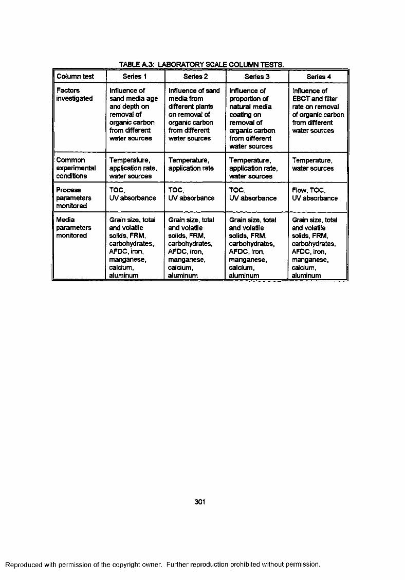
TABLE A.3: LABORATORY SCALE COLUMN TESTS.
Column test Series 1 Series 2 Series 3 Series 4
Factorsinvestigated
Influence of sand media age and depth on removal of organic carbon from different water sources
Influence of sand media from different plants on removal of organic carbon from different water sources
Influence of proportion of natural media coating on removal of organic carbon from different water sources
Influence of EBCT and filter rate on removal of organic carbon from different water sources
Commonexperimentalconditions
Temperature, application rate, water sources
Temperature, application rate
Temperature, application rate, water sources
Temperature, water sources
Processparametersmonitored
TOC,UV absorbance
TOC,UV absorbance
TOC,UV absorbance
Flow, TOC,UV absorbance
Mediaparametersmonitored
Grain size, toted and volatile solids, FRM, carbohydrates, AFDC, iron, manganese, calcium, aluminum
Grain size, total and volatile solids, FRM, carbohydrates, AFDC, iron, manganese, calcium, aluminum
Grain size, total and volatile solids, FRM, carbohydrates, AFDC, iron, manganese, caldum, aluminum
Grain size, total and volatile solids, FRM, carbohydrates, AFDC, iron, manganese, caldum, aluminum
301
Reproduced with permission of the copyright owner. Further reproduction prohibited without permission.
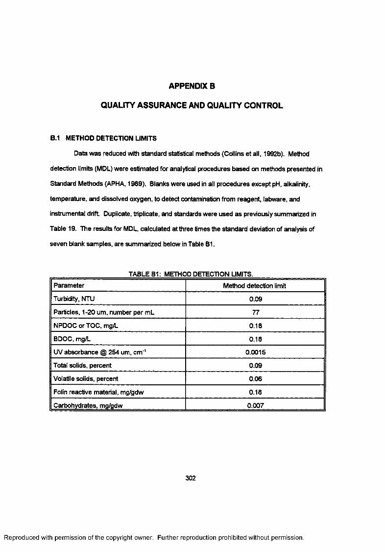
APPENDIX B
QUALITY ASSURANCE AND QUALITY CONTROL
B.1 METHOD DETECTION UMITS
Data was reduced with standard statistical methods (Collins et all, 1992b). Method
detection limits (MDL) were estimated for analytical procedures based on methods presented in
Standard Methods (APHA, 1989). Blanks were used in all procedures except pH, alkalinity,
temperature, and dissolved oxygen, to detect contamination from reagent labware, and
instrumental drift Duplicate, triplicate, and standards were used as previously summarized in
Table 19. The results for MDL, calculated at three times the standard deviation of analysis of
seven blank samples, are summarized below in Table B1.
TABLE B1: METHOD DETECTION UMITS.
Parameter Method detection limit
Turbidity, NTU 0.09
Particles, 1-20 um, number per mL 77
NPDOC or TOC, mg/L 0.18
BDOC, mg/L 0.18
UV absorbance @ 254 um, cm'1 0.0015
Total solids, percent 0.09
Volatile solids, percent 0.06
Folin reactive material, mg/gdw 0.18
Carbohydrates, mg/gdw 0.007
302
Reproduced with permission of the copyright owner. Further reproduction prohibited without permission.
B2: SEPARATION OF VARIANCES IN EXPERIMENTAL DATA
The variance in various experimental analyses was analyzed. These analyses determined
the relative significance of the analytical results between replicated analytical tests, between
multiple samples (such as the three cores taken in each filter, or the separate filter depths in each
core), and between filters. For example, if the variance between replicates exceeded that between
samples or filters, then differences between samples would not likely be significant The nested
analyses of variance are presented for the data for the Newark, NY plant in the attached
spreadsheet
303
Reproduced with permission of the copyright owner. Further reproduction prohibited without permission.
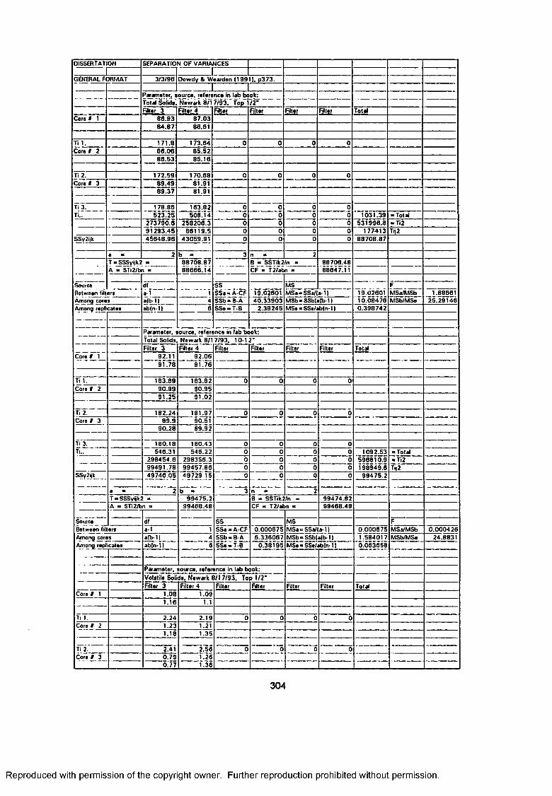
DISSERTATION SEPARATION OF VARIANCES' [ 1
GENERAL FORMAT 3/3 /96 Dowdy & Wearden (1991). p373.
1 1Parameter, source, reference in lab book:Total Solids. Newark 8/1 7/93 . Top 1/2*Filter 3 Filter 4 Filter Filter Filter Filter Total
Com 9 1 86.93 87.0384.87 86.61
Ti 1. 171.8 173.84 0 0 0 0Cora 9 2 86.06 85.52
86.53 85.16
Ti 2. 172.59 170.68 0 0 0 0Cora 9 3 89.49 81.91
89.37 ______8 U 9 2
Ti 3. Ti'..
1 78.86 163.82 00
0 0 0523.25 508.14 0 0 0 1031.39 -T o ta l
273790.6 258206.3 0 0 0 0 531996.8 «T i291293.4545648 .96
86119 .5 0 0 0 0 177413 Tij2SSy2jjk___ 43059.91 0 0 0 0 88708.87
a “ 2 b * 3 n « 2
Sourco
T«SSSyt|k2 A b STi2/b
8 8708 .8788666.14
---------------- 8 ** SSTik2/n * Cf ■ T2/abn «
68706.4888647.11i “
df1 9 02601 10.08476
. ssSSa«A-CF SSb« B-A~
MS FMSa/MSbRetwoon lilt
Among coreare a-1
alb-1| abfn-1)
19.0260140.33903
MSa*SSa/(a-1| 1.88661s 4 MSb*SSb{a(b*1) MSb/MSe 25.29146
Among raplicatos 6 S S e -T -B 2.39245 MSe«SSt/ab(n-11 0.398742
---------Parameter, source, reference in lab book:
Coro 9 1
Total Solids. Newark 8/1 7/93. 10-12*Filter 3 Filter 4 Filter Filter Filter_____ Filter Total
92.11 92.0691.78 91.76
Ti 1.Core 9 2
183.89 183.82 0 0 0 090.99 90.9591.25 91.02
TTY 182.24 181.97 0 0 0 0Cora 9 3 89.9 90.51
90.28 89.92
Ti 3. 1S0.18 180.43 0 0 0 0Ti.. 546.31 546.22 0 0 0
00 1092.53 <s Total
------------------- 298454.6 298356.3 0 0 0 596810.91 98 949 .6
* Ti299491.78 99457 .86 0 0 0 0 Ti|2
SSy2ijk___ 49746 .05 49729 .15 0 ________0 0 0 99475 .2
3a * 2 b » n * 2
Source
T = SSSyijk2 b 99475 .2 B - SSTik2/n - 99474.82A - STi2/bn = 99468.48 CF - T2/abn - 99468.48
df SS MS FBetween filters a-1 1 S S a -A C F
S S b -B -A SSe = T-B
0.0006756.336067
MSa=SSa/ MSb«SSb(
a-1) 0 .000675 MSa/MSb 0.000426Among cores alb-1) 4 a(b-1) 1.584017 MSb/MSe 24.8831Among replicates ab(n -ll 6 0.38195 MSe*SSe/ab(n*1) 0.063658
----------------- -------------------
Parameter, source, reference in lab book:Volatile Solids. Newark 8/17/93, Top 1/2-Filter 3 Filter 4 Filter Filter Filter Filter Total
Core 9 1 1.08 1.091.16 1.1
Ti 1. 2.24 2.19 0 0 0 0Core 9 2 1.23 1.21
------------------- 1.18 1.35
Ti 2. 2.41 2.56 0 0 0 0Core 9 3 0 .79 1.26
0.77 1.36
304
Reproduced with permission of the copyright owner. Further reproduction prohibited without permission.
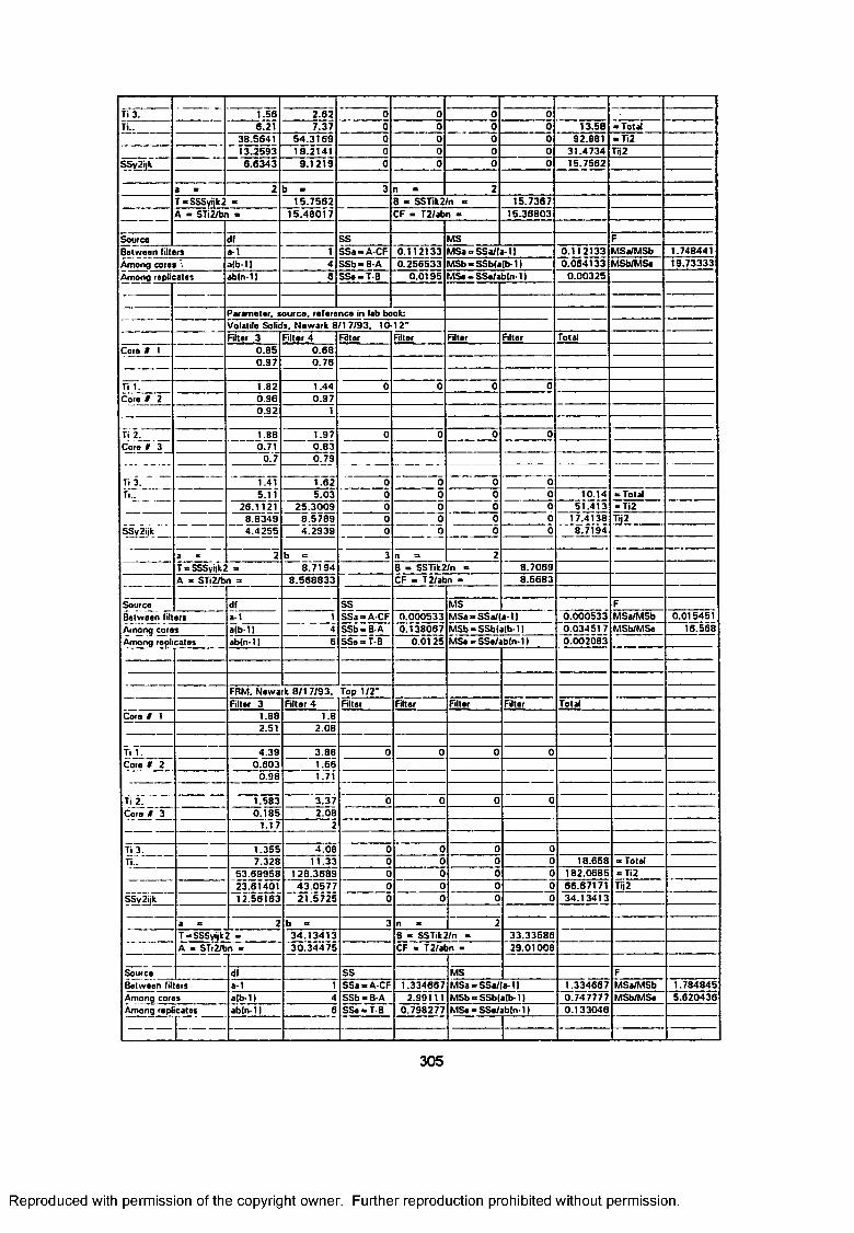
Ti 3. 1.56 2.62 0 0 0 0Ti.. 6.21 7.37
5 4 .3 16 90 0 0 0 13.58 -T o ta l
38.5641 0 0 0 0 92.881 — Ti2
SSy2ijif13.2593 18.2141 0 0 0 0 31.4734 Tij26 .6343 9 .1219 0 0 0 0 15.7562
a “ 2 b - 3 n - 2T c SSSyijk2 - 15 .7562 B - SSTik2/n - 15.7367
---------------- A - STi2/bn - 15 .48017 CF » T2/abn « 15.36803
Sourco df SS MS FBotwaon filters a-1 1
4S S a -A C F 0.112133 M Sa-SSa/la-1) 0.112133 MSa/MSb 1.748441
Among cores a lb -11 S S b -B -A 0.256533 M S b -S S b (a lb -l) 0 .064133 MSb/MSe 19.73333Among replicates ab(n-1) 6 SSe = T-B 0.0195 M Se-SSe/abln-1) 0.00325
-----------------Parameter, source, reference in lab book:Volatile Solids. Newark 8/1 7/93 . 10-12 '
Core 1 T T ~Filter 3 Filter 4 Filter Filter Filter Filter Total
0 .85 0 .680.97 0 .76
Ti 1. 1.82 1.44 0 0 0 0Core * 2 0 .96 0 .97
0 .92 1
Ti 2 ._____Core 9 3
1.880.71
1.970 .83
0 0 0 0
Ti 3.fi.^ "_
0.7 0.79
T .iT 01.62 0 0 05.11 5 .03 0 0 0 0 10.14 -T o ta l
28.1121 25 .30098 .57894T2939
0 0 0 0 51.41317.4138~8.7194
= Ti2
----------------
8 .83494.4255
0 0 0 0 T,j2SSy2ijk 0 0 0 0
a « 2 b = 3 n — 2T=SSSyljk2 = 8 .7194 B - SSTik2/n - 8 .7069
---------------- A - STi2/bn = 8 .5 6 88 3 3 CF = T 2/abn - 8 .5683
Source df SS MS FBetween filters a-1 1 S Sa-A-CF 0.000533 MSa - SSa/|a-11 0.000533 MSa/MSb 0.015451Among cores Among replicates
a lb-11 4 SSb = B-A SSe = T-B
0.1380670.0125
MSb - SSfalalb-11 0.0345170.002083
MSb/MSe 16.568abln-11 6 MSe — SSe/abln-11
FRM. Newark 8/1 7/93. Top 1 /2 'Filter 3 Filter 4 Filter Filter Filter Filter Total
Core 9 1 1.88 1.82.51 2.08
T iJ ^ ___Core 9 2
Ti 2.Core 9 3
4.39 3.881.66
0 0 0 00 .603
0.98 1.71
1.583 3 .37 0 0 0 00 .185 2.08
1.17 2
Ti 3. Ti.. "
1.355 4 .08 0 0 0 07.328 11.33 0 0 0 0 18.658 -T o ta l
53.69958 128 .3689 0 0 0 0 182.0685 = Ti2
SSy2i|k23.6140112.56163
4 3 .0 57 721.5725
0 0 0 0 66.6717134.13413
Tij20 0 0 0
a » 2 b - 3 n - 2T = SSSyijk2 - 3 4 .13413 B - SSTik2/n - 33.33586
----__ A » STi2/bn - 3 0 .3 44 75 CF - T 2/abn - 29.01008
Source df SS MS FBetween filters a-1 1 S S a -A C F 1.334667 MSa - SSa/la-11 1.334667 MSa/MSb 1.784845Among cores alb-1) 4 S S b-B -A 2.99111 MSb - SSblalb-11 0.747777 MSb/MSe 5.620436Among replicates abln-1| 6 SSe - T-B 0.798277 M Se-SSe/abln-1| 0.133046
-- ------ ------- —
305
Reproduced with permission of the copyright owner. Further reproduction prohibited without permission.
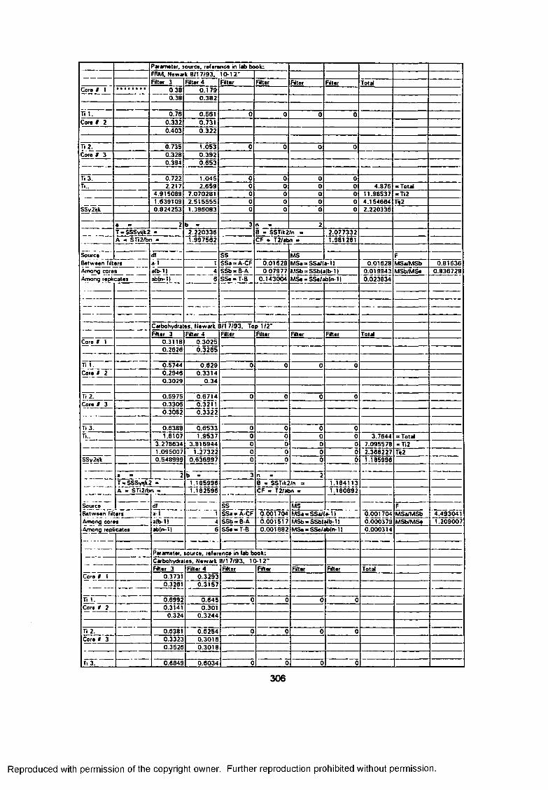
Parameter, source, reference in lab book:FRM. Newark 8/1 7/93. 10-12"Filter 3 Filter 4 Filter Filter Filter Filter Total
Cora 9 1 0 38 0.38
0.1790.382
Ti 1. 0.76 0.561 0 0 0 0Core $ 2 0.332 0.731
0.403 0 .322
Ti 2. 0.735 1.053 0 0 0 0Cora 9 3 0.328 0 .392
0.394 0 .653
Ti 3. 0.722 1.045 0 0 0 0TV._______ ------------------ 2.217 2.659 0 0 0 0 4.876 * Total
4.915089 7.070281 0 0 0 0 11.98537 * T i21.639109 2.515555 0 0 0 0 4.154664 Tij2
SSy2tjk 0.824253 1.396083 0 0 0 0 2.220336
a * 2 b « 3 n « 2T *S S S yijk2 * 2.220336
1.9975628 * SSTik2/n - 2 .077332
A * STi2/bn « CF * T 2/abn « 1.981281
Source df________a-1
SS MS FBetween filters Among cores
1 SSa * A-CF S S b*B -A ~ S S e * T-B
0.01628 MSa * SSa/(a-1) 0.01628 MSa/MSb 0.81636a (b -1 [___abfn-T)
46
0 07977 0 .143004
M Sb*SSb(a(b-1) 0.019943 MSb/MSa 0.836728Among replicates MSe * SSe/abfn-1) 0.023834
- . . .--------- -------- ----------
Carbohydrates. Newark 8/1 7/93. Top 1/2"
Core 9 1Filter 3 Filter 4 Filler Filter Filter Filter Total
0.3118 0.30250.2626 0.3265
Ti 1.Core 9 2
0.5744 0.629 0 0 0 00.2946 0.33140.3029 0.34
T. 2. 0.5975 0.6714 0 0 0 0Core 9 3 0.3306 0.3211
0.3082 0 .3322
r, 3. 0.6388 0.6533 0 0 0 0TV 1.8107 1.9537 0 0 0 0 3.7644 a Total
3 .278634 3.816944 0 0 0 0 7.095578 = Ti21.095007 1.27322 0 0 0 0 2.368227 Ti|2
SSy2ijlc 0.548999 0 .636997 0 0 0 0 1.185996
a = 2 b - 3 n * 2----------------
------- --- T *SSSyt|k2 = 1.185996 B * SSTik2/n * 1.184113A « STi2/bn « 1.182596 CF * T2/abn * 1.180892
Source-
4
df SS MS FBetween filters a-1 S S a * A-CF
S S b * B-A0.001704 MSa*SSa/(a-1) 0.001704 MSa/MSb 4.493041
Among cores a(b-l) 0 .001517 MSb*SSb(a(b-1) 0.000379 MSb/MSa 1.209007Among replicates abfn-1) 6 S S e * T-B 0.001882 M S e * SSe/abfn-1) 0.000314
--------Parameter, source, reference in lab book:
- *---------Carbohydrates. Newark 8/1 7/93 . 10-12*Filter 3 Filter 4 Filter Filter Filter Filter Total
Core f 1 0.3731 0 .3293
----- ---------- 0.3261 0 .3157
r. i. 0.6992 0.645 0 0 0 0Cora 9 2 0.3141 0.301
0.324 0.3244
r. 2. 0.6381 0.6254 0 0 0 0Core 9 3 0.3323 0.3016
0.3526 0.3018
f r y----------
0.6849 0.6034 0 0 0 0
306
Reproduced with permission of the copyright owner. Further reproduction prohibited without permission.
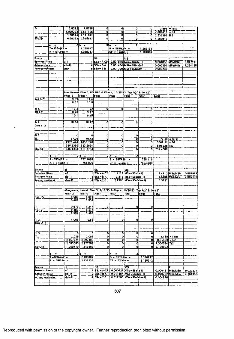
Ti.. 2.0222 1.8738 0 0 0 0 3 .896 » Total
---------- 4 .089293 3.511126 0 0 0 0 7 .600419 a Ti21.365140.68393
1.171242 0 0 0 0 2.536382 Tij2SSy2tjk 0 .585987 0 0 0 0 1.269917
a ■ 2 b - 3 n 8 2T a SSSyijk2 ■ 1.269917 B a SSTik2/n a 1.268191A • STi2/bn - 1.266737 CF « T2/abn - 1.264901
Source df1
SSSSa =* A-CF 0.001835
MS F5.047191Between filters
Among coresa-1 MSaaSSa/|a-1) 0 .001835 MSa/MSbaCb-11 4 S S b«B A 0.001454 MSb a SSbfalb-1) 0 .000364 MSb/MSa 1.264125
Among replicates ab(n-l) 6 SSe - T-B 0.001726 MSe a SSe/ab(n-1) 0 .000288
Top 1/2"
---------- Iron. Newark Filter 3. 8/1 7 /93 & Fdter 4. 10/26/93 Top t /2 " & 10-1 2"Filter 3 Filter 4 Fdter Filter Filter Filter Total
---------- 9 .83 11.48.37 10.6
Ti 1. 18.2 22 0 0 0 010-12" 8 .76 9.27
9.1510.1
----------T<_2.____Core f 3
18.86 18.42 0 0 0 0
Ti 3. 0 0 0 0 0 0Ti.. 37.06 40.42 0 0 0 0 77.48 • Total
1373.444 1633.776 0 0 0 0 3007.22 = Ti2
SSy2rik---------- 686 .9396 823.2964 0 0 0 0 1510.236 Ti|2
345 .4334 411.9754 0 0 0 0 757.4088
a = 2 b = 2 n a 2T»SSSyr)k2 « 757.4088 B a SSTik2/n a 755.118A & STi2/bn a 751 805 CF a T2/abn ** 750.3938
Source df SS MS FBetween filters a-1 1 SSa =* A-CF 1.4112 MSaaSSa/la-U 1.4112 MSa/MSb 0.851917Between lev Among repT
els a(b-1| 2 SSb a 8- A SSe = T -¥ ~
3.313 MSb a SSb|a(b-1) 1.65650.5727
MSb/MSa 2.892439cates ab(n- ) 4 2.2908 MSe * SSe/ab(n-1)
Manganese. Newark Filter 3. 8 /17 /93 & Filter 4 . 10/26/93 Top 1/2’ & 10-12*Filter 3 Filter 4 Filter Filter Filter Filter Total
Top 1/2" 0 .505 0.6930 .468 0.554
n 1. 10-12"
0 .973 1.2470.4470.403
0 0 0 00 .4690 .597
fry. 1.066 0.85 0 0 0 0Core i 3
Ti 3.T iJ ____
SSy2t|k
---------- 0 0 00
0 0 ’ 0
02.039
4.1575212.0830851.050419
2.097 0 0 4.136 • Total4 .397409 2.2 77509 1.149383
0 0 0 0 8.55493'4 .3 6 0 5 9 4
• Ti20 0
00 0 U 2
0 0 0 2.199802
a = 2 b a 2 n a 2T sSSSytjk2 - 2.199802 8 a SSTik2/n « 2.180297A a STi2/bn a 2.138733 CF a T 2/abn a 2.138312
Source df SS MS FBetween filters a-1 1 SSa a A-CF 0.000421
0.041564MSaaSSa/la-1) 0.000421 MSa/MSb 0.020234
Between levels a|b-1 24
S S b -B -A M Sb-SSblJlb-1) 0.020782 MSb/MSe 4.261933Among replicates abln- } SSe a T-B 0.019505 MSe * SSe/ab(n-11 0.004876
---------- ----------
307
Reproduced with permission of the copyright owner. Further reproduction prohibited without permission.
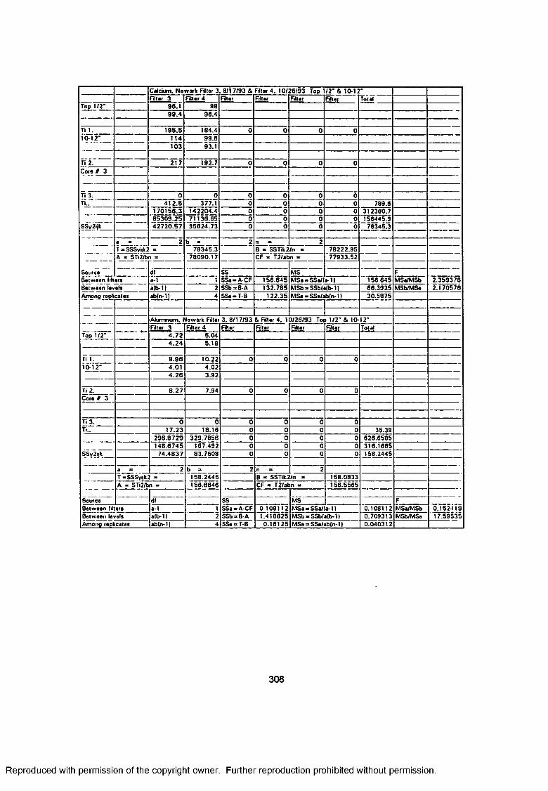
Calcium. Newark Filter 3. 0 /17/93 & Filter 4. 10/26 /93 Top 1/2’ & 10-12 'Filter 3 Filter 4 Filter Filter Filter F3ter Total
Top 1 /2 ’ 96.1 88
----------------- 9 9 .4 96.4
Ti 1. 195.5 184.4 0 0 0 010*12’ __ 114 99.6
93.1103
r i 2. 217 192.7 0 0 0 0Cora 8 3
----—
Ti 3. 0 0 0 0 0 0Ti.. 4 12 .5 377.1 0 0 0 0 789.6
170156.3 142204.4 0 0 0 0 312360.7
SSv2tjiT8 53 09 .254 27 2 0 .5 7
71136.6535624.73
0 0 0 0 156445.978345.30 0 0 0
Source
a » 2 b - 78345.3
78090.17
________ 2 n — 2l*S S S vt|k2 A - STi2S
s B « SSTik2/n - 78222.9577933.52n — CF « T 2/abn «
------------------df - SS MS F
Between filters Between levels
a-1 SSa-A-CF 156.645 MSa - SSa/(a-1) 156.645 MSa/MSb 2.359378a lb -11 2 SSb-B*A 132.785 MSb —SSb(a(b-1| 66.3925 MSb/MSe 2.170576
Among replicates ab(n-11 4 SSe-T-B 122.35 M Se-SSe/abfn* 11 30.5875
---------- Aluminum. Newark Filter 3. 8 /17 /93 & Filter 4 . 10/26/93 Top 1/2’ & 10*12’Filter 3 Filter 4 Filter Fdtar Filter Filter Total
Top 1/2“ 4 .7 2 5.044 .2 4 5.18
f i 1. 8 .9 6 10.22 0 0 0 010-12’ 4.01 4.02
4 .2 6 3.92
T i2 .______Core 8 3
8 .2 7 7.94 0 0 0 0
Ti 3. 0 0 0 0 0 0T i„ 17.23 18.16 0 0 0 0 35.39
296 .8729 329.7856 0 0 0 0 626.6585
SSy2ijk148.6745 167.492 0 0 0 0 316.1665
74.4837 83.7608 0 0 0 0 158.2445
a - 2 b * 158.2445
2 n - 2T-SSSyi|k2 * B - SSTik2/n — 158.0833
Source
A = STi2/bn = 156.6646 CF * T2/abn - 156.5565
----------df SS MS F
Between filters a-1 1 SSa-A-CF 0.108112 M S a -S S a /fa -l) 0.108112 MSa/MSb 0.152419Between le\ Among repl
els alb* 11 2 S S b-B -A 1.418625 MSb-SSb(a(b*1| 0.709313 MSb/MSe 17.59535cates abln-11 4 S Se-T-B 0.16125 M S e - SSe/abfn-11 0.040312
308
Reproduced with permission of the copyright owner. Further reproduction prohibited without permission.
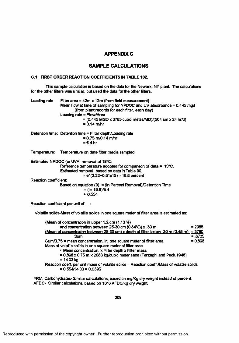
APPENDIX C
SAMPLE CALCULATIONS
C.1 FIRST ORDER REACTION COEFFICIENTS IN TABLE 102.
This sample calculation is based on the data for the Newark, NY plant The calculationsfor the other filters was similar, but used the data for the other filters.
Loading rate: Filter area = 42m x 12m (from field measurement)Mean flow at time of sampling for NPDOC and UV absorbance = 0.445 mgd
(from plant records for each filter, each day)Loading rate = Flow/Area
= (0.445 MGD x 3785 cubic metes/MD)/(504 sm x 24 hr/d)= 0.14 m/hr
Detention time: Detention time = Filter depth/Loading rate= 0.75 m/0.14 m/hr = 5.4 hr
Temperature: Temperature on date filter media sampled.
Estimated NPDOC (or UVA) removal at 15°C:Reference temperature adopted for comparison of data = 15°C.Estimated removal, based on data in Table 90.
= eA(2.22+0.51x15) = 19.8 percentReaction coefficient:
Based on equation (9), = (In Percent Removal)/Detention Time = (In 19.8)/5.4 = 0.554
Reaction coefficient per unit of ....:
Volatile solids-Mass of volatile solids in one square meter of filter area is estimated as:
(Mean of concentration in upper 1.2 cm {1.13 %}and concentration between 25-30 cm {0.84%}) x .30 m =.2955
(Mean of concentration between 25-30 cm) x depth of filter below .30 m (0.45 mi =.3780 Sum = .6735
Sum/0.75 = mean concentration, in one square meter of filter area = 0.898Mass of volatile solids in one square meter of filter area
= Mean concentration, x Filter depth x Filter mass = 0.898 x 0.75 m x 2083 kg/cubic meter sand (Terzaghi and Peck,1948)= 14.03 kg
Reaction coeff. per unit mass of volatile solids = Reaction coeff./Mass of volatile solids = 0.554/14.03 = 0.0395
FRM, Carbohydrates- Similar calculations, based on mg/Kg dry weight instead of percent AFDC- Similar calculations, based on 10*6 AFDC/Kg dry weight
309
Reproduced with permission of the copyright owner. Further reproduction prohibited without permission.
Related Documents