Full Chapter - Puget Sound Nearshore Ecosystem Restoration Project

Puget Sound Nearshore Ecosystem Restoration Project Strategic Restoration Conceptual Engineering – Design Report Appendix C: Applied Geomorphology Guidelines and Hierarchy of Openings March 2011

Applied Geomorphology Guidelines – Revised Draft Phase 2 Document

PSNERP Conceptual Design December 20 2010

These Applied Geomorphology Guidelines will be used by the ESA team’s conceptual designs. The

Guidelines will be used as needed in the designs and to aid in quality control review. These guidelines

may be revised to account for lessons learned during Phase 2 and for subsequent use.

The guidelines are intended only for conceptual design by the PSNERP team. These guidelines are

established partly to provide a means of developing uniform designs, for quality control and precision,

but also to facilitating future refinements. Further research and data collection are required to develop

guidelines for broader application.

These guidelines use empirical models calibrated with data collected from field sites. Therefore, these

guidelines are most useful when the site parameters lie within the range of the calibration data.

Parameters include tide range, sediment and vegetation, fluvial effects, salinity (which affects plant

types and geomorphology), and in some cases wave and littoral climate. Comprehensive data sets are

not presently available for Puget Sound. The guidelines are based on both local data sets and data sets

from other locations, with some adjustments, primarily for tide range. Therefore, the accuracy of the

regressions provided here can be considered approximate. Historic data from the site (e.g. channel

width from a T‐Sheet) or nearby reference data (e.g. Hood’s data for the Skagit, Barnard’s data for

Discovery Bay marshes) may be used instead of these guidelines.

The Guidelines are organized as follows:

1. Tides: Tide design parameters are identified for NOS tide stations selected to represent the varying

tides in Puget Sound. Tide ranges are tabulated. Tidal datum conversion from Mean Lower Low Water

(MLLW) to North American Vertical Datum (NAVD88) are provided at each tide station.

2. Tidal Marsh Channels: Regression lines and graphs are provided to relate channel geometry (channel

cross‐sectional area, width and depth) to marsh area and tidal prism. A set of regressions and graphs are

provided for each tide station identified in (1), based on the tide range. A procedure is provided to

estimate channel geometry with combined tidal and stream discharge.

3. Tidally‐Influenced Fluvial Channels: Guidance for tidally influenced fluvial channels is to use historic

data, remnant channel geometry and available published data on a site‐specific basis.

4. Tidal Inlets: A set of graphs are provided for tidal inlets where wave action and littoral drift affect the

channel geometry and, in particular, limit the tide range. The graphs allow prediction of the tidal prism

necessary for an open inlet and the size of the inlet cross section for a given tidal prism.

5. Beach Geometry: Guidance is provided to estimate the berm elevation of coarse sediment beaches.

1. Tides:

The Puget Sound Nearshore Ecosystem Restoration Project (PSNERP) has defined sub basins of Puget

Sound (Figure 1). Tide stations have been selected to characterize the tidal regime for each sub basin.

Since the tides vary along each arm of Puget Sound (for example, the tide is amplified with distance

south through Hood Canal), several tide stations are indentified for each sub basin, as shown in Figure 1.

Table 1 lists the tide stations and their tidal datums published by the National Ocean Service (NOS). A

conversion between tidal datums and the project vertical datum (NAVD88) are provided. The

conversions are those published by the NOS or are based on a review of the tidal benchmarks and

provided by Pacific Surveying and Engineering (PSE) and ESA PWA as part of this project. The sources of

the conversion and level of confidence are provided.

Each action should define the tidal datums and NAVD conversion used and the sources.

kj

kj

kj

kj

kj

kj

kj

kj

kj

kj

kj

kj

kj

kj

Bellingham, 9449211

Budd inlet, 9446807

Everett, WA, 9447659

Barron Point, 9446742

Crescent Bay, 9443826

Cherry Point, 9449424

Friday Harbor, 9449880

Port Townsend, 9444900Port Angeles, WA 9444090

Union, Hood Canal, 9445478

Seattle, Puget Sound, 9447130

Seabeck, Hood Canal, 9445296

La Conner, Swinomish Slough, 9448558

Yoman Point, Anderson Island, 9446705

Whidbey

Budd Inlet

Hood Canal Central Puget Sound

Strait of Juan De Fuca

South Central Puget Sound

North Central Puget Sound

San Juan Islands and Strait of Georgia

PSNERPfigure X

NOAA Tide Gauge LocationsPWA Ref# -

G:\2036_PSNERP\mxds\base_map±Source: NOAANote: Subregion names are bold with NOAA tide gauge reference number.

0 20 4010Miles

kj NOAA tide gauges

Action areas

River

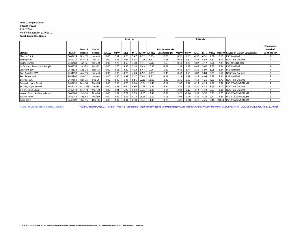
2036.01 Puget Sound

D.Kunz (PWA)

11/22/2010

Modfied B.Battalio, 12/9/2010

Puget Sound Tide Gages

Station NOS #

Start of

Record

End of

Record MLLW MLW MSL MTL MHW MHHW

MLLW to NAVD

Conversion (ft) MLLW MLW MSL MTL MHW MHHW Source of Datum Conversion

Conversion

Level of

Confidence*

Cherry Point 9449424 Nov‐71 present 0.00 2.61 5.28 5.47 8.32 9.15 ‐0.96 ‐0.96 1.65 4.32 4.51 7.36 8.19 PSE Verrified 2

Bellingham 9449211 Mar‐73 Jul‐75 0.00 2.35 4.95 5.07 7.79 8.51 ‐0.48 ‐0.48 1.87 4.47 4.59 7.31 8.03 NOS Tidal Datums 4

Friday Harbor 9449880 Jan‐32 present 0.00 2.29 4.55 4.70 7.11 7.76 ‐0.53 ‐0.53 1.76 4.02 4.17 6.58 7.23 PSE, WSDOT data 3

La Conner, Swinomish Slough 9448558 Jun‐35 Feb‐73 0.00 2.70 5.96 5.18 9.43 10.35 ‐1.51 ‐1.51 1.19 4.45 3.67 7.92 8.84 PSE Verrified 4

Crescent Bay 9443826 Sep‐78 Nov‐78 0.00 2.16 4.22 4.32 6.47 7.06 ‐0.42 ‐0.42 1.74 3.80 3.90 6.05 6.64 PSE Verrified 4

Port Angeles, WA 9444090 Aug‐75 present 0.00 1.93 4.25 4.23 6.52 7.07 ‐0.43 ‐0.43 1.50 3.82 3.80 6.09 6.64 NOS Tidal Datums 4

Port Townsend 9444900 Dec‐71 present 0.00 2.50 4.99 5.17 7.84 8.52 ‐1.11 ‐1.11 1.39 3.88 4.06 6.73 7.41 PSE Verrified 3

Everett, WA 9447659 Dec‐76 Feb‐96 0.00 2.80 6.48 6.51 10.21 11.09 ‐2.30 ‐2.30 0.50 4.18 4.21 7.91 8.79 NOS Tidal Datums 4

Seabeck, Hood Canal 9445296 Mar‐35 Mar‐78 0.00 2.99 6.75 6.76 10.54 11.49 ‐2.62 ‐2.62 0.37 4.13 4.14 7.92 8.87 PSE, VDATUM ONLY!! 1

Seattle, Puget Sound 9447130 Jan ‐ 1899 Sep‐88 0.00 2.83 6.64 6.66 10.49 11.36 ‐2.34 ‐2.34 0.49 4.30 4.32 8.15 9.02 NOS Tidal Datums 4

Union, Hood Canal 9445478 Mar‐73 Mar‐78 0.00 3.01 6.96 6.94 10.87 11.85 ‐2.84 ‐2.84 0.17 4.12 4.10 8.03 9.01 NOS Tidal Datums 4

Yoman Point, Anderson Island 9446705 Feb‐78 Nov‐96 0.00 2.94 7.71 7.75 12.55 13.48 ‐3.78 ‐3.78 ‐0.84 3.93 3.97 8.77 9.70 PSE, VDATUM ONLY!! 1

Barron Point 9446742 Sep‐88 Mar‐89 0.00 3.02 8.29 8.28 13.55 11.52 ‐4.08 ‐4.08 ‐1.06 4.21 4.20 9.47 7.44 PSE, VDATUM ONLY!! 1

Budd Inlet 9446807 Apr‐96 Dec‐96 0.00 3.07 8.31 8.30 13.53 14.48 ‐4.05 ‐4.05 ‐0.98 4.26 4.25 9.48 10.43 PSE, VDATUM ONLY!! 1

* Level of Confidence: 4 highest, 1 lowest. "\\Mars\Projects\2036.01_PSNERP_Phase_1_Conceptual_Engineering\Applied Geomorphology Guidelines\NAVD MLLW Conversions\PSE Survey PSNERP_DATUM_CONVERSIONS 113010.pdf"

ft MLLW ft NAVD

J:\2036.01_PSNERP_Phase_1_Conceptual_Engineering\Applied Geomorphology Guidelines\NAVD MLLW Conversions\2036_PSNERP_TidalDatums v2 103010.xlsJ:\2036.01_PSNERP_Phase_1_Conceptual_Engineering\Applied Geomorphology Guidelines\NAVD MLLW Conversions\2036_PSNERP_TidalDatums v2 103010.xls

b.battalio

Typewritten Text

Table 1: Tides Stations, tidal datums and NAVD conversions.

2. Tidal Salt Marsh Channels (Channel Modification, Dike Removal, Hydraulic

Connection)

Tidal marsh channels are often sized based on applied geomorphology, typically using hydraulic

geometry or allometry (Williams et al, 2002; Hood, 2002). Unfortunately, existing data sets are not

adequate to develop guidelines for Puget Sound, and research indicates large variation between systems

and locations (Hood, 2007; 2002). Still, some basis is needed to size channels in the conceptual designs

as these are key drivers of quantity and cost estimates. Therefore, the guidelines presented here can be

considered more of an engineering method and not vetted from a scientific perspective.

Hydraulic geometry has been used primarily in the study of fluvial and tidal systems, where channel

parameters such as stream width or depth are regressed with area of the watershed (used as a

surrogate for tidal prism and discharge). The form of the equation is typically a power function:

Y = a*xn,

Where x is a independent variable (eg marsh area or watershed area),Y is the dependent variable (tidal

channel width or stream depth), a and n are empirically derived coefficients determined from a

regression of the log‐transformed independent and dependent variables.

The hydraulic geometry of tidal channel parameters has been investigated in Washington at the Chehalis

estuary by Hood (2002) and at the Skagit delta by Hood (2007). In the Chehalis work, log‐transformed

slough outlet width and outlet depth are shown to scale tightly (r2 >0.95 for both) with outlet length for

the Chehalis river sloughs. However, when three other nearby systems are analyzed in a similar fashion,

there are significant differences (95% confidence level) in the regression estimates for nearly all of the

systems analyzed. Hood (2002) indicates that these differences are likely a result of watershed

processes, such as run off or soils, and that these differences must be integrated into the development

of a restoration project. Furthermore, two of the systems investigated (Willapa River and South Fork

Willapa River sloughs) undergo the same tidal regime, but have somewhat differing hydraulic geometry

scaling relations.

Similar scaling regressions were performed in the Skagit delta, but in this work, outlet channel depth

was not included in the analyses (Hood, 2007). As above, there are significant differences in the scaling

relationships between channel outlet width and marsh island area for similar, nearby locations. In the

Skagit delta area, these differences are likely driven by sedimentation and discharge from the Skagit

river (Hood, 2007).

Approximate Hydraulic Geometry for Puget Sound, Extrapolating San Francisco Bay Regressions

The most expeditious means of developing guidelines for sizing tidal marsh channels is to modify the

guidelines for San Francisco Bay (Williams et al, 2002; PWA, 1995). San Francisco Bay data sets are large

and have been used successfully in design of marshes from a few acres to thousands of acres. While

Puget Sound marshes should have different geometry due to different sediments, salinities and plants

and greater rainfall effects, the primary difference is believed to be driven by the larger tide ranges.

These regressions are intended to represent future equilibrium conditions. In most cases, these

dimensions are recommended for construction, with modification for constructability and slope stability

if important. Overall, channels can be expected to evolve along with the marsh and take decades to

reach an equilibrium condition, largely depending on sediment supply and vegetation establishment.

To account for the larger tide range in the Puget Sound area (diurnal range 7’ to 16’ with an average of

about 10.5’), we adjusted the regression lines for San Francisco Bay data. First, we compared the large

San Francisco bay data set (typical diurnal tide range about 5.8ft) with the subset from southern San

Francisco Bay where the tides are much larger (range about 8.8ft). We then calculated the change in

regression lines between the two data sets, and related the differences to percent increase in tide

range. We then prorated this increase based on the tide ranges in Puget Sound.

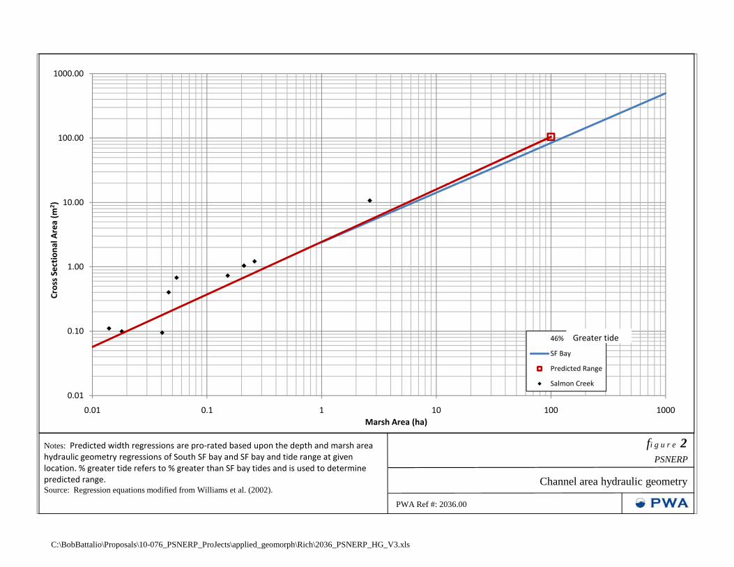
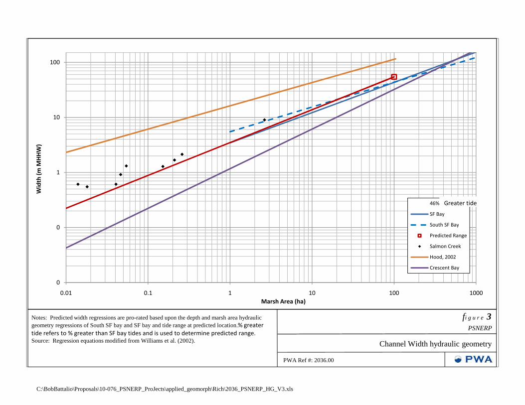
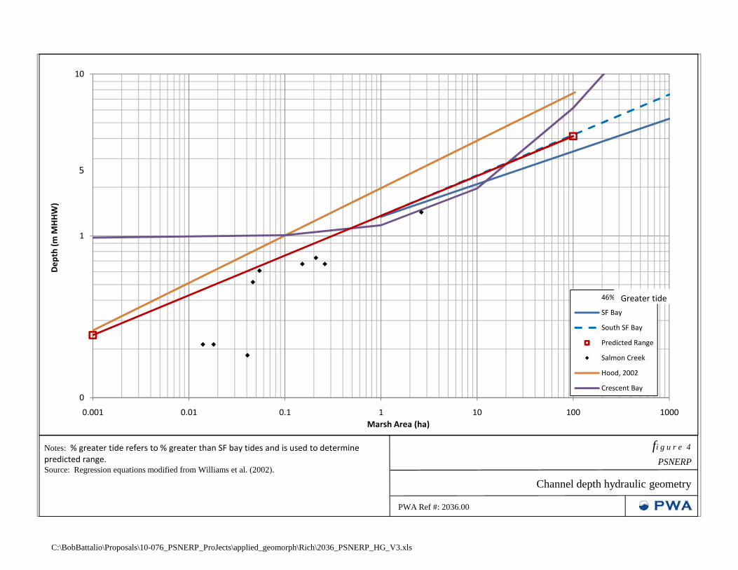
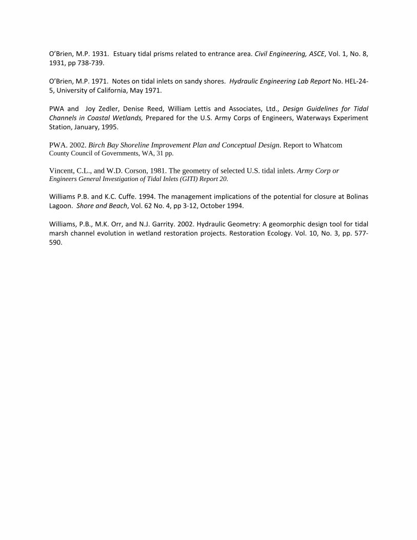
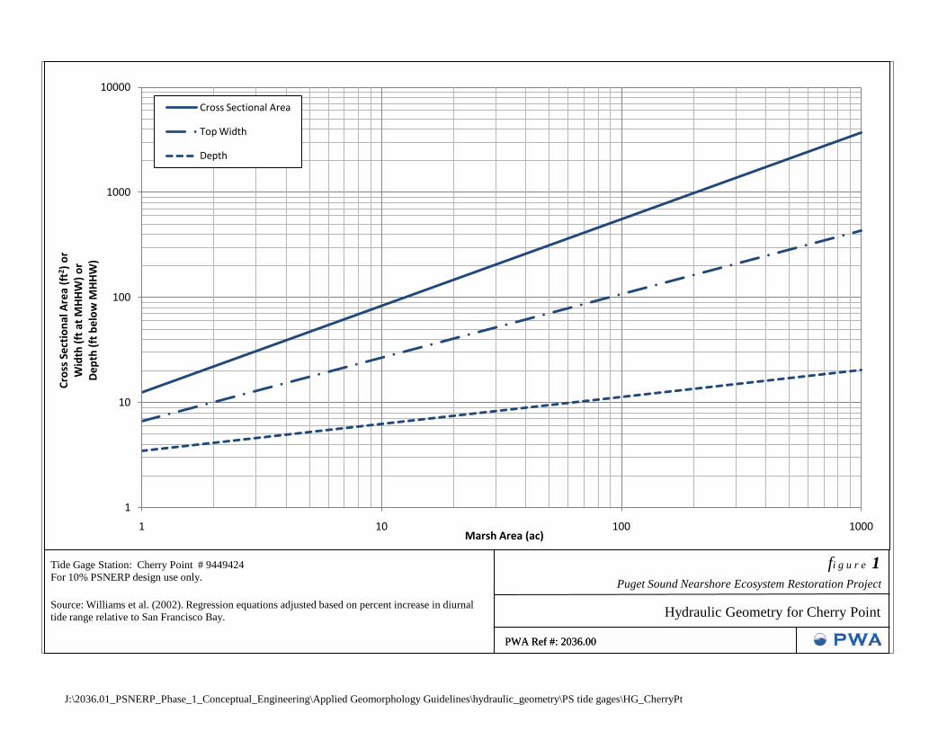
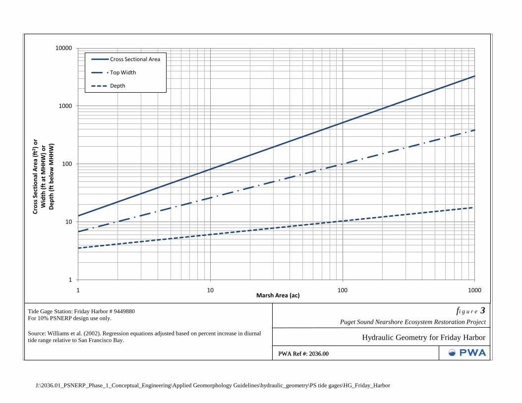
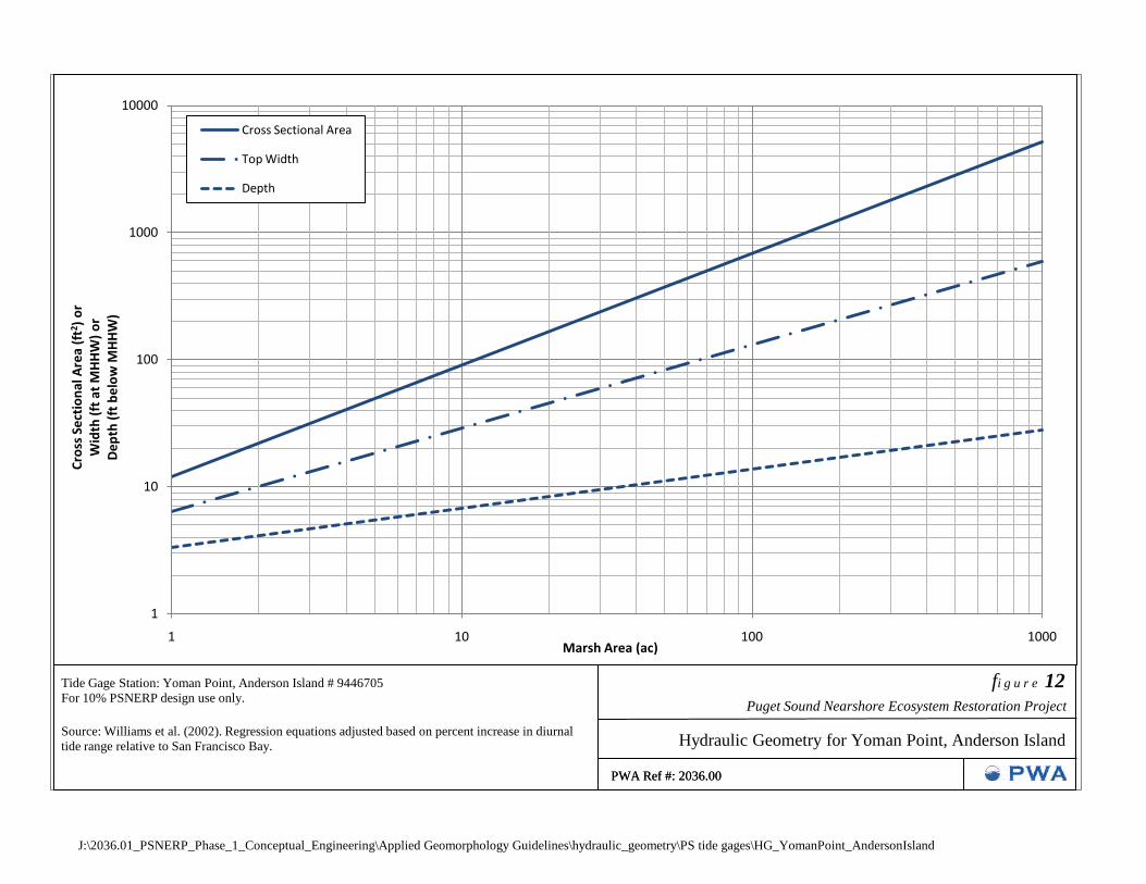
Figures 2, 3 and 4 show data from San Francisco Bay (Williams et al, 2002) and Discovery Bay (Barnard,

project worksheets, 2010), and regression lines by Hood (2002) and PWA (2003). The recommended

regressions are those in red. These are example regressions for one tide station.

The above methodology was applied to 14 tide ranges defined at tide gauges distributed throughout the

study area. This resulted in adjusted regression lines for each of the tide stations that are listed in

section 1. Fourteen graphs (one for each tide station) are provided in the Appendix. Each graph includes

three lines:

Channel Cross section area (feet squared) vs. Marsh Area (acres);

Channel Width (feet) vs. Marsh Area (acres); and,

Channel Depth (feet) vs. Marsh Area (acres).

Upsizing to include stream discharge effects and additional tidal prism

The above discussion is based on tidal prism being the primary channel forming parameter, and uses

marsh area as surrogate for tidal prism. Many Puget Sound marshes have significant freshwater inputs

which add to the scouring power during ebb tides and therefore can be expected to increase the size of

larger channels. To calculate the hydraulic geometry of a channel that incorporates fluvial discharge, the

following methods are proposed. First, calculate the volume of water associated with fluvial discharge

over the ebb period. Second, calculate the channel cross‐sectional area from the marsh area. Third,

using the Williams et al (2002) graph of tidal prism versus cross‐sectional area:

a) locate the initial estimated cross‐sectional area,

b) estimate the associated tidal prism,

1.00

10.00

100.00

1000.00

Cross Sectional Area (m

2)

C:\BobBattalio\Proposals\10-076_PSNERP_ProJects\applied_geomorph\Rich\2036_PSNERP_HG_V3.xls

0.01

0.10

0.01 0.1 1 10 100 1000

Marsh Area (ha)

46%

SF Bay

Predicted Range

Salmon Creek

Notes: Predicted width regressions are pro‐rated based upon the depth and marsh area hydraulic geometry regressions of South SF bay and SF bay and tide range at given location. % greater tide refers to % greater than SF bay tides and is used to determine predicted range.Source: Regression equations modified from Williams et al. (2002).

Channel area hydraulic geometry

fi g u r e 2

PWA Ref #: 2036.00

PSNERP

Greater tide

0

1

10

100

Width (m M

HHW)

46%

SF Bay

South SF Bay

Greater tide


0

0

0.01 0.1 1 10 100 1000

Marsh Area (ha)

South SF Bay

Predicted Range

Salmon Creek

Hood, 2002

Crescent Bay

Notes: Predicted width regressions are pro-rated based upon the depth and marsh area hydraulic geometry regressions of South SF bay and SF bay and tide range at predicted location.% greater tide refers to % greater than SF bay tides and is used to determine predicted range.Source: Regression equations modified from Williams et al. (2002). Channel Width hydraulic geometry

fi g u r e 3

PWA Ref #: 2036.00

PSNERP

1

10

Depth (m M

HHW)

46%

SF Bay

5

Greater tide


0

0.001 0.01 0.1 1 10 100 1000

Marsh Area (ha)

South SF Bay

Predicted Range

Salmon Creek

Hood, 2002

Crescent Bay

Notes: % greater tide refers to % greater than SF bay tides and is used to determine predicted range.Source: Regression equations modified from Williams et al. (2002).

Channel depth hydraulic geometry

fi g u r e 4

PWA Ref #: 2036.00

PSNERP

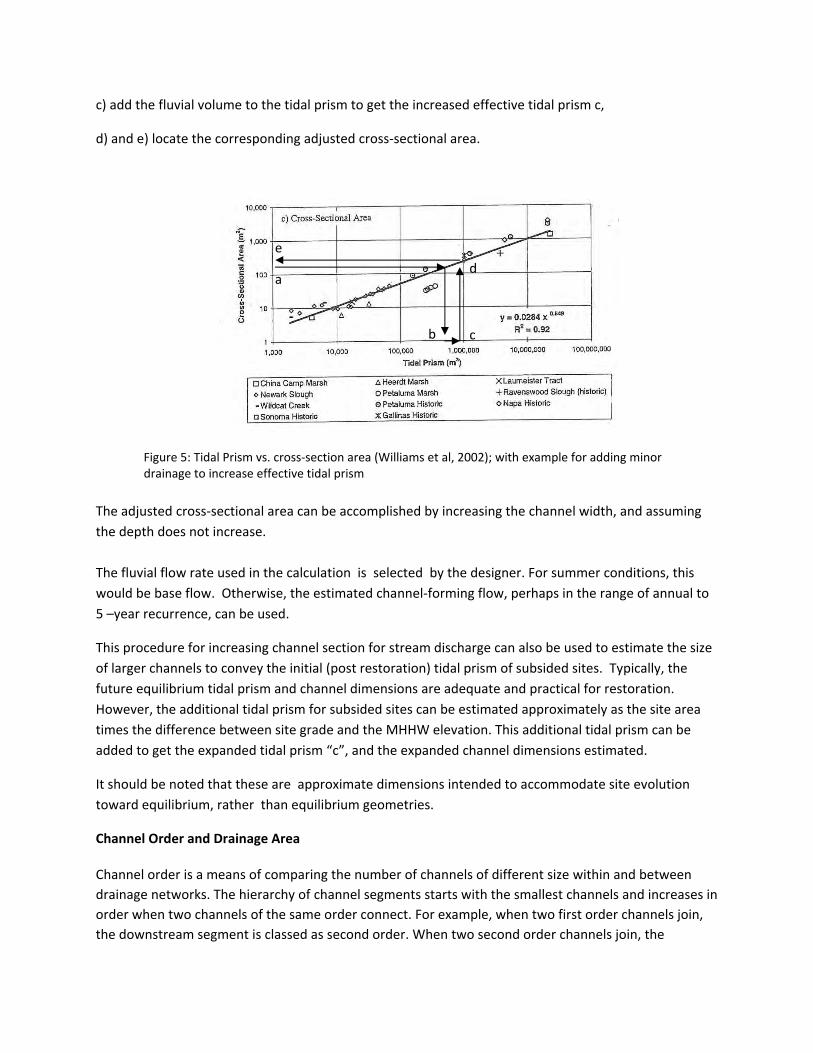
c) add the fluvial volume to the tidal prism to get the increased effective tidal prism c,

d) and e) locate the corresponding adjusted cross‐sectional area.

Figure 5: Tidal Prism vs. cross‐section area (Williams et al, 2002); with example for adding minor drainage to increase effective tidal prism

The adjusted cross‐sectional area can be accomplished by increasing the channel width, and assuming

the depth does not increase.

The fluvial flow rate used in the calculation is selected by the designer. For summer conditions, this

would be base flow. Otherwise, the estimated channel‐forming flow, perhaps in the range of annual to

5 –year recurrence, can be used.

This procedure for increasing channel section for stream discharge can also be used to estimate the size

of larger channels to convey the initial (post restoration) tidal prism of subsided sites. Typically, the

future equilibrium tidal prism and channel dimensions are adequate and practical for restoration.

However, the additional tidal prism for subsided sites can be estimated approximately as the site area

times the difference between site grade and the MHHW elevation. This additional tidal prism can be

added to get the expanded tidal prism “c”, and the expanded channel dimensions estimated.

It should be noted that these are approximate dimensions intended to accommodate site evolution

toward equilibrium, rather than equilibrium geometries.

Channel Order and Drainage Area

Channel order is a means of comparing the number of channels of different size within and between

drainage networks. The hierarchy of channel segments starts with the smallest channels and increases in

order when two channels of the same order connect. For example, when two first order channels join,

the downstream segment is classed as second order. When two second order channels join, the

a

b c

d

e

downstream segment becomes third order. A first order channel joining a third order channel does not

change the order of the downstream segment. The system is defined by the highest order of channel;

for instance a tidal drainage network may be described as ‘third order’.

Horton (1945) found that channel order is related to a number of metrics describing the channel

network:

number of channel segments;

segment length;

drainage area.

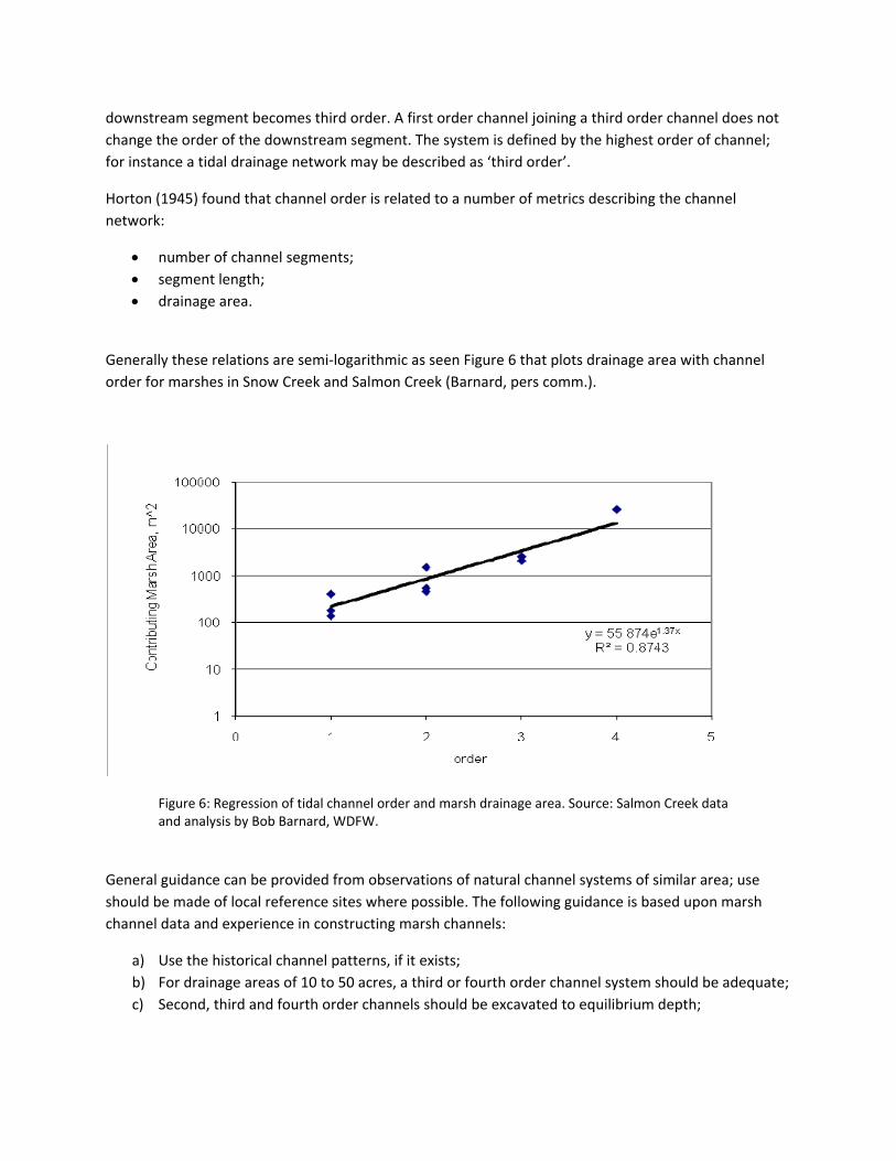
Generally these relations are semi‐logarithmic as seen Figure 6 that plots drainage area with channel

order for marshes in Snow Creek and Salmon Creek (Barnard, pers comm.).

Figure 6: Regression of tidal channel order and marsh drainage area. Source: Salmon Creek data and analysis by Bob Barnard, WDFW.

General guidance can be provided from observations of natural channel systems of similar area; use

should be made of local reference sites where possible. The following guidance is based upon marsh

channel data and experience in constructing marsh channels:

a) Use the historical channel patterns, if it exists;

b) For drainage areas of 10 to 50 acres, a third or fourth order channel system should be adequate;

c) Second, third and fourth order channels should be excavated to equilibrium depth;

d) First order channels may not be practical to cut, especially if the site is subsided and expected to

accrete sediment;

e) If the site is being graded, the marsh slope should be graded down below MHHW and sloped

towards the channels to allow drainage and encourage channel network development.

3. Intertidal ‐ Fluvial (channel modification, dike removal)

Given the paucity of data available, design guidelines for tidally‐influenced fluvial channels is not

practical within the time and budget constraints of this project. Hence, we recommend use of historic

maps of the site, dimensions of remnant channels, and measurements at nearby reference sites if

available.

4. Tidal Inlet (coarse sediment) (Channel Modification, Dike Removal,

Hydraulic Connection)

Hydraulic geometry relationships between tidal prism and the cross‐sectional area of the inlet channel

are perhaps the most common criteria applied to predict the stability of tidal inlets (Battalio, et al,

2006). These are empirical relationships based on surveys of stable inlets and take the form:

Ae = C n

where Ae is the minimum cross‐sectional area, is the tidal prism, and C and n are empirically derived

parameters. Jarrett (1976) examined earlier work by O’Brien (1931) for Pacific Coast inlets, and

established relationships for sites along the Gulf, Pacific and Atlantic coasts. His results were further

divided among inlets with and without jetties. Although the expressions established by Jarrett are

considered the best available predictors for equilibrium cross‐sectional areas, small inlets (small inlets

can be defined as those with thalwegs near or above MLLW) tend to exhibit equilibrium area much

larger than predicted by these tidal prism relationships (Hughes, 2002).

The cross‐sectional area of the inlet channel, Ae, is related to the effective tidal prism by:

Ae = 0.65ka (CIP)8/9

where

T)1S(

WC

8/32/1

8/1

I

eS dg

W is the inlet width at mean tide level (meters), T is the tidal period (typically use semi‐diurnal 12.4

hours, which is 44,640 seconds), de is the median grain size (in meters), g gravitational acceleration (9.81

m/sec2), ka is an empirical coefficient (with a best‐fit value of 1.34), and P is the effective tidal prism

(cubic meters). Ss is the specific gravity of the sediment ( rs/rw)which is often taken to be around 2.6

for quartz and other rock.

The highest point in the channel thalweg typically occurs as the channel crosses the flood shoal and

controls the low water elevation in the marsh. Relatively large wave events can induce a control at the

receiving water side (eg. the ebb shoal or spit in Puget Sound) as well. Due to the complexities of ebb

and flood shoal geometries and the difficulty in field data collection, the narrowest, deepest section of

the inlets (aka “throat”) are typically used as the reference section. Figure 7 shows the general

relationships measured at the Crissy Field Lagoon “throat” in San Francisco Bay. The key parameter is

the lagoon low water, which controls the effective tidal prism of the lagoon. The lagoon low water is

variable, as it results from the sill elevation formed bay wave transport of littoral sediments against the

scour of ebb tides. Inlet morphology also has an effect, which is greatly influenced by littoral drift

parameters including structural controls such as reefs and jetties.

Figure 7. Effective tide range and inlet cross‐section.

Considerable scatter in the data suggest that not all of the relevant processes are included in these

simple relationships. Therefore, they should only be used as a first approximation and interpreted as

representative of long‐term average conditions. Significant variations in inlet cross‐section can occur

over the spring‐neap tide cycle, during storms when wave attack is more intense, or following large

flood events (DeTemple, 1999). This is especially true for small dynamic systems. A process‐based tidal

prism relationship developed by Hughes (2002) shows better agreement between small and large tidal

inlets, and more promise for application to Puget Sound lagoons (Figure 8).

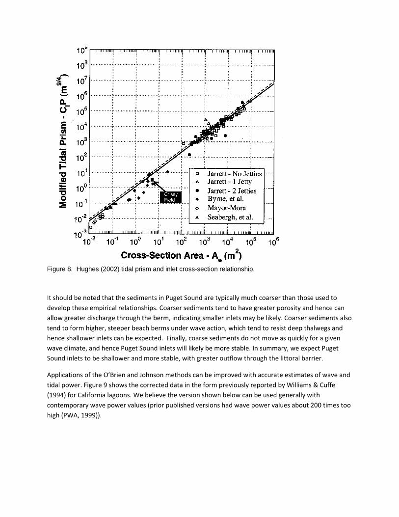
Figure 8. Hughes (2002) tidal prism and inlet cross-section relationship.

It should be noted that the sediments in Puget Sound are typically much coarser than those used to

develop these empirical relationships. Coarser sediments tend to have greater porosity and hence can

allow greater discharge through the berm, indicating smaller inlets may be likely. Coarser sediments also

tend to form higher, steeper beach berms under wave action, which tend to resist deep thalwegs and

hence shallower inlets can be expected. Finally, coarse sediments do not move as quickly for a given

wave climate, and hence Puget Sound inlets will likely be more stable. In summary, we expect Puget

Sound inlets to be shallower and more stable, with greater outflow through the littoral barrier.

Applications of the O’Brien and Johnson methods can be improved with accurate estimates of wave and

tidal power. Figure 9 shows the corrected data in the form previously reported by Williams & Cuffe

(1994) for California lagoons. We believe the version shown below can be used generally with

contemporary wave power values (prior published versions had wave power values about 200 times too

high (PWA, 1999)).

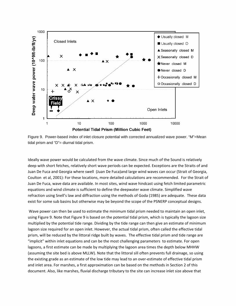
Figure 9. Power-based index of inlet closure potential with corrected annualized wave power. “M”=Mean

tidal prism and “D”= diurnal tidal prism.

Ideally wave power would be calculated from the wave climate. Since much of the Sound is relatively

deep with short fetches, relatively short wave periods can be expected. Exceptions are the Straits of and

Juan De Fuca and Georgia where swell (Juan De Fuca)and large wind waves can occur (Strait of Georgia,

Coulton et al, 2001): For these locations, more detailed calculations are recommended. For the Strait of

Juan De Fuca, wave data are available. In most sites, wind wave hindcast using fetch limited parametric

equations and wind climate is sufficient to define the deepwater wave climate. Simplified wave

refraction using Snell’s law and diffraction using the methods of Goda (1985) are adequate. These data

exist for some sub basins but otherwise may be beyond the scope of the PSNERP conceptual designs.

Wave power can then be used to estimate the minimum tidal prism needed to maintain an open inlet,

using Figure 9. Note that Figure 9 is based on the potential tidal prism, which is typically the lagoon size

multiplied by the potential tide range. Dividing by the tide range can then give an estimate of minimum

lagoon size required for an open inlet. However, the actual tidal prism, often called the effective tidal

prism, will be reduced by the littoral ridge built by waves. The effective tidal prism and tide range are

“implicit” within inlet equations and can be the most challenging parameters to estimate. For open

lagoons, a first estimate can be made by multiplying the lagoon area times the depth below MHHW

(assuming the site bed is above MLLW). Note that the littoral sill often prevents full drainage, so using

the existing grade as an estimate of the low tide may lead to an over‐estimate of effective tidal prism

and inlet area. For marshes, a first approximation can be based on the methods in Section 2 of this

document. Also, like marshes, fluvial discharge tributary to the site can increase inlet size above that

based on tidal prism alone. Once the effective tidal prism is estimated, it will be used to estimate the

required inlet cross section geometry using Figure 8 and selected aspect ratios (width to depth).

The best available relationship for small tidal inlets in littoral systems is Hughes (2002; Figure 8). A

review of this equation indicates that it is very sensitive to grain size, with larger grain sizes resulting in

smaller predicted inlet cross sections. We recommend using a default of 1 mm which will help keep the

equation within the range of data sources and bias the area calculation to the high side: In general, over‐

excavation of the inlet results in less risk of subsequent closure. Further research is needed to inform

use for coarse sediment shores.

It should be noted that over‐excavation will induce a perturbation that can reduce sediment supply to

adjacent shores. Excavated sediment compatible with the littoral sediment should be placed down drift

to mitigate the subsequent interruption of longshore transport during inlet evolution. For new inlets,

placement of littoral sediments should be considered to mitigate the sediment deficit induced by flood

and ebb shoal formation. The effect can extend updrift as well but to a lesser extent.

Once area is calculated, width and depth are selected. Ideally, an estimate of one of these parameters

will be available. For example, the inlet width from an historic map can be used, and then the depth can

calculated based on an assumed shape (see below).

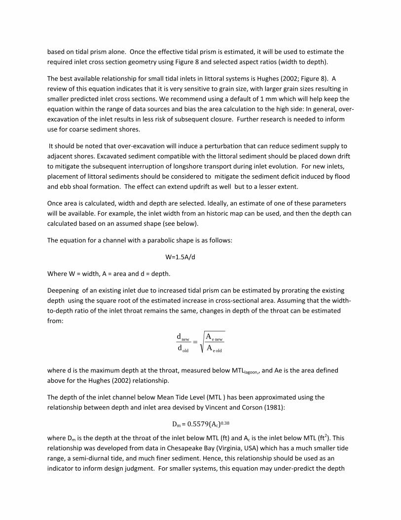
The equation for a channel with a parabolic shape is as follows:

W=1.5A/d

Where W = width, A = area and d = depth.

Deepening of an existing inlet due to increased tidal prism can be estimated by prorating the existing

depth using the square root of the estimated increase in cross‐sectional area. Assuming that the width‐

to‐depth ratio of the inlet throat remains the same, changes in depth of the throat can be estimated

from:

old e

new e

old

new

A

A

d

d

where d is the maximum depth at the throat, measured below MTLlagoon,, and Ae is the area defined

above for the Hughes (2002) relationship.

The depth of the inlet channel below Mean Tide Level (MTL ) has been approximated using the

relationship between depth and inlet area devised by Vincent and Corson (1981):

Dm = 0.5579(Ac)0.38

where Dm is the depth at the throat of the inlet below MTL (ft) and Ac is the inlet below MTL (ft2). This

relationship was developed from data in Chesapeake Bay (Virginia, USA) which has a much smaller tide

range, a semi‐diurnal tide, and much finer sediment. Hence, this relationship should be used as an

indicator to inform design judgment. For smaller systems, this equation may under‐predict the depth

due to its derivation with data from areas with smaller tide ranges. If this equation is used and predicts

depths significantly above MLLW, over‐excavation is recommended.

Reference site data can be used instead of or in addition to the methods proposed here.

5. Beach (coarse sediment) (bulkhead removal, groin removal)

The morphology of coarse sediment beaches includes a steep foreshore (swash zone) leading up to a flat

terrace or berm (Bauer, 1974; Lorang, 2002 ). The profile morphology and terms are shown by the

example in Figure 9 (Birch Bay, Whatcom County, Bauer, 1975). The swash zone slope is affected by

sediment size and wave climate. For most Puget Sound locations, the swash zone has a typical slope

around 7:1 with a range between 5:1 and 10:1 (horizontal: vertical). Steeper slopes can be expected for

coarser and more uniform sized sediments, and higher wave exposure. The berm elevation is typically

considered the result of wave runup that builds the berm to a level just below the annual maximum

total water level (total water level is defined as the Puget Sound water level plus wave runup).

Figure 10 shows a conceptual profile of coarse beach dynamics (Bauer, 1975). Note that Figure 10 shows

a berm configured to provide protection to inland development and includes extra volume as a “storm

buffer,” with the berm crest elevation about 6.5’ above MHHW. Given PSNERP’s focus on restoration,

berm heights should typically not be over‐built for protective purposes. Figures 11 and 12 provide an

example of a reference site in Whatcom County (PWA, 2002). The berm crest is around 11.3’ to 12.8’

NAVD (converted from NGVD by adding 3.8’), and about 4 feet above MHHW. Note the wood above the

berm indicating that the total water level exceeds the berm crest in natural conditions. Therefore, we

recommend under‐building the berm slightly to allow shaping by wave action. Slight under‐building

avoids the potential adverse effects of unnatural morphology and while limiting sediment demand to fill

the “void” resulting removal of fill or armoring.

Figure 10. Description of coarse sediment beach profile morphology, for a protective berm (Bauer, 1975).

Figures 11 and 12. Semi-Ah-Moo Beach. Photograph of beach swash zone and berm (left); Elevation

cross sections of swash zone slope and berm (right). Source, PWA, 1975.

For PSNERP conceptual designs, the geometry of nearby reference sites can be used to develop the

restored profile and estimate quantities. Alternatively, some basic parameters should be sufficient. A

slope of around 5:1 to 10:1 with a typical of 7:1 is recommended. This should be checked and adjusted

based on consideration of local geometry, reference sites, size of sediment and wave exposure. The

berm elevation can be estimated as the height of the annual wave runup (R) on the profile using the

following equation:

R2% = Static Setup + Runup

= 0.2 H0 + 0.6r (m/(H0/L0)1/2)H0

The above equation is based on the surf similarity parameter / Iriabarren number; m is the beach slope,

r is an empirical coefficient, H0 is the significant deep water wave height and L0 is the deep water wave

length . The wave values used should be on the order of an annual to 5 year return period. (Note that

the term “2%” for the runup does not refer to annual frequency, but rather the exceedance within an

event, e.g. the significant exceedance is typically considered 33% and the rms 50%).

It is recommended that a composite slope of about 10:1 (m=0.1) is used to account for larger waves

breaking offshore of the swash formed foreshore. Also, the result should be adjusted downward to

account for the permeability of the coarse sediment and a factor of about r=0.8 is recommended.

Wave runup on natural beaches does not typically exceed about three times the wave height. For

steeper waves on porous (gravel, cobble) sediments, the runup is reduced and a maximum of about two

times the wave height can be expected. We therefore recommend that a reasonable range for runup in

sheltered waters (not exposed to ocean swell) is between 0.5 and 2 times the wave height, and on

coarse sediment shores (gravels and cobble) will not typically exceed 1 times the wave height.

Since the berm is formed by the total water level with an approximate annual exceedance, the more

extreme wave runup value (1 to 5 year recurrence) should be added to a typical high tide, on the order

of MHHW or MHHW with a surge / setup added: A setup due to meteorological effects can be on the

order of 1 foot. Alternatively, an annual high water level can be combined with a smaller, nominal wave

height likely to occur simultaneously with the high tide.

For cases where much larger waves break far offshore of the berm, wave setup for the larger offshore

waves should be added. A static wave set up can be approximately estimated as 0.2 times incident wave

height (FEMA, 2005). The groupiness and randomness of the waves also results in longer‐period

dynamics often called dynamic setup. Accounting for dynamic setup and combining with static setup

and runup can be complex. However, for the conditions associated with PSNERP it is recommended that

a total wave setup of about 0.3 times the deepwater wave height is a reasonable estimate of total setup

due to larger waves breaking offshore.

We recommend a minimum beach berm elevation of 1.5 ft above MHHW.

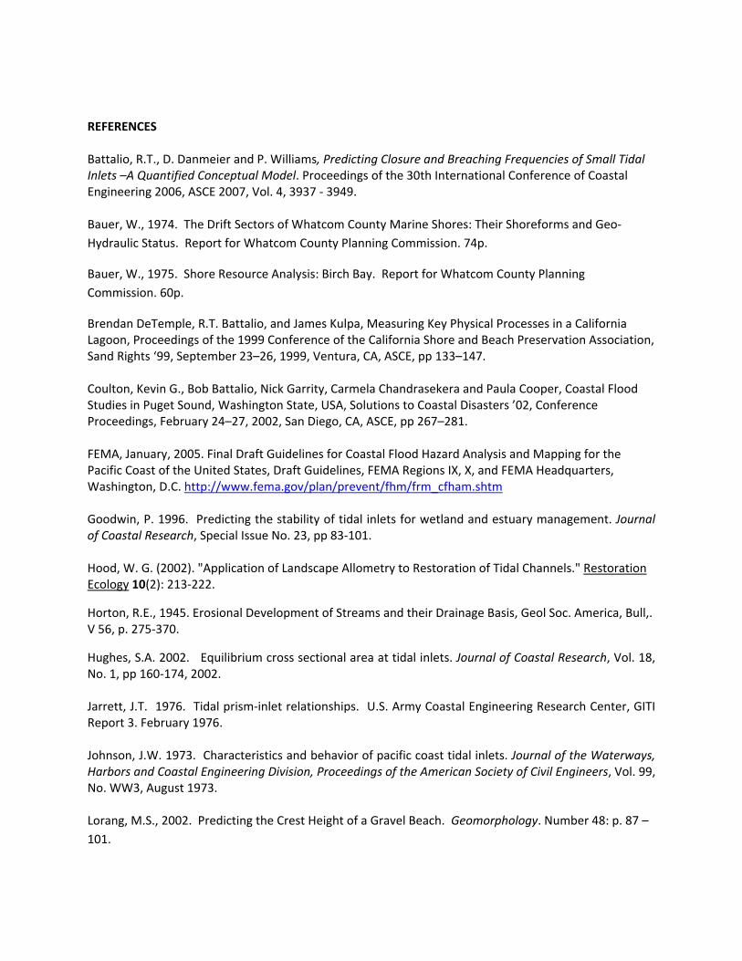
REFERENCES Battalio, R.T., D. Danmeier and P. Williams, Predicting Closure and Breaching Frequencies of Small Tidal Inlets –A Quantified Conceptual Model. Proceedings of the 30th International Conference of Coastal Engineering 2006, ASCE 2007, Vol. 4, 3937 ‐ 3949. Bauer, W., 1974. The Drift Sectors of Whatcom County Marine Shores: Their Shoreforms and Geo‐

Hydraulic Status. Report for Whatcom County Planning Commission. 74p.

Bauer, W., 1975. Shore Resource Analysis: Birch Bay. Report for Whatcom County Planning

Commission. 60p.

Brendan DeTemple, R.T. Battalio, and James Kulpa, Measuring Key Physical Processes in a California Lagoon, Proceedings of the 1999 Conference of the California Shore and Beach Preservation Association, Sand Rights ‘99, September 23–26, 1999, Ventura, CA, ASCE, pp 133–147. Coulton, Kevin G., Bob Battalio, Nick Garrity, Carmela Chandrasekera and Paula Cooper, Coastal Flood Studies in Puget Sound, Washington State, USA, Solutions to Coastal Disasters ’02, Conference Proceedings, February 24–27, 2002, San Diego, CA, ASCE, pp 267–281. FEMA, January, 2005. Final Draft Guidelines for Coastal Flood Hazard Analysis and Mapping for the Pacific Coast of the United States, Draft Guidelines, FEMA Regions IX, X, and FEMA Headquarters, Washington, D.C. http://www.fema.gov/plan/prevent/fhm/frm_cfham.shtm Goodwin, P. 1996. Predicting the stability of tidal inlets for wetland and estuary management. Journal of Coastal Research, Special Issue No. 23, pp 83‐101. Hood, W. G. (2002). "Application of Landscape Allometry to Restoration of Tidal Channels." Restoration Ecology 10(2): 213‐222.

Horton, R.E., 1945. Erosional Development of Streams and their Drainage Basis, Geol Soc. America, Bull,. V 56, p. 275‐370.

Hughes, S.A. 2002. Equilibrium cross sectional area at tidal inlets. Journal of Coastal Research, Vol. 18, No. 1, pp 160‐174, 2002. Jarrett, J.T. 1976. Tidal prism‐inlet relationships. U.S. Army Coastal Engineering Research Center, GITI Report 3. February 1976. Johnson, J.W. 1973. Characteristics and behavior of pacific coast tidal inlets. Journal of the Waterways, Harbors and Coastal Engineering Division, Proceedings of the American Society of Civil Engineers, Vol. 99, No. WW3, August 1973. Lorang, M.S., 2002. Predicting the Crest Height of a Gravel Beach. Geomorphology. Number 48: p. 87 –

101.

O’Brien, M.P. 1931. Estuary tidal prisms related to entrance area. Civil Engineering, ASCE, Vol. 1, No. 8, 1931, pp 738‐739. O’Brien, M.P. 1971. Notes on tidal inlets on sandy shores. Hydraulic Engineering Lab Report No. HEL‐24‐5, University of California, May 1971. PWA and Joy Zedler, Denise Reed, William Lettis and Associates, Ltd., Design Guidelines for Tidal Channels in Coastal Wetlands, Prepared for the U.S. Army Corps of Engineers, Waterways Experiment Station, January, 1995. PWA. 2002. Birch Bay Shoreline Improvement Plan and Conceptual Design. Report to Whatcom County Council of Governments, WA, 31 pp. Vincent, C.L., and W.D. Corson, 1981. The geometry of selected U.S. tidal inlets. Army Corp or Engineers General Investigation of Tidal Inlets (GITI) Report 20. Williams P.B. and K.C. Cuffe. 1994. The management implications of the potential for closure at Bolinas Lagoon. Shore and Beach, Vol. 62 No. 4, pp 3‐12, October 1994. Williams, P.B., M.K. Orr, and N.J. Garrity. 2002. Hydraulic Geometry: A geomorphic design tool for tidal marsh channel evolution in wetland restoration projects. Restoration Ecology. Vol. 10, No. 3, pp. 577‐590.

Appendix A: NAVD Conversions from Pacific Survey and Engineering, 2010

1

Bob Battalio

From: Adam Morrow [[email protected]]Sent: Tuesday, November 30, 2010 9:35 AMTo: Margaret ClancyCc: Bob BattalioSubject: PSNERP Datum ConversionsAttachments: PSNERP_DATUM_CONVERSIONS.pdf

Margaret, In an effort to wrap up our work on this project to date and provide you with an item that had been discussed in some detail over the past few months, we have attached a spreadsheet that details our Tidal-NAVD 88 vertical datum conversions that can be used for pre-selected sites. The spreadsheet includes conversions for areas that were noted as not available in Bob Battalio's previously emailed spreadsheet. With a few exceptions, we were able to find consistent datum conversions for tidal regions throughout Puget Sound. Where we could not, we listed the applicable VDATUM conversion related to the reference tidal gauge. For your use, we also included a column that indicates our level of confidence for each conversion, based on the availability of published benchmark information and/or conflicts between published data and VDATUM results. We hope that this proves useful for the design team in the continued efforts to provide 10% design documents for the project. We are ready and willing to respond to questions about this information as needed to help you complete your Phase 2 work. I look forward to hearing from you in the near future about opportunities to continue to provide services on this project. From our research work to date, I suspect that we now have a good database of information from which we can provide cost estimates for necessary survey and base mapping work at each site if that is deemed necessary. Thanks. -Adam

Adam Morrow, PLS Pacific Surveying and Engineering 1812 Cornwall Avenue Bellingham, WA 98225 (360) 671-7387 (360) 671-4685 (fax)

Appendix B: Graphs of Tidal Wetland Channel Dimensions vs. Marsh Area

J:\2036.01_PSNERP_Phase_1_Conceptual_Engineering\Applied Geomorphology Guidelines\hydraulic_geometry\PS tide gages\HG_CherryPt

1

10

100

1000

10000

1 10 100 1000

Cros

s Sec

tiona

l Are

a (ft

2 ) o

rW

idth

(ft a

t MHH

W) o

rDe

pth

(ft b

elow

MHH

W)

Marsh Area (ac)

Cross Sectional Area

Top Width

Depth

Tide Gage Station: Cherry Point # 9449424For 10% PSNERP design use only.

Source: Williams et al. (2002). Regression equations adjusted based on percent increase in diurnal tide range relative to San Francisco Bay. Hydraulic Geometry for Cherry Point

fi g u r e 1

PWA Ref #: 2036.00

Puget Sound Nearshore Ecosystem Restoration Project

PWA Ref #: 2036.00

J:\2036.01_PSNERP_Phase_1_Conceptual_Engineering\Applied Geomorphology Guidelines\hydraulic_geometry\PS tide gages\HG_Bellingham

1

10

100

1000

10000

1 10 100 1000

Cros

s Sec

tiona

l Are

a (ft

2 ) o

rW

idth

(ft a

t MHH

W) o

rDe

pth

(ft b

elow

MHH

W)

Marsh Area (ac)


Top Width

Depth

Tide Gage Station: Bellingham # 9449211For 10% PSNERP design use only.

Source: Williams et al. (2002). Regression equations adjusted based on percent increase in diurnal tide range relative to San Francisco Bay. Hydraulic Geometry for Bellingham

fi g u r e 2

PWA Ref #: 2036.00


PWA Ref #: 2036.00

J:\2036.01_PSNERP_Phase_1_Conceptual_Engineering\Applied Geomorphology Guidelines\hydraulic_geometry\PS tide gages\HG_Friday_Harbor

1

10

100

1000

10000

1 10 100 1000

Cros

s Sec

tiona

l Are

a (ft

2 ) o

rW

idth

(ft a

t MHH

W) o

rDe

pth

(ft b

elow

MHH

W)

Marsh Area (ac)


Top Width

Depth

Tide Gage Station: Friday Harbor # 9449880For 10% PSNERP design use only.

Source: Williams et al. (2002). Regression equations adjusted based on percent increase in diurnal tide range relative to San Francisco Bay. Hydraulic Geometry for Friday Harbor

fi g u r e 3

PWA Ref #: 2036.00


PWA Ref #: 2036.00

J:\2036.01_PSNERP_Phase_1_Conceptual_Engineering\Applied Geomorphology Guidelines\hydraulic_geometry\PS tide gages\HG_LaConner_SwinomishSlough

1

10

100

1000

10000

1 10 100 1000

Cros

s Sec

tiona

l Are

a (ft

2 ) o

rW

idth

(ft a

t MHH

W) o

rDe

pth

(ft b

elow

MHH

W)

Marsh Area (ac)


Top Width

Depth

Tide Gage Station: La Conner, Swinomish Slough # 9448558For 10% PSNERP design use only.

Source: Williams et al. (2002). Regression equations adjusted based on percent increase in diurnal tide range relative to San Francisco Bay. Hydraulic Geometry for La Conner, Swinomish Slough

fi g u r e 4

PWA Ref #: 2036.00


PWA Ref #: 2036.00

J:\2036.01_PSNERP_Phase_1_Conceptual_Engineering\Applied Geomorphology Guidelines\hydraulic_geometry\PS tide gages\HG_Crescent_Bay

1

10

100

1000

10000

1 10 100 1000

Cros

s Sec

tiona

l Are

a (ft

2 ) o

rW

idth

(ft a

t MHH

W) o

rDe

pth

(ft b

elow

MHH

W)

Marsh Area (ac)


Top Width

Depth

Tide Gage Station: Crescent Bay # 9443826For 10% PSNERP design use only.

Source: Williams et al. (2002). Regression equations adjusted based on percent increase in diurnal tide range relative to San Francisco Bay. Hydraulic Geometry for Crescent Bay

fi g u r e 5

PWA Ref #: 2036.00


PWA Ref #: 2036.00

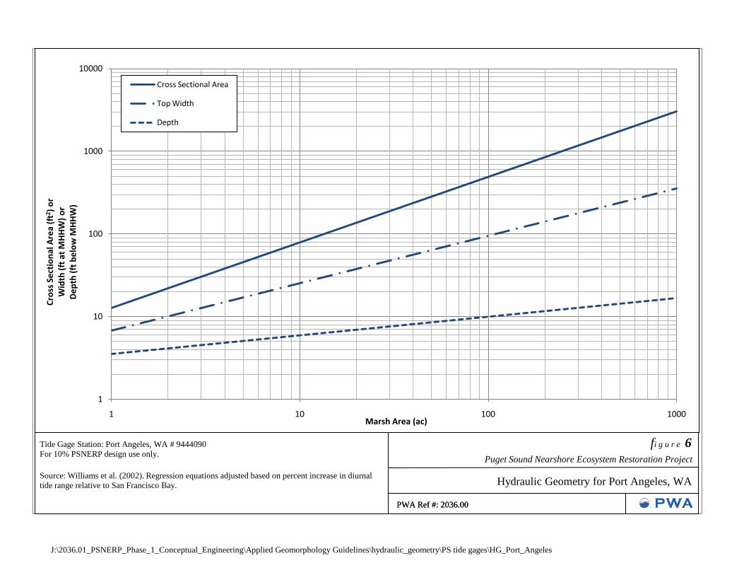
J:\2036.01_PSNERP_Phase_1_Conceptual_Engineering\Applied Geomorphology Guidelines\hydraulic_geometry\PS tide gages\HG_Port_Angeles

1

10

100

1000

10000

1 10 100 1000

Cros

s Sec

tiona

l Are

a (ft

2 ) o

rW

idth

(ft a

t MHH

W) o

rDe

pth

(ft b

elow

MHH

W)

Marsh Area (ac)


Top Width

Depth

Tide Gage Station: Port Angeles, WA # 9444090For 10% PSNERP design use only.

Source: Williams et al. (2002). Regression equations adjusted based on percent increase in diurnal tide range relative to San Francisco Bay. Hydraulic Geometry for Port Angeles, WA

fi g u r e 6

PWA Ref #: 2036.00


PWA Ref #: 2036.00

J:\2036.01_PSNERP_Phase_1_Conceptual_Engineering\Applied Geomorphology Guidelines\hydraulic_geometry\PS tide gages\HG_Port_Townsend

1

10

100

1000

10000

1 10 100 1000

Cros

s Sec

tiona

l Are

a (ft

2 ) o

rW

idth

(ft a

t MHH

W) o

rDe

pth

(ft b

elow

MHH

W)

Marsh Area (ac)


Top Width

Depth

Tide Gage Station: Port Townsend # 9444900For 10% PSNERP design use only.

Source: Williams et al. (2002). Regression equations adjusted based on percent increase in diurnal tide range relative to San Francisco Bay. Hydraulic Geometry for Port Townsend

fi g u r e 7

PWA Ref #: 2036.00


PWA Ref #: 2036.00

J:\2036.01_PSNERP_Phase_1_Conceptual_Engineering\Applied Geomorphology Guidelines\hydraulic_geometry\PS tide gages\HG_Everett

1

10

100

1000

10000

1 10 100 1000

Cros

s Sec

tiona

l Are

a (ft

2 ) o

rW

idth

(ft a

t MHH

W) o

rDe

pth

(ft b

elow

MHH

W)

Marsh Area (ac)


Top Width

Depth

Tide Gage Station: Everett, WA # 9447659For 10% PSNERP design use only.

Source: Williams et al. (2002). Regression equations adjusted based on percent increase in diurnal tide range relative to San Francisco Bay. Hydraulic Geometry for Everett, WA

fi g u r e 8

PWA Ref #: 2036.00


PWA Ref #: 2036.00

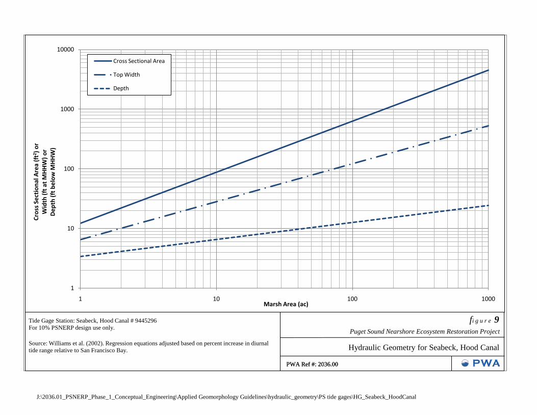
J:\2036.01_PSNERP_Phase_1_Conceptual_Engineering\Applied Geomorphology Guidelines\hydraulic_geometry\PS tide gages\HG_Seabeck_HoodCanal

1

10

100

1000

10000

1 10 100 1000

Cros

s Sec

tiona

l Are

a (ft

2 ) o

rW

idth

(ft a

t MHH

W) o

rDe

pth

(ft b

elow

MHH

W)

Marsh Area (ac)


Top Width

Depth

Tide Gage Station: Seabeck, Hood Canal # 9445296For 10% PSNERP design use only.

Source: Williams et al. (2002). Regression equations adjusted based on percent increase in diurnal tide range relative to San Francisco Bay. Hydraulic Geometry for Seabeck, Hood Canal

fi g u r e 9

PWA Ref #: 2036.00


PWA Ref #: 2036.00

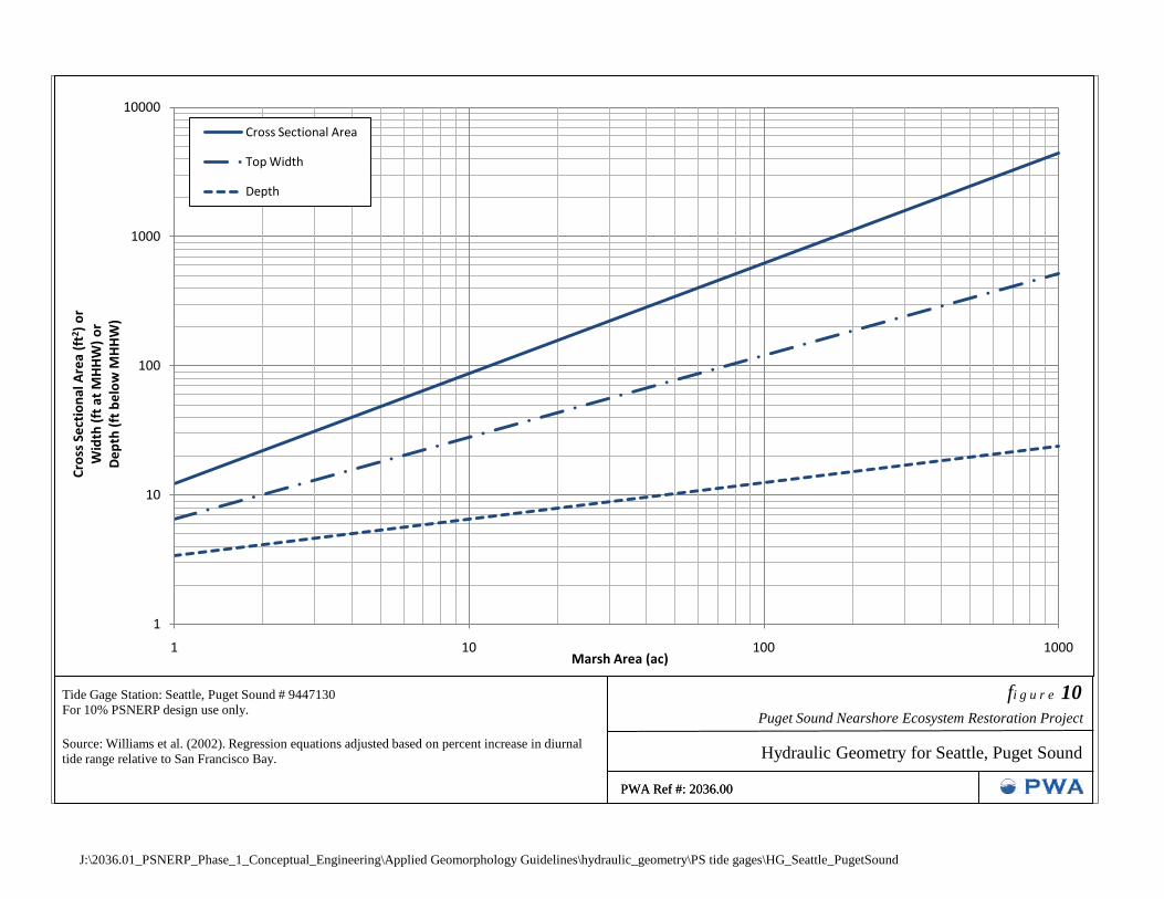
J:\2036.01_PSNERP_Phase_1_Conceptual_Engineering\Applied Geomorphology Guidelines\hydraulic_geometry\PS tide gages\HG_Seattle_PugetSound

1

10

100

1000

10000

1 10 100 1000

Cros

s Sec

tiona

l Are

a (ft

2 ) o

rW

idth

(ft a

t MHH

W) o

rDe

pth

(ft b

elow

MHH

W)

Marsh Area (ac)


Top Width

Depth

Tide Gage Station: Seattle, Puget Sound # 9447130For 10% PSNERP design use only.

Source: Williams et al. (2002). Regression equations adjusted based on percent increase in diurnal tide range relative to San Francisco Bay. Hydraulic Geometry for Seattle, Puget Sound

fi g u r e 10

PWA Ref #: 2036.00


PWA Ref #: 2036.00

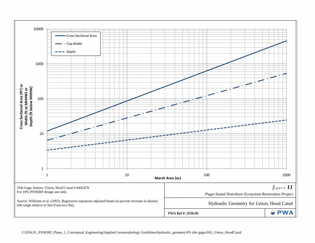
J:\2036.01_PSNERP_Phase_1_Conceptual_Engineering\Applied Geomorphology Guidelines\hydraulic_geometry\PS tide gages\HG_Union_HoodCanal

1

10

100

1000

10000

1 10 100 1000

Cros

s Sec

tiona

l Are

a (ft

2 ) o

rW

idth

(ft a

t MHH

W) o

rDe

pth

(ft b

elow

MHH

W)

Marsh Area (ac)


Top Width

Depth

Tide Gage Station: Union, Hood Canal # 9445478For 10% PSNERP design use only.

Source: Williams et al. (2002). Regression equations adjusted based on percent increase in diurnal tide range relative to San Francisco Bay. Hydraulic Geometry for Union, Hood Canal

fi g u r e 11

PWA Ref #: 2036.00


PWA Ref #: 2036.00

J:\2036.01_PSNERP_Phase_1_Conceptual_Engineering\Applied Geomorphology Guidelines\hydraulic_geometry\PS tide gages\HG_YomanPoint_AndersonIsland

1

10

100

1000

10000

1 10 100 1000

Cros

s Sec

tiona

l Are

a (ft

2 ) o

rW

idth

(ft a

t MHH

W) o

rDe

pth

(ft b

elow

MHH

W)

Marsh Area (ac)


Top Width

Depth

Tide Gage Station: Yoman Point, Anderson Island # 9446705For 10% PSNERP design use only.

Source: Williams et al. (2002). Regression equations adjusted based on percent increase in diurnal tide range relative to San Francisco Bay. Hydraulic Geometry for Yoman Point, Anderson Island

fi g u r e 12

PWA Ref #: 2036.00


PWA Ref #: 2036.00

J:\2036.01_PSNERP_Phase_1_Conceptual_Engineering\Applied Geomorphology Guidelines\hydraulic_geometry\PS tide gages\HG_Barron_Point

1

10

100

1000

10000

1 10 100 1000

Cros

s Sec

tiona

l Are

a (ft

2 ) o

rW

idth

(ft a

t MHH

W) o

rDe

pth

(ft b

elow

MHH

W)

Marsh Area (ac)


Top Width

Depth

Tide Gage Station: Barron Point # 9446742For 10% PSNERP design use only.

Source: Williams et al. (2002). Regression equations adjusted based on percent increase in diurnal tide range relative to San Francisco Bay. Hydraulic Geometry for Barron Point

fi g u r e 13

PWA Ref #: 2036.00


PWA Ref #: 2036.00

J:\2036.01_PSNERP_Phase_1_Conceptual_Engineering\Applied Geomorphology Guidelines\hydraulic_geometry\PS tide gages\HG_Budd_Inlet

1

10

100

1000

10000

1 10 100 1000

Cros

s Sec

tiona

l Are

a (ft

2 ) o

rW

idth

(ft a

t MHH

W) o

rDe

pth

(ft b

elow

MHH

W)

Marsh Area (ac)


Top Width

Depth

Tide Gage Station: Budd Inlet # 9446807For 10% PSNERP design use only.

Source: Williams et al. (2002). Regression equations adjusted based on percent increase in diurnal tide range relative to San Francisco Bay. Hydraulic Geometry for Budd Inlet

fi g u r e 14

PWA Ref #: 2036.00


PWA Ref #: 2036.00

550 Kearny Street

Suite 900

San Francisco, CA 94108

415.262.2300 phone

415.262.2303 fax

www.pwa-ltd.com

memorandum

date December 22, 2010 to Bob Barnard, Curtis Tanner, PSNERP

Conceptual Design Team from Phil Williams and Jeremy Lowe subject PSNERP - Hierarchy of Benefits

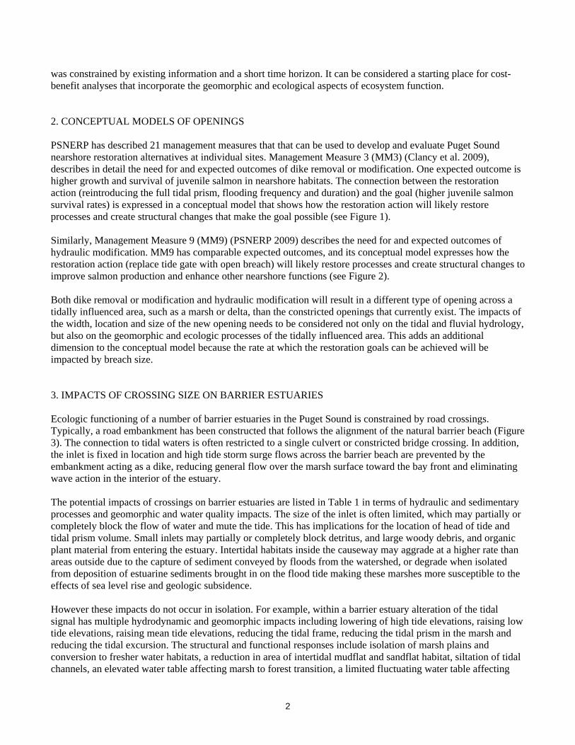
1. INTRODUCTION The purpose of this memo is to describe a hierarchy of benefits that will likely accrue to the natural processes, structure, and function of an ecosystem for variously located and sized openings in crossings of tidal and tidally influenced fluvial channels. We describe benefits in terms of ecosystem process, structure and function. By understanding what these benefits are, and how they impact the nearshore system crossings can be designed to provide maximum benefits more efficiently. There is a dearth of information regarding the ecological impacts of constructing bridges or culverts across tidally influenced areas in the scientific literature. While hydrological and hydraulic impacts, such as amount and extent of anticipated scouring and longshore transport of sediment, are carefully considered during crossing design, impacts to overall geomorphology and ecological function are not. This may be because many decisions establishing culvert or bridge crossing design practice were made prior to 1969, before the passage of federal and state statutes that require inclusion of environmental impacts. Almost all tidal channel crossings were, and sometimes still are, designed to simply optimize hydraulic conveyance for drainage or design floods at least cost. The loss of connectivity that occurs when dikes are constructed across wetlands and floodplains is well documented. Embanked bridge crossings can generate similar environmental impacts because they too may restrict the flow of animals, water, sediment, organic plant material and detritus. Today, however, there is an opportunity to assess and rectify the impacts of existing structures through restoration. The question that will need to be addressed is:

‘what are the tradeoffs between enhanced ecologic benefits and restoration costs for breaches or bridges larger than those required for hydraulic conveyance?’

The hierarchy of benefits represents a new approach to crossing design by expanding its view from the minimum opening size that the hydraulics requires to one that considers how location and size of openings will impact the morphology and ecology of the ecosystem. This hierarchy of benefits will aid PSNERP decision makers by shedding light on whether a dike removal or a dike modification, and associated construction and monitoring costs, is warranted given particular parameters. It is a tool devised for this specific project, and its development

2

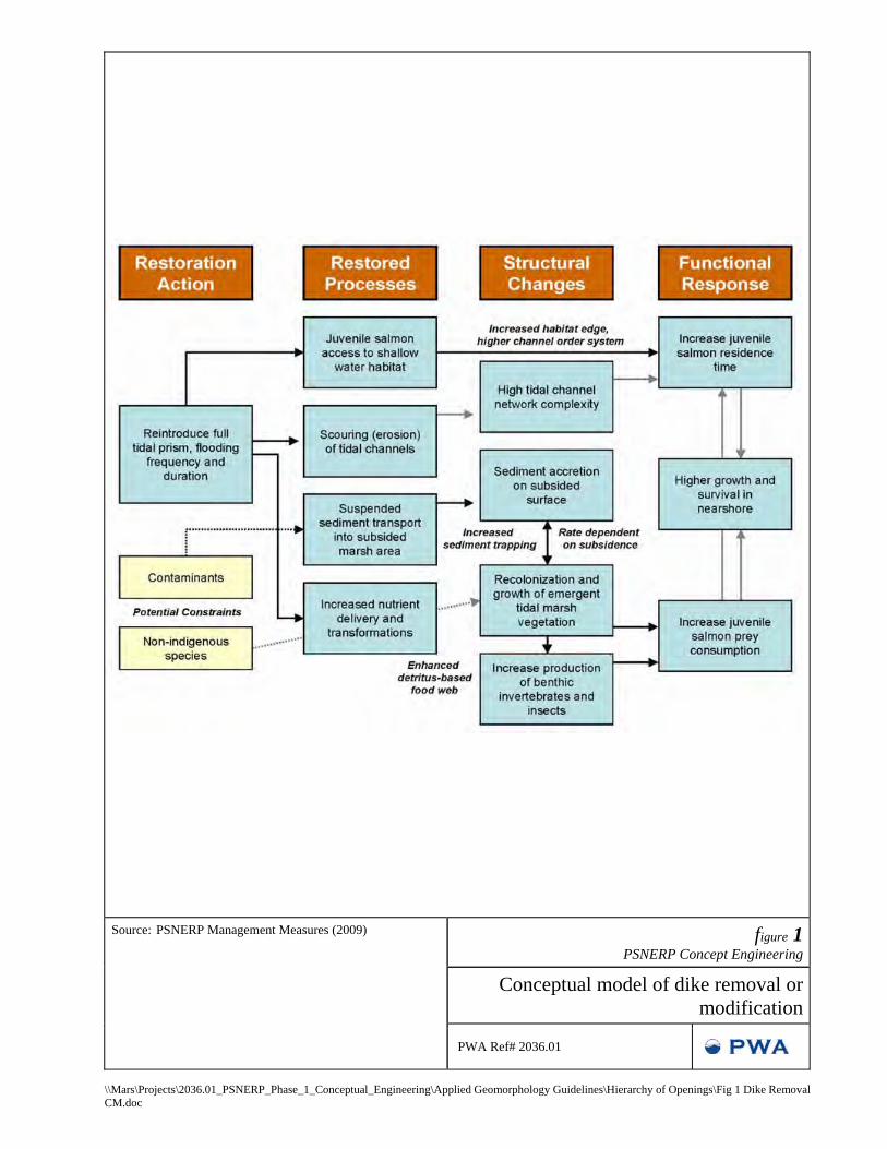
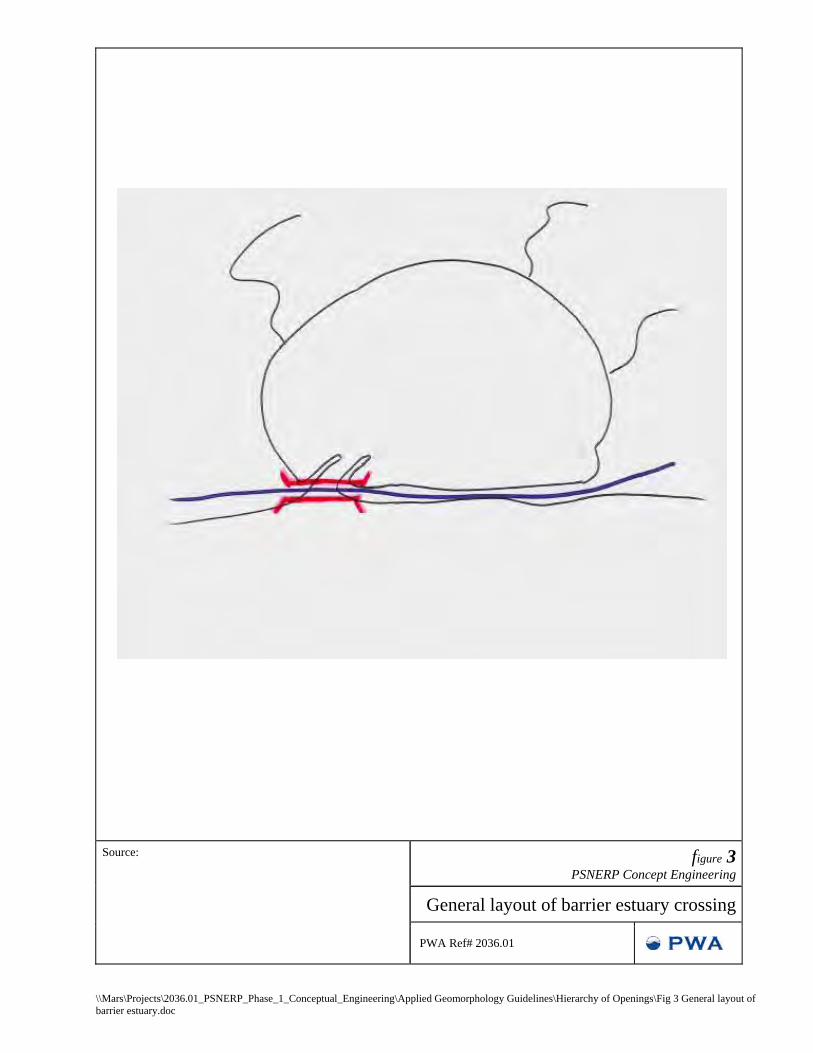
was constrained by existing information and a short time horizon. It can be considered a starting place for cost-benefit analyses that incorporate the geomorphic and ecological aspects of ecosystem function. 2. CONCEPTUAL MODELS OF OPENINGS PSNERP has described 21 management measures that that can be used to develop and evaluate Puget Sound nearshore restoration alternatives at individual sites. Management Measure 3 (MM3) (Clancy et al. 2009), describes in detail the need for and expected outcomes of dike removal or modification. One expected outcome is higher growth and survival of juvenile salmon in nearshore habitats. The connection between the restoration action (reintroducing the full tidal prism, flooding frequency and duration) and the goal (higher juvenile salmon survival rates) is expressed in a conceptual model that shows how the restoration action will likely restore processes and create structural changes that make the goal possible (see Figure 1). Similarly, Management Measure 9 (MM9) (PSNERP 2009) describes the need for and expected outcomes of hydraulic modification. MM9 has comparable expected outcomes, and its conceptual model expresses how the restoration action (replace tide gate with open breach) will likely restore processes and create structural changes to improve salmon production and enhance other nearshore functions (see Figure 2). Both dike removal or modification and hydraulic modification will result in a different type of opening across a tidally influenced area, such as a marsh or delta, than the constricted openings that currently exist. The impacts of the width, location and size of the new opening needs to be considered not only on the tidal and fluvial hydrology, but also on the geomorphic and ecologic processes of the tidally influenced area. This adds an additional dimension to the conceptual model because the rate at which the restoration goals can be achieved will be impacted by breach size. 3. IMPACTS OF CROSSING SIZE ON BARRIER ESTUARIES Ecologic functioning of a number of barrier estuaries in the Puget Sound is constrained by road crossings. Typically, a road embankment has been constructed that follows the alignment of the natural barrier beach (Figure 3). The connection to tidal waters is often restricted to a single culvert or constricted bridge crossing. In addition, the inlet is fixed in location and high tide storm surge flows across the barrier beach are prevented by the embankment acting as a dike, reducing general flow over the marsh surface toward the bay front and eliminating wave action in the interior of the estuary. The potential impacts of crossings on barrier estuaries are listed in Table 1 in terms of hydraulic and sedimentary processes and geomorphic and water quality impacts. The size of the inlet is often limited, which may partially or completely block the flow of water and mute the tide. This has implications for the location of head of tide and tidal prism volume. Small inlets may partially or completely block detritus, and large woody debris, and organic plant material from entering the estuary. Intertidal habitats inside the causeway may aggrade at a higher rate than areas outside due to the capture of sediment conveyed by floods from the watershed, or degrade when isolated from deposition of estuarine sediments brought in on the flood tide making these marshes more susceptible to the effects of sea level rise and geologic subsidence. However these impacts do not occur in isolation. For example, within a barrier estuary alteration of the tidal signal has multiple hydrodynamic and geomorphic impacts including lowering of high tide elevations, raising low tide elevations, raising mean tide elevations, reducing the tidal frame, reducing the tidal prism in the marsh and reducing the tidal excursion. The structural and functional responses include isolation of marsh plains and conversion to fresher water habitats, a reduction in area of intertidal mudflat and sandflat habitat, siltation of tidal channels, an elevated water table affecting marsh to forest transition, a limited fluctuating water table affecting

3

plant growth, atrophy of the channel system due to sedimentation and reduced channel connectivity, and passive advective transport of organisms into the estuary through baroclinic circulation. The combination of embankment and reduced inlet size reduce both the area of habitat and habitat connectivity which in turn impacts all aspects of ecosystem function: distribution and abundance of species, community dynamics, productivity, and invasive species. In restoring the ecosystem functions of these estuaries, the main tool is to decrease the hydraulic constriction due to the crossing and increase the habitat connectivity. The size of the opening will determine the type and amount of ecosystem processes that are impacted. The largest possible opening size will eliminate these impacts, while a small opening size will likely produce all of them. Intermediately sized openings will have impacts between these two endpoints. 3.1 Benefits of Increasing Bridge Crossing Size To illustrate how much ecological benefits increase as opening size increases, we have carried out a first-cut qualitative assessment of five general categories of crossings as described below (see Figure 5):

1. Existing conditions. This assumes a raised embankment along the barrier beach and tidal flow restricted to a single culvert or narrow bridge crossing sized to drain the area landward of the barrier. Tidal regime will be strongly muted. All flows over the barrier beach will be blocked by the embankment.

2. Expand the inlet size with large culverts or bridge crossing to allow regular tidal inundation of the

area landward of the barrier. The inlet crossing is designed to be the minimum size to allow the full average diurnal tidal range within the estuary based on the hydraulic geometry for tidal channels. However, tidal velocities will be greater than naturally occurring at the inlet requiring armoring to prevent scour and lateral migration. In addition storm surge tides will still be constricted. All flows over the barrier beach will be blocked by the embankment.

3. Expand the inlet size to allow for a naturally adjusting channel inlet to form. This would require a

clear span bridge designed wide enough to allow a natural convex sided inlet channel that can adjust to storm surge tides. All flows over the barrier beach are blocked by the embankment.

4. Expand the inlet crossing to allow for lateral migration of the inlet channel. A bridge would be

sized not only for the appropriate inlet channel morphology but also for historic migration width. Laterally meandering inlets have a tendency to ‘reset’ the estuarine drainage system and marsh habitats through bank erosion and migrating flood tide shoals All flows over the barrier beach are blocked by the embankment.

5. Complete removal of tidal barriers. This would include a bridge crossing to allow inlet migration

and replacement of the embankment with an elevated causeway on pilings. The former road embankment would be graded down to natural beach crest elevations to allow for storm surge inundation and transport of large woody debris (LWD) into the estuary. The input of LWD creates habitat structure for all trophic levels from algae to invertebrates to fishes and wildlife; it allows for various species to seek shelter, find food, spawn, roost or nest. LWD also impacts sediment movement, potentially creating beach berms. More recently, LWD has been cited in facilitating tidal marsh succession acts by providing a nursery habitat for salt-intolerant species (Maser and Sedell).

4

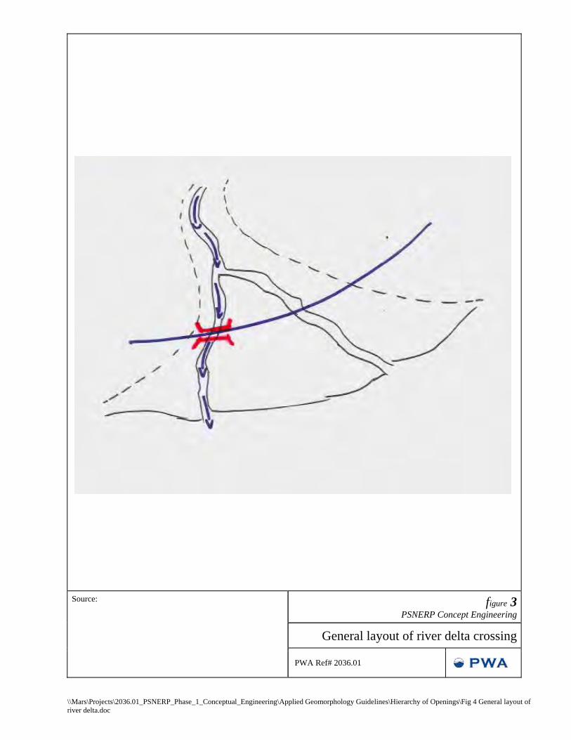
Table 1 shows in detail how various process alterations impact ecosystem structure and function. Figures 5 uses this information to qualitatively assign values to restored processes according to opening size. 4. IMPACTS OF CROSSING SIZE AND LOCATION ON RIVER DELTAS River deltas are dynamic geomorphic landscapes, with river distributary channels that evolve and migrate in response to major floods. They sustain a gradient of wetland habitat types from forested floodplains to forested tidal wetland to tidal marsh and mudflat. Roadways traverse river deltas at many locations in Puget Sound (Figure 4). Typically these have been constructed for convenience on embankments on the flat intertidal areas across the delta front and have concentrated river flows at a single bridge crossing location. Fixing the river channel in this way can significantly reduce the area of active delta. Upstream the river is restrained from avulsing into different distributary channels, resulting in a reduced variety of habitat types, and because of increased sediment deposition, the floodplain and former intertidal habitats aggrade. Downstream, single bridge crossings may partially or completely block the flow of sediment that sustains marsh habitats. Channelizing the outflow of riverine sediment along a single alignment forces delta progradation, changes salinity distribution and causes impacts to natural systems. For instance, the size and location of bridge crossings are factors that will ultimately determine the viability of a salmon population. A population will become more viable if the size and location of the new opening adds new habitat, connects habitat and increases habitat capacity. New tidal or distributary channels will help to increase all three of these criteria, which alter the distribution and composition of life history strategies and result in an increase in viability. 4.1 Benefits of Increasing Bridge Crossing Size To illustrate how ecologic benefits of river delta habits could be restored with increasing the size of bridge crossings we have conducted a first cut qualitative assessment of the four alternatives described below (see Figure 6):

1. Existing conditions. Assumes the roadway has been constructed on an elevated embankment that prevents tidal and river flows, and the bridge crossing itself has been sized to the typical design flood. Channel avulsions and distributary channel formation are restricted to the area downstream of the crossing. Elsewhere downstream of the embankment, tidal marshes are not replenished by sedimentation and relict distributary channels silt in. Upstream former intertidal wetlands convert to floodplains and the river channel is prevented from migrating or avulsing with river training structures that simplify habitat structure within the river channel.

2. Additional bridge crossing. The existing bridge crossing is duplicated at a location where a major

distributary channel had been blocked off by the embankment. This would encourage a channel avulsion upstream and permit the main river to switch its course between two crossings, doubling the size of the active delta.

3. Extended bridge crossings allow for channel migration. Bridge spans are widened to allow for

historic rates of lateral channel migration. Laterally meandering channels ‘reset’ the fluvial system through bank erosion and subsequent deposition in point bars. This introduces sediment and LWD into channels from stream banks, and promotes the exchange of nutrient-rich soils into the fluvial system. The erosion of banks, and subsequent deposition, results in a dynamic system with a mosaic of habitat types.

5

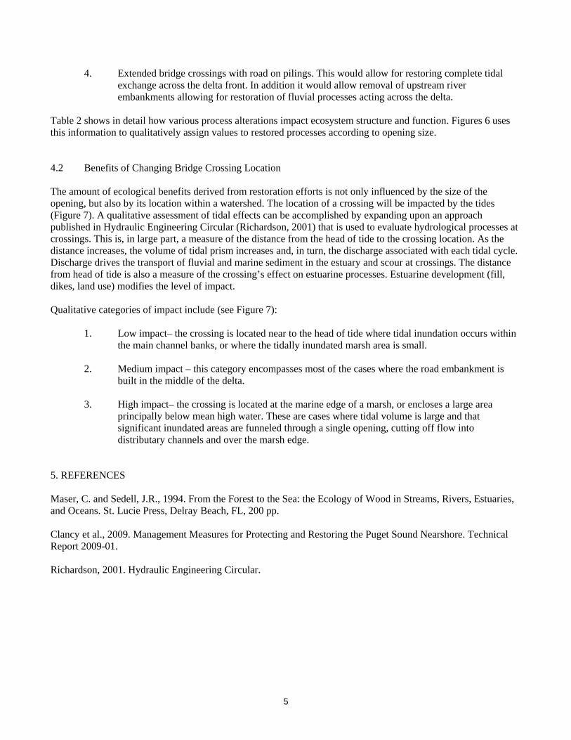
4. Extended bridge crossings with road on pilings. This would allow for restoring complete tidal exchange across the delta front. In addition it would allow removal of upstream river embankments allowing for restoration of fluvial processes acting across the delta.

Table 2 shows in detail how various process alterations impact ecosystem structure and function. Figures 6 uses this information to qualitatively assign values to restored processes according to opening size. 4.2 Benefits of Changing Bridge Crossing Location The amount of ecological benefits derived from restoration efforts is not only influenced by the size of the opening, but also by its location within a watershed. The location of a crossing will be impacted by the tides (Figure 7). A qualitative assessment of tidal effects can be accomplished by expanding upon an approach published in Hydraulic Engineering Circular (Richardson, 2001) that is used to evaluate hydrological processes at crossings. This is, in large part, a measure of the distance from the head of tide to the crossing location. As the distance increases, the volume of tidal prism increases and, in turn, the discharge associated with each tidal cycle. Discharge drives the transport of fluvial and marine sediment in the estuary and scour at crossings. The distance from head of tide is also a measure of the crossing’s effect on estuarine processes. Estuarine development (fill, dikes, land use) modifies the level of impact. Qualitative categories of impact include (see Figure 7):

1. Low impact– the crossing is located near to the head of tide where tidal inundation occurs within the main channel banks, or where the tidally inundated marsh area is small.

2. Medium impact – this category encompasses most of the cases where the road embankment is

built in the middle of the delta.

3. High impact– the crossing is located at the marine edge of a marsh, or encloses a large area principally below mean high water. These are cases where tidal volume is large and that significant inundated areas are funneled through a single opening, cutting off flow into distributary channels and over the marsh edge.

5. REFERENCES Maser, C. and Sedell, J.R., 1994. From the Forest to the Sea: the Ecology of Wood in Streams, Rivers, Estuaries, and Oceans. St. Lucie Press, Delray Beach, FL, 200 pp. Clancy et al., 2009. Management Measures for Protecting and Restoring the Puget Sound Nearshore. Technical Report 2009-01. Richardson, 2001. Hydraulic Engineering Circular.

Table 1. POTENTIAL ADVERSE IMPACTS OF CROSSINGS ON BARRIER ESTUARIES BARRIER ESTUARIES - Assumes culverted entrance, road embankment along beach alignment, watershed relatively small relative to estuary. BARRIER ESTUARIES Process Structural Impact Functional Response HYDRAULIC/ HYDRODYNAMIC PROCESS IMPACTS

Alteration of tidal stage characteristics (#2)

Lowering of high tide elevations Isolation of marsh plains, conversion to fresher habitats

Raising low tide elevations Reduction in area of intertidal mudflat/sandflat habitat

Raising mean tide elevations Water table elevated affecting marsh to forest transition

Reduction in tidal frame Water table fluctuation limited affecting plant growth

Reduction in tidal prism in marsh Channel system atrophies through sedimentation; reduced channel connectivity

Reduced tidal excursion Passive advective transport of organisms in and out of estuary diminished

Alteration of salinity distribution (#5)

Vertical salinity stratification degraded through mixing

Reduction of passive transport of organisms into estuary through baroclinic circulation

Salinity mixing zone length truncated

‘Squeezing’and reduction of brackish zone habitats

Elimination of storm surge overwash across beach (#3, 4)

Transport of large woody debris into marsh

Habitat heterogeneity reduced

Mobilization of detritus due to storm surge wave action eliminated

Export of nutrients to estuary reduced

SEDIMENTARY PROCESS IMPACTS

Alluvial sedimentation altered by backwater affects

Fine sediment accumulates on marsh plain

Shift to upland habitats

Coarse sediment accumulates in tidal channels

Loss of blind channel habitat

Estuarine sedimentation limited by reduction in tidal flows (#1)

Reduced tidal prism reduces sediment delivery to marsh plain, causes lowering relative to tidal frame

Reduced productivity of marsh vegetation

Increased turbidity in tidal channels due to loss of marsh plain sediment sink

Adverse affect on benthic organisms and eelgrass

GEOMORPHIC IMPACTS Alteration of entrance channel morphology from broad shallow to narrow

Increased tidal velocity through entrance creates scour holes

Increased fish mortality

Channel location fixed instead of lateral migration affecting ebb and flood shoal extent

Adverse affect on benthic organisms

Fixed channel location may lead to permanent closure of confined marsh by longshore drift

Eliminates exchange of water, sediment, nutrients and organisms

Atrophied tidal drainage system Tidal channels shallower Degraded estuarine habitat Dendritic tidal channel system

becomes disconnected Estuarine habitat degraded

Marsh plain elevations changed Lowered marsh plain Reduced marsh productivity Areas raised by alluvial

sedimentation Change to freshwater or upland species

WATER QUALITY IMPACTS Increased residence time (#6) Reduction in tidal exchange Algal blooms in marsh channels, anoxic in poorly drained holes

Reduction in tidal excursion Export of water column productivity to larger estuary limited

Accumulation of toxics Reduced tidal scouring allows accumulation of polluted sediments from watershed

Toxic affects on organisms

Reduced residence time means concentration of dissolved pollutants in water column is higher

Toxic affects on organisms

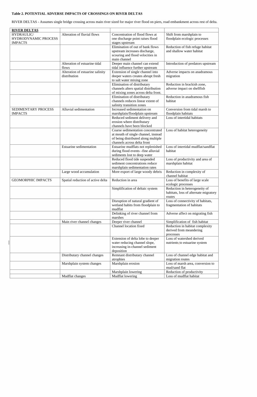
Table 2. POTENTIAL ADVERSE IMPACTS OF CROSSINGS ON RIVER DELTAS RIVER DELTAS - Assumes single bridge crossing across main river sized for major river flood on piers, road embankment across rest of delta. RIVER DELTAS HYDRAULIC/ HYDRODYNAMIC PROCESS IMPACTS

Alteration of fluvial flows Concentration of flood flows at one discharge point raises flood stages upstream

Shift from marshplain to floodplain ecologic processes

Elimination of out of bank flows upstream increases discharge, scouring and flood velocities in main channel

Reduction of fish refuge habitat and shallow water habitat

Alteration of estuarine tidal flows

Deeper main channel can extend tidal influence further upstream

Introduction of predators upstream

Alteration of estuarine salinity distribution

Extension of single channel into deeper waters creates abrupt fresh to salt water mixing zone

Adverse impacts on anadramous migration

Elimination of distributary channels alters spatial distribution of mixing zones across delta front.

Reduction in brackish zone, adverse impact on shellfish

Elimination of distributary channels reduces linear extent of salinity transition zones

Reduction in anadramous fish habitat

SEDIMENTARY PROCESS IMPACTS

Alluvial sedimentation Increased sedimentation on marshplain/floodplain upstream

Conversion from tidal marsh to floodplain habitats

Reduced sediment delivery and erosion where distributary channels have been blocked

Loss of intertidal habitats

Coarse sedimentation concentrated at mouth of single channel, instead of being distributed along multiple channels across delta front

Loss of habitat heterogeneity

Estuarine sedimentation Estuarine mudflats not replenished during flood events –fine alluvial sediments lost to deep water

Loss of intertidal mudflat/sandflat habitat

Reduced flood tide suspended sediment concentrations reduce marshplain sedimentation rates

Loss of productivity and area of marshplain habitat

Large wood accumulation More export of large woody debris Reduction in complexity of channel habitat

GEOMORPHIC IMPACTS Spatial reduction of active delta Reduction in area Loss of benefits of large scale ecologic processes

Simplification of deltaic system Reduction in heterogeneity of habitats, loss of alternate migratory routes

Disruption of natural gradient of wetland habits from floodplain to mudflat

Loss of connectivity of habitats, fragmentation of habitats

Delinking of river channel from marshes

Adverse affect on migrating fish

Main river channel changes Deeper river channel Simplification of fish habitat Channel location fixed Reduction in habitat complexity

derived from meandering processes

Extension of delta lobe to deeper water reducing channel slope, increasing in-channel sediment deposition

Loss of watershed derived nutrients to estuarine system

Distributary channel changes Remnant distributary channel atrophies

Loss of channel edge habitat and migration routes

Marshplain system changes Marshplain erosion Loss of marsh area, conversion to mud/sand flat

Marshplain lowering Reduction of productivity Mudflat changes Mudflat lowering Loss of mudflat habitat

\\Mars\Projects\2036.01_PSNERP_Phase_1_Conceptual_Engineering\Applied Geomorphology Guidelines\Hierarchy of Openings\Fig 1 Dike Removal CM.doc

figure 1PSNERP Concept Engineering

Conceptual model of dike removal or modification

Source: PSNERP Management Measures (2009)

PWA Ref# 2036.01

\\Mars\Projects\2036.01_PSNERP_Phase_1_Conceptual_Engineering\Applied Geomorphology Guidelines\Hierarchy of Openings\Fig 2 Hydraulic Mod CM.doc


Conceptual model of hydraulic modification

Source: PSNERP Management Measures (2009)

PWA Ref# 2036.01

\\Mars\Projects\2036.01_PSNERP_Phase_1_Conceptual_Engineering\Applied Geomorphology Guidelines\Hierarchy of Openings\Fig 3 General layout of barrier estuary.doc


General layout of barrier estuary crossing

Source:

PWA Ref# 2036.01

\\Mars\Projects\2036.01_PSNERP_Phase_1_Conceptual_Engineering\Applied Geomorphology Guidelines\Hierarchy of Openings\Fig 4 General layout of river delta.doc


General layout of river delta crossing

Source:

PWA Ref# 2036.01

\\Mars\Projects\2036.01_PSNERP_Phase_1_Conceptual_Engineering\Applied Geomorphology Guidelines\Hierarchy of Openings\Fig 5 Benefits for a barrier estuary.doc


Benefits of widening crossings of a barrier estuary

Source:

PWA Ref# 2036.01

\\Mars\Projects\2036.01_PSNERP_Phase_1_Conceptual_Engineering\Applied Geomorphology Guidelines\Hierarchy of Openings\Fig 6 Benefits for a river delta.doc


Benefits of widening crossings of a river delta

Source:

PWA Ref# 2036.01

\\Mars\Projects\2036.01_PSNERP_Phase_1_Conceptual_Engineering\Applied Geomorphology Guidelines\Hierarchy of Openings\Fig 7 Location of Crossing.doc

figure 7 PSNERP Concept Engineering

Location of crossing

Source:

PWA Ref# 2036.01

Full Chapter - Puget Sound Nearshore Ecosystem Restoration Project

Documents