1 FSIM: A Feature Similarity Index for Image Quality Assessment Lin Zhang a , Student Member, IEEE, Lei Zhang a,1 , Member, IEEE Xuanqin Mou b , Member, IEEE, and David Zhang a , Fellow, IEEE a Department of Computing, The Hong Kong Polytechnic University, Hong Kong b Institute of Image Processing and Pattern Recognition, Xi'an Jiaotong University, China Abstract: Image quality assessment (IQA) aims to use computational models to measure the image quality consistently with subjective evaluations. The well-known structural-similarity (SSIM) index brings IQA from pixel-based stage to structure-based stage. In this paper, a novel feature-similarity (FSIM) index for full reference IQA is proposed based on the fact that human visual system (HVS) understands an image mainly according to its low-level features. Specifically, the phase congruency (PC), which is a dimensionless measure of the significance of a local structure, is used as the primary feature in FSIM. Considering that PC is contrast invariant while the contrast information does affect HVS’ perception of image quality, the image gradient magnitude (GM) is employed as the secondary feature in FSIM. PC and GM play complementary roles in characterizing the image local quality. After obtaining the local quality map, we use PC again as a weighting function to derive a single quality score. Extensive experiments performed on six benchmark IQA databases demonstrate that FSIM can achieve much higher consistency with the subjective evaluations than state-of-the-art IQA metrics. Index Terms: Image quality assessment, phase congruency, gradient, low-level feature I. INTRODUCTION With the rapid proliferation of digital imaging and communication technologies, image quality assessment (IQA) has been becoming an important issue in numerous applications such as image acquisition, transmission, compression, restoration and enhancement, etc. Since the subjective IQA methods cannot be 1 Corresponding author. Email: [email protected] . This project is supported by the Hong Kong RGC General Research Fund (PolyU 5330/07E), the Ho Tung Fund (5-ZH25) and and NSFC 90920003.

Welcome message from author
This document is posted to help you gain knowledge. Please leave a comment to let me know what you think about it! Share it to your friends and learn new things together.
Transcript

1
FSIM A Feature Similarity Index for Image Quality Assessment
Lin Zhanga Student Member IEEE Lei Zhanga1 Member IEEE Xuanqin Moub Member IEEE and David Zhanga Fellow IEEE
aDepartment of Computing The Hong Kong Polytechnic University Hong Kong bInstitute of Image Processing and Pattern Recognition Xian Jiaotong University China
Abstract Image quality assessment (IQA) aims to use computational models to measure the image quality
consistently with subjective evaluations The well-known structural-similarity (SSIM) index brings IQA from
pixel-based stage to structure-based stage In this paper a novel feature-similarity (FSIM) index for full
reference IQA is proposed based on the fact that human visual system (HVS) understands an image mainly
according to its low-level features Specifically the phase congruency (PC) which is a dimensionless
measure of the significance of a local structure is used as the primary feature in FSIM Considering that PC
is contrast invariant while the contrast information does affect HVSrsquo perception of image quality the image
gradient magnitude (GM) is employed as the secondary feature in FSIM PC and GM play complementary
roles in characterizing the image local quality After obtaining the local quality map we use PC again as a
weighting function to derive a single quality score Extensive experiments performed on six benchmark IQA
databases demonstrate that FSIM can achieve much higher consistency with the subjective evaluations than
state-of-the-art IQA metrics
Index Terms Image quality assessment phase congruency gradient low-level feature
I INTRODUCTION
With the rapid proliferation of digital imaging and communication technologies image quality assessment
(IQA) has been becoming an important issue in numerous applications such as image acquisition
transmission compression restoration and enhancement etc Since the subjective IQA methods cannot be
1 Corresponding author Email cslzhangcomppolyueduhk This project is supported by the Hong Kong RGC General Research
Fund (PolyU 533007E) the Ho Tung Fund (5-ZH25) and and NSFC 90920003
2
readily and routinely used for many scenarios eg real-time and automated systems it is necessary to
develop objective IQA metrics to automatically and robustly measure the image quality Meanwhile it is
anticipated that the evaluation results should be statistically consistent with those of the human observers To
this end the scientific community has developed various IQA methods in the past decades According to the
availability of a reference image objective IQA metrics can be classified as full reference (FR) no-reference
(NR) and reduced-reference (RR) methods [1] In this paper the discussion is confined to FR methods
where the original ldquodistortion freerdquo image is known as the reference image
The conventional metrics such as the peak signal-to-noise ratio (PSNR) and the mean squared error
(MSE) operate directly on the intensity of the image and they do not correlate well with the subjective
fidelity ratings Thus many efforts have been made on designing human visual system (HVS) based IQA
metrics Such kinds of models emphasize the importance of HVSrsquo sensitivity to different visual signals such
as the luminance the contrast the frequency content and the interaction between different signal
components [2-4] The noise quality measure (NQM) [2] and the visual signal-to-noise ratio (VSNR) [3] are
two representatives Methods such as the structural similarity (SSIM) index [1] are motivated by the need to
capture the loss of structure in the image SSIM is based on the hypothesis that HVS is highly adapted to
extract the structural information from the visual scene therefore a measurement of structural similarity
should provide a good approximation of perceived image quality The multi-scale extension of SSIM called
MS-SSIM [5] produces better results than its single-scale counterpart In [6] the authors presented a
3-component weighted SSIM (3-SSIM) by assigning different weights to the SSIM scores according to the
local region type edge texture or smooth area In [7] Sheikh et al introduced the information theory into
image fidelity measurement and proposed the information fidelity criterion (IFC) for IQA by quantifying the
information shared between the distorted and the reference images IFC was later extended to the visual
information fidelity (VIF) metric in [4] In [8] Sampat et al made use of the steerable complex wavelet
transform to measure the structural similarity of the two images and proposed the CW-SSIM index
Recent studies conducted in [9] and [10] have demonstrated that SSIM MS-SSIM and VIF could offer
statistically much better performance in predicting imagesrsquo fidelity than the other IQA metrics However
SSIM and MS-SSIM share a common deficiency that when pooling a single quality score from the local
quality map (or the local distortion measurement map) all positions are considered to have the same
importance In VIF images are decomposed in different sub-bands and these sub-bands can have different
3
weights at the pooling stage [11] however within each sub-band every position is still given the same
importance Such pooling strategies are not consistent with the intuition that different locations on an image
can have very different contributions to HVSrsquo perception of the image This is corroborated by a recent study
[12 13] where the authors found that by incorporating appropriate spatially varying weights the
performance of some IQA metrics eg SSIM VIF and PSNR could be improved But unfortunately they
did not present an automated method to generate such weights
The great success of SSIM and its extensions owes to the fact that HVS is adapted to the structural
information in images The visual information in an image however is often very redundant while the HVS
understands an image mainly based on its low-level features such as edges and zero-crossings [14-16] In
other words the salient low-level features convey crucial information for the HVS to interpret the scene
Accordingly perceptible image degradations will lead to perceptible changes in image low-level features
and hence a good IQA metric could be devised by comparing the low-level feature sets between the
reference image and the distorted image Based on the above analysis in this paper we propose a novel
low-level feature similarity induced FR IQA metric namely FSIM (Feature SIMilarity)
One key issue is then what kinds of features could be used in designing FSIM Based on the
physiological and psychophysical evidence it is found that visually discernable features coincide with those
points where the Fourier waves at different frequencies have congruent phases [16-19] That is at points of
high phase congruency (PC) we can extract highly informative features Such a conclusion has been further
corroborated by some recent studies in neurobiology using functional magnetic resonance imaging (fMRI)
[20] Therefore PC is used as the primary feature in computing FSIM Meanwhile considering that PC is
contrast invariant but image local contrast does affect HVSrsquo perception on the image quality the image
gradient magnitude (GM) is computed as the secondary feature to encode contrast information PC and GM
are complementary and they reflect different aspects of the HVS in assessing the local quality of the input
image After computing the local similarity map PC is utilized again as a weighting function to derive a
single similarity score Although FSIM is designed for grayscale images (or the luminance components of
color images) the chrominance information can be easily incorporated by means of a simple extension of
FSIM and we call this extension FSIMC
Actually PC has already been used for IQA in the literature In [21] Liu and Laganiegravere proposed a
PC-based IQA metric In their method PC maps are partitioned into sub-blocks of size 5times5 Then the cross
4
correlation is used to measure the similarity between two corresponding PC sub-blocks The overall
similarity score is obtained by averaging the cross correlation values from all block pairs In [22] PC was
extended to phase coherence which can be used to characterize the image blur Based on [22] Hassen et al
proposed an NR IQA metric to assess the sharpness of an input image [23]
The proposed FSIM and FSIMC are evaluated on six benchmark IQA databases in comparison with eight
state-of-the-art IQA methods The extensive experimental results show that FSIM and FSIMC can achieve
very high consistency with human subjective evaluations outperforming all the other competitors
Particularly FSIM and FSIMC work consistently well across all the databases while other methods may
work well only on some specific databases To facilitate repeatable experimental verifications and
comparisons the Matlab source code of the proposed FSIMFSIMC indices and our evaluation results are
available online at httpwwwcomppolyueduhk~cslzhangIQAFSIMFSIMhtm
The remainder of this paper is organized as follows Section II discusses the extraction of PC and GM
Section III presents in detail the computation of the FSIM and FSIMC indices Section IV reports the
experimental results Finally Section V concludes the paper
II EXTRACTION OF PHASE CONGRUENCY AND GRADIENT MAGNITUDE
A Phase congruency (PC)
Rather than define features directly at points with sharp changes in intensity the PC model postulates that
features are perceived at points where the Fourier components are maximal in phase Based on the
physiological and psychophysical evidences the PC theory provides a simple but biologically plausible
model of how mammalian visual systems detect and identify features in an image [16-20] PC can be
considered as a dimensionless measure for the significance of a local structure
Under the definition of PC in [17] there can be different implementations to compute the PC map of a
given image In this paper we adopt the method developed by Kovesi in [19] which is widely used in
literature We start from the 1D signal g(x) Denote by Me n and Mo
n the even-symmetric and odd-symmetric
filters on scale n and they form a quadrature pair Responses of each quadrature pair to the signal will form a
response vector at position x on scale n [en(x) on(x)] = [g(x) Me n g(x) Mo
n ] and the local amplitude on
5
scale n is 2 2( ) ( ) ( )n n nA x e x o x= + Let F(x) = sumnen(x) and H(x) = sumnon(x) The 1D PC can be computed as
( ) ( )( ) ( )nnPC x E x A xε= + sum (1)
where ( )2 2( ) ( )E x F x H x= + and ε is a small positive constant
With respect to the quadrature pair of filters ie Me n and Mo
n Gabor filters [24] and log-Gabor filters [25]
are two widely used candidates We adopt the log-Gabor filters because 1) one cannot construct Gabor filters
of arbitrarily bandwidth and still maintain a reasonably small DC component in the even-symmetric filter
while log-Gabor filters by definition have no DC component and 2) the transfer function of the log-Gabor
filter has an extended tail at the high frequency end which makes it more capable to encode natural images
than ordinary Gabor filters [19 25] The transfer function of a log-Gabor filter in the frequency domain is
G(ω) = exp(-(log(ωω0))22σ2 r ) where ω0 is the filterrsquos center frequency and σr controls the filterrsquos bandwidth
To compute the PC of 2D grayscale images we can apply the 1D analysis over several orientations and
then combine the results using some rule The 1D log-Gabor filters described above can be extended to 2D
ones by simply applying some spreading function across the filter perpendicular to its orientation One
widely used spreading function is Gaussian [19 26-28] According to [19] there are some good reasons to
choose Gaussian Particularly the phase of any function would stay unaffected after being smoothed with
Gaussian Thus the phase congruency would be preserved By using Gaussian as the spreading function the
2D log-Gabor function has the following transfer function
( )( ) ( )220
2 2 2
log ( ) exp exp
2 2j
jr
Gθ
θ θω ωω θ
σ σ
⎛ ⎞⎛ ⎞ minus⎜ ⎟⎜ ⎟= minus sdot minus⎜ ⎟⎜ ⎟
⎝ ⎠ ⎝ ⎠ (2)
where θj = jπ J j = 01hellip J-1 is the orientation angle of the filter J is the number of orientations and σθ
determines the filterrsquos angular bandwidth An example of the 2D log-Gabor filter in the frequency domain
with ω0 = 16 θj = 0 σr = 03 and σθ = 04 is shown in Fig 1
By modulating ω0 and θj and convolving G2 with the 2D image we get a set of responses at each point x
as ( ) ( )j jn ne oθ θ
⎡ ⎤⎣ ⎦x x The local amplitude on scale n and orientation θj is 2 2
( ) ( ) ( )j j jn n nA e oθ θ θ= +x x x
and the local energy along orientation θj is ( )22( ) ( )j j j
E F Hθ θ θ= +x x x where ( ) ( )j jnn
F eθ θ= sumx x and
( ) ( )j jnn
H oθ θ= sumx x The 2D PC at x is defined as
6
2
( )( )
( )j
j
jD
nn j
EPC
Aθ
θε=
+sumsum sum
xx
x (3)
It should be noted that PC2D(x) is a real number within 0 ~ 1 Examples of the PC maps of 2D images can be
found in Fig 2
(a) (b) (c)
Fig 1 An example of the log-Gabor filter in the frequency domain with ω0 = 16 θj = 0 σr = 03 and σθ = 04 (a) The radial component of the filter (b) The angular component of the filter (c) The log-Gabor filter which is the product of the radial component and the angular component
B Gradient magnitude (GM)
Image gradient computation is a traditional topic in image processing Gradient operators can be expressed
by convolution masks Three commonly used gradient operators are the Sobel operator [29] the Prewitt
operator [29] and the Scharr operator [30] Their performances will be examined in the section of
experimental results The partial derivatives Gx(x) and Gy(x) of the image f(x) along horizontal and vertical
directions using the three gradient operators are listed in Table I The gradient magnitude (GM) of f(x) is then
defined as 2 2x yG G G= +
TABLE I PARTIAL DERIVATIVES OF f(x) USING DIFFERENT GRADIENT OPERATORS
Sobel Prewitt Scharr
Gx(x) 1 1
1 2 0 ( )4
1 1f
0 minus⎡ ⎤⎢ ⎥ minus 2⎢ ⎥⎢ ⎥ 0 minus⎣ ⎦
x
1 11 0 ( )3
1 1f
0 minus⎡ ⎤⎢ ⎥1 minus1⎢ ⎥⎢ ⎥ 0 minus⎣ ⎦
x 1 0 ( )
163
f3 0 minus 3⎡ ⎤
⎢ ⎥10 minus10⎢ ⎥⎢ ⎥3 0 minus⎣ ⎦
x
Gy(x) 1 2 1
1 0 0 0 ( )4
1 2 1f
⎡ ⎤⎢ ⎥ ⎢ ⎥⎢ ⎥minus minus minus⎣ ⎦
x 1 1
1 0 0 0 ( )3
1 1 1f
1 ⎡ ⎤⎢ ⎥ ⎢ ⎥⎢ ⎥minus minus minus⎣ ⎦
x 1 0 0 0 ( )16
3 10 3f
3 10 3⎡ ⎤⎢ ⎥ ⎢ ⎥⎢ ⎥minus minus minus⎣ ⎦
x
7
III THE FEATURE SIMILARITY (FSIM) INDEX With the extracted PC and GM feature maps in this section we present a novel Feature SIMilarity (FSIM)
index for IQA Suppose that we are going to calculate the similarity between images f1 and f2 Denote by PC1
and PC2 the PC maps extracted from f1 and f2 and G1 and G2 the GM maps extracted from them It should be
noted that for color images PC and GM features are extracted from their luminance channels FSIM will be
defined and computed based on PC1 PC2 G1 and G2 Furthermore by incorporating the image chrominance
information into FSIM an IQA index for color images denoted by FSIMC will be obtained
A The FSIM index
The computation of FSIM index consists of two stages In the first stage the local similarity map is
computed and then in the second stage we pool the similarity map into a single similarity score
We separate the feature similarity measurement between f1(x) and f2(x) into two components each for
PC or GM First the similarity measure for PC1(x) and PC2(x) is defined as
1 2 12 2
1 2 1
2 ( ) ( )( )( ) ( )PC
PC PC TSPC PC T
sdot +=
+ +x xx
x x (4)
where T1 is a positive constant to increase the stability of SPC (such a consideration was also included in
SSIM [1]) In practice the determination of T1 depends on the dynamic range of PC values Eq (4) is a
commonly used measure to define the similarity of two positive real numbers [1] and its result ranges within
(0 1] Similarly the GM values G1(x) and G2(x) are compared and the similarity measure is defined as
1 2 22 2
1 2 2
2 ( ) ( )( )( ) ( )G
G G TSG G T
sdot +=
+ +x xx
x x (5)
where T2 is a positive constant depending on the dynamic range of GM values In our experiments both T1
and T2 will be fixed to all databases so that the proposed FSIM can be conveniently used Then SPC(x) and
SG(x) are combined to get the similarity SL(x) of f1(x) and f2(x) We define SL(x) as
( ) [ ( )] [ ( )]L PC GS S Sα β= sdotx x x (6)
where α and β are parameters used to adjust the relative importance of PC and GM features In this paper we
set α = β =1 for simplicity Thus SL(x) = SPC(x)SG(x)
Having obtained the similarity SL(x) at each location x the overall similarity between f1 and f2 can be
8
calculated However different locations have different contributions to HVSrsquo perception of the image For
example edge locations convey more crucial visual information than the locations within a smooth area
Since human visual cortex is sensitive to phase congruent structures [20] the PC value at a location can
reflect how likely it is a perceptibly significant structure point Intuitively for a given location x if anyone of
f1(x) and f2(x) has a significant PC value it implies that this position x will have a high impact on HVS in
evaluating the similarity between f1 and f2 Therefore we use PCm(x) = max(PC1(x) PC2(x)) to weight the
importance of SL(x) in the overall similarity between f1 and f2 and accordingly the FSIM index between f1
and f2 is defined as
( ) ( )FSIM
( )L m
m
S PCPC
isinΩ
isinΩ
sdot= sum
sumx
x
x xx
(7)
where Ω means the whole image spatial domain
B Extension to color image quality assessment
The FSIM index is designed for grayscale images or the luminance components of color images Since the
chrominance information will also affect HVS in understanding the images better performance can be
expected if the chrominance information is incorporated in FSIM for color IQA Such a goal can be achieved
by applying a straightforward extension to the FSIM framework
At first the original RGB color images are converted into another color space where the luminance can
be separated from the chrominance To this end we adopt the widely used YIQ color space [31] in which Y
represents the luminance information and I and Q convey the chrominance information The transform from
the RGB space to the YIQ space can be accomplished via [31]
0299 0587 01140596 0274 03220211 0523 0312
Y RI GQ B
⎡ ⎤ ⎡ ⎤ ⎡ ⎤⎢ ⎥ ⎢ ⎥ ⎢ ⎥= minus minus⎢ ⎥ ⎢ ⎥ ⎢ ⎥⎢ ⎥ ⎢ ⎥ ⎢ ⎥ minus ⎣ ⎦ ⎣ ⎦ ⎣ ⎦
(8)
Let I1 (I2) and Q1 (Q2) be the I and Q chromatic channels of the image f1 (f2) respectively Similar to the
definitions of SPC(x) and SG(x) we define the similarity between chromatic features as
1 2 32 2
1 2 3
2 ( ) ( )( )( ) ( )I
I I TSI I T
sdot +=
+ +x xx
x x 1 2 4
2 21 2 4
2 ( ) ( )( )( ) ( )Q
Q Q TSQ Q T
sdot +=
+ +x xx
x x (9)
9
f1 f2
PC1 PC2 G1 G2
SPC SG
( ) ( ) ( ) ( ) ( )FSIM
( )PC G I Q m
Cm
S S S S PCPC
λ
Ω
Ω
⎡ ⎤sdot sdot sdot sdot⎣ ⎦=sum
sumx x x x x
x
I1 Q1I2 Q2Y1
YIQ decomposition
PCm
Y2
SI SQ
Fig 2 Illustration for the FSIMFSIMC index computation f1 is the reference image and f2 is a distorted version of f1
where T3 and T4 are positive constants Since I and Q components have nearly the same dynamic range in
this paper we set T3 = T4 for simplicity SI(x) and SQ(x) can then be combined to get the chrominance
similarity measure denoted by SC(x) of f1(x) and f2(x)
( ) ( ) ( )C I QS S S= sdotx x x (10)
Finally the FSIM index can be extended to FSIMC by incorporating the chromatic information in a
straightforward manner
[ ]( ) ( ) ( )FSIM
( )L C m
Cm
S S PCPC
λisinΩ
isinΩ
sdot sdot= sum
sumx
x
x x xx
(11)
where λ gt 0 is the parameter used to adjust the importance of the chromatic components The procedures to
calculate the FSIMFSIMC indices are illustrated in Fig 2 If the chromatic information is ignored in Fig 2
the FSIMC index is reduced to the FSIM index
IV EXPERIMENTAL RESULTS AND DISCUSSIONS
A Databases and methods for comparison
To the best of our knowledge there are six publicly available image databases in the IQA community
10
including TID2008 [10] CSIQ [32] LIVE [33] IVC [34] MICT [35] and A57 [36] All of them will be used
here for algorithm validation and comparison The characteristics of these six databases are summarized in
Table II
TABLE II BENCHMARK TEST DATABASES FOR IQA
Database Source Images Distorted Images Distortion Types Image Type Observers TID2008 25 1700 17 color 838
CSIQ 30 866 6 color 35 LIVE 29 779 5 color 161 IVC 10 185 4 color 15
MICT 14 168 2 color 16 A57 3 54 6 gray unknown
The performance of the proposed FSIM and FSIMC indices will be evaluated and compared with eight
representative IQA metrics including seven state-of-the-arts (SSIM [1] MS-SSIM [5] VIF [4] VSNR [3]
IFC [7] NQM [2] and Liu et alrsquos method [21]) and the classical PSNR For Liu et alrsquos method [21] we
implemented it by ourselves For SSIM [1] we used the implementation provided by the author which is
available at [37] For all the other methods evaluated we used the public software MeTriX MuX [38] The
Matlab source code of the proposed FSIMFSIMC indices is available online at
httpwwwcomppolyueduhk~cslzhangIQAFSIMFSIMhtm
Four commonly used performance metrics are employed to evaluate the competing IQA metrics The
first two are the Spearman rank-order correlation coefficient (SROCC) and the Kendall rank-order
correlation coefficient (KROCC) which can measure the prediction monotonicity of an IQA metric These
two metrics operate only on the rank of the data points and ignore the relative distance between data points
To compute the other two metrics we need to apply a regression analysis as suggested by the video quality
experts group (VQEG) [39] to provide a nonlinear mapping between the objective scores and the subjective
mean opinion scores (MOS) The third metric is the Pearson linear correlation coefficient (PLCC) between
MOS and the objective scores after nonlinear regression The fourth metric is the root mean squared error
(RMSE) between MOS and the objective scores after nonlinear regression For the nonlinear regression we
used the following mapping function [9]
2 31 4 5( )
1 1( )2 1 xf x x
eβ ββ β βminus⎛ ⎞= minus + +⎜ ⎟+⎝ ⎠
(12)
11
where βi i =1 2 hellip 5 are the parameters to be fitted A better objective IQA measure is expected to have
higher SROCC KROCC and PLCC while lower RMSE values
B Determination of parameters
There are several parameters need to be determined for FSIM and FSIMC To this end we tuned the
parameters based on a sub-dataset of TID2008 database which contains the first 8 reference images in
TID2008 and the associated 544 distorted images The 8 reference images used in the tuning process are
shown in Fig 3 The tuning criterion was that the parameter value leading to a higher SROCC would be
chosen As a result the parameters required in the proposed methods were set as n = 4 J = 4 σr = 05978 σθ
= 06545 T1 = 085 T2 = 160 T3 = T4 = 200 and λ = 003 Besides the center frequencies of the log-Gabor
filters at four scales were set as 16 112 124 and 148 These parameters were then fixed for all the
following experiments conducted In fact we have also used the last 8 reference images (and the associated
544 distorted ones) to tune parameters and obtained very similar parameters to the ones reported here This
may imply that any 8 reference images in the TID2008 database work equally well in tuning parameters for
FSIMFSIMC However this conclusion is hard to prove theoretically or even experimentally because there
are C8 25=1081575 different ways to select 8 out of the 25 reference images in TID2008
(a) (b) (c) (d)
(e) (f) (g) (h)
Fig 3 Eight reference images used for the parameter tuning process They are extracted from the TID2008 database
It should be noted that the FSIMFSIMC indices will be most effective if used on the appropriate scale
12
The precisely ldquorightrdquo scale depends on both the image resolution and the viewing distance and hence is
difficult to be obtained In practice we used the following empirical steps proposed by Wang [37] to
determine the scale for images viewed from a typical distance 1) let F = max(1 round(N 256)) where N is
the number of pixels in image height or width 2) average local F times F pixels and then down-sample the
image by a factor of F
C Gradient operator selection
TABLE III SROCC VALUES USING THREE GRADIENT OPERATORS
Database SROCC Sobel 08797
Prewitt 08776Scharr 08825
In our proposed IQA metrics FSIMFSIMC the gradient magnitude (GM) needs to be calculated To this end
three commonly used gradient operators listed in Table I were examined and the one providing the best
result was selected Such a gradient operator selection process was carried out by assuming that all the
parameters discussed in Section IV-B were fixed The selection criterion was also that the gradient operator
leading to a higher SROCC would be selected The sub-dataset used in Section IV-B was used here The
SROCC values obtained by the three gradient operators on the tuning dataset are listed in Table III from
which we can see that the Scharr operator could achieve slightly better performance than the other two Thus
in all of the following experiments the Scharr operator was used to calculate the gradient in FSIMFSIMC
D Example to demonstrate the effectiveness of FSIMFSIMC
In this subsection we use an example to demonstrate the effectiveness of FSIMFSIMC in evaluating the
perceptible image quality Fig 4a is the I17 reference image in the TID2008 database and Figs 4b ~ 4f show
five distorted images of I17 I17_01_2 I17_03_2 I17_09_1 I17_11_2 and I17_12_2 Distortion types of
Figs 4b ~ 4f are ldquoadditive Gaussian noiserdquo ldquospatially correlated noiserdquo ldquoimage denoisingrdquo ldquoJPEG 2000
compressionrdquo and ldquoJPEG transformation errorsrdquo respectively According to the naming convention of
TID2008 the last number (the last digit) of the imagersquos name represents the distortion degree and a greater
number indicates a severer distortion We compute the image quality of Figs 4b ~ 4f using various IQA
metrics and the results are summarized in Table IV We also list the subjective scores (extracted from
13
TID2008) of these 5 images in Table IV For each IQA metric and the subjective evaluation higher scores
mean higher image quality
(a) (b) (c)
(d) (e) (f)
Fig 4 (a) A reference image (b) ~ (f) are the distorted versions of (a) in the TID2008 database Distortion types of (b) ~ (f) are ldquoadditive Gaussian noiserdquo ldquospatially correlated noiserdquo ldquoimage denoisingrdquo ldquoJPEG 2000 compressionrdquo and ldquoJPEG transformation errorsrdquo respectively
(a) (b) (c)
(d) (e) (f)
Fig 5 (a) ~ (f) are PC maps extracted from images Figs 4a ~ 4f respectively (a) is the PC map of the reference image while (b) ~ (f) are the PC maps of the distorted images (b) and (d) are more similar to (a) than (c) (e) and (f) In (c) (e) and (f) regions with obvious differences to the corresponding regions in (a) are marked by colorful rectangles
14
In order to show the correlation of each IQA metric with the subjective evaluation more clearly in Table
V we rank the images according to their quality scores computed by each metric as well as the subjective
evaluation From Tables IV and V we can see that the quality scores computed by FSIMFSIMC correlate
with the subjective evaluation much better than the other IQA metrics From Table V we can also see that
other than the proposed FSIMFSIMC metrics all the other IQA metrics cannot give the same ranking as the
subjective evaluations
TABLE IV QUALITY EVALUATION OF IAMGES IN FIG 4
Fig 4b Fig 4c Fig 4d Fig 4e Fig 4f
Subjective score 52222 40571 61389 33429 52000 FSIM 09776 09281 09827 09085 09583 FSIMC 09741 09195 09817 09071 09582
MS-SSIM 09590 09109 09832 09170 09633 VIF 05803 04037 05670 01876 06484
SSIM 09268 08419 09686 08464 09306 IFC 35416 23441 39036 11710 80318
VSNR 307669 226702 322891 211772 186739 NQM 295608 210153 294932 194725 163083 [21] 08790 07158 09110 06503 09172
PSNR 271845 271577 340126 270330 269246
TABLE V RANKING OF IMAGES ACCORDING TO THEIR QUALITY COMPUTED BY EACH IQA METRIC
Fig 4b Fig 4c Fig 4d Fig 4e Fig 4f Subjective score 2 4 1 5 3
FSIM 2 4 1 5 3 FSIMC 2 4 1 5 3
MS-SSIM 3 5 1 4 2 VIF 2 4 3 5 1
SSIM 3 5 1 4 2 IFC 3 4 2 5 1
VSNR 2 3 1 4 5 NQM 1 3 2 4 5 [21] 3 4 2 5 1
PSNR 2 3 1 4 5
The success of FSIMFSIMC actually owes to the proper use of PC maps Figs 5a ~ 5f show the PC
maps of the images in Figs 4a ~ 4f respectively We can see that images in Figs 4b and 4d have better
perceptible qualities than those in Figs 4c 4e and 4f meanwhile by visually examination we can see that
maps in Figs 5b and 5d (PC maps of images in Figs 4b and 4d) are more similar to the map in Fig 5a (PC
15
map of the reference image in Fig 4a) than the maps in Figs 5c 5e and 5f (PC maps of images in Figs 4c
4e and 4f) In order to facilitate visual examination in Figs 5c 5e and 5f regions with obvious differences
to the corresponding regions in Fig 5a are marked by rectangles For example in Fig 5c the neck region
marked by the yellow rectangle has a perceptible difference to the same region in Fig 5a This example
clearly illustrates that images of higher quality will have more similar PC maps to that of the reference image
than images of lower quality Therefore by properly making use of PC maps in FSIMFSIMC we can predict
the image quality consistently with human subjective evaluations More statistically convincing results will
be presented in the next two sub-sections
E Overall performance comparison
TABLE VI PERFORMANCE COMPARISON OF IQA METRICS ON 6 BENCHMARK DATABASES
FSIM FSIMC MS-SSIM VIF SSIM IFC VSNR NQM [21] PSNR
TID 2008
SROCC 08805 08840 08528 07496 07749 05692 07046 06243 07388 05245KROCC 06946 06991 06543 05863 05768 04261 05340 04608 05414 03696PLCC 08738 08762 08425 08090 07732 07359 06820 06135 07679 05309RMSE 06525 06468 07299 07888 08511 09086 09815 10598 08595 11372
CSIQ SROCC 09242 09310 09138 09193 08756 07482 08106 07402 07642 08057KROCC 07567 07690 07397 07534 06907 05740 06247 05638 05811 06080PLCC 09120 09192 08998 09277 08613 08381 08002 07433 08222 08001RMSE 01077 01034 01145 00980 01334 01432 01575 01756 01494 01575
LIVE SROCC 09634 09645 09445 09631 09479 09234 09274 09086 08650 08755KROCC 08337 08363 07922 08270 07963 07540 07616 07413 06781 06864PLCC 09597 09613 09430 09598 09449 09248 09231 09122 08765 08721RMSE 76780 75296 90956 76734 89455 10392 10506 11193 13155 13368
IVC SROCC 09262 09293 08847 08966 09018 08978 07983 08347 08383 06885KROCC 07564 07636 07012 07165 07223 07192 06036 06342 06441 05220PLCC 09376 09392 08934 09028 09119 09080 08032 08498 08454 07199RMSE 04236 04183 05474 05239 04999 05105 07258 06421 06507 08456
MICT SROCC 09059 09067 08864 09086 08794 08387 08614 08911 06923 06130KROCC 07302 07303 07029 07329 06939 06413 06762 07129 05152 04447PLCC 09078 09075 08935 09144 08887 08434 08710 08955 07208 06426RMSE 05248 05257 05621 05066 05738 06723 06147 05569 08674 09588
SROCC 09181 - 08394 06223 08066 03185 09355 07981 07155 06189A57 KROCC 07639 - 06478 04589 06058 02378 08031 05932 05275 04309
PLCC 09252 - 08504 06158 08017 04548 09472 08020 07399 06587 RMSE 00933 - 01293 01936 01469 02189 00781 01468 01653 01849
In this section we compare the general performance of the competing IQA metrics Table VI lists the
SROCC KROCC PLCC and RMSE results of FSIMFSIMC and the other 8 IQA algorithms on the
TID2008 CSIQ LIVE IVC MICT and A57 databases For each performance measure the three IQA
indices producing the best results are highlighted in boldface for each database It should be noted that
except for FSIMC all the other IQA indices are based on the luminance component of the image From Table
16
VI we can see that the proposed feature-similarity based IQA metric FSIM or FSIMC performs consistently
well across all the databases In order to demonstrate this consistency more clearly in Table VII we list the
performance ranking of all the IQA metrics according to their SROCC values For fairness the FSIMC index
which also exploits the chrominance information of images is excluded in Table VII
TABLE VII RANKING OF IQA METRICSrsquo PERFORMANCE (EXCEPT FOR FSIMC) ON SIX DATABASES
TID2008 CSIQ LIVE IVC MICT A57
FSIM 1 1 1 1 2 2 MS-SSIM 2 3 4 5 4 3
VIF 4 2 2 4 1 7 SSIM 3 4 3 2 5 4 IFC 8 8 6 3 7 9
VSNR 6 5 5 8 6 1 NQM 7 9 7 7 3 5 [21] 5 7 9 6 8 6
PSNR 9 6 8 9 9 8
04 05 06 07 08 09 10
2
4
6
8
Objective score by MS-SSIM
MO
S
Images in TID2008Curve fitted
04 05 06 07 08 09 1
0
2
4
6
8
Objective score by SSIM
MO
S
Images in TID2008Curve fitted with logistic function
0 02 04 06 08 1 12 14
0
2
4
6
8
Objective score by VIF
MO
S
Images in TID2008Curve fitted
(a) (b) (c)
0 100 200 300 400 500 600 7000
2
4
6
8
Objective score by VSNR
MO
S
Images in TID2008Curve fitted
0 20 40 60 80 100
0
2
4
6
8
Objective score by IFC
MO
S
Images in TID2008Curve fitted
0 10 20 30 40 50
0
2
4
6
8
Objective score by NQM
MO
S
Images in TID2008Curve fitted
(d) (e) (f)
10 15 20 25 30 35 400
2
4
6
8
Objective score by PSNR
MO
S
Images in TID2008Curve fitted with logistic function
0 02 04 06 08 1
0
2
4
6
8
Objective score by Liu [21]
MO
S
Images in TID2008Curve fitted with logistic function
05 06 07 08 09 10
2
4
6
8
Objective score by FSIM
MO
S
Images in TID2008Curve fitted with logistic function
(g) (h) (i)
Fig 6 Scatter plots of subjective MOS versus scores obtained by model prediction on the TID 2008 database (a) MS-SSIM (b) SSIM (c) VIF (d) VSNR (e) IFC (f) NQM (g) PSNR (h) method in [21] and (i) FSIM
17
From the experimental results summarized in Table VI and Table VII we can see that our methods
achieve the best results on almost all the databases except for MICT and A57 Even on these two databases
however the proposed FSIM (or FSIMC) is only slightly worse than the best results Moreover considering
the scales of the databases including the number of images the number of distortion types and the number
of observers we think that the results obtained on TID2008 CSIQ LIVE and IVC are much more
convincing than those obtained on MICT and A57 Overall speaking FSIM and FSIMC achieve the most
consistent and stable performance across all the 6 databases By contrast for the other methods they may
work well on some databases but fail to provide good results on other databases For example although VIF
can get very pleasing results on LIVE it performs poorly on TID2008 and A57 The experimental results
also demonstrate that the chromatic information of an image does affect its perceptible quality since FSIMC
has better performance than FSIM on all color image databases Fig 6 shows the scatter distributions of
subjective MOS versus the predicted scores by FSIM and the other 8 IQA indices on the TID 2008 database
The curves shown in Fig 6 were obtained by a nonlinear fitting according to Eq (12) From Fig 6 one can
see that the objective scores predicted by FSIM correlate much more consistently with the subjective
evaluations than the other methods
F Performance on individual distortion types
In this experiment we examined the performance of the competing methods on different image distortion
types We used the SROCC score which is a widely accepted and used evaluation measure for IQA metrics
[1 39] as the evaluation measure By using the other measures such as KROCC PLCC and RMSE similar
conclusions could be drawn The three largest databases TID2008 CSIQ and LIVE were used in this
experiment The experimental results are summarized in Table VIII For each database and each distortion
type the first 3 IQA indices producing the highest SROCC values are highlighted in boldface We can have
some observations based on the results listed in Table VIII In general when the distortion type is known
beforehand FSIMC performs the best while FSIM and VIF have comparable performance FSIM FSIMC
and VIF perform much better than the other IQA indices Compared with VIF FSIM and FSIMC are more
capable in dealing with the distortions of ldquodenoisingrdquo ldquoquantization noiserdquo and ldquomean shiftrdquo By contrast
for the distortions of ldquomasked noiserdquo and ldquoimpulse noiserdquo VIF performs better than FSIM and FSIMC
18
Moreover results in Table VIII once again corroborates that the chromatic information does affect the
perceptible quality since FSIMC has better performance than FSIM on each database for nearly all the
distortion types
TABLE VIII SROCC VALUES OF IQA METRICS FOR EACH DISTORTION TYPE
FSIM FSIMC MS-SSIM VIF SSIM IFC VSNR NQM [21] PSNR
TID 2008
awgn 08566 08758 08094 08799 08107 05817 07728 07679 05069 09114awgn-color 08527 08931 08064 08785 08029 05528 07793 07490 04625 09068
spatial corr-noise 08483 08711 08195 08703 08144 05984 07665 07720 06065 09229masked noise 08021 08264 08155 08698 07795 07326 07295 07067 05301 08487high-fre-noise 09093 09156 08685 09075 08729 07361 08811 09015 06935 09323impulse noise 07452 07719 06868 08331 06732 05334 06471 07616 04537 09177
quantization noise 08564 08726 08537 07956 08531 05911 08270 08209 06214 08699blur 09472 09472 09607 09546 09544 08766 09330 08846 08883 08682
denoising 09603 09618 09571 09189 09530 08002 09286 09450 07878 09381jpg-comp 09279 09294 09348 09170 09252 08181 09174 09075 08186 09011
jpg2k-comp 09773 09780 09736 09713 09625 09445 09515 09532 09301 08300jpg-trans-error 08708 08756 08736 08582 08678 07966 08056 07373 08334 07665
jpg2k-trans-error 08544 08555 08525 08510 08577 07303 07909 07262 07164 07765pattern-noise 07491 07514 07336 07608 07107 08410 05716 06800 07677 05931
block-distortion 08492 08464 07617 08320 08462 06767 01926 02348 07282 05852mean shift 06720 06554 07374 05132 07231 04375 03715 05245 03487 06974
contrast 06481 06510 06400 08190 05246 02748 04239 06191 03883 06126
CSIQ
awgn 09262 09359 09471 09571 08974 08460 09241 09384 07501 09363
jpg-comp 09654 09664 09622 09705 09546 09395 09036 09527 09088 08882
jpg2k-comp 09685 09704 09691 09672 09606 09262 09480 09631 08886 09363
1f noise 09234 09370 09330 09509 08922 08279 09084 09119 07905 09338
blur 09729 09729 09720 09747 09609 09593 09446 09584 09551 09289
contrast 09420 09438 09521 09361 07922 05416 08700 09479 04326 08622 jpg2k-comp 09717 09724 09654 09683 09614 09100 09551 09435 08533 08954
LIVE jpg-comp 09834 09840 09793 09842 09764 09440 09657 09647 09127 08809
awgn 09652 09716 09731 09845 09694 09377 09785 09863 09079 09854blur 09708 09708 09584 09722 09517 09649 09413 08397 09365 07823
jpg2k-trans-error 09499 09519 09321 09652 09556 09644 09027 08147 08765 08907
V CONCLUSIONS
In this paper we proposed a novel low-level feature based image quality assessment (IQA) metric namely
Feature-SIMilarity (FSIM) index The underlying principle of FSIM is that HVS perceives an image mainly
19
based on its salient low-level features Specifically two kinds of features the phase congruency (PC) and the
gradient magnitude (GM) are used in FSIM and they represent complementary aspects of the image visual
quality The PC value is also used to weight the contribution of each point to the overall similarity of two
images We then extended FSIM to FSIMC by incorporating the image chromatic features into consideration
The FSIM and FSIMC indices were compared with eight representative and prominent IQA metrics on six
benchmark databases and very promising results were obtained by FSIM and FSIMC When the distortion
type is known beforehand FSIMC performs the best while FSIM achieves comparable performance with VIF
When all the distortion types are involved (ie all the images in a test database are used) FSIM and FSIMC
outperform all the other IQA metrics used in comparison Particularly they perform consistently well across
all the test databases validating that they are very robust IQA metrics
REFERENCES
[1] Z Wang AC Bovik HR Sheikh and EP Simoncelli ldquoImage quality assessment from error visibility to
structural similarityrdquo IEEE Trans Image Process vol 13 no 4 pp 600-612 Apr 2004
[2] N Damera-Venkata TD Kite WS Geisler BL Evans and AC Bovik ldquoImage quality assessment based on a
degradation modelrdquo IEEE Trans Image Process vol 9 no 4 pp 636-650 Apr 2000
[3] DM Chandler and SS Hemami ldquoVSNR a wavelet-based visual signal-to-noise ratio for natural imagesrdquo IEEE
Trans Image Process vol 16 no 9 pp 2284-2298 Sep 2007
[4] HR Sheikh and AC Bovik ldquoImage information and visual qualityrdquo IEEE Trans Image Process vol 15 no 2
pp 430-444 Feb 2006
[5] Z Wang EP Simoncelli and AC Bovik ldquoMulti-scale structural similarity for image quality assessmentrdquo
presented at the IEEE Asilomar Conf Signals Systems and Computers Nov 2003
[6] C Li and AC Bovik ldquoThree-component weighted structural similarity indexrdquo in Proc SPIE vol 7242 2009
[7] HR Sheikh AC Bovik and G de Veciana ldquoAn information fidelity criterion for image quality assessment using
natural scene statisticsrdquo IEEE Trans Image Process vol 14 no 12 pp 2117-2128 Dec 2005
[8] MP Sampat Z Wang S Gupta AC Bovik and MK Markey ldquoComplex wavelet structural similarity a new
image similarity indexrdquo IEEE Trans Image Process vol 18 no 11 pp 2385-2401 Nov 2009
[9] HR Sheikh MF Sabir and AC Bovik ldquoA statistical evaluation of recent full reference image quality
assessment algorithmsrdquo IEEE Trans Image Process vol 15 no 11 pp 3440-3451 Nov 2006
20
[10] N Ponomarenko V Lukin A Zelensky K Egiazarian M Carli and F Battisti ldquoTID2008 - A database for
evaluation of full-reference visual quality assessment metricsrdquo Advances of Modern Radioelectronics vol 10 pp
30-45 2009
[11] Z Wang and Q Li ldquoInformation content weighting for perceptual image quality assessmentrdquo IEEE Trans Image
Process accepted
[12] EC Larson and DM Chandler ldquoUnveiling relationships between regions of interest and image fidelity metricsrdquo
in Proc SPIE Visual Comm and Image Process vol 6822 pp 6822A1-16 Jan 2008
[13] EC Larson C Vu and DM Chandler ldquoCan visual fixation patterns improve image fidelity assessmentrdquo in
Proc IEEE Int Conf Image Process 2008 pp 2572-2575
[14] D Marr Vision New York W H Freeman and Company 1980
[15] D Marr and E Hildreth ldquoTheory of edge detectionrdquo Proc R Soc Lond B vol 207 no 1167 pp 187-217 Feb
1980
[16] MC Morrone and DC Burr ldquoFeature detection in human vision a phase-dependent energy modelrdquo Proc R Soc
Lond B vol 235 no 1280 pp 221-245 Dec 1988
[17] MC Morrone J Ross DC Burr and R Owens ldquoMach bands are phase dependentrdquo Nature vol 324 no 6049
pp 250-253 Nov 1986
[18] MC Morrone and RA Owens ldquoFeature detection from local energyrdquo Pattern Recognit Letters vol 6 no 5 pp
303-313 Dec 1987
[19] P Kovesi ldquoImage features from phase congruencyrdquo Videre J Comp Vis Res vol 1 no 3 pp 1-26 1999
[20] L Henriksson A Hyvaumlrinen and S Vanni ldquoRepresentation of cross-frequency spatial phase relationships in
human visual cortexrdquo J Neuroscience vol 29 no 45 pp 14342-14351 Nov 2009
[21] Z Liu and R Laganiegravere ldquoPhase congruence measurement for image similarity assessmentrdquo Pattern Recognit
Letters vol 28 no 1 pp 166-172 Jan 2007
[22] Z Wang and EP Simoncelli ldquoLocal phase coherence and the perception of blurrdquo in Adv Neural Information
Processing Systems 2004 pp 786-792
[23] R Hassen Z Wang and M Salama ldquoNo-reference image sharpness assessment based on local phase coherence
measurementrdquo in Proc IEEE Int Conf Acoust Speech and Signal Processing 2010 pp 2434-2437
[24] D Gabor ldquoTheory of communicationrdquo J Inst Elec Eng vol 93 no III pp 429-457 1946
[25] D J Field ldquoRelations between the statistics of natural images and the response properties of cortical cellsrdquo J Opt
Soc Am A vol 4 no 12 pp 2379-2394 Dec 1987
21
[26] C Mancas-Thillou and B Gosselin ldquoCharacter segmentation-by-recognition using log-Gabor filtersrdquo in Proc Int
Conf Pattern Recognit 2006 pp 901-904
[27] S Fischer F Šroubek L Perrinet R Redondo and G Cristoacutebal ldquoSelf-invertible 2D log-Gabor waveletsrdquo Int J
Computer Vision vol 75 no 2 pp 231-246 Nov 2007
[28] W Wang J Li F Huang and H Feng ldquoDesign and implementation of log-Gabor filter in fingerprint image
enhancementrdquo Pattern Recognit Letters vol 29 no 3 pp 301-308 Feb 2008
[29] R Jain R Kasturi and BG Schunck Machine Vision McGraw-Hill Inc 1995
[30] B Jaumlhne H Haubecker and P Geibler Handbook of Computer Vision and Applications Academic Press 1999
[31] C Yang and SH Kwok ldquoEfficient gamut clipping for color image processing using LHS and YIQrdquo Optical
Engineering vol 42 no 3 pp701-711 Mar 2003
[32] EC Larson and DM Chandler ldquoCategorical Image Quality (CSIQ) Databaserdquo httpvisionokstateeducsiq
[33] HR Sheikh K Seshadrinathan AK Moorthy Z Wang AC Bovik and LK Cormack ldquoImage and video
quality assessment research at LIVErdquo httpliveeceutexaseduresearchquality
[34] A Ninassi P Le Callet and F Autrusseau ldquoSubjective quality assessment-IVC databaserdquo
httpwww2irccynec-nantesfrivcdb
[35] Y Horita K Shibata Y Kawayoke and ZM Parves Sazzad ldquoMICT Image Quality Evaluation Databaserdquo
httpmictengu-toyamaacjpmictindex2html
[36] DM Chandler and SS Hemami ldquoA57 databaserdquo httpfoulardececornelledudmc27vsnrvsnrhtml
[37] Z Wang ldquoSSIM Index for Image Quality Assessmentrdquo httpwwweceuwaterlooca~z70wangresearchssim
[38] M Gaubatz and SS Hemami ldquoMeTriX MuX Visual Quality Assessment Packagerdquo
httpfoulardececornelledugaubatzmetrix_mux
[39] VQEG ldquoFinal report from the video quality experts group on the validation of objective models of video quality
assessmentrdquo httpwwwvqegorg 2000

2
readily and routinely used for many scenarios eg real-time and automated systems it is necessary to
develop objective IQA metrics to automatically and robustly measure the image quality Meanwhile it is
anticipated that the evaluation results should be statistically consistent with those of the human observers To
this end the scientific community has developed various IQA methods in the past decades According to the
availability of a reference image objective IQA metrics can be classified as full reference (FR) no-reference
(NR) and reduced-reference (RR) methods [1] In this paper the discussion is confined to FR methods
where the original ldquodistortion freerdquo image is known as the reference image
The conventional metrics such as the peak signal-to-noise ratio (PSNR) and the mean squared error
(MSE) operate directly on the intensity of the image and they do not correlate well with the subjective
fidelity ratings Thus many efforts have been made on designing human visual system (HVS) based IQA
metrics Such kinds of models emphasize the importance of HVSrsquo sensitivity to different visual signals such
as the luminance the contrast the frequency content and the interaction between different signal
components [2-4] The noise quality measure (NQM) [2] and the visual signal-to-noise ratio (VSNR) [3] are
two representatives Methods such as the structural similarity (SSIM) index [1] are motivated by the need to
capture the loss of structure in the image SSIM is based on the hypothesis that HVS is highly adapted to
extract the structural information from the visual scene therefore a measurement of structural similarity
should provide a good approximation of perceived image quality The multi-scale extension of SSIM called
MS-SSIM [5] produces better results than its single-scale counterpart In [6] the authors presented a
3-component weighted SSIM (3-SSIM) by assigning different weights to the SSIM scores according to the
local region type edge texture or smooth area In [7] Sheikh et al introduced the information theory into
image fidelity measurement and proposed the information fidelity criterion (IFC) for IQA by quantifying the
information shared between the distorted and the reference images IFC was later extended to the visual
information fidelity (VIF) metric in [4] In [8] Sampat et al made use of the steerable complex wavelet
transform to measure the structural similarity of the two images and proposed the CW-SSIM index
Recent studies conducted in [9] and [10] have demonstrated that SSIM MS-SSIM and VIF could offer
statistically much better performance in predicting imagesrsquo fidelity than the other IQA metrics However
SSIM and MS-SSIM share a common deficiency that when pooling a single quality score from the local
quality map (or the local distortion measurement map) all positions are considered to have the same
importance In VIF images are decomposed in different sub-bands and these sub-bands can have different
3
weights at the pooling stage [11] however within each sub-band every position is still given the same
importance Such pooling strategies are not consistent with the intuition that different locations on an image
can have very different contributions to HVSrsquo perception of the image This is corroborated by a recent study
[12 13] where the authors found that by incorporating appropriate spatially varying weights the
performance of some IQA metrics eg SSIM VIF and PSNR could be improved But unfortunately they
did not present an automated method to generate such weights
The great success of SSIM and its extensions owes to the fact that HVS is adapted to the structural
information in images The visual information in an image however is often very redundant while the HVS
understands an image mainly based on its low-level features such as edges and zero-crossings [14-16] In
other words the salient low-level features convey crucial information for the HVS to interpret the scene
Accordingly perceptible image degradations will lead to perceptible changes in image low-level features
and hence a good IQA metric could be devised by comparing the low-level feature sets between the
reference image and the distorted image Based on the above analysis in this paper we propose a novel
low-level feature similarity induced FR IQA metric namely FSIM (Feature SIMilarity)
One key issue is then what kinds of features could be used in designing FSIM Based on the
physiological and psychophysical evidence it is found that visually discernable features coincide with those
points where the Fourier waves at different frequencies have congruent phases [16-19] That is at points of
high phase congruency (PC) we can extract highly informative features Such a conclusion has been further
corroborated by some recent studies in neurobiology using functional magnetic resonance imaging (fMRI)
[20] Therefore PC is used as the primary feature in computing FSIM Meanwhile considering that PC is
contrast invariant but image local contrast does affect HVSrsquo perception on the image quality the image
gradient magnitude (GM) is computed as the secondary feature to encode contrast information PC and GM
are complementary and they reflect different aspects of the HVS in assessing the local quality of the input
image After computing the local similarity map PC is utilized again as a weighting function to derive a
single similarity score Although FSIM is designed for grayscale images (or the luminance components of
color images) the chrominance information can be easily incorporated by means of a simple extension of
FSIM and we call this extension FSIMC
Actually PC has already been used for IQA in the literature In [21] Liu and Laganiegravere proposed a
PC-based IQA metric In their method PC maps are partitioned into sub-blocks of size 5times5 Then the cross
4
correlation is used to measure the similarity between two corresponding PC sub-blocks The overall
similarity score is obtained by averaging the cross correlation values from all block pairs In [22] PC was
extended to phase coherence which can be used to characterize the image blur Based on [22] Hassen et al
proposed an NR IQA metric to assess the sharpness of an input image [23]
The proposed FSIM and FSIMC are evaluated on six benchmark IQA databases in comparison with eight
state-of-the-art IQA methods The extensive experimental results show that FSIM and FSIMC can achieve
very high consistency with human subjective evaluations outperforming all the other competitors
Particularly FSIM and FSIMC work consistently well across all the databases while other methods may
work well only on some specific databases To facilitate repeatable experimental verifications and
comparisons the Matlab source code of the proposed FSIMFSIMC indices and our evaluation results are
available online at httpwwwcomppolyueduhk~cslzhangIQAFSIMFSIMhtm
The remainder of this paper is organized as follows Section II discusses the extraction of PC and GM
Section III presents in detail the computation of the FSIM and FSIMC indices Section IV reports the
experimental results Finally Section V concludes the paper
II EXTRACTION OF PHASE CONGRUENCY AND GRADIENT MAGNITUDE
A Phase congruency (PC)
Rather than define features directly at points with sharp changes in intensity the PC model postulates that
features are perceived at points where the Fourier components are maximal in phase Based on the
physiological and psychophysical evidences the PC theory provides a simple but biologically plausible
model of how mammalian visual systems detect and identify features in an image [16-20] PC can be
considered as a dimensionless measure for the significance of a local structure
Under the definition of PC in [17] there can be different implementations to compute the PC map of a
given image In this paper we adopt the method developed by Kovesi in [19] which is widely used in
literature We start from the 1D signal g(x) Denote by Me n and Mo
n the even-symmetric and odd-symmetric
filters on scale n and they form a quadrature pair Responses of each quadrature pair to the signal will form a
response vector at position x on scale n [en(x) on(x)] = [g(x) Me n g(x) Mo
n ] and the local amplitude on
5
scale n is 2 2( ) ( ) ( )n n nA x e x o x= + Let F(x) = sumnen(x) and H(x) = sumnon(x) The 1D PC can be computed as
( ) ( )( ) ( )nnPC x E x A xε= + sum (1)
where ( )2 2( ) ( )E x F x H x= + and ε is a small positive constant
With respect to the quadrature pair of filters ie Me n and Mo
n Gabor filters [24] and log-Gabor filters [25]
are two widely used candidates We adopt the log-Gabor filters because 1) one cannot construct Gabor filters
of arbitrarily bandwidth and still maintain a reasonably small DC component in the even-symmetric filter
while log-Gabor filters by definition have no DC component and 2) the transfer function of the log-Gabor
filter has an extended tail at the high frequency end which makes it more capable to encode natural images
than ordinary Gabor filters [19 25] The transfer function of a log-Gabor filter in the frequency domain is
G(ω) = exp(-(log(ωω0))22σ2 r ) where ω0 is the filterrsquos center frequency and σr controls the filterrsquos bandwidth
To compute the PC of 2D grayscale images we can apply the 1D analysis over several orientations and
then combine the results using some rule The 1D log-Gabor filters described above can be extended to 2D
ones by simply applying some spreading function across the filter perpendicular to its orientation One
widely used spreading function is Gaussian [19 26-28] According to [19] there are some good reasons to
choose Gaussian Particularly the phase of any function would stay unaffected after being smoothed with
Gaussian Thus the phase congruency would be preserved By using Gaussian as the spreading function the
2D log-Gabor function has the following transfer function
( )( ) ( )220
2 2 2
log ( ) exp exp
2 2j
jr
Gθ
θ θω ωω θ
σ σ
⎛ ⎞⎛ ⎞ minus⎜ ⎟⎜ ⎟= minus sdot minus⎜ ⎟⎜ ⎟
⎝ ⎠ ⎝ ⎠ (2)
where θj = jπ J j = 01hellip J-1 is the orientation angle of the filter J is the number of orientations and σθ
determines the filterrsquos angular bandwidth An example of the 2D log-Gabor filter in the frequency domain
with ω0 = 16 θj = 0 σr = 03 and σθ = 04 is shown in Fig 1
By modulating ω0 and θj and convolving G2 with the 2D image we get a set of responses at each point x
as ( ) ( )j jn ne oθ θ
⎡ ⎤⎣ ⎦x x The local amplitude on scale n and orientation θj is 2 2
( ) ( ) ( )j j jn n nA e oθ θ θ= +x x x
and the local energy along orientation θj is ( )22( ) ( )j j j
E F Hθ θ θ= +x x x where ( ) ( )j jnn
F eθ θ= sumx x and
( ) ( )j jnn
H oθ θ= sumx x The 2D PC at x is defined as
6
2
( )( )
( )j
j
jD
nn j
EPC
Aθ
θε=
+sumsum sum
xx
x (3)
It should be noted that PC2D(x) is a real number within 0 ~ 1 Examples of the PC maps of 2D images can be
found in Fig 2
(a) (b) (c)
Fig 1 An example of the log-Gabor filter in the frequency domain with ω0 = 16 θj = 0 σr = 03 and σθ = 04 (a) The radial component of the filter (b) The angular component of the filter (c) The log-Gabor filter which is the product of the radial component and the angular component
B Gradient magnitude (GM)
Image gradient computation is a traditional topic in image processing Gradient operators can be expressed
by convolution masks Three commonly used gradient operators are the Sobel operator [29] the Prewitt
operator [29] and the Scharr operator [30] Their performances will be examined in the section of
experimental results The partial derivatives Gx(x) and Gy(x) of the image f(x) along horizontal and vertical
directions using the three gradient operators are listed in Table I The gradient magnitude (GM) of f(x) is then
defined as 2 2x yG G G= +
TABLE I PARTIAL DERIVATIVES OF f(x) USING DIFFERENT GRADIENT OPERATORS
Sobel Prewitt Scharr
Gx(x) 1 1
1 2 0 ( )4
1 1f
0 minus⎡ ⎤⎢ ⎥ minus 2⎢ ⎥⎢ ⎥ 0 minus⎣ ⎦
x
1 11 0 ( )3
1 1f
0 minus⎡ ⎤⎢ ⎥1 minus1⎢ ⎥⎢ ⎥ 0 minus⎣ ⎦
x 1 0 ( )
163
f3 0 minus 3⎡ ⎤
⎢ ⎥10 minus10⎢ ⎥⎢ ⎥3 0 minus⎣ ⎦
x
Gy(x) 1 2 1
1 0 0 0 ( )4
1 2 1f
⎡ ⎤⎢ ⎥ ⎢ ⎥⎢ ⎥minus minus minus⎣ ⎦
x 1 1
1 0 0 0 ( )3
1 1 1f
1 ⎡ ⎤⎢ ⎥ ⎢ ⎥⎢ ⎥minus minus minus⎣ ⎦
x 1 0 0 0 ( )16
3 10 3f
3 10 3⎡ ⎤⎢ ⎥ ⎢ ⎥⎢ ⎥minus minus minus⎣ ⎦
x
7
III THE FEATURE SIMILARITY (FSIM) INDEX With the extracted PC and GM feature maps in this section we present a novel Feature SIMilarity (FSIM)
index for IQA Suppose that we are going to calculate the similarity between images f1 and f2 Denote by PC1
and PC2 the PC maps extracted from f1 and f2 and G1 and G2 the GM maps extracted from them It should be
noted that for color images PC and GM features are extracted from their luminance channels FSIM will be
defined and computed based on PC1 PC2 G1 and G2 Furthermore by incorporating the image chrominance
information into FSIM an IQA index for color images denoted by FSIMC will be obtained
A The FSIM index
The computation of FSIM index consists of two stages In the first stage the local similarity map is
computed and then in the second stage we pool the similarity map into a single similarity score
We separate the feature similarity measurement between f1(x) and f2(x) into two components each for
PC or GM First the similarity measure for PC1(x) and PC2(x) is defined as
1 2 12 2
1 2 1
2 ( ) ( )( )( ) ( )PC
PC PC TSPC PC T
sdot +=
+ +x xx
x x (4)
where T1 is a positive constant to increase the stability of SPC (such a consideration was also included in
SSIM [1]) In practice the determination of T1 depends on the dynamic range of PC values Eq (4) is a
commonly used measure to define the similarity of two positive real numbers [1] and its result ranges within
(0 1] Similarly the GM values G1(x) and G2(x) are compared and the similarity measure is defined as
1 2 22 2
1 2 2
2 ( ) ( )( )( ) ( )G
G G TSG G T
sdot +=
+ +x xx
x x (5)
where T2 is a positive constant depending on the dynamic range of GM values In our experiments both T1
and T2 will be fixed to all databases so that the proposed FSIM can be conveniently used Then SPC(x) and
SG(x) are combined to get the similarity SL(x) of f1(x) and f2(x) We define SL(x) as
( ) [ ( )] [ ( )]L PC GS S Sα β= sdotx x x (6)
where α and β are parameters used to adjust the relative importance of PC and GM features In this paper we
set α = β =1 for simplicity Thus SL(x) = SPC(x)SG(x)
Having obtained the similarity SL(x) at each location x the overall similarity between f1 and f2 can be
8
calculated However different locations have different contributions to HVSrsquo perception of the image For
example edge locations convey more crucial visual information than the locations within a smooth area
Since human visual cortex is sensitive to phase congruent structures [20] the PC value at a location can
reflect how likely it is a perceptibly significant structure point Intuitively for a given location x if anyone of
f1(x) and f2(x) has a significant PC value it implies that this position x will have a high impact on HVS in
evaluating the similarity between f1 and f2 Therefore we use PCm(x) = max(PC1(x) PC2(x)) to weight the
importance of SL(x) in the overall similarity between f1 and f2 and accordingly the FSIM index between f1
and f2 is defined as
( ) ( )FSIM
( )L m
m
S PCPC
isinΩ
isinΩ
sdot= sum
sumx
x
x xx
(7)
where Ω means the whole image spatial domain
B Extension to color image quality assessment
The FSIM index is designed for grayscale images or the luminance components of color images Since the
chrominance information will also affect HVS in understanding the images better performance can be
expected if the chrominance information is incorporated in FSIM for color IQA Such a goal can be achieved
by applying a straightforward extension to the FSIM framework
At first the original RGB color images are converted into another color space where the luminance can
be separated from the chrominance To this end we adopt the widely used YIQ color space [31] in which Y
represents the luminance information and I and Q convey the chrominance information The transform from
the RGB space to the YIQ space can be accomplished via [31]
0299 0587 01140596 0274 03220211 0523 0312
Y RI GQ B
⎡ ⎤ ⎡ ⎤ ⎡ ⎤⎢ ⎥ ⎢ ⎥ ⎢ ⎥= minus minus⎢ ⎥ ⎢ ⎥ ⎢ ⎥⎢ ⎥ ⎢ ⎥ ⎢ ⎥ minus ⎣ ⎦ ⎣ ⎦ ⎣ ⎦
(8)
Let I1 (I2) and Q1 (Q2) be the I and Q chromatic channels of the image f1 (f2) respectively Similar to the
definitions of SPC(x) and SG(x) we define the similarity between chromatic features as
1 2 32 2
1 2 3
2 ( ) ( )( )( ) ( )I
I I TSI I T
sdot +=
+ +x xx
x x 1 2 4
2 21 2 4
2 ( ) ( )( )( ) ( )Q
Q Q TSQ Q T
sdot +=
+ +x xx
x x (9)
9
f1 f2
PC1 PC2 G1 G2
SPC SG
( ) ( ) ( ) ( ) ( )FSIM
( )PC G I Q m
Cm
S S S S PCPC
λ
Ω
Ω
⎡ ⎤sdot sdot sdot sdot⎣ ⎦=sum
sumx x x x x
x
I1 Q1I2 Q2Y1
YIQ decomposition
PCm
Y2
SI SQ
Fig 2 Illustration for the FSIMFSIMC index computation f1 is the reference image and f2 is a distorted version of f1
where T3 and T4 are positive constants Since I and Q components have nearly the same dynamic range in
this paper we set T3 = T4 for simplicity SI(x) and SQ(x) can then be combined to get the chrominance
similarity measure denoted by SC(x) of f1(x) and f2(x)
( ) ( ) ( )C I QS S S= sdotx x x (10)
Finally the FSIM index can be extended to FSIMC by incorporating the chromatic information in a
straightforward manner
[ ]( ) ( ) ( )FSIM
( )L C m
Cm
S S PCPC
λisinΩ
isinΩ
sdot sdot= sum
sumx
x
x x xx
(11)
where λ gt 0 is the parameter used to adjust the importance of the chromatic components The procedures to
calculate the FSIMFSIMC indices are illustrated in Fig 2 If the chromatic information is ignored in Fig 2
the FSIMC index is reduced to the FSIM index
IV EXPERIMENTAL RESULTS AND DISCUSSIONS
A Databases and methods for comparison
To the best of our knowledge there are six publicly available image databases in the IQA community
10
including TID2008 [10] CSIQ [32] LIVE [33] IVC [34] MICT [35] and A57 [36] All of them will be used
here for algorithm validation and comparison The characteristics of these six databases are summarized in
Table II
TABLE II BENCHMARK TEST DATABASES FOR IQA
Database Source Images Distorted Images Distortion Types Image Type Observers TID2008 25 1700 17 color 838
CSIQ 30 866 6 color 35 LIVE 29 779 5 color 161 IVC 10 185 4 color 15
MICT 14 168 2 color 16 A57 3 54 6 gray unknown
The performance of the proposed FSIM and FSIMC indices will be evaluated and compared with eight
representative IQA metrics including seven state-of-the-arts (SSIM [1] MS-SSIM [5] VIF [4] VSNR [3]
IFC [7] NQM [2] and Liu et alrsquos method [21]) and the classical PSNR For Liu et alrsquos method [21] we
implemented it by ourselves For SSIM [1] we used the implementation provided by the author which is
available at [37] For all the other methods evaluated we used the public software MeTriX MuX [38] The
Matlab source code of the proposed FSIMFSIMC indices is available online at
httpwwwcomppolyueduhk~cslzhangIQAFSIMFSIMhtm
Four commonly used performance metrics are employed to evaluate the competing IQA metrics The
first two are the Spearman rank-order correlation coefficient (SROCC) and the Kendall rank-order
correlation coefficient (KROCC) which can measure the prediction monotonicity of an IQA metric These
two metrics operate only on the rank of the data points and ignore the relative distance between data points
To compute the other two metrics we need to apply a regression analysis as suggested by the video quality
experts group (VQEG) [39] to provide a nonlinear mapping between the objective scores and the subjective
mean opinion scores (MOS) The third metric is the Pearson linear correlation coefficient (PLCC) between
MOS and the objective scores after nonlinear regression The fourth metric is the root mean squared error
(RMSE) between MOS and the objective scores after nonlinear regression For the nonlinear regression we
used the following mapping function [9]
2 31 4 5( )
1 1( )2 1 xf x x
eβ ββ β βminus⎛ ⎞= minus + +⎜ ⎟+⎝ ⎠
(12)
11
where βi i =1 2 hellip 5 are the parameters to be fitted A better objective IQA measure is expected to have
higher SROCC KROCC and PLCC while lower RMSE values
B Determination of parameters
There are several parameters need to be determined for FSIM and FSIMC To this end we tuned the
parameters based on a sub-dataset of TID2008 database which contains the first 8 reference images in
TID2008 and the associated 544 distorted images The 8 reference images used in the tuning process are
shown in Fig 3 The tuning criterion was that the parameter value leading to a higher SROCC would be
chosen As a result the parameters required in the proposed methods were set as n = 4 J = 4 σr = 05978 σθ
= 06545 T1 = 085 T2 = 160 T3 = T4 = 200 and λ = 003 Besides the center frequencies of the log-Gabor
filters at four scales were set as 16 112 124 and 148 These parameters were then fixed for all the
following experiments conducted In fact we have also used the last 8 reference images (and the associated
544 distorted ones) to tune parameters and obtained very similar parameters to the ones reported here This
may imply that any 8 reference images in the TID2008 database work equally well in tuning parameters for
FSIMFSIMC However this conclusion is hard to prove theoretically or even experimentally because there
are C8 25=1081575 different ways to select 8 out of the 25 reference images in TID2008
(a) (b) (c) (d)
(e) (f) (g) (h)
Fig 3 Eight reference images used for the parameter tuning process They are extracted from the TID2008 database
It should be noted that the FSIMFSIMC indices will be most effective if used on the appropriate scale
12
The precisely ldquorightrdquo scale depends on both the image resolution and the viewing distance and hence is
difficult to be obtained In practice we used the following empirical steps proposed by Wang [37] to
determine the scale for images viewed from a typical distance 1) let F = max(1 round(N 256)) where N is
the number of pixels in image height or width 2) average local F times F pixels and then down-sample the
image by a factor of F
C Gradient operator selection
TABLE III SROCC VALUES USING THREE GRADIENT OPERATORS
Database SROCC Sobel 08797
Prewitt 08776Scharr 08825
In our proposed IQA metrics FSIMFSIMC the gradient magnitude (GM) needs to be calculated To this end
three commonly used gradient operators listed in Table I were examined and the one providing the best
result was selected Such a gradient operator selection process was carried out by assuming that all the
parameters discussed in Section IV-B were fixed The selection criterion was also that the gradient operator
leading to a higher SROCC would be selected The sub-dataset used in Section IV-B was used here The
SROCC values obtained by the three gradient operators on the tuning dataset are listed in Table III from
which we can see that the Scharr operator could achieve slightly better performance than the other two Thus
in all of the following experiments the Scharr operator was used to calculate the gradient in FSIMFSIMC
D Example to demonstrate the effectiveness of FSIMFSIMC
In this subsection we use an example to demonstrate the effectiveness of FSIMFSIMC in evaluating the
perceptible image quality Fig 4a is the I17 reference image in the TID2008 database and Figs 4b ~ 4f show
five distorted images of I17 I17_01_2 I17_03_2 I17_09_1 I17_11_2 and I17_12_2 Distortion types of
Figs 4b ~ 4f are ldquoadditive Gaussian noiserdquo ldquospatially correlated noiserdquo ldquoimage denoisingrdquo ldquoJPEG 2000
compressionrdquo and ldquoJPEG transformation errorsrdquo respectively According to the naming convention of
TID2008 the last number (the last digit) of the imagersquos name represents the distortion degree and a greater
number indicates a severer distortion We compute the image quality of Figs 4b ~ 4f using various IQA
metrics and the results are summarized in Table IV We also list the subjective scores (extracted from
13
TID2008) of these 5 images in Table IV For each IQA metric and the subjective evaluation higher scores
mean higher image quality
(a) (b) (c)
(d) (e) (f)
Fig 4 (a) A reference image (b) ~ (f) are the distorted versions of (a) in the TID2008 database Distortion types of (b) ~ (f) are ldquoadditive Gaussian noiserdquo ldquospatially correlated noiserdquo ldquoimage denoisingrdquo ldquoJPEG 2000 compressionrdquo and ldquoJPEG transformation errorsrdquo respectively
(a) (b) (c)
(d) (e) (f)
Fig 5 (a) ~ (f) are PC maps extracted from images Figs 4a ~ 4f respectively (a) is the PC map of the reference image while (b) ~ (f) are the PC maps of the distorted images (b) and (d) are more similar to (a) than (c) (e) and (f) In (c) (e) and (f) regions with obvious differences to the corresponding regions in (a) are marked by colorful rectangles
14
In order to show the correlation of each IQA metric with the subjective evaluation more clearly in Table
V we rank the images according to their quality scores computed by each metric as well as the subjective
evaluation From Tables IV and V we can see that the quality scores computed by FSIMFSIMC correlate
with the subjective evaluation much better than the other IQA metrics From Table V we can also see that
other than the proposed FSIMFSIMC metrics all the other IQA metrics cannot give the same ranking as the
subjective evaluations
TABLE IV QUALITY EVALUATION OF IAMGES IN FIG 4
Fig 4b Fig 4c Fig 4d Fig 4e Fig 4f
Subjective score 52222 40571 61389 33429 52000 FSIM 09776 09281 09827 09085 09583 FSIMC 09741 09195 09817 09071 09582
MS-SSIM 09590 09109 09832 09170 09633 VIF 05803 04037 05670 01876 06484
SSIM 09268 08419 09686 08464 09306 IFC 35416 23441 39036 11710 80318
VSNR 307669 226702 322891 211772 186739 NQM 295608 210153 294932 194725 163083 [21] 08790 07158 09110 06503 09172
PSNR 271845 271577 340126 270330 269246
TABLE V RANKING OF IMAGES ACCORDING TO THEIR QUALITY COMPUTED BY EACH IQA METRIC
Fig 4b Fig 4c Fig 4d Fig 4e Fig 4f Subjective score 2 4 1 5 3
FSIM 2 4 1 5 3 FSIMC 2 4 1 5 3
MS-SSIM 3 5 1 4 2 VIF 2 4 3 5 1
SSIM 3 5 1 4 2 IFC 3 4 2 5 1
VSNR 2 3 1 4 5 NQM 1 3 2 4 5 [21] 3 4 2 5 1
PSNR 2 3 1 4 5
The success of FSIMFSIMC actually owes to the proper use of PC maps Figs 5a ~ 5f show the PC
maps of the images in Figs 4a ~ 4f respectively We can see that images in Figs 4b and 4d have better
perceptible qualities than those in Figs 4c 4e and 4f meanwhile by visually examination we can see that
maps in Figs 5b and 5d (PC maps of images in Figs 4b and 4d) are more similar to the map in Fig 5a (PC
15
map of the reference image in Fig 4a) than the maps in Figs 5c 5e and 5f (PC maps of images in Figs 4c
4e and 4f) In order to facilitate visual examination in Figs 5c 5e and 5f regions with obvious differences
to the corresponding regions in Fig 5a are marked by rectangles For example in Fig 5c the neck region
marked by the yellow rectangle has a perceptible difference to the same region in Fig 5a This example
clearly illustrates that images of higher quality will have more similar PC maps to that of the reference image
than images of lower quality Therefore by properly making use of PC maps in FSIMFSIMC we can predict
the image quality consistently with human subjective evaluations More statistically convincing results will
be presented in the next two sub-sections
E Overall performance comparison
TABLE VI PERFORMANCE COMPARISON OF IQA METRICS ON 6 BENCHMARK DATABASES
FSIM FSIMC MS-SSIM VIF SSIM IFC VSNR NQM [21] PSNR
TID 2008
SROCC 08805 08840 08528 07496 07749 05692 07046 06243 07388 05245KROCC 06946 06991 06543 05863 05768 04261 05340 04608 05414 03696PLCC 08738 08762 08425 08090 07732 07359 06820 06135 07679 05309RMSE 06525 06468 07299 07888 08511 09086 09815 10598 08595 11372
CSIQ SROCC 09242 09310 09138 09193 08756 07482 08106 07402 07642 08057KROCC 07567 07690 07397 07534 06907 05740 06247 05638 05811 06080PLCC 09120 09192 08998 09277 08613 08381 08002 07433 08222 08001RMSE 01077 01034 01145 00980 01334 01432 01575 01756 01494 01575
LIVE SROCC 09634 09645 09445 09631 09479 09234 09274 09086 08650 08755KROCC 08337 08363 07922 08270 07963 07540 07616 07413 06781 06864PLCC 09597 09613 09430 09598 09449 09248 09231 09122 08765 08721RMSE 76780 75296 90956 76734 89455 10392 10506 11193 13155 13368
IVC SROCC 09262 09293 08847 08966 09018 08978 07983 08347 08383 06885KROCC 07564 07636 07012 07165 07223 07192 06036 06342 06441 05220PLCC 09376 09392 08934 09028 09119 09080 08032 08498 08454 07199RMSE 04236 04183 05474 05239 04999 05105 07258 06421 06507 08456
MICT SROCC 09059 09067 08864 09086 08794 08387 08614 08911 06923 06130KROCC 07302 07303 07029 07329 06939 06413 06762 07129 05152 04447PLCC 09078 09075 08935 09144 08887 08434 08710 08955 07208 06426RMSE 05248 05257 05621 05066 05738 06723 06147 05569 08674 09588
SROCC 09181 - 08394 06223 08066 03185 09355 07981 07155 06189A57 KROCC 07639 - 06478 04589 06058 02378 08031 05932 05275 04309
PLCC 09252 - 08504 06158 08017 04548 09472 08020 07399 06587 RMSE 00933 - 01293 01936 01469 02189 00781 01468 01653 01849
In this section we compare the general performance of the competing IQA metrics Table VI lists the
SROCC KROCC PLCC and RMSE results of FSIMFSIMC and the other 8 IQA algorithms on the
TID2008 CSIQ LIVE IVC MICT and A57 databases For each performance measure the three IQA
indices producing the best results are highlighted in boldface for each database It should be noted that
except for FSIMC all the other IQA indices are based on the luminance component of the image From Table
16
VI we can see that the proposed feature-similarity based IQA metric FSIM or FSIMC performs consistently
well across all the databases In order to demonstrate this consistency more clearly in Table VII we list the
performance ranking of all the IQA metrics according to their SROCC values For fairness the FSIMC index
which also exploits the chrominance information of images is excluded in Table VII
TABLE VII RANKING OF IQA METRICSrsquo PERFORMANCE (EXCEPT FOR FSIMC) ON SIX DATABASES
TID2008 CSIQ LIVE IVC MICT A57
FSIM 1 1 1 1 2 2 MS-SSIM 2 3 4 5 4 3
VIF 4 2 2 4 1 7 SSIM 3 4 3 2 5 4 IFC 8 8 6 3 7 9
VSNR 6 5 5 8 6 1 NQM 7 9 7 7 3 5 [21] 5 7 9 6 8 6
PSNR 9 6 8 9 9 8
04 05 06 07 08 09 10
2
4
6
8
Objective score by MS-SSIM
MO
S
Images in TID2008Curve fitted
04 05 06 07 08 09 1
0
2
4
6
8
Objective score by SSIM
MO
S
Images in TID2008Curve fitted with logistic function
0 02 04 06 08 1 12 14
0
2
4
6
8
Objective score by VIF
MO
S
Images in TID2008Curve fitted
(a) (b) (c)
0 100 200 300 400 500 600 7000
2
4
6
8
Objective score by VSNR
MO
S
Images in TID2008Curve fitted
0 20 40 60 80 100
0
2
4
6
8
Objective score by IFC
MO
S
Images in TID2008Curve fitted
0 10 20 30 40 50
0
2
4
6
8
Objective score by NQM
MO
S
Images in TID2008Curve fitted
(d) (e) (f)
10 15 20 25 30 35 400
2
4
6
8
Objective score by PSNR
MO
S
Images in TID2008Curve fitted with logistic function
0 02 04 06 08 1
0
2
4
6
8
Objective score by Liu [21]
MO
S
Images in TID2008Curve fitted with logistic function
05 06 07 08 09 10
2
4
6
8
Objective score by FSIM
MO
S
Images in TID2008Curve fitted with logistic function
(g) (h) (i)
Fig 6 Scatter plots of subjective MOS versus scores obtained by model prediction on the TID 2008 database (a) MS-SSIM (b) SSIM (c) VIF (d) VSNR (e) IFC (f) NQM (g) PSNR (h) method in [21] and (i) FSIM
17
From the experimental results summarized in Table VI and Table VII we can see that our methods
achieve the best results on almost all the databases except for MICT and A57 Even on these two databases
however the proposed FSIM (or FSIMC) is only slightly worse than the best results Moreover considering
the scales of the databases including the number of images the number of distortion types and the number
of observers we think that the results obtained on TID2008 CSIQ LIVE and IVC are much more
convincing than those obtained on MICT and A57 Overall speaking FSIM and FSIMC achieve the most
consistent and stable performance across all the 6 databases By contrast for the other methods they may
work well on some databases but fail to provide good results on other databases For example although VIF
can get very pleasing results on LIVE it performs poorly on TID2008 and A57 The experimental results
also demonstrate that the chromatic information of an image does affect its perceptible quality since FSIMC
has better performance than FSIM on all color image databases Fig 6 shows the scatter distributions of
subjective MOS versus the predicted scores by FSIM and the other 8 IQA indices on the TID 2008 database
The curves shown in Fig 6 were obtained by a nonlinear fitting according to Eq (12) From Fig 6 one can
see that the objective scores predicted by FSIM correlate much more consistently with the subjective
evaluations than the other methods
F Performance on individual distortion types
In this experiment we examined the performance of the competing methods on different image distortion
types We used the SROCC score which is a widely accepted and used evaluation measure for IQA metrics
[1 39] as the evaluation measure By using the other measures such as KROCC PLCC and RMSE similar
conclusions could be drawn The three largest databases TID2008 CSIQ and LIVE were used in this
experiment The experimental results are summarized in Table VIII For each database and each distortion
type the first 3 IQA indices producing the highest SROCC values are highlighted in boldface We can have
some observations based on the results listed in Table VIII In general when the distortion type is known
beforehand FSIMC performs the best while FSIM and VIF have comparable performance FSIM FSIMC
and VIF perform much better than the other IQA indices Compared with VIF FSIM and FSIMC are more
capable in dealing with the distortions of ldquodenoisingrdquo ldquoquantization noiserdquo and ldquomean shiftrdquo By contrast
for the distortions of ldquomasked noiserdquo and ldquoimpulse noiserdquo VIF performs better than FSIM and FSIMC
18
Moreover results in Table VIII once again corroborates that the chromatic information does affect the
perceptible quality since FSIMC has better performance than FSIM on each database for nearly all the
distortion types
TABLE VIII SROCC VALUES OF IQA METRICS FOR EACH DISTORTION TYPE
FSIM FSIMC MS-SSIM VIF SSIM IFC VSNR NQM [21] PSNR
TID 2008
awgn 08566 08758 08094 08799 08107 05817 07728 07679 05069 09114awgn-color 08527 08931 08064 08785 08029 05528 07793 07490 04625 09068
spatial corr-noise 08483 08711 08195 08703 08144 05984 07665 07720 06065 09229masked noise 08021 08264 08155 08698 07795 07326 07295 07067 05301 08487high-fre-noise 09093 09156 08685 09075 08729 07361 08811 09015 06935 09323impulse noise 07452 07719 06868 08331 06732 05334 06471 07616 04537 09177
quantization noise 08564 08726 08537 07956 08531 05911 08270 08209 06214 08699blur 09472 09472 09607 09546 09544 08766 09330 08846 08883 08682
denoising 09603 09618 09571 09189 09530 08002 09286 09450 07878 09381jpg-comp 09279 09294 09348 09170 09252 08181 09174 09075 08186 09011
jpg2k-comp 09773 09780 09736 09713 09625 09445 09515 09532 09301 08300jpg-trans-error 08708 08756 08736 08582 08678 07966 08056 07373 08334 07665
jpg2k-trans-error 08544 08555 08525 08510 08577 07303 07909 07262 07164 07765pattern-noise 07491 07514 07336 07608 07107 08410 05716 06800 07677 05931
block-distortion 08492 08464 07617 08320 08462 06767 01926 02348 07282 05852mean shift 06720 06554 07374 05132 07231 04375 03715 05245 03487 06974
contrast 06481 06510 06400 08190 05246 02748 04239 06191 03883 06126
CSIQ
awgn 09262 09359 09471 09571 08974 08460 09241 09384 07501 09363
jpg-comp 09654 09664 09622 09705 09546 09395 09036 09527 09088 08882
jpg2k-comp 09685 09704 09691 09672 09606 09262 09480 09631 08886 09363
1f noise 09234 09370 09330 09509 08922 08279 09084 09119 07905 09338
blur 09729 09729 09720 09747 09609 09593 09446 09584 09551 09289
contrast 09420 09438 09521 09361 07922 05416 08700 09479 04326 08622 jpg2k-comp 09717 09724 09654 09683 09614 09100 09551 09435 08533 08954
LIVE jpg-comp 09834 09840 09793 09842 09764 09440 09657 09647 09127 08809
awgn 09652 09716 09731 09845 09694 09377 09785 09863 09079 09854blur 09708 09708 09584 09722 09517 09649 09413 08397 09365 07823
jpg2k-trans-error 09499 09519 09321 09652 09556 09644 09027 08147 08765 08907
V CONCLUSIONS
In this paper we proposed a novel low-level feature based image quality assessment (IQA) metric namely
Feature-SIMilarity (FSIM) index The underlying principle of FSIM is that HVS perceives an image mainly
19
based on its salient low-level features Specifically two kinds of features the phase congruency (PC) and the
gradient magnitude (GM) are used in FSIM and they represent complementary aspects of the image visual
quality The PC value is also used to weight the contribution of each point to the overall similarity of two
images We then extended FSIM to FSIMC by incorporating the image chromatic features into consideration
The FSIM and FSIMC indices were compared with eight representative and prominent IQA metrics on six
benchmark databases and very promising results were obtained by FSIM and FSIMC When the distortion
type is known beforehand FSIMC performs the best while FSIM achieves comparable performance with VIF
When all the distortion types are involved (ie all the images in a test database are used) FSIM and FSIMC
outperform all the other IQA metrics used in comparison Particularly they perform consistently well across
all the test databases validating that they are very robust IQA metrics
REFERENCES
[1] Z Wang AC Bovik HR Sheikh and EP Simoncelli ldquoImage quality assessment from error visibility to
structural similarityrdquo IEEE Trans Image Process vol 13 no 4 pp 600-612 Apr 2004
[2] N Damera-Venkata TD Kite WS Geisler BL Evans and AC Bovik ldquoImage quality assessment based on a
degradation modelrdquo IEEE Trans Image Process vol 9 no 4 pp 636-650 Apr 2000
[3] DM Chandler and SS Hemami ldquoVSNR a wavelet-based visual signal-to-noise ratio for natural imagesrdquo IEEE
Trans Image Process vol 16 no 9 pp 2284-2298 Sep 2007
[4] HR Sheikh and AC Bovik ldquoImage information and visual qualityrdquo IEEE Trans Image Process vol 15 no 2
pp 430-444 Feb 2006
[5] Z Wang EP Simoncelli and AC Bovik ldquoMulti-scale structural similarity for image quality assessmentrdquo
presented at the IEEE Asilomar Conf Signals Systems and Computers Nov 2003
[6] C Li and AC Bovik ldquoThree-component weighted structural similarity indexrdquo in Proc SPIE vol 7242 2009
[7] HR Sheikh AC Bovik and G de Veciana ldquoAn information fidelity criterion for image quality assessment using
natural scene statisticsrdquo IEEE Trans Image Process vol 14 no 12 pp 2117-2128 Dec 2005
[8] MP Sampat Z Wang S Gupta AC Bovik and MK Markey ldquoComplex wavelet structural similarity a new
image similarity indexrdquo IEEE Trans Image Process vol 18 no 11 pp 2385-2401 Nov 2009
[9] HR Sheikh MF Sabir and AC Bovik ldquoA statistical evaluation of recent full reference image quality
assessment algorithmsrdquo IEEE Trans Image Process vol 15 no 11 pp 3440-3451 Nov 2006
20
[10] N Ponomarenko V Lukin A Zelensky K Egiazarian M Carli and F Battisti ldquoTID2008 - A database for
evaluation of full-reference visual quality assessment metricsrdquo Advances of Modern Radioelectronics vol 10 pp
30-45 2009
[11] Z Wang and Q Li ldquoInformation content weighting for perceptual image quality assessmentrdquo IEEE Trans Image
Process accepted
[12] EC Larson and DM Chandler ldquoUnveiling relationships between regions of interest and image fidelity metricsrdquo
in Proc SPIE Visual Comm and Image Process vol 6822 pp 6822A1-16 Jan 2008
[13] EC Larson C Vu and DM Chandler ldquoCan visual fixation patterns improve image fidelity assessmentrdquo in
Proc IEEE Int Conf Image Process 2008 pp 2572-2575
[14] D Marr Vision New York W H Freeman and Company 1980
[15] D Marr and E Hildreth ldquoTheory of edge detectionrdquo Proc R Soc Lond B vol 207 no 1167 pp 187-217 Feb
1980
[16] MC Morrone and DC Burr ldquoFeature detection in human vision a phase-dependent energy modelrdquo Proc R Soc
Lond B vol 235 no 1280 pp 221-245 Dec 1988
[17] MC Morrone J Ross DC Burr and R Owens ldquoMach bands are phase dependentrdquo Nature vol 324 no 6049
pp 250-253 Nov 1986
[18] MC Morrone and RA Owens ldquoFeature detection from local energyrdquo Pattern Recognit Letters vol 6 no 5 pp
303-313 Dec 1987
[19] P Kovesi ldquoImage features from phase congruencyrdquo Videre J Comp Vis Res vol 1 no 3 pp 1-26 1999
[20] L Henriksson A Hyvaumlrinen and S Vanni ldquoRepresentation of cross-frequency spatial phase relationships in
human visual cortexrdquo J Neuroscience vol 29 no 45 pp 14342-14351 Nov 2009
[21] Z Liu and R Laganiegravere ldquoPhase congruence measurement for image similarity assessmentrdquo Pattern Recognit
Letters vol 28 no 1 pp 166-172 Jan 2007
[22] Z Wang and EP Simoncelli ldquoLocal phase coherence and the perception of blurrdquo in Adv Neural Information
Processing Systems 2004 pp 786-792
[23] R Hassen Z Wang and M Salama ldquoNo-reference image sharpness assessment based on local phase coherence
measurementrdquo in Proc IEEE Int Conf Acoust Speech and Signal Processing 2010 pp 2434-2437
[24] D Gabor ldquoTheory of communicationrdquo J Inst Elec Eng vol 93 no III pp 429-457 1946
[25] D J Field ldquoRelations between the statistics of natural images and the response properties of cortical cellsrdquo J Opt
Soc Am A vol 4 no 12 pp 2379-2394 Dec 1987
21
[26] C Mancas-Thillou and B Gosselin ldquoCharacter segmentation-by-recognition using log-Gabor filtersrdquo in Proc Int
Conf Pattern Recognit 2006 pp 901-904
[27] S Fischer F Šroubek L Perrinet R Redondo and G Cristoacutebal ldquoSelf-invertible 2D log-Gabor waveletsrdquo Int J
Computer Vision vol 75 no 2 pp 231-246 Nov 2007
[28] W Wang J Li F Huang and H Feng ldquoDesign and implementation of log-Gabor filter in fingerprint image
enhancementrdquo Pattern Recognit Letters vol 29 no 3 pp 301-308 Feb 2008
[29] R Jain R Kasturi and BG Schunck Machine Vision McGraw-Hill Inc 1995
[30] B Jaumlhne H Haubecker and P Geibler Handbook of Computer Vision and Applications Academic Press 1999
[31] C Yang and SH Kwok ldquoEfficient gamut clipping for color image processing using LHS and YIQrdquo Optical
Engineering vol 42 no 3 pp701-711 Mar 2003
[32] EC Larson and DM Chandler ldquoCategorical Image Quality (CSIQ) Databaserdquo httpvisionokstateeducsiq
[33] HR Sheikh K Seshadrinathan AK Moorthy Z Wang AC Bovik and LK Cormack ldquoImage and video
quality assessment research at LIVErdquo httpliveeceutexaseduresearchquality
[34] A Ninassi P Le Callet and F Autrusseau ldquoSubjective quality assessment-IVC databaserdquo
httpwww2irccynec-nantesfrivcdb
[35] Y Horita K Shibata Y Kawayoke and ZM Parves Sazzad ldquoMICT Image Quality Evaluation Databaserdquo
httpmictengu-toyamaacjpmictindex2html
[36] DM Chandler and SS Hemami ldquoA57 databaserdquo httpfoulardececornelledudmc27vsnrvsnrhtml
[37] Z Wang ldquoSSIM Index for Image Quality Assessmentrdquo httpwwweceuwaterlooca~z70wangresearchssim
[38] M Gaubatz and SS Hemami ldquoMeTriX MuX Visual Quality Assessment Packagerdquo
httpfoulardececornelledugaubatzmetrix_mux
[39] VQEG ldquoFinal report from the video quality experts group on the validation of objective models of video quality
assessmentrdquo httpwwwvqegorg 2000

4
correlation is used to measure the similarity between two corresponding PC sub-blocks The overall
similarity score is obtained by averaging the cross correlation values from all block pairs In [22] PC was
extended to phase coherence which can be used to characterize the image blur Based on [22] Hassen et al
proposed an NR IQA metric to assess the sharpness of an input image [23]
The proposed FSIM and FSIMC are evaluated on six benchmark IQA databases in comparison with eight
state-of-the-art IQA methods The extensive experimental results show that FSIM and FSIMC can achieve
very high consistency with human subjective evaluations outperforming all the other competitors
Particularly FSIM and FSIMC work consistently well across all the databases while other methods may
work well only on some specific databases To facilitate repeatable experimental verifications and
comparisons the Matlab source code of the proposed FSIMFSIMC indices and our evaluation results are
available online at httpwwwcomppolyueduhk~cslzhangIQAFSIMFSIMhtm
The remainder of this paper is organized as follows Section II discusses the extraction of PC and GM
Section III presents in detail the computation of the FSIM and FSIMC indices Section IV reports the
experimental results Finally Section V concludes the paper
II EXTRACTION OF PHASE CONGRUENCY AND GRADIENT MAGNITUDE
A Phase congruency (PC)
Rather than define features directly at points with sharp changes in intensity the PC model postulates that
features are perceived at points where the Fourier components are maximal in phase Based on the
physiological and psychophysical evidences the PC theory provides a simple but biologically plausible
model of how mammalian visual systems detect and identify features in an image [16-20] PC can be
considered as a dimensionless measure for the significance of a local structure
Under the definition of PC in [17] there can be different implementations to compute the PC map of a
given image In this paper we adopt the method developed by Kovesi in [19] which is widely used in
literature We start from the 1D signal g(x) Denote by Me n and Mo
n the even-symmetric and odd-symmetric
filters on scale n and they form a quadrature pair Responses of each quadrature pair to the signal will form a
response vector at position x on scale n [en(x) on(x)] = [g(x) Me n g(x) Mo
n ] and the local amplitude on
5
scale n is 2 2( ) ( ) ( )n n nA x e x o x= + Let F(x) = sumnen(x) and H(x) = sumnon(x) The 1D PC can be computed as
( ) ( )( ) ( )nnPC x E x A xε= + sum (1)
where ( )2 2( ) ( )E x F x H x= + and ε is a small positive constant
With respect to the quadrature pair of filters ie Me n and Mo
n Gabor filters [24] and log-Gabor filters [25]
are two widely used candidates We adopt the log-Gabor filters because 1) one cannot construct Gabor filters
of arbitrarily bandwidth and still maintain a reasonably small DC component in the even-symmetric filter
while log-Gabor filters by definition have no DC component and 2) the transfer function of the log-Gabor
filter has an extended tail at the high frequency end which makes it more capable to encode natural images
than ordinary Gabor filters [19 25] The transfer function of a log-Gabor filter in the frequency domain is
G(ω) = exp(-(log(ωω0))22σ2 r ) where ω0 is the filterrsquos center frequency and σr controls the filterrsquos bandwidth
To compute the PC of 2D grayscale images we can apply the 1D analysis over several orientations and
then combine the results using some rule The 1D log-Gabor filters described above can be extended to 2D
ones by simply applying some spreading function across the filter perpendicular to its orientation One
widely used spreading function is Gaussian [19 26-28] According to [19] there are some good reasons to
choose Gaussian Particularly the phase of any function would stay unaffected after being smoothed with
Gaussian Thus the phase congruency would be preserved By using Gaussian as the spreading function the
2D log-Gabor function has the following transfer function
( )( ) ( )220
2 2 2
log ( ) exp exp
2 2j
jr
Gθ
θ θω ωω θ
σ σ
⎛ ⎞⎛ ⎞ minus⎜ ⎟⎜ ⎟= minus sdot minus⎜ ⎟⎜ ⎟
⎝ ⎠ ⎝ ⎠ (2)
where θj = jπ J j = 01hellip J-1 is the orientation angle of the filter J is the number of orientations and σθ
determines the filterrsquos angular bandwidth An example of the 2D log-Gabor filter in the frequency domain
with ω0 = 16 θj = 0 σr = 03 and σθ = 04 is shown in Fig 1
By modulating ω0 and θj and convolving G2 with the 2D image we get a set of responses at each point x
as ( ) ( )j jn ne oθ θ
⎡ ⎤⎣ ⎦x x The local amplitude on scale n and orientation θj is 2 2
( ) ( ) ( )j j jn n nA e oθ θ θ= +x x x
and the local energy along orientation θj is ( )22( ) ( )j j j
E F Hθ θ θ= +x x x where ( ) ( )j jnn
F eθ θ= sumx x and
( ) ( )j jnn
H oθ θ= sumx x The 2D PC at x is defined as
6
2
( )( )
( )j
j
jD
nn j
EPC
Aθ
θε=
+sumsum sum
xx
x (3)
It should be noted that PC2D(x) is a real number within 0 ~ 1 Examples of the PC maps of 2D images can be
found in Fig 2
(a) (b) (c)
Fig 1 An example of the log-Gabor filter in the frequency domain with ω0 = 16 θj = 0 σr = 03 and σθ = 04 (a) The radial component of the filter (b) The angular component of the filter (c) The log-Gabor filter which is the product of the radial component and the angular component
B Gradient magnitude (GM)
Image gradient computation is a traditional topic in image processing Gradient operators can be expressed
by convolution masks Three commonly used gradient operators are the Sobel operator [29] the Prewitt
operator [29] and the Scharr operator [30] Their performances will be examined in the section of
experimental results The partial derivatives Gx(x) and Gy(x) of the image f(x) along horizontal and vertical
directions using the three gradient operators are listed in Table I The gradient magnitude (GM) of f(x) is then
defined as 2 2x yG G G= +
TABLE I PARTIAL DERIVATIVES OF f(x) USING DIFFERENT GRADIENT OPERATORS
Sobel Prewitt Scharr
Gx(x) 1 1
1 2 0 ( )4
1 1f
0 minus⎡ ⎤⎢ ⎥ minus 2⎢ ⎥⎢ ⎥ 0 minus⎣ ⎦
x
1 11 0 ( )3
1 1f
0 minus⎡ ⎤⎢ ⎥1 minus1⎢ ⎥⎢ ⎥ 0 minus⎣ ⎦
x 1 0 ( )
163
f3 0 minus 3⎡ ⎤
⎢ ⎥10 minus10⎢ ⎥⎢ ⎥3 0 minus⎣ ⎦
x
Gy(x) 1 2 1
1 0 0 0 ( )4
1 2 1f
⎡ ⎤⎢ ⎥ ⎢ ⎥⎢ ⎥minus minus minus⎣ ⎦
x 1 1
1 0 0 0 ( )3
1 1 1f
1 ⎡ ⎤⎢ ⎥ ⎢ ⎥⎢ ⎥minus minus minus⎣ ⎦
x 1 0 0 0 ( )16
3 10 3f
3 10 3⎡ ⎤⎢ ⎥ ⎢ ⎥⎢ ⎥minus minus minus⎣ ⎦
x
7
III THE FEATURE SIMILARITY (FSIM) INDEX With the extracted PC and GM feature maps in this section we present a novel Feature SIMilarity (FSIM)
index for IQA Suppose that we are going to calculate the similarity between images f1 and f2 Denote by PC1
and PC2 the PC maps extracted from f1 and f2 and G1 and G2 the GM maps extracted from them It should be
noted that for color images PC and GM features are extracted from their luminance channels FSIM will be
defined and computed based on PC1 PC2 G1 and G2 Furthermore by incorporating the image chrominance
information into FSIM an IQA index for color images denoted by FSIMC will be obtained
A The FSIM index
The computation of FSIM index consists of two stages In the first stage the local similarity map is
computed and then in the second stage we pool the similarity map into a single similarity score
We separate the feature similarity measurement between f1(x) and f2(x) into two components each for
PC or GM First the similarity measure for PC1(x) and PC2(x) is defined as
1 2 12 2
1 2 1
2 ( ) ( )( )( ) ( )PC
PC PC TSPC PC T
sdot +=
+ +x xx
x x (4)
where T1 is a positive constant to increase the stability of SPC (such a consideration was also included in
SSIM [1]) In practice the determination of T1 depends on the dynamic range of PC values Eq (4) is a
commonly used measure to define the similarity of two positive real numbers [1] and its result ranges within
(0 1] Similarly the GM values G1(x) and G2(x) are compared and the similarity measure is defined as
1 2 22 2
1 2 2
2 ( ) ( )( )( ) ( )G
G G TSG G T
sdot +=
+ +x xx
x x (5)
where T2 is a positive constant depending on the dynamic range of GM values In our experiments both T1
and T2 will be fixed to all databases so that the proposed FSIM can be conveniently used Then SPC(x) and
SG(x) are combined to get the similarity SL(x) of f1(x) and f2(x) We define SL(x) as
( ) [ ( )] [ ( )]L PC GS S Sα β= sdotx x x (6)
where α and β are parameters used to adjust the relative importance of PC and GM features In this paper we
set α = β =1 for simplicity Thus SL(x) = SPC(x)SG(x)
Having obtained the similarity SL(x) at each location x the overall similarity between f1 and f2 can be
8
calculated However different locations have different contributions to HVSrsquo perception of the image For
example edge locations convey more crucial visual information than the locations within a smooth area
Since human visual cortex is sensitive to phase congruent structures [20] the PC value at a location can
reflect how likely it is a perceptibly significant structure point Intuitively for a given location x if anyone of
f1(x) and f2(x) has a significant PC value it implies that this position x will have a high impact on HVS in
evaluating the similarity between f1 and f2 Therefore we use PCm(x) = max(PC1(x) PC2(x)) to weight the
importance of SL(x) in the overall similarity between f1 and f2 and accordingly the FSIM index between f1
and f2 is defined as
( ) ( )FSIM
( )L m
m
S PCPC
isinΩ
isinΩ
sdot= sum
sumx
x
x xx
(7)
where Ω means the whole image spatial domain
B Extension to color image quality assessment
The FSIM index is designed for grayscale images or the luminance components of color images Since the
chrominance information will also affect HVS in understanding the images better performance can be
expected if the chrominance information is incorporated in FSIM for color IQA Such a goal can be achieved
by applying a straightforward extension to the FSIM framework
At first the original RGB color images are converted into another color space where the luminance can
be separated from the chrominance To this end we adopt the widely used YIQ color space [31] in which Y
represents the luminance information and I and Q convey the chrominance information The transform from
the RGB space to the YIQ space can be accomplished via [31]
0299 0587 01140596 0274 03220211 0523 0312
Y RI GQ B
⎡ ⎤ ⎡ ⎤ ⎡ ⎤⎢ ⎥ ⎢ ⎥ ⎢ ⎥= minus minus⎢ ⎥ ⎢ ⎥ ⎢ ⎥⎢ ⎥ ⎢ ⎥ ⎢ ⎥ minus ⎣ ⎦ ⎣ ⎦ ⎣ ⎦
(8)
Let I1 (I2) and Q1 (Q2) be the I and Q chromatic channels of the image f1 (f2) respectively Similar to the
definitions of SPC(x) and SG(x) we define the similarity between chromatic features as
1 2 32 2
1 2 3
2 ( ) ( )( )( ) ( )I
I I TSI I T
sdot +=
+ +x xx
x x 1 2 4
2 21 2 4
2 ( ) ( )( )( ) ( )Q
Q Q TSQ Q T
sdot +=
+ +x xx
x x (9)
9
f1 f2
PC1 PC2 G1 G2
SPC SG
( ) ( ) ( ) ( ) ( )FSIM
( )PC G I Q m
Cm
S S S S PCPC
λ
Ω
Ω
⎡ ⎤sdot sdot sdot sdot⎣ ⎦=sum
sumx x x x x
x
I1 Q1I2 Q2Y1
YIQ decomposition
PCm
Y2
SI SQ
Fig 2 Illustration for the FSIMFSIMC index computation f1 is the reference image and f2 is a distorted version of f1
where T3 and T4 are positive constants Since I and Q components have nearly the same dynamic range in
this paper we set T3 = T4 for simplicity SI(x) and SQ(x) can then be combined to get the chrominance
similarity measure denoted by SC(x) of f1(x) and f2(x)
( ) ( ) ( )C I QS S S= sdotx x x (10)
Finally the FSIM index can be extended to FSIMC by incorporating the chromatic information in a
straightforward manner
[ ]( ) ( ) ( )FSIM
( )L C m
Cm
S S PCPC
λisinΩ
isinΩ
sdot sdot= sum
sumx
x
x x xx
(11)
where λ gt 0 is the parameter used to adjust the importance of the chromatic components The procedures to
calculate the FSIMFSIMC indices are illustrated in Fig 2 If the chromatic information is ignored in Fig 2
the FSIMC index is reduced to the FSIM index
IV EXPERIMENTAL RESULTS AND DISCUSSIONS
A Databases and methods for comparison
To the best of our knowledge there are six publicly available image databases in the IQA community
10
including TID2008 [10] CSIQ [32] LIVE [33] IVC [34] MICT [35] and A57 [36] All of them will be used
here for algorithm validation and comparison The characteristics of these six databases are summarized in
Table II
TABLE II BENCHMARK TEST DATABASES FOR IQA
Database Source Images Distorted Images Distortion Types Image Type Observers TID2008 25 1700 17 color 838
CSIQ 30 866 6 color 35 LIVE 29 779 5 color 161 IVC 10 185 4 color 15
MICT 14 168 2 color 16 A57 3 54 6 gray unknown
The performance of the proposed FSIM and FSIMC indices will be evaluated and compared with eight
representative IQA metrics including seven state-of-the-arts (SSIM [1] MS-SSIM [5] VIF [4] VSNR [3]
IFC [7] NQM [2] and Liu et alrsquos method [21]) and the classical PSNR For Liu et alrsquos method [21] we
implemented it by ourselves For SSIM [1] we used the implementation provided by the author which is
available at [37] For all the other methods evaluated we used the public software MeTriX MuX [38] The
Matlab source code of the proposed FSIMFSIMC indices is available online at
httpwwwcomppolyueduhk~cslzhangIQAFSIMFSIMhtm
Four commonly used performance metrics are employed to evaluate the competing IQA metrics The
first two are the Spearman rank-order correlation coefficient (SROCC) and the Kendall rank-order
correlation coefficient (KROCC) which can measure the prediction monotonicity of an IQA metric These
two metrics operate only on the rank of the data points and ignore the relative distance between data points
To compute the other two metrics we need to apply a regression analysis as suggested by the video quality
experts group (VQEG) [39] to provide a nonlinear mapping between the objective scores and the subjective
mean opinion scores (MOS) The third metric is the Pearson linear correlation coefficient (PLCC) between
MOS and the objective scores after nonlinear regression The fourth metric is the root mean squared error
(RMSE) between MOS and the objective scores after nonlinear regression For the nonlinear regression we
used the following mapping function [9]
2 31 4 5( )
1 1( )2 1 xf x x
eβ ββ β βminus⎛ ⎞= minus + +⎜ ⎟+⎝ ⎠
(12)
11
where βi i =1 2 hellip 5 are the parameters to be fitted A better objective IQA measure is expected to have
higher SROCC KROCC and PLCC while lower RMSE values
B Determination of parameters
There are several parameters need to be determined for FSIM and FSIMC To this end we tuned the
parameters based on a sub-dataset of TID2008 database which contains the first 8 reference images in
TID2008 and the associated 544 distorted images The 8 reference images used in the tuning process are
shown in Fig 3 The tuning criterion was that the parameter value leading to a higher SROCC would be
chosen As a result the parameters required in the proposed methods were set as n = 4 J = 4 σr = 05978 σθ
= 06545 T1 = 085 T2 = 160 T3 = T4 = 200 and λ = 003 Besides the center frequencies of the log-Gabor
filters at four scales were set as 16 112 124 and 148 These parameters were then fixed for all the
following experiments conducted In fact we have also used the last 8 reference images (and the associated
544 distorted ones) to tune parameters and obtained very similar parameters to the ones reported here This
may imply that any 8 reference images in the TID2008 database work equally well in tuning parameters for
FSIMFSIMC However this conclusion is hard to prove theoretically or even experimentally because there
are C8 25=1081575 different ways to select 8 out of the 25 reference images in TID2008
(a) (b) (c) (d)
(e) (f) (g) (h)
Fig 3 Eight reference images used for the parameter tuning process They are extracted from the TID2008 database
It should be noted that the FSIMFSIMC indices will be most effective if used on the appropriate scale
12
The precisely ldquorightrdquo scale depends on both the image resolution and the viewing distance and hence is
difficult to be obtained In practice we used the following empirical steps proposed by Wang [37] to
determine the scale for images viewed from a typical distance 1) let F = max(1 round(N 256)) where N is
the number of pixels in image height or width 2) average local F times F pixels and then down-sample the
image by a factor of F
C Gradient operator selection
TABLE III SROCC VALUES USING THREE GRADIENT OPERATORS
Database SROCC Sobel 08797
Prewitt 08776Scharr 08825
In our proposed IQA metrics FSIMFSIMC the gradient magnitude (GM) needs to be calculated To this end
three commonly used gradient operators listed in Table I were examined and the one providing the best
result was selected Such a gradient operator selection process was carried out by assuming that all the
parameters discussed in Section IV-B were fixed The selection criterion was also that the gradient operator
leading to a higher SROCC would be selected The sub-dataset used in Section IV-B was used here The
SROCC values obtained by the three gradient operators on the tuning dataset are listed in Table III from
which we can see that the Scharr operator could achieve slightly better performance than the other two Thus
in all of the following experiments the Scharr operator was used to calculate the gradient in FSIMFSIMC
D Example to demonstrate the effectiveness of FSIMFSIMC
In this subsection we use an example to demonstrate the effectiveness of FSIMFSIMC in evaluating the
perceptible image quality Fig 4a is the I17 reference image in the TID2008 database and Figs 4b ~ 4f show
five distorted images of I17 I17_01_2 I17_03_2 I17_09_1 I17_11_2 and I17_12_2 Distortion types of
Figs 4b ~ 4f are ldquoadditive Gaussian noiserdquo ldquospatially correlated noiserdquo ldquoimage denoisingrdquo ldquoJPEG 2000
compressionrdquo and ldquoJPEG transformation errorsrdquo respectively According to the naming convention of
TID2008 the last number (the last digit) of the imagersquos name represents the distortion degree and a greater
number indicates a severer distortion We compute the image quality of Figs 4b ~ 4f using various IQA
metrics and the results are summarized in Table IV We also list the subjective scores (extracted from
13
TID2008) of these 5 images in Table IV For each IQA metric and the subjective evaluation higher scores
mean higher image quality
(a) (b) (c)
(d) (e) (f)
Fig 4 (a) A reference image (b) ~ (f) are the distorted versions of (a) in the TID2008 database Distortion types of (b) ~ (f) are ldquoadditive Gaussian noiserdquo ldquospatially correlated noiserdquo ldquoimage denoisingrdquo ldquoJPEG 2000 compressionrdquo and ldquoJPEG transformation errorsrdquo respectively
(a) (b) (c)
(d) (e) (f)
Fig 5 (a) ~ (f) are PC maps extracted from images Figs 4a ~ 4f respectively (a) is the PC map of the reference image while (b) ~ (f) are the PC maps of the distorted images (b) and (d) are more similar to (a) than (c) (e) and (f) In (c) (e) and (f) regions with obvious differences to the corresponding regions in (a) are marked by colorful rectangles
14
In order to show the correlation of each IQA metric with the subjective evaluation more clearly in Table
V we rank the images according to their quality scores computed by each metric as well as the subjective
evaluation From Tables IV and V we can see that the quality scores computed by FSIMFSIMC correlate
with the subjective evaluation much better than the other IQA metrics From Table V we can also see that
other than the proposed FSIMFSIMC metrics all the other IQA metrics cannot give the same ranking as the
subjective evaluations
TABLE IV QUALITY EVALUATION OF IAMGES IN FIG 4
Fig 4b Fig 4c Fig 4d Fig 4e Fig 4f
Subjective score 52222 40571 61389 33429 52000 FSIM 09776 09281 09827 09085 09583 FSIMC 09741 09195 09817 09071 09582
MS-SSIM 09590 09109 09832 09170 09633 VIF 05803 04037 05670 01876 06484
SSIM 09268 08419 09686 08464 09306 IFC 35416 23441 39036 11710 80318
VSNR 307669 226702 322891 211772 186739 NQM 295608 210153 294932 194725 163083 [21] 08790 07158 09110 06503 09172
PSNR 271845 271577 340126 270330 269246
TABLE V RANKING OF IMAGES ACCORDING TO THEIR QUALITY COMPUTED BY EACH IQA METRIC
Fig 4b Fig 4c Fig 4d Fig 4e Fig 4f Subjective score 2 4 1 5 3
FSIM 2 4 1 5 3 FSIMC 2 4 1 5 3
MS-SSIM 3 5 1 4 2 VIF 2 4 3 5 1
SSIM 3 5 1 4 2 IFC 3 4 2 5 1
VSNR 2 3 1 4 5 NQM 1 3 2 4 5 [21] 3 4 2 5 1
PSNR 2 3 1 4 5
The success of FSIMFSIMC actually owes to the proper use of PC maps Figs 5a ~ 5f show the PC
maps of the images in Figs 4a ~ 4f respectively We can see that images in Figs 4b and 4d have better
perceptible qualities than those in Figs 4c 4e and 4f meanwhile by visually examination we can see that
maps in Figs 5b and 5d (PC maps of images in Figs 4b and 4d) are more similar to the map in Fig 5a (PC
15
map of the reference image in Fig 4a) than the maps in Figs 5c 5e and 5f (PC maps of images in Figs 4c
4e and 4f) In order to facilitate visual examination in Figs 5c 5e and 5f regions with obvious differences
to the corresponding regions in Fig 5a are marked by rectangles For example in Fig 5c the neck region
marked by the yellow rectangle has a perceptible difference to the same region in Fig 5a This example
clearly illustrates that images of higher quality will have more similar PC maps to that of the reference image
than images of lower quality Therefore by properly making use of PC maps in FSIMFSIMC we can predict
the image quality consistently with human subjective evaluations More statistically convincing results will
be presented in the next two sub-sections
E Overall performance comparison
TABLE VI PERFORMANCE COMPARISON OF IQA METRICS ON 6 BENCHMARK DATABASES
FSIM FSIMC MS-SSIM VIF SSIM IFC VSNR NQM [21] PSNR
TID 2008
SROCC 08805 08840 08528 07496 07749 05692 07046 06243 07388 05245KROCC 06946 06991 06543 05863 05768 04261 05340 04608 05414 03696PLCC 08738 08762 08425 08090 07732 07359 06820 06135 07679 05309RMSE 06525 06468 07299 07888 08511 09086 09815 10598 08595 11372
CSIQ SROCC 09242 09310 09138 09193 08756 07482 08106 07402 07642 08057KROCC 07567 07690 07397 07534 06907 05740 06247 05638 05811 06080PLCC 09120 09192 08998 09277 08613 08381 08002 07433 08222 08001RMSE 01077 01034 01145 00980 01334 01432 01575 01756 01494 01575
LIVE SROCC 09634 09645 09445 09631 09479 09234 09274 09086 08650 08755KROCC 08337 08363 07922 08270 07963 07540 07616 07413 06781 06864PLCC 09597 09613 09430 09598 09449 09248 09231 09122 08765 08721RMSE 76780 75296 90956 76734 89455 10392 10506 11193 13155 13368
IVC SROCC 09262 09293 08847 08966 09018 08978 07983 08347 08383 06885KROCC 07564 07636 07012 07165 07223 07192 06036 06342 06441 05220PLCC 09376 09392 08934 09028 09119 09080 08032 08498 08454 07199RMSE 04236 04183 05474 05239 04999 05105 07258 06421 06507 08456
MICT SROCC 09059 09067 08864 09086 08794 08387 08614 08911 06923 06130KROCC 07302 07303 07029 07329 06939 06413 06762 07129 05152 04447PLCC 09078 09075 08935 09144 08887 08434 08710 08955 07208 06426RMSE 05248 05257 05621 05066 05738 06723 06147 05569 08674 09588
SROCC 09181 - 08394 06223 08066 03185 09355 07981 07155 06189A57 KROCC 07639 - 06478 04589 06058 02378 08031 05932 05275 04309
PLCC 09252 - 08504 06158 08017 04548 09472 08020 07399 06587 RMSE 00933 - 01293 01936 01469 02189 00781 01468 01653 01849
In this section we compare the general performance of the competing IQA metrics Table VI lists the
SROCC KROCC PLCC and RMSE results of FSIMFSIMC and the other 8 IQA algorithms on the
TID2008 CSIQ LIVE IVC MICT and A57 databases For each performance measure the three IQA
indices producing the best results are highlighted in boldface for each database It should be noted that
except for FSIMC all the other IQA indices are based on the luminance component of the image From Table
16
VI we can see that the proposed feature-similarity based IQA metric FSIM or FSIMC performs consistently
well across all the databases In order to demonstrate this consistency more clearly in Table VII we list the
performance ranking of all the IQA metrics according to their SROCC values For fairness the FSIMC index
which also exploits the chrominance information of images is excluded in Table VII
TABLE VII RANKING OF IQA METRICSrsquo PERFORMANCE (EXCEPT FOR FSIMC) ON SIX DATABASES
TID2008 CSIQ LIVE IVC MICT A57
FSIM 1 1 1 1 2 2 MS-SSIM 2 3 4 5 4 3
VIF 4 2 2 4 1 7 SSIM 3 4 3 2 5 4 IFC 8 8 6 3 7 9
VSNR 6 5 5 8 6 1 NQM 7 9 7 7 3 5 [21] 5 7 9 6 8 6
PSNR 9 6 8 9 9 8
04 05 06 07 08 09 10
2
4
6
8
Objective score by MS-SSIM
MO
S
Images in TID2008Curve fitted
04 05 06 07 08 09 1
0
2
4
6
8
Objective score by SSIM
MO
S
Images in TID2008Curve fitted with logistic function
0 02 04 06 08 1 12 14
0
2
4
6
8
Objective score by VIF
MO
S
Images in TID2008Curve fitted
(a) (b) (c)
0 100 200 300 400 500 600 7000
2
4
6
8
Objective score by VSNR
MO
S
Images in TID2008Curve fitted
0 20 40 60 80 100
0
2
4
6
8
Objective score by IFC
MO
S
Images in TID2008Curve fitted
0 10 20 30 40 50
0
2
4
6
8
Objective score by NQM
MO
S
Images in TID2008Curve fitted
(d) (e) (f)
10 15 20 25 30 35 400
2
4
6
8
Objective score by PSNR
MO
S
Images in TID2008Curve fitted with logistic function
0 02 04 06 08 1
0
2
4
6
8
Objective score by Liu [21]
MO
S
Images in TID2008Curve fitted with logistic function
05 06 07 08 09 10
2
4
6
8
Objective score by FSIM
MO
S
Images in TID2008Curve fitted with logistic function
(g) (h) (i)
Fig 6 Scatter plots of subjective MOS versus scores obtained by model prediction on the TID 2008 database (a) MS-SSIM (b) SSIM (c) VIF (d) VSNR (e) IFC (f) NQM (g) PSNR (h) method in [21] and (i) FSIM
17
From the experimental results summarized in Table VI and Table VII we can see that our methods
achieve the best results on almost all the databases except for MICT and A57 Even on these two databases
however the proposed FSIM (or FSIMC) is only slightly worse than the best results Moreover considering
the scales of the databases including the number of images the number of distortion types and the number
of observers we think that the results obtained on TID2008 CSIQ LIVE and IVC are much more
convincing than those obtained on MICT and A57 Overall speaking FSIM and FSIMC achieve the most
consistent and stable performance across all the 6 databases By contrast for the other methods they may
work well on some databases but fail to provide good results on other databases For example although VIF
can get very pleasing results on LIVE it performs poorly on TID2008 and A57 The experimental results
also demonstrate that the chromatic information of an image does affect its perceptible quality since FSIMC
has better performance than FSIM on all color image databases Fig 6 shows the scatter distributions of
subjective MOS versus the predicted scores by FSIM and the other 8 IQA indices on the TID 2008 database
The curves shown in Fig 6 were obtained by a nonlinear fitting according to Eq (12) From Fig 6 one can
see that the objective scores predicted by FSIM correlate much more consistently with the subjective
evaluations than the other methods
F Performance on individual distortion types
In this experiment we examined the performance of the competing methods on different image distortion
types We used the SROCC score which is a widely accepted and used evaluation measure for IQA metrics
[1 39] as the evaluation measure By using the other measures such as KROCC PLCC and RMSE similar
conclusions could be drawn The three largest databases TID2008 CSIQ and LIVE were used in this
experiment The experimental results are summarized in Table VIII For each database and each distortion
type the first 3 IQA indices producing the highest SROCC values are highlighted in boldface We can have
some observations based on the results listed in Table VIII In general when the distortion type is known
beforehand FSIMC performs the best while FSIM and VIF have comparable performance FSIM FSIMC
and VIF perform much better than the other IQA indices Compared with VIF FSIM and FSIMC are more
capable in dealing with the distortions of ldquodenoisingrdquo ldquoquantization noiserdquo and ldquomean shiftrdquo By contrast
for the distortions of ldquomasked noiserdquo and ldquoimpulse noiserdquo VIF performs better than FSIM and FSIMC
18
Moreover results in Table VIII once again corroborates that the chromatic information does affect the
perceptible quality since FSIMC has better performance than FSIM on each database for nearly all the
distortion types
TABLE VIII SROCC VALUES OF IQA METRICS FOR EACH DISTORTION TYPE
FSIM FSIMC MS-SSIM VIF SSIM IFC VSNR NQM [21] PSNR
TID 2008
awgn 08566 08758 08094 08799 08107 05817 07728 07679 05069 09114awgn-color 08527 08931 08064 08785 08029 05528 07793 07490 04625 09068
spatial corr-noise 08483 08711 08195 08703 08144 05984 07665 07720 06065 09229masked noise 08021 08264 08155 08698 07795 07326 07295 07067 05301 08487high-fre-noise 09093 09156 08685 09075 08729 07361 08811 09015 06935 09323impulse noise 07452 07719 06868 08331 06732 05334 06471 07616 04537 09177
quantization noise 08564 08726 08537 07956 08531 05911 08270 08209 06214 08699blur 09472 09472 09607 09546 09544 08766 09330 08846 08883 08682
denoising 09603 09618 09571 09189 09530 08002 09286 09450 07878 09381jpg-comp 09279 09294 09348 09170 09252 08181 09174 09075 08186 09011
jpg2k-comp 09773 09780 09736 09713 09625 09445 09515 09532 09301 08300jpg-trans-error 08708 08756 08736 08582 08678 07966 08056 07373 08334 07665
jpg2k-trans-error 08544 08555 08525 08510 08577 07303 07909 07262 07164 07765pattern-noise 07491 07514 07336 07608 07107 08410 05716 06800 07677 05931
block-distortion 08492 08464 07617 08320 08462 06767 01926 02348 07282 05852mean shift 06720 06554 07374 05132 07231 04375 03715 05245 03487 06974
contrast 06481 06510 06400 08190 05246 02748 04239 06191 03883 06126
CSIQ
awgn 09262 09359 09471 09571 08974 08460 09241 09384 07501 09363
jpg-comp 09654 09664 09622 09705 09546 09395 09036 09527 09088 08882
jpg2k-comp 09685 09704 09691 09672 09606 09262 09480 09631 08886 09363
1f noise 09234 09370 09330 09509 08922 08279 09084 09119 07905 09338
blur 09729 09729 09720 09747 09609 09593 09446 09584 09551 09289
contrast 09420 09438 09521 09361 07922 05416 08700 09479 04326 08622 jpg2k-comp 09717 09724 09654 09683 09614 09100 09551 09435 08533 08954
LIVE jpg-comp 09834 09840 09793 09842 09764 09440 09657 09647 09127 08809
awgn 09652 09716 09731 09845 09694 09377 09785 09863 09079 09854blur 09708 09708 09584 09722 09517 09649 09413 08397 09365 07823
jpg2k-trans-error 09499 09519 09321 09652 09556 09644 09027 08147 08765 08907
V CONCLUSIONS
In this paper we proposed a novel low-level feature based image quality assessment (IQA) metric namely
Feature-SIMilarity (FSIM) index The underlying principle of FSIM is that HVS perceives an image mainly
19
based on its salient low-level features Specifically two kinds of features the phase congruency (PC) and the
gradient magnitude (GM) are used in FSIM and they represent complementary aspects of the image visual
quality The PC value is also used to weight the contribution of each point to the overall similarity of two
images We then extended FSIM to FSIMC by incorporating the image chromatic features into consideration
The FSIM and FSIMC indices were compared with eight representative and prominent IQA metrics on six
benchmark databases and very promising results were obtained by FSIM and FSIMC When the distortion
type is known beforehand FSIMC performs the best while FSIM achieves comparable performance with VIF
When all the distortion types are involved (ie all the images in a test database are used) FSIM and FSIMC
outperform all the other IQA metrics used in comparison Particularly they perform consistently well across
all the test databases validating that they are very robust IQA metrics
REFERENCES
[1] Z Wang AC Bovik HR Sheikh and EP Simoncelli ldquoImage quality assessment from error visibility to
structural similarityrdquo IEEE Trans Image Process vol 13 no 4 pp 600-612 Apr 2004
[2] N Damera-Venkata TD Kite WS Geisler BL Evans and AC Bovik ldquoImage quality assessment based on a
degradation modelrdquo IEEE Trans Image Process vol 9 no 4 pp 636-650 Apr 2000
[3] DM Chandler and SS Hemami ldquoVSNR a wavelet-based visual signal-to-noise ratio for natural imagesrdquo IEEE
Trans Image Process vol 16 no 9 pp 2284-2298 Sep 2007
[4] HR Sheikh and AC Bovik ldquoImage information and visual qualityrdquo IEEE Trans Image Process vol 15 no 2
pp 430-444 Feb 2006
[5] Z Wang EP Simoncelli and AC Bovik ldquoMulti-scale structural similarity for image quality assessmentrdquo
presented at the IEEE Asilomar Conf Signals Systems and Computers Nov 2003
[6] C Li and AC Bovik ldquoThree-component weighted structural similarity indexrdquo in Proc SPIE vol 7242 2009
[7] HR Sheikh AC Bovik and G de Veciana ldquoAn information fidelity criterion for image quality assessment using
natural scene statisticsrdquo IEEE Trans Image Process vol 14 no 12 pp 2117-2128 Dec 2005
[8] MP Sampat Z Wang S Gupta AC Bovik and MK Markey ldquoComplex wavelet structural similarity a new
image similarity indexrdquo IEEE Trans Image Process vol 18 no 11 pp 2385-2401 Nov 2009
[9] HR Sheikh MF Sabir and AC Bovik ldquoA statistical evaluation of recent full reference image quality
assessment algorithmsrdquo IEEE Trans Image Process vol 15 no 11 pp 3440-3451 Nov 2006
20
[10] N Ponomarenko V Lukin A Zelensky K Egiazarian M Carli and F Battisti ldquoTID2008 - A database for
evaluation of full-reference visual quality assessment metricsrdquo Advances of Modern Radioelectronics vol 10 pp
30-45 2009
[11] Z Wang and Q Li ldquoInformation content weighting for perceptual image quality assessmentrdquo IEEE Trans Image
Process accepted
[12] EC Larson and DM Chandler ldquoUnveiling relationships between regions of interest and image fidelity metricsrdquo
in Proc SPIE Visual Comm and Image Process vol 6822 pp 6822A1-16 Jan 2008
[13] EC Larson C Vu and DM Chandler ldquoCan visual fixation patterns improve image fidelity assessmentrdquo in
Proc IEEE Int Conf Image Process 2008 pp 2572-2575
[14] D Marr Vision New York W H Freeman and Company 1980
[15] D Marr and E Hildreth ldquoTheory of edge detectionrdquo Proc R Soc Lond B vol 207 no 1167 pp 187-217 Feb
1980
[16] MC Morrone and DC Burr ldquoFeature detection in human vision a phase-dependent energy modelrdquo Proc R Soc
Lond B vol 235 no 1280 pp 221-245 Dec 1988
[17] MC Morrone J Ross DC Burr and R Owens ldquoMach bands are phase dependentrdquo Nature vol 324 no 6049
pp 250-253 Nov 1986
[18] MC Morrone and RA Owens ldquoFeature detection from local energyrdquo Pattern Recognit Letters vol 6 no 5 pp
303-313 Dec 1987
[19] P Kovesi ldquoImage features from phase congruencyrdquo Videre J Comp Vis Res vol 1 no 3 pp 1-26 1999
[20] L Henriksson A Hyvaumlrinen and S Vanni ldquoRepresentation of cross-frequency spatial phase relationships in
human visual cortexrdquo J Neuroscience vol 29 no 45 pp 14342-14351 Nov 2009
[21] Z Liu and R Laganiegravere ldquoPhase congruence measurement for image similarity assessmentrdquo Pattern Recognit
Letters vol 28 no 1 pp 166-172 Jan 2007
[22] Z Wang and EP Simoncelli ldquoLocal phase coherence and the perception of blurrdquo in Adv Neural Information
Processing Systems 2004 pp 786-792
[23] R Hassen Z Wang and M Salama ldquoNo-reference image sharpness assessment based on local phase coherence
measurementrdquo in Proc IEEE Int Conf Acoust Speech and Signal Processing 2010 pp 2434-2437
[24] D Gabor ldquoTheory of communicationrdquo J Inst Elec Eng vol 93 no III pp 429-457 1946
[25] D J Field ldquoRelations between the statistics of natural images and the response properties of cortical cellsrdquo J Opt
Soc Am A vol 4 no 12 pp 2379-2394 Dec 1987
21
[26] C Mancas-Thillou and B Gosselin ldquoCharacter segmentation-by-recognition using log-Gabor filtersrdquo in Proc Int
Conf Pattern Recognit 2006 pp 901-904
[27] S Fischer F Šroubek L Perrinet R Redondo and G Cristoacutebal ldquoSelf-invertible 2D log-Gabor waveletsrdquo Int J
Computer Vision vol 75 no 2 pp 231-246 Nov 2007
[28] W Wang J Li F Huang and H Feng ldquoDesign and implementation of log-Gabor filter in fingerprint image
enhancementrdquo Pattern Recognit Letters vol 29 no 3 pp 301-308 Feb 2008
[29] R Jain R Kasturi and BG Schunck Machine Vision McGraw-Hill Inc 1995
[30] B Jaumlhne H Haubecker and P Geibler Handbook of Computer Vision and Applications Academic Press 1999
[31] C Yang and SH Kwok ldquoEfficient gamut clipping for color image processing using LHS and YIQrdquo Optical
Engineering vol 42 no 3 pp701-711 Mar 2003
[32] EC Larson and DM Chandler ldquoCategorical Image Quality (CSIQ) Databaserdquo httpvisionokstateeducsiq
[33] HR Sheikh K Seshadrinathan AK Moorthy Z Wang AC Bovik and LK Cormack ldquoImage and video
quality assessment research at LIVErdquo httpliveeceutexaseduresearchquality
[34] A Ninassi P Le Callet and F Autrusseau ldquoSubjective quality assessment-IVC databaserdquo
httpwww2irccynec-nantesfrivcdb
[35] Y Horita K Shibata Y Kawayoke and ZM Parves Sazzad ldquoMICT Image Quality Evaluation Databaserdquo
httpmictengu-toyamaacjpmictindex2html
[36] DM Chandler and SS Hemami ldquoA57 databaserdquo httpfoulardececornelledudmc27vsnrvsnrhtml
[37] Z Wang ldquoSSIM Index for Image Quality Assessmentrdquo httpwwweceuwaterlooca~z70wangresearchssim
[38] M Gaubatz and SS Hemami ldquoMeTriX MuX Visual Quality Assessment Packagerdquo
httpfoulardececornelledugaubatzmetrix_mux
[39] VQEG ldquoFinal report from the video quality experts group on the validation of objective models of video quality
assessmentrdquo httpwwwvqegorg 2000
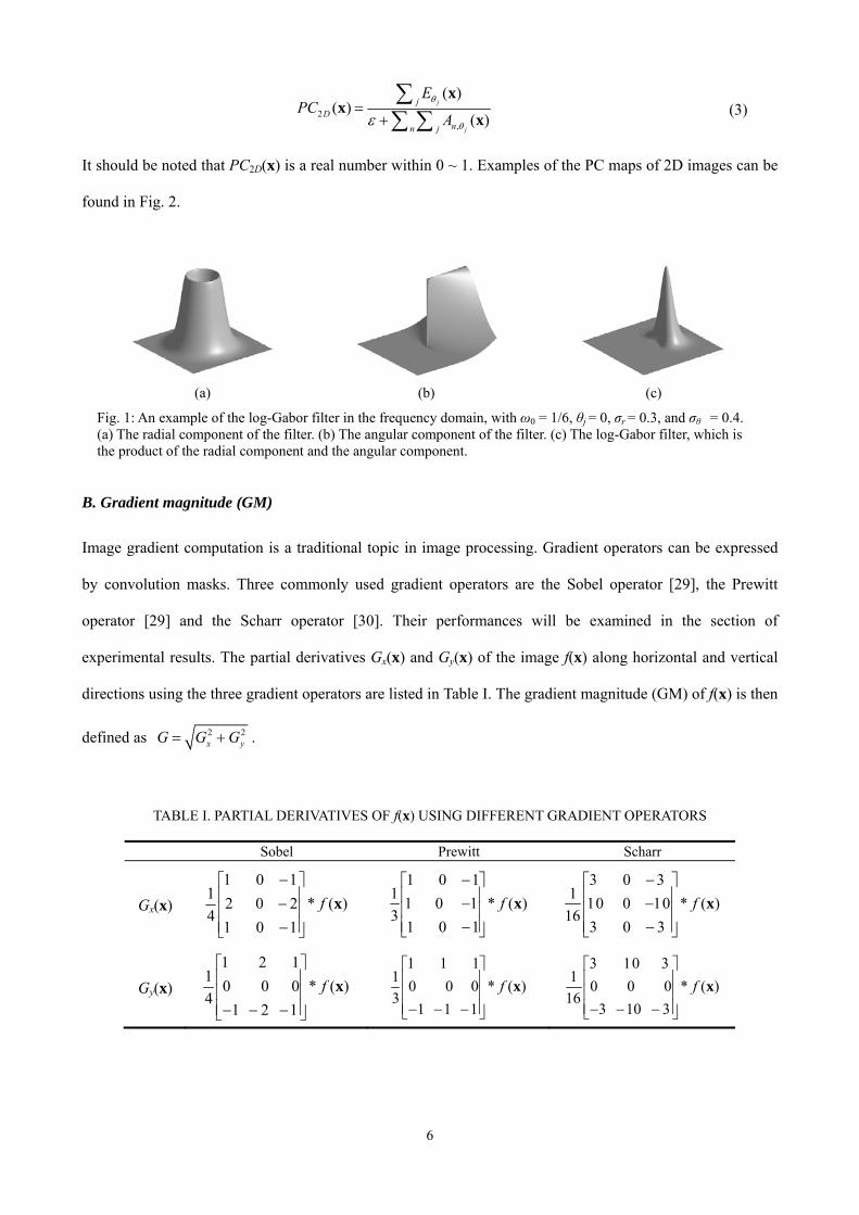
6
2
( )( )
( )j
j
jD
nn j
EPC
Aθ
θε=
+sumsum sum
xx
x (3)
It should be noted that PC2D(x) is a real number within 0 ~ 1 Examples of the PC maps of 2D images can be
found in Fig 2
(a) (b) (c)
Fig 1 An example of the log-Gabor filter in the frequency domain with ω0 = 16 θj = 0 σr = 03 and σθ = 04 (a) The radial component of the filter (b) The angular component of the filter (c) The log-Gabor filter which is the product of the radial component and the angular component
B Gradient magnitude (GM)
Image gradient computation is a traditional topic in image processing Gradient operators can be expressed
by convolution masks Three commonly used gradient operators are the Sobel operator [29] the Prewitt
operator [29] and the Scharr operator [30] Their performances will be examined in the section of
experimental results The partial derivatives Gx(x) and Gy(x) of the image f(x) along horizontal and vertical
directions using the three gradient operators are listed in Table I The gradient magnitude (GM) of f(x) is then
defined as 2 2x yG G G= +
TABLE I PARTIAL DERIVATIVES OF f(x) USING DIFFERENT GRADIENT OPERATORS
Sobel Prewitt Scharr
Gx(x) 1 1
1 2 0 ( )4
1 1f
0 minus⎡ ⎤⎢ ⎥ minus 2⎢ ⎥⎢ ⎥ 0 minus⎣ ⎦
x
1 11 0 ( )3
1 1f
0 minus⎡ ⎤⎢ ⎥1 minus1⎢ ⎥⎢ ⎥ 0 minus⎣ ⎦
x 1 0 ( )
163
f3 0 minus 3⎡ ⎤
⎢ ⎥10 minus10⎢ ⎥⎢ ⎥3 0 minus⎣ ⎦
x
Gy(x) 1 2 1
1 0 0 0 ( )4
1 2 1f
⎡ ⎤⎢ ⎥ ⎢ ⎥⎢ ⎥minus minus minus⎣ ⎦
x 1 1
1 0 0 0 ( )3
1 1 1f
1 ⎡ ⎤⎢ ⎥ ⎢ ⎥⎢ ⎥minus minus minus⎣ ⎦
x 1 0 0 0 ( )16
3 10 3f
3 10 3⎡ ⎤⎢ ⎥ ⎢ ⎥⎢ ⎥minus minus minus⎣ ⎦
x
7
III THE FEATURE SIMILARITY (FSIM) INDEX With the extracted PC and GM feature maps in this section we present a novel Feature SIMilarity (FSIM)
index for IQA Suppose that we are going to calculate the similarity between images f1 and f2 Denote by PC1
and PC2 the PC maps extracted from f1 and f2 and G1 and G2 the GM maps extracted from them It should be
noted that for color images PC and GM features are extracted from their luminance channels FSIM will be
defined and computed based on PC1 PC2 G1 and G2 Furthermore by incorporating the image chrominance
information into FSIM an IQA index for color images denoted by FSIMC will be obtained
A The FSIM index
The computation of FSIM index consists of two stages In the first stage the local similarity map is
computed and then in the second stage we pool the similarity map into a single similarity score
We separate the feature similarity measurement between f1(x) and f2(x) into two components each for
PC or GM First the similarity measure for PC1(x) and PC2(x) is defined as
1 2 12 2
1 2 1
2 ( ) ( )( )( ) ( )PC
PC PC TSPC PC T
sdot +=
+ +x xx
x x (4)
where T1 is a positive constant to increase the stability of SPC (such a consideration was also included in
SSIM [1]) In practice the determination of T1 depends on the dynamic range of PC values Eq (4) is a
commonly used measure to define the similarity of two positive real numbers [1] and its result ranges within
(0 1] Similarly the GM values G1(x) and G2(x) are compared and the similarity measure is defined as
1 2 22 2
1 2 2
2 ( ) ( )( )( ) ( )G
G G TSG G T
sdot +=
+ +x xx
x x (5)
where T2 is a positive constant depending on the dynamic range of GM values In our experiments both T1
and T2 will be fixed to all databases so that the proposed FSIM can be conveniently used Then SPC(x) and
SG(x) are combined to get the similarity SL(x) of f1(x) and f2(x) We define SL(x) as
( ) [ ( )] [ ( )]L PC GS S Sα β= sdotx x x (6)
where α and β are parameters used to adjust the relative importance of PC and GM features In this paper we
set α = β =1 for simplicity Thus SL(x) = SPC(x)SG(x)
Having obtained the similarity SL(x) at each location x the overall similarity between f1 and f2 can be
8
calculated However different locations have different contributions to HVSrsquo perception of the image For
example edge locations convey more crucial visual information than the locations within a smooth area
Since human visual cortex is sensitive to phase congruent structures [20] the PC value at a location can
reflect how likely it is a perceptibly significant structure point Intuitively for a given location x if anyone of
f1(x) and f2(x) has a significant PC value it implies that this position x will have a high impact on HVS in
evaluating the similarity between f1 and f2 Therefore we use PCm(x) = max(PC1(x) PC2(x)) to weight the
importance of SL(x) in the overall similarity between f1 and f2 and accordingly the FSIM index between f1
and f2 is defined as
( ) ( )FSIM
( )L m
m
S PCPC
isinΩ
isinΩ
sdot= sum
sumx
x
x xx
(7)
where Ω means the whole image spatial domain
B Extension to color image quality assessment
The FSIM index is designed for grayscale images or the luminance components of color images Since the
chrominance information will also affect HVS in understanding the images better performance can be
expected if the chrominance information is incorporated in FSIM for color IQA Such a goal can be achieved
by applying a straightforward extension to the FSIM framework
At first the original RGB color images are converted into another color space where the luminance can
be separated from the chrominance To this end we adopt the widely used YIQ color space [31] in which Y
represents the luminance information and I and Q convey the chrominance information The transform from
the RGB space to the YIQ space can be accomplished via [31]
0299 0587 01140596 0274 03220211 0523 0312
Y RI GQ B
⎡ ⎤ ⎡ ⎤ ⎡ ⎤⎢ ⎥ ⎢ ⎥ ⎢ ⎥= minus minus⎢ ⎥ ⎢ ⎥ ⎢ ⎥⎢ ⎥ ⎢ ⎥ ⎢ ⎥ minus ⎣ ⎦ ⎣ ⎦ ⎣ ⎦
(8)
Let I1 (I2) and Q1 (Q2) be the I and Q chromatic channels of the image f1 (f2) respectively Similar to the
definitions of SPC(x) and SG(x) we define the similarity between chromatic features as
1 2 32 2
1 2 3
2 ( ) ( )( )( ) ( )I
I I TSI I T
sdot +=
+ +x xx
x x 1 2 4
2 21 2 4
2 ( ) ( )( )( ) ( )Q
Q Q TSQ Q T
sdot +=
+ +x xx
x x (9)
9
f1 f2
PC1 PC2 G1 G2
SPC SG
( ) ( ) ( ) ( ) ( )FSIM
( )PC G I Q m
Cm
S S S S PCPC
λ
Ω
Ω
⎡ ⎤sdot sdot sdot sdot⎣ ⎦=sum
sumx x x x x
x
I1 Q1I2 Q2Y1
YIQ decomposition
PCm
Y2
SI SQ
Fig 2 Illustration for the FSIMFSIMC index computation f1 is the reference image and f2 is a distorted version of f1
where T3 and T4 are positive constants Since I and Q components have nearly the same dynamic range in
this paper we set T3 = T4 for simplicity SI(x) and SQ(x) can then be combined to get the chrominance
similarity measure denoted by SC(x) of f1(x) and f2(x)
( ) ( ) ( )C I QS S S= sdotx x x (10)
Finally the FSIM index can be extended to FSIMC by incorporating the chromatic information in a
straightforward manner
[ ]( ) ( ) ( )FSIM
( )L C m
Cm
S S PCPC
λisinΩ
isinΩ
sdot sdot= sum
sumx
x
x x xx
(11)
where λ gt 0 is the parameter used to adjust the importance of the chromatic components The procedures to
calculate the FSIMFSIMC indices are illustrated in Fig 2 If the chromatic information is ignored in Fig 2
the FSIMC index is reduced to the FSIM index
IV EXPERIMENTAL RESULTS AND DISCUSSIONS
A Databases and methods for comparison
To the best of our knowledge there are six publicly available image databases in the IQA community
10
including TID2008 [10] CSIQ [32] LIVE [33] IVC [34] MICT [35] and A57 [36] All of them will be used
here for algorithm validation and comparison The characteristics of these six databases are summarized in
Table II
TABLE II BENCHMARK TEST DATABASES FOR IQA
Database Source Images Distorted Images Distortion Types Image Type Observers TID2008 25 1700 17 color 838
CSIQ 30 866 6 color 35 LIVE 29 779 5 color 161 IVC 10 185 4 color 15
MICT 14 168 2 color 16 A57 3 54 6 gray unknown
The performance of the proposed FSIM and FSIMC indices will be evaluated and compared with eight
representative IQA metrics including seven state-of-the-arts (SSIM [1] MS-SSIM [5] VIF [4] VSNR [3]
IFC [7] NQM [2] and Liu et alrsquos method [21]) and the classical PSNR For Liu et alrsquos method [21] we
implemented it by ourselves For SSIM [1] we used the implementation provided by the author which is
available at [37] For all the other methods evaluated we used the public software MeTriX MuX [38] The
Matlab source code of the proposed FSIMFSIMC indices is available online at
httpwwwcomppolyueduhk~cslzhangIQAFSIMFSIMhtm
Four commonly used performance metrics are employed to evaluate the competing IQA metrics The
first two are the Spearman rank-order correlation coefficient (SROCC) and the Kendall rank-order
correlation coefficient (KROCC) which can measure the prediction monotonicity of an IQA metric These
two metrics operate only on the rank of the data points and ignore the relative distance between data points
To compute the other two metrics we need to apply a regression analysis as suggested by the video quality
experts group (VQEG) [39] to provide a nonlinear mapping between the objective scores and the subjective
mean opinion scores (MOS) The third metric is the Pearson linear correlation coefficient (PLCC) between
MOS and the objective scores after nonlinear regression The fourth metric is the root mean squared error
(RMSE) between MOS and the objective scores after nonlinear regression For the nonlinear regression we
used the following mapping function [9]
2 31 4 5( )
1 1( )2 1 xf x x
eβ ββ β βminus⎛ ⎞= minus + +⎜ ⎟+⎝ ⎠
(12)
11
where βi i =1 2 hellip 5 are the parameters to be fitted A better objective IQA measure is expected to have
higher SROCC KROCC and PLCC while lower RMSE values
B Determination of parameters
There are several parameters need to be determined for FSIM and FSIMC To this end we tuned the
parameters based on a sub-dataset of TID2008 database which contains the first 8 reference images in
TID2008 and the associated 544 distorted images The 8 reference images used in the tuning process are
shown in Fig 3 The tuning criterion was that the parameter value leading to a higher SROCC would be
chosen As a result the parameters required in the proposed methods were set as n = 4 J = 4 σr = 05978 σθ
= 06545 T1 = 085 T2 = 160 T3 = T4 = 200 and λ = 003 Besides the center frequencies of the log-Gabor
filters at four scales were set as 16 112 124 and 148 These parameters were then fixed for all the
following experiments conducted In fact we have also used the last 8 reference images (and the associated
544 distorted ones) to tune parameters and obtained very similar parameters to the ones reported here This
may imply that any 8 reference images in the TID2008 database work equally well in tuning parameters for
FSIMFSIMC However this conclusion is hard to prove theoretically or even experimentally because there
are C8 25=1081575 different ways to select 8 out of the 25 reference images in TID2008
(a) (b) (c) (d)
(e) (f) (g) (h)
Fig 3 Eight reference images used for the parameter tuning process They are extracted from the TID2008 database
It should be noted that the FSIMFSIMC indices will be most effective if used on the appropriate scale
12
The precisely ldquorightrdquo scale depends on both the image resolution and the viewing distance and hence is
difficult to be obtained In practice we used the following empirical steps proposed by Wang [37] to
determine the scale for images viewed from a typical distance 1) let F = max(1 round(N 256)) where N is
the number of pixels in image height or width 2) average local F times F pixels and then down-sample the
image by a factor of F
C Gradient operator selection
TABLE III SROCC VALUES USING THREE GRADIENT OPERATORS
Database SROCC Sobel 08797
Prewitt 08776Scharr 08825
In our proposed IQA metrics FSIMFSIMC the gradient magnitude (GM) needs to be calculated To this end
three commonly used gradient operators listed in Table I were examined and the one providing the best
result was selected Such a gradient operator selection process was carried out by assuming that all the
parameters discussed in Section IV-B were fixed The selection criterion was also that the gradient operator
leading to a higher SROCC would be selected The sub-dataset used in Section IV-B was used here The
SROCC values obtained by the three gradient operators on the tuning dataset are listed in Table III from
which we can see that the Scharr operator could achieve slightly better performance than the other two Thus
in all of the following experiments the Scharr operator was used to calculate the gradient in FSIMFSIMC
D Example to demonstrate the effectiveness of FSIMFSIMC
In this subsection we use an example to demonstrate the effectiveness of FSIMFSIMC in evaluating the
perceptible image quality Fig 4a is the I17 reference image in the TID2008 database and Figs 4b ~ 4f show
five distorted images of I17 I17_01_2 I17_03_2 I17_09_1 I17_11_2 and I17_12_2 Distortion types of
Figs 4b ~ 4f are ldquoadditive Gaussian noiserdquo ldquospatially correlated noiserdquo ldquoimage denoisingrdquo ldquoJPEG 2000
compressionrdquo and ldquoJPEG transformation errorsrdquo respectively According to the naming convention of
TID2008 the last number (the last digit) of the imagersquos name represents the distortion degree and a greater
number indicates a severer distortion We compute the image quality of Figs 4b ~ 4f using various IQA
metrics and the results are summarized in Table IV We also list the subjective scores (extracted from
13
TID2008) of these 5 images in Table IV For each IQA metric and the subjective evaluation higher scores
mean higher image quality
(a) (b) (c)
(d) (e) (f)
Fig 4 (a) A reference image (b) ~ (f) are the distorted versions of (a) in the TID2008 database Distortion types of (b) ~ (f) are ldquoadditive Gaussian noiserdquo ldquospatially correlated noiserdquo ldquoimage denoisingrdquo ldquoJPEG 2000 compressionrdquo and ldquoJPEG transformation errorsrdquo respectively
(a) (b) (c)
(d) (e) (f)
Fig 5 (a) ~ (f) are PC maps extracted from images Figs 4a ~ 4f respectively (a) is the PC map of the reference image while (b) ~ (f) are the PC maps of the distorted images (b) and (d) are more similar to (a) than (c) (e) and (f) In (c) (e) and (f) regions with obvious differences to the corresponding regions in (a) are marked by colorful rectangles
14
In order to show the correlation of each IQA metric with the subjective evaluation more clearly in Table
V we rank the images according to their quality scores computed by each metric as well as the subjective
evaluation From Tables IV and V we can see that the quality scores computed by FSIMFSIMC correlate
with the subjective evaluation much better than the other IQA metrics From Table V we can also see that
other than the proposed FSIMFSIMC metrics all the other IQA metrics cannot give the same ranking as the
subjective evaluations
TABLE IV QUALITY EVALUATION OF IAMGES IN FIG 4
Fig 4b Fig 4c Fig 4d Fig 4e Fig 4f
Subjective score 52222 40571 61389 33429 52000 FSIM 09776 09281 09827 09085 09583 FSIMC 09741 09195 09817 09071 09582
MS-SSIM 09590 09109 09832 09170 09633 VIF 05803 04037 05670 01876 06484
SSIM 09268 08419 09686 08464 09306 IFC 35416 23441 39036 11710 80318
VSNR 307669 226702 322891 211772 186739 NQM 295608 210153 294932 194725 163083 [21] 08790 07158 09110 06503 09172
PSNR 271845 271577 340126 270330 269246
TABLE V RANKING OF IMAGES ACCORDING TO THEIR QUALITY COMPUTED BY EACH IQA METRIC
Fig 4b Fig 4c Fig 4d Fig 4e Fig 4f Subjective score 2 4 1 5 3
FSIM 2 4 1 5 3 FSIMC 2 4 1 5 3
MS-SSIM 3 5 1 4 2 VIF 2 4 3 5 1
SSIM 3 5 1 4 2 IFC 3 4 2 5 1
VSNR 2 3 1 4 5 NQM 1 3 2 4 5 [21] 3 4 2 5 1
PSNR 2 3 1 4 5
The success of FSIMFSIMC actually owes to the proper use of PC maps Figs 5a ~ 5f show the PC
maps of the images in Figs 4a ~ 4f respectively We can see that images in Figs 4b and 4d have better
perceptible qualities than those in Figs 4c 4e and 4f meanwhile by visually examination we can see that
maps in Figs 5b and 5d (PC maps of images in Figs 4b and 4d) are more similar to the map in Fig 5a (PC
15
map of the reference image in Fig 4a) than the maps in Figs 5c 5e and 5f (PC maps of images in Figs 4c
4e and 4f) In order to facilitate visual examination in Figs 5c 5e and 5f regions with obvious differences
to the corresponding regions in Fig 5a are marked by rectangles For example in Fig 5c the neck region
marked by the yellow rectangle has a perceptible difference to the same region in Fig 5a This example
clearly illustrates that images of higher quality will have more similar PC maps to that of the reference image
than images of lower quality Therefore by properly making use of PC maps in FSIMFSIMC we can predict
the image quality consistently with human subjective evaluations More statistically convincing results will
be presented in the next two sub-sections
E Overall performance comparison
TABLE VI PERFORMANCE COMPARISON OF IQA METRICS ON 6 BENCHMARK DATABASES
FSIM FSIMC MS-SSIM VIF SSIM IFC VSNR NQM [21] PSNR
TID 2008
SROCC 08805 08840 08528 07496 07749 05692 07046 06243 07388 05245KROCC 06946 06991 06543 05863 05768 04261 05340 04608 05414 03696PLCC 08738 08762 08425 08090 07732 07359 06820 06135 07679 05309RMSE 06525 06468 07299 07888 08511 09086 09815 10598 08595 11372
CSIQ SROCC 09242 09310 09138 09193 08756 07482 08106 07402 07642 08057KROCC 07567 07690 07397 07534 06907 05740 06247 05638 05811 06080PLCC 09120 09192 08998 09277 08613 08381 08002 07433 08222 08001RMSE 01077 01034 01145 00980 01334 01432 01575 01756 01494 01575
LIVE SROCC 09634 09645 09445 09631 09479 09234 09274 09086 08650 08755KROCC 08337 08363 07922 08270 07963 07540 07616 07413 06781 06864PLCC 09597 09613 09430 09598 09449 09248 09231 09122 08765 08721RMSE 76780 75296 90956 76734 89455 10392 10506 11193 13155 13368
IVC SROCC 09262 09293 08847 08966 09018 08978 07983 08347 08383 06885KROCC 07564 07636 07012 07165 07223 07192 06036 06342 06441 05220PLCC 09376 09392 08934 09028 09119 09080 08032 08498 08454 07199RMSE 04236 04183 05474 05239 04999 05105 07258 06421 06507 08456
MICT SROCC 09059 09067 08864 09086 08794 08387 08614 08911 06923 06130KROCC 07302 07303 07029 07329 06939 06413 06762 07129 05152 04447PLCC 09078 09075 08935 09144 08887 08434 08710 08955 07208 06426RMSE 05248 05257 05621 05066 05738 06723 06147 05569 08674 09588
SROCC 09181 - 08394 06223 08066 03185 09355 07981 07155 06189A57 KROCC 07639 - 06478 04589 06058 02378 08031 05932 05275 04309
PLCC 09252 - 08504 06158 08017 04548 09472 08020 07399 06587 RMSE 00933 - 01293 01936 01469 02189 00781 01468 01653 01849
In this section we compare the general performance of the competing IQA metrics Table VI lists the
SROCC KROCC PLCC and RMSE results of FSIMFSIMC and the other 8 IQA algorithms on the
TID2008 CSIQ LIVE IVC MICT and A57 databases For each performance measure the three IQA
indices producing the best results are highlighted in boldface for each database It should be noted that
except for FSIMC all the other IQA indices are based on the luminance component of the image From Table
16
VI we can see that the proposed feature-similarity based IQA metric FSIM or FSIMC performs consistently
well across all the databases In order to demonstrate this consistency more clearly in Table VII we list the
performance ranking of all the IQA metrics according to their SROCC values For fairness the FSIMC index
which also exploits the chrominance information of images is excluded in Table VII
TABLE VII RANKING OF IQA METRICSrsquo PERFORMANCE (EXCEPT FOR FSIMC) ON SIX DATABASES
TID2008 CSIQ LIVE IVC MICT A57
FSIM 1 1 1 1 2 2 MS-SSIM 2 3 4 5 4 3
VIF 4 2 2 4 1 7 SSIM 3 4 3 2 5 4 IFC 8 8 6 3 7 9
VSNR 6 5 5 8 6 1 NQM 7 9 7 7 3 5 [21] 5 7 9 6 8 6
PSNR 9 6 8 9 9 8
04 05 06 07 08 09 10
2
4
6
8
Objective score by MS-SSIM
MO
S
Images in TID2008Curve fitted
04 05 06 07 08 09 1
0
2
4
6
8
Objective score by SSIM
MO
S
Images in TID2008Curve fitted with logistic function
0 02 04 06 08 1 12 14
0
2
4
6
8
Objective score by VIF
MO
S
Images in TID2008Curve fitted
(a) (b) (c)
0 100 200 300 400 500 600 7000
2
4
6
8
Objective score by VSNR
MO
S
Images in TID2008Curve fitted
0 20 40 60 80 100
0
2
4
6
8
Objective score by IFC
MO
S
Images in TID2008Curve fitted
0 10 20 30 40 50
0
2
4
6
8
Objective score by NQM
MO
S
Images in TID2008Curve fitted
(d) (e) (f)
10 15 20 25 30 35 400
2
4
6
8
Objective score by PSNR
MO
S
Images in TID2008Curve fitted with logistic function
0 02 04 06 08 1
0
2
4
6
8
Objective score by Liu [21]
MO
S
Images in TID2008Curve fitted with logistic function
05 06 07 08 09 10
2
4
6
8
Objective score by FSIM
MO
S
Images in TID2008Curve fitted with logistic function
(g) (h) (i)
Fig 6 Scatter plots of subjective MOS versus scores obtained by model prediction on the TID 2008 database (a) MS-SSIM (b) SSIM (c) VIF (d) VSNR (e) IFC (f) NQM (g) PSNR (h) method in [21] and (i) FSIM
17
From the experimental results summarized in Table VI and Table VII we can see that our methods
achieve the best results on almost all the databases except for MICT and A57 Even on these two databases
however the proposed FSIM (or FSIMC) is only slightly worse than the best results Moreover considering
the scales of the databases including the number of images the number of distortion types and the number
of observers we think that the results obtained on TID2008 CSIQ LIVE and IVC are much more
convincing than those obtained on MICT and A57 Overall speaking FSIM and FSIMC achieve the most
consistent and stable performance across all the 6 databases By contrast for the other methods they may
work well on some databases but fail to provide good results on other databases For example although VIF
can get very pleasing results on LIVE it performs poorly on TID2008 and A57 The experimental results
also demonstrate that the chromatic information of an image does affect its perceptible quality since FSIMC
has better performance than FSIM on all color image databases Fig 6 shows the scatter distributions of
subjective MOS versus the predicted scores by FSIM and the other 8 IQA indices on the TID 2008 database
The curves shown in Fig 6 were obtained by a nonlinear fitting according to Eq (12) From Fig 6 one can
see that the objective scores predicted by FSIM correlate much more consistently with the subjective
evaluations than the other methods
F Performance on individual distortion types
In this experiment we examined the performance of the competing methods on different image distortion
types We used the SROCC score which is a widely accepted and used evaluation measure for IQA metrics
[1 39] as the evaluation measure By using the other measures such as KROCC PLCC and RMSE similar
conclusions could be drawn The three largest databases TID2008 CSIQ and LIVE were used in this
experiment The experimental results are summarized in Table VIII For each database and each distortion
type the first 3 IQA indices producing the highest SROCC values are highlighted in boldface We can have
some observations based on the results listed in Table VIII In general when the distortion type is known
beforehand FSIMC performs the best while FSIM and VIF have comparable performance FSIM FSIMC
and VIF perform much better than the other IQA indices Compared with VIF FSIM and FSIMC are more
capable in dealing with the distortions of ldquodenoisingrdquo ldquoquantization noiserdquo and ldquomean shiftrdquo By contrast
for the distortions of ldquomasked noiserdquo and ldquoimpulse noiserdquo VIF performs better than FSIM and FSIMC
18
Moreover results in Table VIII once again corroborates that the chromatic information does affect the
perceptible quality since FSIMC has better performance than FSIM on each database for nearly all the
distortion types
TABLE VIII SROCC VALUES OF IQA METRICS FOR EACH DISTORTION TYPE
FSIM FSIMC MS-SSIM VIF SSIM IFC VSNR NQM [21] PSNR
TID 2008
awgn 08566 08758 08094 08799 08107 05817 07728 07679 05069 09114awgn-color 08527 08931 08064 08785 08029 05528 07793 07490 04625 09068
spatial corr-noise 08483 08711 08195 08703 08144 05984 07665 07720 06065 09229masked noise 08021 08264 08155 08698 07795 07326 07295 07067 05301 08487high-fre-noise 09093 09156 08685 09075 08729 07361 08811 09015 06935 09323impulse noise 07452 07719 06868 08331 06732 05334 06471 07616 04537 09177
quantization noise 08564 08726 08537 07956 08531 05911 08270 08209 06214 08699blur 09472 09472 09607 09546 09544 08766 09330 08846 08883 08682
denoising 09603 09618 09571 09189 09530 08002 09286 09450 07878 09381jpg-comp 09279 09294 09348 09170 09252 08181 09174 09075 08186 09011
jpg2k-comp 09773 09780 09736 09713 09625 09445 09515 09532 09301 08300jpg-trans-error 08708 08756 08736 08582 08678 07966 08056 07373 08334 07665
jpg2k-trans-error 08544 08555 08525 08510 08577 07303 07909 07262 07164 07765pattern-noise 07491 07514 07336 07608 07107 08410 05716 06800 07677 05931
block-distortion 08492 08464 07617 08320 08462 06767 01926 02348 07282 05852mean shift 06720 06554 07374 05132 07231 04375 03715 05245 03487 06974
contrast 06481 06510 06400 08190 05246 02748 04239 06191 03883 06126
CSIQ
awgn 09262 09359 09471 09571 08974 08460 09241 09384 07501 09363
jpg-comp 09654 09664 09622 09705 09546 09395 09036 09527 09088 08882
jpg2k-comp 09685 09704 09691 09672 09606 09262 09480 09631 08886 09363
1f noise 09234 09370 09330 09509 08922 08279 09084 09119 07905 09338
blur 09729 09729 09720 09747 09609 09593 09446 09584 09551 09289
contrast 09420 09438 09521 09361 07922 05416 08700 09479 04326 08622 jpg2k-comp 09717 09724 09654 09683 09614 09100 09551 09435 08533 08954
LIVE jpg-comp 09834 09840 09793 09842 09764 09440 09657 09647 09127 08809
awgn 09652 09716 09731 09845 09694 09377 09785 09863 09079 09854blur 09708 09708 09584 09722 09517 09649 09413 08397 09365 07823
jpg2k-trans-error 09499 09519 09321 09652 09556 09644 09027 08147 08765 08907
V CONCLUSIONS
In this paper we proposed a novel low-level feature based image quality assessment (IQA) metric namely
Feature-SIMilarity (FSIM) index The underlying principle of FSIM is that HVS perceives an image mainly
19
based on its salient low-level features Specifically two kinds of features the phase congruency (PC) and the
gradient magnitude (GM) are used in FSIM and they represent complementary aspects of the image visual
quality The PC value is also used to weight the contribution of each point to the overall similarity of two
images We then extended FSIM to FSIMC by incorporating the image chromatic features into consideration
The FSIM and FSIMC indices were compared with eight representative and prominent IQA metrics on six
benchmark databases and very promising results were obtained by FSIM and FSIMC When the distortion
type is known beforehand FSIMC performs the best while FSIM achieves comparable performance with VIF
When all the distortion types are involved (ie all the images in a test database are used) FSIM and FSIMC
outperform all the other IQA metrics used in comparison Particularly they perform consistently well across
all the test databases validating that they are very robust IQA metrics
REFERENCES
[1] Z Wang AC Bovik HR Sheikh and EP Simoncelli ldquoImage quality assessment from error visibility to
structural similarityrdquo IEEE Trans Image Process vol 13 no 4 pp 600-612 Apr 2004
[2] N Damera-Venkata TD Kite WS Geisler BL Evans and AC Bovik ldquoImage quality assessment based on a
degradation modelrdquo IEEE Trans Image Process vol 9 no 4 pp 636-650 Apr 2000
[3] DM Chandler and SS Hemami ldquoVSNR a wavelet-based visual signal-to-noise ratio for natural imagesrdquo IEEE
Trans Image Process vol 16 no 9 pp 2284-2298 Sep 2007
[4] HR Sheikh and AC Bovik ldquoImage information and visual qualityrdquo IEEE Trans Image Process vol 15 no 2
pp 430-444 Feb 2006
[5] Z Wang EP Simoncelli and AC Bovik ldquoMulti-scale structural similarity for image quality assessmentrdquo
presented at the IEEE Asilomar Conf Signals Systems and Computers Nov 2003
[6] C Li and AC Bovik ldquoThree-component weighted structural similarity indexrdquo in Proc SPIE vol 7242 2009
[7] HR Sheikh AC Bovik and G de Veciana ldquoAn information fidelity criterion for image quality assessment using
natural scene statisticsrdquo IEEE Trans Image Process vol 14 no 12 pp 2117-2128 Dec 2005
[8] MP Sampat Z Wang S Gupta AC Bovik and MK Markey ldquoComplex wavelet structural similarity a new
image similarity indexrdquo IEEE Trans Image Process vol 18 no 11 pp 2385-2401 Nov 2009
[9] HR Sheikh MF Sabir and AC Bovik ldquoA statistical evaluation of recent full reference image quality
assessment algorithmsrdquo IEEE Trans Image Process vol 15 no 11 pp 3440-3451 Nov 2006
20
[10] N Ponomarenko V Lukin A Zelensky K Egiazarian M Carli and F Battisti ldquoTID2008 - A database for
evaluation of full-reference visual quality assessment metricsrdquo Advances of Modern Radioelectronics vol 10 pp
30-45 2009
[11] Z Wang and Q Li ldquoInformation content weighting for perceptual image quality assessmentrdquo IEEE Trans Image
Process accepted
[12] EC Larson and DM Chandler ldquoUnveiling relationships between regions of interest and image fidelity metricsrdquo
in Proc SPIE Visual Comm and Image Process vol 6822 pp 6822A1-16 Jan 2008
[13] EC Larson C Vu and DM Chandler ldquoCan visual fixation patterns improve image fidelity assessmentrdquo in
Proc IEEE Int Conf Image Process 2008 pp 2572-2575
[14] D Marr Vision New York W H Freeman and Company 1980
[15] D Marr and E Hildreth ldquoTheory of edge detectionrdquo Proc R Soc Lond B vol 207 no 1167 pp 187-217 Feb
1980
[16] MC Morrone and DC Burr ldquoFeature detection in human vision a phase-dependent energy modelrdquo Proc R Soc
Lond B vol 235 no 1280 pp 221-245 Dec 1988
[17] MC Morrone J Ross DC Burr and R Owens ldquoMach bands are phase dependentrdquo Nature vol 324 no 6049
pp 250-253 Nov 1986
[18] MC Morrone and RA Owens ldquoFeature detection from local energyrdquo Pattern Recognit Letters vol 6 no 5 pp
303-313 Dec 1987
[19] P Kovesi ldquoImage features from phase congruencyrdquo Videre J Comp Vis Res vol 1 no 3 pp 1-26 1999
[20] L Henriksson A Hyvaumlrinen and S Vanni ldquoRepresentation of cross-frequency spatial phase relationships in
human visual cortexrdquo J Neuroscience vol 29 no 45 pp 14342-14351 Nov 2009
[21] Z Liu and R Laganiegravere ldquoPhase congruence measurement for image similarity assessmentrdquo Pattern Recognit
Letters vol 28 no 1 pp 166-172 Jan 2007
[22] Z Wang and EP Simoncelli ldquoLocal phase coherence and the perception of blurrdquo in Adv Neural Information
Processing Systems 2004 pp 786-792
[23] R Hassen Z Wang and M Salama ldquoNo-reference image sharpness assessment based on local phase coherence
measurementrdquo in Proc IEEE Int Conf Acoust Speech and Signal Processing 2010 pp 2434-2437
[24] D Gabor ldquoTheory of communicationrdquo J Inst Elec Eng vol 93 no III pp 429-457 1946
[25] D J Field ldquoRelations between the statistics of natural images and the response properties of cortical cellsrdquo J Opt
Soc Am A vol 4 no 12 pp 2379-2394 Dec 1987
21
[26] C Mancas-Thillou and B Gosselin ldquoCharacter segmentation-by-recognition using log-Gabor filtersrdquo in Proc Int
Conf Pattern Recognit 2006 pp 901-904
[27] S Fischer F Šroubek L Perrinet R Redondo and G Cristoacutebal ldquoSelf-invertible 2D log-Gabor waveletsrdquo Int J
Computer Vision vol 75 no 2 pp 231-246 Nov 2007
[28] W Wang J Li F Huang and H Feng ldquoDesign and implementation of log-Gabor filter in fingerprint image
enhancementrdquo Pattern Recognit Letters vol 29 no 3 pp 301-308 Feb 2008
[29] R Jain R Kasturi and BG Schunck Machine Vision McGraw-Hill Inc 1995
[30] B Jaumlhne H Haubecker and P Geibler Handbook of Computer Vision and Applications Academic Press 1999
[31] C Yang and SH Kwok ldquoEfficient gamut clipping for color image processing using LHS and YIQrdquo Optical
Engineering vol 42 no 3 pp701-711 Mar 2003
[32] EC Larson and DM Chandler ldquoCategorical Image Quality (CSIQ) Databaserdquo httpvisionokstateeducsiq
[33] HR Sheikh K Seshadrinathan AK Moorthy Z Wang AC Bovik and LK Cormack ldquoImage and video
quality assessment research at LIVErdquo httpliveeceutexaseduresearchquality
[34] A Ninassi P Le Callet and F Autrusseau ldquoSubjective quality assessment-IVC databaserdquo
httpwww2irccynec-nantesfrivcdb
[35] Y Horita K Shibata Y Kawayoke and ZM Parves Sazzad ldquoMICT Image Quality Evaluation Databaserdquo
httpmictengu-toyamaacjpmictindex2html
[36] DM Chandler and SS Hemami ldquoA57 databaserdquo httpfoulardececornelledudmc27vsnrvsnrhtml
[37] Z Wang ldquoSSIM Index for Image Quality Assessmentrdquo httpwwweceuwaterlooca~z70wangresearchssim
[38] M Gaubatz and SS Hemami ldquoMeTriX MuX Visual Quality Assessment Packagerdquo
httpfoulardececornelledugaubatzmetrix_mux
[39] VQEG ldquoFinal report from the video quality experts group on the validation of objective models of video quality
assessmentrdquo httpwwwvqegorg 2000
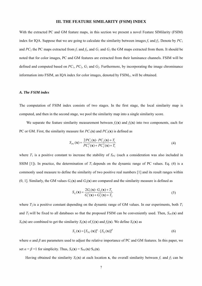
8
calculated However different locations have different contributions to HVSrsquo perception of the image For
example edge locations convey more crucial visual information than the locations within a smooth area
Since human visual cortex is sensitive to phase congruent structures [20] the PC value at a location can
reflect how likely it is a perceptibly significant structure point Intuitively for a given location x if anyone of
f1(x) and f2(x) has a significant PC value it implies that this position x will have a high impact on HVS in
evaluating the similarity between f1 and f2 Therefore we use PCm(x) = max(PC1(x) PC2(x)) to weight the
importance of SL(x) in the overall similarity between f1 and f2 and accordingly the FSIM index between f1
and f2 is defined as
( ) ( )FSIM
( )L m
m
S PCPC
isinΩ
isinΩ
sdot= sum
sumx
x
x xx
(7)
where Ω means the whole image spatial domain
B Extension to color image quality assessment
The FSIM index is designed for grayscale images or the luminance components of color images Since the
chrominance information will also affect HVS in understanding the images better performance can be
expected if the chrominance information is incorporated in FSIM for color IQA Such a goal can be achieved
by applying a straightforward extension to the FSIM framework
At first the original RGB color images are converted into another color space where the luminance can
be separated from the chrominance To this end we adopt the widely used YIQ color space [31] in which Y
represents the luminance information and I and Q convey the chrominance information The transform from
the RGB space to the YIQ space can be accomplished via [31]
0299 0587 01140596 0274 03220211 0523 0312
Y RI GQ B
⎡ ⎤ ⎡ ⎤ ⎡ ⎤⎢ ⎥ ⎢ ⎥ ⎢ ⎥= minus minus⎢ ⎥ ⎢ ⎥ ⎢ ⎥⎢ ⎥ ⎢ ⎥ ⎢ ⎥ minus ⎣ ⎦ ⎣ ⎦ ⎣ ⎦
(8)
Let I1 (I2) and Q1 (Q2) be the I and Q chromatic channels of the image f1 (f2) respectively Similar to the
definitions of SPC(x) and SG(x) we define the similarity between chromatic features as
1 2 32 2
1 2 3
2 ( ) ( )( )( ) ( )I
I I TSI I T
sdot +=
+ +x xx
x x 1 2 4
2 21 2 4
2 ( ) ( )( )( ) ( )Q
Q Q TSQ Q T
sdot +=
+ +x xx
x x (9)
9
f1 f2
PC1 PC2 G1 G2
SPC SG
( ) ( ) ( ) ( ) ( )FSIM
( )PC G I Q m
Cm
S S S S PCPC
λ
Ω
Ω
⎡ ⎤sdot sdot sdot sdot⎣ ⎦=sum
sumx x x x x
x
I1 Q1I2 Q2Y1
YIQ decomposition
PCm
Y2
SI SQ
Fig 2 Illustration for the FSIMFSIMC index computation f1 is the reference image and f2 is a distorted version of f1
where T3 and T4 are positive constants Since I and Q components have nearly the same dynamic range in
this paper we set T3 = T4 for simplicity SI(x) and SQ(x) can then be combined to get the chrominance
similarity measure denoted by SC(x) of f1(x) and f2(x)
( ) ( ) ( )C I QS S S= sdotx x x (10)
Finally the FSIM index can be extended to FSIMC by incorporating the chromatic information in a
straightforward manner
[ ]( ) ( ) ( )FSIM
( )L C m
Cm
S S PCPC
λisinΩ
isinΩ
sdot sdot= sum
sumx
x
x x xx
(11)
where λ gt 0 is the parameter used to adjust the importance of the chromatic components The procedures to
calculate the FSIMFSIMC indices are illustrated in Fig 2 If the chromatic information is ignored in Fig 2
the FSIMC index is reduced to the FSIM index
IV EXPERIMENTAL RESULTS AND DISCUSSIONS
A Databases and methods for comparison
To the best of our knowledge there are six publicly available image databases in the IQA community
10
including TID2008 [10] CSIQ [32] LIVE [33] IVC [34] MICT [35] and A57 [36] All of them will be used
here for algorithm validation and comparison The characteristics of these six databases are summarized in
Table II
TABLE II BENCHMARK TEST DATABASES FOR IQA
Database Source Images Distorted Images Distortion Types Image Type Observers TID2008 25 1700 17 color 838
CSIQ 30 866 6 color 35 LIVE 29 779 5 color 161 IVC 10 185 4 color 15
MICT 14 168 2 color 16 A57 3 54 6 gray unknown
The performance of the proposed FSIM and FSIMC indices will be evaluated and compared with eight
representative IQA metrics including seven state-of-the-arts (SSIM [1] MS-SSIM [5] VIF [4] VSNR [3]
IFC [7] NQM [2] and Liu et alrsquos method [21]) and the classical PSNR For Liu et alrsquos method [21] we
implemented it by ourselves For SSIM [1] we used the implementation provided by the author which is
available at [37] For all the other methods evaluated we used the public software MeTriX MuX [38] The
Matlab source code of the proposed FSIMFSIMC indices is available online at
httpwwwcomppolyueduhk~cslzhangIQAFSIMFSIMhtm
Four commonly used performance metrics are employed to evaluate the competing IQA metrics The
first two are the Spearman rank-order correlation coefficient (SROCC) and the Kendall rank-order
correlation coefficient (KROCC) which can measure the prediction monotonicity of an IQA metric These
two metrics operate only on the rank of the data points and ignore the relative distance between data points
To compute the other two metrics we need to apply a regression analysis as suggested by the video quality
experts group (VQEG) [39] to provide a nonlinear mapping between the objective scores and the subjective
mean opinion scores (MOS) The third metric is the Pearson linear correlation coefficient (PLCC) between
MOS and the objective scores after nonlinear regression The fourth metric is the root mean squared error
(RMSE) between MOS and the objective scores after nonlinear regression For the nonlinear regression we
used the following mapping function [9]
2 31 4 5( )
1 1( )2 1 xf x x
eβ ββ β βminus⎛ ⎞= minus + +⎜ ⎟+⎝ ⎠
(12)
11
where βi i =1 2 hellip 5 are the parameters to be fitted A better objective IQA measure is expected to have
higher SROCC KROCC and PLCC while lower RMSE values
B Determination of parameters
There are several parameters need to be determined for FSIM and FSIMC To this end we tuned the
parameters based on a sub-dataset of TID2008 database which contains the first 8 reference images in
TID2008 and the associated 544 distorted images The 8 reference images used in the tuning process are
shown in Fig 3 The tuning criterion was that the parameter value leading to a higher SROCC would be
chosen As a result the parameters required in the proposed methods were set as n = 4 J = 4 σr = 05978 σθ
= 06545 T1 = 085 T2 = 160 T3 = T4 = 200 and λ = 003 Besides the center frequencies of the log-Gabor
filters at four scales were set as 16 112 124 and 148 These parameters were then fixed for all the
following experiments conducted In fact we have also used the last 8 reference images (and the associated
544 distorted ones) to tune parameters and obtained very similar parameters to the ones reported here This
may imply that any 8 reference images in the TID2008 database work equally well in tuning parameters for
FSIMFSIMC However this conclusion is hard to prove theoretically or even experimentally because there
are C8 25=1081575 different ways to select 8 out of the 25 reference images in TID2008
(a) (b) (c) (d)
(e) (f) (g) (h)
Fig 3 Eight reference images used for the parameter tuning process They are extracted from the TID2008 database
It should be noted that the FSIMFSIMC indices will be most effective if used on the appropriate scale
12
The precisely ldquorightrdquo scale depends on both the image resolution and the viewing distance and hence is
difficult to be obtained In practice we used the following empirical steps proposed by Wang [37] to
determine the scale for images viewed from a typical distance 1) let F = max(1 round(N 256)) where N is
the number of pixels in image height or width 2) average local F times F pixels and then down-sample the
image by a factor of F
C Gradient operator selection
TABLE III SROCC VALUES USING THREE GRADIENT OPERATORS
Database SROCC Sobel 08797
Prewitt 08776Scharr 08825
In our proposed IQA metrics FSIMFSIMC the gradient magnitude (GM) needs to be calculated To this end
three commonly used gradient operators listed in Table I were examined and the one providing the best
result was selected Such a gradient operator selection process was carried out by assuming that all the
parameters discussed in Section IV-B were fixed The selection criterion was also that the gradient operator
leading to a higher SROCC would be selected The sub-dataset used in Section IV-B was used here The
SROCC values obtained by the three gradient operators on the tuning dataset are listed in Table III from
which we can see that the Scharr operator could achieve slightly better performance than the other two Thus
in all of the following experiments the Scharr operator was used to calculate the gradient in FSIMFSIMC
D Example to demonstrate the effectiveness of FSIMFSIMC
In this subsection we use an example to demonstrate the effectiveness of FSIMFSIMC in evaluating the
perceptible image quality Fig 4a is the I17 reference image in the TID2008 database and Figs 4b ~ 4f show
five distorted images of I17 I17_01_2 I17_03_2 I17_09_1 I17_11_2 and I17_12_2 Distortion types of
Figs 4b ~ 4f are ldquoadditive Gaussian noiserdquo ldquospatially correlated noiserdquo ldquoimage denoisingrdquo ldquoJPEG 2000
compressionrdquo and ldquoJPEG transformation errorsrdquo respectively According to the naming convention of
TID2008 the last number (the last digit) of the imagersquos name represents the distortion degree and a greater
number indicates a severer distortion We compute the image quality of Figs 4b ~ 4f using various IQA
metrics and the results are summarized in Table IV We also list the subjective scores (extracted from
13
TID2008) of these 5 images in Table IV For each IQA metric and the subjective evaluation higher scores
mean higher image quality
(a) (b) (c)
(d) (e) (f)
Fig 4 (a) A reference image (b) ~ (f) are the distorted versions of (a) in the TID2008 database Distortion types of (b) ~ (f) are ldquoadditive Gaussian noiserdquo ldquospatially correlated noiserdquo ldquoimage denoisingrdquo ldquoJPEG 2000 compressionrdquo and ldquoJPEG transformation errorsrdquo respectively
(a) (b) (c)
(d) (e) (f)
Fig 5 (a) ~ (f) are PC maps extracted from images Figs 4a ~ 4f respectively (a) is the PC map of the reference image while (b) ~ (f) are the PC maps of the distorted images (b) and (d) are more similar to (a) than (c) (e) and (f) In (c) (e) and (f) regions with obvious differences to the corresponding regions in (a) are marked by colorful rectangles
14
In order to show the correlation of each IQA metric with the subjective evaluation more clearly in Table
V we rank the images according to their quality scores computed by each metric as well as the subjective
evaluation From Tables IV and V we can see that the quality scores computed by FSIMFSIMC correlate
with the subjective evaluation much better than the other IQA metrics From Table V we can also see that
other than the proposed FSIMFSIMC metrics all the other IQA metrics cannot give the same ranking as the
subjective evaluations
TABLE IV QUALITY EVALUATION OF IAMGES IN FIG 4
Fig 4b Fig 4c Fig 4d Fig 4e Fig 4f
Subjective score 52222 40571 61389 33429 52000 FSIM 09776 09281 09827 09085 09583 FSIMC 09741 09195 09817 09071 09582
MS-SSIM 09590 09109 09832 09170 09633 VIF 05803 04037 05670 01876 06484
SSIM 09268 08419 09686 08464 09306 IFC 35416 23441 39036 11710 80318
VSNR 307669 226702 322891 211772 186739 NQM 295608 210153 294932 194725 163083 [21] 08790 07158 09110 06503 09172
PSNR 271845 271577 340126 270330 269246
TABLE V RANKING OF IMAGES ACCORDING TO THEIR QUALITY COMPUTED BY EACH IQA METRIC
Fig 4b Fig 4c Fig 4d Fig 4e Fig 4f Subjective score 2 4 1 5 3
FSIM 2 4 1 5 3 FSIMC 2 4 1 5 3
MS-SSIM 3 5 1 4 2 VIF 2 4 3 5 1
SSIM 3 5 1 4 2 IFC 3 4 2 5 1
VSNR 2 3 1 4 5 NQM 1 3 2 4 5 [21] 3 4 2 5 1
PSNR 2 3 1 4 5
The success of FSIMFSIMC actually owes to the proper use of PC maps Figs 5a ~ 5f show the PC
maps of the images in Figs 4a ~ 4f respectively We can see that images in Figs 4b and 4d have better
perceptible qualities than those in Figs 4c 4e and 4f meanwhile by visually examination we can see that
maps in Figs 5b and 5d (PC maps of images in Figs 4b and 4d) are more similar to the map in Fig 5a (PC
15
map of the reference image in Fig 4a) than the maps in Figs 5c 5e and 5f (PC maps of images in Figs 4c
4e and 4f) In order to facilitate visual examination in Figs 5c 5e and 5f regions with obvious differences
to the corresponding regions in Fig 5a are marked by rectangles For example in Fig 5c the neck region
marked by the yellow rectangle has a perceptible difference to the same region in Fig 5a This example
clearly illustrates that images of higher quality will have more similar PC maps to that of the reference image
than images of lower quality Therefore by properly making use of PC maps in FSIMFSIMC we can predict
the image quality consistently with human subjective evaluations More statistically convincing results will
be presented in the next two sub-sections
E Overall performance comparison
TABLE VI PERFORMANCE COMPARISON OF IQA METRICS ON 6 BENCHMARK DATABASES
FSIM FSIMC MS-SSIM VIF SSIM IFC VSNR NQM [21] PSNR
TID 2008
SROCC 08805 08840 08528 07496 07749 05692 07046 06243 07388 05245KROCC 06946 06991 06543 05863 05768 04261 05340 04608 05414 03696PLCC 08738 08762 08425 08090 07732 07359 06820 06135 07679 05309RMSE 06525 06468 07299 07888 08511 09086 09815 10598 08595 11372
CSIQ SROCC 09242 09310 09138 09193 08756 07482 08106 07402 07642 08057KROCC 07567 07690 07397 07534 06907 05740 06247 05638 05811 06080PLCC 09120 09192 08998 09277 08613 08381 08002 07433 08222 08001RMSE 01077 01034 01145 00980 01334 01432 01575 01756 01494 01575
LIVE SROCC 09634 09645 09445 09631 09479 09234 09274 09086 08650 08755KROCC 08337 08363 07922 08270 07963 07540 07616 07413 06781 06864PLCC 09597 09613 09430 09598 09449 09248 09231 09122 08765 08721RMSE 76780 75296 90956 76734 89455 10392 10506 11193 13155 13368
IVC SROCC 09262 09293 08847 08966 09018 08978 07983 08347 08383 06885KROCC 07564 07636 07012 07165 07223 07192 06036 06342 06441 05220PLCC 09376 09392 08934 09028 09119 09080 08032 08498 08454 07199RMSE 04236 04183 05474 05239 04999 05105 07258 06421 06507 08456
MICT SROCC 09059 09067 08864 09086 08794 08387 08614 08911 06923 06130KROCC 07302 07303 07029 07329 06939 06413 06762 07129 05152 04447PLCC 09078 09075 08935 09144 08887 08434 08710 08955 07208 06426RMSE 05248 05257 05621 05066 05738 06723 06147 05569 08674 09588
SROCC 09181 - 08394 06223 08066 03185 09355 07981 07155 06189A57 KROCC 07639 - 06478 04589 06058 02378 08031 05932 05275 04309
PLCC 09252 - 08504 06158 08017 04548 09472 08020 07399 06587 RMSE 00933 - 01293 01936 01469 02189 00781 01468 01653 01849
In this section we compare the general performance of the competing IQA metrics Table VI lists the
SROCC KROCC PLCC and RMSE results of FSIMFSIMC and the other 8 IQA algorithms on the
TID2008 CSIQ LIVE IVC MICT and A57 databases For each performance measure the three IQA
indices producing the best results are highlighted in boldface for each database It should be noted that
except for FSIMC all the other IQA indices are based on the luminance component of the image From Table
16
VI we can see that the proposed feature-similarity based IQA metric FSIM or FSIMC performs consistently
well across all the databases In order to demonstrate this consistency more clearly in Table VII we list the
performance ranking of all the IQA metrics according to their SROCC values For fairness the FSIMC index
which also exploits the chrominance information of images is excluded in Table VII
TABLE VII RANKING OF IQA METRICSrsquo PERFORMANCE (EXCEPT FOR FSIMC) ON SIX DATABASES
TID2008 CSIQ LIVE IVC MICT A57
FSIM 1 1 1 1 2 2 MS-SSIM 2 3 4 5 4 3
VIF 4 2 2 4 1 7 SSIM 3 4 3 2 5 4 IFC 8 8 6 3 7 9
VSNR 6 5 5 8 6 1 NQM 7 9 7 7 3 5 [21] 5 7 9 6 8 6
PSNR 9 6 8 9 9 8
04 05 06 07 08 09 10
2
4
6
8
Objective score by MS-SSIM
MO
S
Images in TID2008Curve fitted
04 05 06 07 08 09 1
0
2
4
6
8
Objective score by SSIM
MO
S
Images in TID2008Curve fitted with logistic function
0 02 04 06 08 1 12 14
0
2
4
6
8
Objective score by VIF
MO
S
Images in TID2008Curve fitted
(a) (b) (c)
0 100 200 300 400 500 600 7000
2
4
6
8
Objective score by VSNR
MO
S
Images in TID2008Curve fitted
0 20 40 60 80 100
0
2
4
6
8
Objective score by IFC
MO
S
Images in TID2008Curve fitted
0 10 20 30 40 50
0
2
4
6
8
Objective score by NQM
MO
S
Images in TID2008Curve fitted
(d) (e) (f)
10 15 20 25 30 35 400
2
4
6
8
Objective score by PSNR
MO
S
Images in TID2008Curve fitted with logistic function
0 02 04 06 08 1
0
2
4
6
8
Objective score by Liu [21]
MO
S
Images in TID2008Curve fitted with logistic function
05 06 07 08 09 10
2
4
6
8
Objective score by FSIM
MO
S
Images in TID2008Curve fitted with logistic function
(g) (h) (i)
Fig 6 Scatter plots of subjective MOS versus scores obtained by model prediction on the TID 2008 database (a) MS-SSIM (b) SSIM (c) VIF (d) VSNR (e) IFC (f) NQM (g) PSNR (h) method in [21] and (i) FSIM
17
From the experimental results summarized in Table VI and Table VII we can see that our methods
achieve the best results on almost all the databases except for MICT and A57 Even on these two databases
however the proposed FSIM (or FSIMC) is only slightly worse than the best results Moreover considering
the scales of the databases including the number of images the number of distortion types and the number
of observers we think that the results obtained on TID2008 CSIQ LIVE and IVC are much more
convincing than those obtained on MICT and A57 Overall speaking FSIM and FSIMC achieve the most
consistent and stable performance across all the 6 databases By contrast for the other methods they may
work well on some databases but fail to provide good results on other databases For example although VIF
can get very pleasing results on LIVE it performs poorly on TID2008 and A57 The experimental results
also demonstrate that the chromatic information of an image does affect its perceptible quality since FSIMC
has better performance than FSIM on all color image databases Fig 6 shows the scatter distributions of
subjective MOS versus the predicted scores by FSIM and the other 8 IQA indices on the TID 2008 database
The curves shown in Fig 6 were obtained by a nonlinear fitting according to Eq (12) From Fig 6 one can
see that the objective scores predicted by FSIM correlate much more consistently with the subjective
evaluations than the other methods
F Performance on individual distortion types
In this experiment we examined the performance of the competing methods on different image distortion
types We used the SROCC score which is a widely accepted and used evaluation measure for IQA metrics
[1 39] as the evaluation measure By using the other measures such as KROCC PLCC and RMSE similar
conclusions could be drawn The three largest databases TID2008 CSIQ and LIVE were used in this
experiment The experimental results are summarized in Table VIII For each database and each distortion
type the first 3 IQA indices producing the highest SROCC values are highlighted in boldface We can have
some observations based on the results listed in Table VIII In general when the distortion type is known
beforehand FSIMC performs the best while FSIM and VIF have comparable performance FSIM FSIMC
and VIF perform much better than the other IQA indices Compared with VIF FSIM and FSIMC are more
capable in dealing with the distortions of ldquodenoisingrdquo ldquoquantization noiserdquo and ldquomean shiftrdquo By contrast
for the distortions of ldquomasked noiserdquo and ldquoimpulse noiserdquo VIF performs better than FSIM and FSIMC
18
Moreover results in Table VIII once again corroborates that the chromatic information does affect the
perceptible quality since FSIMC has better performance than FSIM on each database for nearly all the
distortion types
TABLE VIII SROCC VALUES OF IQA METRICS FOR EACH DISTORTION TYPE
FSIM FSIMC MS-SSIM VIF SSIM IFC VSNR NQM [21] PSNR
TID 2008
awgn 08566 08758 08094 08799 08107 05817 07728 07679 05069 09114awgn-color 08527 08931 08064 08785 08029 05528 07793 07490 04625 09068
spatial corr-noise 08483 08711 08195 08703 08144 05984 07665 07720 06065 09229masked noise 08021 08264 08155 08698 07795 07326 07295 07067 05301 08487high-fre-noise 09093 09156 08685 09075 08729 07361 08811 09015 06935 09323impulse noise 07452 07719 06868 08331 06732 05334 06471 07616 04537 09177
quantization noise 08564 08726 08537 07956 08531 05911 08270 08209 06214 08699blur 09472 09472 09607 09546 09544 08766 09330 08846 08883 08682
denoising 09603 09618 09571 09189 09530 08002 09286 09450 07878 09381jpg-comp 09279 09294 09348 09170 09252 08181 09174 09075 08186 09011
jpg2k-comp 09773 09780 09736 09713 09625 09445 09515 09532 09301 08300jpg-trans-error 08708 08756 08736 08582 08678 07966 08056 07373 08334 07665
jpg2k-trans-error 08544 08555 08525 08510 08577 07303 07909 07262 07164 07765pattern-noise 07491 07514 07336 07608 07107 08410 05716 06800 07677 05931
block-distortion 08492 08464 07617 08320 08462 06767 01926 02348 07282 05852mean shift 06720 06554 07374 05132 07231 04375 03715 05245 03487 06974
contrast 06481 06510 06400 08190 05246 02748 04239 06191 03883 06126
CSIQ
awgn 09262 09359 09471 09571 08974 08460 09241 09384 07501 09363
jpg-comp 09654 09664 09622 09705 09546 09395 09036 09527 09088 08882
jpg2k-comp 09685 09704 09691 09672 09606 09262 09480 09631 08886 09363
1f noise 09234 09370 09330 09509 08922 08279 09084 09119 07905 09338
blur 09729 09729 09720 09747 09609 09593 09446 09584 09551 09289
contrast 09420 09438 09521 09361 07922 05416 08700 09479 04326 08622 jpg2k-comp 09717 09724 09654 09683 09614 09100 09551 09435 08533 08954
LIVE jpg-comp 09834 09840 09793 09842 09764 09440 09657 09647 09127 08809
awgn 09652 09716 09731 09845 09694 09377 09785 09863 09079 09854blur 09708 09708 09584 09722 09517 09649 09413 08397 09365 07823
jpg2k-trans-error 09499 09519 09321 09652 09556 09644 09027 08147 08765 08907
V CONCLUSIONS
In this paper we proposed a novel low-level feature based image quality assessment (IQA) metric namely
Feature-SIMilarity (FSIM) index The underlying principle of FSIM is that HVS perceives an image mainly
19
based on its salient low-level features Specifically two kinds of features the phase congruency (PC) and the
gradient magnitude (GM) are used in FSIM and they represent complementary aspects of the image visual
quality The PC value is also used to weight the contribution of each point to the overall similarity of two
images We then extended FSIM to FSIMC by incorporating the image chromatic features into consideration
The FSIM and FSIMC indices were compared with eight representative and prominent IQA metrics on six
benchmark databases and very promising results were obtained by FSIM and FSIMC When the distortion
type is known beforehand FSIMC performs the best while FSIM achieves comparable performance with VIF
When all the distortion types are involved (ie all the images in a test database are used) FSIM and FSIMC
outperform all the other IQA metrics used in comparison Particularly they perform consistently well across
all the test databases validating that they are very robust IQA metrics
REFERENCES
[1] Z Wang AC Bovik HR Sheikh and EP Simoncelli ldquoImage quality assessment from error visibility to
structural similarityrdquo IEEE Trans Image Process vol 13 no 4 pp 600-612 Apr 2004
[2] N Damera-Venkata TD Kite WS Geisler BL Evans and AC Bovik ldquoImage quality assessment based on a
degradation modelrdquo IEEE Trans Image Process vol 9 no 4 pp 636-650 Apr 2000
[3] DM Chandler and SS Hemami ldquoVSNR a wavelet-based visual signal-to-noise ratio for natural imagesrdquo IEEE
Trans Image Process vol 16 no 9 pp 2284-2298 Sep 2007
[4] HR Sheikh and AC Bovik ldquoImage information and visual qualityrdquo IEEE Trans Image Process vol 15 no 2
pp 430-444 Feb 2006
[5] Z Wang EP Simoncelli and AC Bovik ldquoMulti-scale structural similarity for image quality assessmentrdquo
presented at the IEEE Asilomar Conf Signals Systems and Computers Nov 2003
[6] C Li and AC Bovik ldquoThree-component weighted structural similarity indexrdquo in Proc SPIE vol 7242 2009
[7] HR Sheikh AC Bovik and G de Veciana ldquoAn information fidelity criterion for image quality assessment using
natural scene statisticsrdquo IEEE Trans Image Process vol 14 no 12 pp 2117-2128 Dec 2005
[8] MP Sampat Z Wang S Gupta AC Bovik and MK Markey ldquoComplex wavelet structural similarity a new
image similarity indexrdquo IEEE Trans Image Process vol 18 no 11 pp 2385-2401 Nov 2009
[9] HR Sheikh MF Sabir and AC Bovik ldquoA statistical evaluation of recent full reference image quality
assessment algorithmsrdquo IEEE Trans Image Process vol 15 no 11 pp 3440-3451 Nov 2006
20
[10] N Ponomarenko V Lukin A Zelensky K Egiazarian M Carli and F Battisti ldquoTID2008 - A database for
evaluation of full-reference visual quality assessment metricsrdquo Advances of Modern Radioelectronics vol 10 pp
30-45 2009
[11] Z Wang and Q Li ldquoInformation content weighting for perceptual image quality assessmentrdquo IEEE Trans Image
Process accepted
[12] EC Larson and DM Chandler ldquoUnveiling relationships between regions of interest and image fidelity metricsrdquo
in Proc SPIE Visual Comm and Image Process vol 6822 pp 6822A1-16 Jan 2008
[13] EC Larson C Vu and DM Chandler ldquoCan visual fixation patterns improve image fidelity assessmentrdquo in
Proc IEEE Int Conf Image Process 2008 pp 2572-2575
[14] D Marr Vision New York W H Freeman and Company 1980
[15] D Marr and E Hildreth ldquoTheory of edge detectionrdquo Proc R Soc Lond B vol 207 no 1167 pp 187-217 Feb
1980
[16] MC Morrone and DC Burr ldquoFeature detection in human vision a phase-dependent energy modelrdquo Proc R Soc
Lond B vol 235 no 1280 pp 221-245 Dec 1988
[17] MC Morrone J Ross DC Burr and R Owens ldquoMach bands are phase dependentrdquo Nature vol 324 no 6049
pp 250-253 Nov 1986
[18] MC Morrone and RA Owens ldquoFeature detection from local energyrdquo Pattern Recognit Letters vol 6 no 5 pp
303-313 Dec 1987
[19] P Kovesi ldquoImage features from phase congruencyrdquo Videre J Comp Vis Res vol 1 no 3 pp 1-26 1999
[20] L Henriksson A Hyvaumlrinen and S Vanni ldquoRepresentation of cross-frequency spatial phase relationships in
human visual cortexrdquo J Neuroscience vol 29 no 45 pp 14342-14351 Nov 2009
[21] Z Liu and R Laganiegravere ldquoPhase congruence measurement for image similarity assessmentrdquo Pattern Recognit
Letters vol 28 no 1 pp 166-172 Jan 2007
[22] Z Wang and EP Simoncelli ldquoLocal phase coherence and the perception of blurrdquo in Adv Neural Information
Processing Systems 2004 pp 786-792
[23] R Hassen Z Wang and M Salama ldquoNo-reference image sharpness assessment based on local phase coherence
measurementrdquo in Proc IEEE Int Conf Acoust Speech and Signal Processing 2010 pp 2434-2437
[24] D Gabor ldquoTheory of communicationrdquo J Inst Elec Eng vol 93 no III pp 429-457 1946
[25] D J Field ldquoRelations between the statistics of natural images and the response properties of cortical cellsrdquo J Opt
Soc Am A vol 4 no 12 pp 2379-2394 Dec 1987
21
[26] C Mancas-Thillou and B Gosselin ldquoCharacter segmentation-by-recognition using log-Gabor filtersrdquo in Proc Int
Conf Pattern Recognit 2006 pp 901-904
[27] S Fischer F Šroubek L Perrinet R Redondo and G Cristoacutebal ldquoSelf-invertible 2D log-Gabor waveletsrdquo Int J
Computer Vision vol 75 no 2 pp 231-246 Nov 2007
[28] W Wang J Li F Huang and H Feng ldquoDesign and implementation of log-Gabor filter in fingerprint image
enhancementrdquo Pattern Recognit Letters vol 29 no 3 pp 301-308 Feb 2008
[29] R Jain R Kasturi and BG Schunck Machine Vision McGraw-Hill Inc 1995
[30] B Jaumlhne H Haubecker and P Geibler Handbook of Computer Vision and Applications Academic Press 1999
[31] C Yang and SH Kwok ldquoEfficient gamut clipping for color image processing using LHS and YIQrdquo Optical
Engineering vol 42 no 3 pp701-711 Mar 2003
[32] EC Larson and DM Chandler ldquoCategorical Image Quality (CSIQ) Databaserdquo httpvisionokstateeducsiq
[33] HR Sheikh K Seshadrinathan AK Moorthy Z Wang AC Bovik and LK Cormack ldquoImage and video
quality assessment research at LIVErdquo httpliveeceutexaseduresearchquality
[34] A Ninassi P Le Callet and F Autrusseau ldquoSubjective quality assessment-IVC databaserdquo
httpwww2irccynec-nantesfrivcdb
[35] Y Horita K Shibata Y Kawayoke and ZM Parves Sazzad ldquoMICT Image Quality Evaluation Databaserdquo
httpmictengu-toyamaacjpmictindex2html
[36] DM Chandler and SS Hemami ldquoA57 databaserdquo httpfoulardececornelledudmc27vsnrvsnrhtml
[37] Z Wang ldquoSSIM Index for Image Quality Assessmentrdquo httpwwweceuwaterlooca~z70wangresearchssim
[38] M Gaubatz and SS Hemami ldquoMeTriX MuX Visual Quality Assessment Packagerdquo
httpfoulardececornelledugaubatzmetrix_mux
[39] VQEG ldquoFinal report from the video quality experts group on the validation of objective models of video quality
assessmentrdquo httpwwwvqegorg 2000
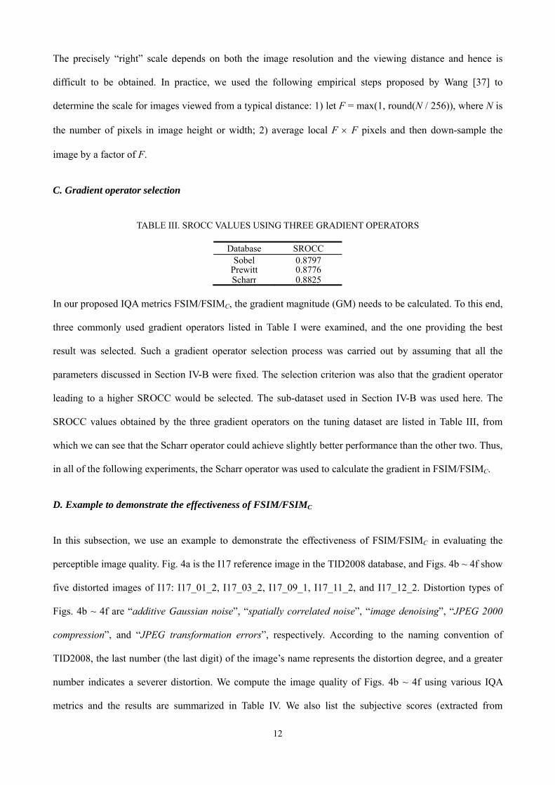
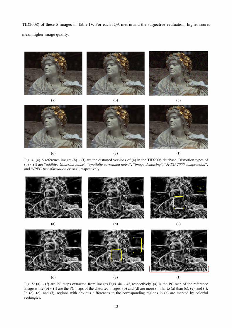
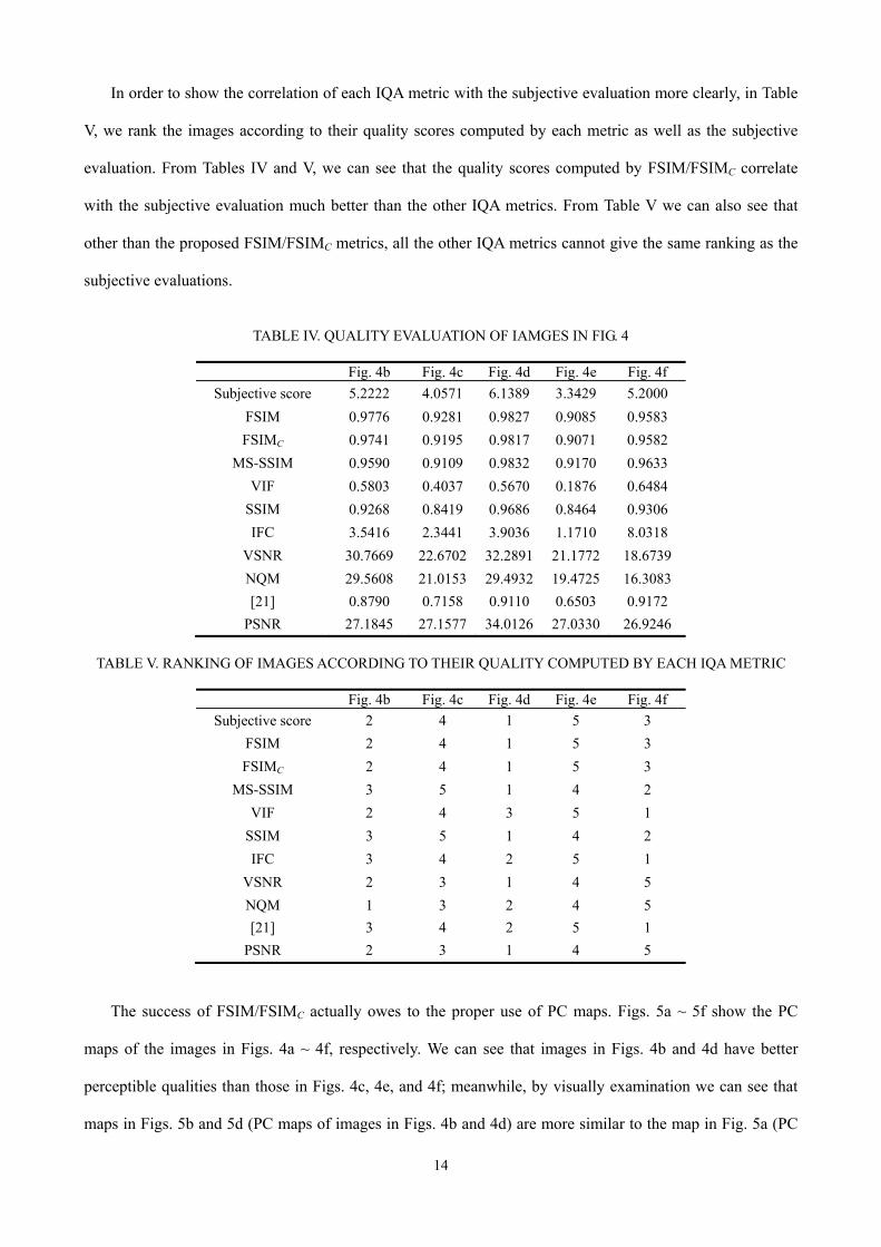
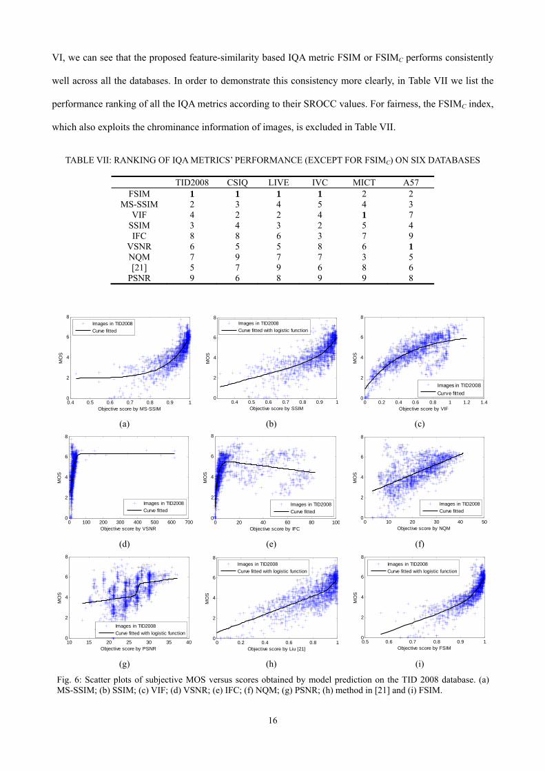
Related Documents