Frozen-RANS Turbulence Model Corrections for Wind Turbine ...

Frozen-RANS Turbulence Model Corrections for WindTurbine Wakes in Stable, Neutral and UnstableAtmospheric Boundary Layers

Master of Science Thesis

L.M. Kokee

Frozen-RANS Turbulence Model Corrections forWind Turbine Wakes in Stable, Neutral and

Unstable Atmospheric Boundary Layers

Master of Science Thesisby

L.M. Kokee

to obtain the degree of Master of Science in Aerospace Engineering at the Delft University of Technology and Masterof Science in Engineering (European Wind Energy) at the Technical University of Denmark,

to be defended publicly on Thursday, August 30, 2021 at 10:00 AM.

Student number: 4466268Project duration: November, 2020 - July, 2021Supervisors: Dr. H. Sarlak, DTU

Dr. R.P. Dwight, TU DelftIr. J. Steiner, TU Delft

An electronic version of this thesis is available at http://repository.tudelft.nl/.

i

Abstract

Computational Fluid Dynamics (CFD) based on RANS models remain the standard but suffer from high errorsin complex flows. In particular, turbulent kinetic energy is over-produced in high strain rate regions, such as thenear-wake of wind turbine flows. Data-driven turbulence modelling methods aim to derive novel turbulence modelswith lower uncertainties, which generalize well to a certain class of flows. The state-of-the-art constitutes to firstderive model-form corrections of a selected baseline model from high fidelity reference data, followed by regressing thecorrections in terms of RANS-known flow features. For data-driven wind turbine wake modelling, industrial-scale windturbines and non-neutral atmospheric boundary layers have yet to be considered. In this thesis, the first steps aremade to address this research gap.

First, Large-Eddy Simulation (LES) data is generated and validated against literature. The considered cases areunder neutral, convective and stable atmospheric conditions. The frozen-RANS methodology, a technique used toderive turbulence model corrections given the high fidelity data, is then extended to non-neutral conditions. The newframework now provides corrections to both the Boussinesq eddy viscosity hypothesis for the Reynolds stress and thegradient-diffusion hypothesis for the turbulent heat flux.

By injecting the obtained corrections into dynamic Reynolds-Averaged Navier-Stokes (RANS) simulations, thebaseline turbulence model deficiencies are corrected. In particular, high rate-of-strain regions now no longer showan overproduction of mechanical turbulence. Similarly, the lack of buoyant turbulence production in the free-streamatmosphere under convective conditions is solved. In the stable case, too large values of buoyant destruction inthe free-stream and buoyant production in the wake are adequately corrected for. For the neutral and stable case,the corrected models produce wake velocity profiles that show excellent agreement with the LES reference data.Issues in the wall stress solution of the convective LES propagate to issues in the corrected RANS solutions, provingthe necessity of high-quality data. Furthermore, it is shown that for most cases a single scalar correction to theturbulent heat flux, as opposed to the full vector correction, is sufficient for improving the error introduced by thegradient-diffusion hypothesis. This result is considerable since the simpler correction would be much easier to regressin terms of mean RANS-known quantities. The computational cost of the corrected RANS models is around the sameas that of baseline RANS models; only 2%-5% of the LES computational cost.

ii

Preface

This thesis is the final deliverable that marks the completion of the European Wind Energy Master. The past twoyears have been incredibly eventful: moving to Denmark to start a new adventure, moving house during the midst ofa pandemic and, of course diving deep into the subject matter in this thesis. Although I am excited to tackle newchallenges, I will cherish the memories I have gained during this master and during this thesis.

I would like to thank my supervisors Richard, Julia and Hamid, for their support. Their guidance has helped menavigate, for the first time, the scientific landscape. Additionally, they have provided me with invaluable support insolving the many technical problems I encountered throughout the entire period of the thesis. I would also like tothank my family, friends and the ones close to me for continually providing me support and helping me become who Iam today.

L.M. KokeeCopenhagen, July 2021

iii

Contents

List of Figures vii

List of Tables x

Nomenclature xi

1 Introduction 11.1 Background . . . . . . . . . . . . . . . . . . . . . . . . . . . . . . . . . . . . . . . . . . . . . . . . 11.2 Research Questions . . . . . . . . . . . . . . . . . . . . . . . . . . . . . . . . . . . . . . . . . . . . 21.3 Research Objectives . . . . . . . . . . . . . . . . . . . . . . . . . . . . . . . . . . . . . . . . . . . . 21.4 Report Structure . . . . . . . . . . . . . . . . . . . . . . . . . . . . . . . . . . . . . . . . . . . . . . 3

2 The Atmospheric Boundary Layer and Wind Turbine Flows 42.1 Driving Forces in the Atmosphere . . . . . . . . . . . . . . . . . . . . . . . . . . . . . . . . . . . . . 42.2 Atmospheric Stability . . . . . . . . . . . . . . . . . . . . . . . . . . . . . . . . . . . . . . . . . . . 52.3 Monin-Obukhov Similarity . . . . . . . . . . . . . . . . . . . . . . . . . . . . . . . . . . . . . . . . . 62.4 Wind Turbines and Wakes . . . . . . . . . . . . . . . . . . . . . . . . . . . . . . . . . . . . . . . . . 7

3 Computational Fluid Dynamics and Turbulence Modelling 103.1 Direct Numerical Simulation . . . . . . . . . . . . . . . . . . . . . . . . . . . . . . . . . . . . . . . 103.2 Large Eddy Simulation . . . . . . . . . . . . . . . . . . . . . . . . . . . . . . . . . . . . . . . . . . 113.3 Reynolds-Averaged Navier-Stokes . . . . . . . . . . . . . . . . . . . . . . . . . . . . . . . . . . . . . 11

3.3.1 k − ε Model . . . . . . . . . . . . . . . . . . . . . . . . . . . . . . . . . . . . . . . . . . . . 123.3.2 Improvements to the k − ε and k − ω Models . . . . . . . . . . . . . . . . . . . . . . . . . . 133.3.3 Non-Linear Eddy-Viscosity Models . . . . . . . . . . . . . . . . . . . . . . . . . . . . . . . . 143.3.4 Reynolds Stress Models . . . . . . . . . . . . . . . . . . . . . . . . . . . . . . . . . . . . . . 143.3.5 Scalar Flux Models . . . . . . . . . . . . . . . . . . . . . . . . . . . . . . . . . . . . . . . . 143.3.6 Non-Neutral Atmospheres . . . . . . . . . . . . . . . . . . . . . . . . . . . . . . . . . . . . . 15

3.4 Turbine Modelling in CFD . . . . . . . . . . . . . . . . . . . . . . . . . . . . . . . . . . . . . . . . . 153.5 Data-Driven Turbulence Modelling . . . . . . . . . . . . . . . . . . . . . . . . . . . . . . . . . . . . 16

3.5.1 Statistical Inference and Uncertainty Quantification . . . . . . . . . . . . . . . . . . . . . . . 163.5.2 Machine Learning . . . . . . . . . . . . . . . . . . . . . . . . . . . . . . . . . . . . . . . . . 17

4 Methodology 214.1 Large-Eddy Simulations . . . . . . . . . . . . . . . . . . . . . . . . . . . . . . . . . . . . . . . . . . 21

4.1.1 Case Definitions . . . . . . . . . . . . . . . . . . . . . . . . . . . . . . . . . . . . . . . . . . 214.1.2 Governing Equations . . . . . . . . . . . . . . . . . . . . . . . . . . . . . . . . . . . . . . . 214.1.3 Numerical Schemes . . . . . . . . . . . . . . . . . . . . . . . . . . . . . . . . . . . . . . . . 224.1.4 Precursor-Successor Approach . . . . . . . . . . . . . . . . . . . . . . . . . . . . . . . . . . 224.1.5 Initial Conditions . . . . . . . . . . . . . . . . . . . . . . . . . . . . . . . . . . . . . . . . . 234.1.6 Boundary Conditions . . . . . . . . . . . . . . . . . . . . . . . . . . . . . . . . . . . . . . . 244.1.7 Turbine Representation . . . . . . . . . . . . . . . . . . . . . . . . . . . . . . . . . . . . . . 274.1.8 Domain and Mesh . . . . . . . . . . . . . . . . . . . . . . . . . . . . . . . . . . . . . . . . . 27

4.2 Frozen-RANS . . . . . . . . . . . . . . . . . . . . . . . . . . . . . . . . . . . . . . . . . . . . . . . 274.2.1 Baseline k − ε model . . . . . . . . . . . . . . . . . . . . . . . . . . . . . . . . . . . . . . . 274.2.2 Postulation of model-form error . . . . . . . . . . . . . . . . . . . . . . . . . . . . . . . . . . 284.2.3 Algorithm Description . . . . . . . . . . . . . . . . . . . . . . . . . . . . . . . . . . . . . . . 294.2.4 Numerical Schemes . . . . . . . . . . . . . . . . . . . . . . . . . . . . . . . . . . . . . . . . 294.2.5 Boundary Conditions . . . . . . . . . . . . . . . . . . . . . . . . . . . . . . . . . . . . . . . 29

iv

4.2.6 Consistency with LES System . . . . . . . . . . . . . . . . . . . . . . . . . . . . . . . . . . . 304.3 Corrected RANS . . . . . . . . . . . . . . . . . . . . . . . . . . . . . . . . . . . . . . . . . . . . . . 31

4.3.1 Governing and Model Equations . . . . . . . . . . . . . . . . . . . . . . . . . . . . . . . . . 314.3.2 Momentum Forcing . . . . . . . . . . . . . . . . . . . . . . . . . . . . . . . . . . . . . . . . 324.3.3 Initial and Boundary Conditions . . . . . . . . . . . . . . . . . . . . . . . . . . . . . . . . . 32

5 Large-Eddy Simulation Results 345.1 Validation Case 1: GABLS . . . . . . . . . . . . . . . . . . . . . . . . . . . . . . . . . . . . . . . . 345.2 Validation Case 2: Abkar & Moin Convective Planetary Boundary Layer . . . . . . . . . . . . . . . . 375.3 Validation Case 3: Rough Wall Atmospheric Log-Law . . . . . . . . . . . . . . . . . . . . . . . . . . 395.4 Main Case Results . . . . . . . . . . . . . . . . . . . . . . . . . . . . . . . . . . . . . . . . . . . . . 40

5.4.1 Neutral Boundary Layer . . . . . . . . . . . . . . . . . . . . . . . . . . . . . . . . . . . . . . 405.4.2 Stable Boundary Layer . . . . . . . . . . . . . . . . . . . . . . . . . . . . . . . . . . . . . . 415.4.3 Convective Boundary Layer . . . . . . . . . . . . . . . . . . . . . . . . . . . . . . . . . . . . 43

5.5 Averaging Period Sensitivity Study . . . . . . . . . . . . . . . . . . . . . . . . . . . . . . . . . . . . 44

6 Frozen-RANS Results 496.1 Neutral Boundary Layer . . . . . . . . . . . . . . . . . . . . . . . . . . . . . . . . . . . . . . . . . . 496.2 Stable Boundary Layer . . . . . . . . . . . . . . . . . . . . . . . . . . . . . . . . . . . . . . . . . . 50

6.2.1 k − ε Model-Form Errors . . . . . . . . . . . . . . . . . . . . . . . . . . . . . . . . . . . . . 506.2.2 Gradient-Diffusion Hypothesis Error . . . . . . . . . . . . . . . . . . . . . . . . . . . . . . . 50

6.3 Convective Boundary Layer . . . . . . . . . . . . . . . . . . . . . . . . . . . . . . . . . . . . . . . . 526.3.1 k − ε Model-Form Errors . . . . . . . . . . . . . . . . . . . . . . . . . . . . . . . . . . . . . 526.3.2 Gradient-Diffusion Hypothesis Error . . . . . . . . . . . . . . . . . . . . . . . . . . . . . . . 53

7 Corrected RANS 577.1 Neutral Boundary Layer . . . . . . . . . . . . . . . . . . . . . . . . . . . . . . . . . . . . . . . . . . 57

7.1.1 Free-Stream Flow . . . . . . . . . . . . . . . . . . . . . . . . . . . . . . . . . . . . . . . . . 577.1.2 Wind Turbine Flow . . . . . . . . . . . . . . . . . . . . . . . . . . . . . . . . . . . . . . . . 57

7.2 Stable Boundary Layer . . . . . . . . . . . . . . . . . . . . . . . . . . . . . . . . . . . . . . . . . . 607.2.1 Free-Stream Flow . . . . . . . . . . . . . . . . . . . . . . . . . . . . . . . . . . . . . . . . . 607.2.2 Wind Turbine Flow . . . . . . . . . . . . . . . . . . . . . . . . . . . . . . . . . . . . . . . . 61

7.3 Convective Boundary Layer . . . . . . . . . . . . . . . . . . . . . . . . . . . . . . . . . . . . . . . . 637.3.1 Free-Stream Flow . . . . . . . . . . . . . . . . . . . . . . . . . . . . . . . . . . . . . . . . . 647.3.2 Wind Turbine Flow . . . . . . . . . . . . . . . . . . . . . . . . . . . . . . . . . . . . . . . . 64

7.4 Averaging Period Effect . . . . . . . . . . . . . . . . . . . . . . . . . . . . . . . . . . . . . . . . . . 707.5 Computational Cost . . . . . . . . . . . . . . . . . . . . . . . . . . . . . . . . . . . . . . . . . . . . 727.6 Discussion . . . . . . . . . . . . . . . . . . . . . . . . . . . . . . . . . . . . . . . . . . . . . . . . . 73

8 Conclusions and Recommendation 758.1 Conclusions . . . . . . . . . . . . . . . . . . . . . . . . . . . . . . . . . . . . . . . . . . . . . . . . 758.2 Recommendations . . . . . . . . . . . . . . . . . . . . . . . . . . . . . . . . . . . . . . . . . . . . . 77

Appendices 84

A LES Successor Results 85A.1 Neutral Boundary Layer Case . . . . . . . . . . . . . . . . . . . . . . . . . . . . . . . . . . . . . . . 85A.2 Stable Boundary Layer Case . . . . . . . . . . . . . . . . . . . . . . . . . . . . . . . . . . . . . . . . 86A.3 Convective Boundary Layer Case . . . . . . . . . . . . . . . . . . . . . . . . . . . . . . . . . . . . . 87

A.3.1 Averaging Period 1 Hour . . . . . . . . . . . . . . . . . . . . . . . . . . . . . . . . . . . . . 87A.3.2 Averaging Period 5 Hours . . . . . . . . . . . . . . . . . . . . . . . . . . . . . . . . . . . . . 87

v

vi

List of Figures

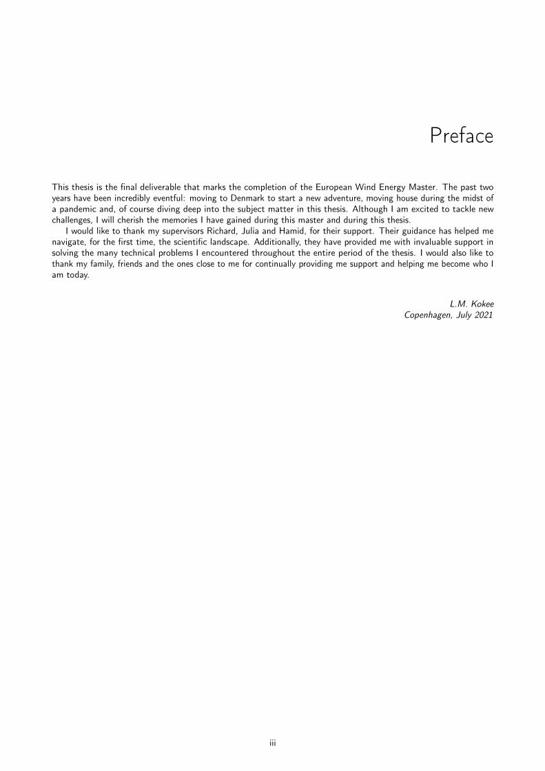
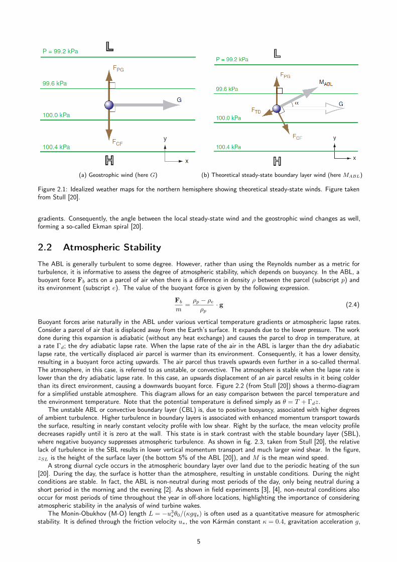
2.1 Idealized weather maps for the northern hemisphere showing theoretical steady-state winds. Figuretaken from Stull [20]. . . . . . . . . . . . . . . . . . . . . . . . . . . . . . . . . . . . . . . . . . . . 5

2.2 Thermo-diagram for a simplified unstable atmosphere. The rising parcel is compared to its environmentin temperature (left) and potential temperature (right). Figure from [20]. . . . . . . . . . . . . . . . 6

2.3 Typical velocity profiles for the unstable, stable and neutral boundary layer. The figure is taken andadapted from Stull [20]. . . . . . . . . . . . . . . . . . . . . . . . . . . . . . . . . . . . . . . . . . . 7

2.4 Schematic of the resultant force acting on the blade element and the decomposed forces. Figureobtained from Porté-Agel, Wu, Lu, et al. [26]. . . . . . . . . . . . . . . . . . . . . . . . . . . . . . . 8

2.5 Schematic of the wake and its distinct regions. Figure obtained from Porté-Agel, Bastankhah, andShamsoddin [28]. . . . . . . . . . . . . . . . . . . . . . . . . . . . . . . . . . . . . . . . . . . . . . 9

2.6 Velocity and potential temperature contours from LES for very stable conditions (left plots) andunstable conditions (right plots). Figure obtained from Machefaux, Larsen, Koblitz, et al. [17]. . . . . 9

3.1 Technical flowchart of the SpaRTA (Sparse Regression of Turbulent Stress Anisotropy) methodology.Figure taken from Schmelzer, Dwight, and Cinnella [13]. . . . . . . . . . . . . . . . . . . . . . . . . 18

3.2 Two numerical solutions . . . . . . . . . . . . . . . . . . . . . . . . . . . . . . . . . . . . . . . . . . 19

4.1 Schematic of the precursor-successor approach to providing inflow conditions for wind turbine flows.The figure is obtained from Matthew J. Churchfield, Lee, Michalakes, et al. [83]. . . . . . . . . . . . 23

4.2 Initial conditions for the potential temperature θ for the CBL case (left) and the SBL case (right) . . 244.3 Flowchart for the Frozen-RANS method to computing model-form errors . . . . . . . . . . . . . . . . 30

5.1 Stable boundary layer case validation results. Left: U (solid) and V (dashed) components of velocity.Right: temperature distribution. Thin black lines represent the GABLS data. . . . . . . . . . . . . . 34

5.2 Stable boundary layer case validation results for the Resolved Reynolds stress components. Thin blacklines represent the GABLS data. . . . . . . . . . . . . . . . . . . . . . . . . . . . . . . . . . . . . . 35

5.3 Stable boundary layer case validation results for the Resolved heat flux components. Thin black linesrepresent the GABLS data. . . . . . . . . . . . . . . . . . . . . . . . . . . . . . . . . . . . . . . . . 35

5.4 Stable boundary layer case validation results for the Vertical momentum flux decomposed into theResolved and SGS components. Thin black lines represent the GABLS data. . . . . . . . . . . . . . . 36

5.5 Convective boundary layer case validation result. Left: Planar averages of mean U (solid) and V(dashed) components of velocity. Right: Planar average of mean potential temperature distribution. . 37

5.6 Convective boundary layer case validation results for the planar averages of the horizontal (left) andvertical (right) resolved stresses, compared to field aircraft observations. . . . . . . . . . . . . . . . . 37

5.7 Convective boundary layer case validation results for the planar averages of the vertical momentumflux decomposed into the Resolved and SGS components. . . . . . . . . . . . . . . . . . . . . . . . . 38

5.8 Convective boundary layer case validation results for planar averages of the vertical heat flux decomposedinto the Resolved and SGS components. . . . . . . . . . . . . . . . . . . . . . . . . . . . . . . . . . 38

5.9 Neutral boundary layer case horizontal velocity planar averages compared to the rough wall ABL log-law 395.10 Neutral boundary layer case convergence based on friction velocity u∗ time series . . . . . . . . . . . 405.11 Neutral boundary layer velocity profiles in the induction region . . . . . . . . . . . . . . . . . . . . . 415.12 Neutral boundary layer velocity and velocity deficit profiles in the wake . . . . . . . . . . . . . . . . . 415.13 Stable boundary layer case convergence based on friction velocity u∗ time series . . . . . . . . . . . . 425.14 Stable boundary layer case wall heat flux qw time series . . . . . . . . . . . . . . . . . . . . . . . . . 425.15 Stable boundary layer induction region velocity profiles . . . . . . . . . . . . . . . . . . . . . . . . . 425.16 Stable boundary layer velocity and velocity deficit profiles in the wake . . . . . . . . . . . . . . . . . 435.17 Convective boundary layer case convergence based on friction velocity u∗ time series . . . . . . . . . 435.18 Convective boundary layer precursor Reynolds stress components . . . . . . . . . . . . . . . . . . . . 44

vii

5.19 CBL case precursor turbulent kinetic energy . . . . . . . . . . . . . . . . . . . . . . . . . . . . . . . 445.20 Convective boundary layer induction region velocity profiles . . . . . . . . . . . . . . . . . . . . . . . 445.21 Convective boundary layer velocity and velocity deficit profiles in the wake . . . . . . . . . . . . . . . 455.22 Sensitivity of wake velocity deficit profiles to the time averaging period for the CBL case . . . . . . . 455.23 Sensitivity of wake turbulent kinetic energy profiles to the time averaging period for the CBL case . . 465.24 Sensitivity of wake potential temperature profiles to the time averaging period for the CBL case . . . 465.25 Sensitivity of wake wall-normal turbulent heat-flux profiles to the time averaging period for the CBL case 475.26 Monin-Obukhov length time series for the convective boundary layer case with Tavg = 5 h . . . . . . 47

6.1 Frozen-RANS results for the NBL precursor case showing the normalized anisotropy error . . . . . . . 506.2 Frozen-RANS results for the NBL precursor case . . . . . . . . . . . . . . . . . . . . . . . . . . . . . 516.3 Contours of frozen-RANS corrections for NBL wind turbine flow, plotted at −1 ≤ x/D ≤ 9 relative to

the turbine . . . . . . . . . . . . . . . . . . . . . . . . . . . . . . . . . . . . . . . . . . . . . . . . . 516.4 Frozen-RANS results for the SBL precursor case showing the normalized anisotropy error . . . . . . . 526.5 Frozen-RANS results for the CBL precursor case . . . . . . . . . . . . . . . . . . . . . . . . . . . . . 526.6 Contours of frozen-RANS corrections for SBL wind turbine flow, plotted at −1 ≤ x/D ≤ 9 relative to

the turbine . . . . . . . . . . . . . . . . . . . . . . . . . . . . . . . . . . . . . . . . . . . . . . . . . 536.7 Frozen-RANS results for the SBL free-stream flow showing the turbulent heat flux error . . . . . . . . 536.8 Frozen-RANS results for the SBL free-stream flow showing various effects of the turbulence heat flux

error . . . . . . . . . . . . . . . . . . . . . . . . . . . . . . . . . . . . . . . . . . . . . . . . . . . . 546.9 Frozen-RANS results for the SBL wind turbine flow showing buoyant turbulence production error,

plotted at −1 ≤ x/D ≤ 9 relative to the turbine . . . . . . . . . . . . . . . . . . . . . . . . . . . . . 546.10 Frozen-RANS results for the CBL precursor case showing the normalized anisotropy error . . . . . . . 546.11 Frozen-RANS results for the CBL precursor case . . . . . . . . . . . . . . . . . . . . . . . . . . . . . 556.12 Contours of frozen-RANS corrections for CBL wind turbine flow, plotted at −1 ≤ x/D ≤ 9 relative to

the turbine . . . . . . . . . . . . . . . . . . . . . . . . . . . . . . . . . . . . . . . . . . . . . . . . . 556.13 Frozen-RANS results for the CBL precursor case showing the turbulent heat flux error . . . . . . . . 566.14 Frozen-RANS results showing various effects of the turbulence heat flux error, plotted at −1 ≤ x/D ≤ 9

relative to the turbine . . . . . . . . . . . . . . . . . . . . . . . . . . . . . . . . . . . . . . . . . . . 566.15 Frozen-RANS results for the CBL successor case showing buoyant turbulence production error . . . . 56

7.1 Free-stream CBL corrected RANS profiles compared to the baseline and to LES . . . . . . . . . . . . 577.2 Corrected RANS Reynolds stress results for the free-stream NBL case . . . . . . . . . . . . . . . . . 587.3 Corrected RANS wake velocity deficit profiles for the NBL case . . . . . . . . . . . . . . . . . . . . . 587.4 Corrected RANS horizontal wake turbulent kinetic energy profiles for the NBL case . . . . . . . . . . 597.5 Corrected RANS velocity results for the free-stream SBL case . . . . . . . . . . . . . . . . . . . . . . 607.6 Free-stream SBL corrected RANS profiles compared to the baseline and to LES . . . . . . . . . . . . 607.7 Corrected RANS Reynolds stress results for the free-stream SBL case . . . . . . . . . . . . . . . . . 617.8 Corrected RANS turbulent heat flux results for the free-stream SBL case . . . . . . . . . . . . . . . . 617.9 Corrected RANS wake velocity deficit profiles for the SBL case . . . . . . . . . . . . . . . . . . . . . 627.10 Corrected RANS wake turbulent kinetic energy profiles for the SBL case . . . . . . . . . . . . . . . . 627.11 Corrected RANS wake Reynolds stress xz-component profiles for the SBL case . . . . . . . . . . . . 637.12 Corrected RANS wake potential temperature profiles for the SBL case . . . . . . . . . . . . . . . . . 637.13 Corrected RANS wake wall-normal heat flux profiles for the SBL case . . . . . . . . . . . . . . . . . 647.14 Corrected RANS velocity results for the free-stream CBL case . . . . . . . . . . . . . . . . . . . . . 657.15 Free-stream CBL corrected RANS profiles compared to the baseline and to LES . . . . . . . . . . . . 657.16 Corrected RANS Reynolds stress results for the free-stream CBL case . . . . . . . . . . . . . . . . . 667.17 Corrected RANS turbulent heat flux results for the free-stream CBL case . . . . . . . . . . . . . . . 667.18 Corrected RANS wake velocity deficit profiles for the CBL case . . . . . . . . . . . . . . . . . . . . . 677.19 Corrected RANS wake turbulent kinetic energy profiles for the CBL case . . . . . . . . . . . . . . . . 677.20 Corrected RANS wake Reynolds stress xz-component profiles for the CBL case . . . . . . . . . . . . 687.21 Corrected RANS wake wall-normal turbulent heat flux profiles for the CBL case . . . . . . . . . . . . 687.22 Corrected RANS wake potential temperature profiles for the CBL case . . . . . . . . . . . . . . . . . 697.23 Corrected RANS wake eddy viscosity for the CBL case, compared to the frozen case eddy viscosity . . 697.24 Corrected RANS wake velocity deficit profiles for the CBL case using a five-hour averaging period . . 707.25 Corrected RANS wake turbulent kinetic energy profiles for the CBL case using a five-hour averaging

period . . . . . . . . . . . . . . . . . . . . . . . . . . . . . . . . . . . . . . . . . . . . . . . . . . . 717.26 Corrected RANS wake wall-normal turbulent heat flux profiles for the CBL case using a five-hour

averaging period . . . . . . . . . . . . . . . . . . . . . . . . . . . . . . . . . . . . . . . . . . . . . . 717.27 NBL case RANS residuals for the corrections applied right from simulation start (instant), gradually

over 100 iterations (100 It) and for the baseline k − ε model (baseline) . . . . . . . . . . . . . . . . 72

viii

A.1 Neutral boundary layer velocity and velocity deficit profiles in the wake . . . . . . . . . . . . . . . . . 85A.2 Neutral boundary layer wake TKE profiles . . . . . . . . . . . . . . . . . . . . . . . . . . . . . . . . 85A.3 Stable boundary layer velocity and velocity deficit profiles in the wake . . . . . . . . . . . . . . . . . 86A.4 Stable boundary layer wake TKE profiles . . . . . . . . . . . . . . . . . . . . . . . . . . . . . . . . . 86A.5 Stable boundary layer vertical wake heat-flux profiles . . . . . . . . . . . . . . . . . . . . . . . . . . 86A.6 Stable boundary layer horizontal wake heat-flux profiles . . . . . . . . . . . . . . . . . . . . . . . . . 87A.7 Convective boundary layer velocity and velocity deficit profiles in the wake obtained with Tavg = 1 h . 87A.8 Convective boundary layer wake TKE profiles obtained with Tavg = 1 h . . . . . . . . . . . . . . . . 88A.9 Convective boundary layer vertical wake heat-flux profiles . . . . . . . . . . . . . . . . . . . . . . . . 88A.10 Convective boundary layer horizontal wake heat-flux profiles obtained with Tavg = 1 h . . . . . . . . 88A.11 Convective boundary layer velocity and velocity deficit profiles in the wake obtained with Tavg = 5 h . 89A.12 Convective boundary layer wake TKE profiles obtained with Tavg = 5 h . . . . . . . . . . . . . . . . 89A.13 Convective boundary layer vertical wake heat-flux profiles obtained with Tavg = 5 h . . . . . . . . . . 89A.14 Convective boundary layer horizontal wake heat-flux profiles obtained with Tavg = 5 h . . . . . . . . 90

ix

List of Tables

2.1 Atmospheric stability classes, as defined by the Monin-Obukhov Length. Table obtained from Peña,Gryning, and Mann [21]. . . . . . . . . . . . . . . . . . . . . . . . . . . . . . . . . . . . . . . . . . 6

2.2 Empirically determined coefficients of the Monin-Obukhov functions . . . . . . . . . . . . . . . . . . 8

4.1 General parameters and conditions used in the LES cases . . . . . . . . . . . . . . . . . . . . . . . . 214.2 Finite volume schemes for LES solver . . . . . . . . . . . . . . . . . . . . . . . . . . . . . . . . . . . 224.3 Boundary conditions of the LES precursor cases under neutral (N), stable (S) and unstable (U) conditions 254.4 Boundary conditions of the LES successor cases under neutral (N), stable (S) and unstable (U) conditions 264.5 Domain size Lx · Ly · Lz for the LES precursor and successor stages . . . . . . . . . . . . . . . . . . 274.6 Mesh resolution and refinement zones for the CBL precursor case . . . . . . . . . . . . . . . . . . . . 274.7 Standard model coefficients for the selected k − ε ABL model, under neutral, stable and unstable

conditions . . . . . . . . . . . . . . . . . . . . . . . . . . . . . . . . . . . . . . . . . . . . . . . . . 284.8 Finite volume schemes for RANS and frozen-RANS solvers . . . . . . . . . . . . . . . . . . . . . . . 294.9 Boundary conditions for the Frozen-RANS cases . . . . . . . . . . . . . . . . . . . . . . . . . . . . . 314.10 LES friction velocity and wall turbulent kinetic energy . . . . . . . . . . . . . . . . . . . . . . . . . . 314.11 k − ε model coefficients that ensure consistency with the LES reference for the NBL case, SBL and

CBL case . . . . . . . . . . . . . . . . . . . . . . . . . . . . . . . . . . . . . . . . . . . . . . . . . . 314.12 Mean LES rotor revolutions per minute (RPM) and pitch angle, used as input settings for the RANS

cases . . . . . . . . . . . . . . . . . . . . . . . . . . . . . . . . . . . . . . . . . . . . . . . . . . . . 324.13 Boundary conditions for the RANS cases under neutral (N), stable (S) and unstable (U) conditions . 33

5.1 General time-averaged LES results . . . . . . . . . . . . . . . . . . . . . . . . . . . . . . . . . . . . 40

6.1 Shear and buoyancy production based normalization metrics for the frozen correction figures. D =126 m and zi = 1070 m. . . . . . . . . . . . . . . . . . . . . . . . . . . . . . . . . . . . . . . . . . 49

7.1 Computational cost for the various models, measured by wall-clock time and core-time . . . . . . . . 72

x

Nomenclature

Acronyms

ABL Atmospheric boundary layer

ADM Actuator disc model

ALM Actuator line model

CAD Computer aided design

CBL Convective boundary layer

CFD Computational fluid dynamics

CFL Courant-Friedrichs-Lewy

DNS Direct Numerical Simulation

FS Free-stream

GDH Gradient diffusion hypothesis

LES Large-Eddy Simulation

LEVM Linear eddy-viscosity model

LiDAR Light detection and ranging

M-O Monin-Obukhov

MAP Maximum a posteriori estimate

MOST Monin-Obukhov similarity theory

NLEVM Non-linear eddy viscosity model

RANS Reynolds Averaged Navier-Stokes

RSM Reynolds stress model

SBL Stable boundary layer

SOWFA Simulator for Offshore Wind Farm Applications

SpaRTA Sparse Regression of Turbulent Stress Anisotropy

SST Shear stress transport

TKE Turbulent kinetic energy

Greek Symbols

δ Discrepancy or error

δij Kronecker delta −

ε Dissipation rate m2/s3

ε Gaussian mapping width parameter −

xi

η Kolmogorov scale m

Γd Dry adiabatic lapse rate K/m

κ Von Karman constant −

ν Kinematic viscosity m2/s

ω Earth’s rotation rate rad/s

ω Specific dissipation rate 1/s

φ Latitude rad

Φh Monin-Obukhov function for temperature −

Φm Monin-Obukhov function for velocity −

Ψh Integrated Monin-Obukhov function for temperature

Ψm Integrated Monin-Obukhov function for velocity

ρ Density kg/m3

ρk Buoyant density −

τSGSij Sub-grid (sub-filter) stress tensor m2/s2

θ Measurement (or reference) data

θ Potential temperature K

θ∗ Surface layer temperature scale K

Roman Symbols

L Characteristic length m

U Mean stream-wise flow velocity m/s

∆U Mean stream-wise velocity deficit m/s

P Probability

M Model

u′iu′j Reynolds stress tensor m2/s2

u′jθ′ Turbulent heat-flux Km/s

u Filtered velocity m/s

B Buoyant turbulent production m2/s3

bij Normalized Reynolds stress anisotropy tensor −

b∆ij Model-form error of Reynolds stress anisotropy

c Model coefficients

D Drag force N

F Force N

G Geostrophic wind speed m/s

gi Gravitational acceleration m/s2

k Turbulent kinetic energy m2/s2

kSGS Sub-grid scale turbulent kinetic energy m2/s2

L Lift force N

xii

L Monin-Obukhov length m

M Theoretical steady state ABL wind speed m/s

m Fluid parcel or object mass kg

p Static pressure N/m2

P Mean static pressure N/m2

Pk Mechanical turbulent production m2/s3

Pr Prandtl number −

Prt Turbulent Prandtl number −

q∆j Turbulent heat-flux error Km/s

qSGSj Sub-grid (sub-filter) scale heat flux Km/s

qs Surface heat flux Km/s

R k transport equation residual (error)

Re Reynolds Number −

Rib Bulk Richardson number −

Sij The mean strain-rate tensor 1/s

t Time s

T Temperature K

u′ Fluctuating velocity m/s

u′′ Sub-filter velocity m/s

u∗ Friction velocity m/s

U0 Free-stream velocity m/s

ui Velocity m/s

Ui Mean velocity m/s

x Stream-wise coordinate m

y Lateral coordinate m

z Wall-normal coordinate m

z0 Roughness length m

xiii

1

Introduction

1.1 Background

It is projected that wind energy will cover 22%-30% of Europe’s energy demand by 2030. A significant increase fromthe 15% wind energy share in 2015 [1]. Off-shore wind energy will likely increase in share due to the ever-increasingproject scales. To meet these targets, the levelized cost of energy of offshore wind needs to be further reduced. Inorder to do so, turbine manufacturers and operators require detailed knowledge about the conditions in which turbineswill operate.

The design and optimization of wind turbines and wind farms is a complex process. The turbine wakes are turbulentregions of a velocity deficit with the free-steam. Any turbine immersed in a wake will have lower power productionand higher fatigue loading. Designers must therefore understand the structure and dynamics of wind turbine wakes,as well as the interaction of multiple wakes in a farm. The relationship of wake dynamics with atmospheric stabilityis also important. On-shore, the atmospheric boundary layer (ABL) is stable or unstable most periods of the day,only being neutral during a short period in the morning and the evening [2]. Field experiments [3], [4] show thatnon-neutral conditions also occur for most periods of time throughout the year in off-shore locations.

Currently, Large-Eddy Simulation (LES) is the most appropriate method of simulating wind farm flows. Themost significant scales of turbulent motion are fully resolved, leading to accurate solutions that include most of thephysical phenomena in real wind farms. Reynolds-Averaged Navier-Stokes (RANS) simulations have a computationcost of about two orders of magnitude lower compared to LES [5], making them the tool of choice in industry. RANSmodels come in a multiplicity of flavours, with linear-eddy viscosity models (LEVM) the most popular and commonones [6]. The reduced computational cost of these models, however, comes at a price. The assumptions made inthe turbulence models fail in a several complex, but common, flow cases[7], [8], including wind turbine flows [9].The main problems include an over-prediction of turbulent kinetic energy in the edges of the near wake, resulting inincreased turbulent mixing and an under-prediction of the wake velocity deficit. Numerous attempts have been madeto construct engineering fixes to the turbulence models to improve the velocity predictions in the wake, with varyingsuccess. Most fixes do not generalize well beyond training cases and fail to account for atmospheric stability, leavingroom for improvement.

Data-driven turbulence models aim to improve the limitations of turbulence models by assimilating higher-fidelityreference data. Various machine learning algorithms have been applied to turbulence modelling. Deep neural networksemerged first, as these have become massively popular in numerous other fields of science [10]. The drawback of’black-box’ methods, such as neural nets and random forests, is the lack of interpretability. The modeller is unableto evaluate the relation that is learned by the algorithm or manually tweak the model to match physical needs orimprove stability. Symbolic data-driven techniques, on the other hand, output explicit algebraic relations. Geneexpression programming has been successfully demonstrated by Weatheritt and Sandberg [11] and Weatheritt andSandberg [12], and Schmelzer, Dwight, and Cinnella [13] demonstrated a novel framework for symbolic data-driventurbulence modelling; Sparse Regression of Turbulent Stress Anisotropy (SpaRTA). An additional benefit of a symbolicapproach is that the resulting models are easily implemented in RANS solvers. Instead of applying machine learningdirectly to generalize the Reynolds stress tensor, it is more effective to first assess the error an existing turbulencemodel has with respect to the reference data, and then generalize that error with machine learning [14]. The twoapproaches commonly used for evaluating the turbulence model error are (i) Bayesian statistical inference, and (ii)frozen-RANS. With Bayesian inference, full-field data is not required. Frozen-RANS based approaches, on the otherhand, do require full-field reference data but do not require an expensive inversion process [13]. It was shown fork-corrective-frozen-RANS (a development from the basic version) that a near-perfect match with the reference data isobtained when the derived error is injected into RANS as a correction [5], [13].

Steiner, Dwight, and Viré [5] applied the SpaRTA methodology to moderate Reynolds number wind turbineflows and significantly improved the baseline turbulence model. This study constituted an intermediate step between

1

canonical flows and industrial-scale flows. Future work in this research avenue is to apply SpaRTA to such full-scaleflows and to improve numerical stability on various mesh resolutions. In most literature on data-driven turbulencemodelling, the energy or temperature equation was not included. Some studies attempt to discover new scalar fluxmodels using machine learning [15], [16], but these did not test the derived models in coupled RANS solvers. Theyonly considered a priori determination of the heat flux on mean LES fields. This is likely due to the limitations ofthe underlying RANS turbulence model. To the best of the author’s knowledge, simultaneous data-driven turbulencemodel improvements for the Reynolds stress and scalar-flux in heated flows have not yet been considered.

In this thesis, the research gap of simultaneous data-driven Reynolds stress and scalar-flux modelling improvementswill be addressed while considering wind turbine wake flows under neutral, stable and unstable atmospheric conditions.Several LES studies for wind turbine flows in non-neutral conditions have already been conducted in literature [17]–[19][19]. Unfortunately, for some of these studies, the time-averaged field data is no longer saved, while for others thespecific data required for the present study was never saved at all. For this reason, and to ensure a certain quality,in-house large-eddy simulations are developed and validated within this thesis. Afterwards, the existing frozen-RANSframework is extended to obtain the model-form error of the turbulent heat flux. This framework will be applied toseveral non-neutral cases. The novel frozen-RANS framework is then validated by injecting the obtained model-formerrors, now as corrections, into the RANS turbulence model during simulation run time. The performance of thecorrected RANS model is then evaluated by comparison against the baseline RANS model and the LES reference data.This thesis aims to pave the way for further research on machine learning of turbulence models for industrial-scalewind turbines for non-neutral atmospheric conditions.

1.2 Research Questions

The project can be deemed finished when the research questions (RQ) and their sub-questions (SQ) have beenanswered. The various research questions are:

(RQ1): What are the model-form errors of the k − ε and GDH model in stable and unstable wind turbineflows, and how do they differ from neutral wind turbine flows?

(RQ2): What are the considerations injecting the model-form corrections into the RANS equations duringsimulation?

(RQ3): What is the accuracy of the corrected RANS models compared to the baseline RANS model and theLES model?

(RQ4): How does the computational cost of the corrected RANS model compare to the baseline and LESmodels?

(RQ5): How is the frozen-RANS framework best extended to stable and unstable conditions?

1.3 Research Objectives

To answer the research questions, the main research objective, and the sub-objectives must be achieved.

"To contribute to algebraic data-driven turbulence model development, and the understanding of turbulencefor industrial-scale wind turbine flows in neutral and non-neutral atmospheric conditions, by inferring themodel form error of the benchmark k − ε turbulence model and the gradient-diffusion scalar-flux modelfrom high fidelity data."

The following sub-objectives (SO) are formulated in support of the main objective.

(SO1): To generate ground-truth reference data by running Large-Eddy Simulations with the open-sourceCFD package OpenFOAM-SOWFA.

(SO2): To determine the model form corrections of the k − ε and Gradient-Diffusion Hypothesis models byformulating a novel frozen-RANS framework in OpenFOAM-SOWFA.

(SO3): To validate the model form corrections by injecting them into the OpenFOAM-SOWFA solvers andcomparing against the ground truth.

(SO4): To determine the regions and mechanisms of baseline turbulence model failure by assessing thevalidated model form corrections.

2

1.4 Report Structure

Firstly, the thesis contains a summary of the relevant literature on the atmospheric boundary layer, atmosphericstability and wind turbine flows in chapter 2. Chapter 3 contains a summary of the relevant literature on CFD,turbulence modelling and data-driven turbulence model improvements. The complete methodology of LES datageneration, frozen-RANS framework and the corrected RANS simulations are presented in chapter 4. The LES resultsand validation are shown in chapter 5, after which the frozen-RANS model-form errors are discussed in chapter 6.The corrected RANS models are tested against the baseline and the LES model in chapter 7. Finally, the conclusionsand recommendations to future work are discussed in chapter 8.

3

2

The Atmospheric Boundary Layer and WindTurbine Flows

When a solid object is immersed in a fluid flow, a boundary layer forms over the surface of the object. Adhesioncauses the fluid to have the same velocity as the object on the surface of the object, and diffusive effects smooth thevelocity profile, which becomes the free stream velocity outside of the boundary layer. Laminar boundary layers arecharacterized by the fluid moving in orderly parallel shear layers, whereas turbulent boundary layers are characterizedby chaotic motions in the fluid, higher degrees of mixing and higher skin friction. The Reynolds number of the flow,defined as the ratio between the inertial and viscous forces, is used to determine or indicate whether a flow is laminar,turbulent or in a state of transition between the two. The Reynolds number is defined based on a characteristic lengthof the flow L.

Re =UL

ν(2.1)

U and ν are the free stream velocity and the kinematic viscosity, respectively. The bottom 300 m-3 km of thetroposphere is known as the atmospheric boundary layer (ABL). Just as with any other boundary layer, the flowvelocity is zero at the surface and equal to the free-stream outside of the boundary layer, which is the geostrophic windspeed in case of the atmospheric boundary layer. The ABL is the only part of the atmosphere that is directly affectedby the presence of the Earth’s surface. Besides the drag due to surface roughness, these effects are the heating of airduring the day, cooling of air during the night, and changes in humidity and pollutant concentration [20].

The geostrophic wind speed and driving forces in the ABL are discussed in section 2.1. Atmospheric stability andMonin-Obukhov similarity theory are discussed in section 2.2 and section 2.3, respectively. Finally, a brief summary ofwind turbine flows is presented in section 2.4.

2.1 Driving Forces in the Atmosphere

The winds in Earth’s atmosphere are driven by a multiplicity of forces. Generally speaking, these wind driving forcesare time-varying and depend on heat and moisture, which are convected with the air. This results in a complicatedcoupling that we refer to as weather [20]. The geostrophic wind speed is defined as the wind speed in which the freeatmosphere (the part of the troposphere above the atmospheric boundary layer) is in geostrophic balance. In otherwords, the geostrophic wind speed is the theoretical steady-state wind speed above the ABL [20]. Two forces areimportant for the determination of the geostrophic wind speed: the horizontal pressure gradient force and the Coriolisforce. The pressure gradient force and the Coriolis force are by eq. (2.2) and eq. (2.3), respectively.

FPGm

= −1

ρ∇P (2.2)

FCm

= −2Ω × U , Ω = ω

0cos(φ)sin(φ)

(2.3)

Here, ω is Earth’s rotation rate and φ is the latitude. Since the pressure gradient force and the Coriolis force are theonly acting forces, and the Coriolis force acts normal to the velocity vector per definition, both forces cancel out andthe geostrophic wind blows parallel to the isobars in weather maps. This is illustrated in fig. 2.1a, taken from Stull[20]. When considering the theoretical steady-state wind speed inside the ABL, the surface drag force needs to beconsidered as well. This drag not only slows the wind but also rotates it with respect to the geostrophic wind speed.In fig. 2.1b, also taken from Stull [20], it is seen that the vector sum of the drag and the Coriolis force cancel thepressure gradient force. The theoretical steady-state forces vary as a function of depth in the ABL due to the local

4

(a) Geostrophic wind (here G) (b) Theoretical steady-state boundary layer wind (here MABL)

Figure 2.1: Idealized weather maps for the northern hemisphere showing theoretical steady-state winds. Figure takenfrom Stull [20].

gradients. Consequently, the angle between the local steady-state wind and the geostrophic wind changes as well,forming a so-called Ekman spiral [20].

2.2 Atmospheric Stability

The ABL is generally turbulent to some degree. However, rather than using the Reynolds number as a metric forturbulence, it is informative to assess the degree of atmospheric stability, which depends on buoyancy. In the ABL, abuoyant force Fb acts on a parcel of air when there is a difference in density ρ between the parcel (subscript p) andits environment (subscript e). The value of the buoyant force is given by the following expression.

Fbm

=ρp − ρeρp

· g (2.4)

Buoyant forces arise naturally in the ABL under various vertical temperature gradients or atmospheric lapse rates.Consider a parcel of air that is displaced away from the Earth’s surface. It expands due to the lower pressure. The workdone during this expansion is adiabatic (without any heat exchange) and causes the parcel to drop in temperature, ata rate Γd; the dry adiabatic lapse rate. When the lapse rate of the air in the ABL is larger than the dry adiabaticlapse rate, the vertically displaced air parcel is warmer than its environment. Consequently, it has a lower density,resulting in a buoyant force acting upwards. The air parcel thus travels upwards even further in a so-called thermal.The atmosphere, in this case, is referred to as unstable, or convective. The atmosphere is stable when the lapse rate islower than the dry adiabatic lapse rate. In this case, an upwards displacement of an air parcel results in it being colderthan its direct environment, causing a downwards buoyant force. Figure 2.2 (from Stull [20]) shows a thermo-diagramfor a simplified unstable atmosphere. This diagram allows for an easy comparison between the parcel temperature andthe environment temperature. Note that the potential temperature is defined simply as θ = T + Γdz.

The unstable ABL or convective boundary layer (CBL) is, due to positive buoyancy, associated with higher degreesof ambient turbulence. Higher turbulence in boundary layers is associated with enhanced momentum transport towardsthe surface, resulting in nearly constant velocity profile with low shear. Right by the surface, the mean velocity profiledecreases rapidly until it is zero at the wall. This state is in stark contrast with the stable boundary layer (SBL),where negative buoyancy suppresses atmospheric turbulence. As shown in fig. 2.3, taken from Stull [20], the relativelack of turbulence in the SBL results in lower vertical momentum transport and much larger wind shear. In the figure,zSL is the height of the surface layer (the bottom 5% of the ABL [20]), and M is the mean wind speed.

A strong diurnal cycle occurs in the atmospheric boundary layer over land due to the periodic heating of the sun[20]. During the day, the surface is hotter than the atmosphere, resulting in unstable conditions. During the nightconditions are stable. In fact, the ABL is non-neutral during most periods of the day, only being neutral during ashort period in the morning and the evening [2]. As shown in field experiments [3], [4], non-neutral conditions alsooccur for most periods of time throughout the year in off-shore locations, highlighting the importance of consideringatmospheric stability in the analysis of wind turbine wakes.

The Monin-Obukhov (M-O) length L = −u3∗θ0/(κgqs) is often used as a quantitative measure for atmospheric

stability. It is defined through the friction velocity u∗, the von Karman constant κ = 0.4, gravitation acceleration g,

5

Figure 2.2: Thermo-diagram for a simplified unstable atmosphere. The rising parcel is compared to its environment intemperature (left) and potential temperature (right). Figure from [20].

the surface heat flux qs and the reference potential temperature θ0. Peña, Gryning, and Mann [21] distinguishedbetween several stability classifications based on the Monin-Obukhov Length. These classifications are shown intable 2.1. Another common method for quantifying atmospheric stability in field measurements is the Bulk-Richardsonapproach, based on Rib, the Bulk-Richardson number [17]. Pandolfo [22] derived simple empirical relationships thatrelate the Bulk-Richardson number to the Monin-Obukhov length.

Table 2.1: Atmospheric stability classes, as defined by the Monin-Obukhov Length. Table obtained from Peña, Gryning,and Mann [21].

Monin-Obukhov length Stability class−100 ≤ L ≤ −50 Very unstable−200 ≤ L ≤ −100 Unstable−500 ≤ L ≤ −200 Near unstable|L| > 500 Neutral

200 ≤ L ≤ 500 Near stable50 ≤ L ≤ 200 Stable10 ≤ L ≤ 50 Very stable

2.3 Monin-Obukhov Similarity

Monin-Obukhov similarity theory describes the structure of the surface layer, the lowest part of the ABL. Usingdimensional analysis and the Buckingham-Pi theorem, two non-dimensional independent variables are said to befunctionally related, making one a dependant variable. The formulation is such that the dependant variable is afunction only of the z/L, L being the Monin-Obukhov (M-O) length. The resulting expression for the constant surfacelayer wind speed gradient is given by eq. (2.5). The surface layer potential temperature gradient is given by eq. (2.6).

κz

u∗

∂U

∂z= Φm

(z

L

)(2.5)

κz

θ∗

∂θ

∂z= Φh

(z

L

)(2.6)

6

Figure 2.3: Typical velocity profiles for the unstable, stable and neutral boundary layer. The figure is taken andadapted from Stull [20].

The functions Φm and Φh are called the M-O functions. They are said to be universal, meaning they are identicalfor all surface layers that are locally homogeneous and quasi-steady. The surface layer temperature scale is definedas θ∗ =

θ0u2∗

gκL . The M-O functions are linear in the stable region but have a more complex form in the unstableregion. Using an analytical formulation for the functions allows for integration of eq. (2.5) and eq. (2.6), resulting inexpressions for the mean velocity profile eq. (2.7), and mean potential temperature profile eq. (2.8). These expressionsare, however, only valid in the surface layer, which roughly constitutes the bottom 5% of the ABL [20].

U(z) =u∗κ

[ln

(z

z0

)−Ψm

( zL

)](2.7)

Θ(z) = θ0 +θ∗κ

[ln

(z

z0

)−Ψh

( zL

)](2.8)

The roughness length z0 a parameter which characterizes the surface roughness. It is reported in Laan, Kelly, andSørensen [23] that the most commonly used functions for Φm and Φh, and the resulting Ψm and Ψh are those ofthe field measurements of Dyer [24] and Businger, Wyngaard, Izumi, et al. [25]. They are shown in eq. (2.9) andeq. (2.10), with the corresponding coefficients shown in table 2.2.

Ψm = ln

[1

8(1 + Φ−2

m )(1 + Φ−1m )2

]− 2arctan(Φ−1

m ) +π

2

Unstable conditions Ψh = (1 + σθ)ln[1

2(1 + Φ−1

h )]

+ (1− σθ)ln[1

2(−1 + Φ−1

h

](2.9)

Φm =(

1− γ1z

L

)−1/4

Φh = σθ

(1− γ2

z

L

)−1/2

Ψm = −β zL

Stable conditions Ψh = (1− σθ)ln( zL

)− β z

L(2.10)

Φm = 1 + βz

L

Φh = σθ + βz

L

2.4 Wind Turbines and Wakes

Wind turbines are energy conversion devices that extract momentum from the air. At the level of the blade cross-section(or blade-element), the flow around the blade-element induces a result force F , as shown in fig. 2.4, obtained from

7

Table 2.2: Empirically determined coefficients of the Monin-Obukhov functions

σθ β γ1 γ2

Businger, Wyngaard, Izumi, et al. [25] 0.74 4.7 15 9Dyer [24] 1 5 16 16

Porté-Agel, Wu, Lu, et al. [26]. The sum, over all three blades, of the normal component Fx results in a thrust forceon the turbine. The tangential components Fθ contribute towards the torque that drives the generator.

Figure 2.4: Schematic of the resultant force acting on the blade element and the decomposed forces. Figure obtainedfrom Porté-Agel, Wu, Lu, et al. [26].

By Newton’s third law, the wind turbine blades produce a stream-wise and tangential force that acts upon theair, affecting the flow field. Distinct regions are often distinguished when discussing wind turbine flows. Upwind ofthe turbine, there is the induction region, which is characterised by decelerated air. Downwind of the turbine, thereis the wake region, which is characterised by a velocity deficit (due to the momentum extraction) and by increasedturbulence. The wake is further divided into the near wake and the far wake. The near wake stretches until 2-4 rotordiameters downwind of the turbine. In this region, one will find coherent helical vortical structures that originatefrom the blade tips and from the turbine hub. The flow field in the near wake is directly affected by the blade, huband nacelle geometry [27]. The far wake, however, is independent of the specific geometry and can be characterisedby the global operating parameters, such as the tip-speed ratio and thrust coefficient. Large scale meandering isobserved in turbine wakes in the atmospheric boundary layer. These motions are associated with very large turbulentfluctuations in the atmosphere. Figure 2.5 shows a schematic of the flow around wind turbines. The figure is takenfrom Porté-Agel, Bastankhah, and Shamsoddin [28].

Understanding the behaviour of the far wake is crucial because wind turbines in large wind farms usually operatein the far wake of upstream turbines. The mean stream-wise velocity deficit ∆U = U0 − U , U0 being the meanstream-wise incoming velocity, is shown to closely match the axisymmetric Gaussian distribution in wind tunnelexperiments of a wind turbine in boundary layer flow [29]. Since the Gaussian profile is self-similar, the normalized(by magnitude and width) velocity deficit profile is independent of stream-wise position in the far wake. This hasfacilitated the development of several analytical models. It should be noted that the Gaussian profile is only observedfor standalone turbines, not for turbines that operate in the wakes of other turbines. As the distance from the turbineincreases, the wake expands and the velocity recovers due to turbulent mixing with the undisturbed air outside of thewake.

It was shown in field measurements [17], [30], [31] that The wake deficit and rate of recovery depend strongly onatmospheric stability. The quicker wake recovery for unstable cases is associated with wake meandering caused bylarge convective motions [17], as well as an earlier breakdown of tip vortices, resulting in higher entrainment withthe flow outside of the wake [28]. Figure 2.6 shows contour plots of instantaneous and time-averaged velocity for avery stable atmosphere (left) and an unstable atmosphere (right), obtained from Machefaux, Larsen, Koblitz, et al.[17]. The authors show a higher meandering amplitude for the unstable case, but also mention that these LES resultsstill under-predict the unstable meandering magnitude compared to their field experiments. Consequently, their LESslightly under-predicts wake recovery.

8

Figure 2.5: Schematic of the wake and its distinct regions. Figure obtained from Porté-Agel, Bastankhah, andShamsoddin [28].

Figure 2.6: Velocity and potential temperature contours from LES for very stable conditions (left plots) and unstableconditions (right plots). Figure obtained from Machefaux, Larsen, Koblitz, et al. [17].

9

3

Computational Fluid Dynamics and TurbulenceModelling

Computational Fluid Dynamics (CFD) is the field of science that involves methods for finding numerical solutionsto the governing equations of fluid flow. These equations are the conservation of mass, momentum and energy,and are often referred to as the Navier-Stokes equations. There are various methods to solve these equations, eachwith a different level of fidelity and computational cost. The three main methods are Direct Numerical Simulation,Large-Eddy Simulation and Reynolds-Averaged Simulation. These are discussed in section 3.1, section 3.2 andsection 3.3, respectively. A short discussion on buoyancy is included in section 3.1. Section 3.4 presents variousmethods of handling turbines in CFD and, finally, data-driven turbulence modelling approaches are discussed insection 3.5.

3.1 Direct Numerical Simulation

Direct Numerical Simulation (DNS) is the CFD type in which the governing equations are solved as is, without anyturbulence model. All turbulent scales are fully resolved. Excluding the energy equation, and assuming constantdensity, the Navier-Stokes equations are as follows.

∂ui∂xi

= 0 (3.1)

∂ui∂t

+∂uiuj∂xj

= −1

ρ

∂p

∂xi+ ν

∂2ui∂xj∂xj

+ gi (3.2)

With ui the fluid velocity, p the static pressure, ν the kinematic viscosity and gi the gravitational acceleration vector.A requirement when doing DNS is that the mesh needs to be sufficiently fine in order to resolve any turbulent eddybetween the largest scales in the flow, of size L, and the smallest Kolmogorov scales, of size η. The size ratio betweenthe Kolmogorov scale and the largest scale is known given by the following equation [7].

η

L= Re−3/4 (3.3)

Most fluid flows in nature and engineering are of very large Reynolds number. As such, a very fine mesh is required inorder to resolve the Kolmogorov scales. The computational cost of DNS is therefore prohibitive for most practicalcases.

Strictly speaking, the full compressible governing equations are required in the CFD formulation for atmosphericboundary layers, since temperature variations result in density variations. However, using the Boussinesq buoyancyapproximation for the buoyant force term allows for the use of the incompressible flow equations. The approximationis obtained by expanding the gravitational force term in the momentum equation, ρgi into a constant reference term,indicated by subscript 0, and a term that constitutes the difference with the constant.

ρgi = ρ0gi + (ρ− ρ0)gi (3.4)

Here, ρ is the density which varies with temperature T and ρ0 is the constant reference density. A first-order Taylorexpansion for ρ(T ), with β = − ∂ρ

∂T |T=T0 the coefficient of thermal expansion, is then introduced. The expression forthe Boussinesq approximation is given below in terms of temperature T and potential temperature θ = T + Γdz, withΓd the dry adiabatic lapse rate.

ρ

ρ0gi = ρkgi = gi(1− β(T − T0)) = gi(1− β(θ − θ0)) (3.5)

10

In the momentum equation, eq. (3.2), the gravitational acceleration vector gi is then replaced by ρkgi, and thebuoyant density ρk is found by solving the scalar transport equation for the potential temperature θ.

∂θ

∂t+∂θuj∂xj

=ν

Pr

∂2θ

∂xj∂xj(3.6)

3.2 Large Eddy Simulation

In Large Eddy Simulations (LES), the problem of having to resolve the up to the Kolmogorov scales is solved byseparating the scales using a filter (...). This filter is applied to the full solution u(x, t), letting through a resolvedcomponent and filtering out a sub-filter component.

u(x, t) = u(x, t) + u′′(x, t) (3.7)

The LES equations are derived by applying the filtering operation to the Navier-Stokes equations, eq. (3.1) andeq. (3.2). This yields the LES equations, eq. (3.8) and eq. (3.9), and the LES scalar transport equation eq. (3.10).

∂ui∂xi

= 0 (3.8)

∂ui∂t

+∂uiuj∂xj

= −1

ρ

∂p

∂xi+

∂

∂xj

(ν∂ui∂xj− τSFSij

)+ ρkgi , τSFSij = uiuj − uiuj (3.9)

∂θ

∂t+∂θuj∂xj

=∂

∂xj

(ν

Pr

∂θ

∂xj− qSFSj

), qSFSj = θuj − θuj (3.10)

With δij the Kronecker delta. The quantity τSFSij is the sub-filter stress tensor and qSFSj the sub-filter scale heat flux.These quantities account for the effect of the sub-filter turbulent fluctuations on the resolved (or filtered) flow. Bothquantities require modelling, since, in the simulations, filtered products such as uiuj are unknown. It is important tonote that, in most Large Eddy Simulations, the filter (...) is not explicitly defined. Rather, it is defined implicitly bythe local mesh, since no turbulent fluctuations of size smaller than the local mesh can be resolved in the simulation.In such LES, the term sub-filter is often exchanged with sub-grid, and τSFSij is exchanged with τSGSij .

The simplest closure model for the deviatoric part of the SGS stress tensor is the model of Smagorinsky [32].

τSGSij − 2

3kSGSδij = −2νSGSSij = −2∆2C2

s |S|Sij (3.11)

Here, kSGS = 12τ

SGSkk is the SGS turbulent kinetic energy, νSGS is the SGS viscosity, Sij is the resolved strain rate

tensor with magnitude |S|, ∆ is the local filter width, often taken as the cube root volume of the cell, and Cs is amodel constant. The isotropic part of the stress tensor is absorbed into the pressure term, forming a modified pressurepM = p+ 2

3kSGS . In the basic Smagorinsky model Cs is set as a constant. More sophisticated models, such as the

Dynamic Smagorinsky model [33] use an explicitly defined filter to locally optimize the value of the model coefficient.Another noteworthy LES closure is the WALE model [34], which was specifically designed to have correct cubic nearwall scaling of the SGS viscosity without a dynamic procedure. The choice of sub-grid scale model does, however, nothave a significant impact on the time averaged wake structure if the mesh is sufficiently fine [35].

3.3 Reynolds-Averaged Navier-Stokes

In LES, the largest turbulent scales are revolved, and the effect of the smaller scales are modelled. Another approachis to resolve no turbulence and represent all turbulence by models. This approach is referred to as Reynolds-AveragedNavier-Stokes (RANS). RANS allows much coarser meshes resulting in much lower associated computational costs.The RANS equations are derived by first decomposing all relevant quantities in the governing equations into a meanpart (indicated by capital letters or symbols) and a fluctuating part with zero mean (indicated by a prime).

u(x, t) = U(x) + u′(x, t) (3.12)

The governing equations are than ensemble averaged (...). This results in the RANS equations eq. (3.13) andeq. (3.14), and the RANS scalar transport equation eq. (3.15).

∂Ui∂xi

= 0 (3.13)

11

∂UiUj∂xj

= −1

ρ

∂P

∂xi+

∂

∂xj

(ν∂Ui∂xj− u′iu′j

)+ ρkgi (3.14)

∂ΘUj∂xj

=∂

∂xj

(ν

Pr

∂Θ

∂xj− u′jθ′

)(3.15)

The Reynolds decomposition and ensemble averaging introduce the Reynolds stress tensor (or the turbulentmomentum flux) u′iu

′j in the momentum equation and the turbulent heat flux u′jθ′ in the potential temperature

conservation equation. Similarly, as with LES, these fluxes depend on quantities that are unknown and, thus, requiremodelling.

Due to the modelling of the turbulent fluxes, uncertainty is introduced in the RANS equations at several levels.These levels are described in [14] from level L1 to level L4. L1 is the uncertainty due to the averaging operationcombined with the nonlinear advection term. It is fundamentally impossible for the closure model to exactly reconstructthe turbulent fluxes, since information is lost in the averaging process, regardless of the choice of model. L2 is theuncertainty due to the model form error of the closure model selected or developed. L3 is the uncertainty due to thechoice of functional form within the model. Finally, L4 is the uncertainty due to the calibration of model coefficients.Perfect turbulence models will inherently still be subject to L1 uncertainty. Uncertainty is also introduced into theLES solution due to modelling. However, this uncertainty is much lower since the largest, energy-containing, turbulentscales are resolved, and not subject to modelling errors.

The most common turbulence models for the Reynolds stress are based upon the Boussinesq eddy-viscosityhypothesis [36]. This theory relates the deviatoric part of the Reynolds stress to the hypothetical ’eddy viscosity andthe mean rate of strain tensor Sij .

u′iu′j −

2

3kδij = −2νtSij (3.16)

Since this expression for the Reynolds stress is linear with the mean rate of strain, these models are referred to as lineareddy-viscosity models (LEVM). The adequacy of this assumption is questionable for a large number of flows. Eventhough the eddy-viscosity is analogous to the molecular viscosity, it is not a real physical quantity, so the hypothesis isnot informed by real physics [6]. It has also been shown, using multiple DNS data-sets, that there is poor alignmentbetween the Reynolds stress tensor and the mean rate of strain [37]. This results in the hypothesis failing for flowswith sudden changes in rate of strain, flows with strong streamline curvatures and three-dimensional flows [6], as wellas flows with anisotropic turbulence [7].

3.3.1 k − ε ModelDespite their shortcomings, LEVMs have always been the most popular turbulence model type. One of the first andmost popular LEVM is the k − ε model of Launder and Spalding [38]. This model calculates the eddy viscosity νtfrom the turbulent kinetic energy (TKE) k and the dissipation rate ε.

νt = Cµk2

ε(3.17)

The TKE and the dissipation rate are given by their respective transport equations. The k transport equation isderived by manipulation of the momentum equation. The ε transport equation is, however, mostly empirical in itsnature, further introducing errors in the model [6].

Dk

Dt= Pk +B − ε+

∂

∂xj

[(ν +

νtσk

) ∂k∂xj

](3.18)

Dε

Dt=ε

k(C1εPk − C2εε+ C3εB) +

∂

∂xj

[(ν +

νtσe

) ∂ε∂xj

](3.19)

σk and σε are known as the Schmidth numbers. And C1ε , C2ε and C3ε are model coefficients. Pk is the shear(mechanical) production of turbulence and B is the buoyant production of turbulence, with θ0 being the referencepotential temperature.

Pk = −u′iu′j∂Ui∂xj

B = − giθ0u′iθ′

The k − ε model is a simple, complete and robust turbulence model. It is implemented in most RANS solvers andis applicable to a wide range of simple flows. Nevertheless, its accuracy is limited. The standard model is unable tocorrectly predict the atmospheric boundary layer turbulence due to its incapability of predicting anisotropic turbulence

12

[7]. Additionally, the standard k − ε, as well as the k − ω model, fails in the region of high strain in the near wakeof a wind turbine. In these regions, an overproduction of turbulent kinetic energy results in high mixing and anunder-predicted wake velocity deficit [9], [39]–[42]. Réthoré [40] found that two assumptions, made in the Boussinesqhypothesis, are violated in wind turbine wake flows. The first assumption is that the flow particles remain constant intheir velocity over the turbulent time scale. This assumption is violated around the rotor, in the region of large adversepressure gradients. The main contribution to the TKE build-up, due to this violation, is due to the over-predictedaxial normal Reynolds stress −u′1u′1. The second violated assumption is that the fluid velocity is linear over a locallength scale. These assumptions do not seem to hold at the interface between the wake and the free-stream.

3.3.2 Improvements to the k − ε and k − ω ModelsNumerous attempts have been made to overcome the wake deficit under-prediction issue, observed when usingthe k − ε or k − ω turbulence model. El Kasmi and Masson [39] tested the addition of a source term in the εmodel equation. This source term activates in the near wake, suppressing local TKE overproduction. In a studyby Prospathopoulos, Politis, Rados, et al. [41], several changes were proposed and tested to overcome the wakedeficit issue. Firstly, a source term, similar to the one tested by El Kasmi and Masson, was added to the dissipationequation, now instead for the k − ω model. Additionally, the authors attempted to modify the value of the modelcoefficients in order to change the turbulence decay ratio. Both changes resulted in better wake deficit predictions.However, the changes did not generalize well to other test cases. Furthermore, the authors tested a method thatadds a realizability limit to the turbulence timescale. This method was originally developed by Durbin [43] with theobjective of improving stagnation point flows. Since similarly high turbulent time scale values are observed in someregions in the near wake, the Durbin method is also applicable in the current context. Although physics informed andwithout the need for calibration, no desired results were obtained. Finally, model constants were adjusted in orderto enforce consistency with Monin-Obukhov similarity theory for stable atmospheric boundary layers. The results,however, showed a considerable underestimation of turbulence in the near wake.

Réthoré [40] constructed additional eddy viscosity limiters based on the local pressure gradient and on Realizabilityby the Schwartz inequalities. The limiters essentially attempt to correcting the identified violations to the assumptionsof the Boussinesq hypothesis. The adverse pressure gradient based limiter is shown to have better agreement withLES close to the rotor, where the adverse pressure gradient is large, but poor further away from the rotor. TheRealizability limiter showed some improvements at the wake interface but was overall not consistent enough with LES.

Laan, Sørensen, Réthoré, et al. [9] developed a k − ε extension with a variable Cµ (the model constant ineq. (3.17)), through a limiter function called fp. The limiter function is a simplified version of the cubic non-lineareddy viscosity model of Apsley and Leschziner [44], with all non-linear terms omitted from the formulation. Thestress-strain relationship is still linear, so only isotropic turbulence is predicted meaning that the Reynolds stresspredictions are not improved, only wake deficit predictions. The proposed model is tested against the baseline modelfor several LES data sets and experiments. The k − ε− fp model shows improvements for close to all cases. Only inthe case of high total turbulence intensity did the the baseline k− ε model agree better with LES. In further work vander Laan and Andersen [45] the k − ε− fp was compared against the the Realizable k − ε of Shih, Liou, Shabbir, etal. [46], and k − ε with limiter function based on Durbin’s model [43] by testing against LES reference data for lowand high ambient turbulence intensity. It was found that all models were able to predict the turbulent time scale well,but only the k− ε− fp model and the Shih model predicted the correct turbulent length scale. The k− ε− fp modelwas tested further on wind farm scale [47]. In particular, power output was obtained from the RANS simulationsand compared to field measurements from the Wieringermeer, Lillegrund and Horns Rev wind farms. The k − ε− fpshowed good agreement with measurements, implying that correct wake deficit profiles translate reasonably to windfarm power output. It was, however, also observed by the authors that the model was not able to predict correct poweroutputs for measurements obtained in non-neutral atmospheric stability. This highlights the need for a turbulencemodel that is able to correctly, and generally, predict wind turbine wake profiles for stratified atmospheres.

It is known that the standard k − ω turbulence model suffers from the same shortcomings in wind turbine wakesas the standard k − ε model [41]. However, the most common extension to this model, Menter’s k − ω shear-tresstransport (SST) model [48], has proven to produce satisfactory results in numerous aeronautics application [49]. Thek−ω SST model has improved performance in adverse pressure gradient boundary layer over the baseline model, sincean upper limit is placed on the stress intensity ratio, which would normally overshoot in adverse pressure gradients.Furthermore, a blending function is employed which switches to the k − ε model outside of the boundary layer. Thek − ω SST model is compared by Antonini, Romero, and Amon [50] with the standard k − ω and k − ε models, aswell as the Reynolds stress model. Comparisons with two experimental data set show that the k − ω SST model hascomparable performance to the more complex Reynolds stress model, unlike the standard k − ε and k − ω models. Inother work, Antonini, Romero, and Amon [51] showed that wind direction uncertainty needs to be taken into accountin order to make fair comparisons between RANS flow field predictions and experimental data.

Shives and Crawford [52] also tested the k − ω SST model, as well as an extension to the model, against severalcases from two experimental sites. It was found that the k − ω SST model, although it provides satisfactory resultsfor velocity profiles, under-predicts turbulent kinetic energy. This TKE deficit is related to the fact that tip vortices,

13

and the turbulence due to their breakdown in the wake, are not resolved or accounted for in actuator disc RANSsimulations. The proposed k − ω SST model extension intends to solve this issue by including a source term in the kequation. The source term only adds TKE in a specific region in the near wake, and was tuned for the test cases. Theproposed model extension compares excellent to the experimental data, both in velocity deficit and in turbulencelevels. The authors note, however, that tip vortex breakdown depends on the ambient turbulence intensity, and thatcurrently the model does not account for this. Furthermore, ad hoc corrections like these likely do not generalize well.

3.3.3 Non-Linear Eddy-Viscosity ModelsNon-linear eddy viscosity models (NLEVM) provide a more appropriate and realistic description of the Reynolds stresstensor by assuming a non-linear stress-strain relationship [53]. The Boussinesq hypothesis, eq. (3.16) can, within thisframework, be seen as a leading term in a larger expansion for the Reynolds stress [6]. Pope [54] laid the foundationfor NLEV modelling by generalising the eddy-viscosity hypothesis. The anisotropy tensor bij = u′ii

′j/k − 2

3δij can beexpressed as a tensor polynomial based on products of the strain rate tensor Sij and the rotation rate tensor Ωij . Thecomplete set of ten bases tensors, expressed as T (λ)

ij , is found by the generalised Cayleigh-Hamilton theorem. Thetensor polynomial expression for the anisotropy tensor is given in eq. (3.20).

bij =

10∑λ=1

c(λ)(ηi)T(λ)ij (sij , ωij) (3.20)

The tensor bases T (λ)ij are a function of the dimensionless strain rate tensor sij and the dimensionless rotation rate

tensor ωij , and c(λ) are the corresponding coefficients.

sij =1

2

k

ε

(∂Ui∂xj

+∂Uj∂xi

), ωij =

1

2

k

ε

(∂Ui∂xj− ∂Uj∂xi

)(3.21)

For an exact expression of the tensor bases, the reader is referred to the work of Laan, Sørensen, Réthoré, et al. [55].Laan, Sørensen, Réthoré, et al. [55] tested two NLEVMs for several cases from an experimental site. The models

tested were modified versions of the cubic NLEVM of Apsley and Leschziner [44], and the quartic NLEVM of Taulbee[56]. The non-linear stress-strain relationship allows for the formulation of anisotropic stresses. This improves theperformance of non-linear models compared to linear eddy viscosity models, both in terms of stress and velocityprofiles. The main drawback of the tested NLEVMs were numerical instabilities for high levels of ambient turbulenceintensity and for finer grid resolutions.

3.3.4 Reynolds Stress ModelsReynolds stress models (RSM) circumvent the deficiencies of the Boussinesq eddy-viscosity hypothesis in a naturalway and thus offer potential benefits in numerous complex flows [6], [53]. Instead of finding a relationship betweenthe Reynolds stress and mean flow quantities, mediated by the hypothetical eddy-viscosity, RSM directly calculate theReynolds stress from a transport equation. Cabezón, Migoya, and Crespo [42] tested such a RSM against modelsbased on parabolic approximations to the governing equations, the standard k − ε model and the Realizable k − εmodel of Shih, Liou, Shabbir, et al. [46]. All models are tested against LES data, obtained by Jimenez, Crespo, Migoya,et al. [57], and experimental data from the Sexbierum experiments. The tested RSM showed some improvements overthe baseline in both the near wake and far wake. However, improvements were not consistent and only one case wasused for testing, which brings to question generality. Besides the lack of significant improvement, RSM are rathercomplicated compared to LEVM, and require solving additional modelling challenges, such as that of the pressurestrain correlation tensor [6].

3.3.5 Scalar Flux ModelsThe most common model for the scalar flux is the gradient diffusion hypothesis (GDH), which assumed the heat fluxis aligned with the mean gradient.

−u′iθ′ =νtPrt

∂θ

∂xi(3.22)

With Prt the turbulent Prandtl number. Other models include the generalised gradient diffusion hypothesis (GGDH)of Daly and Harlow [58], given in eq. (3.23), and the higher-order generalised gradient diffusion hypothesis (HOGGDH)of Abe and Suga [59], given in eq. (3.24).

−u′iθ′ = C ′θk

εu′iu′j

∂θ

∂xj(3.23)

14

−u′iθ′ = C ′′θk

ε

u′iu′ku′ku′j

k

∂θ

∂xj(3.24)

With C ′θ and C ′′θ being model constants and kε an approximation to the turbulent time scale τ . Ling, Ryan, Bodart,

et al. [60] tested these three scalar flux models for a film cooling case. Reference LES velocity and pressure fieldswere used to ensure no Reynolds stress modelling errors were included in the scalar flux errors. It was found that theHOGGDG was the most accurate far from the wall, and that, generally speaking, all models had some errors close tothe wall. As one would expect, the GDH was the least accurate. The errors observed close to the wall could be anindicator of similar errors occurring in the turbulent heat flux of atmospheric boundary layers.

3.3.6 Non-Neutral AtmospheresSeveral efforts have been made to improve RANS predictions of non-neutral atmospheres. Alinot and Masson [61]made the Cε,3, the coefficient that governs buoyancy in the ε equation, a function of the stability to enforce MOSTprofiles. Laan, Kelly, and Sørensen [23] recognized that the k equation is not in balance with MOST, resulting in theinlet profile changing slowly when distance is covered in the domain. To prevent this, they added a source term in thek equation. Together with a variable Cε,3, the modification ensures sustained MOST profiles up to 50 km.

Han, Liu, Xu, et al. [62] tested the MOST consistent turbulence model of Laan, Kelly, and Sørensen [23], as wellas the turbulence models of Alinot and Masson [61] and of El-Askary, Sakr, AbdelSalam, et al. [63], by applyingthem to a wind turbine wake flow for neutral and stable conditions. The method of El Kasmi and Masson [39] isused, in addition, to overcome the issue of under-predicted wake velocity deficit. The gradient diffusion hypothesisheat flux turbulence model is used to close the energy equation in all cases, except for in the model of El-Askary,Sakr, AbdelSalam, et al. [63], in which the energy equation is not solved. It is found that, in stable conditions, theMOST consistency results in over-predicted surface normal velocity gradients compared to LiDAR (light detectionand ranging) field measurements. Additionally, wake velocity profiles do not agree with the measurements presentedfrom two experimental cases. The authors attribute this to the over-predicted velocity gradient. Based on theseobservations, the model of Laan, Kelly, and Sørensen [23] is adjusted to match the surface normal velocity gradientobserved in measurements. The resulting model performs better in the near wake, but is equally inadequate in thefar wake as the original models, for the first experimental case. Agreement as improved considerably in the secondexperimental case, but now instead for the far wake. The authors expect that these mixed results might be dueto LiDAR measurement inaccuracies and the effects of complex terrain not being accounted for in the numericalsimulations. This study highlights that two sets of modifications are required to the basic turbulence models in orderto produce results that agree with measurements or higher fidelity data. Next to a correction aimed to improve windturbine wake profiles, a correction is needed for ensuring turbulence model consistency with the non-neutral boundarylayer profiles. Furthermore, further work is required to construct and test turbulence models that consistently matchexperimental and LES profiles in both the near- and far-wake under non-neutral conditions.

3.4 Turbine Modelling in CFD

In CFD, wind turbines can be represented with various degrees of fidelity [64]. The most physically sound representationis to directly model the rotor, nacelle and tower with a CAD model, and refine the surface mesh until sufficientresolution is obtained in the boundary layers. LES requires the mesh to be refined until the inertial sub-range. Atthe surfaces, this requirement results in extremely fine meshes, making this approach of direct modelling oftentimesinfeasible.

Actuator line models (ALM)[65] constitute a lower fidelity method of representing wind turbines in CFD. In thismethod, the rotor blades are substituted by body forces which act along lines that coincide with the blades. Theforces are found by assessing the local inflow velocity and direction, and by using airfoil lookup tables. Since the linecoordinates generally do not coincide with the cell centre coordinates, the line body forces must be mapped to thesurrounding cells. This is often done by a Guassian function to avoid instabilities, in which r represents the distancebetween the line section center and the cell center, and ε is a parameter which governs the width of the mapping [66].

fmesh =flineε3π3/2

exp[− (r/ε)2

](3.25)

Actuator line models can only be used in unsteady CFD codes, since the applied body forces rotate with exactly therotational speed of the turbine they represent. This puts an additional requirement on the maximum time-step size∆t besides the Courant-Friedrichs-Lewy (CFL) condition; the tip of the blade should not pass through more than asingle cell over a time-step.

Actuator disc models (ADM) are a time averaged version of actuator line models in which turbines are representedby a disc that spans the swept area of the turbine blades [67]. This turbine representation is thus suitable for steady

15

CFD codes, such as RANS, as well as unsteady codes. The forces in ADM, which are also obtained from airfoil lookuptables, are scaled by a solidity factor σ = NAb

Arto account for the averaging. Here, N is the number of blades, Ab is

the area of the disc section and Ar is the swept area of the turbine. The lift L and drag D of a disc section withchord c and width w is given below.

L = σCL(α)1

2ρV 2cw (3.26)

D = σCD(α)1

2ρv2cw (3.27)

An actuator line model and actuator disc turbine model are compared in LES by Martínez Tossas, Leonardi, Churchfield,et al. [64]. The actuator line representation is the most physically complete, since tip and root vortices are resolved.The instantaneous flow field of the ADM matches the ALM flow field in the far wake, but not in the near wake.However, when results are time averaged, flow fields from both turbine representations agree with each other, also inthe near wake. Furthermore, it is recommended to use a parameter ε of twice the local grid size to avoid numericalinstabilities in the solver. For the remainder of this research, Large-Eddy Simulations will be conducted with actuatordisc turbine representations since (i) the computation cost is lower and (ii) the time averaged fields, which are neededfor RANS model improvements, agree well with ALM.

3.5 Data-Driven Turbulence Modelling

Duraisamy, Iaccarino, and Xiao [14] explain that, historically, data has been used to improve turbulence models inseveral distinct methodologies. The first turbulence models were calibrated with experimental data in a simple manner.A set of model coefficients c were tuned until one or more outputs of the modelM(c) agreed sufficiently well withthe measurement data θ. Usually, measurements uncertainties were not included. Besides simple calibration, thesemethodologies are statistical inference and various machine learning approaches.

3.5.1 Statistical Inference and Uncertainty QuantificationStatistical inference, often referred to in literature as Bayesian inversion, is a more advanced method of improvingmodels by assimilating data. This framework is entirely probabilistic, meaning that measurement uncertainties areincluded, and that the model coefficients are uncertain random variables. In this methodology, the modeller must firstmake a choice for a prior probability distribution of the model coefficients P(c) based on previous studies, physicalinsight or on intuition. The likelihood P(θ|c) is defined as the conditional probability of the data given the prior modelcoefficients. The posterior P(c|θ), defined as the probability distribution of the uncertain model coefficients given thedata, is then found by Bayes’ theorem.

P(c|θ) =P(c) · P(θ|c)

P(θ)(3.28)

Since probability densities integrate to unity, the normalization factor P(θ) is not required. The knowledge that theposterior is proportional to the product of the prior and likelihood is sufficient. With the posterior distributions for thecoefficients c inferred from the data, one can take the most likely values to obtain the maximum a posteriori estimate(MAP) of the coefficients [68]. If it is assumed that both the error distribution and the coefficient distribution areGaussian of form, an explicit expressions for the MAP of the coefficients. Using the MAP coefficients in furthersimulations yields MAP values for the relevant output quantities. The full posterior distribution of the coefficients ccan also be propagated through the model and the simulation to provide uncertainty estimations of relevant outputs.

The methods discussed thus far in this section only attempt to reduce (or quantify) uncertainty at level L4; atthe level of model coefficients. Model form uncertainty thus remains unchanged, even after calibration. Emory,Pecnik, and Iaccarino [69] first introduced a method of structural uncertainty quantification which aimed to provideuncertainty bounds to output quantities directly from L2 and L3 uncertainty. In this method, the normalized anisotropytensor is decomposed and perturbed towards various altered states but constrained under physical limits, such as therealizability constraint. Works on structural uncertainty quantification, such as these, demonstrate how basic RANSturbulence models fail in reference to experimental or higher-fidelity data.

An extended approach to statistical inference is to explicitly formulate a stochastic discrepancy function δ as a partof the model, which represents the difference between the model output and the data. Just as with the coefficientsc, δ needs a prior distribution and will, after the inference process, have a posterior distribution. The maximuma posteriori discrepancy function can be embedded to the calibrated model to obtain improved results. Although,this highly depends on the mathematical form of the discrepancy function the modeller chooses for the problem.Furthermore, the posterior discrepancy function is case specific and does not generalize to other cases, even if thegeometry is similar.

16

3.5.2 Machine LearningSupervised machine learning techniques have gained increasing attention in turbulence modelling literature recently.Ling, Kurzawski, and Templeton [10] first demonstrated its potential by formulating a deep neural network to modelthe Reynolds stress anisotropy tensor. This was achieved by utilizing the generalized eddy-viscosity hypothesis of Pope[54], who postulated a non-linear stress-strain relationship. As mentioned in section 3.3.3, the anisotropy tensor isexpressed as a tensor polynomial, the basis tensors being products of the non-dimensional strain rate and rotation ratetensors. In the machine learning framework, the coefficients c in the polynomial are a layer in the neural network,and are functions of flow features η and the training data θ. The five invariants of Pope’s tensor bases are used asfeatures (input) for the neural network.

bij =

10∑λ=1

c(λ)(η, θ)T(λ)ij (3.29)

Using Pope’s Galilean invariant tensor bases T (λ)ij allows the modeller to directly embed this invariance into the

resulting model. Ling et al. obtained improved Reynolds stress and mean flow predictions, as well as the prediction ofsecondary flow features that linear eddy viscosity models fails to predict, such as corner flow in a square duct. Theauthors acknowledged that the Reynolds stress tensor from DNS might not be the best choice for training for thepurpose of matching RANS mean flow fields to the DNS fields.

Wu, Xiao, Sun, et al. [70] showed that explicit data-driven models for the Reynolds stress leads to an ill-conditionedsystem, especially at high Reynolds numbers. With their derived metric for conditioning, they showed that errorsin ill-conditioned models are amplified to the mean flow field compared to well-conditioned models, even if theill-conditioned models produce more accurate Reynolds stress tensors. This behaviour was observed in variousdata-driven turbulence modelling studies, amongst which the study of Wang, Wu, and Xiao [71], in which randomforests were used to discover the model. Wu, Xiao, Sun, et al. [70] also report that data-driven corrections to turbulenttransport equations, and machine learning of algebraic models are less affected by the issue of conditioning. Duraisamy,Iaccarino, and Xiao [14] also conclude that direct learning of DNS quantities could produce unexpected outcomes dueto inconsistencies with the RANS system. They recommend, instead, to apply machine learning algorithms to learngeneralized discrepancy functions with, or within, existing RANS models. The discrepancy functions can have multiplefunctional forms within the model. It is also possible that multiple discrepancy functions are used simultaneously.This was successfully demonstrated by Schmelzer, Dwight, and Cinnella [13], who learned algebraic corrections for theReynolds stress anisotropy and the turbulence kinetic energy production using the k − ω SST as baseline model.

Artificial neural networks, and deep learning in particular, have become massively popular tools in various fieldsof science [72]. It is no surprise that that neural networks have found their way into turbulence modelling research,as they offer great flexibility towards representing complex non-linear relations. However, flexible as they might be,they are a true black box. In the context of turbulence modelling, the model coefficients are replaced by the neuralnetwork itself. The same is true for random forest algorithms. This means it is practically impossible to extractinsights out of the learned turbulence models. Symbolic data-driven models inherently overcome this limitation as theyoutput an algebraic expressions. Weatheritt and Sandberg [11] and Weatheritt and Sandberg [12] use gene expressionprogramming, an evolutionary algorithm, to model a new stress-strain relationship. The new learned explicit algebraicstress models are easily implemented in a solver for testing. Schmelzer, Dwight, and Cinnella [13] developed anotherframework for learning improved turbulence models; Sparse Regression of Turbulent Stress Anisotropy (SpaRTA).The model form error (or discrepancy) of the normalised anisotropy tensor b∆ij is defined as the difference betweenthe reference data (DNS or LES) normalized anisotropy and the RANS model (baseline) normalized anisotropyboij = −νtk Sij . This leads to a new stress-strain relationship, eq. (3.30).

u′iu′j = 2k

(bij +

1

3δij

)(3.30)

bij = −νtkSij + b∆ij (3.31)

The evaluation of the eddy-viscosity νt, however, requires knowledge about the specific dissipation rate ω. To makesure the dissipation rate is consistent with the RANS framework, the ’frozen approach’ is used [73]. The dissipationequation of the baseline turbulence model is evaluated passively on the frozen LES fields, as was successfully done byWeatheritt and Sandberg [12]. Due to modelling approximations the k transport equation is not naturally consistentwith the reference data. Furthermore, the inclusion of b∆ij changes the Reynolds stress, which changes the turbulentkinetic energy production Pk. An additional term R is defined as the residual of the k transport equation, to ensurefull consistency with there reference data. The augmented system is solved iteratively on the frozen reference datafields until the value of ω converges. The final value of b∆ij and R are then the model form error of the baselinek − ω SST model. This methodology, named k-corrective-frozen-RANS, is an inexpensive alternative to the statisticalinversion process described in Duraisamy, Iaccarino, and Xiao [14]. Although, unlike with statistical inversion full fieldreference data is required.

17

With the model form error known, the SpaRTA approach follows with the following four steps. (i) Building alibrary of candidate functions. (ii) Use logistic regression, together with sparsity promoting elastic net regularization,to find a set of unique abstract models given the candidate functions. (iii) Infer the model by least squares regression.Use additional L2-norm regularization so that the resulting models have small coefficients and convergence in CFD isbetter. (iv) Test inferred models by cross-validation; test the models on a case which was not used for training. Inthis final step, the modeller should try to find the right combination of elastic net weight ans regularization type instep (ii), as well as the appropriate amount of L2-regularization in step (iii), to ensure the model does not over-fit thedata and strikes the right balance between accuracy and convergence. Figure 3.1, taken from Schmelzer, Dwight, andCinnella [13], shows a flowchart of the entire methodology. It is shown that insertion of the model form error, asoptimal corrections, into the turbulence model result in a near perfect match with the mean DNS flow. Furthermore,the SpaRTA learned turbulence models show good agreement with the learning data and significant improvementsover the baseline k − ω SST model, demonstrating the potential of the method.

Figure 3.1: Technical flowchart of the SpaRTA (Sparse Regression of Turbulent Stress Anisotropy) methodology.Figure taken from Schmelzer, Dwight, and Cinnella [13].

The SpaRTA framework was applied to three-dimensional higher Reynolds number cases [5], [74]. Steiner, Dwight,and Viré [5] inferred turbulence models for wind turbine wake flows on wind tunnel scale. A much richer set ofinput features was used, in part because of the three-dimensional nature of wind turbine flows. A pre-processingstep is added to the methodology, in which the number of features is reduced by assessing the mutual information afeature has with the optimal corrections. Only the set of the most important features are selected so that overallcomputational cost of the model discovery steps remain manageable. Stream-wise velocity profiles and TKE profilesare shown for a dual turbine constellation case in fig. 3.2a and fig. 3.2b, respectively. The second turbine (T2) isimmersed in the wake of the first turbine (T1). Once again, insertion of the optimal corrections from the frozenapproach resulted in wake velocity profiles that were consistent with the LES reference data. The learned modelsshowed significant improvements over the baseline k− ε model. This is a significant result, since k− ε and other basicturbulence models fail to accurately predict wind turbine wake flows, as discussed in detail in section 3.3.1. The othersnote that a few of the obtained models were unstable, highlighting the importance of appropriate model selection.

18

(a) Stream-wise velocity

(b) Turbulent kinetic energy

Figure 3.2: Comparison between the LES reference data, the baseline RANS model, the frozen-RANS predictions andthe corrected models for a dual turbine constellation. Figure taken from Steiner, Dwight, and Viré [5].

19

Future work includes understanding these abilities, considering non-neutral atmospheric stability and industrial scaleflows. In summary, learning of algebraic models using SpaRTA has potential because there are less issues with modelconditioning [70]. Furthermore, the models can be interpreted to gain physical insights, they can be tweaked toimprove numerical stability and they are easily implemented in CFD solvers.

Errors in the Reynolds stress propagates to uncertainty the scalar-flux by two mechanisms; altering the mean flowand altering the input for the scalar flux model [75]. Besides this effect, in heated flows, error in the scalar-flux modelis propagated back to the mean flow by buoyancy related terms in the momentum equation and in the turbulenttransport equation. Machine learning was first used in scalar-flux modelling to learn the values of model coefficients[76], [77]. Weatheritt, Zhao, Sandberg, et al. [15] first generalized the scalar fluxed itself, based on not only theReynolds stress and temperature gradient, but also on invariants of the strain and rotation rate tensors. The alignmentof the basis vectors with the reference scalar-flux is checked a priori, since well aligned bases are required in order toproduce an satisfactory model. It was found that no particular basis vector had good alignment everywhere, justifyingthe approach of data-driven model inference from multiple basis vectors and enabling the reduction of the numberof bases. The resulting algebraic scalar flux models outperformed the gradient-diffusion hypothesis in all test casesin terms of heat flux. The resulting velocity profiles are not reported. In a similar study, Milani, Ling, and Eaton[16] successfully implemented the tensor bases neural network to the scalar-flux [10], also in the jet in cross-flowcase. The model was not coupled to a RANS solver but rather applied to the LES fields to predict the heat-flux.Although data-driven modelling of the heat-flux is still very much in its infancy, good potential is demonstratedin the mentioned studies by improving the scalar flux predictions. There is still a gap however; it is not clear howthe accuracy of the mean flow field improves when data-driven models are applied to both the Reynolds stress andscalar-flux simultaneously.

20

4

Methodology

4.1 Large-Eddy Simulations

In the present thesis, three cases are used to demonstrate the methodology: the neutral boundary layer (NBL) case,the convective boundary layer (CBL) and the stable boundary layer (SBL) case. This section presents the methodologyfor running Large-Eddy Simulations in SOWFA-6 to generate reference data on these cases.

4.1.1 Case DefinitionsThe general strategy for generating high-quality reference data is to first develop the LES setup and methodologyby validation against scientific literature for non-neutral atmospheric boundary layer flows. Firstly, the GEWEXAtmospheric Boundary Layer Study (GABLS) [78] is selected for validating the SBL case setup. This inter-comparisonstudy contains data from multiple participants and thereby offers a range of output values. Secondly, the unstablystratified case of Abkar and Moin [79] is used for the validation of the CBL. Finally, all cases are validated against theanalytical log-law for rough wall atmospheric boundary layer flows, eq. (2.7).

The general case parameters of the SBL case and CBL case are the same as those presented in the validationliterature. The NBL case is a modification of the SBL case. Only the initial temperature condition and wall temperatureflux are modified such that stable conditions are maintained in the NBL case simulations. The general case parametersare summarized in table 4.1.

Table 4.1: General parameters and conditions used in the LES cases

NBL SBL CBLReference density ρ0 [kg/m3] 1.225 1.225 1.225Prandtl number Pr 0.7 0.7 0.7Kinematic viscosity ν [m2/s] 1.569E-5 1.569E-5 1.569E-5Reference potential temperature θ0 [K] 263.5 263.5 301.78Von Karman constant κ 0.4 0.4 0.4Latitude φ [] 73.0 73.0 43.36Earth’s rotation period P [hr] 24 24 24Roughness length z0 [m] 0.1 0.1 0.16

4.1.2 Governing EquationsThe governing LES equations solved in SOWFA-6 are given in eq. (4.1), eq. (4.2) and eq. (4.3).

∂ui∂xi

= 0 (4.1)

∂ui∂t

+∂uiuj∂xj

= − 1

ρ0

∂p

∂xi+

∂

∂xj

(ν∂ui∂xj− τSGSij − τw,ij

)+

(θ − θ0

θ0

)gi − 2εi3kΩ3uk + Si +

1

ρ0fTi (4.2)

In the SOWFA-6 formulation, 1ρ0

∂p∂xi

is the density normalized pressure gradient as deviation from the hydrostaticcomponent and the mean horizontal pressure gradient. The wall stress is enforced by adding the term τw,ij . Si is themomentum source term. Theoretically, it is the horizontal mean pressure gradient that drives the flow. Practically, itsvalue is controlled such that the horizontal mean wind speed is constant at a certain reference height. Furthermore,

21

Ω3 = 2πP ·3600 sin(φ) with P Earth’s rate of rotation and φ the latitude. Finally, turbine actuator forces are represented

by fTi .∂θ

∂t+∂θuj∂xj

=∂

∂xj

(ν

Pr

∂θ

∂xj+ qw,j − qSGSj

)(4.3)

As was done with the wall stress in eq. (4.2), the wall heat flux is added as the source term qw,j .

As is standardly implemented in SOWFA-6, the sub-grid scale turbulent fluxes are parameterized with the one equationDeardoff model for planetary boundary layer flows [80], [81]. This model assumes a stability dependant sub-grid lengthscale l which is a function of stability. The value of l decreases for stably stratified conditions to include the effect ofturbulence suppression.

l = min

(∆ , 0.76

√kSGS

( ∂θ∂xi

giθ0

)−1/2)

(4.4)

The local grid size ∆ is computed as the cube root of the volume of the respective cell and kSGS is the sub-grid scaleturbulent kinetic energy, which is governed by a transport equation. The formulation for the SGS eddy viscosity isshown in eq. (4.5).

νSGS = lCk√kSGS (4.5)

The model coefficient Ck = 0.1, whereas the coefficient Ce = 0.19 + 0.74 l∆ , such that its Ce = 0.93 when l = ∆

for neutral or unstable conditions [82]. For the SGS heat flux, the gradient diffusion hypothesis model is used.Equation (4.6) and eq. (4.7) show the corresponding expressions.

qSGSj = − νSGSPrSGS

( ∂θ∂xj

)(4.6)

PrSGS =(

1 +2l

∆

)−1

(4.7)

4.1.3 Numerical SchemesThe differential operators in eq. (4.1), eq. (4.2) and eq. (4.3) are discretized with second-order finite volumes schemes.Table 4.2 summarizes which schemes are used for which operators. An additional constraint on the time-marching isthat the CFL number does not exceed 0.75.

Table 4.2: Finite volume schemes for LES solver

Operator Scheme Order∂∂t (time) CrankNicolson 0.9 second∇ (gradient) Gauss linear second

∇· (divergence) ui, θ: Gauss localBlended linear upwind secondRemaining: Gauss linear second

∇2 (Laplacian) Gauss linear corrected secondSurface-normal gradient corrected second

4.1.4 Precursor-Successor ApproachThe governing equations are solved on a rectangular domain in which the air flows from the west face to the east face.The precursor-successor approach is used to generate realistic turbulent conditions at the west boundary [83]. In theprecursor stage of the simulation, no wind turbines are present in the domain. The west and east boundaries as wellas the north and south boundaries are connected by cyclic boundary conditions. The flow is driven by the momentumsource term Si which is controlled to maintain a constant horizontal velocity at a reference height. The simulation iscontinued until turbulence has developed fully. From this point onwards, the flow is said to be statistically stationaryand boundary plane data of the west boundary is collected at every time step until the end of the precursor simulation.

In the successor stage of the simulation, the wind turbines are present in the domain and the west and eastboundaries become inflow and outflow boundaries. The inflow conditions at the west boundary are prescribed fromthe boundary planes saved during the precursor stage. The driving momentum source term Si during the successorstage is set as the mean of the precursor momentum source. A schematic of the precursor-successor concept is shownin fig. 4.1 [83].

In chapter 5, it will be shown how the present LES framework is developed and validation against literature. It isimportant to note that the validation cases are similar to the precursor stage, as the west and east boundaries are

22

Figure 4.1: Schematic of the precursor-successor approach to providing inflow conditions for wind turbine flows. Thefigure is obtained from Matthew J. Churchfield, Lee, Michalakes, et al. [83].

connected by cyclic boundary conditions and no wind turbines are present in the domain. However, the precursorstages of the final turbine simulations vary slightly from the validation case in the wind direction. In the precursor, themomentum source is always controlled such that the hub-height velocity as a zero lateral component (i.e. Vhub = 0)so that the flow is generally aligned with the coordinate axis and flows from west to east. For the validation cases,however, the momentum source is controlled such that the geostrophic wind speed matches the values reported in theliterature used for validation, resulting in a generally non-zero lateral wind speed at hub-height.

Simulation time and Statistical Stationarity

The simulation validation cases are kept the same as in the reference literature; 2.5 hr for the CBL case and 9 hr forthe SBL case. The precursor cases last 1.5 hr longer than the validation case so that the boundary plane data can becollected during this period. For the NBL case, the precursor is run for 6.5 hr of total simulation time. With thistime, the case is statistically stationary for at least the final 1.5 hr, meaning the friction velocity u∗ and mean forcingno longer change. All successor cases run for the 1.5 hr that coincides with the collection of boundary plane data inthe respective precursor stage.

The main output for the Large-Eddy Simulations are the time-averaged statistics such as the mean velocity field,Reynolds stress tensor and turbulent heat flux. In all precursor and successor cases, these statistics are obtained byaveraging over the very final hour of simulation time using data from every timestep.

4.1.5 Initial Conditions

Precursor stage

For all three precursor cases, the velocity field is initialized as a uniform which is equal to geostrophic velocity, whichwas Ui = (9, 0, 0) m/s for the NBL case and the SBL case, and Ui = (10, 0, 0) m/s for the CBL case. Additionally,the velocity in the stream-wise and span-wise direction, U and V , are perturbed so that the development of turbulenceis promoted.

The initial condition for the potential temperature is θ, together with the wall heat flux, the determining factorfor atmospheric stability in a Large-Eddy Simulation. For the NBL case, the initial temperature is uniform with avalue equal to the reference potential temperature θ0. The initial potential temperature conditions for the CBL andSBL are set according to Abkar and Moin [79] and Beare, Macvean, Holtslag, et al. [78], respectively. The initialcondition is a function height z only, as shown in fig. 4.2. In the CBL case, the θ = 300 K until z = 937 m, afterwhich there is a strong capping inversion in which the temperature rises ∗ K in 126 m. Above the capping inversion,the temperature rises with 3 K/km. The strong capping inversion effectively sets the height of the initial boundarylayer by suppressing turbulence locally. For the SBL case, the θ = 265 K until z = 100 m, after which it rises with1 K/km.

The initial condition for SGS kinetic energy is set as uniform kSGS = 0.5 m2/s2 for all three cases. Finally, theinitial condition for the SGS eddy viscosity is set as uniform νSGS = 0 m2/s.

Successor Stage

For the initial conditions of the successor stage, the usual approach is to use the instantaneous field data from theprecursor case. This field data should be taken at the time in the precursor at which the successor starts and boundarydata is collected for inflow. However, in the present LES setup, the precursor domain and mesh are generally not thesame as those of the successor, as explained in section 4.1.8. The alternative approach used here is to first take planaraverages for the velocity and temperature of the precursor field. These planar averages are then written to successorcase. The downside of this method is the lack of proper turbulence in the initial conditions, as is particularly visible in

23

0 5θ− θ0 [K]

0

500

1000

1500

2000

z[m

]

1.6 1.8 2.0θ− θ0 [K]

0

100

200

300

400

500

600

z[m

]

Figure 4.2: Initial conditions for the potential temperature θ for the CBL case (left) and the SBL case (right)

the velocity field. However, as will be shown in section 5.4, turbulence is still propagated through the domain due tothe turbulent inflow conditions, and the flow reaches statistical stationarity relatively quickly. Similarly to the precursorstage, the SGS kinetic energy and SGS eddy viscosity are initialized as kSGS = 0.5 m2/s2 and νSGS = 0 m2/s.

4.1.6 Boundary ConditionsThe Schumann-Grötzbach boundary condition is used for the wall stress at the lower boundary. This model relates thelocal instantaneous wall shear stress τi3 to rough wall ABL log-law from Monin-Obukhov similarity theory.

τw = u2∗ =

( < ur > κ

ln(z/z0)−Ψm

)2

(4.8)

τi3 = − ui< ur >

τw , i = 1, 2 (4.9)

The wall parallel velocity is given by ur =√u2

1 + u22, and < ... > indicates the planar average operator. For the

determination of the stability dependant term Ψm, which was defined in eq. (2.10) and eq. (2.9), the Monin-Obukhovcoefficients β = 4.9 and γ1 = 15 are used.

Next tho the Schumann-Grötzbach boundary condition for the wall stress, it is customary to use the no-slipboundary condition for the velocity at the lower wall. Although this is possible, it is recommended in default SOWFA-6to use boundary condition velocityABLWallFunction. This boundary condition sets the velocity at the first cell offthe wall such that the wall-normal velocity gradient at the wall is equal to the wall-normal velocity gradient at thetop face of the first cell. The purpose of this is to supply a proper vertical velocity gradient to the SGS model. Asshown in section 5.1, velocityABLWallFunction produces better stress results for the present setup. As such, thecondition is used for the NBL and SBL cases. In section 5.2 it is shown that the no-slip condition must be used forthe CBL case.

For the wall heat flux, a fixed uniform value of qw = 0.24 Km/s is used for the CBL case, while a constanttemperature change of −0.25 K/h is prescribed for the SBL case, starting from 265 K at the start of the simulation.Given the surface temperature, the instantaneous heat flux is computed using the fixedHeatingRate boundarycondition which evaluates the following expression.

qw =κu∗∆θ

σθln(zz0

)− ψh

(4.10)

Here, ∆θ is the temperature difference between the surface and the fluid at the first cell, Ψh is the Monin-Obukhovfunction for the heat flux with the coefficients for its determination being σθ = 1 and γ2 = 9.

All other boundary conditions are listed in table 4.3 for the precursor stage and table 4.4 for the successorstage. The value corresponding to a fixed value or gradient boundary condition is indicated as well. Note thattimeVaryingMappedFixedValue represent the boundary condition that reads and applies the boundary plane datafrom the precursor stage.

24

Table 4.3: Boundary conditions of the LES precursor cases under neutral (N), stable (S) and unstable (U) conditions

Lower Upper West South East North

ui

N velocityABLWallFunctionslip cyclic cyclic cyclic cyclicS velocityABLWallFunction

U noSlipp fixedFluxPressure fixedFluxPressure cyclic cyclic cyclic cyclic

θ

NzeroGradient

zeroGradientcylic cyclic cyclic cyclicS fixedGradient 0.003

U fixedGradient 0.001τw SchumannGrotzbach fixedValue 0 cyclic cyclic cyclic cyclic

qw

N fixedValue 0fixedValue 0 cyclic cyclic cyclic cyclicS fixedHeatingRate

U fixedValue qwνSGS fixedValue 0 fixedValue 0 cyclic cyclic cyclic cyclickSGS zeroGradient zeroGradient cyclic cyclic cyclic cyclic

25

Table4.4:

Bou

ndarycond

ition

sof

theLE

Ssuccessorcasesun

derneutral(N),

stable

(S)andun

stable

(U)cond

ition

s

Lower

Upp

erWest

South

East

North

ui

Nve

loci

tyAB

LWal

lFun

ctio

nsl

ipti

meVa

ryin

gMap

pedF

ixed

Valu

ecy

clic

inletO

utlet

cycl

icS

velo

city

ABLW

allF

unct

ion

Uno

Slip

pfi

xedF

luxP

ress

ure

fixe

dFlu

xPre

ssur

efi

xedF

luxP

ress

ure

cycl

icze

roGr

adie

ntcy

clic

θ

NzeroGradient

zero

Grad

ient

time

Vary

ingM

appe

dFix

edVa

lue

cycl

iczeroGradient

cycl

icS

fixe

dGra

dien

t0.001

Ufi

xedG

radi

ent0.003

τ wSc

huma

nnGr

otzb

ach

fixe

dVal

ue0

fixe

dVal

ue0

cycl

icfi

xedV

alue

0cy

clic

q w

Nfi

xedV

alue

0fi

xedV

alue

0fi

xedV

alue

0cy

clic

fixe

dVal

ue0

cycl

icS

fixe

dHea

ting

Rate

Ufi

xedV

alue

q wν SGS

fixe

dVal

ue0

fixe

dVal

ue0

zero

Grad

ient

cycl

icze

roGr

adie

ntcy

clic

kSGS

zero

Grad

ient

zero

Grad

ient

zero

Grad

ient

cycl

icze

roGr

adie

ntcy

clic

26

4.1.7 Turbine RepresentationFor the turbine, the NREL 5 MW Reference Turbine is used [84]. This three-bladed upwind turbine is representativeof modern industrial-scale off-shore wind turbines. As described in section 3.4, the actuator disc model (ADM) isthe preferred method for wind turbine parameterization over the actuator line model (ALM) in the LES cases forthe present study. The primary reason for this is the significantly lower computational cost required coupled with acomparable accuracy for the time-averaged fields, which are our main quantities of interest in the LES cases. In theLarge-Eddy Simulations, the wind turbine power production is controlled by two independent basic control systems: thegenerator-torque controller and the collective rotor blade pitch controller. The generator torque controller effectivelycontrols the rotational speed of the wind turbine and is mostly active below the rated operating point where powerproduction is maximized. The blade pitch controller is active above rated speed such that power production is limited.A detailed description of the parameters of the two control systems can be found in the NREL technical report[84].

4.1.8 Domain and MeshThe LES equations are solved on a rectangular domain with sizes as shown in table 4.5. For the precursor NBL andSBL cases, the domain size is reduced in stream-wise length to save computational cost. For the CBL case, thedomain is large to allow large convective eddies to form.

Table 4.5: Domain size Lx · Ly · Lz for the LES precursor and successor stages

NBL CBL SBLPrecursor 800 m · 800 m · 800 m 5000 m · 2000 m · 2000 m 600 m · 600 m m600 mSuccessor 2000 m · 800 m · 800 m 5000 m · 2000 m · 2000 m 2000 m · 600 m · 600 m

For actuator disc turbine representations, 25 grid cells are required per rotor diameter [85]. This translates toa mesh resolution of 5 m at the turbine. As such, the NBL and SBL case mesh resolution ∆x ·∆y ·∆z is set as5 m · 5 m · 5 m below z = 200 m and is coarsened to 10 m · 10 m · 10 m above z = 200 m. For the convectiveboundary layer, multiple refinement zones are used to limit the total cell count for such a large domain. The meshdefinitions are presented in table 4.6.

Table 4.6: Mesh resolution and refinement zones for the CBL precursor case

∆x [m] ∆y [m] ∆z [m] position x [m] position y [m] position z [m]

precursor Background 100 100 40 - - -Refinement 1 50 50 20 0 ≤ x ≤ 2000 0 ≤ y ≤ 2000 0 ≤ z < 1500

successorBackground 100 40 40 - - -Refinement 1 50 20 20 0 ≤ x ≤ 2000 0 ≤ y ≤ 2000 0 ≤ z < 1500Refinement 2 25 10 10 0 ≤ x < 2640 685 < y < 1315 0 ≤ z < 504Refinement 3 12.5 5 5 0 ≤ x < 2010 811 < y < 1189 0 ≤ z < 378

4.2 Frozen-RANS

The goal of the frozen-RANS method is to find the model-form errors between a baseline RANS turbulence modeland time-averaged high fidelity reference data. These errors are postulated where the baseline RANS model is knownto suffer from simplifying assumptions, and such that the RANS model becomes consistent with the reference data.For selecting the baseline model, it is convenient to choose simple and commonly used models. This allows us to gaininsight into the failure mechanisms of these models and leverage fast convergence rates during the simulations. Thelatter is not only important now, but also, particularly when machine learning techniques are used to generalize thefrozen-RANS corrections, and when these models are applied to novel cases. Furthermore, in order to demonstrate thenovel frozen-RANS framework, the complexity of the baseline model is an arbitrary matter beyond computational time.

4.2.1 Baseline k − ε modelFor the baseline model, the requirements are that atmospheric stratification is considered. The basic k − ε modeldescribed of Duynkerke [86] and Wyngaard [87] is selected. More sophisticated k− ε models do exist for the stratifiedABL, such as the model of Koblitz [88]. However, to demonstrate the novel frozen approach a simple model issufficient. The transport equations of the selected model are given in eq. (4.11) and eq. (4.12).

Dk

Dt= Pk +B − ε+

∂

∂xj

[(ν +

νtσk

) ∂k∂xj

](4.11)

27

Dε

Dt=ε

k

(Cε1Pk − Cε2ε+ Cε3B + Cε4

B2

ε

)+

∂

∂xj

[(ν +

νtσe

) ∂ε∂xj

](4.12)

The model coefficients are a function of atmospheric stratification. For the neutral case, Cε3 = Cε4 = 0, sincethere are no temperature variations. For the unstable case, Cε3 = Cε1 and Cε4 = 0. For the stable case Cε3 = 0.5and Cε4 = 1.0. For the other model coefficients standard values for ABL flows are used [89]. All standard modelcoefficients are summarised in table 4.7

Table 4.7: Standard model coefficients for the selected k− ε ABL model, under neutral, stable and unstable conditions

Cµ Cε,1 Cε,2 Cε,3 Cε,4 σk σεk − ε ABL neutral 0.03 1.21 1.92 0 0 1.00 1.30k − ε ABL stable 0.03 1.21 1.92 0.5 1 1.00 1.30k − ε ABL unstable 0.03 1.21 1.92 1.21 0 1.00 1.30

For the turbulent heat flux, the gradient diffusion hypothesis model, eq. (3.22), is used as this is the most commonand simple model.

−u′iθ′ =νtPrt

∂θ

∂xi

Prt = 0.85 is used in all frozen-RANS and RANS cases since Li [90] have shown that the turbulent Prandtl numberasymptotically reaches this value for the large Peclet numbers observed in the atmospheric boundary layer.

4.2.2 Postulation of model-form errorWith the baseline model known, the model-form error can be postulated. With the addition of this error in the model,the complete RANS and turbulence model equations become fully consistent with the time-averaged LES referencesystem. In terms of terminology, an unknown error is usually referred to as uncertainty, while a known error can becorrected for. Since the frozen-RANS approach derives exact known model-form errors, the term model-form error isoften interchanged with the term correction. The corrections are postulated in the Reynolds stress anisotropy, theturbulent kinetic energy transport equation, and in the current framework, in the turbulent heat flux.

Normalised anisotropy error

Following Weatheritt and Sandberg [12], a correction to the normalised Reynolds stress anisotropy b∆ij is defined ineq. (4.13).

bij =u′iu′j − 2

3kδij

2k= bBoussinesqij + b∆ij =

−2νtSij2k

+ b∆ij (4.13)

The change to the normalised anisotropy impacts the RANS model directly at the Boussinesq hypothesis since theterm bBoussinesqij is normally an approximating model for bij . Additionally, the change impacts the expression for theshear production of turbulence in the k and ε transport equations.

Pk = −u′iu′j∂Ui∂xj

= PBoussinesqk + P∆k = 2νtSij

∂Ui∂xj− 2kb∆ij

∂Ui∂xj

Transport equation residual

As shown by Schmelzer, Dwight, and Cinnella [13], the k-transport equation is not exactly satisfied on mean LESfields, even with the addition of the correction term b∆ij . As such a residual R to the k transport equation is neededfor the RANS system to be consistent with LES.

Dk

Dt= Pk +R+B − ε+

∂

∂xj

[(ν +

νtσk

) ∂k∂xj

](4.14)

The k transport equation residual R can be considered as an additional term for turbulence production or destructioninside the transport equation. As such, R also appears in the ε transport equation.

Dε

Dt=ε

k

(Cε1(Pk +R)− Cε2ε+ Cε3B + Cε4

B2

ε

)+

∂

∂xj

[(ν +

νtσe

) ∂ε∂xj

](4.15)

28

Turbulent heat flux error

In the scalar transport equation for the potential temperature eq. (3.15), the unknown turbulent heat flux u′jθ′ ismodelled by the Gradient-Diffusion Hypothesis (GDH). Equation (4.16) shows how the turbulent heat flux error q∆

j isdefined as the difference between the GDH value and the LES value.

θ′u′j = qGDHj + q∆j = − νt

Prt

∂Θ

∂xj+ q∆

j (4.16)

With the addition of the turbulent heat flux error, q∆j , the scalar transport equation for potential temperature

becomes the expression given in eq. (4.17).

∂ΘUj∂xj

=∂

∂xj

[(ν

Pr+

νtPrt

)∂Θ

∂xj

]−∂q∆j

∂xj(4.17)

Additionally to the altered form of the potential temperature transport equation, the expression for the buoyantproduction of turbulence in the k and ε transport equations change as shown below. The gravitational vector used isgj = (0, 0,−9.81).

B =gjθ0u′jθ′ = BGDH +B∆ =

gjθ0

νtPrt

∂Θ

∂xj− gjθ0q∆j

4.2.3 Algorithm Description

In order for the corrections R, b∆ij and q∆j to be calculated, the fields for νt and ε are required. The k − ε equations

with corrections are iteratively solved on the frozen LES fields to do so. Figure 4.3 shows the flow of the algorithm.First, all variables that are known or calculated from LES are loaded in and frozen, meaning they are not updatedor recalculated throughout the process. Frozen variables are indicated with an asterisk. After all corrections and εare initialized as zero, and νt is initialized with 10−5, the main loop is started. The turbulence production termsare calculated, including the effect of the normalised anisotropy correction b∆ij and the heat flux correction q∆

j . Theepsilon equation is evaluated to update ε, after which νt is updated. Finally, the values for all corrections are updated.The process is repeated until the residual for epsilon drops below 10−10.

4.2.4 Numerical SchemesThe numerical schemes for the froze-RANS approach are the same as those of the RANS simulation. The usedschemes are shown in table 4.8.

Table 4.8: Finite volume schemes for RANS and frozen-RANS solvers

Operator Scheme Order∂∂t (time) steadyState -

∇ (gradient) Ui,Θ: cellLimited Gauss linear 1.0 secondRemaining: Gauss linear second

∇· (divergence)

Ui: bounded Gauss linearUpwindV secondΘ: bounded Gauss linearUpwind secondk, ε, R: bounded Gauss upwind first

Remaining: Gauss linear second∇2 (Laplacian) Gauss linear corrected second

Surface-normal gradient corrected second

4.2.5 Boundary ConditionsIn OpenFOAM-6, the wall stress in typical neutral ABL RANS simulations is set by the νt nutkAtmRoughWallFunction.The boundary condition is adapted to include the effects of atmospheric stratification in the ABL log-law by addingthe integrated Monin-Obukhov function Ψm. The modified expressions, now represented by the boundary conditionnutkStratAtmRoughWallFunction, are shown in eq. (4.18). The condition is used in all present frozen-RANS andRANS simulations. All other boundary conditions for the frozen-RANS method are shown in table 4.9.

τw/ρ = ν∂U

∂z|wall = u2

∗ = u∗U1κ[

log(z1z0

)−Ψm

] = C1/4µ

√k

U1κ[log(z1z0

)−Ψm

] ∼= (ν + νt)U1

z1(4.18)

29

No

Yes

Figure 4.3: Flowchart for the Frozen-RANS method to computing model-form errors

4.2.6 Consistency with LES SystemIn order to ensure the frozen-RANS cases are consistent with LES in terms of wall stress and driving force, u∗ needsto matched. This is done by changing the k− ε model coefficients Cµ and Cε1 according to eq. (4.19) and eq. (4.20).These relations relate the coefficients to the wall stress under wall equilibrium turbulence [89].

Cµ =u4∗

k|2w(4.19)

30

Table 4.9: Boundary conditions for the Frozen-RANS cases

Lower Upper West South East Northνt nutkStratAtmRoughWallFunction slip zeroGradient cyclic zeroGradient cyclick kqRWallFunction slip zeroGradient cyclic zeroGradient cyclicε epsilonWallFunction slip zeroGradient cyclic zeroGradient cyclicR calculated calculated calculated cyclic calculated cyclicb∆ij calculated calculated calculated cyclic calculated cyclicq∆j calculated calculated calculated cyclic calculated cyclic

Cε1 = Cε2 −κ2√Cµσε

(4.20)

Here, the total wall turbulent kinetic energy is obtained from the reference LES case as k|w = kResolved|w + kSGS |w.The friction velocity u∗ is obtained as the mean from the final hour of simulation time of the precursor case. Thevalues of k|w and u∗ are shown in table 4.10, and the corresponding model coefficients are shown in table 4.11.

Table 4.10: LES friction velocity and wall turbulent kinetic energy

u∗ k|wallNeutral 0.40 0.54Stable 0.25 0.06Unstable 0.57 4.39

Table 4.11: k − ε model coefficients that ensure consistency with the LES reference for the NBL case, SBL and CBLcase

Cµ Cε,1 Cε,2 Cε,3 Cε,4 σk σεstandard k − ε ABL 0.03 1.21 1.92 0 0 1.00 1.30NBL case 0.085 1.50 1.92 0 0 1.00 1.30SBL case 1.17 1.81 1.92 0.5 1 1.00 1.30CBL case 0.0056 0.28 1.92 0.28 0 1.00 1.30

4.3 Corrected RANS

With the turbulence model corrections R and b∆ij , and the turbulent heat flux model correction q∆j known from

frozen-RANS, they can be injected back into the models during the RANS simulation. The hypothesis being that theinjection results in significant improvements in the Reynolds stress profiles, the turbulent kinetic energy profiles and inthe turbulent heat flux profiles. These improvements should in turn result in near-perfect matches for the velocity andpotential temperature. If this is the case, the frozen-RANS framework can be applied to a set of similar LES referenceflows for wind turbines in non-neutral atmospheres. The resulting corrections can then be used as input data formachine techniques to construct generalized corrected turbulence models that can be applied in a predictive setting.

4.3.1 Governing and Model EquationsThe governing RANS equations solved in SOWFA-6 are shown in eq. (4.21), eq. (4.22) and eq. (4.23).

∂Ui∂xi

= 0 (4.21)

∂UiUj∂xj

= − 1

ρ0

∂P

∂xi+

∂

∂xj

(ν∂Ui∂xj− u′iu′j

)+

(Θ− θ0

θ0

)gi − 2εi3kΩ3Uk + Si +

1

ρ0fTi (4.22)

∂ΘUj∂xj

=∂

∂xj

(ν

Pr

∂Θ

∂xj− θ′u′j

)(4.23)

The momentum source Si is taken as the mean value of the LES precursor case. The turbine forcing term fTi iscalculated once again by the actuator disc model. Now, however, the pitch and rotor speed are not regulated by the

31

Table 4.12: Mean LES rotor revolutions per minute (RPM) and pitch angle, used as input settings for the RANS cases

mean RPM mean rotor pitch []

NBL 9.09 0.0SBL 9.301463494059407 0.0CBL 8.43 0.0

controllers as in LES but instead kept fixed at the mean LES values shown in table 4.12.

The turbulence model turbulent heat flux model equations are the same as the frozen-RANS model equationsdescribed in section 4.2.2. The known model-form errors or corrections, calculated by the frozen method, are injectedinto the model equations. A blending term F is introduced that switches off the corrections 30 m below the upperboundary to avoid interaction with the boundary conditions. The blending term can also be used to switch of certaincorrections at the lower wall. Additionally, a relaxation term γ is introduced that ramps from 0 to 1 in the span of 50or 100 iterations, depending on whether the domain is empty, for simulating free-stream flow, or contains the turbine.

R = γRFRR

b∆ij = γbFbb∆ij

q∆j = γbFbq

∆j

(4.24)

4.3.2 Momentum Forcing

4.3.3 Initial and Boundary ConditionsFor the initial conditions, the LES field for Ui, P and Θ are used. The initial fields for k, ε and νt are taken as thefinal fields from the respective frozen case. For the inflow conditions, the frozen cases act as precursors to the RANSstages. During the frozen stage, boundary plane data is collected at the inflow boundary for U , Θ, k, ε and νt. Theboundary plane data of the final frozen iterations (the iteration upon which ε has converged) is then used as inflowdata for the RANS case. This is represented by the mappedFixedValue boundary condition in OpenFOAM-6. Allother boundary conditions for the RANS simulations are shown in table 4.13.

32

Table4.13:Bou

ndarycond

ition

sfortheRANScasesun

derneutral(N),stable

(S)andun

stable

(U)cond

ition

s

Lower

Upp

erWest

South

East

North

Ui

noSl

ipsl

ipma

pped

Fixe

dVal

uecy

clic

inle

tOut

let

cycl

icPrgh

fixe

dFlu

xPre

ssur

efi

xedF

luxP

ress

ure

fixe

dFlu

xPre

ssur

ecy

clic

zero

Grad

ient

cycl

ic

θN

zeroGradient

zero

Grad

ient

mappedF

ixedValue

cycl

iczeroGradient

cycl

icS

fixe

dGra

dien

t0.

001

Ufi

xedG

radi

ent

0.00

3

q w

Nfi

xedV

alue

0fixedValue

0fixedValue

0cy

clic

fixedValue

0cy

clic

Sfi

xedV

alue

q wU

fixe

dVal

ue0.

24ν t

nutk

Stra

tAtm

Roug

hWal

lFun

ctio

nsl

ipma

pped

Fixe

dVal

uecy

clic

zero

Grad

ient

cycl

ick

kqRW

allF

unct

ion

slip

mapp

edFi

xedV

alue

cycl

icze

roGr

adie

ntcy

clic

εep

silo

nWal

lFun

ctio

nsl

ipma

pped

Fixe

dVal

uecy

clic

zero

Grad

ient

cycl

ic

33

5

Large-Eddy Simulation Results

In this chapter, the LES results are presented. First, the validation of the setup is discussed in section 5.1 for thestable case, in section 5.2 for the convective case and in section 5.3 for the neutral case. Afterwards, in section 5.4,the most important results from the main precursor and successor cases are shown. All other LES successor resultsare shown in chapter A. Unless stated otherwise, all validation and precursor results are both temporally and spatially(in-plane) averaged, while the successor results are only temporally averaged profiles along a certain line.

5.1 Validation Case 1: GABLS

In this section, the validation for the SBL case is shown. Simulation results are plotted against the GABLS data [78]which is shown as a set of black lines. All of the GABLS profiles are obtained with a uniform mesh resolution of3.125 m. This is slightly finer than the mesh resolution of the SOWFA-6 cases, which have a 5 m resolution belowz = 250 m and a 10 m resolution above.

In the LES development, particular attention is paid to the choice of velocity boundary condition on the lowerwall, next to validating the general setup and mesh resolution. As described in section 4.1.6, the boundary conditionvelocityABLWallFunction is used in SOWFA-6 to limit the wall-normal velocity gradient that is supplied to the SGSmodel. The no-slip boundary condition is normally used in other LES solvers. In the validaton plots, both boundaryconditions are tested and compared with the GABLS data.

Figure 5.1 shows the time-averaged profiles of velocity and temperature for the present LES and the GABLS LEScases. The SOWFA-6 results agree with the GABLS data, which displays moderate spread. The boundary layer height,measured as the lowest location at which the wind speed can be considered geostrophic, varies from 200 m to 240 mbetween the cases. In terms of potential temperature, the profiles show a positive wall-normal gradient throughoutthe domain, indicating purely stable conditions. The difference between the two boundary conditions is negligible forboth velocity and temperature.

0.0 2.5 5.0 7.5 10.0U,V [m/s]

0

50

100

150

200

250

300

z[m

]

0 1 2θ− θ0 [K]

0

50

100

150

200

250

300velocityABLWallFunctionnoSlip

Figure 5.1: Stable boundary layer case validation results. Left: U (solid) and V (dashed) components of velocity.Right: temperature distribution. Thin black lines represent the GABLS data.

The components of the resolved Reynolds stress tensor are shown plotted against the GABLS data in fig. 5.2. Atthe wall, a large spread is observed in the GABLS data. The SOWFA-6 LES results show good agreements in general,

34

but a small peak is observed in the v′v′ and w′w′ components right below the top of the boundary layer at z = 180 m.The pattern seems to be present in some of the GABLS cases as well, although less pronounced. The small localpeaks are not thought to be mesh dependant, since they do not occur at the coarsening height of z = 250 m.

0.00 0.25u′u′

0

100

200

300

z[m

]

0.0 0.2v′v′

0

100

200

300

z[m

]0.00 0.05

w′w′

0

100

200

300

z[m

]

velocityABLWallFunctionnoSlip

0.0 0.1u′v′

0

100

200

300

z[m

]

−0.05 0.00u′w′

0

100

200

300

z[m

]

−0.025 0.000v′w′

0

100

200

300

z[m

]

Figure 5.2: Stable boundary layer case validation results for the Resolved Reynolds stress components. Thin blacklines represent the GABLS data.

The resolved heat flux components are shown in fig. 5.3. Simulation results agree reasonably with the GABLSdata. For the x component, the predicted magnitudes are slightly higher than the GABLS values, while the match isbetter around the top of the boundary layer. For the y component, the predicted values are right on the edge ofthe GABLS range throughout the height of the boundary layer. For the z component, the predicted magnitudes areslightly lower than the reference close to the wall but agree well above. Once again, the choice of velocity boundarycondition does not play a significant effect.

−0.0250.000 0.025θ ′u′

0

50

100

150

200

250

300

z[m

]

−0.025 0.000 0.025θ ′v′

0

50

100

150

200

250

300

z[m

]

−0.010−0.005 0.000θ ′w′

0

50

100

150

200

250

300

z[m

]

velocityABLWallFunctionnoSlip

Figure 5.3: Stable boundary layer case validation results for the Resolved heat flux components. Thin black linesrepresent the GABLS data.

In fig. 5.4 the vertical momentum flux, or xz component of the Reynolds stress, is shown decomposed into theresolved component, the SGS component and the total. In the total momentum flux plots for the SOWFA-6 LEScases, the xz component of the average wall shear stress τw,xz is added at the wall. In the actual simulation code,the wall stress is introduced as a source term to the momentum equation. A large difference is observed in the SGScomponent of the momentum flux at the wall. For the no-slip condition, the value is significantly larger than forthe velocityABLWallFunction condition or than for any of the GABLS cases. This results in a spike in the totalmomentum flux for the no-slip condition. Although both velocity boundary conditions show discontinuous behaviourclose to the wall, it can be concluded that velocityABLWallFunction produces results that closer agree with the

35

validation data. Since the choice of velocity boundary condition does not have a large effect on the prediction qualityof the velocity, temperature, resolved Reynolds stress and resolved heat flux profiles, the velocity boundary conditionvelocityABLWallFunction is the preferred choice in the present setup. The condition is used for all SBL and NBLcases, but can not be used for the CBL cases, as is explained in section 5.2.

−0.5 0.0τResolvedxz /u2

*

0

50

100

150

200

250

z[m

]

−1 0τSGSxz /u2

*

0

50

100

150

200

250

z[m

]

−1 0τTotalxz /u2

*

0

50

100

150

200

250

z[m

]

velocityABLWallFunctionnoSlip

Figure 5.4: Stable boundary layer case validation results for the Vertical momentum flux decomposed into the Resolvedand SGS components. Thin black lines represent the GABLS data.

36

5.2 Validation Case 2: Abkar & Moin Convective Planetary BoundaryLayer

In this section, the validation for the CBL case is shown. The convective case of Abkar and Moin [79] is used asreference data. Throughout the section, their data is labelled as ’Abkar & Moin’. Figure 5.5 shows the simulationresults for the mean planar average velocity and potential temperature profiles. The velocity profiles obtained usingthe velocityABLWallFunction show a large discrepancy with the validation data below the boundary layer heightzi, which is defined as the wall-normal location where the wall-normal turbulent heat flux is lowest. Additionally, anoscillating pattern is seen right in the lower part of the boundary layer, with the strongest oscillation right at the wall.The results for the no-slip condition show much greater agreement with the validation data. Moderate discrepanciesexist in the stream-wise velocity in the upper part of the boundary layer and around the capping inversion. As the windturbine in the successor stage only stretches until z = 150.6 m or z/zi = 0.146, the velocity mismatch at the boundarylayer top likely does not affect the quality of the successor solution. Considering Abkar & Moin used a pseudo-spectralcode for their LES, and OpenFOAM is a finite volume code, the velocity results for the no-slip case are satisfactory. Boththe potential temperature profiles obtained with no-slip condition and the velocityABLWallFunction conditionagree well with the reference, with the no-slip condition providing a slightly better match at the wall.

0.0 2.5 5.0 7.5 10.0U,V [m/s]

0.0

0.2

0.4

0.6

0.8

1.0

1.2

1.4

z/z i

0 2 4 6 8θ− θ0 [K]

0.0

0.2

0.4

0.6

0.8

1.0

1.2

1.4z/z i

velocityABLWallFunctionnoSlipAbkar & Moin

Figure 5.5: Convective boundary layer case validation result. Left: Planar averages of mean U (solid) and V (dashed)components of velocity. Right: Planar average of mean potential temperature distribution.

Figure 5.6 shows planar average profiles of the horizontal and vertical resolved stress. The values are normalisedby the convective velocity w∗ = 3

√((|g|/θ0)qwzi). Additionally, fig. 5.6 shows field observations obtained by aircraft

in the Air Mass Transformation Experiment [91]. The results from both velocity boundary conditions lie on the lowend of the range of the field observations. For the vertical resolved stress, the no-slip condition produces an excellentmatch with both observations and the validation LES results.

0.0 0.2 0.40.5(u′u′ + v′v′)/w2

*

0.0

0.2

0.4

0.6

0.8

1.0

1.2

1.4

z/z i

0.0 0.2 0.4w′w′/w2

*

0.0

0.2

0.4

0.6

0.8

1.0

1.2

1.4

z/z i

velocityABLWallFunctionnoSlipAbkar & Moinobservations

Figure 5.6: Convective boundary layer case validation results for the planar averages of the horizontal (left) andvertical (right) resolved stresses, compared to field aircraft observations.

37

−0.5 0.0τResolvedxz /u2*

0.00

0.25

0.50

0.75

1.00

1.25

1.50z/z i

−5 0τSGSxz /u2*

0.00

0.25

0.50

0.75

1.00

1.25

1.50

z/z i

−5 0τTotalxz /u2*

0.00

0.25

0.50

0.75

1.00

1.25

1.50

z/z i

velocityABLWallFunctionnoSlipAbkar & Moin

Figure 5.7: Convective boundary layer case validation results for the planar averages of the vertical momentum fluxdecomposed into the Resolved and SGS components.

0.0 0.5qResolved3 /qw

0.00

0.25

0.50

0.75

1.00

1.25

1.50

z/z i

0.0 0.5qSGS3 /qw

0.00

0.25

0.50

0.75

1.00

1.25

1.50

z/z i

0 1qTotal3 /qw

0.00

0.25

0.50

0.75

1.00

1.25

1.50z/z i

velocityABLWallFunctionnoSlipAbkar & Moin

Figure 5.8: Convective boundary layer case validation results for planar averages of the vertical heat flux decomposedinto the Resolved and SGS components.

The momentum flux is compared with the validation case in fig. 5.7. In accordance with the results obtained forthe stable boundary layer, using the no-slip condition for velocity at the wall results in a high value of SGS momentumflux at the wall, which carries over to the total momentum flux. upwards of this peak in momentum flux, the no-slipactually produces a much closer match with the validation case than velocityABLWallFunction does.Figure 5.8 shows the vertical component of the turbulent heat flux. At the wall, the value of qw = 0.24 is added tothe total vertical heat flux. During simulation runtime, this value is not added to the resolved or SGS component ofthe heat flux, but rather added as a source term to the temperature equation, as seen in eq. (4.3). The results fromboth velocity boundary conditions agree well in the middle and upper part of the boundary layer. However, as was thecase with the momentum flux, the no-slip condition produces a better match in the lower part of the boundary layer.Only at the height of the first two cells does the total heat flux disagree with the reference.

38

5.3 Validation Case 3: Rough Wall Atmospheric Log-Law

As was established in the section 5.1, the use of the velocity boundary condition velocityABLWallFunction ispreferred over the no-slip condition if possible. As another check, the NBL case, which is essentially the GABLS casemodified to be neutrally stratified, is compared against the atmospheric boundary layer log-law (eq. (2.7)) in fig. 5.9.The agreement is well throughout most of the domain. At the first cell, the velocity is lower than log-law. This is thedirect working of the boundary condition velocityABLWallFunction. Since the match is generally well and theprofile is smooth, unlike how it was for the CBL case, the boundary conditions is deemed suitable for the NBL case.

0.4 0.6 0.8 1.0 1.2Uhor/Uhub

10−1

100

101z/z h

ubSOWFAABL log-law

Figure 5.9: Neutral boundary layer case horizontal velocity planar averages compared to the rough wall ABL log-law

39

5.4 Main Case Results

The main precursor and successor results are shown in this section. For the successor stage, only velocity deficitprofiles are shown. Kinetic energy and heat flux profiles will be shown and discussed in detail in chapter 7, where theyare compared to the corrected RANS profiles. The complete set of LES successor wake profiles are also shown inAppendix chapter A. Note that the successor profiles are not spatially averaged but samples along lines in certainparts of the domain. All results are time-averaged unless otherwise stated.

In table 5.1, the general results of the LES precursor and successor cases are summarized. All quantities tabulatedare time averages of the final hour of simulation time, during which the simulations are (quasi-)stationary. In all cases,the wind turbine operates in the lowly loaded region and below its rated point of 12.1 RPM [84].

Table 5.1: General time-averaged LES results

NBL SBL CBLHub-height velocity Uhub [m/s] 7.50 7.45 7.15Friction velocity u∗ [m/s] 0.40 0.25 0.57Wall heat-flux qw [Km/s] 0.0 -0.011 0.24Monin-Obukhov length L [m] ∞ 100.0 -61.4Thrust coefficient CT 0.82 0.80 0.70Power coefficient CP 0.57 0.56 0.44turbine RPM 9.09 9.00 8.43turbine pitch φ [] 0.0 0.0 0.0

5.4.1 Neutral Boundary LayerIn order to assess statistical stationarity, the friction velocity of the simulations is plotted over time in fig. 5.10. A levelfriction velocity or equivalent wall stress time series indicates a stationary. Time averaging should only be done whenthe flow is stationary and for a long enough period. The figure shows how the successor case starts 1.5 hr before theend of the precursor. In other words, boundary plane data is collected during this window. The time averages ofboth the precursor and successor stages are taken over the final hour of the simulation so that the averaging periodscoincide. This hour constitutes roughly 14 flow-throughs. All time-averages are taken over a period during which theflow can be considered stationary.

−6 −5 −4 −3 −2 −1 0t− tend [h]

0.0

0.1

0.2

0.3

0.4

0.5

0.6

0.7

0.8

u*[m

/s]

start time averagestart successor case

(a) Precursor

−1.4 −1.2 −1.0 −0.8 −0.6 −0.4 −0.2 0.0t− tend [h]

0.20

0.25

0.30

0.35

0.40

0.45

0.50

0.55

0.60

u*[m

/s]

start time average

(b) Successor

Figure 5.10: Neutral boundary layer case convergence based on friction velocity u∗ time series

Velocity profiles along vertical lines upstream of the wind turbine are plotted in fig. 5.11. The effect of the turbineforcing shows as the velocity decreases closer to the turbine. The profile at 1.5 rotor diameters D upstream of theturbine is considered outside of the induction region, and is used as free-stream velocity to calculate later velocitydeficit profiles.

Figure 5.12 shows vertical wake velocity and wake velocity deficit profiles on the left, and horizontal wake profileson the right. All profiles are collected along lines at the indicated stream-wise stations with respect to the turbine.

40

0.6 0.7 0.8 0.9 1.0 1.1 1.2U/Uhub

0.0

0.5

1.0

1.5

2.0

2.5

3.0

z/D

-1.5D-1D-0.5D

Figure 5.11: Neutral boundary layer velocity profiles in the induction region

The velocity deficit is clear, and a slow wake-recovery is observed. Furthermore, in the far wake, the horizontal velocitydeficit profiles appear to be Gaussian of shape, as is reported in literature.

0.6 0.8 1.0 1.2U/Uhub

0.0

0.5

1.0

1.5

2.0

2.5

3.0

z/D

-1.5D2D3D5D7D9D

−0.4 −0.2 0.0(U−U−3D)/Uhub

0.0

0.5

1.0

1.5

2.0

2.5

3.0

(a) Vertical

0.6 0.8 1.0U/Uhub

1.52.02.53.03.54.04.55.0

y/D

−0.4 −0.2 0.0(U−U−3D)/Uhub

1.52.02.53.03.54.04.55.0 2D

3D5D7D9D

(b) Horizontal

Figure 5.12: Neutral boundary layer velocity and velocity deficit profiles in the wake

5.4.2 Stable Boundary LayerFigure 5.13 shows the friction velocity time series for the precursor and successor case. The result is slightly differentthan the neutral case, as the friction velocity appears to stabilize after 1.5 hr of simulation time but then graduallydecreases. This decrease is due to the lower wall heat flux boundary condition. Instead of prescribing a fixed negativesurface heat flux, it is considered best practice for stable boundary layer LES to prescribe a constant temperaturechange. In this case, the wall temperature change is set to −0.25 K/hr, as was done for the GABLS validation case.This results in variable surface heat flux over time until the flow reaches quasi-stationarity, as is shown in fig. 5.14.Again, all time averages are taken over the final hour of simulation time, constituting roughly 14 flow-throughs.Furthermore, all averages are taken during quasi-stationary flow conditions. The flow is considered, quasi-stationary, asopposed to stationary since the temperature in the domain still changes over time due to the non-zero heat balance.

Velocity profiles along vertical lines upstream of the wind turbine are plotted in fig. 5.15. The effect of the turbineforcing shows as the velocity decreases closer to the turbine. A much higher velocity gradient is observed compared tothe neutral case, along with a low-level jet. The profile at 1.5 rotor diameters D upstream of the turbine is consideredoutside of the induction region, and is used as free-stream velocity to calculate later velocity deficit profiles. Somemesh-dependant effect is seen in the velocity profiles at the mesh coarsening level of z/D ≈ 2.

Figure 5.16 shows vertical wake velocity and wake velocity deficit profiles on the left, and horizontal wake profileson the right. The velocity deficit is clear, and a slow wake-recovery is observed once more. Compared to the neutral

41

−10 −8 −6 −4 −2 0t− tend [h]

0.0

0.1

0.2

0.3

0.4

0.5

0.6u*[m

/s]

start time averagestart successor case

(a) Precursor

−1.4 −1.2 −1.0 −0.8 −0.6 −0.4 −0.2 0.0t− tend [h]

0.200

0.225

0.250

0.275

0.300

0.325

0.350

0.375

0.400

u*[m

/s]

start time average

(b) Successor

Figure 5.13: Stable boundary layer case convergence based on friction velocity u∗ time series

−10 −8 −6 −4 −2 0t− tend [h]

0.0000

0.0025

0.0050

0.0075

0.0100

0.0125

0.0150

0.0175

0.0200

−qw[Km/s]

start time averagestart successor case

Figure 5.14: Stable boundary layer case wall heat flux qw time series

0.6 0.8 1.0 1.2U/Uhub

0.0

0.5

1.0

1.5

2.0

2.5

3.0

3.5

z/D

-1.5D-1D-0.5D

Figure 5.15: Stable boundary layer induction region velocity profiles

case, the wake appears to be significantly thinner, as less spreading is observed. Even until, 9D downstream of therotor plane, the wake is strictly limited to the lateral and wall-normal coordinates of the wind turbine rotor. Again,Gaussian-shaped velocity deficit profiles are observed in the far-wake.

42

0.50 0.75 1.00 1.25U/Uhub

0.0

0.5

1.0

1.5

2.0

2.5

3.0

3.5

z/D

-1.5D

−0.4 −0.2 0.0(U−U−1.5D)/Uhub

0.0

0.5

1.0

1.5

2.0

2.5

3.0

3.52D3D5D7D9D

(a) Vertical

0.50 0.75 1.00 1.25U/Uhub

0.0

0.5

1.0

1.5

2.0

2.5

3.0

3.5

z/D

-1.5D

−0.4 −0.2 0.0(U−U−1.5D)/Uhub

0.0

0.5

1.0

1.5

2.0

2.5

3.0

3.52D3D5D7D9D

(b) Horizontal

Figure 5.16: Stable boundary layer velocity and velocity deficit profiles in the wake

5.4.3 Convective Boundary LayerFigure 5.17 shows the friction velocity time series for the convective boundary layer precursor and successor stages.After the initial development of turbulence, the flow becomes fully quasi-stationary, since the prescribed heat fluxis constant over time. The averaging period of 1 hr constitutes 5 flow-throughs. The amount is significantly lessthan in the neutral and stable case due to the larger stream-wise domain length; 5 km for unstable versus 2 km forneutral and stable. In section 5.2 it was discussed how the use of the no-slip condition as lower wall velocity boundary

−4 −3 −2 −1 0t− tend [h]

0.2

0.3

0.4

0.5

0.6

0.7

0.8

0.9

1.0

u*[m

/s]

start time averagestart successor case

(a) Precursor

−1.4 −1.2 −1.0 −0.8 −0.6 −0.4 −0.2 0.0t− tend [h]

0.40

0.45

0.50

0.55

0.60

0.65

0.70

0.75

u*[m

/s]

start time average

(b) Successor

Figure 5.17: Convective boundary layer case convergence based on friction velocity u∗ time series

condition resulted in a high xz component of the SGS stress tensor. Planar average profiles of the resolved and SGSstress tensor of the precursor are plotted in fig. 5.18. The same high SGS stress observed in the xz component areseen in the xx, yy and zz components, resulting in large total stresses at the wall. Figure 5.19 shows a similar patternfor the turbulent kinetic energy.

The velocity profiles in the induction region are shown in fig. 5.20. The induction effect can be seen until about 3Dupstream of the turbine, as the difference between the 5D and 3D profiles is negligible. The 5D profile is used as thefree-stream in further velocity deficit plots. Even though these results are time-averaged, some non-smooth patternsare observed in the profiles, suggesting the averaging window of 1 hr ≈ 5 flow-throughs might not be sufficient.

The wake velocity and velocity deficit profiles for the unstable case are shown in fig. 5.21. Wake recoveryoccurs much quicker than for the neutral and stable case, with the wake being nearly fully recovered at 9 diametersdownstream. Furthermore, the lateral wake spread is much greater under convective conditions as well. These are allresults that are expected when turbulence production is promoted in the free-stream atmosphere.

43

0 5 10u′u′/u2

*

0.0

0.5

1.0

1.5

z/z i

totalresolvedSGS

0 5v′v′/u2

*

0.0

0.5

1.0

1.5

z/z i

0.0 2.5 5.0w′w′/u2

*

0.0

0.5

1.0

1.5

z/z i

−0.5 0.0u′v′/u2

*

0.0

0.5

1.0

1.5

z/z i

−5.0 −2.5 0.0u′w′/u2

*

0.0

0.5

1.0

1.5

z[m

]

0.00 0.05 0.10v′w′/u2

*

0.0

0.5

1.0

1.5

z[m

]

Figure 5.18: Convective boundary layer precursor Reynolds stress components

0.0 2.5 5.0 7.5 10.0 12.5k/u2

*

0.0

0.2

0.4

0.6

0.8

1.0

1.2

1.4

z/z i

totalresolvedSGS

Figure 5.19: CBL case precursor turbulent kinetic energy

0.5 0.6 0.7 0.8 0.9 1.0 1.1U/Uhub

0.0

0.5

1.0

1.5

2.0

2.5

3.0

3.5

z/D

-5D-3D-1D-0.5D

Figure 5.20: Convective boundary layer induction region velocity profiles

5.5 Averaging Period Sensitivity Study

For the convective boundary layer, the velocity profiles show high levels of non-smooth structure, particularly inthe far-wake. Similar patterns are observed for the turbulent kinetic energy and turbulent heat fluxes in Appendix

44

0.6 0.8 1.0U/Uhub

0.0

0.5

1.0

1.5

2.0

2.5

3.0

3.5

z/D

-5D2D3D5D7D9D

−0.3 −0.2 −0.1 0.0(U−U−5D)/Uhub

0.0

0.5

1.0

1.5

2.0

2.5

3.0

3.5

(a) Vertical

0.8 1.0U/Uhub

6.06.57.07.58.08.59.09.5

y/D

−0.2 0.0(U−U−5D)/Uhub

6.06.57.07.58.08.59.09.5 2D

3D5D7D9D

(b) Horizontal

Figure 5.21: Convective boundary layer velocity and velocity deficit profiles in the wake

chapter A. This is an undesirable result, as time-averaged profiles are typically smooth. The non-smooth profiles inthe far-wake are attributed to large-scale turbulent structures with long time scales. The near-wake results appearsmooth since the turbulent structures here are of much smaller spatial and temporal scales. Similarly, the neutral andstable boundary layer time-averaged profiles are smoother because the more stable boundary layer (relative to theconvective boundary layer) limits the observed turbulent sales. The stable boundary layer turbulent heat flux profilesare an exception, as these results also contain some non-smooth structure. The stable boundary layer, however, is notincluded in the averaging period analysis due to limitations in time.

The non-smooth far-wake profiles in the convective boundary layer successor suggest that larger averaging periodsare required. The effect of the averaging window is therefore investigated and presented in this section. Five resultsare shown; representing time averaging windows that range from 1 hour in duration to five duration. All results areobtained with the time averaging window starting at the same simulation time. Additionally, all convective boundarylayer LES successor results with a 5-hour averaging period are shown in Appendix chapter A.

−0.4 −0.2 0.00.0

0.5

1.0

1.5

2.0

2.5

3.0

z/D

2D

−0.2 0.00.0

0.5

1.0

1.5

2.0

2.5

3.05D

−0.1 0.00.0

0.5

1.0

1.5

2.0

2.5

3.09D

Tavg=1 hTavg=2 hTavg=3 hTavg=4 hTavg=5 h

−0.4 −0.2 0.0(U−U0)/Uhub

6.5

7.0

7.5

8.0

8.5

9.0

y/D

−0.2 −0.1 0.0(U−U0)/Uhub

6.5

7.0

7.5

8.0

8.5

9.0

−0.1 0.0(U−U0)/Uhub

6.5

7.0

7.5

8.0

8.5

9.0

Figure 5.22: Sensitivity of wake velocity deficit profiles to the time averaging period for the CBL case

45

5.0 7.5 10.00.0

0.5

1.0

1.5

2.0

2.5

3.0z/D

2D

5.0 7.5 10.00.0

0.5

1.0

1.5

2.0

2.5

3.05D

5.0 7.5 10.00.0

0.5

1.0

1.5

2.0

2.5

3.09D

Tavg=1 hTavg=2 hTavg=3 hTavg=4 hTavg=5 h

5.0 7.5 10.0k/u2

*

6.5

7.0

7.5

8.0

8.5

9.0

y/D

5.0 7.5 10.0k/u2

*

6.5

7.0

7.5

8.0

8.5

9.0

5.0 7.5 10.0k/u2

*

6.5

7.0

7.5

8.0

8.5

9.0

Figure 5.23: Sensitivity of wake turbulent kinetic energy profiles to the time averaging period for the CBL case

2 4 60.0

0.5

1.0

1.5

2.0

2.5

3.0

z/D

2D

2 4 60.0

0.5

1.0

1.5

2.0

2.5

3.05D

2 4 60.0

0.5

1.0

1.5

2.0

2.5

3.09D

Tavg=1 hTavg=2 hTavg=3 hTavg=4 hTavg=5 h

1 2 3 4Θ− θ0 [K]

6.5

7.0

7.5

8.0

8.5

9.0

y/D

1 2 3 4Θ− θ0 [K]

6.5

7.0

7.5

8.0

8.5

9.0

1 2 3 4Θ− θ0 [K]

6.5

7.0

7.5

8.0

8.5

9.0

Figure 5.24: Sensitivity of wake potential temperature profiles to the time averaging period for the CBL case

Wake velocity deficit profiles are shown in fig. 5.22. At 2D downstream of the turbine rotor, only minor differencesare observed in the location of the wind turbine wake. At 5D and 9D downstream of the rotor, non-smooth profilesare successfully smoothed by longer averaging periods. The strong wall speed-up effect observed for Tavg = 1 h is nolonger present for the longer averaging duration. It can not be said, however, that the profiles converge to the same

46

0 1 20.0

0.5

1.0

1.5

2.0

2.5

3.0z/D

2D

0 1 20.0

0.5

1.0

1.5

2.0

2.5

3.05D

0 1 20.0

0.5

1.0

1.5

2.0

2.5

3.09D

Tavg=1 hTavg=2 hTavg=3 hTavg=4 hTavg=5 h

0 1 2θ ′w′/qw

6.5

7.0

7.5

8.0

8.5

9.0

y'/D

0 1 2θ ′w′/qw

6.5

7.0

7.5

8.0

8.5

9.0

0 1 2θ ′w′/qw

6.5

7.0

7.5

8.0

8.5

9.0

Figure 5.25: Sensitivity of wake wall-normal turbulent heat-flux profiles to the time averaging period for the CBL case

values as some drift is sen at all stations.For the turbulent kinetic energy, shown in fig. 5.23, increasing the time averaging duration also smooths the profiles

significantly. The drift between the different profiles is, however, even stronger than with the velocity. Particularly,there is a large drift between Tavg = 3 h and Tavg = 4 h in the wall-normal profiles. For span-wise wake profiles, thedrift is strongest in between the shorter averaging windows.

The small drift observed in the velocity deficit and TKE profiles is a result of the accumulation of heat in thedomain. This is seen clearly in the mean potential temperature profiles shown in fig. 5.24. The accumulation of heatresults in the flow state changing slowly over time. In a sense, this means that besides turbulent variations aroundsome mean, an additional time-varying bias exists in the solution, which is averaged out in the present formulation.What effect this has on the frozen-RANS and RANS simulation results is unknown.

−8 −6 −4 −2 0t− tend [h]

−140

−120

−100

−80

−60

−40

−20

0

L[m

]

start time averagestart successor case

Figure 5.26: Monin-Obukhov length time series for the convective boundary layer case with Tavg = 5 h

Finally, the heat flux profiles are shown in fig. 5.25. A drastic variation is seen between Tavg = 3 h and Tavg = 4 h.It looks to be related to the smaller variation seen in the kinetic energy profiles. It seems as though some eventoccurred between these times that triggered a massive increase in wall-normal turbulent fluctuations for the rest of

47

the simulation. It is likely that at some point in time one or more very large convective eddies formed in the domainand were recycled for by the periodic boundary conditions at the precursor inflow and outflow boundaries. Since thesuccessor inflow data is obtained from a recording of the precursor inflow boundary, these large convective turbulentmotions carried over the successor case. As seen in fig. 5.26, the event that causes the large shift in heat flux andTKE does not have an influence on the Monin-Obukhov length. Besides this result, it is noteworthy that a largedegree of non-smooth structure is still present in the Tavg = 5 h profiles.

Although longer averaging periods indeed result in smoother time-averages, the change in averaging period doesnot seem to improve the frozen-RANS and corrected RANS solution quality. The effect of the LES averaging periodon these techniques is shown and discussed in section 7.4.

48

6

Frozen-RANS Results

For all three cases, the frozen-RANS method is first applied to the precursor case. This gives us insight into how wellthe baseline model replicates the LES free-stream flow. Afterwards, results are shown for the frozen approach appliedto the successor case, giving an indication of the baseline model’s ability to represent the wind turbine wake.

All model-form errors, or equivalently corrections, as well as their effect on shear and buoyant turbulent production,are plotted relative to the respective LES reference value, indicated by the superscript *. However, since the transportequation residual R does not have a direct LES value, it is shown normalized with another metric: the mean Boussinesqshear production or gradient-diffusion hypothesis (GDH) buoyancy production in the lowest part of the boundary layer.This metric is chosen so that it is easy to compare values against production terms that might typically be observed inRANS simulations close to the wall. The definition and value for the metrics vary depending on the stability case andare summarized in table 6.1.

Table 6.1: Shear and buoyancy production based normalization metrics for the frozen correction figures. D = 126 mand zi = 1070 m.

Case Shear production metric [m2/s] Buoyancy production metric [m2/s]

NBL meanz/D<1(PBoussinesqk ) = 0.0194 -SBL meanz/D<1(PBoussinesqk ) = 0.0168 meanz/D<1(BGDH) = −1.49 · 10−3

CBL meanz/zi<0.1(PBoussinesqk ) = 3.83 · 10−3 meanz/zi<0.1(BGDH) = 9.57 · 10−4

6.1 Neutral Boundary Layer

Figure 6.1 shows planar averages of the normalized anisotropy error b∆ij compared to the Boussinesq and LES (asterix*) values. For the 11, 22, 33 and 12 components, the Boussinesq hypothesis completely fails to predict any anisotropy,meaning the b∆ij completely accounts for the LES reference value. For the 13 and 23 components, the Boussinesqhypothesis provides a reasonable prediction. As such, the corrections remain small. Figure 6.2a shows how theanisotropy error affects the shear turbulence production term. The quantity P∆

k represents the direct effect of thenormalized anisotropy error. It is shown to correct for an overproduction of turbulence at the wall. The transportequation residual R, shown in fig. 6.2b, has a negative value right at the wall and shows a positive peak above.Additionally, mesh defended oscillations are seen below the coarsening height. Considering the small normalizationvalue (table 6.1), the transport equation residual values are considered small as well.

The effect of the anisotropy error on the shear production of turbulence is shown for the successor case in fig. 6.3a.The negative value around the wind turbine rotor shows that the baseline model over-produces mechanical turbulencearound the rotor and in the upper part of the near-wake, as is consistent with literature. Contours for the transportequation residual R are shown in fig. 6.3b. Large positive and negative values are observed next to each other atthe upper edge of the near wake. In the far wake, some noise is observed. Additionally, negative values are seenright upstream of the rotor and at the wall below the rotor. The corrections P∆

k and R generally show much greatermagnitudes when considering the wind turbine flow. This makes sense considering the increased complexity comparedto standard ABL flows and the limitations of the Boussinesq hypothesis.

49

0.0 0.2b11

0

2

4

6z/D

0.0 0.2b22

0

2

4

6

z/D

−0.2 0.0b33

0

2

4

6

z/D

bΔij

bBoussinesqij

bΔij

−0.05 0.00b12

0

2

4

6

z/D

−0.2 0.0b13

0

2

4

6z[m

]

−0.25 0.00 0.25b23

0

2

4

6

z[m

]Figure 6.1: Frozen-RANS results for the NBL precursor case showing the normalized anisotropy error

6.2 Stable Boundary Layer

6.2.1 k − ε Model-Form ErrorsThe normalized anisotropy error is plotted against the Boussinesq and LES (asterix *) values in fig. 6.4. As was thecase with the neutral case, the Boussinesq model fails to produce any meaningful values for the 11, 22, 33 and 12components. However, the Boussinesq model now also fails to produce well-matching results for the other components,leading to large correction values for every single component.

The effect of b∆ij on shear production is visualized by plotting P∆k against the Boussinesq and LES values in

fig. 6.5a. A similar pattern is observed with the neutral case; P∆k corrects for an overproduction of mechanical

turbulence close to the wall. Additionally, P∆k corrects for a small production of turbulence right above the peak at

the wall until z/D ≈ 1.7. In fig. 6.5b, a very large wall value is observed for the transport equation residual R.Contours for P∆

k and R are shown in fig. 6.6. The shear production correction shows the baseline model over-produces turbulence at the rotor and around the upper edge of the near wake, as was the case under neutral conditions.The transport equation residual R shows a similar pattern at the rotor and at the wall below the rotor with smallnegative values. In the wake, the patterns has changed considerably. Large positive values are observed at the upperedge of the far wake. Furthermore, no noisy patterns are observed.

6.2.2 Gradient-Diffusion Hypothesis ErrorThe turbulent heat flux corrections are shown in fig. 6.7 together with the LES value and the value from theGradient-Diffusion Hypothesis (GDH) model. The GDH model only predicts a wall normal heat flux value as thepotential temperature only varies in the wall-normal direction. Throughout the entire boundary layer depth, q∆

z

corrects for a turbulent heat flux correction that is too great.The difference in angle between the GDH and LES turbulent heat fluxes is calculated according to eq. (6.1).

∠q∗j , qGDHj =

q∗j qGDHj

|q∗j ||qGDHj |(6.1)

This difference is shown in fig. 6.8a together with the ratio of the magnitudes of the two vectors. It can be seen thatthe angle difference varies from 70 to 90. The gradient-diffusion hypothesis thus completely fails at predicting thedirection of the turbulent heat flux. The ratio of magnitudes ranges from 0.1 to around 5, showing that the constantturbulent Prandtl number is violated. The effect of q∆

j on the buoyancy production of turbulence is shown in fig. 6.8b.As buoyancy production is governed only by the wall-normal component of the turbulent heat flux, the figure showsessentially the same pattern as the wall-normal part of fig. 6.7. Throughout the entire boundary layer, the GDH modelshows exceedingly high values of buoyant destruction.

50

−0.1 0.0 0.1 0.2Pk [m2/s]

0

1

2

3

4

5

6z/D

PΔk

PBoussinesqk

P Δk

(a) Shear turbulence production

−1.0 −0.5 0.0 0.5 1.0 1.5R/meanz/D<1(PBoussinesqk )

0

1

2

3

4

5

6

z/D

(b) k transport equation residual

Figure 6.2: Frozen-RANS results for the NBL precursor case

(a) Shear turbulence production correction

(b) k transport equation residual

Figure 6.3: Contours of frozen-RANS corrections for NBL wind turbine flow, plotted at −1 ≤ x/D ≤ 9 relative to theturbine

Figure 6.9 shows contours of the buoyancy production correction in wind turbine flow case. Downstream of therotor plane, the buoyancy production correction decreases in magnitude compared to the free-stream value. Thisindicates that the baseline model wall-normal turbulent heat flux shows greater agreement with the LES reference inthe near-wake than in the free-stream. This improvement stems from the fact that the LES buoyancy destructionvalues grow in the wake while the potential temperature, and consequently the GDH buoyancy production, hardlychanges in the wake (as is shown in chapter 7). In the far-wake the value of the buoyancy production correction flipssign, indicating the GDH model destroys too little turbulence locally.

51

−0.25 0.00 0.25b11

0

2

4z/D

−0.2 0.0 0.2b22

0

2

4

z/D

−0.2 0.0 0.2b33

0

2

4

z/D

bΔij

bBoussinesqij

bΔij

−0.2 0.0 0.2b12

0

2

4

z/D

−1 0 1b13

0

2

4z[m

]

−1 0 1b23

0

2

4

z[m

]Figure 6.4: Frozen-RANS results for the SBL precursor case showing the normalized anisotropy error

−0.10 −0.05 0.00 0.05 0.10Pk [m2/s]

0

1

2

3

4

z/D

PΔk

PBoussinesqk

P Δk

(a) Shear turbulence production

0 1 2 3 4 5R/meanz/D<1(PBoussinesqk )

0

1

2

3

4

z/D

(b) k transport equation residual

Figure 6.5: Frozen-RANS results for the CBL precursor case

6.3 Convective Boundary Layer

6.3.1 k − ε Model-Form Errorsfig. 6.10 shows the components of the normalized anisotropy error. As was the case for the NBL and SBL cases,the Boussinesq hypothesis fails in predicting the 11, 22, 33 ans 12 components. Additionally, the corrections forthe 13 and 23 components are large, particulary around the strong capping inversion. The effect of the anisotropycorrection on the shear production of turbulence is visualized in fig. 6.11a. As expected from the anisotropy results,the correction is large primarily at the wall and in the capping inversion. In the capping inversion, the Boussinesqmodel produces mechanical turbulence, whereas none is produced if the anisotropy is corrected for. At the wall,Boussinesq under-predicts turbulence production. Figure 6.11b shows a mostly negative transport equation residualbelow the capping inversion with a strong positive very close to the wall. The positive might be a result of the highwall turbulence kinetic energy produced by the SGS model, as discussed in section 5.2.

Figure 6.12a shows the shear production error P∆k for the successor case. As was the case in the neutral case, the

the standard k− ε model suffers from an overproduction of mechanical turbulence around the rotor. The value of P∆k

is large at the wall, as was already seen in fig. 6.11a. Figure 6.12b shows contours of the transport equation residualR in the turbine wake region. Large levels of noise is observed with no clear structure. The noise magnitude seems

52

(a) Shear turbulence production correction

(b) k transport equation residual

Figure 6.6: Contours of frozen-RANS corrections for SBL wind turbine flow, plotted at −1 ≤ x/D ≤ 9 relative to theturbine

−2 0 2qx/qw

0

1

2

3

4

z/D

0 1 2 3qy/qw

0

1

2

3

4

z/D

−5 0 5qz/qw

0

1

2

3

4

z/D

qΔjqGDHj

q Δj

Figure 6.7: Frozen-RANS results for the SBL free-stream flow showing the turbulent heat flux error

to increase considerably in the upper part of the turbine wake. The noise is likely a artefact of oscillations in thetime-averaged LES data. Convective boundary layer simulations where performed using a Crank-Nicholson parameterof 0.8 instead of 0.9, with the purpose of preventing such oscillations. Based on these contours, using even lowervalues is warranted.

6.3.2 Gradient-Diffusion Hypothesis ErrorThe turbulent heat flux errors are shown in fig. 6.13 together with the LES value and the value from the Gradient-Diffusion Hypothesis (GDH) model. Due to the strong vertical temperature gradient in the capping inversion, theGDH model predicts a negative vertical heat flux which is barely present in LES. At the lower wall, the GDH modelpredicts values much lower than the LES values. In the x and y components of the heat flux, the GDH fails to

53

60 80 100∠q *

j , qGDHj [∘]

0∘0

0∘5

1∘0

1∘5

2∘0

2∘5

3∘0

z/D

10−1 100 101

|qGDHj |/|q*j |

0∘0

0∘5

1∘0

1∘5

2∘0

2∘5

3∘0

z/D

(a) Angle error (left) and magnitude error (right) of the Gradient-DiffusionHypothesis model

−0.002 0.000 0.002B [m2/s]

0

1

2

3

4

z/D

BΔ

BGDH

B Δ

(b) Effect on buoyant turbulence production

Figure 6.8: Frozen-RANS results for the SBL free-stream flow showing various effects of the turbulence heat flux error

Figure 6.9: Frozen-RANS results for the SBL wind turbine flow showing buoyant turbulence production error, plottedat −1 ≤ x/D ≤ 9 relative to the turbine

0.0 0.2b11

0.0

0.5

1.0

1.5

z/z i

−0.1 0.0 0.1b22

0.0

0.5

1.0

1.5

z/z i

−0.2 0.0b33

0.0

0.5

1.0

1.5

z/z i

bΔij

bBoussinesqij

bΔij

−0.1 0.0b12

0.0

0.5

1.0

1.5

z/z i

−0.25 0.00 0.25b13

0.0

0.5

1.0

1.5

z[m

]

0.0 0.2b23

0.0

0.5

1.0

1.5

z[m

]

Figure 6.10: Frozen-RANS results for the CBL precursor case showing the normalized anisotropy error

produce any non-zero values since the temperature gradient does not have non-zero wall-parallel components. Theangle difference between the GDH and LES heat flux, together with the ratio of magnitude, is shown in fig. 6.14a.

54

0.00 0.05 0.10 0.15Pk [m2/s]

0.00

0.25

0.50

0.75

1.00

1.25

1.50z/z i

PΔk

PBoussinesqk

P Δk

(a) Shear turbulence production

−2 0 2 4R/meanz/zi<0.1(PBoussinesq

k )

0.00

0.25

0.50

0.75

1.00

1.25

1.50

z/z i

(b) k transport equation residual

Figure 6.11: Frozen-RANS results for the CBL precursor case

(a) Shear turbulence production correction

(b) k transport equation residual

Figure 6.12: Contours of frozen-RANS corrections for CBL wind turbine flow, plotted at −1 ≤ x/D ≤ 9 relative tothe turbine

In the lower part of the boundary layer, the angle error is the lowest with values below 50 since there is a verticaltemperature gradient. However, in the absence of this vertical gradient, and in the capping inversion above, the angleerror becomes extremely large. It can be concluded that the gradient diffusion hypothesis is an extremely poor modelfor predicting the turbulent heat flux direction. The magnitude of the GDH heat flux is much lower than the LESvalue inside the boundary layer and varies greatly as function of height. This suggests that the constant turbulentPrandtl number is inadequate when combined with the gradient-diffusion hypothesis. Figure 6.14b shows the effect ofthe heat flux error on the buoyant production of turbulence. Due its definition, buoyant turbulence production showslargely the same patterns as the vertical component of the heat flux. GDH predicts high buoyancy production in thecapping inversion, while this is barely the case in the LES model. Furthermore, GDH severely under-predicts buoyancyproduction in the lower part of the boundary layer.

55

0 2qx/qw

0.0

0.2

0.4

0.6

0.8

1.0

1.2

1.4

z/z i

−1 0qy/qw

0.0

0.2

0.4

0.6

0.8

1.0

1.2

1.4

z/z i

−5 0 5qz/qw

0.0

0.2

0.4

0.6

0.8

1.0

1.2

1.4

z/z i

qΔj

qGDHj

q Δj

Figure 6.13: Frozen-RANS results for the CBL precursor case showing the turbulent heat flux error

0 50 100 150∠q *

j , qGDHj [∘]

0∘00

0∘25

0∘50

0∘75

1∘00

1∘25

1∘50

z/z i

10−1 100

|qGDHj |/|q*

j |

0∘00

0∘25

0∘50

0∘75

1∘00

1∘25

1∘50

z/z i

(a) Angle error (left) and magnitude error (right) of the Gradient-DiffusionHypothesis model

−0.04 −0.02 0.00 0.02 0.04B [m2/s]

0.00

0.25

0.50

0.75

1.00

1.25

1.50

z/z i

BΔ

BGDH

B Δ

(b) Effect on buoyant turbulence production

Figure 6.14: Frozen-RANS results showing various effects of the turbulence heat flux error, plotted at −1 ≤ x/D ≤ 9relative to the turbine

Contour plots of the buoyancy production correction are shown in fig. 6.15. The value increases slightly in theupper region of the wind turbine wake as was also the case in the stable boundary layer wind turbine wake. Additionally,small negative values are observed right above the wall. This pattern is not seen in the free-stream solution shown infig. 6.14b. Besides the presence of the turbine, the likely reason for this discrepancy is that the successor simulationuses a much finer mesh resolution of ∆z = 5 m around the wind turbine compared to the ∆z = 20 m of the precursorsimulation.

Figure 6.15: Frozen-RANS results for the CBL successor case showing buoyant turbulence production error

56

7

Corrected RANS

In this chapter, the corrections to the baseline turbulence model are inserted dynamically into the RANS simulation toobtain corrected RANS solutions. The results are compared to results obtained by the baseline uncorrected k − εmodel and to time-averaged LES results. For all three stability cases, a distinction is made between the free-streamflow and the successor flow.

7.1 Neutral Boundary Layer

7.1.1 Free-Stream FlowThe velocity components are plotted in fig. 7.1a. Both the baseline model and the corrected model agree well withthe reference. For the turbulent kinetic energy, shown in fig. 7.1b, the corrected model matches the reference. Thebaseline model has a slightly lower TKE in the lower part of the boundary layer.

4 6 8 10U [m/s]

0

1

2

3

4

5

6

z/D

LESk− εk− ε corrected

−2 −1 0V [m/s]

0

1

2

3

4

5

6

z/D

(a) Velocity

0 1 2 3 4 5 6k/u2

*

0

1

2

3

4

5

6

z/D

LESk− εk− ε corrected

(b) Turbulent kinetic energy

Figure 7.1: Free-stream CBL corrected RANS profiles compared to the baseline and to LES

The Reynolds stress components are shown in fig. 7.2. The corrected model shows near-perfect agreement withLES for each component. The baseline model only produces an adequate match for the xz component. The xx, yyand zz have the same values since in the definition of the Reynolds stress, shown in eq. (7.1), the strain rate tensoronly has non-zero xz and yz components.

u′iu′j =

2

3kδij − 2νtSij (7.1)

7.1.2 Wind Turbine FlowFigure 7.3 shows wall-normal wake velocity deficit in the top set of plots and lateral wake velocity deficit in the bottomset. Results are shown 2, 5 and 9 diameters D downstream of the wind turbine. The thin black lines indicate therotor center and the upper and lower or north and south edge of the wind turbine rotor. The corrected model shows

57

0.0 2.5 5.0 7.5u′u′/u2

*

0

2

4

6

z/D

1 2 3v′v′/u2

*

0

2

4

6

z/D

0 1 2 3w′w′/u2

*

0

2

4

6

z/D

LESk− εk− ε corrected

−0.2 0.0 0.2u′v′/u2

*

0

2

4

6

z/D

−1.5 −1.0 −0.5 0.0u′w′/u2

*

0

2

4

6z[m

]

0.0 0.2 0.4v′w′/u2

*

0

2

4

6

z[m

]Figure 7.2: Corrected RANS Reynolds stress results for the free-stream NBL case

−0.4 −0.2 0.00.0

0.5

1.0

1.5

2.0

2.5

3.0

z/D

2D

−0.2 0.00.0

0.5

1.0

1.5

2.0

2.5

3.05D

−0.2 −0.1 0.00.0

0.5

1.0

1.5

2.0

2.5

3.09D

LESk− εk− ε corrected

−0.4 −0.2 0.0(U−U0)/Uhub

2.0

2.5

3.0

3.5

4.0

4.5

y/D

−0.2 0.0(U−U0)/Uhub

2.0

2.5

3.0

3.5

4.0

4.5

−0.2 −0.1 0.0(U−U0)/Uhub

2.0

2.5

3.0

3.5

4.0

4.5

Figure 7.3: Corrected RANS wake velocity deficit profiles for the NBL case

good agreement at all stations and adequately handles the shortcomings of the baseline model, which produces alower wake velocity deficit in the near wake. Interestingly, at 9D downstream of the turbine, both the baseline andcorrected model produce a correct velocity deficit magnitude, but it is only the corrected model that produces profileswith the correct shape.

The wake turbulent kinetic energy profiles are shown in ??. The corrected model shows near-perfect agreementwith the reference. In the near wake, the turbulent kinetic energy of the baseline model is much larger throughout theheight and width around the turbine. The overproduction of mechanical turbulence was observed in fig. 6.3a as a very

58

0 5 10 150.0

0.5

1.0

1.5

2.0

2.5

3.0z/D

2D

0 5 100.0

0.5

1.0

1.5

2.0

2.5

3.05D

0 5 100.0

0.5

1.0

1.5

2.0

2.5

3.09D

LESk− εk− ε corrected

5 10k/u2

*

2.0

2.5

3.0

3.5

4.0

4.5

y/D

5 10k/u2

*

2.0

2.5

3.0

3.5

4.0

4.5

2.5 5.0 7.5k/u2

*

2.0

2.5

3.0

3.5

4.0

4.5

Figure 7.4: Corrected RANS horizontal wake turbulent kinetic energy profiles for the NBL case

local effect; P∆k was negative only around the wind turbine rotor and at the upper part of the near wake. As such,

both the TKE and the velocity show large discrepancies with the reference in the near wake.

59

7.2 Stable Boundary Layer

In this section, three different methods of inserting the frozen-RANS obtained corrections are tested. The first methodis inserting the full set of corrections: b∆ij , R and q∆

j . In the second method, a simplification is made in the correctionto the turbulent heat flux; only the wall-normal component q∆

3 is injected instead of the full vector correction. In thethird method, the turbulent heat flux is not corrected at all.

7.2.1 Free-Stream Flow

2 4 6 8U [m/s]

0

1

2

3

4

z/D

−2 0V [m/s]

0

1

2

3

4

z/D

LESk− εk− ε correct bΔ

ij ΔRΔ qΔj

k− ε correct bΔij ΔRΔ qΔ

3

k− ε correct bΔij ΔR

Figure 7.5: Corrected RANS velocity results for the free-stream SBL case

−0.5 0.0 0.5 1.0 1.5 2.0Θ− θ0 [K]

0

1

2

3

4

z/D

LESk− εk− ε correct bΔ

ij ΔRΔ qΔj

k− ε correct bΔij ΔRΔ qΔ

3

k− ε correct bΔij ΔR

(a) Potential temperature

0 1 2 3 4 5k/u2

*

0

1

2

3

4

z/D

LESk− εk− ε correct bΔ

ij ΔRΔ qΔj

k− ε correct bΔij ΔRΔ qΔ

3

k− ε correct bΔij ΔR

(b) Turbulent kinetic energy

Figure 7.6: Free-stream SBL corrected RANS profiles compared to the baseline and to LES

The corrected k − ε model results for free-stream velocity are shown in fig. 7.5. All models agree well with thereference values, even the baseline k − ε model. Even though the baseline models shows discrepancies with LES forthe momentum fluxes, it appears that the profiles do not evolve much due to the short stream-wise length of theprecursor domain. Similarly, the potential temperature, shown in fig. 7.6a, does not evolve regardless of heat fluxdiscrepancies. Figure 7.6b shows how the baseline model has a lower peak TKE in the lower part of the boundarylayer. As is the case with Reynolds stress, shown in fig. 7.7, both models ’correct b∆ij , R, q

∆j ’ and ’correct b∆ij , R, q

∆3 ’

agree perfectly with the reference. The model that does not correct for the heat flux shows a lower TKE in the upperregion of the stable boundary layer as well as discrepancies in the Reynolds stress. The lower TKE is explained bythe larger values of buoyant destruction due to the larger heat flux magnitude values seen in fig. 7.8. In the samefigure, only the model with the full corrections reproduces all heat flux components accurately. As expected, themodels ’correct b∆ij , R, q

∆3 ’ and ’correct b∆ij , R’ do not produce any non-zero value of wall-parallel heat flux due to

their definition. It can be concluded that a scalar correction to the wall-normal heat flux is sufficient for obtainingaccurate velocity, TKE and Reynolds stress results, at least for the free-stream flow.

60

0.0 2.5 5.0u′u′/u2

*

0

2

4

z/D

0 1 2v′v′/u2

*

0

2

4

z/D

0 1w′w′/u2

*

0

2

4

z/D

LESk− εk− ε correct bΔ

ij ΔRΔ qΔj

k− ε correct bΔij ΔRΔ qΔ

3

k− ε correct bΔij ΔR

−0.5 0.0 0.5u′v′/u2

*

0

2

4

z/D

−2 −1 0u′w′/u2

*

0

2

4

z[m

]

0 1v′w′/u2

*

0

2

4

z[m

]

Figure 7.7: Corrected RANS Reynolds stress results for the free-stream SBL case

−2.5 0.0 2.5θ ′u′/qw

0

1

2

3

4

z/D

0 2θ ′v′/qw

0

1

2

3

4

z/D

0 2θ ′w′/qw

0

1

2

3

4

z/D

LESk− εk− ε correct bΔ

ij ΔRΔ qΔj

k− ε correct bΔij ΔRΔ qΔ

3

k− ε correct bΔij ΔR

Figure 7.8: Corrected RANS turbulent heat flux results for the free-stream SBL case

7.2.2 Wind Turbine FlowWake velocity deficit profiles are shown in fig. 7.9. All corrected models show generally good agreement with thereference, with the models that included the heat flux correction showing slightly better agreement. The RANS modelsshow a small discrepancy with the LES values at and right above the wall in the far wake. Interestingly, this patternwas not at all observed for the neutral case. A further discussion on the matter is provided in section 7.6. The baselinemodel produces an adequate wake velocity deficit magnitude, but only in the very near wake. In the far-wake, thevelocity deficit is over-predicted by the baseline model due to a severely under-predicted turbulent kinetic energy in allregions of the wake, as is seen in fig. 7.10. The corrected modules that include the heat flux correction show perfectTKE agreement, while the agreement is good but slightly worse for the corrected model that does not include a heatflux correction. Similar patterns are seen for the xz component of the Reynolds stress, shown in fig. 7.11. Althoughthe heat flux corrections are by no means negligible, the main driver for velocity, kinetic energy and Reynolds stressimprovements is the correction to the normalized Reynolds stress anisotropy and the transport equation Residual.The wake potential temperature profiles in fig. 7.12 are shown to be insensitive to the choice of model. As was thecase for the free-stream flow, the errors of the baseline model do not accumulate noticeably over the span-wise lengthof the domain. Since some spatial variation is observed, convective and diffusive transport seems to dominate theturbulent transport of the potential temperature.The wall-normal heat flux profiles are shown in fig. 7.13. The baseline k − ε model fails to produce accurate heat flux

61

−0.50 −0.25 0.000.0

0.5

1.0

1.5

2.0

2.5

3.0z/D

2D

−0.4 −0.2 0.00.0

0.5

1.0

1.5

2.0

2.5

3.05D

−0.2 0.00.0

0.5

1.0

1.5

2.0

2.5

3.09D

LESk− εk− ε correct bΔ

ij ,R, qΔj

k− ε correct bΔij ,R, qΔ

3

k− ε correct bΔij ,R

−0.50 −0.25 0.00ΔU−U0)/Uhub

−2

−1

0

1

2

y′/D

−0.4 −0.2 0.0ΔU−U0)/Uhub

−2

−1

0

1

2

−0.2 0.0ΔU−U0)/Uhub

−2

−1

0

1

2

Figure 7.9: Corrected RANS wake velocity deficit profiles for the SBL case

0 5 10 150.0

0.5

1.0

1.5

2.0

2.5

3.0

z/D

2D

0 10 200.0

0.5

1.0

1.5

2.0

2.5

3.05D

0 10 200.0

0.5

1.0

1.5

2.0

2.5

3.09D

LESk− εk− ε correct bΔ

ij ,R, qΔj

k− ε correct bΔij ,R, qΔ

3

k− ε correct bΔij ,R

0 10 20k/u2

Δ

−2

−1

0

1

2

y′ /D

0 10 20k/u2

Δ

−2

−1

0

1

2

0 10 20k/u2

Δ

−2

−1

0

1

2

Figure 7.10: Corrected RANS wake turbulent kinetic energy profiles for the SBL case

results at all stations. The models that include the heat flux correction show perfect agreement. The model thatexcludes the heat flux correction only shows large discrepancies in the near wake, resulting in buoyancy destructionvalues that are larger than the reference LES. This leads to the slightly lower TKE observed in fig. 7.10 and theslightly higher wake deficit observed in fig. 7.9.

62

−5 00.0

0.5

1.0

1.5

2.0

2.5

3.0z/D

2D

−5 00.0

0.5

1.0

1.5

2.0

2.5

3.05D

−5 00.0

0.5

1.0

1.5

2.0

2.5

3.09D

LESk− εk− ε correct bΔ

ij ,R, qΔj

k− ε correct bΔij ,R, qΔ

3

k− ε correct bΔij ,R

0 5u′w′/u2

Δ

−2

−1

0

1

2

y′/D

−5 0 5u′w′/u2

Δ

−2

−1

0

1

2

−5 0u′w′/u2

Δ

−2

−1

0

1

2

Figure 7.11: Corrected RANS wake Reynolds stress xz-component profiles for the SBL case

−1 0 1 20.0

0.5

1.0

1.5

2.0

2.5

3.0

z/D

2D

−1 0 1 20.0

0.5

1.0

1.5

2.0

2.5

3.05D

−1 0 1 20.0

0.5

1.0

1.5

2.0

2.5

3.09D

LESk− εk− ε correct bΔ

ij ΔRΔ qΔj

k− ε correct bΔij ΔRΔ qΔ

3

k− ε correct bΔij ΔR

−1 0 1Θ− θ0 [K]

−2

−1

0

1

2

y′/D

−1 0 1Θ− θ0 [K]

−2

−1

0

1

2

−1 0 1Θ− θ0 [K]

−2

−1

0

1

2

Figure 7.12: Corrected RANS wake potential temperature profiles for the SBL case

7.3 Convective Boundary Layer

In this section, a distinction is made between corrected k− ε cases depending on where in the domain the model-formcorrections are applied. To this extent, the blending functions Fb is set to 0 where the anisotropy corrections are not

63

0 20.00.51.01.52.02.53.0

z/D

2D

0.0 2.5 5.00.00.51.01.52.02.53.0

5D

0.0 2.5 5.00.00.51.01.52.02.53.0

9DLESk− εk− ε correct bΔ

ij ,R, qΔj

k− ε correct bΔij ,R, qΔ

3

k− ε correct bΔij ,R

0 1 2θ ′w′/qw

−2

−1

0

1

2

yΔ/D

0 5 10θ ′w′/qw

−2

−1

0

1

2

0.0 2.5 5.0θ ′w′/qw

−2

−1

0

1

2

Figure 7.13: Corrected RANS wake wall-normal heat flux profiles for the SBL case

applied. Equation (4.24) shows how the corrections from the frozen case are applied to the RANS simulations. Theequation is repeated here.

R = γRFRR

b∆ij = γbFbb∆ij

q∆j = γqFqq

∆j

As with the other stability cases, all blending functions are set to 0 within 30 m of the upper wall. For the caselabelled ’k − ε corr. b∆ij 20 m’, the term Fb = 0 below z = 20 m. Similarly, ’k − ε corr. b∆ij 10 m’ indicates Fb = 0for z < 10 m. For the case labelled ’k − ε corrected’, all corrections are applied until the lower wall.

7.3.1 Free-Stream Flow

The velocity profiles for the free-steam CBL case are shown in fig. 7.14. Corrected case b∆ij 20 m and the baselinecase both match the reference. The standard corrected case, however, shows a sharp discontinuity at the wall. Sinceturning off the anisotropy correction at the wall improves the results, the issue is likely a cascading effect of thenonphysical total stress tensor at the wall in the CBL case.

The discontinuity observed in the velocity profile is also observed in the kinetic energy and Reynolds stress profiles,shown in fig. 7.15b and fig. 7.16. Not applying the anisotropy correction below z = 20 m does improve the profiles,but does not provide a perfect match. In particular, the turbulent kinetic energy and the xx, yy and xz componentsof the Reynolds stress show lower near-wall values. Not applying the corrections locally seems to result in therespective variables closer matching the baseline RANS values. Both corrected models show good agreements forthe vertical heat flux in fig. 7.17, The standard corrected model shows slightly higher at the peak than the reference LES.

The potential temperature distribution is shown in fig. 7.15a. In a domain of this size, the temperature is insensitiveto the model chosen as the errors do not accumulate sufficiently to influence the temperature within the distancefrom the inflow plane to the outflow plane. The effect of the scalar heat flux correction to the potential temperaturetransport equation would likely be more evident if the domain was several kilometers long.

7.3.2 Wind Turbine FlowFigure 7.18 shows the velocity deficit profiles in the wake at 2D, 5D and 9D downstream of the rotor plane. Thebaseline k − ε model shows a reasonable near wake agreement but a much lower wake recovery rate. The corrected

64

6 8 10U [m/s]

0.0

0.2

0.4

0.6

0.8

1.0

1.2

1.4

z/z i

−2 −1 0V [m/s]

0.0

0.2

0.4

0.6

0.8

1.0

1.2

1.4

z/z i

LESk− εk− ε corrected k− ε corr. bΔ

ij 20 m

Figure 7.14: Corrected RANS velocity results for the free-stream CBL case

304 306 308 310T [K]

0.0

0.2

0.4

0.6

0.8

1.0

1.2

1.4

z/z i

LESk− εk− ε corrected k− ε corr. bΔ

ij 20 m

(a) Potential temperature

0 5 10 15k/u2

*

0.0

0.2

0.4

0.6

0.8

1.0

1.2

1.4

z/z i

LESk− εk− ε corrected k− ε corr. bΔ

ij 20 m

(b) Turbulent kinetic energy

Figure 7.15: Free-stream CBL corrected RANS profiles compared to the baseline and to LES

models show agreement away from the wall but sharp discontinuities close to the wall, particularly at 5D and 9D.Unlike for the free-stream flow, moving up the application region for b∆ij does not improve the solution quality. Itinstead results in the profiles sharply transitioning to, and even overshooting, the baseline k − ε value. In the lateralvelocity deficit profiles, all corrected RANS models show some disagreement with the LES reference on the south end.In the middle of the domain, however, the match with LES is much closer and constitutes a significant improvementover the baseline model.

The TKE profiles are plotted in fig. 7.19. The baseline model shows an under-prediction in TKE in the near wakeand above the wake. The turbulence under-prediction is the primary driver for the slow wake recovery observed in thevelocity deficit profiles. The corrected RANS models all show better agreement with the LES reference away from thewall. At the wall, the values significantly exceed the LES value, including for the baseline RANS case. Particularly at2D, the wall TKE value for the standard k − ε corrected model has a considerable magnitude. The pattern is similarto the pattern observed for the corrected RANS free-stream wall TKE in fig. 7.15b, although there the agreementwith the LES reference was better. It seems that introducing the anisotropy correction further away from the walldoes not improve the TKE predictions, since the baseline RANS model performs rather poorly at the wall as well. Inthe lateral TKE profiles, shown in ??, the corrected RANS discrepancies grow larger towards the south end.

The wall-normal turbulent heat flux is plotted in fig. 7.21. In the wake profiles, the effect of the turbine is hardlyvisible. Only a small change in flux is observed at the 2D station for the GDH flux. As was the case with thefree-stream flow, the baseline severely under-predicts wall-normal heat flux, resulting in lower buoyancy production,lower wake TKE and lower wake recovery. At the wall, there is some discrepancy between the corrected RANS heatflux and the reference heat flux. As the potential temperature profiles, shown in fig. 7.22, agree well with the reference,and turbulent Prandtl number is constant across models, the observed discrepancy is a product of a discrepancy in

65

0 5 10u′u′/u2

*

0.0

0.5

1.0

1.5

z/z i

0 5 10v′v′/u2

*

0.0

0.5

1.0

1.5

z/z i

0 5w′w′/u2

*

0.0

0.5

1.0

1.5

z/z i

LESk− εk− ε corrected k− ε corr. bΔ

ij 20 m

−0.5 0.0u′v′/u2

*

0.0

0.5

1.0

1.5

z/z i

−5.0 −2.5 0.0u′w′/u2

*

0.0

0.5

1.0

1.5zΔm

]

0.00 0.05 0.10v′w′/u2

*

0.0

0.5

1.0

1.5

zΔm

]Figure 7.16: Corrected RANS Reynolds stress results for the free-stream CBL case

0.0 0.5θ ′u′

0.00

0.25

0.50

0.75

1.00

1.25

1.50

z/z i

−0.25 0.00θ ′v′

0.00

0.25

0.50

0.75

1.00

1.25

1.50

z/z i

0.0 0.2θ ′w′

0.00

0.25

0.50

0.75

1.00

1.25

1.50

z/z i

LESk− εk− ε corrected k− ε corr. bΔ

ij 20 m

Figure 7.17: Corrected RANS turbulent heat flux results for the free-stream CBL case

the eddy viscosity νt between the frozen-RANS and the dynamic corrected RANS.

qj = qGDHj + q∆j = − νt

Prt

∂Θ

∂xj+ q∆

j

In fig. 7.23 the dynamic RANS eddy viscosity is compared to the eddy viscosity obtained from frozen-RANS. It doesappear to be slightly lower than the reference value, but not to the same extent or with the same shape as thedifference seen in fig. 7.22. Some other effects, possibly related to the wall velocity and kinetic energy mismatch,might be at play.

66

−0.4 −0.2 0.00.0

0.5

1.0

1.5

2.0

2.5

3.0

z/D

2D

−0.2 0.00.0

0.5

1.0

1.5

2.0

2.5

3.05D

−0.1 0.00.0

0.5

1.0

1.5

2.0

2.5

3.09D

LESk− εk− ε correctedk− ε corr. bΔ

ij 10 m

k− ε corr. bΔij 20 m

−0.4 −0.2 0.0ΔU−U0)/Uhub

6.5

7.0

7.5

8.0

8.5

9.0

y/D

−0.2 −0.1 0.0ΔU−U0)/Uhub

6.5

7.0

7.5

8.0

8.5

9.0

−0.1 0.0ΔU−U0)/Uhub

6.5

7.0

7.5

8.0

8.5

9.0

Figure 7.18: Corrected RANS wake velocity deficit profiles for the CBL case

5.0 7.5 10.00.0

0.5

1.0

1.5

2.0

2.5

3.0

z/D

2D

5.0 7.5 10.00.0

0.5

1.0

1.5

2.0

2.5

3.05D

5.0 7.5 10.00.0

0.5

1.0

1.5

2.0

2.5

3.09D

LESk− εk− ε correctedk− ε corr. bΔ

ij 10 m

k− ε corr. bΔij 20 m

5.0 7.5 10.0k/u2

Δ

6.5

7.0

7.5

8.0

8.5

9.0

y/D

5.0 7.5 10.0k/u2

Δ

6.5

7.0

7.5

8.0

8.5

9.0

5.0 7.5 10.0k/u2

Δ

6.5

7.0

7.5

8.0

8.5

9.0

Figure 7.19: Corrected RANS wake turbulent kinetic energy profiles for the CBL case

67

−2 00.0

0.5

1.0

1.5

2.0

2.5

3.0

z/D

2D

−2 −1 00.0

0.5

1.0

1.5

2.0

2.5

3.05D

−1 00.0

0.5

1.0

1.5

2.0

2.5

3.09D

LESk− εk− ε correctedk− ε corr. bΔ

ij 10 m

k− ε corr. bΔij 20 m

−2 −1 0u′w′/u2

Δ

6.5

7.0

7.5

8.0

8.5

9.0

y/D

−2 −1 0u′w′/u2

Δ

6.5

7.0

7.5

8.0

8.5

9.0

−2 −1 0u′w′/u2

Δ

6.5

7.0

7.5

8.0

8.5

9.0

Figure 7.20: Corrected RANS wake Reynolds stress xz-component profiles for the CBL case

0 10.0

0.5

1.0

1.5

2.0

2.5

3.0

z/D

2D

0 10.0

0.5

1.0

1.5

2.0

2.5

3.05D

0 10.0

0.5

1.0

1.5

2.0

2.5

3.09D

LESk− εk− ε correctedk− ε corr. bΔ

ij 10 m

k− ε corr. bΔij 20 m

0 1θ ′w′/qw

6.5

7.0

7.5

8.0

8.5

9.0

yΔ/D

0 1θ ′w′/qw

6.5

7.0

7.5

8.0

8.5

9.0

0 1θ ′w′/qw

6.5

7.0

7.5

8.0

8.5

9.0

Figure 7.21: Corrected RANS wake wall-normal turbulent heat flux profiles for the CBL case

68

1 2 3 40.0

0.5

1.0

1.5

2.0

2.5

3.0

z/D

2D

1 2 3 40.0

0.5

1.0

1.5

2.0

2.5

3.05D

1 2 3 40.0

0.5

1.0

1.5

2.0

2.5

3.09D

LESk− εk− ε correctedk− ε corr. bΔ

ij 10 m

k− ε corr. bΔij 20 m

1.0 1.5 2.0 2.5Θ− θ0 [K]

Δ.5

7.0

7.5

8.0

8.5

9.0

y/D

1.0 1.5 2.0 2.5Θ− θ0 [K]

Δ.5

7.0

7.5

8.0

8.5

9.0

1.0 1.5 2.0 2.5Θ− θ0 [K]

Δ.5

7.0

7.5

8.0

8.5

9.0

Figure 7.22: Corrected RANS wake potential temperature profiles for the CBL case

0 50νt, 2D

0.0

0.5

1.0

1.5

2.0

2.5

3.0

3.5

z/D

0 50νt, 5D

0.0

0.5

1.0

1.5

2.0

2.5

3.0

3.5

z/D

0 50νt, 9D

0.0

0.5

1.0

1.5

2.0

2.5

3.0

3.5

z/D

frozenk− εk− ε corrected

Figure 7.23: Corrected RANS wake eddy viscosity for the CBL case, compared to the frozen case eddy viscosity

69

7.4 Averaging Period Effect

This section presents corrected RANS results for the convective case with a one-hour averaging period and a 5-houraveraging period. Only solutions at stations 5D and 9D downstream of the rotor plane are shown as the errors werelargest here. Additionally, the turbulent time scales in the far-wake are greater than in the near-wake.

The wake velocity deficit profiles are shown in fig. 7.24. Not surprisingly, the wall discontinuity persists for thelonger averaging period. Additionally, the Tavg = 5 h profiles show similar discrepancies with the reference as theoriginal profiles, the velocity deficit is over-predicted at 5D and mismatches occur on the outside edge of the boundarylayer in the span-wise direction.

−0.1 0.00

1

2

3

z/D

5D, Tavg=1 h

LES k− ε k− ε corrected

−0.1 0.00

1

2

35D, Tavg=5 h

−0.05 0.000

1

2

39D, Tavg=1 h

−0.05 0.000

1

2

39D, Tavg=5 h

−0.1 0.0(U−U0)/Uhub

7

8

9

y/D

−0.1 0.0(U−U0)/Uhub

7

8

9

−0.1 0.0(U−U0)/Uhub

7

8

9

−0.05 0.00(U−U0)/Uhub

7

8

9

Figure 7.24: Corrected RANS wake velocity deficit profiles for the CBL case using a five-hour averaging period

Figure 7.25 shows the wake kinetic energy profiles. Now, a more drastic difference is observed with the originalprofiles; the kinetic energy is over-predicted by the corrected RANS model at and right below hub-height. Themismatch at the outer edge of the span-wise plots is also much greater with the larger averaging period.

For the wall-normal turbulent heat flux, shown in fig. 7.26, no difference in pattern is observed between theTavg = 1 h and Tavg = 5 h profiles. The heat flux is still under-predicted compared to the reference.

70

4 6 80

1

2

3

z/D

5D, Tavg=1 h

LES k− ε k− ε corrected

6 80

1

2

35D, Tavg=5 h

5.0 7.50

1

2

39D, Tavg=1 h

6 80

1

2

39D, Tavg=5 h

6 8k/u2

*

7

8

9

y/D

6 8k/u2

*

7

8

9

6 8k/u2

*

7

8

9

6 8k/u2

*

7

8

9

Figure 7.25: Corrected RANS wake turbulent kinetic energy profiles for the CBL case using a five-hour averagingperiod

0.0 0.5 1.00

1

2

3

z/D

5D, Tavg=1 h

LES k− ε k− ε corrected

0 10

1

2

35D, Tavg=5 h

0.0 0.5 1.00

1

2

39D, Tavg=1 h

0 10

1

2

39D, Tavg=5 h

0.0 0.5 1.0θ ′w′/qw

7

8

9

y/D

0 1θ ′w′/qw

7

8

9

0.0 0.5 1.0θ ′w′/qw

7

8

9

0 1θ ′w′/qw

7

8

9

Figure 7.26: Corrected RANS wake wall-normal turbulent heat flux profiles for the CBL case using a five-hour averagingperiod

71

7.5 Computational Cost

In order to estimate the computational cost of the corrected RANS simulations, RANS convergence is first assessedby plotting the residual history for the neutral case in fig. 7.27. The figure shows the difference between instantlyapplied corrections, gradually applied corrections over a hundred iterations and the baseline RANS model. The gradualintroduction of corrections is achieved by increasing the relaxation term γ in eq. (4.24) from zero to one. Surprisingly,the residual analysis shows that the corrected models’ convergence much better than the baseline model, at least forthe neutral case. The corrected simulations reach a residual level of 10−3 within 250 iterations, while the baselinesimulation only does so after 800 iterations. This indicates that the injection of corrections results in a system that issatisfied easier by the governing and model equations. Towards the end of the simulation, the baseline simulationresidual convergence rate seems to be closer to corrected cases.

0 500 1000

10−4

10−2

100

P

0 500 100010−6

10−5

10−4

10−3U

0 500 100010−6

10−5

10−4

10−3

V

instant100 Itbaseline

0 500 1000Iteration

10−5

10−4

10−3

10−2

W

0 500 1000Iteration

10−6

10−5

10−4

10−3

ε

0 500 1000Iteration

10−5

10−4

10−3

k

Figure 7.27: NBL case RANS residuals for the corrections applied right from simulation start (instant), gradually over100 iterations (100 It) and for the baseline k − ε model (baseline)

The computational cost, measured by the number by core-time (total wall clock-time multiplied with the numberof cores), is shown in table 7.1. When considering these results of computational cost, one also needs to take intoaccount the number of cores used to run the simulation. The communication between different cores for computationsduring parallel processing results in extra overhead that increases the computation cost. As a result, computations runon fewer cores are inherently more efficient although they take longer to run in terms of wall clock-time. The questionof parallel processing efficiency and computational cost is incredibly complex and depends not only on the softwarethat is executed but also on the hardware. The results presented in table 7.1 should be interpreted with this in mind.

As expected, the corrected RANS models are able to leverage the computational cost decrease of RANS comparedto LES. In terms of computations performed, the extra terms hardly add any work to the models. In fact, the correctedRANS models even show a minor speed-up compared to the baseline RANS models due to quicker convergence. Thecomputational cost of predicting average wake profiles with the new RANS models comes in at only 2− 5% of theLES cost.

Table 7.1: Computational cost for the various models, measured by wall-clock time and core-time

Model type NBL SBL CBL

LES Cores 32 100 32Wall clock-time [h] 29 12 24Core-time [h] 930 1179 767

RANS baseline Cores 40 80 24Wall clock-time [h] 0.91 0.25 1.7Core-time [h] 36 20 40

RANS corrected Cores 40 72 24Wall clock-time [h] 0.76 0.28 1.4Core-time [h] 31 20 34

72

7.6 Discussion

SBL velocity mismatch and wall shear stress

In fig. 7.9, a velocity mismatch was observed at the wall in the far wake. The effect could be caused by the followingtwo reasons. Firstly, there might be some discrepancy between the RANS wall stress boundary condition and theLES wall stress boundary condition that is not addressed. The RANS model coefficient Cµ is determined from planarand temporal average of uLES∗ and kLESwall , as described in section 4.2.6. Then, during the RANS simulation, thefixed Cµ and the spatially varying kRANSwall are used to determine the spatially varying uLES∗ , which in turn is usedto determine the local RANS wall stress. This local RANS wall stress is not guaranteed to be consistent with thelocal LES stress, since information was lost in the spatial averaging of uLES∗ and kLESwall . Perhaps, a solution to thediscrepancy would be to assign a spatially varying Cµ based on the local LES wall kinetic energy and friction velocity.However, in fig. 7.10 it was observed that the fixed Cµ leads to corrected RANS profiles with a perfect kinetic energymatch, even at the wall. It might, therefore, be beneficial to keep this fixed Cµ formulation for the entire internalfield, and only allow it to vary spatially at the lower boundary field. The second possible reason for the discrepancyis the nonphysical velocity boundary condition velocityABLWallFunction used in the LES formulation. It wasdiscussed in section 5.1 that the use of this boundary condition is preferred to avoid nonphysical wall SGS stresses.However, the custom boundary condition’s change on the velocity profile might affect the frozen-RANS solution and,consequently, the corrected RANS solutions in ways that are not properly understood. In any case, a more formalinvestigation is required to determine the cause of this issue, especially considering it is not present at all for theneutral case. Besides, fixing the wall stress LES issue, it is crucial to compare the fields of the LES and RANS wallstresses for both the neutral and the stable case.

Scalar correction to the wall-normal turbulent heat flux

In chapter 6, it was shown that the gradient diffusion hypothesis is an extremely poor model for predicting thedirection of the turbulent heat flux. The difference in angle with the LES heat flux was consistently larger than 70

throughout both stratified boundary layers. Additionally, it was shown that the constant turbulent Prandtl numberassumption is clearly violated in both cases. This would lead one to believe a full vector correction to the turbulentheat flux is necessary for accurate RANS results. This is true if CFD users are interested in knowing the direction ofthe heat flux, or if they would like to know the accurate transport of some other passive scalar that is modelled by thegradient diffusion hypothesis. However, in most analyses such as these, knowing the value of wall-parallel turbulentheat fluxes is unnecessary. The stable boundary layer corrected RANS analysis showed that, in this case, using a singlescalar correction for only the wall-normal component of the heat flux is perfectly reasonable. The velocity, potentialtemperature and turbulence quantities were all predicted with equal near-perfect accuracy as when the full vectorcorrection was used.

Only the scalar correction is necessary for the following reasons. For the domain sizes considered, potentialtemperature transport is almost completely governed by the convective term. Turbulent diffusion term, which is muchlarger than molecular diffusion, plays a negligible effect on the potential temperature distribution. For both the stableand convective boundary layer wind turbine flow, the baseline k − ε GDH model predicted the potential temperaturedistribution equally well as the corrected models and perfectly matched the LES reference. When much larger domainsizes, on the order of tens of kilometers, are considered the turbulent heat flux error might accumulate and lead to amismatch in potential temperature far downstream of the inflow boundary. Secondly, the stream-wise and span-wisecomponents of the turbulent heat flux correction q∆

j do not affect the level of buoyant turbulent production, at leastif the gravitational vector is aligned with the z axis. As such, only a correct wall-normal turbulent heat flux affects theturbulent production, which in turn affects the velocity distribution.

The effect of averaging period

It was shown in section 5.5 that the LES successor profiles in the far-wake of the convective boundary layer gotsmoother when the length of the averaging window was increased. This shows that a one-hour averaging window isnot sufficient in the convective boundary layer. One would expect that this leads to discrepancies when attemptingto match corrected RANS profiles to the reference LES. However, it was shown in section 7.4 that using a largeraveraging period did not lead to improved solutions for the convective boundary layer corrected RANS profiles. Infact, the solution quality decreased for the turbulent kinetic energy profiles.

This unexpected result might be caused by the changing state of stratified boundary layers over time. When heatis added to the convective boundary layer, the flow state slowly changes over time. This was seen as a slow but steadydrift in time-averaged profiles. This effect is not limited to this theoretical work. The actual atmospheric boundarylayer is never completely steady. Even when if the geostrophic wind velocity is kept fixed in a theoretical exercise, thediurnal cycle would still result in a constantly changing state. At best, the realistic atmospheric boundary layers arequasi-steady, as is the case for the statistically stationary convective and stable boundary layers studied in the present

73

thesis. This inherent unsteadiness of the ABL presents a problem for the present RANS and frozen-RANS analysis.Ideally, when comparing RANS against LES, the LES time averages are long so that the obtained profiles are smoothand no longer change when the averaging window is made any greater. However, for such long averaging windows,there is a non-zero bias in the profiles due to the changing state. The effect of this bias is smallest when using a veryshort time-averaging window.

The present analysis of averaging period on the RANS analysis does not show if there is some kind of satisfactoryaveraging window duration that produces the best results. It can even be said that the convective boundary layerresults were not of high enough quality in any case, convolution the results. It would therefore be interesting toperform a similar analysis for the stable boundary layer. Due to limitations in time, this was no longer possible in thisthesis.

Another solution to the problem of averaging period for stratified ABL LES might be to compute the total energyadded to the domain at the lower boundary and subtract it evenly from the entire domain at every time step. Thiswould mean it would be possible for the stratified boundary layer to reach a true steady-state enabling longer averagingperiods. It is unsure, however, whether the specific flow features, such as the capping inversion and the low-level jet,would remain a part of the steady-state solution.

74

8

Conclusions and Recommendation

The main objective of this thesis was to contribute to data-driven turbulence model developments, and the understandingof turbulence, for wind turbine wake flows. The contributions of the work lie in several factors. Firstly, high fidelityLES reference data was generated and archived so that it may benefit other’s research as well. Secondly, the effects ofnon-neutral atmospheric conditions as well as Coriolis force are considered. Finally, the frozen-RANS analysis is donefor a representative industrial-scale wind turbine flow.

After the generation of LES reference data, the frozen-RANS framework was extended to include model-form errorof the turbulent heat flux and its impact on other turbulence quantities. The model-form errors were then injected, ascorrections, into RANS simulations and compared against the LES data and the baseline model. The results wereanalysed and discussed, with a focus on discrepancies between simulations and possible strategies to overcome these.Based on these analyses, conclusions are drawn in section 8.1 and recommendations for future work are given insection 8.2.

8.1 Conclusions

RQ1: What are the model-form errors of the k− ε and GDH model in stable and unstable windturbine flows, and how do they differ from neutral wind turbine flows?

Visualizing the model-form correction of the normalized anisotropy tensor shows that anisotropy in theatmospheric boundary layer is not reproduced by the baseline model. Only the xz and yz componentshave a non-zero strain rate. As such, these are the only components for which the baseline modelproduces a non-zero value. For the neutral free-stream ABL, the baseline model predicts these componentsreasonably well. But for the stratified cases, the predictions for these components show large discrepancieswith LES, resulting in high values of the anisotropy correction for all components. For the neutral andstable boundary layer, the effect of the anisotropy on the shear production is turbulence is a correctionfor an overproduction at the wall by the baseline k − ε model equations. For the convective case, theanisotropy results in a correction for an under-production of shear turbulence at the wall. Additionally,the over-production of shear turbulence in the strong capping inversion is corrected for. When consideringthe wind turbine, the anisotropy corrects for an over-production of turbulence in the near wake for allstability cases.

The residual to the k transport equations seems to be the most dependant on atmospheric stability. Forthe free-stream, the correction adds to the transport equation at the wall, while it is negative for theconvective case in the entire boundary layer depth. For the turbine wake in the stable case, the residualshows a very clear structure as it has large positive values at the upper edge of the far wake and lownegative values at the rotor plane. For the neutral boundary layer wake, the residual moderate noiselevels while the signal is completely dominated by large values of noise for the convective case. Numericalinstabilities in the large-eddy simulation are the likely cause for this noise.

The turbulent heat flux correction, and the angle between the modelled and the reference heat flux,show that the gradient-diffusion hypothesis completely fails to produce accurate heat flux direction andmagnitude. For the stable case, the correction accounts for a negative wall-normal heat flux that is toolarge in magnitude in the free-stream boundary layer, resulting in too much buoyant destruction by thebaseline model. In the wake, the heat flux correction corrects for too little buoyant destruction. For theconvective case, the heat flux correction corrects for too little buoyant production in the boundary layerand in the wind turbine wake but corrects for an extreme over-destruction of turbulence in the cappinginversion.

75

RQ2: What are the considerations injecting the model-form corrections into the RANS equationsduring simulation?

There are a few considerations when injecting the static frozen-RANS corrections to dynamic RANSsolvers. Firstly, the corrections can be applied to various parts of the simulation domain by multiplyingthem with a blending term F before injecting. In both the present RANS simulations and those done inSteiner, Dwight, and Viré [5], it was found that using the blending function to turn off the correctionsat the upper wall is necessary for the correct RANS simulations to converge. Generally speaking, themodel-form corrections should be applied throughout the rest of the domain, so until and including thefirst wall-normal cell. In the present convective boundary layer LES, the use of the one equation Deardoffmodel with this SOWFA-6 setup produces an erroneous SGS stress tensor and kinetic energy at the lowerwall. Excluding the anisotropy correction from this near-wall region improved the corrected RANS resultsfor the free-stream case compared to fully including all corrections, demonstrating another use for theblending function. It is always preferred, though, to use reference data that is of the best possible quality,particularly at the lower wall, since this region is hard but important to model.Before injecting them into the RANS system, the corrections are also multiplied with the relaxation termso that they can be gradually introduced. Neutral case results indicate that gradual injection results inslightly faster convergence than immediate full injection.

RQ3: What is the accuracy and the computational demand of the corrected RANS modelscompared to the baseline RANS model and the LES model?

For the free-stream flow, the baseline models provide satisfactory velocity and potential temperaturepredictions for all stability cases. The stream-wise lengths of the domains are not long enough for the errorin the baseline turbulence to accumulate and effect the solution. The effect of the corrections becomenoticeable when observing the secondary statistics; the turbulent kinetic energy, Reynolds stress, and theturbulent heat flux. In all cases the baseline models show an under-prediction of ambient turbulence. Forthe neutral and stable cases, the corrected RANS turbulence kinetic energy and Reynolds stress accuracyare close to perfect. The corrected RANS heat flux for the stable free-stream boundary layer also showsnear perfect agreement. For the convective case, the corrected RANS profiles improve significantly butshow some wall wall discrepancies. The issue is improved slightly by excluding the anisotropy correctionbelow a certain height close to the wall. In general, the corrected RANS models provide accurate solutionsfor the complex flow features not typically handled well in RANS; the low level jet in the stable atmosphereand the capping inversion in the convective atmosphere.

With the inclusion of the wind turbine, the flow complexity increases significantly. The baseline modelvelocity predictions in the wake show large discrepancies with the reference data. For the neutral case, thenear-wake wake velocity discrepancy is largest while the opposite is true for both stratified boundary layers.For the neutral case, the injection of the model-form corrections completely fix the well documented k− εlimitation of an overproduction of kinetic energy in the near wake, resulting in near perfect velocity andturbulent statistics.

For the stable case, the corrected RANS results also show impressive accuracy. In every statistic, thematch is excellent, with the exception of a slightly lower wall velocity in the far-wake. It was discussedthat the most likely reasons are an inconsistency between the RANS and LES wall stress formulations andthe possibly non-physical LES velocity boundary condition.

For the unstable case, the velocity and TKE prediction accuracy is extremely poor at the lower wall,particularly in the far-wake. The most likely reason for this is the nonphysical wall SGS stresses observedin the LES. When the anisotropy correction is excluded in the near wall region, the quantities tend tothe values produced the baseline RANS simulations. Since these did not match the reference either, theprediction quality at the wall is not improved with this strategy. Away from the wall, above the lowertip of the wind turbine, the corrected RANS velocity and TKE do agree better with the LES reference,showing that there is indeed merit to the approach if high-quality reference data is used. The correctedRANS heat flux profiles on the other hand show good agreement with the reference. Since the heat fluxaffects the turbulence production, and the TKE affects the velocity, the heat flux correction contributesconsiderably to the improvements observed in the velocity profiles away from the wall.

RQ4: How does the computational cost of the corrected RANS model compare to the baselineand LES models?

For all stability cases, the computational cost of the corrected RANS models is shown to be slightly lower

76

than that of the baseline model. It is computationally inexpensive to introduce a static field into themodel equations. Additionally, the addition of the corrections seems to result in a system which bettersatisfies the governing and model equations, resulting in quicker convergence. The computational cost ofthe corrected RANS model presents only 2%-5% of the cost of the LES model. When the model-formcorrections are regressed in terms of flow-features known in RANS, the computational cost would go upslightly depending on the complexity of the regression model. Still, it is expected that the methodologywould remain cost-competitive with standard RANS models.

RQ5: How is the frozen-RANS framework best extended to stable and convective atmosphericconditions?

When attempting to correct the GDH model for the turbulent heat flux, one can either correct thewall-normal heat flux, or the entire vector. The former option, which could be enforced as a variableturbulent Prandtl, presents a much more simple solution. The latter option, on the other hand, is muchmore general. A full vector correction would improve both the error in the heat flux magnitude anddirection, both of which were shown to be extreme in the stratified boundary layers. However, it wasshown that, if the user is not interested in the direction of the flux or the wall-parallel components, thescalar correction to the wall-normal heat flux is sufficient. Over the stream-wise domain lengths considered,the wall-parallel components do not at all improve the modelled quantities. Instead, only the wall-normalheat flux component drives the buoyant production of turbulence. In the stable boundary layer results, itwas shown that only injecting the wall-normal heat flux correction results in predictions equally accurate asthe predictions obtained with the full vector heat flux correction, at least for the velocity, temperature andturbulence quantities. The implications of a scalar correction to the wall-normal heat flux being sufficientfor most cases are considerable. Not only is simplicity generally favourable, but regressing a model fora scalar correction would constitute a much easier modelling challenge than regressing the full vectorcorrection. The result is only true for for flat-terrain wind turbine flows in domains that are not too long.

Returning the main objective to contribute to the understanding of turbulence in non-neutral wind turbine flows,the analyses in this thesis have shown that the gradient-diffusion hypothesis for the turbulent heat flux is violated,and that some kind of heat flux correction is necessary for non-neutral atmospheric conditions. However, a scalarcorrection such as a variable turbulent Prandtl number model is shown to be sufficient for accurate wake velocity andturbulence predictions. The work has shown that the current frozen-RANS framework can be successfully applied tonon-neutral atmospheres and to industrial scale wind turbines. Provided that high quality reference data is available,LES quality solutions can be obtained a computational cost of that is two orders of magnitude lower.

8.2 Recommendations

The first and most important recommendation in future work is to produce reference LES data that is of higher quality.In the current setup, use of the velocity boundary condition velocityABLWallFunction is necessary to avoid highSGS stresses at the wall. This comes at the cost of a slightly lower, non-physical, wall velocity which does not agreewith the log-law. In the unstable case, the condition could not be used, and the no slip condition had to be usedinstead, resulting in non-physically high wall stresses. Preferably, wall damping functions are applied to limit the SGSviscosity so that the no slip condition can be used, as is customary for wall-modelled LES. Alternatively, an SGS modelwith a dynamic procedure could also be used.Furthermore, high degrees of roughness and structure in time averaged wake profiles show that the convective LEScase has not been averaged for long enough. The averaging period of 1 h or roughly five flow-throughs was increasedto 5 h but the results, although smoothed, did not improve for the corrected RANS analyses. A more thoroughinvestigation is required into the possibility of modelling the inherently unsteady atmospheric boundary layer withsteady-state techniques like RANS.

As concluded, only a scalar turbulent heat flux correction is required for the accurate modelling of the non-neutralboundary layer under the condition that the terrain is flat and the stream-wise length of the domain is not too long.What constitutes as too long remains an open question, and it is not a trivial one since off-shore wind farms aregetting larger and larger. It is recommended that future work is dedicated to quantifying a limit for when the scalarcorrection is sufficient.

Splitting up the applied corrections into a free-stream term and turbine specific term can be useful for turning offeither one of the two locally. Furthermore, it is useful when applying machine learning algorithms to learn improvedmodels. It is more appropriate to have a separate model for only the free-stream and a separate model for onlyturbines corrections. This would also help in getting physical insight from the models, as it is easier to interpret modelterms that are only derived for one specific purpose.

77

Bibliography

[1] A. Nghiem and I. Pineda, “Wind energy in europe: Scenarios for 2030,” WindEurope, Tech. Rep., 2017.[Online]. Available: https://windeurope.org/data-and-analysis/product/wind-energy-in-europe-scenarios-for-2030/.

[2] G. Svensson, A. A. M. Holtslag, V. Kumar, T. Mauritsen, G. J. Steeneveld, W. M. Angevine, E. Bazile, A.Beljaars, E. I. F. De Bruijn, A. Cheng, et al., “Evaluation of the diurnal cycle in the atmospheric boundary layerover land as represented by a variety of single-column models: The second gabls experiment,” Boundary-LayerMeteorology, vol. 140, no. 2, pp. 177–206, 2011.

[3] K. S. Hansen, R. J. Barthelmie, L. E. Jensen, and A. Sommer, “The impact of turbulence intensity andatmospheric stability on power deficits due to wind turbine wakes at horns rev wind farm,” Wind Energy, vol. 15,no. 1, pp. 183–196, 2012. doi: https://doi.org/10.1002/we.512. eprint: https://onlinelibrary.wiley.com/doi/pdf/10.1002/we.512. [Online]. Available: https://onlinelibrary.wiley.com/doi/abs/10.1002/we.512.

[4] R. J. Barthelmie and L. E. Jensen, “Evaluation of wind farm efficiency and wind turbine wakes at the nystedoffshore wind farm,” Wind Energy, vol. 13, no. 6, pp. 573–586, 2010. doi: https://doi.org/10.1002/we.408.eprint: https://onlinelibrary.wiley.com/doi/pdf/10.1002/we.408. [Online]. Available: https://onlinelibrary.wiley.com/doi/abs/10.1002/we.408.

[5] J. Steiner, R. P. Dwight, and A. Viré, “Data-driven turbulence modeling for wind turbine wakes under neutralconditions,” 2020, Submitted for publication.

[6] D. C. Wilcox, Turbulence Modelling for CFD (Third Edition). 2006.

[7] S. B. Pope, Turbulent Flows. Cambridge University Press, 2000. doi: 10.1017/CBO9780511840531.

[8] B. Sanderse, S. P. van der Pijl, and B. Koren, “Review of computational fluid dynamics for wind turbine wakeaerodynamics,” Wind Energy, vol. 14, no. 7, pp. 799–819, 2011. doi: https://doi.org/10.1002/we.458.eprint: https://onlinelibrary.wiley.com/doi/pdf/10.1002/we.458. [Online]. Available: https://onlinelibrary.wiley.com/doi/abs/10.1002/we.458.

[9] M. P. van der Laan, N. N. Sørensen, P.-E. M. Réthoré, J. Mann, M. C. Kelly, N. Troldborg, J. G. Schepers,and E. Machefaux, “An improved k-ε model applied to a wind turbine wake in atmospheric turbulence,”Wind Energy, vol. 18, no. 5, pp. 889–907, 2015. doi: https://doi.org/10.1002/we.1736. eprint:https://onlinelibrary.wiley.com/doi/pdf/10.1002/we.1736. [Online]. Available: https://onlinelibrary.wiley.com/doi/abs/10.1002/we.1736.

[10] J. Ling, A. Kurzawski, and J. Templeton, “Reynolds averaged turbulence modelling using deep neural networkswith embedded invariance,” Journal of Fluid Mechanics, vol. 807, pp. 155–166, 2016.

[11] J. Weatheritt and R. D. Sandberg, “A novel evolutionary algorithm applied to algebraic modifications of therans stress–strain relationship,” Journal of Computational Physics, vol. 325, pp. 22–37, 2016, issn: 0021-9991.doi: https://doi.org/10.1016/j.jcp.2016.08.015. [Online]. Available: http://www.sciencedirect.com/science/article/pii/S0021999116303643.

[12] J. Weatheritt and R. D. Sandberg, “The development of algebraic stress models using a novel evolutionaryalgorithm,” International Journal of Heat and Fluid Flow, vol. 68, pp. 298–318, 2017, issn: 0142-727X.doi: https://doi.org/10.1016/j.ijheatfluidflow.2017.09.017. [Online]. Available: http://www.sciencedirect.com/science/article/pii/S0142727X17303223.

[13] M. Schmelzer, R. P. Dwight, and P. Cinnella, “Discovery of algebraic reynolds-stress models using sparsesymbolic regression,” Flow, Turbulence and Combustion, no. 104, pp. 579–603, 2020, https://doi.org/10.1007/s10494-019-00089-x.

78

[14] K. Duraisamy, G. Iaccarino, and H. Xiao, “Turbulence modeling in the age of data,” Annual Review of FluidMechanics, vol. 51, no. 1, pp. 357–377, 2019. doi: 10.1146/annurev-fluid-010518-040547. eprint:https://doi.org/10.1146/annurev-fluid-010518-040547. [Online]. Available: https://doi.org/10.1146/annurev-fluid-010518-040547.

[15] J. Weatheritt, Y. Zhao, R. D. Sandberg, S. Mizukami, and K. Tanimoto, “Data-driven scalar-flux modeldevelopment with application to jet in cross flow,” International Journal of Heat and Mass Transfer, vol. 147,p. 118 931, 2020, issn: 0017-9310. doi: \urlhttps://doi.org/10.1016/j.ijheatmasstransfer.2019.118931. [Online]. Available: %5Curl%7Bhttp://www.sciencedirect.com/science/article/pii/S0017931019329187%7D.

[16] P. M. Milani, J. Ling, and J. K. Eaton, “Turbulent scalar flux in inclined jets in crossflow: Counter gradienttransport and deep learning modelling,” arXiv preprint arXiv:2001.04600, 2020.

[17] E. Machefaux, G. C. Larsen, T. Koblitz, N. Troldborg, M. C. Kelly, A. Chougule, K. S. Hansen, and J. S.Rodrigo, “An experimental and numerical study of the atmospheric stability impact on wind turbine wakes,”Wind Energy, vol. 19, no. 10, pp. 1785–1805, 2016. doi: https://doi.org/10.1002/we.1950. eprint:https://onlinelibrary.wiley.com/doi/pdf/10.1002/we.1950. [Online]. Available: https://onlinelibrary.wiley.com/doi/abs/10.1002/we.1950.

[18] Xie S. and C. L. Archer, “A numerical study ofwind-turbine wakes for three atmospheric stability conditions,”Boundary-Layer Meteorol, no. 165, pp. 87–112, 2017, DOI 10.1007/s10546-017-0259-9.

[19] N. S. Ghaisas, C. L. Archer, Xie Shengbai, Wu Sicheng, and E. Maguire, “Evaluation of layout and atmosphericstability effects in wind farms using large-eddy simulation,” Wind Energy, vol. 20, no. 7, pp. 1227–1240, 2017.

[20] R. Stull, Practical Meteorology: An Algebra-based Survey of Atmospheric Science. University of British Columbia,2017.

[21] A. Peña, S.-E. Gryning, and J. Mann, “On the length-scale of the wind profile,” Quarterly Journal of the RoyalMeteorological Society, vol. 136, no. 653, pp. 2119–2131, 2010.

[22] J. P. Pandolfo, “Wind and temperature profiles for constant-flux boundary layers in lapse conditions witha variable eddy conductivity to eddy viscosity ratio,” Journal of the Atmospheric Sciences, vol. 23, no. 5,pp. 495–502, 1966.

[23] M. P. van der Laan, M. C. Kelly, and N. N. Sørensen, “A new k-epsilon model consistent with monin–obukhovsimilarity theory,” Wind Energy, vol. 20, no. 3, pp. 479–489, 2017. doi: https://doi.org/10.1002/we.2017.eprint: https://onlinelibrary.wiley.com/doi/pdf/10.1002/we.2017. [Online]. Available: https://onlinelibrary.wiley.com/doi/abs/10.1002/we.2017.

[24] A. J. Dyer, “A review of flux-profile relationships,” Boundary-Layer Meteorology, vol. 7, no. 3, pp. 363–372,1974.

[25] J. A. Businger, J. C. Wyngaard, Y. Izumi, and E. F. Bradley, “Flux-profile relationships in the atmosphericsurface layer,” Journal of the atmospheric Sciences, vol. 28, no. 2, pp. 181–189, 1971.

[26] F. Porté-Agel, Y.-T. Wu, H. Lu, and R. J. Conzemius, “Large-eddy simulation of atmospheric boundary layerflow through wind turbines and wind farms,” Journal of Wind Engineering and Industrial Aerodynamics,vol. 99, no. 4, pp. 154–168, 2011, The Fifth International Symposium on Computational Wind Engineering,issn: 0167-6105. doi: https://doi.org/10.1016/j.jweia.2011.01.011. [Online]. Available: http://www.sciencedirect.com/science/article/pii/S0167610511000134.

[27] A. Crespo, J. Hernandez, and S. Frandsen, “Survey of modelling methods for wind turbine wakes and windfarms,” Wind Energy: An International Journal for Progress and Applications in Wind Power ConversionTechnology, vol. 2, no. 1, pp. 1–24, 1999.

[28] F. Porté-Agel, M. Bastankhah, and S. Shamsoddin, “Wind-turbine and wind-farm flows: A review,” Boundary-Layer Meteorology, vol. 174, no. 1, pp. 1–59, 2020.

[29] L. P. Chamorro and F. Porté-Agel, “A wind-tunnel investigation of wind-turbine wakes: Boundary-layer turbulenceeffects,” Boundary-layer meteorology, vol. 132, no. 1, pp. 129–149, 2009.

[30] M. Magnusson and A.-S. Smedman, “Influence of atmospheric stability on wind turbine wakes,” Wind Engineering,pp. 139–152, 1994.

[31] R. W. Baker and S. N. Walker, “Wake measurements behind a large horizontal axis wind turbine generator,”Solar Energy, vol. 33, no. 1, pp. 5–12, 1984.

[32] J. Smagorinsky, “General circulation experiments with the primitive equations: I. the basic experiment,” MonthlyWeather Review, vol. 91, no. 3, pp. 99–164, 1Mar. 1963. doi: 10.1175/1520-0493(1963)091<0099:GCEWTP>2.3.CO;2. [Online]. Available: https://journals.ametsoc.org/view/journals/mwre/91/3/1520-0493_1963_091_0099_gcewtp_2_3_co_2.xml.

79

[33] M. Germano, U. Piomelli, P. Moin, and W. H. Cabot, “A dynamic subgrid-scale eddy viscosity model,” Physicsof Fluids A: Fluid Dynamics, vol. 3, no. 7, pp. 1760–1765, 1991.

[34] F. Nicoud and F. Ducros, “Subgrid-scale stress modelling based on the square of the velocity gradient tensor,”Flow, turbulence and Combustion, vol. 62, no. 3, pp. 183–200, 1999.

[35] H. Sarlak, “Large eddy simulation of turbulent flows in wind energy,” PhD thesisTechnical University of Denmark,2014.

[36] J. Boussinesq, “Essai sur la théorie des eaux courantes,” Impr. nationale (Paris), 1877.

[37] F. G. Schmitt, “About boussinesq’s turbulent viscosity hypothesis: Historical remarks and a direct evaluation ofits validity,” Comptes Rendus Mécanique, vol. 335, no. 9, pp. 617–627, 2007, Joseph Boussinesq, a Scientist ofbygone days and present times, issn: 1631-0721. doi: https://doi.org/10.1016/j.crme.2007.08.004.[Online]. Available: http://www.sciencedirect.com/science/article/pii/S1631072107001386.

[38] B. E. Launder and D. B. Spalding, “The numerical computation of turbulent flows,” Computer Methodsin Applied Mechanics and Engineering, vol. 3, no. 2, pp. 269–289, 1974, issn: 0045-7825. doi: https://doi.org/10.1016/0045-7825(74)90029-2. [Online]. Available: http://www.sciencedirect.com/science/article/pii/0045782574900292.

[39] A. El Kasmi and C. Masson, “An extended k–ε model for turbulent flow through horizontal-axis wind turbines,”Journal of Wind Engineering and Industrial Aerodynamics, vol. 96, no. 1, pp. 103–122, 2008, issn: 0167-6105.doi: https://doi.org/10.1016/j.jweia.2007.03.007. [Online]. Available: http://www.sciencedirect.com/science/article/pii/S0167610507000943.

[40] P.-E. M. Réthoré, “Wind turbine wake in atmospheric turbulence,” English, Ph.D. dissertation, Oct. 2009, isbn:978-87-550-3785-4.

[41] J. M. Prospathopoulos, E. S. Politis, K. G. Rados, and P. K. Chaviaropoulos, “Evaluation of the effects ofturbulence model enhancements on wind turbine wake predictions,” Wind Energy, vol. 14, no. 2, pp. 285–300,doi: https://doi.org/10.1002/we.419. eprint: https://www.onlinelibrary.wiley.com/doi/pdf/10.1002/we.419. [Online]. Available: https://www.onlinelibrary.wiley.com/doi/abs/10.1002/we.419.

[42] D. Cabezón, E. Migoya, and A. Crespo, “Comparison of turbulence models for the computational fluid dynamicssimulation of wind turbine wakes in the atmospheric boundary layer,” Wind Energy, vol. 14, no. 7, pp. 909–921,2011. doi: https://doi.org/10.1002/we.516. eprint: https://onlinelibrary.wiley.com/doi/pdf/10.1002/we.516. [Online]. Available: https://onlinelibrary.wiley.com/doi/abs/10.1002/we.516.

[43] P. A. Durbin, “On the k-3 stagnation point anomaly,” International Journal of Heat and Fluid Flow, vol. 17,no. 1, pp. 89–90, 1996, issn: 0142-727X. doi: https://doi.org/10.1016/0142-727X(95)00073-Y.[Online]. Available: http://www.sciencedirect.com/science/article/pii/0142727X9500073Y.

[44] D. D. Apsley and M. A. Leschziner, “A new low-reynolds-number nonlinear two-equation turbulence modelfor complex flows,” International Journal of Heat and Fluid Flow, vol. 19, no. 3, pp. 209–222, 1998, issn:0142-727X. doi: https://doi.org/10.1016/S0142- 727X(97)10007- 8. [Online]. Available: http://www.sciencedirect.com/science/article/pii/S0142727X97100078.

[45] M. P. van der Laan and S. J. Andersen, “The turbulence scales of a wind turbine wake: A revisit of extendedk-epsilon models,” Journal of Physics: Conference Series, vol. 1037, p. 072 001, Jun. 2018. doi: 10.1088/1742-6596/1037/7/072001. [Online]. Available: https://doi.org/10.1088%2F1742-6596%2F1037%2F7%2F072001.

[46] T.-H. Shih, W. W. Liou, A. Shabbir, Z. Yang, and J. Zhu, “A new k-ε eddy viscosity model for high reynoldsnumber turbulent flows,” Computers & fluids, vol. 24, no. 3, pp. 227–238, 1995.

[47] M. P. van der Laan, N. N. Sørensen, P.-E. Réthoré, J. Mann, M. C. Kelly, N. Troldborg, K. S. Hansen, andJ. P. Murcia, “The k-ε-fp model applied to wind farms,” Wind Energy, vol. 18, no. 12, pp. 2065–2084, 2015.doi: https://doi.org/10.1002/we.1804. eprint: https://onlinelibrary.wiley.com/doi/pdf/10.1002/we.1804. [Online]. Available: https://onlinelibrary.wiley.com/doi/abs/10.1002/we.1804.

[48] F. Menter, “Zonal two equation k-w turbulence models for aerodynamic flows,” in 23rd Fluid Dynamics,Plasmadynamics, and Lasers Conference. doi: 10.2514/6.1993-2906. eprint: https://arc.aiaa.org/doi/pdf/10.2514/6.1993-2906. [Online]. Available: https://arc.aiaa.org/doi/abs/10.2514/6.1993-2906.

[49] “Models with scalar variables,” in Statistical Theory and Modeling for Turbulent Flows. John Wiley & Sons, Ltd,2010, ch. 6, pp. 109–154, isbn: 9780470972076. doi: https://doi.org/10.1002/9780470972076.ch6.eprint: https://onlinelibrary.wiley.com/doi/pdf/10.1002/9780470972076.ch6. [Online]. Available:https://onlinelibrary.wiley.com/doi/abs/10.1002/9780470972076.ch6.

80

[50] E. G. A. Antonini, D. A. Romero, and C. H. Amon, “Analysis and Modifications of Turbulence Models for WindTurbine Wake Simulations in Atmospheric Boundary Layers,” Journal of Solar Energy Engineering, vol. 140, no. 3,Mar. 2018, 031007, issn: 0199-6231. doi: 10.1115/1.4039377. eprint: https://asmedigitalcollection.asme.org/solarenergyengineering/article-pdf/140/3/031007/6330434/sol\_140\_03\_031007.pdf. [Online]. Available: https://doi.org/10.1115/1.4039377.

[51] ——, “Improving cfd wind farm simulations incorporating wind direction uncertainty,” Renewable Energy,vol. 133, pp. 1011–1023, 2019, issn: 0960-1481. doi: https://doi.org/10.1016/j.renene.2018.10.084.[Online]. Available: http://www.sciencedirect.com/science/article/pii/S0960148118312801.

[52] M. Shives and C. Crawford, “Adapted two-equation turbulence closures for actuator disk rans simulationsof wind & tidal turbine wakes,” Renewable Energy, vol. 92, pp. 273–292, 2016, issn: 0960-1481. doi:https://doi.org/10.1016/j.renene.2016.02.026. [Online]. Available: http://www.sciencedirect.com/science/article/pii/S0960148116301276.

[53] A. Hellsten and S. Wallin, “Explicit algebraic reynolds stress and non-linear eddy-viscosity models,” Inter-national Journal of Computational Fluid Dynamics, vol. 23, no. 4, pp. 349–361, 2009. doi: 10.1080/10618560902776828. eprint: https://doi.org/10.1080/10618560902776828. [Online]. Available: https://doi.org/10.1080/10618560902776828.

[54] S. B. Pope, “A more general effective-viscosity hypothesis,” Journal of Fluid Mechanics, vol. 72, no. 2, pp. 331–340, 1975. doi: 10.1017/S0022112075003382.

[55] M. P. van der Laan, N. N. Sørensen, P.-E. Réthoré, J. Mann, M. C. Kelly, and J. G. Schepers, “Nonlinear eddyviscosity models applied to wind turbine wakes,” English, in Proceedings of the 2013 International Conferenceon aerodynamics of Offshore Wind Energy Systems and wakes (ICOWES2013), International Conference onaerodynamics of Offshore Wind Energy Systems and wakes (ICOWES 2013), ICOWES ; Conference date:17-06-2013 Through 19-06-2013, Technical University of Denmark, 2013, pp. 514–525.

[56] D. B. Taulbee, “An improved algebraic reynolds stress model and corresponding nonlinear stress model,”Physics of Fluids A: Fluid Dynamics, vol. 4, no. 11, pp. 2555–2561, 1992. doi: 10.1063/1.858442. eprint:https://doi.org/10.1063/1.858442. [Online]. Available: https://doi.org/10.1063/1.858442.

[57] A. Jimenez, A. Crespo, E. Migoya, and J. Garcia, “Advances in large-eddy simulation of a wind turbine wake,”Journal of Physics: Conference Series, vol. 75, pp. 12–41, 2007, issn: 1742-6596. doi: 10.1088/1742-6596/75/1/012041. [Online]. Available: https://iopscience.iop.org/article/10.1088/1742-6596/75/1/012041.

[58] B. J. Daly and F. H. Harlow, “Transport equations in turbulence,” The Physics of Fluids, vol. 13, no. 11,pp. 2634–2649, 1970.

[59] K. Abe and K. Suga, “Towards the development of a reynolds-averaged algebraic turbulent scalar-flux model,”International Journal of Heat and Fluid Flow, vol. 22, no. 1, pp. 19–29, 2001.

[60] J. Ling, K. J. Ryan, J. Bodart, and J. K. Eaton, “Analysis of turbulent scalar flux models for a discrete hole filmcooling flow,” Journal of Turbomachinery, vol. 138, no. 1, 2016.

[61] C. Alinot and C. Masson, “k-εModel for the Atmospheric Boundary Layer Under Various Thermal Stratifications,”Journal of Solar Energy Engineering, vol. 127, no. 4, pp. 438–443, Jun. 2005, issn: 0199-6231. doi: 10.1115/1.2035704. eprint: https://asmedigitalcollection.asme.org/solarenergyengineering/article-pdf/127/4/438/5728008/438\_1.pdf. [Online]. Available: https://doi.org/10.1115/1.2035704.

[62] X. Han, D. Liu, C. Xu, W. Shen, L. Li, and F. Xue, “Monin-obukhov similarity theory for modeling ofwind turbine wakes under atmospheric stable conditions: Breakdown and modifications,” Applied Sciences(Switzerland), vol. 9, no. 20, 2019, cited By 0. doi: 10.3390/app9204256. [Online]. Available: https://www.scopus.com/inward/record.uri?eid=2-s2.0-85074147973&doi=10.3390%5C%2fapp9204256&partnerID=40&md5=83130eab237945ef1a61595cc9141e79.

[63] W. A. El-Askary, I. M. Sakr, A. M. AbdelSalam, and M. R. Abuhegazy, “Modeling of wind turbine wakes underthermally-stratified atmospheric boundary layer,” Journal of Wind Engineering and Industrial Aerodynamics,vol. 160, pp. 1–15, 2017, issn: 0167-6105. doi: https://doi.org/10.1016/j.jweia.2016.11.001.[Online]. Available: http://www.sciencedirect.com/science/article/pii/S0167610516302409.

[64] L. Martínez Tossas, S. Leonardi, M. Churchfield, and P. Moriarty, “A comparison of actuator disk andactuator line wind turbine models and best practices for their use,” Jan. 2012, isbn: 978-1-60086-936-5. doi:10.2514/6.2012-900.

[65] J. N. Sørensen and W. Z. Shen, “Numerical Modeling of Wind Turbine Wakes,” Journal of Fluids Engineering,vol. 124, no. 2, pp. 393–399, May 2002, issn: 0098-2202. doi: 10.1115/1.1471361. eprint: https://asmedigitalcollection.asme.org/fluidsengineering/article-pdf/124/2/393/5678518/393\_1.pdf. [Online]. Available: https://doi.org/10.1115/1.1471361.

81

[66] L. Martínez Tossas, S. Leonardi, M. Churchfield, and P. Moriarty, “A comparison of actuator disk andactuator line wind turbine models and best practices for their use,” Jan. 2012, isbn: 978-1-60086-936-5. doi:10.2514/6.2012-900.

[67] R. Mikkelsen, “Actuator disc methods applied to wind turbines,” English, Ph.D. dissertation, Jan. 2004, isbn:87-7475-296-0.

[68] R. C. Aster, B. Borchers, and C. H. Thurber, Parameter estimation and inverse problems. Elsevier, 2018.

[69] M. Emory, R. Pecnik, and G. Iaccarino, “Modeling structural uncertainties in reynolds-averaged computationsof shock/boundary layer interactions,” in 49th AIAA Aerospace Sciences Meeting including the New HorizonsForum and Aerospace Exposition, 2011, p. 479.

[70] J.-L. Wu, H. Xiao, R. Sun, and Q. Wang, “Rans equations with explicit data-driven reynolds stress closure canbe ill-conditioned,” arXiv preprint arXiv:1803.05581, 2018.

[71] J.-X. Wang, J.-L. Wu, and H. Xiao, “Physics-informed machine learning approach for reconstructing reynoldsstress modeling discrepancies based on dns data,” Physical Review Fluids, vol. 2, no. 3, p. 034 603, 2017.

[72] Y. LeCun, Y. Bengio, and G. Hinton, “Deep learning,” Nature, vol. 521, no. 7553, pp. 436–444, 2015.

[73] S. Parneix, D. Laurence, and P. Durbin, “A procedure for using dns databases,” 1998.

[74] J. P. Huijing, R. P. Dwight, and M. Schmelzer, “Data-driven rans closures for three-dimensional flows aroundbluff bodies,” arXiv preprint arXiv:2010.11831, 2020.

[75] Z. Hao and C. Gorlé, “Quantifying turbulence model uncertainty in reynolds-averaged navier–stokes simulationsof a pin-fin array. part 2: Scalar transport,” Computers Fluids, vol. 209, p. 104 642, 2020, issn: 0045-7930. doi: https://doi.org/10.1016/j.compfluid.2020.104642. [Online]. Available: http://www.sciencedirect.com/science/article/pii/S0045793020302140.

[76] P. M. Milani, J. Ling, G. Saez-Mischlich, J. Bodart, and J. K. Eaton, “A machine learning approach fordetermining the turbulent diffusivity in film cooling flows,” Journal of Turbomachinery, vol. 140, no. 2, 2018.

[77] R. D. Sandberg, R. Tan, J. Weatheritt, A. Ooi, A. Haghiri, V. Michelassi, and G. Laskowski, “Applyingmachine learnt explicit algebraic stress and scalar flux models to a fundamental trailing edge slot,” Journal ofTurbomachinery, vol. 140, no. 10, 2018.

[78] R. J. Beare, M. K. Macvean, A. A. Holtslag, J. Cuxart, I. Esau, J.-C. Golaz, M. A. Jimenez, M. Khairoutdinov,B. Kosovic, D. Lewellen, et al., “An intercomparison of large-eddy simulations of the stable boundary layer,”Boundary-Layer Meteorology, vol. 118, no. 2, pp. 247–272, 2006.

[79] M. Abkar and P. Moin, “Large-eddy simulation of thermally stratified atmospheric boundary-layer flow using aminimum dissipation model,” Boundary-layer meteorology, vol. 165, no. 3, pp. 405–419, 2017.

[80] J. W. Deardorff, “Stratocumulus-capped mixed layers derived from a three-dimensional model,” Boundary-LayerMeteorology, vol. 18, no. 4, pp. 495–527, 1980.

[81] C.-H. Moeng, “A large-eddy-simulation model for the study of planetary boundary-layer turbulence,” Journal ofthe Atmospheric Sciences, vol. 41, no. 13, pp. 2052–2062, 1984.

[82] C.-H. Moeng and J. C. Wyngaard, “Spectral analysis of large-eddy simulations of the convective boundarylayer,” Journal of the Atmospheric Sciences, vol. 45, no. 23, pp. 3573–3587, 1988.

[83] M. Matthew J. Churchfield, S. Lee, J. Michalakes, and P. J. Moriarty, “A numerical study of the effects ofatmospheric and wake turbulence on wind turbine dynamics,” Journal of Turbulence, vol. 13, N14, 2012. doi:10.1080/14685248.2012.668191. eprint: https://doi.org/10.1080/14685248.2012.668191. [Online].Available: https://doi.org/10.1080/14685248.2012.668191.

[84] J. Jonkman, S. Butterfield, W. Musial, and G. Scott, “Definition of a 5-mw reference wind turbine for offshoresystem development,” Feb. 2009. doi: 10.2172/947422. [Online]. Available: https://www.osti.gov/biblio/947422.

[85] C. L. Archer, S. Mirzaeisefat, and S. Lee, “Quantifying the sensitivity of wind farm performance to array layoutoptions using large-eddy simulation,” Geophysical Research Letters, vol. 40, no. 18, pp. 4963–4970, 2013. doi:https://doi.org/10.1002/grl.50911. eprint: https://agupubs.onlinelibrary.wiley.com/doi/pdf/10.1002/grl.50911. [Online]. Available: https://agupubs.onlinelibrary.wiley.com/doi/abs/10.1002/grl.50911.

[86] P. G. Duynkerke, “Application of the e–ε turbulence closure model to the neutral and stable atmosphericboundary layer,” Journal of Atmospheric Sciences, vol. 45, no. 5, pp. 865–880, 1Mar. 1988. doi: 10.1175/1520-0469(1988)045<0865:AOTTCM>2.0.CO;2. [Online]. Available: https://journals.ametsoc.org/view/journals/atsc/45/5/1520-0469_1988_045_0865_aottcm_2_0_co_2.xml.

82

[87] J. C. Wyngaard, “Modeling the planetary boundary layer—extension to the stable case,” Boundary-LayerMeteorology, vol. 9, no. 4, pp. 441–460, 1975.

[88] T. Koblitz, CFD Modeling of Non-Neutral Atmospheric Boundary Layer Conditions. DTU Wind Energy, 2013.

[89] N. Sørensen, “General purpose flow solver applied to flow over hills,” English, Published 2003, Ph.D. dissertation,1995.

[90] D. Li, “Turbulent prandtl number in the atmospheric boundary layer-where are we now?” Atmospheric Research,vol. 216, pp. 86–105, 2019.

[91] D. H. Lenschow, J. C. Wyngaard, and W. T. Pennell, “Mean-field and second-moment budgets in a baroclinic,convective boundary layer,” Journal of Atmospheric Sciences, vol. 37, no. 6, pp. 1313–1326, 1Jun. 1980.doi: 10.1175/1520-0469(1980)037<1313:MFASMB>2.0.CO;2. [Online]. Available: https://journals.ametsoc.org/view/journals/atsc/37/6/1520-0469_1980_037_1313_mfasmb_2_0_co_2.xml.

83

Appendices

84

A

LES Successor Results

A.1 Neutral Boundary Layer Case

0.6 0.8 1.0 1.2U/Uhub

0.0

0.5

1.0

1.5

2.0

2.5

3.0

z/D

-1.5D2D3D5D7D9D

−0.4 −0.2 0.0(U−U−3D)/Uhub

0.0

0.5

1.0

1.5

2.0

2.5

3.0

(a) Vertical

0.6 0.8 1.0U/Uhub

1.52.02.53.03.54.04.55.0

y/D

−0.4 −0.2 0.0(U−U−3D)/Uhub

1.52.02.53.03.54.04.55.0 2D

3D5D7D9D

(b) Horizontal

Figure A.1: Neutral boundary layer velocity and velocity deficit profiles in the wake

0 2 4 6 8k/u2

*

0.0

0.5

1.0

1.5

2.0

2.5

3.0

z/D

-1.5D2D3D5D7D9D

(a) Vertical

1 2 3 4 5 6 7 8k/u2

*

2

3

4

5

y/D

-1.5D2D3D5D7D9D

(b) Horizontal

Figure A.2: Neutral boundary layer wake TKE profiles

85

A.2 Stable Boundary Layer Case

0.50 0.75 1.00 1.25U/Uhub

0.0

0.5

1.0

1.5

2.0

2.5

3.0

3.5

z/D

-1.5D

−0.4 −0.2 0.0(U−U−1.5D)/Uhub

0.0

0.5

1.0

1.5

2.0

2.5

3.0

3.52D3D5D7D9D

(a) Vertical

0.50 0.75 1.00 1.25U/Uhub

0.0

0.5

1.0

1.5

2.0

2.5

3.0

3.5

z/D

-1.5D

−0.4 −0.2 0.0(U−U−1.5D)/Uhub

0.0

0.5

1.0

1.5

2.0

2.5

3.0

3.52D3D5D7D9D

(b) Horizontal

Figure A.3: Stable boundary layer velocity and velocity deficit profiles in the wake

0 5 10 15 20 25k/u2

*

0.0

0.5

1.0

1.5

2.0

2.5

3.0

3.5

z/D

-1.5D2D3D5D7D9D

(a) Vertical

0 5 10 15 20 25k/u2

*

−2

−1

0

1

2

y'/D

-1D2D3D5D7D9D

(b) Horizontal

Figure A.4: Stable boundary layer wake TKE profiles

−5 0θ ′u′/qw

0.0

0.5

1.0

1.5

2.0

2.5

3.0

3.5

z/D

0 5θ ′v′/qw

0.0

0.5

1.0

1.5

2.0

2.5

3.0

3.5

0 5θ ′w′/qw

0.0

0.5

1.0

1.5

2.0

2.5

3.0

3.5-1.5D2D3D5D7D9D

Figure A.5: Stable boundary layer vertical wake heat-flux profiles

86

−5 0θ ′u′/qw

−2

−1

0

1

2

y'/D

0 5θ ′v′/qw

−2

−1

0

1

2

0 5θ ′w′/qw

−2

−1

0

1

2-1.5D2D3D5D7D9D

Figure A.6: Stable boundary layer horizontal wake heat-flux profiles

A.3 Convective Boundary Layer Case

A.3.1 Averaging Period 1 Hour

0.6 0.8 1.0U/Uhub

0.0

0.5

1.0

1.5

2.0

2.5

3.0

3.5

z/D

-5D2D3D5D7D9D

−0.3 −0.2 −0.1 0.0(U−U−5D)/Uhub

0.0

0.5

1.0

1.5

2.0

2.5

3.0

3.5

(a) Vertical

0.8 1.0U/Uhub

6.06.57.07.58.08.59.09.5

y/D

−0.2 0.0(U−U−5D)/Uhub

6.06.57.07.58.08.59.09.5 2D

3D5D7D9D

(b) Horizontal

Figure A.7: Convective boundary layer velocity and velocity deficit profiles in the wake obtained with Tavg = 1 h

A.3.2 Averaging Period 5 Hours

87

4 5 6 7 8 9k/u2

*

0.00.51.01.52.02.53.03.5

z/D

-3D2D3D5D7D9D

(a) Vertical

4 5 6 7 8 9 10k/u2

*

6

7

8

9

y/D

-3D2D3D5D7D9D

(b) Horizontal

Figure A.8: Convective boundary layer wake TKE profiles obtained with Tavg = 1 h

−2 −1 0θ ′u′/qw

0.0

0.5

1.0

1.5

2.0

2.5

3.0

3.5

0.0 0.5 1.0θ ′v′/qw

0.0

0.5

1.0

1.5

2.0

2.5

3.0

3.5

0.50 0.75 1.00 1.25θ ′w′/qw

0.0

0.5

1.0

1.5

2.0

2.5

3.0

3.5-3D2D3D5D7D9D

Figure A.9: Convective boundary layer vertical wake heat-flux profiles

−1.0 −0.5 0.0 0.5θ ′u′/qw

6

7

8

9

0.0 0.5 1.0θ ′v′/qw

6

7

8

9

0.75 1.00 1.25θ ′w′/qw

6

7

8

9

-3D2D3D5D7D9D

Figure A.10: Convective boundary layer horizontal wake heat-flux profiles obtained with Tavg = 1 h

88

0.6 0.8 1.0U/Uhub

0.0

0.5

1.0

1.5

2.0

2.5

3.0

3.5

z/D

-5D2D3D5D7D9D

−0.3 −0.2 −0.1 0.0(U−U−5D)/Uhub

0.0

0.5

1.0

1.5

2.0

2.5

3.0

3.5

(a) Vertical

0.8 1.0U/Uhub

6.06.57.07.58.08.59.09.5

y/D

−0.2 0.0(U−U−5D)/Uhub

6.06.57.07.58.08.59.09.5 2D

3D5D7D9D

(b) Horizontal

Figure A.11: Convective boundary layer velocity and velocity deficit profiles in the wake obtained with Tavg = 5 h

4 5 6 7 8 9k/u2

*

0.00.51.01.52.02.53.03.5

z/D

-3D2D3D5D7D9D

(a) Vertical

4 5 6 7 8 9 10k/u2

*

6

7

8

9

y/D

-3D2D3D5D7D9D

(b) Horizontal

Figure A.12: Convective boundary layer wake TKE profiles obtained with Tavg = 5 h

−2 −1 0θ ′u′/qw

0.0

0.5

1.0

1.5

2.0

2.5

3.0

3.5

−1.0 −0.5 0.0θ ′v′/qw

0.0

0.5

1.0

1.5

2.0

2.5

3.0

3.5

0.5 1.0 1.5θ ′w′/qw

0.0

0.5

1.0

1.5

2.0

2.5

3.0

3.5-3D2D3D5D7D9D

Figure A.13: Convective boundary layer vertical wake heat-flux profiles obtained with Tavg = 5 h

89

−1 0θ ′u′/qw

6

7

8

9

−2 −1 0θ ′v′/qw

6

7

8

9

1.0 1.5θ ′w′/qw

6

7

8

9

-3D2D3D5D7D9D

Figure A.14: Convective boundary layer horizontal wake heat-flux profiles obtained with Tavg = 5 h

90