Frost heave predictions of buried chilled gas pipelines with the effect of permafrost

Available online at www.sciencedirect.com

nology 53 (2008) 382–396www.elsevier.com/locate/coldregions

Cold Regions Science and Tech

Frost heave predictions of buried chilled gas pipelineswith the effect of permafrost

Koui Kim a,⁎, Wei Zhou b, Scott L. Huang c

a Dept. of Civil and Environmental Engineering, University of Alaska Fairbanks, Fairbanks, AK, USAb Dept. of Geology and Geological Engineering, Colorado School of Mines, Golden, CO, USA

c Dept. of Mining and Geological Engineering, University of Alaska Fairbanks, Fairbanks, AK, USA

Received 1 March 2007; accepted 19 January 2008

Abstract

Frost heave is an anticipated issue for the arctic pipeline design. In this study, the pipe displacement due to frost heave is assumed asthe amount of soil heave at the free-field area, where the influence of the restraint of pipeline in frozen ground is negligible. To predictthe pipe displacement, a quasi two-dimensional explicit finite differencemodel was developed and Segregation Potential (SP) conceptwas applied to the model. The developed frost heave model was verified by a full-scale buried chilled gas pipeline experiment inFairbanks, Alaska. The simulated thermal analysis results agreed with the observed results. Simulation of the pipe displacement wasconducted for two ground conditions— with and without permafrost. In the case with permafrost, rising of the permafrost table wassimulated. The result indicated that pipe displacement stops when the freezing front reaches the permafrost table. However, heavecontinues for the ground free of permafrost. Segregation heave played a more significant role to the total heave in the case of nopermafrost than that with permafrost. The total heave without permafrost was 30% more than that with permafrost in a 25-yearsimulation.© 2008 Elsevier B.V. All rights reserved.

Keywords: Frost heave; Pipeline; Permafrost; Segregation potential concept; Groundwater table

1. Introduction

The interest of gas development in the energy field onthe North Slope of Alaska, such as Prudhoe Bay, hasincreased recently. For the sake of security and environ-ment, a buried chilled pipeline system is recommended totransport the gas from the energy field to markets in the 48continental states of the U.S. It is unavoidable that theproposed gas pipeline would pass through both continuousand discontinuous permafrost terrains. The advantages of a

⁎ Corresponding author.E-mail address: [email protected] (K. Kim).

0165-232X/$ - see front matter © 2008 Elsevier B.V. All rights reserved.doi:10.1016/j.coldregions.2008.01.002

buried chilled pipeline include preventing permafrostdegradation and thaw settlement. Although permafrostcould be preserved by a buried chilled pipeline, the frostheave issue would be anticipated in unfrozen zones. One ofthe major sources of the induced load to the pipelines is thedifferential heave near the interface between two types ofsoil with different frost heave susceptibilities or betweenfrozen and unfrozen soils. The University of Alaska Fair-banks (UAF) and Hokkaido University, Japan, hadconducted a full-scale field experiment to determine thedifferential frost heave around a 105 m long pipe near thefrozen-unfrozen boundary from December 1999 to August2003. In addition to the UAF frost heave experiment

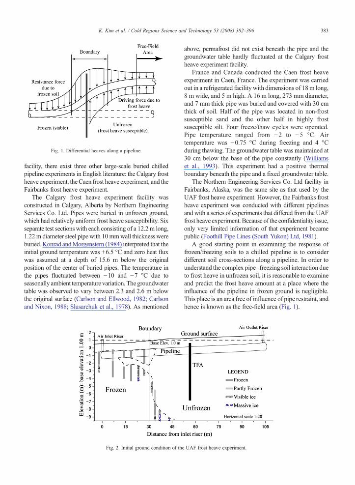
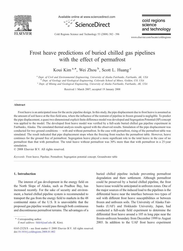
Fig. 1. Differential heaves along a pipeline.

383K. Kim et al. / Cold Regions Science and Technology 53 (2008) 382–396

facility, there exist three other large-scale buried chilledpipeline experiments in English literature: the Calgary frostheave experiment, theCaen frost heave experiment, and theFairbanks frost heave experiment.

The Calgary frost heave experiment facility wasconstructed in Calgary, Alberta by Northern EngineeringServices Co. Ltd. Pipes were buried in unfrozen ground,which had relatively uniform frost heave susceptibility. Sixseparate test sections with each consisting of a 12.2m long,1.22m diameter steel pipe with 10mmwall thickness wereburied. Konrad andMorgenstern (1984) interpreted that theinitial ground temperature was +6.5 °C and zero heat fluxwas assumed at a depth of 15.6 m below the originalposition of the center of buried pipes. The temperature inthe pipes fluctuated between −10 and −7 °C due toseasonally ambient temperature variation. The groundwatertable was observed to vary between 2.3 and 2.6 m belowthe original surface (Carlson and Ellwood, 1982; Carlsonand Nixon, 1988; Slusarchuk et al., 1978). As mentioned

Fig. 2. Initial ground condition of the

above, permafrost did not exist beneath the pipe and thegroundwater table hardly fluctuated at the Calgary frostheave experiment facility.

France and Canada conducted the Caen frost heaveexperiment in Caen, France. The experiment was carriedout in a refrigerated facility with dimensions of 18m long,8 m wide, and 5 m high. A 16 m long, 273 mm diameter,and 7 mm thick pipe was buried and covered with 30 cmthick of soil. Half of the pipe was located in non-frostsusceptible sand and the other half in highly frostsusceptible silt. Four freeze/thaw cycles were operated.Pipe temperature ranged from −2 to −5 °C. Airtemperature was −0.75 °C during freezing and 4 °Cduring thawing. The groundwater table was maintained at30 cm below the base of the pipe constantly (Williamset al., 1993). This experiment had a positive thermalboundary beneath the pipe and a fixed groundwater table.

The Northern Engineering Services Co. Ltd facility inFairbanks, Alaska, was the same site as that used by theUAF frost heave experiment. However, the Fairbanks frostheave experiment was conducted with different pipelinesand with a series of experiments that differed from the UAFfrost heave experiment. Because of the confidentiality issue,only very limited information of that experiment becamepublic (Foothill Pipe Lines (South Yukon) Ltd, 1981).

A good starting point in examining the response offrozen/freezing soils to a chilled pipeline is to considerdifferent soil cross-sections along a pipeline. In order tounderstand the complex pipe–freezing soil interaction dueto frost heave in unfrozen soil, it is reasonable to examineand predict the frost heave amount at a place where theinfluence of the pipeline in frozen ground is negligible.This place is an area free of influence of pipe restraint, andhence is known as the free-field area (Fig. 1).

UAF frost heave experiment.

384 K. Kim et al. / Cold Regions Science and Technology 53 (2008) 382–396

In the following sections, the UAF frost heaveexperiment at Fairbanks, Alaska is described first. Adescription of a quasi two-dimensional frost heave modelto estimate the amount of pipemovement at the UAF frostheave test facility follows. Finally, the results of numericalsimulation with the effect of permafrost using thedeveloped frost heave model are presented.

2. UAF frost heave experiment facility

Huang et al. (2004) has described the UAF frost heaveexperiment facility in detail. As indicated, a 0.914 mdiameter, 105 m long chilled pipeline with X65 grade and9mmwall thicknesswas used. The first 30mof the pipelinewere in a shallower supra-permafrost table area and the rest75mwere in unfrozen ground— a deeper supra-permafrosttable area. The pipe was covered with approximately 0.9 mof in-situ soil. The pipe crossed a boundary betweenpermafrost and unfrozen ground as shown in Fig. 2. Thereference elevation was defined as 1.00 m.

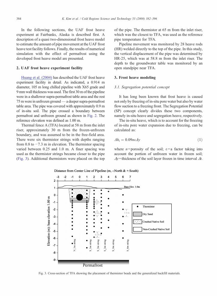
Thermal fence A (TFA) located at 58 m from the inletriser, approximately 30 m from the frozen-unfrozenboundary, and was assumed to be in the free-field area.There were six thermistor strings with depths rangingfrom 0.8 to −7.3 m in elevation. The thermistor spacingvaried between 0.25 and 1.0 m. A finer spacing wasused as the thermistor strings became closer to the pipe(Fig. 3). Additional thermistors were placed on the top

Fig. 3. Cross-section of TFA showing the placement of the

of the pipe. The thermistor at 65 m from the inlet riser,which was the closest to TFA, was used as the referencepipe temperature for TFA.

Pipeline movement was monitored by 28 heave rods(HR) welded directly to the top of the pipe. In this study,the vertical displacement of the pipe was determined byHR-25, which was at 58.8 m from the inlet riser. Thedepth to the groundwater table was monitored by anopen standpipe near TFA.

3. Frost heave modeling

3.1. Segregation potential concept

It has long been known that frost heave is causednot only by freezing of in-situ porewater but also bywaterflow suction to a freezing front. The Segregation Potential(SP) concept clearly divides these two components,namely in-situ heave and segregation heave, respectively.

The in-situ heave, which is to account for the freezingof in-situ pore water expansion due to freezing, can becalculated as:

Dhi ¼ 0:09neDy ð1Þ

where n=porosity of the soil; ε=a factor taking intoaccount the portion of unfrozen water in frozen soil;Δy=thickness of the soil layer frozen in time interval Δt.

rmistor beads and the generalized backfill materials.

385K. Kim et al. / Cold Regions Science and Technology 53 (2008) 382–396

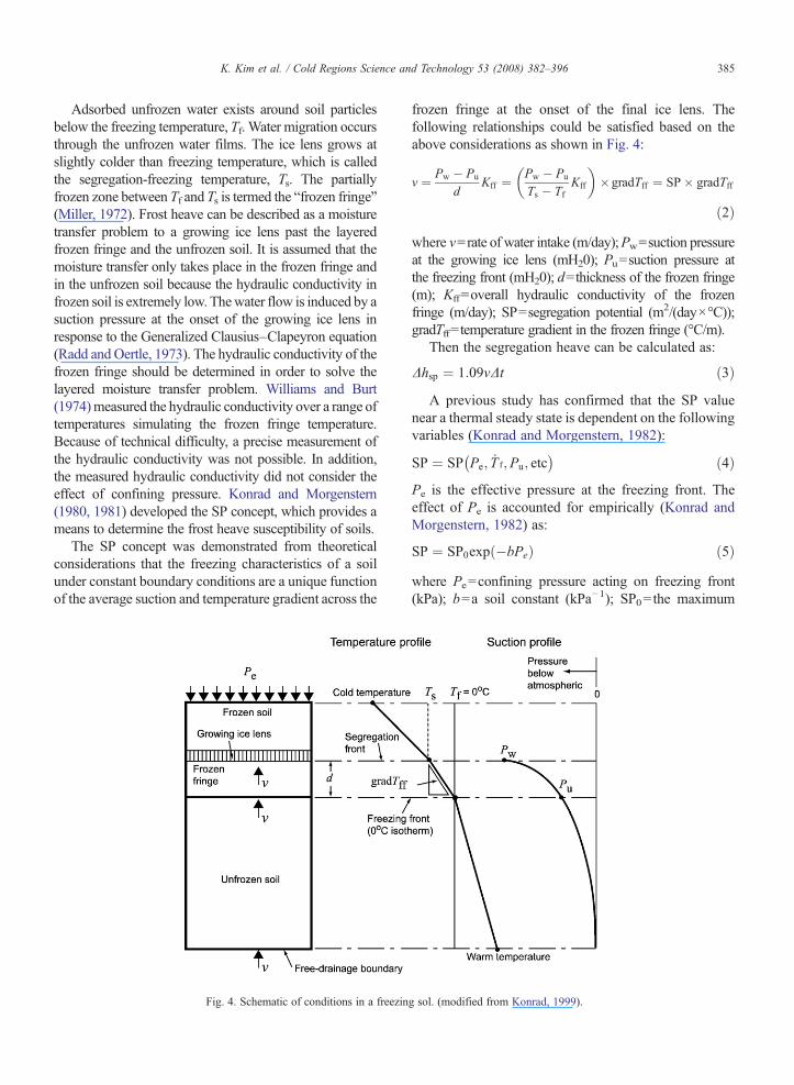
Adsorbed unfrozen water exists around soil particlesbelow the freezing temperature, Tf. Water migration occursthrough the unfrozen water films. The ice lens grows atslightly colder than freezing temperature, which is calledthe segregation-freezing temperature, Ts. The partiallyfrozen zone between Tf and Ts is termed the “frozen fringe”(Miller, 1972). Frost heave can be described as a moisturetransfer problem to a growing ice lens past the layeredfrozen fringe and the unfrozen soil. It is assumed that themoisture transfer only takes place in the frozen fringe andin the unfrozen soil because the hydraulic conductivity infrozen soil is extremely low. Thewater flow is induced by asuction pressure at the onset of the growing ice lens inresponse to the Generalized Clausius–Clapeyron equation(Radd and Oertle, 1973). The hydraulic conductivity of thefrozen fringe should be determined in order to solve thelayered moisture transfer problem. Williams and Burt(1974)measured the hydraulic conductivity over a range oftemperatures simulating the frozen fringe temperature.Because of technical difficulty, a precise measurement ofthe hydraulic conductivity was not possible. In addition,the measured hydraulic conductivity did not consider theeffect of confining pressure. Konrad and Morgenstern(1980, 1981) developed the SP concept, which provides ameans to determine the frost heave susceptibility of soils.

The SP concept was demonstrated from theoreticalconsiderations that the freezing characteristics of a soilunder constant boundary conditions are a unique functionof the average suction and temperature gradient across the

Fig. 4. Schematic of conditions in a freezin

frozen fringe at the onset of the final ice lens. Thefollowing relationships could be satisfied based on theabove considerations as shown in Fig. 4:

v ¼ Pw � Pu

dKff ¼ Pw � Pu

Ts � TfKff

� ��gradTff ¼ SP� gradTff

ð2Þwhere v=rate of water intake (m/day);Pw=suction pressureat the growing ice lens (mH20); Pu=suction pressure atthe freezing front (mH20); d=thickness of the frozen fringe(m); Kff=overall hydraulic conductivity of the frozenfringe (m/day); SP=segregation potential (m2/(day×°C));gradTff=temperature gradient in the frozen fringe (°C/m).

Then the segregation heave can be calculated as:

Dhsp ¼ 1:09vDt ð3ÞA previous study has confirmed that the SP value

near a thermal steady state is dependent on the followingvariables (Konrad and Morgenstern, 1982):

SP ¼ SP Pe;:T f;Pu; etc

� � ð4ÞPe is the effective pressure at the freezing front. Theeffect of Pe is accounted for empirically (Konrad andMorgenstern, 1982) as:

SP ¼ SP0exp �bPeð Þ ð5Þwhere Pe=confining pressure acting on freezing front(kPa); b=a soil constant (kPa−1); SP0= the maximum

g sol. (modified from Konrad, 1999).

386 K. Kim et al. / Cold Regions Science and Technology 53 (2008) 382–396

value of segregation potential that occurs at zero externalpressure (m2/(day×°C)). Tf is the rate of cooling of thefrozen fringe. The cooling rates are very small in the fieldcondition. The cooling rates at the formation of the finalice lens by the frost heave test of a constant temperatureboundary are reasonable to apply to the field condition(Konrad and Morgenstern, 1984). From Eq. (2), the SPvalue decreases with increasing Pu. In most fieldconditions, Pu is fairly small because of the small rateof water intake. It is reasonable to use the SP valuedetermined by a laboratory frost heave test in which thewarm plate temperature is close to the freezing point,because the thermal boundary condition creates a smallPu value due to the short unfrozen soil sample.

The total heave is obtained by adding Eqs. (1) and (3):

Dht ¼ Dhi þ Dhsp ð6ÞSeveral frost heave models simulated the pipe behavior

of theCalgary andCaen frost heave experiments at the free-field area. The SP concept was successfully applied inradially symmetrical one-dimensional problem, which didnot take into account of the thermal input from the groundsurface (Konrad andMorgenstern, 1984). Twodimensionalfrost heave simulations with the SP concept were alsosucceeded (e.g. Carlson and Nixon, 1988; Konrad andShen, 1996; Nixon, 1986). Those simulations were con-ducted using the SP value determined by laboratory frostheave tests. Undisturbed soil sampleswere used in the tests.

Coupled heat and moisture transfer models were alsoapplied for the pipeline simulation. (e.g. Razaqpur andWang, 1996; Selvadurai et al., 1999; Shar and Razaqpur,1993; Shen and Ladanyi, 1991). However, the hydraulicconductivity of the frozen fringe used in the simulationswas not directly measured. Furthermore, a trail-and-errorapproach was used to adjust the hydraulic conductivities toobtain a match of the result. All those applied models relyon the assumption that the Generalized Clausius–Clap-eyron equation, which relates ice and water pressure totemperature, holds anywhere in the frozen fringe.However,it is noted that the dynamics of phase change andwater flowin the frozen fringe make it impossible for the GeneralizedClausius–Clapeyron equation to hold anywhere but at theice lens where water flow is halted. (e.g. Miyata, 1998).

As shown in Eq. (2), the SP concept obtains an overallfrozen fringe characteristic including the suction gradi-ent and the hydraulic conductivity by laboratory frostheave tests. With the determined overall frozen fringecharacteristic, the SP parameters can empirically com-pensate the uncertainties of both the hydraulic con-ductivity measurement and the ice-water-temperaturerelationship in the frozen fringe. Also, it is an advantageof the SP concept that the only two parameters, Pe and

gradTff, are the input parameters during the frost heavecalculation.

3.2. Heat transfer

Since the rate of water migration for frost heave issmall enough, the primary mode of heat transfer can beassumed as heat conduction only. Heat transfer for afreezing soil with homogeneous and isotropic thermalproperties is governed by:

kD2T ¼ CaATAt

ð7Þ

where k=thermal conductivity (W/(m×°C)); T=soiltemperature (°C); t=time (s); Ca=apparent heat capacity(J/(m3×°C)).

The apparent heat capacity method used in numericalanalysis includes latent heat by adjusting the value of heatcapacity when freezing or thawing takes place. Nodetemperatures are checked at each time step to ascertainwhether they are within the phase change temperatures,which are given separately in terms of solidus and liquidustemperatures. When latent heat is generated in the phasechange, it is added to the specific heat as:

Ca ¼ C þ LTI

ð8Þ

where C=sensible heat capacity (J/(m3×°C)); L=latentheat (J/m3); TI= liquidus temperature (°C)–solidustemperature (°C).

4. Comparison between observed data andsimulated results

The developed frost heave model was verified using theUAF frost heave experimental data at TFA. Explicit finitedifference solutionwas applied to the developed frost heavemodel. To simplify the simulation process, the numericallyuncoupled temperature solution and the mass transfer cou-pling were applied. For any particular time step, the tem-perature distribution was first calculated and then thistemperature solution was used to determine the locations ofthe freezing front and the frozen fringe. With the positionsdetermined, the SP concept was used to calculate the vol-ume expansion due to in-situ freezing and water migrationto the frozen fringe. Visual Basic Editor was used foradding subroutines and functions of these analyses.

4.1. Initial and boundary conditions

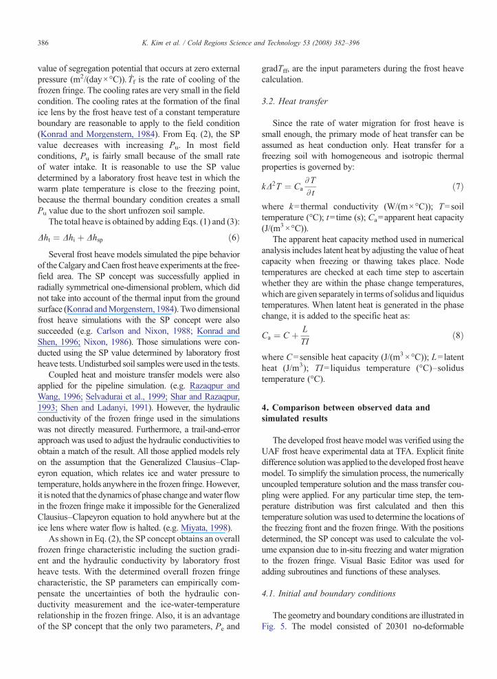
The geometry and boundary conditions are illustrated inFig. 5. The model consisted of 20301 no-deformable

Table 1Thermal properties of Fairbanks silt

Thermal conductivity(W/(m°C))

Heat capacity(kJ/(m3°C))

Latent heat(kJ/m3)

Phase change temperature(°C)

Thawed Frozen Thawed Frozen Solidus Liquidas

Fairbanks silt 1.52 2.72 3188 2281 114 106 −0.1 0

387K. Kim et al. / Cold Regions Science and Technology 53 (2008) 382–396

nodes. The time step was set at a constant of 2 hours.Thermal properties were determined using a dry unitweight of 12.8 kN/m3, water content at w=40%, andunfrozenwater content atwu=7%. The amount of unfrozenwater was representative of the frozen soil at the site. Theseproperties were based on fully-saturated in-situ soilsamples beneath the pipe. Thermal conductivity needle-probe method was applied to obtain thermal conductivityvalues. Phase change temperatures, solidus and liquidustemperature, were defined as −0.1 and 0 °C, respectively.The applied thermal properties are shown in Table 1.

A pipe with 0.8 m diameter was buried with 1 moverburden. The mean pipe temperature through theoperation was approximately −8.5 °C. Since the pipetemperature fluctuated with time, a step temperature wasapplied to the numerical simulation. The phases weredivided into every 60 days each. The average temperatureduring each phase was defined as input pipe temperature.The air temperature was converted to the ground surfacetemperature by n-factor. Zero heat flux was applied at thevertical boundaries, whichwere 20m from the pipe center.

Fig. 5. Initial and boundar

The initial ground temperature was created by thefollowing procedure. First, a temperature of +1 °C wasapplied to all nodes from the ground surface to 10m deep.The temperature of the bottom horizontal boundary (20 mbelow the ground surface) was fixed at−0.1 °C. The sametemperature, −0.1 °C, was also applied to all nodes below10 m to simulate the existence of permafrost. Then, themodel was executed without the pipe temperature inputfor 5 years. Finally, −1 °C was applied to an area of 2 mwide and 1.8 m deep at the center. It was assumed as thetrench for the pipe was excavated during wintertime. Theinitial temperature distribution is shown in Fig. 5.

Nixon (2003) reported SP characteristics for theFairbanks frost heave experiment. Two SP values werereported because of variations in clay fraction in dif-ferent undisturbed soil samples obtained at the site. Inaddition, the authors conducted two frost heave testsusing remolded samples from the test site. These resultsare shown in Fig. 6. The frost heave tests results arewithin the reported values. The upper values, SP0=22.7×10−5 m2/(day×°C) and b=0.02596 kPa−1, were

y conditions at TFA.

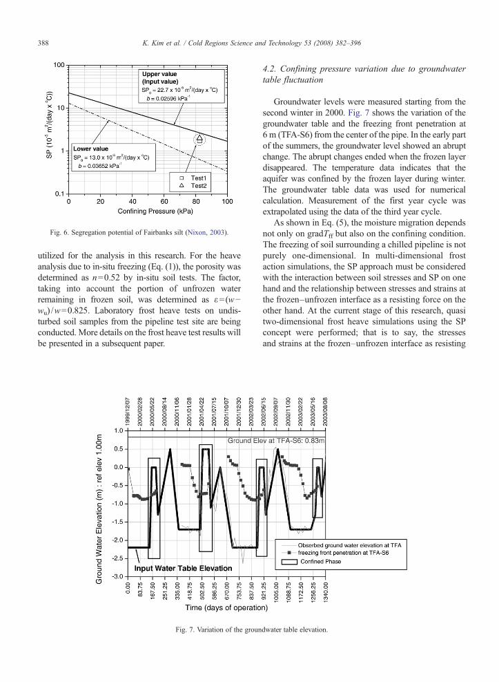
Fig. 6. Segregation potential of Fairbanks silt (Nixon, 2003).

388 K. Kim et al. / Cold Regions Science and Technology 53 (2008) 382–396

utilized for the analysis in this research. For the heaveanalysis due to in-situ freezing (Eq. (1)), the porosity wasdetermined as n=0.52 by in-situ soil tests. The factor,taking into account the portion of unfrozen waterremaining in frozen soil, was determined as ε=(w−wu) /w=0.825. Laboratory frost heave tests on undis-turbed soil samples from the pipeline test site are beingconducted. More details on the frost heave test results willbe presented in a subsequent paper.

Fig. 7. Variation of the groun

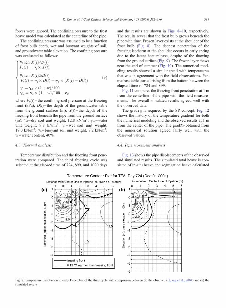
4.2. Confining pressure variation due to groundwatertable fluctuation

Groundwater levels were measured starting from thesecond winter in 2000. Fig. 7 shows the variation of thegroundwater table and the freezing front penetration at6 m (TFA-S6) from the center of the pipe. In the early partof the summers, the groundwater level showed an abruptchange. The abrupt changes ended when the frozen layerdisappeared. The temperature data indicates that theaquifer was confined by the frozen layer during winter.The groundwater table data was used for numericalcalculation. Measurement of the first year cycle wasextrapolated using the data of the third year cycle.

As shown in Eq. (5), the moisture migration dependsnot only on gradTff but also on the confining condition.The freezing of soil surrounding a chilled pipeline is notpurely one-dimensional. In multi-dimensional frostaction simulations, the SP approach must be consideredwith the interaction between soil stresses and SP on onehand and the relationship between stresses and strains atthe frozen–unfrozen interface as a resisting force on theother hand. At the current stage of this research, quasitwo-dimensional frost heave simulations using the SPconcept were performed; that is to say, the stressesand strains at the frozen–unfrozen interface as resisting

dwater table elevation.

389K. Kim et al. / Cold Regions Science and Technology 53 (2008) 382–396

forces were ignored. The confining pressure to the frostheave model was calculated at the centerline of the pipe.

The confining pressure was assumed to be a functionof frost bulb depth, wet and buoyant weights of soil,and groundwater table elevation. The confining pressurewas evaluated as follows:

When X tð ÞbD tð ÞPe tð Þ ¼ gt � X tð ÞWhen X tð ÞzD tð ÞPe tð Þ ¼ gt � D tð Þ þ gb � X tð Þ � D tð Þð Þgt ¼ gd � 1þ wð Þ=100gb ¼ gd � 1þ wð Þ=100� rw

8>>>>>>>><>>>>>>>>:

ð9Þ

where Pe(t)= the confining soil pressure at the freezingfront (kPa); D(t)= the depth of the groundwater tablefrom the ground surface (m); X(t)= the depth of thefreezing front beneath the pipe from the ground surface(m); γd=dry soil unit weight, 12.8 kN/m3; γw=waterunit weight; 9.8 kN/m3; γt =wet soil unit weight,18.0 kN/m3; γb=buoyant soil unit weight, 8.2 kN/m3;w=water content, 40%.

4.3. Thermal analysis

Temperature distribution and the freezing front pene-tration were compared. The third freezing cycle wasselected at the elapsed time of 724, 899, and 1020 days

Fig. 8. Temperature distribution in early December of the third cycle with csimulated results.

and the results are shown in Figs. 8–10, respectively.The results reveal that the frost bulb grows beneath thepipe with time. Frozen layer exists at the shoulder of thefrost bulb (Fig. 8). The deepest penetration of thefreezing isotherm at the shoulder occurs in early springdue to the latent heat release, despite of the thawingfrom the ground surface (Fig. 9). The frozen layer thawsnear the end of summer (Fig. 10). The numerical mod-eling results showed a similar trend with temperaturesthat was in agreement with the field observations. Per-mafrost table started rising from the bottom between theelapsed time of 724 and 899.

Fig. 11 compares the freezing front penetration at 1 mfrom the centerline of the pipe with the field measure-ments. The overall simulated results agreed well withthe observed data.

The gradTff is required by the SP concept. Fig. 12shows the history of the temperature gradient for boththe numerical modeling and the observed results at 1 mfrom the center of the pipe. The gradTff obtained fromthe numerical solution agreed fairly well with theobserved values.

4.4. Pipe movement analysis

Fig. 13 shows the pipe displacements of the observedand simulated results. The simulated total heave is con-sisted of in-situ heave and segregation heave calculated

omparison between (a) the observed (Huang et al., 2004) and (b) the

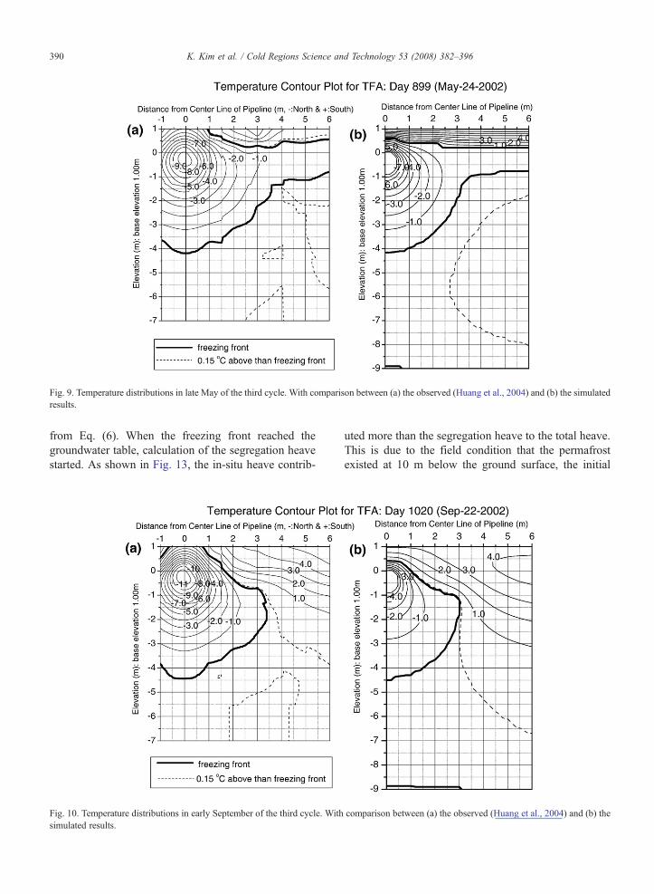
Fig. 9. Temperature distributions in late May of the third cycle. With comparison between (a) the observed (Huang et al., 2004) and (b) the simulatedresults.

390 K. Kim et al. / Cold Regions Science and Technology 53 (2008) 382–396

from Eq. (6). When the freezing front reached thegroundwater table, calculation of the segregation heavestarted. As shown in Fig. 13, the in-situ heave contrib-

Fig. 10. Temperature distributions in early September of the third cycle. Withsimulated results.

uted more than the segregation heave to the total heave.This is due to the field condition that the permafrostexisted at 10 m below the ground surface, the initial

comparison between (a) the observed (Huang et al., 2004) and (b) the

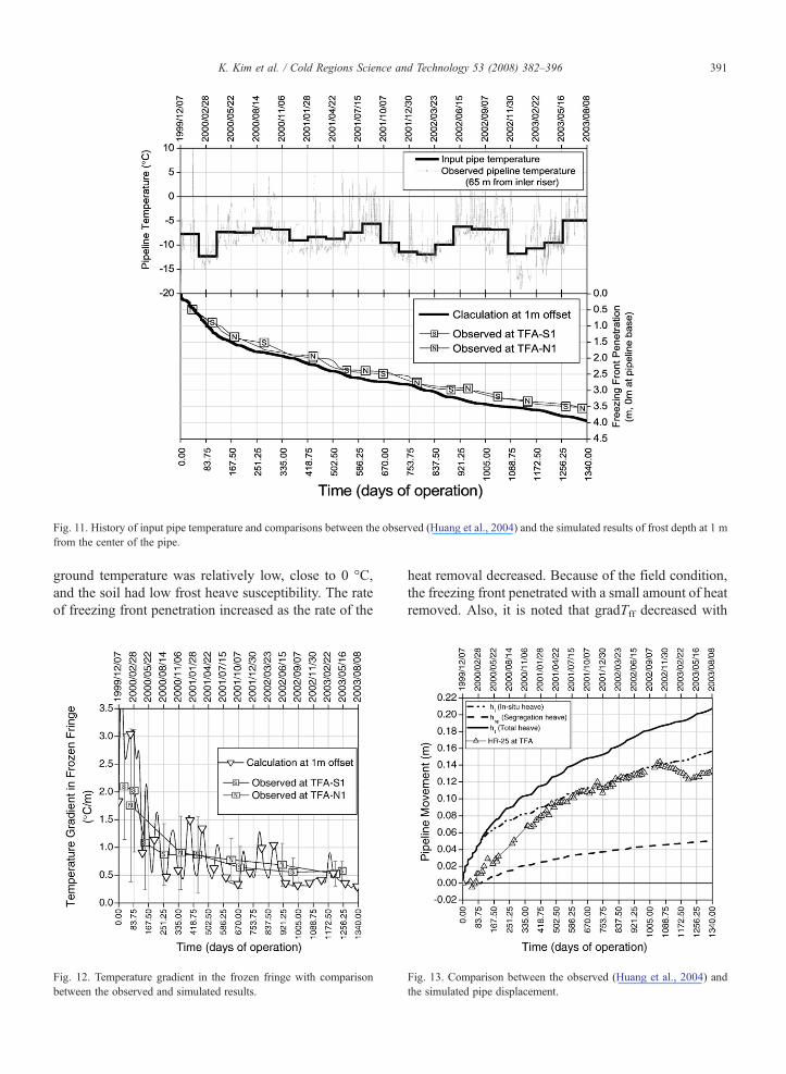
Fig. 11. History of input pipe temperature and comparisons between the observed (Huang et al., 2004) and the simulated results of frost depth at 1 mfrom the center of the pipe.

391K. Kim et al. / Cold Regions Science and Technology 53 (2008) 382–396

ground temperature was relatively low, close to 0 °C,and the soil had low frost heave susceptibility. The rateof freezing front penetration increased as the rate of the

Fig. 12. Temperature gradient in the frozen fringe with comparisonbetween the observed and simulated results.

heat removal decreased. Because of the field condition,the freezing front penetrated with a small amount of heatremoved. Also, it is noted that gradTff decreased with

Fig. 13. Comparison between the observed (Huang et al., 2004) andthe simulated pipe displacement.

392 K. Kim et al. / Cold Regions Science and Technology 53 (2008) 382–396

increasing freezing front penetration as shown inFig. 12. Between the above-mentioned reasons, theexistence of permafrost below the pipe was likely theprimary reason why segregation heave did not dominatethe process.

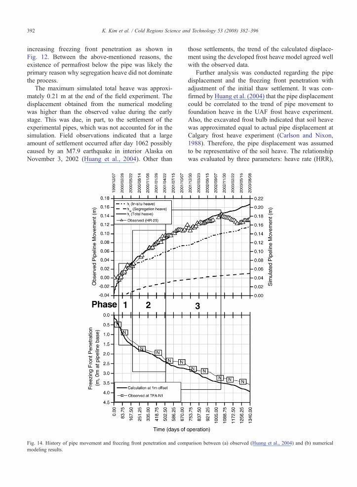
The maximum simulated total heave was approxi-mately 0.21 m at the end of the field experiment. Thedisplacement obtained from the numerical modelingwas higher than the observed value during the earlystage. This was due, in part, to the settlement of theexperimental pipes, which was not accounted for in thesimulation. Field observations indicated that a largeamount of settlement occurred after day 1062 possiblycaused by an M7.9 earthquake in interior Alaska onNovember 3, 2002 (Huang et al., 2004). Other than

Fig. 14. History of pipe movement and freezing front penetration and commodeling results.

those settlements, the trend of the calculated displace-ment using the developed frost heave model agreed wellwith the observed data.

Further analysis was conducted regarding the pipedisplacement and the freezing front penetration withadjustment of the initial thaw settlement. It was con-firmed by Huang et al. (2004) that the pipe displacementcould be correlated to the trend of pipe movement tofoundation heave in the UAF frost heave experiment.Also, the excavated frost bulb indicated that soil heavewas approximated equal to actual pipe displacement atCalgary frost heave experiment (Carlson and Nixon,1988). Therefore, the pipe displacement was assumedto be representative of the soil heave. The relationshipwas evaluated by three parameters: heave rate (HRR),

parison between (a) observed (Huang et al., 2004) and (b) numerical

393K. Kim et al. / Cold Regions Science and Technology 53 (2008) 382–396

penetration rate (PRR), and frost heave ratio (FHR).Those are defined as:

HRR mm=dayð Þ ¼ Pipe displacement ðmmÞtime ðdayÞ ð10Þ

PRR mm=dayð Þ¼ Freezing front peneatration at 1m offset from the pipe ðmmÞtime ðdayÞ

ð11Þ

FHR %ð Þ ¼ Pipe displacement mmð ÞFreezing front peneatration at 1m offset from the pipe mmð Þ�100

ð12ÞThe pipe displacement by numerical method was

adjusted for the initial settlement as shown in Fig. 14.Three phases were defined that were free from theinitial settlement and the earthquake effect. Phase 1was characterized by a higher heave rate and penetra-tion rate, and followed by Phases 2 and 3 with slowerheave rates and penetration rates.

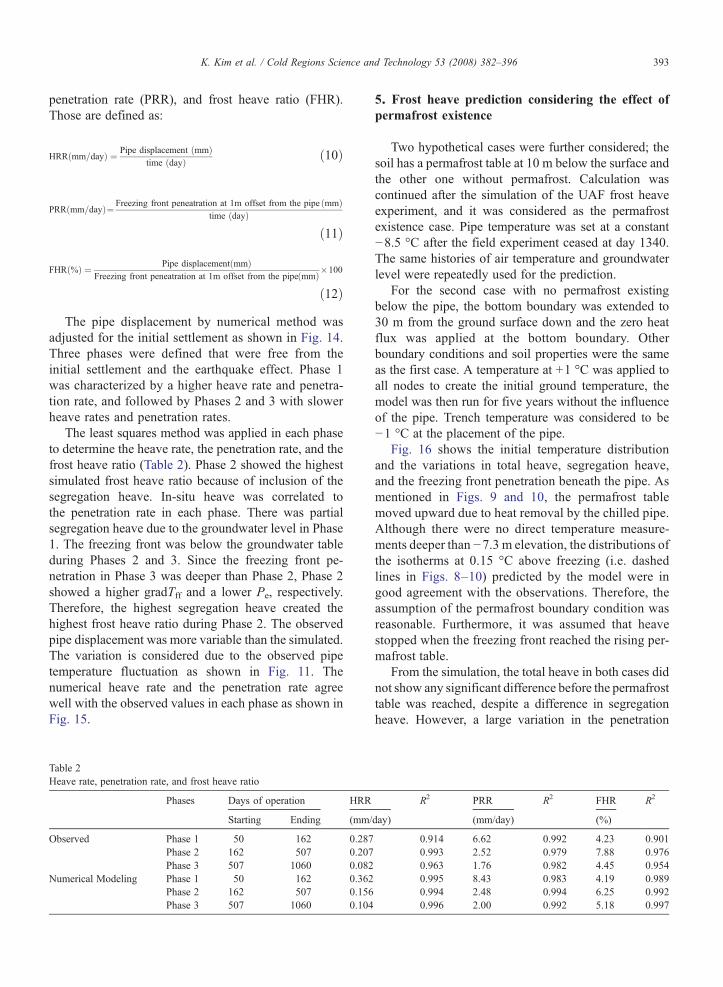
The least squares method was applied in each phaseto determine the heave rate, the penetration rate, and thefrost heave ratio (Table 2). Phase 2 showed the highestsimulated frost heave ratio because of inclusion of thesegregation heave. In-situ heave was correlated tothe penetration rate in each phase. There was partialsegregation heave due to the groundwater level in Phase1. The freezing front was below the groundwater tableduring Phases 2 and 3. Since the freezing front pe-netration in Phase 3 was deeper than Phase 2, Phase 2showed a higher gradTff and a lower Pe, respectively.Therefore, the highest segregation heave created thehighest frost heave ratio during Phase 2. The observedpipe displacement was more variable than the simulated.The variation is considered due to the observed pipetemperature fluctuation as shown in Fig. 11. Thenumerical heave rate and the penetration rate agreewell with the observed values in each phase as shown inFig. 15.

Table 2Heave rate, penetration rate, and frost heave ratio

Phases Days of operation HRR

Starting Ending (mm/

Observed Phase 1 50 162 0.287Phase 2 162 507 0.207Phase 3 507 1060 0.082

Numerical Modeling Phase 1 50 162 0.362Phase 2 162 507 0.156Phase 3 507 1060 0.104

5. Frost heave prediction considering the effect ofpermafrost existence

Two hypothetical cases were further considered; thesoil has a permafrost table at 10 m below the surface andthe other one without permafrost. Calculation wascontinued after the simulation of the UAF frost heaveexperiment, and it was considered as the permafrostexistence case. Pipe temperature was set at a constant−8.5 °C after the field experiment ceased at day 1340.The same histories of air temperature and groundwaterlevel were repeatedly used for the prediction.

For the second case with no permafrost existingbelow the pipe, the bottom boundary was extended to30 m from the ground surface down and the zero heatflux was applied at the bottom boundary. Otherboundary conditions and soil properties were the sameas the first case. A temperature at +1 °C was applied toall nodes to create the initial ground temperature, themodel was then run for five years without the influenceof the pipe. Trench temperature was considered to be−1 °C at the placement of the pipe.

Fig. 16 shows the initial temperature distributionand the variations in total heave, segregation heave,and the freezing front penetration beneath the pipe. Asmentioned in Figs. 9 and 10, the permafrost tablemoved upward due to heat removal by the chilled pipe.Although there were no direct temperature measure-ments deeper than −7.3 m elevation, the distributions ofthe isotherms at 0.15 °C above freezing (i.e. dashedlines in Figs. 8–10) predicted by the model were ingood agreement with the observations. Therefore, theassumption of the permafrost boundary condition wasreasonable. Furthermore, it was assumed that heavestopped when the freezing front reached the rising per-mafrost table.

From the simulation, the total heave in both cases didnot show any significant difference before the permafrosttable was reached, despite a difference in segregationheave. However, a large variation in the penetration

R2 PRR R2 FHR R2

day) (mm/day) (%)

0.914 6.62 0.992 4.23 0.9010.993 2.52 0.979 7.88 0.9760.963 1.76 0.982 4.45 0.9540.995 8.43 0.983 4.19 0.9890.994 2.48 0.994 6.25 0.9920.996 2.00 0.992 5.18 0.997

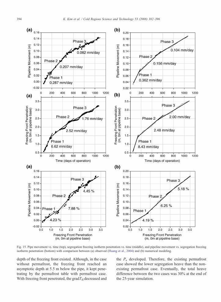
Fig. 15. Pipe movement vs. time (top), segregation freezing isotherm penetration vs. time (middle), and pipeline movement vs. segregation freezingisotherm penetration (bottom) with comparison between (a) observed (Huang et al., 2004) and (b) numerical modeling.

394 K. Kim et al. / Cold Regions Science and Technology 53 (2008) 382–396

depth of the freezing front existed. Although, in the casewithout permafrost, the freezing front reached anasymptotic depth at 5.5 m below the pipe, it kept pene-trating by the permafrost table with permafrost case.With freezing front penetrated, the gradTff decreased and

the Pe developed. Therefore, the existing permafrostcase showed the lower segregation heave than the non-existing permafrost case. Eventually, the total heavedifference between the two cases was 30% at the end ofthe 25-year simulation.

Fig. 16. Prediction considering the effect of the permafrost existence using the developed frost heave model.

395K. Kim et al. / Cold Regions Science and Technology 53 (2008) 382–396

With the projected global climate change, thewarming and degradation of permafrost is likely tooccur along a proposed route of gas pipeline in thearctic regions. With permafrost disappearing, higherfrost heave would be likely to occur than otherwise.The effect of changing permafrost condition willundoubtedly be an important factor to the arctic gaspipeline design.

6. Discussion and conclusions

A quasi two-dimensional frost heave model wasdeveloped considering fluctuation of the groundwatertable. A fixed-node finite difference mesh was applied tothe model subject to the following assumptions: (1) unitweight and thermal properties of soil were constant, and(2) resistance to upward motion of the frost bulb wasnegligible at the free-field area.

The predictions of the freezing front depth and thepipe displacement due to frost heave by the model agreedwell with field observations except during the time whenpipe settlement occurred. Significant findings from thisstudy are:

1. The in-situ heave contributed more to the total heavethan the segregation heave at the free-field area at the

UAF frost heave experiment site due in part to smallheat extraction and the permafrost existence.

2. The pipe movement was simulated in three phases.Phase 1, the freezing front partially above the ground-water table, the results showed that the frost heave ratioof the numerical modeling was 4.19%. The existenceof permafrost increased the freezing front penetrationrate. The deeper the freezing front penetration, the lessthe temperature gradient in the frozen fringe and thehigher the confining pressure developed. In Phase 2,the frost heave ratio was the highest at 6.25%, and inPhase 3, it decreased to 5.18%.

3. Simulation of the pipe displacement was conductedfor two ground conditions — with and withoutpermafrost. In the case with permafrost, rising of thepermafrost table was simulated. The result indicatedthat pipe displacement stopped when the downwardfreezing front reached the permafrost table. However,heave continued for the ground free of permafrost.Segregation heave played a more significant role tothe total heave in the case without permafrost thanthat with permafrost. The difference of total heavebetween the two cases was 30%.

The developed numerical model reasonably estimatedthe pipe displacement and freezing front penetration

396 K. Kim et al. / Cold Regions Science and Technology 53 (2008) 382–396

during the selected phases. However, amore sophisticatedfinite element (FE) model is being developed. The FEmodel will consider changes in unit weight, thetemperature dependent non-linear thermal properties, aswell as the resistance to upward movement of the frostbulb. Deforming mesh will be applied to the FE model.Results of the FEmodel will be presented in a subsequentpaper. The developed finite difference frost heave modeldiscussed in this paper could be useful to verify andvalidate the FE model.

Acknowledgements

This field experiment was funded by Japan Scienceand Technology Corporation (JST) and the numericalsimulation of the studywas supported byAlaska EPSCoRGraduate Research Fellowship. The financial assistancefrom these two organizations is appreciated. The authorsacknowledge Dr. S. Kanie, HokkaidoUniversity in Japan,for his profound suggestions regarding numerical model-ing. And special thanks are due toMr.M.Bray, Universityof Alaska Fairbanks, for his field experimental works andsuggestions.

References

Carlson, L.E., Ellwood, J.R., 1982. Field test results of operatinga chilled, buried pipeline in unfrozen ground. Proceedings of4th Canadian Permafrost Conference, Calgary, Alberta, Canada,pp. 475–480.

Carlson, L.E., Nixon, J.F., 1988. Subsoil investigation of ice lensing atthe Calgary, Canada, frost heave test facility. Canadian GeotechnicalJournal 25, 307–319.

Foothill Pipe Lines (South Yukon) Ltd, 1981. Plans for dealing withfrost-heave and thaw settlement: addendum to the environmentalimpact statement for the Yukon section of the Alaska Highway GasPipeline. Calgary, Alberta, Canada, pp. 1–46.

Huang, S.L., Bray, M.T., Akagawa, S., Fukuda, M., 2004. Fieldinvestigation of soil heave by a large diameter chilled gas pipelineexperiment, Fairbanks, Alaska. Journal of Cold Regions Engineering18, 2–34.

Konrad, J.M., 1999. Frost susceptibility related to soil index properties.Canadian Geotechnical Journal 36, 403–417.

Konrad, J.M., Morgenstern, N.R., 1980. A mechanistic theory of icelens formation in fine-grained soils. Canadian Geotechnical Journal17, 473–486.

Konrad, J.M., Morgenstern, N.R., 1981. The segregation potential of afreezing soil. Canadian Geotechnical Journal 18, 482–491.

Konrad, J.M., Morgenstern, N.R., 1982. Effects of applied pressure onfreezing soils. Canadian Geotechnical Journal 19, 494–505.

Konrad, J.M., Morgenstern, N.R., 1984. Frost heave prediction ofchilled pipelines buried in unfrozen soils. Canadian GeotechnicalJournal 21, 100–115.

Konrad, J.M., Shen, M., 1996. 2-D frost action modeling using thesegregation potential of soils. Cold Regions Science and Technology24, 263–278.

Miller, R.D., 1972. Freezing and heaving of saturated and unsaturatedsoils. Highway Research Record 393, 1–11.

Miyata, Y., 1998. A thermodynamic study of liquid transportation infreezing porous media. JSME International Journal Series B 41,601–609.

Nixon, J.F., 1986. Pipeline frost heave predictions using a 2-D thermalmodel. ASCE Research on Transportation Facilities in ColdRegions, pp. 67–82.

Nixon, J.F., 2003. Conceptual Geotechnical/Geothermal Design Basis.Radd, F.J., Oertle, D.H., 1973. Experimental pressure studies of frost

heave mechanisms and the growth-fusion behavior of ice.Proceedings of the 2nd International Conference on Permafrost,Yakutsk, USSR, pp. 377–384.

Razaqpur, A.G., Wang, D., 1996. Frost-induced deformations andstresses in pipelines. International Journal of Pressure Vessels andPiping 69, 105–118.

Selvadurai, A.P.S., Hu, J., Konuk, I., 1999. Computational modellingof frost heave induced soil-pipeline interaction: II. Modelling ofexperiments at the Caen test facility. Cold Regions Science andTechnology 29, 229–257.

Shar, K.R., Razaqpur, A.G., 1993. A two-dimensional frost heavemodel for buried pipelines. International Journal for NumericalMethods in Engineering 36, 2545–2566.

Shen, M., Ladanyi, B., 1991. Soil-pipe interaction during frost heavingaround a buried chilled pipeline. Proceedings of the SixthInternational Specialty Conference,West Lebanon, NH, pp. 11–21.

Slusarchuk, W.A., Clark, J.I., Nixon, J.F., Morgenstern, N.R., Gaskin,P.N., 1978. Field test results of a chilled pipeline buried in unfrozenground. Proceedings of 3rd International Conference on Perma-frost, Edmonton, Alberta, Canada, pp. 878–883.

Williams, P.J., Burt, T.P., 1974. Measurement of hydraulic conductiv-ity of frozen soils. Canadian Geotechnical Journal 11, 647–650.

Williams, P.J., Riseborough, D.W., Smith, M.W., 1993. The France-Canada joint study of deformation of an experimental pipe line bydifferential frost heave. International Journal of Offshore and PolarEngineering 3, 56–60.