From Stylized to Quantitative Spatial Models of Cities · NEG came from Krugman (1991), who developed a model that showed that the emergence of an industrialized ﬁcoreﬂand an

Economic Quarterly– Volume 102, Number 3– Third Quarter 2016– Pages 169—192

From Stylized toQuantitative Spatial Modelsof Cities

Sonya Ravindranath Waddell and Pierre-Daniel Sarte

1. INTRODUCTION

Understanding how and why factors of production locate within andaround urban areas has been compelling social scientists for at least150 years. Within mainstream economics, urban economists have beendeveloping modern theories of city systems at least since the 1960s.However, modeling spatial interactions is highly complex, and, there-fore, the theoretical literature on economic geography has necessarilyfocused on stylized settings. For example, a model may have a centralbusiness district– where firms are assumed to be located– surroundedby a symmetric circle or on a symmetric line. As the population grows,the scarcity of land prevents consumers (who are also workers) from allsettling close to the center, so people move out to where commutingcosts are higher but housing costs are lower.

In the models of new economic geography (NEG), urban econo-mists have incorporated advances developed in industrial organization,international trade, and economic growth to remove technical barri-ers to modeling cities. The field of NEG was initiated primarily bythree authors: Fujita (1988), Krugman (1991), and Venables (1996),who all use general equilibrium models with some version of monop-olistic competition. The NEG models have been useful in helping topin down preferences, technology, and endowments and have provided

We thank Daniel Schwam and Daniel Ober-Reynolds for helpful research assistance. The views expressed herein are those of the authors and do not necessarily represent the views of the Federal Reserve Bank of Richmond or the Federal Reserve System. We thank Urvi Neelakantan, Santiago Pinto, and John Weinberg for helpful comments and suggestions.

DOI: http://doi.org/10.21144/eq1020301

170 Federal Reserve Bank of Richmond Economic Quarterly

some fundamental theoretical explanation for the uneven distributionof economic activity, for multiple equilibria in location choices, and fora small (possibly temporary) asymmetric shock across sites to generatea large permanent imbalance in the distribution of economic activities.However, these models have also imposed structure that is not neces-sarily evident in the data, and the limitation of the analysis to stylizedspatial settings has not enabled an empirical literature that could di-rectly corroborate the theory. In other words, the stylized models haveonly guided empirical estimation in a way that is divorced from thestructure of those models, resulting in empirical research that has beendevoid of strong structural interpretations.

More recently, the introduction of quantitative models of interna-tional trade (in particular Eaton and Kortum [2002]) have served todevelop a framework that connects closely to the observed data. Thisresearch does not aim to provide a fundamental explanation for theagglomeration of economic activity but instead aims to provide an em-pirically relevant quantitative model. This article describes the pro-gression from a simple canonical model of NEG to its counterpart inthe quantitative spatial framework. Section 2 engages the literatureto develop and understand the progression from the stylized models ofthe NEG literature to the quantitative spatial models. Section 3 walksthrough a version of the stylized model, with a linear monocentric city.Section 4 introduces its counterpart as a quantitative spatial model aswas laid out in Redding and Rossi-Hansberg (forthcoming). Section 5provides an example of how the spatial model can be matched to de-tailed microdata that describe actual interactions in the city. Section6 concludes.

2. LITERATURE REVIEW

The standard monocentric model of cities came out of a history ofwork to model spatial allocations. The prototype for understandinghow factors of production distribute themselves across land, and howprices govern that distribution, was developed by Johann Heinrich vonThünen in the mid-nineteenth century to describe the pattern of agri-cultural activities in preindustrial Germany. Von Thünen’s model in-cludes an exogenously located marketplace in which all transactions re-garding final goods must occur and the differences in land rent and useare determined predominantly by transport costs (Fujita and Thisse2002). The von Thünen model was both formalized mathematicallyand enhanced in the second half of the twentieth century– includingthe formalization of bid-rent curves by William Alonso in his basic ur-ban land model. This basic urban model includes a monocentric city

Waddell & Sarte: From Stylized to Quantitative Spatial Models of Cities171

with a center, home to the central business district (CBD), where alljobs are located. The space surrounding the CBD is assumed to be ho-mogenous with only one spatial characteristic: its distance to the CBD.Both the work of von Thünen and that of Alonso depended upon themonocentricity of production activities– i.e., the models rely on oneCBD (or market) with surrounding land used for residential (or agri-cultural) purposes.

Although many early models assumed the existence of the CBD,later work formalized mechanisms for the agglomeration forces thatcreate concentrations of economic activity. The models of NEG, assummarized in Fujita et al. (1999), Fujita and Thisse (2002), and Otta-viano and Thisse (2004), create the framework to explain the imbalancein the distribution of economic activity and better understand how asmall shock can generate that imbalance. These NEG models went along way toward overcoming the fundamental problem that kept eco-nomic geography and location theory at the periphery of mainstreameconomic theory for so long: regional specialization and trade cannotarise in the competitive equilibrium of an economy with homogenousspace. This spatial impossibility theorem is discussed more thoroughlyin Ottaviano and Thisse (2004) and articulated mathematically in Fu-jita and Thisse (2002).

Important ideas underlie the development of the NEG models.These ideas (as described in Ottaviano and Thisse [2004]) include thatthe distribution of economic activity is the outcome of a trade-off be-tween various forms of increasing returns and different mobility costs;price competition, high transport costs, and land use foster the disper-sion of production and consumption, and, therefore, firms are likely tocluster in large metropolitan areas when they sell differentiated prod-ucts and transport costs are low. Cities provide a wide array of fi-nal goods and specialized labor markets that make them attractive toconsumers/workers, and agglomeration is the outcome of cumulativeprocesses involving both the supply and demand sides. The contribu-tion of NEG was to link those ideas together in a general equilibriumframework with imperfect competition. Some of the earliest work inNEG came from Krugman (1991), who developed a model that showedthat the emergence of an industrialized “core”and an agricultural “pe-riphery”pattern depends on transportation costs, economies of scale,and the share of manufacturing in national income (i.e., in consump-tion expenditures). More specifically, in his model, lower transporta-tion costs, a higher manufacturing share, or stronger economies ofscale will result in the concentration of manufacturing in the regionthat gets a head start compared to other regions. Venables (1996)wrote a model where imperfect competition and transport costs create


forward and backward linkages between industries in different loca-tions. He finds that even without labor mobility, agglomeration can begenerated through the location decisions of firms in industries that arelinked through an input-output structure. The models above developan argument for agglomeration into a single center of activity. How-ever, other NEG models, most notably Fujita and Ogawa (1982) andLucas and Rossi-Hansberg (2002), introduced nonmonocentric modelswhere businesses and housing can be located anywhere in the city. Thelatter models constitute a first step toward building frameworks thatmore accurately capture the heterogeneity in economic activity acrossspace.

Unfortunately, although the theoretical work on NEG has been rel-atively rich, the empirical research has been comparatively less rich; es-tablishing causality and controlling for confounding factors has provedchallenging in the empirical realm. One challenge, as articulated byRedding and Rossi-Hansberg (forthcoming), is that the complexity ofthe theoretical models has limited the analysis to stylized spatial set-tings, such as a few locations, a circle, or a line, and the resulting em-pirical research has been primarily reduced form in nature. As a result,it is diffi cult to provide a structural interpretation of the estimated co-effi cients, and the empirical models cannot either withstand the Lucascritique (coeffi cients might change with different policy interventions)or necessarily generalize to more realistic environments.

Empirical work, such as the spatial model laid out in Section 4, hasbeen instructed by another field of economics. Developments in theinternational trade literature have offered mechanisms for better mod-eling the distribution of economic activity across urban areas. Eatonand Kortum (2002) developed a model of international trade that cap-tures both the comparative advantage that encourages trade and thegeographic barriers that inhibit it (e.g., transport costs, tariffs and quo-tas, challenges negotiating trade deals, etc.). They use the model tosolve for the the world trading equilibrium and examine its response topolicies.

This framework from the trade literature– combined with the avail-ability of increasingly more granular data– enabled the emergence ofnew quantitative spatial models in urban economics in which one cancarry out general equilibrium counterfactual policy exercises. In ad-dition to offering methodological insights and a mechanism for policyanalysis, these quantitative spatial models have made substantive con-tributions that borrow from, and contribute to, the theoretical litera-ture. For example, Redding and Sturm (2008) provide evidence for acausal relationship between market access and the spatial distributionof economic activity. They show that the division of Germany after


World War II led to a sharp decline in population growth in West Ger-man cities close to the new border relative to other West German citiesand that this decline was more pronounced for small cities than forlarge cities. As another example, models such as those developed inAhlfeldt et al. (2015) and Monte et al. (2016), allow for heterogenousgradients of economic activity within cities that can be matched di-rectly to microdata and that can only be approximated in models suchas Fujita and Ogawa (1982) and Lucas and Rossi-Hansberg (2002).

The next section walks through a canonical monocentric urbanmodel and highlights key features that made that model attractivefor thinking about the distribution of economic activity across space.In particular, this urban model allows many of a city’s features to beendogenous, including its size, population, employment, wages, andcommercial land rents. In addition, at different locations within thecity, residential population, residential prices, and the consumption ofhousing services can also be endogenous. In this model, as in the av-erage city, production is concentrated at the center, where the CBDis located, rent gradients decline with distance from the CBD, andpopulation density tends to decrease away from the city center.

3. A STYLIZED MODEL OF CITIES

We consider a linear monocentric city with locations defined on theinterval [−B,B], where ` denotes the distance from the city center.Each location ` is endowed with one unit of land available either forresidential housing or production. This analysis focuses on residentiallocalization decisions, i.e., the decisions of households rather than firms.

The Central Business District

All production takes place at the city center, ` = 0, which defines theCBD. Production per unit of land is given by

Y = A(L)Lβ, (1)

where L denotes labor input and A(L) denotes a production external-ity. For simplicity, let A(L) = ALα, α < 1 − β < 1, and denote thewage paid to workers by w. This condition ensures that labor demand,L, is decreasing in the wage, w. There exists a unit mass of firms (as-suming firms are small and do not internalize the externality) wherethe representative firm solves

maxL

A(L)Lβ − wL.


It follows that

βA(L)Lβ−1 = w ⇔ L =

(Aβ

w

) 11−α−β

. (2)

We assume a competitive market with free entry so that in equi-librium firms obtain zero profits. Therefore, the commercial bid rentfaced by firms in the business district is

qb = (1− β)A1

1−α−β

(β

w

) α+β1−α−β

. (3)

Residential Areas

Workers live in the city at different locations, ` ∈ [−B,B]\{0}, andcommute to the city center. Workers who reside at ` consume goods,c(`), housing services, h(`), and experience a commuting cost, κ(`) ∈[1,∞), that reduces the utility derived from housing and increases withdistance from the CBD. In particular, the utility of a worker commut-

ing from location ` to the CBD is given by s(c(`)γ

)γ (h(`)

(1−γ)κ(`)

)1−γ,

where γ ∈ (0, 1) and s is a service amenity conferred by the city. Thisapproach to modeling commuting costs departs somewhat from themore traditional approach of assuming that disposable income (thusconsumption of housing and nonhousing goods) declines with distancefrom the CBD. In this case, similar to Ahlfeldt et al. (2015), commut-ing costs enter the utility function multiplicatively, which, as they note,is isomorphic to a formulation in terms of a reduction in effective unitsof labor. Commuting costs are then ultimately proportional to wagesin the indirect utility function.

Conditional on living at location `, a worker then solves

u(`) = maxc(`),h(`)

s

(c(`)

γ

)γ ( h(`)

(1− γ)κ(`)

)1−γ,

γ ∈ (0, 1)

subject to c(`) + qr(`)h(`) = w,

where qr(`) is the price of a unit of residential housing services atlocation `. Hence, we have that

c(`) = γw, (4)

h(`) =(1− γ)w

qr(`), (5)


and

u(`) = s [w]γ[

w

κ(`)qr(`)

]1−γ

= sw [κ(`)qr(`)]γ−1 . (6)

The Residential Market

Let u denote the utility available to workers from residing in alternativecities. To the extent that workers can move to or from another city andare free to reside at any location within the city, it must be the casethat in equilibrium u(`) = u ∀` ∈ [−B,B]. Therefore, from equation(6), we have that, for any location `,

sw [κ(`)qr(`)]γ−1 = sw [κ(B)qrB]γ−1 , (7)

where qrB is the price of land at the boundary of the city defined by theopportunity cost of land at that location, such as an agricultural landrent. Rewriting equation (7) gives residential land rents at differentlocations within the city,

qr(`) =κ(B)

κ(`)qrB, (8)

where κ(B)κ(`) ≥ 1 ∀` ∈ [−B,B], since κ(`) increases with distance from

the city center. Thus, residential land rents are highest near the CBDand decrease toward the boundaries of the city as commuting becomesmore expensive. However, as seen from equation (5), total housingexpenditures in this framework are constant across all locations in thecity since qr(`)h(`) = (1−γ)w, where (1−γ) then represents the incomeshare of housing expenditures.

Recall that each location ` ∈ [−B,B] is endowed with one unit ofland available for housing. Let R(`) denote the residential populationliving at `. We assume that all available land in the city is fully devel-oped and used by residents. Then, equilibrium in the housing sectorrequires that

R(`)h(`) = 1. (9)


In addition, the residential population living at different locations ` inthe city must sum up to the supply of labor working in the CBD,

B∫−B

R(`)d` = L

⇒B∫−B

1

h(`)d` = L (10)

Solving for the City Equilibrium

We now describe the city equilibrium, first solving for equilibrium wagesas a function of the model parameters, from which all other city allo-cations immediately follow.

Given equations (5) and (8), equation (10) becomes

B∫−B

1

h(`)d` =

B∫−B

qr(`)

(1− γ)wd` =

κ(B)qrB(1− γ)w

B∫−B

1

κ(`)d` = L, (11)

which defines the boundaries of the city, B(L,w), as a function of itspopulation and wages given the model’s parameters.

Consider for instance the simple symmetric case where κ(`) = eκ|`|

so that κ(0) = 1 and κ(B) = eκB > 1. Then,

B∫−B

1κ(`)d` gives

B∫−B

1

κ(`)d` =

B∫−B

e−κ|`|d` = 2

B∫0

e−κ`d` = 2(−e−κ`κ|B0 ) =

2

κ(1− e−κB),

so that equation (11) becomes

2κe

κBqrB(1− e−κB)

(1− γ)w=

2κq

rB(eκB − 1)

(1− γ)w= L

⇒ eκB = 1 +κ(1− γ)wL

2qrB.

Using the labor demand equation in equation (2), conditional onthe model parameters, the boundaries of the city may then alternatively


be expressed in terms of wages only,

eκB = 1 +κ(1− γ)w

2qrB

(Aβ

w

) 11−α−β

= 1 +κ(1− γ)(Aβ)

11−α−βw

−α−β1−α−β

2qrB.

Using this last expression, we can solve for equilibrium wages inthe city as a function of the model parameters only. Specifically, notethat residents’utility at the boundary is given by

u = sw

[qrB +

κ(1− γ)(Aβ)1

1−α−βw−α−β1−α−β

2

]γ−1

, (12)

which defines w∗ = w(s, κ, γ, A, α, β, qrB, u).

Proposition 1: There exists a unique w∗ that solves equation (12).

Proof: Define f(w) = sw

[qrB + κ(1−γ)(Aβ)

11−α−β w


2

]γ−1

. Then

limw→0 f(w) = 0, limw→∞ f(w) =∞, and, since f(w) is continuousin w, there exists w∗ such that u = f(w∗). Moreover, since f(w) isstrictly increasing in w, w∗ is unique.

Given w∗, all other allocations in the city then immediately follow.In particular, as mentioned in the proposition, given parameter restric-tions, the RHS of equation (12) is increasing in w so that w∗ then in-creases with u. Thus, as the reservation utility from living elsewhere, u,

increases, the city population, L∗ =(Aβw∗

) 11−α−β

, falls as residents leave

the city, and its boundaries, B∗ = 1κ log(1 + κ(1−γ)(Aβ)

11−α−β w


2qrB),

shrink.The stylized model described above is rich enough to allow for many

of a city’s features to be endogenous, including its size, population, em-ployment, wages, and commercial land rents. In addition, at differentlocations within the city, residential population, residential prices, andthe consumption of housing services can also be endogenous. Theseallocations are such that there exists a very direct link between com-muting costs to the CBD and residential prices. Specifically, takingequation (8) and using the functional form for commuting costs de-scribed above, we can derive a simple expression for the elasticity ofresidential prices with respect to commuting costs.

Proposition 2: The elasticity of residential prices with respect tocommuting costs, εqr,κ, is given by κ(B − |`|).


Proof:

qr(`) =eκB

eκ|`|qrB = eκ(B−|`|)qrB

εqr,κ =∂qr(`)

∂κ· κ

qr(`)= (B − |`|)eκ(B−|`|)qrB ·

κ

eκ(B−|`|)qrB= κ(B − |`|).

The proposition above highlights the effect of commuting costs onprices; specifically, this effect is mitigated as we move away from theemployment center and is zero at the boundary. Intuitively, away fromthe city center, residential prices become increasingly pinned down bythe agricultural land rent rather than economic activity near the center.

Despite its richness, the stylized model we have just described im-poses a number of restrictions on the structure of the city, includ-ing its monocentric nature with all production being concentrated inthe CBD. Furthermore, residential prices decline monotonically as onemoves away from the city center, and there exists a general symmetryand an evenness in allocations and prices across space. This smoothand symmetric aspect of the city is illustrated in Figure 1. In thatfigure, residential population is highest near the CBD, where the com-mute is relatively cheap, and decreases monotonically away from thecenter with the fewest workers living near the boundaries of the city.

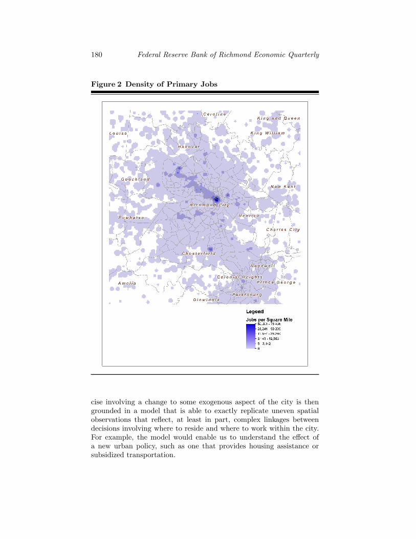
In practice, of course, economic activity is more unevenly distrib-uted across space. For example, Figure 2 shows that the city of Rich-mond, Virginia, has multiple employment clusters, one indeed in thecenter of the city but two others to the south and west.

This activity reflects a balance of agglomeration forces (e.g., pro-duction externalities) and dispersion forces (e.g., commuting costs) thatplay out in intricate and interrelated ways across space and that leadto substantial variations in allocations and prices across a city. For ex-ample, production may take place in different parts of the city so thatcities with multiple production centers are not uncommon. In fact,some productive activity potentially takes place at every location in thecity. Moreover, residential prices, even if they tend to fall away from acentral point in the city, seldom fall monotonically with distance fromthat center. Instead, residential rents can exhibit substantial variationacross locations within the city. This variation reflects the potentialcomplexity of linkages within the city where, for example, the residentpopulation at a given location may depend on the entire distribution ofwages offered across the city. Thus, in the next section, we show how


Figure 1 Allocations and Prices in the Monocentric Model

to modify the stylized model presented in this section in a way thatcan quantitatively account for the spatial allocations and prices it ismeant to study.

4. A QUANTITATIVE SPATIAL MODEL OF CITIES

In this section, we show how to adapt the stylized model of the pre-vious section to allow for the heterogeneity in spatial allocations andprices that is typically observed in cities. In doing so, we preserve thebasic assumptions on preferences, technology, and endowments of ourstylized model to keep the frameworks comparable. Instead of thinkingof the city as located on an interval [−B,B], we will think of the cityas composed of J distinct locations, indexed by j ∈ {1, ..., J} (or i). Inthe mapping to data, these locations may represent city blocks, censustracts, or counties. It is this key change that will allow us to ensurethat the model is at least able to match given observed spatial alloca-tions of, for example, resident population, land rents, employment, orwages across locations in a city. Any subsequent counterfactual exer-


Figure 2 Density of Primary Jobs

cise involving a change to some exogenous aspect of the city is thengrounded in a model that is able to exactly replicate uneven spatialobservations that reflect, at least in part, complex linkages betweendecisions involving where to reside and where to work within the city.For example, the model would enable us to understand the effect ofa new urban policy, such as one that provides housing assistance orsubsidized transportation.


In a model where every location could potentially be used for bothresidential and production purposes, a central component of a quan-titative spatial model is the representation and matching of distinctpairwise commuting flows from any location j in the city to any otherlocation i. This step will rely on an approach developed by Eaton andKortum (2002) in modeling trade flows between locations. As in themodel developed in the previous section, this analysis will focus on res-idential localization decisions, i.e., the decisions of households ratherthan firms. Unlike in the previous model, the commercial bid rentschedule is nondegenerate and reflects variations in productivity andwages across locations.

Firms

Production per unit of land in the business district of each location iis given by

Yi = A(Li)Lβi , (13)

analogously to equation (1), where Li denotes labor input and A(Li)denotes a production externality that we assume is local (so only em-ployment in i affects the productivity of businesses in i). For simplicity,let A(Li) = AiL

αi , α < 1 − β < 1, and denote the wage paid to work-

ers in location i by wi. There exists a unit mass of firms (assumingthat firms are small and do not internalize the externality) where therepresentative firm solves

maxLi

A(Li)Lβi − wiLi.

It follows that

βA(Li)Lβ−1i = w ⇔ Li =

(Aiβ

wi

) 11−α−β

. (14)

As in the previous model, firms operate in a competitive market withfree entry and thus obtain zero profits in equilibrium. The impliedcommercial bid rent schedule faced by firms in the business district is

qbi = (1− β)A1

1−α−βi

(β

wi

) α+β1−α−β .

(15)

Note the similarities between equations (14) and (15), and the analo-gous equations in the previous section, equations (2) and (3).


Residents

In each location j of the city, there exists a residential area composed ofa continuum of residents who commute to the business areas of differentlocations i for work. These residents differ in their preferences for whereto work in the city according to a random idiosyncratic components. Unlike the previous model where s was a city amenity distributeduniformly across locations, in this model, s is an individual-specificpreference component. Conditional on living in a particular locationj, this preference component captures the idea that residents of j mayhave idiosyncratic reasons for commuting to different locations i in thecity. We model the idiosyncratic preference component associated withresiding in location j and working in location i as scaling the utility ofthe residents of region j, where s is drawn from a Fréchet distributionspecific to that particular commute,

Fij(s) = e−λijs−θ, λij > 0, θ > 0. (16)

Residents of j who commute to i incur an associated cost, κij ∈[1,∞), that, analogous to the previous section, reduces the utility de-rived from housing. Thus, conditional on living in j and working in i,the problem of a resident having drawn idiosyncratic utility s is givenby

uij(s) = maxcij(s),hij(s)

s

(cij(s)

γj

)γj ( hij(s)

(1− γj)κij

)1−γj,

γj ∈ (0, 1)

subject to cij(s) + qrjhij(s) = wi,

where qrj is the price of a unit of residential housing services at locationj. Hence, we have that

cij(s) = γjwi, (17)

hij(s) =(1− γj)wi

qrj, (18)

and

uij(s) = s [wi]γj

[wiκijqrj

]1−γj

= swi[κijq

rj

]γj−1. (19)

Note the similarities between equations (17), (18), and (19) and theanalogous equations in the previous sections, equations (4), (5), and(6).


Aggregation

The setup we have just described allows for a considerable degree ofheterogeneity within the city compared to the stylized model presentedearlier. In particular, all locations allow for simultaneous use by bothbusinesses and residents (mixed use), individuals living in any locationmay commute to any other location for work, and commute costs be-tween any two locations are specific to that pair of locations, so thatit is possible to take into account the particular geographical makeupor road infrastructure of a city. However, having allowed for this highlevel of heterogeneity in the city, it becomes important to be able toaggregate economic activity at the level of a location, such as a censustract for practical purposes. The steps in this subsection address thisquestion.

Distribution of Utility

Since residents of j who work in i have different preferences s, drawnfrom equation (16), for commuting to that location, it follows that

Gij(u) = Pr(uij < u) = Fij

u[κijq

rj

]1−γj

wi

,

or

Gij(u) = e−Φiju−θ, Φij = λijw

θi

[κijq

rj

](γj−1)θ. (20)

Each resident of j chooses to commute to the location i that offersmaximum utility of all possible locations. Therefore,

Gj(u) = Pr(maxi{uij} < u) =

∏i

Pr(uij < u)

=∏i

e−Φiju−θ.

Thus, it follows that

Gj(u) = e−Φju−θ, Φj =

∑i

Φij . (21)

In other words, the distribution of resident utility in each location jof the city is itself a Fréchet distribution. The expected utility fromresiding in j is then given by

uj = Γ

(θ − 1

θ

)(qrj)γj−1

(∑i

λijwθi κ

(γj−1)θ

ij

) 1θ

, (22)


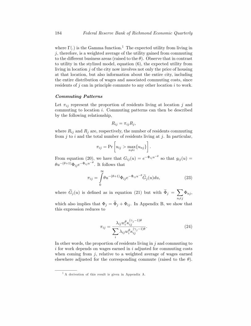
where Γ(.) is the Gamma function.1 The expected utility from living inj, therefore, is a weighted average of the utility gained from commutingto the different business areas (raised to the θ). Observe that in contrastto utility in the stylized model, equation (6), the expected utility fromliving in location j of the city now involves not only the price of housingat that location, but also information about the entire city, includingthe entire distribution of wages and associated commuting costs, sinceresidents of j can in principle commute to any other location i to work.

Commuting Patterns

Let πij represent the proportion of residents living at location j andcommuting to location i. Commuting patterns can then be describedby the following relationship,

Rij = πijRj ,

where Rij and Rj are, respectively, the number of residents commutingfrom j to i and the total number of residents living at j. In particular,

πij = Pr

[uij > max

n6=i{unj}

].

From equation (20), we have that Gij(u) = e−Φiju−θso that gij(u) =

θu−(θ+1)Φije−Φiju

−θ. It follows that

πij =

∞∫0


−θGj(u)du, (23)

where Gj(u) is defined as in equation (21) but with Φj =∑n6=j

Φnj ,

which also implies that Φj = Φj + Φij . In Appendix B, we show thatthis expression reduces to

πij =λijw

θi κ

(γj−1)θ

ij∑i

λijwθi κ(γj−1)θ

ij

. (24)

In other words, the proportion of residents living in j and commuting toi for work depends on wages earned in i adjusted for commuting costswhen coming from j, relative to a weighted average of wages earnedelsewhere adjusted for the corresponding commute (raised to the θ).

1 A derivation of this result is given in Appendix A.


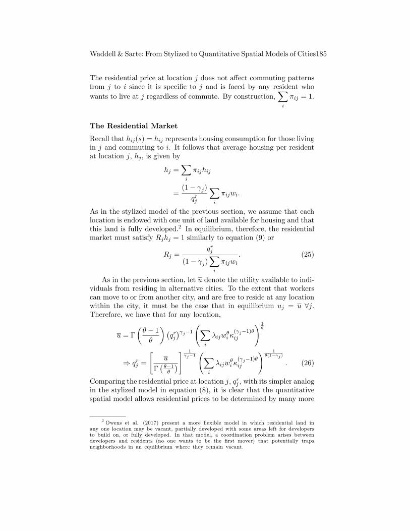
The residential price at location j does not affect commuting patternsfrom j to i since it is specific to j and is faced by any resident whowants to live at j regardless of commute. By construction,

∑i

πij = 1.

The Residential Market

Recall that hij(s) = hij represents housing consumption for those livingin j and commuting to i. It follows that average housing per residentat location j, hj , is given by

hj =∑i

πijhij

=(1− γj)qrj

∑i

πijwi.

As in the stylized model of the previous section, we assume that eachlocation is endowed with one unit of land available for housing and thatthis land is fully developed.2 In equilibrium, therefore, the residentialmarket must satisfy Rjhj = 1 similarly to equation (9) or

Rj =qrj

(1− γj)∑i

πijwi. (25)

As in the previous section, let u denote the utility available to indi-viduals from residing in alternative cities. To the extent that workerscan move to or from another city, and are free to reside at any locationwithin the city, it must be the case that in equilibrium uj = u ∀j.Therefore, we have that for any location,

u = Γ

(θ − 1

θ

)(qrj)γj−1

(∑i

λijwθi κ

(γj−1)θ

ij

) 1θ

⇒ qrj =

[u

Γ(θ−1θ

)] 1γj−1

(∑i

λijwθi κ

(γj−1)θ

ij

) 1θ(1−γj)

. (26)

Comparing the residential price at location j, qrj , with its simpler analogin the stylized model in equation (8), it is clear that the quantitativespatial model allows residential prices to be determined by many more

2 Owens et al. (2017) present a more flexible model in which residential land inany one location may be vacant, partially developed with some areas left for developersto build on, or fully developed. In that model, a coordination problem arises betweendevelopers and residents (no one wants to be the first mover) that potentially trapsneighborhoods in an equilibrium where they remain vacant.


factors, including the distribution of wages across all locations in thecity as well as all commuting costs. It is this richness that allowsfor spatial variation in allocations and prices across locations in thecity that is unavailable in the more stylized framework of the previoussection.

The City Labor Market

Since πijRj denotes the number of residents living in location j whocommute to the business area of location i for work, labor marketclearing in the city requires that

Li =

J∑j=1

πijRj ,

or alternatively (Aiβ

wi

) 11−α−β

=J∑j=1

πijRj . (27)

Solving for the City Equilibrium

We represent the parameters of the quantitative spatial model in avector, P = (α, β, θ, u, γj , Ai, κij , λij). Conditional on P, equations(24), (25), (26), and (27) then make up a system of J2 + 3J equationsin the same number of unknowns, πij(P), Rj(P), qrj (P), and wi(P).

Importantly, the equilibrium allocations in this model allow for con-siderably more heterogeneity than in the stylized model of the previoussection. Since they are specific to locations within the city, equilibriumallocations of the quantitative spatial model such as commuting pat-terns, πij(P), or equilibrium prices, such as residential prices, qrj (P),and wages, wi(P), may be directly matched to their data counterpartat the block or census tract level. In contrast, equilibrium allocationsof the stylized model in the previous section could only be indexed bydistance, `, from a central point in the city. The next section addressesthis last point in more detail.

Unlike the conventional monocentric model of the previous section,equilibrium existence and uniqueness are more challenging to prove in aquantitative spatial framework. However, Appendix C summarizes thekey equations needed to compute the model equilibrium and providesan algorithm that yields the corresponding numerical solution giventhe model’s parameters, P. Moreover, despite its added complexity, thequantitative spatial model retains some degree of analytical tractability.


For instance, as in the monocentric model of the previous section, wecan derive a simple expression for the elasticity of residential priceswith respect to commuting costs.

Proposition 3: The elasticity of residential prices with respect tocommuting costs, εqrj ,κij , is given by −πij .

Proof: We have that qrj =

(u

Γ( θ−1θ )

) 1γj−1

(∑i λijw

θi κ

(γj−1)θ

ij

) 1θ(1−γj) .

Then

∂qrj∂κij

=(u

Γ(θ−1θ

)) 1γj−1 1

θ(1− γj)

(∑i

λijwθi κ

(γj−1)θ

ij

) 1θ(1−γj)

−1

(γj−1)θλijwθi κ

(γj−1)θ−1

ij

= −1 ·λijw

θi κ

(γj−1)θ−1

ij∑i λijw

θi κ

(γj−1)θ

ij

qrj

It follows that

εqrj ,κij =∂qrj∂κij

· κijqrj

= −λijw

θi κ

(γj−1)θ−1

ij qrj∑i λijw

θi κ

(γj−1)θ

ij

· κijqrj

= −πij .

This finding is intuitive. A 1 percent increase in commute costsbetween any two locations, κij , lowers residential prices by the shareof residents affected by that commute. In this relatively simple spatialenvironment, even if it allows for more flexibility than the monocentricsetup, the relationship is exact. More importantly, unlike the analogouselasticity in the more stylized model, the share of residents is itself anendogenous outcome that depends on all of the city’s characteristics,P, and thus will move along with the entire distribution of wages andpopulation across locations in any policy experiment.

5. MATCHING THE QUANTITATIVE SPATIALMODEL TO URBAN MICRODATA

As elaborated upon in earlier sections, it is now possible to model citiesby matching these types of quantitative spatial models to available mi-crodata. For the purpose of the discussion below, the parameters in Pfall into two broad classifications: citywide parameters and location-or neighborhood-specific parameters. The parameters in P that are


not location specific have generally accepted values in the literature.For example, Monte et al. (2016) estimate θ (the parameter that gov-erns the shape of the distribution of the idiosyncratic preference, s, ofcommuting from i to j) to be 4.43. Ciccone and Hall (1996) estimateα (the production externality) to be 0.06, and Ahlfeldt et al. (2015)estimate β (the parameter that defines the relationship between laborand output, separate from the externality) to be 0.80, while u is anormalizing constant. The parameters that are location-specific poten-tially present a greater computational challenge since there are manyof them. For example, in a city with 1, 000 census tracts, there are1, 000, 000 λij’s. Other location-specific parameters, such as pairwisecommuting costs, κij , may be directly calibrated to data on distancesor commuting times.

The Longitudinal Employer-Household Dynamics Origin-DestinationEmployment Statistics provide reliable data on cities at the census tractlevel, including commuting patterns (πij), resident population (Rj),employment (Li), and wages (wi). Other detailed data on cities arealso available; for example, residential prices (qrj ) are available fromCoreLogic or county assessors’offi ces. In general, such data show con-siderable unevenness across space within a city.

We now describe how, in our simple framework, the location-specificparameters of our quantitative spatial model may be calibrated to ex-actly match, in equilibrium, all pairwise commuting patterns, πij , theexact distribution of population across space, Rj , and thus also thedistribution of employment, Li, and the exact distribution of wages inthe city, wi, in a given benchmark period. In particular, we choosethe parameters of the model (λij , γj , Ai) to match the observations(πij , Rj , wi) as equilibrium outcomes. In this way, counterfactual ex-ercises involving a change to some exogenous aspect of the city, or achange in urban policy, are rooted in a model that, as a benchmark, isable to exactly match basic observed allocations and prices in the cityas equilibrium outcomes.

Recall that commuting patterns, πij , are given by equation (24),

πij =λijw

θi κ

(γj−1)θ

ij∑i

λijwθi κ(γj−1)θ

ij

,

where κij ∈ [1,∞). If πij = 0, then either λij = 0 or κij → ∞.Commuting patterns can be alternatively expressed in terms of theHead and Ries (2001) index,

πijπjj

=λijw

θi κ

(γj−1)θ

ij

λjjwθjκ(γj−1)θ

jj

.


Then, conditional on θ = 4.43 and values for γj , the preference pa-rameters, λij , can then be chosen to be consistent with commutingpatterns,

λij = πij

(wjwi

)θ ( κijκmin

)(1−γj)θ (λjjπjj

), (28)

where κmin is a lower bound on κjj .3 Since κij may be directly inferredfrom commuting costs data, this approach to obtaining λij to matchcommuting patterns presumes we are also able to match wages, wi, aspart of the model inversion. We show below that this can indeed bedone through the choice of location-specific productivities, Ai. Withthis in mind, we first choose γj so as to match the distribution ofresident population across space, Rj , conditional on πij and wi.

The number of residents in location j is given by

Rj =qrj

(1− γj)∑

i πijwi. (29)

Using equations (26) and (28) with κmin = 1, and the normalization(λjjπjj

)= 1, for all locations j, equation (29) simplifies to

Rj(γj) =

(Γ(θ−1θ

)wj

u

) 11−γj 1

(1− γj)∑

i πijwi. (30)

Notice that as γj → 0+, Rj(γj)→Γ( θ−1θ )wju∑i πijwi

and as γj → 1−, Rj(γj)→

∞. Therefore, one may choose u so that Rj >Γ( θ−1θ )wju∑i πijwi

for all j andnumerically solve the expression in equation (30) to obtain a set of γjthat exactly matches the distribution of Rj , conditional on πij and wi.Since the distribution of γj then depends on u, and γj represents theshare of income spent on housing in a given census tract j, we chooseu so that the mean of γj is 0.76 as in Ahlfeldt et al. (2015).

Since commuting patterns πij can be exactly matched, given γj andwages wi, through the choice of λij in equation (28), it remains onlyto ensure that the model is consistent with the spatial distributionof wages in an equilibrium benchmark version of the model. Usingequation (26), we can write the city labor market clearing condition,equation (27) as (

Aiβ

wi

) 11−α−β

=

J∑j=1

πijRj ,

3 Since∑i

πij = 1, one needs to also normalize the λij’s, for example,λjjκjj

= 1 ∀j.


in which case we can simply choose location-specific productivities,Ai, to ensure that equilibrium benchmark wages exactly match thedistribution of wages in the city,

Ai =wiβ

J∑j=1

πijRj

1−α−β

. (31)

Observe that on the righthand side of equation (31), we are free to usethe data on commuting patterns, πij , and residential population, Rj ,since those are matched by construction through the choices of λij andγj in equations (28) and (30).

6. CONCLUSION

The development of the new quantitative equilibrium models has initi-ated a more robust and realistic framework with which to model cities.This framework will enable urban economists to provide empiricallydriven insight into future theoretical or structural work on how citiesgrow, shrink, and change. By offering a more accurate grounding forempirical models, it will also allow for more robust counterfactual pol-icy exercises that can inform practitioners and policymakers regardingstrategies for urban development.


REFERENCES

Ahlfeldt, Gabriel M., Stephen J. Redding, Daniel M. Sturm, andNikolaus Wolf. 2015. “The Economics of Density: Evidence fromthe Berlin Wall.”Econometrica 83 (November): 2127—89.

Ciccone, Antonio, and Robert E. Hall. 1996. “Productivity and theDensity of Economic Activity.”American Economic Review 86(March): 54—70.

Eaton, Jonathan, and Samuel Kortum. 2002. “Technology,Geography, and Trade.”Econometrica 70 (September): 1741—79.

Fujita, Masahisa. 1988. “A Monopolistic Competition Model ofSpatial Agglomeration: Differentiated Product Approach.”Regional Science and Urban Economics 18 (February): 87—124.

Fujita, Masahisa, Paul Krugman, and Anthony J. Venables. 1999. TheSpatial Economy: Cities, Regions, and International Trade.Cambridge, Mass.: MIT Press.

Fujita, Masahisa, and Hideaki Ogawa. 1982. “Multiple Equilibria andStructural Transition of Non-Monocentric Urban Configurations.”Regional Science and Urban Economics 12 (May): 161—96.

Fujita, Masahisa, and Jacques-François Thisse. 2002. Economics ofAgglomeration: Cities, Industrial Location, and Regional Growth.Cambridge: Cambridge University Press.

Krugman, Paul. 1991. “Increasing Returns and EconomicGeography.”Journal of Political Economy 99 (June): 483—99.

Lucas, Robert E., and Esteban Rossi-Hansberg. 2002. “On theInternal Structure of Cities.”Econometrica 70 (July): 1445—76.

Monte, Ferdinando, Stephen J. Redding, and Esteban Rossi-Hansberg.2016. “Commuting, Migration, and Local EmploymentElasticities.”Princeton University Working Paper (October).

Ottaviano, Gianmarco, and Jacques-François Thisse. 2004.“Agglomeration and Economic Geography.”In Handbook ofRegional and Urban Economics, vol. 4, ed. J. Vernon Hendersonand Jacques-François Thisse. North Holland: Elsevier: 2563—608.

Owens, Raymond III, Esteban Rossi-Hansberg, and Pierre-DanielSarte. 2017. “Rethinking Detroit.”Working Paper 23146.Cambridge, Mass.: National Bureau of Economic Research.(February).


Redding, Stephen J., and Esteban Rossi-Hansberg. Forthcoming.“Quantitative Spatial Economics.”Annual Review of Economics.

Redding, Stephen J., and Daniel M. Sturm. 2008. “The Costs ofRemoteness: Evidence from German Division and Reunification.”American Economic Review 98 (December): 1766—97.

Venables, Anthony J. 1996. “Equilibrium Locations of VerticallyLinked Industries.”International Economic Review 37 (May):341—59.


APPENDIX: APPENDIX A

Under the maintained assumptions, expected utility at location j isgiven by

uj =

∞∫0

θΦju−θe−Φju

−θdu.

Consider the change in variables,

y = Φju−θ, dy = −θΦju

−(θ+1)du.

Then, we have that

uj =

∞∫0

Φ1θj y−1θ e−ydy = Γ

(θ − 1

θ

)Φ

1θj ,

from which equation (22) in the text follows.

APPENDIX: APPENDIX B

From equation (23), we have that

πij =

∞∫0


−θe−Φju

−θdu

=

∞∫0

θu−(θ+1)Φije−Φju

−θdu.

Consider the change of variables,

y = Φju−θ, dy = −θΦju

−(θ+1)du.


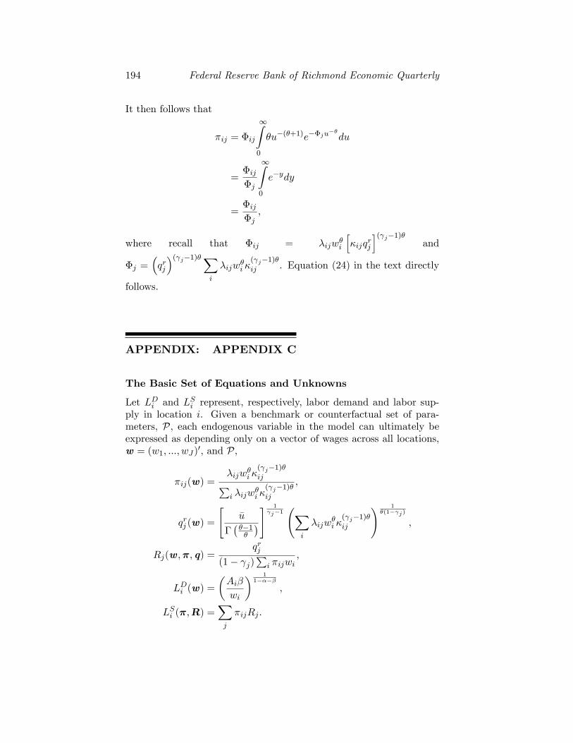
It then follows that

πij = Φij

∞∫0

θu−(θ+1)e−Φju−θdu

=Φij

Φj

∞∫0

e−ydy

=Φij

Φj,

where recall that Φij = λijwθi

[κijq

rj

](γj−1)θand

Φj =(qrj

)(γj−1)θ∑i

λijwθi κ

(γj−1)θ

ij . Equation (24) in the text directly

follows.

APPENDIX: APPENDIX C

The Basic Set of Equations and Unknowns

Let LDi and LSi represent, respectively, labor demand and labor sup-ply in location i. Given a benchmark or counterfactual set of para-meters, P, each endogenous variable in the model can ultimately beexpressed as depending only on a vector of wages across all locations,w = (w1, ..., wJ)′, and P,

πij(w) =λijw

θi κ

(γj−1)θ

ij∑i λijw

θi κ

(γj−1)θ

ij

,

qrj (w) =

[u

Γ(θ−1θ

)] 1γj−1

(∑i

λijwθi κ

(γj−1)θ

ij

) 1θ(1−γj)

,

Rj(w,π, q) =qrj

(1− γj)∑

i πijwi,

LDi (w) =

(Aiβ

wi

) 11−α−β

,

LSi (π,R) =∑j

πijRj .


Then, finding an equilibrium of the model is equivalent to finding avector of wages that clears the labor market; LDi (w) = LSi (w) for alllocations i = 1, ..., J . Put another way, the task is to find a vectorw∗ ∈ RJ+ such that

(LDi − LSi )(w∗) =

(Aiβ

wi

) 11−α−β

−∑j

λijwθi κ

(γj−1)θ

ij∑i λijw

θi κ

(γj−1)θ

ij

[u

Γ( θ−1θ )

] 1γj−1

(∑i λijw

θi κ

(γj−1)θ

ij

) 1θ(1−γj)

(1− γj)∑

i

λijwθi κ(γj−1)θij∑

i λijwθi κ

(γj−1)θij

wi

= 0

Several algorithms exist to numerically solve nonlinear system of equa-tions, and MATLAB’s fsolve function handles this particular systemwell.

Numerical Algorithm

Some quantitative spatial models can result in systems whose features(such as nondifferentiability in the presence of thresholds or bindingconstraints on available land) make traditional algorithms diffi cult toapply. In such cases, a simple “guess-and-iterate”method can be con-structed to calculate solutions. We outline such a method here as itapplies to our model.

1. Choose a tolerance level ε > 0 and guess a vector of wages, wn.

2. Calculate the implied matrix of flows: πij(wn) =λijw

θn,iκ

(γj−1)θij∑

i λijwθn,iκ

(γj−1)θij

.

3. Calculate the implied prices:

qrj (wn) =

[u

Γ( θ−1θ )

] 1γj−1

(∑i λijw

θn,iκ

(γj−1)θ

ij

) 1θ(1−γj) .

4. Using the prices and flows calculated in steps two and three, cal-

culate the implied number of residents: Rj(wn) =qrj (wn)

(1−γj)∑i πij(wn)wi

.

5. Using the residents calculated in step four, calculate the impliedlabor supply in each labor market: LSi (wn) =

∑j πij(wn)Rj(wn).

6. Calculate the implied labor demand in each labor market: LDi (wn) =(Aiβwi

) 11−α−β

.


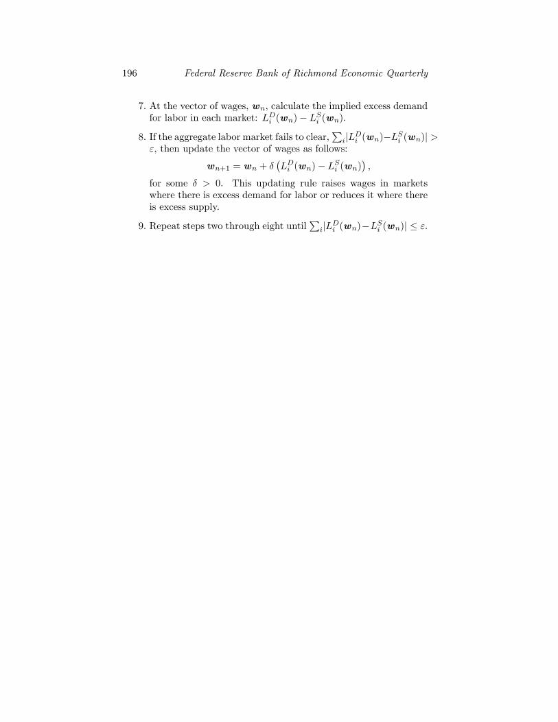
7. At the vector of wages, wn, calculate the implied excess demandfor labor in each market: LDi (wn)− LSi (wn).

8. If the aggregate labor market fails to clear,∑

i|LDi (wn)−LSi (wn)| >ε, then update the vector of wages as follows:

wn+1 = wn + δ(LDi (wn)− LSi (wn)

),

for some δ > 0. This updating rule raises wages in marketswhere there is excess demand for labor or reduces it where thereis excess supply.

9. Repeat steps two through eight until∑

i|LDi (wn)−LSi (wn)| ≤ ε.

From Stylized to Quantitative Spatial Models of Cities · NEG came from Krugman (1991), who developed a model that showed that the emergence of an industrialized ﬁcoreﬂand an

Documents