From snakes to region-based active contours defined by region-dependent parameters

From snakes to region-based active contours

defined by region-dependent parameters

Stephanie Jehan-Besson1, Muriel Gastaud1, Frederic Precioso1,

Michel Barlaud1, Gilles Aubert2, Eric Debreuve1

1Laboratoire I3S, UMR CNRS 6070, Les Algorithmes, Bat. Euclide B,2000, route des lucioles, BP 121, 06903 Sophia Antipolis Cedex, France

2Laboratoire Dieudonne, UMR CNRS 6621, Universite de Nice-Sophia Antipolis,Parc Valrose, 06108 Nice Cedex 2, France

[email protected]

This synthetic paper deals with image and sequence segmentation whenlooking at the segmentation task from a criterion optimization point of view.Such a segmentation criterion involves so-called (boundary and region) de-scriptors which, in the general case, may depend on their respective boundaryor region. This dependency must be taken into account when computing thecriterion derivative with respect to the unknown object domain (defined byits boundary). If not, some correctional terms may be omitted. This article fo-cuses computing the derivative of the segmentation criterion using a dynamicscheme. The presented scheme is general enough to provide a framework fora wide variety of applications in segmentation. It also provides a theoreticalmeaning to the active contour philosophy. c© 2003 Optical Society of America

1. Introduction

This paper does the synthesis of several years of development in active contour seg-mentation conducted at I3S (Informatique, Signaux et Systemes de Sophia Antipolis)and Dieudonne laboratories, CNRS (French National Research Center) and UniversityOf Nice-Sophia Antipolis, France.

The purpose of segmentation is to isolate an object (or several objects) of interestin an image or a sequence. Given an initial contour (a closed curve), the active contourtechnique consists in applying locally a force (or displacement, or velocity) such thatthe initial contour evolves toward the contour of the object of interest. This force isderived from a characterization of the object formally written as a criterion to beoptimized.

A. Boundary-Based Active Contours

In boundary-based active contour techniques, the object is characterized by propertiesof its contour only. The original active contour developments were called snakes.1 Onlythe convex hull of objects could be segmented because these techniques were based

1

on a minimum length penalty. In order to be able to segment concave objects, aballoon force was heuristically introduced. It was later theoretically justified as aminimum area constraint2 balancing the minimum length constraint. The geodesicactive contour technique3 is the most general form of boundary-based techniques.The criterion corresponding to this technique is

J(Γ) =

∫

Γ

k(x) dx (1)

where Γ is a contour, k is a positive function “describing” the object of interest, andx is a point of the image. The active contour evolution equation3 is

∂Γ

∂τ= (κk −∇k · N )N (2)

where τ is the evolution parameter (Γ(τ = 0) = Γ0, initial contour, and Γ(τ → ∞) →segmentation), κ is the curvature of Γ, operator · represents the inner product, andN is the inward normal. Actually, this equation should be written with κ(x), k(x),and N (x) where x is a point of Γ(τ). The contour minimizing J can be interpreted asthe curve of minimum length in the metric defined by function k. If k is the constantfunction equal to one, Eq. (2) is called the geometric heat equation by analogy withthe heat diffusion equation. Function k can also be a function of the gradient of theimage. For instance,

k(x) =1

1 + |∇I(x)|(3)

where I is the image and ∇ is the intensity gradient. In this case, the object contouris simply characterized by a curve following high gradients. As a consequence, thetechnique is effective only if the contrast between the object and the backgroundis high. Moreover, high gradients in an image may correspond to the boundaries ofobjects that are not of interest. Regardless of function k, information on the boundaryis too local for segmentation of complex scenes. A global, more sophisticated objectcharacterization is needed.

B. Region-Based Active Contours

In order to better characterize an object and to be less sensitive to noise, region-basedactive contour techniques were proposed.4,5 A region is represented by mathematicalexpressions called “descriptors” in this paper. Two kinds of region are usually consid-ered: The object of interest and the background. Note that region-based/boundary-based hybrid techniques are common.6–9 In the general case, descriptors may dependon their respective regions, for instance, statistical features such as mean intensity orvariance within the region.10 The general form of a criterion including both region-based and boundary-based terms is

J(Ωin) =

∫

Ωin

kin(Ωin, x) dx + η

∫

Γ

kb(x) dx (4)

2

where Ωin is the domain inside Γ and η is a positive constant. An example of descriptorkin is

kin(Ωin, x) = (µ(Ωin) − I(x))2 (5)

where µ is the mean intensity

µ(Ωin) =

∫

Ωin

I(x) dx∫

Ωin

dx. (6)

Function (3) is an example of descriptor kb. Classically the integral on domain Ωin

in criterion (4) is reduced to an integral along Γ using the Green-Riemann theo-rem6–8,11–13 or continuous media mechanics techniques.14,15 Two active contour ap-proaches are possible to minimize the resulting criterion: (i) It is possible to determinethe evolution of an active contour from τ to τ +dτ without computing a velocity: Thedisplacement of a point of the contour is chosen among small random displacementsas the one leading to the locally optimal criterion value.6,11 However this implies tocompute the criterion value several times for each point; (ii) Alternatively, differen-tiating the criterion with respect to τ allows to find an expression of the appropriatedisplacement, or velocity, for each point.7,8, 12,13 In this case the region-dependencyof the descriptors must be taken into account. If not,7,8, 12–15 some correctional termsin the expression of the velocity may be omitted.

2. Accounting For Region Dependency

In this paper, the region-dependency of descriptors is taken into account in the deriva-tion of the velocity. It is shown that it induces additional terms leading to a greateraccuracy of segmentation. The development is general enough to provide a frameworkfor region-based active contour. It is inspired by shape optimization techniques.16,17

A. Problem Statement

Let us consider an image composed of background and one object of interest, each ofwhich having unique properties represented by descriptors kout and kin, respectively.The object boundary has also properties represented by descriptor kb. For a givendomain Ωin, let us define the following general criterion

J(Ωin) = α

∫

Ωin

kin(Ωin, x) dx + β

∫

Ωout

kout(Ωout, x) dx +

∫

Γ

kb(x) dx (7)

where α and β are positive constants, Ωin, Ωout, and Γ are such that

Ωin ∪ Γ ∪ Ωout = image domain D

Γ = ∂Ωin = ∂Ωout

Ωin = domain inside Γ, (8)

and kin, kout, and kb are positive functions such that

kin is minimum in the object, e.g., function (5)kout is minimum in the background, e.g., kout = 0,meaning that no specific information is available for the backgroundkb is minimum on the object boundary, e.g., function (3)

. (9)

3

Therefore, the minimum of criterion (7) is reached if Ωin segments the object ofinterest. The proposed segmentation method is based on the active contour technique(see Subsection 2.B below). Let us give the notations here. Domains Ωin and Ωout andcontour Γ are respectively replaced with dynamic versions depending on evolutionparameter τ . At τ equal to zero, an initial domain Ωin(τ = 0) = Ω0

in is defined, eithermanually or automatically (equivalently, Ωout(τ = 0) = Ω0

out and Γ(τ = 0) = Γ0). Theactive contour converges toward the object boundary as τ increases. It increases bydτ at each iteration when discretizing the evolution equation for computer coding.

B. Differentiating the Criterion

The set of domains Ωin is not a vectorial space. Direct computation of the derivativeof criterion (7) with respect to Ωin is not possible. The proposed solution is to usea dynamic scheme where Ωin becomes continuously dependent on an evolution pa-rameter denoted by τ . As τ increases, Ωin(τ) must act as a minimizing sequence ofcriterion (7). It is equivalent to finding a family of domain transforms Tτ such that T0

is the identity and Tτ (Ω0in) = Ωin(τ) where Ω0

in is an initial contour. As a consequence,the active contour philosophy of the proposed method has a theoretical explanationrather than being used as an implementation tool for an energy minimization problem.Criterion (7) becomes

J(Ωin(τ)) = α

∫

Ωin(τ)

kin(Ωin(τ), x) dx + β

∫

Ωout(τ)

kout(Ωout(τ), x) dx +

∫

Γ(τ)

kb(x) dx

(10)which can be rewritten

J(τ) = α

∫

Ωin(τ)

kin(τ, x) dx + β

∫

Ωout(τ)

kout(τ, x) dx +

∫

Γ(τ)

kb(x) dx . (11)

Criterion (11) is composed of two types of integrals:

J1(τ) =

∫

Ω(τ)

k(τ, x) dx (region integral) (12)

J2(τ) =

∫

Γ(τ)

kb(x) dx (contour integral) (13)

For simplicity, k(τ, x) will be written k and kb(x) will be written kb.

1. Region Integral

Theorem 1 16,17 Let D be the image domain (Ω(τ) ⊂ D). Let k be a smooth functionon R+ × D. Then

dJ1

dτ(τ) = J ′

1(τ) =

∫

Ω(τ)

∂k

∂τdx −

∫

∂Ω(τ)

v · Nk dx (14)

where v (actually v(τ, x)) is the velocity of ∂Ω(τ) and N (actually N (τ, x)) is theinward unit normal to ∂Ω(τ).

4

J ′1(τ) is called the Eulerian derivative of J1(Ω(τ)) in the direction of v at τ . It repre-

sents the variation of J1(τ) due to both the deformation of integration domain Ω(τ)according to v and the variation of k. The variation of k is also due to the deformationof domain Ω(τ).

Corollary 1 18 Let D be the image domain. Let Ωin(τ), Ωout(τ), and Γ(τ) be twodomains and a boundary as defined by Eqs. (8). Let kin, respectively kout, be a smoothfunction on R+ × Ωin(τ), respectively R+ × Ωout(τ). Let J1(τ) be

J1(τ) =

∫

Ωin(τ)

kin(τ, x) dx +

∫

Ωout(τ)

kout(τ, x) dx . (15)

Then

dJ1

dτ(τ) = J ′

1(τ)

=

∫

D

∂K

∂τdx −

∫

Γ(τ)

v · N [[K]] dx −

∫

∂Ωout(τ)\Γ(τ)

w · NΩoutK dx

(16)

where K is the function equal to kin in Ωin(τ) and kout in Ωout(τ), [[K]] is the jump ofK across Γ(τ) and it is equal to kin − kout, ∂Ωout(τ)\Γ(τ) is the boundary of Ωout(τ)excluding Γ(τ) (namely ∂D), w is the velocity of ∂Ωout(τ)\Γ(τ), and NΩout

is theinward unit normal to ∂Ωout(τ)\Γ(τ).

Corollary 1 is obtained by applying theorem 1 with Ωin(τ), kin and D = Ωin(τ) for thefirst integral of (15) and with Ωout(τ), kout and D = Ωout(τ) for the second integral(see Appendix). Note that the image domain being fixed, velocity w is equal to zeroand so is the last integral of (16).

2. Contour Integral

The derivative of J2(τ) is classical.3

dJ2

dτ(τ) = J ′

2(τ) =

∫

Γ(τ)

(∇kb · N − kbκ)v · N dx (17)

where κ (actually κ(τ, x)) is the curvature of Γ(τ).

3. Complete Criterion

Finally, the derivative of criterion (11) is

J ′(τ) = α

∫

Ωin(τ)

∂kin

∂τdx + β

∫

Ωout(τ)

∂kout

∂τdx +

∫

Γ(τ)

(βkout − αkin + ∇kb · N − kbκ)v · N dx . (18)

5

The first two integrals in (18) can be reduced to a boundary integral:18

α

∫

Ωin(τ)

∂kin

∂τdx + β

∫

Ωout(τ)

∂kout

∂τdx =

∫

Γ(τ)

H(kin, kout)v · N dx (19)

where H(kin, kout) represents the additional terms mentioned at the beginning ofsection 2. As a consequence, derivative (18) can be rewritten

J ′(τ) =

∫

Γ(τ)

ρv · N dx (20)

withρ = H(kin, kout) + βkout − αkin + ∇kb · N − kbκ . (21)

Velocity v is unknown. It must be chosen so that the value of (20) is negative in orderto make criterion (11) decrease. Note that this result can be obtained by a classicalcalculus of variation approach although the development is tedious.19

C. Evolution Equation

A way to ensure negativity of derivative (20) is to chose v = −ρN . Derivative (20)is then

J ′(τ) = −

∫

Γ(τ)

ρ2 dx . (22)

Since velocity v can also be written ∂Γ∂τ

, the evolution equation of the active contouris

Γ(0) = Γ0∂Γ∂τ

(τ, x) = −ρ(τ, x)N (τ, x) for all τ ≥ 0 and x ∈ Γ(τ). (23)

Equation (23) means that, starting from initial contour Γ0, active contour Γ evolvesuntil velocity amplitude ρ is equal to zero everywhere along the contour. In otherwords, active contour Γ at τ + dτ is obtained by deforming active contour Γ at τ ac-cording to local velocity −ρN , if it is not equal to zero. If region descriptors kin andkout are region-independent (i.e., if they do not depend on Ωin(τ)), then H(kin, kout)is equal to zero. However this is not a necessary condition. Note that Eq. (23) solvesthe segmentation problem (the primary goal) and computes the parameters involvedin the descriptors simultaneously. These parameters could be used for indexing andretrieval tasks. For example, if kin is defined to be minimum in regions with an ho-mogeneous blue color, the corresponding parameter is the mean value of the bluecomponent within the region. If the segmentation method is applied to a set of RGBimages, the parameter values can be stored along with the blue region contours afterwhich the image database can be queried for images containing homogeneous regionswith a given blue component value.

D. Examples Of Descriptors18,20

1. Constant Intensity

An example of a region descriptor that is region-independent is

kin(τ, x) = φ(δ − I(x)) (24)

6

where φ is a smooth, positive, even function increasing on R+. This descriptor canbe used to segment a region of known intensity δ. If kout is defined similarly, thenH(kin, kout) is equal to zero.

2. Mean Intensity

The mean intensity within Ωin(τ) is

µ(τ) =

∫

Ωin(τ)I(x) dx

∫

Ωin(τ)dx

. (25)

If descriptor kin is φ(µ(τ) − I(x)) and kout is equal to zero, then

H(kin, kout)(τ, x) = −µ(τ) − I(x)∫

Ωin(τ)dy

∫

Ωin(τ)

φ′(µ(τ) − I(y)) dy (26)

If φ is the square function, then H(kin, kout) is equal to zero.13,14 This descriptor canbe used to segment an homogeneous region of unknown intensity.

3. Variance

The variance within Ωin(τ) is

σ2(τ) =

∫

Ωin(τ)(µ(τ) − I(x))2 dx∫

Ωin(τ)dx

(27)

where µ(τ) is defined as in (25). If descriptor kin is φ(σ2(τ)) and kout is equal to zero,then

H(kin, kout)(τ, x) = φ′(σ2(τ))[σ2(τ) − (µ(τ) − I(x))2] (28)

Note that H(kin, kout) depends on x whereas the descriptor (hence, the criterion) doesnot. This descriptor can be used to segment a region with low noise or low intensityvariation.

4. Shape Of Reference

When segmenting a region using appropriate descriptors, it can be useful to constrainthe active contour to stay close to a shape of reference. This can be done using thefollowing criterion20

J2(τ) =

∫

Γ(τ)

kb(τ, x) dx =

∫

Γ(τ)

φ(d(x, Γref)) dx (29)

where d(x, Γref) is the signed distance to Γref at x, i.e.,

d(x, Γref) =

+|x − y(x)| if x is outside Γref

−|x − y(x)| otherwise(30)

where y(x) is the closest point to x belonging to Γref , and φ is a smooth, positive, evenfunction increasing on R+. In criterion (13), boundary descriptor kb does not depend

7

on τ , i.e., on the boundary. Computation of the derivative of boundary-dependentdescriptor (29) is different from the developments mentioned in Subsection 2.B. Itcan be shown20 that the derivative is

J ′2(τ) = −

∫

Γ(τ)

(φ′(d)N ref · N + φ(d)κ)v · N dx (31)

where d is a short notation for d(x, Γref) and N ref is the inward unit normal to Γref aty(x). The deformation between the shape of reference and the segmentation contouris a free-form deformation (i.e., deformation with unlimited degrees of freedom) asopposed to a parametric transform21,22 (i.e., global deformation with few degrees offreedom, e.g., a combination of a translation, a rotation, and a scaling). Althoughthe derivatives of the criteria may be similar in both cases, the parametric transformapproach tends to turn the segmentation problem into an iterative best fit searchamong the set of contours obtained by parametric transform.

3. Active Contour Implementation

A. From Parametric To Implicit

The first implementations of the active contour technique were based on a parametric,or explicit, description of the contour.1 It corresponds to a Lagrangian approach.However, management of the evolution, particularly topology changes and samplingdensity along the contour, is not simple.23 Instead, an Eulerian approach known asthe level set technique24,25 can be used. In two dimensions, the contour is implicitlyrepresented as the intersection of a surface u = f(x), where x ∈ D and elevation f is acontinuous function with positive and negative values, with the plane of elevation zero.The contour can also be seen as the isocontour of level zero on the surface. In threedimensions, the contour is the isosurface of level zero in a volume. In n dimensions, thecontour is the hyperplane of level zero with the space filled in with the values of a real,continuous function. Note that the contour can actually be composed of several closedcontours without intersections with each other. By a continuous change of functionf , a contour can appear or disappear without explicit handling. Unfortunately, evenwith the narrow band implementation,26,27 the level set technique has a rather highcomputational cost and extension of the velocity to levels other than the zero levelis not straightforward28,29 while it is theoretically necessary. Moreover, a curvatureterm (minimum length penalty) is usually added to the velocity expression in orderto decrease the influence of image noise on the evolution. However, the curvaturebeing a second derivative term, its numerical approximation is usually not accurate.Similarly, the level set gradient (equivalent to the isocontour normal) is numericallyapproximated. The fast marching technique30 is another Eulerian approach to theactive contour representation. It could be seen as the limit case where the narrowband is one grid element thick. This technique is much faster than the level settechnique. However it can be applied only if one can guarantee that the velocityexpression keeps the same sign during evolution.

8

B. Splines: Back To The Parametric Approach

A cubic B-spline has several interesting properties: It is a C2 curve,31 it is an inter-polation curve that minimizes a term close to the square curvature,32 and it has ananalytical equation (depending on control points) between each pair of consecutivesampling points (pi, pi+1). It minimizes the following criterion with the constraint thatit passes through the sampling points

JCubicS(Γ) =

∫

Γ

Γ”(x)2 dx (32)

where Γ” is the second derivative of Γ with respect to the arc length parameter. Notethat the sampling points correspond to the ends, or knots, of the spline segments. Thevelocity has to be computed at the sampling points only. If the sampling is regular,the normal and the curvature can be computed using an exact, fast, recursive filter-ing algorithm applied to the control points. Therefore, the spline implementation ismuch less time consuming than the level set technique.33,34 Moreover, the minimumcurvature-type term property helps in decreasing the influence of noise without theneed to add a curvature term to the velocity. Nevertheless, noise in the image stillimplies noise in the velocity which, if sampling is fine, usually leads to an irregularcontour because, despite the smooth curvature property, a cubic B-spline is an in-terpolation curve. Finally, let us recall that, unlike with level sets, management oftopology changes has to be performed explicitly and is not an easy task. Also note thatthe number of sampling points is a parameter. Less sampling points implies a curvemore rigid, or smoother, preventing from segmenting regions with a high curvature.

C. Smoothing Splines

A smoothing spline is an approximation curve controlled by a parameter balancing thetrade-off between interpolation error and smoothness.35,36 It minimizes the followingcriterion

JSmoothS(Γ) = λ

∫

Γ

Γ”(x)2 dx +∑

i

(pi − Γi)2 (33)

where λ is a parameter, pi is a sampling point, and Γi is a knot. Note that knots donot correspond to sampling points anymore. The smoothing spline is only constrainedto be confined to a “band” surrounding the sampling points. The smaller parameterλ, the narrower the band. When λ is equal to zero, the smoothing spline is a classicalinterpolation spline. Thus, if sampling is fine and noise is high, the smoothing splinecan still be smooth. As with cubic B-splines, normal and curvature can be computedexactly and efficiently.

4. Examples Of Applications

The following results were obtained using the level set technique except otherwisenoted.

9

A. Image Segmentation

1. Region Competition

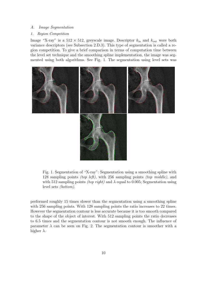
Image “X-ray” is a 512 × 512, greyscale image. Descriptor kin and kout were bothvariance descriptors (see Subsection 2.D.3). This type of segmentation is called a re-gion competition. To give a brief comparison in terms of computation time betweenthe level set technique and the smoothing spline implementation, the image was seg-mented using both algorithms. See Fig. 1. The segmentation using level sets was

Fig. 1. Segmentation of “X-ray”: Segmentation using a smoothing spline with128 sampling points (top left), with 256 sampling points (top middle), andwith 512 sampling points (top right) and λ equal to 0.005; Segmentation usinglevel sets (bottom).

performed roughly 15 times slower than the segmentation using a smoothing splinewith 256 sampling points. With 128 sampling points the ratio increases to 22 times.However the segmentation contour is less accurate because it is too smooth comparedto the shape of the object of interest. With 512 sampling points the ratio decreasesto 6.5 times and the segmentation contour is not smooth enough. The influence ofparameter λ can be seen on Fig. 2. The segmentation contour is smoother with ahigher λ.

10

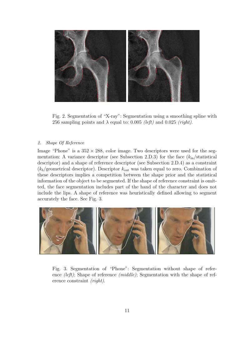
Fig. 2. Segmentation of “X-ray”: Segmentation using a smoothing spline with256 sampling points and λ equal to: 0.005 (left) and 0.025 (right).

2. Shape Of Reference

Image “Phone” is a 352 × 288, color image. Two descriptors were used for the seg-mentation: A variance descriptor (see Subsection 2.D.3) for the face (kin/statisticaldescriptor) and a shape of reference descriptor (see Subsection 2.D.4) as a constraint(kb/geometrical descriptor). Descriptor kout was taken equal to zero. Combination ofthese descriptors implies a competition between the shape prior and the statisticalinformation of the object to be segmented. If the shape of reference constraint is omit-ted, the face segmentation includes part of the hand of the character and does notinclude the lips. A shape of reference was heuristically defined allowing to segmentaccurately the face. See Fig. 3.

Fig. 3. Segmentation of “Phone”: Segmentation without shape of refer-ence (left); Shape of reference (middle); Segmentation with the shape of ref-erence constraint (right).

11

B. Sequence Segmentation

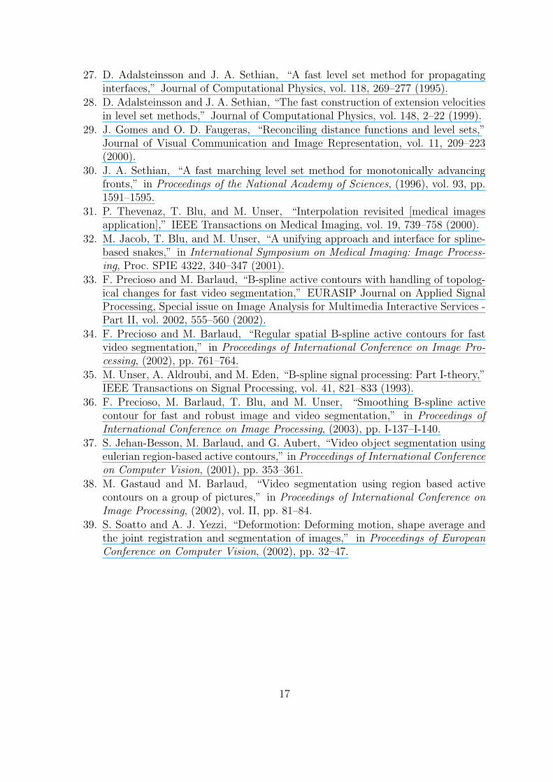
Sequence “Akiyo” is composed of three hundred 352 × 288, color images. Descriptorkin was taken equal to a constant penalty. Descriptor kout was defined as the differencebetween the current image and a robust estimate of the background image computedusing the nb previous images37 (nb = 20), or less for the first nb images. This descriptortakes advantage of the temporal information of the sequence: It is a motion detector.In case of a moving background due to camera motion, a mosaicking technique canbe used to estimate the background image.38 Descriptor kout was taken equal to zero.The first image of the sequence was not segmented since no previous images wereavailable to estimate the background. See Fig. 4 and 5.

Fig. 4. Segmentation of Akiyo: Image 2, evolution from the initial contour untilconvergence.

C. Tracking

Sequence “Erik” is composed of fifty 256 × 256, color images. Given a segmentationof Erik’s face in the first image, the purpose was to track the face throughout thesequence using the segmentation of the previous image to constrain the segmentationof the current frame.20 See Fig. 6. Two descriptors were used: A variance descriptor(see Subsection 2.D.3) for the face (kin/statistical descriptor) and a shape of refer-ence descriptor (see Subsection 2.D.4) as a constraint (kb/geometrical descriptor).Descriptor kout was taken equal to zero. The shape of reference in the current imagewas defined as an affine transform (i.e., a combination of a translation, a rotation,and a scaling) of the segmentation contour in the previous image. This transform canbe interpreted as the global motion of the object of interest between the previous and

12

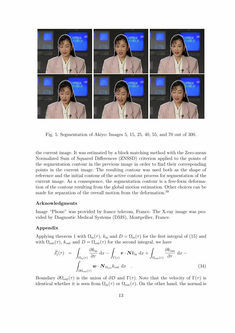
Fig. 5. Segmentation of Akiyo: Images 5, 15, 25, 40, 55, and 70 out of 300.

the current image. It was estimated by a block matching method with the Zero-meanNormalized Sum of Squared Differences (ZNSSD) criterion applied to the points ofthe segmentation contour in the previous image in order to find their correspondingpoints in the current image. The resulting contour was used both as the shape ofreference and the initial contour of the active contour process for segmentation of thecurrent image. As a consequence, the segmentation contour is a free-form deforma-tion of the contour resulting from the global motion estimation. Other choices can bemade for separation of the overall motion from the deformation.39

Acknowledgments

Image “Phone” was provided by france telecom, France. The X-ray image was pro-vided by Diagnostic Medical Systems (DMS), Montpellier, France.

Appendix

Applying theorem 1 with Ωin(τ), kin and D = Ωin(τ) for the first integral of (15) andwith Ωout(τ), kout and D = Ωout(τ) for the second integral, we have

J ′1(τ) =

∫

Ωin(τ)

∂kin

∂τdx −

∫

Γ(τ)

v · Nkin dx +

∫

Ωout(τ)

∂kout

∂τdx −

∫

∂Ωout(τ)

w · NΩoutkout dx . (34)

Boundary ∂Ωout(τ) is the union of ∂D and Γ(τ). Note that the velocity of Γ(τ) isidentical whether it is seen from Ωin(τ) or Ωout(τ). On the other hand, the normal is

13

Fig. 6. Tracking of Erik’s face: Images 1, 10, 27, 40, and 50 out of 50.

opposite. Therefore

J ′1(τ) =

∫

Ωin(τ)

∂kin

∂τdx −

∫

Γ(τ)

v · Nkin dx +

∫

Ωout(τ)

∂kout

∂τdx −

∫

Γ(τ)

v · (−N )kout dx −

∫

∂Ωout(τ)\Γ(τ)

w · NΩoutkout dx (35)

=

∫

Ωin(τ)

∂kin

∂τdx −

∫

Γ(τ)

v · N (kin − kout) dx +

∫

Ωout(τ)

∂kout

∂τdx −

∫

∂Ωout(τ)\Γ(τ)

w · NΩoutkout dx . (36)

14

Let K be the function equal to kin in Ωin(τ) and kout in Ωout(τ) and let [[K]] be thejump of K across Γ(τ): [[K]](x) = kin(x) − kout(x) for x ∈ Γ(τ). Finally

J ′1(τ) =

∫

Ωin(τ)

∂kin

∂τdx +

∫

Ωout(τ)

∂kout

∂τdx −

∫

Γ(τ)

v · N (kin − kout) dx −

∫

∂Ωout(τ)\Γ(τ)

w · NΩoutkout dx (37)

=

∫

Ωin(τ)

∂K

∂τdx +

∫

Ωout(τ)

∂K

∂τdx −

∫

Γ(τ)

v · N [[K]] dx −

∫

∂Ωout(τ)\Γ(τ)

w · NΩoutK dx (38)

=

∫

D

∂K

∂τdx −

∫

Γ(τ)

v · N [[K]] dx −

∫

∂Ωout(τ)\Γ(τ)

w · NΩoutK dx .(39)

References

1. M. Kass, A. Witkin, and D. Terzopoulos, “Snakes: Active contour models,” In-ternational Journal of Computer Vision, vol. 1, 321–332 (1988).

2. L. Cohen, “On active contour models and balloons,” Computer Vision, Graphicsand Image Processing: Image Understanding, vol. 53, 211–218 (1991).

3. V. Caselles, R. Kimmel, and G. Sapiro, “Geodesic active contours,” InternationalJournal of Computer Vision, vol. 22, 61–79 (1997).

4. L. Cohen, E. Bardinet, and N. Ayache, “Reconstruction of digital terrain modelwith a lake,” in Conference on Geometric Methods in Computer Vision II, Proc.SPIE 2031, 38–50 (1993).

5. R. Ronfard, “Region-based strategies for active contour models,” InternationalJournal of Computer Vision, vol. 13, 229–251 (1994).

6. A. Chakraborty, L. Staib, and J. Duncan, “Deformable boundary finding in med-ical images by integrating gradient and region information,” IEEE Transactionson Medical Imaging, vol. 15, 859–870 (1996).

7. S. Zhu and A. Yuille, “Region competition: unifying snakes, region growing, andbayes/MDL for multiband image segmentation,” IEEE Transactions on PatternAnalysis and Machine Intelligence, vol. 18, 884–900 (1996).

8. N. Paragios and R. Deriche, “Geodesic active regions for motion estimationand tracking,” in Proceedings of International Conference on Computer Vision,(1999), pp. 688–694.

9. N. Paragios and R. Deriche, “Geodesic active regions and level set methods forsupervised texture segmentation,” International Journal of Computer Vision, vol.46, 223–247 (2002).

10. A. J. Yezzi, A. Tsai, and A. Willsky, “A statistical approach to snakes for bimodaland trimodal imagery,” in Proceedings of International Conference on ComputerVision, (1999), pp. 898–903.

11. C. Chesnaud, P. Refregier, and V. Boulet, “Statistical region snake-based seg-mentation adapted to different physical noise models,” IEEE Transactions on

15

Pattern Analysis and Machine Intelligence, vol. 21, 1145–1156 (1999).

12. C. Samson, L. Blanc-Feraud, G. Aubert, and J. Zerubia, “A level set model forimage classification,” International Journal of Computer Vision, vol. 40, 187–197(2000).

13. T. Chan and L. Vese, “Active contours without edges,” IEEE Transactions onImage Processing, vol. 10, 266–277 (2001).

14. E. Debreuve, M. Barlaud, G. Aubert, and J. Darcourt, “Space time segmenta-tion using level set active contours applied to myocardial gated SPECT,” IEEETransactions on Medical Imaging, vol. 20, 643–659 (2001).

15. O. Amadieu, E. Debreuve, M. Barlaud, and G. Aubert, “Inward and outwardcurve evolution using level set method,” in Proceedings of International Confer-ence on Image Processing, (1999), pp. 188–192.

16. J. Sokolowski and J.-P. Zolesio, Introduction to shape optimization: Shape sensi-tivity analysis (Springer-Verlag, Berlin, 1992).

17. M. C. Delfour and J.-P. Zolesio, Shapes and geometries: Analysis, DifferentialCalculus and Optimization (Society for Industrial and Applied Mathematics,Philadelphia, 2001).

18. S. Jehan-Besson, M. Barlaud, and G. Aubert, “DREAM2S: Deformable regionsdriven by an eulerian accurate minimization method for image and video segmen-tation,” International Journal of Computer Vision, vol. 53, 45–70 (2003).

19. G. Aubert, M. Barlaud, O. Faugeras, and S. Jehan-Besson, “Image segmentationusing active contours: Calculus of variations or shape gradients?,” SIAM Journalof Applied Mathematics, vol. 63, 2128–2154 (2003).

20. M. Gastaud, M. Barlaud, and G. Aubert, “Tracking video objects using activecontours,” in Proceedings of Workshop on Motion and Video Computing, (2002),pp. 90–95.

21. Y. Chen, H. D. Tagare, S. Thiruvenkadam, F. Huang, D. Wilson, K. S. Gopinath,R. W. Briggs, and E. A. Geiser, “Using prior shapes in geometric active contoursin a variational framework,” International Journal of Computer Vision, vol. 50,315–328 (2002).

22. D. Cremers, F. Tischhauser, J. Weickert, and C. Schnorr, “Diffusion snakes:Introducing statistical shape knowledge into the mumford-shah functional,” In-ternational Journal of Computer Vision, vol. 50, 295–313 (2002).

23. P. Charbonnier and O. Cuisenaire, “Une etude des contours actifs : modelesclassique, geometrique et geodesique,” Technical Report 163, Laboratoire detelecommunications et teledetection, Universite catholique de Louvain, 1996.

24. S. Osher and J. A. Sethian, “Fronts propagating with curvature-dependent speed:Algorithms based on hamilton-jacobi formulations,” Journal of ComputationalPhysics, vol. 79, 12–49 (1988).

25. G. Barles, “Remarks on a flame propagation model,” Technical Report 464,Projet Sinus, Institut National de Recherche en Informatique et en Automatique(INRIA) de Sophia Antipolis, Sophia Antipolis, France, 1985.

26. D. L. Chopp, “Computing minimal surfaces via level set curvature flow,” Journalof Computational Physics, vol. 106, 77–91 (1993).

16

27. D. Adalsteinsson and J. A. Sethian, “A fast level set method for propagatinginterfaces,” Journal of Computational Physics, vol. 118, 269–277 (1995).

28. D. Adalsteinsson and J. A. Sethian, “The fast construction of extension velocitiesin level set methods,” Journal of Computational Physics, vol. 148, 2–22 (1999).

29. J. Gomes and O. D. Faugeras, “Reconciling distance functions and level sets,”Journal of Visual Communication and Image Representation, vol. 11, 209–223(2000).

30. J. A. Sethian, “A fast marching level set method for monotonically advancingfronts,” in Proceedings of the National Academy of Sciences, (1996), vol. 93, pp.1591–1595.

31. P. Thevenaz, T. Blu, and M. Unser, “Interpolation revisited [medical imagesapplication],” IEEE Transactions on Medical Imaging, vol. 19, 739–758 (2000).

32. M. Jacob, T. Blu, and M. Unser, “A unifying approach and interface for spline-based snakes,” in International Symposium on Medical Imaging: Image Process-ing, Proc. SPIE 4322, 340–347 (2001).

33. F. Precioso and M. Barlaud, “B-spline active contours with handling of topolog-ical changes for fast video segmentation,” EURASIP Journal on Applied SignalProcessing, Special issue on Image Analysis for Multimedia Interactive Services -Part II, vol. 2002, 555–560 (2002).

34. F. Precioso and M. Barlaud, “Regular spatial B-spline active contours for fastvideo segmentation,” in Proceedings of International Conference on Image Pro-cessing, (2002), pp. 761–764.

35. M. Unser, A. Aldroubi, and M. Eden, “B-spline signal processing: Part I-theory,”IEEE Transactions on Signal Processing, vol. 41, 821–833 (1993).

36. F. Precioso, M. Barlaud, T. Blu, and M. Unser, “Smoothing B-spline activecontour for fast and robust image and video segmentation,” in Proceedings ofInternational Conference on Image Processing, (2003), pp. I-137–I-140.

37. S. Jehan-Besson, M. Barlaud, and G. Aubert, “Video object segmentation usingeulerian region-based active contours,” in Proceedings of International Conferenceon Computer Vision, (2001), pp. 353–361.

38. M. Gastaud and M. Barlaud, “Video segmentation using region based activecontours on a group of pictures,” in Proceedings of International Conference onImage Processing, (2002), vol. II, pp. 81–84.

39. S. Soatto and A. J. Yezzi, “Deformotion: Deforming motion, shape average andthe joint registration and segmentation of images,” in Proceedings of EuropeanConference on Computer Vision, (2002), pp. 32–47.

17