from fourier transforms to wavelet analysis: mathematical ...

FROM FOURIER TRANSFORMS TO WAVELET ANALYSIS:

MATHEMATICAL CONCEPTS AND EXAMPLES

LY TRANMAY 15, 2006

Abstract. This paper studies two data analytic methods: Fourier transformsand wavelets. Fourier transforms approximate a function by decomposing itinto sums of sinusoidal functions, while wavelet analysis makes use of motherwavelets. Both methods are capable of detecting dominant frequencies in thesignals; however, wavelets are more efficient in dealing with time-frequencyanalysis. Due to the limited scope of this paper, only Fast Fourier Transform(FFT) and three families of wavelets are examined: Haar wavelet, DaubJ ,and CoifI wavelets. Examples for both methods work on one dimensionaldata sets such as sound signals. Some simple wavelet applications includecompression of audio signals, denoising problems, and multiresolution analysis.These applications are given for comparison purposes between Fourier and

wavelet analysis, as well as among wavelet families.Although wavelets are a recent discovery, their efficacy has been acknowl-

edged in a host of fields, both theoretical and practical. Their applicationscan be expanded to two or higher dimensional data sets. Although they areomitted in this paper, more information is available in [7] or many other bookson wavelet applications.

1. Introduction

Wavelets are a recent discovery in mathematics; however, their rapid develop-ment and wide range of applications make them more powerful than many otherlong-existing analytical tools. Conventionally, wavelets are often compared to theFourier transform to promote their advantages. This paper will take a similarapproach in attempt to illustrate wavelet transform in various applications.

The Fourier transform makes use of Fourier series, named in honor of JosephFourier (1768-1830), who proposed to represent functions as an infinite sum of si-nusoidal functions [1]. Joseph Fourier was the first to use such series to studyheat equations. After him, many mathematicians such as Euler, d’Alembert, andDaniel Bernoulli continued to investigate and develop Fourier analysis [1]. Fromthe original series, various Fourier transforms were derived: the continuous Fouriertransform, discrete Fourier transform, fast Fourier transform, short-time Fouriertransform, etc... Fourier analysis is adopted in many scientific applications, espe-cially in dealing with signal processing. As the applications grew more complexover time, the Fourier transform started to reveal its inefficiencies when workingwith time series or data with certain characteristics. Despite the attempt to tailorthe method to different groups of data, the Fourier transform remained inadequate.Consequently, wavelets received more attention as they proved able to overcomethe difficulties.

Date: May 15, 2006.

1

2 LY TRAN MAY 15, 2006

The first block of wavelet theory was started by Alfred Haar in the early 20thcentury [2]. Other important contributors include Goupillaud, Grossman, Mor-let, Daubechies, Mallat and Delprat. Their different focuses helped to enrich thewavelet families and widen the range of wavelet applications. Because of the simi-larities, wavelet analysis is applicable in all the fields where Fourier transform wasinitially adopted. It is especially useful in image processing, data compression,heart-rate analysis, climatology, speech recognition, and computer graphics.

This paper focuses on only a few aspects of each analysis. The first section dis-cusses Fourier series in different representations: sinusoidal functions and complexexponential. A discretization method is also introduced so as to provide support forthe discussion of Fast Fourier Transform (FFT). After illustrating Fourier analysiswith concrete examples, the paper will turn to the Fourier transform’s shortcom-ings, which give rise to wavelets .

The second section discusses three families of wavelets: the Haar wavelets,Daubechies wavelets, and Coiflets. Concepts and general mechanisms will be pro-vided in detail for Haar wavelets and omitted for the others. Finally, we will look atthe advantages of wavelets over Fourier transform through a number of examples.

The paper uses three main references: Course notes in Modeling II, A Primer onWavelets and their Scientific Applications by James Walker, and A First Course inWavelets with Fourier Analysis by Boggess and Narcowich. As the paper is aimedat readers at undergraduate level, mathematical background of linear algebra andbasic calculus is assumed.

2. Fourier Analysis

Fourier analysis, which is useful in many scientific applications, makes use ofFourier series in dealing with data sets. In this section, a few representationsof Fourier series and related concepts will be introduced. Consequently, severalexamples will implement these defined concepts to illustrate the idea of Fourieranalysis.

2.1. Fourier Series.

2.1.1. Sine and Cosine Representation. A Fourier series is the expression of anyfunction f(x) : R → R as an infinite sum of sine and cosine functions:

(1) f(x) = a0 +

∞∑

k=1

ak sin(kx) +

∞∑

m=1

bm cos(mx).

In this section, we work with continuous functions on [0, 2π], and thus, it isnecessary to familiarize ourselves with the vector space of such functions. It isan infinite dimensional vector space, denoted C[0, 2π], where each point on thecontinuous interval [0, 2π] represents a dimension. Then, an orthogonal basis ofC[0, 2π] is:

{1, sin(kx), cos(mx)|k, m = 1, 2, 3, ...}.Fourier series can also be employed to write any continuous function f(x) : C[0, 2π] →C[0, 2π]. Concepts such as inner product, norm, and distance between two func-tions in an infinite dimensional vector space are defined in a similar manner to thatof a finite dimensional vector space. However, the infinite sum gives rise to the useof an integral in the definition:

WAVELETS 3

- Inner Product: The inner product of two continuous functions f(x), g(x) ∈C[0, 2π] is

< f, g >=

∫ 2π

0

f(x)g(x)dx.

- Norm: Recall that the norm of a vector in finite dimensional vector spaceis calculated as ‖ ~x ‖2=< ~x, ~x >. Norm is defined similarly for a functionin infinite dimensional space C[0, 2π]:

‖ f ‖2=< f, f >=

∫ 2π

0

f2(x)dx.

- Angle between two functions: The inner product of f and g can also bewritten as

< f, g >=‖ f ‖‖ g ‖ cos(θ).

The angle between two functions, θ, can be achieved from the above equa-tion.

- Distance Distance between two continuous functions f and g is defined as‖ f − g ‖.

The inner product formula can be applied to prove that the basis mentionedabove is indeed orthogonal. Let us consider six possible inner products of the basis

vector functions:∫ 2π

0sin(kx)dx,

∫ 2π

0cos(mx)dx,

∫ 2π

0sin(kx) sin(mx)dx (k 6= m),

∫ 2π

0 sin(kx) cos(mx)dx (k 6= m),∫ 2π

0 cos(kx) cos(mx)dx (k 6= m). The followingtrignometric identities [3] are helpful in proving that all six inner products areequal to 0, implying an orthogonal basis:

sin(x) cos(y) =1

2[sin(x + y) + sin(x − y)],

cos(x) cos(y) =1

2[cos(x + y) + cos(x − y)],

sin(x) sin(y) =1

2[cos(x − y) − cos(x + y)].

2.1.2. Function Coefficients. Coefficients of f can be obtained by projecting f onthe corresponding basis vectors (similar to that of finite dimensional space):

a0 =< f, 1 >

< 1, 1 >=

1

2π

∫ 2π

0

f(x)dx,

ak =< f, sin(kx) >

< sin(kx), sin(kx) >=

1

π

∫ 2π

0

sin(kx)f(x)dx,

bm =< f, cos(mx) >

< cos(mx), cos(mx) >=

1

π

∫ 2π

0

cos(mx)f(x)dx.

2.1.3. Complex Form. Instead of taking the integral of individual sine and cosinefunctions, the complex form representation of Fourier series enables us to computethe various inner product integrals simultaneously. The transformation makes useof Euler’s formula [3]

eiθ = cos(θ) + i sin(θ).

Simple algebra yields

ak sin(kx) + bk cos(kx) =bk − iak

2eikx +

bk + iak

2e−ikx.

4 LY TRAN MAY 15, 2006

Thus, if we let c0 = a0/2, ck = bk−iak

2 , and c−k = bk+iak

2 , then the complex formrepresentation of the Fourier series is

f(x) =∞∑

k=−∞ckeikx.

Then differentiation and integration can be calculated simultaneously [4]:

d

dθeiθ = ieiθ = − sin(θ) + i cos(θ),

∫

eiθdθ =1

ieiθ = sin(θ) − i cos(θ).

To illustrate the convenience of Euler’s formula, let us compute < x, sin(3x) > and< x, cos(3x) > using the complex exponential.

Note that

< x, e3ix > =

∫ 2π

0

xe3ixdx =

∫ 2π

0

x cos(3x)dx + i

∫ 2π

0

x sin(3x)dx

= < x, cos(3x) > +i < x, sin(3x) > .

On the other hand, integration by parts yields∫ 2π

0

xe3ixdx =( x

3ie3ix − 1

3i

∫

e3ixdx)∣

∣

∣

2π

0

=( x

3ie3ix +

1

9e3ix

)∣

∣

∣

2π

0

=2π

3ie6πi +

1

9e6πi − 1

9.

Since e6πi = cos(6π) + i sin(6π) = 1, it follows that∫ 2π

0

xe3ixdx =2π

3i= −i

2π

3.

Therefore,

< x, cos(3x) > = 0,

< x, sin(3x) > = −2π

3.

Integrating two functions separately would have doubled the work.

2.1.4. Fourier Transformation. Fourier transformation is a method frequently usedin signal processing. As the name suggests, it transforms a set of data into a Fourierseries. Due to limitation, this paper will only introduce Fast Fourier Transform(FFT).

Discretization. Most data sets are available as a collection of data points.Therefore, the assumption that the function is continuous is no longer required.However, a continuous function can always be represented by N points for somepositive integer N . A process in which a continuous function is translated into Nrepresentative points is called discretization. Discretization translates an infinitedimensional vector space into a finite one [4].

To discretize a function, we choose a finite number of points that representthe function from which the function itself can be sketched. Consider functionsy1 = cos(π

4 t) and y1 = cos( 7π4 t) with 0 ≤ t ≤ 64. In Figure 1, these functions

WAVELETS 5

a)∆t = 0.1 b) ∆t = 1

0 1 2 3 4 5 6 7 8 9 10−1

−0.8

−0.6

−0.4

−0.2

0

0.2

0.4

0.6

0.8

1

y1 = cos((pi/4)*k)y2 = cos(7pi/4)*k

0 1 2 3 4 5 6 7 8 9 10−1

−0.8

−0.6

−0.4

−0.2

0

0.2

0.4

0.6

0.8

1

y1 = cos((pi/4)*k)y2 = cos(7pi/4)*k

Figure 1. Functions y1 = cos(π4 t) and y2 = cos( 7π

4 t) with differ-ent ∆t

are plotted with different increments of t (∆t) of 1 and 0.1. When ∆t = 0.1, twofunctions are different, but when ∆t = 1, the values plotted are essentially the same.This suggests that ∆t = 1 is too large to differentiate these two functions. Thesame pattern is observed for any pair of sine or cosine functions that are conjugateof each other (for example, cos(αt) and cos(βt), where α + β = 2π).

Formulas When a continuous function is discretized into N points for FFT,N is usually a power of 2 for computational reasons. Suppose that N points{f0, f1, ..., fN−1} are spaced out evenly on the interval [0, 2π], then the k-th pointin Fourier series form is

(2) Fk =

N∑

n=1

fne−2πi

N·(k−1)(n−1)

for 1 ≤ k ≤ N . Recall that for two vectors x, y in complex plane, their innerproduct is defined as

< x, y >= xT y.

Thus, equation (2) is in fact an inner product between F = [f1, f2, ..., fN ]T and

[e−2πi

N·0·(k−1), e−

2πi

N·(k−1), e−

2πi

N·2(k−1), ..., e−

2πi

N·(k−1)(N−1)] for any integer k in in-

terval [1, N ]. Hence, we can represent equation (2) by a product of F and an N×Nmatrix C, whose entries are determined as follows:

Ckj = e2πi

N·(k−1)(j−1).

This process is called Fourier transformation. C is the transformation matrix.Instead of dealing with integrals, we now face easier matrix operations:

F1

F2

...FN

= e2πi

NA ×

f1

f2

...fN

,

where

A =

0 0 0 . . . 00 1 2 . . . N − 1...

...0 N − 1 2(N − 1) . . . (N − 1)(N − 1)

6 LY TRAN MAY 15, 2006

The above cross product suggests that the inverse transformation process is alsofeasible:

(3) fn =1

N

N∑

k=1

Fke2πi

N·(k−1)(n−1)

for 1 ≤ n ≤ N .Expansion to function f on the interval [α, β] The process of Fourier trans-

formation can be extended to any function on the interval [α, β] with the appropriatediscretization process. Discretize the function f into N equal subintervals, so thateach subinterval is

(4) ∆x =β − α

Nor β − α = N · ∆x.

and we have N points {x1, x2, ...xN} on the interval [α, β]. To perform FFT, wecan find an one-to-one correspondence from the function f to [0, 2π]:

xj ∈ [α, β] → tj =2π

β − α· (xj − α) ∈ [0, 2π].

The inverse process is:

tj ∈ [0, 2π] → xj = α +β − α

2π· tj ∈ [α, β].

Substitute equation (4) in, we get:

tj =2π

N · ∆x· (xj − α) or xj = α +

N · ∆x

2π· tj .

The above equation suggests that discretizing f(x) over [α, β] is the same asf( 2π

N ·∆x(xj − α)) over [0, 2π]. Therefore, we can use the function

f(x) = a0 +

∞∑

k=1

ak cos(k2π

N · ∆x(x − α)) +

∞∑

m=1

bm sin(m2π

N · ∆x(x − α))

for Fourier transformation.To summarize, if we have N points with spacing ∆x, labeled as {f0, f1, . . . , fN}

on the interval [α, β], then the relationship between function f and its FFT isexpressed in the following equations:

(5) fn = a0 +

N/2∑

k=1

ak cos(k2π

N · ∆xxn) +

N/2∑

m=1

bm sin(m2π

N · ∆xxn),

where

a0 =F1

N,

ak =2

N· Real(Fk+1),

bm = − 2

N· Imag(Fm+1).

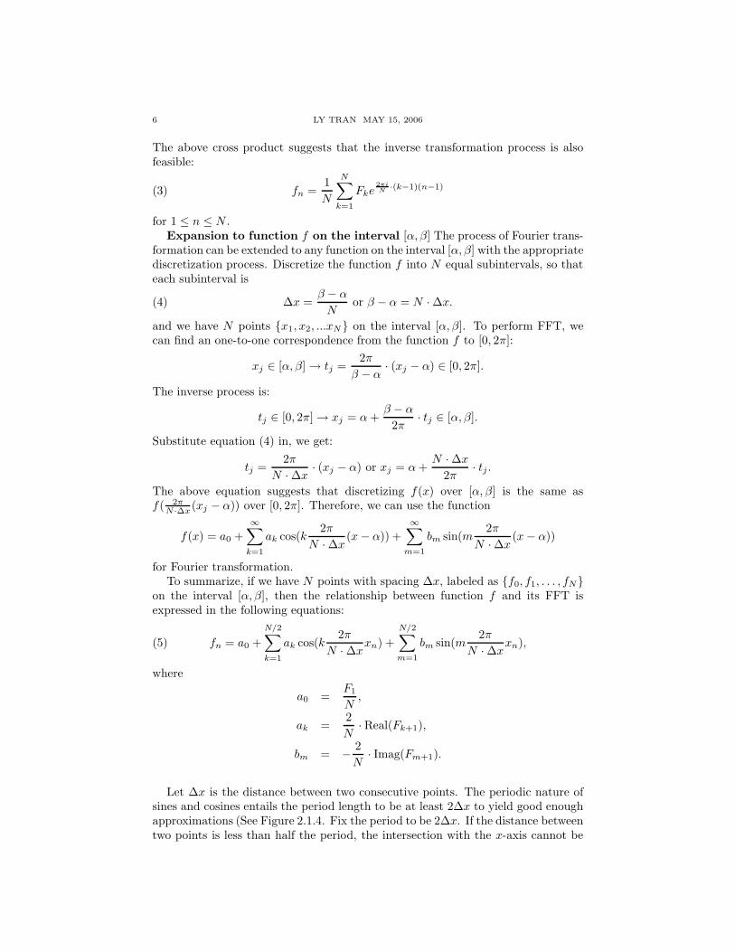
Let ∆x is the distance between two consecutive points. The periodic nature ofsines and cosines entails the period length to be at least 2∆x to yield good enoughapproximations (See Figure 2.1.4. Fix the period to be 2∆x. If the distance betweentwo points is less than half the period, the intersection with the x-axis cannot be

WAVELETS 7

Figure 2. ∆x and the period length

detected, and hence imprecise estimation is possible. A similar situation occurswhen the distance between two points is larger than half the period.) Thus, it isbest to have ∆x as the distance between two points, or 2∆x as the period length.For this reason, k and m range from 1 to N/2 in equation (5).

From what we know about trignometric functions sin(At) and cos(At), we have:

- The functions’ periods are

Period =2π

A=

N∆x

k.

- The functions’ frequencies are

Frequency =A

2π=

k

N∆x.

As k, m = 1, 2, . . . , N2 , the periods measured in time unit per cycle are

N · ∆x,N

2· ∆x, . . . , 2 · ∆x.

and the frequencies measured in cycles per time unit are

1

N· 1

∆x,

2

N· 1

∆x, . . . ,

1

2· 1

∆x.

As k changes from 1 to N2 , some functions sin(ktn) and cos(ktn) might con-

tribute more to the original function fn than others. To measure each function’s“importance”, we define a new concept, frequency content of k, which is given by

freq(k) =√

a2k + b2

k.

A plot of k against the frequency content yields the power spectrum of a signal.

2.2. Applications. In this section, we will examine how FFT is applied in simpleexamples.

8 LY TRAN MAY 15, 2006

0 50 100 1500

500

1000

1500

2000

2500

3000

3500

4000

4500

k

Freq

uenc

y

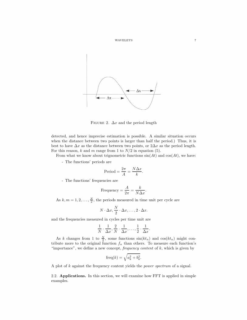
Figure 3. Power spectrum of the sunspot data.

2.2.1. Sunspot Example. Data from sunspots have interested scientists for hundredsof years, as they are the indicator for radiation from the sun and therefore have aneffect on many scientific fields [5]. MatLab has a collection of data recording thenumber of sunspots counted on the sun every year between 1700 and 1987. UsingFourier transformation, we will analyze the data to find periodicity in the number ofsunspots. Let the domain be 288 years from 1700 to 1987 (thus N = 288, ∆x = 1).So k will go from 1 to 143 (= N

2 ).After the data are loaded, the frequency content of each k is plotted against

k (see Figure 3). The plot peaks at the 26th position, which suggests that thecomponent functions with k = 26 contribute the most to the FFT. Hence, theperiod of the sunspot cycle can be estimated using k = 26, which yields

N · ∆x

k=

288 · 126

≈ 11.08 years.

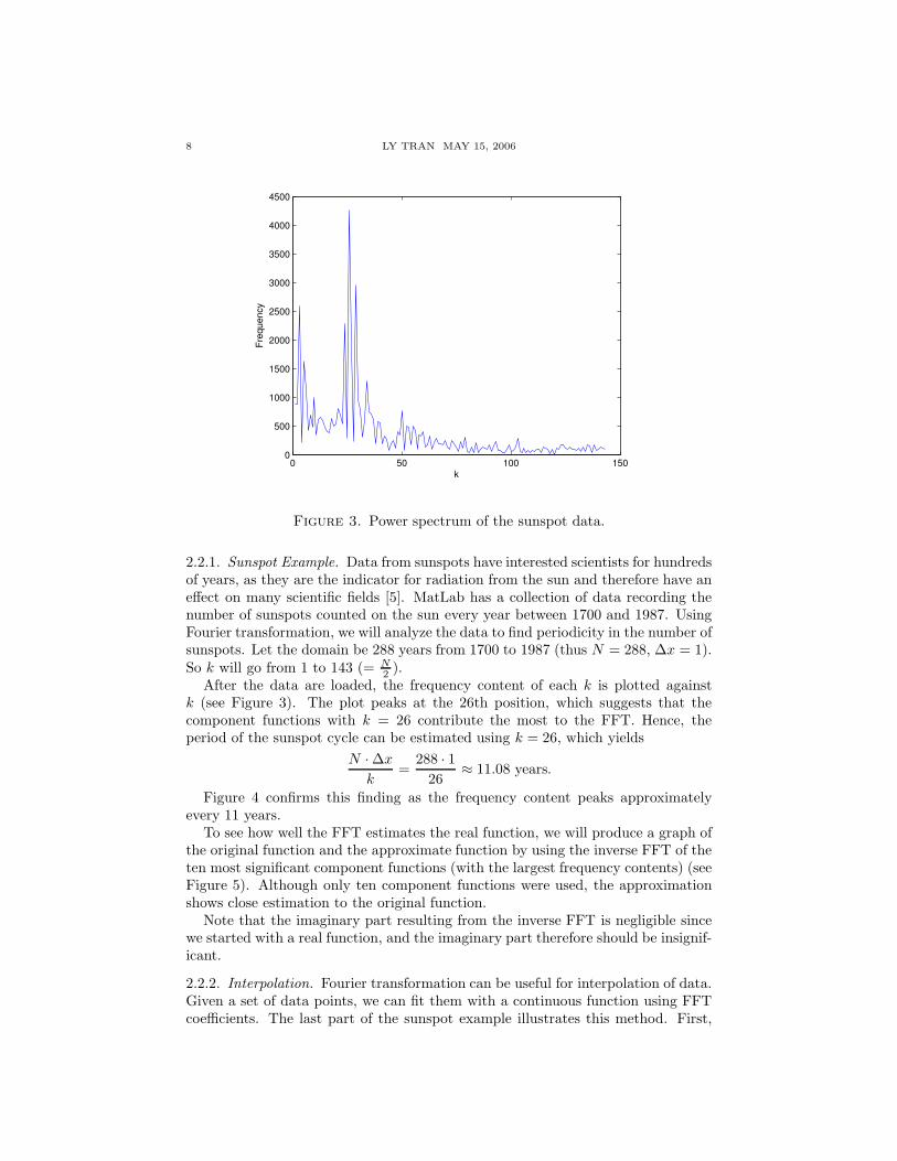
Figure 4 confirms this finding as the frequency content peaks approximatelyevery 11 years.

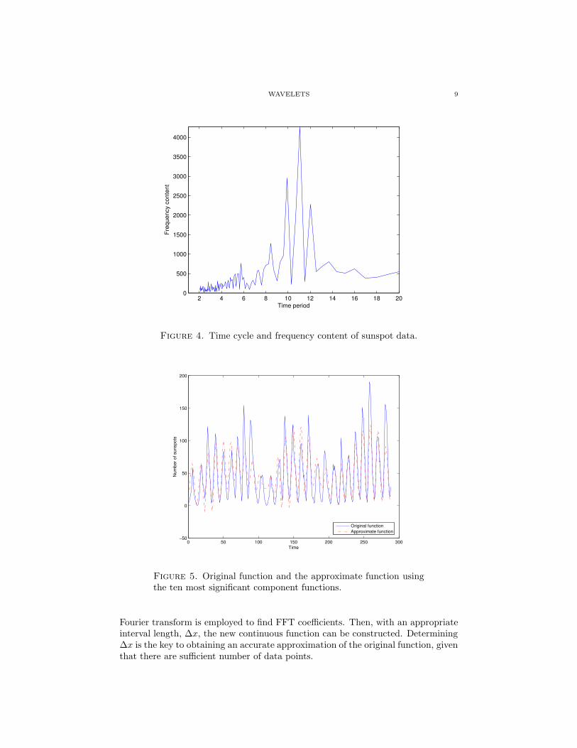
To see how well the FFT estimates the real function, we will produce a graph ofthe original function and the approximate function by using the inverse FFT of theten most significant component functions (with the largest frequency contents) (seeFigure 5). Although only ten component functions were used, the approximationshows close estimation to the original function.

Note that the imaginary part resulting from the inverse FFT is negligible sincewe started with a real function, and the imaginary part therefore should be insignif-icant.

2.2.2. Interpolation. Fourier transformation can be useful for interpolation of data.Given a set of data points, we can fit them with a continuous function using FFTcoefficients. The last part of the sunspot example illustrates this method. First,

WAVELETS 9

2 4 6 8 10 12 14 16 18 200

500

1000

1500

2000

2500

3000

3500

4000

Time period

Freq

uenc

y co

nten

t

Figure 4. Time cycle and frequency content of sunspot data.

0 50 100 150 200 250 300−50

0

50

100

150

200

Time

Num

ber o

f sun

spot

s

Original functionApproximate function

Figure 5. Original function and the approximate function usingthe ten most significant component functions.

Fourier transform is employed to find FFT coefficients. Then, with an appropriateinterval length, ∆x, the new continuous function can be constructed. Determining∆x is the key to obtaining an accurate approximation of the original function, giventhat there are sufficient number of data points.

10 LY TRAN MAY 15, 2006

0 2 4 6 8 10 12 14 16 18 20−1

−0.8

−0.6

−0.4

−0.2

0

0.2

0.4

0.6

0.8

1

x

f(x)

original functionappr. function, m=1appr. function, m=2

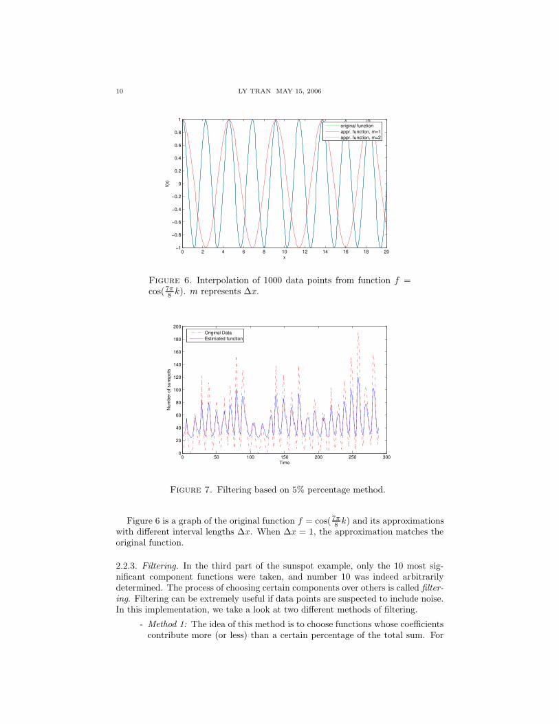
Figure 6. Interpolation of 1000 data points from function f =cos( 7π

8 k). m represents ∆x.

0 50 100 150 200 250 3000

20

40

60

80

100

120

140

160

180

200

Time

Num

ber o

f sun

spot

s

Original DataEstimated function

Figure 7. Filtering based on 5% percentage method.

Figure 6 is a graph of the original function f = cos( 7π8 k) and its approximations

with different interval lengths ∆x. When ∆x = 1, the approximation matches theoriginal function.

2.2.3. Filtering. In the third part of the sunspot example, only the 10 most sig-nificant component functions were taken, and number 10 was indeed arbitrarilydetermined. The process of choosing certain components over others is called filter-ing. Filtering can be extremely useful if data points are suspected to include noise.In this implementation, we take a look at two different methods of filtering.

- Method 1: The idea of this method is to choose functions whose coefficientscontribute more (or less) than a certain percentage of the total sum. For

WAVELETS 11

0 50 100 150 200 250 300−50

0

50

100

150

200

Time

Num

ber o

f sun

spot

s

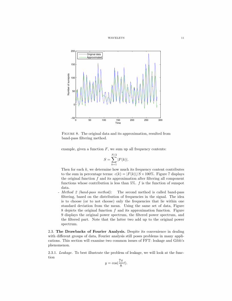
Original dataApproximated

Figure 8. The original data and its approximation, resulted fromband-pass filtering method.

example, given a function F , we sum up all frequency contents:

S =

N/2∑

k=1

|F (k)|.

Then for each k, we determine how much its frequency content contributesto the sum in percentage terms: c(k) = |F (k)|/S×100%. Figure 7 displaysthe original function f and its approximation after filtering all componentfunctions whose contribution is less than 5%. f is the function of sunspotdata.

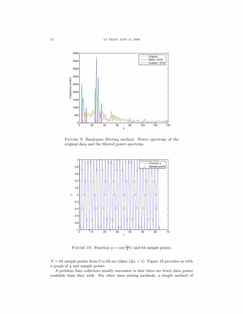
- Method 2 (band-pass method): The second method is called band-passfiltering, based on the distribution of frequencies in the signal. The ideais to choose (or to not choose) only the frequencies that lie within onestandard deviation from the mean. Using the same set of data, Figure8 depicts the original function f and its approximation function. Figure9 displays the original power spectrum, the filtered power spectrum, andthe filtered part. Note that the latter two add up to the original powerspectrum.

2.3. The Drawbacks of Fourier Analysis. Despite its convenience in dealingwith different groups of data, Fourier analysis still poses problems in many appli-cations. This section will examine two common issues of FFT: leakage and Gibb’sphenomenon.

2.3.1. Leakage. To best illustrate the problem of leakage, we will look at the func-tion

y = cos(7π

8t).

12 LY TRAN MAY 15, 2006

0 20 40 60 80 100 120 1400

500

1000

1500

2000

2500

3000

3500

4000

4500

k

Freq

uenc

y co

nten

t

OriginalWithin 1STDOutside 1 STD

Figure 9. Band-pass filtering method. Power spectrum of theoriginal data and the filtered power spectrum.

0 10 20 30 40 50 60 70−1

−0.8

−0.6

−0.4

−0.2

0

0.2

0.4

0.6

0.8

1

t

y

Function ySample points

Figure 10. Function y = cos( 7π8 t) and 64 sample points.

N = 64 sample points from 0 to 63 are taken (∆x = 1). Figure 10 provides us witha graph of y and sample points.

A problem data collectors usually encounter is that there are fewer data pointsavailable than they wish. For other data mining methods, a simple method of

WAVELETS 13

a) 64 sample points b) 52 sample points

0 10 20 30 40 50 60 700

5

10

15

20

25

30

35

t

Freq

uenc

y co

nten

t

0 10 20 30 40 50 60 700

2

4

6

8

10

12

14

16

t

Freq

uenc

y co

nten

t

Figure 11. Power Spectra of the FFT of function y with a) 64sample points and b) 52 sample points (the rest are zeroed).

zeroing the rest of the sample points can be used. However, it is not the samefor Fourier transform: Figure 11(a) plots power spectrum of the FFT of y with 64sample points, and Figure 11(b) plots the same thing, however, the last 10 samplepoints are zeroed.

The frequency contents in Figure 11(a) reflect function y better; while the fre-quency contents in Figure 11(b) appear to include some noise. From these graphs,we can conclude that adding zeros does not help in case of sample points shortage.This effect is known as “leakage”: while the frequency content of the signal did notchange, the power spectrum did [4].

2.3.2. Gibb’s Phenomenon. In many cases, an attempt to fit a function with discon-tinuities or steep slopes using Fourier transform fails. The reason is that FFT onlyyields smooth functions. This creates a problem known as Gibb’s phenomenon.

For example, take a look at a square wave function defined as follow:

f(x) =

{

1, if 2kπ ≤ x ≤ (2k + 1)π−1, if (2k + 1)π ≤ x ≤ 2(k + 1)π

for any nonnegative integer k.Then f can be written as sum of odd harmonics [4]:

f(x) = sin(x) +sin(3x)

3+

sin(5x)

5+ . . .

=

∞∑

k=1

1

2k − 1sin((2k − 1)x).

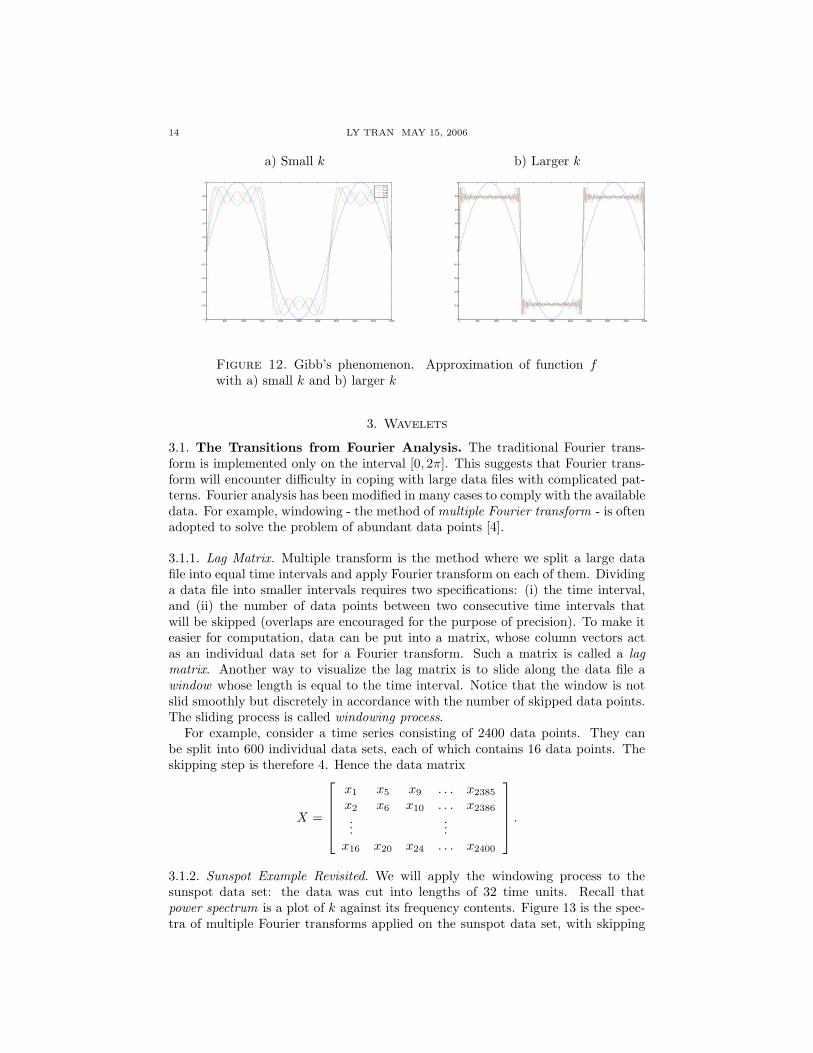
The larger k is, the better the function f is approximated. Figure 12 illustratesthis fact: even with large k, the values at the points of discontinuities cannot beapproximated. Thus, a perfect square wave can never be obtained.

14 LY TRAN MAY 15, 2006

a) Small k b) Larger k

0 500 1000 1500 2000 2500 3000 3500 4000 4500 5000−1

−0.8

−0.6

−0.4

−0.2

0

0.2

0.4

0.6

0.8

1

k=1k=3k=5k=7

0 500 1000 1500 2000 2500 3000 3500 4000 4500 5000−1

−0.8

−0.6

−0.4

−0.2

0

0.2

0.4

0.6

0.8

1

Figure 12. Gibb’s phenomenon. Approximation of function fwith a) small k and b) larger k

3. Wavelets

3.1. The Transitions from Fourier Analysis. The traditional Fourier trans-form is implemented only on the interval [0, 2π]. This suggests that Fourier trans-form will encounter difficulty in coping with large data files with complicated pat-terns. Fourier analysis has been modified in many cases to comply with the availabledata. For example, windowing - the method of multiple Fourier transform - is oftenadopted to solve the problem of abundant data points [4].

3.1.1. Lag Matrix. Multiple transform is the method where we split a large datafile into equal time intervals and apply Fourier transform on each of them. Dividinga data file into smaller intervals requires two specifications: (i) the time interval,and (ii) the number of data points between two consecutive time intervals thatwill be skipped (overlaps are encouraged for the purpose of precision). To make iteasier for computation, data can be put into a matrix, whose column vectors actas an individual data set for a Fourier transform. Such a matrix is called a lagmatrix. Another way to visualize the lag matrix is to slide along the data file awindow whose length is equal to the time interval. Notice that the window is notslid smoothly but discretely in accordance with the number of skipped data points.The sliding process is called windowing process.

For example, consider a time series consisting of 2400 data points. They canbe split into 600 individual data sets, each of which contains 16 data points. Theskipping step is therefore 4. Hence the data matrix

X =

x1 x5 x9 . . . x2385

x2 x6 x10 . . . x2386

......

x16 x20 x24 . . . x2400

.

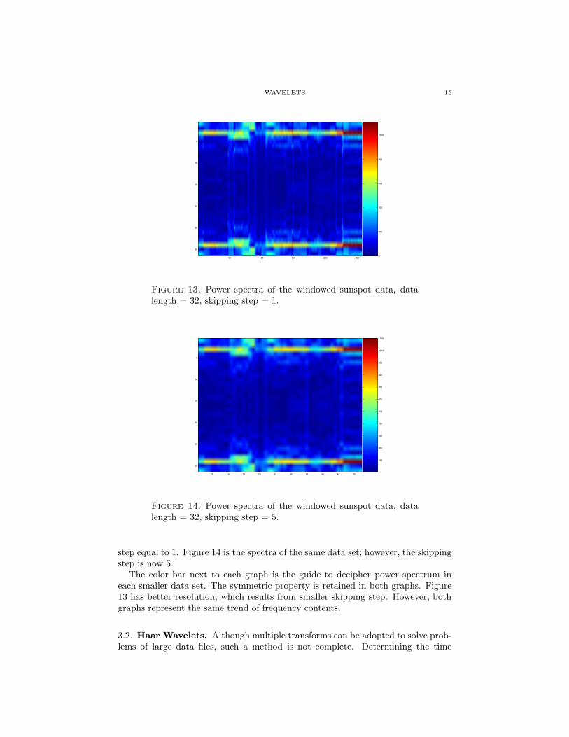
3.1.2. Sunspot Example Revisited. We will apply the windowing process to thesunspot data set: the data was cut into lengths of 32 time units. Recall thatpower spectrum is a plot of k against its frequency contents. Figure 13 is the spec-tra of multiple Fourier transforms applied on the sunspot data set, with skipping

WAVELETS 15

50 100 150 200 250

5

10

15

20

25

30

0

200

400

600

800

1000

Figure 13. Power spectra of the windowed sunspot data, datalength = 32, skipping step = 1.

5 10 15 20 25 30 35 40 45 50

5

10

15

20

25

30

100

200

300

400

500

600

700

800

900

1000

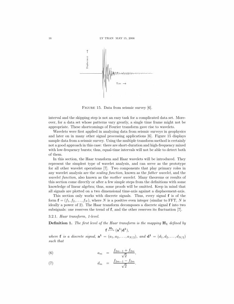
1100

Figure 14. Power spectra of the windowed sunspot data, datalength = 32, skipping step = 5.

step equal to 1. Figure 14 is the spectra of the same data set; however, the skippingstep is now 5.

The color bar next to each graph is the guide to decipher power spectrum ineach smaller data set. The symmetric property is retained in both graphs. Figure13 has better resolution, which results from smaller skipping step. However, bothgraphs represent the same trend of frequency contents.

3.2. Haar Wavelets. Although multiple transforms can be adopted to solve prob-lems of large data files, such a method is not complete. Determining the time

16 LY TRAN MAY 15, 2006

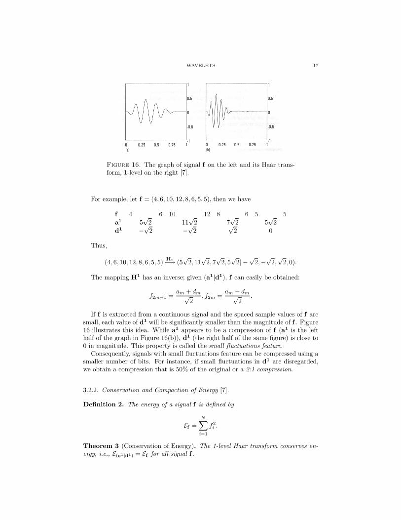
Figure 15. Data from seismic survey [6].

interval and the skipping step is not an easy task for a complicated data set. More-over, for a data set whose patterns vary greatly, a single time frame might not beappropriate. These shortcomings of Fourier transform gave rise to wavelets.

Wavelets were first applied in analyzing data from seismic surveys in geophysicsand later on in many other signal processing applications [6]. Figure 15 displayssample data from a seismic survey. Using the multiple transform method is certainlynot a good approach in this case: there are short-duration and high-frequency mixedwith low-frequency bursts; thus, equal-time intervals will not be able to detect bothof them.

In this section, the Haar transform and Haar wavelets will be introduced. Theyrepresent the simplest type of wavelet analysis, and can serve as the prototypefor all other wavelet operations [7]. Two components that play primary roles inany wavelet analysis are the scaling function, known as the father wavelet, and thewavelet function, also known as the mother wavelet. Many theorems or results ofthis section come directly or after a few simple steps from the definitions with someknowledge of linear algebra; thus, some proofs will be omitted. Keep in mind thatall signals are plotted on a two dimensional time-axis against a displacement-axis.

This section only works with discrete signals. Thus, every signal f is of theform f = (f1, f2, . . . , fN ), where N is a positive even integer (similar to FFT, N isideally a power of 2). The Haar transform decomposes a discrete signal f into twosubsignals: one reserves the trend of f , and the other reserves its fluctuation [7].

3.2.1. Haar transform, 1-level.

Definition 1. The first level of the Haar transform is the mapping H1 defined by

fH17−→ (a1|d1),

where f is a discrete signal, a1 = (a1, a2, . . . , aN/2), and d1 = (d1, d2, . . . , dN/2)such that

am =f2m−1 + f2m√

2,(6)

dm =f2m−1 − f2m√

2.(7)

WAVELETS 17

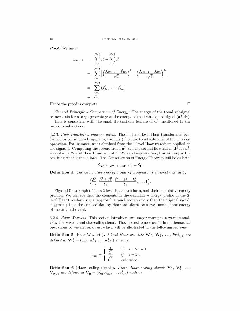
Figure 16. The graph of signal f on the left and its Haar trans-form, 1-level on the right [7].

For example, let f = (4, 6, 10, 12, 8, 6, 5, 5), then we have

f 4 6 10 12 8 6 5 5

a1 5√

2 11√

2 7√

2 5√

2

d1 −√

2 −√

2√

2 0

Thus,

(4, 6, 10, 12, 8, 6, 5, 5)H17−→ (5

√2, 11

√2, 7

√2, 5

√2| −

√2,−

√2,√

2, 0).

The mapping H1 has an inverse; given (a1|d1), f can easily be obtained:

f2m−1 =am + dm√

2, f2m =

am − dm√2

.

If f is extracted from a continuous signal and the spaced sample values of f aresmall, each value of d1 will be significantly smaller than the magnitude of f . Figure16 illustrates this idea. While a1 appears to be a compression of f (a1 is the lefthalf of the graph in Figure 16(b)), d1 (the right half of the same figure) is close to0 in magnitude. This property is called the small fluctuations feature.

Consequently, signals with small fluctuations feature can be compressed using asmaller number of bits. For instance, if small fluctuations in d1 are disregarded,we obtain a compression that is 50% of the original or a 2:1 compression.

3.2.2. Conservation and Compaction of Energy [7].

Definition 2. The energy of a signal f is defined by

Ef =

N∑

i=1

f2i .

Theorem 3 (Conservation of Energy). The 1-level Haar transform conserves en-ergy, i.e., E(a1|d1) = Ef for all signal f .

18 LY TRAN MAY 15, 2006

Proof. We have

Ea1|d1 =

N/2∑

i=1

a2i +

N/2∑

i=1

d2i

=

N/2∑

i=1

[(f2m−1 + f2m√2

)2

+(f2m−1 − f2m√

2

)2]

=

N/2∑

i=1

(

f22m−1 + f2

2m

)

= Ef

Hence the proof is complete. �

General Principle - Compaction of Energy: The energy of the trend subsignala1 accounts for a large percentage of the energy of the transformed signal (a1|d1).

This is consistent with the small fluctuations feature of d1 mentioned in theprevious subsection.

3.2.3. Haar transform, multiple levels. The multiple level Haar transform is per-formed by consecutively applying Formula (1) on the trend subsignal of the previousoperation. For instance, a1 is obtained from the 1-level Haar transform applied onthe signal f . Computing the second trend a2 and the second fluctuation d2 for a1,we obtain a 2-level Haar transform of f . We can keep on doing this as long as theresulting trend signal allows. The Conservation of Energy Theorem still holds here:

E(an|dn|dn−1|...|d2|d1) = Ef .

Definition 4. The cumulative energy profile of a signal f is a signal defined by

(f21

Ef

,f21 + f2

2

Ef

,f21 + f2

2 + f23

Ef

, . . . , 1)

.

Figure 17 is a graph of f , its 2-level Haar transform, and their cumulative energyprofiles. We can see that the elements in the cumulative energy profile of the 2-level Haar transform signal approach 1 much more rapidly than the original signal,suggesting that the compression by Haar transform conserves most of the energyof the original signal.

3.2.4. Haar Wavelets. This section introduces two major concepts in wavelet anal-ysis: the wavelet and the scaling signal. They are extremely useful in mathematicaloperations of wavelet analysis, which will be illustrated in the following sections.

Definition 5 (Haar Wavelets). 1-level Haar wavelets W11, W1

2, . . ., W1

N/2 are

defined as W1n

= (w1n1, w

1n2, . . . , w

1nN ) such as

w1ni =

1√2

if i = 2n − 1−1√

2if i = 2n

0 otherwise.

Definition 6 (Haar scaling signals). 1-level Haar scaling signals V11, V1

2, . . .,V1

N/2 are defined as V1n = (v1

n1, v1n2, . . . , v

1nN ) such as

WAVELETS 19

Figure 17. The graph of a) signal f , b) 2-level Haar transformof signal f , c) the cumulative energy profile of signal f and d) thecumulative energy profile of its 2-level Haar transform[7].

v1ni =

1√2

if i = 2n− 11√2

if i = 2n

0 otherwise.

So, the 1-level Haar wavelets are:

W1

1 = (1√2,− 1√

2, 0, 0, . . . , 0),

W1

2 = (0, 0,1√2,− 1√

2, 0, 0, . . . , 0),

...

W1

N/2 = (0, 0, . . . , 0,1√2,− 1√

2),

and the 1-level Haar scaling signals are:

V1

1= (

1√2,

1√2, 0, 0, . . . , 0),

V1

2= (0, 0,

1√2,

1√2, 0, 0, . . . , 0),

...

V1

N/2 = (0, 0, . . . , 0,1√2,

1√2).

20 LY TRAN MAY 15, 2006

A relationship can be established between subsignals of f and the 1-level Haarwavelets and scaling signals, using the familiar scalar product (known as the dotproduct in Linear Algebra):

am = f · V1

m,

dm = f · W1

m.

For any type of wavelets, the mother wavelets act as a window sliding along thesignal (translation), whereas the scaling signals allow zooming in and out at eachpoint (dilation).

We can also define multiple level Haar wavelets Wmn = (wm

n1, wmn2, . . . , w

mnN ) and

scaling signals Vmn

= (vmn1, v

mn2, . . . , v

mnN ) in a similar manner:

vmni =

{ 1√2

if 2m−1n + 1 ≤ i ≤ 2mn

0 otherwise,

wmni =

1√2

if 2m−1n + 1 ≤ i ≤ 3 × 2m−2n−1√

2if 3 × 2m−2n + 1 ≤ i ≤ 2mn

0 otherwise.

For example,

V2

2= (0, 0, 0, 0,

1√2,

1√2,

1√2,

1√2, 0, 0, . . . , 0),

W2

2 = (0, 0, 0, 0,1√2,

1√2,−1√

2,−1√

2, 0, 0, . . . , 0).

Consequently, we can obtain multiple level Haar transform from multiple level Haarwavelets and scaling signals:

am =(

f ·Vm

1, f ·Vm

2, . . . , f · Vm

N/2m

)

,

dm =(

f ·Wm

1, f · Wm

2, . . . , f · Wm

N/2m

)

.

The multiple level Haar wavelets and scaling signals are essential in Haar waveletanalysis. Similar to the coefficients in Fourier transform, they provide the meansto analyze the signals. More details will be provided in later sections.

3.3. Daubechies Wavelets. Haar wavelets are considered the most basic of all.In 1988, Ingrid Daubechies discovered another family of wavelets that were namedafter her [8]. Unlike Haar wavelets, Daubechies wavelets are continuous. Conse-quently, they work better with continuous signals. They also have longer supports,i.e. they use more values from the original signals to produce averages and dif-ferences. These improvements enable Daubechies wavelets to handle complicatedsignals more accurately.

We will first examine the simplest of the Daubechies family of wavelets: theDaub4 wavelets. Although the scaling and wavelet numbers are different, the ideaof the Daubechies wavelets and Daubechies wavelet transform are very similar tothat of the Haar wavelets.

Since all wavelet analyses are similar in definitions and properties, the followingsections on different types of wavelets will not go into particulars. The previoussection on Haar wavelet analysis might be useful as a reference.

WAVELETS 21

3.3.1. Definitions. The Daub4 wavelets use four coefficients for their scaling signalsand wavelets, compared to two in that of Haar wavelets.

The scaling coefficients of Daub4 wavelets are

α1 =1 +

√3

4√

2, α2 =

3 +√

3

4√

2, α3 =

3 −√

3

4√

2, α4 =

1 −√

3

4√

2,

and the wavelet coefficients are:

β1 = α4, β2 = −α3, β3 = α2, β4 = −α1.

Then, the first level Daub4 scaling signals are V1n = (v1, v2, ...vN ), for n =

1, 2, ..., N/2, in which [7]

vi =

α1 if i = 2n − 1α2 if i = 2nα3 if i = (2n + 1) mod Nα4 if i = (2n + 2) mod N0 otherwise.

The first level Daub4 wavelets W1n = (w1, w2, ...wN ), for n = 1, 2, ..., N/2, are

defined similarly [7]:

wi =

β1 if i = 2n− 1β2 if i = 2nβ3 if i = (2n + 1) mod Nβ4 if i = (2n + 2) mod N0 otherwise.

According to the definition, we have the 1-level Daub4 wavelets:

W1

1= (β1, β2, β3, β4, 0, 0, . . . , 0)

W1

2 = (0, 0, β1, β2, β3, β4, 0, 0, . . . , 0)

W1

3 = (0, 0, 0, 0, β1, β2, β3, β4, 0, 0, . . . , 0)

...

W1

N/2−1= (0, 0, . . . , 0, β1, β2, β3, β4)

W1

N/2 = (β3, β4, 0, 0, . . . , 0, β1, β2),

and the 1-level Daub4 scaling signals:

V1

1= (α1, α2, α3, α4, 0, 0, . . . , 0)

V1

2 = (0, 0, α1, α2, α3, α4, 0, 0, . . . , 0)

V1

3 = (0, 0, 0, 0, α1, α2, α3, α4, 0, 0, . . . , 0)

...

V1

N/2−1= (0, 0, . . . , 0, α1, α2, α3, α4)

V1

N/2 = (α3, α4, 0, 0, . . . , 0, α1, α2).

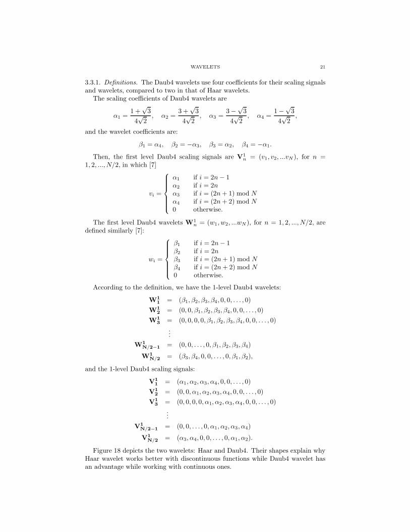
Figure 18 depicts the two wavelets: Haar and Daub4. Their shapes explain whyHaar wavelet works better with discontinuous functions while Daub4 wavelet hasan advantage while working with continuous ones.

22 LY TRAN MAY 15, 2006

Figure 18. (a) Left figure: Haar wavelet, (b) Right figure: Daub4wavelet

Notice that the scaling signals and wavelets are orthogonal to each other. Thiscan be easily proved using the scaling and wavelet numbers’ properties stated inthe next section.

3.3.2. The coefficients’ properties. The wavelet and scaling coefficients satisfy con-ditions that are essential for the properties of wavelets

α21 + α2

2 + α23 + α2

4 = 1,

α1 + α2 + α3 + α4 =√

2,

β21 + β2

2 + β23 + β2

4 = 1,

β1 + β2 + β3 + β4 = 0.

These identities can be used to prove the orthogonality among all scaling signalsand wavelets.

3.3.3. Daub4 First and Multiple-Level Transforms. Much like 1-level Haar trans-

form, Daub4 transform is defined as the mapping fD17−→ (a1|d1). Each element in

the first trend subsignal a1 = (a1, . . . , aN/2) is the scalar product ai = f ·V1i . Simi-

larly, the fluctuation subsignal d1 = (d1, . . . , dN/2) is the scalar product di = f ·W1i .

Let us define the elementary signals V01, V0

2, ..., V0

Nas

V0

1= (1, 0, 0, . . . , 0)

V0

2 = (0, 1, 0, 0 . . . , 0)

...

V0

N= (0, 0, . . . , 0, 1).

We recognize that

V1m = α1V

02m−1 + α2V

02m + α3V

02m+1 + α4V

02m+2,

W1m = β1V

02m−1 + β2V

02m + β3V

02m+1 + β4V

02m+2,

where the sub index is mod N .Higher level Daub4 transforms are obtained by applying the 1-level Daub4 trans-

form consecutively on the trend subsignal of the previous level transform. Thehigher level scaling signals and wavelets are defined accordingly:

(8)Vk

m = α1Vk−12m−1 + α2V

k−12m + α3V

k−12m+1 + α4V

k−12m+2

Wkm = β1V

k−12m−1 + β2V

k−12m + β3V

k−12m+1 + β4V

k−12m+2.

WAVELETS 23

Figure 19. (a) Signal A. (b) 2-level Daub4 transform. (c) and(d) Magnifications of the signal’s graph in two small squares; thesignal is approximately linear [7].

The above formulas can be modified and applied to any kind of wavelets. Tosummarize, the first and multiple-level Daub4 transforms are achieved from thesewavelets and scaling signals:

(9)am =

(

f ·Vm1

, f ·Vm2

, . . . , f · Vm

N/2m

)

,

dm =(

f ·Wm1

, f · Wm2

, . . . , f · Wm

N/2m

)

,

which are similar to those of Haar transforms.

3.3.4. The Daub4 Transform’s Property [7].

Property 1. If a signal f is approximately linear over the support of a k-level Daub4wavelet Wk

m, then the k-level fluctuation value f ·Wkm is approximately zero [7].

The support of a k-level wavelet depends on the number k. For example, the1-level Daub4 wavelet has 4 time-unit support (4 non-zero coefficients); the 2-level Daub4 wavelet has 6 time-unit support, etc... Figure 19 illustrates this idea:magnifications of the original signal appear linear; and the fluctuation subsignalsseem to be 0. This property is useful in determining whether Daub4 wavelets areadequate for certain applications.

Property 2. Similar to Haar transform, Daub4 transforms also conserve energy.

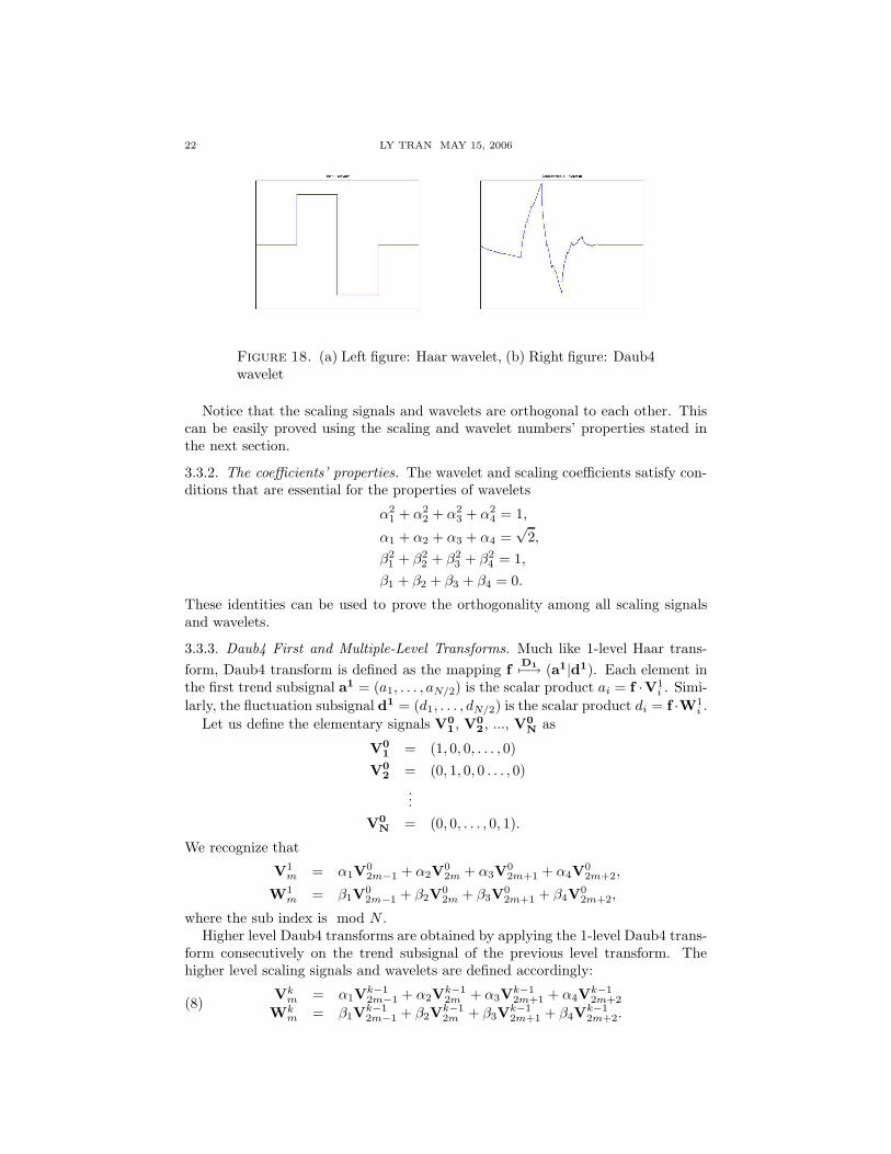
The proof for this can be found in [7]. Figure 20 compares the efficiency of Haartransform and Daub4 transform. The upper graphs show that the detail subsignalsfrom Daub4 transform are significantly less than that from Haar transform. As aresult, the cumulative energy of Daub4 transform reaches 1 much faster.

24 LY TRAN MAY 15, 2006

Figure 20. (a)2-level Haar transform of signal A. (b) 2-levelDaub4 transform on the same signal. (c) Cumulative energy profilefor the Haar transform in (a). and (d) Cumulative energy profilefor the Daub4 transform in (b)[7].

3.4. Other Daubechies Wavelets. Other Daubechies wavelets are very similar toDaub4 wavelets. Ingrid Daubechies developed two families of wavelets: the DaubJwavelets (for J = 4, 6, 8, . . . , 20) and the CoifI wavelets (for I = 6, 12, 18, 24, 30)[7].

3.4.1. DaubJ Wavelets. We provide a general definition for DaubJ wavelets (forJ = 4, 6, 8, . . . , 20) as done in [7]. For each J , the scaling numbers αi (for i =1, 2, ..., J) are computed. The wavelet numbers are then defined accordingly:

βi = (−1)i+1αJ−i.

The 1-level Daub4 scaling signals are: V1n = (v1, v2, ...vN ), for n = 1, 2, ..., N/2, in

which

vi =

α1 if i = (2n − 1) mod Nα2 if i = (2n) mod N...αJ−1 if i = (2n + J − 3) mod NαJ if i = (2n + J − 2) mod N0 otherwise.

WAVELETS 25

The 1-level Daub4 wavelets are:W1n = (w1, w2, ...wN ), for n = 1, 2, ..., N/2, in

which

wi =

β1 if i = (2n − 1) mod Nβ2 if i = (2n) mod N...βJ−1 if i = (2n + J − 3) mod NβJ if i = (2n + J − 2) mod N0 otherwise.

The scaling numbers and wavelet numbers of DaubJ transform still satisfy someidentities:

α21 + α2

2 + . . . + α2J−1 + α2

J = 1,

α1 + α2 + . . . + αJ−1 + αJ =√

2,

0iβ1 + 1iβ2 + . . . + (J − 2)iβJ−1 + (J − 1)iβJ = 0,

for i = 0, 1, ..., J − 4.

The multiple level DaubJ transforms are defined similarly to Daub4. The 1-leveltransform is applied consecutively on the previous level’s trend signal to achieve ahigher transform.

3.4.2. Coiflets. Like the DaubJ family, the CoifI family, also known as the “coiflets”,consists of different wavelets defined in a similar manner [7]. Thus, we will examinethe representative Coif6, which should give us good understanding of the family ingeneral.

The six Coif6 scaling numbers are:

α1 = 1−√

716

√2, α2 = 5+

√7

16√

2, α3 = 14+2

√7

16√

2,

α4 = 14−2√

716

√2

, α5 = 1−√

716

√2, α6 = −3+

√7

16√

2.

The wavelet numbers are defined based on the scaling numbers:

βi = (−1)i+1αJ−i.

Besides common identities, the Coif6 scaling numbers satisfy additional ones:

α1 + α2 + α3 + α4 + α5 + α6 =√

2

(−2)iα1 + (−1)iα2 + 0iα3 + 1iα4 + 2iα5 + 3iα6 = 0

for i = 1, 2,

β1 + β2 + β3 + β4 + β5 + β6 = 0

0β1 + 1β2 + 2β3 + 3β4 + 4β5 + 5β6 = 0.

The Coif6 first level scaling signals V1n = (v1, v2, ...vN ), and wavelets W1

n =(w1, w2, ...wN ), for n = 1, 2, ..., N/2, are also determined slightly differently [7]:

vi =

α1 if i = (2n − 3) mod Nα2 if i = (2n − 2) mod Nα3 if i = (2n − 1) mod Nα4 if i = (2n) mod Nα5 if i = (2n + 1) mod Nα6 if i = (2n + 2) mod N0 otherwise,

26 LY TRAN MAY 15, 2006

wi =

β1 if i = (2n − 3) mod Nβ2 if i = (2n − 2) mod Nβ3 if i = (2n − 1) mod Nβ4 if i = (2n) mod Nβ5 if i = (2n + 1) mod Nβ6 if i = (2n + 2) mod N0 otherwise.

Formulas (8) and (9) may be employed to find higher level wavelets, scalingsignals, and to perform Coiflet transforms at different levels. Coiflets share allproperties with Haar and DaubJ wavelets.

3.5. Wavelet Applications. In this section, some basic applications of waveletanalysis will be introduced. The Haar wavelet will be examined in all applicationsas a model for other types of wavelets. Since wavelet analytical mechanisms aresimilar across different families of wavelets, more complex wavelets will be exam-ined without elaborate explanation. Juxtaposition of two or more different waveletanalyses in one application will help indicate one wavelet’s advantages over theothers.

3.5.1. Multiresolution Analysis. Since discrete signals are subjects of wavelet anal-ysis in this paper, all elementary algebraic operations such as addition, subtraction,and scalar multiplication can be performed on any two or more signals. Multireso-lution analysis allows the original signal to be built up from lower resolution signalsand necessary details.

Definition 7 (First Signals). The First Average Signal A1 is defined by

A1 =( a1√

2,

a1√2,

a2√2,

a2√2, . . . ,

aN/2√2

,aN/2√

2

)

.

The First Detail Signal D1 is defined by

D1 =( d1√

2,−d1√

2,

d2√2,−d2√

2, . . . ,

dN/2√2

,−dN/2√

2

)

.

Recalling the elementary signals defined in the previous section, we have:

f =

N∑

i=1

fiV0

i .(10)

The above formula is called the natural expansion of a signal f in terms of thenatural basis of signals V0

1, V02, . . ., V0

N.

WAVELETS 27

Figure 21. The graph of signal A built up from 10-level HaarMRA. Ten averaged signals from A10 to A1 are displayed fromtop to bottom, from left to right [7].

It follows that

f =( a1√

2,

a1√2,

a2√2,

a2√2, . . . ,

aN/2√2

,aN/2√

2

)

+( d1√

2,−d1√

2,

d2√2, . . . ,

dN/2√2

,−dN/2√

2

)

= A1 + D1

=

N/2∑

i=1

aiV1

i +

N/2∑

i=1

diW1

i

=

N/2∑

i=1

(

f ·V1

i

)

V1

i +

N/2∑

i=1

(

f · W1

i

)

W1

i .

This is the first level of Haar multiresolution analysis (MRA). Since the multiplelevel Haar transform can be applied consecutively on average subsignals, we canexpand further to obtain multiple level Haar MRA:

f = Ak + Dk + . . . + D2 + D1,

in which

Ak =

N/2k

∑

i=1

(

f · Vk

i

)

Vk

i

Dk =

N/2k

∑

i=1

(

f · Wk

i

)

Wk

i.

The values(

f · Vk

i

)

and(

f · Wk

i

)

are called wavelet coefficients. Each of thecomponent signals has lower resolution than f ; however, if a high-enough level ofMRA is employed, the original f can be obtained. In Figure 21, the original signalwas achieved after 10 levels of Haar MRA. Since the original signal is continuous,Daubechies wavelets yield better results. Figure 22 and Figure 23 show that morecomplex wavelets approach the original signal after fewer steps of MRA.

28 LY TRAN MAY 15, 2006

Figure 22. Daub4 MRA of the same signal. The graph are of 10averaged signals A10 through A1 [7].

Figure 23. Daub20 MRA of the same signal. The graph are of10 averaged signals A10 through A1 [7].

3.5.2. Compression of Audio Signals. There are two basic categories of compressiontechniques: lossless compression and lossy compression [7]. A lossless compressiontechnique yields a decompression free in error from the original signal, while a de-compression resulted from lossy compression suffers a degree of inaccuracy. How-ever, the lossy compression usually succeeds more often at reducing the size of thedata set. The wavelet transform is a lossy compression technique.

Method of Wavelet Transform Compression [7]Step 1. Perform a wavelet transform of the signalStep 2. Set equal to 0 all values of the wavelet transform which are insignificant,

i.e., which lie below some threshold value.Step 3. Transmit only the significant, non-zero values of the transform obtained

from Step 2. This should be a much smaller data set than the original signal.Step 4. At the receiving end, perform the inverse wavelet transform of the

data transmitted in Step 3, assigning zero values to the insignificant values whichwere not transmitted. This decompression step produces an approximation of theoriginal signal.

Figures 24 and 25 are two examples of compression using wavelet transformmethod. Because of the nature of Haar wavelets, discrete signals like signal 1in Figure 24 can be more easily compressed with high degree of accuracy, whilecontinuous signals such as signal 2 in Figure 25 are much harder to compress,

WAVELETS 29

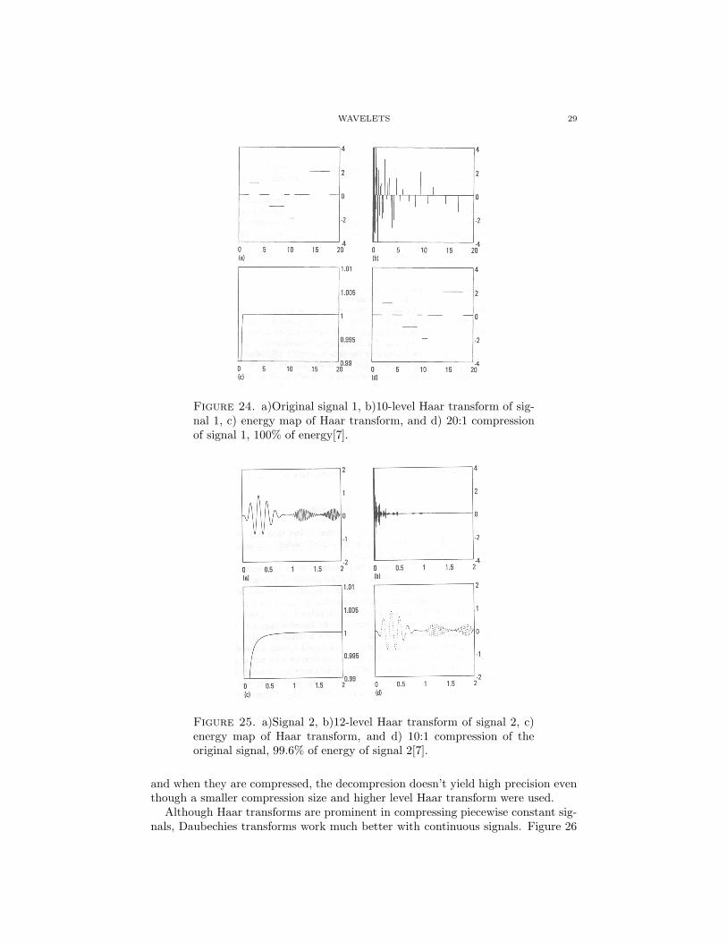
Figure 24. a)Original signal 1, b)10-level Haar transform of sig-nal 1, c) energy map of Haar transform, and d) 20:1 compressionof signal 1, 100% of energy[7].

Figure 25. a)Signal 2, b)12-level Haar transform of signal 2, c)energy map of Haar transform, and d) 10:1 compression of theoriginal signal, 99.6% of energy of signal 2[7].

and when they are compressed, the decompresion doesn’t yield high precision eventhough a smaller compression size and higher level Haar transform were used.

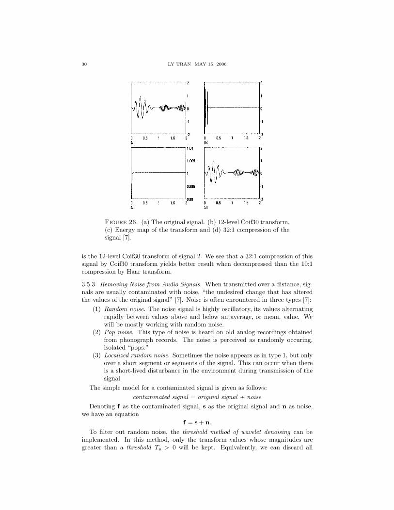
Although Haar transforms are prominent in compressing piecewise constant sig-nals, Daubechies transforms work much better with continuous signals. Figure 26

30 LY TRAN MAY 15, 2006

Figure 26. (a) The original signal. (b) 12-level Coif30 transform.(c) Energy map of the transform and (d) 32:1 compression of thesignal [7].

is the 12-level Coif30 transform of signal 2. We see that a 32:1 compression of thissignal by Coif30 transform yields better result when decompressed than the 10:1compression by Haar transform.

3.5.3. Removing Noise from Audio Signals. When transmitted over a distance, sig-nals are usually contaminated with noise, “the undesired change that has alteredthe values of the original signal” [7]. Noise is often encountered in three types [7]:

(1) Random noise. The noise signal is highly oscillatory, its values alternatingrapidly between values above and below an average, or mean, value. Wewill be mostly working with random noise.

(2) Pop noise. This type of noise is heard on old analog recordings obtainedfrom phonograph records. The noise is perceived as randomly occuring,isolated “pops.”

(3) Localized random noise. Sometimes the noise appears as in type 1, but onlyover a short segment or segments of the signal. This can occur when thereis a short-lived disturbance in the environment during transmission of thesignal.

The simple model for a contaminated signal is given as follows:

contaminated signal = original signal + noise

Denoting f as the contaminated signal, s as the original signal and n as noise,we have an equation

f = s + n.

To filter out random noise, the threshold method of wavelet denoising can beimplemented. In this method, only the transform values whose magnitudes aregreater than a threshold Ts > 0 will be kept. Equivalently, we can discard all

WAVELETS 31

Figure 27. a) Signal B, 210 values. b) 10-level Haar transform ofsignal B. The two horizontal lines are at values of ±.25 (the de-noising threshold). c) Thresholded transform. d) Denoised signal[7].

the transform values whose magnitudes lie below a noise threshold Tn satisfyingTn < Ts.

The Root mean Square Error (RMSE) is used to measure the effectiveness ofnoise removal method:

RMSE =

√

∑Ni=1(fi − si)2

N

=

√

∑Ni=1(ni)2

N

=

√En√N

.

Smaller RMSE indicates a better denoising result. This is similar to the least squaremethod in determining error for a set of data.

Figure 27 is a denoising example of signal 1. Part (a) of Figure 27 suggests thatsome random noise was added to the original signal. Part (b) shows the denoisingthreshold to be used on 10-level Haar transform of the contaminated signal, part (c)shows the Haar transform after the noise was filtered, and part (d) is the denoisedsignal. The result is fairly consistent with the original signal given in the previousreport. The RMSE between signal B and signal 1 is 0.057. After denoising, theRMSE reduces to 0.011.

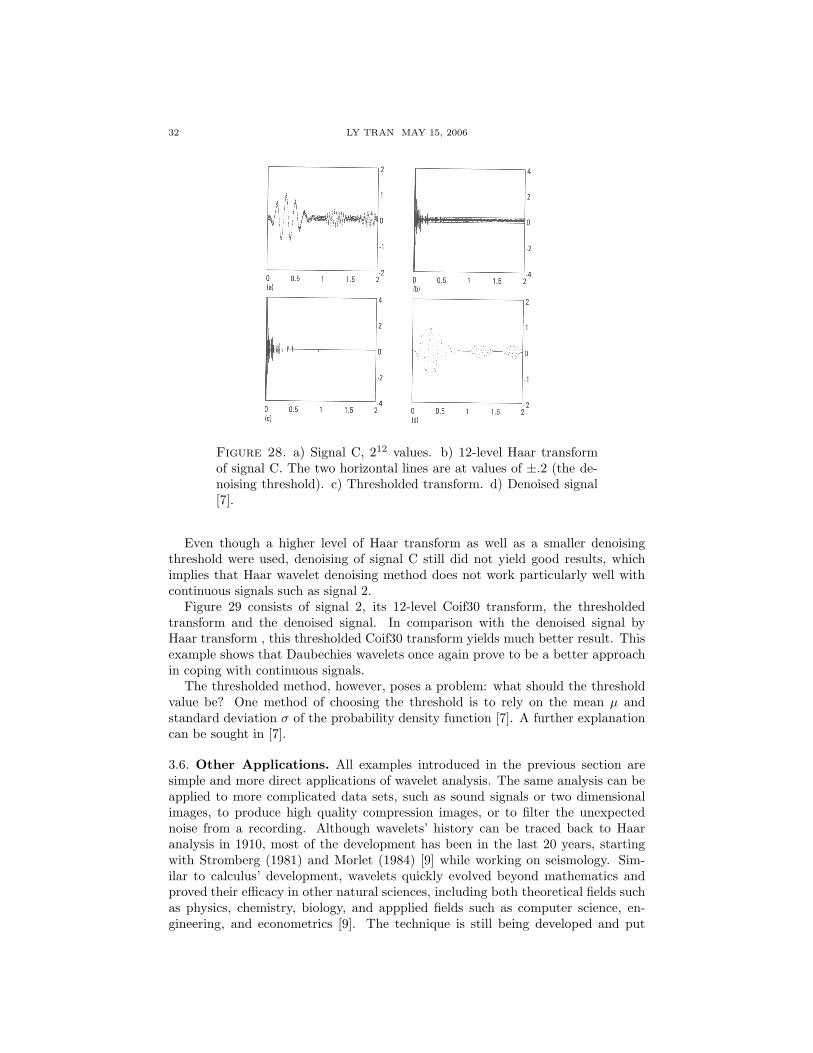
Figure 28 is another example of denoising method applied on signal 2. For thissignal, 212 values were used, together with a higher level of Haar transform (12instead of 10), and a smaller denoising threshold (0.2 instead of 0.25). The RMSEbetween signal C and signal 2 is 0.057. After denoising, the RMSE is 0.035.

32 LY TRAN MAY 15, 2006

Figure 28. a) Signal C, 212 values. b) 12-level Haar transformof signal C. The two horizontal lines are at values of ±.2 (the de-noising threshold). c) Thresholded transform. d) Denoised signal[7].

Even though a higher level of Haar transform as well as a smaller denoisingthreshold were used, denoising of signal C still did not yield good results, whichimplies that Haar wavelet denoising method does not work particularly well withcontinuous signals such as signal 2.

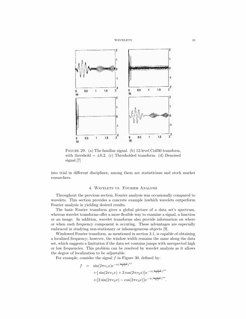
Figure 29 consists of signal 2, its 12-level Coif30 transform, the thresholdedtransform and the denoised signal. In comparison with the denoised signal byHaar transform , this thresholded Coif30 transform yields much better result. Thisexample shows that Daubechies wavelets once again prove to be a better approachin coping with continuous signals.

The thresholded method, however, poses a problem: what should the thresholdvalue be? One method of choosing the threshold is to rely on the mean µ andstandard deviation σ of the probability density function [7]. A further explanationcan be sought in [7].

3.6. Other Applications. All examples introduced in the previous section aresimple and more direct applications of wavelet analysis. The same analysis can beapplied to more complicated data sets, such as sound signals or two dimensionalimages, to produce high quality compression images, or to filter the unexpectednoise from a recording. Although wavelets’ history can be traced back to Haaranalysis in 1910, most of the development has been in the last 20 years, startingwith Stromberg (1981) and Morlet (1984) [9] while working on seismology. Sim-ilar to calculus’ development, wavelets quickly evolved beyond mathematics andproved their efficacy in other natural sciences, including both theoretical fields suchas physics, chemistry, biology, and appplied fields such as computer science, en-gineering, and econometrics [9]. The technique is still being developed and put

WAVELETS 33

Figure 29. (a) The familiar signal. (b) 12-level Coif30 transform,with threshold = ±0.2. (c) Thresholded transform. (d) Denoisedsignal.[7]

into trial in different disciplines, among them are statisticians and stock marketresearchers.

4. Wavelets vs. Fourier Analysis

Throughout the previous section, Fourier analysis was occasionally compared towavelets. This section provides a concrete example inwhich wavelets outperformFourier analysis in yielding desired results.

The basic Fourier transform gives a global picture of a data set’s spectrum,whereas wavelet transforms offer a more flexible way to examine a signal, a functionor an image. In addition, wavelet transforms also provide information on whereor when each frequency component is occuring. These advantages are especiallyembraced in studying non-stationary or inhomogeneous objects [9].

Windowed Fourier transform, as mentioned in section 3.1, is capable of obtaininga localized frequency; however, the window width remains the same along the dataset, which suggests a limitation if the data set contains jumps with unexpected highor low frequencies. This problem can be resolved by wavelet analysis as it allowsthe degree of localization to be adjustable.

For example, consider the signal f in Figure 30, defined by:

f = sin(2πv1x)e−π( x−0.2

0.1)10

+(

sin(2πv1x) + 2 cos(2πv2x))

e−π( x−0.5

0.1)10

+(

2 sin(2πv2x) − cos(2πv3x))

e−π( x−0.5

0.1)10 .

34 LY TRAN MAY 15, 2006

0 0.1 0.2 0.3 0.4 0.5 0.6 0.7 0.8 0.9 1−10

−8

−6

−4

−2

0

2

4

6

8

10

Figure 30. The original signal f .

0 50 100 150 200 250 300 350 400 450 5000

50

100

150

200

250

300

350

k

frequ

ency

Figure 31. The power spectrum of signal f .

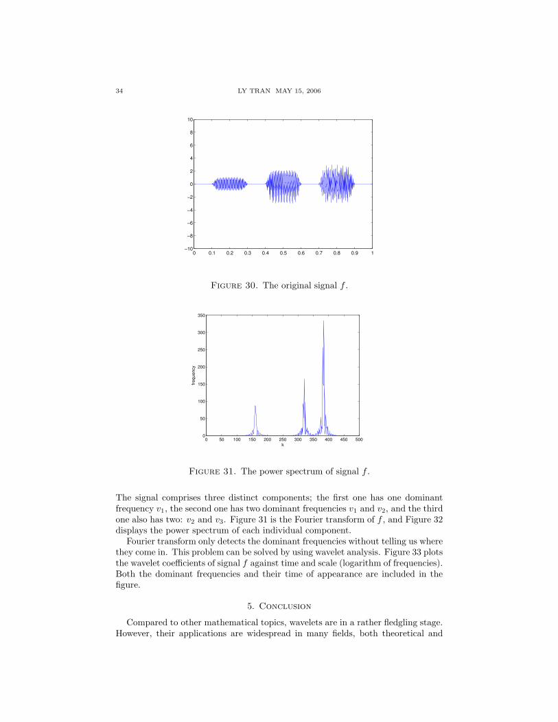
The signal comprises three distinct components; the first one has one dominantfrequency v1, the second one has two dominant frequencies v1 and v2, and the thirdone also has two: v2 and v3. Figure 31 is the Fourier transform of f , and Figure 32displays the power spectrum of each individual component.

Fourier transform only detects the dominant frequencies without telling us wherethey come in. This problem can be solved by using wavelet analysis. Figure 33 plotsthe wavelet coefficients of signal f against time and scale (logarithm of frequencies).Both the dominant frequencies and their time of appearance are included in thefigure.

5. Conclusion

Compared to other mathematical topics, wavelets are in a rather fledgling stage.However, their applications are widespread in many fields, both theoretical and

WAVELETS 35

0 200 400 600 800 1000 12000

200

400

600

800

1000

k

frequ

ency

0 200 400 600 800 1000 12000

200

400

600

800

1000

k

frequ

ency

0 200 400 600 800 1000 12000

200

400

600

800

1000

k

frequ

ency

Figure 32. The power spectra for each component.

100200

300400

500

12345678

0.2

0.4

0.6

0.8

TimeScale

Mag

nitu

de

100200

300400

500

24

68

0.2

0.4

0.6

0.8

Time

Mag

nitu

de

Figure 33. Wavelet transform of signal f . The plot is capturedat two different angles

36 LY TRAN MAY 15, 2006

practical. Arising from the Fourier analysis’ failure to cope with large and complexdata files, wavelets rapidly develop to resolve these problems.

This paper briefly introduced Fourier series and chose Fast Fourier Transform(FFT) to be the representative method for Fourier analysis. A modification of FFT- the windowing process or short-term Fourier transform - was also examined as atransition before moving to wavelets. Since all wavelets are constructed similarly,the first and simplest, the Haar wavelet, was studied first and in more detail.Two other families of wavelets were mentioned in the paper: DaubJ wavelets andCoiflets. Some simple applications of wavelet analysis mentioned in the paperinclude multiresolution analysis, the denoising problem and compression of audiosignals. These applications also provide a basis to make a comparison betweenFourier and wavelet analyses.

All examples in this paper, including discrete data and audio signals, are one-dimensional. However, wavelet analysis is capable of dealing with higher dimen-sional data sets, such as pictures. Information on wavelet analysis on 2D data setscan be found in [7] or most books on applications of wavelets. More complex appli-cations of wavelets, such as signal detection and applications in statistics, can alsobe topics for further study.

References

[1] WikiPedia, Fourier Series. http://en.wikipedia.org/wiki/Fourier_series[2] WikiPedia, Fourier Series. http://en.wikipedia.org/wiki/Wavelets[3] Stewart, James. Calculus Early Transcendentals, 4th Edition.[4] Fourier Analysis, Course Notes, Modeling II.[5] Sunspots. Retrieved from website http://www.exploratorium.edu/sunspots/activity.

html.[6] Boggess, A. and Narcowich, F., A First Course in Wavelets with Fourier Analysis. New

Jersey 2001.[7] Walker, J. , A Primer on Wavelets and their Scientific Applications. CRC Press LLC 1999.[8] Riddle, L. Ingrid Daubechies. Biographies of Women Mathematicians. Retrieved on Dec 1,

2005 from website http://www.agnesscott.edu/lriddle/women/daub.htm

[9] Abramovich, F., Bailey, T. and Sapatinas, T.. Wavelet Analysis and Its Statistical Applica-tions. The Statistician, Vol. 49, No. 1 (2000), pp 1-29.