From a vibration measurement on a machine, the damping ratio and undamped vibration frequency are calculated as 0.36 and 24 Hz, respectively. Vibration.

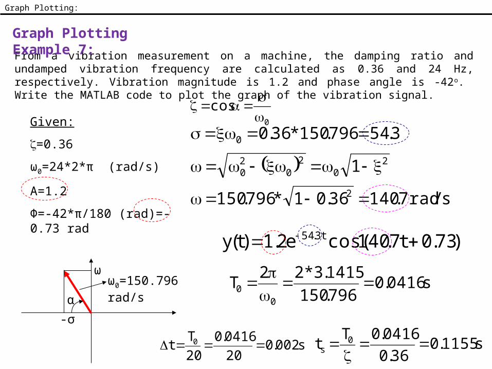
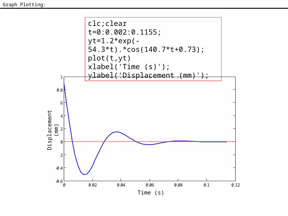
From a vibration measurement on a machine, the damping ratio and undamped vibration frequency are calculated as 0.36 and 24 Hz, respectively. Vibration magnitude is 1.2 and phase angle is -42o. Write the MATLAB code to plot the graph of the vibration signal.

Graph Plotting:

Graph Plotting Example 7:

)73.0t7.140cos(e2.1)t(y t3.54

Given:

=0.36

ω0=24*2*π (rad/s)

A=1.2

Φ=-42*π/180 (rad)=-0.73 rad

ω0=150.796 rad/sω

-σ

3.54796.150*36.00

s/rad7.14036.01*796.150

12

20

20

20

α

0

cos

s0416.0796.1501415.3*22

T0

0

s002.0200416.0

20T

t 0 s1155.036.0

0416.0Tt 0

s

Graph Plotting:

0 0.02 0.04 0.06 0.08 0.1 0.12-0.6

-0.4

-0.2

0

0.2

0.4

0.6

0.8

1

Zaman (s)

y

clc;cleart=0:0.002:0.1155;yt=1.2*exp(-54.3*t).*cos(140.7*t+0.73);plot(t,yt)xlabel(‘Time (s)');ylabel(‘Displacement (mm)');

Time (s)

Dis

plac

emen

t (m

m)

Roots of a polynomial:

020t6t5t3 24 Find the roots of the polynomial.

with Matlab>> p=[3 0 5 6 -20]>> roots(p)

ans =

-1.5495 0.1829 + 1.8977i 0.1829 - 1.8977i 1.1838

-2 -1.5 -1 -0.5 0 0.5 1 1.5 2

-20

-10

0

10

20

30

40

50

60

t

3 t4+5 t2+6 t-20

1.1838-1.5495

>>ezplot('3*t^4+5*t^2+6*t-20',-2,2)

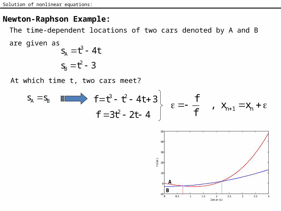
Newton-Raphson Example:

Solution of nonlinear equations:

The time-dependent locations of two cars denoted by A and B

are given as

3ts

t4ts2

B

3A

At which time t, two cars meet?

BA ss 3t4ttf 23

4t2t3f 2

n1n xx,

ff

0 0.5 1 1.5 2 2.5 3 3.5 4-10

0

10

20

30

40

50

Zaman (s)

Yol

(m

)

A

B

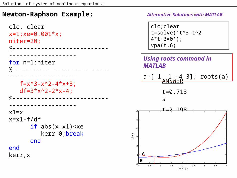
Newton-Raphson Example:

Solutions of system of nonlinear equations:

ANSWER

t=0.713 s

t=2.198 s

0 0.5 1 1.5 2 2.5 3 3.5 4-10

0

10

20

30

40

50

Zaman (s)

Yol

(m

)

A

B

Using roots command in MATLAB

a=[ 1 -1 -4 3]; roots(a)

clc;cleart=solve('t^3-t^2-4*t+3=0');vpa(t,6)

Alternative Solutions with MATLAB

clc, clearx=1;xe=0.001*x;niter=20;%----------------------------------------------for n=1:niter%---------------------------------------------- f=x^3-x^2-4*x+3; df=3*x^2-2*x-4;%---------------------------------------------- x1=x x=x1-f/df if abs(x-x1)<xe kerr=0;break endendkerr,x

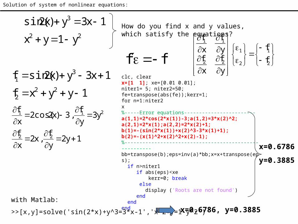
Solution of system of nonlinear equations:

22

3

y1yx

1x3y)x2sin(

How do you find x and y values, which satisfy the equations?

1yyxf

1x3y)x2sin(f22

2

31

ff

2

1

2

1

22

11

ff

yf

xf

yf

xf

1y2yf

,x2xf

y3yf

,3)x2cos(2xf

22

211

x=0.6786

y=0.3885

with Matlab:

>>[x,y]=solve('sin(2*x)+y^3=3*x-1','x^2+y=1-y^2') x=0.6786, y=0.3885

clc, clearx=[1 1]; xe=[0.01 0.01];niter1= 5; niter2=50;fe=transpose(abs(fe));kerr=1;for n=1:niter2x%-----Error equations------------------------a(1,1)=2*cos(2*x(1))-3;a(1,2)=3*x(2)^2;a(2,1)=2*x(1);a(2,2)=2*x(2)+1;b(1)=-(sin(2*x(1))+x(2)^3-3*x(1)+1);b(2)=-(x(1)^2+x(2)^2+x(2)-1);%-------------------------------------------------------bb=transpose(b);eps=inv(a)*bb;x=x+transpose(eps); if n>niter1 if abs(eps)<xe kerr=0; break else display ('Roots are not found') end endend

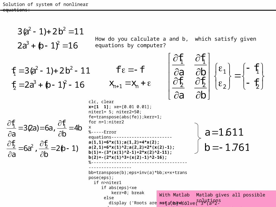
Solution of system of nonlinear equations:

16)1b(a2

11b2)1a(323

22

How do you calculate a and b, which satisfy given equations by computer?

16)1b(a2f

11b2)1a(3f23

2

221

ff n1n xx

2

1

2

1

22

11

ff

bf

af

bf

af

)1b(2bf

,a6af

b4bf

,a6)a2(3af

222

11

With Matlab

>>[a,b]=solve('3*(a^2-1)+2*b^2=11','2*a^3+(b-1)^2=16')

Matlab gives all possible solutions

761.1b611.1a

clc, clearx=[1 1]; xe=[0.01 0.01];niter1= 5; niter2=50;fe=transpose(abs(fe));kerr=1;for n=1:niter2x%-----Error equations------------------------a(1,1)=6*x(1);a(1,2)=4*x(2);a(2,1)=6*x(1)^2;a(2,2)=2*(x(2)-1);b(1)=-(3*(x(1)^2-1)+2*x(2)^2-11);b(2)=-(2*x(1)^3+(x(2)-1)^2-16);%-------------------------------------------------------bb=transpose(b);eps=inv(a)*bb;x=x+transpose(eps); if n>niter1 if abs(eps)<xe kerr=0; break else display ('Roots are not found') end endend

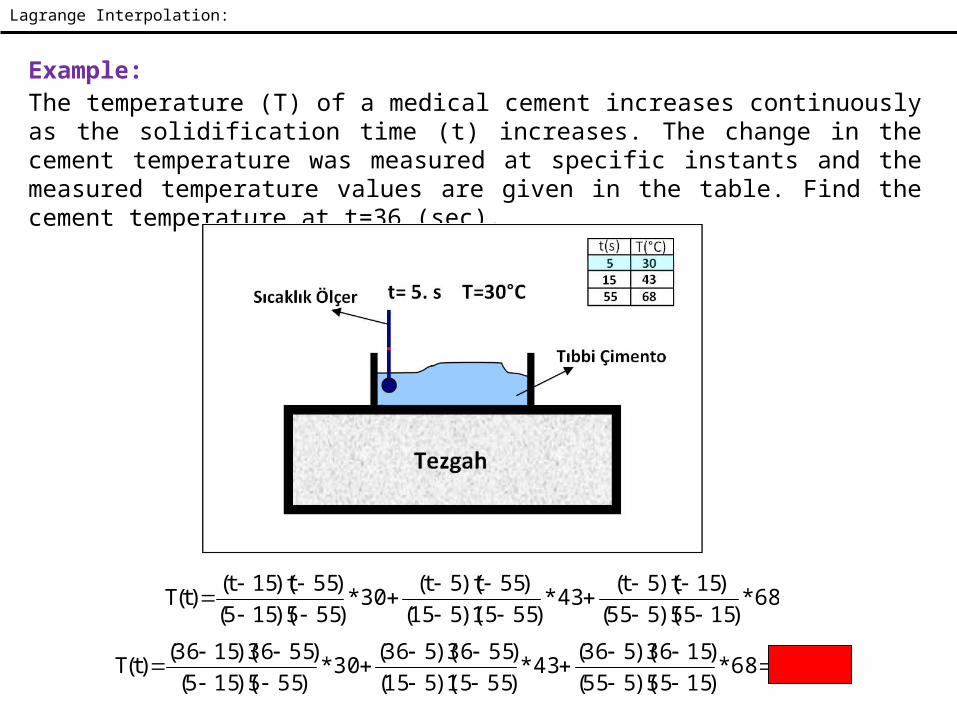
Lagrange Interpolation:

Example:The temperature (T) of a medical cement increases continuously as the solidification time (t) increases. The change in the cement temperature was measured at specific instants and the measured temperature values are given in the table. Find the cement temperature at t=36 (sec).

68*)1555)(555(

)15t)(5t(43*

)5515)(515()55t)(5t(

30*)555)(155()55t)(15t(

)t(T

C51.6168*)1555)(555()1536)(536(

43*)5515)(515()5536)(536(

30*)555)(155(

)5536)(1536()t(T o

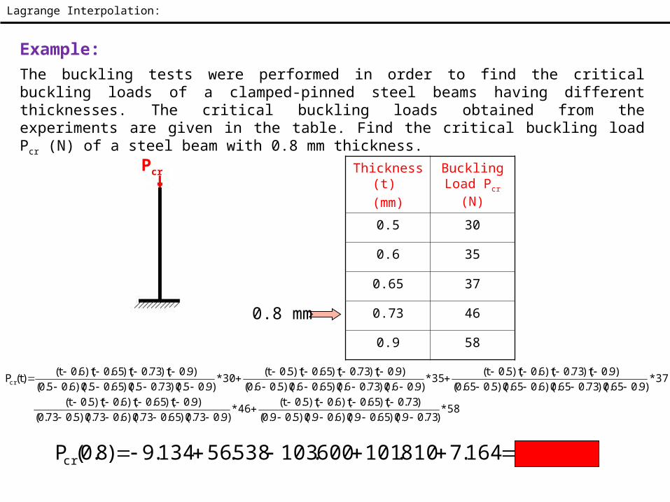
Lagrange Interpolation:

Example:The buckling tests were performed in order to find the critical buckling loads of a clamped-pinned steel beams having different thicknesses. The critical buckling loads obtained from the experiments are given in the table. Find the critical buckling load Pcr (N) of a steel beam with 0.8 mm thickness.

Thickness (t) (mm)

Buckling Load Pcr (N)

0.5 30

0.6 35

0.65 37

0.73 46

0.9 580.8 mm

58*)73.09.0)(65.09.0)(6.09.0)(5.09.0(

)73.0t)(65.0t)(6.0t)(5.0t(46*

)9.073.0)(65.073.0)(6.073.0)(5.073.0()9.0t)(65.0t)(6.0t)(5.0t(

37*)9.065.0)(73.065.0)(6.065.0)(5.065.0(

)9.0t)(73.0t)(6.0t)(5.0t(35*

)9.06.0)(73.06.0)(65.06.0)(5.06.0()9.0t)(73.0t)(65.0t)(5.0t(

30*)9.05.0)(73.05.0)(65.05.0)(6.05.0(

)9.0t)(73.0t)(65.0t)(6.0t()t(Pcr

N779.52164.7810.101600.103538.56134.9)8.0(Pcr

Pcr

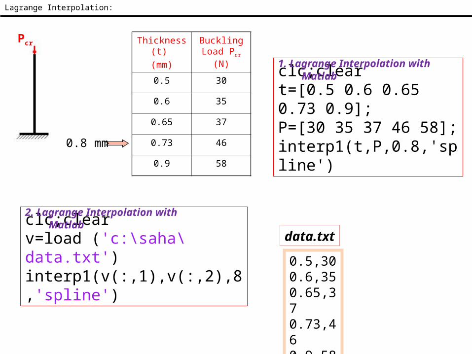
Lagrange Interpolation:

Thickness (t) (mm)

Buckling Load Pcr (N)

0.5 30

0.6 35

0.65 37

0.73 46

0.9 580.8 mm

clc;cleart=[0.5 0.6 0.65 0.73 0.9];P=[30 35 37 46 58];interp1(t,P,0.8,'spline')

Pcr

0.5,300.6,350.65,370.73,460.9,58

data.txtclc;clearv=load ('c:\saha\data.txt')interp1(v(:,1),v(:,2),8,'spline')

1. Lagrange Interpolation with Matlab

2. Lagrange Interpolation with Matlab

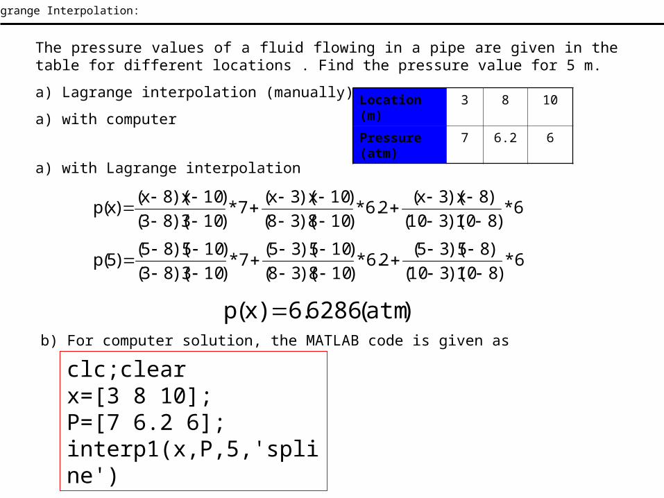
The pressure values of a fluid flowing in a pipe are given in the table for different locations . Find the pressure value for 5 m.

a) Lagrange interpolation (manually)

a) with computer

Location (m) 3 8 10

Pressure (atm) 7 6.2 6

a) with Lagrange interpolation

6*)810)(310(

)8x)(3x(2.6*

)108)(38()10x)(3x(

7*)103)(83()10x)(8x(

)x(p

6*)810)(310(

)85)(35(2.6*

)108)(38()105)(35(

7*)103)(83()105)(85(

)5(p

)atm(6286.6)x(p b) For computer solution, the MATLAB code is given as

clc;clearx=[3 8 10];P=[7 6.2 6];interp1(x,P,5,'spline')

Lagrange Interpolation:

The x and y coordinates of three points on the screen, which were clicked by a CAD user are given in the figure. Find the y value of the curve obtained from these points at x=50.

x y

25 -10

40 20

70 5

b) How do you find the answer manually?

)5()4070)(2570(

)40x)(25x()20(

)7040)(2540()70x)(25x(

)10()7025)(4025(

)70x)(40x()x(y

1108.269259.0222.2296296.2)50(y

Result: 26.111

a)How do you find the answer with computer?

clc;clearx=[25 40 70];y=[-10 20 5];interp1(x,y,50,'spline')

Lagrange Interpolation:

Simpson’s Rule:

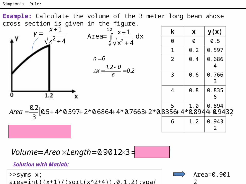
Example: Calculate the volume of the 3 meter long beam whose cross section is given in the figure.

2.06

02.1x

6n

k x y(x)0 0 0.5

1 0.2 0.597

2 0.4 0.6864

3 0.6 0.7663

4 0.8 0.8356

5 1.0 0.8944

6 1.2 0.9432

2.1

02

dx4x

1xArea

9432089440483560276630468640259704503

20..*.*.*.*.*.

.Area

2m9012.0Area

370362390120 m..LengthAreaVolume

>>syms x; area=int((x+1)/(sqrt(x^2+4)),0,1.2);vpa(area,5)

Solution with Matlab:

Area=0.9012

4

12

x

xy

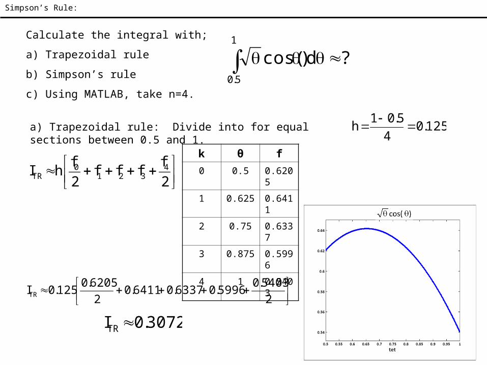
Simpson’s Rule:

Calculate the integral with;

a) Trapezoidal rule

b) Simpson’s rule

c) Using MATLAB, take n=4.

?d)cos(1

5.0

a) Trapezoidal rule: Divide into for equal sections between 0.5 and 1. 125.04

5.01h

2f

fff2f

hI 4321

0TR

k θ f

0 0.5 0.6205

1 0.625 0.6411

2 0.75 0.6337

3 0.875 0.5996

4 1 0.5403

25403.0

5996.06337.06411.02

6205.0125.0ITR

3072.0ITR

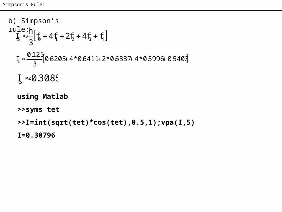
Simpson’s Rule:

43210S ff4f2f4f3h

I

b) Simpson’s rule:

5403.05996.0*46337.0*26411.0*46205.03125.0

IS

3085.0IS

using Matlab

>>syms tet

>>I=int(sqrt(tet)*cos(tet),0.5,1);vpa(I,5)

I=0.30796

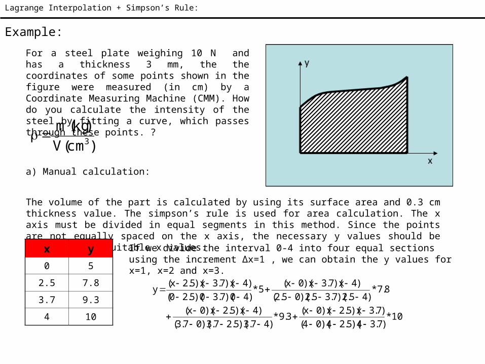
Lagrange Interpolation + Simpson’s Rule:

For a steel plate weighing 10 N and has a thickness 3 mm, the the coordinates of some points shown in the figure were measured (in cm) by a Coordinate Measuring Machine (CMM). How do you calculate the intensity of the steel by fitting a curve, which passes through these points. ?

)cm(V)kg(m3

a) Manual calculation:

The volume of the part is calculated by using its surface area and 0.3 cm thickness value. The simpson’s rule is used for area calculation. The x axis must be divided in equal segments in this method. Since the points are not equally spaced on the x axis, the necessary y values should be calculated at suitable x values.

x y

0 5

2.5 7.8

3.7 9.3

4 10

If we divide the interval 0-4 into four equal sections using the increment ∆x=1 , we can obtain the y values for x=1, x=2 and x=3.

10*)7.34)(5.24)(04()7.3x)(5.2x)(0x(

3.9*)47.3)(5.27.3)(07.3(

)4x)(5.2x)(0x(

8.7*)45.2)(7.35.2)(05.2(

)4x)(7.3x)(0x(5*

)40)(7.30)(5.20()4x)(7.3x)(5.2x(

y

Example:

10*)7.34)(5.24)(04()7.31)(5.21)(01(

3.9*)47.3)(5.27.3)(07.3(

)41)(5.21)(01(

8.7*)45.2)(7.35.2)(05.2(

)41)(7.31)(01(5*

)40)(7.30)(5.20()41)(7.31)(5.21(

)1(y

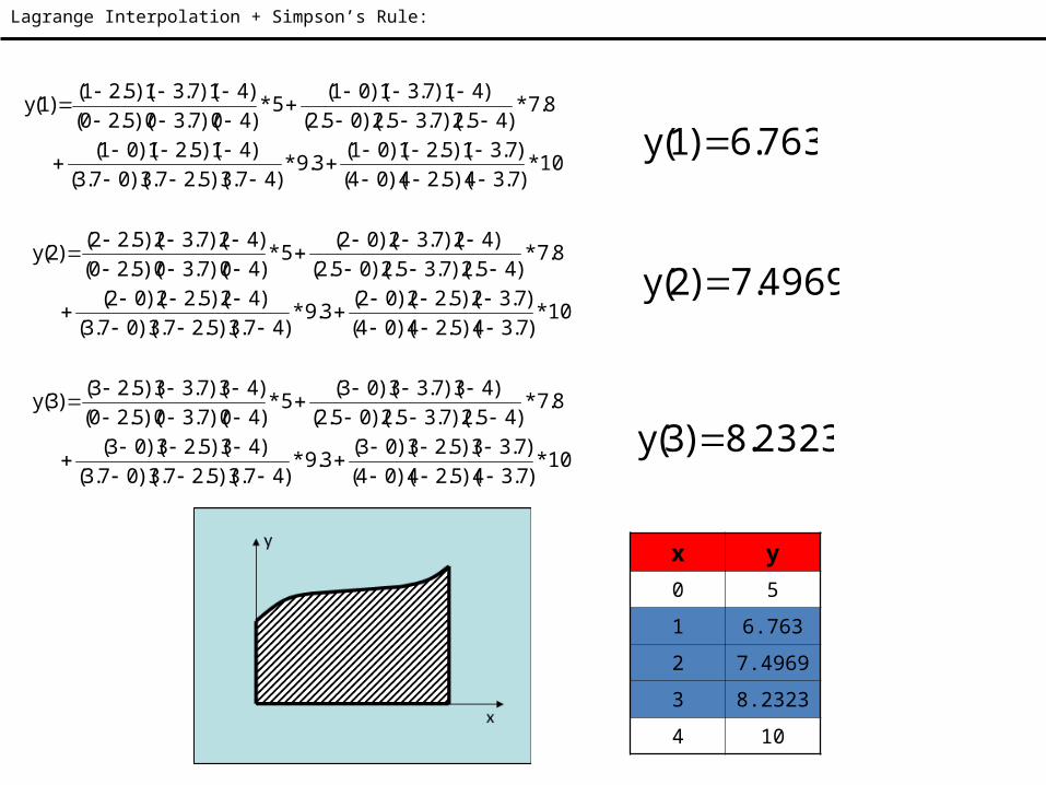
Lagrange Interpolation + Simpson’s Rule:

763.6)1(y

10*)7.34)(5.24)(04()7.32)(5.22)(02(

3.9*)47.3)(5.27.3)(07.3(

)42)(5.22)(02(

8.7*)45.2)(7.35.2)(05.2(

)42)(7.32)(02(5*

)40)(7.30)(5.20()42)(7.32)(5.22(

)2(y

4969.7)2(y

10*)7.34)(5.24)(04()7.33)(5.23)(03(

3.9*)47.3)(5.27.3)(07.3(

)43)(5.23)(03(

8.7*)45.2)(7.35.2)(05.2(

)43)(7.33)(03(5*

)40)(7.30)(5.20()43)(7.33)(5.23(

)3(y

2323.8)3(y

x y

0 5

1 6.763

2 7.4969

3 8.2323

4 10

Lagrange Interpolation + Simpson’s Rule:

b) With computer:

For calculation with computer, MATLAB code is arranged to find the y values for x=1, x=2 and x=3 and the code Lagr.I is run.

The area of the plate can be calculated by using Simpson’s rule. Then, the density of the steel can be calculated as mentioned before.

43210 ff4f2f4f3h

IA

102323.8*44969.7*2763.6*4531

IA 2cm9917.29A 3cm9983.52.0*9917.29t*AV

kg0193.181.9

10m 3cm

kg16994.0

9983.50193.1

Vm

14

04h

clc;clearx=[0 2.5 3.7 4];y=[5 7.8 9.3 10];interp1(x,y,1,'spline')

interp1(x,y,2,'spline')

interp1(x,y,3,'spline')

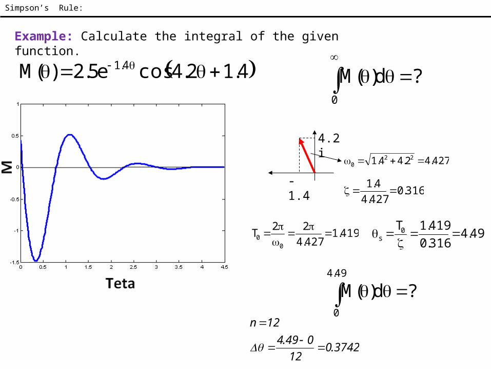
Simpson’s Rule:

4.12.4cose5.2)(M 4.1

0

?d)(M

-1.4

4.2i

427.42.44.1 220

316.0427.4

4.1

49.4316.0419.1T0

s

419.1427.422

T0

0

49.4

0

?d)(M

3742.012

049.4

12n

Example: Calculate the integral of the given function.

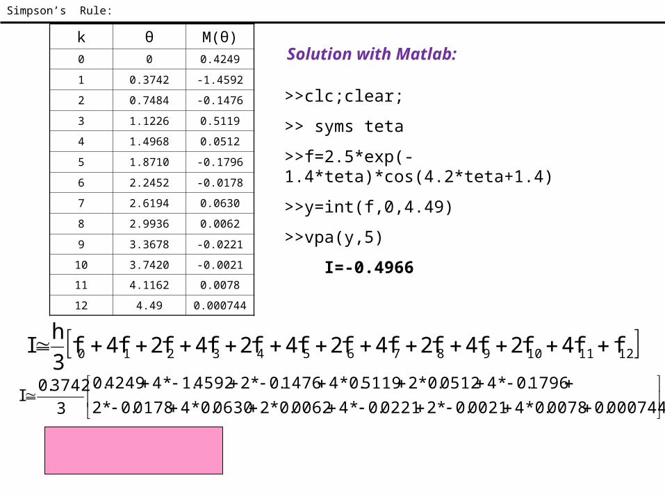
k θ M(θ)0 0 0.4249

1 0.3742 -1.4592

2 0.7484 -0.1476

3 1.1226 0.5119

4 1.4968 0.0512

5 1.8710 -0.1796

6 2.2452 -0.0178

7 2.6194 0.0630

8 2.9936 0.0062

9 3.3678 -0.0221

10 3.7420 -0.0021

11 4.1162 0.0078

12 4.49 0.000744

1211109876543210 ff4f2f4f2f4f2f4f2f4f2f4f3h

I

000744.00078.0*40021.0*20221.0*40062.0*20630.0*40178.0*21796.0*40512.0*25119.0*41476.0*24592.1*44249.0

33742.0

I

5123.0I

Solution with Matlab:

>>clc;clear;

>> syms teta

>>f=2.5*exp(-1.4*teta)*cos(4.2*teta+1.4)

>>y=int(f,0,4.49)

>>vpa(y,5)

I=-0.4966

Simpson’s Rule:

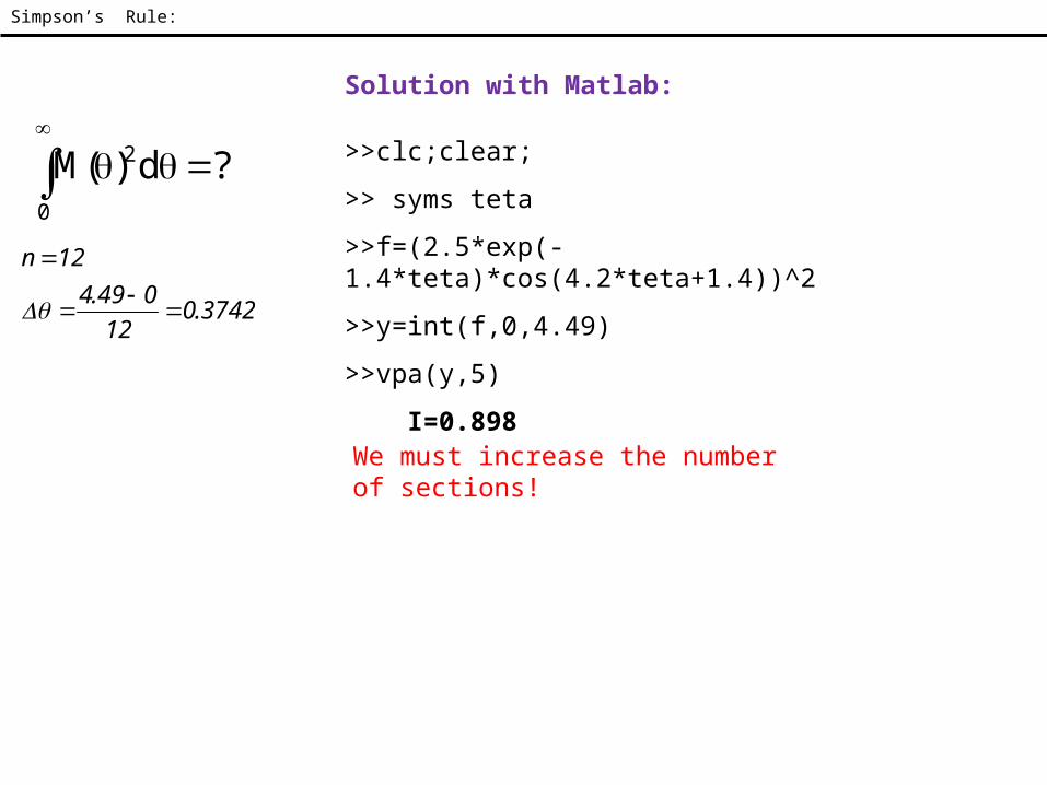
Example:

Simpson’s Rule:

0

2 ?d)(M

3742.012

049.4

12n

k θ M2(θ)

0 0 0.1806

1 0.3742 2.1293

2 0.7484 0.0218

3 1.1226 0.2621

4 1.4968 0.0026

5 1.8710 0.0323

6 2.2452 0.000316

7 2.6194 0.0040

8 2.9936 3.81x10-5

9 3.3678 4.88x10-4

10 3.7420 4.598x10-6

11 4.1162 6.013x10-5

12 4.49 5.541x10-7

75

645

10x541.510x013.6*4

10x59.4*210x88.4*410x81.3*20040.0*4000316.0*2

0323.0*40026.0*22621.0*40218.0*21293.2*41806.0

33742.0

I

2402.1I

4.12.4cose5.2)(M 4.1

Simpson’s Rule:

0

2 ?d)(M

3742.012

049.4

12n

Solution with Matlab:

We must increase the number of sections!

>>clc;clear;

>> syms teta

>>f=(2.5*exp(-1.4*teta)*cos(4.2*teta+1.4))^2

>>y=int(f,0,4.49)

>>vpa(y,5)

I=0.898

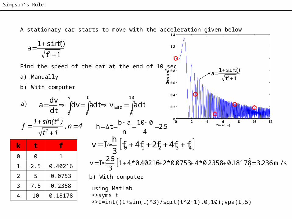
Simpson’s Rule:

A stationary car starts to move with the acceleration given below

1t

)tsin(1a

2

3

Find the speed of the car at the end of 10 seconds

a) Manually

b) With computer

0 2 4 6 8 10 120

0.2

0.4

0.6

0.8

1

1.2

1.4

Zaman (s)

İvm

e m

/s2

a)

10

010t

v

0

t

0

dtavdtadvdtdv

a

1t

)tsin(1a

2

3

5.24

010n

abth

k t f0 0 1

1 2.5 0.40216

2 5 0.0753

3 7.5 0.2358

4 10 0.18178

4n,1t

)tsin(1f

2

3

43210 ff4f2f4f3h

Iv

s/m236.318178.02358.0*40753.0*240216.0*4135.2

Iv

b) With computer

using Matlab>>syms t>>I=int((1+sin(t)^3)/sqrt(t^2+1),0,10);vpa(I,5)

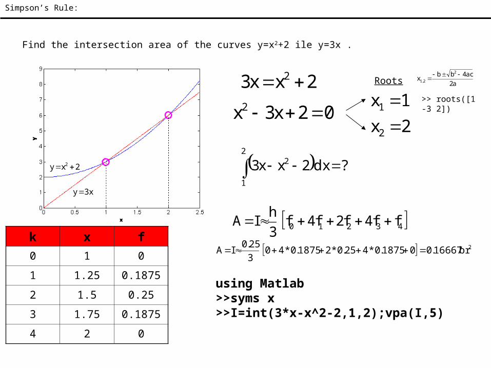
Simpson’s Rule:

Find the intersection area of the curves y=x2+2 ile y=3x .

2xy 2

x3y

2xx3 2

02x3x2

Roots

2x1x

2

1

a2ac4bb

x2

2,1

2

1

2 ?dx2xx3

k x f0 1 0

1 1.25 0.1875

2 1.5 0.25

3 1.75 0.1875

4 2 0

43210 ff4f2f4f3h

IA

2br16667.001875.0*425.0*21875.0*40325.0

IA

using Matlab>>syms x>>I=int(3*x-x^2-2,1,2);vpa(I,5)

>> roots([1 -3 2])

System of linear equations:

05uzwz612w3u9z3w

How do you calculate u,w and z with computer?

5zwu12z6w3

9z3wu

5129

zwu

111630311

5129

111630311

zwu 1

With Matlabclc;cleara=[-1 1 -3;0 3 -6;1 1 1];b=[9;12;5];c=inv(a)*b 3z

10w8u

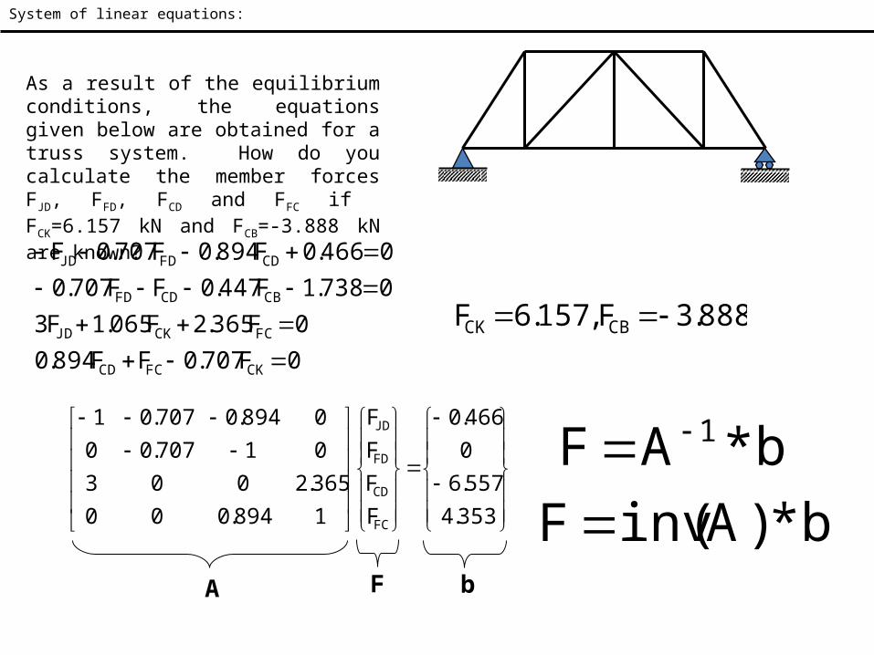
System of linear equations:

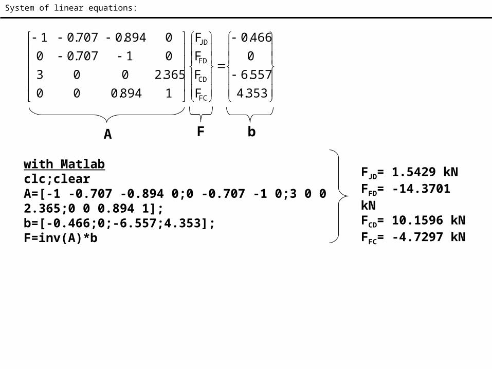
As a result of the equilibrium conditions, the equations given below are obtained for a truss system. How do you calculate the member forces FJD, FFD, FCD and FFC if FCK=6.157 kN and FCB=-3.888 kN are known?

0F707.0FF894.00F365.2F065.1F3

0738.1F447.0FF707.00466.0F894.0F707.0F

CKFCCD

FCCKJD

CBCDFD

CDFDJD

888.3F,157.6F CBCK

353.4557.6

0466.0

FFFF

1894.000365.200301707.000894.0707.01

FC

CD

FD

JD

A bF

b*AF 1b*)A(invF

System of linear equations:

353.4557.6

0466.0

FFFF

1894.000365.200301707.000894.0707.01

FC

CD

FD

JD

A bF

with Matlabclc;clearA=[-1 -0.707 -0.894 0;0 -0.707 -1 0;3 0 0 2.365;0 0 0.894 1];b=[-0.466;0;-6.557;4.353];F=inv(A)*b

FJD= 1.5429 kNFFD= -14.3701 kNFCD= 10.1596 kNFFC= -4.7297 kN