Frequent Closures as a Concise Representation for Binary Data Mining

Frequent Closures as a Concise Representation for Binary Data Mining

Jean-Frangois Boulicaut and Artur Bykowski

Laboratoire d'Ingenierie des Systemes d'Information Institut NationaJ des Sciences Appliquees de Lyon, Batiment 501

F-69621 Villeurbanne cedex, France {Jeem-Fremcois.Boulicaut,Artur.Bykowski}01isi.insa-lyon.fr

Abstract. Frequent set discovery from binary data is an important problem in data mining. It concerns the discovery of a concise repre­sentation of large tables from which descriptive rules can be derived, e.g., the popular association rules. Our work concerns the study of two representations, namely frequent sets and frequent closures. N. Pasquier and colleagues designed the close algorithm that provides frequent sets via the discovery of frequent closures. When one mines highly corre­lated data, apriori-based algorithms clearly fail while close remains tractable. We discuss our implementation of close and the experimental evidence we got from two real-life binary data mining processes. Then, we introduce the concept of almost-closure (generation of every frequent set from frequent almost-closures remains possible but with a bounded error on frequency). To the best of our knowledge, this is a new concept and, here again, we provide some experimental evidence of its add-value.

1 Context and Motivations

One of the obvious hot topics of data mining research in the last five years has been frequent set discovery from binary data. It concerns the discovery of set of attributes from large binary tables such that these attributes are true within a same line often enough. It is then easy to derive rules that describe the data e.g., the popular association rules [2] though the interest of frequent sets goes further [8]. In this paper, we discuss the computation and the use of frequent sets considered as an interesting descriptive representation of binary table for typical rule mining processes.

When looking for a generic statement, it is possible to formulate a data mining task as a query over an intensionally defined collection of patterns [4]. Given a schema R for a database, let ( P R , £, V) denote the pattern domain where VYL is a language of patterns, £ is an evaluation function that defines pattern semantics, and V is a set of result values. Given r, an instance of R, 8 maps each 6 € P R to an element of V. Then, a mining task is the computation of the subset of T'R that fulfil interestingness requirements. This can be formalized as the computation of T/i(r, P R , q) = [6 & VR \ q{T, 9) is true} where predicate q indicates whether a sentence is considered interesting. Typically, this predicate is

T. Terano, H.Liu, and A.L.P. Chen (Eds.); PAKDD 2000, LNAI 1805, pp. 62-73 , 2000. © Springer-Verlag Berlin Heidelberg 2000

Frequent Closures as a Concise Representation for Binary Data Mining 63

A 1 1 1 0 1 0

B 1 0 1 1 1 0

c 1 1 1 1 1 0

D 1 0 1 0 0 0

E 1 0 0 0 0 1

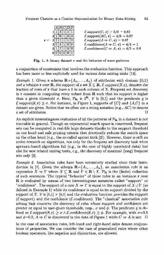
£.support(C, r) = 5/6 = 0.83 £.support(AC, r) = 4/6 = 0.67 f .support(yl => C, r) = 0.67 f .confidence(yl =i> C, r) = 4/4 = 1 f .confidence(C => A, r) = 4/5 = 0.8

Fig. 1. A binary dataset r and the behavior of some patterns

a conjunction of constraints that involves the evaluation function. This approach has been more or less explicitely used for various data mining tasks [13].

Example 1. Given a schema R = { J 4 I , . . . ,.A„} of attributes with domain {0,1} and a relation r over R, the support of a set X C R, ^.support(X,r), denotes the fraction of rows of r that have a 1 in each column of X. FVequent set discovery in r consists in computing every subset from R such that its support is higher than a given threshold a. Here, P R is 2^, V is [0,1] and the predicate q is .S'.support(^, r) > a. For instance, in Figure 1, supports of {C} and {A,C} in a dataset are given. Notice that we often use a string notation (e.g., AC) to denote a set of attributes. D

An explicit interestingness evaluation of all the patterns of P R in a dataset is not tractable in general. Though an exponential search space is concerned, frequent sets can be computed in real-life large datasets thanks to the support threshold on one hand and safe pruning criteria that drastically reduces the search space on the other hand (e.g., the so-called apriori trick [2]). However, there is still an active research on algorithms, not only for the frequent set discovery task when apriori-based algorithms fail (e.g., in the case of highly correlated data) but also for new related mining tasks, e.g., the discovery of maximal (long) frequent sets only [3].

Example 2. Association rules have been extensively studied since their intro­duction in [1]. Given the schema R={yl i , . . . ,yl„}, an association rule is an expression X =^ y where X C R and Y € R \ X. P R is the (finite) collection of such sentences. The typical "behavior" of these rules in an instance r over R is evaluated by means of two interestingness measures called "support" or "confidence". The support of a rule X =^Y is equal to the support oi XUY (as defined in Example 1) while its confidence is equal to its support divided by the support of X. V is [0,1] x [0,1] and the evaluation function provides the support (5.support) and the confidence (£^.confidence). The "classical" association rule mining task concerns the discovery of rules whose support and confidence are greater or equal to user-given thresholds, resp., a and </>. The predicate q is de­fined as £.support(^, v) > a A £.confidence(0, r) > (j>. For example, with a=0.b and (^=0.9, A =^ C is discovered in the data of Figure 1 while C =^ A'ls not. •

In the case of association rules, left-hand and right-hand sides denote conjunc­tions of properties. We can consider the case of generalized rules where other boolean operators, like negation and disjunction, are allowed.

64 J.-F. Boulicaut and A. Bykowski

Example 3. The rule A/\-^E => C is an example of a generalized rule which might be extracted from the data in Figure 1. Its support is 0.5 and its confidence is 1. Mining such rules is very complex and we do not know any efficient strategy to explore the search space for generalized rules. D

As we are interested in very large datasets, an important issue is whether the explicit interestingness evaluation of a collection of patterns remains tractable. The answer can come from the computation of concise representations as defined in [8]. Given a database schema R, a dataset r and a language of patterns V-R., a concise representation for r and 'PR, is a structure that makes possible to answer queries of the form "How many times p € T'R occur in r" approximately correctly and more efficiently than by looking at r itself. By the way, some concise representations might enable to provide exact answers.

This paper deals with two related concise representations of binary data, namely frequent sets and frequent closures. Not only the extraction of these rep­resentations is discussed but we also point out their specific add-value when con­sidered as concise representations for rule mining. Beside well-studied a p r i o r i -based algorithms, we consider the c lose algorithm that provides frequent clo­sures [10]. We implemented it and made experiments over real data. Furthermore, we propose the new concept of almost-do sure and sketch the min-ex algorithm to mine it. The main idea here is to accept a small incertitude on set frequency since, at that cost, more useful mining tasks become tractable.

2 Frequent Sets As a Concise Representat ion of Binciry Data

At first, we adapt the formal definition of [8] to the kind of concise representation we need. Formally, if an evaluation function Q, a member of 0 (the class of evaluation functions), is an application from a class of structures 5={sj | i € / } into the interval [0,1], an e-adequate representation for 5 with respect to O is a class of structures W={ri ] i S / } and an alternative evaluation function m: 0 x W -> [0,1] such that for all Q G ©ands j € 5 we have: ] Q{si)-m{Q,ri) \< e. I denotes a finite (or infinite) index set of S.

Example 4- Let us illustrate the definition on classical concepts from program­ming languages. Assume <S is a class, e.g. float, Sj is an instance of S, e.g. 0.02, and 0 is the set of proper functions on that class, e.g. {sin, cos}. A concise rep­resentation can be the couple {H,m), Ti being another class, e.g. short, and m an alternative way to evaluate Q, e.g. using a table of values of sin and cos for all angles from {0, 1, . . . , 359}. Now, there is an alternative way to compute sin{x) and cos{x). Instead of Si=0.02, we store ri—round{0.02 x 360/27r) mod 360, i.e., 1. When the value of sin(0.02) is needed, we can use Tn{sin, 1) that returns the value stored in the table associated to sin. Clearly, the result is approximate, but the error is bound and the result is known at a much lower cost. •

If the functions from 0 share a lot of intermediate results, and the number of evaluations justifies it, a concise representation can be made of the intermediate

Frequent Closures as a Concise Representation for Binary Data Mining 65

results from which all functions from Q can be evaluated. Such a concise rep­resentation avoids going back to the data. The alternative data representation memory requirement might be smaller as well.

Let us now consider the class S of binary relational schema over the set of attributes R. Instances Si £ S are relational tables. A query Q £ 0 over an instance Si of S, denoted Q{si), is a function whose result is to be found with an alternative (e-adequate) representation. H denotes the alternative class of structures and the counterpart of evaluations, denoted by m, must be a mapping from 0 X H into [0,1]. The error due to the new representation r, of Si (thus compared to the result of Q{si) on the original structure) must be at most e for any instance of Sj.

Example 5. Let r denote a binary relation over R = { A i , . . . , J4„} and consider the set 0={5.support(X, r) | X C R} , where f .support(X, r) is the function that returns the support of X in r (see Example 1). Given a frequency threshold a, let FSa denote the collection of all frequent sets with their supports. Let AltSup{X, FS^) denote the support of a frequent set X. FSa and the function m{£.suppoTt(X,r),FSty) = AltSup{X,FS^) for X e FS„, 0 elsewhere, is a (7-adequate representation for O over the binary relations defined on R. D

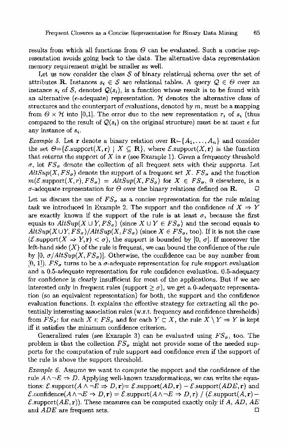
Let us discuss the use of FS^ as a concise representation for the rule mining task we introduced in Example 2. The support and the confidence oi X => Y are exactly known if the support of the rule is at least a, because the first equals to AltSup{X U Y, FS^) (since X UY € FS„) and the second equals to AltSup{XuY,FSa)/AltSup{X,FS<,) (since X e FS^, too). If it is not the case (f .support(X =^ F, r) < cr), the support is bounded by [0, <T]. If moreover the left-hand side (X) of the rule is frequent, we can bound the confidence of the rule by [0, a/AltSup{X,FS„)]. Otherwise, the confidence can be any number from [0, 1]). FS(r turns to be a a-adequate representation for rule support evaluation and a 0.5-adequate representation for rule confidence evaluation. 0.5-adequacy for confidence is clearly insufficient for most of the applications. But if we are interested only in frequent rules (support > cr), we get a 0-adequate representa­tion (so an equivalent representation) for both, the support and the confidence evaluation functions. It explains the effective strategy for extracting all the po­tentially interesting association rules (w.r.t. frequency and confidence thresholds) from FScr'- for each X 6 FS^ and for each F c X, the rule X \Y =^ Y is kept iff it satisfies the minimum confidence criterion.

Generalized rules (see Example 3) can be evaluated using FS,^, too. The problem is that the collection FS„ might not provide some of the needed sup­ports for the computation of rule support and confidence even if the support of the rule is above the support threshold.

Example 6. Assume we want to compute the support and the confidence of the rule AA-IE => D. Applying well-known transformations, we can write the equa­tions: f .support(A A -lE =^ D,r)= f .support(j4D,r) — f .support(AD£^, r) and £.confidence(^A-i£ => £),r) = <f.support(AA-'E ^ D,T) / (£".support(A, r) -£.s\xppovt{AE, r)). These measures can be computed exactly only if A, AD, AE and ADE are frequent sets. •

66 J.-F. Boulicaut and A. Bykowski

If we consider several negations and disjunctions, the number of terms will in­crease and the need for the support of infrequent sets will increase too. Since the computation of the support of all sets is clearly untractable, infrequent con-juncts will give rise to an incertitude [8]. However, this might be acceptable for practical applications. It becomes clear that the adequacy of frequent sets as a concise representation depends on how frequent are the patterns of interest, i.e., the more a pattern is frequent, the less an incertitude will aSect the result.

3 Computing Frequent Sets and Frequent Closures

The a p r i o r i algorithm is defined in [2] and we assume that the reader is familiar with it. It is a levelwise method based on the itemset lattice (i.e., the sets of at­tributes ordered by set inclusion). The algorithm searches in the lattice starting from singletons and identifies level by level larger frequent sets until the maximal frequent sets are found, i.e., the collection of sets that are frequent while none of their supersets is frequent. This collection is denoted by Bd'^{FS,j) and is called the positive border of FS^ [13]. A safe pruning strategy (supersets of infrequent sets can not be frequent) has been shown to be the very efficient for the com­putation of FSa in many real-life datasets. One of the identified drawbacks of apriori-based algorithms is their untractability for highly correlated data min­ing. Data are correlated when the truth value of an attribute or a set of attributes determine the truth value of another one (in other terms, association rules with high confidence hold in it). The problem with correlated data originates from the fact that each rule with high confidence pushes the positive border back by one level for a significant part of the itemset lattice (when a does not change). Highly correlated data contain several such rules, thus pushing back the positive border by several levels. Consequently, the extraction slows down drastically or can even turn to be untractable. An algorithm that would avoid counting sup­port for a great part of frequent sets would accelerate the process. This is the assumption of useful algorithms like max-miner [3] that provides Bd'^{FSa) but not FSa- We will consider hereafter an algorithm that avoids counting support for many frequent sets though it provides -FS'cr, i.e., every frequent set and its support.

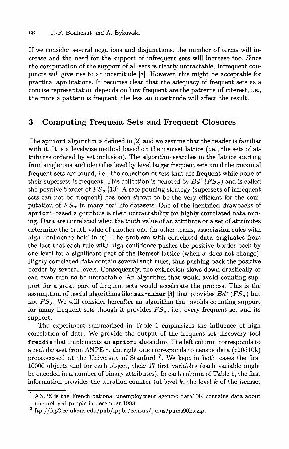
The experiment summarized in Table 1 emphasizes the influence of high correlation of data. We provide the output of the frequent set discovery tool f reddie that implements an a p r i o r i algorithm. The left column corresponds to a real dataset from ANPE ,̂ the right one corresponds to census data (c20dl0k) preprocessed at the University of Stanford ^. We kept in both cases the first 10000 objects and for each object, their 17 first variables (each variable might be encoded in a number of binary attributes). In each column of Table 1, the first information provides the iteration counter (at level k, the level k of the itemset

^ ANPE is the French national unemployment agency: datalOK contains data about unemployed people in december 1998.

^ ftp://ftp2.cc.ukans.edu/pub/ippbr/census/pums/pums90ks.zip.

Frequent Closures as a Concise Representation for Binary Data Mining 67

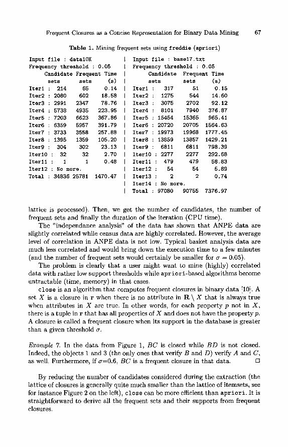
Table 1. Mining frequent sets using f reddie (apriori)

Input i ile : datalOK Frequency threshold 0.05

Candidate Frequent Time

sets

Iterl :

Iter2 :

Iters :

Iter4 :

Iters :

Iters :

Iter7 :

Iters :

Iter9 :

IterlO

Iterll

Iterl2

Total :

214 2080

2991

5738

7203

6359

3733

1395

304 : 32

: 1

sets

65 602

2347

4935

6623

5957

3558

1359

302 32 1

: No more.

34836 25781

(s) 0.14

18.58

78.76

223.95

367.86

391.79

257.88

105.20

23.13

2.70

0.48

1470.47

Input file : basel7.txt

Frequency threshold :

Candidate

sets

Iterl :

Iter2 :

Iter3 :

Iter4 :

Iters :

Iter6 :

Iter7 :

Iter8 :

Iter9 :

IterlO

Iterll

Iterl2

Iterl3

Iterl4

Total :

317 1275

3075

8101

15454

20720

19973

13859

6811

: 2277

: 479

: 54

: 2

0.05

Frequent Time

sets

51 544

2702

7940

15365

20705

19968

13857

6811

2277

479 54 2

: No more.

97080 90755

(s) 0.15

14.60

92.12

376.87

965.41

1564.63

1777.45

1429.21

798.39

292.68

58.83

5.89

0.74

7376.97

lattice is processed). Then, we get the number of candidates, the number of frequent sets and finally the duration of the iteration (CPU time).

The " independance analysis" of the data has shown that ANPE data are slightly correlated while census data are highly correlated. However, the average level of correlation in ANPE data is not low. Typical basket analysis data are much less correlated and would bring down the execution time to a few minutes (and the number of frequent sets would certainly be smaller for a = 0.05).

The problem is clearly that a user might want to mine (highly) correlated data with rather low support thresholds while apriori-based algorithms become untractable (time, memory) in that cases.

c lose is an algorithm that computes frequent closures in binary data [10]. A set X is a closure in r when there is no attribute in R \ .X' that is always true when attributes in X are true. In other words, for each property p not in X, there is a tuple in r that has all properties of X and does not have the property p. A closure is called a frequent closure when its support in the database is greater than a given threshold a.

Example 7. In the data from Figure 1, BC is closed while BD is not closed. Indeed, the objects 1 and 3 (the only ones that verify B and D) verify A and C, as well. Furthermore, if <7=0.6, BC is a frequent closure in that data. •

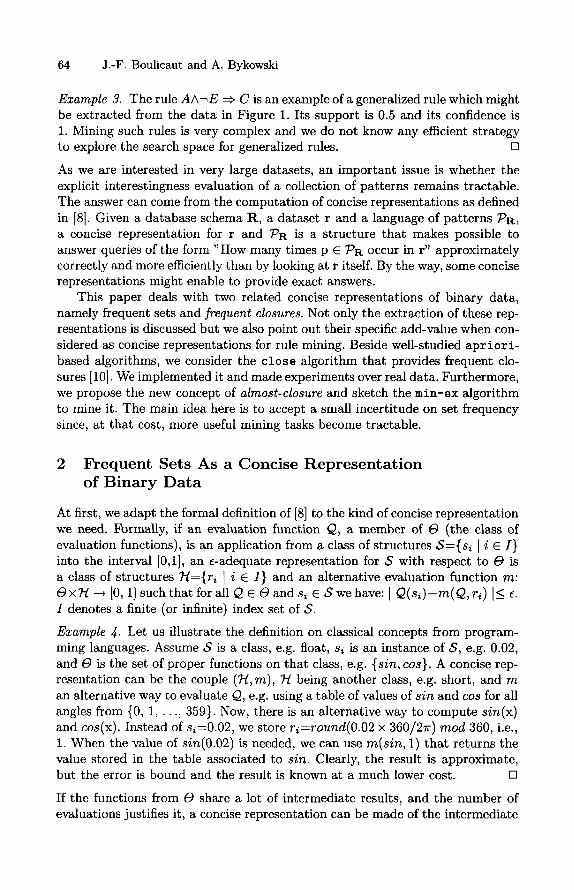
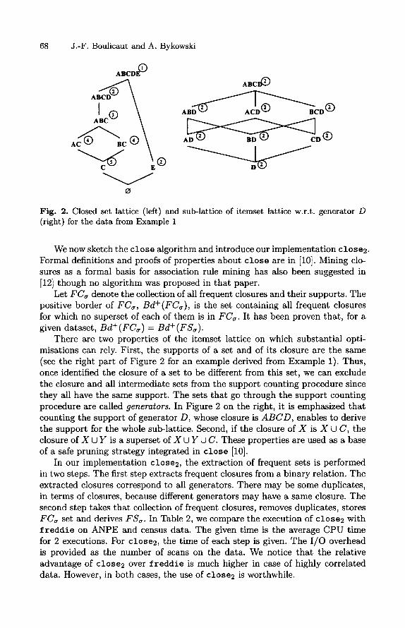
By reducing the number of candidates considered during the extraction (the lattice of closures is generally quite much smaller than the lattice of itemsets, see for instance Figure 2 on the left), c lose can be more efficient than a p r i o r i . It is straightforward to derive all the frequent sets and their supports from frequent closures.

68 J.-F. Boulicaut and A. Bykowski

BCD ©

CD ©

Fig. 2. Closed set lattice (left) and sub-lattice of itemset lattice w.r.t. generator D (right) for the data from Example 1

We now sketch the c lose algorithm and introduce our implementation close2. Formal definitions and proofs of properties about c lose are in [10]. Mining clo­sures as a formal basis for association rule mining has also been suggested in [12] though no algorithm was proposed in that paper.

Let FCa denote the collection of all frequent closures and their supports. The positive border of FCa, Bd^{FC„), is the set containing all frequent closures for which no superset of each of them is in FC„. It has been proven that, for a given dataset, Bd+{FCa) = Bd+{FS<r).

There are two properties of the itemset lattice on which substantial opti­misations can rely. First, the supports of a set and of its closure are the same (see the right part of Figure 2 for an example derived from Example 1). Thus, once identified the closure of a set to be different from this set, we can exclude the closure and all intermediate sets from the support counting procedure since they all have the same support. The sets that go through the support counting procedure are called generators. In Figure 2 on the right, it is emphasized that counting the support of generator D, whose closure is ABCD, enables to derive the support for the whole sub-lattice. Second, if the closure oi X is X U C, the closure of X U y is a superset oi XUYUC. These properties are used as a base of a safe pruning strategy integrated in close [10].

In our implementation close2, the extraction of frequent sets is performed in two steps. The first step extracts frequent closures from a binary relation. The extracted closures correspond to all generators. There may be some duplicates, in terms of closures, because different generators may have a same closure. The second step takes that collection of frequent closures, removes duplicates, stores FCa set and derives FSa- In Table 2, we compare the execution of close2 with f reddie on ANPE and census data. The given time is the average CPU time for 2 executions. For close2, the time of each step is given. The I/O overhead is provided as the number of scans on the data. We notice that the relative advantage of close2 over f reddie is much higher in case of highly correlated data. However, in both cases, the use of close2 is worthwhile.

Frequent Closures as a Concise Representation for Binary Data Mining 69

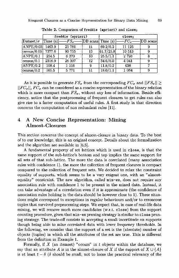
Table 2.

Dataset/cr

ANPE/0.05 census/0.05 ANPE/0.1 census/0.1 ANPE/0.2 census/0.2

Comparison of freddie

freddie (apriori) Time (s)

1463.9 7377.6 254.5

2316.9 108.4 565.5

FS„

25 781 90 755 6 370 26 307 1 516 5 771

DB scans

11 13 10 12 9 11

(apriori 1 and close2

close2 Time (s)

69.2/6.2 61.7/25.8 25.5/1.1 34.6/6.0 11.8/0.2 18.0/1.1

FCa

11 125 10 513 2 798 4 041 638

1 064

DB scans

9 9 8 9 7 9

As it is possible to generate FS^ from the corresponding FC^ and ||F5ff|| > ||FC<j||, FCa can be considered as a concise representation of the binary relation which is more compact than FSa, without any loss of information. Beside effi­ciency, notice that the postprocessing of frequent closures to get rules can also give rise to a faster computation of useful rules. A first study in that direction concerns the computation of non redundant rules [11].

4 A New Concise Representat ion: Mining Almost-Closures

This section concerns the concept of almost-closure in binary data. To the best of to our knowledge, this is an original concept. Details about the formalization and the algorithm are available in [6,5].

A fundamental property of set lattices which is used in c lose , is that the same support of the sub-lattice's bottom and top implies the same support for all sets of that sub-lattice. The more the data is correlated (many association rules with confidence 1), the more the collection of frequent closures is compact compared to the collection of frequent sets. We decided to relax the constraint equality of supports, which seems to be a very exigent one, with an "almost-equality" constraint. The new algorithm, called min-ex, does not require any association rule with confidence 1 to be present in the mined data. Instead, it can take advantage of a correlation even if it is approximate (the confidence of association rules holding in the data should be however close to 1). These situa­tions might correspond to exceptions in regular behaviours and/or to erroneous tuples that survived preprocessing steps. We expect that, in case of real-life data mining, we will remove much more candidates (w.r.t. close) from the support counting procedure, given that min-ex pruning strategy is similar to c lose prun­ing strategy. The trade-off consists in accepting a small incertitude on supports though being able to mine correlated data with lower frequency thresholds. In the following, we consider that the support of a set is the (absolute) number of objects (tuples) in which all the attributes of the set are true. This is different from the definition in Example 1.

Formally, if X (an itemset) "occurs" in t objects within the database, we say that an attribute A is in the almost-closure of X if the support of X U {A} is at least t — 6 {6 should be small, not to loose the practical relevancy of the

70 J.-F. Boulicaut and A. Bykowski

extracted information). The almost-closure of X is the set containing all such attributes. Conceptually, a closure is a special case of an almost-closure when 6=0.

Example 8. In data from Figure 1, considering the generator C, one finds that A and B are in the almost-closure of C for 6=1 while none of them was in its closure. D

Now, let us explain where the incertitude comes from. Assume that the almost-closure of X equals to X U {A,B,C}. Let the support of X be sx , and the supports of X U {A}, X U {B} and X U {C} be respectively sx — SA, SX — SB and Sx — sc where SA, SB and sc are positive numbers lower than 6. We have considered two possibilities for output content. The first stores for each frequent almost-closure: generator items (elements of X, in the example), generator sup­port (sx) and almost-closure's supplement items {A, B and C). The second adds to each item a from the almost-closure supplement the difference of sup­port between X and X U {A} (this difference is called miss-number hereafter). In our example that part corresponds to SA, SB and sc- These values have to be known, because to decide if an item is in the almost-closure, they must be at hand. Miss-numbers are values of miss-counters at the end of the corresponding database pass.

The fact, that, for instance, B and C are in the almost-closure of X only implies that they occur almost always with X. Assume that we are in the second case of output (miss-numbers stored). Prom the supports oi X, X U {B} and X U {C} we can not infer the support of X U {B, C}, because we do not know if the misses occurred on the same objects (support would be sx — Tnax{sA, SB)) or on disjoint ones (support would he sx — SA — SB)- All intermediate cases are allowed, too. Storing miss-numbers greatly improves the precision of the resulting supports, above all when they are small, compared to 6. Therefore, we choose this solution, even if it increases the volume of output (in terms of quantity of information, not in terms of number of elements). FaC^ denotes the collection of all frequent almost-closures for threshold a and is the output of min-ex.

An important property about closures has been preserved. Still, if the almost-closure oi X is X U C, the almost-closure of X U y is a superset of X U y U C. Let us prove it. Attribute A is in the almost-closure of X iff £.support(X, r) — f .support(X U {j4},r) < 6. In other words, the number of objects that have all properties of X and do not have the property A is at most 6. Clearly, the number of objects satisfying a set of properties can not grow if we enforce that property with a new constraint. Therefore, the number of objects that have all properties of X and all properties of Y and do not have the property A can not be greater than 6. So, all elements of the almost-closure of X (i.e. C) must be present in the almost-closure oi X\JY.

This property may be used as a basis of an efficient safe pruning strategy, analogously to the pruning strategy of close. We have been looking for such a strategy. The one implemented in the actual implementation of min-ex seems to be reliable [6]. However, in spite of numerous tries, we did not establish a proof that it is safe. We have not found either a counterexample. We checked the

Frequent Closures as a Concise Representation for Binaxy Data Mining 71

completeness in our practical experiments. However, proving the incompleteness or the completeness of our algorithm remains an open problem though it does not prevent its use for practical applications.

Deriving frequent sets from frequent almost-closures is as straightforward as for close. The difference is that now there is an incertitude on the support of some frequent sets.

The sub-lattices (corresponding to almost-closures) of which the support range, due to S, crosses the threshold is kept in the result set, leading to the collection FaC„ that enables to derive a superset of FS^r- This is a safety mea­sure: we do not want to prune out sub-lattices of which some itemsets are known to be frequent, for the sake of completeness.

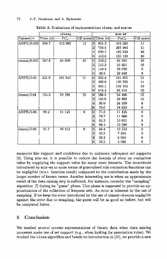
We did several experiments using min-ex on census and ANPE datasets (see Table 3). A first remark is that it confirms that c lose and min-ex with 6=0 are functionally equivalent. In the case of closeg, the reduction of the size of FCa w.r.t. the corresponding FS^ highlights the tight-correlation level (relative number of rules with confidence 1) of the data. In the same way, the further reduction of output ( FaC,r compared to FCa^ ) for different values of 6, points out the loose-correlation level (relative number of association rules that are nearly "logical" ones).

Let us now discuss the add-value of min-ex w.r.t. c lose for highly correlated data mining like census data mining. First of all, we must recall that a too high value of 6 might provide a "fuzzy" FaC„ collection, leading to, e.g., rules with too high incertitude on evaluation functions.

Consider the CPU time needed by the extraction of FaC^. It has been more than halved (census data) for 5=6 and the tested frequency thresholds. Next, the I/O activity (number of database passes) has been reduced, an important criterion if the I/O turns to be a bottleneck of the system. A third advantage is that the output collection size has shrunk and we assume that further subsequent knowledge extraction steps will be faster.

Another way to demonstrate the add-value of min-ex can be derived from Table 3. We can extract the following concise representations of census data: either FCQ.OI with c lose or FaCo.oos with min-ex and 5 = 2. It took the same time (154.3 vs. 155.2 sec, 10 passes for both executions) and we got a similar-sized output collection (52166 vs. 55401 itemsets). It is possible without incerti­tude (FCo.oi) or with a very good precision [5=2) on the frequent set supports {FaCo.oos)- The difference is that, using min-ex, we gained knowledge about all phenomena of frequency between 0.5% and 1% at almost no price. However, we must notice that in case of uncorrelated data, the memory consumption and CPU load due to maintaining miss-counters may affect the performances (See in Table 3 the extraction time evolution for ANPE/cr=:0.05). Only, with a signifi­cant reduction of number of candidates (thus only in case of correlated data), the memory consumption will recover (e.g., see A N P E / C T = 0 . 0 0 5 or census/o-=0.05).

Applications. A promising application of min-ex would be to enable the discov­ery of repetitive but scarce behaviours. Another application concerns generalized rule mining. Generalized rules, if generated from FS„, have an incertitude on

72 J.-F. Boulicaut and A. Bykowski

Table 3. Evaluations of implementations close2 and min-ex

Dataset/(7

ANPE/0.005

census/0.005

ANPE/0.01

census/0.01

ANPE/0.05

census/0.05

close2 Time (s)

816.7

197.8

421.8

154.3

69.2

61.7

FC^

412 092

85 950

161 855

52 166

11 125

10 513

DB scans

11

10

11

10

9

9

min-ex 5

0 2 4 6 0 2 4 6 0 2 4 6 0 2 4 6 0 2 4 6 0 2 4 6

Time (s)

851.3 759.5 639.7 553.0 216.2 155.2 118.4 98.5

450.4 466.8 445.1 416.4 166.2 124.9 95.0 79.0 71.5 79.7 85.3 88.4 64.4 50.2 38.2 32.2

FaC„

412 092 265 964 182 829 135 136 85 950 55 401 39 036 29 848 161 855 130 765 104 162 84 318 52 166 33 992 24 109 18 822 11 125 11 066 10 931 10 588 10 513 7 294 5 090 4 086

DB scans

11 11 10 10 10 10 8 8 11 11 10 10 10 10 8 8 9 9 9 9 9 9 8 8

measures like support and confidence due to unknown infrequent set supports [8]. Using min-ex, it is possible to reduce the bounds of error on evaluation value by supplying the support value for many more itemsets. The incertitude introduced by min-ex to some terms of generalized rule evaluation functions can be negligible (w.r.t. function result) compared to the contribution made by the larger number of known terms. Another interesting use is when an approximate result of the data mining step is sufficient. For instance, consider the "sampling" algorithm [7] during its "guess" phase. This phase is supposed to provide an ap­proximation of the collection of frequent sets. An error is inherent to the use of sampling. If we keep the error introduced by the use of almost-closures negligible against the error due to sampling, the guess will be as good as before, but will be computed faster.

5 Conclusion

We studied several concise representations of binary data when data mining processes make use of set support (e.g., when looking for association rules). We studied the close algorithm and beside its introduction in [10], we provide a new

Frequent Closures as a Concise Representation for Binary Data Mining 73

implementation and experimental evidences about its add-value for the concise representation of (highly) correlated data . It has lead us to the definition of the concept of almost-closure and, here again, we provided experimental evidences of its interest when we are looking for concise representation in difficult cases (correlated da ta and low frequency thresholds). The discovery of almost-closed frequent sets gave rise to tricky problems w.r.t. the completeness of the mining task. Completeness of min-ex remains an open problem at tha t t ime and we are currently working on it.

A c k n o w l e d g e m e n t s . The authors thank H. Toivonen from the University of Helsinki for letting us use the f r e d d i e software tool and the Rhone depar tmenta l direction of A N P E who provided data . Last but not least, we want to thank C. Rigotti for stimulating discussions.

References

1. R. Agrawal, T. Imielinski, and A. Swami. Mining association rules between sets of items in large databases. In: Proc. SIGMOD'93, Washington DC (USA), pages 207 - 216, May 1993, ACM Press.

2. R. Agrawal, H. Mannila, R. Srikant, H. Toivonen, and A. I. Verkamo. Fast discovery of association rules. In: Advances in Knowledge Discovery and Data Mining, pages 307 - 328, 1996, AAAI Press.

3. R.J. Bayardo. Efficiently mining of long patterns from databases. In: Proc. SIG-MOD'98, Seattle (USA), pages 85 - 93, June 1998, ACM Press.

4. J-F. Boulicaut, M. Klemettinen, and H. Mannila. Modeling KDD processes within the Inductive Database Framework. In: Proc. DaWak'99, Florence (I), pages 293 -302, September 1999, Springer-Verlag, LNCS 1676.

5. J-F. Boulicaut, A. Bykowski, and C. Rigotti. Mining almost-closures in highly correlated data. Research Report LISI INSA Lyon, 2000, 20 pages.

6. A. Bykowski. Frequent set discovery in highly correlated data. Master of Science thesis, INSA Lyon, July 1999, 30 pages.

7. H. Toivonen. Sampling large databases for association rules. In: Proc. VLDB'96, Mumbay (India), pages 134 - 145, September 1996, Morgan Kaufmann.

8. H. Mannila and H. Toivonen. Multiple uses of frequent sets and condensed rep­resentations. In; Proc. KDD'96, Portland (USA), pages 189 - 194, August 1996, AAAI Press.

9. H. Mannila. Inductive databases and condensed representations for data mining. In: Proc. ILPS'97, Port Jefferson, Long Island N.Y. (USA), pages 21 - 30, October 1997, MIT Press.

10. N. Pasquier, Y. Bastide, R. Taouil, and L. Lakhal. Efficient mining of association rules using closed itemset lattices. Information Systems, Volume 24 (1), pages 25 - 46, 1999.

11. N. Pasquier, Y. Bastide, R. Taouil, and L. Lakhal. Closed set discovery of small covers for association rules. In: Proc. BDA'99, Bordeaux (F), pages 53 - 68, October 1999.

12. M. Zaki and M. Ogihara. Theoretical foundations of association rules. In: Proc. Workshop post-SIGMOD DMKD'98, Seattle (USA), pages 85 - 93, June 1998.

13. H. Mannila and H. Toivonen. Levelwise search and borders of theories in knowledge discovery. Data Mining and Knowledge Discovery, 1(3):241 - 258, 1997.