Frequent closed itemset based algorithms: a thorough structural and analytical survey

Frequent closed itemset based algorithms: A thoroughstructural and analytical survey

S. Ben YahiaFaculte des Sciences de Tunis

Campus Universitaire1060, Tunis, Tunisie

[email protected]

T. HamrouniFaculte des Sciences de Tunis

Campus Universitaire1060, Tunis, Tunisie

[email protected]

E. Mephu NguifoCRIL-CNRS, IUT de LensRue de l’Universite SP 16

62307 Lens Cedex, [email protected]

ABSTRACTAs a side effect of the digitalization of unprecedented amountof data, traditional retrieval tools proved to be unable to ex-tract hidden and valuable knowledge. Data Mining, with aclear promise to provide adequate tools and/or techniquesto do so, is the discovery of hidden information that can beretrieved from datasets. In this paper, we present a struc-tural and analytical survey of frequent closed itemset (FCI)based algorithms for mining association rules. Indeed, weprovide a structural classification, in four categories, and acomparison of these algorithms based on criteria that weintroduce. We also present an analytical comparison ofFCI-based algorithms using benchmark dense and sparsedatasets as well as ”worst case” datasets. Aiming to standbeyond classical performance analysis, we intend to providea focal point on performance analysis based on memory con-sumption and advantages and/or limitations of optimizationstrategies, used in the FCI-based algorithms.

1. INTRODUCTIONThe survival of the association rule extraction technique isowed to the retrieval of compactly sized with added-valueknowledge. In this respect, the last decade witnessed aparticular interest in the definition of condensed represen-tations, e.g., closed itemsets [31], free itemsets [6], non-derivable itemsets [7], essential itemsets [9], etc. The def-inition of these condensed representations mainly relies onthe inclusion-exclusion principle and Bonferroni inequali-ties, which were of extensive use in addressing many enu-meration problems [14].

The study of the extraction of closed itemsets grasped theinterest of the data mining community. Indeed, frequentclosed itemset (FCI) based algorithms were introduced tomainly tackle two complementary problems. On the onehand, FCI-based algorithms present an effective mining ap-proach for dense extraction contexts. In such contexts, largeequivalence classes are obtained. FCIs, standing on the topof the hierarchy induced by each equivalence class, allow toinformatively infer the supports of FIs, standing within thefrequent minimal generators (FMGs) and their associatedFCIs. Note that the FMGs correspond to the frequent 0-free itemsets [6] and to the frequent key patterns [35].Unfortunately, typically sparse contexts represent a ”night-mare” for FCI-based algorithms, which have to bear useless

and costly closure computations. The low performances onsparse contexts are quite expected, since the FCI searchspace tends to overlap with that of FIs.

On the other hand, FCI-based algorithms, which heavilydraw on Formal Concept Analysis (FCA) mathematical set-tings [40], present a novel alternative with a clear promiseto dramatically reduce, without information loss, the size ofthe association rule set that can be drawn from both syn-thetic and real-life datasets. The result of such a reductionis a reasonably-sized subset of association rules that can beseen as an irreducible nucleus of association rules, commonlyknown as ”generic basis” of association rules [30].

In this paper, we present a structural and analytical com-parative study of FCI-based algorithms. Hence, we clas-sify FCI-based algorithms into four disjoint categories. Wethen introduce some features (or dimensions) allowing tohighlight the major differences between the most prominentFCI-based algorithms for mining association rules (currentand future). Performances of these algorithms are assessedand compared on benchmark dense and space datasets aswell as ”worst case” datasets [18]. Interestingly enough, theproposed analytical comparison goes beyond those respec-tively proposed by Zheng et al. [43; 44], in which only sparsedatasets were of interest, and Goethals and Zaki [16], whereonly performance curves are showed. Indeed, we try notonly to show performance curves, but also to explain theseperformances based on advantages and/or limitations of op-timization strategies used in these algorithms. To obtain anin-depth insight, we also assess the memory consumption ofthe surveyed algorithms in conjunction with the evolution ofgathered information, in main memory, during the miningprocess.

It is important to mention that in this survey, we put the fo-cus on FCI-based algorithms especially designed for datasetshaving much more transactions than items. Nevertheless,some recent algorithms are dedicated to other kind of datasetslike the COFI-Closed algorithm [11] for mining extremelylarge datasets (having millions of transactions) and the Car-penter [28] and Farmer [10] algorithms for mining genomicdatasets (having much more items than transactions).

We think that this survey can be regarded as complemen-tary to some existing ones. For example, for FI-based algo-rithms, we can cite the survey of Hipp et al. [20], that ofAggarwal [1] for maximal FI-based algorithms and that ofKuznetsov and Ob”edkov [22] for concept lattice algorithms.As the FCI representation is concise w.r.t. that of FIs, thissurvey is also closely related to that of Calders et al. [8] in

Page 93Volume 8, Issue 1SIGKDD Explorations

which the authors give a general overview about differentconcise representations (like closed itemsets, free itemsets,non-derivable itemsets, etc).

The remainder of the paper is organized as follows: sec-tion 2 presents basic definitions of the FCA mathematicalsettings. Section 3 sketches a critical classification and acomparison of FCI-based algorithms thanks to criteria thatwe introduce. Section 4 reports an analytical comparisonof FCI-based algorithms on benchmark and ”worst case”datasets. Section 5 concludes this paper and points out fu-ture perspectives.

2. BASIC DEFINITIONSIn this section, we present basic definitions that will be ofuse in the remainder.

Definition 1. (Formal context) A formal context (oran extraction context) is a triplet K = (O, I,R), where Orepresents a finite set of objects (or transactions), I is a finiteset of items (or attributes) and R is a binary (incidence)relation (i.e., R ⊆ O × I). Each couple (o, i) ∈ R expressesthat the object o ∈ O contains the item i ∈ I.

The closure operator γ induces an equivalence relation onthe power set of items portioning it into disjoint subsetscalled equivalence classes. The largest element (w.r.t. thenumber of items) in each equivalence class is called a closed

itemset and is defined as follows:

Definition 2. (Closed Itemset) An itemset I ⊆ I is saidto be closed if and only if γ(I) = I [31]. The support of I,denoted by Supp(I), is equal to the number of objects inK that contain I. I is said to be frequent if Supp(I) isgreater than or equal to a user-specified minimum supportthreshold, denoted minsup. The frequency of I in K is equal

to Supp(I)|O|

.

Definition 3. (Iceberg Galois lattice) Let FCIK bethe set of the FCIs extracted from an extraction context K.When the set FCIK is partially ordered with set inclusion,the resulting structure (L, ⊆) only preserves the Join oper-ator [15]. This structure is called a join semi-lattice or anupper semi-lattice and is, hereafter, referred to as ”IcebergGalois lattice” [27; 35].

Definition 4. (Upper cover) The upper cover of an FCIf (denoted Covu(f)) consists of the FCIs that immediatelycover f in the Iceberg Galois lattice. The set Covu(f) isgiven as follows: Covu(f) = {f1 | f1 ∈ FCIK and f ⊂ f1and @ f2 ∈ FCIK s.t. f ⊂ f2 ⊂ f1}.

Definition 5. (Minimal Generator) An itemset g ⊆ Iis said to be a minimal generator of a closed itemset f , if andonly if γ(g) = f and @ g

1⊂ g s.t. γ(g

1) = f [3]. Thus, the

set MGf of the minimal generators associated to a closeditemset f is: MGf = {g ⊆ I | γ(g) = f and @ g

1⊂ g s.t.

γ(g1) = f}.

Therefore, the problem of mining association rules mightbe reformulated, under the point of view of the FCI-basedalgorithms, as follows:

1. Discover both distinct ”closure systems”, i.e., sets ofsets which are closed under the intersection operator,namely the FCI set and the FMG set. Also, the uppercover of each FCI should be available.

2. From the information discovered in the first step, i.e.,both closure systems and the upper covers, derive genericbases of association rules (from which all remainingrules can be derived).

In the next section, we present a structural survey of FCI-based algorithms.

3. FCI-BASED ALGORITHMSIn this section, we start by introducing a classification ofthese algorithms after which we give their main characteris-tics.

3.1 FCI-based algorithm classificationIn general, the criterion used to classify FCI-based algo-rithms is inherited from the FI mining stuff, i.e., the tech-nique used to traverse the search space. Nevertheless, weadd a supplementary category that we call ”Hybrid withoutduplication” and this for different reasons explained here-after. Hence, FCI-based algorithms can be roughly splitinto four categories, namely ”Test-and-generate”, ”Divide-and-conquer”, ”Hybrid” and ”Hybrid without duplication”.

1. First category: ”Test-and-generate” technique: Themost known algorithms which adopt this technique areClose [31], A-Close [32] and Titanic [35]. Thesealgorithms stress on the optimization of a level-wiseprocess for the discovery of both closure systems pre-viously mentioned. As a starting point, they considerthe already known meet-irreducible set, i.e., items ofthe ground set I. This set is further extended by self-joined compound elements – using the combinatorialphase of Apriori-Gen [2] – during the explorationprocess. Candidate sets are pruned using the conjunc-tion of statistical metrics (e.g., the support measure)and heuristics essentially based on structural proper-ties of CIs and MGs (e.g., the fact that the MG set isan order ideal (or down-set) of (2I , ⊆) [35]).

2. Second category: ”Divide-and-conquer” technique:The most known algorithm which adopts this tech-nique is Closet [33]. The latter introduced the use ofthe highly compact data structure FP-tree (Frequent-Pattern tree) [19] within the FCI discovery process.Using a depth-first traversal of the search space, Closettries to split the extraction context, stored in a globalFP-tree, into smaller sub-contexts and to recursivelyapply the FCI mining process on these sub-contexts.The mining process also heavily relies on the searchspace pruning. This pruning is also based on statisti-cal metrics in conjunction with introduced heuristics.Some improvements or alternatives of this algorithmwere proposed, mainly Closet+ [39] and FP-Close[17], while respecting its driving idea.

3. Third category: ”Hybrid” technique: Algorithmsadopting this technique use properties of both previ-ously mentioned techniques. ChARM [42] algorithm isthe most known. Unlike other methods which exploitonly the (closed) itemset search space, ChARM simul-taneously explores both the CI search space and thatof transactions thanks to an introduced data structurecalled IT-tree (Itemset-Tidset tree) [42]. Each nodein the IT-tree contains an FCI candidate and the list

Page 94Volume 8, Issue 1SIGKDD Explorations

of the transactions to which it belongs. This list iscalled tidset [42]. ChARM explores the search spacein a depth-first manner, like algorithms of the ”Divide-and-conquer” technique, without splitting the extrac-tion context into smaller sub-contexts. However, itgenerates each time a single candidate, like algorithmsof the ”Test-and-generate” technique. Then, it tries totest whether it is an FCI or not, using tidset intersec-tions and subsumption checking. The mining processalso heavily draws on the search space pruning. Thispruning is based on imposed statistical metrics in con-junction with introduced heuristics.

4. Fourth category: ”Hybrid without duplication”

technique: Two main algorithms were proposed adopt-ing this technique, namely DCI-Closed [25; 26] andLCM [36; 37]. Both algorithms can only be consideredas improvements of ChARM as they inherit the use oftidsets (1) and the hybrid traverse of the search spaceadopted in ChARM. However, we choose to classifythese two algorithms in a new category. Indeed, theyavoid the main drawback of previously proposed algo-rithms, namely the high cost of subsumption checkingallowing to discard generators whose closures were al-ready mined (case of the second and the third category(2)). To this end, DCI-Closed and LCM traverse thesearch space in a depth-first manner. After discov-ering an FCI f , they generate a new generator g byextending f with a frequent item i, i /∈ f . Using atotal order relation on frequent items, DCI-Closedand LCM verify if g infringes this order by perform-ing tests using only the tidset of f and those of thefrequent items. If g is not discarded, then g is anorder preserving generator of a new FCI. Then, itsclosure is computed using the previously mentionedtidsets. Hence, both algorithms extract the set of theFCIs in a linear time of its size [25; 36]. In addition,these algorithms do not need to store, in main mem-ory, the set containing the previously mined FCIs sincethey do not require performing subsumption checking.The differences between DCI-closed and LCM arethe strategies for taking closure and the adopted datastructures for storing the extraction context in mainmemory.

3.2 FCI-based algorithm characteristicsBased on the reformulation of the mining problem from thepoint of view of the FCI-based approach and its promises tolosslessly reduce in size the association rule set, we presentin what follows some features (or dimensions) allowing: onthe one hand, to assess the percentage of achievement ofsuch promised goals and on the other hand, to highlightthe major differences between the FCI-based algorithms formining association rules (current and future).

1. Exploration technique: three techniques are usedto explore the search space, namely ”Test-and-generate”,”Divide-and-conquer” and ”Hybrid”.

2. Architecture: the architecture dimension depends onhow a given algorithm is designed: a sequential func-

1Called tidlists in [25; 26] and denotations in [36; 37].2In the case of the first category, an FCI can be computedmore than once.

tion in a centralized single processor architecture, ormore suited to a parallel treatment in a multiproces-sor or distributed architecture, e.g., Closet and DCI-Closed;

3. Parallelism strategy: parallel algorithms can be fur-ther described as task, data or hybrid parallelism;

4. Data source type: this feature indicates the type ofthe input data: (extended) market basket data (alsoknown as horizontal data), vertical data, relationaldata, plain text, multimedia data, etc;

5. Information storage: different data structures areused to keep track of the information required to analgorithm execution (to store candidates, the extrac-tion context, etc). The most privileged structure seemsto be the trie structure.

6. Generator choice: some algorithms chose FMGs asgenerators of each FCI. Hence, closure computationsare performed after discovering either the whole FMGset or only a subset of it (e.g., FMGs having a commonsize). Other algorithms adopt a technique based on thefact that each time that a frequent generator is found,its closure is computed. This makes possible to createnew frequent generator candidates starting from thealready found FCI [25].

7. Closure computation: the closure of an itemset Xcan be computed thanks to the following two differ-ent methods. In the first method, the closure of Xis the result of the intersection of the transactions towhich it belongs. In the second method, its closure iscomputed in an incremental manner by searching foritems that verify the following property (3): ψ(X) ⊆ψ(i) ⇒ i ∈ γ(X), such that i ∈ I and i /∈ X [35]. Theclosure computation can also be performed on-line oroff-line. In the former case, each time that a subsetof the whole (minimal) generator set is found, the clo-sure of each element of this subset is calculated. Inthe latter case, the closure computation of the whole(minimal) generator set is done at the same step [25].

8. Possibility of redundant closure computation:Since an FCI can have more than one generator, thesame closure can be computed more than once unlesssome tests are performed. This dimension indicateswhether a redundant closure computation is possible.Otherwise, it shows how this redundant computationis avoided.

9. Output type: here we focus on the type of the de-rived association rules: e.g., boolean, fuzzy, spatial,temporal, generalized, qualitative, etc;

10. Generated output: this feature indicates the knowl-edge extracted by a given algorithm. The value ”genericARs” means that only a lossless and non-redundantsubset of association rules is derived. Whereas, thevalue ”redundant ARs” indicates that all (redundant)association rules can be derived from the generatedoutput.

3ψ(X) indicates the tidset of the itemset X.

Page 95Volume 8, Issue 1SIGKDD Explorations

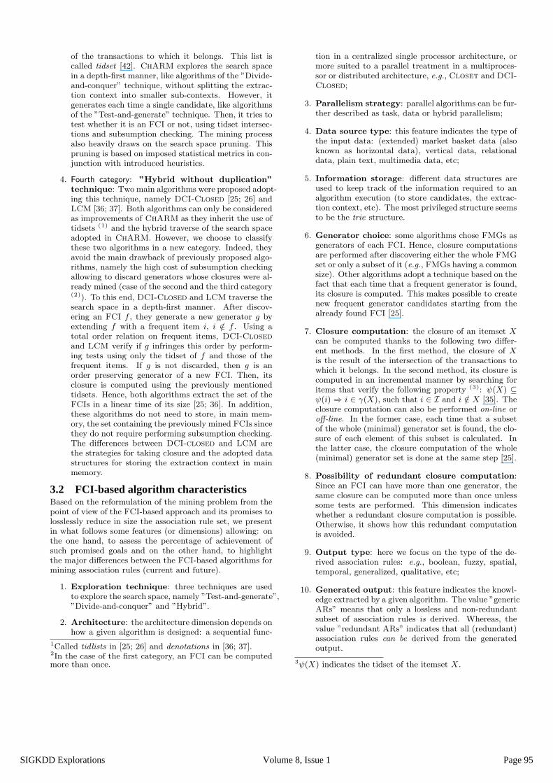
Features First category Second category Third category Fourth categoryArchitecture sequential parallel sequential parallelParallelism strategy none none none noneExploration technique Test-and-generate Divide-and-conquer Hybrid HybridData source type horizontal horizontal horizontal, vertical horizontal, verticalInformation storage trie trie trie bitmap matrix (DCI-

Closed), simple arrays(LCM)

Generator choice minimal generators generators generators generatorsClosure computation intersection operation,

on-line for both Closeand Titanic and off-linefor A-Close

incremental search andon-line

incremental search andon-line

incremental search andon-line

Possibility of redundantclosure computation

yes no, using subsumptionchecking

no, using subsumptionchecking

no, using order preserv-ing tests

Output type boolean boolean boolean booleanGenerated output the FCIs, their associ-

ated FMGs and the re-dundant ARs

the FCIs and the redun-dant ARs

the FCIs and the redun-dant ARs

the FCIs and the redun-dant ARs

Most known algo-rithms

Close, A-Close andTitanic

Closet, Closet+ andFP-Close

ChARM DCI-Closed and LCM

Table 1: Characteristics of the four categories.

Table 1 summarizes a categorization of the FCI-based al-gorithms w.r.t. the previously described basic dimensions.The last but one entry in Table 1 sheds light on the factthat, unfortunately, none of the reported algorithms is ableto fulfill the problem reformulation goals, mentioned in theprevious section. The origin of this failure is due to the factof neglecting the importance – especially from a data min-ing frenzy towards performances – of maintaining the ordercovering the relationship between the FCIs. This is quiteexpected since the aforementioned algorithms avoid bear-ing a costly precedence-order construction fee. Hence, nomore than the generic basis of exact association rules canbe straightforwardly derived. To be able to extract approx-imate generic association rules, they need to be associatedwith another appropriate algorithm allowing to build theIceberg Galois lattice, e.g., that proposed by Valtchev et

al. [38].

By comparing the main FCI-based algorithms, we can alsonote the following remarks:

• Among the previously mentioned algorithms, only Ti-tanic, DCI-Closed and LCM consider the equiva-lence class whose the associated FMG is the emptyset. Thus, all remaining algorithms need to performan additional treatment to compute the empty set clo-sure.

• Pruning strategies adopted by Titanic are an improve-ment of those of A-Close by avoiding the cost of ”un-necessary” traversals of previously extracted FMGsthanks to the estimated support pruning strategy, aswill be explained later in the next section. Those ofCloset and ChARM (resp. DCI-Closed and LCM)can also be considered as the same.

• The main weakness of the Close, A-Close and Ti-tanic algorithms is the redundant computation of thesame FCI if this latter has more than one FMG. Thisproblem is avoided by the Closet and ChARM al-gorithms using subsumption checking. Unfortunately,to speed up subsumption checking, both algorithmsare obliged to maintain the retained FCIs in main

memory. The DCI-Closed and LCM algorithms aremainly dedicated to tackle this problem. Thus, theytry to extract the set of the FCIs without duplicategeneration (hence in a linear time) and without main-taining it in main memory, using astute duplicate de-tection strategies.

It is important to note that, for all considered FCI-based al-gorithms, a suitable buffer management scheme is missing.Indeed, this scheme is required to handle this problem when-ever necessary since generating a huge number of candidatesets might cause the memory buffer to overflow. To handlethis issue, the candidate generation step should be modifiedin order to consider that a portion of the required (gener-ated) information may be disk resident (saved on disk). Inthis case, we may need to perform an external sort as donein [34].

4. EXPERIMENTAL COMPARISONIn this section, we give an analytical survey of the FCI-based algorithms considered in the previous section. Ex-periments were carried out on a Pentium IV with a CPUclock rate of 2.4 GHz and 512 MB of main memory (with2 GB of swap space). To rate the different behaviors of theconsidered algorithms, we ran experiments on both bench-mark and ”worst case” datasets, whose characteristics aredetailed in what follows. The Close, A-Close, Titanic,ChARM (with ‘-h -e 1 -d -H 1‘ options), FP-Close, DCI-Closed and LCM ver. 2 algorithms were tested on theLinux distribution S.u.s.e 9.0, and their original makefileversions were compiled using gcc 3.3.1. Since Closet+ (4)

was provided as a Windows executable, it was comparedunder Windows XP Professional on the same experimentalenvironment. The source codes of the Close, A-Close, Ti-tanic, FP-Close, ChARM, DCI-Closed and LCM algo-rithms and the Closet+ Windows binary executable werekindly provided by their respective authors.

4Since in [39], Closet+ performances already proved tobe definitely better than those of Closet, we did not useCloset in the tests.

Page 96Volume 8, Issue 1SIGKDD Explorations

To report our results, we use runtime, i.e., the period be-tween input and output, instead of using the CPU time mea-sured in some literature (e.g., [17; 37]). The memory con-sumption is measured using the GNU glibc tool memusage,considering only the maximum heap size since stack use ismuch smaller than heap size. To make the measurementsmore reliable, no other application was running on the ma-chine while experiments were running and none of the dif-ferent executables displays the list of the discovered FCIson the screen, nor writes it down on a disk-resident file.

4.1 Test dataset descriptionAlgorithms were tested on two types of datasets: benchmarkand ”worst case”. A ”worst case” context is introducedthanks to the following definition:

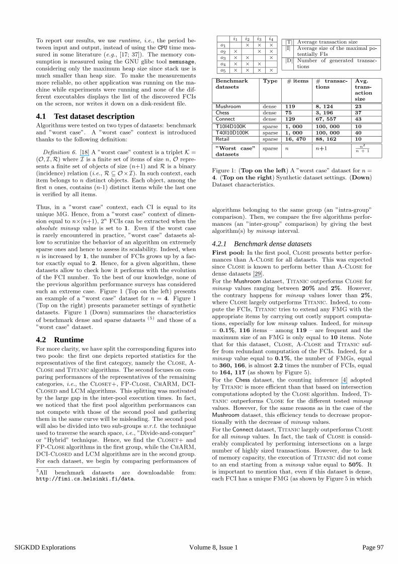
Definition 6. [18] A ”worst case” context is a triplet K =(O, I,R) where I is a finite set of items of size n, O repre-sents a finite set of objects of size (n+1) and R is a binary(incidence) relation (i.e., R ⊆ O×I). In such context, eachitem belongs to n distinct objects. Each object, among thefirst n ones, contains (n-1) distinct items while the last oneis verified by all items.

Thus, in a ”worst case” context, each CI is equal to itsunique MG. Hence, from a ”worst case” context of dimen-sion equal to n×(n+1), 2n FCIs can be extracted when theabsolute minsup value is set to 1. Even if the worst caseis rarely encountered in practice, ”worst case” datasets al-low to scrutinize the behavior of an algorithm on extremelysparse ones and hence to assess its scalability. Indeed, whenn is increased by 1, the number of FCIs grows up by a fac-tor exactly equal to 2. Hence, for a given algorithm, thesedatasets allow to check how it performs with the evolutionof the FCI number. To the best of our knowledge, none ofthe previous algorithm performance surveys has consideredsuch an extreme case. Figure 1 (Top on the left) presentsan example of a ”worst case” dataset for n = 4. Figure 1(Top on the right) presents parameter settings of syntheticdatasets. Figure 1 (Down) summarizes the characteristics

of benchmark dense and sparse datasets (5) and those of a”worst case” dataset.

4.2 RuntimeFor more clarity, we have split the corresponding figures intotwo pools: the first one depicts reported statistics for therepresentatives of the first category, namely the Close, A-Close and Titanic algorithms. The second focuses on com-paring performances of the representatives of the remainingcategories, i.e., the Closet+, FP-Close, ChARM, DCI-Closed and LCM algorithms. This splitting was motivatedby the large gap in the inter-pool execution times. In fact,we noticed that the first pool algorithm performances cannot compete with those of the second pool and gatheringthem in the same curve will be misleading. The second poolwill also be divided into two sub-groups w.r.t. the techniqueused to traverse the search space, i.e., ”Divide-and-conquer”or ”Hybrid” technique. Hence, we find the Closet+ andFP-Close algorithms in the first group, while the ChARM,DCI-Closed and LCM algorithms are in the second group.For each dataset, we begin by comparing performances of

5All benchmark datasets are downloadable from:http://fimi.cs.helsinki.fi/data.

i1 i2 i3 i4

o1 × × ×o2 × × ×o3 × × ×o4 × × ×o5 × × × ×

|T| Average transaction size|I| Average size of the maximal po-

tentially FIs|D| Number of generated transac-

tions

Benchmarkdatasets

Type # items # transac-tions

Avg.trans-actionsize

Mushroom dense 119 8, 124 23

Chess dense 75 3, 196 37

Connect dense 129 67, 557 43

T10I4D100K sparse 1, 000 100, 000 10

T40I10D100K sparse 1, 000 100, 000 40

Retail sparse 16, 470 88, 162 10

”Worst case”datasets

sparse n n+1 n2

n + 1

Figure 1: (Top on the left) A ”worst case” dataset for n =4. (Top on the right) Synthetic dataset settings. (Down)Dataset characteristics.

algorithms belonging to the same group (an ”intra-group”comparison). Then, we compare the five algorithms perfor-mances (an ”inter-group” comparison) by giving the bestalgorithm(s) by minsup interval.

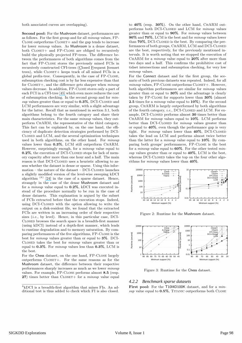
4.2.1 Benchmark dense datasetsFirst pool: In the first pool, Close presents better perfor-mances than A-Close for all datasets. This was expectedsince Close is known to perform better than A-Close fordense datasets [29].

For the Mushroom dataset, Titanic outperforms Close forminsup values ranging between 20% and 2%. However,the contrary happens for minsup values lower than 2%,where Close largely outperforms Titanic. Indeed, to com-pute the FCIs, Titanic tries to extend any FMG with theappropriate items by carrying out costly support computa-tions, especially for low minsup values. Indeed, for minsup

= 0.1%, 116 items – among 119 – are frequent and themaximum size of an FMG is only equal to 10 items. Notethat for this dataset, Close, A-Close and Titanic suf-fer from redundant computation of the FCIs. Indeed, for aminsup value equal to 0.1%, the number of FMGs, equalto 360, 166, is almost 2.2 times the number of FCIs, equalto 164, 117 (as shown by Figure 5).

For the Chess dataset, the counting inference [4] adoptedby Titanic is more efficient than that based on intersectioncomputations adopted by the Close algorithm. Indeed, Ti-tanic outperforms Close for the different tested minsup

values. However, for the same reasons as in the case of theMushroom dataset, this efficiency tends to decrease propor-tionally with the decrease of minsup values.

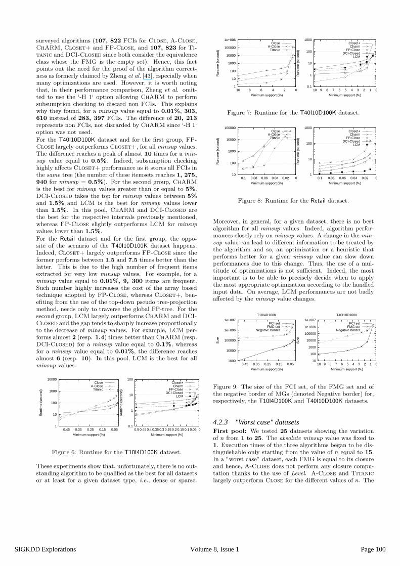
For the Connect dataset, Titanic largely outperforms Closefor all minsup values. In fact, the task of Close is consid-erably complicated by performing intersections on a largenumber of highly sized transactions. However, due to lackof memory capacity, the execution of Titanic did not cometo an end starting from a minsup value equal to 50%. Itis important to mention that, even if this dataset is dense,each FCI has a unique FMG (as shown by Figure 5 in which

Page 97Volume 8, Issue 1SIGKDD Explorations

both associated curves are overlapping).

Second pool: For the Mushroom dataset, performances areas follows. For the first group and for all minsup values, FP-Close outperforms Closet+ and the gap tends to increasefor lower minsup values. As Mushroom is a dense dataset,both Closet+ and FP-Close are obliged to recursivelybuild the physically projected FP-trees. The difference be-tween the performances of both algorithms comes from thefact that FP-Close stores the previously mined FCIs inrecursively constructed CFI-trees (Closed Frequent Itemsettrees), while Closet+ keeps track of all mined FCIs in aglobal prefix-tree. Consequently, in the case of FP-Close,subsumption checking cost is by far less expensive than thatfor Closet+, and the difference gets sharper when minsup

values decrease. In addition, FP-Close stores only a part ofeach FCI in a CFI-tree [45] which even more reduces the costof subsumption checking. In the second group and for min-

sup values greater than or equal to 0.3%, DCI-Closed andLCM performances are very similar, with a slight advantagefor the latter. Recall that as mentioned in section 3.1, bothalgorithms belong to the fourth category and share theirmain characteristics. For the same minsup values, they out-perform ChARM, the representative of the third category.This fact can be explained by, on the one hand, the effi-ciency of duplicate detection strategies performed by DCI-Closed and LCM, and the several optimization techniquesused in both algorithms, on the other hand. For minsup

values lower than 0.3%, LCM still outperform ChARM.However, surprisingly enough, for a minsup value equal to0.2%, the execution of DCI-Closed stops for lack of mem-ory capacity after more than one hour and a half. The mainreason is that DCI-Closed uses a heuristic allowing to as-sess whether the dataset is dense or sparse. Using this infor-mation – the nature of the dataset – DCI-Closed launchesa slightly modified version of the level-wise sweeping kDCIalgorithm (6) [24] in the case of a sparse dataset. Hence,strangely in the case of the dense Mushroom dataset andfor a minsup value equal to 0.2%, kDCI was executed in-stead of the procedure normally to be run in the case ofdense datasets. This explanation is argued by the subsetof FCIs extracted before that the execution stops. Indeed,using DCI-Closed with the option allowing to write theoutput on a disk-resident file, we found that the extractedFCIs are written in an increasing order of their respectivesizes (i.e., by level). Hence, in this particular case, DCI-Closed browses the search space in a breadth-first manner(using kDCI) instead of a depth-first manner, which leadsto runtime degradation and to memory saturation. By com-paring performances of the five algorithms, FP-Close is thebest for minsup values greater than or equal to 3%. DCI-Closed takes the best for minsup values greater than orequal to 0.3%. For minsup values less than 0.3%, LCM isthe best.

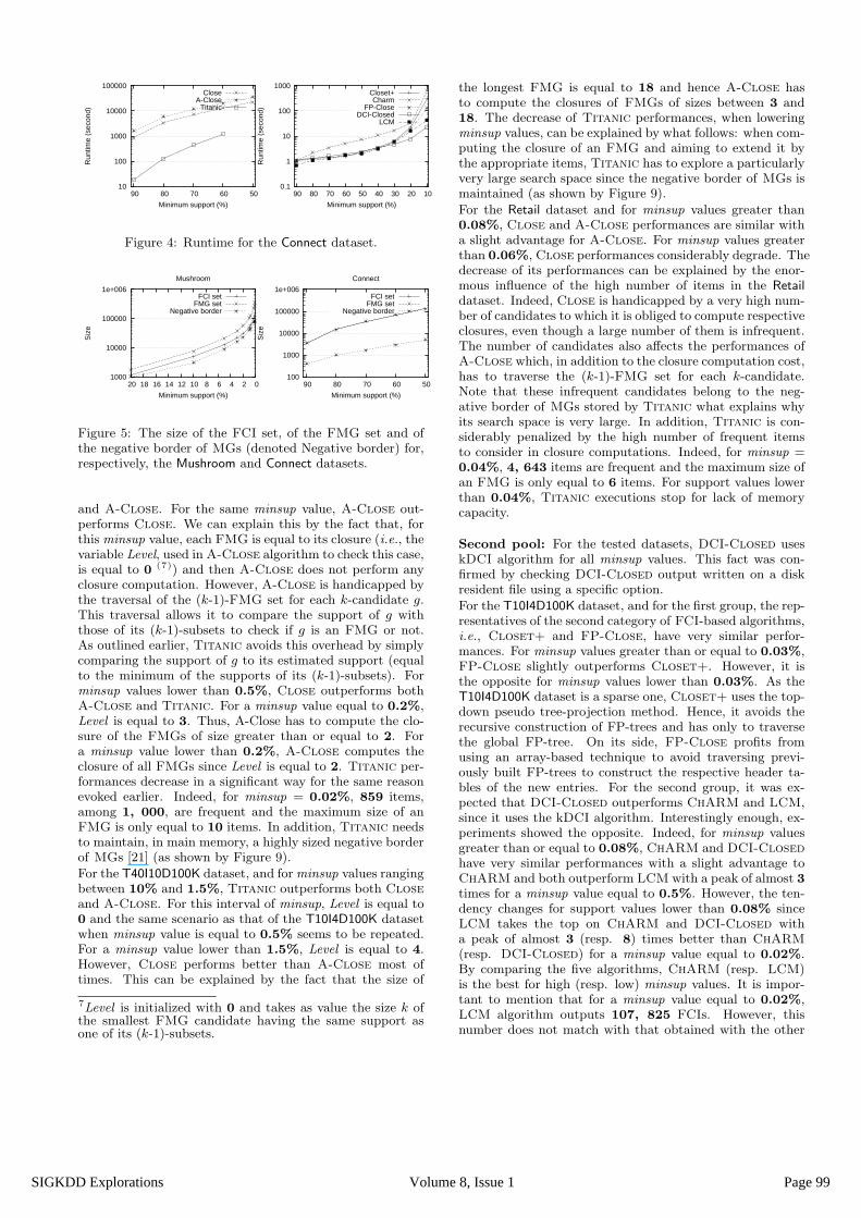
For the Chess dataset, on the one hand, FP-Close largelyoutperforms Closet+. For the same reasons as for theMushroom dataset, the difference between their respectiveperformances sharply increases as much as we lower minsup

values. For example, FP-Close performs almost 8.5 (resp.27) times better than Closet+ for a minsup value equal

6kDCI is a breadth-first algorithm that mines FIs. An ad-ditional test is thus added to check which FI is also closed.

to 40% (resp. 30%). On the other hand, ChARM out-performs both DCI-Closed and LCM for minsup valuesgreater than or equal to 90%. For minsup values between90% and 70%, LCM is the best and for minsup values lowerthan 70%, DCI-Closed is the best. By comparing the per-formances of both groups, ChARM, LCM and DCI-Closedare the best, respectively, for the previously mentioned in-tervals. It is worth noting that we stopped the execution ofChARM for a minsup value equal to 20% after more thantwo days and a half. This confirms the prohibitive cost oftidset intersections and subsumption checking, for very lowminsup values.

For the Connect dataset and for the first group, the sce-nario of both previous datasets was repeated. Indeed, for allminsup values, FP-Close outperforms Closet+. However,both algorithm performances are similar for minsup valuesgreater than or equal to 30% and the advantage is clearlytaken by FP-Close for supports lower than 30% (almost2.5 times for a minsup value equal to 10%). For the secondgroup, ChARM is largely outperformed by both algorithmsof the fourth category, i.e., DCI-Closed and LCM. For ex-ample, DCI-Closed performs almost 30 times better thanChARM for minsup values equal to 10%. LCM performsbetter than DCI-Closed for minsup values greater thanor equal to 40%, even though the performance gap is verytight. For minsup values lower than 40%, DCI-Closedtakes the lead on LCM and performs almost twice betterthan the latter for a minsup value equal to 10%. By com-paring both groups’ performances, FP-Close is the bestfor a minsup value equal to 60%. For the other tested min-

sup values greater than or equal to 40%, LCM is the best,whereas DCI-Closed takes the top on the four other algo-rithms for minsup values lower than 40%.

1

10

100

1000

10000

100000

2 4 6 8 10 12 14 16 18 20

Run

time

(sec

ond)

Minimum support (%)

CloseA-Close

Titanic

0.01

0.1

1

10

0 2 4 6 8 10 12 14 16 18 20

Run

time

(sec

ond)

Minimum support (%)

Closet+Charm

FP-CloseDCI-Closed

LCM

Figure 2: Runtime for the Mushroom dataset.

1

10

100

1000

10000

45 50 55 60 65 70 75 80 85 90

Run

time

(sec

ond)

Minimum support (%)

CloseA-Close

Titanic

0.01

0.1

1

10

100

1000

10000

20 30 40 50 60 70 80 90

Run

time

(sec

ond)

Minimum support (%)

Closet+Charm

FP-CloseDCI-Closed

LCM

Figure 3: Runtime for the Chess dataset.

4.2.2 Benchmark sparse datasetsFirst pool: For the T10I4D100K dataset, and for a min-

sup value equal to 0.5%, Titanic outperforms both Close

Page 98Volume 8, Issue 1SIGKDD Explorations

10

100

1000

10000

100000

50 60 70 80 90

Run

time

(sec

ond)

Minimum support (%)

CloseA-Close

Titanic

0.1

1

10

100

1000

10 20 30 40 50 60 70 80 90

Run

time

(sec

ond)

Minimum support (%)

Closet+Charm

FP-CloseDCI-Closed

LCM

Figure 4: Runtime for the Connect dataset.

1000

10000

100000

1e+006

0 2 4 6 8 10 12 14 16 18 20

Siz

e

Minimum support (%)

Mushroom

FCI setFMG set

Negative border

100

1000

10000

100000

1e+006

50 60 70 80 90

Siz

e

Minimum support (%)

Connect

FCI setFMG set

Negative border

Figure 5: The size of the FCI set, of the FMG set and ofthe negative border of MGs (denoted Negative border) for,respectively, the Mushroom and Connect datasets.

and A-Close. For the same minsup value, A-Close out-performs Close. We can explain this by the fact that, forthis minsup value, each FMG is equal to its closure (i.e., thevariable Level, used in A-Close algorithm to check this case,is equal to 0 (7)) and then A-Close does not perform anyclosure computation. However, A-Close is handicapped bythe traversal of the (k-1)-FMG set for each k-candidate g.This traversal allows it to compare the support of g withthose of its (k-1)-subsets to check if g is an FMG or not.As outlined earlier, Titanic avoids this overhead by simplycomparing the support of g to its estimated support (equalto the minimum of the supports of its (k-1)-subsets). Forminsup values lower than 0.5%, Close outperforms bothA-Close and Titanic. For a minsup value equal to 0.2%,Level is equal to 3. Thus, A-Close has to compute the clo-sure of the FMGs of size greater than or equal to 2. Fora minsup value lower than 0.2%, A-Close computes theclosure of all FMGs since Level is equal to 2. Titanic per-formances decrease in a significant way for the same reasonevoked earlier. Indeed, for minsup = 0.02%, 859 items,among 1, 000, are frequent and the maximum size of anFMG is only equal to 10 items. In addition, Titanic needsto maintain, in main memory, a highly sized negative borderof MGs [21] (as shown by Figure 9).

For the T40I10D100K dataset, and for minsup values rangingbetween 10% and 1.5%, Titanic outperforms both Closeand A-Close. For this interval of minsup, Level is equal to0 and the same scenario as that of the T10I4D100K datasetwhen minsup value is equal to 0.5% seems to be repeated.For a minsup value lower than 1.5%, Level is equal to 4.However, Close performs better than A-Close most oftimes. This can be explained by the fact that the size of

7Level is initialized with 0 and takes as value the size k ofthe smallest FMG candidate having the same support asone of its (k-1)-subsets.

the longest FMG is equal to 18 and hence A-Close hasto compute the closures of FMGs of sizes between 3 and18. The decrease of Titanic performances, when loweringminsup values, can be explained by what follows: when com-puting the closure of an FMG and aiming to extend it bythe appropriate items, Titanic has to explore a particularlyvery large search space since the negative border of MGs ismaintained (as shown by Figure 9).

For the Retail dataset and for minsup values greater than0.08%, Close and A-Close performances are similar witha slight advantage for A-Close. For minsup values greaterthan 0.06%, Close performances considerably degrade. Thedecrease of its performances can be explained by the enor-mous influence of the high number of items in the Retail

dataset. Indeed, Close is handicapped by a very high num-ber of candidates to which it is obliged to compute respectiveclosures, even though a large number of them is infrequent.The number of candidates also affects the performances ofA-Close which, in addition to the closure computation cost,has to traverse the (k-1)-FMG set for each k-candidate.Note that these infrequent candidates belong to the neg-ative border of MGs stored by Titanic what explains whyits search space is very large. In addition, Titanic is con-siderably penalized by the high number of frequent itemsto consider in closure computations. Indeed, for minsup =0.04%, 4, 643 items are frequent and the maximum size ofan FMG is only equal to 6 items. For support values lowerthan 0.04%, Titanic executions stop for lack of memorycapacity.

Second pool: For the tested datasets, DCI-Closed useskDCI algorithm for all minsup values. This fact was con-firmed by checking DCI-Closed output written on a diskresident file using a specific option.

For the T10I4D100K dataset, and for the first group, the rep-resentatives of the second category of FCI-based algorithms,i.e., Closet+ and FP-Close, have very similar perfor-mances. For minsup values greater than or equal to 0.03%,FP-Close slightly outperforms Closet+. However, it isthe opposite for minsup values lower than 0.03%. As theT10I4D100K dataset is a sparse one, Closet+ uses the top-down pseudo tree-projection method. Hence, it avoids therecursive construction of FP-trees and has only to traversethe global FP-tree. On its side, FP-Close profits fromusing an array-based technique to avoid traversing previ-ously built FP-trees to construct the respective header ta-bles of the new entries. For the second group, it was ex-pected that DCI-Closed outperforms ChARM and LCM,since it uses the kDCI algorithm. Interestingly enough, ex-periments showed the opposite. Indeed, for minsup valuesgreater than or equal to 0.08%, ChARM and DCI-Closedhave very similar performances with a slight advantage toChARM and both outperform LCM with a peak of almost 3

times for a minsup value equal to 0.5%. However, the ten-dency changes for support values lower than 0.08% sinceLCM takes the top on ChARM and DCI-Closed witha peak of almost 3 (resp. 8) times better than ChARM(resp. DCI-Closed) for a minsup value equal to 0.02%.By comparing the five algorithms, ChARM (resp. LCM)is the best for high (resp. low) minsup values. It is impor-tant to mention that for a minsup value equal to 0.02%,LCM algorithm outputs 107, 825 FCIs. However, thisnumber does not match with that obtained with the other

Page 99Volume 8, Issue 1SIGKDD Explorations

surveyed algorithms (107, 822 FCIs for Close, A-Close,ChARM, Closet+ and FP-Close, and 107, 823 for Ti-tanic and DCI-Closed since both consider the equivalenceclass whose the FMG is the empty set). Hence, this factpoints out the need for the proof of the algorithm correct-ness as formerly claimed by Zheng et al. [43], especially whenmany optimizations are used. However, it is worth notingthat, in their performance comparison, Zheng et al. omit-ted to use the ‘-H 1‘ option allowing ChARM to performsubsumption checking to discard non FCIs. This explainswhy they found, for a minsup value equal to 0.01%, 303,

610 instead of 283, 397 FCIs. The difference of 20, 213

represents non FCIs, not discarded by ChARM since ‘-H 1‘option was not used.

For the T40I10D100K dataset and for the first group, FP-Close largely outperforms Closet+, for all minsup values.The difference reaches a peak of almost 10 times for a min-

sup value equal to 0.5%. Indeed, subsumption checkinghighly affects Closet+ performance as it stores all FCIs inthe same tree (the number of these itemsets reaches 1, 275,

940 for minsup = 0.5%). For the second group, ChARMis the best for minsup values greater than or equal to 5%.DCI-Closed takes the top for minsup values between 5%

and 1.5% and LCM is the best for minsup values lowerthan 1.5%. In this pool, ChARM and DCI-Closed arethe best for the respective intervals previously mentioned,whereas FP-Close slightly outperforms LCM for minsup

values lower than 1.5%.

For the Retail dataset and for the first group, the oppo-site of the scenario of the T40I10D100K dataset happens.Indeed, Closet+ largely outperforms FP-Close since theformer performs between 1.5 and 7.5 times better than thelatter. This is due to the high number of frequent itemsextracted for very low minsup values. For example, for aminsup value equal to 0.01%, 9, 300 items are frequent.Such number highly increases the cost of the array basedtechnique adopted by FP-Close, whereas Closet+, ben-efiting from the use of the top-down pseudo tree-projectionmethod, needs only to traverse the global FP-tree. For thesecond group, LCM largely outperforms ChARM and DCI-Closed and the gap tends to sharply increase proportionallyto the decrease of minsup values. For example, LCM per-forms almost 2 (resp. 1.4) times better than ChARM (resp.DCI-Closed) for a minsup value equal to 0.1%, whereasfor a minsup value equal to 0.01%, the difference reachesalmost 6 (resp. 10). In this pool, LCM is the best for allminsup values.

1

10

100

1000

10000

0.05 0.15 0.25 0.35 0.45

Run

time

(sec

ond)

Minimum support (%)

CloseA-Close

Titanic

0.1

1

10

100

0 0.05 0.1 0.15 0.2 0.25 0.3 0.35 0.4 0.45 0.5

Run

time

(sec

ond)

Minimum support (%)

Closet+Charm

FP-CloseDCI-Closed

LCM

Figure 6: Runtime for the T10I4D100K dataset.

These experiments show that, unfortunately, there is no out-standing algorithm to be qualified as the best for all datasetsor at least for a given dataset type, i.e., dense or sparse.

1

10

100

1000

10000

100000

1e+006

0 2 4 6 8 10

Run

time

(sec

ond)

Minimum support (%)

CloseA-Close

Titanic

0.1

1

10

100

1000

0 1 2 3 4 5 6 7 8 9 10

Run

time

(sec

ond)

Minimum support (%)

Closet+Charm

FP-CloseDCI-Closed

LCM

Figure 7: Runtime for the T40I10D100K dataset.

10

100

1000

10000

100000

0 0.02 0.04 0.06 0.08 0.1

Run

time

(sec

ond)

Minimum support (%)

CloseA-Close

Titanic

1

10

100

1000

0 0.02 0.04 0.06 0.08 0.1

Run

time

(sec

ond)

Minimum support (%)

Closet+Charm

FP-CloseDCI-Closed

LCM

Figure 8: Runtime for the Retail dataset.

Moreover, in general, for a given dataset, there is no bestalgorithm for all minsup values. Indeed, algorithm perfor-mances closely rely on minsup values. A change in the min-

sup value can lead to different information to be treated bythe algorithm and so, an optimization or a heuristic thatperforms better for a given minsup value can slow downperformances due to this change. Thus, the use of a mul-titude of optimizations is not sufficient. Indeed, the mostimportant is to be able to precisely decide when to applythe most appropriate optimization according to the handledinput data. On average, LCM performances are not badlyaffected by the minsup value changes.

1000

10000

100000

1e+006

1e+007

0.05 0.15 0.25 0.35 0.45

Siz

e

Minimum support (%)

T10I4D100K

FCI setFMG set

Negative border

10

100

1000

10000

100000

1e+006

1e+007

0 1 2 3 4 5 6 7 8 9 10

Siz

e

Minimum support (%)

T40I10D100K

FCI setFMG set

Negative border

Figure 9: The size of the FCI set, of the FMG set and ofthe negative border of MGs (denoted Negative border) for,respectively, the T10I4D100K and T40I10D100K datasets.

4.2.3 "Worst case" datasetsFirst pool: We tested 25 datasets showing the variationof n from 1 to 25. The absolute minsup value was fixed to1. Execution times of the three algorithms began to be dis-tinguishable only starting from the value of n equal to 15.In a ”worst case” dataset, each FMG is equal to its closureand hence, A-Close does not perform any closure compu-tation thanks to the use of Level. A-Close and Titaniclargely outperform Close for the different values of n. The

Page 100Volume 8, Issue 1SIGKDD Explorations

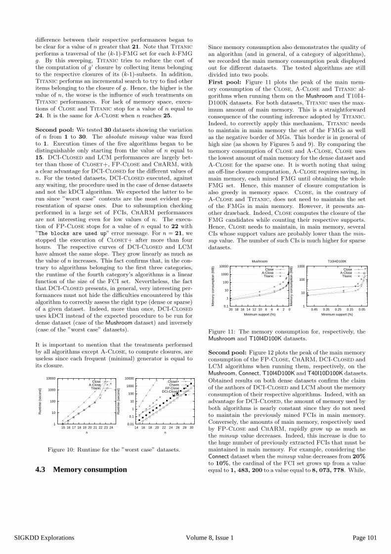
difference between their respective performances began tobe clear for a value of n greater that 21. Note that Titanicperforms a traversal of the (k-1)-FMG set for each k-FMGg. By this sweeping, Titanic tries to reduce the cost ofthe computation of g’ closure by collecting items belongingto the respective closures of its (k-1)-subsets. In addition,Titanic performs an incremental search to try to find otheritems belonging to the closure of g. Hence, the higher is thevalue of n, the worse is the influence of such treatments onTitanic performances. For lack of memory space, execu-tions of Close and Titanic stop for a value of n equal to24. It is the same for A-Close when n reaches 25.

Second pool: We tested 30 datasets showing the variationof n from 1 to 30. The absolute minsup value was fixedto 1. Execution times of the five algorithms began to bedistinguishable only starting from the value of n equal to15. DCI-Closed and LCM performances are largely bet-ter than those of Closet+, FP-Close and ChARM, witha clear advantage for DCI-Closed for the different values ofn. For the tested datasets, DCI-Closed executed, againstany waiting, the procedure used in the case of dense datasetsand not the kDCI algorithm. We expected the latter to berun since ”worst case” contexts are the most evident rep-resentation of sparse ones. Due to subsumption checkingperformed in a large set of FCIs, ChARM performancesare not interesting even for low values of n. The execu-tion of FP-Close stops for a value of n equal to 22 with”The blocks are used up” error message. For n = 21, westopped the execution of Closet+ after more than fourhours. The respective curves of DCI-Closed and LCMhave almost the same slope. They grow linearly as much asthe value of n increases. This fact confirms that, in the con-trary to algorithms belonging to the first three categories,the runtime of the fourth category’s algorithms is a linearfunction of the size of the FCI set. Nevertheless, the factthat DCI-Closed presents, in general, very interesting per-formances must not hide the difficulties encountered by thisalgorithm to correctly assess the right type (dense or sparse)of a given dataset. Indeed, more than once, DCI-Closeduses kDCI instead of the expected procedure to be run fordense dataset (case of the Mushroom dataset) and inversely(case of the ”worst case” datasets).

It is important to mention that the treatments performedby all algorithms except A-Close, to compute closures, areuseless since each frequent (minimal) generator is equal toits closure.

1

10

100

1000

10000

15 16 17 18 19 20 21 22 23 24

Run

time

(sec

ond)

n

CloseA-Close

Titanic

0.01

0.1

1

10

100

1000

10000

14 16 18 20 22 24 26 28 30

Run

time

(sec

ond)

n

Closet+Charm

FP-CloseDCI-Closed

LCM

Figure 10: Runtime for the ”worst case” datasets.

4.3 Memory consumption

Since memory consumption also demonstrates the quality ofan algorithm (and in general, of a category of algorithms),we recorded the main memory consumption peak displayedout for different datasets. The tested algorithms are stilldivided into two pools.

First pool: Figure 11 plots the peak of the main mem-ory consumption of the Close, A-Close and Titanic al-gorithms when running them on the Mushroom and T10I4-D100K datasets. For both datasets, Titanic uses the max-imum amount of main memory. This is a straightforwardconsequence of the counting inference adopted by Titanic.Indeed, to correctly apply this mechanism, Titanic needsto maintain in main memory the set of the FMGs as wellas the negative border of MGs. This border is in general ofhigh size (as shown by Figures 5 and 9). By comparing thememory consumption of Close and A-Close, Close usesthe lowest amount of main memory for the dense dataset andA-Close for the sparse one. It is worth noting that usingan off-line closure computation, A-Close requires saving, inmain memory, each mined FMG until obtaining the wholeFMG set. Hence, this manner of closure computation isalso greedy in memory space. Close, in the contrary ofA-Close and Titanic, does not need to maintain the setof the FMGs in main memory. However, it presents an-other drawback. Indeed, Close computes the closure of theFMG candidates while counting their respective supports.Hence, Close needs to maintain, in main memory, severalCIs whose support values are probably lower than the min-

sup value. The number of such CIs is much higher for sparsedatasets.

0.1

1

10

100

1000

10000

0 2 4 6 8 10 12 14 16 18 20

Mem

ory

cons

umpt

ion

(MB

)

Minimum support (%)

Mushroom

CloseA-Close

Titanic

1

10

100

1000

0.05 0.15 0.25 0.35 0.45

Mem

ory

cons

umpt

ion

(MB

)

Minimum support (%)

T10I4D100K

CloseA-Close

Titanic

Figure 11: The memory consumption for, respectively, theMushroom and T10I4D100K datasets.

Second pool: Figure 12 plots the peak of the main memoryconsumption of the FP-Close, ChARM, DCI-Closed andLCM algorithms when running them, respectively, on theMushroom, Connect, T10I4D100K and T40I10D100K datasets.

Obtained results on both dense datasets confirm the claimof the authors of DCI-Closed and LCM about the memoryconsumption of their respective algorithms. Indeed, with anadvantage for DCI-Closed, the amount of memory used byboth algorithms is nearly constant since they do not needto maintain the previously mined FCIs in main memory.Conversely, the amounts of main memory, respectively usedby FP-Close and ChARM, rapidly grow up as much asthe minsup value decreases. Indeed, this increase is due tothe huge number of previously extracted FCIs that must bemaintained in main memory. For example, considering theConnect dataset when the minsup value decreases from 20%

to 10%, the cardinal of the FCI set grows up from a valueequal to 1, 483, 200 to a value equal to 8, 073, 778. While,

Page 101Volume 8, Issue 1SIGKDD Explorations

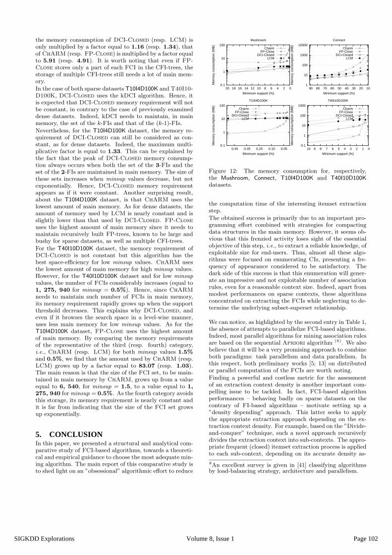
the memory consumption of DCI-Closed (resp. LCM) isonly multiplied by a factor equal to 1.16 (resp. 1.34), thatof ChARM (resp. FP-Close) is multiplied by a factor equalto 5.91 (resp. 4.91). It is worth noting that even if FP-Close stores only a part of each FCI in the CFI-trees, thestorage of multiple CFI-trees still needs a lot of main mem-ory.

In the case of both sparse datasets T10I4D100K and T40I10-D100K, DCI-Closed uses the kDCI algorithm. Hence, itis expected that DCI-Closed memory requirement will notbe constant, in contrary to the case of previously examineddense datasets. Indeed, kDCI needs to maintain, in mainmemory, the set of the k-FIs and that of the (k-1)-FIs.

Nevertheless, for the T10I4D100K dataset, the memory re-quirement of DCI-Closed can still be considered as con-stant, as for dense datasets. Indeed, the maximum multi-plicative factor is equal to 1.33. This can be explained bythe fact that the peak of DCI-Closed memory consump-tion always occurs when both the set of the 3-FIs and theset of the 2-FIs are maintained in main memory. The size ofthese sets increases when minsup values decrease, but notexponentially. Hence, DCI-Closed memory requirementappears as if it were constant. Another surprising result,about the T10I4D100K dataset, is that ChARM uses thelowest amount of main memory. As for dense datasets, theamount of memory used by LCM is nearly constant and isslightly lower than that used by DCI-Closed. FP-Closeuses the highest amount of main memory since it needs tomaintain recursively built FP-trees, known to be large andbushy for sparse datasets, as well as multiple CFI-trees.

For the T40I10D100K dataset, the memory requirement ofDCI-Closed is not constant but this algorithm has thebest space-efficiency for low minsup values. ChARM usesthe lowest amount of main memory for high minsup values.However, for the T40I10D100K dataset and for low minsup

values, the number of FCIs considerably increases (equal to1, 275, 940 for minsup = 0.5%). Hence, since ChARMneeds to maintain such number of FCIs in main memory,its memory requirement rapidly grows up when the supportthreshold decreases. This explains why DCI-Closed, andeven if it browses the search space in a level-wise manner,uses less main memory for low minsup values. As for theT10I4D100K dataset, FP-Close uses the highest amountof main memory. By comparing the memory requirementsof the representative of the third (resp. fourth) category,i.e., ChARM (resp. LCM) for both minsup values 1.5%

and 0.5%, we find that the amount used by ChARM (resp.LCM) grows up by a factor equal to 83.07 (resp. 1.03).The main reason is that the size of the FCI set, to be main-tained in main memory by ChARM, grows up from a valueequal to 6, 540, for minsup = 1.5, to a value equal to 1,

275, 940 for minsup = 0.5%. As the fourth category avoidsthis storage, its memory requirement is nearly constant andit is far from indicating that the size of the FCI set growsup exponentially.

5. CONCLUSIONIn this paper, we presented a structural and analytical com-parative study of FCI-based algorithms, towards a theoreti-cal and empirical guidance to choose the most adequate min-ing algorithm. The main report of this comparative study isto shed light on an ”obsessional” algorithmic effort to reduce

0.1

1

10

100

0 2 4 6 8 10 12 14 16 18 20

Mem

ory

cons

umpt

ion

(MB

)

Minimum support (%)

Mushroom

CharmFP-Close

DCI-ClosedLCM

1

10

100

1000

10000

10 20 30 40 50 60 70 80 90

Mem

ory

cons

umpt

ion

(MB

)

Minimum support (%)

Connect

CharmFP-Close

DCI-ClosedLCM

0.1

1

10

100

0.05 0.15 0.25 0.35 0.45

Mem

ory

cons

umpt

ion

(MB

)

Minimum support (%)

T10I4D100K

CharmFP-Close

DCI-ClosedLCM

0.1

1

10

100

1000

0 1 2 3 4 5 6 7 8 9 10

Mem

ory

cons

umpt

ion

(MB

)

Minimum support (%)

T40I10D100K

CharmFP-Close

DCI-ClosedLCM

Figure 12: The memory consumption for, respectively,the Mushroom, Connect, T10I4D100K and T40I10D100K

datasets.

the computation time of the interesting itemset extractionstep.

The obtained success is primarily due to an important pro-gramming effort combined with strategies for compactingdata structures in the main memory. However, it seems ob-vious that this frenzied activity loses sight of the essentialobjective of this step, i.e., to extract a reliable knowledge, ofexploitable size for end-users. Thus, almost all these algo-rithms were focused on enumerating CIs, presenting a fre-quency of appearance considered to be satisfactory. Thedark side of this success is that this enumeration will gener-ate an impressive and not exploitable number of associationrules, even for a reasonable context size. Indeed, apart frommodest performances on sparse contexts, these algorithmsconcentrated on extracting the FCIs while neglecting to de-termine the underlying subset-superset relationship.

We can notice, as highlighted by the second entry in Table 1,the absence of attempts to parallelize FCI-based algorithms.Indeed, most parallel algorithms for mining association rulesare based on the sequential Apriori algorithm (8). We alsobelieve that it will be a very promising approach to combineboth paradigms: task parallelism and data parallelism. Inthis respect, both preliminary works [5; 13] on distributedor parallel computation of the FCIs are worth noting.

Finding a powerful and costless metric for the assessmentof an extraction context density is another important com-pelling issue to be tackled. In fact, FCI-based algorithmperformances – behaving badly on sparse datasets on thecontrary of FI-based algorithms – motivate setting up a”density depending” approach. This latter seeks to applythe appropriate extraction approach depending on the ex-traction context density. For example, based on the ”Divide-and-conquer” technique, such a novel approach recursivelydivides the extraction context into sub-contexts. The appro-priate frequent (closed) itemset extraction process is appliedto each sub-context, depending on its accurate density as-

8An excellent survey is given in [41] classifying algorithmsby load-balancing strategy, architecture and parallelism.

Page 102Volume 8, Issue 1SIGKDD Explorations

sessment.

An in-depth study of dataset characteristics is bashfully be-ginning to grasp the community interest. In fact, thesecharacteristics have an important impact on algorithm per-formances. A finer structural characterization of handleddatasets – beyond the number of transactions/items, theaverage transaction size or the density – permits a betterunderstanding of the behavior of algorithms. In this re-spect, two preliminary works are worth mentioning. Thefirst studies the distribution of the negative border and itscomplement, the positive one [12], while the second workproposes some results about the average number of frequent(closed) itemsets, using probabilistic techniques (e.g., theBernoulli law) [23].

Other avenues for future work address the challenging issuesof mining richly structured and genomic contexts. For ex-ample, in genomic contexts, mined knowledge is closely de-pendent of the discretization method, i.e., how the originalcontext is translated to a binary one. Usually, a gene is con-sidered to be present in a biological situation if its expressionlevel exceeds (or not) a given threshold (e.g, its expressionlevel average in the different biological situations). Clearly,such translation is far from being information lossless. Ac-tually, the main drawback is that the discretization is notable to describe the ”actual” biological situation. For thisreason, it is of paramount importance to handle an extendedextraction context, i.e., without binarizing the original con-text. In this respect, introducing soft computing techniquesseems to be a promising issue.

Finally, well adapted visualization models are badly missing.In fact, useful relationships between nonintuitive variablesare the jewels that data mining techniques hope to locate.However, the unmanageably large association rule sets, com-pounded with their low precision, often makes the perusalof knowledge ineffective, their exploitation time-consumingand frustrating for the user. This fact is reinforced sincethe user does not know beforehand what the data miningprocess will discover. It is a much bigger leap to take theoutput of the system and to translate it into a natural rep-resentation matching with what the end-user has in mind.

AcknowledgementsWe are grateful to the anonymous reviewers for their help-ful comments. We also thank C. Dubois, J.J. Givry and C.Zimny for English proofreading. This work is partially sup-ported by the French-Tunisian project CMCU 05G1412.

6. REFERENCES[1] C. C. Aggarwal. Towards long pattern generation in dense

databases. In ACM-SIGKDD Explorations, volume 3(1),pages 20–26, July 2001.

[2] R. Agrawal and R. Srikant. Fast algorithms for mining as-sociation rules. In J. B. Bocca, M. Jarke, and C. Zaniolo,editors, Proceedings of the 20th International Conference onVery Large Databases, Santiago, Chile, pages 478–499, June1994.

[3] Y. Bastide, N. Pasquier, R. Taouil, G. Stumme, andL. Lakhal. Mining minimal non-redundant association rulesusing frequent closed itemsets. In Proceedings of the 1stInternational Conference on Computational Logic (DOOD2000), Springer-Verlag, LNAI, volume 1861, London, UK,pages 972–986, July 2000.

[4] Y. Bastide, R. Taouil, N. Pasquier, G. Stumme, andL. Lakhal. Mining frequent patterns with counting inference.In Proceeding of the 6th ACM-SIGKDD International Con-ference on Knowledge Discovery and Data Mining, Boston,Massachusetts, USA, volume 2(2), pages 66–75, 20-23 Au-gust 2000.

[5] S. BenYahia, Y. Slimani, and J. Rezgui. A divide and con-quer approach for deriving partially ordered sub-structures.In Proceedings of the International 9th Pacific-Asia Confer-ence on Knowledge Data Discovery (PAKDD 2005), LNAI,volume 3518, Springer-Verlag, Hanoi, Vietnam, pages 91–96, 18-20 May 2005.

[6] J.-F. Boulicaut, A. Bykowski, and C. Rigotti. Free-sets: Acondensed representation of boolean data for the approxi-mation of frequency queries. In Jounal of Data Mining andKnowledge Discovery (DMKD), 7 (1):5–22, 2003.

[7] T. Calders and B. Goethals. Mining all non-derivable fre-quent itemsets. In T. Elomaa, H. Mannila, and H. Toivo-nen, editors, Proceedings of the 6th European Confer-ence on Principles of Knowledge Discovery and Data Min-ing (PKDD 2002), LNCS, volume 2431, Springer-Verlag,Helsinki, Finland, pages 74–85, 19-23 August 2002.

[8] T. Calders, C. Rigotti, and J.-F. Boulicaut. A survey oncondensed representations for frequent sets. In ConstraintBased Mining, Springer-Verlag, LNAI, volume 3848, pages64–80, 2006.

[9] A. Casali, R. Cicchetti, and L. Lakhal. Essential patterns: Aperfect cover of frequent patterns. In A Min Tjoa and J. Tru-jillo, editors, Proceedings of the 7th International Conferenceon Data Warehousing and Knowledge Discovery (DaWaK2005), Springer-Verlag, LNCS, volume 3589, Copenhagen,Denmark, pages 428–437, 22-26 August 2005.

[10] G. Cong, K. H. Tung, X. Xu, F. Pan, and J. Yang. Farmer:finding interesting rule groups in microarray datasets. InProceedings of the 2004 ACM SIGMOD International con-ference on Management of data, Paris, France, pages 143–154, 2004.

[11] M. El-Hajj and O. Zaiane. Finding all frequent patternsstarting from the closure. In the International Conferenceon Advanced Data Mining and Applications, Wuhan, China,pages 67–74, July 2005.

[12] F. Flouvat, F. De Marchi, and J-M. Petit. A thorough ex-perimental study of datasets for frequent itemsets. In Pro-ceedings of the 5th IEEE International Conference on DataMining (ICDM 2005), New Orleans, USA, pages 162–169,November 2005.

[13] H. Fu and E. Mephu Nguifo. Partitioning large data to scaleup lattice-based algorithm. In Proceedings of IEEE Interna-tional Conference on Tools with Artificial Intelligence (IC-TAI 2003), Sacramento, California, USA, pages 537–541,November 2003.

[14] J. Galambos and I. Simonelli. Bonferroni-type inequalitieswith applications. Springer-Verlag, 2000.

[15] B. Ganter and R. Wille. Formal Concept Analysis. Springer-Verlag, 1999.

[16] B. Goethals and M. J. Zaki. FIMI’03: Workshop on fre-quent itemset mining implementations. In B. Goethals andM. J. Zaki, editors, Proceedings of the IEEE ICDM Work-shop on Frequent Itemset Mining Implementations (FIMI2003), volume 90 of CEUR Workshop Proceedings, Mel-bourne, Florida, USA, 19 November 2003.

[17] G. Grahne and J. Zhu. Efficiently using prefix-trees in min-ing frequent itemsets. In B. Goethals and M. J. Zaki, edi-tors, Proceedings of the IEEE ICDM Workshop on FrequentItemset Mining Implementations (FIMI 2003), volume 90 ofCEUR Workshop Proceedings, Melbourne, Florida, USA, 19November 2003.

Page 103Volume 8, Issue 1SIGKDD Explorations

[18] T. Hamrouni, S. BenYahia, and Y. Slimani. Avoiding theitemset closure computation ”pitfall”. In Proceedings of the3rd International Conference on Concept Lattices and theirApplications (CLA 2005), Olomouc, Czech Republic, pages46–59, 7–9 September 2005.

[19] J. Han, J. Pei, and Y. Yin. Mining frequent patterns withoutcandidate generation. In Proceedings of the ACM-SIGMODInternational Conference on Management of Data (SIG-MOD’00), Dallas, Texas, USA, pages 1–12, May 2000.

[20] J. Hipp, U. Gntzer, and G. Nakhaeizadeh. Algorithms forassociation rule mining - a general survey and comparison.In ACM-SIGKDD Explorations, volume 2(1), pages 58–64,July 2000.

[21] M. Kryszkiewicz. Concise representation of frequent patternsbased on disjunction-free generators. In Proceedings of the1st IEEE International Conference on Data Mining (ICDM2001), San Jose, California, USA, pages 305–312, 2001.

[22] S. O. Kuznetsov and S. A. Ob”edkov. Comparing perfor-mance of algorithms for generating concept lattices. In Jour-nal of Experimental and Theoretical Artificial Intelligence(JETAI), volume 14(2-3), pages 189–216, 2002.

[23] L. Lhote, F. Rioult, and A. Soulet. Average number of fre-quent and closed pattern in random databases. In Proceed-ings of the 7th Conference Francophone d’Apprentissage Au-tomatique (CAp 2005), Presses Universitaires de Grenoble,Nice, France, pages 345–360, 30 May - 03 June 2005.

[24] C. Lucchese, S. Orlando, P. Palmerini, R. Perego, and F. Sil-vestri. kDCI: A multi-strategy algorithm for mining frequentsets. In B. Goethals and M. J. Zaki, editors, Proceedings ofthe IEEE ICDM Workshop on Frequent Itemset Mining Im-plementations (FIMI 2003), volume 90 of CEUR WorkshopProceedings, Melbourne, Florida, USA, 19 November 2003.

[25] C. Lucchese, S. Orlando, and R. Perego. Fast and memoryefficient mining of frequent closed itemsets. In IEEE JournalTransactions on Knowledge and Data Engineering (TKDE),18 (1):21–36, January 2006.

[26] C. Lucchesse, S. Orlando, and R. Perego. DCI-Closed: Afast and memory efficient algorithm to mine frequent closeditemsets. In B. Goethals, M. J. Zaki, and R. Bayardo, edi-tors, Proceedings of the IEEE ICDM Workshop on FrequentItemset Mining Implementations (FIMI 2004), volume 126of CEUR Workshop Proceedings, Brighton, UK, 1 November2004.

[27] E. Mephu Nguifo. Gallois lattice: A framework for conceptlearning, design, evaluation and refinement. In Proceedingsof IEEE International Conference on Tools with ArtificialIntelligence (ICTAI 1994), New-Orleans, USA, pages 461–467, November 1994.

[28] F. Pan, G. Cong, K. H. Tung, J. Yang, and M. J. Zaki. Car-penter: finding closed patterns in long biological datasets.In Proceedings of the 9th ACM SIGKDD International con-ference on Knowledge discovery and data mining, pages 637–642, 2003.

[29] N. Pasquier. Datamining : Algorithmes d’extraction etde reduction des regles d’association dans les bases de

donnees. These de doctorat, Ecole Doctorale Sciences pourl’Ingenieur de Clermont Ferrand, Universite Clermont Fer-rand II, France, Janvier 2000.

[30] N. Pasquier. Mining association rules using formal conceptanalysis. In Proceedings of the 8th International Conferenceon Conceptual Structures (ICCS 2000), Springer-Verlag,LNAI, volume 1867, Darmstadt, Germany, pages 259–264,August 2000.

[31] N. Pasquier, Y. Bastide, R. Taouil, and L. Lakhal. Effi-cient mining of association rules using closed itemset lattices.Journal of Information Systems, 24(1):25–46, 1999.

[32] N. Pasquier, Y. Bastide, R. Touil, and L. Lakhal. Discover-ing frequent closed itemsets for association rules. In C. Beeriand P. Buneman, editors, Proceedings of 7th InternationalConference on Database Theory (ICDT 1999), LNCS, vol-ume 1540, Springer-Verlag, Jerusalem, Israel, pages 398–416, January 1999.

[33] J. Pei, J. Han, and R. Mao. Closet: An efficient algo-rithm for mining frequent closed itemsets. In Proceedings ofthe ACM-SIGMOD International Workshop on Data Min-ing and Knowledge Discovery (DMKD 2000), Dallas, Texas,USA, pages 21–30, 2000.

[34] R. Srikant. Fast algorithms for mining association rules andsequential patterns. Ph. D dissertation, University of Wis-consin, Madison, USA, 1996.

[35] G. Stumme, R. Taouil, Y. Bastide, N. Pasquier, andL. Lakhal. Computing iceberg concept lattices with Ti-tanic. Journal on Knowledge and Data Engineering (KDE),2(42):189–222, 2002.

[36] T. Uno, T. Asai, Y. Uchida, and H. Arimura. An efficientalgorithm for enumerating closed patterns in transactiondatabases. Proceedings of the 7th International Conferenceon Discovery Science, Padova, Italy, pages 16–31, 2-5 Octo-ber 2004.

[37] T. Uno, M. Kiyomi, and H. Arimura. LCM ver. 2: Efficientmining algorithms for frequent/closed/maximal itemsets. InB. Goethals, M. J. Zaki, and R. Bayardo, editors, Proceed-ings of the IEEE ICDM Workshop on Frequent Itemset Min-ing Implementations (FIMI 2004), volume 126 of CEURWorkshop Proceedings, Brighton, UK, 1 November 2004.

[38] P. Valtchev, R. Missaoui, and P. Lebrun. A fast algorithm forbuilding the Hasse diagram of a Galois lattice. In Proceedingsof the Colloque LaCIM 2000, Montreal, Canada, pages 293–306, September 2000.

[39] J. Wang, J. Han, and J. Pei. Closet+: Searching for the beststrategies for mining frequent closed itemsets. In Proceed-ings of the 9th ACM-SIGKDD International Conference onKnowledge Discovery and Data Mining (KDD 2003), Wash-ington D. C., USA, pages 236–245, 24-27 August 2003.

[40] R. Wille. Restructuring lattices theory: An approach basedon hierarchies of concepts. I. Rival, editor, Ordered Sets,Reidel, Dordrecht-Boston, p. 445-470, 1982.

[41] M. J. Zaki. Parallel and distributed association mining: Asurvey. In IEEE Journal Concurrency, 7 (4):14–25, October1999.

[42] M. J. Zaki and C. J. Hsiao. ChARM: An efficient algorithmfor closed itemset mining. In Proceedings of the 2nd SIAMInternational Conference on Data Mining, Arlington, Vir-ginia, USA, pages 34–43, April 2002.

[43] Z. Zheng, R. Kohavi, and L. Mason. Real world performanceof association rule algorithms (long version). Availableat http://ai.stanford.edu/users/ronnyk/realworldassoclong-paper.pdf. Accessed on February 15th 2006.

[44] Z. Zheng, R. Kohavi, and L. Mason. Real world perfor-mance of association rule algorithms. In F. Provost andR. Srikant, editors, Proceedings of the 7th ACM SIGKDDInternational Conference on Knowledge Discovery and DataMining, ACM Press, pages 401–406, August 2001.

[45] J. Zhu. Efficiently mining frequent itemsets from very largedatabases. Ph. D thesis, University of Concordia, Montreal,Quebec, Canada, September 2004.

Page 104Volume 8, Issue 1SIGKDD Explorations