FRENCH REFINEMENT OF GROUNDWATER SCENARIOS Report of the UIPP Environmental Methodology Working Group Beigel, C. 1 , Berardozzi, M. 2 , Cecchi, M. 3 , Domange, N. 3 , Guyot, C. 4 , Hammel, K. 5 , Huber, S. 6 , Kahl, G. 7 , Knowles, S. 8 , Loiseau, L. 9 21 July 2011 1 BASF Agro S.A.S., Ecully, France; 2 Dow AgroSciences S.A.S., France; 3 Syngenta Agro S.A.S., Guyancourt, France; 4 Bayer CropScience, Lyon, France; 5 Bayer CropScience, Monheim, Germany; 6 BASF SE, Limburgerhof, Germany; 7 Dr Knoell Consult, Mannheim, Germany; 8 Dow Agrosciences, UK; 9 Syngenta, Basel, Switzerland

Welcome message from author
This document is posted to help you gain knowledge. Please leave a comment to let me know what you think about it! Share it to your friends and learn new things together.
Transcript

FRENCH REFINEMENT OF GROUNDWATER SCENARIOS
Report of the UIPP Environmental Methodology Working Group
Beigel, C.1, Berardozzi, M.2, Cecchi, M.3, Domange, N.3, Guyot, C.4, Hammel, K.5, Huber, S.6, Kahl, G.7, Knowles, S.8, Loiseau, L.9
21 July 2011
1BASF Agro S.A.S., Ecully, France; 2Dow AgroSciences S.A.S., France; 3Syngenta Agro S.A.S., Guyancourt, France; 4Bayer CropScience, Lyon, France; 5Bayer CropScience,
Monheim, Germany; 6BASF SE, Limburgerhof, Germany; 7Dr Knoell Consult, Mannheim, Germany; 8Dow Agrosciences, UK; 9Syngenta, Basel, Switzerland
Acknowledgements
The authors are particularly indebted to the originators and participants of the INRA SSM ComTox precursor workgroup on French groundwater scenarios (Commission d’étude de la toxicité – Sous-groupe environnement – Atelier ESO), namely André-Bernard Delmas (INRA – SSM – Versailles), Brigitte Rémy (INRA – SSM – Versailles), Laure Mamy (INRA – SSM – Versailles), Paul Gaillardon (expert ComTox), Christine Lebas (INRA – Infosol – Orléans), Xavier Morvan (INRA – Infosol – Orléans), Ary Bruand (Université d'Orléans), Benoît Réal (Arvalis – Institut du Végétal), Philippe Adrian (CEHTRA), Igor Dubus (BRGM), Yves Coquet (INRA – INA PG), Enrique Barriuso (INRA – EGC – Grignon), Guy Soulas (Université Bordeaux II), who laid out the key principles of the French groundwater scenarios construction. The authors also wish to thank the many local and international experts that participated in the data collection and elaboration of the FROGS scenarios.
Citation Those wishing to cite this report are advised to use the following reference:
FROGS (2011) “French Refinement Of Groundwater Scenarios” Report of the UIPP Environmental Methodology Working Group version 2.0, 314 pp.
1
Foreword
The placing of plant protection products on the market is regulated by Directive 91/414 (which will be replaced by Regulation 1107/2009). The aim of these regulations is to ensure a high level of protection for both human and animal health and the environment and at the same time to safeguard the competitiveness of Community agriculture. They set the list of approval criteria and requirements which need to be addressed in order to authorize a crop protection product on the market, and the harmonized principles which have to be followed to assess and authorize these products.
At European level, and as far as the protection of groundwater is concerned, an active substance shall only be approved for Annex I listing where it has been established for one or more representative uses (after application of the plant protection product consistent with realistic conditions on use) that the predicted concentration in groundwater (PECgw) of the active substance or of relevant metabolites, degradation or reaction products are below the value of 0.1 µg/L as defined in the Drinking Water Directive (directive 98/83/EC).
The calculation of these PECgw relies on the existence of modelling tools and associated European scenarios, which have been developed and validated under the requirements fixed under Directive 91/414/EC1. These tools and scenarios were set up by the FOCUS (FOrum for the Co-ordination of pesticide fate models and their USe) workgroup in order to describe realistic worst-case conditions As realistic worst-case, an overall vulnerability corresponding to the 90th percentile is defined. This is approximated by combining a 80th percentile value for soil and a 80th percentile value for weather (FOCUS, 2000). The FOCUS workgroup also contributes in creating and updating guidelines for the use and evolution of these tools. Individual Member States have to ensure that for the whole area where the Plant Protection Product will be used that the active substance “can be used safely for most of the relevant environmental conditions.”(FOCUS GW, 2009). However, if this conclusion cannot be reached, unfavourable conditions should be identified and risk management may be considered. So, a key point is to know if authorization may be granted only for certain conditions (certain areas, e.g. climatic zones, or certain factors, e.g. soil pH or clay content) or in other words if risk management may be proposed for ground water. In the absence of adequate national scenarios representative of the environmental conditions of their country, most member states use the FOCUS European scenarios to assess the safety of Plant Protection Products towards Groundwater. For instance, in France, the Agence Nationale de SEcurité Sanitaire (ANSES) considers that the safe use of the Plant Protection Product is demonstrated if the 80th percentile of 1 When models are used for estimation of predicted environmental concentrations they must: - make a best-possible estimation of all relevant processes involved taking into account realistic parameters and assumptions,
- where possible be reliably validated with measurements carried out under circumstances relevant for the use of the model,
- be relevant to the conditions in the area of use.
2

2annual average PECgw at 1-meter depth for all nine EU FOCUS groundwater scenarios (Châteaudun, Hamburg, Kremsmünster, Jokioinen, Okehampton, Piacenza, Porto, Sevilla and Thiva) are under 0.1 µg/L (Farama et al., 2007). In case the PECgw are above 0.1 µg/L for the active substance and relevant metabolites, and/or > 10 µg/L for non-relevant metabolites (AFSSA, 2010, SANCO 221/2000), a refined risk assessment is needed and restriction measures may be enforced such as the limitation of the maximum number of applications per year, timing application or dose reduction. However, the variety, scope and applicability of these measures remain limited. Indeed, the FOCUS scenarios were developed as benchmark scenarios at European scale. Thus the vulnerability they represent for a specific nation cannot be accurately defined. For a refined risk assessment, the underlying agro-pedo-climatic information has to be re-evaluated at national scale to define appropriate scenarios. In contrast to the European FOCUS scenarios, national scenarios also allow to define risk mitigation measures based on soil properties or specific cropping practices. Therefore, the need for a representative set of French scenarios for the assessment of groundwater contamination by Plant Protection Product was identified by the previous Authority in charge of the assessment of PPPs dossiers in France (Commission d’étude de la toxicité des produits antiparasitaires à usage agricole et des produits assimilés, des matières fertilisantes et des supports de culture, ComTox, Structure Scientifique Mixte, INRA-DGAL) and a specific joint workgroup between members of the Authority, technical institutes and UIPP (Union des Industries de Protection des Plantes) was established with the objective to generate adequate French groundwater scenarios based on selection of relevant soil/climatic/agronomic properties (Groupe méthodologie, sous-groupe Environnement, Atelier Eaux souterraines). The joint ComTox workgroup stopped in July 2006 due to the reorganization of the regulatory system for pesticides in France, even though the new regulatory authority in charge of the evaluation of PPPs evaluation in France, AFSSA-DiVE (Agence Française de Sécurité Sanitaire des Aliments – Direction du Végétal), which was created in September 2006, showed continuous interest in the project (Balot, 2007; Balot et al., 2008). The project was continued and completed by a dedicated UIPP workgroup, who finalized the scenarios and produced a workable tool, including a database and a user-friendly model interface, as presented in this report. This report is intended for potential users of FROGS for its regulatory purpose, hence primarily notifiers (companies seeking pesticide registration in France and consultants providing support in dossier preparation) and dossier reviewers (regulators), but also for any party interested in higher-tier national groundwater risk assessment.
2 Deemed representative of an overall 90th percentile vulnerability since combined with 80th percentile vulnerability on soil.
3

4
References: Balot V. 2007. Contribution au développement de scenarios de transfert des produits phytosanitaires vers les eaux souterraines applicable à l’évaluation des risqué réalisée au niveau national, Mémoire de stage de Master 2, Afssa – Université Paris 7 Denis Diderot – Université Paris XII Val de Marne – Ecole Nationale des Ponts et Chaussée, 11 septembre 2007 Balot V., Loiseau L., Alix A. 2008. Développement de scénarios nationaux d’évaluation de transfert des produits phytopharmaceutiques vers les eaux souterainnes, 38ème congrès du Groupe Français des Pesticides (GFP), Brest, France, 21-23 mai 2008 European Union. 2006. Directive 2006/118/EC of the European Parliament and of the Council of 12 December 2006 on the protection of groundwater against pollution and deterioration. Official Journal of the European Union, L372:10-31, 27/12/2006. Farama E., Loiseau L., Alix A. 2007. Evaluation réglementaire du transfert des produits phytopharmaceutiques vers les eaux souterraines – La prise en compte de mesures correctives dans l’évaluation, Les transferts des produits phytosanitaires vers les milieux environnementaux, Toulouse, France, 2-3 octobre 2007 FOCUS. 1995. Leaching Models and EU registration. European Commission Document 4952/VI/95. FOCUS. 2000. FOCUS groundwater scenarios in the EU pesticide registration process. Report of the FOCUS Groundwater Scenarios Workgroup, EC Document Reference Sanco/321/2000 rev 2. 202pp.
FOCUS (2009) “Assessing Potential for Movement of Active Substances and their Metabolites to Ground Water in the EU” Report of the FOCUS Ground Water Work Group, EC Document Reference Sanco/13144/2010 version 1, 604 pp.
Table of Content
Summary ................................................................................................................................ 10
1 Introduction .................................................................................................................... 17
1.1 References ........................................................................................................... 22
2 Delimitation of agronomic units .................................................................................. 23
2.1 Agronomic Unit Concept .................................................................................... 23
2.2 Construction of Agronomic Units ...................................................................... 24
2.2.1 Pertinent descriptors....................................................................................... 24
2.2.2 Construction Method ...................................................................................... 24
2.2.3 Agricultural Statistics ...................................................................................... 25
2.2.4 Environmental Zoning .................................................................................... 26
2.3 Zoning Method of Agronomic Units .................................................................. 29
2.3.1 Overlay of Information Layers ....................................................................... 29
2.3.2 Practical Method of PRA Aggregation ......................................................... 29
2.4 Zoning Results ..................................................................................................... 30
2.4.1 Delimitation of Agronomic Units.................................................................... 30
2.4.2 Crop Land Use ................................................................................................ 33
2.5 References ........................................................................................................... 42
3 Crop Rotations .............................................................................................................. 44
3.1 Crop rotation surveys.......................................................................................... 44
3.2 Probabilistic approach ........................................................................................ 44
3.3 Selected crop rotations for the 31 AU .............................................................. 47
3.4 Implementation of the crop rotations in FROGS ............................................ 51
3.5 References ........................................................................................................... 53
4 Application timing based on BBCH growth stages .................................................. 54
4.1 Phenological sub-model origin .......................................................................... 54
4.2 Phenological sub-model theory......................................................................... 54
5
4.3 Relating development stage Ds to BBCH code .............................................. 56
4.4 Validation .............................................................................................................. 58
4.5 References ........................................................................................................... 65
5 Weather data ................................................................................................................. 66
5.1 Introduction........................................................................................................... 66
5.2 Short description of the MARS database ........................................................ 66
5.3 Summary of the tile selection process in FROGS .......................................... 66
5.4 Parameterisation ................................................................................................. 72
5.5 Adjustments of MARS data for SWAP ............................................................. 73
5.5.1 Problem and proposed solution .................................................................... 73
5.5.2 Impact on PECgw ........................................................................................... 75
5.6 References ........................................................................................................... 79
6 Crop irrigation ................................................................................................................ 80
6.1 Irrigated crops and surfaces in France ............................................................ 81
6.2 Selection of the main irrigated crops in FROGS ............................................ 83
6.3 Determination of relevant AUs for implementing irrigation ........................... 87
6.3.1 Grain Maize...................................................................................................... 87
6.3.2 Fodder maize................................................................................................... 87
6.3.3 Beetroot / Sugar beet ..................................................................................... 90
6.3.4 Potato................................................................................................................ 90
6.4 Irrigation practices for maize, potato and beetroot......................................... 93
6.5 Implementation of irrigation in FROGS ............................................................ 96
6.6 References ........................................................................................................... 97
7 Selection of representative soil-types ........................................................................ 98
7.1 Land use data ...................................................................................................... 98
7.1.1 Agricultural census ......................................................................................... 98
7.1.2 Corine Land Cover.......................................................................................... 98
6

7.2 Soil data ................................................................................................................ 99
7.2.1 BDGSF ............................................................................................................. 99
7.2.2 DONESOL...................................................................................................... 101
7.3 Determination of the relevant regions of cultivation ..................................... 101
7.4 Selection of typical soils within the agricultural regions .............................. 104
7.5 Selection of representative soil profiles ......................................................... 107
7.6 Selected soil-types ............................................................................................ 108
7.7 Selected soil profiles ......................................................................................... 109
7.8 Soil – Agronomic Units relationship................................................................ 111
7.8.1 Distribution of Soils in the Agronomic Units .............................................. 111
7.8.2 Soil Distribution as a function of Crops...................................................... 111
7.9 References ......................................................................................................... 115
8 Parameterization of the soil profiles......................................................................... 116
8.1 Adjustment of Topsoil Organic Carbon Content to BDAT........................... 116
8.1.1 Correction method ........................................................................................ 117
8.1.2 Results and Discussion................................................................................ 120
8.2 Adjustment of soil pH to BDAT........................................................................ 122
8.2.1 Comparison of Original pH with BDAT ...................................................... 122
8.2.2 Correction method ........................................................................................ 124
8.2.3 Correction of pH for subsoil layers ............................................................. 127
8.2.4 Relation between pH measured in Different Solutions ........................... 127
8.3 Estimation of Organic carbon content for subsoil layers ............................. 129
8.4 Soil bulk density................................................................................................. 130
8.5 Soil hydrological parameters ........................................................................... 132
8.6 Soil lower boundary conditions ....................................................................... 138
8.7 Soil numerical layers......................................................................................... 138
8.8 Biodegradation factor........................................................................................ 138
7

8.9 Adjustment of ponding depth and max. number of iterations ..................... 139
8.10 References ......................................................................................................... 141
9 Selection of relevant output for national assessment ........................................... 143
9.1 European Regulatory Framework ................................................................... 143
9.2 FROGS Calculation Procedure ....................................................................... 143
9.3 References ......................................................................................................... 144
10 Test runs using FROGS ....................................................................................... 145
10.1 Input parameters ............................................................................................... 145
10.2 Results for the Dummy Substance C and its metabolite............................. 146
10.2.1 Sugar beet ................................................................................................. 146
10.2.2 Winter wheat.............................................................................................. 151
10.2.3 Winter oilseed rape .................................................................................. 155
10.3 Results for the Dummy Substance D ............................................................. 160
10.3.1 Winter Barley ............................................................................................. 160
10.3.2 Potato ......................................................................................................... 164
10.4 Conclusions........................................................................................................ 168
11 FROGS (v2.2.2.2) - Performances and Limitations ......................................... 169
11.1 Data collection and use .................................................................................... 169
11.1.1 Land use .................................................................................................... 169
11.1.2 Soils ............................................................................................................ 171
11.1.3 Weather...................................................................................................... 173
11.1.4 Crops .......................................................................................................... 174
11.2 Modeling tools.................................................................................................... 175
11.2.1 Choice of associated leaching model .................................................... 175
11.2.2 Specificities of the FROGS tools ............................................................ 176
11.3 Perspectives....................................................................................................... 176
11.4 References ......................................................................................................... 177
8

9
Appendix 1 : Number of scenarios per crop, AU and soil profile................................. 178
Appendix 2 : Agro-climatic Regions ................................................................................. 181
Appendix 3 : Map of annual Precipitation Classes agregated by PRA ...................... 183
Appendix 4 : List of Hydro-ecoregions of Levels 1 and 2 ............................................. 187
Appendix 5 : List of PRA in the Agronomic Units .......................................................... 193
Appendix 6 : List of Cantons in the Agronomic Units .................................................... 209
Appendix 7 : Cultivated Surfaces in the Agronomic Units (ha).................................... 222
Appendix 8 : Crop Density in the Agronomic Units (% Farmland) .............................. 225
Appendix 9 : Probability of occurrence of twelve 3-year crop rotations based on AGRESTE data ................................................................................................................... 228
Appendix 10 : Overlap of the 31 Agronomic Units and administrative Régions and Cantons ................................................................................................................................ 230
Appendix 11 : Emergence and harvest dates for each crop/AU combination........... 232
Appendix 12 : Method of selection of most representative MARS tile for each AU . 239
Appendix 13 : Details of the adjustment of rainfall events ........................................... 243
Appendix 14 : Irrigation acreage per Agronomic Unit for the FROGS irrigated crops............................................................................................................................................... 246
Appendix 15 : Soil Surfaces in the Agronomic Units (ha)............................................. 251
Appendix 16 : Selected scenarios per Crop and associated surfaces (kha) ............. 256
Appendix 17 : Soil hydraulic parameterization ............................................................... 272
Appendix 18 : Test results for Substance C and its metabolite applied to sugar beet............................................................................................................................................... 304
Appendix 19 : FROGS scenarios presenting a 80th temporal PECgw > 10 μg/L for MetC on Winter wheat ....................................................................................................... 307
Appendix 20 : FROGS scenarios presenting a 80th temporal PECgw > 0.1 μg/L for Substance D on Winter barley .......................................................................................... 309
Appendix 21 : Calculation of Available Water Capacity................................................ 312
Summary This report presents the rationale for the design and output of the FROGS modelling tools. National scenarios have been constructed for pesticide-related groundwater risk assessment for sugar beet, winter wheat, oilseed rape, maize fodder, maize grain, winter barley, potato and sunflower. These scenarios consist of the combination of limited number of Agronomic Units (AUs) associated to soil, meteo, crop rotations and phenological information. They have been generated to reflect typical realistic conditions and practices under which arable crops are grown in France. The first step of the construction of the scenarios was the definition of Agronomic Units (AU) (see Chapter 2). AUs are homogeneous geographic entities which show common agricultural (intensity of cultivation, crop rotations) and physical conditions (climate, hydrogeology, climate) for the growing of arable crops. They were obtained by combining information on spatial crop distribution in farmland (agricultural census), agricultural environment types and climatic zones. A total of 31 agronomic regions were defined, which cover the whole of France. These are represented in the following map:
10

Agronomic Units for use in French Refinement of Groundwater Scenarios
No. Agronomic Unit No. Agronomic Unit Not accounted for (1) 0 16 Champagne crayeuse
1 Collines molassiques - Lauragais 17 Beauce - Drouais - Gâtinais 2 Bretagne sud 18 Bordelais - Périgord - Coteaux du Lot 3 Limagnes - Plaine du Forez 19 Perche - Pays d'Auge - Pays d'Ouche 4 Bordure maritime Nord - Picardie -
Normandie 20 Bocages de l'ouest
5 Alsace - Sundgau 21 Ardenne - Argonne - Champagne humide 6 Plaine normande - Bessin 22 Champagne berrichonne - Boischaut 7 Aquitaine - Landes 23 Bas Dauphiné - Vallée du Rhône 8 Bassin de l'Adour 24 Fossé bressan 9 Picardie - Nord - Pas-de-Calais 25 Bretagne centrale 10 Charentes 26 Plateaux de Haute-Saône 11 Bocage normand 27 Provence 12 Barrois - Plateaux bourguignons 28 Plaine du Languedoc-Roussillon 13 Plateau lorrain 29 Boischaut du sud 14 Gâtines - Vallées de Loire 30 Bretagne nord 15 Sologne - Orléanais 31 Ile-de-France
(1) Corresponds to territory for which the proportion of arable land is negligible compared to non-agricultural areas (mainly forests and mountains)
11
Selection of representative soil, climate and cropping conditions within each agronomic unit was then performed as follows:
• Land cultivation (agricultural census 2000) Crops covering a significant surface were identified in each agronomic unit based on the 2000 agricultural census. Thus depending on the surface of the crop within the AU, a crop might or might not be considered relevant for this AU (see Chapter 2).
• Crop rotations (Agreste data, local expertise) Typical rotations were determined for each unit based on local expert knowledge and validated based on available Agreste data (see Chapter 3).
• Crop phenology One of the features of FROGS is to allow representative scheduling of application timing according to the specific crop development stage. This means that the user specifies BBCH code, application rate, and target crop, while the FROGS shell derives the actual application dates for each year in the relevant AUs for the target crop. The actual application dates are calculated in function of the weather data of each AU using crop phenological sub-models implemented in the shell. The phenological sub-models were validated with actual biological data from France (see Chapter 4).
• Climatic data (MARS database, Meteo France)
For each agricultural unit (AU) one MARS tile had to be defined to represent the meteorological conditions within the corresponding AU. The selection was based on the most representative tile regarding agricultural conditions and range of weather conditions within the AU (see Chapter 5).
• Crop irrigation (Agreste, local expertise)
Data obtained from the Agreste database and local expert knowledge (Chambres d’Agriculture) were aggregated for each (AU) (see Chapter 6).
• Agricultural soil properties and parameters (Geographic Database of French Soils [BDGSF], DONESOL 2, BDAT) The distribution of 19 typical agricultural soils selected by INRA (Infosol Unit) was used to determine representative combinations of crops and soils in each agronomic unit. These combinations, which reflect typical farmland situations, are at the basis of national scenarios. Their representativeness can be expressed in terms of surface (see Chapters 7-8).
A total of 1481 scenarios were defined as relevant unique combinations of AU, soil type and crop. The number of defined scenarios varies depending on the selected crop (from 49 for potatoes to 290 for grain maize, see Appendix 1), since not all AUs are relevant for a given crop, and not all soil types are relevant for a given AU. The parameters defining the scenarios are stored in the FROGS database. The FROGS interface (GUI) is then used to generate the relevant model input files for PEARL from the FROGS database, the model batch file to run the scenarios and some basic output files to compile and plot the results. Currently, PEARL is the only model which is used by the FROGS GUI, but in principle, any of the FOCUS so-called chromatographic models (PEARL, PELMO, PRZM) could be used with the parameters in the FROGS database (with some adaptation of the soil parameters,
12

which are expressed differently in PEARL compared to PRZM and PELMO, but are based on the same basic information). Further work would be necessary to implement the scenarios in a preferential flow model such as MACRO, since the relevant model parameters for soil macroporous flow have not been determined. The input data required by the FROGS GUI (active substance parameters, metabolism scheme and application scheme) is the same as required for any standard FOCUS groundwater calculations, except for the application relative to BBCH, which is a specific feature of FROGS. In addition, all specific features of the PEARL model, such as pH-dependent sorption or non-equilibrium sorption, can be used in FROGS. The proposed output format from FROGS is a cumulative agricultural area distribution of predicted environmental concentrations in groundwater from low to high concentrations. Ideally, if all scenarios show minimal potential for leaching, all concentrations will be below 0.1µg/L. However if scenarios representing vulnerable conditions are found, for which the regulatory limit in groundwater is exceeded, these can be easily identified. Based on localization and/or specific soil or hydro-geological conditions, mitigations may be proposed or more refined modeling may be conducted. The FROGS scenarios were originally developed for the main field crops. However, with additional work, ultimately a more complete range of crops may be added, including perennial and other fruit and vegetable crops so that, with further work specific to perennial crops, all of the major crops grown in France could be included. Test runs were performed using parent and metabolites dummy substances, and comparing the FROGS output to the corresponding FOCUS groundwater results. The results demonstrate that the FROGS modelling tool can be used to assess groundwater risk in France. A full discussion of these findings along with suggestions for how the cumulative predicted environmental concentrations can be used in risk assessment are presented (see Chapters 9 and 10). Some use restrictions may also be proposed if specific combinations of crop/soil/climate are identified that show increased potential for leaching to groundwater of the substance of interest. Alternatively, additional higher-tier modeling refinements or other higher tier assessment (e.g. field leaching studies, groundwater monitoring) may be performed to further evaluate the leaching potential on the identified critical conditions.
13

GLOSSARY OF ABREVIATIONS AFSSA Agence Française de Sécurité Sanitaire des Aliments AGRESTE Division of French Ministry of Agriculture dealing with Statistics ANSES Agence Nationale de SEcurité Sanitaire a.s. active substance AU Agronomic Unit AUID Agronomic Unit Identification Number AWC Available Water Content BBCH Biologische Bundesanstalt, Bundessortenamt and CHemical
industry BDAT Base de Données d’Analyse de Terre BDGSF Base de Données Géographique des Sols de France BRGM Bureau de Recherches Géologiques et Minières CGSM Crop Growth Monitoring System CLC Corine Land Cover ComTox Commission d’étude de la toxicité des produits antiparasitaires à
usage agricole et des produits assimilés, des matières fertilisantes et des supports de culture
CORPEN Comité d’Orientation pour des Pratiques agricoles
respectueuses de l’Environnement DGAL Direction générale de l'alimentation DONESOL Base de données nationale des informations spatiales
pédologiques DiVE Direction du Végétal ECPA European Crop Protection Association EEA Europe Environmental Agency ESBN European Soil Bureau ESGDB European Soil Geographical DataBase ETC European Topic Centre EU European Union
14

FAO Food and Agirculture Organization FOCUS FOrum for Co-ordination of pesticide fate models and their Use FROGS French Refinement Of Groundwater Scenarios GAP Good Agricultural Practice GIS Geographical Information System GISSOL Système d'information des sols de France GUI Graphical User Interface GW Groundwater HER Hydro-Eco Régions HYPRES HYdraulic PRoperties of European Soils IFEN Institut Francais de l’ENvironnement INRA Institut national de recherche agronomique INSEE Institut National des Statistiques et des Etudes Economiques JRC Joint Research Centre MACRO MACRO is a one-dimensional, process oriented, dual-
permeability model for water flow and reactive solute transport in soil
MARS Monitoring of Agriculture with remote Sensing OC Organic Carbon OCTOP Organic Carbon content in the TOPsoil layer OECD Orgnaisation for Economic Co-operation and Development PECgw Predicted Environnemental Concentrations for the groundwater PEARL Pesticide Emission Assessment at Regional and Local Scales Pelmo PEsticide Leaching MOdel PRA Petites Régions Agricoles PRZM Pesticide Root Zone Model PTF Pedo-Transfer Function RA Recensement Agricole
15

16
RECLUS Réseau d’Etude des Changements dans les Localisations et les Unités Spatiales
SANCO Directorate-General for Health and Consumer Protection SAU Surface agricole utile SCEES Service Central des Enquêtes et des Etudes Statistiques SETAC Society of Environmental Toxicology and Chemistry SID Soil Type IDentification Number SMU Soil Mapping Units SOLHYDRO Analytical database of hydraulic properties SPADBE Soil Profile Analytical DataBase for Europe STU Soil Typological Units SWAP Soil, Water, Atmosphere and Plant UCS Unité Cartographique de Sol UIPP Union des industries pour la protection des plantes USDA United States Department of Agriculture USR Unité de Sols Regroupés UTS Unité Typologique de Sol UIPP Union des Industries de Protection des Plantes WOFOST WOrld FOod STudies WOSR Winter Oilseed Rape
1 Introduction Objectives of French Refinement Of Groundwater Scenarios (FROGS) EU and national registration processes under Directive 91/414/EEC and subsequent Regulation 1107/2009, require the assessment of the potential of an active ingredient and its metabolites to move to groundwater. However, the assessment objectives are different for EU registration of the active ingredient (Annex I) and product registrations in the Member States. With regard to groundwater contamination at EU level, no official decision scheme for Annex I inclusion of active substances currently exists. The current practice is to propose Annex I inclusion as far as safe use is demonstrated for a relevant crop and a significant area in Europe (FOCUS, 2009) or, as stated in FOCUS (2002):” If a substance is less than 0.1ug/l for at least one but not for all relevant scenarios, then in principle the substance can be included on Annex 1 with respect to leaching to groundwater”. For national assessments, all supported crops and the entire potential use area must be considered. If the active substance cannot be used safely throughout the country, then the registration may be limited to the subset of conditions under which the compound can be used safely. For the development of FROGS, the UIPP workgroup has built on the approach originally designed by the ad hoc ComTox workgroup for conducting the French national assessment. As opposed to a small number of worst-case scenarios, this assumes parameterization of multiple scenarios representing a variety of normal, realistic conditions regarding crop locations, phenology, agronomic practices including cropping rotations, soil types and actual soil profiles of different depths, and climate, based on available information from national and European databases and local expert knowledge. Scenarios which reflect representative combinations of crop, soil and climate conditions were determined by attributing pertinent soil types to Agronomic Units defined as geographic areas in which annual crops are considered as homogeneous with regard to land use, cropping characteristics and most frequent rotations. The overall scheme retained is represented in Figure 1.
17
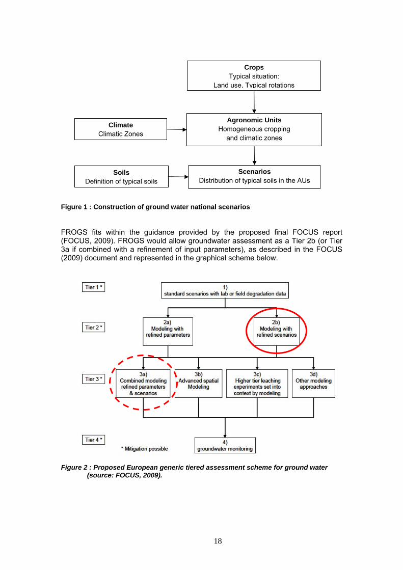
Crops Typical situation:
Land use, Typical rotations
Agronomic Units Homogeneous cropping
and climatic zones
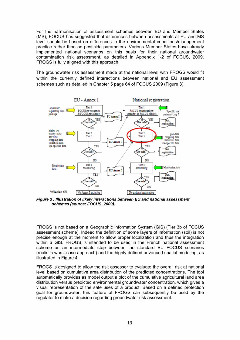
Figure 1 : Construction of ground water national scenarios FROGS fits within the guidance provided by the proposed final FOCUS report (FOCUS, 2009). FROGS would allow groundwater assessment as a Tier 2b (or Tier 3a if combined with a refinement of input parameters), as described in the FOCUS (2009) document and represented in the graphical scheme below.
Figure 2 : Proposed European generic tiered assessment scheme for ground water
(source: FOCUS, 2009).
Soils Definition of typical soils
Scenarios Distribution of typical soils in the AUs
Climate Climatic Zones
18
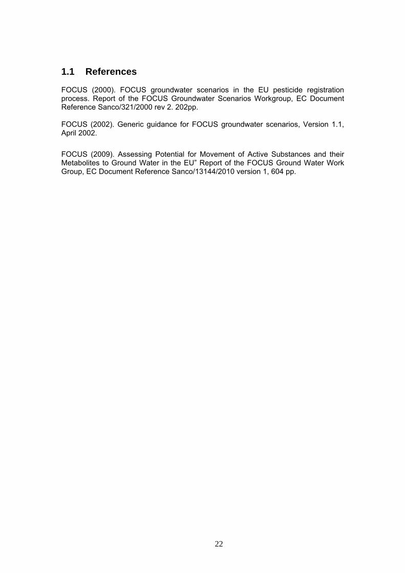
For the harmonisation of assessment schemes between EU and Member States (MS), FOCUS has suggested that differences between assessments at EU and MS level should be based on differences in the environmental conditions/management practice rather than on pesticide parameters. Various Member States have already implemented national scenarios on this basis for their national groundwater contamination risk assessment, as detailed in Appendix 1-2 of FOCUS, 2009. FROGS is fully aligned with this approach. The groundwater risk assessment made at the national level with FROGS would fit within the currently defined interactions between national and EU assessment schemes such as detailed in Chapter 5 page 64 of FOCUS 2009 (Figure 3).
Figure 3 : Illustration of likely interactions between EU and national assessment
schemes (source: FOCUS, 2009).
FROGS is not based on a Geographic Information System (GIS) (Tier 3b of FOCUS assessment scheme). Indeed the definition of some layers of information (soil) is not precise enough at the moment to allow proper localization and thus the integration within a GIS. FROGS is intended to be used in the French national assessment scheme as an intermediate step between the standard EU FOCUS scenarios (realistic worst-case approach) and the highly defined advanced spatial modeling, as illustrated in Figure 4.
FROGS is designed to allow the risk assessor to evaluate the overall risk at national level based on cumulative area distribution of the predicted concentrations. The tool automatically provides as model output a plot of the cumulative agricultural land area distribution versus predicted environmental groundwater concentration, which gives a visual representation of the safe uses of a product. Based on a defined protection goal for groundwater, this feature of FROGS can subsequently be used by the regulator to make a decision regarding groundwater risk assessment.
19

To align FROGS with existing FOCUS recommendations for defining a percentile protection goal, an overall 90th percentile value is targeted. This takes into account the spatial variability for soil and climatic conditions, and the temporal variablility on a multi-year basis in the agricultural use area of a product. An overall 90th percentile protection goal is therefore assumed, which results from an 80th percentile temporal and 80th percentile spatial distribution output from the FROGS model.
FROGS may also be used to identify scenarios and specific conditions that present potential risk to groundwater in order to propose appropriate risk management measures. Scenarios representing vulnerable conditions (soil/climate combinations) for a given pesticide application can be identified so that mitigations may be proposed based on specific soil/climatic properties. Alternatively, these vulnerable conditions may be further investigated through refined groundwater modeling (corresponding to FOCUS Tier 3), or groundwater monitoring (corresponding to FOCUS Tier 4). As an example, vulnerable soils may be identified and located more precisely within a given agronomic unit using local soil maps at the 1/250 000 scale (such as IGCS - Inventaire, Gestion et Conservation des Sols -, when available).
20

Tier 1All FOCUS scenarios 80th percentile PECgw
<0.1µg/L parent & relevant metabolites<10µg/L non-relevant metabolites
Use safe?
Tier 3Advanced mitigations/modeling
Tier 4Monitoring
Tier 2FROGS overall 90th percentile PECgw<0.1µg/L parent & relevant metabolites
<10µg/L non-relevant metabolites
Use safe?
Use safe?
National registration
yes
no
Mitigations required: identify critical scenarios conditions Mitigated FROGS overall 90th percentile PECgw
<0.1µg/L parent & relevant metabolites<10µg/L non-relevant metabolites
National registration
National registration
Use safe?
No national registration
National registration
yes
yes
yes
no
no
no
Figure 4 : Proposed use of FROGS in the French groundwater assessment scheme.
21
1.1 References FOCUS (2000). FOCUS groundwater scenarios in the EU pesticide registration process. Report of the FOCUS Groundwater Scenarios Workgroup, EC Document Reference Sanco/321/2000 rev 2. 202pp. FOCUS (2002). Generic guidance for FOCUS groundwater scenarios, Version 1.1, April 2002.
FOCUS (2009). Assessing Potential for Movement of Active Substances and their Metabolites to Ground Water in the EU” Report of the FOCUS Ground Water Work Group, EC Document Reference Sanco/13144/2010 version 1, 604 pp.
22
2 Delimitation of agronomic units At first level of national evaluation, one assumes that land occupation by various crops (arable crops), cropping characteristics and rotations can be correctly described by a set of typical situations. To define them, the variability of parameters describing soils, crops and climate should be reduced to a limited number of representative cases which can be then converted into scenarios. From this typological description should result a number of cases, necessary and sufficient, compatible with the simplicity specifications of information for modeling and the assessment objectives. The outcome of this process safeguarding a sufficient level of realism is a set of geographic zones corresponding to cropping basins named “Agronomic Units” 2.1 Agronomic Unit Concept Agronomic Units (AUs) are geographic areas in which annual crops are considered as homogeneous with regard to land use (homogenous distribution throughout the AU), cropping characteristics (dates at which key stages are reached) and most frequent rotations. Each unit can be characterized by a set of descriptors to be parameterized for modeling of the fate and behavior of plant protection products in soil. Two different agronomic units should exhibit significant differences with regard to crop land use and/or cropping characteristics. Evidently the concept of agronomic unit is very similar to a geographic cropping basin, such as the Beauce or the Alsace plains, for example. To avoid any possible confusion with this latter concept, which does not necessarily fulfill the requirements for groundwater risk assessment, AUs correspond to areas defined in the restricted framework of ground water risk assessment. AUs were defined for eight important annual crops: sugar beet, winter wheat, oilseed rape, fodder maize, grain maize, winter barley, potato and sunflower. These units are not specific to these crops so that they can also serve for other annual crops providing the same method is used to define the corresponding factors (crop characteristics, rotations, etc.). Selection of soil types in farmland is made in a separate process, independent from the determination of AUs (see Chapter 7). Soils were then allotted to AUs according to their relevance. Due to the selection method and the considerable reduction of variation, typical soil cannot be spatially located in the AUs.
23

2.2 Construction of Agronomic Units The AUs were constructed using a set of pertinent descriptors allowing for the delimitation of zones satisfying the above-mentioned homogeneity criteria using an adapted method. 2.2.1 Pertinent descriptors Three descriptor sets are relevant for the definition of AUs:
- the land use by crops, based on statistical data and most frequent rotations; - the environment, described using geomorphologic and topographic
information, including geologic substratum and soil coverage; - the climate.
These three data sets need to be taken into account simultaneously, considering the relationships between the environment and the land use. While the soil component can be analyzed separately to determine the principal soil types, the environment and the climate factors cannot be considered independently of crops, particularly because of specific requirements of certain crops. To reach the two-fold objective of realism and simplicity for national scenarios, each AU should exhibit a sufficient homogeneity of climatic and cropping factors, so that it can be characterized using a unique set of parameters. In each AU, the proportion of surface covered by a crop, the corresponding crop parameters (key dates for crop development stages), the typical rotations are determined. AUs correspond to defined geographic areas and their spatial delimitation is justified by two main reasons:
- the selection process sets limits of a defined geographic area which corresponds to a cropping basin;
- modeling a set of typical situations provides a distribution of predicted concentrations in groundwater in the cultivated areas which can be weighed by surface of crops potentially treated. This corresponds to an estimate of the safety level of the product use with regard to the treated area.
- 2.2.2 Construction Method Two different approaches may be considered to construct the AUs. Both approaches were already considered in the framework of CORPEN regional audit to determine areas where residues of plant protection products are likely to contaminate water (CORPEN, 2003).
1 Analysis of exhaustive geographic information on crops, climate and soils at high resolution; for instance, crop statistics at canton scale, weather data from synoptic Météo-France weather stations (about 100) using records of 30-year reference period, etc. Creation of homogeneous cropping and climatic zones is achieved by aggregation of elementary data using standard multivariate descriptive statistical methods.
24

2 Use of existing zonings corresponding to typological descriptions of the
territory. Elementary data are already aggregated in the defined zones by a method implicitly including some expertise. Overlay of different information layers after eventual aggregation of adjacent zones allows for the determination of homogenous zones with regard to selected homogeneity criteria (land use, crop characteristics, weather pattern).
This second method was used in the project, considering the availability of means (data and manpower). Consequently, a set of existing zonings descriptive of the environment and the climate was used along with statistics of land occupation by crops to construct the Agronomic Units. Two homogeneity criteria were retained to aggregate or keep separate adjacent zones in the existing zonings: crop parameters, including land use and key cropping dates, and climatic factors, likely to be correlated with crop characteristics. Statistical data of the national agricultural census conducted in 2000, “Recensement agricole 2000” (RA 2000) for eight major crops was also used to build up the Agronomic Units. 2.2.3 Agricultural Statistics RA 2000 is a relatively recent and exhaustive information base providing cultivated surfaces for a number of crops at different administrative scales: community, canton, department and region. Data by canton provide sufficiently accurate information for the description of land use. Cultivated surface by canton is approximately 7800 ha in average, peaking at 35 000 ha in intensively cultivated areas. Changes in the cultivated surfaces of certain crops have been observed since the last census but they are not likely to modify the distribution of crop surfaces in the Agronomic Units. An update of land use data can be envisaged on the basis of the next census planned in 2011. Significant changes in land use can be observed in a decade time step, the main cause being economic since surfaces of opportunistic crops vary relatively quickly according to their profitability. Conversely, a number of crops are known to be more or less closely dependent on environmental characteristics, even though means of modern agriculture have largely reduced this dependency. The old land zoning in “Small Agricultural Regions": Petites Régions Agricoles (PRA) reflects well the relationship between environment and agricultural production. To insure a sufficient stability of the AUs despite short-term changes of land use by certain crops, it is useful to include in their basic determinants a number of stable factors which are also strong determinants of agricultural activities. Land occupation by certain crops in well identified cropping basins or AUs is clearly displayed on crop density maps which represent the proportion of surface covered by the crop of interest in the cultivated surface of a canton. Density thresholds aiming at selecting the cantons in which a crop can be considered as significantly present have been set by INRA in the soil selection process (Morvan & Lebas, 2006, see Chapter 7). Hence, only a certain proportion of the crop surface is taken into account once a density threshold is set, overlooking the cultivated surface in the cantons where the crop is not significantly present.
25
This selection excludes areas which are not cultivated (forests, urban areas) or where arable crops are of little importance (hilly and mountainous zones). The contours of territories are well delineated for crops under the dependence of environmental factors (sugar beet, sunflower). They look imprecise or are even difficult to establish for ubiquitous crops which are less dependent on environmental factors (cereals, maize). Most often, a gradient of crop density is observed from the center to the boundaries of the AU. Inclusion of peripheral cantons in a cropping basin where the crop density is close to the selection threshold is problematic since expanding excessively a cropping basin would contradict the criteria of crop and climate homogeneity. 2.2.4 Environmental Zoning Existing environmental zonings used in the construction of Agronomic Units are described in this section. 2.2.4.1 Small Agricultural Regions The concept of Small Agricultural Region (« Petite région agricole »: PRA) is based on two sets of characteristics of different nature:
- permanent environmental characteristics (geology, geomorphology, topography, pedology, climate, etc.);
- characteristics variable in a decade time frame, linked to the socio-economic framework (farming systems, land use, farm size, etc.).
This land partition, initially designed to collect and process structural and economic data (first publication in 1956) is used with different purposes: data interpretation of demographic and agricultural census, enforcement of certain regulations, etc. (INSEE-SCEES, 1983). Although PRA contours have been modified in certain occasions, the statistical character of the zoning justifies the fact that no fundamental revision has taken place since then (last publication in 1983). Agricultural Regions (« Région agricole »: RA) are defined by grouping several communities, leading to 433 RA in total, 255 being located within one single département (RA intra-département) and 178 in more than one département (RA inter-départements). After splitting the latter with department limits, a total of 713 PRA are obtained. The PRA is defined in function of a same dominant agricultural orientation. It characterizes well the basic agricultural units as a function of both their production and their environmental characteristics. The alternative concept of "Small Natural Region" corresponds to the need for zoning territorial entities on the basis of permanent environmental features. In general, it is possible to split Small Agricultural Regions into several Small Natural Regions with a pedologic significance. An order of magnitude of the average surface for these units is a few thousand hectares. Although attractive, the concept of Small Natural Region was not used since the corresponding zoning is not available for the entire territory.
26
2.2.4.2 Cropping Basins A number of pedologic and agroclimatic reference documents include a territory zoning at the scale of an administrative region or a département. The typological description of the environment and land use they propose reflects relatively well typical situations suitable for scenario construction. For example, the pedologic repository for West (« Référentiel des sols de l’Ouest »: http://www.cript-bretagne.fr) defines 20 cropping basins and 41 soil types in the four administrative regions of West (Basse-Normandie, Bretagne, Pays de la Loire, Poitou-Charentes) These basins are built by grouping 69 Small Agricultural Regions and include from 1 to 7 PRAs by basin. Following the example of the procedure used for the West pedologic Repository, PRA aggregation into larger units can be realized in other areas using geomorphologic and climatic similarity criteria. Nevertheless a reduced number of cropping basins is difficult to achieve. Except for large alluvial plains of main streams, PRA aggregation erases the units corresponding to smaller river plains, for the benefit of larger inter-stream structural units. Furthermore, some PRA, which are well defined geographic entities but have a too small size to constitute an agronomic unit, are in a transition position between agricultural regions with contrasted features. In this case, the decision to aggregate the PRA to one or another adjacent region is arbitrary in absence of precise rules. Similarity criteria at a larger scale are then necessary to achieve a consistent grouping. Various regional agronomic repositories (Ailliot B. et Verbeque B., 1995 ; Delaunois A., Longueval C., 1995 ; Froger D. et al., 1994 ; Jacquin J., Florentin L., 1988) and pedologic repositories (Ballif J.L. et al., 1995 ; Chrétien J., 2000 ; Roque J., 2003 ; Sterckeman et al., 2002), and other national or regional geographic documents (Battiau-Queney Y., 1993 ; Mottet G., 1993), among many others not listed in the bibliography (including information taken from web sites of various organizations such as DIREN, Chambres d’agriculture, etc. and from the GIS layers they provide), describe the environment on a geomorphologic basis. This information was used for grouping PRAs into AUs. 2.2.4.3 Climatic Regions Several agro-climatic zonings can be used for the delimitation of the AUs. 29 agro-climatic regions have been defined by Choisnel, 18 corresponding to cultivated areas, (Appendix 2). Monograph n°4 of Météo-France (Céron J.P. et al., 1991) defines not connected climatic zones for temperature (18 zones), precipitation (18 zones) and solar irradiance (11 zones), along with a reference weather station for each zone. Combination of synthetic maps for these three parameters, which exclude mountainous areas, does not produce a usable climatic zoning. In a same zone of intersection for the three climatic parameters, reference stations often differ. However, the synthetic map for precipitation is in relative good agreement with the large cropping basins.
27

Maps representing classes of annual and seasonal precipitation (quintile), aggregated by PRA were produced by INRA and Météo-France to estimate the risk of erosion (Le Bissonais Y. et al., 1998, 2002). Mean monthly precipitation calculated using 30-year records are one of the parameters used to estimate the erosion intensity. Local weather information provided by 95 primary stations of Météo-France (about one per département) was spatialized at a scale of 5 km square grid using the AURELY method which takes into account the topography. Mean monthly precipitation data are distributed in five classes for each climatic season and the year. The corresponding maps of precipitation aggregated by PRA are shown in Appendix 3. They are used for grouping PRAs with similar seasonal precipitation patterns. Finally, complementary weather information can be found in the document on Hydro-ecoregions (HER) outlined in the next chapter (Wasson J.G. et al., 2002), in particular the analysis of spatial distribution of mean annual precipitation. 2.2.4.4 Hydro-ecorégions Hydro-ecorégions (HER) define a typology of ecosystems for surface water to help establishing reference levels of aquatic invertebrate populations for the Water Framework Directive (Wasson J.G. et al., 2002). A first level (HER-1) identifies the large environment structures corresponding to important changes of at least one fundamental, geographic or climatic parameter. Hence, 22 level-1 Hydro-ecorégions are defined using criteria combining geology, topography and climate which are considered as primary determinants in the functions of continental aquatic ecosystems. A second level (HER-2) identifies zones within which the different parameters can be considered as homogeneous with regard to the global heterogeneity of national territory. It addresses the internal variability of HER of level 1. The list of HER of both levels and the corresponding map is in Appendix 4. Even though Hydro-ecoregions are aiming at establishing a typology of continental fresh waters, the criteria used in the HER construction method belong to general domains (geology, topography, climate) which are combined in an approach mostly based on geomorphologic considerations. An important element in this analysis of the environment is the lithology of geologic materials which, with its permeability characteristics (interstitial, fissure, fracture), largely influences the partition of water between surface and ground resources. Actually, lithology data of geologic materials, complemented by geomorphologic information (geomorphologic maps at the 1/1 000 000 scale, GIP RECLUS Montpellier, 1988-1993) constitutes the physical basis of HER determination. Consequently, Hydro-Ecoregions can also be considered as determinants of terrestrial environment which allows for a reduction of the global variation in a limited set of typical situations. HER contours very often match the limits of mapping units of the 1/1000 000 scale geologic map (BRGM). Furthermore, the physical basis of HER determination helps linking the HER units with anthropic pressures such as agricultural activities. The use of HER in the construction of AUs is described in the following section.
28

2.3 Zoning Method of Agronomic Units 2.3.1 Overlay of Information Layers Considered individually, existing zonings reflect only a part of the criteria needed for the determination of AUs. In addition to the two basic zoning criteria retained (land use by crops and climate), integrated physical environment information was added thanks to the two HER levels. Combination of these three homogeneity criteria of zones allows for a pertinent aggregation of elementary units (cantons, PRAs) into homogeneous AUs. These are defined by expert judgment using the combinations of climatic regions and Hydro-ecoregions as a consistency basis. In an implicit way, a hierarchy is established between the criteria. PRAs which reflect the more or less strict dependency of cultivated crops with the environment characteristics are used as basic elements of the zoning. Difficulties encountered in PRA grouping into larger units result from aggregation uncertainties in the question of to which of two or three adjacent AUs this PRA should be included. This hurdle is overcome thanks to the HER level 2 zoning. It actually provides a sound reason for assembling units which have been differentiated on the basis of particular characteristics. Grouping PRAs which differ on a number of characteristics in a same AU is guided by physical and essentially geomorphologic considerations. This process also takes into account weather information at PRA scale using the annual and seasonal precipitation classes. Climatic homogeneity within the AUs is an important requirement to select a unique representative set of crop parameters. As a second criterion of PRA grouping, land use by crops is not taken into account in the same way according to the crop considered. For ubiquitous crops which are well represented in most of the AUs, the density variation between two adjacent AUs does not usually show a clear transition. In this case, the limits between AUs are set following environmental (physical and/or climatic) limits. The distinction between the two AUs is maintained since it can be fully justified for crops which exhibit a significant density difference between the two Units. Conversely, land use by crops which are not ubiquitous is often consistent with environmental characteristics. In this case, the limit between AUs corresponds to a clear transition in crop density. No rigorous protocol was therefore used in the PRA pooling. Depending on the situations, the limit between adjacent AUs was defined using the weather (precipitation) or the geomorphology (HER 2) parameter. In many cases, the limit was determined using expert judgment rather than following a strict operating procedure. The decisions made about AU boundaries might be arbitrary in a number of cases, but are not expected to have any significant impact on the scenarios, since the overall aim of the AUs is to reflect typical situations that exist more likely around the centroid of the AU polygons rather than close to their limits. 2.3.2 Practical Method of PRA Aggregation The various information layers call for different geographic delimitation bases: administrative limits for crop statistical information (cantons) and PRAs (municipalities), physical limits for Hydro-ecoregions and climate. Hence, the contours of the elementary units cannot strictly overlap. For practical use, AUs are built by PRA aggregation. Consequently the contours follow community limits. Seeing
29
30
that they principally reflect homogeneous typical agronomic situations, AUs do not require to be delimited with very accurate contours, so that limits of PRA groups can serve the purpose. Resulting contours provide a sufficient spatial resolution to follow the limits of physical units represented at scales of 1/1 000 000 (geology) or 1/500 000 (geomorphology). Crop land use in an AU is estimated using information from the cantons which are located within its geographic limits. Ideally, estimation of land use with agricultural statistics at community scale is preferable since AU contours will fully correspond to municipality limits. Such accurate information is not readily available and is probably not needed considering the uncertainties of limits between two adjacent AUs. As a consequence of the different zonings for AUs (PRAs with municipality limits) and crop statistics (cantons), some cantons are intersected by the limits between two, sometimes three, adjacent AUs. Hence the following rule is applied to allot the canton to one or the other AU. A canton polygon intersected by two adjacent AUs is allotted to the AU which covers the largest surface of the polygon, or eventually best matches the limit between the two AUs. This rule assumes a regular distribution of the cultivated surfaces in the canton. In absence of more accurate information on land use in the canton, this assumption is necessary, although it is likely to be wrong in certain cases, particularly when the limit between the two AUs corresponds to physical boundaries. A decreasing gradient of crop density is frequently observed in the AUs from the center to the boundaries. If the crop considered is not present in an adjacent AU, the limit with the former can be arbitrary. Conversely, such difference is not necessarily observed with another crop which is more ubiquitous. This is the reason why climatic and geomorphologic criteria (HER) are of primary importance in the delimitation and have been preferred to strict land occupation by crops. Consequently, the spatial distribution of a crop can be uneven in a large AU. 2.4 Zoning Results 2.4.1 Delimitation of Agronomic Units The method outlined in the previous section leads to 31 AUs which include between 2 and 32 Small Agricultural Regions (PRA). They are named explicitly in reference with cropping basins (Table 1). Agronomic Unit code "0" corresponds to the excluded territory (forests, urban areas, mountainous zones, areas with small surface of arable crops). AU surfaces range between 335 and 2118 kha, with a mean value of 1238 kha. SAU (Surface Agricole Utilisée) correspond to cultivated surfaces in the AUs and are expressed as kha and percentage of the total AU surface. The contours of the AUs are represented in Figure 5. Each AU is a set as Small Agricultural Regions (PRA) as shown on Figure 6, the list of which is given in Appendix 4. Digital geographic information for AUs is provided in the FROGS v2.2.2.2 package under ESRI ArcGis format.

Table 1 : Defined Agronomic Units
SAU (kha)
SAU (kha)
SAU (%)
SAU (%)
Surface (kha)
Surface (kha) AU N° Agronomic Unit AU N° Agronomic Unit
0 Territoire non pris en compte 16303 5735 35.2 16 Champagne crayeuse 1113 728 65.4
1 Collines molassiques - Lauragais 1902 1214 63.8 17 Beauce - Drouais - Gâtinais 1333 958 71.9
2 Bretagne sud 896 456 50.9 18 Bordelais - Périgord - Coteaux du Lot 2068 904 43.7
3 Limagnes - Plaine du Forez 1024 640 62.5 19 Perche - Pays d'Auge - Pays d'Ouche 1385 869 62.7
4 Bordure maritime Nord - Picardie - Normandie 1825 1267 69.5 20 Bocages de l'ouest 2002 1341 67.0
Ardenne - Argonne - Champagne humide 5 Alsace - Sundgau 588 285 48.5 21 913 556 60.9
6 Plaine normande - Bessin 335 250 74.5 22 Champagne berrichonne - Boischaut 1640 1050 64.0
7 Aquitaine - Landes 1263 161 12.8 23 Bas Dauphiné - Vallée du Rhône 1025 443 43.2
8 Bassin de l'Adour 1058 584 55.1 24 Fossé bressan 1036 558 53.9
9 Picardie - Nord - Pas-de-Calais 1587 1101 69.4 25 Bretagne centrale 685 431 62.9
10 Charentes 1917 1333 69.6 26 Plateaux de Haute-Saône 784 348 44.4
11 Bocage normand 1467 1105 75.3 27 Provence 892 177 19.9
12 Barrois - Plateaux bourguignons 2118 1040 49.1 28 Plaine du Languedoc-Roussillon 1000 359 35.9
13 Plateau lorrain 1139 637 56.0 29 Boischaut du sud 712 503 70.7
14 Gâtines - Vallées de Loire 1099 629 57.2 30 Bretagne nord 1246 836 67.1
15 Sologne - Orléanais 698 154 22.1 31 Ile-de-France 1637 905 55.3
31
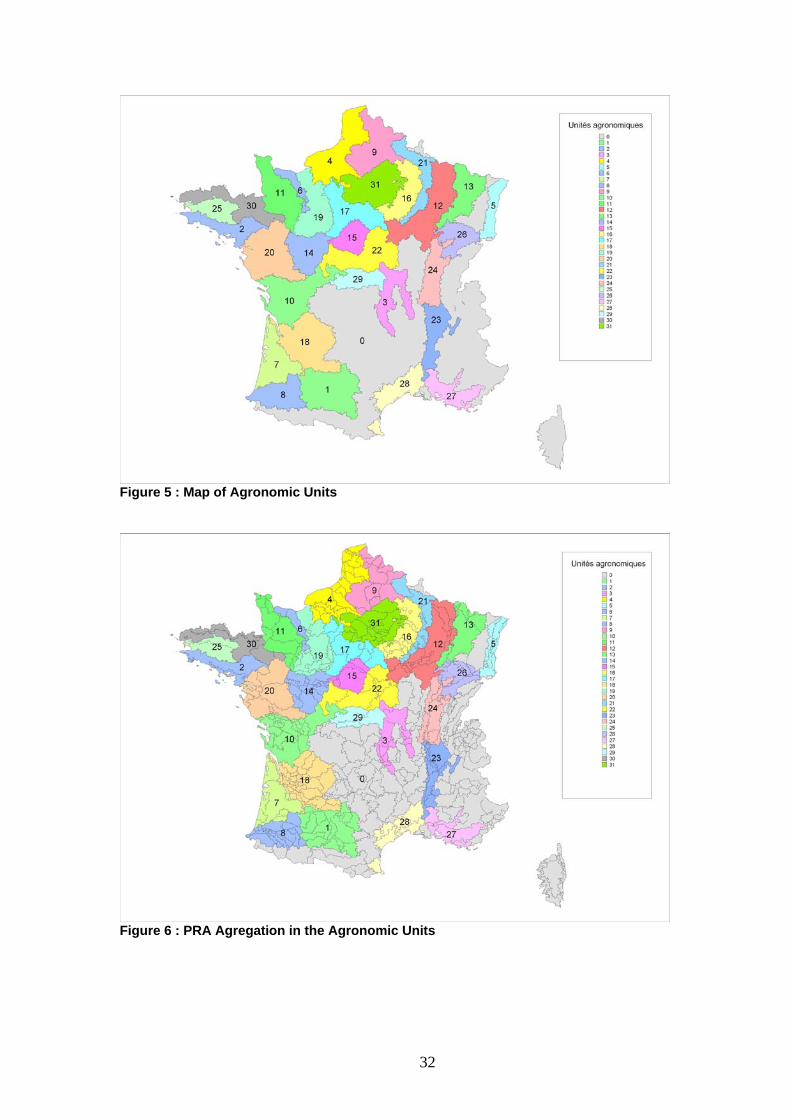
Figure 5 : Map of Agronomic Units
Figure 6 : PRA Agregation in the Agronomic Units
32
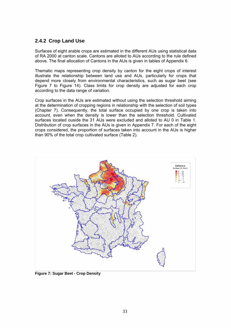
2.4.2 Crop Land Use Surfaces of eight arable crops are estimated in the different AUs using statistical data of RA 2000 at canton scale. Cantons are alloted to AUs according to the rule defined above. The final allocation of Cantons in the AUs is given in tables of Appendix 6. Thematic maps representing crop density by canton for the eight crops of interest illustrate the relationship between land use and AUs, particularly for crops that depend more closely from environmental characteristics, such as sugar beet (see Figure 7 to Figure 14). Class limits for crop density are adjusted for each crop according to the data range of variation. Crop surfaces in the AUs are estimated without using the selection threshold aiming at the determination of cropping regions in relationship with the selection of soil types (Chapter 7). Consequently, the total surface occupied by one crop is taken into account, even when the density is lower than the selection threshold. Cultivated surfaces located ouside the 31 AUs were excluded and alloted to AU 0 in Table 1. Distribution of crop surfaces in the AUs is given in Appendix 7. For each of the eight crops considered, the proportion of surfaces taken into account in the AUs is higher than 90% of the total crop cultivated surface (Table 2).
Figure 7: Sugar Beet - Crop Density
33

Figure 8: Winter Wheat - Crop Density
Figure 9: Oilseed Rape - Crop Density
34

Figure 10: Maize Fodder - Crop Density
Figure 11: Maize Grain - Crop Density
35
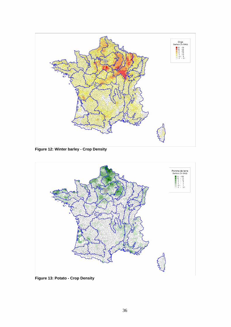
Figure 12: Winter barley - Crop Density
Figure 13: Potato - Crop Density
36
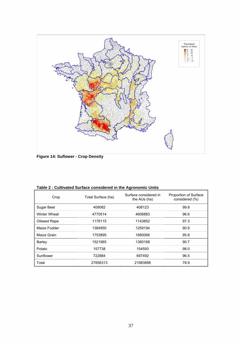
Figure 14: Suflower - Crop Density
Table 2 : Cultivated Surface considered in the Agronomic Units
Surface considered in the AUs (ha)
Proportion of Surface considered (%) Crop Total Surface (ha)
Sugar Beet 409082 408123 99.8
Winter Wheat 4770514 4606883 96.6
Oilseed Rape 1176115 1143852 97.3
Maize Fodder 1384950 1259194 90.9
Maize Grain 1753895 1680066 95.8
Barley 1521965 1380168 90.7
Potato 157738 154593 98.0
Sunflower 722884 697492 96.5
Total 27856313 21983898 78.9
37

Importance of surfaces in the Agronomic Units is qualitatively represented according to four surface boundaries: 5 000 ha, 10 000 ha, 50 000 ha and 100 000 ha) in Table 3, where surfaces are expressed as kHa. This representation by color codes is used throughout this document in descriptive tables of crop surfaces. The number of AUs retained as a function of a surface threshold is indicated at the bottom of Table 3. This number varies largely according to the crop and the class surface. For instance, the potato surface in the AUs is always less than 100 000 ha and is higher than 50 000 ha in only one AU. Conversely, winter wheat is present in a large number of AUs, most of them belonging to the surface class corresponding to surfaces higher than 100 000 ha. Surfaces taken into account as a function of thresholds and corresponding proportions in the total cultivated surface are indicated in Table 4. Surfaces ranging between 5 000 and 10 000 ha do not significantly increase the proportion of surfaces taken into account in the AUs. The distribution of crops in the Agronomic Units as a function of density classes (proportion of surface for a crop in the cultivated surface of the AU) is shown in Appendix 8. Class limits, specific for each crop, are indicated at the bottom of the table. Implicitly, this approach recalls the representativity thresholds defined in the INRA study.
38

39
Table 3 : Distribution of crops in the AUs by Surface Classes (kha)
AU Agronomic Unit
Sug
ar B
eet
Win
terW
heat
Oils
eed
Rap
e
Mai
ze F
oder
Mai
zerG
rain
Bar
ley
Pot
ato
Sun
flow
er
1 Collines molassiques - Lauragais 0 75 22 19 141 39 0 177
2 Bretagne sud 0 64 8 72 32 13 1 1
3 Limagnes - Plaine du Forez 3 79 12 16 36 16 1 9
4 Bordure Nord - Picardie - Normandie 57 363 41 99 10 115 23 0
5 Alsace - Sundgau 5 35 4 11 126 5 1 0
6 Plaine normande - Bessin 6 66 8 21 5 13 1 1
7 Aquitaine - Landes 0 1 0 1 75 0 1 1
8 Bassin de l'Adour 0 5 1 30 246 3 0 2
9 Picardie - Nord - Pas-de-Calais 127 460 28 46 28 85 64 0
10 Charentes 0 280 77 42 174 73 1 168
11 Bocage normand 0 132 11 200 17 19 2 2
12 Barrois - Plateaux bourguignons 2 293 181 37 12 180 0 6
13 Plateau lorrain 0 124 65 42 6 53 0 1
14 Gâtines - Vallées de Loire 0 170 43 21 58 33 0 78
15 Sologne - Orléanais 0 32 12 3 19 9 1 6
16 Champagne crayeuse 71 246 55 4 21 122 18 9
17 Beauce - Drouais - Gâtinais 35 403 108 4 56 122 7 14
18 Bordelais - Périgord - Coteaux du Lot 0 95 9 30 134 26 2 45
19 Perche - Pays d'Auge - Pays d'Ouche 2 212 56 64 51 48 0 11
20 Bocages de l'ouest 0 177 28 174 49 30 1 35
21 Ardenne - Argonne - Champagne H. 12 120 41 32 23 53 2 3
22 Champagne berrichonne - Boischaut 0 312 145 15 42 95 0 55
23 Bas Dauphiné - Vallée du Rhône 0 49 10 11 64 15 1 23
24 Fossé bressan 4 99 32 17 84 30 1 18
25 Bretagne centrale 0 69 6 68 29 20 3 0
26 Plateaux de Haute-Saône 0 49 23 16 18 22 0 5
27 Provence 0 1 2 0 3 1 1 5
28 Plaine du Languedoc-Roussillon 0 1 2 0 2 1 0 5
29 Boischaut du sud 0 52 18 11 6 19 0 13
30 Bretagne nord 0 167 17 147 60 33 10 0
31 Ile-de-France 82 377 77 7 53 88 12 2
No. of AUs with Surface ≥ 100 000 ha 1 15 3 3 5 4 0 2
No. of AUs with Surface ≥ 50 000 ha 4 23 8 7 13 10 1 4
No. of AUs with Surface ≥ 10 000 ha 6 27 22 24 26 25 5 11
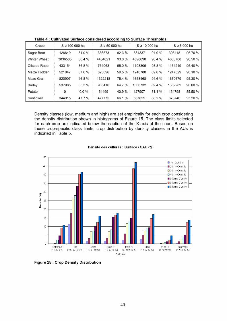
Table 4 : Cultivated Surface considered according to Surface Thresholds Crope S ≥ 100 000 ha S ≥ 50 000 ha S ≥ 10 000 ha S ≥ 5 000 ha
Sugar Beet 126649 31.0 % 336573 82.3 % 384337 94.0 % 395448 96.70 %
Winter Wheat 3836585 80.4 % 4434621 93.0 % 4598698 96.4 % 4603708 96.50 %
Oilseed Rape 433154 36.8 % 764063 65.0 % 1103306 93.8 % 1134219 96.40 %
Maize Fodder 521047 37.6 % 823896 59.5 % 1240788 89.6 % 1247329 90.10 %
Maze Grain 820907 46.8 % 1322218 75.4 % 1658468 94.6 % 1670679 95.30 %
Barley 537985 35.3 % 985416 64.7 % 1360732 89.4 % 1369982 90.00 %
Potato 0 0.0 % 64499 40.9 % 127907 81.1 % 134798 85.50 %
Sunflower 344915 47.7 % 477775 66.1 % 637825 88.2 % 673740 93.20 %
Density classes (low, medium and high) are set empirically for each crop considering the density distribution shown in histograms of Figure 15. The class limits selected for each crop are indicated below the caption of the X-axis of the chart. Based on these crop-specific class limits, crop distribution by density classes in the AUs is indicated in Table 5.
Figure 15 : Crop Density Distribution
40

41
Table 5 : Distribution of Crops in the AUs by Density Classes
AU Agronomic Unit
Sug
ar B
eet
Win
ter W
heat
Oils
eed
Rap
e
Mai
ze F
odde
r
Mai
ze G
rain
Bar
ley
Pot
ato
Sun
flow
er
1 Collines molassiques - Lauragais 0,0 6,0 1,8 1,5 11,3 3,1 0,0 14,2
2 Bretagne sud 0,0 13,8 1,7 15,6 6,9 2,7 0,2 0,1
3 Limagnes - Plaine du Forez 0,5 12,9 2,0 2,6 5,9 2,7 0,1 1,5
4 Bordure Nord - Picardie - Normandie 4,6 29,6 3,4 8,1 0,8 9,4 1,9 0,0
5 Alsace - Sundgau 1,9 12,6 1,4 3,8 45,5 1,7 0,4 0,1
6 Plaine normande - Bessin 2,3 26,3 3,1 8,2 2,0 5,3 0,3 0,6
7 Aquitaine - Landes 0,0 0,7 0,0 0,7 47,8 0,2 0,6 0,5
8 Bassin de l'Adour 0,0 0,8 0,2 5,0 41,7 0,4 0,0 0,3
9 Picardie - Nord - Pas-de-Calais 11,1 40,3 2,5 4,0 2,5 7,5 5,7 0,0
10 Charentes 0,0 21,2 5,9 3,2 13,2 5,5 0,1 12,7
11 Bocage normand 0,0 11,9 1,0 18,0 1,6 1,7 0,2 0,2
12 Barrois - Plateaux bourguignons 0,2 28,0 17,3 3,5 1,2 17,2 0,0 0,6
13 Plateau lorrain 0,0 19,4 10,2 6,6 0,9 8,3 0,0 0,1
14 Gâtines - Vallées de Loire 0,0 26,7 6,7 3,3 9,2 5,2 0,0 12,2
15 Sologne - Orléanais 0,3 20,1 7,5 1,6 11,9 5,9 0,6 4,0
16 Champagne crayeuse 9,7 33,5 7,5 0,5 2,8 16,6 2,5 1,3
17 Beauce - Drouais - Gâtinais 3,7 42,1 11,2 0,5 5,8 12,7 0,7 1,5
18 Bordelais - Périgord - Coteaux du Lot 0,0 10,3 1,0 3,2 14,5 2,8 0,2 4,9
19 Perche - Pays d'Auge - Pays d'Ouche 0,2 24,3 6,4 7,3 5,8 5,5 0,1 1,3
20 Bocages de l'ouest 0,0 13,1 2,1 12,9 3,6 2,2 0,1 2,6
21 Ardenne - Argonne - Champagne H. 2,2 21,5 7,4 5,7 4,1 9,5 0,3 0,5
22 Champagne berrichonne - Boischaut 0,0 29,5 13,6 1,4 3,9 9,0 0,0 5,2
23 Bas Dauphiné - Vallée du Rhône 0,0 10,8 2,3 2,5 14,3 3,3 0,3 5,2
24 Fossé bressan 0,8 17,7 5,7 3,1 15,0 5,3 0,2 3,1
25 Bretagne centrale 0,0 16,0 1,4 15,9 6,7 4,5 0,7 0,0
26 Plateaux de Haute-Saône 0,0 13,9 6,6 4,6 5,2 6,3 0,0 1,4
27 Provence 0,0 0,7 1,1 0,0 1,4 0,5 0,4 2,6
28 Plaine du Languedoc-Roussillon 0,0 0,2 0,6 0,0 0,4 0,4 0,1 1,4
29 Boischaut du sud 0,0 10,0 3,5 2,2 1,2 3,7 0,0 2,4
30 Bretagne nord 0,0 19,8 2,0 17,5 7,2 3,9 1,2 0,0
31 Ile-de-France 8,8 40,3 8,3 0,7 5,6 9,4 1,3 0,3
No. of AUs of high density class 3 4 4 4 3 3 1 3
No. of AUs of medium density class 4 13 13 11 9 10 2 3
No. of AUs of low density class 8 26 28 25 21 27 5 17

The distributions shown in Table 3 and Table 5 are similar, with a few additional AU x Crop combinations in the analysis of densities corresponding to surfaces below 10 000 ha. Consequently, surface classes were used to characterize the importance of crops in the AUs (Table 3). 2.5 References
Ailliot B. & Verbeque B. (1995). Les terres de Beauce. Chambres d’Agriculture d’Eure-et-Loir, du Loiret et du Loir-et-Cher.
Arvalis - Institut du vegetal. (2003). Atlas agroclimatique du maïs.
Ballif J.L., Guérin H., Muller J.C. (1995). Éléments d’agronomie champenoise. Connaissance des sols et de leur fonctionnement. Rendzines sur craie et sols associés. INRA Editions. Barthès J.P., Bornand M., Falipou P. (1999) Référentiel Pédologique de la France. Pédopaysages de l’Aude, du Gard, de l’Hérault, de la Lozère et des Pyrénées Orientales (4 volumes). INRA Editions. Battiau-Queney Y. (1993). Le relief de la France - Coupes et croquis. Masson géographie. Ceron J.P., Desroziers M., Merlier C., Perarnaud V., Schneider M. (1991). Régions climatiques - Températures, précipitations, insolation. Météo-France, Monographie n°4. Choisnel E. Agrométéorologie. Techniques de l’ingénieur. Chrétien J. (2000). Référentiel pédologique de Bourgogne à 1/250 000. INRA. CORPEN (2003). Comité d’orientation pour des pratiques agricoles respectueuses de l’environnement (CORPEN). Éléments méthodologiques pour un diagnostic régional et un suivi de la contamination des eaux liée à l’utilisation des produits phytosanitaires. Groupe Phytoprat-SIG, Mai 2003. Delaunois A., Longueval C. (1995). Les grands ensembles morpho-pédologiques de la région Midi-Pyrénées. Chambre régionale d’agriculture de Midi-Pyrénées. FOCUS (2000). FOCUS Ground Water Scenarios in the Review of active Substances. Report of the FOCUS Groundswater Scenarios Workgroup EC. Document Reference Sanco/321/2000 rev. 2, Nov. 2000. Froger D., Moulin J., Servant J. (1994). Les terres de Gâtines, Boischaut-Nord, Pays-Fort Chambre d’Agriculture de la région Centre. INSEE-SCEES (1983). Code et nomenclature des régions agricoles de la France au 1er janvier 1980. Jacquin J., Florentin L. (1988). Atlas des sols de Lorraine. Presses Universitaires de Nancy.
42

43
Le Bissonnais Y., Montier C., Daroussin J., King D. (1998). Cartographie de l’aléa « Érosion des sols » en France. IFEN, Collection Études et Travaux n°18, août 1998. Le Bissonnais Y., Thorette J., Bardet C., Daroussin J. (2002). L’érosion hydrique des sols en France. INRA - IFEN, novembre 2002. Lenfant A. (1989). Référentiel agronomique - Les sols des pays de Loire. Chambre d’agriculture des Pays de la Loire. Morvan X., Lebas C. (2006). Détermination de profils types de sols par régions de culture. INRA Unité Infosol, Orléans. Mottet G. (1993). Géographie physique de la France. Presses Universitaires de France, 3ème édition. OECD (1999). OECD Environment Directorate. Environmental Exposure Assessment Strategies for Existing Industrial Chemicals in OECD Member Countries. OECD Series on Testing and Assessment, Number 17. Document 77030, Apr. 21, 1999. Roque J. (2003). Référentiel régional pédologique d’Ile de France à 1/250 000. INRA. Schaefer H., Dust M., Gottesbüren B., Jones R., Maund S., Maycock R., Yon D. (2003). ECPA Position Paper on the Development of National Ground Water Scenarios within the European Union. European Crop Protection Association, March 11, 2003. Sterckeman T., Douay F., Fourrier H., Proix N. (2002). Référentiel pédo-géochimique du Nord - Pas de Calais. INRA - ISA (Laboratoire Sols et Environnement). Rapport final, 15 octobre 2002. Wasson J.G., Chandesris A., Pella H., Blanc L. (2002). Les hydro-écorégions de France métropolitaine - Approche régionale de la typologie des eaux courantes et éléments pour la définition des peuplements de référence d’invertébrés. Cemagref : Programme de recherche Hydreco, contrat n°2001-06-9-084-U, juin 2002.
3 Crop Rotations In order to be as representative as possible of standard agricultural practices, typical crop rotations are implemented in FROGS. Surveys were conducted with field experts from Arvalis – Institut du Végétal and from UIPP members to identify the most common crop rotation or rotations associated to the different relevant crop – AU combinations. These crop rotations were further checked using a probabilistic approach based on Agreste data (Agreste, 2001), and in some circumstances the probabilistic approach was used to select the most representative rotation between two possible typical crop rotations. The selected crop rotations were implemented in FROGS with some adaptations in order to fit the PEARL crop calendar concept. 3.1 Crop rotation surveys Surveys were conducted to determine the most typical crop rotations (in order of importance) associated with each relevant crop – AU combination (see Chapter 2). Each of the crops considered in FROGS, i.e. winter wheat, winter barley, oilseed rape, fodder maize, grain maize, potatoes, sunflower, were considered separately in the surveys, as a so-called primary crop, to get the most typical crop rotation for the crop under consideration in a given AU as opposed to the most typical crop rotation in the AU. This means that the same crop may appear in different rotations in the same AU, and that a primary crop may appear as rotation crop when looking at another primary crop. For example, Sugar beet-Winter Wheat-Winter Wheat may be the most typical crop rotation when considering sugar beet as primary crop, while Winter Wheat-Maize fodder would be the most typical crop rotation in the same AU when considering winter wheat as primary crop. This means that in the AU in question (Limagnes – Plaine du Forez), sugar beet (not a major crop in that AU but still representing a significant surface area) is most often associated with winter wheat, while winter wheat (a major crop in that AU) is most often not associated with sugar beet but rather with fodder maize. The results of the surveys gave between 3 to 5 possible crop rotations for each Agronomic Unit3. Rotation periods extending from 2 to 6 six years were obtained. Information on typical planting, emergence and harvest dates for the crops included in the rotations were also collected in the surveys. 3.2 Probabilistic approach For sugar beet, wheat, oilseed rape, grain maize, fodder maize and barley, the Ministry of Agriculture conducted a survey that included information on previous crop in the same field (Agreste, 2001). These data are available at administrative Region level and are summarized in Table 6.
3 The first survey was conducted before the AUs were fully delimited and mapped. The initial data collection was made based on geographical zones (e.g. Flandre maritime, Drouais-Thymerais, Nord-Pas-de-Calais (sauf littoral)) corresponding to well-known cropping regions for the local experts and which are very close to the current AU definition. Subsequent data collection was made based on the actual AUs. To ease the reading of this document, these cropping regions are considered equivalent to AU and as a consequence only the AU names are used.
44
45
Table 6 Acreage of previous crop for each primary crop available in Agreste (2001)
Primary crop Oilseed rape Barley Wheat Maize Sugarbeet
Previous Crop (year n-1) Wheat Barley Wheat Barley Maize Wheat MaizeOilseed
rape Sunflower Others Wheat MaizeOther
cereals Wheat Barley others
(% acreage) Alsace - - - - - 9% 73% 9% 1% 8% 17% 73% 2% - - - Aquitaine - - - - - 13% 23% 4% 34% 26% 5% 84% 2% - - - Auvergne - - - - - 34% 27% 13% 9% 18% 38% 43% 8% - - - Basse Normandie - - - - - 13% 50% 14% 0% 24% 40% 41% 7% - - - Bourgogne 35% 63% 85% 8% 1% 19% 8% 54% 9% 10% 23% 44% 15% - - - Bretagne - - 52% 5% 33% 11% 65% 6% 0% 17% 30% 36% 12% - - - Centre 62% 35% 79% 8% 4% 26% 13% 34% 10% 17% 46% 31% 11% - - - Champagne Ardenne 35% 63% 72% 7% 3% 13% 7% 35% 2% 43% 58% 35% 6% France Comté 46% 46% 67% 12% 9% 8% 32% 45% 6% 8% 27% 39% 21% - - - Haute Normandie 56% 43% 74% 7% 6% 23% 20% 23% 0% 33% 48% 22% 22% - - - Ile de France 59% 40% 81% 10% 5% 24% 13% 23% 1% 37% 72% 12% 11% 74% 26% 1% Lorraine 38% 60% 72% 14% 6% 21% 14% 58% 1% 5% 41% 34% 20% - - - Midi Pyrénées - - 18% 23% 11% 18% 13% 7% 44% 18% 9% 67% 7% - - - Nord pas de calais 85% 6% 0% 13% 20% 3% 0% 63% 63% 14% 17% 71% 23% 6% Pays de la loire - - - - - 14% 48% 17% 11% 11% 27% 42% 6% - - - Picardie 48% 51% 84% 4% 3% 20% 12% 10% 0% 57% 53% 15% 21% 85% 13% 2% Poitou charentes 72% 22% 48% 8% 13% 12% 11% 28% 40% 8% 22% 57% 7% - - -
Adm
inis
trat
ive
regi
on
Rhones Alpes - - - - - 21% 31% 17% 18% 12% 17% 62% 11% - - - (-): indicate that no information were available in Agreste

From these data, the probabilities of having specific 3-year crop rotations were calculated. For instance the probability of having the rotation oilseed rape – winter wheat – winter barley in the “Ile de France” region was calculated by multiplying the probability of having oilseed rape before winter wheat (i.e., 23 %) by the probability of having winter wheat before winter barley (i.e., 81%) by the probability of having winter barley before oilseed rape (i.e., 40%). The resulting probability is therefore 7.45%. These probabilities were calculated for 12 potential 3-year crop rotations and are reported in Appendix 9. When no information were available in Agreste on the possibility of having one crop followed by another (e.g., wheat before oilseed rape in Alsace), the probability was assumed to be zero. As the probabilities were calculated by “Région administrative”, they were attributed to the relevant 31 AUs based on the overlap between the AU and the “Région” as illustrated in Appendix 10. It is emphasized that these probabilities were only used to confirm or to choose between possible crop rotations identified from the survey, they cannot be used alone as only some major crops were included in the Ministry’s survey (Agreste, 2001). One should also note that more recent data have become available (Agreste, 2006). Whilst these include updated data on previous crops in the same field and new information for Sunflower, Potato and Peas, it is considered that these will not drastically change the choice of crop rotation that were based mainly on a survey conducted with field experts. For eleven crop/AU combinations, 4-year rotations were identified to be most representative. These rotations would require a run time of 86 years (6 years warm up period + twenty 4-year rotations). However, the run time of PEARL 3.3.3 (based on the hydrological module Swap209e) is currently limited to a maximum of 70 years, so that not more than three crops can be included in one rotation (for a run time of 66 years) in the current version of FROGS. The run time restriction in SWAP should be removed in the next PEARL version (PEARL 4.4.4) so that 4-year rotations could be implemented in a future version of FROGS once this new version of PEARL is released. For the time being the 4-year rotations were changed to 3-year rotations based on expert knowledge (Table 7). Switching from a 4-year rotation to a 3-year rotation is considered conservative, since the interval between applications is shorter (or equal if applications are also made to secondary crops). Also for most cases the effect of the averaging procedure (chapter 9) will be smaller for 3-year rotations than for 4-year rotations. Since for most substances/application scenarios one year with high concentrations is followed by years with lower concentrations an averaging over 3 years would lead to higher concentrations compared to an averaging over 4 years.
46
Table 7 Adjusted 4-annual rotations to fit the needs of PEARL3.3.3 AU code Primary crop Original 4-annual rotation New 3-annual rotation
Oilseed rape-Winter Wheat-Sunflower-Barley
Oilseed rape-Winter wheat-Barley Oilseed rape
Barley-Oilseed rape-Winter Wheat-Sunflower
Barley-Oilseed rape-Winter wheat Barley 10
Sunflower-Winter Wheat-Oilseed rape-Barley
Sunflower-Winter wheat-Barley Sunflower
Oilseed rape-Winter Wheat-Sunflower-Winter Wheat
Oilseed rape-Winter wheat-Barley Oilseed rape
Barley-Oilseed rape-Winter Wheat-Sunflower
Barley-Oilseed rape-Winter wheat Barley 14
Sunflower-Winter Wheat-Oilseed rape-Winter Wheat
Sunflower-Winter wheat-Winter wheat Sunflower
17 Sunflower Sunflower-Winter Wheat-Oilseed rape-Winter Wheat
Sunflower-Winter wheat-Winter wheat
Oilseed rape-Winter Wheat-Maize-Winter Wheat
Oilseed rape-Winter wheat-Barley Oilseed rape
20 Sunflower-Winter Wheat-Oilseed rape-Winter Wheat
Sunflower -Winter wheat-Oilseed rape Sunflower
Maize fodder-Winter Wheat-Oilseed rape-Winter Wheat
Maize fodder-Oilseed rape-Winter Wheat Maize fodder
22 Sunflower-Winter Wheat-Oilseed rape-Winter Wheat
Sunflower-winter wheat-Oilseed rape Sunflower
3.3 Selected crop rotations for the 31 AU The crop rotations implemented in each AU for each primary crop are summarised in Table 8. In few scenarios in which maize is included as rotational crop, no distinction is made between fodder and grain maize. Hence another crop was introduced, called “maize”, with identical crop parameterization as grain and fodder maize.
47

Table 8 Crop rotations implemented in FROGS for each AU and each primary crop AU code
Rotation length (years) AU Name Primary crop Crop rotation
Winter Wheat Winter Wheat-Sunflower 2 Oilseed rape Oilseed rape-Winter Wheat-Sunflower 3 Maize fodder Maize fodder 1 Maize grain Maize grain-Winter Wheat 2 Barley Barley-Winter Wheat-Sunflower 3
Collines molassiques - Lauragais 1
Sunflower Sunflower-Winter Wheat 2 Winter Wheat Winter Wheat-Maize fodder-Barley 3 Oilseed rape Oilseed rape-Winter Wheat-Maize fodder 3 Maize fodder Maize fodder-Winter Wheat-Barley 3 Maize grain Maize grain-Winter Wheat 2 2 Bretagne sud
Barley Barley-Maize fodder-Winter Wheat 3 Sunflower Sunflower-Winter Wheat 2 Sugar beet Sugar beet-Winter Wheat-Winter Wheat 3 Winter Wheat Winter Wheat-Maize fodder 2 Oilseed rape Oilseed rape-Winter Wheat-Barley 3 Maize fodder Maize fodder-Winter Wheat 2 Maize grain Maize grain-Barley-Winter Wheat 3
Limagnes - Plaine du Forez 3
Barley Barley-Winter Wheat-Sugar beet 3 Sunflower Sunflower-Winter Wheat 2 Sugar beet Sugar beet-Winter Wheat-Winter Wheat 3 Winter Wheat Winter Wheat-Barley-Maize fodder 3 Oilseed rape Oilseed rape-Winter Wheat-Barley 3 Maize fodder Maize fodder-Winter Wheat-Barley 3 Maize grain Maize grain-Winter Wheat 2
Bordure Nord - Picardie - Normandie 4
Barley Barley-Winter Wheat-Sugar beet 3 Potato Potato-Winter Wheat-Barley 3 Sugar beet Sugar beet-Maize grain-Maize grain 3 Winter Wheat Winter Wheat-Maize grain 2 Oilseed rape Oilseed rape-Winter Wheat-Barley 3 Maize fodder Maize fodder 1 5 Alsace - Sundgau
Maize grain Maize grain 1 Barley Barley-Winter Wheat-Oilseed rape 3 Sugar beet Sugar beet-Winter Wheat-Maize fodder 3 Winter Wheat Winter Wheat-Maize fodder 2 Oilseed rape Oilseed rape-Winter Wheat-Barley 3 Maize fodder Maize fodder-Winter Wheat-Barley 3 Maize grain Maize grain-Maize fodder-Winter Wheat 3 Barley Barley-Oilseed rape-Winter Wheat 3
Plaine normande - Bessin 6
Potato Potato-Winter Wheat-Barley 3 Sunflower Sunflower-Winter Wheat 2 Winter Wheat Winter Wheat-Maize grain 2 Maize fodder Maize fodder 1 Maize grain Maize grain 1 7 Aquitaine - Landes
Sunflower Sunflower-Winter Wheat-Oilseed rape 3 Winter Wheat Winter Wheat-Maize grain 2 Oilseed rape Oilseed rape-Winter Wheat-Maize 3 Maize fodder Maize fodder 1 Maize grain Maize grain 1 8 Bassin de l'Adour
Barley Barley-Winter Wheat-Oilseed rape 3 Sunflower Sunflower-Winter Wheat 2 Sugar beet Sugar beet-Winter Wheat-Barley 3 Winter Wheat Winter Wheat-Barley-Sugar beet 3 Oilseed rape Oilseed rape-Winter Wheat-Barley 3 Maize fodder Maize fodder-Winter Wheat-Barley 3 Maize grain Maize grain-Winter Wheat 2
Picardie - Nord - Pas-de-Calais 9
Barley Barley-Winter Wheat-Winter Wheat 3 Potato Potato-Winter Wheat-Barley 3 Winter Wheat Winter Wheat-Barley-Oilseed rape 3 Oilseed rape Oilseed rape-Winter Wheat-Barley 3
10 Charentes
Maize fodder Maize fodder-Winter Wheat 2 Maize grain Maize grain-Winter Wheat 2 Barley Barley-Oilseed rape-Winter Wheat 3
48
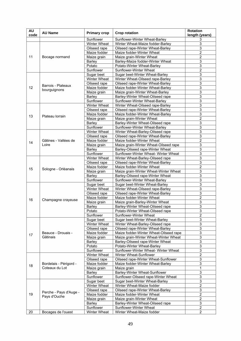
AU code
Rotation length (years) AU Name Primary crop Crop rotation
Sunflower Sunflower-Winter Wheat-Barley 3 Winter Wheat Winter Wheat-Maize fodder-Barley 3 Oilseed rape Oilseed rape-Winter Wheat-Barley 3 Maize fodder Maize fodder-Winter Wheat 2 Maize grain Maize grain-Winter Wheat 2 Barley Barley-Maize fodder-Winter Wheat 3
11 Bocage normand
Potato Potato-Winter Wheat-Barley 3 Sunflower Sunflower-Winter Wheat 2 Sugar beet Sugar beet-Winter Wheat-Barley 3 Winter Wheat Winter Wheat-Oilseed rape-Barley 3 Oilseed rape Oilseed rape-Winter Wheat-Barley 3 Maize fodder Maize fodder-Winter Wheat-Barley 3 Maize grain Maize grain-Winter Wheat-Barley 3
Barrois - Plateaux bourguignons 12
Barley Barley-Winter Wheat-Oilseed rape 3 Sunflower Sunflower-Winter Wheat-Barley 3 Winter Wheat Winter Wheat-Oilseed rape-Barley 3 Oilseed rape Oilseed rape-Winter Wheat-Barley 3 Maize fodder Maize fodder-Winter Wheat-Barley 3 Maize grain Maize grain-Winter Wheat 2 13 Plateau lorrain
Barley Barley-Winter Wheat-Oilseed rape 3 Sunflower Sunflower-Winter Wheat-Barley 3 Winter Wheat Winter Wheat-Barley-Oilseed rape 3 Oilseed rape Oilseed rape-Winter Wheat-Barley 3 Maize fodder Maize fodder-Winter Wheat 2 Maize grain Maize grain-Winter Wheat-Oilseed rape 3 Barley Barley-Oilseed rape-Winter Wheat 3
Gâtines - Vallées de Loire 14
Sunflower Sunflower-Winter Wheat- Winter Wheat 3 Winter Wheat Winter Wheat-Barley-Oilseed rape 3 Oilseed rape Oilseed rape-Winter Wheat-Barley 3 Maize fodder Maize fodder-Winter Wheat 2 Maize grain Maize grain-Winter Wheat-Winter Wheat 3 15 Sologne - Orléanais
Barley Barley-Oilseed rape-Winter Wheat 3 Sunflower Sunflower-Winter Wheat-Barley 3 Sugar beet Sugar beet-Winter Wheat-Barley 3 Winter Wheat Winter Wheat-Oilseed rape-Barley 3 Oilseed rape Oilseed rape-Winter Wheat-Barley 3 Maize fodder Maize fodder-Winter Wheat 2 Maize grain Maize grain-Barley-Winter Wheat 3 16 Champagne crayeuse
Barley Barley-Winter Wheat-Oilseed rape 3 Potato Potato-Winter Wheat-Oilseed rape 3 Sunflower Sunflower-Winter Wheat 2 Sugar beet Sugar beet-Winter Wheat-Barley 3 Winter Wheat Winter Wheat-Barley-Oilseed rape 3 Oilseed rape Oilseed rape-Winter Wheat-Barley 3 Maize fodder Maize fodder-Winter Wheat-Oilseed rape 3 Maize grain Maize grain-Winter Wheat-Winter Wheat 3 Barley Barley-Oilseed rape-Winter Wheat 3
Beauce - Drouais - Gâtinais 17
Potato Potato-Winter Wheat-Barley 3 Sunflower Sunflower-Winter Wheat- Winter Wheat 3 Winter Wheat Winter Wheat-Sunflower 2 Oilseed rape Oilseed rape-Winter Wheat-Sunflower 3 Maize fodder Maize fodder-Winter Wheat-Barley 3 Maize grain Maize grain 1 Barley Barley-Winter Wheat-Sunflower 3
Bordelais - Périgord - Coteaux du Lot 18
Sunflower Sunflower-Oilseed rape-Winter Wheat 3 Sugar beet Sugar beet-Winter Wheat-Barley 3 Winter Wheat Winter Wheat-Maize fodder 2 Oilseed rape Oilseed rape-Winter Wheat-Barley 3 Maize fodder Maize fodder-Winter Wheat 2 Maize grain Maize grain-Winter Wheat 2
Perche - Pays d'Auge - Pays d'Ouche 19
Barley Barley-Winter Wheat-Oilseed rape 3 Sunflower Sunflower-Winter Wheat 2
20 Bocages de l'ouest Winter Wheat Winter Wheat-Maize fodder 2
49

AU code
Rotation length (years) AU Name Primary crop Crop rotation
Oilseed rape Oilseed rape-Winter Wheat-Barley 3 Maize fodder Maize fodder-Winter Wheat 2 Maize grain Maize grain-Winter Wheat 2 Barley Barley-Winter Wheat-Maize fodder 3 Sunflower Sunflower-Winter Wheat-Oilseed rape 3 Sugar beet Sugar beet-Winter Wheat-Barley 3 Winter Wheat Winter Wheat-Oilseed rape-Barley 3 Oilseed rape Oilseed rape-Winter Wheat-Barley 3 Maize fodder Maize fodder-Winter Wheat 2 Maize grain Maize grain-Winter Wheat-Barley 3 Barley Barley-Winter Wheat-Oilseed rape 3
Ardenne - Argonne - Champagne H. 21
Potato Potato-Winter Wheat-Oilseed rape 3 Sunflower Sunflower-Winter Wheat 2 Winter Wheat Winter Wheat-Barley-Oilseed rape 3 Oilseed rape Oilseed rape-Winter Wheat-Barley 3 Maize fodder Maize fodder-Oilseed rape-Winter Wheat 3 Maize grain Maize grain-Winter Wheat-Barley 3 Barley Barley-Oilseed rape-Winter Wheat 3
Champagne berrichonne - Boischaut 22
Sunflower Sunflower-Winter Wheat-Oilseed rape 3 Winter Wheat Winter Wheat-Maize grain 2 Oilseed rape Oilseed rape-Winter Wheat-Barley 3 Maize fodder Maize fodder-Winter Wheat-Oilseed rape 3 Maize grain Maize grain 1 Barley Barley-Winter Wheat-Winter Wheat 3
Bas Dauphiné - Vallée du Rhône 23
Sunflower Sunflower-Winter Wheat-Barley 3 Sugar beet Sugar beet-Winter Wheat-Barley 3 Winter Wheat Winter Wheat-Oilseed rape-Barley 3 Oilseed rape Oilseed rape-Winter Wheat-Barley 3 Maize fodder Maize fodder-Winter Wheat 2 Maize grain Maize grain-Barley-Winter Wheat 3
24 Fossé bressan
Barley Barley-Winter Wheat-Oilseed rape 3 Sunflower Sunflower-Winter Wheat 2 Winter Wheat Winter Wheat-Maize fodder-Barley 3 Oilseed rape Oilseed rape-Winter Wheat-Barley 3 Maize fodder Maize fodder-Winter Wheat-Barley 3 Maize grain Maize grain-Winter Wheat 2 25 Bretagne centrale
Barley Barley-Maize fodder-Winter Wheat 3 Potato Potato-Winter Wheat-Barley 3 Winter Wheat Winter Wheat-Oilseed rape-Barley 3 Oilseed rape Oilseed rape-Winter Wheat-Barley 3 Maize fodder Maize fodder-Winter Wheat-Barley 3 Maize grain Maize grain-Winter Wheat-Oilseed rape 3 Barley Barley-Winter Wheat-Oilseed rape 3
Plateaux de Haute-Saône 26
Sunflower Sunflower-Winter Wheat-Barley 3 Maize grain Maize grain 1 27 Provence Sunflower Sunflower-Winter Wheat 2 Maize grain Maize grain 1 Plaine du Languedoc-
Roussillon 28 Sunflower Sunflower-Winter Wheat 2 Winter Wheat Winter Wheat-Barley-Oilseed rape 3 Oilseed rape Oilseed rape-Winter Wheat-Barley 3 Maize fodder Maize fodder-Winter Wheat-Winter Wheat 3 Maize grain Maize grain-Winter Wheat-Barley 3 29 Boischaut du sud
Barley Barley-Maize-Winter Wheat 3 Sunflower Sunflower-Winter Wheat-Barley 3 Winter Wheat Winter Wheat-Maize fodder-Barley 3 Oilseed rape Oilseed rape-Winter Wheat-Maize fodder 3 Maize fodder Maize fodder-Winter Wheat-Barley 3 Maize grain Maize grain-Winter Wheat 2 30 Bretagne nord
Barley Barley-Maize fodder-Winter Wheat 3 Potato Potato-Winter Wheat-Barley 3 Sugar beet Sugar beet-Winter Wheat-Barley 3 Winter Wheat Winter Wheat-Barley-Oilseed rape 3
31 Ile-de-France
Oilseed rape Oilseed rape-Winter Wheat-Barley 3
50
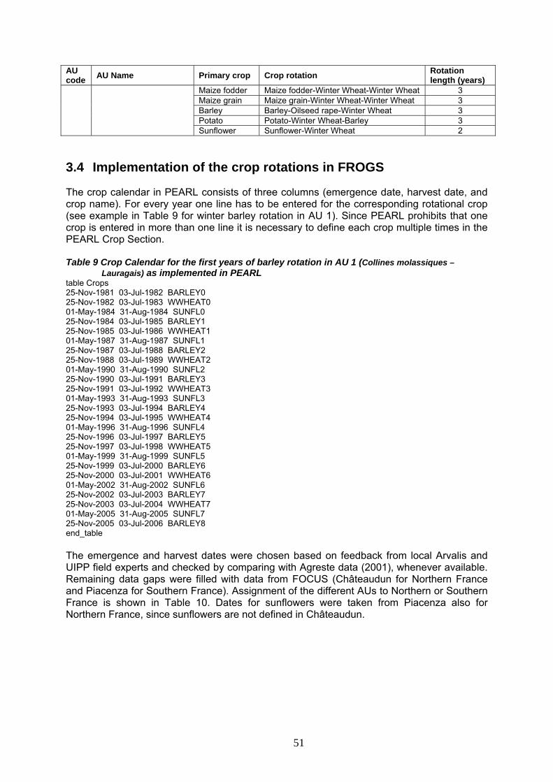
AU code
Rotation length (years) AU Name Primary crop Crop rotation
Maize fodder Maize fodder-Winter Wheat-Winter Wheat 3 Maize grain Maize grain-Winter Wheat-Winter Wheat 3 Barley Barley-Oilseed rape-Winter Wheat 3 Potato Potato-Winter Wheat-Barley 3 Sunflower Sunflower-Winter Wheat 2
3.4 Implementation of the crop rotations in FROGS The crop calendar in PEARL consists of three columns (emergence date, harvest date, and crop name). For every year one line has to be entered for the corresponding rotational crop (see example in Table 9 for winter barley rotation in AU 1). Since PEARL prohibits that one crop is entered in more than one line it is necessary to define each crop multiple times in the PEARL Crop Section. Table 9 Crop Calendar for the first years of barley rotation in AU 1 (Collines molassiques –
Lauragais) as implemented in PEARL table Crops 25-Nov-1981 03-Jul-1982 BARLEY0 25-Nov-1982 03-Jul-1983 WWHEAT0 01-May-1984 31-Aug-1984 SUNFL0 25-Nov-1984 03-Jul-1985 BARLEY1 25-Nov-1985 03-Jul-1986 WWHEAT1 01-May-1987 31-Aug-1987 SUNFL1 25-Nov-1987 03-Jul-1988 BARLEY2 25-Nov-1988 03-Jul-1989 WWHEAT2 01-May-1990 31-Aug-1990 SUNFL2 25-Nov-1990 03-Jul-1991 BARLEY3 25-Nov-1991 03-Jul-1992 WWHEAT3 01-May-1993 31-Aug-1993 SUNFL3 25-Nov-1993 03-Jul-1994 BARLEY4 25-Nov-1994 03-Jul-1995 WWHEAT4 01-May-1996 31-Aug-1996 SUNFL4 25-Nov-1996 03-Jul-1997 BARLEY5 25-Nov-1997 03-Jul-1998 WWHEAT5 01-May-1999 31-Aug-1999 SUNFL5 25-Nov-1999 03-Jul-2000 BARLEY6 25-Nov-2000 03-Jul-2001 WWHEAT6 01-May-2002 31-Aug-2002 SUNFL6 25-Nov-2002 03-Jul-2003 BARLEY7 25-Nov-2003 03-Jul-2004 WWHEAT7 01-May-2005 31-Aug-2005 SUNFL7 25-Nov-2005 03-Jul-2006 BARLEY8 end_table The emergence and harvest dates were chosen based on feedback from local Arvalis and UIPP field experts and checked by comparing with Agreste data (2001), whenever available. Remaining data gaps were filled with data from FOCUS (Châteaudun for Northern France and Piacenza for Southern France). Assignment of the different AUs to Northern or Southern France is shown in Table 10. Dates for sunflowers were taken from Piacenza also for Northern France, since sunflowers are not defined in Châteaudun.
51
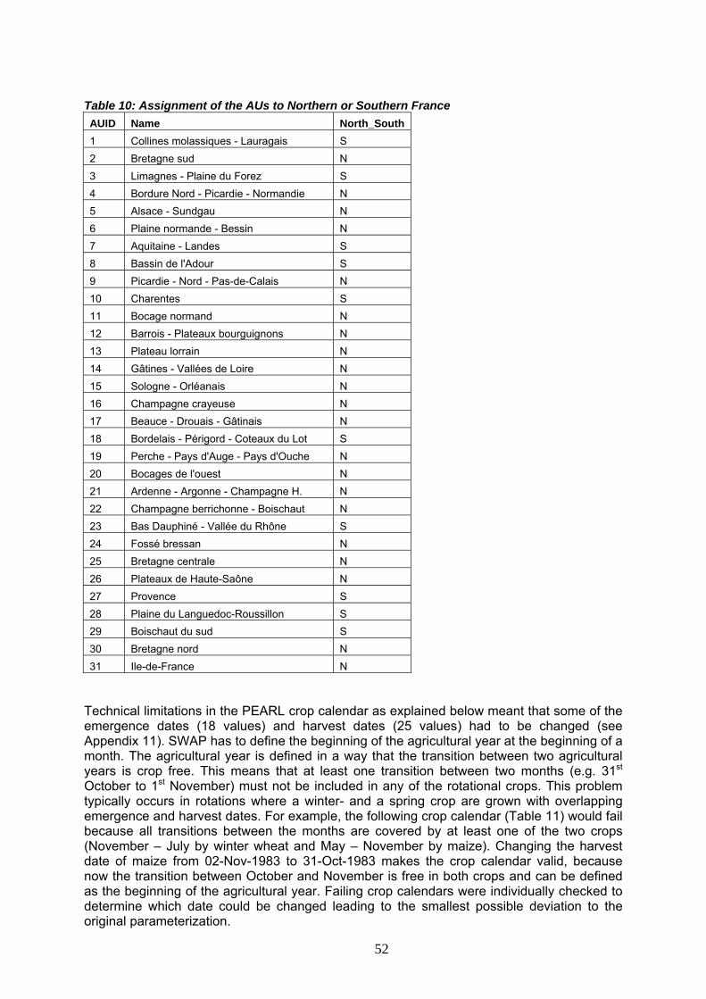
Table 10: Assignment of the AUs to Northern or Southern France AUID Name North_South 1 Collines molassiques - Lauragais S 2 Bretagne sud N 3 Limagnes - Plaine du Forez S 4 Bordure Nord - Picardie - Normandie N 5 Alsace - Sundgau N 6 Plaine normande - Bessin N 7 Aquitaine - Landes S 8 Bassin de l'Adour S 9 Picardie - Nord - Pas-de-Calais N 10 Charentes S 11 Bocage normand N 12 Barrois - Plateaux bourguignons N 13 Plateau lorrain N 14 Gâtines - Vallées de Loire N 15 Sologne - Orléanais N 16 Champagne crayeuse N 17 Beauce - Drouais - Gâtinais N 18 Bordelais - Périgord - Coteaux du Lot S 19 Perche - Pays d'Auge - Pays d'Ouche N 20 Bocages de l'ouest N 21 Ardenne - Argonne - Champagne H. N 22 Champagne berrichonne - Boischaut N 23 Bas Dauphiné - Vallée du Rhône S 24 Fossé bressan N 25 Bretagne centrale N 26 Plateaux de Haute-Saône N 27 Provence S 28 Plaine du Languedoc-Roussillon S 29 Boischaut du sud S 30 Bretagne nord N 31 Ile-de-France N
Technical limitations in the PEARL crop calendar as explained below meant that some of the emergence dates (18 values) and harvest dates (25 values) had to be changed (see Appendix 11). SWAP has to define the beginning of the agricultural year at the beginning of a month. The agricultural year is defined in a way that the transition between two agricultural years is crop free. This means that at least one transition between two months (e.g. 31st October to 1st November) must not be included in any of the rotational crops. This problem typically occurs in rotations where a winter- and a spring crop are grown with overlapping emergence and harvest dates. For example, the following crop calendar (Table 11) would fail because all transitions between the months are covered by at least one of the two crops (November – July by winter wheat and May – November by maize). Changing the harvest date of maize from 02-Nov-1983 to 31-Oct-1983 makes the crop calendar valid, because now the transition between October and November is free in both crops and can be defined as the beginning of the agricultural year. Failing crop calendars were individually checked to determine which date could be changed leading to the smallest possible deviation to the original parameterization.
52

53
Table 11: Example of an invalid crop calendar (no agricultural year can be defined, left) and corrected crop calendar (right) table Crops table Crops 15-Nov-1981 08-Jul-1982 WWHEAT 15-Nov-1981 08-Jul-1982 WWHEAT 08-May-1983 02-Nov-1983 MAIZEG 08-May-1983 31-Oct-1983 MAIZEG end table end table All emergence and harvest dates are listed in Appendix 11, together with comments on the source of the data and whether the dates were changed due to the limitations of the PEARL crop calendar. 3.5 References Agreste 2001. Enquête sur les pratiques culturales, La statistique agricole SCEES – Collection chiffres et données n°159. Agreste 2006. Enquête pratiques culturales 2006, Données en ligne (http://agreste.agriculture.gouv.fr/).

4 Application timing based on BBCH growth stages
In the FOCUS scenarios and models, applications can only be made at specific dates or relative to emergence or harvest. The same application dates are used over the whole simulation period of 26 years. The FROGS interface allows scheduling of the pesticide applications relative to the crop development (in accordance with the BBCH growth stages as specified in the GAP), taking into account spatial and temporal variations in crop development in function of the meteorological conditions of each scenario and year of application. This means that the user specifies the BBCH code, application rate, and target crop, and the FROGS interface then derives the actual application dates from the corresponding crop phenological sub-model implemented in the shell.
4.1 Phenological sub-model origin Phenology is largely based on the temperature sum gathered by the respective crop. In the shell the same algorithm as in the crop sub-model (SWAP) of FOCUS Pearl 3.3.3 is implemented. It should be noted that SWAP contains the same phenology related routines as the model WOFOST, which is used by JRC (http://mars.jrc.it/mars/About-us/AGRI4CAST) for the European Crop Growth Monitoring System (CGSM). Crop-specific parameters, including phenological parameters (see below for definitions), were gathered by Boons-Prins et al. (1993) and were also used in FROGS. For winter oilseed rape (WOSR), phenological development cannot be simulated successfully with consideration of temperature sums only. Habekotté (1997) presents a more detailed model comprising temperature sums, influence of photoperiod, as well as vernalization.
4.2 Phenological sub-model theory Phenological development is expressed in development stage Ds (-) [0 at emergence, 1 at flowering, 2 at maturity]. Ds is a function of temperature sum.
(j = day number, Teff = effective daily termperature, Tsum,i = temperature sum required to complete certain growth stage) Effective daily temperature Teff is defined by a minimum temperature (Tlb) for development and a maximum temperature (Tub) where development saturates: For Tavg <= Tlb Teff = 0, Tlb < Tavg < Tub Teff = Tavg - Tlb, Tavg >= Tub Teff = Tub - Tlb.
54
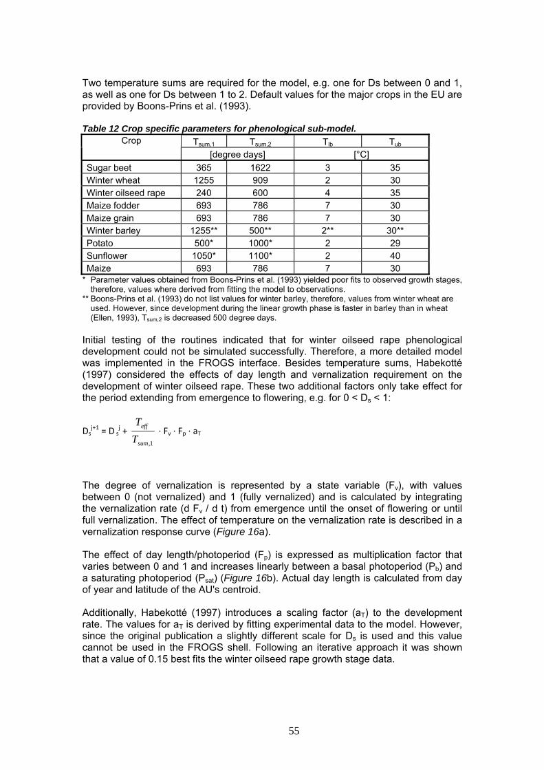
Two temperature sums are required for the model, e.g. one for Ds between 0 and 1, as well as one for Ds between 1 to 2. Default values for the major crops in the EU are provided by Boons-Prins et al. (1993). Table 12 Crop specific parameters for phenological sub-model.
Tsum,1 Tsum,2 Tlb Tub Crop [degree days] [°C]
Sugar beet 365 1622 3 35 Winter wheat 1255 909 2 30 Winter oilseed rape 240 600 4 35 Maize fodder 693 786 7 30 Maize grain 693 786 7 30 Winter barley 1255** 500** 2** 30** Potato 500* 1000* 2 29 Sunflower 1050* 1100* 2 40 Maize 693 786 7 30
* Parameter values obtained from Boons-Prins et al. (1993) yielded poor fits to observed growth stages, therefore, values where derived from fitting the model to observations.
** Boons-Prins et al. (1993) do not list values for winter barley, therefore, values from winter wheat are used. However, since development during the linear growth phase is faster in barley than in wheat (Ellen, 1993), Tsum,2 is decreased 500 degree days.
Initial testing of the routines indicated that for winter oilseed rape phenological development could not be simulated successfully. Therefore, a more detailed model was implemented in the FROGS interface. Besides temperature sums, Habekotté (1997) considered the effects of day length and vernalization requirement on the development of winter oilseed rape. These two additional factors only take effect for the period extending from emergence to flowering, e.g. for 0 < Ds < 1:
1,sum
eff
TT
Dsj+1 = D s
j + ∙ Fv ∙ Fp ∙ aT
The degree of vernalization is represented by a state variable (Fv), with values between 0 (not vernalized) and 1 (fully vernalized) and is calculated by integrating the vernalization rate (d Fv / d t) from emergence until the onset of flowering or until full vernalization. The effect of temperature on the vernalization rate is described in a vernalization response curve ( a). Figure 16 The effect of day length/photoperiod (Fp) is expressed as multiplication factor that varies between 0 and 1 and increases linearly between a basal photoperiod (Pb) and a saturating photoperiod (Psat) (Figure 16b). Actual day length is calculated from day of year and latitude of the AU's centroid. Additionally, Habekotté (1997) introduces a scaling factor (aT) to the development rate. The values for aT is derived by fitting experimental data to the model. However, since the original publication a slightly different scale for Ds is used and this value cannot be used in the FROGS shell. Following an iterative approach it was shown that a value of 0.15 best fits the winter oilseed rape growth stage data.
55

Figure 16 Effect of vernalization (left) and photoperiod (right) on winter oilseed rape (from Habekotté, 1997)
Table 13 Parameters for detailed winter oilseed rape model (based on Habekotté, 1997). Parameter Unit Value
Vernalization Rv,max d-1 °C-1 0.014553 Tv,max °C 17.2022 Tv,min °C -3.7182 Tv,op1 °C 0.726 Tv,op2 °C 5.377
Photoperiod Pb h 8
Psat h 14 Scaling factor
aT d-1 °C-1 0.15
4.3 Relating development stage Ds to BBCH code JRC [http://agsys.cra-cin.it/tools/cropml/help/] provides the following definitions that can be related to BBCH (Table 14). A piecewise-linear relationship was constructed from the Ds-BBCH correspondences (Figure 17). Table 14 Correspondence between development stage and BBCH code. Ds BBCH Emergence: 0 9 Beginning of tillering: 0.25 21 Mid tillering: 0.35 25 Panicle initiation: 0.6 30 Full Heading: 0.9 59 Full Flowering: 1 65 Full Grain filling: 1.5 75 Physiological maturity: 2 90
56

0 0.5 1 1.5 20
10
20
30
40
50
60
70
80
90
Ds (-)
BB
CH
(-)
Figure 17 Piecewise-linear relationship between development stage (Ds) and BBCH code. For the bi-annual crop sugar beet, a different relationship is required since harvest occurs at BBCH 50. Boons-Prins (1993) assign Ds = 1 to the stage where the crop canopy starts covering the ground fully. This growth stage corresponds to BBCH 40. Hence, the piecewise-linear relationship for sugar beet was constructed as shown in Table 15 and Figure 18. Table 15 Correspondence between development stage and BBCH code for sugar beets Ds BBCH Emergence: 0 9 Full ground cover (LAI = 2.5): 1 40 Harvest: 2 49
57
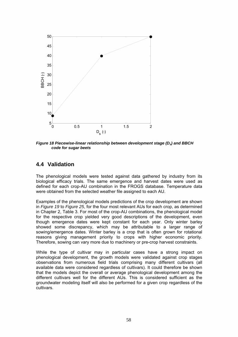
0 0.5 1 1.5 25
10
15
20
25
30
35
40
45
50
Ds (-)
BB
CH
(-)
Figure 18 Piecewise-linear relationship between development stage (Ds) and BBCH code for sugar beets
4.4 Validation The phenological models were tested against data gathered by industry from its biological efficacy trials. The same emergence and harvest dates were used as defined for each crop-AU combination in the FROGS database. Temperature data were obtained from the selected weather file assigned to each AU. Examples of the phenological models predictions of the crop development are shown in to Figure 19 Figure 25, for the four most relevant AUs for each crop, as determined in Chapter 2, Table 3. For most of the crop-AU combinations, the phenological model for the respective crop yielded very good descriptions of the development, even though emergence dates were kept constant for each year. Only winter barley showed some discrepancy, which may be attributable to a larger range of sowing/emergence dates. Winter barley is a crop that is often grown for rotational reasons giving management priority to crops with higher economic priority. Therefore, sowing can vary more due to machinery or pre-crop harvest constraints. While the type of cultivar may in particular cases have a strong impact on phenological development, the growth models were validated against crop stages observations from numerous field trials comprising many different cultivars (all available data were considered regardless of cultivars). It could therefore be shown that the models depict the overall or average phenological development among the different cultivars well for the different AUs. This is considered sufficient as the groundwater modeling itself will also be performed for a given crop regardless of the cultivars.
58

Figure 19 Sugar beet development in the four most representative AUs
59
Figure 20 Winter wheat development in the four most representative AUs
60
Figure 21 Winter oilseed rape development in the four most representative AUs
61

Figure 22 Maize (fodder and grain) development in the four most representative AUs (8, 10 grain maize; 11, 20 fodder maize). Phenology observations and phenology model do not distinguish fodder and grain maize.
62
Figure 23 Winter barley development in the four most representative AUs
63

Figure 24 Potato development in the four most representative AUs
64

Figure 25 Sunflower development in the four most representative AUs (AU 18 is actually the 5th representative AU, however, for the 4th representative AU 22 no measurement data are available for the time period considered)
4.5 References Boons-Prins, E.R., G.H.J. de Koning, C.A. van Diepen and F.W.T. Penning de Vries, 1993. Crop specific simulation parameters for yield forecasting across the European Community. Simulation Rep. 32, CABO-DLO and SC-DLO, Wageningen, The Netherlands. Ellen, J. 1993. Growth, yield and composition of four winter cereals. I. Biomass, grain yield and yield formation. Netherlands Journal of Agricultural Science 41: 153-165. Habekotté, B. 1997. A model of the phenological development of winter oilseed rape (Brassica napus L.). Field Crops Research 54: 127-136.
65

5 Weather data
5.1 Introduction The MARS database [MARS, 2004] was used as meteorological input for FROGS, since it uses data from local weather stations (partially interpolated) and is commonly accepted in the European scientific and regulatory community. For each agricultural unit (AU) one MARS tile was selected as representative of the meteorological conditions within the AU. The selection process is summarized in the following section. For further details refer to Appendix 12. The basic principle of the selection process was that the selected tile should be the most representative one in terms of climate and regarding agricultural occupation (i.e. relevance to the AU under consideration).
5.2 Short description of the MARS database The MARS database consists of tiles or grid-cells (50 * 50 km) that cover Europe. Each tile consists of a data set of long-term daily weather records. The weather data describe the “average” conditions in one grid and not the conditions at the grid cell centre. Most parameter values were collected on local weather station level and interpolated for the whole grid-cell. Since global radiation and potential evaporation are not widely measured they are calculated from available measured meteorological parameters. In order to determine representative meteorological conditions for one grid-cell the most suitable stations were identified. Suitability of stations was determined using four criteria: distance between station and grid centre, difference in altitude, difference in distance to coast, climatic barrier separation (e.g. mountains). After identifying up to four suitable stations for one grid-cell, a simple averaging procedure was applied for most parameters (corrected for altitude in case of temperature and vapour pressure). Only rainfall was not interpolated but rather taken from the most suitable station. Missing data values were filled with long-term average data of that day for that station. For more details on the MARS-data set and the interpolation procedure please refer to van der Goot and Orlandi (2003).
5.3 Summary of the tile selection process in FROGS The driving objective in selecting the meteo data for each the AUs was to be as representative as possible of the main agricultural conditions in that AU. It was therefore not the aim to implement any conservativity or worst-case assumptions in the weather scenarios. In order to find the most representative MARS-tile regarding agricultural conditions for each AU, the agricultural occupation of the cantons was extracted from the Agreste database. A map of the cantons was intersected with the AUs and the MARS
66

tiles in GIS. For each MARS tile the agricultural occupation within one AU was calculated. The tile with the largest agricultural area in each AU was selected as the default tile. In the following, the tile with largest acrigultural occupation in one AU is noted T1,AU. The tile with the second largest occupation is noted T2,AU. In additional steps it was checked if this default tile could be accepted as the weather scenario for an AU or if there were objective reasons (geographically separated agricultural areas, high variability of climatic conditions, relative location to mountains or the coast) to choose another tile. The procedure is summarized in Figure 26.
Yes Select T1,AU
Case-by-case decision (4b)
No
STEP 3. Is agricultural area of T1,AU >25% larger than that of T2,AU?
Yes
No Select T1,AU
Yes
Case by case decision (4a)
No STEP 1. Are T1,AU and T,2AU neighbored?
STEP 2. Is difference in rain sum or average temp. between T1,AU and T2,AU > CV*T1,France?
Figure 26: Decision tree for confirmation of the selection of weather tile for each AU
• In STEP 1 it was determined whether there are AUs in which two geographically separated agricultural areas exist. This was assumed to be true when the two tiles with largest agricultural occupation are not adjacent. In these cases it was decided by expert knowledge which of the two areas is most representative for the agricultural conditions in the AU (STEP 4a). If no preference could be identified the default tile was kept.
• In the cases where only one main agricultural area was identified, the range
of climatic conditions within the AU was evaluated in STEP 2. If the variability within the unit is too large it was checked on a case-by-case basis whether another MARS-tile might be more suitable than T1,AU to represent the weather conditions for the AU.
The usage of 26 years of weather data already contains a certain (temporal) variability in rainfall and temperature. It is assumed that spatial variability has
67

to be considered additionally only in cases where it is larger than the temporal variability. Therefore, the average temporal variability identifies the acceptable spatial variability threshold. To evaluate the temporal variability the standard deviation of annual rain fall sums and annual average temperatures were calculated for the most representative tile (T1,AU) and divided by the mean over the 30-year period to derive the coefficient of variation (CV) for each AU. The mean CV was calculated for all AUs for rain and temperature (CVrain = 0.19, CVtemp = 0.06) as an expression of the temporal variability of these 31 tiles. This was identified to be about 160 mm/a (4800 mm over the whole period of 30 years) of rainfall sum and 0.7°C average temperature if multiplied by the mean values (T1,France = 25296 mm and 11.6 °C) of all MARS tiles in France. The usage of the CV (instead of the standard deviation) from the T1,AU tiles ensures that the threshold is proportionate to the mean value of all MARS tiles (T1,France). In STEP 2 it is therefore checked whether the difference in rainfall sum and average temperature between the two main tiles T1,AU and T2,AU is larger than allowable based on the temporal variability included in the default tiles. In case that the spatial differences are smaller than 4800 mm or 0.7 °C, it is assumed that the spatial variability is already covered by the temporal variability of the default tiles T1,AU. In these cases the default tile is selected.
• In case the spatial variability within the main agricultural area is too high it
was checked in STEP 3 whether the agricultural occupation of the default tile is much larger than that of the next most representative tile within the AU. As a threshold a pragmatic value of 25% was chosen since only few AUs (3 in case of rain and 5 in case of temperature) were affected by this threshold. In case the T1,AU tile has an agricultural occupation which is at least 25% larger than the occupation of the T2,AU tile, the T1,AU default tile was chosen for the weather scenario. This ensures that a default tile which is representative of a very large agricultural area is not rejected in favor of a tile with a relatively small occupation. In case of similar agricultural occupation of the most representative tiles within one agricultural region, it was investigated if the tiles are influenced by their position in the landscape (distance to mountain ranges or the coast). It was then decided on a case-by-case basis which tile represented the corresponding AU best (STEP 4b).
Applying the above-described selection scheme, in the end the default tile with the largest agricultural area was confirmed for all AUs. The MARS ID and the geographic position of the selected MARS-tiles are given in Table 16, Table 18 and Figure 27. For a more detailed description of the selection process and its results refer to the Appendix 12.
68

Table 16: Selected MARS-tiles for each AU
CODE_AU Mars Code CODE_AU Mars Code 1 43044 16 53050 2 52041 17 53047 3 48049 18 46044 4 57048 19 52045 5 51055 20 50042 6 55044 21 53051 7 44042 22 50048 8 43043 23 46052 9 56048 24 50052 10 48043 25 53040 11 53043 26 51053 12 51051 27 42052 13 54054 28 42050 14 50044 29 49047 15 51047 30 53041
31 54049
In order to confirm that the selected tiles were indeed representative of the average conditions in the AU, the rainfall and temperature data of the MARS tile selected for each AU (T1,AU) was compared to the median rainfall and temperature data of all tiles within the respective AU. The sum of rainfall (and the average temperature) over 30 years was calculated for each selected tile. Then for each AU the median of the rainfall sums (and average temperatures; MedAU) was calculated from the tiles located within the AU. The normalized difference of the rainfall (or temperature) is then calculated by (VT1,AU-MedAU)/MedAU, with VT1,AU being the rainfall sum (or average temperature) of the selected default tile for one AU. The results of these calculations are shown in Table 17. The observed small differences (in general <10%) indicate that the conditions in the selected tiles can indeed be considered as representative in all AUs. The only exception is AU 30, where the rainfall of the selected tile is about 20% below the median rainfall. A closer inspection of AU30 revealed that tiles with small agricultural occupation (<20% of the agricultural area) have large median rainfall (30310 mm) while the rest of the AU (>80% of the agricultural area) is characterized by mainly low rainfall (22861 mm). Calculating the difference to the main agricultural area shows that the selected tile is only 6% below the median rainfall. In about half of the AUs the conditions are slightly more favorable than the median of the AU, while in the other half they are more conservative or no difference can be observed. Overall, it can be concluded that average conditions are met.
69
Figure 27: Location of the selected MARS tiles within the Agronomic Units
70

Table 17: Normalized differences in rainfall sum and average temperature between T1,AU and the median of each AU
Normalized Difference in
average Temperature
(-)
Normalized Difference in Rainfall
sum (-)
AU
1 -0.06 0.01 2 -0.14 0.01 3 -0.06 0.04 4 0.05 -0.02 5 -0.04 0.01 6 0.00 0.02 7 0.01 0.00 8 -0.11 -0.01 9 -0.04 -0.01
10 0.12 0.02 11 0.00 0.00 12 0.00 -0.01 13 -0.11 0.01 14 0.00 0.02 15 -0.05 0.01 16 0.07 0.00 17 -0.11 -0.01 18 -0.03 -0.04 19 -0.05 0.04 20 0.12 0.00 21 0.07 0.09 22 0.02 0.00 23 0.05 -0.06 24 -0.11 0.01 25 -0.11 0.00 26 0.08 0.03 27 -0.03 -0.05 28 0.00 0.04 29 0.00 0.00 30 -0.18 0.00 31 -0.03 0.00
71

5.4 Parameterisation The MARS meteo data was downloaded in 2008. The parameters listed in Table 18 are available for the time frame from 1975 – 2006 in daily resolution. For the scenario calculation the years 1981 – 2006 are used. Table 18: Available daily MARS data
Value Description MAXIMUM_TEMPERATURE maximum temperature (°C) MINIMUM_TEMPERATURE minimum temperature (°C) VAPOUR_PRESSURE mean daily vapour pressure (hPa) WINDSPEED mean daily windspeed at 10m (m/s) RAINFALL mean daily rainfall (mm) E0 Penman potential evaporation from a free water surface
(mm/d) ES0 Penman potential evaporation from a moist bare soil
surface (mm/d) ET0 Penman potential transpiration from a crop canopy (mm/d)
daily global radiation (kJ/m2/d) CALCULATED_RADIATION For PEARL input all parameters listed in Table 19 are necessary to be defined in the .met file. Table 19: Required daily PEARL input data and the corresponding MARS data PEARL Input MARS Parameter Daily global radiation (kJ/m2/d), between 0 and 5 E6 CALCULATED_RADIATION
MINIMUM_TEMPERATURE Minimum daily temperature (°C), between -50 and 35MAXIMUM_TEMPERATURE Maximum daily temperature (°C), between -30 and
60 Average vapor pressure (kPa), between 0 and 10 VAPOUR_PRESSURE / 10 Average windspeed (m/s), between 0 and 50 WINDSPEED Daily precipitation (mm/d), between 0 and 1000 RAINFALL Reference evapotranspiration (mm/d), between 0 and 100
ES0
PEARL implements the option of calculating the potential evapotranspiration with the Penman-Monteith or the Makkink approach. The Penman-Monteith approach was selected for use in FROGS, because it is the most sophisticated approach and can be used with the crop factors as given in the FOCUS ground water scenarios. This is preferred over the MARS-calculated evapotranspiration values, which are calculated by the Penman approach (the predecessor of the Penman-Monteith approach). Hence, although the reference evapotranspiration values from MARS are included in the FROGS *.met files, these are not considered since potential evapotranspiration is calculated by PEARL (alternatively a dummy value such as -99 could have been used).
72
5.5 Adjustments of MARS data for SWAP 5.5.1 Problem and proposed solution Following scenario testing, it was observed that the hydrological module in PEARL, SWAP collapses in the case of extraordinary large rainfall events combined with a soil characterized by low hydraulic conductivity. This was observed for 58 out of 1481 scenarios (considering all crops), even after making some adjustments to the soil maximum ponding depth and maximum number of iterations in SWAP, as explained in Chapter 8.5. This problem is specific to PEARL and is considered to be an artifact of the way its hydrological model handles runoff. Clearly in such instances of soils characterized by low hydraulic conductivity, which are therefore quickly saturated by water, extraordinarily strong rainfall events will result in significant surface runoff, the excess water which cannot infiltrate the soil being evacuated by Hortonian overland flow. However, the SWAP model in PEARL is only able to simulate runoff to a limited extent, as opposed to PRZM or PELMO. This problem may be resolved in future versions of the PEARL model, but at the moment cannot be solved other than by modifying the scenario parameters (soil and/or rainfall). As a result, in order to conservatively force water through the soil profile, extraordinarily large rainfall events resulting in model crashes were split over 2-4 days. Stretching the rainfall over a longer time period allows the water to percolate into the soil without causing numerical problems in SWAP. A maximum of 2 rainfall events over the whole 26-year simulation period were split for any given scenario originally causing numerical problems in SWAP. For example in Figure 28 the daily rainfall of AU12 is shown as original (top) and split (bottom). It is important to note that the total amount of rain is not altered. Only the intensity is changed in a way that in total more water is able to infiltrate and percolate through the soil. Details of the adjustments made to the rainfall events and scenarios to which the adjusted rainfall was applied are provided in Appendix 13.
73

Unmodified
0102030405060708090
100
01/0
1/19
75
01/0
1/19
77
01/0
1/19
79
01/0
1/19
81
01/0
1/19
83
01/0
1/19
85
01/0
1/19
87
01/0
1/19
89
01/0
1/19
91
01/0
1/19
93
01/0
1/19
95
01/0
1/19
97
01/0
1/19
99
01/0
1/20
01
01/0
1/20
03
01/0
1/20
05
Date
Rai
n (m
m)
Modified
0102030405060708090
100
01/0
1/19
75
01/0
1/19
77
01/0
1/19
79
01/0
1/19
81
01/0
1/19
83
01/0
1/19
85
01/0
1/19
87
01/0
1/19
89
01/0
1/19
91
01/0
1/19
93
01/0
1/19
95
01/0
1/19
97
01/0
1/19
99
01/0
1/20
01
01/0
1/20
03
01/0
1/20
05
Date
Rai
n (m
m)
Figure 28: Original (Top) and splitted (Bottom) daily rain of AU 12. Only one event on 12.11.1996 (93 mm) was splitted over 3 days (12-14.11.1996) with a daily intensity of 31 mm.
74
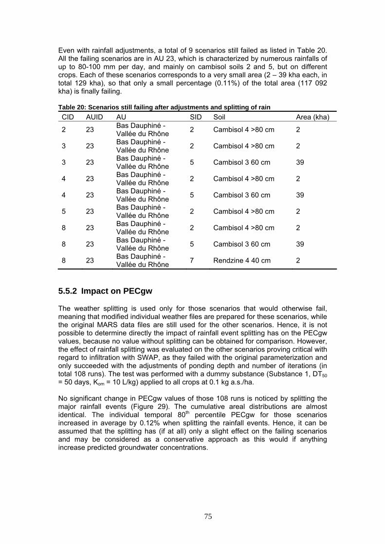
Even with rainfall adjustments, a total of 9 scenarios still failed as listed in Table 20. All the failing scenarios are in AU 23, which is characterized by numerous rainfalls of up to 80-100 mm per day, and mainly on cambisol soils 2 and 5, but on different crops. Each of these scenarios corresponds to a very small area (2 – 39 kha each, in total 129 kha), so that only a small percentage (0.11%) of the total area (117 092 kha) is finally failing. Table 20: Scenarios still failing after adjustments and splitting of rain CID AUID AU SID Soil Area (kha)
Bas Dauphiné - Vallée du Rhône 2 23 2 Cambisol 4 >80 cm 2
Bas Dauphiné - Vallée du Rhône 3 23 2 Cambisol 4 >80 cm 2
Bas Dauphiné - Vallée du Rhône 3 23 5 Cambisol 3 60 cm 39
Bas Dauphiné - Vallée du Rhône 4 23 2 Cambisol 4 >80 cm 2
Bas Dauphiné - Vallée du Rhône 4 23 5 Cambisol 3 60 cm 39
Bas Dauphiné - Vallée du Rhône 5 23 2 Cambisol 4 >80 cm 2
Bas Dauphiné - Vallée du Rhône 8 23 2 Cambisol 4 >80 cm 2
Bas Dauphiné - Vallée du Rhône 5 Cambisol 3 60 cm 39 8 23
Bas Dauphiné - Vallée du Rhône 8 23 7 Rendzine 4 40 cm 2
5.5.2 Impact on PECgw The weather splitting is used only for those scenarios that would otherwise fail, meaning that modified individual weather files are prepared for these scenarios, while the original MARS data files are still used for the other scenarios. Hence, it is not possible to determine directly the impact of rainfall event splitting has on the PECgw values, because no value without splitting can be obtained for comparison. However, the effect of rainfall splitting was evaluated on the other scenarios proving critical with regard to infiltration with SWAP, as they failed with the original parameterization and only succeeded with the adjustments of ponding depth and number of iterations (in total 108 runs). The test was performed with a dummy substance (Substance 1, DT50 = 50 days, Kom = 10 L/kg) applied to all crops at 0.1 kg a.s./ha. No significant change in PECgw values of those 108 runs is noticed by splitting the major rainfall events (Figure 29). The cumulative areal distributions are almost identical. The individual temporal 80th percentile PECgw for those scenarios increased in average by 0.12% when splitting the rainfall events. Hence, it can be assumed that the splitting has (if at all) only a slight effect on the failing scenarios and may be considered as a conservative approach as this would if anything increase predicted groundwater concentrations.
75

0
0.1
0.2
0.3
0.4
0.5
0.6
0.7
0.8
0.9
1
0 1 2 3 4 5 6 7
PECgw (µg/L)
Cum
ulat
ive
Are
al D
istr
ibut
ion
(-)
Not-SplittedSplitted
Figure 29: Cumulative areal distribution of the PECgw values with the
parameterizations after adjustment (with normal and splitted weather) for all crops. The only runs considered and plotted here are those which failed with normal parameterization, but succeeded after the adjustments (108 scenarios)
For further examination of the potential impact of rainfall splitting on predicted groundwater concentrations, the PECgw values of 4 dummy test substances applied to winter oilseed rape at different application rates (0.1, 0.2, and 0.35 kg a.s./ha for Substance 1, 2, and 3, respectively) are listed in Table 21 to Table 24 for the 7 winter oilseed rape scenarios failing with the original parameterization and only succeeding with the adjustments of ponding depth and number of iterations. The four test substances are characterized by different properties in order to test a range of sorption and degradation characteristics. Substance 1 is the same test substance as used in the test runs above (DT50 = 50 days, Kom = 10 L/kg). Substance 2 corresponds to the FOCUS dummy substance C (DT50 = 20 days, Kom = 100 L/kg) and Substance 3 is the metabolite of FOCUS dummy substance C (DT50 = 100 days, Kom = 30 L/kg). Substance 4 corresponds to the FOCUS dummy substance D (DT50 = 20 days, Kom = 35 L/kg). The relative change between the PECgw values of unsplit and splitted rainfall was normalized to the mean of all scenarios for the same crop and substance (Equation 1). This indicates how relevant the change is in relation to the average level of the PEC distribution, and therefore takes into account the absolute level of the PEC values.
( )( ) 100*S
SUX −=Equation 1:
76

where X is the relative change of the PEC values, S is the PEC value calculated with the splitted weather scenario, U is the PEC-value of the unsplit weather scenario, and S is the mean of the PECgw values of all unsplit scenarios for the crop. Table 21: PECgw values of Substance 1 critical scenarios (failing with the original parameterization, but succeeding with adjustments) for winter oilseed rape. Crop AUID SID Area (kha) PECgw (µg/l) Rel. change (X)
Unsplit weather (U)
Split weather (S)
normalized to range (%)
3 8 1 5 1.244 1.244 0.00 3 23 1 18 2.101 2.096 0.19 3 10 2 36 2.386 2.386 -0.01 3 18 2 287 2.010 2.004 0.21 3 23 4 213 2.450 2.450 0.00 3 10 5 121 2.849 2.849 -0.02 3 8 1 5 1.244 1.244 0.00
Table 22: PECgw values of Substance 2 critical scenarios (failing with the original parameterization, but succeeding with adjustments) for winter oilseed rape. Crop AUID SID Area (kha) PECgw (µg/l) Rel. change (X)
Unsplit weather (U)
Split weather (S)
normalized to range (%)
3 8 1 5 9.78E-09 9.87E-09 0.00 3 23 1 18 3.99E-06 3.99E-06 0.00 3 18 2 287 8.31E-07 9.08E-07 -0.01 3 23 4 213 2.45E-05 2.44E-05 0.00 3 10 5 121 3.86E-06 3.96E-06 -0.02 3 18 5 19 2.79E-05 2.74E-05 0.07 3 8 1 5 9.78E-09 9.87E-09 0.00
77

Table 23: PECgw values of Substance 3 critical scenarios (failing with the original parameterization, but succeeding with adjustments) for winter oilseed rape. Crop AUID SID Area (kha) PECgw (µg/l) Rel. change (X)
Unsplit weather (U)
normalized to range
normalized to range (%)
3 8 1 5 2.110 2.109 0.02 3 23 1 18 3.871 3.870 0.02 3 10 2 36 2.725 2.727 -0.05 3 18 2 287 3.394 3.401 -0.22 3 10 5 121 2.722 2.714 0.23 3 18 5 19 3.394 3.394 -0.01 3 8 1 5 2.110 2.109 0.02
Table 24: PECgw values of Substance 4 critical scenarios (failing with the original parameterization, but succeeding with adjustments) for winter oilseed rape. Crop AUID SID Area (kha) PECgw (µg/l) Rel. change (X)
Unsplit weather (U)
Splitted weather (S)
normalized to range (%)
3 8 1 5 0.004 0.004 0.00 3 23 1 18 0.020 0.020 -0.01 3 10 2 36 0.018 0.018 0.00 3 18 2 287 0.017 0.019 -0.06 3 23 4 213 0.038 0.038 0.01 3 10 5 121 0.059 0.059 0.00 3 18 5 19 0.055 0.055 -0.01
For all the tested dummy substances, the relative changes are very small. There appears to be no strong influence of the splitting of rainfall events on the individual PECgw values for the range of DT50 – Kom combinations tested. Moreover, when looking at the overall cumulative areal distribution, which considers all relevant scenarios for the given crop including all scenarios not requiring any adjustments (see example for Substance 4 on winter oilseed rape in Figure 30), it is clear that minor differences in a few individual scenarios due to splitting of rainfall events will not change the overall results.
78
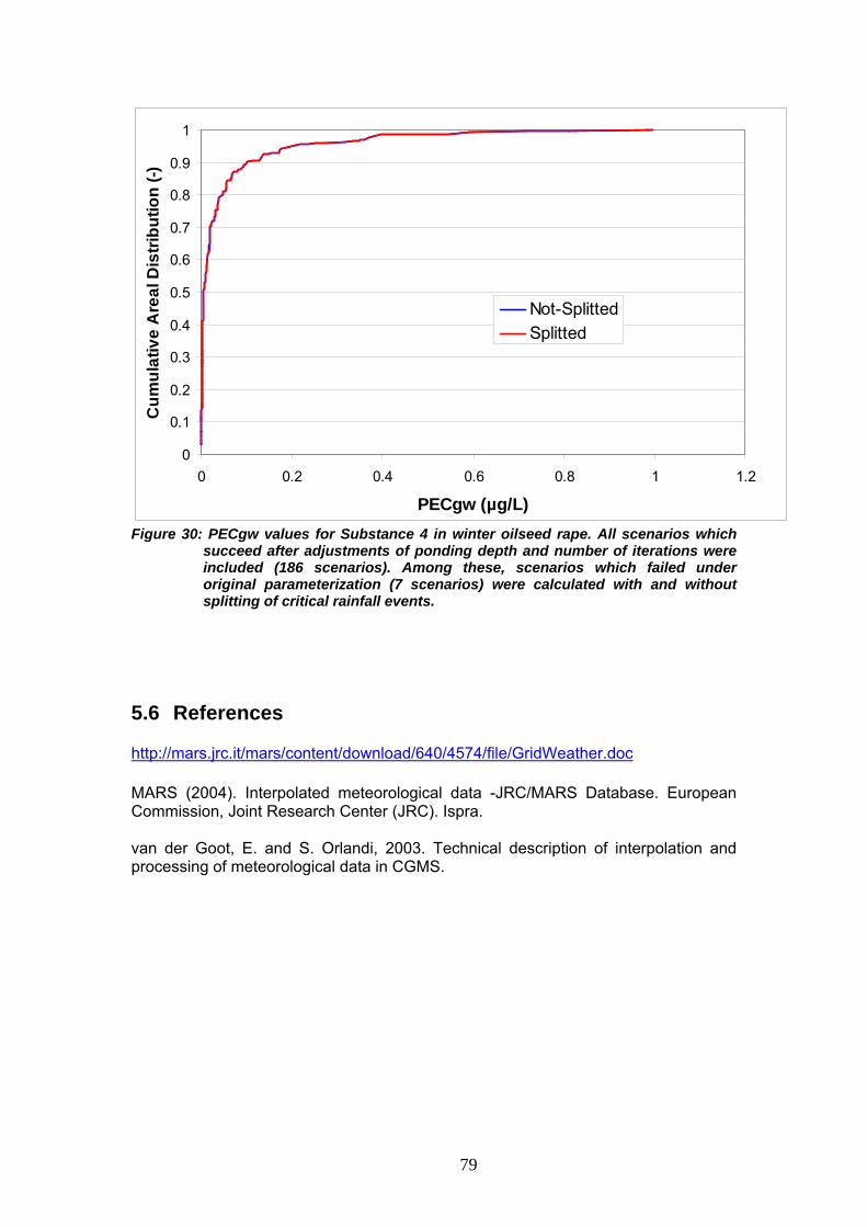
0
0.1
0.2
0.3
0.4
0.5
0.6
0.7
0.8
0.9
1
0 0.2 0.4 0.6 0.8 1 1.2
PECgw (µg/L)
Cum
ulat
ive
Are
al D
istri
butio
n (-)
Not-SplittedSplitted
Figure 30: PECgw values for Substance 4 in winter oilseed rape. All scenarios which
succeed after adjustments of ponding depth and number of iterations were included (186 scenarios). Among these, scenarios which failed under original parameterization (7 scenarios) were calculated with and without splitting of critical rainfall events.
5.6 References http://mars.jrc.it/mars/content/download/640/4574/file/GridWeather.doc MARS (2004). Interpolated meteorological data -JRC/MARS Database. European Commission, Joint Research Center (JRC). Ispra. van der Goot, E. and S. Orlandi, 2003. Technical description of interpolation and processing of meteorological data in CGMS.
79

6 Crop irrigation Crop irrigation is implemented in FROGS for the main irrigated crops, i.e. maize, sugar beets and potatoes. Average irrigation schedules corresponding to standard practices in the different AUs of interest, expressed as x irrigation events of volume of water y from a start date z and interval i between two events, were entered as PEARL irrigation files. The methodology to implement irrigation in FROGS follows a stepwise approach as illustrated in Figure 31.
1 – Collection of irrigated surface for each crop included in FROGS from the Agricultural Census (Agreste, 2001)
2- Selection of the main irrigated crops
3- For each selected crop, determination of the Agronomic Unit where irrigation is significant (irrigation > x% of the total crop in the AU and > y ha)
4- Collection of irrigation practices for the selected crops and AU
Figure 31 Methodology used to implement irrigation in FROGS
80

6.1 Irrigated crops and surfaces in France Data on irrigated crops were obtained from the French agricultural census: Recensement Agricole 2000 (Agreste, 2001). Total irrigated acreage of crops that are currently included in FROGS (hereafter called “FROGS crops”) are summarized in Table 25. Table 25 Irrigation acreage from Agreste (2001)
Cumulative acreage (% of FROGS crops
irrigated) Acreage (% of FROGS
crops irrigated) Acreage (ha) Total FROGS crop irrigated 1151375 - Irrigated Grain maize 780952 67.8 67.8 Irrigated Fodder maize 105085 9.1 77.0 Sum of oilseed crops irrigated (a) 66774 5.8 82.8 Sum of other irrigated cereals (b) 63831 5.5 88.3 Irrigated potato 56424 4.9 93.2 Irrigated sugarbeet 34257 3.0 96.2 Irrigated Hard wheat 17378 1.5 97.7 Irrigated wheat 15182 1.3 99.0 Irrigated Sunflower 11492 1.0 100.0
(a) including oilseed rape (b) including barley
These data were aggregated for each agronomic unit (AU). Table 26 summarizes the acreage of irrigation for the 31 AUs. Seventeen AUs represent over 90% of the irrigated surface, and these also correspond to the most intensive AUs for irrigation.
81

Table 26 Irrigated acreage for the 31 Agronomic Units FROGS
crops Irrigated (ha)
Cumulative Irrigation (% Total FROGS crops irrigated)
FROGS crops irrigated (% AU_SAU)
Code AU
SAU (ha) (a) Name AU
Collines molassiques - Lauragais 1 1243320 154609 13.4 12.4 Charentes 10 1322839 151400 26.6 11.4 Beauce - Drouais - Gatinais 17 958676 108899 36.0 11.4 Bordelais - Perigord - Coteaux du Lot 18 921868 100474 44.8 10.9 Bassin de l'Adour 8 589991 94154 52.9 16.0 Aquitaine - Landes 7 157250 70271 59.0 44.7 Bocages de l'ouest 20 1353504 55366 63.9 4.1 Alsace - Sundgau 5 276558 50726 68.3 18.3 Bas Dauphine - Vallee du Rhône 23 450219 50672 72.7 11.3 Gatines - Vallees de Loire 14 636638 39878 76.1 6.3 Champagne berrichonne - Boischaut 22 1059459 36827 79.3 3.5 Limagnes - Plaine du Forez 3 612973 27407 81.7 4.5 Perche - Pays d'Auge - Pays d'Ouche 19 871648 24106 83.8 2.8 Picardie - Nord - Pas-de-Calais 9 1141433 22674 85.8 2.0 Sologne - Orleanais 15 157615 19395 87.4 12.3 Fosse bressan 24 559439 15261 88.8 2.7 Champagne crayeuse 16 732977 13101 89.9 1.8 Plaine du Languedoc-Roussillon 28 375316 11160 90.9 3.0 Ile-de-France 31 931602 10502 91.8 1.1 Provence 27 192698 7423 92.4 3.9 Boischaut du sud 29 521777 4937 92.9 0.9 Bordure maritime Nord - Picardie - Normandie 4 1224365 4877 93.3 0.4 Bocage normand 11 1112296 3356 93.6 0.3 Bretagne sud 2 459222 1771 93.7 0.4 Ardenne - Argonne - Champagne humide 21 556896 1392 93.9 0.2 Bretagne nord 30 841643 1169 94.0 0.1 Plaine normande - Bessin 6 251501 1151 94.1 0.5 Barrois - Plateaux bourguignons 12 1046559 926 94.1 0.1 Bretagne centrale 25 430730 700 94.2 0.2 Plateaux de Haute-Saone 26 350511 347 94.2 0.1 Plateau lorrain 13 640234 80 94.2 0.0 Territoire non pris en compte 0 5872415 66364 100.0 1.1 Total 27854172 1151375 - - (a): SAU = Surface Agricole Utile = Arable land
82

Figure 32 Agronomic Unit representing 90% of the irrigated crops included in FROGS
(cumulative irrigation area - % Total FROGS crops irrigated)
6.2 Selection of the main irrigated crops in FROGS Detailed irrigation surface by crops for each AU clearly indicate that maize is the main irrigated crop for most of the AUs (Figure 33 and Table 27). However there are some AUs in which irrigated potato and sugar beet can be very important (e.g., 91.1 % of the irrigated FROGS crops in Picardie are potato).
83
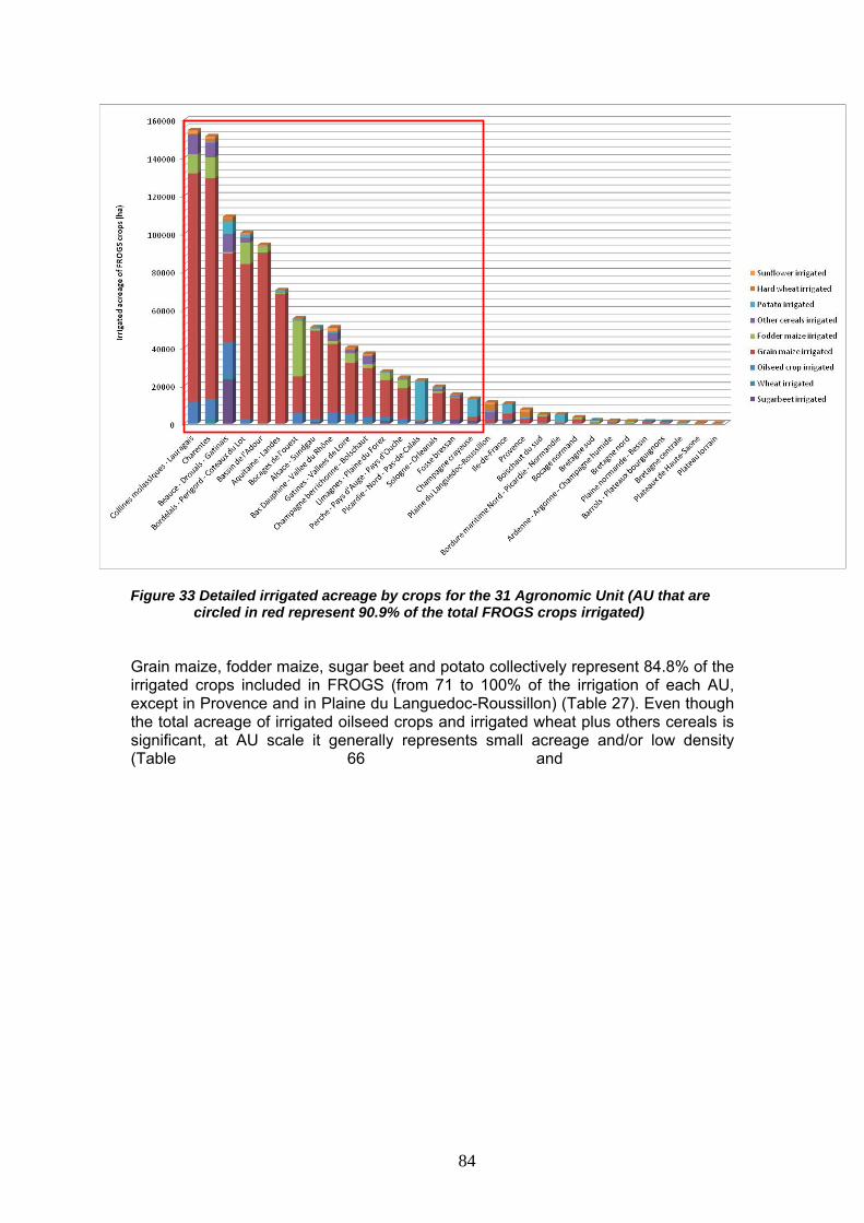
Figure 33 Detailed irrigated acreage by crops for the 31 Agronomic Unit (AU that are circled in red represent 90.9% of the total FROGS crops irrigated)
Grain maize, fodder maize, sugar beet and potato collectively represent 84.8% of the irrigated crops included in FROGS (from 71 to 100% of the irrigation of each AU, except in Provence and in Plaine du Languedoc-Roussillon) (Table 27). Even though the total acreage of irrigated oilseed crops and irrigated wheat plus others cereals is significant, at AU scale it generally represents small acreage and/or low density (Table 66 and
84

Table 67 in Appendix 14). It was therefore decided to implement irrigation only on grain maize, fodder maize, sugar beet and potato.
85

Table 27 Relative acreage of the main 4 individual irrigated crops within each
Agronomic Unit Grain Maize Irrigated (%)*
Fodder Maize Irrigated (%)*
Sum of the main 4 individual irrigated crops (%)*
Potato Irrigated (%)*
Beetroot Irrigated (%)*
Code AU Name AU
Collines molassiques - Lauragais 1 77.9 6.5 0.1 0.0 84.6 Charentes 10 76.9 7.3 0.3 0.0 84.5 Beauce - Drouais - Gatinais 17 42.9 0.6 6.0 21.4 71.0 Bordelais - Perigord - Coteaux du Lot 18 81.4 11.3 1.6 0.0 94.3 Bassin de l'Adour 8 95.6 3.5 0.0 0.0 99.2 Aquitaine - Landes 7 97.1 1.0 1.3 0.1 99.4 Bocages de l'ouest 20 35.3 52.8 1.1 0.0 89.2 Alsace - Sundgau 5 91.7 2.4 0.6 1.8 96.5 Bas Dauphine - Vallee du Rhône 23 71.2 3.2 1.3 0.0 75.7 Gatines - Vallees de Loire 14 67.6 12.6 0.2 0.0 80.4 Champagne berrichonne - Boischaut 22 69.8 5.4 0.7 0.7 76.6 Limagnes - Plaine du Forez 3 70.5 14.7 0.9 5.5 91.5 Perche - Pays d'Auge - Pays d'Ouche 19 66.8 18.7 0.7 0.2 86.5 Picardie - Nord - Pas-de-Calais 9 1.5 0.5 91.1 3.7 96.9 Sologne - Orleanais 15 74.7 4.4 4.2 1.7 85.0 Fosse bressan 24 72.3 2.7 3.6 14.7 93.4 Champagne crayeuse 16 14.6 0.5 71.2 11.9 98.3 Plaine du Languedoc-Roussillon 28 14.2 0.4 4.0 0.0 18.6 Ile-de-France 31 25.4 0.8 48.0 17.7 91.9 Provence 27 27.2 0.1 9.3 0.0 36.6 Boischaut du sud 29 64.0 20.2 0.3 1.1 85.6 Bordure maritime Nord - Picardie - Normandie 4 5.5 4.5 81.4 6.6 98.1 Bocage normand 11 57.7 25.3 2.3 0.0 85.3 Bretagne sud 2 33.6 56.2 6.5 0.0 96.4 Ardenne - Argonne - Champagne humide 21 46.0 1.5 39.6 9.4 96.6 Bretagne nord 30 21.0 50.6 18.7 0.9 91.1 Plaine normande - Bessin 6 43.1 7.6 10.8 19.7 81.2 Barrois - Plateaux bourguignons 12 52.4 14.3 4.1 14.0 84.8 Bretagne centrale 25 8.0 5.0 87.0 0.0 100.0 Plateaux de Haute-Saone 26 83.3 13.8 0.6 0.9 98.6 Plateau lorrain 13 97.5 0.0 2.5 0.0 100.0 Territoire non pris en compte
61.5 0 37.3 22.0 1.6 0.6
*: expressed as percent of the total FROGS crops irrigated in each AU
86
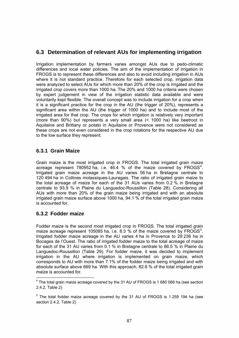
6.3 Determination of relevant AUs for implementing irrigation Irrigation implementation by farmers varies amongst AUs due to pedo-climatic differences and local water policies. The aim of the implementation of irrigation in FROGS is to represent these differences and also to avoid including irrigation in AUs where it is not standard practice. Therefore for each selected crop, irrigation data were analyzed to select AUs for which more than 20% of the crop is irrigated and the irrigated crop covers more than 1000 ha. The 20% and 1000 ha criteria were chosen by expert judgement in view of the irrigation statistic data available and were voluntarily kept flexible. The overall concept was to include irrigation for a crop when it is a significant practice for the crop in the AU (the trigger of 20%), represents a significant area within the AU (the trigger of 1000 ha) and to include most of the irrigated area for that crop. The crops for which irrigation is relatively very important (more than 90%) but represents a very small area (< 1000 ha) like beetroot in Aquitaine and Brittany or potato in Aquitaine or Provence were not considered as these crops are not even considered in the crop rotations for the respective AU due to the low surface they represent.
6.3.1 Grain Maize Grain maize is the most irrigated crop in FROGS. The total irrigated grain maize acreage represent 780952 ha, i.e. 46.4 % of the maize covered by FROGS4. Irrigated grain maize acreage in the AU varies 56 ha in Bretagne centrale to 120 494 ha in Collines molassiques-Lauragais. The ratio of irrigated grain maize to the total acreage of maize for each of the 31 AUs varies from 0.2 % in Bretagne centrale to 93.9 % in Plaine du Languedoc-Roussillon (Table 28). Considering all AUs with more than 20% of the grain maize being irrigated and with an absolute irrigated grain maize surface above 1000 ha, 94.1 % of the total irrigated grain maize is accounted for.
6.3.2 Fodder maize Fodder maize is the second most irrigated crop in FROGS. The total irrigated grain maize acreage represent 105085 ha, i.e. 8.3 % of the maize covered by FROGS5. Irrigated fodder maize acreage in the AU varies 4 ha in Provence to 29 236 ha in Bocages de l’Ouest. The ratio of irrigated fodder maize to the total acreage of maize for each of the 31 AU varies from 0.1 % in Bretagne centrale to 86.5 % in Plaine du Languedoc-Roussillon (Table 29). For fodder maize, it was decided to implement irrigation in the AU where irrigation is implemented on grain maize, which corresponds to AU with more than 7.1% of the fodder maize being irrigated and with absolute surface above 669 ha. With this approach, 82.6 % of the total irrigated grain maize is accounted for.
4 The total grain maize acreage covered by the 31 AU of FROGS is 1 680 066 ha (see section 2.4.2, ) Table 2
5 The total fodder maize acreage covered by the 31 AU of FROGS is 1 259 194 ha (see section 2.4.2, Table 2)
87
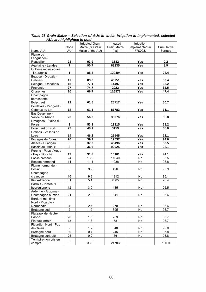
Table 28 Grain Maize – Selection of AUs in which irrigation is implemented, selected
AUs are highlighted in bold Irrigated Grain Maize (% Grain
Maize of the AU)
Irrigated Grain Maize
(ha)
Irrigation implemented in
FROGS Code AU
Cumulative Surface Name AU
Plaine du Languedoc-Roussillon 28 93.9 1582 Yes 0.2
7 90.7 68235 Yes 8.9 Aquitaine - Landes Collines molassiques - Lauragais 1 85.4 120494 Yes 24.4 Beauce - Drouais - Gatinais 17 83.6 46751 Yes 30.4
15 77.1 14497 Yes 32.2 Sologne - Orleanais 27 74.7 2022 Yes 32.5 Provence 10 66.7 116376 Yes 47.4 Charentes
Champagne berrichonne - Boischaut 22 61.5 25717 Yes 50.7 Bordelais - Perigord - Coteaux du Lot 18 61.1 81783 Yes 61.1 Bas Dauphine - Vallee du Rhône 23 56.0 36076 Yes 65.8 Limagnes - Plaine du Forez 3 53.3 19315 Yes 68.2
29 49.1 3159 Yes 68.6 Boischaut du sud Gatines - Vallees de Loire 14 46.2 26945 Yes 72.1
20 39.9 19537 Yes 74.6 Bocages de l'ouest 5 37.0 46496 Yes 80.5 Alsace - Sundgau 8 36.6 90025 Yes 92.1 Bassin de l'Adour
Perche - Pays d'Auge - Pays d'Ouche 19 31.8 16101 Yes 94.1 Fosse bressan 24 13.2 11040 No 95.5 Bocage normand 11 11.1 1938 No 95.8 Plaine normande - Bessin 6 9.9 496 No 95.9 Champagne crayeuse 16 9.3 1912 No 96.1 Ile-de-France 31 5.1 2665 No 96.4 Barrois - Plateaux bourguignons 12 3.9 485 No 96.5 Ardenne - Argonne - Champagne humide 21 2.8 641 No 96.6 Bordure maritime Nord - Picardie - Normandie 4 2.7 270 No 96.6 Bretagne sud 2 1.9 595 No 96.7 Plateaux de Haute-Saone 26 1.6 289 No 96.7 Plateau lorrain 13 1.3 78 No 96.7 Picardie - Nord - Pas-de-Calais 9 1.2 348 No 96.8 Bretagne nord 30 0.4 245 No 96.8 Bretagne centrale 25 0.2 56 No 96.8 Territoire non pris en compte 0 33.6 24783 100.0
88
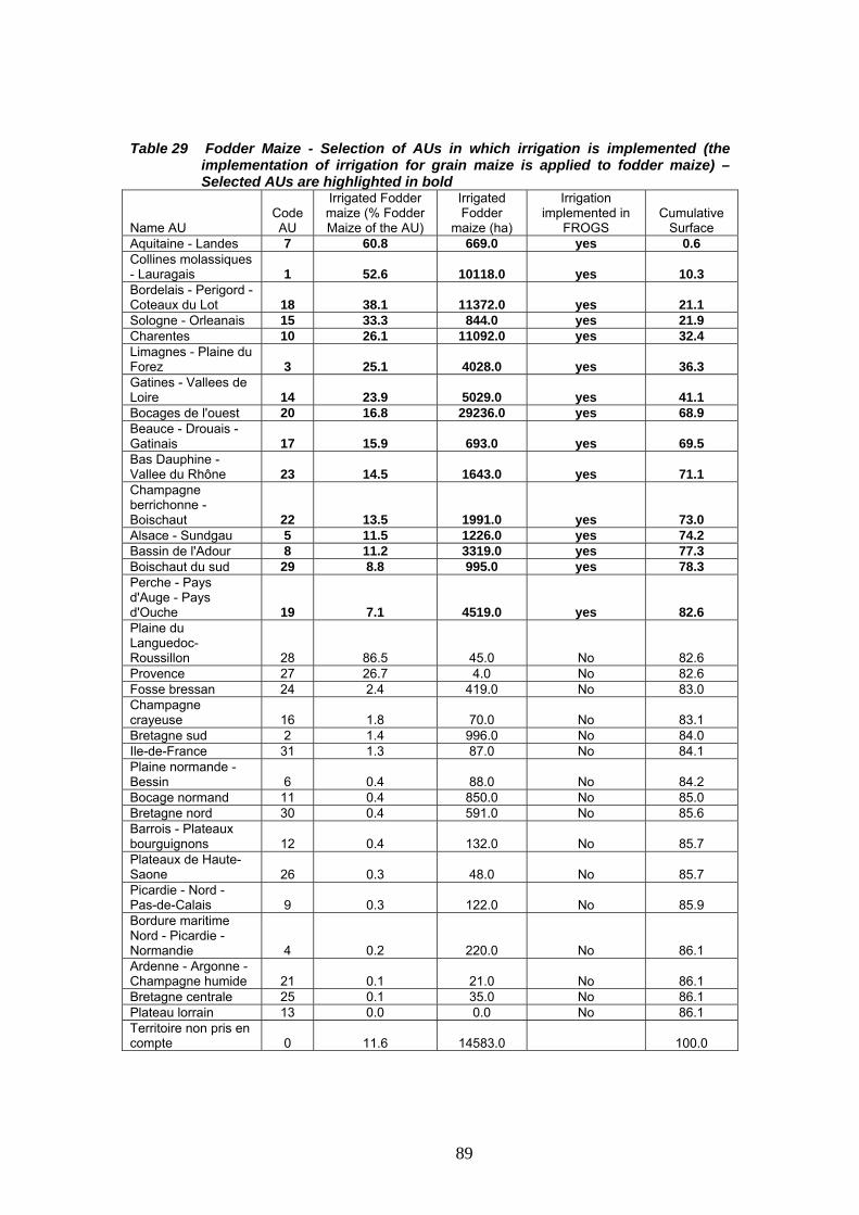
Table 29 Fodder Maize - Selection of AUs in which irrigation is implemented (the implementation of irrigation for grain maize is applied to fodder maize) – Selected AUs are highlighted in bold
Irrigated Fodder maize (% Fodder Maize of the AU)
Irrigated Fodder
maize (ha)
Irrigation implemented in
FROGS Code AU
Cumulative Surface Name AU
7 60.8 669.0 yes 0.6 Aquitaine - Landes Collines molassiques - Lauragais 1 52.6 10118.0 yes 10.3 Bordelais - Perigord - Coteaux du Lot 18 38.1 11372.0 yes 21.1
15 33.3 844.0 yes 21.9 Sologne - Orleanais 10 26.1 11092.0 yes 32.4 Charentes
Limagnes - Plaine du Forez 3 25.1 4028.0 yes 36.3 Gatines - Vallees de Loire 14 23.9 5029.0 yes 41.1
20 16.8 29236.0 yes 68.9 Bocages de l'ouest Beauce - Drouais - Gatinais 17 15.9 693.0 yes 69.5 Bas Dauphine - Vallee du Rhône 23 14.5 1643.0 yes 71.1 Champagne berrichonne - Boischaut 22 13.5 1991.0 yes 73.0
5 11.5 1226.0 yes 74.2 Alsace - Sundgau 8 11.2 3319.0 yes 77.3 Bassin de l'Adour 29 8.8 995.0 yes 78.3 Boischaut du sud
Perche - Pays d'Auge - Pays d'Ouche 19 7.1 4519.0 yes 82.6 Plaine du Languedoc-Roussillon 28 86.5 45.0 No 82.6 Provence 27 26.7 4.0 No 82.6 Fosse bressan 24 2.4 419.0 No 83.0 Champagne crayeuse 16 1.8 70.0 No 83.1 Bretagne sud 2 1.4 996.0 No 84.0 Ile-de-France 31 1.3 87.0 No 84.1 Plaine normande - Bessin 6 0.4 88.0 No 84.2 Bocage normand 11 0.4 850.0 No 85.0 Bretagne nord 30 0.4 591.0 No 85.6 Barrois - Plateaux bourguignons 12 0.4 132.0 No 85.7 Plateaux de Haute-Saone 26 0.3 48.0 No 85.7 Picardie - Nord - Pas-de-Calais 9 0.3 122.0 No 85.9 Bordure maritime Nord - Picardie - Normandie 4 0.2 220.0 No 86.1 Ardenne - Argonne - Champagne humide 21 0.1 21.0 No 86.1 Bretagne centrale 25 0.1 35.0 No 86.1 Plateau lorrain 13 0.0 0.0 No 86.1 Territoire non pris en compte 0 11.6 14583.0 100.0
89

6.3.3 Beetroot / Sugar beet The total irrigated beetroot / sugar beet acreage represent 34257 ha, i.e. 8.4 % of the beetroot covered by FROGS6. Irrigated beetroot acreage in the AU varies from 3 ha in Plateaux de Haute-Sâone to 23 327 ha in Beauce-Drouais-Gâtinais. The ratio of irrigated beetroot to the total acreage of beetroot for each of the 31 AU varies from 0.6 % in Bordure maritime nord – Picardie - Normandie to 100 % in Aquitaine-Landes (Table 30). Considering all AUs with more than 20% of the beetroot being irrigated and with an absolute irrigated beetroot above 1000 ha, 79 % of the total irrigated beetroot is accounted for.
6.3.4 Potato The total irrigated potato acreage represent 56 424 ha, i.e. 36.5% of the potato covered by FROGS7. Irrigated potato acreage in the AU varies from 2 ha in Plateau Lorrain to 20 665 ha in Picardie-Nord-Pas-de-Calais. The ratio of irrigated potato to the total acreage of potato for each of the 31 AU varies from 1.5 % in Plateau Lorrain to 99.3 % in Aquitaine-Landes (Table 31). Considering all AUs with more than 20% of the potato being irrigated and with an absolute irrigated potato above 1000 ha, 73.7 % of the total irrigated potato is accounted for. It was decided to also include the Bordure maritime Nord – Picardie – Normandie unit, resulting in an overall coverage of 80.8 % of the total irrigated potato.
6 The total sugar beet acreage covered by the 31 AU of FROGS is 408 123 ha (see section 2.4.2, ) Table 2
Table 2
7 The total potato acreage covered by the 31 AU of FROGS is 154 593 ha (see section 2.4.2, )
90
Table 30 Beetroot/Sugar beet – Selection of AU in which irrigation is implemented
(irrigation intensity >20%, absolute surface > 1000 ha) – selected AUs are highlighted in bold
Irrigated Beetroot (%
Beetroot of the AU)
Irrigated Beetroot
(ha)
Irrigation implemented in
FROGS Code AU
Cumulative Surface Name AU
Beauce - Drouais - Gatinais 17 65.9 23327 Yes 68.1
24 52.8 2236 Yes 74.6 Fosse bressan Limagnes - Plaine du Forez 3 44.7 1503 Yes 79.0 Aquitaine - Landes 7 100.0 38 No 79.1 Bretagne nord 30 90.9 10 No 79.1 Collines molassiques - Lauragais 1 84.6 22 No 79.2 Sologne - Orleanais 15 77.1 336 No 80.2 Bordelais - Perigord - Coteaux du Lot 18 76.9 30 No 80.3 Champagne berrichonne - Boischaut 22 69.7 260 No 81.0 Boischaut du sud 29 23.0 56 No 81.2 Alsace - Sundgau 5 17.2 916 No 83.9 Barrois - Plateaux bourguignons 12 7.4 130 No 84.3 Plateaux de Haute-Saone 26 7.0 3 No 84.3 Plaine normande - Bessin 6 3.9 227 No 84.9 Perche - Pays d'Auge - Pays d'Ouche 19 3.4 52 No 85.1 Ile-de-France 31 2.3 1858 No 90.5 Champagne crayeuse 16 2.2 1562 No 95.1 Ardenne - Argonne - Champagne humide 21 1.1 131 No 95.4 Picardie - Nord - Pas-de-Calais 9 0.7 845 No 97.9 Bordure maritime Nord - Picardie - Normandie 4 0.6 324 No 98.9 Charentes 10 0.0 0 No 98.9 Bassin de l'Adour 8 0.0 0 No 98.9 Bocages de l'ouest 20 0.0 0 No 98.9 Bas Dauphine - Vallee du Rhône
0 23 0.0 No 98.9
Gatines - Vallees de Loire
0 14 0.0 No 98.9
Plaine du Languedoc-Roussillon 28 0.0
0 No 98.9
Provence 27 0.0 0 No 98.9 Bocage normand 11 0.0 0 No 98.9 Bretagne sud 2 0.0 0 No 98.9 Bretagne centrale 25 0.0 0 No 98.9 Plateau lorrain 13 0.0 0 No 98.9 Territoire non pris en compte 0 40.8 391 No 100.0
91

Table 31 Potato - Selection of AU in which irrigation is implemented (irrigation intensity
>20%, absolute surface > 1000 ha) – selected AU are highlighted in bold Irrigated Potato (% Potato of the
UA)
Irrigation implemented in
FROGS Code AU
Irrigated Potato (ha)
Cumulative Surface Name AU
Beauce - Drouais - Gatinais 17 95.2 6562 Yes 11.6
16 51.1 9334 Yes 28.2 Champagne crayeuse 31 41.4 5037 Yes 37.1 Ile-de-France
Picardie - Nord - Pas-de-Calais 9 32.0 20665 Yes 73.7 Bordure maritime Nord - Picardie - Normandie 4 17.3 3968 Yes 80.8 Aquitaine - Landes 7 99.3 930 No 82.4 Provence 27 92.5 694 No 83.6 Sologne - Orleanais 15 92.2 808 No 85.1 Champagne berrichonne - Boischaut 22 91.3 241 No 85.5 Plaine du Languedoc-Roussillon 28 90.8 445 No 86.3 Bordelais - Perigord - Coteaux du Lot 18 90.4 1612 No 89.1 Bocages de l'ouest 20 75.8 617 No 90.2 Charentes 10 73.5 516 No 91.1 Collines molassiques - Lauragais 1 55.4 107 No 91.3 Bas Dauphine - Vallee du Rhône 23 53.8 652 No 92.5 Fosse bressan 24 52.3 552 No 93.5 Boischaut du sud 29 51.6 16 No 93.5 Gatines - Vallees de Loire 14 51.1 94 No 93.7 Limagnes - Plaine du Forez 3 47.2 239 No 94.1 Perche - Pays d'Auge - Pays d'Ouche 19 39.5 180 No 94.4 Bassin de l'Adour 8 36.5 31 No 94.5 Ardenne - Argonne - Champagne humide 21 36.3 551 No 95.4 Alsace - Sundgau 5 28.0 303 No 96.0 Bretagne centrale 25 20.6 609 No 97.1 Bretagne sud 2 14.9 116 No 97.3 Plaine normande - Bessin 6 14.1 124 No 97.5 Barrois - Plateaux bourguignons 12 11.2 38 No 97.5 Bocage normand 11 4.4 76 No 97.7 Plateaux de Haute-Saone 26 3.3 2 No 97.7 Bretagne nord 30 2.2 219 No 98.1 Plateau lorrain 13 1.5 2 No 98.1 Territoire non pris en compte 0 34.5 1084 100.0
92
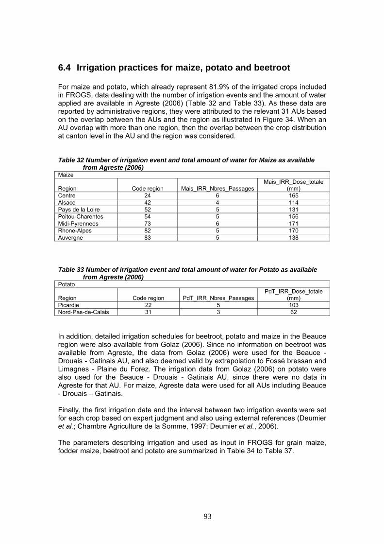
6.4 Irrigation practices for maize, potato and beetroot For maize and potato, which already represent 81.9% of the irrigated crops included in FROGS, data dealing with the number of irrigation events and the amount of water applied are available in Agreste (2006) (Table 32 and Table 33). As these data are reported by administrative regions, they were attributed to the relevant 31 AUs based on the overlap between the AUs and the region as illustrated in Figure 34. When an AU overlap with more than one region, then the overlap between the crop distribution at canton level in the AU and the region was considered. Table 32 Number of irrigation event and total amount of water for Maize as available
from Agreste (2006) Maize
Region Code region Mais_IRR_Nbres_Passages Mais_IRR_Dose_totale
(mm) Centre 24 6 165 Alsace 42 4 114 Pays de la Loire 52 5 131 Poitou-Charentes 54 5 156 Midi-Pyrennees 73 6 171 Rhone-Alpes 82 5 170 Auvergne 83 5 138 Table 33 Number of irrigation event and total amount of water for Potato as available
from Agreste (2006) Potato
Region Code region PdT_IRR_Nbres_Passages PdT_IRR_Dose_totale
(mm) Picardie 22 5 103 Nord-Pas-de-Calais 31 3 62 In addition, detailed irrigation schedules for beetroot, potato and maize in the Beauce region were also available from Golaz (2006). Since no information on beetroot was available from Agreste, the data from Golaz (2006) were used for the Beauce - Drouais - Gatinais AU, and also deemed valid by extrapolation to Fossé bressan and Limagnes - Plaine du Forez. The irrigation data from Golaz (2006) on potato were also used for the Beauce - Drouais - Gatinais AU, since there were no data in Agreste for that AU. For maize, Agreste data were used for all AUs including Beauce - Drouais – Gatinais. Finally, the first irrigation date and the interval between two irrigation events were set for each crop based on expert judgment and also using external references (Deumier et al.; Chambre Agriculture de la Somme, 1997; Deumier et al., 2006). The parameters describing irrigation and used as input in FROGS for grain maize, fodder maize, beetroot and potato are summarized in Table 34 to Table 37.
93

Figure 34 Overlap of the 31 Agronomic Units (colored blocks) and the “Régions administratives” (red lines) - Small unit (black lines) represent the "Cantons".
94

Table 34 Grain Maize - Main parameters describing irrigation
First irrigation
date Interval between 2 irrigation events (d)
Number of irrigation events
Amount of water/event (mm) Nom UA
Plaine du Languedoc-Roussillon 15 June 8 7 24 Aquitaine - Landes 15 June 8 7 24 Collines molassiques - Lauragais 15 June 8 7 24 Beauce - Drouais - Gatinais 1 July 9 6 28 Sologne - Orleanais 1 July 9 6 28 Provence 15 June 8 7 24 Charentes 15 June 9 6 28 Champagne berrichonne - Boischaut 1 July 9 6 28 Bordelais - Perigord - Coteaux du Lot 15 June 8 7 24 Bas Dauphine - Vallee du Rhône 15 June 11 5 34 Limagnes - Plaine du Forez 15 June 11 5 34 Boischaut du sud 15 June 9 6 28 Gatines - Vallees de Loire 1 July 9 6 28 Bocages de l'ouest 1 July 11 5 31 Alsace - Sundgau 1 July 14 4 29 Bassin de l'Adour 15 June 8 7 24 Perche - Pays d'Auge - Pays d'Ouche 1 July 9 6 28 Table 35 Fodder Maize - Main parameters describing irrigation
First irrigation
date Interval between 2 irrigation events (d)
Number of irrigation event
Amount of water/event (mm) Nom UA
Aquitaine - Landes 15 June 8 7 24 Collines molassiques - Lauragais 15 June 8 7 24 Bordelais - Perigord - Coteaux du Lot 15 June 8 7 24 Sologne - Orleanais 1 July 9 6 28 Charentes 15 June 9 6 28 Limagnes - Plaine du Forez 15 June 11 5 34 Gatines - Vallees de Loire 1 July 9 6 28 Bocages de l'ouest 1 July 11 5 31 Beauce - Drouais - Gatinais 1 July 9 6 28 Bas Dauphine - Vallee du Rhône 15 June 11 5 34 Champagne berrichonne - Boischaut 1 July 9 6 28 Alsace - Sundgau 1 July 14 4 29 Bassin de l'Adour 15 June 8 7 24 Boischaut du sud 15 June 9 6 28 Perche - Pays d'Auge - Pays d'Ouche 1 July 9 6 28
95

Table 36 Beetroot/Sugarbeet - Main parameters describing irrigation
First irrigation
date Interval between 2 irrigation events (d)
Number of irrigation event
Amount of water/event (mm) Nom UA
Beauce - Drouais - Gatinais
11 June 7 4 35
Fosse bressan 11 June 7 4 35 Limagnes - Plaine du Forez
11 June 7 4 35
Table 37 Potato - Main parameters describing irrigation
First irrigation
date Interval between 2 irrigation events (d)
Number of irrigation event
Amount of water/event (mm) Nom UA
Beauce - Drouais - Gatinais 21 May 4 7 25 Champagne crayeuse 1 June 8 5 21 Ile-de-France 1 June 8 5 21 Picardie - Nord - Pas-de-Calais 1 June 8 5 21 Bordure maritime Nord - Picardie - Normandie 1 June 8 5 21
6.5 Implementation of irrigation in FROGS The above-listed irrigation schedules for the relevant crop – AU combinations were included in the FROGS database. Irrigation is implemented on the same fixed dates year by year over the whole simulation period and does not take into account the actual soil moisture content or temporal meteorological variations over that period. The fixed irrigation scheduling also does not account for weather events, which means that postponing of scheduled irrigation due to rainfall is not considered. However, as pointed out by Golaz (2006), ideal irrigation calendars based on soil moisture content and weather forecasts are seldom used in reality in the field, as the irrigation scheduling is in fact a compromise between crop water needs, water retention capacity of the soil and practical constraints related to equipment and timing of irrigations (for given field and crop among all irrigated fields and crops at the farm level). During the main irrigation period it is difficult for farmers to adjust inputs, since increasing irrigation dose would increase irrigation time, and therefore delay following irrigation (next field in farm irrigation rotation program). In reality irrigation scheduling is often not that flexible due to lack of equipment and irrigation rounds are made regardless of particular weather events. The implementation of irrigation in FROGS based on fixed dates is therefore justified. Irrigation schemes are implemented the same way in FROGS as they are in standard FOCUS simulations, i.e. irrigation water is applied directly to the soil surface. Canopy processes are not simulated. The relevant irrigation schemes were considered in the generation of the pre-run SWAP soil hydrology (*.pfo files).
96
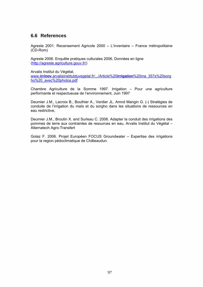
6.6 References Agreste 2001. Recensement Agricole 2000 – L’inventaire – France métropolitaine (CD-Rom) Agreste 2006. Enquête pratiques culturales 2006, Données en ligne (http://agreste.agriculture.gouv.fr/) Arvalis Institut du Végétal, www.irrinov.arvalisinstitutduvegetal.fr/.../Article%20irrigation%20ma_357s%20sorgho%20_avec%20photos.pdf Chambre Agriculture de la Somme 1997. Irrigation – Pour une agriculture performante et respectueuse de l’environnement, Juin 1997 Deumier J.M., Lacroix B., Bouthier A., Verdier JL. Amnd Mangin G. (-) Stratégies de conduite de l’irrigation du maïs et du sorgho dans les situations de ressources en eau restrictive, Deumier J.M., Broutin X. and Surleau C. 2006. Adapter la conduit des irrigations des pommes de terre aux contraintes de resources en eau, Arvalis Institut du Végétal – Alternatech Agro-Transfert Golaz F. 2006. Projet Européen FOCUS Groundwater – Expertise des irrigations pour la region pédoclimatique de Châteaudun.
97
7 Selection of representative soil-types INRA INFOSOL Orléans was mandated by SSM to select a limited number of representative soil-types at national level and representative soil profiles associated with these soil-types for the ComTox groundwater scenarios workgroup. The selection of representative soils was limited to the arable land representative for the cultivation of the selected field crops (cereals, maize, sunflower, oilseed rape, sugar beets and potatoes), which means that these soils are not necessarily representative of other crops, e.g. vegetable crops and perennial crops such as orchards fruits and grapevines. The arable land relevant for production of the selected field crops was determined using the 2000 agricultural census and Corine Land Cover database. Within the relevant surface, INRA then used the BDGSF soil database to select a total of 19 predominant soil-types. Finally, representative soil profiles were selected from the DONESOL2 database for each of the 19 soil-types. INRA reported its work in Morvan & Le Bas, 2006 (in French), and this report is the main basis for this chapter on the selection of representative soils. 7.1 Land use data 7.1.1 Agricultural census The agricultural census (recensement agricole) is a ten-yearly census organized by the French Ministry for Food, Agriculture and Fisheries. It contains information at the farm scale on population, production, production methods and side-activities (on-site processing, tourism). INRA extracted from the 2000 agricultural census the latest available detailed information on the cultivation of the selected field crops at the canton administrative level (canton = administrative district consisting of several communes (municipalities); there are 4039 cantons in France). 7.1.2 Corine Land Cover The Corine Land Cover (CLC) database is a European geographical database for land use coordinated by the European Environment Agency (EEA). CLC 2000 (ETC, 2000) is the year 2000 update of the first CLC database which was finalised in the early 1990s as part of the European Commission programme to COoRdinate INformation on the Environment (Corine). In France, IFEN has been responsible for the Corine data production, maintenance and diffusion. IFEN (Institut Français de l’Environnement) joined SOeS (Service de l’Observation et des Statistiques) in July 2008. The database contains land use information at a scale of 1/100000. The CLC 2000 database was used to delimit arable land within the selected cantons and exclude all non-cropped land. The database was updated in 2006, but INRA conducted the analysis using the 2000 database, in line with the timing of the agricultural census.
98
7.2 Soil data 7.2.1 BDGSF For detailed information on soils and to identify the dominant soils for the different crops, INRA used the Geographical DataBase of French Soils (BDGSF, Base de Données Géographique des Sols de France), which contains information on soil types at a scale of 1/1000000. BDGSF is managed by GIS Sol, a conglomerate of French administrative institutes and scientific partners. These data are also part of the European Soil Geographical DataBase (ESGDB, Finke et al. 2001) since GIS Sol participates in this program as member of the European Soil Bureau (ESBN). The soil classification in BDGSF is adapted from standard FAO terminology (FAO, 1974) to include French specificities. The different soil types are identified in BDGSF as Unités Typologiques de Sol (UTS = STU, Soil Typological Units in ESDB), however given the scale of 1/1000000 of the database, the data do not permit to delimit and locate precisely these different UTS (917 in total). Instead, UTS are regrouped in Unités Cartographiques de Sol (UCS = SMU, Soil Mapping Units in ESDB). These UCS are defined by their geometry (set of polygons described by their shape and geographical position) and their composition in term of relative contribution of the different UTS that are included in the UCS. They can therefore be spatially located and consist of well-identified UTS, but the UTS themselves cannot be located within the UCS, only their relative proportion in the UCS is known. One should note that the same UTS can be found in different UCS (Figure 35).
99

- Geometrically defined by a polygon- Composed of UTS 10
(which is also part of UCS 1)
- Geometrically defined by 2 polygons- Composed of UTS 10 and 11
- Geometrically defined by 1 polygon- Composed of UTS 12
- Geometrically defined by 3 polygons- Composed of UTS 13 and 14
The concept of pedologicallandscape…
… and its translation in terms of spatial database
POLYGONS attributes
UCS attributes
UTS attributes
… and its translation in terms of spatial database
POLYGONS attributes
UCS attributes
UTS attributes
Figure 35 Relationship between geographical (UCS) and typological (UTS)
representation of soils in the BDGSF database (adapted from BDGSF and ESGDB on-line documentation)
100
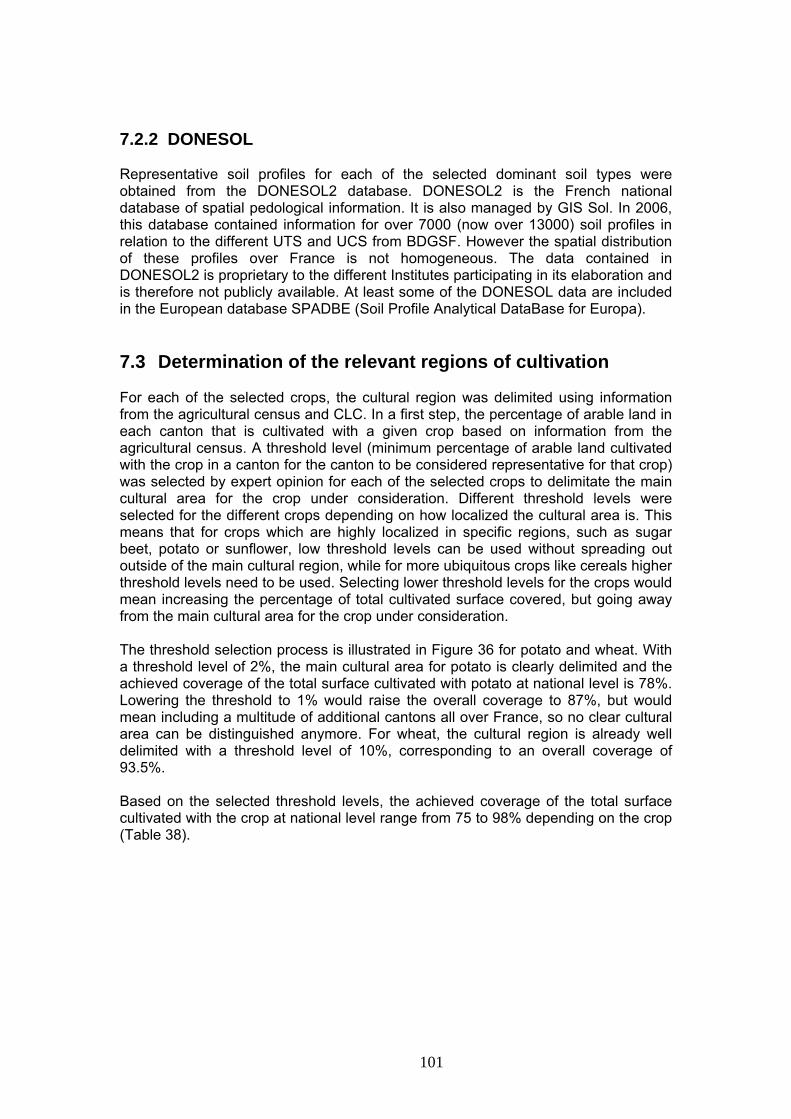
7.2.2 DONESOL Representative soil profiles for each of the selected dominant soil types were obtained from the DONESOL2 database. DONESOL2 is the French national database of spatial pedological information. It is also managed by GIS Sol. In 2006, this database contained information for over 7000 (now over 13000) soil profiles in relation to the different UTS and UCS from BDGSF. However the spatial distribution of these profiles over France is not homogeneous. The data contained in DONESOL2 is proprietary to the different Institutes participating in its elaboration and is therefore not publicly available. At least some of the DONESOL data are included in the European database SPADBE (Soil Profile Analytical DataBase for Europa). 7.3 Determination of the relevant regions of cultivation For each of the selected crops, the cultural region was delimited using information from the agricultural census and CLC. In a first step, the percentage of arable land in each canton that is cultivated with a given crop based on information from the agricultural census. A threshold level (minimum percentage of arable land cultivated with the crop in a canton for the canton to be considered representative for that crop) was selected by expert opinion for each of the selected crops to delimitate the main cultural area for the crop under consideration. Different threshold levels were selected for the different crops depending on how localized the cultural area is. This means that for crops which are highly localized in specific regions, such as sugar beet, potato or sunflower, low threshold levels can be used without spreading out outside of the main cultural region, while for more ubiquitous crops like cereals higher threshold levels need to be used. Selecting lower threshold levels for the crops would mean increasing the percentage of total cultivated surface covered, but going away from the main cultural area for the crop under consideration. The threshold selection process is illustrated in Figure 36 for potato and wheat. With a threshold level of 2%, the main cultural area for potato is clearly delimited and the achieved coverage of the total surface cultivated with potato at national level is 78%. Lowering the threshold to 1% would raise the overall coverage to 87%, but would mean including a multitude of additional cantons all over France, so no clear cultural area can be distinguished anymore. For wheat, the cultural region is already well delimited with a threshold level of 10%, corresponding to an overall coverage of 93.5%. Based on the selected threshold levels, the achieved coverage of the total surface cultivated with the crop at national level range from 75 to 98% depending on the crop (Table 38).
101
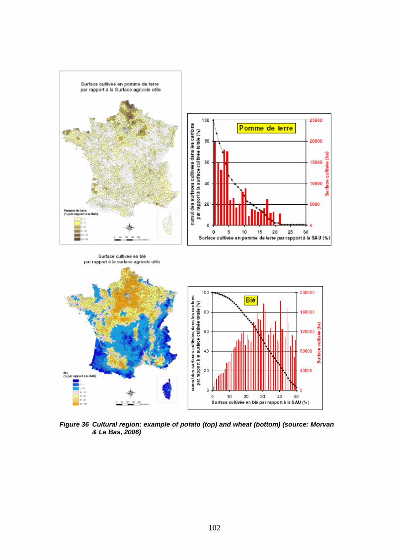
Figure 36 Cultural region: example of potato (top) and wheat (bottom) (source: Morvan
& Le Bas, 2006)
102
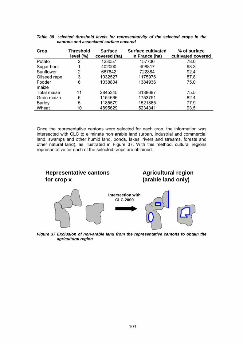
Table 38 Selected threshold levels for representativity of the selected crops in the
cantons and associated surface covered
Crop Threshold level (%)
Surface covered (ha)
Surface cultivated in France (ha)
% of surface cultivated covered
Potato 2 123057 157736 78.0 Sugar beet 1 402000 408817 98.3 Sunflower 2 667842 722884 92.4 Oilseed rape 3 1032527 1175976 87.8 Fodder maize
6 1038804 1384936 75.0
Total maize 11 2845345 3138687 75.5 Grain maize 6 1154666 1753751 82.4 Barley 5 1185579 1521865 77.9 Wheat 10 4895629 5234341 93.5 Once the representative cantons were selected for each crop, the information was intersected with CLC to eliminate non arable land (urban, industrial and commercial land, swamps and other humid land, ponds, lakes, rivers and streams, forests and other natural land), as illustrated in Figure 37. With this method, cultural regions representative for each of the selected crops are obtained.
Representative cantons for crop x
Agricultural region(arable land only)
Intersection withCLC 2000
Representative cantons for crop x
Agricultural region(arable land only)
Intersection withCLC 2000
Figure 37 Exclusion of non-arable land from the representative cantons to obtain the
agricultural region
103
7.4 Selection of typical soils within the agricultural regions For determination of the dominant soil types for each crop, the cultural region for the crop under consideration was intersected with the BDGSF. This is performed in successive steps as follows:
1. The surface associated with the different UCS within the cantons arable land is calculated. This gives the arable surface of each UCS by canton.
2. This surface is then multiplied by the % of arable land cultivated with the crop of interest in the canton to obtain the surface of soil representative for that crop in each canton.
3. This representative surface per canton is then summed up for all the relevant cantons in the crop cultural region to provide the representative surface of the UCS for the whole cultural region.
4. The representative surface for each UTS is then back-calculated from the UCS surface, by multiplying the UCS surface by the relative percentage of each UTS within that UCS.
5. UTS were then regrouped in clusters of UTS of similar properties (USR, Unité de Sols Regroupés). The reason for this regrouping was that UTS are characterized in BDGSF by textural class (Figure 38), number of horizons and soil depth, but also by additional criterias that are not necessarily relevant for the setting up of groundwater scenarios within the scope of FROGS (i.e. leaching at the bottom of the soil profile) such as composition of the bedrock, slope, etc. Grouping UTS in USR was performed based on textural class, number of horizons and soil depth, meaning that all the soils contained in a given USR are of the same textural class and are comparable in terms of number of horizons and depth of the profile. The grouping resulted in 96 different USR (from 917 UTS).
6. The surface represented by each USR in the cultural region is calculated from the UTS surface, by summing up the surface associated to the different UTS relevant for the USR in question.
7. While the different UTS within a USR have the same textural class, number of horizons and depth of profile, these include soils from different origin and of different denomination according to FAO pedogenesis classification. In order to account for the different physico-chemical environment associated to the particular origin of the soils, and to facilitate the link with the soil profile database DONESOL, the soils of the same denomination within the USR were regrouped and these USR subgroups were considered as the different soil types relevant for FROGS.
8. For each crop and associated cultural region, the representative soil types are classified in function of the surface and associated percentage of the cultural region they represent. The most dominant soils are actually common to the majority of the different cultural regions, which is to be expected since due to crop rotations the same cantons are representative for different crops and are therefore accounted in several agricultural regions. It is therefore possible with a limited number of soil types to achieve a good representation of the most relevant soils for all crops considered.
104

% sand
% silt% clay
% sand
% silt% clay
Figure 38 Textural classification in BDGSF
Canton UCS Surface arable land (ha)
586 20 300 586 25 120 587 20 30 587 25 40 587 28 100 588 28 100 595 25 100 595 28 50 595 34 120
Canton % of arable land cultivated with crop x
586 2.5 587 10.0 588 2.0 595 5.0
x
Canton UCS Surface cultivated with crop x (ha)
586 20 7.5 586 25 3 587 20 3 587 25 4 587 28 10 588 28 2 595 25 5 595 28 2.5 595 34 6
UCS Surface cultivated with crop x (ha)
20 10.5 25 12 28 12 34 6
Sum by UCS
UCS to UTS
UCS UTS % of UTS in UCS 20 330 38 20 331 62 25 337 50 25 338 25 25 339 25 28 350 100 34 400 33 34 401 67
UTS Surface cultivated with crop x (ha)
330 4 331 6.5 337 6 338 3 339 3 350 12 400 2 401 4
Figure 39 Extraction of the dominant UTS in the agricultural region for crop x
(steps 2-4 of above-described methodology, adapted from Morvan & Le Bas, 2006)
105

UTS to USR
UTS Surface cultivated with crop x (ha)
330 4 331 6.5 337 6 338 3 339 3 350 12 400 2 401 4
UTS USR 330 1 331 2 337 2 338 2 339 3 350 4 400 1 401 3
USR Surface cultivated with crop x (ha)
1 6 2 15.5 3 7 4 12
USR Soil denomination
Surface cultivated with crop x (ha)
1 Luvisol 4.5 1 Cambisol 1.0 1 Gleysol 0.5 2 Rendzine 8.5 2 Podzoluvisol 5.0 2 Cambisol 2.0 3 Luvisol 5.5 3 Fluvisol 1.5 4 Luvisol 8.0 4 Cambisol 2.0 4 Rendzine 2.0
USR to soil-types (split by soilpedogenesisdenomination)
Figure 40 Extraction of the dominant USR and soil-types in the agricultural region for
crop x (steps 5-7 of above-described methodology, adapted from Morvan & Le Bas, 2006)
106

7.5 Selection of representative soil profiles Representative soil profiles for the dominant soil-types extracted from the BDGSF were selected from the DONESOL2 database. While the pedogenesis classification in BDGSF is according to FAO, most soil profiles contained in DONESOL2 are classified according to the RP 1995 (Référentiel Pédologique 1995, Baize, 1995) classification, which is more detailed. Correspondence between these two classifications is provided in Table 39. Table 39 Correspondence between FAO and RP 1995 soil classifications FAO, 1974 classification RP 1995
classification Luvisol Luvisol
Cambisol Brunisol Podzoluvisol Degraded Luvisol
Rendzine Rendisol Rendosol Calcisol Calcosol
Fluvisol Fluviosol Gleysol Reductisol
Rédoxysol Solonchak Salisol
Sodisol Arénosol Arénosol
All the relevant soil profiles corresponding to a given selected soil-type were first extracted from DONESOL2 according to the following criteria:
• Land cover (cultivated soil) • Soil denomination • Texture of the soil horizons • Depth of the soil profile • Geographical location (preferentially within the cultural regions)
This lead to the identification of a number of representative soil profiles for each of the 19 soil-types. A single representative soil profile was selected among these soils according to the following criteria:
• Profiles with measured OC content (not available for all profiles) • Preference for soil profiles with textural analysis performed without
decarbonation (since dissolving with acid for removal of the carbonates results in destruction of soil particles)
• Soil profile with parameters (OC content, particle size distribution, depth of profile) in the medium range within the available soil profiles for the soil-type (exclusion of soils with extreme characteristics)
• Preference for soil profiles originating from the main cultural regions (in case there were several soil profiles satisfying the medium range criteria,
107

preference was allocated to soil profiles originating from a well defined cultural region, such as that for sugar beets or sunflower)
7.6 Selected soil-types According to the followed stepwise approach, 19 dominant soil-types were identified (Table 40). These dominant soil-types cover a variety of pedogenesis classes, textural classes and depth of the soil profile. These 19 soil-types represent altogether between 57.2% (oilseed rape) and 73.9% (sugar beets) of the cultural regions for the respective crops (Morvan & Le Bas, 2006). Each additional soil-type would only add a minor contribution to the total represented surface of the cultural regions (<1-2%) and it was therefore decided to limit the soil selection to these 19 soil-types. Among these soils, the solonchak soil-type 18, which is a very particular soil with unusually high organic carbon content, turned out not to be relevant for the crops considered in FROGS (see section 7.8.2 and Appendix 16) and was therefore not considered any further. Table 40 FAO 1974 pedogenesis classification, BDGSF textural class and depth of
profile of the selected soil-types n° soil-type FAO denomination Texture class Depth of profile
1 Luvisol 3 >80 cm 2 Cambisol 4 >80 cm 3 Rendzine 2 >80 cm 4 Luvisol 2 >80 cm 5 Cambisol 3 60 cm 6 Rendzine 2 60 cm 7 Rendzine 4 40 cm 8 Fluvisol 2 >80 cm 9 Fluvisol 1 >80 cm
10 Gleysol 4 >80 cm 11 Cambisol 2 60 cm 12 Podzoluvisol 3 >80 cm 13 Cambisol 3 >80 cm 14 Podzoluvisol 2 >80 cm 15 Cambisol 2 >80 cm 16 Rendzine 3 60 cm 17 Rendzine 3 >80 cm 18 Solonchak 4 >80 cm 19 Arenosol 1 >80 cm
108
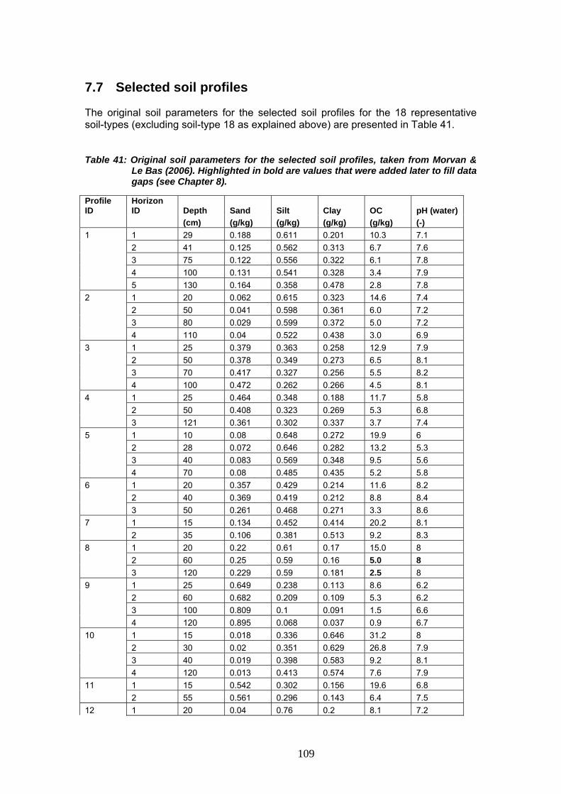
109
7.7 Selected soil profiles The original soil parameters for the selected soil profiles for the 18 representative soil-types (excluding soil-type 18 as explained above) are presented in Table 41. Table 41: Original soil parameters for the selected soil profiles, taken from Morvan &
Le Bas (2006). Highlighted in bold are values that were added later to fill data gaps (see Chapter 8).
Profile ID
Horizon ID Depth Sand Silt Clay OC pH (water)
(cm) (g/kg) (g/kg) (g/kg) (g/kg) (-) 1 1 29 0.188 0.611 0.201 10.3 7.1 2 41 0.125 0.562 0.313 6.7 7.6 3 75 0.122 0.556 0.322 6.1 7.8 4 100 0.131 0.541 0.328 3.4 7.9 5 130 0.164 0.358 0.478 2.8 7.8 2 1 20 0.062 0.615 0.323 14.6 7.4 2 50 0.041 0.598 0.361 6.0 7.2 3 80 0.029 0.599 0.372 5.0 7.2 4 110 0.04 0.522 0.438 3.0 6.9 3 1 25 0.379 0.363 0.258 12.9 7.9 2 50 0.378 0.349 0.273 6.5 8.1 3 70 0.417 0.327 0.256 5.5 8.2 4 100 0.472 0.262 0.266 4.5 8.1 4 1 25 0.464 0.348 0.188 11.7 5.8 2 50 0.408 0.323 0.269 5.3 6.8 3 121 0.361 0.302 0.337 3.7 7.4 5 1 10 0.08 0.648 0.272 19.9 6 2 28 0.072 0.646 0.282 13.2 5.3 3 40 0.083 0.569 0.348 9.5 5.6 4 70 0.08 0.485 0.435 5.2 5.8 6 1 20 0.357 0.429 0.214 11.6 8.2 2 40 0.369 0.419 0.212 8.8 8.4 3 50 0.261 0.468 0.271 3.3 8.6 7 1 15 0.134 0.452 0.414 20.2 8.1 2 35 0.106 0.381 0.513 9.2 8.3 8 1 20 0.22 0.61 0.17 15.0 8 2 60 0.25 0.59 0.16 5.0 8 3 120 0.229 0.59 0.181 2.5 8 9 1 25 0.649 0.238 0.113 8.6 6.2 2 60 0.682 0.209 0.109 5.3 6.2 3 100 0.809 0.1 0.091 1.5 6.6 4 120 0.895 0.068 0.037 0.9 6.7 10 1 15 0.018 0.336 0.646 31.2 8 2 30 0.02 0.351 0.629 26.8 7.9 3 40 0.019 0.398 0.583 9.2 8.1 4 120 0.013 0.413 0.574 7.6 7.9 11 1 15 0.542 0.302 0.156 19.6 6.8 2 55 0.561 0.296 0.143 6.4 7.5 12 1 20 0.04 0.76 0.2 8.1 7.2

2 35 0.04 0.76 0.2 8.1 7.2 3 60 0.05 0.69 0.26 1.5 7.1
7.1 4 140 0.08 0.67 0.25 0.1 13 1 20 0.038 0.682 0.28 11.0 7.8 2 50 0.027 0.698 0.275 6.6 7.5 3 110 0.013 0.615 0.372 3.8 7.5 4 130 0.04 0.687 0.273 1.9 7.9 14 1 3 0.197 0.707 0.096 32.5 4.2 2 10 0.189 0.713 0.098 32.5 4.4 3 36 0.195 0.7 0.105 8.1 4.7 4 64 0.155 0.719 0.126 3.0 4.6 5 80 0.077 0.788 0.135 2.0 4.8 6 95 0.137 0.624 0.239 2.3 4.9 7 132 0.203 0.284 0.513 2.7 5.1 8 0.088 0.356 0.556 2.4 5.1 15 1 25 0.337 0.469 0.194 11.6 6 2 35 0.323 0.495 0.182 11.5 6 3 48 0.28 0.55 0.17 5.7 6.3 4 100 0.31 0.51 0.18 3.1 6.4 5 110 0.3 0.5 0.2 2.1 6.4 16 1 30 0.091 0.6 0.309 11.1 8.2 2 60 0.188 0.529 0.283 5.4 8.6 17 1 8 0.072 0.631 0.297 14.6 8 2 28 0.07 0.628 0.302 14.2 8.1 3 40 0.227 0.479 0.294 8.0 8.3 4 75 0.306 0.48 0.214 2.7 8.5 5 120 0.407 0.326 0.267 2.1 8.7 19 1 28 0.843 0.111 0.046 7.3 5.8 2 38 0.885 0.081 0.034 1.6 6.3 3 56 0.894 0.077 0.029 1.0 6.7 4 90 0.957 0.022 0.021 1.0 6.1 5 130 0.961 0.014 0.025 0.5 6.6
110

7.8 Soil – Agronomic Units relationship The selected soil types and corresponding soil profiles are linked to the AUs in order to combine soil, crop and climatic information and finalize the construction of the scenarios. 7.8.1 Distribution of Soils in the Agronomic Units The surfaces of the 19 representative soil types in the AUs were calculated by INRA Infosol (Appendix 15). Results expressed as kHa are given in Table 42. Surface boundaries defined by the thresholds of 5 000, 10 000, 50 000 et 100 000 ha are displayed in this table using a color coding, to help selecting pertinent soils according to the degree of accuracy wished in the assessment. Soils with surfaces lower than 1 000 ha are not displayed in the table. 7.8.2 Soil Distribution as a function of Crops The surfaces of the relevant soils in the relevant cropping regions were calculated by INRA Infosol and are indicated in Table 43 (Annexe 2, choix n°3 of Morvan & Le Bas, 2006). The corresponding proportions of surface are given in Table 44, using the same color coding for the different surface classes of 5 000, 10 000, 50 000 and 100 000 ha. These tables show the global partition of soils among the different crops, i.e. which soils are relevant for which crops. Therefore, only those combinations of soils and crops listed in the tables were considered as scenarios in FROGS and soil – crop combinations not appearing in the tables were excluded as non-representative of standard growing conditions or marginal. The final soil – crop – AU combinations selected as scenarios are listed together with the surface they each represent in Tables of Appendix 16. These include for each crop the AUs representing surfaces around or above 1000 ha (see Appendix 7) and realistic soil – crop combinations as explained above.
111
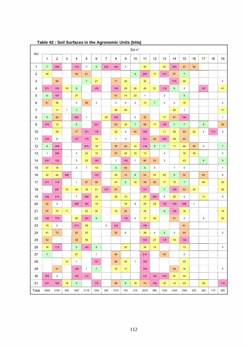
112
Table 42 : Soil Surfaces in the Agronomic Units (kHa) Sol n°
AU 1 2 3 4 5 6 7 8 9 10 11 12 13 14 15 16 17 18 19
1 7 498 116 3 5 239 182 4 43 34 293 57 93
2 35 98 61 6 205 17 101 67 7
3 89 7 21 71 25 35 215 30 4
4 571 103 18 8 105 150 28 26 45 21 118 6 2 167 41
5 6 187 37 87 14 23 1 3 5
6 61 38 2 56 2 3 4 2 12 7 3 2 10 2
7 11 1 7 48 20 20 1 17
8 5 66 253 1 25 102 0 52 17 91 184 1
9 570 13 6 221 60 32 7 96 17 105 7 7 8 55
10 36 77 121 118 22 4 60 328 11 36 64 22 3 113 3
11 235 9 131 179 15 1 3 161 93 248 48 82
12 6 326 670 18 55 62 18 118 6 7 11 46 58 3 7
13 1 246 3 24 15 57 25 16 13 3 18 18 2
14 201 125 3 23 140 1 100 1 66 53 3 43 9 9
15 37 16 3 1 14 5 60 6 4 1 0 1
16 32 46 468 123 30 72 9 54 23 29 9 54 62 8
17 411 119 1 67 99 47 5 16 59 62 17 15 7 46 25
18 287 19 48 19 41 127 97 131 7 159 53 33 25
19 342 213 7 426 39 29 12 25 283 4 20 4 11 5
20 52 3 269 162 10 18 9 25 26 133 130 496 1
21 97 70 11 42 34 10 60 26 8 128 18 16
22 162 175 26 230 9 118 4 17 46 51 4 5 32
23 18 2 213 39 2 124 159 61
24 41 73 52 53 50 6 39 4 5 4 64 2
25 53 58 59 103 27 116 18 122
26 16 113 5 145 9 22 34 14 13 3
27 7 27 1 84 214 55 0
28 14 1 121 89 25 1 150 45
29 57 106 1 7 16 17 190 59 16 4
30 255 2 103 112 137 102 278 31 32
31 331 182 18 5 175 95 8 19 74 158 16 14 23 39 110
Total 3549 3103 549 1667 2116 1343 393 1514 743 219 2618 965 1324 1434 1565 225 354 114 369

Table 43 : Soil Surfaces in the cropping Regions Sugar Beet
Winter Wheat
Oilseed Rape
Maize Fodder
Maize Grain Soil N° Barley Potato Sunflower
1 119684 866205 125752 135990 78044 179641 47239 26544
2 24721 521979 111059 32247 217419 124510 138120
3 54268 157327 22702 85226 12916
4 161081 31057 92331 223496 64631
5 294782 113453 69006 40690 109577 33352
6 83509 451256 16420 115981 19465 45137
7 43676
8 19280 177579 26471 125526 35025 6183 38343
9 11936 99954 25245 19624 31663 14223
10 16660
11 85126 49126 56743
12 196041 49566 41334 88183 42478 3965
13 19732 216287 123544 47707 33881 7614
14 37528 112314 46053
15 91791 104246 36072
16 16301
17 21544
18
19 15336 74172
Total 348466 3216663 573269 708897 1123035 757982 97382 559198
113

Table 44 : Distribution of Soils in the cropping Regions (%) Sugar Beet
Winter Wheat
Oilseed Rape
Maize Fodder
Maize Grain Soil N° Barley Potato Sunflower
1 25.4 16.9 12.6 13.3 44.4 13.9 31.4 3.3
2 5.2 10.2 11.2 3.2 12.3 9.6 17.3
3 11.5 3.1 2.3 6.6 8.6
4 3.2 3.1 9.0 12.7 8.1
5 5.8 11.4 6.8 2.3 8.5 4.2
6 17.7 8.9 4.7 9.0 12.9 5.7
7 5.5
8 4.1 3.5 2.7 7.1 2.7 4.1 4.8
9 2.5 2.0 2.5 1.1 2.4 1.8
10 0.9
11 8.3 2.8 7.1
12 3.8 5.0 4.0 5.0 3.3 2.6
13 4.2 4.2 12.1 2.7 2.6 5.1
14 3.0 6.4 5.7
15 9.0 5.9 4.5
16 2.0
17 2.2
18
19 3.3 1.5
Total 73.9 63.1 57.7 69.4 63.6 58.6 64.7 70.0
114
7.9 References Agricultural census: http://www.agreste.agriculture.gouv.fr/publications/recensement-agricole-58/ Baize D., 1995. Référentiel pédologique. Paris, ed. INRA. BDGSF database: http://www.gissol.fr/programme/bdgsf/bdgsf.php CORINE Land Cover (CLC) database: http://www.eea.europa.eu/themes/landuse http://www.stats.environnement.developpement-durable.gouv.fr/bases-de-donnees/occupation-des-sols-corine-land-cover.html DONESOL database : http://www.gissol.fr/outil/donesol/donesol.php ESDB : http://eusoils.jrc.ec.europa.eu/ESDB_Archive/ESDB/index.htm ETC 2000. European Topic Centre CORINE Land Cover Database, Version 12/2000. European Topic Centre of Landcover (ETC/LC). Kiruna, Sweden UNESCO (United Nations Educational, Scientific and Cultural Organization). 1974. FAO/UNESCO Soil map of the world, 1:5,000,000 Vol. 1 Paris: UNESCO. Finke, P., R. Hartwich, R. Dudal, J. Ibàñez, M. Jamagne, D. King, L. Montanarella and N. Yassoglou (2001). GEOREFERENCED SOIL DATABASE FOR EUROPE. Manual of procedures. Version 1.1. European Soil Bureau Research Report No. 5, EUR 18092 EN INRA (2005b). Base de Données Géographique des Sols de France, descriptif du contenu. http://gissol.orleans.inra.fr/programme/bdgsf/contenu.php INRA (2005c). Base de données nationale des informations spatiales pédologiques. http://gissol.orleans.inra.fr/outil/donesol/donesol.php Morvan, Y. & Le Bas, C. 2006. Détermination de profils types de sol par régions de cultures. Report of INRA, Unité Infosol, Orléans. SPADBE database (also refered to as SPADE): http://eusoils.jrc.ec.europa.eu/esbn/SPADE.html
115
8 Parameterization of the soil profiles Soil water flow is described in PEARL with the Richards equation, which requires the Mualem-van Genuchten functions. Parameter values for the Mualem-Van Genuchten functions must therefore be provided, however these are not available from the DONESOL2 database and consequently needed to be estimated using pedotransfer functions (PTF). The most commonly used PTF available from the literature were tested against measured water retention curves for a variety of French soils and the HYPRES functions were consequently selected for estimation of the Mualem-Van Genuchten for FROGS. Soil bulk density is one of the required parameters for HYPRES. In the majority of cases it was not available from DONESOL, so this parameter was also estimated using PTF. In addition, a few subsoil layers OC content and pH values were missing from the selected DONESOL soil profiles and had to be estimated. Finally, the topsoil OC content and the pH of the soils were corrected based on the comprehensive data available from BDAT to better reflect spatial variation in surface OC between AUs. Whenever possible, the same PTF as used in the PEARL model were used to estimate these parameters, for consistency with the model and for consistency with the approach taken in the FOCUS scenarios. These PTF were first checked against available measured data for French soils to confirm applicability to French conditions. 8.1 Adjustment of Topsoil Organic Carbon Content to BDAT Among all soil properties probably the content of organic carbon (OC) is the most important with respect to the leaching of most pesticides, with the exception of ionic substance, in which case soil pH is key and the use of pH-dependent sorption in PEARL is recommended. The content of OC generally determines the sorption and thereby the relative mobility of non-ionic compounds. The OC of soils may vary significantly due to soil type, vegetation and climate (Jones et al., 2004). Thus the 18 topsoil OC values from the profile set might be too few to represent large areas in the order of 100 000 km2 as considered here. The soil profiles selected to represent the 19 soil types were taken from the DONESOL database which shows a considerable variation of the geographic distribution of the soil samples. The number of profiles available for a specific soil type is indeed highly variable between the various regions. Most of the profiles selected to represent the 18 soil types were taken from the Centre region where the profiles are particularly abundant (Morvan & Lebas, 2006). This is also the region where the organic carbon content of the top soil layer is the most depleted. Therefore a large French database on topsoil properties denoted as BDAT (Base de données d’analyses de terre) (INRA, 2005) was used to adjust the topsoil OC at regional level. This database provides statistical descriptors (mean, median and several quantils) of physico-chemical parameters of the topsoil (texture, OC, pH and CaCO3) at canton level based on a large number of individual samples.
116

8.1.1 Correction method The adjustment of surface OC content of the selected DONESOL soils using BDAT data was based on areal median values OCmed at the spatial scale of the AU. This means that in 50 % of the area of a specific AU, OC < OCmed, and in the other 50 % OC > OCmed. The adjustment considers the uppermost 0.3 m of the soil which represents the sampling depth underlying the BDAT values. The BDAT values used were denoted as “Carbone organique, oxydation humique” from the time period 2000 -2004. As mentioned above the BDAT data are compiled at canton level of which the median values were used (“med : médiane”). These values can be considered as the most robust ones. The spatial resolution of these data is relatively high (2286 cantons in the 31 AU). As consequence of this adjustment, the topsoil (0 - 0.3 m) OC for a given soil depends on the AU. First, the %OC values of the DONESOL soils were calculated for the top 30 cm. For this purpose a depth-weighted mean value was calculated in case the first horizon was < 0.3-m thick, according to Equation 2 Equation 2: %OC(DONESOL soil) = Σi=1,n(%OCi Δzi) / Σi=1,n(Δzi),
Where n is the number of horizons to reach a depth of 0.3 m, Δzi is thickness of horizon i in the soil layer from 0 to 0.3 m, and Σi=1,n(Δzi) = 0.3 m.
The %OCmed (representing the median, i.e. 50 % percentile) of the INRA soils was then calculated as follows. The relevant DONESOL soils for a specific AU are sorted by their %OC (0 - 0.3 m) in ascending order. The relative surface of a specific soil is used to calculated the corresponding areal percentiles, i.e. the areal percentile PA is equal to the cumulative relative surface. The procedure is illustrated in the following example:
Soil A has an OC content of 1.0% and a relative surface of 0.2, soil B has an OC content of 1.4 % and a relative surface of 0.5, and soil C has an OC content of 1.6 % and a relative surface of 0.3. Then OC (PA=20%)=1%, OC (PA=20+50=70%)=1.4%, and OC (PA=20+50+30=100%)=1.6%. In other words, for 20 % of the surface the OC is 1.0 % or lower, for 70 % of the surface the OC is 1.4% or lower, and for 100% of the surface the OC is 1.6% or lower.
Although the number of soils per AU is greater than in the example above, in most cases the %OCmed is not met directly. In such cases %OCmed is determined by linear interpolation between the two percentile values surrounding PA = 50 % (see also Table 45 for AU = 3 as example). For the example above these percentiles are PA = 20% and PA = 70%, so %OCmed = 1.0% + (50% - 20%) × (1.4% - 1.0%) /(70% - 20%) = 1.24%. The same procedure as above is applied to the BDAT values. Because there are sufficient data per AU interpolation was not necessary to obtain %OC (PA = 50 %). The corresponding data for AU = 3 as example are shown in Table 46. Finally a correction factor is derived as %OCmed (BDAT) / %OCmed. (DONESOL).
117

118
Table 45: Percentiles of OC contents calculated based on the selected DONESOL
soils, example of Agricultural Unit 3 AU Soil Area Surface OC Percentile OCmed No. No. (kha) fraction (%, 0-0.3 m) (%) (%, 0-0.3 m) 3 19 4 0.008 0.69 0.8 3 9 25 0.050 0.81 5.8 3 6 21 0.042 1.06 10.1 3 15 30 0.060 1.16 16.1 3 2 89 0.179 1.17 34.0 3 8 71 0.143 1.20 48.3 1.22 3 11 35 0.070 1.30 55.3 3 5 7 0.014 1.52 56.7 3 14 215 0.433 1.62 100.0 Table 46: Percentiles of OC content calculated based on BDAT1, example of AU 3. The
50th percentile OC is given in bold. Canton Area2) OC3) AU Percentile Name No. (kha) (%) (%) DORNES 5810 17 0.93 3 3 CHATELDON 6309 3 0.99 3 3 YZEURE 333 13 1.05 3 6 CHEVAGNES 304 29 1.08 3 10 NEUILLY-LE-REAL 325 19 1.11 3 14 SAINT-HAON-LE-CHATEL 4227 9 1.12 3 15 ROANNE-SUD 4234 5 1.25 3 16 MOULINS-SUD 323 3 1.27 3 17 DOMPIERRE-SUR-BESBRE 307 23 1.28 3 21 PERREUX 4214 10 1.29 3 22 LEZOUX 6322 11 1.29 3 24 BRIOUDE-NORD 4305 6 1.31 3 25 SAINT-GALMIER 4223 8 1.33 3 27 DONJON 308 26 1.34 3 31 MONTBRISON 4209 15 1.34 3 34 SAINT-JUST-SAINT-RAMBERT 4231 10 1.34 3 35 BOURBON-LANCY 7103 20 1.35 3 39 SAINT-SYMPHORIEN-DE-LAY 4232 18 1.37 3 42 IMPHY 5832 11 1.40 3 43 AUBIERE 6355 1 1.44 3 44 SAINT-POURCAIN-SUR-SIOULE 326 17 1.45 3 47 DIGOIN 7117 7 1.47 3 48 CHARLIEU 4205 11 1.48 3 50 BILLOM 6306 7 1.50 3 51 MARINGUES 6324 5 1.51 3 52 SAINT-PIERRE-LE-MOÛTIER 5822 18 1.55 3 55 ROANNE-NORD 4216 4 1.56 3 55 CLERMONT-FERRAND 6398 1 1.56 3 56 COURPIERE 6315 6 1.63 3 57 NEVERS-SUD 5830 4 1.68 3 57 ENNEZAT 6317 10 1.70 3 59 RIOM 6399 2 1.74 3 61 ESCUROLLES 310 12 1.74 3 61 GERZAT 6359 2 1.74 3 62 PACAUDIERE 4212 14 1.74 3 64 RANDAN 6332 9 1.74 3 66 COMBRONDE 6314 7 1.75 3 67 CHAMPEIX 6308 9 1.79 3 69
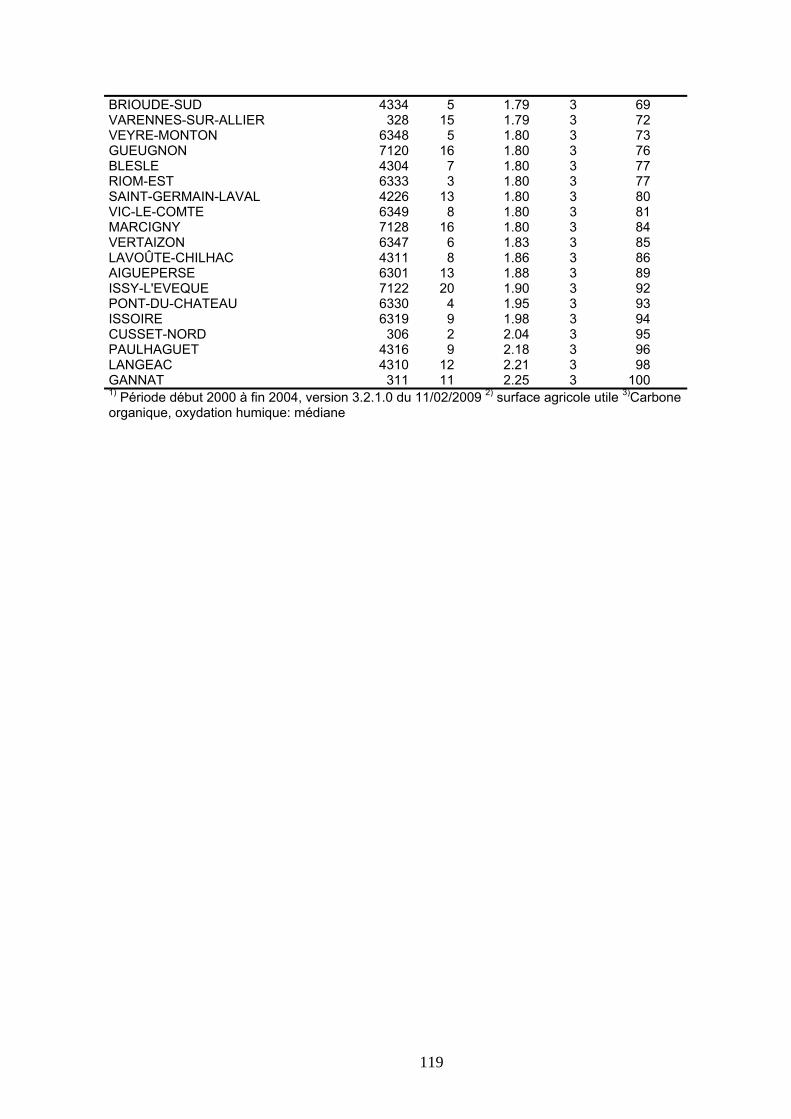
BRIOUDE-SUD 4334 5 1.79 3 69 VARENNES-SUR-ALLIER 328 15 1.79 3 72 VEYRE-MONTON 6348 5 1.80 3 73 GUEUGNON 7120 16 1.80 3 76 BLESLE 4304 7 1.80 3 77 RIOM-EST 6333 3 1.80 3 77 SAINT-GERMAIN-LAVAL 4226 13 1.80 3 80 VIC-LE-COMTE 6349 8 1.80 3 81 MARCIGNY 7128 16 1.80 3 84 VERTAIZON 6347 6 1.83 3 85 LAVOÛTE-CHILHAC 4311 8 1.86 3 86 AIGUEPERSE 6301 13 1.88 3 89 ISSY-L'EVEQUE 7122 20 1.90 3 92 PONT-DU-CHATEAU 6330 4 1.95 3 93 ISSOIRE 6319 9 1.98 3 94 CUSSET-NORD 306 2 2.04 3 95 PAULHAGUET 4316 9 2.18 3 96 LANGEAC 4310 12 2.21 3 98 GANNAT 311 11 2.25 3 100 1) Période début 2000 à fin 2004, version 3.2.1.0 du 11/02/2009 2) surface agricole utile 3)Carbone organique, oxydation humique: médiane
119

8.1.2 Results and Discussion The areal median %OCmed obtained for the selected DONESOL soils and those derived from BDAT are shown in Table 47. The corresponding correction factors range from 0.7 to 2.41.
Table 47: Areal median OCmed for DONESOL soils and derived from BDAT AU DONESOL BDAT Correction No. OCmed (%) OCmed (%) factor 1 1.17 1.01 0.86 2 1.19 2.26 1.91 3 1.22 1.48 1.21 4 1.01 1.10 1.09 5 1.17 1.19 1.02 6 1.16 1.74 1.50 7 1.18 0.97 0.82 8 1.13 1.33 1.18 9 1.00 1.10 1.10
10 1.24 1.57 1.26 11 1.03 1.85 1.80 12 1.30 1.89 1.45 13 1.17 1.55 1.33 14 1.06 1.09 1.03 15 0.86 0.78 0.91 16 1.18 1.67 1.42 17 1.01 1.10 1.08 18 1.18 0.95 0.80 19 1.16 1.23 1.06 20 1.13 1.45 1.29 21 1.16 1.51 1.30 22 1.16 1.32 1.14 23 1.18 1.15 0.98 24 1.16 1.13 0.98 25 1.08 2.60 2.41 26 1.18 1.46 1.24 27 1.20 1.02 0.85 28 1.19 0.83 0.70 29 1.20 1.37 1.14 30 0.99 1.65 1.66 31 1.06 1.00 0.94
The median correction factor is 1.14, e.g. the adjusted topsoil %OC are on average slightly higher than the DONESOL soils values. The overall distributions of topsoil %OC before and after corrected were calculated for all AUs together, i.e. for the whole of France, and compared with the BDAT distribution in Figure 41. The overall BDAT OC distribution is as expected very well reproduced after application of the correction factors shown in Table 47 to the DONESOL values on an AU basis. It is also clear from the figure that the original DONESOL OC distribution was biased towards lower values for OC of 1 % and more, while the proportion of OC values < 1% was properly represented.
120

0
0.1
0.2
0.3
0.4
0.5
0.6
0.7
0.8
0.9
1
5 10 15 20 25 30OC (g/kg)
Cum
ulat
ive
prob
abili
ty
BDATDONESOL originalDONESOL corrected area median
Figure 41: Distribution of topsoil OC for DONESOL soils, derived from BDAT, and INRA soils corrected over all AU.
The BDAT OC data were further compared with European databases suitable to derive OC values for France. The European databases considered were the SPADE 2 (Finke et al., 2001) soil data base and the OCTOP map (Jones et al., 2004). The BDAT OC database was preferred because it comprises much more data than SPADE 2, and because the values were measured and not estimated as is the case for OCTOP. The target area was defined as arable land (nonirrigated and permanently irrigated) in France based on CORINE land cover (ETC, 2000). For comparison the areal median %OCmed were used. For SPADE 2 an OCmed value of 1.5 % and for OCTOP an OCmed value of 1.6 % were obtained which are similar to OCmed = 1.34 % obtained for BDAT (Figure 41). The %OCmed derived from BDAT is thus considered consistent with the other databases. It is slightly lower than the other values and therefore more protective with respect to leaching.
121

8.2 Adjustment of soil pH to BDAT Degradation rates and sorption properties of some particular pesticides can be substantially influenced by soil pH. For example, the sorption of weak acids is dependent on the pH of the soil and degree of dissociation (Dubus et al., 2001). A corresponding model is implemented in the PEARL program which can be used also in the FROGS system. In case of pH dependent degradation the PEARL model does not provide a comparable module. For compounds with pH-dependent degradation or sorption, the soil pH may be of equal importance as the soil OC (see section OC correction). The soil pH is depending on a number of environmental factors in addition to soil type such as topography, geology and land use to name only the most important. The soil pH is therefore expected to exhibit substantial spatial variation. For example, Reuter et al. (2008) found a variability, i.e. standard deviation of about 0.6 pH units at field-scale (approximately 3 km) and of about 0.9 pH units at a scale of 50 - 100 km. Thus the 18 soil pH profiles from the DONESOL profile set appeared too few to reliably represent an area roughly as large as the arable land of total France. Note that soil 18 (solonchak) represented less than 0.5 % of the total surface. This soil did not appear representative for any of the selected crops and was therefore not implemented in FROGS as soil scenario. For the reasons given above it was concluded, as for the topsoil soil OC%, to compare the areal distribution of pH derived from the DONESOL soils selected with corresponding data derived from the comprehensive BDAT (Base de données d’analyses de terre) database (INRA, 2005). In case of major deviations the topsoil pH values were to be adjusted so that they fit the BDAT distribution. The pH values for the DONESOL soils are given as pH measured in aqueous solution (pH water). Therefore, the pH water values from BDAT were used for consistency and only the pH water is considered in the following. For the PEARL model the type of pH used is irrelevant as long as soil pH type and pH type used for the sorption module are consistent. However, since it is mentioned in the PEARL documentation that pH measured in CaCl2 (pHCaCl2) is preferred, pHwater was transformed to pHCaCl2 using the transfer functions given in section 8.2.4.
8.2.1 Comparison of Original pH with BDAT The BDAT values used were denoted as “ph eau” from the time period 2000 -2004. The BDAT data are representative for the uppermost 0.3 m of the soil and are compiled at canton level. The median values at canton level were used (“med : médiane”) which can be considered as the most robust values. The spatial resolution of these data is relatively high (2286 cantons in the 31 AU). The area fraction for a specific pH was calculated using the agricultural area (sau: surface agricole utile) per associated canton as given in BDAT normalised to the total agricultural area. The area distribution was finally determined by sorting the cantons by their pH in ascending order and cumulating the area fractions. Correspondingly, the pH values of the DONESOL soils were calculated for the top 30 cm as was done for OC (section OC correction). For this purpose a depth weighted mean value was calculated in case the first horizon was less than 0.3 m thick, pH(DONESOL soil) = Σi=1,n(pHi Δzi) / Σi=1,n(Δzi), where n is the number of horizons to reach a depth of 0.3 m, Δzi is thickness of horizon i in the soil layer from 0 to 0.3 m
122

and Σi=1,n(Δzi) = 0.3 m. The area fraction for a specific soil (with specific pH) was calculated using the area fraction in the AU multiplied with the area of the AU, summed up over all AU, and finally normalised to the total area of all AU. The area distribution was finally determined by sorting the soils by their pH in ascending order and cumulating the area fractions ( ). Table 48 The comparison of the two distributions over all AU shows clearly that there are substantial differences (Figure 42). Especially for low pH (soil 14) a shift of more than one pH unit would be necessary to match the corresponding BDAT value. In contrast to the corresponding OC areal distributions (Figure 41) the pH distributions do not have a similar shape. In case of OC, the original DONESOL soil areal percentiles were consistently higher than the corresponding BDAT percentiles (indicating more soils with lower OC). However, the original DONESOL soil pH areal percentiles are higher for low pH (indicating more acidic soils), lower for neutral soils (e.g. no soils between pH = 6.5 and pH = 7) and similar for alkaline soils compared to the corresponding BDAT probabilities.
0
0.1
0.2
0.3
0.4
0.5
0.6
0.7
0.8
0.9
1
4 5 6 7 8 9pH water
Are
al p
roba
bilit
y
BDAT
DONESOL
Figure 42: Distribution of topsoil pH for DONESOL soils and derived from BDAT
Due to considerable differences between the two distributions it was deemed appropriate to adjust the topsoil pH values to fit better to the BDAT distribution.
123
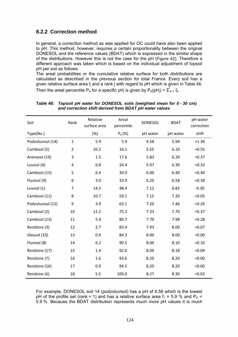
8.2.2 Correction method In general, a correction method as was applied for OC could have also been applied to pH. This method, however, requires a certain proportionality between the original DONESOL and the reference values (BDAT) which is expressed in the similar shape of the distributions. However this is not the case for the pH (Figure 42). Therefore a different approach was taken which is based on the individual adjustment of topsoil pH per soil as follows. The areal probabilities or the cumulative relative surface for both distributions are calculated as described in the previous section for total France. Every soil has a given relative surface area fj and a rank j with regard to pH which is given in Table 48. Then the areal percentile PA for a specific pHj is given by PA(pHj) = Σ
jk=1 fk.
Table 48: Topsoil pH water for DONESOL soils (weighted mean for 0 - 30 cm) and correction shift derived from BDAT pH water values
Relative surface area
Areal percentile
pH water correction
Soil Rank DONESOL BDAT
Type(No.) (%) PA (%) pH water pH water shift
Podzoluvisol (14) 1 5.9 5.9 4.58 5.94 +1.36
Cambisol (5) 2 10.2 16.1 5.55 6.10 +0.55
Arenosol (19) 3 1.5 17.6 5.83 6.20 +0.37
Luvisol (4) 4 6.8 24.4 5.97 6.30 +0.33
Cambisol (15) 5 6.4 30.9 6.00 6.40 +0.40
Fluvisol (9) 6 3.0 33.9 6.20 6.58 +0.38
Luvisol (1) 7 14.5 48.4 7.12 6.82 ‐0.30
8 10.7 59.1 7.15 7.20 +0.05 Cambisol (11)
Podzoluvisol (12) 9 3.9 63.1 7.20 7.46 +0.26
Cambisol (2) 10 12.2 75.3 7.33 7.70 +0.37
Cambisol (13) 11 5.4 80.7 7.70 7.98 +0.28
Rendzine (3) 12 2.7 83.4 7.93 8.00 +0.07
Gleysol (10) 13 0.9 84.3 8.00 8.00 +0.00
8.00 8.10 +0.10 Fluvisol (8) 14 6.2 90.5
Rendzine (17) 15 1.4 92.0 8.09 8.18 +0.09
Rendzine (7) 16 1.6 93.6 8.20 8.20 +0.00
Rendzine (16) 17 0.9 94.5 8.20 8.20 +0.00
Rendzine (6) 18 5.5 100.0 8.27 8.30 +0.03
For example, DONESOL soil 14 (podzoluvisol) has a pH of 4.58 which is the lowest pH of the profile set (rank = 1) and has a relative surface area f1 = 5.9 % and PA = 5.9 %. Because the BDAT distribution represents much more pH values it is much
124

smoother than the DONESOL pH distribution and a representative pH value has to be selected for 0 % < PA < 5.9 %. For this purpose the class centre between the lower and upper areal percentile, 0.5 × (PA(pHj-1) + PA(pHj)), of the DONESOL pH distribution is selected which leads to a good adjustment of both distributions. So for pH of rank 1 the BDAT pH value is obtained as the one for which PA = 0.5 × (0 % + 5.9 %) = 2.95 % leading to pH = 5.94. For soil 5 with pH rank 2, f2 = 10.2 % and PA = 10.2 % + 5.9 % = 16.1 %. The corresponding BDAT pH for which PA = 0.5 × (5.9 % + 16.1 %) = 11.0 % yields a value of pH = 6.1. This procedure is applied to all soils and finally the correction is defined by the shift which represents the difference between DONESOL and BDAT pH for the specific PA (Table 48). A comparison between the original DONESOL, BDAT and adjusted to BDAT pH distribution is shown in . Figure 43
0
0.1
0.2
0.3
0.4
0.5
0.6
0.7
0.8
0.9
1
4 5 6 7 8 9pH water
Are
al p
roba
bilit
y
BDATDONESOL originalDONESOL corrected per soil
Figure 43: Distribution of topsoil pH for DONESOL soils, derived from BDAT and
DONESOL soil corrected. The vertical position of horizontal lines indicates the reference areal probability for the correction and its length indicates the magnitude of the correction.
Inspection of Figure 43 shows that the correction proposed leads to a good approximation of the BDAT distribution. In general an adjustment at AU level would be also possible which could provide an even better approximation of the BDAT data at regional scale. This would lead to individual corrections at AU level which, due to the smaller spatial scale, would potentially require considering not only median values but also other percentiles. To assess the necessity of such a more complex approach, the representation of individual AU by the proposed correction was considered. If the representation is sufficient a refined approach would not be required. For this purpose the range of corrected pH (the soil with min. and max. pH after the correction) was compared to the inner 90th areal percentile (5th and 95th areal percentile) of the canton median pH for individual AU (Figure 44). The result of this comparison is that the range of pH values within a specific AU as given by BDAT is well represented by the range of
125

topsoil pH obtained after the correction described above. Although a correction at AU level would probably lead to a better representation, the increase in accuracy is not expected sufficiently significant to justify the additional effort to derive a correction at AU level.
5.0
5.5
6.0
6.5
7.0
7.5
8.0
8.5
9.0
0 1 2 3 4 5 6 7 8 9 10 11 12 13 14 15 16 17 18 19 20 21 22 23 24 25 26 27 28 29 30 31
AU
pH(w
ater
)
5th areal percentile of BDAT median pH 95th areal percentile of BDAT median pHmin. soil pH after correction max. soil pH after correction
Figure 44: Comparison between 5th and 95th areal percentile of the BDAT canton
median topsoil pH for individual AU (Agronomic Units) and topsoil pH after proposed correction (min. and max. pH after the correction).
For soil 14 a major correction by +1.36 pH units is necessary, for soil 5 a medium correction by +0.55 pH units is obtained. For the other soils the correction is moderate to minor, ranging form -0.3 to +0.4 pH units. Because the correction for soil 14 is relatively large, the BDAT 10th percentile pH values were considered. These indicate the variability of pH at canton level. If this variability is large compared to the variability over all cantons, the surface area of soils with pH far below the median could have been underestimated. However, a pH of 4.58 as for soil 14 (weighted mean for 0 - 30 cm) is practically not found in the BDAT data even as 10th percentile (PA < 0.000001 %, corresponding to 1 canton). A pH of 5.55 as for soil 5 or lower representing a 10th percentile at canton level is found for 18 % of the total surface area, i.e PA = 18 %. Presuming that the 10th percentile pH of a canton represents approximately 10 % of the surface area, the total relative surface area with pH ≤ 5.55 is only 10 % of 18 % which is 1.8 %. Therefore it was concluded that the correction described above is appropriate to adjust the original topsoil pH of the DONESOL soils to the reference values derived from the BDAT database. The relatively large correction for soils 14 and 5 based on median values at canton level was confirmed by consideration of the distribution within cantons (10th percentile values).
126

8.2.3 Correction of pH for subsoil layers Generally, the pH values for the subsoil of the selected DONESOL soil profiles are relatively similar to the value in the topsoil. There is also a tendency that the pH slightly increases with depth for most of the soils (13 of 18) which is consistent with the expectation due to soil genesis. Normally progressing formation and development of a soil leads to acidification because cations released by weathering are leached from the profile. Because soil formation takes place from top to bottom, cation leaching and acidification is more intense at the top and decreasing with depth. To conserve this natural gradient in soil pH and to not introduce artificial pH skips from topsoil to subsoil it is considered most appropriate to apply the same correction to the subsoil pH as was applied to topsoil pH.
8.2.4 Relation between pH measured in Different Solutions Soil pH values are typically measured in different solutions (water, KCl, CaCl2). Thus the situation may occur that the dependency of sorption for a specific compound is defined, for example, in terms of pH measured in CaCl2 solution (pHCaCl2). However, FROGS soil pH values are given in terms of pH measured in aqueous solution (pHwater). In order to transform pH values obtained in different solutions it is recommended to use the pedotransfer function developed and validated by Reuter et al. (2008) given as :
pHwater = (pHCaCl2 + 0.427) / 0.9761 (R2 = 0.92, n = 1997) pHCaCl2 = 1.0572 × pHKCl + 0.123 (R2 = 0.90, n = 377)
The following order is obtained, pHKCl < pHCaCl2 < pHwater. Since in PEARL 3.3.3 pHCaCl2 –values are preferred, the corrected pHwater-values are transformed to pHCaCl2 –values by the first of the above equations. Examples for the correction of pHwater and its conversion to pHCaCl2 are given for the first layer of each selected soil profile in Table 49. The pHCaCl2 values are the values finally implemented in the FROGS-database.
127

Table 49 : pH-correction and conversion examples for the first layer of each soil
pHwater (DONESOL)
pHwater (corrected)
pHCaCl2 Shift SID HID (corrected) 1 1 7.10 -0.30 6.80 6.21 2 1 7.40 0.37 7.77 7.16 3 1 7.90 0.07 7.97 7.35 4 1 5.80 0.33 6.13 5.56 5 1 6.00 0.55 6.55 5.97 6 1 8.20 0.03 8.23 7.61 7 1 8.10 0.00 8.10 7.48 8 1 8.00 0.10 8.10 7.48 9 1 6.20 0.38 6.58 6.00 10 1 8.00 0.00 8.00 7.38 11 1 6.80 0.05 6.85 6.26 12 1 7.20 0.26 7.46 6.85 13 1 7.80 0.28 8.08 7.46 14 1 4.20 1.36 5.56 5.00 15 1 6.00 0.40 6.40 5.82 16 1 8.20 0.00 8.20 7.58 17 1 8.00 0.09 8.09 7.47 19 1 5.80 0.37 6.17 5.60
128

8.3 Estimation of Organic carbon content for subsoil layers Measured OC content were available in DONESOL for all the selected soil profiles, however for a limited number of soil layers values were missing (soil 8, 20-60 et 60-120 cm; soil 13, 110-130 cm; soil 15, 35-50, 50-100 and 100-110 cm; soil 19, 90-130 cm). Organic carbon content in subsoils may be estimated based on the soil horizon depth according to a PTF derived by Bruand et al., 2006 (personal communication). This function (Equation 3) was derived from available measured data from the region Ile-de-France.
8.2
8.2x028.0
e1)ee(29.122.0)x(c −
−−
−−⋅
+= Equation 3:
with x = depth (cm) c(x) = OC content (%)
The applicability of the PTF to subsoil profiles outside of the region Ile-de-France region still needs to be checked. A comparison of estimated OC content versus measured values for the deeper layers of the 18 selected soil profiles shows that the PTF provides reasonable estimates of the OC content (Figure 45). The ComTox workgroup considered the PTF as acceptable and consequently used it to complete the OC content for the selected soil profiles.
0
5
10
15
20
25
30
0 5 10 15Estimated OC content (g/kg)
Mea
sure
d O
C c
onte
nt (g
/kg)
Figure 45 Comparison of OC contents estimated from the soil depth with measured
values for the selected soil profiles
129
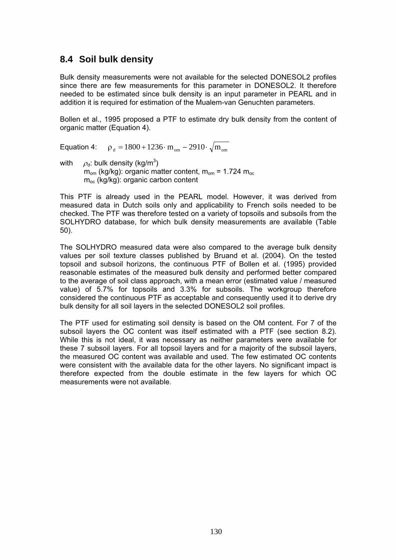
8.4 Soil bulk density Bulk density measurements were not available for the selected DONESOL2 profiles since there are few measurements for this parameter in DONESOL2. It therefore needed to be estimated since bulk density is an input parameter in PEARL and in addition it is required for estimation of the Mualem-van Genuchten parameters. Bollen et al., 1995 proposed a PTF to estimate dry bulk density from the content of organic matter (Equation 4).
omomd m2910m12361800 ⋅−⋅+=ρEquation 4:
with ρd: bulk density (kg/m3) mom (kg/kg): organic matter content, mom = 1.724 moc moc (kg/kg): organic carbon content
This PTF is already used in the PEARL model. However, it was derived from measured data in Dutch soils only and applicability to French soils needed to be checked. The PTF was therefore tested on a variety of topsoils and subsoils from the SOLHYDRO database, for which bulk density measurements are available (Table 50). The SOLHYDRO measured data were also compared to the average bulk density values per soil texture classes published by Bruand et al. (2004). On the tested topsoil and subsoil horizons, the continuous PTF of Bollen et al. (1995) provided reasonable estimates of the measured bulk density and performed better compared to the average of soil class approach, with a mean error (estimated value / measured value) of 5.7% for topsoils and 3.3% for subsoils. The workgroup therefore considered the continuous PTF as acceptable and consequently used it to derive dry bulk density for all soil layers in the selected DONESOL2 soil profiles. The PTF used for estimating soil density is based on the OM content. For 7 of the subsoil layers the OC content was itself estimated with a PTF (see section 8.2). While this is not ideal, it was necessary as neither parameters were available for these 7 subsoil layers. For all topsoil layers and for a majority of the subsoil layers, the measured OC content was available and used. The few estimated OC contents were consistent with the available data for the other layers. No significant impact is therefore expected from the double estimate in the few layers for which OC measurements were not available.
130
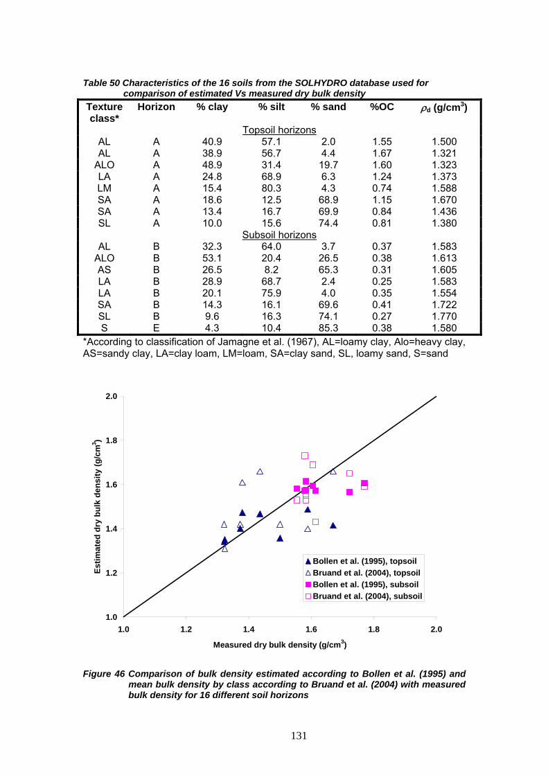
Table 50 Characteristics of the 16 soils from the SOLHYDRO database used for
comparison of estimated Vs measured dry bulk density ρd (g/cm3) Texture
class* Horizon % clay % silt % sand %OC
Topsoil horizons AL A 40.9 57.1 2.0 1.55 1.500 AL A 38.9 56.7 4.4 1.67 1.321
ALO A 48.9 31.4 19.7 1.60 1.323 LA A 24.8 68.9 6.3 1.24 1.373 LM A 15.4 80.3 4.3 0.74 1.588 SA A 18.6 12.5 68.9 1.15 1.670 SA A 13.4 16.7 69.9 0.84 1.436 SL A 10.0 15.6 74.4 0.81 1.380
Subsoil horizons AL B 32.3 64.0 3.7 0.37 1.583
ALO B 53.1 20.4 26.5 0.38 1.613 AS B 26.5 8.2 65.3 0.31 1.605 LA B 28.9 68.7 2.4 0.25 1.583 LA B 20.1 75.9 4.0 0.35 1.554 SA B 14.3 16.1 69.6 0.41 1.722 SL B 9.6 16.3 74.1 0.27 1.770 S E 4.3 10.4 85.3 0.38 1.580
*According to classification of Jamagne et al. (1967), AL=loamy clay, Alo=heavy clay, AS=sandy clay, LA=clay loam, LM=loam, SA=clay sand, SL, loamy sand, S=sand
1.0
1.2
1.4
1.6
1.8
2.0
1.0 1.2 1.4 1.6 1.8 2.0
Measured dry bulk density (g/cm3)
Estim
ated
dry
bul
k de
nsity
(g/c
m3 )
Bollen et al. (1995), topsoilBruand et al. (2004), topsoilBollen et al. (1995), subsoilBruand et al. (2004), subsoil
Figure 46 Comparison of bulk density estimated according to Bollen et al. (1995) and
mean bulk density by class according to Bruand et al. (2004) with measured bulk density for 16 different soil horizons
131

8.5 Soil hydrological parameters The hydrological properties of the soils are described in PEARL according to the Mualem - van Genuchten functions (van Genuchten, 1980) (Equation 5 to Equation 7).
( )( )[ ]mn
rsr
h1h
α+
θ−θ+θ=θEquation 5:
Equation 6: ( ) ( )[ ]2mm/1ees S11SKhK −−= λ
rs
reS
θ−θθ−θ
=Equation 7: (relative water saturation)
With the following hydrological parameters: - Residual volumetric water content, θr (m3/m3) - Saturated volumetric water content, θs (m3/m3) - α (alpha parameter) - n et m (exponent parameters), with m = 1-1/n in the form of the Mualem -
van Genuchten functions used in PEARL - λ (lambda parameter) - Saturated hydrolic conductivity, Ks (m/d) These parameters are best estimated by fitting of measured θ (h) and K (h) curves for the soil of interest, however θ (h) and K (h) measurements are in many cases not available and a number of PTF have been derived to estimate these parameters. Among the most commonly used PTF for parameterization of scenarios for groundwater modeling are the following three models: 1/ Rosetta version 1.2 (Riverside USDA Salinity Laboratory, United States,
Schaap et al. 2001) is a hierarchical model using textural class, textural distribution, bulk density and one or two water retention points as input parameters. There is no differentiation in the model between topsoil and subsoil horizons. The PTF were derived from an array of soils, mostly originating from the US, but also containing some EU soils.
2/ HYPRES (Wösten et al, 1999) propose class and continuous PTF using
bulk density, textural distribution and organic matter content as input parameters. A correction factor is included for subsoil horizons. The PTF were derived from an array of European soils, mostly originating from Germany, but also containing some French soils.
3/ Vereecken et al (1989) proposed continuous PTF using bulk density,
textural distribution and organic matter content as input parameters. There is no differentiation in the model between topsoil and subsoil horizons. The PTF were derived from Belgium soils exclusively. One should note that in this model, the parameter m is set to 1 as opposed to 1-1/n in the other PTF and in the PEARL model (different form of the Mualem – van Genuchten functions). Revised PTF based on the Vereecken database were published in 2009 (Weynants et al., 2009) among other things constraining m to 1-1/n.
132

These PTF were all derived by more or less complex regression analysis on a selection of soils for which θ (h) and K (h) had been measured and the Mualem – van Genuchten parameters estimated from these measured θ (h) and K (h) curves. In all three cases, the regression coefficients for some of the parameters were relatively low, indicating that the PTF cannot be expected to perform well for all soils. In addition, these PTF are most representative of the soils used in the respective regression analyses (mostly US soils for Rosetta, mostly German soils for HYPRES, and exclusively Belgium soils for Vereecken) and applicability to other soil types needs to be checked. The workgroup tested the Rosetta, HYPRES continuous, original Vereecken and revised Vereecken PTF against 16 French soils from the SOLHYDRO database, for which bulk density, textural distribution, organic matter content and water content at different pressure heads (pF1, 1.5, 2, 2.5, 3, 3.5 and 4.2) had been measured (Table 2). These 16 soils (8 topsoils and 8 subsoils) were selected to represent a variety of soil types, from sand to heavy clay. The Mualem-van Genuchten parameters were estimated for each soil with the 4 selected PTF models, then the respective θ (h) curves were calculated with the estimated Mualem-van Genuchten parameters, and finally these were plotted against the measured water content at different pressure heads. The calculations were performed twice, first with the measured soil bulk density, and second with the estimated soil bulk density calculated according to Bollen et al., 1995 (see above), to check the impact of the estimation of the bulk density on the estimation of the hydrological parameters. The respective quality of fit of the θ (h) curves was evaluated for the different PTF models using a statistical chi-square (χ2) test. The χ2 test considers the deviations between observed (measured) and calculated values in relation to the uncertainty associated to the measurements. The uncertainty associated to the measured θ (h) from the SOLHYDRO database is not known, but the χ2 test is used here to compare the different PTF models, by determining the minimum error percentage for which the test is passed for each PTF. The χ2 is calculated according to Equation 8.
∑ ⋅−
= 2
22
)O 100/err()OC(χEquation 8:
Οwith C = estimated value, O = observed value, = mean of observed values,
err = error percentage associated to measurements If χ2 > tabulated , then the model is not appropriate according to the selected significance level.
2,m αχ
with m = levels of freedom, α = probability to obtain χ2 superior or equal by chance
133

The tabulated for a selected significance level of 5% are obtained in Excel 2000 using the CHIINV(α,m) function. The minimum error percentage (err) for which the test is passed is determined according to
205.0,mχ
Equation 9.
∑ −⋅
χ⋅=
α2
2
2,m O
)OC(1100errEquation 9:
For a given soil, the PTF model that best predicts the measured θ (h) is the one which gives the lowest minimum error percentage.
Surface horizon, loamy clay, measured bulk density
0.0
0.1
0.2
0.3
0.4
0.5
1.E-01 1.E+01 1.E+03 1.E+05 1.E+07 1.E+09 1.E+11
Pressure head (cm)
Volu
met
ric w
ater
con
tent
(cm
3 /cm
3 )
MeasuredHYPRESRosettaVereeckenVereecken revisited
Surface horizon, loamy clay, estimated bulk density
0.0
0.1
0.2
0.3
0.4
0.5
1.E-01 1.E+01 1.E+03 1.E+05 1.E+07 1.E+09 1.E+11
Pressure head (cm)
Volu
met
ric w
ater
con
tent
(cm
3 /cm
3 )
MeasuredHYPRESVereeckenVereecken revisitedRosetta
Surface horizon, loam, measured bulk density
0.0
0.1
0.2
0.3
0.4
0.5
1.E-01 1.E+01 1.E+03 1.E+05 1.E+07 1.E+09 1.E+11
Pressure head (cm)
Volu
met
ric w
ater
con
tent
(cm
3 /cm
3 )
MeasuredHYPRESVereeckenVereecken revisitedRosetta
Surface horizon, loam, estimated bulk density
0.0
0.1
0.2
0.3
0.4
0.5
1.E-01 1.E+01 1.E+03 1.E+05 1.E+07 1.E+09 1.E+11
Pressure head (cm)
Volu
met
ric w
ater
con
tent
(cm
3 /cm
3 )
MeasuredHYPRESVereeckenVereecken revisitedRosetta
Surface horizon, sandy loam, measured bulk density
0.0
0.1
0.2
0.3
0.4
0.5
1.E-01 1.E+01 1.E+03 1.E+05 1.E+07 1.E+09 1.E+11
Pressure head (cm)
Volu
met
ric w
ater
con
tent
(cm
3 /cm
3 )
MeasuredHYPRESVereeckenVereecken revisitedRosetta
Surface horizon, sandy loam, estimated bulk density
0.0
0.1
0.2
0.3
0.4
0.5
1.E-01 1.E+01 1.E+03 1.E+05 1.E+07 1.E+09 1.E+11
Pressure head (cm)
Volu
met
ric w
ater
con
tent
(cm
3 /cm
3 )
MeasuredHYPRESVereeckenVereecken revisitedRosetta
Figure 47 Comparison between measured θ (h) and θ (h) estimated with Rosetta,
HYPRES, Vereecken and revisited Vereecken PTF for 3 soil types from loamy clay, loam and sandy loam topsoils, considering measured bulk density (left figures) and estimated bulk density (right figures)
134

Subsoil horizon, heavy clay, measured bulk density
0.0
0.1
0.2
0.3
0.4
0.5
1.E-01 1.E+01 1.E+03 1.E+05 1.E+07 1.E+09 1.E+11
Pressure head (cm)
Volu
met
ric w
ater
con
tent
(cm
3 /cm
3 )
MeasuredHYPRESVereeckenVereecken revisitedRosetta
Subsoil horizon, heavy clay, estimated bulk density
0.0
0.1
0.2
0.3
0.4
0.5
1.E-01 1.E+01 1.E+03 1.E+05 1.E+07 1.E+09 1.E+11
Pressure head (cm)
Volu
met
ric w
ater
con
tent
(cm
3 /cm
3 )
MeasuredHYPRESVereeckenRosettaVereecken revisited
Subsoil horizon, clay loam, measured bulk density
0.0
0.1
0.2
0.3
0.4
0.5
1.E-01 1.E+01 1.E+03 1.E+05 1.E+07 1.E+09 1.E+11
Pressure head (cm)
Volu
met
ric w
ater
con
tent
(cm
3 /cm
3 ) MeasuredHYPRESVereeckenVereecken revisitedRosetta
Subsoil horizon, clay loam, estimated bulk density
0.0
0.1
0.2
0.3
0.4
0.5
1.E-01 1.E+01 1.E+03 1.E+05 1.E+07 1.E+09 1.E+11
Pressure head (cm)
Volu
met
ric w
ater
con
tent
(cm
3 /cm
3 ) MeasuredHYPRESVereeckenVereecken revisitedRosetta
Subsoil horizon, sand, measured bulk density
0.0
0.1
0.2
0.3
0.4
0.5
1.E-01 1.E+01 1.E+03 1.E+05 1.E+07 1.E+09 1.E+11
Pressure head (cm)
Volu
met
ric w
ater
con
tent
(cm
3 /cm
3 ) MeasuredHYPRESVereeckenVereecken revisitedRosetta
Subsoil horizon, sand, estimated bulk density
0.0
0.1
0.2
0.3
0.4
1.E-01 1.E+01 1.E+03 1.E+05 1.E+07 1.E+09 1.E+11
Pressure head (cm)
Volu
met
ric w
ater
con
tent
(cm
3 /cm
3 ) MeasuredHYPRESVereeckenVereecken revisitedRosetta
Figure 48 Comparison between measured θ (h) and θ (h) estimated with Rosetta,
HYPRES, Vereecken and revisited Vereecken PTF for 3 soil types from heavy clay, clay loam and sand subsoils, considering measured bulk density (left figures) and estimated bulk density (right figures)
Not surprisingly, none of the 4 tested PTF is able to estimate perfectly the water retention curves of the 16 different soils. Nevertheless, it is evident from the fits shown in as well as the minimum Chi2 errors listed in Figure 47 and Figure 48 Table 51 that HYPRES performed better than the other PTF, especially regarding subsoils. In general, the Vereecken and Rosetta PTF did not provide satisfactory description of the retention curves, although the revisited Vereecken performed much better than the original Vereecken PTF. The minimum Chi2 error values were higher for sandy soil types compared to soils of finer texture, for topsoils as well as for subsoils. The use of bulk density values estimated according to Bollen et al. (1995) as opposed to
135
136
measured bulk density had little impact on the description of the water retention curves. Similar investigations regarding the estimation of conductivity were not performed since measured conductivity curves were not available for the selected soils, and would be more difficult to evaluate. Measurements of the saturated conductivity are particularly complex, since this parameter is known to be highly variable in space (even at the field scale) as well as in time (seasonal variations) and depending on the soil workup (disturbed Vs undisturbed). Based on these conclusions of the comparative PTF test on the θ (h) curves, the workgroup decided to use the HYPRES PTF for estimation of all the Mualem-van Genuchten parameters. In addition, the HYPRES PTF have the following advantages compared to the other tested PTF:
- the HYPRES model provides better soil representativity, since these PTF were derived from a European database containing a number of French soils, even though the majority of soils were from Germany (Rosetta is based on US soils exclusively and Vereecken is based on Belgian soils);
- the HYPRES model is the only one that differentiates between topsoil
horizons and subsoil horizons, with the use of a correction factor for subsoils;
- the HYPRES PTF are fully in line with the Mualem-van Genuchten functions
as used in PEARL and MACRO, when the original Vereecken PTF were based on a different expression of the parameter m.
One should note that these PTF for the description of the water retention curve, although based on the same equations used in the Richards-based models (PEARL and MACRO), would also be valid for the reservoir-based models (PRZM and PELMO) since these models require as input parameters water contents at different pressure heads, which would also need to be estimated. All relevant hydraulic parameters estimated with HYPRES for the different soil-types are listed in Appendix 17.

Table 51 Minimum Chi2 error (in %) obtained for the comparison of measured θ (h) versus θ (h) estimated with Rosetta, HYPRES and
Vereecken PTF Soil texture* HYPRES Vereecken Revisited Vereecken Rosetta Measured ρd Estimated ρd Measured ρd Estimated ρd Measured ρd Estimated ρd Measured ρd Estimated ρdTopsoil horizons AL 4.4 3.3 6.2 8.5 4.2 7.2 14.9 14.5 AL 8.3 7.5 13.9 13.3 12.8 12.2 16.3 16.0 ALo 8.0 7.0 14.5 13.8 15.5 14.8 14.6 14.3 LA 9.5 8.5 12.6 11.7 12.0 11.2 17.3 16.7 LM 6.0 5.5 7.9 8.2 5.0 6.7 8.0 9.4 SA 17.3 18.3 10.7 17.7 12.9 17.6 17.4 22.5 SA 19.4 17.8 26.5 25.6 30.9 29.7 24.1 22.7 SL 26.8 20.8 33.2 30.9 39.0 35.1 28.8 24.3 Subsoil horizons AL 4.1 4.3 4.3 4.5 6.2 6.4 15.0 15.0 ALo 3.1 4.3 7.1 8.3 11.2 12.3 12.0 12.2 AS 18.8 18.7 10.1 10.2 9.7 9.7 15.8 15.9 LA 2.7 1.9 2.3 2.0 5.7 5.4 15.9 15.9 LA 7.3 6.8 6.0 5.5 6.8 6.1 11.4 11.1 SA 6.5 11.4 12.5 17.8 16.4 21.7 11.0 16.9 SL 11.1 17.7 20.9 27.6 24.9 31.7 13.6 21.2 S 18.9 19.3 38.2 38.4 42.0 42.4 27.3 27.7 *According to classification of Jamagne et al. (1967), ALo = heavy clay, AL = loamy clay, AS = sandy clay, LA = clay loam, LM = loam, SA = clayey sand, SL = loamy sand, S = sand
137

8.6 Soil lower boundary conditions The PEARL input file parameter OptLbo determines which type of boundary condition is used by the hydrological model SWAP for the bottom of the soil profile. For all FROGS scenarios the value of OptLbo is set to FreeDrain (= free drainage). This case assumes unit gradient at the lower boundary (flux equals unsaturated conductivity of lowest soil layer). In addition, in order to avoid boundary effects on the model simulations, the last soil horizon of each of the soil profiles as listed in Table 41 was artificially extended to 200 cm in FROGS, similar to what was done in the standard European FOCUS scenarios. This extension of the deepest soil layer is reflected in Appendix 17. The output concentrations for the evaluation are calculated at the bottom of the soil profile as listed in Table 41. 8.7 Soil numerical layers For setting up the numerical layers/compartments for the selected soil profiles in PEARL, a similar resolution as in the FOCUS-chateaudun scenario in PEARL 3.3.3 was used. This means 2.5-cm numerical layers/compartments from 0 to 50 cm depth, 5-cm numerical layers from 50 to 100 cm depth and 10-cm layers/compartments for depths >100 cm. In addition, a high resolution of 1-cm numerical layers/compartments was added for about 10 cm around the target depth (bottom of the soil profiles as listed in Table 41). These basic rules for the resolution were applied to all soils, but relaxed to overcome the following two limitations:
1) The boundaries of the horizons in the selected soil profiles are often overlapping the depths of 50 cm or 100 cm. Hence, in some instances the resolution was changed earlier or later than 50 or 100 cm to better match the horizon boundaries.
2) It is not always possible to reach the wished resolution with an integer as layer number. For example in Soil 3 the last horizon has a depth of 0.95 m. To reach a resolution of 10 cm the number of layers must be 9.5. Instead, the layer number was set to 10, yielding a resolution of 9.5 cm.
The selected numerical resolutions of the soil layers are listed in the tables of Appendix 17. 8.8 Biodegradation factor For setting up the biodegradation factor in PEARL for the adjustment of the degradation rate with soil depth, similar rules as in the FOCUS scenarios were used. Between 0-30 cm, a biodegradation factor of 1 is applied, between 30-60 cm the biodegradation factor is 0.5, and between 60-100 cm the biodegradation factor is 0.3. The target depth in FOCUS is 1 meter, so no degradation is considered in the FOCUS scenarios below 100 cm. In contrast, the target depth in FROGS is at the bottom of the soil profiles, which ranges from 40 to 140 cm. For those soils extending beyond 100 cm, the biodegradation factor was set to 0.15 below 100 cm, since there are no indications that degradation stops abruptly at 100 cm and organic carbon is observed down to the very bottom of the profiles, which is interpreted as indication of biological activitiy. It was therefore assumed that the degradation is indeed substantially lower (half of the biodegradation factor between 60-100 cm) but not zero. Finally, in the extension of the last horizon as explained in Chapter 8.6, no degradation is considered and the biodegradation factor is set to 0.
138

8.9 Adjustment of ponding depth and max. number of iterations In order to prevent the hydrology module in PEARL, SWAP from collapsing in the case of large rainfall events combined with low soil hydraulic conductivity, some adjustments were made in all scenarios to the soil maximum ponding depth and maximum number of iterations in SWAP:
a) The “Maximum Number of Iterations” was increased from 10 000 to 1 000 000. This gives SWAP more time to converge.
b) The “Maximum Ponding Depth” was increased from 0.002 m to 0.005 m. This parameter defines how high water may pond on the soil surface with out being routed out of the system. It appears that SWAP tends to crash if this depth is reached. Increasing this parameter buffers large rain events and prevents that too much water is declared as “surface runoff”.
Since the adjustments applied to all scenarios (not only to the originally failing ones) it has to be shown that the changes do not influence the PECgw values significantly. For testing a relatively mobile substance was used (Sub1: DT50 = 50 days, kom = 10 L/kg). Figure 49 (all crops) and Figure 50 (winter oilseed rape only) show that no large differences between the areal distributions of the PEC values can be observed for those runs which execute with normal parameterization and with adjustments. Hence, it can be concluded that no significant influence of the adjustments on the PECgw values exist. On average the PECgw values increase with the adjustment by 0.1% for all crops and 0.09% for only winter oilseed rape.
0
0.1
0.2
0.3
0.4
0.5
0.6
0.7
0.8
0.9
1
0 2 4 6 8 10 12 14 16
PECgw (µg/L)
Cum
ulat
ive
Are
al D
istri
butio
n (-)
OriginalAdjusted
Figure 49: Cumulative areal distributions of the PECgw values from the "Original" parameterization and the parameterization with adjusted iterations and maximum ponding depth (“Adjusted”) for all crops. To be comparable for both curves only those scenarios are included, which succeeded with both parameterizations.
139
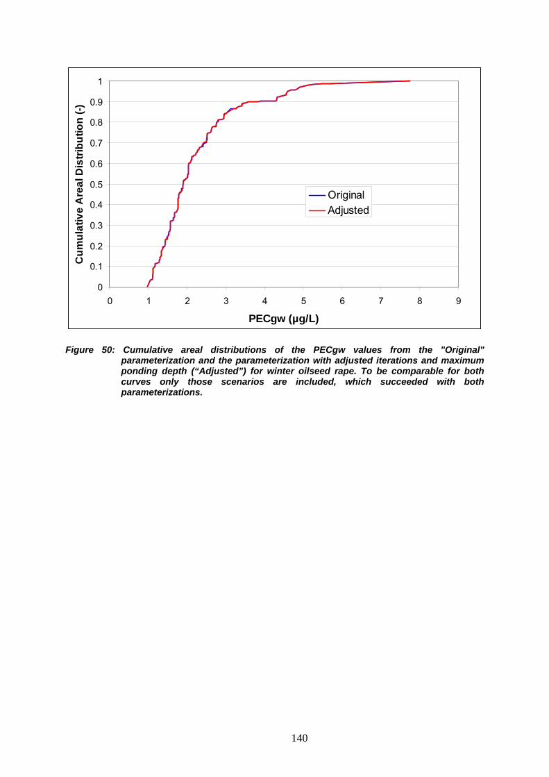
0
0.1
0.2
0.3
0.4
0.5
0.6
0.7
0.8
0.9
1
0 1 2 3 4 5 6 7 8 9
PECgw (µg/L)
Cum
ulat
ive
Are
al D
istri
butio
n (-)
OriginalAdjusted
Figure 50: Cumulative areal distributions of the PECgw values from the "Original" parameterization and the parameterization with adjusted iterations and maximum ponding depth (“Adjusted”) for winter oilseed rape. To be comparable for both curves only those scenarios are included, which succeeded with both parameterizations.
140
8.10 References BDGSF database: http://www.gissol.fr/programme/bdgsf/bdgsf.php Bollen, M.J.S.; Bekhuis, F.H.W.M.; Reiling, R. and Scheper, E. 1995. Towards a spatial pattern of the vulnerability of soil and groundwater. RIVM report no. 711901012, Bilthoven, the Netherlands. (In Dutch.). Bruand, A., Duval, O. et Cousin, I. 2004. Estimation des propriétés de rétention en eau des sols à partir de la base de données SOLHYDRO: une première proposition combinant le type d'horizon, sa texture et sa densité apparente. Etude et Gestion des Sols, Volume 11, 3, 2004, 323-332. CORINE Land Cover (CLC) database: http://www.ifen.fr/bases-de-donnees/occupation-des-sols-corine-land-cover.html http://www.eea.europa.eu/themes/landuse DONESOL database : http://www.gissol.fr/outil/donesol/donesol.php Dubus, I. G., E. Barriuso and R. Calvet (2001). Sorption of weak organic acids in soil: clofencet, 2,4-D and salicylic acid. Chemosphere 45: 767 –774. ESDB : http://eusoils.jrc.ec.europa.eu/ESDB_Archive/ESDB/index.htm ETC 2000. European Topic Centre CORINE Land Cover Database, Version 12/2000.
European Topic Centre of Landcover (ETC/LC). Kiruna, Sweden Finke, P., R. Hartwich, R. Dudal, J. Ibàñez, M. Jamagne, D. King, L. Montanarella and N.
Yassoglou (2001). GEOREFERENCED SOIL DATABASE FOR EUROPE. Manual of procedures. Version 1.1. European Soil Bureau Research Report No. 5, EUR 18092 EN
INRA (2005a). Base de Données Analyse des Terres.
http://www.gissol.fr/programme/bdat/bdat.php INRA (2005b). Base de Données Géographique des Sols de France, descriptif du contenu.
http://gissol.orleans.inra.fr/programme/bdgsf/contenu.php INRA (2005c). Base de données nationale des informations spatiales pédologiques.
http://gissol.orleans.inra.fr/outil/donesol/donesol.php Jamagne, M. 1967. Bases et techniques d'une cartographie des sols. Annales agronomiques. Hors serie 18, 142 pages. Jamagne, M., Bétrémieux, R., Bégon, J.C. and Mori, A., 1977. Quelques données sur la variabilité dans le milieu naturel de la réserve en eau des sols. Bulletin technique Inf. 324-325, 627-641. Jones, R. J. A., R. Hiederer, E. Rusco, P. J. Loveland and L. Montanarella 2004. The map of organic carbon in topsoils in Europe, Version 1.2, September 2003: Explanation of Special Publication Ispra 2004 No.72 (S.P.I.04.72). European Soil Bureau Research Report No. 17. Office for Official Publications of the European Communities, Luxembourg
141
Morvan, Y. & Le Bas, C. 2006. Détermination de profils types de sol par régions de cultures. Report of INRA, Unité Infosol, Orléans. Reuter, H. I., L. R. Lado, T. Hengl and L. Montanarella (2008). CONTINENTAL-SCALE DIGITAL SOIL MAPPING USING EUROPEAN SOIL PROFILE DATA: SOIL PH. Hamburger Beiträge zur Physischen Geographie und Landschaftsökologie 19: 91-102. Rosetta model:
http://www.ars.usda.gov/Services/docs.htm?docid=8953 http://www.cals.arizona.edu/research/rosetta/index.html
Schaap, M.G.; Leij, F.J. and van Genuchten, M. Th. 1999. A bootstrap-neural network approach to predict soil hydraulic parameters. In: van Genuchten, M.Th., F.J. Leij, and L. Wu (eds), Proc. Int. Workshop, Characterization and Measurements of the Hydraulic Properties of Unsaturated Porous Media, pp 1237-1250, University of California, Riverside, CA. Schaap, M.G.; Leij, F.J. and van Genuchten, M. Th. 2001. Rosetta: a computer program for estimating soil hydraulic parameters with hierarchical pedotransfer functions. Journal of Hydrology, 251:163-176. Van Genuchten, M.Th. 1980. A closed form for predicting the hydraulic conductivity of unsaturated soils. Soil Sci. Soc. Am. J. (44):892-898. Vereecken, H; Maes, J.; Feyen, J and Darius, P. 1989. Estimating the soil moisture retention characteristic from texture, bulk density and carbon content. Soil Science Vol. 148 (6), 389-403. Weynants, M; Vereecken, H and Javaux, M. 2009. Revisiting Vereecken pedotransfer functions: introducing a closed-form hydraulic model. Vadose Zone J. 8:86–95. Wösten, J.H.M; Lilly, A.; Nemes, A. and Le bas, C. 1999. Development and use of a database of hydraulic properties of European soils. Geoderma 90, 169-185.
142

9 Selection of relevant output for national assessment
9.1 European Regulatory Framework The target protection goal at EU level is a maximum annual average concentration in groundwater of 0.1 µg/L for active substances and relevant metabolites considering an overall 90th percentile vulnerability of scenarios (FOCUS, 2000). This should take into account spatial variability (e.g. of soil conditions) and temporal variability (inter-annual variability of the weather conditions) over the simulation period. The overall 90th percentile can be approximated by taking the spatial 80th percentile and the temporal 80th percentile. This protection goal is also recommended for assessment at national level in the latest draft FOCUS groundwater report (FOCUS, 2008).
For applications every other year or every three years (as is the case for most FROGS-rotations), it is recommended in FOCUS (2000) and confirmed in FOCUS (2008) to calculate flux-weighted average values over the rotation period for a total simulation period of 20 rotations (i.e. 40 years for applications every other year and 60 years for applications every three years, plus 6 years of warm-up period) and then select the 80th percentile of these 20 values. This temporal 80th percentile is approximated by the 17th value of the ranked concentrations (FOCUS, 2000) or the average of the 16th and 17th value (FOCUS, 2008).
9.2 FROGS Calculation Procedure The evaluation procedure within FROGS is following closely the approach described in the European regulatory framework. Calculation is always performed for 6 warm-up years followed by 20 rotations (resulting in 26 years, 46 years, or 66 years for 1-, 2-, and 3-year rotations, respectively). The output is the concentration in the leachate at the bottom of the soil profile (as opposed to a target depth of 1-meter in FOCUS).
Since no conservativity assumption was made during the set-up of the FROGS-scenarios regarding climate, soil and crop, the spatial 80th percentile can be derived from the area-weighted cumulative frequency distribution of the concentrations from the relevant scenarios for the considered crop (FOCUS, 2008, p. 58 and 128). This is then combined with the temporal 80th to achieve an overall 90th percentile.
To calculate the temporal 80th percentile, the average concentrations over each rotation (Crot [µg/L]) are calculated for every run according to Equation 10.
∑∑=
FlvFocAmaLea
Crot 100Equation 10:
where AmaLea [kg/ha] is the annual area substance mass leached from the target layer (bottom of soil profile) and FlvFoc [m³/m²] is the volume of water leached from the target layer (bottom of soil profile).
143

144
The sums are calculated from the beginning of the year in which the main crop emerges until the end of the 2nd or 3rd year for 2- or 3-year rotations, respectively. The temporal 80th percentile is approximated by the 17th value of the ranked concentrations according to FOCUS (2000).
To derive the spatial 80th percentile the temporal 80th percentile concentrations from all runs are sorted by ascending order, and their cumulative areas are divided by the total area. This leads to an area-weighted cumulative frequency distribution of the concentrations. As the overall 90th percentile the concentration is selected at which the cumulative area is 80% of the total area. In most cases no concentration at exactly the 80th percentile can be derived, so that a linear interpolation between the closest concentrations below and above the spatial 80th percentile is made.
9.3 References
FOCUS (2000). FOCUS groundwater scenarios in the EU pesticide registration process.
FOCUS (2009). Assessing Potential for Movement of Active Substances and their Metabolites to Ground Water in the EU” Report of the FOCUS Ground Water Work Group, EC Document Reference Sanco/13144/2010 version 1, 604 pp.
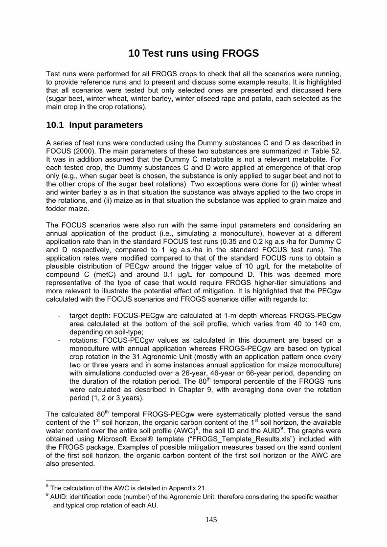
10 Test runs using FROGS Test runs were performed for all FROGS crops to check that all the scenarios were running, to provide reference runs and to present and discuss some example results. It is highlighted that all scenarios were tested but only selected ones are presented and discussed here (sugar beet, winter wheat, winter barley, winter oilseed rape and potato, each selected as the main crop in the crop rotations).
10.1 Input parameters A series of test runs were conducted using the Dummy substances C and D as described in FOCUS (2000). The main parameters of these two substances are summarized in Table 52. It was in addition assumed that the Dummy C metabolite is not a relevant metabolite. For each tested crop, the Dummy substances C and D were applied at emergence of that crop only (e.g., when sugar beet is chosen, the substance is only applied to sugar beet and not to the other crops of the sugar beet rotations). Two exceptions were done for (i) winter wheat and winter barley a as in that situation the substance was always applied to the two crops in the rotations, and (ii) maize as in that situation the substance was applied to grain maize and fodder maize. The FOCUS scenarios were also run with the same input parameters and considering an annual application of the product (i.e., simulating a monoculture), however at a different application rate than in the standard FOCUS test runs (0.35 and 0.2 kg a.s /ha for Dummy C and D respectively, compared to 1 kg a.s./ha in the standard FOCUS test runs). The application rates were modified compared to that of the standard FOCUS runs to obtain a plausible distribution of PECgw around the trigger value of 10 µg/L for the metabolite of compound C (metC) and around 0.1 µg/L for compound D. This was deemed more representative of the type of case that would require FROGS higher-tier simulations and more relevant to illustrate the potential effect of mitigation. It is highlighted that the PECgw calculated with the FOCUS scenarios and FROGS scenarios differ with regards to:
- target depth: FOCUS-PECgw are calculated at 1-m depth whereas FROGS-PECgw area calculated at the bottom of the soil profile, which varies from 40 to 140 cm, depending on soil-type;
- rotations: FOCUS-PECgw values as calculated in this document are based on a monoculture with annual application whereas FROGS-PECgw are based on typical crop rotation in the 31 Agronomic Unit (mostly with an application pattern once every two or three years and in some instances annual application for maize monoculture) with simulations conducted over a 26-year, 46-year or 66-year period, depending on the duration of the rotation period. The 80th temporal percentile of the FROGS runs were calculated as described in Chapter 9, with averaging done over the rotation period (1, 2 or 3 years).
The calculated 80th temporal FROGS-PECgw were systematically plotted versus the sand content of the 1st soil horizon, the organic carbon content of the 1st soil horizon, the available water content over the entire soil profile (AWC)8 9, the soil ID and the AUID . The graphs were obtained using Microsoft Excel® template (“FROGS_Template_Results.xls”) included with the FROGS package. Examples of possible mitigation measures based on the sand content of the first soil horizon, the organic carbon content of the first soil horizon or the AWC are also presented.
8 The calculation of the AWC is detailed in . Appendix 219 AUID: identification code (number) of the Agronomic Unit, therefore considering the specific weather
and typical crop rotation of each AU.
145

Table 52 Main input parameters used for the test runs using Dummy substance C (with metabolite) and Dummy substance D
Dummy C Dummy C metabolite Dummy D DT50 (days) 20 100 20 ffM (-) - 0.71 from parent - Kom/Koc (dm3/kg) 100 / 172 30 / 52 35 / 60 1/n (-) 0.9 0.9 0.9 MW (g/mol) 200 150 300 Crop uptake factor (-) 0.5 0.5 0.5 Q10 2.58 2.58 2.58 Application rate (g/ha) 350 - 200 Application date/stage emergence - emergence
10.2 Results for the Dummy Substance C and its metabolite
10.2.1 Sugar beet The results of the test runs for the Dummy substance C and its metabolites using the FOCUS scenarios are presented in Table 53. The leaching of substance C is very limited whereas the PECgw for the metabolite indicate a high leaching potential.
Table 53 80th percentile concentrations for Substance C and its metabolite following application to sugar beet
FOCUS scenario
PECgw (μg/L)
Substance C Metabolite C Chateaudun <0.001 10.082 Hamburg <0.001 11.514 Jokioinen <0.001 9.088 Kremsmünster <0.001 8.582 Okehampton <0.001 8.924 Piacenza <0.001 8.485 Porto <0.001 1.365 Sevilla <0.001 5.346 Thiva <0.001 6.793
The results of the test runs using FROGS for sugar beet are presented as cumulative areal distribution of the 80th percentile in time of PECgw (Figure 51 and Figure 52). They represent a total area of 6 884 000 ha. The detailed results of the corresponding 83 scenarios are presented in Appendix 18.
The FROGS PECgw also indicate a very low leaching potential of Substance C, the maximum PECgw being 0.006 μg/L. The PECgw of FOCUS Piacenza scenario corresponds to the 99th spatial percentile (Figure 51). For the metabolite of substance C, the 80th temporal percentile of PECgw calculated with the FROGS-scenarios are in the same range as calculated with the FOCUS scenarios (from 1.295 to 8.921 μg/L). The 80th spatial percentile of the 80th temporal percentile PECgw for Metabolite C, corresponding to a joint 90th vulnerability percentile, is 3.760 μg/L (Figure 52).
146
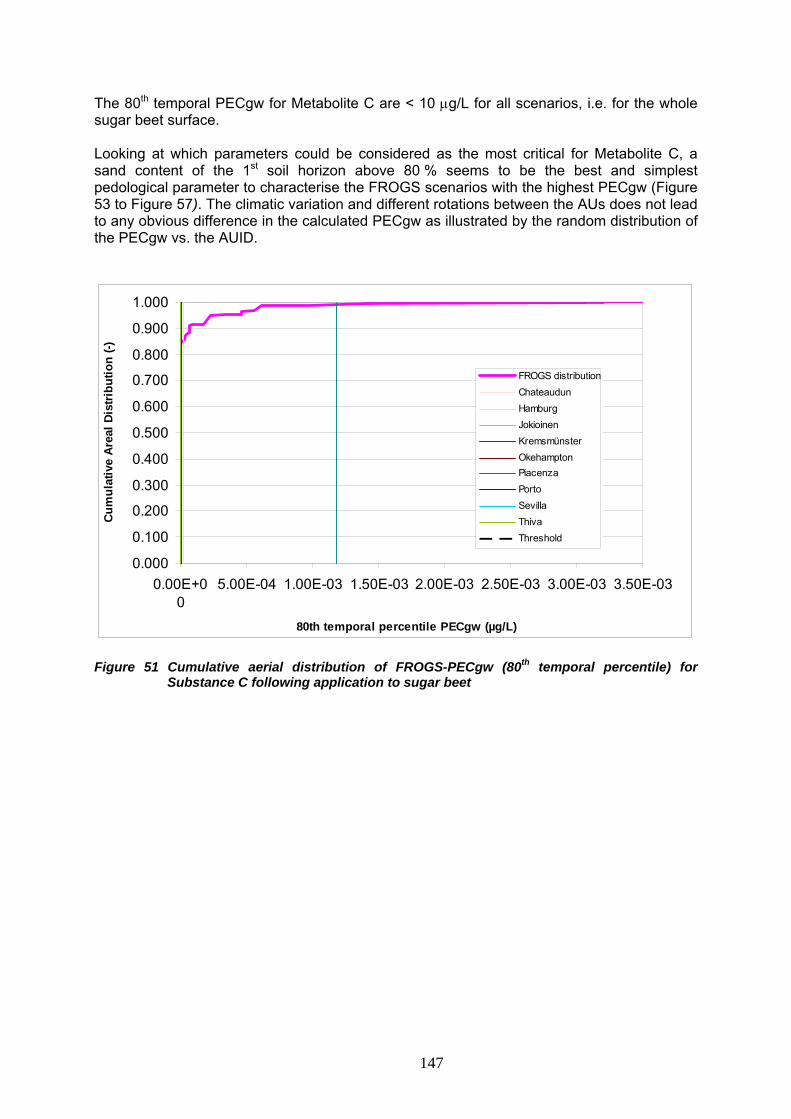
The 80th temporal PECgw for Metabolite C are < 10 μg/L for all scenarios, i.e. for the whole sugar beet surface. Looking at which parameters could be considered as the most critical for Metabolite C, a sand content of the 1st soil horizon above 80 % seems to be the best and simplest pedological parameter to characterise the FROGS scenarios with the highest PECgw (Figure 53 to Figure 57). The climatic variation and different rotations between the AUs does not lead to any obvious difference in the calculated PECgw as illustrated by the random distribution of the PECgw vs. the AUID.
0.000
0.100
0.200
0.300
0.400
0.500
0.600
0.700
0.800
0.900
1.000
0.00E+00
5.00E-04 1.00E-03 1.50E-03 2.00E-03 2.50E-03 3.00E-03 3.50E-03
80th temporal percentile PECgw (µg/L)
Cum
ulat
ive
Area
l Dis
trib
utio
n (-)
FROGS distributionChateaudunHamburgJokioinenKremsmünsterOkehamptonPiacenzaPortoSevillaThivaThreshold
Figure 51 Cumulative aerial distribution of FROGS-PECgw (80th temporal percentile) for
Substance C following application to sugar beet
147

0
0.1
0.2
0.3
0.4
0.5
0.6
0.7
0.8
0.9
1
0 2 4 6 8 10 12 180th temporal percentile PECgw (µg/L)
Cum
ulat
ive
Are
al D
istri
butio
n (-)
4
FROGS distributionChateaudunHamburgJokioinenKremsmünsterOkehamptonPiacenzaPortoSevillaThivaThreshold
Figure 52 Cumulative aerial distribution of FROGS-PECgw (80th temporal percentile) for Metabolite C following application of Substance C to sugar beet
0
1
2
3
4
5
6
7
8
9
10
0 10 20 30 40 50 60 70 80 90
Sand Content (%)
80th
tem
pora
l per
cent
ile P
ECgw
(µg/
L) Soil1
Soil2
Soil3
Soil6
Soil8
Soil9
Soil13
Soil19
Figure 53 80th temporal percentile PECgw vs. sand content of the 1st soil horizon properties (MetC – Sugar beet)
148
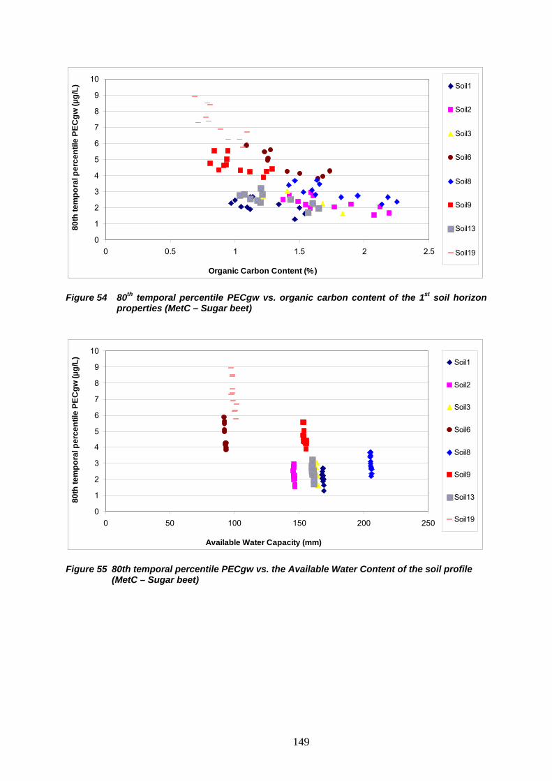
0
1
2
3
4
5
6
7
8
9
10
0 0.5 1 1.5 2 2.5
Organic Carbon Content (%)
80th
tem
pora
l per
cent
ile P
ECgw
(µg/
L) Soil1
Soil2
Soil3
Soil6
Soil8
Soil9
Soil13
Soil19
Figure 54 80th temporal percentile PECgw vs. organic carbon content of the 1st soil horizon properties (MetC – Sugar beet)
0
1
2
3
4
5
6
7
8
9
10
0 50 100 150 200 250
Available Water Capacity (mm)
80th
tem
pora
l per
cent
ile P
ECgw
(µg/
L) Soil1
Soil2
Soil3
Soil6
Soil8
Soil9
Soil13
Soil19
Figure 55 80th temporal percentile PECgw vs. the Available Water Content of the soil profile (MetC – Sugar beet)
149
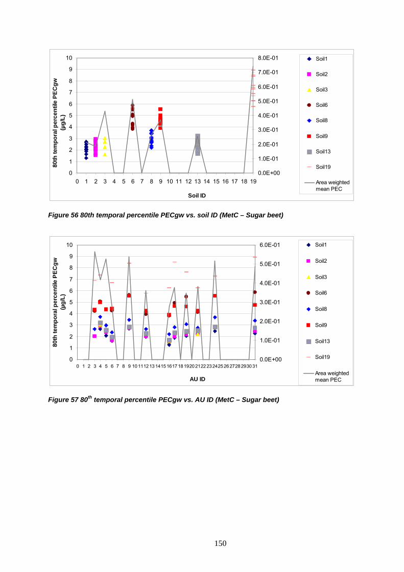
0
1
2
3
4
5
6
7
8
9
10
0 1 2 3 4 5 6 7 8 9 10 11 12 13 14 15 16 17 18 19
Soil ID
80th
tem
pora
l per
cent
ile P
ECgw
(µ
g/L)
0.0E+00
1.0E-01
2.0E-01
3.0E-01
4.0E-01
5.0E-01
6.0E-01
7.0E-01
8.0E-01
Are
a w
eigh
ted
mea
n PE
C (µ
g/L)
Soil1
Soil2
Soil3
Soil6
Soil8
Soil9
Soil13
Soil19
Area weightedmean PEC
Figure 56 80th temporal percentile PECgw vs. soil ID (MetC – Sugar beet)
0
1
2
3
4
5
6
7
8
9
10
0 1 2 3 4 5 6 7 8 9 10111213141516171819202122232425262728293031
AU ID
80th
tem
pora
l per
cent
ile P
ECgw
(µ
g/L)
0.0E+00
1.0E-01
2.0E-01
3.0E-01
4.0E-01
5.0E-01
6.0E-01
Are
a w
eigh
ted
mea
n PE
C (µ
g/L)
Soil1
Soil2
Soil3
Soil6
Soil8
Soil9
Soil13
Soil19
Area weightedmean PEC
Figure 57 80th temporal percentile PECgw vs. AU ID (MetC – Sugar beet)
150

10.2.2 Winter wheat The results of the test runs for the Dummy substance C and its metabolites using the FOCUS scenarios are presented in Table 54. Similar to the scenarios in sugar beets the leaching of substance C is very limited whereas the PECgw for the metabolite indicate a high leaching potential. Table 54 80th percentile concentrations for Substance C and its metabolite following
application to winter wheat FOCUS scenario PECgw (μg/L) Substance C Metabolite C Chateaudun <0.001 8.645 Hamburg <0.001 12.110 Jokioinen <0.001 9.748 Kremsmünster <0.001 8.893 Okehampton <0.001 10.530 Piacenza 0.004 9.336 Porto <0.001 1.665 Sevilla <0.001 2.120 Thiva <0.001 7.110 The results of the test runs using the FROGS scenarios for winter wheat (also including application to winter barley as rotational crop) are presented as cumulative areal distribution in Figure 58 and Figure 59. They represent an overall area of 16 819 kha. The detailed results of the corresponding 233 scenarios are included in the electronic distribution of the tool. The FROGS PECgw also indicate a very low leaching potential of Substance C. The maximum PECgw is 0.133 μg/L, however the 80th temporal percentile PECgw are less than 0.1 μg/L for scenarios representing altogether 99.7 % of the winter cereals surface. The 80th spatial percentile of the 80th temporal percentile PECgw for Substance C, corresponding to an overall 90th vulnerability percentile, is <0.001 μg/L (Figure 58). For Metabolite C, the 80th temporal percentile of PECgw calculated with the FROGS-scenarios are in the same range as those calculated with the FOCUS scenarios (from 1.795 to 15.92 μg/L). The 80th spatial percentile of the 80th temporal percentile PECgw for Metabolite C, corresponding to a joint 90th vulnerability percentile, is 6.178 μg/L (Figure 59). The 80th temporal PECgw is less than 10 μg/L for scenarios representing altogether 94.4 % of the winter cereals surface. Only 25 scenarios out of 233 resulted in PECgw >10 μg/L, corresponding to the soil 19, soil 12, soil 9 and soil 6 (see detailed results in Appendix 19). Since the overall 90th percentile PECgw is <10 µg/L, mitigations would not be necessary. Looking at what would be the most critical parameters regarding Metabolite C leaching potential, an available water content (AWC) below 100 mm for the entire soil profile appears to be the main pedological parameter to characterise most of the FROGS scenarios with a PECgw above 10 μg/L (Figure 60 to Figure 64). The climatic variation and rotation differences between AUs do not lead to any obvious difference for the calculated PECgw as illustrated by the random distribution of the PECgw vs. the AUID.
151
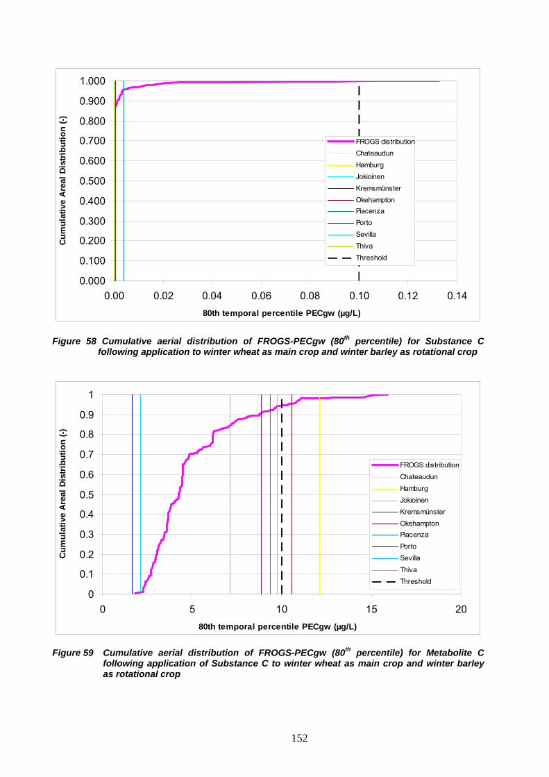
0.000
0.100
0.200
0.300
0.400
0.500
0.600
0.700
0.800
0.900
1.000
0.00 0.02 0.04 0.06 0.08 0.10 0.12 0.1480th temporal percentile PECgw (µg/L)
Cum
ulat
ive
Are
al D
istri
butio
n (-)
FROGS distributionChateaudunHamburgJokioinenKremsmünsterOkehamptonPiacenzaPortoSevillaThivaThreshold
Figure 58 Cumulative aerial distribution of FROGS-PECgw (80th percentile) for Substance C following application to winter wheat as main crop and winter barley as rotational crop
0
0.1
0.2
0.3
0.4
0.5
0.6
0.7
0.8
0.9
1
0 5 10 15 2080th temporal percentile PECgw (µg/L)
Cum
ulat
ive
Area
l Dis
trib
utio
n (-)
FROGS distributionChateaudunHamburgJokioinenKremsmünsterOkehamptonPiacenzaPortoSevillaThivaThreshold
Figure 59 Cumulative aerial distribution of FROGS-PECgw (80th percentile) for Metabolite C following application of Substance C to winter wheat as main crop and winter barley as rotational crop
152
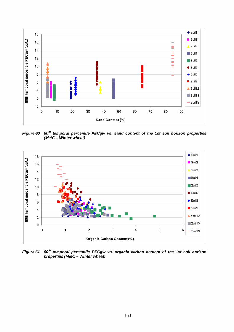
0
2
4
6
8
10
12
14
16
18
0 10 20 30 40 50 60 70 80 90
Sand Content (%)
80th
tem
pora
l per
cent
ile P
ECgw
(µg/
L)
Soil1
Soil2
Soil3
Soil4
Soil5
Soil6
Soil8
Soil9
Soil12
Soil13
Soil19
Figure 60 80th temporal percentile PECgw vs. sand content of the 1st soil horizon properties (MetC – Winter wheat)
0
2
4
6
8
10
12
14
16
18
0 1 2 3 4 5 6
Organic Carbon Content (%)
80th
tem
pora
l per
cent
ile P
ECgw
(µg/
L)
Soil1
Soil2
Soil3
Soil4
Soil5
Soil6
Soil8
Soil9
Soil12
Soil13
Soil19
Figure 61 80th temporal percentile PECgw vs. organic carbon content of the 1st soil horizon properties (MetC – Winter wheat)
153
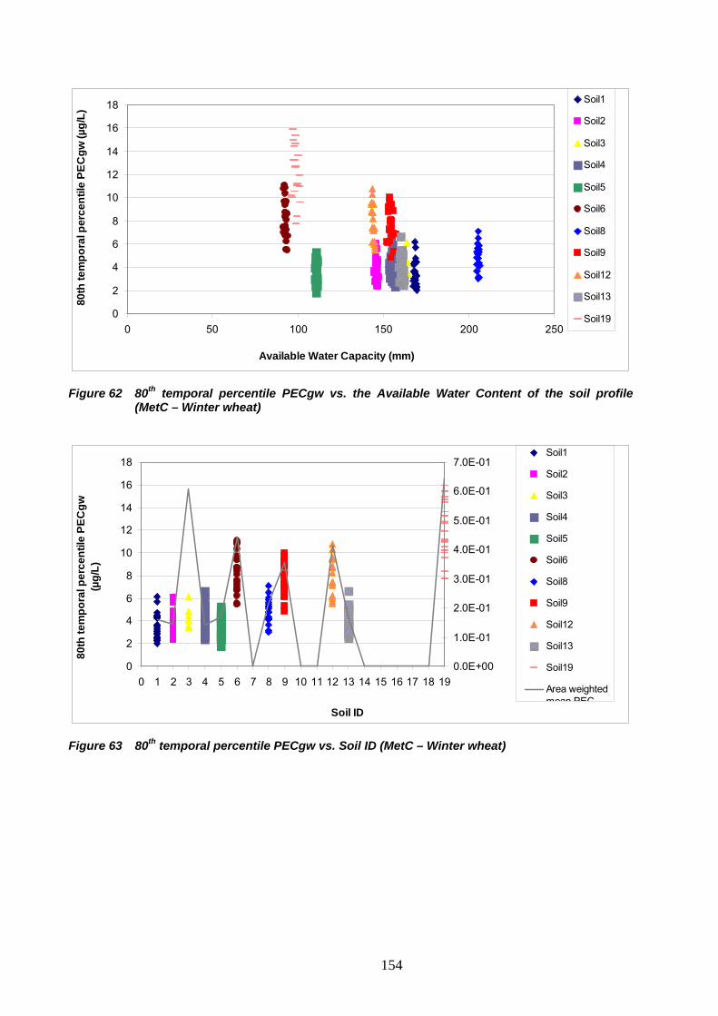
0
2
4
6
8
10
12
14
16
18
0 50 100 150 200 250
Available Water Capacity (mm)
80th
tem
pora
l per
cent
ile P
ECgw
(µg/
L)
Soil1
Soil2
Soil3
Soil4
Soil5
Soil6
Soil8
Soil9
Soil12
Soil13
Soil19
Figure 62 80th temporal percentile PECgw vs. the Available Water Content of the soil profile (MetC – Winter wheat)
0
2
4
6
8
10
12
14
16
18
0 1 2 3 4 5 6 7 8 9 10 11 12 13 14 15 16 17 18 19
Soil ID
80th
tem
pora
l per
cent
ile P
ECgw
(µ
g/L)
0.0E+00
1.0E-01
2.0E-01
3.0E-01
4.0E-01
5.0E-01
6.0E-01
7.0E-01
Are
a w
eigh
ted
mea
n PE
C (µ
g/L)
Soil1
Soil2
Soil3
Soil4
Soil5
Soil6
Soil8
Soil9
Soil12
Soil13
Soil19
Area weightedmean PEC
Figure 63 80th temporal percentile PECgw vs. Soil ID (MetC – Winter wheat)
154

0
2
4
6
8
10
12
14
16
18
0 1 2 3 4 5 6 7 8 9 10111213141516171819202122232425262728293031
AU ID
80th
tem
pora
l per
cent
ile P
ECgw
(µ
g/L)
0.0E+00
2.0E-01
4.0E-01
6.0E-01
8.0E-01
1.0E+00
1.2E+00
Are
a w
eigh
ted
mea
n PE
C (µ
g/L)
Soil1
Soil2
Soil3
Soil4
Soil5
Soil6
Soil8
Soil9
Soil12
Soil13
Soil19
Area weightedmean PEC
Figure 64 80th temporal percentile PECgw vs. AU ID (MetC – Winter wheat)
10.2.3 Winter oilseed rape The results of the test runs for the Dummy substance C and its metabolite using the FOCUS scenarios are presented in Table 55. The leaching of substance C is very limited whereas the PECgw for the metabolite indicate a high leaching potential. Table 55 80th percentile concentrations for Substance C and its metabolite applied annually to
winter oilseed rape FOCUS scenario PECgw (μg/L) Substance C Metabolite C Chateaudun <0.001 10.547 Hamburg <0.001 12.902 Jokioinen - - Kremsmünster <0.001 9.460 Okehampton <0.001 10.602 Piacenza 0.004 10.562 Porto <0.001 2.311 Sevilla - - Thiva - - The results of the test runs using the FROGS scenarios for winter oilseed rape are presented as cumulative areal distribution in Figure 65 and Figure 66. They represent an overall area of 15 408 kha. The detailed results of the corresponding 195 scenarios are included in the FROGS package. The FROGS PECgw also indicate a very low leaching potential of Substance C. For Metabolite C, the 80th temporal percentile of PECgw calculated with the FROGS-scenarios are in the same range as calculated with the FOCUS scenarios (from 1.006 to 7.237 μg/L). The 80th spatial percentile of the 80th temporal percentile PECgw for Metabolite C, corresponding to an overall 90th percentile, is 4.234 μg/L. The FROGS-scenarios indicate that for 100 % of winter oilseed rape area, the 80th temporal PECgw would be less than 10 μg/L.
155
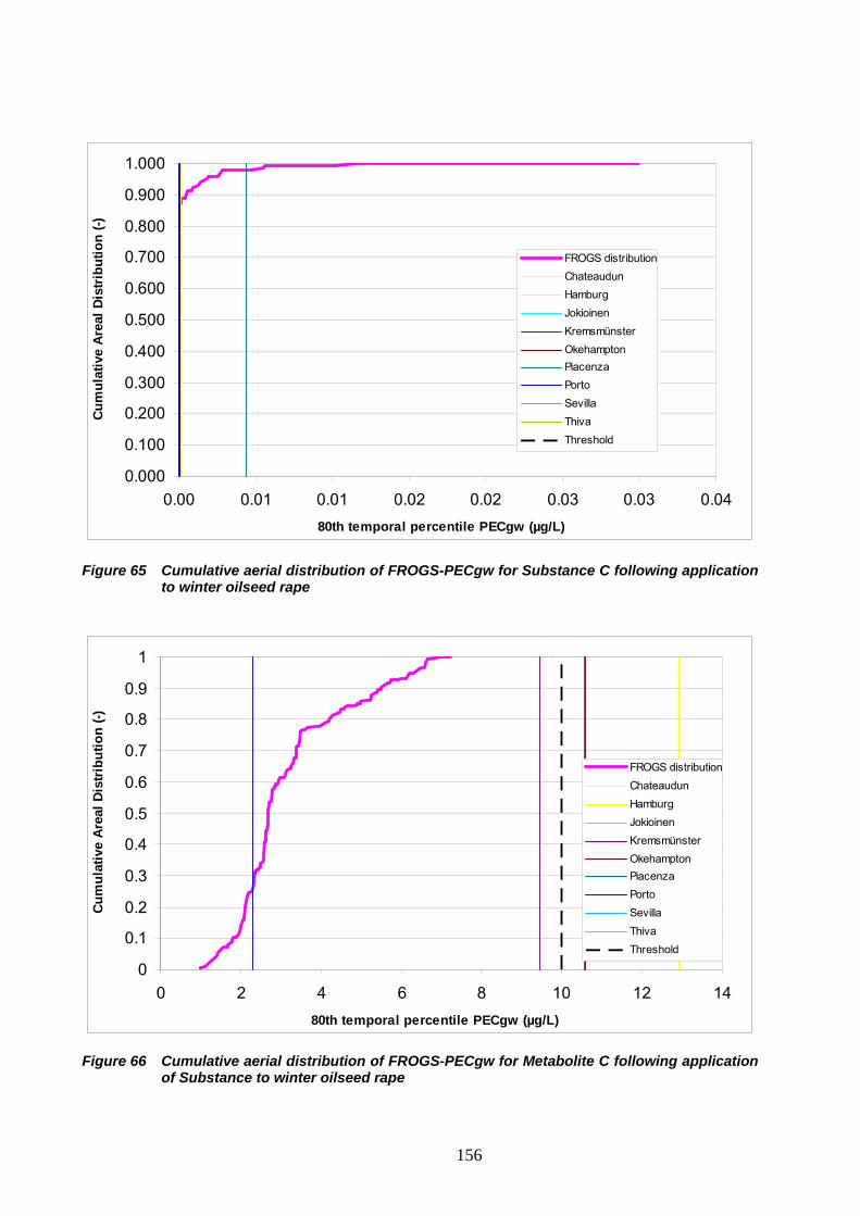
0.000
0.100
0.200
0.300
0.400
0.500
0.600
0.700
0.800
0.900
1.000
0.00 0.01 0.01 0.02 0.02 0.03 0.03 0.0480th temporal percentile PECgw (µg/L)
Cum
ulat
ive
Are
al D
istri
butio
n (-)
FROGS distributionChateaudunHamburgJokioinenKremsmünsterOkehamptonPiacenzaPortoSevillaThivaThreshold
Figure 65 Cumulative aerial distribution of FROGS-PECgw for Substance C following application to winter oilseed rape
0
0.1
0.2
0.3
0.4
0.5
0.6
0.7
0.8
0.9
1
0 2 4 6 8 10 12 180th temporal percentile PECgw (µg/L)
Cum
ulat
ive
Area
l Dis
trib
utio
n (-)
4
FROGS distributionChateaudunHamburgJokioinenKremsmünsterOkehamptonPiacenzaPortoSevillaThivaThreshold
Figure 66 Cumulative aerial distribution of FROGS-PECgw for Metabolite C following application of Substance to winter oilseed rape
156

Looking at the most critical parameters regarding the leaching potential of Metabolite C, an available water content (AWC) below 100 mm for the entire soil profile seems to be the main pedological parameter to characterise most of the FROGS scenarios with a PECgw above 10 μg/L (Figure 67 to Figure 71). The climatic variation and rotation differences between AUs do not lead to any obvious difference for the calculated PECgw as illustrated by the random distribution of the PECgw vs. the AUID.
0
1
2
3
4
5
6
7
8
0 10 20 30 40 50 60 70
Sand Content (%)
80th
tem
pora
l per
cent
ile P
ECgw
(µg/
L)
Soil1
Soil2
Soil3
Soil4
Soil5
Soil6
Soil8
Soil9
Soil12
Soil17
Figure 67 80th temporal percentile PECgw vs. sand content of the 1st soil horizon properties (MetC – Winter oilseed rape)
0
1
2
3
4
5
6
7
8
0 1 2 3 4 5 6
Organic Carbon Content (%)
80th
tem
pora
l per
cent
ile P
ECgw
(µg/
L)
Soil1
Soil2
Soil3
Soil4
Soil5
Soil6
Soil8
Soil9
Soil12
Soil17
Figure 68 80th temporal percentile PECgw vs. organic carbon content of the 1st soil horizon properties (MetC – Winter oilseed rape)
157
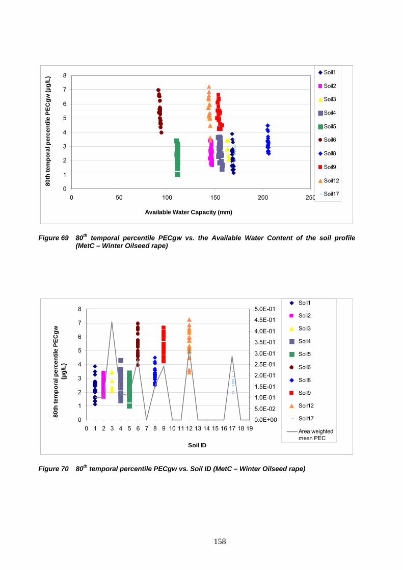
0
1
2
3
4
5
6
7
8
0 50 100 150 200 250
Available Water Capacity (mm)
80th
tem
pora
l per
cent
ile P
ECgw
(µg/
L)
Soil1
Soil2
Soil3
Soil4
Soil5
Soil6
Soil8
Soil9
Soil12
Soil17
Figure 69 80th temporal percentile PECgw vs. the Available Water Content of the soil profile (MetC – Winter Oilseed rape)
0
1
2
3
4
5
6
7
8
0 1 2 3 4 5 6 7 8 9 10 11 12 13 14 15 16 17 18 19
Soil ID
80th
tem
pora
l per
cent
ile P
ECgw
(µ
g/L)
0.0E+00
5.0E-02
1.0E-01
1.5E-01
2.0E-01
2.5E-01
3.0E-01
3.5E-01
4.0E-01
4.5E-01
5.0E-01A
rea
wei
ghte
d m
ean
PEC
(µg/
L)Soil1
Soil2
Soil3
Soil4
Soil5
Soil6
Soil8
Soil9
Soil12
Soil17
Area weightedmean PEC
Figure 70 80th temporal percentile PECgw vs. Soil ID (MetC – Winter Oilseed rape)
158
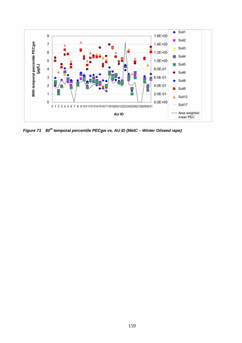
0
1
2
3
4
5
6
7
8
0 1 2 3 4 5 6 7 8 9 10111213141516171819202122232425262728293031
AU ID
80th
tem
pora
l per
cent
ile P
ECgw
(µ
g/L)
0.0E+00
2.0E-01
4.0E-01
6.0E-01
8.0E-01
1.0E+00
1.2E+00
1.4E+00
1.6E+00
Are
a w
eigh
ted
mea
n PE
C (µ
g/L)
Soil1
Soil2
Soil3
Soil4
Soil5
Soil6
Soil8
Soil9
Soil12
Soil17
Area weightedmean PEC
Figure 71 80th temporal percentile PECgw vs. AU ID (MetC – Winter Oilseed rape)
159

10.3 Results for the Dummy Substance D
10.3.1 Winter Barley The results of the test runs for the Dummy substance D using the FOCUS scenarios are presented in Table 56. Table 56 80th percentile concentrations for Substance D following application to winter barley
FOCUS scenario PECgw (microg/L) Substance D Chateaudun 0.029 Hamburg 0.285 Jokioinen 0.043 Kremsmünster 0.096 Okehampton 0.356 Piacenza 0.314 Porto 0.001 Sevilla 0.005 Thiva 0.018
The results of the test runs using the FROGS scenarios for winter barley as primary crop and also including application to winter wheat as rotational crop are presented as cumulative areal distribution of the 80th percentile in time of PECgw (Figure 72). They represent an area of 14 732 kha. The detailed results of the corresponding 183 scenarios are available in the FROGS package. The 80th temporal percentile of PECgw calculated with the FROGS-scenarios are between <0.001 and 1.648 μg/L. The 80th spatial percentile of the 80th temporal percentile PECgw for Substance D, corresponding to an overall 90th percentile, is 0.113 μg/L. The FROGS-scenarios indicate that for 78.9 % of winter barley surface, the 80th temporal PECgw should be less than 0.1 μg/L. A total of 54 scenarios out of 183 resulted in PECgw >0.1 μg/L (see details in Appendix 20). Looking at the critical parameters for leaching potential of Substance D, an available water content (AWC) below 100 mm appears to be the main pedological parameters to characterise the FROGS scenarios with a PECgw above 0.1 μg/L (Figure 74 to Figure 77). Applying a mitigation measure to avoid application of substance D on soils having an AWC < 100 mm would decrease the surface with PECgw above 0.1 μg/L from 3 120 kha to 1 922 kha. The resulting cumulative distribution indicates that the PECgw would be less than 0.1 μg/L for 85.8 % of mitigated winter barley surface (Figure 78). The climatic variation and rotation differences between AUs do not lead to any obvious difference for the calculated PECgw as illustrated by the random distribution of the PECgw vs. the AUID.
160

0.000
0.100
0.200
0.300
0.400
0.500
0.600
0.700
0.800
0.900
1.000
0.0 0.5 1.0 1.5 2.080th temporal percentile PECgw (µg/L)
Cum
ulat
ive
Are
al D
istri
butio
n (-)
FROGS distributionChateaudunHamburgJokioinenKremsmünsterOkehamptonPiacenzaPortoSevillaThivaThreshold
Figure 72 Cumulative aerial distribution of FROGS-PECgw (80th temporal percentile) for Substance D following application to winter barley as primary crop and winter wheat as rotational crop
0
0.2
0.4
0.6
0.8
1
1.2
1.4
1.6
1.8
0 10 20 30 40 50 60 70
Sand Content (%)
80th
tem
pora
l per
cent
ile P
ECgw
(µg/
L)
Soil1
Soil2
Soil3
Soil5
Soil6
Soil8
Soil9
Soil12
Soil13
Figure 73 80th temporal percentile PECgw vs. sand content of the 1st soil horizon properties (SubD – Winter barley)
161
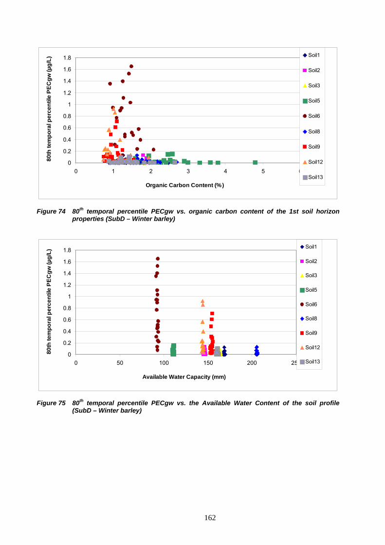
0
0.2
0.4
0.6
0.8
1
1.2
1.4
1.6
1.8
0 1 2 3 4 5 6
Organic Carbon Content (%)
80th
tem
pora
l per
cent
ile P
ECgw
(µg/
L)Soil1
Soil2
Soil3
Soil5
Soil6
Soil8
Soil9
Soil12
Soil13
Figure 74 80th temporal percentile PECgw vs. organic carbon content of the 1st soil horizon properties (SubD – Winter barley)
0
0.2
0.4
0.6
0.8
1
1.2
1.4
1.6
1.8
0 50 100 150 200 250
Available Water Capacity (mm)
80th
tem
pora
l per
cent
ile P
ECgw
(µg/
L)
Soil1
Soil2
Soil3
Soil5
Soil6
Soil8
Soil9
Soil12
Soil13
Figure 75 80th temporal percentile PECgw vs. the Available Water Content of the soil profile (SubD – Winter barley)
162

0
0.2
0.4
0.6
0.8
1
1.2
1.4
1.6
1.8
0 1 2 3 4 5 6 7 8 9 10 11 12 1314 15 16 1718 19
Soil ID
80th
tem
pora
l per
cent
ile P
ECgw
(µ
g/L)
0.0E+00
5.0E-03
1.0E-02
1.5E-02
2.0E-02
2.5E-02
3.0E-02
3.5E-02
4.0E-02
4.5E-02
Are
a w
eigh
ted
mea
n PE
C (µ
g/L)
Soil1
Soil2
Soil3
Soil5
Soil6
Soil8
Soil9
Soil12
Soil13
Area weightedmean PEC
Figure 76 80th temporal percentile PECgw vs. Soil ID (SubD – Winter barley)
0
0.2
0.4
0.6
0.8
1
1.2
1.4
1.6
1.8
0 1 2 3 4 5 6 7 8 910111213141516171819202122232425262728293031
AU ID
80th
tem
pora
l per
cent
ile P
ECgw
(µ
g/L)
0.0E+00
1.0E-02
2.0E-02
3.0E-02
4.0E-02
5.0E-02
6.0E-02
7.0E-02
8.0E-02
Are
a w
eigh
ted
mea
n PE
C (µ
g/L)
Soil1
Soil2
Soil3
Soil5
Soil6
Soil8
Soil9
Soil12
Soil13
Area weightedmean PEC
Figure 77 80th temporal percentile PECgw vs. AU ID (SubD – Winter barley)
163
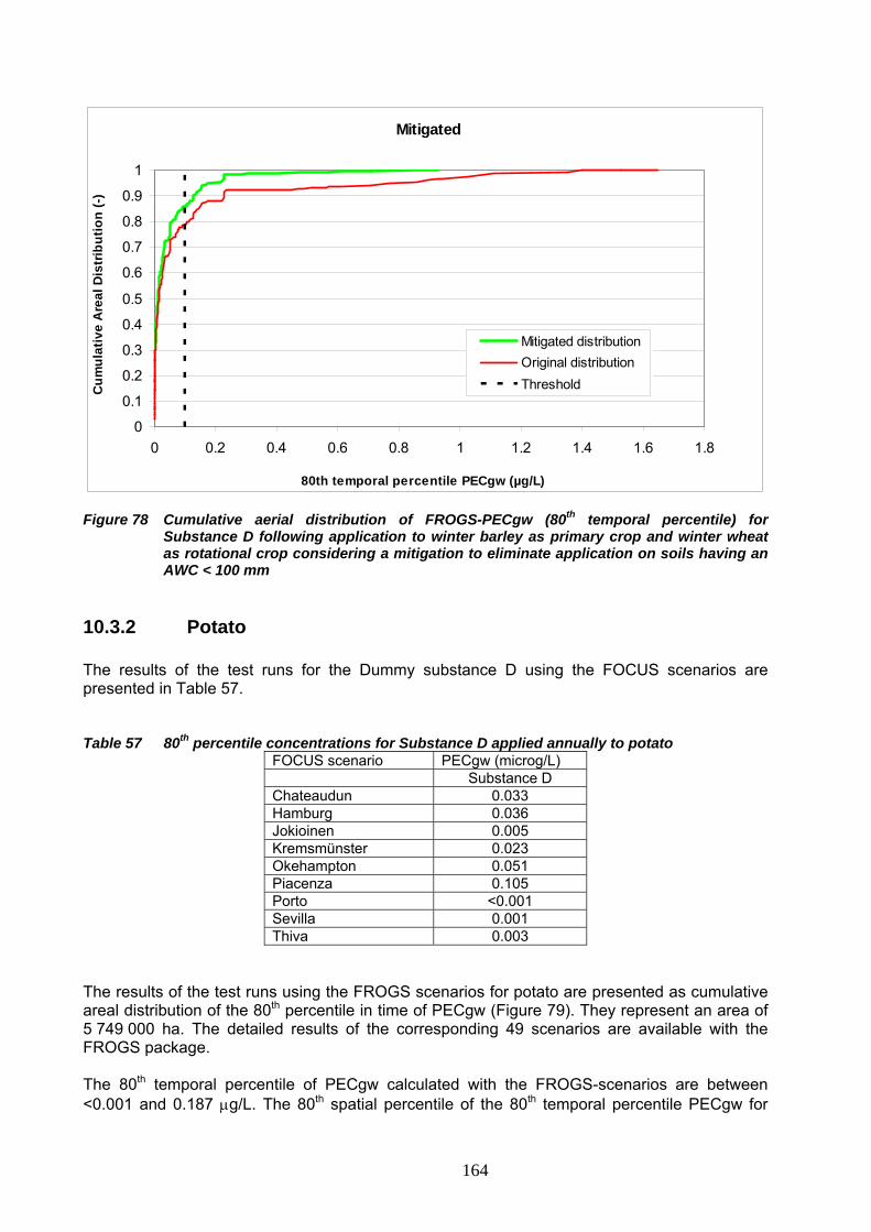
Mitigated
0
0.1
0.2
0.3
0.4
0.5
0.6
0.7
0.8
0.9
1
0 0.2 0.4 0.6 0.8 1 1.2 1.4 1.6 1.8
80th temporal percentile PECgw (µg/L)
Cum
ulat
ive
Are
al D
istr
ibut
ion
(-)
Mitigated distributionOriginal distributionThreshold
Figure 78 Cumulative aerial distribution of FROGS-PECgw (80th temporal percentile) for Substance D following application to winter barley as primary crop and winter wheat as rotational crop considering a mitigation to eliminate application on soils having an AWC < 100 mm
10.3.2 Potato The results of the test runs for the Dummy substance D using the FOCUS scenarios are presented in Table 57. Table 57 80th percentile concentrations for Substance D applied annually to potato
FOCUS scenario PECgw (microg/L) Substance D Chateaudun 0.033 Hamburg 0.036 Jokioinen 0.005 Kremsmünster 0.023 Okehampton 0.051 Piacenza 0.105 Porto <0.001 Sevilla 0.001 Thiva 0.003
The results of the test runs using the FROGS scenarios for potato are presented as cumulative areal distribution of the 80th percentile in time of PECgw (Figure 79). They represent an area of 5 749 000 ha. The detailed results of the corresponding 49 scenarios are available with the FROGS package. The 80th temporal percentile of PECgw calculated with the FROGS-scenarios are between <0.001 and 0.187 μg/L. The 80th spatial percentile of the 80th temporal percentile PECgw for
164
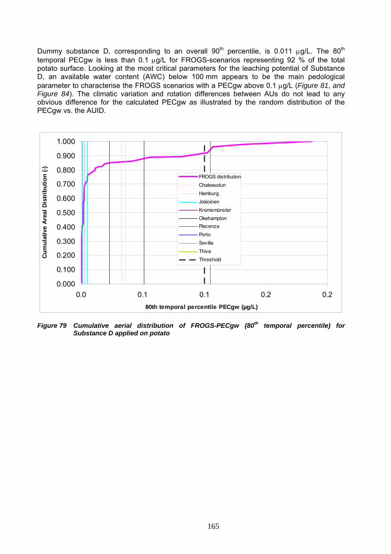
Dummy substance D, corresponding to an overall 90th percentile, is 0.011 μg/L. The 80th temporal PECgw is less than 0.1 μg/L for FROGS-scenarios representing 92 % of the total potato surface. Looking at the most critical parameters for the leaching potential of Substance D, an available water content (AWC) below 100 mm appears to be the main pedological parameter to characterise the FROGS scenarios with a PECgw above 0.1 μg/L ( , and Figure 81Figure 84). The climatic variation and rotation differences between AUs do not lead to any obvious difference for the calculated PECgw as illustrated by the random distribution of the PECgw vs. the AUID.
0.000
0.100
0.200
0.300
0.400
0.500
0.600
0.700
0.800
0.900
1.000
0.0 0.1 0.1 0.2 0.280th temporal percentile PECgw (µg/L)
Cum
ulat
ive
Are
al D
istri
butio
n (-)
FROGS distributionChateaudunHamburgJokioinenKremsmünsterOkehamptonPiacenzaPortoSevillaThivaThreshold
Figure 79 Cumulative aerial distribution of FROGS-PECgw (80th temporal percentile) for Substance D applied on potato
165
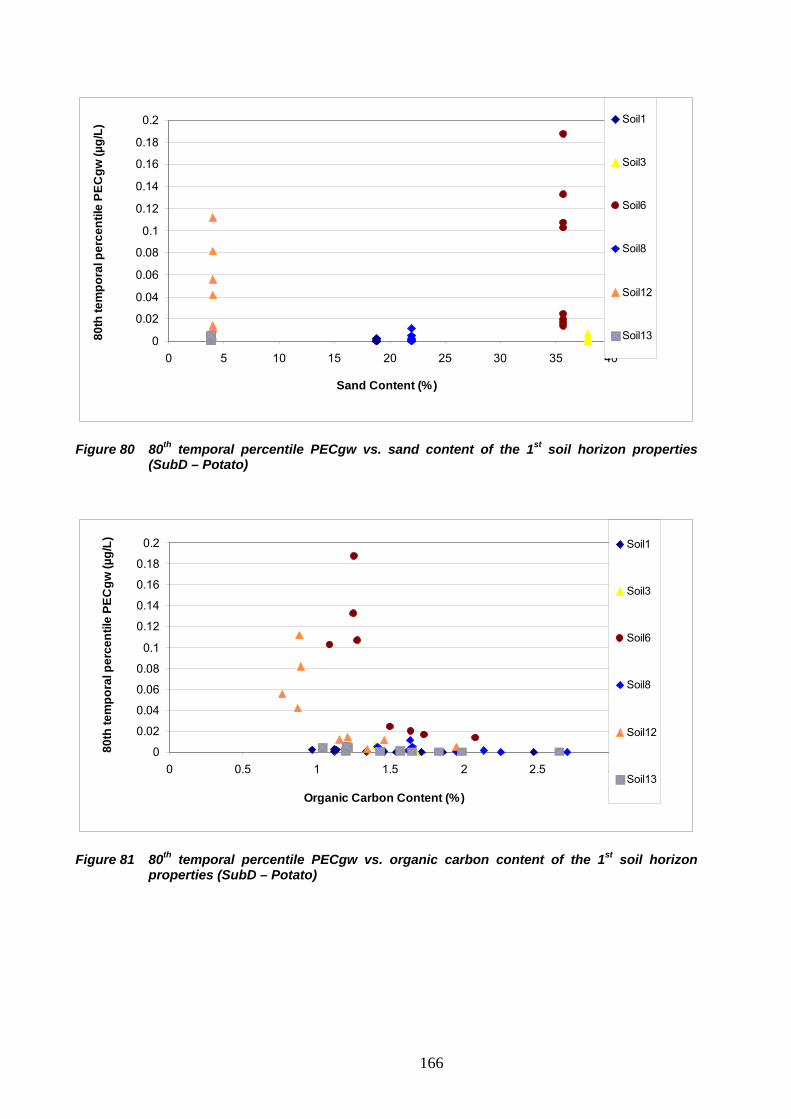
0
0.02
0.04
0.06
0.08
0.1
0.12
0.14
0.16
0.18
0.2
0 5 10 15 20 25 30 35 40
Sand Content (%)
80th
tem
pora
l per
cent
ile P
ECgw
(µg/
L)
Soil1
Soil3
Soil6
Soil8
Soil12
Soil13
Figure 80 80th temporal percentile PECgw vs. sand content of the 1st soil horizon properties (SubD – Potato)
0
0.02
0.04
0.06
0.08
0.1
0.12
0.14
0.16
0.18
0.2
0 0.5 1 1.5 2 2.5 3
Organic Carbon Content (%)
80th
tem
pora
l per
cent
ile P
ECgw
(µg/
L) Soil1
Soil3
Soil6
Soil8
Soil12
Soil13
Figure 81 80th temporal percentile PECgw vs. organic carbon content of the 1st soil horizon properties (SubD – Potato)
166

0
0.02
0.04
0.06
0.08
0.1
0.12
0.14
0.16
0.18
0.2
0 50 100 150 200 250
Available Water Capacity (mm)
80th
tem
pora
l per
cent
ile P
ECgw
(µg/
L) Soil1
Soil3
Soil6
Soil8
Soil12
Soil13
Figure 82 80th temporal percentile PECgw vs. the Available Water Content of the soil profile (SubD – Potato)
0
0.02
0.04
0.06
0.08
0.1
0.12
0.14
0.16
0.18
0.2
0 1 2 3 4 5 6 7 8 9 10111213141516171819
Soil ID
80th
tem
pora
l per
cent
ile P
ECgw
(µ
g/L)
0.0E+00
2.0E-03
4.0E-03
6.0E-03
8.0E-03
1.0E-02
1.2E-02
1.4E-02
Are
a w
eigh
ted
mea
n PE
C (µ
g/L)
Soil1
Soil2
Soil3
Soil6
Soil8
Soil12
Soil13
Area weightedmean PEC
Figure 83 80th temporal percentile PECgw vs. Soil ID (SubD – Potato)
167

0
0.02
0.04
0.06
0.08
0.1
0.12
0.14
0.16
0.18
0.2
0 1 2 3 4 5 6 7 8 910111213141516171819202122232425262728293031
AU ID
80th
tem
pora
l per
cent
ile P
ECgw
(µ
g/L)
0.0E+00
1.0E-03
2.0E-03
3.0E-03
4.0E-03
5.0E-03
6.0E-03
7.0E-03
Are
a w
eigh
ted
mea
n PE
C (µ
g/L)
Soil1
Soil3
Soil6
Soil8
Soil12
Soil13
Area weightedmean PEC
Figure 84 80th temporal percentile PECgw vs. AU ID (SubD – Potato)
10.4 Conclusions Test runs were conducted with two dummy substances (Substance C + Metabolite C and Substance D) to compare results with the standard FOCUS scenarios and evaluate potential mitigation measures proposals. The results of these reference runs are provided with the FROGS package. The five example presented in this chapter demonstrate that FROGS can provide useful information to determine the most critical parameters for a given substance and application scenario and to propose mitigation measures based on simple soil characteristics if the target protection goal is not met. Soils 19, 12, 9 and 6 appear to be the most vulnerable soils. Soil 19 and 9 are both characterized by a high sand content (83.8% for soil 19 and 64.9 % for soil 9) leading to the highest hydraulic conductivities (Ksat) of the 19 FROGS soils. Soil 12 is characterized by an organic carbon content below 1% in 19 AUs out of 31, and soil 6 is characterized by an available water content below 100mm. The results obtained also indicate that climate variation and different rotations (represented by the different AUs) are much less critical than the inherent soil properties as there was no clear relation seen between the AUID and the PECgw. However, these conclusions are based on a limited number of test runs and additional work is needed to investigate the overall sensitivity of the FROGS scenarios.
168

11 FROGS (v2.2.2.2) - Performances and Limitations The objective of this chapter is to give an overview of the performances and limitations of the FROGS (v2.2.2.2) system resulting from the choices made during the construction and parameterization of the national scenarios, from the choice of groundwater model associated to the scenarios, and from the FROGS tools themselves. The advantages and drawbacks inherent to the data collection and use decisions made in the different domains of interest for building the scenarios (soil, crops, weather), and advantages and drawbacks of the various modeling tools are explored. This review is also aiming at clarifying the tasks to undertake in priority to enhance the capabilities of the FROGS system. 11.1 Data collection and use The performances and limitations of the FROGS system are directly related to the availability and quality of information used to construct the scenarios, regarding land use, soils and weather. In addition, the temporal variability of this information needs to be addressed, in particular regarding how often the databases are updated and whether this would warrant an update of the scenarios themselves. 11.1.1 Land use The concept of agronomic unit (AU) refers to geographic areas considered as homogeneous with regard to soil occupation by agricultural activities and environmental conditions. It is similar to the concept of cropping basin except that it is defined in the strict context of groundwater risk assessment. The rationale used to build the agronomic units is two-fold since it uses statistics of land use by crops and information on environmental conditions, both domains being not independent one from the other. The zoning of agronomic units was achieved without a considerable investment in data acquisition, by making use and consolidating existing zoning information on various criteria (weather, environment, crops, etc.). AU zoning represents a simplification of reality with unavoidable information loss. What is lost in this process is the range of variation of crop and environmental characteristics which is already partly hidden in the zoning used in the AU construction. A set of 722 PRAs (PRA: “Petite Région Agricole”, “Small Agricultural Region”) forms the building blocks of this construction. PRAs are grouped into AUs using similarity criteria for land use and weather pattern. The number of PRAs is indicative of the diversity of agricultural and environmental conditions at county scale. PRA grouping according to environmental criteria is achieved using the Hydro-ecoregion zoning (Wason et al. 2002), which is based on robust geomorphology determinants. One assumes that this necessary simplification resulting from PRA aggregation can be overlooked compared to the differences which discriminate the AUs between themselves. In other words, the AU zoning is based on the assumption that the intra-AU variation is significantly lower than the inter-AU variation. The geographic contours of the agronomic units do not need to be accurate since what matters is the description of representative agricultural activities and environmental conditions. The delineation of the agronomic units could be improved in certain areas where uncertainties are remaining. However, such corrections are considered as minor and are not likely to induce significant changes in the overall system.
169

The agronomic units are effectively representative of typical situations, which are mostly the result of expert judgment rather than the output of data processing techniques. The range of conditions included in an agronomic unit made of a set of PRAs is difficult to apprehend and quantify since the PRA zoning itself results from expert judgment. As a result, one cannot be sure that the difference between two adjacent agronomic units is significantly greater than the range of variation within the AUs or within the PRAs that constitute these AUs. Better understanding and more accurate determination of the range of parameter variation within the AU should help in estimating to which degree the risk is covered when assessed using only a limited number or typical situations. It would also give hints on whether a refined assessment may be needed using more accurate information. Information on representative soil types is not directly part of the agronomic unit concept, although geological and pedogenesis homogeneity are inherent to the PRA and Hydro-ecoregion zoning and therefore to the AU zoning. Nevertheless, a large and systematic variation in the agronomic units comes from the soil description, i.e. AU are not supposed to be homogeneous regarding soil types. The soil selection process was handled separately by experts in the domain (INRA Infosol), and it is clear from the number of selected soil types allocated to each AU that soil heterogeneity is accounted for. While contrasted situations present within the AUs like plateaus and alluvial plains are not apparent anymore from the scenarios (there are no plateau or alluvial plains scenarios), such situations are still taken into account in the risk assessment through the corresponding soil types, provided they represent a significant cultivated surface in the AU. For example, there are 2 fluvisols among the 19 representative soil types, which would cover alluvial plains. Given the geographical nature of the AUs, the AU zoning as homogeneous entities is expected to remain stable in time, at least on the short-term and mid-term (decades). Environmental characteristics should remain fairly stable, unless significant climate changes occur, which could in turn affect land use (based on hydrology and temperature conditions changes). Cropping characteristics do evolve in time based on technological and economical trends, but this is unlikely to affect the AU zoning at any significant extent in the short to mid-term. Indeed, the PRA zoning dates from 1946, and following some initial administrative modifications, has not changed since 1987. Similarly, the hydro-ecoregion zoning is considered as a stable zoning based on homogeneous and stable geological, relief and climatic parameters. The need for updating of the scenarios following updates of the databases, including the upcoming 2010 agricultural census (Recensement Général Agricole, 2010) will be examined on case-by-case basis in future versions of FROGS. The 2010 agricultural census (2010) may for example be used to check whether there have been significant changes in the land use by the different crop categories, which may impact the proportion of surfaces taken into account in the AUs or excluded. Provided that more accurate descriptive information becomes available within the agronomic units, one could also reasonably verify that the intra-AU variation is smaller than the inter-AU variation for some parameters such as land use.
170
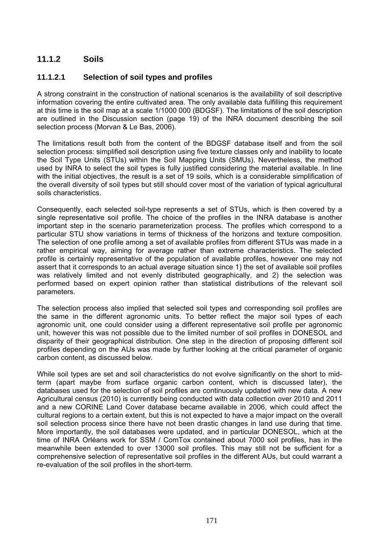
11.1.2 Soils 11.1.2.1 Selection of soil types and profiles A strong constraint in the construction of national scenarios is the availability of soil descriptive information covering the entire cultivated area. The only available data fulfilling this requirement at this time is the soil map at a scale 1/1000 000 (BDGSF). The limitations of the soil description are outlined in the Discussion section (page 19) of the INRA document describing the soil selection process (Morvan & Le Bas, 2006). The limitations result both from the content of the BDGSF database itself and from the soil selection process: simplified soil description using five texture classes only and inability to locate the Soil Type Units (STUs) within the Soil Mapping Units (SMUs). Nevertheless, the method used by INRA to select the soil types is fully justified considering the material available. In line with the initial objectives, the result is a set of 19 soils, which is a considerable simplification of the overall diversity of soil types but still should cover most of the variation of typical agricultural soils characteristics. Consequently, each selected soil-type represents a set of STUs, which is then covered by a single representative soil profile. The choice of the profiles in the INRA database is another important step in the scenario parameterization process. The profiles which correspond to a particular STU show variations in terms of thickness of the horizons and texture composition. The selection of one profile among a set of available profiles from different STUs was made in a rather empirical way, aiming for average rather than extreme characteristics. The selected profile is certainly representative of the population of available profiles, however one may not assert that it corresponds to an actual average situation since 1) the set of available soil profiles was relatively limited and not evenly distributed geographically, and 2) the selection was performed based on expert opinion rather than statistical distributions of the relevant soil parameters. The selection process also implied that selected soil types and corresponding soil profiles are the same in the different agronomic units. To better reflect the major soil types of each agronomic unit, one could consider using a different representative soil profile per agronomic unit, however this was not possible due to the limited number of soil profiles in DONESOL and disparity of their geographical distribution. One step in the direction of proposing different soil profiles depending on the AUs was made by further looking at the critical parameter of organic carbon content, as discussed below. While soil types are set and soil characteristics do not evolve significantly on the short to mid-term (apart maybe from surface organic carbon content, which is discussed later), the databases used for the selection of soil profiles are continuously updated with new data. A new Agricultural census (2010) is currently being conducted with data collection over 2010 and 2011 and a new CORINE Land Cover database became available in 2006, which could affect the cultural regions to a certain extent, but this is not expected to have a major impact on the overall soil selection process since there have not been drastic changes in land use during that time. More importantly, the soil databases were updated, and in particular DONESOL, which at the time of INRA Orléans work for SSM / ComTox contained about 7000 soil profiles, has in the meanwhile been extended to over 13000 soil profiles. This may still not be sufficient for a comprehensive selection of representative soil profiles in the different AUs, but could warrant a re-evaluation of the soil profiles in the short-term.
171
11.1.2.2 Location of soils in the agronomic units The location of the soils within the agronomic units is not known. The surface of the soils in the agronomic units was estimated by INRA. As stated above, the location of the STUs within the SMUs is not possible. In addition, since each selected soil represents a number of STUs, sometimes large, the delineation of the contours would be in any case misleading. This is also true for more accurate soil maps, which most often describe associations of soils, not single soils. A direct implication of the fact that the selected soil types cannot be located is that no direct link can be established between STUs and land use. Nevertheless, the method of selection minimized the selection of soils which are not significantly cultivated, thanks to the use of agricultural statistics (Agriculture census 2000) and soil occupation (CORINE Land Cover 2000), so it is clear that selected soil are representative of cultivated land. Another direct implication of the impossibility to locate the soil types within the AUs is that it makes the link with aquifers rather difficult. Consequently, the link with aquifers (regarding presence and type) is not covered in FROGS, but may be considered in a higher-tier refinement if necessary. 11.1.2.3 Soil organic carbon As already mentioned and as noted by INRA (Morvan & Le Bas, 2006), the geographic distribution of the available soil profiles corresponding to the selected soil types is not homogeneous. A high number of these profiles are located in the Centre region where the organic carbon content (OC) is depleted by intensive farming practices, the decline of the OC content being mostly the result of tilling practices (deep ploughing). Consequently, the OC content of the selected soil profiles is relatively low compared to the real situation in agronomic units located outside the area of depleted OC. For realism purposes, there was a clear need for correction of the OC content of the top soil layer, especially considering the importance of this factor in the retention and mobility of pesticide substances. The procedure for adjustment of the OC content of the top soil layer is described in details in Chapter 8.1 of this document. A correction factor is calculated for each agronomic unit and applied to all soils in the unit, so that the global OC concentration at this scale matches the average OC content determined using data of soil analysis in the same geographic zone (BDAT). The correction is based on actual measurements of characteristics of cultivated soils, independent from the database used to select the soils. Although this correction might appear artificial, it is justified thanks to the realism of the BDAT data and the rationale of the procedure. Among various possible methods, the corrections use OC median values to minimize the influence of extreme data. The data are weighted by surface, in order to best estimate average values as characteristics of typical situations. The OC correction is achieved at the scale of individual agronomic units using a specific correction factor per unit. The correction is the same for each soil in the unit since a specific correction factor could not be estimated for each soil individually. After OC correction, soils are defined specifically for each agronomic unit, even though the soils of the same type differ only on the OC adjusted content. Considering this new set of soils, it would have been more logical to select profiles of the different soil types specifically within each agronomic unit, in order to avoid smoothing of the variation of characteristics between the agronomic units and the need for OC correction. Once again, this was not possible at the time since the availability of soil profiles for each agronomic unit is the limiting step of the method.
172

The OC correction was conducted using the latest available data, from the 2000-2004 period. Surface organic carbon content is known to evolve with time, as it is very much affected by the farming practices, as discussed above regarding the Orléans region, but the 2000-2004 data are considered adequate as OC evolvement is still a relatively slow process. Unless the whole soil selection process is revisited in the short-term, it is recommended that the OC correction should be checked once newer data become available. 11.1.2.4 Soil types and crops The proportion of the total surface covered by each of the 8 crops is known for the 19 soils at national level. However, the surface of crop cultivated on each soil in the agronomic units may currently only be estimated under the simplified assumption that this proportion is the same for each unit. Consequently, in the current version of the tool, the relationship between crops and soil type was only considered as an exclusion criteria, to eliminate unrealistic crop-soil combinations. In a future version of the tool, it is planned to also consider the crop - soil type relationship at AU level in order to refine the surface associated to each scenario. The relationship between crops and soils might originate from specific physiology requirements. For instance, water supply is a key factor in sugar beet cultivation so that the crop is excluded from areas where the water holding capacity of soil is not sufficiently high, except if irrigated. Furthermore, stony soils are not suitable for all crops for quality purposes. Concurrently, the presence of certain crops is more likely on soils responding to specific characteristics. The typical rotation oilseed rape – winter wheat – barley is frequently found on soils which suffer from summer drought, the crops being harvested at the time the soil water storage is totally depleted. Local soil – crop relationships are known by agronomists but are not taken into account in the system. Hence, particular combinations of soils and crops could be not representative for particular AUs. Hence caution should be exercised when such combinations appear that would in addition represent conditions conducive to leaching. Cropping characteristics do evolve in time based on technological (e.g. oilseed rape for biofuel) and economical (market pricing) trends. This is true at national level (overall surface associated to a given crop), but also at local or AU level, with some crops becoming more or less predominant regionally. The overall proportion of surface covered by the crops was obtained based the 2000 CORINE Land Cover database, which has since been updated with the 2006 CLC, but the 2000 data were deemed more relevant for use in association with the 2000 census. Changes in cropping characteristics compared to the 2000 data will have to be monitored once the 2010 census data and next CLC data become available, and in case major differences in surfaces are observed, these may be implemented in the FROGS database. 11.1.3 Weather Meteorological data in FROGS are taken from the MARS database, which is widely accepted in the European scientific and regulatory community. The selection of a representative tile for each AU was performed based on agricultural occupation as primary selection criteria, meaning that the tile representing the most agricultural surface in the AU was selected. Additional criteria such as variability of climatic conditions within the AUs and proximity to mountains or sea were also considered. Keeping in mind that one of the underlying principles of the scenario construction process was to cover a variety of normal, realistic conditions rather than worst-case situations and given the limiting step of the soil selection, which prevented true GIS scenarios, the selection of a single MARS tile per AU is justified and the variability of weather situations considered with the 31 different weather tiles corresponding to the 31 AUs is deemed sufficient for the level of detail considered in FROGS. In case preferential flow is included in a future FROGS version the current implementation of the meteo data may need to be reevaluated. The system is also flexible enough that additional MARS tiles may be taken into account if refined
173

modeling is required in a higher-tier to further evaluate particular vulnerable conditions highlighted with the FROGS v2.2.2.2 scenarios. The scenarios cover a 26-year period of meteorological data, from January 1, 1981 to December 31, 2006, with the first 6 years for the warm-up of the model regarding soil hydrology, and pesticide applications over the next 20 years (or 40 or 60 for 2- or 3-year rotations, with the same 20 years of data repeated). This time period is sufficiently recent and long to be considered representative and include a wide variety of conditions. Unless major climate changes are documented, it is not deemed necessary to update these data in the short to mid-term. Nevertheless, if changes are warranted and granted that newer data become available, these could be easily implemented in a further version of the FROGS tools. 11.1.4 Crops The FROGS (v2.2.2.2) system was originally developed for 8 major arable crops in France. It is the intention of the work group to extend the scope of crops considered within FROGS in a next version of the tools, the primary focus being put on the major perennial crops, vineyards and orchards. The extension to other minor arable crops could also be contemplated on a longer term. Thanks to a versatile design, new arable crops can be easily included by documenting the relevant tables of the Access® FROGS.mdb database. The system architecture makes the inclusion of perennial crops also possible. Once again, the difficulties are on the side of scenario construction: data collection, definition of typical situations and corresponding parameterization. The method used for the 8 first crops as described in this document is applicable to other crops, providing sufficient information is available. However, the development of scenarios for perennial crops, vineyards and orchards, is likely to call for specific information, particularly soils, considering the particular environmental conditions of vines and tree cultivation. It is not clear whether the soil selection method used for arable crops is applicable to perennial crops. With the possibility to define rotations with one or several target crops, product use can be evaluated in very realistic conditions. The crop rotations at AU level were selected based on local expert knowledge and backed up by probabilistic calculations based on AGRESTE information. These are therefore considered realistic enough even though some variability within the AUs may be lost. Although a particular effort was devoted to the collection of crop data at the scale of AUs, comprehensive information could not be achieved for all AUs. Hence, FOCUS information was used in the parameterization of crop parameters for a number of crop – AU combinations. According to the AU considered, data from the Châteaudun or Piacenza FOCUS scenarios were used for crop dates (emergence, harvest dates in table 6: tblCropDates). Complementary information on crop dates may be accessible in the short term to replace these default FOCUS values. Modeling calls for a number of crop parameters which values are not accurately known unless by default (LAI, Crop factor, Rooting depth, Crop height in table 8: tblCropPar). Unfortunately, specific information for these parameters is scarce and could not be adequately customized as a function of AUs and soils. Quality improvement of these crop parameters is strongly dependent on information availability. Some local changes in rotation trends with time may occur depending on socio-economic considerations (e.g. increase of acreage of industrial crops for biofuel). Such changes may over time result in different typical rotations than selected in FROGS v2.2.2.2 on the basis of local expert knowledge and 2001 AGRESTE data. It is therefore recommended that the selected rotations be checked again in the mid-term against updated AGRESTE information. If changes are warranted, these could easily be implemented in a further version of the FROGS tools.
174

11.2 Modeling tools The FROGS tools were designed in a way that all available options of the selected leaching model may be used, that all parameters specific to the FROGS scenarios may be accessible to the user through the Access® FROGS.mdb database, and that additional scenarios may be implemented within the tool. The FROGS tools are therefore flexible and versatile, and the scenario parameterization fully transparent. In terms of modeling capabilities, the technical performances and limitations of the FROGS system are for the most part directly linked to performances and limitations of the leaching model to which it is associated. 11.2.1 Choice of associated leaching model The selection of representative weather, soil, crops and crop rotations for the FROGS scenarios is not model-specific. The limiting step in the current scenarios is the description and parameterization of the soil hydrological processes. Description of the soil hydrology processes is also one of the major points of distinction between leaching models, e.g. preferential flow vs. chromatographic flow, tipping-bucket vs. Richard’s equation. Based on the available soil data, the FROGS scenarios could be implemented in any chromatographic-type leaching model. The current parameterization in the V1.0 version of FROGS was performed for the Richard’s based model PEARL, including the relevant Mualem-van Genuchten parameters, but parameters for tipping-bucket models (PRZM / PELMO) may be relatively easily determined. In this first version of the FROGS system, no parameters were determined for preferential flow, and it is not clear if sufficient information would be available from the DONESOL database to determine such parameters. Pedotransfer functions could potentially be used to estimate some or all of the preferential flow parameters required for macroporous flow models such as MACRO or the upcoming version of PEARL, but these should first be tested and validated on representative French soils to make sure they are applicable before including in FROGS. The current version of the PEARL model as used in FOCUS, FOCUS_PEARL_3.3.3, includes a fully flexible pesticide metabolization scheme working for any number of metabolites and any route, and options such as pH-dependent sorption or aged sorption. All these features of the PEARL model are also fully operational in the FROGS system. Any new options or changes implemented in a new future version of PEARL may first require testing and implementation in a future version of FROGS, especially if new parameters are required. The use of the PEARL model also means that some limitations of this model also apply to FROGS:
- The use of a crop calendar and agricultural year concept in PEARL implies that some of the emergence and/or harvest dates in the FROGS crop rotation scenarios had to be adapted as described in Chapter 3.4.
- Due to collapsing of the hydrology module in PEARL, SWAP in the case of extraordinary large rainfall events combined with soil characterized by low hydraulic conductivity, some adaptations had to be implemented in the FROGS weather and soil parameterization, as described in Chapters 5.4 and 8.5. Even with these adjustments, a few scenarios still fail as listed in Table 20.
- Due to a limit set in the SWAP code, the PEARL model is currently restricted to a maximum of 70 years of simulation for a single run. This means that 4-year rotations, which would result in an 86-year simulation, could not be implemented in FROGS although these would be the most representative rotation for some limited crop – AU combinations, as listed in Table 7.
175
11.2.2 Specificities of the FROGS tools While in the standard FOCUS scenarios the selected output is the average predicted concentration in leaching water at a reference depth of 1 meter, the output in the FROGS scenarios is the concentration in the leaching water at the bottom of the soil profile, which range from 40 to 140 cm depending on the soil. In both cases, these output concentrations at target depths should only be viewed as indicator of the exposure to ground water and are not to be confused with actual concentrations in the saturated zone or groundwater table. One feature of the FROGS interface that is in addition to the standard FOCUS parameterization is the scheduling of pesticide applications relative to the crop development. This feature allows to describe the pesticide application scenario in full accordance with the BBCH growth stages as specified in the GAP, and to take into account spatial (from 1 AU to the other) and temporal (from 1 year to the other) variations in function of the meteorological conditions, where the application would be performed every year at the same time in FOCUS. FROGS offers limited post-processing of the output concentrations, such as a graphical depiction of the surface aerial distribution of the 80th percentile average concentration at the bottom of the profiles. Any further post-processing, e.g. output concentration in function of specific critical scenario parameters (surface OC content, pH, available water content, rainfall, temperature, etc.) would need in this first version of the tools to be performed outside of the FROGS interface, for example exporting the summary output file to Excel or other data processing / graphical software. 11.3 Perspectives The construction of national scenarios was moved by a constant concern for realism in the description of the agronomic, soil and climate situations. Consequently, evaluations can be made in conditions reflecting faithfully the product use pattern. Simulations using these scenarios provide a distribution of the PECgw which cover a diversity of typical situations in the cultivated area. These results, weighted by surface, represent an estimate of the degree of safety of a product use. Considering the characteristics of certain soils, and in case of products exhibiting a significant potential for movement in soil, combinations with weather conditions are probably conducive to PECgw values higher than 0.1 µg/L. Expressing and interpreting the distribution of the PECgw as a function of factors of influence on leaching, such as organic carbon content of the top soil layer, water holding capacity of the profile, etc. also gives the possibility to define workable risk mitigation measures. The efficacy of these measures can also be evaluated with the system. Sensitivity and uncertainty analyses of leaching model and scenarios may prove useful in order to determine which scenario parameters have the most impact on the calculated PECgw and should therefore be refined in priority. Dubus & Brown (2002) and Dubus et al. (2003) performed sensitivity analyses of the four pesticide leaching models originally used in FOCUS, including PESTLA, a precursor of the model PEARL, and performed a first-step uncertainty analysis for the model MACRO. These studies showed that water flow as predicted by the models were mostly affected by meteorlogical variables, while pesticide losses were most sensitive to pesticide input parameters related to sorption and degradation, and in some cases could also be very largely affected by the soil hydrological properties. These conclusions should likely also apply to PEARL. Sensitivity and uncertainty analyses specific to FROGS were not performed, as these evaluations were beyond the scope of the working group. Care was taken to reduce uncertainty regarding critical parameters, such as the soil organic carbon content, or sensitive areas, such as application timing, by use of refined data and models. However, there
176

177
are many model parameters of which impact on calculated PECgw is not yet explored. Therefore the workgroup welcomes scientific initiatives to quantifiy sensitivity and uncertainty associated with the generic approaches used in modelling systems like FROGS. Some of the above-mentioned limitations of the FROGS v2.2.2.2 system can reasonably be overcome thanks to an improved parameterization based on descriptive information of better quality in the domains of interest for scenarios. Many weaknesses result mainly from the soil part which already needed to be fixed (OC content). About five years after the start of the national scenarios project, information of better quality has become available, which offers serious perspectives to overcome some of the present limitations regarding soil selection and enhance the system performances. These can be foreseen in the context of a future version of the system. 11.4 References Wasson J.G., Chandesris A., Pella H., Blanc. (2002). Les hydro-écorégions de France métropolitaine. Approche régionale de la typologie des eaux courantes et éléments pour la définition des peuplements de référence d’invertébrés. Programme de recherche HYDRECO (LHQ), Contrat n° 2001 06 9 084 U. Cemagref. Morvan X., Le Bas C. (2006) Détermination de profils types de sols par regions de culture. INRA Infosol, Orléans. Base de Données Analyse des Terres (BDAT) : INRA Unité Infosol, Orléans. http://www.gissol.fr/programme/bdat/bdat.php CORINE Land Cover (CLC) database: http://www.ifen.fr/bases-de-donnees/occupation-des-sols-corine-land-cover.html http://www.eea.europa.eu/themes/landuse DONESOL database : INRA Unité Infosol, Orléans. http://www.gissol.fr/outil/donesol/donesol.php Dubus I., Brown C. and Beulke S. (2003). Sensitivity analyses for four pesticide leaching models. Pest Manag Sci 59:962-982.
Dubus I. & Brown C. (2002). Sensitivity and first-step uncertainty analyses for the preferential flow model MACRO. J. Environ. Qual. 31 :227-240.

Appendix 1 : Number of scenarios per crop, AU and soil profile
178

Table 58 : Number of scenarios per Agronomic Unit
Agronomic Unit Number of scenarios Alsace ‐ Sundgau 36Aquitaine ‐ Landes 22Ardenne ‐ Argonne ‐ Champagne H. 62Barrois ‐ Plateaux bourguignons 61Bas Dauphiné ‐ Vallée du Rhône 35Bassin de l'Adour 43Beauce ‐ Drouais ‐ Gâtinais 70Bocage normand 60Bocages de l'ouest 52Boischaut du sud 41Bordelais ‐ Périgord ‐ Coteaux du Lot 45Bordure Nord ‐ Picardie ‐ Normandie 60Bretagne centrale 32Bretagne nord 37Bretagne sud 36Champagne berrichonne ‐ Boischaut 49Champagne crayeuse 64Charentes 48Fossé bressan 58Gâtines ‐ Vallées de Loire 55Ile‐de‐France 69Limagnes ‐ Plaine du Forez 41Perche ‐ Pays d'Auge ‐ Pays d'Ouche 64Picardie ‐ Nord ‐ Pas‐de‐Calais 55Plaine du Languedoc‐Roussillon 12Plaine normande ‐ Bessin 69Plateau lorrain 50Plateaux de Haute‐Saône 44Provence 10Sologne ‐ Orléanais 49Collines molassiques ‐ Lauragais 52Grand Total 1481
179

Table 59 : Number of scenarios per Soil Type
Soil ID Number of scenarios 1 1622 1683 244 1235 1366 1027 48 1349 12410 1511 8312 9913 11014 6815 8116 617 1019 32Grand Total 1481
Table 60: Number of scenarios per Crop
Crop Number of scenarios Maize fodder 219Maize grain 290Oilseed rape 195Potato 49Sugar beet 83Sunflower 229Winter Barley 183Winter Wheat 233Grand Total 1481
180
Appendix 2 : Agro-climatic Regions
181
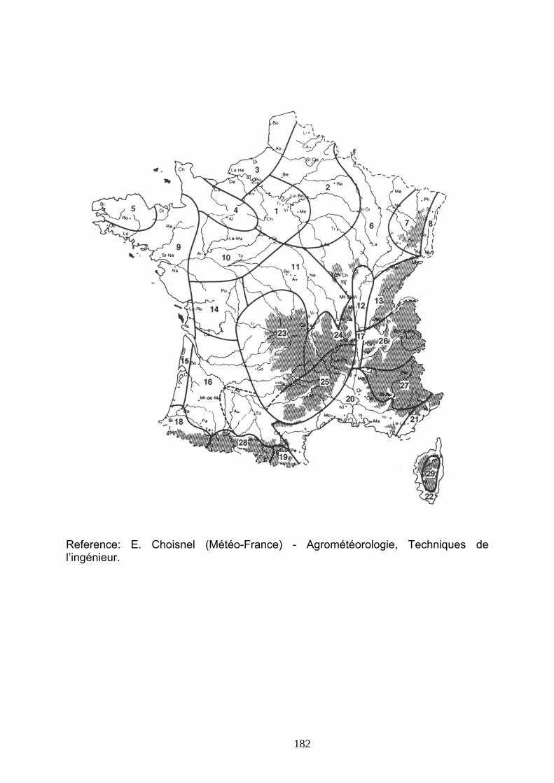
Reference: E. Choisnel (Météo-France) - Agrométéorologie, Techniques de l’ingénieur.
182

Appendix 3 : Map of annual Precipitation Classes agregated by PRA
183

184

185

186

Appendix 4 : List of Hydro-ecoregions of Levels 1 and 2
187
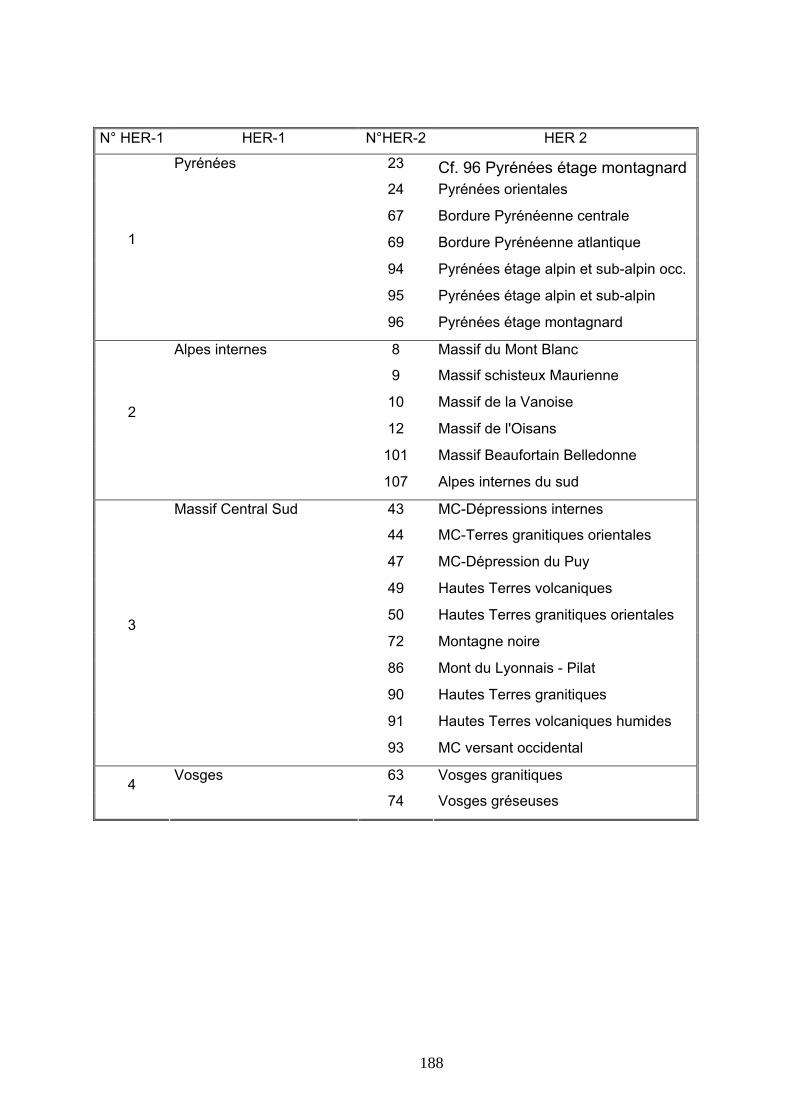
N° HER-1 HER-1 N°HER-2 HER 2
Pyrénées 23 Cf. 96 Pyrénées étage montagnard 24 Pyrénées orientales
67 Bordure Pyrénéenne centrale
69 Bordure Pyrénéenne atlantique 1
94 Pyrénées étage alpin et sub-alpin occ.
95 Pyrénées étage alpin et sub-alpin
96 Pyrénées étage montagnard
Alpes internes 8 Massif du Mont Blanc
9 Massif schisteux Maurienne
10 Massif de la Vanoise
12 Massif de l'Oisans 2
101 Massif Beaufortain Belledonne
107 Alpes internes du sud
Massif Central Sud 43 MC-Dépressions internes
44 MC-Terres granitiques orientales
47 MC-Dépression du Puy
49 Hautes Terres volcaniques
50 Hautes Terres granitiques orientales
72 Montagne noire 3
86 Mont du Lyonnais - Pilat
90 Hautes Terres granitiques
91 Hautes Terres volcaniques humides
93 MC versant occidental
Vosges 63 Vosges granitiques 4 74 Vosges gréseuses
188
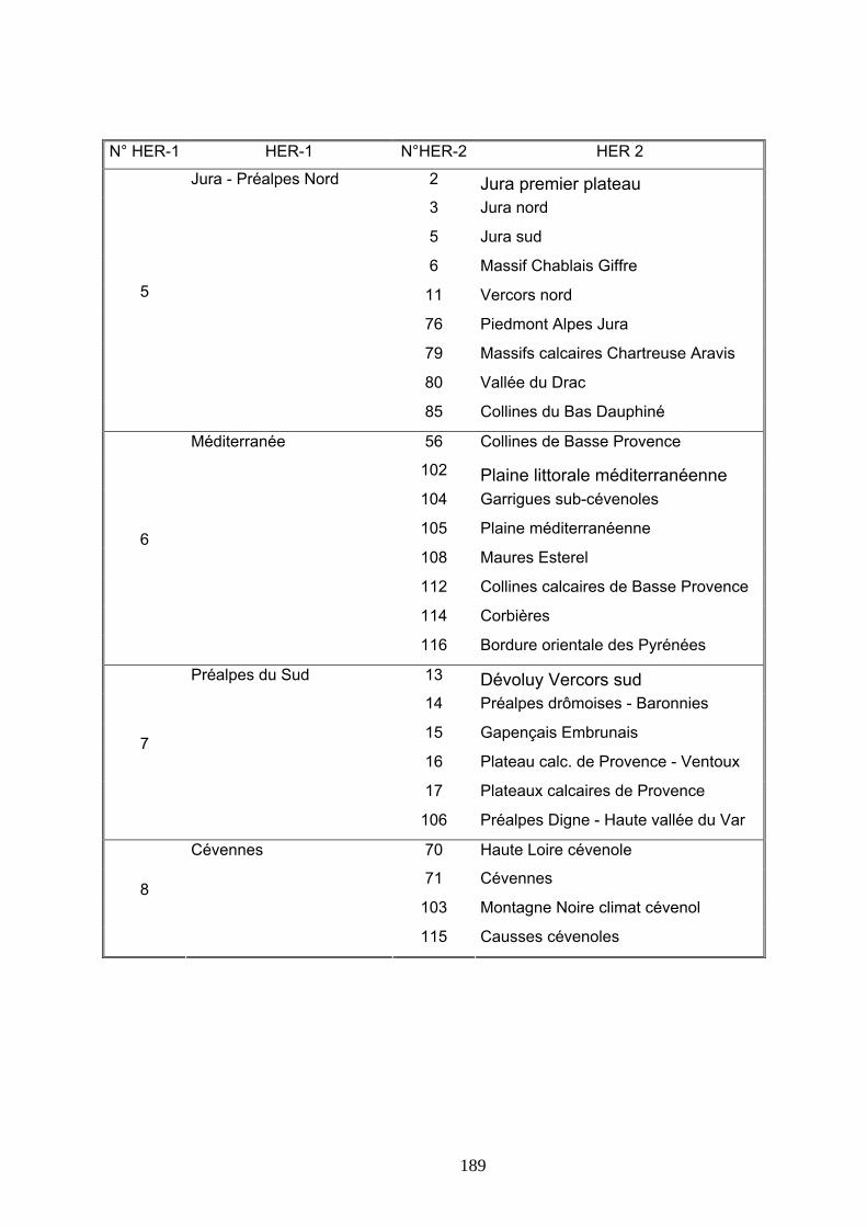
N° HER-1 HER-1 N°HER-2 HER 2
Jura - Préalpes Nord 2 Jura premier plateau 3 Jura nord
5 Jura sud
6 Massif Chablais Giffre
11 Vercors nord 5
76 Piedmont Alpes Jura
79 Massifs calcaires Chartreuse Aravis
80 Vallée du Drac
85 Collines du Bas Dauphiné
Méditerranée 56 Collines de Basse Provence
102 Plaine littorale méditerranéenne 104 Garrigues sub-cévenoles
105 Plaine méditerranéenne
108 Maures Esterel 6
112 Collines calcaires de Basse Provence
114 Corbières
116 Bordure orientale des Pyrénées
Préalpes du Sud 13 Dévoluy Vercors sud 14 Préalpes drômoises - Baronnies
15 Gapençais Embrunais
16 Plateau calc. de Provence - Ventoux 7
17 Plateaux calcaires de Provence
106 Préalpes Digne - Haute vallée du Var
Cévennes 70 Haute Loire cévenole
71 Cévennes
103 Montagne Noire climat cévenol 8
115 Causses cévenoles
189

N° HER-1 HER-1 N°HER-2 HER 2
Tables calcaires 30 Pays de Caen
32 Boulonnais
35 Pays de Bray
BP-lle de France 36 37 Cotentin est
38 TC-auréole crétacé 9
40 Champagne humide
41 Tables calcaires sud Loire
54 TC-nord Loire-Perche
57 TC-Haute Normandie Picardie
97 TC-Charentes Poitou
Côtes calcaires Est 1 Plateau calcaire Haute Saône
25 Plateau lorrain
26 Bassin de Forbach
27 Plaine de Woëvre
51 Bazois Auxois
53 BP-Côtes calcaires 10
75 Collines de Haute-Saône
82 Côtes de Macon
98 Collines sous-Vosgiennes
99 Côtes de Bourgogne
Causses calcaires 64 Collines Calcaires de Dordogne 11 65 Causses du Quercy
Armoricain 55 MA-nord est
58 MA-sud intérieur
59 MA-ouest 12
60 MA-est intérieur
13 Landes 21 Landes
190

N° HER-1 HER-1 N°HER-2 HER 2
Coteaux aquitains 66 Coteaux molassiques nord Aquitaine
68 Coteaux molassiques est Aquitaine
77 Coteaux molassiques bassin Adour 14
78 Coteaux molassiques centre
Plaine Saône 4 Forêt de Chaux
7 Dombes
81 Plaine de Bourgogne 15
84 Bresse
Corse 22 Corse 16 88 Corse plaine d'Aléria
Dépressions sédimentaires 45 Plaine du Forez
46 Limagne de l'Allier 17
52 Fossés tectoniques
Alsace 61 Alsace - collines
62 Alsace - plaine 18
73 Collines du Sundgau
19 Grands Causses 113 Grands Causses
Dépôts argilo-sableux 28 Sologne - Forêt d'Orléans
31 Flandres intérieure
33 Douai - Condé 20
39 Thiérache
42 Epandages éluviaux
Massif Central Nord 48 Montagne bourbonnaise
87 Morvan - Charollais
89 Hautes Terres limousines 21
92 MC Plateau limousin
22 Ardennes 34 Ardennes
191

Map of Hydro-ecoregions of Levels 1 et 2
192
Appendix 5 : List of PRA in the Agronomic Units
193

Agronomic Unit n°1: Collines molassiques - Lauragais N°
PRA N° UA PRA
1 147 Haut-Armagnac
1 149 Ténarèze
1 151 Gaillacois
1 152 Coteaux molassiques
1 153 Plaine de l'Albigeois et du Castrais
1 154 Bas-Quercy de Monclar
1 383 Astarac
1 384 Lomagne
1 385 Coteaux du Gers
1 389 Coteaux de Gascogne
1 390 Vallées et terrasses de la Garonne supérieure
1 391 Lauragais
1 392 Volvestre et Razès
1 395 Causses du Quercy
1 398 Coteaux néracois
Agronomic Unit n°2: Bretagne sud
N° PRA PRA N° UA
2 103 Zone légumière de la Pénéplaine Sud
2 363 Pénéplaine bretonne Sud
2 364 Littoral breton Sud
Agronomic Unit n°3: Limagnes - Plaine du Forez
N° PRA N° UA PRA
3 165 Périphérie des Dômes
3 175 Plaine de la Dore
3 176 Limagne viticole
3 177 Brivadois
3 180 Entre Loire et Allier
3 189 Plateau de Neulise
3 190 Plaine roannaise
3 191 Côte roannaise
3 193 Plaine du Forez
3 426 Limagne agricole
3 427 Limagne de Lembron et de Brioude
3 429 Sologne bourbonnaise
194
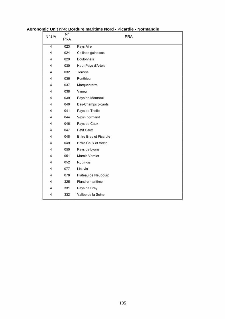
Agronomic Unit n°4: Bordure maritime Nord - Picardie - Normandie N°
PRA N° UA PRA
4 023 Pays Aire
4 024 Collines guinoises
4 029 Boulonnais
4 030 Haut-Pays d'Artois
4 032 Ternois
4 036 Ponthieu
4 037 Marquenterre
4 038 Vimeu
4 039 Pays de Montreuil
4 040 Bas-Champs picards
4 041 Pays de Thelle
4 044 Vexin normand
4 046 Pays de Caux
4 047 Petit Caux
4 048 Entre Bray et Picardie
4 049 Entre Caux et Vexin
4 050 Pays de Lyons
4 051 Marais Vernier
4 052 Roumois
4 077 Lieuvin
4 078 Plateau de Neubourg
4 325 Flandre maritime
4 331 Pays de Bray
4 332 Vallée de la Seine
195

Agronomic Unit n°5: Alsace - Sundgau N°
PRA N° UA PRA
5 001 Hardt
5 002 Ochsenfeld
5 301 Plaine du Rhin
5 302 Ried
5 303 Sundgau
5 304 Région sous-vosgienne
Agronomic Unit n°6: Plaine normande - Bessin
N° PRA N° UA PRA
6 085 Bessin
6 355 Plaine normande
Agronomic Unit n°7: Aquitaine - Landes
N° PRA N° UA PRA
7 130 Pays de Born
7 131 Marensin
7 132 Marenne
7 133 Marsan
7 134 Petites Landes de Roquefort
7 135 Petites Landes de Villandraut
7 137 Landes du Médoc
7 378 Grandes Landes
196

Agronomic Unit n°8: Bassin de l’Adour N°
PRA N° UA PRA
8 138 Côte basque
8 139 Coteaux du Pays basque
8 141 Coteaux entre les Gaves
8 143 Vallée de l'Adour
8 144 Seignanx
8 145 Pays de Gosse
8 148 Coteaux de Bigorre
8 150 Haute vallée de l'Adour
8 379 Vallée du Gave d'Oloron
8 380 Vallée du Gave de Pau
8 381 Coteaux du Béarn
8 382 Chalosse
8 386 Vic-Bilh
8 387 Tursan et Rivière basse
8 388 Bas-Armagnac
Agronomic Unit n°9: Picardie - Nord - Pas de Calais
N° PRA PRA N° UA
9 025 Flandre intérieure
9 026 Région de Lille
9 027 Pévèle
9 028 Plaine de la Scarpe
9 031 Béthunois
9 033 Hainaut
9 034 Saint-Quentinois et Laonnois
9 035 Santerre
9 042 Clermontois
9 043 Noyonnais
9 324 Plaine de la Lys
9 326 Artois-Cambrésis
9 327 Plateau picard
197

Agronomic Unit n°10: Charentes N°
PRA N° UA PRA
10 109 Plateau mellois
10 111 Marais de Rochefort et Marennes
10 113 Angoumois-Ruffecois
10 366 Entre plaine, Bocage et Gâtine
10 367 Plaine de la Mothe-Lezay
10 369 Marais poitevin desséché
10 370 Marais poitevin mouillé
10 371 Plaines vendéenne et niortaise
10 372 Terre rouge à châtaigniers
10 374 Aunis
10 375 Saintonge agricole
10 377 Saintonge viticole
10 438 Brandes et Brenne
Agronomic Unit n°11: Bocage normand
N° PRA N° UA PRA
11 081 La Hague
11 082 Bocage de Valognes
11 083 Val de Saire
11 084 Cotentin
11 086 Bocage de Coutances et Saint-Lô
11 087 Avranchin
11 093 Bocage sabolien
11 095 Région d'embouche de l'Erve
11 354 Bocage normand
11 357 Région de Fougères et de Mayenne
198

Agronomic Unit n°12: Barrois - Plateaux bourguignons N°
PRA N° UA PRA
12 010 Tonnerois
12 011 Vignoble du Barrois
12 186 Plateaux de Bourgogne
12 305 La Haye
12 308 Pays Haut-lorrain
12 311 Plateau langrois, montagne
12 313 Côtes de Meuse
12 314 Barrois
12 316 Woëvre
12 322 Vallées de l'Yonne à la Marne
Agronomic Unit n°13: Plateau lorrain
N° PRA N° UA PRA
13 003 Warndt
13 004 Vallée de la Moselle
13 306 Plateau lorrain Sud
13 310 Bassigny-Châtenois
13 473 Plateau lorrain Nord
199
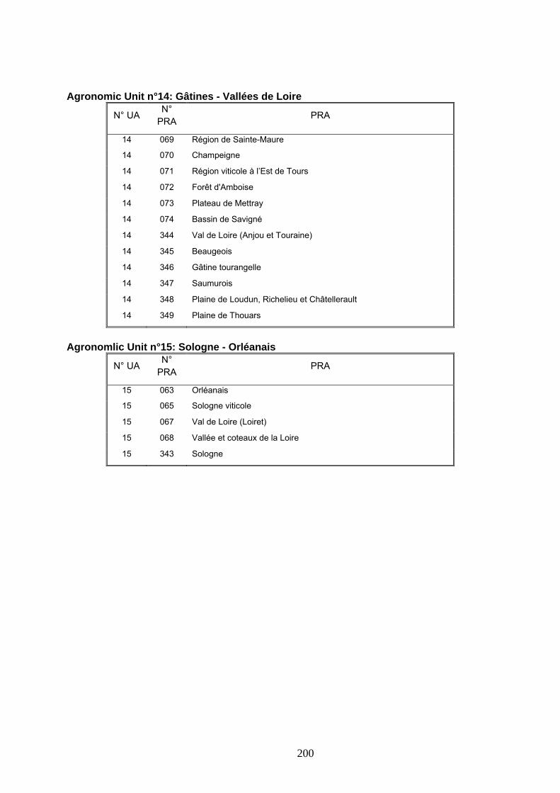
Agronomic Unit n°14: Gâtines - Vallées de Loire N°
PRA N° UA PRA
14 069 Région de Sainte-Maure
14 070 Champeigne
14 071 Région viticole à l’Est de Tours
14 072 Forêt d'Amboise
14 073 Plateau de Mettray
14 074 Bassin de Savigné
14 344 Val de Loire (Anjou et Touraine)
14 345 Beaugeois
14 346 Gâtine tourangelle
14 347 Saumurois
14 348 Plaine de Loudun, Richelieu et Châtellerault
14 349 Plaine de Thouars
Agronomlic Unit n°15: Sologne - Orléanais
N° PRA PRA N° UA
15 063 Orléanais
15 065 Sologne viticole
15 067 Val de Loire (Loiret)
15 068 Vallée et coteaux de la Loire
15 343 Sologne
200

Agronomic Unit n°16: Champagne crayeuse N°
PRA N° UA PRA
16 013 Vallée de la Champagne crayeuse
16 015 Plaine de Troyes
16 016 Vallée de la Marne
16 018 Pays rémois
16 019 Vallée du Nogentais
16 317 Champagne crayeuse
16 319 Pays d'Othe
16 320 Bassée et Basse-Yonne
Agronomic Unit n°17: Beauce - Drouais - Gâtinais
N° PRA N° UA PRA
17 064 Pays de Bière et forêt de Fontainebleau
17 079 Plateau d'Evreux Saint-André
17 334 Drouais
17 338 Gâtinais pauvre
17 339 Gâtinais riche
17 341 Beauce dunoise
17 342 Beauce
Agronomic Unit n°18: Bordelais - Périgord - Coteaux du Lot
N° PRA N° UA PRA
18 112 Montmorélien
18 114 Médoc
18 115 Bas-Médoc
18 116 Ilot de Polyculture de Civrac
18 117 Blayais
201
Agronomic Unit n°18: Bordelais - Périgord - Coteaux du Lot (continued) 18 118 Libournais
18 119 Vallée de l'Isle
18 120 Région de polyculture de Saint-Ciers
18 121 Entre-deux-Mers viticole
18 122 Ouest Entre-deux-Mers
18 123 Ilot de Polyculture de Baron
18 124 Benauge boisée
18 125 Benauge (polyculture)
18 126 Ceinture laitière et légumière de Bordeaux
18 127 Ilot de Polyculture de Pujols
18 128 Côtes du Bordelais
18 129 Graves
18 136 Petites Landes du Bazadais
18 155 Bas-Quercy de Montpezat
18 156 Coteaux nord du Lot-et-Garonne
18 157 Coteaux bordure Landes
18 158 Ribéracois
18 376 Saintonge boisée
18 396 Quercy blanc
18 399 Pays de Serres
18 400 Vallée de la Garonne
18 401 Bergeracois
18 402 Duras
18 403 Périgord blanc
18 404 Périgord noir
18 405 Double périgourdine
18 406 Landais
202
Agronomic Unit n°19: Perche - Pays d’Auge - Pays d’Ouche N°
PRA N° UA PRA
19 075 Perche Vendômois
19 076 Faux Perche
19 088 Merlerault
19 089 Vallée de la Sarthe et Région mancelle
19 090 Belinois
19 091 Plateau calaisien
19 092 Champagne mancelle
19 094 Saosnois
19 350 Vallée du Loir
19 351 Perche
19 352 Pays d'Ouche
19 353 Pays d'Auge
Agronomic Unit n°20: Bocages de l’ouest
N° PRA PRA N° UA
20 104 Pays de Châteaubriant
20 105 Plateaux boisés nantais
20 106 Estuaire de la Loire
20 107 Région urbaine et maraîchère de Nantes
20 108 Pays de Retz
20 110 Bocage de Chantonnay
20 356 Bocage angevin
20 365 Marais breton
20 368 Bas-Bocage et Gâtine
20 373 Haut-Bocage
203

Agronomic Unit n°21: Ardenne - Argonne - Champagne humide N°
PRA N° UA PRA
21 012 Vallage
21 014 Plaine de Brienne
21 020 Vallée de la Champagne humide
21 022 Crêtes pré-ardennaises
21 315 Argonne
21 318 Champagne humide
21 321 Perthois
21 323 Thiérache
Agronomic Unit n°22: Champagne berrichonne - Boischaut
N° PRA N° UA PRA
22 340 Puisaye
22 434 Champagne berrichonne
22 435 Boischaut du Nord
22 439 Sancerrois
22 066 Val de Loire (Cher)
22 179 Vallée de Germigny
22 185 Bourgogne nivernaise
22 188 Nivernais central
204

Agronomic Unit n°23: Bas Dauphiné - Vallée du Rhône N°
PRA N° UA PRA
23 196 Zone maraîchère de Lyon
23 199 Bas-Dauphiné
23 200 Zone fruitière et viticole du Lyonnais
23 217 Vallée du Grésivaudan
23 221 Région de Royans
23 240 Plaines rhodaniennes
23 241 Valloire
23 242 Gallaure et Herbasse
23 243 Pays de Bourdeaux
23 464 Tricastin
23 465 Vallée du Rhône
Agronomic Unit n°24: Fossé bressan
N° PRA N° UA PRA
24 195 Vallée de la Saône
24 197 Zone de grande culture entre Saône et Beaujolais
24 198 Dombes
24 201 Coteaux en bordure des Dombes
24 202 Bresse chalonnaise
24 203 Val d'Amour et forêt de Chaux
24 204 Val de Saône
24 205 Plaine grayloise
24 206 Finage
24 440 Plaine viticole de Bourgogne
24 444 Beaujolais viticole-Mâconnais
24 446 Bresse
205
Agronomic Unit n°25: Bretagne centrale N°
PRA N° UA PRA
25 101 Zone de Plougastel-Daoulas
25 102 Presqu’île de Crozon
25 360 Landes des Monts d'Arrée et du Méné
25 362 Landes de Châteaulin et Pontivy
Agronomic Unit n°26: Plateaux de Haute-Saône
N° PRA N° UA PRA
26 005 Région sous-vosgienne de Haute-Saône
26 006 Région vosgienne de Haute-Saône
26 007 Région des Plateaux
26 008 Plateau langrois-Apance
26 009 Plateau langrois-Amance
26 312 Vingeanne
26 447 Plaines et basses vallées de la Saône, du Doubs et de l'Ognon
26 448 Trouée de Belfort
Agronomic Unit n°27: Provence
N° PRA N° UA PRA
27 246 Crau
27 466 Val de Durance
27 467 Comtat
27 468 Coteaux de Provence
27 469 Littoral de Provence
206
Agronomic Unit n°28: Plaine du Languedoc-Roussillon N°
PRA N° UA PRA
28 252 Plaine du Roussillon
28 254 Crû Banyuls
28 415 Soubergues
28 416 Garrigues
28 471 Plaine viticole du Bas-Languedoc
Agronomic Unit n°29: Boischaut du sud
N° PRA N° UA PRA
29 178 Bocage bourbonnais
29 436 Boischaut du Sud
29 437 Bas-Berry
Agronomic Unit n°30: Bretagne nord
N° PRA N° UA PRA
30 096 Région de polyculture de Laval
30 097 Région centrale
30 098 Polders du Mont-Saint-Michel
30 099 Marais de Dol
30 100 Zone côtière de Brest
30 358 Littoral breton Nord
30 359 Bretagne centrale
30 361 Pénéplaine bretonne nord
207
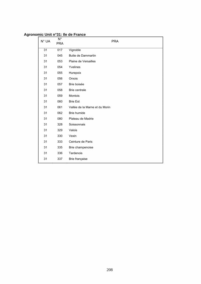
Agronomic Unit n°31: Ile de France N°
PRA N° UA PRA
31 017 Vignoble
31 045 Butte de Dammartin
31 053 Plaine de Versailles
31 054 Yvelines
31 055 Hurepoix
31 056 Orxois
31 057 Brie boisée
31 058 Brie centrale
31 059 Montois
31 060 Brie Est
31 061 Vallée de la Marne et du Morin
31 062 Brie humide
31 080 Plateau de Madrie
31 328 Soissonnais
31 329 Valois
31 330 Vexin
31 333 Ceinture de Paris
31 335 Brie champenoise
31 336 Tardenois
31 337 Brie française
208
Appendix 6 : List of Cantons in the Agronomic Units
209
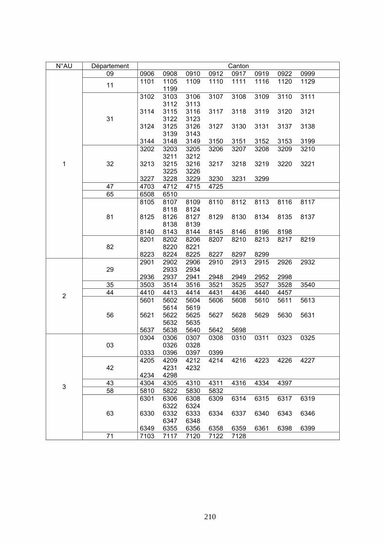
N°AU Département Canton 09 0906 0908 0910 0912 0917 0919 0922 0999
1101 1105 1109 1110 1111 1116 1120 1129 1199 11
3102 3103 3106 3107 3108 3109 3110 3111 3112 3113 3114 3115 3116 3117 3118 3119 3120 3121 3122 3123 3124 3125 3126 3127 3130 3131 3137 3138 3139 3143 3144 3148 3149 3150 3151 3152 3153 3199
31
3202 3203 3205 3206 3207 3208 3209 3210 3211 3212 3213 3215 3216 3217 3218 3219 3220 3221 3225 3226 3227 3228 3229 3230 3231 3299
32 1
47 4703 4712 4715 4725 65 6508 6510
8105 8107 8109 8110 8112 8113 8116 8117 8118 8124 8125 8126 8127 8129 8130 8134 8135 8137 8138 8139 8140 8143 8144 8145 8146 8196 8198
81
8201 8202 8206 8207 8210 8213 8217 8219 8220 8221 8223 8224 8225 8227 8297 8299
82
2901 2902 2906 2910 2913 2915 2926 2932 2933 2934 2936 2937 2941 2948 2949 2952 2998
29
35 3503 3514 3516 3521 3525 3527 3528 3540 44 4410 4413 4414 4431 4436 4440 4457 2
5601 5602 5604 5606 5608 5610 5611 5613 5614 5619 5621 5622 5625 5627 5628 5629 5630 5631 5632 5635 5637 5638 5640 5642 5698
56
0304 0306 0307 0308 0310 0311 0323 0325 0326 0328 0333 0396 0397 0399
03
4205 4209 4212 4214 4216 4223 4226 4227 4231 4232 4234 4298
42
43 4304 4305 4310 4311 4316 4334 4397 58 5810 5822 5830 5832 3
6301 6306 6308 6309 6314 6315 6317 6319 6322 6324 6330 6332 6333 6334 6337 6340 6343 6346 6347 6348 6349 6355 6356 6358 6359 6361 6398 6399
63
71 7103 7117 7120 7122 7128
210
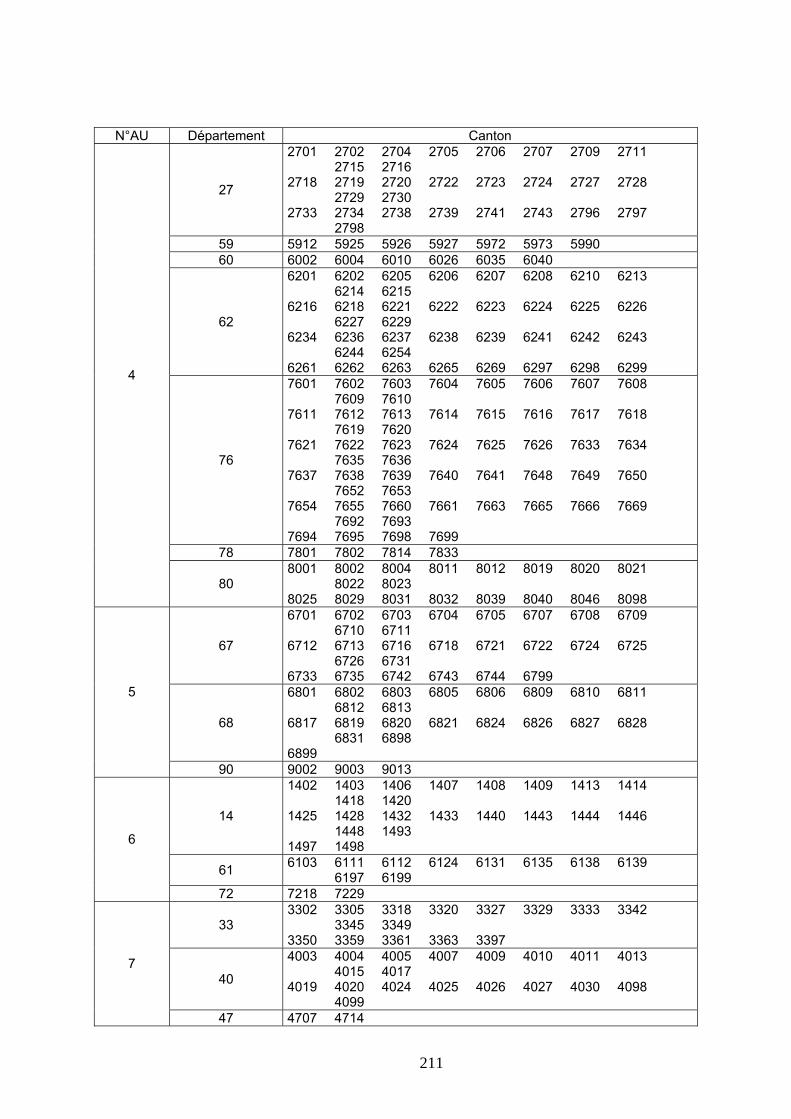
N°AU Département Canton 2701 2702 2704 2705 2706 2707 2709 2711 2715 2716 2718 2719 2720 2722 2723 2724 2727 2728 2729 2730 2733 2734 2738 2739 2741 2743 2796 2797 2798
27
59 5912 5925 5926 5927 5972 5973 5990 60 6002 6004 6010 6026 6035 6040
6201 6202 6205 6206 6207 6208 6210 6213 6214 6215 6216 6218 6221 6222 6223 6224 6225 6226 6227 6229 6234 6236 6237 6238 6239 6241 6242 6243 6244 6254 6261 6262 6263 6265 6269 6297 6298 6299
62
76
7601 7602 7603 7604 7605 7606 7607 7608 7609 7610 7611 7612 7613 7614 7615 7616 7617 7618 7619 7620 7621 7622 7623 7624 7625 7626 7633 7634 7635 7636 7637 7638 7639 7640 7641 7648 7649 7650 7652 7653 7654 7655 7660 7661 7663 7665 7666 7669 7692 7693 7694 7695 7698 7699
4
78 7801 7802 7814 7833 8001 8002 8004 8011 8012 8019 8020 8021 8022 8023 8025 8029 8031 8032 8039 8040 8046 8098
80
6701 6702 6703 6704 6705 6707 6708 6709 6710 6711 6712 6713 6716 6718 6721 6722 6724 6725 6726 6731 6733 6735 6742 6743 6744 6799
67
68
6801 6802 6803 6805 6806 6809 6810 6811 6812 6813 6817 6819 6820 6821 6824 6826 6827 6828 6831 6898 6899
5
90 9002 9003 9013 1402 1403 1406 1407 1408 1409 1413 1414 1418 1420 1425 1428 1432 1433 1440 1443 1444 1446 1448 1493 1497 1498
14
6
6103 6111 6112 6124 6131 6135 6138 6139 6197 6199 61
72 7218 7229 3302 3305 3318 3320 3327 3329 3333 3342 3345 3349 3350 3359 3361 3363 3397
33
4003 4004 4005 4007 4009 4010 4011 4013 4015 4017 4019 4020 4024 4025 4026 4027 4030 4098 4099
40 7
47 4707 4714
211

N°AU Département Canton 32 3201 3204 3214 3222 3223 3224
4001 4002 4006 4008 4012 4014 4016 4018 4021 4022 4023 4028 4029 4097
40
6403 6405 6407 6409 6410 6411 6412 6413 6414 6415 6417 6418 6419 6420 6421 6422 6423 6424 6425 6426 6427 6428 6429 6431 6432 6434 6436 6437 6438 6440 6441 6445 6446 6447 6448 6451 6452 6490 6491 6492 6495 6496 6497 6498 6499
64 8
6509 6514 6516 6517 6518 6521 6522 6523 6524 6525 6533 6534 6599
65
0203 0206 0209 0213 0216 0218 0219 0220 0225 0227 0229 0233 0237 0239 0240 0242 0297 0298
02
5901 5902 5905 5906 5907 5908 5909 5910 5911 5913 5914 5915 5916 5917 5918 5919 5920 5921 5922 5923 5924 5928 5929 5930 5931 5933 5938 5940 5942 5943 5944 5945 5946 5947 5948 5949 5950 5951 5954 5955 5956 5957 5958 5960 5961 5962 5963 5965 5966 5967 5968 5969 5970 5971 5974 5977 5978 5984 5985 5987 5988 5989 5991 5993 5994 5995 5996 5997 5998 5999
59
6006 6008 6009 6011 6013 6014 6015 6016 6017 6018 6019 6020 6021 6022 6024 6027 6028 6029 6031 6032 6033 6039 6041 6099
60 9
6203 6204 6209 6211 6212 6217 6219 6220 6228 6230 6231 6232 6233 6235 6240 6245 6246 6248 6249 6250 6251 6252 6253 6255 6256 6257 6259 6260 6264 6267 6268 6270 6271 6272 6273 6274 6275 6277 6288 6289 6290 6291 6292 6296
62
8003 8005 8006 8007 8008 8009 8010 8013 8014 8015 8016 8017 8018 8024 8026 8027 8028 8030 8033 8034 8035 8036 8037 8038 8041 8042 8044 8045 8099
80
212

N°AU Département Canton 1601 1605 1606 1607 1612 1613 1616 1617 1618 1622 1623 1624 1625 1627 1629 1630 1631 1633 1635 1697 1698
16
1701 1702 1703 1704 1705 1706 1707 1708 1709 1710 1711 1712 1713 1714 1715 1716 1717 1720 1721 1725 1726 1727 1728 1729 1730 1731 1732 1733 1734 1735 1736 1737 1738 1739 1740 1743 1744 1746 1749 1750 1751 1796 1797 1798 1799
17
10
36 3602 3619 7903 7905 7906 7908 7910 7911 7912 7913 7914 7916 7919 7920 7921 7923 7925 7926 7928 7998 7999
79
8502 8507 8509 8511 8512 8513 8517 8527 8528 85
8601 8602 8603 8604 8605 8606 8608 8613 8614 8617 8620 8624 8625 8626 8628 8629 8633 8634 8635 8636 8699
86
1401 1404 1411 1412 1416 1417 1430 1431 1436 1437 1438
14
35 3512 3513 3520 3535 3536 3597 5001 5002 5003 5004 5005 5006 5007 5008 5009 5010 5012 5013 5014 5015 5016 5017 5018 5019 5020 5021 5022 5023 5024 5025 5026 5027 5028 5029 5030 5031 5032 5033 5034 5035 5036 5037 5038 5039 5040 5041 5042 5043 5044 5045 5046 5047 5048 5050 5051 5052 5095 5097 5098 5099
50
11
5301 5303 5305 5308 5310 5311 5312 5313 5314 5315 5316 5320 5321 5322 5323 5324 5326 5327 5399
53
6102 6104 6107 6108 6110 6114 6115 6117 6122 6127 6129 6133 6140 6196
61
72 7212 7227 7230
213
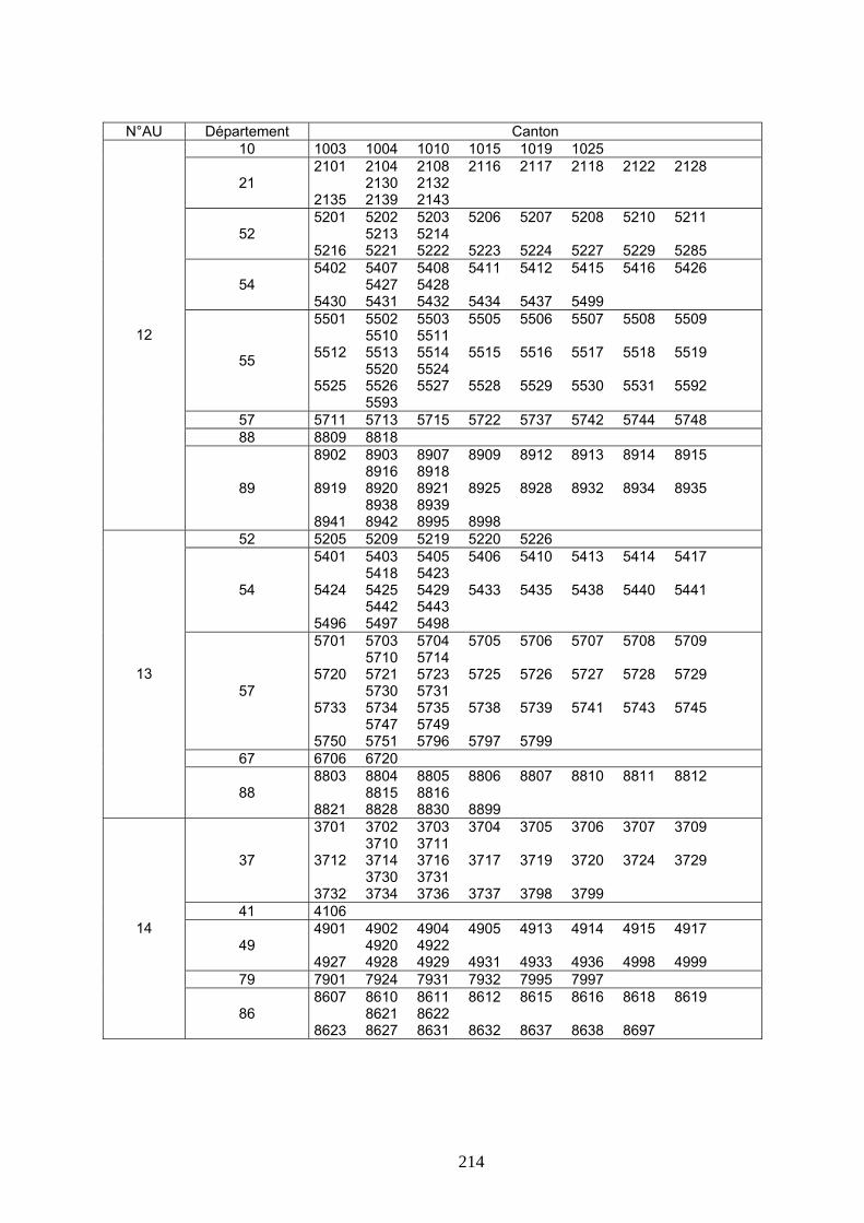
N°AU Département Canton
10 1003 1004 1010 1015 1019 1025 2101 2104 2108 2116 2117 2118 2122 2128 2130 2132 2135 2139 2143
21
5201 5202 5203 5206 5207 5208 5210 5211 5213 5214 5216 5221 5222 5223 5224 5227 5229 5285
52
5402 5407 5408 5411 5412 5415 5416 5426 5427 5428 5430 5431 5432 5434 5437 5499
54
5501 5502 5503 5505 5506 5507 5508 5509 5510 5511 5512 5513 5514 5515 5516 5517 5518 5519 5520 5524 5525 5526 5527 5528 5529 5530 5531 5592 5593
55
12
57 5711 5713 5715 5722 5737 5742 5744 5748 88 8809 8818
8902 8903 8907 8909 8912 8913 8914 8915 8916 8918 8919 8920 8921 8925 8928 8932 8934 8935 8938 8939 8941 8942 8995 8998
89
52 5205 5209 5219 5220 5226 5401 5403 5405 5406 5410 5413 5414 5417 5418 5423 5424 5425 5429 5433 5435 5438 5440 5441 5442 5443 5496 5497 5498
54
5701 5703 5704 5705 5706 5707 5708 5709 5710 5714 5720 5721 5723 5725 5726 5727 5728 5729 5730 5731 5733 5734 5735 5738 5739 5741 5743 5745 5747 5749 5750 5751 5796 5797 5799
57 13
67 6706 6720 8803 8804 8805 8806 8807 8810 8811 8812 8815 8816 8821 8828 8830 8899
88
3701 3702 3703 3704 3705 3706 3707 3709 3710 3711 3712 3714 3716 3717 3719 3720 3724 3729 3730 3731 3732 3734 3736 3737 3798 3799
37
41 4106
49 4901 4902 4904 4905 4913 4914 4915 4917 4920 4922 4927 4928 4929 4931 4933 4936 4998 4999
14
79 7901 7924 7931 7932 7995 7997 8607 8610 8611 8612 8615 8616 8618 8619 8621 8622 8623 8627 8631 8632 8637 8638 8697
86
214
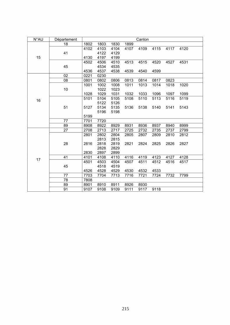
N°AU Département Canton 18 1802 1803 1830 1899
4102 4103 4104 4107 4109 4115 4117 4120 4122 4129 4130 4197 4199
41 15
4502 4506 4510 4513 4515 4520 4527 4531 4534 4535 4536 4537 4538 4539 4540 4599
45
02 0221 0230 08 0801 0802 0806 0813 0814 0817 0823
1001 1002 1008 1011 1013 1014 1018 1020 1022 1023 1028 1029 1031 1032 1033 1096 1097 1099
10
5101 5104 5105 5108 5110 5113 5116 5119 5122 5126 5127 5134 5135 5136 5138 5140 5141 5143 5196 5198 5199
51
16
77 7701 7720 89 8908 8922 8929 8931 8936 8937 8940 8999 27 2708 2713 2717 2725 2732 2735 2737 2799
2801 2802 2804 2805 2807 2809 2810 2812 2813 2815 2816 2818 2819 2821 2824 2825 2826 2827 2828 2829 2830 2897 2899
28
41 4101 4108 4110 4116 4119 4123 4127 4128
45 4501 4503 4504 4507 4511 4512 4516 4517 4518 4519 4526 4528 4529 4530 4532 4533
17
77 7703 7704 7713 7716 7721 7724 7732 7799 78 7808 89 8901 8910 8911 8926 8930 91 9107 9108 9109 9111 9117 9118
215
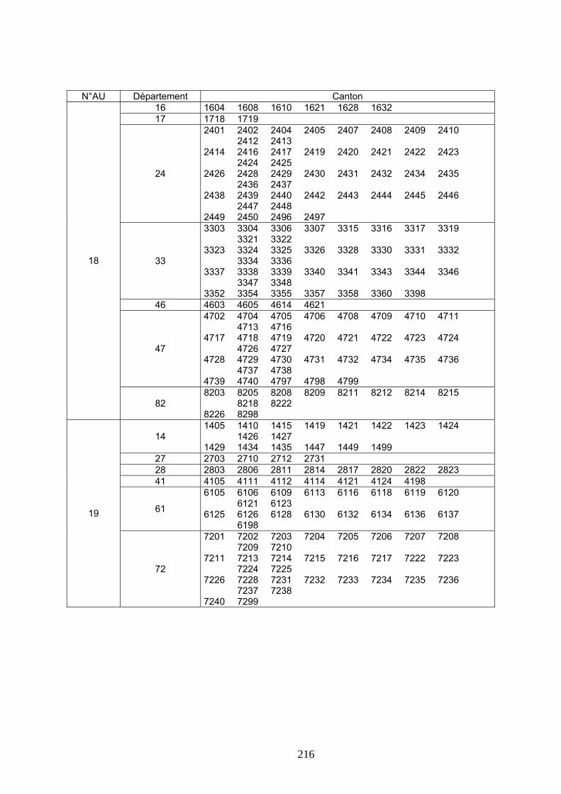
N°AU Département Canton 16 1604 1608 1610 1621 1628 1632 17 1718 1719
2401 2402 2404 2405 2407 2408 2409 2410 2412 2413 2414 2416 2417 2419 2420 2421 2422 2423 2424 2425 2426 2428 2429 2430 2431 2432 2434 2435 2436 2437 2438 2439 2440 2442 2443 2444 2445 2446 2447 2448 2449 2450 2496 2497
24
3303 3304 3306 3307 3315 3316 3317 3319 3321 3322 3323 3324 3325 3326 3328 3330 3331 3332 3334 3336 3337 3338 3339 3340 3341 3343 3344 3346 3347 3348 3352 3354 3355 3357 3358 3360 3398
33 18
46 4603 4605 4614 4621 4702 4704 4705 4706 4708 4709 4710 4711 4713 4716 4717 4718 4719 4720 4721 4722 4723 4724 4726 4727 4728 4729 4730 4731 4732 4734 4735 4736 4737 4738 4739 4740 4797 4798 4799
47
8203 8205 8208 8209 8211 8212 8214 8215 8218 8222 8226 8298
82
1405 1410 1415 1419 1421 1422 1423 1424 1426 1427 1429 1434 1435 1447 1449 1499
14
27 2703 2710 2712 2731 28 2803 2806 2811 2814 2817 2820 2822 2823 41 4105 4111 4112 4114 4121 4124 4198
6105 6106 6109 6113 6116 6118 6119 6120 6121 6123 6125 6126 6128 6130 6132 6134 6136 6137 6198
61 19
7201 7202 7203 7204 7205 7206 7207 7208 7209 7210 7211 7213 7214 7215 7216 7217 7222 7223 7224 7225 7226 7228 7231 7232 7233 7234 7235 7236 7237 7238 7240 7299
72
216

N°AU Département Canton 4401 4402 4403 4404 4405 4406 4407 4408 4409 4411 4412 4415 4416 4417 4418 4419 4427 4428 4429 4430 4432 4433 4434 4435 4437 4438 4441 4442 4443 4444 4445 4446 4447 4450 4451 4454 4459 4496 4497 4498 4499
44
4906 4907 4908 4909 4910 4911 4912 4916 4918 4919 4921 4923 4924 4925 4926 4930 4932 4934 4935 4938 4939 4940 4941 4997
49 20
53 5304 5306 5307 5309 5325 5331 5332 5397 7902 7904 7907 7909 7915 7917 7918 7922 7927 7929 7930
79
8501 8503 8504 8505 8506 8508 8510 8514 8515 8516 8518 8519 8520 8521 8522 8523 8524 8525 8526 8529 8530 8531 8598
85
86 8630 02 0202 0205 0217 0223 0226 0234
0803 0804 0807 0808 0809 0812 0815 0818 0819 0820 0821 0825 0828 0830 0831 0833 0898 0899
08
10 1005 1006 1007 1009 1012 1017 1021 51 5115 5123 5124 5128 5132 5133
21
52 5218 5228 5230 5231 5232 5286 55 5504 5521 5522 5523 59 5903 5904 5932 5959 5964 5986
1801 1804 1806 1807 1808 1810 1812 1813 1814 1815 1816 1817 1819 1820 1821 1823 1824 1825 1826 1828 1835 1898
18
3605 3606 3608 3610 3612 3613 3614 3615 3618 3621 3622 3623 3624 3625 3698 3699
36
37 3708 3713 3715 3718 41 4113 4118
22
45 4505 4508 4509 4514 5801 5802 5804 5805 5806 5807 5808 5809 5817 5818 5819 5820 5821 5823 5824 5825 5826 5827 5828 5829 5831 5898 5899
58
89 8906 8924 8927 8933
217
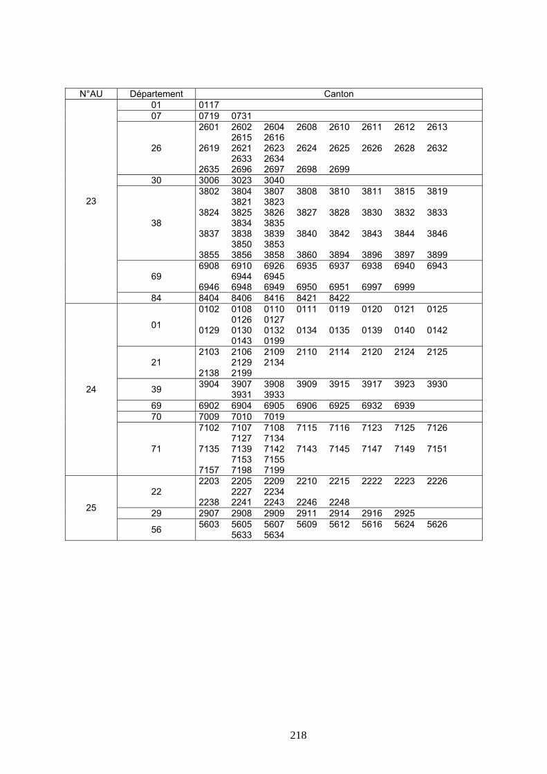
N°AU Département Canton 01 0117 07 0719 0731
2601 2602 2604 2608 2610 2611 2612 2613 2615 2616 2619 2621 2623 2624 2625 2626 2628 2632 2633 2634 2635 2696 2697 2698 2699
26
30 3006 3023 3040 3802 3804 3807 3808 3810 3811 3815 3819 3821 3823 3824 3825 3826 3827 3828 3830 3832 3833 3834 3835 3837 3838 3839 3840 3842 3843 3844 3846 3850 3853 3855 3856 3858 3860 3894 3896 3897 3899
38
23
6908 6910 6926 6935 6937 6938 6940 6943 6944 6945 6946 6948 6949 6950 6951 6997 6999
69
84 8404 8406 8416 8421 8422 0102 0108 0110 0111 0119 0120 0121 0125 0126 0127 0129 0130 0132 0134 0135 0139 0140 0142 0143 0199
01
2103 2106 2109 2110 2114 2120 2124 2125 2129 2134 2138 2199
21
3904 3907 3908 3909 3915 3917 3923 3930 3931 3933 39 24
69 6902 6904 6905 6906 6925 6932 6939 70 7009 7010 7019
7102 7107 7108 7115 7116 7123 7125 7126 7127 7134 7135 7139 7142 7143 7145 7147 7149 7151 7153 7155 7157 7198 7199
71
2203 2205 2209 2210 2215 2222 2223 2226 2227 2234 2238 2241 2243 2246 2248
22
29 2907 2908 2909 2911 2914 2916 2925 25
5603 5605 5607 5609 5612 5616 5624 5626 5633 5634 56
218

N°AU Département Canton 21 2113
2502 2503 2504 2507 2510 2513 2514 2518 2522 2523 2528 2530 2531 2534 2535 2595 2599
25
39 3912 3913 3914 3918 3924 3996 52 5204 5212 5215 5217
7001 7002 7003 7004 7005 7006 7008 7011 7012 7013 7014 7015 7016 7017 7018 7020 7021 7022 7023 7024 7025 7026 7027 7028 7029 7030 7031 7032 7093 7094 7095 7096
70
26
90 9006 9010 9011 9015 9099 04 0413 0419 0432 0498
1301 1302 1303 1305 1306 1307 1308 1309 1310 1311 1312 1326 1327 1329 1331 1332 1333 1334 1335 1336 1348 1349 1350 1351 1352 1353 1395 1396 1397 1399
13
83
8302 8303 8304 8305 8306 8309 8311 8312 8316 8317 8318 8320 8321 8323 8336 8338 8340 8341 8342 8397 8398 8399
27
8402 8405 8409 8410 8411 8413 8417 8423 8497 8498 8499
84
11 1114 1133 1197 3001 3005 3007 3009 3014 3015 3016 3020 3021 3022 3024 3026 3027 3028 3030 3031 3032 3035 3037 3038 3041 3045 3046 3099
30
3401 3402 3403 3405 3406 3407 3409 3410 3411 3412 3413 3414 3415 3416 3417 3418 3419 3420 3421 3423 3425 3426 3428 3429 3430 3432 3435 3438 3439 3444 3446 3447 3448 3449 3497 3498 3499
34
28
6601 6603 6605 6612 6614 6617 6619 6620 6624 6627 6628 6629 6630 6631 6699
66
219
N°AU Département Canton 0301 0302 0303 0312 0313 0316 0319 0324 0327 0331 0334 0398
03
18 1809 1811 1818 1822 1827 29
23 2306 2308 2310 2314 2325 36 3601 3603 3604 3609 3611 3616 3617 3620
2201 2202 2204 2206 2207 2208 2211 2212 2213 2214 2216 2217 2218 2219 2220 2221 2224 2225 2228 2229 2230 2231 2232 2233 2235 2236 2237 2239 2240 2242 2247 2249 2250 2251 2298 2299
22
2903 2912 2917 2918 2919 2920 2921 2922 2923 2924 2927 2928 2929 2930 2931 2938 2939 2940 2942 2943 2944 2946 2951 2999
29 30
3501 3502 3504 3505 3506 3507 3508 3509 3510 3511 3515 3517 3518 3519 3522 3523 3524 3526 3531 3533 3534 3538 3539 3541 3542 3543 3546 3547 3549 3552 3553 3596 3598 3599
35
53 5302 5317 5319 5328 5398 56 5615 5620 5623 5636
220

N°AU Département Canton 0201 0204 0207 0208 0210 0211 0212 0214 0215 0222 0224 0231 0232 0235 0236 0238 0241 0299
02
10 1016 1026 27 2714 2721 2726 2736 2740 2742
5102 5103 5107 5109 5112 5114 5117 5118 5125 5129 5130 5131 5137 5197
51
6001 6005 6007 6012 6023 6025 6030 6034 6036 6037 6097 6098
60
7702 7705 7706 7707 7708 7709 7710 7711 7712 7714 7715 7717 7718 7719 7722 7723 7725 7726 7727 7728 7729 7731 7733 7734 7735 7737 7740 7741 7742 7743 7797 7798
77
7804 7805 7806 7807 7809 7810 7811 7813 7815 7816 7817 7818 7819 7820 7821 7822 7823 7825 7828 7829 7830 7832 7834 7835 7836 7838 7839 7897 7898 7899
78 31
9101 9102 9103 9104 9110 9113 9114 9116 9120 9121 9122 9123 9124 9128 9129 9130 9132 9133 9134 9135 9138 9140 9143 9196
91
92 9210 9236 9238 9285 9286 9287 9296 9299 9306 9310 9314 9315 9331 9332 9333 9340 9392 9393 9395 9396 9398
93
9402 9415 9426 9438 9442 9444 9446 9493 9494 9495 9497 9499
94
9503 9505 9506 9507 9508 9509 9511 9513 9514 9515 9516 9517 9518 9519 9520 9521 9522 9524 9525 9526 9527 9528 9529 9530 9531 9534 9535 9537 9538 9539 9596 9598 9599
95
221

Appendix 7 : Cultivated Surfaces in the Agronomic Units (ha)
222
223
AU Agronomic Unit Farmland Sugar Beet
Winter Wheat
Oilseed Rape
Maize Fodder
0 Territoire non pris en compte 5872415 959 163631 32263 125756
1 Collines molassiques - Lauragais 1243320 26 74776 22317 19250
2 Bretagne sud 459222 0 63500 7879 71647
3 Limagnes - Plaine du Forez 612973 3362 79113 12363 16067
4 Bordure Nord - Picardie - Normandie 1224365 56688 363017 41370 98897
5 Alsace - Sundgau 276558 5329 34977 3847 10641
6 Plaine normande - Bessin 251501 5782 66030 7704 20654
7 Aquitaine - Landes 157250 38 1168 75 1101
8 Bassin de l'Adour 589991 0 5010 1310 29513
9 Picardie - Nord - Pas-de-Calais 1141433 126649 459961 28371 45855
10 Charentes 1322839 0 280245 77433 42446
11 Bocage normand 1112296 470 132248 11266 199765
12 Barrois - Plateaux bourguignons 1046559 1760 293047 180778 36693
13 Plateau lorrain 640234 111 124460 65140 42248
14 Gâtines - Vallées de Loire 636638 0 170152 42635 21026
15 Sologne - Orléanais 157615 436 31706 11745 2533
16 Champagne crayeuse 732977 71302 245674 55073 3809
17 Beauce - Drouais - Gâtinais 958676 35405 403317 107814 4355
18 Bordelais - Périgord - Coteaux du Lot 921868 39 94733 9232 29847
19 Perche - Pays d'Auge - Pays d'Ouche 871648 1528 211764 55775 63920
20 Bocages de l'ouest 1353504 0 177493 28482 173968
21 Ardenne - Argonne - Champagne H. 556896 12359 119573 41003 31641
22 Champagne berrichonne - Boischaut 1059459 373 312054 144562 14713
23 Bas Dauphiné - Vallée du Rhône 450219 0 48572 10369 11339
24 Fossé bressan 559439 4234 98743 31610 17394
25 Bretagne centrale 430730 0 68970 6098 68385
26 Plateaux de Haute-Saône 350511 43 48822 23051 16196
27 Provence 192698 0 1328 2096 15
28 Plaine du Languedoc-Roussillon 375316 0 679 2305 52
29 Boischaut du sud 521777 244 52171 18066 11369
30 Bretagne nord 841643 11 167040 16595 147314
31 Ile-de-France 933743 81934 376540 77488 6541
Surface AU (1-31) (ha) 21983898 408123 4606883 1143852 1259194
Total Surface AU (0-31) (ha) 27856313 409082 4770514 1176115 1384950
Surface AU / Total Surface (%) 78.9 99.8 96.6 97.3 90.9

224
AU Agronomic Unit Farmland Maize Grain Barley Potato Sunflower
0 Territoire non pris en compte 5872415 73829 141797 3145 25392
1 Collines molassiques - Lauragais 1243320 141110 38668 193 176800
2 Bretagne sud 459222 31900 12542 776 600
3 Limagnes - Plaine du Forez 612973 36263 16260 506 9025
4 Bordure Nord - Picardie - Normandie 1224365 10035 115245 22903 181
5 Alsace - Sundgau 276558 125800 4831 1084 353
6 Plaine normande - Bessin 251501 4995 13282 879 1460
7 Aquitaine - Landes 157250 75225 371 937 768
8 Bassin de l'Adour 589991 245792 2634 85 1927
9 Picardie - Nord - Pas-de-Calais 1141433 28249 85081 64499 268
10 Charentes 1322839 174380 73179 702 168115
11 Bocage normand 1112296 17493 18804 1718 2383
12 Barrois - Plateaux bourguignons 1046559 12471 179518 339 6052
13 Plateau lorrain 640234 5780 52982 132 543
14 Gâtines - Vallées de Loire 636638 58277 33399 184 77511
15 Sologne - Orléanais 157615 18814 9250 876 6250
16 Champagne crayeuse 732977 20509 121718 18260 9372
17 Beauce - Drouais - Gâtinais 958676 55928 121504 6891 14341
18 Bordelais - Périgord - Coteaux du Lot 921868 133825 26123 1784 45260
19 Perche - Pays d'Auge - Pays d'Ouche 871648 50636 47518 456 11493
20 Bocages de l'ouest 1353504 49014 30163 814 35234
21 Ardenne - Argonne - Champagne H. 556896 22599 52654 1517 2614
22 Champagne berrichonne - Boischaut 1059459 41809 95322 264 55349
23 Bas Dauphiné - Vallée du Rhône 450219 64413 14844 1211 23482
24 Fossé bressan 559439 83884 29514 1056 17570
25 Bretagne centrale 430730 29026 19525 2951 5
26 Plateaux de Haute-Saône 350511 18068 22222 60 4863
27 Provence 192698 2708 970 750 4934
28 Plaine du Languedoc-Roussillon 375316 1684 1380 490 5216
29 Boischaut du sud 521777 6431 19432 31 12670
30 Bretagne nord 841643 60294 33020 10085 402
31 Ile-de-France 933743 52654 88213 12160 2451
Surface UA (1-31) (ha) 21983898 1680066 1380168 154593 697492
Total Surface AU (0-31) (ha) 27856313 1753895 1521965 157738 722884
Surface AU / Total Surface (%) 78.9 95.8 90.7 98.0 96.5

Appendix 8 : Crop Density in the Agronomic Units (% Farmland)
225
226
AU Agronomic Unit Sugar Beet Winter Wheat
Oilseed Rape
Maize Fodder
0 Territoire non pris en compte 0.02 2.79 0.55 2.14
1 Collines molassiques - Lauragais 0.00 6.01 1.79 1.55
2 Bretagne sud 0.00 13.83 1.72 15.60
3 Limagnes - Plaine du Forez 0.55 12.91 2.02 2.62
4 Bordure Nord - Picardie - Normandie 4.63 29.65 3.38 8.08
5 Alsace - Sundgau 1.93 12.65 1.39 3.85
6 Plaine normande - Bessin 2.30 26.25 3.06 8.21
7 Aquitaine - Landes 0.02 0.74 0.05 0.70
8 Bassin de l'Adour 0.00 0.85 0.22 5.00
9 Picardie - Nord - Pas-de-Calais 11.10 40.30 2.49 4.02
10 Charentes 0.00 21.19 5.85 3.21
11 Bocage normand 0.04 11.89 1.01 17.96
12 Barrois - Plateaux bourguignons 0.17 28.00 17.27 3.51
13 Plateau lorrain 0.02 19.44 10.17 6.60
14 Gâtines - Vallées de Loire 0.00 26.73 6.70 3.30
15 Sologne - Orléanais 0.28 20.12 7.45 1.61
16 Champagne crayeuse 9.73 33.52 7.51 0.52
17 Beauce - Drouais - Gâtinais 3.69 42.07 11.25 0.45
18 Bordelais - Périgord - Coteaux du Lot 0.00 10.28 1.00 3.24
19 Perche - Pays d'Auge - Pays d'Ouche 0.18 24.29 6.40 7.33
20 Bocages de l'ouest 0.00 13.11 2.10 12.85
21 Ardenne - Argonne - Champagne H. 2.22 21.47 7.36 5.68
22 Champagne berrichonne - Boischaut 0.04 29.45 13.64 1.39
23 Bas Dauphiné - Vallée du Rhône 0.00 10.79 2.30 2.52
24 Fossé bressan 0.76 17.65 5.65 3.11
25 Bretagne centrale 0.00 16.01 1.42 15.88
26 Plateaux de Haute-Saône 0.01 13.93 6.58 4.62
27 Provence 0.00 0.69 1.09 0.01
28 Plaine du Languedoc-Roussillon 0.00 0.18 0.61 0.01
29 Boischaut du sud 0.05 10.00 3.46 2.18
30 Bretagne nord 0.00 19.85 1.97 17.50
31 Ile-de-France 8.77 40.33 8.30 0.70
Upper Class Limits ≥ 8 % ≥ 30 % ≥ 10 % ≥ 15 %
Medium Class Limits [4-8 %[ [20-30 %[ [5-10 %[ [5-15 %[
Lower Class Limits [1-4 %[ [10-20 %[ [1-5 %[ [1-5 %[
227
AU Agronomic Unit Maize Grain Barley Potato Sunflower
0 Territoire non pris en compte 1.26 2.41 0.05 0.43
1 Collines molassiques - Lauragais 11.35 3.11 0.02 14.22
2 Bretagne sud 6.95 2.73 0.17 0.13
3 Limagnes - Plaine du Forez 5.92 2.65 0.08 1.47
4 Bordure Nord - Picardie - Normandie 0.82 9.41 1.87 0.01
5 Alsace - Sundgau 45.49 1.75 0.39 0.13
6 Plaine normande - Bessin 1.99 5.28 0.35 0.58
7 Aquitaine - Landes 47.84 0.24 0.60 0.49
8 Bassin de l'Adour 41.66 0.45 0.01 0.33
9 Picardie - Nord - Pas-de-Calais 2.47 7.45 5.65 0.02
10 Charentes 13.18 5.53 0.05 12.71
11 Bocage normand 1.57 1.69 0.15 0.21
12 Barrois - Plateaux bourguignons 1.19 17.15 0.03 0.58
13 Plateau lorrain 0.90 8.28 0.02 0.08
14 Gâtines - Vallées de Loire 9.15 5.25 0.03 12.18
15 Sologne - Orléanais 11.94 5.87 0.56 3.97
16 Champagne crayeuse 2.80 16.61 2.49 1.28
17 Beauce - Drouais - Gâtinais 5.83 12.67 0.72 1.50
18 Bordelais - Périgord - Coteaux du Lot 14.52 2.83 0.19 4.91
19 Perche - Pays d'Auge - Pays d'Ouche 5.81 5.45 0.05 1.32
20 Bocages de l'ouest 3.62 2.23 0.06 2.60
21 Ardenne - Argonne - Champagne H. 4.06 9.45 0.27 0.47
22 Champagne berrichonne - Boischaut 3.95 9.00 0.02 5.22
23 Bas Dauphiné - Vallée du Rhône 14.31 3.30 0.27 5.22
24 Fossé bressan 14.99 5.28 0.19 3.14
25 Bretagne centrale 6.74 4.53 0.69 0.00
26 Plateaux de Haute-Saône 5.15 6.34 0.02 1.39
27 Provence 1.41 0.50 0.39 2.56
28 Plaine du Languedoc-Roussillon 0.45 0.37 0.13 1.39
29 Boischaut du sud 1.23 3.72 0.01 2.43
30 Bretagne nord 7.16 3.92 1.20 0.03
31 Ile-de-France 5.64 9.45 1.30 0.26
Upper Class Limits ≥ 40 % ≥ 10 % ≥ 5 % ≥ 10 %
Medium Class Limits [10-40 %[ [6-10 %[ [2-5 %[ [4-10 %[
Lower Class Limits [3-10 %[ [1-6 %[ [1-2 %[ [1-4 %[

Appendix 9 : Probability of occurrence of twelve 3-year crop rotations based on AGRESTE data
228

Table 61 Probability of occurrence of 12 3-year crop rotations OW
B OWW
MBO*
MWB
SWB*
MMM
WWW
WBW
MWM
MMW
MWO
SWW
(%) Alsace 0.00 0.00 0.00 0.00 0.00 38.9
0 0.07 0.00 2.11 9.06 0.00 0.00
Aquitaine 0.00 0.00 0.00 0.00 0.00 59.27
0.22 0.00 0.06 0.97 0.00 0.00
Auvergne 0.00 0.00 0.00 0.00 0.00 7.95 3.93 0.00 3.90 4.41 0.00 0.00 Basse Normandie 0.00 0.00 0.00 0.00 0.00 6.89 0.22 0.00 8.00 8.20 0.00 0.00 Bourgogne 28.9
2 3.59 0.09 1.02 0.00 8.52 0.69 7.23 0.42 0.81 0.42 0.00
Bretagne 0.00 0.00 0.00 4.06 0.00 4.67 0.13 4.60 5.85 7.02 0.00 0.00 Centre 9.40 5.48 0.15 1.13 0.00 2.98 1.76 10.6
1 2.75 1.85 0.89 0.00
Champagne Ardenne
15.88
1.59 0.00 0.00 10.84
0.00 0.22 22.29
0.00 0.00 0.00 3.24
France Comté 13.87
1.66 0.87 4.50 0.00 5.93 0.05 3.59 2.33 3.37 3.09 0.00
Haute Normandie 7.32 2.96 0.57 3.26 0.00 1.06 1.22 18.07
4.61 2.11 2.46 0.00
ile de France 7.45 3.26 0.22 1.16 7.79 0.17 1.38 24.28
6.74 1.12 0.84 6.57
Lorraine 25.06
4.63 0.72 2.02 0.00 3.93 0.93 2.59 2.35 1.95 1.06 0.00
midi Pyrénées 0.00 0.00 0.00 0.16 0.00 30.08
0.58 0.58 0.11 0.78 0.00 0.00
Nord pas de calais 0.00 0.00 0.00 2.89 12.32
0.27 0.22 45.52
7.94 1.76 0.00 5.81
pays de la loire 0.00 0.00 0.00 0.00 0.00 7.41 0.27 0.00 3.50 5.44 0.00 0.00 Picardie 4.28 0.96 0.32 2.12 6.22 0.34 0.80 40.2
2 3.37 0.95 1.21 9.69
Poitou charentes 2.96 2.42 0.20 0.37 0.00 18.52
0.17 1.84 0.53 1.38 0.55 0.00
Rhones Alpes 0.00 0.00 0.00 0.00 0.00 23.83
0.93 0.00 0.90 3.27 0.00 0.00
O = Oilseed rape, W = Winter Wheat, B = Winter Barley, M = Maize (fodder and grain), S = Sugar beet
229

Appendix 10 : Overlap of the 31 Agronomic Units and administrative Régions and Cantons
230

Figure 85 Overlap of the 31 Agronomic Units (colored blocks) and the “Régions administratives” (red lines) - Small unit (black lines) represent the "Cantons"
231

Appendix 11 : Emergence and harvest dates for each crop/AU combination
232

Table 62: Emergence and harvest dates for each crop/AU combination (with source and
remarks on changes due to the crop calendar (CC)). Changed dates are marked in bold CID AUID Emergence Harvest Comment_Emergence Comment_Harvest 1 3 20-03 15-09 FOCUS Piacenza FOCUS Piacenza 1 4 25-04 15-10 Local expert Local expert 1 5 10-04 20-10 Local expert Local expert
Local expert (changed due to CC) 1 6 20-04 31-10 Local expert
1 9 25-04 15-10 Local expert Local expert
FOCUS chateaudun (changed due to CC) 1 12 16-04 30-09 FOCUS chateaudun
1 16 21-04 25-10 Local expert Local expert 1 17 15-04 15-10 Local expert Local expert 1 19 16-04 15-10 FOCUS chateaudun FOCUS chateaudun 1 21 23-04 31-10 Agreste Agreste 1 24 16-04 15-10 FOCUS chateaudun FOCUS chateaudun 1 31 05-04 20-10 Local expert Local expert 2 1 25-11 03-07 Local expert Local expert 2 2 10-11 25-07 Local expert Local expert 2 3 15-11 20-07 Local expert Local expert 2 4 01-11 15-08 Local expert Local expert 2 5 25-10 20-07 Local expert Local expert 2 6 01-11 15-08 Local expert Local expert 2 7 15-11 08-07 Agreste Agreste 2 8 15-11 08-07 Agreste Agreste 2 9 01-11 10-08 Local expert Local expert 2 10 01-11 14-07 Local expert Local expert 2 11 01-11 15-08 Local expert Local expert
Local expert (changed due to CC) 2 12 05-10 31-07 Local expert
Local expert (changed due to CC) 2 13 05-10 31-07 Local expert
2 14 25-10 25-07 Local expert Local expert
Local expert (changed due to CC) 2 15 01-11 23-07 Local expert
Local expert (changed due to CC) 2 16 01-11 05-08 Local expert
Local expert (changed due to CC) 2 17 01-11 20-07 Local expert
2 18 25-11 03-07 Local expert Local expert 2 19 01-11 15-08 Local expert Local expert
Local expert (changed due to CC) 2 20 01-11 15-07 Local expert
Local expert (changed due to CC) 2 21 01-11 05-08 Local expert
Local expert (changed due to CC) 2 22 01-11 10-07 Local expert
2 23 05-11 10-07 Local expert Local expert
233

234
2 24 01-11 20-07 Local expert (changed due to CC) Local expert
2 25 10-11 25-07 Local expert Local expert 2 26 20-10 20-07 Local expert Local expert 2 27 01-12 01-07 FOCUS Piacenza FOCUS Piacenza 2 28 01-12 01-07 FOCUS Piacenza FOCUS Piacenza 2 29 07-11 23-07 Agreste Agreste 2 30 01-12 10-08 Local expert Local expert
2 31 01-11 25-07 Local expert (changed due to CC) Local expert
3 1 08-09 08-07 Agreste Agreste 3 2 08-09 08-07 Agreste Agreste 3 3 08-09 08-07 Agreste Agreste 3 4 09-09 14-07 Local expert Local expert 3 5 07-09 10-07 FOCUS chateaudun FOCUS chateaudun 3 6 12-09 14-07 Local expert Local expert 3 7 05-10 20-06 FOCUS Piacenza FOCUS Piacenza 3 8 05-10 20-06 FOCUS Piacenza FOCUS Piacenza 3 9 09-09 14-07 Local expert Local expert 3 10 10-09 01-07 Local expert Local expert 3 11 15-09 23-07 Agreste Agreste 3 12 27-08 12-07 Local expert Local expert 3 13 27-08 12-07 Local expert Local expert
3 14 01-10 08-07 Agreste Agreste (changed due to CC)
3 15 08-09 08-07 Agreste Agreste
3 16 01-09 15-07 Agreste (changed due to CC) Local expert
3 17 05-09 15-07 Local expert Local expert 3 18 10-09 01-07 Local expert Local expert 3 19 09-09 14-07 Local expert Local expert 3 20 08-09 08-07 Agreste Agreste
3 21 01-10 15-07 Agreste (changed due to CC) Local expert
3 22 05-09 01-08 Local expert Local expert 3 23 05-09 01-07 Local expert Local expert 3 24 01-09 05-07 Local expert Local expert 3 25 08-09 08-07 Agreste Agreste
3 26 01-10 15-07 Agreste (changed due to CC) Agreste
3 27 05-10 20-06 FOCUS Piacenza FOCUS Piacenza 3 28 05-10 20-06 FOCUS Piacenza FOCUS Piacenza 3 29 08-09 08-07 Agreste Agreste 3 30 05-09 15-07 Local expert Local expert 3 31 05-09 15-07 Local expert Local expert 4 1 10-05 30-09 Agreste Agreste
4 2 10-05 31-08 Local expert Local expert (changed due to CC)
4 3 10-05 23-09 Agreste Agreste 4 4 25-05 20-09 Local expert Local expert

4 5 01-05 20-09 Local expert Local expert 4 6 18-05 08-10 Agreste Agreste 4 7 18-05 30-09 Agreste Agreste 4 8 18-05 30-09 Agreste Agreste 4 9 25-05 20-09 Local expert Local expert 4 10 10-05 23-09 Agreste Agreste 4 11 05-05 10-10 Local expert Local expert 4 12 10-05 15-09 Local expert Local expert 4 13 10-05 15-09 Local expert Local expert 4 14 10-05 15-09 Agreste Agreste 4 15 10-05 15-09 Agreste Agreste 4 16 30-04 20-08 Local expert Local expert
Agreste (changed due to CC) 4 17 10-05 31-08 Agreste
4 18 18-05 30-09 Agreste Agreste 4 19 05-05 10-10 Local expert Local expert 4 20 05-05 25-09 Local expert Local expert 4 21 10-05 20-08 Local expert Local expert
Agreste (changed due to CC) 4 22 10-05 31-08 Agreste
Local expert (changed due to CC) 4 23 05-05 31-08 Local expert
Agreste (changed due to CC) 4 24 18-05 30-09 Agreste
4 25 10-05 20-09 Local expert Local expert 4 26 18-05 23-09 Agreste Agreste 4 29 15-05 23-09 FOCUS Piacenza Agreste
Local expert (changed due to CC) 4 30 20-05 31-08 Local expert
FOCUS chateaudun (changed due to CC) 4 31 01-05 30-09 FOCUS chateaudun
5 1 01-05 15-10 Local expert Local expert 5 2 10-05 15-10 Local expert Local expert 5 3 10-05 31-10 Agreste Agreste 5 4 18-05 31-10 Agreste Agreste
Local expert (changed due to CC) 5 5 01-05 30-09 Local expert
Local expert (changed due to CC) 5 6 10-05 31-10 Local expert
5 7 08-05 20-10 Local expert Local expert 5 8 08-05 20-10 Local expert Local expert 5 9 21-05 20-10 Local expert Local expert 5 10 01-05 15-10 Local expert Local expert 5 11 18-05 01-10 Agreste FOCUS chateaudun
Local expert (changed due to CC) 5 12 10-05 30-09 Local expert
Local expert (changed due to CC) 5 13 10-05 30-09 Local expert
Agreste (changed due to CC) 5 14 10-05 30-09 Agreste
5 15 10-05 23-10 Agreste Agreste
235

236
5 16 03-05 20-09 Agreste Local expert 5 17 10-05 10-10 Local expert Local expert 5 18 01-05 15-10 Local expert Local expert 5 19 18-05 01-10 Agreste FOCUS chateaudun 5 20 18-05 23-10 Agreste Agreste 5 21 03-05 23-10 Agreste Agreste 5 22 10-05 23-10 Agreste Agreste 5 23 30-04 10-10 Local expert Local expert 5 24 01-05 05-10 Local expert Local expert 5 25 10-05 15-10 Local expert Local expert
5 26 18-05 30-09 Agreste Agreste (changed due to CC)
5 27 15-05 30-10 FOCUS Piacenza FOCUS Piacenza 5 28 15-05 30-10 FOCUS Piacenza FOCUS Piacenza 5 29 15-05 31-10 FOCUS Piacenza Agreste 5 30 20-05 10-11 Local expert Local expert 5 31 10-05 10-10 Local expert Local expert 6 1 25-11 03-07 Local expert Local expert 6 2 10-11 25-07 Local expert Local expert 6 3 15-11 20-07 Local expert Local expert 6 4 01-11 15-08 Local expert Local expert 6 5 25-10 20-07 Local expert Local expert 6 6 01-11 15-08 Local expert Local expert 6 8 01-12 01-07 FOCUS Piacenza FOCUS Piacenza 6 9 01-11 10-08 Local expert Local expert 6 10 01-11 14-07 Local expert Local expert 6 11 01-11 15-08 Local expert Local expert 6 12 05-10 21-07 Local expert Local expert 6 13 05-10 21-07 Local expert Local expert 6 14 25-10 25-07 Local expert Local expert 6 15 20-10 23-07 Local expert Local expert
6 16 01-11 05-08 Local expert (changed due to CC) Local expert
6 17 01-11 20-07 Local expert (changed due to CC) Local expert
6 18 25-11 03-07 Local expert Local expert 6 19 01-11 15-08 Local expert Local expert 6 20 20-10 10-07 Local expert Local expert
6 21 01-11 05-08 Local expert (changed due to CC) Local expert
6 22 01-11 10-07 Local expert (changed due to CC) Local expert
6 23 05-11 10-07 Local expert Local expert
6 24 01-11 20-07 Local expert (changed due to CC) Local expert
6 25 10-11 25-07 Local expert Local expert 6 26 20-10 20-07 Local expert Local expert 6 27 26-10 15-07 FOCUS Piacenza FOCUS Piacenza 6 28 26-10 15-07 FOCUS Piacenza FOCUS Piacenza

Agreste (changed due to CC) 6 29 01-11 08-07 Agreste
6 30 01-12 10-08 Local expert Local expert
Local expert (changed due to CC) 6 31 01-11 25-07 Local expert
7 2 30-04 01-09 FOCUS chateaudun FOCUS chateaudun 7 3 20-04 10-09 FOCUS Piacenza FOCUS Piacenza 7 4 22-04 10-07 Local expert Local expert 7 5 30-04 01-09 FOCUS chateaudun FOCUS chateaudun 7 6 30-04 01-09 FOCUS chateaudun FOCUS chateaudun 7 7 20-04 10-09 FOCUS Piacenza FOCUS Piacenza 7 9 21-05 15-09 Local expert Local expert 7 10 20-04 10-09 FOCUS Piacenza FOCUS Piacenza 7 11 22-04 10-07 Local expert Local expert 7 15 30-04 01-09 FOCUS chateaudun FOCUS chateaudun
Local expert (changed due to CC) 7 16 11-05 30-08 Local expert
7 17 06-05 15-08 Local expert Local expert 7 18 20-04 10-09 FOCUS Piacenza FOCUS Piacenza 7 20 30-04 01-09 FOCUS chateaudun FOCUS chateaudun 7 21 30-04 01-09 FOCUS chateaudun FOCUS chateaudun 7 23 20-04 10-09 FOCUS Piacenza FOCUS Piacenza 7 24 30-04 01-09 FOCUS chateaudun FOCUS chateaudun 7 25 22-04 10-07 Local expert Local expert 7 27 20-04 10-09 FOCUS Piacenza FOCUS Piacenza 7 30 22-04 10-07 Local expert Local expert 7 31 06-05 10-08 Local expert Local expert
Local expert (changed due to CC) 8 1 01-05 31-08 Local expert
8 2 20-04 20-09 FOCUS Piacenza FOCUS Piacenza 8 3 06-05 15-09 Agreste Agreste 8 6 20-04 20-09 FOCUS Piacenza FOCUS Piacenza 8 7 20-04 20-09 FOCUS Piacenza FOCUS Piacenza 8 8 20-04 20-09 FOCUS Piacenza FOCUS Piacenza 8 10 01-05 31-08 Local expert Local expert 8 11 20-04 20-09 FOCUS Piacenza FOCUS Piacenza 8 12 06-05 15-09 Agreste Agreste 8 13 20-04 20-09 FOCUS Piacenza FOCUS Piacenza 8 14 20-04 31-08 Local expert Local expert 8 15 06-05 15-09 Agreste Agreste 8 16 25-04 25-09 Local expert Local expert
Agreste (changed due to CC) 8 17 06-05 31-08 Agreste
Local expert (changed due to CC) 8 18 01-05 31-08 Local expert
8 19 06-05 15-09 Agreste Agreste
Local expert (changed due to CC) 8 20 20-04 31-08 Local expert
8 21 20-04 20-09 FOCUS Piacenza FOCUS Piacenza
237
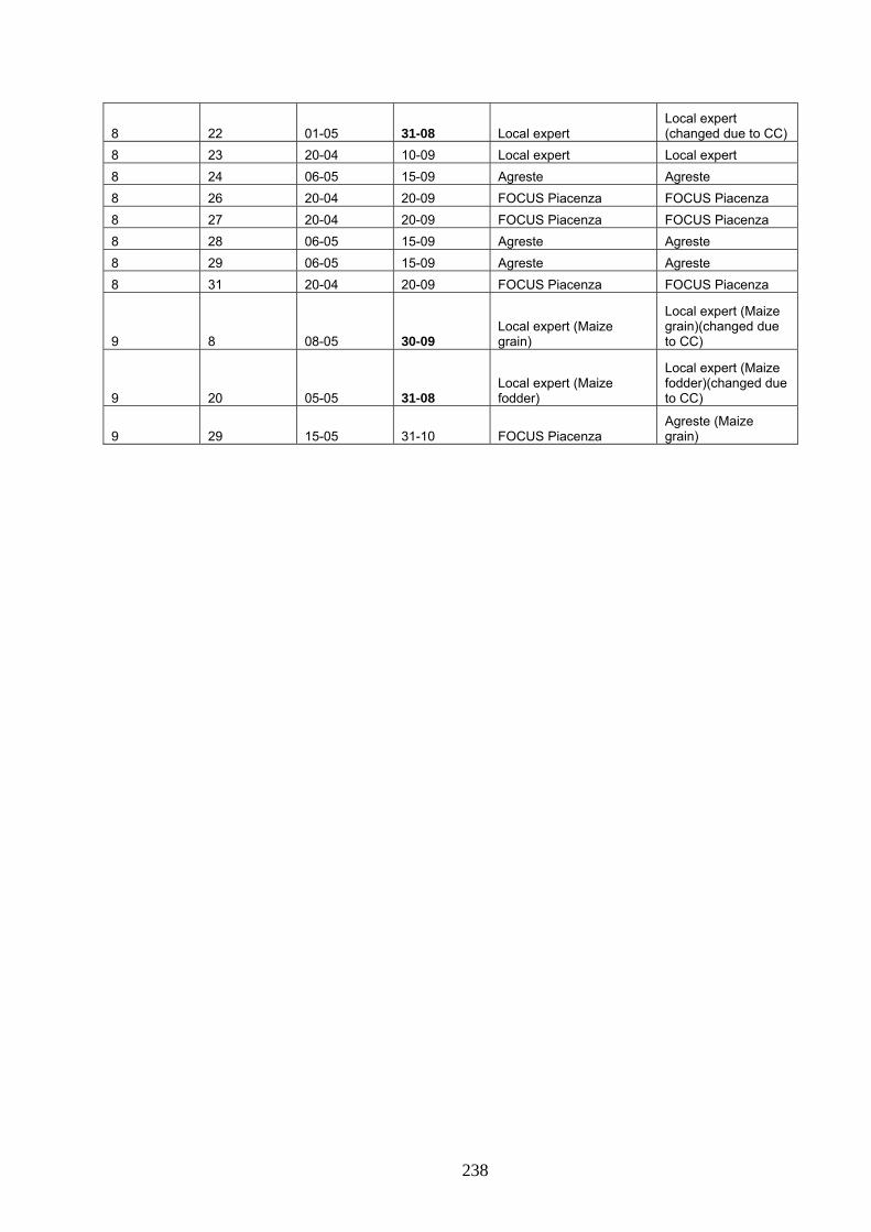
Local expert (changed due to CC) 8 22 01-05 31-08 Local expert
8 23 20-04 10-09 Local expert Local expert 8 24 06-05 15-09 Agreste Agreste 8 26 20-04 20-09 FOCUS Piacenza FOCUS Piacenza 8 27 20-04 20-09 FOCUS Piacenza FOCUS Piacenza 8 28 06-05 15-09 Agreste Agreste 8 29 06-05 15-09 Agreste Agreste 8 31 20-04 20-09 FOCUS Piacenza FOCUS Piacenza
Local expert (Maize grain)(changed due to CC)
Local expert (Maize grain) 9 8 08-05 30-09
Local expert (Maize fodder)(changed due to CC)
Local expert (Maize fodder) 9 20 05-05 31-08
9 29 15-05 31-10 FOCUS Piacenza Agreste (Maize grain)
238

Appendix 12 : Method of selection of most representative MARS tile for each AU
239

Method of selection of most representative MARS tile for each AU The selection of the most appropriate MARS tile was based on agricultural area. Corresponding data were taken from the Agreste database, where for each Canton in France the agricultural area is given. The areas corresponding to fruit trees and vines were excluded, so that only arable land was considered. The tile with the largest occupation of agricultural area within the corresponding AU was selected by default. However, it was then checked if more than one major agricultural area existed in the AU and if the variability of weather conditions within the AU is acceptably small. In such cases, it was decided based on expert’s opinion if other tiles might be more suitable as weather scenario (e.g. by relative geographic location to mountain ranges, the sea,…). Calculation of the agricultural area per tile/AU combination:
• The administrative map of the cantons was intersected with the map of the AUs and a map of the location of the MARS-tiles. For each of the generated polygons the area was calculated.
• The area of each polygon (as an intersection of canton/AU/MARS tile) is multiplied with the agricultural occupation of its corresponding cantons. This gives an “Area Index” (Ia) of how much agricultural area is located within this polygon.
• The single Ia`s of each polygon located in each tile/AU combination were summed up, so that for each AU the tiles can be ranked by their agricultural occupation. A tile with the “Agricultural Area Index” (Ii) is in the following denoted as Ti,AU, where i is the rank of the tile within one AU. T1,AU denotes the tile with the largest agricultural occupation.
Calculation of threshold for acceptance of variability: The underlying assumption for an acceptable variability is that the level of variability over time is also acceptable over space.
• For each MARS- tile in France the rainfall sum (r) and the average mean temperature (t) was calculated over the 30 years (1971-2001).
• For each of the 31 T1,AU tiles the standard deviation of the annual rainfall sum and annual average temperature is calculated and devided by the mean, indicating the temporal variability within each AU as the coefficient of variation (CV). The mean of the 2 data sets consisting each of 31 entries (1 CV per AU), gives the average coefficient of variation (CVtemp and CVrain) of the T1,AU tiles in average over all AUs (CVrain = 0.19 and CVtemp = 0.06).
• For all tiles in France the mean of the rainfall sum and the temperature was calculated over the 30 years. Multiplied by the CV’s this identifies the acceptable differences Xac in rainfall sum and average temperature within one AU (4800 mm rainfall sum [160 mm/a] and 0.7 °C).
Selection of most representative tile for each AU:
STEP 1. It is tested whether there are AUs in which two geographically separate agricultural areas exist. Therefore the location of the two tiles within the AU which inherit the largest agricultural occupation (T1,AU and T2,AU) is compared with GIS.
a. Are they neighbored, go to STEP 2 b. Are they not neighbored, go to STEP 4a
STEP 2. The difference XAU of the parameters rainfall sum and average temperature of the most representative tiles T1,AU and T2,AU is compared with the acceptable difference (Xac of the corresponding parameter), to test whether the variability in the climatic conditions between the two main tiles is acceptable small.
240
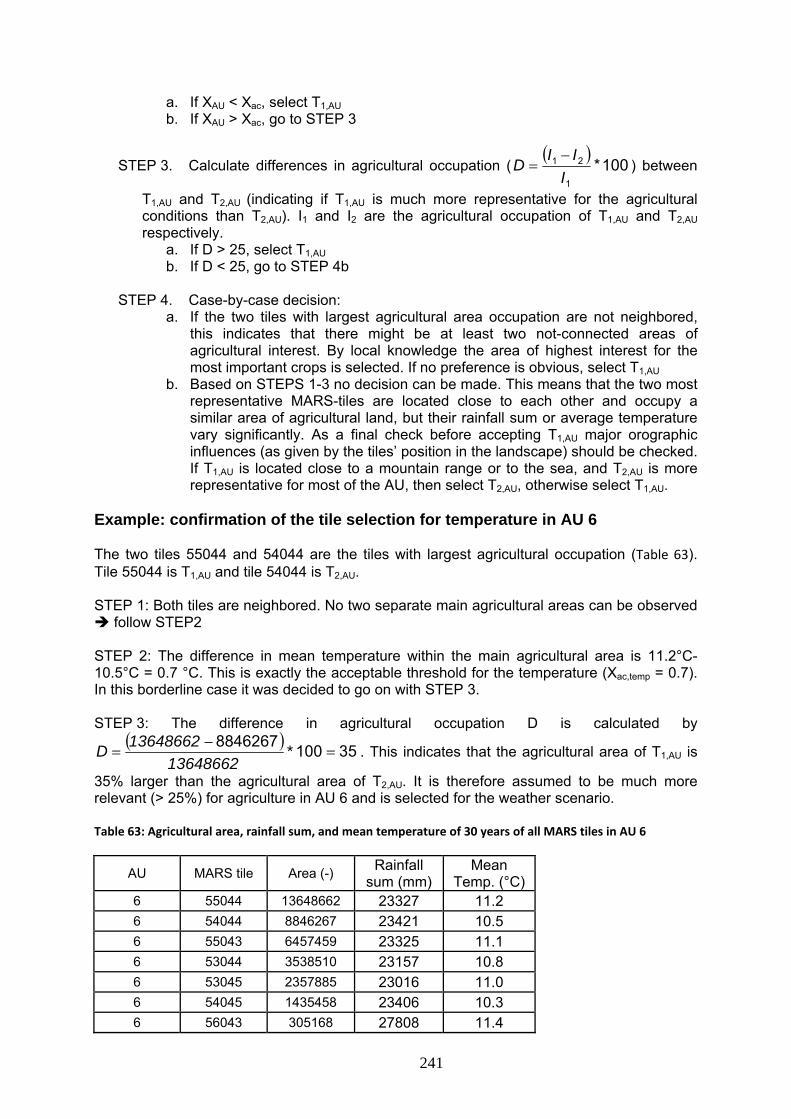
a. If XAU < Xac, select T1,AU b. If XAU > Xac, go to STEP 3
( ) 100*
1
21
IIID −
=STEP 3. Calculate differences in agricultural occupation ( ) between
T1,AU and T2,AU (indicating if T1,AU is much more representative for the agricultural conditions than T2,AU). I1 and I2 are the agricultural occupation of T1,AU and T2,AU respectively.
a. If D > 25, select T1,AU b. If D < 25, go to STEP 4b
STEP 4. Case-by-case decision:
a. If the two tiles with largest agricultural area occupation are not neighbored, this indicates that there might be at least two not-connected areas of agricultural interest. By local knowledge the area of highest interest for the most important crops is selected. If no preference is obvious, select T1,AU
b. Based on STEPS 1-3 no decision can be made. This means that the two most representative MARS-tiles are located close to each other and occupy a similar area of agricultural land, but their rainfall sum or average temperature vary significantly. As a final check before accepting T1,AU major orographic influences (as given by the tiles’ position in the landscape) should be checked. If T1,AU is located close to a mountain range or to the sea, and T2,AU is more representative for most of the AU, then select T2,AU, otherwise select T1,AU.
Example: confirmation of the tile selection for temperature in AU 6 The two tiles 55044 and 54044 are the tiles with largest agricultural occupation (Table 63). Tile 55044 is T1,AU and tile 54044 is T2,AU. STEP 1: Both tiles are neighbored. No two separate main agricultural areas can be observed
follow STEP2 STEP 2: The difference in mean temperature within the main agricultural area is 11.2°C-10.5°C = 0.7 °C. This is exactly the acceptable threshold for the temperature (Xac,temp = 0.7). In this borderline case it was decided to go on with STEP 3. STEP 3: The difference in agricultural occupation D is calculated by
( ) 351008846267=
−= *
1364866213648662D . This indicates that the agricultural area of T1,AU is
35% larger than the agricultural area of T2,AU. It is therefore assumed to be much more relevant (> 25%) for agriculture in AU 6 and is selected for the weather scenario. Table 63: Agricultural area, rainfall sum, and mean temperature of 30 years of all MARS tiles in AU 6
Rainfall sum (mm)
Mean Temp. (°C) AU MARS tile Area (-)
6 55044 13648662 23327 11.2 6 54044 8846267 23421 10.5 6 55043 6457459 23325 11.1 6 53044 3538510 23157 10.8 6 53045 2357885 23016 11.0 6 54045 1435458 23406 10.3 6 56043 305168 27808 11.4
241
Results STEP 1: All AUs passed, except AU 22 STEP 4a STEP 2: rain: All AUs passed, except AU 2, 25, 26 STEP 3 temp: All AUs passed, except AU 6, 21, 23, 27, 28 STEP 3 STEP 3: rain: All AUs passed temp: All AUs passed, except AU 23, 27, 28 STEP 4b STEP 4a: for AU 22: Tile 55046 and 50048 are not neighbored, but are located in the same
area. No significant differences in agriculture can be identified in these areas T1 is selected
STEP 4b: AU23, all 3 tiles are influenced by mountains (either Jura or Massif Central) as is the whole AU T1 is selected; AU27, the AU is influenced by mountains and by the sea. Tile 42052 is closer to the mountains, Tile 42051 closer to the sea, hence no preference identified T1 is selected; AU28, the AU is strongly influenced by the sea. Tile 42050 is located at the sea and therefore preferred T1 is selected.
For all AUs the tiles with the largest agricultural area were selected. Their MARS-ID and their location within the AUs are given in Table 16 and Figure 27.
242

Appendix 13 : Details of the adjustment of rainfall events
243

Table 64 : Splitting of rainfall event from original MARS-data set (1981-2006). The split is
repeated in the following years due to the duplication of the weather records for 2- or 3-annual rotations.
AU MARS tile Date Original rainfall event
Modified rainfall event
26/06/1990 58.0 29.0 3 48049 27/06/1990 0.0 29.0 06/10/1982 78.0 43.0
8 43043 07/10/1982 8.0 43.0 12/11/1996 93.0 31.0 13/11/1996 0.0 31.0 12 51051 14/11/1996 0.0 31.0 08/08/1992 88.0 48.7 09/08/1992 57.0 48.7 18 46044 10/08/1992 1.0 48.7 28/12/1995 70.0 38.5
18 46044 29/12/1995 7.0 38.5 25/09/1999 169.0 85.0
23 46052 26/09/1999 1.0 85.0 12/11/1996 93.0 31.0 13/11/1996 0.0 31.0 24 50052 14/11/1996 0.0 31.0 14/09/2004 206.0 70.0 15/09/2004 0.0 70.0 27 42052 16/09/2004 4.0 70.0
Table 65: Scenarios to which the adjusted rainfall was applied
CID AUID SID Meteo file 2 3 2 48049_S 2 3 5 48049_S 4 3 2 48049_S 4 3 5 48049_S 5 3 2 48049_S 5 3 5 48049_S 3 8 2 43043_S 8 8 7 43043_S 8 8 14 43043_S 1 12 1 51051_S 1 12 2 51051_S 2 12 1 51051_S 2 12 2 51051_S 2 12 5 51051_S 3 12 1 51051_S 3 12 2 51051_S 3 12 5 51051_S 4 12 1 51051_S 4 12 2 51051_S 4 12 5 51051_S
244
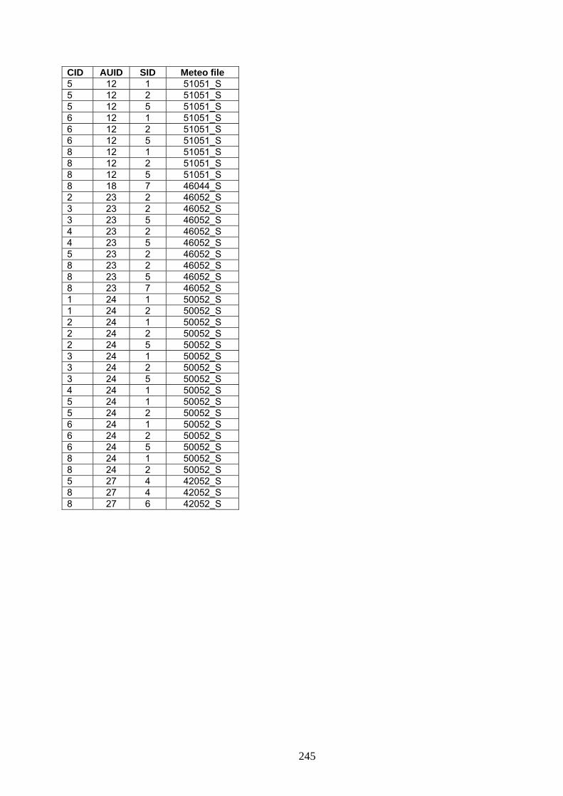
CID AUID SID Meteo file 5 12 1 51051_S 5 12 2 51051_S 5 12 5 51051_S 6 12 1 51051_S 6 12 2 51051_S 6 12 5 51051_S 8 12 1 51051_S 8 12 2 51051_S 8 12 5 51051_S 8 18 7 46044_S 2 23 2 46052_S 3 23 2 46052_S 3 23 5 46052_S 4 23 2 46052_S 4 23 5 46052_S 5 23 2 46052_S 8 23 2 46052_S 8 23 5 46052_S 8 23 7 46052_S 1 24 1 50052_S 1 24 2 50052_S 2 24 1 50052_S 2 24 2 50052_S 2 24 5 50052_S 3 24 1 50052_S 3 24 2 50052_S 3 24 5 50052_S 4 24 1 50052_S 5 24 1 50052_S 5 24 2 50052_S 6 24 1 50052_S 6 24 2 50052_S 6 24 5 50052_S 8 24 1 50052_S 8 24 2 50052_S 5 27 4 42052_S 8 27 4 42052_S 8 27 6 42052_S
245
Appendix 14 : Irrigation acreage per Agronomic Unit for the FROGS irrigated crops
246
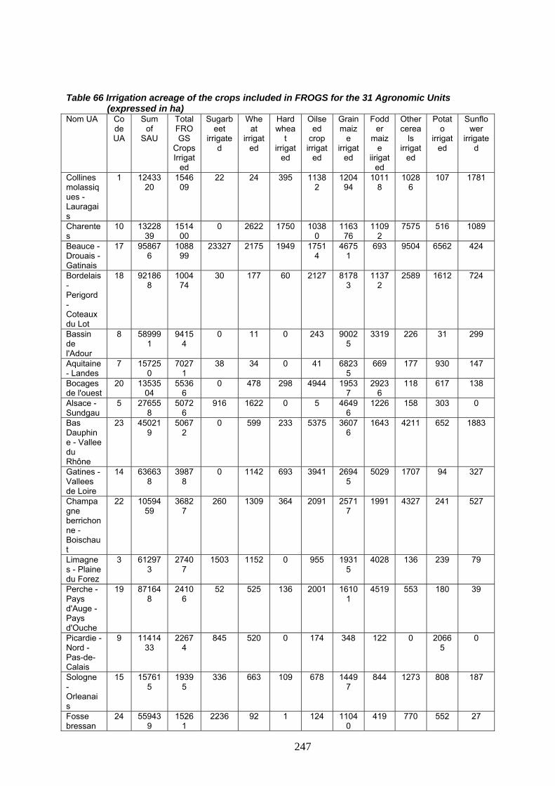
Table 66 Irrigation acreage of the crops included in FROGS for the 31 Agronomic Units
(expressed in ha) Nom UA Co
de UA
Sum of
SAU
Total FROGS
Crops Irrigat
ed
Sugarbeet
irrigated
Wheat
irrigated
Hard whea
t irrigat
ed
Oilseed
crop irrigat
ed
Grain maiz
e irrigat
ed
Fodder
maize
iirigated
Other cerea
ls irrigat
ed
Potato
irrigated
Sunflower
irrigated
Collines molassiques - Lauragais
1 1243320
154609
22 24 395 11382
120494
10118
10286
107 1781
Charentes
10 1322839
151400
0 2622 1750 10380
116376
11092
7575 516 1089
Beauce - Drouais - Gatinais
17 958676
108899
23327 2175 1949 17514
46751
693 9504 6562 424
Bordelais - Perigord - Coteaux du Lot
18 921868
100474
30 177 60 2127 81783
11372
2589 1612 724
Bassin de l'Adour
8 589991
94154
0 11 0 243 90025
3319 226 31 299
Aquitaine - Landes
7 157250
70271
38 34 0 41 68235
669 177 930 147
Bocages de l'ouest
20 1353504
55366
0 478 298 4944 19537
29236
118 617 138
Alsace - Sundgau
5 276558
50726
916 1622 0 5 46496
1226 158 303 0
Bas Dauphine - Vallee du Rhône
23 450219
50672
0 599 233 5375 36076
1643 4211 652 1883
Gatines - Vallees de Loire
14 636638
39878
0 1142 693 3941 26945
5029 1707 94 327
Champagne berrichonne - Boischaut
22 1059459
36827
260 1309 364 2091 25717
1991 4327 241 527
Limagnes - Plaine du Forez
3 612973
27407
1503 1152 0 955 19315
4028 136 239 79
Perche - Pays d'Auge - Pays d'Ouche
19 871648
24106
52 525 136 2001 16101
4519 553 180 39
Picardie - Nord - Pas-de-Calais
9 1141433
22674
845 520 0 174 348 122 0 20665
0
Sologne - Orleanais
15 157615
19395
336 663 109 678 14497
844 1273 808 187
Fosse bressan
24 559439
15261
2236 92 1 124 11040
419 770 552 27
247
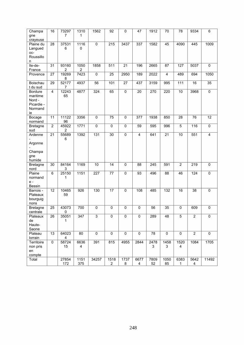
Champagne crayeuse
16 732977
13101
1562 92 0 47 1912 70 78 9334 6
Plaine du Languedoc-Roussillon
28 375316
11160
0 215 3437 337 1582 45 4090 445 1009
Ile-de-France
31 931602
10502
1858 511 21 196 2665 87 127 5037 0
Provence 27 192698
7423 0 25 2950 189 2022 4 489 694 1050
Boischaut du sud
29 521777
4937 56 101 27 437 3159 995 111 16 35
Bordure maritime Nord - Picardie - Normandie
4 1224365
4877 324 65 0 20 270 220 10 3968 0
Bocage normand
11 1112296
3356 0 75 0 377 1938 850 28 76 12
Bretagne sud
2 459222
1771 0 0 0 59 595 996 5 116 0
Ardenne - Argonne - Champagne humide
21 556896
1392 131 30 0 4 641 21 10 551 4
Bretagne nord
30 841643
1169 10 14 0 88 245 591 2 219 0
Plaine normande - Bessin
6 251501
1151 227 77 0 93 496 88 46 124 0
Barrois - Plateaux bourguignons
12 1046559
926 130 17 0 108 485 132 16 38 0
Bretagne centrale
25 430730
700 0 0 0 0 56 35 0 609 0
Plateaux de Haute-Saone
26 350511
347 3 0 0 0 289 48 5 2 0
Plateau lorrain
13 640234
80 0 0 0 0 78 0 0 2 0
Territoire non pris en compte
0 5872415
66364
391 815 4955 2844 24783
14583
15204
1084 1705
Total 27854172
1151375
34257 15182
17378
66774
780952
105085
63831
56424
11492
248

Table 67 Density of irrigation for the crops included in FROGS in the 31 Agronomic Units (expressed in % of irrigated crop surface vs. crop surface)
Nom UA Code UA
Sum of
SAU
Total FROGS
Crops Irrigat
ed
Sugarbeet
irrigated
Wheat
irrigated
Hard whea
t irrigat
ed
Oilseed
crop irrigat
ed
Grain maiz
e irrigat
ed
Fodder
maize
iirigated
Other cerea
ls irrigat
ed
Potato
irrigated
Sunflower
irrigated
Collines molassiques - Lauragais
1 1243320
154609
84.6 0.0 0.3 - 85.4 52.6 - 55.4 -
Charentes
10 1322839
151400
0.0 0.9 8.8 - 66.7 26.1 - 73.5 -
Beauce - Drouais - Gatinais
17 958676
108899
65.9 0.5 4.8 - 83.6 15.9 - 95.2 -
Bordelais - Perigord - Coteaux du Lot
18 921868
100474
76.9 0.2 2.3 - 61.1 38.1 - 90.4 -
Bassin de l'Adour
8 589991
94154
0.0 0.1 0.0 - 36.6 11.2 - 36.5 -
Aquitaine - Landes
7 157250
70271
100.0 2.8 0.0 - 90.7 60.8 - 99.3 -
Bocages de l'ouest
20 1353504
55366
0.0 0.3 15.9 - 39.9 16.8 - 75.8 -
Alsace - Sundgau
5 276558
50726
17.2 4.6 0.0 - 37.0 11.5 - 28.0 -
Bas Dauphine - Vallee du Rhône-
23 450219
50672
0.0 1.2 2.4 - 56.0 14.5 - 53.8 -
Gatines - Vallees de Loire
14 636638
39878
0.0 0.7 4.1 - 46.2 23.9 - 51.1 -
Champagne berrichonne - Boischaut
22 1059459
36827
69.7 0.4 6.3 - 61.5 13.5 - 91.3 -
Limagnes - Plaine du Forez
3 612973
27407
44.7 1.5 0.0 - 53.3 25.1 - 47.2 -
Perche - Pays d'Auge - Pays d'Ouche
19 871648
24106
3.4 0.2 4.0 - 31.8 7.1 - 39.5 -
Picardie - Nord - Pas-de-Calais
9 1141433
22674
0.7 0.1 0.0 - 1.2 0.3 - 32.0 -
Sologne - Orleanais
15 157615
19395
77.1 2.1 4.1 - 77.1 33.3 - 92.2 -
Fosse bressan
24 559439
15261
52.8 0.1 4.3 - 13.2 2.4 - 52.3 -
Champagne
16 732977
13101
2.2 0.0 0.0 - 9.3 1.8 - 51.1 -
249
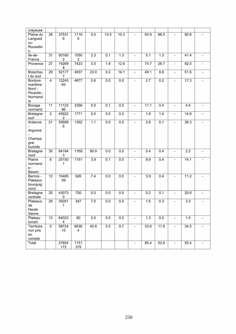
crayeuse Plaine du Languedoc-Roussillon
28 375316
11160
0.0 13.5 10.3 - 93.9 86.5 - 90.8 -
Ile-de-France
31 931602
10502
2.3 0.1 1.3 - 5.1 1.3 - 41.4 -
Provence 27 192698
7423 0.0 1.9 12.6 - 74.7 26.7 - 92.5 -
Boischaut du sud
29 521777
4937 23.0 0.2 14.1 - 49.1 8.8 - 51.6 -
Bordure maritime Nord - Picardie - Normandie
4 1224365
4877 0.6 0.0 0.0 - 2.7 0.2 - 17.3 -
Bocage normand
11 1112296
3356 0.0 0.1 0.0 - 11.1 0.4 - 4.4 -
Bretagne sud
2 459222
1771 0.0 0.0 0.0 - 1.9 1.4 - 14.9 -
Ardenne - Argonne - Champagne humide
21 556896
1392 1.1 0.0 0.0 - 2.8 0.1 - 36.3 -
Bretagne nord
30 841643
1169 90.9 0.0 0.0 - 0.4 0.4 - 2.2 -
Plaine normande - Bessin
6 251501
1151 3.9 0.1 0.0 - 9.9 0.4 - 14.1 -
Barrois - Plateaux bourguignons
12 1046559
926 7.4 0.0 0.0 - 3.9 0.4 - 11.2 -
Bretagne centrale
25 430730
700 0.0 0.0 0.0 - 0.2 0.1 - 20.6 -
Plateaux de Haute-Saone
26 350511
347 7.0 0.0 0.0 - 1.6 0.3 - 3.3 -
Plateau lorrain
13 640234
80 0.0 0.0 0.0 - 1.3 0.0 - 1.5 -
Territoire non pris en compte
0 5872415
66364
40.8 0.5 9.7 - 33.6 11.6 - 34.5 -
Total 27854172
1151375
- 85.4 52.6 - 55.4 -
250
Appendix 15 : Soil Surfaces in the Agronomic Units (ha)
251
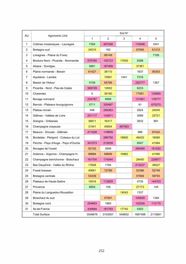
252
Soil N° AU Agronomic Unit
1 2 3 4 5
1 Collines molassiques - Lauragais 7304 497548 116406 3341
2 Bretagne sud 34510 162 97956 61212
3 Limagnes - Plaine du Forez 89149 7195
4 Bordure Nord - Picardie - Normandie 570785 102723 17930 8388
5 Alsace - Sundgau 5881 187469 37361
6 Plaine normande - Bessin 61427 38110 1837 56303
7 Aquitaine - Landes 10991 1441 7316
8 Bassin de l'Adour 5156 65789 252777 1367
9 Picardie - Nord - Pas-de-Calais 569729 12652 6233
10 Charentes 5 36180 77061 120665
11 Bocage normand 234787 8999 131061 178777
12 Barrois - Plateaux bourguignons 5711 326487 91 670275
13 Plateau lorrain 548 246363 2924 24045
14 Gâtines - Vallées de Loire 201117 124871 3066 22721
15 Sologne - Orléanais 36811 16317 2832 891
16 Champagne crayeuse 31541 45654 467583
17 Beauce - Drouais - Gâtinais 411028 118809 988 67424
18 Bordelais - Périgord - Coteaux du Lot 286750 18900 48432 18580
19 Perche - Pays d'Auge - Pays d'Ouche 341573 212639 6547 41564
20 Bocages de l'ouest 52102 2858 269480 161552
21 Ardenne - Argonne - Champagne H. 96884 69699 10962 41590
22 Champagne berrichonne - Boischaut 161704 174544 26450 229677
23 Bas Dauphiné - Vallée du Rhône 17828 1784 213237 38527
24 Fossé bressan 40661 72789 52386 52746
25 Bretagne centrale 53439 57669 58793
26 Plateaux de Haute-Saône 15916 112829 4735 144703
27 Provence 6850 109 27173 145
28 Plaine du Languedoc-Roussillon 14043 1337
29 Boischaut du sud 57091 105928 1392
30 Bretagne nord 254693 1860 102526 112175
31 Ile-de-France 330684 181783 17742 5303
Total Surface 3548676 3103007 548602 1667498 2115661
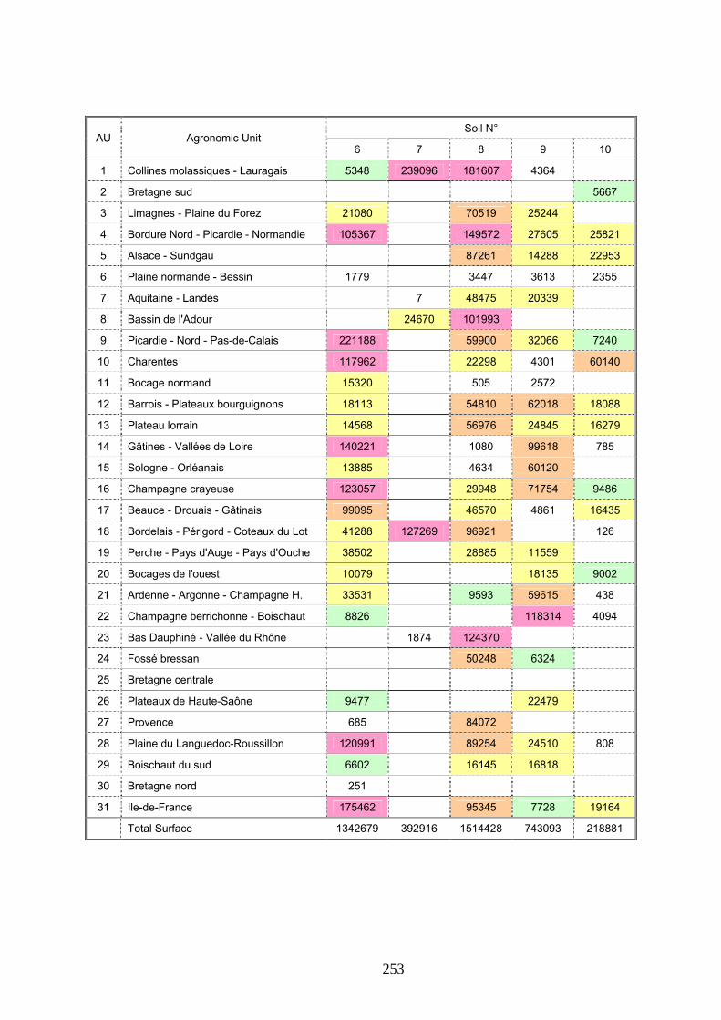
253
Soil N° AU Agronomic Unit
6 7 8 9 10
1 Collines molassiques - Lauragais 5348 239096 181607 4364
2 Bretagne sud 5667
3 Limagnes - Plaine du Forez 21080 70519 25244
4 Bordure Nord - Picardie - Normandie 105367 149572 27605 25821
5 Alsace - Sundgau 87261 14288 22953
6 Plaine normande - Bessin 1779 3447 3613 2355
7 Aquitaine - Landes 7 48475 20339
8 Bassin de l'Adour 24670 101993
9 Picardie - Nord - Pas-de-Calais 221188 59900 32066 7240
10 Charentes 117962 22298 4301 60140
11 Bocage normand 15320 505 2572
12 Barrois - Plateaux bourguignons 18113 54810 62018 18088
13 Plateau lorrain 14568 56976 24845 16279
14 Gâtines - Vallées de Loire 140221 1080 99618 785
15 Sologne - Orléanais 13885 4634 60120
16 Champagne crayeuse 123057 29948 71754 9486
17 Beauce - Drouais - Gâtinais 99095 46570 4861 16435
18 Bordelais - Périgord - Coteaux du Lot 41288 127269 96921 126
19 Perche - Pays d'Auge - Pays d'Ouche 38502 28885 11559
20 Bocages de l'ouest 10079 18135 9002
21 Ardenne - Argonne - Champagne H. 33531 9593 59615 438
22 Champagne berrichonne - Boischaut 8826 118314 4094
23 Bas Dauphiné - Vallée du Rhône 1874 124370
24 Fossé bressan 50248 6324
25 Bretagne centrale
26 Plateaux de Haute-Saône 9477 22479
27 Provence 685 84072
28 Plaine du Languedoc-Roussillon 120991 89254 24510 808
29 Boischaut du sud 6602 16145 16818
30 Bretagne nord 251
31 Ile-de-France 175462 95345 7728 19164
Total Surface 1342679 392916 1514428 743093 218881
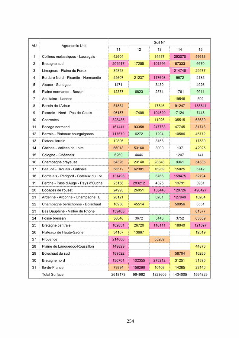
254
Soil N° AU Agronomic Unit
11 12 13 14 15
1 Collines molassiques - Lauragais 42604 34487 293070 56618
2 Bretagne sud 204917 17255 101396 67333 6670
3 Limagnes - Plaine du Forez 34853 214748 29577
4 Bordure Nord - Picardie - Normandie 44607 21237 117608 5672 2185
5 Alsace - Sundgau 1471 3430 4926
6 Plaine normande - Bessin 12387 6823 2874 1761 9911
7 Aquitaine - Landes 19546 502
8 Bassin de l'Adour 51854 17346 91247 183841
9 Picardie - Nord - Pas-de-Calais 96157 17408 104529 7124 7445
10 Charentes 328486 1 11026 35515 63689
11 Bocage normand 161441 93358 247763 47745 81743
12 Barrois - Plateaux bourguignons 117670 6272 7294 10586 45772
13 Plateau lorrain 12806 3158 17530
14 Gâtines - Vallées de Loire 66018 53160 3000 137 42925
15 Sologne - Orléanais 6269 4446 1207 141
16 Champagne crayeuse 54326 23140 28848 9361 54335
17 Beauce - Drouais - Gâtinais 58512 62381 16939 15025 6742
18 Bordelais - Périgord - Coteaux du Lot 131496 6766 159475 52794
19 Perche - Pays d'Auge - Pays d'Ouche 25156 283212 4325 19791 3961
20 Bocages de l'ouest 24993 26051 133448 129726 496427
21 Ardenne - Argonne - Champagne H. 26121 8281 127949 18284
22 Champagne berrichonne - Boischaut 16930 45514 50956 3551
23 Bas Dauphiné - Vallée du Rhône 159463 61377
24 Fossé bressan 38646 3672 5148 3752 63559
25 Bretagne centrale 102831 26720 116111 18040 121597
26 Plateaux de Haute-Saône 34107 13667 12519
27 Provence 214006 55209
28 Plaine du Languedoc-Roussillon 149829 44876
29 Boischaut du sud 189522 58704 16286
30 Bretagne nord 136701 102355 278212 31251 31896
31 Ile-de-France 73994 158290 16408 14285 23146
Total Surface 2618173 964962 1323606 1434005 1564829

Soil N° AU Agronomic Unit
16 17 18 19 Total
1 Collines molassiques - Lauragais 92851 1574644
2 Bretagne sud 597079
3 Limagnes - Plaine du Forez 4041 496406
4 Bordure Nord - Picardie - Normandie 167218 40930 1407648
5 Alsace - Sundgau 151 365190
6 Plaine normande - Bessin 1526 204153
7 Aquitaine - Landes 16555 125172
8 Bassin de l'Adour 904 796944
9 Picardie - Nord - Pas-de-Calais 8325 55226 1205222
10 Charentes 21810 3039 113497 2639 1018315
11 Bocage normand 109 1204181
12 Barrois - Plateaux bourguignons 57692 3318 6904 1411101
13 Plateau lorrain 18274 2112 440428
14 Gâtines - Vallées de Loire 8629 8553 775901
15 Sologne - Orléanais 928 148482
16 Champagne crayeuse 62459 7526 1019019
17 Beauce - Drouais - Gâtinais 46409 24761 995980
18 Bordelais - Périgord - Coteaux du Lot 32638 24821 1046255
19 Perche - Pays d'Auge - Pays d'Ouche 10915 4530 1033157
20 Bocages de l'ouest 1377 369 1335599
21 Ardenne - Argonne - Champagne H. 68 15677 518692
22 Champagne berrichonne - Boischaut 5436 31843 877838
23 Bas Dauphiné - Vallée du Rhône 618461
24 Fossé bressan 2179 392111
25 Bretagne centrale 555201
26 Plateaux de Haute-Saône 3018 373449
27 Provence 388250
28 Plaine du Languedoc-Roussillon 445647
29 Boischaut du sud 3807 472296
30 Bretagne nord 1051921
31 Ile-de-France 38738 109946 1268018
Total Surface 224711 354486 113865 368683 24162762
255
Appendix 16 : Selected scenarios per Crop and associated surfaces (kha)
256

Crop: Sugar Beet Soil ID 1 2 3 6 8 9 AU
1 Collines molassiques - Lauragais 2 Bretagne sud 3 Limagnes - Plaine du Forez 89 21 71 25
4 Bordure Nord - Picardie - Normandie 571 103 18 105 150 28
5 Alsace - Sundgau 6 187 87 14
6 Plaine normande - Bessin 61 38 2 3 4
7 Aquitaine - Landes
8 Bassin de l'Adour
9 Picardie - Nord - Pas-de-Calais 570 13 221 60 32
10 Charentes
11 Bocage normand
12 Barrois - Plateaux bourguignons 6 326 18 55 62
13 Plateau lorrain
14 Gâtines - Vallées de Loire
15 Sologne - Orléanais
16 Champagne crayeuse 32 46 468 123 30 72
17 Beauce - Drouais - Gâtinais 411 119 99 47 5
18 Bordelais - Périgord - Coteaux du Lot
19 Perche - Pays d'Auge - Pays d'Ouche 342 213 39 29 12
20 Bocages de l'ouest
21 Ardenne - Argonne - Champagne H. 97 70 11 34 10 60
22 Champagne berrichonne - Boischaut
23 Bas Dauphiné - Vallée du Rhône
24 Fossé bressan 41 73 50 6
25 Bretagne centrale
26 Plateaux de Haute-Saône
27 Provence
28 Plaine du Languedoc-Roussillon
29 Boischaut du sud
30 Bretagne nord
31 Ile-de-France 331 182 18 175 95 8
257

Crop: Sugar Beet Soil N° 13 19
AU
1 Collines molassiques - Lauragais 2 Bretagne sud 3 Limagnes - Plaine du Forez 4
4 Bordure Nord - Picardie - Normandie 118 41
5 Alsace - Sundgau 3
6 Plaine normande - Bessin 3 2
7 Aquitaine - Landes
8 Bassin de l'Adour
9 Picardie - Nord - Pas-de-Calais 105 55
10 Charentes
11 Bocage normand
12 Barrois - Plateaux bourguignons 7 7
13 Plateau lorrain
14 Gâtines - Vallées de Loire
15 Sologne - Orléanais
16 Champagne crayeuse 29 8
17 Beauce - Drouais - Gâtinais 17 25
18 Bordelais - Périgord - Coteaux du Lot
19 Perche - Pays d'Auge - Pays d'Ouche 4 5
20 Bocages de l'ouest
21 Ardenne - Argonne - Champagne H. 8 16
22 Champagne berrichonne - Boischaut
23 Bas Dauphiné - Vallée du Rhône
24 Fossé bressan 5 2
25 Bretagne centrale
26 Plateaux de Haute-Saône
27 Provence
28 Plaine du Languedoc-Roussillon
29 Boischaut du sud
30 Bretagne nord
31 Ile-de-France 16 110
258

Crop: Winter Wheat Soil N° 1 2 3 4 5 6
AU
7 498 116 3 5 1 Collines molassiques - Lauragais
35 98 61 2 Bretagne sud
89 7 21 3 Limagnes - Plaine du Forez
571 103 18 8 105 4 Bordure Nord - Picardie - Normandie
6 187 37 5 Alsace - Sundgau
61 38 2 56 2 6 Plaine normande - Bessin
7 Aquitaine - Landes 11 1 7
8 Bassin de l'Adour 5 66 253 1
570 13 6 221 9 Picardie - Nord - Pas-de-Calais
36 77 121 118 10 Charentes
235 9 131 179 15 11 Bocage normand
6 326 670 18 12 Barrois - Plateaux bourguignons
1 246 3 24 15 13 Plateau lorrain
201 125 3 23 140 14 Gâtines - Vallées de Loire
37 16 15 Sologne - Orléanais 3 1 14
32 46 468 123 16 Champagne crayeuse
411 119 1 67 99 17 Beauce - Drouais - Gâtinais
287 19 48 19 41 18 Bordelais - Périgord - Coteaux du Lot
342 213 7 426 39 19 Perche - Pays d'Auge - Pays d'Ouche
52 3 269 162 10 20 Bocages de l'ouest
97 70 11 42 34 21 Ardenne - Argonne - Champagne H.
162 175 26 230 9 22 Champagne berrichonne - Boischaut
18 2 213 39 23 Bas Dauphiné - Vallée du Rhône
41 73 52 53 24 Fossé bressan
53 58 59 25 Bretagne centrale
16 5 145 9 26 Plateaux de Haute-Saône 113
27 Provence
28 Plaine du Languedoc-Roussillon
57 106 1 7 29 Boischaut du sud
255 2 103 112 30 Bretagne nord
331 182 18 5 175 31 Ile-de-France
259

Crop: Winter Wheat Soil N° 8 9 12 13 19
AU Crop Surface in Farmland Surface (%)
182 4 34 1 Collines molassiques - Lauragais
17 101 2 Bretagne sud
71 25 4 3 Limagnes - Plaine du Forez
150 28 21 118 41 4 Bordure Nord - Picardie - Normandie
87 3 5 Alsace - Sundgau 14
3 4 7 3 6 Plaine normande - Bessin 2
7 Aquitaine - Landes 48 20 17
8 Bassin de l'Adour 102 17 1
60 32 17 105 55 9 Picardie - Nord - Pas-de-Calais
22 4 11 3 10 Charentes
1 3 93 248 11 Bocage normand
55 62 6 7 7 12 Barrois - Plateaux bourguignons
57 25 3 2 13 Plateau lorrain
1 100 53 3 9 14 Gâtines - Vallées de Loire
5 15 Sologne - Orléanais 60 4 1
30 72 23 29 8 16 Champagne crayeuse
47 5 62 17 25 17 Beauce - Drouais - Gâtinais
97 7 25 18 Bordelais - Périgord - Coteaux du Lot
29 12 283 4 5 19 Perche - Pays d'Auge - Pays d'Ouche
18 26 133 20 Bocages de l'ouest
10 60 8 16 21 Ardenne - Argonne - Champagne H.
118 46 32 22 Champagne berrichonne - Boischaut
124 23 Bas Dauphiné - Vallée du Rhône
50 6 4 5 2 24 Fossé bressan
27 116 25 Bretagne centrale
26 Plateaux de Haute-Saône 22 14 3
27 Provence
28 Plaine du Languedoc-Roussillon
16 29 Boischaut du sud 17 4
102 278 30 Bretagne nord
95 8 158 16 110 31 Ile-de-France
260
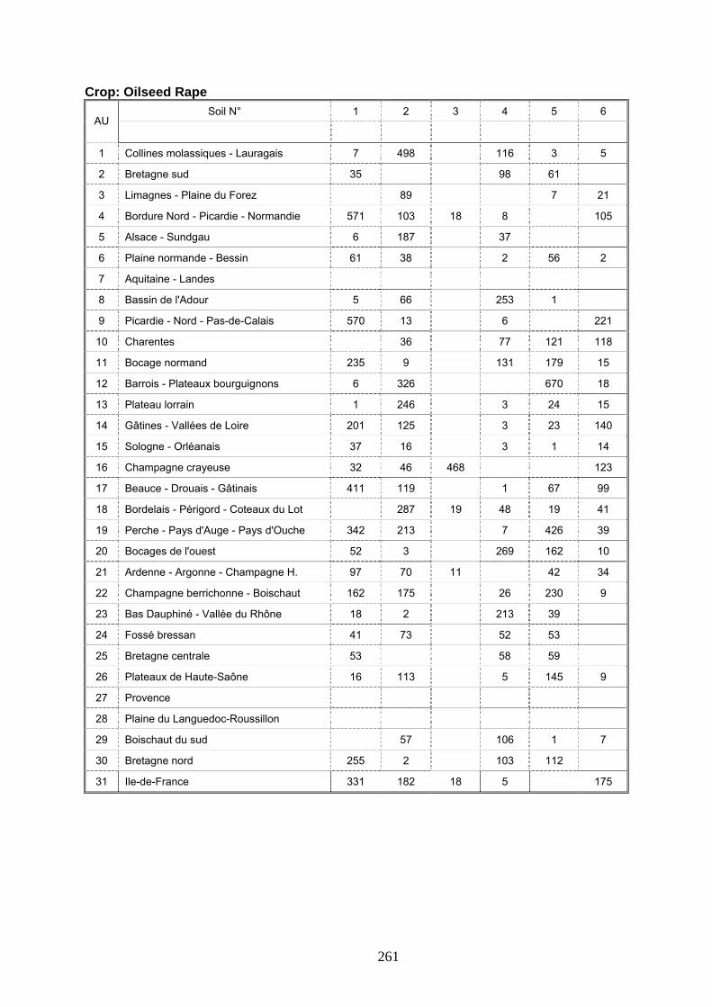
Crop: Oilseed Rape Soil N° 1 2 3 4 5 6
AU
7 498 1 Collines molassiques - Lauragais 116 3 5
35 2 Bretagne sud 98 61
89 3 Limagnes - Plaine du Forez 7 21
571 103 18 8 105 4 Bordure Nord - Picardie - Normandie
5 Alsace - Sundgau 6 187 37
6 Plaine normande - Bessin 61 38 2 56 2
7 Aquitaine - Landes
8 Bassin de l'Adour 5 66 253 1
9 Picardie - Nord - Pas-de-Calais 570 13 6 221
36 77 121 118 10 Charentes
235 9 11 Bocage normand 131 179 15
6 326 670 18 12 Barrois - Plateaux bourguignons
1 246 3 24 15 13 Plateau lorrain
201 125 3 23 140 14 Gâtines - Vallées de Loire
37 16 15 Sologne - Orléanais 3 1 14
32 46 468 123 16 Champagne crayeuse
411 119 1 67 99 17 Beauce - Drouais - Gâtinais
287 18 Bordelais - Périgord - Coteaux du Lot 19 48 19 41
342 213 7 426 39 19 Perche - Pays d'Auge - Pays d'Ouche
52 3 20 Bocages de l'ouest 269 162 10
97 70 11 42 34 21 Ardenne - Argonne - Champagne H.
162 175 26 230 9 22 Champagne berrichonne - Boischaut
18 2 23 Bas Dauphiné - Vallée du Rhône 213 39
41 73 24 Fossé bressan 52 53
25 Bretagne centrale 53 58 59
16 26 Plateaux de Haute-Saône 113 5 145 9
27 Provence
28 Plaine du Languedoc-Roussillon
57 29 Boischaut du sud 106 1 7
255 2 30 Bretagne nord 103 112
331 182 18 5 175 31 Ile-de-France
261

Crop: Oilseed Rape Soil N° 8 9 12 17
AU
1 Collines molassiques - Lauragais 182 4
2 Bretagne sud 17
3 Limagnes - Plaine du Forez 71 25
150 28 21 4 Bordure Nord - Picardie - Normandie 167
5 Alsace - Sundgau 87 14
6 Plaine normande - Bessin 3 4 7
7 Aquitaine - Landes
8 Bassin de l'Adour 102
17 9 Picardie - Nord - Pas-de-Calais 60 32 8
10 Charentes 22 4 3
11 Bocage normand 1 3 93
55 62 6 3 12 Barrois - Plateaux bourguignons
57 25 13 Plateau lorrain
1 100 53 14 Gâtines - Vallées de Loire 9
15 Sologne - Orléanais 5 60 4
30 72 23 62 16 Champagne crayeuse
47 5 62 46 17 Beauce - Drouais - Gâtinais
18 Bordelais - Périgord - Coteaux du Lot 97
29 12 283 11 19 Perche - Pays d'Auge - Pays d'Ouche
26 20 Bocages de l'ouest 18
10 60 21 Ardenne - Argonne - Champagne H.
118 46 5 22 Champagne berrichonne - Boischaut
23 Bas Dauphiné - Vallée du Rhône 124
4 24 Fossé bressan 50 6
25 Bretagne centrale 27
14 26 Plateaux de Haute-Saône 22
27 Provence
28 Plaine du Languedoc-Roussillon
29 Boischaut du sud 16 17
30 Bretagne nord 102
95 8 158 39 31 Ile-de-France
262

Crop: Maize Fodder Soil N° 1 2 4 5 11 12
AU
7 1 Collines molassiques - Lauragais 498 116 3 43
35 98 61 205 17 2 Bretagne sud
7 35 3 Limagnes - Plaine du Forez 89
571 103 8 45 21 4 Bordure Nord - Picardie - Normandie
6 5 Alsace - Sundgau 187 37 1
61 6 Plaine normande - Bessin 38 2 56 12 7
7 Aquitaine - Landes 11 7
5 8 Bassin de l'Adour 66 253 1 52
570 13 6 96 17 9 Picardie - Nord - Pas-de-Calais
36 77 121 328 10 Charentes
235 9 131 179 161 93 11 Bocage normand
6 326 670 118 6 12 Barrois - Plateaux bourguignons
1 246 3 24 13 13 Plateau lorrain
201 14 Gâtines - Vallées de Loire 125 3 23 66 53
15 Sologne - Orléanais 37 16 3 1 6 4
16 Champagne crayeuse 32 46 54 23
17 Beauce - Drouais - Gâtinais 411 119 1 67 59 62
18 Bordelais - Périgord - Coteaux du Lot 287 48 19 131
342 213 7 426 25 283 19 Perche - Pays d'Auge - Pays d'Ouche
52 3 269 162 25 26 20 Bocages de l'ouest
97 70 42 26 21 Ardenne - Argonne - Champagne H.
162 22 Champagne berrichonne - Boischaut 175 26 230 17 46
18 23 Bas Dauphiné - Vallée du Rhône 2 213 39 159
41 24 Fossé bressan 73 52 53 39 4
53 58 59 103 27 25 Bretagne centrale
16 26 Plateaux de Haute-Saône 113 5 145 34 14
27 Provence
28 Plaine du Languedoc-Roussillon
29 Boischaut du sud 57 106 1 190
255 2 103 112 137 102 30 Bretagne nord
31 Ile-de-France 331 182 5 74 158
263

Crop: Maize Fodder Soil N° 13 14 15
AU
34 1 Collines molassiques - Lauragais 293 57
101 67 7 2 Bretagne sud
3 Limagnes - Plaine du Forez 215 30
118 6 2 4 Bordure Nord - Picardie - Normandie
3 5 Alsace - Sundgau 5
3 6 Plaine normande - Bessin 2 10
7 Aquitaine - Landes 20 1
17 91 184 8 Bassin de l'Adour
105 7 7 9 Picardie - Nord - Pas-de-Calais
11 36 64 10 Charentes
248 48 82 11 Bocage normand
7 11 46 12 Barrois - Plateaux bourguignons
3 18 13 Plateau lorrain
3 14 Gâtines - Vallées de Loire 43
15 Sologne - Orléanais 1
16 Champagne crayeuse 29 9 54
17 Beauce - Drouais - Gâtinais 17 15 7
7 159 53 18 Bordelais - Périgord - Coteaux du Lot
4 20 4 19 Perche - Pays d'Auge - Pays d'Ouche
133 130 496 20 Bocages de l'ouest
8 128 18 21 Ardenne - Argonne - Champagne H.
22 Champagne berrichonne - Boischaut 51 4
23 Bas Dauphiné - Vallée du Rhône 61
5 24 Fossé bressan 4 64
116 18 122 25 Bretagne centrale
26 Plateaux de Haute-Saône 13
27 Provence
28 Plaine du Languedoc-Roussillon
29 Boischaut du sud 59 16
278 31 32 30 Bretagne nord
31 Ile-de-France 16 14 23
264

Crop: Maize Grain Soil N° 1 2 4 5 8 9
AU
7 498 116 3 182 4 1 Collines molassiques - Lauragais
35 98 2 Bretagne sud 61
89 3 Limagnes - Plaine du Forez 7 71 25
103 8 4 Bordure Nord - Picardie - Normandie 571 150 28
6 187 37 87 14 5 Alsace - Sundgau
6 Plaine normande - Bessin 61 38 2 56 3 4
11 7 48 7 Aquitaine - Landes 20
5 66 253 1 102 8 Bassin de l'Adour
570 13 6 9 Picardie - Nord - Pas-de-Calais 60 32
36 77 121 22 4 10 Charentes
9 131 11 Bocage normand 235 179 1 3
326 12 Barrois - Plateaux bourguignons 6 670 55 62
13 Plateau lorrain 1 246 3 24 57 25
201 125 3 23 1 14 Gâtines - Vallées de Loire 100
16 3 15 Sologne - Orléanais 37 1 5 60
46 16 Champagne crayeuse 32 30 72
411 119 1 67 47 17 Beauce - Drouais - Gâtinais 5
287 48 19 97 18 Bordelais - Périgord - Coteaux du Lot
342 213 7 426 29 19 Perche - Pays d'Auge - Pays d'Ouche 12
52 3 269 162 20 Bocages de l'ouest 18
70 21 Ardenne - Argonne - Champagne H. 97 42 10 60
162 175 26 22 Champagne berrichonne - Boischaut 230 118
18 2 213 39 124 23 Bas Dauphiné - Vallée du Rhône
41 73 52 53 50 24 Fossé bressan 6
53 58 25 Bretagne centrale 59
5 26 Plateaux de Haute-Saône 16 113 145 22
27 Provence 7 27 84
28 Plaine du Languedoc-Roussillon 1 89 25
29 Boischaut du sud 57 106 1 16 17
255 2 103 112 30 Bretagne nord
331 182 5 95 31 Ile-de-France 8
265

Crop: Maize Grain Soil N° 10 11 12 13 14 15
AU
43 34 293 1 Collines molassiques - Lauragais 57
205 2 Bretagne sud 6 17 101 67 7
35 215 3 Limagnes - Plaine du Forez 30
4 Bordure Nord - Picardie - Normandie 26 45 21 118 6 2
23 1 3 5 Alsace - Sundgau 5
6 Plaine normande - Bessin 2 12 7 3 2 10
20 7 Aquitaine - Landes 1
52 17 91 8 Bassin de l'Adour 184
96 9 Picardie - Nord - Pas-de-Calais 7 17 105 7 7
60 328 11 36 10 Charentes 64
248 48 11 Bocage normand 161 93 82
12 Barrois - Plateaux bourguignons 18 118 6 7 11 46
13 Plateau lorrain 16 13 3 18
1 66 53 3 14 Gâtines - Vallées de Loire 43
1 15 Sologne - Orléanais 6 4
54 16 Champagne crayeuse 9 23 29 9 54
16 59 62 17 15 17 Beauce - Drouais - Gâtinais 7
131 7 159 18 Bordelais - Périgord - Coteaux du Lot 53
25 283 4 20 19 Perche - Pays d'Auge - Pays d'Ouche 4
9 25 26 133 130 20 Bocages de l'ouest 496
26 21 Ardenne - Argonne - Champagne H. 8 128 18
4 17 46 51 22 Champagne berrichonne - Boischaut 4
159 23 Bas Dauphiné - Vallée du Rhône 61
39 4 5 4 24 Fossé bressan 64
103 25 Bretagne centrale 27 116 18 122
26 Plateaux de Haute-Saône 34 14 13
27 Provence 214 55
28 Plaine du Languedoc-Roussillon 1 150 45
29 Boischaut du sud 190 59 16
137 102 278 31 30 Bretagne nord 32
19 74 158 16 14 31 Ile-de-France 23
266

Crop: Barley Soil N° 1 2 3 5 6 8
AU
7 498 3 5 182 1 Collines molassiques - Lauragais
35 2 Bretagne sud 61
89 7 21 3 Limagnes - Plaine du Forez 71
571 103 18 105 150 4 Bordure Nord - Picardie - Normandie
5 Alsace - Sundgau 6 187 87
61 38 6 Plaine normande - Bessin 56 2 3
7 Aquitaine - Landes
8 Bassin de l'Adour 5 66 1 102
570 13 221 60 9 Picardie - Nord - Pas-de-Calais
36 121 118 22 10 Charentes
235 9 179 15 11 Bocage normand 1
6 326 670 18 55 12 Barrois - Plateaux bourguignons
1 246 24 15 57 13 Plateau lorrain
201 125 23 140 14 Gâtines - Vallées de Loire 1
37 15 Sologne - Orléanais 16 1 14 5
32 46 468 123 30 16 Champagne crayeuse
411 119 67 99 47 17 Beauce - Drouais - Gâtinais
287 19 19 41 18 Bordelais - Périgord - Coteaux du Lot 97
342 213 426 39 29 19 Perche - Pays d'Auge - Pays d'Ouche
52 3 162 10 20 Bocages de l'ouest
97 70 11 42 34 10 21 Ardenne - Argonne - Champagne H.
162 175 230 9 22 Champagne berrichonne - Boischaut
18 2 23 Bas Dauphiné - Vallée du Rhône 39 124
41 73 53 24 Fossé bressan 50
53 59 25 Bretagne centrale
16 145 9 26 Plateaux de Haute-Saône 113
27 Provence
28 Plaine du Languedoc-Roussillon
57 1 7 29 Boischaut du sud 16
255 2 112 30 Bretagne nord
331 182 18 175 95 31 Ile-de-France
267

Crop: Barley Soil N° 9 12 13
AU Crop Surface in Farmland Surface (%)
34 1 Collines molassiques - Lauragais 4
2 Bretagne sud 17 101
3 Limagnes - Plaine du Forez 25
28 21 118 4 Bordure Nord - Picardie - Normandie
5 Alsace - Sundgau 14 3
6 Plaine normande - Bessin 4 7 3
7 Aquitaine - Landes
8 Bassin de l'Adour 17
32 17 105 9 Picardie - Nord - Pas-de-Calais
4 11 10 Charentes
11 Bocage normand 3 93 248
62 6 7 12 Barrois - Plateaux bourguignons
25 3 13 Plateau lorrain
53 14 Gâtines - Vallées de Loire 100 3
15 Sologne - Orléanais 60 4
72 23 29 16 Champagne crayeuse
5 62 17 17 Beauce - Drouais - Gâtinais
18 Bordelais - Périgord - Coteaux du Lot 7
12 283 4 19 Perche - Pays d'Auge - Pays d'Ouche
20 Bocages de l'ouest 18 26 133
60 8 21 Ardenne - Argonne - Champagne H.
118 46 22 Champagne berrichonne - Boischaut
23 Bas Dauphiné - Vallée du Rhône
24 Fossé bressan 6 4 5
25 Bretagne centrale 27 116
26 Plateaux de Haute-Saône 22 14
27 Provence
28 Plaine du Languedoc-Roussillon
29 Boischaut du sud 17
102 30 Bretagne nord 278
8 158 16 31 Ile-de-France
268
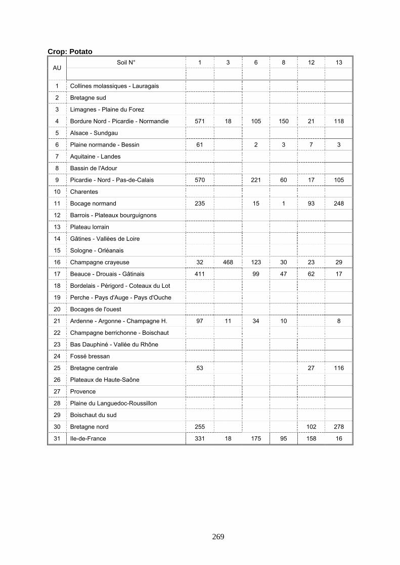
Crop: Potato Soil N° 1 3 6 8 12 13
AU
1 Collines molassiques - Lauragais 2 Bretagne sud 3 Limagnes - Plaine du Forez
571 18 105 118 4 Bordure Nord - Picardie - Normandie 150 21
5 Alsace - Sundgau
6 Plaine normande - Bessin 61 2 3 7 3
7 Aquitaine - Landes
8 Bassin de l'Adour
570 221 60 17 105 9 Picardie - Nord - Pas-de-Calais
10 Charentes
11 Bocage normand 235 15 1 93 248
12 Barrois - Plateaux bourguignons
13 Plateau lorrain
14 Gâtines - Vallées de Loire
15 Sologne - Orléanais
32 468 123 16 Champagne crayeuse 30 23 29
17 Beauce - Drouais - Gâtinais 411 99 47 62 17
18 Bordelais - Périgord - Coteaux du Lot
19 Perche - Pays d'Auge - Pays d'Ouche
20 Bocages de l'ouest
21 Ardenne - Argonne - Champagne H. 97 11 34 10 8
22 Champagne berrichonne - Boischaut
23 Bas Dauphiné - Vallée du Rhône
24 Fossé bressan
25 Bretagne centrale 53 27 116
26 Plateaux de Haute-Saône
27 Provence
28 Plaine du Languedoc-Roussillon
29 Boischaut du sud
255 30 Bretagne nord 102 278
331 18 175 31 Ile-de-France 95 158 16
269
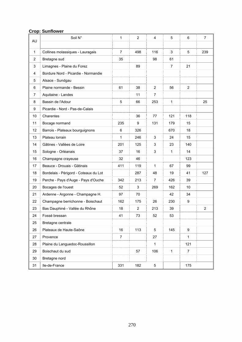
Crop: Sunflower Soil N° 1 2 4 5 6 7
AU
7 498 116 3 5 239 1 Collines molassiques - Lauragais
2 Bretagne sud 35 98 61
89 3 Limagnes - Plaine du Forez 7 21
4 Bordure Nord - Picardie - Normandie
5 Alsace - Sundgau
6 Plaine normande - Bessin 61 38 2 56 2
7 Aquitaine - Landes 11 7
8 Bassin de l'Adour 5 66 253 1 25
9 Picardie - Nord - Pas-de-Calais
36 77 121 118 10 Charentes
11 Bocage normand 235 9 131 179 15
326 12 Barrois - Plateaux bourguignons 6 670 18
13 Plateau lorrain 1 246 3 24 15
201 125 3 23 140 14 Gâtines - Vallées de Loire
16 15 Sologne - Orléanais 37 3 1 14
46 16 Champagne crayeuse 32 123
119 1 17 Beauce - Drouais - Gâtinais 411 67 99
287 48 19 41 127 18 Bordelais - Périgord - Coteaux du Lot
213 19 Perche - Pays d'Auge - Pays d'Ouche 342 7 426 39
52 3 269 162 10 20 Bocages de l'ouest
21 Ardenne - Argonne - Champagne H. 97 70 42 34
162 175 26 230 9 22 Champagne berrichonne - Boischaut
2 213 2 23 Bas Dauphiné - Vallée du Rhône 18 39
73 52 24 Fossé bressan 41 53
25 Bretagne centrale
26 Plateaux de Haute-Saône 16 113 5 145 9
27 Provence 7 27 1
28 Plaine du Languedoc-Roussillon 1 121
57 106 29 Boischaut du sud 1 7
30 Bretagne nord
31 Ile-de-France 331 182 5 175
270
Crop: Sunflower Soil N° 8 9 11 14 15 16
AU
182 4 43 293 57 93 1 Collines molassiques - Lauragais
2 Bretagne sud 205 67 7
3 Limagnes - Plaine du Forez 71 25 35 215 30
4 Bordure Nord - Picardie - Normandie
5 Alsace - Sundgau
6 Plaine normande - Bessin 3 4 12 2 10
7 Aquitaine - Landes 48 20 20 1
8 Bassin de l'Adour 102 52 91 184
9 Picardie - Nord - Pas-de-Calais
22 4 328 36 64 22 10 Charentes
11 Bocage normand 1 3 161 48 82
12 Barrois - Plateaux bourguignons 55 62 118 11 46 58
13 Plateau lorrain 57 25 13 18 18
1 100 66 43 14 Gâtines - Vallées de Loire
15 Sologne - Orléanais 5 60 6 1
16 Champagne crayeuse 30 72 54 9 54
59 17 Beauce - Drouais - Gâtinais 47 5 15 7
97 18 Bordelais - Périgord - Coteaux du Lot 131 159 53 33
19 Perche - Pays d'Auge - Pays d'Ouche 29 12 25 20 4
20 Bocages de l'ouest 18 25 130 496 1
21 Ardenne - Argonne - Champagne H. 10 60 26 128 18
22 Champagne berrichonne - Boischaut 118 17 51 4
124 23 Bas Dauphiné - Vallée du Rhône 159 61
39 4 24 Fossé bressan 50 6 64
25 Bretagne centrale
26 Plateaux de Haute-Saône 22 34 13
27 Provence 84 214
28 Plaine du Languedoc-Roussillon 89 25 150 45
29 Boischaut du sud 16 17 190 59 16
30 Bretagne nord
31 Ile-de-France 95 8 74 14 23
271

Appendix 17 : Soil hydraulic parameterization
272

273
1/ SOIL HYDRAULIC PARAMETERIZATION FOR SOIL-TYPE 1
Table 68: Topsoil horizons parameters for the relevant AU/soil combinations (topsoil parameter values differ for each AU due to OC correction) for soil-type 1
AU ID
Horizon ID
Horizon Thickness (cm)
Numerical layers
(-)
pH CaCl2
(-)
Saturated water content (m3/m3)
Residual water content (m3/m3)
Alpha
(1/cm)
n (-) Saturated conductivity (m/day)
L (-) Rho (g/cm3)
1 1 0.29 12 6.21 0.4170 0.01 0.0185 1.2093 0.1199 -2.4903 1459.2 2 0.01 1 6.70 0.4067 0.01 0.0187 1.1493 0.1129 -3.5634 1522.2 2 1 0.29 12 6.21 0.4596 0.01 0.0234 1.1887 0.1340 -2.5147 1306.6 2 0.01 1 6.70 0.4424 0.01 0.0229 1.1470 0.1370 -3.5287 1395.5 4 1 0.29 12 6.21 0.4283 0.01 0.0198 1.2055 0.1256 -2.5347 1419.1 2 0.01 1 6.70 0.4162 0.01 0.0199 1.1497 0.1206 -3.5908 1489.1 5 1 0.29 12 6.21 0.4250 0.01 0.0194 1.2067 0.1240 -2.5252 1430.9 2 0.01 1 6.70 0.4134 0.01 0.0196 1.1496 0.1184 -3.5860 1498.8 6 1 0.29 12 6.21 0.4453 0.01 0.0217 1.1973 0.1315 -2.5457 1358.0 2 0.01 1 6.70 0.4305 0.01 0.0216 1.1489 0.1305 -3.5790 1438.4 8 1 0.29 12 6.21 0.4324 0.01 0.0203 1.2037 0.1273 -2.5431 1404.3 2 0.01 1 6.70 0.4196 0.01 0.0203 1.1496 0.1232 -3.5934 1476.8 9 1 0.29 12 6.21 0.4289 0.01 0.0199 1.2052 0.1258 -2.5361 1417.1 2 0.01 1 6.70 0.4167 0.01 0.0200 1.1497 0.1210 -3.5914 1487.4 11 1 0.29 12 6.21 0.4562 0.01 0.0230 1.1909 0.1336 -2.5248 1318.8 2 0.01 1 6.70 0.4396 0.01 0.0226 1.1475 0.1356 -3.5436 1405.7 12 1 0.29 12 6.21 0.4436 0.01 0.0215 1.1983 0.1310 -2.5472 1364.4 2 0.01 1 6.70 0.4290 0.01 0.0214 1.1490 0.1295 -3.5829 1443.7 13 1 0.29 12 6.21 0.4386 0.01 0.0210 1.2008 0.1296 -2.5484 1382.2 2 0.01 1 6.70 0.4248 0.01 0.0210 1.1494 0.1268 -3.5906 1458.5 14 1 0.29 12 6.21 0.4254 0.01 0.0195 1.2066 0.1242 -2.5264 1429.6 2 0.01 1 6.70 0.4137 0.01 0.0196 1.1496 0.1187 -3.5866 1497.7 15 1 0.29 12 6.21 0.4194 0.01 0.0188 1.2086 0.1212 -2.5026 1450.7 2 0.01 1 6.70 0.4087 0.01 0.0190 1.1494 0.1146 -3.5718 1515.2 16 1 0.29 12 6.21 0.4423 0.01 0.0214 1.1989 0.1307 -2.5479 1368.8 2 0.01 1 6.70 0.4279 0.01 0.0213 1.1491 0.1289 -3.5852 1447.4 17 1 0.29 12 6.21 0.4281 0.01 0.0198 1.2056 0.1255 -2.5341 1420.0 2 0.01 1 6.70 0.4160 0.01 0.0199 1.1497 0.1204 -3.5905 1489.8 19 1 0.29 12 6.21 0.4271 0.01 0.0197 1.2059 0.1250 -2.5314 1423.6 2 0.01 1 6.70 0.4151 0.01 0.0198 1.1497 0.1198 -3.5893 1492.8 20 1 0.29 12 6.21 0.4371 0.01 0.0208 1.2016 0.1290 -2.5479 1387.7 2 0.01 1 6.70 0.4235 0.01 0.0208 1.1495 0.1260 -3.5920 1463.1 21 1 0.29 12 6.21 0.4374 0.01 0.0208 1.2014 0.1291 -2.5480 1386.6 2 0.01 1 6.70 0.4238 0.01 0.0208 1.1494 0.1261 -3.5917 1462.1 22 1 0.29 12 6.21 0.4305 0.01 0.0200 1.2046 0.1265 -2.5396 1411.4 2 0.01 1 6.70 0.4180 0.01 0.0201 1.1497 0.1220 -3.5926 1482.7 23 1 0.29 12 6.21 0.4229 0.01 0.0192 1.2075 0.1230 -2.5177 1438.3 2 0.01 1 6.70 0.4117 0.01 0.0194 1.1496 0.1170 -3.5816 1504.9 24 1 0.29 12 6.21 0.4229 0.01 0.0192 1.2075 0.1230 -2.5175 1438.5 2 0.01 1 6.70 0.4116 0.01 0.0193 1.1496 0.1170 -3.5815 1505.1 25 1 0.29 12 6.21 0.4748 0.01 0.0253 1.1783 0.1342 -2.4526 1251.2 2 0.01 1 6.70 0.4551 0.01 0.0243 1.1438 0.1421 -3.4417 1349.1 26 1 0.29 12 6.21 0.4347 0.01 0.0205 1.2027 0.1282 -2.5460 1396.1

2 0.01 1 6.70 0.4216 0.01 0.0206 1.1496 0.1246 -3.5933 1470.0 27 1 0.29 12 6.21 0.4164 0.01 0.0184 1.2095 0.1195 -2.4867 1461.5 2 0.01 1 6.70 0.4062 0.01 0.0187 1.1492 0.1124 -3.5608 1524.1 30 1 0.29 12 6.21 0.4512 0.01 0.0224 1.1939 0.1328 -2.5366 1336.7 2 0.01 1 6.70 0.4354 0.01 0.0222 1.1482 0.1334 -3.5621 1420.6 31 1 0.29 12 6.21 0.4212 0.01 0.0190 1.2080 0.1222 -2.5109 1444.2 2 0.01 1 6.70 0.4102 0.01 0.0192 1.1495 0.1159 -3.5773 1509.8
Table 69: Subsoil horizons parameters for soil-type 1
AU ID
Horizon ID
Horizon Thickness (cm)
Numerical layers
Residual water content (m3/m3)
Alpha n (-) Saturated conductivity (m/day)
L (-) Rho (g/cm3)
Saturated water content (m3/m3)
pH CaCl2
(1/cm) (-) (-)
all 3 0.11 4 0.4220 0.01 0.0191 1.1195 0.117 -3.5842 1501.536.70 4 0.19 4 0.4188 0.01 0.0187 1.1157 0.1095 -3.6399 1514.586.89 5 0.15 3 0.4188 0.01 0.0187 1.1157 0.1095 -3.6399 1514.586.89 6 0.25 5 0.3987 0.01 0.0169 1.1105 0.0896 -3.5579 1584.456.99 7 0.25 3 0.3992 0.01 0.0195 1.0696 0.0387 -4.2722 1603.796.89 8 0.1 10 0.3992 0.01 0.0195 1.0696 0.0387 -4.2722 1603.796.89 9 0.65 7 0.3992 0.01 0.0195 1.0696 0.0387 -4.2722 1603.796.89
274
275
2/ SOIL HYDRAULIC PARAMETERIZATION FOR SOIL-TYPE 2
Table 70: Topsoil horizons parameters for the relevant AU/soil combinations (topsoil parameter values differ for each AU due to OC correction) for soil-type 2
AU ID
Horizon ID
Horizon Thickness (cm)
Numerical layers
(-)
pH CaCl2
(-)
Saturated water content (m3/m3)
Residual water content (m3/m3)
Alpha
(1/cm)
n (-) Saturated conductivity (m/day)
L (-) Rho (g/cm3)
1 1 0.2 8 7.16 0.4417 0.01 0.0195 1.1457 0.1045 -3.4859 1398.5 2 0.1 4 6.96 0.4054 0.01 0.0150 1.1333 0.0823 -3.7378 1536.5 3 1 0.2 8 7.16 0.4606 0.01 0.0217 1.1410 0.1100 -3.3418 1329.3 2 0.1 4 6.96 0.4189 0.01 0.0166 1.1347 0.0911 -3.7544 1489.6 4 1 0.2 8 7.16 0.4545 0.01 0.0210 1.1428 0.1086 -3.3960 1352.0 2 0.1 4 6.96 0.4145 0.01 0.0161 1.1344 0.0884 -3.7560 1505.0 5 1 0.2 8 7.16 0.4507 0.01 0.0206 1.1437 0.1075 -3.4255 1365.6 2 0.1 4 6.96 0.4118 0.01 0.0158 1.1341 0.0866 -3.7538 1514.3 6 1 0.2 8 7.16 0.4736 0.01 0.0232 1.1365 0.1119 -3.2084 1281.2 2 0.1 4 6.96 0.4281 0.01 0.0176 1.1349 0.0963 -3.7311 1456.7 7 1 0.2 8 7.16 0.4392 0.01 0.0193 1.1461 0.1035 -3.4995 1407.5 2 0.1 4 6.96 0.4037 0.01 0.0148 1.1330 0.0810 -3.7305 1542.5 8 1 0.2 8 7.16 0.4592 0.01 0.0215 1.1414 0.1097 -3.3554 1334.8 2 0.1 4 6.96 0.4178 0.01 0.0164 1.1346 0.0904 -3.7554 1493.3 9 1 0.2 8 7.16 0.4551 0.01 0.0211 1.1426 0.1087 -3.3905 1349.6 2 0.1 4 6.96 0.4149 0.01 0.0161 1.1344 0.0887 -3.7562 1503.4 10 1 0.2 8 7.16 0.4630 0.01 0.0220 1.1402 0.1105 -3.3192 1320.6 2 0.1 4 6.96 0.4206 0.01 0.0168 1.1348 0.0921 -3.7521 1483.6 11 1 0.2 8 7.16 0.4857 0.01 0.0248 1.1316 0.1124 -3.0655 1236.1 2 0.1 4 6.96 0.4368 0.01 0.0185 1.1345 0.1006 -3.6874 1425.6 12 1 0.2 8 7.16 0.4716 0.01 0.0230 1.1372 0.1117 -3.2303 1288.6 2 0.1 4 6.96 0.4267 0.01 0.0174 1.1349 0.0956 -3.7363 1461.8 13 1 0.2 8 7.16 0.4661 0.01 0.0223 1.1392 0.1110 -3.2886 1309.2 2 0.1 4 6.96 0.4228 0.01 0.0170 1.1348 0.0934 -3.7477 1475.8 14 1 0.2 8 7.16 0.4512 0.01 0.0206 1.1436 0.1076 -3.4224 1364.1 2 0.1 4 6.96 0.4121 0.01 0.0158 1.1342 0.0868 -3.7542 1513.2 15 1 0.2 8 7.16 0.4444 0.01 0.0199 1.1452 0.1055 -3.4695 1388.7 2 0.1 4 6.96 0.4073 0.01 0.0153 1.1336 0.0836 -3.7443 1529.8 16 1 0.2 8 7.16 0.4703 0.01 0.0228 1.1377 0.1116 -3.2452 1293.7 2 0.1 4 6.96 0.4257 0.01 0.0173 1.1349 0.0950 -3.7396 1465.3 17 1 0.2 8 7.16 0.4542 0.01 0.0209 1.1429 0.1085 -3.3983 1353.0 2 0.1 4 6.96 0.4143 0.01 0.0160 1.1344 0.0882 -3.7560 1505.7 18 1 0.2 8 7.16 0.4378 0.01 0.0191 1.1464 0.1029 -3.5064 1412.5 2 0.1 4 6.96 0.4027 0.01 0.0147 1.1328 0.0803 -3.7260 1545.9 19 1 0.2 8 7.16 0.4531 0.01 0.0208 1.1432 0.1082 -3.4074 1357.1 2 0.1 4 6.96 0.4135 0.01 0.0160 1.1343 0.0877 -3.7555 1508.5 20 1 0.2 8 7.16 0.4644 0.01 0.0221 1.1398 0.1107 -3.3060 1315.6 2 0.1 4 6.96 0.4215 0.01 0.0169 1.1348 0.0927 -3.7504 1480.2 21 1 0.2 8 7.16 0.4647 0.01 0.0222 1.1397 0.1108 -3.3024 1314.3 2 0.1 4 6.96 0.4218 0.01 0.0169 1.1348 0.0928 -3.7499 1479.3 22 1 0.2 8 7.16 0.4569 0.01 0.0213 1.1421 0.1092 -3.3751 1343.0 2 0.1 4 6.96 0.4162 0.01 0.0163 1.1345 0.0895 -3.7562 1498.9
23 1 0.2 8 7.16 0.4484 0.01 0.0203 1.1443 0.1068 -3.4428 1374.2 2 0.1 4 6.96 0.4101 0.01 0.0156 1.1339 0.0855 -3.7512 1520.1 24 1 0.2 8 7.16 0.4483 0.01 0.0203 1.1443 0.1068 -3.4433 1374.4 2 0.1 4 6.96 0.4101 0.01 0.0156 1.1339 0.0855 -3.7511 1520.2 29 1 0.2 8 7.16 0.4570 0.01 0.0213 1.1421 0.1092 -3.3744 1342.7 2 0.1 4 6.96 0.4163 0.01 0.0163 1.1345 0.0895 -3.7561 1498.7 30 1 0.2 8 7.16 0.4802 0.01 0.0241 1.1339 0.1123 -3.1324 1256.7 2 0.1 4 6.96 0.4329 0.01 0.0181 1.1347 0.0988 -3.7097 1439.8 31 1 0.2 8 7.16 0.4465 0.01 0.0201 1.1447 0.1062 -3.4560 1381.1 2 0.1 4 6.96 0.4088 0.01 0.0154 1.1338 0.0846 -3.7482 1524.7
Table 71: Subsoil horizons parameters for soil-type 2
AU ID
Horizon ID
Horizon Thickness (cm)
Numerical layers
Residual water content (m3/m3)
Alpha n (-) Saturated conductivity (m/day)
L (-) Rho (g/cm3)
pH CaCl2
Saturated water content (m3/m3)
(1/cm) (-) (-)
all 3 0.2 8 0.4210 0.01 0.0149 1.1034 0.0835 -3.7528 1516.8 6.96 4 0.1 2 0.4149 0.01 0.0137 1.0994 0.0740 -3.7747 1540.5 6.96 5 0.2 4 0.4149 0.01 0.0137 1.0994 0.0740 -3.7747 1540.5 6.96 6 0.2 4 0.4019 0.01 0.0128 1.0784 0.0455 -3.9787 1597.1 6.67 7 0.15 15 0.4019 0.01 0.0128 1.0784 0.0455 -3.9787 1597.1 6.67 8 0.85 9 0.4019 0.01 0.0128 1.0784 0.0455 -3.9787 1597.1 6.67
276

277
3/ SOIL HYDRAULIC PARAMETERIZATION FOR SOIL-TYPE 3
Table 72: Topsoil horizons parameters for the relevant AU/soil combinations (topsoil parameter values differ for each AU due to OC correction) for soil-type 3
AU ID
Horizon ID
Horizon Thickness (cm)
Numerical layers
(-)
pH CaCl2
(-)
Saturated water content (m3/m3)
Residual water content (m3/m3)
Alpha
(1/cm)
n (-) Saturated conductivity (m/day)
L (-) Rho (g/cm3)
4 1 0.25 10 7.35 0.4438 0.01 0.0409 1.1635 0.3510 -3.5135 1377.0 2 0.05 2 7.55 0.4119 0.01 0.0397 1.1632 0.3133 -3.6907 1493.5 7 1 0.25 10 7.35 0.4291 0.01 0.0399 1.1677 0.3339 -3.5554 1429.6 2 0.05 2 7.55 0.4007 0.01 0.0383 1.1630 0.2894 -3.6364 1532.5 16 1 0.25 10 7.35 0.4590 0.01 0.0417 1.1575 0.3619 -3.4269 1321.6 2 0.05 2 7.55 0.4235 0.01 0.0408 1.1621 0.3344 -3.7042 1452.4 18 1 0.25 10 7.35 0.4278 0.01 0.0398 1.1680 0.3321 -3.5569 1434.3 2 0.05 2 7.55 0.3997 0.01 0.0381 1.1629 0.2871 -3.6293 1535.9 21 1 0.25 10 7.35 0.4536 0.01 0.0414 1.1598 0.3589 -3.4617 1341.1 2 0.05 2 7.55 0.4194 0.01 0.0405 1.1626 0.3275 -3.7040 1466.9 26 1 0.25 10 7.35 0.4508 0.01 0.0413 1.1610 0.3569 -3.4785 1351.6 2 0.05 2 7.55 0.4172 0.01 0.0403 1.1628 0.3235 -3.7019 1474.7 28 1 0.25 10 7.35 0.4218 0.01 0.0393 1.1691 0.3230 -3.5577 1455.8 2 0.05 2 7.55 0.3952 0.01 0.0375 1.1625 0.2762 -3.5911 1551.7 31 1 0.25 10 7.35 0.4361 0.01 0.0405 1.1659 0.3429 -3.5412 1404.6 2 0.05 2 7.55 0.4060 0.01 0.0390 1.1632 0.3012 -3.6678 1514.0
Table 73: Subsoil horizons parameters for soil-type 3
AU ID
Horizon ID
Horizon Thickness (cm)
Numerical layers
(-)
pH CaCl2
(-)
Saturated water content (m3/m3)
Residual water content (m3/m3)
Alpha
(1/cm)
n (-) Saturated conductivity (m/day)
L (-) Rho (g/cm3)
all 3 0.2 8 7.55 0.4142 0.01 0.0396 1.1342 0.1695 -3.6784 1505.8 4 0.1 2 7.65 0.4059 0.01 0.0423 1.1431 0.1773 -3.5273 1528.4 5 0.1 2 7.65 0.4059 0.01 0.0423 1.1431 0.1773 -3.5273 1528.4 6 0.25 5 7.55 0.3967 0.01 0.0508 1.1394 0.1653 -3.6869 1553.3 7 0.1 10 7.55 0.3967 0.01 0.0508 1.1394 0.1653 -3.6869 1553.3 8 0.95 10 7.55 0.3967 0.01 0.0508 1.1394 0.1653 -3.6869 1553.3
278
4/ SOIL HYDRAULIC PARAMETERIZATION FOR SOIL-TYPE 4
Table 74: Topsoil horizons parameters for the relevant AU/soil combinations (topsoil parameter values differ for each AU due to OC correction) for soil-type 4
AU ID
Horizon ID
Horizon Thickness (cm)
Numerical layers
(-)
pH CaCl2
(-)
Saturated water content (m3/m3)
Residual water content (m3/m3)
Alpha
(1/cm)
n (-) Saturated conductivity (m/day)
L (-) Rho (g/cm3)
1 1 0.25 10 5.56 0.4221 0.01 0.0405 1.2093 0.3801 -2.8509 1438.4 2 0.05 2 6.53 0.3942 0.01 0.0409 1.1650 0.3067 -3.5976 1552.6 2 1 0.25 10 5.56 0.4668 0.01 0.0426 1.1841 0.4141 -2.7981 1277.5 2 0.05 2 6.53 0.4266 0.01 0.0443 1.1639 0.3788 -3.7133 1438.9 4 1 0.25 10 5.56 0.4340 0.01 0.0413 1.2042 0.3958 -2.8733 1396.1 2 0.05 2 6.53 0.4028 0.01 0.0421 1.1657 0.3291 -3.6639 1523.0 5 1 0.25 10 5.56 0.4305 0.01 0.0411 1.2058 0.3917 -2.8701 1408.5 2 0.05 2 6.53 0.4002 0.01 0.0417 1.1656 0.3228 -3.6476 1531.7 6 1 0.25 10 5.56 0.4519 0.01 0.0420 1.1941 0.4103 -2.8528 1331.6 2 0.05 2 6.53 0.4157 0.01 0.0435 1.1653 0.3584 -3.7123 1477.4 7 1 0.25 10 5.56 0.4198 0.01 0.0403 1.2101 0.3765 -2.8425 1446.6 2 0.05 2 6.53 0.3925 0.01 0.0406 1.1648 0.3021 -3.5810 1558.3 8 1 0.25 10 5.56 0.4383 0.01 0.0415 1.2020 0.4004 -2.8737 1380.4 2 0.05 2 6.53 0.4059 0.01 0.0425 1.1657 0.3367 -3.6810 1511.9 9 1 0.25 10 5.56 0.4346 0.01 0.0413 1.2039 0.3965 -2.8736 1393.9 2 0.05 2 6.53 0.4032 0.01 0.0421 1.1657 0.3302 -3.6665 1521.4 10 1 0.25 10 5.56 0.4419 0.01 0.0416 1.2000 0.4037 -2.8713 1367.5 2 0.05 2 6.53 0.4085 0.01 0.0428 1.1657 0.3428 -3.6924 1502.8 11 1 0.25 10 5.56 0.4633 0.01 0.0424 1.1866 0.4138 -2.8136 1290.3 2 0.05 2 6.53 0.4240 0.01 0.0442 1.1643 0.3743 -3.7159 1448.1 13 1 0.25 10 5.56 0.4448 0.01 0.0418 1.1984 0.4059 -2.8676 1357.1 2 0.05 2 6.53 0.4106 0.01 0.0430 1.1657 0.3475 -3.6999 1495.5 14 1 0.25 10 5.56 0.4309 0.01 0.0411 1.2056 0.3922 -2.8705 1407.1 2 0.05 2 6.53 0.4005 0.01 0.0418 1.1656 0.3235 -3.6495 1530.7 15 1 0.25 10 5.56 0.4246 0.01 0.0407 1.2083 0.3838 -2.8584 1429.4 2 0.05 2 6.53 0.3960 0.01 0.0412 1.1652 0.3117 -3.6142 1546.3 17 1 0.25 10 5.56 0.4337 0.01 0.0413 1.2043 0.3955 -2.8731 1397.0 2 0.05 2 6.53 0.4026 0.01 0.0421 1.1657 0.3286 -3.6628 1523.6 18 1 0.25 10 5.56 0.4185 0.01 0.0402 1.2105 0.3744 -2.8373 1451.0 2 0.05 2 6.53 0.3916 0.01 0.0405 1.1647 0.2995 -3.5714 1561.4 19 1 0.25 10 5.56 0.4326 0.01 0.0412 1.2048 0.3943 -2.8724 1400.8 2 0.05 2 6.53 0.4018 0.01 0.0420 1.1656 0.3267 -3.6580 1526.3 20 1 0.25 10 5.56 0.4432 0.01 0.0417 1.1993 0.4047 -2.8699 1362.9 2 0.05 2 6.53 0.4094 0.01 0.0429 1.1657 0.3449 -3.6959 1499.6 22 1 0.25 10 5.56 0.4362 0.01 0.0414 1.2030 0.3983 -2.8740 1387.9 2 0.05 2 6.53 0.4044 0.01 0.0423 1.1657 0.3331 -3.6733 1517.2 23 1 0.25 10 5.56 0.4283 0.01 0.0409 1.2068 0.3889 -2.8667 1416.3 2 0.05 2 6.53 0.3987 0.01 0.0415 1.1655 0.3187 -3.6361 1537.1 24 1 0.25 10 5.56 0.4282 0.01 0.0409 1.2068 0.3889 -2.8666 1416.5 2 0.05 2 6.53 0.3986 0.01 0.0415 1.1655 0.3186 -3.6357 1537.3 25 1 0.25 10 5.56 0.4829 0.01 0.0433 1.1723 0.4104 -2.7143 1219.3 2 0.05 2 6.53 0.4383 0.01 0.0449 1.1612 0.3963 -3.6817 1397.1
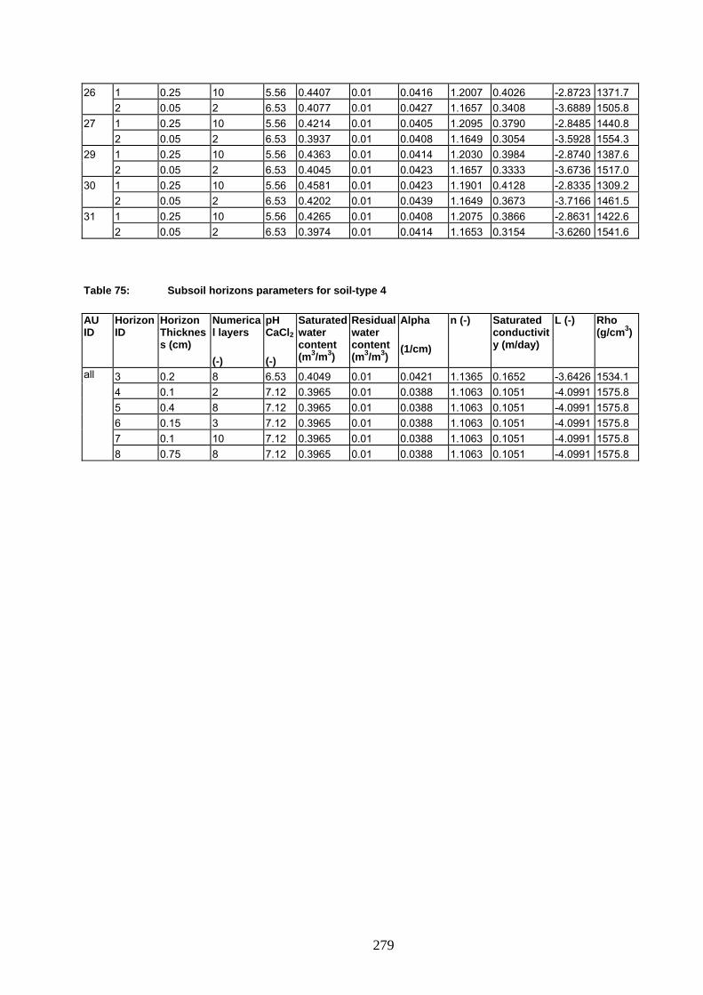
26 1 0.25 10 5.56 0.4407 0.01 0.0416 1.2007 0.4026 -2.8723 1371.7 2 0.05 2 6.53 0.4077 0.01 0.0427 1.1657 0.3408 -3.6889 1505.8 27 1 0.25 10 5.56 0.4214 0.01 0.0405 1.2095 0.3790 -2.8485 1440.8 2 0.05 2 6.53 0.3937 0.01 0.0408 1.1649 0.3054 -3.5928 1554.3 29 1 0.25 10 5.56 0.4363 0.01 0.0414 1.2030 0.3984 -2.8740 1387.6 2 0.05 2 6.53 0.4045 0.01 0.0423 1.1657 0.3333 -3.6736 1517.0 30 1 0.25 10 5.56 0.4581 0.01 0.0423 1.1901 0.4128 -2.8335 1309.2 2 0.05 2 6.53 0.4202 0.01 0.0439 1.1649 0.3673 -3.7166 1461.5 31 1 0.25 10 5.56 0.4265 0.01 0.0408 1.2075 0.3866 -2.8631 1422.6 2 0.05 2 6.53 0.3974 0.01 0.0414 1.1653 0.3154 -3.6260 1541.6
Table 75: Subsoil horizons parameters for soil-type 4
AU ID
Horizon ID
Horizon Thickness (cm)
Numerical layers
Residual water content (m3/m3)
Alpha n (-) Saturated conductivity (m/day)
L (-) Rho (g/cm3)
pH CaCl2
Saturated water content (m3/m3)
(1/cm) (-) (-)
all 3 0.2 8 6.53 0.4049 0.01 0.0421 1.1365 0.1652 -3.6426 1534.1 4 0.1 2 7.12 0.3965 0.01 0.0388 1.1063 0.1051 -4.0991 1575.8 5 0.4 8 7.12 0.3965 0.01 0.0388 1.1063 0.1051 -4.0991 1575.8 6 0.15 3 7.12 0.3965 0.01 0.0388 1.1063 0.1051 -4.0991 1575.8 7 0.1 10 7.12 0.3965 0.01 0.0388 1.1063 0.1051 -4.0991 1575.8 8 0.75 8 7.12 0.3965 0.01 0.0388 1.1063 0.1051 -4.0991 1575.8
279

280
5/ SOIL HYDRAULIC PARAMETERIZATION FOR SOIL-TYPE 5
Table 76: Topsoil horizons parameters for the relevant AU/soil combinations (topsoil parameter values differ for each AU due to OC correction) for soil-type 5
AU ID
Horizon ID
Horizon Thickness (cm)
Numerical layers
(-)
pH CaCl2
(-)
Saturated water content (m3/m3)
Residual water content (m3/m3)
Alpha
(1/cm)
n (-) Saturated conductivity (m/day)
L (-) Rho (g/cm3)
1 1 0.1 4 5.97 0.4551 0.01 0.0206 1.1609 0.1020 -3.0627 1336.5 2 0.18 8 5.28 0.4335 0.01 0.0181 1.1638 0.0954 -3.2228 1417.0 3 0.02 1 5.58 0.4233 0.01 0.0191 1.1377 0.1110 -3.7524 1472.0 2 1 0.1 4 5.97 0.5091 0.01 0.0291 1.1330 0.1004 -2.5881 1136.8 2 0.18 8 5.28 0.4798 0.01 0.0238 1.1462 0.1036 -2.9263 1247.7 3 0.02 1 5.58 0.4640 0.01 0.0235 1.1320 0.1296 -3.4661 1324.6 3 1 0.1 4 5.97 0.4765 0.01 0.0234 1.1510 0.1040 -2.9034 1257.9 2 0.18 8 5.28 0.4518 0.01 0.0202 1.1585 0.1008 -3.1474 1350.7 3 0.02 1 5.58 0.4394 0.01 0.0209 1.1368 0.1204 -3.6837 1414.5 6 1 0.1 4 5.97 0.4912 0.01 0.0256 1.1431 0.1032 -2.7671 1203.5 2 0.18 8 5.28 0.4644 0.01 0.0217 1.1535 0.1029 -3.0607 1304.6 3 0.02 1 5.58 0.4504 0.01 0.0221 1.1351 0.1253 -3.6005 1374.3 8 1 0.1 4 5.97 0.4748 0.01 0.0232 1.1519 0.1039 -2.9178 1264.1 2 0.18 8 5.28 0.4504 0.01 0.0200 1.1590 0.1005 -3.1557 1355.9 3 0.02 1 5.58 0.4381 0.01 0.0208 1.1369 0.1197 -3.6915 1419.0 10 1 0.1 4 5.97 0.4792 0.01 0.0238 1.1496 0.1039 -2.8797 1247.9 2 0.18 8 5.28 0.4542 0.01 0.0205 1.1576 0.1013 -3.1334 1342.3 3 0.02 1 5.58 0.4414 0.01 0.0211 1.1365 0.1214 -3.6705 1407.1 11 1 0.1 4 5.97 0.5049 0.01 0.0282 1.1354 0.1012 -2.6308 1152.6 2 0.18 8 5.28 0.4762 0.01 0.0233 1.1480 0.1036 -2.9604 1261.2 3 0.02 1 5.58 0.4608 0.01 0.0232 1.1328 0.1288 -3.5008 1336.4 12 1 0.1 4 5.97 0.4889 0.01 0.0253 1.1443 0.1034 -2.7889 1211.8 2 0.18 8 5.28 0.4625 0.01 0.0215 1.1543 0.1026 -3.0755 1311.6 3 0.02 1 5.58 0.4488 0.01 0.0219 1.1354 0.1246 -3.6149 1380.4 13 1 0.1 4 5.97 0.4827 0.01 0.0243 1.1477 0.1038 -2.8480 1235.1 2 0.18 8 5.28 0.4571 0.01 0.0208 1.1565 0.1018 -3.1140 1331.4 3 0.02 1 5.58 0.4440 0.01 0.0214 1.1362 0.1226 -3.6520 1397.6 14 1 0.1 4 5.97 0.4658 0.01 0.0220 1.1563 0.1034 -2.9905 1297.4 2 0.18 8 5.28 0.4427 0.01 0.0191 1.1615 0.0984 -3.1937 1384.1 3 0.02 1 5.58 0.4313 0.01 0.0200 1.1375 0.1160 -3.7266 1443.4 15 1 0.1 4 5.97 0.4582 0.01 0.0210 1.1597 0.1025 -3.0437 1325.3 2 0.18 8 5.28 0.4362 0.01 0.0184 1.1632 0.0963 -3.2163 1407.6 3 0.02 1 5.58 0.4256 0.01 0.0194 1.1377 0.1125 -3.7468 1463.8 17 1 0.1 4 5.97 0.4692 0.01 0.0224 1.1546 0.1037 -2.9640 1284.7 2 0.18 8 5.28 0.4456 0.01 0.0195 1.1606 0.0993 -3.1806 1373.4 3 0.02 1 5.58 0.4339 0.01 0.0203 1.1373 0.1175 -3.7146 1434.2 18 1 0.1 4 5.97 0.4508 0.01 0.0201 1.1626 0.1011 -3.0872 1352.4 2 0.18 8 5.28 0.4298 0.01 0.0176 1.1646 0.0939 -3.2293 1430.4 3 0.02 1 5.58 0.4200 0.01 0.0187 1.1376 0.1088 -3.7576 1483.5 19 1 0.1 4 5.97 0.4680 0.01 0.0222 1.1552 0.1036 -2.9740 1289.4 2 0.18 8 5.28 0.4445 0.01 0.0193 1.1609 0.0990 -3.1857 1377.4 3 0.02 1 5.58 0.4329 0.01 0.0202 1.1374 0.1169 -3.7193 1437.6
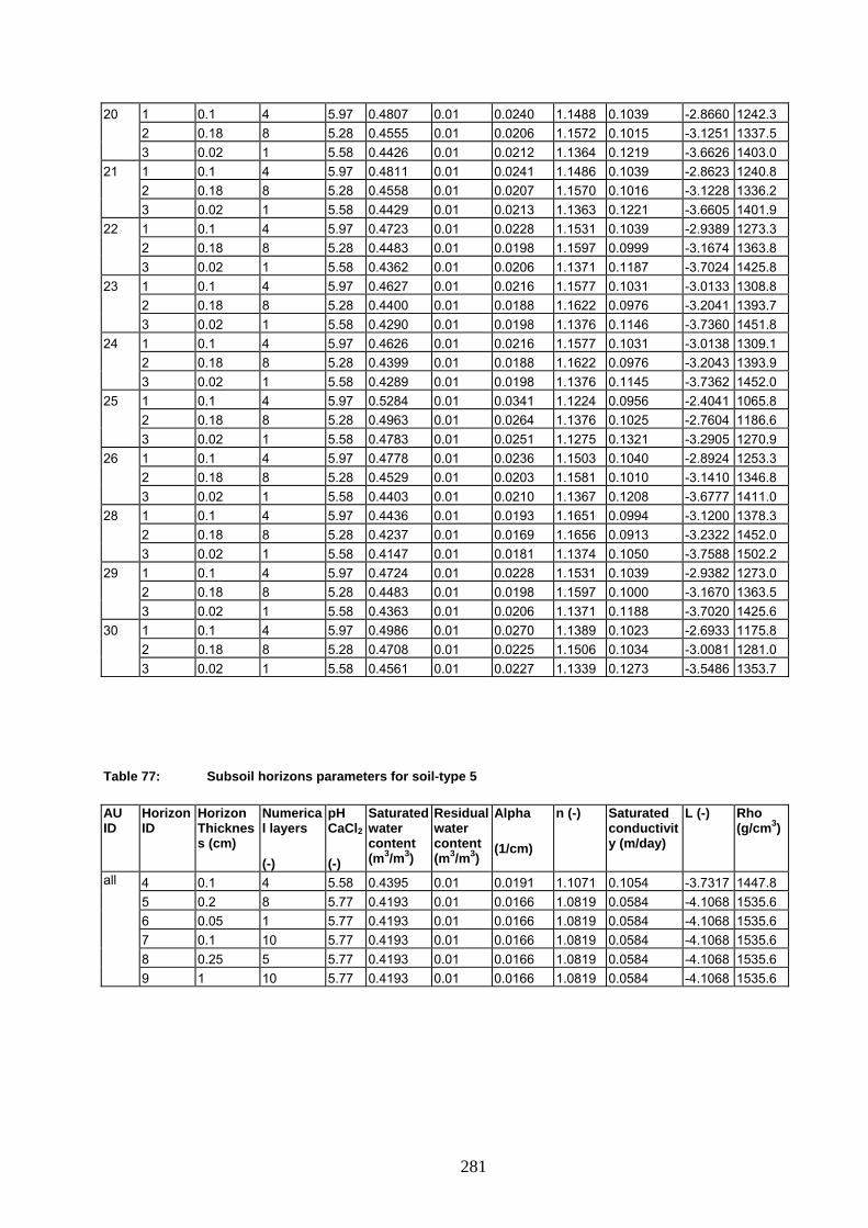
281
20 1 0.1 4 5.97 0.4807 0.01 0.0240 1.1488 0.1039 -2.8660 1242.3 2 0.18 8 5.28 0.4555 0.01 0.0206 1.1572 0.1015 -3.1251 1337.5 3 0.02 1 5.58 0.4426 0.01 0.0212 1.1364 0.1219 -3.6626 1403.0 21 1 0.1 4 5.97 0.4811 0.01 0.0241 1.1486 0.1039 -2.8623 1240.8 2 0.18 8 5.28 0.4558 0.01 0.0207 1.1570 0.1016 -3.1228 1336.2 3 0.02 1 5.58 0.4429 0.01 0.0213 1.1363 0.1221 -3.6605 1401.9 22 1 0.1 4 5.97 0.4723 0.01 0.0228 1.1531 0.1039 -2.9389 1273.3 2 0.18 8 5.28 0.4483 0.01 0.0198 1.1597 0.0999 -3.1674 1363.8 3 0.02 1 5.58 0.4362 0.01 0.0206 1.1371 0.1187 -3.7024 1425.8 23 1 0.1 4 5.97 0.4627 0.01 0.0216 1.1577 0.1031 -3.0133 1308.8 2 0.18 8 5.28 0.4400 0.01 0.0188 1.1622 0.0976 -3.2041 1393.7 3 0.02 1 5.58 0.4290 0.01 0.0198 1.1376 0.1146 -3.7360 1451.8 24 1 0.1 4 5.97 0.4626 0.01 0.0216 1.1577 0.1031 -3.0138 1309.1 2 0.18 8 5.28 0.4399 0.01 0.0188 1.1622 0.0976 -3.2043 1393.9 3 0.02 1 5.58 0.4289 0.01 0.0198 1.1376 0.1145 -3.7362 1452.0 25 1 0.1 4 5.97 0.5284 0.01 0.0341 1.1224 0.0956 -2.4041 1065.8 2 0.18 8 5.28 0.4963 0.01 0.0264 1.1376 0.1025 -2.7604 1186.6 3 0.02 1 5.58 0.4783 0.01 0.0251 1.1275 0.1321 -3.2905 1270.9 26 1 0.1 4 5.97 0.4778 0.01 0.0236 1.1503 0.1040 -2.8924 1253.3 2 0.18 8 5.28 0.4529 0.01 0.0203 1.1581 0.1010 -3.1410 1346.8 3 0.02 1 5.58 0.4403 0.01 0.0210 1.1367 0.1208 -3.6777 1411.0 28 1 0.1 4 5.97 0.4436 0.01 0.0193 1.1651 0.0994 -3.1200 1378.3 2 0.18 8 5.28 0.4237 0.01 0.0169 1.1656 0.0913 -3.2322 1452.0 3 0.02 1 5.58 0.4147 0.01 0.0181 1.1374 0.1050 -3.7588 1502.2 29 1 0.1 4 5.97 0.4724 0.01 0.0228 1.1531 0.1039 -2.9382 1273.0 2 0.18 8 5.28 0.4483 0.01 0.0198 1.1597 0.1000 -3.1670 1363.5 3 0.02 1 5.58 0.4363 0.01 0.0206 1.1371 0.1188 -3.7020 1425.6 30 1 0.1 4 5.97 0.4986 0.01 0.0270 1.1389 0.1023 -2.6933 1175.8 2 0.18 8 5.28 0.4708 0.01 0.0225 1.1506 0.1034 -3.0081 1281.0 3 0.02 1 5.58 0.4561 0.01 0.0227 1.1339 0.1273 -3.5486 1353.7
Table 77: Subsoil horizons parameters for soil-type 5
AU ID
Horizon ID
Horizon Thickness (cm)
Numerical layers
(-)
pH CaCl2
(-)
Saturated water content (m3/m3)
Residual water content (m3/m3)
Alpha
(1/cm)
n (-) Saturated conductivity (m/day)
L (-) Rho (g/cm3)
all 4 0.1 4 5.58 0.4395 0.01 0.0191 1.1071 0.1054 -3.7317 1447.8 5 0.2 8 5.77 0.4193 0.01 0.0166 1.0819 0.0584 -4.1068 1535.6 6 0.05 1 5.77 0.4193 0.01 0.0166 1.0819 0.0584 -4.1068 1535.6 7 0.1 10 5.77 0.4193 0.01 0.0166 1.0819 0.0584 -4.1068 1535.6 8 0.25 5 5.77 0.4193 0.01 0.0166 1.0819 0.0584 -4.1068 1535.6 9 1 10 5.77 0.4193 0.01 0.0166 1.0819 0.0584 -4.1068 1535.6

282
6/ SOIL HYDRAULIC PARAMETERIZATION FOR SOIL-TYPE 6
Table 78: Topsoil horizons parameters for the relevant AU/soil combinations (topsoil parameter values differ for each AU due to OC correction) for soil-type 6
AU ID
Horizon ID
Horizon Thickness (cm)
Numerical layers
(-)
pH CaCl2
(-)
Saturated water content (m3/m3)
Residual water content (m3/m3)
Alpha
(1/cm)
n (-) Saturated conductivity (m/day)
L (-) Rho (g/cm3)
1 1 0.2 8 7.61 0.4239 0.01 0.0327 1.1927 0.2687 -3.0055 1440.1 2 0.1 4 7.80 0.4116 0.01 0.0323 1.1965 0.2643 -2.9571 1483.3 3 1 0.2 8 7.61 0.4414 0.01 0.0343 1.1861 0.2848 -3.0100 1377.5 2 0.1 4 7.80 0.4273 0.01 0.0340 1.1924 0.2846 -3.0135 1427.6 4 1 0.2 8 7.61 0.4357 0.01 0.0338 1.1886 0.2804 -3.0159 1398.0 2 0.1 4 7.80 0.4221 0.01 0.0334 1.1940 0.2787 -3.0025 1445.9 6 1 0.2 8 7.61 0.4535 0.01 0.0352 1.1801 0.2916 -2.9776 1333.8 2 0.1 4 7.80 0.4381 0.01 0.0349 1.1883 0.2950 -3.0160 1388.7 9 1 0.2 8 7.61 0.4363 0.01 0.0338 1.1883 0.2809 -3.0156 1395.8 2 0.1 4 7.80 0.4227 0.01 0.0335 1.1939 0.2794 -3.0040 1444.0 10 1 0.2 8 7.61 0.4436 0.01 0.0345 1.1851 0.2863 -3.0060 1369.5 2 0.1 4 7.80 0.4293 0.01 0.0341 1.1917 0.2868 -3.0159 1420.6 11 1 0.2 8 7.61 0.4648 0.01 0.0361 1.1735 0.2947 -2.9270 1292.7 2 0.1 4 7.80 0.4483 0.01 0.0357 1.1834 0.3020 -2.9965 1352.0 12 1 0.2 8 7.61 0.4517 0.01 0.0351 1.1811 0.2908 -2.9842 1340.5 2 0.1 4 7.80 0.4365 0.01 0.0348 1.1890 0.2936 -3.0173 1394.7 13 1 0.2 8 7.61 0.4465 0.01 0.0347 1.1837 0.2881 -2.9995 1359.2 2 0.1 4 7.80 0.4318 0.01 0.0344 1.1908 0.2894 -3.0177 1411.4 14 1 0.2 8 7.61 0.4326 0.01 0.0335 1.1898 0.2777 -3.0163 1409.0 2 0.1 4 7.80 0.4194 0.01 0.0332 1.1948 0.2752 -2.9938 1455.7 15 1 0.2 8 7.61 0.4264 0.01 0.0329 1.1919 0.2715 -3.0105 1431.2 2 0.1 4 7.80 0.4138 0.01 0.0325 1.1960 0.2676 -2.9695 1475.4 16 1 0.2 8 7.61 0.4504 0.01 0.0350 1.1817 0.2902 -2.9884 1345.2 2 0.1 4 7.80 0.4353 0.01 0.0347 1.1894 0.2926 -3.0178 1398.8 17 1 0.2 8 7.61 0.4354 0.01 0.0338 1.1887 0.2802 -3.0160 1399.0 2 0.1 4 7.80 0.4219 0.01 0.0334 1.1941 0.2784 -3.0019 1446.7 18 1 0.2 8 7.61 0.4204 0.01 0.0323 1.1937 0.2645 -2.9955 1452.7 2 0.1 4 7.80 0.4084 0.01 0.0319 1.1970 0.2594 -2.9366 1494.5 19 1 0.2 8 7.61 0.4344 0.01 0.0337 1.1891 0.2793 -3.0163 1402.7 2 0.1 4 7.80 0.4210 0.01 0.0333 1.1943 0.2772 -2.9991 1450.1 20 1 0.2 8 7.61 0.4449 0.01 0.0346 1.1845 0.2871 -3.0033 1365.0 2 0.1 4 7.80 0.4304 0.01 0.0343 1.1913 0.2879 -3.0169 1416.5 21 1 0.2 8 7.61 0.4452 0.01 0.0346 1.1843 0.2873 -3.0026 1363.8 2 0.1 4 7.80 0.4307 0.01 0.0343 1.1912 0.2882 -3.0171 1415.5 22 1 0.2 8 7.61 0.4380 0.01 0.0340 1.1876 0.2823 -3.0144 1389.8 2 0.1 4 7.80 0.4242 0.01 0.0337 1.1934 0.2811 -3.0077 1438.6 26 1 0.2 8 7.61 0.4424 0.01 0.0344 1.1856 0.2855 -3.0083 1373.8 2 0.1 4 7.80 0.4282 0.01 0.0340 1.1921 0.2856 -3.0147 1424.3 27 1 0.2 8 7.61 0.4232 0.01 0.0326 1.1929 0.2679 -3.0038 1442.5 2 0.1 4 7.80 0.4110 0.01 0.0322 1.1966 0.2634 -2.9534 1485.5 28 1 0.2 8 7.61 0.4146 0.01 0.0316 1.1950 0.2571 -2.9719 1473.2 2 0.1 4 7.80 0.4032 0.01 0.0312 1.1975 0.2510 -2.8958 1512.6
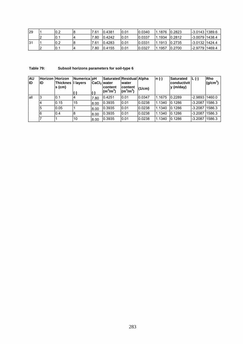
29 1 0.2 8 7.61 0.4381 0.01 0.0340 1.1876 0.2823 -3.0143 1389.6 2 0.1 4 7.80 0.4242 0.01 0.0337 1.1934 0.2812 -3.0079 1438.4 31 1 0.2 8 7.61 0.4283 0.01 0.0331 1.1913 0.2735 -3.0132 1424.4 2 0.1 4 7.80 0.4155 0.01 0.0327 1.1957 0.2700 -2.9779 1469.4
Table 79: Subsoil horizons parameters for soil-type 6
AU ID
Horizon ID
Horizon Thickness (cm)
Numerical layers
Residual water content (m3/m3)
Alpha n (-) Saturated conductivity (m/day)
L (-) Rho (g/cm3)
pH CaCl2
Saturated water content (m3/m3)
(1/cm) (-) (-)
all 3 0.1 4 0.4251 0.01 0.0347 1.1675 0.2289 -2.9893 1460.0 7.80 4 0.15 15 0.3935 0.01 0.0238 1.1340 0.1286 -3.2087 1586.3 8.00 5 0.05 1 0.3935 0.01 0.0238 1.1340 0.1286 -3.2087 1586.3 8.00 6 0.4 8 0.3935 0.01 0.0238 1.1340 0.1286 -3.2087 1586.3 8.00 7 1 10 0.3935 0.01 0.0238 1.1340 0.1286 -3.2087 1586.3 8.00
283
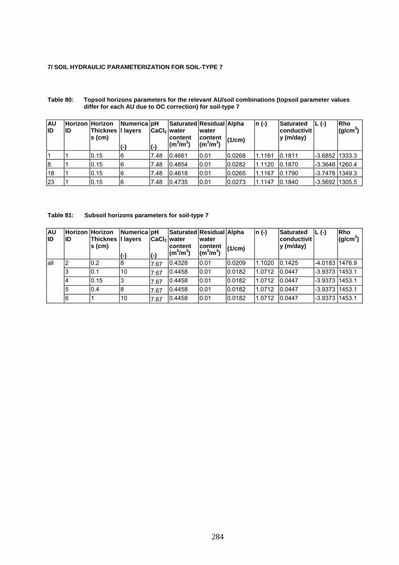
7/ SOIL HYDRAULIC PARAMETERIZATION FOR SOIL-TYPE 7
Table 80: Topsoil horizons parameters for the relevant AU/soil combinations (topsoil parameter values differ for each AU due to OC correction) for soil-type 7
AU ID
Horizon ID
Horizon Thickness (cm)
Numerical layers
Residual water content (m3/m3)
Alpha n (-) Saturated conductivity (m/day)
L (-) Rho (g/cm3)
Saturated water content (m3/m3)
pH CaCl2
(1/cm) (-) (-)
1 1 0.15 6 7.48 0.4661 0.01 0.0268 1.1161 0.1811 -3.6852 1333.3 8 1 0.15 6 7.48 0.4854 0.01 0.0282 1.1120 0.1870 -3.3646 1260.4 18 1 0.15 6 7.48 0.4618 0.01 0.0265 1.1167 0.1790 -3.7478 1349.3 23 1 0.15 6 7.48 0.4735 0.01 0.0273 1.1147 0.1840 -3.5692 1305.5
Table 81: Subsoil horizons parameters for soil-type 7
AU ID
Horizon ID
Horizon Thickness (cm)
Numerical layers
Residual water content (m3/m3)
Alpha n (-) Saturated conductivity (m/day)
L (-) Rho (g/cm3)
pH CaCl2
Saturated water content (m3/m3)
(1/cm) (-) (-)
all 2 0.2 8 0.4328 0.01 0.0209 1.1020 0.1425 -4.0183 1476.9 7.67 3 0.1 10 0.4458 0.01 0.0182 1.0712 0.0447 -3.9373 1453.1 7.67 4 0.15 3 0.4458 0.01 0.0182 1.0712 0.0447 -3.9373 1453.1 7.67 5 0.4 8 0.4458 0.01 0.0182 1.0712 0.0447 -3.9373 1453.1 7.67 6 1 10 0.4458 0.01 0.0182 1.0712 0.0447 -3.9373 1453.1 7.67
284

285
8/ SOIL HYDRAULIC PARAMETERIZATION FOR SOIL-TYPE 8
Table 82: Topsoil horizons parameters for the relevant AU/soil combinations (topsoil parameter values differ for each AU due to OC correction) for soil-type 8
AU ID
Horizon ID
Horizon Thickness (cm)
Numerical layers
(-)
pH CaCl2
(-)
Saturated water content (m3/m3)
Residual water content (m3/m3)
Alpha
(1/cm)
n (-) Saturated conductivity (m/day)
L (-) Rho (g/cm3)
1 1 0.2 8 7.48 0.4337 0.01 0.0201 1.2239 0.1322 -2.1620 1393.4 2 0.1 4 7.48 0.3919 0.01 0.0162 1.2456 0.1190 -1.6841 1539.6 3 1 0.2 8 7.48 0.4531 0.01 0.0223 1.2111 0.1368 -2.1797 1323.5 2 0.1 4 7.48 0.4051 0.01 0.0178 1.2432 0.1301 -1.8672 1493.3 4 1 0.2 8 7.48 0.4468 0.01 0.0216 1.2156 0.1358 -2.1812 1346.4 2 0.1 4 7.48 0.4008 0.01 0.0173 1.2443 0.1267 -1.8151 1508.5 5 1 0.2 8 7.48 0.4429 0.01 0.0211 1.2182 0.1349 -2.1789 1360.2 2 0.1 4 7.48 0.3982 0.01 0.0169 1.2448 0.1246 -1.7802 1517.7 6 1 0.2 8 7.48 0.4666 0.01 0.0239 1.2007 0.1375 -2.1582 1274.8 2 0.1 4 7.48 0.4143 0.01 0.0189 1.2401 0.1365 -1.9560 1460.8 7 1 0.2 8 7.48 0.4311 0.01 0.0198 1.2253 0.1312 -2.1543 1402.5 2 0.1 4 7.48 0.3901 0.01 0.0160 1.2457 0.1174 -1.6544 1545.6 8 1 0.2 8 7.48 0.4516 0.01 0.0221 1.2122 0.1366 -2.1806 1329.0 2 0.1 4 7.48 0.4041 0.01 0.0177 1.2435 0.1293 -1.8553 1497.0 9 1 0.2 8 7.48 0.4475 0.01 0.0216 1.2151 0.1359 -2.1813 1343.9 2 0.1 4 7.48 0.4012 0.01 0.0173 1.2442 0.1271 -1.8210 1506.9 10 1 0.2 8 7.48 0.4556 0.01 0.0226 1.2092 0.1371 -2.1775 1314.6 2 0.1 4 7.48 0.4068 0.01 0.0180 1.2427 0.1314 -1.8856 1487.4 11 1 0.2 8 7.48 0.4793 0.01 0.0255 1.1903 0.1365 -2.1211 1229.2 2 0.1 4 7.48 0.4230 0.01 0.0198 1.2362 0.1415 -2.0158 1430.0 12 1 0.2 8 7.48 0.4646 0.01 0.0236 1.2023 0.1376 -2.1629 1282.3 2 0.1 4 7.48 0.4129 0.01 0.0187 1.2406 0.1356 -1.9441 1465.8 13 1 0.2 8 7.48 0.4588 0.01 0.0229 1.2068 0.1374 -2.1734 1303.1 2 0.1 4 7.48 0.4090 0.01 0.0182 1.2420 0.1329 -1.9079 1479.7 14 1 0.2 8 7.48 0.4434 0.01 0.0212 1.2179 0.1350 -2.1793 1358.6 2 0.1 4 7.48 0.3984 0.01 0.0170 1.2447 0.1248 -1.7842 1516.7 15 1 0.2 8 7.48 0.4364 0.01 0.0204 1.2223 0.1331 -2.1689 1383.5 2 0.1 4 7.48 0.3937 0.01 0.0164 1.2454 0.1207 -1.7147 1533.1 16 1 0.2 8 7.48 0.4631 0.01 0.0234 1.2035 0.1375 -2.1658 1287.5 2 0.1 4 7.48 0.4119 0.01 0.0186 1.2410 0.1349 -1.9356 1469.3 17 1 0.2 8 7.48 0.4465 0.01 0.0215 1.2158 0.1357 -2.1811 1347.4 2 0.1 4 7.48 0.4006 0.01 0.0172 1.2443 0.1266 -1.8126 1509.2 18 1 0.2 8 7.48 0.4297 0.01 0.0197 1.2261 0.1307 -2.1494 1407.5 2 0.1 4 7.48 0.3892 0.01 0.0158 1.2458 0.1165 -1.6376 1548.9 19 1 0.2 8 7.48 0.4453 0.01 0.0214 1.2166 0.1355 -2.1806 1351.6 2 0.1 4 7.48 0.3998 0.01 0.0171 1.2445 0.1259 -1.8023 1512.0 21 1 0.2 8 7.48 0.4574 0.01 0.0228 1.2079 0.1373 -2.1754 1308.2 2 0.1 4 7.48 0.4080 0.01 0.0181 1.2423 0.1322 -1.8981 1483.1 23 1 0.2 8 7.48 0.4405 0.01 0.0209 1.2197 0.1343 -2.1761 1368.8 2 0.1 4 7.48 0.3965 0.01 0.0167 1.2451 0.1232 -1.7568 1523.4 24 1 0.2 8 7.48 0.4405 0.01 0.0209 1.2198 0.1343 -2.1760 1369.1 2 0.1 4 7.48 0.3965 0.01 0.0167 1.2451 0.1231 -1.7561 1523.6

27 1 0.2 8 7.48 0.4329 0.01 0.0200 1.2243 0.1319 -2.1599 1396.1 2 0.1 4 7.48 0.3914 0.01 0.0161 1.2457 0.1185 -1.6754 1541.4 28 1 0.2 8 7.48 0.4233 0.01 0.0189 1.2293 0.1279 -2.1211 1430.4 2 0.1 4 7.48 0.3849 0.01 0.0153 1.2458 0.1121 -1.5544 1563.9 29 1 0.2 8 7.48 0.4494 0.01 0.0219 1.2138 0.1363 -2.1813 1336.9 2 0.1 4 7.48 0.4026 0.01 0.0175 1.2438 0.1282 -1.8375 1502.3 31 1 0.2 8 7.48 0.4386 0.01 0.0206 1.2210 0.1337 -2.1731 1375.8 2 0.1 4 7.48 0.3952 0.01 0.0166 1.2452 0.1220 -1.7370 1528.1
Table 83: Subsoil horizons parameters for soil-type 8
AU ID
Horizon ID
Horizon Thickness (cm)
Numerical layers
Residual water content (m3/m3)
Alpha n (-) Saturated conductivity (m/day)
L (-) Rho (g/cm3)
pH CaCl2
Saturated water content (m3/m3)
(1/cm) (-) (-)
all 3 0.3 6 0.4072 0.01 0.0183 1.2183 0.2132 -1.7700 1520.2 7.48 4 0.4 8 0.3809 0.01 0.0148 1.1971 0.1500 -1.5435 1615.4 7.48 5 0.15 2 0.3809 0.01 0.0148 1.1971 0.1500 -1.5435 1615.4 7.48 6 0.1 10 0.3809 0.01 0.0148 1.1971 0.1500 -1.5435 1615.4 7.48 7 0.75 8 0.3809 0.01 0.0148 1.1971 0.1500 -1.5435 1615.4 7.48
286

287
9/ SOIL HYDRAULIC PARAMETERIZATION FOR SOIL-TYPE 9
Table 84: Topsoil horizons parameters for the relevant AU/soil combinations (topsoil parameter values differ for each AU due to OC correction) for soil-type 9
AU ID
Horizon ID
Horizon Thickness (cm)
Numerical layers
(-)
pH CaCl2
(-)
Saturated water content (m3/m3)
Residual water content (m3/m3)
Alpha
(1/cm)
n (-) Saturated conductivity (m/day)
L (-) Rho (g/cm3)
1 1 0.25 10 6.00 0.4015 0.01 0.0491 1.2898 0.5694 -1.7894 1487.1 2 0.05 2 6.00 0.3816 0.03 0.0520 1.3051 0.5676 -1.4856 1551.7 3 1 0.25 10 6.00 0.4170 0.01 0.0495 1.2807 0.6093 -1.9336 1432.0 2 0.05 2 6.00 0.3943 0.03 0.0529 1.3016 0.6211 -1.6984 1507.4 4 1 0.25 10 6.00 0.4119 0.01 0.0494 1.2841 0.5978 -1.8944 1450.1 2 0.05 2 6.00 0.3901 0.03 0.0527 1.3030 0.6048 -1.6366 1522.0 5 1 0.25 10 6.00 0.4089 0.01 0.0494 1.2859 0.5901 -1.8671 1461.0 2 0.05 2 6.00 0.3876 0.03 0.0525 1.3038 0.5944 -1.5958 1530.7 6 1 0.25 10 6.00 0.4279 0.01 0.0493 1.2725 0.6288 -1.9950 1393.5 2 0.05 2 6.00 0.4032 0.03 0.0531 1.2974 0.6519 -1.8078 1476.3 7 1 0.25 10 6.00 0.3994 0.01 0.0490 1.2907 0.5631 -1.7648 1494.2 2 0.05 2 6.00 0.3800 0.03 0.0518 1.3054 0.5597 -1.4521 1557.4 9 1 0.25 10 6.00 0.4125 0.01 0.0494 1.2837 0.5991 -1.8989 1448.2 2 0.05 2 6.00 0.3906 0.03 0.0527 1.3029 0.6066 -1.6435 1520.4 10 1 0.25 10 6.00 0.4190 0.01 0.0495 1.2793 0.6134 -1.9469 1425.0 2 0.05 2 6.00 0.3959 0.03 0.0530 1.3009 0.6271 -1.7205 1501.7 11 1 0.25 10 6.00 0.4381 0.01 0.0490 1.2636 0.6411 -2.0297 1357.2 2 0.05 2 6.00 0.4115 0.03 0.0531 1.2924 0.6762 -1.8870 1446.8 12 1 0.25 10 6.00 0.4262 0.01 0.0493 1.2739 0.6262 -1.9873 1399.5 2 0.05 2 6.00 0.4018 0.03 0.0531 1.2981 0.6475 -1.7928 1481.1 13 1 0.25 10 6.00 0.4216 0.01 0.0494 1.2775 0.6183 -1.9627 1415.9 2 0.05 2 6.00 0.3980 0.03 0.0530 1.3000 0.6346 -1.7477 1494.4 14 1 0.25 10 6.00 0.4092 0.01 0.0494 1.2857 0.5910 -1.8703 1459.8 2 0.05 2 6.00 0.3879 0.03 0.0525 1.3037 0.5956 -1.6004 1529.7 15 1 0.25 10 6.00 0.4037 0.01 0.0492 1.2887 0.5759 -1.8146 1479.3 2 0.05 2 6.00 0.3834 0.03 0.0521 1.3048 0.5759 -1.5204 1545.4 16 1 0.25 10 6.00 0.4251 0.01 0.0494 1.2748 0.6244 -1.9817 1403.6 2 0.05 2 6.00 0.4009 0.03 0.0531 1.2986 0.6444 -1.7820 1484.4 17 1 0.25 10 6.00 0.4117 0.01 0.0494 1.2842 0.5972 -1.8924 1450.9 2 0.05 2 6.00 0.3900 0.03 0.0526 1.3031 0.6040 -1.6336 1522.6 19 1 0.25 10 6.00 0.4108 0.01 0.0494 1.2848 0.5949 -1.8844 1454.2 2 0.05 2 6.00 0.3892 0.03 0.0526 1.3033 0.6009 -1.6215 1525.3 20 1 0.25 10 6.00 0.4201 0.01 0.0494 1.2785 0.6156 -1.9540 1421.0 2 0.05 2 6.00 0.3968 0.03 0.0530 1.3005 0.6304 -1.7326 1498.5 21 1 0.25 10 6.00 0.4204 0.01 0.0494 1.2783 0.6161 -1.9559 1420.0 2 0.05 2 6.00 0.3971 0.03 0.0530 1.3004 0.6313 -1.7357 1497.7 22 1 0.25 10 6.00 0.4140 0.01 0.0495 1.2828 0.6025 -1.9109 1442.9 2 0.05 2 6.00 0.3918 0.03 0.0528 1.3025 0.6114 -1.6621 1516.2 24 1 0.25 10 6.00 0.4069 0.01 0.0493 1.2870 0.5849 -1.8481 1468.0 2 0.05 2 6.00 0.3860 0.03 0.0524 1.3042 0.5875 -1.5679 1536.3 26 1 0.25 10 6.00 0.4180 0.01 0.0495 1.2801 0.6112 -1.9399 1428.8 2 0.05 2 6.00 0.3951 0.03 0.0529 1.3012 0.6239 -1.7088 1504.8
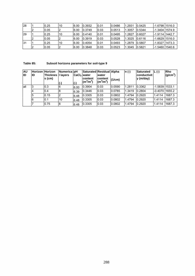
28 1 0.25 10 6.00 0.3932 0.01 0.0486 1.2931 0.5425 -1.6798 1516.0 2 0.05 2 6.00 0.3749 0.03 0.0513 1.3057 0.5344 -1.3404 1574.9 29 1 0.25 10 6.00 0.4140 0.01 0.0495 1.2827 0.6027 -1.9114 1442.7 2 0.05 2 6.00 0.3919 0.03 0.0528 1.3025 0.6116 -1.6629 1516.0 31 1 0.25 10 6.00 0.4054 0.01 0.0493 1.2879 0.5807 -1.8327 1473.3 2 0.05 2 6.00 0.3848 0.03 0.0523 1.3045 0.5821 -1.5460 1540.6
Table 85: Subsoil horizons parameters for soil-type 9
AU ID
Horizon ID
Horizon Thickness (cm)
Numerical layers
pH CaCl2
Saturated water content (m3/m3)
Residual water content (m3/m3)
Alpha n (-) Saturated conductivity (m/day)
L (-) Rho (g/cm3)
(1/cm) (-) (-)
all 3 0.3 6 0.3904 0.03 0.0590 1.2811 0.3362 -1.5839 1533.1 6.00 4 0.4 8 0.3446 0.03 0.0785 1.3419 0.2804 -0.4070 1655.2 6.39 5 0.15 2 0.3305 0.03 0.0802 1.4794 0.2920 1.4114 1687.3 6.48 6 0.1 10 0.3305 0.03 0.0802 1.4794 0.2920 1.4114 1687.3 6.48 7 0.75 8 0.3305 0.03 0.0802 1.4794 0.2920 1.4114 1687.3 6.48
288

289
10/ SOIL HYDRAULIC PARAMETERIZATION FOR SOIL-TYPE 10
Table 86: Topsoil horizons parameters for the relevant AU/soil combinations (topsoil parameter values differ for each AU due to OC correction) for soil-type 10
AU ID
Horizon ID
Horizon Thickness (cm)
Numerical layers
(-)
pH CaCl2
(-)
Saturated water content (m3/m3)
Residual water content (m3/m3)
Alpha
(1/cm)
n (-) Saturated conductivity (m/day)
L (-) Rho (g/cm3)
2 1 0.15 6 7.38 0.5598 0.01 0.0155 1.0940 0.0800 1.2913 995.1 2 0.15 6 7.28 0.5482 0.01 0.0157 1.0940 0.0800 0.5088 1045.5 4 1 0.15 6 7.38 0.5206 0.01 0.0131 1.0990 0.0800 -0.3668 1168.0 2 0.15 6 7.28 0.5101 0.01 0.0139 1.0991 0.0800 -1.0492 1209.3 5 1 0.15 6 7.38 0.5163 0.01 0.0130 1.0995 0.0800 -0.5505 1186.4 2 0.15 6 7.28 0.5058 0.01 0.0138 1.0995 0.0800 -1.2135 1226.8 6 1 0.15 6 7.38 0.5424 0.01 0.0140 1.0962 0.0800 0.5701 1073.2 2 0.15 6 7.28 0.5313 0.01 0.0146 1.0965 0.0800 -0.1885 1119.6 9 1 0.15 6 7.38 0.5214 0.01 0.0131 1.0989 0.0800 -0.3343 1164.7 2 0.15 6 7.28 0.5108 0.01 0.0139 1.0990 0.0800 -1.0201 1206.2 10 1 0.15 6 7.38 0.5305 0.01 0.0134 1.0978 0.0800 0.0549 1125.6 2 0.15 6 7.28 0.5196 0.01 0.0141 1.0981 0.0800 -0.6670 1169.3 12 1 0.15 6 7.38 0.5402 0.01 0.0139 1.0965 0.0800 0.4749 1083.0 2 0.15 6 7.28 0.5291 0.01 0.0145 1.0968 0.0800 -0.2780 1128.9 13 1 0.15 6 7.38 0.5340 0.01 0.0135 1.0974 0.0800 0.2059 1110.4 2 0.15 6 7.28 0.5230 0.01 0.0142 1.0976 0.0800 -0.5282 1154.9 14 1 0.15 6 7.38 0.5167 0.01 0.0130 1.0994 0.0800 -0.5300 1184.4 2 0.15 6 7.28 0.5063 0.01 0.0138 1.0994 0.0800 -1.1952 1224.8 16 1 0.15 6 7.38 0.5387 0.01 0.0138 1.0967 0.0800 0.4086 1089.8 2 0.15 6 7.28 0.5276 0.01 0.0144 1.0970 0.0800 -0.3400 1135.3 17 1 0.15 6 7.38 0.5203 0.01 0.0131 1.0991 0.0800 -0.3805 1169.3 2 0.15 6 7.28 0.5098 0.01 0.0139 1.0991 0.0800 -1.0615 1210.6 20 1 0.15 6 7.38 0.5320 0.01 0.0135 1.0976 0.0800 0.1210 1119.0 2 0.15 6 7.28 0.5211 0.01 0.0142 1.0979 0.0800 -0.6063 1163.0 22 1 0.15 6 7.38 0.5235 0.01 0.0132 1.0987 0.0800 -0.2452 1155.8 2 0.15 6 7.28 0.5128 0.01 0.0139 1.0988 0.0800 -0.9398 1197.8 28 1 0.15 6 7.38 0.4931 0.01 0.0127 1.1007 0.0800 -1.4661 1281.3 2 0.15 6 7.28 0.4835 0.01 0.0135 1.1001 0.0800 -2.0134 1316.1 31 1 0.15 6 7.38 0.5112 0.01 0.0129 1.0999 0.0800 -0.7585 1207.5 2 0.15 6 7.28 0.5010 0.01 0.0137 1.0998 0.0800 -1.3979 1246.6
Table 87: Subsoil horizons parameters for soil-type 10
AU ID
Horizon ID
Horizon Thickness (cm)
Numerical layers
(-)
pH CaCl2
(-)
Saturated water content (m3/m3)
Residual water content (m3/m3)
Alpha
(1/cm)
n (-) Saturated conductivity (m/day)
L (-) Rho (g/cm3)
all 3 0.1 4 7.48 0.4509 0.01 0.0119 1.0642 0.0850 -3.4105 1453.1 4 0.2 4 7.28 0.4422 0.01 0.0116 1.0640 0.0850 -3.5949 1483.1 5 0.4 8 7.28 0.4422 0.01 0.0116 1.0640 0.0850 -3.5949 1483.1 6 0.15 2 7.28 0.4422 0.01 0.0116 1.0640 0.0850 -3.5949 1483.1 7 0.1 10 7.28 0.4422 0.01 0.0116 1.0640 0.0850 -3.5949 1483.1 8 0.75 8 7.28 0.4422 0.01 0.0116 1.0640 0.0850 -3.5949 1483.1
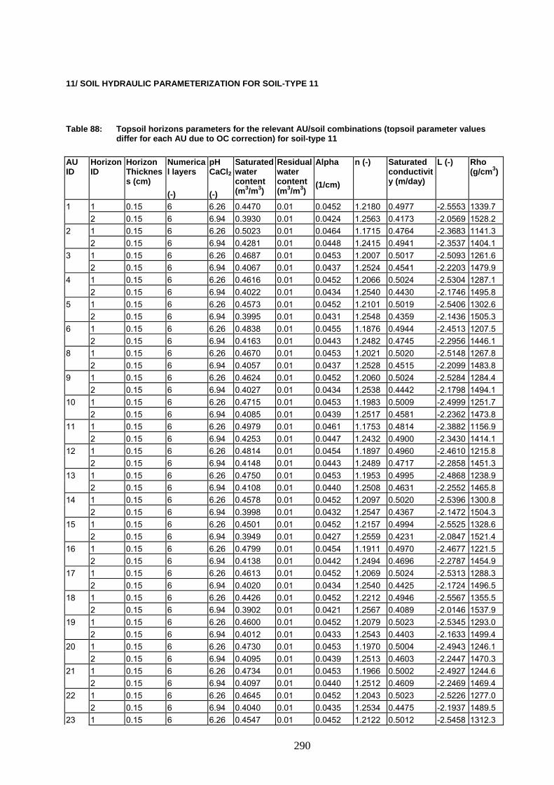
290
11/ SOIL HYDRAULIC PARAMETERIZATION FOR SOIL-TYPE 11
Table 88: Topsoil horizons parameters for the relevant AU/soil combinations (topsoil parameter values differ for each AU due to OC correction) for soil-type 11
AU ID
Horizon ID
Horizon Thickness (cm)
Numerical layers
(-)
pH CaCl2
(-)
Saturated water content (m3/m3)
Residual water content (m3/m3)
Alpha
(1/cm)
n (-) Saturated conductivity (m/day)
L (-) Rho (g/cm3)
1 1 0.15 6 6.26 0.4470 0.01 0.0452 1.2180 0.4977 -2.5553 1339.7 2 0.15 6 6.94 0.3930 0.01 0.0424 1.2563 0.4173 -2.0569 1528.2 2 1 0.15 6 6.26 0.5023 0.01 0.0464 1.1715 0.4764 -2.3683 1141.3 2 0.15 6 6.94 0.4281 0.01 0.0448 1.2415 0.4941 -2.3537 1404.1 3 1 0.15 6 6.26 0.4687 0.01 0.0453 1.2007 0.5017 -2.5093 1261.6 2 0.15 6 6.94 0.4067 0.01 0.0437 1.2524 0.4541 -2.2203 1479.9 4 1 0.15 6 6.26 0.4616 0.01 0.0452 1.2066 0.5024 -2.5304 1287.1 2 0.15 6 6.94 0.4022 0.01 0.0434 1.2540 0.4430 -2.1746 1495.8 5 1 0.15 6 6.26 0.4573 0.01 0.0452 1.2101 0.5019 -2.5406 1302.6 2 0.15 6 6.94 0.3995 0.01 0.0431 1.2548 0.4359 -2.1436 1505.3 6 1 0.15 6 6.26 0.4838 0.01 0.0455 1.1876 0.4944 -2.4513 1207.5 2 0.15 6 6.94 0.4163 0.01 0.0443 1.2482 0.4745 -2.2956 1446.1 8 1 0.15 6 6.26 0.4670 0.01 0.0453 1.2021 0.5020 -2.5148 1267.8 2 0.15 6 6.94 0.4057 0.01 0.0437 1.2528 0.4515 -2.2099 1483.8 9 1 0.15 6 6.26 0.4624 0.01 0.0452 1.2060 0.5024 -2.5284 1284.4 2 0.15 6 6.94 0.4027 0.01 0.0434 1.2538 0.4442 -2.1798 1494.1 10 1 0.15 6 6.26 0.4715 0.01 0.0453 1.1983 0.5009 -2.4999 1251.7 2 0.15 6 6.94 0.4085 0.01 0.0439 1.2517 0.4581 -2.2362 1473.8 11 1 0.15 6 6.26 0.4979 0.01 0.0461 1.1753 0.4814 -2.3882 1156.9 2 0.15 6 6.94 0.4253 0.01 0.0447 1.2432 0.4900 -2.3430 1414.1 12 1 0.15 6 6.26 0.4814 0.01 0.0454 1.1897 0.4960 -2.4610 1215.8 2 0.15 6 6.94 0.4148 0.01 0.0443 1.2489 0.4717 -2.2858 1451.3 13 1 0.15 6 6.26 0.4750 0.01 0.0453 1.1953 0.4995 -2.4868 1238.9 2 0.15 6 6.94 0.4108 0.01 0.0440 1.2508 0.4631 -2.2552 1465.8 14 1 0.15 6 6.26 0.4578 0.01 0.0452 1.2097 0.5020 -2.5396 1300.8 2 0.15 6 6.94 0.3998 0.01 0.0432 1.2547 0.4367 -2.1472 1504.3 15 1 0.15 6 6.26 0.4501 0.01 0.0452 1.2157 0.4994 -2.5525 1328.6 2 0.15 6 6.94 0.3949 0.01 0.0427 1.2559 0.4231 -2.0847 1521.4 16 1 0.15 6 6.26 0.4799 0.01 0.0454 1.1911 0.4970 -2.4677 1221.5 2 0.15 6 6.94 0.4138 0.01 0.0442 1.2494 0.4696 -2.2787 1454.9 17 1 0.15 6 6.26 0.4613 0.01 0.0452 1.2069 0.5024 -2.5313 1288.3 2 0.15 6 6.94 0.4020 0.01 0.0434 1.2540 0.4425 -2.1724 1496.5 18 1 0.15 6 6.26 0.4426 0.01 0.0452 1.2212 0.4946 -2.5567 1355.5 2 0.15 6 6.94 0.3902 0.01 0.0421 1.2567 0.4089 -2.0146 1537.9 19 1 0.15 6 6.26 0.4600 0.01 0.0452 1.2079 0.5023 -2.5345 1293.0 2 0.15 6 6.94 0.4012 0.01 0.0433 1.2543 0.4403 -2.1633 1499.4 20 1 0.15 6 6.26 0.4730 0.01 0.0453 1.1970 0.5004 -2.4943 1246.1 2 0.15 6 6.94 0.4095 0.01 0.0439 1.2513 0.4603 -2.2447 1470.3 21 1 0.15 6 6.26 0.4734 0.01 0.0453 1.1966 0.5002 -2.4927 1244.6 2 0.15 6 6.94 0.4097 0.01 0.0440 1.2512 0.4609 -2.2469 1469.4 22 1 0.15 6 6.26 0.4645 0.01 0.0452 1.2043 0.5023 -2.5226 1277.0 2 0.15 6 6.94 0.4040 0.01 0.0435 1.2534 0.4475 -2.1937 1489.5 23 1 0.15 6 6.26 0.4547 0.01 0.0452 1.2122 0.5012 -2.5458 1312.3
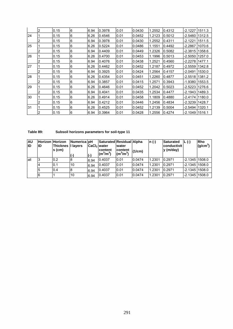
2 0.15 6 6.94 0.3978 0.01 0.0430 1.2552 0.4312 -2.1227 1511.3 24 1 0.15 6 6.26 0.4546 0.01 0.0452 1.2123 0.5012 -2.5460 1312.5 2 0.15 6 6.94 0.3978 0.01 0.0430 1.2552 0.4311 -2.1221 1511.5 25 1 0.15 6 6.26 0.5224 0.01 0.0486 1.1551 0.4492 -2.2867 1070.6 2 0.15 6 6.94 0.4409 0.01 0.0449 1.2326 0.5082 -2.3815 1358.6 26 1 0.15 6 6.26 0.4700 0.01 0.0453 1.1996 0.5013 -2.5050 1257.0 2 0.15 6 6.94 0.4076 0.01 0.0438 1.2521 0.4560 -2.2278 1477.1 27 1 0.15 6 6.26 0.4462 0.01 0.0452 1.2187 0.4972 -2.5559 1342.8 2 0.15 6 6.94 0.3925 0.01 0.0424 1.2564 0.4157 -2.0491 1530.0 28 1 0.15 6 6.26 0.4354 0.01 0.0451 1.2260 0.4877 -2.5518 1381.2 2 0.15 6 6.94 0.3857 0.01 0.0415 1.2571 0.3943 -1.9380 1553.5 29 1 0.15 6 6.26 0.4646 0.01 0.0452 1.2042 0.5023 -2.5223 1276.6 2 0.15 6 6.94 0.4041 0.01 0.0435 1.2534 0.4477 -2.1943 1489.3 30 1 0.15 6 6.26 0.4914 0.01 0.0458 1.1809 0.4880 -2.4174 1180.0 2 0.15 6 6.94 0.4212 0.01 0.0446 1.2456 0.4834 -2.3239 1428.7 31 1 0.15 6 6.26 0.4525 0.01 0.0452 1.2139 0.5004 -2.5494 1320.1 2 0.15 6 6.94 0.3964 0.01 0.0428 1.2556 0.4274 -2.1049 1516.1
Table 89: Subsoil horizons parameters for soil-type 11
AU ID
Horizon ID
Horizon Thickness (cm)
Numerical layers
Residual water content (m3/m3)
Alpha n (-) Saturated conductivity (m/day)
L (-) Rho (g/cm3)
pH CaCl2
Saturated water content (m3/m3)
(1/cm) (-) (-)
all 3 0.2 8 0.4037 0.01 0.0474 1.2301 0.2971 -2.1345 1508.0 6.94 4 0.1 10 0.4037 0.01 0.0474 1.2301 0.2971 -2.1345 1508.0 6.94 5 0.4 8 0.4037 0.01 0.0474 1.2301 0.2971 -2.1345 1508.0 6.94 6 1 10 0.4037 0.01 0.0474 1.2301 0.2971 -2.1345 1508.0 6.94
291

292
12/ SOIL HYDRAULIC PARAMETERIZATION FOR SOIL-TYPE 12
Table 90: Topsoil horizons parameters for the relevant AU/soil combinations (topsoil parameter values differ for each AU due to OC correction) for soil-type 12
AU ID
Horizon ID
Horizon Thickness (cm)
Numerical layers
(-)
pH CaCl2
(-)
Saturated water content (m3/m3)
Residual water content (m3/m3)
Alpha
(1/cm)
n (-) Saturated conductivity (m/day)
L (-) Rho (g/cm3)
2 1 0.2 8 6.85 0.4429 0.01 0.0148 1.2077 0.0230 -2.2650 1358.3 2 0.05 2 6.85 0.4429 0.01 0.0148 1.2077 0.0230 -2.2650 1358.3 4 1 0.2 8 6.85 0.4144 0.01 0.0117 1.2204 0.0230 -2.1856 1459.9 2 0.05 2 6.85 0.4144 0.01 0.0117 1.2204 0.0230 -2.1856 1459.9 6 1 0.2 8 6.85 0.4299 0.01 0.0134 1.2145 0.0230 -2.2520 1404.7 2 0.05 2 6.85 0.4299 0.01 0.0134 1.2145 0.0230 -2.2520 1404.7 9 1 0.2 8 6.85 0.4150 0.01 0.0118 1.2202 0.0230 -2.1889 1458.0 2 0.05 2 6.85 0.4150 0.01 0.0118 1.2202 0.0230 -2.1889 1458.0 11 1 0.2 8 6.85 0.4398 0.01 0.0145 1.2094 0.0230 -2.2649 1369.3 2 0.05 2 6.85 0.4398 0.01 0.0145 1.2094 0.0230 -2.2649 1369.3 12 1 0.2 8 6.85 0.4283 0.01 0.0132 1.2152 0.0230 -2.2479 1410.5 2 0.05 2 6.85 0.4283 0.01 0.0132 1.2152 0.0230 -2.2479 1410.5 14 1 0.2 8 6.85 0.4118 0.01 0.0115 1.2211 0.0230 -2.1675 1469.3 2 0.05 2 6.85 0.4118 0.01 0.0115 1.2211 0.0230 -2.1675 1469.3 15 1 0.2 8 6.85 0.4064 0.01 0.0109 1.2224 0.0230 -2.1238 1488.3 2 0.05 2 6.85 0.4064 0.01 0.0109 1.2224 0.0230 -2.1238 1488.3 16 1 0.2 8 6.85 0.4272 0.01 0.0131 1.2157 0.0230 -2.2447 1414.5 2 0.05 2 6.85 0.4272 0.01 0.0131 1.2157 0.0230 -2.2447 1414.5 17 1 0.2 8 6.85 0.4142 0.01 0.0117 1.2205 0.0230 -2.1841 1460.7 2 0.05 2 6.85 0.4142 0.01 0.0117 1.2205 0.0230 -2.1841 1460.7 19 1 0.2 8 6.85 0.4133 0.01 0.0116 1.2207 0.0230 -2.1782 1463.9 2 0.05 2 6.85 0.4133 0.01 0.0116 1.2207 0.0230 -2.1782 1463.9 20 1 0.2 8 6.85 0.4224 0.01 0.0126 1.2177 0.0230 -2.2276 1431.6 2 0.05 2 6.85 0.4224 0.01 0.0126 1.2177 0.0230 -2.2276 1431.6 22 1 0.2 8 6.85 0.4164 0.01 0.0119 1.2198 0.0230 -2.1977 1452.8 2 0.05 2 6.85 0.4164 0.01 0.0119 1.2198 0.0230 -2.1977 1452.8 24 1 0.2 8 6.85 0.4095 0.01 0.0112 1.2217 0.0230 -2.1503 1477.3 2 0.05 2 6.85 0.4095 0.01 0.0112 1.2217 0.0230 -2.1503 1477.3 25 1 0.2 8 6.85 0.4568 0.01 0.0165 1.1989 0.0230 -2.2457 1308.0 2 0.05 2 6.85 0.4568 0.01 0.0165 1.1989 0.0230 -2.2457 1308.0 26 1 0.2 8 6.85 0.4203 0.01 0.0124 1.2185 0.0230 -2.2181 1439.1 2 0.05 2 6.85 0.4203 0.01 0.0124 1.2185 0.0230 -2.2181 1439.1 30 1 0.2 8 6.85 0.4353 0.01 0.0140 1.2118 0.0230 -2.2615 1385.5 2 0.05 2 6.85 0.4353 0.01 0.0140 1.2118 0.0230 -2.2615 1385.5 31 1 0.2 8 6.85 0.4080 0.01 0.0111 1.2221 0.0230 -2.1382 1482.4 2 0.05 2 6.85 0.4080 0.01 0.0111 1.2221 0.0230 -2.1382 1482.4

Table 91: Subsoil horizons parameters for soil-type 12
Saturated water content (m3/m3)
AU ID
Horizon ID
Horizon Thickness (cm)
Numerical layers
pH CaCl2
Residual water content (m3/m3)
Alpha n (-) Saturated conductivity (m/day)
L (-) Rho (g/cm3)
(1/cm) (-) (-)
all 3 0.05 2 0.4233 0.01 0.0120 1.1918 0.0230 -2.1588 1473.4 6.85 4 0.3 6 0.3743 0.01 0.0089 1.1400 0.0400 -2.1131 1655.2 6.76 5 0.4 8 0.3422 0.01 0.0373 1.0608 0.0400 0.4496 1759.1 6.76 6 0.35 4 0.3422 0.01 0.0373 1.0608 0.0400 0.4496 1759.1 6.76 7 0.1 10 0.3422 0.01 0.0373 1.0608 0.0400 0.4496 1759.1 6.76 8 0.55 6 0.3422 0.01 0.0373 1.0608 0.0400 0.4496 1759.1 6.76
293
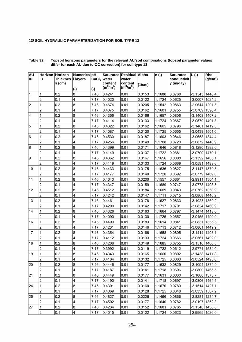
294
13/ SOIL HYDRAULIC PARAMETERIZATION FOR SOIL-TYPE 13
Table 92: Topsoil horizons parameters for the relevant AU/soil combinations (topsoil parameter values differ for each AU due to OC correction) for soil-type 13
AU ID
Horizon ID
Horizon Thickness (cm)
Numerical layers
(-)
pH CaCl2
(-)
Saturated water content (m3/m3)
Residual water content (m3/m3)
Alpha
(1/cm)
n (-) Saturated conductivity (m/day)
L (-) Rho (g/cm3)
1 1 0.2 8 7.46 0.4241 0.01 0.0153 1.1680 0.0768 -3.1543 1448.4 2 0.1 4 7.17 0.4020 0.01 0.0122 1.1724 0.0625 -3.0007 1524.2 2 1 0.2 8 7.46 0.4674 0.01 0.0205 1.1542 0.0863 -2.9644 1291.5 2 0.1 4 7.17 0.4375 0.01 0.0162 1.1681 0.0755 -3.0709 1398.4 4 1 0.2 8 7.46 0.4356 0.01 0.0166 1.1657 0.0806 -3.1408 1407.2 2 0.1 4 7.17 0.4114 0.01 0.0133 1.1724 0.0667 -3.0570 1491.3 5 1 0.2 8 7.46 0.4322 0.01 0.0162 1.1665 0.0796 -3.1481 1419.3 2 0.1 4 7.17 0.4087 0.01 0.0130 1.1725 0.0655 -3.0439 1501.0 6 1 0.2 8 7.46 0.4530 0.01 0.0187 1.1603 0.0846 -3.0658 1344.4 2 0.1 4 7.17 0.4256 0.01 0.0149 1.1708 0.0720 -3.0872 1440.9 8 1 0.2 8 7.46 0.4399 0.01 0.0171 1.1646 0.0818 -3.1280 1392.0 2 0.1 4 7.17 0.4149 0.01 0.0137 1.1722 0.0681 -3.0700 1479.1 9 1 0.2 8 7.46 0.4362 0.01 0.0167 1.1656 0.0808 -3.1392 1405.1 2 0.1 4 7.17 0.4119 0.01 0.0133 1.1724 0.0669 -3.0591 1489.6 10 1 0.2 8 7.46 0.4433 0.01 0.0175 1.1636 0.0827 -3.1147 1379.3 2 0.1 4 7.17 0.4177 0.01 0.0140 1.1720 0.0692 -3.0779 1469.0 11 1 0.2 8 7.46 0.4640 0.01 0.0200 1.1557 0.0861 -2.9911 1304.1 2 0.1 4 7.17 0.4347 0.01 0.0159 1.1689 0.0747 -3.0778 1408.5 12 1 0.2 8 7.46 0.4512 0.01 0.0184 1.1609 0.0843 -3.0762 1350.9 2 0.1 4 7.17 0.4242 0.01 0.0147 1.1711 0.0715 -3.0868 1446.2 13 1 0.2 8 7.46 0.4461 0.01 0.0178 1.1627 0.0833 -3.1023 1369.2 2 0.1 4 7.17 0.4200 0.01 0.0142 1.1717 0.0701 -3.0824 1460.9 14 1 0.2 8 7.46 0.4326 0.01 0.0163 1.1664 0.0797 -3.1474 1418.0 2 0.1 4 7.17 0.4090 0.01 0.0130 1.1725 0.0657 -3.0455 1499.9 16 1 0.2 8 7.46 0.4499 0.01 0.0183 1.1614 0.0841 -3.0831 1355.5 2 0.1 4 7.17 0.4231 0.01 0.0146 1.1713 0.0712 -3.0861 1449.9 17 1 0.2 8 7.46 0.4354 0.01 0.0166 1.1658 0.0805 -3.1414 1408.1 2 0.1 4 7.17 0.4112 0.01 0.0133 1.1724 0.0666 -3.0561 1492.0 18 1 0.2 8 7.46 0.4206 0.01 0.0149 1.1685 0.0755 -3.1516 1460.8 2 0.1 4 7.17 0.3992 0.01 0.0119 1.1722 0.0612 -2.9771 1534.0 19 1 0.2 8 7.46 0.4343 0.01 0.0165 1.1660 0.0802 -3.1438 1411.8 2 0.1 4 7.17 0.4104 0.01 0.0132 1.1725 0.0663 -3.0524 1495.0 20 1 0.2 8 7.46 0.4446 0.01 0.0177 1.1632 0.0829 -3.1094 1374.9 2 0.1 4 7.17 0.4187 0.01 0.0141 1.1718 0.0696 -3.0800 1465.5 21 1 0.2 8 7.46 0.4449 0.01 0.0177 1.1631 0.0830 -3.1080 1373.7 2 0.1 4 7.17 0.4190 0.01 0.0141 1.1718 0.0697 -3.0806 1464.5 24 1 0.2 8 7.46 0.4301 0.01 0.0160 1.1670 0.0789 -3.1514 1427.1 2 0.1 4 7.17 0.4069 0.01 0.0128 1.1725 0.0648 -3.0339 1507.2 25 1 0.2 8 7.46 0.4827 0.01 0.0226 1.1466 0.0866 -2.8281 1234.7 2 0.1 4 7.17 0.4502 0.01 0.0177 1.1640 0.0782 -3.0197 1352.3 27 1 0.2 8 7.46 0.4234 0.01 0.0152 1.1681 0.0765 -3.1540 1450.8 2 0.1 4 7.17 0.4015 0.01 0.0122 1.1724 0.0623 -2.9965 1526.0
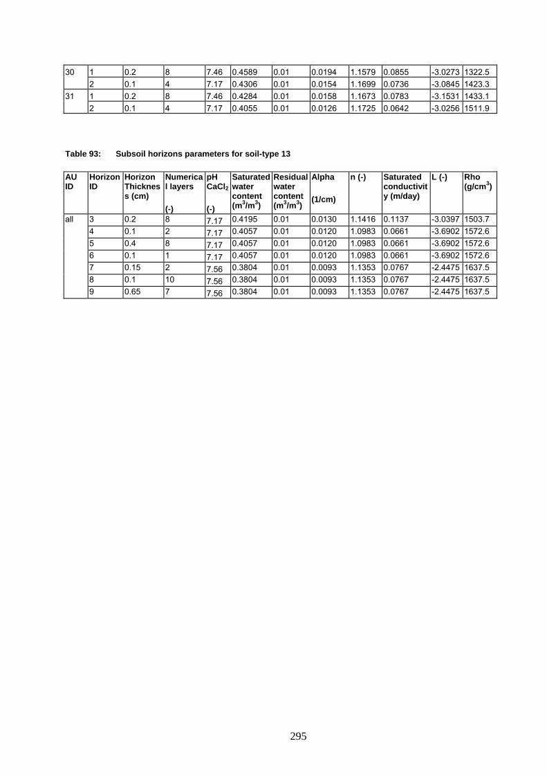
30 1 0.2 8 7.46 0.4589 0.01 0.0194 1.1579 0.0855 -3.0273 1322.5 2 0.1 4 7.17 0.4306 0.01 0.0154 1.1699 0.0736 -3.0845 1423.3 31 1 0.2 8 7.46 0.4284 0.01 0.0158 1.1673 0.0783 -3.1531 1433.1 2 0.1 4 7.17 0.4055 0.01 0.0126 1.1725 0.0642 -3.0256 1511.9
Table 93: Subsoil horizons parameters for soil-type 13
AU ID
Horizon ID
Horizon Thickness (cm)
Numerical layers
Residual water content (m3/m3)
Alpha n (-) Saturated conductivity (m/day)
L (-) Rho (g/cm3)
pH CaCl2
Saturated water content (m3/m3)
(1/cm) (-) (-)
all 3 0.2 8 0.4195 0.01 0.0130 1.1416 0.1137 -3.0397 1503.7 7.17 4 0.1 2 0.4057 0.01 0.0120 1.0983 0.0661 -3.6902 1572.6 7.17 5 0.4 8 0.4057 0.01 0.0120 1.0983 0.0661 -3.6902 1572.6 7.17 6 0.1 1 0.4057 0.01 0.0120 1.0983 0.0661 -3.6902 1572.6 7.17 7 0.15 2 0.3804 0.01 0.0093 1.1353 0.0767 -2.4475 1637.5 7.56 8 0.1 10 0.3804 0.01 0.0093 1.1353 0.0767 -2.4475 1637.5 7.56 9 0.65 7 0.3804 0.01 0.0093 1.1353 0.0767 -2.4475 1637.5 7.56
295
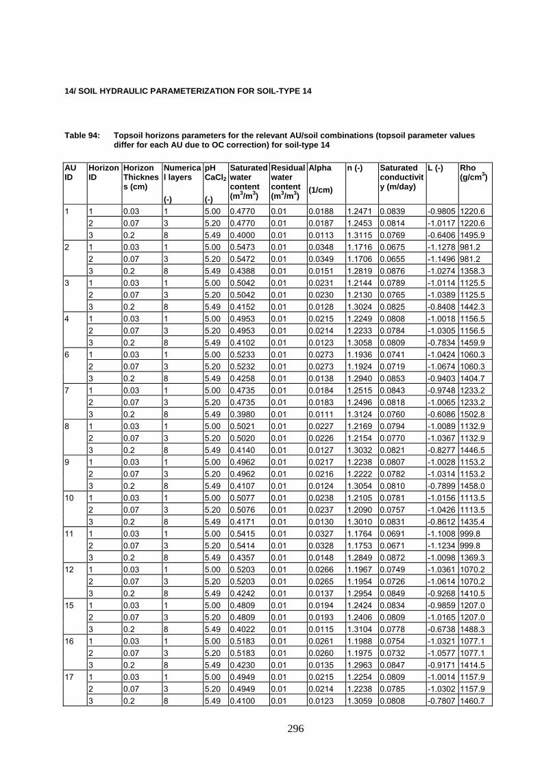
296
14/ SOIL HYDRAULIC PARAMETERIZATION FOR SOIL-TYPE 14
Table 94: Topsoil horizons parameters for the relevant AU/soil combinations (topsoil parameter values differ for each AU due to OC correction) for soil-type 14
AU ID
Horizon ID
Horizon Thickness (cm)
Numerical layers
(-)
pH CaCl2
(-)
Saturated water content (m3/m3)
Residual water content (m3/m3)
Alpha
(1/cm)
n (-) Saturated conductivity (m/day)
L (-) Rho (g/cm3)
1 1 0.03 1 5.00 0.4770 0.01 0.0188 1.2471 0.0839 -0.9805 1220.6 2 0.07 3 5.20 0.4770 0.01 0.0187 1.2453 0.0814 -1.0117 1220.6 3 0.2 8 5.49 0.4000 0.01 0.0113 1.3115 0.0769 -0.6406 1495.9 2 1 0.03 1 5.00 0.5473 0.01 0.0348 1.1716 0.0675 -1.1278 981.2 2 0.07 3 5.20 0.5472 0.01 0.0349 1.1706 0.0655 -1.1496 981.2 3 0.2 8 5.49 0.4388 0.01 0.0151 1.2819 0.0876 -1.0274 1358.3 3 1 0.03 1 5.00 0.5042 0.01 0.0231 1.2144 0.0789 -1.0114 1125.5 2 0.07 3 5.20 0.5042 0.01 0.0230 1.2130 0.0765 -1.0389 1125.5 3 0.2 8 5.49 0.4152 0.01 0.0128 1.3024 0.0825 -0.8408 1442.3 4 1 0.03 1 5.00 0.4953 0.01 0.0215 1.2249 0.0808 -1.0018 1156.5 2 0.07 3 5.20 0.4953 0.01 0.0214 1.2233 0.0784 -1.0305 1156.5 3 0.2 8 5.49 0.4102 0.01 0.0123 1.3058 0.0809 -0.7834 1459.9 6 1 0.03 1 5.00 0.5233 0.01 0.0273 1.1936 0.0741 -1.0424 1060.3 2 0.07 3 5.20 0.5232 0.01 0.0273 1.1924 0.0719 -1.0674 1060.3 3 0.2 8 5.49 0.4258 0.01 0.0138 1.2940 0.0853 -0.9403 1404.7 7 1 0.03 1 5.00 0.4735 0.01 0.0184 1.2515 0.0843 -0.9748 1233.2 2 0.07 3 5.20 0.4735 0.01 0.0183 1.2496 0.0818 -1.0065 1233.2 3 0.2 8 5.49 0.3980 0.01 0.0111 1.3124 0.0760 -0.6086 1502.8 8 1 0.03 1 5.00 0.5021 0.01 0.0227 1.2169 0.0794 -1.0089 1132.9 2 0.07 3 5.20 0.5020 0.01 0.0226 1.2154 0.0770 -1.0367 1132.9 3 0.2 8 5.49 0.4140 0.01 0.0127 1.3032 0.0821 -0.8277 1446.5 9 1 0.03 1 5.00 0.4962 0.01 0.0217 1.2238 0.0807 -1.0028 1153.2 2 0.07 3 5.20 0.4962 0.01 0.0216 1.2222 0.0782 -1.0314 1153.2 3 0.2 8 5.49 0.4107 0.01 0.0124 1.3054 0.0810 -0.7899 1458.0 10 1 0.03 1 5.00 0.5077 0.01 0.0238 1.2105 0.0781 -1.0156 1113.5 2 0.07 3 5.20 0.5076 0.01 0.0237 1.2090 0.0757 -1.0426 1113.5 3 0.2 8 5.49 0.4171 0.01 0.0130 1.3010 0.0831 -0.8612 1435.4 11 1 0.03 1 5.00 0.5415 0.01 0.0327 1.1764 0.0691 -1.1008 999.8 2 0.07 3 5.20 0.5414 0.01 0.0328 1.1753 0.0671 -1.1234 999.8 3 0.2 8 5.49 0.4357 0.01 0.0148 1.2849 0.0872 -1.0098 1369.3 12 1 0.03 1 5.00 0.5203 0.01 0.0266 1.1967 0.0749 -1.0361 1070.2 2 0.07 3 5.20 0.5203 0.01 0.0265 1.1954 0.0726 -1.0614 1070.2 3 0.2 8 5.49 0.4242 0.01 0.0137 1.2954 0.0849 -0.9268 1410.5 15 1 0.03 1 5.00 0.4809 0.01 0.0194 1.2424 0.0834 -0.9859 1207.0 2 0.07 3 5.20 0.4809 0.01 0.0193 1.2406 0.0809 -1.0165 1207.0 3 0.2 8 5.49 0.4022 0.01 0.0115 1.3104 0.0778 -0.6738 1488.3 16 1 0.03 1 5.00 0.5183 0.01 0.0261 1.1988 0.0754 -1.0321 1077.1 2 0.07 3 5.20 0.5183 0.01 0.0260 1.1975 0.0732 -1.0577 1077.1 3 0.2 8 5.49 0.4230 0.01 0.0135 1.2963 0.0847 -0.9171 1414.5 17 1 0.03 1 5.00 0.4949 0.01 0.0215 1.2254 0.0809 -1.0014 1157.9 2 0.07 3 5.20 0.4949 0.01 0.0214 1.2238 0.0785 -1.0302 1157.9 3 0.2 8 5.49 0.4100 0.01 0.0123 1.3059 0.0808 -0.7807 1460.7
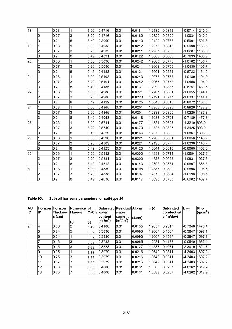
297
18 1 0.03 1 5.00 0.4716 0.01 0.0181 1.2539 0.0845 -0.9714 1240.0 2 0.07 3 5.20 0.4716 0.01 0.0180 1.2520 0.0820 -1.0034 1240.0 3 0.2 8 5.49 0.3969 0.01 0.0110 1.3129 0.0755 -0.5904 1506.6 19 1 0.03 1 5.00 0.4933 0.01 0.0212 1.2273 0.0813 -0.9998 1163.5 2 0.07 3 5.20 0.4932 0.01 0.0211 1.2257 0.0788 -1.0287 1163.5 3 0.2 8 5.49 0.4091 0.01 0.0122 1.3065 0.0805 -0.7693 1463.9 20 1 0.03 1 5.00 0.5096 0.01 0.0242 1.2083 0.0776 -1.0182 1106.7 2 0.07 3 5.20 0.5096 0.01 0.0241 1.2069 0.0753 -1.0450 1106.7 3 0.2 8 5.49 0.4182 0.01 0.0131 1.3001 0.0834 -0.8722 1431.6 21 1 0.03 1 5.00 0.5102 0.01 0.0243 1.2077 0.0775 -1.0189 1104.9 2 0.07 3 5.20 0.5101 0.01 0.0242 1.2063 0.0752 -1.0456 1104.9 3 0.2 8 5.49 0.4185 0.01 0.0131 1.2999 0.0835 -0.8751 1430.5 22 1 0.03 1 5.00 0.4988 0.01 0.0221 1.2207 0.0801 -1.0055 1144.1 2 0.07 3 5.20 0.4988 0.01 0.0220 1.2191 0.0777 -1.0337 1144.1 3 0.2 8 5.49 0.4122 0.01 0.0125 1.3045 0.0815 -0.8072 1452.8 24 1 0.03 1 5.00 0.4865 0.01 0.0201 1.2355 0.0825 -0.9926 1187.3 2 0.07 3 5.20 0.4865 0.01 0.0201 1.2338 0.0800 -1.0225 1187.3 3 0.2 8 5.49 0.4053 0.01 0.0118 1.3088 0.0791 -0.7189 1477.3 25 1 0.03 1 5.00 0.5741 0.01 0.0477 1.1534 0.0605 -1.3240 898.0 2 0.07 3 5.20 0.5740 0.01 0.0479 1.1525 0.0587 -1.3425 898.0 3 0.2 8 5.49 0.4529 0.01 0.0166 1.2670 0.0886 -1.0867 1308.0 29 1 0.03 1 5.00 0.4990 0.01 0.0221 1.2205 0.0801 -1.0056 1143.7 2 0.07 3 5.20 0.4989 0.01 0.0221 1.2190 0.0777 -1.0338 1143.7 3 0.2 8 5.49 0.4123 0.01 0.0125 1.3044 0.0816 -0.8080 1452.6 30 1 0.03 1 5.00 0.5332 0.01 0.0300 1.1839 0.0714 -1.0694 1027.3 2 0.07 3 5.20 0.5331 0.01 0.0300 1.1828 0.0693 -1.0931 1027.3 3 0.2 8 5.49 0.4312 0.01 0.0143 1.2892 0.0864 -0.9807 1385.5 31 1 0.03 1 5.00 0.4839 0.01 0.0198 1.2388 0.0829 -0.9896 1196.6 2 0.07 3 5.20 0.4838 0.01 0.0197 1.2370 0.0804 -1.0198 1196.6 3 0.2 8 5.49 0.4038 0.01 0.0117 1.3096 0.0785 -0.6982 1482.4
Table 95: Subsoil horizons parameters for soil-type 14
AU ID
Horizon ID
Horizon Thickness (cm)
Numerical layers
(-)
pH CaCl2
(-)
Saturated water content (m3/m3)
Residual water content (m3/m3)
Alpha
(1/cm)
n (-) Saturated conductivity (m/day)
L (-) Rho (g/cm3)
all 4 0.06 2 5.49 0.4180 0.01 0.0135 1.2857 0.2317 -0.7340 1473.4 5 0.24 5 5.39 0.3836 0.01 0.0093 1.2667 0.1587 -0.3847 1597.1 6 0.04 1 5.39 0.3836 0.01 0.0093 1.2667 0.1587 -0.3847 1597.1 7 0.16 3 5.59 0.3733 0.01 0.0065 1.2581 0.1138 -0.0540 1633.4 8 0.15 3 5.68 0.3828 0.01 0.0127 1.1538 0.1081 -2.3019 1621.7 9 0.05 1 5.88 0.3979 0.01 0.0216 1.0649 0.0311 -4.3403 1607.2 10 0.25 3 5.88 0.3979 0.01 0.0216 1.0649 0.0311 -4.3403 1607.2 11 0.07 7 5.88 0.3979 0.01 0.0216 1.0649 0.0311 -4.3403 1607.2 12 0.03 3 5.88 0.4000 0.01 0.0131 1.0583 0.0207 -4.0262 1617.9 13 0.65 7 5.88 0.4000 0.01 0.0131 1.0583 0.0207 -4.0262 1617.9
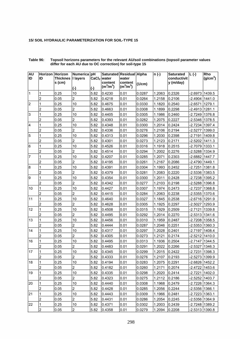
298
15/ SOIL HYDRAULIC PARAMETERIZATION FOR SOIL-TYPE 15
Table 96: Topsoil horizons parameters for the relevant AU/soil combinations (topsoil parameter values differ for each AU due to OC correction) for soil-type 15
AU ID
Horizon ID
Horizon Thickness (cm)
Numerical layers
(-)
pH CaCl2
(-)
Saturated water content (m3/m3)
Residual water content (m3/m3)
Alpha
(1/cm)
n (-) Saturated conductivity (m/day)
L (-) Rho (g/cm3)
1 1 0.25 10 5.82 0.4230 0.01 0.0287 1.2063 0.2326 -2.6973 1439.5 2 0.05 2 5.82 0.4218 0.01 0.0264 1.2158 0.2106 -2.4904 1441.0 2 1 0.25 10 5.82 0.4675 0.01 0.0330 1.1820 0.2540 -2.6571 1279.1 2 0.05 2 5.82 0.4663 0.01 0.0308 1.1899 0.2298 -2.4913 1281.1 3 1 0.25 10 5.82 0.4405 0.01 0.0305 1.1986 0.2460 -2.7249 1376.8 2 0.05 2 5.82 0.4393 0.01 0.0282 1.2075 0.2227 -2.5346 1378.5 4 1 0.25 10 5.82 0.4348 0.01 0.0300 1.2014 0.2424 -2.7234 1397.4 2 0.05 2 5.82 0.4336 0.01 0.0276 1.2106 0.2194 -2.5277 1399.0 5 1 0.25 10 5.82 0.4313 0.01 0.0296 1.2030 0.2398 -2.7191 1409.8 2 0.05 2 5.82 0.4301 0.01 0.0273 1.2123 0.2171 -2.5202 1411.3 6 1 0.25 10 5.82 0.4526 0.01 0.0316 1.1918 0.2515 -2.7079 1333.1 2 0.05 2 5.82 0.4514 0.01 0.0294 1.2002 0.2276 -2.5288 1334.9 7 1 0.25 10 5.82 0.4207 0.01 0.0285 1.2071 0.2303 -2.6882 1447.7 2 0.05 2 5.82 0.4195 0.01 0.0261 1.2167 0.2086 -2.4790 1449.1 8 1 0.25 10 5.82 0.4391 0.01 0.0304 1.1993 0.2452 -2.7251 1381.8 2 0.05 2 5.82 0.4379 0.01 0.0281 1.2083 0.2220 -2.5336 1383.5 9 1 0.25 10 5.82 0.4354 0.01 0.0300 1.2011 0.2428 -2.7238 1395.2 2 0.05 2 5.82 0.4342 0.01 0.0277 1.2103 0.2198 -2.5288 1396.8 10 1 0.25 10 5.82 0.4427 0.01 0.0307 1.1974 0.2473 -2.7237 1368.8 2 0.05 2 5.82 0.4415 0.01 0.0284 1.2063 0.2238 -2.5355 1370.6 11 1 0.25 10 5.82 0.4640 0.01 0.0327 1.1845 0.2538 -2.6716 1291.9 2 0.05 2 5.82 0.4628 0.01 0.0305 1.1925 0.2297 -2.5027 1293.9 12 1 0.25 10 5.82 0.4508 0.01 0.0315 1.1929 0.2509 -2.7121 1339.8 2 0.05 2 5.82 0.4495 0.01 0.0292 1.2014 0.2270 -2.5313 1341.6 13 1 0.25 10 5.82 0.4456 0.01 0.0310 1.1959 0.2487 -2.7208 1358.5 2 0.05 2 5.82 0.4444 0.01 0.0287 1.2046 0.2251 -2.5353 1360.3 14 1 0.25 10 5.82 0.4317 0.01 0.0297 1.2028 0.2401 -2.7197 1408.4 2 0.05 2 5.82 0.4305 0.01 0.0273 1.2121 0.2174 -2.5212 1410.0 16 1 0.25 10 5.82 0.4495 0.01 0.0313 1.1936 0.2504 -2.7147 1344.5 2 0.05 2 5.82 0.4483 0.01 0.0291 1.2022 0.2266 -2.5327 1346.3 17 1 0.25 10 5.82 0.4345 0.01 0.0299 1.2015 0.2422 -2.7231 1398.3 2 0.05 2 5.82 0.4333 0.01 0.0276 1.2107 0.2193 -2.5273 1399.9 18 1 0.25 10 5.82 0.4194 0.01 0.0283 1.2075 0.2291 -2.6826 1452.2 2 0.05 2 5.82 0.4182 0.01 0.0260 1.2171 0.2074 -2.4722 1453.6 19 1 0.25 10 5.82 0.4335 0.01 0.0298 1.2020 0.2414 -2.7221 1402.0 2 0.05 2 5.82 0.4323 0.01 0.0275 1.2112 0.2186 -2.5252 1403.7 20 1 0.25 10 5.82 0.4440 0.01 0.0308 1.1968 0.2479 -2.7226 1364.3 2 0.05 2 5.82 0.4428 0.01 0.0285 1.2056 0.2244 -2.5356 1366.1 21 1 0.25 10 5.82 0.4443 0.01 0.0309 1.1966 0.2481 -2.7223 1363.1 2 0.05 2 5.82 0.4431 0.01 0.0286 1.2054 0.2245 -2.5356 1364.9 22 1 0.25 10 5.82 0.4371 0.01 0.0302 1.2003 0.2439 -2.7248 1389.2 2 0.05 2 5.82 0.4358 0.01 0.0279 1.2094 0.2208 -2.5313 1390.8

299
23 1 0.25 10 5.82 0.4291 0.01 0.0294 1.2039 0.2381 -2.7151 1417.5 2 0.05 2 5.82 0.4279 0.01 0.0270 1.2133 0.2156 -2.5141 1419.1 24 1 0.25 10 5.82 0.4291 0.01 0.0294 1.2039 0.2380 -2.7149 1417.7 2 0.05 2 5.82 0.4279 0.01 0.0270 1.2133 0.2155 -2.5139 1419.3 25 1 0.25 10 5.82 0.4835 0.01 0.0346 1.1706 0.2521 -2.5769 1221.0 2 0.05 2 5.82 0.4823 0.01 0.0325 1.1778 0.2279 -2.4251 1223.3 26 1 0.25 10 5.82 0.4415 0.01 0.0306 1.1981 0.2466 -2.7244 1373.1 2 0.05 2 5.82 0.4403 0.01 0.0283 1.2070 0.2232 -2.5351 1374.8 28 1 0.25 10 5.82 0.4136 0.01 0.0277 1.2091 0.2227 -2.6509 1472.6 2 0.05 2 5.82 0.4125 0.01 0.0253 1.2189 0.2018 -2.4348 1474.0 29 1 0.25 10 5.82 0.4371 0.01 0.0302 1.2003 0.2440 -2.7248 1388.9 2 0.05 2 5.82 0.4359 0.01 0.0279 1.2094 0.2209 -2.5314 1390.6 30 1 0.25 10 5.82 0.4588 0.01 0.0322 1.1879 0.2531 -2.6903 1310.7 2 0.05 2 5.82 0.4576 0.01 0.0300 1.1961 0.2290 -2.5167 1312.6 31 1 0.25 10 5.82 0.4274 0.01 0.0292 1.2046 0.2366 -2.7110 1423.8 2 0.05 2 5.82 0.4262 0.01 0.0269 1.2140 0.2142 -2.5083 1425.3
Table 97: Subsoil horizons parameters for soil-type 15
AU ID
Horizon ID
Horizon Thickness (cm)
Numerical layers
(-)
pH CaCl2
(-)
Saturated water content (m3/m3)
Residual water content (m3/m3)
Alpha
(1/cm)
n (-) Saturated conductivity (m/day)
L (-) Rho (g/cm3)
all 3 0.05 2 5.82 0.4374 0.01 0.0291 1.1867 0.2547 -2.5176 1414.8 4 0.13 5 6.11 0.4062 0.01 0.0209 1.2070 0.2143 -1.9971 1524.6 5 0.12 2 6.21 0.3863 0.01 0.0209 1.1958 0.1793 -1.8729 1594.2 6 0.4 8 6.21 0.3863 0.01 0.0209 1.1958 0.1793 -1.8729 1594.2 7 0.05 1 6.21 0.3769 0.01 0.0202 1.1759 0.1445 -1.9340 1629.8 8 0.1 10 6.21 0.3769 0.01 0.0202 1.1759 0.1445 -1.9340 1629.8 9 0.85 9 6.21 0.3769 0.01 0.0202 1.1759 0.1445 -1.9340 1629.8

16/ SOIL HYDRAULIC PARAMETERIZATION FOR SOIL-TYPE 16
Table 98: Topsoil horizons parameters for the relevant AU/soil combinations (topsoil parameter values differ for each AU due to OC correction) for soil-type 16
AU ID
Horizon ID
Horizon Thickness (cm)
Numerical layers
Residual water content (m3/m3)
Alpha n (-) Saturated conductivity (m/day)
L (-) Rho (g/cm3)
Saturated water content (m3/m3)
pH CaCl2
(1/cm) (-) (-)
1 1 0.3 12 7.58 0.4275 0.01 0.0191 1.1520 0.1090 -3.4946 1446.9 10 1 0.3 12 7.58 0.4467 0.01 0.0213 1.1486 0.1176 -3.4153 1377.6 12 1 0.3 12 7.58 0.4546 0.01 0.0222 1.1465 0.1201 -3.3609 1349.1 13 1 0.3 12 7.58 0.4495 0.01 0.0217 1.1479 0.1186 -3.3972 1367.4 18 1 0.3 12 7.58 0.4240 0.01 0.0187 1.1523 0.1071 -3.4992 1459.3 20 1 0.3 12 7.58 0.4480 0.01 0.0215 1.1483 0.1180 -3.4076 1373.1
Table 99: Subsoil horizons parameters for soil-type 16
Saturated water content (m3/m3)
AU ID
Horizon ID
Horizon Thickness (cm)
Numerical layers
pH CaCl2
Residual water content (m3/m3)
Alpha n (-) Saturated conductivity (m/day)
L (-) Rho (g/cm3)
(1/cm) (-) (-)
all 2 0.2 8 0.4113 0.01 0.0211 1.1312 0.1328 -3.3849 1530.7 7.97 3 0.1 10 0.4113 0.01 0.0211 1.1312 0.1328 -3.3849 1530.7 7.97 4 0.4 8 0.4113 0.01 0.0211 1.1312 0.1328 -3.3849 1530.7 7.97 5 1 10 0.4113 0.01 0.0211 1.1312 0.1328 -3.3849 1530.7 7.97
300

301
17/ SOIL HYDRAULIC PARAMETERIZATION FOR SOIL-TYPE 17
Table 100: Topsoil horizons parameters for the relevant AU/soil combinations (topsoil parameter values differ for each AU due to OC correction) for soil-type 17
AU ID
Horizon ID
Horizon Thickness (cm)
Numerical layers
(-)
pH CaCl2
(-)
Saturated water content (m3/m3)
Residual water content (m3/m3)
Alpha
(1/cm)
n (-) Saturated conductivity (m/day)
L (-) Rho (g/cm3)
4 1 0.08 3 7.47 0.4527 0.01 0.0207 1.1521 0.1056 -3.2587 1352.0 2 0.2 8 7.57 0.4514 0.01 0.0206 1.1507 0.1058 -3.2988 1357.7 3 0.02 1 7.76 0.4230 0.01 0.0272 1.1544 0.1885 -3.6235 1461.9 9 1 0.08 3 7.47 0.4533 0.01 0.0208 1.1519 0.1057 -3.2542 1349.6 2 0.2 8 7.57 0.4521 0.01 0.0207 1.1505 0.1059 -3.2944 1355.3 3 0.02 1 7.76 0.4235 0.01 0.0273 1.1544 0.1890 -3.6233 1460.0 10 1 0.08 3 7.47 0.4612 0.01 0.0217 1.1491 0.1073 -3.1948 1320.6 2 0.2 8 7.57 0.4599 0.01 0.0216 1.1479 0.1077 -3.2353 1326.6 3 0.02 1 7.76 0.4298 0.01 0.0280 1.1536 0.1949 -3.6149 1437.5 12 1 0.08 3 7.47 0.4699 0.01 0.0228 1.1457 0.1084 -3.1190 1288.6 2 0.2 8 7.57 0.4685 0.01 0.0226 1.1447 0.1089 -3.1599 1295.1 3 0.02 1 7.76 0.4367 0.01 0.0288 1.1525 0.2007 -3.5942 1412.8 14 1 0.08 3 7.47 0.4493 0.01 0.0203 1.1532 0.1047 -3.2802 1364.1 2 0.2 8 7.57 0.4481 0.01 0.0202 1.1517 0.1049 -3.3200 1369.7 3 0.02 1 7.76 0.4204 0.01 0.0269 1.1546 0.1858 -3.6234 1471.2 16 1 0.08 3 7.47 0.4685 0.01 0.0226 1.1463 0.1083 -3.1318 1293.7 2 0.2 8 7.57 0.4671 0.01 0.0224 1.1452 0.1088 -3.1726 1300.1 3 0.02 1 7.76 0.4356 0.01 0.0286 1.1527 0.1998 -3.5982 1416.7 17 1 0.08 3 7.47 0.4524 0.01 0.0207 1.1522 0.1055 -3.2606 1353.0 2 0.2 8 7.57 0.4512 0.01 0.0206 1.1508 0.1057 -3.3006 1358.7 3 0.02 1 7.76 0.4228 0.01 0.0272 1.1544 0.1882 -3.6236 1462.6 19 1 0.08 3 7.47 0.4512 0.01 0.0205 1.1526 0.1052 -3.2681 1357.1 2 0.2 8 7.57 0.4500 0.01 0.0204 1.1511 0.1054 -3.3080 1362.8 3 0.02 1 7.76 0.4219 0.01 0.0271 1.1545 0.1873 -3.6237 1465.8 22 1 0.08 3 7.47 0.4551 0.01 0.0210 1.1513 0.1062 -3.2415 1343.0 2 0.2 8 7.57 0.4539 0.01 0.0209 1.1500 0.1064 -3.2818 1348.8 3 0.02 1 7.76 0.4250 0.01 0.0275 1.1542 0.1904 -3.6223 1454.9 31 1 0.08 3 7.47 0.4446 0.01 0.0198 1.1545 0.1034 -3.3068 1381.1
Table 101: Subsoil horizons parameters for soil-type 17
AU ID
Horizon ID
Horizon Thickness (cm)
Numerical layers
(-)
pH CaCl2
(-)
Saturated water content (m3/m3)
Residual water content (m3/m3)
Alpha
(1/cm)
n (-) Saturated conductivity (m/day)
L (-) Rho (g/cm3)
all 4 0.1 4 7.76 0.4272 0.01 0.0266 1.1253 0.1474 -3.6228 1475.3 5 0.2 4 7.96 0.3841 0.01 0.0227 1.1670 0.1529 -2.3712 1607.2 6 0.15 3 7.96 0.3841 0.01 0.0227 1.1670 0.1529 -2.3712 1607.2 7 0.25 5 8.15 0.3771 0.01 0.0374 1.1321 0.1212 -3.2103 1629.4 8 0.15 2 8.15 0.3771 0.01 0.0374 1.1321 0.1212 -3.2103 1629.4 9 0.1 10 8.15 0.3771 0.01 0.0374 1.1321 0.1212 -3.2103 1629.4 10 0.75 8 8.15 0.3771 0.01 0.0374 1.1321 0.1212 -3.2103 1629.4
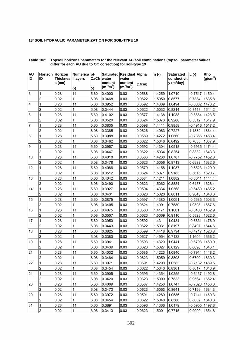
302
18/ SOIL HYDRAULIC PARAMETERIZATION FOR SOIL-TYPE 19
Table 102: Topsoil horizons parameters for the relevant AU/soil combinations (topsoil parameter values differ for each AU due to OC correction) for soil-type 19
AU ID
Horizon ID
Horizon Thickness (cm)
Numerical layers
(-)
pH CaCl2
(-)
Saturated water content (m3/m3)
Residual water content (m3/m3)
Alpha
(1/cm)
n (-) Saturated conductivity (m/day)
L (-) Rho (g/cm3)
3 1 0.28 11 5.60 0.4000 0.03 0.0588 1.4259 1.0710 -0.7517 1459.4 2 0.02 1 6.08 0.3468 0.03 0.0622 1.5050 0.8577 0.7384 1635.8 4 1 0.28 11 5.60 0.3952 0.03 0.0592 1.4309 1.0494 -0.6862 1476.2 2 0.02 1 6.08 0.3444 0.03 0.0622 1.5032 0.8214 0.8448 1644.2 6 1 0.28 11 5.60 0.4102 0.03 0.0577 1.4138 1.1088 -0.8684 1423.5 2 0.02 1 6.08 0.3520 0.03 0.0624 1.5073 0.9288 0.5312 1617.9 7 1 0.28 11 5.60 0.3835 0.03 0.0598 1.4411 0.9858 -0.4916 1517.2 2 0.02 1 6.08 0.3385 0.03 0.0626 1.4963 0.7227 1.1332 1664.4 8 1 0.28 11 5.60 0.3988 0.03 0.0589 1.4272 1.0660 -0.7366 1463.4 2 0.02 1 6.08 0.3462 0.03 0.0622 1.5046 0.8492 0.7635 1637.9 9 1 0.28 11 5.60 0.3957 0.03 0.0592 1.4304 1.0518 -0.6935 1474.4 2 0.02 1 6.08 0.3447 0.03 0.0622 1.5034 0.8254 0.8332 1643.3 10 1 0.28 11 5.60 0.4018 0.03 0.0586 1.4238 1.0787 -0.7752 1452.8 2 0.02 1 6.08 0.3478 0.03 0.0623 1.5056 0.8713 0.6988 1632.6 12 1 0.28 11 5.60 0.4086 0.03 0.0579 1.4158 1.1037 -0.8523 1429.0 2 0.02 1 6.08 0.3512 0.03 0.0624 1.5071 0.9183 0.5615 1620.7 13 1 0.28 11 5.60 0.4042 0.03 0.0584 1.4211 1.0882 -0.8041 1444.4 2 0.02 1 6.08 0.3490 0.03 0.0623 1.5062 0.8884 0.6487 1628.4 14 1 0.28 11 5.60 0.3927 0.03 0.0594 1.4334 1.0368 -0.6480 1485.2 2 0.02 1 6.08 0.3431 0.03 0.0623 1.5020 0.8011 0.9043 1648.6 15 1 0.28 11 5.60 0.3875 0.03 0.0597 1.4380 1.0091 -0.5635 1503.3 2 0.02 1 6.08 0.3405 0.03 0.0624 1.4991 0.7580 1.0305 1657.6 16 1 0.28 11 5.60 0.4075 0.03 0.0580 1.4171 1.1001 -0.8408 1432.9 2 0.02 1 6.08 0.3507 0.03 0.0623 1.5069 0.9110 0.5828 1622.6 17 1 0.28 11 5.60 0.3950 0.03 0.0592 1.4311 1.0484 -0.6831 1476.9 2 0.02 1 6.08 0.3443 0.03 0.0622 1.5031 0.8197 0.8497 1644.6 18 1 0.28 11 5.60 0.3825 0.03 0.0599 1.4418 0.9794 -0.4717 1520.8 2 0.02 1 6.08 0.3380 0.03 0.0627 1.4954 0.7132 1.1609 1666.2 19 1 0.28 11 5.60 0.3941 0.03 0.0593 1.4320 1.0441 -0.6703 1480.0 2 0.02 1 6.08 0.3439 0.03 0.0623 1.5027 0.8129 0.8698 1646.1 21 1 0.28 11 5.60 0.4032 0.03 0.0585 1.4223 1.0840 -0.7914 1448.2 2 0.02 1 6.08 0.3484 0.03 0.0623 1.5059 0.8808 0.6709 1630.3 22 1 0.28 11 5.60 0.3971 0.03 0.0591 1.4290 1.0583 -0.7132 1469.5 2 0.02 1 6.08 0.3454 0.03 0.0622 1.5040 0.8361 0.8017 1640.9 24 1 0.28 11 5.60 0.3905 0.03 0.0595 1.4354 1.0255 -0.6137 1492.8 2 0.02 1 6.08 0.3420 0.03 0.0623 1.5009 0.7833 0.9564 1652.4 26 1 0.28 11 5.60 0.4009 0.03 0.0587 1.4250 1.0747 -0.7628 1456.3 2 0.02 1 6.08 0.3473 0.03 0.0623 1.5053 0.8641 0.7199 1634.3 29 1 0.28 11 5.60 0.3972 0.03 0.0591 1.4289 1.0586 -0.7141 1469.3 2 0.02 1 6.08 0.3454 0.03 0.0622 1.5040 0.8366 0.8002 1640.8 31 1 0.28 11 5.60 0.3891 0.03 0.0596 1.4366 1.0179 -0.5905 1497.8 2 0.02 1 6.08 0.3413 0.03 0.0623 1.5001 0.7715 0.9909 1654.8

Table 103: Subsoil horizons parameters for soil-type 19
AU ID
Horizon ID
Horizon Thickness (cm)
Numerical layers
pH CaCl2
Saturated water content (m3/m3)
Residual water content (m3/m3)
Alpha n (-) Saturated conductivity (m/day)
L (-) Rho (g/cm3)
(1/cm) (-) (-)
all 3 0.08 3 0.3439 0.03 0.0738 1.4894 0.3690 0.9309 1650.6 6.08 4 0.18 4 0.3352 0.03 0.0754 1.4938 0.3016 1.5401 1681.3 6.47 5 0.04 1 0.3231 0.03 0.0852 1.6778 0.5780 1.6328 1681.3 5.89 6 0.3 6 0.3231 0.03 0.0852 1.6778 0.5780 1.6328 1681.3 5.89 7 0.1 2 0.3077 0.03 0.1003 1.6560 0.4409 2.2306 1715.6 6.38 8 0.25 3 0.3077 0.03 0.1003 1.6560 0.4409 2.2306 1715.6 6.38 9 0.1 10 0.3077 0.03 0.1003 1.6560 0.4409 2.2306 1715.6 6.38 10 0.65 7 0.3077 0.03 0.1003 1.6560 0.4409 2.2306 1715.6 6.38
303

Appendix 18 : Test results for Substance C and its metabolite applied to sugar beet
304
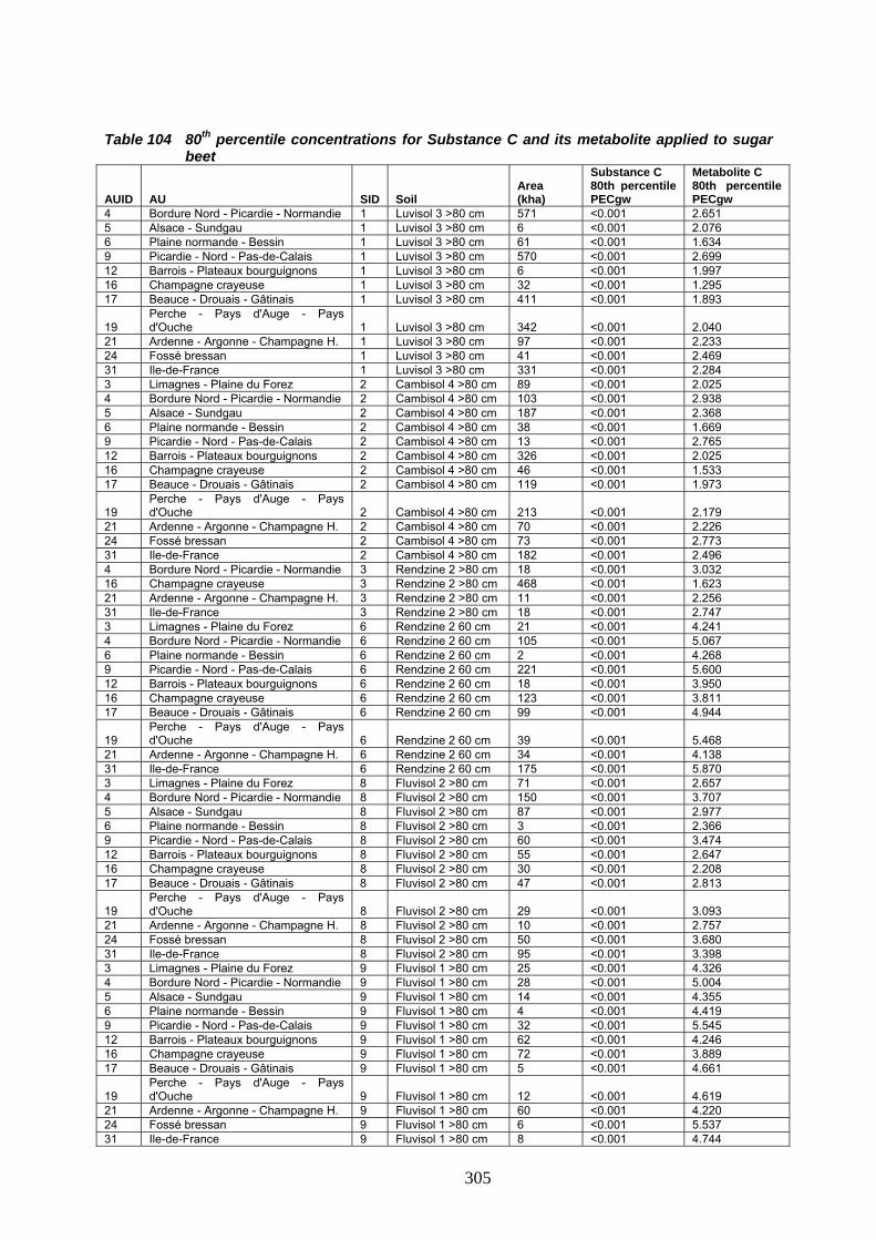
305
Table 104 80th percentile concentrations for Substance C and its metabolite applied to sugar
beet
AUID AU SID Soil Area (kha)
Substance C 80th percentile PECgw
Metabolite C 80th percentile PECgw
4 Bordure Nord - Picardie - Normandie 1 Luvisol 3 >80 cm 571 <0.001 2.651 5 Alsace - Sundgau 1 Luvisol 3 >80 cm 6 <0.001 2.076 6 Plaine normande - Bessin 1 Luvisol 3 >80 cm 61 <0.001 1.634 9 Picardie - Nord - Pas-de-Calais 1 Luvisol 3 >80 cm 570 <0.001 2.699 12 Barrois - Plateaux bourguignons 1 Luvisol 3 >80 cm 6 <0.001 1.997 16 Champagne crayeuse 1 Luvisol 3 >80 cm 32 <0.001 1.295 17 Beauce - Drouais - Gâtinais 1 Luvisol 3 >80 cm 411 <0.001 1.893
19 Perche - Pays d'Auge - Pays d'Ouche 1 Luvisol 3 >80 cm 342 <0.001 2.040
21 Ardenne - Argonne - Champagne H. 1 Luvisol 3 >80 cm 97 <0.001 2.233 24 Fossé bressan 1 Luvisol 3 >80 cm 41 <0.001 2.469 31 Ile-de-France 1 Luvisol 3 >80 cm 331 <0.001 2.284 3 Limagnes - Plaine du Forez 2 Cambisol 4 >80 cm 89 <0.001 2.025 4 Bordure Nord - Picardie - Normandie 2 Cambisol 4 >80 cm 103 <0.001 2.938 5 Alsace - Sundgau 2 Cambisol 4 >80 cm 187 <0.001 2.368 6 Plaine normande - Bessin 2 Cambisol 4 >80 cm 38 <0.001 1.669 9 Picardie - Nord - Pas-de-Calais 2 Cambisol 4 >80 cm 13 <0.001 2.765 12 Barrois - Plateaux bourguignons 2 Cambisol 4 >80 cm 326 <0.001 2.025 16 Champagne crayeuse 2 Cambisol 4 >80 cm 46 <0.001 1.533 17 Beauce - Drouais - Gâtinais 2 Cambisol 4 >80 cm 119 <0.001 1.973
19 Perche - Pays d'Auge - Pays d'Ouche 2 Cambisol 4 >80 cm 213 <0.001 2.179
21 Ardenne - Argonne - Champagne H. 2 Cambisol 4 >80 cm 70 <0.001 2.226 24 Fossé bressan 2 Cambisol 4 >80 cm 73 <0.001 2.773 31 Ile-de-France 2 Cambisol 4 >80 cm 182 <0.001 2.496 4 Bordure Nord - Picardie - Normandie 3 Rendzine 2 >80 cm 18 <0.001 3.032 16 Champagne crayeuse 3 Rendzine 2 >80 cm 468 <0.001 1.623 21 Ardenne - Argonne - Champagne H. 3 Rendzine 2 >80 cm 11 <0.001 2.256 31 Ile-de-France 3 Rendzine 2 >80 cm 18 <0.001 2.747 3 Limagnes - Plaine du Forez 6 Rendzine 2 60 cm 21 <0.001 4.241 4 Bordure Nord - Picardie - Normandie 6 Rendzine 2 60 cm 105 <0.001 5.067 6 Plaine normande - Bessin 6 Rendzine 2 60 cm 2 <0.001 4.268 9 Picardie - Nord - Pas-de-Calais 6 Rendzine 2 60 cm 221 <0.001 5.600 12 Barrois - Plateaux bourguignons 6 Rendzine 2 60 cm 18 <0.001 3.950 16 Champagne crayeuse 6 Rendzine 2 60 cm 123 <0.001 3.811 17 Beauce - Drouais - Gâtinais 6 Rendzine 2 60 cm 99 <0.001 4.944
19 Perche - Pays d'Auge - Pays d'Ouche 6 Rendzine 2 60 cm 39 <0.001 5.468
21 Ardenne - Argonne - Champagne H. 6 Rendzine 2 60 cm 34 <0.001 4.138 31 Ile-de-France 6 Rendzine 2 60 cm 175 <0.001 5.870 3 Limagnes - Plaine du Forez 8 Fluvisol 2 >80 cm 71 <0.001 2.657 4 Bordure Nord - Picardie - Normandie 8 Fluvisol 2 >80 cm 150 <0.001 3.707 5 Alsace - Sundgau 8 Fluvisol 2 >80 cm 87 <0.001 2.977 6 Plaine normande - Bessin 8 Fluvisol 2 >80 cm 3 <0.001 2.366 9 Picardie - Nord - Pas-de-Calais 8 Fluvisol 2 >80 cm 60 <0.001 3.474 12 Barrois - Plateaux bourguignons 8 Fluvisol 2 >80 cm 55 <0.001 2.647 16 Champagne crayeuse 8 Fluvisol 2 >80 cm 30 <0.001 2.208 17 Beauce - Drouais - Gâtinais 8 Fluvisol 2 >80 cm 47 <0.001 2.813
19 Perche - Pays d'Auge - Pays d'Ouche 8 Fluvisol 2 >80 cm 29 <0.001 3.093
21 Ardenne - Argonne - Champagne H. 8 Fluvisol 2 >80 cm 10 <0.001 2.757 24 Fossé bressan 8 Fluvisol 2 >80 cm 50 <0.001 3.680 31 Ile-de-France 8 Fluvisol 2 >80 cm 95 <0.001 3.398 3 Limagnes - Plaine du Forez 9 Fluvisol 1 >80 cm 25 <0.001 4.326 4 Bordure Nord - Picardie - Normandie 9 Fluvisol 1 >80 cm 28 <0.001 5.004 5 Alsace - Sundgau 9 Fluvisol 1 >80 cm 14 <0.001 4.355 6 Plaine normande - Bessin 9 Fluvisol 1 >80 cm 4 <0.001 4.419 9 Picardie - Nord - Pas-de-Calais 9 Fluvisol 1 >80 cm 32 <0.001 5.545 12 Barrois - Plateaux bourguignons 9 Fluvisol 1 >80 cm 62 <0.001 4.246 16 Champagne crayeuse 9 Fluvisol 1 >80 cm 72 <0.001 3.889 17 Beauce - Drouais - Gâtinais 9 Fluvisol 1 >80 cm 5 <0.001 4.661
19 Perche - Pays d'Auge - Pays d'Ouche 9 Fluvisol 1 >80 cm 12 <0.001 4.619
21 Ardenne - Argonne - Champagne H. 9 Fluvisol 1 >80 cm 60 <0.001 4.220 24 Fossé bressan 9 Fluvisol 1 >80 cm 6 <0.001 5.537 31 Ile-de-France 9 Fluvisol 1 >80 cm 8 <0.001 4.744

Substance C Metabolite C 80th percentile PECgw
80th percentile PECgw
Area (kha) AUID AU SID Soil
4 Bordure Nord - Picardie - Normandie 13 Cambisol 3 >80 cm 118 <0.001 3.215 5 Alsace - Sundgau 13 Cambisol 3 >80 cm 3 <0.001 2.555 6 Plaine normande - Bessin 13 Cambisol 3 >80 cm 3 <0.001 1.967 9 Picardie - Nord - Pas-de-Calais 13 Cambisol 3 >80 cm 105 <0.001 2.857 12 Barrois - Plateaux bourguignons 13 Cambisol 3 >80 cm 7 <0.001 2.281 16 Champagne crayeuse 13 Cambisol 3 >80 cm 29 <0.001 1.712 17 Beauce - Drouais - Gâtinais 13 Cambisol 3 >80 cm 17 <0.001 2.329
Perche - Pays d'Auge - Pays d'Ouche 19 13 Cambisol 3 >80 cm 4 <0.001 2.458
21 Ardenne - Argonne - Champagne H. 13 Cambisol 3 >80 cm 8 <0.001 2.524 24 Fossé bressan 13 Cambisol 3 >80 cm 5 <0.001 2.838 31 Ile-de-France 13 Cambisol 3 >80 cm 16 <0.001 2.770 3 Limagnes - Plaine du Forez 19 Arenosol 1 >80 cm 4 <0.001 6.883 4 Bordure Nord - Picardie - Normandie 19 Arenosol 1 >80 cm 41 0.003 7.380 6 Plaine normande - Bessin 19 Arenosol 1 >80 cm 2 <0.001 6.691 9 Picardie - Nord - Pas-de-Calais 19 Arenosol 1 >80 cm 55 0.001 8.398 12 Barrois - Plateaux bourguignons 19 Arenosol 1 >80 cm 7 <0.001 5.760 16 Champagne crayeuse 19 Arenosol 1 >80 cm 8 <0.001 6.261 17 Beauce - Drouais - Gâtinais 19 Arenosol 1 >80 cm 25 <0.001 8.498
Perche - Pays d'Auge - Pays d'Ouche 19 19 Arenosol 1 >80 cm 5 <0.001 7.617
21 Ardenne - Argonne - Champagne H. 19 Arenosol 1 >80 cm 16 <0.001 6.242 24 Fossé bressan 19 Arenosol 1 >80 cm 2 0.006 7.266 31 Ile-de-France 19 Arenosol 1 >80 cm 110 <0.001 8.921
306

Appendix 19 : FROGS scenarios presenting a 80th temporal PECgw > 10 μg/L for MetC on Winter wheat
307
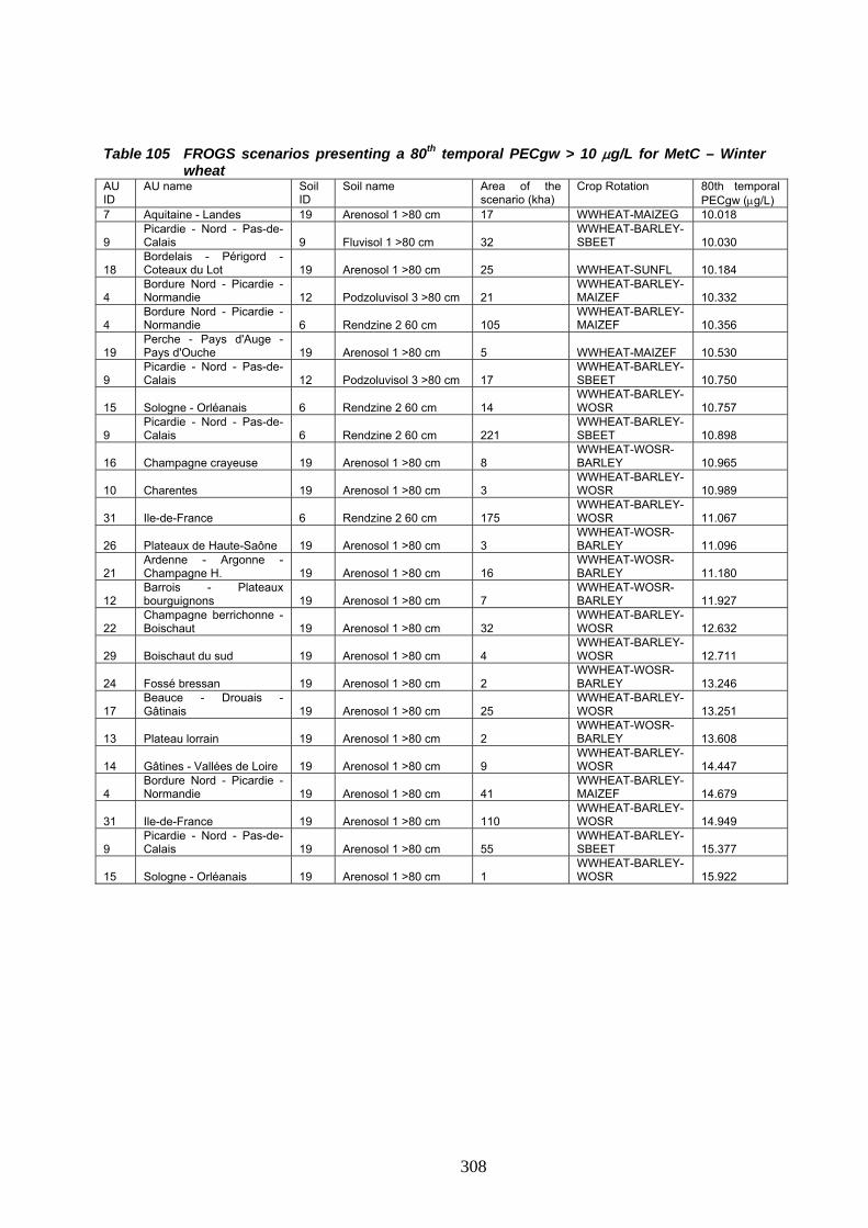
Table 105 FROGS scenarios presenting a 80th temporal PECgw > 10 μg/L for MetC – Winter
wheat AU ID
AU name Soil ID
Soil name Area of the scenario (kha)
Crop Rotation 80th temporal PECgw (μg/L)
7 Aquitaine - Landes 19 Arenosol 1 >80 cm 17 WWHEAT-MAIZEG 10.018 Picardie - Nord - Pas-de-Calais
WWHEAT-BARLEY-SBEET 9 9 Fluvisol 1 >80 cm 32 10.030
Bordelais - Périgord - Coteaux du Lot 18 19 Arenosol 1 >80 cm 25 WWHEAT-SUNFL 10.184 Bordure Nord - Picardie - Normandie
WWHEAT-BARLEY-MAIZEF 4 12 Podzoluvisol 3 >80 cm 21 10.332
Bordure Nord - Picardie - Normandie
WWHEAT-BARLEY-MAIZEF 4 6 Rendzine 2 60 cm 105 10.356
Perche - Pays d'Auge - Pays d'Ouche 19 19 Arenosol 1 >80 cm 5 WWHEAT-MAIZEF 10.530 Picardie - Nord - Pas-de-Calais
WWHEAT-BARLEY-SBEET 9 12 Podzoluvisol 3 >80 cm 17 10.750 WWHEAT-BARLEY-WOSR 15 Sologne - Orléanais 6 Rendzine 2 60 cm 14 10.757
Picardie - Nord - Pas-de-Calais
WWHEAT-BARLEY-SBEET 9 6 Rendzine 2 60 cm 221 10.898 WWHEAT-WOSR-BARLEY 16 Champagne crayeuse 19 Arenosol 1 >80 cm 8 10.965 WWHEAT-BARLEY-WOSR 10 Charentes 19 Arenosol 1 >80 cm 3 10.989 WWHEAT-BARLEY-WOSR 31 Ile-de-France 6 Rendzine 2 60 cm 175 11.067 WWHEAT-WOSR-BARLEY 26 Plateaux de Haute-Saône 19 Arenosol 1 >80 cm 3 11.096
Ardenne - Argonne - Champagne H.
WWHEAT-WOSR-BARLEY 21 19 Arenosol 1 >80 cm 16 11.180
Barrois - Plateaux bourguignons
WWHEAT-WOSR-BARLEY 12 19 Arenosol 1 >80 cm 7 11.927
Champagne berrichonne - Boischaut
WWHEAT-BARLEY-WOSR 22 19 Arenosol 1 >80 cm 32 12.632 WWHEAT-BARLEY-WOSR 29 Boischaut du sud 19 Arenosol 1 >80 cm 4 12.711 WWHEAT-WOSR-BARLEY 24 Fossé bressan 19 Arenosol 1 >80 cm 2 13.246
Beauce - Drouais - Gâtinais
WWHEAT-BARLEY-WOSR 17 19 Arenosol 1 >80 cm 25 13.251 WWHEAT-WOSR-BARLEY 13 Plateau lorrain 19 Arenosol 1 >80 cm 2 13.608 WWHEAT-BARLEY-WOSR 14 Gâtines - Vallées de Loire 19 Arenosol 1 >80 cm 9 14.447
Bordure Nord - Picardie - Normandie
WWHEAT-BARLEY-MAIZEF 4 19 Arenosol 1 >80 cm 41 14.679 WWHEAT-BARLEY-WOSR 31 Ile-de-France 19 Arenosol 1 >80 cm 110 14.949
Picardie - Nord - Pas-de-Calais
WWHEAT-BARLEY-SBEET 9 19 Arenosol 1 >80 cm 55 15.377 WWHEAT-BARLEY-WOSR 15 Sologne - Orléanais 19 Arenosol 1 >80 cm 1 15.922
308
Appendix 20 : FROGS scenarios presenting a 80th temporal PECgw > 0.1 μg/L for Substance D on Winter barley
309

310
Table 106 FROGS scenarios presenting a 80th temporal PECgw > 0.1 μg/L for Substance D –
Winter barley AU ID
AU name Soil ID
Soil name Area of the scenario (kha)
Crop Rotation 80th temporal PECgw (μg/L)
29 Boischaut du sud 9 Fluvisol 1 >80 cm 17 BARLEY-MAIZE-WWHEAT 0.100
1 Collines molassiques - Lauragais 9 Fluvisol 1 >80 cm 4 BARLEY-WWHEAT-SUNFL 0.106
20 Bocages de l'ouest 13 Cambisol 3 >80 cm 133 BARLEY-WWHEAT-MAIZEF 0.107 31 Ile-de-France 9 Fluvisol 1 >80 cm 8 BARLEY-WOSR-WWHEAT 0.111 5 Alsace - Sundgau 9 Fluvisol 1 >80 cm 14 BARLEY-WWHEAT-WOSR 0.114
6 Plaine normande - Bessin 12 Podzoluvisol 3 >80 cm 7 BARLEY-WOSR-WWHEAT 0.115
23 Bas Dauphiné - Vallée du Rhône 8 Fluvisol 2 >80 cm 124
BARLEY-WWHEAT-WWHEAT 0.117
23 Bas Dauphiné - Vallée du Rhône 5 Cambisol 3 60 cm 39
BARLEY-WWHEAT-WWHEAT 0.124
26 Plateaux de Haute-Saône 1 Luvisol 3 >80 cm 16 BARLEY-WWHEAT-WOSR 0.128 26 Plateaux de Haute-Saône 2 Cambisol 4 >80 cm 113 BARLEY-WWHEAT-WOSR 0.129
4 Bordure Nord - Picardie - Normandie 8 Fluvisol 2 >80 cm 150 BARLEY-WWHEAT-SBEET 0.129
17 Beauce - Drouais - Gâtinais 6 Rendzine 2 60 cm 99 BARLEY-WOSR-WWHEAT 0.132
13 Plateau lorrain 9 Fluvisol 1 >80 cm 25 BARLEY-WWHEAT-WOSR 0.135
11 Bocage normand 12 Podzoluvisol 3 >80 cm 93 BARLEY-MAIZEF-WWHEAT 0.137
24 Fossé bressan 9 Fluvisol 1 >80 cm 6 BARLEY-WWHEAT-WOSR 0.140
19 Perche - Pays d'Auge - Pays d'Ouche 9 Fluvisol 1 >80 cm 12 BARLEY-WWHEAT-WOSR 0.141
14 Gâtines - Vallées de Loire 12 Podzoluvisol 3 >80 cm 53 BARLEY-WOSR-WWHEAT 0.146
26 Plateaux de Haute-Saône 5 Cambisol 3 60 cm 145 BARLEY-WWHEAT-WOSR 0.151 20 Bocages de l'ouest 5 Cambisol 3 60 cm 162 BARLEY-WWHEAT-MAIZEF 0.155
21 Ardenne - Argonne - Champagne H. 9 Fluvisol 1 >80 cm 60 BARLEY-WWHEAT-WOSR 0.170
22 Champagne berrichonne - Boischaut 12
Podzoluvisol 3 >80 cm 46 BARLEY-WOSR-WWHEAT 0.177
12 Barrois - Plateaux bourguignons 9 Fluvisol 1 >80 cm 62 BARLEY-WWHEAT-WOSR 0.217
11 Bocage normand 6 Rendzine 2 60 cm 15 BARLEY-MAIZEF-WWHEAT 0.221
31 Ile-de-France 12 Podzoluvisol 3 >80 cm 158 BARLEY-WOSR-WWHEAT 0.227
19 Perche - Pays d'Auge - Pays d'Ouche 12
Podzoluvisol 3 >80 cm 283 BARLEY-WWHEAT-WOSR 0.228
16 Champagne crayeuse 6 Rendzine 2 60 cm 123 BARLEY-WWHEAT-WOSR 0.236
24 Fossé bressan 12 Podzoluvisol 3 >80 cm 4 BARLEY-WWHEAT-WOSR 0.246
10 Charentes 9 Fluvisol 1 >80 cm 4 BARLEY-WOSR-WWHEAT 0.282 15 Sologne - Orléanais 6 Rendzine 2 60 cm 14 BARLEY-WOSR-WWHEAT 0.307
9 Picardie - Nord - Pas-de-Calais 9 Fluvisol 1 >80 cm 32
BARLEY-WWHEAT-WWHEAT 0.309
6 Plaine normande - Bessin 6 Rendzine 2 60 cm 2 BARLEY-WOSR-WWHEAT 0.390
12 Barrois - Plateaux bourguignons 12
Podzoluvisol 3 >80 cm 6 BARLEY-WWHEAT-WOSR 0.399
22 Champagne berrichonne - Boischaut 6 Rendzine 2 60 cm 9 BARLEY-WOSR-WWHEAT 0.449
13 Plateau lorrain 6 Rendzine 2 60 cm 15 BARLEY-WWHEAT-WOSR 0.469
4 Bordure Nord - Picardie - Normandie 9 Fluvisol 1 >80 cm 28 BARLEY-WWHEAT-SBEET 0.481
29 Boischaut du sud 6 Rendzine 2 60 cm 7 BARLEY-MAIZE-WWHEAT 0.486
21 Ardenne - Argonne - Champagne H. 6 Rendzine 2 60 cm 34 BARLEY-WWHEAT-WOSR 0.515
4 Bordure Nord - Picardie - Normandie 12
Podzoluvisol 3 >80 cm 21 BARLEY-WWHEAT-SBEET 0.565
9 Picardie - Nord - Pas-de-Calais 12
Podzoluvisol 3 >80 cm 17
BARLEY-WWHEAT-WWHEAT 0.569
12 Barrois - Plateaux bourguignons 6 Rendzine 2 60 cm 18 BARLEY-WWHEAT-WOSR 0.576
26 Plateaux de Haute-Saône 9 Fluvisol 1 >80 cm 22 BARLEY-WWHEAT-WOSR 0.608 20 Bocages de l'ouest 9 Fluvisol 1 >80 cm 18 BARLEY-WWHEAT-MAIZEF 0.708 31 Ile-de-France 6 Rendzine 2 60 cm 175 BARLEY-WOSR-WWHEAT 0.768
AU ID
AU name Soil ID
Soil name Area of the scenario (kha)
Crop Rotation 80th temporal PECgw (μg/L)
Podzoluvisol 3 >80 cm 20 Bocages de l'ouest 12 26 BARLEY-WWHEAT-MAIZEF 0.860
14 Gâtines - Vallées de Loire 6 Rendzine 2 60 cm 140 BARLEY-WOSR-WWHEAT 0.896 Podzoluvisol 3 >80 cm 26 Plateaux de Haute-Saône 12 14 BARLEY-WWHEAT-WOSR 0.927
Perche - Pays d'Auge - Pays d'Ouche 19 6 Rendzine 2 60 cm 39 BARLEY-WWHEAT-WOSR 0.939 Collines molassiques - Lauragais 1 6 Rendzine 2 60 cm 5 BARLEY-WWHEAT-SUNFL 0.941
10 Charentes 6 Rendzine 2 60 cm 118 BARLEY-WOSR-WWHEAT 1.030 Picardie - Nord - Pas-de-Calais
BARLEY-WWHEAT-WWHEAT 9 6 Rendzine 2 60 cm 221 1.109
Bordelais - Périgord - Coteaux du Lot 18 6 Rendzine 2 60 cm 41 BARLEY-WWHEAT-SUNFL 1.353 Bordure Nord - Picardie - Normandie 4 6 Rendzine 2 60 cm 105 BARLEY-WWHEAT-SBEET 1.399
26 Plateaux de Haute-Saône 6 Rendzine 2 60 cm 9 BARLEY-WWHEAT-WOSR 1.527 20 Bocages de l'ouest 6 Rendzine 2 60 cm 10 BARLEY-WWHEAT-MAIZEF 1.648
311
Appendix 21 : Calculation of Available Water Capacity
312

Calculation of Available Water Capacity Conceptually the available water capacity (AWC) is the amount of water accessible to a crop. This is determined by the storage properties of the soil which are closely related to texture and the root depth. As a convention the root depth is assumed to reach down to 1 m unless the profile is not developed down to this depth or there are other restrictions to root growth (e.g. stagnant water, massive soil layers). For the soils considered here the profile depth is exclusively used as potential restriction to root growth.
Available water in a certain soil layer of thickness Δz is defined as the difference between the water content ΘF at field capacity (pF = 2) and the water content ΘWP at the wilting point (pF = 4.2) multiplied by Δz, as can be calculated using the hydraulic parameters (see Appendix 17) and the water retention function of Van Genuchten [1980]10 which is implemented in PEARL. The total available water AWC is the sum for n layers representing the root depth zr as
( ) ri
n iii
n iWPiF zzzAWC =ΔΔ−= ∑∑ == 11 ,θθ
were zr = 1 m or the development depth of the soil profile if smaller than 1 m.
313
10 Van Genuchten, M. T. (1980). A closed‐form equation for predicting the hydraulic conductivity of unsaturated soils. Soil Science Society of American Journal 44: 892 ‐ 898.
Related Documents