Universit¨ at Hamburg Department Physik Spinor Tonks-Girardeau gases and ultracold molecules Dissertation zur Erlangung des Doktorgrades des Departments Physik der Universit ¨ at Hambur g vorgelegt von Frank Deuretzbac her aus Halle (Saale) Hamburg 2008

Welcome message from author
This document is posted to help you gain knowledge. Please leave a comment to let me know what you think about it! Share it to your friends and learn new things together.
Transcript

8/3/2019 Frank Deuretzbacher- Spinor Tonks-Girardeau gases and ultracold molecules
http://slidepdf.com/reader/full/frank-deuretzbacher-spinor-tonks-girardeau-gases-and-ultracold-molecules 1/151
Universitat
Hamburg
Department
Physik
Spinor Tonks-Girardeau gases andultracold molecules
Dissertationzur Erlangung des Doktorgrades
des Departments Physik
der Universitat Hamburg
vorgelegt von
Frank Deuretzbacher
aus Halle (Saale)
Hamburg
2008

8/3/2019 Frank Deuretzbacher- Spinor Tonks-Girardeau gases and ultracold molecules
http://slidepdf.com/reader/full/frank-deuretzbacher-spinor-tonks-girardeau-gases-and-ultracold-molecules 2/151
Gutachterin/Gutachter der Dissertation: Prof. Dr. Daniela Pfannkuche
Prof. Dr. Stephanie M. Reimann
Prof. Dr. Maciej Lewenstein
Gutachterin/Gutachter der Disputation: Prof. Dr. Daniela Pfannkuche
Prof. Dr. Klaus Sengstock
Datum der Disputation: 15. Dezember 2008
Vorsitzender des Prufungsausschusses: PD Dr. Alexander Chudnovskiy
Vorsitzender des Promotionsausschusses: Prof. Dr. Robert Klanner
Dekan des Fachbereiches f ur Mathematik,
Informatik und Naturwissenschaften: Prof. Dr. Arno Fruhwald
8/3/2019 Frank Deuretzbacher- Spinor Tonks-Girardeau gases and ultracold molecules
http://slidepdf.com/reader/full/frank-deuretzbacher-spinor-tonks-girardeau-gases-and-ultracold-molecules 3/151
Abstract
The research field of ultracold atomic quantum gases has been developing rapidly during the lastyears. That is due to the extremely flexible toolbox of the experimenters, which allows them to
simulate for example a plenty of very different solid-state phenomena and to perform ultraslow
chemical reactions in a controlled reversible manner.
One of the newest research objects are one-dimensional atomic systems in optical lattices. In
cigar-shaped optical traps the free motion of the particles can be restricted to one dimension.
The tight transverse confinement, moreover, extremely strengthens the effective forces leading to
strong correlations between the particles.
In the first chapters of this thesis I study properties of quasi-one-dimensional Bose gases with
contact interactions. For this reason I have developed an exact diagonalization approach, which
allows for an accurate construction of the many-body wave function of few particles. During the
development of the exact-diagonalization programming code I oriented myself on experiments,
which have been performed in the group of K. Sengstock on spinor Bose-Einstein condensates.
At first I study the influence of the interaction strength on the properties of a spin polarized
Bose gas. As long as the repulsive forces are weak, the particles behave like typical bosons, i. e.,
due to the permutation symmetry of the many-particle wave function they favor to occupy the same
single-particle state. In that regime, the main impact of the weak repulsion is a broadening and
flattening of the single-particle wave function in order to reduce the mean distance between the
bosons. In the opposite limit, an extremely strong (or even infinite) repulsive contact force prevents
the bosons from staying at the same position, thereby mimicing Pauli’s exclusion principle. Indeed
it is observed that hard-core bosons behave in many respects like noninteracting fermions.
Here I study the interaction-driven fermionization of quasi-one-dimensional bosons and its effecton the most important measurable quantities. It is shown that the momentum distribution reflects
the permutation symmetry and the correlations of the many-particle wave function. Moreover, it
clearly distinguishes between the above mentioned interaction regimes. In this work the bound-
aries of these regimes are determined for small finite-size systems.
Next, I study a one-dimensional Bose gas of hard-core particles (i. e. the repulsive contact forces
between the point-like particles shall be infinite) with spin degrees of freedom. For that reason
an easy-to-use analytical formula of the exact many-body wave function of the highly correlated
bosons is derived. The construction scheme is based on M. Girardeau’s original idea of a Fermi-
Bose map for spinless particles. As a striking consequence of our mapping we find that one-
dimensional hard-core particles (bosons or fermions) with spin degrees of freedom behave in many
respects like noninteracting spinless fermions and noninteracting distinguishable spins. Therefore,the energy spectrum of this highly correlated many-particle system can be constructed easily.
Moreover, the analytical formula of the many-body wave function is the basis of an illustrative
construction scheme for the spin densities, which resemble a chain of localized spins.
Again, the momentum distribution is particularly interesting. Now its form strongly depends on
the spin configuration of the one-dimensional system. The momentum distribution of spinless
hard-core bosons shows striking differences from that of spinless noninteracting fermions. Here,
by contrast, in some spin configurations the momentum distribution of the system shows clear
fermionic signatures. Moreover, the construction scheme for the wave functions is also applicable
to isospin-1/2 bosons, which e. g. represent Bose-Bose mixtures and two-level atoms.

8/3/2019 Frank Deuretzbacher- Spinor Tonks-Girardeau gases and ultracold molecules
http://slidepdf.com/reader/full/frank-deuretzbacher-spinor-tonks-girardeau-gases-and-ultracold-molecules 4/151
The second part of this thesis deals with the ultracold chemical reaction of 40K and 87Rb atoms.
C. Ospelkaus et al. produced molecules from atom pairs in a controlled reversible manner by
means of a Feshbach resonance. This groundbreaking experiment was an important step towards
the production of ultracold polar molecules (in their internal vibrational ground state). This might
enable the realization of quantum gases with long-range interactions in the near future. Here, I
develop a theoretical approach for the description of the molecule formation in a three-dimensionaloptical lattice. This approach might also be useful for other atomic mixtures with large mass ratios.

8/3/2019 Frank Deuretzbacher- Spinor Tonks-Girardeau gases and ultracold molecules
http://slidepdf.com/reader/full/frank-deuretzbacher-spinor-tonks-girardeau-gases-and-ultracold-molecules 5/151
Zusammenfassung
Das Gebiet der ultrakalten Quantengase hat sich in den letzten Jahren rasant entwickelt. Dasliegt auch an dem schier unerschopflichen Werkzeugkasten der Experimentatoren, der z. B. die
quantenmechanische Simulation unterschiedlichster Festkorperphanomene und die kontrollierte
Durchfuhrung chemischer Reaktionen ermoglicht, die bei ultratiefen Temperaturen sozusagen in
Zeitlupe ablaufen.
Die neuesten Untersuchungsobjekte sind eindimensionale Systeme in optischen Gittern. Ein zi-
garrenf ormiges Einschlusspotential beschrankt dabei die freie Bewegung der Teilchen auf eine
Dimension, was daruber hinaus zur Folge hat, dass die effektiven Krafte zwischen den Teilchen
extrem verstarkt werden. Das fuhrt zu starken Korrelationen zwischen den Teilchen.
In den ersten Kapiteln dieser Dissertation werden die quantenmechanischen Eigenschaften von
quasi-eindimensionalen Bose-Gasen mit einer extrem kurzreichweitigen Kontaktwechselwirkung
untersucht. Zu diesem Zweck wurde eine Exakte Diagonalisierung entwickelt, die eine ge-
naue Konstruktion der Vielteilchenwellenfunktion von wenigen Teilchen ermoglicht. Als Vorbild
dienten Experimente der Gruppe von K. Sengstock zu Spinor Bose-Einstein Kondensaten.
Es wurde zunachst der Einfluss der Wechselwirkungsstarke auf die Eigenschaften eines spinpo-
larisierten Bose-Gases untersucht. Solange die abstoßenden Kontaktkrafte zwischen den Teilchen
klein sind, verhalten sie sich wie typische Bosonen, die sich auf Grund der Symmetrie der Viel-
teilchenwellenfunktion unter beliebigen Teilchenvertauschungen bevorzugt im selben stationaren
Bewegungszustand aufhalten. Die Einteilchenwellenfunktion, die diesen stationaren Bewegungs-
zustand beschreibt, wird durch die repulsiven Kontaktkrafte lediglich verbreitert, um den mittle-
ren Abstand zwischen den Teilchen zu reduzieren. Eine sehr starke (unendlich große) abstoßende
Kontaktkraft hindert die Bosonen hingegen in ihrem Bestreben, den selben quantenmechanischen
Zustand einzunehmen. Die unendlich starke Abstoßung simuliert vielmehr das Pauli-Prinzip, wo-
durch sich die Bosonen, ahnlich wie Fermionen, nicht mehr am selben Ort aufhalten k onnen.
Es wird tatsachlich beobachtet, dass Bosonen unter diesen Bedingungen viele Eigenschaften von
nichtwechselwirkenden Fermionen annehmen.
Diese sogenannte Fermionisierung quasi-eindimensionaler Bosonen mit zunehmender Kontaktab-
stoßung wird hier im Detail anhand wichtiger Messgroßen untersucht. Dabei zeigt insbesondere
die Impulsverteilung des Systems ein interessantes Verhalten, da sich in ihrer Form sowohl die
Permutationssymmetrie als auch die Korrelationen der Gesamtwellenfunktion widerspiegeln. Es
wird in dieser Arbeit erstmals gezeigt, dass sich bestimmte Merkmale der Impulsverteilung auch
zur Bestimmung der Grenzen der oben beschriebenen typischen Wechselwirkungsbereiche eignen.
Im nachsten Schritt wird ein eindimensionales Bose-Gas mit Spinfreiheitsgraden und (un-endlich) starker Kontaktabstoßung untersucht. Zu diesem Zweck wird, aufbauend auf den Ide-
en von M. D. Girardeau, eine vergleichsweise einfache analytische Formel fur die exakten
Vielteilchen-Eigenfunktionen des Hamiltonoperators entwickelt. Die verbluffende Konsequenz
dieser Formel ist die Aussage, dass sich eindimensionale Teilchen (sowohl Bosonen als auch
Fermionen) mit Spinfreiheitsgraden im Bereich unendlich starker Kontaktabstoßung gleichzeitig
wie nichtwechselwirkende spinlose Fermionen und nichtwechselwirkende unterscheidbare Spins
verhalten. Dadurch setzt sich das Energiespekrum solcher Systeme in einfacher Weise aus dem
Spektrum dieser beiden Teilchensorten zusammen. Außerdem lasst sich aus der Formel der exak-
ten Vielteilchen-Wellenfunktionen ein anschauliches Konstruktionsverfahren f ur die Spindichten

8/3/2019 Frank Deuretzbacher- Spinor Tonks-Girardeau gases and ultracold molecules
http://slidepdf.com/reader/full/frank-deuretzbacher-spinor-tonks-girardeau-gases-and-ultracold-molecules 6/151
ableiten. Es zeigt sich, dass diese einer Kette von lokalisierten Spins gleichen, deren Orientierung
sich in einfacher Weise von der angegebenen Wellenfunktion ablesen l asst.
Besonders interessant ist abermals das Verhalten der Impulsverteilung, deren Form stark von der
Spinkonfiguration des eindimensionalen Systems abhangt. Es zeigt sich nun auch im Impulsraum
eine große Ahnlichkeit zwischen Bosonen und Fermionen. Daruber hinaus ist das Konstruktions-
verfahren auch auf Isospin-1/2 Bosonensysteme anwendbar, welche sich z. B. durch Mischungen
oder mit Hilfe von Zwei-Niveau Atome realisieren lassen.
Der zweite Teil dieser Arbeit widmet sich dem Gebiet der ultrakalten Chemie. In dem von C. Os-
pelkaus et al. durchgef uhrten Experiment wurden Kalium- und Rubidiumatome mit Hilfe einer
Feshbachresonanz kontrolliert zur Reaktion gebracht. Dieses Schlusselexperiment ermoglichte
erst kurzlich die Herstellung von ultrakalten polaren Molekulen (im internen Vibrationsgrund-
zustand), wodurch in naher Zukunft moglicherweise Quantengase mit langreichweitigen Wech-
selwirkungen realisiert werden k onnen. Es wird hier ein einfaches Verfahren entwickelt, welches
eine genaue Beschreibung der Kalium-Rubidium Verbindung in einem dreidimensionalen opti-
schen Gitter ermoglicht. Die dabei entwickelte Methode k onnte auch f ur andere Mischsysteme
mit großen Massenunterschieden der einzelnen Bestandteile von Bedeutung sein.
8/3/2019 Frank Deuretzbacher- Spinor Tonks-Girardeau gases and ultracold molecules
http://slidepdf.com/reader/full/frank-deuretzbacher-spinor-tonks-girardeau-gases-and-ultracold-molecules 7/151
Publikationen
Teile dieser Dissertation sind in meiner Di-
plomarbeit [1] und in den folgenden Arbeiten
veroffentlicht worden:
Publications
Parts of this thesis have been published in my
diploma thesis [1] and in the following papers:
[2] F. Deuretzbacher, K. Bongs, K. Sengstock and D. Pfannkuche, Evolution from a Bose-
Einstein condensate to a Tonks-Girardeau gas: An exact diagonalization study, Physical
Review A 75, 013614 (2007).
[3] F. Deuretzbacher, K. Plassmeier, D. Pfannkuche, F. Werner, C. Ospelkaus, S. Ospelkaus,
K. Sengstock and K. Bongs, Heteronuclear molecules in an optical lattice: Theory and
experiment , Physical Review A 77, 032726 (2008).
[4] F. Deuretzbacher, K. Fredenhagen, D. Becker, K. Bongs, K. Sengstock and D. Pfannkuche, Exact Solution of Strongly Interacting Quasi-One-Dimensional Spinor Bose Gases, Phys.
Rev. Lett. 100, 160405 (2008).

8/3/2019 Frank Deuretzbacher- Spinor Tonks-Girardeau gases and ultracold molecules
http://slidepdf.com/reader/full/frank-deuretzbacher-spinor-tonks-girardeau-gases-and-ultracold-molecules 8/151

8/3/2019 Frank Deuretzbacher- Spinor Tonks-Girardeau gases and ultracold molecules
http://slidepdf.com/reader/full/frank-deuretzbacher-spinor-tonks-girardeau-gases-and-ultracold-molecules 9/151
Contents
1 Introduction 1
2 Modeling of ultracold spin-1 atoms 4
2.1 Hamiltonian for spin-1 atoms . . . . . . . . . . . . . . . . . . . . . . . . . . . . 4
2.1.1 Derivation of the Zeeman Hamiltonian . . . . . . . . . . . . . . . . . . 7
2.1.2 Derivation of the Interaction Hamiltonian . . . . . . . . . . . . . . . . . 10
2.2 Energy scales and parameter regimes . . . . . . . . . . . . . . . . . . . . . . . . 142.3 Exact diagonalization and second quantization . . . . . . . . . . . . . . . . . . . 17
2.4 Single-particle basis . . . . . . . . . . . . . . . . . . . . . . . . . . . . . . . . . 18
2.5 Generation of the many-particle basis . . . . . . . . . . . . . . . . . . . . . . . 19
2.6 Calculation of the Hamiltonian matrix . . . . . . . . . . . . . . . . . . . . . . . 21
2.7 Numerical diagonalization of the Hamiltonian matrix . . . . . . . . . . . . . . . 27
2.8 Calculation of system properties . . . . . . . . . . . . . . . . . . . . . . . . . . 27
2.9 Testing / convergence . . . . . . . . . . . . . . . . . . . . . . . . . . . . . . . . 30
3 Evolution from a BEC to a Tonks-Girardeau gas 35
3.1 Effective quasi-one-dimensional Hamiltonian . . . . . . . . . . . . . . . . . . . 35
3.2 Weakly interacting regime: Mean-field approximation . . . . . . . . . . . . . . . 37
3.3 Strongly interacting regime: Girardeau’s Fermi-Bose mapping . . . . . . . . . . 39
3.4 Evolution of various ground-state properties . . . . . . . . . . . . . . . . . . . . 42
3.5 Excitation spectrum . . . . . . . . . . . . . . . . . . . . . . . . . . . . . . . . . 51
4 The spinor Tonks-Girardeau gas 54
4.1 Analytical solution for hard-core particles with spin . . . . . . . . . . . . . . . . 54
4.2 Large but finite repulsion . . . . . . . . . . . . . . . . . . . . . . . . . . . . . . 64
4.3 Spin densities of the ground states . . . . . . . . . . . . . . . . . . . . . . . . . 70
4.4 Momentum distributions of the ground states . . . . . . . . . . . . . . . . . . . 73
5 Ultracold heteronuclear Feshbach molecules 76
5.1 S-wave scattering in free space . . . . . . . . . . . . . . . . . . . . . . . . . . . 76
5.2 S-wave scattering in a harmonic trap . . . . . . . . . . . . . . . . . . . . . . . . 84
5.3 Regularized delta potential . . . . . . . . . . . . . . . . . . . . . . . . . . . . . 90
5.4 Feshbach resonance . . . . . . . . . . . . . . . . . . . . . . . . . . . . . . . . . 93
5.5 A short description of the experiment . . . . . . . . . . . . . . . . . . . . . . . 96
5.6 Two interacting atoms at a single lattice site . . . . . . . . . . . . . . . . . . . . 98
5.7 Experimental vs. theoretical spectrum. Resonance position . . . . . . . . . . . . 107
5.8 Efficiency of rf association . . . . . . . . . . . . . . . . . . . . . . . . . . . . . 109
5.9 Lifetime . . . . . . . . . . . . . . . . . . . . . . . . . . . . . . . . . . . . . . . 112
i

8/3/2019 Frank Deuretzbacher- Spinor Tonks-Girardeau gases and ultracold molecules
http://slidepdf.com/reader/full/frank-deuretzbacher-spinor-tonks-girardeau-gases-and-ultracold-molecules 10/151
6 Conclusions and outlook 116
A Particle densities 118
B Weber’s differential equation 124
C Rabi model 126
D Table of constants 132
ii

8/3/2019 Frank Deuretzbacher- Spinor Tonks-Girardeau gases and ultracold molecules
http://slidepdf.com/reader/full/frank-deuretzbacher-spinor-tonks-girardeau-gases-and-ultracold-molecules 11/151
Chapter 1
Introduction
The subject of this thesis are Tonks-Girardeau gases with spin degrees of freedom and ultracold
heteronuclear Feshbach molecules. A Tonks-Girardeau gas is a one-dimensional Bose gas of
point-like hard spheres. It is named after Lewi Tonks und Marvin D. Girardeau. In 1936 L. Tonksfirst derived the equation of state of a one-dimensional gas of hard spheres [ 5], motivated by the
research done at the laboratories of General Electric on monoatomic films of caesium on tungsten.
Later in 1960 M. D. Girardeau found an elegant way to construct the exact many-particle wave
function of one-dimensional hard-core bosons from that of spinless noninteracting fermions [ 6].
More precisely, he found out that the wave function of one-dimensional hard-core bosons
ψ(∞)bosons can be constructed exactly from the corresponding wave function of spinless noninteracting
fermions ψ(0)fermions simply by a multiplication of the latter with the so-called unit antisymmetric
function A: ψ(∞)bosons = A ψ
(0)fermions
see Eq. (3.7) for the definition of A
. This equation constitutes
a bijective map between noninteracting fermions and bosons with infinite δ repulsion. As a direct
consequence the energy spectra of the two systems and all the properties which are calculated fromthe square of the wave function are identical. However, the momentum distributions are still quite
different due to the different permutation symmetries of the bosonic and fermionic wave functions.
Girardeau’s idea turned out to be extremely useful for the understanding of one-dimensional
systems and it inspired other theorists to search for further exact solutions. Shortly later in 1963
E. H. Lieb and W. Liniger solved exactly a gas of one-dimensional spinless bosons which inter-
act via contact potentials of finite strength in the thermodynamic limit [7, 8]. That solution was
generalized to particles with arbitrary permutation symmetry by C. N. Yang [9] and to bosons at
finite temperatures by C. N. Yang and C. P. Yang [10]. These papers form the basis of an effective
harmonic-fluid approach to the low-energy properties of one-dimensional systems by means of the
Luttinger liquid model [11, 12, 13] (see Ref. [14] for an introduction to the method).
However, although these systems seemed to be rather interesting for many theorists it was im-possible during a couple of decades to realize the quasi-one-dimensional regime in experiments.
That situation changed with the rapid progress in the field of ultracold atoms. Since the realization
of Bose-Einstein condensation (BEC) in atomic gases in 1995 the first groundbreaking experi-
ments have mainly been performed in the weakly interacting regime in two or three dimensions
(see Refs. [15, 16] for a review). In first experiments with cigar-shaped optical dipole traps [17]
dark solitons [18] and quantum phase fluctuations [19] have been studied in the weakly interacting
regime. However, extremely elongated trap geometries, which are needed to reach the strongly in-
teracting regime, became only recently available in optical lattices [20]. Finally, in the year 2004
two experimental groups even reached the Tonks-Girardeau regime [21, 22]. Moreover, Luttinger-
1

8/3/2019 Frank Deuretzbacher- Spinor Tonks-Girardeau gases and ultracold molecules
http://slidepdf.com/reader/full/frank-deuretzbacher-spinor-tonks-girardeau-gases-and-ultracold-molecules 12/151
2 CHAPTER 1. INTRODUCTION
liquid behavior, which has been theoretically predicted in Ref. [23] for ultracold atomic gases, has
been observed in several experiments with cold atoms in optical lattices [24, 25] and electrons in
quantum wires [26] and carbon nanotubes [27, 28, 29].
When one-dimensional systems with stronger interactions came into reach experimentally it was
realized that these systems have an inhomogeneous trapping potential with a finite size so that the
methods, which are based on the approach of E. H. Lieb and W. Liniger, were not directly applica-
ble. Moreover, it is rather difficult to extract correlation properties from the Lieb-Liniger solution.
The solution of Girardeau [6] on the other hand is valid for arbitrary trap geometries but unfortu-
nately only for an infinitely strong δ repulsion. It was thus necessary to develop new approaches
which account for the finite size, the inhomogeneity and the finite interaction strength of the atomic
gases. These new approaches are based on the Lieb-Liniger method [30, 31, 32, 33, 34, 35],
quantum Monte Carlo techniques [36, 37], the numerical density-matrix renormalization group
(DMRG) approach [38, 39, 40], the Multi-Configuration Time-Dependent Hartree (MCTDH)
method [41, 42] and the numerical exact-diagonalization technique [1, 2, 3, 4, 43, 44], which
is used throughout this thesis.
In the experiments of Kinoshita et al. [21, 45] the strength of the effective one-dimensionalδ
repul-
sion has been tuned by means of the transverse confinement. This is possible since in the quasi-
one-dimensional regime the effective one-dimensional interaction becomes proportional to the
transverse level spacing of the cigar-shaped trap. Accordingly, I study in chapter 3 the interaction-
driven evolution of a one-dimensional spin-polarized few boson system from a Bose-Einstein con-
densate to a Tonks-Girardeau gas. I use the exact-diagonalization method for the analysis of the
system, which I explain in detail in chapter 2 for the specific system of bosons with spin-dependent
contact forces. It is shown in chapter 3 that the momentum distribution of the spin-polarized sys-
tem shows a particularly interesting evolution when the interaction strength is increased.
In chapter 4 I analyze the ground-state properties of a Tonks-Girardeau gas with additional spin
degrees of freedom. So far most experiments, which studied the ground-state properties and the
spin dynamics of weakly interacting isospin-1/2 [46], spin-1 [47, 48, 49] or spin-2 [50, 51, 52, 53]Bose-Einstein condensates, have been successfully explained within the mean-field picture and
the single-mode approximation [54, 55, 56, 57, 58, 59, 60]. Moreover, coherent spin dynamics of
only two atoms at each site of a deep three-dimensional optical lattice has been studied in a series
of recent experiments [61, 62, 63]. However, in cigar-shaped traps with stronger interactions
the single-mode approximation is not applicable [64, 65, 66]. In that regime interesting spin
textures have been observed [67, 53], which are so far not completely understood. The results of
chapter 4 contribute to an understanding of these quasi-one-dimensional systems with spin degrees
of freedom from the viewpoint of an infinitely strong repulsion between the particles.
Girardeau’s concept of a bijective map between bosons and fermions has been extended to other
systems such as fermionic Tonks-Girardeau gases [68] and very recently also to mixtures [69]
and two-level atoms [70, 71]. Surprisingly, thus far no Fermi-Bose map existed for the importantsystem of particles with spin degrees of freedom. A solution of that problem is given in chapter 4
based on Girardeau’s original idea for spinless bosons [6]. There, an easy-to-use analytical for-
mula for the many-body wave functions of hard-core particles with spin is given. That formula
constitutes a bijective map between noninteracting spinless fermions and noninteracting distin-
guishable spins on the one hand and hard-core particles with spin on the other hand. As a result
the energy spectrum of the strongly interacting spinful particles is simply the sum of the spectra
of noninteracting spinless fermions and noninteracting distinguishable spins. Further, an illustra-
tive construction scheme for the spin densities is derived and it is shown for the example of three
spin-1 bosons that the analytical limiting solutions can be used to approximate realistic systems
8/3/2019 Frank Deuretzbacher- Spinor Tonks-Girardeau gases and ultracold molecules
http://slidepdf.com/reader/full/frank-deuretzbacher-spinor-tonks-girardeau-gases-and-ultracold-molecules 13/151
3
with large but finite interactions. Again, the momentum distribution shows a particularly interest-
ing behavior, which is now strongly dependent on the spin configuration of the one-dimensional
system and which exhibits fermionic features in some spin configurations.
Finally, chapter 5 deals with the production of ultracold heteronuclear molecules from 40K and87Rb atoms by means of radio-frequency (rf) association in the vicinity of a magnetic-field
Feshbach resonance [72, 73, 74]. In the first sections of that chapter I introduce important con-
cepts concerning the interactions in ultracold atomic gases. In particular I solve the problem of
two atoms in a three-dimensional rotationally symmetric harmonic trap, which interact via a box-
like potential. In the zero-range limit I obtain the result of Busch et al. [75], which shows that the
extremely short-range interaction potentials of ultracold atoms can be modeled by a regularized δpotential. That solution (which already includes the interaction between the particles) is the basis
of a detailed theoretical analysis of the experiment of C. Ospelkaus et al. [72] in the following
sections of chapter 5. In particular it was necessary for a precise determination of the two-atom
wave function to account for the coupling between center-of-mass and relative motion due to the
anharmonic corrections of the single lattice sites and the different masses of the atoms. We derive
a simple exact-diagonalization approach to that problem, which allows us not only to precisely
determine the location of the Feshbach resonance but also the efficiency of the rf association and
the lifetime of the molecules.

8/3/2019 Frank Deuretzbacher- Spinor Tonks-Girardeau gases and ultracold molecules
http://slidepdf.com/reader/full/frank-deuretzbacher-spinor-tonks-girardeau-gases-and-ultracold-molecules 14/151
Chapter 2
Modeling of ultracold spin-1 atoms
The main results of Secs. 2.5 to 2.9 have been published in my diploma thesis [1] and the main
parts of the exact diagonalization have been implemented during that time.
In this chapter I describe the methods which are the basis of the following chapters 3 and 4. In
Sec. 2.1 I present the Hamiltonian of the system and I discuss its properties and symmetries. In
the corresponding subsections 2.1.1 and 2.1.2 I derive the effective Zeeman Hamiltonian and in-
teraction potential respectively. In Secs. 2.3 to 2.8 I describe the implementation of a numerical
diagonalization of the many-particle Hamiltonian (2.5) and finally, in Sec. 2.9, I compare my nu-
merical results to known exact solutions in some limiting cases: the Tonks-Girardeau solution [6]
for a quasi-one-dimensional spin-polarized system, the solution of C. K. Law, H. Pu and N. P.
Bigelow [56] for a zero-dimensional system of bosonic spins and the two-particle solution [75, 76].
2.1 Hamiltonian for spin-1 atoms
Spin-independent harmonic trap: We consider a neutral 87Rb atom with spin f = 1. The atom is
confined by means of an optical dipole trap which provides a spin-independent harmonic potential
V trap =1
2m
ω2xx2 + ω2
yy2 + ω2zz2⊗ 1 .
Here, m is the mass of the 87Rb atom (see appendix D), ωx, ωy and ωz are the trap frequencies
of the x-, y- and z-direction, and 1 is the 3 × 3 dimensional identity matrix. V trap is a 3 × 3dimensional matrix since a spin-1 particle with motional and spin degrees of freedom is described
by a 3-component wave function
ψ(r) =
mf =−1,0,1
ψmf (r)|mf ,
with |1 = (1, 0, 0)T , |0 = (0, 1, 0)T and |−1 = (0, 0, 1)T . In each spin state the atom feels the
same trapping potential since V trap is diagonal in spin space. Furthermore, V trap commutes with
the parity operators of the x-, y- and z-direction Πx : x → −x, Πy : y → −y and Πz : z → −zsince V trap(x,y ,z) = V trap(±x, ±y, ±z). In most experiments of Refs. [52, 53] the transverse trap
frequencies ωy and ωz are much larger than the axial trap frequency ωx so that the system becomes
quasi-one-dimensional.
4

8/3/2019 Frank Deuretzbacher- Spinor Tonks-Girardeau gases and ultracold molecules
http://slidepdf.com/reader/full/frank-deuretzbacher-spinor-tonks-girardeau-gases-and-ultracold-molecules 15/151
2.1. HAMILTONIAN FOR SPIN-1 ATOMS 5
Zeeman Hamiltonian: A homogeneous magnetic field along the z-axis couples to the atomic spin
leading to the Zeeman Hamiltonian
V Z = −µBB
2f z − µ2
BB2
2C hfs
1 − 1
4f 2z
. (2.1)
Here, µB is Bohr’s magneton, B is the strength of the applied magnetic field, f z is the dimen-
sionless spin-1 matrix of the z-direction and C hfs is the hyperfine constant (see appendix D). The
dimensionless spin-1 matrices are given by
f x =1√
2
0 1 01 0 10 1 0
, f y =1√
2
0 −i 0i 0 −i
0 i 0
and f z =
1 0 00 0 00 0 −1
.
The first term of V Z is the usual linear and the second term is the quadratic Zeeman energy. Its
origin is explained in subsection 2.1.1.
Interaction Hamiltonian: Two spin-1 atoms interact with each other via a short-ranged spin-
dependent potential which is given by [54, 55]
V int. = δ(r1 − r2)
g0 1
⊗2 + g2 f 1 · f 2
(2.2)
with the interaction strengths g0 and g2 (note that g0 and g2 have dimension energy × volume
since the δ potential has dimension 1/volume). V int. is a 9 × 9 dimensional matrix since two
spin-1 particles with motional and spin degrees of freedom are described by a 9-component wave
function
ψ(r1, r2) =
mf ,mf =−1,0,1
ψmf ,mf
(r1, r2)|mf , mf ,
with
|mf , m
f
=
|mf
⊗ |mf
. 1
⊗2 = 1
⊗1 , f 1 = (f x,1, f y,1, f z,1) = (f x
⊗1 , f y
⊗1 , f z
⊗1 )
are the spin-1 matrices of the first atom and f 2 = (f x,2, f y,2, f z,2) = ( 1 ⊗ f x, 1 ⊗ f y, 1 ⊗ f z) are
the spin-1 matrices of the second atom. The scalar product f 1 · f 2 has to be evaluated according to
f 1 · f 2 = f x,1f x,2 + f y,1f y,2 + f z,1f z,2 = (f x ⊗ 1
)(1 ⊗ f x) + . . . = f x ⊗ f x + . . . .
The first term of the interaction potential (2.2) is spin-independent (i. e. diagonal in spin space)
and the second term is spin-dependent (i. e. non-diagonal in spin space). The scalar product f 1 · f 2can be expressed by means of the F 2 operator and the identity matrix. We use
F 2 =
f 1 + f 2
2= f 21 + f 22 + 2 f 1 · f 2 = 4
1
⊗2 + 2 f 1 · f 2
f 21 = f 22 = 2
1
⊗2
.
Thus, f 1 · f 2 = F 2/2 − 21
⊗2
and we can rewrite the interaction Hamiltonian (2.2) according to
V int. = δ(r1 − r2)
(g0 − 2g2) 1
⊗2 + (g2/2) F 2
. (2.3)
Therefore, V int. commutes with F z = f z,1 + f z,2 and F 2. The interaction strengths g0 and g2 are
given by [54, 55]
g0 =4π2
m× a0 + 2a2
3and g2 =
4π2
m× a2 − a0
3
8/3/2019 Frank Deuretzbacher- Spinor Tonks-Girardeau gases and ultracold molecules
http://slidepdf.com/reader/full/frank-deuretzbacher-spinor-tonks-girardeau-gases-and-ultracold-molecules 16/151
6 CHAPTER 2. MODELING OF ULTRACOLD SPIN-1 ATOMS
with the scattering lengths a0 and a2 ( is Planck’s constant). The interaction potential which
the atoms feel depends on the 2-atom spin F leading to the scattering lengths a0 (if F = 0)
and a2 (if F = 2). For 87Rb, a0 = 101.8 aB and a2 = 100.4 aB [77] (aB is the Bohr radius).
Therefore, the spin-dependent part of the interaction is approximately 200 times smaller than the
spin-independent part of the interaction, g0/
|g2
| ≈200. I will derive the interaction Hamiltonian
in subsection 2.1.2.
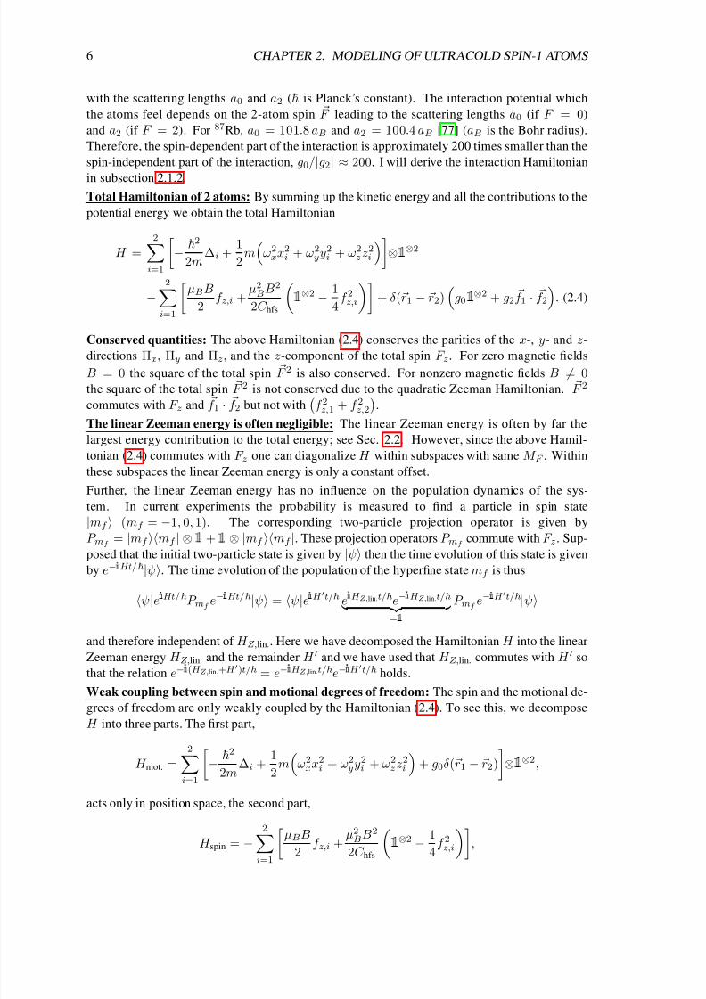
Total Hamiltonian of 2 atoms: By summing up the kinetic energy and all the contributions to the
potential energy we obtain the total Hamiltonian
H =2i=1
−
2
2m∆i +
1
2m
ω2xx2i + ω2
yy2i + ω2zz2i
⊗ 1
⊗2
−2i=1
µBB
2f z,i +
µ2BB2
2C hfs
1
⊗2 − 1
4f 2z,i
+ δ(r1 − r2)
g0 1
⊗2 + g2 f 1 · f 2
. (2.4)
Conserved quantities: The above Hamiltonian (2.4) conserves the parities of the x-, y- and z-
directions Πx, Πy and Πz, and the z-component of the total spin F z. For zero magnetic fields
B = 0 the square of the total spin F 2 is also conserved. For nonzero magnetic fields B = 0the square of the total spin F 2 is not conserved due to the quadratic Zeeman Hamiltonian. F 2
commutes with F z and f 1 · f 2 but not with
f 2z,1 + f 2z,2
.
The linear Zeeman energy is often negligible: The linear Zeeman energy is often by far the
largest energy contribution to the total energy; see Sec. 2.2. However, since the above Hamil-
tonian (2.4) commutes with F z one can diagonalize H within subspaces with same M F . Within
these subspaces the linear Zeeman energy is only a constant offset.
Further, the linear Zeeman energy has no influence on the population dynamics of the sys-
tem. In current experiments the probability is measured to find a particle in spin state
|mf (mf = −1, 0, 1). The corresponding two-particle projection operator is given byP mf
= |mf mf | ⊗ 1 + 1 ⊗ |mf mf |. These projection operators P mf commute with F z . Sup-
posed that the initial two-particle state is given by |ψ then the time evolution of this state is given
by e− i Ht/|ψ. The time evolution of the population of the hyperfine state mf is thus
ψ|e i Ht/P mf e−
i Ht/|ψ = ψ|ei H t/ ei H Z,lin.t/e− i H Z,lin.t/ =1
P mf e−
i H t/|ψ
and therefore independent of H Z,lin.. Here we have decomposed the Hamiltonian H into the linear
Zeeman energy H Z,lin. and the remainder H and we have used that H Z,lin. commutes with H so
that the relation e− i (H Z,lin.+H )t/ = e− i H Z,lin.t/e− i H t/ holds.
Weak coupling between spin and motional degrees of freedom: The spin and the motional de-
grees of freedom are only weakly coupled by the Hamiltonian (2.4). To see this, we decompose
H into three parts. The first part,
H mot. =2i=1
−
2
2m∆i +
1
2m
ω2xx2i + ω2
yy2i + ω2zz2i
+ g0δ(r1 − r2)
⊗1
⊗2,
acts only in position space, the second part,
H spin = −2i=1
µBB
2f z,i +
µ2BB2
2C hfs
1
⊗2 − 1
4f 2z,i
,

8/3/2019 Frank Deuretzbacher- Spinor Tonks-Girardeau gases and ultracold molecules
http://slidepdf.com/reader/full/frank-deuretzbacher-spinor-tonks-girardeau-gases-and-ultracold-molecules 17/151
2.1. HAMILTONIAN FOR SPIN-1 ATOMS 7
acts only in spin space and the third part,
H mot.–spin = g2δ(r1 − r2) f 1 · f 2 ,
weakly couples the motional to the spin degrees of freedom. The shape of the motional wave
function is mainly determined by H mot. since it already contains the (large) spin-independent in-teraction. Due to the weak coupling of the motional and the spin degrees of freedom via H mot.–spin
it is often a good strategy to diagonalize H in the eigenbasis of (H mot. + H spin). 1
Generalization to N atoms: Generalization of the above two-particle Hamiltonian (2.4) to N particles is straightforward
H =N i=1
−
2
2m∆i +
1
2m
ω2xx2i + ω2
yy2i + ω2zz2i
⊗ 1
⊗N
−N
i=1 µBB
2f z,i +
µ2BB2
2C hfs 1
⊗N − 1
4f 2z,i
+
i<jδ(ri − r j)
g0 1
⊗N + g2 f i · f j
. (2.5)
Here, f z,i = 1
⊗(i−1) ⊗ f z ⊗ 1
⊗(N −i) f x,i, f y,i accordingly
and the scalar product f i · f j has to
be evaluated according to f i · f j = f x,if x,j + f y,if y,j + f z,if z,j .
2.1.1 Derivation of the Zeeman Hamiltonian
For the derivation of the Zeeman Hamiltonian (2.1) we have to regard that the atomic spin f is
composed of a nuclear spin i and an electron spin s. 87Rb atoms have a nuclear spin of i = 3/2and an electron spin of s = 1/2 resulting in a total spin of f = 1 or 2. Both spins interact with
each other and an external magnetic field
H Z = geµBBsz − $ $ $ $ $ gnµnBiz + C hfss · i. (2.6)
Here, ge ≈ 2 is the electron g-factor, gn is the nuclear g-factor, µn is the nuclear magneton, s =(sx, sy, sz) and i = (ix, iy, iz) are the dimensionless spin-1/2 and spin-3/2 matrices respectively.
We can savely neglect the second term of Eq. (2.6) since gnµn/geµB ≈ 10−11. H Z can be
diagonalized exactly analytically. Its energy spectrum is plotted in Fig. 2.1.
At zero magnetic field H Z consists only of the spin-spin coupling which is diagonal in the basis
of total spin. Using
f 2 = (s + i )2 = s 2 + i 2 + 2s · i ⇒ s · i = f 2/2 − 9/4 1 (2.7)
we obtain the hyperfine shifts
C hfs s · i |f = 1, mf = −5/4 C hfs |f = 1, mf and
C hfs s · i |f = 2, mf = +3/4 C hfs |f = 2, mf .
1So far I did not discuss the additional symmetry restrictions of the two-particle wave function. In the weakly
interacting regimeˆ
when g0/(lxlylz) is small compared to the level spacings ωx, ωy and ωz
˜the two bosons
occupy the same motional (mean-field) ground state and one can describe the system within the symmetric spin space
by using a renormalized spin-dependent interaction strength g2 (see the discussion in Sec. 2.2; this is the so-called
single-mode approximation which is e. g. used in Ref. [56]). In the strongly interacting regime, however, the motional
wave functions are highly correlated and nonsymmetric within different spin components (see Secs. 4.1 and 4.2).
8/3/2019 Frank Deuretzbacher- Spinor Tonks-Girardeau gases and ultracold molecules
http://slidepdf.com/reader/full/frank-deuretzbacher-spinor-tonks-girardeau-gases-and-ultracold-molecules 18/151
8 CHAPTER 2. MODELING OF ULTRACOLD SPIN-1 ATOMS
0 1000 2000 3000 4000
0
2
4
6
8
10
−2
−4−6
−8
−10
f = 2
f = 1
mf = +2
mf = −2
mf = −1
mf = +1
ms = +1/2
ms = −1/2
|f, mf |mi,ms
B
f
B
s
coupling
mi = 3/2
mi = −3/2
mi = 3/2
mi = −3/2−
5
4C hfs
+3
4C hfs
≈ +µBB
≈ −µBB
i
B (G)
E
( h G H z )
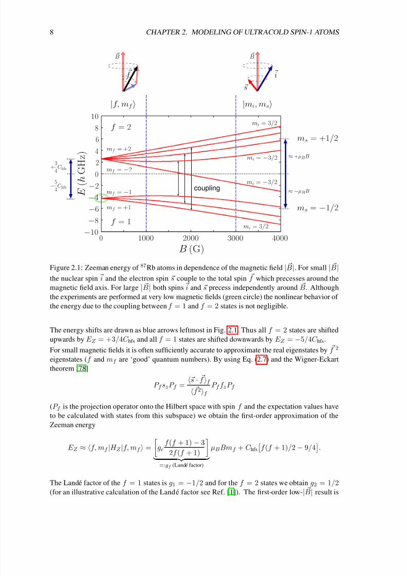
Figure 2.1: Zeeman energy of 87Rb atoms in dependence of the magnetic field | B|. For small | B|the nuclear spin i and the electron spin s couple to the total spin f which precesses around the
magnetic field axis. For large | B| both spins i and s precess independently around B. Although
the experiments are performed at very low magnetic fields (green circle) the nonlinear behavior of
the energy due to the coupling between f = 1 and f = 2 states is not negligible.
The energy shifts are drawn as blue arrows leftmost in Fig. 2.1. Thus all f = 2 states are shifted
upwards by E Z = +3/4C hfs and all f = 1 states are shifted downwards by E Z = −5/4C hfs.
For small magnetic fields it is often sufficiently accurate to approximate the real eigenstates by f 2
eigenstates (f and mf are ‘good’ quantum numbers). By using Eq. (2.7) and the Wigner-Eckart
theorem [78]
P f szP f =s · f f f 2f
P f f zP f
(P f is the projection operator onto the Hilbert space with spin f and the expectation values have
to be calculated with states from this subspace) we obtain the first-order approximation of the
Zeeman energy
E Z ≈ f, mf |H Z |f, mf =
ge
f (f + 1) − 3
2f (f + 1)
=:gf (Lande factor)
µBBmf + C hfs
f (f + 1)/2 − 9/4
.
The Lande factor of the f = 1 states is g1 = −1/2 and for the f = 2 states we obtain g2 = 1/2(for an illustrative calculation of the Lande factor see Ref. [1]). The first-order low-| B| result is

8/3/2019 Frank Deuretzbacher- Spinor Tonks-Girardeau gases and ultracold molecules
http://slidepdf.com/reader/full/frank-deuretzbacher-spinor-tonks-girardeau-gases-and-ultracold-molecules 19/151
2.1. HAMILTONIAN FOR SPIN-1 ATOMS 9
thus given by
E Z (f = 1) ≈ −5/4C hfs − µBBmf /2 and E Z (f = 2) ≈ +3/4C hfs + µBBmf /2 . (2.8)
This behavior can be seen in Fig. 2.1 in the region B < 1000 G. Note that for f = 2 the state with
mf = 2 has highest energy whereas for f = 1 the state with mf =
−1 has highest energy due to
the negative sign of the Lande factor.
Let us now consider the other extreme case of large magnetic fields 2µBB C hfs. Here it is
sufficiently accurate to approximate the real eigenstates by (iz, sz) eigenstates (mi and ms are
‘good’ quantum numbers). By using the relations
s · i = iz ⊗ sz +1
2(i+ ⊗ s− + i− ⊗ s+) (2.9)
with i± ≡ ix ± i iy (and analog for s±) and
i±|i, mi =
i(i + 1) − mi(mi ± 1)|i, mi ± 1 (and analog for s±) (2.10)
we obtain the first-order approximation of the Zeeman energy in the region of large magnetic fields
E Z ≈ mi, ms|H Z |mi, ms = 2µBBms + C hfsmims. (2.11)
Thus in the region B > 3000 G we observe two multiplets which are shifted by an average energy
of ∆E ≈ ±µBB (see the blue arrows rightmost of Fig. 2.1). The average spacing between the
four states of each multiplet is ∆E ≈ C hfs/2. Note again that the ordering within the lower
multiplet is inverted since ms = −1/2.
In the intermediate region 1000 G < B < 3000 G the energy depends nonlinearly on B (ex-
cept for the fully stretched states) and the coupling between states with same mf
|1, mf ↔|2, mf , mf = −1, 0, 1
continuously rotates f 2 into (iz, sz) eigenstates. Note, that the energy of
the fully stretched states
|2, 2= |3/2, 1/2 and |2,−2= |−3/2,−1/2
depends linearly on B for
all magnetic fields since they are not coupled to other states. They are thus eigenstates of H Z forall magnetic fields and their energy is exactly given by Eqs. ( 2.8) or (2.11). To determine the en-
ergy of the other states for all magnetic fields we have to calculate and diagonalize the 8×8 matrix
of H Z . Since only pairs of states with same mf are mutually coupled this task reduces to a diago-
nalization of three 2×2 matrices. Here we do this calculation only for the pair of states |2, −1 and
|1, −1. We switch into the (iz, sz) representation since the calculation of the off-diagonal matrix
element is easier to perform with the given Eqs. (2.9) and (2.10). The state |2, −1 transforms into
the state | − 3/2, 1/2 and the state |1, −1 transforms into the state | − 1/2, −1/2 (see Fig. 2.1).
The matrix element of H Z between these states is −3/2, 1/2|H Z | − 1/2, −1/2 =√
3/2 C hfs.
The resulting 2 × 2 matrix is given by
see Eq. (2.11) for the diagonal elements
H (subspace)Z = −
3/4 C hfs
+ µB
B√
3/2 C hfs√3/2 C hfs +1/4 C hfs − µBB . (2.12)
The eigenvalues of this matrix are
E ± = −C hfs/4 ±
C 2hfs − C hfsµBB + µ2BB2. (2.13)
For small magnetic fields one can perform a Taylor expansion in B. For the lower energy
which
belongs to the state |ψ− ≈ |1, −1 we obtain
E Z (|1, −1) = −C hfs
4− C hfs
1 − µBB
C hfs
+µ2BB2
C hfs
≈ −5C hfs
4+
µBB
2− 3µ2
BB2
8C hfs
. (2.14)
8/3/2019 Frank Deuretzbacher- Spinor Tonks-Girardeau gases and ultracold molecules
http://slidepdf.com/reader/full/frank-deuretzbacher-spinor-tonks-girardeau-gases-and-ultracold-molecules 20/151
10 CHAPTER 2. MODELING OF ULTRACOLD SPIN-1 ATOMS
The result now contains the hyperfine shift, the linear and the quadratic Zeeman energy. Similar
calculations can be performed for the other states. The general result for the Zeeman shift, which
is valid for all quantum numbers (f, mf ), is given by
E Z = −C hfs
4 + (−1)f C hfs +
µBB
2 mf +
µ2BB2
2C hfs 1 −m2f
4 . (2.15)
In current experiments all the atoms are initially prepared in spin state f = 1 and the magnetic
field strength is of the order of a few Gauss, which is indicated by the green circle in Fig. 2.1.
During observation time the total spin of the atomic system F =i
f i is conserved. Thus the
hyperfine shift and the linear Zeeman energy are only a constant offset which has no influence on
the system. The quadratic Zeeman shift, however, is of the order of the interaction energy and thus
not negligible.
The off-diagonal elements of H Z also lead to a mixing of f = 1 and f = 2 states. The above
state |ψ−, e.g., is a superposition |ψ− = α|1, −1 + β |2, −1. Assuming a magnetic field
strength of one Gauss, which is a typical experimental value, we obtain α = 0.99999998 andβ = 0.0002. Such a small admixture of f = 2 states has no influence on the properties of the
system and we can safely assume α = 1 and β = 0. In the effective Zeeman Hamiltonian for the
spin f = 1 atoms (2.1) we have neglected the constant hyperfine shift and the small admixture of
the |f = 2, mf states.
2.1.2 Derivation of the Interaction Hamiltonian
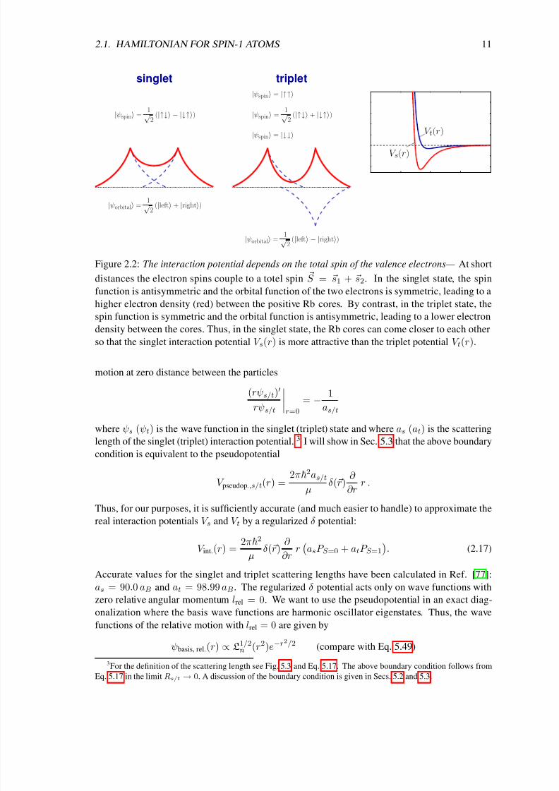
The interaction potential depends on the total spin of the valence electrons: We consider the
interaction between two 87Rb atoms at zero magnetic field B = 0. Again, we have to regard that
the atomic spins are composed of a nuclear spin i and an electron spin s. At close distances the
electron spins of the two atoms couple to the total electron spin S = s1 + s2. The interactionbetween the two atoms depends on the absolute value of S : In the singlet state, S = 0, it is more
attractive than in the triplet state, S = 1, since in the first case the electron density between the Rb
cores is higher; see Fig. 2.2. The interaction Hamiltonian is therefore given by
V int.(r) = V s(r)P S =0 + V t(r)P S =1 (2.16)
where P S =0 (P S =1) is the projection operator into the S = 0 (1) subspace and where V s (V t) is
the singlet (triplet) interaction potential.
Delta approximation: We consider situations where the range of the singlet and triplet potential
Rs and Rt is much smaller than the typical wave length of the wave functions of the interacting
particles. This length scale is of the order of the oscillator length losc., i. e., we consider situations
where max(Rs, Rt) losc..2 Under these conditions the whole impact of the interaction potential
reduces to a boundary condition on the logarithmic derivative of the wave function of the relative
2To be more precisely: Of course the interaction potentials V s and V t may have many bound states which lead to
the formation of tightly bound molecules; see Fig. 5.1(a) and the discussion in Secs. 5.1 and 5.2. The extent of these
molecules is much smaller than the range of the interaction. But here we are not interested in these tightly bound
molecules but in the deformation of the low-energy wave functions of the trap by the short-ranged interaction; see the
wave functions in Fig. 5.6 (apart from the red wave function in (a)). These low-energy trap states are in fact highly
excited states and thus they are metastable (the ground-state molecule has lowest energy). However, the formation of
tightly bound molecules is suppressed due to several conservation laws and since the overlap with the trap states is
negligibly small so that there is enough observation time to study the metastable low-energy trap states.
8/3/2019 Frank Deuretzbacher- Spinor Tonks-Girardeau gases and ultracold molecules
http://slidepdf.com/reader/full/frank-deuretzbacher-spinor-tonks-girardeau-gases-and-ultracold-molecules 21/151
2.1. HAMILTONIAN FOR SPIN-1 ATOMS 11
|ψorbital =1√2(|left + |right)
|ψorbital =1√2(|left − |right)
|ψspin =1√2(|↑↓ − |↓↑) |ψspin =
1√2(|↑↓ + |↓↑)
|ψspin = |↑↑
|ψspin = |↓↓
singlet triplet
V s(r)
V t(r)
Figure 2.2: The interaction potential depends on the total spin of the valence electrons— At short
distances the electron spins couple to a totel spin S = s1 + s2. In the singlet state, the spinfunction is antisymmetric and the orbital function of the two electrons is symmetric, leading to a
higher electron density (red) between the positive Rb cores. By contrast, in the triplet state, the
spin function is symmetric and the orbital function is antisymmetric, leading to a lower electron
density between the cores. Thus, in the singlet state, the Rb cores can come closer to each other
so that the singlet interaction potential V s(r) is more attractive than the triplet potential V t(r).
motion at zero distance between the particles
(rψs/t)
rψs/t r=0
= − 1
as/t
where ψs (ψt) is the wave function in the singlet (triplet) state and where as (at) is the scattering
length of the singlet (triplet) interaction potential. 3 I will show in Sec. 5.3 that the above boundary
condition is equivalent to the pseudopotential
V pseudop.,s/t(r) =2π2as/t
µδ(r)
∂
∂rr .
Thus, for our purposes, it is sufficiently accurate (and much easier to handle) to approximate the
real interaction potentials V s and V t by a regularized δ potential:
V int.
(r) =2π2
µδ(r)
∂
∂rr a
sP S =0
+ atP S =1. (2.17)
Accurate values for the singlet and triplet scattering lengths have been calculated in Ref. [77]:
as = 90.0 aB and at = 98.99 aB. The regularized δ potential acts only on wave functions with
zero relative angular momentum lrel = 0. We want to use the pseudopotential in an exact diag-
onalization where the basis wave functions are harmonic oscillator eigenstates. Thus, the wave
functions of the relative motion with lrel = 0 are given by
ψbasis, rel.(r) ∝ L1/2n (r2)e−r
2/2 (compare with Eq. 5.49)
3For the definition of the scattering length see Fig. 5.3 and Eq. 5.17. The above boundary condition follows from
Eq. 5.17 in the limit Rs/t → 0. A discussion of the boundary condition is given in Secs. 5.2 and 5.3.

8/3/2019 Frank Deuretzbacher- Spinor Tonks-Girardeau gases and ultracold molecules
http://slidepdf.com/reader/full/frank-deuretzbacher-spinor-tonks-girardeau-gases-and-ultracold-molecules 22/151
12 CHAPTER 2. MODELING OF ULTRACOLD SPIN-1 ATOMS
where Lba(z) are the generalized Laguerre polynomials. The derivative of these wave functions at
the origin is zero∂
∂rL1/2n (r2)e−r
2/2
r=0
= 0 .
We hence obtain
∂
∂r
rψbasis, rel.(r)
r=0
= ψbasis, rel.(0) + @ @ @ @ @ @ @ 0 · ψ
basis, rel.(0) . (2.18)
Thus, we can neglect the operator ∂ ∂r r in Eq. 2.17 and obtain the interaction potential 4
V int.(r) =2π2
µδ(r)
asP S =0 + atP S =1
. (2.19)
Effective interaction Hamiltonian for spin-1 atoms: Since the interaction between two atoms
depends on the absolute value of the total electron spin S (singlet or triplet), the atomic spin f can in principle be changed after the scattering. However, typical trap frequencies are orders of
magnitude smaller than the hyperfine splitting 2C hfs. Thus, when the system is very cold, two
atoms in f = 1 will remain in the same multiplet after the scattering since there is not enough
energy to promote either atom to f = 2. Therefore, the effective low-energy interaction preserves
the spin f of the individual atoms [54]. I will show in the following that, in the f 1 = f 2 = 1subspace (i. e. the subspace where both atoms have spin 1), the interaction potential is given by
V int.(r) =2π2
µδ(r)
aF =0P F =0 + aF =2P F =2
(2.20)
where P F =0 (P F =2) is the projection operator into the F = 0(2) subspace
F = f 1 + f 2 is the
total spin of the two atoms
and where aF =0 and aF =2 are the corresponding scattering lengths.
Derivation of Eq. (2.20) from Eq. (2.19) — At zero magnetic field two interacting atoms withnuclear and electron spins
i1, s1
and
i2, s2
are described by the Hamiltonian
H = C hfs
i1 · s1 + i2 · s2
+
H kin. + V trap
⊗ 1 +2π2
µδ(r)
asP S =0 + atP S =1
.
The first term H hfs is the hyperfine coupling between the nuclear and electron spins and the remain-
der H consists of the kinetic, potential and interaction energy of the two atoms. The differences
of the energy eigenvalues of H hfs are of the order of a few hGHz: ∆E hfs = 2C hfs ≈ 7 hGHz. By
contrast, the differences of the energy eigenvalues of H are typically of the order of a few hHz up
to several hkHz
the largest trap frequencies which have been achieved in deep optical lattices are
of the order of
≈0.1 hMHz; see Table 2.1. Thus, to first order, H is well approximated by H hfs.
Using Eq. 2.7 we obtain
H hfs =C hfs
2
f 21 + f 22 − 91
.
Therefore, the eigenvectors of H hfs are given by the eigenvectors of
f 21 + f 22
and the eigenval-
ues are given by
E hfs =C hfs
2
f 1(f 1 + 1) + f 2(f 2 + 1) − 9
,
4The second summand of Eq. 2.18 is negligible as long as ψbasis, rel.(0) < ∞ (or, more precisely, as long as
ψbasis, rel.(r) does not have a 1/r singularity at the origin). The wave functions of noninteracting particles are always
smooth at r = 0.

8/3/2019 Frank Deuretzbacher- Spinor Tonks-Girardeau gases and ultracold molecules
http://slidepdf.com/reader/full/frank-deuretzbacher-spinor-tonks-girardeau-gases-and-ultracold-molecules 23/151
2.1. HAMILTONIAN FOR SPIN-1 ATOMS 13
i. e.,
E hfs =
− 5C hfs/2 if f 1 = f 2 = 1
− C hfs/2 if f 1 = 1 and f 2 = 2 or f 1 = 2 and f 2 = 1
3C hfs/2 if f 1 = f 2 = 2 .
The ground-state multiplet is ninefold degenerate since two spins with f = 1 can couple to onestate with spin F = 0, three states with F = 1 and five states with F = 2.
Let us now switch on H . Then, the degeneracy of the ground-state multiplet is lifted and we
observe the following energy structure: There is one state with an energy of −5C hfs/2+E 1(as, at),
there are three states with an energy of −5C hfs/2 + E 2(as, at) and there are five states with an
energy of −5C hfs/2 + E 3(as, at). That is not surprising since H commutes with F z and F 2. 5
Hence, the degenerate eigenstates have spin F = 0, 1 and 2, respectively. Since
f 21 + f 22
does
not commute with P S =0 and P S =1, each state contains admixtures from the higher multiplets of
H hfs due to the coupling to these states via the interaction ( 2.19). However, according to the above
discussion, these admixtures are negligible since ∆E hfs ∆E . Therefore, we may approximate
H within the lowest multiplet by the Hamiltonian
H = E 1(as, at)P f 1=f 2=1, F =0 + E 2(as, at)P f 1=f 2=1, F =1 + E 3(as, at)P f 1=f 2=1, F =2
where P f 1=f 2=1, F projects into the subspace where both atoms have spin 1 and total spin F . In
the following we abbreviate these projectors by P F .
Each energy is related to a scattering length
E 1 ↔ aF =0, E 2 ↔ aF =1 and E 3 ↔ aF =2
via
Eq. (5.50) and thus we may write the low-energy interaction Hamiltonian according to
V int.(r) =2π2
µδ(r)
aF =0P F =0 + aF =1P F =1 + aF =2P F =2
.
Finally we regard that the F = 1 spin functions are antisymmetric and thus the correspondingrelative wave functions must be antisymmetric too (we are considering bosons). These wave
functions are zero at r = 0 and thus the matrix elements of the operator δ(r)P F =1 are always zero
for bosonic wave functions. After neglecting this part of the above Hamiltonian, we finally arrive
at Eq. (2.20).
An alternative notation: We may express the operator P F =0 as a linear combination of the oper-
ators 1 , f 1 · f 2 and P F =1:
P F =0 = α1 + β f 1 · f 2 + γP F =1 .
First, we convert the operator f 1 · f 2:
F 2 = f 1 + f 22 = f 21 + f 22 + 2 f 1 · f 2
⇔ 2 f 1 · f 2 = F 2 − 41 ⇔ f 1 · f 2 = F 2/2 − 2 1
and obtain the equation
P F =0 = (α − 2β ) 1 +β
2 F 2 + γP F =1 . (2.21)
In order to determine the coefficients, we calculate the expectation value of (2.21) with the F 2, F z
eigenvectors |F = 0, mF = 0, |F = 1, mF and |F = 2, mF . We obtain a set of
5I checked these commutation relations by means of MATHEMATICA

8/3/2019 Frank Deuretzbacher- Spinor Tonks-Girardeau gases and ultracold molecules
http://slidepdf.com/reader/full/frank-deuretzbacher-spinor-tonks-girardeau-gases-and-ultracold-molecules 24/151
14 CHAPTER 2. MODELING OF ULTRACOLD SPIN-1 ATOMS
three coupled equations
1 = α − 2β (expectation value with |F = 0, mF = 0)
0 = α − 2β + β + γ (expectation value with |F = 1, mF )
0 = α−
2β + 3β (expectation value with|F = 2, m
F )
from which we easily extract the coefficients α = 1/3, β = −1/3 and γ = −2/3. Thus, the
operator P F =0 may be rewritten as
P F =0 =1
31 − 1
3 f 1 · f 2 − 2
3P F =1 . (2.22)
In an analogous calculation we obtain for P F =2:
P F =2 =2
31 +
1
3 f 1 · f 2 − 1
3P F =1 . (2.23)
Using Eqs. (2.22) and (2.23) we obtain from Eq. (2.20)
V int.(r) =2π2
µδ(r)
aF =0 + 2aF =2
31 +
aF =2 − aF =0
3 f 1 · f 2
$ $ $ $ $ $
$ $ $ $ $
− 2aF =0 + aF =2
3P F =1
.
Again, we can neglect the third summand since the expectation value of the operator δ(r)P F =1 is
always zero for bosonic wave functions. Using µ = m/2 we finally obtain Eq. (2.2).
2.2 Energy scales and parameter regimes
Energy scales: Trap frequencies— Before I proceed I will calculate the typical energy scales of our system. Table 2.1 shows typical trap frequencies of several experiments. The trap frequencies
of each direction ωx, ωy and ωz can be varied independently. The trap frequencies of the optical
dipole traps used in Hamburg vary from a few to several hundred Hz. In the experiments of
Kinoshita et al. at Penn State University an extremely elongated, quasi-one-dimensional trap
was used. Here, the axial trap frequency was only ωx = 2π × 27.5 Hz whereas the transverse
trap frequencies were three orders of magnitude larger ωy = ωz 2π × 70.7 kHz. Large trap
frequencies in all three dimensions can be achieved in a deep optical lattice (Mainz).
Table 2.1: Trap frequencies of several experiments.
ωx ωy ωzHamburg 1D [53] 2π × 16.7 Hz 2π × 118 Hz 2π × 690 Hz
Hamburg 3D [53] 2π × 92 Hz 2π × 103 Hz 2π × 138 Hz
Penn State [21] 2π × 27.5 Hz up to 2π × 70.7 kHz up to 2π × 70.7 kHz
Mainz [63] 2π × 43.6 kHz 2π × 43.6 kHz 2π × 43.6 kHz
Interaction energy— According to the discussion in section 2.1, the level spacing of the trap has
to be compared to the spin-independent interaction energy since the interplay of these two energy
contributions determines the shape of the motional wave function. To get a rough estimate, we

8/3/2019 Frank Deuretzbacher- Spinor Tonks-Girardeau gases and ultracold molecules
http://slidepdf.com/reader/full/frank-deuretzbacher-spinor-tonks-girardeau-gases-and-ultracold-molecules 25/151
2.2. ENERGY SCALES AND PARAMETER REGIMES 15
calculate the spin-independent interaction energy of two atoms which reside in the ground state of
the harmonic trap (see Sec. 2.4 for the eigenfunctions of the harmonic oscillator)
ψ(r1, r2) =
i=1,2
φ0(xi)φ0(yi)φ0(zi) with φ0(u) =1
lu√
πe−
12 (u/lu)
2.
Here, lu = /(mωu) is the oscillator length of the u = x,y ,z-direction. According to Eq. (2.2),
the spin-independent interaction energy of the above state is given by
E int.,0 = g0
drψ(r, r)2 = g0
dxφ4
0(x)
dyφ4
0(y)
dzφ4
0(z).
The one-dimensional integrals I u =
duφ40 have dimension 1/lu. To see this, we decompose
each quantity into a dimensionless quantity (which we mark by a tilde symbol) and its unit
u =
ulu, φ0(u) =
φ0(u)
1√lu
(u = x,y ,z).
By inserting these relations into the corresponding interaction integrals we obtain I u = I u/lu withI x = I y = I z = 1/√
2π. The interation energy becomes
ωu = 2π × f u
E int.,0 =g0
lxlylz√
2π3
=4π2
m× a0 + 2a2
3×
m3 ¨ ¨
¨ (2π)3
3× f xf yf z × 1
¨ ¨ ¨ √
2π3
.
As can be seen, the interaction energy increases when the trap frequencies are made larger since
then the particles are enclosed within a smaller volume, E int.,0 ∝ 1/(lxlylz) ∝ f xf yf z.
Again, we decompose each quantity into a product of a dimensionless number and its unit in order
to calculate the interaction energy in units of hHz
= Js, m = m kg, ai = ai aB (i = 0, 2) aB = aB m,
f u = f u Hz (u = x,y ,z), h = h Js ⇔ J = 1/h hHz ,
with = 1.05457163 × 10⁻³⁴, m = 1.443160648 × 10⁻²⁵, a0 = 101.8, . . . , (see appendix D for
the constants). Finally we obtain the interaction energy in hHz
E int.,0 =
4π2m × a0 + 2a23
× aB × m33 × 1h
=:C int.
f x f y f z hHz (2.24)
with C int. ≈ 4 × 10⁻⁴ in typical experiments. The spin-dependent interaction energy E int.,2 is
approximately 200 times smaller since |g2|/g0 ≈ 1/200.
Linear Zeeman energy— In the experiments performed in Hamburg and Mainz [63, 49] the mag-
netic field strength was of the order of 1 G. According to Eq. (2.1), the splitting of the linear
Zeeman energy is given by ∆E Z,lin. = µBB/2. Similar to the above calculation we determine the
constant C Z,lin. which gives the linear Zeeman energy ∆E Z,lin. in hHz if B is given in G
∆E Z,lin. =
µB2
h104
C Z,lin.
B hHz
8/3/2019 Frank Deuretzbacher- Spinor Tonks-Girardeau gases and ultracold molecules
http://slidepdf.com/reader/full/frank-deuretzbacher-spinor-tonks-girardeau-gases-and-ultracold-molecules 26/151
16 CHAPTER 2. MODELING OF ULTRACOLD SPIN-1 ATOMS
with µB = µB J/T, B = B G, 1T = 104 G and C Z,lin. ≈ 700 × 103. Thus, for a magnetic
field strength of 1 G we obtain 700 hkHz which is by far the largest energy scale in our system.
However, as discussed in section 2.1, the linear Zeeman energy has no influence on the population
dynamics of our system and within subspaces with same M F it is only a constant, negligible offset.
Hence, this large energy contribution can often be neglected.
Quadratic Zeeman energy— The energy shift due to the quadratic Zeeman Hamiltonian is given
by ∆E Z,quad. = µ2BB2/(8C hfs); see Eq. (2.1). Similar to the above calculation we obtain
∆E Z,quad. =
µ2B
8 × 10¹⁷ h2 C hfs
C Z,quad.
B2 hHz
with C hfs ≈ 3.4 × 10⁹ and C Z,quad. ≈ 72. Hence, for a magnetic field strength of 1 G we obtain a
quadratic Zeeman energy of 72 hHz.
Parameter regimes: Let me now calculate the different energy contributions for some typical
experiments with ultracold87
Rb atoms.Two atoms in a deep optical lattice well— In the spin-dynamics experiments of Widera et al. [63] a
deep optical lattice was used to confine two atoms at each lattice site. Around the minima, the sites
are well approximated by harmonic oscillator potentials. From Eq. (2.24) and the frequencies of
Table 2.1, we calculate a spin-independent interaction energy of E int.,0 ≈ 3.6 hkHz. That is only
0.08 times the level spacing. Thus, we expect that both atoms reside in the Gaussian ground state
of the trap which is only slightly deformed by the repulsion between the atoms.
The linear Zeeman energy can be neglected since the z-component of the total spin F z is con-
served. Further, the spatial two-atom ground-state wave function is permutationally symmetric
so that the dynamics takes place within the symmetric spin space which is spanned by the two
states
|mf,1, mf,2
=
|0, 0
and (
|1,
−1
+
| −1, 1
) /
√2. Moreover, the dynamics of the system
depends on the initial state and the ratio of the quadratic Zeeman energy compared to the spin-dependent interaction energy. This ratio can be tuned by the magnetic field and the confinement.
The spin-dependent interaction energy is of the order of E int.,2 ≈ −16.6 hHz. This en-
ergy has to be compared to the shift of the quadratic Zeeman energy when two spins are flipped:
2∆E Z,quad.. Both energies are of the same order for a magnetic field strength of approximately
0.34 G since 2∆E Z,quad.(0.34 G) ≈ 16.6 hHz. Thus, we expect that the interplay of both energy
contributions strongly influences the population dynamics of the two atoms around 0.34 G.
Large particle numbers and weak interactions— For both Hamburg experiments [53] we obtain a
two-particle interaction energy of E (2)int.,0 ≈ 0.5 hHz. That is quite weak compared to the smallest
level spacing of the trap, E (2)int.,0/(ωx) ≈ 0.03 (1D) or ≈ 0.005 (3D). We are therefore in the
weakly interacting regime. Of course the N -particle interaction energy grows rapidly with thenumber of particles E
(N )int.,0 ∝ N (N − 1)/2 and since the number of particles is typically given by
N = 3× 10⁵ [51] we obtain for a condensate: E (N )int.,0 ≈ 41 hGHz. That is quite much compared to
the kinetic and potential energy E kin. +E trap = 1/2(16.7+118+690) hHz×3×105 ≈ 0.12 hGHz
(1D) and thus we expect that the ground-state wave function is substantially deformed to reduce
the interaction energy. However, due to the weak two-particle interaction, we can still assume that
all the particles reside in the same mean-field orbital.
Few atoms in a quasi-one-dimensional trap— For the quasi-one-dimensional trap of Kinoshita et
al. [21] we obtain a two-particle interaction of E int.,0 ≈ 146 hHz. That is approximately 5.3 times
larger than the level spacing of the x-direction but ≈ 500 times smaller than the level spacing of

8/3/2019 Frank Deuretzbacher- Spinor Tonks-Girardeau gases and ultracold molecules
http://slidepdf.com/reader/full/frank-deuretzbacher-spinor-tonks-girardeau-gases-and-ultracold-molecules 27/151
2.3. EXACT DIAGONALIZATION AND SECOND QUANTIZATION 17
the transverse y- and z-directions. Thus we expect, on the one hand, that the atoms reside in the
ground state of the transverse directions so that we can describe the system by a one-dimensional
Schrodinger equation. On the other hand, we expect a substantial deformation of the ground-state
wave function with strong correlations between the particles along the axial direction.
2.3 Exact diagonalization and second quantization
Exact diagonalization: The exact diagonalization method is usually used to calculate the low-
energy eigenspectrum and eigenfunctions of a time-independent Hamiltonian. The evolution of a
wave function |ψ(t) is determined by the time-dependent Schrodinger equation
i d
dt|ψ(t) = H (t)|ψ(t).
In the case of a time-independent Hamiltonian H (t) = H , the energy eigenfunctions change as
a function of time only by a complex phase factor |ψ(t) = e−i Et/|ψ. The eigenfunctions |ψand eigenenergies E are determined by the stationary Schrodinger equation
H |ψ = E |ψ. (2.25)
In order to solve this eigenvalue problem we choose an arbitrary basis of the Hilbert space
|n, n = 1, 2, . . . and project Eq. (2.25) on the individual states |n
n|H n
|n n |ψ = E n|ψ (for all n).
This set of equations can be written in matrix form
H 11 H 12 H 13
· · ·H 21 H 22 H 23 · · ·H 31 H 32 H 33 · · ·
......
.... . .
c1
c2c3...
= E c1
c2c3...
(2.26)
with H nn ≡ n|H |n and cn ≡ n|ψ. The eigenenergies of the stationary Schrodinger
equation (2.25) are given by the eigenvalues of the Hamiltonian matrix (H nn ) and correspond-
ingly the eigenfunctions |ψ are determined from the eigenvectors (c1, c2, . . .) of Eq. (2.26) by
|ψ =n cn|n. In the case of a complete basis |n the result is exact.
We diagonalize the Hamiltonian matrix (H nn ) numerically by using efficient algorithms
(ARPACK, NAG). The dimension of the Hilbert space of our problem is infinite but we must re-
strict the basis
|n
to a finite number due to CPU and memory limitations resulting in deviations
between the real and the numerically obtained eigenenergies and eigenfunctions. The accuracy of
our calculations depends on a ‘good choice’ of basis functions |n and their number. Our main
task is to generate the basis and to calculate the Hamiltonian matrix (H nn ) and, afterwards, to
calculate the desired observables from the given coefficients of the eigenvectors.
Second quantization: When dealing with many particles it is a rather cumbersome task to con-
struct permutationally symmetric or antisymmetric wave functions and to calculate matrix ele-
ments of some operators by using these wave functions. Second quantization is an efficient tool to
calculate these matrix elements. Here, I will give a brief description of the method for bosons.
In second quantization bosonic many-particle wave functions are represented by number states
|n1, n2, . . ., where ni is the number of bosons which occupy the ith single-particle basis state.

8/3/2019 Frank Deuretzbacher- Spinor Tonks-Girardeau gases and ultracold molecules
http://slidepdf.com/reader/full/frank-deuretzbacher-spinor-tonks-girardeau-gases-and-ultracold-molecules 28/151
18 CHAPTER 2. MODELING OF ULTRACOLD SPIN-1 ATOMS
All many-particle operators can be expressed by means of creation and annihilation operators a†iand ai. These operators act as follows on the occupation number states
a†i | . . . , ni, . . . =√
ni + 1| . . . , ni + 1, . . ., ai| . . . , ni, . . . =√
ni| . . . , ni − 1, . . ., (2.27)
and they obey the commutation relationsai, a† j
= δij,
ai, a j
= 0, and
a†i , a† j
= 0 .
One important class of many-particle operators, such as the density operator, can be written as a
sum of single-particle operatorsν f ν . Such an operator is translated into second quantization
by the prescription ν
f ν =ij
i|f | ja†ia j . (2.28)
A second class of operators, such as the interaction operator, is a double sum of two-particle
operators µ<ν g
µν
. These operators are constructed by the prescription:µ<ν
gµν =1
2
ijkl
ij|g|kla†ia† jakal . (2.29)
An introduction into second quantization is given in the book of Gordon Baym [ 79] and a deriva-
tion of formula (2.28) is presented in the book of Eugen Fick [80]. 6
2.4 Single-particle basis
The first step of an exact diagonalization is to choose a proper basis. I have decided for theenergy eigenfunctions of the noninteracting bosons. Thus, the number states |n1, n2, . . . represent
permutationally symmetric energy eigenstates of noninteracting bosons with ni bosons occupying
the ith energy eigenstate of the single-particle problem. Here, I determine the energy eigenvalues
and eigenfunctions of one particle since they occur in the matrix elements i|f | j and ij|g|kl of
Eqs. (2.28) and (2.29). In the case of one particle Eq. (2.5) becomes
H =
−
2
2m∆ +
1
2m
ω2xx2 + ω2
yy2 + ω2zz2
⊗1 − µBB
2f z − µ2
BB2
2C hfs
1 − 1
4f 2z
.
The energy spectrum of H is given by
E =
nx +1
2
ωx+
ny +
1
2
ωy+
nz +
1
2
ωz− µBB
2α−µ2
BB2
2C hfs
1 − 1
4α2 (2.30)
with nx, ny, nz = 0, 1, 2, . . . and α = 0, ±1. The corresponding eigenfunctions are given by
ψnα(r) = ψnx (x)ψny (y)ψnz (z)|α6The general formula of a two-particle operator, which is valid for bosons and fermions, is given by
Pµ<ν gµν =
1/2P
ijklij|g|kla†i a†j alak, i. e., the annihilation operators ak and al occur in reversed order. This is equal to
Eq. (2.29) for bosons since ak and al commute. But for fermions both equations are not equal since the fermionic
annihilation operators anticommute.

8/3/2019 Frank Deuretzbacher- Spinor Tonks-Girardeau gases and ultracold molecules
http://slidepdf.com/reader/full/frank-deuretzbacher-spinor-tonks-girardeau-gases-and-ultracold-molecules 29/151
2.5. GENERATION OF THE MANY-PARTICLE BASIS 19
0 2 4−2−4
0.8
0.4
0
−0.4
−0.8
0 2 4−2−4
0.8
0.4
0
−0.4
−0.8
0 2 4−2−4
0.8
0.4
0
−0.4
−0.8
0 2 4−2−4
0.8
0.4
0
−0.4
−0.8
ground state
0 2 4−2−4
0.
8
0.4
0
−0.4
−0.8
1/2 hω
1st excited state
2nd excited state
3rd excited state
4th excited state
+1 hω
states with even parity states with odd parity
Figure 2.3: Energy spectrum and eigenfunctions of the one-dimensional harmonic oscillator.
where n = (nx, ny, nz) is a multi-index, ψnu (u) (u = x,y ,z) are the eigenfunctions of the one-
dimensional harmonic oscillator and|α
=|f = 1, m
f = α
(α = 0,
±1) are the eigenfunctions
of f 2 = 21 and f z. The wave functions ψnu (u) are given by
ψnu (u) =1
lu 2nu nu!√
πH nu (u/lu)e−
12(u/lu)2
where lu = /(mωu) is the oscillator length of the u-direction and
H nu (u/lu) =
nu/2s=0
(−1)snu!
(nu − 2s)! s!(2 u/lu)nu−2s
are the Hermite polynomials.
x
is the largest integer smaller than x. The eigenfunctions of the
one-dimensional harmonic oscillator have a well-defined parity
Πuψnu(u) = ψnu (−u) = (−1)nu ψnu (u) .
The energy spectrum and the lowest harmonic oscillator eigenfunctions are visualized in Fig. 2.3.
2.5 Generation of the many-particle basis
In the following chapters we want to study the low-energy properties of the system. We assume
here that the low-energy eigenfunctions of the interacting system can be accurately represented by
8/3/2019 Frank Deuretzbacher- Spinor Tonks-Girardeau gases and ultracold molecules
http://slidepdf.com/reader/full/frank-deuretzbacher-spinor-tonks-girardeau-gases-and-ultracold-molecules 30/151
20 CHAPTER 2. MODELING OF ULTRACOLD SPIN-1 ATOMS
a superposition of low-energy basis functions of the noninteracting system. 7 Therefore, we con-
struct all the basis functions of the noninteracting system below a certain energy cutoff. Moreover,
we make use of the conserved quantities, namely the parities Πx, Πy and Πz, and the z-component
of the total spin F z. The parities Πx, Πy and Πz of a many-particle state are given by
Πu|N = (iα)
(−1)nuiN iα
|N (u = x,y ,z) (2.31)
with |N = | . . . ; (N iα : nxi, nyi, nzi, α); . . .. In this notation N iα particles occupy the single-
particle state |nxi, nyi, nzi, α. I have developed the following recursive construction scheme for
the many-particle basis states:
Given a magnetization F z = M , we construct the noninteracting ground state
|(N − M : 0, 0, 0, 0);(M : 0, 0, 0, 1) with N − M particles in state |nx, ny, nz, α = |0, 0, 0, 0and M particles in state |0, 0, 0, 1, i. e., all the particles reside in the motional ground state
|nx, ny, nz = |0, 0, 0, N − M particles have spin |α = |0 and M particles have spin
|α = |1 to achieve a magnetization of M . 8 We have put as many as possible particles into
the |α = |0 spin state since it has the lowest quadratic Zeeman energy. We have 4 possibilities toconstruct excited states, based on this ground state, by adding the energy differences ∆E x = ωx,
∆E y = ωy, ∆E z = ωz and 2∆E Z,quad.:
|(N − M − 1 : 0, 0, 0, 0);(M : 0, 0, 0, 1); (1 : 1, 0, 0, 0) (+∆E x)
|(N − M − 1 : 0, 0, 0, 0);(M : 0, 0, 0, 1); (1 : 0, 1, 0, 0) (+∆E y)
|(N − M − 1 : 0, 0, 0, 0);(M : 0, 0, 0, 1); (1 : 0, 0, 1, 0) (+∆E z)
|(N − M − 2 : 0, 0, 0, 0);(M + 1 : 0, 0, 0, 1); (1 : 0, 0, 0, −1) (+2∆E Z,quad.).
In the first three states we have occupied the first excited state of the x-, y- and z-direction by
one particle and in the fourth state we have taken 2 particles out of the spin state |α = |0 and
put them into the spin states |α = |1 and |α = |−1. By comparing the energies of these 4states we find the first excited state of the many-particle basis. We choose this state and discard
the remaining three states. Similarly, we find the second excited state(s) of the many-particle basis
by adding excitations to the first excited state. We repeat the procedure until we have found all the
basis functions below a certain energy cutoff.
The recursion generates only states with the same magnetization M since the z-component of
the total spin F z is conserved during the process 2 × |0 → |1 + |−1. Finally, we select all
the many-particle states with the same parities (Πx, Πy, Πz) = (1, 1, 1), (−1, 1, 1), . . . (there are
23 = 8 possibilities) and save them in the corresponding files.
Often we already know at the beginning that the system will be two- (if ωx, ωy ωz), one-
(if ωx
ωy, ωz) ore zero-dimensional (if the two-particle interaction is much smaller than the
level spacing of the trap). Then, we allow only for the excitations (∆E x, ∆E y, 2∆E Z,quad.) if thesystem is two-dimensional, (∆E x, 2∆E Z,quad.) if the system is one-dimensional or 2∆E Z,quad. if
the system is zero-dimensional.
On the one hand, the described construction scheme is quite flexible, but, on the other hand, it is
rather time consuming — especially in the three-dimensional case — due to the many compar-
isons of energies. It turned out to be better to generate in a first step the spinless many-particle
wave functions | . . . ; (N iα : nxi, nyi, nzi); . . . and in a second step all the possible spinful many-
particle wave functions from a given spinless one. Such a recursion has been implemented by Kim
7We test the validity of this assumption later in Sec. 2.9.8For M < 0 we construct the ground state |(N − M : 0, 0, 0, 0);(M : 0, 0, 0, −1).

8/3/2019 Frank Deuretzbacher- Spinor Tonks-Girardeau gases and ultracold molecules
http://slidepdf.com/reader/full/frank-deuretzbacher-spinor-tonks-girardeau-gases-and-ultracold-molecules 31/151
2.6. CALCULATION OF THE HAMILTONIAN MATRIX 21
Plassmeier [81] and I used his program lately during my Ph.D. thesis. Furthermore, I applied my
program almost exclusively to one-dimensional trapping geometries and in this case we do not
need to compare energies since all the newly generated (spinless) states have the same energy:
|N : nx = 0
+∆E x
−→ |(N
−1 : 0); (1 : 1)
+∆E x
−→|(N − 1 : 0); (1 : 2) and |(N − 2 : 0); (2 : 1) +∆E x−→|(N − 1 : 0); (1 : 3), |(N − 2 : 0); (1 : 1); (1 : 2) and |(N − 3 : 0); (3 : 1) +∆E x−→ . . . .
However, I hopefully demonstrated that it is possible to construct recursively all the many-particle
basis states below a certain energy cutoff with well-defined magnetization and parities.
2.6 Calculation of the Hamiltonian matrix
In this section I will calculate the matrix elements of the many-particle Hamiltonian (2.5). I havechosen the permutationally symmetric eigenfunctions of the noninteracting Hamiltonian as basis
states. First, I introduce an alternative notation for the occupation number states
| . . . ; (N iα : nxi, nyi, nzi, α); . . . new notation−→ | . . . , N iα, . . . (2.32)
where i = (nxi, nyi, nzi) is a multi-index. Here, each position within the occupation number state
corresponds to a single-particle state |nxi, nyi, nzi, α. These states shall represent the bosonic
eigenfunctions of the noninteracting Hamiltonian.
The Hamiltonian (2.5) consists of two parts: H = H 0 + V int.. The first part H 0 is the Hamiltonian
of the noninteracting system and the second part V int. is the interaction Hamiltonian. H 0 is already
diagonal in the chosen representation but V int. is non-diagonal.
First I will calculate the Hamiltonian of the noninteracting system which is given by
H 0 =N i=1
−
2
2m∆i +
1
2m
ω2xx2i + ω2
yy2i + ω2zz2i
⊗ 1
⊗N
−N i=1
µBB
2f z,i +
µ2BB2
2C hfs
1
⊗N − 1
4f 2z,i
. (2.33)
H 0 is a single-particle operator. According to Eq. (2.28) we obtain its second-quantized form 9
H 0 =
(iα)( jβ )
iα|−
2
2m∆⊗ 1 +
1
2m
ω2xx2 + ω2
yy2 + ω2zz2⊗ 1
−µBB
2f z − µ2
BB2
2C hfs
1 − 1
4f 2z
| jβ a†iαa jβ . (2.34)
9My notation is a little bit inconsistent: The indices i, j = 1, 2, . . . , N in the first-quantized operators (2.33)
and (2.36) are simple numbers. By contrast, in the second-quantized operators (2.34), (2.37) and in the occupation
number states (2.32) i = (nxi, nyi, nzi), j = (nxj, nyj , nzj ), k = (nxk, nyk, nzk) and l = (nxl, nyl, nzl) symbolize
multi-indices.

8/3/2019 Frank Deuretzbacher- Spinor Tonks-Girardeau gases and ultracold molecules
http://slidepdf.com/reader/full/frank-deuretzbacher-spinor-tonks-girardeau-gases-and-ultracold-molecules 32/151
22 CHAPTER 2. MODELING OF ULTRACOLD SPIN-1 ATOMS
Using Eq. (2.30) and the orthonormality of the single-particle basis iα| jβ = δijδαβ we obtain
H 0 =(iα)
nxi +
1
2
ωx +
nyi +
1
2
ωy +
nzi +
1
2
ωz
−µBB2
α − µ2BB2
2C hfs
1 − 14
α2a†iαaiα .
Now we multiply from left with the conjugate transpose of |N = | . . . , N iα, . . . and from right
with |N = | . . . , N iα, . . ., use Eqs. (2.27), the orthonormality of the occupation number states
N |N = δNN and obtain the matrix elements
N |H 0|N = δNN
(iα)N iα
nxi +
1
2
ωx +
nyi +
1
2
ωy +
nzi +
1
2
ωz
−µBB
2α − µ2
BB2
2C hfs
1 − 1
4α2
. (2.35)
Next, we calculate the matrix elements of the Interaction Hamiltonian which is given by
V int. =i<j
δ(ri − r j)
g0 1
⊗N + g2 f i · f j
. (2.36)
V int. is a two-particle operator. According to Eq. (2.29) we obtain the second-quantized form
V int. =1
2
(iα)(jβ)(kγ)(lδ)
ij|δ(r1 − r2)|kl αβ |g0 1
⊗2 + g2 f 1 · f 2|γδ a†iαa† jβ akγ alδ . (2.37)
We introduce the abbreviations
I ijkl = ij|δ(r1 − r2)|kl =
dr1dr2 δ(r1 − r2)ij|r1r2r1r2|kl =
drψi(r)ψ j(r)ψk(r)ψl(r)
for the interaction integrals and
gαβγδ =
αβ
|g0 1
⊗2 + g2 f 1
· f 2|γδ
for the interaction-strength matrix. Next, we multiply from left with the conjugate transpose of
|N = | . . . , N iα, . . ., from right with |N = | . . . , N iα, . . . and obtain the matrix elements
N |V int.|N =1
2
(iα)(jβ)(kγ)(lδ)
gαβγδ I ijkl N |a†iαa† jβ akγ alδ|N .
These matrix elements have been calculated in my diploma thesis [1] using Eqs. (2.27) and the
orthonormality of the occupation number states N |N = δNN . Here, I give only the results for
completeness:

8/3/2019 Frank Deuretzbacher- Spinor Tonks-Girardeau gases and ultracold molecules
http://slidepdf.com/reader/full/frank-deuretzbacher-spinor-tonks-girardeau-gases-and-ultracold-molecules 33/151
2.6. CALCULATION OF THE HAMILTONIAN MATRIX 23
Six different bra-ket combinations can be distinguished which lead to nonzero matrix elements
N |V int.|N . In the first case, bra and ket are equal |N = |N and we obtain for the diagonal
elements of the interaction matrix
N |V int.|N = (iα)
1
2 gααααI iiiiN iα(N iα − 1) + (iα)<( jβ )
2gαβαβ I ijijN iαN jβ .
In the first term, we sum over all occupied positions within the number state | . . . , N iα, . . .. The
second term is a double sum. The outer sum runs over all occupied positions within the number
state | . . . , N iα, . . . and the inner sum runs over all occupied positions to the right of position
(iα), i. e., over all states | . . . , N iα, . . . , N jβ , . . ..
In the second case, bra and ket differ at two positions by two particles. We obtain
..., N p,...,N q,...|V int.|..., N p + 2,...,N q − 2,... =1
2gI qqpp
(N p + 2)(N p + 1)N q(N q − 1) .
In the third case, bra and ket differ at two positions by one particle
..., N p,...,N q,...|V int.|...,N p + 1,...,N q − 1,... =(iα)=( p),(q)
2gααI qipi
N q(N p + 1)N iα
+gI qqpq N q(N p + 1)(N q − 1) + gI qppp N q(N p + 1)N p .
In the fourth case, one single-particle state of the ket is occupied with two more and two states of
the ket are occupied with one less particle than in the bra
...,N p,...,N qσ ,...,N sφ,...|V int.|...,N p + 2,...,N qσ − 1,...,N sφ − 1,...= gσφI qspp
(N p + 2)(N p + 1)N qσN sφ .
In the fifth case, one single-particle state of the ket is occupied with two less and two states of the
ket are occupied with one more particle than in the bra
...,N p,...,N qσ ,...,N sφ,...|V int.|...,N p − 2,...,N qσ + 1,...,N sφ + 1,...= gσφI ppqs
(N sφ + 1)(N qσ + 1)(N p − 1)N p .
Finally, in the sixth case, two states of the ket are occupied with one more and two states of the
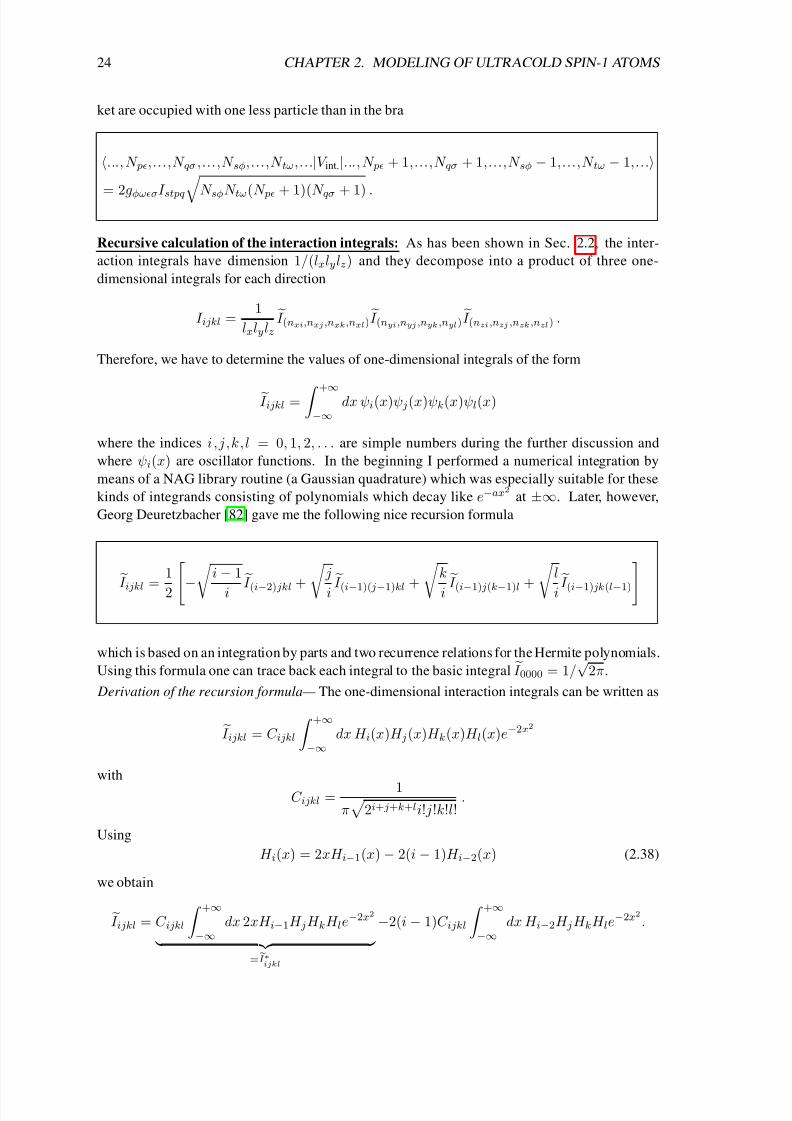
8/3/2019 Frank Deuretzbacher- Spinor Tonks-Girardeau gases and ultracold molecules
http://slidepdf.com/reader/full/frank-deuretzbacher-spinor-tonks-girardeau-gases-and-ultracold-molecules 34/151
24 CHAPTER 2. MODELING OF ULTRACOLD SPIN-1 ATOMS
ket are occupied with one less particle than in the bra
..., N p,...,N qσ ,...,N sφ,...,N tω,...|V int.|..., N p + 1,...,N qσ + 1,...,N sφ − 1,...,N tω − 1,...
= 2gφωσI stpq N sφN tω(N p + 1)(N qσ + 1) .
Recursive calculation of the interaction integrals: As has been shown in Sec. 2.2, the inter-
action integrals have dimension 1/(lxlylz) and they decompose into a product of three one-
dimensional integrals for each direction
I ijkl =1
lxlylzI (nxi,nxj ,nxk,nxl)
I (nyi,nyj ,nyk ,nyl)I (nzi ,nzj ,nzk ,nzl) .
Therefore, we have to determine the values of one-dimensional integrals of the form
I ijkl = +∞−∞
dx ψi(x)ψ j(x)ψk(x)ψl(x)
where the indices i,j,k,l = 0, 1, 2, . . . are simple numbers during the further discussion and
where ψi(x) are oscillator functions. In the beginning I performed a numerical integration by
means of a NAG library routine (a Gaussian quadrature) which was especially suitable for these
kinds of integrands consisting of polynomials which decay like e−ax2 at ±∞. Later, however,
Georg Deuretzbacher [82] gave me the following nice recursion formula
I ijkl =
1
2 − i −1
i I (i−2) jkl + ji I (i−1)( j−1)kl + ki I (i−1) j(k−1)l + li I (i−1) jk(l−1)which is based on an integration by parts and two recurrence relations for the Hermite polynomials.
Using this formula one can trace back each integral to the basic integral I 0000 = 1/√
2π.
Derivation of the recursion formula— The one-dimensional interaction integrals can be written as
I ijkl = C ijkl
+∞−∞
dx H i(x)H j(x)H k(x)H l(x)e−2x2
with
C ijkl = 1π
2i+ j+k+li! j!k!l!.
Using
H i(x) = 2xH i−1(x) − 2(i − 1)H i−2(x) (2.38)
we obtain
I ijkl = C ijkl
+∞−∞
dx 2xH i−1H jH kH le−2x2
=eI ∗ijkl
−2(i − 1)C ijkl
+∞−∞
dx H i−2H jH kH le−2x2.

8/3/2019 Frank Deuretzbacher- Spinor Tonks-Girardeau gases and ultracold molecules
http://slidepdf.com/reader/full/frank-deuretzbacher-spinor-tonks-girardeau-gases-and-ultracold-molecules 35/151
2.6. CALCULATION OF THE HAMILTONIAN MATRIX 25
We use
e−2x2
= −4xe−2x2 and integrate by parts:
I ∗ijkl = −1
2C ijkl
+∞−∞
dxH i−1H jH kH ld
dxe−2x2
= @ @ @ @ @ @ @ @ @ @ @ @
@ @ @
−1
2 C ijklH iH jH kH l−1e−2x2+∞−∞ +
1
2 C ijkl +∞−∞ dxd
dxH i−1H jH kH le−2x2
.
Now we use
H n = 2nH n−1
and obtain
I ∗ijkl = (i − 1)C ijkl
+∞−∞
dxH i−2H jH kH le−2x2 + j C ijkl
+∞−∞
dxH i−1H j−1H kH le−2x2
+k C ijkl
+∞−∞
dxH i−1H jH k−1H le−2x2 + l C ijkl
+∞−∞
dxH i−1H jH kH l−1e−2x2
.
It follows that
I ijkl = −(i − 1)C ijkl
+∞−∞
dxH i−2H jH kH le−2x2 + j C ijkl
+∞−∞
dxH i−1H j−1H kH le−2x2
+k C ijkl
+∞−∞
dxH i−1H jH k−1H le−2x2 + l C ijkl
+∞−∞
dxH i−1H jH kH l−1e−2x2.
Now we transform the coefficients:
(i − 1)C ijkl = (i − 1)1
π 4 ·2(i−2)+ j+k+li(i
−1)(i
−2)! j!k!l!
=1
2
i − 1
iC (i−2) jkl
j C ijkl = j1
π
4 · 2(i−1)+( j−1)+k+li j (i − 1)!( j − 1)!k!l!=
1
2
ji
C (i−1)( j−1)kl
and obtain the final form of the recursion.
Building up of an integral table— Based on the recursion formula I have built up an integral table
starting from the basic integral I 0000 = 1/√
2π. All the integrals of level L = i + j + k + l are
obtained from the integrals of the preceding level L − 2. Only the normal-ordered integrals with
i j k l are saved since all the integrals, obtained by rearranging a given set of indices, are
equal. The second level L = 2, for example, consists of the two normal-ordered integrals I 2000and
I 1100 which are calculated according to
I 2000 = − 12 · √2
I 0000 = − 14√
πand I 1100 = 1
2I 0000 = 1√
23√
π.
All the integrals of the next level L = 4, namely I 4000, I 3100, I 2200 and I 1111 are superpositions
of these two integrals of level L = 2 and so forth. Therefore, the task is to construct a chain of
integrals as follows: First, the indices of level L + 2 have to be generated from the indices of
level L and then the corresponding integrals have to be calculated using the recursion. In order to
accelerate the read out of the integral table, each level L is directly accessed. 10
10The recursion is fairly stable: I have computed interaction integrals up to level L = 600 by means of the recursion
and checked the accuracy by means of MATHEMATICA. For eI 150,150,150,150 I found a relative deviation of only 3×10⁻⁸.
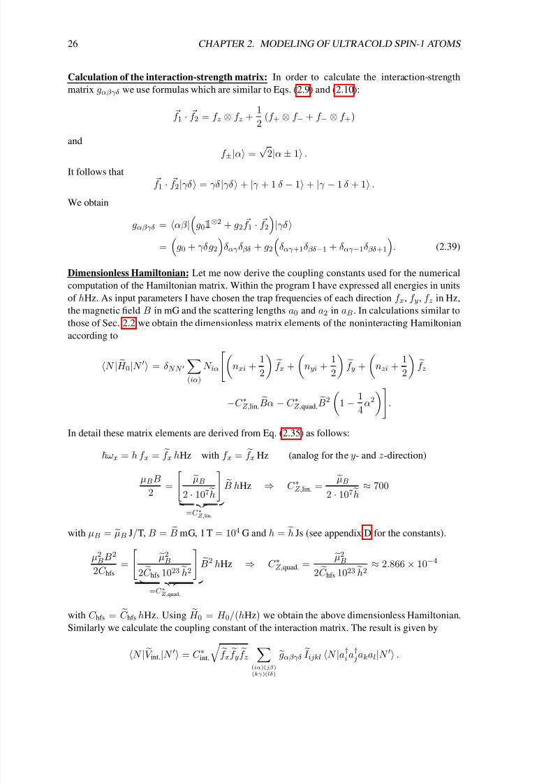
8/3/2019 Frank Deuretzbacher- Spinor Tonks-Girardeau gases and ultracold molecules
http://slidepdf.com/reader/full/frank-deuretzbacher-spinor-tonks-girardeau-gases-and-ultracold-molecules 36/151
26 CHAPTER 2. MODELING OF ULTRACOLD SPIN-1 ATOMS
Calculation of the interaction-strength matrix: In order to calculate the interaction-strength
matrix gαβγδ we use formulas which are similar to Eqs. (2.9) and (2.10):
f 1 · f 2 = f z ⊗ f z +1
2(f + ⊗ f − + f − ⊗ f +)
and
f ±|α =√
2|α ± 1 .
It follows that f 1 · f 2|γδ = γδ |γδ + |γ + 1 δ − 1 + |γ − 1 δ + 1 .
We obtain
gαβγδ = αβ |
g0 1
⊗2 + g2 f 1 · f 2
|γδ
=
g0 + γδg2
δαγ δβδ + g2
δαγ +1δβδ−1 + δαγ −1δβδ+1
. (2.39)
Dimensionless Hamiltonian: Let me now derive the coupling constants used for the numericalcomputation of the Hamiltonian matrix. Within the program I have expressed all energies in units
of hHz. As input parameters I have chosen the trap frequencies of each direction f x, f y, f z in Hz,
the magnetic field B in mG and the scattering lengths a0 and a2 in aB . In calculations similar to
those of Sec. 2.2 we obtain the dimensionless matrix elements of the noninteracting Hamiltonian
according to
N | H 0|N = δNN (iα)
N iα
nxi +
1
2
f x +
nyi +
1
2
f y +
nzi +
1
2
f z
−C ∗Z,lin. Bα
−C ∗Z,quad. B21
−1
4
α2.
In detail these matrix elements are derived from Eq. (2.35) as follows:
ωx = h f x = f x hHz with f x = f x Hz (analog for the y- and z-direction)
µBB
2=
µB2 · 107h
=C ∗Z,lin.
B hHz ⇒ C ∗Z,lin. =µB
2 · 107h ≈ 700
with µB =
µB J/T, B =
B mG, 1 T = 104 G and h =
h Js (see appendix D for the constants).
µ2BB2
2C hfs
= µ2
B
2 C hfs 1023 h2
=C ∗Z,quad.
B2 hHz ⇒ C ∗Z,quad. =µ2B
2 C hfs 1023 h2≈ 2.866 × 10⁻⁴
with C hfs = C hfs hHz. Using H 0 = H 0/(hHz) we obtain the above dimensionless Hamiltonian.
Similarly we calculate the coupling constant of the interaction matrix. The result is given by
N |V int.|N = C ∗int.
f x f y f z
(iα)(jβ)(kγ)(lδ)
gαβγδ I ijkl N |a†ia† jakal|N .

8/3/2019 Frank Deuretzbacher- Spinor Tonks-Girardeau gases and ultracold molecules
http://slidepdf.com/reader/full/frank-deuretzbacher-spinor-tonks-girardeau-gases-and-ultracold-molecules 37/151
2.7. NUMERICAL DIAGONALIZATION OF THE HAMILTONIAN MATRIX 27
Here, we have defined I ijkl = I ijkl/(lxlylz) and gαβγδ = gαβγδ 4π2aB/m
. The coupling
constant of the interaction is calculated as follows
1
2
4π2aBm
1
lxlylz=
1
2
4π
2
aB
m m3(2π)3
31
h
=C ∗int.
f x
f y
f z hHz
⇒ C ∗int. =1
2
4π2aBm m3(2π)33 1h ≈ 3.083 × 10⁻⁵ .
Here, we used = Js, aB = aB m, m = m kg
mass of 87Rb
, lu = /(mωu), ωu = 2πf u
(u = x,y ,z) and h = h Js. Again, the interaction Hamiltonian V int. is related to its dimensionless
counterpart according to V int. = V int. hHz.
2.7 Numerical diagonalization of the Hamiltonian matrix
In principle the main work is done when we built up the basis and calculated the Hamiltonian
matrix. What remains is to pass the Hamiltonian matrix to an efficient sparse-matrix diagonaliza-
tion routine. In the beginning I used the NAG library (mark 19). What I especially liked was the
excellent documentation of the NAG making it possible (even for a beginner) to implement the
diagonalization routines quickly. However, some day Kim Plassmeier realized that MATHEMATICA
diagonalizes orders of magnitude faster than the NAG (mark 19) since it uses a newer algorithm of
the LAPACK library. Since then I use Kim’s implementation [81] of the sparse-matrix diagonal-
ization routine of the LAPACK library. I heared that the newest NAG (mark 21) is considerably
faster (since it also uses this new algorithm), however, it was not available at my university.
The results of a numerical diagonalization are the desired number of lowest eigenenergies and
eigenvectors, given as an array of coefficients (. . . , cN , . . .)T , which are the desired coefficients
of the expansion |ψ =N cN |N . We will need these coefficients later together with the corre-
sponding number states |N when we want to calculate any further system properties.
2.8 Calculation of system properties
Arbitrary properties of an eigenstate |ψ are given by the expectation values of the corresponding
operators ψ|O|ψ. Since we know the eigenvector (. . . , cN , . . .)T such an expectation value is
given by
ψ|O|ψ =NN
cN cN ONN =
. . . cN . . . ...
· · · ONN · · ·...
...
cN ...
(2.40)
with ONN = N |O|N . Therefore, we are done, when we know the matrix elements of the
desired operator. These matrix elements will be calculated in the following for selected operators.
In the numerical implementation we mostly computed the sum of Eq. (2.40) (in the case
of the densities, momentum distributions and correlation functions). In other cases, however, it
is more efficient to calculate first the matrix ONN and to perform matrix-vector multiplications
hereafter as shown in Eq. (2.40). This method was used by Kim Plassmeier for the calculation
8/3/2019 Frank Deuretzbacher- Spinor Tonks-Girardeau gases and ultracold molecules
http://slidepdf.com/reader/full/frank-deuretzbacher-spinor-tonks-girardeau-gases-and-ultracold-molecules 38/151
28 CHAPTER 2. MODELING OF ULTRACOLD SPIN-1 ATOMS
of the expectation value F 2 [81]. The main advantage of this method is that, once the matrixONN has been calculated, one can quickly compute the expectation values of all the given
eigenvectors.
Density: The density is the probability to find one particle at position r. For one particle it is given
by ψ2(r). The corresponding one-particle operator is the projection on position r:
|r r | ⊗ 1 spin .
The matrix elements of the N -particle density are therefore given by
N |ρ(r )|N =
(iα)( jβ )
iα||r r | ⊗ 1 spin
| jβ N |a†iαa jβ |N
=
(iα)( jβ )
δαβ ψi(r )ψ j(r )N |a†iαa jβ |N (2.41)
with ψi(r ) = ψnxi (x)ψnyi (y)ψnzi (z). We obtain for the diagonal elements
N |ρ(r )|N = iα
ψ2i (r )N iα .
Only in one case, when bra and ket differ at two positions by one particle, we obtain nonzero
non-diagonal elements which are given by
..., N p,...,N qσ ,...|ρ(r )|..., N p + 1,...,N qσ − 1,... = δσψ p(r )ψq(r )
N qσ(N p + 1)
The oscillator functions are computed recursively. Using (2.38) we obtain the recursion formula
ψn(x) =
2
nx ψn−1(x) −
n − 1
nψn−2(x) .
Spin density: The spin density is the probability to find one particle at position r in spin state |γ .
The corresponding one-particle operator is the projection on state |rγ :
|rγ rγ | .
The matrix elements of the N -particle spin density are thus given by
N |ργ (r )|N =
(iα)( jβ )
δαγ δβγ ψi(r )ψ j(r )N |a†iαa jβ |N .
Kinetic energy of the x-direction: The kinetic energy of one particle along the x-axis is given by
− 2
2m∂ 2
∂x2= − 2
2ml2x
∂ 2
∂ x2= −ωx
2∂ 2
∂ x2= − f x
2∂ 2
∂ x2hHz .
We introduce creation and annihilation operators of oscillator quantum numbers
b =1√
2
x + i px =1√
2
x +∂
∂ x
, b† =1√
2
x − i px =1√
2
x − ∂
∂ x
where the dimensionless momentum operator is given by px = − i ∂/∂ x. The action of these
operators on the eigenstates of the harmonic oscillator is given by
b†|nx =√
nx + 1|nx + 1, b|nx =√
nx|nx − 1,

8/3/2019 Frank Deuretzbacher- Spinor Tonks-Girardeau gases and ultracold molecules
http://slidepdf.com/reader/full/frank-deuretzbacher-spinor-tonks-girardeau-gases-and-ultracold-molecules 39/151
2.8. CALCULATION OF SYSTEM PROPERTIES 29
similar to Eqs. (2.27). We express the position operator x and the partial derivative ∂/∂ x by means
of these creation and annihilation operators:
x =
1√2
b + b†
,
∂
∂
x
=1√
2
b − b†
.
We obtain for the kinetic energy
− 2
2m
∂ 2
∂x2= −
f x4
b − b†
b − b†
hHz = −
f x4
b2 − bb† − b†b + b†
2
hHz .
The one-particle matrix elements of the kinetic energy of the x-direction are therefore given by
iα|− 2
2m
∂ 2
∂x2
| jβ = −
f x4
hHz δαβ δnyinyj δnzinzj
×
nxj(nxj − 1)δnxinxj−2 −
2nxj + 1
δnxinxj +
(nxj + 1)(nxj + 2)δnxinxj+2
.
Similarly, we obtain for the potential energy of the x-direction
iα|
1
2mω2
xx2
| jβ =
f x4
hHz δαβ δnyinyj δnzinzj
×
nxj(nxj − 1)δnxinxj−2 +
2nxj + 1
δnxinxj +
(nxj + 1)(nxj + 2)δnxinxj+2
.
Momentum distribution: The probability to find one particle with momentum p is given by
| p p | ⊗ 1 spin .
The single-particle matrix element of that operator is given by
iα|| p p | ⊗ 1 spin
| jβ = δαβ i| p p | j = δαβ χ
∗i ( p )χ j( p )
with
χi( p ) = p |i =
dr p |r r |i =
1√2π
3
dr ψi(r )e− i p·r/ .
One can show that the Fourier transform of the oscillator functions is given by
χn( px) = (−i )nψn( px) (2.42)
(ψn is an oscillator function) and that they obey the recursive relation
χn( px) = − 2n
i px χn−1( px) + n − 1
nχn−2( px) .
Correlation function: The correlation function is the probability to find one particle at position rand the other at r . The corresponding two-particle operator is given by
|r r r r | ⊗ 1 spin .
The two-particle matrix elements of that operator are evaluated according to
iαjβ |
|r r r r | ⊗ 1 spin
|kγ lδ = δαγ δβδψi(r )ψ j(r )ψk(r )ψl(r ) .

8/3/2019 Frank Deuretzbacher- Spinor Tonks-Girardeau gases and ultracold molecules
http://slidepdf.com/reader/full/frank-deuretzbacher-spinor-tonks-girardeau-gases-and-ultracold-molecules 40/151
30 CHAPTER 2. MODELING OF ULTRACOLD SPIN-1 ATOMS
The matrix elements of the N -particle correlation function are thus given by
N |ρ(r , r )|N =1
2
(iα)(jβ)(kγ)(lδ)
δαγ δβδψi(r )ψ j(r )ψk(r )ψl(r )N |a†iαa† jβ akγ alδ|N .
These matrix elements are evaluated in a similar way as has been done for the interaction operator.However, take care that the product ψi(r )ψ j(r )ψk(r )ψl(r ) has different symmetries than the
interaction integrals I ijkl =
dr ψi(r )ψ j(r )ψk(r )ψl(r ).
Local correlation function: The local correlation function is the probability to find the two parti-
cles at the same position dr |r r r r | ⊗ 1 spin .
The N -particle matrix elements of that operator are given by
N |ρlocal corr.|N =1
2 (iα)(jβ)
(kγ)(lδ)
δαγ δβδI ijklN |a†iαa† jβ akγ alδ|N
which is the interaction operator when δαγ δβδ is replaced by the interaction-strength matrix gαβγδ.
Square of total spin: The operator F 2 is a sum of a single- and a two-particle operator – like the
Hamiltonian of our system. We calculate for two particles
F 2 =
f 1 + f 2
2= f 21 + f 22 + 2 f 1 · f 2 = 2 1 + 2 1 + 2 f 1 · f 2 .
Thus, the second-quantized form of that operator is given by
F 2 = 2
(iα)( jβ )iα| 1 | jβ a†iαa jβ +
(iα)(jβ)(kγ)(lδ)
iαjβ | f 1 · f 2|kγ lδa†iαa† jβ akγ alδ .
The single-particle matrix element is given by
iα| 1 | jβ = δijδαβ
and the two-particle matrix element is given by
see the calculation of the interaction-strength
matrix (2.39)
iαjβ | f 1 · f 2|kγ lδ = δikδ jl
γδ δαγ δβδ + δαγ +1δβδ−1 + δαγ −1δβδ+1
.
The F 2 operator has been implemented by Kim Plassmeier [81].
2.9 Testing / convergence
Since one can make mistakes in every step of an exact diagonalization, we need tests to check our
results. We are here in the fortunate situation that there are many nontrivial testing cases available.
Comparison with the Tonks-Girardeau gas: One-dimensional spinless bosons with infinite δrepulsion behave in many respects like noninteracting fermions since the exact ground-state wave
function is given by the absolute value of the Slater determinant [6]:
ψ(∞)bosons(x1, x2, . . . , xN ) =
det
ψi(x j)
i, j = 1, 2, . . . , N .

8/3/2019 Frank Deuretzbacher- Spinor Tonks-Girardeau gases and ultracold molecules
http://slidepdf.com/reader/full/frank-deuretzbacher-spinor-tonks-girardeau-gases-and-ultracold-molecules 41/151
2.9. TESTING / CONVERGENCE 31
0 100 200 300 400 500−0.3
−0.2
−0.1
0
0.1
0.2
0.3
0.4
number of basis state
V a l u e
o f c o e f f
i c i e n t
increasing energy
Figure 2.4: Coefficient distribution of the ground state of the spin-polarized quasi-one-dimensional
strongly-interacting system. Shown are the coefficients of the expansion |ψ =N cN |N .
Here, ψi(x) is the ith eigenfunction of the single-particle Hamiltonian. It follows immediatly from
this solution that all the quantities which are calculated from the square of the wave function,ψ(∞)bosons
2= det
ψi(x j)
2
(2.43)
– like the N -particle density, the correlation function and all the energy contributions – are equal
to those of noninteracting fermions. I will show later in Sec. 3.8 that Eq. (2.43) holds also for the
excited states (but with the corresponding Slater determinant).
In our system, the particles have spin 1. But in the spin-polarized case F z = ±N , when all
the spins of the initial state point up- or downwards, the system can be described by a spinless
wave function since the N -particle spin function |1, 1, . . . , 1 or |−1, −1, . . . , −1 is the same
at all times (I have shown in Sec. 2.1 that F z is conserved and thus no spin-changing collisions
can occur). Hence, the spin function can be neglected for the description of the system. Therefore,
in the spin-polarized case, when the system is quasi-one-dimensional (i. e. ωx ωy, ωz) and
when the repulsion between the particles is strong, the bosons should behave like noninteracting
fermions. In a first test, we thus checked whether the total energies of all the low-energy states
were equal to those of noninteracting fermions, i. e., we checked whether the ground-state energy
E g = N 2/2 ωx and the level spacing ∆E = 1 ωx were equal (apart from a constant offset
from the Zeeman energy and the transverse directions). This is a nontrivial test of the Hamiltonian
since the basis states of the noninteracting Hamiltonian are strongly mixed up in the low-energy
eigenstates of the strongly interacting system, as shown in Fig. 2.4 for the ground state. Later, we
also checked the density operator and the correlation function in the Tonks-Girardeau limit.
Comparison with the solution of C. K. Law, H. Pu and N. P. Bigelow [56]: In order to test the
spin part of the Hamiltonian we can compare with the solution of C. K. Law et al. [56]. The
solution is valid for zero-dimensional systems, i. e., all the particles reside in the motional ground
state, and zero magnetic field. In that case the basis is finite. The occupation number states are
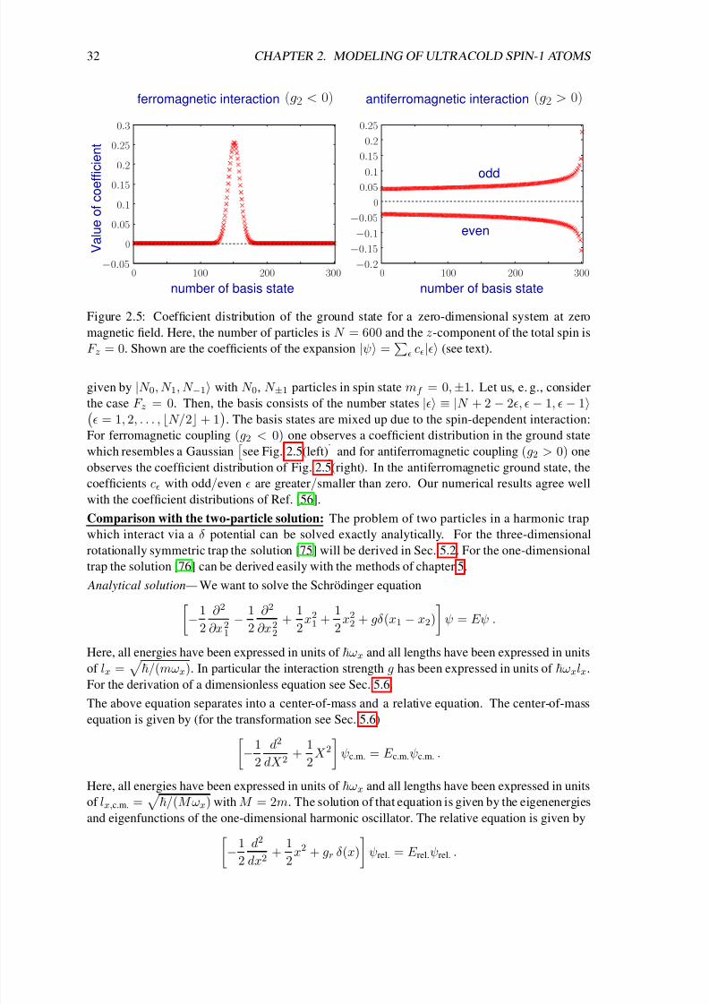
8/3/2019 Frank Deuretzbacher- Spinor Tonks-Girardeau gases and ultracold molecules
http://slidepdf.com/reader/full/frank-deuretzbacher-spinor-tonks-girardeau-gases-and-ultracold-molecules 42/151
32 CHAPTER 2. MODELING OF ULTRACOLD SPIN-1 ATOMS
0 100 200 300
0
0.1
0.2
0.3
number of basis state
V a l u e
o f c o e f f i c i e n t
−0.05
0.05
0.15
0.25
0 100 200 300
0
0.
1
0.2
number of basis state
−0.05
0.05
0.15
0.25
−0.1
−0.15
−0.2
odd
even
ferromagnetic interaction (g2 < 0) antiferromagnetic interaction (g2 > 0)
Figure 2.5: Coefficient distribution of the ground state for a zero-dimensional system at zero
magnetic field. Here, the number of particles is N = 600 and the z-component of the total spin is
F z = 0. Shown are the coefficients of the expansion |ψ = c| (see text).
given by |N 0, N 1, N −1 with N 0, N ±1 particles in spin state mf = 0, ±1. Let us, e. g., consider
the case F z = 0. Then, the basis consists of the number states | ≡ |N + 2 − 2, − 1, − 1 = 1, 2, . . . , N/2 + 1
. The basis states are mixed up due to the spin-dependent interaction:
For ferromagnetic coupling (g2 < 0) one observes a coefficient distribution in the ground state
which resembles a Gaussian
see Fig. 2.5(left)
and for antiferromagnetic coupling (g2 > 0) one
observes the coefficient distribution of Fig. 2.5(right). In the antiferromagnetic ground state, the
coefficients c with odd/even are greater/smaller than zero. Our numerical results agree well
with the coefficient distributions of Ref. [56].
Comparison with the two-particle solution: The problem of two particles in a harmonic trap
which interact via a δ potential can be solved exactly analytically. For the three-dimensional
rotationally symmetric trap the solution [75] will be derived in Sec. 5.2. For the one-dimensional
trap the solution [76] can be derived easily with the methods of chapter 5.
Analytical solution— We want to solve the Schrodinger equation−1
2
∂ 2
∂x21
− 1
2
∂ 2
∂x22
+1
2x21 +
1
2x22 + gδ(x1 − x2)
ψ = Eψ .
Here, all energies have been expressed in units of ωx and all lengths have been expressed in units
of lx = /(mωx). In particular the interaction strength g has been expressed in units of ωxlx.
For the derivation of a dimensionless equation see Sec. 5.6.
The above equation separates into a center-of-mass and a relative equation. The center-of-massequation is given by (for the transformation see Sec. 5.6)
−1
2
d2
dX 2+
1
2X 2
ψc.m. = E c.m.ψc.m. .
Here, all energies have been expressed in units of ωx and all lengths have been expressed in units
of lx,c.m. = /(M ωx) with M = 2m. The solution of that equation is given by the eigenenergies
and eigenfunctions of the one-dimensional harmonic oscillator. The relative equation is given by−1
2
d2
dx2+
1
2x2 + gr δ(x)
ψrel. = E rel.ψrel. .

8/3/2019 Frank Deuretzbacher- Spinor Tonks-Girardeau gases and ultracold molecules
http://slidepdf.com/reader/full/frank-deuretzbacher-spinor-tonks-girardeau-gases-and-ultracold-molecules 43/151
2.9. TESTING / CONVERGENCE 33
Here, all energies have been expressed in units of ωx and all lengths have been expressed in units
of lx,rel. = /(µωx) with µ = m/2. The interaction strength gr is now expressed in units of
ωxlx,rel.. It is related to g as follows
g = gωxlx = grωxlx,rel.
⇒ gr = glx
lx,rel.
.
Here, g and gr are the dimensionless interaction strengths. We omit the tilde symbol and obtain
the relation
gr = g/√
2 (2.44)
since lx,rel. =√
2 lx. In the region x = 0, the δ potential is zero and the relative equation trans-
forms to
ψrel. − x2ψrel. + 2E rel.ψrel. = 0 .
I solve this equation in appendix B. Due to the boundary condition ψrel.(x) = 0 for |x| → ∞ we
obtain the solution
see Eqs. (5.28) and (5.34)
ψrel. = A U −E rel.;√2x = A DE rel.−1/2
√2x = B U −E rel.
2+ 1
4; 1
2; x2 e−x
2/2 (2.45)
where A and B = A 2E rel./2−1/4 are normalization constants. B is given by
B2 = 2E rel.+1/2π−1/2 Γ(1/2 − E rel.)
Ψ(3/4 − E rel./2) − Ψ(1/4 − E rel./2). (2.46)
B2 differs by a factor 2 from Eq. (5.63) since
∞−∞ = 2
∞0 .
It remains to determine E rel.. The
δ potential is equivalent to the boundary condition [83]
lim→0dψrel.
dx − dψrel.
dx − = 2 gr ψrel.(0) .(2.47)
Since ψrel.(−x) = ψrel.(x) it follows that ψrel.(−) = −ψ
rel.() and the boundary condition be-
comes
lim→0
dψrel.
dx
= gr ψrel.(0) ⇔ ψrel.(0+)
ψrel.(0)= gr .
Note the similarity to the boundary condition 5.41 in three dimensions! In Sec. 5.2 we will derive
Eq. (5.40), which determines the energy as a function of the scattering length as, from the bound-
ary condition 5.41. Thus, we obtain the energy of the relative motion E rel. simply by replacing
−1/as by the interaction strength gr in Eq. (5.40):
− 2 Γ(3/4 − E rel./2)Γ(1/4 − E rel./2) = gr . (2.48)
Finally, in order to compare with the numerical solution, we have to construct the total two-particle
wave function:
ψ = ψc.m.
X
lxlx,c.m.
ψrel.
x
lxlx,rel.
= ψc.m.
x1 + x2√
2
ψrel.
x1 − x2√
2
(given in units of lx). I note, that one has to regard Eq. (2.44) for the comparison with the numerics.
Comparison with the numerical solution— Fig. 2.6 shows a comparison of the exact (black
dashed) to the numerical solution (colored solid lines) for different interaction strengths g. The
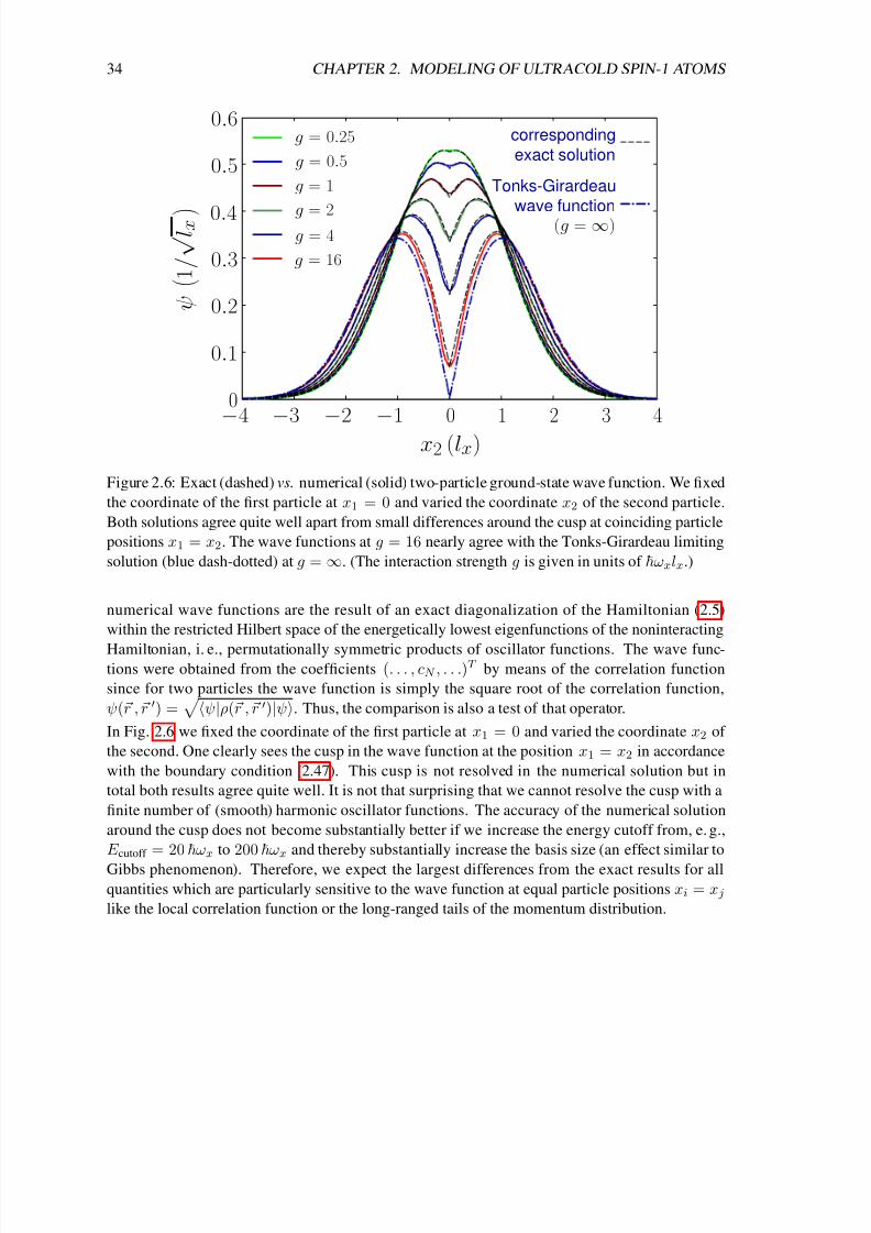
8/3/2019 Frank Deuretzbacher- Spinor Tonks-Girardeau gases and ultracold molecules
http://slidepdf.com/reader/full/frank-deuretzbacher-spinor-tonks-girardeau-gases-and-ultracold-molecules 44/151
34 CHAPTER 2. MODELING OF ULTRACOLD SPIN-1 ATOMS
0 1 2 3 4−1−2−3−40
0.1
0.2
0.3
0.4
0.5
0.6
x2 (lx)
ψ
1 / √ l x
g = 0.25
g = 0.5
g = 1
g = 2g = 4
g = 16
corresponding
exact solution
Tonks-Girardeau
wave function(g =∞)
Figure 2.6: Exact (dashed) vs. numerical (solid) two-particle ground-state wave function. We fixed
the coordinate of the first particle at x1 = 0 and varied the coordinate x2 of the second particle.
Both solutions agree quite well apart from small differences around the cusp at coinciding particle
positions x1 = x2. The wave functions at g = 16 nearly agree with the Tonks-Girardeau limiting
solution (blue dash-dotted) at g = ∞. (The interaction strength g is given in units of ωxlx.)
numerical wave functions are the result of an exact diagonalization of the Hamiltonian (2.5)
within the restricted Hilbert space of the energetically lowest eigenfunctions of the noninteracting
Hamiltonian, i. e., permutationally symmetric products of oscillator functions. The wave func-tions were obtained from the coefficients (. . . , cN , . . .)T by means of the correlation function
since for two particles the wave function is simply the square root of the correlation function,
ψ(r , r ) = ψ|ρ(r , r )|ψ. Thus, the comparison is also a test of that operator.
In Fig. 2.6 we fixed the coordinate of the first particle at x1 = 0 and varied the coordinate x2 of
the second. One clearly sees the cusp in the wave function at the position x1 = x2 in accordance
with the boundary condition (2.47). This cusp is not resolved in the numerical solution but in
total both results agree quite well. It is not that surprising that we cannot resolve the cusp with a
finite number of (smooth) harmonic oscillator functions. The accuracy of the numerical solution
around the cusp does not become substantially better if we increase the energy cutoff from, e. g.,
E cutoff = 20 ωx to 200 ωx and thereby substantially increase the basis size (an effect similar to
Gibbs phenomenon). Therefore, we expect the largest differences from the exact results for all
quantities which are particularly sensitive to the wave function at equal particle positions xi = x jlike the local correlation function or the long-ranged tails of the momentum distribution.

8/3/2019 Frank Deuretzbacher- Spinor Tonks-Girardeau gases and ultracold molecules
http://slidepdf.com/reader/full/frank-deuretzbacher-spinor-tonks-girardeau-gases-and-ultracold-molecules 45/151
Chapter 3
Evolution from a Bose-Einstein
condensate to a Tonks-Girardeau gas
The main results of this chapter have been published in Ref. [2]. Parts have been published in mydiploma thesis [1].
Subject of this chapter is a study of the interaction-driven evolution of a quasi-one-dimensional
system of spinless hard-core bosons. First, in Sec. 3.1, I derive the effective Hamiltonian of spin-
less quasi-one-dimensional bosons. In Secs. 3.2 and 3.3 I discuss the two limiting regimes of
weak and infinitely strong δ repulsion. In Sec. 3.4 I study the interaction-driven evolution of
various ground-state properties. Besides the pair correlation function I will identify the momen-
tum distribution as a reliable indicator for transitions of the system between three characteristic
regimes, the Bose-Einstein-condenstate (BEC) regime, an intermediate regime with strong short-
range correlations and the Tonks-Girardeau regime. I will quantify the interaction strength for
the transitions by means of two characteristic features of the momentum distribution. In the last
section 3.5 I will finally discuss the low-energy excitation spectrum of the boson system. Related
studies on that subject have been performed by S. Zollner et al. [41, 42] and by Y. Hao et al. [35].
3.1 Effective quasi-one-dimensional Hamiltonian
We consider a system of spin-polarized quasi-one-dimensional bosons, i. e., the axial level spacing
ωx and the interaction energy E int.,0
estimated by Eq. (2.24)
shall be much smaller than the
transverse level spacings ωy and ωz and the N -particle spin function is given by
|1, 1, . . . , 1
or
|−1, −1, . . . , −1. In the experiment of Kinoshita et al. [21] for example we have ω⊥/ωx ≈ 2600with ω⊥ = ωy = ωz
and ω⊥/E int.,0 ≈ 500 (see the discussion in the end of Sec. 2.2) so
that these conditions are rather well satisfied. But let me start the discussion with the complete
Hamiltonian (2.4) of two particles
H =2i=1
−
2
2m∆i +
1
2m
ω2xx2i + ω2
yy2i + ω2zz2i
⊗1
⊗2
−2i=1
µBB
2f z,i +
µ2BB2
2C hfs
1
⊗2 − 1
4f 2z,i
+ δ(r1 − r2)
g0 1
⊗2 + g2 f 1 · f 2
.
35

8/3/2019 Frank Deuretzbacher- Spinor Tonks-Girardeau gases and ultracold molecules
http://slidepdf.com/reader/full/frank-deuretzbacher-spinor-tonks-girardeau-gases-and-ultracold-molecules 46/151
36 CHAPTER 3. EVOLUTION FROM A BEC TO A TONKS-GIRARDEAU GAS
Let us assume that the two particles are initially in spin state |1, 1. 1 This state is an eigenstate of
the spin part of the above Hamiltonian since
f 1 · f 2 |1, 1 =
f z ⊗ f z +
1
2(f + ⊗ f − + f − ⊗ f +)
|1, 1 = |1, 1
and thus the spin-polarized state |1, 1 is not coupled to states with other spin orientations by the
spin-dependent interaction g2δ(r1 − r2) f 1 · f 2. Since
1, 1|
g0 1
⊗2 + g2 f 1 · f 2
|1, 1 = g0 + g2 =
4π2a2m
the effective spinless Hamiltonian (within the subspace F z = 2) is given by
1, 1|H |1, 1 =2i=1
− 2
2m∆i +
1
2m
ω2xx2i + ω2
yy2i + ω2zz2i
+
4π2a2m
δ(r1 − r2) + E Z,offset
where the Zeeman energy
E Z,offset = −2
µBB
2+
µ2BB2
2C hfs
1 − 1
4
is a constant offset energy within this subspace. Now we assume that the two particles reside in
the ground state of the transverse direction since the interaction energy is such small compared to
the transverse level spacing
ψ⊥ = ψ0(y1)ψ0(z1)ψ0(y2)ψ0(z2) .
Here, ψ0 is the ground state of the one-dimensional harmonic oscillator. We integrate over the
transverse direction and obtain the effective Hamiltonian
1, 1|⊗ ψ⊥|H |ψ⊥⊗ |1, 1 =2i=1
−
2
2m
∂ 2
∂x2i
+1
2mω2
xx2i
+ gδ(x1 − x2) + E Z,offset + E ⊥,offset
where the ground-state energy of the transverse motion is given by
E ⊥,offset = 2
1
2ωy +
1
2ωz
and where the effective one-dimensional interaction strength is given by
g =4π2a2
mψ⊥|δ(y1 − y2)δ(z1 − z2)|ψ⊥ =
4π2a2m
1
lylz
1
2π= 2 ω⊥ a2 . (3.1)
Here we used
dyψ40(y)
dzψ4
0(z) = 1/(2πlylz) and l⊥ = ly = lz = /(mω⊥). The effective
Hamiltonian for the axial wave function ψaxial is thus given by
H =2i=1
−
2
2m
∂ 2
∂x2i
+1
2mω2x2
i
+ gδ(x1 − x2) .
1The discussion is analogous for the state |− 1, −1.

8/3/2019 Frank Deuretzbacher- Spinor Tonks-Girardeau gases and ultracold molecules
http://slidepdf.com/reader/full/frank-deuretzbacher-spinor-tonks-girardeau-gases-and-ultracold-molecules 47/151
3.2. WEAKLY INTERACTING REGIME: MEAN-FIELD APPROXIMATION 37
Here I renamed the frequency ω = ωx and I neglected the constant offset energies. Generalization
to N particles is straightforward
H =N
i=1− 2
2m
∂ 2
∂x2i
+1
2mω2x2
i+ g
i<jδ(xi − x j) . (3.2)
Finally I note that the scattering length a2 is affected by a tight transverse confinement. 2 It has
been shown in Refs. [84, 85] that the effective scattering length a2,eff. is given by
a2,eff. = γ a2 with γ =1
1 − 1.46 a2/√
2l⊥ .
However, for the transvere confinement considered here (see the frequencies of Ref. [ 21] in Ta-
ble 2.1) the scattering length a2 is only marginally modified since
1 < γ < 1.16 for 0 < ω⊥ < 2π × 70.7 kHz .
3.2 Weakly interacting regime: Mean-field approximation
For vanishing interactions all the bosons occupy the ground state of the harmonic trap ψ0(x) and
the many-particle wave function is given by ψ(x1, x2, . . . , xN ) =N i=1 ψ0(xi). Similarly, in the
weakly interacting regime it is sufficiently accurate to assume that all the bosons condense into
the same mean-field wave function ψm.f.(x) so that the many-particle wave function is given by
ψ(x1, x2, . . . , xN ) ≈N i=1
ψm.f.(xi) . (3.3)
However, the mean-field orbital is deformed due to the interaction between the bosons. The opti-
mal shape of ψm.f.(x) minimizes the total energy of the above state (3.3) with the Hamiltonian (3.2)
E (ψm.f.) =
dx
N ψ∗
m.f.(x)
−
2
2m
d2
dx2+
1
2mω2x2
ψm.f.(x) +
N (N − 1)
2gψm.f.(x)
4.
The Gross-Pitaevskii equation is obtained from this energy functional by using a variational pro-
cedure [15, 16]−
2
2m
d2
dx2+
1
2mω2x2 + (N − 1)g
ψm.f.(x)
2
ψm.f.(x) = µ ψm.f.(x) (3.4)
where µ is the chemical potential. Eq. (3.4) is a nonlinear differential equation. Different from an
ordinary single-particle Schrodinger equation there is an additional mean-field potential
V m.f.(x) = (N − 1)gψm.f.(x)
22The three-dimensional scattering length as is usually determined from the phase shift δ0 of the scattered wave in
the limit of zero energy and zero confinement, where tan δ0 = −kas. A tight confinement affects the behavior of
the radial wave function at r = R (where R is the range of the interaction potential), thus leading to a modification
of the scattering length.ˆ
See Sec. 5.1 for the discussion of the short-ranged interaction between two particles in the
trap-free case — in particular Eq. (5.17) for the definition of the scattering length and Eq. (5.20) for the relation between
the scattering length and the phase shift. The influence of the confinement is discussed in Sec. 5.2. Note that all the
quantities in that section are given in units of the oscillator length and the level spacing of the trap.˜
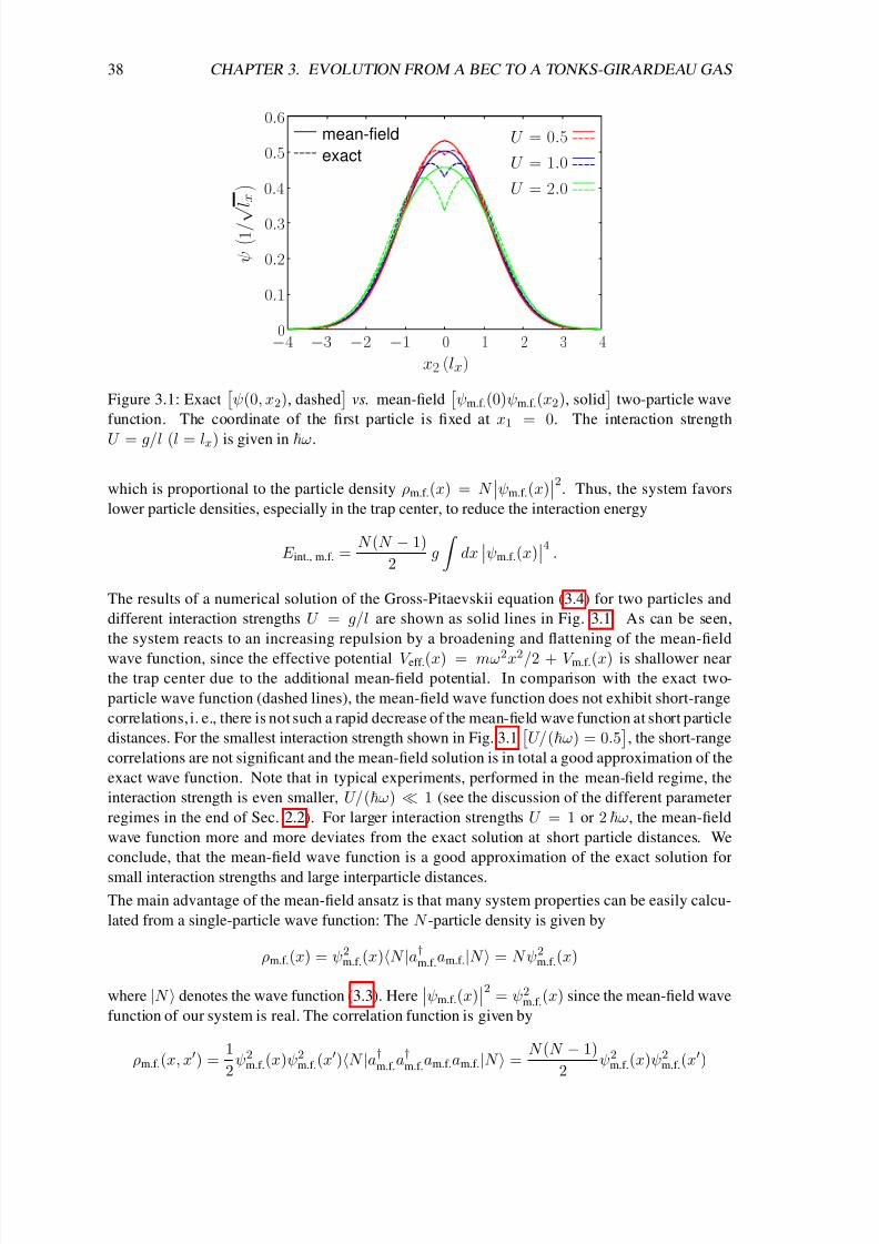
8/3/2019 Frank Deuretzbacher- Spinor Tonks-Girardeau gases and ultracold molecules
http://slidepdf.com/reader/full/frank-deuretzbacher-spinor-tonks-girardeau-gases-and-ultracold-molecules 48/151
38 CHAPTER 3. EVOLUTION FROM A BEC TO A TONKS-GIRARDEAU GAS
0 1 2 3 4−1−2−3−40
0.1
0.2
0.3
0.4
0.5
0.6
x2 (lx)
ψ
1 / √
l x
mean-field
exact
U = 0.5
U = 1.0
U = 2.0
Figure 3.1: Exact
ψ(0, x2), dashed
vs. mean-field
ψm.f.(0)ψm.f.(x2), solid
two-particle wave
function. The coordinate of the first particle is fixed at x1 = 0. The interaction strength
U = g/l (l = lx) is given in ω.
which is proportional to the particle density ρm.f.(x) = N ψm.f.(x)
2. Thus, the system favors
lower particle densities, especially in the trap center, to reduce the interaction energy
E int., m.f. =N (N − 1)
2g
dxψm.f.(x)
4 .
The results of a numerical solution of the Gross-Pitaevskii equation (3.4) for two particles and
different interaction strengths U = g/l are shown as solid lines in Fig. 3.1. As can be seen,
the system reacts to an increasing repulsion by a broadening and flattening of the mean-field
wave function, since the effective potential V eff.(x) = mω2x2/2 + V m.f.(x) is shallower near
the trap center due to the additional mean-field potential. In comparison with the exact two-
particle wave function (dashed lines), the mean-field wave function does not exhibit short-range
correlations, i. e., there is not such a rapid decrease of the mean-field wave function at short particle
distances. For the smallest interaction strength shown in Fig. 3.1
U/(ω) = 0.5
, the short-range
correlations are not significant and the mean-field solution is in total a good approximation of the
exact wave function. Note that in typical experiments, performed in the mean-field regime, the
interaction strength is even smaller, U/(ω) 1 (see the discussion of the different parameter
regimes in the end of Sec. 2.2). For larger interaction strengths U = 1 or 2 ω, the mean-field
wave function more and more deviates from the exact solution at short particle distances. We
conclude, that the mean-field wave function is a good approximation of the exact solution for
small interaction strengths and large interparticle distances.
The main advantage of the mean-field ansatz is that many system properties can be easily calcu-
lated from a single-particle wave function: The N -particle density is given by
ρm.f.(x) = ψ2m.f.(x)N |a†m.f.am.f.|N = N ψ2
m.f.(x)
where |N denotes the wave function (3.3). Hereψm.f.(x)
2 = ψ2m.f.(x) since the mean-field wave
function of our system is real. The correlation function is given by
ρm.f.(x, x) =1
2ψ2
m.f.(x)ψ2m.f.(x)N |a†m.f.a
†m.f.am.f.am.f.|N =
N (N − 1)
2ψ2
m.f.(x)ψ2m.f.(x)

8/3/2019 Frank Deuretzbacher- Spinor Tonks-Girardeau gases and ultracold molecules
http://slidepdf.com/reader/full/frank-deuretzbacher-spinor-tonks-girardeau-gases-and-ultracold-molecules 49/151
3.3. STRONGLY INTERACTING REGIME: GIRARDEAU’S FERMI-BOSE MAPPING 39
and thus it is proportional to the density when one particle coordinate is fixed. The kinetic energy
is given by
E kin., m.f. = N 2
2m
dx
dψm.f.(x)
dx
2and so forth ... Later in Sec. 3.4 I will determine the parameter regime where the mean-field
approximation is sufficiently accurate.
3.3 Strongly interacting regime: Girardeau’s Fermi-Bose mapping
Not only in the weakly interacting regime but also in the opposite limit of very strong repulsion
there exists a simple method to analyze the system. Surprisingly it is even easier to calculate the
exact many-particle wave function of the strongly interacting bosons than the mean-field wave
function in the weakly interacting regime.
We are considering spinless one-dimensional bosons which interact via a δ potential. The Hamil-
tonian of that system is given by
H =N i=1
−
2
2m
∂ 2
∂x2i
+1
2mω2x2
i
+ g
i<j
δ(xi − x j) .
(see the derivation of Eq. (3.2) in Sec. 3.1). One can derive from Eq. (2.47) that the interaction
Hamiltonian gi<j δ(xi − x j) is equivalent to the boundary condition
∂
∂xi− ∂
∂x j
ψ|xi=xj+ −
∂
∂xi− ∂
∂x j
ψ|xi=xj− =
2mg
2ψ|xi=xj , (3.5)
i. e., ψ has cusps whenever two particles touch and the jumps in the derivative of ψ are 2mg/2.
We are interested in the solution of the limiting case of infinite repulsiong = ∞
. In that case
it follows from the boundary condition (3.5) that the wave function has to be zero whenever two
particle coordinates are equal
ψ(x1, x2, . . . , xN ) = 0 if xi = x j .
Thus, we are searching for solutions of the Schrodinger equation of noninteracting particles which
are zero on the surface xi = x j ≡ (x1, x2, . . . , xN ) ∈ RN , xi = x j and which are permuta-
tionally symmetric:
ψ solves
N
i=1
−
2
2m
∂ 2
∂x2i
+1
2mω2x2
i
ψ = Eψ in RN \ xi = x j (3.6a)
ψ(x1, x2, . . . , xN ) = 0 on the surface xi = x j (3.6b)
ψ has Bose symmetry (is permutationally symmetric). (3.6c)
Eq. (3.6a) and the boundary condition (3.6b) are readily fulfilled by the wave functions of nonin-
teracting fermions ψ(0)fermions(x1, x2, . . . , xN ). These wave functions are given by the Slater deter-
minant of the occupied single-particle orbitals. However, fermionic wave functions are antisym-
metric under any permutations of particle coordinates. In order to construct a Bose wave function
from the fermionic solution of (3.6a) we introduce the so-called “unit antisymmetric function”
A(x1, x2, . . . , xN ) =i<j
sign(xi − x j) (3.7)
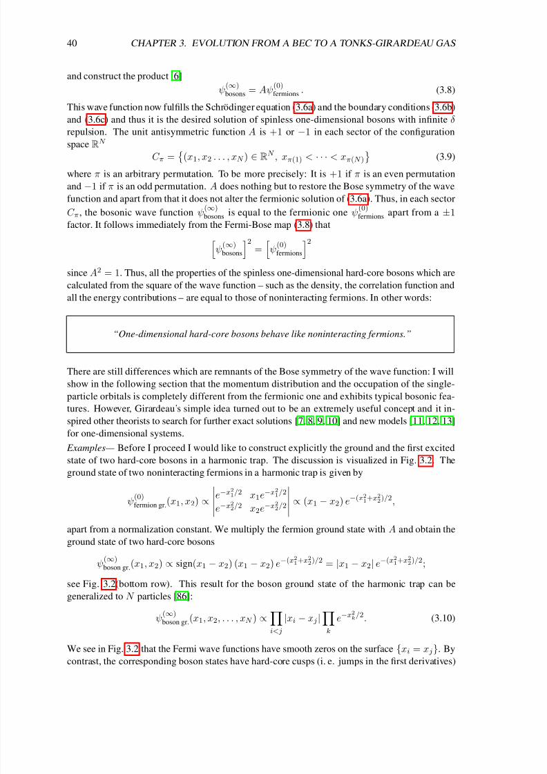
8/3/2019 Frank Deuretzbacher- Spinor Tonks-Girardeau gases and ultracold molecules
http://slidepdf.com/reader/full/frank-deuretzbacher-spinor-tonks-girardeau-gases-and-ultracold-molecules 50/151
40 CHAPTER 3. EVOLUTION FROM A BEC TO A TONKS-GIRARDEAU GAS
and construct the product [6]
ψ(∞)bosons = Aψ
(0)fermions . (3.8)
This wave function now fulfills the Schrodinger equation (3.6a) and the boundary conditions (3.6b)
and (3.6c) and thus it is the desired solution of spinless one-dimensional bosons with infinite δ
repulsion. The unit antisymmetric function A is +1 or −1 in each sector of the configurationspace RN
C π =
(x1, x2 . . . , xN ) ∈ RN , xπ(1) < · · · < xπ(N )
(3.9)
where π is an arbitrary permutation. To be more precisely: It is +1 if π is an even permutation
and −1 if π is an odd permutation. A does nothing but to restore the Bose symmetry of the wave
function and apart from that it does not alter the fermionic solution of (3.6a). Thus, in each sector
C π, the bosonic wave function ψ(∞)bosons is equal to the fermionic one ψ
(0)fermions apart from a ±1
factor. It follows immediately from the Fermi-Bose map (3.8) thatψ(∞)bosons
2=
ψ(0)fermions
2since A2 = 1. Thus, all the properties of the spinless one-dimensional hard-core bosons which arecalculated from the square of the wave function – such as the density, the correlation function and
all the energy contributions – are equal to those of noninteracting fermions. In other words:
“One-dimensional hard-core bosons behave like noninteracting fermions.”
There are still differences which are remnants of the Bose symmetry of the wave function: I will
show in the following section that the momentum distribution and the occupation of the single-
particle orbitals is completely different from the fermionic one and exhibits typical bosonic fea-
tures. However, Girardeau’s simple idea turned out to be an extremely useful concept and it in-spired other theorists to search for further exact solutions [7, 8, 9, 10] and new models [11, 12, 13]
for one-dimensional systems.
Examples— Before I proceed I would like to construct explicitly the ground and the first excited
state of two hard-core bosons in a harmonic trap. The discussion is visualized in Fig. 3.2. The
ground state of two noninteracting fermions in a harmonic trap is given by
ψ(0)fermion gr.(x1, x2) ∝
e−x21/2 x1e−x
21/2
e−x22/2 x2e−x22/2
∝ (x1 − x2) e−(x21+x22)/2,
apart from a normalization constant. We multiply the fermion ground state with A and obtain the
ground state of two hard-core bosons
ψ(∞)boson gr.(x1, x2) ∝ sign(x1 − x2) (x1 − x2) e−(x21+x
22)/2 = |x1 − x2| e−(x21+x
22)/2;
see Fig. 3.2(bottom row). This result for the boson ground state of the harmonic trap can be
generalized to N particles [86]:
ψ(∞)boson gr.(x1, x2, . . . , xN ) ∝
i<j
|xi − x j |k
e−x2k/2. (3.10)
We see in Fig. 3.2 that the Fermi wave functions have smooth zeros on the surface xi = x j. By
contrast, the corresponding boson states have hard-core cusps (i. e. jumps in the first derivatives)

8/3/2019 Frank Deuretzbacher- Spinor Tonks-Girardeau gases and ultracold molecules
http://slidepdf.com/reader/full/frank-deuretzbacher-spinor-tonks-girardeau-gases-and-ultracold-molecules 51/151
3.3. STRONGLY INTERACTING REGIME: GIRARDEAU’S FERMI-BOSE MAPPING 41
2 fermions 2 bosons
g r o u n d s
t a t e
mapping
f i r s t e
x c i t e d s
t a t e
mapping
x1 = 0
ψ(0)fermions ∝ (x1 − x2)e−(x2
1+x22)/2 ψ
(∞)bosons ∝ |x1 − x2|e
−(x21+x2
2)/2
ψ(0)fermions ∝ (x2
1 − x22)e−(x2
1+x22)/2 ψ
(∞)bosons ∝ (x1 + x2)|x1 − x2|e
−(x21+x2
2)/2
x1 = 1
x1 = 1
ψ=0
x1
x2
x1 < x2
x2 < x1
configuration space
Schrödinger equation
of noninteracting
particles
Schrödinger equation
of noninteracting
particles
x1 = x2
x1 = 0
Figure 3.2: Sketch of Girardeau’s Fermi-Bose map for two particles. Bottom row: ground state,
upper row: first excited state, right: configuration space.
at the collision points xi = x j. One can show for a general trapping potential that the boson
ground state is always given by the absolute value of the corresponding fermion ground state [6]
ψ(∞)boson gr. = Aψ
(0)fermion gr. =
ψ(0)fermion gr.
since all the zeros of the Fermi ground state are located on the surface xi = x j and there are no
further zeros within the sectors C π.
Let me now construct the first excited state. The first excited state of two noninteracting fermionsin a harmonic trap is given by
ψ(0)fermion 1st(x1, x2) ∝
e−x21/2 (2x2
1 − 1)e−x21/2
e−x22/2 (2x22 − 1)e−x22/2
∝ x21 − x2
2
e−(x21+x
22)/2 .
We multiply this state with the unit antisymmetric function A and obtain the first excited state of
two hard-core bosons
ψ(∞)boson 1st(x1, x2) ∝ sign(x1 − x2)
x21 − x2
2
e−(x21+x
22)/2 = (x1 + x2) |x1 − x2| e−(x21+x
22)/2 .
We see that this state has interaction cusps on the “surface” x1
−x2 = 0 and additional smooth
zeros on the “surface” x1 + x2 = 0 which runs through the sectors x1 < x2 and x2 < x1. Hence,the sign of the wave function of the first excited state changes not only on the sector boundaries
∂C π but also within the sectors C π. Anyway, one can generalize Eq. (3.10) according to
ψ(∞)bosons(x1, x2, . . . , xN ) ∝ f b(x1, x2, . . . , xN )
i<j
|xi − x j|k
e−x2k/2 (3.11)
with f b being some permutationally symmetric polynomial. For the ground state we have f b = 1and for the first excited state we have f b = x1 + x2 + . . . + xN .
3
3I checked the relation (3.11) for the lowest excited states of the harmonic trap and different particle numbers by
means of MATHEMATICA but I did not proof it.

8/3/2019 Frank Deuretzbacher- Spinor Tonks-Girardeau gases and ultracold molecules
http://slidepdf.com/reader/full/frank-deuretzbacher-spinor-tonks-girardeau-gases-and-ultracold-molecules 52/151
42 CHAPTER 3. EVOLUTION FROM A BEC TO A TONKS-GIRARDEAU GAS
Some ground-state properties— The N -particle ground-state density is given by
ρ(x) =N −1i=0
ψ2i (x)
where ψi is the ith eigenstate of the single-particle problem and the correlation function is givenby [86]
ρ(x, x) =
0i<jN −1
ψi(x)ψ j(x) − ψi(x)ψ j(x)2 .
For the total energy in the harmonic trap we obtain
E tot. =N −1i=0
i +
1
2
ω =
N 2
2ω .
Kinetic and potential energy are equal in the harmonic trap and given by E kin. = E pot. = E tot./2.
The interaction energy is zero like for noninteracting fermions despite the infinite repulsion be-
tween the bosons, since the wave function is zero at xi = x j.
3.4 Evolution of various ground-state properties
In this section I will study the interaction-driven crossover of few bosons from the mean-field to the
Tonks-Girardeau regime. I performed calculations for up to seven particles but here I will concen-
trate on my results achieved for five bosons. I will show that one can discriminate between three
regimes: the mean-field regime, an intermediate regime and the Tonks-Girardeau regime. Besides
the pair correlation function I will identify the momentum distribution as a reliable indicator for
transitions between these regimes.
Density: I start my discussion with the particle density ρ(x) which is shown in Fig. 3.3. In thespinless one-dimensional system considered here the N -particle density is given by
ρ(x) =
Ψ†(x)Ψ(x)
where Ψ(x) =i ψi(x)ai is the field operator
ai is the bosonic annihilation operator for a parti-
cle in the ith eigenstate ψi of the axial harmonic oscillator; the general formula for spinful bosons
in three dimensions is given by Eq. (2.41)
. At small interaction strengths U the density reflects
the conventional mean-field behavior (see Sec. 3.2) and ρ(x) ≈ ρm.f.(x) = N ψ2m.f.(x). In this
regime all the bosons condense into the same single-particle wavefunction ψ(x1, x2, . . . , xN ) ≈
N i=1 ψm.f.(xi) and thus the many-boson system is well described by ψm.f.(x) which solves the
Gross-Pitaevskii equation. The system reacts to an increasing repulsive interaction with a den-sity which becomes broader and flatter [30, 36, 35, 41, 39]. In the strong interaction regime
density oscillations appear (see e. g. the curve at U = 8 ω in Fig. 3.3) and with further increas-
ing U the density of the bosons converges towards the density of five noninteracting fermions
ρ(x) ≈ ρfermions(x) =4i=0 ψ2
i (x), as predicted by Girardeau [6]. Both densities agree at
U = 20 ω indicating that the limit of infinite repulsion is practically reached. Thus, the den-
sity oscillations reflect the structure of the occupied orbitals in the harmonic trap. In contrast to
Ref. [87] which predicts the oscillations to appear one after the other, when the repulsion between
the bosons becomes stronger, I observe a simultaneous formation of five density maxima. These
density oscillations are absent in mean-field calculations [88, 30]. However, for large particle
numbers these oscillations die out and are barely visible.
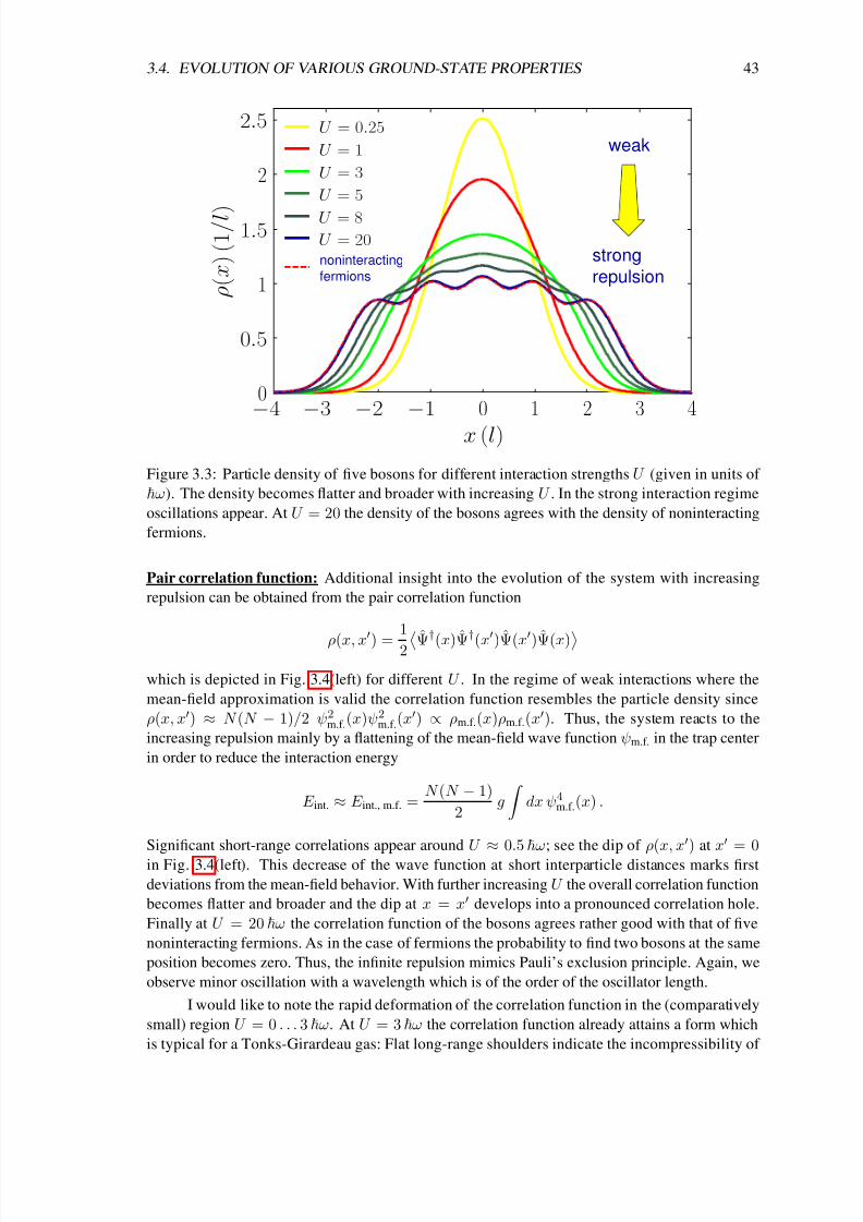
8/3/2019 Frank Deuretzbacher- Spinor Tonks-Girardeau gases and ultracold molecules
http://slidepdf.com/reader/full/frank-deuretzbacher-spinor-tonks-girardeau-gases-and-ultracold-molecules 53/151
3.4. EVOLUTION OF VARIOUS GROUND-STATE PROPERTIES 43
U = 0.25
U = 1
U = 3
U = 5
U = 8U = 20noninteracting
fermions
weak
strong
repulsion
−4 −3 −2 −1 0 1 2 3 40
0.5
1
1.5
2
2.5
x (l)
ρ ( x )
( 1 / l )
Figure 3.3: Particle density of five bosons for different interaction strengths U (given in units of
ω). The density becomes flatter and broader with increasing U . In the strong interaction regime
oscillations appear. At U = 20 the density of the bosons agrees with the density of noninteracting
fermions.
Pair correlation function: Additional insight into the evolution of the system with increasing
repulsion can be obtained from the pair correlation function
ρ(x, x) =
1
2Ψ†(x)Ψ†(x)Ψ(x)Ψ(x)which is depicted in Fig. 3.4(left) for different U . In the regime of weak interactions where the
mean-field approximation is valid the correlation function resembles the particle density since
ρ(x, x) ≈ N (N − 1)/2 ψ2m.f.(x)ψ2
m.f.(x) ∝ ρm.f.(x)ρm.f.(x). Thus, the system reacts to the
increasing repulsion mainly by a flattening of the mean-field wave function ψm.f. in the trap center
in order to reduce the interaction energy
E int. ≈ E int., m.f. =N (N − 1)
2g
dx ψ4
m.f.(x) .
Significant short-range correlations appear around U ≈
0.5 ω; see the dip of ρ(x, x) at x = 0in Fig. 3.4(left). This decrease of the wave function at short interparticle distances marks first
deviations from the mean-field behavior. With further increasing U the overall correlation function
becomes flatter and broader and the dip at x = x develops into a pronounced correlation hole.
Finally at U = 20 ω the correlation function of the bosons agrees rather good with that of five
noninteracting fermions. As in the case of fermions the probability to find two bosons at the same
position becomes zero. Thus, the infinite repulsion mimics Pauli’s exclusion principle. Again, we
observe minor oscillation with a wavelength which is of the order of the oscillator length.
I would like to note the rapid deformation of the correlation function in the (comparatively
small) region U = 0 . . . 3 ω. At U = 3 ω the correlation function already attains a form which
is typical for a Tonks-Girardeau gas: Flat long-range shoulders indicate the incompressibility of
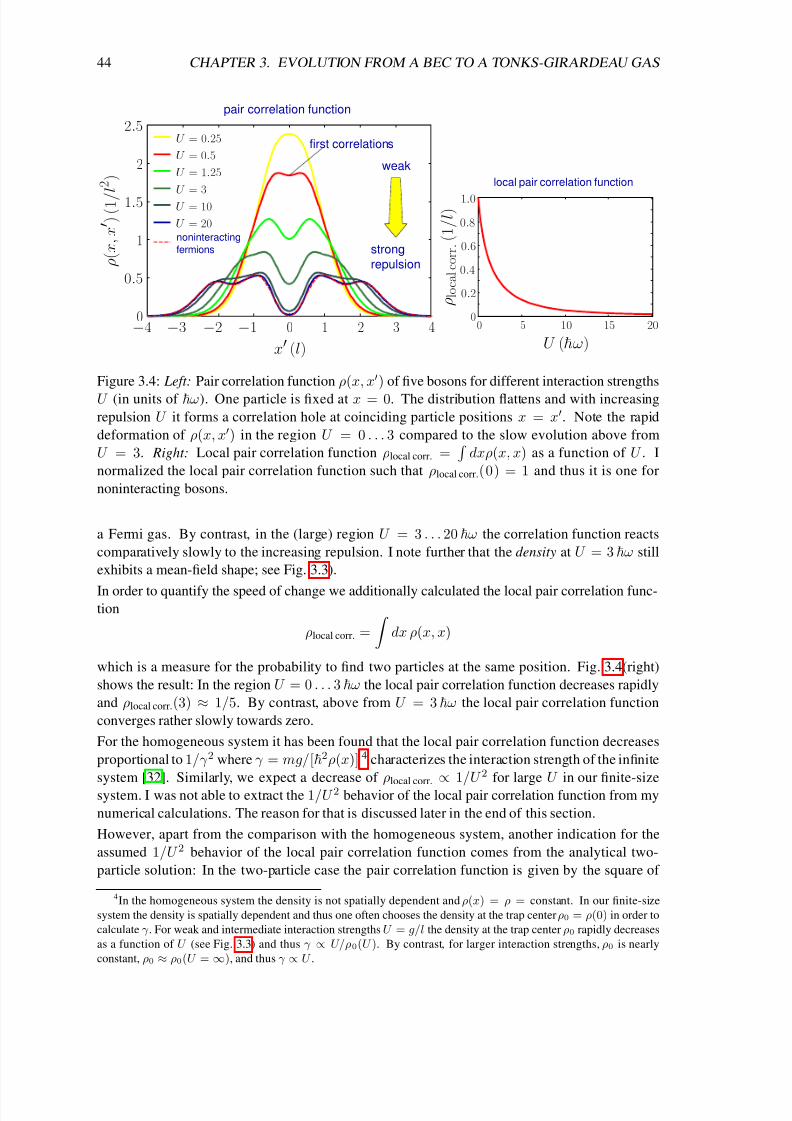
8/3/2019 Frank Deuretzbacher- Spinor Tonks-Girardeau gases and ultracold molecules
http://slidepdf.com/reader/full/frank-deuretzbacher-spinor-tonks-girardeau-gases-and-ultracold-molecules 54/151
44 CHAPTER 3. EVOLUTION FROM A BEC TO A TONKS-GIRARDEAU GAS
−4 −3 −2 −1 0 1 2 3 40
0.5
1
1.5
2
2.5U = 0.25
U = 0.5
U = 1.25
U = 3
U = 10
U = 20noninteracting
fermions
weak
strong
repulsion
x′ (l)
ρ ( x ,
x ′ ) ( 1 /
l 2 )
first correlations
pair correlation function
0 5 10 15 200
0.2
0.4
0.6
ρ l o c a l c o r r .
( 1 / l )
U (hω)
local pair correlation function
0.8
1.0
Figure 3.4: Left: Pair correlation function ρ(x, x) of five bosons for different interaction strengths
U (in units of ω). One particle is fixed at x = 0. The distribution flattens and with increasing
repulsion U it forms a correlation hole at coinciding particle positions x = x. Note the rapid
deformation of ρ(x, x) in the region U = 0 . . . 3 compared to the slow evolution above from
U = 3. Right: Local pair correlation function ρlocal corr. =
dxρ(x, x) as a function of U . I
normalized the local pair correlation function such that ρlocal corr.(0) = 1 and thus it is one for
noninteracting bosons.
a Fermi gas. By contrast, in the (large) region U = 3 . . . 20 ω the correlation function reacts
comparatively slowly to the increasing repulsion. I note further that the density at U = 3 ω still
exhibits a mean-field shape; see Fig. 3.3).
In order to quantify the speed of change we additionally calculated the local pair correlation func-tion
ρlocal corr. =
dx ρ(x, x)
which is a measure for the probability to find two particles at the same position. Fig. 3.4(right)
shows the result: In the region U = 0 . . . 3 ω the local pair correlation function decreases rapidly
and ρlocal corr.(3) ≈ 1/5. By contrast, above from U = 3 ω the local pair correlation function
converges rather slowly towards zero.
For the homogeneous system it has been found that the local pair correlation function decreases
proportional to 1/γ 2 where γ = mg/[2ρ(x)] 4 characterizes the interaction strength of the infinite
system [32]. Similarly, we expect a decrease of ρlocal corr. ∝
1/U 2 for large U in our finite-size
system. I was not able to extract the 1/U 2 behavior of the local pair correlation function from my
numerical calculations. The reason for that is discussed later in the end of this section.
However, apart from the comparison with the homogeneous system, another indication for the
assumed 1/U 2 behavior of the local pair correlation function comes from the analytical two-
particle solution: In the two-particle case the pair correlation function is given by the square of
4In the homogeneous system the density is not spatially dependent and ρ(x) = ρ = constant. In our finite-size
system the density is spatially dependent and thus one often chooses the density at the trap center ρ0 = ρ(0) in order to
calculate γ . For weak and intermediate interaction strengths U = g/l the density at the trap center ρ0 rapidly decreases
as a function of U (see Fig. 3.3) and thus γ ∝ U/ρ0(U ). By contrast, for larger interaction strengths, ρ0 is nearly
constant, ρ0 ≈ ρ0(U = ∞), and thus γ ∝ U .
8/3/2019 Frank Deuretzbacher- Spinor Tonks-Girardeau gases and ultracold molecules
http://slidepdf.com/reader/full/frank-deuretzbacher-spinor-tonks-girardeau-gases-and-ultracold-molecules 55/151
3.4. EVOLUTION OF VARIOUS GROUND-STATE PROPERTIES 45
the wave function, which can be expressed in terms of the center-of-mass and the relative-motion
wave function ψ = ψc.m.(X )ψrel.(x). The local pair correlation function is thus given by
ρlocal corr. =
∞−∞
dx ψ2c.m.(x)
=const.
ψ2rel.(0) .
In Sec. 2.9 we have determined the ground-state wave function of two interacting particles in
a one-dimensional harmonic trap; see Eqs. (2.45), (2.46) and (2.48). We found a close rela-
tion between the one- and the three-dimensional two-particle solution. For example, one ob-
tains the one-dimensional two-particle energy simply by replacing −1/as by gr in the three-
dimensional equation (5.40). In Sec. 5.9 I calculate the lifetime of a three-dimensional molecule;
see Eqs. (5.61), (5.62) and (5.65). The lifetime depends on the probability to find the two con-
stituents of the molecule close to each other and Eq. (5.62) shows that this probability is approx-
imately given by χ2rel.(0)
in three dimensions one often introduces the radial “wave function”
χrel.(r) = r ψrel.(r)
. By replacing −1/as by gr in Eq. (5.65) we thus obtain
ρlocal corr. ∝ ψ2rel.(0) ∝ − 1
gr
1
Ψ(3/4 − E rel./2) − Ψ(1/4 − E rel./2)
(Ψ is the digamma function). In the limit of infinite repulsion (gr = ∞) the energy of the relative
motion converges towards E rel. = 3/2
the total energy is E = N 2/2 = 2 and the center-of-mass
energy is E c.m. = 1/2; all energies are given in units of ω
. A Taylor expansion of the right-hand
side of the above equation around E rel. = 3/2 gives the leading-order result
ρlocal corr. ∝ − 1
gr
E rel. − 3
2
.
Next, we perform a Taylor expansion of the left-hand side of Eq. (2.48) in order to express E rel. asa function of gr and obtain
gr = − 2√π
E rel. − 32
+ higher-order terms . (3.12)
Thus, in the regime of strong repulsion, the local pair correlation function of two particles de-
creases like ρlocal corr. ∝ 1/g2r ∝ 1/U 2. I mention that it has been reported by Y. Hao et al. [35]
that the local correlation function of N 2 particles in a finite-size hard-wall box behaves similar
to the homogeneous case [32]. It is thus highly probable that the local correlation function of
N > 2 particles in a harmonic trap similarly decreases like 1/U 2 for large repulsion.
Different energy contributions: Fig. 3.5 shows the evolution of various contributions to the total
energy with increasing U . The interaction energy (green)
E int. =U
2
dx
Ψ†(x)Ψ†(x)Ψ(x)Ψ(x)
= U
dx ρ(x, x) = U ρlocal corr.
is directly related to the local pair correlation function. In Fig. 3.4(right) we have analyzed the evo-
lution of ρlocal corr. and seen that for small U it decays like 1−f (U ) where f (U ) is some rapidly in-
creasing function. Thus, for small U , the interaction energy grows like E int. ∝ U
1 − f (U ) ∝ U .
For large U , however, it decreases like E int. ∝ 1/U since the local correlation function decreases
like 1/U 2. Somewhere in between, at U ≈ 3 ω for five particles, the interaction energy reaches
its maximum value. It is nearly constant in the region U ≈ 2 . . . 4 ω. We found the maximum

8/3/2019 Frank Deuretzbacher- Spinor Tonks-Girardeau gases and ultracold molecules
http://slidepdf.com/reader/full/frank-deuretzbacher-spinor-tonks-girardeau-gases-and-ultracold-molecules 56/151
46 CHAPTER 3. EVOLUTION FROM A BEC TO A TONKS-GIRARDEAU GAS
0 5 10 15 200
2
4
6
8
10
12
14
U (hω)
e n e r g i e s
( ¯ h ω )
E tot.
E pot.
E kin.
E int.
E kin.
E kin., m.f .
0 1 20.6
1
1.5
Figure 3.5: Evolution of various contributions to the total energy E tot. of five bosons with increas-
ing interaction strength U . The energies evolve towards the accordant energies of noninteracting
fermions. An interesting behavior is shown by the kinetic and the interaction energy. The interac-
tion energy first grows ∝ U , reaches a maximum and then decreases ∝ 1/U (for large U ) since
the short-range correlations decay like 1/U 2. By contrast, the kinetic energy first decreases due
to the flattening and broadening of the overall wave function (“density = wave function” in the
mean-field regime). This effect is overcompensated by the development of short-range correla-
tions which lead to an increase of the kinetic energy above from U ≈ 0.5 ω. As can be seen the
kinetic energy is rather sensitive to these short-range correlations. The minimum of the kinetic
energy thus marks an upper limit of the mean-field regime.
of the interaction energy to be dependent on the number of particles: With increasing number of
particles N its location U max. moves towards larger values of U .
The potential energy (the blue curve in Fig. 3.5) is given by
E pot. =1
2mω2
dx x2
Ψ†(x)Ψ(x)
=ρ(x)
=1
2mω2
x2
It grows continuously from E (0)pot. = N/4 ω = 1.25 ω (for noninteracting bosons) to
E (∞)pot. = N 2/4 ω = 6.25 ω in the Tonks-Girardeau limit. For larger U the increase of the po-tential energy and thus the broadening and flattening of the boson density slows down.
According to the above equation the potential energy is directly related to the width wx = 2 x2
of the N -particle density which has been measured in Ref. [21]. In the Tonks-Girardeau limit
the width of the boson system is given by w(∞)x = 2
N 2/4 l = N l = 5 l. Thus, the mean
interparticle distance dx = wx/N = l. This fact suggests to identify the maxima of the oscillations
of the density with the positions of the individual particles [21] (see Fig. 3.3) since the separation
of the oscsillation maxima is ≈ l. By contrast, in the weakly interacting regime the width is
given by w(0)x = 2
N/2 l =
√2N l and thus the mean interparticle distance is dx = wx/N =
2/N l → 0 for large N , i. e., the bosons sit on top of each other.
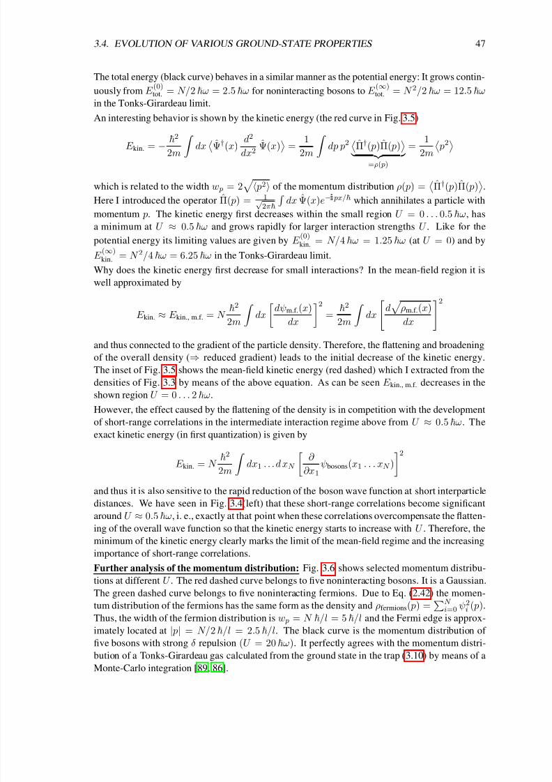
8/3/2019 Frank Deuretzbacher- Spinor Tonks-Girardeau gases and ultracold molecules
http://slidepdf.com/reader/full/frank-deuretzbacher-spinor-tonks-girardeau-gases-and-ultracold-molecules 57/151
3.4. EVOLUTION OF VARIOUS GROUND-STATE PROPERTIES 47
The total energy (black curve) behaves in a similar manner as the potential energy: It grows contin-
uously from E (0)tot. = N/2 ω = 2.5 ω for noninteracting bosons to E
(∞)tot. = N 2/2 ω = 12.5 ω
in the Tonks-Girardeau limit.
An interesting behavior is shown by the kinetic energy (the red curve in Fig. 3.5)
E kin. = − 2
2m dx Ψ†(x) d2
dx2Ψ(x) = 1
2m dp p2 Π†( p)Π( p)
=ρ( p)
= 12m
p2which is related to the width w p = 2
p2 of the momentum distribution ρ( p) =
Π†( p)Π( p)
.
Here I introduced the operator Π( p) = 1√2π
dx Ψ(x)e− i px/ which annihilates a particle with
momentum p. The kinetic energy first decreases within the small region U = 0 . . . 0.5 ω, has
a minimum at U ≈ 0.5 ω and grows rapidly for larger interaction strengths U . Like for the
potential energy its limiting values are given by E (0)kin. = N/4 ω = 1.25 ω (at U = 0) and by
E (∞)kin. = N 2/4 ω = 6.25 ω in the Tonks-Girardeau limit.
Why does the kinetic energy first decrease for small interactions? In the mean-field region it iswell approximated by
E kin. ≈ E kin., m.f. = N 2
2m
dx
dψm.f.(x)
dx
2=
2
2m
dx
d
ρm.f.(x)
dx
2and thus connected to the gradient of the particle density. Therefore, the flattening and broadening
of the overall density (⇒ reduced gradient) leads to the initial decrease of the kinetic energy.
The inset of Fig. 3.5 shows the mean-field kinetic energy (red dashed) which I extracted from the
densities of Fig. 3.3 by means of the above equation. As can be seen E kin., m.f. decreases in the
shown region U = 0 . . . 2 ω.
However, the effect caused by the flattening of the density is in competition with the developmentof short-range correlations in the intermediate interaction regime above from U ≈ 0.5 ω. The
exact kinetic energy (in first quantization) is given by
E kin. = N 2
2m
dx1 . . . d xN
∂
∂x1ψbosons(x1 . . . xN )
2and thus it is also sensitive to the rapid reduction of the boson wave function at short interparticle
distances. We have seen in Fig. 3.4(left) that these short-range correlations become significant
around U ≈ 0.5 ω, i. e., exactly at that point when these correlations overcompensate the flatten-
ing of the overall wave function so that the kinetic energy starts to increase with U . Therefore, the
minimum of the kinetic energy clearly marks the limit of the mean-field regime and the increasing
importance of short-range correlations.
Further analysis of the momentum distribution: Fig. 3.6 shows selected momentum distribu-
tions at different U . The red dashed curve belongs to five noninteracting bosons. It is a Gaussian.
The green dashed curve belongs to five noninteracting fermions. Due to Eq. (2.42) the momen-
tum distribution of the fermions has the same form as the density and ρfermions( p) =N i=0 ψ2
i ( p).
Thus, the width of the fermion distribution is w p = N /l = 5 /l and the Fermi edge is approx-
imately located at | p| = N/2 /l = 2.5 /l. The black curve is the momentum distribution of
five bosons with strong δ repulsion (U = 20 ω). It perfectly agrees with the momentum distri-
bution of a Tonks-Girardeau gas calculated from the ground state in the trap (3.10) by means of a
Monte-Carlo integration [89, 86].
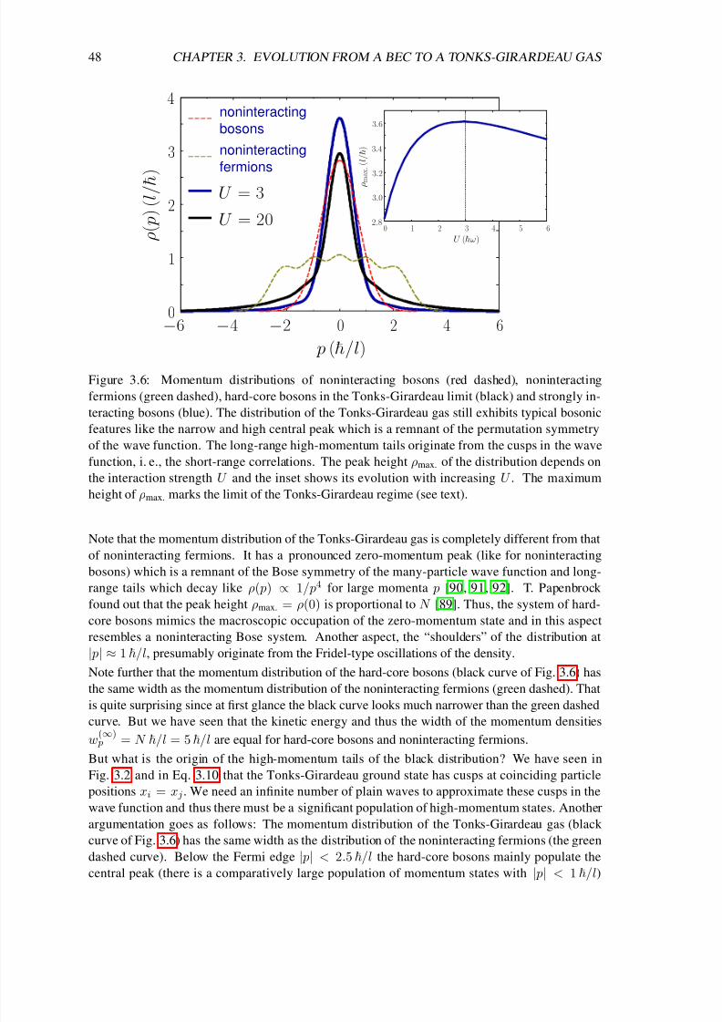
8/3/2019 Frank Deuretzbacher- Spinor Tonks-Girardeau gases and ultracold molecules
http://slidepdf.com/reader/full/frank-deuretzbacher-spinor-tonks-girardeau-gases-and-ultracold-molecules 58/151
48 CHAPTER 3. EVOLUTION FROM A BEC TO A TONKS-GIRARDEAU GAS
0 2 4 6−2−4−6
p (h/l)
0
1
2
3
4
ρ ( p ) ( l / ¯ h
)
noninteracting
bosons
noninteracting
fermions
U = 3
U = 200 1 2 3 4 5 6
2.8
3.0
3.2
3.4
3.6
U (hω)
ρ m
a x .
( l / ¯ h )
Figure 3.6: Momentum distributions of noninteracting bosons (red dashed), noninteracting
fermions (green dashed), hard-core bosons in the Tonks-Girardeau limit (black) and strongly in-
teracting bosons (blue). The distribution of the Tonks-Girardeau gas still exhibits typical bosonic
features like the narrow and high central peak which is a remnant of the permutation symmetry
of the wave function. The long-range high-momentum tails originate from the cusps in the wave
function, i. e., the short-range correlations. The peak height ρmax. of the distribution depends on
the interaction strength U and the inset shows its evolution with increasing U . The maximum
height of ρmax. marks the limit of the Tonks-Girardeau regime (see text).
Note that the momentum distribution of the Tonks-Girardeau gas is completely different from thatof noninteracting fermions. It has a pronounced zero-momentum peak (like for noninteracting
bosons) which is a remnant of the Bose symmetry of the many-particle wave function and long-
range tails which decay like ρ( p) ∝ 1/p4 for large momenta p [90, 91, 92]. T. Papenbrock
found out that the peak height ρmax. = ρ(0) is proportional to N [89]. Thus, the system of hard-
core bosons mimics the macroscopic occupation of the zero-momentum state and in this aspect
resembles a noninteracting Bose system. Another aspect, the “shoulders” of the distribution at
| p| ≈ 1 /l, presumably originate from the Fridel-type oscillations of the density.
Note further that the momentum distribution of the hard-core bosons (black curve of Fig. 3.6) has
the same width as the momentum distribution of the noninteracting fermions (green dashed). That
is quite surprising since at first glance the black curve looks much narrower than the green dashed
curve. But we have seen that the kinetic energy and thus the width of the momentum densities
w(∞) p = N /l = 5 /l are equal for hard-core bosons and noninteracting fermions.
But what is the origin of the high-momentum tails of the black distribution? We have seen in
Fig. 3.2 and in Eq. 3.10 that the Tonks-Girardeau ground state has cusps at coinciding particle
positions xi = x j . We need an infinite number of plain waves to approximate these cusps in the
wave function and thus there must be a significant population of high-momentum states. Another
argumentation goes as follows: The momentum distribution of the Tonks-Girardeau gas (black
curve of Fig. 3.6) has the same width as the distribution of the noninteracting fermions (the green
dashed curve). Below the Fermi edge | p| < 2.5 /l the hard-core bosons mainly populate the
central peak (there is a comparatively large population of momentum states with | p| < 1 /l)

8/3/2019 Frank Deuretzbacher- Spinor Tonks-Girardeau gases and ultracold molecules
http://slidepdf.com/reader/full/frank-deuretzbacher-spinor-tonks-girardeau-gases-and-ultracold-molecules 59/151
3.4. EVOLUTION OF VARIOUS GROUND-STATE PROPERTIES 49
and thus there must be a sufficiently strong population of high-momentum states above the Fermi
edge in order to achieve the same width as for the noninteracting fermion distribution. I note that
the high-momentum tails of the distribution are mainly responsible for the increase of the kinetic
energy (or width of the momentum distribution) above from U = 0.5 ω since the momentum
density is weighted with p2 in the expectation value
p2
= dp p2ρ( p).
Another interesting aspect concerns the evolution of the height of the central peak. The blue curve
in Fig. 3.6 is the momentum distribution of the bosons at U = 3 ω. As can be seen the peak height
is larger than for noninteracting and hard-core bosons. The inset of Fig. 3.6 shows the evolution
of the peak height which is largest around U = 3 ω. We found the location of this maximum
to be independent of the number of particles. The height of the central peak at its maximum is
approx. 30% larger than at small interaction strength (U ≈ 0) and about 20% larger than at large
interactions (U = 20 ω). This contrast increases with increasing particle number.
What are the two competing mechanisms which cause this behavior? The same effects which
are responsible for the minimum of the kinetic energy at U = 0.5 ω! Due to the flattening
and broadening of the particle density the central peak of the momentum distribution becomes
narrower and higher. On the other hand, the formation of short-range correlations atx = xleads to an increasing population of high momentum states. This effect dominates above U =
3 ω, when the growth of the density width slows down thus leading to a redistribution from
low- towards high-momentum states. At this point the height of the central peak has reached
its maximum. This coincides with the transition behavior visible in the correlation function (see
Fig. 3.4). Therefore, the maximum of the peak height marks the transition towards the Tonks-
Girardeau regime.
Discrimination between the interaction regimes: Let me give a short summary of the most im-
portant results presented so far. Caused by the increasing repulsive interaction the overall boson
wave function flattens, broadens and forms short-range correlations, which prevent the bosons
from sitting on top of each other. Three interaction regimes can be distinguished: the mean-field
and the Tonks-Girardeau regime and an intermediate regime in between. We found the momen-tum distribution of the boson system to be a reliable indicator for transitions between those three
regimes. Its width is extremely sensitive to the formation of short-range correlations and thus the
minimum width at U = 0.5 ω clearly marks the limit of the mean-field regime. By contrast,
the maximum of the peak height at U = 3 ω marks the transition towards the Tonks-Girardeau
regime. The evolution of both features of the momentum distribution is caused by two competing
mechanisms, namely, the broadening and flattening of the overall wave function on the one hand
and the formation of short-range correlations on the other hand.
Occupation of the single-particle states: I finally discuss the occupation number distribution
ni = a†iai of the harmonic oscillator states which is shown in Fig. 3.7. With increasing
interaction strength U the bosons leave the ground state and occupy the excited states of the har-
monic trap. At U = 20 ω the distribution is similar to the distribution shown in [86] for U = ∞.However, we observe a stronger population of single-particle states with even parity compared
to those with odd parity. This effect is most pronounced in mean-field calculations where oc-
cupations of odd parity orbitals are absent. Why? The mean-field ground state has even parity
(see Fig 3.1), i. e., it is symmetric under horizontal flips, and thus the coefficients of the expansion
ψm.f.(x) =i ciψi(x) with ci =
dx ψi(x)ψm.f.(x) are zero for states with odd parity (i. e. states
with i = 1, 3, 5, . . .). The comparatively stronger occupation of single-particle states with even
parity can therefore be interpreted as another remnant of the mean-field regime. 5 M. Girardeau
5Despite the even parity of the many-particle ground state, there is nevertheless a significant population of odd-
parity single-particle wave functions in that state. That is due to the fact that a Fock state |N 0, N 1, N 2, . . .`
where N i

8/3/2019 Frank Deuretzbacher- Spinor Tonks-Girardeau gases and ultracold molecules
http://slidepdf.com/reader/full/frank-deuretzbacher-spinor-tonks-girardeau-gases-and-ultracold-molecules 60/151
50 CHAPTER 3. EVOLUTION FROM A BEC TO A TONKS-GIRARDEAU GAS
1 2 3 4 5 6 7 8
i
0
0
1
2
3
4
5
n i
1 2 3 4 5 6 7 8
i
0
0
1
2
3
4
5
n i
1 2 3 4 5 6 7 8
i
0
0
1
2
3
4
5
n i
1 2 3 4 5 6 7 8
i
0
0
1
2
3
4
5
n i
U = 1 hω U = 3 hω
U = 6 hωU = 20 hω
noninteracting
fermions
Figure 3.7: Occupation number distribution of the harmonic-oscillator eigenstates of five bosons
for different interaction strengths U . With increasing interaction strength U the bosons leave the
ground state and occupy excited states. Single-particle states with even parity are comparatively
stronger populated than those with odd parity. Note the large population of the ground state in
the Tonks-Girardeau limit
given by n0 =√
N 1
due to the permutation symmetry of the
wave function and the significant population of high-energy states above the Fermi edge due to
the cusps in the wave function at coinciding particle positions xi = x j .
et al. [86] and T. Papenbrock [89] found out that the population of the lowest natural orbital 6 is
√N . My calculations are in agreement with a population of the harmonic-oscillator ground stateof n0 =
√N . Again, one sees in Fig. 3.7(bottom right) that the population of the harmonic-
oscillator states is completely different for hard-core bosons and noninteracting fermions. The
occupation of the harmonic-oscillator ground state is much larger than 1, due to the permutation
symmetry of the wave function, and there is a significant population of high-energy states above
the Fermi edge due to the cusps in the wave function at coinciding particle positions xi = x j .
Remarks on the accuracy of my calculations: I already discussed in Sec. 2.9, when I compared
the resultant wave function of my numerical diagonalization with the exact analytical two-particle
wave function (see Fig. 2.6), that the cusps in the wave function at xi = x j are not resolved by
our numerical approach although the overlap between both solutions is very close to one. That is
no wonder since the singular δ potential does not match up very good with the smooth harmonic-
oscillator states (leading to convergence problems similar to Gibbs phenomenon). I guess thatthe convergence would be significantly improved if the δ potential would be smeared out into a
Gaussian of finite width. However, I think that I extensively proved in the previous discussion and
in Sec. 2.9 that my calculations in general converged satisfactory. That is in agreement with the
commonly known statement that the usual δ potential is unproblematic in one dimension.
Anyway, some results have been more accurately calculated using alternative methods, namely,
is the occupation number of the ith oscillator eigenstate ψi
´with an even-numbered population of odd-parity oscillator
functions, N 1 + N 3 + N 5 + . . . = even, still has even parity in total; see Eq. (2.31).6The “natural orbitals” are defined in Ref. [86] as the eigenfunctions of the reduced single-particle density matrix
of the Tonks-Girardeau ground state.
8/3/2019 Frank Deuretzbacher- Spinor Tonks-Girardeau gases and ultracold molecules
http://slidepdf.com/reader/full/frank-deuretzbacher-spinor-tonks-girardeau-gases-and-ultracold-molecules 61/151
3.5. EXCITATION SPECTRUM 51
all the properties which crucially depend on the shape of the wave function at xi = x j . To give
some examples: The correlation functions of Fig. 3.4(left) have cusps at x = x for all nonzero
and finite 0 < U < ∞ not for U = 0 and not for U = ∞ !
as one can derive quickly from
the exact two-particle solution of Sec. 2.9 and as has been shown for the infinite homogeneous
system [37]. Secondly, I cannot extract a 1/U 2 decay of the local pair correlation function for
large U similar to the results of Ref. [32] but I also obtain the same qualitative behavior; as canbe seen in Fig. 3.4(right). The same is true for the 1/p4 decay of the high-momentum tails of the
distributions of Fig. 3.6.
I have performed calculations with different basis lengths in order to estimate the maximum de-
viations of the energies of Fig. 3.5 from its “true” values and in order to insure myself that my
main statements concerning the momentum distribution are correct. From these calculations I ob-
tained, e. g., the following limiting values of the energies at U = 20 ω: E tot., limit = 11.78 ω,
E pot., limit = 5.69 ω, E kin., limit = 5.07 ω and E int., limit = 1.02 ω while the values of Fig. 3.5 are
given by E tot., fig. = 12.32 ω, E pot., fig. = 6.13 ω, E kin., fig. = 5.10 ω and E int., fig. = 1.09 ω.
Thus, the deviation between these energies is 4.6% for the total energy, 7.7% for the potential
energy, 0.6% for the kinetic energy and 7.2% for the interaction energy. Moreover, in order ensure
myself that the limiting energies are in good agreement with the true energies, I cross-checked the
method by means of the exact analytical two-particle solution from which the true energies can be
determined with high precision.
More importantly I am confident that my statement holds true that the three interaction regimes
can be distinguished by means of the momentum distribution since the underlying two compet-
ing mechanisms – the flattening and broadening of the overall wave function and the formation
of short-range correlations – persist independent of the precise shape of the wave function at
xi = x j . Again, I determined the minimum of the width and the maximum of the peak height of
the momentum distribution independently from the exact analytical two-particle solution in order
to cross-check my method. I cannot exclude that the limits of the mean-field regime at U ≈ 0.5 ω
and of the Tonks-Girardeau regime at U ≈ 3
ω weakly depend on the number of particles N .However, for 2 − 7 particles I could not see a dependency on the number of particles. Thus, I
am sure that these values are at least valid for small particle numbers, but, to my knowledge, so
far the quasi-one-dimensional strongly interacting regime has not been entered with large particle
numbers (N ∼ 15 − 18 in the experiment of Ref. [22] and ∼ 54 in Ref. [21]).
3.5 Excitation spectrum
I close my discussion with a study of the excitation spectrum. First, a few remarks about the
energy spectrum in the two limiting regimes of zero and infinite δ repulsion: Both spectra agree
apart from the different ground-state energy. For noninteracting bosons the ground-state energy is
E (0)g = N/2 ω and the level spacing is ∆E = 1 ω. The degeneracy of the lowest levels is given
by
degeneracy = 1, 1, 2, 3, 5, 7, 10, 13, . . . (3.13)
for the ground state and the lowest seven excited states of five bosons since the lowest occupation
number states are given by
|5 → |4, 1 → |3, 2, |4, 0, 1 → |2, 3, |3, 1, 1, |4, 0, 0, 1 → . . .here the ith position of a number state belongs to the (i − 1)th single-particle state
. Since hard-
core bosons behave like noninteracting fermions the ground-state energy is E (∞)g = N 2/2 ω and
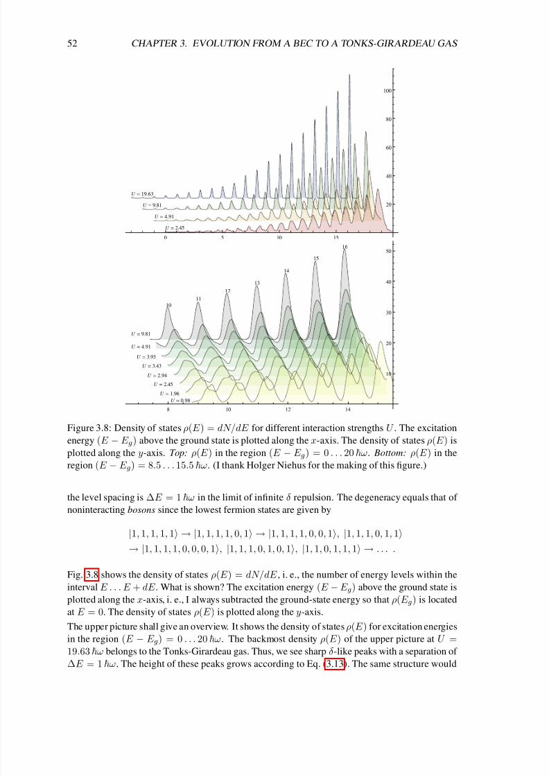
8/3/2019 Frank Deuretzbacher- Spinor Tonks-Girardeau gases and ultracold molecules
http://slidepdf.com/reader/full/frank-deuretzbacher-spinor-tonks-girardeau-gases-and-ultracold-molecules 62/151
52 CHAPTER 3. EVOLUTION FROM A BEC TO A TONKS-GIRARDEAU GAS
U 19.63
U 9.81
U 4.91
U 2.45
0 5 10 15
20
40
60
80
100
U 0.98
U 1.96
U 2.45
U 2.94
U 3.43
U 3.93
U 4.91
U 9.81
10
11
12
13
14
15
16
8 10 12 14
10
20
30
40
50
Figure 3.8: Density of states ρ(E ) = dN/dE for different interaction strengths U . The excitation
energy (E − E g) above the ground state is plotted along the x-axis. The density of states ρ(E ) is
plotted along the y-axis. Top: ρ(E ) in the region (E − E g) = 0 . . . 20 ω. Bottom: ρ(E ) in the
region (E − E g) = 8.5 . . . 15.5 ω. (I thank Holger Niehus for the making of this figure.)
the level spacing is ∆E = 1 ω in the limit of infinite δ repulsion. The degeneracy equals that of
noninteracting bosons since the lowest fermion states are given by
|1, 1, 1, 1, 1
→ |1, 1, 1, 1, 0, 1
→ |1, 1, 1, 1, 0, 0, 1
,
|1, 1, 1, 0, 1, 1
→ |1, 1, 1, 1, 0, 0, 0, 1, |1, 1, 1, 0, 1, 0, 1, |1, 1, 0, 1, 1, 1 → . . . .
Fig. 3.8 shows the density of states ρ(E ) = dN/dE , i. e., the number of energy levels within the
interval E . . . E + dE . What is shown? The excitation energy (E − E g) above the ground state is
plotted along the x-axis, i. e., I always subtracted the ground-state energy so that ρ(E g) is located
at E = 0. The density of states ρ(E ) is plotted along the y-axis.
The upper picture shall give an overview. It shows the density of states ρ(E ) for excitation energies
in the region (E − E g) = 0 . . . 20 ω. The backmost density ρ(E ) of the upper picture at U =19.63 ω belongs to the Tonks-Girardeau gas. Thus, we see sharp δ-like peaks with a separation of
∆E = 1 ω. The height of these peaks grows according to Eq. (3.13). The same structure would

8/3/2019 Frank Deuretzbacher- Spinor Tonks-Girardeau gases and ultracold molecules
http://slidepdf.com/reader/full/frank-deuretzbacher-spinor-tonks-girardeau-gases-and-ultracold-molecules 63/151
3.5. EXCITATION SPECTRUM 53
be observed for noninteracting bosons at U = 0. In between these limiting regimes we observe
a substantial broadening of the peaks but the center of these peaks is still located at 0, 1, 2, . . . .The height of the peaks decreases due to the broadening of the peaks, since they consist of the
same number of states. I observe the largest broadening of the peaks for an interaction strength of
U = 2.45 ω. Below and above this point the peaks become narrower and higher when moving
from U = 2.45 ω towards U = 0 or in the other direction from U = 2.45 ω towards U = ∞.This can be clearly seen in the upper picture of Fig. 3.8: The broadest and flattest peaks belong
to the density of states at U = 2.45 ω and with increasing U the peaks become narrower and
higher; compare with the density of states at U = 4.91, 9.81 and 19.63 ω.
The lower picture of Fig. 3.8 shows the density of states in the region (E − E g) ≈ 8.5 . . . 15.5 ω,
i. e., the 10 − 16th excited level. Here I show more densities ρ(E ) around the critical interaction
strength U ≈ 2.45 ω. One sees in the bottom picture of Fig. 3.8 that the peak height is lowest for
U ≈ 2.45 ω and that it is substantially higher for U = 0.98 or 9.81 ω.
To summarize the result: For zero (U = 0) and infinite δ repulsion (U = ∞) we observe the same
energy structure and each energy level is degenerate according to Eq. ( 3.13). Each multiplet has
a finite widthwE
for nonzero and finite interaction strengths0 < U < ∞
. The widthwE
of the
multiplets is largest for U ≈ 2.5 ω. This critical point coincides quite well with the limit of the
Tonks-Girardeau regime at U ≈ 3 ω which we have determined in the previous section from the
ground-state behavior. However, despite the broadening of the energy levels (i. e., the broadening
of the δ-like peaks) for intermediate repulsions the energy levels are clearly separated from each
other for all interaction strengths and the spacing between the levels is always ∆E = 1 ω.

8/3/2019 Frank Deuretzbacher- Spinor Tonks-Girardeau gases and ultracold molecules
http://slidepdf.com/reader/full/frank-deuretzbacher-spinor-tonks-girardeau-gases-and-ultracold-molecules 64/151
Chapter 4
The spinor Tonks-Girardeau gas
The main results of this chapter have been published in Ref. [4].
Subject of this chapter is a study of spinful one-dimensional bosons with strong δ repulsion. In thefirst section 4.1, I will derive an exact analytical solution for infinite δ repulsion. This solution is
not only valid for spin-1 bosons but for particles with arbitrary permutation symmetry (bosons and
fermions) and arbitrary spin. Moreover, it is applicable to Fermi-Fermi and Bose-Bose mixtures.
An analytical formula for the spin densities will be given in Sec. 4.3. Derivation of that formula has
been given to me by Klaus Fredenhagen [93]. I show the derivation of that formula in appendix A.
In Sec. 4.4 I will present selected momentum distributions of the degenerate ground states. These
distributions have been obtained from the numerical calculations. In Sec. 4.2 I will finally discuss
the structure of the ground-state multiplet for large but finite repulsion. Here I will compare
the numerical results to the exact limiting solutions. Similar results have been found recently for
mixtures of two different atomic species [69], two-level atoms [70, 71] and spin-1/2 fermions[94].
4.1 Analytical solution for hard-core particles with spin
We are searching for the solution of quasi-one-dimensional spin-1 bosons with infinite δ repulsion
at zero magnetic field. The Hamiltonian of such a system is given by
H =N i=1
−
2
2m
∂ 2
∂x2i
+1
2mω2x2
i
1
⊗N +i<j
δ(xi − x j)
g0 1
⊗N + $ $ $ $
g2 f i · f j
. (4.1)
See Sec. 3.1 for the derivation of a quasi-one-dimensional Hamiltonian from Eq. (2.5).
Here, g0
is infinite and the value of g2 is arbitrary. The spin-dependent interaction can be neglected sincethe wave function is already zero at equal particle positions xi = x j . Thus, there is no coupling
between the spin and the motional degrees of freedom in the limit of infinite repulsion, i. e., the
Hamiltonian is diagonal in spin space. It follows that we can restrict ourselves to the solution of
the spinless Hamiltonian
H =N i=1
−
2
2m
∂ 2
∂x2i
+1
2mω2x2
i
+ g0
i<j
δ(xi − x j) , (4.2)
since we obtain a valid solution of the spinful Hamiltonian (4.1) simply by multiplying an
eigenfunction of the spinless Hamiltonian (4.2) with an arbitrary N -particle spin function. If,
54

8/3/2019 Frank Deuretzbacher- Spinor Tonks-Girardeau gases and ultracold molecules
http://slidepdf.com/reader/full/frank-deuretzbacher-spinor-tonks-girardeau-gases-and-ultracold-molecules 65/151
4.1. ANALYTICAL SOLUTION FOR HARD-CORE PARTICLES WITH SPIN 55
e. g., ψ(x1, x2, . . . , xN ) is an eigenfunction of (4.2) then all the 3N spinful wave functions
ψ(x1, x2, . . . , xN )|m1, m2, . . . , mN with m1, m2, . . . , mN = 0, ±1 are automatically eigen-
functions of the Hamiltonian (4.1).
So what is the difference to the spinless problem of section 3.3? In the case of spinless bosons the
wave function has to be symmetric under any permutation π of the particle coordinates:
ψ(x1, x2, . . . , xN ) = ψ
xπ(1), xπ(2), . . . , xπ(N )
.
Here, by contrast, the wave function has to be symmetric under any permutation of the combined
space-spin indices (xi, mi) and it follows that all the single components of the vector-valued wave
function are interrelated to each other by the prescription
ψm1,...,mN (x1, . . . , xN ) = ψmπ(1),...,mπ(N )
xπ(1), . . . , xπ(N )
.
This relation holds true for any permutation π if the vector-valued wave function |ψ describes
spinful bosons. That is a big difference to the spinless case, since now it is not excluded that the
motional wave functions of the individual spin components ψm1,m2,...,mN (x1, x2, . . . , xN ) can benonsymmetric, i. e., it could be that
ψm1,...,mN (x1, . . . , xN ) = ψm1,...,mN
xπ(1), . . . , xπ(N )
!
Consider, e. g., two bosons with spin f = 1. Their two-particle (nine-component vector-valued)
wave function is given by
ψ(x1, x2) =
m1,m2=−1,0,1
ψm1,m2(x1, x2)|m1, m2 .
This wave function shall be symmetric under the exchange of the space-spin indices of the first
and the second particle (x1, m1) ↔ (x2, m2) since we are considering bosons and it follows forall of its components
ψm1,m2(x1, x2) = ψm2,m1(x2, x1) .
So, it follows that the wave-function components ψ1,1(x1, x2), ψ0,0(x1, x2) and ψ−1,−1(x1, x2)are symmetric under the exchange of the coordinates x1 and x2. All the other wave-function com-
ponents ψ1,0(x1, x2), ψ1,−1(x1, x2), ψ0,1(x1, x2), ψ0,−1(x1, x2), ψ−1,1(x1, x2) and ψ−1,0(x1, x2)can, however, be nonsymmetric. They are mutually related to each other, e. g., by the prescrip-
tion ψ1,0(x1, x2) = ψ0,1(x2, x1) but both wave-function components can be nonsymmetric un-
der the exchange of x1 and x2, i. e., it is not excluded that ψ1,0(x1, x2) = ψ1,0(x2, x1) and
ψ0,1(x1, x2) = ψ0,1(x2, x1).
In order to find the bosonic eigenfunctions of the spinful Hamiltonian (4.1), we therefore constructin a first step all the eigenfunctions of the spinless Hamiltonian (4.2). These solutions do not need
to be permutationally symmetric or antisymmetric. Thus, they describe distinguishable spinless
particles with infinite δ repulsion. Similar to Eq. (3.6) the following set of equations and boundary
conditions has to be solved:
ψ solves
N i=1
−
2
2m
∂ 2
∂x2i
+1
2mω2x2
i
ψ = Eψ in RN \ xi = x j (4.3a)
ψ(x1, x2, . . . , xN ) = 0 on the surface xi = x j (4.3b)
ψ does not need to obey any exchange symmetry! (4.3c)
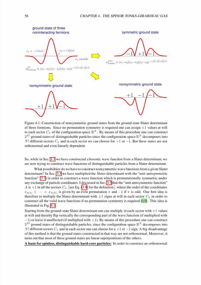
8/3/2019 Frank Deuretzbacher- Spinor Tonks-Girardeau gases and ultracold molecules
http://slidepdf.com/reader/full/frank-deuretzbacher-spinor-tonks-girardeau-gases-and-ultracold-molecules 66/151
56 CHAPTER 4. THE SPINOR TONKS-GIRARDEAU GAS
ground state of three
noninteracting fermions
nonsymmetric ground state
ψ(0)fermions ∝ (x1−x2)(x1−x3)(x2−x3)e−(x2
1+x22+x2
3)/2
symmetric ground state
+1 −1+1
−1+1−1
ψ(∞)bosons ∝ |x1−x2||x1−x3||x2−x3|e
−(x21+x2
2+x23)/2
nonsymmetric ground state
+1 −1
x1 = −1 fixed x2 = 1 fixed
x3 variable
−1
Figure 4.1: Construction of nonsymmetric ground states from the ground-state Slater determinant
of three fermions. Since no permutation symmetry is required one can assign ±1 values at will
to each sector C π of the configuration space RN . By means of this procedure one can construct
2N ! ground states of distinguishable particles since the configuration space RN decomposes into
N ! different sectors C π and in each sector we can choose for +1 or −1. But these states are not
orthonormal and even linearly dependent.
So, while in Sec. 3.3 we have constructed a bosonic wave function from a Slater determinant, we
are now trying to construct wave functions of distinguishable particles from a Slater determinant.
What possibilities do we have to construct nonsymmetric wave functions from a given Slater
determinant? In Sec. 3.3 we have multiplied the Slater determinant with the “unit antisymmetric
function” (3.7) in order to construct a wave function which is permutationally symmetric under
any exchange of particle coordinates. I discussed in Sec. 3.3 that the “unit antisymmetric function”
A is +1 in all the sectors C π
see Eq. (3.9) for the definition
, where the order of the coordinates
xπ(1) < · · · < xπ(N ) is given by an even permutation π and −1 if π is odd. One first idea is
therefore to multiply the Slater determinant with
±1 signs at will in each sector C π in order to
construct all the valid wave functions if no permutation symmetry is required [ 69]. This idea is
illustrated in Fig. 4.1:
Starting from the ground-state Slater determinant one can multiply in each sector with ±1 values
at will and thereby flip vertically the corresponding part of the wave function (if multiplied with
−1) or leave it unaffected (if multiplied with +1). By means of this procedure one can construct
2N ! ground states of distinguishable particles, since the configuration space RN decomposes into
N ! different sectors C π and in each sector one can choose for a +1 or −1 sign. A big disadvantage
of this method is that the ground states constructed in that way are not orthonormal. Moreover, it
turns out that most of these ground states are linear superpositions of the others.
A basis for spinless, distinguishable hard-core particles: In order to construct an orthonormal
8/3/2019 Frank Deuretzbacher- Spinor Tonks-Girardeau gases and ultracold molecules
http://slidepdf.com/reader/full/frank-deuretzbacher-spinor-tonks-girardeau-gases-and-ultracold-molecules 67/151
4.1. ANALYTICAL SOLUTION FOR HARD-CORE PARTICLES WITH SPIN 57
basis of the space of nonsymmetric ground states we try the ansatz:
x1, . . . , xN |π ≡√
N ! A ψ(0)fermion gr. if xπ(1) < · · · < xπ(N )
0 otherwise ,(4.4)
i. e., we take the boson ground state ψ(∞)boson gr. = A ψ
(0)fermion gr., restrict that wave function to the
region C π and multiply with the prefactor√
N ! in order to normalize it. These states are orthog-
onal by construction, since each state ψπ(x1, . . . , xN ) = x1, . . . , xN |π is nonzero only in the
corresponding region C π and there is no overlap between different regions C π and C π . Further,
they are normalized, since
π|π = N !
xπ(1)<...<xπ(N )
dx1 . . . d xN & & A2
ψ(0)fermion gr.(x1, . . . , xN )
2= RN
dx1 . . . d xN ψ(0)fermion gr.(x1, . . . , xN )
2= 1 .
In the second step of the calculation I extended the integration from the region C π to the whole
configuration space RN and I used the symmetry of the square of the Fermi ground stateψ(0)fermion gr.
xπ(1), . . . , xπ(N )
2=
ψ(0)fermion gr.(x1, . . . , xN )
2.
I note that all the wave functions (4.4) have the same ground-state energy E g = N 2/2 ω so
that the space of ground states is N ! times degenerate
there are N ! different permutations of N different items and thus N ! disjoint regions C π
. Moreover, the result (4.4) for the ground state
can be generalized to an arbitrary Slater determinant ψ(0)ith fermion st.(x1, x2, . . . , xN ) and is thus also
valid for the excited states, i. e., one can construct N ! nonsymmetric orthonormal states from the
ith Slater determinant of the noninteracting fermions. Correspondingly, the energies of these statesare given by the energy of that Slater determinant E i = E
ψ(0)ith fermion st.
.
The wave functions (4.4) look a bit strange but they are a valid solution of the set of equations (4.3):
Each wave function ψπ(x1, . . . , xN ) = x1, . . . , xN |π is a solution of the Schrodinger equation
(4.3a) in the region C π, since it is proportional to the ground state of noninteracting fermions.
Outside the region C π it is zero and thus trivially solves (4.3a). Moreover, ψπ(x1, . . . , xN ) is zero
on the surface xi = x j as required by the boundary condition (4.3b).
Let us look at the two-particle ground states of Fig. 4.2 to become more familiar with these
solutions: As discussed in Sec. 3.3 the fermion and boson ground states are given by
ψ(0)fermion gr. ∝ (x1 − x2) e−(x21+x
22)/2 and ψ
(∞)boson gr. ∝ |x1 − x2| e−(x21+x
22)/2 ,
respectively. Since there are no symmetry restrictions we can superimpose both solutions. The
sum of both solutions is the nonsymmetric basis state
ψ(0)fermion gr. + ψ
(∞)boson gr. = |π12 =
√2! ψ
(∞)boson gr. if x2 < x1
0 if x1 < x2 ,
where π12(1) = 2, π12(2) = 1 exchanges the two indices. The difference of both solutions results
in the nonsymmetric basis state
ψ(0)fermion gr. − ψ
(∞)boson gr. = |id =
√2! ψ
(∞)boson gr. if x1 < x2
0 if x2 < x1 ,

8/3/2019 Frank Deuretzbacher- Spinor Tonks-Girardeau gases and ultracold molecules
http://slidepdf.com/reader/full/frank-deuretzbacher-spinor-tonks-girardeau-gases-and-ultracold-molecules 68/151
58 CHAPTER 4. THE SPINOR TONKS-GIRARDEAU GAS
2 fermions 2 bosons
2 distinguishable particles
ψ(0)fermion gr.
∝(x1
−x2)e−(x2
1+x22)/2 ψ
(∞)boson gr.
∝ |x1
−x2
|e−(x2
1+x22)/2
x1 = 0 fixed x1 = 0 fixed x1 = 0 fixed
x2 variable
x2 variable x2 variable
√2!ψ
(∞)boson gr.0
|id
√2!ψ
(∞)boson gr. 0
|π12
Figure 4.2: Construction of nonsymmetric spinless wave functions of two distinguishable parti-
cles. The states |π12 and |id form a basis of the twofold degenerate space of ground states. The
nonsymmetric basis states are superpositions of the fermion and the boson ground states.
where id(1) = 1, id(2) = 2 is the identical permutation. Both solutions describe distinguishable
particles since they are nonsymmetric. There are no further basis states since the configuration
space R2 can only be decomposed into the two disjoint regions C id =
(x1, x2) ∈ R2, x1 < x2
and C π12 =
(x1, x2) ∈ R
2, x2 < x1
. Thus the space of ground states is twofold degenerate.
Analytical solution for spinful hard-core particles: Actually, the main work has already been
done, namely, to construct nonsymmetric motional wave functions which account for the infinite
δ repulsion. The wave functions (4.4) for distinguishable particles solve the Hamiltonian (4.2). As
discussed before, we need only to multiply one of the spinless solutions with an arbitrary many-
particle spin function |χ e.g. |χ = |m1, m2, . . . , mN or any superposition of these states
in
order to obtain a (spinful) solution of the Hamiltonian (4.1):ψ(∞)spinful particle gr.
= |π ⊗ |χ .
However, these solutions are nonsymmetric and thus describe distinguishable hard-core particles
with spin. In order to describe bosons one has to symmetrize this nonsymmetric wave function:
ψ(∞)spinful boson gr. =
√N ! P S |π ⊗ |χ . (4.5)
Here, I introduced the projection into the subspace of the permutationally symmetric wave func-
tions
P S =1
N !
πS N
U (π) .
S N is the symmetric group, i. e., the set of all bijective functions from 1, 2, . . . , N to
1, 2, . . . , N , or, in other words, the set of all permutations of the numbers 1, 2, . . . , N . U (π) is
the permutation operator which exchanges particle indices according to the permutation
π =
1 2 . . . N
π(1) π(2) . . . π(N )

8/3/2019 Frank Deuretzbacher- Spinor Tonks-Girardeau gases and ultracold molecules
http://slidepdf.com/reader/full/frank-deuretzbacher-spinor-tonks-girardeau-gases-and-ultracold-molecules 69/151
4.1. ANALYTICAL SOLUTION FOR HARD-CORE PARTICLES WITH SPIN 59
with π(i) ∈ 1, 2, . . . , N and π(i) = π( j). U (π) acts as follows on an arbitrary stateα1, α2, . . . , αN
where αi are some quantum numbers of the same kind
[95]:
U (π)
α1, α2, . . . , αN
= U (π)
α1
1⊗
α2
2⊗ . . . ⊗
αN
N
= α1π(1) ⊗ α2π(2) ⊗. . .
⊗ αN π(N )=απ−1(1)
1⊗ απ−1(2)
2⊗ . . . ⊗ απ−1(N )
N
=απ−1(1), απ−1(2), . . . , απ−1(N )
. (4.6)
Since U (π) is unitary [95]
U †(π) = U −1(π) = U
π−1
it follows thatα1, α2, . . . , αN
U (π) =
U
π−1α1, α2, . . . , αN
†=
απ(1), απ(2), . . . , απ(N )
.
Thus, the amplitude of some wave function U (π)|ψ at position x1, x2, . . . , xN is given by [95]x1, x2, . . . , xN
U (π)ψ =
xπ(1), xπ(2), . . . , xπ(N )
ψ = ψ
xπ(1), xπ(2), . . . , xπ(N )
. (4.7)
Using the above relations (4.6), (4.7) and Eq. (4.4) we obtain the following formula for the action
of the permutation operator U (π) on the ground state |π ⊗ |m1, m2, . . . , mN :
U (π)π⊗ m1, m2, . . . , mN
=π π
⊗ mπ−1(1), mπ−1(2), . . . , mπ−1(N )
(4.8)
where π π is the composition of the permutations π and π. Now we have collected all the
calculation rules which we need to understand Eq. (4.5).
Since one can choose between N ! different orbital wave functions |π and 3
N
different spin func-tions |m1, m2, . . . , mN with mi = −1, 0, 1, one might think that the ground state of the hard-
core bosons is N ! × 3N times degenerate. But that is not the case. Instead, it turns out that most
of the states constructed by the prescription (4.5) are linearly dependent. If we choose, e. g., the
product wave function |π⊗ |1, 1, . . . , 1 then we obtain by means of Eqs. (4.5) and (4.8) the boson
ground state ψ(∞)spinful boson gr.
=
1√N !
πS N
|π π ⊗ |1, 1, . . . , 1 .
Using Eq. (4.4) we see that
πS N |π
π
= ππ−1S N π = πS N π =
√N ! A ψ
(0)fermion gr. =
√N ! ψ
(∞)boson gr. .
In the first step I substituted π = π π ⇒ π π−1 = π π π−1 ⇒ π π−1 = π and
in the second step I changed the order of the summation. In Eq. (4.4) we have decomposed the
(spinless) wave function A ψ(0)fermion gr. along the boundaries of the sectors C π in order to obtain a
basis for spinless distinguishable particles. Thus, we get back the original state A ψ(0)fermion gr. if we
sum up all the componentsπS N
|π. In the last step I used Girardeau’s Fermi-Bose map (3.8)
for spinless particles. We finally obtain
ψ(∞)spinful boson gr.
= ψ(∞)boson gr. ⊗ |1, 1, . . . , 1 (4.9)
8/3/2019 Frank Deuretzbacher- Spinor Tonks-Girardeau gases and ultracold molecules
http://slidepdf.com/reader/full/frank-deuretzbacher-spinor-tonks-girardeau-gases-and-ultracold-molecules 70/151
60 CHAPTER 4. THE SPINOR TONKS-GIRARDEAU GAS
where ψ
(∞)boson gr. is the spinless boson ground state
. We see that the final result (4.9) does not
depend on the choice of the orbital wave function |π and thus all the N ! initial states|π ⊗
|1, 1, . . . , 1, with π ∈ S N
lead to the same boson state (4.9). So, what remains to do is to find
a construction scheme for a basis of the space of ground states with Bose symmetry.
Map for bosons: Such a basis can be directly constructed from an arbitrary basis of theN
-particle
spin space by means of the unitary map
W =√
N ! P S |id ⊗ 1 spin (4.10)
where id is the identical permutation and where 1 spin is the identity in spin space. So, when we
apply the map W to an arbitrary spin function |χ then we obtain the boson ground state
ψ(∞)spinful boson gr.
= W |χ =
√N ! P S
|id ⊗ |χ
.
In the following I will proof the most important properties of the map W . First, W is linear since
the tensor product is bilinear and since P S is linear.
W preserves the scalar product: The scalar product of two boson ground states W |χ and W |χis given by
χ|W †W |χ = N !χ| ⊗ id|P S |id ⊗ |χ =π∈S N
χ| ⊗ id|π ⊗ U (π)|χ = χ|χ .
In the second step I used that P S is self-adjoined P †S = P S and a projection operator P 2S = P S ,and in the last step I used the orthonormality of the nonsymmetric orbitals id|π = δid,π. Thus, if
the two spin states |χ and |χ are orthogonal then the two boson ground states W |χ and W |χare also orthogonal, and if the spin state |χ is normalized then the boson ground state W |χ is
also normalized. It follows that W is also injective.
W is surjective: An arbitrary boson ground state |ψ is a superposition of the states (4.5)
|ψ =
πm1...mN
cπm1...mN
√N ! P S |π ⊗ |m1, m2, . . . , mN
.
By using |π ⊗ |m1, m2, . . . , mN = U (π)|id ⊗ mπ(1), mπ(2), . . . , mπ(N )
and P S U (π) = P S
we obtain
|ψ = √N ! P S |id ⊗ πm1...mN
cπm1...mN mπ(1), mπ(2), . . . , mπ(N ) =|φ
= W |φ .
Here we used the bilinearity of the tensor product and the linearity of P S . Thus, for any boson
ground state |ψ there exists a spin function |φ with |ψ = W |φ.
Therefore, the map W from the spin space into the space of boson ground states is linear, bijective
and it preserves the scalar product — and thus it is unitary. Due to the bijectivity of the map W
we can immediately determine the degeneracy of the boson ground state, which is given by the
dimension of the spin space.

8/3/2019 Frank Deuretzbacher- Spinor Tonks-Girardeau gases and ultracold molecules
http://slidepdf.com/reader/full/frank-deuretzbacher-spinor-tonks-girardeau-gases-and-ultracold-molecules 71/151
4.1. ANALYTICAL SOLUTION FOR HARD-CORE PARTICLES WITH SPIN 61
Another useful feature is that W commutes with the z-component and the square of the total
spin, F z =N i=1 f z,i and F 2 =
N i=1
f i2
, i. e.,
1 pos. ⊗ F z
W = W F z and
1 pos. ⊗ F 2
W = W F 2
1 pos. is the identity in position space. The proof uses the fact that 1 pos. ⊗ F z and 1 pos. ⊗ F 2are symmetric under any exchange of particle indices so that they commute with P S :
1 pos. ⊗ F z
W =√
N ! P S
1 pos. ⊗ F z |id ⊗ 1 spin =
√N ! P S |id ⊗ F z
=√
N ! P S |id ⊗ 1 spin
F z = W F z
and analog for F 2
. Therefore, if the spin function |χ is an F z and F 2 eigenfunction with the
eigenvalues F and M F then the boson ground state W |χ is also an
1 pos. ⊗ F z
and
1 pos. ⊗ F 2
eigenfunction with the same eigenvalues F and M F .
Construction of a basis of the space of ground states: A basis of the space of ground states can
be directly constructed from an arbitrary basis of the N -particle spin space. One may, for example,choose the spin functions |m1, m2, . . . , mN (mi = −1, 0, 1) as a basis of the N -particle spin
space in order to construct the basis wave functions W |m1, m2, . . . , mN of the space of boson
ground states. In other situations it might be better to choose a basis of spin functions which are
simultaneously eigenfunctions of F z and F 2.
Map for fermions: It is obvious that one obtains a solution with Fermi symmetry if one replaces
P S by P A in Eq. (4.10)
W =√
N ! P A |id ⊗ 1 spin (4.11)
where
P A =1
N !
πS N
sign(π)U (π)
is the projection into the subspace of the permutationally antisymmetric wave functions. The func-
tion sign(π) is +1 if π is even and −1 if π is an odd permutation. The previously discussed prop-
erties of W hold also for W since similarly P †A = P A and P 2A = P A but P AU (π) = sign(π)P A(but that difference is not relevant in the proof of the surjectivity).
The map W allows for the direct construction of a ground state of spinful hard-core fermions
from an arbitrary spin function. I note that two fermions do not feel the δ interaction if they are in
the same single-particle spin state, but they feel it if they occupy different spin states.
The map works with arbitrary spin functions: The previous discussion was not restricted tospecific single-particle spin functions. So, in principle, Eqs. (4.10) and (4.11) work for bosons
or fermions with spin 1/2, 1, 3/2, 2, . . . . Thus, since spin-1/2 bosons 1 (or spin-1/2 fermions)
with a fixed z-component of the total spin F z can be mapped to Bose-Bose mixtures (or Fermi-
Fermi mixtures) and vice versa, formulas (4.10) and (4.11) can also be used to describe these
mixtures of hard-core particles [69].
Equivalence of spin-1/2 systems and mixtures— A many-particle state of a mixture of a- and b-
bosons is represented by the Fock state |N 0a, N 0b, N 1a, N 1b, . . ., where N ia/b is the number of
1In Ref. [46] 87Rb in spin states | ↑ ≡ |f = 2, m = 1 and | ↓ ≡ |f = 1, m = −1 has been used to realize
isospin-1/2 Bose systems.

8/3/2019 Frank Deuretzbacher- Spinor Tonks-Girardeau gases and ultracold molecules
http://slidepdf.com/reader/full/frank-deuretzbacher-spinor-tonks-girardeau-gases-and-ultracold-molecules 72/151
62 CHAPTER 4. THE SPINOR TONKS-GIRARDEAU GAS
a/b-bosons which occupy the ith oscillator eigenstate ψi. Here, I consider the case that the a- and
b-bosons have (nearly) equal masses, which could be realized by choosing different isotopes of an
alkali element. The Hamiltonian of such a Bose-Bose mixture is given by [43]
H mix. = α=a,b dx Ψ†α
(x) −2
2m
d2
dx2
+1
2mω2x2 Ψα(x)
+α=a,b
gα2
dx Ψ†
α(x)Ψ†α(x)Ψα(x)Ψα(x) + gab
dx Ψ†
a(x)Ψ†b(x)Ψb(x)Ψa(x) ,
where gα (α = a, b) and gab are the intra- and interatomic interaction strengths. The Hamiltonian
can also be written in the form
H mix. =α=a,b
dx Ψ†
α(x)
−
2
2m
d2
dx2+
1
2mω2x2
Ψα(x)
+ α,β,γ,δ=a,b
gαβγδ
2 dx Ψ†α(x)Ψ†
β (x)Ψγ (x)Ψδ(x)
with gaaaa ≡ ga, gbbbb ≡ gb, gabab = gabba = gbaab = gbaba ≡ gab/2 and gαβγδ ≡ 0 oth-
erwise. Similarly, a many-particle state of spin-1/2 bosons is represented by the Fock state
|N 0↑, N 0↓, N 1↑, N 1↓, . . ., where N i↑ (N i↓) is the occupation number of the eigenstate ψi|↑ (ψi|↓ ) with ψi being the ith oscillator eigenstate and with the spin function |↑ (|↓ ). The
Hamiltonian of such a spin system is given by [52]
H spin =α=↑,↓
dx Ψ†
α(x)
−
2
2m
d2
dx2+
1
2mω2x2
Ψα(x)
+ α,β,γ,δ=↑,↓
gαβγδ
2 dxˆΨ†α(x)
ˆΨ†β (x)
ˆΨγ (x)
ˆΨδ(x) .
Thus, by replacing a- and b- by ↑- and ↓-labels, we obtain the Fock states and the Hamiltonian of
a spin-1/2 system from those of a Bose-Bose mixture. If the number of a- and b-bosons is given
by N a =iN ia and N b =
iN ib, then the magnetization of the corresponding spin-1/2 Bose
system is given by F z = N a − N b.
Excited states: As discussed before, one can use an arbitrary Slater determinant of the spinless
noninteracting fermions ψ(0)ith fermion st. instead of the ground state in Eq. (4.4). This means that one
can similarly decompose the ith eigenstate of the spinless noninteracting fermions ψ(0)ith fermion st.
along the boundaries of the sectors C π and thereby obtain N ! nonsymmetric orbitals |πi. There-
fore, one can similarly construct a map W i (or W i ) by using the ith eigenfunction of the spinlessnoninteracting fermions
W i =√
N ! P S |idi ⊗ 1 spin
where x1, x2, . . . , xN |idi =√
N ! A ψ(0)ith fermion st. if x1 < x2 < . . . < xN and zero otherwise
(for W i one has to use P A instead). By applying W i to an arbitrary spin function |χ,
W i|χ =√
N ! P S
|idi ⊗ |χ
, (4.12)
one obtains similarly a state of spinful bosons with an excited motional energy E i
where E i is
the energy of the spinless noninteracting fermion state ψ(0)ith fermion st.
.

8/3/2019 Frank Deuretzbacher- Spinor Tonks-Girardeau gases and ultracold molecules
http://slidepdf.com/reader/full/frank-deuretzbacher-spinor-tonks-girardeau-gases-and-ultracold-molecules 73/151
4.1. ANALYTICAL SOLUTION FOR HARD-CORE PARTICLES WITH SPIN 63
∆E = 1 hω
∆E = 1 hω
∆E = 1 hω
degeneracy
1 × 3N
1 × 3N 2 × 3
N
3 × 3N
like noninteracting
spinless fermions
like noninteracting
distinguishable spins
E g = N 2/2 hω
(here: spin-1 particles)
B = 0
|χ = |1, 1, . . ., | − 1, 0, . . ., . . .
E Z (|χ)
E Z (|χ)B = 0
∆E = 1 hω
W i|χ = √N !P S (|idi⊗|χ)
Figure 4.3: Energy spectrum of spin-1 bosons. At zero magnetic field the ground-state energy
and the level spacing equal those of noninteracting spinless fermions. The degeneracy of each
level equals the degeneracy of the corresponding level of the noninteracting spinless fermions
multiplied by the dimension of the spin space. Here, we consider spin-1 particles and thus the
dimension of the spin space is 3N . The degenerate levels split up when a magnetic field is applied.
The energy shift of the boson wave function W i|χ is given by the Zeeman energy of its spin
function E Z (|χ).
Consequences: In the previous text I constructed the wave functions of spinful hard-core parti-cles (bosons and fermions) from the wave functions of noninteracting spinless fermions and from
the wave functions of noninteracting distinguishable spins. The consequences of the mapping
functions Eqs. (4.10) and (4.11) can thus be summarized as follows:
“One-dimensional hard-core particles (bosons or fermions) with spin degrees of freedom
behave like noninteracting spinless fermions and noninteracting distinguishable spins.”
Energy spectrum: The dual behavior of one-dimensional hard-core particles with spin is espe-
cially reflected in the energy spectrum and the (spin) densities (which I will show later in Sec. 4.3).In Fig. 4.3 the energy spectrum of spin-1 hard-core bosons is shown as an example. A direct con-
sequence of the mapping (4.10) and its generalization to the excited states (4.12) is that the energy
of the boson state W i|χ is given by the sum of the motional energy of the spinless noninteracting
fermions E i = E
ψ(0)ith fermion st.
and the Zeeman energy E Z
|χ of the spin function |χ,
E
W i|χ = E
ψ(0)ith fermion st.
+ E Z
|χ. (4.13)
Thus, at zero magnetic field B = 0, we observe the same energy eigenvalues as for the spinless
one-dimensional noninteracting fermions since E Z
|χ
= 0, i. e., the ground-state energy is
8/3/2019 Frank Deuretzbacher- Spinor Tonks-Girardeau gases and ultracold molecules
http://slidepdf.com/reader/full/frank-deuretzbacher-spinor-tonks-girardeau-gases-and-ultracold-molecules 74/151
64 CHAPTER 4. THE SPINOR TONKS-GIRARDEAU GAS
E g = N 2/2 ω and the level spacing is ∆E = 1 ω, as shown in Fig. 4.3(left). However, the
degeneracy of the energy levels is much larger: The second consequence of the mappings (4.10)
and (4.12) is that the degeneracy is given by the product of the degeneracy of the corresponding
level of the noninteracting fermions and the dimension of the N -particle spin space. Thus, the
degeneracy of each level is 3N times larger than for the spinless noninteracting fermions since we
consider spin-1 particles in Fig. 4.3(left).
When a magnetic field is applied along the z-axis the spin functions |χ must also be eigenstates
of the Zeeman Hamiltonian V Z .
It is then automatically guaranteed that the boson state W i|χ is
also an eigenstate of V Z since W commutes with V Z .
An eigenbasis of V Z may, for example, be
given by the spin functions |m1, m2, . . . , mN
with mi = −1, 0, 1
. Thus, the energy levels E isplit up according to Eq. (4.13) and the Zeeman shift of each boson state W i|m1, m2, . . . , mN is
given by the Zeeman shift of the spin function E Z |m1, m2, . . . , mN
; see Fig. 4.3(right).
4.2 Large but finite repulsion
In the limit of infinite repulsion U 0 = ∞ (and at zero magnetic field) the ground state of N spin-1bosons is 3N times degenerate. Any superposition
m1,...,mN
cm1,...,mN W |m1, m2, . . . , mN
with arbitrary coefficients cm1,...,mN
apart from the constraint
m1,...,mN
cm1,...,mN
2 = 1
is
a valid boson ground state. When the spin-independent interaction U 0 is made large but finite
the degenerate ground-state level splits up into a quasidegenerate multiplet. The eigenstates of
this multiplet are still well approximated by the limiting solutions. However, the coefficients
cm1,...,mN of the corresponding limiting solutions are no longer arbitrary but they are determined
by the spin-independent and spin-dependent interactions.
In the following I will first show in Fig. 4.4 that the wave functions of a realistic system (with
large but finite interactions) are well approximated by the Tonks-Girardeau limiting solutions —
if one has once found the right superposition of basis spin functions |m1, m2, . . . , mN . Later
in Fig. 4.5, I will discuss the splitting of the ground-state multiplet of three spin-1 bosons in the
F z = 0 subspace. These findings are not only valid for three particles and Fig. 4.6 summarizes
our observations made for 2 − 5 spin-1 bosons.
Approximation of a realistic wave function by its limiting solution: In the experiment of Ki-
noshita et al. [21] an effective one-dimensional interaction strength of U 15.4 ω has been
achieved. That is deep within the strongly interacting regime, where the realistic wave function is
well approximated by the Tonks-Girardeau limiting solution. This has already been discussed in
Sec. 3.4 and in connection with Fig. 2.6, where the evolution of a (spinless bosonic) two-particle
wave function with increasing repulsion is shown. One sees in Fig. 2.6 that the wave function of
the strongly interacting bosons nearly agrees with the limiting Tonks-Girardeau wave function for
interaction strengths above U 16 ω.
Similarly, we expect that the real wave function of the spin-1 bosons is well approximated by its
limiting solution if the spin-independent repulsion U 0 is sufficiently strong. Fig. 4.4 shows a cut
through the nonzero spin-components of a particular three-boson ground state
x2 = −0.8 l and
x3 = 0.8 l are fixed and x1 is variable
. The red solid line of Fig. 4.4 corresponds to the exact
limiting solution and the blue dashed line has been obtained from a numerical diagonalization of
the Hamiltonian (4.1) for a large but finite repulsion U 0. As can be seen, the agreement between
both solutions is rather good.
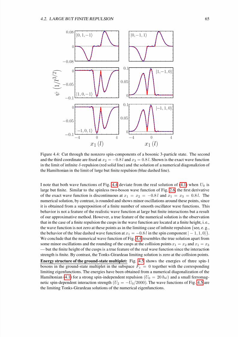
8/3/2019 Frank Deuretzbacher- Spinor Tonks-Girardeau gases and ultracold molecules
http://slidepdf.com/reader/full/frank-deuretzbacher-spinor-tonks-girardeau-gases-and-ultracold-molecules 75/151
4.2. LARGE BUT FINITE REPULSION 65
|0, 1,−1
|1, 0,−1
|−1, 0, 1
0 4−4
0
0.08
−0.08
0
−0.05
−0.1
|0,−1, 1
|1,−1, 0
0
0.05
0.1
|−1, 1, 0
0 4−4
0
0.05
0.10
−0.05
−0.1
x1 (l) x1 (l)
ψ
1 / l 3 / 2
Figure 4.4: Cut through the nonzero spin-components of a bosonic 3-particle state. The second
and the third coordinate are fixed at x2 = −0.8 l and x3 = 0.8 l. Shown is the exact wave function
in the limit of infinite δ-repulsion (red solid line) and the solution of a numerical diagonalizion of
the Hamiltonian in the limit of large but finite repulsion (blue dashed line).
I note that both wave functions of Fig. 4.4 deviate from the real solution of (4.1) when U 0 is
large but finite. Similar to the spinless two-boson wave function of Fig. 2.6, the first derivative
of the exact wave function is discontinuous at x1 = x2 = −0.8 l and x1 = x3 = 0.8 l. The
numerical solution, by contrast, is rounded and shows minor oscillations around these points, since
it is obtained from a superposition of a finite number of smooth oscillator wave functions. This
behavior is not a feature of the realistic wave function at large but finite interactions but a result
of our approximative method. However, a true feature of the numerical solution is the observation
that in the case of a finite repulsion the cusps in the wave function are located at a finite height, i. e.,
the wave function is not zero at these points as in the limiting case of infinite repulsion
see, e. g.,
the behavior of the blue dashed wave function at x1 =−
0.8 l in the spin component
| −1, 1, 0
.
We conclude that the numerical wave function of Fig. 4.4 resembles the true solution apart from
some minor oscillations and the rounding of the cusps at the collision points x1 = x2 and x1 = x3
— but the finite height of the cusps is a true feature of the real wave function since the interaction
strength is finite. By contrast, the Tonks-Girardeau limiting solution is zero at the collision points.
Energy structure of the ground-state multiplet: Fig. 4.5 shows the energies of three spin-1
bosons in the ground-state multiplet in the subspace F z = 0 together with the corresponding
limiting eigenfunctions. The energies have been obtained from a numerical diagonalization of the
Hamiltonian (4.1) for a strong spin-independent repulsion (U 0 = 20 ω) and a small ferromag-
netic spin-dependent interaction strength (U 2 = −U 0/2000). The wave functions of Fig. 4.5 are
the limiting Tonks-Girardeau solutions of the numerical eigenfunctions.

8/3/2019 Frank Deuretzbacher- Spinor Tonks-Girardeau gases and ultracold molecules
http://slidepdf.com/reader/full/frank-deuretzbacher-spinor-tonks-girardeau-gases-and-ultracold-molecules 76/151
66 CHAPTER 4. THE SPINOR TONKS-GIRARDEAU GAS
F = 1
F = 1F = 2
F = 1F = 2
F = 0
F = 3
1 2 3 4 5 6 7
F z = 0
4.455
4.5
−0.08
|0, 1, −1
|1, 0, −1
| − 1, 0, 1
|0, 0, 0
0 4−4
0
|0, −1, 1
| − 1, 1, 0
|1, −1, 0
0 4−4
0 4−4
0 4−4
0 4−4
0 4−4
0 4−4
0
0.08
0
0.08
−0.08
0
−0.1
0
−0.1
0
0.1
0
0.1
|0, 0, 00.12
0 4−40
|0, 1, −1
0 4−40
0.06|0, −1, 1
0 4−40
0.06
|1, 0, −1
0 4−40
0.06|1, −1, 0
0 4−40
0.06
| − 1, 0, 1
0 4−40
0.06| − 1, 1, 0
0 4−40
0.06
|0, 1, −1
|1, 0, −1
| − 1, 0, 1
|0, 0, 0
0 4−4
0
0 4−4
0 4−4
0 4−4
0
−0.12
0
0.06
−0.1
|0, −1, 1
0 4−40
0.12
| − 1, 1, 0
0 4−4
0
0.06
−0.1
0.1
0
−0.06
|1, −1, 0
0 4−4
0.1
0
−0.06
|0, 1, −1
0 4−4
0
|0, −1, 1
0 4−4
|1, 0, −1 |1, −1, 0
| − 1, 0, 1 | − 1, 1, 0
|0, 0, 0
0 4−40
0.16
−0.05
0
−0.05
0 4−4
0
0 4−4−0.05
0
−0.05
0 4−4
0
0 4−4−0.05
0
−0.05
|0, 1, −1
|1, 0, −1
| − 1, 0, 1
|0, 0, 0
0 4−4
0
|0, −1, 1
| − 1, 1, 0
|1, −1, 0
0 4−4
0 4−4
0 4−4
0 4−4
0 4−4
0 4−4
0
−0.08
0.08
0
−0.08
0.08
0
−0.08
0.1
0
−0.08
0.1
0
0.08
−0.1
0
0.08
−0.1
|0, 1, −1
|1, 0, −1
| − 1, 0, 1
|0, 0, 0
0 4−4
0
|0, −1, 1
| − 1, 1, 0
|1, −1, 0
0 4−4 0 4−4
0 4−4
0 4−4
0 4−4
0 4−4
0
0.06
0
0.06
0
0.06
0
0.06
0
0.06
0
0.06
−0.12 −0.12
−0.1 −0.1
−0.1 −0.1
|0, 1, −1
|1, 0, −1
| − 1, 0, 1
|0, 0, 0
0 4−4
0
|0, −1, 1
| − 1, 1, 0
|1, −1, 0
0 4−4 0 4−4
0 4−4 0 4−4
0 4−4 0 4−4
0
−0.08
0.08
0
−0.08
0.08
0
−0.08
0.08
0
−0.08
0.08
0
−0.08
0.08
0
−0.08
0.08
1 2
3 4
5 6
7
level 1
level 2
level 3
level 4
Π = 1
Π = −1
Π = 1
Π = −1
Figure 4.5: Energy structure of the ground-state multiplet of three spin-1 bosons in the subspace
F z = 0. The spin-independent interaction U 0 = 20 ω is large and the spin-dependent interactionU 2 = −U 0/2000 is weak and ferromagnetic. Note the small splitting of the ground-state multiplet,
which is much smaller than the spacing from the first excited multiplet: (4.5 − 4.455)ω =0.045 ω 1 ω. The energy eigenvalues have been obtained from a numerical diagonalization
of the Hamiltonian. The corresponding limiting solutions of the eigenfunctions are also shown.
The 4th eigenstate is the example wave function of Fig. 4.4.
The states are ordered by energy (1: lowest, ..., 7: largest energy). In the F z = 0 subspace the
ground-state multiplet consists of 7 boson wave functions since a basis of the corresponding spin
space is, e. g., given by the states |0, 0, 0, |1, 0, −1, |1, −1, 0, |0, 1, −1, |0, −1, 1, | − 1, 1, 0and
| −1, 0, 1
. For infinite repulsion U 0 =
∞all the seven states acquire the same energy E g =
N 2/2 ω = 4.5 ω. For a large but finite repulsion only the 7th state has exactly that energy and
the energies of the other states are slightly lower. Note that the splitting of the multiplet is much
smaller than the spacing from the first excited multiplet: (4.5 − 4.455)ω = 0.045 ω 1 ω.
With increasing repulsion the states 1 − 6 approach the limiting energy from below.
The 7th state is not affected by the δ repulsion. For all values of U 0 it has the same energy 4.5 ω.
The spin function of that state is antisymmetric under any permutation of two particles
|χ7=1√
6
|0, 1,−1+|1,−1, 0+|−1, 0, 1−|0,−1, 1−|−1, 1, 0−|1, 0,−1
=
√3!P A|0, 1,−1.
Likewise the motional wave function of the corresponding boson ground state is permutationally

8/3/2019 Frank Deuretzbacher- Spinor Tonks-Girardeau gases and ultracold molecules
http://slidepdf.com/reader/full/frank-deuretzbacher-spinor-tonks-girardeau-gases-and-ultracold-molecules 77/151
4.2. LARGE BUT FINITE REPULSION 67
antisymmetric as well
W |χ7 =√
3!P A|id⊗ √3!P A|0, 1, −1 = ψ(0)fermion gr. ⊗
√3!P A|0, 1, −1 , (4.14)
i. e., the orbital function is given by the ground-state Slater determinant of three noninteracting
fermionsψ(0)fermion gr. ∝ (x1 − x2)(x1 − x3)(x2 − x3)e−(x21+x
22+x
23)/2 ,
which is zero at xi = x j and hence the particles in that state do not feel the δ interaction
potential. I note finally that the 7th state is an F 2 and parity eigenstate (F = 0, Π = −1).
By contrast, the 1st and the 2nd state of Fig. 4.5 (which form the 1st level of the multiplet) have
permutationally symmetric motional wave functions and they are strongly influenced by the in-
creasing δ repulsion. One can build two linearly independent symmetric spin functions from the
above states: The state |0, 0, 0, which is already symmetric, and the state√
3! P S |1, 0, −1. For
U 2 = 0 (when the spin-dependent interaction is switched off) both boson ground states W |0, 0, 0and W
√3! P S |1, 0, −1 are energetically degenerate and the system can be in arbitrary superpo-
sitions of these states, which need not to be F 2
eigenstates. The degeneracy is lifted, when U 2is switched on and both states become F 2 eigenstates. One state has total spin F = 3 and is
approximately given by the limiting solution
W |χ1 = W |χF =3 = W
2
5|0, 0, 0 +
3
5
√3! P S |1, 0, −1
(4.15)
and the other state has total spin F = 1 and is approximately given by
W |χ2 = W |χF =1 = W
3
5|0, 0, 0 −
2
5
√3! P S |1, 0, −1
. (4.16)
These states can also be written as W |χ1/2 = ψ(∞)boson gr. ⊗ |χ1/2, i. e., the orbital wave function is
given by the permutationally symmetric spinless Tonks-Girardeau wave function
ψ(∞)boson gr. ∝ |x1 − x2||x1 − x3||x2 − x3|e−(x21+x
22+x
23)/2 . (4.17)
The states W |χ1/2 of the first level are strongestly influenced by the δ interaction, since for a
motional wave function with Bose symmetry the probability is highest to find two particles at the
same position. Both states have evolved from the noninteracting ground-states ψ(0)boson gr. ⊗ |χ1/2
with ψ(0)boson gr. ∝ e−(x21+x22+x23)/2.
Additionally, the energy of the states of the lowest level, which are approximated by W
|χF =3
and
W |χF =1, depends on the sign of the spin-dependent interaction U 2. We found for two particlessee Eq. (2.3)
that the interaction Hamiltonian can be written as
V int. = δ(r1 − r2)
(g0 − 2g2)1
⊗2 + (g2/2) F 2
(4.18)U 0/2 = g0/2/l
. 2 The first term of the interaction (4.18) has already deformed the motional
wave function of both states which is now approximately given by (4.17). The second term has
two effects: Firstly, both states become F 2 eigenstates and, secondly, their energy is shifted by the
2I note that for N 3 particles the spin-dependent interaction is not simply proportional to F 2 as in the two-particle
case. Otherwise all the eigenstates of Fig. 4.5 with same F would have the same energy. However, stillˆ
H int., F 2˜
= 0.
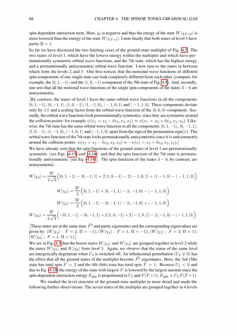
8/3/2019 Frank Deuretzbacher- Spinor Tonks-Girardeau gases and ultracold molecules
http://slidepdf.com/reader/full/frank-deuretzbacher-spinor-tonks-girardeau-gases-and-ultracold-molecules 78/151
68 CHAPTER 4. THE SPINOR TONKS-GIRARDEAU GAS
spin-dependent interaction term. Here, g2 is negative and thus the energy of the state W |χF =3 is
more lowered than the energy of the state W |χF =1. I note finally that both states of level 1 have
parity Π = 1.
So far we have discussed the two limiting cases of the ground-state multiplet of Fig. 4.5: The
two states of level 1, which have the lowest energy within the multiplet and which have per-
mutationally symmetric orbital wave functions, and the 7th state, which has the highest energy
and a permutationally antisymmetric orbital wave function. I now turn to the states in between
which form the levels 2 and 3. One first notices that the motional wave functions of different
spin-components of one single state can look completely different from each other
compare, for
example, the |0, 1, −1- and the |1, 0, −1-component of the 5th state of Fig. 4.5
. And, secondly,
one sees that all the motional wave functions of the single spin-components of the states 3 − 6 are
nonsymmetric.By contrast, the states of level 1 have the same orbital wave functions in all the components
|0, 1, −1, |0, −1, 1, |1, 0, −1, |1, −1, 0, | − 1, 0, 1 and | − 1, 1, 0. These components deviate
only by ±1 and a scaling factor from the orbital wave function of the |0, 0, 0-component. Sec-
ondly, the orbital wave functions look permutationally symmetric, since they are symmetric around
the collision points: for example ψ(x1 = x2 − δx2, x2, x3) ≈ ψ(x1 = x2 + δx2, x2, x3). Like-
wise, the 7th state has the same orbital wave function in all the components |0, 1, −1, |0, −1, 1,
|1, 0, −1, |1, −1, 0, |−1, 0, 1 and |−1, 1, 0 apart from the sign of the permutation sign(π). The
orbital wave function of the 7th state looks permutationally antisymmetric since it is antisymmetric
around the collision points: ψ(x1 = x2 − δx2, x2, x3) ≈ −ψ(x1 = x2 + δx2, x2, x3).
We have already seen that the spin functions of the ground states of level 1 are permutationally
symmetric
see Eqs. (4.15) and (4.16)
and that the spin function of the 7th state is permuta-
tionally antisymmetric
see Eq. (4.14)
. The spin functions of the states 3 − 6, by contrast, are
nonsymmetric:
W |χ3 =W
2 √3|0, 1, −1 − |0, −1, 1 + 2 |1, 0, −1 − 2 | − 1, 0, 1 + |1, −1, 0 − | − 1, 1, 0W |χ4 =
W
2
|0, 1, −1 + |0, −1, 1 − |1, −1, 0 − | − 1, 1, 0
W |χ5 =
W
2
|0, 1, −1 − |0, −1, 1 − |1, −1, 0 + | − 1, 1, 0
W |χ6 =
W
2√
3
−|0, 1, −1− |0, −1, 1 + 2 |1, 0, −1 + 2 |− 1, 0, 1− |1, −1, 0− |− 1, 1, 0
.
These states are at the same time F 2 and parity eigenstates and the corresponding eigenvalues are
given by: (W
|χ3
: F = 2, Π =
−1); (W
|χ4
: F = 1, Π =
−1); (W
|χ5
: F = 2, Π = 1);
(W |χ6 : F = 1, Π = 1).We see in Fig. 4.5 that the boson states W |χ3 and W |χ4 are grouped together in level 2 while
the states W |χ5 and W |χ6 form level 3. Again, we observe that the states of the same level
are energetically degenerate when U 2 is switched off. An infinitesimal perturbation (U 2 = 0) has
the effect that all the ground states of the multiplet become F 2 eigenstates. Here, the 3rd (5th)
state has total spin F = 2 and the 4th (6th) state has total spin F = 1. Because U 2 < 0 and
due to Eq. (4.18) the energy of the state with largest F is lowered by the largest amount since the
spin-dependent interaction energy E spin is proportional to U 2 and F (F +1), E spin ∝ U 2 F (F + 1).
We studied the level structure of the ground-state multiplet in more detail and made the
following further observations: The seven states of the multiplet are grouped together in 4 levels

8/3/2019 Frank Deuretzbacher- Spinor Tonks-Girardeau gases and ultracold molecules
http://slidepdf.com/reader/full/frank-deuretzbacher-spinor-tonks-girardeau-gases-and-ultracold-molecules 79/151
4.2. LARGE BUT FINITE REPULSION 69
quasidegenerate ground-state multiplet
F = N F = N − 2 . . .
F = min.
. . .
F = min.
. . .
Completely symmetric
orbital functions
most antisymmetric
orbital functions
gap due to symmetry
gap due to spin-dependent interaction
U 2 < 0
U 0 = 10 hω (large but finite)
(small, ferromagnetic)
decreasing symmetry
∆E spin ∝ U 2/U 20
F = max.
∆E symmetry ∝ 1/U 0
≈ ψ(∞)spinlessboson gr.⊗ P S |spin
level 1
level 2
Figure 4.6: Sketch of the energy structure of the ground-state multiplet of 2
−5 particles. The
ground-state multiplet splits up into several levels when the δ repulsion is made large but finite.Comparatively large gaps due to the different symmetry of the motional wave functions separate
the different levels from each other. These “symmetry gaps” depend only on the strength of the
spin-independent interaction ∆E symmetry ∝ 1/U 0. The splitting within the levels is furthermore
determined by the spin-dependent interaction strength and ∆E spin ∝ U 2/U 20 . With increasing
level index the motional wave functions of the ground states become more and more permutation-
ally antisymmetric.
(see Fig. 4.5). The symmetry of the motional wave functions decreases with increasing level
index (level 1: permutationally symmetric motional wave functions, ... increasing antisymmetry
..., level 4: permutationally antisymmetric motional wave function). The energy gaps between
different levels are comparatively large and solely determined by the spin-independent interaction
strength ∆E symmetry ∝ 1/U 0.
A similar energy structure has been discussed in Ref. [69] for a
two-component system by means of the two-particle solution; see Eqs. (2.45), (2.46) and (2.48).
From a Taylor expansion of the left-hand side of Eq. (2.48) one obtains Eq. (3.12). Thus, the
energy gap ∆E = E − 3/2 ∝ 1/gr = 1/U .
The comparatively small energy gaps within the
single levels depend also on the spin-dependent interaction strength U 2 and they are given by
∆E spin ∝ U 2/U 20 since the local correlation function ρlocal corr. =
dxρ(x, x) is proportional to
1/U 20 in the limit of strong repulsion [32] and since ∆E spin = U 2 ρlocal corr..
Generalization to other particle numbers: We made similar observations for 2 −5 particles and
I believe that the general structure of the ground-state multiplet is independent of the number of particles N . Fig. 4.6 summarizes the results: The ground-state multiplet decomposes into several
levels. All the states of level 1 have permutationally symmetric motional wave functions — in
agreement with Ref. [96]. The states of different levels are separated from each other by “sym-
metry gaps”. The spacing between the levels solely depends on the spin-independent interaction
strength ∆E symmetry ∝ 1/U 0. The comparatively small gaps within the single levels depend more-
over on the spin-dependent interaction strength ∆E spin ∝ U 2/U 20 . The symmetry of the motional
wave functions decreases with increasing level index, i. e., the states of the energetically highest
level have the most antisymmetric motional wave functions.
Note that one can not build com-
pletely permutationally antisymmetric spin functions for more than three spin-1 particles since,
for example, P A|1, 1, 0, −1 = 0.
Each state of the ground-state multiplet can be approximated

8/3/2019 Frank Deuretzbacher- Spinor Tonks-Girardeau gases and ultracold molecules
http://slidepdf.com/reader/full/frank-deuretzbacher-spinor-tonks-girardeau-gases-and-ultracold-molecules 80/151
70 CHAPTER 4. THE SPINOR TONKS-GIRARDEAU GAS
by a superposition of the basis states W |m1, m2, . . . , mN and the corresponding coefficients
cm1,...,mN are determined by the interaction Hamiltonian. So far we find these coefficients from
the comparison with the numerical solutions (which we have done so far only for three particles).
4.3 Spin densities of the ground states
We found in Sec. 4.1 that hard-core particles with spin behave at the same time like noninteract-
ing spinless fermions and noninteracting distinguishable spins. The dual nature of the particles
became clearly visible in the energy spectrum (see Fig. 4.3). A similar behavior is shown by the
(spin) densities of the system. I will show in the following that the total density of all the degen-
erate ground states always equals that of noninteracting spinless fermions. The spin densities, by
contrast, depend sensitively on the superposition of the spin function and equal those of a chain of
localized particles with the spin orientations given by the spin function; see Fig. 4.7.
First, I will derive the first-quantized form of the spin density. The operator of the probability to
find particle 1 in spin state m is given by
|mm|1 = |mm| ⊗ 1
⊗(N −1) =
m2,...,mN
|m, m2, . . . , mN m, m2, . . . , mN |
=
m1,m2,...,mN
δmm1 |m1, m2, . . . , mN m1, m2, . . . , mN | .
Here, 1 is the identity matrix of the single-particle spin space. This operator is of course not
permutationally symmetric and we cannot measure whether particle 1 is in spin state m since the
particles are indistinguishable. We can only measure whether one particle is in spin state m and
the corresponding symmetrized operator is given by
N i=1
|mm|i =
N i=1
m1,...,mN
δmmi |m1, . . . , mN m1, . . . , mN | .
Likewise we construct the projection operator of finding one particle at position x
N i=1
|xx|i =N i=1
RN
dx1 . . . d xN δ(x − xi)|x1, . . . , xN x1, . . . , xN | .
The spin density is the probability to find one particle in spin state m at position x. The corre-
sponding operator is therefore the projection
ρm(x) =
N i=1
|x mx m|i
=N i=1
m1,...,mN
RN
dx1 . . . d xN δmmi δ(x − xi)
×|x1, . . . , xN ⊗ |m1, . . . , mN m1, . . . , mN | ⊗ x1, . . . , xN | . (4.19)
We want to calculate the spin density of a ground state W |χ which is given by the expectation
value
ρm(x) = χ|W †ρm(x)W |χ = N !χ| ⊗ id| P †S ρm(x) P S |id ⊗ |χ .

8/3/2019 Frank Deuretzbacher- Spinor Tonks-Girardeau gases and ultracold molecules
http://slidepdf.com/reader/full/frank-deuretzbacher-spinor-tonks-girardeau-gases-and-ultracold-molecules 81/151
4.3. SPIN DENSITIES OF THE GROUND STATES 71
P S = P †S is self-adjoined, it commutes with any permutationally symmetric operator
and thus
also with ρm(x)
and it is a projection operator P 2S = P S . We thus obtain
ρm(x) =
π∈S N
χ| ⊗ id|ρm(x)|π ⊗
U (π)|χ
= χ| ⊗ id|ρm(x)|id ⊗ |χ , (4.20)
since id|ρm(x)|π = δid,πid|ρm(x)|id. By inserting Eq. (4.19) into Eq. (4.20) we obtain the
expectation value of the spin density in state W |χ
ρm(x) =i
m1,...,mN
δmmi
m1, . . . , mN |χ2 =: pi(m)
×
dx1 . . . d xN δ(x − xi)x1, . . . , xN |id2
=:ρ(i)
(x)
. (4.21)
Here, we have defined the probability pi(m) to find the ith particle of the system in spin state mand the probability density ρ(i)(x) to find the ith particle of the system, restricted to the standard
sector C id, at point x. Thus, we obtain the following formula for the spin density
ρm(x) =i
pi(m)ρ(i)(x) . (4.22)
An explicit calculation of the probability density ρ(i)(x) (which I will derive in appendix A) yields
the following formula
ρ(i)(x) = ddx N −ik=0
(−1)N −i(N − k − 1)!(i − 1)!(N − k − i)! k!
∂ k∂λk
detB(x) − λ1
λ=0
, (4.23)
where the N × N -matrix B(x) has entries β ij(x) = x−∞ dxψi(x)ψ j(x) with the single-particle
eigenfunctions of the spinless problem ψi
1 is the N × N identity matrix
.
I note that formula (4.22) is independent of the spin and the statistics of the hard-core particles
it
can be applied to spin-1/2, 1, 3/2, . . . bosons or fermions
. Formula (4.23) is independent of the
confining potential and also applicable to the excited states
simply use the corresponding Bi(x)matrix of the excited state W i|χ and the single-particle eigenfunctions of the confining potential
which has to be studied
. In the following I will apply the formula to the ground states of spin-1
hard-core bosons, which are confined in a one-dimensional harmonic trap.
Spin densities of spin-1 bosons: Fig. 4.7 shows the spin densities of selected ground states of 8
spin-1 hard-core bosons in a harmonic trap. The spin density has 3 components which corre-
spond to m = −1, 0, 1. The single components are drawn as a blue dashed (ρ1), red solid (ρ0)
and a green dotted line (ρ−1). In Fig. 4.7(a) and (b) we have also plotted the densities ρ(i)(x)of the particles i = 1 − 8. Note that ρ(i)(x) is not a measurable observable! However, it will
serve as a very useful quantity in order to develop an intuitive understanding of Eq. (4.22). De-
spite the quite complicated form of Eq. (4.23) the densities ρ(i)(x) of the particles i = 1 − 8look rather simple
see Fig. 4.7(a) and (b)
, namely, like Gaussians which are located in a row
along the x-axis, one after the other, at x1 ≈ −3.5 l, x2 ≈ −2.5 l , . . . , x8 ≈ 3.5 l
with
xi =
dxxρ(i)(x)
. One might, therefore, develop the intuitive picture of particles, which are

8/3/2019 Frank Deuretzbacher- Spinor Tonks-Girardeau gases and ultracold molecules
http://slidepdf.com/reader/full/frank-deuretzbacher-spinor-tonks-girardeau-gases-and-ultracold-molecules 82/151
72 CHAPTER 4. THE SPINOR TONKS-GIRARDEAU GAS
(b)
(c) (d)
0−4 4 0
−4 4
0
00
0−4 4
1.4
0.71.4
ρ(1) ρ(8)
0 0 0 0111 1
(a)
00−4 4
1.4
ρ(1) ρ(8)
111 1 1 1 1 1
x (l) x (l)
ρ ( x )
( 1 / l )
Figure 4.7: Spin densities of 8 spin-1 bosons in different ground states (see text). Shown are the
densities ρ(i) (gray dash-dotted line, see text), and the components ρ0 (red solid line), ρ1 (blue
dashed line) and ρ−1 (green dotted line) of the spin density. The spin densities resemble chains of
localized spins.
aligned in a row along the x-axis, by interpreting the square root of the densities ρ(i)(x) as the
wave packets of imaginary particles, ψ(i)(x)
≡ ρ(i)(x) [21] with the spin orientations given by
u (i) ≡ pi(−1), pi(0), pi(1)T the unit vector u (i) has length one. Thus, we obtain the
spin density ρm(x) as follows: We draw the density ρ(i)(x) of the localized particle i as done in
Fig. 4.7(a) and (b), we multiply ρ(i)(x) by pi(m) in order to obtain the spin density of particle i,
ρ(i)m (x) ≡ pi(m)ρ(i)(x), and in the final step we sum up the spin densities of all the eight particles
ρm(x) =i ρ
(i)m (x) — that is precisely the meaning of Eq. (4.22).
Fig. 4.7(a) shows the spin density of the spin-polarized state W |χ+ = W |1, 1, . . .. In the spin-
polarized case all the probabilities pi(1) = 1; see the definition of pi(m) in Eq. (4.21). Therefore,
Eq. (4.22) reduces to
ρ1(x) = i ρ(i)(x) = ρfermion gr.(x) =7
i=0
ψ2i (x) ,
which is the usual density of a spinless Tonks-Girardeau gas. Fig. 4.7(b) shows the spin density of
the ground state W |1, 1, 1, 0, 0, 0, 0, 1. Similarly we obtain pi(1) = 1 for i = 1, 2, 3 and 8,
and pi(0) = 1 for i = 4 − 7. Thus, the spin density ρ1(x) of that state is given by
ρ1(x) = ρ(1)(x) + ρ(2)(x) + ρ(3)(x) + ρ(8)(x) and ρ0(x) is given by ρ0(x) =7i=4 ρ(i)(x), i. e.,
we add the particle densities ρ(1)(x)−ρ(3)(x) and ρ(8)(x) to the component ρ1(x) and the particle
densities ρ(4)(x)−ρ(7)(x) to the component ρ0(x) of the spin density. Finally, Figs. 4.7(c) and (d)
show the spin densities of the ground state W |1, −1, 1, 0, 0, −1, −1, 1 and the superposition state
W (|0, 0, . . . + |1, −1, 1, −1, . . .) /√
2 respectively. We see in Figs. 4.7(b–d) that the spin den-
sities of the hard-core bosons can strongly vary on a rather short length scale, given by the mean
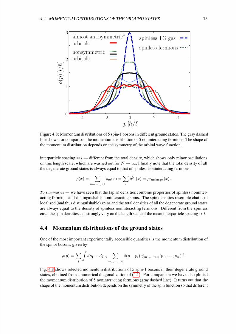
8/3/2019 Frank Deuretzbacher- Spinor Tonks-Girardeau gases and ultracold molecules
http://slidepdf.com/reader/full/frank-deuretzbacher-spinor-tonks-girardeau-gases-and-ultracold-molecules 83/151
4.4. MOMENTUM DISTRIBUTIONS OF THE GROUND STATES 73
0
0
2
2
−2 4
−4
3
1
p [h/l]
ρ ( p
)
[ l / ¯ h ]
spinless TG gas
spinless fermions
“almost antisymmetric”
orbitals
nonsymmetric
orbitals
Figure 4.8: Momentum distributions of 5 spin-1 bosons in different ground states. The gray dashed
line shows for comparison the momentum distribution of 5 noninteracting fermions. The shape of
the momentum distribution depends on the symmetry of the orbital wave function.
interparticle spacing ≈ l — different from the total density, which shows only minor oscillations
on this length scale, which are washed out for N → ∞. I finally note that the total density of all
the degenerate ground states is always equal to that of spinless noninteracting fermions
ρ(x) = m=−1,0,1
ρm(x) = i
ρ(i)(x) = ρfermion gr.(x) .
To summarize — we have seen that the (spin) densities combine properties of spinless noninter-
acting fermions and distinguishable noninteracting spins. The spin densities resemble chains of
localized (and thus distinguishable) spins and the total densities of all the degenerate ground states
are always equal to the density of spinless noninteracting fermions. Different from the spinless
case, the spin densities can strongly vary on the length scale of the mean interparticle spacing ≈ l.
4.4 Momentum distributions of the ground states
One of the most important experimentally accessible quantities is the momentum distribution of
the spinor bosons, given by
ρ( p) =i
dp1 . . . d pN
m1,...,mN
δ( p − pi)|ψm1,...,mN ( p1, . . . , pN )|2.
Fig. 4.8 shows selected momentum distributions of 5 spin-1 bosons in their degenerate ground
states, obtained from a numerical diagonalization of (4.1). For comparison we have also plotted
the momentum distribution of 5 noninteracting fermions (gray dashed line). It turns out that the
shape of the momentum distribution depends on the symmetry of the spin function so that different

8/3/2019 Frank Deuretzbacher- Spinor Tonks-Girardeau gases and ultracold molecules
http://slidepdf.com/reader/full/frank-deuretzbacher-spinor-tonks-girardeau-gases-and-ultracold-molecules 84/151
74 CHAPTER 4. THE SPINOR TONKS-GIRARDEAU GAS
ground states can have completely different momentum distributions. This has to be contrasted
with the total density, which was completely independent of the spin function and equal for each
ground state. States with a completely symmetric spin function |χs have a completely symmetric
orbital function, W |χs = ψ(∞)boson gr.(x1, . . . , xN )|χs, which is given by the usual spinless Tonks-
Girardeau wave function. The momentum distribution of these states is equal to that of a spinless
Tonks-Girardeau gas (blue dash-dotted line), which exhibits a pronounced zero-momentum peak
and long-range, high-momentum tails [90, 92]. The other extreme case is given by a flat and broad
momentum distribution, which resembles the fermionic one (red solid line). In the case of 2 and
3 spin-1 bosons, some spin functions |χa can be completely antisymmetric and thus the corre-
sponding ground state is given by W |χa = ψ(0)fermion gr.(x1, . . . , xN )|χa so that its momentum
distribution is equal to that of spinless fermions. One cannot construct completely antisymmetric
spin functions with more than 3 spin-1 particles. However, it is possible to construct nonsym-
metric spin functions, which are “almost antisymmetric” (see Young’s Tableaux [97]), resulting in
momentum distributions which are almost fermionic. We believe, due to group theoretical argu-
ments [97], that this broadening and flattening of some momentum distributions saturates for large
N . However, as one sees in Fig. 4.8, some spinful bosons aquire Fermi-like momentum distribu-
tions depending on the symmetry of their spin function. That is quite different from the spinless
case, where the momentum distribution clearly exhibits bosonic features. The opposite obser-
vation is made for spinful fermions. Here, the ground states with “almost antisymmetric” spin
functions have momentum distributions which resemble those of spinless hard-core bosons. The
relationship between the symmetry of the motional wave function of a ground state and the shape
of its momentum distribution is sketched in Fig. 4.9. I finally note that all the momentum distribu-
tions of Fig. 4.8 have the same width w p = 2 p2 = 5 /l since the kinetic energy E kin. ∝ p2
is independent of the spin function and equal to that of noninteracting spinless fermions.
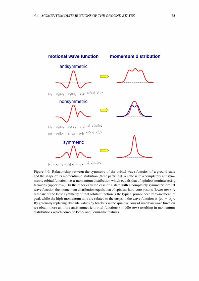
8/3/2019 Frank Deuretzbacher- Spinor Tonks-Girardeau gases and ultracold molecules
http://slidepdf.com/reader/full/frank-deuretzbacher-spinor-tonks-girardeau-gases-and-ultracold-molecules 85/151
4.4. MOMENTUM DISTRIBUTIONS OF THE GROUND STATES 75
(x1 − x2)(x1 − x3)(x2 − x3)e−(x21+x
22+x
23)/2
(x1 − x2)(x1 − x3)|x2 − x3|e−(x21+x
22+x
23)/2
antisymmetric
nonsymmetric
|x1 − x2||x1 − x3||x2 − x3|e−(x21+x
22+x
23)/2
symmetric
motional wave function momentum distribution
(x1 − x2)|x1 − x3||x2 − x3|e−(x21+x
22+x
23)/2
Figure 4.9: Relationship between the symmetry of the orbital wave function of a ground state
and the shape of its momentum distribution (three particles). A state with a completely antisym-
metric orbital function has a momentum distribution which equals that of spinless noninteracting
fermions (upper row). In the other extreme case of a state with a completely symmetric orbital
wave function the momentum distribution equals that of spinless hard-core bosons (lower row). A
remnant of the Bose symmetry of that orbital function is the typical pronounced zero-momentum
peak while the high-momentum tails are related to the cusps in the wave function at xi = x j.
By gradually replacing absolute values by brackets in the spinless Tonks-Girardeau wave function
we obtain more an more antisymmetric orbital functions (middle row) resulting in momentum
distributions which combine Bose- and Fermi-like features.
8/3/2019 Frank Deuretzbacher- Spinor Tonks-Girardeau gases and ultracold molecules
http://slidepdf.com/reader/full/frank-deuretzbacher-spinor-tonks-girardeau-gases-and-ultracold-molecules 86/151
Chapter 5
Ultracold heteronuclear Feshbach
molecules
The main results of Secs. 5.6 – 5.9 have been published in Ref. [3].
The aim of this chapter is a theoretical description of the experiment of C. Ospelkaus et al. [72] on
the formation of ultracold Feshbach molecules from two different atomic elements. In Secs. 5.1 –
5.4 I present simple models for the interaction between ultracold atoms. These models are used to
become familiar with some of the most important concepts, namely the scattering length, the phase
shift, the pseudopotential approximation and Feshbach resonances. In Sec. 5.6 I describe the exact-
diagonalization algorithm used to calculate the low-energy spectrum and the corresponding wave
functions of two interacting atoms at a single site of an optical lattice. In the following sections
5.7 – 5.9 I compare our results to the experimental data and calculate the transfer efficiency of
the rf association and the lifetime of the Feshbach molecules. Related theoretical work has been
published by J. F. Bertelsen and K. Mølmer [98, 99].
5.1 S-wave scattering in free space
Let us consider two atoms in free space (i. e. no external potential) which interact via a spherically
symmetric box potential
V box(r) =
V if r R
0 if r > R.(5.1)
We are searching for the solution of the radial equation
− 2
2µ1r
d2dr2
r + V box(r) − E ψ(r) = 0.
The equation consists of the kinetic energy of the radial motion, the potential energy of the box
and the energy of the relative motion. We restrict our discussion to particles with relative angular
momentum zero (l = 0), i. e., the centrifugal barrier is zero. By substituting
χ(r) ≡ r ψ(r)
the radial equation transforms to
d2χ(r)
dr2+
2µ
2 E − V box(r)
χ(r) = 0 . (5.2)
76

8/3/2019 Frank Deuretzbacher- Spinor Tonks-Girardeau gases and ultracold molecules
http://slidepdf.com/reader/full/frank-deuretzbacher-spinor-tonks-girardeau-gases-and-ultracold-molecules 87/151
5.1. S-WAVE SCATTERING IN FREE SPACE 77
Rr
V
inner region(r < R)
outer region (r > R)
r
V
bound states
free spherical wave
R
inner
region
(r < R)
outer region (r > R)
(a) (b)
0
0
Figure 5.1: Radial wave functions χ(r) of an attractive (a) and a repulsive (b) spherically sym-
metric box potential. Attractive interaction (a): In the inner region χin ∝ sin(Kr). The larger the
wave number K ∝ √E − V the faster the oscillation. In the outer region χout ∝ e−ρr (E < 0) or
χout ∝ sin(kr) (E > 0). The energy spectrum is discrete for E < 0 leading to a finite number of
molecular bound states. For E > 0 the energy spectrum is continuous: The free spherical waves
can have every energy E > 0. Repulsive interaction (b): In the inner region χin ∝ sinh(K r)(E < V ) or χin ∝ sin(Kr) (E > V ). In the borderline case E = V the inner wave function is
just a straight line χin ∝ r. In the outer region χout ∝ sin(kr).
The probability ρ(r) = |ψ(r)|2|Y lm(θ, φ)|2 to find the relative particle at position r shall be finite
everywhere (Y lm are spherical harmonics). Therefore, it is a reasonable constraint that the wave
function ψ(r) is finite everywhere too, in particular at the origin: ψ(0) = finite. Thus, the wave
function χ(r) has to obey the boundary condition χ(0) = 0 [78]. We introduce some abbreviations
≡ 2µE
2, θ ≡ 2µV
2, k ≡ √
, ρ ≡ √−,
K ≡ √ − θ, K ≡ √
θ − = i K. (5.3)
Firstly we want to solve Eq. (5.2) in the inner region (r R). We consider the case > θ. Then,
Eq. (5.2) becomes
χ(r) + K 2χ(r) = 0.
Two linearly independent solutions of this equation are the sine and the cosine function
sin(Kr) and cos(Kr).
But due to the boundary condition χ(0) = 0 only the sine function is a possible solution of the
inner region
χin(r) = A sin(Kr) ( > θ)
(A is a constant). Similarly we obtain
χin(r) = A sinh(K r) ( < θ)
8/3/2019 Frank Deuretzbacher- Spinor Tonks-Girardeau gases and ultracold molecules
http://slidepdf.com/reader/full/frank-deuretzbacher-spinor-tonks-girardeau-gases-and-ultracold-molecules 88/151
78 CHAPTER 5. ULTRACOLD HETERONUCLEAR FESHBACH MOLECULES
in the case < θ since sin(i x) = i sinh(x). We now turn to the outer region (r > R). In the case
< 0 Eq. (5.2) becomes
χ(r) − ρ2χ(r) = 0.
Two linearly independent solutions of this equation are
eρr and e−ρr.
But since eρr blows up as r → ∞ the only possible solution of the outer region is given by
χout(r) = Be−ρr ( < 0)
(B is a constant). In the case > 0 Eq. (5.2) becomes
χ(r) + k2χ(r) = 0.
Two possible linearly independent solutions of this equation are
sin(kr) and cos(kr).
There are no further constrains: The point r = 0 does not belong to the interval [R, ∞) and, since
sin(kr) and cos(kr) belong to the continuous energy spectrum, the wave function does not need
to be normalizable. Thus, any superposition of these functions is a solution of the outer region.
Let us choose the two constants B (amplitude) and δ0 (phase shift) to construct the solution
χout(r) = B
cos δ0 sin(kr) + sin δ0 cos(kr)
= B sin(kr + δ0).
Molecules: The different solutions are now merged at r = R. In the case θ < < 0 we may
obtain molecular bound states
χbound(r) = χin(r) = A sin(Kr) if r Rχout(r) = Be−ρr if r R.
(5.4)
The possible energies of the bound states are determined by the continuity of the logarithmic
derivative at r = R
β 0 ≡ χin(R)
χin(R)=
χout(R)
χout(R)(5.5)
Using (5.4) we obtain
K cos(KR)
sin(KR)= −ρe−ρR
e−ρR.
The possible eigenenergies are thus given by the zeros of the “energy function”
F () ≡ tan√
− θR
+
− θ
(−)= 0. (5.6)
The constant B is determined by the continuity of χ at R
χin(R) = χout(R) ⇒ B = A sin(KR)eρR. (5.7)
Finally the constant A is determined by the normalization condition
A =
∞0
drχ2(r). (5.8)

8/3/2019 Frank Deuretzbacher- Spinor Tonks-Girardeau gases and ultracold molecules
http://slidepdf.com/reader/full/frank-deuretzbacher-spinor-tonks-girardeau-gases-and-ultracold-molecules 89/151
5.1. S-WAVE SCATTERING IN FREE SPACE 79
not a valid
solution
energy of first
bound state
energy of second
bound state
energy of third
bound state
0−10−20−30−40−50−60
−40
−20
0
20
40
ǫ
F (ǫ)
Figure 5.2: “Energy function” F () for parameters R = 1 and θ =−
63. The energy eigenvalues
are the zeros of F (). These are located at 1 = −55.3, 2 = −32.6 and 3 = −0.27. The zero at
= θ = −63 is not a valid solution since it belongs to the wave function χbound(r) = 0. The zeros
are located between the singularities of F (). These are located at sing.(n) = θ +
(2n − 1) π2R2
with n = 1, 2, . . . , nbound (nbound total number of bound states).
Two examples of molecular bound states are depicted in Fig. 5.1(a). The corresponding eigenen-
ergies have been determined numerically by solving Eq. (5.6) by means of MATHEMATICA. An
example plot of the “energy function” is given in Fig. 5.2. We see that the zeros are located
between the singularities of F (). These singularities can be determined easily:
F () = ±∞ ⇒ tan √ − θR = ±∞⇒ √
− θR = (2n − 1)π
2(n = 1, 2, 3, . . .)
⇒ sing.(n) = θ +
(2n − 1)π
2R
2(n = 1, 2, 3, . . . , nbound)
where nbound is the total number of bound states. This number can be calculated as follows: We
assume that the energy of the least bound state is approximately zero ( = 0−). Then, we obtain
from the “energy function”
1
F ( = 0)
= 0
⇒cot
√
−θR = 0
⇒ √−θR = (2n − 1)π
2(n = 1, 2, 3, . . .)
⇒ nbound =
√−θR
π+
1
2
(5.9)
where x is the greatest integer less than or equal to x. Therefore, if the box is too shallow and
too narrow, it might be possible that there exists no bound state at all.
Strongly bound molecules— For strongly bound molecules ( 0) the box potential is practically
infinitely high. Thus the molecular wave function is given by χbound = A sin(Kr) for r Rand zero otherwise. From the boundary condition χbound(R) ≈ 0 we obtain KR ≈ nπ and thus
8/3/2019 Frank Deuretzbacher- Spinor Tonks-Girardeau gases and ultracold molecules
http://slidepdf.com/reader/full/frank-deuretzbacher-spinor-tonks-girardeau-gases-and-ultracold-molecules 90/151
80 CHAPTER 5. ULTRACOLD HETERONUCLEAR FESHBACH MOLECULES
≈ θ + n2(π/R)2 — the well-known result of a particles in a one-dimensional infinite square
well. The wave function is therefore approximately given by χbound ≈ A sin
nπ(r/R)
. Thus,
the inner wave function of the nth strongly bound molecule shows n/2 sine oscillations
compare
with the blue and green wave function of Fig. 5.5(a)
. The mean distance between the atoms is
r
= d r r χ2
bound
≈R/2.
Weakly bound molecules— For weakly bound molecules ( 0) the outer wave function is ap-
proximately given by χout = Be−√− r ≈ B(1 − √− r). We have seen in the derivation of
Eq. (5.9) that in this case K ≈ √−θ ≈ (2nbound − 1)π/(2R) so that the inner wave function is
given by χin ≈ A sin
(2nbound − 1)(π/2)(r/R)
. Thus, the inner wave function of the weakly
bound molecule shows (2nbound − 1)/4 sine oscillations
compare with the red wave function of
Fig. 5.5(a)
. The mean distance between the atoms r approaches +∞ when approaches zero
since then the outer wave function becomes a constant χout ≈ B.
Free spherical waves: We now turn to the case > 0 where the solutions are free spherical waves.
In the case > θ we obtain for the wave function
χfree(r) = χin(r) = A sin(Kr) if r R
χout(r) = B sin(kr + δ0) if r R ( > θ). (5.10)
The phase shift δ0 can be calculated from the logarithmic derivative at R: Using the inner wave
function we obtain
β 0 =χ
in(R)
χin(R)= K cot(KR) ( > θ). (5.11)
From the outer solution we obtain
β 0 =χ
out(R)
χout(R)=
k
cos δ0 cos(kR) − sin δ0 sin(kR)
cos δ0 sin(kR) + sin δ0 cos(kR)= k
cos(kR) − tan δ0 sin(kR)
sin(kR) + tan δ0 cos(kR).
Thus, the phase shift is given by
δ0 = arctank cos(kR) − β 0 sin(kR)
k sin(kR) + β 0 cos(kR)
. (5.12)
The constant A can be deduced from the continuity of χ at R
χin(R) = χout(R) ⇒ A =B sin(kR + δ0)
sin(KR)( > θ). (5.13)
The remaining constant B can be chosen at will since the free spherical waves are not normaliz-
able. I choose B = 1.
The case < θ is very similar since sin(i x) = i sinh(x) and cos(i x) = cosh(x): Simply replace
sin(Kr) by sinh(K r) in Eq. (5.10) to obtain the wave function
χfree(r) =
χin(r) = A sinh(K r) if r R
χout(r) = B sin(kr + δ0) if r R( < θ), (5.14)
replace K cot(KR) by K coth(K R) in (5.11) to obtain the logarithmic derivative
β 0 = K coth(K R) ( < θ) (5.15)
and replace sin(KR) by sinh(K R) in (5.13) to obtain the constant A
A =B sin(kR + δ0)
sinh(K R)( < θ). (5.16)

8/3/2019 Frank Deuretzbacher- Spinor Tonks-Girardeau gases and ultracold molecules
http://slidepdf.com/reader/full/frank-deuretzbacher-spinor-tonks-girardeau-gases-and-ultracold-molecules 91/151
5.1. S-WAVE SCATTERING IN FREE SPACE 81
scattering length as
χ(R)
tangent with gradient χ′(R)
R
V
0 5−10 −5 10
0
0.5
1
1.5
2
−0.5
−1
r
V ( r )
a n d
χ ( r )
Figure 5.3: Definition of the scattering length. The picture shows an attractive potential V (r)(black thick solid line), a radial wave function χ(r) (red thick solid line) and the tangent of χ at
R. We define the scattering length as as the intersection of the tangent of χ at R with the r-axis.
Also in this case the phase shift is given by Eq. (5.12) (since in both cases the outer wave function
χout(r) is the same) but now one has to use Eq. (5.15) for the logarithmic derivative β 0 (since the
inner solutions are different). Again we choose B = 1.
Hard sphere— In the extreme case of a hard sphere (V = ∞) it follows from Eqs. (5.3), (5.12),
(5.15) and (5.16) that K = ∞, A = 0, β 0 = ∞ and δ0 = −kR. Thus the wave function is simply
χfree(r) = sin
k(r − R)
if r R and zero if r R.
Examples of free spherical waves are depicted in Fig. 5.1(a) and (b). For < θ the wave function
grows exponentially in the inner region, χfree ∝ sinh(K r), with K ∝ √V − E . In the borderlinecase = θ the wave function is just a straight line and χfree ∝ r. For > θ the wave function
shows an oscillatory behavior, χfree ∝ sin(Kr), with K ∝ √E − V . In the outer region the wave
function χfree ∝ sin(kr) oscillates with k ∝ √E .
Scattering length: Let me now introduce the concept of the scattering length. We define the
scattering length as as the intersection of the tangent of χ at R with the r-axis, 1 see Fig. 5.3 (this
definition can be applied to any potential with a finite range R). As can be seen in Fig. 5.3 the
following relation holds
χ(R)
R
−as
= χ(R) ⇔ as = R − χ(R)
χ(R)= R − 1
β 0. (5.17)
In the extreme case of a hard sphere V = ∞; see Fig. 5.4(a) the scattering length is simply given
by the radius of the hard sphere
as = R (hard sphere)
since β 0 = ∞. In the case of a soft sphere
0 < E V = finite; see Figs. 5.4(b) and (c)
it
follows from Eqs. (5.17) and (5.15) that the scattering length is given by
as = R − 1
K tanh(K R) (0 < E V ). (5.18)
1See pp. 413-414 of Ref. [97].

8/3/2019 Frank Deuretzbacher- Spinor Tonks-Girardeau gases and ultracold molecules
http://slidepdf.com/reader/full/frank-deuretzbacher-spinor-tonks-girardeau-gases-and-ultracold-molecules 92/151
82 CHAPTER 5. ULTRACOLD HETERONUCLEAR FESHBACH MOLECULES
V = ∞ 0 < E ≪ V = finite E ≈ V
0 1 2 3 4 5 6 7 0 1 2 3 4 5 6 7
0
2
1
−10 1 2 3 4 5 6 7
0
2
1
−1
0
2
1
−1
(a) (b) (c)
KR = π/2− 0.16
0
2
1
−10 1 2 3 4 5 6
(d)
KR = π/2 + 0.16
0
2
1
−10 1 2 3 4−1−2−3−4
(e)
Figure 5.4: Scattering length of several wave functions. The pictures show a wave function χ(r)(red thick solid line) and its tangent at R (black thin dashed line). The radius of the box potential
is R = 1. The scattering length as is the intersection of the tangent of χ at R with the r-axis. (a)
as = R, (b) as = 0.66R, (c) as = 0, (d) as = −3.5R and (e) as = 4.5R.
Thus, if K R 1 the scattering length is as ≈ 0 since tanh(x) ≈ x for small x. On the other
hand, if K R 1 the scattering length is as ≈ R − 1/K since tanh(x) ≈ 1 for large x.
Therefore, in the case of a soft sphere, the following inequality holds:
0 as < R (for 0 < E V = finite).
In the case E > V the scattering length has to be calculated from Eqs. (5.17) and (5.11)
as = R − 1
K tan(KR) (E > V ). (5.19)
Therefore the scattering length varies from −∞ to +∞ depending on KR. In particular as jumps
from −∞ to +∞ if KR → (2n − 1)π/2 (n = 1, 2, . . .); see Figs. 5.4(d) and (e).
Relation between scattering length and phase shift— In the case of a hard sphere as = R and
δ0 = −kR leading to δ0 = −kas. In general we can connect the scattering length with the
phase shift by inserting the logarithmic derivative of the outer solution β 0 = χout(R)/χout(R) into
Eq. (5.17)
as = R −1
k tan(kR + δ0). (5.20)
For k ≈ 0 and R as we obtain tan δ0 = −kas.
Some borderline cases— Strongly bound molecules: Similar to the case of the hard sphere the
wave function is approximately zero at R since χin ≈ A sin
nπ(r/R)
. Therefore, the scattering
length is as ≈ R (more precisely as R); see the tangents of the blue and the green wave
function in Fig. 5.5(a). Weakly bound molecules: The outer wave function is approximately
given by χout ≈ B(1 − √−r). Therefore, as approaches +∞ when approaches zero; see
Figs. 5.5(a-c). Low-energy free waves: The outer wave function is approximately given by χout ≈B cos
k(r − R)
. Thus, at r = R, the gradient of χout is zero and |as| = ∞. More precisely
as = −∞; see Fig. 5.5(d).

8/3/2019 Frank Deuretzbacher- Spinor Tonks-Girardeau gases and ultracold molecules
http://slidepdf.com/reader/full/frank-deuretzbacher-spinor-tonks-girardeau-gases-and-ultracold-molecules 93/151
5.1. S-WAVE SCATTERING IN FREE SPACE 83
0 1 2 3 4 5 6 0 5 10 15 20 25 30 35 40−1.5
−1
−0.5
0
0.5
1
1.5
−1
−0.5
0
0.5
1
0 2 4 6 0 2 4 68 10 8 10−1
−0.5
0
0.5
1
1.5
−0.3
−0.2
−0.1
0
0.1
0.2
0.3
R√−θ = 5 π/2 + 0.15 R
√−θ = 5 π/2 + 0.0035
R√−θ = 5 π/2 + 0.0016 R
√−θ = 5 π/2− 0.007
(a) (b)
(c) (d)
Figure 5.5: (a) Three molecular bound states. Blue: molecule in the lowest vibrational state,
green: molecule in the first excited vibrational state, red: least bound state (with highest vibrational
energy). (b) The extent of the weakly bound molecule tends to infinity when the binding energy
approaches zero. (c) as = +∞ for a least bound state with E = 0− and (d) as = −∞ for a
low-energy free wave with E = 0+.
Weakly bound molecules: We have seen that the binding energy of the least bound state ap-
proaches zero if √−θR = (2n − 1)π/2
see the derivation of Eq. (5.9)
. In Figs. 5.5(a) and
(b) I have chosen the parameters of the attractive box potential according to√−θR 5 π/2 so
that three bound states occur. The blue line is the wave function of the strongest bound molecule
which is in the lowest vibrational state. The green line belongs to a molecule which is in the first
excited vibrational state and the red line belongs to a molecule which is in the second excited
vibrational state. The blue and the green wave function have large binding energies and they are
located within the box potential (r ≈ 0.6R). By contrast the red wave function has an extremely
small binding energy and the mean distance between the atoms is large r ≈
9.2R in the top
right figure. The probability to find the two atoms within the radius R is extremely small.
We can relate the scattering length to the binding energy of the least bound state. Using the
logarithmic derivative of the outer wave function (5.4) we obtain from Eq. (5.17)
as = R +1
ρ⇔ ρ =
1
as − R⇒ E b ≡ −E =
2ρ2
2µ=
2
2µ(as − R)2≈
2
2µa2s(5.21)
for large scattering lengths as R. Further, as is related to the distance r between the atoms.
As can be seen in Fig. 5.5(b), for a weakly bound molecule, the probability to find the particles
8/3/2019 Frank Deuretzbacher- Spinor Tonks-Girardeau gases and ultracold molecules
http://slidepdf.com/reader/full/frank-deuretzbacher-spinor-tonks-girardeau-gases-and-ultracold-molecules 94/151
84 CHAPTER 5. ULTRACOLD HETERONUCLEAR FESHBACH MOLECULES
within a sphere with radius R is negligible compared to the probability to find them outside, R0
drχ2 ≈ 0 and
∞R
drχ2 ≈ 1 .
Sinceχout = Be−
ρr we obtain
1 ≈ ∞R
drχ2out = B2
∞R
dre−2ρr ⇒ B2 = 2ρe2ρR
and the mean distance r is given by
r ≈ ∞R
d r r χ2out = B2
∞R
d r r e−2ρr = R +1
2ρ=
R + as2
. (5.22)
Figs. 5.5(c) and (d) show the evolution from a weakly bound state to a low-energy free wave when
the attractive potential is made shallower. As can be seen as = +∞ when the energy of the least
bound state is infinitesimal small, E = 0−, and as = −∞ for a free wave with E = 0+.
Delta potential: The usual repulsive δ potential has no influence on the scattered wave. To see thiswe consider the potential δR = 3/(4πR3) if r R and zero if r R. The scattered wave shall
have a low fixed energy E . For small enough R we have 0 < E < 3/(4πR3) so that 0 < as < R.
Thus, as → 0 if R → 0. Further, δ0 → 0 if as → 0 and R → 0; see Eq. (5.20).
5.2 S-wave scattering in a harmonic trap
We consider two atoms which interact via the box potential (5.1). Additionally the atoms are
confined by a harmonic oscillator potential. The angular momentum of the relative motion shall
be zero (l = 0). The radial dimensionless equation of the relative motion reads
− 1
2r
d2
dr2r + V box(r) +
1
2r2 − E
ψ(r) = 0.
Here, all lengths have been expressed in units of the oscillator length losc = /(µω) and all
energies have been expressed in units of ω. Again, we substitute χ = rψ and obtain the equation
χ − r2χ + 2
E − V box
χ = 0. (5.23)
Two linearly independent solutions of this equation are given by
y1
−(E − V box);
√2r
, y2
−(E − V box);
√2r
/√
2
where the parabolic cylinder functions y1 and y2 2 are given by
y1(a; z) = 1F 1
a
2+
1
4;
1
2;
z2
2
e−z
2/4, y2(a; z) = z 1F 1
a
2+
3
4;
3
2;
z2
2
e−z
2/4. (5.24)
The function 1F 1(a; b; z) is the confluent hypergeometric function of the first kind 3
1F 1(a; b; z) = 1 +a
bz +
a(a + 1)
b(b + 1)
z2
2+ . . . +
a . . . (a + n − 1)
b . . . (b + n − 1)
zn
n!+ . . . (5.25)
2Entries 19.2.1 and 19.2.3 of Ref. [100] / Wikipedia / Wolfram MathWorld .3Entry 13.1.2 of Ref. [100] / Wikipedia / Wolfram MathWorld .
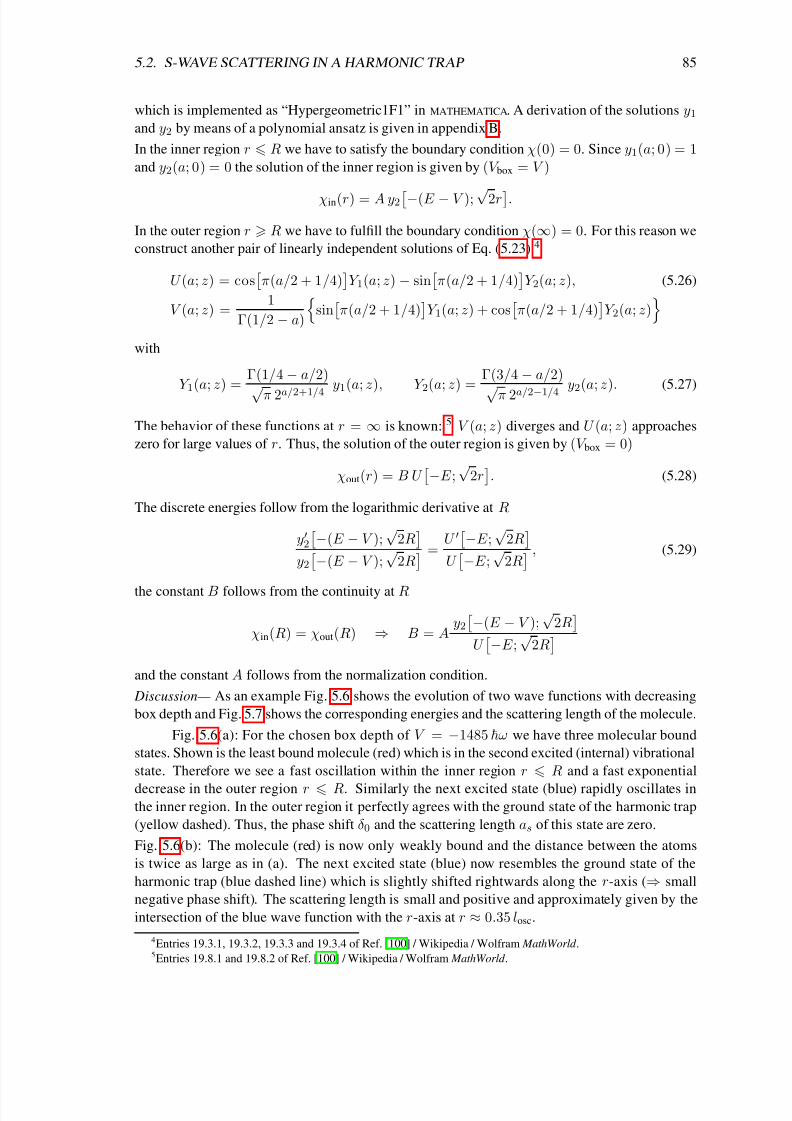
8/3/2019 Frank Deuretzbacher- Spinor Tonks-Girardeau gases and ultracold molecules
http://slidepdf.com/reader/full/frank-deuretzbacher-spinor-tonks-girardeau-gases-and-ultracold-molecules 95/151
5.2. S-WAVE SCATTERING IN A HARMONIC TRAP 85
which is implemented as “Hypergeometric1F1” in MATHEMATICA. A derivation of the solutions y1and y2 by means of a polynomial ansatz is given in appendix B.
In the inner region r R we have to satisfy the boundary condition χ(0) = 0. Since y1(a; 0) = 1and y2(a; 0) = 0 the solution of the inner region is given by (V box = V )
χin(r) = A y2−(E − V ); √2r.In the outer region r R we have to fulfill the boundary condition χ(∞) = 0. For this reason we
construct another pair of linearly independent solutions of Eq. (5.23) 4
U (a; z) = cos
π(a/2 + 1/4)
Y 1(a; z) − sin
π(a/2 + 1/4)
Y 2(a; z), (5.26)
V (a; z) =1
Γ(1/2 − a)
sin
π(a/2 + 1/4)
Y 1(a; z) + cos
π(a/2 + 1/4)
Y 2(a; z)
with
Y 1
(a; z) =Γ(1/4
−a/2)
√π 2a/2+1/4y1
(a; z), Y 2
(a; z) =Γ(3/4
−a/2)
√π 2a/2−1/4y2
(a; z). (5.27)
The behavior of these functions at r = ∞ is known: 5 V (a; z) diverges and U (a; z) approaches
zero for large values of r. Thus, the solution of the outer region is given by (V box = 0)
χout(r) = B U −E ;
√2r
. (5.28)
The discrete energies follow from the logarithmic derivative at R
y2−(E − V );
√2R
y2
−(E − V );
√2R
=
U −E ;
√2R
U
−E ;
√2R
, (5.29)
the constant B follows from the continuity at R
χin(R) = χout(R) ⇒ B = Ay2−(E − V );
√2R
U −E ;
√2R
and the constant A follows from the normalization condition.
Discussion— As an example Fig. 5.6 shows the evolution of two wave functions with decreasing
box depth and Fig. 5.7 shows the corresponding energies and the scattering length of the molecule.
Fig. 5.6(a): For the chosen box depth of V = −1485 ω we have three molecular bound
states. Shown is the least bound molecule (red) which is in the second excited (internal) vibrational
state. Therefore we see a fast oscillation within the inner region r R and a fast exponential
decrease in the outer region r R. Similarly the next excited state (blue) rapidly oscillates inthe inner region. In the outer region it perfectly agrees with the ground state of the harmonic trap
(yellow dashed). Thus, the phase shift δ0 and the scattering length as of this state are zero.
Fig. 5.6(b): The molecule (red) is now only weakly bound and the distance between the atoms
is twice as large as in (a). The next excited state (blue) now resembles the ground state of the
harmonic trap (blue dashed line) which is slightly shifted rightwards along the r-axis (⇒ small
negative phase shift). The scattering length is small and positive and approximately given by the
intersection of the blue wave function with the r-axis at r ≈ 0.35 losc.
4Entries 19.3.1, 19.3.2, 19.3.3 and 19.3.4 of Ref. [100] / Wikipedia / Wolfram MathWorld .5Entries 19.8.1 and 19.8.2 of Ref. [100] / Wikipedia / Wolfram MathWorld .

8/3/2019 Frank Deuretzbacher- Spinor Tonks-Girardeau gases and ultracold molecules
http://slidepdf.com/reader/full/frank-deuretzbacher-spinor-tonks-girardeau-gases-and-ultracold-molecules 96/151
86 CHAPTER 5. ULTRACOLD HETERONUCLEAR FESHBACH MOLECULES
0 1 2 3 4 0 1 2 3 4
−1
−0.5
0
0.5
1
−0.5
−1
0
1
2
−2
V = −800 hω V = −771 hω
(a) (b)
0 1 2 3 4
−1
0
0.5
1
V = −770 hω
(c)
0 1 2 3 4
−1
−0.5
0
0.5
1
V = −760 hω
(d)
0 1 2 3 4
−1
0
1
2
−2
−3
3V = −1485 hω
0 1 2 3 4
V = −745 hω
−1
0
1(e) (f)
Figure 5.6: Evolution of two wave functions with decreasing depth of the box potential. I havechosen R = 0.2 losc for all pictures. (a) The box depth is V = −1485 ω. Red is the molecule,
blue is the wave function with the next highest energy and yellow dashed is the ground state of
the harmonic trap
χ ∝ re−r2/2 since χ = rψ and ψ ∝ e−r2/2
. The molecule is strongly bound.
The distance between the atoms r R/2. The blue wave function perfectly agrees with the
ground state of the harmonic trap in the outer region apart from some fast oscillations in the inner
region. Scattering length as and phase shift δ0 are zero. (b) The scattering length is as ≈ 0.35 losc
and the phase shift is small and negative δ0 ≈ −kas. The outer blue wave function looks like
the ground state of the harmonic trap (blue dashed) which is shifted rightwards along the r-axis.
The molecule is weakly bound and r R. (c) V = −771 ω, as ≈ 10 losc, δ0 ≈ −π/2 and
r ≈ 3.5R. (d) V = −770 ω, as ≈ −12 losc, δ0 ≈ +π/2. (e) V = −760 ω, as ≈ −0.3 losc,
δ0 ≈ −kas small and positive and r ≈ 5R ≈ 1 losc. Red dashed is the ground state and bluedashed is the next excited state of the harmonic trap. The outer red (blue) wave function looks
like the ground (next excited) state of the harmonic trap which is shifted leftwards along the r-
axis. (f) r ≈ 1.13 losc. The red (blue) wave function now perfectly agrees with the ground (next
excited) state of the harmonic trap. Again, as = 0 and δ0 = 0. (a-f) With decreasing box depth
the molecule (ground state) evolves towards the ground (next excited) state of the trap.
Fig. 5.6(c): With decreasing box depth the molecule becomes more and more loosely bound. The
scattering length increases up to a maximum value of as = +∞; see the tangent of the molecular
wave function (black dashed line). Likewise the mean distance r between the atoms is much
larger than R. However,
r
does not converge towards infinity according to Eq. (5.22) due to the
external trapping potential.
Fig. 5.6(d): Similar to the free-space case
see Fig. 5.5
the molecule becomes an unbound pair of
atoms when the scattering length switches from plus to minus infinity. It seems to be a reasonable
definition of the transition point. However, there is no dicontinuous change of the wave function
at this transition point. The wave functions of Figs. 5.6(c) and (d) look almost equal. Only the
gradient of the wave function at R changes slightly from 0− to 0+ leading to an abrupt jump of
intersection of the tangent of the wave function at R with the r-axis. Likewise the phase shift δ0 jumps from −π/2 to +π/2. However, since sin(x − π/2) = − sin(x + π/2) = − cos(x) and
since the minus sign is absorbed by the global phase of the normalization constant, there is no
visible influence on the wave function.

8/3/2019 Frank Deuretzbacher- Spinor Tonks-Girardeau gases and ultracold molecules
http://slidepdf.com/reader/full/frank-deuretzbacher-spinor-tonks-girardeau-gases-and-ultracold-molecules 97/151
5.2. S-WAVE SCATTERING IN A HARMONIC TRAP 87
−840 −820 −800 −780 −760 −740 −720 −700 −840 −820 −800 −780 −760 −740 −720 −700−10
−8
−2
−6
−4
4
0
2
−2
−4
4
0
2
−10 −8 −2−6 −4 40 2 6 8−2
0
−1.5
−
1
−0.5
0.5
1
1.5
V (hω) V (hω)
a s
( l o s c
)
E
( ¯ h ω )
as (losc)
E
( ¯ h ω )
(b) (c,d)
(b)
(c)
(d)
(a) (e) (f)
(e)
(f)
(b)
(c)
(d)(e)
(f)
(a)
Figure 5.7: Left: Evolution of the energy of the weakly bound molecule (red) and the ground
state of the harmonic trap (blue) with decreasing depth of the attractive box potential. The green
crosses mark the corresponding wave functions of Fig. 5.6. Middle: Evolution of the scattering
length of the molecule with decreasing box depth. Right: Energy of the molecule (red) as a
function of the scattering length. Black dashed is an estimate of the molecular energy according
to E = −2/
2µ(as − R)2
which is exact in free space
see Eq. (5.21)
.
With further decreasing trap depth the red wave function, which was formerly a bound molecule,
evolves more and more into a wave function which is very similar to the ground state of the
harmonic oscillator apart from the fast oscillations in the inner region. In Fig. 5.6(e) the red wave
function has already a large overlap with the ground state of the trap (red dashed line). It is only
shifted a little bit leftwards along the r-axis compared to the ground state of the trap (small positive
phase shift). Likewise the blue wave function resembles the next excited state (blue dashed) of the
trap. Thus, the phase shift is small and positive.
The phase shift becomes even zero for V = −745 ω; see Fig. 5.6(f). At this point also the
scattering length is again zero; see the middle picture of Fig 5.7. Now, the red and the blue wave
function perfectly agree with the ground (next excited) state of the harmonic trap in the outer
region. Thus, one can say, that the least bound molecule (ground state of the trap) continuously
evolves into the ground (next excited) state of the trap when the depth of the box potential is made
shallower.
The transition behavior is also visible in the evolution of the energies; see Fig. 5.7(left). Red is
the energy of the molecule and blue is the energy of the ground state of the trap. In a rotationally
symmetric harmonic trap the energy eigenvalues are given by E = (2n + l + 3/2)ω where
n = 0, 1, . . . is the principal quantum number and l = 0, 1, . . . is the relative angular momentum.
The ground-state energy is E 0 = 3/2 ω and the energy of the next excited state with l = 0 is
E 2 = 7/2 ω
this is the second excited state since the state (n, l) = (0, 1) has a lower energy
.
When the box is made shallower from V = −1485 to −780 ω the energy of the molecule (red)
grows rapidly from E = −576 to −1
ω. This increase dramatically slows down in the region V =−780 . . .−745 ω. At V = −745 ω the energy of the former molecule exactly coincides with the
energy of the ground state of the trap E 0 = 3/2 ω. At this point the scattering length is zero and
the former molecule exactly coincides with the ground state of the trap in the outer region. Above
V = −745 ω, in the region V = −745 . . . − 500 ω, the energy of the former molecule is nearly
unaffected by large changes of the box depth, it increases only from E = 1.5 to 1.7 ω. Likewise
the energy of the oscillator ground state (blue) evolves from E 0 = 3/2 ω to E 2 = 7/2 ω. The
change of the energy mainly occures in the small region V = −790 . . . − 750 ω and is fastest
around V = −770 ω where the scattering length jumps from plus to minus infinity. Remarkably
the energy of this state (and all the other harmonic oscillator states) is nearly unaffected by the
large changes of the trap depth below V = −790 ω and above V = −750 ω. This is also true

8/3/2019 Frank Deuretzbacher- Spinor Tonks-Girardeau gases and ultracold molecules
http://slidepdf.com/reader/full/frank-deuretzbacher-spinor-tonks-girardeau-gases-and-ultracold-molecules 98/151
88 CHAPTER 5. ULTRACOLD HETERONUCLEAR FESHBACH MOLECULES
for the wave function (see the change of the scattering length in the middle picture of Fig. 5.7).
Finally, Fig. 5.7(right) shows the energy of the molecule (red) as a function of the scattering
length which are connected through E (V (as)). Black dashed is the free-space energy of the
molecule according to Eq. (5.21). Both curves agree well for small positive scattering lengths
since a tightly bound molecule is nearly unaffected by an additional external trap.
Comparison with the solution of Busch et al.: Firstly, I will show that the outer wave function
(5.28) is equal to the solution of Busch et al. [75]. Eq. (17) of Ref. [75] reads
ψBusch(r) =1
2π−3/2Ae−r
2/2Γ(−ν )U
−ν ;
3
2; r2
(5.30)
where A is a normalization constant, Γ(z) is the gamma function and
U (a,b,z) =π
sin(πb)
1F 1(a; b; z)
Γ(1 + a − b)Γ(b)− z1−b 1
F 1(1 + a − b; 2 − b; z)
Γ(a)Γ(2 − b)
(5.31)
is the confluent hypergeometric function of the second kind 6 which is implemented as “Hyperge-
ometricU” in MATHEMATICA. The index ν is related to the energy according to E = 2ν + 3/2. Idefine the normalization constant B ≡ 1/2π−3/2AΓ(−ν ). Thus, we have to show that
χout(r) = B U −E ;
√2r
= rψBusch(r) = B r U
−E
2+
3
4;
3
2; r2
e−r2/2. (5.32)
One finds 7
U (a; z) = D−a−1/2(z) (5.33)
and 8
Dν (z) = 2ν/2e−z2/4U
−ν
2;
1
2;
z2
2
.
Using these relations we obtain from Eq. (5.28)
χout(r) = B DE −1/2(√
2r) = B U
−E
2+
1
4;
1
2; r2
e−r2/2 (5.34)
with B = B 2E/2−1/4. One finds 9
U (a; b; z) = z1−bU (1 + a − b; 2 − b; z).
Using this relation with a = −E/2 + 1/4, b = 1/2 and z = r2 we finally obtain the right-hand
side of Eq. (5.32). Thus, we may use Eq. (5.28), the right-hand side of Eq. (5.32) or Eq. (5.34) for
the outer wave function χout(r). However, the energy of our system (box potential with radius R)
is still different from the energy of the system of Busch et al. [75] (regularized δ potential) and in
the inner region (r R) the wave function χin(r) strongly deviates from Eq. (5.34).It arises the question, whether the energy of our system becomes equal to the energy of the system
of Busch et al., when the radius of the box becomes infinitesimal small, R → 0, since then both
wave functions agree for all r. Eq. (16) of Ref. [75] reads
√2
Γ(−E/2 + 3/4)
Γ(−E/2 + 1/4)=
1
as(5.35)
6Entry 13.1.3 of Ref. [100] / Wikipedia / Wolfram MathWorld .7Entry 19.3.7 of Ref. [100] / Wolfram MathWorld .8Entry 19.240 of Ref. [101] / Wolfram MathWorld .9Entry 13.1.29 of Ref. [100].

8/3/2019 Frank Deuretzbacher- Spinor Tonks-Girardeau gases and ultracold molecules
http://slidepdf.com/reader/full/frank-deuretzbacher-spinor-tonks-girardeau-gases-and-ultracold-molecules 99/151
5.2. S-WAVE SCATTERING IN A HARMONIC TRAP 89
which determines the energy as a function of the scattering length. By contrast the energy of our
system is determined by Eq. (5.29) and thus a function of V and R.
We have seen in Fig. 5.7 that both, the energy and the scattering length, are functions of the
box depth. Both quantities change dramatically with V around a characteristic value (here V ≈
−770 ω) when a weakly bound state evolves into the ground state of the trap. Thus, E and as are
directly connected with each other through E (V (as)) and we can plot the energy as a function of
the scattering length; see Fig. 5.7(right). Can we directly calculate E as a function of as without
making use of the box depth V ? We remember that the energy is determined by the boundary
condition that the logarithmic derivatives of the inner and outer solutions must agree at r = REq. (5.5)
. Further, we remember that the scattering length is also determined by the logarithmic
derivative at R
Eq. (5.17)
. Using Eq. (5.17) and the outer wave function (5.28) we obtain
√2
U (−E ;√
2R)
U (−E ;√
2R)=
1
R − as(5.36)
which determines the energy as a function of as and R. I would like to note that this formula is
much more useful for practical purposes than Eq. (5.29) since in practice the precise shape of theinteraction potential is often unknown and definitely not given by a simple box. Eq. (5.36) does
not make use of the precise shape of V int.(r). The only parameters which remain of V int.(r) are the
range of the interaction potential R (which might be, e. g., the van der Waals length scale) and the
scattering length as. Both quantities are experimentally accessible.
We would expect that the energy becomes even independent of R when the range of the interaction
potential becomes much smaller than the oscillator length of the relative motion losc = /(µω).
This is indeed the case. In the following I will show that in this case Eq. (5.36) is equal to
Eq. (5.35). For R = 0 Eq. (5.36) reads
1
−as=
√2
U (−E ; 0)
U (−E ; 0)
. (5.37)
We see from Eqs. (5.24) and (5.25) that
y1(a; 0) = 1, y1(a; 0) = 0, y2(a; 0) = 0 and y2(a; 0) = 1.
Using these relations and Eqs. (5.26) and (5.27) we obtain
U (−E ;0) = cosπ
4− E
π
2
Γ(1/4 + E/2)√π21/4−E/2
(5.38)
and
U (−
E ; 0) =−
sinπ
4 −E
π
2 Γ(3/4 + E/2)
√π2−1/4−E/2so that the above equation becomes
1
as= 2 tan
π
4− E
π
2
Γ(3/4 + E/2)
Γ(1/4 + E/2).
Now I use Euler’s reflection formula for the gamma function 10
Γ(z)Γ(1 − z) =π
sin(πz).
10Entry 6.1.17 of Ref. [100] / Wikipedia / Wolfram MathWorld .

8/3/2019 Frank Deuretzbacher- Spinor Tonks-Girardeau gases and ultracold molecules
http://slidepdf.com/reader/full/frank-deuretzbacher-spinor-tonks-girardeau-gases-and-ultracold-molecules 100/151
90 CHAPTER 5. ULTRACOLD HETERONUCLEAR FESHBACH MOLECULES
It follows
Γ
1
4+
E
2
=
π
sinπ4 + E π2
Γ34 − E
2
(5.39)
and
Γ3
4 +
E
2 =
π
sin 3π4 + E π2 Γ 14 − E 2 =
π
cos π4 + E π2 Γ 14 − E 2 .
Using these relations we obtain
1
as= 2 tan
π
4− E
π
2
tan
π
4+ E
π
2
Γ(3/4 − E/2)
Γ(1/4 − E/2)
which is equal to
2Γ(3/4 − E/2)
Γ(1/4 − E/2)=
1
as(5.40)
since tan(π/4 − x)tan(π/4 + x) = 1. Eqs. (5.35) and (5.40) differ only by a factor of √
2.
But this is only due to the unconventional definition of the relative and center-of-mass coordinatesused in Ref. [75]. Both results agree when the usual definitions of the relative and center-of-mass
coordinates are used. Therefore the regularized δ potential is equivalent to the boundary condition
χout(0)
χout(0)= − 1
as(5.41)
on the logarithmic derivative of the outer wave function at the origin [98, 99]. Thus, the boundary
condition (5.41) replaces the usual boundary condition at the origin, χ(0) = 0, which has to be
used in connection with regular interaction potentials.
5.3 Regularized delta potential
In many problems the mean distance r between the particles is much larger than the range R of
the interaction; see, e. g., the wave functions of Fig. 5.6 apart from the strongly bound molecule
in (a). Then the probability to find the particles within the range R is negligible compared to the
probability to find them outside R0 drχ2
in ∞R drχ2
out. Therefore, slight modifications of the
inner wave function (replace χin by χin) have practically no impact on the properties of the system
if still R0 drχ2
in ∞R drχ2
out.
This is shown in Fig 5.8. The real inner wave function (red dashed line) and the real outer wave
function (red solid line) are a magnification of the “oscillator ground state” of Fig. 5.6(e). As
can be seen R0 drχ2
in ∞R drχ2out. One can, e. g., simply replace the inner wave function
χin by the outer wave function χin = χout (blue line), i. e., one simply extends the outer wave
function into the inner region [0, R]. Still R0 drχ2
in ∞R drχ2
out and (nearly) all the properties
of the system are correctly described by this modified wave function. The only problem which
arises from this slight modification is that the probability to find the particle at the origin becomes
infinite: χout(0) = const. ⇒ ψout(0) = χout(0)/0 = ∞. However, as long as we don’t ask for
ρ(0) = |ψout(0)|2 the essential physics of the system is well described. As has been shown in the
last section the extended wave function has to obey the boundary condition (5.41) at the origin
which is equal to Eqs. (5.37) and (5.40) in a harmonic trap.
Now I wish to reintegrate the boundary condition (5.41) into the Schrodinger equation. That
is, I have to reintegrate an interaction potential into the Schrodinger equation such that the outer

8/3/2019 Frank Deuretzbacher- Spinor Tonks-Girardeau gases and ultracold molecules
http://slidepdf.com/reader/full/frank-deuretzbacher-spinor-tonks-girardeau-gases-and-ultracold-molecules 101/151
5.3. REGULARIZED DELTA POTENTIAL 91
0 0.2 0.4 0.6 0.8 1−0.6
−0.4
−0.2
0
0.20.
4
0.6
0.8
1
χout(r)
χin(r)
R
χin,2(r)
χin,1(r)
Figure 5.8: “Oscillator ground state” of Fig. 5.6(e) in the region 0 r 1. Red is the outer
and red dashed is the inner wave function. Since the probability to find the particles within the
range R is negligible compared to the probability to find them outside, R0 drχ2in ∞R drχ2
out,
a modification of the inner wave function (χin → χin) has no influence on the properties of the
system. χin,1 ≡ χout(r): The outer wave function has been extended into the inner region. χin,2:
The inner wave function has been modified according to Eq. (5.42).
wave function obeys the boundary condition (5.41). Since I can choose nearly arbitrary inner wave
functions χin I can construct an interaction potential which is much easier than realistic interaction
potentials. I discuss the procedure firstly for free particles.
Free space— The outer wave function solves the Schrodinger equation of noninteracting particles
and is given by ψout(r) = (B/r) sin(kr + δ0) (free spherical wave) or ψout(r) = (B/r) e−ρr
(molecule). For the inner wave function I choose ψin(r) = (A/R)3/2 − 1/2 (r/R)2:
ψ(r) =
ψin(r) =
A
R
3
2− 1
2
r
R
2if r R
ψout(r) =B
rsin(kr + δ0) or ψout(r) =
B
re−ρr if r R .
(5.42)
The inner wave function χin(r) = r ψin(r) = (A/R)
(3/2) r − 1/2 (r3/R2)
is shown in Fig 5.8
(green line). We wish the wave function to be continuous at R. Then we can express the constant
A by means of the outer wave function
ψin(R) =A
R= ψout(R) ⇒ A = R ψout(R).
Let’s act with the Laplacian on ψ(r). In the inner region we obtain
∆ψin =1
r
d2
dr2(r ψin) = −3A
R3= −4πδR(r)
R ψout(R)
with δR(r) ≡ 1
(4/3)πR3
if r R and δR(r) ≡ 0 if r > R. In the outer region we get in both
cases
∆ψout = −k2 ψout = − ψout or ∆ψout = ρ2 ψout = − ψout.
Thus we obtain, when acting with the kinetic energy operator on the wave function,
− 2
2µ∆ψ(r) = E ψout(r) +
4π2
2µδR(r)
R ψout(R)
.

8/3/2019 Frank Deuretzbacher- Spinor Tonks-Girardeau gases and ultracold molecules
http://slidepdf.com/reader/full/frank-deuretzbacher-spinor-tonks-girardeau-gases-and-ultracold-molecules 102/151
92 CHAPTER 5. ULTRACOLD HETERONUCLEAR FESHBACH MOLECULES
Now we include the boundary condition (5.17) into the equation. We use
1
R − as=
r ψout(r)
r ψout(r)
r=R
⇒ R ψout(R) = (R − as)∂
∂r
r ψout(r)
r=R
and obtain
− 2
2µ∆ψ(r) +
2π2(as − R)
µδR(r)
∂
∂r
r ψout(r)
r=R
= E ψout(r).
In the limit R → 0 this equation becomes−
2
2µ∆ +
2π2asµ
δ(r)∂
∂rr
ψ(r) = E ψ(r)
since δR(r) → δ(r) for R → 0
where the operator
V int.(r) =2π2a
sµ δ(r)
∂
∂r r (5.43)
is the desired pseudopotential which reintegrates the boundary condition (5.41) into the
Schrodinger equation of the noninteracting particles.
Harmonic trap— The derivation is almost equal to the free-space case since we did not use the
specific shape of the free-space solutions. Again, we choose the inner wave function of Eq. ( 5.42).
The outer wave function is now given by ψout(r) = (B/r) U −E ;
√2r
. Again A is given by
A = R ψout(R). Now we slightly modify the Hamiltonian of the inner region
H
(R)
0 ≡ H (in)
0 = − 2
2µ∆ if r R
H (out)0 = − 2
2µ∆ +
1
2µω2r2 if r > R .
We act with this Hamiltonian on the wave function and obtain
H (R)0 ψ(r) = Eψout(r) +
2π2
µδR(r)
R ψout(R)
.
Now we replace R ψout(R) by (R − as)
r ψ(r)r=R
and thereby integrate the boundary condi-
tion (5.17) into the above equation
H (R)
0ψ(r) +
2π2(as
−R)
µδR
(r)∂
∂r r ψout
(r)r=R = Eψout
(r).
In the limit R → 0 the Hamiltonian H (R)0 is solely given by H (out)
0 and the above equation becomes−
2
2µ∆ +
1
2µω2r2 +
2π2asµ
δ(r)∂
∂rr
ψ(r) = E ψ(r) .
Summary— Let me summarize the main steps of the pseudopotential method (for cold atoms).
Outside the range R of the true (short-ranged) interaction potential V int.(r) the outer wave function
ψout(r) is only determined by the Schrodinger equation of noninteracting particles and the bound-
ary condition
r ψout(r)
r ψout(r)
r=R= 1/(R − as). Thus, the whole impact of the true

8/3/2019 Frank Deuretzbacher- Spinor Tonks-Girardeau gases and ultracold molecules
http://slidepdf.com/reader/full/frank-deuretzbacher-spinor-tonks-girardeau-gases-and-ultracold-molecules 103/151
5.4. FESHBACH RESONANCE 93
molecule
molecule
2 atoms
2 atoms d e t u n i n g ∆ ǫ
coupling V c
−10 −5 0 5 10−3
−2
−1
0
1
2
3
detuning ∆ǫ
e n e r g
y
∆µB
(a) (b) (c) (d) (e) (f)
E 1
E 2
Figure 5.9: Left: Sketch of a simple Feshbach-resonance model. Red is the wave function of the
molecule (χ ∝ e−ρr) and blue is the wave function of the noninteracting atoms (χ ∝ re−r2/2).
The molecule and the noninteracting atoms shall have different magnetic momentsµm = µa
. By
applying a homogeneous magnetic field B one can shift the energy of the atoms relative to the
energy of the molecule. The shift is given by ∆E mag. = ∆µ B with ∆µ = µa − µm. For a
certain value B = B0 the energy of the molecule exactly agrees with the energy of the atoms and
the detuning becomes zero ∆ = 0
B0 is the center of the Feshbach resonance
. Around B0
the wave functions of the molecule and the two atoms strongly mix up, provided there is some
additional coupling V c between the two states. Right: Energies of the two eigenstates as a function
of the detuning ∆ for fixed coupling V c = −1. The labels (a-f) correspond to Figs. 5.10(a-f).
interaction potential reduces to a boundary condition on the outer wave function which depends
only on two parameters of V int.(r), namely its range R and the scattering length as. When the mean
distance r between the particles is much larger than R the probability to find both particles withinR is negligible compared to the probability to find them outside,
R0 dr(r ψin)2 ∞
R dr(r ψout)2.
Then, one can replace the inner wave function ψin by ψout so that the wave function is solely given
by ψ = ψout for all r ∈ [0, ∞). After this small modification (see the blue line in Fig. 5.8) still R0 dr(r ψ)2 ∞
R dr(r ψ)2. The extended outer wave function is determined by the Schrodinger
equation of noninteracting particles and the boundary condition
r ψ(r)
(r ψ(r)r=0
= −1/as.
This boundary condition can be included exactly into the Schrodinger equation of the noninteract-
ing particles by means of the regularized δ potential (5.43). Thus, if r R, the true interaction
potential can be replaced by the regularized δ potential. The extended outer wave functions have
a (harmless integrable) 1/r singularity at r = 0 and thus the probability ρ(0) = |ψ(0)|2 = ∞.
However, apart from this deficiency the essential physics is well described by the extended outer
wave functions. 11
5.4 Feshbach resonance
Simple model— A Feshbach resonance occurs if the energy of the least bound state is close to
the energy of the noninteracting atoms. Additionally we need some coupling between both states.
Consider Fig. 5.9(left): Red is the relative wave function of the least bound molecule χmol. ∝ e−ρr
and blue is the relative wave function of the noninteracting atoms χatoms ∝ re−r2/2. The molecule
11See also the discussion in Sec. 2.5 “The Bethe-Peierls model” (pp. 26-29) of Ref. [102] and references therein.

8/3/2019 Frank Deuretzbacher- Spinor Tonks-Girardeau gases and ultracold molecules
http://slidepdf.com/reader/full/frank-deuretzbacher-spinor-tonks-girardeau-gases-and-ultracold-molecules 104/151
94 CHAPTER 5. ULTRACOLD HETERONUCLEAR FESHBACH MOLECULES
and the two atoms have different magnetic moments µm = µa so that an external magnetic field
B shifts the energy of both states relative to each other according to ∆E mag. = ∆µ B with ∆µ =µa−µm. For a certain value of B the energy of the molecule exactly agrees with the energy of the
atoms and the detuning becomes zero ∆ = 0. This value B = B0 is the center of the Feshbach
resonance. Around B0 the wave functions of the molecule and the two atoms strongly mix up if
there is an additional coupling V c between the two states.
The mixing of the two states can be modeled by a simple 2 × 2 matrix
H F. =
0 V c
V c ∆
. (5.44)
The eigenenergies of this Hamiltonian are
E 1 = (∆/2) −
V 2c + (∆/2)2, E 2 = (∆/2) +
V 2c + (∆/2)2
and the corresponding eigenvectors are given by
χ1 = N 1
χmol. − ∆ + (2V c)2 + (∆)2
2V cχatoms
χ2 = N 2
χmol. − ∆ − (2V c)2 + (∆)2
2V cχatoms
where N 1 and N 2 are normalization constants. E 1 and E 2 are plotted in Fig. 5.9(right) as a
function of ∆ for fixed coupling V c = −1. In the limit ∆ = −∞ the coupling V c is negligible
so that H F. is approximately diagonal and E 1 = ∆, E 2 = 0, χ1 = χmol. and χ2 = χatoms.
In the opposite limit ∆ = +∞ we obtain E 1 = 0, E 2 = ∆, χ1 = χatoms and χ2 = χmol..
Therefore, by changing ∆ adiabatically from a positive to a negative value, two noninteracting
atoms evolve continuously into a weakly bound molecule follow the arrow in Fig. 5.9(right).Exactly at ∆ = 0 the energies are given by E 1 = −|V c|, E 2 = +|V c| and the corresponding
eigenvectors are χ1 = (χmol. − χatoms)/√
2 and χ2 = (χmol. + χatoms)/√
2.
Relation between scattering length and detuning— Fig. 5.10 shows several superpositions of a
molecular wave function χmol. and a wave function of two atoms χatoms for a fixed coupling V c =−1 and variable detuning ∆. In this example I have chosen a box depth of V = −780 ω for the
least bound molecule and V = −745 ω for the two atoms so that the outer wave function of the
two atoms exactly coincides with the ground state of the harmonic trap (⇒ as = 0). The shape of
χmol. and χatoms was fixed for all values of ∆.
Fig. 5.10(a): For ∆ = −100 there is no mixing between the two wave functions and χ1 = χmol.
(red) and χ2 = χatoms (blue).
Fig. 5.10(b): For ∆ = −3 the superposition wave functions are given by χ1 ≈ 0.29 χatoms +0.96 χmol. (red) and χ2 ≈ 0.96 χatoms − 0.29 χmol. (blue). This leads to a broadening of the
molecular wave function (red) and a smaller binding energy E b = −E 1
for the corresponding
binding energy see Fig. 5.9(right)
. Likewise the two atoms (blue) move a little bit apart from
each other and their energy E 2 increases. I note that the blue superposition wave function χ2
looks very similar to the blue wave function of Fig. 5.6(b). Therefore, I have varied the box depth
V such that the overlap between the resulting ground state of the trap and the blue superposition
wave function was maximized. The resulting blue dashed wave function belongs to a box depth
of V opt. = −820 ω. It has a small positive scattering length as ≈ 0.3 losc and its overlap with the
blue superposition state is nearly one. The red dashed wave function is the least bound molecule

8/3/2019 Frank Deuretzbacher- Spinor Tonks-Girardeau gases and ultracold molecules
http://slidepdf.com/reader/full/frank-deuretzbacher-spinor-tonks-girardeau-gases-and-ultracold-molecules 105/151
5.4. FESHBACH RESONANCE 95
∆ǫ = −100 ∆ǫ = −3 ∆ǫ = −1
∆ǫ = 1 ∆ǫ = 3 ∆ǫ = 100
(a) (b) (c)
(d) (e) (f)
0 1 2 3 4 0 1 2 3 4 0 1 2 3 4
0 1 2 3 4 0 1 2 3 4 0 1 2 3 4
0 0 0
0 0
1.5
−1.5
1.5
−1.5
2
−2
2
−2
0
2
−2
1.5
−1.5
Figure 5.10: Evolution of the superposition wave functions χ1 and χ2 (see text) with the detuning
∆ (V c = −1 = fixed). The superposition with more than 50% admixture of χmol. is drawn as
a red solid line and the superposition with more than 50% admixture of χatoms is drawn as a blue
solid line. One can adjust the wave functions of Sec. 5.2 (given by the red and the blue dashed
lines) to the superposition wave functions χ1 and χ2 by choosing an optimal trap depth V opt. for
each detuning ∆. Such a fit works quite good for the molecule if ∆ < 0 and |∆| not too large
(i. e. as > 0 not too small), see the red curve of Fig. (c). For the repulsively interacting atomsblue curves of Figs. (b) and (c)
and the attractively interacting atoms
blue curves of Figs. (d)
and (e)
the fit works for all values of ∆.
of the same box V opt. = −820 ω. As can be seen the overlap between the red dashed and the red
wave function is much smaller (overlap ≈ 0.76).
Fig. 5.10(c): For ∆ = −1 the superposition wave functions are given by χ1 ≈ 0.53 χatoms +0.85 χmol. (red) and χ2 ≈ 0.85 χatoms −0.53 χmol. (blue). Again we vary the box depth V such that
a maximum overlap with the corresponding least bound molecule (red dashed) and the ground state
of the trap (blue dashed) is achieved. The optimum box depth is now given by V opt. = −775 ωleading to an overlap of 0.99 between the red and the red dashed wave function and an overlap of
0.91 between the blue and the blue dashed wave function. The scattering lengths of the red and
the blue dashed wave functions are large and positive since we are close to the critical box depth
V
≈ −771 . . .
−770 ω where the scattering length diverges compare with Fig. 5.6(c).
Fig. 5.10(d): For ∆ = +1 the superposition wave functions are given by χ1 ≈ 0.85 χatoms +0.53 χmol. (blue) and χ2 ≈ −0.53 χatoms + 0.85 χmol. (red). The optimum box depth is V opt. =−768 ω and thus the scattering lengths of the dashed wave functions are large and negative
compare with Fig. 5.6(d)
. The overlap between the blue wave functions is approximately one
and it is ≈ 0.74 between the red wave functions.
Fig. 5.10(e): For ∆ = +3 the superposition wave functions are given by χ1 ≈ 0.96 χatoms +0.29 χmol. (blue) and χ2 ≈ −0.29 χatoms + 0.96 χmol. (red). The optimum box depth is V opt. =−760 ω and thus the scattering length of the blue dashed wave function is as ≈ −0.3 losc
compare with Fig. 5.6(e)
. The overlap between the blue wave functions is nearly one.
Fig. 5.10(f): For ∆ = +100 there is no mixing between the two wave functions and χ1 = χatoms

8/3/2019 Frank Deuretzbacher- Spinor Tonks-Girardeau gases and ultracold molecules
http://slidepdf.com/reader/full/frank-deuretzbacher-spinor-tonks-girardeau-gases-and-ultracold-molecules 106/151
96 CHAPTER 5. ULTRACOLD HETERONUCLEAR FESHBACH MOLECULES
(blue) and χ2 = χmol. (red).
Relation between scattering length and magnetic field— We conclude that the scattering length
of the optimally adjusted (dashed) wave functions depends on the detuning as = as(V opt.(∆)).
And since the detuning depends on the strength of the magnetic field B there is also a functional
relation between as and B. This functional relation is given by [103]
as(B) = abg
1 − ∆B
B − B0
(5.45)
where abg is the non-resonant background scattering length, ∆B the magnetic field width of the
resonance and B0 the resonance center position. 12
5.5 A short description of the experiment
I now turn to a short description of the experiment of C. Ospelkaus et al. [72]. More details are
given in the Ph.D. theses of Christian [73] and Silke Ospelkaus [74]. In a first step, an ultracold
(quantum-degenerate) mixture of 40K atoms in the |f = 9/2, mf = 9/2 spin state and 87Rb in the
|f = 2, mf = 2 spin state was achieved by means of radio-frequency (rf) induced sympathetic
cooling in a magnetic trap. Evaporative cooling of the bosonic 87 Rb atoms: The 87Rb atoms
are enclosed in a harmonic potential with a finite height. The barrier of the potential is slightly
lowered for a short period so that the high-energy atoms can escape from the trap. Thereby the
mean kinetic energy of the remaining atoms is lowered. The remaining atoms scatter with each
other which leads to a thermalization at a lower temperature. The cycle is repeated until quantum
degeneracy is achieved. Sympathetic cooling of the fermionic 40K atoms: A pure sample of 40K
atoms does not thermalize since fermions cannot occupy the same position in space due to the
Pauli exclusion principle and thus they do not feel the δ interaction potential. In a mixture, the
fermionic 40K atoms can scatter with the bosonic 87Rb atoms so that a cooling of the 87Rb sample
simultaneously cools the 40K sample.
Afterwards the mixture was transferred into a (shallow) optical dipole trap with final trap frequen-
cies for 87Rb of 2π × 50 Hz. In the optical dipole trap, 87Rb atoms were transferred from |2, 2 to
|1, 1 by a microwave sweep at 20 G and any remaining atoms in the upper hyperfine |f = 2, mf states were removed by a resonant light pulse. Next, the 40K atoms were transferred into the
|9/2, −7/2 state by performing an rf sweep at the same magnetic field with almost 100% effi-
ciency. With the mixture in the 87Rb|1, 1⊗40K|9/2, −7/2 state, the magnetic field was ramped
up to final field values at the Feshbach resonance occurring around 547 G [104]. Note that the pre-
pared state is not Feshbach-resonant at the magnetic field values which have been studied, and that
a final transfer of
40
K into the |9/2, −9/2 state was necessary to access the resonantly interactingstate. This was precisely the transition which has been used to measure the energy spectrum as
outlined further below.
In a next step, a 3D optical lattice was ramped up at a wavelength of λ = 1030 nm, where the
trapping potential for both species is related according to V K = 0.86 V Rb. Due to the different
masses of the two species, the trapping frequencies are ωK =
87/40 · 0.86 ωRb 1.37 ωRb in
the harmonic approximation. The lattice was formed by three retroreflected laser beams. In order
to get a maximum of lattice sites occupied by one boson and one fermion, the best trade-off has
been to limit the particle number at this stage to a few ten thousand.
12See Sec. 2.4 “A two-channel model” (pp. 22-26) of Ref. [102] for a derivation of Eq. (5.45).
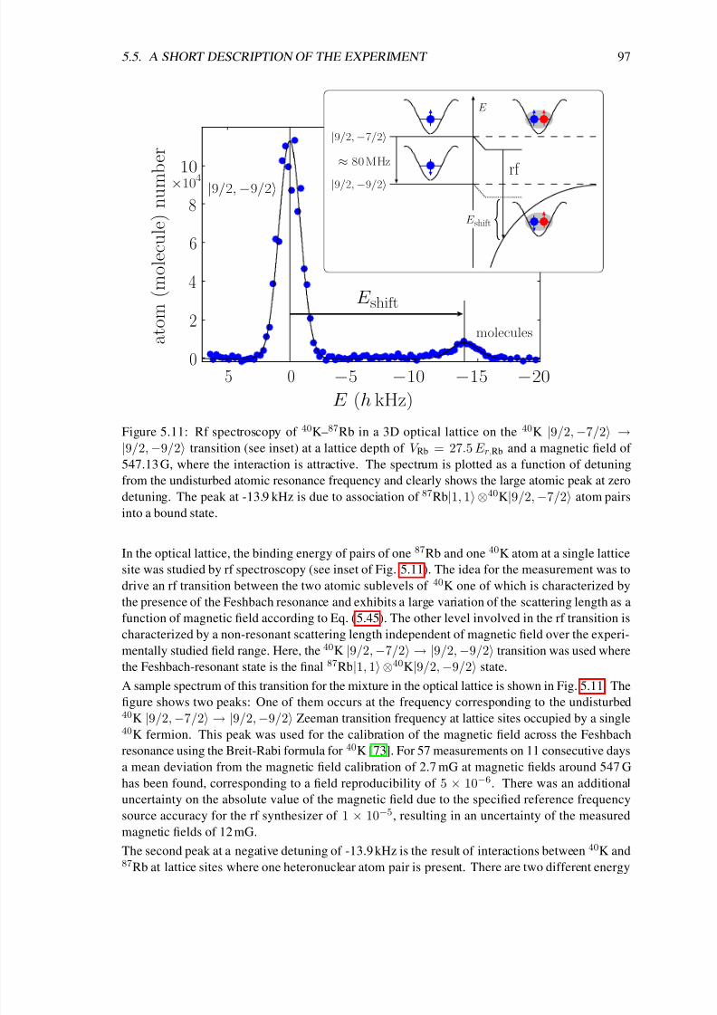
8/3/2019 Frank Deuretzbacher- Spinor Tonks-Girardeau gases and ultracold molecules
http://slidepdf.com/reader/full/frank-deuretzbacher-spinor-tonks-girardeau-gases-and-ultracold-molecules 107/151
5.5. A SHORT DESCRIPTION OF THE EXPERIMENT 97
molecules
|9/2,−9/2
5 00
−5 −10 −15 −20
a t o m
( m o l e c u l e ) n u m
b e r
2
4
6
8
10×104
E shift
E (h kHz)
E
E shift
rf
|9/2,−7/2
|9/2,−9/2
≈ 80MHz
Figure 5.11: Rf spectroscopy of 40K–87Rb in a 3D optical lattice on the 40K |9/2, −7/2 →|9/2, −9/2 transition (see inset) at a lattice depth of V Rb = 27.5 E r,Rb and a magnetic field of
547.13 G, where the interaction is attractive. The spectrum is plotted as a function of detuning
from the undisturbed atomic resonance frequency and clearly shows the large atomic peak at zero
detuning. The peak at -13.9 kHz is due to association of 87Rb|1, 1⊗40K|9/2, −7/2 atom pairs
into a bound state.
In the optical lattice, the binding energy of pairs of one 87Rb and one 40K atom at a single lattice
site was studied by rf spectroscopy (see inset of Fig. 5.11). The idea for the measurement was to
drive an rf transition between the two atomic sublevels of 40K one of which is characterized by
the presence of the Feshbach resonance and exhibits a large variation of the scattering length as a
function of magnetic field according to Eq. (5.45). The other level involved in the rf transition is
characterized by a non-resonant scattering length independent of magnetic field over the experi-
mentally studied field range. Here, the 40K |9/2, −7/2 → |9/2, −9/2 transition was used where
the Feshbach-resonant state is the final 87Rb|1, 1⊗40K|9/2, −9/2 state.
A sample spectrum of this transition for the mixture in the optical lattice is shown in Fig. 5.11. The
figure shows two peaks: One of them occurs at the frequency corresponding to the undisturbed40K |9/2, −7/2 → |9/2, −9/2 Zeeman transition frequency at lattice sites occupied by a single40K fermion. This peak was used for the calibration of the magnetic field across the Feshbach
resonance using the Breit-Rabi formula for 40K [73]. For 57 measurements on 11 consecutive days
a mean deviation from the magnetic field calibration of 2.7 mG at magnetic fields around 547 G
has been found, corresponding to a field reproducibility of 5 × 10⁻⁶. There was an additional
uncertainty on the absolute value of the magnetic field due to the specified reference frequency
source accuracy for the rf synthesizer of 1 × 10⁻⁵, resulting in an uncertainty of the measured
magnetic fields of 12 mG.
The second peak at a negative detuning of -13.9 kHz is the result of interactions between 40K and87Rb at lattice sites where one heteronuclear atom pair is present. There are two different energy

8/3/2019 Frank Deuretzbacher- Spinor Tonks-Girardeau gases and ultracold molecules
http://slidepdf.com/reader/full/frank-deuretzbacher-spinor-tonks-girardeau-gases-and-ultracold-molecules 108/151
98 CHAPTER 5. ULTRACOLD HETERONUCLEAR FESHBACH MOLECULES
shifts causing the observed separation of the peaks: One is the constant, small energy shift of the
initial 87Rb|1, 1⊗40K|9/2, −7/2 state which is independent of B, and the important, magnetic
field sensitive collisional shift which stems from the strong Feshbach-resonant interactions in the87Rb|1, 1⊗40K|9/2, −9/2 final state (inset of Fig. 5.11). In the specific example, the binding
energy of the final state increases the transition frequency as seen in Fig. 5.11.
In order to perform spectroscopy on the aforementioned transition, pulses with a gaussian ampli-
tude envelope (1/e2 full width of 400 µs and total pulse length of 800 µs) have been used, resulting
in an rf 1/e2 half linewidth of 1.7 kHz. The pulse power was chosen such as to achieve full trans-
fer on the single atom transition, i. e. rf pulse parameters including power are identical for all
magnetic fields.
5.6 Modeling of two interacting atoms at a single optical lattice site
Two interacting atoms in a harmonic trap: The Schrodinger equation of two atoms which in-
teract via a regularized δ potential and which are confined in a harmonic potential is given byi=1,2
−
2
2mi∆i +
1
2miω
2r2i
+
2π2asµ
δ(r)∂
∂rr
ψ(r1, r2) = Eψ(r1, r2).
Here, mi is the mass and ri is the position of atom i, ω is the angular frequency of the trap, asis the s-wave scattering length, µ = m1m2/M is the reduced mass, M = m1 + m2 is the total
mass, r = r1 − r2 is the relative position and r = |r1 − r2| is the distance between the atoms.
The first term consists of the kinetic and the potential energy of atom i and the second term is the
regularized δ potential which we have introduced in Sec. 5.3 in order to model the short-ranged
interaction between ultracold atoms. We introduce center-of-mass and relative coordinates
R = (m1r1 + m2r2)/M, r = r1 − r2 ⇔ r1 = R + m2r/M, r2 = R − m1r/M.
By inserting these relations into the above Schrodinger equation, we obtain− 2
2M ∆c.m. +
1
2M ω2R2 − 2
2µ∆rel +
1
2µω2r2 +
2π2asµ
δ(r)∂
∂rr
ψ( R, r) = Eψ( R, r).
We are looking for solutions that are separable into products
ψ( R, r) = ψc.m.( R)ψrel(r).
Putting this into the above equation, we obtain two separate equations for the center-of-mass andthe relative motion
− 2
2M ∆c.m. +
1
2M ω2R2
ψc.m.( R) = E c.m.ψc.m.( R),
−
2
2µ∆rel +
1
2µω2r2 +
2π2asµ
δ(r)∂
∂rr
ψrel(r) = E relψrel(r)
with E = E c.m. + E rel
which can be solved independent of each other. We express all lengths
of the center-of-mass and the relative motion in units of lc.m. =
/(M ω) and lrel =
/(µω)

8/3/2019 Frank Deuretzbacher- Spinor Tonks-Girardeau gases and ultracold molecules
http://slidepdf.com/reader/full/frank-deuretzbacher-spinor-tonks-girardeau-gases-and-ultracold-molecules 109/151
5.6. TWO INTERACTING ATOMS AT A SINGLE LATTICE SITE 99
respectively, and we express all energies in units of ω. The dimensionless Schrodinger equations
of the center-of-mass and the relative motion read−1
2
∆c.m. +
1
2
R2
ψc.m. =
E c.m.
ψc.m.,
−1
2
∆rel +
1
2
r2 + 2π
as
δ(
r)
∂
∂
r
r
ψrel =
E rel
ψrel.
Here, we have separated each quantity into a dimensionless quantity (which we mark by a tilde
symbol) and its unit: ∆c.m. = ∆c.m./l2c.m., R = R lc.m., ψc.m. = ψc.m./l3/2c.m., E c.m. = E c.m. ω,
∆rel = ∆rel/l2rel, r = r lrel, ψrel = ψrel/l3/2rel and E rel = E rel ω. In particular the scattering
length and the δ function are given by as = as lrel and δ = δ/l3rel. One can easily show that the
dimensionless equations are equivalent to the original ones. We keep these relations in mind but
throughout the following text I will always omit the tilde symbol.
Center-of-mass equation— The Schrodinger equation of a particle in a 3D rotationally symmetric
harmonic oscillator has to be solved. The spectrum is given by
E c.m. = 2N + L +3
2(5.46)
with N, L = 0, 1, 2, . . . . The associated eigenfunctions are given by
ψc.m. = RNL(R)Y LM (Θ, Φ)
with M = −L, −L + 1, . . . , L − 1, L . Y LM (Θ, Φ) are spherical harmonics (implemented as
“SphericalHarmonicY” in MATHEMATICA) and the radial eigenfunctions are given by
RNL(R) = ANLRL LL+1/2N (R2) e−R
2/2 (5.47)
with the normalization constant ANL = (2N !)/Γ(N + L + 3/2) and the generalized Laguerre
polynomials Lba (implemented as “LaguerreL” in MATHEMATICA). Alternatively one may also usethe confluent hypergeometric function of the first kind since 13
Lba(z) =
(a + b)!
a!b!1F 1(−a; b + 1; z).
The solution of the radial equation by means of a polynomial ansatz is given in Vol. 2 of Ref. [78].
Relative equation— Two cases have to be considered. In the case of nonzero relative angular mo-
mentum (l = 0) we obtain again the solutions of a 3D rotationally symmetric harmonic oscillatorbut now in units of ωrel and lrel
since the l = 0 wave functions do not feel the δ potential at the
origin. The energy spectrum is given by
E rel = 2n + l + 32
(l = 0) (5.48)
with n = 0, 1, 2, . . . and l = 1, 2, . . . . The associated eigenfunctions are given by
ψrel = Rnl(r)Y lm(θ, φ) (l = 0)
with m = −l, −l + 1, . . . , l − 1, l and
Rnl(r) = Anl rl Ll+1/2n (r2) e−r
2/2 (l = 0) (5.49)
13Eq. (13.128) of Ref. [105] / Wolfram MathWorld .

8/3/2019 Frank Deuretzbacher- Spinor Tonks-Girardeau gases and ultracold molecules
http://slidepdf.com/reader/full/frank-deuretzbacher-spinor-tonks-girardeau-gases-and-ultracold-molecules 110/151
100 CHAPTER 5. ULTRACOLD HETERONUCLEAR FESHBACH MOLECULES
0 421 30
0.3
0.6
0.9
(c)
0 421 3 5
0
0.4
0.8
−0.4
−0.8
0 421 3
0
0.4
0.8
−0.4
−0.8
(f)
0 421 3
0
0.4
0.8
−0.4
(e)
0 421 30
1
2
3 (a)
0 421 30
1
0.5
(d)
0 421 30
0.4
0.8
1.2
(b)
0
6
4
2
−2
−4
−60−4 4−2 2
as (lrel)
E r e l
( ¯ h ω
)
Figure 5.12: Energy spectrum (red) and eigenfunctions χrel = r ψrel (blue) of the l = 0 states.
Note the similarity to the wave functions of Fig. 5.6 outside the range R and to the energy spectrum
of the molecule of Fig. 5.7(right).
where Anl = (2n!)/Γ(n + l + 3/2) is again a normalization constant. In the case of zeroangular momentum (l = 0) the solutions have already been derived in Sec. 5.2. The energy
spectrum is determined by the equation
2Γ(3/4 − E rel/2)
Γ(1/4 − E rel/2)=
1
as(l = 0). (5.50)
It is convenient to define a non-integer effective harmonic oscillator quantum number ν by
E rel = 2ν + 3/2. The associated eigenfunctions are given by
ψrel = Rν (r) = Aν U −ν ;3
2; r2 e−r
2/2 (l = 0) (5.51)
where Aν is a normalization constant which we determine numerically
here, the spherical har-
monic Y 00 = 1/(2√
π) has been included into Aν
.
Energy spectrum (red) and associated wave functions (blue) of the l = 0 states are plotted in
Fig. 5.12. As has been discussed in Sec. 5.2, these wave functions agree with the solutions of a
realistic interaction potential outside the range R; see Fig. 5.6.
Let us move along the energy spectrum starting from the ground state of the noninteracting atomswave function (d), energy E rel = 3/2 ω
. If we increase the scattering length as from zero to
+∞, the wave function continuously transforms into the wave function (f) via (e). These wave
functions belong to repulsively interacting atoms. At as = +∞ these repulsively interacting
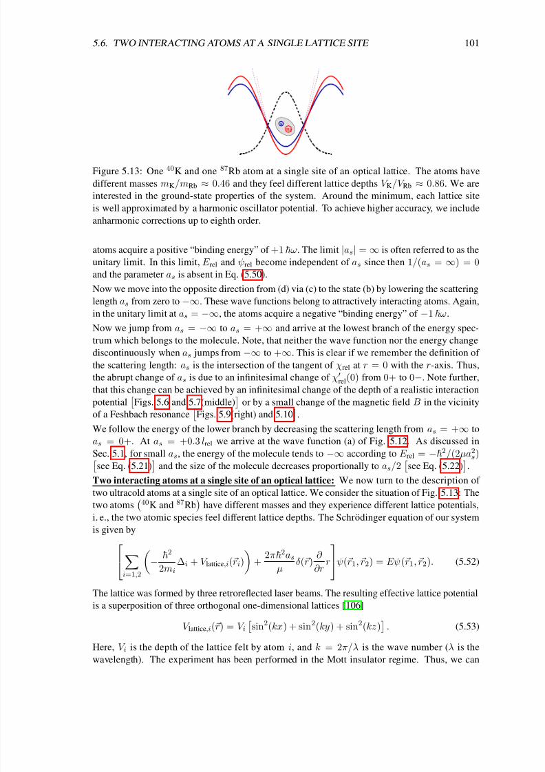
8/3/2019 Frank Deuretzbacher- Spinor Tonks-Girardeau gases and ultracold molecules
http://slidepdf.com/reader/full/frank-deuretzbacher-spinor-tonks-girardeau-gases-and-ultracold-molecules 111/151
5.6. TWO INTERACTING ATOMS AT A SINGLE LATTICE SITE 101
Rb
K
Figure 5.13: One 40K and one 87Rb atom at a single site of an optical lattice. The atoms have
different masses mK/mRb ≈ 0.46 and they feel different lattice depths V K/V Rb ≈ 0.86. We are
interested in the ground-state properties of the system. Around the minimum, each lattice site
is well approximated by a harmonic oscillator potential. To achieve higher accuracy, we include
anharmonic corrections up to eighth order.
atoms acquire a positive “binding energy” of +1 ω. The limit |as| = ∞ is often referred to as the
unitary limit. In this limit, E rel and ψrel become independent of as since then 1/(as =
∞) = 0
and the parameter as is absent in Eq. (5.50).
Now we move into the opposite direction from (d) via (c) to the state (b) by lowering the scattering
length as from zero to −∞. These wave functions belong to attractively interacting atoms. Again,
in the unitary limit at as = −∞, the atoms acquire a negative “binding energy” of −1 ω.
Now we jump from as = −∞ to as = +∞ and arrive at the lowest branch of the energy spec-
trum which belongs to the molecule. Note, that neither the wave function nor the energy change
discontinuously when as jumps from −∞ to +∞. This is clear if we remember the definition of
the scattering length: as is the intersection of the tangent of χrel at r = 0 with the r-axis. Thus,
the abrupt change of as is due to an infinitesimal change of χrel(0) from 0+ to 0−. Note further,
that this change can be achieved by an infinitesimal change of the depth of a realistic interaction
potential Figs. 5.6 and 5.7(middle) or by a small change of the magnetic field B in the vicinityof a Feshbach resonance Figs. 5.9(right) and 5.10.We follow the energy of the lower branch by decreasing the scattering length from as = +∞ to
as = 0+. At as = +0.3 lrel we arrive at the wave function (a) of Fig. 5.12. As discussed in
Sec. 5.1, for small as, the energy of the molecule tends to −∞ according to E rel = −2/(2µa2s)see Eq. (5.21)
and the size of the molecule decreases proportionally to as/2
see Eq. (5.22)
.
Two interacting atoms at a single site of an optical lattice: We now turn to the description of
two ultracold atoms at a single site of an optical lattice. We consider the situation of Fig. 5.13: The
two atoms40K and 87Rb
have different masses and they experience different lattice potentials,
i. e., the two atomic species feel different lattice depths. The Schrodinger equation of our system
is given byi=1,2
−
2
2mi∆i + V lattice,i(ri)
+
2π2asµ
δ(r)∂
∂rr
ψ(r1, r2) = Eψ(r1, r2). (5.52)
The lattice was formed by three retroreflected laser beams. The resulting effective lattice potential
is a superposition of three orthogonal one-dimensional lattices [106]
V lattice,i(r) = V i
sin2(kx) + sin2(ky) + sin2(kz)
. (5.53)
Here, V i is the depth of the lattice felt by atom i, and k = 2π/λ is the wave number (λ is the
wavelength). The experiment has been performed in the Mott insulator regime. Thus, we can

8/3/2019 Frank Deuretzbacher- Spinor Tonks-Girardeau gases and ultracold molecules
http://slidepdf.com/reader/full/frank-deuretzbacher-spinor-tonks-girardeau-gases-and-ultracold-molecules 112/151
102 CHAPTER 5. ULTRACOLD HETERONUCLEAR FESHBACH MOLECULES
neglect tunneling and we can restrict to the description of one atom pair at a single lattice site.
In order to make use of the known solution of two interacting atoms in a harmonic oscillator, we
perform a taylor expansion of the sin2 function around the origin:
sin2(kx) = k2x2
−k4
3
x4 +2k6
45
x6
−. . . .
By inserting this expansion into Eq. (5.53) we obtain
V lattice,i = V i
k2r2 − k4
3
x4 + y4 + z4
+
2k6
45
x6 + y6 + z6
− . . .
(5.54)
with r2 = x2 + y2 + z2. The first term of Eq. (5.54) gives rise to the harmonic approximation
through ωi =
2V ik2/mi, and the remainder gives rise to the anharmonic corrections V corr.. By
inserting Eq. (5.54) into Eq. (5.52) we obtaini=1,2−
2
2mi∆i +
1
2miω
2i r2i+
2π2asµ
δ(r)∂
∂rr + V corr.(r1, r2)
ψ(r1, r2) = Eψ(r1, r2)
where V corr. contains the higher-order terms of (V lattice,1 + V lattice,2). Again, we introduce center-
of-mass and relative coordinates and transform the above Schrodinger equation according to−
2
2M ∆c.m. +
1
2M ω2
c.m.R2 −
2
2µ∆rel +
1
2µω2
relr2 +
2π2asµ
δ(r)∂
∂rr
+µ∆ω2r · R + V corr.( R, r)
ψ( R, r) = Eψ( R, r) (5.55)
where we have defined the frequencies
ωc.m. ≡ m1ω21 + m2ω
22
m1 + m2, ωrel ≡ m2ω
21 + m1ω
22
m1 + m2, and ∆ω ≡ ω2
1 − ω22 . (5.56)
In the previous case both particles felt the same trap frequency ω = ω1 = ω2 and thus
ωc.m. = ωrel = ω and ∆ω = 0. In this case, however, both atoms feel different trap frequencies
ω1 = ω2 and thus ωc.m. = ωrel and ∆ω = 0. Therefore, the first effect of the different trap fre-
quencies ω1 = ω2 is that not only the length scales lc.m. = /(M ωc.m.) and lrel =
/(µωrel)
but also the energy scales ωc.m. and ωrel of the center-of-mass and the relative motion are dif-
ferent. The second effect of the different trap frequencies ω1 = ω2 is that the center-of-mass and
the relative motion are coupled through µ∆ω2r · R. Moreover, the center-of-mass and the rela-
tive motion are coupled due to the anharmonic corrections V corr.( R, r). Since the problem is no
longer separable, there exists no exact analytical solution of Eq. (5.55). Therefore, we perform a
numerically exact diagonalization of the Hamiltonian H = H c.m. + H rel + H couple of Eq. (5.55) by
using the energetically lowest eigenfunctions of the decoupled problem H 0 = H c.m. + H rel. We
expect convergence with rather small matrices since the main contribution to the total energy of
the lowest states (especially the strong interaction) is already included in the diagonal part of H .
Exact diagonalization of the Hamiltonian— The basis functions of the diagonalization are given
by the eigenfunctions of the decoupled problem H 0 = H c.m. + H rel
see Eqs. (5.47), (5.49) and
(5.51); note that the interaction is already included in H 0
R, r
N ,L,M,n,l ,m; as
= RNL(R)Y LM (Θ, Φ)
Rν (as,n)(r) if l = 0
Rnl(r)Y lm(θ, φ) if l = 0 .
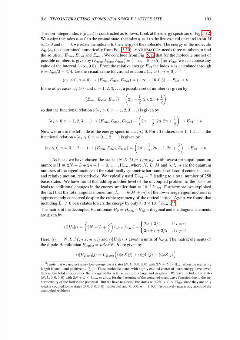
8/3/2019 Frank Deuretzbacher- Spinor Tonks-Girardeau gases and ultracold molecules
http://slidepdf.com/reader/full/frank-deuretzbacher-spinor-tonks-girardeau-gases-and-ultracold-molecules 113/151
5.6. TWO INTERACTING ATOMS AT A SINGLE LATTICE SITE 103
The non-integer index ν (as, n) is constructed as follows: Look at the energy spectrum of Fig. 5.12.
We assign the index n = 0 to the ground state, the index n = 1 to the first excited state and so on. If
as > 0 and n = 0, we relate the index ν to the energy of the molecule. The energy of the molecule
E rel(as) is determined numerically from Eq. (5.50). MATHEMATICA needs three numbers to find
the solution: E min, E start and E max. We conclude from Fig. 5.12 that for the molecule one set of
possible numbers is given by (E min, E start, E max) = (−∞, −10, 0.5) for E start we can choose anyvalue of the interval (−∞, 0.5)
. From the relative energy E rel the index ν is calculated through
ν = E rel/2 − 3/4. Let me visualize the functional relation ν (as > 0, n = 0):
(as > 0, n = 0) → (E min, E start, E max) = (−∞, −10, 0.5) → E rel → ν.
In the other cases, as > 0 and n = 1, 2, 3, . . . , a possible set of numbers is given by
(E min, E start, E max) =
2n − 1
2, 2n, 2n +
1
2
so that the functional relation ν (as > 0, n = 1, 2, 3, . . .) is given by
(as > 0, n = 1, 2, 3, . . .) → (E min, E start, E max) = 2n − 12
, 2n, 2n + 12 → E rel → ν.
Now we turn to the left side of the energy spectrum, as 0. For all indices n = 0, 1, 2, . . . , the
functional relation ν (as 0, n = 0, 1, 2, . . .) is given by
(as 0, n = 0, 1, 2, . . .) → (E min, E start, E max) =
2n +
1
2, 2n + 1, 2n +
3
2
→ E rel → ν.
As basis we have chosen the states |N ,L,M,n,l ,m; as with lowest principal quantum
numbers Π ≡ 2N + L + 2n + l = 0, 1, ..., Πmax, where N , L, M and n, l, m are the quantum
numbers of the eigenfunctions of the rotationally symmetric harmonic oscillator of center-of-mass
and relative motion, respectively. We typically used Πmax = 7 leading to a total number of 258
basis states. We have found that adding another level of the uncoupled problem to the basis set
leads to additional changes in the energy smaller than ≈ 10−3 ωrel. Furthermore, we exploited
the fact that the total angular momentum Lz = (M + m) of the low-energy eigenfunctions is
approximately conserved despite the cubic symmetry of the optical lattice. Again, we found that
including Lz = 0 basis states lowers the energy by only ≈ 3 × 10⁻³ωrel.
14
The matrix of the decoupled Hamiltonian H 0 = H c.m. +H rel is diagonal and the diagonal elements
are given by
i|H 0|i =
2N + L +
3
2
(ωc.m./ωrel) +
2ν + 3/2 if l = 0
2n + l + 3/2 if l = 0 .
Here, |i = |N ,L,M,n,l ,m; as and i|H 0|i is given in units of ωrel. The matrix elements of the dipole Hamiltonian H dipole = µ∆ω2r · R are given by
i|H dipole| j = C dipole
i|xX | j + i|yY | j + i|zZ | j
14I note that we neglect many low-energy basis states |N,L, 0, 0, 0, 0 with 2N + L > Πmax when the scattering
length is small and positive as 0. These molecule states with highly excited center-of-mass energy have never-
theless low total energy since the energy of the relative motion is large and negative. We have included the states
|N,L, 0, 0, 0, 0 with 2N + L ≤ Πmax to allow for the flattening of the center-of-mass wave function due to the an-
harmonicity of the lattice site potential. But we have neglected the states with 2N + L > Πmax since they are only
weakly coupled to the states |0, 0, 0, 0, 0, 0 (molecule) and |0, 0, 0, n = 1, 0, 0 (repulsively interacting atoms of the
decoupled problem).

8/3/2019 Frank Deuretzbacher- Spinor Tonks-Girardeau gases and ultracold molecules
http://slidepdf.com/reader/full/frank-deuretzbacher-spinor-tonks-girardeau-gases-and-ultracold-molecules 114/151
104 CHAPTER 5. ULTRACOLD HETERONUCLEAR FESHBACH MOLECULES
where the coupling constant C dipole is calculated according to
C dipole = µ∆ω2lrellc.m. = ∆ω2 lc.m. µl2relω
2rel = ∆ω
2 lc.m. ωrel
with lc.m. = lc.m./lrel and ∆ω = ∆ω/ωrel. The integrals
i
|xX
| j
, . . . are calculated further below.
Let me first calculate the energy and length scales for a typical set of experimental pa-
rameters: A typical lattice depth, felt by the 87Rb atoms, was chosen to be V Rb = 40.5 E r,Rb
where E r,Rb = 2k2/(2mRb) = h2/(2mRbλ2) is the 87Rb recoil energy. For λ = 1.03 µm
we obtain E r,Rb ≈ 2.16 hkHz and V Rb ≈ 86.6 hkHz (see appendix D for the masses of 87Rb
and 40K). The lattice depth of 40K was a little bit shallower, V K = 0.86 V Rb ≈ 74.8 hkHz.
In the harmonic approximation of one lattice well, the angular trap frequencies are given by
ωRb =
2V Rbk2/mRb = 4π√
40.5 E r,Rb/h ≈ 2π × 27.4 kHz and ωK ≈ 87/40 · 0.86 ωRb
1.37 ωRb ≈ 2π × 37.5 kHz. A comparison of these frequencies with the accordant lattice depths
V Rb/(ωRb) = 86.6/27.4 ≈ 3.2 and V K/(ωK) = 74.8/37.5 ≈ 2 shows that, for the 87Rb atom,
the lattice depth is larger than the energy of the first excited state, while, for the 40K atom, the lat-
tice depth is larger than the ground-state energy of the harmonic oscillator. According to Eq. ( 5.56)
the angular frequencies of the relative and the center-of-mass motion are given by
ωrel ≈ 2π ×
87 · 37.52 + 40 · 27.42
40 + 87kHz ≈ 2π × 34.6 kHz
and
ωc.m. ≈ 2π ×
87 · 27.42 + 40 · 37.52
40 + 87kHz 0.89 ωrel .
The frequency difference ∆ω is given by
∆ω ≈
1.372 − 1(27.4/34.6) ωrel 0.74 ωrel .
The oscillator lengths of the relative and the center-of-mass motion are given by
lrel =
µωrel
≈
1.055 · 10−34(40 + 87)
40 · 87 · 1.66 · 10−27 · 2π · 34.6 · 103m ≈ 103 nm
and
lc.m. =
M ωc.m.
≈
87 · 40
(87 + 40)2 · 0.89lrel 0.49 lrel .
The dipole coupling constant is therefore given by
C dipole ≈ 0.742
· 0.49 ωrel 0.27 ωrel .
Now we turn to the calculation of the integrals i|xX | j, . . . . The dimensionless dipole
integrals i|xX | j, . . . have been calculated in spherical coordinates
i|xX | j = N, L|R|N , LL, M | sinΘcosΦ|L, M ×n, l; as|r|n, l; asl, m| sin θ cos φ|l, m
with similar expressions for i|yY | j and i|zZ | j spherical coordinates: x = r sin θ cos φ, y =r sin θ sin φ and z = r cos θ
. The integrals N, L|R|N , L, L, M | sinΘcosΦ|L, M , n, l =
0; as|r|n, l = 0; as and l, m| sin θ cos φ|l, m have been calculated analytically by means

8/3/2019 Frank Deuretzbacher- Spinor Tonks-Girardeau gases and ultracold molecules
http://slidepdf.com/reader/full/frank-deuretzbacher-spinor-tonks-girardeau-gases-and-ultracold-molecules 115/151
5.6. TWO INTERACTING ATOMS AT A SINGLE LATTICE SITE 105
+ hωrel
− hωrel
−3 −2 −1
0
1 2 3 4
1
2
3
4
5
−1
−2
−30
−4
3/2 (hωcm + hωrel)
3/2 hωcm
as (lrel)
E
( ¯ h ω r e l )
lattice siteand ∆ω = 0
harmonic trapand ∆ω = 0
Figure 5.14: Energy eigenvalues of 40K and 87Rb as a function of the scattering length without
(black dashed line) and with coupling terms (blue solid line) due to the anharmonicity and the
unequal trap frequencies of the lattice for parameters: V Rb = 40.5 E r,Rb, V K = 0.86 V Rb and
λ = 1030 nm. The deviation between the idealized model and the full solution is substantial in
particular for the upper branch.
of the “Integrate” function of MATHEMATICA. Only the integrals n, l = 0; as|r|n, l = 0; asor n, l = 0; as|r|n, l = 0; as have been calculated numerically by means of the “NIntegrate”function of MATHEMATICA. Analytic formulas for the radial integrals are given in Ref. [ 98]. We did
not care about further simplifications since the calculation of the comparatively small Hamiltonian
matrix was sufficiently fast anyway. However, it turns out that the dipole Hamiltonian H dipole does
not contribute to the diagonal elements of H . Therefore, the energy shift, caused by H dipole, was
comparatively small in the deep optical lattice with V Rb = 40.5 E r,Rb.
Now we consider the calculation of the matrix elements of the anharmonic corrections i|V corr.| j.
Since x1 = X + ax and x2 = X − bx with a ≡ m2/M and b ≡ m1/M , the x-dependent part of
the anharmonic corrections V (x)
corr. transforms to
V (x)
corr. =
−k4
3
(V 1x41 + V 2x4
2) + . . . =
−V 1 + V 2
3
k4X 4
−4(V 1a − V 2b)
3
k4xX 3
−2(V 1a2 + V 2b2)k4x2X 2 − 4(V 1a3 − V 2b3)
3k4x3X − V 1a4 + V 2b4
3k4x4 + . . . .
Corresponding expressions are obtained for the y- and z-direction, V (y)
corr. and V (z)
corr.. The transfor-
mation of the anharmonic corrections into center-of-mass and relative coordinates has been done
automatically by means of the algebraic-formula-manipulation functions “Expand” and “Collect”
of MATHEMATICA. Again, the calculation of the matrix elements of the anharmonic corrections
has been performed in spherical coordinates. In the numerical implementation, we have tested
for convergence with terms up to eighth order. We found that including eighth-order corrections
improve the accuracy of the calculation by only ≈ 3 × 10⁻³ωrel.

8/3/2019 Frank Deuretzbacher- Spinor Tonks-Girardeau gases and ultracold molecules
http://slidepdf.com/reader/full/frank-deuretzbacher-spinor-tonks-girardeau-gases-and-ultracold-molecules 116/151
106 CHAPTER 5. ULTRACOLD HETERONUCLEAR FESHBACH MOLECULES
−3 −2 −1
0
1 2 3 4
1
2
3
4
5
−1
−2
−30−4
molecule
atoms
repulsively interacting
atomsattractively interacting
as (lrel)
E
( ¯ h ω r e l )
lattice siteand ∆ω = 0
harmonic trapand ∆ω = 0
Figure 5.15: Low-energy spectrum of the states with a center-of-mass energy 3/2 ωc.m. for 6Li
and 133Cs and the lattice parameters V Li = V Cs = 10 2k2/2µ and λ = 1 µm. The energy is
much more lowered compared to the case of 40K and 87Rb since the mass of the 6Li atom is much
smaller than the mass of the 133Cs atom.
Once the Hamiltonian matrix has been calculated, we diagonalize it numerically by means of the
function “Eigensystem” of MATHEMATICA. The resulting eigenvectors
c(0,0,0,0,0,0), . . .
are the
coefficients of the expansion
|ψ =
N,L,M,n,l,m
c(N,L,M,n,l,m)|N ,L,M,n,l ,m; as
and the corresponding eigenvalues E |ψ are the desired eigenenergies of the interacting atoms at
a single lattice site. The wave function |ψ0 with the lowest energy E 0 belongs to the molecule if
as > 0 and to the attractively interacting atoms if as 0, respectively. For as 0, there are many
molecular wave functions with a highly excited center-of-mass energy. To determine the wave
function of the repulsively interacting atoms, we search for the state withc(0,0,0,1,0,0) 0.5.
Energy spectrum— Fig. 5.14 shows the resulting energy spectrum (blue solid line) compared to
the uncoupled solution (black dashed line), calculated for 40K and 87Rb with the experimental
parameters of Ref. [72]: V Rb = 40.5 E r,Rb, V K = 0.86 V Rb, and λ = 1030 nm. In the case of
heteronuclear atom pairs it is useful to express the lattice depth in units of E r,rel = 2k2/2µ,
which is the kinetic energy given to a particle with reduced mass µ by a photon of momentum k.
Then, V Rb = 40.5 E r,Rb = 12.6 E r,rel. As can be seen from the figure, the deviation between the
idealized model, where the coupling term has been neglected, and the full solution is substantial.
The difference is most pronounced in the repulsively interacting pair branch ( 0.34 ωrel ≈ 20%
of the level spacing) and becomes smaller as we enter the attractively-interacting-atom part of the
spectrum. The molecular branch is relatively unaffected by the coupling term H couple. This is
natural because as we approach a → +0, the role of the external confinement decreases since the
molecule becomes smaller.
The influence of the coupling term H couple is even stronger if we consider molecules with large

8/3/2019 Frank Deuretzbacher- Spinor Tonks-Girardeau gases and ultracold molecules
http://slidepdf.com/reader/full/frank-deuretzbacher-spinor-tonks-girardeau-gases-and-ultracold-molecules 117/151
5.7. EXPERIMENTAL VS. THEORETICAL SPECTRUM. RESONANCE POSITION 107
atom pair E 0 ∆E dipole ∆E corr. ∆E 40K and 87Rb 3.74 -0.12 (29%) -0.27 (71%) -0.396Li and 133Cs 2.88 -0.35 (62%) -0.22 (38%) -0.576Li and 87Rb 2.99 -0.36 (61%) -0.22 (39%) -0.586Li and 40K 3.24 -0.31 (58%) -0.24 (42%) -0.556Li and 7Li 3.92 -0.01 (2%) -0.29 (98%) -0.30
Table 5.1: Influence of the individual coupling terms H dipole and V corr. on the total energy of several
atom pairs. The energies are given in units of ωrel. All values are calculated at as = 4 lrel for
lattice depths of V 1 = V 2 = 10 E r,rel and a wavelength of λ = 1 µm. E 0 = E c.m. + E rel is the
energy of the uncoupled Hamiltonian. Including H dipole into the Hamiltonian reduces the energy
by ∆E dipole and including H dipole + V corr. reduces the energy further by ∆E corr.. The value in
brackets is the percentage contribution of the individual coupling terms to the total change of the
energy ∆E .
mass ratios as in the case of 6Li and 133Cs, see Fig. 5.15. We have chosen the lattice parameters
V Li = V Cs = 10 E r,rel and λ = 1 µm. Here, the energy of the repulsively interacting atoms is
lowered by up to ≈ 0.6 ωrel.
Table 5.1 shows the effect of the individual coupling terms H dipole and V corr. on the energy of
several atom pairs. The energies have been calculated for repulsively interacting atoms at as =4 lrel which is the largest scattering length shown in Figs. 5.14 and 5.15. All the energies of
Table 5.1 are given in units of the level spacing of the relative motion ωrel. Adding the coupling
term H dipole contributes up to 62% to the total change ∆E for 6Li and 133Cs. The strong influence
of H dipole stems from the large mass ratio which results in extremely different trap frequencies ωLi
and ωCs. By contrast, the energy of 6Li and 7Li atoms is nearly not affected by H dipole since the
trap frequencies are almost equal.
5.7 Experimental vs. theoretical spectrum. Resonance position
Next, we compare the calculated energy spectrum of Fig. 5.14 to the measured binding energy
of Ref. [72]. From rf spectra as in Fig. 5.11, the separation between the single atom and the
two-particle (“molecular”) peak has been determined with high precision (typical uncertainty of
250 Hz). From the separation of the two peaks the binding energy has been extracted up to a
constant offset due to nonzero background scattering lengths. At the same time, the atomic peak
was used for a precise magnetic field calibration as described in Sec. 5.5. Spectra as in Fig. 5.11
have been recorded for magnetic field values across the whole resonance and yield the energyspectrum as a function of magnetic field.
Fig. 5.16 shows the measured energy shift across the resonance at a lattice depth of 40.5 E r,Rb as a
function of magnetic field. The energy shift is obtained from Fig. 5.14 by subtracting the motional
energy of the initial 87Rb|1, 1⊗40K|9/2, −7/2 state: E shift = E − E (a−7/2 = −175 aB). 15
In addition, Figs. 5.16 and 5.14 are connected through Eq. (5.45). One branch of the spectrum
is characterized by the presence of a positive “binding energy”, the repulsively interacting pair
branch. In Fig. 5.14, we have seen that this branch continuously transforms into attractively in-
15For the scattering length in the initial 87Rb|1, 1 ⊗40K|9/2, −7/2 state in the considered magnetic field range
544 G < B < 549 G we take the value −175aB [107].
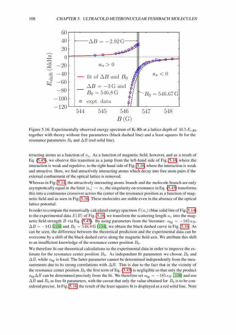
8/3/2019 Frank Deuretzbacher- Spinor Tonks-Girardeau gases and ultracold molecules
http://slidepdf.com/reader/full/frank-deuretzbacher-spinor-tonks-girardeau-gases-and-ultracold-molecules 118/151
108 CHAPTER 5. ULTRACOLD HETERONUCLEAR FESHBACH MOLECULES
544 545 546 547 548−120
−100
−80
−60
−40
−200
20
40
60
fit of ∆B and B0
expt. data
∆B = −3 G andB0 = 546.8 G B0 = 546.67 G
as < 0
as > 0
B (G)
E s h i f t ( h k H
z )
∆B = −2.92 G
Figure 5.16: Experimentally observed energy spectrum of K–Rb at a lattice depth of 40.5 E r,Rb
together with theory without free parameters (black dashed line) and a least squares fit for the
resonance parameters B0 and ∆B (red solid line).
teracting atoms as a function of as. As a function of magnetic field, however, and as a result of
Eq. (5.45), we observe this transition as a jump from the left-hand side of Fig. 5.16, where the
interaction is weak and repulsive, to the right-hand side of Fig. 5.16, where the interaction is weak
and attractive. Here, we find attractively interacting atoms which decay into free atom pairs if the
external confinement of the optical lattice is removed.
Whereas in Fig. 5.14, the attractively interacting atoms branch and the molecule branch are only
asymptotically equal in the limit |as| → ∞, the singularity on resonance in Eq. (5.45) transforms
this into a continuous crossover across the center of the resonance position as a function of mag-
netic field and as seen in Fig. 5.16. These molecules are stable even in the absence of the optical
lattice potential.
In order to compare the numerically calculated energy spectrum E (as) (blue solid line of Fig. 5.14)
to the experimental data E (B) of Fig. 5.16, we transform the scattering length as into the mag-
netic field strength B via Eq. (5.45). By using parameters from the literature: abg = −185 aB,
∆B = −3 G [108] and B0 = 546.8 G [104], we obtain the black dashed curve in Fig. 5.16. As
can be seen, the difference between the theoretical prediction and the experimental data can be
overcome by a shift of the black dashed curve along the magnetic field axis. We attribute this shift
to an insufficient knowledge of the resonance center position B0.
We therefore fit our theoretical calculations to the experimental data in order to improve the es-
timate for the resonance center position B0. As independent fit parameters we choose B0 and
∆B, while abg is fixed. The latter parameter cannot be determined independently from the mea-
surements due to its strong correlations with ∆B. This is due to the fact that in the vicinity of
the resonance center position B0 the first term of Eq. (5.45) is negligible so that only the product
abg∆B can be determined precisely from the fit. We therefore set abg = −185 aB [108] and use
∆B and B0 as free fit parameters, with the caveat that only the value obtained for B0 is to be con-
sidered precise. In Fig. 5.16, the result of the least squares fit is displayed as a red solid line. Note
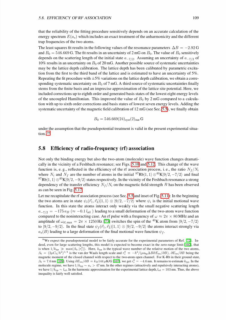
8/3/2019 Frank Deuretzbacher- Spinor Tonks-Girardeau gases and ultracold molecules
http://slidepdf.com/reader/full/frank-deuretzbacher-spinor-tonks-girardeau-gases-and-ultracold-molecules 119/151
5.8. EFFICIENCY OF RF ASSOCIATION 109
that the reliability of the fitting procedure sensitively depends on an accurate calculation of the
energy spectrum E (as) which includes an exact treatment of the anharmonicity and the different
trap frequencies of the two atoms.
The least squares fit results in the following values of the resonance parameters ∆B = −2.92 G
and B0 = 546.669 G. The fit results in an uncertainty of 2 mG on B0. The value of B0 sensitively
depends on the scattering length of the initial state a−7/2. Assuming an uncertainty of a−7/2 of
10% results in an uncertainty on B0 of 20 mG. Another possible source of systematic uncertainties
may be the lattice depth calibration. The lattice depth has been calibrated by parametric excita-
tion from the first to the third band of the lattice and is estimated to have an uncertainty of 5%.
Repeating the fit procedure with ±5% variations on the lattice depth calibration, we obtain a corre-
sponding systematic uncertainty on B0 of 7 mG. A third source of systematic uncertainties finally
stems from the finite basis and an imprecise approximation of the lattice site potential. Here, we
included corrections up to eighth order and generated basis states of the lowest eight energy levels
of the uncoupled Hamiltonian. This improved the value of B0 by 2 mG compared to a calcula-
tion with up to sixth order corrections and basis states of lowest seven energy levels. Adding the
systematic uncertainty of the magnetic field calibration of 12 mG (see Sec. 5.5), we finally obtain
B0 = 546.669(24)syst(2)stat G
under the assumption that the pseudopotential treatment is valid in the present experimental situa-
tion. 16
5.8 Efficiency of radio-frequency (rf) association
Not only the binding energy but also the two-atom (molecule) wave function changes dramati-
cally in the vicinity of a Feshbach resonance; see Figs. 5.10 and 5.12. This change of the wave
function is, e. g., reflected in the efficiency of the rf association process, i. e., the ratio N f /N iwhere N i and N f are the number of atoms in the initial 87Rb|1, 1⊗40K|9/2, −7/2 and final87Rb|1, 1⊗40K|9/2, −9/2 states respectively. In the vicinity of the Feshbach resonance a strong
dependency of the transfer efficiency N f /N i on the magnetic field strength B has been observed
as can be seen in Fig. 5.17.
Let me recapitulate the rf association process (see Sec. 5.5 and inset of Fig. 5.11): In the beginning
the two atoms are in state ψi(r1, r2)|1, 1 ⊗ |9/2, −7/2 where ψi is the initial motional wave
function. In this state the atoms interact only weakly via the small negative scattering length
a−7/2 = −175 aB (≈ −0.1 lrel ) leading to a small deformation of the two-atom wave function
compared to the noninteracting case. An rf pulse with a frequency of ω ≈ 2π × 80 MHz and an
amplitude of ωrf, max = 2π×
1250 Hz [73] switches the spin of the 40K atom from
|9/2,
−7/2
to |9/2, −9/2. In the final state ψf (r1, r2)|1, 1 ⊗ |9/2, −9/2 the atoms interact strongly via
as(B) leading to a large deformation of the final motional wave function ψf .
16We expect the pseudopotential model to be fairly accurate for the experimental parameters of Ref. [72]. In-
deed, even for large scattering lengths, this model is expected to become exact in the zero-range limit [102], that
is when 1/ktyp max(β 6, |r0e |). Here, ktyp is the typical wave number of the relative motion of the two atoms,
β 6 = (2µC 6/2)1/4 is the van der Waals length scale and r0e ≡ −2/(µabg∆B∂ E res/∂B ), ∂E res/∂B being the
magnetic moment of the closed channel with respect to the two-atom open channel. For K-Rb in their ground state,
β 6 = 7.6 nm [109]. Using ∂E res/∂B = kB144 µK/G [107], we get r0e = −4.6 nm. It remains to estimate ktyp. In the
molecule regime, we have 1/ktyp ∼ as > 47 nm. In the other regimes (attractively and repulsively interacting atoms),
we have 1/ktyp ∼ lrel. In the harmonic approximation for the experimental lattice depth, lrel = 103 nm. Thus, the above
inequality is fairly well satisfied.
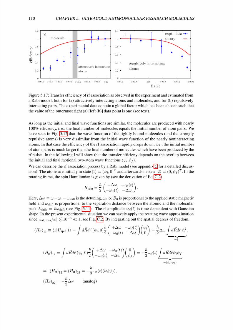
8/3/2019 Frank Deuretzbacher- Spinor Tonks-Girardeau gases and ultracold molecules
http://slidepdf.com/reader/full/frank-deuretzbacher-spinor-tonks-girardeau-gases-and-ultracold-molecules 120/151
110 CHAPTER 5. ULTRACOLD HETERONUCLEAR FESHBACH MOLECULES
e ffi c i e n c y
546.3 546.4 546.5 546.6 546.7 546.8 546.9 5470
0.2
0.4
0.6
0.8
1
1.2
molecule
attractively interacting
atoms
(a) expt. data
theory
545.6 545.8 546 546.2 546.4 546.6
0.2
0.4
0.6
0.8
1
B (G)
repulsively interacting
atoms
0
1.2
(b)
Figure 5.17: Transfer efficiency of rf association as observed in the experiment and estimated from
a Rabi model, both for (a) attractively interacting atoms and molecules, and for (b) repulsively
interacting pairs. The experimental data contain a global factor which has been chosen such that
the value of the outermost right (a) [left (b)] data point is one (see text).
As long as the initial and final wave functions are similar, the molecules are produced with nearly
100% efficiency, i. e., the final number of molecules equals the initial number of atom pairs. We
have seen in Fig. 5.12 that the wave function of the tightly bound molecules (and the strongly
repulsive atoms) is very dissimilar from the initial wave function of the nearly noninteracting
atoms. In that case the efficiency of the rf association rapidly drops down, i. e., the initial number
of atom pairs is much larger than the final number of molecules which have been produced by the
rf pulse. In the following I will show that the transfer efficieny depends on the overlap between
the initial and final motional two-atom wave functions ψi|ψf .
We can describe the rf association process by a Rabi model (see appendix C for a detailed discus-
sion): The atoms are initially in state |1 ≡ (ψi, 0)T
and afterwards in state |2 ≡ (0, ψf )T
. In therotating frame, the spin Hamiltonian is given by (see the derivation of Eq. C.2)
H spin =
2
+∆ω −ωrf (t)
−ωrf (t) −∆ω
.
Here, ∆ω ≡ ω −ω0−ωshift is the detuning, ω0 ∝ B0 is proportional to the applied static magnetic
field and ωshift is proportional to the separation distance between the atomic and the molecular
peak E shift = ωshift (see Fig. 5.11). The rf amplitude ωrf (t) is time-dependent with Gaussian
shape. In the present experimental situation we can savely apply the rotating wave approximation
since |ωrf, max/ω| 10−3 1; see Fig. C.2. By integrating out the spatial degrees of freedom,
(H rf )11 ≡ 1|H spin|1 = d Rdr (ψi, 0)
2 +∆ω
−ωrf (t)
−ωrf (t) −∆ω ψi0 =
2 ∆ω d Rdr ψ2
i =1
,
(H rf )12 =
d Rdr (ψi, 0)
2
+∆ω −ωrf (t)
−ωrf (t) −∆ω
0
ψf
= −
2ωrf (t)
d Rdrψiψf =ψi|ψf
⇒ (H rf )12 = (H rf )21 = −
2ωrf (t)ψi|ψf ,
(H rf )22 = −
2∆ω (analog)

8/3/2019 Frank Deuretzbacher- Spinor Tonks-Girardeau gases and ultracold molecules
http://slidepdf.com/reader/full/frank-deuretzbacher-spinor-tonks-girardeau-gases-and-ultracold-molecules 121/151
5.8. EFFICIENCY OF RF ASSOCIATION 111
we obtain the effective Hamiltonian
H rf =
2
+∆ω −ωrf (t)ψi|ψf
−ωrf (t)ψi|ψf −∆ω
. (5.57)
As can be seen, the off-diagonal elements of Hamiltonian (5.57) are not only proportional to the
rf amplitude ωrf (t), but also to the overlap integral ψi|ψf . Therefore, the transfer probabilitybetween states |1 and |2 corresponds to Rabi flopping with a Rabi frequency reduced by the
overlap integral of ψi and ψf compared to the pure atomic transition.
Exactly on the molecular resonance, we have ω = ω0 + ωshift (→ ∆ω = 0). The on-resonant
result for the transfer probability (efficiency) is thus given by
see Eq. (C.7)
N f /N i = P 1→2 = sin2
1
2ψi|ψf
t0
ωrf (t)dt
(5.58)
which is unity for a transfer between atomic states, where ψi = ψf , when setting the area under the
ωrf (t) curve to
t0 ωrf (t)dt = π. For transfer into the molecular state, the probability decreases
as a function of the wave function overlap integral since the molecular final orbital wave functionbecomes more and more dissimilar from the initial two-body atomic wave function.
In the experiment, the molecules were associated using rf pulses designed to induce a π pulse for
the noninteracting atoms: t0 ωrf (t) dt = π. This π pulse has been kept fixed over the entire range
of magnetic field values investigated. The experimental association efficiency is determined from
the height of the molecular peak (see Fig. 5.11) as a function of magnetic field for constant pulse
parameters and ω = ω0 + ωshift (→ ∆ω = 0) as in the theory above.
Figs. 5.17(a) and 5.17(b) show a comparison between the conversion efficiency as extracted from
the experimental data and the theoretical estimate from equation (5.58). Theory and experiment
show the general trend of dropping association efficiency with increasing binding energy when
the initial and final wave functions become more and more dissimilar. In this context, we define
the experimental conversion efficiency as the ratio of the number of molecules created and theinitial lattice sites which are occupied by exactly one K and one Rb atom. Note that only on these
lattice sites molecules can be created. For the comparison of experimental and theoretical transfer
efficiency, the experimental data have been scaled by a global factor to reproduce a conversion
efficiency of 1 far off the Feshbach resonance where initial and final two-body wave function are
equal. This is necessary, because the initial lattice sites occupied by one K and one Rb atom have
not been determined experimentally.
While the experiments presented here were performed at constant rf pulse parameters, it should
be possible from the above arguments to increase either pulse power or duration or both of the rf
pulse to account for the reduced wave function overlap and thereby always obtain an efficiency of
1. In particular, it should be possible to drive Rabi oscillations between atoms and molecules in a
very similar way as recently demonstrated [110].
The comparison indicates that in the case of association efficiency a better quantitative agreement
might require a two-level Feshbach-resonance model like that of Sec. 5.4. 17 This is in contrast to
the analysis of binding energies and lifetimes (see below), where the good quantitiative agreement
shows that here the δ interaction approximation and the single-channel model of the Feshbach
resonance capture the essential physics. Testing the Rabi oscillation hypothesis for molecules
with rf might provide further insight.
17Using the superposition wave functions of Fig. 5.10 instead would possibly give better results. However, for that
purpose I need to know the parameters ∆(B) and V c of the Hamiltonian matrix (5.44) as well as the scattering length
of the molecular wave function.
8/3/2019 Frank Deuretzbacher- Spinor Tonks-Girardeau gases and ultracold molecules
http://slidepdf.com/reader/full/frank-deuretzbacher-spinor-tonks-girardeau-gases-and-ultracold-molecules 122/151
112 CHAPTER 5. ULTRACOLD HETERONUCLEAR FESHBACH MOLECULES
Figure 5.18: Sketch of expected lattice occupation. The arrows illustrate tunneling of remain-
ing fermionic 40K atoms to the “molecular” shell where they can undergo inelastic three-body
collisions with a 40K-87Rb molecule.
5.9 Lifetime
Molecule formation at atomic Feshbach resonances results in dimers which are very weakly bound.
These dimers can scatter inelastically with other molecules and atoms which limits their lifetimes.
As far as collisions between molecules are concerned, the fermionic character of the molecule
should become more evident the deeper the molecule is bound, thus resulting in suppression of
collisions. As far as collisions with residual atoms are concerned, we expect that inelastic colli-
sions with fermionic atoms in the same spin state as the fermionic component of the molecule, i. e.
in the |9/2, −9/2 state, are suppressed due to the Pauli exclusion principle close to the resonance,
when the atomic character of the molecule’s constituents is still significant [111, 112]. For colli-
sions with bosonic atoms and fermionic atoms in a different internal state, we do not expect any
Pauli-blocking enhanced lifetime, since the residual atom can in principle come arbitrarily near to
the molecule’s constituents.
In our situation, where the molecules are created through rf association, residual fermionic atoms
remain in a different spin state, either in |9/2, −7/2 or |9/2, −5/2 (for the latter case, and for a
description of the experimental procedure, see Ref. [72]). These residual fermionic atoms as well
as the remaining bosonic atoms may therefore limit the stability of the molecular sample.
Molecule creation in the optical lattice introduces a second aspect concerning the lifetime: lattice
occupation and tunneling probabilities. In Fig. 5.18, we have sketched the expected occupation
in the optical lattice. Prior to molecule creation, we expect slightly less than unity filling for the
fermionic component. As far as the bosons are concerned, we expect a central occupation number
between 3 and 5, surrounded by shells of decreasing occupation number. In the rf association
process, molecules are only created in the shell where we have one fermion and one boson per
lattice site. In the outermost region of the lattice, we have lattice sites with only one fermion
which are responsible for the “atomic” peak in the rf spectroscopy signal. After the rf association
process in the “molecular” shell, bosons from neighboring sites as well as fermions remaining in
a different spin state can tunnel to the “molecular” shell and provoke inelastic three-body loss. In

8/3/2019 Frank Deuretzbacher- Spinor Tonks-Girardeau gases and ultracold molecules
http://slidepdf.com/reader/full/frank-deuretzbacher-spinor-tonks-girardeau-gases-and-ultracold-molecules 123/151
5.9. LIFETIME 113
0
140
200
546.4 546.6 546.8 547.0 547.2
100
60
160
120
80
20
40
180
B (G)
l i f e t i m e ( m s
)
Figure 5.19: Lifetime of heteronuclear 40K-87Rb molecules in the optical lattice. The Lifetime is
limited due to residual atoms which can tunnel to lattice sites with molecules and provoke inelastic
three-body loss. The theoretical prediction uses the pseudopotential wave function and contains a
global factor which was adjusted to the experimental data.
our experimental situation, this is more probable for the remaining fermionic atoms, since they
are lighter and have a smaller tunneling time (10 to 20 ms for the lattice depths discussed here).
For the highest binding energies observed in the experiment, we find a limiting lifetime of 10 to
20 ms as seen in Fig. 5.19, which is consistent with the assumption that in this case, three-bodyloss is highly probable once tunneling of a distinguishable residual fermion has occured. Still, for
the more weakly bound molecules and in particular for attractively interacting atoms, we observe
high lifetimes of 120 ms, raising the question of the magnetic field dependence of the lifetime.
We can understand this magnetic field dependence using the pseudopotential model by introducing
a product wave function for the combined wave function of the resonantly interacting atom pair
and a residual fermionic atom after tunneling to a molecular site. We write this three-body wave
function as
ψ(r, R, r3) = ψmol.(r, R)ψ3(r3) (5.59)
where ψmol. is the result of the pseudopotential calculation for the molecule and ψ3 is the ground-
state wave function of the residual atom at the same lattice site. Note that this treatment assumes
weak interactions between the residual atom and the molecule (the interaction between the residual
atom and the molecule’s constituents is on the order of the background scattering length). From
solution (5.59) of the pseudopotential model, the dependence of the loss rate on the scattering
length can be obtained close to the resonance [111, 112]: the loss rate Γ is proportional to the
probability P of finding the three atoms within a small sphere of radius σ, where they can undergo
three-body recombination. This probability is expected to become larger for more deeply bound
molecules, since two of the three atoms are already at a close distance. Up to a global factor, P is independent of the value chosen for σ, provided σ lrel., and also σ as in the molecule
8/3/2019 Frank Deuretzbacher- Spinor Tonks-Girardeau gases and ultracold molecules
http://slidepdf.com/reader/full/frank-deuretzbacher-spinor-tonks-girardeau-gases-and-ultracold-molecules 124/151
114 CHAPTER 5. ULTRACOLD HETERONUCLEAR FESHBACH MOLECULES
regime. More quantitatively, we calculate this probability according to
P =
|r|<σ
|r3− R|<σ
dr d R dr3ψmol.(r, R)
2ψ3(r3)2. (5.60)
The magnetic field dependence of the loss rate is given through Γ ∝ P , and the lifetime is propor-tional to 1/Γ.
In the harmonic trap the molecular wave function separates into a relative and a center-of-mass
wave function ψmol.(r, R) = ψc.m.( R)ψrel.(r) and Eq. (5.60) becomes
P =
|r3− R|<σ
d R dr3ψc.m.( R)
2ψ3(r3)2
=C
|r|<σ
drψrel.(r)
2 (5.61)
where C is a constant which is independent of as. The second integral is proportional to
|r|<σ dr ψrel.(r)2 ∝ σ
0
dr χrel.(r)2(5.34)
= A2 σ
0
dr U 2−E
2+
1
4;
1
2; r2 e−r
2
≈ A2 σ U 2
−E
2+
1
4;
1
2; 0
for σ ≈ 0 (5.62)
where A is a normalization constant. In order to calculate A2 we use the relation 18 ∞0
dz D2ν (z) =
√π2−3/2 Ψ(1/2 − ν/2) − Ψ(−ν/2)
Γ(−ν )
where Ψ(x) ≡ Γ(x)/Γ(x) is the digamma function. From the normalization condition we obtain
1 = ∞
0
dr χrel.(r)2(5.34)
= A2 2−E +1/2
∞
0
dr DE
−1/2
√2r
2
= A2 2−E +1/2 √π
Ψ(3/4 − E/2) − Ψ(1/4 − E/2)
4Γ(1/2 − E )
⇔ A2 = 2E 23/2π−1/2 Γ(1/2 − E )
Ψ(3/4 − E/2) − Ψ(1/4 − E/2). (5.63)
Now we calculate U 2(−E/2 + 1/4; 1/2;0). We obtain
U 2
−E
2+
1
4;
1
2; 0
(5.34)
= 2−E +1/2D2E −1/2(0)
(5.33)= 2−E +1/2U 2(−E ; 0)
(5.38)=
1
π
cos2π
4 −E
π
2Γ2
1
4
+E
2 (5.39)
= cos2π
4− E
π
2
π
sin2π4 + E π2
Γ234 − E
2
=
π
Γ2(3/4 − E/2). (5.64)
In the last step we have used sin(π/2+x) = cos(x) = cos(−x). It follows from Eqs. (5.61–5.64):
P = C 2E Γ(1/2 − E )
Γ2(3/4 − E/2)
1
Ψ(3/4 − E/2) − Ψ(1/4 − E/2)
18Entry 7.711.3 of Ref. [101] / Wolfram MathWorld .

8/3/2019 Frank Deuretzbacher- Spinor Tonks-Girardeau gases and ultracold molecules
http://slidepdf.com/reader/full/frank-deuretzbacher-spinor-tonks-girardeau-gases-and-ultracold-molecules 125/151
5.9. LIFETIME 115
where C is a constant. Since 19
Γ(2z) = (2π)−1/222z−1/2Γ(z)Γ(z + 1/2)
we get
Γ(1/2 − E ) = (2π)−1/2
2−E
Γ(1/4 − E/2)Γ(3/4 − E/2)so that we finally obtain
P = C Γ(1/4 − E/2)
Γ(3/4 − E/2)
1
Ψ(3/4 − E/2) − Ψ(1/4 − E/2)(5.40)
= C as
Ψ(3/4 − E/2) − Ψ(1/4 − E/2). (5.65)
Again, C and C are constants which are independent of as. 20 Eq. (5.65) holds for the har-
monic approximation of one lattice site. However, we found no visible deviation from a numerical
integration of Eq. (5.60) using the eigenfunctions of the complete Hamiltonian (5.55). This is in
agreement with the fact that local properties are insensitive to the geometry of the trap.The lifetime obtained from the calculation is shown in Fig. 5.19 as a red solid line, scaled by a
global factor to allow comparison to the experiment. As can be seen, the theoretical prediction
explains the magnetic field dependence of the lifetime rather well. From an experimental point
of view, we can therefore expect that removal of the remaining atoms using a resonant light pulse
will significantly increase the lifetime of the molecules in the optical lattice.
19Entry 6.1.18 of Ref. [100] / Wolfram MathWorld .20Eq. (5.65) was derived by Felix Werner [113, 114].

8/3/2019 Frank Deuretzbacher- Spinor Tonks-Girardeau gases and ultracold molecules
http://slidepdf.com/reader/full/frank-deuretzbacher-spinor-tonks-girardeau-gases-and-ultracold-molecules 126/151
Chapter 6
Conclusions and outlook
In the previous chapters I studied one-dimensional boson systems of ultracold atoms with special
emphasis on the Tonks-Girardeau limit of strong interactions and ultracold heteronuclear Feshbach
molecules.In chapter 2 I explained in detail the exact-diagonalization approach for bosons with spin-
dependent contact interactions since this approach was used throughout this thesis and since this
method is relatively new in the field of ultracold atoms.
In chapter 3 I studied the interaction-driven evolution of a one-dimensional spin-polarized few
boson system from a Bose-Einstein condensate to a Tonks-Girardeau gas. I analyzed the transition
behavior of the particle density, the pair correlation function, the different contributions to the total
energy, the momentum and the occupation number distribution as well as the low-energy excitation
spectrum of these systems. I found an interesting behavior of the momentum distribution with
increasing interaction strength. The high zero-momentum peak of the momentum distribution was
traced back to the Bose symmetry of the many-particle wave function and the high-momentum
tails were related to the short-range correlations between the particles.
In particular I found that the width of the momentum distribution first decreases, reaches a mini-
mum value at U = 0.5 ω and increases above this value with increasing repulsion between the
bosons. The height of the zero-momentum peak by contrast first increases, reaches its maximum
value at U = 3 ω and decreases above this value with increasing interaction strength. The reason
for that behavior is in both cases an interplay between two effects, namely the broadening and
flattening of the overal wave function and the development of short-range correlations. I used the
above mentioned features of the momentum distribution to discriminate between three interaction
regimes, namely the BEC, an intermediate and the Tonks-Girardeau regime.
In chapter 4 I analyzed the ground-state properties of a Tonks-Girardeau gas with spin degrees
of freedom. First we generalized Girardeau’s Fermi-Bose map for spinless bosons to arbitraryparticles (bosons of fermions) with arbitrary spin. A generalization to these important systems
was surprisingly not given elsewhere before. Our solution is not only valid for bosons with integer
spin or fermions with half-integer spin but also for isospin-1/2 bosons and thus it is also applicable
to Bose-Bose mixtures which have been recently discussed in Ref. [69]. Furthermore our solution
shows that one-dimensional bosons and fermions have the same energy spectra and spin densities
in the regime of an infinitely strong δ repulsion between the particles.
We used the exact limiting wave functions to approximate the wave functions of spin-1 bosons with
large but finite interactions and we discussed the energy structure of the ground-state multiplet. It
would be desirable to extend this approximative scheme to arbitrary particle numbers in a future
116

8/3/2019 Frank Deuretzbacher- Spinor Tonks-Girardeau gases and ultracold molecules
http://slidepdf.com/reader/full/frank-deuretzbacher-spinor-tonks-girardeau-gases-and-ultracold-molecules 127/151
117
project. Further, we found a closed formula for the spin densities of one-dimensional particles,
which is valid for arbitrary particle numbers and (spin-independent) trapping potentials. These
spin densities resemble a chain of localized spins.
Again, the momentum distribution of these systems showed an interesting behavior. I found that
its form strongly depends on the spin configuration of the one-dimensional system. For example
in some spin configurations the momentum distribution of a boson system exhibits clear fermionic
features. Unfortunately I was only able to calculate these momentum distributions numerically
for up to 5 spin-1 bosons. It would be desirable to develop other (numerical) methods which
allow for the calculation of the momentum distribution of larger systems – similar to the approach
of T. Papenbrock [89], who performed calculations of the momentum distribution for up to 160
spinless bosons.
I am sure that it will be possible in the future to precisely manipulate and prepare these quasi-one-
dimensional systems with strong interactions since the first steps into this direction have recently
been done [25]. Our approach might be a useful complementation to other theoretical approaches
in order to develop a microscopic understanding of such systems. In a next step it would be
interesting to study the dynamics of one-dimensional spin systems with strong interactions based
on our approach.
In chapter 5 I studied the formation of heteronuclear molecules from two different atomic species
in a deep three-dimensional optical lattice by means of rf association in the vicinity of a magnetic
field Feshbach resonance. We developed an exact-diagonalization approach to account for the cou-
pling of center-of-mass and relative motion of the two-atom wave function due to the anharmonic
corrections of the lattice sites and the different masses of the two atoms. This method might also
be useful for other mixtures of different atomic species.
In particular we determined the location of the magnetic field Feshbach resonance, we developed a
model of the rf association process and we explained the magnetic field dependence of the lifetime
of the molecules. We compared our results to the experiment of C. Ospelkaus et al. [72] which was
an important key experiment towards the production of ultracold polar molecules in the internalvibrational ground state which has been achieved only recently [115, 116]. These polar molecules
might soon enable the realization of quantum gases with long-range interactions.
8/3/2019 Frank Deuretzbacher- Spinor Tonks-Girardeau gases and ultracold molecules
http://slidepdf.com/reader/full/frank-deuretzbacher-spinor-tonks-girardeau-gases-and-ultracold-molecules 128/151
Appendix A
Particle densities
In this appendix, I will derive Eq. (4.23) for the probability density ρ(i)(x) to find the ith particle
of the system, restricted to the standard sector C id, at point x
ρ(i)(x) =d
dx
N −ik=0
(−1)N −i(N − k − 1)!
(i − 1)!(N − k − i)! k!
∂ k
∂λkdet
B(x) − λ 1
λ=0
. (A.1)
The derivation of this formula has been given to me by Klaus Fredenhagen [93]. The probability
density of the ith particle ρ(i)(x) has been defined in Eq. (4.21) according to
ρ(i)(x) =
dx1 . . . d xN δ(x − xi)
x1, . . . , xN |id2 .
Using the definition of the wave function x1, . . . , xN |id, Eq. (4.4), we obtain
ρ(i)(x) = N ! x1<x2<...<xN
dx1 . . . d xN δ(x − xi)
ψ(0)fermion gr.(x1, x2, . . . , xN )
2.
Note that the integration is restricted to the standard sector C id. We carry out the integration over
the δ function and obtain the expression
ρ(i)(x) = N !
x1<...<xi−1<x<xi+1<...<xN
dx1 . . . d xi−1dxi+1 . . . d xN
×
ψ(0)fermion gr.(x1, . . . , xi−1, x , xi+1, . . . , xN )
2
.
Now we extend the region of integration to the domain x1, . . . , xi−1 < x < xi+1, . . . , xN : We
use the fact that the square of the fermion ground state is totally symmetric and
x1, . . . , xi−1 < x < xi+1, . . . , xN =π,π
xπ(1) < .. . < xπ(i−1) < x < xπ(i+1) < .. . < xπ(N ) ,
where π and π run over all permutations on the sets 1, 2, . . . , i − 1 and i + 1, i + 2, . . . , N ,
respectively. The number of different sets xπ(1) < ... < xπ(i−1) < x < xπ(i+1) < ... < xπ(N )is (i − 1)!(N − i)! and all of these sets have the same size. Thus, we have to devide the integral by
118
8/3/2019 Frank Deuretzbacher- Spinor Tonks-Girardeau gases and ultracold molecules
http://slidepdf.com/reader/full/frank-deuretzbacher-spinor-tonks-girardeau-gases-and-ultracold-molecules 129/151
119
the combinatorial factor (i − 1)!(N − i)!, when we extend the region of integration to the domain
x1, . . . , xi−1 < x < xi+1, . . . , xN :
ρ(i)(x) =N !
(i − 1)!(N − i)!
x−∞
dx1 . . .
x−∞
dxi−1
∞x
dxi+1 . . .
∞x
dxN
×ψ(0)fermion gr.(x1, . . . , xi−1, x , xi+1, . . . , xN )2 .
The ground-state Slater determinant of noninteracting fermions is given by
ψ(0)fermion gr.(x1, . . . , xN ) =
1√N !
π∈S N
sign(π)N i=1
ψπ(i)(xi) .
Here, I denoted the N energetically lowest states of the single-particle problem by ψ1, ψ2, . . . , ψN .We obtain
ρ(i)
(x) =
1
(i − 1)!(N − i)! x−∞ dx1 . . . x−∞ dxi−1 ∞x dxi+1 . . . ∞x dxN
×π,π
sign(π π)ψπ(1)(x1)ψπ(1)(x1) . . . ψπ(i)(x)ψπ(i)(x) . . . ψπ(N )(xN )ψπ(N )(xN ) .
Now we introduce the integrals
β ij(x) =
x−∞
dxψi(x)ψ j(x) = δij − ∞x
dxψi(x)ψ j(x)
and use the fact that β ij(x) = ψi(x)ψ j(x). We obtain
ρ(i)(x) =1
(i − 1)!(N − i)!
π,π
sign(π π)i−1 j=1
β π( j)π( j)(x)
×β π(i)π(i)(x)
N j=i+1
δπ( j)π( j) − β π( j)π( j)(x)
.
In the next step we change the order of the summation: We define the permutation π ≡ π π−1
(⇒ π = π π) and sum over π and π
ρ
(i)
(x) =
1
(i − 1)!(N − i)! π,π sign(π)i−1
j=1 β π( j)π
π( j)(x)×β π(i)ππ(i)(x)
N j=i+1
δπ( j)ππ( j) − β π( j)ππ( j)(x)
.
Here we used sign(π π π) = sign(π). Now we exploit the fact that the order of the factors
within the first and the last product is irrelevant, by which means many terms of the sum over π are
equal. In order to unite these terms we replace the sum over π by the sum over all decompositions
of N ≡ 1, . . . , N into the three disjoint subsets I = π(1), . . . , π(i − 1), J = π(i) and
L = π(i + 1), . . . , π(N ), i. e., we sum over I + J + L = N . Since the order, in which the

8/3/2019 Frank Deuretzbacher- Spinor Tonks-Girardeau gases and ultracold molecules
http://slidepdf.com/reader/full/frank-deuretzbacher-spinor-tonks-girardeau-gases-and-ultracold-molecules 130/151
120 APPENDIX A. PARTICLE DENSITIES
elements within the sets I and L are listed, is irrelevant, we have to multiply with the combinatorial
factor (i − 1)!(N − i)! and obtain
ρ(i)(x) =
I +J +L=N πsign(π)
j∈I β jπ ( j)(x)
j∈J β jπ ( j)(x)
j∈Lδ jπ( j)−β jπ ( j)(x)
. (A.2)
In the next step we want to multiply out the last product. To this end we sum over all decomposi-
tions of L into the two disjoint subsets K = j ∈ L with π( j) = j and M = L \ K
i.e. K is an arbitrary subset of all those elements of L which are mapped onto themselves by π
. The
result is given by j∈L
δ jπ ( j) − β jπ( j)(x)
= (−1)|L|
M +K =L
(−1)|K | j∈M
β jπ( j)(x) . (A.3)
I discuss two examples to become more familiar with that equation. First example— L = 2, 4and π(2) = 2, π(4) = 4. The left-hand side of Eq. (A.3) becomes j∈2,4
δ jπ( j)−β jπ( j)(x)
=
δ22−β 22(x)
δ44−β 44(x)
= 1−β 22(x)−β 44(x)+β 22(x)β 44(x).
There are 4 possible decompositions of L
in all the 4 cases |L| = 2
:
K = L, M = ∅, |K | = 2 ⇒ 1st summand = (−1)2(−1)2 1 = 1
K = 4, M = 2, |K | = 1 ⇒ 2nd summand = (−1)2(−1)1β 22(x) = −β 22(x)
K = 2, M = 4, |K | = 1 ⇒ 3rd summand = (−1)2(−1)1β 44(x) = −β 44(x)
K = ∅, M = L, |K | = 0 ⇒ 4th summand = (−1)2(−1)0β 22(x)β 44(x) = β 22(x)β 44(x) .
Second example— L = 2, 4 and π(2) = 2, π(4) = 5. The left-hand side of Eq. (A.3)
becomes j∈2,4
δ jπ ( j) − β jπ ( j)(x)
=
δ22 − β 22(x)
δ45 − β 45(x)
= −β 45(x) + β 22(x)β 45(x) .
There are 2 possible decompositions of L
in all the 2 cases |L| = 2
:
K = 2, M = 4, |K | = 1 ⇒ 1st summand = (−1)2(−1)1β 45(x) = −β 45(x)
K = ∅, M = L, |K | = 0 ⇒ 2nd summand = (−1)2(−1)0β 22(x)β 45(x) = β 22(x)β 45(x) .
Thus, Eq. (A.3) seems to work properly. Upon combining Eqs. (A.2) and (A.3) and by noting that
|L| = N − i we obtain
ρ(i)(x) = (−1)N −i
I +J +M +K =N
(−1)|K |π
sign(π) j∈I
β jπ( j)(x) j∈J
β jπ ( j)(x) j∈M
β jπ( j)(x) .
(A.4)
Now we unite the sets I and M into the set I + M = P and we sum over all decompositions
of N into the three disjoint subsets P , J and K , i. e., we sum over P + J + K = N . Different
pairs of sets (I 1, M 1) and (I 2, M 2) can lead to the same set P . Example— P = 1, 2, 3, 4, 5 =1, 2, 3 + 4, 5 = 1, 2, 4 + 3, 5. The number of different decompositions of P into two

8/3/2019 Frank Deuretzbacher- Spinor Tonks-Girardeau gases and ultracold molecules
http://slidepdf.com/reader/full/frank-deuretzbacher-spinor-tonks-girardeau-gases-and-ultracold-molecules 131/151
121
disjoint subsets I and M is given by the combinatorial factor |P |!/(|I |!|M |!). By using |I | = i−1,
|M | = |L| − |K | = N − i − |K | and |P | = |I | + |M | = N − |K | − 1 we obtain
ρ(i)(x) =
P +J +K =N
(−1)N −i(N − |K | − 1)!
(i
−1)!(N
− |K
| −i)!
(−1)|K |
π∈S N \K
sign(π)
j∈P β jπ( j)(x)
j∈J β jπ( j)(x) .
(A.5)
Note that we also replaced the inner sum over π ∈ S N in Eq. (A.4) by a sum over π ∈ S N \K in
Eq. (A.5) and thus sign(π) and sign(π) might differ from each other. But they are equal, since
we have excluded only those elements of N which are mapped onto themselves. Example—
N = 1, 2, 3, 4, 5 and
π(1), π(2), π(3), π(4), π(5)
=
3, 2, 5, 4, 1
. K might be
given by K = ∅ π = π
, K = 2 π(1), π(3), π(4), π(5)
=
3, 5, 4, 1
, K = 4π(1), π(2), π(3), π(5)
=
3, 2, 5, 1
or K = 2, 4 π(1), π(3), π(5)
=
3, 5, 1
. But in
all the four cases we obtain sign(π) = sign(π). Next, we perform the sum over all decomposi-
tions of R = P + J with one-element sets J . Using Leibniz’ rule
P +J =R
j∈P
β jπ( j)(x) j∈J
β jπ( j)(x) =d
dx j∈R
β jπ( j)(x)we obtain from Eq. (A.5)
ρ(i)(x) =d
dx
R+K =N
(−1)N −i(N − |K | − 1)!
(i − 1)!(N − |K | − i)!(−1)|K |
π∈S R
sign(π) j∈R
β jπ( j)(x)
.
Now we successively sum up all the decompositions of R + K = N with |K | = 0, 1, . . . ,|L| = N − i
K is a subset of L
ρ(i)(x) = d
dx N −ik=0
(−1)N −i
(N − k − 1)!(i − 1)!(N − k − i)!
(−1)k R+K =N,|K |=k
π∈S R
sign(π) j∈R
β jπ( j)(x).
(A.6)
From a comparison of Eq. (A.6) with Eq. (A.1) we see that it remains to show that
k! (−1)k
R+K =N,|K |=k
π∈S R
sign(π) j∈R
β jπ( j)(x) =∂ k
∂λkdet
B(x) − λ1
λ=0
. (A.7)
The determinant of the N × N matrix
B(x) − λ1
with elements
β ij(x) − λδij
is given by
detB(x)−
λ1 = π∈S N
sign(π) j∈N β jπ( j)
(x)−
λδ jπ( j) . (A.8)
We can apply formula (A.3) to the product j∈N
β jπ( j)(x) − λδ jπ( j)
= (−λ)N
j∈N
δ jπ( j) − β jπ( j)(x)/λ
= (−λ)N (−1)N
R+K =N
(−1)|K | j∈R
β jπ( j)(x)/λ
=
R+K =N
(−λ)|K | j∈R
β jπ( j)(x) . (A.9)
8/3/2019 Frank Deuretzbacher- Spinor Tonks-Girardeau gases and ultracold molecules
http://slidepdf.com/reader/full/frank-deuretzbacher-spinor-tonks-girardeau-gases-and-ultracold-molecules 132/151
122 APPENDIX A. PARTICLE DENSITIES
Here, K = j ∈ N with π( j) = j, R = N \ K and we used λN /λ|R| = λN /λN −|K | = λ|K |.After inserting the result of Eq. (A.9) into Eq. (A.8) we obtain
det
B(x) − λ 1
=π∈S N
sign(π)
R+K =N
(−λ)|K | j∈R
β jπ( j)(x)
= R+K =N
(−λ)|K | π∈S R
sign(π) j∈R
β jπ( j)(x) .
The kth partial derivative of this expression with respect to λ gives the result
∂ k
∂λkdet
B(x) − λ1
=
R+K =N,|K |k
(−1)k|K | . . . (|K | − k + 1)(−λ)|K |−k
×π∈S R
sign(π) j∈R
β jπ( j)(x) .
At λ = 0 only the summands with |K | = k are nonzero and we obtain Eq. (A.7). Test 1— As a test
we check, whether the sum of the particle densities equals the density of noninteracting fermionsi ρ(i)(x) = ρfermion gr.(x). We calculate
N i=1
ρ(i)(x) =d
dx
N i=1
N −ik=0
(−1)N −i(N − k − 1)!
(i − 1)!(N − k − i)! k!
∂ k
∂λkdet
B(x) − λ1
λ=0
.
We change the order of the summationN i=1
N −ik=0 →N −1
k=0
N −ki=1 and compute the inner sum
N i=1
ρ(i)(x) =d
dx
N −1k=0
1
k!
∂ k
∂λkdet
B(x) − λ 1
λ=0
N −ki=1
(−1)N −i(N − k − 1)!
(i − 1)!(N − k − i)!
(−1)N −1δk,N −1
=d
dx (−1)N −1
(N − 1)!∂ N −1
∂λN −1det
B(x) − λ1
λ=0
.
Now we use Eq. (A.7) for k = N − 1 in order to perform the (N − 1)th partial derivative. In that
case
∂ N −1
∂λN −1det
B(x) − λ1
λ=0
= (N − 1)!(−1)N −1
R+K =N,|K |=N −1
π∈S R
sign(π) j∈R
β jπ( j)(x)
= (N − 1)!(−1)N −1N j=1
β jj (x) .
We finally obtainN i=1
ρ(i)(x) =d
dx
N i= j
β jj (x)
=
N j=1
ψ2 j (x) ,
which is the ground-state density of N noninteracting fermions. Test 2— As a second test we
check the normalization of ρ(i)(x), which is given by ∞−∞ dxρ(i)(x) = 1. We calculate ∞
−∞dx
∂
∂xdet
B(x) − λ1
= det
B(x = ∞)
=1
−λ1
− det
B(x = −∞)
=0
−λ 1
= (1 − λ)N − (−λ)N

8/3/2019 Frank Deuretzbacher- Spinor Tonks-Girardeau gases and ultracold molecules
http://slidepdf.com/reader/full/frank-deuretzbacher-spinor-tonks-girardeau-gases-and-ultracold-molecules 133/151
123
and
∂ k
∂λk
(1 − λ)N − (−λ)N
λ=0
=
(−1)k
N !
(N − k)!(1 − λ)N −k − (−1)k
N !
(N − k)!(−λ)N −k
λ=0
= (−
1)kN !
(N − k)!. since k
∈ 0, . . . , N
−1
Thus, we obtain from Eq. (A.1)
N i=1
ρ(i)(x) =N −ik=0
(−1)N −i−k(N − k − 1)!N !
(i − 1)!(N − k − i)!k!(N − k)!= 1 .
The last step can be checked easily with MATHEMATICA.
8/3/2019 Frank Deuretzbacher- Spinor Tonks-Girardeau gases and ultracold molecules
http://slidepdf.com/reader/full/frank-deuretzbacher-spinor-tonks-girardeau-gases-and-ultracold-molecules 134/151
Appendix B
Weber’s differential equation
We want to construct two linearly independent solutions of the differential equation
χ − r2
χ + 2E − V boxχ = 0.
Firstly, I would like to note that the l = 0 eigenfunctions of the three-dimensional isotropic har-
monic oscillator are solutions of this equation 1. That is not that surprising since the energy of the
particle is only shifted by a constant offset
V box = V if r R, V box = 0 if r > R
compared to
the harmonic oscillator problem. The important differences are the two additional boundary condi-
tions at r = R. Since we expect that the solutions of the above equation show the same long-range
behavior as the eigenfunctions of the harmonic oscillator we perform the transformation
χ(r) =: φ(r)e−r2/2
and arrive at the differential equation
φ − 2rφ +
2(E − V box) − 1
φ = 0. (B.1)
We introduce the abbreviation
a ≡ 2(E − V box) − 1 (B.2)
and assume that the solutions of Eq. (B.1) are given by a power series
φ(r) ≡∞n=0
cnrs+n. (B.3)
(This ansatz implies c0 = 0. Otherwise s has to be changed accordingly.) We insert the powerseries (B.3) into the differential equation (B.1), multiply Eq. (B.1) with r2 and obtain
0 =∞n=0
cn(s + n − 1)(s + n)rs+n + cn
a − 2(s + n)
rs+n+2
= (s − 1)sc0rs + s(s + 1)c1rs+1 +
c2(s + 1)(s + 2) + c0(a − 2s)
rs+2 + . . .
+
cn(s + n − 1)(s + n) + cn−2
a − 2(s + n − 2)
rs+n + . . . . (B.4)
1The construction of the eigenfunctions of the three-dimensional isotropic harmonic oscillator by means of a poly-
nomial ansatz is, e. g., given in Vol. 2 of Ref. [78].
124

8/3/2019 Frank Deuretzbacher- Spinor Tonks-Girardeau gases and ultracold molecules
http://slidepdf.com/reader/full/frank-deuretzbacher-spinor-tonks-girardeau-gases-and-ultracold-molecules 135/151
125
If (B.3) is a solution of (B.1) then all the coefficients of (B.4) have to be zero. From the first term
we obtain
s(s − 1)c0 = 0 ⇒ s = 0 or s = 1 (since c0 = 0).
First case— Let us first choose s = 1. From the next term of (B.4) we obtain
2c1 = 0 ⇒ c1 = 0.From the following terms we obtain the recurrence relation
cn(s + n − 1)(s + n) + cn−2
a − 2(s + n − 2)
= 0 ⇒ cn =
2(s + n − 2) − a
(s + n − 1)(s + n)cn−2.
From c1 = 0 and the recurrence formula it follows that all the odd-numbered coefficients are zero.
Therefore, the power series (B.3) is given by
φ(r) = r(c0 + c2r2 + c4r4 + . . .) with cn =2(n − 1) − a
n(n + 1)cn−2. (B.5)
We want to express Eq. (B.5) by means of the confluent hypergeometric function of the first kind
1F 1(a; b; z) = 1 + ab z + a(a + 1)
b(b + 1)z2
2+ . . . + a . . . (a + n − 1)
b . . . (b + n − 1)zn
n!+ . . . . (B.6)
We try the following ansatz
φ(r) = r 1F 1(a; b; r2). (B.7)
In order to bring Eq. (B.7) into agreement with Eq. (B.5) we set c0 ≡ 1. Then, c2 = (2−a)/3! and
c4 = (2−a)(6−a)/5!. Since (2−a)(6−a) = 42 (1/2 − a/4)(3/2 − a/4) and 5! = 2 ·3 ·4 ·5 =23 · 3 · 5 = 25 · 3/2 · 5/2 the coefficient c4 may also be written as
c4 =(1/2 − a/4)(1/2 − a/4 + 1)
2 · 3/2 · (3/2 + 1).
By comparing c4 with the third coefficient of (B.6) we obtain a = 1/2
−a/4 and b = 3/2. Using
(B.2) we obtain the first solution of (B.1)
φ1(r) = r 1F 1
−1
2(E − V box) +
3
4;
3
2; r2
.
Second case— We now choose s = 0. Therefore, the second coefficient of (B.4) is already zero
and we can choose an arbitrary value for c1. But since (c1r + c3r3 + c5r5 + . . .) is proportional
to (B.5) we can choose c1 = 0. Again all the odd-numbered coefficients become zero and (B.3) is
given by
φ(r) = c0 + c2r2 + c4r4 + . . . with cn =2(n − 2) − a
(n − 1)ncn−2.
We try the ansatz
φ(r) = 1F 1(a; b; r2
).We choose c0 = 1. Then, c2 = −a/2 and c4 = (−a)(4 − a)/4!. Since (−a)(4 − a) =42(−a/4)(1 − a/4) and 4! = 2 · 3 · 4 = 23 · 3 = 25 · 3/4 = 25 · 1/2 · (1/2 + 1) the coeffi-
cient c4 may also be written as
c4 =(−a/4)(−a/4 + 1)
2 · 1/2 · (1/2 + 1).
Thus, a = −a/4 and b = 1/2 so that the second solution of (B.1) becomes
φ2(r) = 1F 1
−1
2(E − V box) +
1
4;
1
2; r2
.

8/3/2019 Frank Deuretzbacher- Spinor Tonks-Girardeau gases and ultracold molecules
http://slidepdf.com/reader/full/frank-deuretzbacher-spinor-tonks-girardeau-gases-and-ultracold-molecules 136/151
Appendix C
Rabi model
Hamiltonian matrix and Schr odinger equation: We consider a spin-1/2 in a static magnetic and
radio-frequency (rf) field (see Fig. C.1)
B(t) = B0ez + Brf
ei ωt + e− i ωtex .
The magnetic field B(t) couples to the spin S . The model Hamiltonian reads
H (t) = − M · B(t) = −
gµB S/
· B(t) = −1
2gµBσ · B(t)
= −1
2gµB
B0σz + Brf
ei ωt + e− i ωt
σx
.
Here, M = gµB S/ is the magnetic moment of the spin S , g is the g-factor, µB is Bohr’s
magneton, S = (/2)σ and σ = (σx, σy, σy) are the Pauli matrices
σx =
0 11 0
, σy =
0 − i
i 0
, σz =
1 00 −1
.
We define the frequencies ω0 ≡ gµBB0 and ωrf ≡ gµBBrf . The Hamiltonian becomes
H (t) =
2
−ω0 −ωrf
e i ωt + e− i ωt
−ωrf
e i ωt + e− i ωt
ω0
.
The time-dependent Schrodinger equation is given by
i d
dt ψ(t) = H (t)ψ(t)where
ψ(t)
=
α(t), β (t)
is the wave function that describes the time evolution of the spin-1/2.
Transformation into the rotating frame: It turns out further below that an accurate analytical
(approximate) solution of the above Hamiltonian is possible if we switch into the framework that
rotates with ω around the z-axis. We perform the transformation ψ(t)
= e− i ωtσz/2ψ(t)
⇔ ψ(t)
= ei ωtσz/2 ψ(t)
with the rotation matrix
e i ωtσz/2 =
ei ωt/2 0
0 e− i ωt/2
126

8/3/2019 Frank Deuretzbacher- Spinor Tonks-Girardeau gases and ultracold molecules
http://slidepdf.com/reader/full/frank-deuretzbacher-spinor-tonks-girardeau-gases-and-ultracold-molecules 137/151
127
ω t
Brf (t)
E rf (t)
rotating
framework
B0
S
x
y
z
Figure C.1: A spin in a static magnetic and radio-frequency (rf) field. The electric field does not
couple to the spin.
so that the transformation is given by
α(t), β (t)
=
e i ωt/2
α(t), e− i ωt/2
β (t)
. Using
i ddtψ(t) = −
2ωσzei ωtσz/2 ψ(t)+ i d
dt ψ(t)
the transformed Schrodinger equation reads
i
ei
ωt/2α
e− i ωt/2β
=
2
+ (ω − ω0) e i ωt/2 −ωrf
ei ωt/2 + e− i 3ωt/2
−ωrf
e i 3ωt/2 + e− i ωt/2
− (ω − ω0) e− i ωt/2
αβ
.
We multiply the upper equation with e− i ωt/2 and the lower equation with e+i ωt/2 and obtain
i d
dt
αβ
=
2
+∆ω −ωrf
1 + e− i 2ωt
−ωrf
1 + e i 2ωt
−∆ω
αβ
(C.1)
where we have defined the frequency ∆ω ≡ ω − ω0.Rotating wave approximation: We neglect the − (ωrf /2) e i 2ωt terms of Eq. (C.1) and obtain
i d
dt
αβ
=
2
+∆ω −ωrf
−ωrf −∆ω
αβ
. (C.2)
The resulting Hamiltonian matrix is completely time-independent. Thus we can easily solve
Eq. (C.2) by diagonalizing H . The approximation is good as long as |ωrf /ω| 1; see Fig. C.2.
Diagonalization of the time-independent Hamiltonian: We consider the Hamiltonian matrix
H =
2
∆ω1 −ωrf /∆ω
−ω∗rf
/∆ω−
1 according to the above definition ωrf = gµBBrf / is real but here I would like to discuss the
more general case of a Hermitian 2 × 2 matrix where ωrf is complex (and where ∆ω is real)
. For
convenience, we introduce the angles
tan θ ≡ −|ωrf |∆ω
(0 θ < π) and φ ≡ arg(ωrf ) (0 φ < 2π)
to simplify the further calculations. Using this new set of parameters the Hamiltonian reads
H =
2∆ω
1 tan θ e i φ
tan θ e− i φ −1
.

8/3/2019 Frank Deuretzbacher- Spinor Tonks-Girardeau gases and ultracold molecules
http://slidepdf.com/reader/full/frank-deuretzbacher-spinor-tonks-girardeau-gases-and-ultracold-molecules 138/151
128 APPENDIX C. RABI MODEL
0 1
1
time
t r a n s f e r p r o b a
b i l i t y
Figure C.2: Validity of the rotating wave approximation— Shown is the probability of a spin flip
as a function of time for zero detuning (∆ω = 0). The transfer probability was obtained from a
numerical solution of Eq. (C.1) for ωrf /ω = 1/5 (green), ωrf /ω = 1/20 (blue) and ωrf /ω = 1/100(red). In the rotating wave approximation (for the chosen rf amplitude ωrf = π Hz) the transfer
probability is given by P −(t) = sin2(πt/2)
see Eq. (C.5)
. The numerical solutions show fast
oscillations around the sin2(πt/2) curve. The smaller the ratio ωrf /ω the smaller the amplitude
and the larger the frequency of the oscillations around this curve
see Eq. (C.8)
. As can be seen,
the deviation between the red and the sin2(πt/2) curve is negligibly small.
The eigenenergies are determined by the equation
0 = det(H − 1 E ) =
2∆ω − E
−
2∆ω − E
−
2
4∆ω2 tan2 θ
= E 2 − 2
4∆ω2
1 + tan2 θ
= E 2 −
2∆ω
1
cos θ
2⇒ E ± = ±
2∆ω
1
cos θ.
The eigenvector | ψ+ is determined by the equation
1 tan θ ei φ
tan θ e− i φ −1
α+β +
=
1
cos θ
α+β +
⇒ α+ + tan θ e i φβ + =
1
cos θα+
⇔ α+
1
cos θ− 1
= tan θ e i φβ +
⇔
α+ =
sin θ
1 − cos θei φ
β + (C.3)
8/3/2019 Frank Deuretzbacher- Spinor Tonks-Girardeau gases and ultracold molecules
http://slidepdf.com/reader/full/frank-deuretzbacher-spinor-tonks-girardeau-gases-and-ultracold-molecules 139/151
129
and the normalization condition
1 = |α+|2 + |β +|2 =
sin2 θ
(1 − cos θ)2+ 1
|β +|2 =
2 $ $ $ $ $ $ (1 − cos θ)
(1 − cos θ) ¡ 2|β +|2
⇔ |β +|2
=
1
2 (1 − cos θ) = sin
2θ
2⇒ |β +| = sin
θ
2
⇒ β + = sin
θ
2
ei arg(eβ +). (C.4)
The argument of β + is still undetermined. By inserting (C.4) into (C.3) we obtain α+:
α+ =sin θ
1 − cos θei φ sin
θ
2
e i arg(eβ +) =
sin θ
2sin ¡ 2θ2
e i φ
& & & & &
sin
θ
2
e i arg(eβ +)
=$ $ $
$ $ 2sinθ2
cos
θ2
$ $ $
$ $ 2sin θ2
e i φei arg(eβ +) = cos
θ
2
e i φei arg(eβ +) .
The resulting eigenvector | ψ+ is given by
| ψ+ = ei arg(eβ +)
ei φ cos
θ
2
|+ + sin
θ
2
|−
with |+ ≡ (1, 0) and |− ≡ (0, 1). I choose the global phase according to arg(β +) = 0 so that
we finally obtain
| ψ+ = e i φ cos
θ
2
|+ + sin
θ
2
|− .
The second eigenvector
| ψ−is most conveniently calculated from the orthogonality condition
0 = ψ+| ψ− = e− i φ cos
θ
2
α− + sin
θ
2
β −
⇒ α− = sin
θ
2
and β − = −e− i φ cos
θ
2
so that we obtain
| ψ− = sin
θ
2
|+ − e− i φ cos
θ
2
|− .
Probability of a spin flip: The spin shall be initially in state |+ and we want to calculate the
probability to find it later in state
|−. First I note that
|−|ψ(t)|2 = ψ(t)|−−|ψ(t) = ψ(t)|e− i
ωtσz/2|−−|e i
ωtσz/2| ψ(t)= ψ(t)|−−| @ @ @ @ @ @
@ @ e− i ωtσz/2e i ωtσz/2| ψ(t) = |−| ψ(t)|2
since |−−| commutes with σz . The initial state is
| ψ(t = 0) = |+ = | ψ+ ψ+|+ + | ψ− ψ−|+ .
The time evolution of this state is given by
|ψ(t) = e− i E +t/|
ψ+
ψ+|+ + e− i E −t/|
ψ−
ψ−|+ .

8/3/2019 Frank Deuretzbacher- Spinor Tonks-Girardeau gases and ultracold molecules
http://slidepdf.com/reader/full/frank-deuretzbacher-spinor-tonks-girardeau-gases-and-ultracold-molecules 140/151
130 APPENDIX C. RABI MODEL
We project this wave function on the |− state
−| ψ(t) = e− i E +t/−| ψ+ ψ+|+ + e− i E −t/−| ψ− ψ−|+= e− i E +t/ sin
θ
2e− i φ cos
θ
2− e− i E −t/e−i φ cos
θ
2sin
θ
2= −i e− i φ sin θ
1
2i
e− i E −t/ − e− i E +t/ = −i e− i φ sin θ sin
∆ω
2
1
cos θt
.
Thus, the probability to find the spin in state |− is given by
P −(t) = |−| ψ(t)|2 = sin2 θ sin2
∆ω
2
1
cos θt
.
Since
sin2 θ =tan2 θ
1 + tan2 θ=
|ωrf |2∆ω2 + |ωrf |2
and
cos2 θ =1
1 + tan2 θ⇒ 1
cos θ= ±
1 + tan2 θ
⇒ 1
cos θ= ±
1 +
|ωrf |2∆ω2
= ± 1
∆ω
∆ω2 + |ωrf |2
we finally obtain
P −(t) =|ωrf |2
∆ω2 + |ωrf |2 sin2
1
2
∆ω2 + |ωrf |2 t
. (C.5)
Time-dependent rf amplitude and zero detuning: So far we have assumed that the rf amplitude
ωrf is time-independent. For zero detuning ∆ω = 0 the Schrodinger equation (C.2) becomes
i d
dt
αβ
= −ωrf
2
0 11 0
αβ
. (C.6)
This equation can also be solved analytically if ωrf (t) is time-dependent [113]. 1 We perform the
transformation α =: γ + δ /
√2, β =:
γ − δ /√
2
and obtain from (C.6) the set of equations
i γ + δ
=
−
ωrf (t)
2 γ
− δ and i γ
− δ
=
−
ωrf (t)
2 γ + δ .
We sum up (subtract) both equations and obtain the decoupled equations
i γ = −ωrf (t)
2γ and i
δ = +ωrf (t)
2δ .
We solve both equations by separating variables. The solutions are given by
γ (t) = γ 0e i Ωrf (t)/2 and δ(t) = δ0e− i Ωrf (t)/2 with Ωrf (t) =
t0
ωrf (t)dt.
1The calculation works only for a real rf amplitude.

8/3/2019 Frank Deuretzbacher- Spinor Tonks-Girardeau gases and ultracold molecules
http://slidepdf.com/reader/full/frank-deuretzbacher-spinor-tonks-girardeau-gases-and-ultracold-molecules 141/151
131
The time evolution of a spin is thus given by
| ψ(t) =1√
2
γ 0e i Ωrf (t)/2 + δ0e− i Ωrf (t)/2|+ +
1√2
γ 0e i Ωrf (t)/2 − δ0e− i Ωrf (t)/2|−.
The integration constants are determined by the initial condition | ψ(t) = |+. It follows, that
1 = +| ψ(t = 0) = γ 0 + δ0 /
√2
0 = −| ψ(t = 0) = γ 0 − δ0 /
√2
⇒ γ 0 = δ0 = 1/
√2 .
The time evolution of the spin is now given by
| ψ(t) = cos
1
2
t0
ωrf (t)dt
|+ + i sin
1
2
t0
ωrf (t)dt|− .
Finally we obtain the probability of a spin flip
P −(t) = sin2 12 t0
ωrf (t)dt . (C.7)
Remark— If we neglect the imaginary part of the Hamiltonian matrix of Eq. (C.1) the rf amplitude
is given by ωrf (t) = ωrf
1 + cos(2ωt)
and we obtain the transfer probability
P −(t) = sin2
ωrf
2
t +
1
ωsin(2ωt)
. (C.8)
Thus, we obtain additional oscillations around the sin2 (ωrf t/2) curve with an amplitude which
decreases ∝ 1/ω and a frequency which increases ∝ ω similar to the observation of Fig. C.2.

8/3/2019 Frank Deuretzbacher- Spinor Tonks-Girardeau gases and ultracold molecules
http://slidepdf.com/reader/full/frank-deuretzbacher-spinor-tonks-girardeau-gases-and-ultracold-molecules 142/151
Appendix D
Table of constants
Table D.1: Constants.
Planck’s constant h 6.62606896 × 10⁻³⁴ Js
= h/(2π) 1.05457163 × 10⁻³⁴ Js
atomic mass unit u 1.660538782 × 10⁻²⁷ kg
mass of 87Rb mRb 86.90918053 u
mass of 40K mK 39.96399848 u
Bohr’s magneton µB 9.27400915 × 10⁻²⁴ J/T
nuclear magneton µn 5.05078324 × 10⁻²⁷ J/T
electron g-factor ge 2.0023193043622
nuclear g-factor of 87Rb gn 0.0009951414
hyperfine constant C hfs 3.41734130642
×109 hHz
Bohr radius aB 0.52917720859 × 10⁻¹⁰ m
scattering lengths of spin-1 87Rb a0 101.8 aBa2 100.4 aB
constants of Sec. 2.2
interaction constant C int. 3.949099654 × 10⁻⁴
linear Zeeman energy constant C Z,lin. 699.8123018 × 10³
quadratic Zeeman energy constant C Z,quad. 71.65471837
constants of Sec. 2.6
interaction constant C ∗int. 3.083118598 × 10⁻⁵
linear Zeeman energy constant C ∗Z,lin. 699.8123018
quadratic Zeeman energy constant C ∗Z,quad. 2.866188735 × 10⁻⁴
132

8/3/2019 Frank Deuretzbacher- Spinor Tonks-Girardeau gases and ultracold molecules
http://slidepdf.com/reader/full/frank-deuretzbacher-spinor-tonks-girardeau-gases-and-ultracold-molecules 143/151
Bibliography
[1] F. Deuretzbacher. Spinor Bose-Einstein Kondensate. Diplomarbeit, Universitat Hamburg
(2005). The thesis is available on the home page of the condensed matter theory group.
[2] F. Deuretzbacher, K. Bongs, K. Sengstock and D. Pfannkuche. Evolution from a Bose-
Einstein condensate to a Tonks-Girardeau gas: An exact diagonalization study. Phys. Rev.
A 75, 013614 (2007). doi:10.1103/PhysRevA.75.013614.
[3] F. Deuretzbacher, K. Plassmeier, D. Pfannkuche, F. Werner, C. Ospelkaus, S. Ospelkaus,
K. Sengstock and K. Bongs. Heteronuclear molecules in an optical lattice: Theory and ex-
periment . Phys. Rev. A 77, 032726 (2008). doi:10.1103/PhysRevA.77.032726.
[4] F. Deuretzbacher, K. Fredenhagen, D. Becker, K. Bongs, K. Sengstock and D. Pfannkuche.
Exact Solution of Strongly Interacting Quasi-One-Dimensional Spinor Bose Gases. Phys.
Rev. Lett. 100, 160405 (2008). doi:10.1103/PhysRevLett.100.160405.
[5] L. Tonks. The Complete Equation of State of One, Two and Three-Dimensional Gases of
Hard Elastic Spheres. Phys. Rev. 50, 955 (1936). doi:10.1103/PhysRev.50.955.
[6] M. Girardeau. Relationship between Systems of Impenetrable Bosons and Fermions in One Dimension. J. Math. Phys. 1, 516 (1960). doi:10.1063/1.1703687.
[7] E. H. Lieb and W. Liniger. Exact Analysis of an Interacting Bose Gas. I. The General
Solution and the Ground State. Phys. Rev. 130, 1605 (1963). doi:10.1103/PhysRev.
130.1605.
[8] E. H. Lieb. Exact Analysis of an Interacting Bose Gas. II. The Excitation Spectrum. Phys.
Rev. 130, 1616 (1963). doi:10.1103/PhysRev.130.1616.
[9] C. N. Yang. Some Exact Results for the Many-Body Problem in one Dimension with Re-
pulsive Delta-Function Interaction. Phys. Rev. Lett. 19, 1312 (1967). doi:10.1103/
PhysRevLett.19.1312.
[10] C. N. Yang and C. P. Yang. Thermodynamics of a One-Dimensional System of Bosons with
Repulsive Delta-Function Interaction. Journal of Mathematical Physics 10, 1115 (1969).
doi:10.1063/1.1664947.
[11] J. M. Luttinger. An Exactly Soluble Model of a Many-Fermion System. Journal of Mathe-
matical Physics 4, 1154 (1963). doi:10.1063/1.1704046.
[12] D. C. Mattis and E. H. Lieb. Exact Solution of a Many-Fermion System and Its Associ-
ated Boson Field . Journal of Mathematical Physics 6, 304 (1965). doi:10.1063/1.
1704281.
133

8/3/2019 Frank Deuretzbacher- Spinor Tonks-Girardeau gases and ultracold molecules
http://slidepdf.com/reader/full/frank-deuretzbacher-spinor-tonks-girardeau-gases-and-ultracold-molecules 144/151
134 BIBLIOGRAPHY
[13] F. D. M. Haldane. Effective Harmonic-Fluid Approach to Low-Energy Properties of One-
Dimensional Quantum Fluids. Phys. Rev. Lett. 47, 1840 (1981). doi:10.1103/
PhysRevLett.47.1840.
[14] T. Giamarchi. Quantum Physics in One Dimension. Oxford Science Publications (2004).
[15] F. Dalfovo, S. Giorgini, L. P. Pitaevskii and S. Stringari. Theory of Bose-Einstein condensa-
tion in trapped gases. Rev. Mod. Phys. 71, 463 (1999). doi:10.1103/RevModPhys.
71.463.
[16] A. J. Leggett. Bose-Einstein condensation in the alkali gases: Some fundamental concepts .
Rev. Mod. Phys. 73, 307 (2001). doi:10.1103/RevModPhys.73.307.
[17] K. Bongs, S. Burger, S. Dettmer, D. Hellweg, J. Arlt, W. Ertmer and K. Sengstock.
Waveguide for Bose-Einstein condensates. Phys. Rev. A 63, 031602(R) (2001). doi:
10.1103/PhysRevA.63.031602.
[18] S. Burger, K. Bongs, S. Dettmer, W. Ertmer, K. Sengstock, A. Sanpera, G. V. Shlyapnikovand M. Lewenstein. Dark Solitons in Bose-Einstein Condensates. Phys. Rev. Lett. 83, 5198
(1999). doi:10.1103/PhysRevLett.83.5198.
[19] S. Dettmer, D. Hellweg, P. Ryytty, J. J. Arlt, W. Ertmer, K. Sengstock, D. S. Petrov, G. V.
Shlyapnikov, H. Kreutzmann, L. Santos and M. Lewenstein. Observation of Phase Fluc-
tuations in Elongated Bose-Einstein Condensates. Phys. Rev. Lett. 87, 160406 (2001).
doi:10.1103/PhysRevLett.87.160406.
[20] M. Greiner, I. Bloch, O. Mandel, T. W. Hansch and T. Esslinger. Exploring Phase Coher-
ence in a 2D Lattice of Bose-Einstein Condensates. Phys. Rev. Lett. 87, 160405 (2001).
doi:10.1103/PhysRevLett.87.160405.
[21] T. Kinoshita, T. Wenger and D. S. Weiss. Observation of a One-Dimensional Tonks-
Girardeau Gas. Science 305, 1125 (2004). doi:10.1126/science.1100700.
[22] B. Paredes, A. Widera, V. Murg, O. Mandel, S. Folling, I. Cirac, G. V. Shlyapnikov, T. W.
Hansch and I. Bloch. Tonks-Girardeau gas of ultracold atoms in an optical lattice. Nature
429, 277 (2004). doi:10.1038/nature02530.
[23] H. Monien, M. Linn and N. Elstner. Trapped one-dimensional Bose gas as a Luttinger
liquid . Phys. Rev. A 58, R3395 (1998). doi:10.1103/PhysRevA.58.R3395.
[24] H. Moritz, T. Stoferle, M. Kohl and T. Esslinger. Exciting Collective Oscillations in a
Trapped 1D Gas. Phys. Rev. Lett. 91, 250402 (2003). doi:10.1103/PhysRevLett.91.250402.
[25] A. Widera, S. Trotzky, P. Cheinet, S. Folling, F. Gerbier, I. Bloch, V. Gritsev, M. D.
Lukin and E. Demler. Quantum Spin Dynamics of Mode-Squeezed Luttinger Liquids in
Two-Component Atomic Gases. Phys. Rev. Lett. 100, 140401 (2008). doi:10.1103/
PhysRevLett.100.140401.
[26] O. M. Auslaender, A. Yacoby, R. de Picciotto, K. W. Baldwin, L. N. Pfeiffer and K. W.
West. Tunneling Spectroscopy of the Elementary Excitations in a One-Dimensional Wire.
Science 295, 825 (2002). doi:10.1126/science.1066266.

8/3/2019 Frank Deuretzbacher- Spinor Tonks-Girardeau gases and ultracold molecules
http://slidepdf.com/reader/full/frank-deuretzbacher-spinor-tonks-girardeau-gases-and-ultracold-molecules 145/151
BIBLIOGRAPHY 135
[27] M. Bockrath et al. Luttinger-liquid behaviour in carbon nanotubes. Nature 397, 598 (1999).
doi:10.1038/17569.
[28] H. Ishii et al. Direct observation of Tomonaga-Luttinger-liquid state in carbon nanotubes
at low temperatures. Nature 426, 540 (2003). doi:10.1038/nature02074.
[29] J. Lee, S. Eggert, H. Kim, S.-J. Kahng, H. Shinohara and Y. Kuk. Real Space Imaging of
One-Dimensional Standing Waves: Direct Evidence for a Luttinger Liquid . Phys. Rev. Lett.
93, 166403 (2004). doi:10.1103/PhysRevLett.93.166403.
[30] V. Dunjko, V. Lorent and M. Olshanii. Bosons in Cigar-Shaped Traps: Thomas-Fermi
Regime, Tonks-Girardeau Regime, and In Between. Phys. Rev. Lett. 86, 5413 (2001). doi:
10.1103/PhysRevLett.86.5413.
[31] P. Ohberg and L. Santos. Dynamical Transition from a Quasi-One-Dimensional Bose-
Einstein Condensate to a Tonks-Girardeau Gas. Phys. Rev. Lett. 89, 240402 (2002).
doi:10.1103/PhysRevLett.89.240402.
[32] D. M. Gangardt and G. V. Shlyapnikov. Stability and Phase Coherence of Trapped 1D
Bose Gases. Phys. Rev. Lett. 90, 010401 (2003). doi:10.1103/PhysRevLett.90.
010401.
[33] K. V. Kheruntsyan, D. M. Gangardt, P. D. Drummond and G. V. Shlyapnikov. Finite-
temperature correlations and density profiles of an inhomogeneous interacting one-
dimensional Bose gas. Phys. Rev. A 71, 053615 (2005). doi:10.1103/PhysRevA.
71.053615.
[34] K. Sakmann, A. I. Streltsov, O. E. Alon and L. S. Cederbaum. Exact ground state of finite
Bose-Einstein condensates on a ring. Phys. Rev. A 72, 033613 (2005). doi:10.1103/
PhysRevA.72.033613.
[35] Y. Hao, Y. Zhang, J. Q. Liang and S. Chen. Ground-state properties of one-dimensional
ultracold Bose gases in a hard-wall trap. Phys. Rev. A 73, 063617 (2006). doi:10.
1103/PhysRevA.73.063617.
[36] D. Blume. Fermionization of a bosonic gas under highly elongated confinement: A dif-
fusion quantum Monte Carlo study. Phys. Rev. A 66, 053613 (2002). doi:10.1103/
PhysRevA.66.053613.
[37] G. E. Astrakharchik and S. Giorgini. Correlation functions and momentum distribution of
one-dimensional Bose systems. Phys. Rev. A 68, 031602(R) (2003). doi:10.1103/
PhysRevA.68.031602.
[38] C. Kollath, U. Schollwock, J. von Delft and W. Zwerger. Spatial correlations of trapped
one-dimensional bosons in an optical lattice. Phys. Rev. A 69, 031601(R) (2004). doi:
10.1103/PhysRevA.69.031601.
[39] B. Schmidt and M. Fleischhauer. Exact numerical simulations of a one-dimensional
trapped Bose gas. Phys. Rev. A 75, 021601(R) (2007). doi:10.1103/PhysRevA.
75.021601.
[40] U. Schollwock. The density-matrix renormalization group. Rev. Mod. Phys. 77, 259 (2005).
doi:10.1103/RevModPhys.77.259.
8/3/2019 Frank Deuretzbacher- Spinor Tonks-Girardeau gases and ultracold molecules
http://slidepdf.com/reader/full/frank-deuretzbacher-spinor-tonks-girardeau-gases-and-ultracold-molecules 146/151
136 BIBLIOGRAPHY
[41] S. Zollner, H.-D. Meyer and P. Schmelcher. Ultracold few-boson systems in a double-well
trap. Phys. Rev. A 74, 053612 (2006). doi:10.1103/PhysRevA.74.053612.
[42] S. Zollner. One-dimensional Few-boson Systems in Single- and Double-well Traps. Ph.D.
thesis, University of Heidelberg (2008). urn:nbn:de:bsz:16-opus-86112.
[43] Y. Hao and S. Chen. Ground-state properties of interacting two-component Bose gases in a
one-dimensional harmonic trap. Eur. Phys. J. D 51, 261 (2009). doi:10.1140/epjd/
e2008-00266-0.
[44] X. Yin, Y. Hao, S. Chen and Y. Zhang. Ground-state properties of a few-boson system
in a one-dimensional hard-wall split potential. Phys. Rev. A 78, 013604 (2008). doi:
10.1103/PhysRevA.78.013604.
[45] T. Kinoshita, T. Wenger and D. S. Weiss. Local Pair Correlations in One-Dimensional
Bose Gases. Phys. Rev. Lett. 95, 190406 (2005). doi:10.1103/PhysRevLett.95.
190406.
[46] D. S. Hall, M. R. Matthews, J. R. Ensher, C. E. Wieman and E. A. Cornell. Dynamics of
Component Separation in a Binary Mixture of Bose-Einstein Condensates. Phys. Rev. Lett.
81, 1539 (1998). doi:10.1103/PhysRevLett.81.1539.
[47] J. Stenger, S. Inouye, D. M. Stamper-Kurn, H.-J. Miesner, A. P. Chikkatur and W. Ketterle.
Spin domains in ground-state Bose-Einstein condensates. Nature 396, 345 (1998). doi:
10.1038/24567.
[48] M.-S. Chang, Q. Qin, W. Zhang, L. You and M. S. Chapman. Coherent spinor dynamics in
a spin-1 Bose condensate. Nature Phys. 1, 111 (2005). doi:10.1038/nphys153.
[49] J. Kronjager, C. Becker, M. Brinkmann, R. Walser, P. Navez, K. Bongs and K. Sengstock. Evolution of a spinor condensate: Coherent dynamics, dephasing, and revivals. Phys. Rev.
A 72, 063619 (2005). doi:10.1103/PhysRevA.72.063619.
[50] H. Schmaljohann, M. Erhard, J. Kronjager, M. Kottke, S. van Staa, L. Cacciapuoti, J. J.
Arlt, K. Bongs and K. Sengstock. Dynamics of F = 2 Spinor Bose-Einstein Condensates.
Phys. Rev. Lett. 92, 040402 (2004). doi:10.1103/PhysRevLett.92.040402.
[51] J. Kronjager, C. Becker, P. Navez, K. Bongs and K. Sengstock. Magnetically tuned spin dy-
namics resonance. Phys. Rev. Lett. 97, 110404 (2006). doi:10.1103/PhysRevLett.
97.110404.
[52] H. Schmaljohann. Spindynamik in Bose-Einstein Kondensaten. Ph.D. thesis, Universitat
Hamburg (2004). urn:nbn:de:gbv:18-21508.
[53] J. Kronjager. Coherent Dynamics of Spinor Bose-Einstein Condensates. Ph.D. thesis, Uni-
versitat Hamburg (2007). urn:nbn:de:gbv:18-34281.
[54] T.-L. Ho. Spinor Bose Condensates in Optical Traps. Phys. Rev. Lett. 81, 742 (1998).
doi:10.1103/PhysRevLett.81.742.
[55] T. Ohmi and K. Machida. Bose-Einstein condensation with internal degrees of freedom in
Alkali gases. J. Phys. Soc. Jap. 67, 1822 (1998). doi:10.1143/JPSJ.67.1822.

8/3/2019 Frank Deuretzbacher- Spinor Tonks-Girardeau gases and ultracold molecules
http://slidepdf.com/reader/full/frank-deuretzbacher-spinor-tonks-girardeau-gases-and-ultracold-molecules 147/151
BIBLIOGRAPHY 137
[56] C. Law, H. Pu and N. Bigelow. Quantum Spins Mixing in Spinor Bose-Einstein Conden-
sates. Phys. Rev. Lett. 81, 5257 (1998). doi:10.1103/PhysRevLett.81.5257.
[57] C. V. Ciobanu, S.-K. Yip and T.-L. Ho. Phase diagrams of F = 2 spinor Bose-Einstein con-
densates. Phys. Rev. A 61, 033607 (2000). doi:10.1103/PhysRevA.61.033607.
[58] M. Koashi and M. Ueda. Exact Eigenstates and Magnetic Response of Spin-1 and Spin-
2 Bose-Einstein Condensates. Phys. Rev. Lett. 84, 1066 (2000). doi:10.1103/
PhysRevLett.84.1066.
[59] M. Ueda and M. Koashi. Theory of spin-2 Bose-Einstein condensates: Spin correlations,
magnetic response, and excitation spectra. Phys. Rev. A 65, 063602 (2002). doi:10.
1103/PhysRevA.65.063602.
[60] W. Zhang, D. L. Zhou, M.-S. Chang, M. S. Chapman and L. You. Coherent spin mixing
dynamics in a spin-1 atomic condensate. Phys. Rev. A 72, 013602 (2005). doi:10.
1103/PhysRevA.72.013602.
[61] A. Widera, F. Gerbier, S. Folling, T. Gericke, O. Mandel and I. Bloch. Coherent Collisional
Spin Dynamics in Optical Lattices. Phys. Rev. Lett. 95, 190405 (2005). doi:10.1103/
PhysRevLett.95.190405.
[62] F. Gerbier, A. Widera, S. Folling, O. Mandel and I. Bloch. Resonant control of spin dynam-
ics in ultracold quantum gases by microwave dressing. Phys. Rev. A 73, 041602 (2006).
doi:10.1103/PhysRevA.73.041602.
[63] A. Widera, F. Gerbier, S. Folling, T. Gericke, O. Mandel and I. Bloch. Precision mea-
surement of spin-dependent interaction strengths for spin-1 and spin-2 87 Rb atoms. New
Journal of Physics 8, 152 (2006). doi:10.1088/1367-2630/8/8/152.
[64] W. Zhang, D. L. Zhou, M.-S. Chang, M. S. Chapman and L. You. Dynamical Instability
and Domain Formation in a Spin-1 Bose-Einstein Condensate. Phys. Rev. Lett. 95, 180403
(2005). doi:10.1103/PhysRevLett.95.180403.
[65] H. Saito and M. Ueda. Spontaneous magnetization and structure formation in a spin-1
ferromagnetic Bose-Einstein condensate. Phys. Rev. A 72, 023610 (2005). doi:10.
1103/PhysRevA.72.023610.
[66] H. Saito, Y. Kawaguchi and M. Ueda. Topological defect formation in a quenched ferro-
magnetic Bose-Einstein condensate. Phys. Rev. A 75, 013621 (2007). doi:10.1103/
PhysRevA.75.013621.
[67] L. E. Sadler, J. M. Higbie, S. R. Leslie, M. Vengalattore and D. M. Stamper-Kurn. Spon-
taneous symmetry breaking in a quenched ferromagnetic spinor Bose-Einstein condensate.
Nature 443, 312 (2006). doi:10.1038/nature05094.
[68] T. Cheon and T. Shigehara. Fermion-Boson Duality of One-Dimensional Quantum Particles
with Generalized Contact Interactions. Phys. Rev. Lett. 82, 2536 (1999). doi:10.1103/
PhysRevLett.82.2536.
[69] M. D. Girardeau and A. Minguzzi. Soluble Models of Strongly Interacting Ultracold Gas
Mixtures in Tight Waveguides. Phys. Rev. Lett. 99, 230402 (2007). doi:10.1103/
PhysRevLett.99.230402.

8/3/2019 Frank Deuretzbacher- Spinor Tonks-Girardeau gases and ultracold molecules
http://slidepdf.com/reader/full/frank-deuretzbacher-spinor-tonks-girardeau-gases-and-ultracold-molecules 148/151
138 BIBLIOGRAPHY
[70] S. V. Mousavi, A. del Campo, I. Lizuain and J. G. Muga. Ramsey interferometry with
a two-level generalized Tonks-Girardeau gas. Phys. Rev. A 76, 033607 (2007). doi:
10.1103/PhysRevA.76.033607.
[71] M. D. Girardeau. Soluble Models of Strongly Interacting Two-level Ultracold Gases in
Tight Waveguides with Coupling to the Quantized Electromagnetic Field (2007). arXiv:0707.1884.
[72] C. Ospelkaus, S. Ospelkaus, L. Humbert, P. Ernst, K. Sengstock and K. Bongs. Ultracold
Heteronuclear Molecules in a 3D Optical Lattice. Phys. Rev. Lett. 97, 120402 (2006).
doi:10.1103/PhysRevLett.97.120402.
[73] C. Ospelkaus. Fermi-Bose mixtures: From mean-field interactions to ultracold chemistry.
Ph.D. thesis, Universitat Hamburg (2006). urn:nbn:de:gbv:18-32004.
[74] S. Ospelkaus. Quantum Degenerate Fermi-Bose Mixtures of 40K and 87 Rb in 3D Optical
Lattices. Ph.D. thesis, Universitat Hamburg (2006). urn:nbn:de:gbv:18-32064.
[75] T. Busch, B. G. Englert, K. Rzazewski and M. Wilkens. Two Cold Atoms in a Harmonic
Trap. Found. Phys. 28, 549 (1998). doi:10.1023/A:1018705520999.
[76] M. A. Cirone, K. Goral, K. Rzazewski and M. Wilkens. Bose-Einstein condensation
of two interacting particles. Journal of Physics B 34, 4571 (2001). doi:10.1088/
0953-4075/34/23/304.
[77] E. G. M. van Kempen, S. J. J. M. F. Kokkelmans, D. J. Heinzen and B. J. Verhaar. In-
terisotope determination of ultracold rubidium interactions from three high-precision ex-
periments. Phys. Rev. Lett. 88, 093201 (2002). doi:10.1103/PhysRevLett.88.
093201.
[78] C. Cohen-Tannoudji, B. Diu and F. Laloe. Quantum Mechanics. John Wiley & Sons, New
York (1997).
[79] G. Baym. Lectures on quantum mechanics. Westview Press (1990).
[80] E. Fick. Einf uhrung in die Grundlagen der Quantentheorie. Aula-Verlag (1988).
[81] K. Plassmeier. Private communication (2006/2007).
[82] G. Deuretzbacher. Private communication (2005).
[83] D. J. Griffiths. Introduction to quantum mechanics. Prentice Hall, Englewood Cliffs, NJ
(1994).
[84] M. Olshanii. Atomic Scattering in the Presence of an External Confinement and a Gas of
Impenetrable Bosons. Phys. Rev. Lett. 81, 938 (1998). doi:10.1103/PhysRevLett.
81.938.
[85] Z. Idziaszek and T. Calarco. Two atoms in an anisotropic harmonic trap. Phys. Rev. A 71,
050701 (2005). doi:10.1103/PhysRevA.71.050701.
[86] M. D. Girardeau, E. M. Wright and J. M. Triscari. Ground-state properties of a one-
dimensional system of hard-core bosons in a harmonic trap. Phys. Rev. A 63, 033601
(2001). doi:10.1103/PhysRevA.63.033601.
8/3/2019 Frank Deuretzbacher- Spinor Tonks-Girardeau gases and ultracold molecules
http://slidepdf.com/reader/full/frank-deuretzbacher-spinor-tonks-girardeau-gases-and-ultracold-molecules 149/151
BIBLIOGRAPHY 139
[87] O. E. Alon and L. S. Cederbaum. Pathway from Condensation via Fragmentation to
Fermionization of Cold Bosonic Systems. Phys. Rev. Lett. 95, 140402 (2005). doi:
10.1103/PhysRevLett.95.140402.
[88] E. B. Kolomeisky, T. J. Newman, J. P. Straley and X. Qi. Low-Dimensional Bose Liquids:
Beyond the Gross-Pitaevskii Approximation. Phys. Rev. Lett. 85, 1146 (2000). doi:10.1103/PhysRevLett.85.1146.
[89] T. Papenbrock. Ground-state properties of hard-core bosons in one-dimensional harmonic
traps. Phys. Rev. A 67, 041601 (2003). doi:10.1103/PhysRevA.67.041601.
[90] A. Minguzzi, P. Vignolo and M. P. Tosi. High-momentum tail in the Tonks gas under har-
monic confinement . Phys. Lett. A 294, 222 (2002). doi:10.1016/S0375-9601(02)
00042-7.
[91] G. J. Lapeyre, M. D. Girardeau and E. M. Wright. Momentum distribution for a one-
dimensional trapped gas of hard-core bosons. Phys. Rev. A 66, 023606 (2002). doi:
10.1103/PhysRevA.66.023606.
[92] M. Olshanii and V. Dunjko. Short-Distance Correlation Properties of the Lieb-Liniger
System and Momentum Distributions of Trapped One-Dimensional Atomic Gases. Phys.
Rev. Lett. 91, 090401 (2003). doi:10.1103/PhysRevLett.91.090401.
[93] K. Fredenhagen. Private communication (2007).
[94] L. Guan, S. Chen, Y. Wang and Z.-Q. Ma. Exact solution for strongly interacting Fermi
gases in tight waveguides (2008). arXiv:0806.1773.
[95] F. Schwabl. Quantenmechanik f ur Fortgeschrittene. Springer-Verlag, Berlin, 5th edition
(2008).
[96] E. Eisenberg and E. H. Lieb. Polarization of Interacting Bosons with Spin. Phys. Rev. Lett.
89, 220403 (2002). doi:10.1103/PhysRevLett.89.220403.
[97] J. J. Sakurai. Modern Quantum Mechanics. Addison-Wesley, Reading, MA (1994).
[98] J. F. Bertelsen and K. Mølmer. Association of heteronuclear molecules in a harmonic oscil-
lator well. Phys. Rev. A 76, 043615 (2007). doi:10.1103/PhysRevA.76.043615.
[99] J. F. Bertelsen. Ultracold Atomic Gases - Mixtures and Molecules. Ph.D. thesis, University
of Aarhus (2007). URL http://www.phys.au.dk/main/publications/PhD/
Jesper_Fevre_Bertelsen.pdf.
[100] M. Abramowitz and I. A. Stegun (editors). Handbook of Mathematical Functions. Dover,
New York (1972).
[101] I. S. Gradshteyn and I. M. Ryzhik. Table of Integrals, Series, and Products. Academic
Press, San Diego, CA, 6th edition (2000).
[102] Y. Castin. Basic theory tools for degenerate Fermi gases. In M. Inguscio, W. Ketterle and
C. Salomon (editors), Proceedings of the International School of Physics - Enrico Fermi ,
volume 164. IOS Press (2008). arXiv:cond-mat/0612613v2.

8/3/2019 Frank Deuretzbacher- Spinor Tonks-Girardeau gases and ultracold molecules
http://slidepdf.com/reader/full/frank-deuretzbacher-spinor-tonks-girardeau-gases-and-ultracold-molecules 150/151
140 BIBLIOGRAPHY
[103] T. Kohler, K. Goral and P. S. Julienne. Production of cold molecules via magnetically
tunable Feshbach resonances. Rev. Mod. Phys. 78, 1311 (2006). doi:10.1103/
RevModPhys.78.1311.
[104] S. Ospelkaus, C. Ospelkaus, L. Humbert, K. Sengstock and K. Bongs. Tuning of Heteronu-
clear Interactions in a Degenerate Fermi-Bose Mixture. Phys. Rev. Lett. 97, 120403 (2006).doi:10.1103/PhysRevLett.97.120403.
[105] G. B. Arfken and H. J. Weber. Mathematical Methods for Physicists. Academic Press, San
Diego, CA, 5th edition (2001).
[106] O. Wille. Aufbau eines 3D-optischen Gitters f ur quantenentartete Fermi-Bose-Mischungen
aus 87 Rb und 40K . Diplomarbeit, Universitat Hamburg (2005). The thesis is available on
the home page of the Klaus Sengstock group.
[107] A. Simoni. Private communication (2006).
[108] M. Zaccanti, C. D’Errico, F. Ferlaino, G. Roati, M. Inguscio and G. Modugno. Control
of the interaction in a Fermi-Bose mixture. Phys. Rev. A 74, 041605 (2006). doi:10.
1103/PhysRevA.74.041605.
[109] A. Derevianko, J. F. Babb and A. Dalgarno. High-precision calculations of van der Waals
coefficients for heteronuclear alkali-metal dimers. Phys. Rev. A 63, 052704 (2001). doi:
10.1103/PhysRevA.63.052704.
[110] N. Syassen, D. M. Bauer, M. Lettner, D. Dietze, T. Volz, S. Durr and G. Rempe. Atom-
Molecule Rabi Oscillations in a Mott Insulator . Phys. Rev. Lett. 99, 033201 (2007). doi:
10.1103/PhysRevLett.99.033201.
[111] D. S. Petrov, C. Salomon and G. V. Shlyapnikov. Weakly Bound Dimers of Fermionic Atoms.
Phys. Rev. Lett. 93, 090404 (2004). doi:10.1103/PhysRevLett.93.090404.
[112] D. S. Petrov, C. Salomon and G. V. Shlyapnikov. Scattering properties of weakly
bound dimers of fermionic atoms. Phys. Rev. A 71, 012708 (2005). doi:10.1103/
PhysRevA.71.012708.
[113] F. Werner. Private communication (2007).
[114] F. Werner. Trapped cold atoms with resonant interactions: Unitary gas and three-
body problem. Ph.D. thesis, University Paris VI (2008). URL http://tel.
archives-ouvertes.fr/tel-00285587.
[115] K.-K. Ni, S. Ospelkaus, M. H. G. de Miranda, A. Pe’er, B. Neyenhuis, J. J. Zirbel, S. Ko-
tochigova, P. S. Julienne, D. S. Jin and J. Ye. A High Phase-Space-Density Gas of Polar
Molecules. Science 322, 231 (2008). doi:10.1126/science.1163861.
[116] J. Deiglmayr, A. Grochola, M. Repp, K. Mortlbauer, C. Gluck, J. Lange, O. Dulieu,
R. Wester and M. Weidemuller. Formation of Ultracold Polar Molecules in the Rovi-
brational Ground State. Phys. Rev. Lett. 101, 133004 (2008). doi:10.1103/
PhysRevLett.101.133004.
8/3/2019 Frank Deuretzbacher- Spinor Tonks-Girardeau gases and ultracold molecules
http://slidepdf.com/reader/full/frank-deuretzbacher-spinor-tonks-girardeau-gases-and-ultracold-molecules 151/151
Danksagung
Ich mochte mich zuallererst bei Frau Prof. Daniela Pfannkuche fur die Betreuung meiner Arbeit
bedanken. Sie hat mir die Wahl dieses interessanten Themas ermoglicht, ein optimales Arbeits-
umfeld geschaffen und viele wertvolle Beitrage zu allen Ergebnissen geliefert. Von ihr habe ich
gelernt, die wesentlichen physikalischen Mechanismen zu erkennen und die Ergebnisse meiner
Arbeit in Publikationen und Vortragen zu prasentieren. Durch ihre Begeisterung und ihr Engage-
ment hatte ich stets viel Freude bei der Arbeit.
Ich bin sehr dankbar fur die enge Zusammenarbeit mit Prof. Klaus Sengstock und seiner Gruppe
vom Institut f ur Laserphysik. In den regelmaßigen Meetings wurden oftmals wichtige Ideen ent-
wickelt und ausgetauscht. Insbesondere danke ich Prof. Kai Bongs f ur die intensive Betreuung
meiner Arbeit. Von besonderem Wert war fur mich die Zusammenarbeit mit Christian und Silke
Ospelkaus im Zusammenhang mit den ultrakalten Molek ulen.
Bei Prof. Klaus Fredenhagen vom II. Institut f ur Theoretische Physik bedanke ich mich f ur die
fruchtbare Zusammenarbeit im Zusammenhang mit den Spinor Tonks-Girardeau Gasen.
M i G d k i h f¨ d h A b it kli I h h tt i l i t t Di k
Related Documents