Framing and Schedule Dissemination for Multi-hop … and Schedule Dissemination for Multi-hop TDMA-based Wireless ... Framing and Schedule Dissemination for Multi-hop TDMA ... a source

Framing and Schedule Dissemination forMulti-hop TDMA-based Wireless

Networks

Gaurav Chhawchharia

Department of Computer Science & Engineering

Indian Institute of Technology Kanpur

July 2008

Framing and Schedule Dissemination forMulti-hop TDMA-based Wireless

Networks

A Thesis Submitted

In Partial Fulfillment of the Requirements

For the Degree of

Master of Technology

by

Gaurav Chhawchharia

to the

Department of Computer Science & Engineering

Indian Institute of Technology Kanpur

July 2008

Abstract

TDMA-based protocols with a connection setup mechanism can be used to pro-

vide QoS guarantees in a network. Wireless Mesh Networks (WMNs) are multi-

hop in nature and supporting QoS intensive application on them requires multi-hop

TDMA-based protocol. However, most designs of TDMA-based protocols are limited

to single-hop based settings.

In this work, we have designed, implemented and evaluated a centrally-controlled

TDMA-based MAC protocol for multi-hop wireless networks. To accommodate the

changing traffic requirements of the network, the protocol makes use of dynamic

scheduling, and therefore, has a mechanism for schedule dissemination. This makes

it suitable for real-time voice/video applications.

Our design is not limited to any particular wireless technology. The imple-

mentation is carried out on tmote-sky. The achieved throughput is upto 90% of the

optimal throughput, which is good enough to support 1-2 GSM-quality voice calls si-

multaneously over three hops, and even more, over lesser number of hops. We have

also conducted feasibility studies for 802.11-based platforms and concluded that an

implementation could provide throughput greater than that of the existing CSMA/CA

MAC.

Acknowledgements

I would like to express my sincere gratitude to my supervisor, Prof. Bhaskaran

Raman for his invaluable help during the course of work towards this thesis. He was

a source of constant ideas and encouragement and provided a friendly atmosphere to

work in. Also, as he had moved to IIT Bombay, he took a lot of trouble in taking me

along with him so that I would be under his constant guidance. I am really thankful

to him for everything.

I would also like to thank my supervisor Prof. Dheeraj Sanghi and my program

co-ordinator Prof. Shashank Mehta. It would have been impossible for me to complete

this work without their help. I would also like to thank Dr. Sharad Jaiswal of Alcatel-

Lucent, Bangalore for the fruitful discussions I had with him. I am grateful to Prof.

Surender Baswana for motivating me to work in my area of interest.

I would like to thank my seniors Zahir Koradia, Dattatreya Gokhale, Sayan-

deep Sen, Akhilesh Bhadauria and Dheeraj Golchha for the constant help I have

received from them even after they had graduated from IIT Kanpur. I am thankful

to Nilesh Mishra for the help while working with TinyOS. I also received a lot of help

from numerous people in the TinyOS and MADWiFi mailing lists.

I would also like to thank my sister, Manjari for the help and support that I

received from her throughout the period of my M.Tech.

I would like to thank my batch at IIT Kanpur and the friends at IIT Bombay

for the wonderful and fun-filled two years that I shared with them. I would like to

thank Pradeep Gopaluni in particular.

Finally, I am ever thankful to my family for the love and support without which

it would have been impossible for me to graduate from one of the finest educational

institution of our country.

Gaurav Chhawchharia

July 2008

i

Contents

Acknowledgements i

List of Figures v

List of Tables vi

1 Introduction 1

1.1 Motivation . . . . . . . . . . . . . . . . . . . . . . . . . . . . . . . . . 1

1.2 Problem Statement . . . . . . . . . . . . . . . . . . . . . . . . . . . . 3

1.3 Challenges . . . . . . . . . . . . . . . . . . . . . . . . . . . . . . . . . 4

1.4 Our Contribution . . . . . . . . . . . . . . . . . . . . . . . . . . . . . 4

1.5 Organization of the Report . . . . . . . . . . . . . . . . . . . . . . . . 5

2 Related Work 7

2.1 SRAWAN MAC and Wi-Fi-Re . . . . . . . . . . . . . . . . . . . . . . 7

2.2 802.16j: Multi-Hop WiMax . . . . . . . . . . . . . . . . . . . . . . . . 8

2.3 BriMon . . . . . . . . . . . . . . . . . . . . . . . . . . . . . . . . . . 9

3 Design of Multi-hop Framing and Schedule Dissemination 11

3.1 Requirements . . . . . . . . . . . . . . . . . . . . . . . . . . . . . . . 11

3.2 The Transmission Process . . . . . . . . . . . . . . . . . . . . . . . . 14

3.3 Types of Packets . . . . . . . . . . . . . . . . . . . . . . . . . . . . . 15

3.3.1 Schedule and Schedule-Fragment Packets . . . . . . . . . . . . 16

3.3.2 Control Packet . . . . . . . . . . . . . . . . . . . . . . . . . . 17

3.3.3 Flow-Request and Flow-Request-Aggregate Packets . . . . . . 17

3.3.4 Data Packet . . . . . . . . . . . . . . . . . . . . . . . . . . . . 18

3.3.5 Bandwidth-Request and Bandwidth-Request-Aggregate Packets 18

ii

3.3.6 Tree-Broadcast Packet . . . . . . . . . . . . . . . . . . . . . . 19

3.4 Other Aspects . . . . . . . . . . . . . . . . . . . . . . . . . . . . . . . 19

3.4.1 Contention-based and Contention-Free Requests . . . . . . . . 19

3.4.2 Packet Error and Losses . . . . . . . . . . . . . . . . . . . . . 21

3.4.3 Central Node Reset . . . . . . . . . . . . . . . . . . . . . . . . 21

3.5 The Transmission Process: Re-visited . . . . . . . . . . . . . . . . . . 22

4 Implementation on TinyOS 23

4.1 Overview of Wireless Sensor Networks . . . . . . . . . . . . . . . . . 23

4.2 Overview of the Platform . . . . . . . . . . . . . . . . . . . . . . . . . 24

4.2.1 Tmote-sky . . . . . . . . . . . . . . . . . . . . . . . . . . . . . 24

4.2.2 TinyOS . . . . . . . . . . . . . . . . . . . . . . . . . . . . . . 25

4.3 Component Design . . . . . . . . . . . . . . . . . . . . . . . . . . . . 25

4.3.1 SchedulerM . . . . . . . . . . . . . . . . . . . . . . . . . . . . 26

4.3.2 MHFramingM . . . . . . . . . . . . . . . . . . . . . . . . . . . 27

4.3.3 SendAtTimeM . . . . . . . . . . . . . . . . . . . . . . . . . . 27

4.3.4 UserM . . . . . . . . . . . . . . . . . . . . . . . . . . . . . . . 29

4.4 Selected Details . . . . . . . . . . . . . . . . . . . . . . . . . . . . . . 29

4.4.1 Packet Formats and Disabling Random Backoff . . . . . . . . 29

4.4.2 Time Synchronization . . . . . . . . . . . . . . . . . . . . . . 30

4.4.3 Routing . . . . . . . . . . . . . . . . . . . . . . . . . . . . . . 30

4.4.4 Termination of Idle Connections . . . . . . . . . . . . . . . . . 31

5 Evaluation of the Implementation on TinyOS 32

5.1 Experiment Types and Setup . . . . . . . . . . . . . . . . . . . . . . 32

5.1.1 Back-to-Back Experiment (BTBE) . . . . . . . . . . . . . . . 34

5.1.2 With-Guard-Time Experiment (WGTE) . . . . . . . . . . . . 34

5.1.3 WGTE with Multiple Frames and Hidden Node Scenario (WGTE-

MF) . . . . . . . . . . . . . . . . . . . . . . . . . . . . . . . . 35

5.2 Evaluation Procedure . . . . . . . . . . . . . . . . . . . . . . . . . . . 35

5.2.1 Experiments’ Order . . . . . . . . . . . . . . . . . . . . . . . . 36

5.2.2 Measurement of Optimal Throughput . . . . . . . . . . . . . . 36

5.3 Results and Discussion . . . . . . . . . . . . . . . . . . . . . . . . . . 37

5.3.1 Delay . . . . . . . . . . . . . . . . . . . . . . . . . . . . . . . 37

5.3.2 Data Throughput . . . . . . . . . . . . . . . . . . . . . . . . . 38

iii

5.3.3 System Throughput . . . . . . . . . . . . . . . . . . . . . . . . 40

6 Feasibility on WiFi 43

6.1 Multi-Hop Time-Synchronization on WiFi . . . . . . . . . . . . . . . 43

6.1.1 Overview of Time-Synchronization in IEEE-802.11 . . . . . . 43

6.1.2 Multi-Hop Time-Synchronization on Existing 802.11 Hardware 44

6.2 Achievable Throughput . . . . . . . . . . . . . . . . . . . . . . . . . . 48

6.3 Discussion . . . . . . . . . . . . . . . . . . . . . . . . . . . . . . . . . 53

7 Conclusion and Future Work 54

7.1 Conclusion . . . . . . . . . . . . . . . . . . . . . . . . . . . . . . . . . 54

7.2 Future Work . . . . . . . . . . . . . . . . . . . . . . . . . . . . . . . . 55

A Appendix 56

A.1 Disabling Random Backoff on TinyOS-1.x . . . . . . . . . . . . . . . 56

A.2 Packet and Header Formats in TinyOS Implementation . . . . . . . . 56

A.3 Packet and Header Formats for WiFi Calculations . . . . . . . . . . . 58

References 60

iv

List of Figures

1.1 Structure of a FRACTEL Network . . . . . . . . . . . . . . . . . . . 2

2.1 SRAWAN and Wi-Fi-Re . . . . . . . . . . . . . . . . . . . . . . . . . 8

2.2 802.16j Use-Case . . . . . . . . . . . . . . . . . . . . . . . . . . . . . 9

2.3 BriMon Setting . . . . . . . . . . . . . . . . . . . . . . . . . . . . . . 10

3.1 Example of a network . . . . . . . . . . . . . . . . . . . . . . . . . . . 13

3.2 General Structure of a Packet . . . . . . . . . . . . . . . . . . . . . . 15

4.1 Tmote . . . . . . . . . . . . . . . . . . . . . . . . . . . . . . . . . . . 24

4.2 Component Diagram . . . . . . . . . . . . . . . . . . . . . . . . . . . 26

5.1 Experiment Setup . . . . . . . . . . . . . . . . . . . . . . . . . . . . . 33

5.2 Graph: Number of Bytes in a Flow Vs Per Frame Delay . . . . . . . 38

5.3 Graph: Number of Bytes in a Flow Vs Data Throughput . . . . . . . 39

5.4 Graph: Number of Bytes in a Flow Vs System Throughput . . . . . . 41

6.1 Flow of Incoming Packets . . . . . . . . . . . . . . . . . . . . . . . . 47

6.2 Evaluation Testbed . . . . . . . . . . . . . . . . . . . . . . . . . . . . 47

6.3 Packet Sequence in a Frame . . . . . . . . . . . . . . . . . . . . . . . 51

A.1 General Structure of a Packet in TinyOS implementation . . . . . . . 56

A.2 Header Formats (in bytes) in TinyOS implementation . . . . . . . . . 57

A.3 Packet Formats Assumed in WiFi . . . . . . . . . . . . . . . . . . . . 58

A.4 Header Formats (in bytes) Assumed in WiFi . . . . . . . . . . . . . . 59

v

List of Tables

3.1 Summary of Packet Types . . . . . . . . . . . . . . . . . . . . . . . . 20

4.1 Pseudo-code for Interfaces . . . . . . . . . . . . . . . . . . . . . . . . 28

5.1 Optimal Throughput Values . . . . . . . . . . . . . . . . . . . . . . . 37

5.2 Per Frame Delay for Each Experiment (from WGTE-MF) . . . . . . 38

5.3 Data Throughput for Each Experiment . . . . . . . . . . . . . . . . . 39

5.4 Total Bytes Transmitted and System Throughput for Each Experiment 41

6.1 Synchronization Error . . . . . . . . . . . . . . . . . . . . . . . . . . 48

6.2 Theoretical Performance Estimated for a WiFi Implementation . . . . 50

vi

Chapter 1

Introduction

Wireless mesh networks (WMN) have become increasingly popular in the last couple

of years due to advantages like low setup cost, easy network maintenance, robustness

and reliable service coverage and technology-independence [1]. In WMNs, each node

acts both as a host and a router, forwarding packets on behalf of other nodes, provided

that the nodes are in range of one another. This property can be exploited to extend

wireless connectivity in hard-to-reach locations [2].

1.1 Motivation

Outdoor IEEE 802.11-based [3] mesh networks are increasingly becoming a viable op-

tion for rural connectivity [2, 4]. This is because, the use of off-the-shelf 802.11-based

hardware provides a low-cost option for the platform to be used. Additionally, rural

regions in India are characterized by intermittent power supply, varying population

density and low-income levels. Due to these reasons, it is not a profitable option for

the service providers/operators to roll out communication technologies like GSM and

WiMAX. Taking the above factors into consideration, the solutions being developed

for rural connectivity should be characterized by low service-cost as well as low power

consumption.

Chebrolu et al present a fresh perspective of providing connectivity to rural

regions with the use of commodity 802.11 hardware [5]. The network proposed by

1

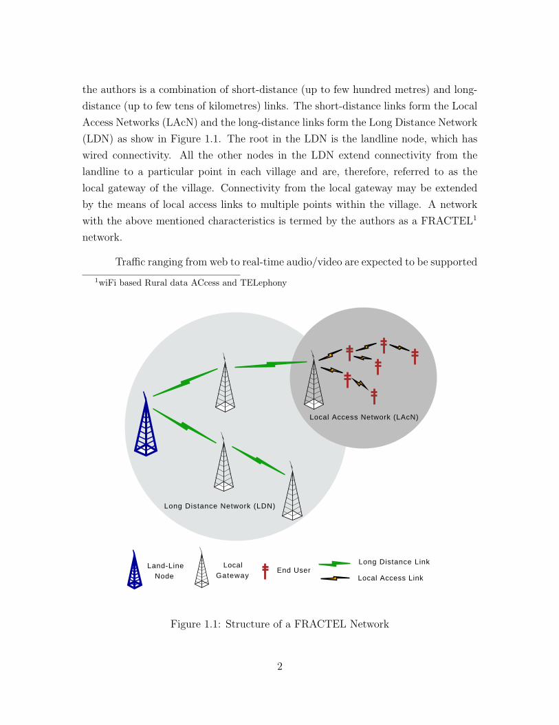
the authors is a combination of short-distance (up to few hundred metres) and long-

distance (up to few tens of kilometres) links. The short-distance links form the Local

Access Networks (LAcN) and the long-distance links form the Long Distance Network

(LDN) as show in Figure 1.1. The root in the LDN is the landline node, which has

wired connectivity. All the other nodes in the LDN extend connectivity from the

landline to a particular point in each village and are, therefore, referred to as the

local gateway of the village. Connectivity from the local gateway may be extended

by the means of local access links to multiple points within the village. A network

with the above mentioned characteristics is termed by the authors as a FRACTEL1

network.

Traffic ranging from web to real-time audio/video are expected to be supported

1wiFi based Rural data ACcess and TELephony

Long Distance Network (LDN)

Local Access Network (LAcN)

Land-Line Node

LocalGateway

End UserLong Distance Link

Local Access Link

Figure 1.1: Structure of a FRACTEL Network

2

in FRACTEL, for which QoS guarantees have to be made. Proper spatial planning of

links can lead to predictable performance [6, 7], without which it is difficult to provide

QoS guarantees. However, even with proper planning, the existing CSMA/CA MAC

of 802.11 does not have a provision for ensuring QoS guarantees. The network in

FRACTEL has an inherent tree structure and, therefore, a centrally-controlled, multi-

hop TDMA-based MAC can be used to provide QoS guarantees. The landline node

can act as the central node (controller) in the LDN, whereas, in the LAcN, the local

gateway can do the same job. Once the use of TDMA MAC has been assumed, the

problem of providing QoS guarantees gets modified to scheduling the links at various

time-slots and channels. This problem can be considered independently in the LDN

and each of the LAcNs [5].

IEEE 802.15.4-based [8] mesh networks are generally deployed for monitoring physical

and environmental conditions. The network is made up of devices called motes, to

which need-based sensors can be attached. Such networks can be used in rural setting

for carrying low-volume voice traffic too [9].

802.15.4 based multi-hop networks can be setup in rural areas with audio

sensors attached to the motes. Push-to-talk and messaging applications can then be

built over them [9]. 802.15.4 is poor is terms of offered data rate (256 kbps at 2.4

GHz). Therefore, to support multiple voice calls, QoS guarantees have to be made.

This can be done using a TDMA-based MAC.

1.2 Problem Statement

The statement of the thesis problem is as follows:

To design, implement and evaluate a centrally-controlled TDMA-based

MAC protocol for multi-hop wireless networks, which incorporates a con-

nection setup mechanism, multi-hop framing, and support for dynamic

scheduling, in order to provide QoS guarantees for real-time applications.

The design aims to be generic in nature and applicable to different kinds of wire-

less technologies. The implementation, on the other hand, has been carried out on

3

802.15.4. Also included as a part of the problem, is the study of performance of the

developed protocol in a network with linear topology.

1.3 Challenges

The problem poses several challenges:

• Since the design is not limited to any particular wireless technology, it should

be suitable for platforms with limited capabilities also. Motes operate on small

processing, memory and power constraints. Therefore, the protocol should be

so designed such that it uses minimal processing and memory and has provision

for power-saving.

• In a multi-hop network, the failure of one of the nodes affects all the nodes

that belong to the subtree of the failed node. Taking this into consideration,

the design should support quick reconstruction of the routing tree as well as

end-to-end connection setup mechanism so that if an intermediate node goes

down, the connection is not broken.

• Synchronization of clocks to a central node in a large network is a difficult

task. Synchronization over multiple hops usually presents uncertainties. These

uncertainties should be accommodated in the design of the framing and schedule

dissemination mechanisms.

• The design should allow for flexibility in terms of making use of any spatial

reuse available in a mesh network.

• We should also allow for dynamic scheduling, since we may have variable bit-rate

real-time flows.

1.4 Our Contribution

In this thesis, a solution to the stated problem is provided. The solution set consists

of the following components:

4

• Design of a centrally-controlled, multi-hop TDMA MAC protocol

– A mechanism for schedule disseminition, which facilitates the dynamic

scheduling. (The actual scheduling problem is not within the scope of this

thesis.)

– A mechanism for flow setup and termination with node-specific delay and

bandwidth guarantees. The delay requirements are specified while connec-

tion is setup. It is up to the scheduler to actually guarantee the delay.

• Implementation of the above designed MAC protocol on tmote platform [10]

using TinyOS [11].

• Study of the effects of fine- versus coarse-grained scheduling on delay and

throughput of the protocol implementation on tmote in a network with linear

topology.

– The throughput achieved is more in case of coarse-grained scheduling.

– There is a trade-off between throughput and delay.

• Study of feasibility of implementation of the above designed mechanism on

802.11b hardware.

– By means of an actual implementation, we have shown that high-precision

time-synchronization in multi-hop networks is possible using 802.11 hard-

ware.

– Theoretically, we have shown that the achievable throughput is good enough

to carry out a practical implementation.

1.5 Organization of the Report

The rest of the thesis is organized as follows:

Chapter 2 provides a background on prior related work. Chapter 3 provides a

general overview of the multi-hop framing and schedule dissemination protocol. We

define various frame types and also examine the requirements of the MAC protocol.

5

Chapter 4 discusses the TinyOS implementation of the protocol on the Tmote sky

802.15.4-based platform. In Chapter 5, we evaluate the TinyOS implementation of the

protocol. In Chapter 6, we conduct a study to see whether it is feasible to implement

our protocol on existing WiFi hardware. In Chapter 7, we conclude the thesis and

discuss the scope for future work.

6

Chapter 2

Related Work

Past work on the design of multi-hop framing mechanisms is limited. In this chapter,

we discuss SRAWAN MAC [12] and Wi-Fi-Re [13], which are 802.11-based single-hop

framing mechanisms, with a view of extending them in a multi-hop scenario. We also

discuss the proposals of IEEE 802.16j [14] working group which seeks to extend IEEE

802.16 [15] to a multi-hop scenario. Finally, we discuss BriMon [16] from which we

have partially borrowed the time-synchronization mechanism.

2.1 SRAWAN MAC and Wi-Fi-Re

Both SRAWAN (Sectorized Rural Area Wireless Access Network) [12] and Wi-Fi-Re

(WiFi Rural Extension) [13] are MAC protocols based on IEEE-802.16 [15] designed

to operate on 802.11 PHY. They aim to provide low-cost Internet access to rural areas

over tens of kilometres.

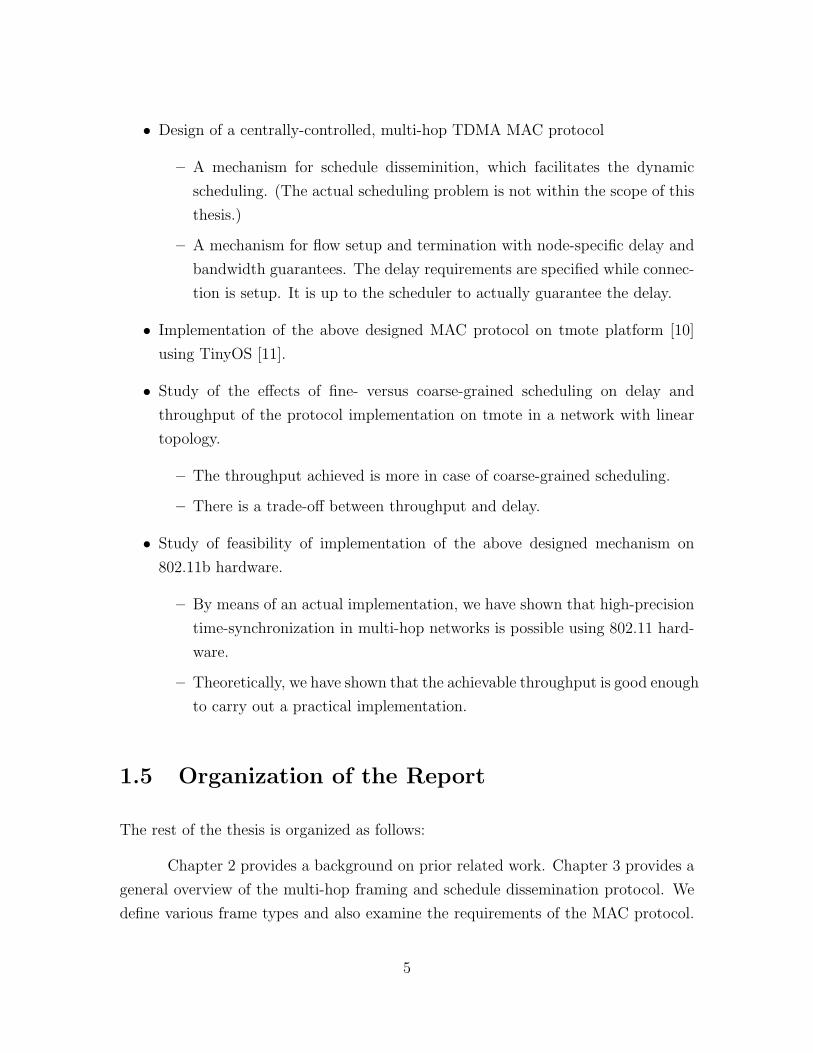
SRAWAN operates in a point-to-multipoint fashion as shown in Figure 2.1(a).

It employs a base-station with a sectorized antenna and several subscriber stations

with directional antennae oriented towards the base-station. Wi-Fi-Re too operates

in a point-to-multipoint fashion, but in a star topology with the base-station having

multiple sectorized antennae as shown in Figure 2.1(b). In both cases, time division

duplexing (TDD) is used to support uplink as well as downlink traffic.

7

BS!

SS!

SS!

SS!

(a) SRAWAN. (Source:[12])

Figure 1.

View of one sector

ST BS

Three sector system

A

B C

ST

Base station

Six sector system

ST

BBase station

A

FC

D E

(b) Wi-Fi-Re. (Source:[13])

Figure 2.1: SRAWAN and Wi-Fi-Re

In both SRAWAN and Wi-Fi-Re, a frame is divided into uplink (UL) and

downlink (UL) sub-frames and has UL-Map and DL-Map. The UL and DL maps

specify when each node transmits and receives. In SRAWAN, each node listens all

the time and simply discards the packets not intended for itself, and therefore, it

does not have a DL-Map. The time synchronization is done by ranging to take into

account the propagation delay. In our design, we do not intend to divide a frame into

downstream and upstream parts. We leave this decision to the scheduler.

Wi-Fi-Re and SRAWAN provide us with an insight of TDMA-based networks.

We study them with a view of extending their design to multi-hop scenario.

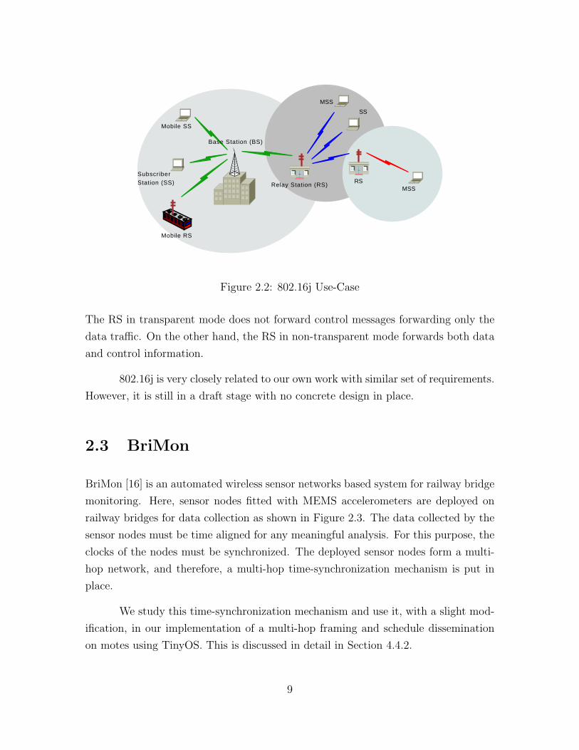
2.2 802.16j: Multi-Hop WiMax

802.16j [14] task force is working on extending 802.16 to a multi-hop scenario. They

plan to achieve throughput and coverage enhancements with the use of relay stations.

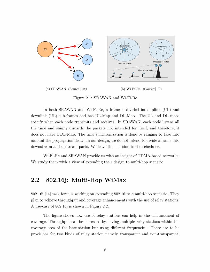
A use-case of 802.16j is shown in Figure 2.2.

The figure shows how use of relay stations can help in the enhancement of

coverage. Throughput can be increased by having multiple relay stations within the

coverage area of the base-station but using different frequencies. There are to be

provisions for two kinds of relay station namely transparent and non-transparent.

8

Relay Station (RS)

Mobile RS

Base Station (BS)

Subscriber Station (SS)

Mobile SS

RSMSS

SS

MSS

Figure 2.2: 802.16j Use-Case

The RS in transparent mode does not forward control messages forwarding only the

data traffic. On the other hand, the RS in non-transparent mode forwards both data

and control information.

802.16j is very closely related to our own work with similar set of requirements.

However, it is still in a draft stage with no concrete design in place.

2.3 BriMon

BriMon [16] is an automated wireless sensor networks based system for railway bridge

monitoring. Here, sensor nodes fitted with MEMS accelerometers are deployed on

railway bridges for data collection as shown in Figure 2.3. The data collected by the

sensor nodes must be time aligned for any meaningful analysis. For this purpose, the

clocks of the nodes must be synchronized. The deployed sensor nodes form a multi-

hop network, and therefore, a multi-hop time-synchronization mechanism is put in

place.

We study this time-synchronization mechanism and use it, with a slight mod-

ification, in our implementation of a multi-hop framing and schedule dissemination

on motes using TinyOS. This is discussed in detail in Section 4.4.2.

9

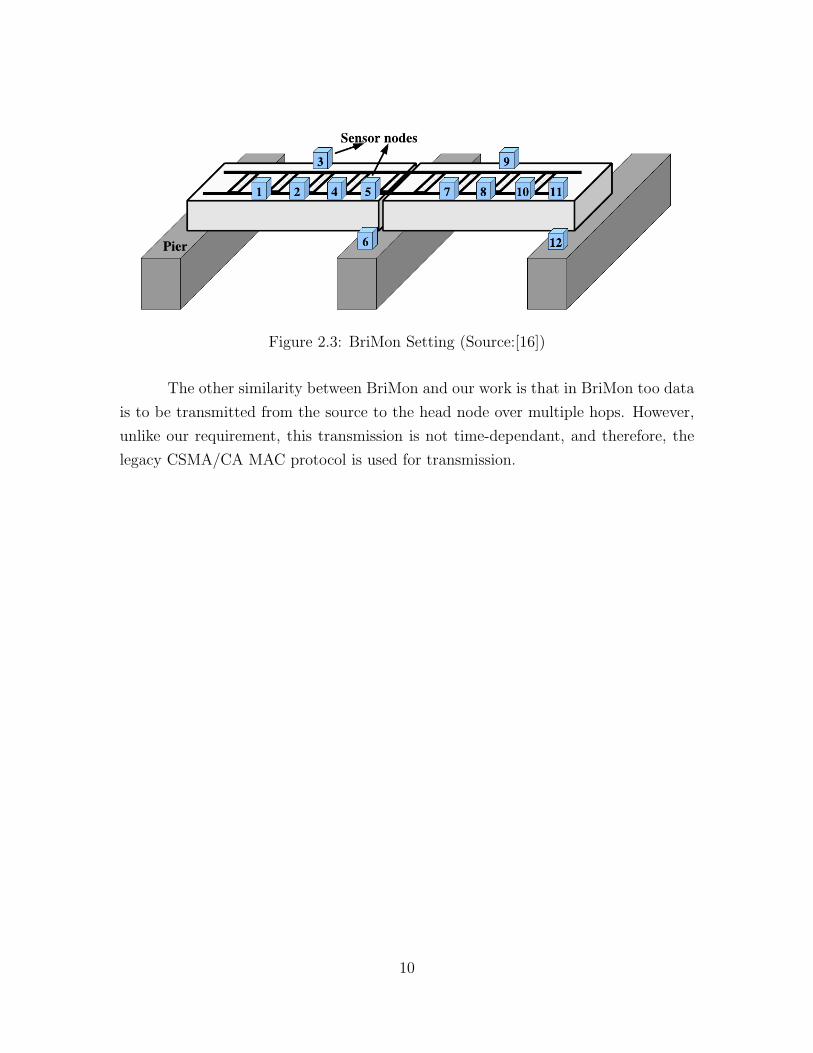
Figure 2.3: BriMon Setting (Source:[16])

The other similarity between BriMon and our work is that in BriMon too data

is to be transmitted from the source to the head node over multiple hops. However,

unlike our requirement, this transmission is not time-dependant, and therefore, the

legacy CSMA/CA MAC protocol is used for transmission.

10

Chapter 3

Design of Multi-hop Framing and

Schedule Dissemination

In this chapter, we present the design of the MAC protocol developed by us for multi-

hop last mile wireless access. The design is not limited to any particular wireless

technology. It could be applied to any suitable TDMA-based architecture. In our

generic description below, we present the design of the various protocol messages

and the various fields in packets which are transmitted. In this description, we have

intentionally left open, details such as the number of bytes for specific packets: these

will depend on the specific wireless technology to which the protocol is applied.

We will first look at the requirements of a multi-hop framing and schedule

dissemination. We will then see how a data transmission is done. Based on the above

we will then design the various types of packets and look at some aspects in the

design. Finally we will revisit the transmission process with the exact type of packets

exchanged at each step.

3.1 Requirements

The requirements of a centrally-controlled multi-hop framing mechanism is as follows:

• A TDMA-based network requires a schedule, which allots time-slots to links.

11

This schedule may be static or dynamic. In our setting, dynamic scheduling is

required because the demands may keep changing. We assume that the central

node runs an algorithm for the computation of the schedule. Therefore, we will

not discuss schedule computation any further.

• In a multi-hop setting, a routing tree is required. The MAC protocol assumes an

underlying routing tree, but since the network topology is not static, the routing

algorithm for the construction of a routing tree would require the services of the

MAC. Therefore, there is a cyclic dependency. Taking this into consideration,

a routing algorithm is needed to run periodically using a flooding primitive.

• The timings mentioned in the schedule are as per a global clock. Therefore,

a mechanism is required to synchronize the clocks on all nodes to the global

clock. This synchronization mechanism itself has to also run on top of the

TDMA MAC protocol. We will discuss the aspect of time-synchronization in

greater detail.

• Once a schedule is computed, a mechanism to disseminate it to all the nodes of

the network is required. The issue of schedule dissemination will be discussed

in greater detail too.

• Since we wish to incorporate the idea of a flow to guarantee QoS in our protocol,

we need flow and bandwidth request mechanisms. (The terminology used here

is consistent with IEEE 802.16 [15]. Flow request is used for a connection setup

defining the traffic requirements in terms of bandwidth and delay. Bandwidth

request, on the other hand, is used to request for bandwidth in addition to the

amount specified in the flow request. Bandwidth request is used to clear the

existing transmit queue.)

• Finally, since the MAC protocol requires data transfer over multiple hops, we

need a mechanism to relay data from the source to destination via (multiple)

intermediate nodes.

Apart from the above stated requirements, there are also some others like provision

for termination of an idle connection. These are implementation specific and will be

explained while discussing the implementation details.

12

Since the requirements of time-synchronization and schedule dissemination

form the central issues in the design of a TDMA-based MAC, it is only appropriate

for us to discuss them in greater detail.

Time Synchronization

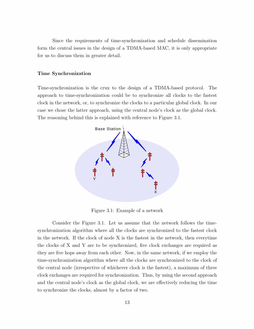
Time-synchronization is the crux to the design of a TDMA-based protocol. The

approach to time-synchronization could be to synchronize all clocks to the fastest

clock in the network, or, to synchronize the clocks to a particular global clock. In our

case we chose the latter approach, using the central node’s clock as the global clock.

The reasoning behind this is explained with reference to Figure 3.1.

Base Station

Y

X

Figure 3.1: Example of a network

Consider the Figure 3.1. Let us assume that the network follows the time-

synchronization algorithm where all the clocks are synchronized to the fastest clock

in the network. If the clock of node X is the fastest in the network, then everytime

the clocks of X and Y are to be synchronized, five clock exchanges are required as

they are five hops away from each other. Now, in the same network, if we employ the

time-synchronization algorithm where all the clocks are synchronized to the clock of

the central node (irrespective of whichever clock is the fastest), a maximum of three

clock exchanges are required for synchronization. Thus, by using the second approach

and the central node’s clock as the global clock, we are effectively reducing the time

to synchronize the clocks, almost by a factor of two.

13

The time-synchronization information is passed to each node from its parent

in the schedule messages.

Schedule Disseminition

The schedule sent by a node contains the transmitting information for all its de-

scendants. A node, on receiving the schedule, extracts the transmitting information

relevant to itself and to its children. It then follows the transmitting information

relevant to itself and transmits the ones relevant to all its children. In this way, in

addition to itself, a node also knows when its children would be transmitting.

In another approach, a node could also be informed of the transmission times

of its parent in addition to that of its children. Using this information a node could

remain in low power state for the duration in which it neither transmits nor receives.

To facilitate the above, a schedule sent by node X (say) must contain the transmission

times of X and the descendants of X. This approach is suitable for technologies which

work on power constraint, e.g., sensor networks.

3.2 The Transmission Process

In this section, we list in a step-wise manner, the events that occur, when a new node

joins the network and wants to transmit.

1. Node A (say) boots up.

2. It synchronizes its clock to the global clock.

3. It associates with the network (A node is deemed to be associated to the network

if the central node has the routing information of that node).

4. It makes a flow request to the central node.

5. It transmits and if there is a build-up in the transmission queue, it requests for

additional bandwidth.

14

6. It terminates the flow.

Based on the above steps, we design the types of packets required. After

designing the types of packets, we will revisit the transmission process, stating the

exact type of packet that will be transmitted at each step.

3.3 Types of Packets

All the types of packets share a common structure: there is a generic header, a

specific header and the payload as shown in Figure 3.2. The structure of the “generic

header” is common to all packets whereas the “specific header” is specific to each

packet type. The payload (if any) too, depends on the type of the packet. Therefore,

our discussion of a particular type of packet would involve discussing its specific

header and the payload. The discussion is summarized in Table 3.1.

Generic Header Specific Header Payload

Figure 3.2: General Structure of a Packet

Before we describe the types of packets (and therefore, the specific headers)

that are needed, it would be appropriate to discuss the generic header. The generic

header houses the packet type field. This is used to identify the type of packet and

also the payload.

In a multi-hop scenario, an intermediate node (which is neither root, nor leaf)

is responsible for relaying packets towards both, the central node and the leaf nodes.

Therefore, we also specify the direction in which the packet is being sent. This will

enable a node A’s (say) parent to discard packets intended for the children of node A

and vice versa. The direction is specified as upstream when the packet is travelling

towards the central node and downstream when the packet is travelling away from

the central node. The transmitter address is also specified in the generic header. It

is the address of the transmitter of that packet. For example, if a packet is sent from

A to C via B, then the transmitter address during transmission from B to C is same

as the address of B.

15

Adding destination address would only complicate the matter as each node

would then be required to have the entire structure of its sub-tree rather than just a

list of its descendants. Instead, packets could be transmitted to all neighbours and

simply discarded at the destination if irrelevant to it. The combination of transmitter

address and the direction specifies a set of possible destinations. Also, a CRC field

is present in the generic header for error detection.

3.3.1 Schedule and Schedule-Fragment Packets

In a TDMA-based network, each node must know exactly when to transmit. This

information is specified in the schedule. The schedule also contains the time synchro-

nization information and the start-time of the schedule.

The payload of schedule is what we term as the scheduling elements. Each

scheduling element specifies parameters for one transmission. There may be many

such scheduling elements in a schedule. For example, to transfer data from central

node to a hop-3 node, three transmissions are required (central node to hop-1, hop-1

to hop-2 and hop-2 to hop-3). Three scheduling elements are needed to specify these

three transmissions. The number of scheduling elements present in a schedule is also

specified in the schedule packet header.

Each scheduling element contains the transmitter address, the starting time

of the transmission, the channel on which to transmit (if such support is to be pro-

vided), the duration of the transmission, the type of packet to be transmitted and

any additional parameters associated with the packet type to be transmitted. For

example, in case of data packet, these additional parameters are the values which

uniquely identify a flow. We will describe these parameters in the sections that fol-

low. The starting time of the transmission is specified relative to the start-time of

the schedule. Duration of the transmission is specified in terms of number of time

units, number of bytes or number of units of the packet payload. This is decided in

advance for a particular implementation.

Maximum Transmission Unit (MTU) is the largest-sized (in terms of number

of bytes) packet that can be sent over a network. It is possible for the schedule to

be larger than the MTU for a particular technology. Keeping the above in mind, we

16

must allow the schedule to be fragmented. We, therefore, introduce the schedule-

fragment packet type. To allow fragmenting of a schedule, we need control field

which is present in the schedule header as well as the schedule-fragment header. The

control field consists of a sequence number, a fragment number and a “more” flag.

The schedule-fragment header consists of only a control field and a field indicating

the number of scheduling elements present in that packet.

3.3.2 Control Packet

When a node boots up, it has no knowledge of who its parent or children are. A

routing protocol, therefore, needs to be run on top of the MAC protocol itself. Con-

trol packets are broadcast packets and slots specified for them in the schedule are

contention-based. For these reasons, a routing algorithm can be implemented over

control packets.

We do not specify any fields in a control packet or how the contention is

resolved. These can be worked out on case-to-case basis. For example, a control

packet itself could have many sub-types. One sub-type could be used for routing,

another could be used to notify the nodes that the central node has booted, etc.

3.3.3 Flow-Request and Flow-Request-Aggregate Packets

Once the central node has the routing information of a node, that node is deemed

to be “associated” to the network. The node, then, must make a flow-request to the

central node in order to transmit the data. This flow-request specifies source-address,

destination-address, the requested flow number, the number of bytes requested and the

interval of time. If n bytes are requested and x is the time-interval, it means that

the connection requires n bytes every x interval of time. Also, it is worth noting that

flow number is requested rather than allotted by the central node. This is because

a node can establish the confirmation of flow establishment by merely looking at the

schedule rather than have a special packet sent to it to confirm flow setup.

Each node, on receiving a flow-request from its children, must relay it to the

central node. For this purpose, a flow-request-aggregate packet is used. A node

17

aggregates the flow-request packets received from its descendants, which is then in-

cluded as a part of payload of the flow-request-aggregate packet. The header of a

flow-request-aggregate packet contains the number of flow-requests included in it.

It is better to aggregate the flow requests rather than send them individually to

the central node. This is because, sending individually will incur overhead of sending

different packets. Also, many more scheduling elements will be required so specify

when exactly each request has to be transmitted.

3.3.4 Data Packet

The data packet is used to transfer the user data between the central node and other

nodes. Data is transferred in the form of flows, and therefore, a prior flow setup is

required for data transfer. Each flow is uniquely identified by a combination of the

source-address, destination-address and the flow number. The data packet header has

as its fields the source-address, destination-address, flow number and the data length.

3.3.5 Bandwidth-Request and Bandwidth-Request-Aggregate

Packets

It may so happen, that for a particular flow, a node requires to transmit more bytes

than what it requested in the flow-setup process. This will result in building of the

transmit queue at the node for that flow. To clear this queue, it sends a request to

the central node asking for more bandwidth for that particular flow. This request

is sent by the use of bandwidth-request packets. In addition to the number of bytes

requested, the bandwidth-request specifies the flowID which is nothing but source-

address, destination-address and the requested flow number taken collectively.

As in the case of flow-request, aggregation is required here too. For this

purpose, we have a bandwidth-request-aggregate packet type. The header contains

only the number of bandwidth-requests field as in the case of flow-request-aggregate

packet.

A bandwidth-request packet may also be used for the purpose of terminating

18

a flow. In the number-of-bytes-requested field, a pre-agreed value can be specified

which indicates that the connection needs to be terminated.

3.3.6 Tree-Broadcast Packet

Many higher layer protocols require the services of a MAC broadcast mechanism. In a

single-hop scenario, the central node simply sends a broadcast message and everyone

in the network receives it. In a multi-hop scenario, however, the intermediate nodes

must relay the broadcast message to their descendants. For this purpose, we have

a tree-broadcast packet. As in the case of control type packet, we do not specify

the fields for a tree-broadcast packet. The fields will need to be worked out on a

case-by-case basis.

The difference between the tree-broadcast and a control packet lies in the fact

that a tree-broadcast will follow the routing tree whereas the control packet does not

assume the presence of a routing tree.

3.4 Other Aspects

3.4.1 Contention-based and Contention-Free Requests

Flow-request and bandwidth-request packets can be transmitted in a contention-

based manner, or, slots can be specifically allotted for them in the schedule. The

latter aspect is contention-free. We leave this, an open issue.

In a contention-free case, a bandwidth-request packet may be piggybacked

with a data packet and flow-requests could be polled. In [17], the author concludes

that the contention-free mode performs better than the contention-based mode in

terms of throughput and delay. Therefore, in our implementation, as discussed in

Chapter 4, we will use the no-contention mode.

19

Type of Header Fields Present Payload Type

generic

type

specific packetdirection

transmitter-addressCRC

control unspecified unspecified

schedule

control

scheduling elementsnumber of scheduling elements

time-synchronization datastart-time

schedule-fragmentcontrol

scheduling elementsnumber of scheduling elements

flow-request

source-address

nonedestination-address

flow numbernumber of bytes

intervalflow-request-aggregate number of flow-request flow-request

data

source-address

user datadestination-address

flow numberlength

bandwidth-request

source-address

nonedestination-address

flow numbernumber of bytes

bandwidth-request-aggregate number of bandwidth-request bandwidth-requesttree-broadcast unspecified unspecified

Table 3.1: Summary of Packet Types

20

3.4.2 Packet Error and Losses

Packet losses and packet error are treated in similar fashion. The CRC field present in

the generic header is used to detect if the packet is received without errors. If packet

contains errors, it is simply discarded. There is no error correction mechanism. From

this point onwards, the terms packet loss and packet error are used interchangeably.

A loss of a control packet is handled by the protocol which makes use of

it. For example, if a lost control packet contained routing information, then its the

responsibility of the routing protocol to handle it.

If any of the fragments of the schedule is lost, the entire schedule is considered

lost and all other fragments are ignored. A loss in the schedule results in the node

waiting for the next schedule doing nothing in this period. In technologies where

multiple data rates are supported, it might be a good idea to transmit the schedule

at the lowest data-rate to minimize its chances of being lost.

A loss of data packet is handled by the higher layer. We do not employ a

retransmission mechanism.

A loss of request-aggregate packet is considered same as loss of multiple request

packets. In case a flow-request packet is lost, there will be no connection-setup and

therefore, no provision in the schedule to transmit. The flow-request is then re-sent.

Similarly, in case a bandwidth-request packet is lost, there will be no allocation of

extra bandwidth. A bandwidth-request is sent with possibly increased requirements.

Most protocols using the services of a broadcast mechanism do not assume

reliability. Therefore, a loss in the tree-broadcast packet is not handled.

3.4.3 Central Node Reset

It is possible that a failure occurs in the central node and a reboot is needed. In such

a case, the routing tree and all existing connections need to be terminated. A “reset”

packet is used to implement this mechanism. The reset packet could be a sub-type of

the control packet, therefore not requiring a packet type of its own. When the central

node reboots, it broadcasts the reset packet and other nodes on receiving it simply

21

forward it and reset their state.

3.5 The Transmission Process: Re-visited

Keeping in mind the various types of packets, we take a look at the transmission

process again.

1. The node A (say) boots up.

2. It waits until it receives a schedule packet.

3. It receives a schedule and uses the timing information to synchronize its clock to

the global clock. It now also knows when a control packet is to be transmitted

and runs the routing algorithm over control packets.

4. Once the central node receives node A’s routing information and adds it to the

routing tree, node A is deemed to be associated to the network.

5. Once node A is associated, the subsequent schedule would contain a slot in

which A could sent a flow request.

6. It sends a flow-request packet.

7. Once the central node receives node A’s flow-request, it assigns node A a trans-

mission slot in the schedule.

8. Node A transmits according to the schedule. Its queue builds up and it sends

a bandwidth-request to clear this queue.

9. It is allotted more bandwidth in the next schedule and transmits accordingly.

10. Node A terminates the flow by sending a bandwidth-request packet with number

of bytes request set to some pre-decided value.

The present design of the MAC protocol is very basic in nature and offers a

lot of room for further enhancement. For example, a mechanism to for retransmission

at the MAC layer may be devised for packet losses.

22

Chapter 4

Implementation on TinyOS

In this chapter, we will discuss the implementation of our protocol on TinyOS. We

will begin with an overview of wireless sensor networks and of the platform used, then

we will move on the designing of the components and finally we will look at some of

the implementation details.

4.1 Overview of Wireless Sensor Networks

A wireless sensor network (WSN) is made of many sensor nodes. These sensor nodes

consist of a processor, sensors, radio and battery. They have low processing capabil-

ities. A sensor node is commonly called a mote. Examples of motes include Mica2,

telos and tmote-sky. The motes are collectively used to monitor certain physical

and environmental conditions such as temperature, pressure, vibration, etc. A sensor

node is generally very small as this facilitates easy deployment. Cost of motes are

variable, with low-cost (around $70) ones being available too.

With the increasing popularity of the motes, it is possible to develop appli-

cation for them which are non-traditional. For example, low-cost motes with audio

sensors attached to them can be used for voice communication [9].

Development of applications for motes involves considerably less effort than

making similar modifications in a 802.11 compliant device driver. This is the reason

23

why we have used mote as the platform for the implementation and evaluation of our

protocol.

4.2 Overview of the Platform

We will now discuss the platform used for our implementation. The hardware platform

used was tmote-sky [10] as it was easily available to us. We used TinyOS [11] as the

operating system platform. We used the Boomerang version 2.0.4 which has tinyos-

1.x.

4.2.1 Tmote-sky

Figure 4.1: Tmote (Source:[10])

Tmote-sky is a mote platform manufactured by Moteiv Corporation. It has a 8

MHz Texas Instruments MSP430 microcontroller with a 10 KB RAM and 48 KB flash.

There is also a 1 MB external flash for data storage. It also has a 250 kbps, 2.4 GHz

IEEE-802.15.4 compliant Chipcon wireless transceiver CC2420, and an integrated on-

board antenna with 50m range for indoors and 125m range for outdoors. Tmote-sky

has support for TinyOS. A tmote is shown in Figure 4.1. Further details can be found

in the Tmote-sky datasheet [10].

24

4.2.2 TinyOS

TinyOS [11] is an open-source operating system and platform developed at University

of California at Berkeley (UCB) for embedded sensor nodes. It is the most widely

used operating system for motes. TinyOS facilitates development of concurrency-

intensive applications which are data driven and work on limited memory and power

requirements.

Applications developed on TinyOS have a modular framework with a set of

components and interfaces. An application “wires” together the interfaces of the set

of components. An interface is a set of commands and events. A command is a sub-

routine which performs some action. An event is also a sub-routine which is signaled

on the completion of a request. An event can be bound to a hardware interrupt. A

component provides some interfaces and uses some interfaces. An interface provider

implements the commands of that interface and the user implements the events.

TinyOS is written in nesC programming language which is a dialect of the C-

programming language. Here, only the application specific component gets compiled

and is transferred to the motes. This facilitates low memory usage and code-reuse.

4.3 Component Design

Before proceeding further, please note that we did not implement the central node.

For the purpose of our evaluation we created a stub for the central node, which sent the

schedule and data. This stub too runs on a mote. However, the design for the central

node should essentially be the same as that of any other node with the exception of

presence of a scheduler in the central node. Therefore in the implementation of the

central node, a large chunk of the code will be re-used from the implementation of

the non-central nodes.

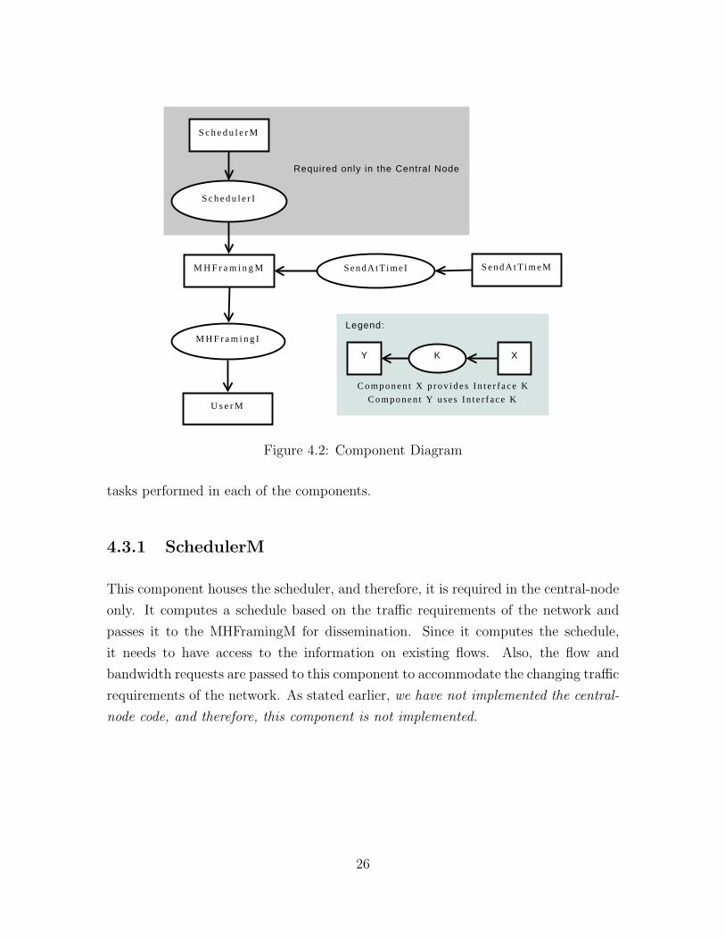
The component design is shown in Figure 4.2. There are four components:

SchedulerM which is present in the central node only, MHFramingM which is the

principal component, SendAtTimeM which is the packetizer and performs the trans-

missions, and UserM which is the “higher-layer“ component. We will now discuss the

25

C o m p o n e n t X p r o v i d e s I n t e r f a c e K

C o m p o n e n t Y u s e s I n t e r f a c e K

Y K X

Legend:

S c h e d u l e r M

S c h e d u l e r I

M H F r a m i n g M

M H F r a m i n g I

U s e r M

S e n d A t T i m e I S e n d A t T i m e M

Required only in the Central Node

Figure 4.2: Component Diagram

tasks performed in each of the components.

4.3.1 SchedulerM

This component houses the scheduler, and therefore, it is required in the central-node

only. It computes a schedule based on the traffic requirements of the network and

passes it to the MHFramingM for dissemination. Since it computes the schedule,

it needs to have access to the information on existing flows. Also, the flow and

bandwidth requests are passed to this component to accommodate the changing traffic

requirements of the network. As stated earlier, we have not implemented the central-

node code, and therefore, this component is not implemented.

26

4.3.2 MHFramingM

This is the principal component. It co-ordinates the functioning of other components.

The following are the functions performed by it:

• Initializes the state and buffer variables on boot-up.

• Handles received packet:

– Accepts only the relevant packets.

– Stores schedule, processes it to extract only the scheduling elements rele-

vant to itself and to its descendants.

– Passes the data packet to the UserM if the data packet are intended for

itself, or, stores it if they are to be relayed.

– Receives flow and bandwidth requests from children and stores them in a

queue from which they can be transmitted in aggregation. In case of the

central node, these flow and bandwidth requests are passed to SchedulerM.

• Handles flow setup and termination requests and data received from UserM

(higher-layer). It also generates bandwidth request when required.

• Stores the parameters and state variables of existing connections.

• Checks periodically, for inactive connections and terminates them.

• Schedules transmissions: The schedule for this is received from parent in case

of client nodes, and from ScheduleM, in case of the central node. When an

alarm for a transmission is fired, the information to be transmitted (data or

management) is sent to SendAtTimeM.

4.3.3 SendAtTimeM

This component is the “packetizer”. It receives the data or the management infor-

mation from MHFramingM and transmits it over the radio. Before transmission,

27

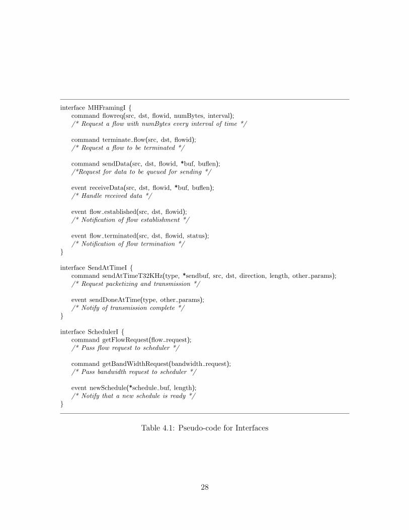
interface MHFramingI {command flowreq(src, dst, flowid, numBytes, interval);/* Request a flow with numBytes every interval of time */

command terminate flow(src, dst, flowid);/* Request a flow to be terminated */

command sendData(src, dst, flowid, *buf, buflen);/*Request for data to be queued for sending */

event receiveData(src, dst, flowid, *buf, buflen);/* Handle received data */

event flow established(src, dst, flowid);/* Notification of flow establishment */

event flow terminated(src, dst, flowid, status);/* Notification of flow termination */

}

interface SendAtTimeI {command sendAtTimeT32KHz(type, *sendbuf, src, dst, direction, length, other params);/* Request packetizing and transmission */

event sendDoneAtTime(type, other params);/* Notify of transmission complete */

}

interface SchedulerI {command getFlowRequest(flow request);/* Pass flow request to scheduler */

command getBandWidthRequest(bandwidth request);/* Pass bandwidth request to scheduler */

event newSchedule(*schedule buf, length);/* Notify that a new schedule is ready */

}

Table 4.1: Pseudo-code for Interfaces

28

however, the information is encapsulated into packets by adding the relevant head-

ers. The maximum transmission unit (MTU) in the CC2420 chip is 128 bytes out

of which 12 bytes are used by the AM header in TinyOS. Therefore, the size of the

packets created by this component does not exceed 116 bytes. If the amount of data

(or management information) is more than what can be handled in a single packet,

then multiple packets are created and are sent one after another. After sending, this

component notifies MHFraming component of successful transmission.

4.3.4 UserM

This is the “higher layer” interface. An application wishing to use the MAC protocol

developed by us should use this component as an interface. Apart from sending and

receiving data, it also requests flow setups and terminations to MHFramingM.

Apart from the components, there are the interfaces namely MHFramingI,

SchedulerI and SendAtTimeI. The pseudo-codes for these are specified in Table 4.1.

4.4 Selected Details

In this section, we will discuss some of the selected details in the implementation of

our protocol on TinyOS. Other details, if required, can be obtained by looking at the

source code.

4.4.1 Packet Formats and Disabling Random Backoff

The packet structure and header formats in our implementation are specified in Ap-

pendix A.2. Only the headers which are used in evaluation are shown. The rest can

be obtained by looking at the source code.

Also, before moving ahead with the implementation it was necessary to disable

the random backoff which is part of the inherent CSMA/CA in TinyOS. The details

for this is specified in Appendix A.1.

29

Please note that in our implementation, we have generously used a number

of bytes for the packet headers. It is possible to increase the throughput slightly by

taking a more miserly approach. The design, however, remains the same.

4.4.2 Time Synchronization

Our time synchronization mechanism is borrowed from BriMon [16] with only a slight

modification. As in BriMon, we maintain an offset variable at each node which has

the difference between the global and the local clocks. Therefore, each time the global

clock value is needed, we simply have to add the offset value to the local clock. The

value of this offset variable is set to 0 in the central node since the global clock is

assumed to be that of the central node.

A schedule packet carries the sender’s timestamp and its offset value. On the

receiver’s side, timestamping is done according to the receiver’s clock when a schedule

arrives. The offset and the global clock values are calculated as follows:

receiverOffset = (senderT imeStamp+ senderOffset)− receiverT imeStampglobalClock = localClock + receiverOffset

In BriMon, if a node misses an update, it uses the previous five updates to

come up with the next update and uses it. We do not have any such mechanism. This

is the only difference between BriMon’s and our time-synchronization scheme. In our

case, the time-synchronization information is carried by the schedule. If a schedule

is missed, a node simply waits for the next schedule.

4.4.3 Routing

In our implementation, we have not implemented a routing protocol. Instead, we

have hard-coded the routing information in each node. The routing protocol, if

implemented, is to be run using the CONTROL packet for which we have provision

in the multi-hop framing mechanism.

30

4.4.4 Termination of Idle Connections

In our implementation, there is a provision of termination of idle connections. For

each flow, an idle count is maintained. This idle count is initialized to 0. On the

arrival of a new schedule the idle count of each flow in the flow table is incremented

by 1. When data is received or transmitted through a particular flow, its idle count

is set to 0. As soon as the idle count reaches a certain threshold value, the flow is

deemed to have been terminated.

A similar mechanism is used when requesting a flow. If a requested flow is not

established within a certain number of schedules, the flow request is resent. If, even

after certain number of retries, a flow is not established, it is deemed as a failure and

notified to the UserM component.

Having discussed the implementation details, we will now discuss the evalua-

tion of our protocol.

31

Chapter 5

Evaluation of the Implementation

on TinyOS

In this chapter, we will present the evaluation of the MAC protocol implementation

on the tmote platform. We will first describe the types of experiments and their

setup, then we will discuss the evaluation procedure and finally, present the various

results and their analysis.

5.1 Experiment Types and Setup

For the purpose of our evaluation, we constructed a network with a linear structure

involving four nodes as shown in the Figure 5.1(a). Such a topology was forced by

hard-coding the parent, children and descendant information into the nodes. A par-

ticular node rejected all packets which were not received from parent or child. At the

head of the network was the central node. On the above described network we con-

ducted experiments to measure the delay, data-throughput and system-throughput.

Before proceeding further, we define the term, frame. A frame is the number of

bytes transmitted cumulatively, by all the nodes in the network (including the central

node), from the start-time of a schedule till the start-time of the next schedule. For

example, let us consider the figure 5.1(a). If there exists only one flow which is from

CN to node-3, then a frame contains the following: schedule transmitted from CN to

32

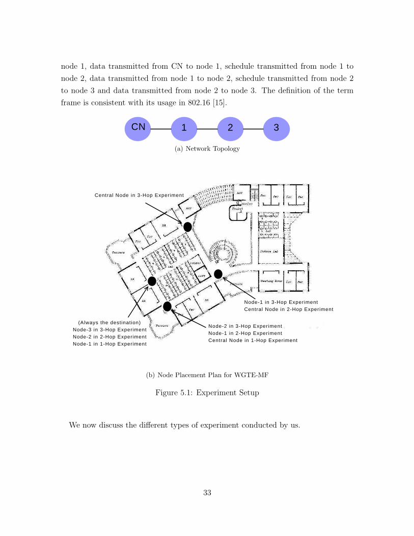
node 1, data transmitted from CN to node 1, schedule transmitted from node 1 to

node 2, data transmitted from node 1 to node 2, schedule transmitted from node 2

to node 3 and data transmitted from node 2 to node 3. The definition of the term

frame is consistent with its usage in 802.16 [15].

CN 1 2 3

(a) Network Topology

Central Node in 3-Hop Experiment

Node-1 in 3-Hop ExperimentCentral Node in 2-Hop Experiment

Node-2 in 3-Hop ExperimentNode-1 in 2-Hop ExperimentCentral Node in 1-Hop Experiment

(Always the destination)Node-3 in 3-Hop ExperimentNode-2 in 2-Hop ExperimentNode-1 in 1-Hop Experiment

(b) Node Placement Plan for WGTE-MF

Figure 5.1: Experiment Setup

We now discuss the different types of experiment conducted by us.

33

5.1.1 Back-to-Back Experiment (BTBE)

In this experiment, the data was sent in a flow from the source (which was the central-

node) to the destination (node-1, node-2 or node-3). For example, if the data was

sent to node-2, then the frame consisted the following transmissions: central-node

sent the schedule, followed by data to node-1, node-1 sent the schedule, followed by

data to node-2.

However, the sent schedule was just a dummy. It was not followed in the

network. Intermediate nodes transmitted, both, schedule and data, as soon as they

finished receiving the same from their parent (and therefore the name back-to-back).

At each intermediate node, the time at which data was received, was recorded. The

obtained time recordings were used to construct an actual schedule, which was then

used in experiment that we describe later.

For example, for n bytes of data sent from the central-node to node-2, the

following events took place:

1. Central-node sent the schedule followed by n bytes of data.

2. Node-1 recorded the time t1 at which it finished receiving n bytes of data.

3. Immediately after the above step, node-1 sent the schedule followed by n bytes

of data.

4. Node-2 recorded the time t2 at which it finished receiving n bytes of data.

Please note that the values t1 and t2 were with respect to the start-time of the

schedule.

5.1.2 With-Guard-Time Experiment (WGTE)

In this experiment too, the data was sent from the source to the destination, but the

intermediate nodes transmitted according to the schedule. In the schedule the values

used for transmission times of the intermediate nodes, were the ones obtained from

the BTBE. Also, a guard time of 1 slot (which is the minimum guard possible) was

34

inserted to take into account, the synchronization error. As per our implementation,

one slot was equivalent to 10 clock ticks even though the synchronization error was

not more than 1-2 clock ticks.

5.1.3 WGTE with Multiple Frames and Hidden Node Sce-

nario (WGTE-MF)

In the previous two experiments, all the nodes were kept within radio range of each

other. In this experiment, we kept the nodes such that only the neighbours, as

per the topology shown in Figure 5.1(a), were within the radio range of each other.

Such a scenario was set on the top floor of the Computer Science and Engineering

Department at IIT Kanpur. The layout is shown in Figure 5.1(b).

On the setting described above, we ran the WGTE, sending multiple frames

continuously instead of just one. On the completion of one frame, the central-node

initiated the next frame without any additional delay. We then recorded the time

taken for the transmission of intended number of frames and averaged out this value

over the number of frames. The resultant, average time taken for transmission of one

frame, was used to calculate the data and the system throughputs. For example, if

f frames were sent and the total time taken was tf , then the average time per frame

wastff

.

5.2 Evaluation Procedure

Before going any further, it is worth mentioning that in our implementation of the

protocol on tinyOS, the maximum size of the payload in a data packet was 106 bytes

(the MTU in tinyOS is 128 bytes). Therefore, in the experiments which we conducted,

we have used the number of data bytes as multiples of 106.

35

5.2.1 Experiments’ Order

In the experiments, we assumed that there existed only one flow in the network which

was between the central-node and node-i. This we called the i-hop experiment. The

values of i used were i = 1, 2, 3. In every i-hop experiment, each frame transferred

j-bytes of data from the central node to node-i. The values of j used were j = 106,

212, 318, 424, 530, 1060, 1590, 2120, 2650, 3120. For each of the 30 possible values

of (i, j), the following steps were followed:

1. The BTBE was run 800 times and the timings recorded. The 99-th percentile

values of the recorded timings were then computed.

2. A schedule was computed based on the 99-th percentile values computed step-1.

3. The schedule was then used in 500 runs of WGTE and the end-time of each

frame (with respect to the start-time of the schedule) was recorded. We then

computed the 99-th percentile values of the end-time.

4. WGTE-MF was conducted using 10 frames for a 1-hop experiment and 50

frames for 2-hop and 3-hop experiments. The schedule used here was same

as that computed in step-2. The time interval used between each frame was the

same as that computed in step-3. Each WGTE-MF was conducted 20 times

and time taken to transmit the stipulated number of frames was recorded in

each case. Timings were considered only for those runs of the experiment in

which all the stipulated number of frames were received successfully, others were

simply discarded. We then took the 95-th percentile value of these recordings

and averaged it out over the number of frames. The resultant average value,

which was the per frame delay, was then used for the computation of the data

and system throughputs. The obtained delay, data and system throughputs are

tabulated in Section 5.3.

5.2.2 Measurement of Optimal Throughput

Apart from the above, we also carried out experiments to estimate the maximum

possible throughput in tmote-sky running tinyOS platform. These experiments were

36

carried out without the implementation of our protocol because the processing delays

involved in our protocol would have resulted in lower throughput values.

We used two nodes and synchronized their clocks by the same mechanism as

the implementation of our protocol. After synchronization, we sent multiple MTU-

sized (128 bytes) packets between them, without adding any delay between successive

packets. The timings before sending and after receiving were recorded. The difference

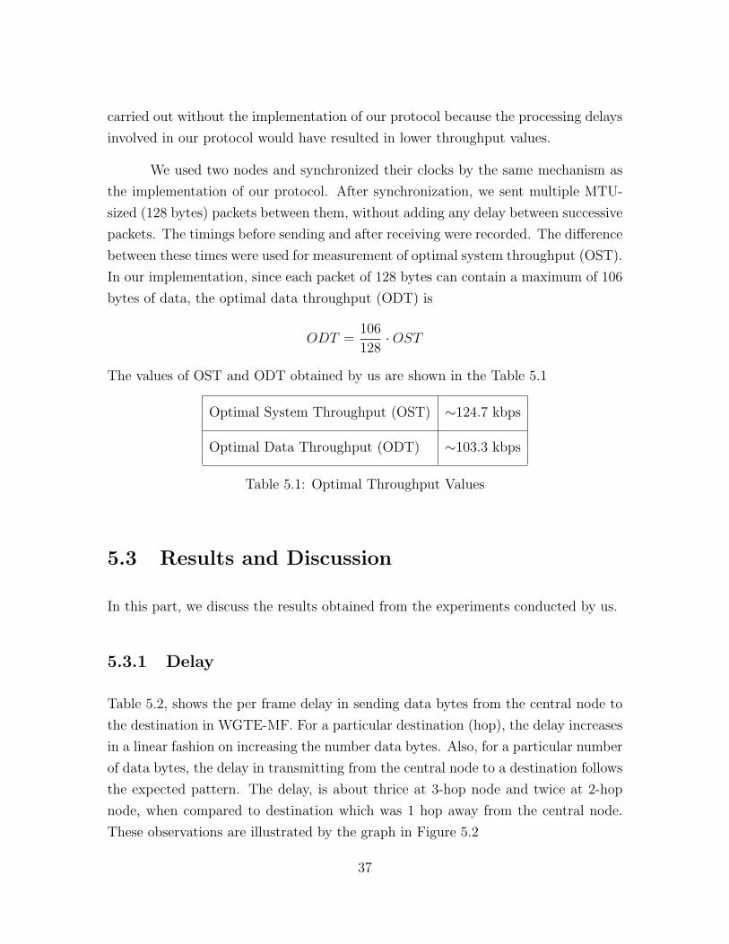
between these times were used for measurement of optimal system throughput (OST).

In our implementation, since each packet of 128 bytes can contain a maximum of 106

bytes of data, the optimal data throughput (ODT) is

ODT =106

128·OST

The values of OST and ODT obtained by us are shown in the Table 5.1

Optimal System Throughput (OST) ∼124.7 kbps

Optimal Data Throughput (ODT) ∼103.3 kbps

Table 5.1: Optimal Throughput Values

5.3 Results and Discussion

In this part, we discuss the results obtained from the experiments conducted by us.

5.3.1 Delay

Table 5.2, shows the per frame delay in sending data bytes from the central node to

the destination in WGTE-MF. For a particular destination (hop), the delay increases

in a linear fashion on increasing the number data bytes. Also, for a particular number

of data bytes, the delay in transmitting from the central node to a destination follows

the expected pattern. The delay, is about thrice at 3-hop node and twice at 2-hop

node, when compared to destination which was 1 hop away from the central node.

These observations are illustrated by the graph in Figure 5.2

37

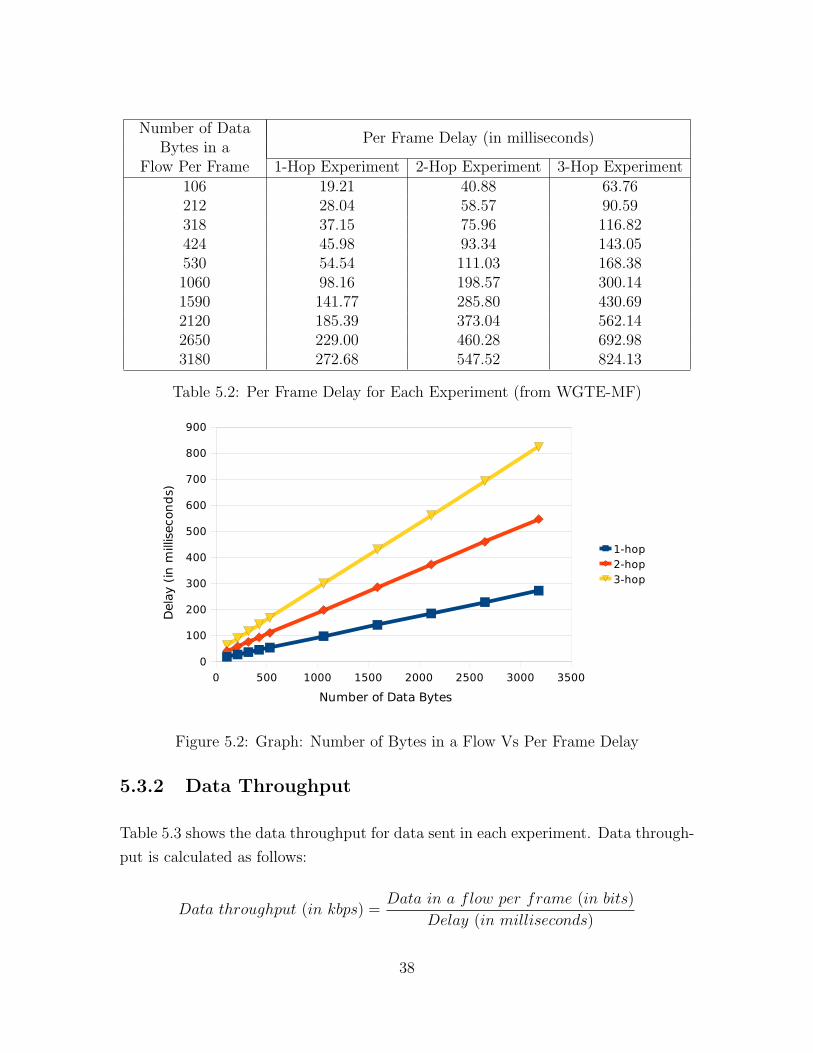
Number of DataBytes in a

Flow Per Frame

Per Frame Delay (in milliseconds)

1-Hop Experiment 2-Hop Experiment 3-Hop Experiment106 19.21 40.88 63.76212 28.04 58.57 90.59318 37.15 75.96 116.82424 45.98 93.34 143.05530 54.54 111.03 168.381060 98.16 198.57 300.141590 141.77 285.80 430.692120 185.39 373.04 562.142650 229.00 460.28 692.983180 272.68 547.52 824.13

Table 5.2: Per Frame Delay for Each Experiment (from WGTE-MF)

� ��� ���� ���� ���� ���� ���� ����

�

���

���

���

���

���

���

���

��

��

��� �

��� �

��� �

"#�$��� %������&����

�����������

������� � �!

Figure 5.2: Graph: Number of Bytes in a Flow Vs Per Frame Delay

5.3.2 Data Throughput

Table 5.3 shows the data throughput for data sent in each experiment. Data through-

put is calculated as follows:

Data throughput (in kbps) =Data in a flow per frame (in bits)

Delay (in milliseconds)

38

The value of the delay used to compute the throughput is taken from Table 5.2.

From Table 5.3, we see that for a particular number of bytes of data, the data

throughput for a 1-hop experiment is twice that of a 2-hop experiment and thrice

that of a 3-hop experiment. This is obvious since sending of data from the central

node to a hop-2 node involves two transmissions and that to a hop-3 node requires

three transmissions.

Number of DataBytes in a

Flow Per Frame

Data Throughput (in kbps)

1-Hop Experiment 2-Hop Experiment 3-Hop Experiment106 44.15 20.74 13.30212 60.48 28.96 18.72318 68.48 33.49 21.78424 73.77 36.34 23.71530 77.74 38.19 25.181060 86.39 42.71 28.251590 89.72 44.51 29.532120 91.48 45.46 30.172650 92.58 46.06 30.593180 93.30 46.46 30.87

Table 5.3: Data Throughput for Each Experiment

� ��� ���� ���� ���� ���� ���� ����

�

��

��

��

��

��

��

��

�

�

���

��� �

��� �

��� �

"#�$��� %������&����

�������� #'��#������($��!

Figure 5.3: Graph: Number of Bytes in a Flow Vs Data Throughput

39

For a particular destination, however, with linear increase in the number of

data bytes, there is a non-linear increase in the data throughput. This is explained

as follows. There is a fixed overhead of the schedule irrespective of the number of

data bytes. As we increase the number of data bytes, there is a decrease in the ratio

of the overhead due to the schedule with respect to the data bytes. Therefore, the

throughput increases. Ideally, as the number of data bytes approaches infinity, this

ratio approaches zero and therefore the data throughput approaches its maximum

value.

For 3-hop experiment, the data throughput varies from about 13 to 31 kbps

for data bytes between 106 and 3180 per frame. All the experiments were conducted

with a single flow only. With increase in the number of flows, the data throughput

per flow will fall by the same factor. The GSM speech codec operates at 13 kbps,

therefore, even across three hops, voice communication between two nodes could be

possible.

The data throughput varies from 21 to 46 kbps for 2-hop experiment, and, from

44 to about 93 kbps for a single hop experiment. These values seem good enough for

multiple voice calls simultaneously.

Also, it is worth noting that the maximum data throughput of about 93 kbps

achieved by us is comparable to the optimal data throughput of about 103 kbps as

stated in Table 5.1. The difference can be attributed to the processing delay in the

microcontroller.

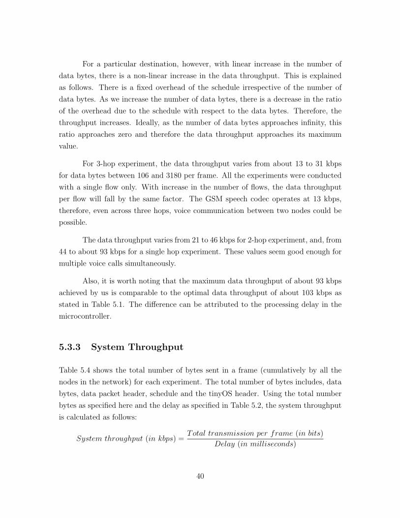
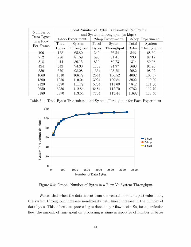
5.3.3 System Throughput

Table 5.4 shows the total number of bytes sent in a frame (cumulatively by all the

nodes in the network) for each experiment. The total number of bytes includes, data

bytes, data packet header, schedule and the tinyOS header. Using the total number

bytes as specified here and the delay as specified in Table 5.2, the system throughput

is calculated as follows:

System throughput (in kbps) =Total transmission per frame (in bits)

Delay (in milliseconds)

40

Number ofData Bytesin a FlowPer Frame

Total Number of Bytes Transmitted Per Frameand System Throughput (in kbps)

1-hop Experiment 2-hop Experiment 3-hop ExperimentTotal System Total System Total SystemBytes Throughput Bytes Throughput Bytes Throughput

106 158 65.80 340 66.54 546 68.50212 286 81.59 596 81.41 930 82.12318 414 89.15 852 89.73 1314 89.98424 542 94.30 1108 94.97 1698 94.96530 670 98.28 1364 98.28 2082 98.921060 1310 106.77 2644 106.52 4002 106.671590 1950 110.04 3924 109.84 5922 110.002120 2590 111.77 5204 111.60 7842 111.602650 3230 112.84 6484 112.70 9762 112.703180 3870 113.54 7764 113.44 11682 113.40

Table 5.4: Total Bytes Transmitted and System Throughput for Each Experiment

� ��� ���� ���� ���� ���� ���� ����

�

��

��

��

�

���

���

��� �

��� �

��� �

"#�$��� %������&����

)��������� #'��#������($��!

Figure 5.4: Graph: Number of Bytes in a Flow Vs System Throughput

We see that when the data is sent from the central node to a particular node,

the system throughput increases non-linearly with linear increase in the number of

data bytes. This is because, processing is done on per flow basis. So, for a particular

flow, the amount of time spent on processing is same irrespective of number of bytes

41

transmitted for the flow. Therefore, when less bytes are sent, more fraction of the

total time is spent on processing and less on transmitting giving a lower throughput.

Ideally, when the number of bytes to be sent by a flow approaches infinity, the sys-

tem throughput will be maximum because the fraction of time spent on processing

approaches zero.

We also see that for a specific number of bytes per flow, the system throughput

is similar for experiments with different number of hops. This is illustrated by the

fact that in Figure 5.4, the lines are almost co-incidental for different experiments.

The above observation can be attributed to the fact that all the intermediate nodes

contribute equal resources in terms of processing and transmission. Thus, for more

number of hops, there is no additional processing delay at each hop.

We would like to highlight that the achievable throughput was close to the

maximum. This is an indicator of the fact the we have managed to keep the processing

delay in our implementation to a minimal.

Finally, to conclude the chapter, we would like to mention, that though the

values obtained in our experiments are specific to the implementation of our design

on TinyOS for tmote-sky, the pattern of the values should remain same across various

wireless technologies. Therefore, the shape of the graphs obtained from experiments

performed on other platforms should be identical to ours. In a nutshell, we do not

expect the behaviour of the protocol to change on a different platform.

42

Chapter 6

Feasibility on WiFi

In this chapter, we will present a study on the feasibility of the implementation of our

protocol on commodity 802.11 hardware. First, we will discuss about the possibility

of high-precision time-synchronization on multi-hop WiFi networks. We will then

calculate the achievable throughput over multiple hops assuming the use of 802.11b

hardware. Finally, we will discuss whether is it feasible and worth the effort to actually

implement our protocol on WiFi hardware.

6.1 Multi-Hop Time-Synchronization on WiFi

In a TDMA-based protocol, time-synchronization is a crucial aspect. Precision re-

quired is of sub-packet duration. The duration of a packet varies from a few hundreds

of microseconds to a few milliseconds. Therefore, only a time-synchronization error

of a few tens of microseconds is acceptable. As per our design, all the clocks in the

network must be synchronized to the central node.

6.1.1 Overview of Time-Synchronization in IEEE-802.11

IEEE-802.11 standard [3] allows a maximum skew of 4 microseconds among the clocks

in a basic service set (BSS). Beacon packets carry sender’s timestamp and are, there-

43

fore, used for the purpose of time-synchronization. The time-synchronization algo-

rithm varies for different modes of operation in a 802.11 network.

Time-Synchronization in Managed Mode

In the managed mode, the network is of a single-hop only with the access point (AP)

at the centre. The AP sends out beacon packets periodically. A client node on

receiving these beacon packets, sets its clock as per the received clock value of the

AP, specified in the beacon.

Time-Synchronization in Ad-Hoc Mode

In ad-hoc mode, a multi-hop network is also possible. Here too, the clocks are syn-

chronized using the beacons. In the network, only one beacon is sent out every beacon

interval time. This is done using a distributed beaconing algorithm. Here, every node

enqueues a beacon packet. At the beacon interval, all the nodes perform a random

back-off before transmitting the beacon. If a node receives a beacon before its own

back-off timer has expired then it simply discards its beacon from the transmit queue.

The clocks in an ad-hoc network are synchronized to the oldest clock. Therefore, for

a beacon, only if the sender’s timestamp is greater than the receiver’s timestamp, the

clock of the receiver is synchronized to that of the sender.

6.1.2 Multi-Hop Time-Synchronization on Existing 802.11

Hardware

Here we will describe the multi-hop time-synchronization mechanism that has been

devised by us. While it may not be possible to incorporate our mechanism in its

current form in a practical implementation of the MAC protocol, it shows that high-

precision time-synchronization over multiple hops to a central clock using the WiFi

hardware is indeed possible.

44

The Approach

Since the ad-hoc mode already supports multi-hop networks, we build on top of it. We

assume that the routing tree routed at the central node is known and therefore, each

node has the MAC address of its parent. Each non-root node has a MAC filter using

which it accepts beacons only from its parent. The time-synchronization mechanism

works as follows:

1. Received beacon is accepted only when received from the parent (the root does

not accept any beacons).

2. If the sender’s timestamp is different from the receiver’s timestamp,

(a) The clock at the receiver is reset.

(b) When the next beacon arrives, the sender’s timestamp will be older than

the receiver’s, whose was just reset. Therefore, according to the synchro-

nization mechanism of ad-hoc mode, the receiver’s clock will be synchro-

nized to that of the sender.

By repeating the above for all nodes, the root’s clock is propagated down the

tree.

Since we have used the open-source MADWiFi driver with a proprietary hard-

ware abstraction layer (HAL), our approach to time-synchronization is influence by

the fact that it is not possible to write values to the clock register without access to

the HAL. It is, however, possible to reset the clock value to 0.

Implementation Details

We carried out the implementation on MADWiFi1 [18]. It is the Linux driver for

802.11a/b/g cards with Atheros chipsets [19]. MADWiFi has a two-layered MAC:

the HAL is proprietary and is provided in binary form only by Atheros, and net80211

stack which is hacked from FreeBSD and modified and maintained by the open-source

community at [18].

1Multi-band Atheros Driver for Wireless Fidelity

45

The implementation was carried out on MADWiFi version 0.9.3.2 which comes

with HAL version 0.9.18.0. We have tested our implementation on linux with kernel

versions 2.6.11, 2.6.20 and 2.6.22. To facilitate our implementation and evaluation

of the time-synchronization mechanism, the functionalities required by us were as

follows:

• Filtering: We needed to ensure that only beacon packets received from the

parent was accepted. The MAC address of the parent was hard-coded in the

driver. For every packet received, the MAC address and the type/subtype of

the packet was checked and it was accepted or rejected accordingly. A MAC

filtering mechanism for managed mode is already present in MADWiFi but

works only sporadically.

• TimeStamp Conversion: By default, the receiver’s timestamp is a 32-bit value

which wraps around every 32ms. For evaluation, we need a larger timestamp

which can be tracked easily.

• For evaluation we needed the per packet header information and received times-

tamp which exists in the kernel space. We added code to pass this information

from the kernel space to the user space using the proc filesystem.

Figure 6.1 shows the flow of incoming packets. It shows the order of invocation

of various functions and the changes made in them. Details of each functions can be

obtained from the source code which is available at [18].

Evaluation

To measure the synchronization error, we setup a testbed with 4 nodes with the

topology as shown in Figure 6.2. All the four nodes were within radio range of each

other. Due to the topology enforced by us (by hard coding the MAC address of

the parent in the driver), each node accepted beacon packets only from its parent.

However, there was no restriction on receiving data packets. Data packets could be

accepted from any source.

After synchronization, one of the nodes broadcasted UDP packets to all other

nodes. At each node, the receiver timestamp was stored. The receiver timestamps

46

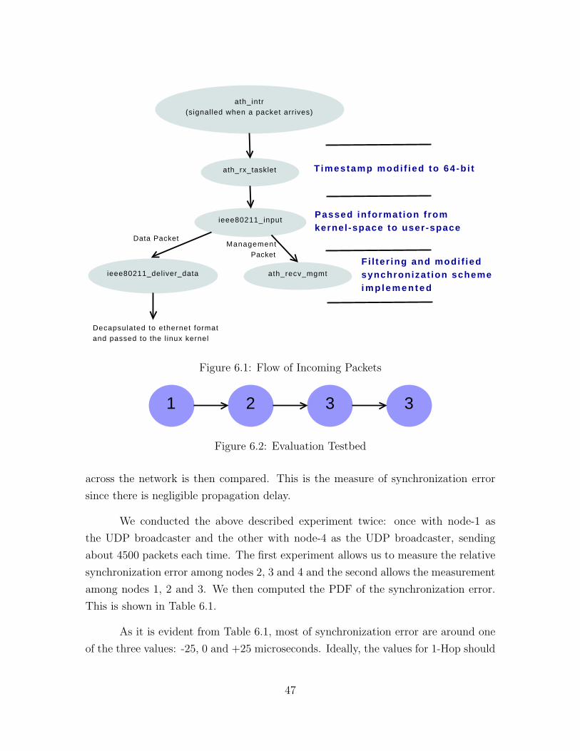
ath_intr(signalled when a packet arrives)

ath_rx_tasklet

ieee80211_input

ieee80211_deliver_data ath_recv_mgmt

Timestamp modi f ied to 64 -b i t

Passed informat ion f rom kernel -space to user-space

Fi l ter ing and modi f iedsynchronizat ion schemei m p l e m e n t e d

Decapsulated to ethernet format and passed to the l inux kernel

Data PacketManagement Packet

Figure 6.1: Flow of Incoming Packets

1 2 3 3

Figure 6.2: Evaluation Testbed

across the network is then compared. This is the measure of synchronization error

since there is negligible propagation delay.

We conducted the above described experiment twice: once with node-1 as

the UDP broadcaster and the other with node-4 as the UDP broadcaster, sending

about 4500 packets each time. The first experiment allows us to measure the relative

synchronization error among nodes 2, 3 and 4 and the second allows the measurement

among nodes 1, 2 and 3. We then computed the PDF of the synchronization error.

This is shown in Table 6.1.

As it is evident from Table 6.1, most of synchronization error are around one

of the three values: -25, 0 and +25 microseconds. Ideally, the values for 1-Hop should

47

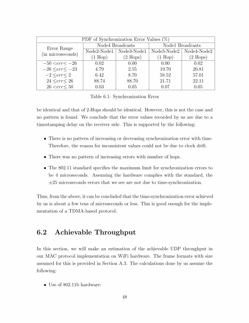
PDF of Synchronization Error Values (%)

Error Range(in microseconds)

Node4 Broadcasts Node1 BroadcastsNode2-Node1 Node3-Node1 Node3-Node2 Node4-Node2

(1 Hop) (2 Hops) (1 Hop) (2 Hops)−50 <err< −26−26 ≤err≤ −23−2 ≤err≤ 224 ≤err≤ 2626 <err≤ 50

0.02 0.00 0.00 0.024.79 2.55 19.70 20.816.42 8.70 58.52 57.0188.74 88.70 21.71 22.110.03 0.05 0.07 0.05

Table 6.1: Synchronization Error

be identical and that of 2-Hops should be identical. However, this is not the case and

no pattern is found. We conclude that the error values recorded by us are due to a

timestamping delay on the receiver side. This is supported by the following:

• There is no pattern of increasing or decreasing synchronization error with time.

Therefore, the reason for inconsistent values could not be due to clock drift.

• There was no pattern of increasing errors with number of hops.

• The 802.11 standard specifies the maximum limit for synchronization errors to

be 4 microseconds. Assuming the hardware complies with the standard, the

±25 microseconds errors that we see are not due to time-synchronization.

Thus, from the above, it can be concluded that the time-synchronization error achieved

by us is about a few tens of microseconds or less. This is good enough for the imple-

mentation of a TDMA-based protocol.

6.2 Achievable Throughput

In this section, we will make an estimation of the achievable UDP throughput in

our MAC protocol implementation on WiFi hardware. The frame formats with size

assumed for this is provided in Section A.3. The calculations done by us assume the

following:

• Use of 802.11b hardware:

48

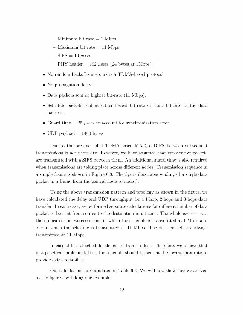
– Minimum bit-rate = 1 Mbps

– Maximum bit-rate = 11 Mbps

– SIFS = 10 µsecs

– PHY header = 192 µsecs (24 bytes at 1Mbps)

• No random backoff since ours is a TDMA-based protocol.

• No propagation delay.

• Data packets sent at highest bit-rate (11 Mbps).

• Schedule packets sent at either lowest bit-rate or same bit-rate as the data

packets.

• Guard time = 25 µsecs to account for synchronization error.

• UDP payload = 1400 bytes

Due to the presence of a TDMA-based MAC, a DIFS between subsequent

transmissions is not necessary. However, we have assumed that consecutive packets

are transmitted with a SIFS between them. An additional guard time is also required

when transmissions are taking place across different nodes. Transmission sequence in

a simple frame is shown in Figure 6.3. The figure illustrates sending of a single data

packet in a frame from the central node to node-3.

Using the above transmission pattern and topology as shown in the figure, we

have calculated the delay and UDP throughput for a 1-hop, 2-hops and 3-hops data

transfer. In each case, we performed separate calculations for different number of data

packet to be sent from source to the destination in a frame. The whole exercise was

then repeated for two cases: one in which the schedule is transmitted at 1 Mbps and

one in which the schedule is transmitted at 11 Mbps. The data packets are always

transmitted at 11 Mbps.

In case of loss of schedule, the entire frame is lost. Therefore, we believe that

in a practical implementation, the schedule should be sent at the lowest data-rate to

provide extra reliability.

Our calculations are tabulated in Table 6.2. We will now show how we arrived

at the figures by taking one example.

49

(a) Estimation of Delay

Number of Delay (in milliseconds)Data Packets 1-Hop Transfer 2-Hop Transfer 3-Hop Transfer

Per Frame X=1 X=11 X=1 X=11 X=1 X=111 1.78 1.49 4.07 3.05 6.83 4.652 3.04 2.75 6.59 5.57 10.61 8.433 4.30 4.01 9.11 8.09 14.39 12.214 5.56 5.27 11.62 10.61 18.17 15.995 6.82 6.53 14.14 13.13 21.95 19.7710 13.12 12.83 26.74 25.72 40.84 38.6615 19.41 19.12 39.33 38.31 59.73 57.5520 25.71 25.42 51.93 50.91 78.62 76.4425 32.01 31.72 64.52 63.50 97.52 95.3330 38.31 38.01 77.12 76.10 116.41 114.23

(b) Estimation of UDP Throughput

Number of UDP Throughput (in Mbps)Data Packets 1-Hop Transfer 2-Hop Transfer 3-Hop Transfer

Per Frame X=1 X=11 X=1 X=11 X=1 X=111 6.29 7.51 2.75 3.67 1.64 2.412 7.37 8.15 3.40 4.02 2.11 2.663 7.81 8.38 3.69 4.15 2.33 2.754 8.06 8.50 3.85 4.22 2.47 2.805 8.21 8.58 3.96 4.27 2.55 2.8310 8.54 8.73 4.19 4.35 2.74 2.9015 8.65 8.79 4.27 4.38 2.81 2.9220 8.71 8.81 4.31 4.40 2.85 2.9325 8.75 8.83 4.34 4.41 2.87 2.9430 8.77 8.84 4.36 4.42 2.89 2.94

Note:X is the data rate (in Mbps) at which the schedule is transmittedEach data packet has 1400 bytes of UDP payloadData is transmitted at 11 Mbps

Table 6.2: Theoretical Performance Estimated for a WiFi Implementation

50

CN 1 2 3

(a) Assumed Topology

SCH DATA

SCH DATA

SCH DATA

Central Node

Node-1

Node-2

t1 t1 t1 t1 t1 t1

t2 t2

t1 = PHY Header + SIFSt2 = Guard-Time for Sync ErrorsSCH = Schedule PacketDATA = Data Packet

FRAME duration

t ransmit ter

t ime

(b) Packet Sequence

Figure 6.3: Packet Sequence in a Frame

Example

Let us consider the case where 3 data packets are to be transferred from the central

node to node-3 in a single frame.

Guard time, tG = 25µsecs

PHY layer overhead and SIFS, per packet, toh = 192 + 10 = 202µsecs

Total number of bytes in a schedule packet with n scheduling elements,

S = (Generic header) + (Schedule header) + n ∗ (Schedule Element Size)

= 8 + 32 + (n ∗ 30) = 40 + 30n

51

At node CN 1 2

Number of Scheduling Elements (n) 4 2 0

Size of schedule (in bytes) (S) 160 100 40

Time to transmit schedule at 1 Mbps (in µsecs) t1,CN t1,Node1 t1,Node2

S ∗ 8/1 + toh 1482 1002 522

Time to transmit schedule at 11 Mbps (in µsecs) t11,CN t11,Node1 t11,Node2

S ∗ 8/11 + toh 318.36 274.73 231.09

For UDP packet of 1400 bytes payload, 8 bytes of UDP header, 20 bytes of IP header,

18 bytes of data header and 8 bytes of generic header is required. Therefore total

number of bytes is 1454.

Time required to transmit 1454 bytes at 11 Mbps,

ta =1454 ∗ 8

11= 1057.45µsecs

Therefore, total time to transmit one data packet with 1400 bytes of UDP payload,

tD = ta + toh = 2202 + 1057.45 = 1259.45µsecs

For transferring 3 packets from central node to node-3, total time required:

when schedule sent at 1 Mbps,

t1 = (t1,CN + 3 ∗ tD) + tG + (t1,Node1 + 3 ∗ tD) + tG + (t1,Node2 + 3 ∗ tD)

= (1482 + 3 ∗ 1259.45) + 25 + (1002 + 3 ∗ 1259.45) + 25 + (522 + 3 ∗ 1259.45)

= 14391.05µsecs = 14.39ms

UDP throughput = 3 ∗ 1400 ∗ 8/t1 = 33600/14391.05 = 2.33Mbps

when schedule sent at 11 Mbps,

t11 = (t11,CN + 3 ∗ tD) + tG + (t11,Node1 + 3 ∗ tD) + tG + (t11,Node2 + 3 ∗ tD)

= (318.36 + 3 ∗ 1259.45) + 25 + (274.73 + 3 ∗ 1259.45)

+25 + (231.09 + 3 ∗ 1259.45)

= 12209.23µsecs = 12.21ms

UDP throughput = 3 ∗ 1400 ∗ 8/t11 = 33600/12209.23 = 2.75Mbps

These values are shown in Table 6.2, under 3-hop transfer for number of packets

per frame equal to 3.

52

6.3 Discussion

We saw that high-precision time-synchronization needed for the implementation of a

multi-hop TDMA protocol is possible. We have also shown by calculations that using

802.11b hardware, the achievable UDP throughput over a single hop can go up to 8.8

Mbps. This value is more than what the existing CSMA/CA protocol can provide.

The achievable UDP throughput over 3-hops, varies from 1.64 to 2.94 Mbps.

A video flow requires bandwidth of 384 kbps. Therefore, in practical implementation

as per our design it should easily be possible to support 3-4 video flows over three

hops. This number would increase significantly for lesser number of hops.

Also, the throughput does not drop significantly if the schedule is sent at low

data-rate. This should definitely be considered as it would lower the loss-rate and

increase the throughput, especially in a noisy environment.

Considering the above discussed factors, it is feasible to implement our design

on the existing 802.11b hardware.

53

Chapter 7

Conclusion and Future Work

7.1 Conclusion

In this work, we have designed a framing and schedule dissemination mechanism for

multi-hop TDMA-based wireless networks. We carried out the implementation for

802.15.4-based platforms using TinyOS environment. We carried out our evaluation

on this implementation, measuring throughput and delay for various frame sizes. We

saw that as the frame size increases, the throughput increases but the delay increases

too. Thus, there is a trade-off between throughput and delay. Also, as the number of

hops increases, the throughput decreases by a factor equal to the number of hops.

The GSM full-rate speech codec operates at 13 kbps. Assuming this is used for

development of push-to-talk applications on motes using our protocol as the under-

lying MAC, 1-2 simultaneous voice calls is likely possible over 3 hops. This number

increases if the number of hops decrease. Therefore, if the requirement is such that

more than 2 connections over 3 hops is required simultaneously then our protocol

may not be suitable. However, voice calls over motes is targeted for rural areas, and

so, it is unlikely that more than 2 calls will be active simultaneously.

We have also conducted a study to see whether an implementation of our

protocol on WiFi hardware is feasible. Since time-synchronization is the crux to

any implementation of a TDMA-based protocol, we implemented a multi-hop time-

synchronization mechanism which shows that it is indeed possible to achieve high-

54

precision time-synchronization over multiple hops using WiFi hardware. We also

performed theoretical calculations for the achievable throughput assuming 802.11b

hardware. The results show that a WiFi implementation is feasible.

7.2 Future Work

With the kind of results obtained, we envision the following as future work:

• Optimization of our implementation on TinyOS to increase throughput. This

can be done by reducing the number of bits/bytes per field in the headers. The

design would remain the same.

• Since the evaluation we conducted was based on downstream traffic, it would

also be good to conduct some studies based on upstream traffic. This could be

done with variable bit-rate video flows.

• The evaluation we have done is for a single flow in a linear topology. This could

be repeated for multiple flows in a more complex network topology to gain a

better understanding.

• Design and implementation of a push-to-talk voice application for 802.15.4-

based platforms.

• Since we have shown theoretically, that our protocol would perform well when

implemented on WiFi, an implementation could be carried out.

55

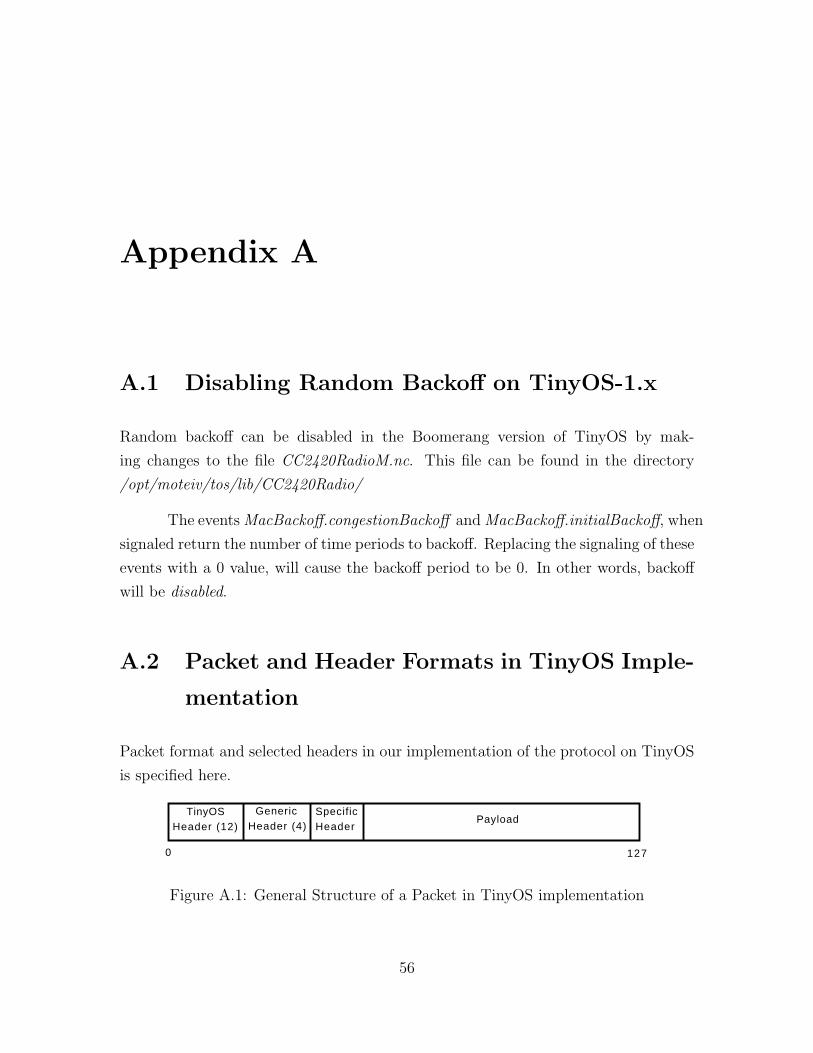
Appendix A

A.1 Disabling Random Backoff on TinyOS-1.x

Random backoff can be disabled in the Boomerang version of TinyOS by mak-

ing changes to the file CC2420RadioM.nc. This file can be found in the directory

/opt/moteiv/tos/lib/CC2420Radio/

The events MacBackoff.congestionBackoff and MacBackoff.initialBackoff, when

signaled return the number of time periods to backoff. Replacing the signaling of these

events with a 0 value, will cause the backoff period to be 0. In other words, backoff

will be disabled.

A.2 Packet and Header Formats in TinyOS Imple-

mentation

Packet format and selected headers in our implementation of the protocol on TinyOS

is specified here.

0 127

TinyOSHeader (12)

GenericHeader (4)

SpecificHeader

Payload

Figure A.1: General Structure of a Packet in TinyOS implementation

56

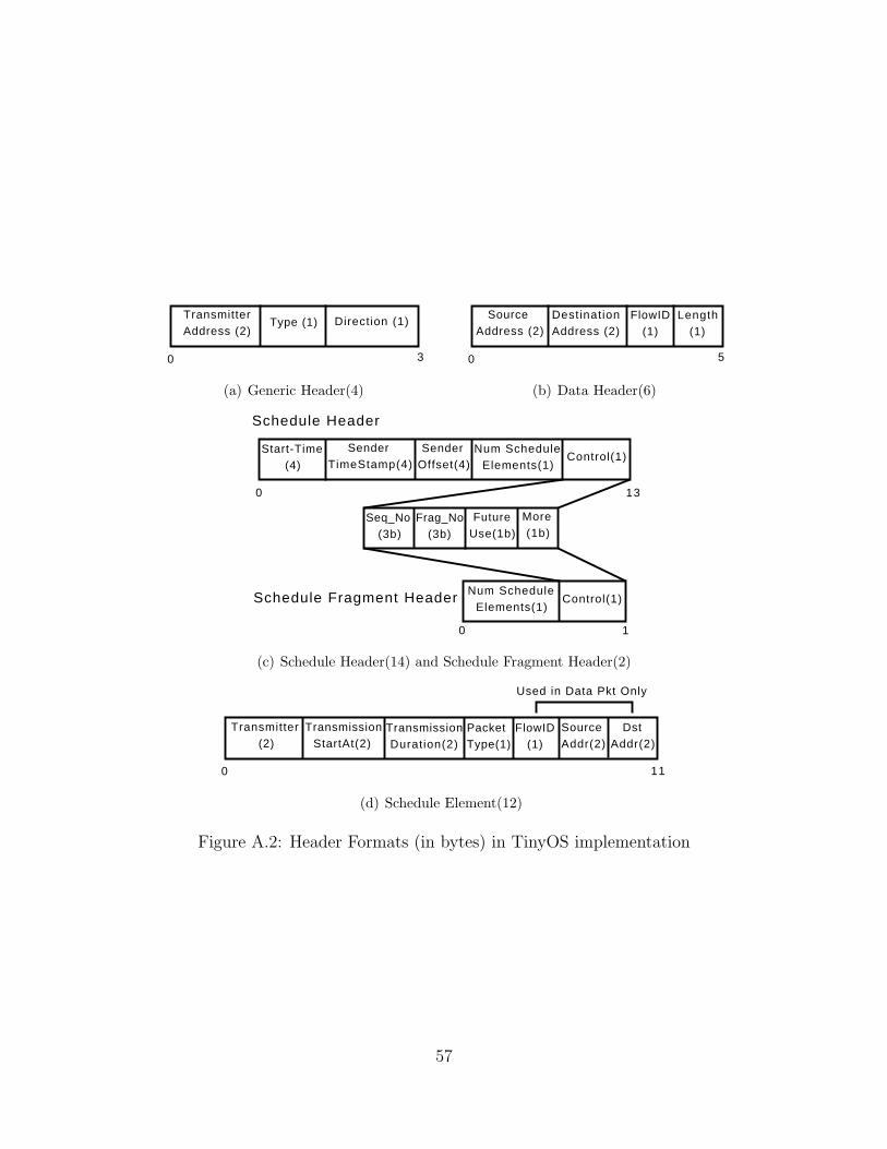
0 3

Transmitter Address (2)

Type (1) Direction (1)

(a) Generic Header(4)

0 5

SourceAddress (2)

FlowID (1)

DestinationAddress (2)

Length (1)

(b) Data Header(6)

0 13

Start-Time (4)

Sender TimeStamp(4)

Sender Offset(4)

Num Schedule Elements(1)

Control(1)

More (1b)

Seq_No (3b)

Frag_No (3b)

FutureUse(1b)

Num Schedule Elements(1)

Control(1)

0 1

Schedule Header

Schedule Fragment Header

(c) Schedule Header(14) and Schedule Fragment Header(2)

0 11

Transmitter (2)

Transmission StartAt(2)

FlowID (1)

Transmission Duration(2)

PacketType(1)

SourceAddr(2)

DstAddr(2)

Used in Data Pkt Only

(d) Schedule Element(12)

Figure A.2: Header Formats (in bytes) in TinyOS implementation

57

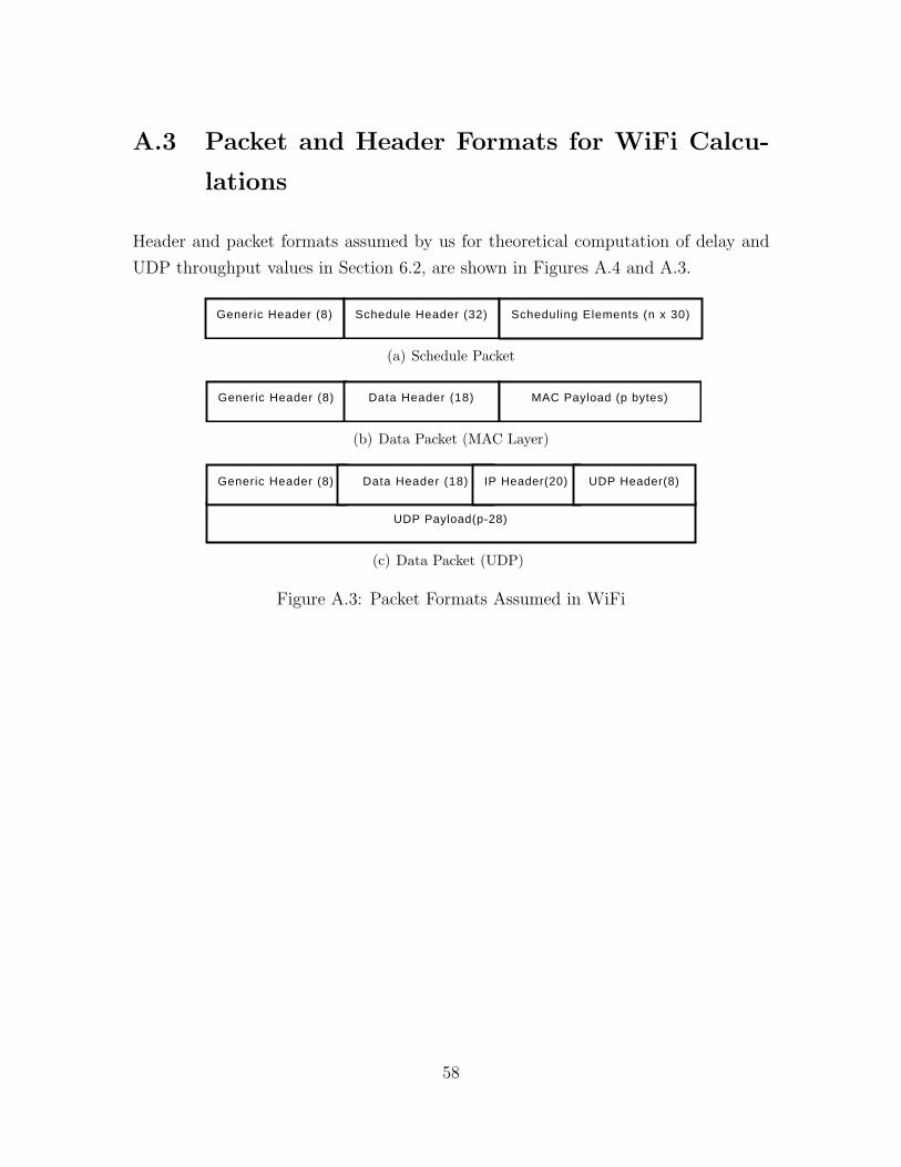
A.3 Packet and Header Formats for WiFi Calcu-

lations

Header and packet formats assumed by us for theoretical computation of delay and

UDP throughput values in Section 6.2, are shown in Figures A.4 and A.3.

Generic Header (8) Schedule Header (32) Scheduling Elements (n x 30)

(a) Schedule Packet

Generic Header (8) Data Header (18) MAC Payload (p bytes)

(b) Data Packet (MAC Layer)

UDP Payload(p-28)

Generic Header (8) Data Header (18) IP Header(20) UDP Header(8)

(c) Data Packet (UDP)

Figure A.3: Packet Formats Assumed in WiFi

58

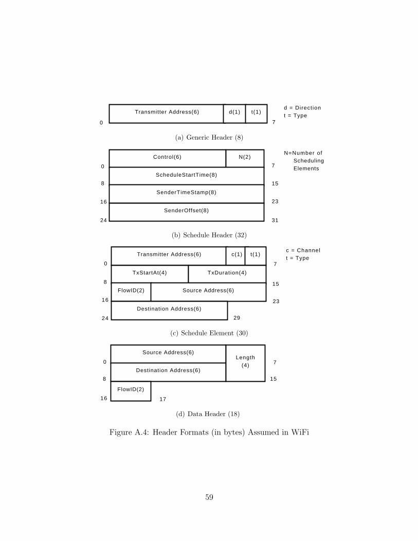
Transmitter Address(6) d(1) t(1)

0 7

d = Direct iont = Type

(a) Generic Header (8)

Control(6) N(2)

ScheduleStartTime(8)

SenderTimeStamp(8)

SenderOffset(8)

0

8

16

24

7

15

23

31

N=Number of Scheduling Elements

(b) Schedule Header (32)

Transmitter Address(6) c(1) t(1)

TxStartAt(4) TxDuration(4)

FlowID(2) Source Address(6)

Destination Address(6)

0

8

16

24

7

15

23

29

c = Channelt = Type

(c) Schedule Element (30)

Source Address(6)

Destination Address(6)

Length(4)

FlowID(2)

0

8

16

7

15

17

(d) Data Header (18)

Figure A.4: Header Formats (in bytes) Assumed in WiFi

59

References

[1] Ian F. Akyildiz, Xudong Wang, and Weilin Wang. Wireless Mesh Networks: A

Survey. Computer Networks Journal (Elsevier), Mar 2005.

[2] Rabin Patra, Sergiu Nedevschi, Sonesh Surana, Anmol Sheth, Lakshminarayanan

Subramanian, and Eric Brewer. WiLDNet: Design and Implementation of High

Performance WiFi Based Long Distance Networks. In USENIX NSDI, Apr 2007.

[3] IEEE Std 802.11-1999. IEEE Standard for Local and Metropolitan Area Net-

works, Part 11, 1999.

[4] Pravin Bhagwat, Bhaskaran Raman, and Dheeraj Sanghi. Turning 802.11 Inside-

Out. In Hotnets-II, Nov 2003.

[5] Kameswari Chebrolu and Bhaskaran Raman. FRACTEL: A Fresh Perspective on

(Rural) Mesh Networks. In ACM SIGCOMM Workshop on Networked Systems

for Developing Regions (NSDR’07), Aug 2007.

[6] Kameswari Chebrolu, Bhaskaran Raman, and Sayandeep Sen. Long-distance

802.11b Links: Performance Measurements and Experience. In MOBICOM, Sep

2006.

[7] Dattatraya Gokhale, Sayandeep Sen, Kameswari Chebrolu, and Bhaskaran Ra-

man. On the Feasibility of the Link Abstraction in (Rural) Mesh Networks. In

IEEE INFOCOM, Apr 2008.

[8] IEEE Std 802.15.4-2006. IEEE Standard for Specific Requirements, Part 15.4:

Wireless MAC and PHY Specifications for Low-Rate WPANs, 2006.

60

[9] Bhaskaran Raman et al. Lo3: Low-power, Low-cost, Local Voice and Messaging

for Rural Regions, In Preparation. http://www.cse.iitb.ac.in/silmaril/

br/doku.php?id=proj:lo3.

[10] Moteiv Corporation. Tmote Sky: Datasheet, 02-06-2006.

[11] TinyOS. Website. http://www.tinyos.net.

[12] Pavan Kumar. Design, Implementation, and Evaluation of new MAC Protocols

for Long Distance 802.11 Networks. Master’s thesis, IIT Kanpur, May 2006.

[13] Krishna Paul, Anitha Varghese, Sridhar Iyer, Bhaskar Ramamurthi, and Anurag

Kumar. WiFiRe: Rural Area Broadband Access Using the WiFi PHY and a

Multisector TDD MAC. IEEE Communications vol.45(1), Jan 2007.

[14] IEEE 802.16’s Relay Task Group. Website. http://wirelessman.org/relay/.

[15] IEEE Std 802.16-2001. IEEE Standard for Local and Metropolitan Area Net-

works, Part 16, 2001.

[16] Kameswari Chebrolu, Bhaskaran Raman, Nilesh Mishra, Phani Kumar Valiveti,

and Raj Kumar. BriMon: A Sensor Network System for Railway Bridge Moni-

toring. In ACM MobiSys, Jun 2008.

[17] Abhishek Maheshwari. Implementation and Evaluation of a MAC Scheduling

Architecture for IEEE 802.16 WirelessMANs. Master’s thesis, IIT Kanpur, May

2006.

[18] MADWiFi. Website. http://www.madwifi.org.

[19] Atheros Communications. Website. http://www.atheros.com.

61