Framework for Evaluating Transportation Control Measures : Energy

Southwest Region University Transportation Center

Framework for Evaluating Transportation Control Measures: Energy, Air Quality,

and Mobility Tradeoffs

SWUTC/94/60034-1

Center for Transportation Research University of Texas at Austin

3208 Red River, Suite 200 Austin, Texas 78705-2650

T hniealR elKlri ec Doaun ti P enta on al!e 1. Report No. I 2. Government Accession No. 3. Recipient's Catalog No.

SWUTC/94/60034-1 4. Title and Subtitle S. Report Date

Framework for Evaluating Transportation Control Measures: Energy, July 1994 Air Quality, and Mobility Tradeoffs 6. Performing Organization Code

7. Autbor(s) 8. Perfonning Organization Report No.

Mark A. Euritt, Jiefeng Qin, Jaroon Meesomboon, and C. Michael Walton 9. Perfonning Organization Name and Address 10. Work Unit No. (TRAIS)

Center for Transportation Research The University of Texas at Austin

11. Contract or Grant No. 3208 Red River, Suite 200 0079 Austin, Texas 78705-2650

12. Sponsoring Agency Name and Address 13. Type of Report and Period Covered

Southwest Region University Transportation Center Texas Transportation Institute The Texas A&M University System 14. Sponsoring Agency Code

College Station, Texas 77843-3135

IS. Supplementary Notes

Supported by a grant from the Office of the Governor of the State of Texas, Energy Office 16. Abstract

Transportation planners. engineers. and air quality analysts are increasingly understanding the need for coordinated efforts in providing efficient and effective transportation systems while addressing serious energy and environmental concerns. Policies must be issued based on broad. coordinated efforts in transportation. air quality. and energy consumption so that optimal strategies for all three components can be implemented. At present, however. transportation planning and air quality analysis models are rather incompatible. Emissions models require detailed inputs which are not generally provided by transportation planning and analysis tools. Traditionally. transportation planning is comprised offour stages: trip generation. trip distribution, mode choice. and network assignment. In general. a forecast population, auto ownership. employment, and land use are inputs into the stages sequentially. This planning process does not adequately account for the manner in which individuals make travel decisions. The only travel-related decision that can be predicted using this traditional planning method is the mode of travel, while transportation control measures (TCMs). affect trip generation and trip distribution as well as route and mode choice.

Variables required for emissions estimation have not routinely been components of transportation planning models. What is needed is a methodology for combining transportation planning and analysis models with emissions factor models for predicting the effectiveness of various TCMs. A matrix of strategies that produce the greatest savings in air emissions and energy consumption can then be developed. The project first reviews different types of emissions and TCMs, and then develops a macro-analysis model--a unified framework--that links the transportation planning and air quality analysis models. The framework can then be used to evaluate, comparatively. the impact of various transportation control measures. which influence either travel time or travel cost, on transportation-related emissions and energy consumption.

The application of the macro-framework is demonstrated through analyses of two sample networks. The results show that the effectiveness ofa TCM depends on the characteristics of the urban environment in which it is implemented. Failure to analyze the implication of a TCM prior to its implementation may yield results inconsistent with environmental and energy policy objectives. In addition. the results show that the choice of an emissions model is very critical in air quality analysis. The inclusion of an inferior emissions estimation model may result in biased conclusions. 17. KeyWords 18. Distribution Statement

transportation planning, transportation control No Restrictions. This document is available to the public through

measures (TCMs), inputs, emissions models, air NTIS: National Technical Information Service

quality, energy consumption, environmental policy, 5285 Port Royal Road methodology, matrix, macro--analysis model Springfield. Virginia 22161 19. Security Classif.( of this report) ~ 20. Security Classif.( of this page) 21. No. of Pages I 22. Price

Unclassified Unclassified 112 Form DOT F 1700.7 (8-72) Reproduction of completed page authorized

FRAMEWORK FOR EVALUATING TRANSPORTATION CONTROL MEASURES: ENERGY, AIR QUALITY,

AND MOBILITY TRADEOFFS

by

Mark A. Euritt Jiefeng Qin

Jaroon Meesomboon C. Michael Walton

Research Report SWUTC/92160034-1

Southwest Region University Transportation Center Center for Transportation Research

The University of Texas at Austin Austin, Texas 78712

JULY 1994

ACKNOWLEDGEMENTS

This publication was developed as part of the University Transportation Centers Program which is funded 50% in oil overcharge funds from Stripper Well settlement as provided by the State of Texas Governor's Energy Office and approved by the U.S. Department of Energy. Mention of trade names or commercial products does not constitute endorsement or recommendation for use.

The authors thank Chris Fiscelli for his invaluable assistance in writing part of Chapters 2, 3, and 4. In addition, the authors thank the staff at the Center for Transportation Research at The University of Texas at Austin for their patience in editing this report.

ii

TABLE OF CONTENTS

Acknowledgments ................................................................ 0 •••••••••••••••• ii

List of Figures .................................................................................................................... v

List of Tables ................................................................................................................... v

Summary ............................................................................................................................ vii

Chapter 1 Introduction ...... ....................................................................................... 1 Background ................................................................................................ 1 Clean Air Legislation .................................................................................... 1

Chapter 2 Mobile Source Emissions ..................................................................... 5 Carbon Monoxide ........................................................................................ 5 Nitrogen Oxides .......................................................................................... 5 Hydrocarbons .............................................................................................. 6 Ozone ........................................................................................................ 6 Particulates ................................................................................................. 6 Sulfur Dioxide .............................................................................................. 6 Carbon Dioxide ............................................................................................ 7 Lead ........................................................................................................... 7

Chapter 3 Transportation Control Measures ...................................................... 1 3 Consumer-Oriented Strategies ................................................................... 1 3

Trip Reduction Ordinances (TROs) .......................................................... 1 3 Vehicle Use Restrictions/Limitations ........................................................ 1 5 Pricing Policies ....................................................................................... 1 6 Alternative Work Schedules .................................................................... 1 7 Parking Management .............................................................................. 17

System Improvements ............................................................................... 1 8 Mass Transit ........................................................................................... 1 9 High-Occupancy Vehicle (HOV) Facilities ................................................. 20 Traffic Flow Improvements ....................................................................... 21 Urban Form Restructuring ....................................................................... 22 Park-and-Ride Areas ............................................................................... 23 Non-Motorized Facility Improvements ....................................................... 23

Chapter 4 Advanced Technologies ................................................... 25 Managing Congestion with IVHS ................................................................. 25 Implications for Air Quality and Energy Consumption .................................... 25

Chapter 5 Methodology ......................................................................................... 27 Demand and Mode Choice Model ............................................................... 30 Traffic Simulation Models ............................................................................ 33 Emissions Estimation Models ..................................................................... 34 Fuel Consumption Estimation Models ......................................................... 35 Dispersion Models ..................................................................................... 36 Cost-Benefit Analysis ................................................................................. 36

Chapter 6 Sample Analysis ................................................................................... 41 Network A ................................................................................................. 42 Network B ................................................................................................. 50

iii

Chapter 7 Discussion and Conclusion ................................................................ 59

References ....................................................................................................................... 63

Appendix A TRAF·NETSIM Input for Network A ................................................... 67

Appendix 8 TRAF-NETSIM Input for Network 8 ................ ................................... 79

Appendix C Emissions Calculation for Network 8 ................................................ 91 C1. Base Case ........................................................................................ 93 C2. HOV-3 Case ..................................................................................... 96 C3. Pricing Case ..................................................................................... 99

iv

LIST OF FIGURES

1 . Relationship Between HC Running Emissions and Speed ................................................. 8

2. Relationship Between CO Running Emissions and Speed ................................................. 9

3. Relationship Between NOx Running Emissions and Speed ............................................. 1 0

4. HC Idle Emission Rates .................................................................................................. 11

5. CO Idle Emission Rates .................................................................................................. 11

6. NOx Idle Emission Rates ............................................................................... , ................ 1 2

7. Model Framework for Evaluating TCMs ............................................................................ 28

8. The Choice Hierarchy .................................................................................................... 31

9. Sample Network A ......................................................................................................... 44

1 O. Sample Network B ......................................................................................................... 51

LIST OF TABLES

1 . Change in National Travel Modes .................................................................................... 3

2. Available Transportation Control Measures .................................................................... 29

3. Effects of TCMs on Utility Functions in Mode Choice Model. ........................................... 32

4a. Air Pollution Emissions and Costs ................................................................................. 37

4b. Air Pollution Emissions and Costs ................................................................................. 38

5a. Pollutant "Going Rates" ................................................................................................ 39

5b. Pollutant "Going Rates" ................................................................................................ 39

6. Some Costs and Benefits Related to TCM Implementation and Air Pollution ................... .40

7a. Mobility and Fuel Consumption Results for Network A ................................................... .46

7b. Mobility and Fuel Consumption Results for Network A ................................................... .4 7

8a. Emission Results for Network A .................................................................................... 48

8b. Emission Results for Network A .................................................................................... 49

9. Travel Time and Mode Split from Residential Area to CBO ............................................... 53

10a. Mobility and Fuel Consumption Results for Network B .................................................... 54

10b. Mobility and Fuel Consumption Results for Network B .................................................... 55

11 a. Emission Results for Network B .................................................................................... 56

11 b. Emission Results for Network B .................................................................................... 57

12a. Comparison of the Emissions Results ........................................................................... 61

12b. Comparison of the Emissions Results ........................................................................... 62

v

vi

···l

SUMMARY

Transportation planners, engineers, and air quality analysts are increasingly

understanding the need for coordinated efforts in providing efficient and effective transportation

systems while addressing serious energy and environmental concerns. Policy-makers in the

present and, particularly, in the near future, must issue policies based on broad, coordinated

efforts in transportation, air quality, and energy consumption so that optimal strategies for all three

components can be implemented. At present, however, transportation planning and air quality

analysiS models are rather incompatible. Emissions models require detailed inputs which are not

generally provided by transportation planning and analysis tools .. Traditionally, transportation

planning is comprised of four stages: trip generation, trip distribution, mode choice, and network

aSSignment. In general, a forecast population, auto ownership, employment, and land use are

inputs into the stages sequentially. This planning process does not adequately account for the

manner in which individuals make travel decisions. The only travel-related decision that can be

predicted using this traditional planning method is the mode of travel, while transportation control

measures (fCMs) affect trip generation and trip distribution as well as route and mode chOice.

Traffic flow improvement, an intended product of TCMs, may cause changes in travel

patterns, e.g., travel time and/or route changes. Equilibration procedures are normally used in

determining flows on each link in a roadway network. However, these procedures are quite limited

in estimating emissions. First, the equilibration procedures give information only about average

flow conditions, while the emissions estimation models usually require different values of speed,

acceleration, and deceleration for different classes of vehicle. Likewise, for fuel consumption

estimation, the values of speed, stop time, and number of stops are essential but are not provided

by the equilibration procedures. Second, it is very difficult to include all dimensions of travel

demand, and the ones that consider frequency, destination, or mode choice in addition to route

choice require the use of aggregate demand models, which do not adequately capture travel

behavior. Finally, the equilibration models may make large errors in estimating traffic volumes and

speeds on network links. A 30 percent error is not unusual [Horowitz, 1982].

Traffic simulation models that are generally used in optimizing traffic signals and predicting

delays can be used to simulate TCMs for some roadway links in a network. Most traffic simulation

models track the positions of vehicles as they move in the network and produce information such

as speed and stop time on a link, which can be used in emissions models. However, these

models require traffic volume as input, except a few models that are demand-responsive and,

thus, are unable to forecast changes in traffic volume caused by a TCM.

vii

A key in the estimation of air pollution is the conversion of traffic data into an amount of

pollutants. This is accomplished through the use of an emissions factor model such as the

Environmental Protection Agency's (EPA) MOBILE model. The model requires very detailed

inputs, which often do not correspond to what is commonly available from transportation planning

models, as stated previously. These include various speeds and vehicle miles of travel (VMT) for

different classes of vehicle, vehicle types, ages of vehicles, accumulated miles of vehicle travel,

maintenance program, analysis year, fuel volatility, daily ambient temperature, altitude and

humidity.

These variables, required for emissions estimation, have not been a component of

transportation planning models. What is needed is a methodology for combining transportation

planning and analysis models with emissions factor models for predicting the effectiveness of

various TCMs. A matrix of strategies that produce the greatest saving in air emissions and energy

consumption can then be developed. This project first reviews different types of emissions and

TCMs, and then develops a macro-analysis model -- a unified framework -- that links the

transportation planning and air quality analysis models. The framework can then be used to

evaluate, comparatively, the impact of various transportation control measures, which influence

either travel time or travel cost, on transportation-related emissions and energy consumption.

The application of the macro-framework is demonstrated through analyses of two sample

networks. The results show that the effectiveness of a TCM depends on the characteristics of the

urban environments in which it is implemented. Failure to analyze the implications of a TCM prior

to its implementation may yield results inconsistent with environmental and energy policy

objectives. In addition, the results show that the choice of an emissions model is very critical in air

quality analysis. The inclusion of an inferior emissions estimation model may result in biased

conclusions.

viii

CHAPTER 1. INTRODUCTION

BACKGROUND

Transportation mobility strategies may be defined as any government intervention which

attempts to alter (improve) existing transportation systems. These strategies have long been

confined to road construction and reconstruction. This has been, and occasionally still is, one of

the most traditional methods of meeting transportation needs on a local or regional level. The

additional capacity of these new roads may provide improved access to outlying areas, relieve

congestion on existing roads, and meet current and future travel demand. These types of actions

are very supply-oriented in that increased demand is matched by increasing the supply of the

system .. Although this technique has been popular in the past, air quality and energy

conservation issues have become more and more important, as have financial constraints.

Federal legislation designating attainment standards for urban areas and the energy crisis of the

1970's have altered ideas pertaining to transportation and mobility. As a result, an increasing

number of transportation professionals are understanding the need to provide efficient and

effective transportation systems while addressing serious environmental and energy concerns.

The relationship between transportation and air quality has been researched extenSively in recent

years, as well as the transportation-energy consumption link. Policy-makers in the present and,

particularly, in the future, must issue policy based on broad, coordinated efforts in transportation,

air quality, and energy consumption so that optimal strategies for all three components may be

implemented.

CLEAN AIR LEGISLATION

Over the past thirty years, the Clean Air Act Amendments have charged the

Environmental Protection Agency (EPA) with achieving air quality standards to protect public

health and welfare. The Act authorizes the EPA to promulgate emission standards for mobile and

stationary emission sources. The Act also delegates responsibility for enforcing emission control

regulations to the states.

During the early 1960's, the federal role on air pollution issues was limited to providing

funds and supporting research. The Clean Air Act in 1963 and subsequent amendments have

set a new standard for air quality in the United States. The federal government has expanded its

role in addressing air quality issues and, particularly, the associated transportation impacts. The

need for coordinated efforts in air quality and transportation is being understood and is supported

by the recent Clean Air Act amendments.

1

In 1977, the President enacted the Clean Air Act Amendments of 1977. The

amendments required states to develop State Implementation Plans (SIPs) for areas not meeting

EPA's National Ambient Air Quality Standards (NAAQS). These SIPs were to demonstrate how

the NAAQS for ozone and carbon monoxide (CO) would be achieved in all areas by the end of

1987. Unfortunately, some regions of the country could not attain the NAAQS for ozone and CO

by December 31, 1987.

The amendments of 1990 establish a new perspective in addressing today's significant air

quality problem. One of the key features of the 1990 Clean Air Act Amendments is the

classification of non-attainment areas in an attempt to match pollution control requirements and

attainment deadlines with the severity of an area's air quality problem. The purpose of this system

is to give the states ultimate responsibility and flexibility to solve the non-attainment problems in

their regions by imposing a combination of prescribed measures dependent on the severity of the

problem. In addition, there are certain contingency measures that will be invoked if the states fail

to reach the goal by the prescribed attainment date.

States with non-attainment areas classified as moderate or greater must develop

adequate plans to reduce hydrocarbon (HC) emissions and oxides of nitrogen (NOx) emissions as

necessary to reach the NAAQS by the prescribed attainment deadline. All other non-attainment

areas must achieve a 24 percent reduction from their 1990 HC emissions by 1999, and must

continue to reduce volatile organic compounds emissions by 3 percent each year until the

NAAQS are attained.

The 1990 Clean Air Act Amendments require states to submit SIP revisions. One of

these sets due in November 1992 was the 1990 State Emission Inventory, which will be the

baseline for the amendment-required reduction. Other SIP revisions include the plans proposed

by the states with non-attainment areas to achieve the NAAQS by the prescribed date.

The emission inventories prepared in 1987 indicated that the mobile sources component

is over 60 percent of the total inventory, while area sources and stationary sources occupy only 15

percent and 25 percent, respectively. It is clear that substantial reductions in the mobile source

component of the emission inventory are necessary in order to meet the minimum reduction

requirements as well as to provide for attainment by the prescribed dates. The changes in the

new law reflect an explicit recognition by Congress that transportation sources are a major and

growing impediment to achieving clean air goals. The problems addressed in the Act include a

recognition of the existing gap between the transportation and air planners, and rapid growth in

vehicle ownership and use in many metropolitan areas. For example, recent surveys have shown

that individuals believe they have less time for leisure activities and that the pace of life seems to

2

be speeding up. As such, time appears to be a more valuable commodity. The effect of the

above forces has been to dramatically decrease the use of modes of transportation other than the

single-occupant vehicle (see Table 1). These changes have led to a dramatic increase in vehicle

miles of travel (VMT) -- a standard measure for motor vehicle activity. Although the requirement for

coordination between transportation and air quality plans has been in the Act since the 1970's,

transportation improvements were never required to conform to air quality plans. The 1990

Amendments directly confront this issue.

Table 1

Change in National Travel Modes

Travel Mode 1975 1985

Drive Alone 65.6% 72.6%

Carpool 19.3% 14.0%

Transit 6.0% 5.2%

Other 9.1% 8.2%

Source: American Housing Survey, U.S. Census Bureau

Mobile source emissions have been identified as a major impediment to better air quality.

Congress recognized this, and the new amendments expand the Department of Transportation's

and EPA's responsibilities in ensuring that transportation plans, programs, and projects respond

to the goals of SIPs. In addition to setting attainment levels of various pollutants for urbanized

areas, transportation control measures have been outlined in the legislation to reduce the amount

of vehicle travel, thereby reducing harmful emissions and possibly improving air quality. (Note:

More efficient and effective use of existing transportation facilities is commonly referred to as

transportation systems management (TSM), whereas the reduction of travel demand is

considered by some to be different; the latter is often called transportation demand management

(TOM). The expression "Transportation Control Measure" encompasses both TSM and TOM.

3

4

CHAPTER 2. MOBILE SOURCE EMISSIONS

There are two basic types of mobile emission reduction measures, namely, 1) new

emission control technologies, including "high technology" inspection and maintenance, and 2)

measures that reduce vehicle modes of travel (VMT). The first approach includes the application

of new emission control systems installed on new vehicles and the inspection of in-use vehicles

to ensure that adequate maintenance is being performed. It imposes another round of

technology changes on the auto and fuel industries. The second approach includes efforts to

encourage more extensive use of public transportation systems primarily through changes in

travel behavior. It is worth noting that the former has seen more advances in the last decade,

whereas the future will require great emphasis on the latter.

Through clear language about transportation control measures (TCMs), the 1990 Clean

Air Act Amendments recognized that vehicle technology could not carry the entire load. Further

reductions in vehicular emissions must rely on VMT-reduction through the development of

transportation control plans. The major objective of this research is to provide a methodology and

framework for evaluating the effectiveness of various TCMs.

In order to fully understand the impacts of various contaminants and the extent to which

TCMs reduce emissions of these pollutants, the behavior and harmful eff·ects of these

substances should be known. The National Ambient Air Quality Standards (NAAQS) set ceilings

on six different contaminants generated primarily from transportation sources. The rest of the

chapter will discuss eight mobile source emissions, six of which are regulated in the NAAQS.

Carbon Monoxide (CO) is a colorless, odorless gas produced by the incomplete

combustion of organic fuels. CO reduces the ability of the blood to carry oxygen, thereby posing

a serious health threat to humans. Cardiovascular disorders may be aggravated and mental

functions impaired by the presence of moderate CO concentrations. High concentrations of this

contaminant may be fatal to humans.

CO concentrations at any given location are highly dependent upon proximity to the

source of the emission. This may be a congested highway or a downtown central business district

(CBO). Generally speaking, CO levels are high near their source, but decr~Ci~se dramatically as the

distance from the source increases. Owing to the behavior of CO in the atmosphere, many

strategies aimed at reducing areas of high CO concentrations ("hot spots") address only small

geographic areas of larger regions. Only recently is CO being viewed as an area-wide problem.

Nitrogen Oxides (NOxJ represent a number of compounds produced during combustion,

including nitrogen monoxide (NO) and nitrogen dioxide (N02). N02 is a brownish gas with a

5

pungent odor. Most NOx are emitted from automobiles as NO and react to form N02, which is a

precursor for acid rain and ozone (03). NOx alone may aggravate respiratory disorders and create

other health problems.

The behavior of NOx in the atmosphere is quite different from that of CO. NOx emissions

are area-wide in nature; therefore, strategies to reduce concentrations of NOx should be at least

regional in scale. Wind and sunlight also playa key role in NOx concentrations at specific sites, but

that role is somewhat unclear, as the level of solar intensity may increase or decrease NOx

depending upon the particular stage of the chemical reaction process.

Hydrocarbons (He) are compounds of carbon and hydrogen and are occasionally referred

to as volatile organic compounds (VOCs). (Note: for the purposes of this report, HC will be

synonymous with VOCs). HC is produced primarily from unburned fuel which escapes in motor

vehicle fuel exhaust. HC, collectively, consists of either methane hydrocarbons or non-methane

hydrocarbons (NMHC). Neither of these is directly harmful to humans, but NMHC or "reactive

hydrocarbons" react with NOx in the presence of sunlight to produce ozone, which is harmful to

human health.

Ozone (03), also referred to as smog, is produced by the reaction of HC and NOx in

sunlight. It is known as a secondary pollutant because it is not emitted directly from mobile or

stationary sources, but rather is formed by reactions of two major mobile source emissions, which

make 03 a major transportation-related contaminant. 03 is a strong pulmonary irritant and eye

irritant, is toxic to plants, and may impair lung functions in humans. High ozone concentrations

may also cause significant damage to crops and ecosystems.

Ozone is an area-wide pollutant greatly affected by wind, sunlight, topographic

characteristics, and temperature. Transportation strategies aimed at reducing 03 must be applied

on at least a regional level. Although it would seem logical that a reduction in precursor emissions

would decrease ozone formation, this is not necessarily true. Consequently, 03 reductions may

be more complicated and possibly not even feasible through the use of transportation control

measures.

Particulates include all solid particles and liquid droplets in the air except pure water. The

NAAQS have regulated particulates with an aerodynamic diameter smaller than 10 micrometers

(PM-10) which encompasses particles small enough to enter the lungs. The health effects of PM-

10 are not extensive, but recent studies indicate that PM-10 may contribute to respiratory cancer.

Aside from this, particulates can impair visibility and cause corrosion of exposed materials.

Sulfur Dioxide (S02) is another contaminant regulated in the NAAQS. S02 is not

considered a major transportation-related emission because it is not produced from the burning of

6

organic fuels in vehicles. Much of the S02 in the atmosphere is produced by electricity­

generating power plants. If electrified rail systems increase dramatically, S02 concentrations are

also likely to increase. The importance of S02 is its strong contribution to the formation of acid

rain, which has major adverse effects on ecosystems, crops, and human health.

Carbon Dioxide is a by-product from the burning of fossil fuels (gaSOline included). Due,

in part, to the increase of gasoline burning, C02 has increased dramatically in the U.S. and around

the world. The importance of the presence of C02 is its contribution to global warming or the

"greenhouse effect." Some scientists believe this warming may eventually shift the climatic

zones, change rainfall patterns, and possibly melt the polar ice caps, causing flooding of

numerous coastal cities and farms.

Lead (Pb) is a poisonous heavy metal which damages the nervous system, harms the

kidneys, and impairs mental functions. Lead in the atmosphere is produced from the burning of

fuel containing lead compounds. As a result of the phase-out of leaded fuels, a substantial

decrease in lead concentrations is being observed, and it is no longer considered a major

problem.

Although eight of the previously mentioned contaminants are very important, only three

major transportation-related emissions -- CO, NOx, and HC -- will be studied in the analysis of this

report. The interrelationships between these pollutants and speed are shown through Figures 1

through 3. These figures illustrate how the basic emission rates for CO, HC, and NOx vary with

speed, as reflected in the MOBILE4.1 * model for a temperature of 780 F (260 C). HC and CO

emission rates decrease on a gram/mile basis with an increase in speed, and are very sensitive to

changes in speed in the range from 0 to 25 mph (0 - 40 krnlhr). The lowest emission rates for HC

and CO are at about 45 mph (72 km/hr) with the rates increasing beyond this speed. The heavy­

duty gasoline truck (HOGT) has the greatest HC and CO emission rates among all types of

vehicles. The NOx emission rate for HOGT, however, is much less than that for the heavy-duty

diesel truck (HOOT). Both of them are well above their counterparts for all other types of vehicles.

The NOx emissions may increase with greater speed. The critical value is around 35 mph (56

km/hr). A study by Evans [1977] suggests that HC emissions are strongly correlated with average

travel speed, while both CO and NOx emissions have a high correlation with acceleration and/or

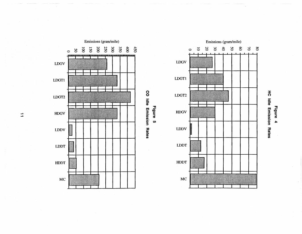
deceleration. Figures 4 through 6 illustrates the basic idle emission rates of HC, CO,and NOx for

different kinds of vehicles in MOBILE4.1. The HC or CO idle emissions from gasoline vehicles or

*More recent versions of MOBILE are now available. However, during the conduct and analysis of the study, only Version 4.1 was available.

7

Figure 1

Relationship Between He Running Emissions and Speed 1,2

16 -X-LOOV

• LOOT! 14

• LOOT2

12 ---C-HDGT

6 LDDV

~ lO ~ • LDDT

i --<>--HDDT ~ ...

OIl 8 '-' til r:: --O--MC .S til til ·s w 6

4

2

o

o lO 20 30 40 50 60

Speed (MPH)

1 Figures 1 - 6 are based on MOBILE4.1 basic emission rates at 780F. 2 LDGV -- Light-Duty Gasoline Vehicle

LDGT1 -- Light-Duty Gasoline Truck 1 LDGT2 -- Light-Duty Gasoline Truck 2 HDGT -- Heavy-Duty Gasoline Truck LDDV -- Light-Duty Diesel Vehicle LDDT -- Light-Duty Diesel Truck HDDT -- Heavy-Duty Diesel Truck Me -- Motorcycle

8

~ ---~--~-~~-~~----~------- -- ~---- ---~~~I

70

Figure 2

Relationship Between CO Running Emissions and Speed

200 -X-LDGV

180 • LDGTl

• LDGT2 160

--C--HDGT

140 I:;;. LDDV

,-, .£ 120 ·s • LDDT

l .... -<>---HDDT en 100 '-'

'" c 0 ---o.-MC

. til '" "s 80

U.l

60

40

20

0

0 10 20 30 40 50 60 70

Speed (MPH)

9

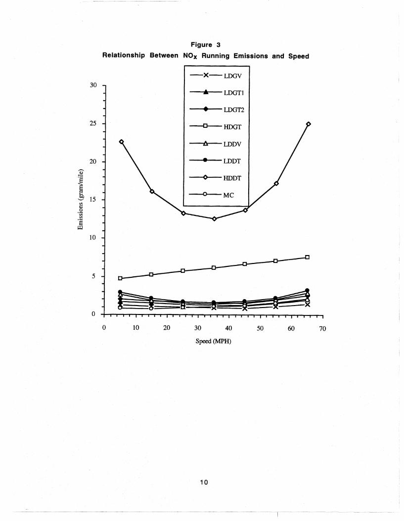
Figure 3

Relationship Between NOx Running Emissions and Speed

-X-LDGV

30 .. LDGTl

• LDGT2

25 -D-HDGT

6. LDDV

20 • LDDT

-----2 Os ~HDDT

] ... bl)

15 '-' --O--MC

(/)

c:: 0 0v; (/)

Os ~

10

5 0-=

~g ~ ~ ~ ~ 0

0 10 20 30 40 50 60 70

Speed (MPH)

10

Emissions (gram/mile)

.......... NNW W ~

o ~ 8 ~ 8 ~ 8 ~ 8

LooV

LOOT! I I LDGTI I~·

-I. IIDGV t~.·, -I.

LDDV 1i111 I

LDDT UlW'11

HDDT

MC

~ VI o

I (') 0

Q. ii' m ~ 3 cg _ .... = CD o· en :::s

:tI I» ~ CD UI

..... o o

LOOV

LOOT!

LooT2

HDGV i$ .

LDDV

LDDT

HDDT

MC

Emissions (gram/mile)

N o W o ~ o VI o g -J o 00 o

::I: (')

c: ii' m ~ 3 CQ _. c UI ... UI CD

o· 0l:Io :::s

:tI I» ~

CD UI

Figure 6

NOx Idle Emission Rates

30

25 ,,-..

~ ·5 20 -E

C<l ... eo 15 '-' V> C 0

.;;j

'" 10 ·5 Ul

5

0

> - N

~ > E-< ~ U

§ b § Q Q ::E :3 :3 :3 ~ ..J

motorcycles are higher than those from diesel vehicles, while diesel engines emit more idle NOx

pollutant. This report will attempt to develop a methodology for estimating the effect of TCMs on

the level of these contaminants in urban areas.

12

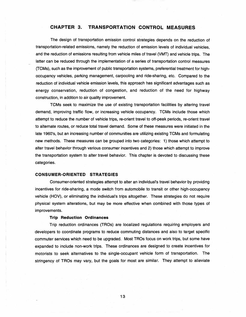
CHAPTER 3. TRANSPORTATION CONTROL MEASURES

The design of transportation emission control strategies depends on the reduction of

transportation-related emissions, namely the reduction of emission levels of individual vehicles,

and the reduction of emissions resulting from vehicle miles of travel (VMT) and vehicle trips. The

latter can be reduced through the implementation of a series of transportation control measures

(TCMs), such as the improvement of public transportation systems, preferential treatment for high­

occupancy vehicles, parking management, carpooling and ride-sharing, etc. Compared to the

reduction of individual vehicle emission levels, this approach has significant advantages such as

energy conservation, reduction of congestion, and reduction of the need for highway

construction, in addition to air quality improvement.

TCMs seek to maximize the use of existing transportation facilities by altering travel

demand, improving traffic flow, or increasing vehicle occupancy. TCMs include those which

attempt to reduce the number of vehicle trips, re-orient travel to off-peak periods, re-orient travel

to alternate routes, or reduce total travel demand. Some of these measures were initiated in the

late 1960's, but an increasing number of communities are utilizing existing TCMs and formulating

new methods. These measures can be grouped into two categories: 1) those which attempt to

alter travel behavior through various consumer incentives and 2) those which attempt to improve

the transportation system to alter travel behavior. This chapter is devoted to discussing these

categories.

CONSUMER-ORIENTED STRATEGIES

Consumer-oriented strategies attempt to alter an individual's travel behavior by providing

incentives for ride-sharing, a mode switch from automobile to transit or other high-occupancy

vehicle (HOV), or eliminating the individual's trips altogether. These strategies do not require

physical system alterations, but may be more effective when combined with those types of

improvements.

Trip Reduction Ordinances

Trip reduction ordinances (TROs) are localized regulations requiring employers and

developers to coordinate programs to reduce commuting distances and also to target specific

commuter services which need to be upgraded. Most TROs focus on work trips, but some have

expanded to include non-work trips. These ordinances are designed to create incentives for

motorists to seek alternatives to the single-occupant vehicle form of transportation. The

stringency of TROs may vary, but the goals for most are similar. They attempt to alleviate

13

congestion, improve local air quality, and reduce costs associated with additional road capacity.

Specific sections of the TROs may not reduce trips, but they provide an avenue by which TOM

measures and incentives for high-occupancy vehicle (HOV) usage may be implemented. This is

usually accomplished through various area-wide ride-share incentives [Urban Land Institute,

1991] [USEPA, 1991].

One of the major goals of TROs is to create individual or employer incentives so that

places of employment will be enticed into reducing the number of vehicle trips which they

generate. Regional carpooling and ride-sharing have considerable potential for incorporation into

TROs to perform this function, since most cars can carry more than four passengers, while

average automobile occupancy in the United States is around 1.4 persons per vehicle for work

trips. There are three types of activities which provide these incentives: commute management

organizations, tax incentives, and transportation management agencies [USEPA, 1991].

Commute management organizations match the supply of commuter services to the

demand of drive-alone alternatives (carpool matching services). Tax incentives for ride-sharing

may include exemptions for shared ride arrangements and subsidies for employers or other

programs which facilitate van-pool, carpool, or transit ridership. Transportation management

associations (TMAs) are groups which employers form to help them capitalize on available

incentives. The association attempts to manage its trip generation through numerous employee

incentives. It should be understood that the creation of a TMA and other incentives alone will not

reduce vehicle trips or emissions. TMAs facilitate the implementation of programs which might not

otherwise exist [USEPA, 1991].

Employer-based or other ride-share incentives can be an extremely important component

in TROs because they help provide the motivation for reducing vehicle trips. The main obstacle

facing the car-poolers or ride-sharers is that they must have trip origins and destinations close to

one another and must travel at the same time. Carpools are more desirable than individual travel

by car because they result in less congestion and emissions. The greatest potential for

carpooling and ride-sharing is work trips. Since carpooling and ride-sharing cannot be organized

or scheduled by any government agency, their use can be encouraged by preferential treatment

on the street and parking restrictions which can be included in automobile user charges.

Congestion may be eased and emissions can be reduced Significantly through

continuous efforts to encourage carpooling or ride-sharing. TROs may also be crucial to energy

savings, as some experts believe ride-sharing is the primary method by which fuel can be

conserved. The major problem with ordinances to reduce emissions or ride-share incentives is

14

that the impacts of these programs are largely unevaluated and the extent to which they focus on

non-work, off-peak trips is limited [USEPA, 1991].

Vehicle Use Restrictions/Limitations

Restrictions on vehicle use generally aim at single-occupant vehicle users. Restrictions

can be area-wide or, sometimes, in a small geographic area of a larger region. These areas are

commonly referred to as automobile restricted zones (ARZs). The shortcoming of these

strategies is their limitation on mobility [USEPA, 1991].

ARZs are designated areas which prohibit or limit automobile use and are usually reserved

for pedestrian and bicycle traffic. They may be effective for the vehicle-prohibited area, particularly

in the case of CO emissions, but may be detrimental to other nearby zones because the traffic and

resultant air quality burden is shifted to another part of the city or region [USEPA, 1991] [Horowitz,

1982].

Other forms of restrictions include no-drive days. To date, these programs are solely

voluntary, but may become mandatory in future years. The objective is to encourage individuals

to search for alternatives to the single-occupant vehicle mode of transportation on certain days of

the week. This is usually implemented through license plate numbers. All automobile owners'

license plate numbers ending with a particular number are encouraged to carpool on a particular

day of the week. No-drive days are estimated to have a minimal impact in reducing emissions and

energy consumption [USEPA, 1991].

Two other less common forms of vehicle use restrictions are traffic cells and central

business district (CBO) tolls. Traffic cells are accessible by origin-destination traffic and not by

through-traffic. As an example, consider a CBO developed along a highway. Motorists traveling

along this highway may access the CBO or pass through this zone to reach another destination.

With a traffic cell in place in the CBO area, motorists using the freeway would be physically barred

from passing through to another zone. The diversion of through-traffic will reduce congestion

along this particular area of the highway, resulting in higher speeds and, therefore, fewer

emissions in the traffic cell area. The implementation of traffic cells may lead to increased circuitry

of travel, which can have adverse effects on energy consumption and possibly on regional

emissions [Horowitz, 1982].

A CBO toll is similar to a pricing measure because a fee is levied on motorists who attempt

to enter a CBO by automobile. Fees for entrance into a CBO may reduce downtown congestion

and improve CO emissions in the downtown area, but may have adverse effects on area

businesses and, like traffic cells, lead to greater circuitry of travel [Bellomo, 1973].

15

Pricing Policies

The concept of pricing - or "road pricing" and "congestion pricing," as it is referred to in

the literature - is to create an economic disincentive for automobile use, and in particular, for

single-occupant vehicle use. The four types of pricing measures which will be discussed in this

chapter are 1) fuel tax increases, 2) vehicle metering, 3) local area licensing, and 4) toll roads.

Increases in gasoline taxes and vehicle metering are similar in nature. Vehicle metering

involves the installation of an odometer in all vehicles. A fee would be levied on the owner of a

vehicle proportionate to the distance the vehicle was driven. This situation is similar to raising fuel

taxes. Fuel tax increases would seem to be more "fair" because drivers of fuel-inefficient vehicles

would be penalized to a greater degree and drivers of alternative-fueled vehicles would not be

penalized at all. It would be difficult to determine the effect of this type of pricing on higher­

polluting vehicles as opposed to lower-polluting vehicles. If fuel tax increases are to reduce VMT

significantly, the increases would have to be very high, thereby introducing political constraints.

Vehicle metering would be difficult to implement legally, practically, and politically, thereby

eliminating it as a realistic solution to mobile source emission reduction and energy conservation

[Horowitz, 1982].

Local area licensing focuses on the reduction of interurban travel as opposed to total

vehicle travel. The driver would be economically penalized for choosing a destination outside the

region in which his/her trip originated. A significant reduction in interurban travel could be

expected, resulting in fewer long-distance trips. This VMT decrease would reduce emissions

slightly, but most of the decreases would be felt outside the urban area. A slight decrease in fuel

consumption could also be expected, but this pricing technique would be difficult to implement

and enforce [Horowitz, 1982].

Toll roads are another method of direct user financing. A fee is charged to motorists

driving on a toll road. Tolls may be effective in reducing congestion along the tolled arterial, but

are not effective for significant regional emission reductions if alternate routes are available. As a

result, energy savings are minimal and, although emissions may be reduced along some

roadways, aggregate emission reduction is limited [Urban Land Institute, 1991].

A recent innovation with toll roads is variable lane charging whereby drivers are allowed to

purchase, or more accurately rent, excess capacity. For example, single-occupant vehicles would

be allowed to buy permits to use an HOV facility. Evaluation of such TCMs must recognize the

impacts on persons at different income levels.

16

Alternative Work Schedules

Since many of the vehicle trips which are generated in a given urban area are work trips

and since many of them occur at the same time, adjusting schedules in the workplace is a rapidly

growing TCM. These types of adjustments attempt to eliminate work trips altogether or divert

them to off-peak time. The three major types of schedule changes are 1) telecommuting, 2)

flextime, and 3) the compressed work week [USEPA, 1991].

Telecommuting is the process by which the employee works at a location other than the

central office. This may be at home or at a satellite work center. If employees stay at home and

work, the work trip is eliminated. This would reduce VMT and the number of cold starts and hot

soaks, which would be beneficial to air quality and, to a lesser extent, reduce energy

consumption. This strategy, at present, may not be plausible because of the lack of investment in

telecommuting networks and in businesses' present state of knowledge about telecommuting.

There is much misunderstanding by employers about telecommuting.

Flextime is the process by which employers may spread their employees' work shifts over

the entire day, thereby reducing peak-period traffic congestion. The number of vehicle trips

would not be reduced, but low levels of service are less likely to occur during the peak hours,

thereby increasing speeds and reducing running emissions and energy consumption

[Rosenbloom, 1988]. Flextime, however, is resisted by many companies and agencies owing to

the management difficulties.

Using a compressed working week, employees travel to work four days instead of five

and, as a result, eliminate two work trips per employee (the journey to work and back on the fifth

day). Because the shift hours will be different on the days the employees do work, at least one of

the two trips will not be made during the peak periods. The U.S. Environmental Protection

Agency (EPA) estimates that these vehicle trip and VMT decreases may result in significant urban

air quality improvements. The main problem is the adverse effect on production output. As a

result, alternative work schedules are not likely to be applied in the near future.

Parking Management

The improved management of vehicle parking spaces can reduce the demand for vehicle

trips by eliminating the trip or providing incentives for the trip to be made by another mode or in a

ride-share arrangement. The four main parking management strategies are 1) control of the

parking supply, 2) preferential parking for HOVs, 3) parking priCing policies, and 4) parking

requirements in zoning codes [USEPA, 1991].

The most common method of contrOlling the parking supply of an area is to set a maximum

ceiling on the number of spaces so that the demand must adjust downward to meet the limited

17

supply. Preferential parking for HOVs can either offer attractively proximal spaces for carpools or

van-pools or eliminate parking fees for HOVs which would normally be levied on single-occupant

vehicles. Parking pricing policies can aim at either increasing existing prices, imposing new fees,

or eliminating parking subsidies. Zoning codes can also be used to manage congestion and the

demand for vehicle trips by limiting the number of parking spaces required for site development

[USEPA, 1991] [Horowitz, 1982].

Parking management strategies are most effective when implemented in dense CBDs

that have limited parking. It is argued, however, that these strategies will have an adverse impact

on downtown businesses. This could lead to increased development and economic activities in

the suburbs, thereby increasing fuel consumption and regional emissions [USEPA, 1991]

[Horowitz, 1982] [Lutin, 1976] [Bellomo, 1973].

Metropolitan areas similar to the New York City area are characterized by their advanced

age, extensive rapid rail systems, and dense CBDs. Other cities displaying these traits are the

large, highly industrialized cities like Chicago, Philadelphia, Washington D.C., Baltimore, etc.

Owing to the characteristics of limited parking spots in these regions, the management of

parking, particularly in the downtown area, may yield significant improvements. These include

reduced CBD traffic congestion and routes leading to the CBD; improved air quality, particularly in

the downtown area; and a reduction in total energy consumption. Depending upon the specific

parking availability of a region, priCing of single-occupant vehicles and proximal spaces reserved

for high-occupancy vehicles may be effective, as well as control of the parking supply in the CBD

area.

If parking management were implemented appropriately and ride-sharing and transit use

increased accordingly, a single-occupant vehicle reduction of up to 30 percent would be possible

in New York City. This translates into a reduction of roughly 6.9 million vehicle trips or nearly 62

million daily VMT. Approximately 132 million vehicle miles (212.4 million vehicle km) are traveled

daily on major arterial and freeways in the New York City urbanized area. This means that

congestion can be cut almost in half if significant parking management improvements were to take

place area-wide. These are lofty improvements and, in reality, would be difficult to achieve.

SYSTEM IMPROVEMENTS

The second major category of TCMs is system improvements, those which involve

altering the transportation system in some way to achieve a reduction in vehicle trip demand or

make the system operate·more effiCiently.

18

Mass Transit

One of the oldest and least complex of all TCMs is the improvement of mass transit

systems. A variety of improvements are feasible and can be grouped into five categories:

1) system expansions, 2) operational improvements, 3) improvement of transit routes, 4)

introduction of rail transit, and 5) market strategies, including reduced transit fare and automobile

user charges [USEPA, 1991].

System expansions can take the form of construction or extensions of fixed guideway

systems or express and circumferential bus service. Various rail options exist, ranging from heavy

rapid rail to light rail. These types of improvements are usually high in cost, characteristic of most

older, industrialized urban areas, and are most effective when highly clustered polynucleated

development exists [USEPA, 1991] [Bellomo, 1973] [Lutin, 1976] [Pikarsky,1978].

Operational modifications focus on improving and optimizing existing transit systems. A

wide variety of strategies can be used, such as schedule modifications, stop-frequency changes,

bus traffic signal preemption, maintenance improvements, and monitoring. These measures are

generally lower in cost than service expansions and, in some cases, can prove to be more cost­

effective.

Most urban area automobile emissions are caused by trips originating and/or terminating

in suburban areas. Hence, the achievement of significant reductions in automobile emissions

must be associated with reductions in suburban travel. In other words urban air quality can be

improved only if suburban motorists shift to higher-occupancy vehicles. Most current transit

systems serve suburban areas very poorly. The obstacle for high-quality transit service in

suburban areas is the difficulty of collecting and distributing passengers in low-density areas.

However, it is feasible to bridge the CBD and suburban residential areas by using a transit system,

which is successfully illustrated by the Shirley Highway HOV lanes in Washington, D.C.

Movement away from single-occupant vehicles to mass transit will require significant

expansion of transit systems. In terms of capacity, rail transit can accommodate from 100-250

persons per vehicle. This compares favorably to bus transit, which can carry between 50-80

persons per vehicle. Rail transit does require significant outlays for construction.

The excessive use of the automobile in cities, especially for work trips, is a result of

underpricing of automobiles. A study by the World Resources Institute found that motor vehicles

are subsidized nearly $300 billion per year, or an equivalent of an additional $2/gallon ($0.53/Iiter)

fuel tax [MacKenzie, 1994]. This underpricing of motor vehicles represents a large subsidy to

automobile users which contributes to the decline of the transit industry in the United States.

Market strategies use economic incentives to increase transit ridership. This can be done through

19

employee incentives, reduced fares, monthly passes, passenger amenities, and other activities.

These strategies are more consumer-induced approaches because they attempt to create

financial incentives for automobile users to switch modes as opposed to improving the transit

service. There are two possible ways to balance transit and automobile user costs. One is to

reduce the transit fare. The other is to increase the cost of automobile use.

The studies and experiments conducted in Atlanta and Boston in the 1970's have shown

that a reduction in transit fares has only a slight effect on auto use. The explanations of this result

are: 1) the existing cost imbalance is caused by the underpricing of auto use, not the overpricing

of transit use; and/or 2) the fare reduction was not accompanied by adequate improvements in

transit service quality. The end result is that a realistic reduction in transit fares is not a feasible way

to reducing automobile use.

The other method to balance the user costs between automobile and transit is to increase

the price of vehicle use to reflect the true value of automobile transportation. A study submitted

to the Department of Transportation concluded that "Peak-hour private auto travel is heavily

subsidized. Charges sufficient to cover the true cost of auto travel in urban areas would surely

cause restructuring of travel behavior and urban form." The only disadvantage of this approach is

that it is burdensome to people who are far removed from high-quality transit systems. To realize

the purpose of reduction in auto use and emissions, the auto user charges should be flexible and

assessed on auto use frequency. The possible methods include fuel tax increases and parking

restrictions. The increase in fuel tax may switch the public to driving small cars, which use less

fuel -- but do not necessarily pollute less -- than large cars, whereas modest reductions in auto use

can be expected in association with high-quality public transit systems.

The effectiveness of future transit systems will depend upon their ability to adapt to new

and changing urban structure. Well-developed downtown areas with connecting developments

are becoming obsolete and are being replaced by dispersed,linear development. If transit

ridership is to increase, new technologies must be used to make systems more useful, cost­

efficient, and attractive to consumers [USEPA, 19911.

High-Occupancy Vehicle (HOV) Facilities

A number of urban areas are experimenting with preferential treatment for HOVs on major

roadways. The speed and reliability of buses can be increased significantly by using exclusive or

reserved lanes. Furthermore, this kind of treatment can be applied to carpools and ride-sharing.

The predominant method is the designation of exclusive lanes for these vehicles. These facilities

may be located on freeways or arterials in a separate right-of-way or buffer-separated. If they are

well-designed for a specific area, significant reductions in travel time can be achieved.

20

The principal purpose of preferential treatment for HOVs is to make them immune to

congestion during peak hour, when the ridership of HOVs is highest, and to make them more

attractive. Some successful examples include the Shirley Highway in Washington, D.C., and the

EI Monte Busway in Los Angeles.

Two considerations should be included in HOV priority treatment. One is that HOV travel

time can be improved substantially only if there is a large portion of preferential treatment along

the vehicle route. For example, a 10-mile priority route can save 5 minutes, but a 2-mile priority

route saves only 1 minute, if the vehicle speed is increased from 30 MPH to 60 MPH. This

phenomenon requires that the HOV priority be treated only on travel routes of relatively long

distance.

The other consideration is the improvement of the quality of bus service system and

carpooling management. Since the essence of priority treatment fm HOVs is to attract more auto

users to mass transit or ride-sharing, the effects of HOV priority treatment on auto use and

emissions rely on the state of the improvement of transit and traffic management measures that

may be taken. Reservation of an exclusive lane for HOVs on the arterial or freeway can only

aggravate air equality if the current transit system remains unchanged because of reduced

roadways [Horowitz, 1982] [USEPA, 1991].

Traffic Flow Improvements

ImproVements in traffic flow most often occur in the form of engineering improvements

along a roadway. Some examples are road widening, speed and signalization improvements,

turn-lane installation, on-street parking prohibition, and contra-flow lanes. These improvements

attempt to achieve a smoother flow of traffic which would reduce speed variations, thereby

benefiting air quality and conserving energy. Three popular forms of improvements are 1) super­

streets, 2) ramp metering, and 3) incident management systems [Horowitz, 1982] [USEPA,

1991 ].

The formation of a super-street is done by making cost-effective improvements to an

existing arterial to increase its capacity. Some examples are signal timing, speed improvements,

no left turns, and other traffic flow techniques, all on the same roadway. The increased capacity of

the these roads will likely attract travelers from congested alternate routes, thereby easing

congestion on those routes. This would reduce running emissions somewhat and conserve

energy which would have otherwise been lost in delays [Urban Land Institute, 1991].

Ramp metering is usually performed at entrance ramps on freeways. When the freeway's

critical point is reached, vehicles are prevented from accessing the freeway. Long queues may

form at these pOints, which increases idling of the queued vehicles and increases emissions near

21

the access ramp. Little or no energy conservation can be expected for the same reason. This

technique may also increase traffic on non-metered roadways. Additional studies have shown

that much of the traffic entering metered roads is from alternate routes, suggesting that overall

travel times are actually improved [Horowitz, 1982] [USEPA, 1991].

Incident management systems can take the form of increased use of roving tow or service

vehicles, detectors in the roadway, or motorist-aid call boxes. The concept is to clear accidents

and breakdowns as quickly as possible by using these systems to respond to congestion caused

by breakdowns or accidents. A Federal Highway Administration (FHWA) study indicated that a

significant reduction in urban congestion can be expected from these systems. This may greatly

reduce running emissions along many highways, particularly during peak periods. Fuel would also

be conserved from the reduced speed variations of vehicles on roadways where incidents occur

[USEPA, 1991].

Urban Form Restructuring

Most strategies attempting to alleviate traffic congestion relate directly to discovering

more efficient methods for travelers to reach their destinations. The concept of altering land use

development in urban areas involves bringing destinations closer to their origins and reducing

society's dependence on the single-occupant automobile. Current urban structure is very

different from older, traditional land development patterns. Centralized patterns are almost

entirely obsolete, and multiple-nuclei urban areas are becoming less common. They are being

replaced by dispersed, linear development which is not compatible to efficient use of current

transportation systems. If urban regions are to address their congestion and mobile source

emissions problems, they need to combine travel demand efforts with urban restructuring.

The three most prominent types of favorable urban structure are 1 ) centralized

development, 2) decentralized development, and 3) polynucleated development. No matter

which scenario is modeled, all three options have the same basic focus. This is to increase

population and employment densities in certain areas and develop transit systems accordingly so

that mass transit systems can become more effective. Land use centralization will most likely

create a trade-off between increased pollutant concentrations in the center city and reduced

regional emissions. Increased center city congestion may also limit substantial energy savings.

Land use decentralization may be beneficial to the center city air quality problem, but longer trip .

lengths will likely result, thereby increasing aggregate emissions and fuel consumption. The

polynucleated development alternative may be the most viable of the three scenarios. It would

likely be the easiest to attain, given present regional urban structure, and it would also be more

conducive to effective transit than the other two options. This would make it the optimal urban

22

I - - - ._-- -

development alternative in relieving congestion, improving air quality, and· reducing energy

consumption. It should be understood that urban restructuring alone will not provide significant

benefits unless it is accompanied by mass transit improvements and other TCMs [Lutin, 1976]

[Pikarsky, 1978] [Urban Land Institute, 1991] [Wilson and Smith, 1987].

Park-and-Ride Areas

Park-and-ride areas provide facilities for a mode switch from automobile to transit to occur.

The goal of constructing these lots is to attract travelers from an area and direct them to their

common destinations via rail transit or some form of HOV. This reduces overall VMT. The reduced

VMT would ease congestion on heavily traveled freeways and provide substantial energy savings.

The effect on air quality is mixed. Benefits will be experienced from the reduced VMT, but

emissions may increase near the lots and routes leading to the lots [Bellomo, 1973] [USEPA,

1991].

Many park-and-ride areas are used in conjunction with other TCMs; therefore, it can be

difficult to assess their contribution to emissions reduction when they are present. The most

effective park-and-ride lots will most likely be those where the governing body incorporates the

facility with other TCMs and factors in the specific characteristics of that urban area.

Non-Motorized Facilities

Other methods which can be used to reduce vehicle traffic include improvements to

bicycle and pedestrian facilities. Some of these improvements are attractive because of their low

cost, negligible social and political implications, and ease of implementation. Some examples of

non-motorized facilities are an increased number of bicycle lanes, routes, paths, maps, sidewalks,

storage and ancillary facilities, and even transit connections to bike paths and walkways. Although

the presence of these facilities will not deter many people from automobile use, only a small

percentage of people would have to switch modes for an area to experience significant results.

This is because of the 100 percent reduction in emissions and fuel consumption from the

elimination of each vehicle trip [USEPA, 1991].

23

24

T ---

CHAPTER 4. ADVANCED TECHNOLOGIES

Most advanced transportation technologies can be categorized into a rapidly developing

concept called Intelligent Vehicle Highway Systems (IVHS). The basic vision of IVHS is to improve

communications among drivers, vehicles, and roadways. This increased communication will

enhance driver information on the road, thereby creating a higher probability of producing faster,

safer trips. The four main techniques utilized in this technology are 1) advanced driver information

systems (ADIS), 2) advanced traffic management systems (ATMS), 3) advanced vehicle control

systems (AVCS), and 4) commercial vehicle operations (CVO) [Urban Land Institute, 1991]

[Working Group on Operational Benefits, 1990].

MANAGING CONGESTION WITH IVHS

A higher level of communication between vehicles and highways should improve traffic

'flow and reduce travel times. With these improvements, an increased capacity level of existing

transportation systems can be expected. IVHS technologies aid in the improvement of many

TCMs, thereby making them more effective. Detectors used in incident management systems,

telecommunications equipment, and demand-responsive signalization are very much a part of

optimizing these TCMs so that they can become more effective. These methods, together with

computerized surveillance, can eliminate some trips and improve speeds on others, which would

help alleviate congestion.

IMPLICATIONS FOR AIR QUALITY AND ENERGY CONSUMPTION

The implementation of IVHS technologies, in particular ATMS and ADIS, will create

potential fuel savings in three ways. Travel times and delays will be reduced, drivers will

experience fewer stops and starts, and excess vehicle miles of travel (VMT) will be eliminated

through the use of the least-distance path choice.

Air quality also may improve with the use of IVHS. Some experts believe VMT growth is

the most important factor in air quality problems, as opposed to vehicle fuel inefficiency. IVHS will

reduce congestion, provide optimum routing, and avoid wasted trips, thereby producing a

smoother traffic flow and reduced VMT. These factors should have an immediate effect on the

level of running emissions generated in urban areas.

Because IVHS' initiatives complement traffic management strategies, its existence will not

be counterproductive in that sense. The extent of IVHS' impact on emissions reduction and

energy conservation depends upon its coordination with other environmentally beneficial

transportation efforts and the cooperation of environmental and transportation officials.

25

26

CHAPTER 5. METHODOLOGY

The traditional four-step transportation planning model in widespread use was mostly

developed for the narrow purpose of transportation engineering, not for air quality and energy

consumption analysis. Many aspects of the current standard practice in transportation modeling

are inadequate to meet the challenges of transportation planning, energy consumption, and air

quality analy_sis in the future. Work needs to be done on immediate quick fixes to support the next

round of air quality conformity analysis.

Over the past two decades there has been relatively little innovation in transportation

planning modeling. The vehicle-trip-oriented models in trip generation focus on vehicle trip

generation instead of person trip generation. They cannot reflect the potential of transportation

control measures (TCMs) to divert short automobile trips to non-motorized modes. A set of

default travel times between origins and destinations assumed by many state Department of

Transportations (DOTs) in trip distribution ignore traffic congestion, which is a major concern in the

analysis of fuel consumption and air quality. This makes the model insensitive to congestion or

changes in transportation capacity. To achieve the purpose of coordinating of transportation

planning, air quality, and energy consumption, models must become sensitive to many more

factors. Travel time needs to be accounted for in the effects of congestion and capacity changes

on spatial and temporal trip distribution and mode choice. A more detailed highway network

simulation model separating link and intersection capacity and delay is needed to improve the

values of travel time.

This report develops a consistent methodology linking transportation planning, energy

consumption, and air quality analysis. The methodology is designed to predict the impact of

TCMs on travel behavior, pollutant emissions, and energy consumption to identify which TCMs

have the greatest potential and appear to be most attractive for implementation within a region. It

provides a bridge of knowledge and common understanding between transportation planners

and regulators charged with improving air quality.

The general framework of the model developed in this project is illustrated in Figure 7.

The model framework consists of five models as well as cost-benefit analysis.

1. Demand and mode choice model. This model is used to predict the changes of

probabilities concerning which mode, destination, and route individuals will choose to travel in an

urban area as a result of implementation of TCMs. The model should encompass all possible

modes that are affected by TCMs. These modes are, for example, non-motorized, drive alone,

27

Mode Split

FIGURE 7

Model Framework for Evaluating TCMs

TCMs

TravelTime Change

28

Implementation Costs

Savings

Pollution Levels

~ -- --r---------

carpool, transit, or even whether the individuals choose not to travel - as a result of

telecommuting, for instance.

2. Traffic simulation model. A traffic simulation model can be used to study effects of

traffic management strategies on the system's operational performance. This performance is

generally expressed in terms of measures of effectiveness such as vehicle miles of travel (VMT),

person miles of travel (PMT), average vehicle speeds, vehicle stops, and average and maximum

queue length. These parameters are importantin the estimation of pollutants.

3. Emissions estimation model. This model takes into account the factors affecting

emissions, such as speed, VMT, vehicle classes, and modes of operation.

4. Fuel consumption estimation mode/. This model estimates the fuel consumption

changes as a result of TCM implementation.

5. Dispersion model. This model is used to estimate emissions concentration as a

function of atmospheric conditions, e.g., winds, temperature, and altitude.

The inputs of the model include a description of the characteristics of the TCMs to be

implemented, baseline information on current travel characteristics, e.g., travel time and/or travel

cost, current socioeconomic attributes, current emissions inventory, and local cost parameters.

The model system is designed to evaluate a broad range of candidate TCMs, which are

listed in Table 2. Moreover, it can be used to measure the effectiveness of user-specified TCMs.

TABLE 2

Available Transportation Control Measures

• Improve Public Transit

Lanes

• Employer-Based Transportation Program

• Traffic Flow Improvements

• Limit Vehicle Use in Downtown Areas

• Bicycle and Pedestrian Facilities

• Reduce Extreme Cold Start Emissions

• Programs for Large Activity Centers and

Vehicles

Special Events

29

• High-Occupancy Vehicle (HOV)

• Trip Reduction Ordinances

• Park-and-Ride/Fringe Parking

• Area-Wide Ride-Sharing Incentives

• Control of Extended Vehicle Idling

• Flexible Work Schedules

• Voluntary Removal of Pre-1980

DEMAND AND MODE CHOICE MODEL

The TCMs identified in the Clean Air Act Amendments of 1990 (CAAA), as shown

previously in Table 2, influence travel decisions primarily in the short-term through frequency,

route, and mode of travel, but may have some long-term effects on workplace location, for

example. TCMs also encompass decisions regarding whether or not an individual chooses to

travel, as well as travel todifferent workplace locations according to different schedules, as a result

of telecommuting and flexible work schedules. The influence of TCMs on travel decisions can be

explained by discrete choice models, which are flexible enough to accommodate long-, medium-,

and short-term decisions.

As discussed earlier, the traditional four-stage transportation planning sequence does

not account for the manner in which individuals make travel decisions, particularly those in the

long- and medium-term time range. As an alternative approach, a discrete choice model may be

used. Figure 8 demonstrates a broad range of behavioral decision making which may influence

the traveler's decision in the long-, medium-, or short-term time range. A transportation system

based on this structure was initially developed by Ben-Akiva and Atherton to analyze potential

energy conservation policies [Ben-A kiva and Atherton, 1977]. Emissions estimated for various

TCMs are merely an extended application of this model. The impacts of TCMs on air pollution

should be assessed for different ranges of travel decisions. Importantly, employment of this

approach takes into account travel decisions for the long, medium, and short terms.

Even though this approach is more applicable than the traditional four-stage planning

models, its outputs are still not sufficient to meet the data requirements of emissions factor

models. The emissions factor models require vehicle type for work and non-work trips, as well as

engine type (gasoline, diesel, or other fuel).

Moreover, the model structure should be adaptable to inclusion of new modes into the

urban transportation system. For instance, if light rail is to be developed, then the model should

yield an accurate share of rail's ridership to investigate the effectiveness of this transit investment.

Also, the model should be able to forecast individual behavior when telecommuting, using

compressed work weeks, or flexible work hours.

Significant variables in the mode choice model generally are transportation level of service

and socioeconomic variables. The transportation level of service variables are travel time,

disaggregated to in-vehicle time, out-of-vehicle time, and travel cost. The socioeconomic

variables include income, workplace, mode availability, and employment denSity. Effects of a TCM

entering the choice model as shown in Figure 7 change values of the utility function variables.

Some effects are summarized in Table 3.

30

FIGURE 8

The Choice Hierarchy

r " Employment location

Residential location Housing type

\, .I11III

~r

r Automobile ownership

Mode to work

\, ......

, r '" Non-work travel

(frequency, destination,

" mode

...II1II

Source: Ben-Akiva and Atherton, 1977

31

Long-Range Decisions

Medium-Range Decisions

Short-Range Decisions

TABLE 3

Effects of TCMs on Utility Functions in Mode Choice Model

TCMs

Improved public transit

• Increase service frequency

• Extend light rail system

• Add new bus route

• Add light rail and bus stations

• Decrease fares

Park-and-ride and fringe parking

Traffic flow improvement

• Build new freeway and arterial

• Increase parking rate

• Increase gasoline price

• Build HOV lanes

• Expand ramp metering with HOV

bypass lane

• Install bus-actuated traffic signals

Work schedule changes

• Flextime

• Telecommuting

Vehicle use limitationsirestrictions

• Auto-free zone

Effects

Reduce transit wait time

Reduce transit travel time

Reduce transit access time

Reduce transit access time

Reduce travel costs

Reduce transit and auto in-vehicle times

Change out-of-vehicle times

Change travel costs

May either reduce or increase travel time

Increase auto cost

Increase auto cost

Reduce ride-share and bus in-vehicle time

Reduce ride-share and transit travel time

Reduce transit travel time

Reduce travel time

Affects trip decisions

Increase travel time

When route choice is predicted, route length can be determined. Then we may assume,

for example, that home-to-work trips are cold started. If the route is longer than 505 seconds or

3.59 miles (5.78 km) (the current U.S. Environmental Protection Agency [EPA] assumption), the

vehicle is in running mode. A fraction of shopping trips may be assumed cold start, with the

remaining portion assumed to be hot start. This should result in a more accurate estimation of

emissions.

32

I

Traffic Simulation Models

As noted earlier, many DOTs assume a static default set of travel times between origins

and destinations for future years. This makes the models insensitive to the effect of major

implementation of TCMs, thus leading to frequent overestimation or underestimation of travel time

savings, congestion reduction, and emission reduction associated with the capacity changes. In

addition to these shortcomings, the models cannot provide the delay time, queue length, vehicle

stops, and acceleration and deceleration, which are key factors in estimating vehicle emissions

and fuel consumption.

Computer simulation models can playa major role in the analysis and assessment of the

transportation network and its components. Simulation is a numerical technique for conducting

experiments on a digital computer, which may include stochastic characteristics, be microscopic or

macroscopic in nature, and involve mathematical models that describe the behavior of a

transportation system over extended periods of real time. Several traffic simulation models are

available for arterial network applications, including TRAF-NETSIM, TRANSYT-7F, and SSTOP, to

study the effects of TCMs aimed at improving traffic flow. The INTRAS model is the only

microscopic computer simulation model available for freeway corridors. There are several

macroscopic models available, including CORQ, FREQ, FRECON2, and KRONOS.

TRANSYT-7F is a macroscopic model which considers platoons of vehicles rather than

individual vehicles. Inputs to TRANSYT-7F include those that can be obtained from the previous

demand and choice model, such as traffic volume resulting from change in modes. Also included

as inputs are saturation flows, signal parameters, existing cruise speed, and intersection

geometry. TRANSYT-7F generates travel times, delays, and stops which can be linked to an

emissions estimation model. Since TRANSYT-7F is a macroscopic model, its outputs indicate

average values, and, therefore, it cannot identity specific vehicle classes, yielding less accurate

emissions estimates.

FRECON2 is a dynamic macroscopic freeway simulation model that can simulate freeway

performance under normal and incident conditions. The model can generate a traffic-responsive

priority entry control strategy and evaluate its effectiveness. The traffic performance measures

include travel times, queue characteristics, delay, fuel consumption, and emissions.

A microscopic traffiC simulation model, like TRAF-NETSIM, can accommodate traffic

controls and track the positions of vehicles as they move through the network. Thus, it is possible

to estimate emissions along the links. Up to 16 classes of vehicles can be specified in TRAF­

NETSIM, with private autos, trucks, buses and carpool vehicles as the default vehicles. However,

TRAF-NETSIM requires traffic volumes as an input. This means it is unable to forecast the

33

changes in the volumes as traffic flow improvement measures are implemented. Several TCMs,

particularly the ones affecting traveltime - e.g., HOV facilities, traffic signal improvement, and

improved public transit - are likely to cause a change in travel time, since they affect the individual

choice and thus traffic volumes. This requires a number of iterations to converge the average

travel time value in the traffic simulation model to the value in the demand and choice model.

NETSIM can be used to evaluate the impact of various congestion mitigation strategies on

energy consumption and air pollution. The fuel consumption and emissions are calculated based

on vehicle speeds, acceleration and deceleration. Unfortunately, NETSIM measures only

automotive emissions; therefore; the emissions analysis is not conclusive. Moreover, NETSIM

emission factors are based on earlier automobile models, and it does not take into account

elevation, temperature, vehicle age, etc., as do other emission models.

Emissions Estimation Models

A key in estimating air pollution is the conversion of vehicle speeds and vehicle classes

into amounts of pollutants. This is accomplished through the use of emissions factor models such

as EMFAC7E in the Califomia area, or HPMS AP and MOBILE in non-California areas.

One of the emissions models that can be used is Highway Performance Monitoring

System Analytical Process (HPMS AP). This method estimates average speeds for various

vehicle types as a function of the initial running speed, the geometry conditions, the number of

speed change and stop cycles, and the fraction of idling time. The average speeds do take into

account idle, acceleration, and deceleration, which are assumed as constants, e.g., 2.5

feeVsecond2 (0.76 m/second2) for speeds above 30 mph (48 km/hr) and 5 feeVsecond2 (1.52

m/second2) for speeds below 30 mph (48 krnlhr).

The other method is the computer software MOBILE. The MOBILE computer model,

developed by EPA, computes the hydrocarbon (HC), carbon monoxide (CO), and nitrogen oxide

(NOx) emissions for eight types of gasoline- and diesel-fueled motor vehicles for different altitude

regions in the United States. The eight types of vehicles include gasoline-fueled light-duty

vehicles, light-duty trucks, heavy-duty vehicles, their diesel counterparts, and motorcycles. It

accounts for many variables that affect the production of emissions by motor vehicles. Among

these variables are vehicle average speed, fuel volatility, daily ambient temperature, altitude,

humidity, vehicle type, age of the vehicle, VMT split of different types of vehicles, maintenance

program, and analysis year. The emission factors can be used, when combined with the

estimated VMT, to calculate the total emissions of a pollutant within a region.

34

--"I - -- ---

A key attribute of the MOBILE model is the calculation of correction factors. The general

emissions factor from MOBILE is a product of a basic emissions rate and a series of correction

factors that account for the above variables. Both basic emissions rates and correction factors are

determined by the Federal Test Procedure. The speed correction factor for each pollutant

included in the composite correction factor is a function of average travel speed and its polynomial

terms. It is an attempt to recognize the fact that many combinations of the amount of time spent in

each of the elements of the driving cycle - accelerating, cruising, decelerating, and idling - can

produce the same average travel speed. For example, the emissions factor for very low driving

speeds employs a greater amount of accelerating, decelerating, and idling than the basic

emissions rate does. Inherently, MOBILE assumes that the amounts of cruising, accelerating,

decelerating, and idling are applicable to all driving situations. Moreover, sensitivity to the amount

of accelerating, decelerating, cruising, and idling, and to the intensity of accelerations and

decelerations, is not included in the model.

A test conducted by Cottrell [1992] shows that the speed correction factors in MOBILE

are accurate for travel speeds between 2.5 and 48 mph (4.0 and 77 km/hr). HPMS AP, however,

is inappropriate for Simulating very low speeds. EPA has released several versions of MOBILE.

MOBILE4.1 was used in this application analysis since the newest version, MOBILE5.0, was not

available.

In estimating emissions, two model types are used for different applications. The

microscale models determine a vehicle's instantaneous exhaust HC, CO, and NOx emissions per

unit time as a function of speed and acceleration, whereas the macroscale models determine total

vehicle emissions or average emissions per unit distance traveled, including trip-end emissions,

during an entire trip or part of a trip. In relation to the framework, both micro- and macro- scale

models can be used in conjunction with the traffic simulation model. For example, in a large urban

network, originating and terminating trips, such as sink/source nodes available in TRAF-NETSIM,

may be used to represent the points where trips start or end. With a known number of trips and

hot soak and start-up emission factors for vehicle type, model year, and age (or the weighted

average over the model years of vehicles in the area of concern), macroscale emissions can be

estimated. When only trip segments are of interest, hot soak and start-up emissions may be

disregarded, thus giving microscale emissions.

Fuel Consumption Estimation Models

Fuel consumption can be estimated by the modal choice model with additional

computations or by some traffic simulation models, e.g., TRAF-NETSIM and TRANSYT-7F. It may

35

be omitted from the framework, but with some limitations. For example, in TRANSYT-7F, a

stepwise multiple regression is used with the model parameters derived from a study of only one

test vehicle, and the model coefficients are adjusted to represent an "average" vehicle. In the

cities where the fuel consumption models have been calibrated to account for specific conditions

such as grade, roadway geometry, mix of vehicles, etc., the outputs from the traffic simulation can

be used in that local fuel consumption model. Variables normally significant for fuel consumption

estimation are travel time, stops, and stop times, which are generally provided by a traffic

simulation model.

Dispersion Models

Volatile organic compound (VOC) outputs from emissions factor models are one of the

inputs for a dispersion model. Dispersion or diffusion models are quantitative models used for

determining the relationship between emissions and atmospheric concentrations of air pollutants.

The pollutants, once emitted, are dispersed by winds, and may chemically react to form new

compounds. An example is ozone (03) produced by the photochemical reaction of HC and NOx.

EPA-approved models for the estimation of ozone levels are the Empirical Kinetics Modeling

Approach (EKMA) or the Urban Airshed Model (UAM). Emissions, temperature, winds, water

vapor, initial concentrations, and the modeling period are model inputs. The models yield ozone

concentrations which are compared to National Ambient Air Ouality Standards (NAAOS).

Cost-Benefit Analysis

Finally, the effectiveness of TCMs should be measured economically through cost­

benefit or cost minimization analysis. The costs should include traditional expenses for new

facilities or improvements, i.e., HOV lanes, improved transit operations, traffic signal

improvements, etc., but should also include vehicle operating, delay, accident, and

environmental costs. The expected benefits are the cost reductions associated with various

alternatives. Some of the costs are difficult to quantify monetarily. Small [1977] developed a

method for estimating the air pollution costs of transport modes by quantifying health and material

damage. With some assumptions, he arrived at the cost per mile of different modes as shown in

Table 4a (cost per km is shown in Table 4b). These costs are based on 1974 economic conditions

and technologies. More recently, the California Air Resource Board (CAR B) has developed

production costs per ton of pollutants for stationary source control measures in California. These

"going rates" are shown in Table 5a (cost per ton) and in Table 5b (cost per metric ton). New

estimates for pollution costs are needed for a more robust analysiS.

36

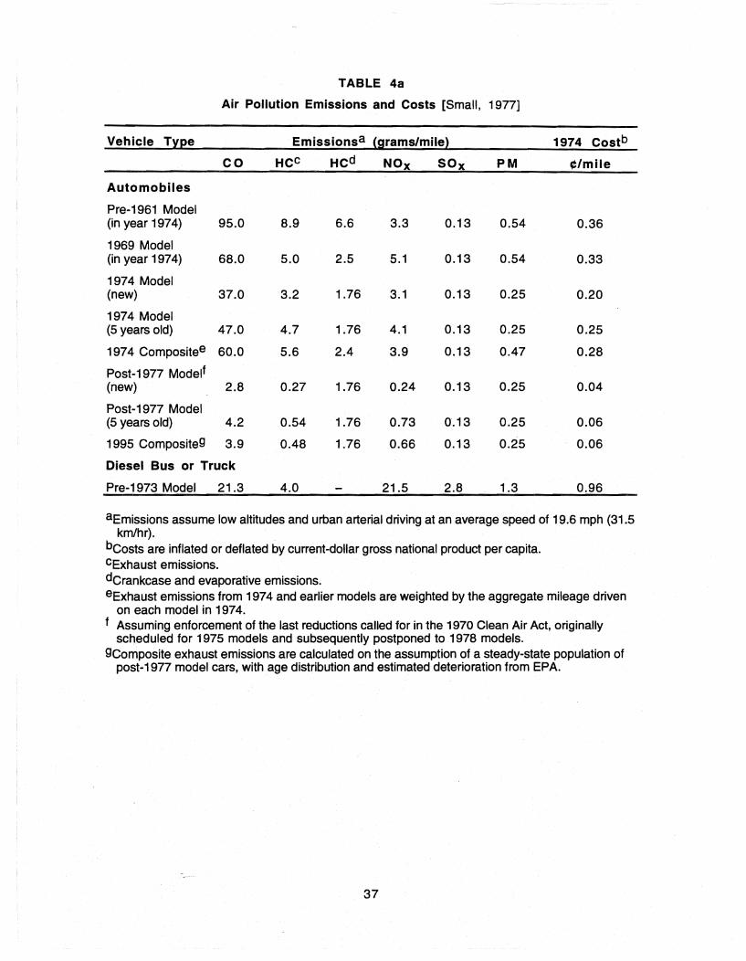
TABLE 4a

Air Pollution Emissions and Costs [Small, 1977]

Vehicle Type

Automobiles

Pre-1961 Model

CO

(in year 1974) 95.0

1969 Model (in year 1974) 68.0

1974 Model (new) 37.0

1974 Model (5 years old) 47.0

1974 Compositee 60.0

Post-1977 Modelf (new) 2.8

Post-1977 Model (5 years old) 4.2

1995 Compositeg 3.9

Diesel Bus or Truck

Pre-1973 Model 21.3

Emissionsa (grams/mile)

HCc HCd NOx SOx

8.9

5.0

3.2

4.7

5.6

0.27

0.54

0.48

4.0

6.6

2.5

1.76

1.76

2.4

1.76

1.76

1.76

3.3

5.1

3.1

4.1

3.9

0.24

0.73

0.66

21.5

0.13

0.13

0.13

0.13

0.13

0.13

0.13

0.13

2.8

PM

0.54

0.54

0.25

0.25

0.47

0.25

0.25

0.25

1.3

1974 Costb

¢/mile

0.36

0.33

0.20

0.25

0.28

0.04

0.06

0.06

0.96

aEmissions assume low altitudes and urban arterial driving at an average speed of 19.6 mph (31.5 km/hr).

bCosts are inflated or deflated by current-dollar gross national product per capita. cExhaust emissions. dCrankcase and evaporative emissions. eExhaust emissions from 1974 and earlier models are weighted by the aggregate mileage driven

on each model in 1974. f Assuming enforcement of the last reductions called for in the 1970 Clean Air Act, originally

scheduled for 1975 models and subsequently postponed to 1978 models. gComposite exhaust emissions are calculated on the assumption of a steady-state population of

post-1977 model cars, with age distribution and estimated deterioration from EPA.

37

_.

TABLE 4b

Air Pollution Emissions and Costs [Small, 1977]

Vehicle· Type Emissionsa (grams/km) 1974 Costb

CO HCc HCd NOx SOx PM ¢/km

Automobiles

Pre-1961 Model (in year 1974) 59.0 5.5 4.1 2.1 0.08 0.34 0.22

1969 Model (in year 1974) 42.3 3.1 1.6 3.2 0.08 0.34 0.21

1974 Model (new) 23.0 2.0 1.09 1.9 0.08 0.16 0.12

1974 Model (5 years old) 29.2 2.9 1.09 2.5 0.08 0.16 0.16

1974 Compositee 37.3 3.5 1.5 2.4 0.08 0.29 0.17

PosH 977 Modelf (new) 1.7 0.17 1.09 0.15 0.08 0.16 0.03

Post-1977 Model (5 years old) 2.6 0.34 1.09 0.45 0.08 0.16 0.04

1995 Compositeg 2.4 0.30 1.09 0.41 0.08 0.16 0.04

Diesel Bus or Truck

Pre-1973 Model 13.2 2.5 13.4 1.7 0.81 0.60

aEmissions assume low altitudes and urban arterial driving at average speed of 31.5 kmlhour. bCosts are inflated or deflated by current-dollar gross national product per capita. cExhaust emissions. dCrankcase and evaporative emissions. eExhaust emissions from 1974 and earlier models are weighted by the aggregate mileage driven

on each model in 1974. fAssuming enforcement of the last reductions called for in the 1970 Clean Air Ace Amendments,

originally scheduled for 1975 models and subsequently postponed to 1978 models. gComposite exhaust emissions are calculated on the assumption of a steady-state population of

post-1977 model cars, with age distribution and estimated deterioration from the U.S. Environmental Protection Agency.

38

------------- ---~- -- -~- ------- --_._- ---- --".- r

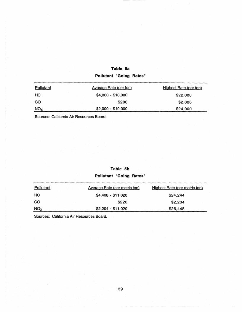
Pollutant

HC

CO NOx

Table 5a

Pollutant "Going Rates"

Average Rate (per ton)

$4,000 - $10,000

$200

$2,000 - $10,000

Sources: California Air Resources Board.

Pollutant

HC

CO NOx

Table 5b

Pollutant "Going Rates"

Average Rate (per metric ton)

$4,408 - $11,020

$220

$2,204 - $11,020

Sources: California Air Resources Board.

39

Highest Rate (per ton)

$22,000

$2,000

$24,000

Highest Rate (per metric ton)

$24,244

$2,204

$26,448

Finally, some expected cost and benefits to urban transportation systems for different

TCMs are summarized in Table 6.

TABLE 6

Some Costs and Benefits Related to TCM Implementation and Air Pollution

Costs Benefits

Improved public transit

• Operation • Fuel consumption reduction

• Additional initial investment • Emissions reduction

Traffic flow improvement

• Construction (HOV lanes) • Fuel consumption reduction for some users

• Operation and enforcement • Travel time saving for some users

Work schedule changes

• Construction and operation of work

satellite centers for telecommuting

• Building energy consumption

• Fuel consumption reduction

• Emissions reduction

• Office space savings and reduced parking

• Telecommunication and computer use requirements

• Congestion near satellite centers

Park and ride and fringe parking

• Facility construction

• Traffic congestion near facilities

(CBO)

• Emissions near facilities

Road pricing

• Travel costs for users

• Fuel consumption reduction for some users

• Emissions reduction in central business district

• Fuel consumption reduction for overall systems

• Emissions reduction

Alternative engines and fuels

• Conversion of engines • Emissions reduction

• Facilities for re-fueling stations

40

--~r------------ - ---------------- -- --

CHAPTER 6. SAMPLE ANALYSIS

Application of the framework is demonstrated through the use of two examples. Two

networks are created to evaluate a few strategies, namely implementation of a high-occupancy

vehicle (HOV) lane or increased auto operating cost, for reducing congestion. For simplicity and

illustrative comparison purposes, the sample networks are linear corridors. Evaluation of

transportation control measures (TCMs) for considerably larger or more complex networks can be

done using the same procedures, provided that computational time and cost as well as computer

capacity are adequate. This is an inherent limitation of this study and the reason for the simple

sample networks. Therefore, in these illustrative sample analyses, only microscale emissions

estimation is considered.

The choice or "split" among several transportation modes depends on both the

socioeconomic characteristics of the decision makers and the transportation alternatives available

to them. The mode choice model used in both networks is a multinomiallogit model developed

by 8en-Akiva and Lerman [1985]. It is assumed that the traveler has the ability to compare all

possible alternatives -- in this case, car, carpool, and bus -- and make the short-range decision to

select the one with the highest utility, which is viewed as the index of his/her socioeconomic

attributes. To predict changes in mode split for either the HOV lane implementation or the auto

operating cost increase, we can use the choice probabilities in the base case (without TCMs) and

the change in utility due only to the affected variable, travel time or operating cost. The probability

of traveler lin" choosing any alternative "i" after the implementation of either of the above two

TCMs can be expressed as:

P~(i) = 3Pn(i)eAVm

'LPnU)eAVjn j=1

where PnG> is the choice probability in the base case; j=1 if auto is selected, j=2 if carpool is the

alternative, and j=3 if bus is chosen. DVjn is the change of individual utility which is formulated as:

. changes in operating cost DV jn = b1 x changes in travel time + b2 x --h"::o:""u-s-eh-o-I:""d'-in-c-o--'m:::"'e--

41

The values of B1 and B2 are usually obtained from a regional survey. They are assumed as

B1 = -0.0307 and B2 = -28.7 in the examples. Similarly, $28,000 is assumed as the average

annual household income.

NETWORK A

In Network A, a highly congested urban street is created. The characteristics of the

network and the street geometry are illustrated in Figure 9. All intersections are signalized.

Turning volume is prescribed and constant for all cases. The volume of 3,520 persons during

peak hour is assumed to travel from node 48 to node 1. The analysis is performed for the peak

period, and the choice of time of day is not under consideration. Traffic volumes entering this

network are assumed to be the same for all cases, except that entering node 48, which varied

according to the modal splits obtained for different cases. Bus service is provided along the main

street.

Six different scenarios are examined for Network A. For each case, several iterations are

required such that the travel time used in the utility function of the mode choice model is, within a

specified tolerance level, equal to that obtained from TRAF-NETSIM. These cases are:

1. Base case. The network geometry, traffic movements, and entering volume were

described above. The person miles of travel (PMT), speed, and fuel consumption from

NETSIM are listed in Table 7.

2. HOV-4. The traffic engineering data and basic geometry are the same as those in the

base case, except the right lane along the main street is reserved for 4-person carpools

and buses.

3. HOV-3. Same as HOV-4, except that a 3-person carpool is used instead of a 4-person.

4. Bus-lane. The extension of cases (2) and (3), with only buses allowed on the HOV lane.

5. No-left-tum. Left turns are not permitted along the main street.

6. Pricing. Operating costs for auto and carpool are increased by 25 percent and 10

percent, respectively. Bus prices remain the same.

The center lane in Network A is assumed to be a reversible lane for inbound/outbound

traffic for morning and afternoon peak periods. Auto occupancy is assumed to be 1.3; carpool

occupancy is 3 for all scenarios except scenario 2, which is 4; bus occupancy is 50 for scenarios 1,

5, and 6 and 70 scenarios for 2, 3, and 4. The simulation time is limited to 15 minutes owing to the

limitation of microcomputer memory.

42

~ -----~--~ -.---~~ ~----------~ i ~

Simulations for non-base-case scenarios are performed in the following manner:

Compute Mode Split By Using

Mode Choice Model

No

43

Compute Vehicle Volume

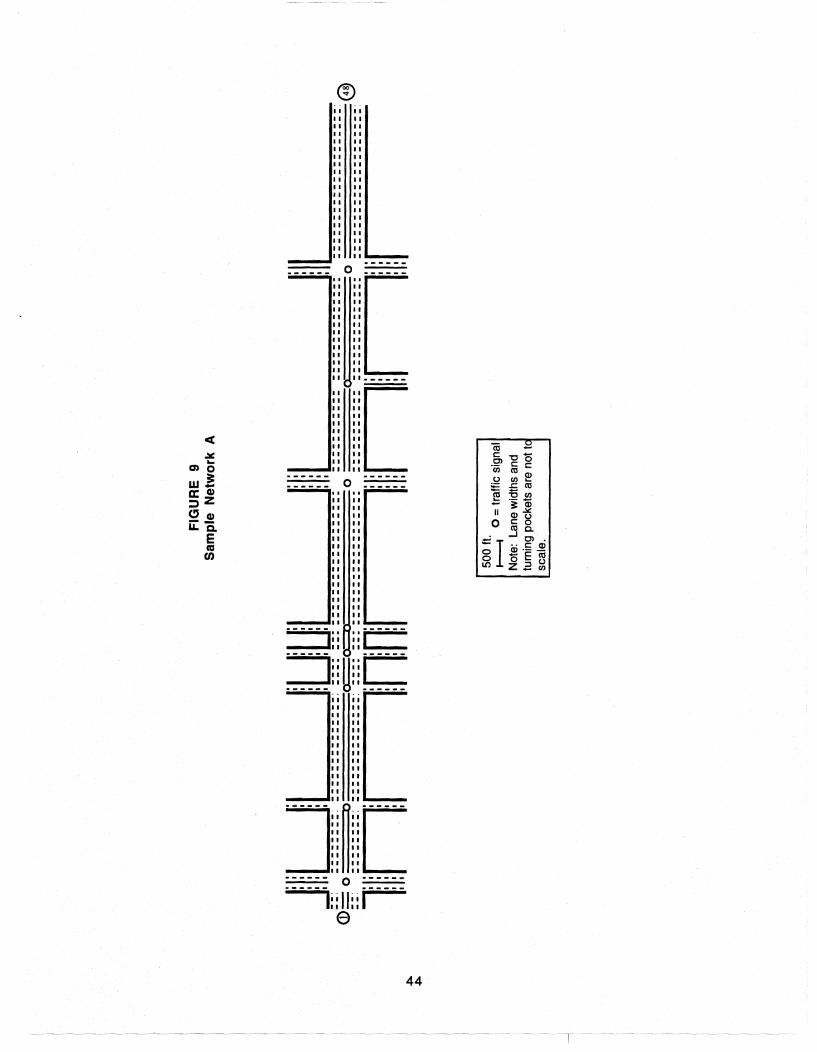
oct .:.: ...

en 0

w.! c:: CD ::3 Z

" CD ii:'E.

E ca en

------------ o ------

II

------

.. ----- ------

.----- 0 ------

r----

J~.[ ------ o -----------l:II::i----­

e

44

a:I ~ c: -go 0)

0 00 a:I c: to) en ~

:;: .r: a:I

~ -0 en o§ Qi

II (J).¥

0 c: to)

ttl 8.. o ....J 0). =r oo C:a5

o (J)o __

o oEttI It) Z 2 ~

In cases 2-6, the speed changes in autos, carpools, and buses after implementation of a

TCM cause the changes in the utility 'function, and in turn yield the switch among the selections of

drive-alone, carpool, and bus. The details of mode split and other traffic measurements at

equilibrium are shown in Table 7.

Mobility can be subjectively evaluated by examining PMT in a unit time period or average

speed. PMT is the same for all scenarios if a given level of demand is being analyzed. For

example, 10,560 PMT is the input value in Network A. Owing to the difference in congestion

levels in peak hour, however, the PMT in a unit time period (in this case, 15 minutes) may exhibit

variation. The lower the congestion level, the shorter the congestion period, and in turn the larger

the PMT in a unit time period during the congestion. The calculations in both networks are limited

to the simulation period. All of the alternatives improve PMT during the 15-minute simulation

period over the base case (except pricing in which PMT remains unchanged). The variations in

PMT -in-15-minutes are due to the different congestion levels. The average speed improves for

the HOV lanes and pricing, but decreases for the bus-lane and no-left-turn scenarios. The

nominal changes for the left-turn outputs are primarily the result of the low percentage of left turns

prescribed in the base case. From an energy standpoint, all scenarios except the no-left-turn

option result in reduced fuel consumption. When accounting for the change in the mode split,

there are some interesting results. All the scenarios, except the no-left-turn option, result in high

vehicle occupancies, i.e., fewer automobile trips.

The speed and VMT resulting from NETSIM are the inputs for the emissions model. The

vehicle emission results from MOBILE4.1 are listed in Table 8. (A more recent MOBILE version is

now available. However, at the time this analysis was conducted, MOBILE4.1 was the current

verSion.) Compared with the results in the base case, only the implementation of an HOV lane

(both HOV-3 and HOV-4) in this network results in effective air pollution reduction. All other

tested strategies achieve minor improvements in air quality. This is due to the fact that the

demand largely exceeds the capacity in the network, which is reflected by the particularly slow

speed in Table 7. The inclusion of an HOVlane can improve the PMT on the HOV lane, while the

traffic in the other lanes of the network remain congested. This increases the denominator in

calculating average emission results (on. per-person per-distance basis), and in turn lowers

average air pollution.

It is evident that properly designed TCMs can both relieve peak hour congestion and

reduce emissions. In addition, TCMs can save significant amounts of money by avoiding the need

for costly roadway expansion. The basic algorithm for TCM cost-effectiveness analysis is:

45

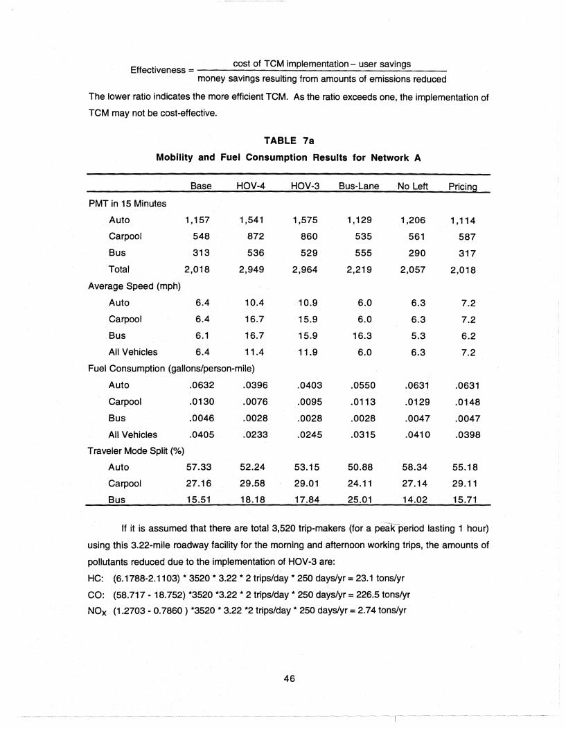
cost of TCM implementation - user savings Effectiveness = --------'------------=---­

money savings resulting from amounts of emissions reduced

The lower ratio indicates the more efficient TCM. As the ratio exceeds one, the implementation of

TCM may not be cost-effective.

TABLE 7a

Mobility and Fuel Consumption Results for Network A

Base HOV-4 HOV-3 Bus-Lane No Left Pricing

PMT in 15 Minutes

Auto 1,157 1,541 1,575 1,129 1,206 1,114

Carpool 548 872 860 535 561 587

Bus 313 536 529 555 290 317

Total 2,018 2,949 2,964 2,219 2,057 2,018

Average Speed (mph)

Auto 6.4 10.4 10.9 6.0 6.3 7.2

Carpool 6.4 16.7 15.9 6.0 6.3 7.2

Bus 6.1 16.7 15.9 16.3 5.3 6.2

All Vehicles 6.4 11.4 11.9 6.0 6.3 7.2

Fuel Consumption (gallons/person-mile)

Auto .0632 .0396 .0403 .0550 .0631 .0631

Carpool .0130 .0076 .0095 .0113 .0129 .0148

Bus .0046 .0028 .0028 .0028 .0047 .0047

All Vehicles .0405 .0233 .0245 .0315 .0410 .0398

Traveler Mode Split (%)

Auto 57.33 52.24 53.15 50.88 58.34 55.18

Carpool 27.16 29.58 29.01 24.11 27.14 29.11

Bus 15.51 18.18 17.84 25.01 14.02 15.71

If it is assumed that there are total 3,520 trip-makers (for a peak-period lasting 1 hour)

using this 3.22-mile roadway facility for the morning and afternoon working trips, the amounts of

pollutants reduced due to the implementation of HOV-3 are:

HC: (6.1788-2.1103) * 3520 * 3.22 * 2 trips/day * 250 days/yr = 23.1 tons/yr

CO: (58.717 - 18.752) *3520 *3.22 * 2 trips/day * 250 days/yr = 226.5 tons/yr

NOx (1.2703 - 0.7860 ) *3520 * 3.22 *2 trips/day * 250 days/yr = 2.74 tons/yr

46

TABLE 7b

Mobility and Fuel Consumption Results for Network A

Base HOV-4 HOV-3 Bus-Lane No Left Pricing

Person-km of Travel in 15 Minutes

Auto 1,862 2,479 2,534 1,817 1,940 1,792

Carpool 882 1,403 1,384 861 903 944

Bus 504 862 851 893 467 510

Total 3,248 4,744 4,769 3,571 3,310 3,246

Average Speed (mph)

Auto 10.3 16.7 17.5 9.7 10.1 11.6

Carpool 10.3 26.9 25.6 9.7 10.1 11.6

Bus 9.8 26.9 25.6 26.2 8.5 10.0

All Vehicles 10.3 18.3 19.2 9.7 10.1 11.6

Fuel Consumption (Iiters/person-km)

Auto .1487 .0932 .0948 .1294 .1484 .1484

Carpool .0306 .0179 .0223 .0266 .0303 .0348

Bus .0108 .0066 .0066 .0066 .0111 .0111

All Vehicles .0953 .0548 .0576 .0741 .0964 .0936

Traveler Mode Split (%)

Auto 57.33 52.24 53.15 50.88 58.34 55.18

Carpool 27.16 29.58 29.01 24.11 27.14 29.11

Bus 15.51 18.18 17.84 25.01 14.02 15.71

If it is assumed that there are total 3,520 trip-makers (for a peak period lasting 1 hour)

using this 5.18 km roadway facility for the morning and afternoon working trips, the amounts of

pollutants reduced due to the implementation of HOV-3 are:

HC: (6.1788-2.1103) * 3520 * 3.22 * 2 trips/day'" 250 days/yr = 21.0 metric tons/yr

CO: (58.717 - 18.752) *3520 *3.22 ... 2 trips/day * 250 days/yr = 205.5 metric tons/yr

NOx (1.2703 - 0.7860 ) *3520 * 3.22 *2 trips/day * 250 days/yr = 2.49 metric tons/yr

47

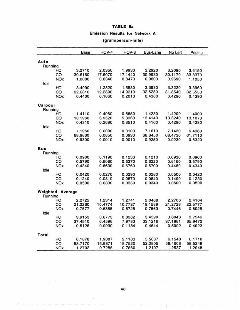
TABLE 8a

Emission Results for Network A

(g ram/person-mile)

Base HOV-4 HOV-3 Bus-Lane No Left Pricing

Auto Running

He 3.2710 2.0350 1.9930 3.2920 3.2090 3.6150 eo 30.6160 17.6070 17.1440 30.9930 30.1170 33.8370 NOx 1.0000 0.8340 0.8470 0.9600 0.9690 1.1050

Idle He 3.4090 1.2820 1.5580 3.3930 3.3230 3.3960 eo 32.6810 12.2890 14.9310 32.5280 31.8540 32.5550 NOx 0.4400 0.1660 0.2010 0.4380 0.4290 0.4390

Carpool Running

He 1.4110 0.4960 0.6650 1.4250 1.4200 1.4000 eo 13.1960 3.9520 5.3360 13.4140 13.3240 13.1070 NOx 0.4310 0.2680 0.3510 0.4160 0.4290 0.4280

Idle He 7.1960 0.0090 0.0100 7.1610 7.1430 6.4380 eo 68.9830 0.0850 0.0930 68.6450 68.4730 61.7110 NOx 0.9300 0.0010 0.0010 0.9250 0.9230 0.8320

Bus Running

He 0.0900 0.1190 0.1230 0.1210 0.0930 0.0900 eo 0.5790 0.6080 0.6370 0.6220 0.6160 0.5790 NOx 0.4340 0.6630 0.6760 0.6700 0.4480 0.4340

Idle He 0.0420 0.0270 0.0290 0.0280 0.0500 0.0420 eo 0.1240 0.0810 0.0870 0.0840 0.1490 0.1230 NOx 0.0500 0.0330 0.0350 0.0340 0.0600 0.0500

Weighted Average Running

He 2.2725 1.2314 1.2741 2.0488 2.2706 2.4164 eo 21.2260 10.4774 10.7737 19.1589 21.2728 22.5777 NOx 0.7577 0.6355 0.6726 0.7563 0.7446 0.8025

Idle He 3.9153 0.6773 0.8362 3.4599 3.8843 3.7546 eo 37.4910 6.4596 7.9783 33.1216 37.1881 35.9472 NOx 0.5126 0.0930 0.1134 0.4544 0.5092 0.4923

Total He 6.1878 1.9087 2.1103 5.5087 6.1548 6.1710 eo 58.7170 16.9371 18.7520 52.2805 58.4608 58.5249 NOx 1.2703 0.7285 0.7860 1.2107 1.2537 1.2948

48

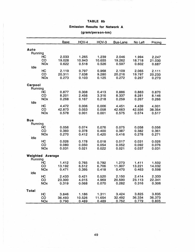
TABLE 8b

Emission Results for Network A

(gram/person-km)

Base HOV-4 HOV-3 Bus-Lane No Left Pricing

Auto Running

HC 2.033 1,265 1.239 2.046 1.994 2.247 CO 19.028 10.943 10.655 19.262 18.718 21.030 NOx 0.622 0.518 0.526 0.597 0.602 0.687

Idle HC 2.119 0.797 0.968 2.109 2.065 2.111 CO 20.311 7.638 9.280 20.216 19.797 20.233 NOx 0.273 0.103 0.125 0.272 0.267 0.273

Carpool Running

HC 0.877 0.308 0.413 0.886 0.883 0.870 CO 8.201 2.456 3.316 8.337 8.281 8.146 NOx 0.268 0.167 0.218 0.259 0.267 0.266

Idle He 4.472 0.006 0.006 4.451 4.439 4.001 CO 42.873 0.053 0.058 42.663 42.556 38.354 NOx 0.578 0.001 0.001 0.575 0.574 0.517

Bus Running

HC 0.056 0.074 0.076 0.075 0.058 0.056 CO 0.360 0.378 0.400 0.387 0.382 0.361 NOx 0.270 0.412 0.420 0.416 0.278 0.271

Idle HC 0.026 0.178 0.018 0.017 0.031 0.026 CO 0.080 0.050 0.054 0.052 0.092 0.076 NOx 0.031 0.021 0.022 0.021 0.037 0.031

Weighted Average Running

HC 1.412 0.765 0.792 1.273 1.411 1.502 CO 13.192 6.512 6.706 11.907 13.221 14.032 NOx 0.471 0.395 0.418 0.470 0.463 0.598

Idle HC 2.433 0.421 0.520 2.150 2.414 2.333 CO 23.300 4.015 4.969 20.590 23.113 22.341 NOx 0.319 0.068 0.070 0.282 0.316 0.306

Total HC 3.846 1.186 1.311 3.424 3.825 3.835 CO 36.493 10.526 11.654 32.492 36.334 36.373 NOx 0.790 0.489 0.489 0.752 0.779 0.805

49

The total savings associated with the emission reductions are $300,000 per year if

hydrocarbon (HC) and nitrogen oxides (NOx) "going rates" (see Table 5) are each assumed as

$10,000 per ton ($11,020 per metric ton). In addition, the annual user savings resulting from fuel

consumption are about $100,000 if gas prices remain at $1.15 per galion ($0.30 per liter). This

shows that it is beneficial on the average to reserve an HOV lane if total cost is less than

$400,000. This limit may be over $1,000,000 if the highest "going rates" are applied. This

analysis is conservative since the commuter savings in time are not included.

NETWORK B

In Network B, an urban arterial street, including three residential zones and a central

business district (CBD), is simulated. The street, illustrated in Figure 10, consists of 9 links from

west to east. The three major residential zones are node 1, node 31, and node 62, and the CBD

is node 10. It is assumed that the number of persons living in the residential zones with the mode

choice alternatives of drive-alone, carpool, and transit bus includes 3,000 persons in node 1 and

1,000 persons each in node 31 and 62. The assumed mode shares are listed as the base case in

Table 9. There is a transit route from each residential area to the CBD. Auto occupancy is

assumed to be 1.3; carpool occupancy is 3 for all scenarios; bus maximum occupancy is 25 for the

base scenario and 30 for the other two study cases in order to meet the demand. The bus

headway is 5 minutes for all three routes, which enables the mass transit servicing under its

maximum capacity. Each case was a 1-hour simulation performed on a PC486DXl50 requiring 45-

50 minutes of real time.

Because of the computation time, only three different cases are examined in this network

simulation:

1. Base case as described above.

2. HOV-3. The right lane along the main street (from node 1 to node 10) is reserved for 3-

person carpools and buses.

3. Pricing. Operating costs for auto and carpool are increased by 25 percent and 10

percent, respectively. No change in selecting bus.

The different travel time from each residential zone to the CBD results in the different

mode shares among travelers in the residential zones. This information is detailed in Table 9. The

weighted averages for the various modes in the network (aggregated values) are listed in Table

10.

The mobility and fuel consumption measurements for the Network B scenarios are

described in Table 10. With respect to the base case, PMT in the simulation period decreases for

50

01 -"

o

FIGURE 10 Sample Network B

--.l1I~ilil III lIL-li~:I III III 11 __ '_ 0) o __ r.::-: o --. 0 0 __ C':'

III 111:1 II

1,000 ft.

f--+-f o = traffic signal

Note: lane widths and turning pockets are not to scale.

o ____________ 0 ______ 0 0 @

'I' , " , , , , , , , , , , , , , , , , @

II III III

the HOV scenario but increases for the pricing option. Likewise, there is a decrease in average

speed for the HOV option and an increase for the pricing option. Average fuel consumption,

however, improved (decreased) for both of the strategies relative to the base case.

The emission results in Table 11 show that the incentives for existing mass transit use can

achieve a limited reduction in pollution. The most attractive strategy examined is the increase in

the auto operating cost, through parking costs, gas taxes, etc. The program reduces the

emissions of HC, carbon monoxide (CO), and NOx by about 2-3 percent on the average per­

person-per-distance basis. The exclusive HOV lane can decrease average emissions from buses

by improving the traffic flow on the HOV lane. These results, however, are offset by the slower

auto movements owing to the reduction in the number of regular lanes. Furthermore, the

carpools which are slowed by the frequently stopped buses at the stations worsen the air

pollution in the network.

52

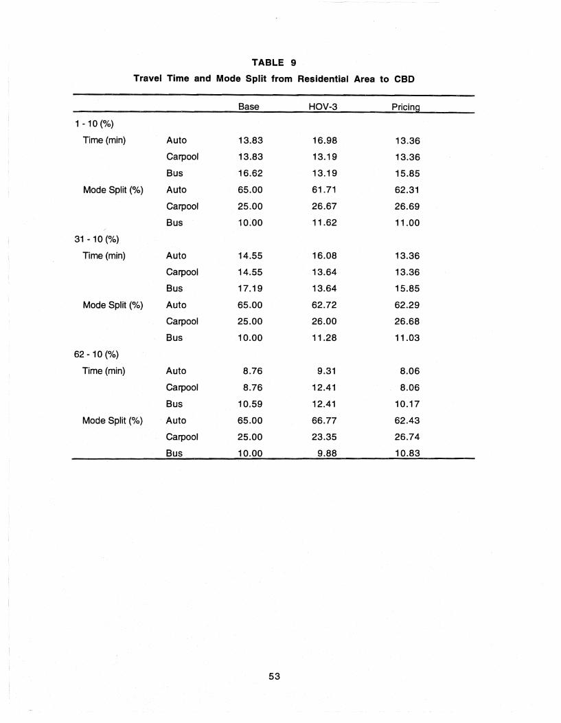
TABLE 9

Travel Time and Mode Split from Residential Area to CBO

Base HOV-3 Pricing

1-10(%)

Time (min) Auto 13.83 16.98 13.36

Carpool 13.83 13.19 13.36

Bus 16.62 13.19 15.85

Mode Split (%) Auto 65.00 61.71 62.31

Carpool 25.00 26.67 26.69

Bus 10.00 11.62 11.00

31 -10 (%)

Time (min) Auto 14.55 16.08 13.36

Carpool 14.55 13.64 13.36

Bus 17.19 13.64 15.85

Mode Split (%) Auto 65.00 62.72 62.29

Carpool 25.00 26.00 26.68

Bus 10.00 11.28 11.03

62 -10 (%)

Time (min) Auto 8.76 9.31 8.06

Carpool 8.76 12.41 8.06

Bus 10.59 12.41 10.17

Mode Split (%) Auto 65.00 66.77 62.43

Carpool 25.00 23.35 26.74

Bus 10.00 9.88 10.83

53

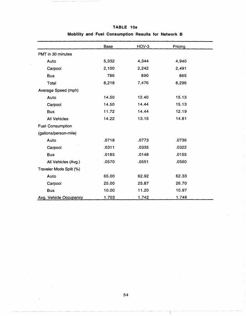
TABLE 10a

Mobility and Fuel Consumption Results for Network B

Base HOV-3 Pricing

PMT in 30 minutes

Auto 5,332 4,344 4,940

Carpool 2,100 2,242 2,491

Bus 786 890 865

Total 8,218 7,476 8,296

Average Speed (mph)

Auto 14.50 12.40 15.13

Carpool 14.50 14.44 15.13

Bus 11.72 14.44 12.19

All Vehicles 14.22 13.15 14.81

Fuel Consumption

(gallons/person-mile)

Auto .0718 .0773 .0736

Carpool .0311 .0335 .0322

Bus .0185 .0148 .0155

All Vehicles (Avg.) .0570 .0551 .0560

Traveler Mode Split (%)

Auto 65.00 62.92 62.33

Carpool 25.00 25.87 26.70

Bus 10.00 11.20 10.97

Avg. Vehicle Occupancy 1.703 1.742 1.748

54

TABLE 10b

Mobility and Fuel Consumption Results for Network B

Base HOV-3 Pricing

PKT in 30 minutes

Auto 8,579 6,989 7,948

Carpool 3,379 3,607 4,008

Bus 1,265 1,432 1,392

Total 13,223 12,028 13,348

Average Speed (km/hr)

Auto 23.33 19.95 24.34

Carpool 23.33 23.23 24.34

Bus 18.86 23.23 19.61

All Vehicles 22.88 21.16 23.83

Fuel Consumption

(liters/person-km)

Auto .1689 .1818 .1731

Carpool .0732 .0788 .0757

Bus .0435 .0348 .0365

All Vehicles (Avg.) .0134 .1296 .1317

Traveler Mode Split (%)

Auto 65.00 62.92 62.33

Carpool 25.00 25.87 26.70

Bus 10.00 11.20 10.97

Avg. Vehicle Occupancy 1.703 1.742 1.748

55

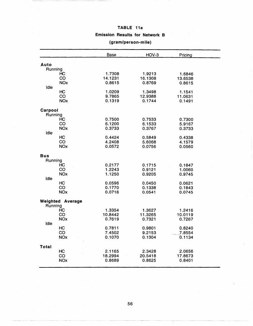
TABLE 11a

Emission Results for Network B

(gram/person-mile)

Base HOV-3 Pricing

Auto Running

HC 1.7308 1.9213 1.6846 CO 14.1231 16.1308 13.6538 NOx 0.8615 0.8769 0.8615

Idle HC 1.0209 1.3498 1.1541 CO 9.7865 12.9388 11.0631 NOx 0.1319 0.1744 0.1491

Carpool Running

HC 0.7500 0.7533 0.7300 CO 6.1200 6.1533 5.9167 NOx 0.3733 0.3767 0.3733

Idle HC 0.4424 0.5849 0.4338 CO 4.2408 5.6068 4.1579 NOx 0.0572 0.0756 0.0560

Bus Running

HC 0.2177 0.1715 0.1847 CO 1.2243 0.9121 1.0060 NOx 1.1250 0.9205 0.9745

Idle HC 0.0596 0.0450 0.0621 CO 0.1770 0.1338 0.1843 NOx 0.0716 0.0541 0.0745

Weighted Average Running

HC 1.3354 1.3627 1.2416 CO 10.8442 11.3265 10.0119 NOx 0.7619 0.7321 0.7267

Idle HC 0.7811 0.9801 0.8240 CO 7.4502 9.2153 ... ].8554 NOx 0.1070 0.1304 0.1134

Total HC 2.1165 2.3428 2.0656 CO 18.2994 20.5418 17.8673 NOx 0.8689 0.8625 0.8401

56

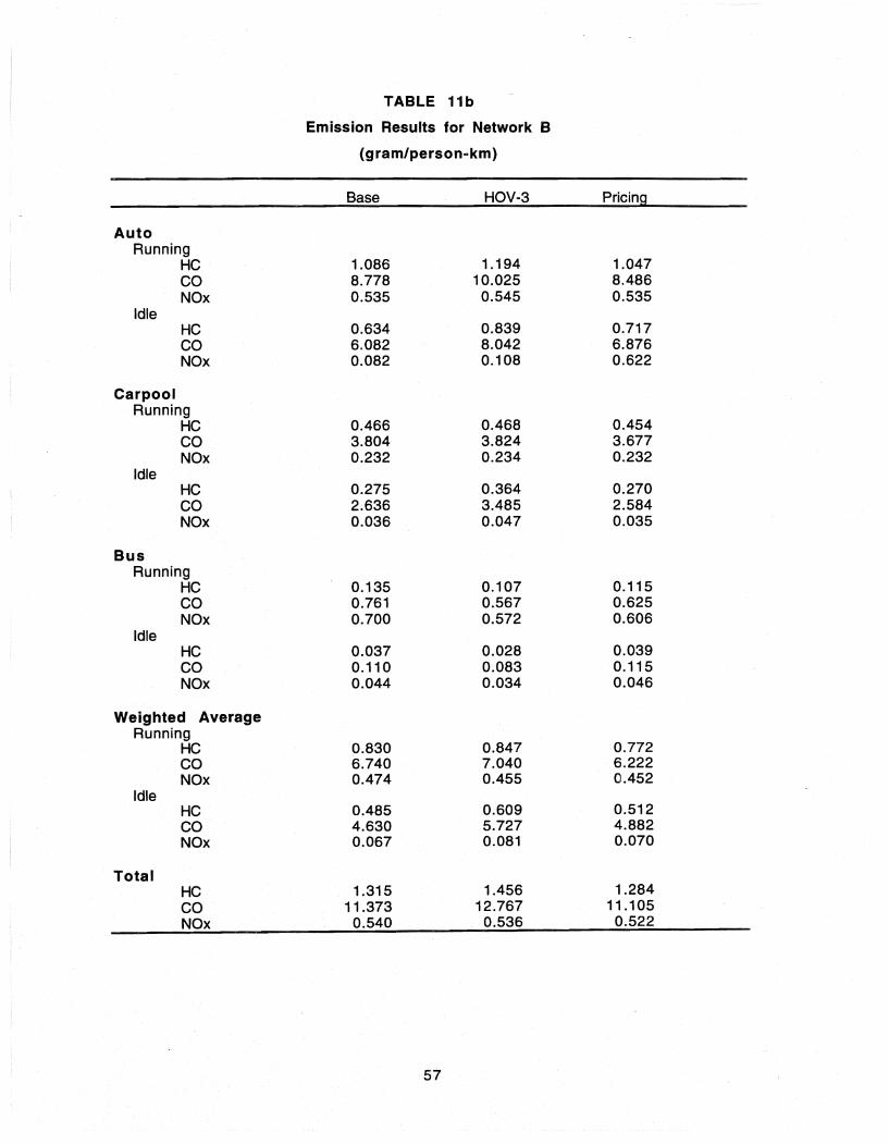
TABLE 11b

Emission Results for Network B

(gram/personakm)

Base HOV-3 Pricing

Auto Running

HC 1.086 1.194 1.047 CO 8.778 10.025 8.486 NOx 0.535 0.545 0.535

Idle HC 0.634 0.839 0.717 CO 6.082 8.042 6.876 NOx 0.082 0.108 0.622

Carpool Running

HC 0.466 0.468 0.454 CO 3.804 3.824 3.677 NOx 0.232 0.234 0.232

Idle HC 0.275 0.364 0.270 CO 2.636 3.485 2.584 NOx 0.036 0.047 0.035

Bus Running

HC 0.135 0.107 0.115 CO 0.761 0.567 0.625 NOx 0.700 0.572 0.606

Idle HC 0.037 0.028 0.039 CO 0.110 0.083 0.115 NOx 0.044 0.034 0.046

Weighted Average Running

HC 0.830 0.847 0.772 CO 6.740 7.040 6.222 NOx 0.474 0.455 0.452

Idle HC 0.485 0.609 0.512 CO 4.630 5.727 4.882 NOx 0.067 0.081 0.070

Total HC 1.315 1.456 1.284 CO 11.373 12.767 11.105 NOx 0.540 0.536 0.522

57

58

CHAPTER 7. DISCUSSION AND CONCLUSION

Although available transportation planning tools cannot be directly used for emissions

estimation, a macro-analysis framework is proposed herein which links the transportation planning

and air quality analysis models in order to develop a matrix of strategies to assist decision makers in

examining specific mobility strategies for an urban area. The purpose of the report is to illustrate a

framework for identifying energy, air quality, and mobility trade-ofts of various congestion

mitigation strategies. Based on this methodological framework, two sample networks are

evaluated in this project. In both central business district (CBD) type networks, the

implementation of transportation control measures (TCM) can decrease overall vehicle miles of

travel (VMT). The air pollution resulting from mobile sources, nevertheless, may not be effectively

alleviated, or it may even be worsened by applying inappropriate TCM strategies. The effects of

TCMs on air quality are more effective as an urban street network becomes more and more

congested. This is illustrated by the two sample networks, which are very congested. In network

A, changing the pattern of vehicle flow can achieve the goal of reducing air pollution, while in

network B it is more effective to increase auto operating costs. The reason for the radically

different results from network A and B may be the extraordinary congestion for drive-alone in

network B, resulting from changing one lane from a regular lane to an HOV lane. The results of

the analysis illustrate the need for careful study before implementation of any TCMs. Failure to

analyze the implications of TCMs prior to their implementation may yield results inconsistent with

environmental and energy policy objectives.

The validity of VMT as a meaningful measure requires careful scrutiny. In network B, it is

quite obvious to reduce VMT by including a HOV lane in order to increase the average vehicle

occupancy. The mobility in the network, however, decreases due to the heavier congestion in

the regular lanes, which is illustrated by the reduced auto speed. The decrease in total VMT

resulting from some TCMs may produce more frequent stop-and-go situations, which may in turn

emit more mobile source pollution.

The effectiveness of the auto operating cost increase in network B reminds us of the role

of pricing in TCM strategies. It turns out that many policy makers are considering a variety of

pricing innovations, though some of them may be difficult to implement under current laws and

regulations. Some states are now realizing substantial increases in transportation revenues

through sales tax increments. In California, these revenues are used to improve specific transit

and transportation infrastructure. Substantial vehicle registration fee increases to help fund TCMs

are also under consideration, as are pollution taxes on the heaviest emitting vehicles. In New

59

York, imposing tolls on previously free bridges is being attempted to link them to specific repair

and maintenance benefits.

The program to reduce automotive pollutants, in order to assure the highest cost­

effectiveness over the entire lifetime of the program, must incorporate both short- and long-term

solutions. The significance of the automobile to urban lifestyles and the considerable cost of

altering its use necessitates a flexible approach to controlling its environmental impacts.

The choice of an emissions model is very critical in air quality analysis. MOBILE4.1 (or the

newer releases) takes into account elevation, temperature, operating modes, cold starts, vehicle

age, etc., which may not be included in other emissions models, yielding more accurate results.

The emissions from NETSIM may result in biased conclusions, e.g., the inclusion of an exclusive

HOV lane in the sample network B is plausible by NETSIM for reducing (hydrocarbon) HC and

(carbon dioxide) CO pollution. However, as illustrated in Table 12, this is not the case using

MOBILE4.1. NETSIM's emissions factors are dated and its analysis is not nearly as sophisticated

as that of MOBILE.

Use of the framework as demonstrated in this report, clearly points to the need for

additional modeling work. Existing models may be calibrated for some analysis but cannot be

relied upon for directing future transportation investment. They can, however, provide some

relative comparison of TCMs. The framework presented in this report should assist analysts in the

interim, while work proceeds on the development of more comprehensive transportation

demand/air quality models.

60

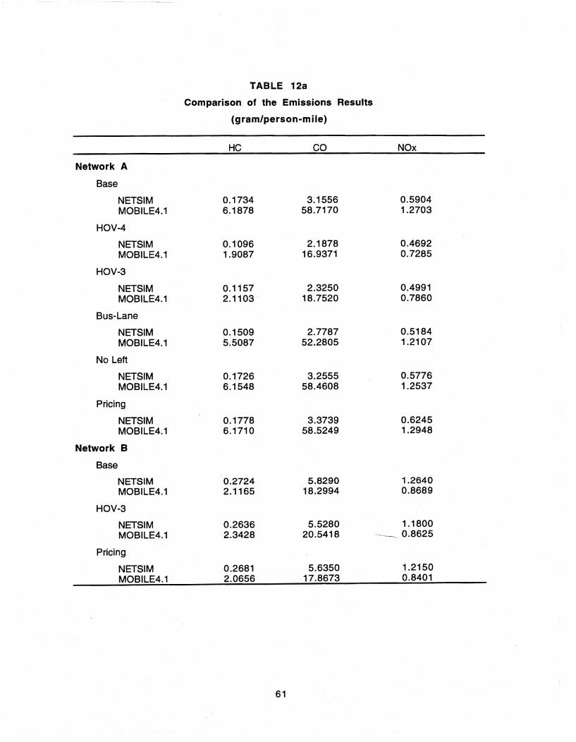
TABLE 12a

Comparison of the Emissions Results

(gram/person-m i1e)

HC CO NOx

Network A

Base

NETSIM 0.1734 3.1556 0.5904 MOBILE4.1 6.1878 58.7170 1.2703

HOV-4

NETSIM 0.1096 2.1878 0.4692 MOBILE4.1 1.9087 16.9371 0.7285

HOV-3

NETSIM 0.1157 2.3250 0.4991 MOBILE4.1 2.1103· 18.7520 0.7860

Bus-Lane

NETSIM 0.1509 2.7787 0.5184 MOBILE4.1 5.5087 52.2805 1.2107

No Left

NETSIM 0.1726 3.2555 0.5776 MOBILE4.1 6.1548 58.4608 1.2537

Pricing

NETSIM 0.1778 3.3739 0.6245 MOBILE4.1 6.1710 58.5249 1.2948

Network B

Base

NETSIM 0.2724 5.8290 1.2640 MOBILE4.1 2.1165 18.2994 0.8689

HOV-3

NETSIM 0.2636 5.5280 1.1800 MOBILE4.1 2.3428 20.5418 .~~ 0.8625

Pricing

NETSIM 0.2681 5.6350 1.2150 MOBILE4.1 2.0656 17.8673 0.8401

61

TABLE 12b

Comparison of the Emissions Results

(gram/person-mile)

HC CO NOx

Network A

Base

NETSIM 0.108 1.961 0.367 MOBILE4.1 3.845 36.493 0.789

HOV-4

NETSIM 0.0682 1.36 0.292 MOBILE4.1 1.186 10.53 0.453

HOV-3

NETSIM 0.072 1.445 0.310 MOBILE4.1 1.312 11.654 0.489

Bus-Lane

NETSIM 0.094 1.727 0.322 MOBILE4.1 3.424 32.493 0.752

No Left

NETSIM 0.107 2.023 0.359 MOBILE4.1 3.826 36.334 0.779

Pricing

NETSIM 0.111 2.097 0.388 MOBILE4.1 3.835 36.374 0.805

Network B

Base

NETSIM 0.167 3.623 0.786 MOBILE4.1 1.315 11.373 0.540

HOV·3

NETSIM 0.164 3.436 0.733 MOBILE4.1 1.456 12.777 0.536

Pricing

NETSIM 0.167 3.502 0.76 MOBILE4.1 1.284 11.11 0.52

62

REFERENCES

Bellomo, Salvatore J., "Methodology for Determining the Relative Cost Effectiveness of Transportation Control Measures," Transportation Research Record 921, Transportation Research Board, Washington, D.C., 1983.

Bellomo, Salvatore J., "Providing for Air Quality and Urban Mobility," Highway Research Record 465, Highway Research Board, Washington, D.C., 1973.

Ben-Akiva, M., and S. R. Lerman, Discrete Choice Analysis -- Theory and Application to Travel Demand, MIT Press, Cambridge, Massachusetts, 1985.

Ben-Akiva, M., and A. Atherton, "Methodology for Short-Range Travel Demand Predictions," Journal of Transport Economics and Policy, September, 19n.

Brunso, Joanna M., and David T. Hartgen, "Consumer Trade-Offs Between Mobility Maintenance and Gasoline Savings," Transportation Research Record 1049, Transportation Research Board, Washington, D.C., 1985.

Campbell, James F., Philip S. Babcock, and Adolf D. May, FRECON2 -- User's Guide, UC8-ITS-TD-84-2, University of California, Berkeley, CA, 1984.

Cheslow, Melvyn D., and J. Kevin Neels, "Effect of Urban Development Patterns on Transportation Energy Use," Transportation Research Record 764, Transportation Research Board, Washington, D.C., 1980.

Cohen, Gerald S., "Transportation Systems Management Actions: A Study of the Energy Costs," Transportation Research Record 764, Transportation Research Board, Washington, D.C., 1980.

Cohen, Harry S., Joseph R. Stowers, and Michael P. Petersilia, Evaluating Urban Transportation System Alternatives, United States Department of Transportation, Washington, D.C., 1978.

Cottrell, Wayne D., "Comparison of Vehicular Emissions in Free-Flow and in Congestion using MOBILE4 and HPMS", paper presented at 71st TRB meeting, Washington, D.C., 1992.

Croke, Kevin G., and Richard Zerbe, Environmental Regulation and Urban Traffic, Technical Report, NSF-RA-E-74-028, The University of Chicago Center for Urban Studies, Chicago, IL, 1974.

Evans, L., Exhaust Emissions, Fuel Consumption and Traffic: Relations Derived from Urban Driving Schedule Data, General Motors Research Laboratories, GMR-2599, 1977.

Horowitz, Joel, Air Quality Analysis for Urban Transportation Planning, MIT Press, Cambridge, Massachusetts, 1982.

Horowitz, Joel, and Steven Kuhrtz, Transportation Controls to Reduce Automobile Use and Improve Air Quality in Cities: The Need, the Options, and Effects on Urban Activity, Technical Report, EPA-400/11-74-002, Environmental Protection Agency, Washington, D.C., 1974.

63

Ingram, Gregory K., The Automobile and the Regulation of its Impact on the Environment: A Land Use Transportation Model for Predicting Mobile Source Emissions, Harvard University, Cambridge, Massachusetts, 1972.

Kim, Kwang-Sik, and J. B. Schneider, "Defining Relationships Between Urban Form and Travel Energy," Transportation Research Record 1049, Transportation Research Board, Washington, D.C., 1985.

Lutin, Jerome, "Energy Savings for Work Trips: Analysis of Alternative Commuting Patterns for New Jersey," Transportation Research Record 561, Transportation Research Board, Washington, D.C., 1976.

MacKenzie, James J., "The Going Rate: What it Really Costs to Drive," paper presented at the 73rd Annual Transportation Research Board Meeting, Washington, D.C., January 13, 1994.

Maxwell, Donald A., and Dennis V. Williamson, "How Much Fuel Does Vanpooling Really Save?," Transportation Research Record 764, Transportation Research Board, Washington, D.C., 1980.

McCoy, Michael, "Transit's Energy Efficiency," Urban Transportation, Eno Foundation for Transportation, Westport, CT,1982.

Morris, Michael, and Antti Talvitie, "Assessment of Energy and Petroleum Consumption in the Buffalo Area," Transportation Research Record 764, Transportation Research Board, Washington, D.C., 1980.

Morrow, David, "Evaluating the Effectiveness of Transportation Control Measures for San Luis Obispo County, California," Transportation Planning and Air Quality: Proceedings of the National Conference ... 1992.

Oppenheim, Norbert, "A Dynamic Model of Urban Retail Location and Shopping Travel," Transportation Research Record 1079, Transportation Research Board, Washington, D.C., 1986.

Pikarsky, Milton, "Land Use and Transportation in an Energy Efficient Society," Transportation Research Record 183, Transportation Research Board, Washington, D.C., 1978.

Revis, Joseph 5., "Short-term Transportation Control Strategies for Air Pollution Control," Highway Research Record 465 ... Highway Research Board, Washington, D.C., 1973.

Rosenbloom, Sandra, "Peak Period Traffic Congestion: A State-Of-The-Art Analysis and Evaluation of Effective Solutions," Strategies to Alleviate Traffic Congestion, Proceedings of ITE's 1987 National Conference, Institute of Transportation Engineers, Washington, D.C., 1988.

Small, K., "Estimating the Air Pollution Costs of Transport Modes," Journal of Transport Economics and Policy, May 19n.

Suhrbier, John H., Implementation and Administration of Air Quality Transportation Control: An Analysis of the Denver, Colorado Area, Technical Report, DOT-P-78-001, U.S. Department of Transportation, Washington, D.C., 1978.

64

Suhrbier, John H., "Cost Effectiveness of Air Quality Control Measures and Impact of the Environmental Review Process," Transportation Research Record 921, Transportation Research Board, Washington, D.C., 1983.

TRAF-NETS/M Users Manual, prepared for U.S. Department of Transportation, Federal Highway Administration, Washington, D.C., 1989.

TRANSYT-7F User's Manual, Release 6, prepared by the Transportation Research Center, University of Florida, Gainesville, Florida, 1988.

United States Environmental Protection Agency, Transportation Control Measure Information Documents, Environmental Protection Agency, Washington, D.C., 1991.

United States General Accounting Office, Traffic Congestion: Federal Efforts to Improve Mobility, Report to the Chairman, Subcommittee on Transportation and Related Agencies, Committee on Appropriations, U.S. Senate, United States General Accounting Office, 1991.

Urban Land Institute, 12 Tools for Improving Mobility and Managing Congestion, Urban Land Institute, Washington, D.C., 1991.

Venezia, Ronald A., "Implications for Transportation of New Federal Air Pollution Controls," Highway Research Record 465, Highway Research Board, Washington, D.C., 1973.

Wickstrom, G. V., "Air Pollution: Implications for Transportation Planning," Highway Research Record 465, Highway Research Board, Washington, D.C., 1973.

Wilson, Stephen C., and Robert L. Smith, Jr., "Impact of Urban Development Alternatives on Transportation Fuel Consumption," Transportation Research Record 1155, Transportation Research Board, Washington, D.C., 1987.

Working Group on Operational Benefits, Intelligent Vehicle Highway Systems: Operational Benefits, Final Report of the Working Group on Operational Benefits: Mobility 2000, 1990.

65

66

Appendix A

TRAF-NETSIM Input for Network A

67

68

1

TTTTTTTTTTT TTTT'I'I'TTTTT TTTTTTTTTTT

TTT TTT TTT 'I'I'T TTT TTT TTT TTT TTT

RRRRRRRRR RRRRRRRRRR RRRRRRRRRRR RRR RRR RRR RRR RRRRRRRRRRR RRRRRRRRRR RRR RRR RRR RRR RRR RRR RRR RRR RRR RRR

AAMAAA AAAAAAMA

AAAAAAAAAAA AAA AAA AAA AAA AAAAAAAAAAA AAAAAAAAAAA AAA AAA AAA AAA AAA AAA AAA AAA AAA AAA

RELEASE DATE = 10/10/89 VERSION 3.00

TRAF SIMULATION MODEL

START OF CASE

FFFFFFFFFFF FFFFFFFFFFF FFFFFFFFFFF FFF FFF FFFFFFF FFFFFFF FFF FFF FFF FFF FFF

****************************************************************************************** ••• ************************************.

TRAF SIMULATION MODEL

DEVELOPED FOR

U. S. DEPARTMENT OF TRANSPORTATION FEDERAL HIGHWAY ADMINISTRATION

TRAFFIC SYSTEMS DIVISION 0******************·**************************··******--_.-.-._----_._._._-------_._._. __ ._---_._._--_._*_.--------_._.-._._._ .. __ .

0 0 0

0 0 1

0 0 0

0

0

0 0 0

0 0 0 0 0 0

START OF CASE 1

----------------_.----_._. __ ._._-------_._. __ ._----_.-----. __ ._----_._* ... _-----------------------------_._._._---_._-----_ ... _---

VALUE

0 0 1

0 0

0 0

700 0

7581 7781

120 60 10

0 0 0 0

AIR QUALITY ANALYSIS

DATE USER

AGENCY

3/ 15/ 93 J.MEESOMBOON UT @ AUSTIN

RUN CONTROL DATA

RUN PARAMETERS AND OPTIONS

RUN IDENTIFICATION NUMBER NEXT CASE CODE = (0,1) IF ANOTHER CASE (DOES NOT, DOES) FOLLOW RUN TYPE CODE = ( I, 2, 3) TO RUN (SIMULATION, ASSIGNMENT, BOTH)

(-1,-2,-3) TO CHECK (SIMULATION, ASSIGNM~~, BOTH) ONLY

NETSIM ENVIRONMENTAL OPTIONS

FUEL/EMISSION RATE TABLES ARE NOT PRINTED SIMULATION: PERFORMED ENVIRONMENTAL MEASURES: CALCULATED RATE TABLES: EMBEDDED TRAJECTORY FILE: NOT WRITTEN INPUT UNITS CODE = (0,1) IF INPUT IS IN (ENGLISH, METRIC) UNITS OUTPUT UNITS CODE = (0,1,2,3) IF OUTPUT IS IN (SAME AS INPUT, ENGLISH, METRIC, BOTH) UNITS CLOCK TIME AT START OF SIMULATION (HHMM) SIGNAL TRANSITION CODE = (0,1,2,3) IF (NO, IMMEDIATE, 2-CYCLE, 3-CYCLE) TRANSITION WAS REQUESTED RANDOM NUMBER SEED RANDOM NUMBER SEED TO GENERATE TRAFFIC STREAM FOR NETS 1M OR LEVEL I SIMULATION

DURATION (SEC) OF TIME PERIOD NO. LENGTH OF A TIME INTERVAL, SECONDS MAXIMUM INITIALIZATION TIME, NUMBER OF TIME INTERVALS NUMBER OF TIME INTERVALS BETWEEN SUCCESSIVE STANDARD OUTPUTS TIME INTERMEDIAT.E OUTPUT WILL BEGIN AT INTERVALS OF 0 SEes. FOR 0 SECS. FOR MICROSCOPIC MOD~ NETSIM MOVEMENT-SPECIFIC OUTPUT CODE = (0,1) (IF NOT, IF) REQUESTED FOR NETSIM SUBNETWORK NETSIM GRAPHICS OUTPUT CODE = (0,1) IF GRAPHICS OUTPUT (IS NOT, IS) REQUESTED

1************·***·**···**··**·******·***·****·····**·· •• **.** •• ******.*** •• **.*.*** •• *** •• **~*.*.*******.*** ••• ** •• ***************.

TIME PERIOD 1 - NETSIM DATA

•••• **.***** ••••••• ********.******.**.*** •• ******* •• ** •• ********************** •••• **** •• * •• ************ ••••••••••• ** ••••••• **** ••. 1

NETSIM LINKS o -LANES- -CHANNEL-

F C U U LOST Q DIS FREE LANE

LENGTH L PKT GRD LINK R DESTINATION NODE OPP. TIME HDWY. SPEED RTOR PED ALIGN STREET LINK FT / M L L R PCT TYPE B234567 LEFT THRU RGHT DIAG NODE SEC SEC MPH/KMPH CODE CODE -MENT NAME

69

70, 1) 300/ 91 2 0 0 0 I' 0000000 a 8001 a a 8001 -:e. S' 1.9 40/ 64 a 0 I-I' 40, 70) 400/ 122 2 a 0 a I' 0000000 a 1 a a 1 2.5' 1.9 40/ 64 a a I-I' 71, 40) 400 / 122 3 a a a 1* 0010000 28 70 2 a 70 2.5* 1.9 40/ 64 a 1 1-1* 41, 71) 1184/ 361 2 a a a 1* 0000000 a 40 a a 40 2.5' 1.9 40/ 64 a a 1-1' 42, 41) 21121 644 2 1 0 a l' 0000000 27 71 3 a 71 2.5* 1.9 40/ 64 0 1 I-I' 43, 42) 528/ 161 2 1 0 a l' 0000000 26 41 4 0 41 2.5* 1.9 40/ 64 a 1 1-1* 44, 43) 264/ 80 2 1 0 a l' 0000000 25 42 5 a 42 2.5' 1.9 40/ 64 a 1 1-1* 45, 44) 2640/ 805 2 1 1 a l' 0000000 24 43 6 a 43 2.5' 1.9 40/ 64 0 1 1-1* 46, 45) 1584/ 483 2 1 1 a 1* 0000000 23 44 7 0 44 2.5' 1.9 40/ 64 a 1 I-I' 47, 46) 1848/ 563 2 1 a a I' 0000000 22 45 0 0 45 2.5' 1.9 40/ 64 a 1 I-I'

( 48, 47) 2904/ 885 2 0 1 0 I' 0000000 21 46 9 0 46 2.5' 1.9 40/ 64 0 1 I-I' (8048, 48) 0/ 0 2 0 0 0 I' 0000000 0 47 0 0 47 2.5* 2.1 0/ a 0 a I-I' (8001, 1) 0/ 0 2 0 0 0 I' 0000000 0 70 a a 70 2.5* 1.9 0/ a a a 1-1' ( 1, 70) 300/ 91 2 a a a I' 0000000 a 40 a a 40 2.5' 1.9 40/ 64 a a I-I' ( 70, 40) 400/ 122 3 a a 0 I' 0010000 2 71 28 0 71 2.5' 1.9 40/ 64 a 1 1-1' ( 40, 71) 400/ 122 2 0 0 0 I' 0000000 0 41 0 0 41 2.5' 1.9 40/ 64 0 0 1-1' ( 71, 41) 1184/ 361 2 1 0 a I' 4000000 3 42 27 a 42 2.5' 1.9 40/ 64 a 1 1-1' ( 41, 42) 2112/ 644 2 1 a 0 I' 4000000 4 43 26 a 43 2.5' 1.9 40/ 64 a 1 I-I' ( 42, 43) 528/ 161 2 1 a a I' 4000000 5 44 25 a 44 2.5' 1.9 40/ 64 a 1 I-I' ( 43, 44) 264/ 80 2 1 a a 1* 4000000 6 45 24 a 45 2.5' 1.9 40/ 64 a 1 I-I' ( 44, 45) 2640/ 805 2 1 1 0 l' 0000000 7 46 23 0 46 2.5' 1.9 40/ 64 a 1 1-1' ( 45, 46) 1584/ 483 2 0 1 a I' 0000000 0 47 22 0 47 2.5' 1.9 40/ 64 0 0 1-1* ( 46, 47) 1848/ 563 2 0 1 a l' 0000000 9 48 21 0 48 2.5' 1.9 40/ 64 a 1 1-1* ( 47, 48) 2904/ 885 2 0 0 0 I' 0000000 0 8048 0 0 0 2.5* 1.9 40/ 64 0 0 1-1' (8028, 28) 0/ 0 2 0 a 0 1* 0000000 a 40 a 0 40 2.5* 2.1 0/ a a a I-I' ( 28, 40) 700/ 213 2 a 1 a 1* 0000000 70 2 71 a 2 2.5* 2.1 30/ 48 a 1 I-I' ( 40, 2) 700/ 213 2 a a a 1* 0000000 a 8002 a a 8002 2.5' 2.1 30/ 48 a a I-I' (8002, 2) 0/ a 2 a a a I' 0000000 a 40 a 0 40 2.5* 2.1 0/ a a a I-I' ( 2, 40) 700/ 213 2 0 1 0 l' 0000000 71 28 70 0 28 2.5* 2.1 30/ 48 0 1 I-I' ( 40, 28) 700/ 213 2 a a a 1* 0000000 0 8028 0 a 8028 2.5' 2.1 30/ 48 a a I-I' (8027, 27) 0/ 0 1 a a a 1* 0000000 a 41 a a 41 2.5' 2.1 0/ a a a I-I' ( 27, 41) 700/ 213 1 0 0 0 1* 0000000 71 3 42 a 3 2.5* 2.1 30/ 48 a 1 1-1* ( 41, 3) 700/ 213 1 a a a I' 0000000 a 8003 0 a 8003 2.5* 2.1 30/ 48 a a 1-1* (8003, 3) 0/ a 1 0 a a I' 0000000 a 41 0 a 41 2.5* 2.1 0/ 0 0 a 1-1' ( 3, 41) 700/ 213 1 0 a a l' 0000000 42 27 71 0 27 2.5* 2.1 30/ 48 0 1 1-1' ( 41, 27) 700/ 213 1 a a a 1* 0000000 a 8027 a a 8027 2.5* 2.1 30/ 48 a a I-I' (8026, 26) 0/ a 1 a 0 0 1* 0000000 a 42 a a 42 2.5' 2.1 0/ 0 a 0 I-I' ( 26, 42) 700/ 213 1 a a a l' 0000000 41 4 43 0 4 2.5' 2.1 30/ 48 0 1 I-I' ( 42, 4) 700/ 213 1 0 0 a l' 0000000 0 8004 0 a 8004 2.5* 2.1 30/ 48 0 0 1-1' (8004, 4) 0/ 0 1 0 0 0 l' 0000000 0 42 0 0 42 2.5' 2.1 0/ 0 a a 1-1* ( 4, 42) 700/ 213 1 a a a 1* 0000000 43 26 41 a 26 2.5' 2.1 30/ 48 a 1 I-I' ( 42, 26) 7001 213 1 a a a I' 0000000 0 8026 a a 8026 2.5* 2.1 30/ 48 a 0 1-1* (8025, 25) 0/ a 1 a 0 a 1* 0000000 a 43 a 0 43 2.5' 2.1 0/ a 0 0 I-I' ( 25, 43) 700/ 213 1 0 0 0 I' 0000000 42 5 44 a 5 2.5* 2.1 30/ 48 0 1 1-1' ( 43, 5) 700/ 213 1 a a a l' 0000000 0 8005 0 0 8005 2.5* 2.1 30/ 48 a 0 1-1*

1

NETS 1M LINKS (CONT.) a -LANES- -CHANNEL-

F C U U LOST Q DIS FREE LANE

LENGTH L PKT GRD LINK R DESTINATION NODE OPP. TIME HDWY. SPEED RTOR PED ALIGN STREET LINK FT / M L L R PCT TYPE B234S67 LEFT THRU RGHT DIAG NODE SEC SEC MPH/KMPH CODE CODE -MENT NAME

(8005, 5) 0/ a 1 a a a I' 0000000 a 43 a a 43 2.5* 2.1 0/ a a a 1-1' ( 5, 43) 700/ 213 1 a 0 a 1* 0000000 44 25 42 0 25 2.5' 2.1 301 48 a 1 1-1' ( 43, 25) 700/ 213 1 0 0 0 1* 0000000 0 8025 0 0 8025 2.5' 2.1 301 48 a 0 1-1' (8024, 24) 0/ 0 1 a a a 1* 0000000 a 44 a a 44 2.5* 2.1 0/ a 0 a 1-1' ( 24, 44) 700/ 213 1 0 1 a 1* 0000000 43 6 45 a 6 2.5* 2.1 30/ 48 a 1 I-I' ( 44, 6) 700/ 213 1 0 a 0 I' 0000000 a 8006 a a 8006 2.5* 2 . .1 30/ 48 a a I-I' (8006, 6) 0/ a 1 a 0 0 1* 0000000 0 44 0 0 44 2.5' 2.1 0/ 0 0 0 I-I' ( 6, 44) 700/ 213 1 0 0 0 1* 0000000 45 24 43 0 24 2.5' 2.1 30/ 48 0 1 I-I' ( 44, 24) 700/ 213 1 0 0 0 I' 0000000 a 8024 a a 8024 2.5* 2.1 30/ 48 a a I-I' (8023, 23) 0/ a 2 a 0 a 1* 0000000 a 45 0 a 45 2.5* 2.1 0/ a a a 1-1' ( 23, 45) 700/ 213 2 a 0 a I' 0000000 44 7 46 a 7 2.5* 2.1 30/ 48 a 1 I-I' ( 45, 7) 700/ 213 2 a a a 1* 0000000 a 8007 a a 8007 2.5* 2.1 30/ 48 a a 1-1' (8007, 7) 0/ a 2 a a a 1* 0000000 a 45 a a 45 2.5' 2.1 0/ a a a 1-1* ( 7, 45) 700/ 213 2 a a 0 1* 0000000 46 23 44 a 23 2.5' 2.1 30/ 48 a 1 1-1* ( 45, 23) 700/ 213 2 a 0 a l' 0000000 0 8023 a 0 8023 2.5' 2.1 30/ 48 a 0 1-1' (8022, 22) 0/ 0 1 a a a I' 0000000 0 46 a 0 46 2.5* 2.1 0/ a a 0 1-1' ( 22, 46) 700/ 213 2 a a a l' 4100000 45 a 47 0 a 2.5* 2.1 30/ 48 a 1 I-I' ( 46, 22) 700/ 213 1 a a a I' 0000000 0 8022 0 0 8022 2.5* 2.1 30/ 48 a 0 I-I' (8021, 21) 0/ 0 1 a a 0 1* 0000000 a 47 a a 47 2.5* 2.1 0/ a a 0 1-1' ( 21, 47) 700/ 213 2 0 0 0 1* 0100000 46 9 48 a 9 2.5* 2.1 30/ 48 0 1 1-1* ( 47, 9) 700/ 213 1 a a 0 l' 0000000 a 8009 a 0 8009 2.5* 2.1 30/ 48 0 0 1-1' (8009, 9) 0/ 0 1 0 0 0 l' 0000000 0 47 0 0 47 2.5* 2.1 0/ a 0 0 1-1' ( 9, 47) 700/ 213 2 0 0 0 1* 0100000 48 21 46 0 21 2.5' 2.1 30/ 48 0 1 1-1' ( 47, 21) 700/ 213 2 a a a I' 0000000 a 8021 a a 8021 2.5* 2.1 30/ 48 a a I-I'

* INDICATES DEFAULT VALUES WERE SPECIFIED

LINK TYPE LANE CHANNELIZATION RTOR PEDESTRIAN CODES CODES CODES

IDENTIFIES THE a UNRESTRICTED a RTOR PERMITTED a NO PEDESTRIANS DISTRIBUTION USED FOR 1 LEFT TURNS ONLY 1 RTOR PROHIBITED 1 LIGHT QUEUE DISC~lliRGE AND 2 BUSES ONLY 2 MODERATE START-UP LOST TIME 3 CLOSED 3 HEAVY

70

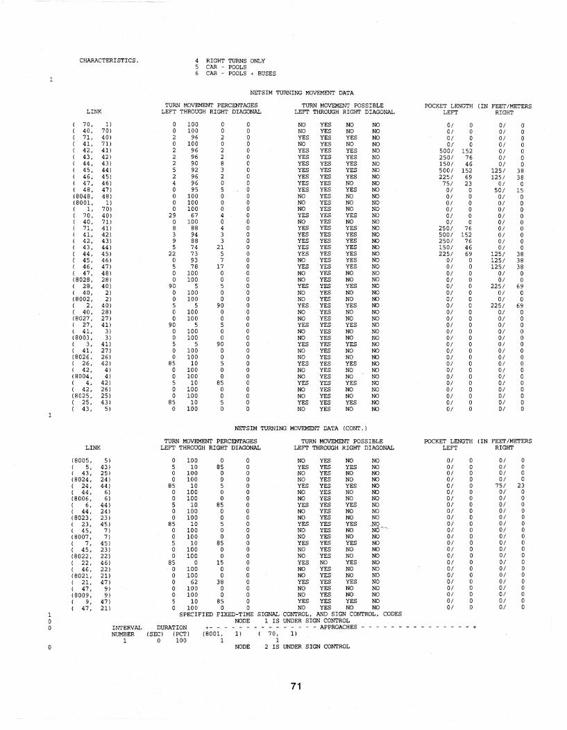
CHARACTERISTICS. 4 RIGHT TURNS ONLY 5 CAR - POOLS 6 CAR - POOLS + BUSES

NETSIM TURNING MOVEMENT DATA

TURN MOVEMENT PERCENTAGES TURN MOVEMENT POSSIBLE POCKET LENGTH (IN FEET/METERS LINK LEFT THROUGH RIGHT DIAGONAL LEFT THROUGH RIGHT DIAGONAL LEFT RIGHT

70, 1) 0 100 0 0 NO YES NO NO 0/ 0 0/ 0 40, 70) 0 100 0 0 NO YES NO NO 0/ 0 0/ 0 71, 40) 2 96 2 a YES YES YES NO 0/ a 0/ 0 41, 71) a 100 a a NO YES NO NO 0/ a 0/ 0 42, 41 ) 2 96 2 0 YES YES YES NO 500/ 152 0/ a 43, 42) 2 96 2 a YES YES YES NO 250/ 76 0/ a 44, 43) 2 90 8 0 YES YES YES NO 150/ 46 0/ a 45, 44) 5 92 3 a YES YES YES NO 500/ 152 125/ 38 46, 45) 2 96 2 a YES YES YES NO 225/ 69 125/ 38 47, 46) 4 96 a a YES YES NO NO 75/ 23 0/ a

( 48, 47) a 95 5 a YES YES YES NO 0/ a 50/ 15 (8048, 48) a 100 a a NO YES NO NO 0/ a 0/ a (8001, 1) a 100 a a NO YES NO NO 0/ a 0/ 0 ( 1, 70) a 100 a a NO YES NO NO 0/ a 0/ a ( 70, 40) 29 67 4 a YES YES YES NO 0/ a 0/ 0 ( 40, 71) a 100 0 0 NO YES NO NO 0/ 0 0/ a ( 71, 41) 8 88 4 a YES YES YES NO 250/ 76 0/ a ( 41, 42) 3 94 3 a YES YES YES NO 500/ 152 0/ 0 ( 42, 43) 9 88 3 a YES YES YES NO 250/ 76 0/ 0 ( 43, 44) 5 74 21 0 YES YES YES NO 150/ 46 0/ 0 ( 44, 45) 22 73 5 a YES YES YES NO 225/ 69 125/ 38 ( 45, 46) a 93 7 a NO YES YES NO 0/ a 125/ 38 ( 46, 47) 5 78 17 a YES YES YES NO 0/ 0 125/ 38 ( 47, 48) a 100 0 0 NO YES NO NO 0/ a 0/ a (8028, 28) a 100 0 a NO YES NO NO 0/ 0 0/ a ( 28, 40) 90 5 5 a YES YES YES NO 0/ a 225/ 69 ( 40, 2) a 100 a a NO YES NO NO 0/ a 0/ a (8002, 2) a 100 a a NO YES NO NO 0/ a 0/ a ( 2, 40) 5 5 90 a YES YES YES NO 0/ a 225/ 69 ( 40, 28) a 100 a a NO YES NO NO 0/ 0 0/ a (8027, 27) a 100 0 a NO YES NO NO 0/ a 0/ a ( 27, 41) 90 5 5 a YES YES YES NO 0/ 0 0/ a ( 41, 3) a 100 a a NO YES NO NO 0/ a 0/ a (8003, 3) a 100 a a NO YES NO NO 0/ a 0/ a ( 3, 41) 5 5 90 a YES YES YES NO 0/ a 0/ a ( 41. 27) a 100 a a NO YES NO NO 0/ a 0/ 0 (8026, 26) a 100 a a NO YES NO NO 0/ 0 0/ a ( 26, 42) 85 10 5 a YES YES YES NO 0/ a 0/ a ( 42, 4) a 100 0 a NO YES NO NO 0/ 0 0/ a (8004, 4) a 100 a a NO YES NO NO 0/ 0 0/ 0 ( 4, 42) 5 10 85 0 YES YES YES NO 0/ a 0/ a ( 42, 26) 0 100 0 a NO YES NO NO 0/ 0 0/ 0 (8025, 25) 0 100 0 0 NO YES NO NO 0/ 0 0/ 0 ( 25, 43) 85 10 5 a YES YES YES NO 0/ 0 0/ 0 ( 43, 5) 0 100 0 0 NO YES NO NO 0/ 0 0/ 0

NETSIM TURNING MOVEMENT DATA (CONT.)

TURN MOVEMENT PERCENTAGES TURN MOVEMENT POSSIBLE POCKET LENGTH (IN FEET /METERS LINK LEFT THROUGH RIGHT DIAGONAL LEFT THROUGH RIGHT DIAGONAL LEFT RIGHT

(8005, 5) 0 100 0 a NO YES NO NO 0/ a 0/ a ( 5, 43) 5 10 85 a YES YES YES NO 0/ 0 0/ 0 ( 43, 25) 0 100 0 a NO YES NO NO 0/ a 0/ 0 (8024, 24) a 100 a 0 NO YES NO NO 0/ a 0/ a ( 24, 44) 85 10 5 0 YES YES YES NO 0/ a 75/ 23 ( 44, 6) a 100 a a NO YES NO NO 0/ a 0/ a (8006, 6) 0 100 a a NO YES NO NO 0/ 0 0/ a ( 6, 44) 5 10 85 a YES YES YES NO 0/ 0 0/ a ( 44, 24) 0 100 a a NO YES NO NO 0/ a 0/ a (8023, 23) a 100 a a NO YES NO NO 0/ a 0/ a ( 23, 45) 85 10 5 a YES YES YES -~g~ 0/ 0 0/ 0 ( 45, 7) a 100 a a NO YES NO 0/ 0 0/ 0 (8007, 7) a 100 a a NO YES NO NO 0/ a 0/ a ( 7, 45 ) 5 10 85 a YES YES YES NO 0/ a 01 0 ( 45, 23) 0 100 a a NO YES NO NO 0/ a 0/ a (8022, 22) a 100 a a NO YES NO NO 0/ a 0/ 0 ( 22, 46) 85 a 15 0 YES NO YES NO 0/ a 0/ 0 ( 46, 22) a 100 a a NO YES NO NO 0/ 0 0/ a (8021. 21) a 100 a a NO YES NO NO 0/ a 0/ a ( 21, 47) a 62 38 a YES YES YES NO 0/ 0 0/ a ( 47, 9) a 100 a a NO YES NO NO 0/ a 0/ a (8009, 9) 0 100 a 0 NO YES NO NO 0/ a 0/ 0 ( 9, 47) 5 10 85 0 YES YES YES NO 0/ a 0/ 0 ( 47, 21 ) a 100 a 0 NO YES NO NO 0/ a 01 a

1 SPECIFIED FIXED-TIME SIGNAL CONTROL, AND SIGN CONTROL, CODES 0 NODE 1 IS UNDER SIGN CONTROL 0 INTERVAL DURATION +- - - - - - - - - - - - APPROACHES - - - - - - - - - +

NUMBER (SEC) (PCT) (8001, 1) ( 70, 1) 1 0 100 1 1

0 NODE 2 IS UNDER SIGN CONTROL

71

0 INTERVAL DURATION ------ - - APPROACHES - - - - - - - - - - - - - - - + NUMBER (SEC) (PCT) (8002, 2) 40, 2)

1 0 100 1 1 0 NODE 3 IS UNDER SIGN CONTROL 0 INTERVAL DURATION - - APPROACHES - - - - - - - - - - - - - - - +

NUMBER (SEC) (PCT) (8003, 3) 41, 3) 1 0 100 1 1

0 NODE 4 IS UNDER SIGN CONTROL 0 INTERVAL DURATION +- - - APPROACHES - - - - - - - - - - - - - - - +

NUMBER (SEC) (PCT) (8004, 4) 42, 4) 1 0 100 1 1

0 NODE 5 IS UNDER SIGN CONTROL a INTERVAL DURATION +- - - APPROACHES - - - - - - - - - - - - - - - +

NUMBER (SEC) (PCT) (8005, 5) 43, 5) 1 a 100 1 1

a NODE 6 IS UNDER SIGN CONTROL a INTERVAL DURATION +- - - APPROACHES - - - - - - - - - - - - - - - .+

NUMBER (SEC) (PCT) (8006, 6) 44, 6) 1 a 100 1 1

a NODE 7 IS UNDER SIGN CONTROL 0 INTERVAL DURATION +- - - APPROACHES - - - - - - - - - - - - - - - +

NUMBER (SEC) (PCT) (8007, 7) 45, 7) 1 0 100 1 1

a NODE 9 IS UNDER SIGN CONTROL 0 INTERVAL DURATION +- - - APPROACHES - - - - - - - - - - - - - - - +

NUMBER (SEC) (PCT) (8009, 9) 47, 9) 1 a 100 1 1

0 NODE 21 IS UNDER SIGN CONTROL 0 INTERVAL DURATION +- - - - - - - - APPROACHES - - - - - ------ - - - - +

NUMBER (SEC) (PCT) (8021, 21) 47, 21) 1 0 100 1 1

1 0 NODE 22 IS UNDER SIGN CONTROL a INTERVAL DURATION +- - - - - - - - - - APPROACHES - - - - - - - - - - - - - - - +

NUMBER (SEC) (PCT) (8022, 22) 46, 22) 1 0 100 1 1

0 NODE 23 IS UNDER SIGN CONTROL 0 INTERVAL DURATION +- - - - - APPROACHES - - - - - - - - - - - - - - - +

NUMBER (SEC) (PCT) (8023, 23) 45, 23) 1 0 100 1 1

0 NODE 24 IS UNDER SIGN CONTROL 0 INTERVAL DURATION +- - - - - APPROACHES - - - - - - - - - - - - - - - +

NUMBER (SEC) (PCT) (8024, 24) 44, 24) 1 0 100 1 1

a NODE 25 IS UNDER SIGN CONTROL 0 INTERVAL DURATION +- - - - - - APPROACHES - - - - - - - - - - - - - - - +

NUMBER (SEC) (PCT) (8025, 25) 43, 25) 1 0 100 1 1

a NODE 26 IS UNDER SIGN CONTROL 0 INTERVAL DURATION +- - - - - - APPROACHES - - - - - - - - - - - - - - - +

NUMBER (SEC) (PCT) (8026, 26) 42, 26) 1 0 100 1 1

0 NODE 27 IS UNDER SIGN CONTROL 0 INTERVAL DURATION +- - - -- - - - - - - - - APPROACHES - - - - - - - - - - - - - - - +

NUMBER (SEC) (PCT) (8027, 27) ( 41, 27) 1 0 100 1 1

0 NODE 28 IS UNDER SIGN CONTROL 0 INTERVAL DURATION - - APPROACHES - - - - - - - - - - - - - - - +

NUMBER (SEC) (PCT) (8028, 28) 40, 28) 1 0 100 1 1

1 0 NODE 40

OFFSET SEC CYCLE LENGTH 90 SEC 0 INTERVAL DURATION +- - - - - - - - APPROACHES - - - - - - - - - +

NUMBER (SEC) (PCT) 70, 40) 2, 40) ( 71, 40) 28, 40) 1 12 13 9 2 9 2 2 4 4 9 2 0 2 3 9 10 1 2 2 2 4 4 4 a 2 2 2 5 32 35 2 9 2 9 6 4 4 2 0 2 0 7 1 1 2 2 2 2 8 20 22 2 2 1 2 9 4 4 2 2 0 2

a NODE 41 OFFSET 50 SEC CYCLE LENGTH 90 SEC

0 INTERVAL DURATION +- - - APPROACHES - - - - - - - - - + NUMBER (SEC) (PCT) 71, 41) 3, 41) 42, 41) 27, 41)

1 59 65 1 2 1 2 2 4 4 0 2 0 2 3 13 14 2 1 2 1 4 4 4 2 0 2 0 5 6 6 1 2 2 2 6 4 4 a 2 2 2

0 NODE 42 OFFSET 12 SEC CYCLE LENGTH 90 SEC

0 INTERVAL DURATION +- APPROACHES - - - - - - - - - +

NUMBER (SEC) (PCT) 41, 42) 4, 42) 43, 42) 26, 42) 1 69 76 1 2 1 2 2 4 4 0 2 a 2 3 13 14 2 1 2 1 4 4 4 2 a 2 0

72

0 NODE 43 OFFSET 2 SEC CYCLE LENGTH 90 SEC

0 INTERVAL DURATION - APPROACHES - - - - - - - - + NUMBER (SEC) (PCT) 42, 43) 5, 43) 44, 43) 25, 43)

1 66 73 1 2 1 2 2 4 4 0 2 0 2 3 16 17 2 1 2 1 4 4 4 2 0 2 0

1 0 NODE 44

OFFSET 83 SEC CYCLE LENGTH 90 SEC 0 INTERVAL DURATION - - APPROACHES

NUMBER (SEC) (PCT) 43, 44) 6, 44) 45, 44) 24, 44) 1 70 77 1 2 1 2 2 4 4 0 2 0 2 3 12 13 2 1 2 1 4- 4 4 2 0 2 0

0 NODE 45 OFFSET 0 SEC CYCLE LENGTH 90 SEC

0 INTERVAL DURATION - APPROACHES - - - - - - - - + NUMBER (SEC) (PCT) 44, 45) 7, 45) 46, 45) 23, 45)

1 23 25 9 2 9 2 2 4 4 9 2 0 2 3 8 8 1 2 2 2 4 4 4 a 2 2 2 5 21 23 2 9 2 9 6 4 4 2 0 2 0 7 22 24 2 2 1 2 8 4 4 2 2 a 2

0 NODE 46 OFFSET 19 SEC CYCLE LENGTH 90 SEC

0 INTERVAL DURATION +- - - APPROACHES - - - + NUMBER (SEC) (PCT) 45, 46) 47, 46) 22, 46)

1 73 81 9 1 2 2 4 4 0 0 2 3 8 8 2 2 1 4 4 4 2 2 a 5 1 1 2 2 2

a NODE 47 OFFSET 70 SEC CYCLE LENGTH 90 SEC

0 INTERVAL DURATION - - APPROACHES - - - + NUMBER (SEC) (PCT) 46, 47) 9, 47) 48, 47) 21, 47)

1 57 63 1 2 9 2 2 4 4 1 2 0 2 3 5 5 1 2 2 2 4 4 4 0 2 2 2 5 16 17 2 9 2 9 6 4 4 2 0 2 a

0 NODE 48 IS UNDER SIGN CONTROL 0 INTERVAL DURATION - - APPROACHES - - - - - - - - - - +

NUMBER (SEC) (PCT) (8048, 48) 47, 48) 1 0 100 1 1

1 0 NODE 70 IS UNDER SIGN CONTROL 0 INTERVAL DURATION +- - - - - - APPROACHES - - - '- - - - - - - - - - - - +

NUMBER (SEC) (PCT) ( 1, 70) 40, 70) 1 a 100 1 1

a NODE 71 IS UNDER SIGN CONTROL a INTERVAL DURATION +- - - - - - APPROACHES - - - - - - - - - - - - - - - +

NUMBER (SEC) (PCT) 40, 71) 41, 71) 1 a 100 1 1

1 INTERPRETATION OF SIGNAL CODES

0 YIELD OR AMBER

1 GREEN

2 RED

3 RED WITH GREEN RIGHT ARROW

4 RED WITH GREEN LEFT ARROW

5 STOP

6 RED WITH GREEN DIAGONAL ARROW

7 NO TURNS-GREEN THRU ARROW

8 RED WITH LEFT AND RIGHT GREEN ARROW

9 NO LEFT TURN-GREEN THRU AND RIGHT 1 TRAFFIC CONTROL TABLE - SIGNS AND FIXED TIME SIGNALS

CONTROL CODES GO PROTECTED NOGO NOT PERMITTED AMBR AMBER PERM PERMITTED NOT PROTECTED PROT PROTECTED STOP STOP SIGN YLD YIELD SIGN

73

NODE SIGN CONTROL

INTERVAL DURATION ------------------------------------------- APPROACHES -------------------------------------------_ (8001, 1) (70, 1)

LEFT THRU RITE DIAG LEFT THRU RITE DIAG LEFT THRU RITE DIAG LEFT THRU RITE DIAG LEFT THRU RITE DIAG o GO GO

NODE 2

INTERVAL DURATION

1 o

NODE 3

INTERVAL DURATION

1 o

NODE 4

INTERVAL DURATION

SIGN CONTROL

------------------------------------------- APPROACHES (8002, 2) ( 40, 2)

LEFT THRU RITE DIAG LEFT THRU RITE DIAG LEFT THRU RITE DIAG LEFT THRU RITE DIAG LEFT THRU RITE DIAG GO GO

SIGN CONTROL

(8003, 3) LEFT THRU RITE DIAG

GO

SIGN CONTROL

APPROACHES ( 41. 3)

LEFT THRU RITE DIAG LEFT THRU RITE DIAG GO

------------------------------------------- APPROACHES (8004, 4) (42, 4)

LEFT THRU RITE DIAG LEFT THRU RITE DIAG

LEFT THRU RITE DIAG LEFT THRU RITE DIAG LEFT THRU RITE DIAG LEFT THRU RITE DIAG LEFT THRU RITE DIAG o GO GO

NODE 5 SIGN CONTROL

INTERVAL DURATION ------------------------------------------- APPROACHES (8005, 5) ( 43, 5)

LEFT THRU RITE DIAG LEFT THRU RITE DIAG LEFT THRU RITE DIAG LEFT THRU RITE DIAG LEFT THRU RITE DIAG o GO GO

NODE 6 SIGN CONTROL

INTERVAL DURATION ------------------------------------------- APPROACHES (8006, 6) ( 44, 6)

LEFT THRU RITE DIAG LEFT THRU RITE DIAG LEFT THRU RITE DIAG LEFT THRU RITE DIAG LEFT THRU RITE DIAG 1 o GO GO

NODE 7 SIGN CONTROL

INTERVAL DURATION ------------------------------------------- APPROACHES (8007, 7) ( 45, 7)

LEFT THRU RITE DIAG LEFT THRU RITE DIAG LEFT THRU RITE DIAG LEFT THRU RITE DIAG LEFT THRU RITE DIAG o GO GO

NODE 9 SIGN CONTROL

INTERVAL DURATION ------------------------------------------- APPROACHES --------------------------------------------(8009, 9) ( 47, 9)

LEFT THRU RITE DIAG LEFT THRU RITE DIAG LEFT THRU RITE DIAG LEFT THRU RITE DIAG LEFT THRU RITE DIAG GO GO

NODE 21 SIGN CONTROL

INTERVAL DURATION ------------------------------------------- APPROACHES --------------------------------------------(8021, 21) ( 47, 21)

LEFT THRU RITE DIAG LEFT THRU RITE DIAG LEFT THRU RITE DIAG LEFT THRU RITE DIAG LEFT THRU RITE DIAG GO GO

NODE 22 SIGN CONTROL

INTERVAL DURATION ------------------------------------------- APPROACHES (8022, 22) ( 46, 22)

LEFT THRU RITE DIAG LEFT THRU RITE DIAG LEFT THRU RITE DIAG LEFT THRU RITE DIAG LEFT THRU RITE DIAG 1 o GO GO

74

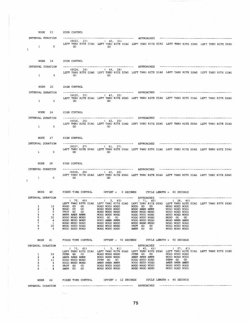
NODE 23 SIGN CONTROL

INTERVAL DURATION ------------------------------------------- APPROACHES (8023, 23) ( 45, 23)

LEFT THRU RITE DrAG LEFT THRU RITE DrAG LEFT THRU RITE DrAG LEFT THRU RITE DIAG LEFT THRU RITE DIAG o GO GO

1

1

NODE 24 SIGN CONTROL

INTERVAL DURATION ------------------------------------------- APPROACHES (8024, 24) ( 44, 24)

LEFT THRU RITE DIAG LEFT THRU RITE DIAG LEFT THRU RITE DIAG LEFT THRU RITE DIAG LEFT THRU RITE DIAG o GO GO

NODE 25 SIGN CONTROL

INTERVAL DURATION ------------------------------------------- APPROACHES (8025, 25) ( 43, 25)

LEFT THRU RITE DIAG LEFT THRU RITE DIAG LEFT THRU RITE DIAG LEFT THRU RITE DIAG LEFT THRU RITE DIAG o GO GO

NODE 26 SIGN CONTROL

INTERVAL DURATION ------------------------------------------- APPROACHES (8026, 26) ( 42, 26)

LEFT THRU RITE DIAG LEFT THRU RITE DIAG LEFT THRU RITE DIAG LEFT THRU RITE DIAG LEFT THRU RITE DIAG o GO GO

NODE 27 SIGN CONTROL

INTERVAL DURATION ------------------------------------------- APPROACHES (8027, 27) ( 41, 27)

LEFT THRU RITE DIAG LEFT THRU RITE DIAG LEFT THRU RITE DIAG LEFT THRU RITE DIAG LEFT THRU RITE DIAG o GO GO

NODE 28 SIGN CONTROL

INTERVAL DURATION - - -- - - ------ - - -- - - -- --- - --- - --- - -- --------- - APPROACHES (8028, 28) ( 40, 28)

LEFT THRU RITE DIAG LEFT THRU RITE DIAG LEFT THRU RITE DIAG LEFT THRU RITE DIAG LEFT THRU RITE DIAG o GO GO

NODE 40

INTERVAL DURATION

1 12 2 4 3 9 4 4 5 32 6 4 7 1 8 20 9 4

NODE 41

INTERVAL DURATION

1 59 2 4 3 13 4 4 5 6 6 4

NODE 42

INTERVAL DURATION

FIXED TIME CONTROL

( 70, 40) LEFT THRU RITE DIAG NOGO GO GO NOGO GO GO PROT GO GO AMBR AMBR AMBR NOGO NOGO· NOGO NOGO NOGO NOGO NOGO NOGO NOGO NOGO NOGO NOGO NOGO NOGO NOGO

FIXED TIME CONTROL

( 71, 41) LEFT THRU RITE DIAG PERM GO GO AMBR AMBR AMBR NOGO NOGO NOGO NOGO. NOGO NOGO PROT GO GO AMBR GO GO

FIXED TIME CONTROL

OFFSET ~ o SECONDS CYCLE LENGTH ~ 90 SECONDS

APPROACHES 2, 40)

LEFT THRU RITE DIAG ( 71, 40)

LEFT THRU RITE DIAG NOGO GO GO

( 28, 40) LEFT THRU RITE DIAG NOGONOGONOGO NOGO NOGO NOGO NOGO NOGO NOGO NOGO NOGO NOGO

NOGO NOGO NOGO NOGO NOGO NOGO NOGO NOGO NOGO NOGO NOGO NOGO NOGO GO GO NOGO AMBR AMBR NOGO NOGO NOGO NOGO NOGO NOGO NOGO NOGO NOGO

NOGO AMBR AMBR NOGO NOGO NOGO NOGO NOGO NOGO NOGO NOGO NOGO NOGO NOGO NOGO NOGO NOGO NOGO PROT GO GO AMBR GO GO

NOGO GO GO NOGO AMBR AMBR NOGONOGONOGO NOGO NOGO NOGO NOGO NOGO NOGO

OFFSET = 50 SECONDS CYCLE LENGTH = 90 SECONDS

APPROACHES ( 3, 41 ) ( 27, 41)

LEFT THRU RITE DIAG

LEFT THRU RITE DIAG NOGO NOGO NOGO

( 42, 41) LEFT THRU RITE DIAG PERM GO GO

LEFT THRU RITE DIAG LEFT THRU RITE DIAG NOGO NOGO NOGO

NOGO NOGO NOGO PERM GO GO AMBR AMBR AMBR NOGO NOGO NOGO NOGO NOGO NOGO

AMBR AMBR AMBR NOGO NOGO NOGO NOGO NOGO NOGO NOGO NOGO NOGO NOGO NOGO NOGO

NOGO NOGO NOGO PERM GO GO AMBR AMBR AMBR NOGO NOGO NOGO NOGONOGONOGO

OFFSET = 12 SECONDS CYCLE LENGTH = 90 SECONDS

------------------------------------------- APPROACHES

75

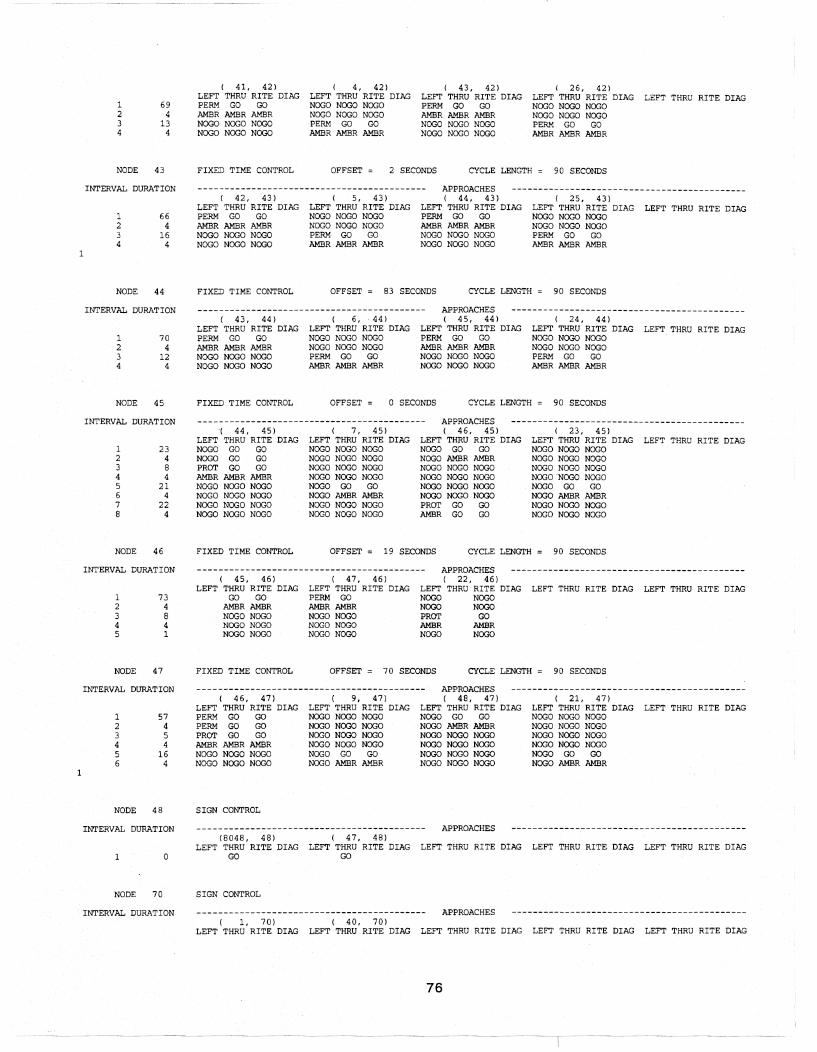
1 69 2 4 3 13 4 4

NODE 43

INTERVAL DURATION

1 66 2 4 3 16 4 4

1

NODE 44

INTERVAL DURATION

1 70 2 4 3 12 4 4

NODE 45

INTERVAL DURATION

1 23 2 4 3 8 4 4 5 21 6 4 7 22 8 4

NODE 46

INTERVAL DURATION

1 73 2 4 3 8 4 4 5 1

NODE 47

INTERVAL DURATION

1 57 2 4 3 5 4 4 5 16 6 4

1

NODE 48

INTERVAL DURATION

( 41, 42) LEFT THRU RITE DIAG PERM GO GO AMBR AMBR AMBR NOGO NOGO NOGO NOGO NOGO NOGO

FIXED TIME CONTROL

( 42, 43) LEFT THRU RITE DIAG PERM GO GO AMBR AMBR AMBR NOGONOGONOGO NOGO NOGO NOGO

FIXED TIME CONTROL

( 43, 44) LEFT THRU RITE DIAG PERM GO GO AMBR AMBR AMBR NOGO NOGO NOGO NOGONOGONOGO

FIXED TIME CONTROL

( 44, 45) LEFT THRU RITE DIAG NOGO GO GO NOGO GO GO PROT GO GO AMBR AMBR AMBR NOGO NOGO NOGO NOGO NOGO NOGO NOGO NOGO NOGO NOGO NOGO NOGO

FIXED TIME CONTROL

( 4, 42) ( 43, 42) ( 26, 42) LEFT THRU RITE DIAG LEFT THRU RITE DIAG LEFT THRU RITE DIAG LEFT THRU RITE DIAG NOGO NOGO NOGO PERM GO GO NOGO NOGO NOGO NOGONOGONOGO AMBR AMBR AMBR NOGO NOGO NOGO PERM GO GO NOGO NOGO NOGO PERM GO GO AMBR AMBR AMBR NOGO NOGO NOGO AMBR AMBR AMBR

OFFSET ~ 2 SECONDS CYCLE LENGTH = 90 SECONDS

( 5, 43) LEFT THRU RITE DIAG NOGO NOGO NOGO NOGO NOGO NOGO PERM GO GO AMBR AMBR AMBR

APPROACHES ( 44, 43)

LEFT THRU RITE DIAG PERM GO GO AMBR AMBR AMBR NOGO NOGO NOGO NOGO NOGO NOGO

( 25, 43) LEFT THRU RITE DIAG LEFT THRU RITE DIAG NOGONOGONOGO NOGO NOGO NOGO PERM GO GO AMBR AMBR AMBR

OFFSET ~ 83 SECONDS CYCLE LENGTH = 90 SECONDS

( 6, 44) LEFT THRU RITE DIAG NOGO NOGO NOGO NOGO NOGO NOGO PERM GO GO AMBR AMBR AMBR

APPROACHES ( 45, 44)

LEFT THRU RITE DIAG PERM GO GO AMBR AMBR AMBR NOGO NOGO NOGO NOGO NOGO NOGO

( 24, 44) LEFT THRU RITE DIAG LEFT THRU RITE DIAG NOGO NOGO NOGO NOGONOGONOGO PERM GO GO AMBR AMBR AMBR

OFFSET ~ o SECONDS CYCLE LENGTH = 90 SECONDS

( 7, 45) LEFT THRU RITE DIAG NOGO NOGO NOGO NOGO NOGO NOGO NOGO NOGO NOGO NOGO NOGO NOGO NOGO GO GO NOGO AMBR AMBR NOGO NOGO NOGO NOGONOGONOGO

APPROACHES ( 46, 45)

LEFT THRU RITE DIAG NOGO GO GO NOGO AMBR AMBR NOGO NOGO NOGO NOGO NOGO NOGO NOGO NOGO NOGO NOGO NOGO NOGO PROT GO GO AMBR GO GO

( 23, 45) LEFT THRU RITE DIAG LEFT THRU RITE DIAG NOGONOGONOGO NOGO NOGO NOGO NOGO NOGO NOGO NOGONOGO NOGO NOGO GO GO NOGO AMBR AMBR NOGO NOGO NOGO NOGO NOGO NOGO

OFFSET = 19 SECONDS CYCLE LENGTH = 90 SECONDS

------------------------------------------- APPROACHES --------------------------------------------1 45, 46)

LEFT THRU RITE DIAG GO GO

AMBR AMBR NOGO NOGO NOGONOGO NOGONOGO

FIXED TIME CONTROL

( 46, 47) LEFT THRU RITE DIAG PERM GO GO PERM GO GO PROT GO GO AMBR AMBR AMBR NOGO NOGO NOGO NOGO NOGO NOGO

SIGN CONTROL

( 47, 46) ( 22, 46) LEFT THRU RITE DIAG LEFT THRU RITE DIAG LEFT THRU RITE DIAG LEFT THRU RITE DIAG PERM GO NOGO NOGO AMBR AMBR NOGO NOGO NOGO NOGO PROT GO NOGO NOGO AMBR AMBR NOGO NOGO NOGO NOGO

OFFSET = 70 SECONDS CYCLE LENGTH = 90 SECONDS

( 9, 47) LEFT THRU RITE DIAG NOGO NOGO NOGO NOGO NOGO NOGO NOGO NOGO NOGO NOGO NOGO NOGO NOGO GO GO NOGO AMBR AMBR

APPROACHES ( 48, 47)

LEFT THRU RITE DIAG NOGO GO GO NOGO AMBR AMBR NOGO NOGO NOGO NOGO NOGO NOGO NOGO NOGO NOGO NOGO NOGO NOGO

( 21, 47) LEFT THRU RITE DIAG NOGO NOGO NOGO NOGO NOGO NOGO NOGO NOGO NOGO NOGO NOGO NOGO NOGO GO GO NOGO AMBR AMBR

LEFT THRU RITE DIAG

------------------------------------------- APPROACHES --------------------------------------------18048, 48) ( 47, 48)

LEFT THRU RITE DIAG LEFT THRU RITE DIAG LEFT THRU RITE DIAG LEFT THRU RITE DIAG LEFT THRU RITE DIAG o GO GO

NODE 70 SIGN CONTROL

INTERVAL DURATION ------------------------------------------- APPROACHES --------------------------------------------1 1, 70) ( 40, 70)

LEFT THRU RITE DIAG LEFT THRU RITE DIAG LEFT THRU RITE DIAG LEFT THRU RITE DIAG LEFT THRU RITE DIAG

76

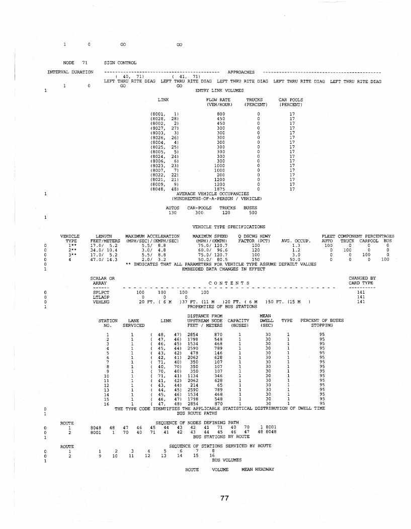
1

1

1

o o o o o 1

o o o 1

0 1

0 0 1

0 0 1

1 o GO GO

NODE 71 SIGN CONTROL

INTERVAL DURATION ------------------------------------------- APPROACHES --------------------------------------------

VEHICLE TYPE 1*' 2*' 3*' 4

ROUTE 1 2

ROUTE 1 2

( 40, 71) LEFT THRU RITE DIAG

GO

( 41, 71) LEFT THRU RITE DIAG LEFT THRU RITE DIAG

GO LEFT THRU RITE DIAG LEFT THRU RITE DrAG

LENGTH FEET/METERS 17.0/ 5.2 34.0/ 10.4 17 .0/ 5.2 47.0/ 14.3

SCALAR OR ARRAY

SPLPCT LTLAGP VEHLNG

STATION NO.

1 2 3 4 5 6 7 8 9

10 11 12 13 14 15 16

ENTRY LINK VOLUMES

LINK FLOW RATE TRUCKS CAR POOLS (VEH/HOUR) (PERCENT) (PERCENT)

(8001, 1) 800 0 17 (8028, 28) 450 0 17 (8002, 2) 450 0 17 (8027, 27) 300 0 17 (8003, 3) 300 0 17 (8026, 26) 300 0 17 (8004, 4) 300 0 17 (8025, 25) 300 0 17 (8005, 5) 300 0 17 (8024, 24) 300 0 17 (8006, 6) 300 0 17 (8023, 23) 1000 0 17 (8007, 7) 1000 0 17 (8022, 22) 200 0 17 (8021, 21) 1200 0 17 (8009, 9) 1200 0 17 (8048, 48) 1875 0 17

AVERAGE VEHICLE OCCUPANCIES (HUNDREDTHS-OF-A-PERSON / VEHICLE)

AUTOS CAR-POOLS TRUCKS BUSES 130 300 120 500

VEHICLE TYPE SPECIFICATIONS

MAXIMUM ACCELERATION HAXIMUM SPEED Q DSCHG HDWY (MPH/SEC)/(KMPH/SEC) (MPH)/(KMPH) FACTOR (PCT) AVG. OCCUP.

5.5/ 8.8 75.0/ 120.7 100 1.3 3.0/ 4.8 60.0/ 96.6 120 1.2 5.5/ 8.8 75.0/ 120.7 100 3.0 2.0/ 3.2 50.0/ 80.5 150 50.0

INDICATES THAT ALL PARAMETERS FOR VEHICLE TYPE ASSUME DEFAULT VALUES EMBEDDED DATA CHANGES IN EFFECT

100 100 o 0

20 FT. ( 6 M

CON TEN T S

100 100 o

)37 FT. (11 M )20 FT. ( 6 M PROPERTIES OF BUS STATIONS

DISTANCE FROM

)50 FT. (15 M

MEAN

FLEET COMPONENT PERCENTAGES AUTO TRUCK CARPOOL BUS

100 0 0 0 o 100 0 0 o 0 100 0 o 0 0 100

CHANGED BY CARD TYPE

141 141 141

LANE LINK UPSTREAM NODE CAPACITY DWELL TYPE PERCENT OF BUSES SERVICED FEET / METERS (BUSES) (SEC) STOPPING

1 48, 47) 2854 870 1 30 1 95 1 47, 46) 1798 548 1 30 1 95 1 46, 45) 1534 468 1 30 1 95 1 45, 44) 2590 789 1 30 1 95 1 43, 42) 478 146 1 30 1 95 1 42, 41) 2062 628 1 30 1 95 1 71, 40) 350 107 1 30 1 95 1 40, 70) 350 107 1 30 1 95 1 70, 40) 350 107 1 30 1 95 1 71, 41) 1134 346 1 30 1 95 1 41, 42) 2062 628 1 30 1 95 1 43, 44) 214 65 1 30 1 95 1 44, 45) 2590 789 1 30 1 95 1 45, 46) 1534 468 1 30 1 95 1 46, 47) 1798 548 1 30 1 95 1 ( 47, 48) 2854 870 1 30 1 95

THE TYPE CODE IDENTIFIES THE APPLICABLE STATISTICAL DISTRIBUTION OF DWELL TIME BUS ROUTE PATHS

SEQUENCE OF NODES DEFINING PATH 8048 48 47 46 45 44 43 42 41 71 40 70 1 8001 8001 1 70 40 71 41 42 43 44 45 46 47 48 8048

BUS STATIONS BY ROUTE

SEQUENCE OF STATIONS SERVICED BY ROUTE 1 2 3 4 5 6 7 8 9 10 11 12 13 14 15 16

BUS VOLUMES

ROUTE VOLUME MEAN HEADWAY

77

o o

1 2

(VEH/HR) 12 12

78

(SEC) 300 300

T

Appendix B

TRAF-NETSIM Input for Network B

79

80

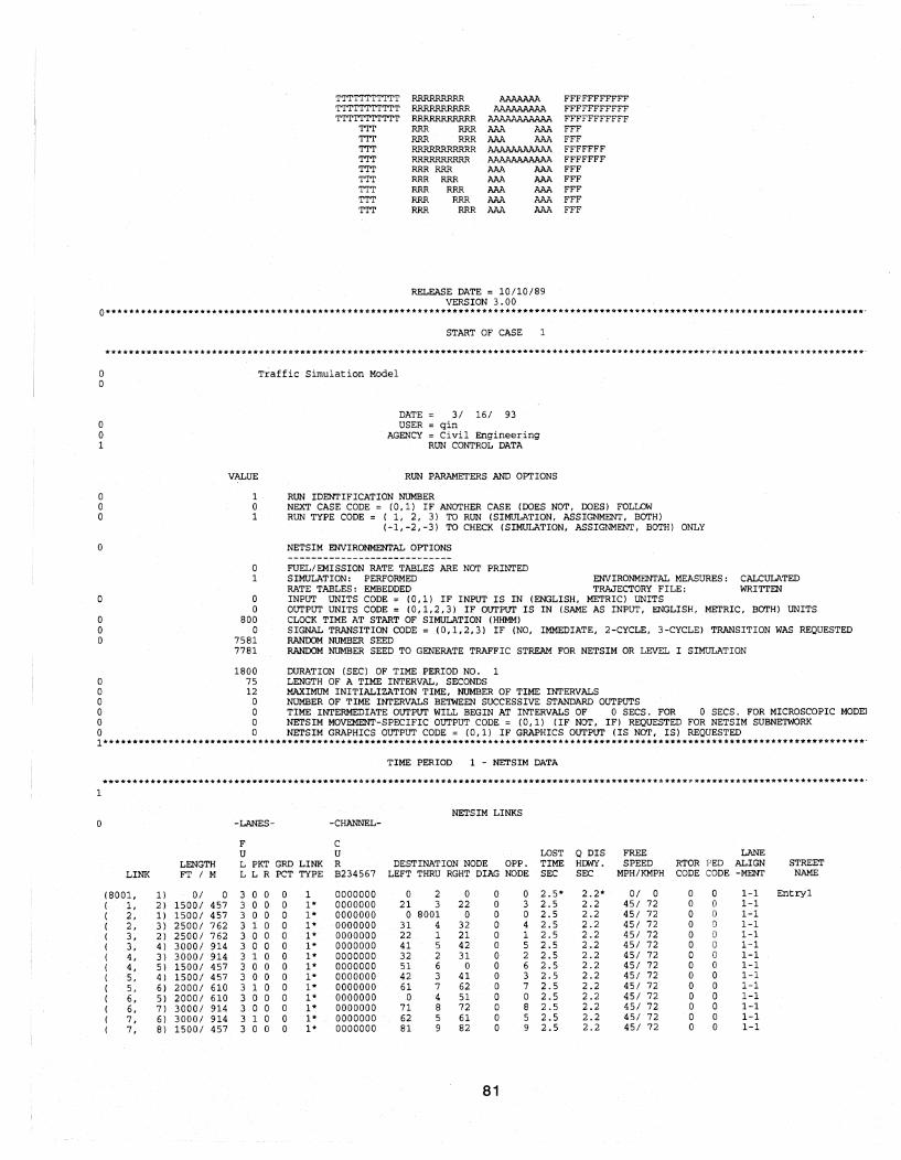
TTTTTTTTTTT 'I'TTTTTTTTTT 'I'TTTTT'I'T'ITT

'I'TT TTT 'I'TT 'I'TT TTT TTT 'I'TT TTT TTT

RRRRRRRRR AAAJ>.N>.A RRRRRRRRRR AAA.>,AJ;AAA RRRRRRRRRRR AAAAlIAAAAAA RRR RRR AAA AAA RRR RRR AAA AAA RRRRRRRRRRR AAAAAAAAAAA RRRRRRRRRR AAAAlIAAAAAA RRR RRR AAA AAA RRR RRR AAA AAA RRR RRR AAA AAA RRR RRR AAA AAA RRR RRR AAA AAA

RELEASE DATE = 10/10/89 VERSION 3. 00

FFFFFFFFFFF FFFFFFFFFFF FFFFFFFFFFF FFF FFF FFFFFFF FFFFFFF FFF FFF FFF FFF FFF

0************************··*****··***·**··**··********************.***************************.*.*.********* •••• ****.*.***********,

a a

a a 1

a a a

a

a

a a a

a a a a a a

START OF CASE

•• ** •• *********.***************.******** •• ****** •• *********.************************************.********.* •• ******.******.*.****.

VALUE

a 1

a a

800 a

7581 7781

1800 75 12 a a a a

Traffic Simulation Model

DATE USER

AGENCY

3/ 16/ 93 qin Civil Engineering

RUN CONTROL DATA

RUN PARAMETERS AND OPTIONS

RUN IDENTIFICATION NUMBER NEXT CASE CODE = (0, 1) IF ANOTHER CASE (DOES NOT, DOES) FOLLCW RUN TYPE CODE = ( 1, 2, 3) TO RUN (SIMULATION, ASSIGNMENT, BOTH)

(-1,-2,-3) TO CHECK (SIMULATION, ASSIGNMENT, BOTH) ONLY

NETSIM ENVIRONMENTAL OPTIONS

FUEL/EMISSION RATE TABLES ARE NOT PRINTED SIMULATION: PERFORMED ENVIRONMENTAL MEi',SURES: CALCULATED RATE TABLES: EMBEDDED TRAJECTORY FILE: WRITTEN INPUT UNITS CODE = (0,1) IF INPUT IS IN (ENGLISH, METRIC) UNITS OUTPUT UNITS CODE = (0,1,2,3) IF OUTPUT IS IN (SAME AS INPUT, ENGLISB, METRIC, BOTH) UNITS CLOCK TIME AT START OF SIMULATION (HHMM) SIGNAL TRANSITION CODE = (0,1,2,3) IF (NO, IMMEDIATE, 2-CYCLE, 3-CYCLE) TRANSITION WAS REQUESTED RANDOM NUMBER SEED RANDOM NUMBER SEED TO GENERATE TRAFFIC STREAM FOR NETS 1M OR LEVEL I SIMULATION

DURATION (SEC) OF TIME PERIOD NO. LENGTH OF A TIME INTERVAL, SECONDS MAXIMUM INITIALIZATION TIME, NUMBER OF TIME INTERVALS NUMBER OF TIME INTERVALS BETWEEN SUCCESSIVE STANDARD OUTPUTS TIME INTERMEDIATE OUTPUT WILL BEGIN AT INTERVALS OF a SECS. FOR a SECS. FOR MICROSCOPIC MODEl NETSIM MOVEMENT-SPECIFIC OUTPUT CODE = (0,1) (IF NOT, IF) REQUESTED FOR NETS 1M SUBNETWORK NETS 1M GRAPHICS OUTPUT CODE = (0,1) IF GRAPHICS OUTPUT (IS NOT, IS) REQUESTED

1*****··********··********··*********·******·***··***· •• ****.******* •• *.*** ••••••••••••• ******* •• **** •• ***************************.

TIME PERIOD 1 - NETSIM DATA

****************************************************** *********************************************~~******* *********************.

1

NETSIM LINKS a -LANES- -CHANNEL-

F C U U LCST Q DIS FREE LANE

LENGTH L PKT GRD LINK R DESTINATION NODE OPP. TIME HDWY. SPEED RTOR FED ALIGN STREET LINK FT / M L L R PCT TYPE B234567 LEFT THRU RGHT DIAG NODE SEC SEC MPH/KMPH CODE CODE -MENT NAME

(8001, 1) 0/ a 3 a a a 1 0000000 a 2 a a a 2.5* 2.2* 0/ a a a 1-1 Entry 1 ( 1, 2) 1500/ 457 3 a a a 1* 0000000 21 3 22 a 3 2.5 2.2 45/ 72 a 0 1-1 ( 2, 1 ) 1500/ 457 3 a 0 a 1* 0000000 a 8001 a a a 2.5 2.2 45/ 72 a 0 1-1 ( 2, 3) 2500/ 762 3 1 a a 1* 0000000 31 4 32 a 4 2.5 2.2 45/ 72 0 0 1-1 ( 3, 2) 2500/ 762 3 a a a 1* 0000000 22 1 21 a 1 2.5 2.2 45/ 72 a 0 1-1 ( 3, 4) 3000/ 914 3 a a a 1* 0000000 41 5 42 a 5 2.5 2.2 45/ 72 a 0 1-1 ( 4, 3) 3000/ 914 3 1 a a 1* 0000000 32 2 31 a 2 2.5 2.2 45/ 72 a 0 1-1 ( 4, 5) 1500/ 457 3 a a a 1* 0000000 51 6 a a 6 2.5 2.2 45/ 72 a 0 1-1 ( 5, 4 ) 1500/ 457 3 a a a 1* 0000000 42 3 41 a 3 2.5 2.2 45/ 72 a a 1-1 ( 5, 6 ) 2000/ 610 3 1 a a 1* 0000000 61 7 62 a 7 2.5 2.2 45/ 72 0 a 1-1 ( 6, 5) 2000/ 610 3 a a 0 1* 0000000 0 4 51 0 a 2.5 2.2 45/ 72 a 0 1-1 ( 6, 7) 3000/ 914 3 a a a 1* 0000000 71 8 72 a 8 2.5 2.2 45/ 72 a a 1-1 ( 7, 6) 3000/ 914 3 1 a a 1* 0000000 62 5 61 a 5 2.5 2.2 45/ 72 a a 1-1 ( 7, 8 ) 1500/ 457 3 a a a 1* 0000000 81 9 82 a 9 2.5 2.2 45/ 72 0 a 1-1

81

8, 7) 1500/ 457 3 a a a l' 0000000 72 6 71 a 6 2.5 2.2 451 72 a a 1-1 8, 9) 2000/ 610 3 a 0 0 1" 0000000 91 10 92 a 10 2.5 2.2 45/ 72 0 0 1-1 9, 8) 20001 610 3 a a a l' 0000000 82 7 81 a 7 2.5 2.2 45/ 72 a a 1-1 9, 10) 1500/ 457 3 a a a l' 0000000 a 8010 0 a a 2.5 2.2 45/ 72 0 a 1-1

( 10, 9) 1500/ 457 3 1 a a l' 0000000 92 8 91 a 8 2.5 2.2 45/ 72 a a 1-1 (8010, 10) 0/ 0 3 0 0 0 1 0000000 0 9 0 0 0 2.5' 2.2' 0/ 0 0 0 1-1 ( 2, 21) 500/ 152 1 0 0 0 l' 0000000 0 8021 0 0 0 2.5 2.2 25/ 40 0 0 1-1 ( 21, 2) 500/ 152 1 0 0 0 l' 0000000 3 22 1 0 22 2.5 2.2 25/ 40 0 0 1-1 (8021, 21 ) 0/ 0 1 0 0 0 1 0000000 a 2 0 0 0 2.5' 2.2' 0/ 0 0 0 1-1 ( 2, 22) 500/ 152 1 0 0 I) l' 0000000 0 8022 a 0 a 2.5 2.2 251 40 0 0 1-1 ( 22, 2) 500/ 152 1 0 a a 1" 0000000 1 21 3 0 21 2.5 2.2 25/ 40 a a 1-1 ( 3, 31) 2500/ 762 2 0 0 0 l' 0000000 0 8031 0 0 0 2.5 2.2 35/ 56 0 a 1-1 ( 31, 3) 2500/ 762 2 1 a 0 l' 0000000 4 32 2 a 32 2.5 2.2 35/ 56 0 0 1-1 (8031, 31) 0/ 0 2 ;) 0 a 1 0000000 0 3 0 0 0 2.5' 2.2' 0/ 0 0 0 1-1 ( 3, 32) 1000/ 305 2 0 0 0 l' 0000000 0 8032 0 0 0 2.5 2.2 35/ 56 0 0 1-1 ( 32, 3 ) 1000/ 305 :2 1 0 0 l' 0000000 2 31 4 0 31 2.5 2.2 35/ 56 0 0 1-1 (8032, 32) 0/ 0 .. 0 0 0 1 0000000 0 3 0 0 0 2.5" 2.2" 0/ 0 0 0 1-1 ( 4, 41) 500/ 152 ., 0 0 0 l' 0000000 0 8041 0 0 0 2.5 2.2 25/ 40 0 0 1-1 ( 41, 4) 500/ 152 1 0 0 0 l' 0000000 5 42 3 0 42 2.5 2.2 25/ 40 0 0 1-1 (8041, 41) 0/ 0 1 0 0 0 1 0000000 0 4 0 0 0 2.5" 2.2' 0/ 0 0 0 1-1 ( 4, 42) 5001 152 1 0 0 0 1" 0000000 0 8042 0 0 0 2.5 2.2 251 40 0 0 1-1 ( 42, 4) 500/ 152 1 0 0 0 1" 0000000 3 41 5 0 41 2.5 2.2 25/ 40 0 0 1-1 (8042, 42) 0/ 0 1 0 0 0 1 0000000 0 4 0 0 0 2.5' 2.2' 0/ 0 0 0 1-1 ( 5, 51) 500/ 152 1 0 0 a l' 0000000 0 8051 0 0 0 2.5 2.2 25/ 40 0 0 1-1 ( 51, 5) 500/ 1"2 1 0 0 0 1* 0000000 6 a 4 0 0 2.5 2.2 25/ 40 0 0 1-1 (8051, 51) 0/ 1 0 0 0 1 0000000 a 5 0 0 0 2.5* 2.2* 0/ 0 0 0 1-1 ( 6, 61) 1000/ 2 0 0 0 1* 0000000 0 8061 0 0 0 2.5 2.2 35/ 56 0 0 1-1 ( 61, 6) 10001 2 1 0 0 l' 0000000 7 62 5 a 62 2.5 2.2 35/ 56 0 0 1-1 (8061, 61) 0/ ;) 2 0 a 0 1 0000000 0 6 0 0 0 2.5* 2.2' 0/ 0 0 0 1-1 ( 6, 62) 2500/ 762 2 0 0 0 l' 0000000 0 8062 0 0 0 2.5 2.2 35/ 56 0 0 1-1 ( 62, 6) 2500/ 762 2 1 0 0 1* 0000000 5 61 7 0 61 2.5 2.2 35/ 56 0 0 1-1

1

NETSIM LINKS (CONT.) -LANES- -CHANNEL-

F C U U LOST Q DIS FREE LANE

LENGTH L PKT GRD LINK R DESTINATION NODE OPP. TIME HDWY. SPEED RTOR PED ALIGN STREET LINK FT / M L L R PCT TYPE B234567 LEFT THRU RGHT DIAG NODE SEC SEC MPH/KMPH CODE CODE -MENT NAME

(8062, 62) 0/ 0 2 0 0 0 0000000 0 6 0 0 0 2.5* 2.2* 0/ 0 0 0 1-1 ( 7, 71) 500/ 152 1 0 0 0 l' 0000000 0 8071 0 0 0 2.5 2.2 25/ 40 0 0 1-1 ( 71, 7) 500/ 152 1 0 0 0 l' 0000000 8 72 6 0 72 2.5 2.2 25/ 40 0 0 1-1 (8071, 71) 0/ 0 1 0 0 0 1 0000000 a 7 a 0 0 2.5' 2.2* 0/ a 0 0 1-1 ( 7, 72) 500/ 152 1 0 0 0 l' 0000000 0 8072 0 0 a 2.5 2.2 25/ 40 0 0 1-1 ( 72, 7) 500/ 152 1 0 0 0 1*, 0000000 6 71 8 0 71 2.5 2.2 251 40 0 0 1-1 (8072, 72) 0/ 0 1 0 0 0 1 0000000 0 7 0 0 0 2.5' 2.2* 0/ a 0 0 1-1 ( 8, 81) 500/ 152 1 0 0 0 l' 0000000 0 8081 0 0 0 2.5 2.2 25/ 40 0 0 1-1 ( 81, 8) 500/ 152 1 0 0 0 l' 0000000 9 82 7 0 82 2.5 2.2 25/ 40 0 0 1-1 (8081, 81) 0/ 0 1 0 0 0 1 0000000 0 8 0 0 0 2.5' 2.2' 0/ 0 0 0 1-1 ( 8, 82) 500/ 152 1 0 0 0 l' 0000000 0 8082 0 0 0 2.5 2.2 25/ 40 0 0 1-1 ( 82, 8) 5001 152 1 0 0 0 l' 0000000 7 81 9 0 81 2.5 2.2 25/ 40 0 0 1-1 (8082, 82) 0/ 0 1 0 0 0 1 0000000 0 8 0 0 0 2.5' 2.2* 0/ 0 0 0 1-1 ( 9, 91) 5001 152 1 0 0 0 1* 0000000 0 8091 0 0 0 2.5 2.2 25/ 40 0 0 1-1 ( 91, 9) 500/ 152 1 0 0 0 l' 0000000 10 92 8 0 92 2.5 2.2 25/ 40 0 0 1-1 (8091, 91) 0/ 0 1 0 0 0 1 0000000 0 9 0 0 0 2.5' 2.2' 0/ 0 0 0 1-1 ( 9, 92) 500/ 152 1 0 0 0 l' 0000000 0 8092 0 0 0 2.5 2.2 25/ 40 0 0 1-1 ( 92, 9) 500/ 152 1 0 0 0 1* 0000000 8 91 10 a 91 2.5 2.2 25/ 40 a a 1-1 (8092, 92) 0/ 0 1 a 0 0 1 0000000 a 9 0 a 0 2.5* 2.2' 0/ a 0 0 1-1 (8022, 22) 0/ 0 1 0 0 a 1 0000000 a 2 a a a 2.5' 2.2' 0/ 0 a a 1-1

, INDICATES DEFAULT VALUES WERE SPECIFIED

LINK TY,'E LANE CHANNELIZATION RTOR PEDESTRIAN CODES CODES CODES

IDENTIFIE,; ','HE 0 UNRESTRICTED 0 RTOR PERMITTED a NO PEDESTRIANS DISTRIBUTIOI':JSED FOR 1 LEFT TURNS ONLY 1 RTOR PROHIBITED 1 LIGHT QUEUE DISCH cF,~S AND 2 BUSES ONLY 2 MODERATE START-UP LC;~ TIME 3 CLOSED 3 HEAVY CHARACTER!' r: :5. 4 RIGHT TURNS ONLY

5 CAR - POOLS 6 CAR - POOLS + BUSES

NETSIM TURNING MOVEMENT DATA

TURN MOVEMENT PERCENTAGES TURN MOVEMENT POSSIBLE POCKET LENGTH (IN FEET/METERS LINK LEFT THROUGH RIGHT DIAGONAL LEFT THROUGH RIGHT DIAGONAL LEFT RIGHT

(8001, 1) 0 100 0 0 NO YES NO NO 0/ 0 0/ 0 ( 1, 2) a 100 a a YES YES YES NO 0/ 0 0/ a ( 2, 1) 0 100 0 0 NO YES NO NO 0/ 0 0/ 0 ( 2, 3) 3 90 7 a YES YES YES NO 300/ 91 0/ 0 ( 3, 2) a 100 a 0 YES YES YES NO 0/ a 0/ a ( 3, 4) 0 100 0 0 YES YES YES NO 0/ 0 0/ a ( 4, 3) 20 60 20 0 YES YES YES NO 300/ 91 0/ 0 ( 4, 5) 0 100 0 0 YES YES NO NO 0/ a 0/ 0

82

5, 4) 0 100 0 0 YES YES YES NO 0/ 0 0/ 0 5, 6) 7 90 3 0 YES YES YES NO 300/ 91 0/ 0 6, 5) 0 100 0 0 NO YES YES NO 0/ 0 0/ 0 6, 7) 0 100 0 0 YES YES YES NO 0/ 0 0/ 0 7, 6 ) 30 60 10 0 YES YES YES NO 300/ 91 0/ 0 7, 8) 0 100 0 0 YES YES YES NO 0/ 0 0/ 0 8, 7) 0 90 10 0 YES YES YES NO 0/ a 0/ 0 8, 9) 0 100 0 0 YES YES YES NO 0/ 0 0/ 0 9, 8) 0 100 0 0 YES YES YES NO 0/ 0 0/ 0 9, 10) 0 100 0 0 NO YES NO NO 0/ 0 0/ 0

( 10, 9 ) 20 60 20 0 YES YES YES NO 300/ 91 0/ 0 (8010, 10) 0 100 0 0 NO YES NO NO 0/ 0 0/ 0 ( 2, 21) 0 100 0 0 NO YES NO NO 0/ 0 0/ 0 ( 21, 2) 100 0 0 0 YES YES YES NO 0/ 0 0/ 0 (8021, 21) 0 100 0 0 NO YES NO NO 0/ 0 0/ 0 ( 2, 22) 0 100 0 0 NO YES NO NO 0/ 0 0/ 0 ( 22, 2) 0 0 100 0 YES YES YES NO 0/ 0 0/ 0 ( 3, 31 ) 0 100 0 0 NO YES NO NO 0/ 0 0/ 0 ( 31, 3) 50 42 8 0 YES YES YES NO 300/ 91 0/ 0 (8031, 31) 0 100 0 0 NO YES NO NO 0/ 0 0/ 0 ( 3, 32) 0 100 0 0 NO YES NO NO 0/ 0 0/ 0 ( 32, 3) 0 0 100 0 YES YES YES NO 300/ 91 0/ 0 (8032, 32) 0 100 0 0 NO YES NO NO 0/ 0 0/ 0 ( 4, 41) 0 100 0 0 NO YES NO NO 0/ 0 0/ 0 ( 41, 4) 100 0 0 0 YES YES YES NO 0/ 0 0/ 0 (8041, 41 ) 0 100 0 0 NO YES NO NO 0/ 0 0/ 0 ( 4, 42) 0 100 0 0 NO YES NO NO 0/ 0 0/ 0 ( 42, 4 ) 0 0 100 0 YES YES YES NO 0/ 0 0/ 0 (8042, 42) 0 100 0 0 NO YES NO NO 0/ 0 0/ 0 ( 5, 51) 0 100 0 0 NO YES NO NO 0/ 0 0/ 0 ( 51, 5) 100 0 0 0 YES NO YES NO 0/ 0 0/ 0 (8051, 51) 0 10.0 0 0 NO YES NO NO 0/ 0 0/ 0 ( 6, 61 ) 0 100 0 0 NO YES NO NO 0/ 0 0/ 0 ( 61, 6 ) 100 0 0 0 YES YES YES NO 300/ 91 0/ 0 (8061, 61) 0 100 0 0 NO YES NO NO 0/ 0 0/ 0 ( 6, 62) 0 100 0 0 NO YES NO NO 0/ 0 0/ 0 ( 62, 6) 8 47 45 0 YES YES YES NO 300/ 91 0/ 0

NETSIM TURNING MOVEMENT DATA (CONT. )

TURN MOVEMENT PERCENTAGES TURN MOVEMENT POSSIBLE POCKET LENGTH (IN FEET/METERS LINK LEFT THROUGH RIGHT DIAGONAL LEFT THROUGH RIGHT DIAGONAL LEFT RIGHT

(8062, 62) 0 100 0 0 NO YES NO NO 0/ 0 0/ 0 ( 7, 71) 0 100 0 0 NO YES NO NO 0/ 0 0/ 0 ( 71, 7) 100 0 0 0 YES YES YES NO 0/ 0 0/ 0 (8071, 71) 0 100 0 0 NO YES NO NO 0/ 0 0/ 0 ( 7, 72) 0 100 0 0 NO YES NO NO 0/ 0 0/ 0 ( 72, 7) 0 0 100 0 YES YES YES NO 0/ 0 0/ 0 (8072, 72) 0 100 0 0 NO YES NO NO 0/ 0 0/ 0 ( 8, 81) 0 100 0 0 NO YES NO NO 0/ 0 0/ 0 ( 81, 8) 100 0 0 0 YES YES YES NO 0/ 0 0/ 0 (8081, 81) 0 100 0 0 NO YES NO NO 0/ 0 0/ 0 ( 8, 82) 0 100 0 0 NO YES NO NO 0/ 0 0/ 0 ( 82, 8 ) 0 0 100 0 YES YES YES NO 0/ 0 0/ 0 (8082, 82) 0 100 0 0 NO YES NO NO 0/ 0 0/ 0 ( 9, 91) 0 100 0 0 NO YES NO NO 0/ 0 0/ 0 ( 91, 9) 100 0 0 0 YES YES YES NO 0/ 0 0/ 0 ( 8091, 91) 0 100 0 0 NO YES NO NO 0/ 0 0/ 0 ( 9, 92) 0 100 0 0 NO YES NO NO 0/ 0 0/ 0 ( 92, 9) 0 0 100 0 YES YES YES NO 0/ 0 0/ 0 (8092, 92) 0 100 0 0 NO YES NO NO 0/ 0 0/ 0 (8022, 22) 0 100 0 0 NO YES NO NO 0/ 0 0/ 0

1 SPECIFIED FIXED-TIME SIGNAL CONTROL, AND SIGN CONTROL, CODES 0 NODE 1 IS UNDER SIGN CONTROL 0 INTERVAL DURATION +- --- - - - - - - - APPROACHES - - - - - - - - - - - - - +

NUMBER (SEC) (PCT) (8001, 1) 2, 1) 1 0 100 1 1

0 NODE 2 OFFSET 0 SEC CYCLE LENGTH 75 SEC

0 INTERVAL DURATION +- - - APPROACHES - - - - - - - - + NUMBER (SEC) (PCT) 1, 2) 21, 2) 22, 2) 3, 2)

1 50 66 1 2 2 1 2 25 33 2 1 1 2

0 NODE 3 OFFSET 45 SEC CYCLE LENGTH 90 SEC

INTERVAL DURATION +- - APPROACHES - - - - - - - - - - + NUMBER (SEC) (PCT) 2, 3) 4, 3 ) ( 31, 3) 32, 3)

1 7 7 1 2 2 2 2 33 36 1 1 2 2 3 5 5 2 1 2 2 4 15 16 2 2 2 1 5 30 33 2 2 1 2

0 NODE 4 OFFSET 15 SEC CYCLE LENGTH 75 SEC

0 INTERVAL DURATION +- - - - - - - APPROACHES - - - - +

NUMBER (SEC) (PCT) 3, 4) 5, 4 ) ( 41, 4) 42, 4) 1 50 66 1 1 2 2 2 25 33 2 2 1 1

0 NODE 5 OFFSET 40 SEC CYCLE LENGTH 65 SEC

83

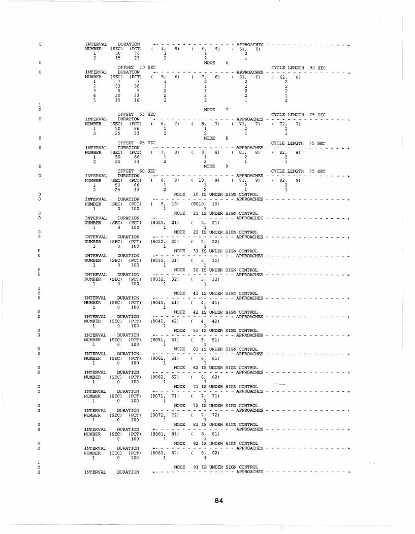
o

o

o

o

o

o

o

o o

o o

o o

o o

o o

1 o o

o o

o o

o o

o o

o o

o o

o o

o o

1 o o

INTERVAL NUMBER

1 2

INTERVAL NUMBER

1 2 3 4 5

INTERVAL NUMBER

1 2

INTERVAL NUMBER

1 2

INTERVAL NUMBER

1 2

INTERVAL NUMBER

1

INTERVAL NUMBER

1

INTERVAL NUMBER

1

INTERVAL NUMBER

1

INTERVAL NUMBER

1

INTERVAL NUMBER

1

INTERVAL NUMBER

1

INTERVAL NUMBER

1

INTERVAL NUMBER

1

INTERVAL NUMBER

1

INTERVAL NUMBER

1

INTERVAL NUMBER

1

INTERVAL NUMBER

1

INTERVAL NUMBER

1

INTERVAL

DURATION (SEC) (PCT)

50 76 15 23

+-4,

1 2

OFFSET 10 SEC DURATION +-

(SEC) (PCT) 5, 7 7 1

33 36 1 5 5 2

30 33 2 15 16 2

OFFSET 55 SEC DURATION

(SEC) (PCT) 50 66 25 33

6, 1 2

OFFSET 25 SEC DURATION +-

(SEC) (PCT) ( 7, 50 66 1 25 33 2

OFFSET 60 DURATION

(SEC) (PCT) 50 66 25 33

DURATION (SEC) (PCT)

o 100

DURATION (SEC) (PCT)

o 100

DURATION (SEC) (PCT)

o 100

DURATION (SEC) (PCT)

o 100

DURATION (SEC) (PCT)

o 100

DURATION (SEC) (PCT)

o 100

DURATION (SEC) (PCT)

o 100

DURATION (SEC) (PCT)

o 100

DURATION (SEC) (PCT)

o 100

DURATION (SEC) (PCT)

o 100

DURATION (SEC) (PCT)

o 100

DURATION (SEC) (PCT)

o 100.

DURATION (SEC) (PCT)

o 100

DURATION (SEC) (PCT)

o 100

SEC +-

+-

8, 1 2

9, 1

+­(8021.

1

+- - -

(8022, 1

+- - -(8031,

1

+-(8032,

1

+- - -( 8041.

1

+- - -(8042,

1

+- - -

(8051, 1

+- - -

(8061, 1

+- - -

(8062, 1

+-(8071,

1

+-(8072,

1

+- - -(8081,

1

+-(8082,

1

5)

6)

7)

8)

6, 5) 1 2 NODE

7, 2 1 1 2 2

6)

- - APPROACHES - - - - - - - - - -51, 5)

6

2

APPROACHES 61, 6)

2 2 2 2 1

CYCLE LENGTH

62, 6) 2 2 2 1 2

90 SEC

NODE 7

8, 7) 1 2 NODE

9, 8) 1 2 NODE

CYCLE LENGTH 75 SEC - - APPROACHES -

8

9

71, 7) 2 1

72, 7) 2 1

CYCLE LENGTH 75 SEC - APPROACHES - -

81. 8) 82, 8) 2 2 1 1

CYCLE LENGTH 75 SEC

- - - +

- - - +

- APPROACHES - - - - + 9) 10, 9) 91. 9) 92, 9)

122 2 1 1

NODE 10 IS UNDER SIGN CONTROL - - - - - - - - - - APPROACHES - - - - - - - - - - +

10) (8010,10) 1

NODE 21 IS UNDER SIGN CONTROL - - - - - - - APPROACHES - - - - - - - - - - - - - - - +

21) 2, 21) 1

NODE 22 IS UNDER SIGN CONTROL - - APPROACHES - - - - - - - - - - - - - - - +

22) 2, 22) 1

NODE 31 IS UNDER SIGN CONTROL - - APPROACHES - - - - - - - - -

31) 3, 31) 1

NODE 32 IS UNDER SIGN CONTROL - - - - - - - APPROACHES - - - - - - - - - - - - - - - +

32) 3, 32) 1

NODE 41 IS UNDER SIGN CONTROL - - - - - - - APPROACHES - - - - - - - - - - - - - - - +

41) 4, 41) 1

NODE 42 IS UNDER SIGN CONTROL - - APPROACHES - - - - - - - - - - - - - - - +

42) 4, 42) 1

NODE 51 IS UNDER SIGN CONTROL - - APPROACHES - - - - - - - - - - - - - - - +

51) 5, 51) 1

NODE 61 IS UNDER SIGN CONTROL - - APPROACHES - - - - - - - - - - - - - - - +

61) 6, 61) 1

NODE 62 IS UNDER SIGN CONTROL - - APPROACHES - - - - - - - - - - - +

62) 6, 62) 1

NODE 71 IS UNDER SIGN CONTROL - - APPROACHES - - - - - - - - - - - +

71) 7, 71) 1

NODE 72 IS UNDER SIGN CONTROL - - APPROACHES - - - - - - - - - - - - - - - +

72) 7, 72) 1

NODE 81 IS UNDER SIGN CONTROL - - APPROACHES - - - - - - - - - - - - - - - +

81) 8, 81) 1

NODE 82 IS UNDER SIGN CONTROL - - APPROACHES - - - - - - - - - - - - - - - +

82) 8, 82) 1

NODE 91 IS UNDER SIGN CONTROL DURATION +- - - - - - - - APPROACHES - - - - - - - - - - - - - - -+

84

NUMBER (SEC) (PCT) (8091, 91) 9, 91) 1 0 100 1 1

0 NODE 92 IS UNDER SIGN CONTROL 0 INTERVAL DURATION +- - - - - - - - APPROACHES - - - - - - - - - - - - - - - +

1

NUMBER (SEC) (PCT) (8092, 92) 9, 92)

CONTROL CODES

NODE

INTERVAL DURATION

1

GO NOGO AMBR PERM = PROT STOP YLD =

0 100 1 1 INTERPRETATION OF SIGNAL CODES

0 YIELD OR AMBER

1 GREEN

2 RED

3 RED WITH GREEN RIGHT ARROW

RED WITH GREEN LEFT ARROW

5 STOP

6 RED WITH GREEN DIAGONAL ARROW

7 NO TURNS-GREEN THRU ARROW

RED WITH LEFT AND RIGHT GREEN ARROW

9 NO LEFT TURN-GREEN THRU AND RIGHT TRAFFIC CONTROL TABLE - SIGNS AND FIXED TIME SIGNALS

PROTECTED NOT PERMITTED AMBER PERMITTED NOT PROTECTED STOP SIGN YIELD SIGN

PROTECTED

SIGN CONTROL

------------------------------------------- APPROACHES (8001, 1) (2, 1)

LEFT THRU RITE DIAG LEFT THRU RITE DIAG LEFT THRU RITE DIAG LEFT THRU RITE DIAG LEFT THRU RITE DIAG o GO GO

NODE 2

INTERVAL DURATION

1 50 2 25

NODE 3

INTERVAL DURATION

1 7 2 33 3 5 4 15 5 30

NODE 4

INTERVAL DURATION

1 50 2 25

NODE 5

INTERVAL DURATION

1 50 2 15

FIXED TIME CONTROL

( 1, 2) LEFT THRU RITE DIAG PERM GO GO NOGO NOGO NOGO

FIXED TIME CONTROL

OFFSET = 0 SECONDS CYCLE LENGTH = 75 SECONDS

(21, 2) LEFT THRU RITE DIAG NOGONOGONOGO PERM GO GO

APPROACHES (22, 2)

LEFT THRU RITE DIAG NOGO NOGO NOGO PERM GO GO

( 3, 2) LEFT THRU RITE DIAG LEFT THRU RITE DIAG PERM GO GO NOGO NOGO NOGO

OFFSET = 45 SECONDS CYCLE LENGTH = 90 SECONDS

------------------------------------------- APPROACHES ( 2, 3)

LEFT THRU RITE DIAG PROT GO GO PERM GO GO NOGO NOGO NOGO NOGO NOGO NOGO NOGO NOGO NOGO

FIXED TIME CONTROL

( 3, 4) LEFT THRU RITE DIAG PERM GO GO NOGO NOGO NOGO

FIXED TIME CONTROL

( 4, 5) LEFT THRU RITE DIAG PROT GO NOGONOGO

4, 3 ) ( 31, 3) ( 32, 3) LEFT THRU RITE DIAG LEFT THRU RITE DIAG LEFT THRU RITE DIAG LEFT THRU RITE DIAG NOGO NOGO NOGO NOGO NOGO NOGO NOGO NOGO NOGO PERM GO GO NOGO NOGO NOGO NOGO NOGO NOGO PROT GO GO NOGO NOGO NOGO NOGO NOGO NOGO NOGO NOGO NOGO NOGO NOGO NOGO PROT GO GO NOGO NOGO NOGO PROT GO GO NOGO NOGO NOGO

OFFSET = 15 SECONDS CYCLE LENGTH = 75 SECONDS

( 5, 4) LEFT THRU RITE DIAG PERM GO GO NOGO NOGO NOGO

APPROACHES (41, 4)

LEFT THRU RITE DIAG NOGO NOGO NOGO PERM GO GO

(42, 4) LEFT THRU RITE DIAG LEFT THRU RITE DIAG NOGO NOGO NOGO PERM GO GO

OFFSET = 40 SECONDS CYCLE LENGTH = 65 SECONDS

( 6, 5) LEFT THRU RITE DIAG

GO GO NOGO NOGO

APPROACHES (51, 5)

LEFT THRU RITE DIAG LEFT THRU RITE DIAG LEFT THRU RITE DIAG NOGO NOGO PROT GO

85

NODE 6

INTERVAL DURATION

1 7 2 33 3 5 4 30 5 15

NODE 7

INTERVAL DURATION

1 50 2 25

NODE 8

INTERVAL DURATION

1 50 2 25

NODE 9

INTERVAL DURATION

1 50 2 25

1

NODE 10

INTERVAL DURATION

1 o

NODE 21

INTERVAL DURATION

1 o

NODE 22

INTERVAL DURATION

1 0

NODE 31

INTERVAL DURATION

1 0

NODE 32

INTERVAL DURATION

1 o

NODE 41

FIXED TIME CONTROL OFFSET = 10 SECONDS CYCLE LENGTH = 90 SECONDS

( 5, 6) LEFT THRU RITE DIAG PROT GO GO PERM GO GO NOGO NOOO NOGO NOGO NOOO NOGO NOGO NOOO NOGO

( 7, 6) LEFT THRU RITE DIAG NOOO NOGO NOOO PERM GO GO PROT GO GO NOOONOOONOOO NOOO NOGO NOOO

APPROACHES ( 61, 6)

LEFT THRU RITE DIAG NOGO NOOO NOGO NOGO NOGO NOGO NOGO NOOO NOGO NOGO NOOO NOGO PROT GO GO

( 62, 6) LEFT THRU RITE DIAG LEFT THRU RITE DIAG NOGO NOGO NOOO NOOO NOGO NOOO NOOO NOGO NOOO PROT GO GO NOOO NOGO NOOO

FIXED TIME CONTROL OFFSET = 55 SECONDS CYCLE LENGTH = 75 SECONDS

( 6, 7) LEFT THRU RITE DIAG PERM GO GO NOGO NOOO NOGO

( 8, 7) LEFT THRU RITE DIAG PERM GO GO NOGO NOGO NOOO

APPROACHES (7l, 7)

LEFT THRU RITE DIAG NOGO NOOO NOGO PERM GO GO

(72, 7) LEFT THRU RITE DIAG LEFT THRU RITE DIAG NOOO NOGO NOOO PERM GO GO

FIXED TIME CONTROL OFFSET = 25 SECONDS CYCLE LENGTH = 75 SECONDS

( 7, 8) (9, 8) LEFT THRU RITE DIAG LEFT THRU RITE DIAG PERM GO GO PERM GO GO NOGO NOOO NOGO NOOO NOGO NOOO

APPROACHES ( 81, 8)

LEFT THRU RITE DIAG NOGO NOOO NOGO PERM GO GO

(82, 8) LEFT THRU RITE DIAG NOOONOOONOOO PERM GO GO

LEFT THRU RITE DIAG

FIXED TIME CONTROL OFFSET = 60 SECONDS CYCLE LENGTH = 75 SECONDS

( 8, 9) (10, 9) LEFT THRU RITE DIAG LEFT THRU RITE DIAG PERM GO GO PERM GO GO NOGO NOOO NOGO NOOO NOOO NOOO

SIGN CONTROL

APPROACHES (91, 9)

LEFT THRU RITE DIAG NOOO NOOO NOGO PERM GO GO

(92, 9) LEFT THRU RITE DIAG LEFT THRU RITE DIAG NOOONOOONOOO PERM GO GO

------------------------------------------- APPROACHES --------------------------------------------( 9, 10) (8010, 10)

LEFT THRU RITE DIAG LEFT THRU RITE DIAG LEFT THRU RITE DIAG LEFT THRU RITE DIAG LEFT THRU RITE DIAG GO GO

SIGN CONTROL

------------------------------------------- APPROACHES (8021, 21)

LEFT THRU RITE DIAG GO

SIGN CONTROL

( 2, 21) LEFT THRU RITE DIAG LEFT THRU RITE DIAG LEFT THRU RITE DIAG LEFT THRU RITE DIAG

GO

- -- - -- - - - - - --- --- - -- - ------- - - - ----- --'-- - - - APPROACHES (8022, 22) (2, 22)

LEFT THRU RITE DIAG LEFTTHRU RITE DIAG LEFT THRU RITE DIAG LEFT THRU RITE DIAG LEFT THRU RITE DIAG GO GO

SIGN CONTROL

------------------------------------------- APPROACHES --------------------------------------------(8031, 31) (3, 31)

LEFT THRU RITE DIAG LEFT THRU RITE DIAG LEFT THRU RITE DIAG LEFT THRU RITE DIAG LEFT THRU RITE DIAG GO GO

SIGN CONTROL

------------------------------------------- APPROACHES (8032, 32)

LEFT THRU RITE DIAG GO

SIGN CONTROL

( 3, 32) LEFT THRU RITE DIAG LEFT THRU RITE DIAG LEFT THRU RITE DIAG LEFT THRU RITE DIAG

GO

86

INTERVAL DURATION ------------------------------------------- APPROACHES (8041, 41) (4, 41)

LEFT THRU RITE DIAG LEFT THRU RITE DIAG LEFT THRU RITE DIAG LEFT THRU RITE DIAG LEFT THRU RITE DIAG o GO GO

NODE 42 SIGN CONTROL

INTERVAL DURATION ------------------------------------------- APPROACHES (8042, 42) (4, 42)

LEFT THRU RITE DIAG LEFT THRU RITE DIAG LEFT THRU RITE DIAG LEFT THRU RITE DIAG LEFT THRU RITE DIAG o GO GO

NODE 51 SIGN CONTROL

INTERVAL DURATION ------------------------------------------- APPROACHES (8051, 51) (5, 51)

LEFT THRU RITE DIAG LEFT THRU RITE DIAG LEFT THRU RITE DIAG LEFT THRU RITE DIAG LEFT THRU RITE DIAG o GO GO

NODE 61

INTERVAL DURATION

1 o

NODE 62

INTERVAL DURATION

1 0

NODE 71

INTERVAL DURATION

1 0

NODE 72

INTERVAL DURATION

1 o

NODE 81

INTERVAL DURATION

1 o

NODE 82

INTERVAL DURATION

1

NODE 91

INTERVAL DURATION

1 o

NODE 92

SIGN CONTROL

------------------------------------------- APPROACHES (8061, 61) (6, 61)

LEFT THRU RITE DIAG LEFT THRU RITE DIAG LEFT THRU RITE DIAG LEFT THRU RITE DIAG LEFT THRU RITE DIAG GO GO

SIGN CONTROL

------------------------------------------- APPROACHES (8062, 62) (6, 62)

LEFT THRU RITE DIAG LEFT THRU RITE DIAG LEFT THRU RITE DIAG LEFT THRU RITE DIAG LEFT THRU RITE DIAG GO GO

SIGN CONTROL

------------------------------------------- APPROACHES (8071, 71) (7, 71)

LEFT THRU RITE DIAG LEFT THRU RITE DIAG LEFT THRU RITE DIAG LEFT THRU RITE DIAG LEFT THRU RITE DIAG GO GO

SIGN CONTROL

------------------------------------------- APPROACHES (8012, 12) (7, 72)

LEFT THRU RITE DIAG LEFT THRURITE DIAG LEFT THRU RITE DIAG LEFT THRU RITE DIAG LEFT THRU RITE DIAG GO GO

SIGN CONTROL

------------------------------------------- APPROACHES (8081, 81) (8, 81)

LEFT THRU RITE DIAG LEFT THRU RITE DIAG LEFT THRU RITE DIAG LEFT THRU RITE DIAG LEFT THRU RITE DIAG GO GO

SIGN CONTROL

------------------------------------------- APPROACHES (8082, 82) (8, 82)

LEFT THRU RITE DIAG LEFT THRU RITE DIAG LEFT THRU RITE DIAG LEFT THRU RITE DIAG LEFT THRU RITE DIAG GO GO

SIGN CONTROL

(8091, 91) LEFT THRU RITE DIAG

GO

SIGN CONTROL

APPROACHES ( 9, 91)

LEFT THRU RITE DIAG LEFT THRU RITE DIAG LEFT THRU RITE DIAG LEFT THRU RITE DIAG GO

87

INTERVAL DURATION ------------------------------------------- APPROACHES (8092, 92) (9, 92)

LEFT THRU RITE DIAG LEFT THRU RITE DIAG LEFT THRU RITE DIAG LEFT THRU RITE DIAG LEFT THRU RITE DIAG 1 GO GO

ENTRY LINK VOLUMES

LINK FLOW RATE TRUCKS CAR POOLS (VEH/HOUR) (PERCENT) (PERCENT)

(8001, 1) 1750 0 14 (8021, 21) 80 a 0 (8022, 22) 60 a a (8031, 31) 1183 a 6 (8032, 32) 150 a a (8041, 41) 70 0 0 (8042, 42) 80 0 0 (8051, 51) 80 0 0 ( 8061, 61) 80 0 0 (8062, 62) 1283 0 6 (8071, 71) 80 a 0 (8072, 72) 100 a a (8081, 81) 80 a a (8082, 82) 60 0 a (8091, 91) 60 a a (8092, 92) 70 a 0 (8010, 10) a 0 0

AVERAGE VEHICLE OCCUPANCIES (HUNDREDTHS-OF-A-PERSON I VEHICLE)

AUTOS CAR-POOLS TRUCKS BUSES 130 300 120 500

0***" WARNING - MESSAGE NUMBER 253, ROUTINE GDMNFN, PARAMETER(S) - P1 = 8010, P2 10 1

VEHICLE TYPE SPECIFICATIONS

VEHICLE LENGTH MAXIMUM ACCELERATION MAXIMUM SPEED Q DSCHG HDWY FLEET COMPONENT PERCENTAGES TYPE FEETlMETERS (MPH/SEC) I (KMPH/SEC) (MPH) I (KMPH) FACTOR (PCT) AVG. OCCUP. AUTO TRUCK CARPOOL BUS

a 1** 17.01 5.2 5.51 8.8 75.01 120.7 100 1.3 100 a a a 0 2** 34.01 10.4 3.01 4.8 60.01 96.6 120 1.2 a 100 a 0 0 3** 17.01 5.2 5.51 8.8 75.01 120.7 100 3.0 0 0 100 a 0 4** 47.01 14.3 2.01 3.3 50.01 80.5 120 50.0 0 0 a 100 a INDICATES THAT ALL PARAMETERS FOR VEHICLE TYPE ASSUME DEFAULT VALUES 1 PROPERTIES OF BUS STATIONS

DISTANCE FROM MEAN STATION LANE LINK UPSTREAM NODE CAPACITY DWELL TYPE PERCENT OF BUSES

NO. SERVICED FEET I METERS (BUSES) (SEC) STOPPING

1 1 1, 2) 1000 305 1 20 1 90 2 1 2, 3) 1500 457 1 20 1 90 3 1 3, 4) 1500 457 1 20 1 90 4 1 4, 5) 1000 305 1 20 1 90 5 1 5, 6) 1500 457 1 20 1 90 6 1 6, 7) 1500 457 1 20 1 90 7 1 7, 8) 1000 305 1 20 1 90 8 1 8, 9) 1000 305 1 20 1 90 9 1 9, 10) 1000 305 1 20 1 90

10 1 31- 3) 500 152 1 20 1 90 11 1 31, 3) 2000 610 1 20 1 90 12 1 62, 6) 500 152 1 20 1 90 13 1 62, 6) 2000 610 1 20 1 90 14 1 la, 9) 1000 305 1 20 1 90 15 1 9, 8) 1000 305 1 20 1 90 16 1 8, 7) 1000 305 1 20 1 90 17 1 7, 6) 2500 762 1 20 1 90 18 1 6, 5) 1000 305 1 20 1 90 19 1 5, 4) 1000 305 1 20 1 90 20 1 4, 3) 2000 610 1 20 1 90 21 1 3, 2) 1000 305 1 a 1 a 22 1 2, 1) 1000 305 1 a 1 a 23 1 3, 31) 500 152 1 a 1 a 24 1 3, 31) 2000 610 1 a 1 a 25 1 6, 62) 500 152 1 a 1 a 26 1 ( 6, 62) 2000 610 1 0 1 a

0 THE TYPE CODE IDENTIFIES THE APPLICABLE STATISTICAL DISTRIBUTION OF DWELL TIME 1 BUS ROUTE PATHS

ROUTE SEQUENCE OF NODES DEFINING PATH a 1 8001 1 2 3 4 5 6 7 8 9 10 8010 a 2 8031 31 3 4 5 6 7 8 9 10 8010 0 3 8062 62 6 7 8 9 10 8010 0 4 8010 10 9 8 7 6 5 4 3 2 1 8001 a 5 8010 10 9 8 7 6 5 4 3 31 8031 0 6 8010 10 9 8 7 6 62 8062 1 BUS STATIONS BY ROUTE

ROUTE SEQUENCE OF STATIONS SERVICED BY ROUTE 0 1 1 2 3 4 5 6 7 8 9 0 2 10 11 3 4 5 6 7 8 9 0 3 12 13 6 7 8 9 0 4 14 15 16 17 18 19 20 21 22

88

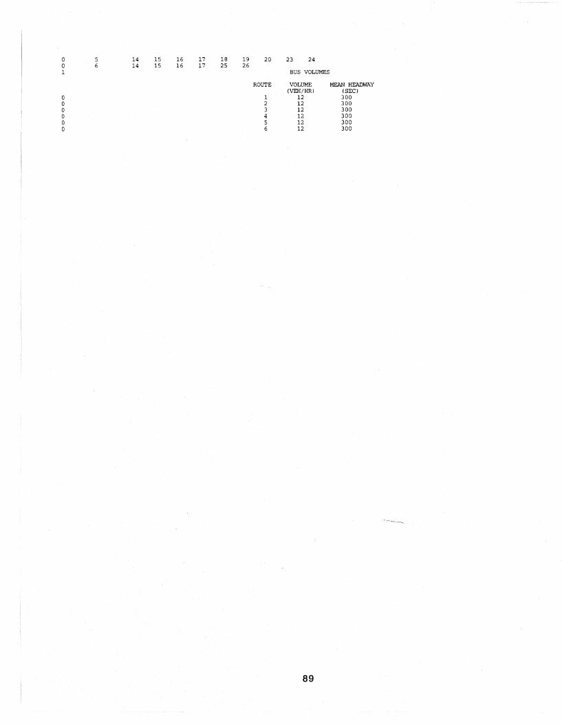
0 14 15 16 17 18 19 20 23 24 0 14 15 16 17 25 26 1 BUS VOLUMES

ROUTE VOLUME MEAN HEADWAY (VEH/HR) (SEC)

0 1 12 300 0 2 12 300 0 3 12 300 0 4 12 300 0 5 12 300 0 6 12 300

89

90

Appendix C

Emissions Calculation for Network B

91

92

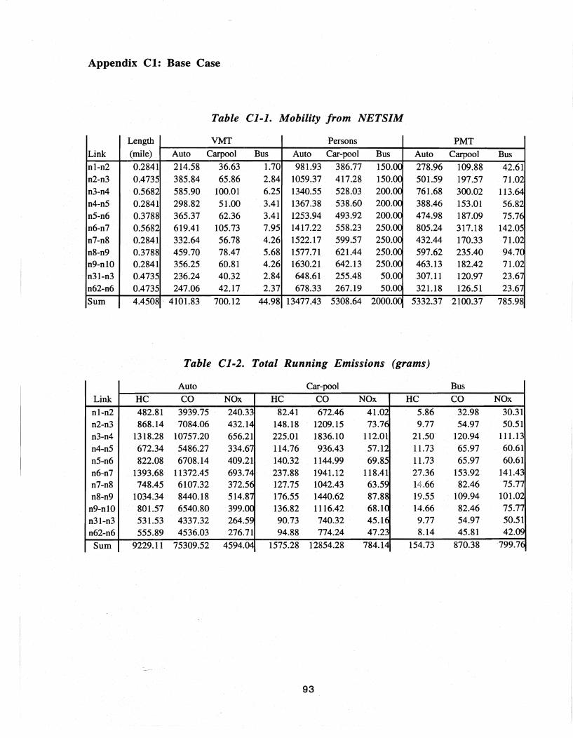
Appendix Cl: Base Case

Table Cl-l. Mobility from NETSIM

Length VMT Persons PMT

Link (mile) Auto Carpool Bus Auto Car-pool Bus Auto Carpool Bus

n1-n2 0.2841 214.58 36.63 1.70 981.93 386.77 150.00 278.96 109.88 42.61 n2-n3 0.4735 385.84 65.86 2.84 1059.37. 417.28 150.00 501.59 197.57 71.02 n3-n4 0.5682 585.90 100m 6.25 1340.55 528.03 200.00 761.68 300.02 113.64 n4-n5 0.2841 298.82 51.00 3.41 1367.38 538.60 200.00 388.46 153.01 56.82 n5-n6 0.3788 365.37 62.36 3.41 1253.94 493.92 200.00 474.98 187.09 75.76 n6-n7 0.5682 619.41 105.73 7.95 1417.22 558.23 250.00 805.24 317.18 142.05 n7-n8 0.2841 332.64 56.78 4.26 1522.17 599.57 250.00 432.44 170.33 71.02 n8-n9 0.3788 459.70 78.47 5.68 1577.71 621.44 250.00 597.62 235.40 94.70 n9-n1O 0.2841 356.25 60.81 4.26 1630.21 642.13 250.00 463.13 182.42 71.02 n31-n3 0.4735 236.24 40.32 2.84 648.61 255.48 50.00 307.11 120.97 23.67 n62-n6 0.4735 247.06 42.17 2.37 678.33 267.19 50.00 321.18 126.51 23.67

Sum 4.4508· 4101.83 700.12 44.98 13477.43 5308.64 2000.00 5332.37 2100.37 785.98

Table Cl-2. Total Running Emissions (grams)

Auto Car-pool Bus . Link HC CO NOx HC CO NOx HC CO NOx

n1-n2 482.81 3939.75 240.33 82.41 672.46 41.02 5.86 32.98 30.31 n2-n3 868.14 7084.06 432.14 148.18 1209.15 73.76 9.77 54.97 50.51 n3-n4 1318.28 10757.20 656.21 225.01 1836.10 112.01 21.50 120.94 111.13 n4-n5 672.34 5486.27 334.6"'1 114.76 936.43 57.12 11.73 65.97 60.61

n5-n6 822.08 6708.14 409.21 140.32 1144.99 69.85 11.73 65.97 60.61 n6-n7 1393.68 11372.45 693.74 237.88 1941.12 118.41 27.36 153.92 141.43 n7-n8 748.45 6107.32 372.56 127.75 1042.43 63.59 1 .66 82.46 75.77

n8-n9 1034.34 8440.18 514.87 176.55 1440.62 87.88 19.55 109.94 101.02

n9-nlO 801.57 6540.80 399.OC 136.82 1116.42 68.10 14.66 82.46 75.77

n31-n3 531.53 4337.32 264.59 90.73 740.32 45.16 9.77 54.97 50.51

n62-n6 555.89 4536.03 276.71 94.88 774.24 47.23 8.14 45.81 42.09

Sum 9229.11 75309.52 4594.04 1575.28 12854.28 784.14 154.73 870.38 799.76

93

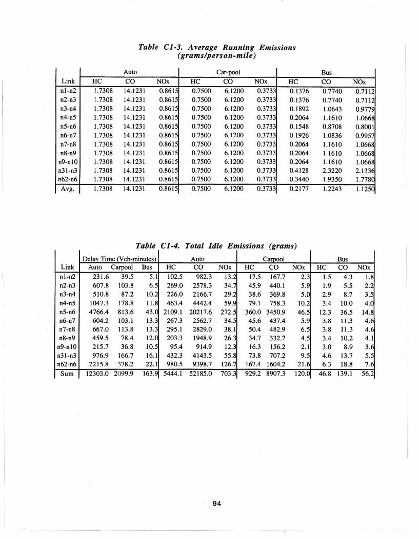
Link n1-n2 n2-n3 n3-n4 n4-n5 n5-n6 n6-n7 n7-n8 n8-09

09-010 n31-n3 n62-n6 Avg.

Link n1-n2 n2-n3 n3-n4 Ii4-n5 n5-n6 n6-n7 n7-n8 n8-n9

n9-nlO n31-n3 n62-n6

Sum

HC 1.7308 1.7308 1.7308 1.7308 1.7308 1.7308 1.7308 1.7308 1.7308 1.7308 1.7308

1.7308

Table Cl-3. Average Running Emissions (grams/person-mile)

Auto Car-pool

CO NOx HC CO NOx HC 14.1231 0.8615 0.7500 6.1200 0.3733 0.1376 14.1231 0.8615 0.7500 6.1200 0.3733 0.1376 14.1231 0.8615 0.7500 6.1200 0.3733 0.1892 14.1231 0.8615 0.7500 6.1200 0.3733 0.2064 14.1231 0.8615 0.7500 6.1200 0.3733 0.1548 14.1231 0.8615 0.7500 6.1200 0.3733 0.1926 14.1231 0.8615 0.7500 6.1200 0.3733 0.2064 14.1231 0.8615 0.7500 6.1200 0.3733 0.2064 14.1231 0.8615 0.7500 6.1200 0.3733 0.2064 14.1231 0.8615 0.7500 6.1200 0.3733 0.4128 14.1231 0.8615 0.7500 6.1200 0.3733 0.3440

14.1231 0.8615 0.7500 6.1200 0.3733 0.2177

Table Cl-4. Total Idle Emissions (grams)

Delay Time (Veh-mioutes) Auto Carpool Auto Carpool Bus HC CO NOx HC CO NOx

231.6 39.5 5.1 102.5 982.3 13.2 17.5 167.7 2.3 607.8 103.8 6.5 269.0 2578.3 34.7 45.9 440.1 5.9 510.8 87.2 10.2 226.0 2166.7 29.2 38.6 369.8 5.0

1047.3 178.8 11.8 463.4 4442.4 59.9 79.1 758.3 10.2 4766.4 813.6 43.0 2109.1 20217.6 272.5 360.0 3450.9 46.5

604.2 103.1 13.3 267.3 2562.7 34.5 45.6 437.4 5.9 667.0 113.8 13.3 295.1 2829.0 38.1 50.4 482.9 6.5 459.5 78.4 12.0 203.3 1948.9 26.3 34.7 332.7 4.5 215.7 36.8 10.5 95.4 914.9 12.3 16.3 156.2 2.1 976.9 166.7 16.1 432.3 4143.5 55.8 73.8 707.2 9.5

2215.8 378.2 22.1 980.5 9398.7 126.7 167.4 1604.2 21.6

12303.0 2099.9 163.9 5444.1 52185.0 703.3 929.2 8907.3 120.0

94

Bus

CO NOx 0.7740 0.7112 0.7740 0.7112 1.0643 0.9779 1.1610 1.0668 0.8708 0.8001 1.0836 0.9957 1.1610 1.0668 1.1610 1.0668 1.1610 1.0668 2.3220 2.1336 1.9350 1.778C 1.2243 1.125C

Bus HC CO NOx

1.5 4.3 1.8 1.9 5.5 2.2 2.9 8.7 3.5 3.4 10.0 4.C

12.3 36.5 14.8 3.8 11.3 4.<: 3.8 11.3 4.~

3.4 10.2 4.1 3.0 8.9 3.6 4.6 13.7 5.5 6.3 18.8 7.6

46.8 139.1 56.2

I

Link HC

nl-n2 0.3673 n2-n3 0.5362 n3-n4 0.2968 n4-n5 1.1930 n5-n6 4.4405 n6-n7 0.3320 n7-n8 0.6825 n8-n9 0.3402

n9-nlO 0.2061 n31-n3 1.4075 n62-n6 3.0528

Avg. 1.0209

Table CI-5. Average Idle Emissions (grams/person-mile)

Auto Carpool

CO NOx HC CO NOx

3.5212 0.0475 0.1592 1.5258 0.0206 5.1402 0.0693 0.2324 2.2274 0.0300 2.8446 0.0383 0.1286 1.2327 0.0166

11.4360 0.1541 0.5170 4.9556 0.0668 42.5655 0.5737 1.9242 18.4450 0.2486

3.1825 0.0429 0.1439 1.3791 0.0186 6.5421 0.0882 0.2957 2.8349 0.0382 3.2612 0.0440 0.1474 1.4132 0.0190 1.9754 0.0266 0.0893 0.8560 0.0115

13.4921 0.1818 0.6099 5.8466 0.0788 29.2631 0.3944 1.3229 12.6807 0.1709

9.7865 0.1319 0.4424 4.2408 0.0572

95

Bus HC CO NOx 0.0342 0.1016 0.0411 0.0262 0.0777 0.0314 0.0257 0.0762 0.0308 0.0594 0.1763 0.0713 0.1622 0.4818 0.1948 0.0268 0.0795 0.0321 0.0535 0.1590 0.0643 0.0362 0.1076 0.0435 0.0423 0.1255 0.0507 0.1944 0.5773 0.2334 0.2668 0.7924 0.3203

0.0596 0.1770 0.0716

Appendix C2: HOV -3 Case

Table C2-1. Mobility from NETSIM

LeIlgth VMT Persons PMT

Link (mile) Auto Carpool Bus Auto Car-pool Bus Auto Carpool nl-n2 0.2841 193.95 43.39 1.70 887.53 458.15 175. 252.14 130.16 n2-n3 0.4735 338.68 75.76 2.84 929.88 480.01 175. 440.28 227.28 n3-n4 0.568 450.08 100.68 6.25 1029.79 531.58 230. 585.11 302.04 n4-n5 0.2841 219.71 49.15 3.41 1005.40 519.00 230. 285.63 147.44 n5-n6 0.3788 284.25 63.58 4.55 975.53 503.58 230. 369.52 190.75 n6-n7 0.568 488.80 109.34 9.09 1118.37 577.32 280. 635.44 328.02 n7-n8 0.2841 265.07 59.29 4.55 1212.95 626.13 280. 344.59 177.88 n8-n9 0.3788 371.79 83.16 6.06 1275.97 658.67 280. 483.32 249.49

n9-nlO 0.2841 290.53 64.99 4.26 1329.47 686.28 377.69 194.97 n31-n3 0.4735 223.10 49.91 2.37 612.55 316.21 290.03 149.72 26. n62-n6 0.4735 215.69 48.25 1.89 592.20 305.70 280.40 144.74 Sum 4.4508 3341.65 747.50 46.97 10969.65 5662.64 2265. 4344.15 2242.49

Table C2-2. Total Running Emissions (grams)

Auto Car-pool Bus Link HC CO NOx HC CO NOx HC CO NOx nl-n2 484.89 4067.22 221.11 98.05 800.90 49.03 5.22 27.73 27.99 n2-n3 846.70 7102.13 386.10 171.22 1398.52 85.61 8.69 46.22 46.65 n3-n4 1125.20 9438.20 513.09 227.53 1858.53 113.77 19.13 101.69 102.63 n4-n5 549.28 4607.37 250.47 111.07 907.26 55.54 10.43 55.47 55.98 n5-n6 710.62 5960.65 324.04 143.70 1173.75 71.85 13.91 73.95 74.64 n6-n7 1222.00 10250.14 557.23 247.11 2018.42 123.55 27.82 147.91 149.27 n7-n8 662.67 5558.45 302.18 134.00 1094.55 67.00 13.91 73.95 74.64 n8-n9 929.46 7796.33 423.84 187.95 1535.22 93.98 18.55 98.61 99.52

n9-nlO 726.33 6092.43 331.21 146.88 1199.70 73.44 13.04 69.33 69.97 n31-n3 557.76 4678.49 254.34 112.79 921.27 56.39 7.24 38.52 38.87 n62-n6 539.23 4523.06 245.89 109.04 890.66 54.52 5.80 30.81 31.1()

Sum 8354.13 70074.47 3809.48 1689.34 13798.79 844.67 143.73 764.20 771.24

96

Table C2-3. Average Running Emissions (grams/person-mile)

Auto Car-pool Bus Link HC CO NOx HC CO NOx HC CO NOx nl-n2 1.9231 16.1308 0.876'l 0.7533 6.1533 0.3767 0.1049 0.5578 0.5630 n2-n3 1.9231 16.1308 0.8769 0.7533 6.1533 0.3767 0.1049 0.5578 0.5630 n3-n4 1.9231 16.1308 0.8769 0.7533 6.1533 0.3767 0.1463 0.7781 0.7853 n4-n5 1.9231 16.1308 0.876'l 0.7533 6.1533 0.3767 0.1597 0.8489 0.8567 n5-n6 1.9231 16.1308 0.8769 0.7533 6.1533 0.3767 0.1597 0.8489 0.8567 n6-n7 1.9231 16.1308 0.8769 0.7533 6.1533 0.3767 0.1749 0.9297 0.9383 n7-n8 1.9231 16.1308 0.8769 0.7533 6.1533 0.3767 0.1749 0.9297 0.9383 n8-n9 1.9231 16.1308 0.8769 0.7533 6.1533 0.3767 0.1749 0.9297 0.9383

n9-nlO 1.9231 16.1308 0.8769 0.7533 6.1533 0.3767 0.1639 0.8716 0.879~

n31-n3 1.9231 16.1308 0.8769 0.7533 6.1533 0.3767 0.2782 1.4791 1.4927 n62-n6 1.9231 16.1308 0.8769 0.7533 6.1533 0.3767 0.2448 1.3016 1.3136 Avg. 1.9231 16.1308 0.8769 0.7533 6.1533 0.3767 0.1715 0.9121 0.9205

Table C2-4. Total Idle Emissions (grams)

Delay Time (Veb-min) Auto Carpool Bus Link Auto Carpool Bus HC CO NOx HC CO NOx HC CO NOx

nl-n2 208.6 46.7 5.1 92.3 884.9 11.9 20.7 198.0 2.7 1.5 4.3 1.8 n2-n3 1368.5 306.1 6.1 605.6 5804.6 78.2 135.5 1298.4 17.5 1.7 5.2 2.1 n3-n4 1592.5 356.2 10.2 704.7 6754.8 91.C 157.6 1511.0 20.4 2.9 8.7 3.5 n4-n5 1218.2 272.5 9.3 539.1 5167.2 69.6 120.6 1155.9 15.6 2.7 7.9 3.2 n5-n6 3683.2 823.9 17.8 1629.8 15622.9 210.6 364.6 3494.7 47.1 5.1 15.1 6.1 n6-n7 474.8 106.2 15.5 210.1 2013.9 27.1 47.0 450.5 6.1 4.4 13.2 5.3 n7-n8 455.1 101.8 15.0 201.4 1930.4 26.(] 45.0 431.8 5.8 4.3 12.7 5.1 n8-n9 389.4 87.1 13.6 172.3 1651.7 22.3 38.5 369.5 5.C 3.9 11.5 4.7

n9-nlO 172.2 38.5 1O.~ 76.2 730.3 9.8 17.0 163.4 2.2 3.0 9.0 3.~

n31-n3 1101.3 246.3 12.~ 487.3 4671.2 63.C 109.0 1044.9 14.1 3.6 10.7 4.1

n62-n6 2587.7 578.8 24.4 1145.0 10976.0 147.9 256.1 2455.2 33.1 7.0 20.7 8.4

Sum 13251.4 2964.2 140.2 5863.7 56208.0 757.5 1311.712573.2 169.5 40.1 119.0 48.1

97

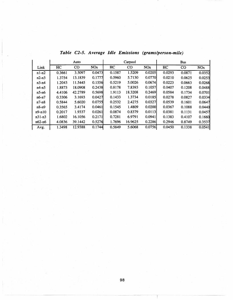
Table C2-S. Average Idle Emissions (grams/person-mile)

Auto Carpool Bus

Link HC CO NOx HC CO NOx HC CO NOx

nl-n2 0.3661 3.5097 0.0473 0.1587 l.5209 0.0205 0.0293 0.0871 0.035L

n2-n3 l.3754 13.1839 0.1777 0.5960 5.7130 0.0770 0.0210 0.0625 0.0253 n3-n4 l.2043 1l.5445 0.155~ 0.5219 5.0026 0.0674 0.0223 0.0663 0.0268 n4-n5 1.8873 18.0908 0.2438 0.8178 7.8393 0.1057 0.0407 0.1208 0.0488 n5-n6 4.4106 42.2789 0.5698 l.9113 18.3208 0.2469 0.0584 0.1734 0.0701 n6-n7 0.3306 3.1693 0.0427 0.1433 l.3734 0.Ql85 0.0278 0.0827 0.0334 n7-n8 0.5844 5.6020 0.0755 0.2532 2.4275 0.0327 0.0539 0.1601 0.064 n8-n9 0.3565 3.4174 0.0461 0.1545 1.4809 0.0200 0.0367 0.1088 0.044C

n9-nlO 0.2017 1.9337 0.0261 0.0874 0.8379 0.Ql13 0.0381 0.1131 0.0457 n31-n3 l.6802 16.1056 0.2171 0.7281 6.9791 0.0941 0.1383 0.4107 0.166C n62-n6 4.0836 39.1442 0.527( 1.7696 16.9625 0.2286 0.2946 0.8749 0.3537

Avg. 1.3498 12.9388 0.1744 0.5849 5.6068 0.0756 0.0450 0.1338 0.0541

98

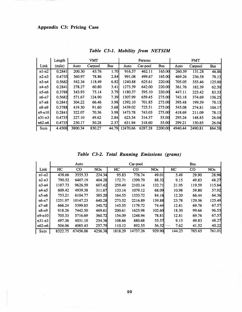
Appendix C3: Pricing Case

Table C3-1. Mobility from NETSIM

Length VMT Persons PMT

Link (mile) Auto Carpool Bus Auto Car-pool Bus Auto Carpool Bus n1-n2 0.2841 200.30 43.76 1.70 916.57 462.11 165.00 260.39 131.28 46.88 n2-n3 0.4735 360.97 78.86 2.84 991.08 499.67 165.00 469.26 236.58 78.13 n3-n4 0.5682 542.34 118.49 6.82 1240.88 625.61 220.00 705.05 355.46 125.00 n4-n5 0.2841 278.27 60.80 3.41 1273.39 642.00 220.00 361.76 182.39 62.5C n5-n6 0.3788 343.93 75.14 3.79 1180.37 595.10 220.00 447.11 225.42 83.33 n6-n7 0.5682 571.67 124.90 7.39 1307.99 659.45 275.00 743.18 374.69 156.25 n7-n8 0.2841 304.22 66.46 3.98 1392.10 701.85 275.00 395.48 199.39 78.13 n8-n9 0.3788 419.30 91.60 5.68 1439.02 725.51 275.00 545.08 274.81 104.1

n9-n10 0.2841 322.07 70.36 3.98 1473.78 743.03 275.00 418.69 211.09 78.13 n31-n3 0.4735 227.10 49.62 2.84 623.54 314.37 55.0C 295.24 148.85 26.04 n62-n6 0.4735 230.17 50.28 2.37 631.94 318.60 55.0C 299.21 150.85 26.04

Sum 4.4508 3800.34 830.27 44.79 12470.66 6287.28 2200.0C 4940.44 2490.81 864.58

Table C3-2. Total Running Emissions (grams)

Auto Car-pool Bus Link HC CO NOx HC CO NOx HC CO NOx

n1-n2 438.66 3555.33 224.34 95.83 776.74 49.01 5.49 29.90 28.96 n2-n3 790.52 6407.19 404.28 172.71 1399.79 88.32 9.15 49.83 48.2"1 n3-n4 1187.73 9626.59 607.42 259.49 2103.14 132.71 21.95 119.59 115.84 n4-n5 609.42 4939.38 311.6"1 133.14 1079.12 68.09 10.98 59.80 57.92 n5-n6 753.21 6104.77 385.2C 164.55 1333.72 84. Hi 12.20 66.44 64.3~

n6-n7 1251.97 10147.23 640.28 273.52 2216.89 139.88 23.78 129.56 125.49 n7-n8 666.24 5399.85 340.72 145.55 1179.72 74.44 12.81 69.76 67.57 n8-n9 918.26 7442.50 469.61 200.61 1625.98 102.6C 18.30 99.66 96.53

n9-nlO 705.33 5716.69 360.72 154.09 1248.94 78.81 12.81 69.76 67.57 n31-n3 497.36 4031.10 254.36 108.66 880.68 55.5"1 9.15 49.83 48.27 n62-n6 504.06 4085.43 257.79 110.12 892.55 56.32 '_. ----- 7.62 41.52 40.22

Sum 8322.75 67456.06 4256.38 1818.29 14737.26 929.90 144.23 785.65 761.01

99

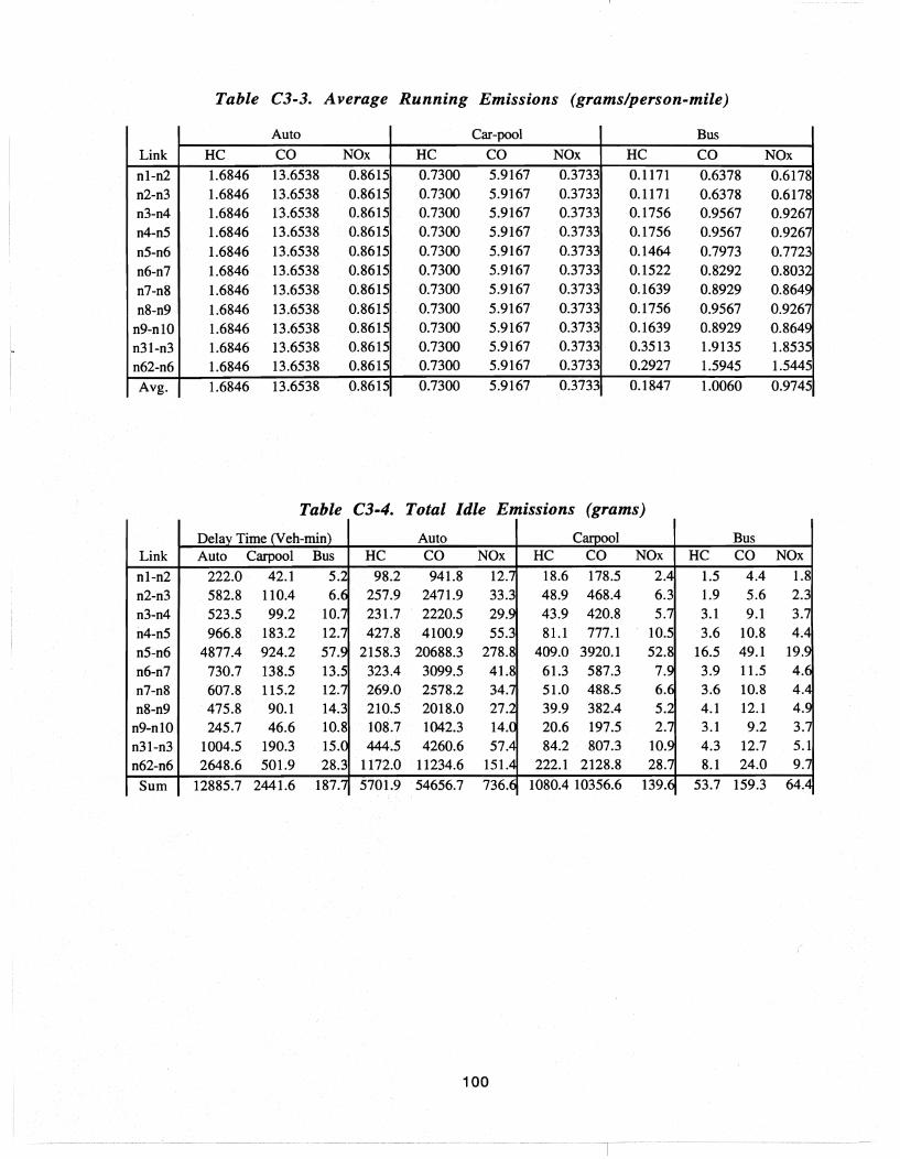
Table C3-3. Average Running Emissions (grams/person-mile)

Auto Car-pool Bus

Link HC CO NOx HC CO NOx HC CO NOx

nl-n2 1.6846 13.6538 0.8615 0.7300 5.9167 0.3733 0.1171 0.6378 0.6178 n2-n3 1.6846 13.6538 0.8615 0.7300 5.9167 0.3733 0.1171 0.6378 0.6178 n3-n4 1.6846 13.6538 0.8615 0.7300 5.9167 0.3733 0.1756 0.9567 0.9261 n4-n5 1.6846 13.6538 0.8615 0.7300 5.9167 0.3733 0.1756 0.9567 0.9261 n5-n6 1.6846 13.6538 0.8615 0.7300 5.9167 0.3733 0.1464 0.7973 0.7723 n6-n7 1.6846 13.6538 0.8615 0.7300 5.9167 0.3733 0.1522 0.8292 0.8032

n7-n8 1.6846 13.6538 0.8615 0.7300 5.9167 0.3733 0.1639 0.8929 0.8649

n8-n9 1.6846 13.6538 0.8615. 0.7300 5.9167 0.3733 0.1756 0.9567 0.9267

n9-nlO 1.6846 13.6538 0.8615 0.7300 5.9167 0.3733 0.1639 0.8929 0.8649

n31-n3 1.6846 13.6538 0.8615 0.7300 5.9167 0.3733 0.3513 1.9135 1.8535

n62-n6 1.6846 13.6538 0.8615 0.7300 5.9167 0.3733 0.2927 1.5945 1.5445

Avg. 1.6846 13.6538 0.8615 0.7300 5.9167 0.3733 0.1847 1.0060 0.9745

Table C3-4. Total Idle Emissions (grams)

Delav Time Neh-min) Auto Carpool Bus Link Auto Carpool Bus HC CO NOx HC CO NOx HC CO NOx

nl-n2 222.0 42.1 5.2 98.2 941.8 12.7 18.6 178.5 2.4 l.5 4.4 1.8 n2-n3 582.8 110.4 6.6 257.9 2471.9 33.3 48.9 468.4 6.3 1.9 5.6 2.3

n3-n4 523.5 99.2 10.7 231.7 2220.5 29.9 43.9 420.8 5.7 3.1 9.1 3.7

n4-n5 966.8 183.2 12.7 427.8 4100.9 55.3 81.1 777.1 10.5 3.6 10.8 4.4

n5-n6 4877.4 924.2 57.9 2158.3 20688.3 278.8 409.0 3920.1 52.8 16.5 49.1 19.'.;

n6-n7 730.7 138.5 13.5 323.4 3099.5 41.8 61.3 587.3 7.9 3.9 11.5 4.6

n7-n8 607.8 115.2 12.7 269.0 2578.2 34."1 51.0 488.5 6.6 3.6 10.8 4.4

n8-n9 475.8 90.1 14.3 210.5 2018.0 27.2 39.9 382.4 5.2 4.1 12.1 4.9

n9-nlO 245.7 46.6 10.8 108.7 1042.3 14.C 20.6 197.5 2.7 3.1 9.2 3.~

n31-n3 1004.5 190.3 15.( 444.5 4260.6 57.4 84.2 807.3 1O.~ 4.3 12.7 5.1 n62-n6 2648.6 50l.9 28.3 1172.0 11234.6 151.4 222.1 2128.8 28.~ 8.1 24.0 9.7

Sum 12885.7 244l.6 187.') 5701.9 54656.7 736.(i 1080.4 10356.6 139] 53.7 159.3 64.<1

100

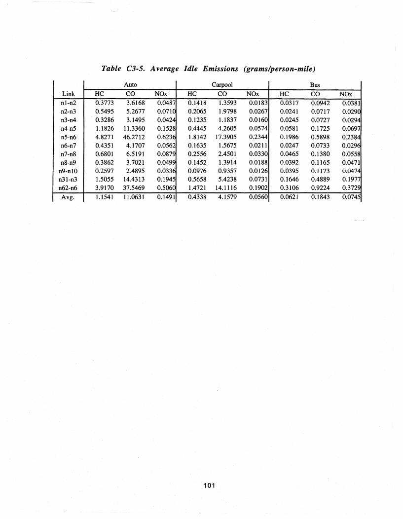
Table C3-S. Average Idle Emissions (grams/person-mile)

Auto Carpool Bus

Link HC CO NOx HC CO NOx HC CO NOx

n1-n2 0.3773 3.6168 0.0487 0.1418 1.3593 0.0183 0.0317 0.0942 0.0381 n2-n3 0.5495 5.2677 0.0710 0.2065 1.9798 0.0267 0.0241 0.0717 0.029C n3-n4 0.3286 3.1495 0.0424 0.1235 1.1837 0.0160 0.0245 0.0727 0.0294 n4-n5 1.1826 11.3360 0.1528 0.4445 4.2605 0.0574 0.0581 0.1725 0.0697 n5-n6 4.8271 46.2712 0.6236 1.8142 17.3905 0.2344 0.1986 0.5898 0.2384 n6-n7 0.4351 4.1707 0.0562 0.1635 1.5675 0.0211 0.0247 0.0733 0.0296 n7-n8 0.6801 6.5191 0.0879 0.2556 2.4501 0.0330 0.0465 0.1380 0.0558 n8-n9 0.3862 3.7021 0.0499 0.1452 1.3914 0.0188 0.0392 0.1165 0.0471

n9-n1O 0.2597 2.4895 0.0336 0.0976 0.9357 0.0126 0.0395 0.1173 0.0474 n31-n3 1.5055 14.4313 0.1945 0.5658 5.4238 0.0731 0.1646 0.4889 0.197" n62-n6 3.9170 37.5469 0.5060 1.4721 14.1116 0.1902 0.3106 0.9224 0.372<)

Avg. 1.1541 11.0631 0.1491 0.4338 4.1579 0.0560 0.0621 0.1843 0.0745

101