Fractions, Functions and Folding arXiv:2108.11382v1 [math ...

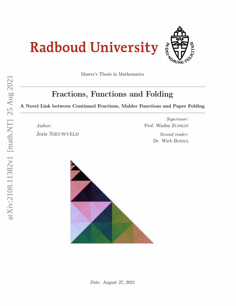
Master’s Thesis in Mathematics

Fractions, Functions and FoldingA Novel Link between Continued Fractions, Mahler Functions and Paper Folding

Author:

Joris Nieuwveld

Supervisor:Prof. Wadim Zudilin

Second reader:Dr. Wieb Bosma

Date: August 27, 2021

arX

iv:2

108.

1138

2v1

[m

ath.

NT

] 2

5 A

ug 2

021

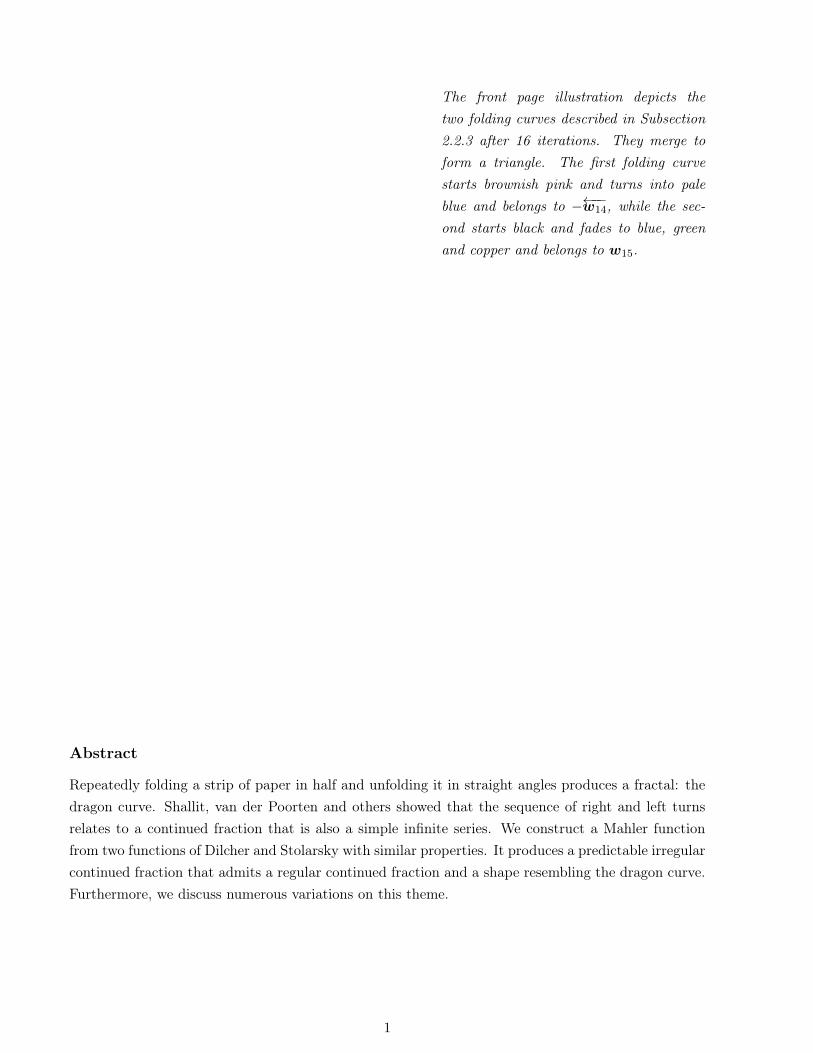
The front page illustration depicts thetwo folding curves described in Subsection2.2.3 after 16 iterations. They merge toform a triangle. The first folding curvestarts brownish pink and turns into paleblue and belongs to −←−−w14, while the sec-ond starts black and fades to blue, greenand copper and belongs to w15.

Abstract

Repeatedly folding a strip of paper in half and unfolding it in straight angles produces a fractal: thedragon curve. Shallit, van der Poorten and others showed that the sequence of right and left turnsrelates to a continued fraction that is also a simple infinite series. We construct a Mahler functionfrom two functions of Dilcher and Stolarsky with similar properties. It produces a predictable irregularcontinued fraction that admits a regular continued fraction and a shape resembling the dragon curve.Furthermore, we discuss numerous variations on this theme.

1

Contents

Introduction 3

1 Four curious power series 51.1 Defining four intertwining power series . . . . . . . . . . . . . . . . . . . . . . . . . . . 5

1.1.1 Two power series . . . . . . . . . . . . . . . . . . . . . . . . . . . . . . . . . . . 51.1.2 Defining the third function . . . . . . . . . . . . . . . . . . . . . . . . . . . . . 71.1.3 The fourth power series: I . . . . . . . . . . . . . . . . . . . . . . . . . . . . . . 9

1.2 Continued fractions . . . . . . . . . . . . . . . . . . . . . . . . . . . . . . . . . . . . . . 111.2.1 A crash course on continued fractions . . . . . . . . . . . . . . . . . . . . . . . 111.2.2 Continued fractions related to F, G, H and I . . . . . . . . . . . . . . . . . . . . 121.2.3 The continued fractions rho and lambda evaluated at roots of unity . . . . . . . 17

2 Folded continued fractions 192.1 An introduction to folded continued fractions . . . . . . . . . . . . . . . . . . . . . . . 19

2.1.1 An example of a folded continued fraction . . . . . . . . . . . . . . . . . . . . . 202.1.2 Paperfolding sequences as curves . . . . . . . . . . . . . . . . . . . . . . . . . . 21

2.2 The folded continued fraction of rho . . . . . . . . . . . . . . . . . . . . . . . . . . . . 222.2.1 Computing a folded continued fraction for rho . . . . . . . . . . . . . . . . . . . 222.2.2 Specializing the folded continued fraction for rho . . . . . . . . . . . . . . . . . 252.2.3 The folding curve of rho . . . . . . . . . . . . . . . . . . . . . . . . . . . . . . . 262.2.4 The folding sequence of rho as a Mahler function . . . . . . . . . . . . . . . . . 28

2.3 Algebraic folded continued fractions . . . . . . . . . . . . . . . . . . . . . . . . . . . . 352.3.1 Defining folded continued fractions . . . . . . . . . . . . . . . . . . . . . . . . . 362.3.2 A cubic folded continued fraction . . . . . . . . . . . . . . . . . . . . . . . . . . 372.3.3 Other examples of folded continued fraction identities . . . . . . . . . . . . . . 41

2.4 An analogue of a result of Cohn . . . . . . . . . . . . . . . . . . . . . . . . . . . . . . . 432.5 Mahler functions, remarkable identities and Fibonacci numbers . . . . . . . . . . . . . 46

3 Hadamard products of Mahler functions 493.1 The space of k-regular functions . . . . . . . . . . . . . . . . . . . . . . . . . . . . . . . 513.2 Complete Hadamard functions . . . . . . . . . . . . . . . . . . . . . . . . . . . . . . . 53

Bibliography 56

2

Introduction

The simple functional equation H(x) = H(x2) + xH(x4) seems to have few interesting properties. Asolution has a power series expansion

H(x) = 1 + x+ x2 + x4 + x5 + x8 + x9 + x10 + x16 + x17 + x18 + x20 + x21 + x32 + · · ·

whose coefficients are all 0 and 1. The series contains long strings of zeros that end at powers of 2,and the number of coefficients 1 relates to the Fibonacci numbers. However, a more profound beautyis hidden inside H. When investigating the functional equation at x 7→ x−1, one finds out that itssolutions ultimately are two functions from Dilcher and Stolarsky [12]. Mimicking these two functions,an irregular continued fraction in a spirit of Ramanujan’s [7, (9.29)] can be found for ρ(x) := H(x)

H(x2):

1 +x

1 +x2

1 +x4

1 +x8

. . .

.

This gives a recipe for defining ρ at many points on the unit circle, where H remains undefined. Only,most strikingly, ρ also allows to be written as a regular continued fraction whose partial quotients are,apart for possibly one, all ±x and form a sequence related to the paperfolding dragon. The presentthesis is a mathematical exposition of numerous features of H and ρ and their close relatives.

Chapter 1 introduces four intertwining Mahler functions that exist within the unit disk. Dilcherand Stolarsky [12] recently constructed the first two, F and G. The third, H, emerges when studyingtheir system of Mahler equations at infinity. Getting only one power series instead of two to solvethe system is already an interesting phenomenon. The fourth, I, is the generating function of theBaum-Sweet sequence and satisfies the never before observed relation xF (x3) +G(x3) = I(x). Next,we construct two continued fractions. The first, λ, was already studied by Dilcher and Stolarsky andrelates to F and G; the second continued fraction is ρ. We prove that λ(x) = xρ(x−3) whenever bothsides make sense and that both assume algebraic values at certain roots of unity.

Chapter 2 begins with recalling Shallit’s and van der Poorten’s link between continued fractions,f(x) =

∑∞n=0 x

2n−1 and the paperfolding dragon [23]. This earliest example of a folded continuedfraction will illustrate how ρ(x) above corresponds to two regular continued fractions whose partial

3

quotients are all, except for possibly one, equal to x and −x. These continued fractions coincidewithin the unit disk but differ outside. Like the paperfolding dragon, the signs of the partial quotientsproduce fractals, and their generating functions induce algebraically independent Mahler functions.The second half of the chapter focuses on more general folded continued fractions. Examples likethe paperfolding dragon and ρ are rare because many others converge to algebraic functions near theorigin. We discuss several cases. Finally, an observation analogous to a result of Cohn [11] as well asa simple method to find identities involving Fibonacci numbers are presented.

In Chapter 3, we study Mahler functions in combination with the Hadamard product, which is thetermwise multiplication of power series. Many well-known spaces of functions are closed under thisoperation, including many large subspaces of Mahler functions. We recall a few of these subspaces,expand them slightly and show that the entire space of Mahler functions does not have this property.Finally, we classify the rational functions whose Hadamard product with each Mahler function isMahler.

Acknowledgements

First and foremost, I am extremely grateful to Wadim Zudilin for his excellent guidance, willingnessto read and respond to my dozens of “quick notes” and enthusiasm for the various unconventionaltangents I chose within this research. I also want to thank my former roommate Dion for his abilityto listen to my ramblings and encouragement. Finally, I thank my parents for their continued supportand the interest they have taken in (the graphical parts) of my thesis.

4

Chapter 1

Four curious power series

In this chapter, we investigate a rabbit hole of functions and the remarkable connections betweenthem. We introduce the functions F , G, H and I, proof a few simple properties and connect thesefunctions with continued fractions.

1.1 Defining four intertwining power series

In this section, four so-called Mahler functions are introduced and linked together. Before definingwhat a Mahler function is, the first two functions are given.

1.1.1 Two power series

The two power series called F and G are defined as the unique power series around q = 0 that satisfyF (0) = G(0) = 1 and the system of equations

F (q) = G(q2) + qF (q4),

G(q) = qF (q2) +G(q4).(1.1.1)

These power series are

F (q) =

∞∑n=0

anqn = 1 + q + q2 + q5 + q6 + q8 + q9 + q10 + · · · and

G(q) =∞∑n=0

bnqn = 1 + q + q3 + q4 + q5 + q11 + q12 + q13 + · · · .

(1.1.2)

They were constructed by Dilcher and Stolarsky in [12] as limits of so-called Stern polynomials. Herewe use the system of equations to define F and G rather than the original construction because thesystem has a unique power series solution. Dilcher and Stolarsky also proved in [12, Proposition 5.1]that the mixed system of F and G can be split into two systems:

F (q) = (1 + q + q2)F (q4)− q4F (q16) and

qG(q) = (1 + q + q2)G(q4)−G(q16).(1.1.3)

5

This makes F and G transparently in a known class functions because of the following definition:

Definition 1.1.1. Let k ≥ 2. An analytic function f ∈ C[[q]] is called a k-Mahler function if thereexist a d ≥ 0 and polynomials A(q), A0(q), A1(q), . . . , Ad(q) ∈ C[q] such that A0(q)Ad(q) 6= 0 and

A(q) +A0(q)f(q) +A1(q)f(qk) + · · ·+Ad(q)f(qk

d)= 0. (1.1.4)

The (linear) functional equation above, solved by a k-Mahler function, is called a k-Mahler equation.Here d is said to be the degree of f . The k-Mahler equation is called homogeneous if A(q) = 0 andinhomogeneous otherwise. If k is clear from the context, it is often omitted from the terminology.

From (1.1.3), we see that F and G satisfy homogeneous 4-Mahler equations of degree 2. Note thatthis implies that F and G also satisfy 2-Mahler equations of degree 4.

By comparing the coefficients of these power series, the uniqueness of the expansions can be shownfrom the system (1.1.1) through a recursion for the coefficients:

an =

bn

2if n ≡ 0 mod 2,

an−14

if n ≡ 1 mod 4,

0 if n ≡ 3 mod 4

and bn =

an−1

2if n ≡ 1 mod 2,

bn4

if n ≡ 0 mod 4,

0 if n ≡ 2 mod 4.

(1.1.5)

The recursions show that the coefficients of F and G are automatic, a property we do not studyin this thesis. In particular, the recursions imply that all coefficients of F and G are either 0 or 1 byinduction. This property is given its own name:

Definition 1.1.2. A {0, 1}-power series is a power series whose coefficients are all 0 or 1.

Furthermore, by [12, Proposition 5.2], F and G satisfy

G(q)G(q2)− qF (q)F (q2) = 1 and F (q)G(q4)− qG(q)F (q4) = 1. (1.1.6)

Such relations falsely suggest there are more algebraic relations between F (q), G(q), F (q2), G(q2).

Definition 1.1.3. Let S be a set of functions over C in variable q. The transcendence degree ofS is the cardinality of the largest subset S′ ⊆ S such that the fields C(q)(S) and C(q)(S′) coincide.The notation used for this is tr deg(S).

A more general notion of transcendence degree exists but is not used here. Obtaining the tran-scendence degree involving all possible F (qd) and G(qd) for all positive integers d turns out to be arather difficult question, but when only studying powers of 2, this is somewhat doable. For example,F(q2d) can be written as a linear combination over C[q] of F (q), G(q), F (q2) and G(q2) by simply

iterating the equations of the system (1.1.1). Therefore,

tr deg(F (q), G(q), F (q2), G(q2), F (q4), G(q4), F (q4), G(q4), F (q8), G(q8), . . .

)= tr deg

(F (q), G(q), F (q2), G(q2)

)≤ 4.

6

Adding G(q)G(q2)− qF (q)F (q2) = 1 (1.1.6) to this conclusion lowers the upper bound to 3. In 2015,Bundschuh and Väänänen proved in [10] that the transcendence degree is indeed equal to 3, and thatthere are no algebraic relations between any three of F (q), G(q), F (q2) and G(q2). There is a relatedresult on the transcendence of these functions [9]:

tr deg(F (q), F (q2), F ′(q), F ′(q2)

)= 4.

To conclude the subsection, notice that F and G are defined everywhere within the unit disk as{0, 1}-power series. However, both cannot be analytically continued any further. That is, the unitcircle forms an impassable boundary [9, Lemma 1].

1.1.2 Defining the third function, H

As the unit circle forms an impassable boundary for F and G, what happens with the system ofequations at the other side of the unit circle seems interesting. To do this, view the system (1.1.1) atinfinity by formally defining F (q) := F (q−1) and G(q) := G(q−1) for all 0 < |q| < 1. This producesthe system of equations

F (q) = G(q2) + q−1F (q4),

G(q) = q−1F (q2) + G(q4),

which does not have a solution in power series. Fortunately, it has a power series solution in q13 , which

one extracts by defining F (q) := q23 F (q) and G(q) := q

13 G(q). Then

F (q) = G(q2) + qF (q4),

G(q) = F (q2) + qG(q4).

This system has a lot of symmetry. Like F and G, we demand F (0) = G(0) = 1 and that both have apower series expansion. Then there is a unique power series solution H(q) = F (q) = G(q). This can bemost easily seen as follows: Define A(q) =

∑∞n=0 xnq

n = F (q)− G(q). Then A(q) = −A(q2) + qA(q4),which gives the following recursion for xn:

xn =

−xn

2if n ≡ 0 mod 2,

xn−14

if n ≡ 1 mod 4,

0 if n ≡ 3 mod 4.

As x0 = A(0) = F (0) − G(0) = 0, all xn are 0 by induction, giving that A(q) is the zero function.Thus, H(q) = F (q) = G(q) is indeed well-defined and satisfies

H(q) = H(q2) + qH(q4). (1.1.7)

7

This gives us

H(q) =∞∑n=0

cnqn = 1 + q + q2 + q4 + q5 + q8 + q9 + q10 + q16 + · · · .

The 2-Mahler solution of equation (1.1.7) that satsifies H(0) = 1 is taken as definition of H(q). Inparticular, H is a Mahler function. Like for F and G, the Mahler equation induces a recursion for thecoefficients of the power series:

cn =

cn

2if n ≡ 0 mod 2,

cn−14

if n ≡ 1 mod 4,

0 if n ≡ 3 mod 4.

(1.1.8)

From this recursion, it follows that H(q) is also a {0, 1}-power series. The sequence (cn)∞n=0 is alreadyknown: cn = 1 if and only if n is in A003714 on the OEIS [21], the so-called ‘Fibbinary’ sequence,the numbers without consecutive 1’s in their binary expansion. This can easily be verified with therecursive properties in (1.1.8). Another property of this sequence is that cn +

(3nn

)≡ 1 mod 2 [21].

Again, mirroring F and G, H can be written as a 4-Mahler function.

Proposition 1.1.4. For all q such that |q| < 1, H also satisfies

H(q) = (1 + q + q2)H(q4)− q6H(q16).

Proof. From the system (1.1.7), it follows that H(q2) = H(q4) + q2H(q8) and H(q4) = H(q8) +

q4H(q16), so

H(q) = (H(q4) + q2H(q8)) + qH(q4) + q2(H(q4)−H(q8)− q4H(q16))

= (1 + q + q2)H(q4)− q6H(q16).

The sole difference between H and F is the presence of a factor −q6 in place of −q4 in the 4-Mahlerequations. This difference changes the power series expansions, and thus the functions, fundamentally.

By iterating equation (1.1.7), it follows that tr deg(H(q), H(q2), H(q4), H(q8), . . .

)≤ 2. This is

remarkable, as the system on the other side of the unit circle has transcendence degree 3. It turns outthat this upper bound is sharp:

Proposition 1.1.5. tr deg(H(q), H(q2), H(q4), H(q8), . . .

)= 2.

Proposition 1.1.5 can be proven with a conventional theorem as in [18], but a short-cut existswithin the same paper for this particular case. This short-cut is given in the next subsection.

8

1.1.3 The fourth power series: I

The existence of H and its accompanying transcendence degree is remarkable but can be explainedby studying it once more at infinity. Thus, let H(q) satisfy

H(q) = H(q2) + q−1H(q4).

Then there is no power series in q that satisfies this equation, but there is one in q13 . To extract this

solution, define I(q) = qH(q3) such that

qI(q) = q2I(q2) + q−3+4I(q4).

Cleaning this up gives that the newly found Mahler equation

I(q) = qI(q2) + I(q4), (1.1.9)

which has a unique power series solution when setting I(0) = 1:

I(q) =∞∑n=0

dnqn = 1 + q + q3 + q4 + q7 + q9 + q12 + q15 + q16 + · · · .

The coefficients of I satisfy

dn =

dn−1

2if n ≡ 1 mod 2,

dn4

if n ≡ 0 mod 4,

0 if n ≡ 3 mod 4,

(1.1.10)

and so I is also a {0, 1}-power series.

In contrast to H, I is a well-known function: It is the generating function of the Baum-Sweetsequence [21, A086747]. This sequence is defined as “dn = 1 if the binary representation of n containsno block of consecutive zeros of odd length; otherwise dn = 0.” For n = 0, this definition is ambiguous,as the binary representation of 0 can be defined as the empty string or 0. The OEIS is in the minoritydefining d0 = 0 while Baum and Sweet [4], Nishioka [18] and Wikipedia [27] use d0 = 1. Hence thefollowing definition is chosen.

Definition 1.1.6. The Baum-Sweet sequence (dn)∞n=0 is defined by d0 = 1, and for all n ≥ 1,dn = 0 when the binary representation contains a block of zeros of odd length and 1 otherwise.

Using equation (1.1.9), it is easily verified that I is indeed the generating function of the Baum-Sweet sequence. We remark that Baum and Sweet introduced their sequence as the unique root ofI(q)3 + q−1I(q) + 1 = 0 in F2((q

−1)) [4].

Like the three other functions, I can also be written in terms of I(q4) and I(q16).

9

Proposition 1.1.7. For all q such that |q| < 1, I(q) satisfies

q3I(q) = (1 + q3 + q6)I(q4)− I(q16).

Proof. From (1.1.9), extract qI(q2) = q3I(q4) + qI(q8) and qI(q8) = q−3I(q4)− q−3I(q16). Thus,

I(q) = q3I(q4) + qI(q8) + I(q4) + q−3I(q4)− q−3I(q16)− qI(q8) = (q−3 + 1 + q3)I(q4)− q−3I(q16)

and by multiplying with q3, the result follows.

While H(q) and F (q3) had almost the same 4-Mahler equation, I(q) and G(q3) satisfy exactly thesame 4-Mahler equation. Moreover, qF (q3) also satisfies this 4-Mahler equation. This is remarkable,but also paves the way for an identity that, to the best of our knowledge, has not yet been observed.

Proposition 1.1.8. For all q such that |q| < 1, I(q) = qF (q3) +G(q3).

Proof. As F (q) = G(q) + qF (q4) and G(q) = qF (q) +G(q4), qF (q3) +G(q3) = qG(q6) + q4F (q12) +

q3F (q6) +G(q12) = q(q2F (q6) +G(q6)) + (q4F (q12) +G(q12)). Then qF (q3) +G(q3) follows the sameMahler equation as I(q). As (1.1.9) gives a unique power series when I(0) = 1 is fixed, verifying theconstant terms on both sides gives the proposition.

Due to the fame of the Baum-Sweet sequence, transcendence results are already known for I.

Theorem 1.1.9 (Example in [18]). I(q) and I(q2) are algebraically independent over C[q].

This theorem gives the short-cut needed to reach the transcendence degree of H(q) and H(q2).Define the Mahler function I(q) as the unique power series whose linear term is 1 and that satisfies

I(q) = q−1I(q2) + I(q4).

The transcendence degree of this function can easily be established:

Lemma 1.1.10. tr deg(I(q), I(q2)

)= 2.

Proof. Apply the proof of the last example in [18] with z = q−1.

From here, H can be reached directly.

Proof of Proposition 1.1.5. We have qH(q3) = q−1 ·q2H(q6)+q4H(q12), and the linear term of qH(q3)

is H(0) = 1, hence I(q) = qH(q3). If H(q) and H(q2) were not algebraically independent over C[q],then there would exist a polynomial P ∈ C[q,H(q), H(q2)] such that P (q,H(q), H(q2)) = 0. Then

P (q3, H(q3), H(q6)) = P (q3, q−1I(q), q−2I(q2)) = 0,

which contradicts Lemma 1.1.10.

10

1.2 Continued fractions

In their work on the power series F and G, Dilcher and Stolarsky [12] already noticed that F and Ghave a connection with continued fractions. For H and I similar constructions exist, but the one forH has another remarkable property – a form as a folded continued fraction that will be described inChapter 2. To state and prove all these connections, a crash course on continued fractions is given.As q is often used in this context, x serves as the main variable in the upcoming sections. All resultsand notations are from [7].

1.2.1 A crash course on continued fractions

Definition 1.2.1. A finite continued fraction is an expression of the form

a0 +1

a1 +1

a2 +1

...+

1

an−1 +1

an

with n ≥ 0, a0 ∈ Z, ai ∈ Z>0 for i = 1, 2, . . . , n. This is denoted by [a0; a1, a2, . . . , an], and the aiare called the partial quotients of the continued fraction.

For example, the continued fraction [1; 2, 3] is 1 + 12+ 1

3

= 1 + 37 = 10

7 . Instead of Z and Z>0, othersets of numbers or even polynomial rings can be used but issues with dividing by 0 may then arise.If there are none, the entire construction can still be used. The advantage of using Z and Z>0 is thatthere is now a unique continued fraction with an 6= 1 for each rational number and no division by zeroproblems occurs [7].

The partial quotients can also be seen as variables. Let pn = pn(a0, a1, . . . , an) and qn =

qn(a0, a1, . . . , an) be polynomials in n+ 1 variables defined by p0 = a0, q0 = 1,

pn = a0pn−1(a1, a2, . . . , an) + qn−1(a1, a2, . . . , an) and

qn = pn−1(a1, a2, . . . , an−1).

Then one can show by induction that pnqn

= [a0; a1, a2, . . . , an]. To simplify some statements, definep−1 = 1 and q−1 = 0. The following lemma will often be used.

Lemma 1.2.2 (Key Lemma, Lemma 2.8 in [7]). For each n ≥ 1,(pn pn−1

qn qn−1

)=

(a0 1

1 0

)(a1 1

1 0

). . .

(an−1 1

1 0

)(an 1

1 0

).

The matrix

(pn pn−1

qn qn−1

)is called the matrix of continuants of the continued fraction. A few

important consequences are:

11

Lemma 1.2.3 (Lemma 2.9 in [7]). Let n ≥ 1. Then pn = anpn−1 + pn−2 and qn = anqn−1 + qn−2.

Lemma 1.2.4 (Theorem 2.14 in [7]). For all n ≥ 0, qnpn−1 − pnqn−1 = (−1)n.

The next ingredient is infinite continued fractions. These are simply defined as the limit ofa sequence of their finite truncations. Famously, the continued fraction [1; 1, 1, 1, 1, 1, 1, . . . ] isequal to 1+

√5

2 , the golden ratio. An infinite continued fraction such that a0 ∈ Z and ai ∈ Z≥1 for alli ≥ 1 always converges. In the opposite direction, for each real irrational number, there is a uniqueinfinite continued fraction that converges to it [7]. Less conventionally, we also define that a sequenceof truncated continued fractions (bn)∞n=0 = ([a0; a1, . . . , an])∞n=0 is parity partial converging if thelimits (b2n)∞n=0 and (b2n+1)

∞n=0 exist (but perhaps differ).

To describe a continued fraction associated to H, a slightly more general notion has to be intro-duced: the irregular continued fraction.

Definition 1.2.5. Let n ≥ 0. Then an irregular continued fraction is an expression of the from

a0 +b1

a1 +b2

a2 +b3

...+

bn−1

an−1 +bnan

denoted by

a0 +b1

a1+b2

a2+b3

a3+ · · ·+

bn

an.

As for usual continued fractions, we similarly define infinite irregular fractions, when the limit oftheir truncations exists, and the same holds for parity partial convergence.

1.2.2 Continued fractions related to F , G, H and I

For all n ≥ 0, define the two continued fractions

λn(x) := [x; x2, x4, x8, . . . , x2n] and

λ+n (x) := [x; x2, x4, x8, . . . , x2n

+ 1](1.2.1)

and the irregular, ‘upside down’, continued fraction

ρn(x) := 1 +x

1+x2

1+x4

1+ · · ·+

x2n−2

1+x2

n−1

1. (1.2.2)

These two continued fractions turn out to be connected with the four Mahler functions discussedbefore. Both λn and ρn are defined for many n on a large subset of C but not everywhere.

12

Example 1.2.6. Let ζ12 denote exp(2πi12 ). Then

λ3(ζ12) = ζ12 +1

ζ212+

1

ζ412= ζ12 +

ζ412

ζ612 + 1= ζ12 +

ζ4120

is not defined.

Naturally, only assign a value to λn(x) and ρn(x) when such problems do not occur for a particularx. The partial convergents of λn and ρn take elegant forms. To find them, define, for all n ≥ 0,

Fn(x) :=

2n−1∑n=0

anxn, Gn(x) :=

2n−1∑n=0

bnxn,

Hn(x) :=2n−1∑n=0

cnxn, In(x) :=

2n−1∑n=0

dnxn.

If n < 0, set Fn(x) = Gn(x) = Hn(x) = In(x) = 1. Clearly, limn→∞ Fn(x) equals F (x) for |x| < 1,and such limits similarly exist for the other three cases. We have the following Mahler-like recursions.

Lemma 1.2.7. Let n ≥ 1. Then

Fn(x) = Gn−1(x2) + xFn−2(x

4), Gn(x) = xFn−1(x2) +Gn−2(x

4),

Hn(x) = Hn−1(x2) + xHn−2(x

4), In(x) = xIn−1(x2) + In−2(x

4).

Proof. All these relations follow from the recursion formulas (1.1.5), (1.1.8) and (1.1.10).

With these expressions, the convergents of the three continued fractions can be written explicitly.

Proposition 1.2.8. For all n ≥ 0,

1. ρn(x) = Hn(x)Hn−1(x2)

.

2. λ+n = In(x)In−1(x2)

.

3. λn(x) equals xFn(x3)Gn−1(x6)

for even n and Gn(x3)x2Fn−1(x6)

for odd n.

Proof. 1. For n = 0, ρ0(x) = 1 = H0(x)H−1(x2)

. Then use induction and Lemma 1.2.7 for the truncatedsums:

ρn+1(x) = 1 +x

ρn(x2)= 1 +

x

Hn(x2)/Hn−1(x4)=xHn−1(x

4) +Hn(x2)

Hn(x2)=Hn+1(x)

Hn(x2).

2. For n = 0, λ+0 (x) = 1 = I0(x)I−1(x2)

; again by induction and Lemma 1.2.7,

λ+n+1(x) = x+1

λ+n (x2)= x+

1

In(x2)/In−1(x4)=In−1(x

4) + xIn(x2)

In(x2)=In+1(x)

In(x2).

13

3. The statement holds true for n = 0 by construction as F0(x) = G−1(x) = 1 and λ0(x) = x.Assume that n > 0 and λn(x) = pn(x)

qn(x)and apply Lemma 1.2.7:

λn+1(x) = x+1

λn(x2)= x+

qn(x2)

pn(x2)=xpn(x2) + qn(x2)

pn(x2).

For even n, qn+1(x) = pn(x2) = Gn−1(x6) and

pn+1(x) = x · x3Fn(x6) +Gn−1(x12) = Gn+1(x

3)

and, for odd n, qn+1(x) = pn(x2) = x2Fn−1(x6) and

pn+1(x) = xGn(x6) + x4Fn−1(x12) = xFn+1(x

3).

Thus, by induction the statement follows.

Now, wherever possible, one can also form (irregular) infinite continued fractions by passing tothe limits

ρ(x) := limn→∞

ρn(x), λ+(x) := limn→∞

λ+n (x) and λ(x) := limn→∞

λn(x).

As F (x), G(x), H(x) and I(x) are defined only for |x| < 1, the limits of the first two exist for all|x| < 1 and are equal to H(x)

H(x2)for ρ(x) and I(x)

I(x2)for λ+(x). Dilcher and Stolarsky found a parity

partial limit for λ(x).

Proposition 1.2.9 (Propositions 6.3 and 7.1 of [12]). For all x such that 0 < |x| < 1,

limn→∞n even

λn(x) =xF (x3)

G(x6)and

limn→∞n odd

λn(x) =G(x3)

x2F (x6).

Moreover, if |x| > 1, limn→∞ λn(x) also exists and is unique.

Thus, the extra +1 in the last partial quotient of λ+n creates usual convergence instead of paritypartial convergence if |x| < 1! On the other side of the unit circle, for |x| > 1, its extra role is lost asx2

n grows quickly, giving that λ(x) = λ+(x) for these |x| > 1. So the oddity of different behaviourinside and outside the unit circle of the Mahler functions is carried out in the continued fractions.

Due to their continued-fraction forms, ρ, λ+ and λ also satisfy Mahler-like identities:

ρ(x) = 1 +x

ρ(x2), λ+(x) = x+

1

λ+(x2)and λ(x) = x+

1

λ(x2).

These are not authentic Mahler equations, and as the examples of λ and λ+ show, the solutions tothe equations are often not unique. Adamczewski studied λ in [1], where he denoted it with C.

As mentioned before, ρ and λ are also closely related, and now this can be clearly stated. Thisgives an explicit link between H and F,G, which were originally defined on disjoint domains.

14

Theorem 1.2.10. Let x ∈ C such that x 6= 0 and λ(x) exists. Then λ(x) = xρ(x−3) where equalityis understood as that for 0 < |x| < 1,

limn→∞

λ2n(x) = limn→∞

xρ2n(x−3) and limn→∞

λ2n+1(x) = limn→∞

xρ2n+1(x−3)

and for |x| > 1,limn→∞

λn(x) = limn→∞

xρn(x−3).

This theorem also explains the dichotomy of the two parity partial limits of λ(x) on one sideof the unit circle. This correlates with the fact that tr deg

(F (x), G(x), F (x2), G(x2)

)= 3 and

tr deg(H(x), H(x2)

)= 2. To prove this theorem rigorously, some work is required.

Lemma 1.2.11. Let n ≥ 0. Then for all x ∈ C \ {0},

Hn(x) =

x22n−1

3 Fn(x−1) if n is even,

x2n+1−1

3 Gn(x−1) if n is odd.

Proof. As always, use induction on n. For n = 0, H0(x) = 1 = F0(x), and so the claim holds.Similarly, for n = 1, H1(x) = 1 + x = x(1 + x−1) = xG1(x

−1). Now apply the identities from Lemma1.2.7 to get, for even n,

Hn+1(x) = Hn(x2) + xHn−1(x4) = (x2)2

2n−13 Fn(x−2) + x(x4)

2n−1+1−13 Gn(x−4)

= x−1x2n+2−1

3 Fn(x−2) + x2n+2−1

3 Gn(x−4) = x2n+2−1

3 Gn+1(x−1)

and, for odd n,

Hn+1(x) = Hn(x2) + xHn−1(x4) = (x2)2

2n+1−13 Gn(x−2) + x(x4)2

2n−1−13 Fn(x−4)

= x22n+1−1

3 Gn(x−2) + x−1 · x22n+1−1

3 Fn(x−4) = x22n+1−1

3 Fn+1(x−1).

Proposition 1.2.12. Let n ≥ 0. Then

ρn(x) =Hn(x)

Hn−1(x2)=

Fn(x−1)

Gn−1(x−2)if n is even,

Gn(x−1)

xFn−1(x−2)if n is odd.

Proof. The statement follows directly from Lemma 1.2.11 as for even n and odd n, respectively,

Hn(x)

Hn−1(x2)=

x22n−1

3 Fn(x−1)

(x2)2n−1+1−1

3 Gn−1(x−2)=

Fn(x−1)

Gn−1(x−2)and

Hn(x)

Hn−1(x2)=

x2n+1−1

3 Gn(x−1)

(x2)22n−1−1

3 Fn(x−2)=

Gn(x−1)

xFn−1(x−2).

15

Proof of Theorem 1.2.10. Apply Propositions 1.2.8 and 1.2.12. For even n,

λn(x) =xFn(x3)

Gn−1(x6)= xρn(x−3)

and, for odd n,

λn(x) =Gn(x3)

x2Fn−1(x6)=

Gn(x3)

x2x−3Fn−1(x6)= xρn(x−3).

For another proof, one can also produce an explicit equivalence transformation of irregular con-tinued fractions. To show that this property is truly inherited from F , G and H, this method waschosen. As λn(x) only converges along n of the same parity for |x| < 1, an immediate consequence isobtained.

Corollary 1.2.13. For all |x| < 1, (ρn(x))∞n=0 converges, and for |x| > 1, (ρn(x))∞n=0 is only paritypartial convergent.

As already mentioned, H and I are cubic roots in F2((x−1)), and Adamczewski [1] claims that λ(x)

is the unique root of λ(x)3 + xλ(x)2 + 1 in F2((x−1)). Hence, by filling in Theorem 1.2.10, ρ(x) is the

unique root of ρ(x)3 + ρ(x)2 + x = 0 over the same field. The symmetries between these polynomialscoming from H and I and from ρ and λ are evident.

Then there is another helpful property of ρ:

Proposition 1.2.14. Let |x| 6= 1 and n ≥ 0. Then ρn(x) + ρn(−x) = 2. In particular, if limits overthe same parity are taken, then ρ(x) + ρ(−x) = 2.

Proof. This is a simple writing-out exercise: ρn(x) + ρn(−x) = 1 + xρn(x2)

+ 1 + −xρn(x2)

= 2.

In the same spirit, a result for λ can be obtained.

Proposition 1.2.15. If |x| 6= 1 and n ≥ 0, λn(x) +λn(−x) = 2. Particularly, if limits over the sameparity are taken, then λ(x) + λ(−x) = 2.

Proposition 1.2.16. If |x| < 1,∏∞k=0 ρ

(x2

k)= H(x) and

∏∞k=0 λ

(x2

k)= I(x).

Proof. Define f(x) :=∏∞k=0 ρ

(x2

k). Then f(0) = 1 and

f(x) = ρ(x)ρ(x2)f(x4) =

(1 +

x

ρ(x2)

)ρ(x2)f(x4) = (ρ(x2) + x)f(x4) = f(x2) + xf(x4).

As such, if |x| < 1, f(x) = H(x), and the case of λ and I follows the same argument.

On another note, Schwartz Reflection Principle [16, Theorem IX.1.1] ensures that H(x) = H(x)

within the unit disk, and so for all |x| < 1, ρ(x) = ρ(x) as ρ(x) = H(x)H(x2)

. To conclude this subsection,we include some numerical findings:

Observation 1.2.17. 1. Within the unit disk, ρ has two simple zeros, which are near −0.440049±0.65651142i. As such, H and ρ have each two zeros, and ρ has two poles within the unit disk.

2. On the real interval (0, 1), ρ(ζ3x) is an oscillating function.

16

1.2.3 The continued fractions ρ and λ evaluated at roots of unity

In this subsection, we study the continued fractions ρ and λ at special roots of unity. As this is exactlythe overlap of the closures of the domains where the limits as n goes to infinity are unique and paritypartial, these roots are interesting. Since F , G, H and I cannot be defined on the unit circle due totheir Mahler equations, it is not expected that ρ and λ can be defined there. Yet, for example, bothρ(1) and λ(1) can be computed easily: The continued fraction [1; 1, 1, 1, 1, . . . ] approaches 1+

√5

2 ,the golden ratio.

Denote the root of unity exp(2πi an) by ζan and all primitive 2nth roots of unity by Xn:

Xn := {ζa2n : 1 ≤ a ≤ 2n and a odd}.

The union of all these roots of unity is denoted by X:

X :=⋃n≥0

Xn.

The set X consists exactly of all complex numbers x such that x2k = 1 for sufficiently large k and isa dense subset of the unit circle. For all x ∈ X, all values of ρ(x) and λ(x) have to do with

√5:

Proposition 1.2.18. For all x ∈ X, ρ(x) and λ(x) are defined and xρ(x−3) = λ(x). In particular, ifx = exp(2πi a2n ) with a odd and n ≥ 0, then x lies in Q(ζ2n ,

√5) but, if n ≥ 2, x is not in Q(ζ2n−1 ,

√5)

nor in Q(ζ2n).

Proof. For n = 0, there is only one nth root of unity: 1, and

ρn(1) = λn(1) = 1 +

n−1 terms︷ ︸︸ ︷1

1+

1

1+ · · ·+

1

1.

This continued fraction converges to 1+√5

2 , which verifies the statement for n = 0. Now let x = ζa2n

with a odd. Then the statement follows from induction on n, since

λ(x) = x+1

λ(x2)= x+

1

x2ρ(x−6)= x

(1 +

x−3

ρ(x−6)

)= xρ(x−3).

Proposition 1.2.19. Let n ≥ 2. Then∑

x∈Xn ρ(x) = 2n−1.

Proof. Apply Proposition 1.2.14 to get 2∑

x∈Xn ρ(x) =∑

x∈Xn(ρ(x) + ρ(−x)

)= 2n−1 · 2.

The maps ρ and λ have some more well-behaved properties when viewed as maps from Xn toQ(ζ2n ,

√5). A little bit of Galois theory is required for the next part. Let Gal(L : K) denote the

Galois group of the field extension L : K.

Lemma 1.2.20. For all n ≥ 0, Q(ζ2n) ∩Q(√

5) = Q.

17

Proof. Because 2 is the only ramified prime of OQ(ζ2n ) [25, Theorem 3.12] and 5 is the discriminantof Q(

√5) [25, Exercise 4.9] and so the only ramified prime of OQ(

√5) [25, Theorem 4.14], we have

OQ(√5) 6⊂ OQ(ζ2n ). Thus,

√5 /∈ OQ(ζ2n ) ⊂ Q(ζ2n). Now, as # Gal(Q(

√5) : Q) = 2, Q(

√5) has only

two subfields, Q and Q(√

5), and so Q(ζ2n) ∩Q(√

5) = Q.

Proposition 1.2.21. Let σ ∈ Gal(Q(ζ2n ,√

5) : Q(√

5)) and σ its restriction to Gal(Q(ζ2n) : Q).Then σ(ρ(x)) = ρ(σ(x)) for all x ∈ X.

Proof. As σ acts trivial on Q(√

5) and is a ring homomorphism,

ρ(σ(x)) = 1 +σ(x)

1+σ(x)2

1+σ(x)4

1+ · · ·+

σ(x)2n−2

1+−1

φ

= 1 +σ(x)

1+σ(x2)

1+σ(x4)

1+ · · ·+

σ(x2

n−2)1

+−1

σ(φ)

= σ(ρ(x)).

Corollary 1.2.22. Let σ ∈ Gal(Q(X,√

5) : Q(√

5)) and σ be its restriction to Gal(Q(X) : Q). Thenfor all x ∈ X, σ(ρ(x)) = ρ(σ(x)).

Proof. This follows from verifying the statement for all x ∈ Xn on the restrictions σ|Q(ζ2n ,√5):Q(

√5)

and σ|Q(ζ2n ):Q and from Proposition 1.2.21.

Corollary 1.2.23. Let n ≥ 0 and z ∈ Xn. Then the Galois conjugates of ρ(z) in Q(Xn,√

5) : Q(√

5)

are all in the set {ρ(x) : x ∈ Xn}.

Thus, on X, the continued fraction ρ has a pleasant form and is well-defined. From the identityλ(x) = xρ(x−3), it follows that similar results are valid for λ(x). Then, as X is dense on the unitcircle, ρ and λ are well-defined on a dense subset of the unit circle.

On the other hand, Example 1.2.6 demonstrates that ρ is not defined at all but finite points ofζ9X and λ at all but finite points of ζ3X. Therefore, both ρ(x) and λ(x) are also undefined on a densesubset of the unit circle.

18

Chapter 2

Folded continued fractions

As mentioned in the previous chapter, H and ρ have an exceptional connection with continued frac-tions. Not only can ρ be manipulated into an easy irregular continued fraction but, peculiarly, alsointo a predictable regular continued fraction. More specifically, it is an example of a so-called foldedcontinued fraction. For comparison, the original folded continued fraction are given. Then the foldedcontinued fraction of ρ is presented and studied, and a few other examples of algebraic functions arediscussed. At the end of the chapter, two related results are discussed.

2.1 An introduction to folded continued fractions

To be able to deal with folded continued fractions, more notation is required.

Notation 2.1.1. Let w = [a0; a1, . . . , an] be a continued fraction. Then it can also be seen as afinite sequence, which will be called a word. Let w be such a word.

• If b is a number and v another word, then [w, b] and [w, v] denote the concatenation of w withb and v, respectively.

• The word −w denotes the negation of w. That is, [−a0; −a1, . . . , −an].

• The word ←−w denotes the reverse of w. That is, [an; an−1, . . . , a0].

• The length of w is denoted by #w and is equal to n+ 1.

The empty word is the word containing no elements and is denoted by [ ]. It’s length is 0.

The following lemma will be used constantly:

Lemma 2.1.2. For a continued fraction w = [a0; a1, . . . , an], we have [−a0; −a1, . . . , −an] =

−[a0; a1, . . . , an] and −←−w =←−−−w.

Proof. The first statement follows by induction and the second one by writing out the definition.

Thus, for a continued fraction w, writing −w is unambiguous.

19

2.1.1 An example of a folded continued fraction

In the late 1970s, Shallit published the first paper [24] on the continued fraction of∑∞

n=0 x−2k for

integers x greater or equal to 3, which, strangely enough, contained almost only ±x. In the 1980sand 1990s, further work was done by, amongst others, Shallit, van der Poorten, Mendèz France andDekking. In 1992, Shallit and van der Poorten coined the name folded continued fraction. One centralresult is the so-called Folding Lemma:

Theorem 2.1.3 (Folding Lemma [7]). Let n ≥ 0, [a0; a1, a2, . . . , an] be a continued fraction, w =

[a1, a2, . . . , an], t not zero, and

(pn pn−1

qn qn−1

)the matrix of continuants of this continued fraction. Then

p2n+1 = qnpnt+ (−1)n, q2n+1 = tq2n and [a0;w, t,−←−w ] =pnqn

+(−1)n

tq2n.

The simplest function that can be written as a folded continued fraction is f(x) := x∑∞

n=0 x−2n

due to Shallit and van der Poorten [23]. It coincides with the continued fraction limn→∞[1; pn] wherep0 is the empty word and pn = [pn−1, x, −

←−−pn−1] for n ≥ 1. Now observe that after each foldingiteration, the continued fraction has length 2n, and that p0 = q0 = 1. Then, by induction and applyingthe Folding Lemma with t = x, it follows that for all n ≥ 1,

p2n−1 = xpmqm + (−1)2n

= x

( n−1∑i=0

x2n−1−2i

)xm−1 + 1 =

n∑i=0

x2n−2i and

q2n−1 = xq2m = x · xm−1 = x2n−1,

where m = 2n−1 − 1. Then the continued fraction [1; pn] approaches

limn→∞

p2n−1q2n−1

= limn→∞

∑ni=0 x

2n−2i

x2n−1= f(x).

Note that f is also a 2-Mahler function as f(x) = xf(x2) + 1.

The recursion for pn starts with pn−1, making the first 2n−1 terms of pn and pn−1 coincide. Thus,the sequence of words pn converges to an infinite continued fraction as n goes to infinity:

limn→∞

pn = [x;x,−x, x, x,−x,−x, x, x, x,−x,−x, x,−x,−x, . . . ].

As all terms are either x or −x, knowing the signs of the partial quotients is sufficient to understandthe entire continued fraction. The corresponding sequence of signs is famous in popular mathematics:the (regular) paperfolding sequence or dragon curve sequence. Hence the name ‘folded continuedfraction’. In Subsection 2.2.2, there is a method presented to remove the −x from the continuedfraction to achieve a regular continued fraction with only positive partial quotients.

20

2.1.2 Paperfolding sequences as curves

The paperfolding sequence is better known as a fractal, graphically the paperfolding dragon ordragon curve, than as a Mahler function or automatic sequence. As the construction is unknown tomany modern mathematicians [26], it is explained here again, following the paper of Tabachnikov [26].

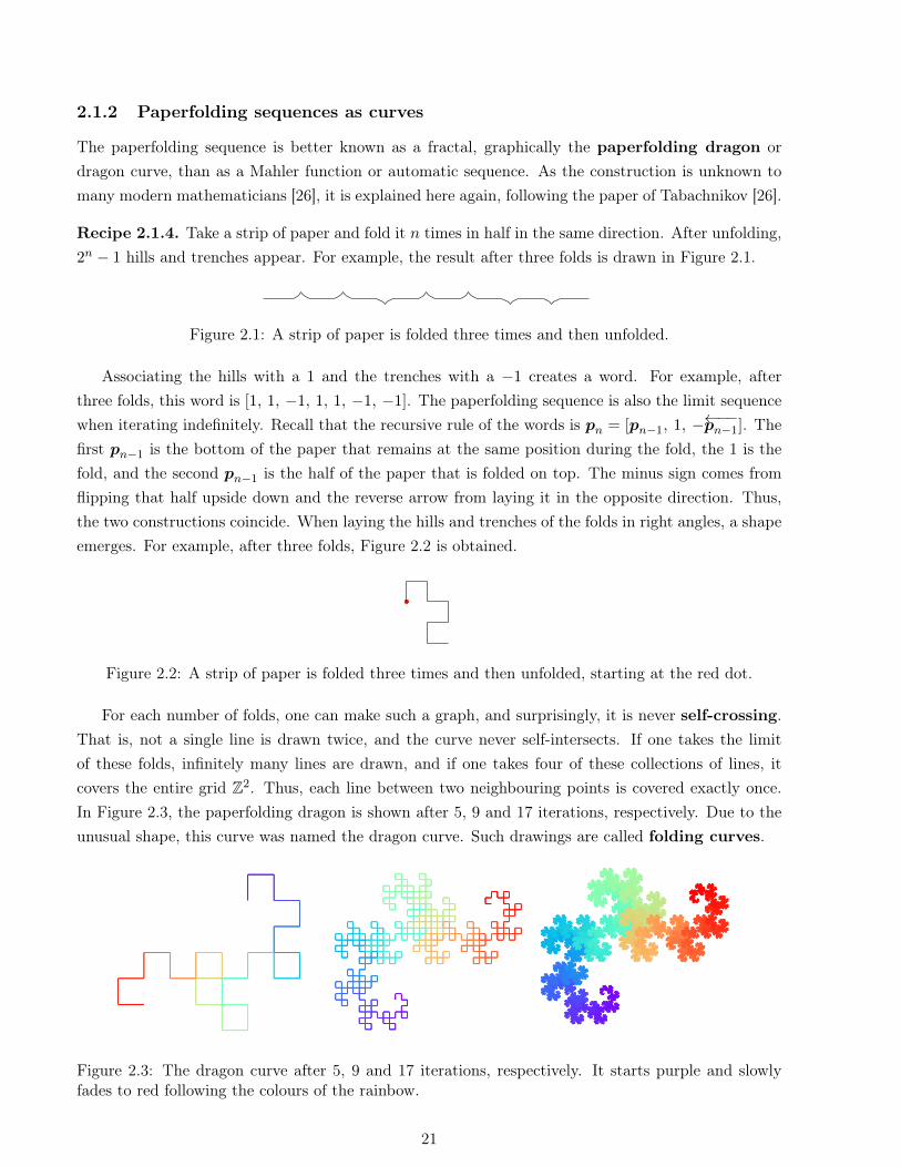
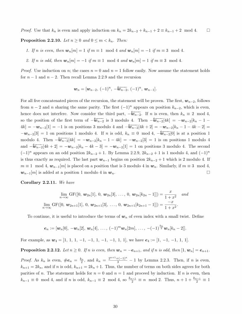
Recipe 2.1.4. Take a strip of paper and fold it n times in half in the same direction. After unfolding,2n − 1 hills and trenches appear. For example, the result after three folds is drawn in Figure 2.1.

Figure 2.1: A strip of paper is folded three times and then unfolded.

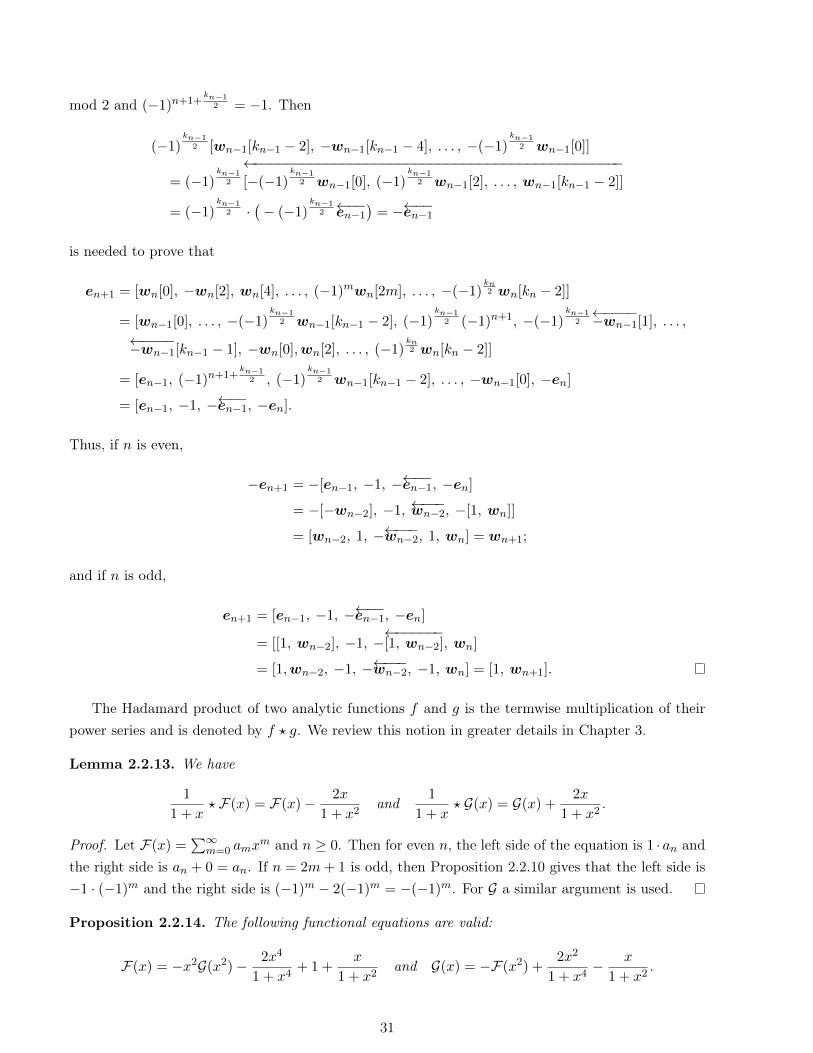
Associating the hills with a 1 and the trenches with a −1 creates a word. For example, afterthree folds, this word is [1, 1, −1, 1, 1, −1, −1]. The paperfolding sequence is also the limit sequencewhen iterating indefinitely. Recall that the recursive rule of the words is pn = [pn−1, 1, −←−−pn−1]. Thefirst pn−1 is the bottom of the paper that remains at the same position during the fold, the 1 is thefold, and the second pn−1 is the half of the paper that is folded on top. The minus sign comes fromflipping that half upside down and the reverse arrow from laying it in the opposite direction. Thus,the two constructions coincide. When laying the hills and trenches of the folds in right angles, a shapeemerges. For example, after three folds, Figure 2.2 is obtained.

Figure 2.2: A strip of paper is folded three times and then unfolded, starting at the red dot.

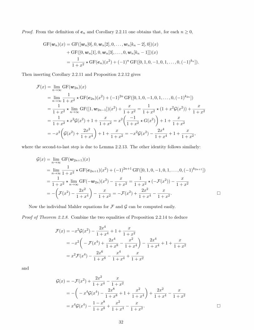
For each number of folds, one can make such a graph, and surprisingly, it is never self-crossing.That is, not a single line is drawn twice, and the curve never self-intersects. If one takes the limitof these folds, infinitely many lines are drawn, and if one takes four of these collections of lines, itcovers the entire grid Z2. Thus, each line between two neighbouring points is covered exactly once.In Figure 2.3, the paperfolding dragon is shown after 5, 9 and 17 iterations, respectively. Due to theunusual shape, this curve was named the dragon curve. Such drawings are called folding curves.

Figure 2.3: The dragon curve after 5, 9 and 17 iterations, respectively. It starts purple and slowlyfades to red following the colours of the rainbow.

21

2.2 The folded continued fraction of ρ

As seen for the regular paperfolding sequence, Mahler functions and folded continued fractions cansometimes live in the same world. So far, only infinite sums and products seem to have been studiedin the literature, such as

∑∞n=0 2−Fn where Fn are the Fibonacci numbers [7]. Because ρ(x) is defined

as an irregular continued fraction, such a regular folded continued fraction is yet unknown.

2.2.1 Computing a folded continued fraction for ρ

For ρ(x), a folded continued fraction exists with a more intricate fold. First, recall that

ρn(x) := 1 +x

1+x2

1+x4

1+ · · ·+

x2n−2

1+x2

n−1

1.

Evaluating the regular continued fractions of these rational functions ρn in Magma [8] gives

ρ0(x) = [1],

ρ1(x) = [1 + x],

ρ2(x) = [1; x, x],

ρ3(x) = [x+ 1; −x, −x, x, x],

ρ4(x) = [1; x, x, x, −x, −x, x, −x, −x, x, x],

ρ5(x) = [x+ 1;−x,−x, x, x,−x,−x,−x, x, x,−x, x, x, x,−x,−x, x,−x,−x, x, x].

It is already remarkable that almost all partial quotients are ±x. Moreover, the words wn seem toconverge along even indices n and along odd indices n. The parity partial convergence of ρ(x) inCorollary 1.2.13 for |x| > 1 explains the existence of the two distinct continued fractions. A carefullook suggests that ρ(x) = [sn(x); wn(x)] with the recursion

wn = [wn−2, (−1)nx, −←−−−wn−2, (−1)nx, wn−1] (2.2.1)

for wn = wn(x), where

sn(x) =

1 if n even,

x+ 1 if n odd.(2.2.2)

This form resembles the folding of p. To begin proving the observed recursions (2.2.1) and (2.2.2), afew technical lemmas need to be set.

Lemma 2.2.1. For all n ≥ 1,

Hn−2(x2)Hn(x)−Hn−1(x)Hn−1(x

2) = (−1)n−1x2n−1.

Proof. Use induction. For n = 1, the left side evaluates to 1 · (x + 1) − 1 · 1 = x, which is correct.

22

Now assume that n ≥ 2. Using Hn(x) = Hn−1(x2) + xHn−2(x

4) for all n ≥ 1, we obtain

Hn−2(x2)Hn(x)−Hn−1(x)Hn−1(x

2)

= Hn−2(x2)(Hn−1(x

2) + qHn−2(x4))−(Hn−2(x

2) + qHn−3(x4))Hn−1(x

2)

= xHn−2(x2)Hn−2(x

4)− xHn−3(x4)Hn−1(x

2) = −x(−1)n−2(x2)2n−1−1 = (−1)n−1x2

n−1.

Lemma 2.2.2. For all n ≥ 1,

Hn(x) = Hn−1(x) + x2n−1

Hn−2(x).

Proof. Recall that Hn(x) =∑2n−1

m=0 cmqm, where cm = 0 if the binary expansion of m contains two

neighbouring 1’s and cm = 1 otherwise. Let m < 2n such that cm = 1. If m < 2n−1, then cm isalready in Hn−1. If m ≥ 2n−1, the binary expansion of m starts with 10, and removing these termsgives a number below 2n−2 corresponding to Hn−2. This leads to the formula.

Let (kn)∞n=0 be the sequence defined by k0 = k1 = 0 and kn = 2kn−2 + kn−1 + 2 for all n ≥ 2.

Lemma 2.2.3. For all n ≥ 0, kn = 2n+1±(−1)n3 − 1 and kn is even.

Proof. Both the closed formula and each term being an even integer follow from induction.

The terms kn+1 form the Jacobsthal sequence, sequence A001045 on the OEIS [21]. This sequenceis also relevant to the construction of F and G using Stern polynomials, determines where the longsequences of zero coefficients in their expansions begin and end, and to the degree of Hn(x). This isnot coincidental. By construction, kn = degHn(x2), which is the degree of the denominator of ρn(x).At this point, only the main theorem remains to be proven.

Theorem 2.2.4. Let n ≥ 0 and x be a real number. Then ρn(x) is expressed as a regular continuedfraction by writing ρn(x) = [sn; wn] for

sn =

1 if n even,

1 + x if n odd,

with wn defined recursively by

wn = [wn−2, (−1)nx, −←−−−wn−2, (−1)nx, wn−1] for n ≥ 2,

w0 = w1 are empty, the length of wn is equal to kn, pkn = Hn(x) and qkn = Hn−1(x2).

Proof. The theorem holds true for n = 0 and 1, and then apply induction. Assume that n ≥ 2. Fromthe recursion, the length of wn is equal to twice the length of wn−2, the length of wn−1 and 2 addedtogether. Thus, the length of wn is indeed kn.

Now let l = kn−1 and m = kn−2. Verifying that wn satisfies this recursion is the most difficultpart. Start along the lines of the proof of the Folding Lemma in [7, Lemma 6.3]. Define

ρn−1 = [a0; a1, a2, . . . , al] and ρn−2 = [b0; b1, b2, . . . , bm],

23

where a0 = sn−1 and b0 = sn−2 such that

wn−1 = [a1; a2, a3, . . . , al] and wn−2 = [b1; b2, b3, . . . , bm].

Then the Key Lemma (Lemma 1.2.2) gives(a0 1

1 0

)(a1 1

1 0

). . .

(al 1

1 0

)=

(pl pl−1

ql ql−1

).

Set t = (−1)nx, and compute [wn−2, t, −←−−−wn−2] by first dealing with [−←−−−wn−2, −b0] as follows:(−bm 1

1 0

). . .

(−b1 1

1 0

)(−b0 1

1 0

)=

((−b0 1

1 0

)(−b1 1

1 0

). . .

(−bm 1

1 0

))T

=

((−1)m+1pm (−1)mqm

(−1)mpm−1 (−1)m−1qm−1

)=

(−pm qm

pm−1 −qm−1

),

because m = kn−1 is even by Lemma 2.2.3. Then −←−−−wn−2 is computed as(−bm 1

1 0

). . .

(−b1 1

1 0

)=

(−pm qm

pm−1 −qm−1

)(0 1

1 b0

)=

(qm b0qm − pm−qm−1 pm−1 − b0qm−1

).

By the Key Lemma for [wn−2, t, −←−−−wn−2], we obtain(b0 1

1 0

). . .

(bm 1

1 0

)(t 1

1 0

)(−bm 1

1 0

). . .

(−b1 1

1 0

)

=

(pm pm−1

qm qm−1

)(t 1

1 0

)(qm b0qm − pm−qm−1 pm−1 − b0qm−1

)

=

(tpm + pm−1 pm

tqm + qm−1 qm

)(qm b0qm − pm−qm−1 pm−1 − b0qm−1

)

=

((tpm + pm−1)qm − qm−1pm (tpm + pm−1)(b0qm − pm) + pm(pm−1 − b0qm−1)(tqm + qm−1)qm − qm−1qm (tqm + qm−1)(b0qm − pm) + qm(pm−1 − b0qm−1)

)

=

(tpmqm + (−1)m tb0pmqm − tp2m + (−1)mb0

tq2m tb0q2m − tqmpm + 1

),

where again (−1)m = 1. Now the Key Lemma is applied to [t, wn−1] to deduce(t 1

1 0

)(a1 1

1 0

)(a2 1

1 0

). . .

(al 1

1 0

)=

(t 1

1 0

)(a0 1

1 0

)−1(pl pl−1

ql ql−1

)

=

(t 1

1 0

)(0 1

1 −a0

)(pl pl−1

ql ql−1

)=

(1 t− a00 1

)(pl pl−1

ql ql−1

)=

(pl + ql(t− a0) ∗

ql ∗

).

Here, the ∗-terms denote expressions that do not matter for the end result. Note that sn−1−sn−2 = x

for even n and sn−1 − sn−2 = −x for odd n. It means that sn−1 − sn−2 = a0 − b0 = (−1)nx = t, and

24

hence t− a0 = −b0. Now the entire recursion [wn−2, (−1)nx, −←−−−wn−2, (−1)nx, wn−1] is computed bymultiplying the matrices found for [wn−2, t, −←−−−wn−2] and [t, wn−1]:(

tpmqm + 1 tb0pmqm − tp2m + b0

tq2m tb0q2m − tqmpm + 1

)(pl − qlb0 ∗

ql ∗

)

=

((tpmqm + 1)(pl − qlb0) + (tpmqmb0 − tp2m + b0)ql ∗

tq2m(pl − qlb0) + (tq2mb0 − tqmpm + 1)ql ∗

)

=

(pl + tpmqmpl − tp2mql ∗ql + tq2mpl − tqmpmql ∗

)=

(pl + (−1)nxpm(qmpl − pmql) ∗ql + (−1)nxqm(qmpl − pmql) ∗

).

As l = kn−1 and m = kn−2, the induction hypothesis gives that pl = Hn−1(x), pm = Hn−2(x),ql = Hn−2(x

2) and pl = Hn−3(x2). Since n ≥ 2, one can apply Lemma 2.2.1 for n− 1:

qmpl − pmql = Hn−3(x2)Hn−1(x)−Hn−2(x)Hn−2(x

2) = −(−1)n−1x2n−1−1 = (−1)nx2

n−1−1.

By Lemma 2.2.2,

pkn = pl + (−1)nxpm(qmpl − pmql) = Hn−1(x) + x2n−1

Hn−2(x) = Hn(x) and

qkn = ql + (−1)nxqm(qmpl − pmql) = Hn−2(x2) + x2

n−1Hn−3(x

2) = Hn−1(x2).

Thus, the formulas for pkn and qkn are valid, and by Proposition 1.2.8, ρn =pknqkn

. This means thatthe recursion for wn and sn−2 = sn are valid.

2.2.2 Specializing the folded continued fraction for ρ

For the regular finite continued fraction of a rational number, [a0; a1, . . . , al], ai is commonly a positiveinteger for all 1 ≤ i ≤ l. The same holds for all i ≥ 1 for an infinite continued fraction [a0; a1, a2, . . . ]

as then there is a one-to-one correspondence between the infinite continued fractions and irrationalnumbers. Theorem 2.2.4 does not give this traditional shape for integer values x as −x shows up too.But one can specialise it into the preferred form as described in [7] with the following helpful lemma.

Lemma 2.2.5. For all x, y and z such that both sides of the equation make sense,

[x; −y, z] = [x− 1; 1, y − 1, −z].

Proof. By the Key Lemma, and the matrices of partial convergents of the two continued fractions are(x 1

1 0

)(−y 1

1 0

)(z 1

1 0

)=

(x+ z − xyz 1− xy

1− yz −y

)and(

x− 1 1

1 0

)(1 1

1 0

)(y − 1 1

1 0

)(−z 1

1 0

)=

(x+ z − xyz xy − 1

1− yz y

).

As the two left entries of the matrices coincide, the lemma follows.

Now the regular continued fraction can be constructed. A continued fraction [a0; a1, . . . , al] such

25

that for each 1 ≤ i ≤ l, ai ∈ {−x, x} can be written as a regular continued fraction that only containsa0, a0 − 1, 1, x− 2, x− 1 and x by using Lemma 2.1.2 and Lemma 2.2.5 repeatedly. For example,

ρ4(x) = [1; x, x, x, −x, −x, x, −x, −x, x, x]

= [1; x, x, x− 1, 1, x− 1, −[−x, x, −x, −x, x, x]]

= [1; x, x, x− 1, 1, x− 1, x, −x, x, x, −x, −x]

= [1; x, x, x− 1, 1, x− 1, x− 1, 1, x− 1, −x, −x, x, x]

= [1; x, x, x− 1, 1, x− 1, x− 1, 1, x− 2, 1, x− 1, x, −x, −x]

= [1; x, x, x− 1, 1, x− 1, x− 1, 1, x− 2, 1, x− 1, x− 1, 1, x− 1, x].

This process can also be generalised in three steps:

1. For all 0 ≤ i ≤ l − 1 such that ai 6= ai+1, insert a 1 between ai and ai+1.

2. Replace every −x by x.

3. For each term x in the new sequence, subtract 1 for each neighbour being equal to 1.

The length of the continued fraction increases by the number of sign changes in the original sequence,which is bounded by l − 1. Thus, the new continued fraction has less than 2l partial quotients. Alsonote that for all m ≥ 3, this method gives a ‘proper’ continued fraction for ρn(m) that only contains1,m− 2,m− 1 and m. In other words, the two parity partial convergents of the continued fraction ofρ(m) are all among four possible numbers. For example, m = 5 gives two continued fractions

[1, 5, 5, 4, 1, 4, 4, 1, 3, 1, 4, 4, 1, 4, 5, 4, 1, 4, 4, 1, . . . ] for even n and

[5; 1, 4, 4, 1, 4, 4, 1, 4, 5, 4, 1, 4, 4, 1, 3, 1, 4, 5, 4, . . . ] for odd n.

2.2.3 The folding curve of ρ

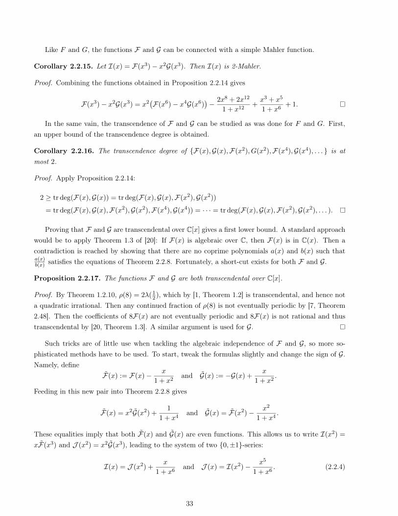
The construction of the folded continued fraction of ρ shares many features with Shallit’s and vander Poorten’s example discussed in Section 2.1. Hence it is natural to investigate whether this newfolded continued fraction shares other properties with the paperfolding sequence. In this subsection,the folding curves of ρ are tackled. As ρ has two convergents, there are two different curves. In Figure2.4, a few examples are present.

26

Figure 2.4: The curves derived from ρ for several values of n. On top, after 6, 10 and 14 iterations,respectively, and, on the bottom after 7 and 13 iterations. It starts purple and slowly fades to redfollowing the colours of the rainbow.

These curves resemble right isosceles triangles that increase in size. They are not perfect triangles,as the diagonals contain ‘hooks’. These hooks are small, local features that do not appear on a globalscale. At the limit, they resemble true triangles. For one parity of n, the side lengths of the trianglesgrow by a factor of two and one triangle is added at the iteration n + 2. The side lengths of thetriangles of opposite parity differ by

√2.

Figure 2.5: The curve for ρ15. Blue is the term w13, green is −←−−w13 and red is w14. Thus, the foldingcurve first goes to the right, then up, and the last term completes the largest triangle.

Computational evidence suggests that these curves are not self-crossing for any n ≥ 0. In Figure2.5, the way the fold works is drawn. The pattern is clear.

Observation 2.2.6. For all n ≥ 0, the curve induced by the parity of the partial quotients of ρ is notself-crossing. Moreover, by taking eight copies of the two limits and rotating and flipping them, theentire Z2 grid can be covered.

27

The appearance of triangles is not surprising as the folding curve of the recursion defined by q0 = []

and qn = [qn−1, (−1)nx, −←−−qn−1] converges to a single triangle. Similarly, recursions giving graduallygrowing dragon curves exist, for example, the folding curve of the recursion defined by v0 = v1 = [ ]

and [vn−2, x, −←−−−vn−2, (−1)nx, vn−1]. Both of these folding curves are presented in Figure 2.6. Thus,there is a strong relation between the folding curves of the paperfolding sequence and w.

Figure 2.6: On the left is the curve for q depicted after 14 iterations. It starts purple and slowly fadesinto red following the colours of the rainbow. On the right is the curve for v after 17 iterations. Blueis the term vn−2, green is −←−−−vn−2 and red is vn−1. The red and green pieces together form a mirrorpaperfolding dragon, just like the red and green curve in Figure 2.5 form a triangle.

To strengthen this connection even further, both qn and wn are also observed to be a foldedcontinued fraction of certain functions, respectively, of

x

∞∑n=0

(−1)nx2n

and 1−x

1−x2

1−x4

1−x8

1− · · · .

2.2.4 The folding sequence of ρ as a Mahler function

The folding recursion for w gives not much structure on the two intertwining sequences consistingsolely of ±1. The Toeplitz construction is another method to generate the paperfolding sequence andalso gives a Mahler equation for its generating function. In this subsection, we show that w posessesthe same structure. The two main strategies to generate the paperfolding sequence are [3, Example5.1.6 and Exercise 5.7]:

1. The folding approach. Let p0 = [] and pn = [pn−1, 1,←−−pn−1] for n ≥ 1. Then the paperfoldingsequence is limn→∞ pn. This definition is used to prove the paperfolding lemma.

2. The Toeplitz construction. Let p0 = [ ] again be the empty word and for n ≥ 1,

pn = [1, pn−1[0], −1, pn−1[1], 1,pn−1[2], −1, pn−1[3], 1, pn−1[4], . . . ].

Here, pn−1[m] is the mth element of pn−1, and the 1 and −1 alternate.

To prove these definitions are equivalent, first show by induction that in the first approach, thesubsequence of terms of even index alternate. That is, pn[0],pn[2],pn[4], . . . are 1,−1, 1,−1, 1, . . . .

28

Then prove the subsequences qn of pn of terms of odd index satisfy qn = [qn−1, 1, ←−−qn−1]. Let P (x)

be the generating function of the paperfolding sequence. Then the Toeplitz construction induces that

P (x) = xP (x2) +1

1 + x2. (2.2.3)

Multiplying both sides with 1 + x2 shows that P (x) is a Mahler function:

(1 + x2)P (x) = (x+ x3)P (x2) + 1.

The limit of the iteration of equality (2.2.3) gives a more direct formula:

P (x) =

∞∑n=0

x2n−1

1 + x2n.

The function P (x) is not rational and not even algebraic over C[x]. If 0 < |α| < 1 is algebraic, thenP (α) is a transcendental number [13, 19].

Now we want to mimic this idea for ρ and w using Theorem 2.2.4. To recap, the words wn of thefolded continued fraction of ρn(x) satisfy w0 = w1 = [ ], and for n ≥ 2,

wn = [wn−2, (−1)nx, −←−−−wn−2, (−1)nx, wn−1].

Each word only contains x and −x, and the sequence of wn converges parity partially. Replace x with1 and −x with −1, to get

wn = [wn−2, (−1)n, −←−−−wn−2, (−1)n, wn−1].

From this recursion, we will compute two generating functions. First introduce some notation:

Notation 2.2.7. Let N ≥ 0 and a = (an)Nn=0 and b = (bn)∞n=0 be sequences. finite and infinite. Thenthe generating function of a, the polynomial

∑Nn=0 anx

n, is denoted by GF(a) and GF(b) is writtenfor the power series

∑∞n=0 bnx

n.

Next, let F(x) = limn→∞GF(w2n) and G(x) = limn→∞GF(w2n+1), to state the Mahler equations.

Theorem 2.2.8. We have

F(x) = x2F(x4)− 2x6

1 + x8+

1

1 + x4+

x

1 + x2and

G(x) = x4G(x4)− 1− x8

1 + x8+

x2

1 + x4− x

1 + x2.

This result has a lengthy proof, but there has to be a starting point somewhere. Recall that kndenotes the length of the word wn. Thus, by Lemma 2.2.3, k0 = k1 = 0, kn = kn−1 + 2kn−2 + 2 forn ≥ 2. We need a refinement modulo 4.

Lemma 2.2.9. For all even n ≥ 2, kn ≡ 2 mod 4 and for all odd n ≥ 1, kn ≡ 0 mod 4.

29

Proof. Use that kn is even and apply induction on kn = 2kn−2 + kn−1 + 2 ≡ kn−1 + 2 mod 4.

Proposition 2.2.10. Let n ≥ 0 and 0 ≤ m < kn. Then:

1. If n is even, then wn[m] = 1 if m ≡ 1 mod 4 and wn[m] = −1 if m ≡ 3 mod 4.

2. If n is odd, then wn[m] = −1 if m ≡ 1 mod 4 and wn[m] = 1 if m ≡ 3 mod 4.

Proof. Use induction on n; the cases n = 0 and n = 1 follow easily. Now assume the statement holdsfor n− 1 and n− 2. Then recall Lemma 2.2.9 and the recursion

wn = [wn−2, (−1)n, −←−−−wn−2, (−1)n, wn−1].

For all five concatenated pieces of the recursion, the statement will be proven. The first, wn−2, followsfrom n − 2 and n sharing the same parity. The first (−1)n appears on position kn−2, which is even,hence does not interfere. Now consider the third part, −←−−−wn−2. If n is even, then kn ≡ 2 mod 4,so the position of the first term of −←−−−wn−2 is 3 modulo 4. Then −←−−−wn−2[4k] = −wn−2[kn − 1 −4k] = −wn−2[1] = −1 is on positions 3 modulo 4 and −←−−−wn−2[4k + 2] = −wn−2[kn − 1 − 4k − 2] =

−wn−2[3] = 1 on positions 1 modulo 4. If n is odd, kn ≡ 0 mod 4, −←−−−wn−2[0] is at a position 1modulo 4. Then −←−−−wn−2[4k] = −wn−2[kn − 1 − 4k] = −wn−2[3] = 1 is on positions 1 modulo 4and −←−−−wn−2[4k + 2] = −wn−2[kn − 4k − 3] = −wn−2[1] = 1 on positions 3 modulo 4. The second(−1)n appears on an odd position 2kn−2 + 1. By Lemma 2.2.9, 2kn−2 + 1 is 1 modulo 4, and (−1)n

is thus exactly as required. The last part wn−1 begins on position 2kn−2 + 1 which is 2 modulo 4. Ifm ≡ 1 mod 4, wn−1[m] is placed on a position that is 3 modulo 4 in wn. Similarly, if m ≡ 3 mod 4,wn−1[m] is added at a position 1 modulo 4 in wn.

Corollary 2.2.11. We have

limn→∞

GF([0, w2n[1], 0, w2n[3], . . . , 0, w2n[k2n − 1]]) =x

1 + x2and

limn→∞

GF([0, w2n+1[1], 0, w2n+1[3], . . . , 0, w2n+1[k2n+1 − 1]]) =−x

1 + x2.

To continue, it is useful to introduce the terms of wn of even index with a small twist. Define

en := [wn[0], −wn[2], wn[4], . . . , (−1)mwn[2m], . . . , −(−1)kn2 wn[kn − 2]].

For example, as w4 = [1, 1, 1, −1, −1, 1, −1, −1, 1, 1], we have e4 := [1, −1, −1, 1, 1].

Proposition 2.2.12. Let n ≥ 0. If n is even, then wn = −en+1, and if n is odd, then [1, wn] = en+1.

Proof. As kn is even, #en = kn2 , and kn = 2n+1+(−1)n

3 − 1 by Lemma 2.2.3. Then, if n is even,kn+1 = 2kn, and if n is odd, kn+1 = 2kn + 1. Thus, the number of terms on both sides agrees for bothparities of n. The statement holds for n = 0 and n = 1 and proceed by induction. If n is even, thenkn−1 ≡ 0 mod 4, and if n is odd, kn−1 ≡ 2 mod 4, so kn−1

2 ≡ n mod 2. Thus, n + 1 + kn−1

2 ≡ 1

30

mod 2 and (−1)n+1+kn−1

2 = −1. Then

(−1)kn−1

2 [wn−1[kn−1 − 2], −wn−1[kn−1 − 4], . . . , −(−1)kn−1

2 wn−1[0]]

= (−1)kn−1

2

←−−−−−−−−−−−−−−−−−−−−−−−−−−−−−−−−−−−−−−−−−−−−−−[−(−1)

kn−12 wn−1[0], (−1)

kn−12 wn−1[2], . . . , wn−1[kn−1 − 2]]

= (−1)kn−1

2 ·(− (−1)

kn−12←−−en−1

)= −←−−en−1

is needed to prove that

en+1 = [wn[0], −wn[2], wn[4], . . . , (−1)mwn[2m], . . . , −(−1)kn2 wn[kn − 2]]

= [wn−1[0], . . . , −(−1)kn−1

2 wn−1[kn−1 − 2], (−1)kn−1

2 (−1)n+1, −(−1)kn−1

2←−−−−−wn−1[1], . . . ,

←−−−−−wn−1[kn−1 − 1], −wn[0],wn[2], . . . , (−1)kn2 wn[kn − 2]]

= [en−1, (−1)n+1+kn−1

2 , (−1)kn−1

2 wn−1[kn−1 − 2], . . . , −wn−1[0], −en]

= [en−1, −1, −←−−en−1, −en].

Thus, if n is even,

−en+1 = −[en−1, −1, −←−−en−1, −en]

= −[−wn−2], −1, ←−−−wn−2, −[1, wn]]

= [wn−2, 1, −←−−−wn−2, 1, wn] = wn+1;

and if n is odd,

en+1 = [en−1, −1, −←−−en−1, −en]

= [[1, wn−2], −1, −←−−−−−−[1, wn−2], wn]

= [1,wn−2, −1, −←−−−wn−2, −1, wn] = [1, wn+1].

The Hadamard product of two analytic functions f and g is the termwise multiplication of theirpower series and is denoted by f ? g. We review this notion in greater details in Chapter 3.

Lemma 2.2.13. We have

1

1 + x? F(x) = F(x)− 2x

1 + x2and

1

1 + x? G(x) = G(x) +

2x

1 + x2.

Proof. Let F(x) =∑∞

m=0 amxm and n ≥ 0. Then for even n, the left side of the equation is 1 ·an and

the right side is an + 0 = an. If n = 2m+ 1 is odd, then Proposition 2.2.10 gives that the left side is−1 · (−1)m and the right side is (−1)m − 2(−1)m = −(−1)m. For G a similar argument is used.

Proposition 2.2.14. The following functional equations are valid:

F(x) = −x2G(x2)− 2x4

1 + x4+ 1 +

x

1 + x2and G(x) = −F(x2) +

2x2

1 + x4− x

1 + x2.

31

Proof. From the definition of en and Corollary 2.2.11 one obtains that, for each n ≥ 0,

GF(wn)(x) = GF([wn[0], 0,wn[2], 0, . . . ,wn[kn − 2], 0])(x)

+ GF([0,wn[1], 0,wn[3], . . . , 0,wn[kn − 1]])(x)

=1

1 + x2?GF(en)(x2) + (−1)n GF([0, 1, 0,−1, 0, 1, . . . , 0, (−1)kn ]).

Then inserting Corollary 2.2.11 and Proposition 2.2.12 gives

F(x) = limn→∞

GF(w2n)(x)

= limn→∞

1

1 + x2?GF(e2n)(x2) + (−1)2n GF([0, 1, 0,−1, 0, 1, . . . , 0, (−1)k2n ])

=1

1 + x2? limn→∞

GF([1,w2n−1])(x2) +

x

1 + x2=

1

1 + x2? (1 + x2G(x2)) +

x

1 + x2

=1

1 + x2? x2G(x2) + 1 +

x

1 + x2= x2

(−1

1 + x2? G(x2)

)+ 1 +

x

1 + x2

= −x2(G(x2) +

2x2

1 + x4

)+ 1 +

x

1 + x2= −x2G(x2)− 2x4

1 + x4+ 1 +

x

1 + x2,

where the second-to-last step is due to Lemma 2.2.13. The other identity follows similarly:

G(x) = limn→∞

GF(w2n+1)(x)

= limn→∞

1

1 + x2?GF(e2n+1)(x

2) + (−1)2n+1 GF([0, 1, 0,−1, 0, 1, . . . , 0, (−1)k2n+1 ])

=1

1 + x2? limn→∞

GF(−w2n)(x2)− x

1 + x2=

1

1 + x2? (−F(x2))− x

1 + x2

= −(F(x2)− 2x2

1 + x4

)− x

1 + x2= −F(x2) +

2x2

1 + x4− x

1 + x2.

Now the individual Mahler equations for F and G can be computed easily.

Proof of Theorem 2.2.8. Combine the two equalities of Proposition 2.2.14 to deduce

F(x) = −x2G(x2)− 2x4

1 + x4+ 1 +

x

1 + x2

= −x2(−F(x4) +

2x4

1 + x8− x2

1 + x4

)− 2x4

1 + x4+ 1 +

x

1 + x2

= x2F(x4)− 2x6

1 + x8− x4

1 + x4+

x

1 + x2

and

G(x) = −F(x2) +2x2

1 + x4− x

1 + x2

= −(− x4G(x4)− 2x8

1 + x8+ 1 +

x2

1 + x4

)+

2x2

1 + x4− x

1 + x2

= x4G(x4)− 1− x8

1 + x8+

x2

1 + x4− x

1 + x2.

32

Like F and G, the functions F and G can be connected with a simple Mahler function.

Corollary 2.2.15. Let I(x) = F(x3)− x2G(x3). Then I(x) is 2-Mahler.

Proof. Combining the functions obtained in Proposition 2.2.14 gives

F(x3)− x2G(x3) = x2(F(x6)− x4G(x6)

)− 2x8 + 2x12

1 + x12+x3 + x5

1 + x6+ 1.

In the same vain, the transcendence of F and G can be studied as was done for F and G. First,an upper bound of the transcendence degree is obtained.

Corollary 2.2.16. The transcendence degree of {F(x),G(x),F(x2), G(x2),F(x4),G(x4), . . . } is atmost 2.

Proof. Apply Proposition 2.2.14:

2 ≥ tr deg(F(x),G(x)) = tr deg(F(x),G(x),F(x2),G(x2))

= tr deg(F(x),G(x),F(x2),G(x2),F(x4),G(x4)) = · · · = tr deg(F(x),G(x),F(x2),G(x2), . . . ).

Proving that F and G are transcendental over C[x] gives a first lower bound. A standard approachwould be to apply Theorem 1.3 of [20]: If F(x) is algebraic over C, then F(x) is in C(x). Then acontradiction is reached by showing that there are no coprime polynomials a(x) and b(x) such thata(x)b(x) satisfies the equations of Theorem 2.2.8. Fortunately, a short-cut exists for both F and G.

Proposition 2.2.17. The functions F and G are both transcendental over C[x].

Proof. By Theorem 1.2.10, ρ(8) = 2λ(12), which by [1, Theorem 1.2] is transcendental, and hence nota quadratic irrational. Then any continued fraction of ρ(8) is not eventually periodic by [7, Theorem2.48]. Then the coefficients of 8F(x) are not eventually periodic and 8F(x) is not rational and thustranscendental by [20, Theorem 1.3]. A similar argument is used for G.

Such tricks are of little use when tackling the algebraic independence of F and G, so more so-phisticated methods have to be used. To start, tweak the formulas slightly and change the sign of G.Namely, define

F(x) := F(x)− x

1 + x2and G(x) := −G(x) +

x

1 + x2.

Feeding in this new pair into Theorem 2.2.8 gives

F(x) = x2G(x2) +1

1 + x4and G(x) = F(x2)− x2

1 + x4.

These equalities imply that both F(x) and G(x) are even functions. This allows us to write I(x2) =

xF(x3) and J (x2) = x2G(x3), leading to the system of two {0,±1}-series:

I(x) = J (x2) +x

1 + x6and J (x) = I(x2)− x5

1 + x6. (2.2.4)

33

By reversing the construction, I(x) and J (x) being algebraically independent over C(x) wouldimply the same for F(x) and G(x). As most theorems for algebraic independence of Mahler functionsdesire homogeneous equations or that the coefficients in front of the functions are all constants, theentire route to I and J has to be taken. A simplified version of a theorem by Nishioka will be used:

Theorem 2.2.18 (Nishioka, Theorem 3.2.2 in [20]). Let m ≥ 1 and f1(x), . . . , fn(x) ∈ C[[x]] satisfyf1(x)...

fn(x)

= A

f1(x

k)...

fn(xk)

+

g1(x)...

gn(x)

where k ≥ 2, A is an n× n matrix over C and gi(x) ∈ C(x). If f1, . . . , fm are algebraically dependentover C, there are c1, . . . , cm ∈ C not all all zero such that

∑mi=0 ci · fi(x) ∈ C(x).

The theorem is unhelpful when dealing with the Mahler equations (2.2.4), so we iterate them once:

I(x) = I(x4) +x

1 + x6− x10

1 + x12, J (x) = J (x4)− x5

1 + x6+

x2

1 + x12.

Theorem 2.2.19. I(x) and J (x) are algebraically independent over C(x).

Proof. Assume the opposite. Apply Nishioka’s theorem (Theorem 2.2.18) with m = 2, k = 4,

A =

(1 0

0 1

), g1(x) =

x

1 + x6− x10

1 + x12and g2(x) = − x5

1 + x6+

x2

1 + x12.

Then there are c1, c2 ∈ C, not both zero, and coprime polynomials a(x) and b(x) such that c1I(x) +

c2J (x) = a(x)b(x) . In other words,

a(x4)

b(x4)=a(x)

b(x)+ c1g1(x) + c2g2(x).

The equation can be transformed into an equation of polynomials: A(x) = B(x) + C(x), where

A(x) = a(x4)b(x)(1 + x6)(1 + x12),

B(x) = a(x)b(x4)(1 + x6)(1 + x12) and

C(x) = b(x)b(x4)(c1(x− x10 + x13 − x16) + c2(x

2 − x5 + x8 − x17))

= b(x)b(x4)x(1− x3)(c1(1 + x3 + x6 + x12) + c2x(1 + x6 + x9 + x12)

)= b(x)b(x4)x(1− x3)c(x).

Using that a(x) and b(x) are coprime and thus a(x4) and b(x4) are coprime as well, we deduce thatb(x) | b(x4)(1 + x6)(1 + x12) and b(x4) | b(x)(1 + x6)(1 + x12).

As b(x4) | b(x)(1 + x6)(1 + x12), x cannot divide b(x), and so b(0) 6= 0. Assume ζ is a root of b(x)

that is not a root of 1− x6. Then, as ζ 6= 0 and ζ6 6= 1, the four fourth roots of ζ are zeros of b(x4)but not of (1 + x6)(1 + x12). Using that b(x4) | b(x)(1 + x6)(1 + x12), these four roots are all roots

34

of b(x). Iterating this process gives an unbounded number of roots of b(x). This contradiction meansthat b(x) | (1 − x6)k for some k ≥ 0. By the same argument, b(x) cannot have two identical rootsthat are zeros of 1− x6. Thus, b(x) | (1− x6) and b(x4) | (1− x24).

From b(x) | (1 − x6) and b(x) | b(x4)(1 + x6)(1 + x12), it follows that b(x) | b(x4). Combine thiswith b(x4) | b(x)(1 + x6)(1 + x12) to conclude that, for y ∈ C, b(y) = 0 if and only if b(y4) = 0 and(1 + y6)(1 + y12) 6= 0. In particular, for y = −ζk3 , where ζ3 = e

2πi3 and k = 0, 1, 2, we have b(ζk3 ) = 0

if and only if b(−ζk3 ) = 0. Thus, deg b(x) is even and deg b(x4) is divisible by 8.

Let ζ be a root of (1 + x6)(1 + x12). If one of the multiplicities ordζ(A), ordζ(B) and ordζ(C) issmaller than the others and m = min(ordζ(A), ordζ(B), ordζ(C)), the limit

limx→ζ

(A(ζ)

(x− ζ)m− B(ζ)

(x− ζ)m− C(ζ)

(x− ζ)m

)involves two zero terms and one non-zero term so cannot be zero. This contradicts A(x)+B(x) = C(x).Let us apply this fact a few times. Since b(x) | (1− x6), b(ζ) 6= 0 and ζ(1− ζ3) 6= 0 as well.

• If b(ζ4) = 0, then a(ζ4) 6= 0 as a(x4) and b(x4) are coprime. Therefore, ordζ(A) = 1 andordζ(B) ≥ 2. Then ordζ(C) = 1, and hence, c(ζ) 6= 0 as b(ζ4) = 0.

• If b(ζ4) 6= 0, then ordζ(C) = ordζ(c). As ordζ(A) ≥ 1 and ordζ(B) ≥ 1, it follows thatordζ(C) ≥ 1. Thus, c(ζ) = 0 as b(ζ4) 6= 0.

To summarise, exactly one of b(ζ4) and c(ζ) is zero. If c(ζ) = 0 for such a root ζ of (1 + x6)(1 + x12),then if ζ is a root of 1 + x12 or 1 + x6, respectively,

c1(ζ3 + ζ6) = −c2ζ(ζ6 + ζ9) and c1(1 + ζ9) = −c2ζ(ζ3 + ζ12).

In both cases, using ζ 6= 0, 1 + ζ3 6= 0 and 1 + ζ9 6= 0, we conclude that c1 = −c2ζ4. Then c(x) has atmost four roots in common with (1 +x6)(1 +x12) as c1 and c2 are constants, not simultaneously zero.Then b(x4) has at least 18−4 = 14 roots in common with (1+x6)(1+x12), and so deg b(x) ≥

⌈144

⌉= 4.

As b(x) | b(x4) and b(x) and (1 +x6)(1 +x12) are coprime, deg b(x4) ≥ 18. Since deg b(x4) is divisibleby 8, it is at least 24. As b(x4) | (1− x24) this implies that b(x4) = 1− x24 and b(x) = 1− x6. Nowdivide the equation A(x) = B(x) + C(x) by b(x4) to obtain

a(x4) = a(x)(1 + x6)(1 + x12) + x(1− x3)(1− x6)c(x).

Thus, a(1) = 4a(1), and so a(1) = 0. A contradiction, as a(x) and b(x) are coprime and b(1) = 0.Thus, a(x) and b(x) do not exist, implying that I(x) and J (x) are algebraically independent.

Corollary 2.2.20. F(x) and G(x) are algebraically independent over C(x).

2.3 Algebraic folded continued fractions

In the previous section, we gave an example of a folded continued fraction that is a quotient of two2-Mahler functions. In this section, folded continued fractions are defined more generally, several

35

examples are given and different choices are discussed. In particular, algebraic functions produced bya folded continued fraction are examined with the help of a few examples.

2.3.1 Defining folded continued fractions

The concept of folded continued fraction can be moulded in many ways, and any such definition ismore or less temporarily useful. In this thesis, a relatively small area is chosen where interestingexamples can turn up. Other cases like

∑∞n=0 2−Fn are fascinating but of a different nature.

Definition 2.3.1. A recursion of words is an infinite sequence (wn)∞n=0 of finite sequences wn

called words such that:

• Each word wn is finite, and all its letters are x or −x.

• There is a decent amount of convergence so that taking a limit limn→∞wn is meaningful.

• A recursion itself means the following: There are r,N ≥ 0 such that for each n ≥ N ,

wn = [vn,1, vn,2, . . . , vn,r],

where each vn,i is equal to

x, −x, wn−1, −wn−1,←−−−wn−1, −←−−−wn−1, . . . , wn−N , −wn−N ,

←−−−−wn−N or −←−−−−wn−N .

Here, x and−x are called constant words and those depending onwn−i non-constant words.

As before, we associate a continued fraction with each word, and the paperfolding sequence (pn)∞n=0

is a recursion of words. Clearly, there is much of a personal taste in this definition, as it does notinclude (−1)nwn−1. Thus, (wn)∞n=0 for ρ is not a recursion of words, but as shown below, that doesnot exclude ρ entirely. Despite the strict definition, many examples are quite similar.

Example 2.3.2. Recall that the original paperfolding sequence satisfies pn = [pn−1, x, −←−−pn−1] for

n ≥ 1 and p0 = [ ]. Consider a few variations:

• Let q0 = [x] and qn = [qn−1, x, −←−−qn−1], then qn+1 = pn, it is just a shift.

• If q0 = [ ] and qn = [qn−1, −x, −←−−qn−1], then qn = −pn.

• If q0 = [ ] and qn = [qn−1, x, −←−−qn−1, x], then [x; qn] = pn+1.

• If q0 = [ ], q1 = [ ] and qn = [qn−2, x, −←−−qn−2], then q2n = q2n−1 = pn. Thus, twice as many

iterations are needed to reach the same continued fraction.

• If q0 = [ ] and qn = [qn−1, x, −←−−qn−1, x, qn−1, −x, −

←−−qn−1]. Then only half the number ofiterations is needed to achieve the same continued fraction p.

In the same way, the folding sequence for ρ can be written without the (−1)n term. Recall thatwn = [wn−2, (−1)nx, −←−−−wn−2, (−1)nx, wn−1]. To remove the (−1)n from the recursion, define

36

w+n = (−1)nwn. It satisfies wn = [w+

n−2, x, −←−−−w+n−2, x, −w

+n−1]. As such, disallowing (−1)nx as a

possible term in the recursion does not exclude ρ from the definition.

Many recursions of words are uninteresting. When only including constant words, a rationalfunction is obtained. With precisely one non-constant word, the limit is eventually periodic, hence aquadratic irrationality. There are also other ways to obtain eventually periodic words, for example bydefining w0 = [x] and wn = [wn−1, wn−1], which converges to [x; x, x, x, x, x, . . . ].

Let kn be #wn − 1. Then in the case of at least two non-constant words, the degrees of the poly-nomials pkn(x) and qkn(x) increase exponentially with each iteration. If pkn(x) and qkn(x) converge(partially) to power series, they fall into two categories:

1. Fast converging recursions. These are recursions for which the number of correct coefficientsof limn→∞ pkn and limn→∞ qkn after n iterations grows exponentially with respect to n. Thepower series for ρ is an example of this type.

2. Slowly converging recursions have, instead of exponential, only a linear in n number of correctcoefficients. The next subsection contains an example of this type.

Although countless slowly converging recursions of words exist, the set of fast converging recursionsof words appears to be limited. All examples we have found are related to either x

∑∞n=0 x

2n or H(x)H(x2)

with slight variations in signs or linear combinations.

2.3.2 A cubic folded continued fraction

In this subsection, a folded continued fraction is shown to be a root of a cubic equation over Q[x].First, the matrix of continuants of wn is shown to satisfy a specific recursion. Then it is establishedthat a particular power series satisfies the same recursion, leading to the equality.

Define the recursion of words (wn)∞n=0 by w0 = [ ] and wn = [wn−1, wn−1, x, −←−−−wn−1, −←−−−wn−1].Furthermore, let kn := #wn − 1.

Lemma 2.3.3. Let n ≥ 1 and m = kn. Then(pkn+1 pkn+1−1

qkn+1 qkn+1−1

)=

(x(p2m + pm−1qm)2 1− xqm(pm + qm−1)(p

2m + pm−1qm)

1 + xqm(pm + qm−1)(p2m + pm−1qm) −xq2m(pm + qm−1)

2

).

Proof. The recursion for wn gives kn+1 = #wn+1 − 1 = 4#wn = 4kn − 4 is even for all n ≥ 1. Thus,pm−1qm − pmqm−1 = (−1)m = 1 by Lemma 1.2.4. Recall that the matrix of continuants of −←−wn is(

(−1)m+1pm (−1)mpm−1

(−1)mqm (−1)m−1qm−1

)=

(−pm pm−1

qm −qm−1

).

Next, the [wn−1, x, −←−−−wn−1] part of the recursion is computed like for paperfolding sequence:(pm pm−1

qm qm−1

)(x 1

1 0

)(−pm qm

pm−1 −qm−1

)= x

(−p2m pmqm

−pmqm q2m

)+

(0 1

1 0

).

37

These cancellations make the rest of the computation slightly easier. We obtain,(pkn+1 pkn+1−1

qkn+1 qkn+1−1

)=

(pm pm−1

qm qm−1

)2(x 1

1 0

)(−pm qm

pm−1 −qm−1

)2

= x

(pm pm−1

qm qm−1

)(−p2m pmqm

−pmqm q2m

)(−pm qm

pm−1 −qm−1

)

+

(pm pm−1

qm qm−1

)(0 1

1 0

)(−pm qm

pm−1 −qm−1

).

Computing the two parts separately gives the required result, since

x

(pm pm−1

qm qm−1

)(−p2m pmqm

−pmqm q2m

)(−pm qm

pm−1 −qm−1

)

= x

(pm pm−1

qm qm−1

)(pm(p2m + pm−1qm) −pmqm(pm + qm−1)

qm(p2m + pm−1qm) −q2m(pm + qm−1)

)

= x

((p2m + pm−1qm)2 −qm(p2m + pm−1qm)(pm + qm−1)

qm(pm + qm−1)(p2m + pm−1qm) −q2m(pm + qm−1)

2

)

and (pm pm−1

qm qm−1

)(0 1

1 0

)(−pm qm

pm−1 −qm−1

)=

(pm pm−1

qm qm−1

)(pm−1 −qm−1−pm qm

)

=

(pmpm−1 − pmpm−1 −pmqm−1 + pm−1qm

qmpm−1 − pmqm−1 −qm−1qm + qmqm−1

)=

(0 1

1 0

).

The limits of pkn , pkn−1, qkn and qkn−1 are observed to converge to power series; explicitly, to

A(x) =∞∑n=0

anxn = x+ 2x3 + 7x5 + 30x7 + 143x9 + 728x11 + · · · ,

B(x) =

∞∑n=0

bnxn = 1− x2 − 3x4 − 12x6 − 55x8 − 273x10 − 1428x12 + · · · ,

C(x) =∞∑n=0

cnxn = 1 + x2 + 3x4 + 12x6 + 55x8 + 273x10 + 1428x12 + · · · ,

D(x) =∞∑n=0

dnxn = −x3 − 4x5 − 18x7 − 88x9 − 455x11 + · · · .

Here, an and dn vanish for even n while bn and cn vanish for odd n. A well-educated guess suggeststhat the non-zero terms of A(x), C(x) and D(x) are given by A006012, A001764 and the negationof A006629 on the OEIS [21], respectively. Then a2n+1 = 1

n+1

(3n+1n

), c2n = 1

2n+1

(3nn

)and d2n+3 =

− 2n+2

(3n+3n

). Meanwhile, B(x) = 2−C(x). These formulas are actually used to define A(x), . . . , D(x).

The OEIS lists the following results: xC(x)2 = A(x), D(x) = −x3C(x)4, C(x) = 1 + x2C(x)3 [21].This implies that D(x) = −xA(x)2. A few more identities are needed.

38

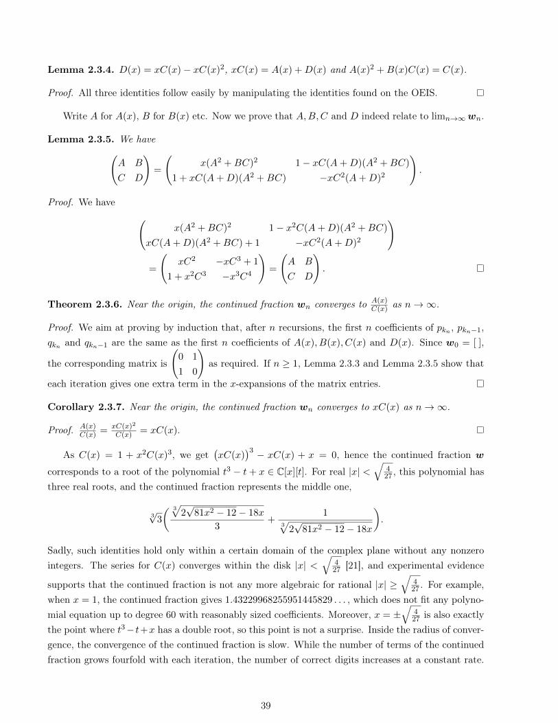
Lemma 2.3.4. D(x) = xC(x)− xC(x)2, xC(x) = A(x) +D(x) and A(x)2 +B(x)C(x) = C(x).

Proof. All three identities follow easily by manipulating the identities found on the OEIS.

Write A for A(x), B for B(x) etc. Now we prove that A,B,C and D indeed relate to limn→∞wn.

Lemma 2.3.5. We have(A B

C D

)=

(x(A2 +BC)2 1− xC(A+D)(A2 +BC)

1 + xC(A+D)(A2 +BC) −xC2(A+D)2

).

Proof. We have (x(A2 +BC)2 1− x2C(A+D)(A2 +BC)

xC(A+D)(A2 +BC) + 1 −xC2(A+D)2

)

=

(xC2 −xC3 + 1

1 + x2C3 −x3C4

)=

(A B

C D

).

Theorem 2.3.6. Near the origin, the continued fraction wn converges to A(x)C(x) as n→∞.

Proof. We aim at proving by induction that, after n recursions, the first n coefficients of pkn , pkn−1,qkn and qkn−1 are the same as the first n coefficients of A(x), B(x), C(x) and D(x). Since w0 = [ ],

the corresponding matrix is

(0 1

1 0

)as required. If n ≥ 1, Lemma 2.3.3 and Lemma 2.3.5 show that

each iteration gives one extra term in the x-expansions of the matrix entries.

Corollary 2.3.7. Near the origin, the continued fraction wn converges to xC(x) as n→∞.

Proof. A(x)C(x) = xC(x)2

C(x) = xC(x).

As C(x) = 1 + x2C(x)3, we get(xC(x)

)3 − xC(x) + x = 0, hence the continued fraction w

corresponds to a root of the polynomial t3 − t+ x ∈ C[x][t]. For real |x| <√

427 , this polynomial has

three real roots, and the continued fraction represents the middle one,

3√

3

( 3√

2√

81x2 − 12− 18x

3+

13√

2√

81x2 − 12− 18x

).

Sadly, such identities hold only within a certain domain of the complex plane without any nonzerointegers. The series for C(x) converges within the disk |x| <

√427 [21], and experimental evidence

supports that the continued fraction is not any more algebraic for rational |x| ≥√

427 . For example,

when x = 1, the continued fraction gives 1.43229968255951445829 . . . , which does not fit any polyno-mial equation up to degree 60 with reasonably sized coefficients. Moreover, x = ±

√427 is also exactly

the point where t3− t+x has a double root, so this point is not a surprise. Inside the radius of conver-gence, the convergence of the continued fraction is slow. While the number of terms of the continuedfraction grows fourfold with each iteration, the number of correct digits increases at a constant rate.

39

In particular, the example is a slowly converging folded continued fraction. In the domain |x| >√

427 ,

the continued fraction seems to be a smooth function with a power series expansion at infinity:

y−1(1 + y2 − y4 + y8 − 2y12 + 2y14 + y16 − 4y18 +O(y20)),

where y = x−1. The convergence towards this power series is fast: the number of correct coefficientsin the power series grows as quickly as the number of terms in the continued fraction. The foldingcurve of this recursion is boring: It is self-crossing, has many gaps and is less self-similar than thedragon curve or the curve for ρ as Figure 2.7 illustrates.

Figure 2.7: The folding curve of the cubic folded continued fraction starts purple and slowly fades tored following the colours of the rainbow. The left curve is drawn after 6 iterations and the right after8 iterations.

Many recursions of words relate to this cubic example. An alternative recursion, v0 = [ ] andvn = [vn−1, −←−−−vn−1, −←−−−vn−1, vn−1, x], gives the exact same cubic and power series A,B,C and D asintroduced earlier. Both converge to the same values within the disk |x| <

√427 , where the matrix

converges, but differ outside this disk. For example,

w(1) = 1.4322996825595144583 · · · = [1, 2, 3, 5, 5, 3, 5, 4, 2, 5, 3, . . . ];

v(1) = 0.60281150560716119896 · · · = [0, 1, 1, 1, 1, 13, 1, 1, 1, 2, 6, . . . ];

w(10) = 10.099000099980200960 · · · = [10, 10, 9, 1, 9, 9, 1, 9, 10, 9, 1, . . . ];

v(10) = 9.9009999000199950014 · · · = [9, 1, 9, 9, 1, 9, 9, 1, 9, 9, 1, . . . ].

The general pattern of w and v also differ wildly as can be seen in Figures 2.7 and 2.8.

40

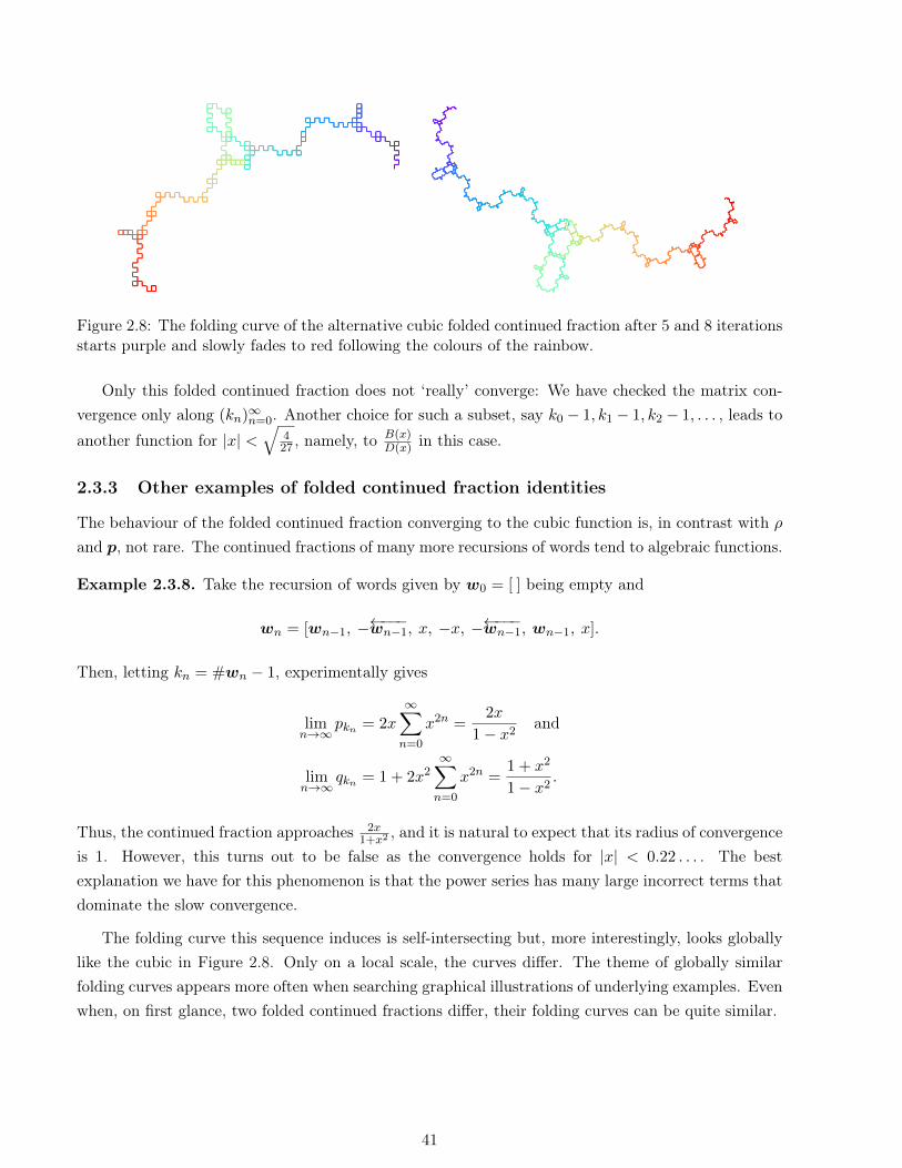
Figure 2.8: The folding curve of the alternative cubic folded continued fraction after 5 and 8 iterationsstarts purple and slowly fades to red following the colours of the rainbow.

Only this folded continued fraction does not ‘really’ converge: We have checked the matrix con-vergence only along (kn)∞n=0. Another choice for such a subset, say k0 − 1, k1 − 1, k2 − 1, . . . , leads to

another function for |x| <√

427 , namely, to B(x)

D(x) in this case.

2.3.3 Other examples of folded continued fraction identities

The behaviour of the folded continued fraction converging to the cubic function is, in contrast with ρand p, not rare. The continued fractions of many more recursions of words tend to algebraic functions.

Example 2.3.8. Take the recursion of words given by w0 = [ ] being empty and

wn = [wn−1, −←−−−wn−1, x, −x, −←−−−wn−1, wn−1, x].

Then, letting kn = #wn − 1, experimentally gives

limn→∞

pkn = 2x∞∑n=0

x2n =2x

1− x2and

limn→∞

qkn = 1 + 2x2∞∑n=0

x2n =1 + x2

1− x2.

Thus, the continued fraction approaches 2x1+x2

, and it is natural to expect that its radius of convergenceis 1. However, this turns out to be false as the convergence holds for |x| < 0.22 . . . . The bestexplanation we have for this phenomenon is that the power series has many large incorrect terms thatdominate the slow convergence.

The folding curve this sequence induces is self-intersecting but, more interestingly, looks globallylike the cubic in Figure 2.8. Only on a local scale, the curves differ. The theme of globally similarfolding curves appears more often when searching graphical illustrations of underlying examples. Evenwhen, on first glance, two folded continued fractions differ, their folding curves can be quite similar.

41

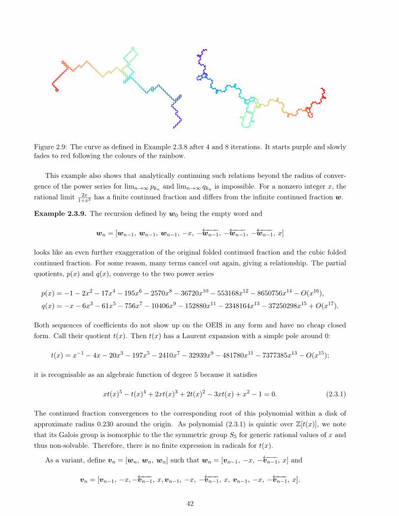
Figure 2.9: The curve as defined in Example 2.3.8 after 4 and 8 iterations. It starts purple and slowlyfades to red following the colours of the rainbow.

This example also shows that analytically continuing such relations beyond the radius of conver-gence of the power series for limn→∞ pkn and limn→∞ qkn is impossible. For a nonzero integer x, therational limit 2x

1+x2has a finite continued fraction and differs from the infinite continued fraction w.

Example 2.3.9. The recursion defined by w0 being the empty word and

wn = [wn−1, wn−1, wn−1, −x, −←−−−wn−1, −←−−−wn−1, −←−−−wn−1, x]

looks like an even further exaggeration of the original folded continued fraction and the cubic foldedcontinued fraction. For some reason, many terms cancel out again, giving a relationship. The partialquotients, p(x) and q(x), converge to the two power series

p(x) = −1− 2x2 − 17x4 − 195x6 − 2570x8 − 36720x10 − 553168x12 − 8650756x14 −O(x16),

q(x) = −x− 6x3 − 61x5 − 756x7 − 10406x9 − 152880x11 − 2348164x13 − 37250298x15 +O(x17).

Both sequences of coefficients do not show up on the OEIS in any form and have no cheap closedform. Call their quotient t(x). Then t(x) has a Laurent expansion with a simple pole around 0:

t(x) = x−1 − 4x− 20x3 − 197x5 − 2410x7 − 32939x9 − 481780x11 − 7377385x13 −O(x15);

it is recognisable as an algebraic function of degree 5 because it satisfies

xt(x)5 − t(x)4 + 2xt(x)3 + 2t(x)2 − 3xt(x) + x2 − 1 = 0. (2.3.1)

The continued fraction convergences to the corresponding root of this polynomial within a disk ofapproximate radius 0.230 around the origin. As polynomial (2.3.1) is quintic over Z[t(x)], we notethat its Galois group is isomorphic to the the symmetric group S5 for generic rational values of x andthus non-solvable. Therefore, there is no finite expression in radicals for t(x).

As a variant, define vn = [wn, wn, wn] such that wn = [vn−1, −x, −←−−−vn−1, x] and

vn = [vn−1, −x,−←−−−vn−1, x,vn−1, −x, −←−−−vn−1, x, vn−1, −x, −←−−−vn−1, x].

42

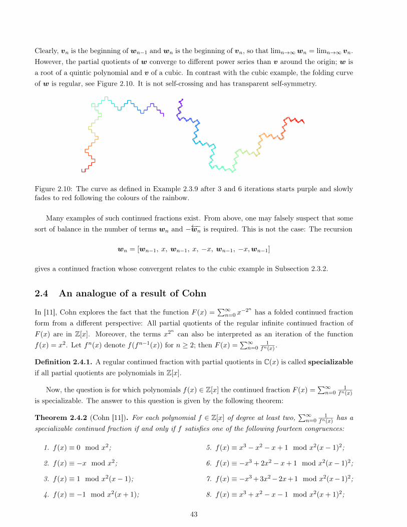
Clearly, vn is the beginning of wn−1 and wn is the beginning of vn, so that limn→∞wn = limn→∞ vn.However, the partial quotients of w converge to different power series than v around the origin; w isa root of a quintic polynomial and v of a cubic. In contrast with the cubic example, the folding curveof w is regular, see Figure 2.10. It is not self-crossing and has transparent self-symmetry.

Figure 2.10: The curve as defined in Example 2.3.9 after 3 and 6 iterations starts purple and slowlyfades to red following the colours of the rainbow.

Many examples of such continued fractions exist. From above, one may falsely suspect that somesort of balance in the number of terms wn and −←−wn is required. This is not the case: The recursion

wn = [wn−1, x, wn−1, x, −x, wn−1, −x,wn−1]

gives a continued fraction whose convergent relates to the cubic example in Subsection 2.3.2.

2.4 An analogue of a result of Cohn

In [11], Cohn explores the fact that the function F (x) =∑∞

n=0 x−2n has a folded continued fraction

form from a different perspective: All partial quotients of the regular infinite continued fraction ofF (x) are in Z[x]. Moreover, the terms x2n can also be interpreted as an iteration of the functionf(x) = x2. Let fn(x) denote f(fn−1(x)) for n ≥ 2; then F (x) =

∑∞n=0

1fn(x) .

Definition 2.4.1. A regular continued fraction with partial quotients in C(x) is called specializableif all partial quotients are polynomials in Z[x].

Now, the question is for which polynomials f(x) ∈ Z[x] the continued fraction F (x) =∑∞

n=01

fn(x)

is specializable. The answer to this question is given by the following theorem:

Theorem 2.4.2 (Cohn [11]). For each polynomial f ∈ Z[x] of degree at least two,∑∞

n=01

fn(x) has aspecializable continued fraction if and only if f satisfies one of the following fourteen congruences:

1. f(x) ≡ 0 mod x2;

2. f(x) ≡ −x mod x2;

3. f(x) ≡ 1 mod x2(x− 1);

4. f(x) ≡ −1 mod x2(x+ 1);

5. f(x) ≡ x3 − x2 − x+ 1 mod x2(x− 1)2;

6. f(x) ≡ −x3 + 2x2 − x+ 1 mod x2(x− 1)2;

7. f(x) ≡ −x3 + 3x2− 2x+ 1 mod x2(x− 1)2;

8. f(x) ≡ x3 + x2 − x− 1 mod x2(x+ 1)2;

43

9. f(x) ≡ −x3 − 2x2 − x− 1 mod x2(x+ 1)2;

10. f(x) ≡ −x3− 3x2− 2x− 1 mod x2(x+ 1)2;

11. f(x) ≡ x2 − x+ 1 mod x2(x− 1)2;

12. f(x) ≡ x2 − 2x+ 1 mod x2(x− 1)2;

13. f(x) ≡ −x2 − x− 1 mod x2(x+ 1)2;

14. f(x) ≡ −x2 − 2x− 1 mod x2(x+ 1)2.

Because ρn(x) is 1+x

1+f(x)

1+f2(x)

1+ · · ·+

fn(x)

1with f(x) = x2, ρ is specializable by Theorem

2.2.4. This motivates asking Cohn’s question for an irregular continued fraction shape of F (x).

Observation 2.4.3. Let f be a polynomial in Z[x] of degree at least two. Then the irregular continued

fraction x+f(x)

1+f2(x)

1+ · · ·+

fn(x)

1has a specializable continued fraction for all n ≥ 0 if f satisfies

one of the following conditions:

1. f(x) ≡ 0 mod x2;

2. f(x) ≡ −1 mod x(x+ 1);

3. f(x) ≡ −x− 1 mod x(x+ 1);

4. f(x) = x2 − 2.

The observation, in contrast with Theorem 2.4.2, does not contain not an ‘if and only if’ condition.For some polynomials, a large iteration for n is needed to discard them, and those that remain do notbelong to obvious classes. A naive computation requires dealing with polynomials of degree (deg f)n,so even testing n = 10 is hard for polynomials of degree 4. All polynomials that may producespecializable continued fractions are −x−2 mod 2x(x+ 2), −2x−2 mod 2x(x+ 2), or −x mod x2.

The continued fraction for f = x2 − 2 is quite remarkable. It appears to be the only polynomialof degree at least 2 and not a multiple of x2 such that the corresponding regular continued fraction isspecializable with partial quotients equal to linear polynomials. Like ρ, it has two limits. These are

[1 + x, −x, x, −x, x, −x, . . . ] and [1, −x, x, −x, x, −x, . . . ].

Save for the first terms, the partial quotients alternate between x and −x. Thus, both parity partiallimits of the continued fraction are quadratic elements of Q[x]. Due to these results, iterating polyno-mials is natural in combination with folded continued fractions. To strengthen this claim, we study aspecial class of recursions of words.

Definition 2.4.4. Let (wn)∞n=0 be a recursion of words defined by w0 = [ ] and the recursion

wn = [wn−1, ±x, −←−−−wn−1, ±x, wn−1, ±x, −←−−−wn−1, ±x, . . . , ±x, wn−1 or −←−−−wn−1],

where each sign is chosen independently and the parts wn−1 and −←−−−wn−1 alternate. Then (wn)∞n=0 iscalled special.

44

To understand why these special recursions are indeed special, we give a few examples wherekn = #wn − 1 and p and q denote pkn−1 and qkn−1 , respectively. For wn = [wn−1, x, −←−−−wn−1],

pkn = xp2 and qkn = xpq + 1.

For wn = [wn−1, x, −←−−−wn−1, x, wn−1],

pkn = p(−x2p2 + 1) and qkn = q(−x2p2 + 1) + xp.

For wn = [wn−1, x, −←−−−wn−1, x, wn−1, x, −←−−−wn−1],

pkn = p(x3p3 + 2xp) and qkn = q(x3p3 + 2xp) + x2p2 + 1.

For wn = [wn−1, x, −←−−−wn−1, x, wn−1, x, −←−−−wn−1, x, wn−1],

pkn = p(x4p4 − 3x2p2 + 1) and qkn = q(x4p4 − 3x2p2 + 1)− 3x3p3 + 2xp.

For wn = [wn−1, x, −←−−−wn−1, x, wn−1, x, −←−−−wn−1, x, wn−1, x, −←−−−wn−1],

pkn = p(x5p5 + 4x3p3 + 3xp) and qkn = q(x5p5 + 4x3p3 + 3xp) + x4p4 + 3x2p2 + 1.

Observe that the equation for pkn only contains p, and the equation for qkn only contains p and q andis linear in the latter. Furthermore, both pkn and qkn have a common term, which is a polynomial inx · p multiplied by p and q, respectively; pkn has no other terms while qkn has an extra term, which isa polynomial in x · p. These observations can be summarised as follows:

Observation 2.4.5. A recursion of words that only contains x,−x,wn−1,−wn−1,←−−−wn−1 and −←−−−wn−1

and satisfies w0 = [ ] gives a recursion for pkn only in terms of x and pkn−1 if and only if the recursionof words is special. Moreover, if the recursion of words is special, there are polynomials P,Q ∈ Z[y]

such that kn = #wn − 1, pkn = pkn−1P (xpkn−1) and qkn = qkn−1P (xpkn−1) + Q(xpkn−1) for n ≥ 0,p−1 = 0 and q−1 = 1.

Assuming the observation, the corresponding continued fraction is a sum of an iterated polynomial:

qknpkn

=qP (xp) +Q(xp)

pP (xp)=q

p+

Q(xp)

pP (xp)=qkn−1

pkn−1

+Q(xp)

pP (xp).

Hence the continued fraction can be written as

limn→∞

wn =(

limn→∞

qknpkn

)−1=

( ∞∑n=0

Q(xPn(1)

)Pn+1(1)

)−1,

where P (y) = yP (xy). For example, if wn = [wn−1, x,−←−−−wn−1, x,wn−1, x,−←−−−wn−1, x,wn−1], thenP (y) = x4y5−3x2y3 +y and Q(y) = −3y3 + 2y. As degP ≥ degQ, this sum converges for all |x| > 1.

Special folded continued fractions also have a very clear connection with real-life paper folding,like the paperfolding dragon. The paper is folded in a number of pieces equal to the number of

45

non-constant terms. The constant terms direct how the paper is folded.

Finally, when all ±x are chosen to be x, P and Q assume a simple form, save for perhaps signs.Coefficients of equal parity are either zero or of the form

(n−kk

)and

(n−k−1

k

), where n is the number

of non-constant terms in the recursion. For example, when there are n = 20 non-constant terms,

P (y) = y19 + 18y17 + 136y15 + 560y13 + 1365y11 + 2002y9 + 1716y7 + 792y5 + 165y3 + 10y,

Q(y) = y18 + 17y16 + 120y14 + 455y12 + 1001y10 + 1287y8 + 924y6 + 330y4 + 45y2 + 1.

The non-zero coefficients of P (y) and the coefficients of Q(y) correspond to(20−kk

)for k = 0, 1, . . . , 9

and(19−kk

)for k = 0, 1, . . . , 9, respectively. Such a connection could be established by induction, but

we will not do this in the current thesis.

2.5 Mahler functions, remarkable identities and Fibonacci numbers

We now move on to a somewhat different theme. Let Fn denote the nth Fibonacci number, Ln thenth Lucas number and φ ≈ 1.618 . . . the golden ratio. Then

F0 = 0, F1 = 1 and Fn = Fn−2 + Fn−1 for all n ≥ 2 and

L0 = 2, L1 = 1 and Ln = Ln−2 + Ln−1 for all n ≥ 2.

Binet’s formula is an elementary tool to work with Fibonacci and Lucas numbers.

Theorem 2.5.1 (Binet’s formula). For all n ≥ 0, Fn = φn−(−φ−1)n√5

and Ln = φn + (−φ)−n.

It implies that

F2n =

1 if n = 0

1−((φ−1)2

n)2

√5(φ−1)2n

if n ≥ 1,and L2n =

1 if n = 0

1+((φ−1)2

n)2

(φ−1)2nif n ≥ 1.

In 1974, I. J. Good [14] published a remarkable identity involving the Fibonacci numbers, namely

∞∑n=0

1

F2n=

7−√

5

2.

In particular, this is an algebraic number. Meanwhile, Becker and Töpfer [6] proved that∑∞

n=01

F2n+1is

transcendental and Nishioka [19] showed that the numbers∑∞

n=0

(1

F2n+1

)l for l ≥ 1 are all algebraicallyindependent of each other. The powers of 2 in the indices of the Fibonacci numbers already suggestthat Good’s identity has something to do with Mahler functions. Such identities have been fairlypopular, being cited dozens of times, and articles are still published about these sums four decadeslater. Good’s identity can be constructed in the following way: Let f(x) =

√5x

1−x2 . Then

√5

1− x=

√5

1− x2+ f(x) =

√5

1− x4+ f(x) + f(x2) =

√5

1− x8+ f(x) + f(x2) + f(x4) = · · · ,

46

and so √5

1− x= lim

n→∞

√5

1− x2n+

n−1∑m=0

f(x2

m)=√

5 +∞∑n=0

f(x2

n)if |x| < 1.

Evaluating∑∞

n=0 f(x2

n) at φ−1 gives the desired result using Binet’s formula.

More general, one finds these identities by choosing a k ≥ 2 and a rational function f(x). Bytaking g(x) := f(x)− f(xk), it follows from telescoping that f(x)− limn→∞ f

(xk

n)=∑∞

n=0 g(xk

n).If almost all of g(x), g(xk), g

(xk

2), . . . evaluate to a combination of Fibonacci and Lucas numbers by

Binet’s formula, and the limit and sum converge, a new identity is born.

Example 2.5.2. Let f(x) = 1√5(1+x2)

. Then g(x) = f(x) − f(x2) = x2(x2−1)√5(1+x2)(1+x4)

= x2−1x√5

x2

1+x4x

1+x2

can be evaluated at φ−1 to get the infinite sum

∞∑n=0

F2n

L2nL2n+1

=3√

5 + 5

30=

√5

10+

1

6.

This construction does not only work for sums. For example, defining g(x) via f(x) = g(x)f(xk)

leads to closed forms for infinite products, while extracting g(x) and h(x) from f(x) = g(x)f(xk)+h(x)

evaluates infinite sums of finite products. For the last mentioned type, both g(xk

n) and h(xkn) haveto assume nice forms using Binet’s formula for almost all n. We have the following example:

Example 2.5.3 (Example of [22]). Let k = 2, f(x) = 1 − x2 and g(x) = −x21−x4 . Then f(x) =

g(x)f(x2) + 1, implies that

f(x) =

∞∑n=0

n−1∏m=0

g(x2

m).

Using that φ−2n = −√

5F2n+1 , we evaluate at x = φ−1 to get

√5− 3

2= f(φ−1)− 1 =

∞∑n=0

1

g(φ−1)g(φ−2) · · · g(φ−2n−1

) − 1 =

∞∑n=1

1(−√

5)nF2F4 · · ·F2n

.

This construction uses an elementary technique and produces a short proof. Different methodswere used in [22]. Similarly, identities with irregular continued fractions can be constructed, whichseem to be not yet discovered. The set up is the following: Let f(x), g(x) and h(x) be rationalfunctions satisfying f(x) = g(x) + h(x)

f(x2). Then fix f(x) and one of g(x) and h(x), compute the other

of g(x) and h(x), and test whether Binet’s formula can be applied to g(xk

n) and h(xk

n) for almostall n. Any continued fraction with a unique limit then produces an identity.

For h(x) = 1, multiple rational functions appear as solutions, but they always seem to have twolimits, and the trick fails. For example, f(x) = x+1

x−1 and g = 2xx2−1 gives

limn→∞

2√5F1

+12√5F2

+12√5F4

+ · · ·+12√

5F2n−1

+12√5F2n

.

The 2√5F2n

is small, making 2√5F2n−1

+(

2√5F2n

)−1 large etc. Therefore, depending on the parity of thecontinued fraction, the result is larger or smaller than 1, hence, the convergence fails.

47

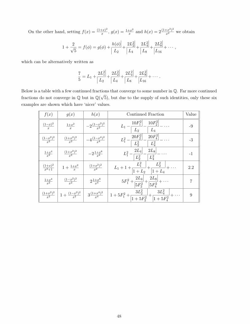
On the other hand, setting f(x) = (1+x)2

x , g(x) = 1+x2

x and h(x) = 2 (1+x2)2

x2we obtain

1 +2√5

= f(φ) = g(φ) +h(φ)

L2

+2L2

2

L4

+2L2

4

L8

+2L2

8

L16

+ · · · ,

which can be alternatively written as

7

5= L1 +

2L21

L2

+2L2

2

L4

+2L2

4

L8

+2L2

8

L16

+ · · · .

Below is a table with a few continued fractions that converge to some number in Q. Far more continuedfractions do not converge in Q but in Q(

√5), but due to the supply of such identities, only these six

examples are shown which have ‘nicer’ values.

f(x) g(x) h(x) Continued Fraction Value

(1−x)2x

1+x2

x −2 (1−x2)2x2

L1 −10F 2

1

L2

−10F 2

2

L4

− · · · -9

(1−x2)2x2

(1+x2)2

x2−4 (1−x4)2

x4L21 −

20F 22

L22

−20F 2

4

L24

− · · · -3

1+x4

x2(1+x2)2

x2−21+x8

x4L21 −

2L4

L22

−2L8

L24

− · · · -1

(1+x)2

x2+11 + 1+x2

x(1+x2)2

x2L1 + 1 +

L21

1 + L2

+L22

1 + L4

+ · · · 2.2

1+x4

x2(1−x2)2x2

21+x8

x45F 2

1 +2L4

5F 22

+2L8

5F 24

+ · · · 7

(1+x2)2

x21 + (1−x2)2

x23 (1+x4)2

x41 + 5F 2

1 +3L2

2

1 + 5F 22

+3L2

4

1 + 5F 24

+ · · · 9

48

Chapter 3

Hadamard products of Mahler functions

The space of k-Mahler functions is known to be closed under several operations, for example additionand multiplication. In this section, its closeness under another operation, the Hadamard product, isstudied. To do this efficiently, we show that the usual definition of a Mahler function can be weakened.Recall that Mahler function were assumed to be analytical and thus have a power series expansionaround the origin.

Theorem 3.0.1. The condition that A0(q)Ad(q) 6= 0 in the definition of a k-Mahler function f(q) ∈C[[q]] \ {0} (Definition 1.1.1) can be weakened to “not all Ai(q) are zero”.

Proof. Without loss of generality, Ad(q) can be assumed to be 0, and if A0(q) = 0, then by the newcondition, there is a smallest number 0 ≤ e < d such that Ae(q) 6= 0. As such, we have the equation

A(q) +Ae(q)f(qke) +Ae+1(q)f(qk

e+1) + · · ·+Ad(q)f(qk

d) = 0. (3.0.1)

Note that C[[q]] can be written as a direct sum of C[[qke]], qC[[qk

e]], . . . , qk

e−1C[[qke]]. As 0 6= f(q) ∈

C[[q]], f(qke) is in the first of these otherwise disjoint vector spaces and in none of the others, projecting

the Mahler equation (3.0.1) onto each of these vector spaces gives a new relation for f(q). As d isminimal, the relations are linearly independent, and hence, as (3.0.1) is another relation for f(q),all but one is zero. Let this sole projection be to qjC[[qk

e]] for a 0 ≤ j < ke. Then qj divides

the polynomial coefficients of the Mahler equation, and so by updating the relation by dividing therelation by qj , all new polynomial coefficients are in C[qk

e]. Evaluating the new equation in q

1ke gives

a usual k-Mahler equation.

Corollary 3.0.2. If f is analytic and dimC(q)(f(q), f(qk), f(qk2), . . . ) is finite, then f is Mahler.

Proof. By the assumption, there is an equation like (3.0.1), and so f is Mahler by Theorem 3.0.1.

This corollary enables us to show the space of k-Mahler functions is closed under several operations.

Example 3.0.3. That the space of k-Mahler functions is closed under addition, can be seen as follows.For a k-Mahler function f of degree df , the vector space C(q)[1, f(q), f(qk), f

(qk

2), . . . ] has dimension

49

at most df + 1. If g is a k-Mahler function of degree dg, then

dimC(q)(1, (f + g)(q), (f + g)(qk), (f + g)

(qk

2), . . .

)≤ dimC(q)

(1, f(q), f(qk), f

(qk

2), . . . , g(q), g(qk), g

(qk

2), . . .

)≤ df + dg + 1

is finite. Thus, f + g satisfies a k-Mahler equation by corollary 3.0.2.

Definition 3.0.4. The Hadamard product of two power series f(q) =∑∞

n=0 cnqn and g(q) =∑∞

n=0 dnqn in C[[q]] is defined as

∑∞n=0 cndnq

n and denoted by f ? g.

Several well-known subsets of C[[q]] are closed under the Hadamard product: the spaces of mono-mials, polynomials, rational functions [15, Theorem 7] and D-functions (functions that satisfy a lineardifferential equation with polynomial coefficients) [15, Theorem 9]. To the best of our knowledge,this question has not yet been answered for the entire space of k-Mahler functions, but Allouche andShallit proved it for a subspace of so-called k-regular functions [2]. This construction is studied inSubsection 3.1. To start, recall a simple observation:

Proposition 3.0.5. Let f(q) =∑∞

n=0 xnqn be a k-Mahler function that satisfies the k-Mahler equation

A(q) +A0(q)f(q) +A1(q)f(qk) + · · ·+Ad(q)f(qk

d)= 0

for some A(q), A0(q), . . . , Ad(q) ∈ C[q] with A0(q)Ad(q) 6= 0 and N = max(degA0(q), . . . ,degAd(q)).If Ai(q) =

∑Nj=0 ai,jq

j and n > degA, then we have

a0,0xn + · · ·+ a0,Nxn−N + a1,0xnk

+ · · ·+ a1,Nxn−Nk

+ · · ·+ ad,N + · · ·+ a1,Nxn−Nkd

= 0.

A rational function f(q) = r(q)s(q) is k-Mahler as s(q)f(q) − r(q) = 0. Moreover, the Hadamard

product is commutative, associative and distributive over addition. Its identity is the rational function1 + q + q2 + · · · = 1

1−q . Only, the Hadamard product of k-Mahler functions is not always k-Mahler.

Example 3.0.6. Let k = 2, f(q) = q+ q2 + q4 + q8 + . . . and g(q) = 11−2q = 1 + 2q+ 4q2 + 8q3 + · · · .

Then f satisfies f(q) = q + f(q2), so both are 2-Mahler. Their Hadamard product is

∞∑n=0

xnqn := (f ? g)(q) = 2q + 4q2 + 16q4 + 256q8 + · · ·+ 22

nq2n

+ · · · .

This means that

xn =

2n if n is a power of 2,

0 otherwise.

If f ? g is 2-Mahler, Proposition 3.0.5 gives a recursion for some N and d. If n is a large power of 2,0 ≤ i ≤ N and 0 ≤ j ≤ d, then n−i

2jis a power of 2 if and only if i = 0. Thus, for large m only a small

number of non zero terms remain, and the recursion becomes

a0,0x2m + a1,0x2m−1 + · · ·+ ad,0x2m−d = 0.

50

As such, the sequence (x2m)∞m=0 =(22m)∞

m=0satisfies a linear recursion while x2m

x2m−1= 22

m−1 tends toinfinity. A contradiction. Thus, f ? g is not 2-Mahler.

Any f(q) with arbitrary long sequences of zeros in its q-expansion does the job in Example 3.0.6,so F , G, H and I from Chapter 1 work as well. One could argue that 1

1−2q is not a ‘legitimate’ Mahlerfunction as it is not defined in the entire unit disk. However, examples without this drawback exist.

Example 3.0.7. If k ≥ 2, α is non-zero and not a root of unity, g(q) = 11−αq and f = q+qk+qk

2+ · · ·

satisfies f(q) = q + f(qk), then (f ? g)(q) = αq + αkqk + αk2qk

2+ · · · and the recursion

a0,0xkm + a1,0xkm−1 + · · ·+ ad,0xkm−d = 0.

is obtained as in Example 3.0.6 for large m. For such large m, αkm−d is a root of a0,0qkd

+ a1,0qkd−1

+

· · ·+ad,0 because xkm = αkm . As α is not a root of unity, all αkm−d differ from each other, giving that

the polynomial has an infinite number of roots and hence is the zero polynomial. Thus, the recursionis trivial and f ? g is not k-Mahler.

Not all numbers on the unit circle are roots of unity or transcendental. For example, Lehmer’spolynomial of degree 10 [17] has 8 roots on the unit circle that are not roots of unity. In general, theprojection of an algebraic number onto the unit circle is algebraic but often not a root of unity.

Meanwhile, there are many pairs Mahler whose Hadamard product is again Mahler.

Example 3.0.8. We call a k-Mahler function special if, as defined in Proposition 3.0.5, all Ai(q) = ai

are constant and A(q) =∑M

i=0 biqi with bi = 0 if i is not a kth power. Examples of special Mahler

functions are f in Example 3.0.6 and g(q) = q+ q2 + 2q4 + 3q8 + · · ·+Fn+1q2n + · · · , where Fn is the

nth Fibonacci number, which satisfies g(q) = g(q2) + g(q4) + q.

There is a natural bijection between the special k-Mahler functions and rational functions definedat q = 0 that preserves the Hadamard product: x1q + xkq

k + xk2qk2 + · · · 7→ x1 + xkq + xk2q

2 + · · · .Thus, the recursion for xn transforms into a linear recursion. As the rational functions are closedunder the Hadamard product [15, Theorem 7], the special k-Mahler functions are as well.

3.1 The space of k-regular functions

Much larger spaces of Mahler functions that are closed under the Hadamard product exist. In thissection, we study a space introduced by Allouche and Shallit [2] and Becker [5].

Definition 3.1.1. The k-kernel of a sequence (xn)∞n=0 is the set of all the subsequences of the form(xken+r)

∞n=0 where e ≥ 0 and 0 ≤ r ≤ ke − 1.

Definition 3.1.2. A sequence (xn)∞n=0 is called k-automatic if its k-kernel is finite and k-regularif its k-kernel is finitely generated.

Naturally, the definitions of k-automatic and k-regular sequences translate to their generatingfunctions. We give a few examples. The k-kernel of 1

1−q consists of one element: (1, 1, . . . ). So 11−q is

51

k-automatic and k-regular. Next, q(1−q)2 has a k-kernel generated by (1, 1, . . . ) and (0, 1, 2, . . . ) and

is k-regular but not k-automatic. Lastly, 11−2q is neither k-automatic nor k-regular. By [2, Theorem

2.10], the coefficients of a k-regular sequence have to grow polynomially.

More generally, a k-regular sequence is k-automatic if and only if it assumes a finite number ofvalues [2, Theorem 2.3]. Moreover, both the sum and Hadamard product of two k-regular sequencesare k-regular [2, Theorem 2.5]. There does not exist an easy characterisation of k-regular functions interms of k-Mahler functional equations, but at least there is a one-sided relationship.

Theorem 3.1.3 (Theorem 1 in [5]). A k-regular function satisfies a homogeneous k-Mahler equation.

The inclusion is strict, as f(q) = 11−2q demonstrates. It satisfies (1− 2q)f(q)− (1− 2q2)f(q2) = 0,

but it is not k-regular as noted above. Becker showed a partial inverse:

Definition 3.1.4. A k-Mahler function as in Proposition 3.0.5 with A(q) = 0 (so homogeneous) andA0(q) = 1 is called a k-Becker function or k-Becker for short.

Theorem 3.1.5 (Theorem 2 in [5]). A k-Becker function is k-regular.

Again, the inclusion is strict. Take f(q) = q, which is k-regular. If f was k-Becker, the linear termof Ai(q)f

(qk

i)= Ai(q)q

ki would be zero and A0(q)f(q) = q would not cancel out in the Mahler equa-tion. An inhomogeneous k-Becker function is a not necessarily homogeneous k-Becker function.

Proposition 3.1.6. An inhomogeneous k-Becker function is k-regular.

Proof. Let f be an inhomogeneous k-Becker function that satisfies the Mahler functional equation

f(q) +A1(q)f(qk) +A2(q)f(qk

2)+ · · ·+Ad(q)f

(qk

d)+A(q) = 0

for some polynomials A1, A2, . . . , Ad, A ∈ C[q] and Ad 6= 0. If A(q) = 0, we are done by Theorem3.1.5. Recall that polynomials are k-regular, and that the space of k-regular sequences is closedunder addition and multiplication [2, Theorem 3.1]. Our goal is to prove that f is a sum of k-regularfunctions and thus k-regular with several reductions.

Step 1. If e = degA and A(q) =∑e

n=0 anqn, there are Mahler functions g0(q), . . . , ga(q) such that

g0(q) +A1(q)g0(qk) +A2(q)g0

(qk

2)+ · · ·+Ad(q)g0

(qk

d)+ a0 = 0

......

ge(q) +A1(q)ge(qk) +A2(q)ge

(qk

2)+ · · ·+Ad(q)ge

(qk

d)+ an = 0

and f(q) =∑

n=0 ge(q), and so, without loss of generality, A(q) can be assumed to be a monomial.Step 2. If A(q) = cqn is a monomial for some c ∈ C \ {0} and n ≥ 0, then

q−nf(q) + q−nA1(q)f(qk) + q−nA2(q)f(qk

2)+ · · ·+ q−nAd(q)f

(qk

d)+ c = 0.

Now A(q) can be assumed to be constant due to the map f(q) to g(q) := f(q)qn which gives

g(q) + qnk−nA1(q)g(qk) + qnk2−nA2(q)f

(qk

2)+ · · ·+ qnk

d−nAd(q)f(qk

d)+ c = 0.

52

Step 3. Assume that A(q) = c, a non-zero constant. Then

f(q) +A1(q)f(qk) +A2f(qk

2)+ · · ·+Adf

(qk

d)+ c = 0 and

f(qk) +A1(qk)f(qk

2)+A2(q

k)f(qk

3)+ · · ·+Ad(q

k)f(qk

d+1)+ c = 0.

Subtracting these two equations gives a homogeneous equation for f . This completes the reduction.

Thus, an inhomogeneous k-Becker function can be written as a sum of homogeneous k-Beckerfunctions scaled by powers of q. If n ≥ 1 and f k-Becker, then f is k-regular by Theorem 3.1.5. As qn

is a polynomial, it is k-regular, and so their product qnf(q) is k-regular. This completes the proof.

Again, this characterisation is incomplete. Take P (q) as introduced in Subsection 2.2.4. It satisfies(1 + q2)P (q) = (q + q3)P (q2) + 1 and is 2-automatic by Theorem 6.5.4 of [3] and thus k-regular, butit is unclear whether P (q) is (inhomogeneous) k-Becker.

3.2 Complete Hadamard functions

The identity function with respect to the Hadamard product is 11−q , so the Hadamard product of any

k-Mahler function and 11−q is again k-Mahler. Such functions are quite rare. We name them:

Definition 3.2.1. A complete Hadamard function is a function f(q) ∈ C[[q]] such that theHadamard product of f and every k-Mahler function is k-Mahler.

Simple examples of complete Hadamard functions are polynomials as their Hadamard productwith a power series is again a polynomial. In this section, an elegant classification of the rationalfunctions with this property is given.

Theorem 3.2.2. A rational function f(q) = r(q)s(q) with r, s ∈ C[q] coprime and s(0) 6= 0 is complete

Hadamard if and only if all roots of s(q) are roots of unity.

Note that the condition s(0) 6= 0 implies that f has a power series expansion. To start, we give afew basic observations on complete Hadamard functions:

Lemma 3.2.3. Let f(q) be complete Hadamard and A ∈ C[q]. Then

1. f(q) is k-Mahler;

2. The space of complete Hadamard functions forms a ring with multiplication being defined theHadamard product and the multiplicative identity being 1

1−q .

3. A(q)f(q) is complete Hadamard.

Proof. Let h(q) be k-Mahler.

1. f(q) = f(q) ? 11−q is k-Mahler.

53

2. Let g(q) be complete Hadamard. The space of complete Hadamard functions is closed underboth addition and the Hadamard product. Then (f + g) ? h = f ? h + g ? h is the sum of twok-Mahler functions and thus k-Mahler. As g is complete Hadamard, g?h is k-Mahler, and hencef ? (g ? h) = (f ? g) ? h as well. The other axioms follow trivially.

3. If α ∈ C, (αf) ? h = α(f ? h) is also k-Mahler, and thus αf(q) is complete Hadamard. Ifh(q) := h(q)−h(0)

q , h(q) is Mahler and analytic. Then

(qf) ? (h) = (qf) ? (g(0) + qh) = (qf) ? (g(0)) + (qf) ? (qh) = 0 + q(f ? h)

is k-Mahler, and thus qf(q) is complete Hadamard. As the ring of complete Hadamard functionsis closed under addition, iterating these two facts gives that A(q)f(q) is complete Hadamard.

A more involved complete Hadamard function is 1(1−q)n for every n ≥ 0.

Lemma 3.2.4. The derivative f ′(q) of a k-Mahler function f is k-Mahler.

Proof. Differentiating the k-Mahler equation of f gives

A′(q) +A′0(q)f(q) +A0(q)f′(q) + · · ·+A′d(q)f

(qk

d)+Ad(q)k

dqkd−1f ′

(qk

d)= 0.

Thus, dimC(q)(1, f(q), f ′(q), f(qk), f ′(qk), f(qk

2), f ′(qk

2), . . . ) ≤ 2d + 2, and so f ′(q) is k-Mahler by

Corollary 3.0.2 as dimC(q)(1, f′(q), f ′(qk), . . . ) is finite.

Lemma 3.2.5. The derivative of a complete Hadamard function is complete Hadamard.

Proof. Let f(q) =∑∞

n=0 anqn be complete Hadamard and g(q) =

∑∞n=0 bnq

n be k-Mahler. Then

f ′(q) ? g(q) =( ∞∑n=0

(n+ 1)an+1qn)?( ∞∑n=0

bnqn)

=

∞∑n=0

(n+ 1)an+1bnqn =

d

dq(f(q) ? qg(q))

is k-Mahler by applying Lemmas 3.2.3 and 3.2.4.

Lemma 3.2.6. For all n ≥ 0, 1(1−q)n is complete Hadamard.

Proof. As 11−q is complete Hadamard, its (n− 1)st derivative (n−1)!

(1−q)n is as well by Lemma 3.2.5.

Now Theorem 3.2.2 can be proven. First, one direction:

Proposition 3.2.7. Let r(q) and s(q) be coprime polynomials and f(q) = r(q)s(q) such that s(0) 6= 0 and

s has a root α that is not a root of unity. Then f(q) is not complete Hadamard.

Proof. If f(q) were complete Hadamard, then p(q)1−α−1q

:= f(q) s(q)1−α−1q

would be complete Hadamard

by Lemma 3.2.3 and as s(q)1−α−1q

is a polynomial. Write

p(q)

1− α−1q=

p(α−1)

1− α−1+ u(q) = p(α−1)

∞∑n=0

α−nqn + u(q)

54

for some polynomial u(q). Thus, like in Example 3.0.7, the Hadamard product of∑∞

n=0 p(α−1)αnqn

with g(q) satisfying g(q) = g(qk)+ q gives rise to a linear recurrence and a polynomial with an infinitenumber of roots. Thus f ? g is not Mahler and f(q) cannot be complete Hadamard.

And the other way around:

Lemma 3.2.8. For all m ≥ 1, 11−qm is complete Hadamard.

Proof. Assume that g(q) =∑∞

n=0 cnqn is k-Mahler. Then

1

1− qm? g(q) =

∞∑n=0

m∑i=0

ζimαnqn =

m∑i=0

g(ζimq).

Thus, as for all 0 ≤ i ≤ m

dimC(q)(1, g(ζimq), g((ζim)kqk), g((ζim)k

2qk

2), . . .

)is finite, {g(ζimq

kj ) : i, j ≥ 0} is finitely generated. Now Corollary 3.0.2 gives that 11−qm ? g(q) is

k-Mahler and thus the proposition.

Proposition 3.2.9. Let r(q) and s(q) be coprime polynomials and f(q) = r(q)s(q) such that all roots of

s are roots of unity. Then f is complete Hadamard.

Proof. If all roots of s(q) are roots of unity, let m be the least common multiple of these orders. Thens(q) divides (1− qm)l for some l ≥ 1. If l = 1, then this case has been treated in the proof of Lemma3.2.8. If l > 1 and g is k-Mahler, then 1

1−qm ? g has a k-Mahler equation and its coefficients follow arecursion by Proposition 3.0.5. As only the coefficients xn−i

kjmatter when i is a multiple of m, it is

seen that all Ai(q) and A(q) are polynomials in C[qm]. Then ( 11−qm ? g)(q

1m ) is also k-Mahler and

(1

(1− qm)l? g

)(q) =

(((1

1− qm? g

)(q

1m )

)?

1

(1− q)l

)(qm)

is k-Mahler, and thus 1(1−qm)l

is complete Hadamard. Thus, r(q)s(q) = r(q)

(1−qm)l(1−qm)l

s(q) is complete

Hadamard by Lemma 3.2.3 as (1−qm)l

s(q) is a polynomial by construction.

Proof of Theorem 3.2.2. Combine Propositions 3.2.7 and 3.2.9.

The natural follow-up question is whether there are irrational complete Hadamard functions, buttheir existence is highly dubious.

55

Bibliography

[1] Boris Adamczewski. Non-converging continued fractions related to the Stern diatomic sequence.Acta Arith, 142(1):67–78, 2010.

[2] Jean-Paul Allouche and Jeffrey Shallit. The ring of k-regular sequences. Theoretical ComputerScience, 98(2):163–197, 1992.

[3] Jean-Paul Allouche and Jeffrey Shallit. Automatic sequences: theory, applications, generaliza-tions. Cambridge university press, 2003.

[4] Leonard E. Baum and Melvin M. Sweet. Continued fractions of algebraic power series in charac-teristic 2. Annals of Mathematics, 103(3):593–610, 1976.

[5] Paul-Georg Becker. k-regular power series and Mahler-type functional equations. Journal ofNumber Theory, 49(3):269–286, 1994.

[6] Paul-Georg Becker and Thomas Töpfer. Transcendency results for sums of reciprocals of linearrecurrences. Mathematische Nachrichten, 168(1):5–17, 1994.

[7] Jonathan Borwein, Alf van der Poorten, Jeffrey Shallit, and Wadim Zudilin. Neverending frac-tions: an introduction to continued fractions, volume 23. Cambridge University Press, 2014.

[8] Wieb Bosma, John Cannon, and Catherine Playoust. The Magma algebra system. I. The userlanguage. J. Symbolic Comput., 24(3-4):235–265, 1997. Computational algebra and numbertheory (London, 1993).

[9] Richard P. Brent, Michael Coons, and Wadim Zudilin. Algebraic independence of Mahler func-tions via radial asymptotics. International Mathematics Research Notices, 2016(2):571–603, 2016.

[10] Peter Bundschuh and Keijo Väänänen. Transcendence results on the generating functions of thecharacteristic functions of certain self-generating sets, II. Acta Arithmetica, 3(167):239–249, 2015.

[11] Henry Cohn. Symmetry and specializability in continued fractions. Acta Arithmetica, 75(4):297–320, 1996.

[12] Karl Dilcher and Kenneth B. Stolarsky. Stern polynomials and double-limit continued fractions.Acta Arithmetica, 140(2):119–134, 2009.

[13] Michel Mendès France and Alfred Jacobus van der Poorten. Arithmetic and analytic propertiesof paper folding sequences. Bulletin of the Australian Mathematical Society, 24(1):123–131, 1981.

56

[14] I.J. Good. A reciprocal series of Fibonacci numbers. The Fibonacci Quarterly, 12(4):346, 1974.

[15] Reinwald Jungen. Sur les séries de Taylor n’ayant que des singularités algébrico-logarithmiquessur leur cercle de convergence. Commentarii Mathematici Helvetici, 3(1):266–306, 1931.

[16] Serge Lang. Complex analysis, volume 103. Springer Science & Business Media, 2013.

[17] Derrick H. Lehmer. Factorization of certain cyclotomic functions. Annals of mathematics,34(3):461–479, 1933.

[18] Kumiko Nishioka. New approach in Mahler’s method. Journal für die Reine und AngewandteMathematik, 407:202–219, 1990.

[19] Kumiko Nishioka. Algebraic independence of reciprocal sums of binary recurrences. Monatsheftefür Mathematik, 123(2):135–148, 1997.

[20] Kumiko Nishioka. Mahler functions and transcendence. Springer, 2006.

[21] OEIS Foundation Inc. The On-Line Encyclopedia of Integer Sequences, 2020. http://oeis.org.

[22] Hideyuki Ohtsuka. Advanced problem H-778: Finding the sum of a reciprocal of products ofFibonacci numbers. The Fibonacci Quarterly, 53(4):372, 2015.

[23] Alfred Jacobus van der Poorten and Jeffrey Shallit. Folded continued fractions. Journal ofNumber Theory, 40(2):237–250, 1992.

[24] Jeffrey Shallit. Simple continued fractions for some irrational numbers. Journal of NumberTheory, 11(2):209–217, 1979.

[25] Peter Stevenhagen. Number rings. Mastermath course, Leiden University, 2019. http:

//websites.math.leidenuniv.nl/algebra/ant.pdf.

[26] Sergei Tabachnikov. Dragon curves revisited. The Mathematical Intelligencer, 36(1):13–17, 2014.

[27] Wikipedia contributors. Baum–Sweet sequence — Wikipedia, the free encyclopedia, 2020. [On-line; accessed 29-October-2020].

57