Published in ASCE Journal of Hydrologic Engineering, 2015 1 FRACTIONAL ENSEMBLE AVERAGE GOVERNING EQUATIONS OF TRANSPORT 1 BY TIME-SPACE NONSTATIONARY STOCHASTIC FRACTIONAL ADVECTIVE 2 VELOCITY AND FRACTIONAL DISPERSION: THEORY 3 M.L.Kavvas 1 F.ASCE, S.Kim 2 , A. Ercan 3 , M.ASCE 4 1 Distinguished Professor, Hydrologic Research Laboratory, and J.Amorocho Hydraulics 5 Laboratory, Department of Civil & Environmental Engineering, University of California, Davis, 6 CA 95616, [email protected] 7 2 Associate Professor, Department of Environmental Engineering, Pukyong National University, 8 South Korea, [email protected] 9 3 Assistant Project Scientist, J.Amorocho Hydraulics Laboratory, Department of Civil & 10 Environmental Engineering, University of California, Davis, CA 95616, [email protected] 11 12 ABSTRACT 13 In this study, starting from a time-space nonstationary general random walk formulation, the 14 pure advection and advection-dispersion forms of the fractional ensemble average governing 15 equations of solute transport by time-space nonstationary stochastic flow fields were developed. 16 In the case of the purely advective fractional ensemble average equation of transport, the 17 advection coefficient is a fractional ensemble average advective flow velocity in fractional time 18 and space that is dependent on both space and time. As such, in this case the time space- 19 nonstationarity of the stochastic advective flow velocity is directly reflected in terms of its mean 20 behavior in the fractional ensemble average transport equation. In fact, the derived purely 21 advective form represents the Lagrangian derivation of the ensemble average mass conservation 22

Welcome message from author
This document is posted to help you gain knowledge. Please leave a comment to let me know what you think about it! Share it to your friends and learn new things together.
Transcript

Published in ASCE Journal of Hydrologic Engineering, 2015
1
FRACTIONAL ENSEMBLE AVERAGE GOVERNING EQUATIONS OF TRANSPORT 1
BY TIME-SPACE NONSTATIONARY STOCHASTIC FRACTIONAL ADVECTIVE 2
VELOCITY AND FRACTIONAL DISPERSION: THEORY 3
M.L.Kavvas1 F.ASCE, S.Kim
2, A. Ercan
3, M.ASCE 4
1 Distinguished Professor, Hydrologic Research Laboratory, and J.Amorocho Hydraulics 5
Laboratory, Department of Civil & Environmental Engineering, University of California, Davis, 6
CA 95616, [email protected] 7
2Associate Professor, Department of Environmental Engineering, Pukyong National University, 8
South Korea, [email protected] 9
3Assistant Project Scientist, J.Amorocho Hydraulics Laboratory, Department of Civil & 10
Environmental Engineering, University of California, Davis, CA 95616, [email protected] 11
12
ABSTRACT 13
In this study, starting from a time-space nonstationary general random walk formulation, the 14
pure advection and advection-dispersion forms of the fractional ensemble average governing 15
equations of solute transport by time-space nonstationary stochastic flow fields were developed. 16
In the case of the purely advective fractional ensemble average equation of transport, the 17
advection coefficient is a fractional ensemble average advective flow velocity in fractional time 18
and space that is dependent on both space and time. As such, in this case the time space-19
nonstationarity of the stochastic advective flow velocity is directly reflected in terms of its mean 20
behavior in the fractional ensemble average transport equation. In fact, the derived purely 21
advective form represents the Lagrangian derivation of the ensemble average mass conservation 22

Published in ASCE Journal of Hydrologic Engineering, 2015
2
equation for solute transport in fractional time-space. In the case of the fractional ensemble 1
average advection-dispersion transport equation, the moment and cumulant forms of the equation 2
are derived separately. In the moment form of the fractional ensemble average advection-3
dispersion equation of transport, the advection coefficient emerges as a combination of the 4
fractional ensemble average advective flow velocity in fractional time and space with an 5
advective term that is due to dispersion. The fractional dispersion coefficient emerges as a 2- 6
moment of the differential displacement per scaled differential time where and denote, 7
respectively, the fractional orders of the space and time derivatives. Since this fractional 8
dispersion coefficient is in moment form, the corresponding ensemble average equation is a 9
moment form of the fractional ensemble average advection-dispersion equation. The cumulant 10
form of the fractional ensemble average advection-dispersion transport equation is derived for 11
two different cases: (i) when the order of the space fractional derivative of the advective term is 12
the same as that of the time derivative while the order of the space fractional derivative of the 13
dispersion term is twice that of the time derivative, and (ii) when the orders of the time and space 14
fractional derivatives are completely different. In case (i) the advection coefficient emerges as a 15
combination of the fractional ensemble average advective flow velocity with an advective term 16
that is due to dispersion, while the cumulant form of the dispersion coefficient emerges as a 17
time-space-dependent variance of the -moment of the differential displacement per scaled time 18
differential , resulting in a fractional advection-dispersion equation. In case (ii) when the 19
orders of the time and space derivatives are completely different, the cumulant form of the 20
fractional dispersion coefficient emerges as a combination of the moment form of the fractional 21
dispersion coefficient and the square of a fractional ensemble average advective velocity. The 22
derived fractional ensemble average governing equations of transport are rich in structure that 23

Published in ASCE Journal of Hydrologic Engineering, 2015
3
can accommodate both the non-Fickian and the Fickian behavior of transport. The non-Fickian 1
transport behavior can be modeled by the derived fractional ensemble average transport 2
equations either by means of the long memory in the underlying stochastic flow, or by means of 3
the time-space nonstationarity of the underlying stochastic flow, or by means of the time and 4
space fractional derivatives of the transport equations. 5
Key Words: fractional Ensemble Average Transport Equation, nonstationary stochastic flow 6
7
INTRODUCTION 8
From the works of Taylor (1922; 1954) and Batchelor (1949) the dispersion coefficient (or 9
turbulent mixing coefficient) for the transport of a solute by a time-space stationary stochastic 10
advective velocity field v[xt, t], where xt is the Lagrangian location of a solute particle at time t 11
in one dimension, may be expressed as (see also Kavvas and Karakas, 1996, 1997), 12
13
, (1) 14
where < v > is the constant ensemble mean of v and Var (v) is the finite constant variance of the 15
time-space stationary stochastic advective velocity v ( ), and Cov denotes the covariance function 16
while Rv denotes the autocorrelation function of the stochastic advective velocity v ( ). The 17
integral on the right-hand-side of (1) becomes the correlation time of the stochastic advective 18
velocity for t = . Under the further assumption of finite correlation time (finite memory) for the 19
stochastic advective velocity, one would then end up with a finite constant value for the 20

Published in ASCE Journal of Hydrologic Engineering, 2015
4
dispersion coefficient for times beyond the correlation time of the advective velocity. That is, for 1
times beyond the correlation time of v( ), 2
, (2) 3
where D is a finite constant in time and space. Within this framework, one can then define a 4
constant dispersion coefficient D for transport of solutes. From Eqns. (1) and (2) it also follows 5
that for times beyond the correlation time of a time-space stationary, finite memory stochastic 6
advective velocity, the variance of the Lagrangian displacement of the solute in a time interval 7
(0,t) becomes proportional to time t. That is, 8
2Dt (3) 9
The behavior of solute transport, as described by Eqns. (2) and (3) is known as “Fickian 10
transport”. This Fickian framework provided the basis for the advection-dispersion equation with 11
a constant dispersion coefficient in transport modeling studies in 1970s and 1980s (Fischer et 12
al.1979; Orlob, 1983 among others). 13
However, various studies of the field data for solute transport in rivers ( Nordin and Sabol, 1974; 14
Nordin and Troutman, 1980; Johnson, 2001) have shown significant deviations from the Fickian 15
behavior. Various laboratory (Silliman and Simpson, 1987; Levy and Berkowitz, 2003) and field 16
studies (Peaudecerf and Sauty, 1978; Sudicky et al., 1983; Sidle et al., 1998) of transport in 17
subsurface porous media have similarly shown significant non-Fickian behavior. As one 18
approach to the modeling of the generally non-Fickian behavior of transport, Meerschaert, 19
Benson, Baumer, Schumer, Zhang and their co-workers (Meerschaert et al. 1999, 2002, 2006; 20
Benson et al. 2000a,b; Baumer et al. 2005, 2007; Schumer et al. 2001, 2009; Zhang et al. 2007, 21

Published in ASCE Journal of Hydrologic Engineering, 2015
5
2008 and 2009) have introduced the fractional advection-dispersion equation (fADE) as a model 1
for transport in heterogeneous subsurface media, while Deng, Singh and their coworkers (Deng 2
et al. 2004; 2005; 2006a,b) and Kim and Kavvas (2006) have introduced the fADE as a model 3
for turbulent transport in surface waters. By theoretical, numerical and field studies the above 4
authors have shown that fADE has a nonlocal structure that can model well the heavy tailed non-5
Fickian dispersion both in subsurface media as well as in rivers and overland flows, mainly by 6
means of a fractional spatial derivative in the dispersion term of the equation. Meanwhile, they 7
have also shown that fADE, with a fractional time derivative, can also model well the long 8
particle waiting times in transport in both surface and subsurface environments. 9
Berkowitz et al. (2006) questioned the fADE model, mentioning that fADE places the 10
mechanism for non-Fickian behavior entirely on the fractional powers of the space and time 11
derivatives in the fADE. They also questioned fADE model’s ability to account for the evolution 12
to a Fickian regime. Neuman and Tartakovsky(2009) mentioned a lack of specific theoretical 13
framework that would lead to fADE equations, and questioned the physical meaning of the 14
fractional parameters in the fADE. They also questioned the flow field stationarity and no-15
correlation assumptions underlying the Continuous Time Random Walk (CTRW) model. 16
This study shall specifically address the above concerns of Berkowitz et al. (2006) and Neuman 17
and Tartakovsky (2009) on fADE by developing the moment and cumulant forms of the 18
ensemble average equations of transport by time-space nonstationary stochastic flow in 19
fractional time and space , starting from a general time-space nonstationary random walk 20
formulation, and deriving the fractional drift and fractional dispersion parameters of transport in 21
terms of the statistical properties of the underlying fractional stochastic flow. 22
Published in ASCE Journal of Hydrologic Engineering, 2015
6
Comprehensive derivations of the ensemble average advection-dispersion equation for 1
conservative and reactive solute transport by time-space nonstationary flow random fields in 2
integer time-space have been accomplished recently (Kavvas and Karakas, 1996 for conservative 3
transport; Kavvas, 2001 for reactive transport). In these derivations, the advective flow velocity 4
random field is nonstationary both in time and space, and there are no restrictions placed on the 5
distribution or the magnitude of variability of the flow velocity field. Not only Kavvas and 6
Karakas (1996) have obtained the ensemble average form of the stochastic advection-dispersion 7
transport equation in second order cumulant form but also the n-point moment equations of 8
conservative transport by time-space nonstationary flow random fields in second order cumulant 9
form. These equations are non-local, having their advection and dispersion coefficients given 10
explicitly in terms of the time-space mean and chronologically-ordered time-space covariance 11
functions of the advective flow velocity random field. The only restriction placed on these 12
derivations is the finite correlation time for the advective flow velocity random field. 13
Accordingly, one can express the ensemble average advection-dispersion equation for 14
multidimensional transport by time-space nonstationary flow random fields by (Kavvas and 15
Karakas, 1996; Kavvas, 2001); 16
17
(4) 18
to the order of the covariance time of the advective flow velocity random field v (second-order 19
cumulant closure). In Eqn. (4) < . > denotes the ensemble averaging operation, c denotes the 20
solute concentration at the three-dimensional spatial location xt at time t, Covo is the time-21

Published in ASCE Journal of Hydrologic Engineering, 2015
7
ordered covariance function of the multidimensional advective velocity random field, and xt-s is 1
the Lagrangian location of particle motion at time t-s. It is formulated as (Kavvas and Karakas, 2
1996; Kavvas, 2001); 3
(5) 4
in terms of the time-ordered exponential which is basically a displacement operator (Lie 5
operator). To first order (Kavvas and Karakas, 1996); 6
. (6) 7
Within the framework of Eqns. (4), (5) and (6), the macrodispersion tensor parameter of the 8
ensemble average advection-dispersion equation (4) for transport by a time-space nonstationary 9
advective flow velocity random field is 10
(7) 11
while the local-scale dispersion tensor is Dji . From Eqn. (7) it follows that due to the finite 12
correlation time assumption for the advective velocity in order to be able to derive Eqn. (4)), the 13
integral in Eqn. (7) (representing the ij element of the macrodispersion tensor) will take finite 14
values at every specified time t as t goes to infinity for every spatial location . However, due 15
to the time-space nonstationary nature of the advective flow velocity random field the time-16
ordered covariance function Covo of the advective velocity will vary with every location and 17
time t. As such, the integral in Eqn. (7) will converge to different constant values at different 18
(xt, t) locations as the process evolves in time and space, as opposed to the dispersion case of 19
time-space stationary advective flow velocity with a constant dispersion parameter for times 20

Published in ASCE Journal of Hydrologic Engineering, 2015
8
beyond the correlation time of the stationary velocity field, as described by Eqns. (1) and (2). 1
Hence, in the case of stochastic transport by time-space nonstationary flow random fields, 2
although the advective flow velocity may have finite correlation time (thin-tailed correlation 3
structure, or short memory), the macrodispersion tensor will not be a constant, and, hence, the 4
stochastic transport will be non-Fickian. This was shown to be the case by detailed Monte Carlo 5
experiments on transport by time-space nonstationary but short memory Saint Venant’s 6
stochastic open channel flow by Liang and Kavvas (2008). This situation is very different from 7
the case of the underlying flow fields with long-memory (with heavy-tailed correlation 8
functions) but are stationary in time and space, as in the case of CTRW (Berkowitz et al. 2006). 9
It is also very different from the case of fractional advection-dispersion equation (fADE) with 10
constant drift and dispersion coefficients with fractional time and space derivatives that yield 11
long memory for solute concentrations. All these cases yield non-Fickian transport behavior but 12
for different reasons. 13
Within the above framework, what seems to be a desirable model of stochastic transport is an 14
ensemble average fractional advection-dispersion equation (fADE) which can yield the 15
appropriate memory structures both in time and space (by means of both fractional time and 16
fractional space derivatives), and which is also based on an underlying time-space nonstationary 17
stochastic flow field in fractional time-space which can take a long memory or short memory 18
structure, to be able to reproduce both the non-Fickian and Fickian transport behavior. In the 19
following, this study will attempt to develop such a model. 20
21
Published in ASCE Journal of Hydrologic Engineering, 2015
9
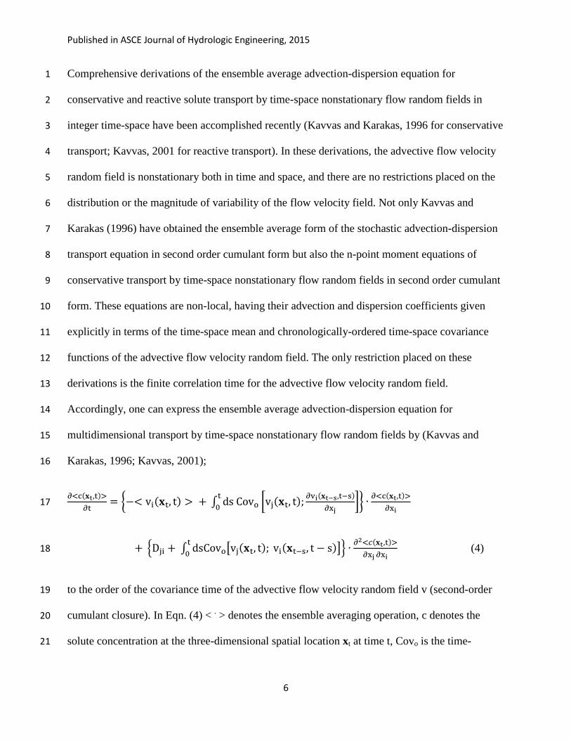
DERIVATION OF FRACTIONAL ENSEMBLE AVERAGE EQUATION OF TRANSPORT 1
BY TIME-SPACE NONSTATIONARY STOCHASTIC FLOW IN ADVECTIVE FORM 2
Over a 1-dimensional spatial lattice with increments x, let us consider a generalized random 3
walk of a solute particle in time with incremental steps of size t. Let the motion of this particle 4
start at time t=0 at the spatial location x(0) = x0. Let the spatial location of this particle at time 5
t+t be x(t+t). Let the concentration at time (t+t) of the ensemble of solute particles that start 6
their motions at a generic space-time origin (x0, 0), be denoted by 7
C(x(t+t), t+t | x0, 0). Let the probability density of finding the transported particle at some 8
spatial location at time t, given that it started its motion at the generic space-time origin (x0, 0), 9
be denoted by P(,t | x0, 0). Then for an initial solute mass of unity, this probability density is 10
equivalent to the ensemble average solute concentration at time-space location (,t) (Csanady, 11
1980). That is, 12
(8) 13
where the symbol < . > denotes the ensemble averaging operation. Hence, the goal of this study 14
is to develop evolution equations for the ensemble average solute concentration <C(,t | xo,0)> in 15
fractional time-space by means of the relationship (8) between the displacement probability 16
density P(, t | xo, 0) and the ensemble average solute concentration <C(, t | xo, 0)>. 17
For a generalized transport process, a particle can make a displacement over the 1-dimensional 18
lattice during a time interval (t, t+Δt) from a location x(t) = x(t+t) – kΔx, k = -…-1,0,+1,…+∞ 19
at time t =nΔt (assuming that it takes n time steps, each of size t, for the particle to reach time t 20
from the time origin t=0) , in order to reach a spatial location x(t+Δt) at time (t+Δt) = (n+1)Δt, 21

Published in ASCE Journal of Hydrologic Engineering, 2015
10
given the whole transport process has started at some time-space location (xo, 0). In other words, 1
during any time interval (t, t+t) the discrete particle displacement x(t+t) – x(t) = kx can start 2
from any location x(t) = x(t+t) – kx, k = - ,…-1,0,+1,…+∞ in order to reach x(t+t) at time 3
t+t. Accordingly, it is possible that the particle can make a very large displacement during the 4
time interval (t, t+t) in either of two directions. However, it is also possible that it can make a 5
very small displacement during this time interval. 6
Within this framework, denoting the probability of finding a particle over the discrete lattice at 7
location x(t+t) given that it started its motion at some space-time origin (xo, 0), by 8
9
the evolution equation for the displacement probability may be written as, 10
(9) 11
where is the probability that the particle will make a 12
displacement of size kΔx = x(t+t) – x(t) during interval (t, t+Δt) given that it was at location 13
x(t) = at time t. As such this probability varies not only with the displacement 14
size and direction, but also with the space-time origin of the displacement. As such, the random 15
walk, described by Eqn. (9) is non-stationary both in space and time. Also in Eqn. (9), 16
is the probability that the particle is at location x(t) = 17
at time t, given that the particle motion has started at ( . 18
Let y= x(t+t) so that Eqn. (9) may be re-written as, 19

Published in ASCE Journal of Hydrologic Engineering, 2015
11
1
(10) 2
+ (11) 3
Since we are considering transport in fractional time-space, Equation (11) can be expanded in 4
fractional time-space increments in terms of generalized Taylor’s series (Odibat and Shawagfeh, 5
2007; Osler, 1972). The generalized Taylor’s series for some function F(x) around z can be 6
expressed as (Odibat and Shawagfeh, 2007), 7
(12) 8
where (.) is the gamma function and the fractional derivative
that appears in Eqn. (12) is 9
a Caputo derivative ( Odibat and Shawagfeh, 2007; Podlubny, 1999). 10
Using Eqn. (12) one can expand Eqn. (11) around (y, t) to obtain, 11
12
13
(13) 14
15

Published in ASCE Journal of Hydrologic Engineering, 2015
12
where for k x(t+t) < x(t), and the solute particle displacement kΔx = x(t+t) - x(t) < 0 is in 1
the direction opposite to the main direction of the motion. Similarly, for k > 0, x(t+t) > x(t), and 2
the solute particle displacement kΔx = x(t+t) - x(t) > 0 is in the main direction of motion. The 3
right-sided Caputo fractional derivative
has been discussed in some detail in Podlubny 4
(1999). Essentially, the direction of the right-sided fractional derivative is opposite to the 5
direction of the standard derivative while the direction of the left-sided fractional derivative 6
is in the same direction as of the standard derivative. In Eqn. (13) k can take any integer 7
value randomly within (-∞ , + ∞). Hence, it is possible for the transported particle to make a 8
wide range of displacements, ranging from very large displacements to very small displacements 9
in two possible directions. 10
Hence, one can express Eqn. (13) as 11
12
13
(14) 14
where the terms in brackets <·> in Eqn. (14), raised to the power jβ, are the jβ-moments of the 15
particle displacement during (t, t+Δt) = (nΔt, (n+1)Δt). 16
In order to obtain transport equations that can be utilized in practice it is necessary to 17
approximate the Eqn. (14) which represents the fractional ensemble average transport in the 18
general setting, to some special cases. In the following, the fractional analogs of the purely 19
Published in ASCE Journal of Hydrologic Engineering, 2015
13
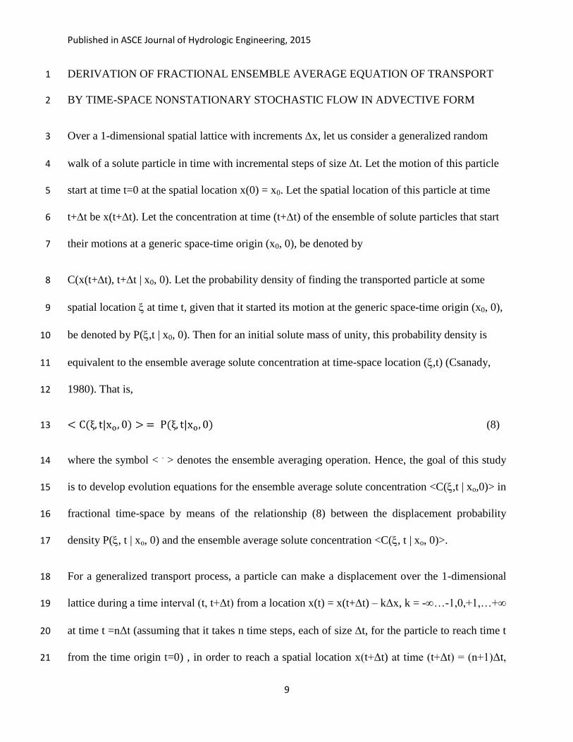
advective and advective-dispersive ensemble average transport equations shall be developed by 1
specializing the general and expansions in Eqn. (14) to the appropriately fixed and 2
powers in time and space. 3
In order to obtain the purely advective form of the fractional ensemble average transport 4
equation it is necessary to approximate Eqn. (14) to just -order in time and β-order in space. 5
Accordingly, retaining the leading terms on both sides of Eqn. (14) (approximating the 6
expansions to j=1), one obtains 7
8
(15) 9
10
+
(16) 11
Now recognizing, 12
, 13
and taking x(t) = x, one can define a time-space ensemble average fractional advective flow 14
velocity , considered only in the direction opposite to the main direction of flow 15
(reverse direction), by 16
, where x(t+t) < x(t), (17) 17
Published in ASCE Journal of Hydrologic Engineering, 2015
14
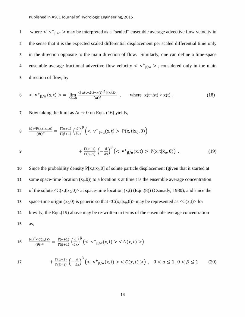
where may be interpreted as a “scaled” ensemble average advective flow velocity in 1
the sense that it is the expected scaled differential displacement per scaled differential time only 2
in the direction opposite to the main direction of flow. Similarly, one can define a time-space 3
ensemble average fractional advective flow velocity , considered only in the main 4
direction of flow, by 5
, where x(t+t) > x(t) . (18) 6
Now taking the limit as t on Eqn. (16) yields, 7
8
. (19) 9
Since the probability density P[x,t|x0,0] of solute particle displacement (given that it started at 10
some space-time location (x0,0)) to a location x at time t is the ensemble average concentration 11
of the solute <C(x,t|x0,0)> at space-time location (x,t) (Eqn.(8)) (Csanady, 1980), and since the 12
space-time origin (x0,0) is generic so that <C(x,t|x0,0)> may be represented as <C(x,t)> for 13
brevity, the Eqn.(19) above may be re-written in terms of the ensemble average concentration 14
as, 15
16
(20) 17

Published in ASCE Journal of Hydrologic Engineering, 2015
15
as the pure advection form of the fractional ensemble average equation of transport (fEATE) by 1
time-space nonstationary stochastic fractional advective flow in fractional time-space. This 2
equation is both the first-order moment and the first order cumulant expansion in terms of 3
since
are both the first moments and the first cumulants of the time-4
space nonstationary stochastic fractional advective flow velocity in the main flow direction and 5
in the reverse direction to flow. In Eqn. (20), the fractional derivatives are Caputo derivatives 6
(Odibat and Shawagfeh, 2007; Podlubny, 1999). 7
It is important to note that at any one location the fluid element is not moving in both the 8
upstream and the downstream directions. Instead, there is a certain probability for the element to 9
move upstream and certain probability to move downstream at any given time and space 10
location, as formulated in Equations (9) and (11) above. The case of flow in two directions at 11
two different sections of a river may happen in a river that is flowing over very mild slopes 12
toward a sea. During a high tide, the sea level may be significantly higher than the water surface 13
at the downstream end of the river, and the sea water may start flowing upstream within the 14
river. This water flow will meet the river flow that is coming from the upstream of the river, 15
somewhere along the river, forming a transition section in the river. Downstream-to-upstream 16
reverse open channel flow may also happen at the river junctions where the hydraulic head in the 17
main river may be higher than that of a joining branch. In such a situation, flow may go from the 18
junction location upstream within the river branch, to meet the flow that is coming from the 19
upstream section of the branch in the downstream direction, somewhere along the branch. These 20
situations correspond to the flow velocity components being both in the direction against the 21
main upstream-to-downstream direction of the river flow and in the direction of the main river 22
flow at two separate reaches of the same river. The defined fractional flow velocity in Eqn. (17) 23

Published in ASCE Journal of Hydrologic Engineering, 2015
16
accounts for such downstream-to-upstream flow conditions, while the fractional flow velocity in 1
Eqn. (18) accounts for the upstream-to-downstream flow conditions. However, in most real-life 2
cases the river flow will be only in the upstream-to-downstream main flow direction, and 3
will be zero, reducing the pure advection form of the fEATE to 4
. (21) 5
In order to gain more physical insight into Eqn. (20), let us consider this equation for the 6
standard integer case = = 1 of the pure advective transport. In this case Eqn. (20) takes the 7
form 8
9
, = 1 (22) 10
11
(23) 12
However, as mentioned earlier, is the ensemble average fractional advective 13
velocity only for the motion in the reverse direction to flow while is the 14
ensemble average fractional advective velocity only for the motion in the main direction of flow. 15
As such, if < (x,t)> represents the ensemble average fractional advective velocity for the 16
motion in both possible directions, then 17
< (x,t)> = -
(24) 18
Published in ASCE Journal of Hydrologic Engineering, 2015
17
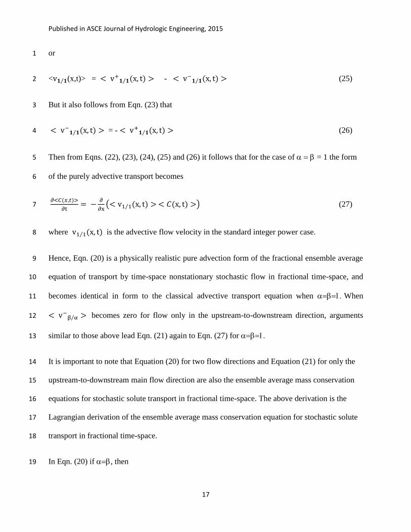
or 1
< (x,t)> = -
(25) 2
But it also follows from Eqn. (23) that 3
= -
(26) 4
Then from Eqns. (22), (23), (24), (25) and (26) it follows that for the case of = 1 the form 5
of the purely advective transport becomes 6
(27) 7
where is the advective flow velocity in the standard integer power case. 8
Hence, Eqn. (20) is a physically realistic pure advection form of the fractional ensemble average 9
equation of transport by time-space nonstationary stochastic flow in fractional time-space, and 10
becomes identical in form to the classical advective transport equation when When 11
becomes zero for flow only in the upstream-to-downstream direction, arguments 12
similar to those above lead Eqn. (21) again to Eqn. (27) for 13
It is important to note that Equation (20) for two flow directions and Equation (21) for only the 14
upstream-to-downstream main flow direction are also the ensemble average mass conservation 15
equations for stochastic solute transport in fractional time-space. The above derivation is the 16
Lagrangian derivation of the ensemble average mass conservation equation for stochastic solute 17
transport in fractional time-space. 18
In Eqn. (20) if , then 19
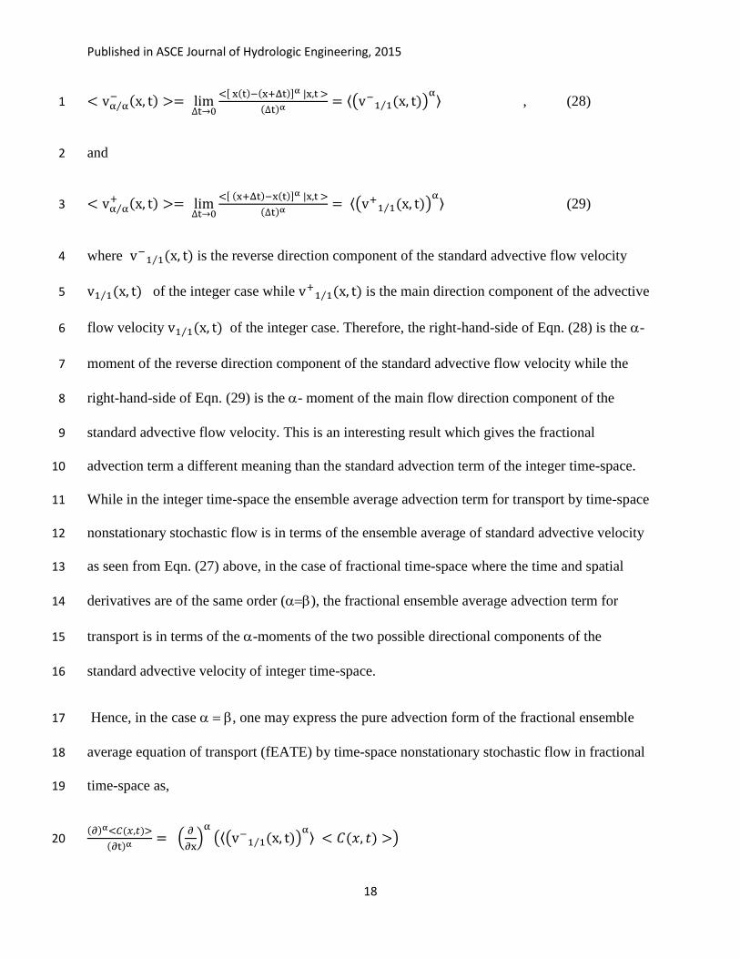
Published in ASCE Journal of Hydrologic Engineering, 2015
18
, (28) 1
and 2
(29) 3
where is the reverse direction component of the standard advective flow velocity 4
of the integer case while is the main direction component of the advective 5
flow velocity of the integer case. Therefore, the right-hand-side of Eqn. (28) is the - 6
moment of the reverse direction component of the standard advective flow velocity while the 7
right-hand-side of Eqn. (29) is the - moment of the main flow direction component of the 8
standard advective flow velocity. This is an interesting result which gives the fractional 9
advection term a different meaning than the standard advection term of the integer time-space. 10
While in the integer time-space the ensemble average advection term for transport by time-space 11
nonstationary stochastic flow is in terms of the ensemble average of standard advective velocity 12
as seen from Eqn. (27) above, in the case of fractional time-space where the time and spatial 13
derivatives are of the same order (), the fractional ensemble average advection term for 14
transport is in terms of the -moments of the two possible directional components of the 15
standard advective velocity of integer time-space. 16
Hence, in the case , one may express the pure advection form of the fractional ensemble 17
average equation of transport (fEATE) by time-space nonstationary stochastic flow in fractional 18
time-space as, 19
20

Published in ASCE Journal of Hydrologic Engineering, 2015
19
(30) 1
in terms of the - moment of the reverse direction component of the standard advective flow 2
velocity and the - moment of the main flow direction component of the standard advective flow 3
velocity. In the mostly-encountered situation of upstream-to-downstream single flow direction, 4
the Eqn. (30) will reduce to 5
(31) 6
As shall be shown in the companion paper by Kim et al. (2014), unlike the standard integer form 7
of the advective transport equation where the solute displacement takes place as the displacement 8
of a distinct front (the piston movement), in the fractional form of the pure advective ensemble 9
average transport equation, due to the above explanation the solute may be spread out around the 10
moving solute front. 11
12
DERIVATION OF FRACTIONAL ENSEMBLE AVERAGE GOVERNING EQUATION OF 13
TRANSPORT BY TIME-SPACE NONSTATIONARY STOCHASTIC FLOW IN 14
ADVECTION-DISPERSION FORM: THE MOMENT FORM 15
In order to obtain a practical advection-dispersion form of the fractional ensemble average 16
transport equation that can be utilized in practice, it is necessary to approximate Equation (14) to 17
-order in time and 2β-order in space. Retaining the first term on the left-hand-side (LHS) and 18
first two terms on the right-hand side (RHS) of Eqn. (14) leads to 19
20

Published in ASCE Journal of Hydrologic Engineering, 2015
20
1
2
, (32) 3
or, 4
5
+
6
7
+
(33) 8
Then proceeding in the same way as in the above pure advection case, but in addition to defining 9
, also defining 10
(34) 11
where represents the dispersion for the fractional movements only in the reverse flow 12
direction, and 13
(35) 14

Published in ASCE Journal of Hydrologic Engineering, 2015
21
represents the dispersion for the fractional movements only in the main flow direction, and then 1
taking the limit as on Eqn. (33) yields a fractional Fokker-Planck-Kolmogorov equation 2
(FFPKE), 3
4
5
6
. (36) 7
Since the probability density P[x,t|x0,0] of solute particle displacement (given that it started at 8
some space-time location (x0,0)) to a particle location (x,t), is the ensemble average 9
concentration of the solute <C(x,t|x0,0)> at space-time location (x,t) (Eqn.(8)) (Csanady, 1980), 10
and since the space-time origin (x0,0) is generic so that <C(x,t|x0,0)> may be represented as 11
<C(x,t)> for brevity, the Eqn.(36) above may be re-written in terms of the ensemble average 12
concentration as, 13
14
15
, (37) 16
which is the moment form of the fractional ensemble average advection-dispersion equation 17
(fEAADE) of transport by time-space nonstationary stochastic flow in fractional time-space. In 18
Published in ASCE Journal of Hydrologic Engineering, 2015
22
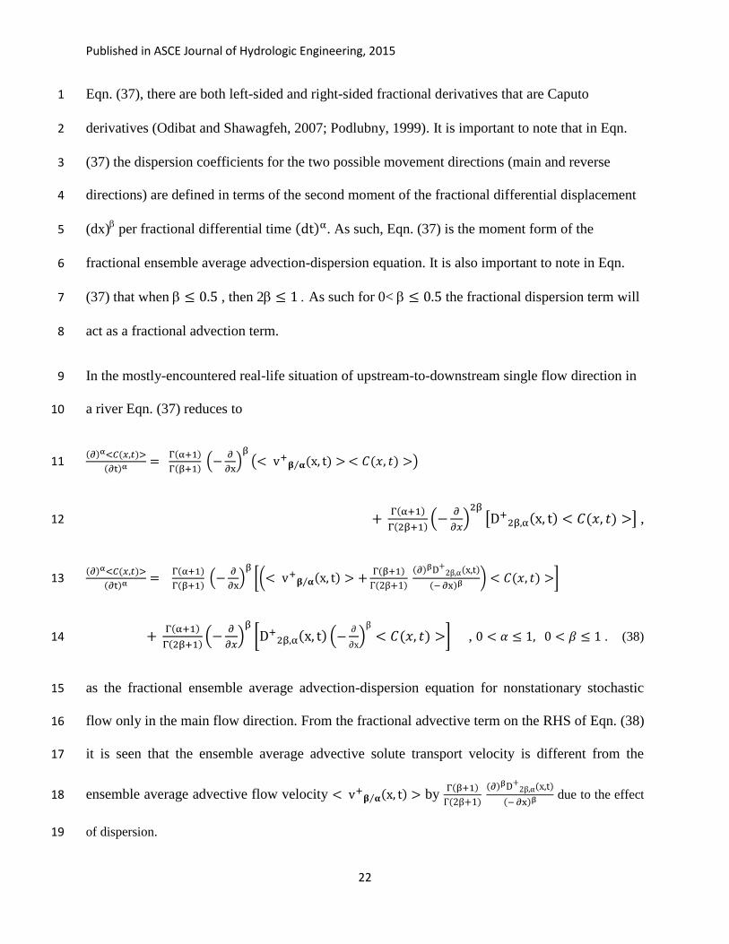
Eqn. (37), there are both left-sided and right-sided fractional derivatives that are Caputo 1
derivatives (Odibat and Shawagfeh, 2007; Podlubny, 1999).It is important to note that in Eqn. 2
(37) the dispersion coefficients for the two possible movement directions (main and reverse 3
directions) are defined in terms of the second moment of the fractional differential displacement 4
(dx) per fractional differential time . As such, Eqn. (37) is the moment form of the 5
fractional ensemble average advection-dispersion equation. It is also important to note in Eqn. 6
(37) that when , then 2 As such for 0< the fractional dispersion term will 7
act as a fractional advection term. 8
In the mostly-encountered real-life situation of upstream-to-downstream single flow direction in 9
a river Eqn. (37) reduces to 10
11
, 12
13
, . (38) 14
as the fractional ensemble average advection-dispersion equation for nonstationary stochastic 15
flow only in the main flow direction. From the fractional advective term on the RHS of Eqn. (38) 16
it is seen that the ensemble average advective solute transport velocity is different from the 17
ensemble average advective flow velocity by
due to the effect 18
of dispersion. 19
Published in ASCE Journal of Hydrologic Engineering, 2015
23
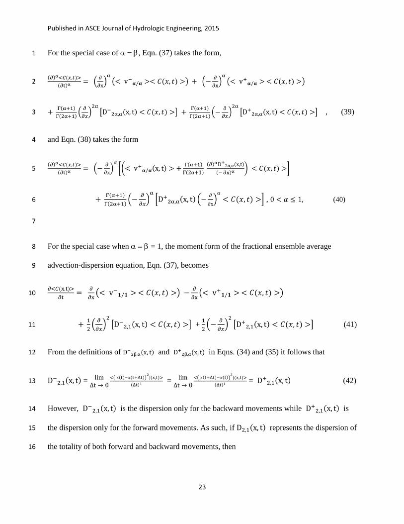
For the special case of , Eqn. (37) takes the form, 1
2
, (39) 3
and Eqn. (38) takes the form 4
5
, (40) 6
7
For the special case when = 1, the moment form of the fractional ensemble average 8
advection-dispersion equation, Eqn. (37), becomes 9
10
+
(41) 11
From the definitions of and
in Eqns. (34) and (35) it follows that 12
=
=
=
(42) 13
However, is the dispersion only for the backward movements while
is 14
the dispersion only for the forward movements. As such, if represents the dispersion of 15
the totality of both forward and backward movements, then 16
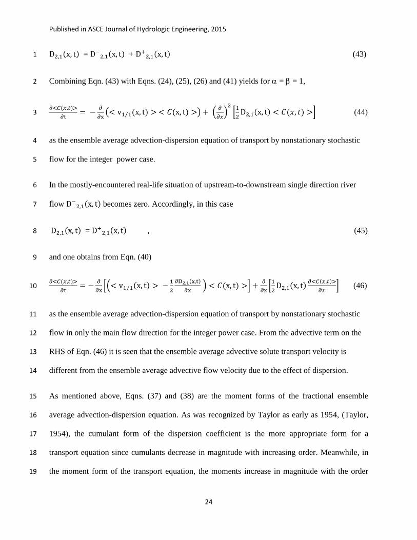
Published in ASCE Journal of Hydrologic Engineering, 2015
24
= +
(43) 1
Combining Eqn. (43) with Eqns. (24), (25), (26) and (41) yields for = = 1, 2
(44) 3
as the ensemble average advection-dispersion equation of transport by nonstationary stochastic 4
flow for the integer power case. 5
In the mostly-encountered real-life situation of upstream-to-downstream single direction river 6
flow becomes zero. Accordingly, in this case 7
= , (45) 8
and one obtains from Eqn. (40) 9
(46) 10
as the ensemble average advection-dispersion equation of transport by nonstationary stochastic 11
flow in only the main flow direction for the integer power case. From the advective term on the 12
RHS of Eqn. (46) it is seen that the ensemble average advective solute transport velocity is 13
different from the ensemble average advective flow velocity due to the effect of dispersion. 14
As mentioned above, Eqns. (37) and (38) are the moment forms of the fractional ensemble 15
average advection-dispersion equation. As was recognized by Taylor as early as 1954, (Taylor, 16
1954), the cumulant form of the dispersion coefficient is the more appropriate form for a 17
transport equation since cumulants decrease in magnitude with increasing order. Meanwhile, in 18
the moment form of the transport equation, the moments increase in magnitude with the order 19
Published in ASCE Journal of Hydrologic Engineering, 2015
25
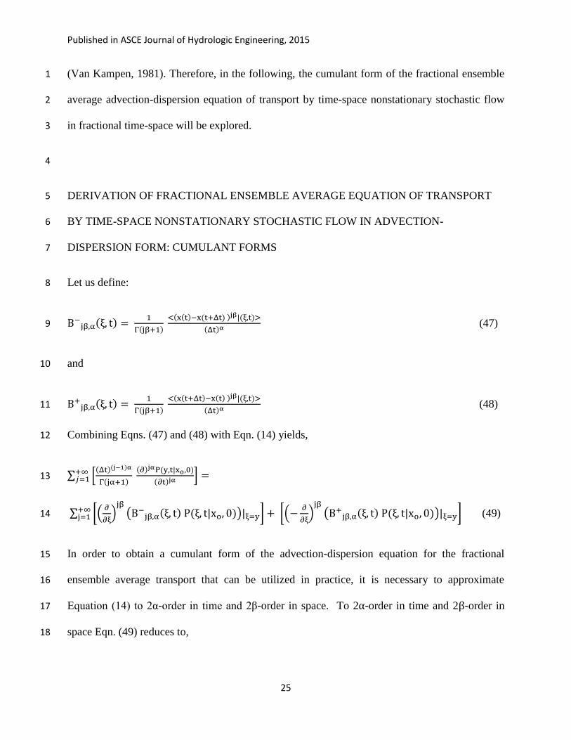
(Van Kampen, 1981). Therefore, in the following, the cumulant form of the fractional ensemble 1
average advection-dispersion equation of transport by time-space nonstationary stochastic flow 2
in fractional time-space will be explored. 3
4
DERIVATION OF FRACTIONAL ENSEMBLE AVERAGE EQUATION OF TRANSPORT 5
BY TIME-SPACE NONSTATIONARY STOCHASTIC FLOW IN ADVECTION-6
DISPERSION FORM: CUMULANT FORMS 7
Let us define: 8
(47) 9
and 10
(48) 11
Combining Eqns. (47) and (48) with Eqn. (14) yields, 12
13
(49) 14
In order to obtain a cumulant form of the advection-dispersion equation for the fractional 15
ensemble average transport that can be utilized in practice, it is necessary to approximate 16
Equation (14) to 2 -order in time and 2β-order in space. To 2 -order in time and 2 -order in 17
space Eqn. (49) reduces to, 18
Published in ASCE Journal of Hydrologic Engineering, 2015
26
1
β
β
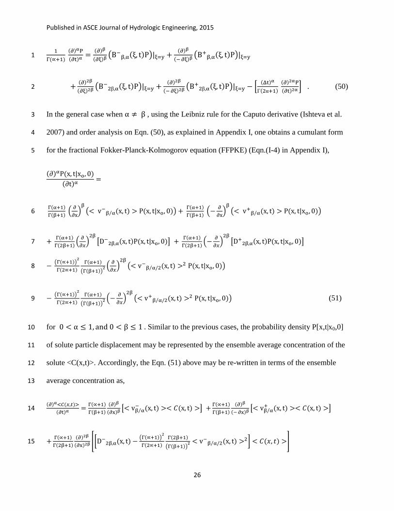
. (50) 2
In the general case when , using the Leibniz rule for the Caputo derivative (Ishteva et al. 3
2007) and order analysis on Eqn. (50), as explained in Appendix I, one obtains a cumulant form 4
for the fractional Fokker-Planck-Kolmogorov equation (FFPKE) (Eqn.(I-4) in Appendix I), 5
6
7
8
(51) 9
for Similar to the previous cases, the probability density P[x,t|x0,0] 10
of solute particle displacement may be represented by the ensemble average concentration of the 11
solute <C(x,t)>. Accordingly, the Eqn. (51) above may be re-written in terms of the ensemble 12
average concentration as, 13
14
15

Published in ASCE Journal of Hydrologic Engineering, 2015
27
(52) 1
for and , as the cumulant form of the fractional ensemble average 2
advection-dispersion equation (fEAADE) of transport by time-space nonstationary stochastic 3
flow in fractional time-space for the general case . 4
In the mostly-encountered real-life situation of upstream-to-downstream single flow direction 5
Eqn. (52) reduces to 6
7
(53) 8
for and , as the cumulant form of the fractional ensemble average 9
advection-dispersion equation (fEAADE) of transport by time-space nonstationary stochastic 10
flow in fractional time-space for the general case . 11
For the case of , the Eqn. (52) reduces to, 12
13
(54) 14
for , as the cumulant form of the fractional ensemble average advection-dispersion 15
equation of transport by time-space nonstationary stochastic flow in fractional time-space when 16
. 17

Published in ASCE Journal of Hydrologic Engineering, 2015
28
In the mostly-encountered real-life situation of upstream-to-downstream single flow direction, 1
for Eqn. (52) reduces to 2
, 3
=
4
, (55) 5
as the cumulant form of the fractional ensemble average advection-dispersion equation of 6
transport by time-space nonstationary stochastic flow in the main flow direction in fractional 7
time-space when . From the fractional advective term on the RHS of Eqn. (55) it is seen 8
that the ensemble average advective solute transport velocity is a combination of the ensemble 9
average advective flow velocity with a term that is due to the effect of dispersion. 10
In Eqn. (54) 11
, (56) 12
and is the variance of the fractional differential displacements per fractional differential time in 13
the reverse direction to the main flow direction, while in Eqns. (54) and (55) 14
(57) 15
is the variance of the fractional differential displacements per fractional differential time in the 16
main flow direction. Accordingly, if one defines 17

Published in ASCE Journal of Hydrologic Engineering, 2015
29
as the variance of the fractional differential displacements per fractional differential time in both 1
of the possible flow directions, then 2
(58) 3
For 1, 4
5
(59) 6
Combining Eqns. (54), (24), (25) and (26) with Eqn. (59) yields for 1, 7
(60) 8
which is in a form similar to that of an ensemble average advection-dispersion equation for 9
transport by nonstationary flow in the integer power case. In the mostly-encountered real-life 10
situation of upstream-to-downstream single flow direction, 11
, (61) 12
and from Eqn. (55) one obtains 13
(62) 14
15

Published in ASCE Journal of Hydrologic Engineering, 2015
30
as the cumulant form of the ensemble average advection-dispersion equation for transport by 1
nonstationary stochastic flow in the main flow direction in the integer power case. 2
3
DISCUSSION AND CONCLUSIONS 4
In this study, starting from a general formulation of the time-space nonstationary random walk of 5
a solute particle, the fractional ensemble average governing equations of transport by time-space 6
nonstationary stochastic flow in fractional time-space were developed in terms of their moment 7
and cumulant forms. First, the purely advective form of the fractional ensemble average equation 8
of transport by time-space nonstationary stochastic advective flow velocity was developed, and 9
is given in Eqn.(20) (for flows in two possible directions) and Eqn.(21) (for flows only in the 10
main flow direction) for the general case when the orders of the time and space fractional 11
derivatives are different ( . From Eqns. (20) and (21) it is seen that the advection 12
coefficient is an ensemble average fractional advective velocity which is an explicit function of 13
space and time, and which is defined in Eqns. (17) and (18) as the expected fractional differential 14
displacement <(dx)> per fractional differential time at a particular space-time position 15
(x,t). <(dx)> may also be interpreted as the -moment of the differential displacement dx. As 16
such, this ensemble average fractional advective velocity varies in space and time and signifies 17
the time-space nonstationary nature of the stochastic advective velocity that transports the solute 18
particles. In the special case when the orders of the time and space fractional derivatives are the 19
same (then the ensemble average fractional advective velocity is expressed as the -20
moment of the corresponding standard advective velocity for the integer time-space, as shown in 21
Eqns. (30) and (31), respectively for two-directional and one-directional flows. This is an 22

Published in ASCE Journal of Hydrologic Engineering, 2015
31
interesting result which gives the fractional advection term a different meaning than the standard 1
advection term in the case of integer time-space. While in the integer time-space the ensemble 2
average advection term for transport by time-space nonstationary stochastic flow is in terms of 3
the ensemble average of standard advective velocity, as seen from Eqn. (4) above, in the case of 4
fractional time-space where the time and spatial derivatives are of the same order (), the 5
fractional ensemble average advection term for transport is in terms of the -moment of the 6
standard advective velocity of integer time-space. As such, while the ensemble average 7
advection term essentially describes a frontal behavior in integer time-space, the corresponding 8
ensemble average advection term in fractional time-space may describe a spreading of the front. 9
This behavior may have significant implications in the application of the fractional ensemble 10
average purely advective transport model to practical problems. As is shown by Kim et al. 11
(2014) in the companion paper to this paper, for transport cases of small dispersion the purely 12
advective fractional transport equation becomes a viable model of transport for both stationary 13
and nonstationary stochastic flows with fractional powers of the transport equation being less 14
than unity. 15
Next, the moment form of the fractional ensemble average advective-dispersive governing 16
equation of transport by time-space nonstationary stochastic flow in fractional time-space was 17
developed, and is given in Eqns. (37) and (38), respectively for two-directional and one-18
directional flows. The two coefficients that emerge in this equation are the ensemble average 19
fractional advective flow velocity which is an explicit function of space and time, and a 20
fractional dispersion coefficient which is also an explicit function of space and time 21
and is defined in terms of the second moment of the fractional differential displacement (dx)) 22
per fractional differential time . As such, Eqns. (37) and (38) are the moment forms of the 23

Published in ASCE Journal of Hydrologic Engineering, 2015
32
fractional ensemble average advection-dispersion equation, respectively for two-directional and 1
one-directional stochastic nonstationary flows. It can be seen from Eqn. (46) that for , the 2
derived moment form of the fractional ensemble average advection-dispersion equation (Eqn. 3
(38)) is in a similar form to the classical advection-dispersion transport equation. 4
As was recognized by Taylor as early as 1954, (Taylor, 1954), the cumulant form of the 5
dispersion coefficient is the more appropriate form for a transport equation since it is the exact 6
second order closure, not needing any information from the higher order cumulants that 7
generally decrease in magnitude with increasing order (Van Kampen, 1981). Therefore, next the 8
cumulant form of the fractional ensemble average advection-dispersion equation of transport by 9
time-space nonstationary stochastic flow was developed for two different cases: (i) when the 10
order of the fractional space derivative of the advective term is the same as that of the time 11
derivative while the order of the fractional space derivative of the dispersion term is twice that of 12
the time derivative, and (ii) when the orders of the time and space fractional derivatives are 13
completely different. In case (i) while the advection coefficient is essentially the same as in the 14
previous cases, the cumulant form of the dispersion coefficient, as given in Eqns.(54) and (55), 15
emerges as a time-space-dependent variance of the fractional differential displacement (dx) per 16
fractional differential time , as defined in Eqns. (56) and (57). Meanwhile, the dispersion 17
coefficient of the moment form of the fractional advection-dispersion equation, defined in Eqns. 18
(34) and (35), is the time-space dependent second moment of the differential displacement (dx) 19
per fractional differential time when = . The basic difference between the two 20
dispersion coefficients is that the one for the cumulant form is the second cumulant (variance) of 21
the fractional differential displacement per fractional differential time while the moment form is 22
the second moment of the fractional differential displacement per fractional differential time. As 23

Published in ASCE Journal of Hydrologic Engineering, 2015
33
will be seen in the accompanying paper by Kim et al. (2014) these forms can render very 1
different modeling results, with the cumulant form being generally superior. The cumulant form 2
of the fractional ensemble average advection-dispersion equation is in a form similar to that of 3
the standard advection-dispersion equation of transport. In case (ii) when the orders of the time 4
and space derivatives are completely different, the cumulant form of the fractional dispersion 5
coefficient emerges as a combination of the moment form of the fractional dispersion coefficient 6
and the square of an ensemble average fractional advective flow velocity. Hence, when 7
compared to the dispersion coefficient of the moment form, the dispersion coefficient of the 8
cumulant form, in the general case when the orders of the time and space derivatives are 9
completely different, contains an extra term accounting for the effect of the ensemble average 10
fractional advective flow velocity on dispersion. 11
In the accompanying paper by Kim et al. (2014), the numerical simulations of transport by 12
stationary and nonstationary flows under various memory lengths show the general superiority of 13
the cumulant form of the fractional transport equation over the moment form when the –14
fractional powers of the transport equation are less than unity. 15
As may be seen from their respective equations, the derived pure advection, and advection-16
dispersion forms of the fractional ensemble average governing equations of transport by time-17
space nonstationary stochastic flow in fractional time-space are rich in structure that can 18
accommodate both the non-Fickian and the Fickian behavior of transport under various memory 19
structures for both the underlying flow fields and the transport. The non-Fickian transport 20
behavior can be described by the fractional ensemble average transport equations, derived in this 21
study, either by means of the long memory in the underlying stochastic flow, or by means of the 22
time-space nonstationarity of the underlying stochastic flow, or by means of the time and space 23
Published in ASCE Journal of Hydrologic Engineering, 2015
34
fractional derivatives of the transport equations. These issues and the performance of the various 1
forms of the fractional ensemble average transport equations (fEATEs), developed here, are 2
explored in the accompanying paper by Kim et al. (2014). 3
4
REFERENCES 5
Batchelor, G.K., (1949): “Diffusion in a field of homogeneous turbulence. 1. Eulerian analysis”, 6
Aust. J. Sci. Res. 2, pp. 437-450 7
Baumer, B., D. Benson and M.M. Meerschaert, (2005): “Advection and dispersion in time and 8
space”, Physica A, 350, pp. 245-262 9
Baumer, B. and M.M. Meerschaert, (2007): “Fractional diffusion with two time scales”, Physica 10
A, 373, pp. 237-251 11
Benson, D.A., S.W. Wheatcraft, M.M. Meerschaert, (2000a): “Application of a fractional 12
advection-dispersion equation”, Water Resour. Res., 36(6), pp. 1403-1412 13
Benson, D.A., S.W. Wheatcraft, M.M. Meerschaert, (2000b): “The fractional-order governing 14
equation of Levy motion”, Water Resour. Res., 36(6), pp. 1413-1423 15
Berkowitz, B., A. Cortis, M. Dentz, H. Scher, (2006): “Modeling non-Fickian transport in 16
geological formations as a continuous time random walk”, Rev. Geophys., RG2003, pp. 1-49 17
Csanady, G.T., (1980): Turbulent Diffusion in the Environment, D. Reidel Pub. Co., 248pp. 18
Deng, Z-Q., V.P. Singh, L. Bengtsson, (2004): “Numerical solution of fractional advection-19
dispersion equation”, J. Hydraulic Engg., 130(5), pp. 422-431 20
Published in ASCE Journal of Hydrologic Engineering, 2015
35
Deng, Z-Q., J.L.M.P. de Lima, and V.P. Singh, (2005): “Fractional kinetic model for first flush 1
of stormwater pollutants”, J. Environ. Engg., 131, pp. 232 2
Deng, Z-Q., L. Bengtsson, V.P. Singh, (2006a): “Parameter estimation for fractional dispersion 3
model for rivers”, Environ. Fluid Mech. 6, pp. 451-475 4
Deng, Z-Q., J.L.M.P. de Lima, M.I.P. de Lima, and V.P. Singh, (2006b): “A fractional 5
dispersion model for overland solute transport”, Water Resour. Res., 42, pp. W03416, 1-14 6
Dentz, M. and D.M. Tartakovsky, (2008): “Self-consistent four-point closure for transport in 7
steady random flows”, Phys. Rev. E, 77(6) 8
Fischer, H.B., E.J.List, R.C.Y.Koh, J.Imberger, N.H.Brooks, (1979): Mixing in Inland and 9
Coastal Waters, Academic Press, Inc., 483pp. 10
Gardiner, C.W., (1985): Handbook of Stochastic Methods, Second Ed. Springer-Verlag, Berlin. 11
Ishteva, M., L. Boyadjiev, R. Scherer, (2007): “On the Caputo operator of fractional calculus 12
and c-Laguerre functions”, Math. Sci. Res. J., 9, 161-170 13
Johnson, H.E. (2001): “Predicting river travel time from hydraulic characteristics”, J. Hydraul. 14
Engg., 127(11), pp. 911-918 15
Kavvas, M.L. and A.Karakas, (1996): “On the stochastic theory of solute transport by unsteady 16
and steady groundwater flow in heterogeneous aquifers”, J. of Hydrology, 179, pp. 321-351 17
Kavvas, M.L. and A.Karakas, (1997): “Corrigendum to ‘On the stochastic theory of solute 18
transport by unsteady and steady groundwater flow in heterogeneous aquifers’ [J. Hydrology, 19
179(1996) 321-351]”, J. of Hydrology, 190, pg. 171 20

Published in ASCE Journal of Hydrologic Engineering, 2015
36
Kavvas, M.L., (2001): “General conservation equation for solute transport in heterogeneous 1
porous media”, J. of Hydrologic Engineering, 6(4), 341-350 2
Kim, S. and M.L. Kavvas, (2006): “Generalized Fick’s law and fractional ADE for pollution 3
transport in a river: detailed derivation”, J. of Hydrologic Engineering, 11(1), pp. 80-83 4
Kim, S., M.L. Kavvas and A. Ercan, (2014): “Fractional ensemble average governing equations 5
of transport by time-space non-stationary stochastic fractional advective velocity and 6
fractional dispersion: Numerical investigation”, J. of Hydrologic Engineering, submitted. 7
Levy, M. and B. Berkowitz, (2003): “Measurement and analysis of non-Fickian dispersion in 8
heterogeneous porous media”, J. Contam. Hydrol., 64, pp. 203-226 9
Liang, L. and M.L.Kavvas, (2008): “Modeling of solute transport and macrodispersion by 10
unsteady stream flow under uncertain conditions”, J. of Hydrologic Engineering, 13(6), 510-11
520 12
Meerschaert, M.M., D.A. Benson, B. Baumer, (1999): “Multidimensional advection and 13
fractional dispersion”, Phys. Rev. E, 59(5), pp.5026-5028 14
Meerschaert, M.M., D.A. Benson, H.P. Scheffler, and B. Baumer, (2002): “Stochastic solution of 15
space-time fractional diffusion equations”, Phys. Rev. E, 65, pp.041103-1 – 04113-4 16
Meerschaert, M.M., J. Mortensen, and S.W. Wheatcraft, (2006): “Fractional vector calculus for 17
fractional advection-dispersion”, Physica A, 367, pp.167-181 18
Metzler, R. and J. Klafter, (2000): “The random walk’s guide to anomalous diffusion: a 19
fractional dynamics approach”, Physics Reports, 339, pp. 1-77 20

Published in ASCE Journal of Hydrologic Engineering, 2015
37
Morales-Casique E., S.P. Neuman, A. Guadagnini, (2006a): “Nonlocal and localized analyses of 1
nonreactive solute transport in bounded randomly heterogeneous porous media: theoretical 2
framework”, Adv. Water Resour., 29(8), pp. 1238-1255 3
Morales-Casique E., S.P. Neuman, A. Guadagnini, (2006b): “Nonlocal and localized analyses of 4
nonreactive solute transport in bounded randomly heterogeneous porous media: 5
computational analysis”, Adv. Water Resour., 29(8), pp. 1399-1418 6
Neuman, S. and D.M. Tartakovsky, (2009): “Perspective on theories of non-Fickian transport in 7
heterogeneous media”, Adv. Water Resour. , 32, pp. 670-680 8
Nordin, C.F. and G.V. Sabol, (1974): “Empirical data on longitudinal dispersion in rivers”, 9
Water Resour. Investigations, 20-74, USGS, CO. 10
Nordin, C.F. and B.M. Troutman, (1980): “Longitudinal dispersion in rivers: the persistence of 11
skewness in observed data”, Water Resour. Res., 16, pp. 123-128 12
Odibat, Z.M. and N.T. Shawagfeh, (2007): “Generalized Taylor formula”, Appl. Math. and 13
Comp., 186, 286-293 14
Orlob, G.T. (Ed.), (1983): Mathematical Modeling of Water Quality: Streams, Lakes, and 15
Reservoirs, IIASA, J. Wiley & Sons, 518 pp. 16
Osler, T.J., (1972): “An integral analogue of Taylor’s series and its use in computing Fourier 17
Transforms”, Math. Comp., 26, pp. 449-460 18
Peaudecerf, G. and J-P. Sauty, (1978): “Application of a mathematical model to the 19
characterization of dispersion effects on groundwater quality”, Prog. Water Tech., 10, pp. 20
443-454 21
Published in ASCE Journal of Hydrologic Engineering, 2015
38
Podlubny, I, (1999): Fractional Differential Equations, Academic Press, San Diego, 340pp. 1
Schumer, R., D.A. Benson, M.M. Meerschaert, and S.W. Wheatcraft, (2001): “Eulerian 2
derivation for the fractional advection-dispersion equation”, J. Contam. Hydrol, 48, pp.69-88 3
Schumer, R., M.M. Meerschaert, and B. Baumer, (2009): “Fractional advection-dispersion 4
equations for modeling transport at the earth surface”, J. Geophys. Res., 114, F00A07, pp.1-5
15 6
Sidle, C., B. Nilson, M. Hansen, and J. Fredericia, (1998): Spatially varying hydraulic and solute 7
transport characteristics of a fractured till determined by field tracer tests, Funen, Denmark”, 8
Water Resour. Res., 34(10), pp.2515-2527 9
Silliman, S.E. and E.S. Simpson, (1987): “Laboratory evidence of the scale effect in dispersion 10
of solutes in porous media”, Water Resour. Res., 23(8), pp. 1667-1673 11
Sudicky, E.A., J.A. Cherry, E.O. Frind, (1983): “ Migration of contaminants in groundwater at a 12
landfill: a case study. 4. A natural-gradient dispersion test”, J. Hydrol. 63, pp. 81-108 13
Taylor, G.I., (1922): “Diffusion by continuous movements”, Proc. London Math. Soc. Ser. A 20, 14
196-211 15
Taylor, G.I., (1954): “The dispersion of matter in turbulent flow through a pipe”, Proc. Royal 16
Soc., Series A, 223, pp. 446-468 17
Van Kampen, N.G., (1981): Stochastic Processes in Physics and Chemistry, North-Holland, 18
419pp. 19
Published in ASCE Journal of Hydrologic Engineering, 2015
39
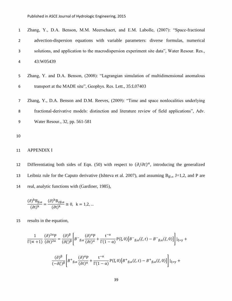
Zhang, Y., D.A. Benson, M.M. Meerschaert, and E.M. Labolle, (2007): “Space-fractional 1
advection-dispersion equations with variable parameters: diverse formulas, numerical 2
solutions, and application to the macrodispersion experiment site data”, Water Resour. Res., 3
43:W05439 4
Zhang, Y. and D.A. Benson, (2008): “Lagrangian simulation of multidimensional anomalous 5
transport at the MADE site”, Geophys. Res. Lett., 35:L07403 6
Zhang, Y., D.A. Benson and D.M. Reeves, (2009): “Time and space nonlocalities underlying 7
fractional-derivative models: distinction and literature review of field applications”, Adv. 8
Water Resour., 32, pp. 561-581 9
10
APPENDIX I 11
Differentiating both sides of Eqn. (50) with respect to , introducing the generalized 12
Leibniz rule for the Caputo derivative (Ishteva et al. 2007), and assuming Bj J=1,2, and P are 13
real, analytic functions with (Gardiner, 1985), 14
results in the equation, 15

Published in ASCE Journal of Hydrologic Engineering, 2015
40
(I-1) 1
2
Multiplying both sides of Equation (I-1) by –
, and then substituting into the 3
resulting equation the expression for
from the Eqn. (50), yields, 4
– Δ
Δ
β
β
β
β
β
β
β
β
5
Δ
β
β
β
β
β
β
β
β
6
Δ
β
β
β
β
-
Δ
β
β
β
β
7
Δ
β
β
β
β
β
β
β
β
Δ
β
β
β
β
β
β
β
β
Δ
β
β
β
β
Δ
β
β
β
β
. 8
(I-2) 9

Published in ASCE Journal of Hydrologic Engineering, 2015
41
Again using the Leibniz rule for the Caputo derivative (Ishteva et al. 2007) on Equation (I-2), 1
along with the definitions (47) and (48) for for j=1,2, and taking the limit as t goes to 2
zero yields 3
– Δ
β
β
4
β
β
5
β
β
β
β
β
β
β
β
β
β β
β β
β β
β (I-3) 6
Combining Equation (I-3) with Equation (50) of the main text while taking the limit as t goes to 7
zero, and introducing the definitions of the fractional ensemble average advective velocity 8
and the fractional dispersion coefficient
of the main text yields the cumulant 9
form of the fractional Fokker-Planck-Kolmogorov Equation (FFPKE) for transport by 10
nonstationary stochastic flow in fractional time-space as 11
12
13
14
(I-4) 15
Published in ASCE Journal of Hydrologic Engineering, 2015
42
for Equation (I-4) is the Equation (51) in the main text. 1
2
3
4
5
6
7
Related Documents