Frac

Applied Mathematical Modelling 37 (2013) 1347–1361

Contents lists available at SciVerse ScienceDirect

Applied Mathematical Modelling

journal homepage: www.elsevier .com/locate /apm

The use of the fractal model to complex resistivity in the interpretationof induced polarization data

V.J.da C. Farias a,⇑, B.R.P. da Rocha b, M.P.da C. da Rocha a, H.R. Tavares a

a PPGME-ICEN, Federal University of Pará, Brazilb PPGEE-IT, Federal University of Pará, Brazil

a r t i c l e i n f o a b s t r a c t

Article history:Received 13 May 2011Received in revised form 20 March 2012Accepted 2 April 2012Available online 10 April 2012

Keywords:Complex resistivityFractalFinite elementForward modelingInverse modeling

0307-904X/$ - see front matter � 2012 Elsevier Inchttp://dx.doi.org/10.1016/j.apm.2012.04.002

⇑ Corresponding author. Tel.: +55 91 32760521.E-mail address: [email protected] (V.J.da C. Farias).

Several researchers demonstrated that spectral parameters in induced polarization can beapplied to discriminate different IP sources. In this paper it was applied an inversion pro-cedure using the Gauss–Newton method to recover the spectral parameters of fractalmodel to complex resistivity. The finite element method was applied to carry out the for-ward modeling. The procedure was applied in synthetic data and simulations were carriedout in five different frequencies. The inversion of the data were carried out in each fre-quency, further the inversion was applied also to each cell of the finite element mesh torecover the fractal parameter in order to analyze the possibility of using the fractal modelparameters in the interpretation of the induced polarization response to this geologicalgeometry. The results showed that the anomalies are well detected by the image of thefractal model parameters.

� 2012 Elsevier Inc. All rights reserved.

1. Introduction

The induced polarization phenomenon (IP) has an electrochemical origin and can be observed in both frequency andtime-domain experiments. At time domain the IP experiments are to obtain the information about chargeability of the mediaunder investigation.

The spectral induced polarization method (SIP) measures the dispersion of the apparent conductivity (resistivity) with thefrequency by means of the inphase and out-of-phase components, normally. That is, the resistivity of the media is consideredlike a complex number and frequency-dependent and these dependencies of the frequency can be described by relaxationmodels.

The relaxation models show the general behavior of the amplitude and phase spectra of the complex resistivity (conduc-tivity) at different frequency for different material. The most used relaxation model is the Cole–Cole, introduced by Cole andCole [1]. However, this relaxation model does not consider the fractal nature of the medium, mainly at the geological medium.

Rocha [2] introduced a relaxation model which consider the fractal effect of the porous surface and include the bulkresponse of rocks. The introduction of the fractal roughness factor allows the analysis of the texture of rocks, which is akey factor in explaining their electrical and transport properties.

In an effort to extract even more information about the subsurface of earth, processes have been developed to estimatethe relaxation model parameters from time and frequency induced polarization data [3–7].

Oldenburg and Li [8] and Yuval and Oldenburg [3] developed a process to estimate the intrinsic Cole–Cole parametersfrom time domain IP surveys. First, they divided the medium into rectangular cells and they assumed that the Cole–Cole

. All rights reserved.

1348 V.J.da C. Farias et al. / Applied Mathematical Modelling 37 (2013) 1347–1361

parameters were constants in each cell. Then, the apparent chargeabilities measured at each time channel were inverted torecover the intrinsic chargeability. Theses intrinsic chargeabilities provided estimates of the chargeability decay curve foreach cell. They carried out a parametric inversion of the chargeability decay curves to recover the Cole–Cole parameters.

Routh et al. [4] presented a procedure where they considered multiple frequency complex resistivity data to recover thespectral parameters of Cole–Cole model. In this procedure, the media also is parameterized into rectangular cells and in eachcell the Cole-Cole parameters were recovered directly from the multiple frequency complex resistivity data.

Kemna et al. [5] obtained information about the spectral behavior of complex resistivity of the media by means of suc-cessive applications of the inversion algorithm to several single-frequency data sets extracted from multi-frequency mea-surements. Subsequently, the Cole–Cole parameters were fitted in each cell.

Loke et al. [6] combined the method of [8] for the inversion of resistivity and IP data with the method of [4] to obtain theCole–Cole parameters.

Rocha and Habashy [9] applied the fractal model of complex resistivity as an intrinsic electrical property of a horizontallystratified media (1-D model) and they analyzed the IP response. They observed that the fractal parameter of the fractal modeldominates the phase angle response of the apparent resistivity.

In this paper it is simulated the shaped bodies (2-D geological model) and it is applied the fractal model to complex resis-tivity as intrinsic electrical property of this medium, the element finite technique is used to forward modeling. This simu-lation is carry out in five different frequencies. To each frequency we carry out the inversion of the complex resistivity,the Gauss–Newton method was applied. After, to each cell of the finite element mesh, we carry out the fractal model param-eters inversion to analyze the possibility of using the fractal model parameters in the qualitative and quantitative interpre-tation of the induced polarization response to this geological geometry. In this model the fractal parameter (g) represents thefractal index, which can be related to the rock texture.

2. The fractal model to complex resistivity

Phenomenological models for fluid conduction based on a single medium are extremely simple and they are not appro-priate for describing the complex behavior of porous sedimentary rocks. A fractal model for the complex resistivity of rockswas first introduced by Rocha [2], it was used an analog circuit including the diffusivity (K) of ions in the vicinity of the elec-trode/electrolyte interface and a fractal parameter (g). Later, Rocha and Habashy [9,10] proposed the adoption of a fractaltime to substitute the diffusivity (K) of ions. The fractal model proposed describes the electrical polarization in porous sed-imentary rocks under in situ conditions. The electrical current propagation in the fractal model is characterized by two paths,one the current flows by a free porous path channel without clays and the second the electrical current flows by a blockedpore with the presence of clay minerals.

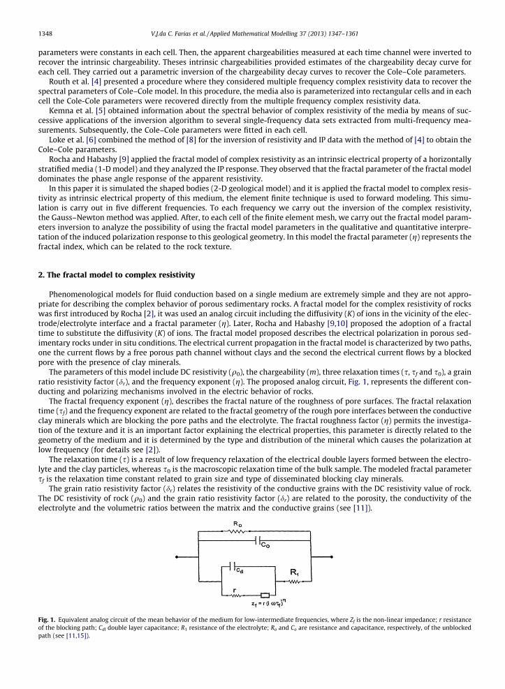
The parameters of this model include DC resistivity (q0), the chargeability (m), three relaxation times (s, sf and s0), a grainratio resistivity factor (dr), and the frequency exponent (g). The proposed analog circuit, Fig. 1, represents the different con-ducting and polarizing mechanisms involved in the electric behavior of rocks.

The fractal frequency exponent (g), describes the fractal nature of the roughness of pore surfaces. The fractal relaxationtime (sf) and the frequency exponent are related to the fractal geometry of the rough pore interfaces between the conductiveclay minerals which are blocking the pore paths and the electrolyte. The fractal roughness factor (g) permits the investiga-tion of the texture and it is an important factor explaining the electrical properties, this parameter is directly related to thegeometry of the medium and it is determined by the type and distribution of the mineral which causes the polarization atlow frequency (for details see [2]).

The relaxation time (s) is a result of low frequency relaxation of the electrical double layers formed between the electro-lyte and the clay particles, whereas s0 is the macroscopic relaxation time of the bulk sample. The modeled fractal parametersf is the relaxation time constant related to grain size and type of disseminated blocking clay minerals.

The grain ratio resistivity factor (dr) relates the resistivity of the conductive grains with the DC resistivity value of rock.The DC resistivity of rock (q0) and the grain ratio resistivity factor (dr) are related to the porosity, the conductivity of theelectrolyte and the volumetric ratios between the matrix and the conductive grains (see [11]).

Fig. 1. Equivalent analog circuit of the mean behavior of the medium for low-intermediate frequencies, where Zf is the non-linear impedance; r resistanceof the blocking path; Cdl double layer capacitance; R1 resistance of the electrolyte; Ro and Co are resistance and capacitance, respectively, of the unblockedpath (see [11,15]).

V.J.da C. Farias et al. / Applied Mathematical Modelling 37 (2013) 1347–1361 1349

The proposed analog circuit (Fig. 1) includes a nonlinear impedance r(ixsf)�g which simulates the effects of the roughnessof the interfaces between the blocking clay minerals and the electrolyte for the very low frequency response of rocks. In thismodel the fractal time (sf) is involved in the charge and energy transfer through the fractal interfaces, it is an independentparameter that can be used as a chronometer to observe the time that an individual ion will take to cross the interface. Thisgeneralized Warburg impedance is in series with the resistance of the blocking grains and both are shunted by the doublelayer capacitance.

The charged double layer within the pores is represented by a resistive term (loss of energy due to collision of the freeions during their motion across the double layer) and a capacitive term (caused by the oscillation of bound charges in thedouble layer), this combination is in series with the resistance of the electrolyte in the blocked pore passages. The un-blockedpore paths are represented by a resistance which corresponds to the normal DC resistivity of the rock. The parallel combina-tion of this resistance with the bulk sample capacitance is finally connected in parallel to the rest of the above mentionedcircuit.

Representing the time dependence of the electric field as eixt, the expression proposed by Rocha [2] for the complexelectrical resistivity q(x) is given by:

qðxÞ ¼ qo 1�m 1� 11þ 1þu

drð1þvÞ

!" #ch; ð1Þ

where

m ¼ R0

R1 þ R0Chargeability;

dr ¼r

R1 þ R0Grain percent resistivity;

ch ¼ 1=ð1þ ixs0Þ;u ¼ ixsð1þ vÞ;

v ¼ ðixsf Þ�g;

s ¼ rCdl Double layer relaxation time;

s0 ¼ R0C0 Sample relaxation time:

The fractal model addresses the roughness of the pore space and it was demonstrated by Rocha and Habashy [10] that thefractal parameter can be identified in layered medium even at great depths. The fractal model was employed to study theoverburden on the complex resistivity under in situ conditions in the frequency range 10 Hz to 100 kHz and pressure range1–40 MPa [11]. Under high pressures the fractal frequency exponent can be used to study the dynamic behavior of the mate-rial when excited by electromagnetic waves while the Cole-Cole model parameters have presented very small correlationwith the petrophysical parameters [11].

3. 2D forward modeling

The geoelectrical modeling reduces to solver the following equation:

�r � ðr�ðx; y; zÞrVðx; y; zÞÞ ¼ Idðx� xsÞdðy� ysÞdðz� zsÞ; ð2Þ

where r⁄ is the complex conductivity of the medium, V is the electrical potential due to current source I at the position(xs,ys,zs). Nevertheless, (2) is valid for steady current, it can be applied for alternating current at low frequencies if the elec-tromagnetic effects can be neglected [12]. In a 2D investigation the y-direction is parallel to the strike of the model. Thus, theconductivity can be written as r⁄(x,y,z) = r⁄(x,z). That is, the medium is considered 2D. However, the source used in geoelec-trical prospecting is assumed as having a 3D distribution. Due to this some authors consider the problem as 2.5D. To reducethis difficult, it is applied the Fourier transformed in (2):

�r � ðr�ðx; zÞr~Vðx; k; zÞÞ þ k2r�ðx; zÞ~Vðx; k; zÞ ¼ Idðx� xsÞdðz� zsÞ ð3Þ

where ~Vðx; k; zÞ ¼R1�1 Vðx; y; zÞe�ikydy is the transformed potential; k is the transformed variable (wavenumbers). Eq. (3) has

to be solved for several discrete wavenumbers k.

3.1. Finite element approximation

Let us consider the following variational form for Eq. (3), as given by
ZX
wf�r � ½r�ðx; zÞr~Vðx; k; zÞ� þ k2r�ðx; zÞ~Vðx; k; zÞ � Idðx� xsÞdðz� zsÞgdX ¼ 0; ð4Þ


where w is a test or weight function that belongs to Hilbert space H1(X). To reduce the integral to terms containing only firstderivatives, the identity below is applied:

wr � ðr�r~VÞ ¼ r � ðwr�r~VÞ � r�r~V � rw: ð5Þ

Inserting (5) into (4), we obtain:

ZXr�r~V � rwdX�

ZXr � ðr�wr~VÞdXþ

ZX

k2r�w~V dX ¼Z

XwIdðx� xsÞdðz� zsÞdX: ð6Þ

The second integral in (6) can be transformed into boundary integral applying the theorem of the divergence, thus

ZXr�r~V � rwdX�

Z@X

r�@ ~V@n

wdCþZ

Xk2r�w~V dX ¼ Iwðxs; zsÞ; ð7Þ

where oX is the boundary of the region X and n denotes outward normal direction of the boundary interface.By partitioning the region X into a number of sub-regions, called finite elements, therefore X =

PeX

e and oX =P

eCe.

Thus, each element acquired a variational form as in (7)

ZXe

r�er~Ve � rwdXe �Z@Xe

r�e @~Ve

@nwdCe þ

ZXe

k2r�ew~Ve dXe ¼ Iwðxs; zsÞ: ð8Þ

By applying the Galerkin’s criterion, the potential can be expressed as:

~Ve ¼Xk

i¼1

~Viwei ðx; zÞ x and z 2 Xe ð9Þ

where we(x,z) are shape functions and k is the total number of nodes in Xe.By substituting (9) into (8) and taking we

j ðx; zÞ ¼ wej ðx; zÞ ðj ¼ 1; . . . ; kÞ, the linear equation system is reached

M~V ¼ b; ð10Þ

where ~V is the vector of the transformed potential and b ¼Pk

j¼1bej is the source vector.

The matrix M is assembled from the element matrix Meij, that is M ¼

Pkj¼1Me

ij, being

Meij ¼

Xk

i¼1

ZXe

r�e rwj � rwi þ k2wjwi

� �dXe þ

Z@Xe

re wj@wi

@n

� �dCe

� �: ð11Þ

Once the conductivity is known in each element of the mesh of finite element and the shape functions are chosen, theelement matrix is obtained by (11), the global matrix M is assembled, the linear system (10) is solved and, thus, one can cal-culate the transformed potential on any node of the mesh.

3.2. Element matrix calculation

The element type (Xe) is determined. Triangles and quadrilaterals elements are the two most common element types em-ployed for the calculation of the element matrix. According to [13] the triangular element has the simplest formulation andits computational storage space required is lower than the quadrilateral element. Therefore, the triangular element will beadopted in this work.

By using linear interpolation in a triangle will result in the following shape functions

w1ðx; zÞ ¼ 12Ae ½ðx2z3 � x3z2Þ þ ðz2 � z3Þxþ ðx3 � x2Þz�;



9>=>;

where xi and zi (i = 1, 2, 3) are the coordinates of the three vertices of the triangle; Ae is the area of element Xe.Eq. (11) without the contour integral can be written in the form

Meij ¼

Xk

i¼1

r�eZ

Xe

@wi

@x@wj

@xþ @wi

@z@wj

@z

� �dXe þ k2

ZXe

wiwjdXe� �

¼ Iwðxs; zsÞ: ð12Þ

Due to symmetry between i and j in (12), the element matrix is consequently symmetric. The above calculation is validonly for inner grid nodes, the procedure for the nodes on the contour will be described at the next section.


3.3. Boundary conditions

In the forward modeling in geoelectrical surrounding, two boundary conditions can be considered. The first, on the earth’ssurface, in the air–earth interface can be considered a conductive medium bounded by an isolating medium. Thus, there is nocurrent flow through these interfaces. The Neumann boundary condition describes this effect, that is

@~V@n¼ 0:

In the finite element scheme, this condition is easily implemented. The second situation, the mesh that represents theconductive medium is extended to the ‘‘infinite’’, by increasing progressively the sizes of the elements to simulate the infi-nite medium. The mixed-boundary conditions as proposed by Dey and Morrison [14] are applied:

@~V@nþ cos h

~Vr¼ 0;

where h is the angle between the radial distance r, connecting the source point and the node at the boundary, and outwardnormal n. The finite element mesh used in this work is the same developed by Farias et al. [15].

3.4. Solution of the linear equation system

The final step of the finite element method is to solve the linear equation system (10). Before presenting the linear equa-tion system techniques applied in this work, it is necessary to remark some characteristic of the matrix M.

The vector ~V in (10) has potential as elements and the vector b consists of the source term of current injection. Thus, the Mis called the conductance matrix. The conductance matrix is assembled from symmetric elementary matrix Me

ij, then, the ma-trix M is also symmetric, but the matrix is not hermitian.

The elements of the matrix M are obtained by ‘‘coupling’’ between adjacent nodes. It is known that there is no ‘‘coupling’’between distant nodes. Therefore, the components of M deriving from distant nodes will be zero. Consequently, the conduc-tance matrix will be sparse.

Depending on the available computer resources a direct or an iterative method to solve the system of algebraic equation(10) can be employed. Farias et al. [15] used the LU factorization (direct method) and the pre-conditioned complex bi-con-jugate gradient algorithm (iterative method) in IP forward modeling, they verified that the LU factorization is fastest than theiterative method applied by them. We will use the LU factorization in this paper.

3.5. Potential calculation

After obtaining the potentials ~Vðx; k; zÞ in the wavenumber domain is necessary to reconstruct the potential V(x,y,z). Toobtain it, the inverse Fourier transform is applied.

Vðx; y; zÞ ¼ 1p

Z þ1

�1

~Vðx; k; zÞeiky dk:

Considering that the electrodes are located in the plane y = 0, the inverse Fourier transform is given by a simpleintegration,

Vðx;0; zÞ ¼ 1p

Z þ1

0

~Vðx; k; zÞdk: ð13Þ

The integral in (13) can be evaluated numerically using the transformed potential ~Vðx; k; zÞ at several wavenumber k. Ourinvestigation has shown that nine wavenumbers yields a sufficient precision to reconstruct the potential V(x,y,z). A furtherincrease in the number of wavenumbers value results in a few improvements in precision. Thus, it was choice nine wave-numbers values in this work. The minimum and maximum limits of k are chosen according to the maximum and minimumdistances between the current and potential electrodes [12]. In the literature, there are different procedures to calculate thepotential V(x,y,z).

Tripp et al. [16] interpolate the transformed potential ~Vðx; k; zÞ by cubic spline method between the limits of k. Consid-ering that for a homogeneous medium the solution of (3) behaves as the modified Bessel function Ko(u) and that the modifiedBessel function is proportional to e�u for large arguments u, Dey and Morrison [14] approximate the potential ~Vðx; k; zÞ by anexponential function between the discrete values of k, followed by the calculation of the integral (13).

Weller et al. [12] considered that the modified Bessel function Ko(u) is proportional to minus the logarithmic function(�lnu) for small arguments u. They applied both exponential and logarithmic approximation, depending on the value ofthe argument u. This procedure improves the precision of the reconstruction of the potential V(x,y,z).

We applied the least square method to approximate the potential ~Vðx; k; zÞ between the discrete values of k by an expo-nential function and a logarithmic function for large and small values of the argument u, respectively.


4. Inverse modeling

The cost (or objective) function being minimized in the inversion is of the same kind as the used by [17] and is given byexpression:

Table 1Parame

Vn-1Vn-2Vn-4

CðmÞ ¼ 12fl½kWd � eðmÞk2 � v2� þ kWmðm�mrÞk2g; ð14Þ

where m is a vector with the model parameters, that is, a vector with the values of resistivities of each subregion; l(0 < l <1) is a Lagrange multiplier (its inverse is called the regularization parameters), that determines the relative impor-tance of the two terms of the cost functions. According to [18,19] the determination of l will produce an estimate of themodel m that has a finite minimum weighted norm (away from a prescribed model mr) and which globally misfits the datato within a prescribed value v (determined from a priori estimates of noise in the data); e(m) = f(m) � dobs is defined asresidual vector; f(m) is the operator of the forward solution; dobs is the measured data vector, usually corrupted with somelevel of noise; mr is the reference model which includes all a priori information on the complex resistivity; v is the pre-scribe value of data misfit; Wm is the inverse of the model covariance matrix; and Wd is the inverse of the data covariancematrix.

To solve the above optimization problem, we employ the iterative Gauss–Newton minimization approach, where eachstep j of the complex linear system is solved to a update Dmj.

4.1. The Gauss–Newton approach

Based on Ref. [19], a brief description will be made on the Gauss–Newton approach. Let us consider the quadratic modelof the cost function which it is formed by taking the first three terms of the Taylor series of the cost function around the jthiteration mj, that is:

Cðmj þ DmjÞ � CðmjÞ þ rCHðmjÞ � Dmj þ12

DmHj � rrCðmjÞ � Dmj; ð15Þ

where the superscript H indicates transposition conjugated and Dmj = mj+1 �mj is the step in mj toward the minimum of thecost function C(m). The gradient vector rCðmÞ of the cost function is given by the following expression:

rCðmÞ ¼ � @C@mj

; j ¼ 1;2;3; . . . ;N� �

¼ lJHðmÞ �WTd �Wd � eðmÞ þWT

m �Wm � ðm�mrÞ;

where J(m) is the M � N Jacobian matrix and is given by the following expression:

JðmÞ ¼ Jki ¼@f ðmkÞ@mi

; k ¼ 1;2;3; . . . ;M; J ¼ 1;2;3; . . . ;N� �

;

where M is the number of measurements and N is the number of unknowns.

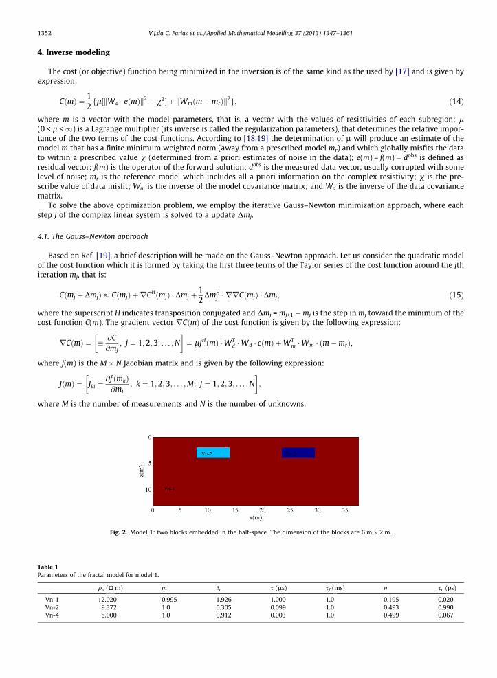
Fig. 2. Model 1: two blocks embedded in the half-space. The dimension of the blocks are 6 m � 2 m.

ters of the fractal model for model 1.

qo (X m) m dr s (ls) sf (ms) g so (ps)

12.020 0.995 1.926 1.000 1.0 0.195 0.0209.372 1.0 0.305 0.099 1.0 0.493 0.9908.000 1.0 0.912 0.003 1.0 0.499 0.067


The Hessian of the cost function C(m) is a N � N matrix given by:

Fig. 3.0.5030

rrCðmÞ ¼ @2C@mi@mj

; i; j ¼ 1;2; . . . ;N

" #¼WT

m �Wm þ l½JTðmÞ �WTd �WdJðmÞ þ QðmÞ�;

Pseudosection of the apparent resistivity in all frequencies to model 1. Amplitude (X m) in top and phase angle (mrad) in bottom: (a) 0.1 Hz; (b)Hz; (c) 2.5298 Hz; (d) 12.7243 Hz and (e) 64 Hz.


where QðmÞ ¼PM

n¼1enðmÞETn and enðmÞ nth element of the weighted vector of residual eðmÞ ¼Wd � eðmÞ, and

EnðmÞ ¼ rrenðmÞ ¼ @2en@xi@xj

i; j ¼ 1;2;3; . . . ;Nh i

:

The value Dmj will be a minimum of (15), if Dmj is a minimum of the quadratic function

Fig. 4.parame

/ðDmÞ ¼ Cðmj þ DmÞ � CðDmjÞ ¼ rCTðmjÞDmþ 12

DmT � rrCðmjÞ � Dm:

The function /(Dm) has a stationary point at Dmj, only if the gradient vector of /(Dm) vanishes at Dmj, i.e.,

r/ðDmjÞ ¼ rrCðmÞ � Dmj þrC ¼ 0:

Thus the stationary point is the solution to the following set of linear equations:

rrC � Dmj ¼ �rC: ð16Þ

That is

½JH �WTd �Wd � JH þWT

m �Wm þ QðmÞ� � Dmj ¼ JH �WTd �Wd � ½dobs � f ðmjÞ� �WT

m �Wm � ðmj �mrjÞ:

The search direction Dmj which is given by the vector that solves (16) is called Newton search direction (Newton meth-od). The Gauss–Newton search method discards the second-order derivatives, to avoid the expensive computation of secondderivatives, in which case the Hessian reduces to:

rrCðmÞ ¼WTm �W

Tm þ l½JTðmÞ �WT

d �Wd � JðmÞ� ð17Þ

and the set of linear equation is now given by

½JH �WTd �Wd � JH þWT

m �Wm� � Dmj ¼ JH �WTd �Wd � ½dobs � f ðmjÞ� �WT

m �Wm � ðmj �mrjÞ:

The set of linear equation can be solved by a numerical method as the gauss elimination method.

4.2. The choice of the Lagrange multiplier

There exist several criteria by which one can select the Lagrange multiplier [18–20]. In this paper, it is used the method,presented by Habashy and Abubakar [19], where adaptively vary the Lagrange multiplier (l) as the iteration proceedsaccording to the amplitude of the previous iterate, that is:

1l¼ kWd � eðmÞk2

kdk2 ;

where d is a constant independent of the iteration steps. According to [19], the above procedure weighs between the first andsecond term of the cost function, that is, l will acquire small values when kWd � eðmÞk undergoes large variations. This willput more weight on the second term of the cost function. It is the more appropriate approach to use in the initial steps of theiteration process where kWd � eðmÞk may exhibit large swings. When kWd � eðmÞk undergoes small variations, l will acquire

Apparent fractal parameter pseudosection recovered from the apparent complex resistivity pseudosection to model 1: (a) fractal parameter (g); (b)ter (dr); (c) chargeability (m); and (d) fractal relaxation time (sf in ms).


large values putting more weight on the first term of the cost function. This correspond to the Gauss–Newton search methodwhich is the more appropriate approach to use as we get closer to minimum of the cost function where kWd � eðmÞkwill con-stantly decrease as the iteration converges to its final steps and where the quadratic model for the cost function becomesmore accurate.

Fig. 5. Inverse model of the model 1 with amplitude (top) and phase angle (bottom) in the frequencies: (a) 0.1 Hz; (b) 0.5030 Hz; (c) 2.5298 Hz; (d)12.7243 Hz and (e) 64 Hz.


5. Results

The 2-D model was divided into 147 � 20 cells, the region of interest it was considered 76 � 10 (760 cells). The measureddata are generated using a dipole–dipole array with dipole length of 2 m, and the electrode configuration consist in introducea current into the medium by pair of electrodes and the voltage is measured in another pair of electrode. The geometric fac-tor to this electrode configuration is presented in (18)

Fig. 6.relaxat

Fig. 7.

Table 2Parame

Oh-1Oh-2Oh-3

K ¼ 2p 1AMþ 1

BN� 1

AN� 1

BM

� ��1

; ð18Þ

where AM, AN, BN and BM are the distances between the electrodes of current (A and B) and the electrodes of potential (Mand N). Importantly, the results obtained here do not depend on the electrode array.

The data were collected using 20 electrodes with 8 n-spacing and the results are represented in the form of pseudo-sec-tions. The simulations were carried out in five different frequencies logarithmically sampled between 0.1 Hz and 64 Hz. Thedata were contaminated with gaussian random noise with standard deviation of 5% of the datum value. The inverse modelwas obtained in the five frequencies and to map a constrained minimization problem to an unconstrained one a nonlineartransformation was applied, the first transformation presented in [19] was used in this paper.

Image of the intrinsic fractal model parameters to model 1: (a) fractal parameter (g); (b) parameter (dr); (c) chargeability (m); and (d) fractalion time parameter (sf in ms).

Model 2: synthetic model consists of a medium of the two layers and a block embedded in the second layer. The dimension of the block is 6 m � 2 m.

ters of the fractal model for model 2.

qo (X m) m dr s (ls) sf (ms) g so (ps)

400 0.439 0.303 0.342 97.8 0.323 0.00530.0 0.608 0.617 0.207 29900 0.238 0.02630.0 0.691 0.292 0.255 13935 0.288 0.024


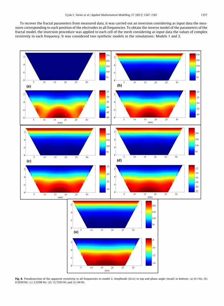
To recover the fractal parameters from measured data, it was carried out an inversion considering as input data the mea-sures corresponding to each position of the electrodes in all frequencies. To obtain the inverse model of the parameters of thefractal model, the inversion procedure was applied to each cell of the mesh considering as input data the values of complexresistivity in each frequency. It was considered two synthetic models in the simulations: Models 1 and 2.

Fig. 8. Pseudosection of the apparent resistivity in all frequencies to model 2. Amplitude (X m) in top and phase angle (mrad) in bottom: (a) 0.1 Hz; (b)0.5030 Hz; (c) 2.5298 Hz; (d) 12.7243 Hz and (e) 64 Hz.


5.1. Model 1

The model 1 (Fig. 2) consists of two blocks buried in the half-space. All medium in this model are chargeable with com-plex resistivity given by fractal model presented in (1). The fractal model parameters of the half-space and of the blocks arepresented in Table 1. According to Rocha [2] the parameters presented in Table 1 correspond to glacial till (half-space) (sam-ple Vn-1 at Table 1), glacial till contaminated with toluene (block at right, sample Vn-2) and glacial till contaminated withethylene (block at left, sample Vn-3).

The values of fractal parameters of the model shown in Table 1 were applied in (1) to obtain the resistivity of each med-ium of the model. These resistivities were applied in the forward modeling (see [15]).

The pseudosections (apparent resistivity) of the forward modeling in all frequencies are showed in Fig. 3. It can be ob-served in these data that the block on the left hand side, ie, the glacial till contaminated by toluene, has influences at theresponse of phase angle of the complex apparent resistivity, but the body located to the right has an imperceptible influenceon the same answer, mostly at the initial frequencies. However, the response in amplitude did not detect the two bodies.

Fig. 4 presents the apparent fractal model parameters (pseudosections) g, dr, m and sf recovered from the apparent com-plex resistivity in all frequencies. The apparent fractal parameters g and dr have the same behavior of the phase angle re-sponse of the apparent complex resistivity in higher frequencies, that is, the two bodies are detected by the image oftheses parameters. The apparent parameters chargeability m and fractal time sf do not detected the bodies.

The amplitude and phase angle of the inverse model in the all frequencies are shown in Fig. 5. One can observe that thecontamination of the half-space (the two blocks) are detected by amplitude and phase angle responses. The block located atleft hand side (the contamination of the half-space by toluene) has a response recovered strongest than the response recov-ered by block located at right hand side (the contamination of the half-space by ethylene), mainly on the angle phaseresponse.

Fig. 6 shows the image of the distribution of the intrinsic fractal model parameters recovered from the inverse model inall frequencies. The image of the parameters g, dr and m, Fig. 6 (a), (c) and (b), respectively, detect the contaminations of thehalf-space by toluene (left block) and by ethylene (right block). The image of the parameters fractal relaxation time (sf),Fig. 6(d), does not detect the presence of the two blocks.

5.2. Model 2

Consider the synthetic model in Fig. 7. It consists of one block buried in the second layer of two layered medium. Again, allmedium are chargeable with complex resistivity given by fractal model presented in (1). The parameters of the model of thefirst layer are of the sample Oh-1, the second layer are of the sample Oh-2 and the block are of the sample Oh-3. All thesesamples are presented in Table 2. According to Rocha [2] the parameters presented in Table 2 correspond to tuff with its nat-ural content of water (Oh-1), uncontaminated smectite soils (Oh-2) and organic waste contaminated smectite soils (Oh-3).

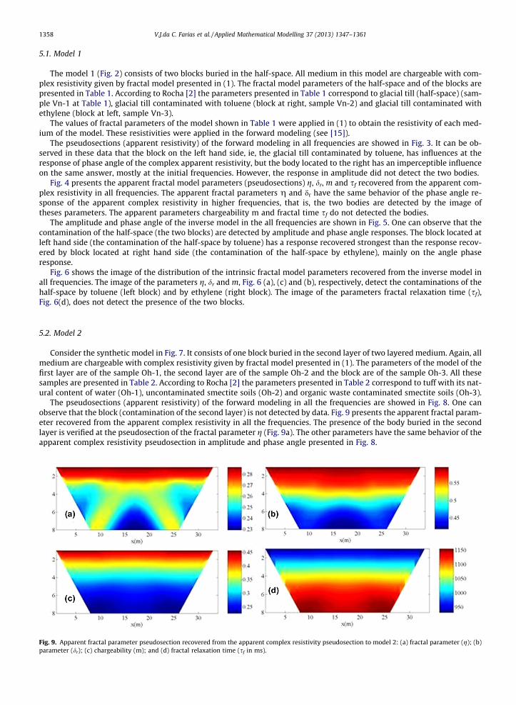
The pseudosections (apparent resistivity) of the forward modeling in all the frequencies are showed in Fig. 8. One canobserve that the block (contamination of the second layer) is not detected by data. Fig. 9 presents the apparent fractal param-eter recovered from the apparent complex resistivity in all the frequencies. The presence of the body buried in the secondlayer is verified at the pseudosection of the fractal parameter g (Fig. 9a). The other parameters have the same behavior of theapparent complex resistivity pseudosection in amplitude and phase angle presented in Fig. 8.

Fig. 9. Apparent fractal parameter pseudosection recovered from the apparent complex resistivity pseudosection to model 2: (a) fractal parameter (g); (b)parameter (dr); (c) chargeability (m); and (d) fractal relaxation time (sf in ms).


The inverse model (amplitude and phase angle) obtained in all the frequencies are shown in Fig. 10. We can observer thatthe response in amplitude has the behavior of the layered medium and the phase angle response detects the contamination(block) of the second layer in low frequency.

Fig. 11 shows the image of the distribution of the intrinsic fractal model parameters recovered from the inverse data in allthe frequencies. The block in the second layer is better observed in the image of the parameters g, dr, m and sf than in inversemodel (Fig. 10).

Fig. 10. Inverse model of the model 2 with amplitude (top) and phase angle(bottom) in the frequencies: (a) 0.1 Hz; (b) 0.5030 Hz; (c) 2.5298 Hz; (d)12.7243 Hz and (e) 64 Hz.

Fig. 11. Image of the intrinsic fractal model parameters to model 2: (a) fractal parameter (g); (b) parameter (dr); (c) chargeability (m); and (d) fractalrelaxation time parameter (sf in ms).


According to [9] the fractal exponent (g) dominates the phase response of the complex resistivity response mainly in lowfrequencies. This is a very important result because in low frequency the fractal parameters carry information about porousroughness. Thus, from field data and with appropriated inversion algorithm it will be possible to make inference about thetransport properties of the investigated material. It is possible, also, starting from the knowledge of the fractal parameter (g)the contamination of the environment may be detected.

6. Conclusion

It carried out the forward and inverse modeling of the induced polarization data and it was considered the fractal modelto complex resistivity as intrinsic electrical property of the medium. The finite element and the Gauss–Newton methodswere applied, respectively, in forward and inverse modeling. It was considered two synthetic models on the simulations.The first model consisted of two blocks buried in the half-space. The second model consisted of one block buried in the sec-ond layer of two layered medium. In both simulations, all media in these models were chargeable with complex resistivitygiven by fractal model.

The simulations were carried out in five different frequencies logarithmically sample between 0.1 and 64 Hz. The inversemodel was obtained in each frequency and it was made an inverse modeling to obtain the parameters of the fractal model toeach cell of mesh grid.

The results showed that the anomalies are well detected by the image of the distribution of the fractal model parameters(g, m, dr and sf). Thus, the fractal model to complex resistivity is an alternative to be used to detected anomalies in geologicalmedium as in the study of the contamination of the environment.

References

[1] K.S. Cole, R.H. Cole, Dispersion and absorption in dielectrics, J. Chem. Phys. 9 (1941) 341–351.[2] B.R.P. da Rocha, Modelo Fractal para Resistividade Complexa de Rochas:Sua Interpretação Petrofísica e Aplicação à Exploração Geoelétrica, Ph.D. Thesis,

Federal University of Pará, 1995.[3] Yuval, D.W. Oldenburg, Computation of cole–cole parameters from IP data, Geophysics 62 (2) (1997) 436–448.[4] P.S. Routh, D.W. Oldenburg, Y. Li, Regularized inversion of spectral IP parameters from complex resistivity data, in: 68th Ann. Internat. Mtg., Soc. Expl.

Geophys., Expanded Abstract.[5] A. Kemna, E. Räkers, L. Dresen. Field applications of complex resistivity tomography, in: 69th Ann. Internat. Mtg., Soc. Expl. Geophys., Expanded

Abstract, 1999.[6] M.H. Loke, J.E. Chambers, R.D. Ogilvy, Inversion of 2D spectral induced polarization imaging data, Geophys. Prospect. 54 (2006) 287–301.[7] V.J.da C. Farias, Interpretation of Induced Polarization Data Using Fractal Model to Complex Resistivity and Tomographic Images, Ph.D. Thesis, Federal

University of Pará, 2004.[8] D.W. Oldenburg, Y. Li, Inversion of induced polarization data, Geophysics 59 (9) (1994) 1327–1341.[9] B.R.P. Rocha, T.M. Habashy, Fractal geometry, porosity and complex resistivity. I: From rough pore interfaces to hand specimens, Developments in

Petrophysics, first ed., vol. 122, Geological Society Publishing House, London, 1997, p. 10. Special publication 122.[10] B.R.P. Rocha, T.M. Habashy, Fractal Geometry, Porosity and Complex Resistivity. II: From Hand Specimen to Field Data, in: Developments in

Petrophysics, first ed., Geological Society Publishing House, London, 1997, p. 10. Special publication 122.[11] Q.M. Malik, B.R.P. Rocha, J.R. Marsden, M.S. King, High pressure electromagnetic fractal behaviour of sedimentary rocks, Progr. Electromagn. Res. 19

(1998) 223–240.[12] A. Weller, M. Seichter, A. Kampke, Induced-polarization modelling using complex electrical conductivities, Geophys. J. Int. 127 (1996) 387–398.[13] E.B. Becker, G.F. Carey, J.T. Oden, Finite Elements an Introduction, vol. I, Prentice-Hall, New Jersey, 1981.


[14] A. Dey, H.F. Morrison, Resistivity modeling for arbitrarily shaped three-dimensional bodies, Geoophysics 44 (1979) 753–780.[15] V.J.C. Farias, C.H.M. Maranhão, B.R.P. da Rocha, N.P.O. Andrade, Induced polarization forward modelling using finite element method and the fractal

model, Appl. Math. Model. 34 (7) (2010) 1849–1860.[16] A.C. Tripp, G.W. Hohmann, C.M. Swift, Two-dimensional Resistivity Inversion, Geophysics 49 (1984) 1708–1717.[17] J.J. Xia, T.M. Habashy, J.A. Kong, Profile inversion in a cylindrically stratified lossy medium, Radio Sci. 29 (1994) 1131–1141.[18] T.M. Habashy, W.C. Chew, E.Y. Chow, Simultaneous reconstruction of permittivity and conductivity profiles in a radially inhomogeneous slab, Radio

Sci. 21 (1986) 635–645.[19] T.M. Habashy, A. Abubakar, A general framework for constraint minimization for the inversion of electromagnetic measurements, Progr. Electromagn.

Res. 46 (2004) 265–312.[20] D.W. Oldenburg, Inversion of electromagnetic data: an overview of new techniques, Surv. Geophys. 11 (1990) 231–270.

Frac

Documents

different frequency

induced polarization

fractal parameter

fractal effect

fractal modelparameters

used relaxation model

fractal roughness factor

fractal nature of themedium