FPT algorithmic techniques: Treewidth (1) Hans L. Bodlaender.

FPT algorithmic techniques:Treewidth (1)

Hans L. Bodlaender

Treewidth2

This talk

1. Roots of treewidth

2. Definition

3. Some applications

4. Using treewidth to obtain FPT algorithms

5. Conclusions

1. Roots

1. Resistance of network of resistors

2. Problems on trees and series parallel graphs

3. Gauss elimination

Treewidth4

Computing the Resistance of Network of Resistors

21

111RRR

21 RRR

R1 R2 R1

R2

Ohm1789-1854

Kirchhoff1824-1887

Treewidth5

Repeated use of the rules

6

2

6

25

1

Has resistance 4

1/6 + 1/2 = 1/(1.5)1.5 + 1.5 + 5 = 81 + 7 = 81/8 + 1/8 = 1/4

1/6 + 1/2 = 1/(1.5)1.5 + 1.5 + 5 = 81 + 7 = 81/8 + 1/8 = 1/4

7

Treewidth6

A tree structureP

6 2

6 25

17

P P

S S

5

6 62 2

7 1

Treewidth7

Series parallel graphs

• Graphs formed by series composition and parallel composition are series parallel graphs

• 1970’s and 1980’s: Many (NP-hard) problems are linear (or polynomial) time solvable on series parallel graphs and trees

• Series parallel graphs have treewidth at most 2

Treewidth8

Trees

• Many NP-hard problems are linear time solvable on trees– Often with Dynamic Programming – Trees have treewidth one

• Trees: glue with one vertex• Series parallel graphs: glue with two vertices.• Treewidth: glue with k vertices…

Treewidth9

Gauss elimination of sparse symmetric matrices

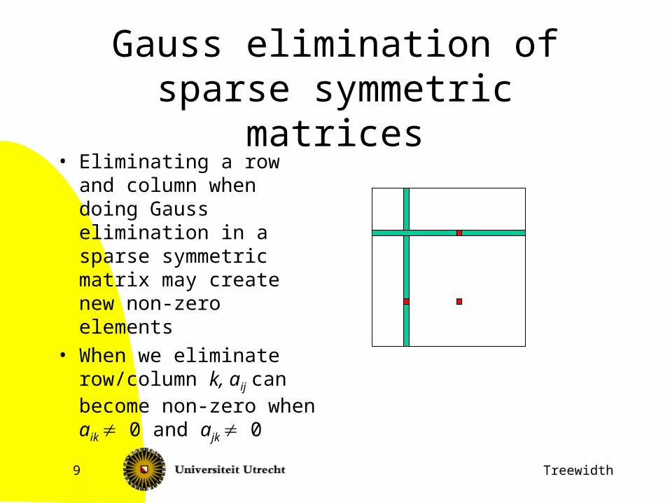
• Eliminating a row and column when doing Gauss elimination in a sparse symmetric matrix may create new non-zero elements

• When we eliminate row/column k, aij can become non-zero whenaik 0 and ajk 0

Treewidth10

Symmetric matrix = Undirected graph

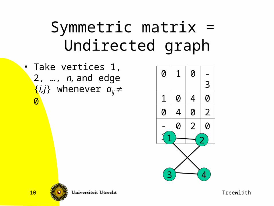
• Take vertices 1, 2, …, n, and edge {i,j} whenever aij 0

0 1 0 -3

1 0 4 0

0 4 0 2

-3 0 2 0

1 2

3 4

Treewidth11

Gauss elimination as Graph elimination

• Eliminating a vertex:– Make its neighborhood a clique and then remove the

vertex• Different vertex orderings (elimination schemes) are

possible– Fill-in: minimum over all elimination schemes of

number of added edges (new non-zero’s)– Chordal graphs: fill-in 0– Treewidth: minimum over all elimination schemes of

maximum degree of vertex when eliminated (min max number of non-zero’s in a row when eliminating row)

2. Treewidth

1. Birth2. Definition3. Complexity4. Representation as ordering problem

Treewidth13

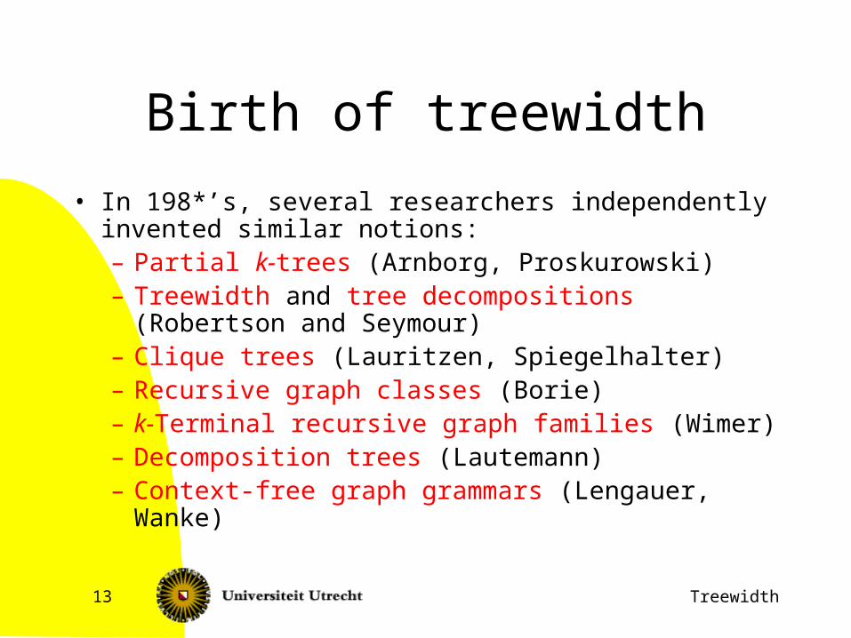
Birth of treewidth

• In 198*’s, several researchers independently invented similar notions:– Partial k-trees (Arnborg, Proskurowski)– Treewidth and tree decompositions (Robertson and

Seymour)– Clique trees (Lauritzen, Spiegelhalter)– Recursive graph classes (Borie)– k-Terminal recursive graph families (Wimer)– Decomposition trees (Lautemann)– Context-free graph grammars (Lengauer, Wanke)

Treewidth14

• A tree decomposition:– Tree with a vertex set

called bag associated to every node.

– For all edges {v,w}: there is a set containing both v and w.

– For every v: the nodes that contain v form a connected subtree.

b c

df

a ab c c

cd

g

gf fa e e

a e

Tree decomposition

f

Treewidth15

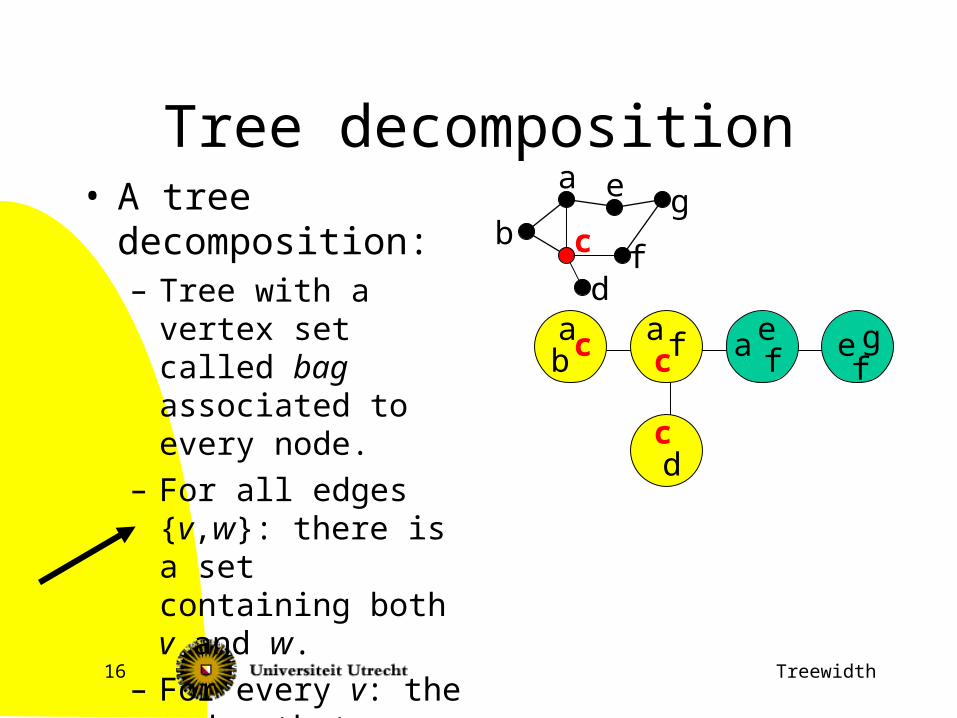
Tree decomposition• A tree decomposition:

– Tree with a vertex set called bag associated to every node.

– For all edges {v,w}: there is a set containing both v and w.

– For every v: the nodes that contain v form a connected subtree.

a ab c c

cd

gf fa e ef

b c

df

ga e

Treewidth16

• A tree decomposition:– Tree with a vertex set

called bag associated to every node.

– For all edges {v,w}: there is a set containing both v and w.

– For every v: the nodes that contain v form a connected subtree.

Tree decomposition

a ab c c

cd

gf fa e ef

b c

df

ga e

Treewidth17

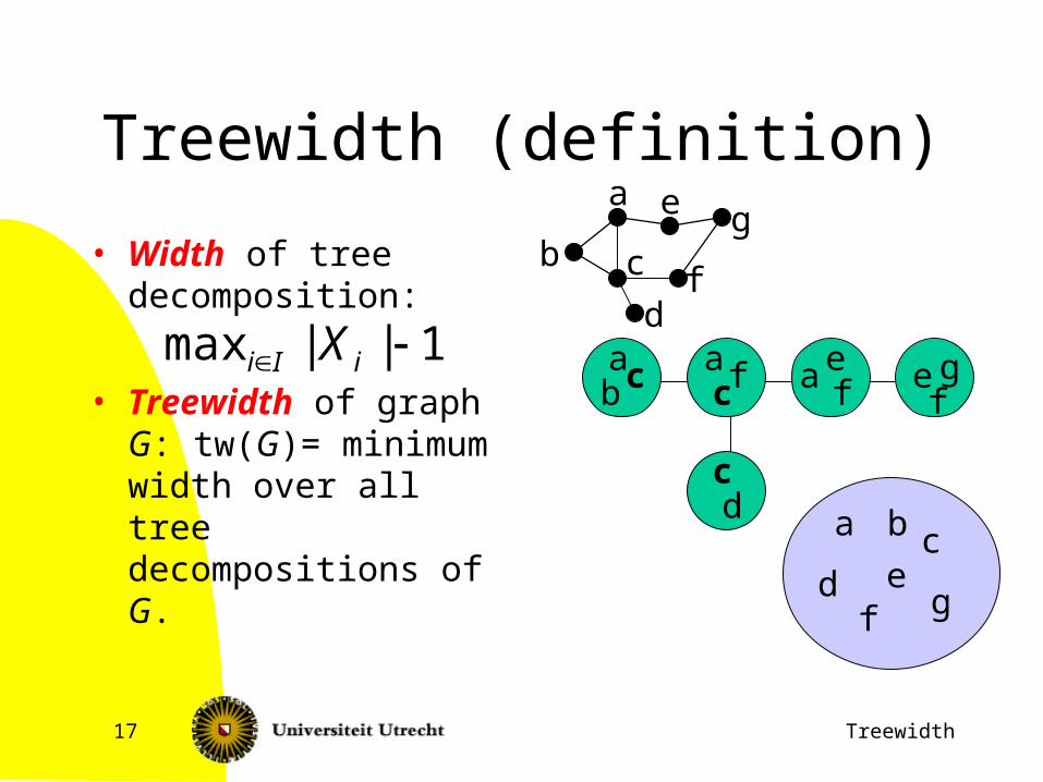
Treewidth (definition)

• Width of tree decomposition:

• Treewidth of graph G: tw(G)= minimum width over all tree decompositions of G. a b c

d ef g

1||max iIi X a ab c c

cd

gf fa e ef

b c

df

ga e

Treewidth18

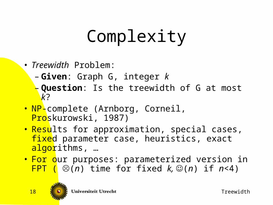
Complexity

• Treewidth Problem:– Given: Graph G, integer k– Question: Is the treewidth of G at most k?

• NP-complete (Arnborg, Corneil, Proskurowski, 1987)

• Results for approximation, special cases, fixed parameter case, heuristics, exact algorithms, …

• For our purposes: parameterized version in FPT ( (n) time for fixed k, (n) if n<4)

Treewidth19

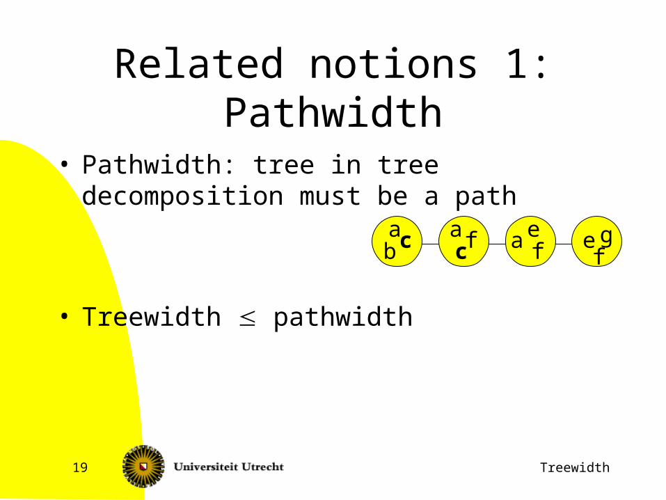
Related notions 1: Pathwidth

• Pathwidth: tree in tree decomposition must be a path

• Treewidth pathwidth

a ab c c

gf fa e ef

Treewidth20

Related notions 2

• Branchwidth = minimum width of branch decomposition

• Branch decomposition: take a binary tree, and a bijection between the leaves of the tree and the edges of G

• Width of an edge e in branch decomposition: number of vertices that are an endpoint of an edge mapped to leaves at both sides of e

• Width of branch decomposition: maximum width of edge in branch decomposition

• Example on board

• Treewidth and branchwidth differ by factor at most 1.5

3. Applications

1. Solving problems with Dynamic Programming

2. Probabilistic Networks

3. Graph minors

Treewidth22

Dynamic programming algorithms

• Many NP-hard (and some PSPACE-hard, or #P-hard) graph problems become polynomial or linear time solvable when restricted to graphs of bounded treewidth (or pathwidth or branchwidth)

– Well known problems like Independent Set, Hamiltonian Circuit, Graph Coloring

• Experiments (Dorn et al., Pönitz & Tittmann)

– Frequency assignment (Koster et al.)

– TSP (Cook, Seymour)

Treewidth23

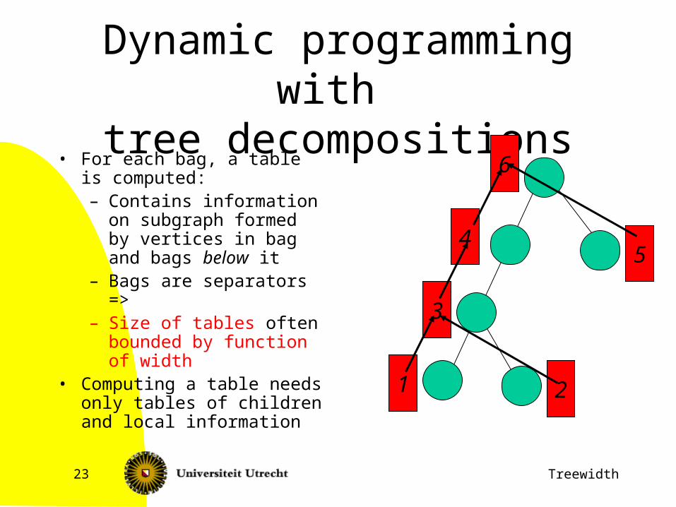
Dynamic programming with

tree decompositions• For each bag, a table is

computed:– Contains information on

subgraph formed by vertices in bag and bags below it

– Bags are separators => – Size of tables often

bounded by function of width

• Computing a table needs only tables of children and local information

1 2

3

4

6

5

Treewidth24

Monadic second order logic

• Linear time algorithm for problems expressible in MSOL or extensions (Courcelle)– Quantification over vertices, sets of vertices,

edges, sets of edges– Adjacency and incidence checks– Or, and, not

• Also optimization

Treewidth25

Example

• An MSOL-formulation for 3-coloring

Treewidth26

Extension

• MinW set of vertices |W|: P(W), with P in MSOL,

• MaxW set of vertices |W|: P(W), with P in MSOL

• MinF set of edges |W|: P(F), with P in MSOL,

• MaxF set of edges |W|: P(F), with P in MSOL

• Example: minimum independent set

Treewidth27

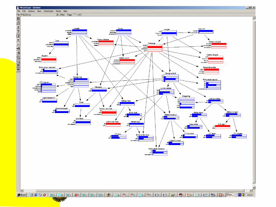
Probabilistic networks

• Underlying decision support systems

• Representation of statistical variables and (in)dependencies by a graph

• Central problem (inference) is #P-complete

• Lauritzen-Spiegelhalter, 1988: linear time solvable when treewidth (of moralized graph) is bounded

– Treewidth appears often small for actual probabilistic networks

– Used in several modern (commercial and freeware) systems

Treewidth28

Treewidth29

Treewidth30

Graph minors

• G is a minor of H, if G can be obtained from H by zero or more vertex deletions, edge deletions and/or edge contractions

• Graph minor theorem (Robertson and Seymour)Let G be a class of graphs that is closed under taking of minors. Then there is a finite set of graphs ob(G), the obstruction set of G, such that a graph H G, if and only if H has no graph in ob(G) as a minor.

Treewidth31

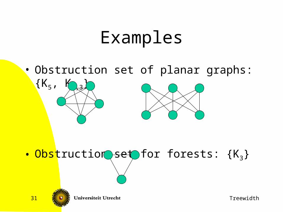
Examples

• Obstruction set of planar graphs: {K5, K3,3}

• Obstruction set for forests: {K3}

Treewidth32

Minor testing

• For fixed H, testing if H is a minor of a given graph can be done in O(n3) time.

• For fixed H, and k, testing if H is a minor of a given graph of treewidth at most k can be done in O(n) time.

• Theorem (Robertson and Seymour): For each planar H, there is a constant cH, such that each graph that does not have H as minor has treewidth at most cH.

Treewidth33

Decision algorithms

• Consequences

– If G is a minor-closed class of graphs, then there exists an O(n3) algorithm for membership-testing for G.

– If G is a minor-closed class of graphs that does not contain all planar graphs, then there exists an O(n3) algorithm for membership-testing for G.

• Do a minor-test for each graph in ob(G).

• Non-constructive!

Treewidth34

Use of minors

• Minor-taking gives sometimes very fast proofs for problems to be in FPT– If a parameter does not increase when taking

minors: O(n3)– If a parameter does not increase when taking

minors, and planar graphs have arbitrary large values: O(n)

• Bad news: non-constructive and usually very impractical algorithm

Treewidth35

Examples of minor closed classes

• Longest Cycle(k): {G | G does not have a cycle of length at least k}

• Longest Path-k

• Treewidth-k

• Genus:{G | G can be drawn without crossing edges on a surface of genus k} (Genus of surface: +- number of “ears”)

Treewidth36

Example: Interval Routing Schemes

• B, Thilikos, Tan, van Leeuwen: use of method for deciding if there is an interval routing scheme

• k-Interval routing:

– Label nodes in network by integers 0, 1, …

– Label each outgoing edge at each node by collection of at most k intervals (disjoint, spanning all integers)

– If we want to route a message to a node with label l, then send it, until it reaches its destination, along the edge with an interval that contains l

– This succeeds via shortest route in a valid scheme

Treewidth37

Graph class k-IRS

• G belongs to k-IRS, if we can label the nodes, such that for each assignment of lengths to edges, there is an assignment of at most k intervals to each outgoing edge, such that the result is a valid scheme– Variants of this class are also studied, and

similar techniques apply• k-IRS is closed under taking of minors!• K2,k+1 k-IRS (from Frederickson and Janardan)

Treewidth38

k-IRS is closed under taking of minors

• Sketch– Removing edge is like giving it very large

length– Contracting edge (u,v): give new node label of

u • Is like giving edge (u,v) zero length• Detail: gap in numbering can be removed

easily

Treewidth39

Testing membership in k-IRS

• Theorem: K2,k+1 k-IRS (from Frederickson and Janardan)

• Consequence: For each k, there is a linear time algorithm that tests if a given graph has treewidth at most k.

4. Using treewidth to obtain FPT results

1. Feedback Vertex Set

2. Convex tree recoloring

Treewidth41

Treewidth as parameter

• Many problems of the form– Given: Graph G, additional information– Parameter: the treewidth of G– Question: some question on G

• Are linear or polynomial time solvable• However, we can also often solve the ‘usual’

variants of problems with treewidth

Treewidth42

Feedback vertex set

• Given: graph G=(V,E), integer k• Parameter: k• Question: is there a set of at most k vertices, that,

when taken out of G gives a forest• Yes-instances have treewidth at most k+1

– Take a tree decomposition of the forest of width 1

– Add all vertices in the feedback vertex set to each bag

Treewidth43

Algorithm for FVS

• Check if the treewidth of G is at most k+1• If not: return NO• Else: solve the problem with dynamic

programming on the tree decomposition of width at most k+1– Algorithm uses O(n) time for fixed k

Treewidth44

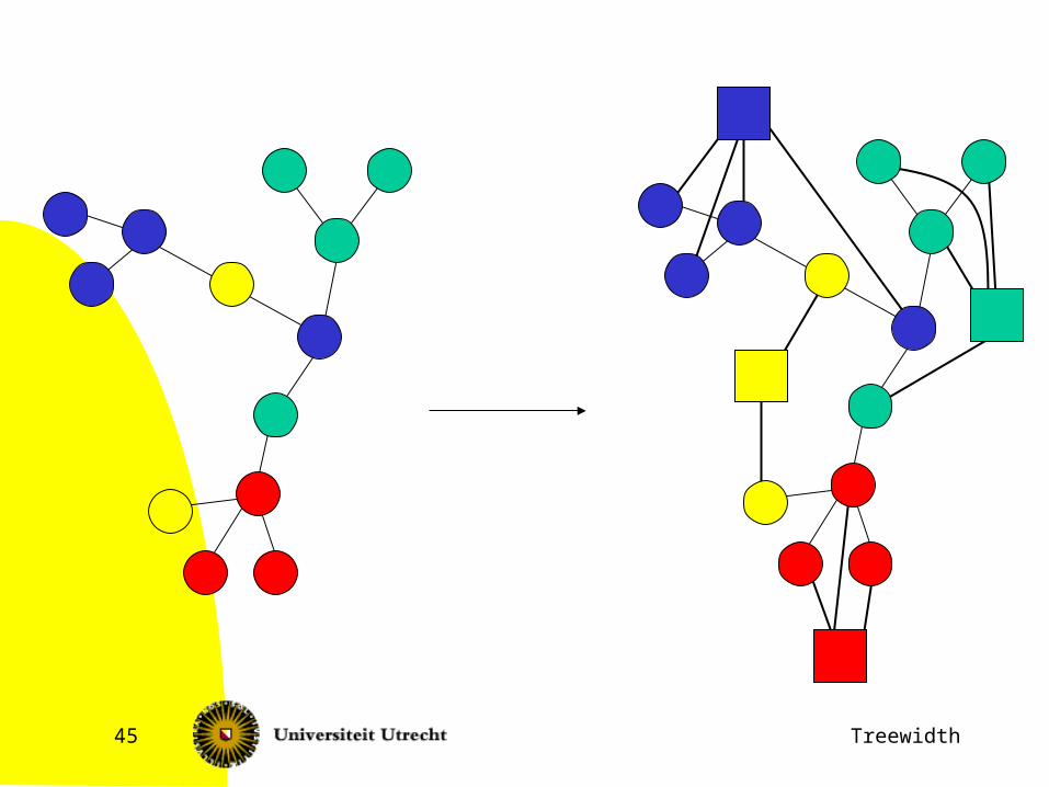
Convex recoloring of trees

• Build a graph from T=(V,E)• Add to T a new vertex for each color, and make

the color-vertex adjacent to all vertices with that color

Treewidth45

Treewidth46

Using G to solve the problem

• If there is a solution with at most k recolored vertices, then G has treewidth at most 2k+3

– Take a tree decomposition of T of width 1

– Add to each bag the vertices of the colors of the vertices in the bag, and the vertices of all broken colors (at most 2k broken colors)

• The problem to decide if T has a convex recoloring with at most k recolored vertices can be formulated as a property in Monadic Second Order Logic on G

• Thus, we can decide, for fixed k, in O(n) time

Treewidth47

Conclusions: treewidth

• Treewidth is a useful tool to show that problems are fixed parameter tractable

• Often– Relatively easy, “fast” proofs and arguments– Relatively slow algorithms

• Sometimes also useful in practice

Treewidth48

Conclusions: FPT

• Fixed parameter complexity is a fruitful and interesting new research area in algorithm design

• Several new (and old) techniques to obtain FPT-algorithms