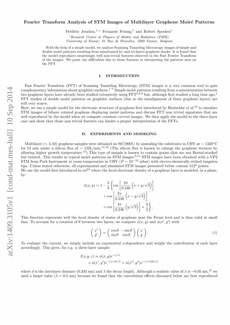
Fourier transform analysis of STM images of multilayer graphene moiré patterns

Fourier Transform Analysis of STM Images of Multilayer Graphene Moire Patterns

Frederic Joucken,1, ∗ Fernande Frising,1 and Robert Sporken1

1Research Center in Physics of Matter and Radiation (PMR),University of Namur, 61 Rue de Bruxelles, 5000 Namur, Belgium

With the help of a simple model, we analyze Scanning Tunneling Microscopy images of simple anddouble moire patterns resulting from misoriented bi- and tri-layers graphene stacks. It is found thatthe model reproduces surprisingly well non-trivial features observed in the Fast Fourier Transformof the images. We point out difficulties due to those features in interpreting the patterns seen onthe FFT.

I. INTRODUCTION

Fast Fourier Transform (FFT) of Scanning Tunneling Microscopy (STM) images is a very common tool to gaincomplementary information about graphitic surfaces.1–7 Simple moire patterns resulting from a misorientation betweentwo graphene layers have already been studied extensively using FFT3,8,9 but, although first studied a long time ago,1

FFT studies of double moire patterns on graphitic surfaces (due to the misalignment of three graphene layers) arestill very scarce.Here, we use a simple model for the electronic structure of graphene first intorduced by Hentschke et al.10 to simulateSTM images of bilayer rotated graphene displaying moire patterns and discuss FFT non trivial signatures that arewell reproduced by the model when we compute constant current images. We then apply the model to the three-layercase and show that those non trivial features can hinder a proper interpretation of the FFTs.

II. EXPERIMENTS AND MODELING

Multilayer (∼ 5-10) graphene samples were obtained on SiC(0001) by annealing the substrates in UHV at ∼ 1320◦Cfor 12 min under a silicon flux of ∼ 1ML/min.11,12 (The silicon flux is known to enlarge the graphene terraces byallowing higher growth temperature.13) This type of sample is known to contain grains that are not Bernal-stackedbut twisted. This results in typical moire patterns on STM images.8,14 STM images have been obtained with a VP2STM from Park Instrument at room temperature in UHV (P ∼ 10−10 mbar) with electro-chemically etched tungstentips. Unless stated otherwise, all experimental and simulated STM images presented below contain 5122 points.We use the model first introduced in ref10 where the local electronic density of a graphene layer is modeled, in a plane,by:

φ(x, y) = 1− 2

9

{cos

[2π

0.246

(x+ y/

√3)]

+ cos

[2π

0.246

(x− y/

√3)]

+ cos

[4π

0.246

(y/√

3)]

+3

2

}.

This function represents well the local density of states of graphene near the Fermi level and is thus valid at smallbias. To account for a rotation of θ between two layers, we compute φ(x, y) and φ(x′, y′) with(

x′

y′

)=

(cos θ − sin θsin θ cos θ

)(xy

). (1)

To evaluate the current, we simply include an exponential z-dependence and weight the contribution of each layeraccordingly. This gives, for e.g. a three-layer sample:

I(x,y, z) ∝ φ(x, y)e−z/λ

+ φ(x′, y′)e−(z+d)/λ + φ(x′′, y′′)e−(z+2d)/λ

where d is the interlayer distance (0.334 nm) and λ the decay length. Although a realistic value of λ is ∼0.05 nm,15 weused a larger value (λ = 0.5 nm) because we found that the convolution effects discussed below are best reproduced

arX

iv:1

409.

3105

v1 [

cond

-mat

.mes

-hal

l] 1

0 Se

p 20

14

2

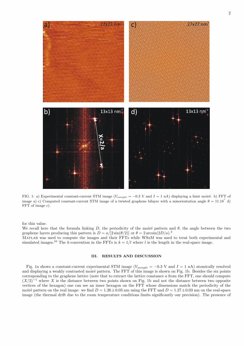
FIG. 1: a) Experimental constant-current STM image (Vsample = −0.3 V and I = 1 nA) displaying a faint moire. b) FFT of

image a) c) Computed constant-current STM image of a twisted graphene bilayer with a misorientation angle θ = 11.18◦

d)FFT of image c).

for this value.We recall here that the formula linking D, the periodicity of the moire pattern and θ, the angle between the twographene layers producing this pattern is D = a/[2 sin(θ/2)] or θ = 2 arcsin(2D/a).3

Matlab was used to compute the images and their FFTs while WSxM was used to treat both experimental andsimulated images.16 The k-convention in the FFTs is k = 1/l where l is the length in the real-space image.

III. RESULTS AND DISCUSSION

Fig. 1a shows a constant-current experimental STM image (Vsample = −0.3 V and I = 1 nA) atomically resolvedand displaying a weakly contrasted moire pattern. The FFT of this image is shown on Fig. 1b. Besides the six pointscorresponding to the graphene lattice (note that to extract the lattice constance a from the FFT, one should compute(X/2)−1 where X is the distance between two points shown on Fig. 1b and not the distance between two oppositevertices of the hexagon) one can see an inner hexagon on the FFT whose dimensions match the periodicity of themoire pattern on the real image: we find D = 1.26±0.03 nm using the FFT and D = 1.27±0.03 nm on the real-spaceimage (the thermal drift due to the room temperature conditions limits significantly our precision). The presence of

3

the moire pattern in the real-space image does not imply the appearance of this hexagon in the FFT since the moirecould appear if the height variations of the tip would simply be the addition of the height variations due to the twolayers taken separately, in which case no signal having the periodicity matching the moire’s would appear in the FFT.So one could think that the presence of the inner hexagon in the FFT in Fig. 1b is a sign of a topographic effect (theheight of the atoms of the top layer is distributed by the moire lattice). It is actually not obvious as this pattern is

reproduced when we compute a constant-current image of twisted bilayer graphene (θ = 11.18◦), shown on Fig. 1c

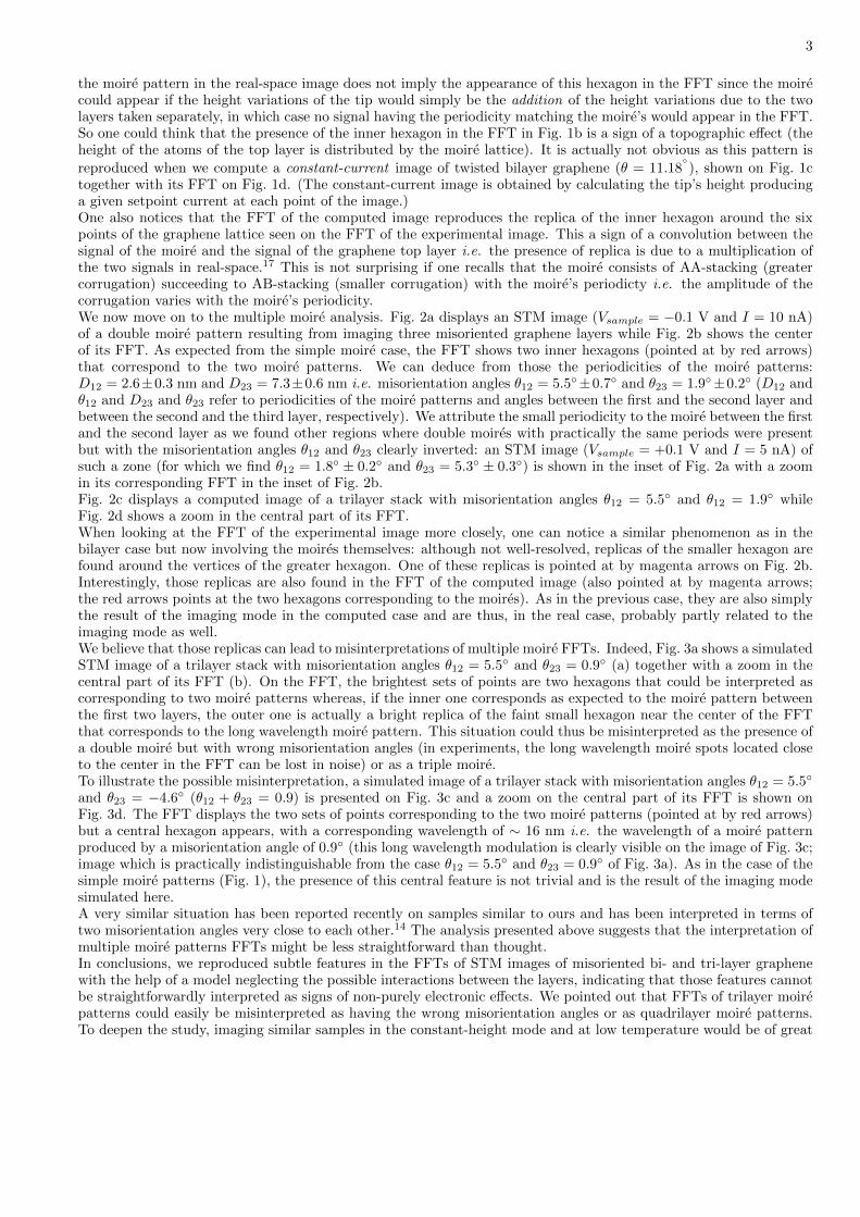
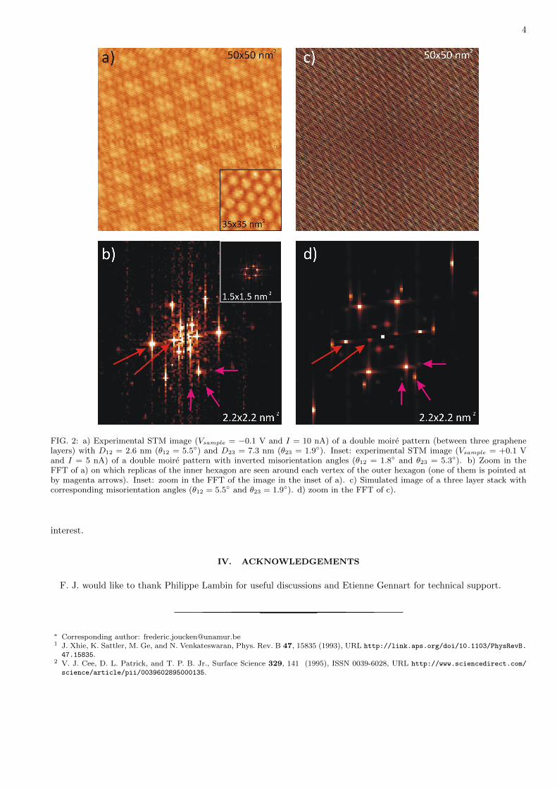
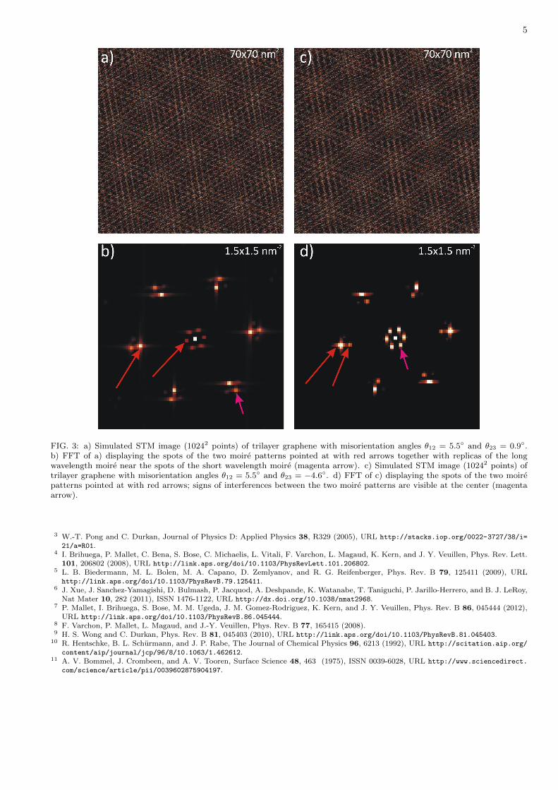
together with its FFT on Fig. 1d. (The constant-current image is obtained by calculating the tip’s height producinga given setpoint current at each point of the image.)One also notices that the FFT of the computed image reproduces the replica of the inner hexagon around the sixpoints of the graphene lattice seen on the FFT of the experimental image. This a sign of a convolution between thesignal of the moire and the signal of the graphene top layer i.e. the presence of replica is due to a multiplication ofthe two signals in real-space.17 This is not surprising if one recalls that the moire consists of AA-stacking (greatercorrugation) succeeding to AB-stacking (smaller corrugation) with the moire’s periodicty i.e. the amplitude of thecorrugation varies with the moire’s periodicity.We now move on to the multiple moire analysis. Fig. 2a displays an STM image (Vsample = −0.1 V and I = 10 nA)of a double moire pattern resulting from imaging three misoriented graphene layers while Fig. 2b shows the centerof its FFT. As expected from the simple moire case, the FFT shows two inner hexagons (pointed at by red arrows)that correspond to the two moire patterns. We can deduce from those the periodicities of the moire patterns:D12 = 2.6±0.3 nm and D23 = 7.3±0.6 nm i.e. misorientation angles θ12 = 5.5◦±0.7◦ and θ23 = 1.9◦±0.2◦ (D12 andθ12 and D23 and θ23 refer to periodicities of the moire patterns and angles between the first and the second layer andbetween the second and the third layer, respectively). We attribute the small periodicity to the moire between the firstand the second layer as we found other regions where double moires with practically the same periods were presentbut with the misorientation angles θ12 and θ23 clearly inverted: an STM image (Vsample = +0.1 V and I = 5 nA) ofsuch a zone (for which we find θ12 = 1.8◦ ± 0.2◦ and θ23 = 5.3◦ ± 0.3◦) is shown in the inset of Fig. 2a with a zoomin its corresponding FFT in the inset of Fig. 2b.Fig. 2c displays a computed image of a trilayer stack with misorientation angles θ12 = 5.5◦ and θ12 = 1.9◦ whileFig. 2d shows a zoom in the central part of its FFT.When looking at the FFT of the experimental image more closely, one can notice a similar phenomenon as in thebilayer case but now involving the moires themselves: although not well-resolved, replicas of the smaller hexagon arefound around the vertices of the greater hexagon. One of these replicas is pointed at by magenta arrows on Fig. 2b.Interestingly, those replicas are also found in the FFT of the computed image (also pointed at by magenta arrows;the red arrows points at the two hexagons corresponding to the moires). As in the previous case, they are also simplythe result of the imaging mode in the computed case and are thus, in the real case, probably partly related to theimaging mode as well.We believe that those replicas can lead to misinterpretations of multiple moire FFTs. Indeed, Fig. 3a shows a simulatedSTM image of a trilayer stack with misorientation angles θ12 = 5.5◦ and θ23 = 0.9◦ (a) together with a zoom in thecentral part of its FFT (b). On the FFT, the brightest sets of points are two hexagons that could be interpreted ascorresponding to two moire patterns whereas, if the inner one corresponds as expected to the moire pattern betweenthe first two layers, the outer one is actually a bright replica of the faint small hexagon near the center of the FFTthat corresponds to the long wavelength moire pattern. This situation could thus be misinterpreted as the presence ofa double moire but with wrong misorientation angles (in experiments, the long wavelength moire spots located closeto the center in the FFT can be lost in noise) or as a triple moire.To illustrate the possible misinterpretation, a simulated image of a trilayer stack with misorientation angles θ12 = 5.5◦

and θ23 = −4.6◦ (θ12 + θ23 = 0.9) is presented on Fig. 3c and a zoom on the central part of its FFT is shown onFig. 3d. The FFT displays the two sets of points corresponding to the two moire patterns (pointed at by red arrows)but a central hexagon appears, with a corresponding wavelength of ∼ 16 nm i.e. the wavelength of a moire patternproduced by a misorientation angle of 0.9◦ (this long wavelength modulation is clearly visible on the image of Fig. 3c;image which is practically indistinguishable from the case θ12 = 5.5◦ and θ23 = 0.9◦ of Fig. 3a). As in the case of thesimple moire patterns (Fig. 1), the presence of this central feature is not trivial and is the result of the imaging modesimulated here.A very similar situation has been reported recently on samples similar to ours and has been interpreted in terms oftwo misorientation angles very close to each other.14 The analysis presented above suggests that the interpretation ofmultiple moire patterns FFTs might be less straightforward than thought.In conclusions, we reproduced subtle features in the FFTs of STM images of misoriented bi- and tri-layer graphenewith the help of a model neglecting the possible interactions between the layers, indicating that those features cannotbe straightforwardly interpreted as signs of non-purely electronic effects. We pointed out that FFTs of trilayer moirepatterns could easily be misinterpreted as having the wrong misorientation angles or as quadrilayer moire patterns.To deepen the study, imaging similar samples in the constant-height mode and at low temperature would be of great

4

FIG. 2: a) Experimental STM image (Vsample = −0.1 V and I = 10 nA) of a double moire pattern (between three graphenelayers) with D12 = 2.6 nm (θ12 = 5.5◦) and D23 = 7.3 nm (θ23 = 1.9◦). Inset: experimental STM image (Vsample = +0.1 Vand I = 5 nA) of a double moire pattern with inverted misorientation angles (θ12 = 1.8◦ and θ23 = 5.3◦). b) Zoom in theFFT of a) on which replicas of the inner hexagon are seen around each vertex of the outer hexagon (one of them is pointed atby magenta arrows). Inset: zoom in the FFT of the image in the inset of a). c) Simulated image of a three layer stack withcorresponding misorientation angles (θ12 = 5.5◦ and θ23 = 1.9◦). d) zoom in the FFT of c).

interest.

IV. ACKNOWLEDGEMENTS

F. J. would like to thank Philippe Lambin for useful discussions and Etienne Gennart for technical support.

∗ Corresponding author: [email protected] J. Xhie, K. Sattler, M. Ge, and N. Venkateswaran, Phys. Rev. B 47, 15835 (1993), URL http://link.aps.org/doi/10.1103/PhysRevB.

47.15835.2 V. J. Cee, D. L. Patrick, and T. P. B. Jr., Surface Science 329, 141 (1995), ISSN 0039-6028, URL http://www.sciencedirect.com/

science/article/pii/0039602895000135.

5

FIG. 3: a) Simulated STM image (10242 points) of trilayer graphene with misorientation angles θ12 = 5.5◦ and θ23 = 0.9◦.b) FFT of a) displaying the spots of the two moire patterns pointed at with red arrows together with replicas of the longwavelength moire near the spots of the short wavelength moire (magenta arrow). c) Simulated STM image (10242 points) oftrilayer graphene with misorientation angles θ12 = 5.5◦ and θ23 = −4.6◦. d) FFT of c) displaying the spots of the two moirepatterns pointed at with red arrows; signs of interferences between the two moire patterns are visible at the center (magentaarrow).

3 W.-T. Pong and C. Durkan, Journal of Physics D: Applied Physics 38, R329 (2005), URL http://stacks.iop.org/0022-3727/38/i=

21/a=R01.4 I. Brihuega, P. Mallet, C. Bena, S. Bose, C. Michaelis, L. Vitali, F. Varchon, L. Magaud, K. Kern, and J. Y. Veuillen, Phys. Rev. Lett.

101, 206802 (2008), URL http://link.aps.org/doi/10.1103/PhysRevLett.101.206802.5 L. B. Biedermann, M. L. Bolen, M. A. Capano, D. Zemlyanov, and R. G. Reifenberger, Phys. Rev. B 79, 125411 (2009), URLhttp://link.aps.org/doi/10.1103/PhysRevB.79.125411.

6 J. Xue, J. Sanchez-Yamagishi, D. Bulmash, P. Jacquod, A. Deshpande, K. Watanabe, T. Taniguchi, P. Jarillo-Herrero, and B. J. LeRoy,Nat Mater 10, 282 (2011), ISSN 1476-1122, URL http://dx.doi.org/10.1038/nmat2968.

7 P. Mallet, I. Brihuega, S. Bose, M. M. Ugeda, J. M. Gomez-Rodriguez, K. Kern, and J. Y. Veuillen, Phys. Rev. B 86, 045444 (2012),URL http://link.aps.org/doi/10.1103/PhysRevB.86.045444.

8 F. Varchon, P. Mallet, L. Magaud, and J.-Y. Veuillen, Phys. Rev. B 77, 165415 (2008).9 H. S. Wong and C. Durkan, Phys. Rev. B 81, 045403 (2010), URL http://link.aps.org/doi/10.1103/PhysRevB.81.045403.

10 R. Hentschke, B. L. Schurmann, and J. P. Rabe, The Journal of Chemical Physics 96, 6213 (1992), URL http://scitation.aip.org/

content/aip/journal/jcp/96/8/10.1063/1.462612.11 A. V. Bommel, J. Crombeen, and A. V. Tooren, Surface Science 48, 463 (1975), ISSN 0039-6028, URL http://www.sciencedirect.

com/science/article/pii/0039602875904197.

6

12 I. Forbeaux, J.-M. Themlin, A. Charrier, F. Thibaudau, and J.-M. Debever, Applied Surface Science 162-163, 406 (2000), ISSN0169-4332, URL http://www.sciencedirect.com/science/article/pii/S0169433200002245.

13 R. M. Tromp and J. B. Hannon, Phys. Rev. Lett. 102, 106104 (2009), URL http://link.aps.org/doi/10.1103/PhysRevLett.102.

106104.14 D. L. Miller, K. D. Kubista, G. M. Rutter, M. Ruan, W. A. de Heer, P. N. First, and J. A. Stroscio, Phys. Rev. B 81, 125427 (2010),

URL http://link.aps.org/doi/10.1103/PhysRevB.81.125427.15 Y. Zhang, V. W. Brar, F. Wang, C. Girit, Y. Yayon, M. Panlasigui, A. Zettl, and M. F. Crommie, Nat Phys 4, 627 (2008).16 I. Horcas, R. Fernandez, J. M. Gomez-Rodrıguez, J. Colchero, J. Gomez-Herrero, and A. M. Baro, Rev. Sci. Instrum. 78, 013705

(2007).17 E. Oran Brigham, The Fast Fourier Transform (Prentice-Hall, 1974).