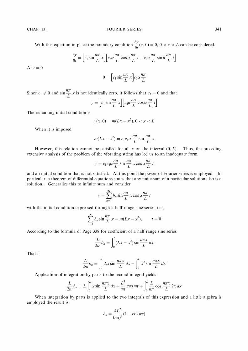
Fourier Series - CAUcau.ac.kr/~mhhgtx/courses/AdvancedMath/references/FourierSeries-Sc… · FOURIER SERIES Let fðxÞ be deﬁned in the interval ð#L;LÞ and outside of this interval

336

Fourier Series

Mathematicians of the eighteenth century, including Daniel Bernoulli and Leonard Euler, expressedthe problem of the vibratory motion of a stretched string through partial di!erential equations that hadno solutions in terms of ‘‘elementary functions.’’ Their resolution of this di"culty was to introduceinfinite series of sine and cosine functions that satisfied the equations. In the early nineteenth century,Joseph Fourier, while studying the problem of heat flow, developed a cohesive theory of such series.Consequently, they were named after him. Fourier series and Fourier integrals are investigated in thisand the next chapter. As you explore the ideas, notice the similarities and di!erences with the chapterson infinite series and improper integrals.

PERIODIC FUNCTIONS

A function f !x" is said to have a period T or to be periodic with period T if for all x, f !x# T" $ f !x",where T is a positive constant. The least value of T > 0 is called the least period or simply the period off !x".

EXAMPLE 1. The function sinx has periods 2!; 4!; 6!; . . . ; since sin !x# 2!"; sin !x# 4!"; sin !x# 6!"; . . . allequal sinx. However, 2! is the least period or the period of sin x.

EXAMPLE 2. The period of sin nx or cos nx, where n is a positive integer, is 2!=n.

EXAMPLE 3. The period of tan x is !.

EXAMPLE 4. A constant has any positive number as period.

Other examples of periodic functions are shown in the graphs of Figures 13-1(a), (b), and (c) below.

f (x)

x

Peri

od f (x) f (x)

x x

Peri

od Peri

od

(a) (b) (c)

Fig. 13-1

Copyright 2002, 1963 by The McGraw-Hill Companies, Inc. Click Here for Terms of Use.

FOURIER SERIES

Let f !x" be defined in the interval !#L;L" and outside of this interval by f !x$ 2L" % f !x", i.e., f !x"is 2L-periodic. It is through this avenue that a new function on an infinite set of real numbers is createdfrom the image on !#L;L". The Fourier series or Fourier expansion corresponding to f !x" is given by

a02$X

1

n%1

an cosn!x

L$ bn sin

n!x

L

! "

!1"

where the Fourier coe!cients an and bn are

an %1

L

#L

#Lf !x" cos n!x

Ldx

n % 0; 1; 2; . . .

bn %1

L

#L

#Lf !x" sin n!x

Ldx

8

>

>

>

<

>

>

>

:

!2"

ORTHOGONALITY CONDITIONS FOR THE SINE AND COSINE FUNCTIONS

Notice that the Fourier coe!cients are integrals. These are obtained by starting with the series, (1),and employing the following properties called orthogonality conditions:

(a)

#L

#Lcos

m!x

Lcos

n!x

Ldx % 0 if m 6% n and L if m % n

(b)

#L

#Lsin

m!x

Lsin

n!x

Ldx % 0 if m 6% n and L if m % n (3)

(c)

#L

#Lsin

m!x

Lcos

n!x

Ldx % 0. Where m and n can assume any positive integer values.

An explanation for calling these orthogonality conditions is given on Page 342. Their application indetermining the Fourier coe!cients is illustrated in the following pair of examples and then demon-strated in detail in Problem 13.4.

EXAMPLE 1. To determine the Fourier coe!cient a0, integrate both sides of the Fourier series (1), i.e.,#L

#Lf !x" dx %

#L

#L

a02

dx$#L

#L

X

1

n%1

an cosn!x

L$ bn sin

n!x

L

n o

dx

Now

#L

#L

a02

dx % a0L;

#L

#lsin

n!x

Ldx % 0;

#L

#Lcos

n!x

Ldx % 0, therefore, a0 %

1

L

#L

#Lf !x" dx

EXAMPLE 2. To determine a1, multiply both sides of (1) by cos!x

Land then integrate. Using the orthogonality

conditions (3)a and (3)c, we obtain a1 %1

L

#L

#Lf !x" cos !x

Ldx. Now see Problem 13.4.

If L % !, the series (1) and the coe!cients (2) or (3) are particularly simple. The function in thiscase has the period 2!.

DIRICHLET CONDITIONS

Suppose that

(1) f !x" is defined except possibly at a finite number of points in !#L;L"(2) f !x" is periodic outside !#L;L" with period 2L

CHAP. 13] FOURIER SERIES 337

(3) f !x" and f 0!x" are piecewise continuous in !#L;L".

Then the series (1) with Fourier coe!cients converges to

!a" f !x" if x is a point of continuity

!b" f !x$ 0" $ f !x# 0"2

if x is a point of discontinuity

Here f !x$ 0" and f !x# 0" are the right- and left-hand limits of f !x" at x and represent lim!!0$

f !x$ !" andlim!!0$

f !x# !", respectively. For a proof see Problems 13.18 through 13.23.

The conditions (1), (2), and (3) imposed on f !x" are su!cient but not necessary, and are generallysatisfied in practice. There are at present no known necessary and su!cient conditions for convergenceof Fourier series. It is of interest that continuity of f !x" does not alone ensure convergence of a Fourierseries.

ODD AND EVEN FUNCTIONS

A function f !x" is called odd if f !#x" % #f !x". Thus, x3; x5 # 3x3 $ 2x; sin x; tan 3x are oddfunctions.

A function f !x" is called even if f !#x" % f !x". Thus, x4; 2x6 # 4x2 $ 5; cos x; ex $ e#x are evenfunctions.

The functions portrayed graphically in Figures 13-1(a) and 13-1!b" are odd and even respectively,but that of Fig. 13-1(c) is neither odd nor even.

In the Fourier series corresponding to an odd function, only sine terms can be present. In theFourier series corresponding to an even function, only cosine terms (and possibly a constant which weshall consider a cosine term) can be present.

HALF RANGE FOURIER SINE OR COSINE SERIES

A half range Fourier sine or cosine series is a series in which only sine terms or only cosine terms arepresent, respectively. When a half range series corresponding to a given function is desired, the functionis generally defined in the interval !0;L" [which is half of the interval !#L;L", thus accounting for thename half range] and then the function is specified as odd or even, so that it is clearly defined in the otherhalf of the interval, namely, !#L; 0". In such case, we have

an % 0; bn %2

L

!L

0f !x" sin n"x

Ldx for half range sine series

bn % 0; an %2

L

!L

0f !x" cos n"x

Ldx for half range cosine series

8

>

>

>

<

>

>

>

:

!4"

PARSEVAL’S IDENTITY

If an and bn are the Fourier coe!cients corresponding to f !x" and if f !x" satisfies the Dirichletconditions.

Then1

L

!L

#Lf f !x"g2 dx % a20

2$X

1

n%1

!a2n $ b2n" (5)

(See Problem 13.13.)

338 FOURIER SERIES [CHAP. 13

DIFFERENTIATION AND INTEGRATION OF FOURIER SERIES

Di!erentiation and integration of Fourier series can be justified by using the theorems on Pages 271and 272, which hold for series in general. It must be emphasized, however, that those theorems providesu"cient conditions and are not necessary. The following theorem for integration is especially useful.

Theorem. The Fourier series corresponding to f !x"may be integrated term by term from a to x, and the

resulting series will converge uniformly to

!x

af !x" dx provided that f !x" is piecewise continuous in

#L @ x @ L and both a and x are in this interval.

COMPLEX NOTATION FOR FOURIER SERIES

Using Euler’s identities,

ei! $ cos ! % i sin !; e#i! $ cos ! # i sin ! !6"

where i $"""""""

#1p

(see Problem 11.48, Chapter 11, Page 295), the Fourier series for f !x" can be written as

f !x" $X

1

n$#1cn e

in"x=L !7"

where

cn $1

2L

!L

#Lf !x"e#in"x=L dx !8"

In writing the equality (7), we are supposing that the Dirichlet conditions are satisfied and furtherthat f !x" is continuous at x. If f !x" is discontinuous at x, the left side of (7) should be replaced by!f !x% 0" % f !x# 0"

2:

BOUNDARY-VALUE PROBLEMS

Boundary-value problems seek to determine solutions of partial di!erential equations satisfyingcertain prescribed conditions called boundary conditions. Some of these problems can be solved byuse of Fourier series (see Problem 13.24).

EXAMPLE. The classical problem of a vibrating string may be idealized in the following way. See Fig. 13-2.

Suppose a string is tautly stretched between points !0; 0" and !L; 0". Suppose the tension, F, is thesame at every point of the string. The string is made tovibrate in the xy plane by pulling it to the parabolicposition g!x" $ m!Lx# x2" and releasing it. (m is anumerically small positive constant.) Its equation willbe of the form y $ f !x; t". The problem of establishingthis equation is idealized by (a) assuming that the con-stant tension, F , is so large as compared to the weight wLof the string that the gravitational force can be neglected,(b) the displacement at any point of the string is so smallthat the length of the string may be taken as L for any ofits positions, and (c) the vibrations are purely transverse.

The force acting on a segment PQ isw

g!x

@2y

@t2;

x < x1 < x%!x; g & 32 ft per sec:2. If # and $ are theangles that F makes with the horizontal, then the vertical


Fig. 13-2

di!erence in tensions is F!sin !" sin "#. This is the force producing the acceleration that accounts forthe vibratory motion.

Now Ffsin !" sin "g $ Ftan !

!!!!!!!!!!!!!!!!!!!!!

1% tan2 !p " tan"

!!!!!!!!!!!!!!!!!!!!!

1% tan2 "p

( )

& Fftan!" tan"g $ F@y

@x!x%!x; t#"

"

@y

@x!x; t#

#

, where the squared terms in the denominator are neglected because the vibrations are small.

Next, equate the two forms of the force, i.e.,

F@y

@x!x%!x; t# " @y

@x!x; t#

" #

$ w

g!x

@2y

@t2

divide by !x, and then let !x ! 0. After letting ! $!!!!!!

Fg

w

r

, the resulting equation is

@2y

@t2$ !2 @

2y

@x2

This homogeneous second partial derivative equation is the classical equation for the vibratingstring. Associated boundary conditions are

y!0; t# $ 0; y!L; t# $ 0; t > 0

The initial conditions are

y!x; 0# $ m!Lx" x2#; @y@t

!x; 0# $ 0; 0 < x < L

The method of solution is to separate variables, i.e., assume

y!x; t# $ G!x#H!t#

Then upon substituting

G!x#H 00!t# $ !2G 00!x#H!t#

Separating variables yields

G 00

G$ k;

H 00

H$ !2k; where k is an arbitrary constant

Since the solution must be periodic, trial solutions are

G!x# $ c1 sin!!!!!!!

"kp

x% c2 cos!!!!!!!

"kp

x; < 0

H!t# $ c3 sin !!!!!!!!

"kp

t% c4 cos !!!!!!!!

"kp

t

Therefore

y $ GH $ 'c1 sin!!!!!!!

"kp

x% c2 cos!!!!!!!

"kp

x('c3 sin !!!!!!!!

"kp

t% c4 cos!!!!!!!!

"kp

t(

The initial condition y $ 0 at x $ 0 for all t leads to the evaluation c2 $ 0.Thus

y $ 'c1 sin!!!!!!!

"kp

x('c3 sin !!!!!!!!

"kp

t% c4 cos!!!!!!!!

"kp

t(

Now impose the boundary condition y $ 0 at x $ L, thus 0 $ 'c1 sin!!!!!!!

"kp

L('c3 sin !!!!!!!!

"kp

t%c4 cos!

!!!!!!!

"kp

t(:c1 6$ 0 as that would imply y $ 0 and a trivial solution. The next simplest solution results from the

choice!!!!!!!

"kp

$ n#

L, since y $ c1 sin

n#

Lx

h i

c3 sin !n#

lt% c4 cos!

n#

Lt

h i

and the first factor is zero when

x $ L.


With this equation in place the boundary condition@y

@t!x; 0" # 0, 0 < x < L can be considered.

@y

@t# c1 sin

n!

Lx

h i

c3"n!

Lcos"

n!

Lt$ c4"

n!

Lsin "

n!

Lt

h i

At t # 0

0 # c1 sinn!

Lx

h i

c3"n!

L

Since c1 6# 0 and sinn!

Lx is not identically zero, it follows that c3 # 0 and that

y # c1 sinn!

Lx

h i

c4"n!

Lcos"

n!

Lt

h i

The remaining initial condition is

y!x; 0" # m!Lx$ x2"; 0 < x < L

When it is imposed

m!Lx$ x2" # c1c4"n!

Lsin

n!

Lx

However, this relation cannot be satisfied for all x on the interval !0;L". Thus, the precedingextensive analysis of the problem of the vibrating string has led us to an inadequate form

y # c1c4"n!

Lsin

n!

Lx cos"

n!

Lt

and an initial condition that is not satisfied. At this point the power of Fourier series is employed. Inparticular, a theorem of di!erential equations states that any finite sum of a particular solution also is asolution. Generalize this to infinite sum and consider

y #X

1

n#1

bn sinn!

Lx cos "

n!

Lt

with the initial condition expressed through a half range sine series, i.e.,

X

1

n#1

bn sinn!

Lx # m!Lx$ x2"; t # 0

According to the formula of Page 338 for coe"cient of a half range sine series

L

2mbn #

!L

0!Lx$ x2" sin n!x

Ldx

That is

L

2mbn #

!L

0Lx sin

n!x

Ldx$

!L

0x2 sin

n!x

Ldx

Application of integration by parts to the second integral yields

L

2mbn # L

!L

0x sin

n!x

Ldx% L3

n!cos n!%

!L

0

L

n!cos

n!x

L2x dx

When integration by parts is applied to the two integrals of this expression and a little algebra isemployed the result is

bn #4L2

!n!"3!1$ cos n!"


Therefore,

y !X

1

n!1

bn sinn!

Lx cos"

n!

Lt

with the coe!cients bn defined above.

ORTHOGONAL FUNCTIONS

Two vectors A and B are called orthogonal (perpendicular) if A " B ! 0 or A1B1 # A2B2 # A3B3 ! 0,where A ! A1i# A2j# A3k and B ! B1i# B2j# B3k. Although not geometrically or physically evi-dent, these ideas can be generalized to include vectors with more than three components. In particular,we can think of a function, say, A$x%, as being a vector with an infinity of components (i.e., an infinitedimensional vector), the value of each component being specified by substituting a particular value of x insome interval $a; b%. It is natural in such case to define two functions, A$x% and B$x%, as orthogonal in$a; b% if

!b

aA$x%B$x% dx ! 0 $9%

A vector A is called a unit vector or normalized vector if its magnitude is unity, i.e., if A " A ! A2 ! 1.Extending the concept, we say that the function A$x% is normal or normalized in $a; b% if

!b

afA$x%g2 dx ! 1 $10%

From the above it is clear that we can consider a set of functions f#k$x%g; k ! 1; 2; 3; . . . ; having theproperties

!b

a#m$x%#n$x% dx ! 0 m 6! n $11%

!b

af#m$x%g2 dx ! 1 m ! 1; 2; 3; . . . $12%

In such case, each member of the set is orthogonal to every other member of the set and is alsonormalized. We call such a set of functions an orthonormal set.

The equations (11) and (12) can be summarized by writing

!b

a#m$x%#n$x% dx ! $mn $13%

where $mn, called Kronecker’s symbol, is defined as 0 if m 6! n and 1 if m ! n.Just as any vector r in three dimensions can be expanded in a set of mutually orthogonal unit vectors

i; j; k in the form r ! c1i# c2j# c3k, so we consider the possibility of expanding a function f $x% in a setof orthonormal functions, i.e.,

f $x% !X

1

n!1

cn#n$x% a @ x @ b $14%

As we have seen, Fourier series are constructed from orthogonal functions. Generalizations ofFourier series are of great interest and utility both from theoretical and applied viewpoints.


Solved Problems

FOURIER SERIES

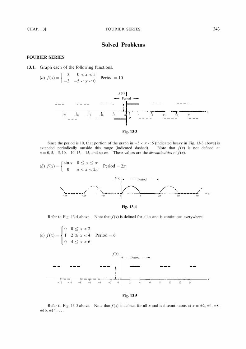
13.1. Graph each of the following functions.

!a" f !x" #3 0 < x < 5

$3 $5 < x < 0Period # 10

!

Since the period is 10, that portion of the graph in $5 < x < 5 (indicated heavy in Fig. 13-3 above) isextended periodically outside this range (indicated dashed). Note that f !x" is not defined atx # 0; 5;$5; 10;$10; 15;$15, and so on. These values are the discontinuities of f !x".

!b" f !x" #sin x 0 @ x @ !

0 ! < x < 2!Period # 2!

!

Refer to Fig. 13-4 above. Note that f !x" is defined for all x and is continuous everywhere.

!c" f !x" #0 0 @ x < 2

1 2 @ x < 4

0 4 @ x < 6

Period # 6

8

>

<

>

:

Refer to Fig. 13-5 above. Note that f !x" is defined for all x and is discontinuous at x # %2;%4;%8;%10;%14; . . . .


Period

f (x)

_25 _20 _15 _10 _5 53

3

0 10 15 20 25x

Fig. 13-3

Periodf (x)

4px

3p2pp0_p_2p_3p

Fig. 13-4

14x

121086420_2_4_6_8_10_12

1

Periodf (x)

Fig. 13-5

13.2. Prove

!L

!Lsin

k!x

Ldx "

!L

!Lcos

k!x

Ldx " 0 if k " 1; 2; 3; . . . .

!L

!Lsin

k!x

Ldx " ! L

k!cos

k!x

L

"

"

"

"

L

!L

" ! L

k!cos k!# L

k!cos$!k!% " 0

!L

!Lcos

k!x

Ldx " L

k!sin

k!x

L

"

"

"

"

L

!L

" L

k!sin k!! L

k!sin$!k!% " 0

13.3. Prove (a)

!L

!Lcos

m!x

Lcos

n!x

Ldx "

!L

!Lsin

m!x

Lsin

n!x

Ldx " 0 m 6" n

L m " n

#

(b)

!L

!Lsin

m!x

Lcos

n!x

Ldx " 0

where m and n can assume any of the values 1; 2; 3; . . . .

(a) From trigonometry: cosA cosB " 12 fcos$A! B% # cos$A# B%g; sinA sinB " 1

2 fcos$A! B% ! cos$A# B%g:

Then, if m 6" n, by Problem 13.2,

!L

!Lcos

m!x

Lcos

n!x

Ldx " 1

2

!L

!Lcos

$m! n%!xL

# cos$m# n%!x

L

# $

dx " 0

Similarly, if m 6" n,

!L

!Lsin

m!x

Lsin

n!x

Ldx " 1

2

!L

!Lcos

$m! n%!xL

! cos$m# n%!x

L

# $

dx " 0

If m " n, we have

!L

!Lcos

m!x

Lcos

n!x

Ldx " 1

2

!L

!L1# cos

2n!x

L

% &

dx " L

!L

!Lsin

m!x

Lsin

n!x

Ldx " 1

2

!L

!L1! cos

2n!x

L

% &

dx " L

Note that if m " n these integrals are equal to 2L and 0 respectively.

(b) We have sinA cosB " 12 fsin$A! B% # sin$A# B%g. Then by Problem 13.2, if m 6" n,

!L

!Lsin

m!x

Lcos

n!x

Ldx " 1

2

!L

!Lsin

$m! n%!xL

# sin$m# n%!x

L

# $

dx " 0

If m " n,

!L

!Lsin

m!x

Lcos

n!x

Ldx " 1

2

!L

!Lsin

2n!x

Ldx " 0

The results of parts (a) and (b) remain valid even when the limits of integration !L;L are replacedby c; c# 2L, respectively.

13.4. If the series A#X

1

n"1

an cosn!x

L# bn sin

n!x

L

' (

converges uniformly to f $x% in $!L;L%, show that

for n " 1; 2; 3; . . . ;

$a% an "1

L

!L

!Lf $x% cos n!x

Ldx; $b% bn "

1

L

!L

!Lf $x% sin n!x

Ldx; $c% A " a0

2:


(a) Multiplying

f !x" # A$X

1

n#1

an cosn!x

L$ bn sin

n!x

L

! "

!1"

by cosm!x

Land integrating from %L to L, using Problem 13.3, we have

#L

%Lf !x" cos m!x

Ldx # A

#L

%Lcos

m!x

Ldx

$X

1

n#1

an

#L

%Lcos

m!x

Lcos

n!x

Ldx$ bn

#L

%Lcos

m!x

Lsin

n!x

Ldx

$ %

# amL if m 6# 0

am # 1

L

#L

%Lf !x" cos m!x

Ldx if m # 1; 2; 3; . . .Thus

(b) Multiplying (1) by sinm!x

Land integrating from %L to L, using Problem 13.3, we have

#L

%Lf !x" sin m!x

Ldx # A

#L

%Lsin

m!x

Ldx

$X

1

n#1

an

#L

%Lsin

m!x

Lcos

n!x

Ldx$ bn

#L

%Lsin

m!x

Lsin

n!x

Ldx

$ %

# bmL

bm # 1

L

#L

%Lf !x" sin m!x

Ldx if m # 1; 2; 3; . . .Thus

(c) Integrating of (1) from %L to L, using Problem 13.2, gives

#L

%Lf !x" dx # 2AL or A # 1

2L

#L

%Lf !x" dx

Putting m # 0 in the result of part (a), we find a0 #1

L

#L

%Lf !x" dx and so A # a0

2.

The above results also hold when the integration limits %L;L are replaced by c; c$ 2L:Note that in all parts above, interchange of summation and integration is valid because the series is

assumed to converge uniformly to f !x" in !%L;L". Even when this assumption is not warranted, thecoe!cients am and bm as obtained above are called Fourier coe!cients corresponding to f !x", and thecorresponding series with these values of am and bm is called the Fourier series corresponding to f !x".An important problem in this case is to investigate conditions under which this series actually convergesto f !x". Su!cient conditions for this convergence are the Dirichlet conditions established in Problems13.18 through 13.23.

13.5. (a) Find the Fourier coe!cients corresponding to the function

f !x" # 0 %5 < x < 03 0 < x < 5

Period # 10

$

(b) Write the corresponding Fourier series.(c) How should f !x" be defined at x # %5; x # 0; and x # 5 in order that the Fourier series will

converge to f !x" for %5 @ x @ 5?

The graph of f !x" is shown in Fig. 13-6.


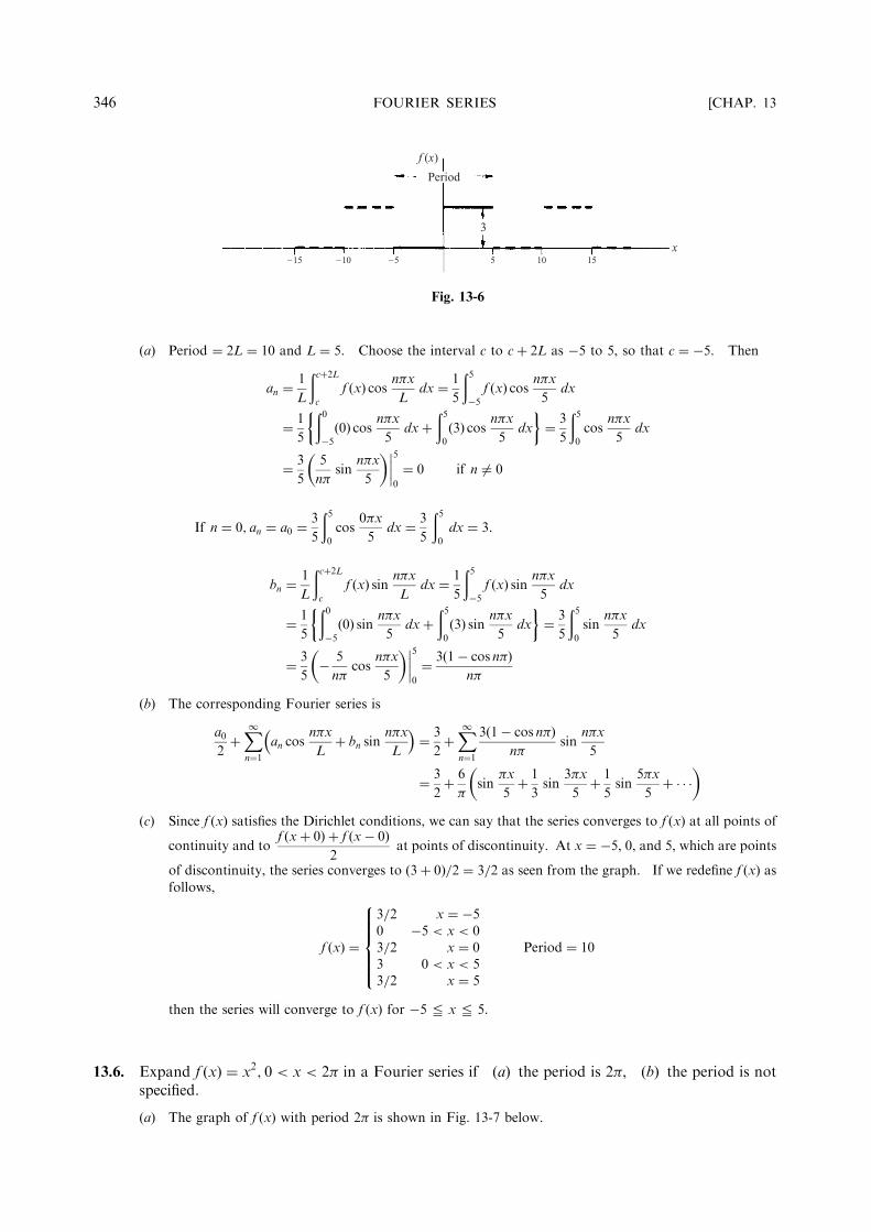
(a) Period ! 2L ! 10 and L ! 5. Choose the interval c to c" 2L as #5 to 5, so that c ! #5. Then

an !1

L

!c"2L

cf $x% cos n!x

Ldx ! 1

5

!5

#5f $x% cos n!x

5dx

! 1

5

!0

#5$0% cos n!x

5dx"

!5

0$3% cos n!x

5dx

" #

! 3

5

!5

0cos

n!x

5dx

! 3

5

5

n!sin

n!x

5

$ %&

&

&

&

5

0

! 0 if n 6! 0

If n ! 0; an ! a0 !3

5

!5

0cos

0!x

5dx ! 3

5

!5

0dx ! 3:

bn !1

L

!c"2L

cf $x% sin n!x

Ldx ! 1

5

!5

#5f $x% sin n!x

5dx

! 1

5

!0

#5$0% sin n!x

5dx"

!5

0$3% sin n!x

5dx

" #

! 3

5

!5

0sin

n!x

5dx

! 3

5# 5

n!cos

n!x

5

$ %&

&

&

&

5

0

! 3$1# cos n!%n!

(b) The corresponding Fourier series is

a02"X

1

n!1

an cosn!x

L" bn sin

n!x

L

' (

! 3

2"X

1

n!1

3$1# cos n!%n!

sinn!x

5

! 3

2" 6

!sin

!x

5" 1

3sin

3!x

5" 1

5sin

5!x

5" & & &

$ %

(c) Since f $x% satisfies the Dirichlet conditions, we can say that the series converges to f $x% at all points of

continuity and tof $x" 0% " f $x# 0%

2at points of discontinuity. At x ! #5, 0, and 5, which are points

of discontinuity, the series converges to $3" 0%=2 ! 3=2 as seen from the graph. If we redefine f $x% asfollows,

f $x% !

3=2 x ! #50 #5 < x < 03=2 x ! 03 0 < x < 53=2 x ! 5

Period ! 10

8

>

>

>

>

<

>

>

>

>

:

then the series will converge to f $x% for #5 @ x @ 5.

13.6. Expand f $x% ! x2; 0 < x < 2! in a Fourier series if (a) the period is 2!, (b) the period is notspecified.

(a) The graph of f $x% with period 2! is shown in Fig. 13-7 below.


_15 _10 _5 5

3

10x

15

Period

f (x)

Fig. 13-6

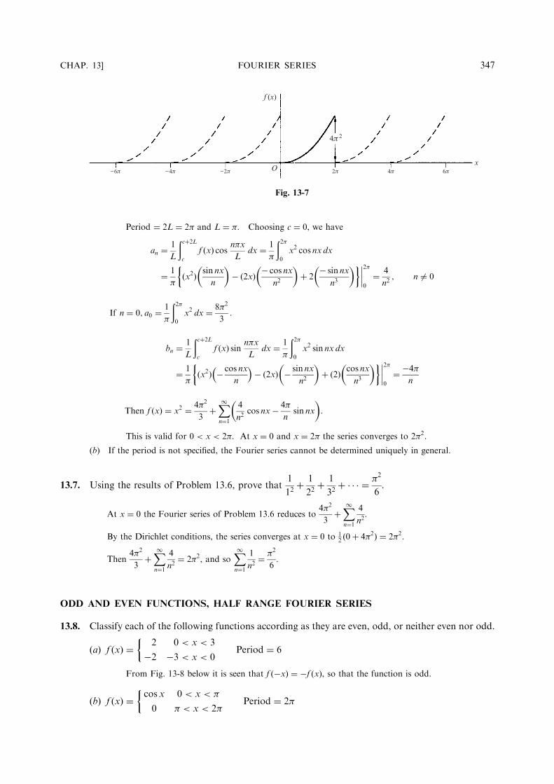
Period ! 2L ! 2! and L ! !. Choosing c ! 0, we have

an !1

L

!c"2L

cf #x$ cos n!x

Ldx ! 1

!

!2!

0x2 cos nx dx

! 1

!#x2$ sin nx

n

" #

% #2x$ % cos nx

n2

" #

" 2% sin nx

n3

" #$ %&

&

&

&

2!

0

! 4

n2; n 6! 0

If n ! 0; a0 !1

!

!2!

0x2 dx ! 8!2

3:

bn !1

L

!c"2L

cf #x$ sin n!x

Ldx ! 1

!

!2!

0x2 sin nx dx

! 1

!#x2$ % cos nx

n

' (

% #2x$ % sin nx

n2

" #

" #2$ cos nx

n3

" #$ %&

&

&

&

2!

0

! %4!

n

Then f #x$ ! x2 ! 4!2

3"X

1

n!1

4

n2cos nx% 4!

nsin nx

" #

:

This is valid for 0 < x < 2!. At x ! 0 and x ! 2! the series converges to 2!2.

(b) If the period is not specified, the Fourier series cannot be determined uniquely in general.

13.7. Using the results of Problem 13.6, prove that1

12" 1

22" 1

32" & & & ! !2

6.

At x ! 0 the Fourier series of Problem 13.6 reduces to4!2

3"X

1

n!1

4

n2.

By the Dirichlet conditions, the series converges at x ! 0 to 12 #0" 4!2$ ! 2!2.

Then4!2

3"X

1

n!1

4

n2! 2!2, and so

X

1

n!1

1

n2! !2

6.

ODD AND EVEN FUNCTIONS, HALF RANGE FOURIER SERIES

13.8. Classify each of the following functions according as they are even, odd, or neither even nor odd.

#a$ f #x$ !2 0 < x < 3

%2 %3 < x < 0Period ! 6

$

From Fig. 13-8 below it is seen that f #%x$ ! %f #x$, so that the function is odd.

#b$ f #x$ !cos x 0 < x < !

0 ! < x < 2!Period ! 2!

$


_6p _4p _2p O 2p 4p 6px

f (x)

4p2

Fig. 13-7

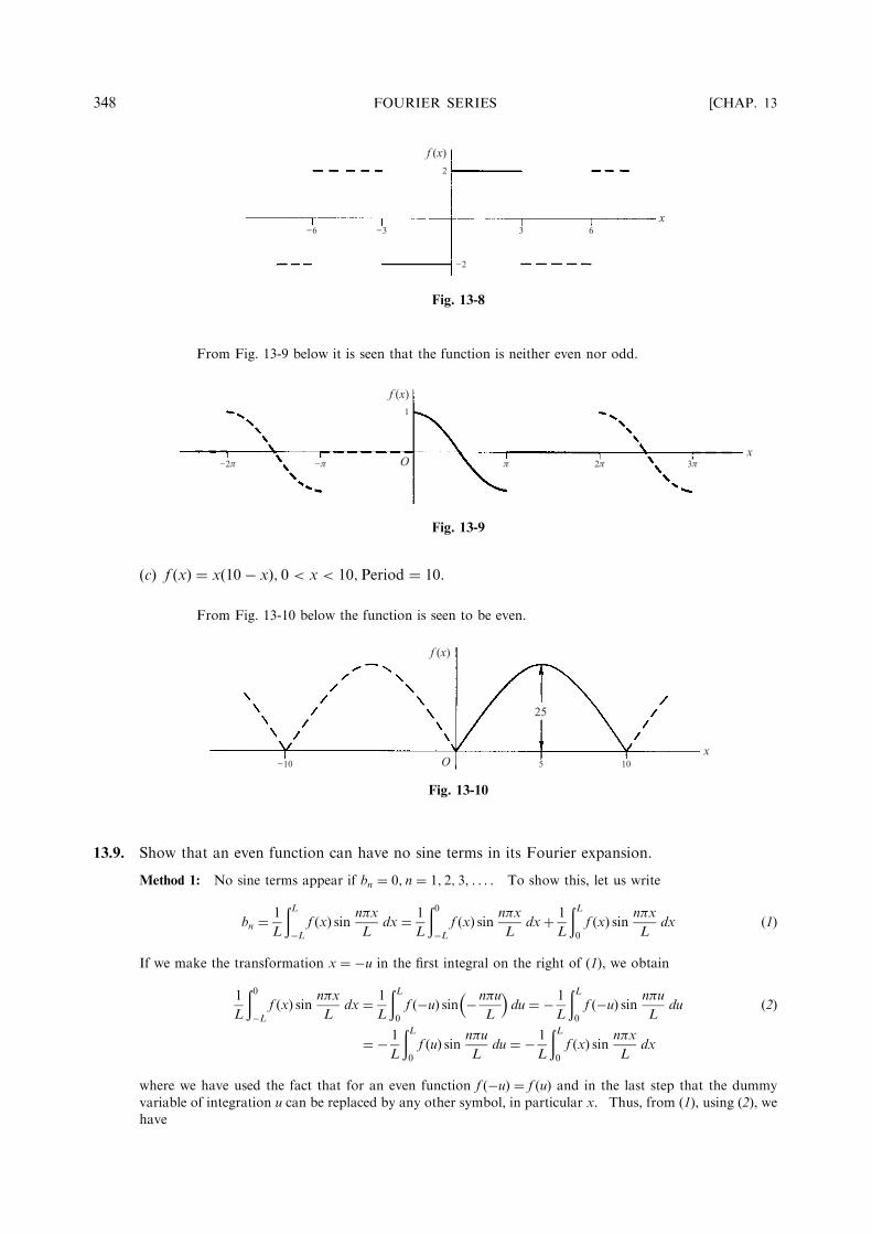
From Fig. 13-9 below it is seen that the function is neither even nor odd.

!c" f !x" # x!10$ x"; 0 < x < 10;Period # 10:

From Fig. 13-10 below the function is seen to be even.

13.9. Show that an even function can have no sine terms in its Fourier expansion.

Method 1: No sine terms appear if bn # 0; n # 1; 2; 3; . . . . To show this, let us write

bn #1

L

!L

$Lf !x" sin n!x

Ldx # 1

L

!0

$Lf !x" sin n!x

Ldx% 1

L

!L

0f !x" sin n!x

Ldx !1"

If we make the transformation x # $u in the first integral on the right of (1), we obtain

1

L

!0

$Lf !x" sin n!x

Ldx # 1

L

!L

0f !$u" sin $ n!u

L

" #

du # $ 1

L

!L

0f !$u" sin n!u

Ldu !2"

# $ 1

L

!L

0f !u" sin n!u

Ldu # $ 1

L

!L

0f !x" sin n!x

Ldx

where we have used the fact that for an even function f !$u" # f !u" and in the last step that the dummyvariable of integration u can be replaced by any other symbol, in particular x. Thus, from (1), using (2), wehave


f (x)2

_2

_6 _3 3 6x

Fig. 13-8

f (x)

O

1

_2p _p p 2p 3px

Fig. 13-9

f (x)

O

25

_10 5 10x

Fig. 13-10

bn ! " 1

L

!L

0f #x$ sin n!x

Ldx% 1

L

!L

0f #x$ sin n!x

Ldx ! 0

f #x$ ! a02%X

1

n!1

an cosn!x

L% bn sin

n!x

L

" #

:Method 2: Assume

f #"x$ ! a02%X

1

n!1

an cosn!x

L" bN sin

n!x

L

" #

:Then

If f #x$ is even, f #"x$ ! f #x$. Hence,

a02%X

1

n!1

an cosn!x

L% bn sin

n!x

L

" #

! a02%X

1

n!1

an cosn!x

L" bn sin

n!x

L

" #

X

1

n!1

bn sinn!x

L! 0; i.e., f #x$ ! a0

2%X

1

n!1

an cosn!x

Land so

and no sine terms appear.In a similar manner we can show that an odd function has no cosine terms (or constant term) in its

Fourier expansion.

13.10. If f #x$ is even, show that (a) an !2

L

!L

0f #x$ cos n!x

Ldx; #b$ bn ! 0.

an !1

L

!L

"Lf #x$ cos n!x

Ldx ! 1

L

!0

"Lf #x$ cos n!x

Ldx% 1

L

!L

0f #x$ cos n!x

Ldx#a$

Letting x ! "u,

1

L

!0

"Lf #x$ cos n!x

Ldx ! 1

L

!L

0f #"u$ cos "n!u

L

" #

du ! 1

L

!L

0f #u$ cos n!u

Ldu

since by definition of an even function f #"u$ ! f #u$. Then

an !1

L

!L

0f #u$ cos n!u

Ldu% 1

L

!L

0f #x$ cos n!x

Ldx ! 2

L

!L

0f #x$ cos n!x

Ldx

(b) This follows by Method 1 of Problem 13.9.

13.11. Expand f #x$ ! sin x; 0 < x < !, in a Fourier cosine series.

A Fourier series consisting of cosine terms alone is obtained only for an even function. Hence, weextend the definition of f #x$ so that it becomes even (dashed part of Fig. 13-11 below). With this extension,f #x$ is then defined in an interval of length 2!. Taking the period as 2!, we have 2L ! 2! so that L ! !.

By Problem 13.10, bn ! 0 and

an !2

L

!L

0f #x$ cos n!x

Ldx ! 2

!

!!

0sinx cos nx dx


f (x)

O_2p _p p 2px

Fig. 13-11

! 1

!

!!

0fsin"x# nx$ # sin"x% nx$g ! 1

!% cos"n# 1$x

n# 1# cos"n% 1$x

n% 1

" #$

$

$

$

!

0

! 1

!

1% cos"n# 1$!n# 1

# cos"n% 1$!% 1

n% 1

" #

! 1

!

1# cos n!

n# 1% 1# cos n!

n% 1

" #

! %2"1# cos n!$!"n2 % 1$

if n 6! 1:

For n ! 1; a1 !2

!

!!

0sin x cos x dx ! 2

!

sin2 x

2

$

$

$

$

!

0

! 0:

For n ! 0; a0 !2

!

!!

0sin x dx ! 2

!"% cos x$

$

$

$

$

!

0

! 4

!:

f "x$ ! 2

!% 2

!

X

1

n!2

"1# cos n!$n2 % 1

cos nxThen

! 2

!% 4

!

cos 2x

22 % 1# cos 4x

42 % 1# cos 6x

62 % 1# & & &

% &

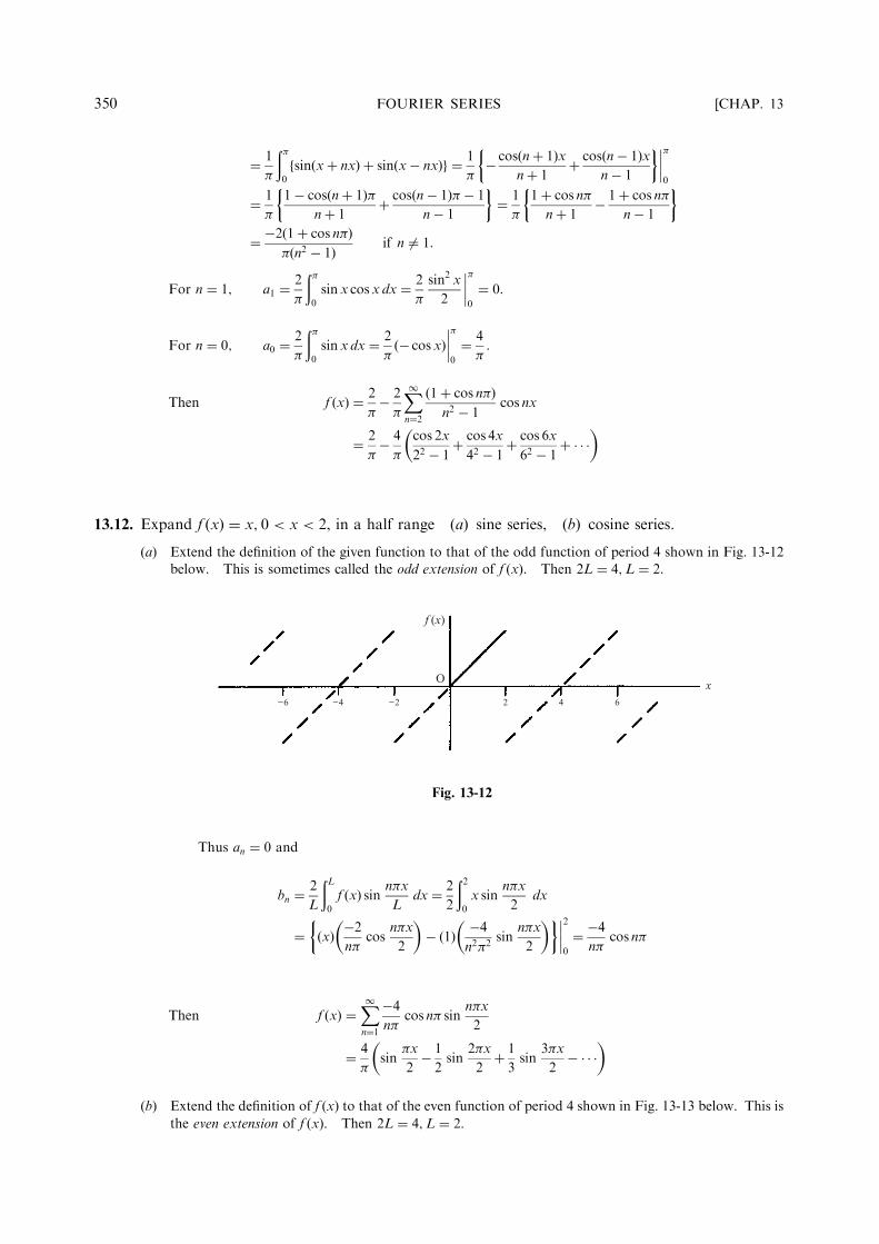
13.12. Expand f "x$ ! x; 0 < x < 2, in a half range (a) sine series, (b) cosine series.

(a) Extend the definition of the given function to that of the odd function of period 4 shown in Fig. 13-12below. This is sometimes called the odd extension of f "x$. Then 2L ! 4;L ! 2.

Thus an ! 0 and

bn !2

L

!L

0f "x$ sin n!x

Ldx ! 2

2

!2

0x sin

n!x

2dx

! "x$ %2

n!cos

n!x

2

% &

% "1$ %4

n2!2sin

n!x

2

% &" #$

$

$

$

2

0

! %4

n!cos n!

f "x$ !X

1

n!1

%4

n!cos n! sin

n!x

2Then

! 4

!sin

!x

2% 1

2sin

2!x

2# 1

3sin

3!x

2% & & &

% &

(b) Extend the definition of f "x$ to that of the even function of period 4 shown in Fig. 13-13 below. This isthe even extension of f "x$. Then 2L ! 4;L ! 2.


f (x)

O

_6 _4 _2 2 4 6

x

Fig. 13-12

Thus bn ! 0,

an !2

L

!L

0f "x# cos n!x

Ldx ! 2

2

!2

0x cos

n!x

2dx

! "x# 2

n!sin

n!x

2

" #

$ "1# $4

n2!2cos

n!x

2

" #$ %&

&

&

&

2

0

! 4

n2!2"cos n!$ 1# If n 6! 0

If n ! 0; a0 !!2

0x dx ! 2:

f "x# ! 1%X

1

n!1

4

n2!2"cos n!$ 1# cos n!x

2Then

! 1$ 8

!2cos

!x

2% 1

32cos

3!x

2% 1

52cos

5!x

2% & & &

" #

It should be noted that the given function f "x# ! x, 0 < x < 2, is represented equally well by thetwo di!erent series in (a) and (b).


13.13. Assuming that the Fourier series corresponding to f "x# converges uniformly to f "x# in "$L;L#,prove Parseval’s identity

1

L

!L

$Lf f "x#g2 dx ! a20

2%!"a2n % b2n#

where the integral is assumed to exist.

If f "x# ! a02%X

1

n!1

an cosn!x

L% bn sin

n!x

L

' (

, then multiplying by f "x# and integrating term by term

from $L to L (which is justified since the series is uniformly convergent) we obtain

!L

$Lf f "x#g2 dx ! a0

2

!L

$Lf "x# dx%

X

1

n!1

an

!L

$Lf "x# cos n!x

Ldx% bn

!L

$Lf "x# sin n!x

Ldx

$ %

! a202L% L

X

1

n!1

"a2n % b2n# "1#

where we have used the results!L

$Lf "x# cos n!x

Ldx ! Lan;

!L

$Lf "x# sin n!x

Ldx ! Lbn;

!L

$Lf "x# dx ! La0 "2#

obtained from the Fourier coe!cients.


f (x)

O_6 _4 _2 2 4 6

x

Fig. 13-13

The required result follows on dividing both sides of (1) by L. Parseval’s identity is valid under lessrestrictive conditions than that imposed here.

13.14. (a) Write Parseval’s identity corresponding to the Fourier series of Problem 13.12(b).

(b) Determine from (a) the sum S of the series1

14! 1

24! 1

34! " " " ! 1

n4! " " " .

(a) Here L # 2; a0 # 2; an #4

n2!2$cos n!% 1&; n 6# 0; bn # 0.

Then Parseval’s identity becomes

1

2

!2

%2f f $x&g2 dx # 1

2

!2

%2x2 dx # $2&2

2!X

1

n#1

16

n4!4$cos n!% 1&2

or8

3# 2! 64

!4

1

14! 1

34! 1

54! " " "

" #

; i.e.,1

14! 1

34! 1

54! " " " # !4

96:

$b& S # 1

14! 1

24! 1

34! " " " # 1

14! 1

34! 1

54! " " "

" #

! 1

24! 1

44! 1

64! " " "

" #

# 1

14! 1

34! 1

54! " " "

" #

! 1

241

14! 1

24! 1

34! " " "

" #

# !4

96! S

16; from which S # !4

90

13.15. Prove that for all positive integers M,

a202!X

M

n#1

$a2n ! b2n&@1

L

!L

%Lf f $x&g2 dx

where an and bn are the Fourier coe!cients corresponding to f $x&, and f $x& is assumed piecewisecontinuous in $%L;L&.

Let SM$x& # a02!X

M

n#1

an cosn!x

L! bn sin

n!x

L

$ %

(1)

For M # 1; 2; 3; . . . this is the sequence of partial sums of the Fourier series corresponding to f $x&.We have

!L

%Lf f $x& % SM$x&g2 dx A 0 $2&

since the integrand is non-negative. Expanding the integrand, we obtain

2

!L

%Lf $x&SM$x& dx%

!L

%LS2M$x& dx @

!L

%Lf f $x&g2 dx $3&

Multiplying both sides of (1) by 2 f $x& and integrating from %L to L, using equations (2) of Problem13.13, gives

2

!L

%Lf $x&SM$x& dx # 2L

a202!X

M

n#1

$a2n ! b2n&( )

$4&

Also, squaring (1) and integrating from %L to L, using Problem 13.3, we find

!L

%LS2M$x& dx # L

a202!X

M

n#1

$a2n ! b2n&( )

$5&

Substitution of (4) and (5) into (3) and dividing by L yields the required result.


Taking the limit as M ! 1, we obtain Bessel’s inequality

a202!X

1

n"1

#a2n ! b2n$ @1

L

!L

%Lf f #x$g2 dx #6$

If the equality holds, we have Parseval’s identity (Problem 13.13).We can think of SM#x$ as representing an approximation to f #x$, while the left-hand side of (2), divided

by 2L, represents the mean square error of the approximation. Parseval’s identity indicates that as M ! 1the mean square error approaches zero, while Bessels’ inequality indicates the possibility that this meansquare error does not approach zero.

The results are connected with the idea of completeness of an orthonormal set. If, for example, we wereto leave out one or more terms in a Fourier series (say cos 4!x=L, for example), we could never get the meansquare error to approach zero no matter how many terms we took. For an analogy with three-dimensionalvectors, see Problem 13.60.


13.16. (a) Find a Fourier series for f #x$ " x2; 0 < x < 2, by integrating the series of Problem 13.12(a).

(b) Use (a) to evaluate the seriesX

1

n"1

#%1$n%1

n2.

(a) From Problem 13.12(a),

x " 4

!sin

!x

2% 1

2sin

2!x

2! 1

3sin

3!x

2% & & &

" #

#1$

Integrating both sides from 0 to x (applying the theorem of Page 339) and multiplying by 2, we find

x2 " C % 16

!2cos

!x

2% 1

22cos

2!x

2! 1

32cos

3!x

2% & & &

" #

#2$

where C " 16

!21% 1

22! 1

32% 1

42! & & &

" #

:

(b) To determine C in another way, note that (2) represents the Fourier cosine series for x2 in 0 < x < 2.Then since L " 2 in this case,

C " a02" 1

L

!L

0f #x$ " 1

2

!2

0x2 dx " 4

3

Then from the value of C in (a), we have

X

1

n"1

#%1$n%1

n2" 1% 1

22! 1

32" 1

42! & & & " !2

16& 43" !2

12

13.17. Show that term by term di!erentiation of the series in Problem 13.12(a) is not valid.

Term by term differentiation yields 2 cos!x

2% cos

2!x

2! cos

3!x

2% & & &

" #

:

Since the nth term of this series does not approach 0, the series does not converge for any value of x.


CONVERGENCE OF FOURIER SERIES

13.18. Prove that (a) 12 ! cos t! cos 2t! " " " ! cosMt #

sin$M ! 12%t

2 sin 12 t

(b)1

!

!!

0

sin$M ! 12%t

2 sin 12 t

dt # 1

2;

1

!

!0

&!

sin$M ! 12%t

2 sin 12 t

dt # 1

2:

(a) We have cos nt sin 12 t #

12 fsin$n!

12%t& sin$n& 1

2%tg.Then summing from n # 1 to M,

sin 12 tfcos t! cos 2t! " " " ! cosMtg # $sin 3

2 t& sin 12 t% ! $sin 5

2 t& sin 32 t%

! " " " ! sin$M ! 12%t& sin$M & 1

2%t" #

# 12 fsin$M ! 1

2%t& sin 12 tg

On dividing by sin 12 t and adding 1

2, the required result follows.

(b) Integrating the result in (a) from &! to 0 and 0 to !, respectively. This gives the required results, sincethe integrals of all the cosine terms are zero.

13.19. Prove that limn!1

!!

&!f $x% sin nx dx # lim

n!1

!!

&!f $x% cos nx dx # 0 if f $x% is piecewise continuous.

This follows at once from Problem 13.15, since if the seriesa202!X

1

n#1

$a2n ! b2n% is convergent, limn!1

an #limn!1

bn # 0.

The result is sometimes called Riemann’s theorem.

13.20. Prove that limM!1

!!

&!f $x% sin$M ! 1

2%x dx # 0 if f $x% is piecewise continuous.

We have!!

&!f $x% sin$M ! 1

2%x dx #!!

&!f f $x% sin 1

2 xg cosMxdx!!!

&!f f $x% cos 12 xg sinMxdx

Then the required result follows at once by using the result of Problem 13.19, with f $x% replaced byf $x% sin 1

2 x and f $x% cos 12 x respectively, which are piecewise continuous if f $x% is.The result can also be proved when the integration limits are a and b instead of &! and !.

13.21. Assuming that L # !, i.e., that the Fourier series corresponding to f $x% has period 2L # 2!, showthat

SM$x% # a02!X

M

n#1

$an cos nx! bn sin nx% #1

!

!!

&!f $t! x%

sin$M ! 12%t

2 sin 12 t

dt

Using the formulas for the Fourier coe!cients with L # !, we have

an cos nx! bn sin nx # 1

!

!!

&!f $u% cos nu du

$ %

cos nx! 1

!

!!

&!f $u% sin nu du

$ %

sin nx

# 1

!

!!

&!f $u% cos nu cos nx! sin nu sin nx$ % du

# 1

!

!!

&!f $u% cos n$u& x% du

a02# 1

2!

!!

&!f $u% duAlso,


SM!x" # a02$X

M

n#1

!an cos nx$ bn sin nx"Then

# 1

2!

!!

%!f !u" du$ 1

!

X

M

n#1

!!

%!f !u" cos n!u% x" du

# 1

!

!!

%!f !u" 1

2$X

M

n#1

cos n!u% x"( )

du

# 1

!

!!

%!f !u"

sin!M $ 12"!u% x"

2 sin 12 !u% x"

du

using Problem 13.18. Letting u% x # t, we have

SM!x" # 1

!

!!%x

%!%xf !t$ x"

sin!M $ 12"t

2 sin 12 t

dt

Since the integrand has period 2!, we can replace the interval %!% x;!% x by any other interval oflength 2!, in particular, %!;!. Thus, we obtain the required result.

13.22. Prove that

SM!x" % f !x$ 0" $ f !x% 0"2

" #

# 1

!

!0

%!

f !t$ x" % f !x% 0"2 sin 1

2 t

!

sin!M $ 12"t dt

$ 1

!

!!

0

f !t$ x" % f !x$ 0"2 sin 1

2 t

!

sin!M $ 12"t dt

From Problem 13.21,

SM!x" # 1

!

!0

%!f !t$ x"

sin!M $ 12"t

2 sin 12 t

dt$ 1

!

!!

0f !t$ x"

sin!M $ 12"t

2 sin 12 t

dt !1"

Multiplying the integrals of Problem 13.18(b) by f !x% 0" and f !x$ 0", respectively,

f !x$ 0" $ f !x% 0"2

# 1

!

!0

%!f !x% 0"

sin!M $ 12"t

2 sin 12 t

dt$ 1

!

!!

0f !x$ 0"

sin!M $ 12"t

2 sin 12 t

dt !2"

Subtracting (2) from (1) yields the required result.

13.23. If f !x" and f 0!x" are piecewise continuous in !%!;!", prove that

limM!1

SM!x" # f !x$ 0" $ f !x% 0"2

The functionf !t$ x" % f !x$ 0"

2 sin 12 t

is piecewise continuous in 0 < t @ ! because f !x" is piecewise con-tinous.

Also, limt!0$

f !t$ x" % f !x$ 0"2 sin 1

2 t# lim

t!0$

f !t$ x" % f !x$ 0"t

& t

2 sin 12 t

# limt!0$

f !t$ x" % f !x$ 0"t

exists,

since by hypothesis f 0!x" is piecewise continuous so that the right-hand derivative of f !x" at each x exists.

Thus,f !t$ x" % f !x% 0"

2 sin 12 t

is piecewise continous in 0 @ t @ !.

Similarly,f !t$ x" % f !x% 0"

2 sin 12 t

is piecewise continous in %! @ t @ 0.


Then from Problems 13.20 and 13.22, we have

limM!1

SM!x" # f !x$ 0" $ f !x# 0"2

! "

% 0 or limM!1

SM!x" % f !x$ 0" $ f !x# 0"2


13.24. Find a solution U!x; t" of the boundary-value problem

@U

@t% 3

@2U

@x2t > 0; 0 < x < 2

U!0; t" % 0;U!2; t" % 0 t > 0

U!x; 0" % x 0 < x < 2

A method commonly employed in practice is to assume the existence of a solution of the partialdi!erential equation having the particular form U!x; t" % X!x"T!t", where X!x" and T!t" are functions ofx and t, respectively, which we shall try to determine. For this reason the method is often called the methodof separation of variables.

Substitution in the di!erential equation yields

!1" @

@t!XT" % 3

@2

@x2!XT" or !2" X

dT

dt% 3T

d2X

dx2

where we have written X and T in place of X!x" and T!t".Equation (2) can be written as

1

3T

dT

dt% 1

X

d2X

dx2!3"

Since one side depends only on t and the other only on x, and since x and t are independent variables, it isclear that each side must be a constant c.

In Problem 13.47 we see that if c A 0, a solution satisfying the given boundary conditions cannot exist.Let us thus assume that c is a negative constant which we write as #!2. Then from (3) we obtain two

ordinary di!erentiation equations

dT

dt$ 3!2T % 0;

d2X

dx2$ !2X % 0 !4"

whose solutions are respectively

T % C1e#3!2t; X % A1 cos !x$ B1 sin !x !5"

A solution is given by the product of X and T which can be written

U!x; t" % e#3!2t!A cos !x$ B sin !x" !6"

where A and B are constants.We now seek to determine A and B so that (6) satisfies the given boundary conditions. To satisfy the

condition U!0; t" % 0, we must have

e#s!2t!A" % 0 or A % 0 !7"

so that (6) becomes

U!x; t" % Be#s!2t sin !x !8"

To satisfy the condition U!2; t" % 0, we must then have

Be#s!2t sin 2! % 0 !9"


Since B ! 0 makes the solution (8) identically zero, we avoid this choice and instead take

sin 2! ! 0; i.e., 2! ! m" or ! ! m"

2"10#

where m ! 0;$1;$2; . . . .Substitution in (8) now shows that a solution satisfying the first two boundary conditions is

U"x; t# ! Bme%3m2"2t=4 sin

m"x

2"11#

where we have replaced B by Bm, indicating that di!erent constants can be used for di!erent values of m.If we now attempt to satisfy the last boundary condition U"x; 0# ! x; 0 < x < 2, we find it to be

impossible using (11). However, upon recognizing the fact that sums of solutions having the form (11)are also solutions (called the principle of superposition), we are led to the possible solution

U"x; t# !X

1

m!1

Bme%3m2"2t=4 sin

m"x

2"12#

From the condition U"x; 0# ! x; 0 < x < 2, we see, on placing t ! 0, that (12) becomes

x !X

1

m!1

Bm sinm"x

20 < x < 2 "13#

This, however, is equivalent to the problem of expanding the function f "x# ! x for 0 < x < 2 into a sine

series. The solution to this is given in Problem 13.12(a), from which we see that Bm ! %4

m"cosm" so that

(12) becomes

U"x; t# !X

1

m!1

% 4

m"cosm"

! "

e%3m2"2t=4 sinm"x

2"14#

which is a formal solution. To check that (14) is actually a solution, we must show that it satisfies the partialdi!erential equation and the boundary conditions. The proof consists in justification of term by termdi!erentiation and use of limiting procedures for infinite series and may be accomplished by methods ofChapter 11.

The boundary value problem considered here has an interpretation in the theory of heat conduction.

The equation@U

@t! k

@2U

@x2is the equation for heat conduction in a thin rod or wire located on the x-axis

between x ! 0 and x ! L if the surface of the wire is insulated so that heat cannot enter or escape. U"x; t# isthe temperature at any place x in the rod at time t. The constant k ! K=s# (where K is the thermalconductivity, s is the specific heat, and # is the density of the conducting material) is called the di!usivity.The boundary conditions U"0; t# ! 0 and U"L; t# ! 0 indicate that the end temperatures of the rod are keptat zero units for all time t > 0, while U"x; 0# indicates the initial temperature at any point x of the rod. Inthis problem the length of the rod is L ! 2 units, while the di!usivity is k ! 3 units.

ORTHOGONAL FUNCTIONS

13.25. (a) Show that the set of functions

1; sin"x

L; cos

"x

L; sin

2"x

L; cos

2"x

L; sin

3"x

L; cos

3"x

L; . . .

forms an orthogonal set in the interval "%L;L#.(b) Determine the corresponding normalizing constants for the set in (a) so that the set isorthonormal in "%L;L#.

(a) This follows at once from the results of Problems 13.2 and 13.3.

(b) By Problem 13.3,#L

%Lsin2

m"x

Ldx ! L;

#L

%Lcos2

m"x

Ldx ! L


!L

!L

""""

1

L

r

sinm!x

L

!2

dx " 1;

!L

!L

""""

1

L

r

cosm!x

L

!2

dx " 1Then

!L

!L#1$2 dx " 2L or

!L

!L

1""""""

2Lp

# $2

dx " 1Also,

Thus the required orthonormal set is given by

1""""""

2Lp ;

1""""

Lp sin

!x

L;1""""

Lp cos

!x

L;1""""

Lp sin

2!x

L;1""""

Lp cos

2!x

L; . . .

MISCELLANEOUS PROBLEMS

13.26. Find a Fourier series for f #x$ " cos"x;!! @ x @ !, where " 6" 0;%1;%2;%3; . . . .

We shall take the period as 2! so that 2L " 2!;L " !. Since the function is even, bn " 0 and

an "2

L

!L

0f #x$ cos nx dx " 2

!

!!

0cos"x cos nx dx

" 1

!

!!

0fcos#"! n$x& cos#"& n$xg dx

" 1

!

sin#"! n$!"! n

& sin#"& n$!"& n

% &

" 2" sin "! cos n!

!#"2 ! n2$

"0 "2 sin"!

"!

Then

cos "x " sin"!

"!& 2" sin"!

!

X

1

n"1

cos n!

"2 ! n2cos nx

" sin"!

!

1

"! 2"

"2 ! 12cos x& 2"

"2 ! 22cos 2x! 2"

"2 ! 32cos 3x& ' ' '

# $

13.27. Prove that sin x " x 1! x2

!2

!

1! x2

#2!$2

!

1! x2

#3!$2

!

' ' ' .

Let x " ! in the Fourier series obtained in Problem 13.26. Then

cos" " sin"!

!

1

"& 2"

"2 ! 12& 2"

"2 ! 22& 2"

"2 ! 32& ' ' '

# $

or

! cot "!! 1

"" 2"

"2 ! 12& 2"

"2 ! 22& 2"

"2 ! 32& ' ' ' #1$

This result is of interest since it represents an expansion of the contangent into partial fractions.By the Weierstrass M test, the series on the right of (1) converges uniformly for 0 @ j"j @ jxj < 1 and

the left-hand side of (1) approaches zero as " ! 0, as is seen by using L’Hospital’s rule. Thus, we canintegrate both sides of (1) from 0 to x to obtain

!x

0! cot"!! 1

"

# $

d" "!x

0

2"

"2 ! 1d"&

!x

0

2"

"2 ! 22d"& ' ' '

lnsin"!

"!

# $'

'

'

'

x

0

" ln 1! x2

12

!

& ln 1! x2

22

!

& ' ' 'or


lnsin!x

!x

! "

! limn!1

ln 1" x2

12

!

# ln 1" x2

22

!

# $ $ $ # ln 1" x2

n2

!

i.e.,

! limn!1

ln 1" x2

12

!

1" x2

22

!

$ $ $ 1" x2

n2

!( )

! ln limn!1

1" x2

12

!

1" x2

22

!

$ $ $ 1" x2

n2

!( )

so that

sin!x

!x! lim

n!11" x2

12

!

1" x2

22

!

$ $ $ 1" x2

n2

!

! 1" x2

12

!

1" x2

22

!

$ $ $ %2&

Replacing x by x=!, we obtain

sin x ! x 1" x2

!2

!

1" x2

%2!&2

!

$ $ $ %3&

called the infinite product for sin x, which can be shown valid for all x. The result is of interest since itcorresponds to a factorization of sinx in a manner analogous to factorization of a polynomial.

13.28. Prove that!

2! 2 $ 2 $ 4 $ 4 $ 6 $ 6 $ 8 $ 8 . . .

1 $ 3 $ 3 $ 5 $ 5 $ 7 $ 7 $ 9 . . ..

Let x ! 1=2 in equation (2) of Problem 13.27. Then,

2

!! 1" 1

22

! "

1" 1

42

! "

1" 1

62

! "

$ $ $ ! 1

2$ 32

! "

3

4$ 54

! "

5

6$ 76

! "

$ $ $

Taking reciprocals of both sides, we obtain the required result, which is often called Wallis’ product.

Supplementary Problems

FOURIER SERIES

13.29. Graph each of the following functions and find their corresponding Fourier series using properties of evenand odd functions wherever applicable.

%a& f %x& !8 0 < x < 2

"8 2 < x < 4Period 4 %b& f %x& !

"x "4 @ x @ 0

x 0 @ x @ 4Period 8

##

%c& f %x& ! 4x; 0 < x < 10; Period 10 %d& f %x& !2x 0 @ x < 3

0 "3 < x < 0Period 6

#

Ans: %a& 16

!

X

1

n!1

%1" cos n!&n

sinn!x

2%b& 2" 8

!2

X

1

n!1

%1" cos n!&n2

cosn!x

4

%c& 20" 40

!

X

1

n!1

1

nsin

n!x

5%d& 3

2#X

1

n!1

6%cos n!" 1&n2!2

cosn!x

3" 6 cos n!

n!sin

n!x

3

# $

13.30. In each part of Problem 13.29, tell where the discontinuities of f %x& are located and to what value the seriesconverges at the discontunities.Ans. (a) x ! 0;'2;'4; . . . ; 0 %b& no discontinuities (c) x ! 0;'10;'20; . . . ; 20

(d) x ! '3;'9;'15; . . . ; 3



13.31. Expand f !x" # 2$ x 0 < x < 4x$ 6 4 < x < 8

!

in a Fourier series of period 8.

Ans:16

!2cos

!x

4% 1

32cos

3!x

4% 1

52cos

5!x

4% & & &

! "

13.32. (a) Expand f !x" # cos x; 0 < x < !, in a Fourier sine series.(b) How should f !x" be defined at x # 0 and x # ! so that the series will converge to f !x" for 0 @ x @ !?

Ans: !a" 8

!

X

1

n#1

n sin 2nx

4n2 $ 1!b" f !0" # f !!" # 0

13.33. (a) Expand in a Fourier series f !x" # cos x; 0 < x < ! if the period is !; and (b) compare with the result ofProblem 13.32, explaining the similarities and di!erences if any.Ans. Answer is the same as in Problem 13.32.

13.34. Expand f !x" # x 0 < x < 48$ x 4 < x < 8

!

in a series of (a) sines, (b) cosines.

Ans: !a" 32

!2

X

1

n#1

1

n2sin

n!

2sin

n!x

8!b" 16

!2

X

1

n#1

2 cos n!=2$ cos n!$ 1

n2

# $

cosn!x

8

13.35. Prove that for 0 @ x @ !,

!a" x!!$ x" # !2

6$ cos 2x

12% cos 4x

22% cos 6x

32% & & &

# $

!b" x!!$ x" # 8

!

sinx

13% sin 3x

33% sin 5

53% & & &

# $

13.36. Use the preceding problem to show that

!a"X

1

n#1

1

n2# !2

6; !b"

X

1

n#1

!$1"n$1

n2# !2

12; !c"

X

1

n#1

!$1"n$1

!2n$ 1"3# !3

32:

13.37. Show that1

13% 1

33$ 1

53$ 1

73% 1

93% 1

113$ & & & # 3!2

%%%

2p

16.


13.38. (a) Show that for $! < x < !,

x # 2sinx

1$ sin 2x

2% sin 3x

3$ & & &

# $

(b) By integrating the result of (a), show that for $! @ x @ !,

x2 # !2

3$ 4

cos x

12$ cos 2x

22% cos 3x

32$ & & &

# $

(c) By integrating the result of (b), show that for $! @ x @ !,

x!!$ x"!!% x" # 12sinx

13$ sin 2x

23% sin 3x

33$ & & &

# $

13.39. (a) Show that for $! < x < !,

x cos x # $ 1

2sinx% 2

2

1 & 3sin 2x$ 3

2 & 4sin 3x% 4

3 & 5sin 4x$ & & &

# $

(b) Use (a) to show that for $! @ x @ !,

x sin x # 1$ 1

2cos x$ 2

cos 2x

1 & 3$ cos 3x

2 & 4% cos 4x

3 & 5$ & & &

# $


13.40. By di!erentiating the result of Problem 13.35(b), prove that for 0 @ x @ !,

x ! !

2" 4

!

cos x

12# cos 3x

32# cos 5x

52# $ $ $

! "


13.41. By using Problem 13.35 and Parseval’s identity, show that

%a&X

1

n!1

1

n4! !4

90%b&

X

1

n!1

1

n6! !6

945

13.42. Show that1

12 $ 32# 1

32 $ 52# 1

52 $ 72# $ $ $ ! !2 " 8

16. [Hint: Use Problem 13.11.]

13.43. Show that (a)X

1

n!1

1

%2n" 1&4! !4

96; %b&

X

1

n!1

1

%2n" 1&6! !6

960.

13.44. Show that1

12 $ 22 $ 32# 1

22 $ 32 $ 42# 1

32 # 42 # 52# $ $ $ ! 4!2 " 39

16.


13.45. (a) Solve@U

@t! 2

@2U

@x2subject to the conditions U%0; t& ! 0;U%4; t& ! 0;U%x; 0& ! 3 sin!x" 2 sin 5!x, where

0 < x < 4; t > 0.

(b) Give a possible physical interpretation of the problem and solution.

Ans: %a& U%x; t& ! 3e"2!2t sin!x" 2e"50!2t sin 5!x.

13.46. Solve@U

@t! @2U

@x2subject to the conditions U%0; t& ! 0;U%6; t& ! 0;U%x; 0& ! 1 0 < x < 3

0 3 < x < 6

#

and interpret

physically.

Ans: U%x; t& !X

1

m!1

21" cos%m!=3&

m!

$ %

e"m2!2t=36 sinm!x

6

13.47. Show that if each side of equation (3), Page 356, is a constant c where c A 0, then there is no solutionsatisfying the boundary-value problem.

13.48. A flexible string of length ! is tightly stretched between points x ! 0 and x ! ! on the x-axis, its ends arefixed at these points. When set into small transverse vibration, the displacement Y%x; t& from the x-axis of

any point x at time t is given by@2Y

@t2! a2

@2Y

@x2, where a2 ! T=";T ! tension, " ! mass per unit length.

(a) Find a solution of this equation (sometimes called the wave equation) with a2 ! 4 which satisfies theconditions Y%0; t& ! 0;Y%!; t& ! 0;Y%x; 0& ! 0:1 sinx# 0:01 sin 4x;Yt%x; 0& ! 0 for 0 < x < !; t > 0.(b) Interpret physically the boundary conditions in (a) and the solution.Ans. (a) Y%x; t& ! 0:1 sinx cos 2t# 0:01 sin 4x cos 8t

13.49. (a) Solve the boundary-value problem@2Y

@t2! 9

@2Y

@x2subject to the conditions Y%0; t& ! 0;Y%2; t& ! 0,

Y%x; 0& ! 0:05x%2" x&;Yt%x; 0& ! 0, where 0 < x < 2; t > 0. (b) Interpret physically.

Ans: %a& Y%x; t& ! 1:6

!3

X

1

n!1

1

%2n" 1&3sin

%2n" 1&!x2

cos3%2n" 1&!t

2

13.50. Solve the boundary-value problem@U

@t! @2U

@x2;U%0; t& ! 1;U%!; t& ! 3;U%x; 0& ! 2.

[Hint: Let U%x; t& ! V%x; t& # F%x& and choose F%x& so as to simplify the di!erential equation and boundaryconditions for V%x; t&:'

Ans: U!x; t" # 1$ 2x

!$X

1

m#1

4 cosm!

m!e%m2t sinmx

13.51. Give a physical interpretation to Problem 13.50.

13.52. Solve Problem 13.49 with the boundary conditions for Y!x; 0" and Yt!x; 0" interchanged, i.e., Y!x; " # 0;Yt!x; 0" # 0:05x!2% x", and give a physical interpretation.

Ans: Y!x; t" # 3:2

3!4

X

1

n#1

1

!2n% 1"4sin

!2n% 1"!x2

sin3!2n% 1"!t

2

13.53. Verify that the boundary-value problem of Problem 13.24 actually has the solution (14), Page 357.

MISCELLANEOUS PROBLEMS

13.54. If %! < x < ! and " 6# 0;&1;&2; . . . ; prove that

!

2

sin"x

sin "!# sin x

12 % "2% 2 sin 2x

22 % "2$ 3 sin 3x

32 % "2% ' ' '

13.55. If %! < x < !, prove that

!a" !

2

sinh "x

sinh "!# sin x

"2 $ 12% 2 sin 2x

"2 $ 23$ 3 sin 3x

"2 $ 32% ' ' '

!b" !

2

cosh"x

sinh "!# 1

2"% " cos x

"2 $ 12$ " cos 2x

"2 $ 22% ' ' '

13.56. Prove that sinh x # x 1$ x2

!2

!

1$ x2

!2!"2

!

1$ x2

!3!"2

!

' ' '

13.57. Prove that cos x # 1% 4x2

!2

!

1% 4x2

!3!"2

!

1% 4x2

!5!"2

!

' ' '

[Hint: cos x # !sin 2x"=!2 sin x":(

13.58. Show that (a)

!!!

2p

2# 1 ' 3 ' 5 ' 7 ' 9 ' 22 ' 13 ' 15 . . .

2 ' 2 ' 6 ' 6 ' 10 ' 10 ' 14 ' 14 . . .

(b) !!!!

2p

# 44 ' 4 ' 8 ' 8 ' 12 ' 12 ' 16 ' 16 . . .3 ' 5 ' 7 ' 9 ' 11 ' 13 ' 15 ' 17 . . .

" #

13.59. Let r be any three dimensional vector. Show that

(a) !r ' i"2 $ !r ' j"2 @ !r"2; !b" !r ' i"2 $ !r ' j"2 $ !r ' k"2 # r2

and discusse these with reference to Parseval’s identity.

13.60. If f#n!x"g; n # 1; 2; 3; . . . is orthonormal in (a; b), prove that

$b

af !x" %

X

1

n#1

cn#n!x"( )2

dx is a minimum when

cn #$b

af !x"#n!x" dx

Discuss the relevance of this result to Fourier series.


Fourier Series - CAUcau.ac.kr/~mhhgtx/courses/AdvancedMath/references/FourierSeries-Sc… · FOURIER SERIES Let fðxÞ be deﬁned in the interval ð#L;LÞ and outside of this interval

Documents