Fourier Series

Chapter 12

Fourier Series

12.1 Motivation

Many problems in physics involve vibrations and oscillations. Often the os-cillatory motion is simple (e.g. weights on springs, pendulums, harmonicwaves etc.) and can be represented as single sine or cosine functions. How-ever, in many cases, (electromagnetism, heat conduction, quantum theory,etc.) the waveforms are not simple and, unlike sines and cosines, can bedifficult to treat analytically.

Fourier methods give us a set of powerful tools for representing any periodicfunction as a sum of sines and cosines. The Fourier series of a function,f(x), with period 2L is,

f(x) =1

2a0 +

∞∑

n=1

(

an cosnπx

L+ bn sin

nπx

L

)

. (12.1)

To see how this works, let us consider a sound wave. The vibration of atuning fork produces a sound wave of a given frequency. If we plot thepressure as a function of distance, x, or time, t, it looks like a single sinewave, or a ’pure tone’ (Fig. 12.1: left). When a note is played on a flute,we get a more complex sound (Fig. 12.1: centre). The note that we get ismade up from the sum of many pure tones: the fundamental and differentharmonics with frequencies 2,3,4,. . . times the frequency of the fundamental(Fig. 12.1: right). This is the Fourier series.

Fourier methods are used very heavily in signal and data analysis. ByFourier analysing a signal - essentially by expanding it in the form of Eq. (12.1)- we can immediately tell which harmonics are the important ones. For ex-

1

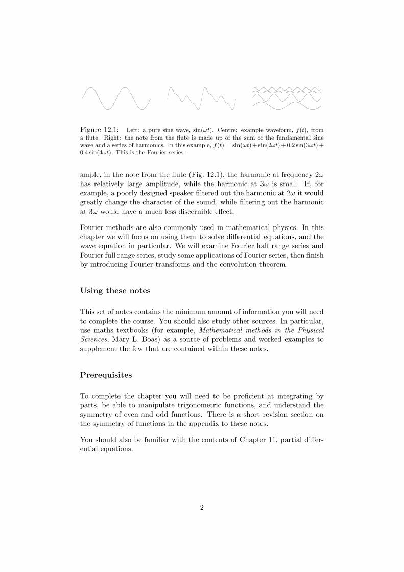
Figure 12.1: Left: a pure sine wave, sin(ωt). Centre: example waveform, f(t), froma flute. Right: the note from the flute is made up of the sum of the fundamental sinewave and a series of harmonics. In this example, f(t) = sin(ωt)+ sin(2ωt)+0.2 sin(3ωt)+0.4 sin(4ωt). This is the Fourier series.

ample, in the note from the flute (Fig. 12.1), the harmonic at frequency 2ωhas relatively large amplitude, while the harmonic at 3ω is small. If, forexample, a poorly designed speaker filtered out the harmonic at 2ω it wouldgreatly change the character of the sound, while filtering out the harmonicat 3ω would have a much less discernible effect.

Fourier methods are also commonly used in mathematical physics. In thischapter we will focus on using them to solve differential equations, and thewave equation in particular. We will examine Fourier half range series andFourier full range series, study some applications of Fourier series, then finishby introducing Fourier transforms and the convolution theorem.

Using these notes

This set of notes contains the minimum amount of information you will needto complete the course. You should also study other sources. In particular,use maths textbooks (for example, Mathematical methods in the Physical

Sciences, Mary L. Boas) as a source of problems and worked examples tosupplement the few that are contained within these notes.

Prerequisites

To complete the chapter you will need to be proficient at integrating byparts, be able to manipulate trigonometric functions, and understand thesymmetry of even and odd functions. There is a short revision section onthe symmetry of functions in the appendix to these notes.

You should also be familiar with the contents of Chapter 11, partial differ-ential equations.

2

12.2 Fourier half range sine series

In chapter 11 we calculated the separable solutions for a wave on a string thatis fixed at both ends, at x = 0 and at x = L. In general, the displacementof such a string is,

y(x, t) =∞∑

n=1

sinnπx

L

(

an sinnπct

L+ bn cos

nπct

L

)

, (12.2)

where each of the an and bn for n = 1, 2, 3 . . . is an arbitrary constant thatwe can set once we know the boundary conditions for any given problem.The range 0 to L is called the half range because it is half the maximumwavelength or spatial period.

Consider the case when the string is initially at rest and has initial dis-placement y(x, 0) = f(x). Then, by substituting t = 0 into Eq. (12.2) wefind

f(x) =∞∑

n=1

bn sinnπx

L. (12.3)

Given any function, f(x), can we find the coefficients, bn, such that Eq. (12.3)is satisfied? Remarkably, yes! This is Fourier’s theorem.

Equation (12.3) is the Fourier half range sine series of a function, f(x). Thisis a very powerful result. It tells us that, within the range 0 to L, we canwrite any (physically reasonable) function as a sum of sine waves.

Fourier sine series coefficients

The Fourier half-range sine series coefficients, bn, are given by,

bn =2

L

∫ L

0f(x) sin

nπx

Ldx. (12.4)

Derivation of the Fourier sine series coefficients

The formula for the bn can be derived directly from the Fourier seriesrepresentation (Eq. (12.3)). First, multiply both sides of Eq. (12.3) bysin(mπx/L) then integrate from 0 to L. This gives,

∫ L

0f(x) sin

mπx

Ldx =

∞∑

n=1

bn

∫ L

0sin

nπx

Lsin

mπx

Ldx.

3

The integral on the right hand side is a standard integral (Eq. (A.2)) withresult (L/2)δnm, where δnm is a Kronecker delta defined in Eq. (A.1). Essen-tially, when the two sine waves in the integral on the right have a differingwavelength they interfere destructively and cancel to zero. We only geta non-zero result for the integral when the wavelengths are the same andn = m.

Substituting in the result from Eq. (A.2), we have,∫ L

0f(x) sin

mπx

Ldx =

∞∑

n=1

bnL

2δnm = bm

L

2.

Finally, rearranging this equation and replacing the symbol m with n wefind Eq. (12.4), the formula for the Fourier series sine coefficients.

Using the Fourier series results

We can now use the results from Eq. (12.3) and Eq.(12.4) to find the Fourierhalf range sine series for any function, f(x).

Example 12.1. Calculate the Fourier series representation of the function,f(x) = 1 in 0 ≤ x < L.

We wish to represent the function, f(x), as a Fourier sine series,

f(x) = 1 =

∞∑

n=1

bn sinnπx

L.

To do this, we simply need to calculate the appropriate Fourier coefficients,bn, using Eq. (12.4),

bn =2

L

∫ L

0f(x) sin

nπx

Ldx =

2

L

∫ L

0sin

nπx

Ldx,

= − 2

L

L

nπ

[

cosnπx

L

]L

0,

= − 2

L

L

nπ(cos(nπ)− 1) .

We can simplify this equation using the result that cos(nπ) = (−1)n. Then,

bn =2

nπ(1− (−1)n) ,

=

{

0 if n is even4nπ if n is odd.

(12.5)

4

So, the Fourier sine series of f(x) = 1 for 0 ≤ x < L is,

1 =∑

n,odd

4

nπsin

nπx

L, (12.6)

where the notation ’n, odd’, simply means to take only the odd integer termsin the summation. We could also write this explicitly by defining a newinteger counter, m = 0, 1, 2, . . .∞, and setting n = 2m + 1 so that n isalways odd,

1 =∞∑

m=0

4

(2m+ 1)πsin

(2m+ 1)πx

L.

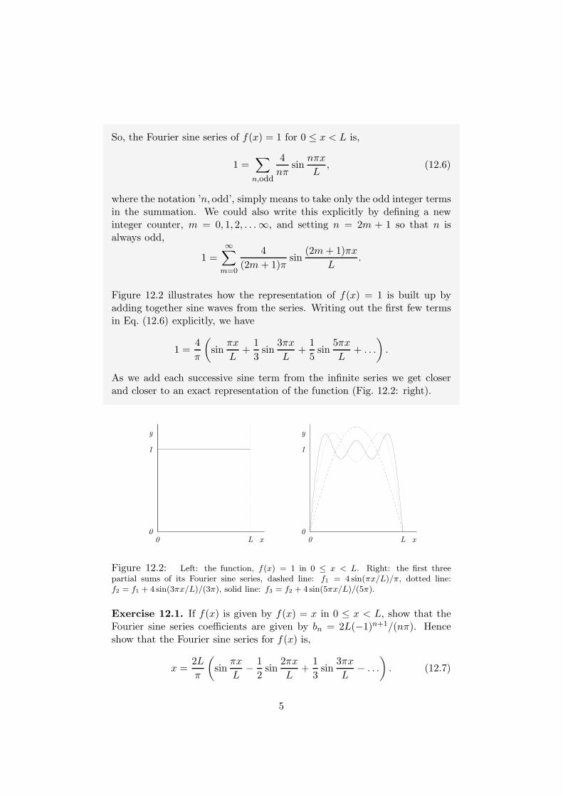
Figure 12.2 illustrates how the representation of f(x) = 1 is built up byadding together sine waves from the series. Writing out the first few termsin Eq. (12.6) explicitly, we have

1 =4

π

(

sinπx

L+

1

3sin

3πx

L+

1

5sin

5πx

L+ . . .

)

.

As we add each successive sine term from the infinite series we get closerand closer to an exact representation of the function (Fig. 12.2: right).

0

1

0 L x

y

0

1

0 L x

y

Figure 12.2: Left: the function, f(x) = 1 in 0 ≤ x < L. Right: the first threepartial sums of its Fourier sine series, dashed line: f1 = 4 sin(πx/L)/π, dotted line:f2 = f1 + 4 sin(3πx/L)/(3π), solid line: f3 = f2 + 4 sin(5πx/L)/(5π).

Exercise 12.1. If f(x) is given by f(x) = x in 0 ≤ x < L, show that theFourier sine series coefficients are given by bn = 2L(−1)n+1/(nπ). Henceshow that the Fourier sine series for f(x) is,

x =2L

π

(

sinπx

L− 1

2sin

2πx

L+

1

3sin

3πx

L− . . .

)

. (12.7)

5

0

L

0 L x

y

0

1

0 L x

y

Figure 12.3: Left: the function, f(x) = x in 0 ≤ x < L. Right: the first threepartial sums of its Fourier sine series, dashed line: f1 = 2L sin(πx/L)/π, dotted line:f2 = f1 − 2L sin(2πx/L)/(2π), solid line: f3 = f2 + 2L sin(3πx/L)/(3π).

Exercise 12.2. A function, g(x) is defined by,

g(x) =

{

x/L if 0 ≤ x < L/2

1− x/L if L/2 ≤ x < L.

By expanding g(x) as a Fourier sine series show that,

g(x) =∑

n,odd

4(−1)n−1

2

n2π2sin

nπx

L.

Hint : The integral for bn can be split into the sum of two parts, for example∫ ba f(x)dx =

∫ ca f(x)dx+

∫ bc f(x)dx where a < c < b.

0

0.5

0 L x

y

0

0.5

0 L x

y

Figure 12.4: Left: the function, g(x) from Ex. 2. Right: the first three partialsums of its Fourier sine series, dashed line: f1 = 4 sin(πx/L)/π2, dotted line f2 = f1 −4 sin(3πx/L)/(9π2), solid line f3 = f2 + 4 sin(5πx/L)/(25π2).

6

12.2.1 Application to differential equations

The wave equation

The separable solutions to the wave equation for a string fixed at x = 0 andx = L are,

y(x, t) =

∞∑

n=1

sinnπx

L

(

An sinnπct

L+Bn cos

nπct

L

)

. (12.8)

Armed with results (12.3) and (12.4) we can now find the coefficients An

and Bn given a set of initial conditions.

Let us examine the general case when the string is given an initial displace-ment, y(x, 0) = p(x) and an initial velocity, yt(x, 0) = q(x). By substitutingt = 0 into Eq. (12.8) we immediately find that

y(x, 0) = p(x) =∞∑

n=1

Bn sinnπx

L.

This looks like the Fourier sine series of p(x) with Fourier series coefficients,Bn. So, to find the coefficients, Bn, we simply need to apply the formula inEq. (12.4),

Bn =2

L

∫ L

0p(x) sin

nπx

Ldx. (12.9)

We can follow a similar process to find the An. First, find the transversevelocity of the string at t = 0,

yt(x, t) =∂y

∂t=

∞∑

n=1

sinnπx

L

(

Annπc

Lcos

nπct

L−Bn

nπc

Lsin

nπct

L

)

.

So, at t = 0,

yt(x, 0) = q(x) =∞∑

n=1

(

Annπc

L

)

sinnπx

L.

Again, this looks like the Fourier sine series of q(x) with Fourier series coef-ficients Annπc/L. So, again, to find Annπc/L we simply need to apply theformula in Eq. (12.4),

(

Annπc

L

)

=2

L

∫ L

0q(x) sin

nπx

Ldx,

⇒ An =2

nπc

∫ L

0q(x) sin

nπx

Ldx. (12.10)

7

Example 12.2. A string fixed at x = 0 and at x = L is given constantinitial velocity, yt(x, 0) = v, and zero initial displacement, y(x, 0) = 0. Findy(x, t).

In general,

y(x, t) =

∞∑

n=1

sinnπx

L

(

An sinnπct

L+Bn cos

nπct

L

)

.

To find y(x, t) given a set of initial conditions, substitute the initial con-ditions into the general solution, find equations involving the unknown co-efficients An and Bn, then calculate An and Bn using the formula for theFourier sine series coefficients, Eq. (12.4).

At t = 0 the displacement of the string is zero, so

0 =∞∑

n=1

Bn sinnπx

L

⇒ Bn = 0.

At t = 0 the initial velocity is v, so

v =

∞∑

n=1

(

Annπc

L

)

sinnπx

L.

(12.11)

This is just the Fourier series representation of a constant, v. So,(

Annπc

L

)

=2

L

∫ L

0v sin

nπx

Ldx.

Then, using the result from Eq. (12.5),

(

Annπc

L

)

=

{

0 if n is even4vnπ if n is odd

⇒ An =

{

0 if n is even

4vL/(n2π2c) if n is odd.

Once we have calculated the An and Bn we can write down the full solutiony(x, t) that describes the displacement of the string as a function of x andt. In the case when the initial displacement is 0 and the initial velocity is v,

y(x, t) =∞∑

n=1

4vL

n2π2csin

nπx

Lsin

nπct

L. (12.12)

8

Exercise 12.3. The initial displacement of a string of length L fixed atits end points is given by y(x, 0) = αx, where α is a constant. The initialvelocity is zero. Find the solution for y(x, t) as an infinite series.

Exercise 12.4. A string is fixed at its end points at x = 0 and x = L.If the initial displacement is y(x, 0) = sin(πx/L) and the initial velocity isyt(x, 0) = x, find the solution for y(x, t) as an infinite series.

Exercise 12.5. A string fixed at its end points is released from rest withinitial displacement y(x, 0) = exp(−α2(x − L/2)2) where α ≫ 1/L. Findthe displacement, y(x, t) at time t.

Hint : If αL is large then

∫ L

0e−α2(x−L/2)2 sin

nπx

L≈

√π

αe−n2π2/4L2α2

sinnπ

2.

-1

0

1

x

y

L

-1

0

1

x

y

L

-1

0

1

x

y

L

-1

0

1

x

y

L

Figure 12.5: Wave from exercise 12.5. From left to right the panels show the displace-ment (solid line) and transverse velocity (dashed line) of the string at t = 0, t = L/4c,t = 3L/4c and t = L/c.

Other differential equations

We can use the techniques from section 12.2.1 to find the solutions to otherdifferential equations.

As a brief example, let us consider the solution to Laplace equation forthe electrostatic potential on a metal plate, ∇2φ(x, y) = 0. Imagine thepotential, φ(x, y) → 0 as y → ∞ and is set to zero at x = 0 and x = L, then

φ(x, y) =

∞∑

n=1

Bn sinnπx

Le−nπy/L.

If the potential at y = 0 has the form p(x), then

y(x, 0) = p(x) =

∞∑

n=1

Bn sinnπx

L,

9

and we can calculate the coefficients simply by applying the formula for theFourier sine series coefficients,

Bn =2

L

∫ L

0p(x) sin

nπx

Ldx.

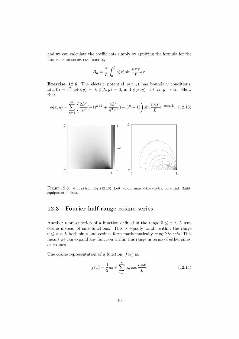
Exercise 12.6. The electric potential φ(x, y) has boundary conditions,φ(x, 0) = x2, φ(0, y) = 0, φ(L, y) = 0, and φ(x, y) → 0 as y → ∞. Showthat

φ(x, y) =

∞∑

n=1

(

2L2

nπ(−1)n+1 +

4L2

n3π3((−1)n − 1)

)

sinnπx

Le−nπy/L. (12.13)

0 L0

L

0

0.5

1

0

L

0 L

Figure 12.6: φ(x, y) from Eq. (12.13). Left: colour map of the electric potential. Right:equipotential lines.

12.3 Fourier half range cosine series

Another representation of a function defined in the range 0 ≤ x < L usescosine instead of sine functions. This is equally valid: within the range0 ≤ x < L both sines and cosines form mathematically complete sets. Thismeans we can expand any function within this range in terms of either sines,or cosines.

The cosine representation of a function, f(x) is,

f(x) =1

2a0 +

∞∑

n=1

an cosnπx

L. (12.14)

10

Fourier cosine series coefficients

The coefficients an, n = 0, 1, 2, . . . are given by,

an =2

L

∫ L

0f(x) cos

nπx

Ldx. (12.15)

Usually it is much easier to calculate a0 separately from all the other an.Then a0 is simply,

a0 =2

L

∫ L

0f(x)dx. (12.16)

Note that 12a0 is simply the average of the function, f(x) in the range 0 ≤

x < L.

Derivation of Fourier cosine series coefficients

The derivation for an is along similar lines to that of the Fourier sine seriescoefficients. First multiply both sides of Eq. (12.14) by cos(mπx/L) andintegrate from 0 to L,

∫ L

0f(x) cos

mπx

Ldx =

1

2a0

∫ L

0cos

mπx

Ldx+

∞∑

n=1

an

∫ L

0cos

nπx

Lcos

mπx

Ldx.

(12.17)From the standard integral (A.3) all the terms in the sum on the right ofEq. (12.17) are zero except for the one with m = n. Then, if m = n,

∫ L

0f(x) cos

mπx

Ldx = am

∫ L

0cos2

mπx

L=

L

2am,

and by rearranging and replacing m by n we have the result in Eq. (12.15).

If we choose m = 0 in Eq. (12.17) then cos(mπx/L) = 1 and all the termsin the sum go to zero. We are left with,

∫ L

0f(x)dx =

1

2a0

∫ L

0dx =

L

2ao,

which, after rearranging is identical to the result for a0 in Eq. (12.16).

11

Using the Fourier cosine series results

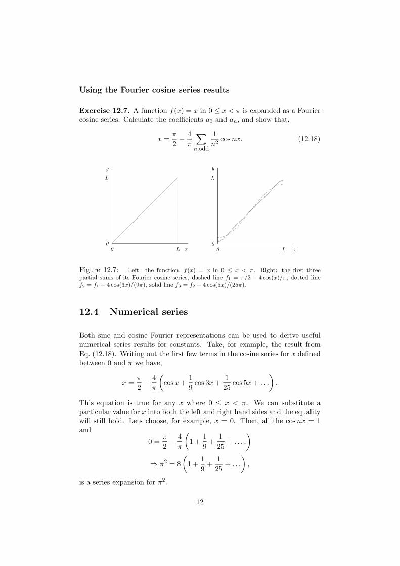
Exercise 12.7. A function f(x) = x in 0 ≤ x < π is expanded as a Fouriercosine series. Calculate the coefficients a0 and an, and show that,

x =π

2− 4

π

∑

n,odd

1

n2cosnx. (12.18)

0

L

0 L x

y

0

L

0 L x

y

Figure 12.7: Left: the function, f(x) = x in 0 ≤ x < π. Right: the first threepartial sums of its Fourier cosine series, dashed line f1 = π/2 − 4 cos(x)/π, dotted linef2 = f1 − 4 cos(3x)/(9π), solid line f3 = f2 − 4 cos(5x)/(25π).

12.4 Numerical series

Both sine and cosine Fourier representations can be used to derive usefulnumerical series results for constants. Take, for example, the result fromEq. (12.18). Writing out the first few terms in the cosine series for x definedbetween 0 and π we have,

x =π

2− 4

π

(

cos x+1

9cos 3x+

1

25cos 5x+ . . .

)

.

This equation is true for any x where 0 ≤ x < π. We can substitute aparticular value for x into both the left and right hand sides and the equalitywill still hold. Lets choose, for example, x = 0. Then, all the cosnx = 1and

0 =π

2− 4

π

(

1 +1

9+

1

25+ . . . .

)

⇒ π2 = 8

(

1 +1

9+

1

25+ . . .

)

,

is a series expansion for π2.

12

Exercise 12.8. A function, f(x), is defined by

f(x) =

{

1 0 ≤ x < L/2

0 L/2 ≤ x < L.

Expand f(x) as a Fourier cosine series and show that an = 0 if n is evenand that, if n is odd,

an =2

nπ(−1)(n−1)/2. (12.19)

Write down the cosine series for f(x) in 0 ≤ x < L and deduce that

π

4= 1− 1

3+

1

5− 1

7.

12.5 Periodic extension of Fourier series

So far we have examined the sine and cosine Fourier series representations offunctions within a limited range, 0 ≤ x < L. However, both sine and cosinesrepeat periodically. So, if we plot the Fourier series representations outsideof this range we will get functions that repeat periodically with wavelength2L.

Outside the given finite range, the Fourier series of f(x) represents a periodicextension of the function with f(x+ 2L) = f(x).

To understand the periodic extension of Fourier series it is important tofirst understand the symmetry of even and odd functions. There is a shortrevision section on even and odd functions in the appendix.

Even and odd symmetry of periodic functions

Sine waves are odd, so any Fourier sine series representation of a periodicfunction must have odd symmetry. Similarly, cosine waves are even, so anyFourier cosine series representation of a periodic function must have evensymmetry.

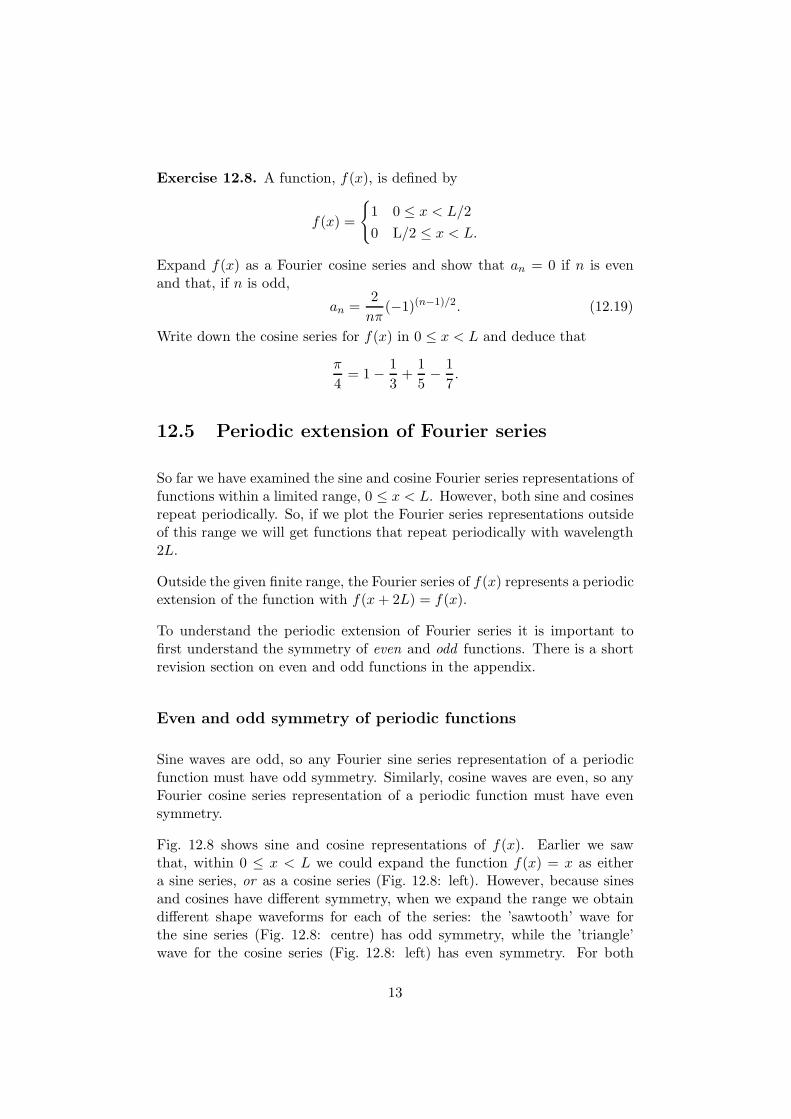
Fig. 12.8 shows sine and cosine representations of f(x). Earlier we sawthat, within 0 ≤ x < L we could expand the function f(x) = x as eithera sine series, or as a cosine series (Fig. 12.8: left). However, because sinesand cosines have different symmetry, when we expand the range we obtaindifferent shape waveforms for each of the series: the ’sawtooth’ wave forthe sine series (Fig. 12.8: centre) has odd symmetry, while the ’triangle’wave for the cosine series (Fig. 12.8: left) has even symmetry. For both

13

periodic extensions, f(x) = f(x + 2L). For the sine series we also havef(x) = −f(−x) and, for the cosine series, f(x) = f(−x).

y

x-L 0 L 2L

y

x-L 0 L 2L

y

x-L 0 L 2L

Figure 12.8: Left: Fourier sine or cosine representation of f(x) = x within 0 ≤ x < L.Center: periodic extension of sine series representation of f(x). Right: periodic extensionof cosine series representation of f(x).

Exercise 12.9. A function is defined by f(x) = x2, for 0 ≤ x < L. Sketchthe Fourier sine and cosine series representations of f(x) in −L ≤ x < 3L.

Exercise 12.10. Within 0 ≤ x < L, f(x) = x can be expanded as a sineseries, Eq. (12.7) or a cosine series Eq. (12.18). What function does each ofthese series represent in the range −L ≤ x < 0?

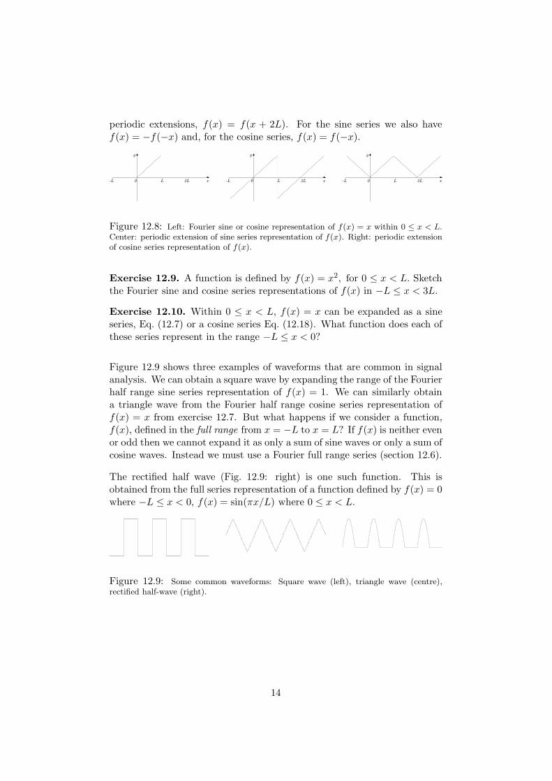
Figure 12.9 shows three examples of waveforms that are common in signalanalysis. We can obtain a square wave by expanding the range of the Fourierhalf range sine series representation of f(x) = 1. We can similarly obtaina triangle wave from the Fourier half range cosine series representation off(x) = x from exercise 12.7. But what happens if we consider a function,f(x), defined in the full range from x = −L to x = L? If f(x) is neither evenor odd then we cannot expand it as only a sum of sine waves or only a sum ofcosine waves. Instead we must use a Fourier full range series (section 12.6).

The rectified half wave (Fig. 12.9: right) is one such function. This isobtained from the full series representation of a function defined by f(x) = 0where −L ≤ x < 0, f(x) = sin(πx/L) where 0 ≤ x < L.

Figure 12.9: Some common waveforms: Square wave (left), triangle wave (centre),rectified half-wave (right).

14

12.6 Fourier full range series

The range 0 to 2L (or, alternatively, −L to L) is called the full range becauseit contains a full wavelength of the periodic function. In this section we willmostly use the range −L to L however, both 0 to 2L, and −L to L areexactly equivalent.

In the range −L to L neither sine or cosine waves form a complete set. If afunction defined between −L and L has odd symmetry it can be representedas a sine series. If a function has even symmetry it can be represented asa cosine series. However, in the general case, to represent a function ofarbitary symmetry, we need to include both sine and cosine terms in therepresentation.

12.6.1 Fourier full range series formula

The full range Fourier series for f(x) in the range −L ≤ x < L is,

f(x) =1

2a0 +

∞∑

n=1

(

an cosnπx

L+ bn sin

nπx

L

)

. (12.20)

The formulae for the Fourier series full range coefficients can be derived ina similar way to the formulae for the sine and cosine half range coefficients.We have,

a0 =1

L

∫ L

−Lf(x)dx

an =1

L

∫ L

−Lf(x) cos

nπx

Ldx

bn =1

L

∫ L

−Lf(x) sin

nπx

Ldx. (12.21)

Note: If the full range is defined to be between 0 to 2L the formulae remainthe same except that the limits of the integration go from 0 to 2L.

Exercise 12.11. A function f(x) = 1 + x within −π ≤ x < π. Calculatethe Fourier full range series of f(x).

Exercise 12.12. Calculate the full range Fourier series for a ’sawtooth’wave, f(x) = x, −π ≤ x < π. Explain why the series is the same as the halfrange sine representation in exercise 12.1. By writing out the result for anappropriately chosen value of x, show that

∞∑

m=0

(−1)m

2m+ 1=

π

4.

15

12.7 Complex form of Fourier Series

Instead of Eq. (12.20) we could equally well write the complex form,

f(x) =

∞∑

n=−∞

cneinπx/L, (12.22)

where,

cn =1

2L

∫ L

−Lf(x)e−inπx/Ldx. (12.23)

Sometimes this form is more convenient than the sine and cosine forms.

Derivation of complex series results

Recalling that sines and cosines can be written in terms of complex expo-nentials we can obtain Eq. (12.22) directly from Eq. (12.20).

f(x) = a0 + a1 cosπx

L+ b1 sin

πx

L+ a2 cos

2πx

L+ b2 sin

2πx

L+ . . .

= a0 + a1eiπx/L + e−iπx/L

2+ b1

eiπx/L − e−iπx/L

2i

+a2ei2πx/L + e−i2πx/L

2+ b2

ei2πx/L − e−i2πx/L

2i+ . . . .

Collecting together exponentials with the same powers we have,

f(x) = . . .+ (a2/2− b2/(2i))e−i2πx/L + (a1/2− b1/(2i))e

−iπx/L + a0

+(a1/2 + b1/(2i))eiπx/L + (a2/2 + b2/(2i))e

i2πx/L + . . .

= . . .+ c−2e−i2πx/L + c−1e

−iπx/L + c0 + c1eiπx/L + c2e

i2πx/L + . . . ,

which is identical to Eq. (12.22).

To find the formula for the complex coefficients, cn, multiply both sides ofEq. (12.22) by e−iπmx/L and integrate,

∫ L

−Lf(x)e−imπx/Ldx =

∞∑

n=−1

cn

∫ L

−Lei(n−m)πx/Ldx.

The integral on the right is a standard integral, Eq. (A.7). Using this resultwe find,

∫ L

−Lf(x)e−imπx/Ldx =

∞∑

n=−∞

cn2Lδnm, (12.24)

then rearranging Eq. (12.24) for cn we obtain the result in Eq. (12.23).

16

Exercise 12.13. If f(x) = 1 + x, −π ≤ x < π show that the complexFourier series coefficients are given by

cn = δn0 +(−1)n+1L

inπ.

Exercise 12.14. A function f(x) = exp(px) in −π ≤ x < π. Expand f(x)as a sum of complex exponentials to show that

f(x) =∞∑

n=−∞

(−1)n

π(p− in)sinh(pπ)einx.

Example 12.3. Show that the result for the complex Fourier series in ex-ercise 12.13 is equal to that obtained in exercise 12.11.

The complex Fourier series for f(x) = 1 + x in −L ≤ x < L, is

f(x) =

∞∑

n=−∞

(

δn0 +(−1)n+1L

inπ

)

einπx/L,

= 1 +

−1∑

n=−∞

(−1)n+1L

inπeinπx/L +

∞∑

n=1

(−1)n+1L

inπeinπx/L.

Then, replacing n by −n in the first summation, and factorising out −L/πwe have,

f(x) = 1 +−L

π

∞∑

n=1

[

(−1)−n

i(−n)ei(−n)πx/L +

(−1)n

ineinπx/L

]

,

= 1 +−L

π

∞∑

n=1

(−1)n

in

[

einπx/L − e−inπx/L]

,

= 1 +

∞∑

n=1

2(−1)n+1L

nπsin

nπx

L, (12.25)

where, in the last step, we have used the fact that einπx/L − e−inπx/L =2i sin(nπx/L).

12.8 Properties of Fourier series

Here we quote without proof some facts about Fourier series that you shouldknow.

17

General properties

a) Except for some pathological functions which do not occur in physicalproblems, we can always expand a function, f(x), defined in a finiteinterval as a Fourier series which will converge with sum f(x) at allpoints at which f(x) is continuous.

b) If f(x) has a discontinuity at x = x0 its Fourier series will converge tothe average of the limit from the left and the limit from the right.

y

xx0

f(x0)

The Fourier series of a discontinu-ous function sums to a value mid-way along the discontinuity.

f(x0) → limǫ→0

1

2(f(x0 + ǫ) + f(x0 − ǫ)) .

c) A Fourier series can be integrated term by term: the resulting seriesalways converges to

∫

f(x)dx.

d) Term by term differentiation of a Fourier series may produce a divergentseries. If the series produced by differentiation does converge then it isthe Fourier series for f ′(x).

Convergence of series

The properties above apply to the converged Fourier series containing aninfinite number of terms. In practice we often calculate the sum of only afinite number of the terms in the series which we use as an approximation.It is important to know when this is likely to give a good approximation.

a) If f(x) or its periodic extension has discontinuities we expect an, bn, cnto be of order 1/n and the convergence is slow.

b) If f(x) or its periodic extension is continuous we expect an, bn, cn to beof order 1/n2 and the convergence is rapid.

c) The Gibbs phenomenom. At a discontinuity (e.g. at x0) convergenceof a Fourier series is slow and a finite sum of N terms will persistentlyunder- or over-estimate f(x) near x0. The size of the overshoot (orundershoot) does not tend to zero as N → ∞, but region of the overshoot(or undershoot) does become narrower as the series converges.

18

y

x

The figure on the left showsthe partial Fourier sine seriesof f(x) = 1, 0 ≤ x < π withnmax = 3 (dotted), nmax = 5dashed and nmax = 25 (solidline) terms.

Exercise 12.15. By using the results above briefly explain why the conver-gence of the half range cosine series representation of x (Eq. 12.18) is muchfaster than that of the sine series representation (Eq. 12.7).

Exercise 12.16. State whether each of the following functions, defined inthe range −π ≤ x < π, can be expanded as (a) a Fourier sine series, (b) acosine series, or (c) a Fourier series containing both sine and cosine terms:(i) x3; (ii) x2 + x ; (iii) exp(x); (iv) |x|.

12.9 Introduction to Fourier Transforms

So far, we have seen that we can express an arbitrary periodic function as aFourier series, a sum of harmonic (sine and cosine) waves.

The Fourier transform gives us an analogous way to represent a generalfunction that is not periodic. Fourier transforms are used in an enormousrange of pure and applied science, including information processing, elec-tronics and communications.

12.9.1 Fourier integrals and transforms

Fourier integrals

The Fourier series of a function f(x) with period λ = 2L can be written as,

f(x) =

∞∑

n=−∞

cneinπx/L =

∞∑

n=−∞

cne2inπx/λ. (12.26)

So, what happens if the function is non-periodic? A non-periodic functionis equivalent to a periodic function in the limit that λ → ∞. So, let usconsider what happens to 12.26 when λ becomes large.

19

First we define a new variable k = 2πn/λ. Then we can think of the Fouriercoefficients, cn as a function, f̃(k) = ckλ/2π defined on a line of points ink-space. The distance between the points in k-space is ∆k = 2π/λ. Then,using a technique often used in quantum mechanics and statistical physics,we can rewrite the sum in Eq. (12.26) as,

f(x) =∞∑

n=−∞

cneikx =

∞∑

n=−∞

f̃(k)eikx =λ

2π

∞∑

n=−∞

f̃(k)eikx∆k.

In the limit as λ → ∞, ∆k → 0 and we can approximate the sum overk-points as an integral dk,

f(x) =λ

2π

∫

∞

−∞

f̃(k)eikxdk.

Finally, if we define F (k) = λf̃(k) we can write,

f(x) =1

2π

∫

∞

−∞

F (k)eikxdk. (12.27)

This is a Fourier integral. It is a representation of an arbitrary (non-periodic)function, f(x), in terms of simple harmonics.

Fourier transforms

To obtain a result for F (k) in Eq. (12.27) we simply apply the formula(Eq. (12.23) for the Fourier series coefficients, cn = ckλ/2π, in the limit asλ → ∞,

F (k) = limλ→∞

λckL/2π =

∫

∞

−∞

f(x)e−ikxdx. (12.28)

F (k) is called the Fourier transform of f(x). The two functions, F (k) andf(x) are called a Fourier transform pair. f(x) is the inverse Fourier trans-form of F (k).

Unfortunately there is no standard definition in the literature of what con-stitutes a transform and what constitutes an inverse transform. The onlyrequirement is that one of Eqs. (12.27) and (12.28) contains e−ikx and onecontains eikx. Similarly there is no set convention for the constant factorsin front of these integrals. We have used a factor 1/2π on the inverse trans-form and 1 on the transform, but you will often see the opposite of this, orsometimes 1/

√2π is used in front of both. This means that, when reading

the literature, you should be careful to identify the conventions used.

20

The argument of the Fourier transform, k, has units that are the reciprocalof the dimensions of the variable x. We will often use x to denote position,in which case k is the wavenumber. Similarly, if the variable is a time, t,the transform variable will be a frequency, often denoted by ω. Physicistsoften talk about using Fourier transforms to transform from real space toreciprocal or k-space, or from the time-domain to the frequency-domain.

Calculating Fourier transforms and integrals

Fourier transforms and integrals are ordinary integrals that can be evaluatedin the usual way. We will consider a specific example: the Fourier transformof a Gaussian.

Example 12.4. Find the Fourier transform of f(x) = exp(−x2/σ2). FromEq. (12.28) we have,

F (k) =

∫

∞

−∞

e−x2/σ2

e−ikxdx =

∫

∞

−∞

e−(x2/σ2+ikx)dx.

This integral is performed with a standard trick. First, we complete thesquare in the argument of the exponential,

x2/σ2 + ikx = (x/σ + ikσ/2)2 + k2σ2/4.

Then,

F (k) = e−k2σ2/4

∫

∞

−∞

e−(x/σ+ikσ/2)2dx,

= σe−k2σ2/4

∫

∞

−∞

e−x′2

dx′, (12.29)

where we have changed variable from x to x′ = x/σ− ikσ/2, so dx′ = dx/σ.In this particular case, the change of variable leaves the limits on the integralunchanged at −∞ and ∞. Then, using the fact that

∫

∞

−∞exp(−x2)dx =

√π,

we find that the Fourier transform of a Gaussian is,

F (k) = σ√πe−k2σ2/4. (12.30)

So the Fourier transform of a Gaussian of half width σ is a Gaussian ofhalf-width 2/σ. ie. a wide Gaussian function in real space transforms to anarrow Gaussian function in k-space and vice-versa.

Exercise 12.17. Show that the Fourier transform of the function defined

21

by f(x) = a for |x| ≤ L, f(x) = 0 for |x| > L is

F (k) =2a sin kL

k.

Exercise 12.18. Find the inverse Fourier transform of F (k) = exp(−k2/4).

12.9.2 Convolutions

In later units you will study in detail the properties of Fourier transforms,including their application in calculating convolutions and correlations. Herewe will briefly introduce a useful result - the convolution theorem.

A convolution integral has the general form

C(x) =

∫

∞

−∞

f(x− x′)g(x′)dx′. (12.31)

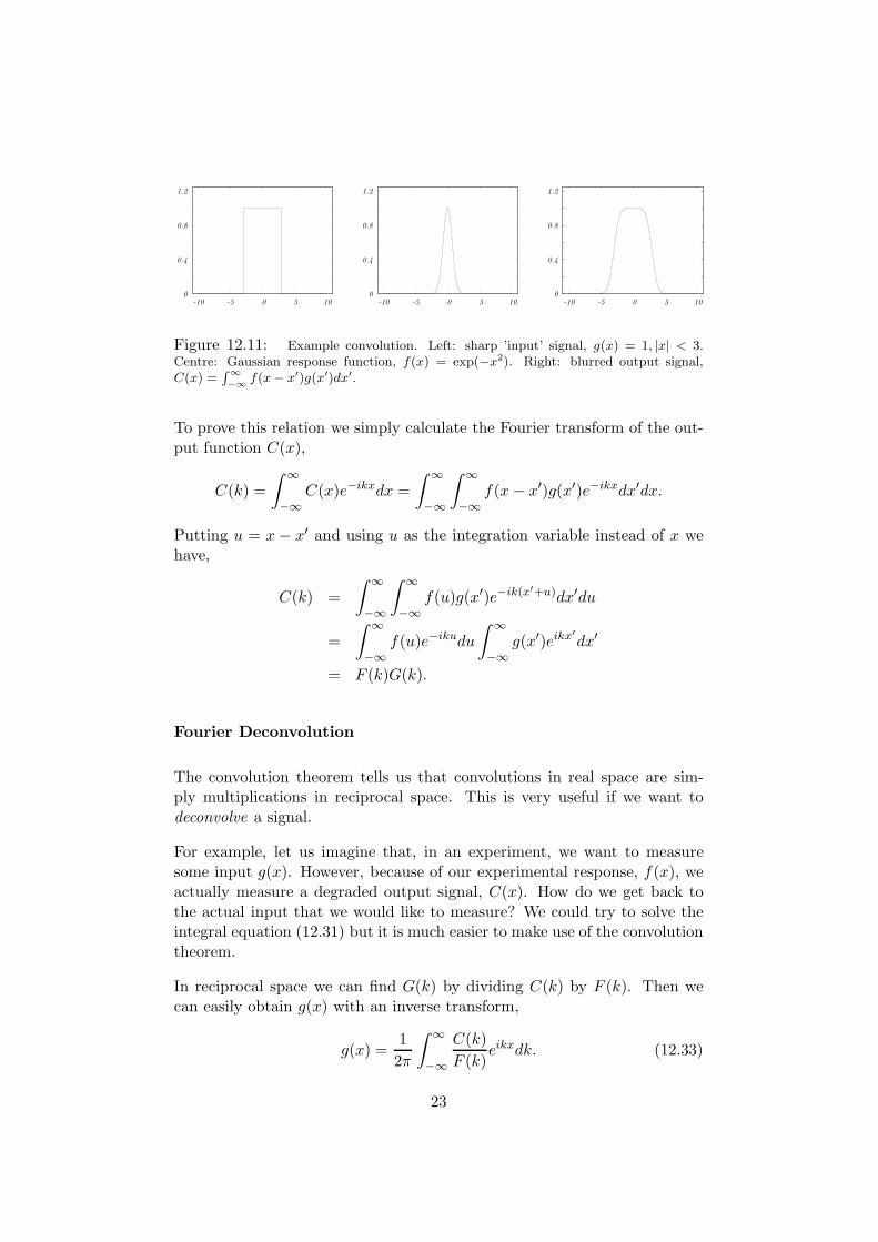
This integral relates an output function, C(x), to the input g(x) and theresponse f(x). Figure 12.10 shows an example from imaging processingwhere we degrade an initially sharp image with a Gaussian ’blur’. Theprocess is illustrated in one dimension in Fig. 12.11: we convolve the input,g(x), with a Gaussian response function, f(x) = exp(−x2), to give the newblurred output C(x) =

∫

∞

−∞f(x − x′)g(x′)dx′. You will often see a similar

effect in experimental physics where some initially sharp ’input’ signal willsuffer from Gaussian broadening as a result of an imprecise experimentalresponse.

Figure 12.10: Image processing with convolutions. A sharp image of a circle (left) isconvolved with a Gaussian response function to give the blurred image (right).

Convolution Theorem

The convolution theorem is a useful relation between the Fourier componentsof the input and output functions. According to the convolution theorem,

C(k) = F (k)G(k). (12.32)

22

0

0.4

0.8

1.2

-10 -5 0 5 10 0

0.4

0.8

1.2

-10 -5 0 5 10 0

0.4

0.8

1.2

-10 -5 0 5 10

Figure 12.11: Example convolution. Left: sharp ’input’ signal, g(x) = 1, |x| < 3.Centre: Gaussian response function, f(x) = exp(−x2). Right: blurred output signal,C(x) =

∫∞

−∞f(x− x′)g(x′)dx′.

To prove this relation we simply calculate the Fourier transform of the out-put function C(x),

C(k) =

∫

∞

−∞

C(x)e−ikxdx =

∫

∞

−∞

∫

∞

−∞

f(x− x′)g(x′)e−ikxdx′dx.

Putting u = x − x′ and using u as the integration variable instead of x wehave,

C(k) =

∫

∞

−∞

∫

∞

−∞

f(u)g(x′)e−ik(x′+u)dx′du

=

∫

∞

−∞

f(u)e−ikudu

∫

∞

−∞

g(x′)eikx′

dx′

= F (k)G(k).

Fourier Deconvolution

The convolution theorem tells us that convolutions in real space are sim-ply multiplications in reciprocal space. This is very useful if we want todeconvolve a signal.

For example, let us imagine that, in an experiment, we want to measuresome input g(x). However, because of our experimental response, f(x), weactually measure a degraded output signal, C(x). How do we get back tothe actual input that we would like to measure? We could try to solve theintegral equation (12.31) but it is much easier to make use of the convolutiontheorem.

In reciprocal space we can find G(k) by dividing C(k) by F (k). Then wecan easily obtain g(x) with an inverse transform,

g(x) =1

2π

∫

∞

−∞

C(k)

F (k)eikxdk. (12.33)

23

Figure 12.12 shows an illustration of this process. An initially blurred imageis sharpened by deconvolving the image with a Gaussian response function.

Figure 12.12: Sharpening of an image by deconvolution. From left to right: orig-inal blurred image C(x, y); Fourier transform of blurred image, C(kx, ky); responsefunction in reciprocal space, F (kx, ky); input function in reciprocal space, G(kx, ky) =C(kx, ky)/F (kx, ky); decovolved image, g(x, y).

Exercise 12.19. Write down the analogous results for the convolution in-tegral and convolution theorem, in the time and frequency domain.

Exercise 12.20. In reciprocal space an experimental signal that has beenbroadened with a Gaussian response function, F (k) =

√π exp(−ak2/4), has

the form C(k) = (2√π/k) exp(−ak2/4) sin k. Use the convolution theorem

to write down the input signal, G(k), in reciprocal space, then transformthis into real space to find the original form of the input, g(x). Hint : Youcan often find a Fourier transform simply by recognising that it is relatedto a known inverse transform.

12.10 Revision points

After completing this unit you should be able to:

a) Appreciate how an arbitrary periodic function can be represented by aninfinite summation of sines and cosines, the Fourier series of a function.

b) Use the Fourier series representation to find the solution of partial differ-ential equations, including the wave equation, satisfying given boundaryconditions.

c) Distinguish between full range (both complex and real form), and half

range sine and cosine Fourier representations of a given function.

d) Write down the formulae for the Fourier series coefficients in each case.

e) Find the Fourier half range and full range series representations of a givenfunction in a finite interval.

24

f) Understand the periodic extensions of Fourier series.

g) Appreciate how an arbitrary non-periodic function can by representedby a Fourier transform.

h) Calculate the Fourier transform and inverse transform of a given function.

i) Prove the convolution theorem from the convolution integral.

12.11 Problems

Exercise 12.21. A function f(θ) = θ3 in 0 ≤ θ < π is expanded in (a) aFourier sine series and (b) a Fourier cosine series. Sketch the form of thefunction represented by these series in the range −π < θ < 3π.

Exercise 12.22. A function f(θ), π ≤ θ < π is known to have a Fourierseries of the form

f(θ) =1

2a0 +

∞∑

n=1

cosnθ.

Show that f(θ) = f(−θ).

Exercise 12.23. Find the Fourier series for f(x) = x2, −π ≤ x < π andshow that

π2

12=

∞∑

n=1

(−1)n+1

n2

Exercise 12.24. Find the Fourier series for the function

f(θ) =

{

α, −π ≤ θ < 0

β, 0 ≤ θ < π,

where α and β are constants. Hint : the neatest approach is to write f(θ)as the sum of a symmetric function and an antisymmetric one.

By setting θ = π/2 show that,

∞∑

n=0

=(−1)n

2n+ 1=

π

4

Exercise 12.25. Find the Fourier series for

f(t) =

{

− sin t, −π ≤ t < 0

sin t, 0 ≤ t < π.

Hence show that∞∑

n=2,4,6,...

1

n2 − 1=

1

2.

25

Exercise 12.26. Expand the function f(x) = x as a half range Fouriercosine series in the range 0 ≤ x < L. What function does this series representin the interval −L ≤ x < L?

Exercise 12.27. Expand the function f(x) = sinπx as a half range Fouriercosine series in the range 0 ≤ x < 1. By considering the series for a suitablevalue of x show that,

∞∑

p=1

(−1)p

4p2 − 1=

1

2− π

4.

Exercise 12.28. Calculate the full range complex Fourier series represen-tation of f(x) = x+ x2.

Exercise 12.29. Show that the Fourier transform of a function defined byf(x) = exp(−a2x) for x ≥ 0, f(x) = 0 otherwise, is 1/(ik + a2).

Exercise 12.30. Calculate the inverse Fourier transform of F (k) = exp(−k2).

26

Appendix A

Additional results

A.1 Kronecker delta

The Kronecker delta is convenient mathematical shorthand. It is definedby

δnm =

{

1 if n = m

0 if n 6= m.(A.1)

A.2 Standard integrals

∫ L

0sin

nπx

Lsin

mπx

Ldx =

{

0 if m = n = 0L2 δmn otherwise

(A.2)

∫ L

0cos

nπx

Lcos

mπx

Ldx =

{

L if m = n = 0L2 δmn otherwise

(A.3)

∫ L

−Lsin

nπx

Lsin

mπx

Ldx =

{

0 if m = n = 0

Lδmn otherwise(A.4)

∫ L

−Lcos

nπx

Lcos

mπx

Ldx =

{

2L if m = n = 0

Lδmn otherwise(A.5)

∫ L

−Lsin

nπx

Lcos

mπx

Ldx = 0 (A.6)

27

∫ L

−Lei(n−m)πx/Ldx = 2Lδnm, (A.7)

A.2.1 Derivation of standard integrals

The results for the standard integrals Eqs. (A.2) to (A.6) can be found usingthe product formulae for trigonometric functions. For example, to obtainEq. (A.2) we write,

∫ L

0sin

mπx

Lsin

nπx

Ldx =

1

2

∫ L

0

(

cos(m− n)πx

L− cos

(n+m)πx

Ldx

)

=1

2

L

(m− n)π

[

sin(m− n)πx

L

]L

0

− 1

2

L

(m+ n)π

[

sin(m+ n)πx

L

]L

0

= 0 if m 6= n, because all the sine terms are zero.

If m = n 6= 0 then the integral becomes,

∫ L

0sin

mπx

Lsin

nπx

Ldx =

∫ L

0sin2

nπx

L

=1

2

∫ L

0

(

1− cos2nπx

L

)

dx

=L

2.

To obtain Eq. (A.7) we have, if n 6= m,

∫ L

−Lexp

(

i(n−m)πx

L

)

dx =

[

L

i(n −m)πexp

(

i(n−m)πx

L

)]L

−L

=L

i(n −m)π

[

ei(n−m)π − e−i(n−m)π]

= 0,

because exp(i(n −m)π) = exp(−i(n−m)π) = cos((n−m)π).

However, if n = m, then

∫ L

−Lexp

(

i(n−m)πx

L

)

dx =

∫ L

−Ldx

= 2L.

28

A.3 Even and Odd functions

A.3.1 Definitions

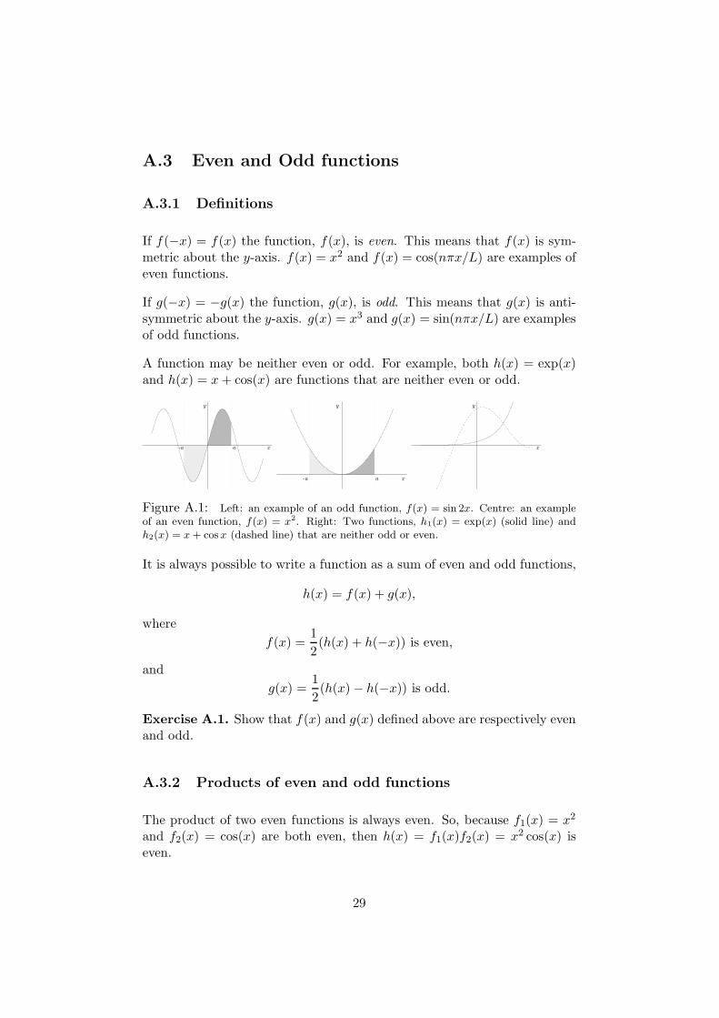
If f(−x) = f(x) the function, f(x), is even. This means that f(x) is sym-metric about the y-axis. f(x) = x2 and f(x) = cos(nπx/L) are examples ofeven functions.

If g(−x) = −g(x) the function, g(x), is odd. This means that g(x) is anti-symmetric about the y-axis. g(x) = x3 and g(x) = sin(nπx/L) are examplesof odd functions.

A function may be neither even or odd. For example, both h(x) = exp(x)and h(x) = x+ cos(x) are functions that are neither even or odd.

x

y

-a a

x

y

-a a

x

y

Figure A.1: Left: an example of an odd function, f(x) = sin 2x. Centre: an exampleof an even function, f(x) = x2. Right: Two functions, h1(x) = exp(x) (solid line) andh2(x) = x+ cosx (dashed line) that are neither odd or even.

It is always possible to write a function as a sum of even and odd functions,

h(x) = f(x) + g(x),

where

f(x) =1

2(h(x) + h(−x)) is even,

and

g(x) =1

2(h(x) − h(−x)) is odd.

Exercise A.1. Show that f(x) and g(x) defined above are respectively evenand odd.

A.3.2 Products of even and odd functions

The product of two even functions is always even. So, because f1(x) = x2

and f2(x) = cos(x) are both even, then h(x) = f1(x)f2(x) = x2 cos(x) iseven.

29

The product of two odd functions is always even. So, because g1(x) = x andg2(x) = sin(x) are both odd, then h(x) = g1(x)g2(x) = x sin(x) is even.

The product of an even function and an odd function is always odd. So,because f(x) = x2 is even and g(x) = sin(x) is odd, then h(x) = f(x)g(x) =x2 sin(x) is odd.

A.3.3 Integrals of even and odd functions

We can make use of symmetry to simplify the integrals of even and oddfunctions between limits that are symmetric about the origin. The integralof any odd function, g(x) between −a and a is simply zero. We can seethis graphically in Fig. A.1: the area under the curve between −a and 0 isequal and opposite to the area under the curve between 0 and a. For anyeven function we have

∫ 0−a f(x)dx =

∫ a0 f(x)dx. Again, this is illustrated

graphically in Fig. A.1.

In general,∫ a

−ah(x)dx =

{

0 if h(x) is odd

2∫ a0 h(x)dx if h(x) is even.

(A.8)

Exercise A.2. Derive the relations in Eq. (A.8). Hint : First split theintegral into two, a part from −a to 0 and a part from 0 to a, then changevariable from x to x′ = −x in the region where x < 0.

30