Fourier Analysis for Beginners Indiana University School of Optometry Coursenotes for V791: Quantitative Methods for Vision Research (Sixth edition) © L.N. Thibos (1989, 1993, 2000, 2003, 2012, 2014)

Welcome message from author
This document is posted to help you gain knowledge. Please leave a comment to let me know what you think about it! Share it to your friends and learn new things together.
Transcript
Fourier Analysis
for Beginners
Indiana University School of Optometry Coursenotes for V791: Quantitative Methods for Vision Research
(Sixth edition)
© L.N. Thibos (1989, 1993, 2000, 2003, 2012, 2014)

Table of Contents Preface.............................................................................................................................v
Chapter 1: Mathematical Preliminaries .....................................................................1 1.A Introduction ...............................................................................................1 1.B Review of some useful concepts of geometry and algebra. ................3
Scalar arithmetic....................................................................................3 Vector arithmetic...................................................................................4 Vector multiplication............................................................................6 Vector length..........................................................................................8 Summary. ...............................................................................................9
1.C Review of phasors and complex numbers.............................................9 Phasor length, the magnitude of complex numbers, and Euler's formula. .....................................................................................10 Multiplying complex numbers ...........................................................12 Statistics of complex numbers.............................................................13
1.D Terminology summary. ...........................................................................13
Chapter 2: Sinusoids, Phasors, and Matrices ..........................................................15 2.A Phasor representation of sinusoidal waveforms. .................................15 2.B Matrix algebra. ...........................................................................................16
Rotation matrices. .................................................................................18 Basis vectors...........................................................................................20 Orthogonal decomposition..................................................................20
Chapter 3: Fourier Analysis of Discrete Functions .................................................23 3.A Introduction. ..............................................................................................23 3.B A Function Sampled at 1 point. ..............................................................24 3.C A Function Sampled at 2 points. ............................................................25 3.D Fourier Analysis is a Linear Transformation. ......................................26 3.E Fourier Analysis is a Change in Basis Vectors. ....................................27 3.F A Function Sampled at 3 points..............................................................29 3.G A Function Sampled at D points............................................................32 3.H Tidying Up................................................................................................34 3.I Parseval's Theorem....................................................................................36 3.J A Statistical Connection............................................................................39 3.K Image Contrast and Compound Gratings............................................41 3.L Fourier Descriptors of the Shape of a Closed Curve ...........................43
Chapter 4: The Frequency Domain............................................................................47 4.A Spectral Analysis.......................................................................................47 4.B Physical Units.............................................................................................48 4.C Cartesian vs. Polar Form. .........................................................................50 4.D Complex Form of Spectral Analysis.......................................................51 4.E Complex Fourier Coefficients. .................................................................53 4.F Relationship between Complex and Trigonometric Fourier Coefficients.........................................................................................................55 4.G Discrete Fourier Transforms in Two or More Dimensions.................58
4.H Matlab's Implementation of the DFT ....................................................59 4.I Parseval's Theorem, Revisited .................................................................60
Chapter 5: Continuous Functions..............................................................................61 5.A Introduction. ..............................................................................................58 5.B Inner products and orthogonality...........................................................63 5.C Symmetry. ..................................................................................................65 5.D Complex-valued functions. .....................................................................67
Chapter 6: Fourier Analysis of Continuous Functions...........................................69 6.A Introduction. ..............................................................................................69 6.B The Fourier Model.....................................................................................69 6.C Practicalities of Obtaining the Fourier Coefficients. ............................71 6.D Theorems....................................................................................................73
1. Linearity .............................................................................................73 2. Shift theorem......................................................................................73 3. Scaling theorem.................................................................................75 4. Differentiation theorem....................................................................76 5. Integration theorem ..........................................................................77
6.E Non-sinusoidal basis functions ...............................................................79
Chapter 7: Sampling Theory.......................................................................................81 7.A Introduction. ..............................................................................................81 7.B The Sampling Theorem.............................................................................81 7.C Aliasing.......................................................................................................83 7.D Parseval's Theorem. ..................................................................................84 7.E Truncation Errors. .....................................................................................85 7.F Truncated Fourier Series & Regression Theory. ...................................86
Chapter 8: Statistical Description of Fourier Coefficients ......................................89 8.A Introduction. ..............................................................................................89 8.B Statistical Assumptions.............................................................................90 8.C Mean and Variance of Fourier Coefficients for Noisy Signals. ..........92 8.D Distribution of Fourier Coefficients for Noisy Signals. .......................94 8.E Distribution of Fourier Coefficients for Random Signals. ...................97 8.F Signal Averaging. ......................................................................................98
Chapter 9: Hypothesis Testing for Fourier Coefficients.........................................101 9.A Introduction. ..............................................................................................101 9.B Regression analysis. ..................................................................................101 9.C Band-limited signals. ................................................................................104 9.D Confidence intervals.................................................................................105 9.E Multivariate statistical analysis of Fourier coefficients........................107
Chapter 10: Directional Data Analysis......................................................................109 10.A Introduction. ............................................................................................109 10.B Determination of mean direction and concentration. ........................109 10.C Hypothesis testing. .................................................................................110 10.D Grouped data...........................................................................................110
10.D The Fourier connection. .........................................................................112 10.E Higher harmonics. ...................................................................................113
Chapter 11: The Fourier Transform...........................................................................115 11.A Introduction. ............................................................................................115 11.B The Inverse Cosine and Sine Transforms.............................................115 11.C The Forward Cosine and Sine Transforms..........................................117 11.D Discrete Spectra vs. Spectral Density ...................................................118 11.E Complex Form of the Fourier Transform.............................................120 11.F Fourier's Theorem....................................................................................121 11.G Relationship between Complex & Trigonometric Transforms. .......121
Chapter 12: Properties of The Fourier Transform ...................................................123 12.A Introduction. ............................................................................................123 12.B Theorems ..................................................................................................123
Linearity .................................................................................................123 Scaling.....................................................................................................123 Time/Space Shift...................................................................................124 Frequency Shift......................................................................................124 Modulation.............................................................................................124 Differentiation .......................................................................................125 Integration..............................................................................................125 Transform of a transform.....................................................................125 Central ordinate ....................................................................................126 Equivalent width...................................................................................126 Convolution ...........................................................................................127 Derivative of a convolution .................................................................127 Cross-correlation ...................................................................................128 Auto-correlation ....................................................................................128 Parseval/Rayleigh ................................................................................128
12.C The convolution operation.....................................................................129 12.D Delta functions ........................................................................................132 12.E Complex conjugate relations..................................................................135 12.F Symmetry relations..................................................................................135 12.H Convolution examples in probability theory and optics ..................136 12.H Variations on the convolution theorem...............................................137
Chapter 13: Signal Analysis........................................................................................139 13.A Introduction. ............................................................................................139 13.B Windowing...............................................................................................139 13.C Sampling with an array of windows....................................................141 13.D Aliasing.....................................................................................................143 13.E Reconstruction and interpolation..........................................................146 13.F. Non-point sampling ................................................................................146 13.G. The coverage factor rule.........................................................................150
Chapter 14: Fourier Optics..........................................................................................155 14.A Introduction. ............................................................................................155 14.B Physical optics and image formation....................................................155
14.C The Fourier optics domain.....................................................................159 14.D Linear systems description of image formation .................................162
Bibliography ..................................................................................................................167 Fourier Series and Transforms........................................................................167 Statistics of Fourier Coefficients .....................................................................167 Directional Data Analysis ................................................................................167 Random Signals and Noise..............................................................................168 Probability Theory & Stochastic Processes....................................................168 Signal Detection Theory...................................................................................168 Applications.......................................................................................................168
Appendices
Fourier Series Rayleigh Z-statistic Fourier Transform Pairs Fourier Theorems

V791 Coursenotes: Quantitative Methods for Vision Research Page v
Natural philosophy is written in this grand book the universe, which stands continually open to our gaze. But the book cannot be understood unless one first learns to comprehend the language and to read the alphabet in which it is composed. It is written in the language of mathematics, and its characters are triangles, circles, and other geometric figures, without which it is humanly impossible to understand a single word of it; without these, one wanders about in a dark labyrinth.
Galileo Galilei, the father of experimental science
V791 Coursenotes: Quantitative Methods for Vision Research Page vi
Preface Fourier analysis is ubiquitous. In countless areas of science, engineering, and
mathematics one finds Fourier analysis routinely used to solve real, important problems. Vision science is no exception: today's graduate student must understand Fourier analysis in order to pursue almost any research topic. This situation has not always been a source of concern. The roots of vision science are in "physiological optics", a term coined by Helmholtz which suggests a field populated more by physicists than by biologists. Indeed, vision science has traditionally attracted students from physics (especially optics) and engineering who were steeped in Fourier analysis as undergraduates. However, these days a vision scientist is just as likely to arrive from a more biological background with no more familiarity with Fourier analysis than with, say, French. Indeed, many of these advanced students are no more conversant with the language of mathematics than they are with other foreign languages, which isn't surprising given the recent demise of foreign language and mathematics requirements at all but the most conservative universities. Consequently, a Fourier analysis course taught in a mathematics, physics, or engineering undergraduate department would be much too difficult for many vision science graduate students simply because of their lack of fluency in the languages of linear algebra, calculus, analytic geometry, and the algebra of complex numbers. It is for these students that the present course was developed.
To communicate with the biologically-oriented vision scientist requires a different approach from that typically used to teach Fourier analysis to physics or engineering students. The traditional sequence is to start with an integral equation involving complex exponentials that defines the Fourier transform of a continuous, complex-valued function defined over all time or space. Given this elegant, comprehensive treatment, the real-world problem of describing the frequency content of a sampled waveform obtained in a laboratory experiment is then treated as a trivial, special case of the more general theory. Here we do just the opposite. Catering to the concrete needs of the pragmatic laboratory scientist, we start with the analysis of real-valued, discrete data sampled for a finite period of time. This allows us to use the much friendlier linear algebra, rather than the intimidating calculus, as a vehicle for learning. It also allows us to use simple spreadsheet computer programs (e.g. Excel), or preferably a more scientific platform like Matlab, to solve real-world problems at a very early stage of the course. With this early success under our belts, we can muster the resolve necessary to tackle the more abstract cases of an infinitely long observation time, complex-valued data, and the analysis of continuous functions. Along the way we review vectors, matrices, and the algebra of complex numbers in preparation for transitioning to the standard Fast Fourier Transform (FFT) algorithm built into Matlab. We also introduce such fundamental concepts as orthogonality, basis functions, convolution, sampling, aliasing, and the statistical reliability of Fourier coefficients computed from real-world data. Ultimately, we aim for students to master not just the tools necessary to solve practical problems and to understand the meaning of the answers, but also to be aware of the limitations of these tools and potential pitfalls if the tools are misapplied.
Chapter 1: Mathematical Preliminaries
1.A Introduction
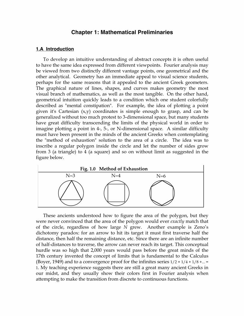
To develop an intuitive understanding of abstract concepts it is often useful to have the same idea expressed from different viewpoints. Fourier analysis may be viewed from two distinctly different vantage points, one geometrical and the other analytical. Geometry has an immediate appeal to visual science students, perhaps for the same reasons that it appealed to the ancient Greek geometers. The graphical nature of lines, shapes, and curves makes geometry the most visual branch of mathematics, as well as the most tangible. On the other hand, geometrical intuition quickly leads to a condition which one student colorfully described as "mental constipation". For example, the idea of plotting a point given it's Cartesian (x,y) coordinates is simple enough to grasp, and can be generalized without too much protest to 3-dimensional space, but many students have great difficulty transcending the limits of the physical world in order to imagine plotting a point in 4-, 5-, or N-dimensional space. A similar difficulty must have been present in the minds of the ancient Greeks when contemplating the "method of exhaustion" solution to the area of a circle. The idea was to inscribe a regular polygon inside the circle and let the number of sides grow from 3 (a triangle) to 4 (a square) and so on without limit as suggested in the figure below.
These ancients understood how to figure the area of the polygon, but they were never convinced that the area of the polygon would ever exactly match that of the circle, regardless of how large N grew. Another example is Zeno’s dichotomy paradox: for an arrow to hit its target it must first traverse half the distance, then half the remaining distance, etc. Since there are an infinite number of half-distances to traverse, the arrow can never reach its target. This conceptual hurdle was so high that 2,000 years would pass before the great minds of the 17th century invented the concept of limits that is fundamental to the Calculus (Boyer, 1949) and to a convergence proof for the infinites series 1/2 + 1/4 + 1/8 +... = 1. My teaching experience suggests there are still a great many ancient Greeks in our midst, and they usually show their colors first in Fourier analysis when attempting to make the transition from discrete to continuous functions.
N=3 N=4 N=6Fig. 1.0 Method of Exhaustion
Chapter 1: Mathematical Preliminaries Page 2
When geometrical intuition fails, analytical reasoning may come to the rescue. If the location of a point in 3-dimensional space is just a list of three numbers (x,y,z), then to locate a point in 4-dimensional space we only need to extend the list (w,x,y,z) by starting a bit earlier in the alphabet! Similarly, we may get around some conceptual difficulties by replacing geometrical objects and manipulations with analytical equations and computations. For these reasons, the early chapters of these coursenotes will carry a dual presentation of ideas, one geometrical and the other analytical. It is hoped that the redundancy of this approach will help the student achieve a depth of understanding beyond that obtained by either method alone.
The modern student may pose the question, "Why should I spend my time learning to do Fourier analysis when I can buy a program for my personal computer that will do it for me at the press of a key?" Indeed, this seems to be the prevailing attitude, for the instruction manual of one popular analysis program remarks that "Fourier analysis is one of those things that everybody does, but nobody understands." Such an attitude may be tolerated in some fields, but not in science. It is a cardinal rule that the experimentalist must understand the principles of operation of any tool used to collect, process, and analyze data. Accordingly, the main goal of this course is to provide students with an understanding of Fourier analysis - what it is, what it does, and why it is useful. As with any tool, one gains an understanding most readily by practicing its use and for this reason homework problems form an integral part of the course. On the other hand, this is not a course in computer programming and therefore we will not consider in any detail the elegant fast Fourier transform (FFT) algorithm which makes modern computer programs so efficient.
There is another, more general reason for studying Fourier analysis. Richard Hamming (1983) reminds us that "The purpose of computing is insight, not numbers!". When insight is obscured by a direct assault upon a problem, often a change in viewpoint will yield success. Fourier analysis is one example of a general strategy for changing viewpoints based on the idea of transformation. The idea is to recast the problem in a different domain, in a new context, so that fresh insight might be gained. The Fourier transform converts the problem from the time or spatial domain to the frequency domain. This turns out to have great practical benefit since many physical problems are easier to understand, and results are easier to compute, in the frequency domain. This is a major attraction of Fourier analysis for engineering: problems are converted to the frequency domain, computations performed, and the answers are transformed back into the original domain of space or time for interpretation in the context of the original problem. Another example, familiar to the previous generation of students, was the taking logarithms to make multiplication or division easier. Thus, by studying Fourier analysis the student is introduced to a very general strategy used in many branches of science for gaining insight through transformational computation.
Chapter 1: Mathematical Preliminaries Page 3
Lastly, we study Fourier analysis because it is the natural tool for describing physical phenomena which are periodic in nature. Examples include the annual cycle of the solar seasons, the monthly cycle of lunar events, daily cycles of circadean rhythms, and other periodic events on time scales of hours, minutes, or seconds such as the swinging pendulum, vibrating strings, or electrical oscillators. The surprising fact is that a tool for describing periodic events can also be used to describe non-periodic events. This notion was a source of great debate in Fourier's time, but today is accepted as the main reason for the ubiquitous applicability of Fourier's analysis in modern science.
1.B Review of some useful concepts of geometry and algebra.
Scalar arithmetic.
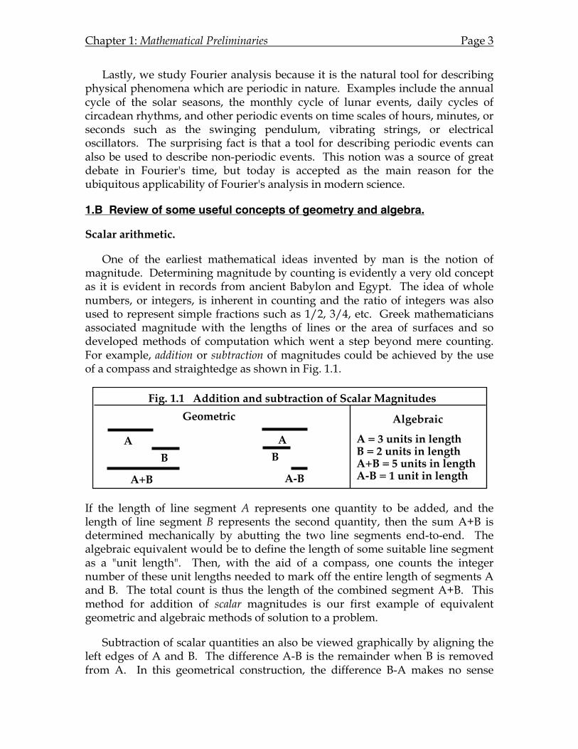
One of the earliest mathematical ideas invented by man is the notion of magnitude. Determining magnitude by counting is evidently a very old concept as it is evident in records from ancient Babylon and Egypt. The idea of whole numbers, or integers, is inherent in counting and the ratio of integers was also used to represent simple fractions such as 1/2, 3/4, etc. Greek mathematicians associated magnitude with the lengths of lines or the area of surfaces and so developed methods of computation which went a step beyond mere counting. For example, addition or subtraction of magnitudes could be achieved by the use of a compass and straightedge as shown in Fig. 1.1.
If the length of line segment A represents one quantity to be added, and the length of line segment B represents the second quantity, then the sum A+B is determined mechanically by abutting the two line segments end-to-end. The algebraic equivalent would be to define the length of some suitable line segment as a "unit length". Then, with the aid of a compass, one counts the integer number of these unit lengths needed to mark off the entire length of segments A and B. The total count is thus the length of the combined segment A+B. This method for addition of scalar magnitudes is our first example of equivalent geometric and algebraic methods of solution to a problem.
Subtraction of scalar quantities an also be viewed graphically by aligning the left edges of A and B. The difference A-B is the remainder when B is removed from A. In this geometrical construction, the difference B-A makes no sense
Fig. 1.1 Addition and subtraction of Scalar Magnitudes
AB
A+B
Geometric Algebraic
A = 3 units in lengthB = 2 units in lengthA+B = 5 units in lengthA-B = 1 unit in length
AB
A-B
Chapter 1: Mathematical Preliminaries Page 4
because B is not long enough to encompass A. Handling this situation is what prompted Arabic mathematicians to define the concept of negative numbers, which they called “false” or “fictitious” to acknowledge that counting real objects never produces negative numbers. On the other hand, negative numbers become very real concepts in accounting when you spend more than you earn!
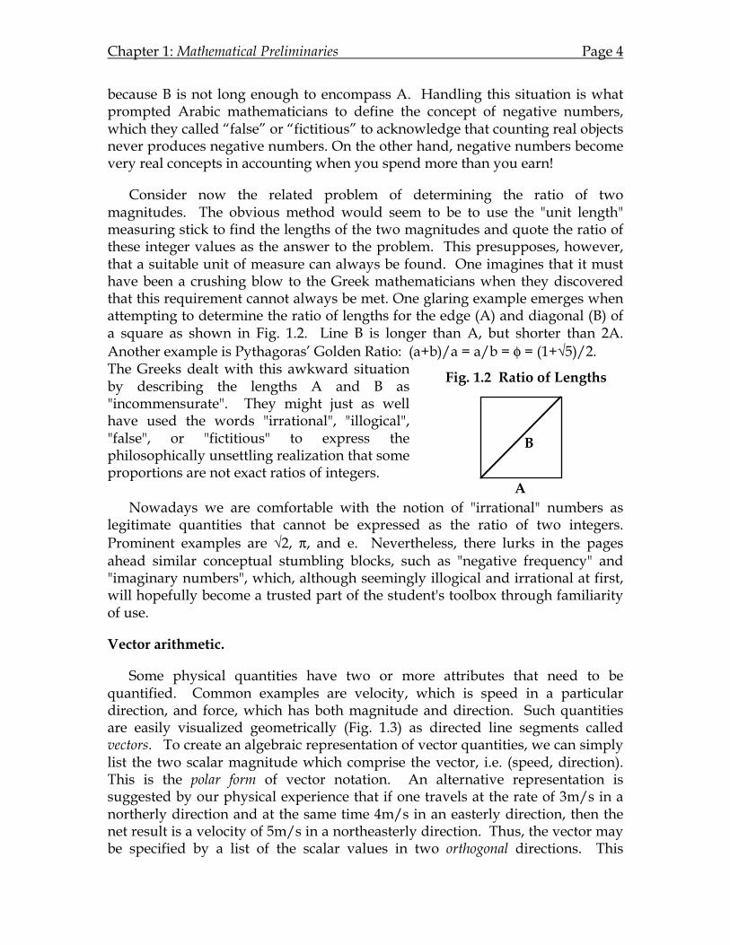
Consider now the related problem of determining the ratio of two magnitudes. The obvious method would seem to be to use the "unit length" measuring stick to find the lengths of the two magnitudes and quote the ratio of these integer values as the answer to the problem. This presupposes, however, that a suitable unit of measure can always be found. One imagines that it must have been a crushing blow to the Greek mathematicians when they discovered that this requirement cannot always be met. One glaring example emerges when attempting to determine the ratio of lengths for the edge (A) and diagonal (B) of a square as shown in Fig. 1.2. Line B is longer than A, but shorter than 2A. Another example is Pythagoras’ Golden Ratio: (a+b)/a = a/b = φ = (1+√5)/2. The Greeks dealt with this awkward situation by describing the lengths A and B as "incommensurate". They might just as well have used the words "irrational", "illogical", "false", or "fictitious" to express the philosophically unsettling realization that some proportions are not exact ratios of integers.
Nowadays we are comfortable with the notion of "irrational" numbers as
legitimate quantities that cannot be expressed as the ratio of two integers. Prominent examples are √2, π, and e. Nevertheless, there lurks in the pages ahead similar conceptual stumbling blocks, such as "negative frequency" and "imaginary numbers", which, although seemingly illogical and irrational at first, will hopefully become a trusted part of the student's toolbox through familiarity of use.
Vector arithmetic.
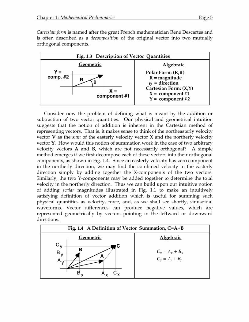
Some physical quantities have two or more attributes that need to be quantified. Common examples are velocity, which is speed in a particular direction, and force, which has both magnitude and direction. Such quantities are easily visualized geometrically (Fig. 1.3) as directed line segments called vectors. To create an algebraic representation of vector quantities, we can simply list the two scalar magnitude which comprise the vector, i.e. (speed, direction). This is the polar form of vector notation. An alternative representation is suggested by our physical experience that if one travels at the rate of 3m/s in a northerly direction and at the same time 4m/s in an easterly direction, then the net result is a velocity of 5m/s in a northeasterly direction. Thus, the vector may be specified by a list of the scalar values in two orthogonal directions. This
Fig. 1.2 Ratio of Lengths
A
B
Chapter 1: Mathematical Preliminaries Page 5
Cartesian form is named after the great French mathematician René Descartes and is often described as a decomposition of the original vector into two mutually orthogonal components.
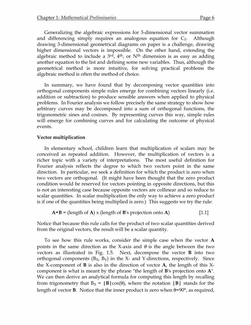
Consider now the problem of defining what is meant by the addition or subtraction of two vector quantities. Our physical and geometrical intuition suggests that the notion of addition is inherent in the Cartesian method of representing vectors. That is, it makes sense to think of the northeasterly velocity vector V as the sum of the easterly velocity vector X and the northerly velocity vector Y. How would this notion of summation work in the case of two arbitrary velocity vectors A and B, which are not necessarily orthogonal? A simple method emerges if we first decompose each of these vectors into their orthogonal components, as shown in Fig. 1.4. Since an easterly velocity has zero component in the northerly direction, we may find the combined velocity in the easterly direction simply by adding together the X-components of the two vectors. Similarly, the two Y-components may be added together to determine the total velocity in the northerly direction. Thus we can build upon our intuitive notion of adding scalar magnitudes illustrated in Fig. 1.1 to make an intuitively satisfying definition of vector addition which is useful for summing such physical quantities as velocity, force, and, as we shall see shortly, sinusoidal waveforms. Vector differences can produce negative values, which are represented geometrically by vectors pointing in the leftward or downward directions.
Fig. 1.3 Description of Vector Quantities
X =component #1
Y = comp. #2
Geometric Algebraic
Polar Form: (R, ) R = magnitude = directionCartesian Form: (X,Y) X = component #1 Y = component #2
!
!
!R
Fig. 1.4 A Definition of Vector Summation, C=A+B
A
A
Geometric Algebraic
x
y
x
y
B
B
AB
CCX = AX + BXCY = AY + BY
Cx
Cy
Chapter 1: Mathematical Preliminaries Page 6
Generalizing the algebraic expressions for 3-dimensional vector summation and differencing simply requires an analogous equation for CZ. Although drawing 3-dimensional geometrical diagrams on paper is a challenge, drawing higher dimensional vectors is impossible. On the other hand, extending the algebraic method to include a 3rd, 4th, or Nth dimension is as easy as adding another equation to the list and defining some new variables. Thus, although the geometrical method is more intuitive, for solving practical problems the algebraic method is often the method of choice.
In summary, we have found that by decomposing vector quantities into orthogonal components simple rules emerge for combining vectors linearly (i.e. addition or subtraction) to produce sensible answers when applied to physical problems. In Fourier analysis we follow precisely the same strategy to show how arbitrary curves may be decomposed into a sum of orthogonal functions, the trigonometric sines and cosines. By representing curves this way, simple rules will emerge for combining curves and for calculating the outcome of physical events.
Vector multiplication
In elementary school, children learn that multiplication of scalars may be conceived as repeated addition. However, the multiplication of vectors is a richer topic with a variety of interpretations. The most useful definition for Fourier analysis reflects the degree to which two vectors point in the same direction. In particular, we seek a definition for which the product is zero when two vectors are orthogonal. (It might have been thought that the zero product condition would be reserved for vectors pointing in opposite directions, but this is not an interesting case because opposite vectors are collinear and so reduce to scalar quantities. In scalar multiplication the only way to achieve a zero product is if one of the quantities being multiplied is zero.) This suggests we try the rule:
A•B = (length of A) x (length of B's projection onto A) [1.1]
Notice that because this rule calls for the product of two scalar quantities derived from the original vectors, the result will be a scalar quantity.
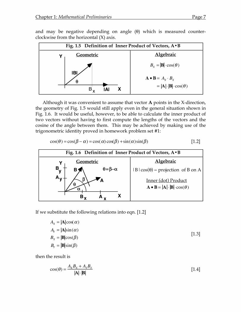
To see how this rule works, consider the simple case when the vector A points in the same direction as the X-axis and θ is the angle between the two vectors as illustrated in Fig. 1.5. Next, decompose the vector B into two orthogonal components (BX, BY) in the X- and Y-directions, respectively. Since the X-component of B is also in the direction of vector A, the length of this X-component is what is meant by the phrase "the length of B's projection onto A". We can then derive an analytical formula for computing this length by recalling from trigonometry that BX = |B|cos(θ), where the notation |B| stands for the length of vector B. Notice that the inner product is zero when θ=90°, as required,
Chapter 1: Mathematical Preliminaries Page 7
and may be negative depending on angle (θ) which is measured counter-clockwise from the horizontal (X) axis.
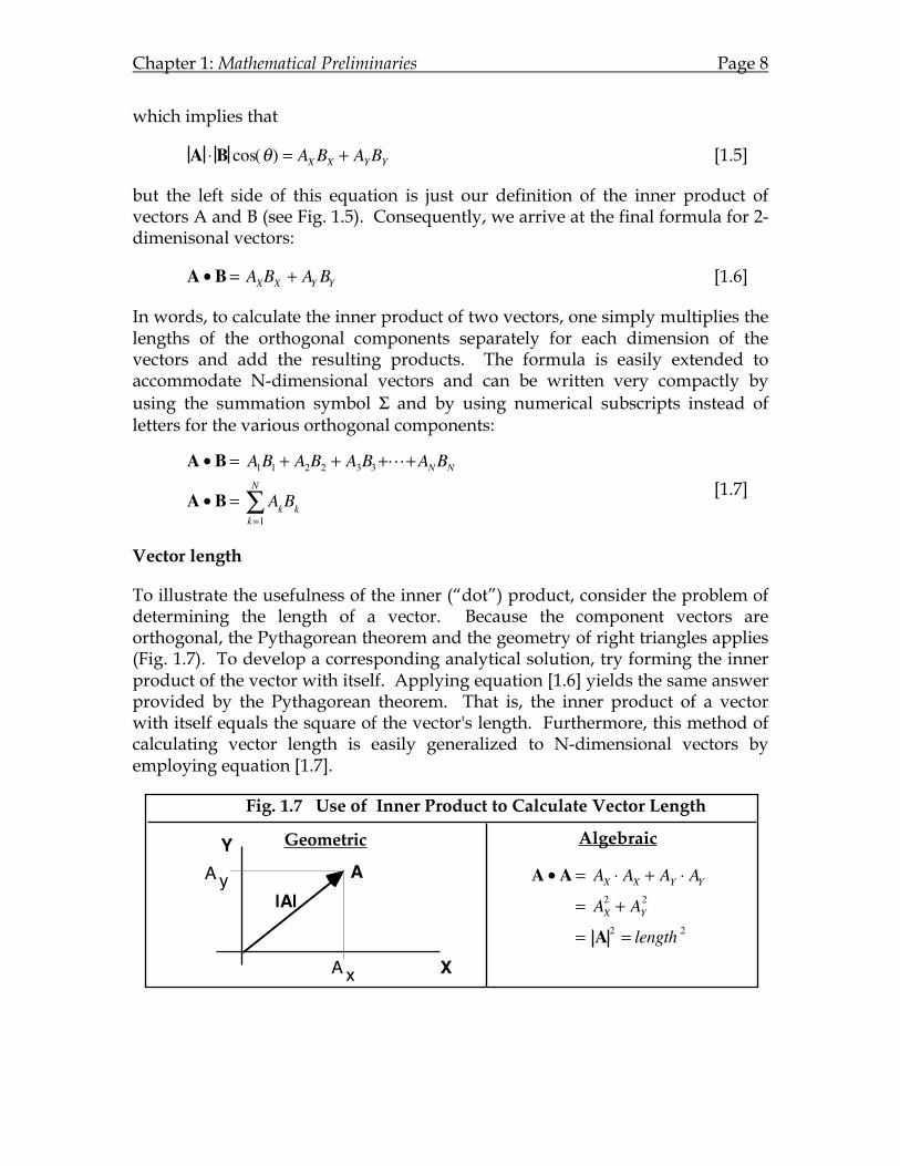
Although it was convenient to assume that vector A points in the X-direction, the geometry of Fig. 1.5 would still apply even in the general situation shown in Fig. 1.6. It would be useful, however, to be able to calculate the inner product of two vectors without having to first compute the lengths of the vectors and the cosine of the angle between them. This may be achieved by making use of the trigonometric identity proved in homework problem set #1:
cos(θ ) = cos(β − α ) = cos(α) cos(β ) + sin(α )sin(β) [1.2]
If we substitute the following relations into eqn. [1.2]
AX = A cos(α )AY = A sin(α )BX = B cos(β)BY = B sin(β)
[1.3]
then the result is
cos(θ) = AXBX + AYBYA ⋅ B
[1.4]
Fig. 1.5 Definition of Inner Product of Vectors, A•B
Geometric Algebraic
xB |A|
|B|
X
Y
!A • B = AX " BX
= A " B "cos(! )
BX = B "cos(! )
Fig. 1.6 Definition of Inner Product of Vectors, A•B
Geometric Algebraic
A
B
X
Y
!"
#
! = #$"
A • B = A % B %cos(! )
|B|cos( ) = projection of B on A!
Inner (dot) Product
A x
B
Bx
yAy
Chapter 1: Mathematical Preliminaries Page 8
which implies that
A ⋅ B cos(θ) = AXBX + AYBY [1.5]
but the left side of this equation is just our definition of the inner product of vectors A and B (see Fig. 1.5). Consequently, we arrive at the final formula for 2-dimenisonal vectors:
A • B = AXBX + AY BY [1.6]
In words, to calculate the inner product of two vectors, one simply multiplies the lengths of the orthogonal components separately for each dimension of the vectors and add the resulting products. The formula is easily extended to accommodate N-dimensional vectors and can be written very compactly by using the summation symbol Σ and by using numerical subscripts instead of letters for the various orthogonal components:
A • B = A1B1 + A2B2 + A3B3++ANBN
A • B = AkBkk=1
N
∑ [1.7]
Vector length
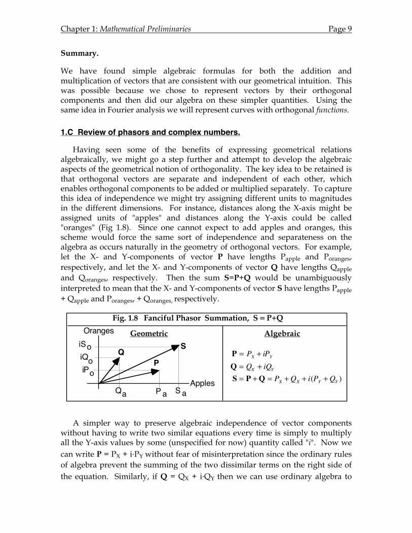
To illustrate the usefulness of the inner (“dot”) product, consider the problem of determining the length of a vector. Because the component vectors are orthogonal, the Pythagorean theorem and the geometry of right triangles applies (Fig. 1.7). To develop a corresponding analytical solution, try forming the inner product of the vector with itself. Applying equation [1.6] yields the same answer provided by the Pythagorean theorem. That is, the inner product of a vector with itself equals the square of the vector's length. Furthermore, this method of calculating vector length is easily generalized to N-dimensional vectors by employing equation [1.7].
Fig. 1.7 Use of Inner Product to Calculate Vector Length
Geometric Algebraic
xA
|A|
X
YA •A = AX ! AX + AY ! AY
= AX2 + AY
2
= A 2 = length 2
AyA
Chapter 1: Mathematical Preliminaries Page 9
Summary.
We have found simple algebraic formulas for both the addition and multiplication of vectors that are consistent with our geometrical intuition. This was possible because we chose to represent vectors by their orthogonal components and then did our algebra on these simpler quantities. Using the same idea in Fourier analysis we will represent curves with orthogonal functions.
1.C Review of phasors and complex numbers.
Having seen some of the benefits of expressing geometrical relations algebraically, we might go a step further and attempt to develop the algebraic aspects of the geometrical notion of orthogonality. The key idea to be retained is that orthogonal vectors are separate and independent of each other, which enables orthogonal components to be added or multiplied separately. To capture this idea of independence we might try assigning different units to magnitudes in the different dimensions. For instance, distances along the X-axis might be assigned units of "apples" and distances along the Y-axis could be called "oranges" (Fig 1.8). Since one cannot expect to add apples and oranges, this scheme would force the same sort of independence and separateness on the algebra as occurs naturally in the geometry of orthogonal vectors. For example, let the X- and Y-components of vector P have lengths Papple and Poranges, respectively, and let the X- and Y-components of vector Q have lengths Qapple and Qoranges, respectively. Then the sum S=P+Q would be unambiguously interpreted to mean that the X- and Y-components of vector S have lengths Papple + Qapple and Poranges, + Qoranges, respectively.
A simpler way to preserve algebraic independence of vector components without having to write two similar equations every time is simply to multiply all the Y-axis values by some (unspecified for now) quantity called "i". Now we can write P = PX + i.PY without fear of misinterpretation since the ordinary rules of algebra prevent the summing of the two dissimilar terms on the right side of the equation. Similarly, if Q = QX + i.QY then we can use ordinary algebra to
Fig. 1.8 Fanciful Phasor Summation, S = P+Q
P
iP
Geometric Algebraic
a
o
a
o
iQ
Q
PQ
S
Sa
iSo
Apples
Oranges
P = PX + iPY
Q = QX + iQY
S = P +Q = PX +QX + i(PY +QY )
Chapter 1: Mathematical Preliminaries Page 10
determine the sum S=P+Q = PX + QX + i.PY + i.QY = (PX + QX ) + i.(PY + QY) without fear of mixing apples with oranges. In the engineering discipline, 2-dimensional vectors written this way are often called "phasors".
Phasor length, the magnitude of complex numbers, and Euler’s formula
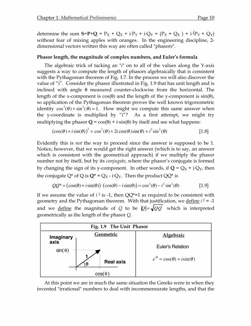
The algebraic trick of tacking an "i" on to all of the values along the Y-axis suggests a way to compute the length of phasors algebraically that is consistent with the Pythagorean theorem of Fig. 1.7. In the process we will also discover the value of “i”. Consider the phasor illustrated in Fig. 1.9 that has unit length and is inclined with angle θ measured counter-clockwise from the horizontal. The length of the x-component is cos(θ) and the length of the y-component is sin(θ), so application of the Pythagorean theorem proves the well known trigonometric identity cos2(θ ) + sin2(θ) = 1. How might we compute this same answer when the y-coordinate is multiplied by “i”? As a first attempt, we might try multiplying the phasor Q = cos(θ) + i.sin(θ) by itself and see what happens:
cos(θ ) + i sin(θ)( )2 = cos2 (θ ) + 2i cos(θ )sin(θ) + i2 sin2 (θ) [1.8]
Evidently this is not the way to proceed since the answer is supposed to be 1. Notice, however, that we would get the right answer (which is to say, an answer which is consistent with the geometrical approach) if we multiply the phasor number not by itself, but by its conjugate, where the phasor’s conjugate is formed by changing the sign of its y-component. In other words, if Q = QX + i.QY, then
the conjugate Q* of Q is Q* = QX - i.QY. Then the product QQ* is
QQ* = cos(θ) + i sin(θ)( ) ⋅ cos(θ) − i sin(θ)( ) = cos2 (θ) − i2 sin2 (θ) [1.9]
If we assume the value of i 2 is -1, then QQ*=1 as required to be consistent with geometry and the Pythagorean theorem. With that justification, we define i 2 = -1 and we define the magnitude of Q to be Q = QQ* which is interpreted geometrically as the length of the phasor Q.
At this point we are in much the same situation the Greeks were in when they invented "irrational" numbers to deal with incommensurate lengths, and that the
Fig. 1.9 The Unit Phasor
Geometric Algebraic
1Real axis
Imaginaryaxis
!
cos( )
sin( )
!
!
ei! = cos(!) + isin(! )
Euler's Relation
Chapter 1: Mathematical Preliminaries Page 11
Arabs were in when they invented negative "fictitious" numbers to handle subtracting a large number from a small number. Since the square of any real number is positive, the definition i 2 = -1 is seemingly impossible, so the quantity “i” must surely be "imaginary"! In short, we have invented an entirely new kind of quantity and with it the notion of complex numbers, which is the name given to the algebraic correlate to our geometric phasors. Complex numbers are thus the sum of ordinary "real" quantities and these new "imaginary" quantities created by multiplying real numbers by the quantity i= √-1. We may now drop our little charade and admit that apples are real, oranges are imaginary, and complex fruit salad needs both!
The skeptical student may be wary of the seemingly arbitrary nature of the two definitions imposed above, justified pragmatically by the fact that they lead to the desired answer. However, this type of justification is not unusual in mathematics, which is, after all, an invention, not a physical science subject to the laws of nature. The only constraint placed on mathematical inventiveness is that definitions and operations be internally consistent, which is our justification for the definitions needed to make complex numbers useful in Fourier analysis.
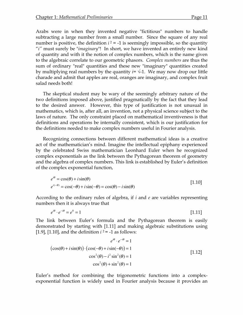
Recognizing connections between different mathematical ideas is a creative act of the mathematician’s mind. Imagine the intellectual epiphany experienced by the celebrated Swiss mathematician Leonhard Euler when he recognized complex exponentials as the link between the Pythagorean theorem of geometry and the algebra of complex numbers. This link is established by Euler’s definition of the complex exponential function,
eiθ = cos(θ) + i sin(θ)ei(−θ ) = cos(−θ) + i sin(−θ) = cos(θ) − i sin(θ)
[1.10]
According to the ordinary rules of algebra, if i and e are variables representing numbers then it is always true that
eiθ ⋅ e− iθ = e0 = 1 [1.11]
The link between Euler’s formula and the Pythagorean theorem is easily demonstrated by starting with [1.11] and making algebraic substitutions using [1.9], [1.10], and the definition i 2 = -1 as follows:
eiθ ⋅ e− iθ = 1cos(θ) + i sin(θ)( ) ⋅ cos(−θ) + i sin(−θ)( ) = 1
cos2 (θ) − i2 sin2 (θ) = 1cos2 (θ) + sin2 (θ) = 1
[1.12]
Euler’s method for combining the trigonometric functions into a complex-exponential function is widely used in Fourier analysis because it provides an
Chapter 1: Mathematical Preliminaries Page 12
efficient way to represent the sine and cosine components of a waveform by a single function. In so doing, however, both positive and negative frequencies are required which may be confusing for beginners. In this book we proceed more slowly by first gaining familiarity with Fourier analysis using ordinary trigonometric functions, for which frequencies are always positive, before adopting the complex exponential functions.
Multiplying complex numbers
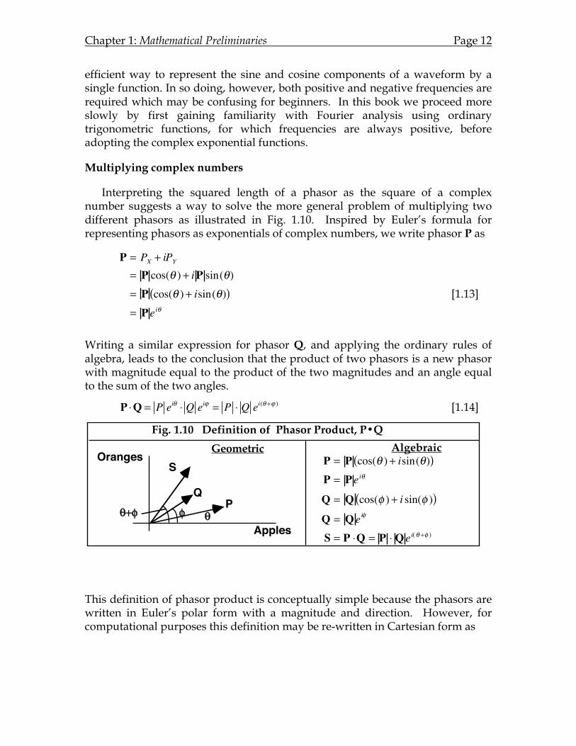
Interpreting the squared length of a phasor as the square of a complex number suggests a way to solve the more general problem of multiplying two different phasors as illustrated in Fig. 1.10. Inspired by Euler’s formula for representing phasors as exponentials of complex numbers, we write phasor P as
P = PX + iPY
= P cos(θ ) + iP sin(θ)= P cos(θ ) + isin(θ)( )= P eiθ
[1.13]
Writing a similar expression for phasor Q, and applying the ordinary rules of algebra, leads to the conclusion that the product of two phasors is a new phasor with magnitude equal to the product of the two magnitudes and an angle equal to the sum of the two angles.
P ⋅Q = P eiθ ⋅ Q eiϕ = P ⋅ Q ei(θ+ϕ ) [1.14]
This definition of phasor product is conceptually simple because the phasors are written in Euler’s polar form with a magnitude and direction. However, for computational purposes this definition may be re-written in Cartesian form as
Fig. 1.10 Definition of Phasor Product, P•Q
Geometric Algebraic
PQ
Apples
Oranges
!"
S
!+"
P = P cos(! ) + isin(!)( )P = P ei!
Q = Q cos(" ) + i sin(" )( )Q = Q ei"
S = P #Q = P # Q ei(! +" )
Chapter 1: Mathematical Preliminaries Page 13
P = a + ib; Q = c + idPQ = ac + iad + ibc + i2bd = ac − bd( ) + i ad + bc( ) [1.15]
Statistics of complex numbers.
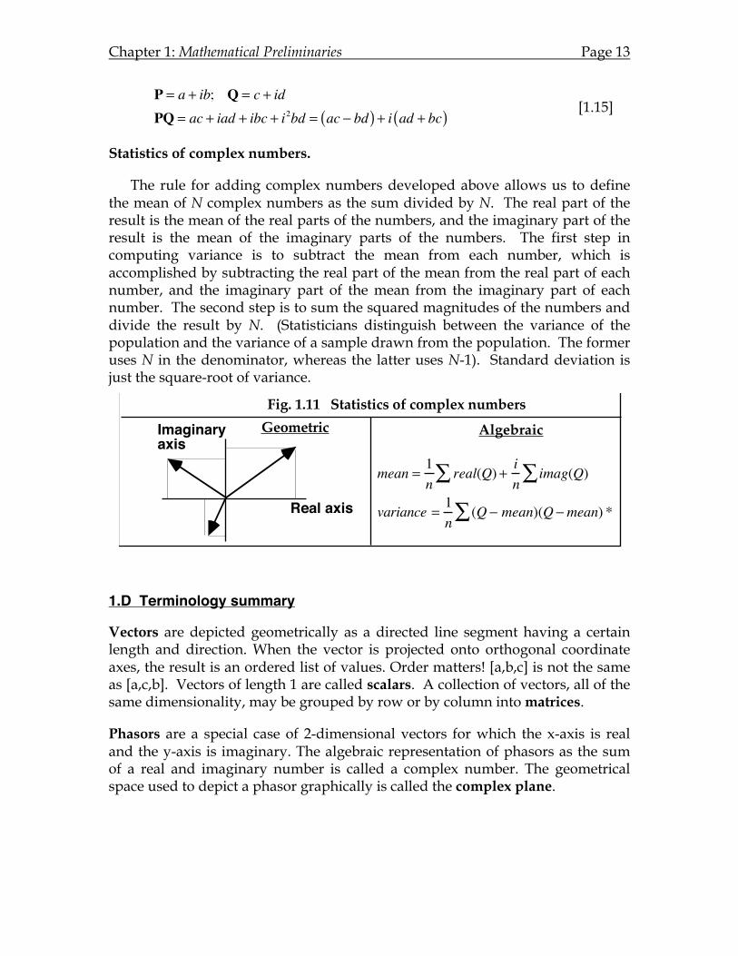
The rule for adding complex numbers developed above allows us to define the mean of N complex numbers as the sum divided by N. The real part of the result is the mean of the real parts of the numbers, and the imaginary part of the result is the mean of the imaginary parts of the numbers. The first step in computing variance is to subtract the mean from each number, which is accomplished by subtracting the real part of the mean from the real part of each number, and the imaginary part of the mean from the imaginary part of each number. The second step is to sum the squared magnitudes of the numbers and divide the result by N. (Statisticians distinguish between the variance of the population and the variance of a sample drawn from the population. The former uses N in the denominator, whereas the latter uses N-1). Standard deviation is just the square-root of variance.
1.D Terminology summary
Vectors are depicted geometrically as a directed line segment having a certain length and direction. When the vector is projected onto orthogonal coordinate axes, the result is an ordered list of values. Order matters! [a,b,c] is not the same as [a,c,b]. Vectors of length 1 are called scalars. A collection of vectors, all of the same dimensionality, may be grouped by row or by column into matrices.
Phasors are a special case of 2-dimensional vectors for which the x-axis is real and the y-axis is imaginary. The algebraic representation of phasors as the sum of a real and imaginary number is called a complex number. The geometrical space used to depict a phasor graphically is called the complex plane.
Fig. 1.11 Statistics of complex numbers
Geometric Algebraic
Real axis
Imaginaryaxis
mean = 1n
real(Q)! +in
imag(Q)!
variance = 1n
(Q " mean)(Q "mean) *!

Chapter 1: Mathematical Preliminaries Page 14
Chapter 2: Sinusoids, Phasors, and Matrices Page 15
Chapter 2: Sinusoids, Phasors, and Matrices
2.A Phasor representation of sinusoidal waveforms.
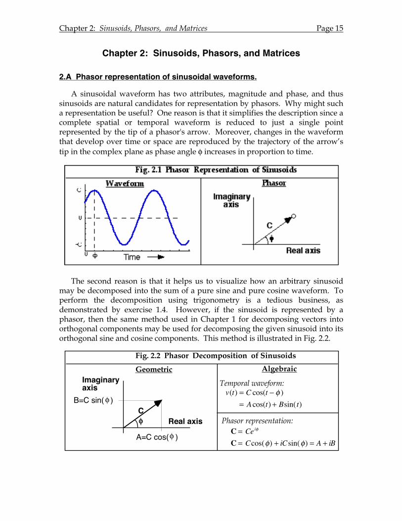
A sinusoidal waveform has two attributes, magnitude and phase, and thus sinusoids are natural candidates for representation by phasors. Why might such a representation be useful? One reason is that it simplifies the description since a complete spatial or temporal waveform is reduced to just a single point represented by the tip of a phasor's arrow. Moreover, changes in the waveform that develop over time or space are reproduced by the trajectory of the arrow’s tip in the complex plane as phase angle φ increases in proportion to time.
The second reason is that it helps us to visualize how an arbitrary sinusoid may be decomposed into the sum of a pure sine and pure cosine waveform. To perform the decomposition using trigonometry is a tedious business, as demonstrated by exercise 1.4. However, if the sinusoid is represented by a phasor, then the same method used in Chapter 1 for decomposing vectors into orthogonal components may be used for decomposing the given sinusoid into its orthogonal sine and cosine components. This method is illustrated in Fig. 2.2.
Fig. 2.2 Phasor Decomposition of Sinusoids
Geometric Algebraic
CReal axis
Imaginaryaxis
!
A=C cos( )
B=C sin( )!
!
Phasor representation:
Temporal waveform:v(t) = C cos(t " ! )
= A cos(t) + Bsin(t)
C = Cei!
C = Ccos(!) + iCsin(!) = A + iB
Chapter 2: Sinusoids, Phasors, and Matrices Page 16
The phasor C can be represented algebraically in either of two forms. In the polar form, C is the product of the amplitude C of the modulation with a complex exponential eiφ that represents the phase of the waveform. Letting phase vary linearly with time recreates the waveform shape. In the Cartesian form, C is the sum of a "real" quantity (the amplitude of the cosine component) and an "imaginary" quantity (the amplitude of the sine component). The advantage of these representations is that the ordinary rules of algebra for adding and multiplying may be used to add and scale sinusoids without resorting to tedious trigonometry. For example, if the temporal waveform v(t) is represented by the phasor P and w(t) is represented by Q, then the sum v(t)+w(t) will correspond to the phasor S=P+Q in Fig. 1.8. Similarly, if the waveform v(t) passes through a filter which scales the amplitude and shifts the phase in a manner described by complex number Q, then the output of the filter will correspond to the phasor S=P.Q as shown in Fig. 1.9.
2.B Matrix algebra.
As shown in Chapter 1, the inner product of two vectors reflects the degree to which two vectors point in the same direction. For this reason the inner product is useful for determining the component of one vector in the direction of the other vector. A compact formula for computing the inner product was found in exercise 1.1 to be
d = (ai1
N
∑ bi) = sum (a.*b) = dot (a,b) [2.1]
[Note: text in Courier font indicates a MATLAB command]. An alternative notation for the inner product commonly used in matrix algebra yields the same answer (but with notational difference a.*b versus a*b’):
d = a1 a2 a3[ ] ⋅b1b2b3
⎡
⎣
⎢ ⎢ ⎢ ⎢
⎤
⎦
⎥ ⎥ ⎥ ⎥
= a*b' (if a, b are row vectors) [2.2]
= a’*b (if a, b are column vectors)
Initially, eqns. [2.1], [2.2] were developed for vectors with real-valued elements. To generalize the concept of an inner product to handle the case of complex-valued elements, one of the vectors must be converted first to its complex conjugate. This is necessary to get the right answers, just as we found in Chapter 1 when discussing the length of a phasor, or magnitude of a complex number. Standard textbooks of linear algebra (e.g. Applied Linear Algebra by Ben Nobel) and MATLAB computing language adopt the convention of conjugating the first of the two vectors (i.e. changing the sign of the imaginary component of column vectors). Thus, for complex-valued column vectors, eqn. 2.2 generalizes to
Chapter 2: Sinusoids, Phasors, and Matrices Page 17
d = a1* a2
* a3*[ ] ⋅
b1b2b3
⎡
⎣
⎢ ⎢ ⎢
⎤
⎦
⎥ ⎥ ⎥
= sum(conj(a).*b) =dot(a,b) =a’*b [2.3]
Because eqn, [2.2] for real vectors is just a special case of [2.3] for complex-valued vectors, many textbooks use the more general, complex notation for developing theory. In Matlab, the same notation applies to both cases. However, order is important for complex-valued vectors since dot(a,b) = (dot(b,a))*. To keep the algebraic notation as simple as possible, we will continue to assume the elements of vectors and matrices are real-valued until later chapters.
One advantage of matrix notation is that it is easily expanded to allow for the multiplication of vectors with matrices to compute a series of inner products. For example, the matrix equation
p1p2p3
⎡
⎣
⎢ ⎢ ⎢ ⎢
⎤
⎦
⎥ ⎥ ⎥ ⎥
=a1 a2 a3b1 b2 b3c1 c2 c3
⎡
⎣
⎢ ⎢ ⎢ ⎢
⎤
⎦
⎥ ⎥ ⎥ ⎥ ⋅d1d2d3
⎡
⎣
⎢ ⎢ ⎢ ⎢
⎤
⎦
⎥ ⎥ ⎥ ⎥
[2.4]
is interpreted to mean: "perform the inner product of (row) vector a with (column) vector d and store the result as the first component of the vector p. Next, perform the inner product of (row) vector b with (column) vector d and store the result as the second component of the vector p. Finally, perform the inner product of (row) vector c with (column) vector d and store the result as the third component of the vector p." In other words, one may evaluate the product of a matrix and a vector by breaking the matrix down into row vectors and performing an inner product of the given vector with each row in turn. In short, matrix multiplication is nothing more than repeated inner products that convert one vector into another.
The form of equation [2.4] suggests a very general scheme for transforming an "input" vector d into an "output" vector p. That is, we may say that if p=[M].d then matrix M has transformed vector vector d into vector p. Often the elements of M are thought of as "weighting factors" which are applied to the vector d to produce p. For example, the first component of output vector p is equal to a weighted sum of the components of the input vector
p1 = a1d1 + a2d2 + a3d3 . [2.5]
Since the weighted components of the input vector are added together to produce the output vector, matrix multiplication is referred to as a linear transformation which explains why matrix algebra is also called linear algebra.
Chapter 2: Sinusoids, Phasors, and Matrices Page 18
Matrix algebra is widely used for describing linear physical systems that can be conceived as transforming an input signal into an output signal. For example, the electrical signal from a microphone is digitized and recorded on a compact disk as a sequence of vectors, with each vector representing the strength of the signal at one instant in time. Subsequent amplification and filtering of these vectors to alter the pitch or loudness is done by multiplying each of these input vectors by the appropriate matrix to produce a sequence of output vectors which then drive loudspeakers to produce sound. Examples from vision science would include the processing of light images by the optical system of the eye, linear models of retinal and cortical processing of neural images within the visual pathways, and kinematic control of eye rotations.
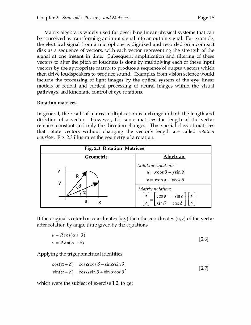
Rotation matrices.
In general, the result of matrix multiplication is a change in both the length and direction of a vector. However, for some matrices the length of the vector remains constant and only the direction changes. This special class of matrices that rotate vectors without changing the vector’s length are called rotation matrices. Fig. 2.3 illustrates the geometry of a rotation.
If the original vector has coordinates (x,y) then the coordinates (u,v) of the vector after rotation by angle δ are given by the equations
u = R cos(α + δ )v = Rsin(α + δ)
. [2.6]
Applying the trigonometrical identities
cos(α + δ ) = cosα cosδ − sinα sinδsin(α + δ ) = cosα sinδ + sinα cosδ
. [2.7]
which were the subject of exercise 1.2, to get
Fig. 2.3 Rotation Matrices
Geometric Algebraic
!" Matrix notation:
Rotation equations:
x
y
u
v u = x cos" # ysin "v = x sin" + ycos"
uv$
% & & '
( ) )
=cos" # sin"sin" cos"
$
% & &
'
( ) ) *xy$
% & & '
( ) )
R
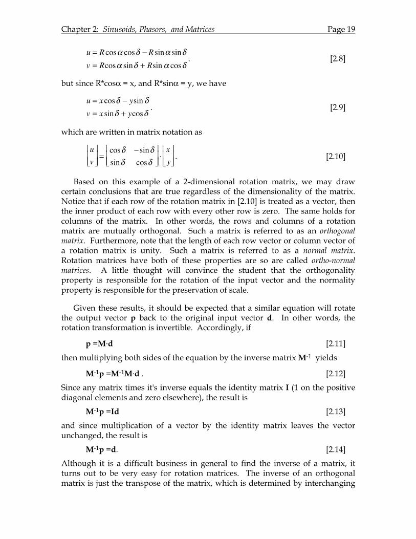
Chapter 2: Sinusoids, Phasors, and Matrices Page 19
u = R cosα cosδ − R sinα sinδv = Rcosα sinδ + Rsinα cosδ
. [2.8]
but since R*cosα = x, and R*sinα = y, we have
u = x cosδ − ysin δv = x sinδ + ycosδ
. [2.9]
which are written in matrix notation as
uv⎡
⎣ ⎢ ⎢ ⎤
⎦ ⎥ ⎥
=cosδ − sinδsinδ cosδ
⎡
⎣ ⎢ ⎢
⎤
⎦ ⎥ ⎥ ⋅xy⎡
⎣ ⎢ ⎢ ⎤
⎦ ⎥ ⎥ . [2.10]
Based on this example of a 2-dimensional rotation matrix, we may draw certain conclusions that are true regardless of the dimensionality of the matrix. Notice that if each row of the rotation matrix in [2.10] is treated as a vector, then the inner product of each row with every other row is zero. The same holds for columns of the matrix. In other words, the rows and columns of a rotation matrix are mutually orthogonal. Such a matrix is referred to as an orthogonal matrix. Furthermore, note that the length of each row vector or column vector of a rotation matrix is unity. Such a matrix is referred to as a normal matrix. Rotation matrices have both of these properties are so are called ortho-normal matrices. A little thought will convince the student that the orthogonality property is responsible for the rotation of the input vector and the normality property is responsible for the preservation of scale.
Given these results, it should be expected that a similar equation will rotate the output vector p back to the original input vector d. In other words, the rotation transformation is invertible. Accordingly, if
p =M.d [2.11]
then multiplying both sides of the equation by the inverse matrix M-1 yields
M-1p =M-1M.d . [2.12]
Since any matrix times it's inverse equals the identity matrix I (1 on the positive diagonal elements and zero elsewhere), the result is
M-1p =Id [2.13]
and since multiplication of a vector by the identity matrix leaves the vector unchanged, the result is
M-1p =d. [2.14]
Although it is a difficult business in general to find the inverse of a matrix, it turns out to be very easy for rotation matrices. The inverse of an orthogonal matrix is just the transpose of the matrix, which is determined by interchanging
Chapter 2: Sinusoids, Phasors, and Matrices Page 20
rows and columns (i.e. flip the matrix about it's positive diagonal). The complementary equation to [2.10] is therefore
xy⎡
⎣ ⎢ ⎢ ⎤
⎦ ⎥ ⎥
=cosδ sinδ−sin δ cosδ
⎡
⎣ ⎢ ⎢
⎤
⎦ ⎥ ⎥ ⋅uv⎡
⎣ ⎢ ⎢ ⎤
⎦ ⎥ ⎥ . [2.15]
Basis vectors.
To prepare for Fourier analysis, it is useful to review the following ideas and terminology from linear algebra. If u and v are non-zero vectors pointing in different directions, then they are linearly independent. A potential trap must be avoided at this point in the usage of the phrase "different direction". In common English usage, North and South are considered opposite directions. However, in the present mathematical usage of the word direction, which rests upon the inner product rule, it is better to think of the orthogonal directions North and East as being opposite whereas North and South are the same direction but opposite signs. With this in mind, a more precise expression of the idea of linear independence is to require the cosine of the angle between the two vectors be different from ±1, which is the same as saying |u•v|≠ |u|.|v|. Given two linearly independent vectors u and v, any vector c in the plane of u and v can be found by the linear combination c=Au + Bv. For this reason, linearly independent (but not necessarily orthogonal) vectors u and v are said to form a basis for the 2-dimensional space of the plane in which they reside. Since any pair of linearly independent vectors will span their own space, there are an infinite number of vector pairs that form a basis for the space. If a particular pair of basis vectors happen to be orthogonal (i.e. u•v=0) then they provide an orthogonal basis for the space. For example, the conventional X-Y axes of a Cartesian reference frame form an orthogonal basis for 2-dimensional space. Orthogonal basis vectors are usually more convenient than non-orthogonal vectors to use as a coordinate reference frame because each vector has zero component in the direction of the other.
The foregoing statements may be generalized for higher dimensional spaces as follows. N-dimensional space will be spanned by any set of N linearly independent vectors, which means that every vector in the set must point in a different direction. If all N vectors are mutually orthogonal, then they form an orthogonal basis for the space. As shown in the next chapter, Fourier analysis may be conceived as a change in basis from the ordinary Cartesian coordinates to an orthogonal set of vectors based on the trigonometric functions sine and cosine.
Change in basis vectors and orthogonal decompositions
Given a vector specified by its coordinates in one frame of reference, we may wish to specify the same vector in an alternative reference frame. This is the same problem as changing the basis vectors for the space containing the given
Chapter 2: Sinusoids, Phasors, and Matrices Page 21
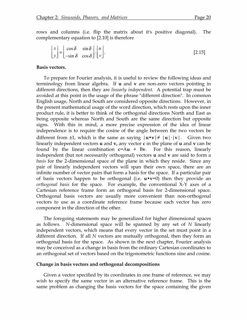
vector. If the new basis vectors are mutually orthogonal, then the process could also be described as a decomposition of the given vector into orthogonal components. (Fourier analysis, for example, is an orthogonal decomposition of a vector of measurements into a reference frame representing the Fourier coefficients. Geometrically this decomposition corresponds to a change in basis vectors by rotation and re-scaling.) An algebraic description of changing basis vectors emerges by thinking geometrically and recalling that the projection of one vector onto another is computed via the inner product. For example, the component of vector V in the x-direction is computed by forming the inner product of V with the unit basis vector x=[1,0]. Similarly, the component of vector V in the y-direction is computed by forming the inner product of V with the unit basis vector y=[0,1]. These operations correspond to multiplication of the original vector V by the identity matrix as indicated in Fig. 2.4.
In general, if the (x,y) coordinates of orthogonal basis vectors x', y' are x' = [a,b] and y' = [c,d] then the coordinates of V in the (x',y') coordinate frame are computed by projecting V=(Vx,Vy) onto the (x', y') axes as follows:
Vx’ = component of V in x' direction = [a,b]•[Vx,Vy]′ (project V onto x’) Vy’ = component of V in y' direction = [c,d]•[Vx,Vy]′ (project V onto y’)
This pair of equations can be written compactly in matrix notation as
V ′x
V ′y
⎡
⎣⎢⎢
⎤
⎦⎥⎥= a b
c d⎡
⎣⎢
⎤
⎦⎥ ⋅
VxVy
⎡
⎣⎢⎢
⎤
⎦⎥⎥
[2.16]
and noting the inner product [a,b] •[ c,d] ′ = 0 because axes x', y' are orthogonal.
In summary, a change of basis can be implemented by multiplying the original vector by a transformation matrix, the rows of which represent the new unit basis vectors. In Fourier analysis, the new basis vectors are obtained by sampling the trigonometrical sine and cosine functions. The resulting transformation matrix converts a data vector into a vector of Fourier coefficients.

Chapter 2: Sinusoids, Phasors, and Matrices Page 22
Chapter 3: Fourier Analysis of Discrete Functions
3.A Introduction. In his historical introduction to the classic text Theory of Fourier's Series and
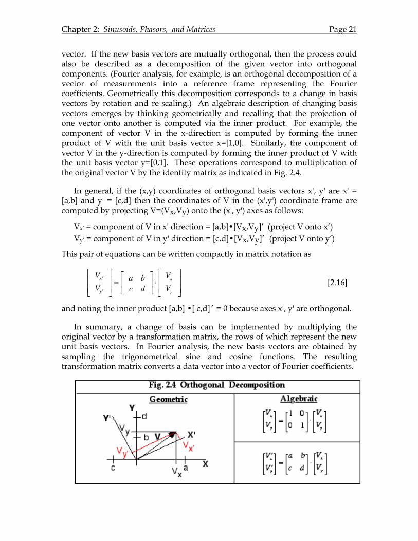
Integrals, Carslaw (1921) recounts the controversy raging in the middle of the eighteenth century over the question of whether an arbitrary function can be represented as the sum of a series of weighted sinusoids. Many of Europe's most prominent mathematicians participated in the debate, including Euler, D'Alembert, Bernoulli, Lagrange, Dirichlet, and Poisson. At that time, it was recognized that periodic functions, like the vibration of a string, could be represented by a trigonometrical series. However, it was not at all clear that a non-periodic function could be so represented, especially if it required an unlimited number of sines and cosines that might not necessarily converge to a stable sum. Fourier, who is credited with resolving this issue, was interested in the theory of heat. A pivotal problem central to the mathematical issue and its practical application was to understand the temperature profile of the earth at various depths beneath the surface. A typical profile Y=f(X) might look like the heavy curve illustrated in Fig. 3.1
Although the temperature profile in this example is defined only from the earth's surface (X=0) to a depth X=L, suppose we replicate the given curve many times and connect the segments end-to-end as shown by the light curves in the figure. The result would be a periodic function of period L that can be made to stretch as far as we like in both the positive-X and negative-X directions. This artificial periodicity is intended to raise our expectations of success in representing such a function by a sum of sinusoids, which also exist over the entire length of the X-axis. Obviously the sum of sinusoids will fit the original function over the interval (0-L) if it fits the periodic function over the entire X-axis. The figure also makes it clear that the period of each sinusoidal component must be some multiple of L because otherwise some intervals will be different from others, which is incompatible with the idea of periodicity. The name given to the harmonically related series of sinusoids required to reproduce the function Y=f(X) exactly is the Fourier series.
Fig. 3.1 Temperature Profile of Earth's Surface
0 L X=depth beneath surface
Y=Temperature
Y=f(X)
Chapter 3: Fourier Analysis of Discrete Functions Page 24
Before tackling the difficult problem of finding the Fourier series for a continuous function defined over a finite interval, we will begin with the easier problem of determining the Fourier series when the given function consists of a discrete series of Y-values evenly spaced along the X-axis. This problem is not only easier but also of more practical interest to the experimentalist who needs to analyze a series of discrete measurements of some physical variable, or perhaps uses a computer to sample a continuous process at regular intervals.
3.B A Function Sampled at 1 point.
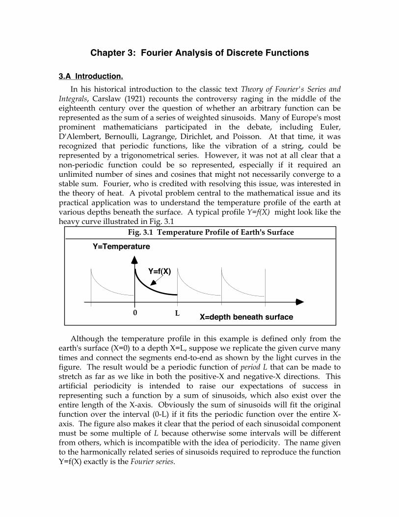
Consider the extreme case where a function Y(X) is known for only one value of X. For example, in the study of heat illustrated in Fig. 3.1, suppose we have a raw data set consisting of a single measurement Y0 taken at the position X=0. To experience the flavor of more challenging cases to come, imagine modeling this single measurement by the function
Y = f (X ) = m [3.1]
where m is an unknown parameter for which we need to determine a numerical value. The obvious choice is to let m=Y0. The problem is illustrated graphically in Fig. 3.2 and the solution is the heavy, horizontal line passing through the datum point. This horizontal line is the Fourier series for this case of D=1 samples and the parameter m is called a Fourier coefficient. Although this is a rather trivial example of Fourier analysis, it illustrates the first step in a more general process.
If we engage in the process of replicating the data set in order to produce a periodic function, the same Fourier series passes through all of the replicated data points as expected. Notice, however, that the fitted line is an exceedingly poor representation of the underlying continuous curve. The reason, of course, is that we were provided with only a single measurement; to achieve a better fit to the underlying function we need more samples.
Fig. 3.2 Fourier Analysis of 1-Sample Data Set
0 L X=depth beneath surface
Y=TemperatureY = f (X ) = m
Y0
Chapter 3: Fourier Analysis of Discrete Functions Page 25
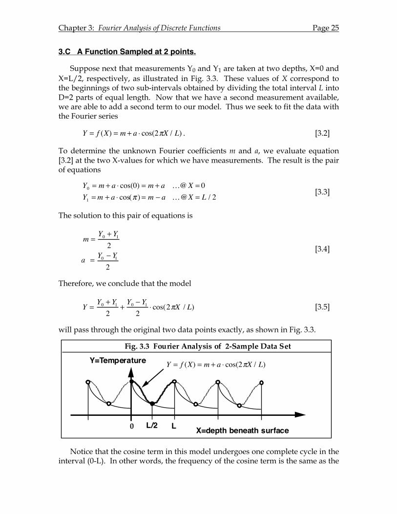
3.C A Function Sampled at 2 points.
Suppose next that measurements Y0 and Y1 are taken at two depths, X=0 and X=L/2, respectively, as illustrated in Fig. 3.3. These values of X correspond to the beginnings of two sub-intervals obtained by dividing the total interval L into D=2 parts of equal length. Now that we have a second measurement available, we are able to add a second term to our model. Thus we seek to fit the data with the Fourier series
Y = f (X) = m + a ⋅ cos(2πX / L) . [3.2]
To determine the unknown Fourier coefficients m and a, we evaluate equation [3.2] at the two X-values for which we have measurements. The result is the pair of equations
Y0 = m + a ⋅ cos(0) = m + a …@X = 0Y1 =m + a ⋅ cos(π ) = m − a …@X = L / 2 [3.3]
The solution to this pair of equations is
m =
Y0 + Y12
a = Y0 − Y12
[3.4]
Therefore, we conclude that the model
Y =Y0 + Y12
+Y0 − Y12
⋅ cos(2πX / L) [3.5]
will pass through the original two data points exactly, as shown in Fig. 3.3.
Notice that the cosine term in this model undergoes one complete cycle in the interval (0-L). In other words, the frequency of the cosine term is the same as the
Fig. 3.3 Fourier Analysis of 2-Sample Data Set
0 L X=depth beneath surface
Y=Temperature
L/2
Y = f (X) = m + a ! cos(2"X / L)
Chapter 3: Fourier Analysis of Discrete Functions Page 26
frequency of the periodic waveform of the underlying function. For this reason, this cosine is said be the fundamental harmonic term in the Fourier series. This new model of a constant plus a cosine function is clearly a better match to the underlying function than was the previous model, which had only the constant term. On the other hand, it is important to remember that although the mathematical model exists over the entire X-axis, it only applies to the physical problem over the interval of observation (0-L) and within that interval the model strictly applies only to the two points actually measured. Outside the interval the model is absurd since there is every reason to expect that the physical profile is not periodic. Even within the interval the model may not make sense for X-values in between the actual data points. To judge the usefulness of the model as an interpolation function we must appeal to our understanding of the physical system under study. In a later section we will expand this example to include D=3 samples, but before we do that we need to look more deeply into the process of Fourier analysis which we have just introduced.
3.D Fourier Analysis is a Linear Transformation. As the preceding example has demonstrated, Fourier analysis of discrete
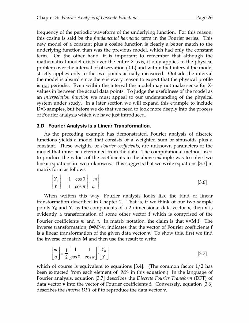
functions yields a model that consists of a weighted sum of sinusoids plus a constant. These weights, or Fourier coefficients, are unknown parameters of the model that must be determined from the data. The computational method used to produce the values of the coefficients in the above example was to solve two linear equations in two unknowns. This suggests that we write equations [3.3] in matrix form as follows
Y0Y1
⎡
⎣ ⎢ ⎢
⎤
⎦ ⎥ ⎥ =
1 cos 01 cos π
⎡
⎣ ⎢ ⎢
⎤
⎦ ⎥ ⎥ ⋅
ma
⎡
⎣ ⎢ ⎢
⎤
⎦ ⎥ ⎥ [3.6]
When written this way, Fourier analysis looks like the kind of linear transformation described in Chapter 2. That is, if we think of our two sample points Y0 and Y1 as the components of a 2-dimensional data vector v, then v is evidently a transformation of some other vector f which is comprised of the Fourier coefficients m and a. In matrix notation, the claim is that v=M.f. The inverse transformation, f=M-1v, indicates that the vector of Fourier coefficients f is a linear transformation of the given data vector v. To show this, first we find the inverse of matrix M and then use the result to write
ma
⎡
⎣ ⎢ ⎢
⎤
⎦ ⎥ ⎥
=12
1 1cos 0 cosπ⎡
⎣ ⎢ ⎢
⎤
⎦ ⎥ ⎥ ⋅Y0Y1
⎡
⎣ ⎢ ⎢
⎤
⎦ ⎥ ⎥ [3.7]
which of course is equivalent to equations [3.4]. (The common factor 1/2 has been extracted from each element of M-1 in this equation.) In the language of Fourier analysis, equation [3.7] describes the Discrete Fourier Transform (DFT) of data vector v into the vector of Fourier coefficients f. Conversely, equation [3.6] describes the Inverse DFT of f to reproduce the data vector v.
Chapter 3: Fourier Analysis of Discrete Functions Page 27
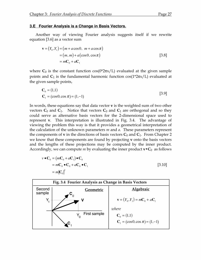
3.E Fourier Analysis is a Change in Basis Vectors.
Another way of viewing Fourier analysis suggests itself if we rewrite equation [3.6] as a vector sum
v = Y0 ,Y1( ) = m + acos0, m + acosπ( )= m, m( ) + a cos0, cosπ( )= mC0 + aC1
[3.8]
where C0 is the constant function cos(0*2πx/L) evaluated at the given sample points and C1 is the fundamental harmonic function cos(1*2πx/L) evaluated at the given sample points,
C0 = 1,1( )C1 = cos0, cos π( ) = 1,−1( )
[3.9]
In words, these equations say that data vector v is the weighted sum of two other vectors C0 and C1. Notice that vectors C0 and C1 are orthogonal and so they could serve as alternative basis vectors for the 2-dimensional space used to represent v. This interpretation is illustrated in Fig. 3.4. The advantage of viewing the problem this way is that it provides a geometrical interpretation of the calculation of the unknown parameters m and a. These parameters represent the components of v in the directions of basis vectors C0 and C1. From Chapter 2 we know that these components are found by projecting v onto the basis vectors and the lengths of these projections may be computed by the inner product. Accordingly, we can compute m by evaluating the inner product v•C0 as follows
v •C0 = mC0 + aC1( ) •C0
= mC0 •C0 + aC0 •C1
= mC02
[3.10]
Fig. 3.4 Fourier Analysis as Change in Basis Vectors
Geometric Algebraic
First sample
Y1
Second sample
Y0
VC0
C1
v = Y0,Y1( ) = mC0 + aC1
C0 = 1,1( )C1 = cos0, cos !( ) = 1,"1( )
where
Chapter 3: Fourier Analysis of Discrete Functions Page 28
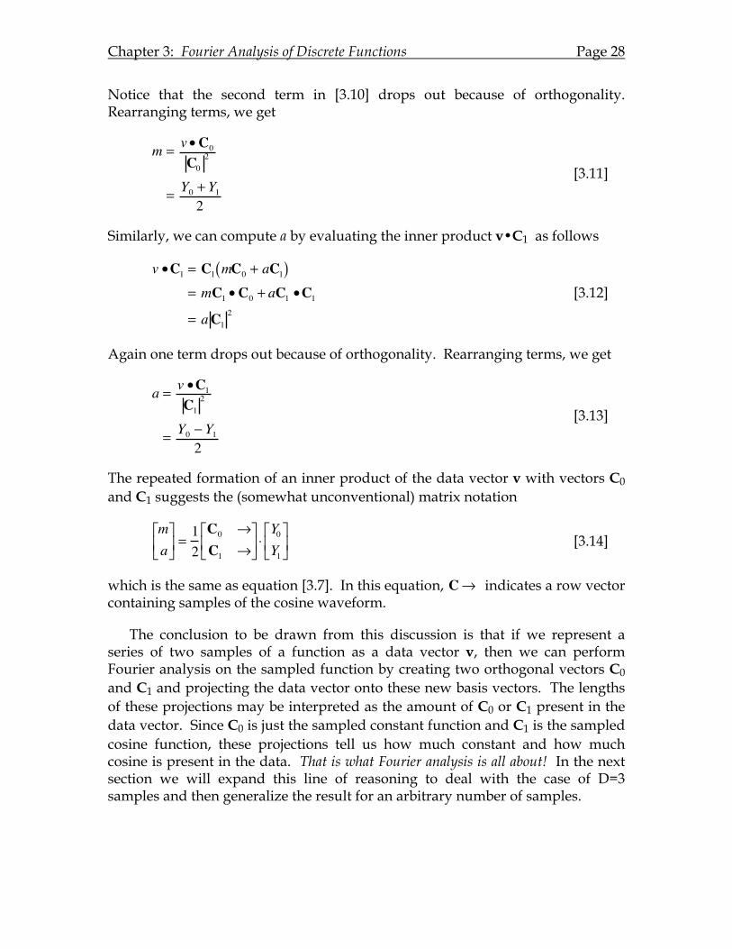
Notice that the second term in [3.10] drops out because of orthogonality. Rearranging terms, we get
m = v •C0
C02
= Y0 + Y12
[3.11]
Similarly, we can compute a by evaluating the inner product v•C1 as follows
v •C1 = C1 mC0 + aC1( )= mC1 •C0 + aC1 •C1= aC1
2
[3.12]
Again one term drops out because of orthogonality. Rearranging terms, we get
a = v •C1C1
2
= Y0 − Y12
[3.13]
The repeated formation of an inner product of the data vector v with vectors C0 and C1 suggests the (somewhat unconventional) matrix notation
ma⎡ ⎣ ⎢
⎤ ⎦ ⎥ =
12C0 →C1 →
⎡ ⎣ ⎢
⎤ ⎦ ⎥ ⋅
Y0Y1⎡ ⎣ ⎢
⎤ ⎦ ⎥ [3.14]
which is the same as equation [3.7]. In this equation, C→ indicates a row vector containing samples of the cosine waveform.
The conclusion to be drawn from this discussion is that if we represent a series of two samples of a function as a data vector v, then we can perform Fourier analysis on the sampled function by creating two orthogonal vectors C0 and C1 and projecting the data vector onto these new basis vectors. The lengths of these projections may be interpreted as the amount of C0 or C1 present in the data vector. Since C0 is just the sampled constant function and C1 is the sampled cosine function, these projections tell us how much constant and how much cosine is present in the data. That is what Fourier analysis is all about! In the next section we will expand this line of reasoning to deal with the case of D=3 samples and then generalize the result for an arbitrary number of samples.
Chapter 3: Fourier Analysis of Discrete Functions Page 29
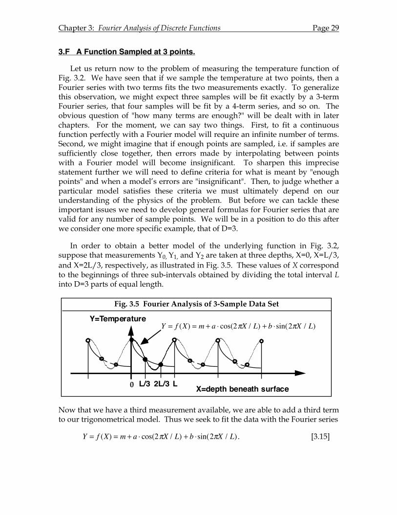
3.F A Function Sampled at 3 points.
Let us return now to the problem of measuring the temperature function of Fig. 3.2. We have seen that if we sample the temperature at two points, then a Fourier series with two terms fits the two measurements exactly. To generalize this observation, we might expect three samples will be fit exactly by a 3-term Fourier series, that four samples will be fit by a 4-term series, and so on. The obvious question of "how many terms are enough?" will be dealt with in later chapters. For the moment, we can say two things. First, to fit a continuous function perfectly with a Fourier model will require an infinite number of terms. Second, we might imagine that if enough points are sampled, i.e. if samples are sufficiently close together, then errors made by interpolating between points with a Fourier model will become insignificant. To sharpen this imprecise statement further we will need to define criteria for what is meant by "enough points" and when a model’s errors are "insignificant". Then, to judge whether a particular model satisfies these criteria we must ultimately depend on our understanding of the physics of the problem. But before we can tackle these important issues we need to develop general formulas for Fourier series that are valid for any number of sample points. We will be in a position to do this after we consider one more specific example, that of D=3.
In order to obtain a better model of the underlying function in Fig. 3.2, suppose that measurements Y0, Y1, and Y2 are taken at three depths, X=0, X=L/3, and X=2L/3, respectively, as illustrated in Fig. 3.5. These values of X correspond to the beginnings of three sub-intervals obtained by dividing the total interval L into D=3 parts of equal length.
Now that we have a third measurement available, we are able to add a third term to our trigonometrical model. Thus we seek to fit the data with the Fourier series
Y = f (X) = m + a ⋅ cos(2πX / L) + b ⋅sin(2πX / L) . [3.15]
0 L X=depth beneath surface
Y=Temperature
Fig. 3.5 Fourier Analysis of 3-Sample Data Set
L/3 2L/3
Y = f (X) = m + a ! cos(2"X / L) + b !sin(2"X / L)
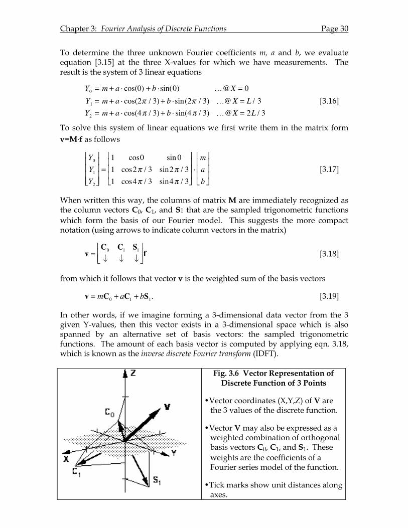
Chapter 3: Fourier Analysis of Discrete Functions Page 30
To determine the three unknown Fourier coefficients m, a and b, we evaluate equation [3.15] at the three X-values for which we have measurements. The result is the system of 3 linear equations
Y0 = m + a ⋅ cos(0) + b ⋅sin(0) …@X = 0Y1 = m + a ⋅ cos(2π / 3) + b ⋅sin(2π / 3) …@X = L / 3Y2 = m + a ⋅ cos(4π / 3) + b ⋅ sin(4π / 3) …@X = 2L / 3
[3.16]
To solve this system of linear equations we first write them in the matrix form v=M.f as follows
Y0Y1Y2
⎡
⎣
⎢ ⎢ ⎢ ⎢
⎤
⎦
⎥ ⎥ ⎥ ⎥
=1 cos0 sin 01 cos2π / 3 sin2π / 31 cos4π / 3 sin4π / 3
⎡
⎣
⎢ ⎢ ⎢
⎤
⎦
⎥ ⎥ ⎥ ⋅mab
⎡
⎣
⎢ ⎢ ⎢
⎤
⎦
⎥ ⎥ ⎥ [3.17]
When written this way, the columns of matrix M are immediately recognized as the column vectors C0, C1, and S1 that are the sampled trigonometric functions which form the basis of our Fourier model. This suggests the more compact notation (using arrows to indicate column vectors in the matrix)
v =C0 C1 S1↓ ↓ ↓
⎡
⎣ ⎢ ⎢
⎤
⎦ ⎥ ⎥ f [3.18]
from which it follows that vector v is the weighted sum of the basis vectors
v = mC0 + aC1 + bS1. [3.19]
In other words, if we imagine forming a 3-dimensional data vector from the 3 given Y-values, then this vector exists in a 3-dimensional space which is also spanned by an alternative set of basis vectors: the sampled trigonometric functions. The amount of each basis vector is computed by applying eqn. 3.18, which is known as the inverse discrete Fourier transform (IDFT).
Fig. 3.6 Vector Representation of Discrete Function of 3 Points
•Vector coordinates (X,Y,Z) of V are the 3 values of the discrete function.
•Vector V may also be expressed as a weighted combination of orthogonal basis vectors C0, C1, and S1. These weights are the coefficients of a Fourier series model of the function.
•Tick marks show unit distances along axes.
Chapter 3: Fourier Analysis of Discrete Functions Page 31
Thus our data vector may be conceived as the weighted sum of these basis vectors and the corresponding weights are the unknown Fourier coefficients we desire. This geometrical perspective on the problem suggests that to determine the Fourier coefficients we should project the data vector onto each basis vector in turn by forming the inner product. For example, projecting v onto C0 gives
v •C0 = (mC0 + aC1 + bS1) •C0
= mC0 •C0 + aC1 •C0 + bS1 •C0
= mC0 •C0
= mC02
. [3.20]
Note that all but one term vanishes because of orthogonality. From exercise 3.3 we know that the squared length of C0 is D, the dimensionality of the problem (D=3 in this example). Thus the first Fourier coefficient is
m =v •C0
D. [3.21]
By a similar line of reasoning we obtain the other two Fourier coefficients
a = v •C1
D / 2
b = v • S1D / 2
. [3.22]
These last two equations may be combined to give the matrix form (using arrows to denote row vectors in the matrix)
mab
⎡
⎣
⎢ ⎢ ⎢
⎤
⎦
⎥ ⎥ ⎥
=C0 / D→2C1 / D→2S1 / D→
⎡
⎣
⎢ ⎢ ⎢ ⎢
⎤
⎦
⎥ ⎥ ⎥ ⎥
Y0Y1Y2
⎡
⎣
⎢ ⎢ ⎢ ⎢
⎤
⎦
⎥ ⎥ ⎥ ⎥
[3.23]
which can be simplified by extracting the common factor 2/D to give the forward discrete Fourier transform (DFT)
f =2D
C0 / 2→C1 →S1→
⎡
⎣
⎢ ⎢ ⎢ ⎢
⎤
⎦
⎥ ⎥ ⎥ ⎥ v [3.24]
In summary, equations [3.16] through [3.19] are different ways of expressing the inverse DFT for the case of D=3. As such, they tell us how to "reconstruct" the measured data points from the Fourier coefficients. But we needed to solve the opposite problem: given the measured values, determine the unknown
Chapter 3: Fourier Analysis of Discrete Functions Page 32
Fourier coefficients. In other words, we sought the forward DFT, f=M-1v, which means we had to find the inverse of matrix M. Our method of solution took advantage of the orthogonality of the trigonometrical basis vectors by repeatedly forming the inner product of the data vector with each of the trigonometrical basis vectors. When each inner product is divided by the length of the corresponding basis function, the result is interpreted geometrically as the length of the projection of v onto the basis vectors. These lengths equal the Fourier coefficients in the model.
3.G A Function Sampled at D points.
The preceding examples of D=1, 2, and 3 point the way towards a general method for determining the Fourier coefficients for a trigonometrical model suitable for an arbitrary number of points. In section 3.A we reasoned that the periods of all of the trigonometric elements in the model must be some integer fraction of the observation interval. That is, the period must equal L/k where k is an integer which we will call the harmonic number. Thus, the model we seek will be a Fourier series of the form
Y = f (X) = m + ak ⋅ cos(2πkX / L) + bk ⋅sin(2πkX / L)k=1
N
∑ [3.25]
which is perhaps easier to grasp if we simplify the notation a bit by making a change of variables
Y = f (X) = m + ak ⋅ coskθ + bk ⋅sin kθ
k=1
N
∑ , …θ = 2πX / L [3.26]
where D = 2N when D is even, and D=2N+1 when D is odd. As before, we assume the X-interval from 0 to L is subdivided into D equal parts and the Y-values occur at the beginnings of each of these sub-intervals so that θ j = 2πj / D . If the interval runs from S to S+L, then the values of θ are θ j = 2π (S + jL / D) / L .
For D data points there are D unknown Fourier coefficients to be determined. If equation [3.26] is evaluated at every X-value for which we have measurements, then the result is a system of D linear equations which, when written in matrix form, are
Y0Y1Y2Y3YD
⎡
⎣
⎢⎢⎢⎢⎢⎢⎢⎢
⎤
⎦
⎥⎥⎥⎥⎥⎥⎥⎥
=
C0 C1 S1 … CN SN↓ ↓ ↓ ↓ ↓
⎡
⎣
⎢⎢⎢⎢⎢⎢⎢
⎤
⎦
⎥⎥⎥⎥⎥⎥⎥
•
ma1b1aNbN
⎡
⎣
⎢⎢⎢⎢⎢⎢⎢⎢
⎤
⎦
⎥⎥⎥⎥⎥⎥⎥⎥
[3.27]
Chapter 3: Fourier Analysis of Discrete Functions Page 33
which is compactly written as an inner product of f with a matrix of column vectors
v =
C0 C1 S1 CN SN↓ ↓ ↓ ↓ ↓
⎡
⎣ ⎢ ⎢
⎤
⎦ ⎥ ⎥
• f [3.28]
Equations [3.27] and [3.28] shows the inverse discrete Fourier transform (IDFT) when D is odd. When D is even, the last column (SN) in the matrix and the last Fourier coefficient (bN) are omitted.
To obtain the forward DFT, we conceive of our D data points as a vector in D-dimensional space that may be expressed as the weighted sum of trigonometrical basis vectors. The corresponding weights are the unknown Fourier coefficients obtained by projecting the data vector onto each of the basis vectors in turn by forming the inner product. For example, projecting v onto Ck gives
v •Ck = (mC0 + a1C1 + b1S1 + a2C2 + b2S2+…+aNCN + bNSN ) •Ck
= akCk •Ck
= ak Ck2
= akD / 2
[3.29]
Note that all but one term in the expanded inner product vanishes because of orthogonality. Recall from exercise 3.3 that the squared length of Ck equals D/2, so the k-th cosine Fourier coefficient is given by the simple formula
ak =2Dv •Ck
=2D⋅ Y j coskθ jj= 0
D−1
∑ …θ j = 2πXj / L [3.30]
A corresponding formula holds for the k-th sine coefficient
bk =2Dv •Sk
=2D⋅ Y j sin kθ jj= 0
D−1
∑ … θ j = 2πX j / L. [3.31]
These last two equations thus define every Fourier coefficient except for two special cases that do not include the factor 2. The reason this factor is missing is because the squared length of the corresponding basis vector is D rather than D/2. One special case is the first Fourier coefficient, m, which is the mean value and the other special case is the last Fourier coefficient, CN, when D is even.
Chapter 3: Fourier Analysis of Discrete Functions Page 34
Notice that these results demonstrate that any particular Fourier coefficient may be calculated without regard to the other Fourier coefficients. This is a simplifying consequence of the orthogonality of the sampled sinusoids. One practical implication of this result is that it is not necessary to calculate all of the Fourier coefficients of the model if only some are of interest. On the other hand, if all of the Fourier coefficients are to be computed, then it is convenient to calculate them all at once by the matrix multiplication as follows
ma1b1aNbN
⎡
⎣
⎢ ⎢ ⎢ ⎢ ⎢ ⎢ ⎢ ⎢ ⎢
⎤
⎦
⎥ ⎥ ⎥ ⎥ ⎥ ⎥ ⎥ ⎥ ⎥
=
C0 / D →2C1 / D →2S1 / D →
2CN / D →2SN / D →
⎡
⎣
⎢ ⎢ ⎢ ⎢ ⎢ ⎢ ⎢ ⎢ ⎢
⎤
⎦
⎥ ⎥ ⎥ ⎥ ⎥ ⎥ ⎥ ⎥ ⎥
•
Y0Y1Y2Y3
Y2 N +1
⎡
⎣
⎢ ⎢ ⎢ ⎢ ⎢ ⎢ ⎢ ⎢ ⎢
⎤
⎦
⎥ ⎥ ⎥ ⎥ ⎥ ⎥ ⎥ ⎥ ⎥
[3.32]
which can be simplified by extracting the common factor 2/D to give
f =2D
C0 / 2 →C1 →S1 →CN →SN →
⎡
⎣
⎢ ⎢ ⎢ ⎢ ⎢ ⎢ ⎢ ⎢ ⎢
⎤
⎦
⎥ ⎥ ⎥ ⎥ ⎥ ⎥ ⎥ ⎥ ⎥
•v [3.33]
3.H Tidying Up.
Although valid, the general equations just developed have a couple of aesthetically unpleasant features that obscure an important geometrical interpretation of Fourier analysis. First, there is the need for a special formula for calculating the mean coefficient m. Equation [3.30] generates an answer which is exactly twice the mean if we set k=0. That is, a0 = 2m. This suggests that we make a change of variables in our model so that we won't need to regard the constant term as a special case. With this change of variable, the model becomes
Y = y(X) = a0
2+ ak ⋅ coskθ + bk ⋅ sin kθ
k=1
N
∑ , …θ = 2πX / L [3.34]
which is the form of the Fourier series generally quoted in text books.
Next, there is the unsightly factor 2 in the top element of the matrix in equation [3.33]. This anomaly results from the fact that all of the trigonometric basis vectors have squared length D/2 except for C0, which has squared length
Chapter 3: Fourier Analysis of Discrete Functions Page 35
D. This suggests that we multiply C0 in equation [3.27] by √2/√2 and then factor out the √2 in the numerator and put it into the a0 term in the vector of Fourier coefficients as shown below in equation [3.35]
Y0Y1Y2Y3Y2N
⎡
⎣
⎢⎢⎢⎢⎢⎢⎢⎢
⎤
⎦
⎥⎥⎥⎥⎥⎥⎥⎥
=
C0
2C1 S1 … CN SN
↓ ↓ ↓ ↓ ↓
⎡
⎣
⎢⎢⎢⎢⎢⎢⎢⎢⎢
⎤
⎦
⎥⎥⎥⎥⎥⎥⎥⎥⎥
•
a0 / 2a1b1aNbN
⎡
⎣
⎢⎢⎢⎢⎢⎢⎢⎢
⎤
⎦
⎥⎥⎥⎥⎥⎥⎥⎥
[3.35]
Since every column vector in the trigonometrical matrices now has length √(D/2), let us extract this common factor so that each column will have unit length. To keep the equations from looking messy, we first define the following unit basis vectors
c0 =C0 / 2D / 2
= C0
D
ck =Ck
D / 2
sk =SkD / 2
[3.36]
so that equation [3.35] now becomes
Y0Y1Y2Y3Y2N
⎡
⎣
⎢⎢⎢⎢⎢⎢⎢⎢
⎤
⎦
⎥⎥⎥⎥⎥⎥⎥⎥
= D / 2 ⋅
c0 c1 s1 … cN sN↓ ↓ ↓ ↓ ↓
⎡
⎣
⎢⎢⎢⎢⎢⎢⎢
⎤
⎦
⎥⎥⎥⎥⎥⎥⎥
•
a0 / 2a1b1aNbN
⎡
⎣
⎢⎢⎢⎢⎢⎢⎢⎢
⎤
⎦
⎥⎥⎥⎥⎥⎥⎥⎥
[3.37]
which is written in our compact notation as
v = D / 2 ⋅
c0 c1 s1 cN sN↓ ↓ ↓ ↓ ↓
⎡
⎣ ⎢ ⎢
⎤
⎦ ⎥ ⎥
• f (inverse DFT)
[3.38]
Chapter 3: Fourier Analysis of Discrete Functions Page 36
taking care to remember that the first element of f, the vector of Fourier coefficients, is different by the factor √2 from earlier usage. Also note that if D is even then the last Fourier coefficient in [3.37] is aN /√2.
A major advantage of expressing the inverse DFT in the form of equation [3.38] is that the matrix of trigonometric vectors is orthonormal, which means that the inverse matrix is just the transpose. Therefore, we can immediately write the forward DFT by inspection:
f = 2 / D ⋅
c0 →c1 →s1 →cN →sN →
⎡
⎣
⎢ ⎢ ⎢ ⎢ ⎢ ⎢ ⎢ ⎢ ⎢
⎤
⎦
⎥ ⎥ ⎥ ⎥ ⎥ ⎥ ⎥ ⎥ ⎥
• v (forward DFT)
[3.39]
The symmetrical pair of equations, [3.38] and [3.39] would be easily programmed on a computer.
A second advantage of this form of the DFT equations is that it reveals the essential simplicity of the underlying geometry of Fourier analysis. Since the matrix of trigonometric vectors is orthonormal, it is recognized as a rotation matrix. In other words, the data vector v is transformed into a Fourier vector f by a rotation and change of scale (represented by the constant multiplier √(2/D) in equation 3.39). Naturally the length of the data vector should be the same regardless of which frame of reference it is calculated in. This geometrical notion is formulated below as Parseval's Theorem, which can be also interpreted physically as a statement of conservation of energy.
3.I Parseval's Theorem.
Having defined two sets of orthonormal basis vectors for the D-dimensional space in which the data vector v is represented, it is instructive to compute the length of v with respect to these two coordinate reference frames for comparison. We have learned previously that the inner product of v with itself yields the squared length of the vector. We must be careful in such a calculation, however, because we have seen that the two reference frames differ in scale. One way to make sure that these scale factors are accounted for is to represent the data vector as a weighted sum of unit vectors pointing in the cardinal directions of the coordinate reference frame. In other words, let
v = Y1u1 + Y2u2 + + YDuD [3.40]
Chapter 3: Fourier Analysis of Discrete Functions Page 37
where the unit basis vector uk with respect to the first reference frame has coordinate 0 for every dimension except the k-th dimension, for which the coordinate is 1. For example,
u1 = (1, 0, 0, 0,, 0)u2 = (0,1,0,0,,0)uD = (0,0,0,0,,1)
[3.41]
Now forming the inner product of v with itself is easily evaluated because many terms vanish due to the orthogonality of the basis vectors, and the remaining terms contain the factor u•u, which is unity because the basis vectors are unit length. Thus we have,
v 2 = v • v = (Y1u1 + Y2u 2 ++ YDuD) ⋅(Y1u1 + Y2u2 + +YDuD)= (Y1u1 + Y2u 2 ++ YDuD) ⋅Y1u1 +(Y1u1 + Y2u2 + + YDuD) ⋅Y2u2 +(Y1u1 + Y2u2 + + YDuD) ⋅Y3u3 +
(Y1u1 + Y2u2 + + YDuD) ⋅YDuD
= Y12u1 • u1 + Y2
2u2 •u 2 ++ YD2uD • uD
= Yk2k=1
D
∑
[3.42]
which is simply the Pythagorean theorem for D-dimensional space. Notice that equation [3.42] simplifies so dramatically because each line in the expanded form reduces to a single term due to the orthogonality of the unit basis vectors ui.
By a similar line of reasoning, we find that
f = a02u1 + a1u2 + b1u3 + a2u4 + b2u5 +…
f 2 = f if = f i a02u1 + f ia1u2 + f ib1u3 + f ia2u4 + f ib2u5 +…
=a02
⎛⎝⎜
⎞⎠⎟2
+ a1( )2 + b1( )2 + a2( )2 + b2( )2 +…
=a02
2+ ak
2 + bk2
k=1
N
∑⎡
⎣⎢
⎤
⎦⎥
[3.43]
Chapter 3: Fourier Analysis of Discrete Functions Page 38
Now if we repeat the above process when v is represented in the alternative coordinate reference frame defined by the sampled trigonometric functions according to eqn. [3.38], the result is
v 2 = v • v
= D / 2( a02c0 + a1c1 + b1s1 ++ aNc N + bNsN ) ⋅
D / 2( a02c0 + a1c1 + b1s1 + + aNcN + bNsN )
= D2( a02c0 + a1c1 + b1s1 ++ aNc N + bNsN ) ⋅
a02c0 +⎡
⎣ ⎢
( a02c0 + a1c1 + b1s1 ++ aNc N + bNsN ) ⋅ a1c1 +
( a02c0 + a1c1 + b1s1 ++ aNc N + bNsN ) ⋅b1s1 +
( a02c0 + a1c1 + b1s1 ++ aNc N + bNsN ) ⋅ aNc N +
( a02c0 + a1c1 + b1s1 ++ aNc N + bNsN ) ⋅bNsN
⎤ ⎦ ⎥
= D2
a02
2c0 •c0 + a12c1 •c1 + b12s1 • s1 + + aN2cN •c N + bN2 sN • sN
⎡ ⎣ ⎢
⎤ ⎦ ⎥
=D2
a02
2+ ak2
k=1
N
∑ + bk2⎡ ⎣ ⎢
⎤ ⎦ ⎥
[3.44]
Combining the results of eqns. [3.43] and [3.44] we obtain the following identity,
v 2 = Yk2
k=1
D
∑ =D2
a02
2+ ak
2
k=1
N
∑ + bk2⎡
⎣⎢
⎤
⎦⎥ =
D2f 2 [3.45]
which is known as Parseval's Theorem. In words, Parseval's theorem states that the length of the data vector may be computed either in the space/time domain (the first coordinate reference frame) or in the Fourier domain (the second coordinate reference frame). The significance of the theorem is that it provides a link between the two domains which is based on the squared length of the data vector. In future chapters we will see how the squared length of the vector may be interpreted in many physical situations as the amount of energy in a signal and the squared Fourier coefficients are equivalent to the amount of energy in the terms of the Fourier series model. In this sense, Parseval's theorem is an energy-conservation theorem since it says that a signal contains the same amount
Chapter 3: Fourier Analysis of Discrete Functions Page 39
of energy regardless of whether that energy is computed in the space/time domain or in the Fourier/frequency domain.
3.J A Statistical Connection
Another interpretation of Parseval's theorem is in connection with statistics. If we rearrange eqn. [3.45] by moving the constant term (m=a0/2) to the left side we get
1D
Yk2
k =1
D
∑ −m2 =12
ak2
k=1
N
∑ + bk2 [3.46]
Now the left side of this equation is recognized as the variance of the Y-values in the discrete function being modeled whereas the right side of the equation is one-half of the sum of the squared amplitudes of the trigonometric Fourier coefficients. Again, since the squared amplitudes of the Fourier coefficients are associated with the energy in the model, this equation says that the variance of a set of data points may also be thought of as a measure of the amount of energy in the signal.
Other aspects of statistics also take on a geometrical perspective once data are conceived as vectors in D-dimensional space. For example, the correlation between a set of X-values and corresponding Y-values is defined by Pearson's correlation coefficient
r =(xj − x )(yj − y )
j=1
D
∑
(xj − x )2j=1
D
∑ (yj − y )2j=1
D
∑ [3.47]
If we conceive of the set of X-values as a vector x, then we can "normalize" x by subtracting off the mean X-value from each component of x to produce a new vector x' as follows
x = (x1, x2 ,, xD)x = x (1,1,,1)x'= x − x
[3.48]
If we do the same for the Y-values to produce the normalized vector y', then the numerator of eqn. [3.47] is recognized as the inner product of x' and y'. In a similar flash of insight we notice that the denominator of this equation is the product of the lengths of these two vectors. In short, we see that
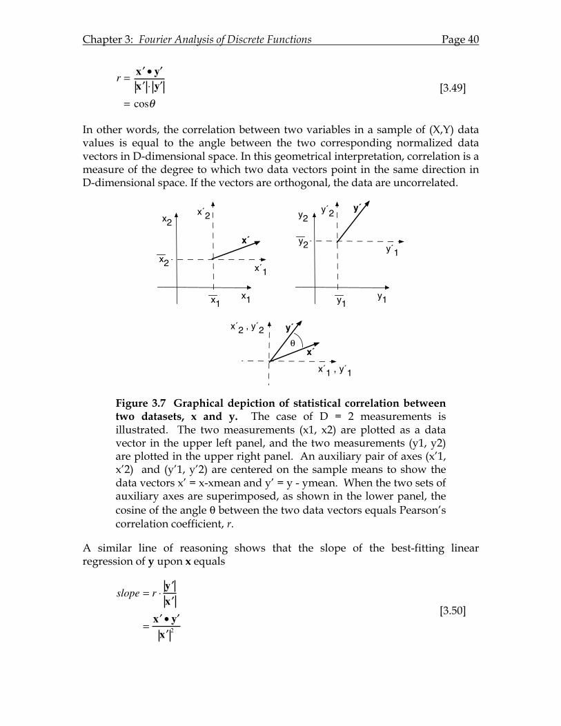
Chapter 3: Fourier Analysis of Discrete Functions Page 40
r = ′ x • ′ y
′ x ⋅ ′ y = cosθ
[3.49]
In other words, the correlation between two variables in a sample of (X,Y) data values is equal to the angle between the two corresponding normalized data vectors in D-dimensional space. In this geometrical interpretation, correlation is a measure of the degree to which two data vectors point in the same direction in D-dimensional space. If the vectors are orthogonal, the data are uncorrelated.
Figure 3.7 Graphical depiction of statistical correlation between two datasets, x and y. The case of D = 2 measurements is illustrated. The two measurements (x1, x2) are plotted as a data vector in the upper left panel, and the two measurements (y1, y2) are plotted in the upper right panel. An auxiliary pair of axes (x’1, x’2) and (y’1, y’2) are centered on the sample means to show the data vectors x’ = x-xmean and y’ = y - ymean. When the two sets of auxiliary axes are superimposed, as shown in the lower panel, the cosine of the angle θ between the two data vectors equals Pearson’s correlation coefficient, r.
A similar line of reasoning shows that the slope of the best-fitting linear regression of y upon x equals
slope = r ⋅ ′ y ′ x
=′ x • ′ y ′ x 2
[3.50]
x1x1 y1
y2x2
x´1
x´2
x2
x´
x´
y1
y´1
y´2
y2
y´
x´1 , y´1
x´2 , y´2 y´!
Chapter 3: Fourier Analysis of Discrete Functions Page 41
3.K Image Contrast and Compound Gratings
Some physical quantities, such as light intensity, are always positive. In such cases, sinusoidal variation is always accompanied by an additive constant that prevents the quantity from becoming negative. In optics, the relative amount of sinusoidal variation of light about the mean is called “contrast” and a sinusoidal spatial pattern of luminance L is called a grating. A universally accepted definition of contrast for a sinusoidal grating is the Michaelson formula
C =Lmax − LminLmax + Lmin
[3.51]
for which the various parameters needed to compute the contrast are obtained simply by inspection of the grating. To see the connection with Fourier analysis, this Michaelson formula may be rewritten as
C =Lmax − Lmin( ) / 2Lmax + Lmin( ) / 2
=amplitudemean
=mL0
[3.52]
Therefore, in Fourier terms, contrast is just the ratio of amplitude m to mean luminance L0.
A general method for computing the contrast of a discrete optical image is based on the standard deviation of the luminance values of all the pixels in a display. Applying this definition of contrast to the case of a sinusoidal grating
L(x) = L0 + m ⋅ cos(2π fx −φ) [3.53]
we invoke Parseval's theorem
1D
Lj2
j=1
D
∑ = L02 +
m2
2 [3.54]
The quantity on the left is the mean of the squared pixel intensities, also known as the second moment of the luminance distribution. Rearranging eqn. [3.54] we find that
2L0
1D
Lj2
j=1
D
∑ − L02 =
mL0
2 ipixel standard deviation / mean luminance = Michaelson contrast
[3.55]
Chapter 3: Fourier Analysis of Discrete Functions Page 42
Recalling that the variance of a distribution equals the second moment - square of first moment, by taking the square root of both sides of equation [3.54] and dividing each side by mean luminance we recover the Michaelson contrast. Therefore, we conclude that the contrast of a sinusoidal grating can be computed as the standard deviation of the pixel luminance values, normalized by the mean luminance.
If n gratings of different harmonic frequencies are superimposed to produce a compound grating, the resulting luminance distribution L(x) of the sum is
L(x) = Lk + mk ⋅ cos(2π fk x −φk )k=1
n
∑
= Lkk=1
n
∑ + mk ⋅ cos(2π fk x −φk )k=1
n
∑
= Lmean + mk ⋅ cos(2π fk x −φk )k=1
n
∑
[3.56]
The Michaelson contrast Ck of the kth component equals mk / Lk, so its amplitude is mk = Ck * Lk. The mean luminance is equal to the sum of the mean luminances of the component gratings, but how should we define the contrast of this compound grating? Again we look for some measure based on the standard deviation of the luminance values of all the pixels in the image and appeal to Parseval's theorem,
Lj2
j=1
D
∑ = D Lmean2 +
12
mk2
k=1
N
∑⎡⎣⎢
⎤⎦⎥
[3.57]
Rearranging eqn. [3.57] we get
1D
Lj2
j=1
D
∑⎛
⎝⎜⎞
⎠⎟− Lmean
2 =12
mk2
k=1
n
∑ [3.58]
The left hand side is the variance of the pixel luminance values of the compound grating and the right side is half the sum of squared amplitudes of the component gratings.
If we substitute into equation [3.58] the definition of contrast of the k-th harmonic, mk = Ck * Lk, then the result can be expressed in terms of the vector of contrasts Ck and mean luminances Lk of the component gratings that comprise the compound grating L(x),
Var L(x)( ) = 12
mk2
k=1
n
∑ =12
CkLk( )2k=1
n
∑ [3.59]
Chapter 3: Fourier Analysis of Discrete Functions Page 43
This result shows that, like random variables, when two gratings are added together to get a compound grating, pixel variance of the compound grating equals the sum of pixel variances of the component gratings. Taking square roots of both sides of equation [3.59] and dividing by the mean luminance gives (in Matlab notation) a simple formula for contrast of the compound grating expressed either in terms of the normalized standard deviation of pixel values, or as the norm of the vector of component amplitudes,
Contrast =2 Stdev L(x)( )
Lmean=norm(C.* L)sum(L)
[3.60]
Although the problem was simplified by performing a 1-dimensional analysis above, the conclusions are valid also for 2-dimensional gratings of any orientation. Matlab program “test_contrast.m” provides a graphical demonstration for a plaid made from gratings of different orientations and spatial frequencies.
3.L Fourier Descriptors of the Shape of a Closed Curve
The silhouette of a plane figure forms a closed curve that defines the boundary between the figure and the background. Fourier analysis can be used to provide a compact description of the curve’s shape and a procedure for interpolating a smooth boundary from sample points on the curve. This method is described briefly in the book "The Image Processing Handbook" by John C. Russ (IEEE press) and "Fourier Descriptors for Plane Closed Curves", by Charles T. Zahn and Ralph Z. Roskies, IEEE Transactions on Computers, Vol 21, No 3, March 1972 p. 269-281.
The key idea of the Fourier descriptor approach to shape description is to treat the object’s boundary as a curve in the complex plane. Each point on the curve is specified by a complex number, or phasor, for which the real part is plotted along the x-axis and the imaginary part is plotted along the y-axis. Implicit in this approach is that the complex number z=x+iy is a function of some parametric parameter, such as time. Thus the real part x(t) and the imaginary part y(t) are both functions of t and the boundary curve is a picture of how these two functions co-vary.
To take a simple example, if x(t)=a*cos(t) and y(t)=a*sin(t) then z=cos(t)+i*sin(t) describes a circle of radius a in the complex plane. If the radius is different in the real and imaginary dimensions the curve becomes an ellipse described by the equations
x(t)=a*cos(t), y(t)=b*sin(t), and z(t)= a*cos(t)+i*b*sin(t). (3.61)
where a and b are the lengths of the semi-axes.
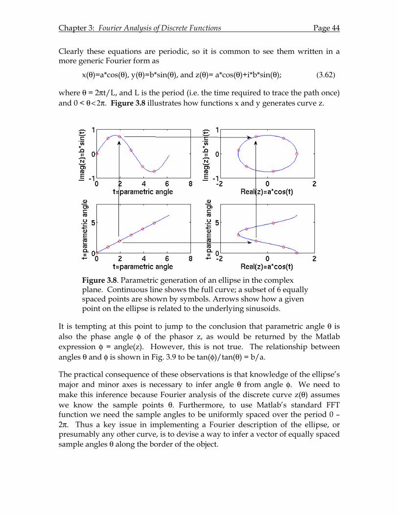
Chapter 3: Fourier Analysis of Discrete Functions Page 44
Clearly these equations are periodic, so it is common to see them written in a more generic Fourier form as
x(θ)=a*cos(θ), y(θ)=b*sin(θ), and z(θ)= a*cos(θ)+i*b*sin(θ); (3.62)
where θ = 2πt/L, and L is the period (i.e. the time required to trace the path once) and 0 < θ < 2π. Figure 3.8 illustrates how functions x and y generates curve z.
Figure 3.8. Parametric generation of an ellipse in the complex plane. Continuous line shows the full curve; a subset of 6 equally spaced points are shown by symbols. Arrows show how a given point on the ellipse is related to the underlying sinusoids.
It is tempting at this point to jump to the conclusion that parametric angle θ is also the phase angle φ of the phasor z, as would be returned by the Matlab expression φ = angle(z). However, this is not true. The relationship between angles θ and φ is shown in Fig. 3.9 to be tan(φ)/tan(θ) = b/a.
The practical consequence of these observations is that knowledge of the ellipse’s major and minor axes is necessary to infer angle θ from angle φ. We need to make this inference because Fourier analysis of the discrete curve z(θ) assumes we know the sample points θ. Furthermore, to use Matlab’s standard FFT function we need the sample angles to be uniformly spaced over the period 0 – 2π. Thus a key issue in implementing a Fourier description of the ellipse, or presumably any other curve, is to devise a way to infer a vector of equally spaced sample angles θ along the border of the object.
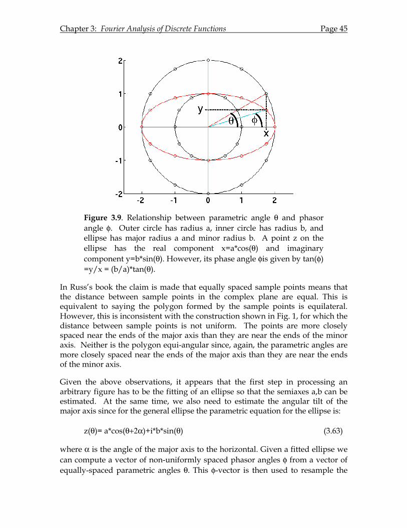
Chapter 3: Fourier Analysis of Discrete Functions Page 45
Figure 3.9. Relationship between parametric angle θ and phasor angle φ. Outer circle has radius a, inner circle has radius b, and ellipse has major radius a and minor radius b. A point z on the ellipse has the real component x=a*cos(θ) and imaginary component y=b*sin(θ). However, its phase angle φis given by tan(φ) =y/x = (b/a)*tan(θ).
In Russ’s book the claim is made that equally spaced sample points means that the distance between sample points in the complex plane are equal. This is equivalent to saying the polygon formed by the sample points is equilateral. However, this is inconsistent with the construction shown in Fig. 1, for which the distance between sample points is not uniform. The points are more closely spaced near the ends of the major axis than they are near the ends of the minor axis. Neither is the polygon equi-angular since, again, the parametric angles are more closely spaced near the ends of the major axis than they are near the ends of the minor axis.
Given the above observations, it appears that the first step in processing an arbitrary figure has to be the fitting of an ellipse so that the semiaxes a,b can be estimated. At the same time, we also need to estimate the angular tilt of the major axis since for the general ellipse the parametric equation for the ellipse is: z(θ)= a*cos(θ+2α)+i*b*sin(θ) (3.63)
where α is the angle of the major axis to the horizontal. Given a fitted ellipse we can compute a vector of non-uniformly spaced phasor angles φ from a vector of equally-spaced parametric angles θ. This φ-vector is then used to resample the
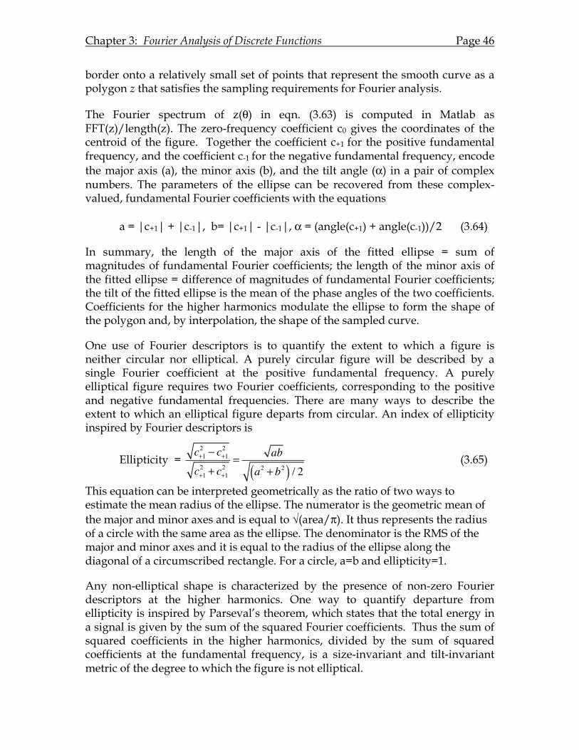
Chapter 3: Fourier Analysis of Discrete Functions Page 46
border onto a relatively small set of points that represent the smooth curve as a polygon z that satisfies the sampling requirements for Fourier analysis.
The Fourier spectrum of z(θ) in eqn. (3.63) is computed in Matlab as FFT(z)/length(z). The zero-frequency coefficient c0 gives the coordinates of the centroid of the figure. Together the coefficient c+1 for the positive fundamental frequency, and the coefficient c-1 for the negative fundamental frequency, encode the major axis (a), the minor axis (b), and the tilt angle (α) in a pair of complex numbers. The parameters of the ellipse can be recovered from these complex-valued, fundamental Fourier coefficients with the equations a = |c+1| + |c-1|, b= |c+1| - |c-1|, α = (angle(c+1) + angle(c-1))/2 (3.64)
In summary, the length of the major axis of the fitted ellipse = sum of magnitudes of fundamental Fourier coefficients; the length of the minor axis of the fitted ellipse = difference of magnitudes of fundamental Fourier coefficients; the tilt of the fitted ellipse is the mean of the phase angles of the two coefficients. Coefficients for the higher harmonics modulate the ellipse to form the shape of the polygon and, by interpolation, the shape of the sampled curve.
One use of Fourier descriptors is to quantify the extent to which a figure is neither circular nor elliptical. A purely circular figure will be described by a single Fourier coefficient at the positive fundamental frequency. A purely elliptical figure requires two Fourier coefficients, corresponding to the positive and negative fundamental frequencies. There are many ways to describe the extent to which an elliptical figure departs from circular. An index of ellipticity inspired by Fourier descriptors is
Ellipticity = c+12 − c+1
2
c+12 + c+1
2= ab
a2 + b2( ) / 2 (3.65)
This equation can be interpreted geometrically as the ratio of two ways to estimate the mean radius of the ellipse. The numerator is the geometric mean of the major and minor axes and is equal to √(area/π). It thus represents the radius of a circle with the same area as the ellipse. The denominator is the RMS of the major and minor axes and it is equal to the radius of the ellipse along the diagonal of a circumscribed rectangle. For a circle, a=b and ellipticity=1.
Any non-elliptical shape is characterized by the presence of non-zero Fourier descriptors at the higher harmonics. One way to quantify departure from ellipticity is inspired by Parseval’s theorem, which states that the total energy in a signal is given by the sum of the squared Fourier coefficients. Thus the sum of squared coefficients in the higher harmonics, divided by the sum of squared coefficients at the fundamental frequency, is a size-invariant and tilt-invariant metric of the degree to which the figure is not elliptical.
Chapter 4: The Frequency Domain
4.A Spectral Analysis.
The previous chapter showed how to perform Fourier analysis of discrete data. In order to derive formulas for the various Fourier coefficients of a trigonometric, Fourier series model, we employed a "vectorization" process in which the values of the discrete function to be modeled were treated as coordinates of a D-dimensional vector. A specific example (from exercise 4.1) of this vectorization process is illustrated for the case of D=3 in the transition from Fig. 4.1A to 4.1B. Claude Shannon, the founder of information theory, described this process as taking a complicated object (a waveform) defined in a simple space (a 2-dimensional plane) and converting it into a simple object (a point) in an exceedingly complicated, N-dimensional space. In Chapter 3 we learned that this space is also spanned by the set of trigonometric vectors formed by sampling the harmonic series of sine and cosine waves. These new basis vectors are mutually orthogonal and they form a new coordinate reference frame, as shown in Fig. 4.1C, which is rotated with respect to the original reference frame used to plot the data vector in Fig. 4.1B. Fourier analysis was then recognized as the act of projecting the data vector onto the trigonometrical basis vectors to produce the Fourier coefficients of the model. This entire process is thus an example of formulating a problem from a different viewpoint in order to gain insight into the nature of the problem and to simplify the computation of the solution.
To display and interpret the results of Fourier analysis, the D-dimensional vector of Fourier coefficients is usually "de-vectorized" in order to be displayed as a new discrete function, as illustrated in the transition from Fig. 4.1C to 4.1D. Notice that the pair of graphs in Fig. 4.1D have a common X-axis, which is the harmonic number, and the Y-axes show the magnitudes of the cosine (including the constant term) and the sine Fourier coefficients. Since the harmonic number is directly proportional to the frequency of oscillation of the various trigonometric functions in the model, Fig. 4.1D is evidently a graphical display of the amount of each frequency component present in the model. By analogy with the effect of a glass prism on light, such a graph is called the frequency spectrum of the original, discrete data function.
Although the computational process of Fourier analysis follows the sequence of stages illustrated by Fig. 4A→B→C→D, the intermediate stages (B,C) are not necessary for appreciating the relationship between the space/time domain (Fig. 4A) and the frequency domain (Fig. 4D). The forward discrete Fourier transform (DFT) converts a discrete function y(t) into the frequency/spectral domain (4A→4D), and the inverse DFT converts the spectrum back into the time/space domain (4D→4A). The two domains are complementary ways of looking at the same data and, accordingly, no new information is gained by Fourier analysis, only a new perspective.
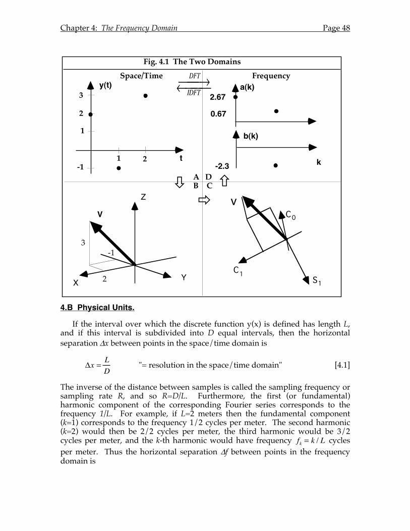
Chapter 4: The Frequency Domain Page 48
4.B Physical Units.
If the interval over which the discrete function y(x) is defined has length L, and if this interval is subdivided into D equal intervals, then the horizontal separation Δx between points in the space/time domain is
Δx = LD
"= resolution in the space/time domain" [4.1]
The inverse of the distance between samples is called the sampling frequency or sampling rate R, and so R=D/L. Furthermore, the first (or fundamental) harmonic component of the corresponding Fourier series corresponds to the frequency 1/L. For example, if L=2 meters then the fundamental component (k=1) corresponds to the frequency 1/2 cycles per meter. The second harmonic (k=2) would then be 2/2 cycles per meter, the third harmonic would be 3/2 cycles per meter, and the k-th harmonic would have frequency fk = k / L cycles per meter. Thus the horizontal separation Δf between points in the frequency domain is
S1
Fig. 4.1 The Two Domains
V
Z
YX 2
-13
Space/Time Frequencya(k)
b(k)
k
y(t)
t1 2
1
2
3
-1
2.67
0.67
-2.3A DB C! "#
DFT! " ! ! IDFT# ! ! !
vC0
C1
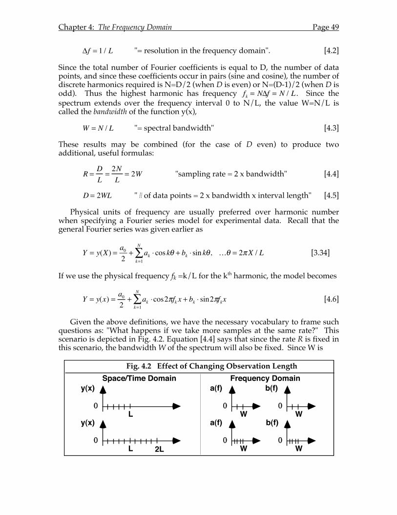
Chapter 4: The Frequency Domain Page 49
Δf = 1 / L "= resolution in the frequency domain". [4.2]
Since the total number of Fourier coefficients is equal to D, the number of data points, and since these coefficients occur in pairs (sine and cosine), the number of discrete harmonics required is N=D/2 (when D is even) or N=(D-1)/2 (when D is odd). Thus the highest harmonic has frequency fk = NΔf = N / L . Since the spectrum extends over the frequency interval 0 to N/L, the value W=N/L is called the bandwidth of the function y(x),
W = N / L "= spectral bandwidth" [4.3]
These results may be combined (for the case of D even) to produce two additional, useful formulas:
R =DL=2NL
= 2W "sampling rate = 2 x bandwidth" [4.4]
D = 2WL "# of data points = 2 x bandwidth x interval length" [4.5]
Physical units of frequency are usually preferred over harmonic number when specifying a Fourier series model for experimental data. Recall that the general Fourier series was given earlier as
Y = y(X) = a0
2+ ak ⋅ coskθ + bk ⋅ sin kθ
k=1
N
∑ , …θ = 2πX / L [3.34]
If we use the physical frequency fk =k/L for the kth harmonic, the model becomes
Y = y(x) = a02
+ ak ⋅cos2πfk x + bk ⋅ sin2πfkxk=1
N
∑ [4.6]
Given the above definitions, we have the necessary vocabulary to frame such questions as: "What happens if we take more samples at the same rate?" This scenario is depicted in Fig. 4.2. Equation [4.4] says that since the rate R is fixed in this scenario, the bandwidth W of the spectrum will also be fixed. Since W is
Fig. 4.2 Effect of Changing Observation Length
0
y(x)
L0
a(f)
W0
b(f)
W
0
y(x)
L 2L0
a(f)
W0
b(f)
W
Space/Time Domain Frequency Domain
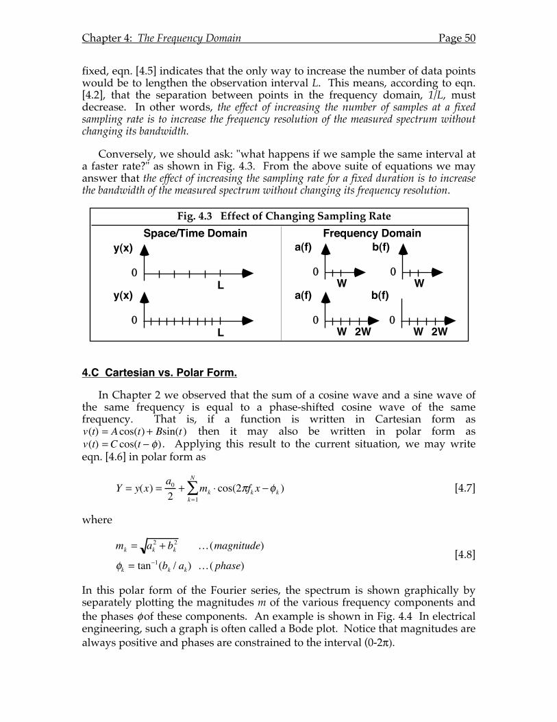
Chapter 4: The Frequency Domain Page 50
fixed, eqn. [4.5] indicates that the only way to increase the number of data points would be to lengthen the observation interval L. This means, according to eqn. [4.2], that the separation between points in the frequency domain, 1/L, must decrease. In other words, the effect of increasing the number of samples at a fixed sampling rate is to increase the frequency resolution of the measured spectrum without changing its bandwidth.
Conversely, we should ask: "what happens if we sample the same interval at a faster rate?" as shown in Fig. 4.3. From the above suite of equations we may answer that the effect of increasing the sampling rate for a fixed duration is to increase the bandwidth of the measured spectrum without changing its frequency resolution.
4.C Cartesian vs. Polar Form.
In Chapter 2 we observed that the sum of a cosine wave and a sine wave of the same frequency is equal to a phase-shifted cosine wave of the same frequency. That is, if a function is written in Cartesian form as v(t) = A cos(t) + Bsin(t ) then it may also be written in polar form as v(t) = C cos(t − φ) . Applying this result to the current situation, we may write eqn. [4.6] in polar form as
Y = y(x) = a02
+ mk ⋅ cos(2πfk x −φk )k=1
N
∑ [4.7]
where
mk = ak2 + bk2 …(magnitude)
φk = tan−1(bk / ak) …( phase) [4.8]
In this polar form of the Fourier series, the spectrum is shown graphically by separately plotting the magnitudes m of the various frequency components and the phases φ of these components. An example is shown in Fig. 4.4 In electrical engineering, such a graph is often called a Bode plot. Notice that magnitudes are always positive and phases are constrained to the interval (0-2π).
Fig. 4.3 Effect of Changing Sampling Rate
0
a(f)
W0
b(f)
W
Space/Time Domain Frequency Domain
0
y(x)
L
0
y(x)
L0
a(f)
W 2W0
b(f)
W 2W
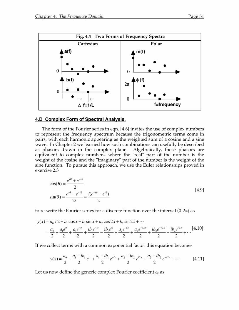
Chapter 4: The Frequency Domain Page 51
4.D Complex Form of Spectral Analysis.
The form of the Fourier series in eqn. [4.6] invites the use of complex numbers to represent the frequency spectrum because the trigonometric terms come in pairs, with each harmonic appearing as the weighted sum of a cosine and a sine wave. In Chapter 2 we learned how such combinations can usefully be described as phasors drawn in the complex plane. Algebraically, these phasors are equivalent to complex numbers, where the "real" part of the number is the weight of the cosine and the "imaginary" part of the number is the weight of the sine function. To pursue this approach, we use the Euler relationships proved in exercise 2.3
cos(θ) = e
iθ + e−iθ
2
sin(θ ) = eiθ − e− iθ
2i=i(e−iθ − eiθ )
2
[4.9]
to re-write the Fourier series for a discrete function over the interval (0-2π) as
y(x) = a0 / 2 + a1 cos x + b1 sin x + a2 cos2x + b2 sin2x +
=a02+a1e
ix
2+a1e
− ix
2+ib1e
− ix
2−ib1e
ix
2+a2e
i2x
2+a2e
− i2x
2+ib2e
− i2x
2−ib2e
i2x
2+
[4.10]
If we collect terms with a common exponential factor this equation becomes
y(x) = a0
2+a1 − ib12
eix + a1 + ib12
e− ix + a2 − ib22
ei2x + a2 + ib22
e− i2x + [4.11]
Let us now define the generic complex Fourier coefficient ck as
Fig. 4.4 Two Forms of Frequency Spectra
Cartesian Polar
f=1/L!
m(f)
0
2"
0
0
0
f=frequency
a(f)
b(f) (f)#
$ %
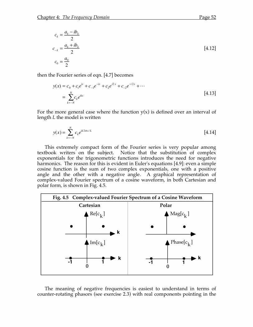
Chapter 4: The Frequency Domain Page 52
ck =ak − ibk2
c− k =ak + ibk2
c0 =a02
[4.12]
then the Fourier series of eqn. [4.7] becomes
y(x) = c0 + c1eix + c−1e
−ix + c2ei2 x + c−2e
−i 2x +
= ckeikxk= −N
N
∑ [4.13]
For the more general case where the function y(x) is defined over an interval of length L the model is written
y(x) = ckeik2π x /L
k=−N
N
∑ [4.14]
This extremely compact form of the Fourier series is very popular among textbook writers on the subject. Notice that the substitution of complex exponentials for the trigonometric functions introduces the need for negative harmonics. The reason for this is evident in Euler's equations [4.9]: even a simple cosine function is the sum of two complex exponentials, one with a positive angle and the other with a negative angle. A graphical representation of complex-valued Fourier spectrum of a cosine waveform, in both Cartesian and polar form, is shown in Fig. 4.5.
The meaning of negative frequencies is easiest to understand in terms of counter-rotating phasors (see exercise 2.3) with real components pointing in the
Fig. 4.5 Complex-valued Fourier Spectrum of a Cosine Waveform
Cartesian Polar
0
k-1 1
0
k
k-1 1
Mag[c ]k
Phase[c ]k
Re[c ]k
Im[c ]k
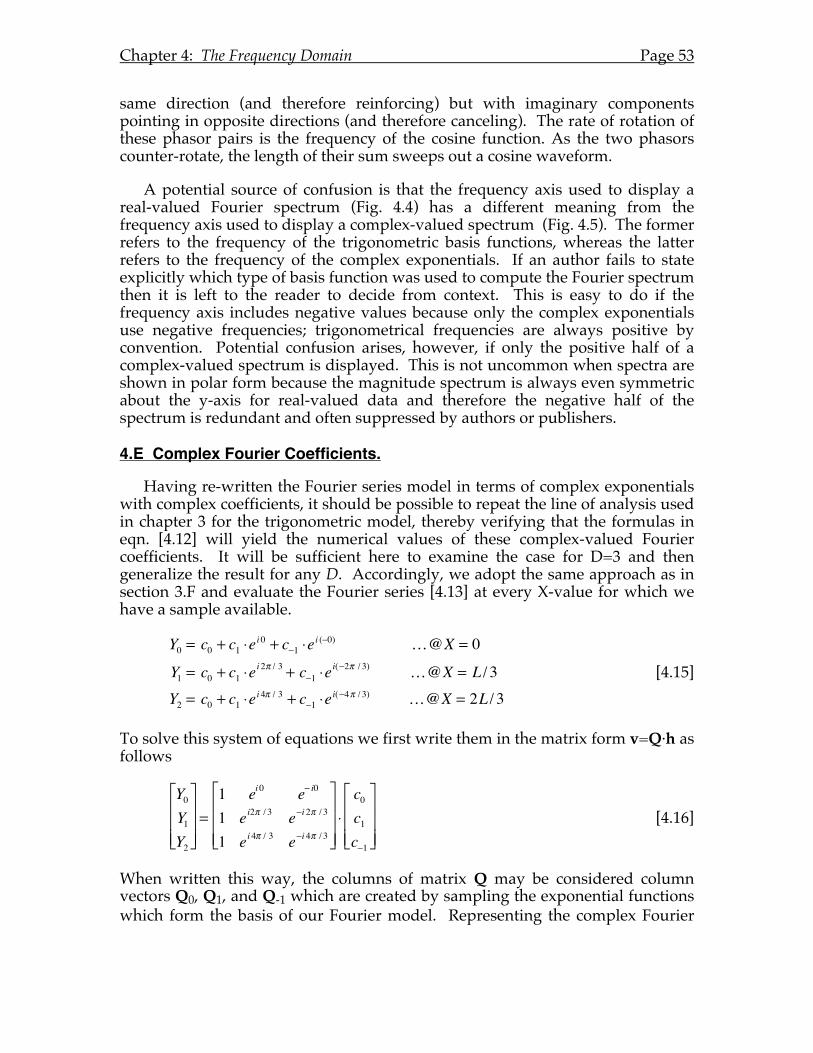
Chapter 4: The Frequency Domain Page 53
same direction (and therefore reinforcing) but with imaginary components pointing in opposite directions (and therefore canceling). The rate of rotation of these phasor pairs is the frequency of the cosine function. As the two phasors counter-rotate, the length of their sum sweeps out a cosine waveform.
A potential source of confusion is that the frequency axis used to display a real-valued Fourier spectrum (Fig. 4.4) has a different meaning from the frequency axis used to display a complex-valued spectrum (Fig. 4.5). The former refers to the frequency of the trigonometric basis functions, whereas the latter refers to the frequency of the complex exponentials. If an author fails to state explicitly which type of basis function was used to compute the Fourier spectrum then it is left to the reader to decide from context. This is easy to do if the frequency axis includes negative values because only the complex exponentials use negative frequencies; trigonometrical frequencies are always positive by convention. Potential confusion arises, however, if only the positive half of a complex-valued spectrum is displayed. This is not uncommon when spectra are shown in polar form because the magnitude spectrum is always even symmetric about the y-axis for real-valued data and therefore the negative half of the spectrum is redundant and often suppressed by authors or publishers.
4.E Complex Fourier Coefficients.
Having re-written the Fourier series model in terms of complex exponentials with complex coefficients, it should be possible to repeat the line of analysis used in chapter 3 for the trigonometric model, thereby verifying that the formulas in eqn. [4.12] will yield the numerical values of these complex-valued Fourier coefficients. It will be sufficient here to examine the case for D=3 and then generalize the result for any D. Accordingly, we adopt the same approach as in section 3.F and evaluate the Fourier series [4.13] at every X-value for which we have a sample available.
Y0 = c0 + c1 ⋅ei 0 + c−1 ⋅ei (−0) …@X = 0
Y1 = c0 + c1 ⋅ei 2π / 3 + c−1 ⋅e
i(−2π / 3) …@X = L / 3Y2 = c0 + c1 ⋅ei 4π / 3 + c−1 ⋅ei(−4π / 3) …@X = 2L / 3
[4.15]
To solve this system of equations we first write them in the matrix form v=Q.h as follows
Y0Y1Y2
⎡
⎣
⎢ ⎢ ⎢
⎤
⎦
⎥ ⎥ ⎥
=1 ei 0 e− i0
1 ei2π / 3 e−i 2π / 3
1 ei 4π / 3 e−i 4π / 3
⎡
⎣
⎢ ⎢ ⎢
⎤
⎦
⎥ ⎥ ⎥ ⋅c0c1c−1
⎡
⎣
⎢ ⎢ ⎢
⎤
⎦
⎥ ⎥ ⎥
[4.16]
When written this way, the columns of matrix Q may be considered column vectors Q0, Q1, and Q-1 which are created by sampling the exponential functions which form the basis of our Fourier model. Representing the complex Fourier
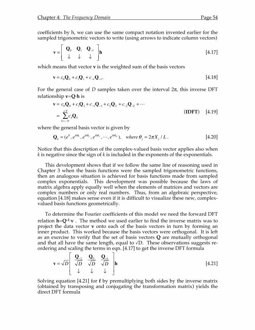
Chapter 4: The Frequency Domain Page 54
coefficients by h, we can use the same compact notation invented earlier for the sampled trigonometric vectors to write (using arrows to indicate column vectors)
v =Q0 Q1 Q−1
↓ ↓ ↓
⎡
⎣⎢⎢
⎤
⎦⎥⎥h [4.17]
which means that vector v is the weighted sum of the basis vectors
v = c0Q0 + c1Q1 + c−1Q−1. [4.18]
For the general case of D samples taken over the interval 2π, this inverse DFT relationship v=Q.h is
v = c0Q0 + c1Q1 + c−1Q−1 + c2Q2 + c−2Q−2 +
= ckQkk= −N
+N
∑ (IDFT) [4.19]
where the general basis vector is given by
Qk = (e0 , eikθ1 , eikθ2 , eikθ3 ,, eikθN ), whereθ j = 2πXj / L . [4.20]
Notice that this description of the complex-valued basis vector applies also when k is negative since the sign of k is included in the exponents of the exponentials.
This development shows that if we follow the same line of reasoning used in Chapter 3 when the basis functions were the sampled trigonometric functions, then an analogous situation is achieved for basis functions made from sampled complex exponentials. This development was possible because the laws of matrix algebra apply equally well when the elements of matrices and vectors are complex numbers or only real numbers. Thus, from an algebraic perspective, equation [4.18] makes sense even if it is difficult to visualize these new, complex-valued basis functions geometrically.
To determine the Fourier coefficients of this model we need the forward DFT relation h=Q-1.v . The method we used earlier to find the inverse matrix was to project the data vector v onto each of the basis vectors in turn by forming an inner product. This worked because the basis vectors were orthogonal. It is left as an exercise to verify that the set of basis vectors Q are mutually orthogonal and that all have the same length, equal to √D. These observations suggests re-ordering and scaling the terms in eqn. [4.17] to get the inverse DFT formula
v = DQ−1
DQ0
DQ+1
D↓ ↓ ↓
⎡
⎣
⎢⎢⎢
⎤
⎦
⎥⎥⎥h [4.21]
Solving equation [4.21] for f by premultiplying both sides by the inverse matrix (obtained by transposing and conjugating the transformation matrix) yields the direct DFT formula
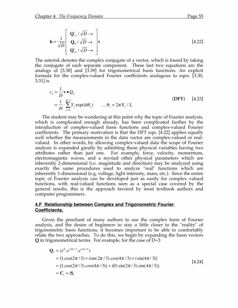
Chapter 4: The Frequency Domain Page 55
h = 1D
Q−1∗ / D →
Q0 / D →
Q+1∗ / D →
⎡
⎣
⎢⎢⎢⎢
⎤
⎦
⎥⎥⎥⎥
v [4.22]
The asterisk denotes the complex conjugate of a vector, which is found by taking the conjugate of each separate component. These last two equations are the analogs of [3.38] and [3.39] for trigonometrical basis functions. An explicit formula for the complex-valued Fourier coefficients analagous to eqns. [3.30, 3.31] is
ck =1Dv •Qk
=1D⋅ Yj exp(ikθ j )j=0
D−1
∑ …θ j = 2πXj / L (DFT) [4.23]
The student may be wondering at this point why the topic of Fourier analysis, which is complicated enough already, has been complicated further by the introduction of complex-valued basis functions and complex-valued Fourier coefficients. The primary motivation is that the DFT eqn. [4.22] applies equally well whether the measurements in the data vector are complex-valued or real-valued. In other words, by allowing complex-valued data the scope of Fourier analysis is expanded greatly by admitting those physical variables having two attributes rather than just one. For example, force, velocity, momentum, electromagnetic waves, and a myriad other physical parameters which are inherently 2-dimensional (i.e. magnitude and direction) may be analyzed using exactly the same procedures used to analyze "real" functions which are inherently 1-dimensional (e.g. voltage, light intensity, mass, etc.). Since the entire topic of Fourier analysis can be developed just as easily for complex valued functions, with real-valued functions seen as a special case covered by the general results, this is the approach favored by most textbook authors and computer programmers.
4.F Relationship between Complex and Trigonometric Fourier Coefficients.
Given the penchant of many authors to use the complex form of Fourier analysis, and the desire of beginners to stay a little closer to the "reality" of trigonometric basis functions, it becomes important to be able to comfortably relate the two approaches. To do this, we begin by expanding the basis vectors Q in trigonometrical terms. For example, for the case of D=3
Q1 = (e0,ei 2π / 3,ei 4π / 3 )= 1,cos(2π / 3) + isin( 2π / 3),cos(4π / 3) + i sin(4π / 3)( )= 1,cos(2π / 3),cos(4π / 3)( ) + i 0,sin(2π / 3),sin(4π / 3)( )= C1 + iS1
[4.24]
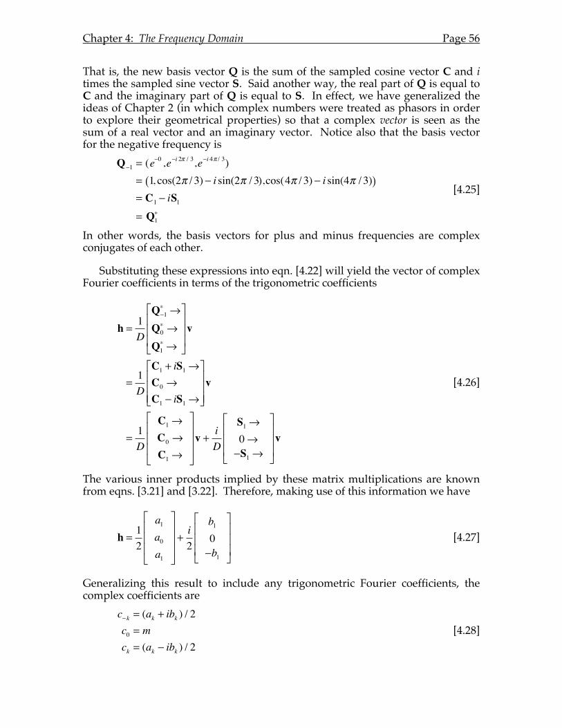
Chapter 4: The Frequency Domain Page 56
That is, the new basis vector Q is the sum of the sampled cosine vector C and i times the sampled sine vector S. Said another way, the real part of Q is equal to C and the imaginary part of Q is equal to S. In effect, we have generalized the ideas of Chapter 2 (in which complex numbers were treated as phasors in order to explore their geometrical properties) so that a complex vector is seen as the sum of a real vector and an imaginary vector. Notice also that the basis vector for the negative frequency is
Q−1 = (e−0 ,e−i 2π / 3,e−i 4π / 3)
= 1, cos(2π / 3) − i sin(2π / 3),cos(4π / 3) − i sin(4π / 3)( )= C1 − iS1= Q1
∗
[4.25]
In other words, the basis vectors for plus and minus frequencies are complex conjugates of each other.
Substituting these expressions into eqn. [4.22] will yield the vector of complex Fourier coefficients in terms of the trigonometric coefficients
h = 1D
Q−1∗ →
Q0∗ →
Q1∗ →
⎡
⎣
⎢⎢⎢
⎤
⎦
⎥⎥⎥v
=1D
C1 + iS1 →C0 →C1 − iS1 →
⎡
⎣
⎢⎢⎢
⎤
⎦
⎥⎥⎥v
=1D
C1 →C0 →C1 →
⎡
⎣
⎢⎢⎢
⎤
⎦
⎥⎥⎥v + i
D
S1 →0→−S1 →
⎡
⎣
⎢⎢⎢
⎤
⎦
⎥⎥⎥v
[4.26]
The various inner products implied by these matrix multiplications are known from eqns. [3.21] and [3.22]. Therefore, making use of this information we have
h = 12
a1a0a1
⎡
⎣
⎢⎢⎢
⎤
⎦
⎥⎥⎥+i2
b10−b1
⎡
⎣
⎢⎢⎢
⎤
⎦
⎥⎥⎥
[4.27]
Generalizing this result to include any trigonometric Fourier coefficients, the complex coefficients are
c−k = (ak + ibk ) / 2c0 = mck = (ak − ibk ) / 2
[4.28]
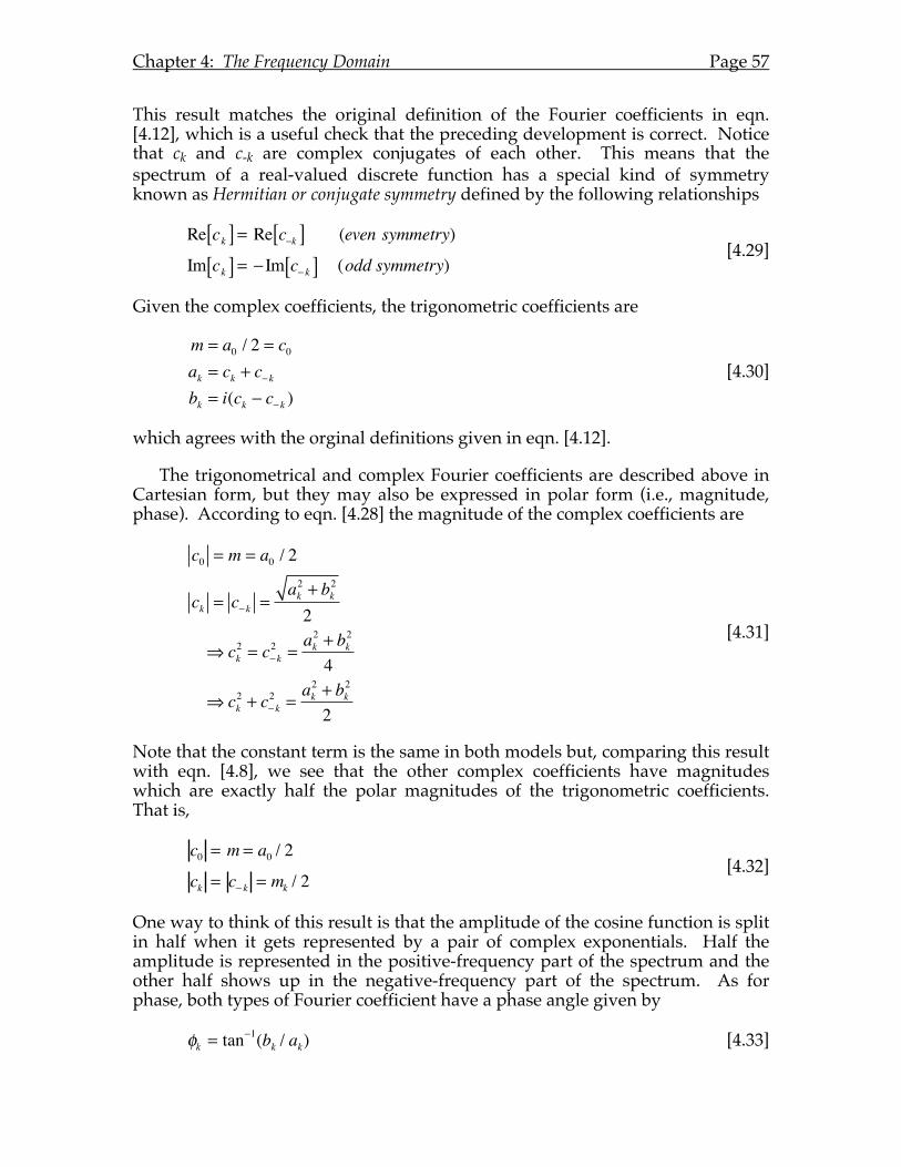
Chapter 4: The Frequency Domain Page 57
This result matches the original definition of the Fourier coefficients in eqn. [4.12], which is a useful check that the preceding development is correct. Notice that ck and c-k are complex conjugates of each other. This means that the spectrum of a real-valued discrete function has a special kind of symmetry known as Hermitian or conjugate symmetry defined by the following relationships
Re ck[ ] = Re c−k[ ] (even symmetry)
Im ck[ ] = − Im c− k[ ] (odd symmetry) [4.29]
Given the complex coefficients, the trigonometric coefficients are
m = a0 / 2 = c0ak = ck + c−kbk = i(ck − c−k )
[4.30]
which agrees with the orginal definitions given in eqn. [4.12].
The trigonometrical and complex Fourier coefficients are described above in Cartesian form, but they may also be expressed in polar form (i.e., magnitude, phase). According to eqn. [4.28] the magnitude of the complex coefficients are
c0 = m = a0 / 2
ck = c−k =ak2 + bk
2
2
⇒ ck2 = c−k
2 =ak2 + bk
2
4
⇒ ck2 + c−k
2 =ak2 + bk
2
2
[4.31]
Note that the constant term is the same in both models but, comparing this result with eqn. [4.8], we see that the other complex coefficients have magnitudes which are exactly half the polar magnitudes of the trigonometric coefficients. That is,
c0 = m = a0 / 2
ck = c− k = mk / 2 [4.32]
One way to think of this result is that the amplitude of the cosine function is split in half when it gets represented by a pair of complex exponentials. Half the amplitude is represented in the positive-frequency part of the spectrum and the other half shows up in the negative-frequency part of the spectrum. As for phase, both types of Fourier coefficient have a phase angle given by
φk = tan−1(bk / ak) [4.33]
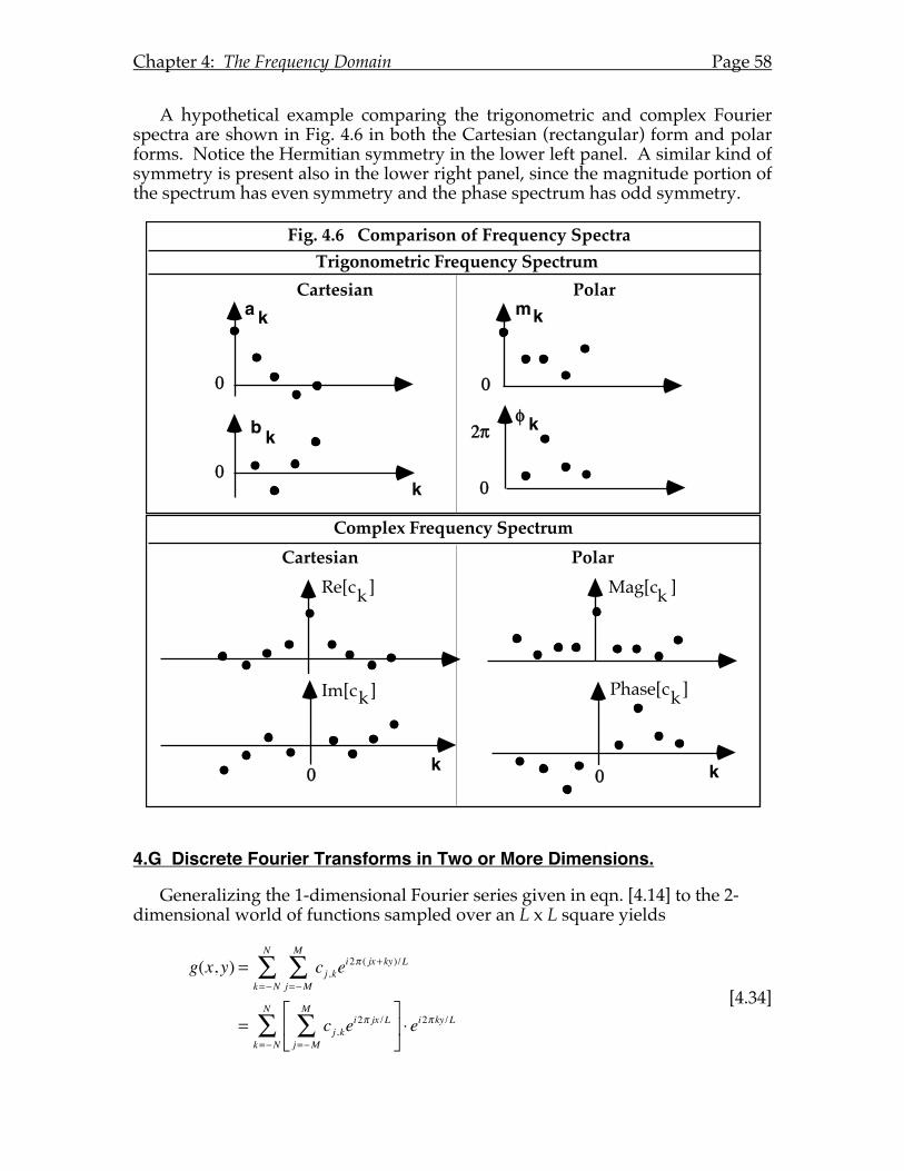
Chapter 4: The Frequency Domain Page 58
A hypothetical example comparing the trigonometric and complex Fourier spectra are shown in Fig. 4.6 in both the Cartesian (rectangular) form and polar forms. Notice the Hermitian symmetry in the lower left panel. A similar kind of symmetry is present also in the lower right panel, since the magnitude portion of the spectrum has even symmetry and the phase spectrum has odd symmetry.
4.G Discrete Fourier Transforms in Two or More Dimensions.
Generalizing the 1-dimensional Fourier series given in eqn. [4.14] to the 2-dimensional world of functions sampled over an L x L square yields
g(x, y) = cj ,ke
i2π ( jx+ ky)/L
j=−M
M
∑k=−N
N
∑
= cj ,kei2π jx /L
j=−M
M
∑⎡⎣⎢
⎤
⎦⎥
k=−N
N
∑ ⋅ ei2π ky /L [4.34]
Fig. 4.6 Comparison of Frequency Spectra
Cartesian Polarm
0
2!
0
"
Complex Frequency Spectrum
Cartesian Polar
0 k0
k
k
Mag[c ]k
Phase[c ]k
Re[c ]k
Im[c ]k
Trigonometric Frequency Spectrum
0
a k
0
b k
k
k
Chapter 4: The Frequency Domain Page 59
Notice the the expression inside the brackets is a 1-dimensional Fourier series, for which the coefficients ci,k are found by a series of 1-dimensional DFTs computed on the rows of the data matrix. The result is a 2-dimensional matrix of Fourier coefficients that now becomes the "data" to be subjected to a series of DFTs computed on the columns. Thus a 2-dimensional DFT boils down to a series of two 1-dimensional DFTs, the first of which is computed for the original data and the second computed on the results of the first. This approach can easily be generalized to 3-dimensional volumetric data and so on to N-dimensions.
4.H Matlab's Implementation of the DFT
According to the Matlab documentation, FFT(x) returns the discrete Fourier transform (DFT) of vector x. For length D input vector x, the DFT is a length N vector f, with elements
f (k) = x(n)exp −i2π (k −1)(n −1) / D( ), 1 <= k <= Dn=1
D
∑ [4.35]
Note that the use of (n-1) in this formula implies that MATLAB is assuming that the sample times begin at 0 and the interval length is 2pi. This means the user is responsible for keeping track of phase shifts and physical frequencies associated with the actual sample times. (We will deal with phase shifts in Chapter 6). An alternative method used in the homework exercises uses the true sample times to compute the sampled basis functions. Also note that the definition of eqn. 4.35 does not include the normalizing contstant 1/D needed to make the transformational matrix orthonormal. Furthermore, according to the documentation, the relationship between the DFT and the Fourier coefficients a and b in the Fourier series
x(n) = a0 +1L
a(k)cos 2πkt(n)( ) + b(k)sin 2πkt(n)( )k=1
D / 2
∑ [4.36]
is
a0 = 2 * f (1) / Dak = 2 * real f (k +1)[ ] / Dbk = 2 * imag f (k + 1)[ ] / D
[4.37]
where x is a vector of length D containing the discrete values of a continuous signal sampled at times t with spacing Δt = L/D. The difference between eqn. [4.36] and our [3.34] indicates a different convention for defining the Fourier series. We chose to include the number of sample points D in the transformation matrix in order to achieve an orthornormal matrix, and consequently the factor D is included in our Fourier coefficients. Matlab, however, excludes D from the transformation matrix and therefore this factor must be included explicitly in the Fourier series of eqn. [4.36]. These differences have implications for variance bookkeeping using Parseval's theorem.
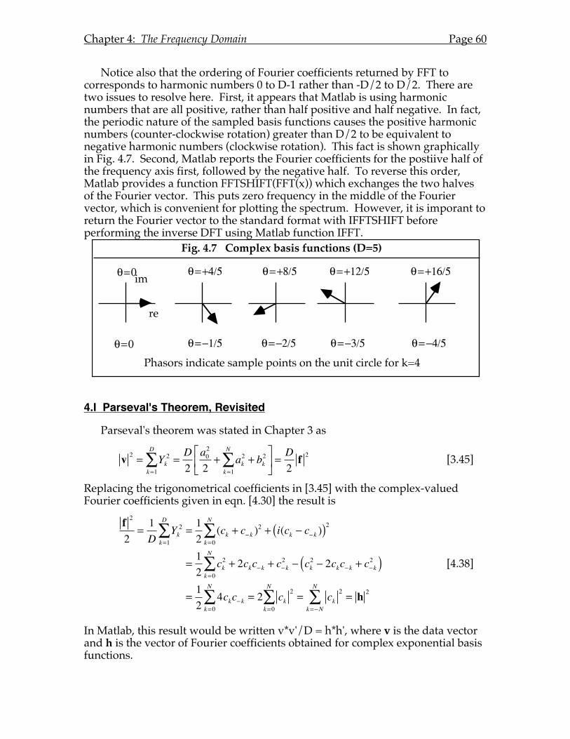
Chapter 4: The Frequency Domain Page 60
Notice also that the ordering of Fourier coefficients returned by FFT to corresponds to harmonic numbers 0 to D-1 rather than -D/2 to D/2. There are two issues to resolve here. First, it appears that Matlab is using harmonic numbers that are all positive, rather than half positive and half negative. In fact, the periodic nature of the sampled basis functions causes the positive harmonic numbers (counter-clockwise rotation) greater than D/2 to be equivalent to negative harmonic numbers (clockwise rotation). This fact is shown graphically in Fig. 4.7. Second, Matlab reports the Fourier coefficients for the postiive half of the frequency axis first, followed by the negative half. To reverse this order, Matlab provides a function FFTSHIFT(FFT(x)) which exchanges the two halves of the Fourier vector. This puts zero frequency in the middle of the Fourier vector, which is convenient for plotting the spectrum. However, it is imporant to return the Fourier vector to the standard format with IFFTSHIFT before performing the inverse DFT using Matlab function IFFT.
4.I Parseval's Theorem, Revisited
Parseval's theorem was stated in Chapter 3 as
v 2 = Yk2
k=1
D
∑ =D2
a02
2+ ak
2
k=1
N
∑ + bk2⎡
⎣⎢
⎤
⎦⎥ =
D2f 2 [3.45]
Replacing the trigonometrical coefficients in [3.45] with the complex-valued Fourier coefficients given in eqn. [4.30] the result is
f 2
2=1D
Yk2
k=1
D
∑ =12
(ck + c−k )2 + i(ck − c−k )( )2
k=0
N
∑
=12
ck2 + 2ckc−k + c−k
2 − ck2 − 2ckc−k + c−k
2( )k=0
N
∑
=12
4ckc−kk=0
N
∑ = 2 ck2
k=0
N
∑ = ck2
k=−N
N
∑ = h 2
[4.38]
In Matlab, this result would be written v*v'/D = h*h', where v is the data vector and h is the vector of Fourier coefficients obtained for complex exponential basis functions.
Fig. 4.7 Complex basis functions (D=5)
! = 0
! = 0
! = +4/5
! = "1/5
! = +8/5
! = "2/5
re
im! = +12/5
! = "3/5
! = +16/5
! = "4/5
Phasors indicate sample points on the unit circle for k=4
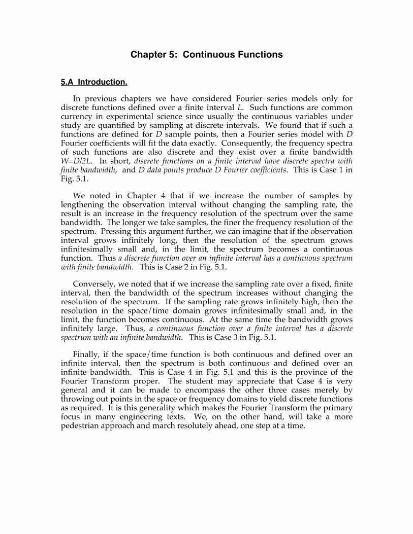
Chapter 5: Continuous Functions
5.A Introduction.
In previous chapters we have considered Fourier series models only for discrete functions defined over a finite interval L. Such functions are common currency in experimental science since usually the continuous variables under study are quantified by sampling at discrete intervals. We found that if such a functions are defined for D sample points, then a Fourier series model with D Fourier coefficients will fit the data exactly. Consequently, the frequency spectra of such functions are also discrete and they exist over a finite bandwidth W=D/2L. In short, discrete functions on a finite interval have discrete spectra with finite bandwidth, and D data points produce D Fourier coefficients. This is Case 1 in Fig. 5.1.
We noted in Chapter 4 that if we increase the number of samples by lengthening the observation interval without changing the sampling rate, the result is an increase in the frequency resolution of the spectrum over the same bandwidth. The longer we take samples, the finer the frequency resolution of the spectrum. Pressing this argument further, we can imagine that if the observation interval grows infinitely long, then the resolution of the spectrum grows infinitesimally small and, in the limit, the spectrum becomes a continuous function. Thus a discrete function over an infinite interval has a continuous spectrum with finite bandwidth. This is Case 2 in Fig. 5.1.
Conversely, we noted that if we increase the sampling rate over a fixed, finite interval, then the bandwidth of the spectrum increases without changing the resolution of the spectrum. If the sampling rate grows infinitely high, then the resolution in the space/time domain grows infinitesimally small and, in the limit, the function becomes continuous. At the same time the bandwidth grows infinitely large. Thus, a continuous function over a finite interval has a discrete spectrum with an infinite bandwidth. This is Case 3 in Fig. 5.1.
Finally, if the space/time function is both continuous and defined over an infinite interval, then the spectrum is both continuous and defined over an infinite bandwidth. This is Case 4 in Fig. 5.1 and this is the province of the Fourier Transform proper. The student may appreciate that Case 4 is very general and it can be made to encompass the other three cases merely by throwing out points in the space or frequency domains to yield discrete functions as required. It is this generality which makes the Fourier Transform the primary focus in many engineering texts. We, on the other hand, will take a more pedestrian approach and march resolutely ahead, one step at a time.
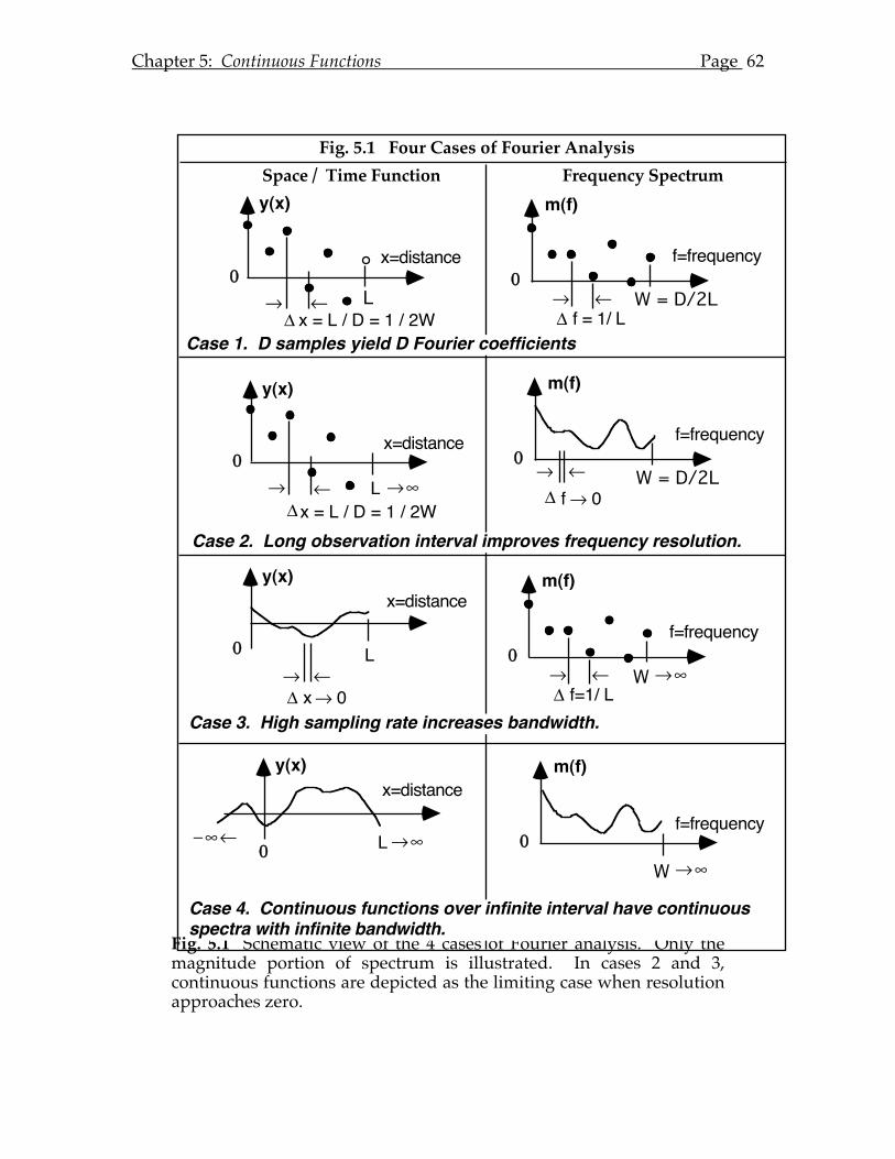
Chapter 5: Continuous Functions Page
62
Fig. 5.1 Schematic view of the 4 cases of Fourier analysis. Only the magnitude portion of spectrum is illustrated. In cases 2 and 3, continuous functions are depicted as the limiting case when resolution approaches zero.
Fig. 5.1 Four Cases of Fourier Analysis
Frequency SpectrumSpace / Time Function
0
y(x)
! "# x = L / D = 1 / 2W
x=distance
L
m(f)
0f=frequency
! "# f = 1/ L
W = D/2L
Case 1. D samples yield D Fourier coefficients
f=frequency
m(f)
0! " W = D/2L# f ! 0
0
y(x)
! "#
x=distance
L ! $
Case 2. Long observation interval improves frequency resolution.
m(f)
0f=frequency
! "# f=1/ L
0
y(x)
! "
x=distance
L
# x! 0W ! $
Case 3. High sampling rate increases bandwidth.
0
y(x)x=distance
L! $% $ "
Case 4. Continuous functions over infinite interval have continuous spectra with infinite bandwidth.
m(f)
0
W ! $
f=frequency
x = L / D = 1 / 2W
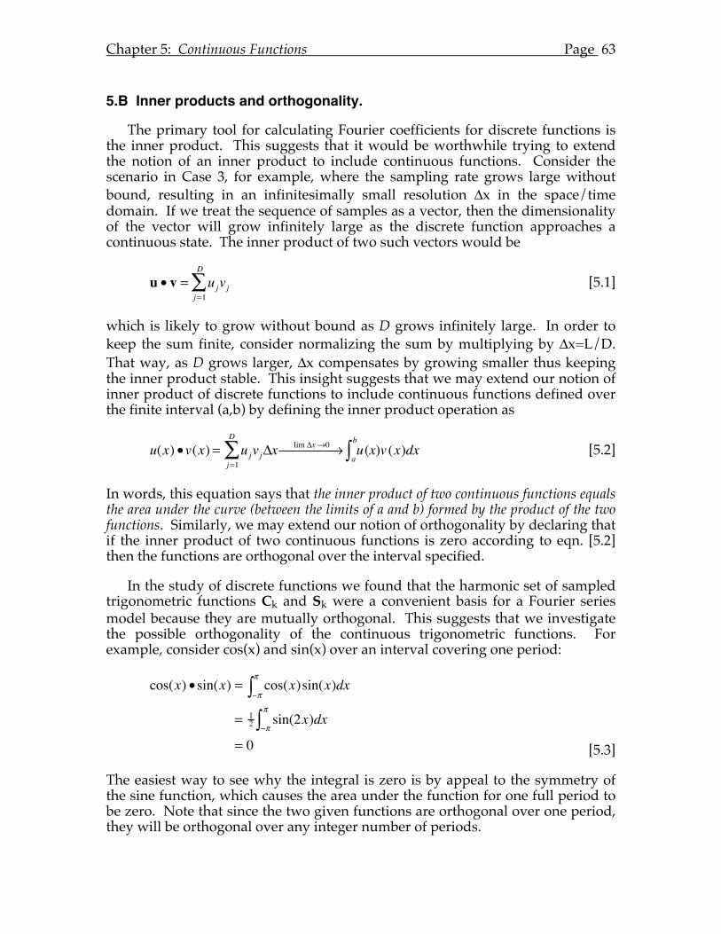
Chapter 5: Continuous Functions Page
63
5.B Inner products and orthogonality.
The primary tool for calculating Fourier coefficients for discrete functions is the inner product. This suggests that it would be worthwhile trying to extend the notion of an inner product to include continuous functions. Consider the scenario in Case 3, for example, where the sampling rate grows large without bound, resulting in an infinitesimally small resolution Δx in the space/time domain. If we treat the sequence of samples as a vector, then the dimensionality of the vector will grow infinitely large as the discrete function approaches a continuous state. The inner product of two such vectors would be
u • v = ujvjj=1
D
∑ [5.1]
which is likely to grow without bound as D grows infinitely large. In order to keep the sum finite, consider normalizing the sum by multiplying by Δx=L/D. That way, as D grows larger, Δx compensates by growing smaller thus keeping the inner product stable. This insight suggests that we may extend our notion of inner product of discrete functions to include continuous functions defined over the finite interval (a,b) by defining the inner product operation as
u(x) •v(x) = ujvjΔxj=1
D
∑ lim Δx→0⎯ → ⎯ ⎯ ⎯ u(x)v (x)dxa
b
∫ [5.2]
In words, this equation says that the inner product of two continuous functions equals the area under the curve (between the limits of a and b) formed by the product of the two functions. Similarly, we may extend our notion of orthogonality by declaring that if the inner product of two continuous functions is zero according to eqn. [5.2] then the functions are orthogonal over the interval specified.
In the study of discrete functions we found that the harmonic set of sampled trigonometric functions Ck and Sk were a convenient basis for a Fourier series model because they are mutually orthogonal. This suggests that we investigate the possible orthogonality of the continuous trigonometric functions. For example, consider cos(x) and sin(x) over an interval covering one period:
cos(x) • sin(x) = cos(x)sin(x)dx−π
π
∫= 1
2 sin(2x)dx−π
π
∫= 0 [5.3]
The easiest way to see why the integral is zero is by appeal to the symmetry of the sine function, which causes the area under the function for one full period to be zero. Note that since the two given functions are orthogonal over one period, they will be orthogonal over any integer number of periods.
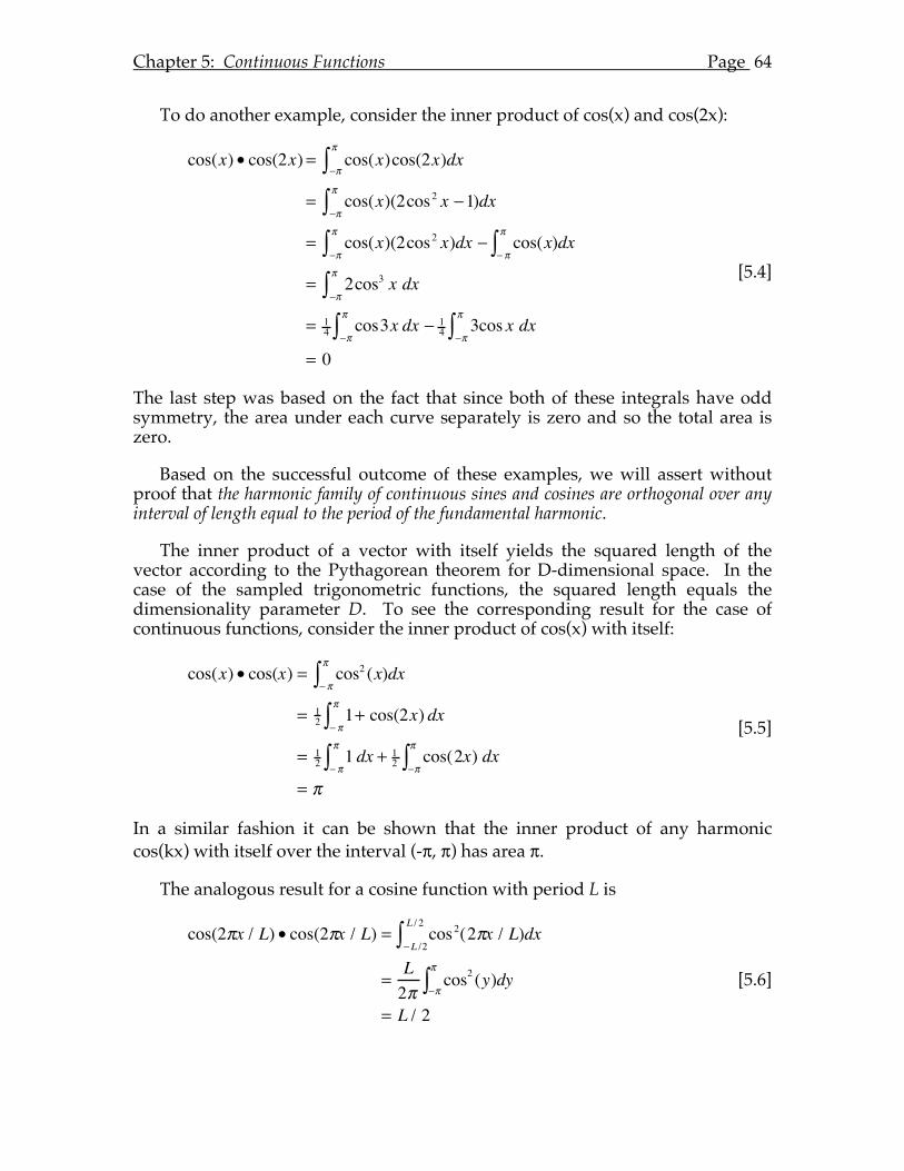
Chapter 5: Continuous Functions Page
64
To do another example, consider the inner product of cos(x) and cos(2x):
cos(x) • cos(2x) = cos(x)cos(2x)dx−π
π
∫= cos(x)(2cos2 x −1)dx
−π
π
∫= cos(x)(2cos2 x)dx
−π
π
∫ − cos(x)dx− π
π
∫= 2cos3 x dx
−π
π
∫= 1
4 cos3x dx−π
π
∫ − 14 3cos x dx
−π
π
∫= 0
[5.4]
The last step was based on the fact that since both of these integrals have odd symmetry, the area under each curve separately is zero and so the total area is zero.
Based on the successful outcome of these examples, we will assert without proof that the harmonic family of continuous sines and cosines are orthogonal over any interval of length equal to the period of the fundamental harmonic.
The inner product of a vector with itself yields the squared length of the vector according to the Pythagorean theorem for D-dimensional space. In the case of the sampled trigonometric functions, the squared length equals the dimensionality parameter D. To see the corresponding result for the case of continuous functions, consider the inner product of cos(x) with itself:
cos(x) • cos(x) = cos2 (x)dx− π
π
∫= 1
2 1+ cos(2x) dx− π
π
∫= 1
2 1 dx− π
π
∫ + 12 cos(2x) dx
−π
π
∫= π
[5.5]
In a similar fashion it can be shown that the inner product of any harmonic cos(kx) with itself over the interval (-π, π) has area π.
The analogous result for a cosine function with period L is
cos(2πx / L) • cos(2πx / L) = cos2(2πx / L)dx−L /2
L / 2
∫=
L2π
cos2 (y)dy−π
π
∫= L / 2
[5.6]
Chapter 5: Continuous Functions Page
65
where simplification was achieved by a substitution of variables y=2πx/L, for which dy/dx = 2π/L. Thus in general
cos(2πjx / L)• cos(2πkx /L) = 0 if j ≠ k= L / 2 if j = k
sin(2πjx / L) • sin(2πkx /L) = 0 if j ≠ k= L / 2 if j = k
cos(2πjx / L) • sin(2πkx /L) = 0 all j, k
[5.7]
The inner product of a continuous function with itself has an important interpretation in many physical situations. For example, Ohm's law of electrical circuits states that the power dissipated by a resister equals the squared voltage divided by resistance. If v(t) describes the time course of voltage across a 1 ohm resistor, then the time-course of power consumption is v2(t) and the total amount of energy consumed over the interval from 0 to T seconds is
energy = v2 (t) dt = v(t) • v(t)0
T
∫ [5.8]
The average power consumption over the interval is given by dividing the total energy consumed by the length of the interval
energyT
= mean power = 1T v2(t) dt
0
T
∫ [5.9]
For example, the average power consumption by a 1 Ohm resistor for a voltage waveform v(t) = A cos(x) equals A2/2.
Similarly, if v(t) is the instantaneous velocity of an object with unit mass then the integral in eqn. [5.8] equals the total amount of kinetic energy stored by the object. By analogy, even in contexts quite removed from similar physical situations, the inner product of a function with itself is often described as being equal to the amount of energy in the function.
5.C Symmetry.
The computation of Fourier coefficients for discrete functions involved forming the inner product of the data vector with the sampled trigonometric functions, so the student should not be too surprised when we find that the inner product also appears when computing Fourier coefficients for continuous functions. Since the inner product of continuous functions requires the evaluation of an integral, any shortcuts that ease this burden will be most useful. One such shortcut is based on symmetry and for this reason we make a short digression here on some general aspects of symmetrical functions.
Two types of symmetry are possible for ordinary, real-valued functions of 1 variable. If y(x)=y(-x) then the function y(x) is said to have even symmetry,
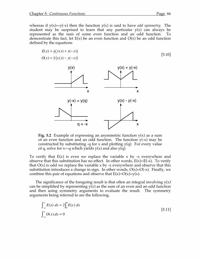
Chapter 5: Continuous Functions Page
66
whereas if y(x)=-y(-x) then the function y(x) is said to have odd symmetry. The student may be surprised to learn that any particular y(x) can always be represented as the sum of some even function and an odd function. To demonstrate this fact, let E(x) be an even function and O(x) be an odd function defined by the equations
E(x) = 1
2 y(x) + y(−x)( )O(x) = 1
2 y(x) − y(−x)( ) [5.10]
Fig. 5.2 Example of expressing an asymmetric function y(x) as a sum of an even function and an odd function. The function y(-x) may be constructed by substituting -q for x and plotting y(q). For every value of q, solve for x=-q which yields y(x) and also y(q).
To verify that E(x) is even we replace the variable x by -x everywhere and observe that this substitution has no effect. In other words, E(x)=E(-x). To verify that O(x) is odd we replace the variable x by -x everywhere and observe that this substitution introduces a change in sign. In other words, O(x)=O(-x). Finally, we combine this pair of equations and observe that E(x)+O(x)=y(x).
The significance of the foregoing result is that often an integral involving y(x) can be simplified by representing y(x) as the sum of an even and an odd function and then using symmetry arguments to evaluate the result. The symmetry arguments being referred to are the following.
E(x)
−a
a
∫ dx = 2 E(x )0
a
∫ dx
O(x)−a
a
∫ dx = 0 [5.11]
y(x)
x
y(x) - y(-x)
x
y(x) + y(-x)
x
y(-x) = y(q)
q = -x
Chapter 5: Continuous Functions Page
67
5.D Complex-valued functions.
A third kind of symmetry emerges when considering complex valued functions of 1 variable (e.g. y(x)=2x + i 5x)). If some function y(x) is complex-valued, then it may be represented as the sum of a purely real function yR(x) and a purely imaginary function yI(x). If the function y(x) has even symmetry, then
y(x) = y(− x)
yR (x) + iyI(x) = yR(−x) + iyI (−x) [5.12]
Equating the real and imaginary parts of this equation separately we see that
yR (x) = yR(−x)yI (x) = yI (−x)
[5.13]
In other words, if y(x) is even then both the real and imaginary parts of y(x) are even. A similar exercise will demonstrate to the student that if y(x) is odd, then both the real and imaginary components of y(x) are odd.
A different kind of symmetry mentioned previously is when the real part of y(x) is even but the imaginary part of y(x) is odd. In this case,
yR(x) = yR(−x)yI(x) = −yI (−x)
yR (x) + iyI(x) = yR(−x) − iyI (−x)
y(x) = y∗(−x)
[5.14]
Generalizing the notion of complex conjugate developed earlier for complex numbers, we could say that the function y(x) has conjugate symmetry, or Hermitian symmetry.
Conjugate symmetry plays a large part in Fourier analysis of continuous functions. For example, the basis functions of the form eix = cos x + isin x are Hermitian. Furthermore, in Chapter 4 it was observed that the complex Fourier coefficients for real-valued data vectors have conjugate symmetry: ck = c−k
∗ . When the spectrum becomes continuous, as in cases 2 and 4 in Fig. 5.1, then the spectrum is a complex-valued function. In the next chapter we will show that such a spectrum possesses conjugate symmetry. Some symmetry relations listed in Bracewell's textbook The Fourier Transform and Its Applications (p.14) are given in Table 12.2 in Chapter 12.

Chapter 5: Continuous Functions Page
68
Chapter 6: Fourier Analysis of Continuous Functions
6.A Introduction.
In the introduction to Chapter 3 we posed the question of whether or not an arbitrary function defined over a finite interval of time or space can be represented as the sum of a series of weighted sinusoids. We delayed answering that question temporarily while we dealt with the easier question of whether a sampled function can be represented by a weighted sum of sampled sinusoids. We found that indeed it was possible to fit a set of D data points exactly by a Fourier series model with D coefficients. In the process, we developed simple formulas that allowed us to calculate these unknown Fourier coefficients for any vector of data values. Then, in Chapter 5 we returned to the original problem and argued by extension of these results that a continuous function defined over a finite interval will have a discrete spectrum with an infinite bandwidth. This is Case 3 illustrated in Fig. 5.1. The task now is to formulate an appropriate model for this case and then determine formulas for calculating the unknown Fourier coefficients.
6.B The Fourier Model. Given an arbitrary, real-valued function y(x), we wish to represent this
function exactly over a finite interval by a Fourier series with an infinite number of terms. Accordingly, the model we seek is just eqn. [3.34] extended to have an infinite number of harmonics. To simplify the notation initially, let us assume that y(x) is defined over the interval (-π,π) so the Fourier series is
y(x) = a0 / 2 + ak ⋅ coskx + bk ⋅ sin kxk=1
∞
∑ , all x in the range (-π,π) [6.1]
The method used previously to determine the unknown Fourier coefficients was to evaluate the inner product of the given discrete function with the basis functions of the model. In the discrete case, the basis functions were the sampled trigonometric functions. Now, in the continuous case, the basis functions are the continuous trigonometric functions. Accordingly, we need to form the inner product of eqn. [6.1] with each harmonic function in turn. For example, to find the kth harmonic coefficient ak, we form the inner product with the basis function and examine each term in the sum,
cos kx • f (x) = coskx • a0 / 2+ coskx • a1 cos x + coskx • b1 sin x+ coskx • a2 cos2x + coskx •b2 sin 2x++ coskx • ak coskx + coskx • bk sinkx+
= ak(cos kx •cos kx)= akπ
[6.2]
Chapter 6: Fourier Analysis of Continuous Functions Page 70
Notice that the infinite series on the right side of eqn. [6.2] collapses to a single term because of orthogonality. The inner product cos kx •cos kx equals L/2=π according to eqn. [5.7]. Therefore, we may conclude from eqn. [6.2] that the coefficient ak, is given by the formula
ak = 1
π coskx • f (x)
= 1π y(x)coskx
−π
π
∫ dx [6.3]
Notice that this formula works also for the constant term a0 since if k=0, then eqn. [6.3] yields twice the mean value. When this result is inserted into the model of eqn. [6.1], the constant term is just the mean value of the function y(x) as required. A similar line of reasoning leads to an analogous formula for the sine coefficient bk
bk = 1π y(x)sin kx
−π
π
∫ dx [6.4]
To obtain the more general formulas which apply when the function y(x) is defined over any finite interval of length L, we replace x by 2πx/L to get
y(x) = a0 / 2 + ak ⋅ cos2πkx / L + bk ⋅ sin2πkx / Lk=1
∞
∑ ,
where
ak = 2L y(x)cosk2π x / L
L0
L0 +L∫ dx
bk = 2L y(x)sin k2π x / L
L0
L0 +L∫ dx
[6.5]
This last result is the form of Fourier series commonly seen in textbooks because it is general enough to allow analysis of one full period with arbitrary starting point.
The trigonometric model of eqn. [6.1] is useful only for real-valued functions. However, we may extend the model to include complex-valued functions just as we did earlier for discrete functions (see eqn. [4.14]). To do so the Fourier series model is written in terms of complex coefficients as
y(x) = ckeik2π x /L
k=−∞
∞
∑ [6.6]
where we take our inspiration for the definition of the complex coefficients from eqn. [4.12] and eqn. [6.5]:
Chapter 6: Fourier Analysis of Continuous Functions Page 71
ck =ak − ibk2
for k > 0
ck =ak + ibk2
for k < 0
ck = 1L y(x)cosk2π x / L
L0
L0 +L∫ dx − i 1L y(x)sin k2π x / LL0
L0 +L∫ dx
= 1L y(x)e− ik2π x /L
L0
L0 +L∫ dx
[6.7]
In this model the continuous complex exponential are the orthogonal basis functions for representing any complex-valued function. Since real-valued functions are just a special case of complex-valued functions, the model of eqn. [6.6] subsumes the model of eqn. [6.1] and so is often preferred in textbooks.
6.C Practicalities of Obtaining the Fourier Coefficients.
The preceding section has demonstrated that there is little conceptual difference between the Fourier analysis of discrete and continuous functions over a finite interval. From a practical standpoint, however, there is a large difference in the mechanics of calculating the Fourier coefficients of the model. Anyone who can do arithmetic can compute the inner products required in the Fourier analysis of discrete functions. However, to do Fourier analysis of continuous functions requires an ability to do calculus. If evaluating an integral is deemed a last resort, then several alternative strategies are worth exploring.
• Look it up in a reference book. Spectra of many common waveforms have been determined and answers are in handbooks of mathematical functions (e.g. see Bracewell's pictorial dictionary of Fourier transform pairs )
• Use symmetry arguments to assert that certain coefficients are zero.
• Break the given function down into a sum of of more elementary functions for which the Fourier series is known. Because of linearity, the spectrum of a sum of functions is equal to the sum of their spectra.
• Approximate the given function by sampling it D times and numerically calculate the corresponding finite Fourier series.
• Use theorems to derive new Fourier series from old ones without doing a lot of extra work.
• Use the brute force method and do the calculus. An efficient strategy is to leave the harmonic number k as a variable so that a formula is produced which determines all of the Fourier coefficients at once.
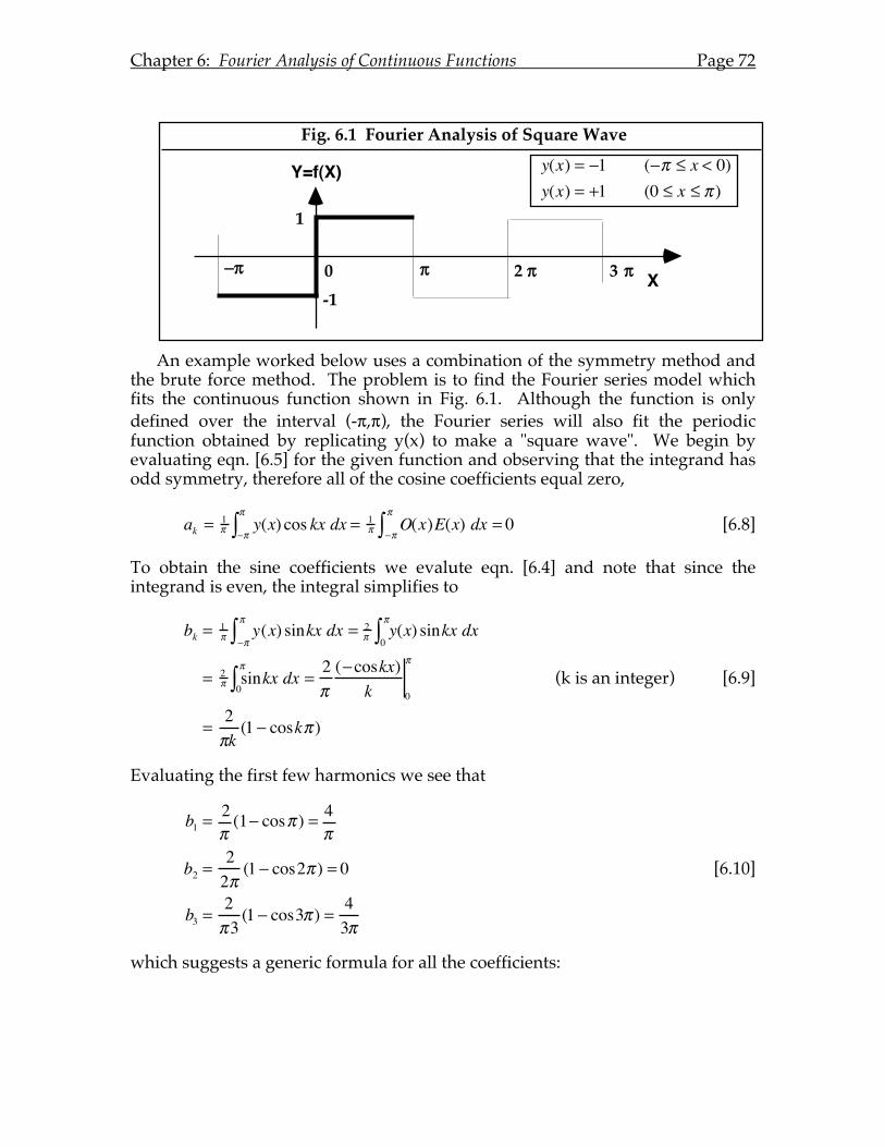
Chapter 6: Fourier Analysis of Continuous Functions Page 72
An example worked below uses a combination of the symmetry method and the brute force method. The problem is to find the Fourier series model which fits the continuous function shown in Fig. 6.1. Although the function is only defined over the interval (-π,π), the Fourier series will also fit the periodic function obtained by replicating y(x) to make a "square wave". We begin by evaluating eqn. [6.5] for the given function and observing that the integrand has odd symmetry, therefore all of the cosine coefficients equal zero,
ak = 1π y(x) cos kx
−π
π
∫ dx = 1π O(x)E(x)
−π
π
∫ dx = 0 [6.8]
To obtain the sine coefficients we evalute eqn. [6.4] and note that since the integrand is even, the integral simplifies to
bk = 1π y(x) sinkx
−π
π
∫ dx = 2π y(x) sinkx
0
π
∫ dx
= 2π sinkx
0
π
∫ dx = 2π(−coskx)
k 0
π
=2πk(1 − coskπ )
(k is an integer) [6.9]
Evaluating the first few harmonics we see that
b1 =2π(1− cosπ ) = 4
π
b2 =22π(1 − cos2π ) = 0
b3 =2π3(1 − cos3π ) = 4
3π
[6.10]
which suggests a generic formula for all the coefficients:
Fig. 6.1 Fourier Analysis of Square Wave
0
1
X
Y=f(X)
!"!
-1
y(x) = "1 ("! # x < 0)y(x) = +1 (0 # x # ! )
3 !2 !
Chapter 6: Fourier Analysis of Continuous Functions Page 73
bk =
4kπ
for k = odd
bk = 0 for k = even [6.11]
Substituting these coefficients back into the model of eqn. [6.1] we get
y(x) = 4π(sin x + 1
3 sin3x + 15 sin5x +)
=4π
sin kxkk =odd
∑ [6.12]
Thus we have the Fourier series model for a square wave in "sine phase". A similar formula may be determined for the square wave in "cosine phase".
6.D Theorems
1. Linearity
A common way of describing Fourier analysis is that it is a linear operation. There are two general properties of any linear operation which have to do with scaling and adding. In the present context, these properties are:
1a. if f(x) has the Fourier coefficients ak and bk, then scaling f(x) by a constant s to produce the new function g(x)=s.f(x) will also scale the Fourier coefficients by s. That is, the coefficients for g(x) will be s.ak, s.bk. This theorem is easily verified by substituting the new function into the coefficient generating functions in eqn. [6.5].
1b. if f(x) has the Fourier coefficients ak and bk, and if g(x) has the Fourier coefficients αk and βk, then the function f(x)+g(x) will have Fourier coefficients ak+ αk and bk +βk. This theorem follows from the fact that the integrals in eqn. [6.5] are themselves linear operations, so if the integrand is the sum of two functions, the integral can be broken into the sum of two integrals, each of which corresponds to the fourier coefficients of the component functions f or g.
2. Shift theorem
If the origin of the time or space reference frame shifts by an amount x´, then the effect is to induce a phase shift in the spectrum of a function. This result is easy to demonstrate algebraically if the original function f(x) is given by the Fourier series in polar form as
y(x) = a0 / 2 + mk ⋅ cos(kx −φk )k=1
∞
∑ [6.13]
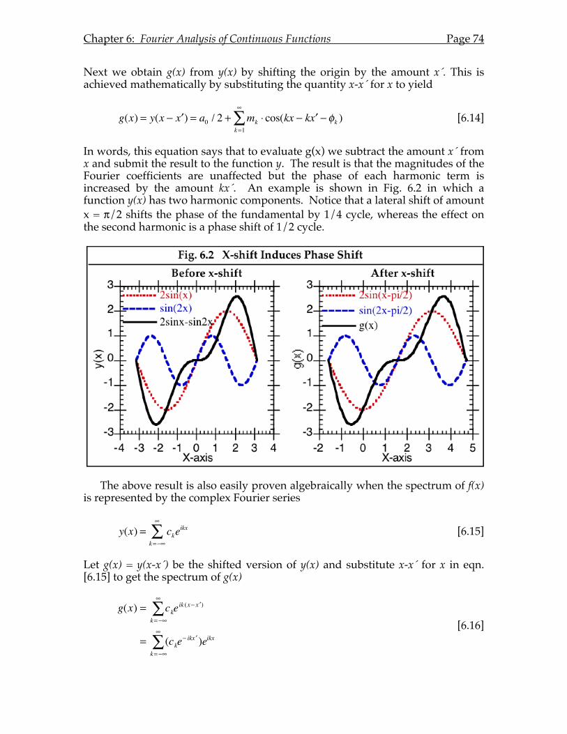
Chapter 6: Fourier Analysis of Continuous Functions Page 74
Next we obtain g(x) from y(x) by shifting the origin by the amount x´. This is achieved mathematically by substituting the quantity x-x´ for x to yield
g(x) = y(x − ′x ) = a0 / 2 + mk ⋅ cos(kx − k ′x −φk )k=1
∞
∑ [6.14]
In words, this equation says that to evaluate g(x) we subtract the amount x´ from x and submit the result to the function y. The result is that the magnitudes of the Fourier coefficients are unaffected but the phase of each harmonic term is increased by the amount kx´. An example is shown in Fig. 6.2 in which a function y(x) has two harmonic components. Notice that a lateral shift of amount x = π/2 shifts the phase of the fundamental by 1/4 cycle, whereas the effect on the second harmonic is a phase shift of 1/2 cycle.
The above result is also easily proven algebraically when the spectrum of f(x) is represented by the complex Fourier series
y(x) = ckeikx
k=−∞
∞
∑ [6.15]
Let g(x) = y(x-x´) be the shifted version of y(x) and substitute x-x´ for x in eqn. [6.15] to get the spectrum of g(x)
g(x) = ckeik (x− ′ x )
k = −∞
∞
∑
= (cke− ik ′ x )eikx
k = −∞
∞
∑ [6.16]
Chapter 6: Fourier Analysis of Continuous Functions Page 75
The new Fourier coefficient is thus seen to be the old coefficient times eikx´. But we know from Chapter 2 that multiplication by the unit phasor e-iθ has the effect of rotating the given phasor by the angle θ, which is to say the phase is shifted by amount θ. Notice that the amount of phase shift is directly proportional to the harmonic number k and to the amount of displacement x´.
Although more cumbersome algebraically, the Cartesian form of this theorem may provide some insight to the student. If f(x) is given by the Fourier series
y(x) = a0 / 2 + ak ⋅ coskx + bk ⋅ sin kxk=1
∞
∑ [6.17]
and g(x) is obtained from f(x) by shifting the origin by x´ to give
g(x) = a0 / 2 + ak ⋅ cosk( x − ′ x ) + bk ⋅ sink(x − ′ x )k =1
∞
∑ [6.18]
In order to re-write this last equation as a standard Fourier series and thus reveal the new Fourier coefficients,
g(x) = a0 / 2 + ′ a k ⋅ coskx + ′ b k ⋅sin kxk =1
∞
∑ [6.19]
we apply the trigonometrical identities of eqn. [2.6]
cos(α + δ ) = cosα cosδ − sinα sinδsin(α + δ ) = cosα sinδ + sinα cosδ
. [2.6]
To see how the result is going to turn out, consider the k-th harmonic term
ak ⋅ cosk(x − ′x ) + bk ⋅ sin k(x − ′x )= ak ⋅ (coskx cosk ′x + sin kx sin k ′x ) + bk ⋅ (sin kx cosk ′x − coskx sin k ′x )= (ak cosk ′x − bk sin k ′x )coskx + (bk cosk ′x + ak sin k ′x )sin kx
[6.20]
Thus the new Fourier coefficients are
′ a k = ak cos k ′ x − bk sin k ′ x ′ b k = bk cosk ′ x + ak sin k ′ x
[6.21]
which are recognized as rotated versions of the phasors (ak,bk). In agreement with the solution obtained in polar form above, the amount of rotation is kx.
3. Scaling theorem
If the scale of the time or space reference frame changes by the factor s , then the effect is to inversely scale the frequency axis of the spectrum of the function.
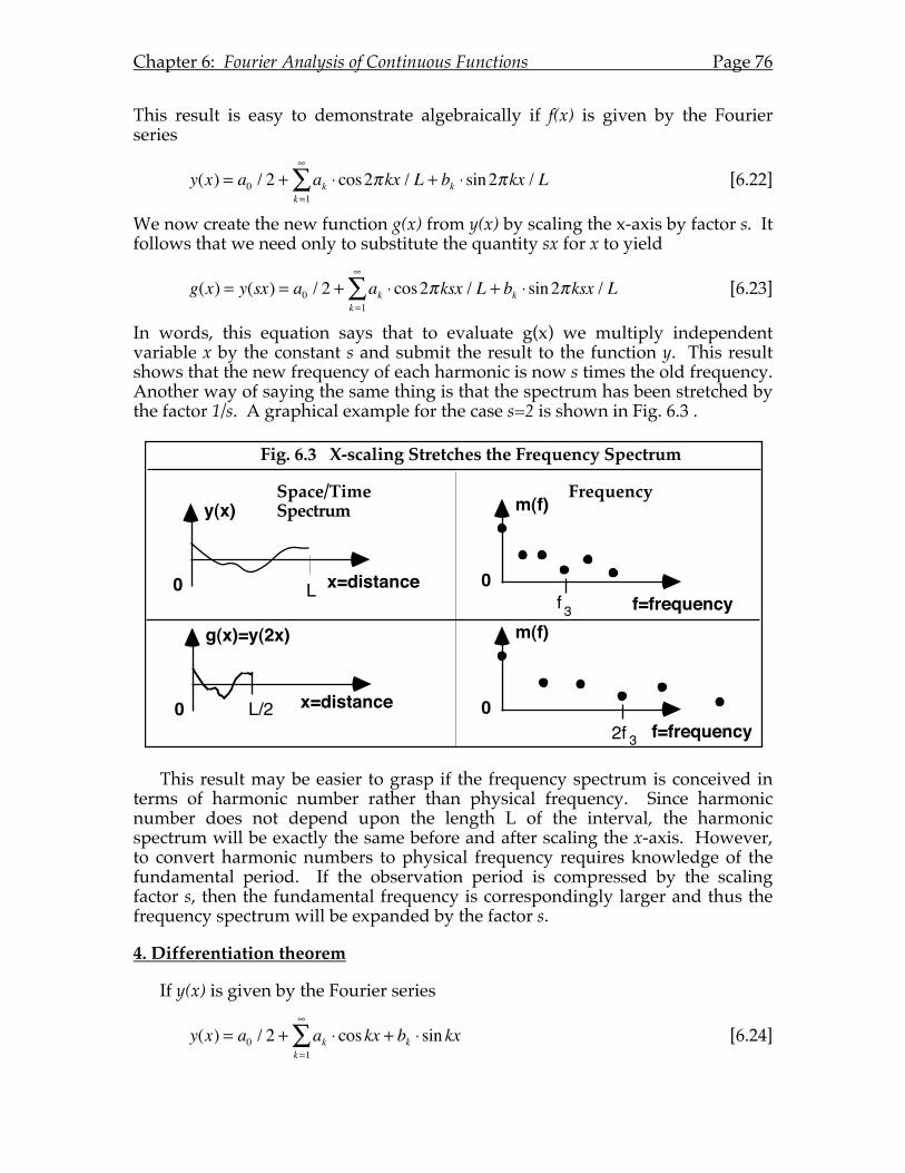
Chapter 6: Fourier Analysis of Continuous Functions Page 76
This result is easy to demonstrate algebraically if f(x) is given by the Fourier series
y(x) = a0 / 2 + ak ⋅ cos2πkx / L + bk ⋅ sin2πkxk=1
∞
∑ / L [6.22]
We now create the new function g(x) from y(x) by scaling the x-axis by factor s. It follows that we need only to substitute the quantity sx for x to yield
g(x) = y(sx) = a0 / 2 + ak ⋅ cos2πksx / L + bk ⋅ sin2πksxk=1
∞
∑ / L [6.23]
In words, this equation says that to evaluate g(x) we multiply independent variable x by the constant s and submit the result to the function y. This result shows that the new frequency of each harmonic is now s times the old frequency. Another way of saying the same thing is that the spectrum has been stretched by the factor 1/s. A graphical example for the case s=2 is shown in Fig. 6.3 .
This result may be easier to grasp if the frequency spectrum is conceived in
terms of harmonic number rather than physical frequency. Since harmonic number does not depend upon the length L of the interval, the harmonic spectrum will be exactly the same before and after scaling the x-axis. However, to convert harmonic numbers to physical frequency requires knowledge of the fundamental period. If the observation period is compressed by the scaling factor s, then the fundamental frequency is correspondingly larger and thus the frequency spectrum will be expanded by the factor s.
4. Differentiation theorem
If y(x) is given by the Fourier series
y(x) = a0 / 2 + ak ⋅ coskx + bk ⋅ sin kxk=1
∞
∑ [6.24]
Fig. 6.3 X-scaling Stretches the Frequency Spectrum
Space/Time Frequency Spectrum
0
y(x)
x=distanceL
m(f)
0f=frequencyf 3
0
g(x)=y(2x)
x=distanceL/2
m(f)
0f=frequency2f 3
Chapter 6: Fourier Analysis of Continuous Functions Page 77
and a new function g(x) is created by differentiating y(x) with respect to x, then the model for g(x) is
g(x) = dydx
= kbk ⋅ cos(kx) − kak ⋅ sin(kx)k=1
∞
∑ [6.25]
This shows that the new ak equals k times the old bk and that the new bk equals -k times the old ak . The reason the coefficients are scaled by the harmonic number is that the rate of change of higher harmonics is greater so the derivative must be greater. For example, the function y(x) in Fig. 6.1 has the Fourier coefficients b1=2, b2=-1. According to this theorem, the derivative of y(x) should have the Fourier coefficients a1=2, a2=-2. This is verified by differentiating y(x) directly to get 2 cosx − 2cos2x .
The above result may be interpreted as a rotation and scaling of the spectrum in the complex plane. To see this, let f(x) be represented by the Fourier series
y(x) = ckeikx
k=−∞
∞
∑ [6.26]
and a new function g(x) is created by differentiating y(x) with respect to x, then the model for g(x) is
g(x) = dy(x)dx
=ddx
ckeikx
k=−∞
∞
∑⎛⎝⎜⎞⎠⎟
= ikckeikx
k=−∞
∞
∑
[6.27]
In words, the effect of differentiating a function is to rotate each phasor ck by 90° (the factor i) and to scale all of the Fourier coefficients by the harmonic number k.
5. Integration theorem
If y(x) is given by the Fourier series
y(x) = a0 / 2 + ak ⋅ coskx + bk ⋅ sin kxk=1
∞
∑ [6.28]
and a new function g(x) is created by integrating y(x) with respect to x, then the model for g(x) is
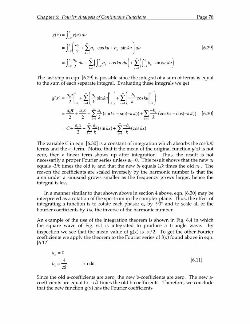
Chapter 6: Fourier Analysis of Continuous Functions Page 78
g(x) = y(u)−π
x
∫ du
=a02+ ak ⋅ cosku + bk ⋅ sin ku
k=1
∞
∑⎛⎝⎜
⎞⎠⎟−π
x
∫ du
=a02−π
x
∫ du + ak ⋅ cosku−π
x
∫ du( )k=1
∞
∑ + bk ⋅ sin ku−π
x
∫ du( )k=1
∞
∑
[6.29]
The last step in eqn. [6.29] is possible since the integral of a sum of terms is equal to the sum of each separate integral. Evaluating these integrals we get
g(x) =a0u2 − π
x
+akksinku
−π
x⎛
⎝ ⎜
⎞
⎠ ⎟
k=1
∞
∑ +−bkkcosku
− π
x⎛
⎝ ⎜
⎞
⎠ ⎟
k=1
∞
∑
=a0π2
+a0x2
+akksinkx − sin(−kπ )( )
k=1
∞
∑ +−bkk
coskx − cos(−kπ )( )k=1
∞
∑
= C +a0x2
+akksin kx( )
k =1
∞
∑ +−bkkcos kx( )
k=1
∞
∑
[6.30]
The variable C in eqn. [6.30] is a constant of integration which absorbs the cos(kπ) terms and the a0 term. Notice that if the mean of the original function y(x) is not zero, then a linear term shows up after integration. Thus, the result is not necessarily a proper Fourier series unless a0=0. This result shows that the new ak equals -1/k times the old bk and that the new bk equals 1/k times the old ak . The reason the coefficients are scaled inversely by the harmonic number is that the area under a sinusoid grows smaller as the frequency grows larger, hence the integral is less.
In a manner similar to that shown above in section 4 above, eqn. [6.30] may be interpreted as a rotation of the spectrum in the complex plane. Thus, the effect of integrating a function is to rotate each phasor ck by -90° and to scale all of the Fourier coefficients by 1/k, the inverse of the harmonic number.
An example of the use of the integration theorem is shown in Fig. 6.4 in which the square wave of Fig. 6.1 is integrated to produce a triangle wave. By inspection we see that the mean value of g(x) is -π/2. To get the other Fourier coefficients we apply the theorem to the Fourier series of f(x) found above in eqn. [6.12]
ak = 0
bk =4πk
k odd [6.11]
Since the old a-coefficients are zero, the new b-coefficients are zero. The new a-coefficients are equal to -1/k times the old b-coefficients. Therefore, we conclude that the new function g(x) has the Fourier coefficients
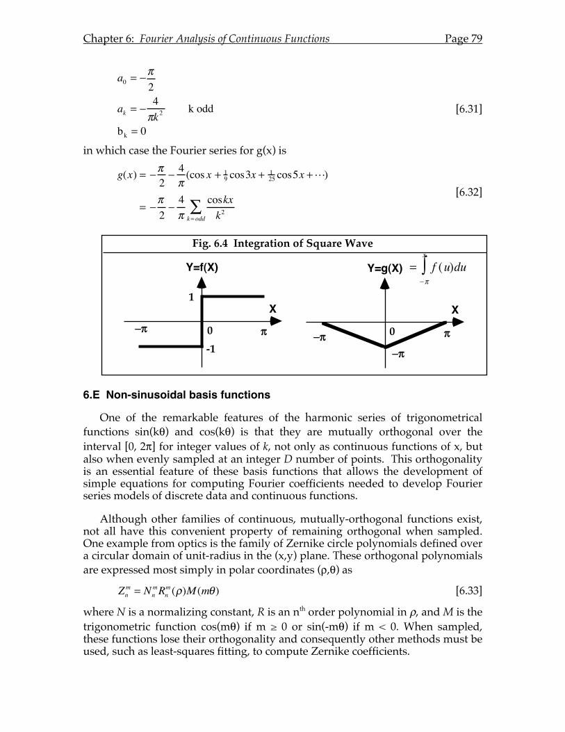
Chapter 6: Fourier Analysis of Continuous Functions Page 79
a0 = −π2
ak = −4
πk 2 k odd
bk = 0
[6.31]
in which case the Fourier series for g(x) is
g(x) = −π2− 4π(cos x + 1
9 cos3x + 125 cos5x +)
= −π2−4π
coskxk2k= odd
∑ [6.32]
6.E Non-sinusoidal basis functions
One of the remarkable features of the harmonic series of trigonometrical functions sin(kθ) and cos(kθ) is that they are mutually orthogonal over the interval [0, 2π] for integer values of k, not only as continuous functions of x, but also when evenly sampled at an integer D number of points. This orthogonality is an essential feature of these basis functions that allows the development of simple equations for computing Fourier coefficients needed to develop Fourier series models of discrete data and continuous functions.
Although other families of continuous, mutually-orthogonal functions exist, not all have this convenient property of remaining orthogonal when sampled. One example from optics is the family of Zernike circle polynomials defined over a circular domain of unit-radius in the (x,y) plane. These orthogonal polynomials are expressed most simply in polar coordinates (ρ,θ) as
Znm = Nn
mRnm (ρ)M (mθ) [6.33]
where N is a normalizing constant, R is an nth order polynomial in ρ, and M is the trigonometric function cos(mθ) if m ≥ 0 or sin(-mθ) if m < 0. When sampled, these functions lose their orthogonality and consequently other methods must be used, such as least-squares fitting, to compute Zernike coefficients.
Fig. 6.4 Integration of Square Wave
0
X
Y=g(X)
!"!0
1X
Y=f(X)
!"!
-1 "!
= f (u)du"!
x
#

Chapter 6: Fourier Analysis of Continuous Functions Page 80
Chapter 7: Sampling Theory
7.A Introduction.
In Chapter 6 we found that there is little conceptual difference between the Fourier analysis of discrete and continuous functions over a finite interval. Both types of functions have discrete spectra, the only difference being that discrete functions have a finite number of harmonic components (Case 1 in Fig. 5.1), whereas a continuous function, in principle, has an infinite number of harmonics (Case 3 in Fig. 5.1). However, a curious result emerges from the homework set #6. In one problem (6.1), it is found that the spectrum of a continuous function and the sampled version of that function are significantly different, whereas in another problem (6.2) the two spectra are exactly the same over the range of harmonics for which a comparison is possible. This indicates that under certain circumstances a function is completely determined by a finite number of samples. In this chapter we explore the conditions for which this result obtains.
7.B The Sampling Theorem.
In general, a continuous function defined over a finite interval can be represented by a Fourier series with an infinite number of terms as shown in Chapter 6
f (x) = a0 / 2 + ak ⋅ coskx + bk ⋅sin kxk=1
∞
∑ [6.1]
However, it may happen that for some functions the Fourier coefficients are all zero for all frequencies greater than some value W. For such spectra, we may think of W as the bandwidth of the spectrum. Notice a subtle difference between previous usage and this use of the term bandwidth. When discussing discrete functions, which have finite spectra, we used the term bandwidth to mean the highest frequency defined in the spectrum. In that case, W = D/2L. That definition implies that all continuous functions have infinite bandwidth because D = ∞. An alternative definition allows continuous functions to have finite bandwidth if the magnitudes of all Fourier coefficients are zero beyond some limiting frequency W. This is a much more useful definition for practical purposes and so that is how the term bandwidth is normally used.
Consider now the consequences of a continuous function having finite bandwidth. An example is shown in Fig. 7.1 in which the frequency spectrum is non-zero only for the constant term and the first three harmonics. Now imagine trying to "reconstruct" the space/time function from this spectrum. We have two options in this regard. First, we could pretend that all frequencies higher than W don't exist, in which case the IDFT operation will produce a discrete function shown by the solid points in the left side of Fig. 7.1 On the other hand, we could use the entire frequency spectrum which is defined for an infinite number of harmonics and in this case the Fourier series will produce the continuous function shown in the figure. Now we assert that the continuous reconstructed
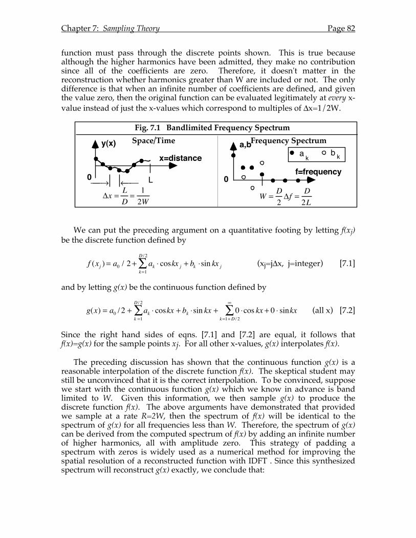
Chapter 7: Sampling Theory Page 82
function must pass through the discrete points shown. This is true because although the higher harmonics have been admitted, they make no contribution since all of the coefficients are zero. Therefore, it doesn't matter in the reconstruction whether harmonics greater than W are included or not. The only difference is that when an infinite number of coefficients are defined, and given the value zero, then the original function can be evaluated legitimately at every x-value instead of just the x-values which correspond to multiples of Δx=1/2W.
We can put the preceding argument on a quantitative footing by letting f(xj) be the discrete function defined by
f (xj ) = a0 / 2 + ak ⋅ coskx j + bk ⋅sin kx jk=1
D / 2
∑ (xj=jΔx, j=integer) [7.1]
and by letting g(x) be the continuous function defined by
g(x) = a0 / 2 + ak ⋅ coskx + bk ⋅sin kxk =1
D / 2
∑ + 0 ⋅cos kx + 0 ⋅ sinkxk=1+D / 2
∞
∑ (all x) [7.2]
Since the right hand sides of eqns. [7.1] and [7.2] are equal, it follows that f(x)=g(x) for the sample points xj. For all other x-values, g(x) interpolates f(x).
The preceding discussion has shown that the continuous function g(x) is a reasonable interpolation of the discrete function f(x). The skeptical student may still be unconvinced that it is the correct interpolation. To be convinced, suppose we start with the continuous function g(x) which we know in advance is band limited to W. Given this information, we then sample g(x) to produce the discrete function f(x). The above arguments have demonstrated that provided we sample at a rate R=2W, then the spectrum of f(x) will be identical to the spectrum of g(x) for all frequencies less than W. Therefore, the spectrum of g(x) can be derived from the computed spectrum of f(x) by adding an infinite number of higher harmonics, all with amplitude zero. This strategy of padding a spectrum with zeros is widely used as a numerical method for improving the spatial resolution of a reconstructed function with IDFT . Since this synthesized spectrum will reconstruct g(x) exactly, we conclude that:
Fig. 7.1 Bandlimited Frequency SpectrumSpace/Time Frequency Spectrum
f=frequency
a k b k
!x =LD
=12W
0
y(x)
x=distance
L" # " $ " "
W =D2!f =
D2L
a,b
0
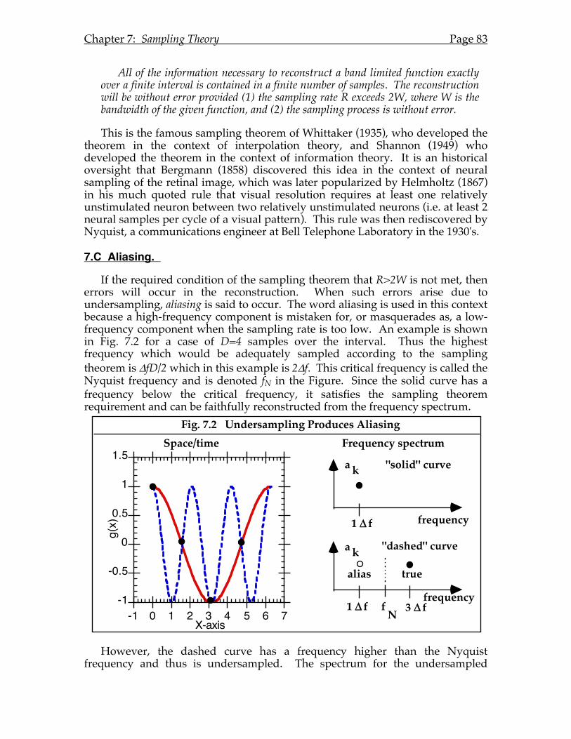
Chapter 7: Sampling Theory Page 83
All of the information necessary to reconstruct a band limited function exactly over a finite interval is contained in a finite number of samples. The reconstruction will be without error provided (1) the sampling rate R exceeds 2W, where W is the bandwidth of the given function, and (2) the sampling process is without error.
This is the famous sampling theorem of Whittaker (1935), who developed the theorem in the context of interpolation theory, and Shannon (1949) who developed the theorem in the context of information theory. It is an historical oversight that Bergmann (1858) discovered this idea in the context of neural sampling of the retinal image, which was later popularized by Helmholtz (1867) in his much quoted rule that visual resolution requires at least one relatively unstimulated neuron between two relatively unstimulated neurons (i.e. at least 2 neural samples per cycle of a visual pattern). This rule was then rediscovered by Nyquist, a communications engineer at Bell Telephone Laboratory in the 1930's.
7.C Aliasing.
If the required condition of the sampling theorem that R>2W is not met, then errors will occur in the reconstruction. When such errors arise due to undersampling, aliasing is said to occur. The word aliasing is used in this context because a high-frequency component is mistaken for, or masquerades as, a low-frequency component when the sampling rate is too low. An example is shown in Fig. 7.2 for a case of D=4 samples over the interval. Thus the highest frequency which would be adequately sampled according to the sampling theorem is ΔfD/2 which in this example is 2Δf. This critical frequency is called the Nyquist frequency and is denoted fN in the Figure. Since the solid curve has a frequency below the critical frequency, it satisfies the sampling theorem requirement and can be faithfully reconstructed from the frequency spectrum.
However, the dashed curve has a frequency higher than the Nyquist frequency and thus is undersampled. The spectrum for the undersampled
-1
-0.5
0
0.5
1
1.5
-1 0
g(x)
1 2 3 4 5 6 7X-axis
Fig. 7.2 Undersampling Produces Aliasing
Space/time Frequency spectrum
frequency
a k
frequency
a k
"solid" curve
"dashed" curve
truealias
1 f!
1 f! 3 f!fN
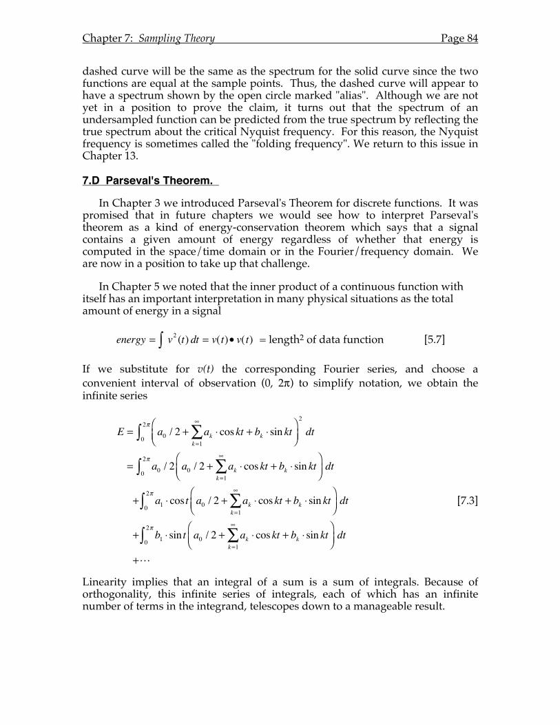
Chapter 7: Sampling Theory Page 84
dashed curve will be the same as the spectrum for the solid curve since the two functions are equal at the sample points. Thus, the dashed curve will appear to have a spectrum shown by the open circle marked "alias". Although we are not yet in a position to prove the claim, it turns out that the spectrum of an undersampled function can be predicted from the true spectrum by reflecting the true spectrum about the critical Nyquist frequency. For this reason, the Nyquist frequency is sometimes called the "folding frequency". We return to this issue in Chapter 13.
7.D Parseval's Theorem.
In Chapter 3 we introduced Parseval's Theorem for discrete functions. It was promised that in future chapters we would see how to interpret Parseval's theorem as a kind of energy-conservation theorem which says that a signal contains a given amount of energy regardless of whether that energy is computed in the space/time domain or in the Fourier/frequency domain. We are now in a position to take up that challenge.
In Chapter 5 we noted that the inner product of a continuous function with itself has an important interpretation in many physical situations as the total amount of energy in a signal
energy = v2 (t) dt = v(t)• v(t)∫ = length2 of data function [5.7]
If we substitute for v(t) the corresponding Fourier series, and choose a convenient interval of observation (0, 2π) to simplify notation, we obtain the infinite series
E = a0 / 2 + ak ⋅ coskt + bk ⋅ sin ktk=1
∞
∑⎛⎝⎜
⎞⎠⎟0
2π
∫2
dt
= a0 / 2 a0 / 2 + ak ⋅ coskt + bk ⋅ sin ktk=1
∞
∑⎛⎝⎜
⎞⎠⎟0
2π
∫ dt
+ a1 ⋅ cos t a0 / 2 + ak ⋅ coskt + bk ⋅ sin ktk=1
∞
∑⎛⎝⎜
⎞⎠⎟0
2π
∫ dt
+ b1 ⋅ sin t a0 / 2 + ak ⋅ coskt + bk ⋅ sin ktk=1
∞
∑⎛⎝⎜
⎞⎠⎟0
2π
∫ dt
+
[7.3]
Linearity implies that an integral of a sum is a sum of integrals. Because of orthogonality, this infinite series of integrals, each of which has an infinite number of terms in the integrand, telescopes down to a manageable result.
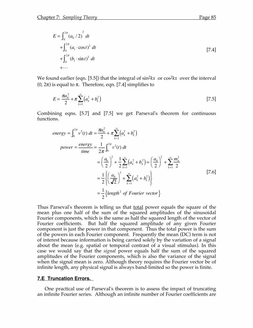
Chapter 7: Sampling Theory Page 85
E = (a0 / 2)0
2π
∫2dt
+ (a1 ⋅ cos t)2
0
2π
∫ dt
+ (b1 ⋅ sin t0
2π
∫ )2 dt
+
[7.4]
We found earlier (eqn. [5.5]) that the integral of sin2kx or cos2kx over the interval (0, 2π) is equal to π. Therefore, eqn. [7.4] simplifies to
E =πa02
2+π ak
2 + bk2( )
k=1
∞
∑ [7.5]
Combining eqns. [5.7] and [7.5] we get Parseval's theorem for continuous functions.
energy = v2(t) dt =0
2π
∫πa02
2+ π ak
2 + bk2( )
k=1
∞
∑
power = energytime
= 12π
v2(t) dt0
2π
∫
=a02
⎛ ⎝
⎞ ⎠
2
+12
ak2 + bk
2( )k=1
∞
∑ =a02
⎛ ⎝
⎞ ⎠
2
+mk2
2k=1
∞
∑
=12
a02
⎛ ⎝
⎞ ⎠
2
+ ak2 + bk
2( )k =1
∞
∑⎧ ⎨ ⎪
⎩ ⎪ ⎫ ⎬ ⎪
⎭ ⎪
= 12length2 of Fourier vector{ }
[7.6]
Thus Parseval's theorem is telling us that total power equals the square of the mean plus one half of the sum of the squared amplitudes of the sinusoidal Fourier components, which is the same as half the squared length of the vector of Fourier coefficients. But half the squared amplitude of any given Fourier component is just the power in that component. Thus the total power is the sum of the powers in each Fourier component. Frequently the mean (DC) term is not of interest because information is being carried solely by the variation of a signal about the mean (e.g. spatial or temporal contrast of a visual stimulus). In this case we would say that the signal power equals half the sum of the squared amplitudes of the Fourier components, which is also the variance of the signal when the signal mean is zero. Although theory requires the Fourier vector be of infinite length, any physical signal is always band-limited so the power is finite.
7.E Truncation Errors.
One practical use of Parseval's theorem is to assess the impact of truncating an infinite Fourier series. Although an infinite number of Fourier coefficients are
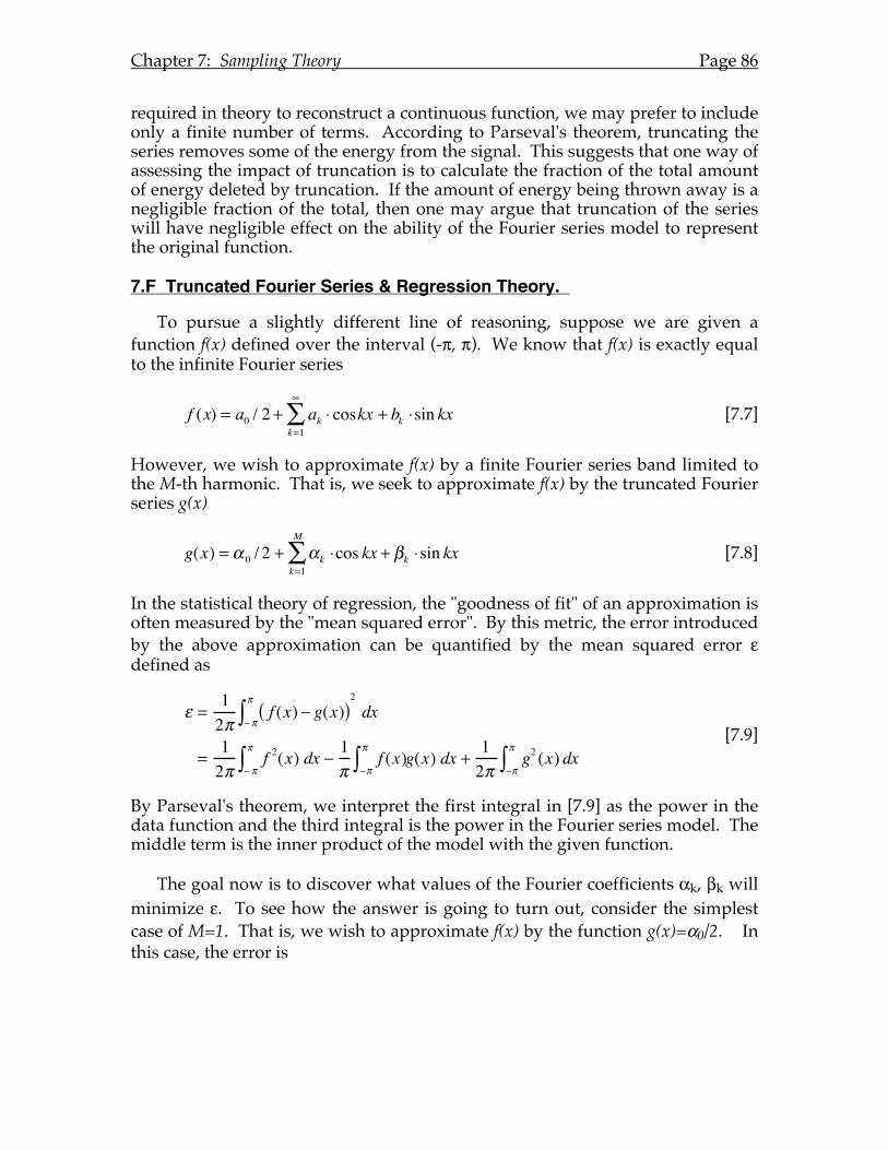
Chapter 7: Sampling Theory Page 86
required in theory to reconstruct a continuous function, we may prefer to include only a finite number of terms. According to Parseval's theorem, truncating the series removes some of the energy from the signal. This suggests that one way of assessing the impact of truncation is to calculate the fraction of the total amount of energy deleted by truncation. If the amount of energy being thrown away is a negligible fraction of the total, then one may argue that truncation of the series will have negligible effect on the ability of the Fourier series model to represent the original function.
7.F Truncated Fourier Series & Regression Theory.
To pursue a slightly different line of reasoning, suppose we are given a function f(x) defined over the interval (-π, π). We know that f(x) is exactly equal to the infinite Fourier series
f (x) = a0 / 2 + ak ⋅ coskx + bk ⋅sin kxk=1
∞
∑ [7.7]
However, we wish to approximate f(x) by a finite Fourier series band limited to the M-th harmonic. That is, we seek to approximate f(x) by the truncated Fourier series g(x)
g(x) = α 0 / 2 + αk ⋅cos kx + βk ⋅sin kxk=1
M
∑ [7.8]
In the statistical theory of regression, the "goodness of fit" of an approximation is often measured by the "mean squared error". By this metric, the error introduced by the above approximation can be quantified by the mean squared error ε defined as
ε =
12π
f (x) − g(x)( )− π
π
∫2
dx
=12π
f 2(x)− π
π
∫ dx − 1π
f (x)−π
π
∫ g(x) dx + 12π
g2 (x)−π
π
∫ dx [7.9]
By Parseval's theorem, we interpret the first integral in [7.9] as the power in the data function and the third integral is the power in the Fourier series model. The middle term is the inner product of the model with the given function.
The goal now is to discover what values of the Fourier coefficients αk, βk will minimize ε. To see how the answer is going to turn out, consider the simplest case of M=1. That is, we wish to approximate f(x) by the function g(x)=α0/2. In this case, the error is
Chapter 7: Sampling Theory Page 87
ε =
12π
f 2(x)− π
π
∫ dx − α 0
2πf (x)
−π
π
∫ dx + α02
4
= power in f (x) − α 0a02
+α 02
4
[7.10]
Adopting the standard approach to minimization problems of this kind, to minimize the error we must differentiate this quadratic eqn. [7.9] with respect to α0 , set the result to zero, and solve for α0. This yields
dεdα0
= −a02
+α 0
2= 0
∴α0 = a0
[7.11]
In words, this result shows that if we approximate f(x) by the function g(x)=constant, the constant which gives the best fit is just the first Fourier coefficient of f(x). In other words, the truncated Fourier series is also the "least squares estimate" of the function f(x).
Before accepting the above conclusion as being generally true, let us consider approximating f(x) by a 3-term Fourier series
g(x) = α 0 / 2 +α1 ⋅ cos x + β1 ⋅sin x [7.12]
Again we investigate the mean squared error
ε = power in f (x)
−1π
f (x)−π
π
∫ (α0 / 2 +α1 ⋅ cosx + β1 ⋅ sin x) dx
+ power in g(x)
[7.13]
The middle term generates three inner products between the given signal and each of the three components of the model. But these inner products are recognized as the definition of Fourier coefficients. Thus the error reduces to
ε = power in f (x)
−α0
2πf (x)
−π
π
∫ dx − α1
πf (x)
−π
π
∫ cos x dx − β1π
f (x)−π
π
∫ sin x dx
+α02
4+α12
2+β12
2
= constant − α0a02
−α1a1 − β1b1 +α02
4+α12
2+β12
2
[7.14]
Now we minimize this error first with respect to α0,
Chapter 7: Sampling Theory Page 88
∂ε∂α0
= −a02
+α 0
2= 0
α0 = a0
[7.15]
then with respect to α1,
∂ε∂α1
= −a1 + α1 = 0
∴α1 = a1 [7.16]
and then with respect to β1.
∂ε∂β1
= −b1 + β1 = 0
∴β1 = b1 [7.17]
Again we find that the truncated Fourier series is also the model which minimizes the mean squared error. Given these specific examples, we assert without further proof that the truncated Fourier series of a function is always the least-squares Fourier model for that function. The same holds true for a partial Fourier series (i.e. a series that is missing some terms) since the proof is essentially term-by-term.
Note that the inclusion of fundamental harmonics did not alter the value of the best constant determined in the first example. This result is due to the orthogonality of the basis functions in the Fourier series. Thus it is true in general that the best Fourier coefficient calculated for the k-th harmonic is independent of the calculation of any other coefficient. Other choices of fitting (i.e. basis) functions that are not mutually orthogonal, for example a polynomial or a Taylor series, do not have this nice property. Thus, when one models data with a polynomial or a Taylor series, the coefficients obtained depend upon the number of terms included in the series. This difficulty does not arise with a Fourier series model because the basis functions are orthogonal.
Our observation that a truncated Fourier series is also a least-squares Fourier model suggests a way to deal with two common situations for which sampled data are unequally spaced. First, data samples may be missing from an empirical record and second, the samples may have been obtained at irregular intervals. In both cases, a least-squares fit of basis functions (trigonometrical or complex exponential) to the data may be used to recover Fourier coefficients of interest. Least-squares algorithms are not as robust as the DFT, and operate one basis function at a time, but nevertheless are a commonly used method in such circumstances.
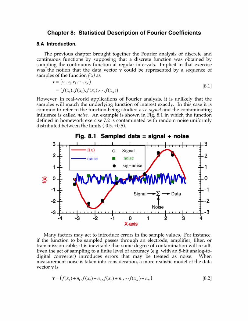
Chapter 8: Statistical Description of Fourier Coefficients
8.A Introduction.
The previous chapter brought together the Fourier analysis of discrete and continuous functions by supposing that a discrete function was obtained by sampling the continuous function at regular intervals. Implicit in that exercise was the notion that the data vector v could be represented by a sequence of samples of the function f(x) as
[8.1]
However, in real-world applications of Fourier analysis, it is unlikely that the samples will match the underlying function of interest exactly. In this case it is common to refer to the function being studied as a signal and the contaminating influence is called noise. An example is shown in Fig. 8.1 in which the function defined in homework exercise 7.2 is contaminated with random noise uniformly distributed between the limits (-0.5, +0.5).
Many factors may act to introduce errors in the sample values. For instance, if the function to be sampled passes through an electrode, amplifier, filter, or transmission cable, it is inevitable that some degree of contamination will result. Even the act of sampling to a finite level of accuracy (e.g. with an 8-bit analog-to-digital converter) introduces errors that may be treated as noise. When measurement noise is taken into consideration, a more realistic model of the data vector v is
[8.2]
v = v1, v2,v3 ,!,vN( )= f (x1), f (x2 ), f (x3 ),!, f (xN )( )
Signal !
Noise
Data
v = f (x1 ) + n1, f (x2 ) + n2 , f (x3) + n3,! f (xN ) + nN( )
Chapter 8: Statistical Description of Fourier Coefficients Page 90
where each of the nj represents a different sample of noise added to the signal f(x). The central question of this chapter is: What happens to the Fourier coefficients associated with f(x) when the signal is contaminated with noise? 8.B Statistical Assumptions.
In order to examine the effect of noise on Fourier coefficients, we must know something about the statistical nature of the noise process. Of all the different types of noise that occur in nature, the simplest and most tractable from a mathematical point of view has the following two properties:
1. The noise is additive. In other words, as indicated in eqn. [8.2], the sample value is equal to the linear sum of the signal being sampled plus the noise.
2. Each sample of noise nj is drawn independently from a noise process (or population) of mean zero and variance σ2.
For the purposes of this introductory course, we will assume that these two conditions are met.
One of the implications of these two assumptions is that the noise is independent of the signal. Two random events A & B are independent if occurrence of one has no influence on the probability of occurrence of the other. Using conditional probability notation, independence means P(B|A)=P(B). In the present context, independence implies the noise does not get larger or smaller just because the signal gets larger or smaller. Another implication is that each sample of noise is drawn from a population that has the same statistical properties as all of the other noise samples. That is, in the jargon of statisticians, the noise value nj is called a random variable and the collection of these random variables is said to be independent and identically distributed. This is in contrast to a case where, say, the noise is larger at the end of an experiment than it was at the beginning, which would violate the assumption of identically distributed noise. Conversely, dependence is evident if the value of noise at time t2 depends on the noise at some previous time t1.
Since each sample point vj in the data vector is assumed to be the sum of a deterministic signal f(xj) and a sample nj of random noise, this means that vj must also be treated as a random variable. Furthermore, since the noise has zero mean and the noise is additive, that implies the mean (or theoretical “expected value”) of vj is equal to f(xj). Since the signal is assumed to be noise-free, the variance of vj is equal to the variance σ 2 of the noise. We write these conclusions mathematically as
vj = f (x j ) + nj (sample = signal + noise) v j = f (x j ) (sample mean = signal) Var(vj ) = σ 2 (sample variance = noise variance) [8.3]
Chapter 8: Statistical Description of Fourier Coefficients Page 91
The technical terms uncorrelation, independence, and orthogonality describe a hierarchy of disconnectedness between two random variables. Random variables A and B are uncorrelated if the expected value of their product equals the product of their individual expectations, E(AB) = E(A) E(B). The two variables are orthogonal if the expected value of their product is zero, E(AB)=0. The two variables are independent if their joint probability equals the product of their individual probabilities, P(A,B)=P(A)P(B). Being uncorrelated is a much weaker condition than independence because it depends only on mean behavior whereas independence depends on all possible values of A and B. If two random variables are independent then they are uncorrelated and, conversely, if two variables are correlated they must be dependent. Thus it is possible for two statistically dependent variables to be uncorrelated. Jointly Gaussian random variables are an important exception to this rue, for in this special case uncorrelated is equivalent to independence.
Another way to envision the difference between correlation and orthogonality is to consider a realization of the random variables. If a random variable A is sampled D times, the resulting vector of sample values (i.e. a realization) can be represented geometrically by a point in D-dimensional space. Similarly, D samples of random variable B are also represented by a point in D-dimensional space. If A and B are orthogonal variables, then the vector from the origin to A should be (on average) perpendicular to the vector from the origin to B, which means the inner product of the two realizations equals zero, which is another way of saying E(AB)=0. Envisioning correlation is similar, but the vectors are first centered relative to their own means. This is achieved by subtracting the mean of the elements in vector A from each element of A to produce a “centered” data vector. Vector B is centered in the same way and then both vectors are drawn in D-dimensional space. If the two centered vectors are perpendicular, the underlying variables A and B are uncorrelated. Since centering can change the angle between the two vectors, the raw data vectors can be perpendicular but when centered they have some oblique angle. In that case the variables A and B are orthogonal but correlated. Conversely, the raw data vectors can be oblique to each other but when centered they become perpendicular, in which case A and B are not orthogonal but are uncorrelated. A third case is when the raw vectors are perpendicular and remain perpendicular when centered, in which case A and B are both orthogonal and uncorrelated.
Although the noise values at time j are assumed to be statistically independent of the noise at time k, the corresponding data values will not be independent because the additive signal will introduce correlation between samples. For example, if a signal is strong at time t, then it is likely to remain strong at a slightly later time. Thus the sum of signal + noise at the earlier time will predict better than chance the sum of signal + noise at the later time. A practical example is predicting tomorrow’s weather by saying it will be the same as today. Of course variations will occur, but it is much more likely that weather on July 2 will be like the weather on July 1 than the weather on December 1.
Chapter 8: Statistical Description of Fourier Coefficients Page 92
8.C Mean and Variance of Fourier Coefficients for Noisy Signals.
Recall from eqns. [3.30] and [3.31] that the Fourier coefficients obtained for a data vector v are given for trigonometrical basis functions by
ak =
2D⋅ vj coskθ jj=0
D−1
∑ …θ j = 2π x j / L [3.30]
bk =
2D⋅ vj sin kθ jj=0
D−1
∑ …θ j = 2π x j / L [3.31]
and for complex exponential basis functions by
ck =
1D⋅ vj exp(ikθ j )j=0
D−1
∑ …θ j = 2π x j / L [4.23]
Now according to eqn. [8.3] each data vector is the sum of signal vector plus a noise vector. This means that the coefficients evaluated by eqns. [3.30, 3.31] may be considered as estimates of the true Fourier coefficients of the signal alone. To see this, we substitute the first equation in [8.3] into [3.30] to get
ˆ a k =2D⋅ f (xj ) + nj( )coskθ j
j= 0
D−1
∑
=2D⋅ f (xj )coskθ j
j= 0
D−1
∑ +2D⋅ nj coskθ j
j= 0
D−1
∑= ak + εk
[8.4]
where the variable â (pronounced a-hat) is the calculated Fourier coefficient. This result reveals that âk is an estimate of the true coefficient ak and is in error by the amount εk, the Fourier coefficient for the vector of noise samples. A similar result applies to the sine coefficients. The corresponding result for the complex coefficients is
ˆ c k =1D⋅ f (xj ) + nj( )exp(ikθ j )
j=0
D−1
∑
=1D⋅ f (xj )exp(ikθ j)
j=0
D−1
∑ +1D⋅ nj exp( ikθ j )
j=0
D−1
∑= ck + εk
[8.5]
The preceding development shows that estimated Fourier coefficients determined for noisy data are also random variables, so we would like to know the mean (i.e. expected value) and variance of these coefficients. Since each estimated Fourier coefficient is the sum of a constant (ak) and a random variable
Chapter 8: Statistical Description of Fourier Coefficients Page 93
(εk), variability in â is due entirely to the random error term εk. From the theory of probability we know that if Y is a random variable of mean µ and variance σ2, and if s is some scalar constant, then the new random variable Z=sY has mean sµ and variance s2σ2. This implies that the general term nj (2/D) cos(kθj) in eqn. [8.4] is a random variable with mean 0 and variance [σ (2/D) cos(kθj)]2 . Another result from probability theory is that if Y and Z are independent, identically distributed random variables of means µ, ν and variances σ2, τ2 respectively, then the new random variable W=Y+Z has mean µ+ν and variance σ2 + τ2 . In short, when random variables add their means add and their variances add. Applying this result to the second summation in eqn. [8.4] we see that εk is the sum of D random variables, each of which has mean 0 and variance (4σ2/D2)cos2kθ. Consequently, the mean of εk = 0 and variance of εk is given by
Var(εk ) = (4σ 2 / D2 )(coskθ j )2
j=0
D−1
∑ =4σ 2
D2 cos2 kθ jj=0
D−1
∑
=4σ 2
D2 ⋅D2=2σ 2
Dfor k ≠ 0
=4σ 2
D2 ⋅D =4σ 2
Dfor k = 0
[8.6]
The simplification of eqn. [8.6] is based on the fact that the squared length of the sampled cosine function is equal to D/2, except when k=0, in which case it equals D (see exercise 3.3). The emergence of k=0 as a special case is rather awkward mathematically. It could be avoided by rescaling the a0 coefficient by √2 for the purpose of computing variance as was done in connection with Parseval's theorem (see eqn. [7.6]).
For the complex Fourier coefficients, the general term (1 / D)exp(ikθ j )nj is a
random variable with mean 0 and variance (1 / D) exp(ikθ j )( )2σ 2 . The sum of D such random variables, gives the following formula for noise variance
Var(ε k) =
σ 2
D2 exp(ikθ j )( )2j=0
D−1
∑
=σ 2
D2 ⋅D =σ 2
D
[8.6a]
One advantage of the complex Fourier coefficients is that the contant term is not a special case.
Given these results, we can now provide values for the first two statistical moments of the estimated Fourier coefficients. From eqn. [8.4] we know that the random variable âk is the sum of the deterministic coefficient ak and the random variable εk with zero mean and variance given by eqn. [8.6]. Consequently,
Chapter 8: Statistical Description of Fourier Coefficients Page 94
Mean( ˆ a k ) = ak
Var( ˆ a k ) = 2σ 2
Dfor k ≠ 0
=4σ 2
Dfor k = 0
[8.7]
and similar equations hold for estimates of the sine coefficients. The corresponding equation for complex Fourier coefficients is
Mean( ˆ c k) = ck
Var( ˆ c k) =σ 2
D [8.7a]
Notice that since the variance of a0 is 4σ2/D then the variance of a0 /2 , which is to say the variance of the mean, equals σ2/D and so the standard deviation of the mean is σ/√D. (This result is more obvious for c0.) This is a familiar result from elementary statistics. In statistics the standard deviation of the mean of D data values is usually called the standard error of the mean and is equal to σ/√D, where σ is the standard deviation of the population from which the data are drawn.
In summary, under the assumption of additive, independent noise, the variances of all the trigonometric Fourier coefficient estimates (except a0 ) are equal to the noise variance times 2/D. The variances of all the complex Fourier coefficient estimates are equal to the noise variance times 1/D. This suggests one way to reduce the variance of the estimate is to increase D, the number of sample points. A figure of merit called the signal-to-noise ratio (SNR) is often used to quantify the reliability of a signal. The SNR of a particular Fourier coefficient could be taken as the ratio of the mean (for example, ck) to the standard deviation σ/√D. By this definition, the SNR=ck√D/σ of an estimated Fourier coefficient increases as √D and decreases in proportion to σ, the amount of noise.
8.D Probability Distribution of Fourier Coefficients for Noisy Signals.
The mean and variance are useful summary statistics of a random variable, but a more complete characterization is in terms of a probability distribution. Given a deterministic signal, the probability distribution of the Fourier coefficients calculated for D samples of a noisy waveform depend upon the probability distribution of the added noise. As is typically the case in the elementary analysis of noisy signals, we will assume from now on that the noise has the Gaussian (or normal) probability density, N(µ,σ2), of mean µ and variance σ2. Under this assumption, the probability P that the noise signal at any instant lies somewhere in the range (a,b) is given by the area under the Gaussian probability density function between these limits
Chapter 8: Statistical Description of Fourier Coefficients Page 95
P =1
σ 2πa
b
∫ exp(−(x − µ)2
2σ 2 ) dx [8.8]
Several justifications for the Gaussian assumption may be offered. First, many physical noise sources are well modeled by this particular probability function. This is not surprising because the central limit theorem of probability theory states that the sum of a large number of independent variables tends to Gaussian regardless of the probability distributions of the individual variables. Another reason is expediency: this assumption makes the current problem tractable. One result of probability theory is that the Gaussian distribution is closed under addition, which means that the weighted sum of any number of Gaussian random variables remains Gaussian. Since the random variable εk is the weighted sum of noise variables, if the noise is Gaussian then so are the estimates of the Fourier coefficients. In short, additive Gaussian noise produces Gaussian Fourier coefficients.
The Gaussian distribution has only two parameters, the mean and variance, which are known from the more general results of section 8.C above. Thus, we can summarize the preceding results by stating that the estimates of the Fourier coefficients are distributed as normal (i.e. Gaussian) random variables with the following means and variances (read "~N(a,b)" as "has a Normal distribution with mean a and variance b"):
ˆ a k ~ N(ak,2σ2 / D)
ˆ b k ~ N(bk,2σ2 / D)
ˆ c k ~ N(ck ,σ 2 / D) [8.9]
Another random variable of interest is the power in the k-th harmonic. It was shown in eqn. [7.6] that signal power is one-half the square of the (polar) amplitude. Therefore, the estimated signal power pk in the k-th harmonic is
pk = mk2 / 2 = ak
2 + bk2( ) / 2 = ck2 + c−k2 [8.10]
From probability theory we know that if X is a standardized Gaussian random variable with zero mean and unit variance, i.e. if X~N(0,1), then the variable Z=X2 is distributed as a chi-squared variable with 1 degree of freedom. That is, Z ~ χ2
1. This result is useful in the present context if we standardize our estimates of the Fourier coefficients in eqn. [8.9] by subtracting off the mean and dividing by the standard deviation. This means that the squared, standardized Fourier coefficients are distributed as χ2
ak − ak2σ 2 / D
⎛⎝⎜
⎞⎠⎟
2
χ12 and ck − ck
σ 2 / D
⎛⎝⎜
⎞⎠⎟
2
χ12 [8.11]
Chapter 8: Statistical Description of Fourier Coefficients Page 96
A similar statement holds for the bk and c-k coefficients. Now, from probability theory we also know that if random variables X and Y are both distributed as chi-squared with 1 degree of freedom, then the variable Z=X+Y is distributed as chi-squared with 2 degrees of freedom. This implies that
ak − ak( )2 + bk − bk( )22σ 2 / D
χ22 and
ck − ck( )2 + c−k − c−k( )2σ 2 / D
χ22 [8.12]
An important practical application of this last result is testing for the presence of signals at particular harmonic frequencies. In this case, a null-hypothesis that might be advanced is that the Fourier coefficients of the k-th harmonic are zero. Under this hypothesis, eqn. [8.12] simplifies to
ak( )2 + bk( )22σ 2 / D
χ22 and
ck( )2 + c−k( )2σ 2 / D
χ22 [8.13]
Combining this result with the definition of the signal power in eqn. [8.10] we see that
pkσ 2 / D
=Power in kth harmonicAverage noise power
χ22 = relative power of kth harmonic [8.14]
To interpret this last result, note that the denominator of the left side of eqn. [8.14] is the total power of the noise source divided by the number of Fourier coefficients determined. This interpretation comes from our understanding of Parseval's theorem given in eqn. [3.45] and the fact that σ2 is the expected value of the sample variance s2 obtained for any particular data vector comprised of D points sampled from the noise source. Thus, according to this interpretation, the denominator of [8.14] is the expected amount of noise power per coefficient, which is to say, the average power in the noise power spectrum. The ratio at the left is therefore the measured amount of power in the k-th harmonic, normalized by the average noise power. If we call this unitless quantity the relative power of the k-th harmonic, then eqn. [8.14] means that relative power in the kth harmonic is distributed as χ2 under the null hypothesis that there is zero signal power at the k-th harmonic.
In the next chapter we will make use of the result in eqn. [8.14] to construct a statistical test of the null hypothesis. In the meantime, it is worth recalling that the mean of a χ2 variable is equal to the number of degrees of freedom of the variable, and the variance is equal to twice the mean. Since signal power pk is a scaled χ2 variable under the null hypothesis, we know immediately that the standard deviation of pk (i.e. the square-root of the variance) is equal to the mean (eqn 8.15), which implies SNR=1 in this case. Usually such a low SNR is unacceptable, which calls for methods to improve the SNR described below.
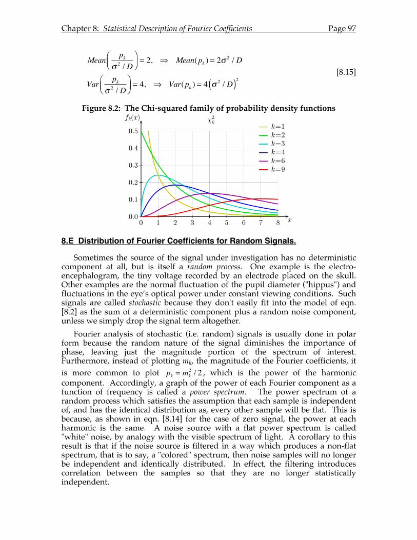
Chapter 8: Statistical Description of Fourier Coefficients Page 97
Mean pk
σ 2 / D⎛⎝⎜
⎞⎠⎟= 2, ⇒ Mean(pk ) = 2σ
2 / D
Var pkσ 2 / D
⎛⎝⎜
⎞⎠⎟= 4, ⇒ Var(pk ) = 4 σ 2 / D( )2
[8.15]
Figure 8.2: The Chi-squared family of probability density functions
8.E Distribution of Fourier Coefficients for Random Signals.
Sometimes the source of the signal under investigation has no deterministic component at all, but is itself a random process. One example is the electro-encephalogram, the tiny voltage recorded by an electrode placed on the skull. Other examples are the normal fluctuation of the pupil diameter ("hippus") and fluctuations in the eye’s optical power under constant viewing conditions. Such signals are called stochastic because they don't easily fit into the model of eqn. [8.2] as the sum of a deterministic component plus a random noise component, unless we simply drop the signal term altogether.
Fourier analysis of stochastic (i.e. random) signals is usually done in polar form because the random nature of the signal diminishes the importance of phase, leaving just the magnitude portion of the spectrum of interest. Furthermore, instead of plotting mk, the magnitude of the Fourier coefficients, it is more common to plot pk = mk
2 / 2 , which is the power of the harmonic component. Accordingly, a graph of the power of each Fourier component as a function of frequency is called a power spectrum. The power spectrum of a random process which satisfies the assumption that each sample is independent of, and has the identical distribution as, every other sample will be flat. This is because, as shown in eqn. [8.14] for the case of zero signal, the power at each harmonic is the same. A noise source with a flat power spectrum is called "white" noise, by analogy with the visible spectrum of light. A corollary to this result is that if the noise source is filtered in a way which produces a non-flat spectrum, that is to say, a "colored" spectrum, then noise samples will no longer be independent and identically distributed. In effect, the filtering introduces correlation between the samples so that they are no longer statistically independent.
Chapter 8: Statistical Description of Fourier Coefficients Page 98
At the end of section 8.D the observation was made that, in the absence of a deterministic signal, the standard deviation of pk is equal to the mean, which implies SNR=1. The meaning of "signal" in this context is the estimated value of pk , the power of the k-th harmonic component of the random signal. Typically such a low value of SNR is unacceptable and so means for improving the reliability are sought. One method is to repeat the process of sampling the waveform and computing the power spectrum. If M spectra are added together, the power at each harmonic will be the sum of M random variables, each of which is distributed as χ2 with 2 degrees of freedom. Thus, the total power will be distributed as χ2 with 2M degrees of freedom, for which the mean is 2M and the standard deviation is 2√M. Average power is the total power divided by M,
pk
1M
χ22
M∑
1M
χ2M2 [8.16]
for which the mean, variance and SNR are
[8.17]
We conclude, therefore, that the reliability of an estimated power spectrum for stochastic signals created by averaging M individual spectra increases in proportion to √M.
An equivalent technique is to average M sample vectors and then compute the power spectrum of the mean data vector. Since each component of the data vector increases in reliability in proportion to √M (because the standard error of the mean is inversely proportional to √M), so does the computed power spectrum.
8.F Signal Averaging.
A common method for studying system behavior is to force the system with a periodic stimulus and then measure the response. Any real system will invariably have a noisy response that makes each period of the response, or epoch, slightly different from every other epoch. Conceptually, there are two ways to approach Fourier analysis of such response waveforms. The first is to treat n epochs as one continuous response over an interval of length nL. The other way is to analyze each epoch separately. If the response waveform is sampled D times in each epoch, then both methods will produce nD Fourier coefficients. The difference is that in the first method the coefficients correspond to nD/2 different harmonics whereas in the second method they correspond to n
mean p k( ) =1M
! 2M = 2
variance p k( ) =1M
" #
$ %
2
! 4M =4M
SNR =meanvar iance
=2
2 / M= M
Chapter 8: Statistical Description of Fourier Coefficients Page 99
repetitions of the same D/2 harmonics. In many circumstances, most of the harmonics included in the first method are of no interest. Therefore, the second method provides an opportunity to estimate the statistical reliability of the coefficients measured. This is done in a straightforward manner called spectral averaging. Given n measures of coefficient ak, the mean of ak and the variance of ak can be calculated independently of all of the other coefficients. It should be noted that the mean of ak determined by spectral averaging will exactly equal the value of the coefficient for the corresponding frequency in the first method. This is because the value of the coefficient is found by forming the inner product of the sample values with the sampled sinusoid of interest. The inner product sums across sample points so it doesn't matter if the sums are done all at once (method 1) or on an epoch-by-epoch basis (method 2). Exercise 8.1 is a practical example that verifies this point.
Although it is easy to calculate the mean and variance of Fourier coefficients by the spectral averaging method, specifying the probability distributions of the Fourier coefficients is more awkward. Equation [8.10] says that the standardized coefficient is distributed as χ2 with 1 degree of freedom. This implies that the non-standardized distribution is a scaled, non-central χ2 distribution. Unfortunately the sum of n such random variables is not as easy to deal with. There is some comfort in the central limit theorem of probability theory which states that, regardless of the distribution of ak, the distribution of the mean of ak will become approximately Gaussian if n is large.
Another common way of analyzing multiple epochs is to average the data across epochs to produce a mean waveform which is then subjected to Fourier analysis. This method is called signal averaging. Exercise 8.1 demonstrates that the Fourier coefficients obtained this way are identical to the mean coefficients obtained by spectral averaging. This result is a consequence of Fourier analysis being a linear operation. It does not matter whether one averages the data first followed spectral analysis, or the other way around, spectral analysis followed by averaging.

Chapter 8: Statistical Description of Fourier Coefficients Page 100
Chapter 9: Hypothesis Testing for Fourier Coefficients
9.A Introduction.
In Chapter 8 we looked at Fourier coefficients from a new viewpoint. Although a Fourier series consisting of D terms will fit a discrete data function exactly at D sample points, this series may still not represent a physical system correctly because of measurement errors in the original data values. Thus, from a statistical point of view, the computed Fourier coefficients are merely estimates of the true values that would have been obtained had there been no contamination by noise factors. Because of the presence of noise, these computed coefficients will rarely equal zero when coefficients of the underlying signal is zero. For example, a square wave in sine phase has only odd harmonic components but when noise is added to the square wave the computed coefficients will not necessarily be zero for the even harmonics. Since the ultimate purpose of Fourier analysis is typically to create a reasonable model of the system under study, it becomes important to develop strategies for deciding whether a particular harmonic term is to be omitted from the model on the grounds that noise alone could account for the particular value computed for the coefficient . In other words, we seek methods for testing the null hypothesis that a particular Fourier coefficient is equal to zero.
The problem dealt with in this chapter is similar to that encountered in Chapter 7. There we were investigating the consequences of omitting certain terms from an exact Fourier series model of a deterministic function. We found that although deleting terms introduces error into the model, the amount of error introduced cannot be made any smaller by adjusting the coefficients of the remaining terms in the Fourier series. In other words, the truncated Fourier-series model minimizes the mean squared error. Now we have a slightly different problem wherein the error in the model is caused not by deleting terms but by the inclusion of additive, Gaussian noise that contaminates the data.
A more general problem is to use repeated measures of a vector of Fourier coefficients to determine whether the mean vector is different from a given vector. The given vector might be zero, in which case the question is essentially this: is there any signal at all in the data, or is there only noise? A strategy for dealing with this problem is discussed in section 9E.
9.B Regression analysis.
In the statistical theory of regression, a common method for approaching the "goodness of fit" of a model is to investigate the statistic S defined by the ratio
S =variance of data accounted for by model
residual variance [9.1]
The basic idea here is that the reason a recorded waveform has variance (i.e., is not just a constant) is because of two factors: some underlying, deterministic function and random error. In linear regression, for example, the underlying
Chapter 9: Hypothesis Testiong for Fourier Coefficients Page 102
deterministic function is assumed to be a straight line, which has two free parameters: slope and intercept. Such a model predicts a certain amount of variance in the data (the numerator in [9.1]) but some residual variance is not accounted for by the model (the denominator of [9.1]). If S is large, the implication is that the model is acceptable because it does a good job of accounting for the variance in the data. In the context of Fourier analysis, the words we introduced in Chapter 8 for these two factors which introduce variance were: signal and noise. Thus, the statistic S is very much like the SNR defined earlier since the numerator is a measure of the strength of the underlying signal and the denominator depends upon the amount of noise present.
The use of a summary statistic such as S to test an hypothesis about the adequacy of a model is called a "parametric test" in statistics. In order to develop useful tests of this kind, one needs to know the probability distribution of S. Perhaps the most widely known distribution of this kind is Snedecor's F-distribution (named in honor of Sir R.A. Fisher) that applies when the numerator of eqn. [9.1] is a χ2 variable with a degrees of freedom, divided by a, and the denominator is a χ2 variable with b degrees of freedom, divided by b. That is,
χa2 / a
χb2 / b
~ Fa,b [9.2]
Given the results of Chapter 8 in which it was shown that harmonic power is distributed as χ2 when Gaussian noise alone is present, it should not be surprising to find that an F-test can sometimes be used to test the goodness of fit of a Fourier series model. Hartley (1949) was first to develop such a test and his method is described below.
We know from the version of Parseval's theorem given in eqn. [3.45] that the variance of D sample points is equal to the sum of the powers of the corresponding harmonic components.
Var(Y ) = 1D
Yk2
k=1
D
∑ − m2 =12
ak2
k=1
D /2
∑ + bk2 = ck
2
k≠0∑ = pk
k=1
D /2
∑ [3.45]
Therefore, if the Fourier model under consideration included all D harmonic components, then it would account for all of the variance of the data, there would be zero residual variance, and the model would fit the data exactly. On the other hand, if only some of the harmonics are included in the model, then the harmonics omitted would account for the residual variance. In this case, we can create a statistic like S to decide if the model is still adequate.
To see how this would work, suppose that we include only the k-th harmonic in the Fourier model. In other words, assume all of the other harmonics are noise. According to eqn. [3.45] above, the variance accounted for by this model would be pk. We found earlier in eqn. [8.14] that if we normalize pk by dividing
Chapter 9: Hypothesis Testiong for Fourier Coefficients Page 103
by the expected amount of power under the null hypothesis that only noise is present, then the "relative power" is distributed as χ2 with 2 degrees of freedom.
pkσ 2 / D
~ χ22 [9.3]
Clearly this quantity would serve well as the numerator of an F-statistic. To get the necessary denominator, recall that there would be D-3 residual harmonics in this case. The total amount of relative power in these residuals is the sum of R=(D-3)/2 random variables, each of which is χ2 with 2 degrees of freedom, which is therefore distributed as χ2 with 2R = D-3 degrees of freedom
pj
σ 2 / Dj=1
R
∑ ~ χ2 R2 [9.4]
Now to formulate Hartley's statistic, we divide each of these variables by their respective number of degrees of freedom and form their ratio
H =
pk2σ 2 / D
12R
pjσ 2 / Dj=1
R
∑=
relative power in k-th harmonic/DoFaverage rel. power in residuals/DoF
~ F2,2R [9.5]
Fortunately, the unknown quantity σ appears in both the numerator and denominator and therefore cancels out to leave
H =pk
1R
pjj≠ k∑
~ F2,2R [9.6]
Thus, Hartley's test of the null hypothesis that the signal power in the k-th harmonic is zero is would be to reject the null hypothesis if H > critical value of F2,2R for significance level α. To administer this test for a chosen significance level (typically 5% or 1%), look up the critical value of F in tables of the F-distribution. If the computed test statistic is larger than the tabulated critical value, reject the null hypothesis that the signal power in this harmonic is zero. The significance level is interpreted as the probability of falsely rejecting the null hypothesis.
An example of a signal with additive Gaussian noise is shown in Fig. 9.1A and its magnitude spectrum is shown in Fig. 9.1B. The data vector and vector of complex Fourier coefficients for this dataset (D=11) are given in Table 9.1. The total variance in the data is 1.49, computed either from the Fourier coefficients (excluding the constant term, c0) or directly from the data values. The variance in the harmonic with greatest power, which is the fundamental in this example, is 0.57 and so Hartley's statistic has the value H=0.57/[(1.49-0.57)/4]=2.48, which is not significant compared to the tabulated F-statistic (4.46) at the α=0.05 level,
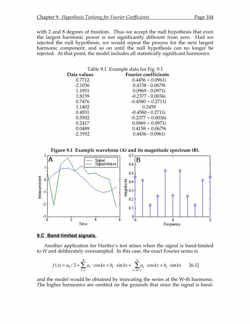
Chapter 9: Hypothesis Testiong for Fourier Coefficients Page 104
with 2 and 8 degrees of freedom. Thus we accept the null hypothesis that even the largest harmonic power is not significantly different from zero. Had we rejected the null hypothesis, we would repeat the process for the next largest harmonic component, and so on until the null hypothesis can no longer be rejected. At that point, the model includes all statistically significant harmonics.
Table 9.1 Example data for Fig. 9.1
Data values Fourier coefficients 0.7712 0.4456 + 0.0961i -2.1036 0.4158 - 0.0679i 1.1951 0.0969 - 0.0971i 1.8159 -0.2377 - 0.0036i 0.7476 -0.4580 + 0.2711i 1.1402 0.2459 0.4931 -0.4580 - 0.2711i 0.5502 -0.2377 + 0.0036i 0.2417 0.0969 + 0.0971i 0.0489 0.4158 + 0.0679i -2.1952 0.4456 - 0.0961i
Figure 9.1 Example waveform (A) and its magnitude spectrum (B).
9.C Band-limited signals.
Another application for Hartley's test arises when the signal is band-limited to W and deliberately oversampled. In this case, the exact Fourier series is
f (x) = a0 / 2 + ak ⋅ coskx + bk ⋅sin kxk=1
W
∑ + ak ⋅ coskx + bk ⋅sin kxk=W +1
N
∑ [6.1]
and the model would be obtained by truncating the series at the W-th harmonic. The higher harmonics are omitted on the grounds that since the signal is band-
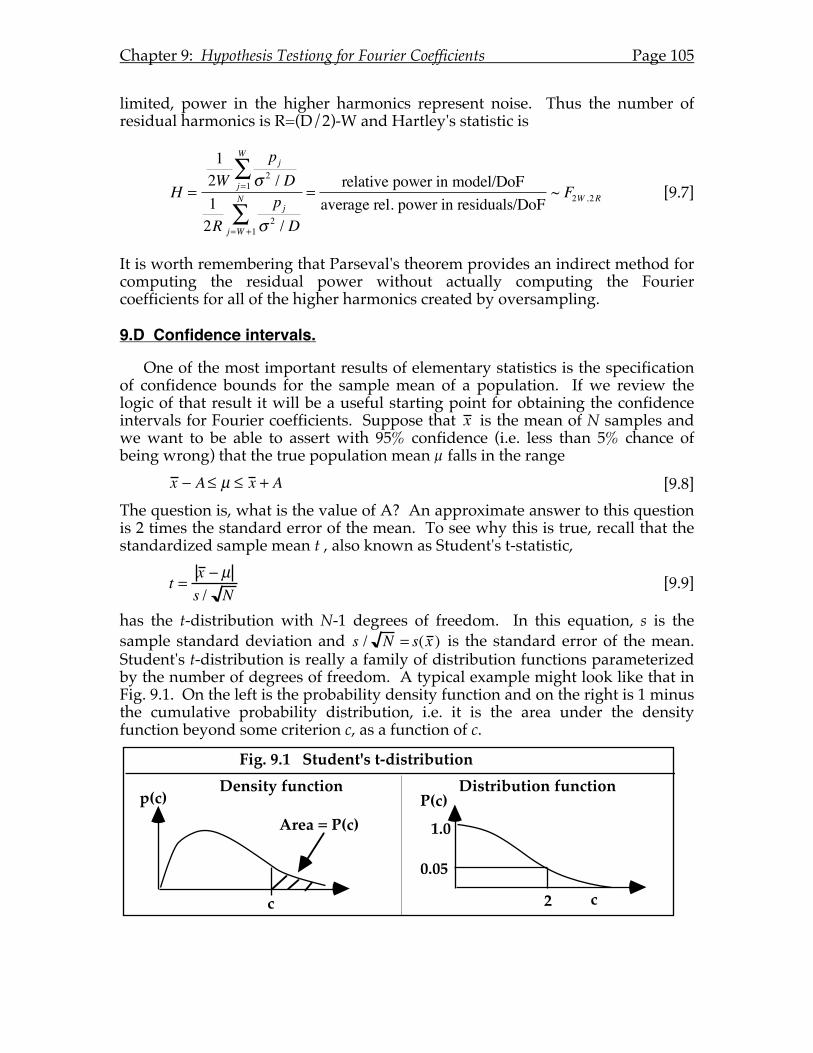
Chapter 9: Hypothesis Testiong for Fourier Coefficients Page 105
limited, power in the higher harmonics represent noise. Thus the number of residual harmonics is R=(D/2)-W and Hartley's statistic is
H =
12W
pjσ 2 / Dj=1
W
∑1
2Rpj
σ 2 / Dj=W +1
N
∑=
relative power in model/DoFaverage rel. power in residuals/DoF
~ F2W ,2R [9.7]
It is worth remembering that Parseval's theorem provides an indirect method for computing the residual power without actually computing the Fourier coefficients for all of the higher harmonics created by oversampling.
9.D Confidence intervals.
One of the most important results of elementary statistics is the specification of confidence bounds for the sample mean of a population. If we review the logic of that result it will be a useful starting point for obtaining the confidence intervals for Fourier coefficients. Suppose that x is the mean of N samples and we want to be able to assert with 95% confidence (i.e. less than 5% chance of being wrong) that the true population mean µ falls in the range
x − A≤ µ ≤ x + A [9.8] The question is, what is the value of A? An approximate answer to this question is 2 times the standard error of the mean. To see why this is true, recall that the standardized sample mean t , also known as Student's t-statistic,
t = x − µs / N
[9.9]
has the t-distribution with N-1 degrees of freedom. In this equation, s is the sample standard deviation and s / N = s(x ) is the standard error of the mean. Student's t-distribution is really a family of distribution functions parameterized by the number of degrees of freedom. A typical example might look like that in Fig. 9.1. On the left is the probability density function and on the right is 1 minus the cumulative probability distribution, i.e. it is the area under the density function beyond some criterion c, as a function of c.
Fig. 9.1 Student's t-distribution
Density function Distribution function
c
P(c)
c
1.0
0.05
2
Area = P(c)
p(c)
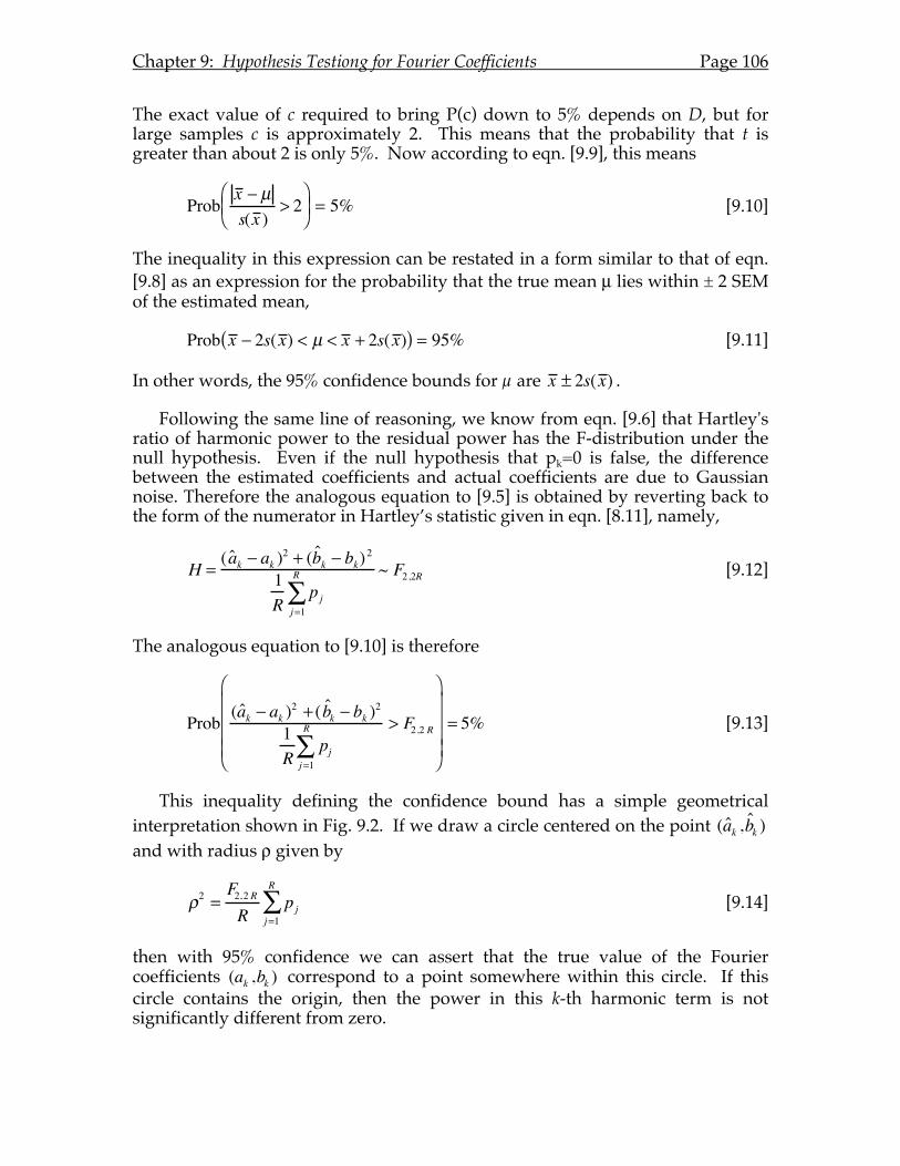
Chapter 9: Hypothesis Testiong for Fourier Coefficients Page 106
The exact value of c required to bring P(c) down to 5% depends on D, but for large samples c is approximately 2. This means that the probability that t is greater than about 2 is only 5%. Now according to eqn. [9.9], this means
Prob x − µs(x )
> 2⎛ ⎝ ⎜
⎞ ⎠ ⎟ = 5% [9.10]
The inequality in this expression can be restated in a form similar to that of eqn. [9.8] as an expression for the probability that the true mean µ lies within ± 2 SEM of the estimated mean,
Prob x − 2s(x ) < µ < x + 2s(x )( ) = 95% [9.11]
In other words, the 95% confidence bounds for µ are x ± 2s(x ) .
Following the same line of reasoning, we know from eqn. [9.6] that Hartley's ratio of harmonic power to the residual power has the F-distribution under the null hypothesis. Even if the null hypothesis that pk=0 is false, the difference between the estimated coefficients and actual coefficients are due to Gaussian noise. Therefore the analogous equation to [9.5] is obtained by reverting back to the form of the numerator in Hartley’s statistic given in eqn. [8.11], namely,
H =( ˆ a k − ak )2 + ( ˆ b k − bk)2
1R
pjj=1
R
∑~ F2,2R [9.12]
The analogous equation to [9.10] is therefore
Prob ( ˆ a k − ak )2 + ( ˆ b k − bk )2
1R
pjj =1
R
∑> F2,2 R
⎛
⎝
⎜ ⎜ ⎜ ⎜
⎞
⎠
⎟ ⎟ ⎟ ⎟
= 5% [9.13]
This inequality defining the confidence bound has a simple geometrical interpretation shown in Fig. 9.2. If we draw a circle centered on the point ( ˆ a k , ˆ b k ) and with radius ρ given by
ρ2 =F2,2 RR
pjj=1
R
∑ [9.14]
then with 95% confidence we can assert that the true value of the Fourier coefficients (ak ,bk ) correspond to a point somewhere within this circle. If this circle contains the origin, then the power in this k-th harmonic term is not significantly different from zero.
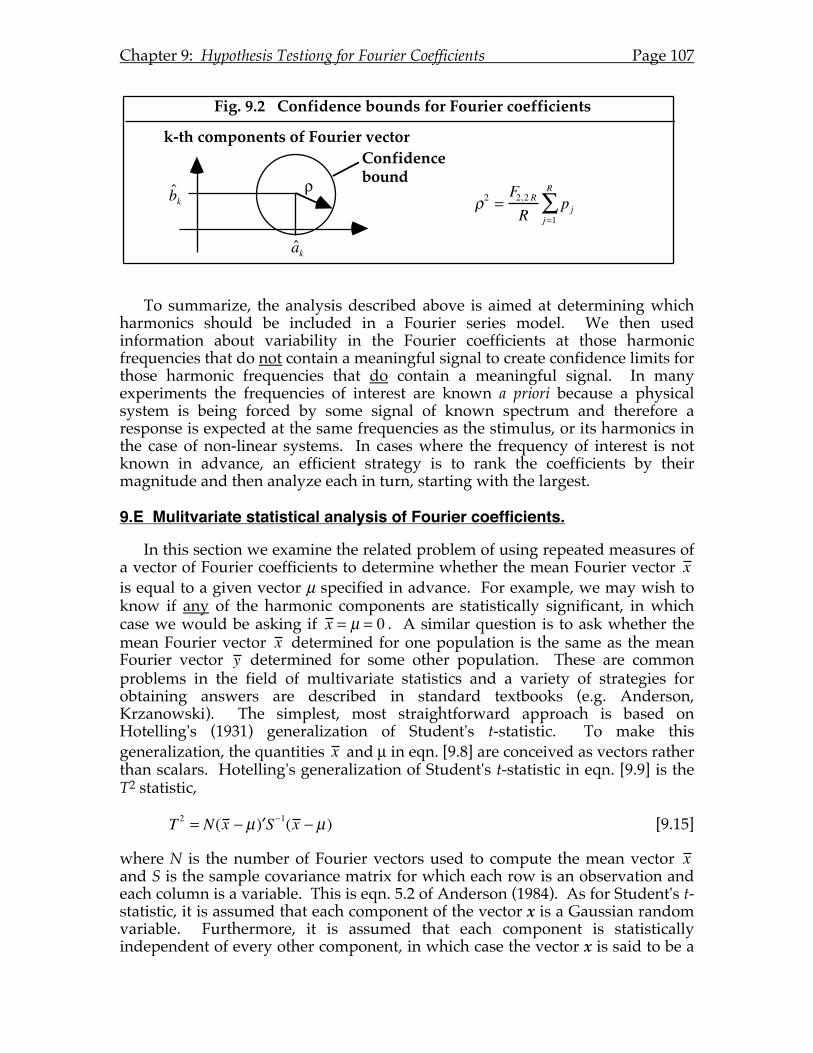
Chapter 9: Hypothesis Testiong for Fourier Coefficients Page 107
To summarize, the analysis described above is aimed at determining which harmonics should be included in a Fourier series model. We then used information about variability in the Fourier coefficients at those harmonic frequencies that do not contain a meaningful signal to create confidence limits for those harmonic frequencies that do contain a meaningful signal. In many experiments the frequencies of interest are known a priori because a physical system is being forced by some signal of known spectrum and therefore a response is expected at the same frequencies as the stimulus, or its harmonics in the case of non-linear systems. In cases where the frequency of interest is not known in advance, an efficient strategy is to rank the coefficients by their magnitude and then analyze each in turn, starting with the largest.
9.E Mulitvariate statistical analysis of Fourier coefficients.
In this section we examine the related problem of using repeated measures of a vector of Fourier coefficients to determine whether the mean Fourier vector x is equal to a given vector µ specified in advance. For example, we may wish to know if any of the harmonic components are statistically significant, in which case we would be asking if x = µ = 0 . A similar question is to ask whether the mean Fourier vector x determined for one population is the same as the mean Fourier vector y determined for some other population. These are common problems in the field of multivariate statistics and a variety of strategies for obtaining answers are described in standard textbooks (e.g. Anderson, Krzanowski). The simplest, most straightforward approach is based on Hotelling's (1931) generalization of Student's t-statistic. To make this generalization, the quantities x and µ in eqn. [9.8] are conceived as vectors rather than scalars. Hotelling's generalization of Student's t-statistic in eqn. [9.9] is the T2 statistic,
T 2 = N(x − µ ′ ) S−1(x − µ) [9.15]
where N is the number of Fourier vectors used to compute the mean vector x and S is the sample covariance matrix for which each row is an observation and each column is a variable. This is eqn. 5.2 of Anderson (1984). As for Student's t-statistic, it is assumed that each component of the vector x is a Gaussian random variable. Furthermore, it is assumed that each component is statistically independent of every other component, in which case the vector x is said to be a
Fig. 9.2 Confidence bounds for Fourier coefficients
k-th components of Fourier vector
ˆ a k
ˆ b k
Confidence bound!
!2 =F2,2 R
Rpj
j=1
R
"
Chapter 9: Hypothesis Testiong for Fourier Coefficients Page 108
multivariate Gaussian random process. Given these assumptions, Hotelling's T2 statistic is directly proportional to an F-statistic.
To test the hypothesis that the mean vector is equal to a given vector, x = µ , we first compute T2 according to eqn. [9.15]. Next, we compute an F-statistic as
Fdf1, df 2 =T 2
N −1df 2df1
(see Matlab program T2OneMean.m} [9.16]
where the lesser degree of freedom df1 = D is the length of the Fourier vector x and the greater degree of freedom is df 2 = N −D . For this test to be valid the number of Fourier vectors N must exceed the number of samples D used to compute each vector. If the value of this F-statistic is greater than the tabulated critical value of the F-distribution for the given degrees of freedom and specified significance level α, then we may reject the hypothesis that x = µ . Specifying the confidence region for the mean vector is harder. Geometrically we can interpret the mean vector x as a point in D-dimensional space. Thus the confidence region is a closed ellipsoid in this hyperspace, centered on the mean. An equation defining this ellipsoid is provided by Anderson (eqn. 11, p. 165). We can assert with confidence 1-α that the true mean lies somewhere inside this ellipsoid. If attention is focused on a single harmonic frequency, then the confidence region reduces to an ellipse in the 2-dimensional space of Fig. 9.2. We have assumed that variability in the measured Fourier coefficients is due to additive, Gaussian noise that is independent of the signal being measured, so the Fourier coefficients will be uncorrelated Gaussian random variables. Consequently, the confidence ellipse will reduce to a circular region. An alternative method for computing the radius of this circular confidence region has been described by Victor and Mast (1991) in terms of their novel statistic Tcirc
2 .
To test the hypothesis that the mean vector x computed from a sample size N1 is equal to a different vector y computed from a sample size N2, we first compute the T2 statistic
T 2 =N1N2
N1 + N2
(x − y ′ ) S−1(x − y ) (see Matlab program T2TwoMeans) [9.17]
Next we compute an F-statistic as
Fdf1, df 2 =T 2
N1 + N2 − 2df 2df1
[9.18]
where the lesser degree of freedom df1 = D is the common length of the two Fourier vectors and the greater degree of freedom is df 2 = N1 + N2 −D −1. If the value of this statistic is greater than the tabulated F-distribution for the given degrees of freedom and chosen significance level α, then we may reject the hypothesis that the two mean vectors of Fourier coefficients are equal.
Chapter 10: Directional Data Analysis
10.A Introduction.
In previous chapters we conceived of a data vector as being an ordered list of numbers. We have seen that the methods of Fourier analysis apply equally well regardless of whether these numbers are real-valued (i.e. scalars) or complex-valued (i.e. 2-D vectors). In this chapter we devote special attention to a class of data which falls somewhere in between the real-valued and the complex-valued. These are 2-D vectors for which the magnitude portion of the vector has no meaning or interest. In other words, we wish to examine data for which only the direction is important. Some examples are the perceived direction of motion of a visual object, the preferred directions of retinal ganglion cells, and the axis of electric dipole generators of the visually-evoked cortical potential.
A separate branch of statistics has evolved to deal with directional data in such diverse fields of biology, geology, and physiology. The primary difference between directional data and other univariate data is that directional data are plotted on a circle rather than the real line. Consequently, directional data are periodic and therefore the formulas devised for calculating simple measures of central tendency and dispersion of data bear a striking resemblance to the formulas of Fourier analysis. This resemblance permits a Fourier interpretation of directional data analysis that reveals the close relationship between these two different methods of data analysis.
10.B Mean direction and concentration about the mean.
Consider the problem of finding the mean of the two compass readings: 5° and 355°. Since both of these directions are very close to the northerly direction, the mean should also be northerly. However, the arithmetic average of the two values is 180°, which is due south. Furthermore, the standard deviation of these two numbers is 175°, which is much larger than is reasonable for two directions which are nearly the same. Clearly a different method of computing the mean and spread of directional data is required if we are to obtain reasonable results. The method devised by Batschelet (1972) and by Mardia (1972) is illustrated in Fig. 10.1 below. The idea is to treat individual directions as the angle made by a unit vector with the horizontal, which may be treated as a unit phasor in the complex plane. Now suppose that these data Ui are summed according to the ordinary rules of vector addition (or summation of complex numbers) and the resultant divided by the number of data points according to the equation
B =1n
Uii=1
n
∑ [10.1]
where Ui is the i-th unit vector, n is the number of vectors summed, and B is the normalized resultant of the vector sum. In the particular example shown, B is a vector of length 0.996 in the horizontal direction. Thus the direction of B is the obvious choice for defining the mean direction while the length of B provides a
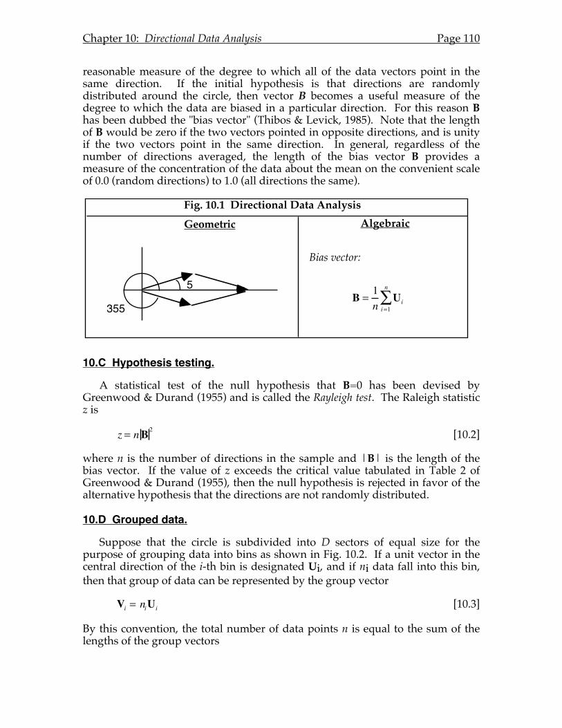
Chapter 10: Directional Data Analysis Page 110
reasonable measure of the degree to which all of the data vectors point in the same direction. If the initial hypothesis is that directions are randomly distributed around the circle, then vector B becomes a useful measure of the degree to which the data are biased in a particular direction. For this reason B has been dubbed the "bias vector" (Thibos & Levick, 1985). Note that the length of B would be zero if the two vectors pointed in opposite directions, and is unity if the two vectors point in the same direction. In general, regardless of the number of directions averaged, the length of the bias vector B provides a measure of the concentration of the data about the mean on the convenient scale of 0.0 (random directions) to 1.0 (all directions the same).
10.C Hypothesis testing.
A statistical test of the null hypothesis that B=0 has been devised by Greenwood & Durand (1955) and is called the Rayleigh test. The Raleigh statistic z is
z = nB2 [10.2]
where n is the number of directions in the sample and |B| is the length of the bias vector. If the value of z exceeds the critical value tabulated in Table 2 of Greenwood & Durand (1955), then the null hypothesis is rejected in favor of the alternative hypothesis that the directions are not randomly distributed.
10.D Grouped data.
Suppose that the circle is subdivided into D sectors of equal size for the purpose of grouping data into bins as shown in Fig. 10.2. If a unit vector in the central direction of the i-th bin is designated Ui, and if ni data fall into this bin, then that group of data can be represented by the group vector
Vi = niUi [10.3]
By this convention, the total number of data points n is equal to the sum of the lengths of the group vectors
Fig. 10.1 Directional Data Analysis
Geometric Algebraic
Bias vector:
355
5B =
1n
Uii=1
n
!
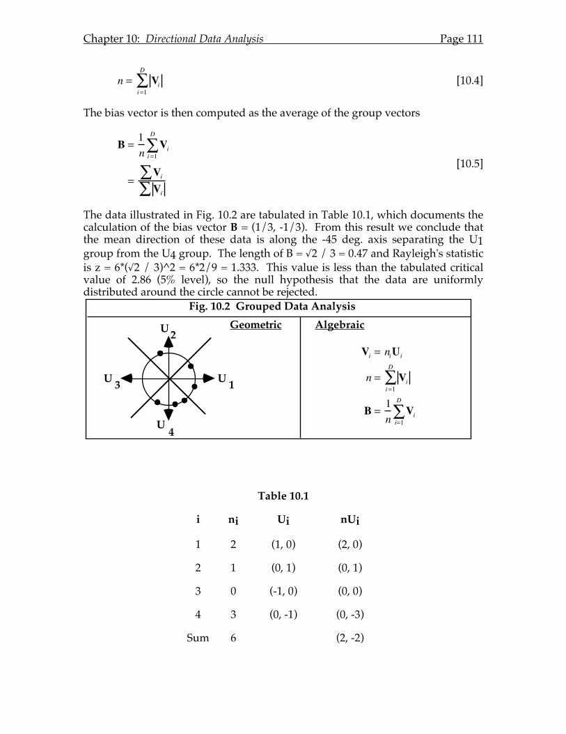
Chapter 10: Directional Data Analysis Page 111
n = Vii=1
D
∑ [10.4]
The bias vector is then computed as the average of the group vectors
B =
1n
Vii=1
D
∑
=Vi∑Vi∑
[10.5]
The data illustrated in Fig. 10.2 are tabulated in Table 10.1, which documents the calculation of the bias vector B = (1/3, -1/3). From this result we conclude that the mean direction of these data is along the -45 deg. axis separating the U1 group from the U4 group. The length of B = √2 / 3 = 0.47 and Rayleigh's statistic is z = 6*(√2 / 3)^2 = 6*2/9 = 1.333. This value is less than the tabulated critical value of 2.86 (5% level), so the null hypothesis that the data are uniformly distributed around the circle cannot be rejected.
Table 10.1
i ni Ui nUi
1 2 (1, 0) (2, 0)
2 1 (0, 1) (0, 1)
3 0 (-1, 0) (0, 0)
4 3 (0, -1) (0, -3)
Sum 6 (2, -2)
Fig. 10.2 Grouped Data Analysis
Geometric Algebraic
Vi = niUi
n = Vii=1
D
!
B =1n
Vii=1
D
!
2U
1U
4U
3U
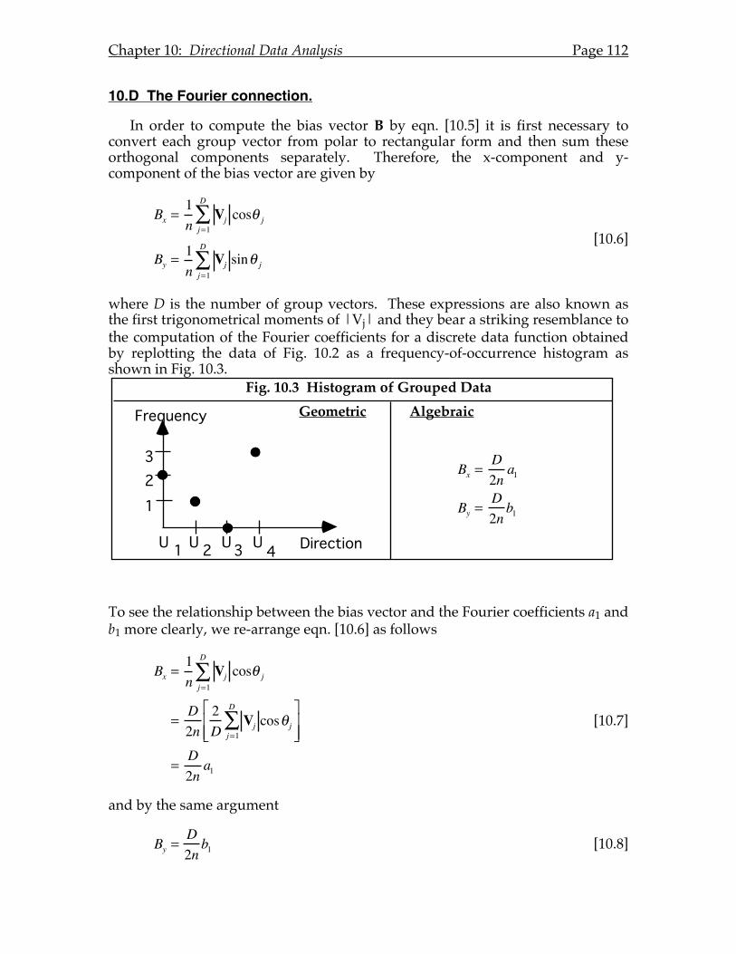
Chapter 10: Directional Data Analysis Page 112
10.D The Fourier connection.
In order to compute the bias vector B by eqn. [10.5] it is first necessary to convert each group vector from polar to rectangular form and then sum these orthogonal components separately. Therefore, the x-component and y-component of the bias vector are given by
Bx =
1n
Vj cosθ jj=1
D
∑
By =1n
Vj sinθ jj=1
D
∑ [10.6]
where D is the number of group vectors. These expressions are also known as the first trigonometrical moments of |Vj| and they bear a striking resemblance to the computation of the Fourier coefficients for a discrete data function obtained by replotting the data of Fig. 10.2 as a frequency-of-occurrence histogram as shown in Fig. 10.3.
To see the relationship between the bias vector and the Fourier coefficients a1 and b1 more clearly, we re-arrange eqn. [10.6] as follows
Bx =1n
Vj cosθ jj=1
D
∑
=D2n
2D
Vj cosθ jj=1
D
∑⎡
⎣ ⎢ ⎢
⎤
⎦ ⎥ ⎥
=D2n
a1
[10.7]
and by the same argument
By =D2nb1 [10.8]
Fig. 10.3 Histogram of Grouped Data
Geometric Algebraic
123
U U UU1 2 3 4 Direction
Frequency
Bx =D2n
a1
By =D2nb1
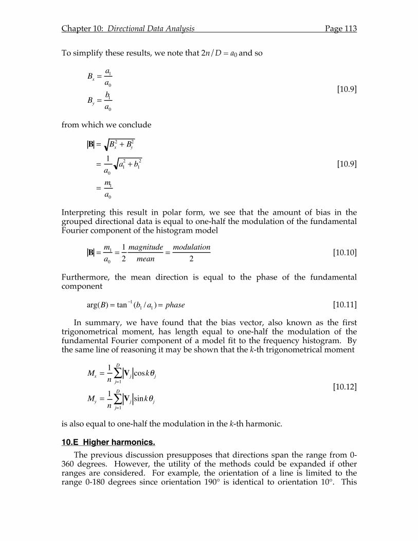
Chapter 10: Directional Data Analysis Page 113
To simplify these results, we note that 2n/D = a0 and so
Bx =
a1a0
By =b1a0
[10.9]
from which we conclude
B = Bx2 + By2
=1a0
a12 + b1
2
=m1a0
[10.9]
Interpreting this result in polar form, we see that the amount of bias in the grouped directional data is equal to one-half the modulation of the fundamental Fourier component of the histogram model
B =m1a0
=12magnitudemean
=modulation
2 [10.10]
Furthermore, the mean direction is equal to the phase of the fundamental component
arg(B) = tan −1 (b1 /a1 ) = phase [10.11]
In summary, we have found that the bias vector, also known as the first trigonometrical moment, has length equal to one-half the modulation of the fundamental Fourier component of a model fit to the frequency histogram. By the same line of reasoning it may be shown that the k-th trigonometrical moment
Mx =
1n
Vj coskθ jj=1
D
∑
My =1n
Vj sinkθ jj=1
D
∑ [10.12]
is also equal to one-half the modulation in the k-th harmonic.
10.E Higher harmonics. The previous discussion presupposes that directions span the range from 0-
360 degrees. However, the utility of the methods could be expanded if other ranges are considered. For example, the orientation of a line is limited to the range 0-180 degrees since orientation 190° is identical to orientation 10°. This
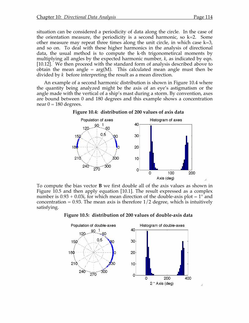
Chapter 10: Directional Data Analysis Page 114
situation can be considered a periodicity of data along the circle. In the case of the orientation measure, the periodicity is a second harmonic, so k=2. Some other measure may repeat three times along the unit circle, in which case k=3, and so on. To deal with these higher harmonics in the analysis of directional data, the usual method is to compute the k-th trigonometircal moments by multiplying all angles by the expected harmonic number, k, as indicated by eqn. [10.12]. We then proceed with the standard form of analysis described above to obtain the mean angle = arg(M). This calculated mean angle must then be divided by k before interpreting the result as a mean direction.
An example of a second harmonic distribution is shown in Figure 10.4 where the quantity being analyzed might be the axis of an eye’s astigmatism or the angle made with the vertical of a ship’s mast during a storm. By convention, axes are bound between 0 and 180 degrees and this example shows a concentration near 0 = 180 degrees.
Figure 10.4: distribution of 200 values of axis data
To compute the bias vector B we first double all of the axis values as shown in Figure 10.5 and then apply equation [10.1]. The result expressed as a complex number is 0.93 + 0.03i, for which mean direction of the double-axis plot = 1° and concentration = 0.93. The mean axis is therefore 1/2 degree, which is intuitively satisfying.
Figure 10.5: distribution of 200 values of double-axis data
Chapter 11: The Fourier Transform
11.A Introduction.
The methods of Fourier analysis described in previous chapters have as their domain three classes of functions: discrete data vectors with finite number of values, discrete vectors with infinite number of values, and continuous functions which are confined to a finite interval. These are cases 1, 2, and 3, respectively, illustrated in Fig. 5.1. The fourth case admits continuous functions defined over an infinite interval. This is the province of the Fourier Transform.
The student may be wondering why it is important to be able to do Fourier analysis on functions defined over an infinite extent when any "real world" function can only be observed over a finite distance, or for a finite length of time. Several reasons can be offered. First, case 4 is so general that it encompasses the other 3 cases. Consequently, the Fourier transform provides a unified approach to a variety of problems, many of which are just special cases of a more general formulation. Second, physical systems are often modeled by continuous functions with infinite extent. For example, the optical image of a point source of light may be described theoretically by a Gaussian function of the form exp(-x2), which exists for all x. Another example is the rate of flow of water out of a tap at the bottom of a bucket of water, which can be modeled as exp(-kt). Fresh insight into the behavior of such systems may be gained by spectral analysis, providing we have the capability to deal with functions defined over all time or space. Third, by removing the restriction in case 3 that continuous functions exist over only a finite interval, the methods of Fourier analysis have developed into a very powerful analytical tool which has proved useful throughout many branches of science and mathematics.
11.B The Inverse Cosine and Sine Transforms.
Our approach to the Fourier transform (case 4) will be by generalizing our earlier results for the analysis of continuous functions over a finite interval (case 3). In Chapter 6 we found that an arbitrary, real-valued function y(x), can be represented exactly by a Fourier series with an infinite number of terms. If y(x) is defined over the interval (-L/2, L/2) then the Fourier model is
y(x) = a0 / 2 + ak ⋅cos2πkx / L + bk ⋅ sin2πkx / Lk=1
∞
∑ [11.1]
As defined in eqn. [4.2], the fundamental frequency of this model is Δf = 1/ L and all of the higher harmonic frequencies fk are integer multiples of this fundamental frequency. That is, fk = k / L = kΔf . Now we are faced with the prospect of letting L→ ∞ which implies that Δf → 0 and consequently the concept of harmonic frequency will cease to be useful.
In order to rescue the situation, we need to disassociate the concepts of physical frequency and harmonic number. To do this, we first change notation
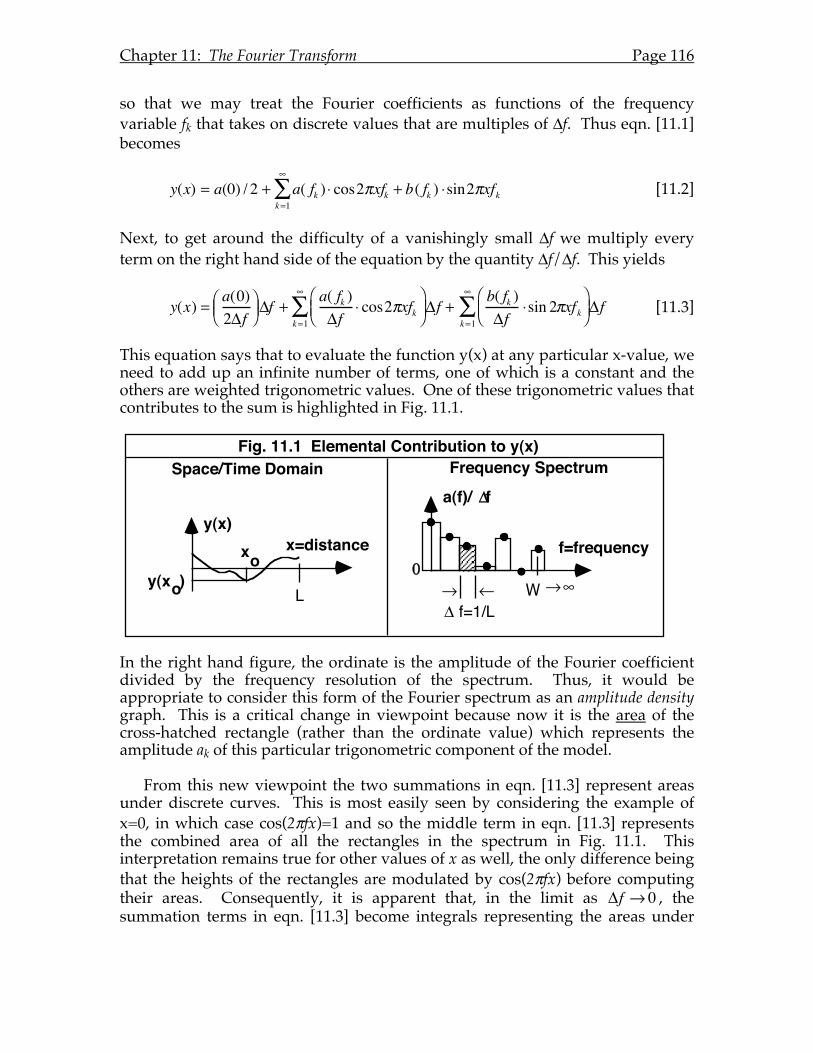
Chapter 11: The Fourier Transform Page 116
so that we may treat the Fourier coefficients as functions of the frequency variable fk that takes on discrete values that are multiples of Δf. Thus eqn. [11.1] becomes
y(x) = a(0) / 2 + a( fk ) ⋅ cos2πxfk + b( fk ) ⋅sin2πxfkk=1
∞
∑ [11.2]
Next, to get around the difficulty of a vanishingly small Δf we multiply every term on the right hand side of the equation by the quantity Δf/Δf. This yields
y(x) =a(0)2Δf
⎛ ⎝ ⎜
⎞ ⎠ ⎟ Δf +
a( fk )Δf
⋅ cos2πxfk⎛ ⎝ ⎜
⎞ ⎠ ⎟
k=1
∞
∑ Δf +b( fk )Δf
⋅sin 2πxfk⎛ ⎝ ⎜
⎞ ⎠ ⎟
k=1
∞
∑ Δf [11.3]
This equation says that to evaluate the function y(x) at any particular x-value, we need to add up an infinite number of terms, one of which is a constant and the others are weighted trigonometric values. One of these trigonometric values that contributes to the sum is highlighted in Fig. 11.1.
In the right hand figure, the ordinate is the amplitude of the Fourier coefficient divided by the frequency resolution of the spectrum. Thus, it would be appropriate to consider this form of the Fourier spectrum as an amplitude density graph. This is a critical change in viewpoint because now it is the area of the cross-hatched rectangle (rather than the ordinate value) which represents the amplitude ak of this particular trigonometric component of the model.
From this new viewpoint the two summations in eqn. [11.3] represent areas under discrete curves. This is most easily seen by considering the example of x=0, in which case cos(2πfx)=1 and so the middle term in eqn. [11.3] represents the combined area of all the rectangles in the spectrum in Fig. 11.1. This interpretation remains true for other values of x as well, the only difference being that the heights of the rectangles are modulated by cos(2πfx) before computing their areas. Consequently, it is apparent that, in the limit as Δf → 0 , the summation terms in eqn. [11.3] become integrals representing the areas under
Fig. 11.1 Elemental Contribution to y(x)
a(f)/ f
0f=frequency
! " W ! #$ f=1/L
$
Space/Time Domain Frequency Spectrum
y(x )o
y(x)x=distance
L
xo
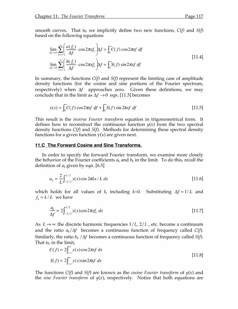
Chapter 11: The Fourier Transform Page 117
smooth curves. That is, we implicitly define two new functions, C(f) and S(f) based on the following equations
limΔ f→ 0
a( fk )Δf
⋅cos2πxfk⎛ ⎝ ⎜
⎞ ⎠ ⎟
k=1
∞
∑ Δf = C( f )0
∞
∫ cos2πxf df
limΔ f→ 0
b( fk )Δf
⋅ cos2πxfk⎛ ⎝ ⎜
⎞ ⎠ ⎟
k=1
∞
∑ Δf = S( f )0
∞
∫ sin2πxf df [11.4]
In summary, the functions C(f) and S(f) represent the limiting case of amplitude density functions (for the cosine and sine portions of the Fourier spectrum, respectively) when Δf approaches zero. Given these definitions, we may conclude that in the limit as Δf → 0 eqn. [11.3] becomes
y(x) = C( f )0
∞
∫ cos2πxf df + S( f )0
∞
∫ sin 2πxf df [11.5]
This result is the inverse Fourier transform equation in trigonometrical form. It defines how to reconstruct the continuous function y(x) from the two spectral density functions C(f) and S(f). Methods for determining these spectral density functions for a given function y(x) are given next.
11.C The Forward Cosine and Sine Transforms.
In order to specify the forward Fourier transform, we examine more closely the behavior of the Fourier coefficients ak and bk in the limit. To do this, recall the definition of ak given by eqn. [6.5]
ak =2L
y(x) cos 2πkx / L−L / 2
L / 2
∫ dx [11.6]
which holds for all values of k, including k=0. Substituting Δf = 1/ L and fk = k / L we have
akΔf
= 2 y(x)cos2πxfk−L / 2
L / 2
∫ dx [11.7]
As L→ ∞ the discrete harmonic frequencies 1/L, 2/L , etc. become a continuum and the ratio ak/Δf becomes a continuous function of frequency called C(f). Similarly, the ratio bk /Δf becomes a continuous function of frequency called S(f). That is, in the limit,
C( f ) = 2 y(x) cos2πxf
−∞
∞
∫ dx
S( f ) = 2 y(x)sin2πxf−∞
∞
∫ dx [11.8]
The functions C(f) and S(f) are known as the cosine Fourier transform of y(x) and the sine Fourier transform of y(x), respectively. Notice that both equations are
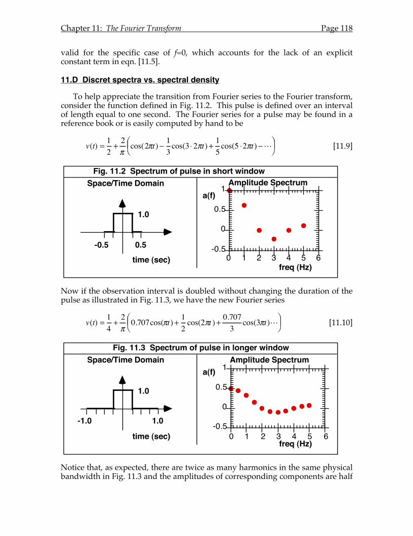
Chapter 11: The Fourier Transform Page 118
valid for the specific case of f=0, which accounts for the lack of an explicit constant term in eqn. [11.5].
11.D Discret spectra vs. spectral density
To help appreciate the transition from Fourier series to the Fourier transform, consider the function defined in Fig. 11.2. This pulse is defined over an interval of length equal to one second. The Fourier series for a pulse may be found in a reference book or is easily computed by hand to be
v(t) =
12
+2πcos(2πt) − 1
3cos(3 ⋅ 2πt) +
15cos(5 ⋅2πt) −⎛
⎝ ⎜ ⎞
⎠ ⎟ [11.9]
Now if the observation interval is doubled without changing the duration of the pulse as illustrated in Fig. 11.3, we have the new Fourier series
v(t) =
14
+2π0.707cos(πt) +
12cos(2πt ) +
0.7073
cos(3πt)⎛ ⎝ ⎜ ⎞
⎠ ⎟ [11.10]
Notice that, as expected, there are twice as many harmonics in the same physical bandwidth in Fig. 11.3 and the amplitudes of corresponding components are half
Fig. 11.2 Spectrum of pulse in short windowSpace/Time Domain Amplitude Spectrum
1.0
0.5-0.5 -0.5
0
0.5
1
0 1 2 3 4 5 6
a(f)
freq (Hz)time (sec)
Fig. 11.3 Spectrum of pulse in longer windowSpace/Time Domain Amplitude Spectrum
1.0
1.0-1.0
a(f)
freq (Hz)time (sec)
-0.5
0
0.5
1
0 1 2 3 4 5 6
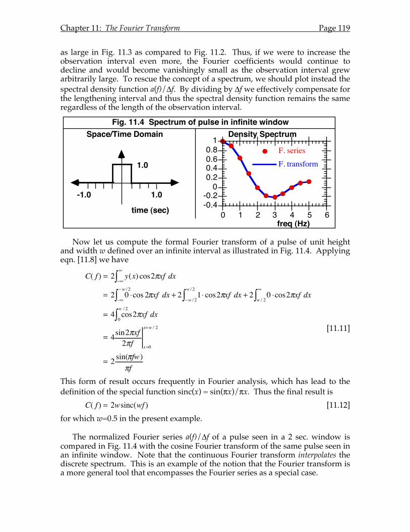
Chapter 11: The Fourier Transform Page 119
as large in Fig. 11.3 as compared to Fig. 11.2. Thus, if we were to increase the observation interval even more, the Fourier coefficients would continue to decline and would become vanishingly small as the observation interval grew arbitrarily large. To rescue the concept of a spectrum, we should plot instead the spectral density function a(f)/Δf. By dividing by Δf we effectively compensate for the lengthening interval and thus the spectral density function remains the same regardless of the length of the observation interval.
Now let us compute the formal Fourier transform of a pulse of unit height
and width w defined over an infinite interval as illustrated in Fig. 11.4. Applying eqn. [11.8] we have
C( f ) = 2 y(x) cos2πxf−∞
∞
∫ dx
= 2 0 ⋅cos 2πxf−∞
−w / 2
∫ dx + 2 1 ⋅ cos2πxf−w / 2
w / 2
∫ dx + 2 0 ⋅cos2πxfw / 2
∞
∫ dx
= 4 cos2πxf0
w / 2
∫ dx
= 4sin2πxf2πf x=0
x=w / 2
= 2 sin(πfw)πf
[11.11]
This form of result occurs frequently in Fourier analysis, which has lead to the definition of the special function sinc(x) = sin(πx)/πx. Thus the final result is C( f ) = 2wsinc(wf ) [11.12] for which w=0.5 in the present example.
The normalized Fourier series a(f)/Δf of a pulse seen in a 2 sec. window is compared in Fig. 11.4 with the cosine Fourier transform of the same pulse seen in an infinite window. Note that the continuous Fourier transform interpolates the discrete spectrum. This is an example of the notion that the Fourier transform is a more general tool that encompasses the Fourier series as a special case.
Fig. 11.4 Spectrum of pulse in infinite windowSpace/Time Domain Density Spectrum
1.0
1.0-1.0
freq (Hz)time (sec) -0.4
-0.20
0.20.40.60.81
0 1 2 3 4 5 6
F. series
F. transform
Chapter 11: The Fourier Transform Page 120
11.E Complex Form of the Fourier Transform.
Although the preceding development is useful for achieving an intuitive understanding of the transition from Fourier series to the Fourier transform, the resulting equations are mainly of historical interest since modern authors invariably choose to represent the Fourier transform in complex form. Starting with the basic formulation of the complex Fourier series given in eqn. [6.6]
y(x) = ckeik2πx / L
k= −∞
∞
∑ [6.6]
we would follow the same approach taken above. Introducing the necessary change of variables and multiplication by Δf/Δf, in the limit as Δf → 0 this equation becomes the inverse Fourier transform
y(x) = Y ( f )−∞
∞
∫ ei2πxf df [11.13]
where Y(f) is the complex frequency spectrum of y(x).
To obtain the forward transform, we begin with the definition of the complex Fourier coefficients for finite continuous functions
ck =
ak − ibk2
=1L
y(x)e− ik2πx / L−L / 2
L / 2
∫ dx [6.7]
As L→ ∞ the discrete harmonic frequencies 1/L, 2/L , etc. become a continuum and the ratio ck/Δf becomes a continuous function of frequency called Y(f). Thus, the forward Fourier transform is defined by the equation
Y ( f ) = y(x)−∞
∞
∫ e−i 2πxf dx [11.14]
By observing the striking similarity between equations 11.13 and [11.14] the student may begin to appreciate one reason for the popularity of the complex form of the Fourier transform operations. The only difference between the forward and reverse transforms is the sign of the exponent in the complex exponential. This exponential term is called the kernel of the integrand and thus we observe that the kernels of the forward and reverse transforms are complex conjugates of each other. Another advantage of the complex form over the trigonometric form is that there is only one integral to specify and solve rather than two. Lastly, and most importantly, the complex form of the transform applies even when function y(x) is complex-valued.
Chapter 11: The Fourier Transform Page 121
11.F Fourier's Theorem.
Fourier's theorem is simply a restatement of the preceding results:
if Y ( f ) = y(x)−∞
∞
∫ e−i 2πxf df [11.14]
then y(x) = Y ( f )−∞
∞
∫ ei2πxf df [11.13]
Some authors prefer to substitute [11.14] into [11.13] to produce the mathematical equivalent of saying “the inverse Fourier transform undoes the forward Fourier transform”,
y(x) = y(x)−∞
∞
∫ e− i2π xf df⎡⎣⎢
⎤⎦⎥−∞
∞
∫ ei2π xf df [11.15]
Fourier’s theorem thus provides a framework for casting functions into the frequency domain and then retrieving them analytically. Applying integral calculus, numerical approximations are replaced by exact, algebraic solutions.
11.G Relationship between Complex & Trigonometric Transforms.
If we substitute trigonometric forms for the kernel in eqn. [11.15] using Euler's theorem eiθ = cosθ + isinθ we obtain for a real-valued function y(x)
Y ( f ) = y(x)−∞
∞
∫ e−i 2πxf df
= y( x)−∞
∞
∫ cos(2πxf ) − i sin(2πxf )[ ] df
= y(x)−∞
∞
∫ cos(2πxf ) df − i y(x)−∞
∞
∫ sin(2πxf ) df
[11.16]
These integrals are recognized from eqn. [11.8] as the sine and cosine Fourier transforms. Thus we conclude that
Y ( f ) = C( f ) − iS( f )
2 for f > 0
=C( f ) + iS( f )
2for f < 0
[11.17]
which is the analogous result to that for Fourier coefficients described in eqn. [6.7]. This result also shows that the Fourier transform Y(f) of a real-valued function y(x) has Hermitian (conjugate) symmetry.

Chapter 11: The Fourier Transform Page 122
Chapter 12: Properties of The Fourier Transform
12.A Introduction.
The power of the Fourier transform derives principally from the many theorems describing the properties of the transformation operation that provide insight into the nature of physical systems. Most of these theorems have been derived within the context of communications engineering to answer questions framed like "if a time signal is manipulated in such-and-such a way, what happens to its Fourier spectrum?" As a result, a way of thinking about the transformation operation has developed in which a Fourier transform pair y(t)↔ Y ( f ) is like the two sides of a coin, with the original time or space signal on one side and its frequency spectrum on the other. The two sides of a Fourier transform pair are complementary views of the same signal and so it makes sense that if some operation is performed on one half of the pair, then some equivalent operation is necessarily performed on the other half.
Many of the concepts underlying the theorems and properties described below were introduced in Chapter 6 in the context of Fourier series. For the most part, these theorems can be extended into the domain of the Fourier transform simply by examining the limit as the length of the observation interval for the signal grows without bound. Consequently, it will be sufficient here simply to list the results. Rigorous proofs of these theorems may be found in standard textbooks (e.g. Bracewell, 1978; Gaskill, 1978). 12.B Theorems
Linearity
Scaling a function scales it's transform pair. Adding two functions corresponds to adding the two frequency spectra.
If h(x)↔ H( f ) then ah(x)↔ aH( f ) [12.1]
If h(x)↔ H( f )g(x)↔G( f ) then h(x) + g(x)↔ H ( f ) +G( f ) [12.2]
Scaling
Multiplication of the scale of the time/space reference frame changes by the factor s inversely scales the frequency axis of the spectrum of the function. For example, stretching a temporal pulse makes the Fourier spectrum narrower and also taller because the area under the pulse increases.
If h(x)↔ H( f ) then h(x / s)↔ s H( f ⋅ s) [12.3]
and sh(x ⋅ s)↔ H( f / s) [12.4]
Chapter 12: Properties of The Fourier Transform Page 124
A simple, but useful, implication of this theorem is that if h(x)↔ H( f ) then h(−x)↔ H(− f ) . In words, flipping the time function about the origin corresponds to flipping its spectrum about the origin.
Notice that this theorem differs from the corresponding theorem for discrete spectra (Fig. 6.3) in that the ordinate scales inversely with the abscissa. This is because the Fourier transform produces a spectral density function rather than a spectral amplitude function, and therefore is sensitive to the scale of the frequency axis.
Time/Space Shift
Displacement in time or space induces a phase shift proportional to frequency and to the amount of displacement. This occurs because a given displacement represents more cycles of phase shift for a high-frequency signal than for a low-frequency signal.
If h(x)↔ H( f ) then h(x − x0 )↔ e−i2πfx 0H ( f ) [12.5]
Frequency Shift
Displacement in frequency multiplies the time/space function by a unit phasor with angle proportional to time/space and to the amount of displacement. Note that if h(x) is real-valued, it will become complex-valued after frequency shifting.
If h(x)↔ H( f ) then h(x)ei2πxf0 ↔ H( f − f0 ) [12.6]
Modulation
Multiplication of a time/space function by a cosine wave splits the frequency spectrum of the function. Half of the spectrum shifts left and half shifts right. This is simply a variant of the shift theorem which makes use of Euler's relationship cos(x) = (eix + e−ix ) / 2
if h(x)↔ H( f ) then h(x)ei2πxf0 ↔ H( f − f0 )
h(x)e −i 2πxf0 ↔ H( f + f0 )
and therefore by the linearity theorem it follows that
h(x)cos(2πxf0 )↔H( f − f0 ) + H( f + f0 )
2
h(x)sin(2πxf0 )↔H( f − f0) + H( f + f0 )
2i [12.7]
The modulation theorem is the basis of transmission of amplitude-modulated radio broadcasts. When a low frequency audio signal is multiplied by a radio-frequency carrier wave, the spectrum of the audio message is shifted to the radio
Chapter 12: Properties of The Fourier Transform Page 125
portion of the electromagnetic spectrum for transmission by an antenna. Similarly, a method for recovery of the audio signal called super-heterodyne demodulation involves multiplying the received signal by a sinusoid with the same frequency as the carrier, thereby demodulating the audio component.
Differentiation
Differentiation of a function induces a 90° phase shift in the spectrum and scales the magnitude of the spectrum in proportion to frequency. Repeated differentiation leads to the general result:
If h(x)↔ H( f ) then dn h(x)dxn
↔ (i2πf )nH ( f ) [12.8]
This theorem explains why differentiation of a signal has the reputation for being a noisy operation. Even if the signal is band-limited, noise will introduce high frequency signals which are greatly amplified by differentiation.
Integration
Integration of a function induces a -90° phase shift in the spectrum and scales the magnitude of the spectrum inversely with frequency.
If h(x)↔ H( f ) then h(u)−∞
x
∫ du↔ H ( f ) /(i2πf ) + constant [12.9]
From this theorem we see that integration is analagous to a low-pass filter which blurs the signal.
Transform of a transform
We normally think of using the inverse Fourier transform to move from the frequency spectrum back to the time/space function. However, if instead the spectrum is subjected to the forward Fourier transform, the result is a time/space function which has been flipped about the y-axis. This gives some appreciation for why the kernels of the two transforms are complex conjugates of each other: the change in sign in the reverse transform flips the function about the y-axis a second time so that the result matches the original function.
If h(t)F⎯ → ⎯ H( f ) then H( f )
F⎯ → ⎯ h(−t) [12.10]
One practical implication of this theorem is a 2-for-1 bonus: every transform pair brings with it a second transform pair at no extra cost.
If h(t)↔ H( f ) then H(t)↔ h(− f ) [12.11]
For example, rect( t)↔ sinc( f ) implies sinc(t)↔ rect(− f ) .
Chapter 12: Properties of The Fourier Transform Page 126
This theorem highlights the fact that the Fourier transform operation is fundamentally a mathematical relation that can be completely divorced from the physical notions of time and frequency. It is simply a method for transforming a function of one variable into a function of another variable. So, for example, in probability theory the Fourier transform is used to convert a probability density function into a moment-generating function, neither of which bear the slightest resemblance to the time or frequency domains.
Central ordinate
By analogy with the mean Fourier coefficient a0, the central ordinate value H(0) (analog of a0 in discrete spectra) represents the total area under the function h(x).
If h(x)↔ H( f ) then H(0) = h(u)−∞
∞
∫ e−i 0du = h(u)−∞
∞
∫ du
For the inverse transform,
h(0) = H(u)−∞
∞
∫ ei 0du
= H(u)−∞
∞
∫ du
= Re H(u)[ ]−∞
∞
∫ du + i Im H(u)[ ]−∞
∞
∫ du
[12.12]
Note that for a real-valued function h(t) the imaginary portion of the spectrum will have odd symmetry, so the area under the real part of the spectrum is all that needs to be computed to find h(0).
For example, in optics the line-spread function (LSF) and the optical transfer function (OTF) are Fourier transform pairs. Therefore, according to the central-ordinate theorem, the central point of the LSF is equal to the area under the OTF. In two dimensions, the transform relationship refers to the point-spread function (PSF) and the OTF. In such 2D cases, the integral must be taken over an area, in which case the result is interpreted as the volume under the 2D surface. This is the basis for computing Strehl’s ratio in the frequency domain.
Equivalent width
A corollary of the central ordinate theorem is
If h(u)
−∞
∞
∫ du = H(0)
h(0) = H (u)−∞
∞
∫ du then
h(u)−∞
∞
∫ du
h(0)=
H (0)H (u)
−∞
∞
∫ du [12.13]
The ratio on the left side of this last expression is called the "equivalent width" of the given function h because it represents the width of a rectangle with the same central ordinate and the same area as h. Likewise, the ratio on the right is the inverse of the equivalent width of H. Thus we conclude that the equivalent width of a function in one domain is the inverse of the equivalent width in the other domain as illustrated in Fig. 12.1. For example, as a pulse in the time
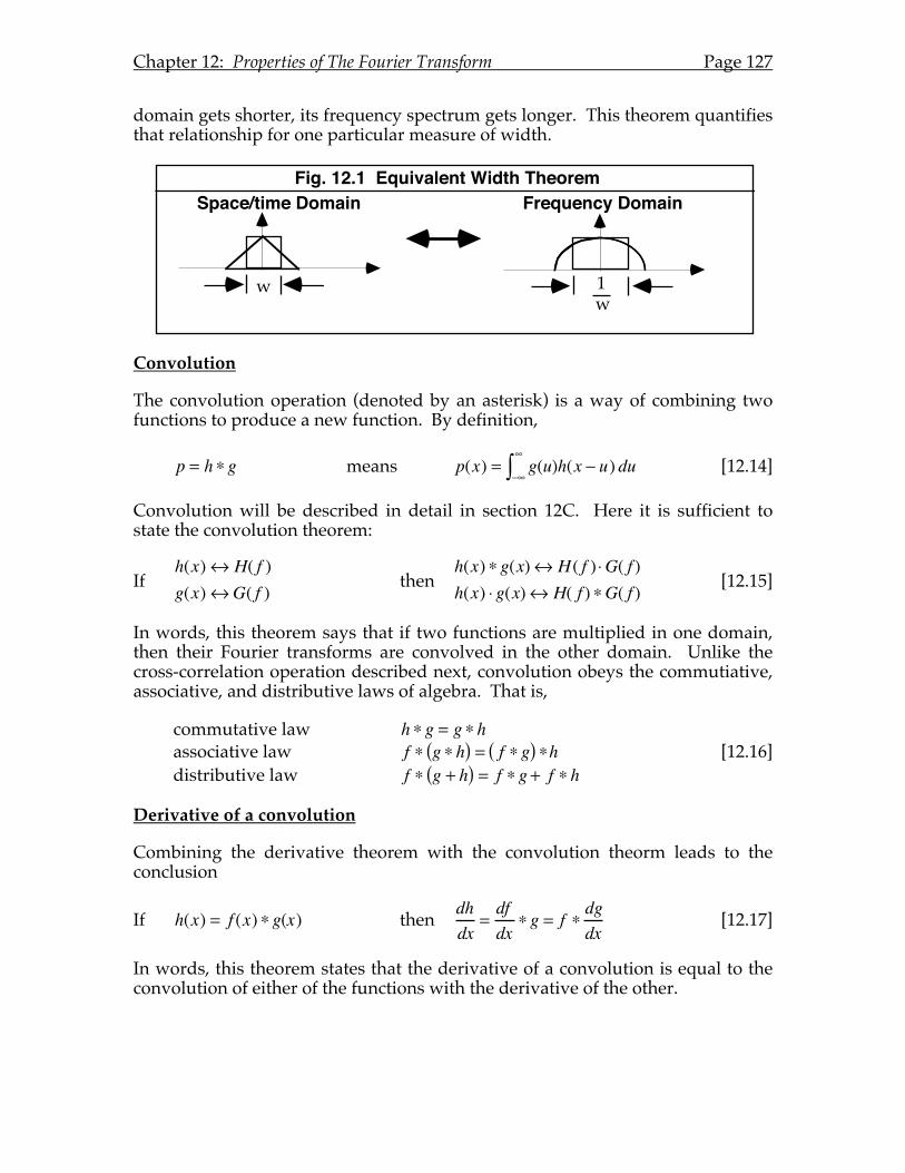
Chapter 12: Properties of The Fourier Transform Page 127
domain gets shorter, its frequency spectrum gets longer. This theorem quantifies that relationship for one particular measure of width.
Convolution
The convolution operation (denoted by an asterisk) is a way of combining two functions to produce a new function. By definition,
p = h ∗ g means p(x) = g(u)h(x − u)−∞
∞
∫ du [12.14]
Convolution will be described in detail in section 12C. Here it is sufficient to state the convolution theorem:
If h(x)↔ H( f )g(x)↔G( f ) then
h(x) ∗ g(x)↔ H ( f ) ⋅G( f )h(x) ⋅ g(x)↔ H( f ) ∗G( f ) [12.15]
In words, this theorem says that if two functions are multiplied in one domain, then their Fourier transforms are convolved in the other domain. Unlike the cross-correlation operation described next, convolution obeys the commutiative, associative, and distributive laws of algebra. That is,
commutative law h ∗ g = g ∗ h associative law f ∗ g ∗ h( ) = f ∗ g( ) ∗h [12.16] distributive law f ∗ g + h( ) = f ∗ g + f ∗ h
Derivative of a convolution
Combining the derivative theorem with the convolution theorm leads to the conclusion
If h(x) = f (x) ∗ g(x) then dhdx
=dfdx
∗ g = f ∗ dgdx
[12.17]
In words, this theorem states that the derivative of a convolution is equal to the convolution of either of the functions with the derivative of the other.
Fig. 12.1 Equivalent Width TheoremSpace/time Domain Frequency Domain
ww1
Chapter 12: Properties of The Fourier Transform Page 128
Cross-correlation
The cross-correlation operation (denoted by a pentagram) is a way of combining two functions to produce a new function that is similar to convolution. By definition,
q = h g means q(x) = g(u − x)h(u )−∞
∞
∫ du [12.18]
The cross-correlation theorem is
If h(x)↔ H( f )g(x)↔G( f ) then
h(x)g(x)↔ H ( f ) ⋅G(− f )h(−x) ⋅ g(x)↔ H ( f )G( f )h(x) ⋅ g(x)↔ H (− f )G( f )
[12.19]
Combining eqns. [12.14] and [12.16] indicates the spectrum of the product of two functions can be computed two ways, h ⋅ g↔ H( f ) ∗G( f ) and h ⋅ g↔ H (− f )G( f ) . Since the spectrum of a function is unique, the implication is that H ( f )∗G( f ) = H (− f )G( f ) [12.20]
which shows the relationship between correlation and convolution.
Auto-correlation
The auto-correlation theorem is the special case of the cross-correlation theorem when the two functions h and g are the same function. In this case, we use the Hermitian symmetry of the Fourier transform to show that:
If h(x)↔ H( f ) then h(x)h(x)↔ H ( f ) ⋅H ∗( f ) [12.21]
The quantity h★h is known as the autocorrelation function of h and the quantity HH* is called the power spectral density function of h. This theorem says that the autocorrelation function and the power spectral density function comprise a Fourier transform pair.
Parseval/Rayleigh
Parseval's energy conservation theorem developed in the context of Fourier series is often called Rayleigh's theorem in the context of Fourier transforms.
If h(x)↔ H( f ) then h(x)2−∞
∞
∫ dx = H ( f ) 2−∞
∞
∫ df [12.22]
which is the analog of eqn. [7.6] developed for discrete spectra. The left hand integral is interpreted as the total amount of energy in the signal as computed in the time domain, whereas the right hand integral is the total amount of energy computed in the frequency domain. The modulus symbols (|~|) serve as a
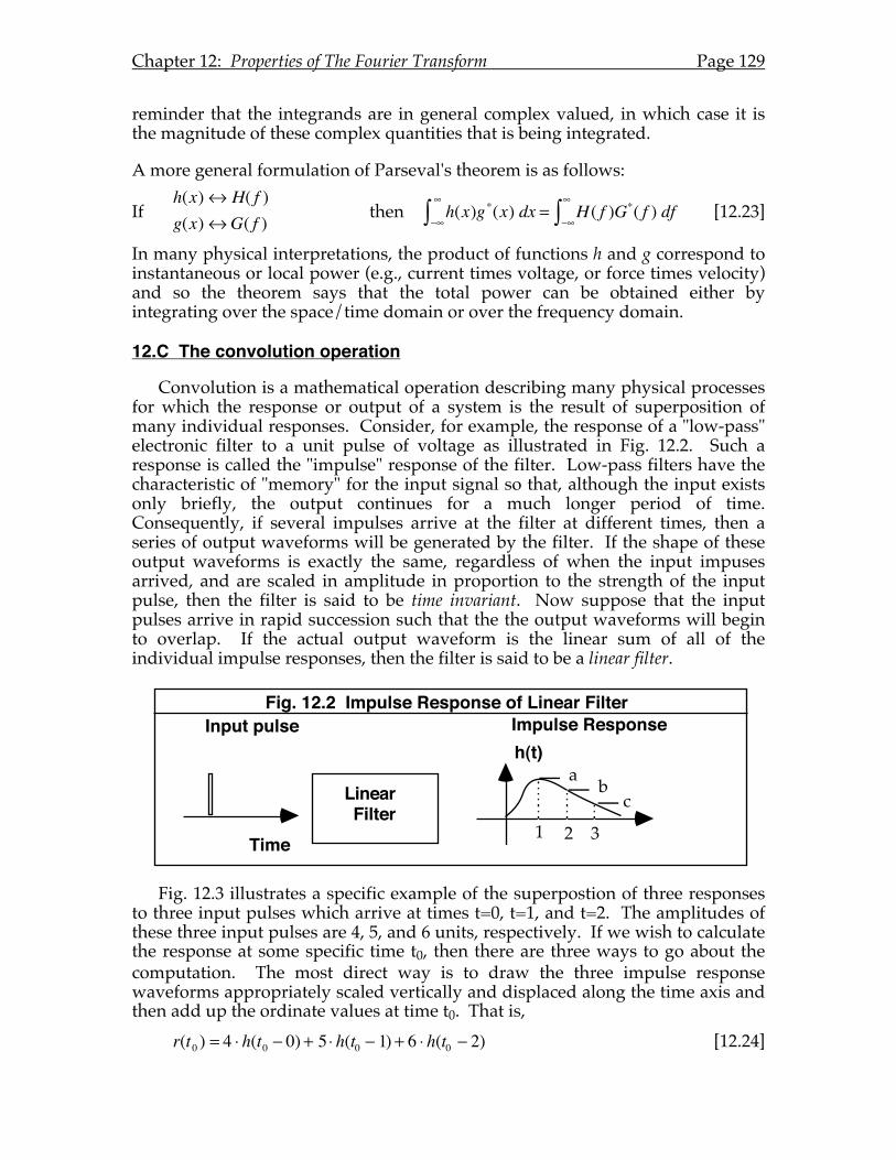
Chapter 12: Properties of The Fourier Transform Page 129
reminder that the integrands are in general complex valued, in which case it is the magnitude of these complex quantities that is being integrated.
A more general formulation of Parseval's theorem is as follows:
If h(x)↔ H( f )g(x)↔G( f ) then h(x)g∗(x)
−∞
∞
∫ dx = H ( f )G∗( f )−∞
∞
∫ df [12.23]
In many physical interpretations, the product of functions h and g correspond to instantaneous or local power (e.g., current times voltage, or force times velocity) and so the theorem says that the total power can be obtained either by integrating over the space/time domain or over the frequency domain.
12.C The convolution operation
Convolution is a mathematical operation describing many physical processes for which the response or output of a system is the result of superposition of many individual responses. Consider, for example, the response of a "low-pass" electronic filter to a unit pulse of voltage as illustrated in Fig. 12.2. Such a response is called the "impulse" response of the filter. Low-pass filters have the characteristic of "memory" for the input signal so that, although the input exists only briefly, the output continues for a much longer period of time. Consequently, if several impulses arrive at the filter at different times, then a series of output waveforms will be generated by the filter. If the shape of these output waveforms is exactly the same, regardless of when the input impuses arrived, and are scaled in amplitude in proportion to the strength of the input pulse, then the filter is said to be time invariant. Now suppose that the input pulses arrive in rapid succession such that the the output waveforms will begin to overlap. If the actual output waveform is the linear sum of all of the individual impulse responses, then the filter is said to be a linear filter.
Fig. 12.3 illustrates a specific example of the superpostion of three responses to three input pulses which arrive at times t=0, t=1, and t=2. The amplitudes of these three input pulses are 4, 5, and 6 units, respectively. If we wish to calculate the response at some specific time t0, then there are three ways to go about the computation. The most direct way is to draw the three impulse response waveforms appropriately scaled vertically and displaced along the time axis and then add up the ordinate values at time t0. That is, r(t0 ) = 4 ⋅ h(t0 − 0) + 5 ⋅ h(t0 − 1) + 6 ⋅ h(t0 − 2) [12.24]
Fig. 12.2 Impulse Response of Linear FilterInput pulse Impulse Response
Linear Filter
Time
h(t)a b
c1 2 3
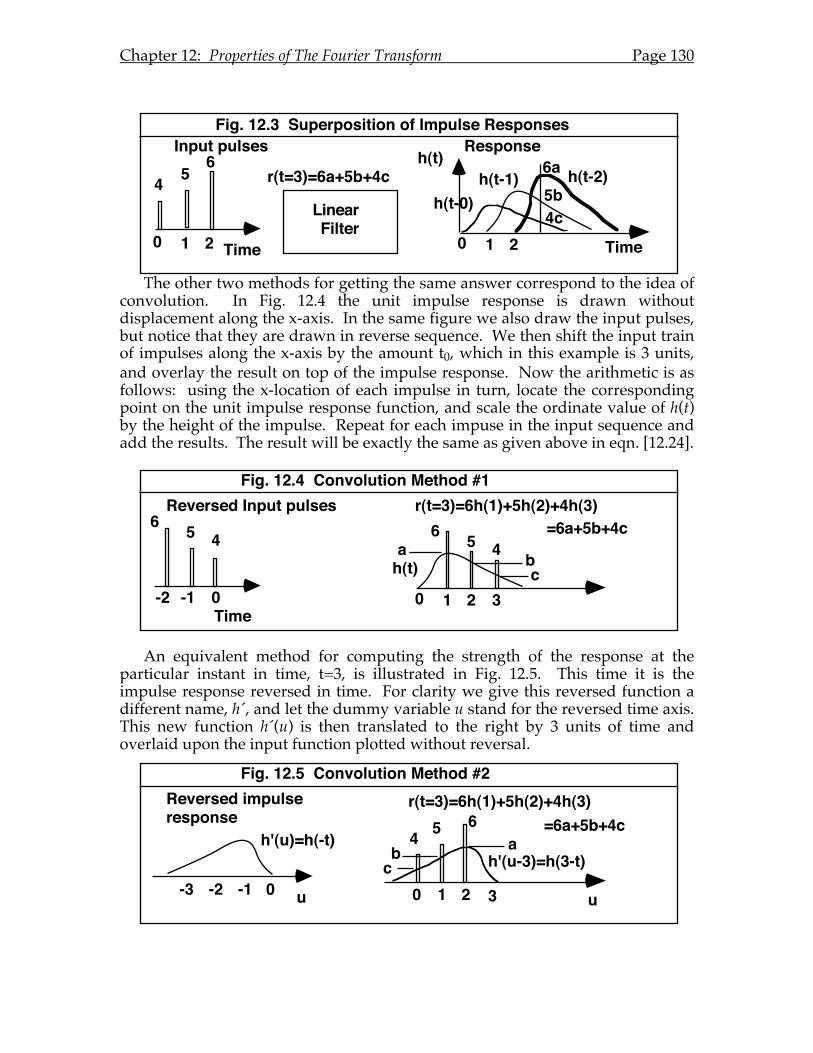
Chapter 12: Properties of The Fourier Transform Page 130
The other two methods for getting the same answer correspond to the idea of convolution. In Fig. 12.4 the unit impulse response is drawn without displacement along the x-axis. In the same figure we also draw the input pulses, but notice that they are drawn in reverse sequence. We then shift the input train of impulses along the x-axis by the amount t0, which in this example is 3 units, and overlay the result on top of the impulse response. Now the arithmetic is as follows: using the x-location of each impulse in turn, locate the corresponding point on the unit impulse response function, and scale the ordinate value of h(t) by the height of the impulse. Repeat for each impuse in the input sequence and add the results. The result will be exactly the same as given above in eqn. [12.24].
An equivalent method for computing the strength of the response at the particular instant in time, t=3, is illustrated in Fig. 12.5. This time it is the impulse response reversed in time. For clarity we give this reversed function a different name, h´, and let the dummy variable u stand for the reversed time axis. This new function h´(u) is then translated to the right by 3 units of time and overlaid upon the input function plotted without reversal.
Fig. 12.3 Superposition of Impulse ResponsesInput pulses Response
Linear Filter
Time
546
0
h(t-0)h(t-1) h(t-2)
h(t)
4c5b6ar(t=3)=6a+5b+4c
1 2 0 1 2 Time
Fig. 12.4 Convolution Method #1 Reversed Input pulses
Time-2
h(t)
r(t=3)=6h(1)+5h(2)+4h(3)
0
5 46
5 46
cba
-1 0 1 2 3
=6a+5b+4c
Fig. 12.5 Convolution Method #2 Reversed impulse response
u
546
h'(u)=h(-t)
r(t=3)=6h(1)+5h(2)+4h(3)
h'(u-3)=h(3-t)
u
cb a
0-1-2-3 0 1 2 3
=6a+5b+4c
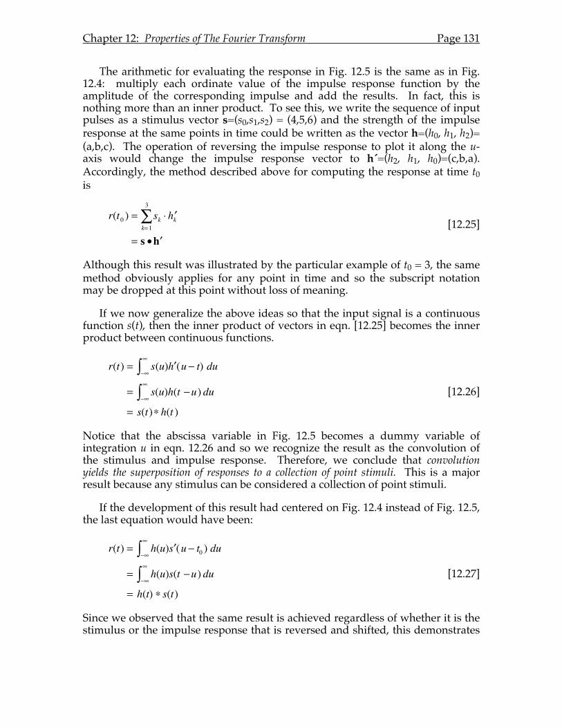
Chapter 12: Properties of The Fourier Transform Page 131
The arithmetic for evaluating the response in Fig. 12.5 is the same as in Fig. 12.4: multiply each ordinate value of the impulse response function by the amplitude of the corresponding impulse and add the results. In fact, this is nothing more than an inner product. To see this, we write the sequence of input pulses as a stimulus vector s=(s0,s1,s2) = (4,5,6) and the strength of the impulse response at the same points in time could be written as the vector h=(h0, h1, h2)= (a,b,c). The operation of reversing the impulse response to plot it along the u-axis would change the impulse response vector to h´=(h2, h1, h0)=(c,b,a). Accordingly, the method described above for computing the response at time t0 is
r(t0 ) = sk ⋅ ′ h k
k= 1
3
∑= s • ′ h
[12.25]
Although this result was illustrated by the particular example of t0 = 3, the same method obviously applies for any point in time and so the subscript notation may be dropped at this point without loss of meaning.
If we now generalize the above ideas so that the input signal is a continuous function s(t), then the inner product of vectors in eqn. [12.25] becomes the inner product between continuous functions.
r(t) = s(u) ′ h (u − t)−∞
∞
∫ du
= s(u)h(t −u)−∞
∞
∫ du
= s(t)∗ h(t )
[12.26]
Notice that the abscissa variable in Fig. 12.5 becomes a dummy variable of integration u in eqn. 12.26 and so we recognize the result as the convolution of the stimulus and impulse response. Therefore, we conclude that convolution yields the superposition of responses to a collection of point stimuli. This is a major result because any stimulus can be considered a collection of point stimuli.
If the development of this result had centered on Fig. 12.4 instead of Fig. 12.5, the last equation would have been:
r(t) = h(u) ′ s (u − t0 )−∞
∞
∫ du
= h(u)s(t −u)−∞
∞
∫ du
= h(t) ∗ s(t)
[12.27]
Since we observed that the same result is achieved regardless of whether it is the stimulus or the impulse response that is reversed and shifted, this demonstrates
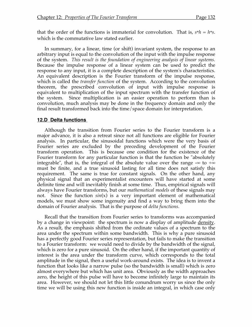
Chapter 12: Properties of The Fourier Transform Page 132
that the order of the functions is immaterial for convolution. That is, s*h = h*s. which is the commutative law stated earlier.
In summary, for a linear, time (or shift) invariant system, the response to an arbitrary input is equal to the convolution of the input with the impulse response of the system. This result is the foundation of engineering analysis of linear systems. Because the impulse response of a linear system can be used to predict the response to any input, it is a complete description of the system's characteristics. An equivalent description is the Fourier transform of the impulse response, which is called the transfer function of the system. According to the convolution theorem, the prescribed convolution of input with impulse response is equivalent to multiplication of the input spectrum with the transfer function of the system. Since multiplication is an easier operation to perform than is convolution, much analysis may be done in the frequency domain and only the final result transformed back into the time/space domain for interpretation.
12.D Delta functions
Although the transition from Fourier series to the Fourier transform is a major advance, it is also a retreat since not all functions are eligible for Fourier analysis. In particular, the sinusoidal functions which were the very basis of Fourier series are excluded by the preceding development of the Fourier transform operation. This is because one condition for the existence of the Fourier transform for any particular function is that the function be "absolutely integrable", that is, the integral of the absolute value over the range -∞ to +∞ must be finite, and a true sinusoid lasting for all time does not satisfy this requirement. The same is true for constant signals. On the other hand, any physical signal that an experimentalist encounters will have started at some definite time and will inevitably finish at some time. Thus, empirical signals will always have Fourier transforms, but our mathematical models of these signals may not. Since the function sin(x) is a very important element of mathematical models, we must show some ingenuity and find a way to bring them into the domain of Fourier analysis. That is the purpose of delta functions.
Recall that the transition from Fourier series to transforms was accompanied by a change in viewpoint: the spectrum is now a display of amplitude density. As a result, the emphasis shifted from the ordinate values of a spectrum to the area under the spectrum within some bandwidth. This is why a pure sinusoid has a perfectly good Fourier series representation, but fails to make the transition to a Fourier transform: we would need to divide by the bandwidth of the signal, which is zero for a pure sinusoid. On the other hand, if the important quantity of interest is the area under the transform curve, which corresponds to the total amplitude in the signal, then a useful work-around exists. The idea is to invent a function that looks like a narrow pulse (so the bandwidth is small) which is zero almost everywhere but which has unit area. Obviously as the width approaches zero, the height of this pulse will have to become infinitely large to maintain its area. However, we should not let this little conundrum worry us since the only time we will be using this new function is inside an integral, in which case only
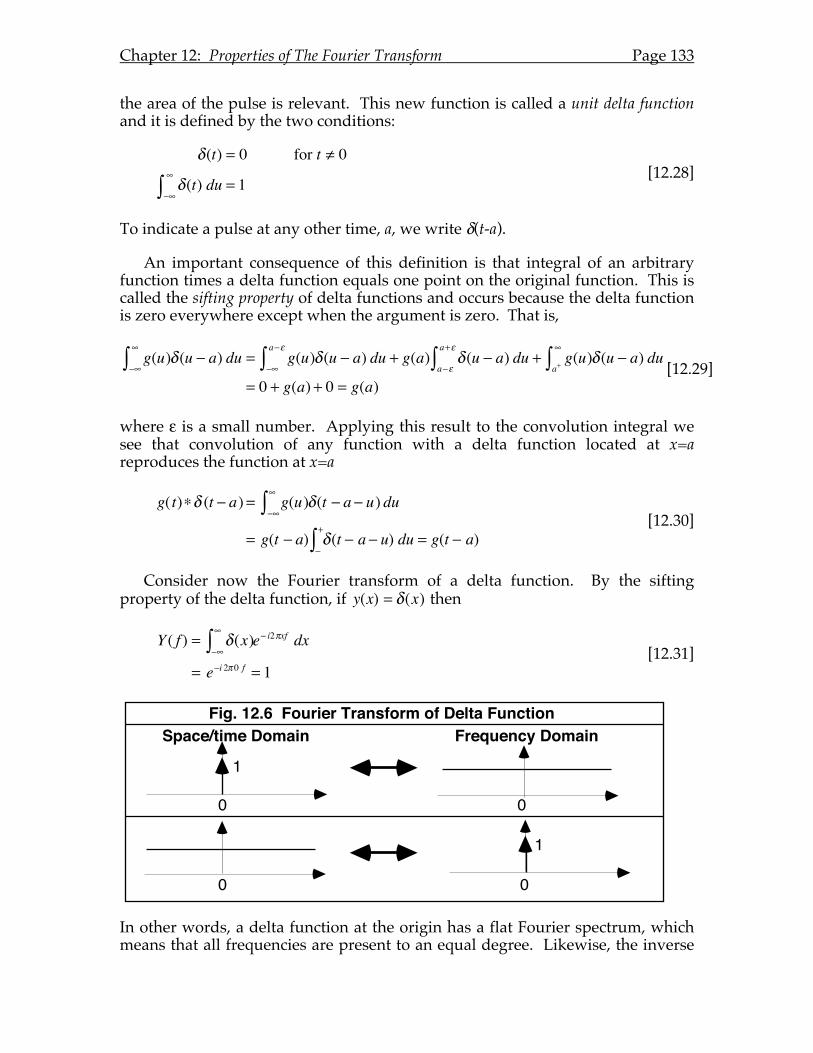
Chapter 12: Properties of The Fourier Transform Page 133
the area of the pulse is relevant. This new function is called a unit delta function and it is defined by the two conditions:
δ(t) = 0 for t ≠ 0
δ(t)−∞
∞
∫ du = 1 [12.28]
To indicate a pulse at any other time, a, we write δ(t-a).
An important consequence of this definition is that integral of an arbitrary function times a delta function equals one point on the original function. This is called the sifting property of delta functions and occurs because the delta function is zero everywhere except when the argument is zero. That is,
g(u)δ (u − a)−∞
∞
∫ du = g(u)δ (u − a)−∞
a−ε
∫ du + g(a) δ (u − a)a−ε
a+ε
∫ du + g(u)δ (u − a)a+
∞
∫ du
= 0 + g(a) + 0 = g(a)[12.29]
where ε is a small number. Applying this result to the convolution integral we see that convolution of any function with a delta function located at x=a reproduces the function at x=a
g( t)∗δ (t − a) = g(u)δ(t − a − u)
−∞
∞
∫ du
= g(t − a) δ(t − a − u)−
+
∫ du = g(t − a) [12.30]
Consider now the Fourier transform of a delta function. By the sifting property of the delta function, if y(x) = δ(x) then
Y ( f ) = δ(x)
−∞
∞
∫ e− i2πxf dx
= e−i 2π 0 f = 1 [12.31]
In other words, a delta function at the origin has a flat Fourier spectrum, which means that all frequencies are present to an equal degree. Likewise, the inverse
Fig. 12.6 Fourier Transform of Delta FunctionSpace/time Domain Frequency Domain
0 0
0 0
1
1
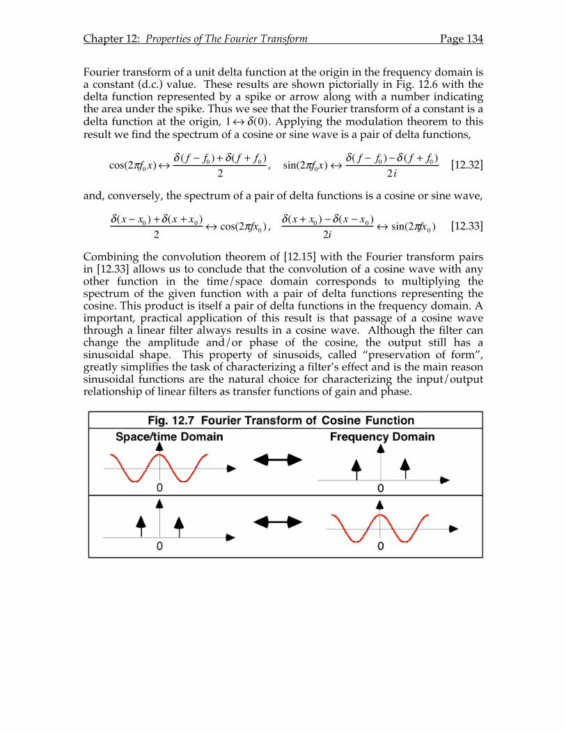
Chapter 12: Properties of The Fourier Transform Page 134
Fourier transform of a unit delta function at the origin in the frequency domain is a constant (d.c.) value. These results are shown pictorially in Fig. 12.6 with the delta function represented by a spike or arrow along with a number indicating the area under the spike. Thus we see that the Fourier transform of a constant is a delta function at the origin, 1↔δ(0) . Applying the modulation theorem to this result we find the spectrum of a cosine or sine wave is a pair of delta functions,
cos(2πf0x)↔δ ( f − f0 ) + δ( f + f0 )
2, sin(2πf0x)↔
δ( f − f0 ) −δ ( f + f0 )2i
[12.32]
and, conversely, the spectrum of a pair of delta functions is a cosine or sine wave,
δ(x − x0 ) +δ(x + x0 )2
↔ cos(2πfx0 ) , δ(x + x0 ) −δ(x − x0 )
2i↔ sin(2πfx0 ) [12.33]
Combining the convolution theorem of [12.15] with the Fourier transform pairs in [12.33] allows us to conclude that the convolution of a cosine wave with any other function in the time/space domain corresponds to multiplying the spectrum of the given function with a pair of delta functions representing the cosine. This product is itself a pair of delta functions in the frequency domain. A important, practical application of this result is that passage of a cosine wave through a linear filter always results in a cosine wave. Although the filter can change the amplitude and/or phase of the cosine, the output still has a sinusoidal shape. This property of sinusoids, called “preservation of form”, greatly simplifies the task of characterizing a filter’s effect and is the main reason sinusoidal functions are the natural choice for characterizing the input/output relationship of linear filters as transfer functions of gain and phase.
!"#$%&
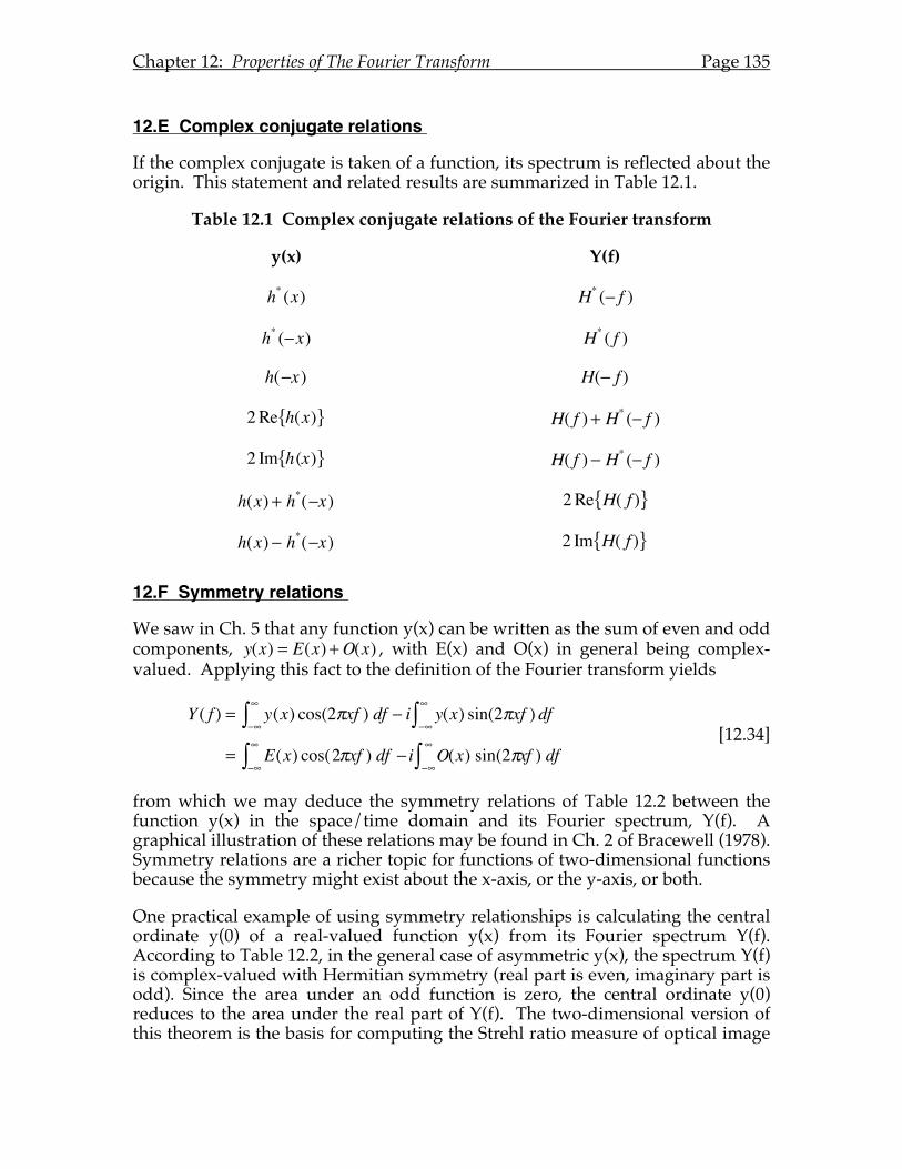
Chapter 12: Properties of The Fourier Transform Page 135
12.E Complex conjugate relations
If the complex conjugate is taken of a function, its spectrum is reflected about the origin. This statement and related results are summarized in Table 12.1.
Table 12.1 Complex conjugate relations of the Fourier transform
y(x) Y(f)
h* (x) H* (− f )
h* (−x) H* ( f )
h(−x) H(− f )
2Re h(x){ } H( f ) + H* (− f )
2 Im h(x){ } H( f ) − H* (− f )
h(x) + h*(−x) 2Re H( f ){ }
h(x) − h*(−x) 2 Im H( f ){ }
12.F Symmetry relations
We saw in Ch. 5 that any function y(x) can be written as the sum of even and odd components, y(x) = E(x) +O(x) , with E(x) and O(x) in general being complex-valued. Applying this fact to the definition of the Fourier transform yields
Y ( f ) = y(x)
−∞
∞
∫ cos(2πxf ) df − i y(x)−∞
∞
∫ sin(2πxf ) df
= E(x)−∞
∞
∫ cos(2πxf ) df − i O(x)−∞
∞
∫ sin(2πxf ) df [12.34]
from which we may deduce the symmetry relations of Table 12.2 between the function y(x) in the space/time domain and its Fourier spectrum, Y(f). A graphical illustration of these relations may be found in Ch. 2 of Bracewell (1978). Symmetry relations are a richer topic for functions of two-dimensional functions because the symmetry might exist about the x-axis, or the y-axis, or both.
One practical example of using symmetry relationships is calculating the central ordinate y(0) of a real-valued function y(x) from its Fourier spectrum Y(f). According to Table 12.2, in the general case of asymmetric y(x), the spectrum Y(f) is complex-valued with Hermitian symmetry (real part is even, imaginary part is odd). Since the area under an odd function is zero, the central ordinate y(0) reduces to the area under the real part of Y(f). The two-dimensional version of this theorem is the basis for computing the Strehl ratio measure of optical image
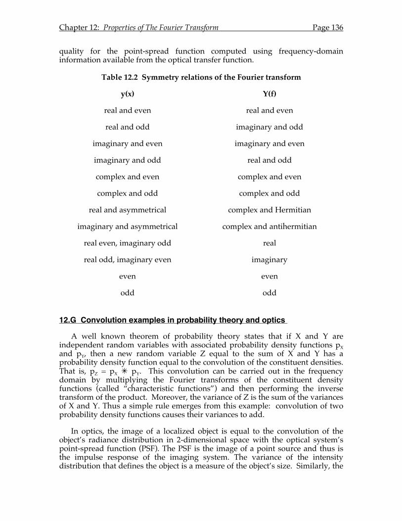
Chapter 12: Properties of The Fourier Transform Page 136
quality for the point-spread function computed using frequency-domain information available from the optical transfer function.
Table 12.2 Symmetry relations of the Fourier transform
y(x) Y(f)
real and even real and even
real and odd imaginary and odd
imaginary and even imaginary and even
imaginary and odd real and odd
complex and even complex and even
complex and odd complex and odd
real and asymmetrical complex and Hermitian
imaginary and asymmetrical complex and antihermitian
real even, imaginary odd real
real odd, imaginary even imaginary
even even
odd odd
12.G Convolution examples in probability theory and optics
A well known theorem of probability theory states that if X and Y are independent random variables with associated probability density functions pX and pY, then a new random variable Z equal to the sum of X and Y has a probability density function equal to the convolution of the constituent densities. That is, pZ = pX pY. This convolution can be carried out in the frequency domain by multiplying the Fourier transforms of the constituent density functions (called “characteristic functions”) and then performing the inverse transform of the product. Moreover, the variance of Z is the sum of the variances of X and Y. Thus a simple rule emerges from this example: convolution of two probability density functions causes their variances to add.
In optics, the image of a localized object is equal to the convolution of the object’s radiance distribution in 2-dimensional space with the optical system’s point-spread function (PSF). The PSF is the image of a point source and thus is the impulse response of the imaging system. The variance of the intensity distribution that defines the object is a measure of the object’s size. Similarly, the
Chapter 12: Properties of The Fourier Transform Page 137
variance of the PSF is a measure of its size. Thus the size of the image is the sum of the size of the object and the size of the PSF. In this way, optical imaging can be conceived as a blurring operation that causes the size of the image to exceed the size of the object by an amount equal to the size of the PSF. This interpretation of convolution for 1-dimensional functions is mentioned by Bracewell (1978) and extended to two-dimensions by Nam et al. (2011) using radial variance as the natural extension to two-dimensions of the concept of size. Radial variance V of an intensity distribution I(x,y) is defined as the second moment about the centroid (xC,yC) in the radial direction, and computed in Cartesian coordinates as
V (I ) = x − xC( )2 + y − yC( )2⎡⎣
⎤⎦
−∞
∞
∫−∞
∞
∫ I(x, y)dxdy [12.35]
12.H Variations on the convolution theorem
The basic convolution theorem h ∗ g↔ H ⋅G of eqn. [12.15] and correlation theorem hg↔ H ⋅G(−) of eqn. [12.19] take on different forms when we allow for complex conjugation and sign reversal of the variables. See Table 12.3 for a summary. The short-hand notation h(-) means h(-x) (i.e. the function has been flipped left-right about the origin) and h* is the complex conjugate of h.
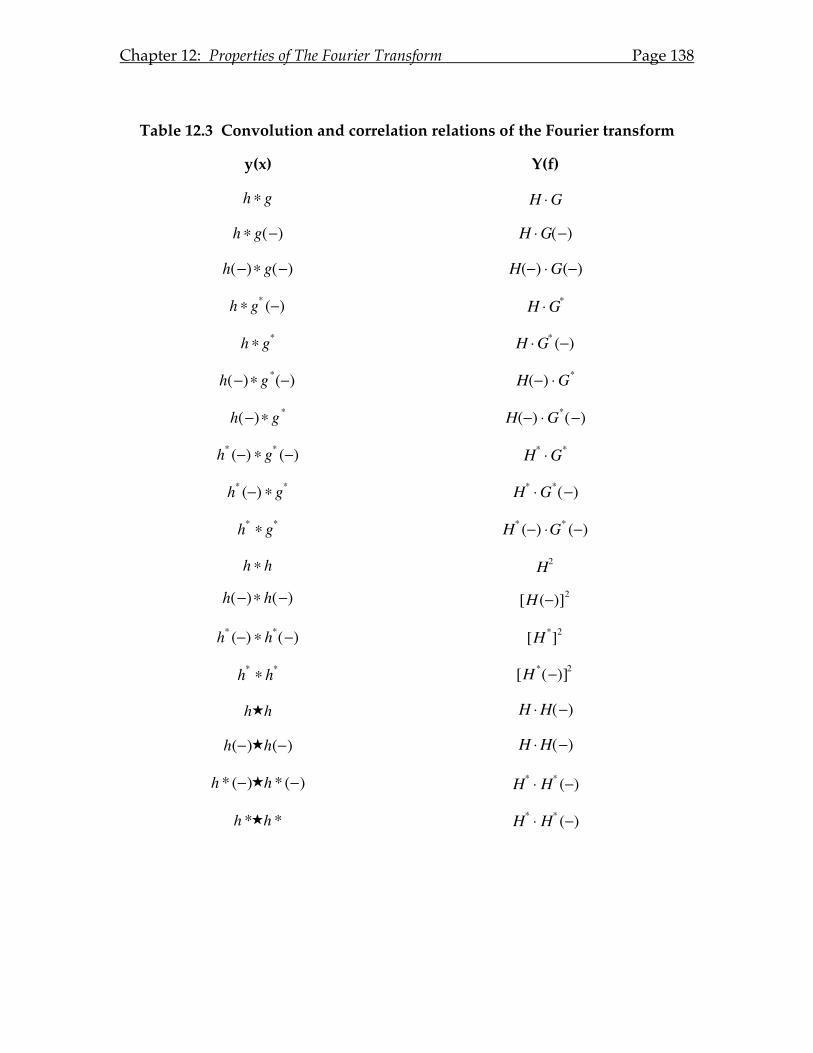
Chapter 12: Properties of The Fourier Transform Page 138
Table 12.3 Convolution and correlation relations of the Fourier transform
y(x) Y(f)
h ∗ g H ⋅G
h ∗ g(−) H ⋅G(−)
h(−)∗ g(−) H(−) ⋅G(−)
h ∗ g* (−) H ⋅G*
h ∗ g* H ⋅G* (−)
h(−)∗ g*(−) H(−) ⋅G*
h(−)∗ g* H(−) ⋅G*(−)
h* (−) ∗ g* (−) H* ⋅G*
h* (−) ∗ g* H* ⋅G*(−)
h* ∗ g* H* (−) ⋅G* (−)
h ∗ h H2
h(−)∗ h(−) [H (−)]2
h* (−) ∗ h*(−) [H *]2
h* ∗ h* [H *(−)]2
hh H ⋅H(−)
h(−)h(−) H ⋅H(−)
h * (−)h * (−) H* ⋅ H* (−)
h *h * H* ⋅ H* (−)
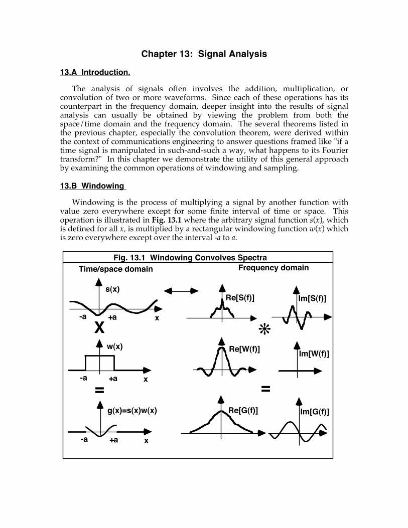
Chapter 13: Signal Analysis
13.A Introduction.
The analysis of signals often involves the addition, multiplication, or convolution of two or more waveforms. Since each of these operations has its counterpart in the frequency domain, deeper insight into the results of signal analysis can usually be obtained by viewing the problem from both the space/time domain and the frequency domain. The several theorems listed in the previous chapter, especially the convolution theorem, were derived within the context of communications engineering to answer questions framed like "if a time signal is manipulated in such-and-such a way, what happens to its Fourier transform?" In this chapter we demonstrate the utility of this general approach by examining the common operations of windowing and sampling.
13.B Windowing
Windowing is the process of multiplying a signal by another function with value zero everywhere except for some finite interval of time or space. This operation is illustrated in Fig. 13.1 where the arbitrary signal function s(x), which is defined for all x, is multiplied by a rectangular windowing function w(x) which is zero everywhere except over the interval -a to a.
Fig. 13.1 Windowing Convolves SpectraTime/space domain Frequency domain
Re[S(f)]
x-a +a
X
=
x-a +a
x-a +a
s(x)
w(x)
g(x)=s(x)w(x)
Im[S(f)]
Im[W(f)]Re[W(f)]
!
=Re[G(f)] Im[G(f)]
Chapter 13: Signal Analysis Page 140
Forming the product g(x)=s(x)w(x) is analogous to looking at the signal through a "window" that reveals just a small segment of the original waveform. Notice that since each of the functions in Fig. 13.1 is defined over all time, each may be subjected to the Fourier transform operation to produce a corresponding spectrum as shown. Any window that has a Fourier transform can be analyzed by the general method given below.
According to the convolution theorem, the Fourier transform of the product s(x)w(x) is equal to the convolution () of the spectrum S(f) of the original function and the spectrum W(f) of the window. That is,
G( f ) = S( f ) ∗W( f ) [13.1]
Recall that, in general, the spectral functions S(f) and W(f) will be complex-valued. If we represent each of these functions explicitly as the sum of a real and an imaginary component and then apply the distributive property of convolution, we find that the solution involves four separate convolutions
G( f ) = Re S( f )[ ] + i Im S( f )[ ]{ }∗ Re W( f )[ ] + iIm W( f )[ ]{ }= Re S( f )[ ]∗Re W( f )[ ]− Im S( f )[ ]∗ Im W( f )[ ]+i Re S( f )[ ]∗ Im W( f )[ ] + Im S( f )[ ]∗Re W( f )[ ]{ }
[13.2]
If the window is symmetric about the origin, as is the case in Fig. 13.1, then the imaginary component of W(f) is zero (by symmetry arguments) and so eqn. [13.2] reduces to
G( f ) = Re S( f )[ ]∗Re W( f )[ ]+ i Im S( f )[ ]∗Re W( f )[ ]{ } [13.3]
If convolution is conceived as a smearing, or blurring operation, then this result says that the effect of windowing is to blur the spectrum of the original signal by an amount that varies inversely with the width of the window.
An important example of the foregoing result is that of a sinusoidal signal, s(x) = cos(2πf0x) , viewed through a rectangular window of width w which, according to eqns. [11.12] and [11.16], has the Fourier transform w sinc(wf ). In this case,
cos(2πf0x)↔δ( f − f0 ) + δ( f + f0 )
2 (signal) [13.4]
rect(x /w)↔ wsinc(wf ) (window) [13.5]
cos(2πf0x)rect(x / w)↔δ( f − f0 ) +δ( f + f0 )
2∗wsinc(wf ) (product) [13.6]
In these equations the special function rect(x) is defined as
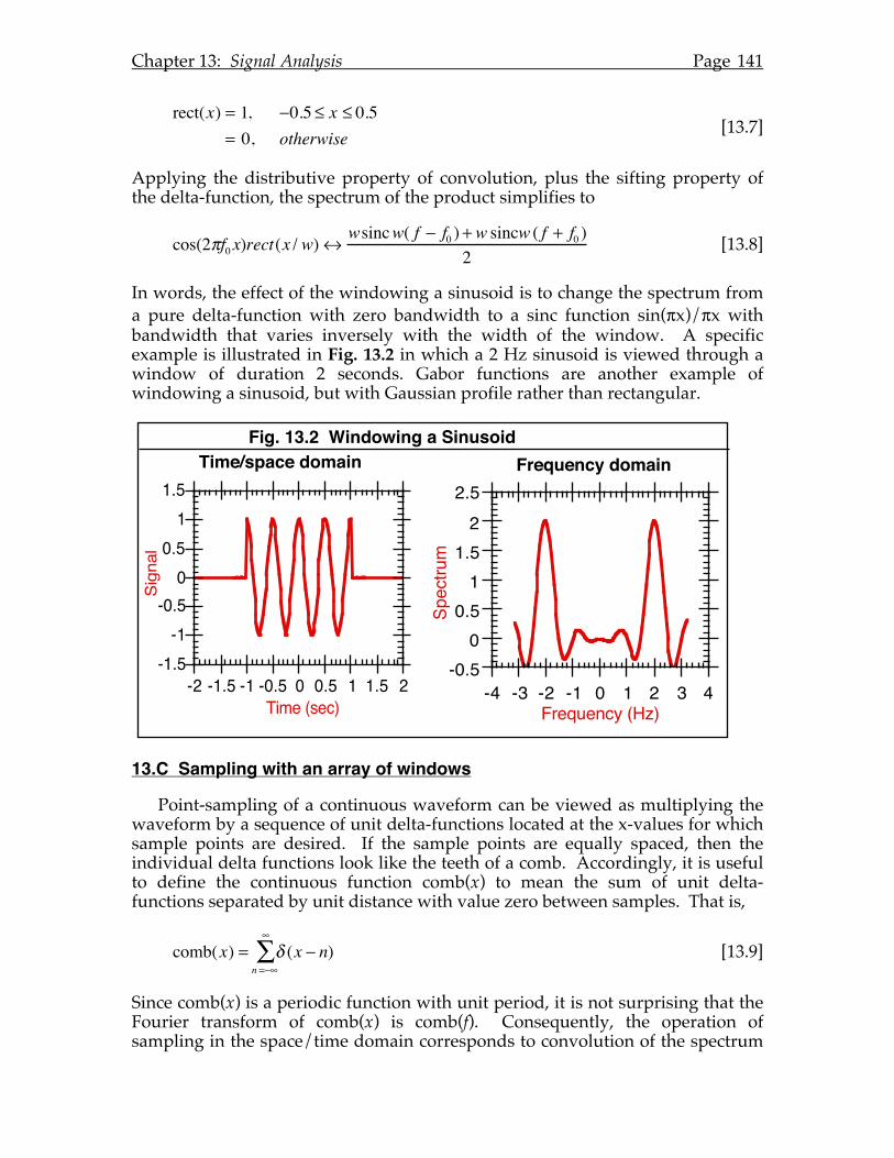
Chapter 13: Signal Analysis Page 141
rect(x) = 1, −0.5 ≤ x ≤ 0.5
= 0, otherwise [13.7]
Applying the distributive property of convolution, plus the sifting property of the delta-function, the spectrum of the product simplifies to
cos(2πf0x)rect(x / w)↔wsincw( f − f0 ) + w sincw ( f + f0 )
2 [13.8]
In words, the effect of the windowing a sinusoid is to change the spectrum from a pure delta-function with zero bandwidth to a sinc function sin(πx)/πx with bandwidth that varies inversely with the width of the window. A specific example is illustrated in Fig. 13.2 in which a 2 Hz sinusoid is viewed through a window of duration 2 seconds. Gabor functions are another example of windowing a sinusoid, but with Gaussian profile rather than rectangular.
13.C Sampling with an array of windows
Point-sampling of a continuous waveform can be viewed as multiplying the waveform by a sequence of unit delta-functions located at the x-values for which sample points are desired. If the sample points are equally spaced, then the individual delta functions look like the teeth of a comb. Accordingly, it is useful to define the continuous function comb(x) to mean the sum of unit delta-functions separated by unit distance with value zero between samples. That is,
comb(x) = δ (x − n)n =−∞
∞
∑ [13.9]
Since comb(x) is a periodic function with unit period, it is not surprising that the Fourier transform of comb(x) is comb(f). Consequently, the operation of sampling in the space/time domain corresponds to convolution of the spectrum
Fig. 13.2 Windowing a SinusoidTime/space domain
-1.5-1
-0.50
0.51
Sign
al
1.5
-2 -1.5 -1 -0.5 0Time (sec)
0.5 1 1.5 2-0.5
00.5
11.5
22.5
Spec
trum
-4 -3 -2 -1 0 1 2 3 4Frequency (Hz)
Frequency domain
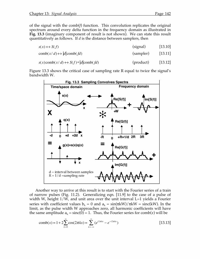
Chapter 13: Signal Analysis Page 142
of the signal with the comb(f) function. This convolution replicates the original spectrum around every delta function in the frequency domain as illustrated in Fig. 13.3 (imaginary component of result is not shown). We can state this result quantitatively as follows. If d is the distance between samplers, then
s(x)↔ S( f ) (signal) [13.10] comb(x / d)↔ d comb( fd) (sampler) [13.11]
s(x)comb(x / d)↔ S( f )∗ d comb( fd) (product) [13.12]
Figure 13.3 shows the critical case of sampling rate R equal to twice the signal’s bandwidth W.
Another way to arrive at this result is to start with the Fourier series of a train of narrow pulses (Fig. 11.2). Generalizing eqn. [11.9] to the case of a pulse of width W, height 1/W, and unit area over the unit interval L=1 yields a Fourier series with coefficient values bk = 0 and ak = sin(πkW)/πkW = sinc(kW). In the limit, as the pulse width W approaches zero, all harmonic coefficients will have the same amplitude ak = sinc(0) = 1. Thus, the Fourier series for comb(x) will be
comb(x) = 1+ 2 cos(2πkx)k=0
∞
∑ = (ei2π kx − e− i2π kx )k=−∞
∞
∑ [13.13]
Chapter 13: Signal Analysis Page 143
Since multiplication of the signal by comb(x) can be done one harmonic at a time, application of the modulation theorem says that multiplication by the k-th harmonic will halve the amplitude of the signal spectrum and shift it to the right (positive frequency direction) and to the left (negative frequency direction) by an amount equal to the frequency of the k-th harmonic. The result of this operation for all of the harmonics is the replication of the signal spectrum at every harmonic of the sampling frequency.
It is important to understand that multiple copies of the frequency spectrum S(f) exist because the sampled function s(x) is a continuous function with value zero for all points between sample points. This is very different from the situation in Chapters 3 & 4 where the signal was unknown between sample points. In that case the data were discrete, not continuous, and therefore the Fourier spectrum was also discrete, with a finite number of harmonics. Classical engineering applications of sampling theory usually treat the sampled signal as a continuous analog signal that is filtered, amplified, and transmitted by analog devices. However, if the samples represent the output of an analog-to-digital conversion, then the value of the signal between samples is indeterminate, not zero, and the spectrum of the sampled data is finite with only one copy of the signal spectrum, not infinite with multiple copies.
13.D Aliasing
As is evident in Fig. 13.3, if the bandwidth w of the signal being sampled is large compared to the distance between delta functions in the frequency spectrum, then the replicated copies will overlap. This is the phenomenon of aliasing encountered previously in Chapter 7. To avoid aliasing requires that w < R / 2 , which means that the bandwidth of the signal must be less than half the sampling frequency. The critical value R/2 is called the Nyquist frequency, which is a property of the sampling process, not the signal being sampled. From a graphical perspective, Shannon's sampling theorem says that as long as the replicated spectra do not overlap then it is possible to recover the original spectrum without error. A simple method for retrieving the original signal from sampled values is described in section 13.E.
Aliasing of two-dimensional space caused by under-sampling with a lattice of sampling elements has additional degrees of freedom related to the geometry of the array (e.g. square or triangular lattices, and possibly rotated). An example of aliasing produced by a triangular lattice of sample points (with zero-values between samples) is shown in Fig. 13.4. These Fourier spectra were computed as the convolution of the spectrum of a sinusoidal grating pattern (a pair of delta functions) with the spectrum of the sampling array (the inverse lattice). If the sampling lattice is triangular with spacing S between samples, then the inverse lattice is triangular with spacing constant 2/(S√3), but transposed and rotated with respect to the sampling lattice. Example spectra are shown for three sampling configurations. Row A depicts the case of sampling a vertical or horizontal grating of spatial frequency slightly higher than the nominal Nyquist frequency of the sampling array. The spectrum of the continuous sinusoidal grating is represented in the left panel by the pair of circles (vertical grating) and
Chapter 13: Signal Analysis Page 144
the pair of crosses (horizontal grating), plus another delta function at the origin representing the mean luminance of the grating. The center panel shows the central portion of the spectrum of a sampling lattice in the 0° orientation, which puts the spectral lattice in the 30° orientation. The circle centered on the origin is a two-dimensional extension of the concept of a Nyquist limit. We call this circle a Nyquist ring because the radius of the ring indicates the highest spatial frequency of the continuous input that can be faithfully represented by the sampled output. Strictly, the Nyquist ring for a triangular lattice is a hexagon defined by a nearest-neighbor rule: all points inside the hexagon are closer to the origin than to any other lattice node. Here we make the simplifying assumption that the Nyquist ring is circular with radius equal to the nominal Nyquist frequency (0.54/S for a triangular lattice).
The right hand panel of Fig. 13.4 shows the result of convolving the left and middle panels to compute the spatial frequency spectrum of the sampled stimulus. Convolution creates multiple copies of the source spectrum, one copy centered on each point in the array spectrum. To use this panel as a graphical method for predicting the alias patterns produced by undersampling, we concentrate our attention on the interior of the Nyquist ring since this is the do- main of spatial frequencies that satisfy the sampling theorem. When the source grating exceeds the Nyquist frequency of the array, the spectrum of the sampled stimulus will fall outside the Nyquist ring. However, other copies of the source spectrum centered on nearby lattice points may fall inside the Nyquist ring, thus masquerading as low-frequency gratings below the Nyquist limit. This process by which high-frequency components masquerade as low-frequency components when under-sampled, sometimes called leaking or folding of the spectrum, is the essence of aliasing. The stimulus spectrum depicted in row B is for the same grating frequency as in row A, but rotated 15°. The spectrum depicted in row C is also for a rotated grating, but a spatial frequency twice the Nyquist frequency.
As noted in Section 13.C, the portion of the spectrum outside the Nyquist ring exists because the sampled grating was assumed to be continuous, with value zero between sampled points. This would be an appropriate model, for example, of a grating masked by an overlaid array of pinhole apertures since the intensity between pinholes would be zero. However, this would be an inappropriate model for the discrete neural image produced when a continuous grating imaged on the retina is sampled by an array of photoreceptors. Although the visual world is spatially continuous, even when masked by an array of pinhole apertures, the neural images carried by discrete arrays of visual neurons are spatially discrete. In more general terms, the difference between the spatially continuous domains of analog sampling and the spatially discrete domain of digital sampling has important consequences for describing their respective frequency spectra because continuous functions have infinite bandwidth, whereas discrete functions have finite bandwidth.
In summary, the frequency spectrum of a discrete, digitally-sampled image would contain only those spatial frequencies inside the Nyquist ring. There is no need for subsequent processing to remove high spatial frequency components beyond the Nyquist limit because they do not exist in the sampled image. For
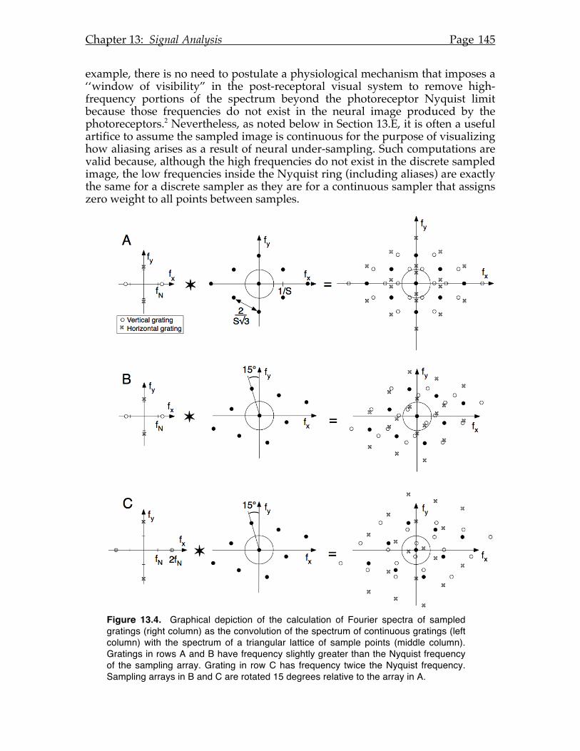
Chapter 13: Signal Analysis Page 145
example, there is no need to postulate a physiological mechanism that imposes a ‘‘window of visibility” in the post-receptoral visual system to remove high-frequency portions of the spectrum beyond the photoreceptor Nyquist limit because those frequencies do not exist in the neural image produced by the photoreceptors.2 Nevertheless, as noted below in Section 13.E, it is often a useful artifice to assume the sampled image is continuous for the purpose of visualizing how aliasing arises as a result of neural under-sampling. Such computations are valid because, although the high frequencies do not exist in the discrete sampled image, the low frequencies inside the Nyquist ring (including aliases) are exactly the same for a discrete sampler as they are for a continuous sampler that assigns zero weight to all points between samples.
Figure 13.4. Graphical depiction of the calculation of Fourier spectra of sampled gratings (right column) as the convolution of the spectrum of continuous gratings (left column) with the spectrum of a triangular lattice of sample points (middle column). Gratings in rows A and B have frequency slightly greater than the Nyquist frequency of the sampling array. Grating in row C has frequency twice the Nyquist frequency. Sampling arrays in B and C are rotated 15 degrees relative to the array in A.
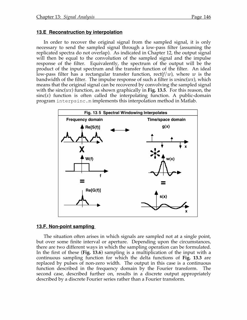
Chapter 13: Signal Analysis Page 146
13.E Reconstruction by interpolation
In order to recover the original signal from the sampled signal, it is only necessary to send the sampled signal through a low-pass filter (assuming the replicated spectra do not overlap). As indicated in Chapter 12, the output signal will then be equal to the convolution of the sampled signal and the impulse response of the filter. Equivalently, the spectrum of the output will be the product of the input spectrum and the transfer function of the filter. An ideal low-pass filter has a rectangular transfer function, rect(f/w), where w is the bandwidth of the filter. The impulse response of such a filter is wsinc(wx), which means that the original signal can be recovered by convolving the sampled signal with the sinc(wx) function, as shown graphically in Fig. 13.5. For this reason, the sinc(x) function is often called the interpolating function. A public-domain program interpsinc.m implements this interpolation method in Matlab.
13.F. Non-point sampling
The situation often arises in which signals are sampled not at a single point, but over some finite interval or aperture. Depending upon the circumstances, there are two different ways in which the sampling operation can be formulated. In the first of these (Fig. 13.6) sampling is a multiplication of the input with a continuous sampling function for which the delta functions of Fig. 13.3 are replaced by pulses of non-zero width. The output in this case is a continuous function described in the frequency domain by the Fourier transform. The second case, described further on, results in a discrete output appropriately described by a discrete Fourier series rather than a Fourier transform.
!
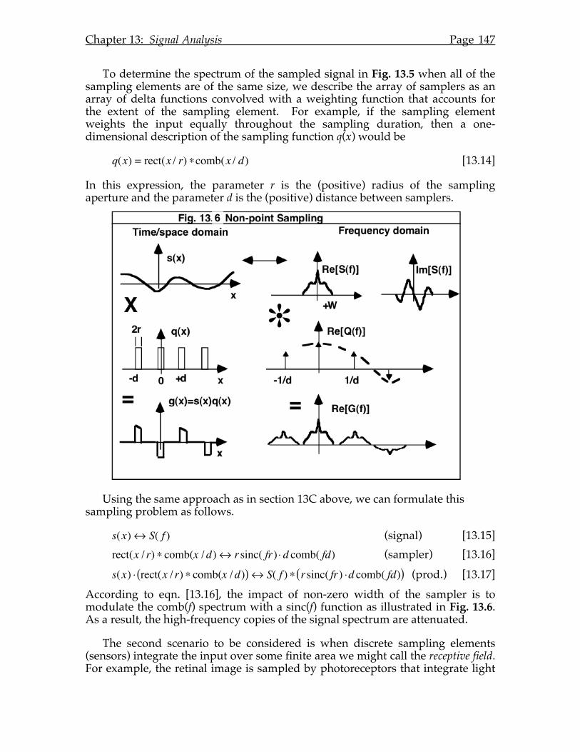
Chapter 13: Signal Analysis Page 147
To determine the spectrum of the sampled signal in Fig. 13.5 when all of the sampling elements are of the same size, we describe the array of samplers as an array of delta functions convolved with a weighting function that accounts for the extent of the sampling element. For example, if the sampling element weights the input equally throughout the sampling duration, then a one-dimensional description of the sampling function q(x) would be
q(x) = rect(x / r) ∗comb(x / d) [13.14]
In this expression, the parameter r is the (positive) radius of the sampling aperture and the parameter d is the (positive) distance between samplers.
Using the same approach as in section 13C above, we can formulate this sampling problem as follows.
s(x)↔ S( f ) (signal) [13.15] rect(x / r) ∗ comb(x /d)↔ rsinc( fr) ⋅ d comb( fd) (sampler) [13.16] s(x) ⋅ rect(x / r) ∗ comb(x /d)( ) ↔ S( f ) ∗ rsinc( fr) ⋅d comb( fd)( ) (prod.) [13.17] According to eqn. [13.16], the impact of non-zero width of the sampler is to modulate the comb(f) spectrum with a sinc(f) function as illustrated in Fig. 13.6. As a result, the high-frequency copies of the signal spectrum are attenuated.
The second scenario to be considered is when discrete sampling elements (sensors) integrate the input over some finite area we might call the receptive field. For example, the retinal image is sampled by photoreceptors that integrate light
!
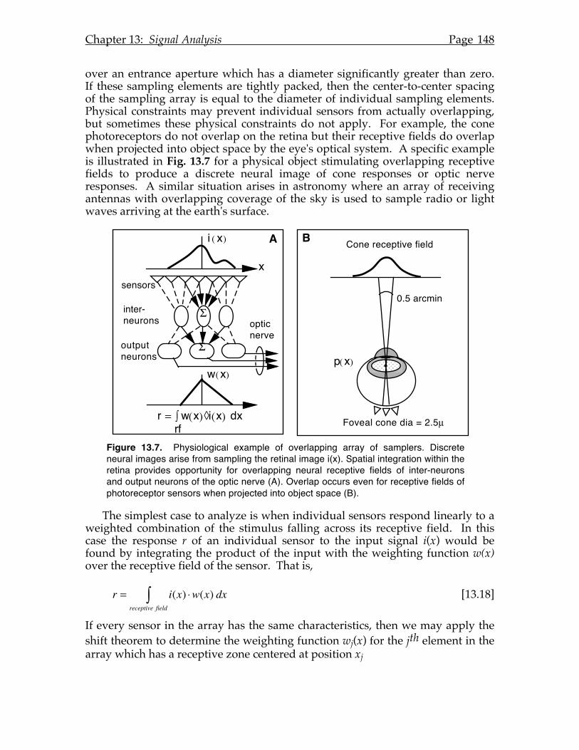
Chapter 13: Signal Analysis Page 148
over an entrance aperture which has a diameter significantly greater than zero. If these sampling elements are tightly packed, then the center-to-center spacing of the sampling array is equal to the diameter of individual sampling elements. Physical constraints may prevent individual sensors from actually overlapping, but sometimes these physical constraints do not apply. For example, the cone photoreceptors do not overlap on the retina but their receptive fields do overlap when projected into object space by the eye's optical system. A specific example is illustrated in Fig. 13.7 for a physical object stimulating overlapping receptive fields to produce a discrete neural image of cone responses or optic nerve responses. A similar situation arises in astronomy where an array of receiving antennas with overlapping coverage of the sky is used to sample radio or light waves arriving at the earth's surface.
Figure 13.7. Physiological example of overlapping array of samplers. Discrete neural images arise from sampling the retinal image i(x). Spatial integration within the retina provides opportunity for overlapping neural receptive fields of inter-neurons and output neurons of the optic nerve (A). Overlap occurs even for receptive fields of photoreceptor sensors when projected into object space (B).
The simplest case to analyze is when individual sensors respond linearly to a weighted combination of the stimulus falling across its receptive field. In this case the response r of an individual sensor to the input signal i(x) would be found by integrating the product of the input with the weighting function w(x) over the receptive field of the sensor. That is,
r = i(x) ⋅w(x) dxreceptive field∫ [13.18]
If every sensor in the array has the same characteristics, then we may apply the shift theorem to determine the weighting function wj(x) for the jth element in the array which has a receptive zone centered at position xj
!!!" ! #"
!!#
!!$ ! %!#" "!#" &#
$'
!!%!#"
()*(+$(
"*,)$-*).$+*(
+.,/.,*).$+*(
+/,"0*)$1)
!!
!!
"
!!/!#"
2+1)34!0+*)!&"3!5!678"
9+*)!$)0)/,"1)!!)4&
:78!3$0;"*
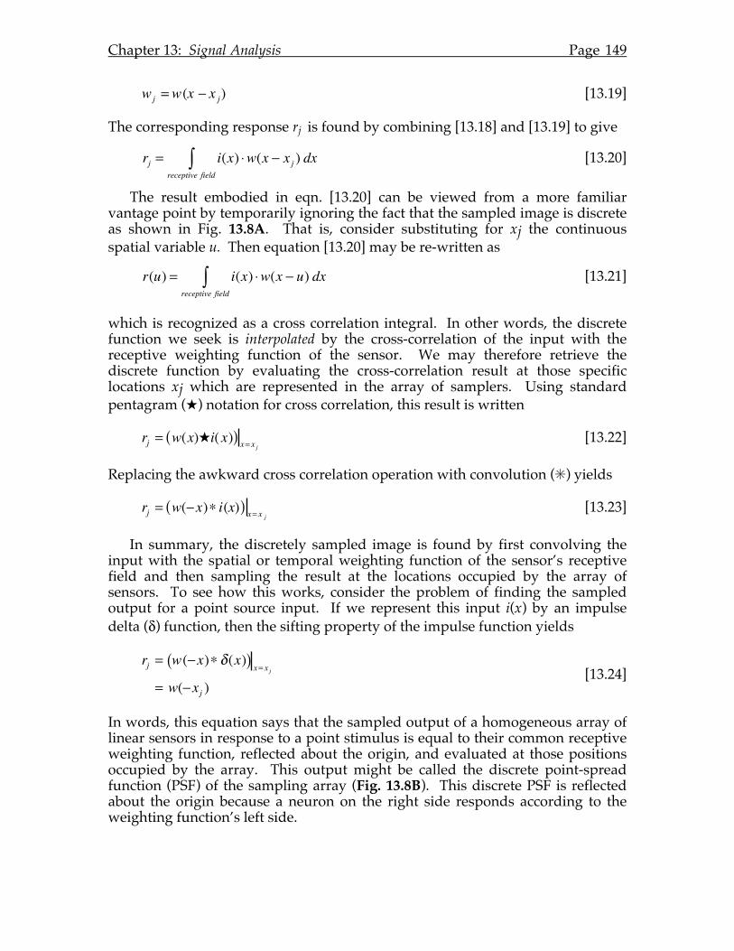
Chapter 13: Signal Analysis Page 149
wj = w(x − x j) [13.19]
The corresponding response rj is found by combining [13.18] and [13.19] to give
rj = i(x) ⋅w(x − x j ) dxreceptive field∫ [13.20]
The result embodied in eqn. [13.20] can be viewed from a more familiar vantage point by temporarily ignoring the fact that the sampled image is discrete as shown in Fig. 13.8A. That is, consider substituting for xj the continuous spatial variable u. Then equation [13.20] may be re-written as
r(u) = i(x) ⋅w(x − u) dxreceptive field∫ [13.21]
which is recognized as a cross correlation integral. In other words, the discrete function we seek is interpolated by the cross-correlation of the input with the receptive weighting function of the sensor. We may therefore retrieve the discrete function by evaluating the cross-correlation result at those specific locations xj which are represented in the array of samplers. Using standard pentagram (★) notation for cross correlation, this result is written
rj = w(x)★i(x)( ) x= x j [13.22]
Replacing the awkward cross correlation operation with convolution (✳) yields
rj = w(−x)∗ i(x)( ) x= x j [13.23]
In summary, the discretely sampled image is found by first convolving the input with the spatial or temporal weighting function of the sensor’s receptive field and then sampling the result at the locations occupied by the array of sensors. To see how this works, consider the problem of finding the sampled output for a point source input. If we represent this input i(x) by an impulse delta (δ) function, then the sifting property of the impulse function yields
rj = w(−x)∗ δ(x)( ) x= x j= w(−xj )
[13.24]
In words, this equation says that the sampled output of a homogeneous array of linear sensors in response to a point stimulus is equal to their common receptive weighting function, reflected about the origin, and evaluated at those positions occupied by the array. This output might be called the discrete point-spread function (PSF) of the sampling array (Fig. 13.8B). This discrete PSF is reflected about the origin because a neuron on the right side responds according to the weighting function’s left side.
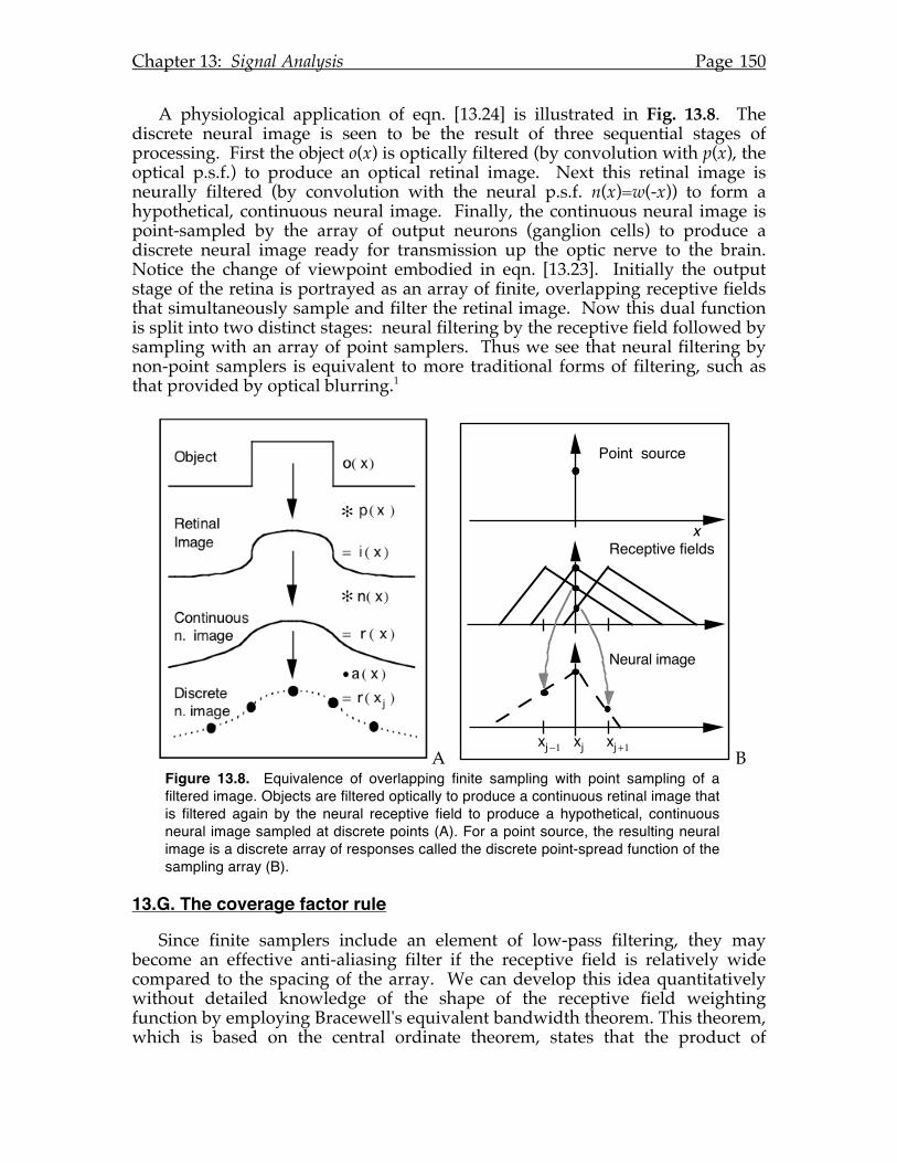
Chapter 13: Signal Analysis Page 150
A physiological application of eqn. [13.24] is illustrated in Fig. 13.8. The discrete neural image is seen to be the result of three sequential stages of processing. First the object o(x) is optically filtered (by convolution with p(x), the optical p.s.f.) to produce an optical retinal image. Next this retinal image is neurally filtered (by convolution with the neural p.s.f. n(x)=w(-x)) to form a hypothetical, continuous neural image. Finally, the continuous neural image is point-sampled by the array of output neurons (ganglion cells) to produce a discrete neural image ready for transmission up the optic nerve to the brain. Notice the change of viewpoint embodied in eqn. [13.23]. Initially the output stage of the retina is portrayed as an array of finite, overlapping receptive fields that simultaneously sample and filter the retinal image. Now this dual function is split into two distinct stages: neural filtering by the receptive field followed by sampling with an array of point samplers. Thus we see that neural filtering by non-point samplers is equivalent to more traditional forms of filtering, such as that provided by optical blurring.1
A B Figure 13.8. Equivalence of overlapping finite sampling with point sampling of a filtered image. Objects are filtered optically to produce a continuous retinal image that is filtered again by the neural receptive field to produce a hypothetical, continuous neural image sampled at discrete points (A). For a point source, the resulting neural image is a discrete array of responses called the discrete point-spread function of the sampling array (B).
13.G. The coverage factor rule
Since finite samplers include an element of low-pass filtering, they may become an effective anti-aliasing filter if the receptive field is relatively wide compared to the spacing of the array. We can develop this idea quantitatively without detailed knowledge of the shape of the receptive field weighting function by employing Bracewell's equivalent bandwidth theorem. This theorem, which is based on the central ordinate theorem, states that the product of
Fig. 13.6. Neural image for a point source of light.
Receptive fields
Neural image
Point source
x
xj
xj+1
xj!1
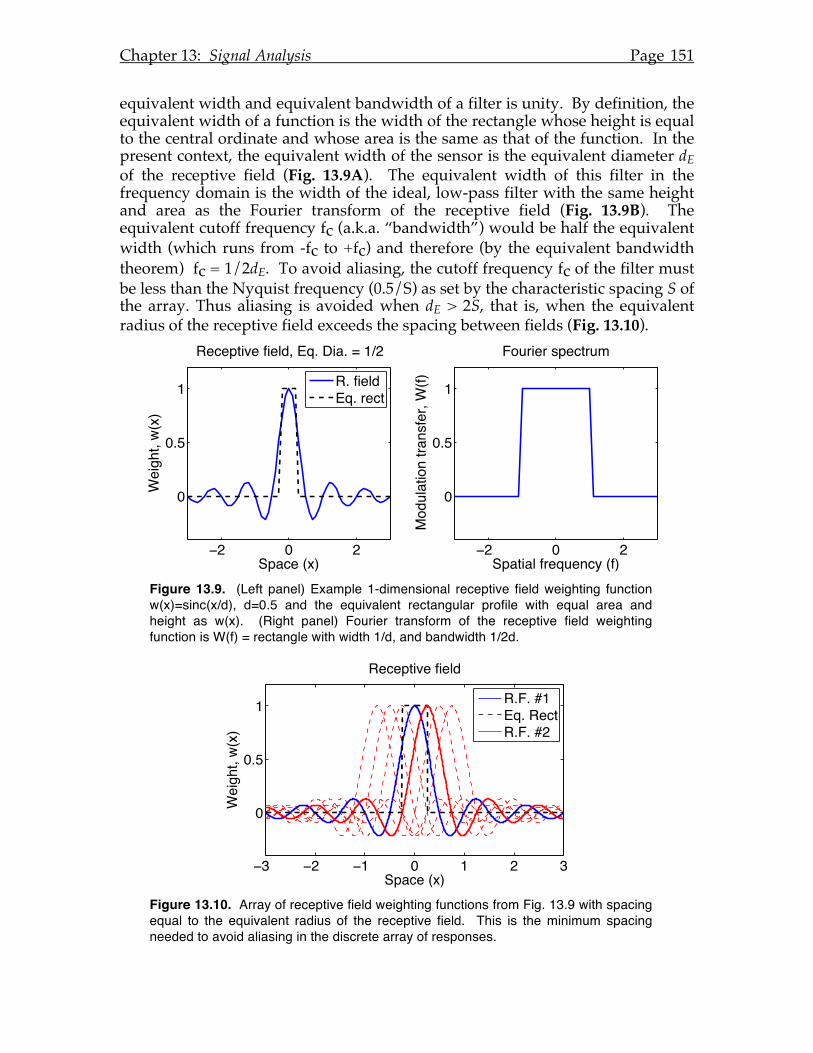
Chapter 13: Signal Analysis Page 151
equivalent width and equivalent bandwidth of a filter is unity. By definition, the equivalent width of a function is the width of the rectangle whose height is equal to the central ordinate and whose area is the same as that of the function. In the present context, the equivalent width of the sensor is the equivalent diameter dE of the receptive field (Fig. 13.9A). The equivalent width of this filter in the frequency domain is the width of the ideal, low-pass filter with the same height and area as the Fourier transform of the receptive field (Fig. 13.9B). The equivalent cutoff frequency fc (a.k.a. “bandwidth”) would be half the equivalent width (which runs from -fc to +fc) and therefore (by the equivalent bandwidth theorem) fc = 1/2dE. To avoid aliasing, the cutoff frequency fc of the filter must be less than the Nyquist frequency (0.5/S) as set by the characteristic spacing S of the array. Thus aliasing is avoided when dE > 2S, that is, when the equivalent radius of the receptive field exceeds the spacing between fields (Fig. 13.10).
Figure 13.9. (Left panel) Example 1-dimensional receptive field weighting function w(x)=sinc(x/d), d=0.5 and the equivalent rectangular profile with equal area and height as w(x). (Right panel) Fourier transform of the receptive field weighting function is W(f) = rectangle with width 1/d, and bandwidth 1/2d.
Figure 13.10. Array of receptive field weighting functions from Fig. 13.9 with spacing equal to the equivalent radius of the receptive field. This is the minimum spacing needed to avoid aliasing in the discrete array of responses.
2 0 2
0
0.5
1
Receptive field, Eq. Dia. = 1/2
Space (x)
Wei
ght,
w(x
)
R. fieldEq. rect
2 0 2
0
0.5
1
Fourier spectrum
Spatial frequency (f)
Mod
ulat
ion
trans
fer,
W(f)
3 2 1 0 1 2 3
0
0.5
1
Receptive field
Space (x)
Wei
ght,
w(x
)
R.F. #1Eq. RectR.F. #2
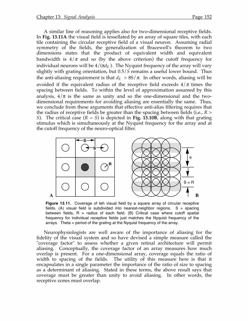
Chapter 13: Signal Analysis Page 152
A similar line of reasoning applies also for two-dimensional receptive fields. In Fig. 13.11A the visual field is tessellated by an array of square tiles, with each tile containing the circular receptive field of a visual neuron. Assuming radial symmetry of the fields, the generalization of Bracewell's theorem to two dimensions states that the product of equivalent width and equivalent bandwidth is 4/π and so (by the above criterion) the cutoff frequency for individual neurons will be 4/(πdE ). The Nyquist frequency of the array will vary slightly with grating orientation, but 0.5/S remains a useful lower bound. Thus the anti-aliasing requirement is that dE > 8S/π. In other words, aliasing will be avoided if the equivalent radius of the receptive field exceeds 4/π times the spacing between fields. To within the level of approximation assumed by this analysis, 4/π is the same as unity and so the one-dimensional and the two-dimensional requirements for avoiding aliasing are essentially the same. Thus, we conclude from these arguments that effective anti-alias filtering requires that the radius of receptive fields be greater than the spacing between fields (i.e., R > S). The critical case (R = S) is depicted in Fig. 13.10B, along with that grating stimulus which is simultaneously at the Nyquist frequency for the array and at the cutoff frequency of the neuro-optical filter.
A B Figure 13.11. Coverage of teh visual field by a square array of circular receptive fields. (A) visual field is subdivided into nearest-neighbor regions. S = spacing between fields, R = radius of each field. (B) Critical case where cutoff spatial frequency for individual receptive fields just matches the Nyquist frequency of the arrays. Theta = period of the grating at the Nyquist frequency of the array.
Neurophysiologists are well aware of the importance of aliasing for the fidelity of the visual system and so have devised a simple measure called the "coverage factor" to assess whether a given retinal architecture will permit aliasing. Conceptually, the coverage factor of an array measures how much overlap is present. For a one-dimensional array, coverage equals the ratio of width to spacing of the fields. The utility of this measure here is that it encapsulates in a single parameter the importance of the ratio of size to spacing as a determinant of aliasing. Stated in these terms, the above result says that coverage must be greater than unity to avoid aliasing. In other words, the receptive zones must overlap.
S
S
R!
S = R
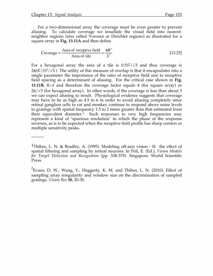
Chapter 13: Signal Analysis Page 153
For a two-dimensional array the coverage must be even greater to prevent aliasing. To calculate coverage we tessellate the visual field into nearest-neighbor regions (also called Voronoi or Dirichlet regions) as illustrated for a square array in Fig. 13.11A and then define
Coverage = Area of receptive fieldArea of tile
=πR2
S2 [13.25]
For a hexagonal array the area of a tile is 0.5S2/√3 and thus coverage is 2π(R/S)2/√3.) The utility of this measure of overlap is that it encapsulates into a single parameter the importance of the ratio of receptive field size to receptive field spacing as a determinant of aliasing. For the critical case shown in Fig. 13.11B, R=S and therefore the coverage factor equals π (for square array) or 2π/√3 (for hexagonal array). In other words, if the coverage is less than about 3 we can expect aliasing to result. Physiological evidence suggests that coverage may have to be as high as 4.5 to 6 in order to avoid aliasing completely since retinal ganglion cells in cat and monkey continue to respond above noise levels to gratings with spatial frequency 1.5 to 2 times greater than that estimated from their equivalent diameter.1 Such responses to very high frequencies may represent a kind of "spurious resolution" in which the phase of the response reverses, as is to be expected when the receptive field profile has sharp corners or multiple sensitivity peaks.
---------
1Thibos, L. N. & Bradley, A. (1995). Modeling off-axis vision - II: the effect of spatial filtering and sampling by retinal neurons. In Peli, E. (Ed.), Vision Models for Target Detection and Recognition (pp. 338-379). Singapore: World Scientific Press.
2Evans, D. W., Wang, Y., Haggerty, K. M. and Thibos, L. N. (2010). Effect of sampling array irregularity and window size on the discrimination of sampled gratings. Vision Res 50, 20-30.

Chapter 13: Signal Analysis Page 154
Chapter 14: Fourier Optics
14.A Introduction
Fourier analysis plays an important role in optics, the science of light and images. Following the successful application of Fourier analysis in communication theory and practice in the early part of the 20th century, optical scientists and engineers began a similar approach to the study of optical systems in the 1950’s. In this new approach Fourier analysis plays several important roles. According to the physical optics theory of image formation, the Fourier transform provides a mathematical distribution of light in the system’s entrance pupil due to a point source of light in the object plane. In the same way, the Fourier transform also links the distribution of light in the exit pupil to the distribution of light in the image plane, the so-called, point spread function (PSF). Fourier analysis is also central to the communications theory approach in which optical imaging systems are conceived as linear filters that convert inputs (the object) to outputs (the image) according to the mathematical operation of convolution between the object and the system’s impulse response (the PSF). Digital computer programs that simulate this convolution operation typically employ the fast Fourier transform (FFT) algorithm to compute the image of an object. The Fourier transform is also used to convert the PSF into a spatial frequency domain description of the filter’s action called the optical transfer function (OTF). To understand why Fourier analysis plays so many key roles in this modern approach to optical systems it is necessary to review briefly the physical theory of image formation.
14.B Physical optics and image formation
The elementary account of image formation illustrated in Fig. 14.1 is based on the geometrical optics notion that light travels in straight lines called rays. All of the rays emitted by a point source of light that are captured by a physical lens of finite size become refracted (i.e. their direction of propagation changes). The intensity of the light is determined by ray density, so the convergence of rays in a region of high density is the geometrical conception of image formation. By this account, the only effect of introducing an aperture before the lens is to limit the spatial distribution of rays that enter the lens. At the margin of the aperture, the transmitted rays define a sharp boundary between light and shadow as suggested by the dashed lines. In fact, as Newton (1670) first observed in the 17th century, light does penetrate the shadow. To take account of this fact of nature we need to replace geometrical optics with a more complete description of light propagation and image formation.
According to the physical optics theory, light propagates in the form of waves that are perpendicular to rays of geometrical optics. A wavefront is defined as the locus of points for which light has oscillated the same number of times after emission from the point source. With each oscillation the light propagates one wavelength of distance, so an equivalent definition of wavefront is the locus of points that are the same optical distance from the point source. Thus a single point source of light emanates spherical wavefronts. Unlike rays, which are
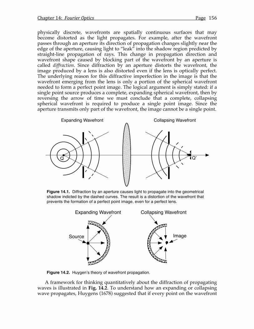
Chapter 14: Fourier Optics Page 156
physically discrete, wavefronts are spatially continuous surfaces that may become distorted as the light propagates. For example, after the wavefront passes through an aperture its direction of propagation changes slightly near the edge of the aperture, causing light to “leak” into the shadow region predicted by straight-line propagation of rays. This change in propagation direction and wavefront shape caused by blocking part of the wavefront by an aperture is called diffraction. Since diffraction by an aperture distorts the wavefront, the image produced by a lens is also distorted even if the lens is optically perfect. The underlying reason for this diffractive imperfection in the image is that the wavefront emerging from the lens is only a portion of the spherical wavefront needed to form a perfect point image. The logical argument is simply stated: if a single point source produces a complete, expanding spherical wavefront, then by reversing the arrow of time we must conclude that a complete, collapsing spherical wavefront is required to produce a single point image. Since the aperture transmits only part of the wavefront, the image cannot be a single point.
Figure 14.1. Diffraction by an aperture causes light to propagate into the geometrical shadow indicted by the dashed curves. The result is a distortion of the wavefront that prevents the formation of a perfect point image, even for a perfect lens.
Figure 14.2. Huygenʼs theory of wavefront propagation.
A framework for thinking quantitatively about the diffraction of propagating waves is illustrated in Fig. 14.2. To understand how an expanding or collapsing wave propagates, Huygens (1678) suggested that if every point on the wavefront
!"#$%&'%()*$+,-./%0 1/22$#3'%()*$+,-./%0
44
!"#$%&'%()*$+,-./%0
1/2.3,
4/55$#6'%()*$+,-./%0
789$(,
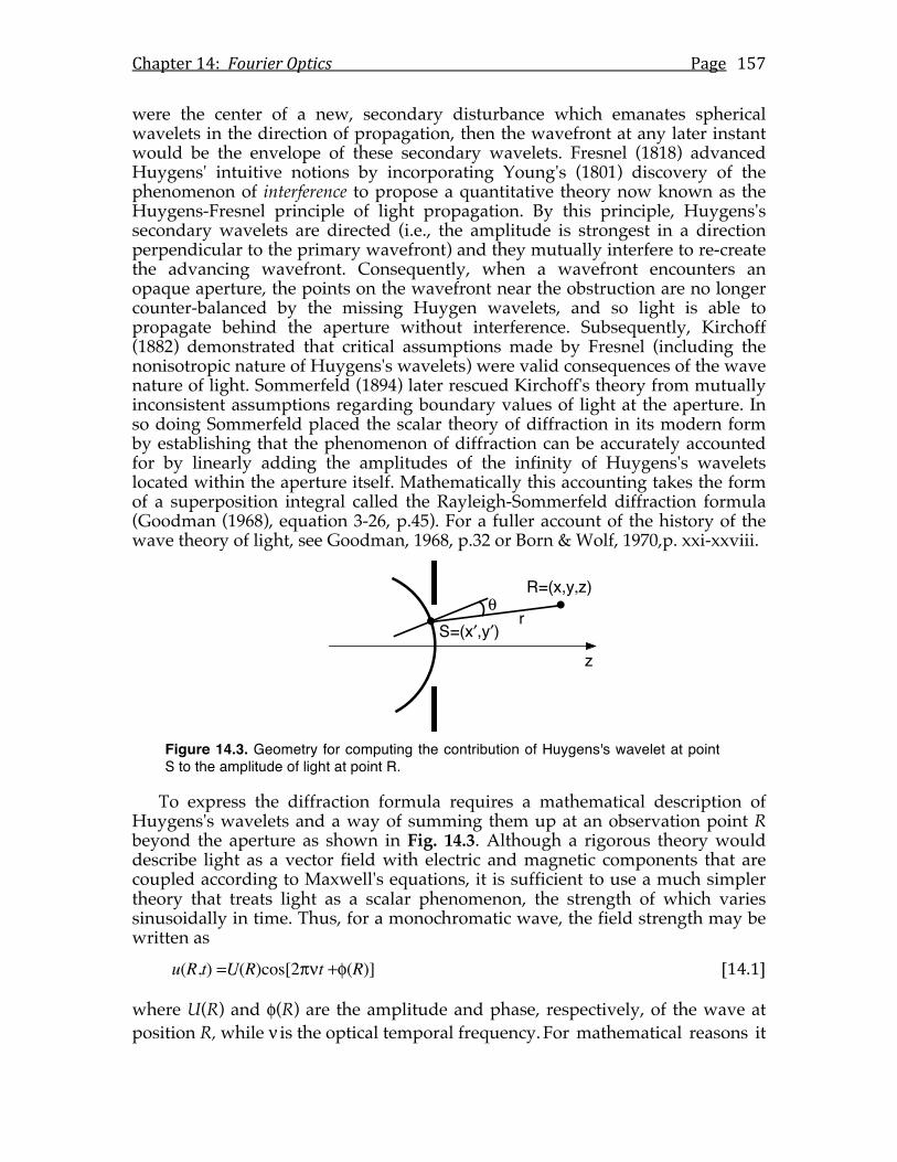
Chapter 14: Fourier Optics Page 157
were the center of a new, secondary disturbance which emanates spherical wavelets in the direction of propagation, then the wavefront at any later instant would be the envelope of these secondary wavelets. Fresnel (1818) advanced Huygens' intuitive notions by incorporating Young's (1801) discovery of the phenomenon of interference to propose a quantitative theory now known as the Huygens-Fresnel principle of light propagation. By this principle, Huygens's secondary wavelets are directed (i.e., the amplitude is strongest in a direction perpendicular to the primary wavefront) and they mutually interfere to re-create the advancing wavefront. Consequently, when a wavefront encounters an opaque aperture, the points on the wavefront near the obstruction are no longer counter-balanced by the missing Huygen wavelets, and so light is able to propagate behind the aperture without interference. Subsequently, Kirchoff (1882) demonstrated that critical assumptions made by Fresnel (including the nonisotropic nature of Huygens's wavelets) were valid consequences of the wave nature of light. Sommerfeld (1894) later rescued Kirchoff's theory from mutually inconsistent assumptions regarding boundary values of light at the aperture. In so doing Sommerfeld placed the scalar theory of diffraction in its modern form by establishing that the phenomenon of diffraction can be accurately accounted for by linearly adding the amplitudes of the infinity of Huygens's wavelets located within the aperture itself. Mathematically this accounting takes the form of a superposition integral called the Rayleigh-Sommerfeld diffraction formula (Goodman (1968), equation 3-26, p.45). For a fuller account of the history of the wave theory of light, see Goodman, 1968, p.32 or Born & Wolf, 1970,p. xxi-xxviii.
Figure 14.3. Geometry for computing the contribution of Huygens's wavelet at point S to the amplitude of light at point R.
To express the diffraction formula requires a mathematical description of Huygens's wavelets and a way of summing them up at an observation point R beyond the aperture as shown in Fig. 14.3. Although a rigorous theory would describe light as a vector field with electric and magnetic components that are coupled according to Maxwell's equations, it is sufficient to use a much simpler theory that treats light as a scalar phenomenon, the strength of which varies sinusoidally in time. Thus, for a monochromatic wave, the field strength may be written as
u(R,t) =U(R)cos[2πνt +φ(R)] [14.1]
where U(R) and φ(R) are the amplitude and phase, respectively, of the wave at position R, while ν is the optical temporal frequency. For mathematical reasons it
!"#$ %& '
(
)"#$%&!('
*
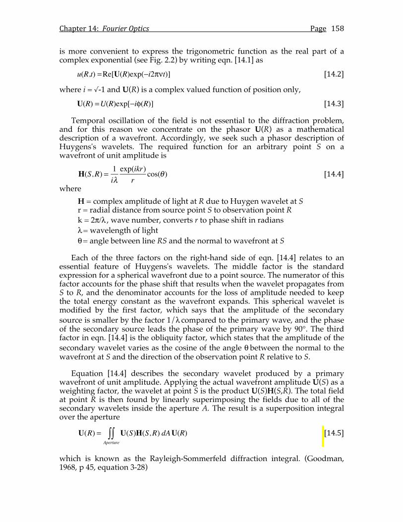
Chapter 14: Fourier Optics Page 158
is more convenient to express the trigonometric function as the real part of a complex exponential (see Fig. 2.2) by writing eqn. [14.1] as
u(R,t) = Re[U(R)exp(−i2πνt)] [14.2]
where i = √-1 and U(R) is a complex valued function of position only,
U(R) = U(R)exp[−iφ(R)] [14.3]
Temporal oscillation of the field is not essential to the diffraction problem, and for this reason we concentrate on the phasor U(R) as a mathematical description of a wavefront. Accordingly, we seek such a phasor description of Huygens's wavelets. The required function for an arbitrary point S on a wavefront of unit amplitude is
H(S,R) = 1iλexp(ikr)
rcos(θ) [14.4]
where H = complex amplitude of light at R due to Huygen wavelet at S r = radial distance from source point S to observation point R k = 2π/λ , wave number, converts r to phase shift in radians λ = wavelength of light θ = angle between line RS and the normal to wavefront at S
Each of the three factors on the right-hand side of eqn. [14.4] relates to an essential feature of Huygens's wavelets. The middle factor is the standard expression for a spherical wavefront due to a point source. The numerator of this factor accounts for the phase shift that results when the wavelet propagates from S to R, and the denominator accounts for the loss of amplitude needed to keep the total energy constant as the wavefront expands. This spherical wavelet is modified by the first factor, which says that the amplitude of the secondary source is smaller by the factor 1/λ compared to the primary wave, and the phase of the secondary source leads the phase of the primary wave by 90°. The third factor in eqn. [14.4] is the obliquity factor, which states that the amplitude of the secondary wavelet varies as the cosine of the angle θ between the normal to the wavefront at S and the direction of the observation point R relative to S.
Equation [14.4] describes the secondary wavelet produced by a primary wavefront of unit amplitude. Applying the actual wavefront amplitude U(S) as a weighting factor, the wavelet at point S is the product U(S)H(S,R). The total field at point R is then found by linearly superimposing the fields due to all of the secondary wavelets inside the aperture A. The result is a superposition integral over the aperture
U(R) = U(S)H(S,R) dAAperture∫∫ U(R) [14.5]
which is known as the Rayleigh-Sommerfeld diffraction integral. (Goodman, 1968, p 45, equation 3-28)
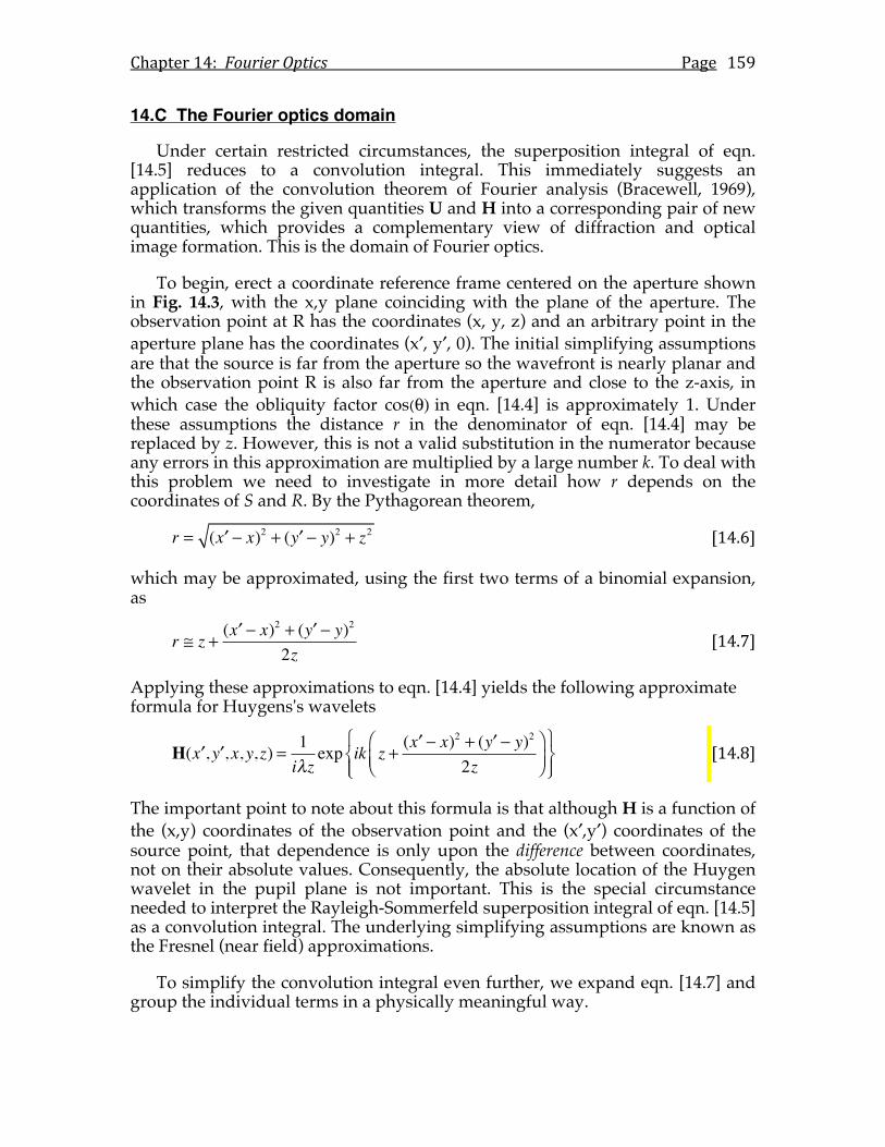
Chapter 14: Fourier Optics Page 159
14.C The Fourier optics domain
Under certain restricted circumstances, the superposition integral of eqn. [14.5] reduces to a convolution integral. This immediately suggests an application of the convolution theorem of Fourier analysis (Bracewell, 1969), which transforms the given quantities U and H into a corresponding pair of new quantities, which provides a complementary view of diffraction and optical image formation. This is the domain of Fourier optics.
To begin, erect a coordinate reference frame centered on the aperture shown in Fig. 14.3, with the x,y plane coinciding with the plane of the aperture. The observation point at R has the coordinates (x, y, z) and an arbitrary point in the aperture plane has the coordinates (x′, y′, 0). The initial simplifying assumptions are that the source is far from the aperture so the wavefront is nearly planar and the observation point R is also far from the aperture and close to the z-axis, in which case the obliquity factor cos(θ) in eqn. [14.4] is approximately 1. Under these assumptions the distance r in the denominator of eqn. [14.4] may be replaced by z. However, this is not a valid substitution in the numerator because any errors in this approximation are multiplied by a large number k. To deal with this problem we need to investigate in more detail how r depends on the coordinates of S and R. By the Pythagorean theorem,
r = ( ′x − x)2 + ( ′y − y)2 + z2 [14.6]
which may be approximated, using the first two terms of a binomial expansion, as
r ≅ z + ( ′x − x)2 + ( ′y − y)2
2z [14.7]
Applying these approximations to eqn. [14.4] yields the following approximate formula for Huygens's wavelets
H( ′x , ′y , x, y, z) = 1iλz
exp ik z + ( ′x − x)2 + ( ′y − y)2
2z⎛⎝⎜
⎞⎠⎟
⎧⎨⎩⎪
⎫⎬⎭⎪
[14.8]
The important point to note about this formula is that although H is a function of the (x,y) coordinates of the observation point and the (x′,y′) coordinates of the source point, that dependence is only upon the difference between coordinates, not on their absolute values. Consequently, the absolute location of the Huygen wavelet in the pupil plane is not important. This is the special circumstance needed to interpret the Rayleigh-Sommerfeld superposition integral of eqn. [14.5] as a convolution integral. The underlying simplifying assumptions are known as the Fresnel (near field) approximations.
To simplify the convolution integral even further, we expand eqn. [14.7] and group the individual terms in a physically meaningful way.
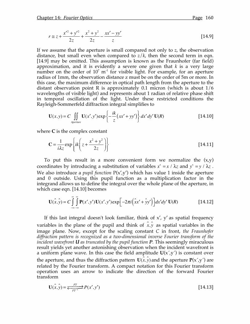
Chapter 14: Fourier Optics Page 160
r ≅ z + ′x 2 + ′y 2
2z+x2 + y2
2z−x ′x − y ′y
z [14.9]
If we assume that the aperture is small compared not only to z, the observation distance, but small even when compared to z/k, then the second term in eqn. [14.9] may be omitted. This assumption is known as the Fraunhofer (far field) approximation, and it is evidently a severe one given that k is a very large number on the order of 107 m-1 for visible light. For example, for an aperture radius of 1mm, the observation distance z must be on the order of 5m or more. In this case, the maximum difference in optical path length from the aperture to the distant observation point R is approximately 0.1 micron (which is about 1/6 wavelengths of visible light) and represents about 1 radian of relative phase shift in temporal oscillation of the light. Under these restricted conditions the Rayleigh-Sommerfeld diffraction integral simplifies to
U(x, y) = C U( ′x , ′y )exp −ikzx ′x + y ′y( )⎧
⎨⎩
⎫⎬⎭d ′x d ′y
Aperture∫∫ U(R) [14.10]
where C is the complex constant
C =1iλz
exp ik z + x2 + y2
2z⎛⎝⎜
⎞⎠⎟
⎧⎨⎩⎪
⎫⎬⎭⎪
[14.11]
To put this result in a more convenient form we normalize the (x,y) coordinates by introducing a substitution of variables xˆ = x / λz and yˆ = y / λz . We also introduce a pupil function P(x′,y′) which has value 1 inside the aperture and 0 outside. Using this pupil function as a multiplication factor in the integrand allows us to define the integral over the whole plane of the aperture, in which case eqn. [14.10] becomes
U(x, y) = C P( ′x , ′y )U( ′x , ′y )
−∞
∞
∫−∞
∞
∫ exp −2πi x ′x + y ′y( )⎡⎣
⎤⎦d ′x d ′y U(R) [14.12]
If this last integral doesn't look familiar, think of x′, y′ as spatial frequency variables in the plane of the pupil and think of x
, y as spatial variables in the image plane. Now, except for the scaling constant C in front, the Fraunhofer diffraction pattern is recognized as a two-dimensional inverse Fourier transform of the incident wavefront U as truncated by the pupil function P. This seemingly miraculous result yields yet another astonishing observation when the incident wavefront is a uniform plane wave. In this case the field amplitude U(x´,y´) is constant over the aperture, and thus the diffraction pattern U(x
, y)and the aperture P(x´,y´) are related by the Fourier transform. A compact notation for this Fourier transform operation uses an arrow to indicate the direction of the forward Fourier transform
U(x, y) = FT
FT −1⎯ →⎯⎯← ⎯⎯⎯ P( ′x , ′y ) [14.13]
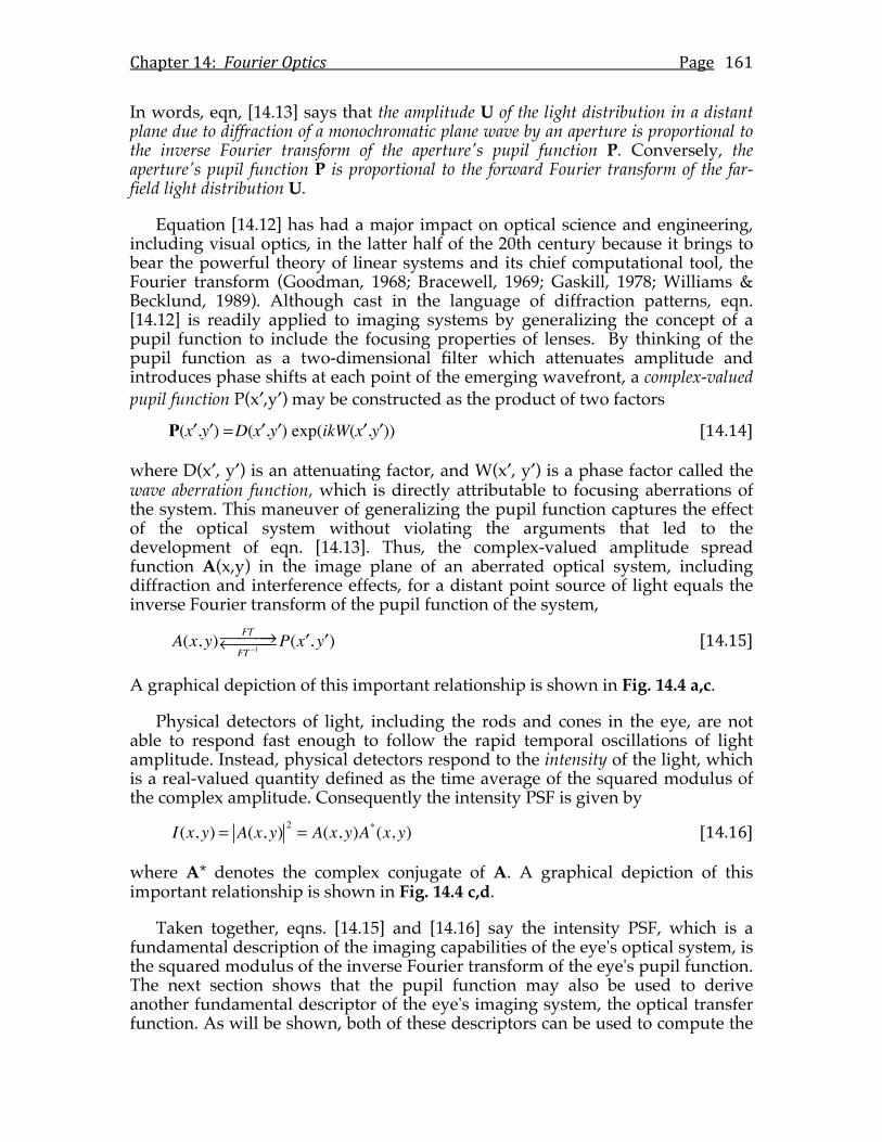
Chapter 14: Fourier Optics Page 161
In words, eqn, [14.13] says that the amplitude U of the light distribution in a distant plane due to diffraction of a monochromatic plane wave by an aperture is proportional to the inverse Fourier transform of the aperture's pupil function P. Conversely, the aperture's pupil function P is proportional to the forward Fourier transform of the far-field light distribution U.
Equation [14.12] has had a major impact on optical science and engineering, including visual optics, in the latter half of the 20th century because it brings to bear the powerful theory of linear systems and its chief computational tool, the Fourier transform (Goodman, 1968; Bracewell, 1969; Gaskill, 1978; Williams & Becklund, 1989). Although cast in the language of diffraction patterns, eqn. [14.12] is readily applied to imaging systems by generalizing the concept of a pupil function to include the focusing properties of lenses. By thinking of the pupil function as a two-dimensional filter which attenuates amplitude and introduces phase shifts at each point of the emerging wavefront, a complex-valued pupil function P(x′,y′) may be constructed as the product of two factors
P(x′,y′) = D(x′,y′) exp(ikW(x′,y′)) [14.14]
where D(x′, y′) is an attenuating factor, and W(x′, y′) is a phase factor called the wave aberration function, which is directly attributable to focusing aberrations of the system. This maneuver of generalizing the pupil function captures the effect of the optical system without violating the arguments that led to the development of eqn. [14.13]. Thus, the complex-valued amplitude spread function A(x,y) in the image plane of an aberrated optical system, including diffraction and interference effects, for a distant point source of light equals the inverse Fourier transform of the pupil function of the system,
A(x, y) FT
FT −1⎯ →⎯⎯← ⎯⎯⎯ P( ′x , ′y ) [14.15]
A graphical depiction of this important relationship is shown in Fig. 14.4 a,c.
Physical detectors of light, including the rods and cones in the eye, are not able to respond fast enough to follow the rapid temporal oscillations of light amplitude. Instead, physical detectors respond to the intensity of the light, which is a real-valued quantity defined as the time average of the squared modulus of the complex amplitude. Consequently the intensity PSF is given by
I(x, y) = A(x, y) 2 = A(x, y)A*(x, y) [14.16]
where A* denotes the complex conjugate of A. A graphical depiction of this important relationship is shown in Fig. 14.4 c,d.
Taken together, eqns. [14.15] and [14.16] say the intensity PSF, which is a fundamental description of the imaging capabilities of the eye's optical system, is the squared modulus of the inverse Fourier transform of the eye's pupil function. The next section shows that the pupil function may also be used to derive another fundamental descriptor of the eye's imaging system, the optical transfer function. As will be shown, both of these descriptors can be used to compute the
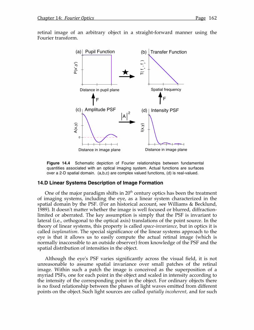
Chapter 14: Fourier Optics Page 162
retinal image of an arbitrary object in a straight-forward manner using the Fourier transform.
Figure 14.4 Schematic depiction of Fourier relationships between fundamental quantities associated with an optical imaging system. Actual functions are surfaces over a 2-D spatial domain. (a,b,c) are complex valued functions, (d) is real-valued.
14.D Linear Systems Description of Image Formation
One of the major paradigm shifts in 20th century optics has been the treatment of imaging systems, including the eye, as a linear system characterized in the spatial domain by the PSF. (For an historical account, see Williams & Becklund, 1989). It doesn't matter whether the image is well focused or blurred, diffraction-limited or aberrated. The key assumption is simply that the PSF is invariant to lateral (i.e., orthogonal to the optical axis) translations of the point source. In the theory of linear systems, this property is called space-invariance, but in optics it is called isoplanatism. The special significance of the linear systems approach to the eye is that it allows us to easily compute the actual retinal image (which is normally inaccessible to an outside observer) from knowledge of the PSF and the spatial distribution of intensities in the object.
Although the eye's PSF varies significantly across the visual field, it is not unreasonable to assume spatial invariance over small patches of the retinal image. Within such a patch the image is conceived as the superposition of a myriad PSFs, one for each point in the object and scaled in intensity according to the intensity of the corresponding point in the object. For ordinary objects there is no fixed relationship between the phases of light waves emitted from different points on the object. Such light sources are called spatially incoherent, and for such
P(x'
,y')
Distance in pupil plane
A2
F
T( f x ,
f y )
Spatial frequency
I(x,y
)
Distance in image plane
F
A(x,
y)
Distance in image plane
0
(a) Pupil Function (b) Transfer Function
(d) Intensity PSF(c) Amplitude PSF
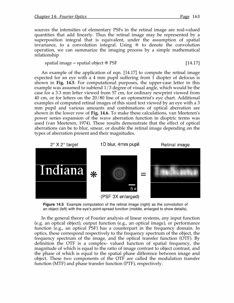
Chapter 14: Fourier Optics Page 163
sources the intensities of elementary PSFs in the retinal image are real-valued quantities that add linearly. Thus the retinal image may be represented by a superposition integral that is equivalent, under the assumption of spatial invariance, to a convolution integral. Using ❊ to denote the convolution operation, we can summarize the imaging process by a simple mathematical relationship spatial image = spatial object ❇ PSF [14.17]
An example of the application of eqn. [14.17] to compute the retinal image expected for an eye with a 4 mm pupil suffering from 1 diopter of defocus is shown in Fig. 14.5. For computational purposes, the upper-case letter in this example was assumed to subtend 1/3 degree of visual angle, which would be the case for a 3.3 mm letter viewed from 57 cm, for ordinary newprint viewed from 40 cm, or for letters on the 20/80 line of an optometrist's eye chart. Additional examples of computed retinal images of this sized text viewed by an eye with a 3 mm pupil and various amounts and combinations of optical aberration are shown in the lower row of Fig. 14.6. To make these calculations, van Meeteren's power series expansion of the wave aberration function in dioptric terms was used (van Meeteren, 1974). These results demonstrate that the effect of optical aberrations can be to blur, smear, or double the retinal image depending on the types of aberration present and their magnitudes.
Figure 14.5 Example computation of the retinal image (right) as the convolution of an object (left) with the eyeʼs point-spread function (middle, enlarged to show details).
In the general theory of Fourier analysis of linear systems, any input function (e.g. an optical object), output function (e.g., an optical image), or performance function (e.g., an optical PSF) has a counterpart in the frequency domain. In optics, these correspond respectively to the frequency spectrum of the object, the frequency spectrum of the image, and the optical transfer function (OTF). By definition the OTF is a complex- valued function of spatial frequency, the magnitude of which is equal to the ratio of image contrast to object contrast, and the phase of which is equal to the spatial phase difference between image and object. These two components of the OTF are called the modulation transfer function (MTF) and phase transfer function (PTF), respectively.
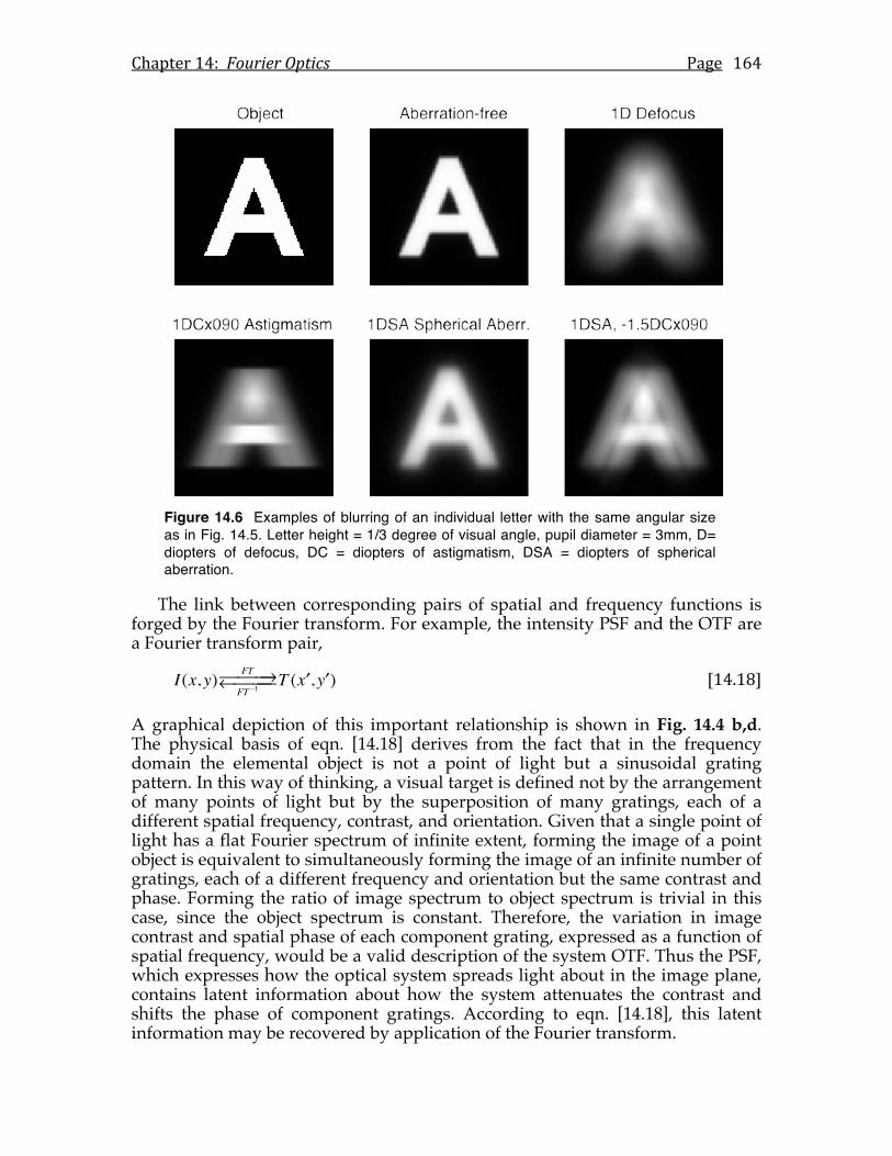
Chapter 14: Fourier Optics Page 164
Figure 14.6 Examples of blurring of an individual letter with the same angular size as in Fig. 14.5. Letter height = 1/3 degree of visual angle, pupil diameter = 3mm, D= diopters of defocus, DC = diopters of astigmatism, DSA = diopters of spherical aberration.
The link between corresponding pairs of spatial and frequency functions is forged by the Fourier transform. For example, the intensity PSF and the OTF are a Fourier transform pair,
I(x, y) FT
FT −1⎯ →⎯⎯← ⎯⎯⎯ T ( ′x , ′y ) [14.18]
A graphical depiction of this important relationship is shown in Fig. 14.4 b,d. The physical basis of eqn. [14.18] derives from the fact that in the frequency domain the elemental object is not a point of light but a sinusoidal grating pattern. In this way of thinking, a visual target is defined not by the arrangement of many points of light but by the superposition of many gratings, each of a different spatial frequency, contrast, and orientation. Given that a single point of light has a flat Fourier spectrum of infinite extent, forming the image of a point object is equivalent to simultaneously forming the image of an infinite number of gratings, each of a different frequency and orientation but the same contrast and phase. Forming the ratio of image spectrum to object spectrum is trivial in this case, since the object spectrum is constant. Therefore, the variation in image contrast and spatial phase of each component grating, expressed as a function of spatial frequency, would be a valid description of the system OTF. Thus the PSF, which expresses how the optical system spreads light about in the image plane, contains latent information about how the system attenuates the contrast and shifts the phase of component gratings. According to eqn. [14.18], this latent information may be recovered by application of the Fourier transform.
Chapter 14: Fourier Optics Page 165
A frequency interpretation of the input-output relationship of eqn. [14.17] requires an important result of Fourier theory known as the convolution theorem. This theorem states that the convolution of two functions in one domain is equivalent to multiplication of the corresponding functions in the other domain (see Chapter 12.B). Applying this theorem to eqn. [14.17] summarizes the imaging process in the frequency domain as a multiplication of the complex-valued object spectrum and complex-valued OTF, image spectrum = object spectrum · OTF [14.19]
Given the above results, two important conclusions may be drawn. The first is a Fourier transform relationship between the PSF and the pupil function. As a preliminary step, evaluate the squared modulus of the amplitude spread function in both domains by using the convolution theorem and the complex conjugate theorem (Bracewell, 1969) in conjunction with eqn. [14.15]
A(x, y) FT
FT −1⎯ →⎯⎯← ⎯⎯⎯ P( ′x , ′y )
A*(x, y) FT
FT −1⎯ →⎯⎯← ⎯⎯⎯ P(− ′x ,− ′y )
A(x, y)A*(x, y) FT
FT −1⎯ →⎯⎯← ⎯⎯⎯ P( ′x , ′y )P(− ′x ,− ′y )
[14.20]
It is customary to translate this convolution relationship into an auto-correlation relationship, denoted by the pentagram (★) symbol (Bracewell, 1969, p. 112, 122), using the rule
P(x′, y′)P*( − x′, − y′) = P(x′, y′)P(x′, y′) [14.21]
Combining eqns. [14.16], [14.20], and [14,21] gives
I(x, y) FT
FT −1⎯ →⎯⎯← ⎯⎯⎯ P( ′x , ′y )P( ′x , ′y ) [14.22]
In words, eqn. [14.22] says that the intensity PSF is the inverse Fourier transform of the auto-correlation of the pupil function.
The second conclusion we may draw from the preceding development completes the matrix of relationships diagrammed in Fig. 14.4. Because the OTF (eqn. 14.18) and the autocorrelation of the pupil function (eqn. 14.22) are both Fourier transforms of the PSF, they must be equal to each other
I(x, y) FT
FT −1⎯ →⎯⎯← ⎯⎯⎯ T( ′x , ′y )
I(x, y) FT
FT −1⎯ →⎯⎯← ⎯⎯⎯ P( ′x , ′y )P( ′x , ′y )
∴T( ′x , ′y ) = P( ′x , ′y )P( ′x , ′y )
[14.23]
A graphical depiction of this important relationship is shown in Fig. 14.4 a,b. This last result puts the pupil function at the very heart of the frequency analysis of imaging systems, just as for the spatial analysis of imaging systems. It also
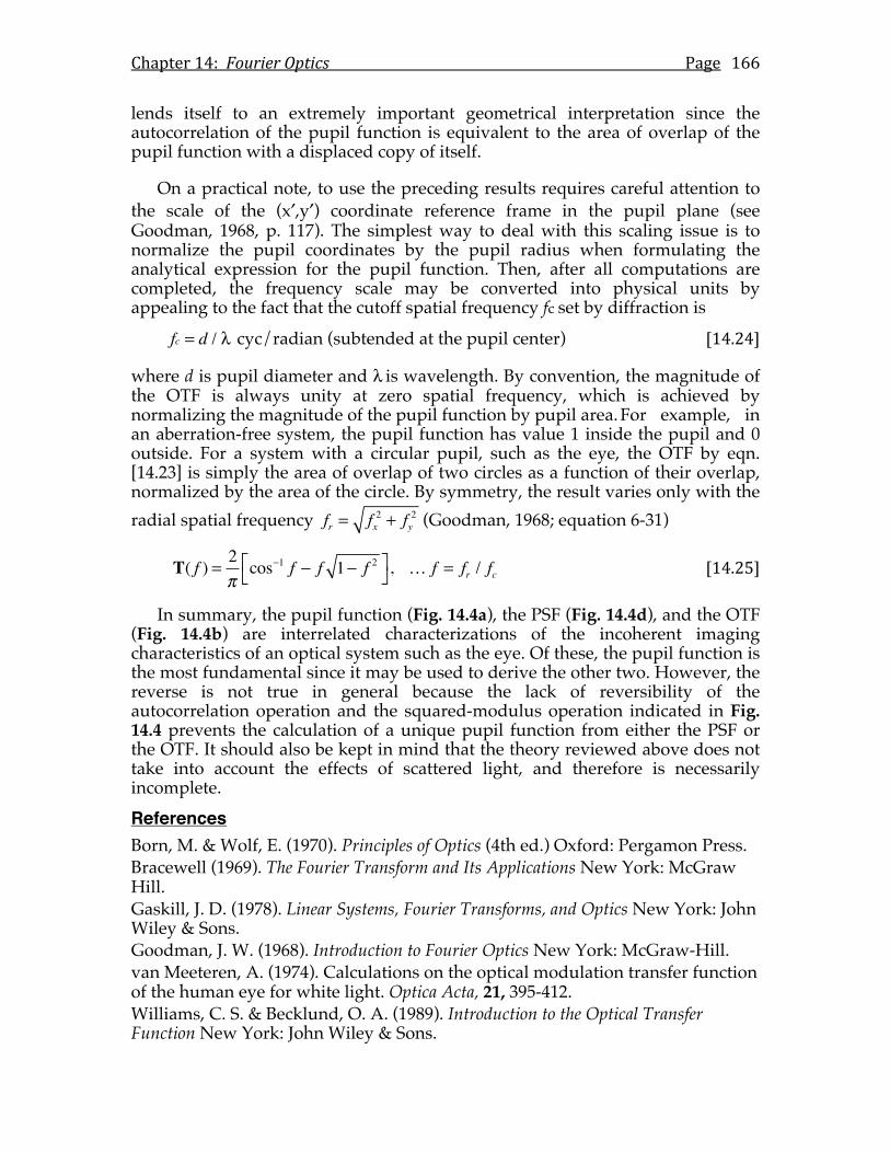
Chapter 14: Fourier Optics Page 166
lends itself to an extremely important geometrical interpretation since the autocorrelation of the pupil function is equivalent to the area of overlap of the pupil function with a displaced copy of itself.
On a practical note, to use the preceding results requires careful attention to the scale of the (x′,y′) coordinate reference frame in the pupil plane (see Goodman, 1968, p. 117). The simplest way to deal with this scaling issue is to normalize the pupil coordinates by the pupil radius when formulating the analytical expression for the pupil function. Then, after all computations are completed, the frequency scale may be converted into physical units by appealing to the fact that the cutoff spatial frequency fc set by diffraction is
fc = d / λ cyc/radian (subtended at the pupil center) [14.24]
where d is pupil diameter and λ is wavelength. By convention, the magnitude of the OTF is always unity at zero spatial frequency, which is achieved by normalizing the magnitude of the pupil function by pupil area. For example, in an aberration-free system, the pupil function has value 1 inside the pupil and 0 outside. For a system with a circular pupil, such as the eye, the OTF by eqn. [14.23] is simply the area of overlap of two circles as a function of their overlap, normalized by the area of the circle. By symmetry, the result varies only with the radial spatial frequency fr = fx
2 + fy2 (Goodman, 1968; equation 6-31)
T( f ) = 2
πcos−1 f − f 1− f 2⎡⎣
⎤⎦, … f = fr / fc [14.25]
In summary, the pupil function (Fig. 14.4a), the PSF (Fig. 14.4d), and the OTF (Fig. 14.4b) are interrelated characterizations of the incoherent imaging characteristics of an optical system such as the eye. Of these, the pupil function is the most fundamental since it may be used to derive the other two. However, the reverse is not true in general because the lack of reversibility of the autocorrelation operation and the squared-modulus operation indicated in Fig. 14.4 prevents the calculation of a unique pupil function from either the PSF or the OTF. It should also be kept in mind that the theory reviewed above does not take into account the effects of scattered light, and therefore is necessarily incomplete. References Born, M. & Wolf, E. (1970). Principles of Optics (4th ed.) Oxford: Pergamon Press. Bracewell (1969). The Fourier Transform and Its Applications New York: McGraw Hill. Gaskill, J. D. (1978). Linear Systems, Fourier Transforms, and Optics New York: John Wiley & Sons. Goodman, J. W. (1968). Introduction to Fourier Optics New York: McGraw-Hill. van Meeteren, A. (1974). Calculations on the optical modulation transfer function of the human eye for white light. Optica Acta, 21, 395-412. Williams, C. S. & Becklund, O. A. (1989). Introduction to the Optical Transfer Function New York: John Wiley & Sons.
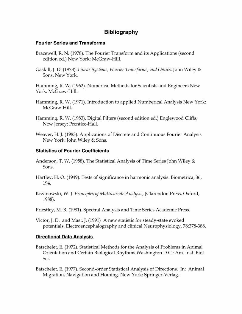
Bibliography
Fourier Series and Transforms
Bracewell, R. N. (1978). The Fourier Transform and its Applications (second edition ed.) New York: McGraw-Hill.
Gaskill, J. D. (1978). Linear Systems, Fourier Transforms, and Optics. John Wiley & Sons, New York.
Hamming, R. W. (1962). Numerical Methods for Scientists and Engineers New York: McGraw-Hill.
Hamming, R. W. (1971). Introduction to applied Numberical Analysis New York: McGraw-Hill.
Hamming, R. W. (1983). Digital Filters (second edition ed.) Englewood Cliffs, New Jersey: Prentice-Hall.
Weaver, H. J. (1983). Applications of Discrete and Continuous Fourier Analysis New York: John Wiley & Sons.
Statistics of Fourier Coefficients
Anderson, T. W. (1958). The Statistical Analysis of Time Series John Wiley & Sons.
Hartley, H. O. (1949). Tests of significance in harmonic analysis. Biometrica, 36, 194.
Krzanowski, W. J. Principles of Multivariate Analysis, (Clarendon Press, Oxford, 1988).
Priestley, M. B. (1981). Spectral Analysis and Time Series Academic Press.
Victor, J. D. and Mast, J. (1991) A new statistic for steady-state evoked potentials. Electroencephalography and clinical Neurophysiology, 78:378-388.
Directional Data Analysis
Batschelet, E. (1972). Statistical Methods for the Analysis of Problems in Animal Orientation and Certain Biological Rhythms Washington D.C.: Am. Inst. Biol. Sci.
Batschelet, E. (1977). Second-order Statistical Analysis of Directions. In: Animal Migration, Navigation and Homing. New York: Springer-Verlag.
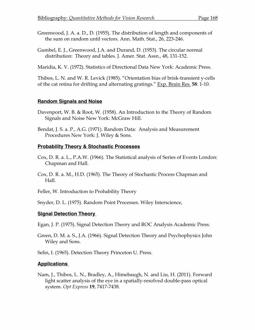
Bibliography: Quantitative Methods for Vision Research Page 168
Greenwood, J. A. a. D., D. (1955). The distribution of length and components of the sum on random until vectors. Ann. Math. Stat., 26, 223-246.
Gumbel, E. J., Greenwood, J.A. and Durand, D. (1953). The circular normal distribution: Theory and tables. J. Amer. Stat. Assn., 48, 131-152.
Maridia, K. V. (1972). Statistics of Directional Data New York: Academic Press.
Thibos, L. N. and W. R. Levick (1985). “Orientation bias of brisk-transient y-cells of the cat retina for drifting and alternating gratings.” Exp. Brain Res. 58: 1-10.
Random Signals and Noise
Davenport, W. B. & Root, W. (1958). An Introduction to the Theory of Random Signals and Noise New York: McGraw Hill.
Bendat, J. S. a. P., A.G. (1971). Random Data: Analysis and Measurement Procedures New York: J. Wiley & Sons.
Probability Theory & Stochastic Processes
Cox, D. R. a. L., P.A.W. (1966). The Statistical analysis of Series of Events London: Chapman and Hall.
Cox, D. R. a. M., H.D. (1965). The Theory of Stochastic Process Chapman and Hall.
Feller, W. Introduction to Probability Theory
Snyder, D. L. (1975). Random Point Processes. Wiley Interscience,
Signal Detection Theory
Egan, J. P. (1975). Signal Detection Theory and ROC Analysis Academic Press.
Green, D. M. a. S., J.A. (1966). Signal Detection Theory and Psychophysics John Wiley and Sons.
Selin, I. (1965). Detection Theory Princeton U. Press.
Applications
Nam, J., Thibos, L. N., Bradley, A., Himebaugh, N. and Liu, H. (2011). Forward light scatter analysis of the eye in a spatially-resolved double-pass optical system. Opt Express 19, 7417-7438.
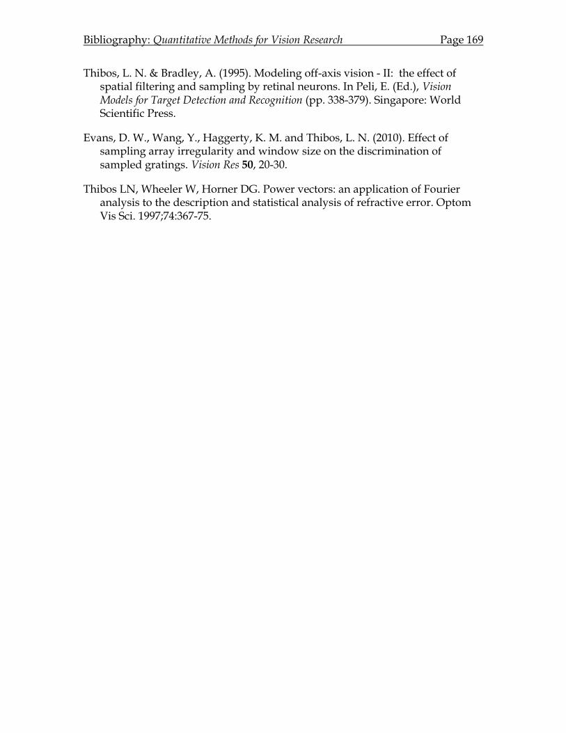
Bibliography: Quantitative Methods for Vision Research Page 169
Thibos, L. N. & Bradley, A. (1995). Modeling off-axis vision - II: the effect of spatial filtering and sampling by retinal neurons. In Peli, E. (Ed.), Vision Models for Target Detection and Recognition (pp. 338-379). Singapore: World Scientific Press.
Evans, D. W., Wang, Y., Haggerty, K. M. and Thibos, L. N. (2010). Effect of sampling array irregularity and window size on the discrimination of sampled gratings. Vision Res 50, 20-30.
Thibos LN, Wheeler W, Horner DG. Power vectors: an application of Fourier analysis to the description and statistical analysis of refractive error. Optom Vis Sci. 1997;74:367-75.
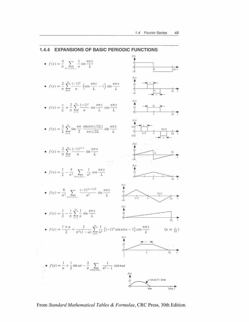
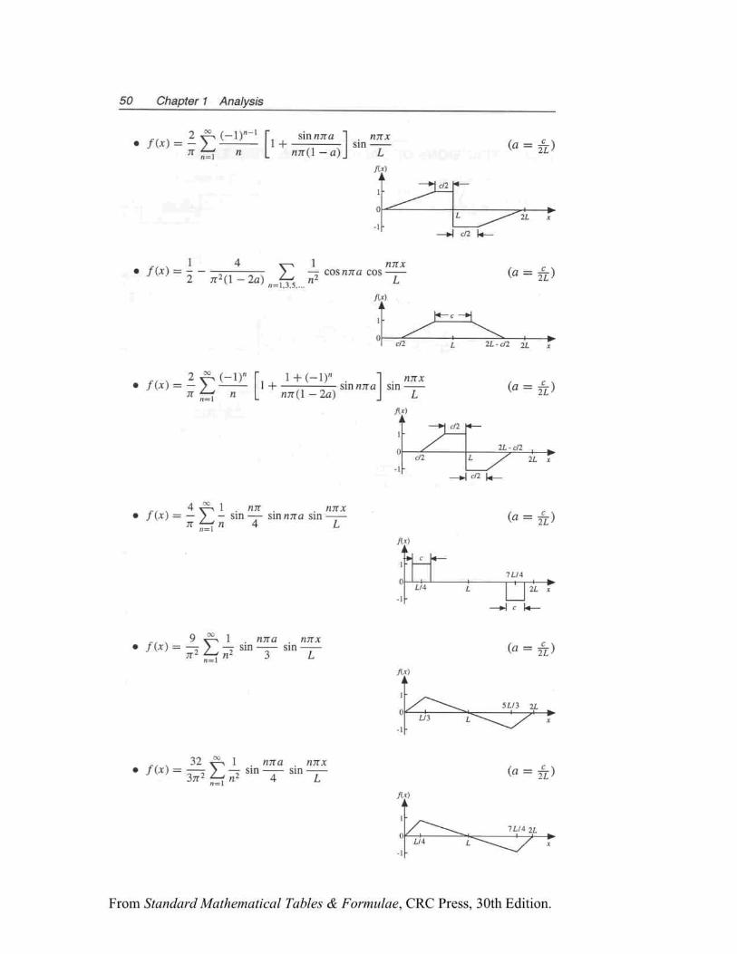
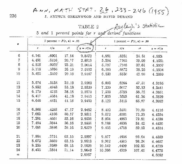
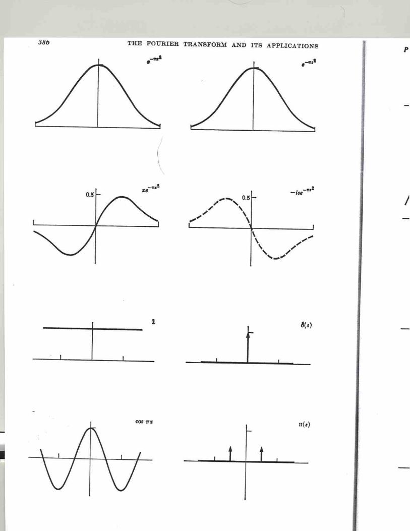
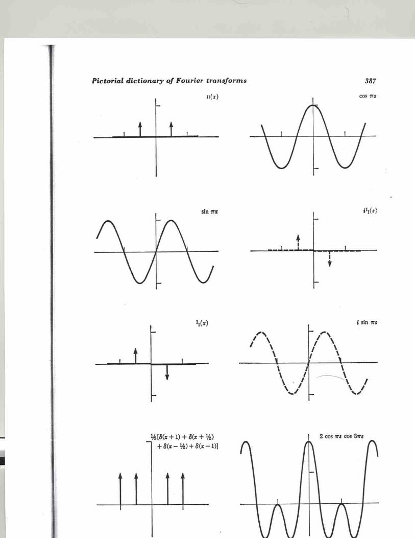
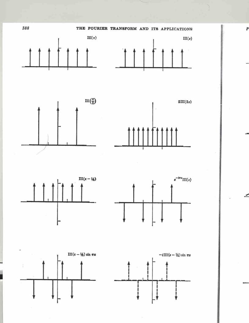
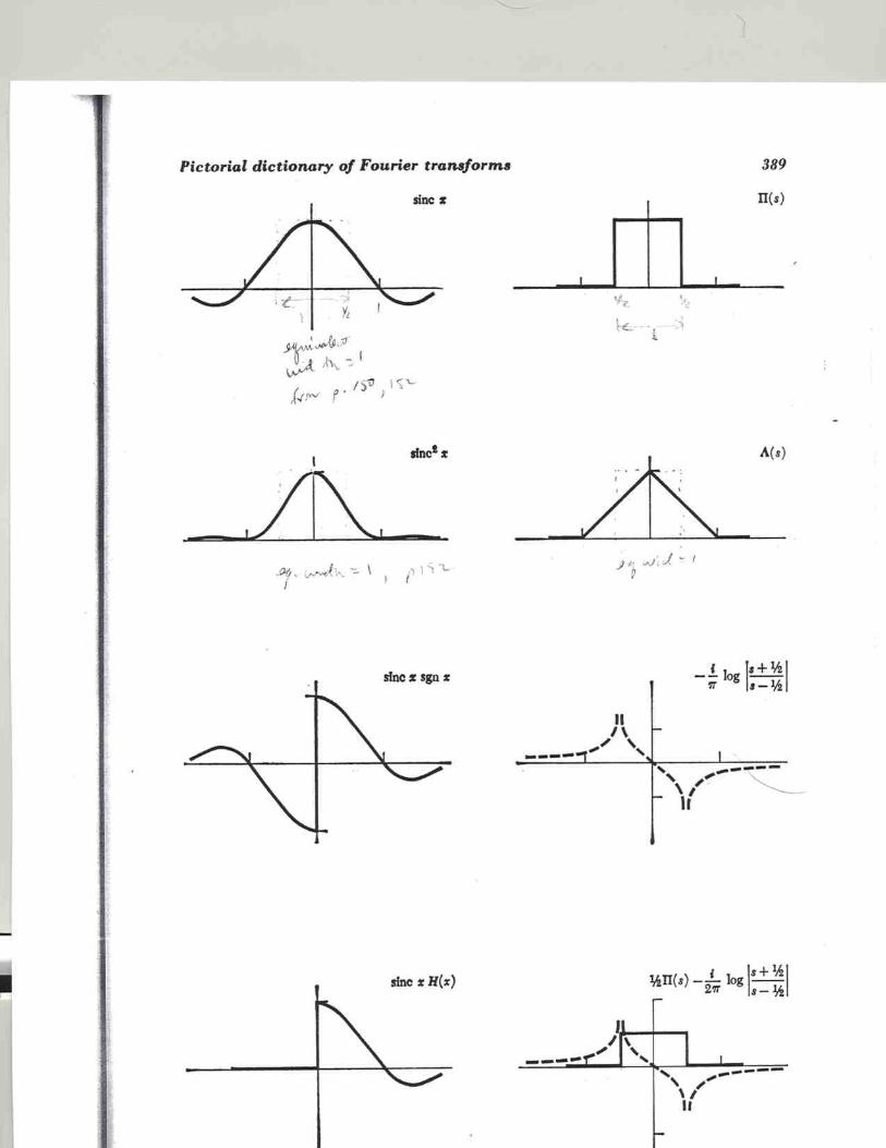
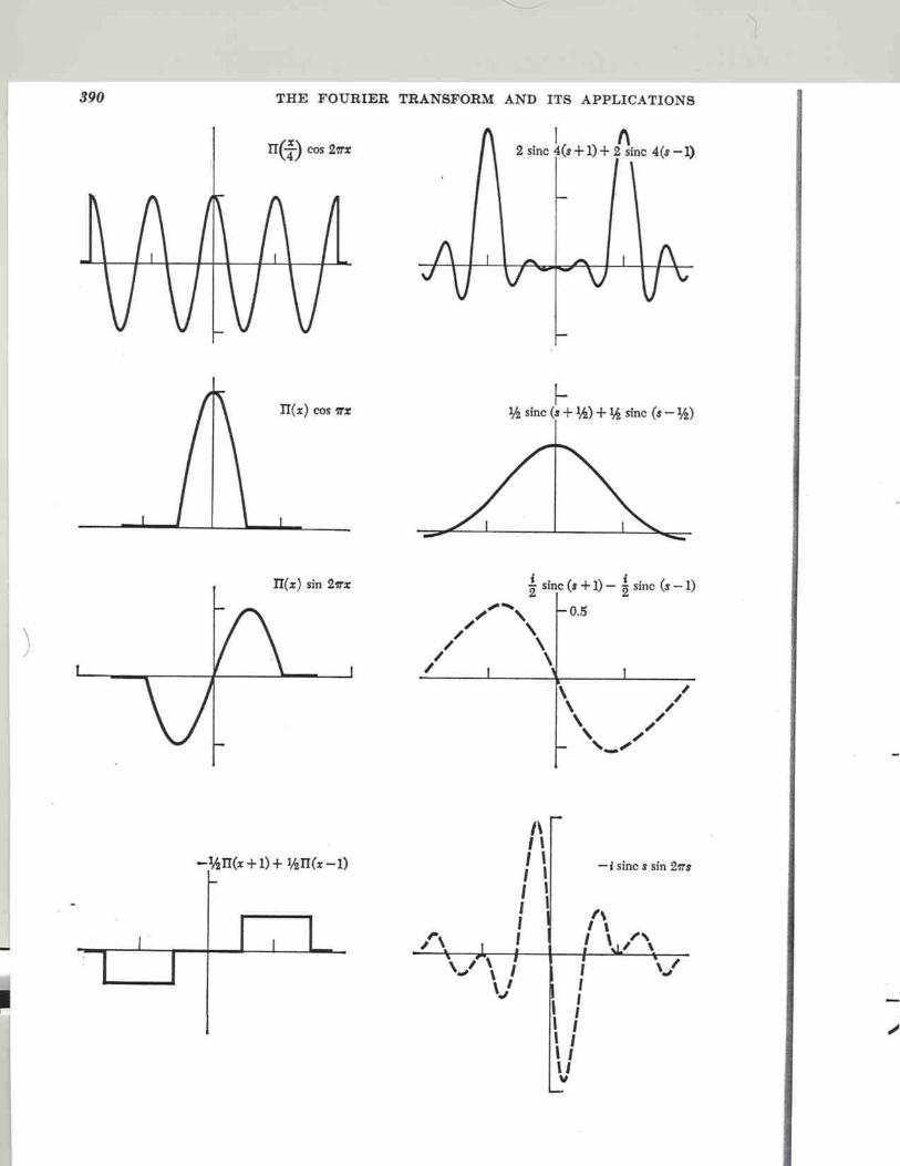
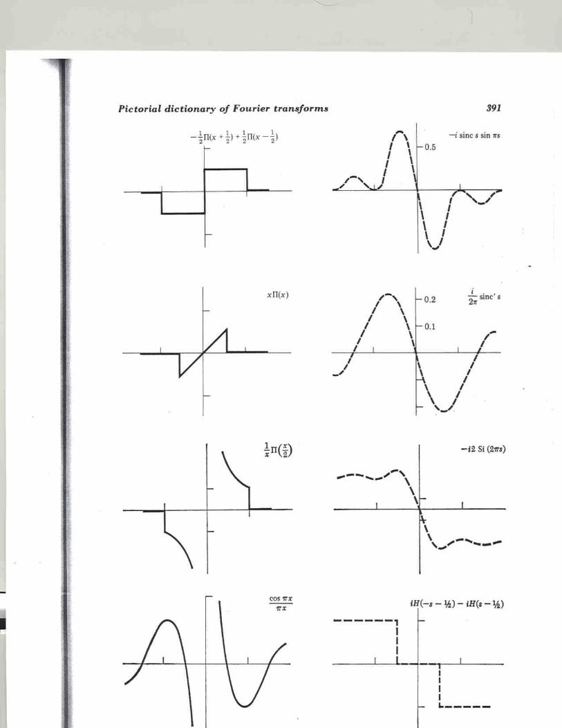
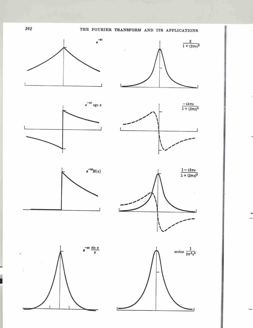
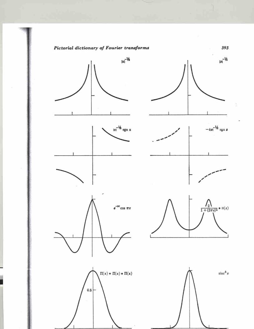
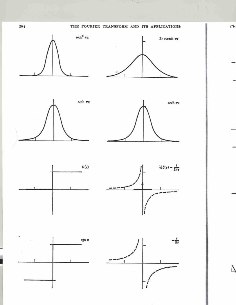
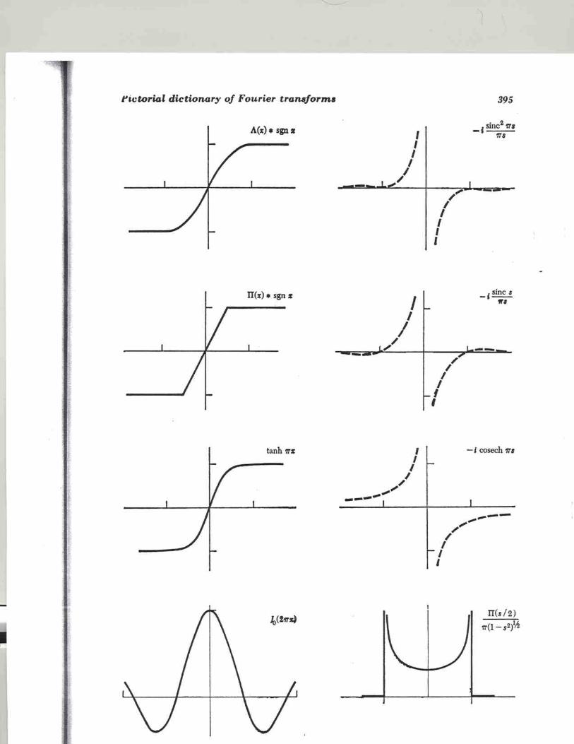
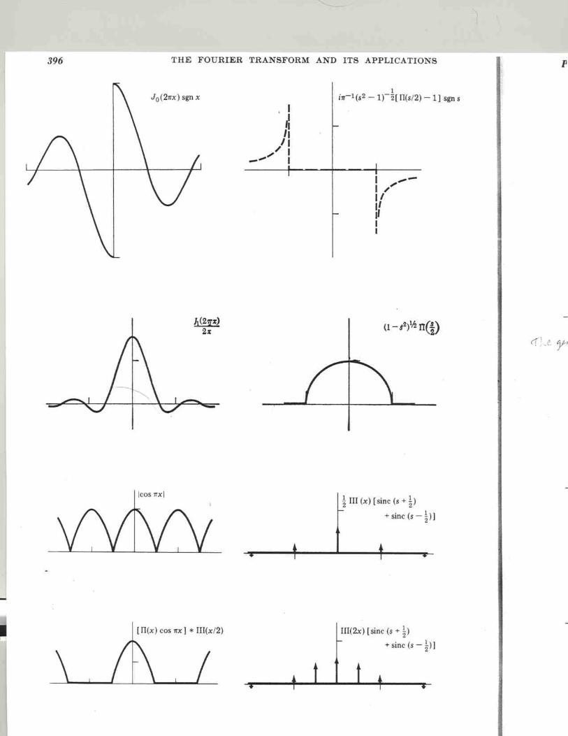
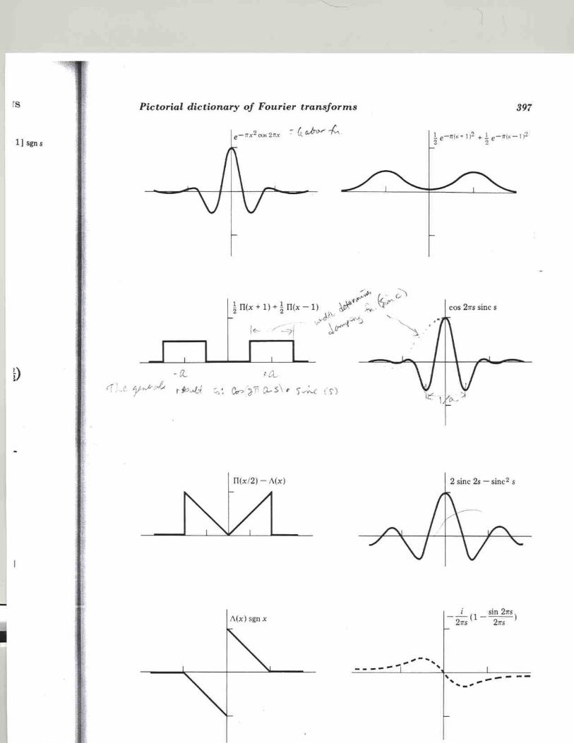
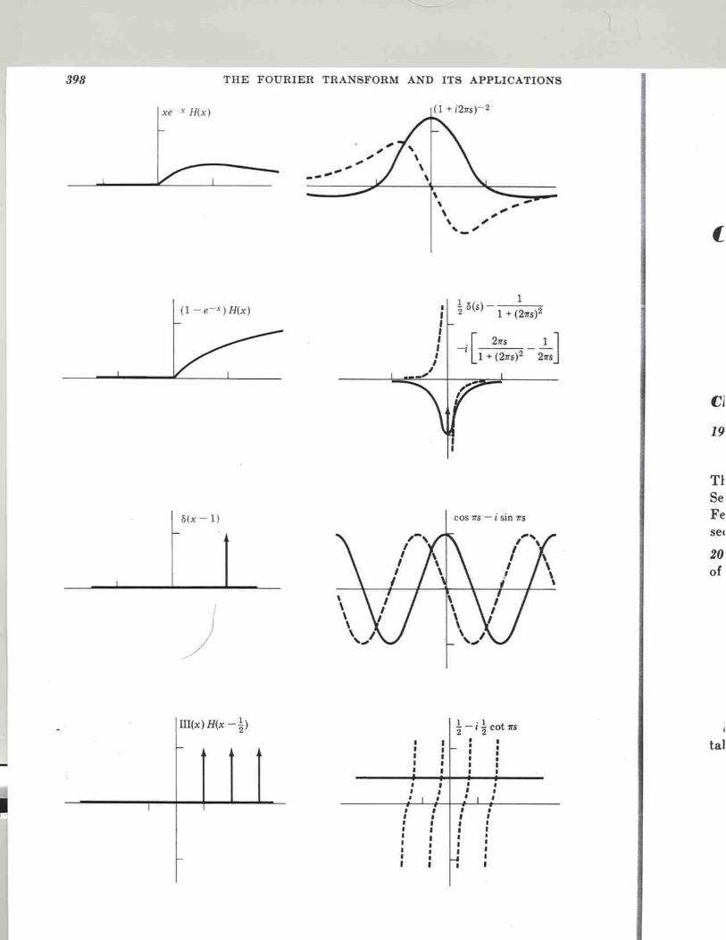
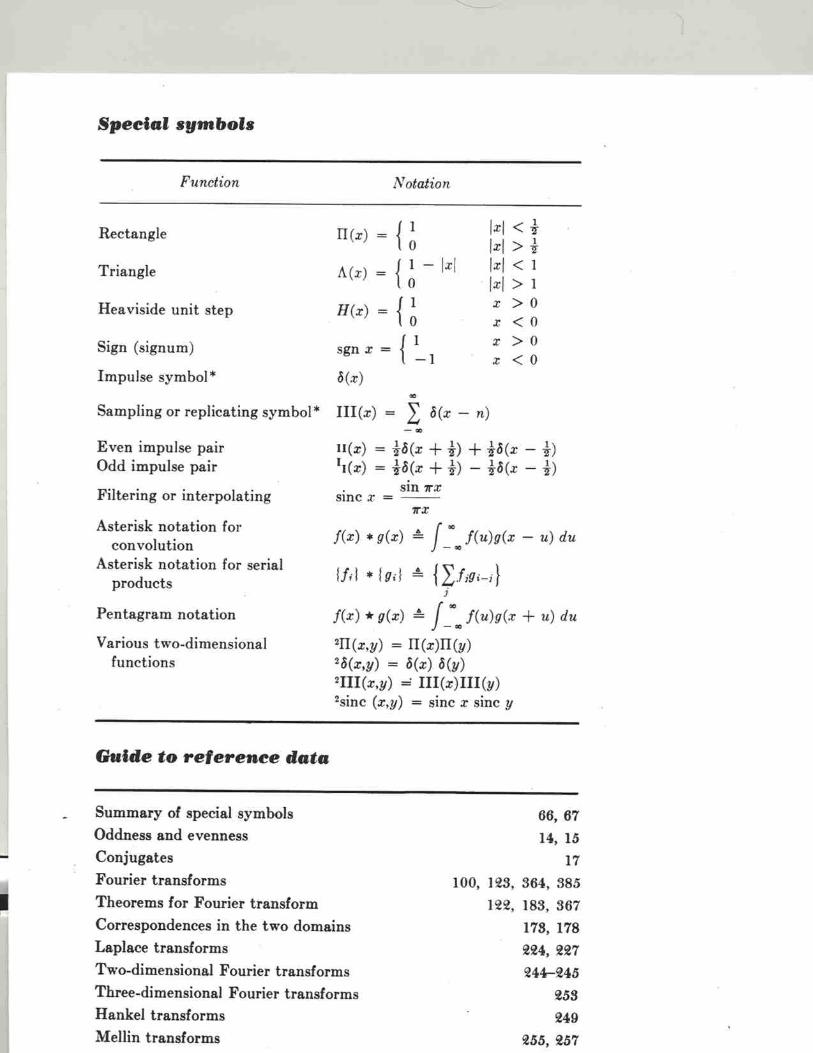
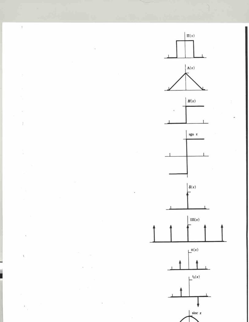
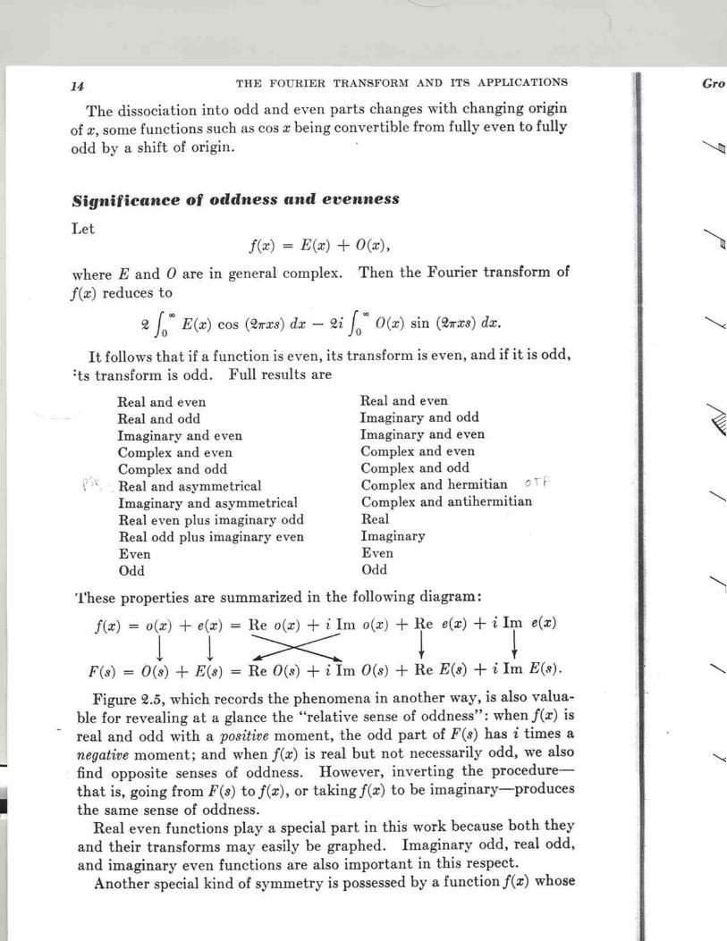
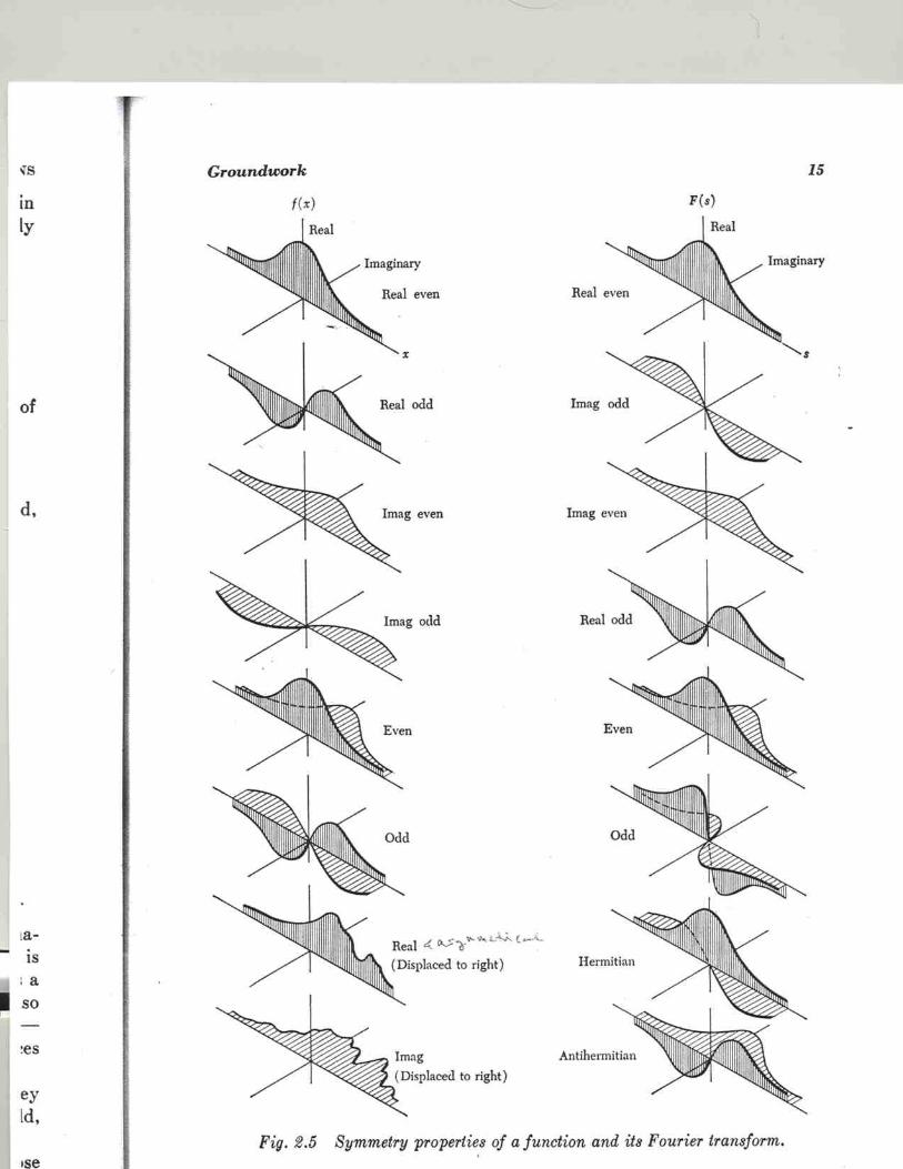
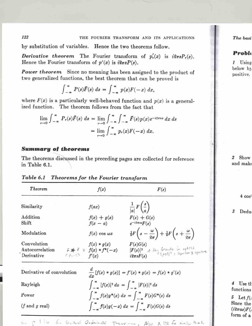
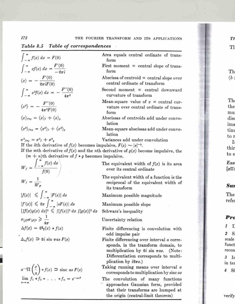
Related Documents


![Reminder Fourier Basis: t [0,1] nZnZ Fourier Series: Fourier Coefficient:](https://static.cupdf.com/doc/110x72/56649d395503460f94a13929/reminder-fourier-basis-t-01-nznz-fourier-series-fourier-coefficient.jpg)