Four-state nanomagnetic logic using multiferroics

FOUR-STATE NANOMAGNETIC LOGIC USING MULTIFERROICS

1,aNoel D’Souza , Jayasimha Atulasimhaa and Supriyo Bandyopadhyayb

(a) Department of Mechanical and Nuclear Engineering,

(b) Department of Electrical and Computer Engineering,

Virginia Commonwealth University, Richmond, VA 23284, USA.

Abstract

The authors show how to implement a 4-state universal logic gate (NOR) using three strain-

coupled magnetostrictive-piezoelectric multiferroic nanomagnets (e.g. Ni/PZT) with biaxial

magnetocrystalline anisotropy. Two of the nanomagnets encode the 2-state input bits in their

magnetization orientations and the third nanomagnet produces the output bit via dipole

interaction with the input nanomagnets. A voltage pulse alternating between -0.2 V and +0.2 V is

applied to the PZT layer of the third nanomagnet and generates alternating tensile and

compressive stress in its Ni layer to produce the output bit, while dissipating ~ 57,000 kT (0.24

fJ) of energy per gate operation.

__________________________

1Corresponding author. E-mail [email protected]

1

Nanomagnetic logic (NML) is an emerging paradigm for low-power computing1-4 where

logic bits 0 and 1 are encoded in two stable magnetization directions parallel to the easy axis of a

single domain nanomagnet with uniaxial shape anisotropy. Bits are switched by flipping the

magnetization of a nanomagnet with an external agent that acts like a clock.

The ultimate energy-efficiency of NML is determined by the clocking methodology, i.e. how

bits are flipped. If a magnetic field generated with a current5, or spin transfer torque6, is used to

flip a nanomagnet’s magnetization, then the energy consumed can be exorbitant, which defeats

the very purpose of NML. However, stress-induced rotation of magnetization in multiferroic

nanomagnets seems to be able to switch magnets with much higher energy efficiency7-9. This is

only now beginning to attract attention7-10.

The magnetization vector of a multiferroic nanomagnet, consisting of a piezoelectric and a

magnetostrictive layer, can be flipped with an electrostatic potential applied to the piezoelectric

layer. The voltage generates a strain that is elastically transferred to the magnetostrictive layer

causing its magnetization to flip. We can embellish the functionality of the multiferroic element

by introducing biaxial magnetocrystalline anisotropy in the magnetostrictive layer, giving it four

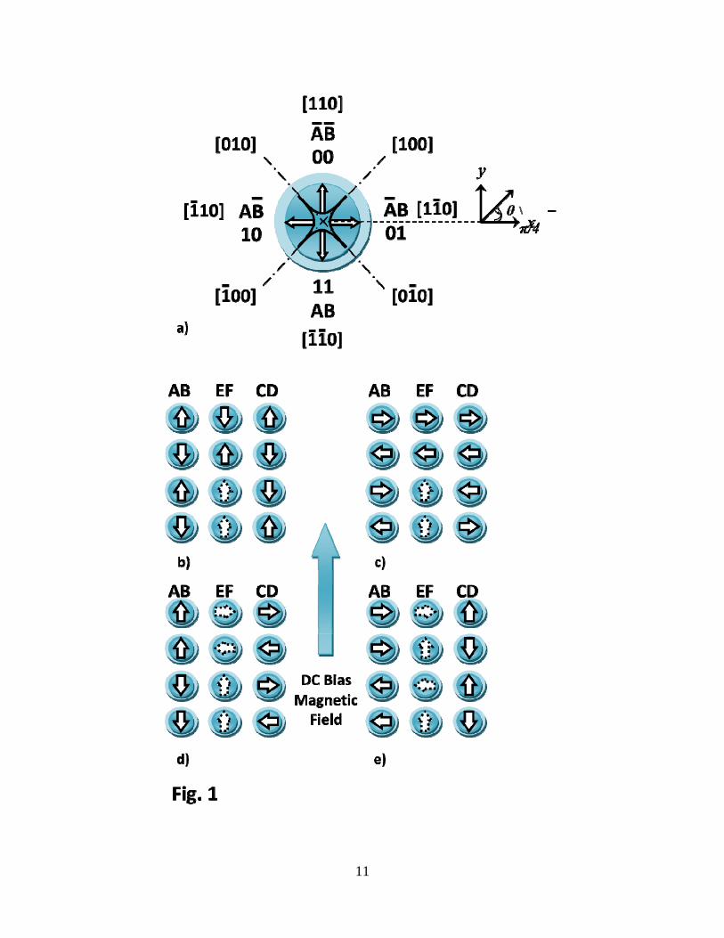
possible stable magnetization directions (‘up’, ‘right’ ,‘down’, ‘left’) that are chosen to encode

four possible 2-bit combinations (00, 01, 11, 10), illustrated in Fig. 1(a). The choice is motivated

by allowing only 1 bit to change for every 90º rotation of magnetization. For single crystal Ni,

with magnetocrystalline anisotropy constant K1< 0, the “easy” directions that encode these states

in the (001) plane are the [110], [11−

0], [1−

1−

0] and [1−

10] directions, as shown in the energy

curves in Fig. 1(a) (saddle-shaped curve, with the four easy directions of magnetization having

lower energy levels than the other principal crystallographic axes).

2

When two nanomagnets are placed next to each other, two types of dipole interaction arise.

The first type arises when the magnetizations are perpendicular to the array axis. In this case,

dipole interaction favors anti-parallel arrangement (or anti-ferromagnetic coupling) of adjacent

magnetizations. The second type arises when the magnetizations are parallel to the array axis. In

this case, dipole-dipole interaction favors a parallel alignment (or ferromagnetic coupling) of

adjacent magnetizations. Using combinations of this dipole-dipole interaction and a small global

static magnetic field to resolve tie situations, we realize a 2-bit NOR universal logic gate as

explained below.

Consider the arrangement shown in Fig. 1 (b) through (e), where the two input nanomagnets,

encoding bits AB and CD, are located on either side of the output nanomagnet encoding bits EF.

Four different scenarios are investigated. The first scenario is shown in Fig. 1(b), where the

magnetization direction of the input magnets is perpendicular to the axis of the nanomagnet

array. When both input magnetizations are oriented up (or down) (first two rows of Fig. 1 b), the

dipole coupling favors a down (or up) orientation of the output nanomagnet. When one input

magnetization points up and the other points down (third and fourth rows of Fig. 1 b), the output

nanomagnet is in a tied state, which we resolve using a global static magnetic field that forces the

output magnetization to point “up”. The second scenario is shown in Fig. 1(c), where input

magnetizations are parallel to the nanomagnet array axis. When both input magnetizations are

oriented left or right (first two rows of Fig. 1 c), the dipole coupling respectively favors left or

right orientation of the output nanomagnet. When one input magnetization points left and the

other points right (third and fourth rows of Fig. 1 c) the output nanomagnet is in a tied state, and

ends up pointing neither left nor right, but orienting upward because of the global bias field. The

third (Fig 1 d) and fourth (Fig 1 e) scenarios are mixed inputs, where one input magnetization

3

points perpendicular (“up/down”) and the other parallel (“left/right”) to the axis of the array,

respectively favoring a “down/up” or “left/right” orientation of the output magnetization. These

result in tied states. If one of the inputs is “up”, the static bias field ensures that the output is

“up”, while if one of the inputs is “down”, the bias field counters this, causing the output to point

either “left” or “right” depending on the second input. The input (AB, CD) and output (EF)

configurations, based on their binary bit representations, are transferred to a Karnaugh map (K-

map) to simplify the logical expression of the output. The output table of the K-map is shown in

Fig. 2. On simplification of the K-map, the result obtained (in Boolean notation) is DBE =

and CAF = , which is NOR logic.

We present detailed simulation results to show that the output magnetization always

represents the NOR function of the inputs, independent of its initial orientation, when we clock

the piezoelectric layer of the output multiferroic nanomagnet with a voltage to generate the

proper stress cycle. To show this, we consider the total energy of the output nanomagnet when its

magnetization vector subtends an angle 2θ with the positive x-axis11:

( ) ( ) ( )

( ) ( ) [ ]

2 202 2 1 3 2 13

2 2 012 100 2 2

2cos cos cos sin sin sin4

3sin 2 4 cos 4 sin4 2 4

total s

s applied

E MR

K M H

3μθ θ θ θ θ θπ

μ

θ

θ π λ σ θ ππ

⎡ ⎤= Ω − + + +⎡ ⎤⎣ ⎦⎣ ⎦

Ω+ − − Ω − − Ω

(1) θ

where the first term is the dipole interaction energy with the neighbors subtending angles and 1θ

3θ with the positive x-axis, the second term is the magnetocrystalline anisotropy energy with

being the first-order magnetocrystalline anisotropy constant, the third term is the stress

anisotropy energy due to stress σ applied along the [100] direction (45

1K

0 with the x-axis) with

being the magnetostrictive constant in the direction of stress, and the last term is the 100λ

4

interaction energy due to the static bias field pointing in the “up” direction, or the [110]

direction. Here,

appliedH

Ω is the permeability of free space, is the saturation magnetization, sM0μ is

the nanomagnet volume, and R is the distance between the centers of two adjacent nanomagnets.

The stress σ is taken as positive for tension and negative for compression.

The energetic of such a system is briefly explained here. For single crystal nickel with K1 <

0, the magnetic easy axes are <111> and hard axes are <100>. We tacitly assume that the two-

dimensional geometry of the nanomagnet precludes out-of-plane magnetization orientation due

to a large magnetostatic energy penalty. Thus, the magnetization is confined to the (001) plane

and [110], [110], [1− −

1−

0] and [110] are the ground states which respectively correspond to the

90°, 0°, -90° and 180° orientations in Fig. 1. The dipole and static magnetic field interaction

energies are not high enough to move the magnetization away from these minima. However,

upon applying a stress, the magnetizations are pushed out of these minima. Since the

magnetostrictive coefficient

−

100λ of Ni is negative, a tensile stress along [100] rotates the

magnetization to either the -45º or the +135º state (depending on which is closest to its initial

state), while a compressive stress along [100] direction rotates the magnetization to either the -

135º or +45º states. When this stress is released, the dipole interactions and the static bias field

determine which of the two adjacent easy directions the output magnetization settles into. Thus,

to rotate the magnetization through 180º one needs both a tensile and compressive stress cycle;

with each half-cycle producing a +90° rotation.

For numerical simulation, the multiferroic nanomagnets were assumed to be made of two

layers: single crystal nickel and lead-zirconate-titanate (PZT) with the following properties for

Ni: -5 5

100λ = -2 × 10 , K1 = -4.5 x 103 J/m3 12, and Young’s modulus Y = 2 × , M = 4.84 × 10 A/m s

5

1011

Pa. The PZT layer can transfer up to 500×10-6

strain to the Ni layer13. The nanomagnets are

assumed to be circular disks with a diameter d = 100 nm and thickness = 10 nm, while the

center-to-center separation (or pitch) is 160 nm. The above parameters were chosen to ensure

that: (i) The magnetocrystalline energy barrier of the nanomagnets is sufficiently high (~0.55 eV

or ~22kT at room temperature) so that the static bit error probability due to spontaneous

magnetization flipping is very low; (ii) The stress anisotropy energy (~1.5 eV) generated in the

magnetostrictive Ni due to a strain of 500×10-6

transferred from the PZT layer can clearly rotate

the magnetization against the magnetocrystalline anisotropy; (iii) The dipole interaction energy

is limited to 0.2 eV, which is lower than the magnetocrystalline anisotropy energy. This prevents

the magnetization from switching spontaneously without the application of the electric-field

induced stress for clocking.

To show that the “output” nanomagnet behaves as desired (for the various configurations

shown in Fig. 1), its total energy (Etotal) is computed as a function of θ2 upon application of the

stress clock cycle , in increments/decrements

of 0.1 MPa up to a maximum amplitude of 100 MPa. For each value of the stress, the local

energy minimum closest to the previous state determines the final magnetization orientation θ

tension relaxation compression relaxation→ → →

2.

We study a particular case: input nanomagnets having magnetization directions as ‘right’ and

‘up’, i.e. AB = ‘01’ and CD = ‘00’ with the output magnet ‘EF’ initially in the ‘down’ (‘11’)

state as shown in Fig 3. All other cases are exhaustively studied in the supplementary material

that accompanies this letter (see Figs S1 to S10 in the supplement, Ref 14). When tensile stress is

applied to the nanomagnet along the [100] direction (i.e. at ) the output magnetization

rotates right and settles at -45° as shown in Fig 3 (a). This is because Ni has negative

magnetostriction and a tensile stress tends to rotate the magnetization away from the 45º stress

45θ °=

6

axis. Of the two perpendicular directions (+135° and -45°), -45° is closer and hence the

magnetization rotates from -90° to -45°. In the next stage, the stress on ‘EF’ is stepped down to

zero. The result, shown in Fig. 3(b), indicates relaxation of the magnet’s magnetization from -45°

to 0° as expected. This can be explained by understanding the effect of the bias field and dipole

interaction on the output magnet. The left input (AB) favors the output magnetization orienting

parallel to it, i.e. pointing right, while the right input (CD) favors the output aligning anti-parallel

to it, i.e. pointing down. However, the global bias field, pointing up, resolves the tie between the

“down” (or -90º) state and “right” (or 0 º) state in favor of the “right” (or 0 º) state, causing the

output magnetization vector to settle to 0° when stress is relaxed to zero. Following this, a

compressive stress is applied to ‘EF’ at +45° that rotates the magnetization from 0° to +45° (Fig.

3(c)). Subsequently, when stress on ‘EF’ is relaxed to zero, the final state of the output magnet

settles back to 0° (‘right’) under the influence of dipole interaction and the bias field as expected.

Thus at the end of the cycle, the output EF = ‘01’ is realized, showing successful NOR operation.

For universality, the initial state of the output nanomagnet should not affect the desired

result. To verify this, we performed simulations for the input combination AB = ‘01’, CD = ‘00’

with the other three possible initial orientations of the output magnet (see Fig. S1, S2 and S3 in

the supplement, Ref 14) and have shown that the final output state EF = ‘01’ is achieved

regardless of its initial orientation. Simulation of the output for all other input gate combinations

are exhaustively covered in the supplementary material (see Fig. S4 - S10, Ref 14).

In conclusion, we have shown the feasibility of four state nanomagnetic logic using

multiferroic nanomagnets. It is obvious that if the initial state of any nanomagnet is not in one of

the four stable states, it will relax to the nearest stable state, thus behaving like an associative

memory element15. They have applications in pattern recognition and other signal processing.

7

Figure Captions

Fig. 1 (a): Ni/PZT multiferroic nanomagnet with single crystal Ni magnetostrictive layer having

a biaxial anisotropy that creates four possible magnetization directions (easy axes) – ‘up’ (00),

‘right’ (01), ‘down’ (11) and ‘left’ (10). The bit assignments (AB, A B−

, B,A−

A−

B−

) are also

shown. The saddle-shaped curve represents the energy profile of the nanomagnet in the

ground/unstressed state, in which the energy minima are located along the easy axes. As a result,

each of these four axes is a possible direction for the magnetization. Nanomagnet array with dc

bias magnetic field showing NOR logic realization for all input combinations. The two input

nanomagnets (AB, CD) are placed on either side of the output magnet (EF). The dotted arrows

indicate the occurrence of a tie-condition (output has two equally possible choices) that is

resolved by the influence of the bias field’s direction. (b) The input combinations have

magnetization directions perpendicular to the magnet array axis, resulting in the output direction

having two possible orientations – ‘up’ or ‘down’ (c) The magnetization direction of the inputs

are parallel to the magnet axis. Consequently, the output orientations are either ‘left’ or ‘right’ or

‘up (tie condition)’. (d) The left input magnet, AB, is either ‘left’ or ‘right’ while the right input,

CD, is either ‘up’ or ‘down’. The output is, therefore, either ‘left’ or ‘right’ for non-tie cases and

‘up’ (determined by bias field) when a tie condition arises. (e) AB is either ‘up’ or ‘down’ while

CD is ‘left’ or ‘right’. Similar to (d), the outputs are either ‘left’, ‘right’ or ‘up (tie condition)’.

Figure 2: A Karnaugh-map representation of the input (AB, CD) combinations is illustrated,

with the output EF indicated in the dotted rectangle, which is then separated into individual ‘E’

and ‘F’ sub-K-maps in order to determine their logical expressions CAF = and DBE = .

8

Figure 3: Energy plots of the output nanomagnet (EF) as a function of the magnetization angle.

The initial conditions used are: AB = ‘01’, CD = ‘00’ and EF = ‘11’. (a) With no stress applied

to magnet EF initially, the magnetization direction begins at -90°. The first stage of the stress

cycle (Tension at +45°) is then initiated, which causes the magnetization to rotate away from the

stress axis to the closest energy minima (-45°). (b) Upon relaxation of stress on EF (stage 2), the

closest energy minimum is at 0° and therefore, the magnetization rotates into that position. (c)

Stage 3 of the stress cycle involves the application of a compressive stress (negative, +45°) on

EF. The energy minima are located along the stress axis; therefore, the magnetization rotates and

settles at +45°. (d) Finally, the stress on EF is relaxed which causes the magnetization to rotate to

the closest energy minimum (0°). The arrows indicate the direction of applied stress and the

resulting magnetization rotation.

9

List of References

1. R. P. Cowburn and M E Welland, Science, 287, 1466-1468 (2000).

2. B. Behin-Aein, S. Salahuddin and S. Datta, IEEE Trans. Nanotech., IEEE Trans.

Nanotech., 8, 505 (2009).

3. G. Csaba, A. Imre, G. H. Bernstein, W. Porod and V. Metlushko, IEEE Trans. Nanotech., 1,

209 (2002).

B. Behin-Aein, D. Datta, S. Salahuddin and S. Datta, Nature Nanotech., 5, 266 (2010). 4.

5. M. T. Alam, M. J. Siddiq, G. H. Bernstein, M. Niemier, W. Porod and X.S Hu , IEEE

Trans. Nanotech., 9, 348 (2010).

6. D.C. Ralph, M.D. Stiles, J. Magn. Mag. Mat., 320, 1190 (2008).

7. J. Atulasimha and S. Bandyopadhyay, Appl. Phys. Lett., 97, 173105, (2010).

8. M. S. Fashami, K. Roy, J. Atulasimha and S. Bandyopadhyay, arXiv:1011.2914v1.

9. K. Roy, S.Bandyopadhyay and J. Atulasimha, arXiv:1012:0819v1.

10. S. A. Wolf, J. Lu, M. R. Stan, E. Chen and D. M. Treger, Proc. IEEE, 98, 2155 (2010).

11. S. Chikazumi, Physics of Magnetism, Wiley New York, 1964.

12. E. W. Lee, Rep. Prog. Phys., 18, 184 (1955).

13. M. Lisca, L. Pintilie, M. Alexe and C.M. Teodorescu, Appl. Surf. Sci., 252, 30 (2006).

14. Supplementary material located at…..

15. V.P. Roychowdhury, D. B. Janes, S. Bandyopadhyay and X. Wang, IEEE Trans. Elec.

Dev., 43, 1688 , (1996); N. Ganguly, P. Maji, B. Sikdar and P. Chaudhuri, IEEE Trans.

Syst. Man Cyber., Part B, 34, 672, (2004).

10

11

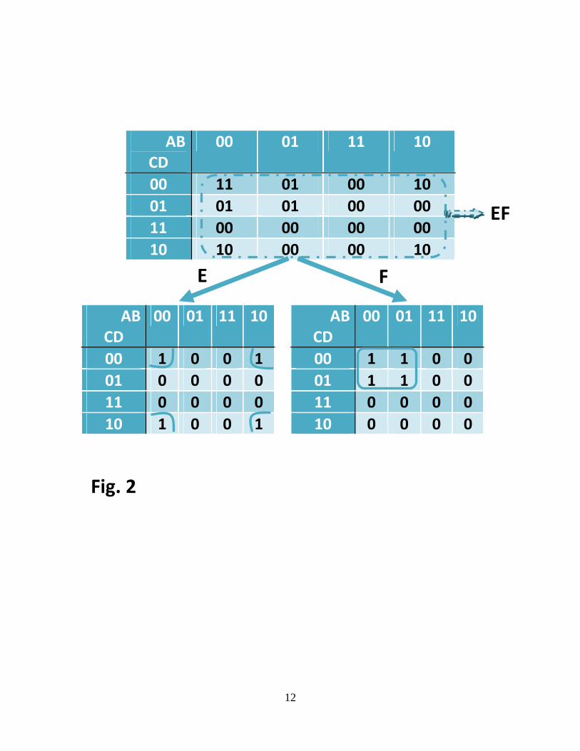
  AB  00  01  11  10 CD 00  11  01  00  10 01  01  01  00  00 11  00  00  00  00 10  10  00  00  10 

  AB CD 

00  01  11 10

00  1  0  0  1 01  0  0  0  0 11  0  0  0  0 10  1  0  0  1 

  ABCD 

00 01  11  10

00  1  1  0  0 01  1  1  0  0 11  0  0  0  0 

EF

E  F

10  0  0  0  0 

Fig. 2 

12

a)  b)

c)  d)

 Fig. 3 

13

SUPPLEMENTARY INFORMATION

FOUR-STATE NANOMAGNETIC LOGIC USING MULTIFERROICS

aNoel D’Souza , Jayasimha Atulasimhaa a , Supriyo Bandyopadhyay

Email: {dsouzanm, jatulasimha, sbandy}@vcu.edu

(a) Department of Mechanical and Nuclear Engineering,

(b) Department of Electrical and Computer Engineering,

Virginia Commonwealth University, Richmond, VA 23284, USA.

In the letter, we showed that dipole-coupled Ni/PZT multiferroic nanomagnets with binary

bits encoded in the four stable magnetization directions (‘up’, ‘down’, ‘left’ and ‘right’) can

implement 4-state NOR logic with the proper clock sequence. We showed this for one particular

input bit combination and for one particular initial state of the output. For the sake of

completeness, we have to show it for all possible input combinations and for all possible initial

state of the output magnet. This is shown here.

Of the sixteen possible input configurations (input bits) and four possible initial states of the

output magnet (output bit), the results and energy plots for one particular input configuration

(AB = ‘right’, CD = ‘up’) and one initial state of the output (magnetization direction pointing

‘down’) was shown in the letter. In this supplement, we consider the other cases in order to be

exhaustive. We first pick the input configuration (AB = ‘right’, CD = ‘up’) discussed in the

letter and show that for this input combination, the final state of the output is independent of the

initial state of the output. There are three other possible initial states of the output (‘left’, ‘right’

and ‘up’) and each of them is examined for the above input combination (Figs. S1 – S3). In each

case, the final output settles in the correct direction (‘right’) conforming to NOR logic. Thus, the

final output is independent of the initial state of the output for this input combination. This

14

means that the output is determined solely by the inputs and hence is a unique, single-valued

function of the inputs.

We also show the results obtained from the seven other unique input combinations when the

initial state of the output is EF = 11 (Figs. S4 – S10). It is obvious that the final state of the

output will be independent of the initial state for these input combinations as well. The remaining

eight input combinations are not examined since they are equivalent to ones examined here due

to symmetry. For all input combinations, the NOR function is always realized.

Supplement Figure Captions

Figure S1: Energy plots of the output magnet representing the bits EF with input bits AB = ‘01’,

CD = ‘00’ and EF = ‘00’ initially. (a) Rotation from +90° to +135° as a consequence of tension

applied along the +45° axis. (b) Upon relaxation of the stress, the magnetization vector rotates

back to +90°. (c) With compression applied on the output magnet along the +45° axis, its

magnetization rotates to +45°. (d) Finally, when the stress is relaxed to zero, the output magnet

rotates its magnetization to 0°, completing the NOR logic operation.

Figure S2: The input combinations AB=’01’, CD=’00’ are the same as in figures S1. The initial

state of the output magnet EF is set at ‘01’. The stress cycle (tension, relaxation, compression,

relaxation) is applied to the output magnet with the magnetization rotating sequentially through -

45°, 0°, +45° and finally settling at 0°, thereby once again completing the NOR operation.

15

Figure S3: AB = ‘01’, CD = ‘00’ as in figure S1. The initial output state is set to EF = ‘10’. The

stress cycle applied to the output magnet causes its magnetization to rotate sequentially through

+135°, +90°, +45° and 0°, thereby completing the NOR operation. Figs. S1-S3 show that the

final state of the output is indeed independent of the initial state and hence determined uniquely

by the inputs.

Figure S4: AB = ‘00’, CD = ‘00’ and EF = ‘11’. Since the inputs are pointing ‘up’, the dipole

interaction pushes the output magnet’s magnetization vector ‘down’. The stress cycle applied to

output magnet causes its magnetization vector to rotate sequentially through -45°, -90°, -135°

and back to -90°, completing the NOR operation.

Figure S5: AB = ‘00’, CD = ‘11’ and EF = ‘11’. The input magnetization directions, on either

side of the output magnet encoding EF, point in opposite directions (‘up’ and ‘down’). As a

result, the dipole interaction of the inputs on the output cancels out. This would result in a tie-

condition when the stress cycle is applied (specifically, during the relaxation phases, when the

magnetization would have two equally likely directions to settle into). However, when a dc bias

magnetic field is applied [Happl = 1000 A/m (~12 Oe)], the energy profile is no longer symmetric

and is slightly biased towards +90°. Now, when the stress cycle is applied to the output magnet,

its magnetization rotates through +135°, +90°, +45° and 90°, thereby once again completing the

NOR operation.

Figure S6: AB = ‘01’, CD = ‘01’ and EF = ‘11’. In this case, the inputs are both pointing

towards the ‘right’. Hence, the dipole interaction shows a strong preference for ferromagnetic

16

coupling (parallel arrangement). This can be seen in the energy profile of the output magnet, EF,

which has an absolute energy minimum located at 0° (‘right’). The magnetization rotation arising

due to the stress cycle applied to the output magnet is from the initial -90° direction to -45°

(since the ferromagnetic coupling due to the dipole interaction is strong, the magnetization

easily rotates to 0° at low values of applied stress. However, at higher stress values, the stress

anisotropy energy is greater than the dipole energy and, consequently, the magnetization settles

at -45°, 0°, +45° before settling to 0°. Ultimately, the NOR operation is once again realized.

Figure S7: AB = ‘01’, CD = ‘10’ and EF = ‘11’. Since the input magnetizations point in

opposite directions, there is no net dipole interaction on the output magnet encoding the bits EF

(similar to the configuration of Fig. S5). Once again, the applied bias magnetic field tips the

energy profile of the output magnet towards +90°. The stress cycle applied to the output magnet

causes its magnetization to rotate through -45°, 0°, +45° and +90°, thus implementing the NOR

operation.

Figure S8: AB = ‘01’, CD = ‘11’ and EF = ‘11’. In this configuration, AB points ‘right’ while

CD points ‘up’. In the first stage of the stress cycle (tension along +45°) on the output magnet,

the magnetization rotates from -90° to -45° (similar to Fig. S6, at low tensile stresses, the

preferred alignment is 0°, parallel to AB. Further increases in stress cause the magnetization to

settle at -45°). Relaxation of the stress then rotates it to 0°, compression takes it to +45° and

ultimately, relaxation causes it to settle at +90°. The NOR operation is realized.

17

Figure S9: AB = ‘10’, CD = ‘00’ and EF = ‘11’. With AB pointing ‘left’ and CD pointing ‘up’,

the dipole interaction is similar to that of the case in Fig. S7, with the output EF preferring a

parallel alignment with AB. The stress cycle applied to the output magnet causes its

magnetization to rotate from the initial direction of -90° to -45°, -90°, -135° and finally, -180°,

thus implementing the NOR function.

Figure S10: AB = ‘10’, CD = ‘11’ and EF = ‘11’. This configuration (AB points ‘left’, CD

points ‘down’) is similar to that of Fig. S8. The applied bias field tries to align the output

magnet's magnetization vector along the +90° direction, without which a tie-condition would

arise (two equally possible directions). The stress cycle applied to the output magnet causes its

magnetization to rotate sequentially through -45°, 0°, +45° and +90°. This completes the NOR

operation.

18

Fig. S1 

c)  d)

a)  b)

19

Fig. S2 

c)  d)

a)  b)

20

Fig. S3 

c)  d)

a)  b)

21

Fig. S4 

c)  d)

a)  b)

22

22

Fig. S5 

c)  d)

a)  b)

23

Fig. S6 

c)  d)

a)  b)

24

Fig. S7 

c)  d)

a)  b)

25

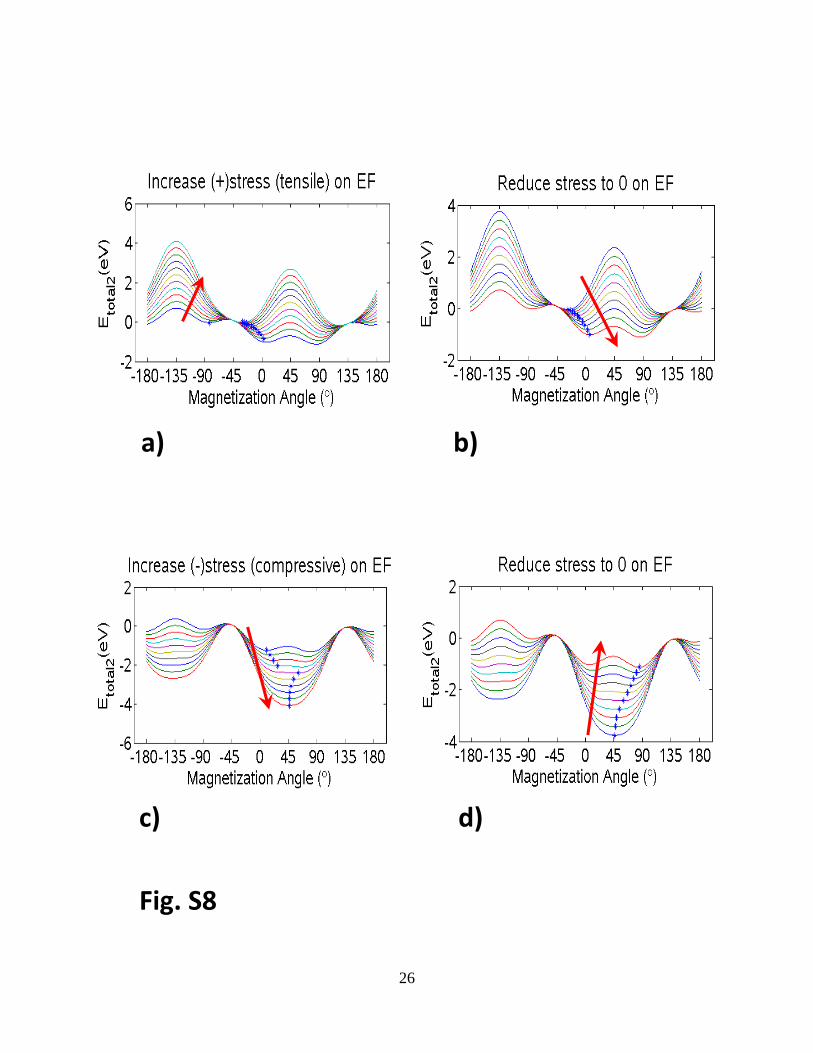
Fig. S8 

c)  d)

a)  b)

26

Fig. S9 

c)  d)

a)  b)

27

a)  b)

c)  d)

Fig. S10 

28