Four slides per page, pdf.

Introduction toTheoretical Computer Science

Motivation

• Automata = abstract computing devices

• Turing studied Turing Machines (= com-puters) before there were any real comput-ers

• We will also look at simpler devices thanTuring machines (Finite State Automata,Pushdown Automata, . . . ), and specifica-tion means, such as grammars and regularexpressions.

• NP-hardness = what cannot be efficientlycomputed.

• Undecidability = what cannot be computedat all.

1

Finite Automata

Finite Automata are used as a model for

• Software for designing digital cicuits

• Lexical analyzer of a compiler

• Searching for keywords in a file or on the

web.

• Software for verifying finite state systems,

such as communication protocols.

2

• Example: Finite Automaton modelling an

on/off switch

Push

Push

Startonoff

• Example: Finite Automaton recognizing the

string then

t th theStart t nh e

then

3

Structural Representations

These are alternative ways of specifying a ma-chine

Grammars: A rule like E ⇒ E+E specifies anarithmetic expression

• Lineup⇒ Person.LineupLineup⇒ Person

says that a lineup is a single person, or a personin front of a lineup.

Regular Expressions: Denote structure of data,e.g.

’[A-Z][a-z]*[][A-Z][A-Z]’

matches Ithaca NY

does not match Palo Alto CA

Question: What expression would matchPalo Alto CA

4

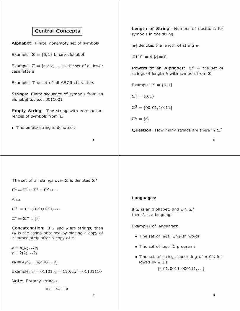
Central Concepts

Alphabet: Finite, nonempty set of symbols

Example: Σ = {0,1} binary alphabet

Example: Σ = {a, b, c, . . . , z} the set of all lower

case letters

Example: The set of all ASCII characters

Strings: Finite sequence of symbols from an

alphabet Σ, e.g. 0011001

Empty String: The string with zero occur-

rences of symbols from Σ

• The empty string is denoted ε

5

Length of String: Number of positions for

symbols in the string.

|w| denotes the length of string w

|0110| = 4, |ε| = 0

Powers of an Alphabet: Σk = the set of

strings of length k with symbols from Σ

Example: Σ = {0,1}

Σ1 = {0,1}

Σ2 = {00,01,10,11}

Σ0 = {ε}

Question: How many strings are there in Σ3

6

The set of all strings over Σ is denoted Σ∗

Σ∗ = Σ0 ∪Σ1 ∪Σ2 ∪ · · ·

Also:

Σ+ = Σ1 ∪Σ2 ∪Σ3 ∪ · · ·

Σ∗ = Σ+ ∪ {ε}

Concatenation: If x and y are strings, thenxy is the string obtained by placing a copy ofy immediately after a copy of x

x = a1a2 . . . aiy = b1b2 . . . bj

xy = a1a2 . . . aib1b2 . . . bj

Example: x = 01101, y = 110, xy = 01101110

Note: For any string x

xε = εx = x

7

Languages:

If Σ is an alphabet, and L ⊆ Σ∗

then L is a language

Examples of languages:

• The set of legal English words

• The set of legal C programs

• The set of strings consisting of n 0’s fol-

lowed by n 1’s

{ε,01,0011,000111, . . .}

8

• The set of strings with equal number of 0’s

and 1’s

{ε,01,10,0011,0101,1001, . . .}

• LP = the set of binary numbers whose

value is prime

{10,11,101,111,1011, . . .}

• The empty language ∅

• The language {ε} consisting of the empty

string

Note: ∅ 6= {ε}

Note2: The underlying alphabet Σ is always

finite

9

Problem: Is a given string w a member of alanguage L?

Example: Is a binary number prime = is it ameber in LP

Is 11101 ∈ LP? What computational resourcesare needed to answer the question.

Usually we think of problems not as a yes/nodecision, but as something that transforms aninput into an output.

Example: Parse a C-program = check if theprogram is correct, and if it is, produce a parsetree.

Let LX be the set of all valid programs in proglang X. If we can show that determining mem-bership in LX is hard, then parsing programswritten in X cannot be easier.

Question: Why?

10

Finite Automata Informally

Protocol for e-commerce using e-money

Allowed events:

1. The customer can pay the store (=sendthe money-file to the store)

2. The customer can cancel the money (likeputting a stop on a check)

3. The store can ship the goods to the cus-tomer

4. The store can redeem the money (=cashthe check)

5. The bank can transfer the money to thestore

11

e-commerce

The protocol for each participant:

1 43

2

transferredeem

cancel

Start

a b

c

d f

e g

Start

(a) Store

(b) Customer (c) Bank

redeem transfer

ship ship

transferredeem

ship

pay

cancel

Start pay

12

Completed protocols:

cancel

1 43

2

transferredeem

cancel

Start

a b

c

d f

e g

Start

(a) Store

(b) Customer (c) Bank

ship shipship

redeem transfer

transferredeempay

pay, cancelship. redeem, transfer,

pay,ship

pay, ship

pay,cancel pay,cancel pay,cancel

pay,cancel pay,cancel pay,cancel

cancel, ship cancel, shippay,redeem, pay,redeem,

Start

13

The entire system as an Automaton:

C C C C C C C

P P P P P P

P P P P P P

P,C P,C

P,C P,C P,C P,C P,C P,CC

C

P S SS

P S SS

P SS

P S SS

a b c d e f g

1

2

3

4

Start

P,C

P,C P,CP,C

R

R

S

T

T

R

RR

R

14

Deterministic Finite Automata

A DFA is a quintuple

A = (Q,Σ, δ, q0, F )

• Q is a finite set of states

• Σ is a finite alphabet (=input symbols)

• δ is a transition function (q, a) 7→ p

• q0 ∈ Q is the start state

• F ⊆ Q is a set of final states

15

Example: An automaton A that accepts

L = {x01y : x, y ∈ {0,1}∗}

The automaton A = ({q0, q1, q2}, {0,1}, δ, q0, {q1})as a transition table:

δ 0 1

→ q0 q2 q0?q1 q1 q1q2 q2 q1

The automaton A as a transition diagram:

1 0

0 1q0 q2 q1 0, 1Start

16

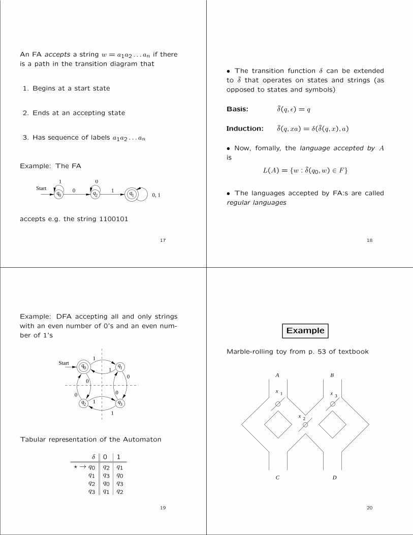
An FA accepts a string w = a1a2 . . . an if there

is a path in the transition diagram that

1. Begins at a start state

2. Ends at an accepting state

3. Has sequence of labels a1a2 . . . an

Example: The FA

1 0

0 1q0 q2 q1 0, 1Start

accepts e.g. the string 1100101

17

• The transition function δ can be extended

to δ that operates on states and strings (as

opposed to states and symbols)

Basis: δ(q, ε) = q

Induction: δ(q, xa) = δ(δ(q, x), a)

• Now, fomally, the language accepted by A

is

L(A) = {w : δ(q0, w) ∈ F}

• The languages accepted by FA:s are called

regular languages

18

Example: DFA accepting all and only strings

with an even number of 0’s and an even num-

ber of 1’s

q q

q q

0 1

2 3

Start

0

0

1

1

0

0

1

1

Tabular representation of the Automaton

δ 0 1

?→ q0 q2 q1q1 q3 q0q2 q0 q3q3 q1 q2

19

Example

Marble-rolling toy from p. 53 of textbook

A B

C D

x

xx3

2

1

20

A state is represented as sequence of three bits

followed by r or a (previous input rejected or

accepted)

For instance, 010a, means

left, right, left, accepted

Tabular representation of DFA for the toy

A B

→ 000r 100r 011r?000a 100r 011r?001a 101r 000a

010r 110r 001a?010a 110r 001a

011r 111r 010a100r 010r 111r?100a 010r 111r

101r 011r 100a?101a 011r 100a

110r 000a 101a?110a 000a 101a

111r 001a 110a

21

Nondeterministic Finite Automata

A NFA can be in several states at once, or,viewded another way, it can “guess” whichstate to go to next

Example: An automaton that accepts all andonly strings ending in 01.

Start 0 1q0 q q

0, 1

1 2

Here is what happens when the NFA processesthe input 00101

q0

q2

q0 q0 q0 q0 q0

q1q1 q1

q2

0 0 1 0 1

(stuck)

(stuck)

22

Formally, a NFA is a quintuple

A = (Q,Σ, δ, q0, F )

• Q is a finite set of states

• Σ is a finite alphabet

• δ is a transition function from Q×Σ to the

powerset of Q

• q0 ∈ Q is the start state

• F ⊆ Q is a set of final states

23

Example: The NFA from the previous slide is

({q0, q1, q2}, {0,1}, δ, q0, {q2})

where δ is the transition function

δ 0 1

→ q0 {q0, q1} {q0}q1 ∅ {q2}?q2 ∅ ∅

24

Extended transition function δ.

Basis: δ(q, ε) = {q}

Induction:

δ(q, xa) =⋃

p∈δ(q,x)

δ(p, a)

Example: Let’s compute δ(q0,00101) on the

blackboard

• Now, fomally, the language accepted by A is

L(A) = {w : δ(q0, w) ∩ F 6= ∅}

25

Let’s prove formally that the NFA

Start 0 1q0 q q

0, 1

1 2

accepts the language {x01 : x ∈ Σ∗}. We’ll do

a mutual induction on the three statements

below

0. w ∈ Σ∗ ⇒ q0 ∈ δ(q0, w)

1. q1 ∈ δ(q0, w)⇔ w = x0

2. q2 ∈ δ(q0, w)⇔ w = x01

26

Basis: If |w| = 0 then w = ε. Then statement

(0) follows from def. For (1) and (2) both

sides are false for ε

Induction: Assume w = xa, where a ∈ {0,1},|x| = n and statements (0)–(2) hold for x. We

will show on the blackboard in class that the

statements hold for xa.

27

Equivalence of DFA and NFA

• NFA’s are usually easier to “program” in.

• Surprisingly, for any NFA N there is a DFA D,

such that L(D) = L(N), and vice versa.

• This involves the subset construction, an im-

portant example how an automaton B can be

generically constructed from another automa-

ton A.

• Given an NFA

N = (QN ,Σ, δN , q0, FN)

we will construct a DFA

D = (QD,Σ, δD, {q0}, FD)

such that

L(D) = L(N)

.28

The details of the subset construction:

• QD = {S : S ⊆ QN}.

Note: |QD| = 2|QN |, although most states in

QD are likely to be garbage.

• FD = {S ⊆ QN : S ∩ FN 6= ∅}

• For every S ⊆ QN and a ∈ Σ,

δD(S, a) =⋃

p∈SδN(p, a)

29

Let’s construct δD from the NFA on slide 26

0 1

∅ ∅ ∅→ {q0} {q0, q1} {q0}{q1} ∅ {q2}?{q2} ∅ ∅{q0, q1} {q0, q1} {q0, q2}?{q0, q2} {q0, q1} {q0}?{q1, q2} ∅ {q2}

?{q0, q1, q2} {q0, q1} {q0, q2}

30

Note: The states of D correspond to subsets

of states of N , but we could have denoted the

states of D by, say, A− F just as well.

0 1

A A A→ B E BC A D?D A AE E F?F E B?G A D?H E F

31

We can often avoid the exponential blow-up

by constructing the transition table for D only

for accessible states S as follows:

Basis: S = {q0} is accessible in D

Induction: If state S is accessible, so are the

states in⋃a∈Σ δD(S, a).

Example: The “subset” DFA with accessible

states only.

Start

{ {q q {q0 0 0, ,q q1 2}}0 1

1 0

0

1

}

32

Theorem 2.11: Let D be the “subset” DFA

of an NFA N . Then L(D) = L(N).

Proof: First we show on an induction on |w|that

δD({q0}, w) = δN(q0, w)

Basis: w = ε. The claim follows from def.

33

Induction:

δD({q0}, xa)def= δD(δD({q0}, x), a)

i.h.= δD(δN(q0, x), a)

cst=

⋃

p∈δN(q0,x)

δN(p, a)

def= δN(q0, xa)

Now (why?) it follows that L(D) = L(N).

34

Theorem 2.12: A language L is accepted by

some DFA if and only if L is accepted by some

NFA.

Proof: The “if” part is Theorem 2.11.

For the “only if” part we note that any DFA

can be converted to an equivalent NFA by mod-

ifying the δD to δN by the rule

• If δD(q, a) = p, then δN(q, a) = {p}.

By induction on |w| it will be shown in the

tutorial that if δD(q0, w) = p, then δN(q0, w) =

{p}.

The claim of the theorem follows.

35

Exponential Blow-Up

There is an NFA N with n+ 1 states that hasno equivalent DFA with fewer than 2n states

Start

0, 1

0, 1 0, 1 0, 1q q qq0 1 2 n

1 0, 1

L(N) = {x1c2c3 · · · cn : x ∈ {0,1}∗, ci ∈ {0,1}}

Suppose an equivalent DFA D with fewer than2n states exists.

D must remember the last n symbols it hasread. There are 2n bitsequences a1a2 . . . an.Since D has fewer that 2n states

∃ q, a1a2 . . . an, b1b2 . . . bn :

a1a2 . . . an 6= b1b2 . . . bn

δD(q0, a1a2 . . . an) = δD(q0, b1b2 . . . bn) = q

36

Since a1a2 . . . an 6= b1b2 . . . bn they must differin at least one position.

Case 1:

1a2 . . . an0b2 . . . bn

Then q has to be both an accepting and anonaccepting state.

Case 2:

a1 . . . ai−11ai+1 . . . anb1 . . . bi−10bi+1 . . . bn

Now δD(q0, a1 . . . ai−11ai+1 . . . an0i−1) =δD(q0, b1 . . . bi−10bi+1 . . . bn0i−1)

and δD(q0, a1 · · · ai−11ai+1 · · · an0i−1) ∈ FD

δD(q0, b1 · · · bi−10bi+1 · · · bn0i−1) /∈ FD37

FA’s with Epsilon-Transitions

An ε-NFA accepting decimal numbers consist-

ing of:

1. An optional + or - sign

2. A string of digits

3. a decimal point

4. another string of digits

One of the strings (2) are (4) are optional

q q q q q

q

0 1 2 3 5

4

Start

0,1,...,9 0,1,...,9

ε ε

0,1,...,9

0,1,...,9

,+,-

.

.

38

An ε-NFA is a quintuple (Q,Σ, δ, q0, F ) where δ

is a function from Q×Σ∪ {ε} to the powerset

of Q.

Example: The ε-NFA from the previous slide

E = ({q0, q1, . . . , q5}, {.,+,−,0,1, . . . ,9} δ, q0, {q5})

where the transition table for δ is

ε +,- . 0, . . . ,9

→ q0 {q1} {q1} ∅ ∅q1 ∅ ∅ {q2} {q1, q4}q2 ∅ ∅ ∅ {q3}q3 {q5} ∅ ∅ {q3}q4 ∅ ∅ {q3} ∅?q5 ∅ ∅ ∅ ∅

39

ECLOSE

We close a state by adding all states reachable

by a sequence εε · · · ε

Inductive definition of ECLOSE(q)

Basis:

q ∈ ECLOSE(q)

Induction:

p ∈ ECLOSE(q) and r ∈ δ(p, ε) ⇒r ∈ ECLOSE(q)

40

Example of ε-closure

1

2 3 6

4 5 7

ε

ε ε

ε

εa

b

For instance,

ECLOSE(1) = {1,2,3,4,6}

41

• Inductive definition of δ for ε-NFA’s

Basis:

δ(q, ε) = ECLOSE(q)

Induction:

δ(q, xa) =⋃

p∈δ(δ(q,x),a)

ECLOSE(p)

Let’s compute on the blackboard in class

δ(q0, 5.6) for the NFA on slide 38

42

Given an ε-NFA

E = (QE,Σ, δE, q0, FE)

we will construct a DFA

D = (QD,Σ, δD, qD, FD)

such that

L(D) = L(E)

Details of the construction:

• QD = {S : S ⊆ QE and S = ECLOSE(S)}

• qD = ECLOSE(q0)

• FD = {S : S ∈ QD and S ∩ FE 6= ∅}

• δD(S, a) =⋃{ECLOSE(p) : p ∈ δ(t, a) for some t ∈ S}

43

Example: ε-NFA E

q q q q q

q

0 1 2 3 5

4

Start

0,1,...,9 0,1,...,9

ε ε

0,1,...,9

0,1,...,9

,+,-

.

.

DFA D corresponding to E

Start

{ { { {

{ {

q q q q

q q

0 1 1, }q

1} , q

4} 2, q

3, q5}

2}3, q5}

0,1,...,9 0,1,...,9

0,1,...,9

0,1,...,9

0,1,...,9

0,1,...,9

+,-

.

.

.

44

Theorem 2.22: A language L is accepted by

some ε-NFA E if and only if L is accepted by

some DFA.

Proof: We use D constructed as above and

show by induction that δD(q0, w) = δE(qD, w)

Basis: δE(q0, ε) = ECLOSE(q0) = qD = δ(qD, ε)

45

Induction:

δE(q0, xa) =⋃

p∈δE(δE(q0,x),a)

ECLOSE(p)

=⋃

p∈δD(δD(qD,x),a)

ECLOSE(p)

=⋃

p∈δD(qD,xa)

ECLOSE(p)

= δD(qD, xa)

46

Regular expressions

A FA (NFA or DFA) is a “blueprint” for con-

tructing a machine recognizing a regular lan-

guage.

A regular expression is a “user-friendly,” declar-

ative way of describing a regular language.

Example: 01∗+ 10∗

Regular expressions are used in e.g.

1. UNIX grep command

2. UNIX Lex (Lexical analyzer generator) and

Flex (Fast Lex) tools.

47

Operations on languages

Union:

L ∪M = {w : w ∈ L or w ∈M}

Concatenation:

L.M = {w : w = xy, x ∈ L, y ∈M}

Powers:

L0 = {ε}, L1 = L, Lk+1 = L.Lk

Kleene Closure:

L∗ =∞⋃

i=0

Li

Question: What are ∅0, ∅i, and ∅∗

48

Building regex’s

Inductive definition of regex’s:

Basis: ε is a regex and ∅ is a regex.L(ε) = {ε}, and L(∅) = ∅.

If a ∈ Σ, then a is a regex.L(a) = {a}.

Induction:

If E is a regex’s, then (E) is a regex.L((E)) = L(E).

If E and F are regex’s, then E + F is a regex.L(E + F ) = L(E) ∪ L(F ).

If E and F are regex’s, then E.F is a regex.L(E.F ) = L(E).L(F ).

If E is a regex’s, then E? is a regex.L(E?) = (L(E))∗.

49

Example: Regex for

L = {w ∈ {0,1}∗ : 0 and 1 alternate in w}

(01)∗+ (10)∗+ 0(10)∗+ 1(01)∗

or, equivalently,

(ε+ 1)(01)∗(ε+ 0)

Order of precedence for operators:

1. Star

2. Dot

3. Plus

Example: 01∗+ 1 is grouped (0(1)∗) + 1

50

Equivalence of FA’s and regex’s

We have already shown that DFA’s, NFA’s,

and ε-NFA’s all are equivalent.

ε-NFA NFA

DFARE

To show FA’s equivalent to regex’s we need to

establish that

1. For every DFA A we can find (construct,

in this case) a regex R, s.t. L(R) = L(A).

2. For every regex R there is a ε-NFA A, s.t.

L(A) = L(R).

51

Theorem 3.4: For every DFA A = (Q,Σ, δ, q0, F )

there is a regex R, s.t. L(R) = L(A).

Proof: Let the states of A be {1,2, . . . , n},with 1 being the start state.

• Let R(k)ij be a regex describing the set of

labels of all paths in A from state i to state

j going through intermediate states {1, . . . , k}only.

i

k

j

52

R(k)ij will be defined inductively. Note that

L

⊕

j∈FR1j

(n)

= L(A)

Basis: k = 0, i.e. no intermediate states.

• Case 1: i 6= j

R(0)ij =

⊕

{a∈Σ:δ(i,a)=j}a

• Case 2: i = j

R(0)ii =

⊕

{a∈Σ:δ(i,a)=i}a

+ ε

53

Induction:

R(k)ij

=

R(k−1)ij

+

R(k−1)ik

(R

(k−1)kk

)∗R

(k−1)kj

R kj(k-1)

R kk(k-1)R ik

(k-1)

i k k k k

Zero or more strings inIn In

j

54

Example: Let’s find R for A, where

L(A) = {x0y : x ∈ {1}∗ and y ∈ {0,1}∗}

1

0Start 0,11 2

R(0)11 ε+ 1

R(0)12 0

R(0)21 ∅

R(0)22 ε+ 0 + 1

55

We will need the following simplification rules:

• (ε+R)∗ = R∗

• R+RS∗ = RS∗

• ∅R = R∅ = ∅ (Annihilation)

• ∅+R = R+ ∅ = R (Identity)

56

R(0)11 ε+ 1

R(0)12 0

R(0)21 ∅

R(0)22 ε+ 0 + 1

R(1)ij = R

(0)ij +R

(0)i1

(R

(0)11

)∗R

(0)1j

By direct substitution Simplified

R(1)11 ε+ 1 + (ε+ 1)(ε+ 1)∗(ε+ 1) 1∗

R(1)12 0 + (ε+ 1)(ε+ 1)∗0 1∗0

R(1)21 ∅+ ∅(ε+ 1)∗(ε+ 1) ∅

R(1)22 ε+ 0 + 1 + ∅(ε+ 1)∗0 ε+ 0 + 1

57

Simplified

R(1)11 1∗

R(1)12 1∗0

R(1)21 ∅

R(1)22 ε+ 0 + 1

R(2)ij = R

(1)ij +R

(1)i2

(R

(1)22

)∗R

(1)2j

By direct substitution

R(2)11 1∗+ 1∗0(ε+ 0 + 1)∗∅

R(2)12 1∗0 + 1∗0(ε+ 0 + 1)∗(ε+ 0 + 1)

R(2)21 ∅+ (ε+ 0 + 1)(ε+ 0 + 1)∗∅

R(2)22 ε+ 0 + 1 + (ε+ 0 + 1)(ε+ 0 + 1)∗(ε+ 0 + 1)

58

By direct substitution

R(2)11 1∗+ 1∗0(ε+ 0 + 1)∗∅

R(2)12 1∗0 + 1∗0(ε+ 0 + 1)∗(ε+ 0 + 1)

R(2)21 ∅+ (ε+ 0 + 1)(ε+ 0 + 1)∗∅

R(2)22 ε+ 0 + 1 + (ε+ 0 + 1)(ε+ 0 + 1)∗(ε+ 0 + 1)

Simplified

R(2)11 1∗

R(2)12 1∗0(0 + 1)∗

R(2)21 ∅

R(2)22 (0 + 1)∗

The final regex for A is

R(2)12 = 1∗0(0 + 1)∗

59

Observations

There are n3 expressions R(k)ij

Each inductive step grows the expression 4-fold

R(n)ij could have size 4n

For all {i, j} ⊆ {1, . . . , n}, R(k)ij uses R(k−1)

kk

so we have to write n2 times the regex R(k−1)kk

We need a more efficient approach:

the state elimination technique

60

The state elimination technique

Let’s label the edges with regex’s instead of

symbols

q

q

p

p

1 1

k m

s

Q

Q

P1

Pm

k

1

11R

R 1m

R km

R k1

S

61

Now, let’s eliminate state s.

11R Q1 P1

R 1m

R k1

R km

Q1 Pm

Q k

Q k

P1

Pm

q

q

p

p

1 1

k m

+ S*

+

+

+

S*

S*

S*

For each accepting state q eliminate from the

original automaton all states exept q0 and q.

62

For each q ∈ F we’ll be left with an Aq thatlooks like

Start

RS

T

U

that corresponds to the regex Eq = (R+SU∗T )∗SU∗

or with Aq looking like

R

Start

corresponding to the regex Eq = R∗

• The final expression is⊕

q∈FEq

63

Example: A, where L(A) = {W : w = x1b, or w =

x1bc, x ∈ {0,1}∗, {b, c} ⊆ {0,1}}

Start

0,1

1 0,1 0,1A B C D

We turn this into an automaton with regex

labels

0 1+

0 1+ 0 1+StartA B C D

1

64

0 1+

0 1+ 0 1+StartA B C D

1

Let’s eliminate state B

0 1+

DC0 1+( ) 0 1+Start

A1

Then we eliminate state C and obtain AD

0 1+

D0 1+( ) 0 1+( )Start

A1

with regex (0 + 1)∗1(0 + 1)(0 + 1)

65

From

0 1+

DC0 1+( ) 0 1+Start

A1

we can eliminate D to obtain AC

0 1+

C0 1+( )Start

A1

with regex (0 + 1)∗1(0 + 1)

• The final expression is the sum of the previ-

ous two regex’s:

(0 + 1)∗1(0 + 1)(0 + 1) + (0 + 1)∗1(0 + 1)

66

From regex’s to ε-NFA’s

Theorem 3.7: For every regex R we can con-

struct and ε-NFA A, s.t. L(A) = L(R).

Proof: By structural induction:

Basis: Automata for ε, ∅, and a.

ε

a

(a)

(b)

(c)

67

Induction: Automata for R+ S, RS, and R∗

(a)

(b)

(c)

R

S

R S

R

ε ε

εε

ε

ε

ε

ε ε

68

Example: We convert (0 + 1)∗1(0 + 1)

ε

ε

ε

ε

0

1

ε

ε

ε

ε

0

1

ε

ε1

Start

(a)

(b)

(c)

0

1

ε ε

ε

ε

ε ε

εε

ε

0

1

ε ε

ε

ε

ε ε

ε

69

Algebraic Laws for languages

• L ∪M = M ∪ L.

Union is commutative.

• (L ∪M) ∪N = L ∪ (M ∪N).

Union is associative.

• (LM)N = L(MN).

Concatenation is associative

Note: Concatenation is not commutative, i.e.,

there are L and M such that LM 6= ML.

70

• ∅ ∪ L = L ∪ ∅ = L.

∅ is identity for union.

• {ε}L = L{ε} = L.

{ε} is left and right identity for concatenation.

• ∅L = L∅ = ∅.

∅ is left and right annihilator for concatenation.

71

• L(M ∪N) = LM ∪ LN .

Concatenation is left distributive over union.

• (M ∪N)L = ML ∪NL.

Concatenation is right distributive over union.

• L ∪ L = L.

Union is idempotent.

• ∅∗ = {ε}, {ε}∗ = {ε}.

• L+ = LL∗ = L∗L, L∗ = L+ ∪ {ε}

72

• (L∗)∗ = L∗. Closure is idempotent

Proof:

w ∈ (L∗)∗ ⇐⇒ w ∈∞⋃

i=0

( ∞⋃

j=0

Lj)i

⇐⇒ ∃k,m ∈ N : w ∈ (Lm)k

⇐⇒ ∃p ∈ N : w ∈ Lp

⇐⇒ w ∈∞⋃

i=0

Li

⇐⇒ w ∈ L∗ �

73

Algebraic Laws for regex’s

Evidently e.g. L((0 + 1)1) = L(01 + 11)

Also e.g. L((00 + 101)11) = L(0011 + 10111).

More generally

L((E + F )G) = L(EG+ FG)

for any regex’s E, F , and G.

• How do we verify that a general identity like

above is true?

1. Prove it by hand.

2. Let the computer prove it.

74

In Chapter 4 we will learn how to test auto-

matically if E = F , for any concrete regex’s

E and F .

We want to test general identities, such as

E + F = F + E, for any regex’s E and F.

Method:

1. “Freeze” E to a1, and F to a2

2. Test automatically if the frozen identity is

true, e.g. if L(a1 + a2) = L(a2 + a1)

Question: Does this always work?

75

Answer: Yes, as long as the identities use only

plus, dot, and star.

Let’s denote a generalized regex, such as (E + F)Eby

E(E,F)

Now we can for instance make the substitution

S = {E/0,F/11} to obtain

S (E(E,F)) = (0 + 11)0

76

Theorem 3.13: Fix a “freezing” substitution

♠ = {E1/a1, E2/a2, . . . , Em/am}.

Let E(E1, E2, . . . , Em) be a generalized regex.

Then for any regex’s E1, E2, . . . , Em,

w ∈ L(E(E1, E2, . . . , Em))

if and only if there are strings wi ∈ L(Ei), s.t.

w = wj1wj2 · · ·wjkand

aj1aj2 · · · ajk ∈ L(E(a1,a2, . . . ,am))

77

For example: Suppose the alphabet is {1,2}.Let E(E1, E2) be (E1 + E2)E1, and let E1 be 1,

and E2 be 2. Then

w ∈ L(E(E1, E2)) = L((E1 + E2)E1) =

({1} ∪ {2}){1} = {11, 21}if and only if

∃w1 ∈ L(E1) = {1}, ∃w2 ∈ L(E2) = {2} : w = wj1wj2

and

aj1aj2 ∈ L(E(a1,a2))) = L((a1+a2)a1) = {a1a1, a2a1}if and only if

j1 = j2 = 1, or j1 = 1, and j2 = 2

78

Proof of Theorem 3.13: We do a structural

induction of E.

Basis: If E = ε, the frozen expression is also ε.

If E = ∅, the frozen expression is also ∅.

If E = a, the frozen expression is also a. Now

w ∈ L(E) if and only if there is u ∈ L(a), s.t.

w = u and u is in the language of the frozen

expression, i.e. u ∈ {a}.

79

Induction:

Case 1: E = F + G.

Then ♠(E) = ♠(F) +♠(G), andL(♠(E)) = L(♠(F)) ∪ L(♠(G))

Let E and and F be regex’s. Then w ∈ L(E + F )if and only if w ∈ L(E) or w ∈ L(F ), if and onlyif a1 ∈ L(♠(F)) or a2 ∈ L(♠(G)), if and only ifa1 ∈ ♠(E), or a2 ∈ ♠(E).

Case 2: E = F.G.

Then ♠(E) = ♠(F).♠(G), andL(♠(E)) = L(♠(F)).L(♠(G))

Let E and and F be regex’s. Then w ∈ L(E.F )if and only if w = w1w2, w1 ∈ L(E) and w2 ∈ L(F ),and a1a2 ∈ L(♠(F)).L(♠(G)) = ♠(E)

Case 3: E = F∗.

Prove this case at home.80

Examples:

To prove (L+M)∗ = (L∗M∗)∗ it is enough to

determine if (a1+a2)∗ is equivalent to (a∗1a∗2)∗

To verify L∗ = L∗L∗ test if a∗1 is equivalent to

a∗1a∗1.

Question: Does L+ML = (L+M)L hold?

81

Theorem 3.14: E(E1, . . . , Em) = F(E1, . . . , Em)⇔L(♠(E)) = L(♠(F))

Proof:

(Only if direction) E(E1, . . . , Em) = F(E1, . . . , Em)

means that L(E(E1, . . . , Em)) = L(F(E1, . . . , Em))

for any concrete regex’s E1, . . . , Em. In partic-

ular then L(♠(E)) = L(♠(F))

(If direction) Let E1, . . . , Em be concrete regex’s.

Suppose L(♠(E)) = L(♠(F)). Then by Theo-

rem 3.13,

w ∈ L(E(E1, . . . Em))⇔

∃wi ∈ L(Ei), w = wj1 · · ·wjm, aj1 · · · ajm ∈ L(♠(E))⇔

∃wi ∈ L(Ei), w = wj1 · · ·wjm, aj1 · · · ajm ∈ L(♠(F))⇔

w ∈ L(F(E1, . . . Em))

82

Examples:

To prove (L+M)∗ = (L∗M∗)∗ it is enough to

determine if (a1+a2)∗ is equivalent to (a∗1a∗2)∗

To verify L∗ = L∗L∗ test if a∗1 is equivalent to

a∗1a∗1.

Question: Does L+ML = (L+M)L hold?

83

Theorem 3.14: E(E1, . . . , Em) = F(E1, . . . , Em)⇔L(♠(E)) = L(♠(F))

Proof:

(Only if direction) E(E1, . . . , Em) = F(E1, . . . , Em)

means that L(E(E1, . . . , Em)) = L(F(E1, . . . , Em))

for any concrete regex’s E1, . . . , Em. In partic-

ular then L(♠(E)) = L(♠(F))

(If direction) Let E1, . . . , Em be concrete regex’s.

Suppose L(♠(E)) = L(♠(F)). Then by Theo-

rem 3.13,

w ∈ L(E(E1, . . . Em))⇔

∃wi ∈ L(Ei), w = wj1 · · ·wjm, aj1 · · · ajm ∈ L(♠(E))⇔

∃wi ∈ L(Ei), w = wj1 · · ·wjm, aj1 · · · ajm ∈ L(♠(F))⇔

w ∈ L(F(E1, . . . Em))

84

Properties of Regular Languages

• Pumping Lemma. Every regular language

satisfies the pumping lemma. If somebody

presents you with fake regular language, use

the pumping lemma to show a contradiction.

• Closure properties. Building automata from

components through operations, e.g. given L

and M we can build an automaton for L ∩M .

• Decision properties. Computational analysis

of automata, e.g. are two automata equiva-

lent.

• Minimization techniques. We can save money

since we can build smaller machines.

85

The Pumping Lemma Informally

Suppose L01 = {0n1n : n ≥ 1} were regular.

Then it would be recognized by some DFA A,

with, say, k states.

Let A read 0k. On the way it will travel as

follows:

ε p0

0 p1

00 p2

. . . . . .

0k pk

⇒ ∃i < j : pi = pj Call this state q.

⇒ δ(p0,0i) = δ(p0,0

j) = q

86

Now you can fool A:

If δ(q,1i) ∈ F the machine will foolishly ac-

cept 0j1i.

If δ(q,1i) /∈ F the machine will foolishly re-

ject 0i1i.

Therefore L01 cannot be regular.

• Let’s generalize the above reasoning.

87

Theorem 4.1.

The Pumping Lemma for Regular Languages.

Let L be regular.

Then ∃n,∀w ∈ L : |w| ≥ n⇒ w = xyz such that

1. y 6= ε

2. |xy| ≤ n

3. ∀k ≥ 0, xykz ∈ L

88

Proof: Suppose L is regular

The L is recognized by some DFA A with, say,

n states.

Let w = a1a2 . . . am ∈ L, m > n.

Let pi = δ(q0, a1a2 . . . ai).

⇒ ∃i < j : pi = pj

89

Now w = xyz, where

1. x = a1a2 . . . ai

2. y = ai+1ai+2 . . . aj

3. z = aj+1aj+2 . . . am

Startpip0

a1 . . . ai

ai+1 . . . aj

aj+1 . . . am

x = z =

y =

Evidently xykz ∈ L, for any k ≥ 0. Q.E.D.

90

Example: Let Leq be the language of strings

with equal number of zero’s and one’s.

Suppose Leq is regular. Then Leq = L(A), for

some DFA A with, say, n states, and w =

0n1n ∈ L(A).

By the pumping lemma w = xyz, |xy| ≤ n,

y 6= ε and xykz ∈ L(A)

w = 000 . . .︸ ︷︷ ︸x

. . .0︸ ︷︷ ︸y

0111 . . .11︸ ︷︷ ︸z

In particular, xz ∈ L(A), but xz has fewer 0’s

than 1’s. ⇒ L(A) 6= Leq.

91

Suppose Lpr = {1p : p is prime } were regular.

Then Lpr = L(A), for some DFA A with, sayn, states.

Choose a prime p ≥ n+ 2.

w =

p︷ ︸︸ ︷111 · · ·︸ ︷︷ ︸

x

· · ·1︸ ︷︷ ︸y

|y|=m

1111 · · ·11︸ ︷︷ ︸z

Now xyp−mz ∈ L(A)

|xyp−mz| = |xz|+ (p−m)|y| =p−m+ (p−m)m = (1 +m)(p−m)which is not prime unless one of the factorsis 1.

• y 6= ε⇒ 1 +m > 1• m = |y| ≤ |xy| ≤ n, p ≥ n+ 2

⇒ p−m ≥ n+ 2− n = 2.⇒ L(A) 6= Lpr.

92

Closure Properties of Regular Languages

Let L and M be regular languages. Then thefollowing languages are all regular:

• Union: L ∪M

• Intersection: L ∩M

• Complement: N

• Difference: L \M

• Reversal: LR = {wR : w ∈ L}

• Closure: L∗.

• Concatenation: L.M

• Homomorphism:h(L) = {h(w) : w ∈ L, h is a homom. }

• Inverse homomorphism:h−1(L) = {w ∈ Σ : h(w) ∈ L, h : Σ→∆ is a homom.}

93

Theorem 4.4. For any regular L and M , L∪Mis regular.

Proof. Let L = L(E) and M = L(F ). Then

L(E + F ) = L ∪M by definition.

Theorem 4.5. If L is a regular language over

Σ, then so is L = Σ∗ \ L.

Proof. Let L be recognized by a DFA

A = (Q,Σ, δ, q0, F ).

Let B = (Q,Σ, δ, q0, Q \ F ). Now L(B) = L.

94

Example:

Let L be recognized by the DFA below

Start

{ {q q {q0 0 0, ,q q1 2}}0 1

1 0

0

1

}

Then L is recognized by

1 0

Start

{ {q q {q0 0 0, ,q q1 2}}0 1

}

1

0

Question: What are the regex’s for L and L

95

Theorem 4.8. If L and M are regular, then

so is L ∩M .

Proof. By DeMorgan’s law L ∩M = L ∪M .

We already that regular languages are closed

under complement and union.

We shall shall also give a nice direct proof, the

Cartesian construction from the e-commerce

example.

96

Theorem 4.8. If L and M are regular, then

so in L ∩M .

Proof. Let L be the language of

AL = (QL,Σ, δL, qL, FL)

and M be the language of

AM = (QM ,Σ, δM , qM , FM)

We assume w.l.o.g. that both automata are

deterministic.

We shall construct an automaton that simu-

lates AL and AM in parallel, and accepts if and

only if both AL and AM accept.

97

If AL goes from state p to state s on reading a,

and AM goes from state q to state t on reading

a, then AL∩M will go from state (p, q) to state

(s, t) on reading a.

Start

Input

AcceptAND

a

L

M

A

A

98

Formally

AL∩M = (QL×QM ,Σ, δL∩M , (qL, qM), FL×FM),

where

δL∩M((p, q), a) = (δL(p, a), δM(q, a))

It will be shown in the tutorial by and induction

on |w| that

δL∩M((qL, qM), w) =(δL(qL, w), δM(qM , w)

)

The claim then follows.

Question: Why?

99

Example: (c) = (a)× (b)

Start

Start

1

0 0,1

0,11

0

(a)

(b)

Start

0,1

p q

r s

pr ps

qr qs

0

1

1

0

0

1

(c)

100

Theorem 4.10. If L and M are regular lan-

guages, then so in L \M .

Proof. Observe that L \ M = L ∩ M . We

already know that regular languages are closed

under complement and intersection.

101

Theorem 4.11. If L is a regular language,

then so is LR.

Proof 1: Let L be recognized by an FA A.

Turn A into an FA for LR, by

1. Reversing all arcs.

2. Make the old start state the new sole ac-

cepting state.

3. Create a new start state p0, with δ(p0, ε) = F

(the old accepting states).

102

Theorem 4.11. If L is a regular language,then so is LR.

Proof 2: Let L be described by a regex E.We shall construct a regex ER, such thatL(ER) = (L(E))R.

We proceed by a structural induction on E.

Basis: If E is ε, ∅, or a, then ER = E.

Induction:

1. E = F +G. Then ER = FR +GR

2. E = F.G. Then ER = GR.FR

3. E = F ∗. Then ER = (FR)∗

We will show by structural induction on E onblackboard in class that

L(ER) = (L(E))R

103

Homomorphisms

A homomorphism on Σ is a function h : Σ→ Θ∗,where Σ and Θ are alphabets.

Let w = a1a2 · · · an ∈ Σ∗. Then

h(w) = h(a1)h(a2) · · ·h(an)

and

h(L) = {h(w) : w ∈ L}

Example: Let h : {0,1} → {a, b}∗ be defined by

h(0) = ab, and h(1) = ε. Now h(0011) = abab.

Example: h(L(10∗1)) = L((ab)∗).

104

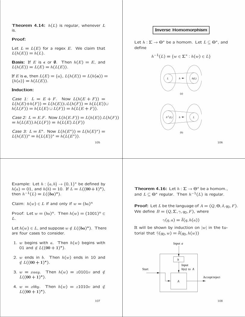
Theorem 4.14: h(L) is regular, whenever Lis.

Proof:

Let L = L(E) for a regex E. We claim thatL(h(E)) = h(L).

Basis: If E is ε or ∅. Then h(E) = E, andL(h(E)) = L(E) = h(L(E)).

If E is a, then L(E) = {a}, L(h(E)) = L(h(a)) ={h(a)} = h(L(E)).

Induction:

Case 1: L = E + F . Now L(h(E + F )) =L(h(E)+h(F )) = L(h(E))∪L(h(F )) = h(L(E))∪h(L(F )) = h(L(E) ∪ L(F )) = h(L(E + F )).

Case 2: L = E.F . Now L(h(E.F )) = L(h(E)).L(h(F ))= h(L(E)).h(L(F )) = h(L(E).L(F ))

Case 3: L = E∗. Now L(h(E∗)) = L(h(E)∗) =L(h(E))∗ = h(L(E))∗ = h(L(E∗)).

105

Inverse Homomorphism

Let h : Σ→ Θ∗ be a homom. Let L ⊆ Θ∗, and

define

h−1(L) = {w ∈ Σ∗ : h(w) ∈ L}

L h(L)

Lh-1 (L)

(a)

(b)

h

h

106

Example: Let h : {a, b} → {0,1}∗ be defined byh(a) = 01, and h(b) = 10. If L = L((00+1)∗),then h−1(L) = L((ba)∗).

Claim: h(w) ∈ L if and only if w = (ba)n

Proof: Let w = (ba)n. Then h(w) = (1001)n ∈L.

Let h(w) ∈ L, and suppose w /∈ L((ba)∗). Thereare four cases to consider.

1. w begins with a. Then h(w) begins with01 and /∈ L((00 + 1)∗).

2. w ends in b. Then h(w) ends in 10 and/∈ L((00 + 1)∗).

3. w = xaay. Then h(w) = z0101v and /∈L((00 + 1)∗).

4. w = xbby. Then h(w) = z1010v and /∈L((00 + 1)∗).

107

Theorem 4.16: Let h : Σ→ Θ∗ be a homom.,

and L ⊆ Θ∗ regular. Then h−1(L) is regular.

Proof: Let L be the language of A = (Q,Θ, δ, q0, F ).

We define B = (Q,Σ, γ, q0, F ), where

γ(q, a) = δ(q, h(a))

It will be shown by induction on |w| in the tu-

torial that γ(q0, w) = δ(q0, h(w))

h(a) AtoStart

Accept/reject

Input a

h

A

Input

108

Decision Properties

We consider the following:

1. Converting among representations for reg-

ular languages.

2. Is L = ∅?

3. Is w ∈ L?

4. Do two descriptions define the same lan-

guage?

109

From NFA’s to DFA’s

Suppose the ε-NFA has n states.

To compute ECLOSE(p) we follow at most n2

arcs.

The DFA has 2n states, for each state S and

each a ∈ Σ we compute δD(S, a) in n3 steps.

Grand total is O(n32n) steps.

If we compute δ for reachable states only, we

need to compute δD(S, a) only s times, where s

is the number of reachable states. Grand total

is O(n3s) steps.

110

From DFA to NFA

All we need to do is to put set brackets aroundthe states. Total O(n) steps.

From FA to regex

We need to compute n3 entries of size up to4n. Total is O(n34n).

The FA is allowed to be a NFA. If we firstwanted to convert the NFA to a DFA, the totaltime would be doubly exponential

From regex to FA’s We can build an expres-sion tree for the regex in n steps.

We can construct the automaton in n steps.

Eliminating ε-transitions takes O(n3) steps.

If you want a DFA, you might need an expo-nential number of steps.

111

Testing emptiness

L(A) 6= ∅ for FA A if and only if a final stateis reachable from the start state in A. TotalO(n2) steps.

Alternatively, we can inspect a regex E and tellif L(E) = ∅. We use the following method:

E = F + G. Now L(E) is empty if and only ifboth L(F ) and L(G) are empty.

E = F.G. Now L(E) is empty if and only ifeither L(F ) or L(G) is empty.

E = F ∗. Now L(E) is never empty, since ε ∈L(E).

E = ε. Now L(E) is not empty.

E = a. Now L(E) is not empty.

E = ∅. Now L(E) is empty.

112

Testing membership

To test w ∈ L(A) for DFA A, simulate A on w.

If |w| = n, this takes O(n) steps.

If A is an NFA and has s states, simulating A

on w takes O(ns2) steps.

If A is an ε-NFA and has s states, simulating

A on w takes O(ns3) steps.

If L = L(E), for regex E of length s, we first

convert E to an ε-NFA with 2s states. Then we

simulate w on this machine, in O(ns3) steps.

113

Example 4.17

Let A = (Q,Σ, δ, q0, F ) be a DFA and L(A) = M .

Let L ⊆ M be those words in w ∈ L(A) forwhich A visits every state in Q at least oncewhen accepting w.

We shall use closure properties of regular lan-guages to prove that L is regular.

Plan of the proof:

M

L

L

L

L

L

1

2

3

4

The language of automaton A

Strings of M

Inverse homomorphism

Intersection with a regular language

Add condition that first state is the start state

Difference with a regular language

Add condition that adjacent states are equal

Difference with regular languages

Add condition that all states appear on the path

Homomorphism

Delete state components, leaving the symbols

with state transitions embedded

114

• M L1

Define T = {[paq] : p, q ∈ Q, a ∈ Σ, δ(p, a) = q}

Let h : T ∗ → Σ∗ be the homom. defined by

h([paq]) = a

Let L1 = h−1(M). Since M is regular, so is L1

Example: Suppose A is given by

δ 0 1→ p q p?q q q

Then T = {[p0q], [p1p], [q0q], [q1q]}.

115

For example h−1(101) ={

[p1p][p0q][p1p],

[p1p][p0q][q1q],

[p1p][q0q][p1p],

[p1p][q0q][q1q],

[q1q][p0q][p1p],

[q1q][p0q][q1q],

[q1q][q0q][p1p],

[q1q][q0q][q1q]}

116

• L1 L2

Define

E1 =⊕

a∈Σ, δ(q0,a)=p

[q0ap]

Let

L2 = L1 ∩(L(E1).T ∗

)

Now L2 is regular and consists of those strings

in L1 starting with [qo . . .][. . .

117

• L2 L3

Define

E2 =⊕

[paq]∈T ∗, [rbs]∈T ∗, q 6=r

[paq][rbs]

Let

L3 = L2 \ T ∗.L(E2).T ∗

Now L3 is regular and consists of those strings

[q0a1p1][p1a2p2] . . . [pn−1anpn]

in T ∗ such that

a1a2 . . . an ∈ L(A)

δ(qo, a1) = p1

δ(pi, ai+1) = pi+1, i ∈ {1,2, . . . , n− 1}

pn ∈ F

118

• L3 L4

Define

Eq =⊕

[ras]∈T ∗, r 6=q, s 6=q

[ras]

Now L3 \ L(E∗q) consists of those strings in L3

that “visit” state q at least once.

Let

L4 = L3 \ L( ⊕

q∈QE∗q)

Now L4 is regular and consists of those strings

in L3 that “visit” all states q ∈ Q at least once.

119

• L4 L

We only need to get rid of the state compo-

nents in the words of L4.

We can do this by letting

L = h(L4)

Now L =

{w : δ(q0, w) ∈ F,∀q ∈ Q ∃xq, y(w = xqy ∧ δ(q0, xq) = q)}

120

Equivalence and Minimization of Automata

Let A = (Q,Σ, δ, q0, F ) be a DFA, and {p, q} ⊆ Q.

We define

p ≡ q ⇔ ∀w ∈ Σ∗ : δ(p, w) ∈ F iff δ(q, w) ∈ F

• If p ≡ q we say that p and q are equivalent

• If p 6≡ q we say that p and q are distinguish-

able

IOW (in other words) p and q are distinguish-

able iff

∃w : δ(p, w) ∈ F and δ(q, w) /∈ F, or vice versa

121

Example:

Start

0

0

1

1

0

1

0

1

10

01

011

0

A B C D

E F G H

δ(C, ε) ∈ F, δ(G, ε) /∈ F ⇒ C 6≡ G

δ(A,01) = C ∈ F, δ(G,01) = E /∈ F ⇒ A 6≡ G

122

What about A and E?

Start

0

0

1

1

0

1

0

1

10

01

011

0

A B C D

E F G H

δ(A, ε) = A /∈ F, δ(E, ε) = E /∈ F

δ(A,1) = F = δ(E,1)

Therefore δ(A,1x) = δ(E,1x) = δ(F, x)

δ(A,00) = G = δ(E,00)

δ(A,01) = C = δ(E,01)

Conclusion: A ≡ E.123

We can compute distinguishable pairs with the

following inductive table filling algorithm:

Basis: If p ∈ F and q 6∈ F , then p 6≡ q.

Induction: If ∃a ∈ Σ : δ(p, a) 6≡ δ(q, a),

then p 6≡ q.

Example:

Applying the table filling algo to DFA A:

B

C

D

E

F

G

H

A B C D E F G

x

x

x

x

x

x

x

x

x

x

x

x

x

x

x

x

x

x

x

x

x

x

x

x x

124

Theorem 4.20: If p and q are not distin-

guished by the TF-algo, then p ≡ q.

Proof: Suppose to the contrary that that there

is a bad pair {p, q}, s.t.

1. ∃w : δ(p, w) ∈ F, δ(q, w) /∈ F , or vice versa.

2. The TF-algo does not distinguish between

p and q.

Let w = a1a2 · · · an be the shortest string that

identifies a bad pair {p, q}.

Now w 6= ε since otherwise the TF-algo would

in the basis distinguish p from q. Thus n ≥ 1.

125

Consider states r = δ(p, a1) and s = δ(q, a1).

Now {r, s} cannot be a bad pair since {r, s}would be indentified by a string shorter than w.

Therefore, the TF-algo must have discovered

that r and s are distinguishable.

But then the TF-algo would distinguish p from

q in the inductive part.

Thus there are no bad pairs and the theorem

is true.

126

Testing Equivalence of Regular Languages

Let L and M be reg langs (each given in some

form).

To test if L = M

1. Convert both L and M to DFA’s.

2. Imagine the DFA that is the union of the

two DFA’s (never mind there are two start

states)

3. If TF-algo says that the two start states

are distinguishable, then L 6= M , otherwise

L = M .

127

Example:

Start

Start

0

0

1

1

0

1 0

1

1

0

A B

C D

E

We can “see” that both DFA accept

L(ε+ (0 + 1)∗0). The result of the TF-algo is

B

C

D

E

A B C D

x

x

x

x

x x

Therefore the two automata are equivalent.

128

Minimization of DFA’s

We can use the TF-algo to minimize a DFA

by merging all equivalent states. IOW, replace

each state p by p/≡.

Example: The DFA on slide 119 has equiva-

lence classes {{A,E}, {B,H}, {C}, {D,F}, {G}}.

The “union” DFA on slide 125 has equivalence

classes {{A,C,D}, {B,E}}.

Note: In order for p/≡ to be an equivalence

class, the relation ≡ has to be an equivalence

relation (reflexive, symmetric, and transitive).

129

Theorem 4.23: If p ≡ q and q ≡ r, then p ≡ r.

Proof: Suppose to the contrary that p 6≡ r.

Then ∃w such that δ(p, w) ∈ F and δ(r, w) 6∈ F ,

or vice versa.

OTH, δ(q, w) is either accpeting or not.

Case 1: δ(q, w) is accepting. Then q 6≡ r.

Case 1: δ(q, w) is not accepting. Then p 6≡ q.

The vice versa case is proved symmetrically

Therefore it must be that p ≡ r.

130

To minimize a DFA A = (Q,Σ, δ, q0, F ) con-

struct a DFA B = (Q/≡,Σ, γ, q0/≡, F/≡), where

γ(p/≡, a) = δ(p, a)/≡

In order for B to be well defined we have to

show that

If p ≡ q then δ(p, a) ≡ δ(q, a)

If δ(p, a) 6≡ δ(q, a), then the TF-algo would con-

clude p 6≡ q, so B is indeed well defined. Note

also that F/≡ contains all and only the accept-

ing states of A.

131

Example: We can minimize

Start

0

0

1

1

0

1

0

1

10

01

011

0

A B C D

E F G H

to obtain

Start

1

0

0

1

1

0

10

1

0A,E

G D,F

B,H C

132

NOTE: We cannot apply the TF-algo to NFA’s.

For example, to minimize

Start

0,1

0

1 0

A B

C

we simply remove state C.

However, A 6≡ C.

133

Why the Minimized DFA Can’t Be Beaten

Let B be the minimized DFA obtained by ap-

plying the TF-algo to DFA A.

We already know that L(A) = L(B).

What if there existed a DFA C, with

L(C) = L(B) and fewer states than B?

Then run the TF-algo on B “union” C.

Since L(B) = L(C) we have qB0 ≡ qC0 .

Also, δ(qB0 , a) ≡ δ(qC0 , a), for any a.

134

Claim: For each state p in B there is at least

one state q in C, s.t. p ≡ q.

Proof of claim: There are no inaccessible states,

so p = δ(qB0 , a1a2 · · · ak), for some string a1a2 · · · ak.

Now q = δ(qC0 , a1a2 · · · ak), and p ≡ q.

Since C has fewer states than B, there must be

two states r and s of B such that r ≡ t ≡ s, for

some state t of C. But then r ≡ s (why?)

which is a contradiction, since B was con-

structed by the TF-algo.

135

Context-Free Grammars and Languages

• We have seen that many languages cannot

be regular. Thus we need to consider larger

classes of langs.

• Contex-Free Languages (CFL’s) played a cen-

tral role natural languages since the 1950’s,

and in compilers since the 1960’s.

• Context-Free Grammars (CFG’s) are the ba-

sis of BNF-syntax.

• Today CFL’s are increasingly important for

XML and their DTD’s.

We’ll look at: CFG’s, the languages they gen-

erate, parse trees, pushdown automata, and

closure properties of CFL’s.

136

Informal example of CFG’s

Consider Lpal = {w ∈ Σ∗ : w = wR}

For example otto ∈ Lpal, madamimadam ∈ Lpal.

In Finnish language e.g. saippuakauppias ∈ Lpal(“soap-merchant”)

Let Σ = {0,1} and suppose Lpal were regular.

Let n be given by the pumping lemma. Then0n10n ∈ Lpal. In reading 0n the FA must makea loop. Omit the loop; contradiction.

Let’s define Lpal inductively:

Basis: ε,0, and 1 are palindromes.

Induction: If w is a palindrome, so are 0w0and 1w1.

Circumscription: Nothing else is a palindrome.

137

CFG’s is a formal mechanism for definitions

such as the one for Lpal.

1. P → ε

2. P → 0

3. P → 1

4. P → 0P0

5. P → 1P1

0 and 1 are terminals

P is a variable (or nonterminal, or syntactic

category)

P is in this grammar also the start symbol.

1–5 are productions (or rules)

138

Formal definition of CFG’s

A context-free grammar is a quadruple

G = (V, T, P, S)

where

V is a finite set of variables.

T is a finite set of terminals.

P is a finite set of productions of the form

A→ α, where A is a variable and α ∈ (V ∪ T )∗

S is a designated variable called the start symbol.

139

Example: Gpal = ({P}, {0,1}, A, P ), where A =

{P → ε, P → 0, P → 1, P → 0P0, P → 1P1}.

Sometimes we group productions with the same

head, e.g. A = {P → ε|0|1|0P0|1P1}.

Example: Regular expressions over {0,1} can

be defined by the grammar

Gregex = ({E}, {0,1}, A,E)

where A =

{E → 0, E → 1, E → E.E,E → E+E,E → E?, E → (E)}

140

Example: (simple) expressions in a typical proglang. Operators are + and *, and argumentsare identfiers, i.e. strings inL((a+ b)(a+ b+ 0 + 1)∗)

The expressions are defined by the grammar

G = ({E, I}, T, P,E)

where T = {+, ∗, (, ), a, b,0,1} and P is the fol-lowing set of productions:

1. E → I

2. E → E + E

3. E → E ∗ E4. E → (E)

5. I → a

6. I → b

7. I → Ia

8. I → Ib

9. I → I0

10. I → I1

141

Derivations using grammars

• Recursive inference, using productions from

body to head

• Derivations, using productions from head to

body.

Example of recursive inference:

String Lang Prod String(s) used

(i) a I 5 -(ii) b I 6 -(iii) b0 I 9 (ii)(iv) b00 I 9 (iii)(v) a E 1 (i)(vi) b00 E 1 (iv)(vii) a+ b00 E 2 (v), (vi)(viii) (a+ b00) E 4 (vii)(ix) a ∗ (a+ b00) E 3 (v), (viii)

142

• Derivations

Let G = (V, T, P, S) be a CFG, A ∈ V ,

{α, β} ⊂ (V ∪ T )∗, and A→ γ ∈ P .

Then we write

αAβ ⇒Gαγβ

or, if G is understood

αAβ ⇒ αγβ

and say that αAβ derives αγβ.

We define∗⇒ to be the reflexive and transitive

closure of ⇒, IOW:

Basis: Let α ∈ (V ∪ T )∗. Then α∗⇒ α.

Induction: If α∗⇒ β, and β ⇒ γ, then α

∗⇒ γ.

143

Example: Derivation of a ∗ (a+ b00) from E in

the grammar of slide 138:

E ⇒ E ∗ E ⇒ I ∗ E ⇒ a ∗ E ⇒ a ∗ (E)⇒

a∗(E+E)⇒ a∗(I+E)⇒ a∗(a+E)⇒ a∗(a+I)⇒

a ∗ (a+ I0)⇒ a ∗ (a+ I00)⇒ a ∗ (a+ b00)

Note: At each step we might have several rules

to choose from, e.g.

I ∗ E ⇒ a ∗ E ⇒ a ∗ (E), versus

I ∗ E ⇒ I ∗ (E)⇒ a ∗ (E).

Note: Not all choices lead to successful deriva-

tions of a particular string, for instance

E ⇒ E + E

won’t lead to a derivation of a ∗ (a+ b00).

144

Leftmost and Rightmost Derivations

Leftmost derivation⇒lm

Always replace the left-

most variable by one of its rule-bodies.

Rightmost derivation ⇒rm

Always replace the

rightmost variable by one of its rule-bodies.

Leftmost: The derivation on the previous slide.

Rightmost:

E ⇒rmE ∗ E ⇒

rm

E∗(E)⇒rmE∗(E+E)⇒

rmE∗(E+I)⇒

rmE∗(E+I0)

⇒rmE ∗(E+I00)⇒

rmE ∗(E+b00)⇒

rmE ∗(I+b00)

⇒rmE ∗ (a+ b00)⇒

rmI ∗ (a+ b00)⇒

rma ∗ (a+ b00)

We can conclude that E∗⇒rma ∗ (a+ b00)

145

The Language of a Grammar

If G(V, T, P, S) is a CFG, then the language of

G is

L(G) = {w ∈ T ∗ : S∗⇒Gw}

i.e. the set of strings over T ∗ derivable from

the start symbol.

If G is a CFG, we call L(G) a context-free lan-

guage.

Example: L(Gpal) is a context-free language.

Theorem 5.7:

L(Gpal) = {w ∈ {0,1}∗ : w = wR}

Proof: (⊇-direction.) Suppose w = wR. We

show by induction on |w| that w ∈ L(Gpal)

146

Basis: |w| = 0, or |w| = 1. Then w is ε,0,

or 1. Since P → ε, P → 0, and P → 1 are

productions, we conclude that P∗⇒G

w in all

base cases.

Induction: Suppose |w| ≥ 2. Since w = wR,

we have w = 0x0, or w = 1x1, and x = xR.

If w = 0x0 we know from the IH that P∗⇒ x.

Then

P ⇒ 0P0∗⇒ 0x0 = w

Thus w ∈ L(Gpal).

The case for w = 1x1 is similar.

147

(⊆-direction.) We assume that w ∈ L(Gpal)and must show that w = wR.

Since w ∈ L(Gpal), we have P∗⇒ w.

We do an induction of the length of∗⇒.

Basis: The derivation P∗⇒ w is done in one

step.

Then w must be ε,0, or 1, all palindromes.

Induction: Let n ≥ 1, and suppose the deriva-tion takes n+ 1 steps. Then we must have

w = 0x0∗⇐ 0P0⇐ P

or

w = 1x1∗⇐ 1P1⇐ P

where the second derivation is done in n steps.

By the IH x is a palindrome, and the inductiveproof is complete.

148

Sentential Forms

Let G = (V, T, P, S) be a CFG, and α ∈ (V ∪T )∗.If

S∗⇒ α

we say that α is a sentential form.

If S ⇒lmα we say that α is a left-sentential form,

and if S ⇒rmα we say that α is a right-sentential

form

Note: L(G) consists of those sentential forms

that are in T ∗.

149

Example: Take G from slide 138. Then E ∗ (I + E)

is a sentential form since

E ⇒ E∗E ⇒ E∗(E)⇒ E∗(E+E)⇒ E∗(I+E)

This derivation is neither leftmost, nor right-

most

Example: a ∗ E is a left-sentential form, since

E ⇒lmE ∗ E ⇒

lmI ∗ E ⇒

lma ∗ E

Example: E∗(E+E) is a right-sentential form,

since

E ⇒rmE ∗ E ⇒

rmE ∗ (E)⇒

rmE ∗ (E + E)

150

Parse Trees

• If w ∈ L(G), for some CFG, then w has a

parse tree, which tells us the (syntactic) struc-

ture of w

• w could be a program, a SQL-query, an XML-

document, etc.

• Parse trees are an alternative representation

to derivations and recursive inferences.

• There can be several parse trees for the same

string

• Ideally there should be only one parse tree

(the “true” structure) for each string, i.e. the

language should be unambiguous.

• Unfortunately, we cannot always remove the

ambiguity.

151

Constructing Parse Trees

Let G = (V, T, P, S) be a CFG. A tree is a parse

tree for G if:

1. Each interior node is labelled by a variable

in V .

2. Each leaf is labelled by a symbol in V ∪ T ∪ {ε}.Any ε-labelled leaf is the only child of its

parent.

3. If an interior node is lablelled A, and its

children (from left to right) labelled

X1, X2, . . . , Xk,

then A→ X1X2 . . . Xk ∈ P .

152

Example: In the grammar

1. E → I

2. E → E + E

3. E → E ∗ E4. E → (E)

···

the following is a parse tree:

E

E + E

I

This parse tree shows the derivation E∗⇒ I+E

153

Example: In the grammar

1. P → ε

2. P → 0

3. P → 1

4. P → 0P0

5. P → 1P1

the following is a parse tree:

P

P

P

0 0

1 1

ε

It shows the derivation of P∗⇒ 0110.

154

The Yield of a Parse Tree

The yield of a parse tree is the string of leaves

from left to right.

Important are those parse trees where:

1. The yield is a terminal string.

2. The root is labelled by the start symbol

We shall see the the set of yields of these

important parse trees is the language of the

grammar.

155

Example: Below is an important parse tree

E

E E*

I

a

E

E E

I

a

I

I

I

b

( )

+

0

0

The yield is a ∗ (a+ b00).

Compare the parse tree with the derivation on

slide 141.156

Let G = (V, T, P, S) be a CFG, and A ∈ V .We are going to show that the following areequivalent:

1. We can determine by recursive inferencethat w is in the language of A

2. A∗⇒ w

3. A∗⇒lmw, and A

∗⇒rmw

4. There is a parse tree of G with root A andyield w.

To prove the equivalences, we use the followingplan.

Recursive

treeParse

inference

Leftmostderivation

RightmostderivationDerivation

157

From Inferences to Trees

Theorem 5.12: Let G = (V, T, P, S) be a

CFG, and suppose we can show w to be in

the language of a variable A. Then there is a

parse tree for G with root A and yield w.

Proof: We do an induction of the length of

the inference.

Basis: One step. Then we must have used a

production A → w. The desired parse tree is

then

A

w

158

Induction: w is inferred in n + 1 steps. Sup-

pose the last step was based on a production

A→ X1X2 · · ·Xk,where Xi ∈ V ∪ T . We break w up as

w1w2 · · ·wk,where wi = Xi, when Xi ∈ T , and when Xi ∈ V,then wi was previously inferred being in Xi, in

at most n steps.

By the IH there are parse trees i with root Xiand yield wi. Then the following is a parse tree

for G with root A and yield w:

A

X X X

w w w

k

k

1 2

1 2 . . .

. . .

159

From trees to derivations

We’ll show how to construct a leftmost deriva-

tion from a parse tree.

Example: In the grammar of slide 6 there clearly

is a derivation

E ⇒ I ⇒ Ib⇒ ab.

Then, for any α and β there is a derivation

αEβ ⇒ αIβ ⇒ αIbβ ⇒ αabβ.

For example, suppose we have a derivation

E ⇒ E + E ⇒ E + (E).

The we can choose α = E + ( and β =) and

continue the derivation as

E + (E)⇒ E + (I)⇒ E + (Ib)⇒ E + (ab).

This is why CFG’s are called context-free.

160

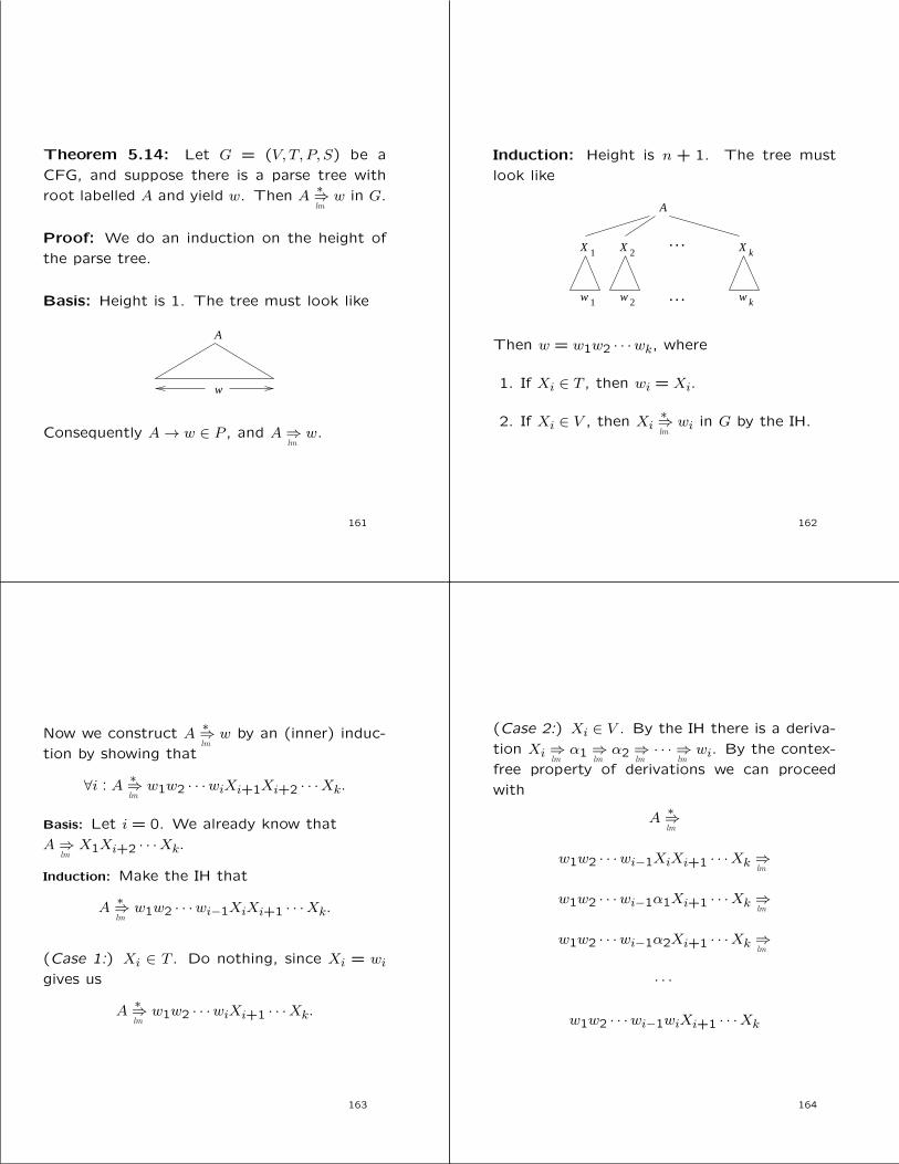
Theorem 5.14: Let G = (V, T, P, S) be a

CFG, and suppose there is a parse tree with

root labelled A and yield w. Then A∗⇒lmw in G.

Proof: We do an induction on the height of

the parse tree.

Basis: Height is 1. The tree must look like

A

w

Consequently A→ w ∈ P , and A⇒lmw.

161

Induction: Height is n + 1. The tree must

look like

A

X X X

w w w

k

k

1 2

1 2 . . .

. . .

Then w = w1w2 · · ·wk, where

1. If Xi ∈ T , then wi = Xi.

2. If Xi ∈ V , then Xi∗⇒lmwi in G by the IH.

162

Now we construct A∗⇒lmw by an (inner) induc-

tion by showing that

∀i : A∗⇒lmw1w2 · · ·wiXi+1Xi+2 · · ·Xk.

Basis: Let i = 0. We already know that

A⇒lmX1Xi+2 · · ·Xk.

Induction: Make the IH that

A∗⇒lmw1w2 · · ·wi−1XiXi+1 · · ·Xk.

(Case 1:) Xi ∈ T . Do nothing, since Xi = wigives us

A∗⇒lmw1w2 · · ·wiXi+1 · · ·Xk.

163

(Case 2:) Xi ∈ V . By the IH there is a deriva-

tion Xi ⇒lmα1 ⇒

lmα2 ⇒

lm· · · ⇒

lmwi. By the contex-

free property of derivations we can proceed

with

A∗⇒lm

w1w2 · · ·wi−1XiXi+1 · · ·Xk ⇒lm

w1w2 · · ·wi−1α1Xi+1 · · ·Xk ⇒lm

w1w2 · · ·wi−1α2Xi+1 · · ·Xk ⇒lm

· · ·

w1w2 · · ·wi−1wiXi+1 · · ·Xk

164

Example: Let’s construct the leftmost deriva-tion for the tree

E

E E*

I

a

E

E E

I

a

I

I

I

b

( )

+

0

0

Suppose we have inductively constructed theleftmost derivation

E ⇒lmI ⇒

lma

corresponding to the leftmost subtree, and theleftmost derivation

E ⇒lm

(E)⇒lm

(E + E)⇒lm

(I + E)⇒lm

(a+ E)⇒lm

(a+ I)⇒lm

(a+ I0)⇒lm

(a+ I00)⇒lm

(a+ b00)

corresponding to the righmost subtree.

165

For the derivation corresponding to the whole

tree we start with E ⇒lmE ∗ E and expand the

first E with the first derivation and the second

E with the second derivation:

E ⇒lm

E ∗ E ⇒lm

I ∗ E ⇒lm

a ∗ E ⇒lm

a ∗ (E)⇒lm

a ∗ (E + E)⇒lm

a ∗ (I + E)⇒lm

a ∗ (a+ E)⇒lm

a ∗ (a+ I)⇒lm

a ∗ (a+ I0)⇒lm

a ∗ (a+ I00)⇒lm

a ∗ (a+ b00)

166

From Derivations to Recursive Inferences

Observation: Suppose that A⇒ X1X2 · · ·Xk∗⇒ w.

Then w = w1w2 · · ·wk, where Xi∗⇒ wi

The factor wi can be extracted from A∗⇒ w by

looking at the expansion of Xi only.

Example: E ⇒ a ∗ b+ a, and

E ⇒ E︸︷︷︸X1

∗︸︷︷︸X2

E︸︷︷︸X3

+︸︷︷︸X4

E︸︷︷︸X5

We have

E ⇒ E ∗ E ⇒ E ∗ E + E ⇒ I ∗ E + E ⇒ I ∗ I + E ⇒I ∗ I + I ⇒ a ∗ I + I ⇒ a ∗ b+ I ⇒ a ∗ b+ a

By looking at the expansion of X3 = E only,we can extract

E ⇒ I ⇒ b.

167

Theorem 5.18: Let G = (V, T, P, S) be a

CFG. Suppose A∗⇒Gw, and that w is a string

of terminals. Then we can infer that w is in

the language of variable A.

Proof: We do an induction on the length of

the derivation A∗⇒Gw.

Basis: One step. If A ⇒Gw there must be a

production A→ w in P . The we can infer that

w is in the language of A.

168

Induction: Suppose A∗⇒G

w in n + 1 steps.

Write the derivation as

A⇒GX1X2 · · ·Xk

∗⇒Gw

The as noted on the previous slide we can

break w as w1w2 · · ·wk where Xi∗⇒Gwi. Fur-

thermore, Xi∗⇒Gwi can use at most n steps.

Now we have a production A → X1X2 · · ·Xk,

and we know by the IH that we can infer wi to

be in the language of Xi.

Therefore we can infer w1w2 · · ·wk to be in the

language of A.

169

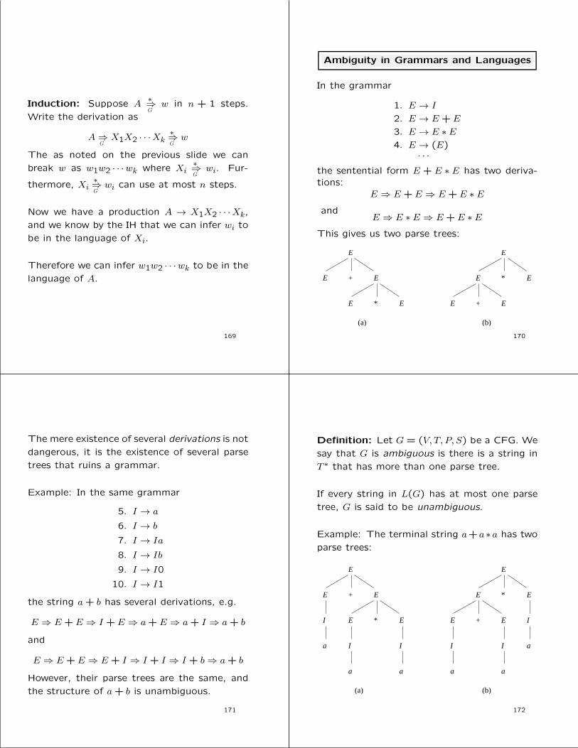
Ambiguity in Grammars and Languages

In the grammar

1. E → I

2. E → E + E

3. E → E ∗ E4. E → (E)

· · ·the sentential form E + E ∗ E has two deriva-tions:

E ⇒ E + E ⇒ E + E ∗ Eand

E ⇒ E ∗ E ⇒ E + E ∗ EThis gives us two parse trees:

+

*

*

+

E

E E

E E

E

E E

EE

(a) (b)

170

The mere existence of several derivations is not

dangerous, it is the existence of several parse

trees that ruins a grammar.

Example: In the same grammar

5. I → a

6. I → b

7. I → Ia

8. I → Ib

9. I → I0

10. I → I1

the string a+ b has several derivations, e.g.

E ⇒ E + E ⇒ I + E ⇒ a+ E ⇒ a+ I ⇒ a+ b

and

E ⇒ E + E ⇒ E + I ⇒ I + I ⇒ I + b⇒ a+ b

However, their parse trees are the same, and

the structure of a+ b is unambiguous.

171

Definition: Let G = (V, T, P, S) be a CFG. We

say that G is ambiguous is there is a string in

T ∗ that has more than one parse tree.

If every string in L(G) has at most one parse

tree, G is said to be unambiguous.

Example: The terminal string a+a∗a has two

parse trees:

I

a I

a

I

a

I

a

I

a

I

a

+

*

*

+

E

E E

E E

E

E E

EE

(a) (b)

172

Removing Ambiguity From Grammars

Good news: Sometimes we can remove ambi-guity “by hand”

Bad news: There is no algorithm to do it

More bad news: Some CFL’s have only am-biguous CFG’s

We are studying the grammar

E → I | E + E | E ∗ E | (E)

I → a | b | Ia | Ib | I0 | I1

There are two problems:

1. There is no precedence between * and +

2. There is no grouping of sequences of op-erators, e.g. is E + E + E meant to beE + (E + E) or (E + E) + E.

173

Solution: We introduce more variables, eachrepresenting expressions of same “binding strength.”

1. A factor is an expresson that cannot bebroken apart by an adjacent * or +. Ourfactors are

(a) Identifiers

(b) A parenthesized expression.

2. A term is an expresson that cannot be bro-ken by +. For instance a ∗ b can be brokenby a1∗ or ∗a1. It cannot be broken by +,since e.g. a1 +a∗ b is (by precedence rules)same as a1 + (a ∗ b), and a ∗ b+ a1 is sameas (a ∗ b) + a1.

3. The rest are expressions, i.e. they can bebroken apart with * or +.

174

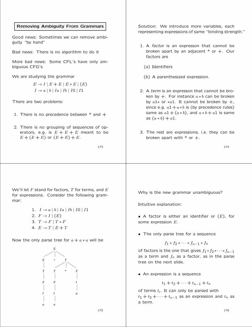
We’ll let F stand for factors, T for terms, and Efor expressions. Consider the following gram-mar:

1. I → a | b | Ia | Ib | I0 | I1

2. F → I | (E)

3. T → F | T ∗ F4. E → T | E + T

Now the only parse tree for a+ a ∗ a will be

F

I

a

F

I

a

T

F

I

a

T

+

*

E

E T

175

Why is the new grammar unambiguous?

Intuitive explanation:

• A factor is either an identifier or (E), for

some expression E.

• The only parse tree for a sequence

f1 ∗ f2 ∗ · · · ∗ fn−1 ∗ fnof factors is the one that gives f1∗f2∗· · ·∗fn−1

as a term and fn as a factor, as in the parse

tree on the next slide.

• An expression is a sequence

t1 + t2 + · · ·+ tn−1 + tn

of terms ti. It can only be parsed with

t1 + t2 + · · ·+ tn−1 as an expression and tn as

a term.

176

*

*

*

T

T F

T F

T

T F

F

.. .

177

Leftmost derivations and Ambiguity

The two parse trees for a+ a ∗ a

I

a I

a

I

a

I

a

I

a

I

a

+

*

*

+

E

E E

E E

E

E E

EE

(a) (b)

give rise to two derivations:

E ⇒lmE + E ⇒

lmI + E ⇒

lma+ E ⇒

lma+ E ∗ E

⇒lma+ I ∗ E ⇒

lma+ a ∗ E ⇒

lma+ a ∗ I ⇒

lma+ a ∗ a

and

E ⇒lmE ∗E ⇒

lmE+E ∗E ⇒

lmI +E ∗E ⇒

lma+E ∗E

⇒lma+ I ∗ E ⇒

lma+ a ∗ E ⇒

lma+ a ∗ I ⇒

lma+ a ∗ a

178

In General:

• One parse tree, but many derivations

• Many leftmost derivation implies many parse

trees.

• Many rightmost derivation implies many parse

trees.

Theorem 5.29: For any CFG G, a terminal

string w has two distinct parse trees if and only

if w has two distinct leftmost derivations from

the start symbol.

179

Sketch of Proof: (Only If.) If the two parse

trees differ, they have a node a which dif-

ferent productions, say A → X1X2 · · ·Xk and

B → Y1Y2 · · ·Ym. The corresponding leftmost

derivations will use derivations based on these

two different productions and will thus be dis-

tinct.

(If.) Let’s look at how we construct a parse

tree from a leftmost derivation. It should now

be clear that two distinct derivations gives rise

to two different parse trees.

180

Inherent Ambiguity

A CFL L is inherently ambiguous if all gram-

mars for L are ambiguous.

Example: Consider L =

{anbncmdm : n ≥ 1,m ≥ 1}∪{anbmcmdn : n ≥ 1,m ≥ 1}.

A grammar for L is

S → AB | CA→ aAb | abB → cBd | cdC → aCd | aDdD → bDc | bc

181

Let’s look at parsing the string aabbccdd.

S

A B

a A b

a b

c B d

c d

(a)

S

C

a C d

a D d

b D c

b c

(b)

182

From this we see that there are two leftmost

derivations:

S ⇒lmAB ⇒

lmaAbB ⇒

lmaabbB ⇒

lmaabbcBd⇒

lmaabbccdd

and

S ⇒lmC ⇒

lmaCd⇒

lmaaDdd⇒

lmaabDcdd⇒

lmaabbccdd

It can be shown that every grammar for L be-

haves like the one above. The language L is

inherently ambiguous.

183

Pushdown Automata

A pushdown automata (PDA) is essentially an

ε-NFA with a stack.

On a transition the PDA:

1. Consumes an input symbol.

2. Goes to a new state (or stays in the old).

3. Replaces the top of the stack by any string

(does nothing, pops the stack, or pushes a

string onto the stack)

Stack

Finitestatecontrol

Input Accept/reject

184

Example: Let’s consider

Lwwr = {wwR : w ∈ {0,1}∗},with “grammar” P → 0P0, P → 1P1, P → ε.

A PDA for Lwwr has tree states, and operates

as follows:

1. Guess that you are reading w. Stay in

state 0, and push the input symbol onto

the stack.

2. Guess that you’re in the middle of wwR.

Go spontanteously to state 1.

3. You’re now reading the head of wR. Com-

pare it to the top of the stack. If they

match, pop the stack, and remain in state 1.

If they don’t match, go to sleep.

4. If the stack is empty, go to state 2 and

accept.

185

The PDA for Lwwr as a transition diagram:

1 ,

ε, Z 0 Z 0 Z 0 Z 0ε , /

1 , 0 / 1 00 , 1 / 0 10 , 0 / 0 0

Z 0 Z 01 ,0 , Z 0 Z 0/ 0

ε, 0 / 0ε, 1 / 1

0 , 0 / ε

q q q0 1 2

1 / 1 1

/

Start

1 , 1 / ε

/ 1

186

PDA formally

A PDA is a seven-tuple:

P = (Q,Σ,Γ, δ, q0, Z0, F ),

where

• Q is a finite set of states,

• Σ is a finite input alphabet,

• Γ is a finite stack alphabet,

• δ : Q×Σ∪{ε}×Γ→ 2Q×Γ∗ is the transition

function,

• q0 is the start state,

• Z0 ∈ Γ is the start symbol for the stack,

and

• F ⊆ Q is the set of accepting states.

187

Example: The PDA

1 ,

ε, Z 0 Z 0 Z 0 Z 0ε , /

1 , 0 / 1 00 , 1 / 0 10 , 0 / 0 0

Z 0 Z 01 ,0 , Z 0 Z 0/ 0

ε, 0 / 0ε, 1 / 1

0 , 0 / ε

q q q0 1 2

1 / 1 1

/

Start

1 , 1 / ε

/ 1

is actually the seven-tuple

P = ({q0, q1, q2}, {0,1}, {0,1, Z0}, δ, q0, Z0, {q2}),where δ is given by the following table (set

brackets missing):

0, Z0 1, Z0 0,0 0,1 1,0 1,1 ε, Z0 ε,0 ε,1

→ q0 q0,0Z0 q0,1Z0 q0,00 q0,01 q0,10 q0,11 q1, Z0 q1,0 q1,1

q1 q1, ε q1, ε q2, Z0

?q2

188

Instantaneous Descriptions

A PDA goes from configuration to configura-

tion when consuming input.

To reason about PDA computation, we use

instantaneous descriptions of the PDA. An ID

is a triple

(q, w, γ)

where q is the state, w the remaining input,

and γ the stack contents.

Let P = (Q,Σ,Γ, δ, q0, Z0, F ) be a PDA. Then

∀w ∈ Σ∗, β ∈ Γ∗ :

(p, α) ∈ δ(q, a,X)⇒ (q, aw,Xβ) ` (p, w, αβ).

We define∗

to be the reflexive-transitive clo-

sure of `.

189

Example: On input 1111 the PDA

1 ,

ε, Z 0 Z 0 Z 0 Z 0ε , /

1 , 0 / 1 00 , 1 / 0 10 , 0 / 0 0

Z 0 Z 01 ,0 , Z 0 Z 0/ 0

ε, 0 / 0ε, 1 / 1

0 , 0 / ε

q q q0 1 2

1 / 1 1

/

Start

1 , 1 / ε

/ 1

has the following computation sequences:

190

)0Z

)0Z

)0Z

)0Z

)0Z

)0Z

)0Z

)0Z

q2( ,

q2( ,

q2( ,

)0Z

)0Z

)0Z

)0Z

)0Z)0Z

)0Z

)0Zq1

q0

q0

q0

q0

q0

q1

q1

q1

q1

q1

q1

q1

q1

1111, 0Z )

111, 1

11, 11

1, 111

ε , 1111

1111,

111, 1

11, 11

1, 111

1111,

11,

11,

1, 1

ε ε ,, 11

ε ,

,(

,(

,(

,(

ε , 1111( ,

,(

( ,

( ,

( ,

( ,

( ,

( ,

( ,

( ,

191

The following properties hold:

1. If an ID sequence is a legal computation for

a PDA, then so is the sequence obtained

by adding an additional string at the end

of component number two.

2. If an ID sequence is a legal computation for

a PDA, then so is the sequence obtained by

adding an additional string at the bottom

of component number three.

3. If an ID sequence is a legal computation

for a PDA, and some tail of the input is

not consumed, then removing this tail from

all ID’s result in a legal computation se-

quence.

192

Theorem 6.5: ∀w ∈ Σ∗, β ∈ Γ∗ :

(q, x, α)∗

(p, y, β)⇒ (q, xw, αγ)∗

(p, yw, βγ).

Proof: Induction on the length of the sequence

to the left.

Note: If γ = ε we have proerty 1, and if w = ε

we have property 2.

Note2: The reverse of the theorem is false.

For property 3 we have

Theorem 6.6:

(q, xw, α)∗

(p, yw, β)⇒ (q, x, α)∗

(p, y, β).

193

Acceptance by final state

Let P = (Q,Σ,Γ, δ, q0, Z0, F ) be a PDA. The

language accepted by P by final state is

L(P ) = {w : (q0, w, Z0)∗

(q, ε, α), q ∈ F}.

Example: The PDA on slide 183 accepts ex-

actly Lwwr.

Let P be the machine. We prove that L(P ) =

Lwwr.

(⊇-direction.) Let x ∈ Lwwr. Then x = wwR,

and the following is a legal computation se-

quence

(q0, wwR, Z0)

∗(q0, w

R, wRZ0) ` (q1, wR, wRZ0)

∗

(q1, ε, Z0) ` (q2, ε, Z0).

194

(⊆-direction.)

Observe that the only way the PDA can enter

q2 is if it is in state q1 with an empty stack.

Thus it is sufficient to show that if (q0, x, Z0)∗

(q1, ε, Z0) then x = wwR, for some word w.

We’ll show by induction on |x| that

(q0, x, α)∗

(q1, ε, α) ⇒ x = wwR.

Basis: If x = ε then x is a palindrome.

Induction: Suppose x = a1a2 . . . an, where n > 0,

and the IH holds for shorter strings.

Ther are two moves for the PDA from ID (q0, x, α):

195

Move 1: The spontaneous (q0, x, α) ` (q1, x, α).

Now (q1, x, α)∗

(q1, ε, β) implies that |β| < |α|,which implies β 6= α.

Move 2: Loop and push (q0, a1a2 . . . an, α) `(q0, a2 . . . an, a1α).

In this case there is a sequence

(q0, a1a2 . . . an, α) ` (q0, a2 . . . an, a1α) ` . . . `(q1, an, a1α) ` (q1, ε, α).

Thus a1 = an and

(q0, a2 . . . an, a1α)∗

(q1, an, a1α).

By Theorem 6.6 we can remove an. Therefore

(q0, a2 . . . an−1, a1α)∗

(q1, ε, a1α).

Then, by the IH a2 . . . an−1 = yyR. Then x =

a1yyRan is a palindrome.

196

Acceptance by Empty Stack

Let P = (Q,Σ,Γ, δ, q0, Z0, F ) be a PDA. The

language accepted by P by empty stack is

N(P ) = {w : (q0, w, Z0)∗

(q, ε, ε)}.Note: q can be any state.

Question: How to modify the palindrome-PDA

to accept by empty stack?

197

From Empty Stack to Final State

Theorem 6.9: If L = N(PN) for some PDAPN = (Q,Σ,Γ, δN , q0, Z0), then ∃ PDA PF , suchthat L = L(PF ).

Proof: Let

PF = (Q ∪ {p0, pf},Σ,Γ ∪ {X0}, δF , p0, X0, {pf})where δF (p0, ε,X0) = {(q0, Z0X0)}, and for allq ∈ Q, a ∈ Σ∪{ε}, Y ∈ Γ : δF (q, a, Y ) = δN(q, a, Y ),and in addition (pf , ε) ∈ δF (q, ε,X0).

X 0 Z 0X 0ε,

ε, X 0 / ε

ε, X 0 / ε

ε, X 0 / ε

ε, X 0 / ε

q/

PN

Startp0 0 pf

198

We have to show that L(PF ) = N(PN).

(⊇direction.) Let w ∈ N(PN). Then

(q0, w, Z0)∗N

(q, ε, ε),

for some q. From Theorem 6.5 we get

(q0, w, Z0X0)∗N

(q, ε,X0).

Since δN ⊂ δF we have

(q0, w, Z0X0)∗F

(q, ε,X0).

We conclude that

(p0, w,X0)F

(q0, w, Z0X0)∗F

(q, ε,X0)F

(pf , ε, ε).

(⊆direction.) By inspecting the diagram.

199

Let’s design PN for for cathing errors in strings

meant to be in the if-else-grammar G

S → ε|SS|iS|iSe.Here e.g. {ieie, iie, iiee} ⊆ G, and e.g. {ei, ieeii} ∩G = ∅.The diagram for PN is

Startq

i, Z/ZZe, Z/ ε

Formally,

PN = ({q}, {i, e}, {Z}, δN , q, Z),

where δN(q, i, Z) = {(q, ZZ)},and δN(q, e, Z) = {(q, ε)}.

200

From PN we can construct

PF = ({p, q, r}, {i, e}, {Z,X0}, δF , p,X0, {r}),where

δF (p, ε,X0) = {(q, ZX0)},δF (q, i, Z) = δN(q, i, Z) = {(q, ZZ)},δF (q, e, Z) = δN(q, e, Z) = {(q, ε)}, and

δF (q, ε,X0) = {(r, ε)}

The diagram for PF is

ε, X 0/ZX 0 ε, X 0 / εq

i, Z/ZZe, Z/ ε

Start

p r

201

From Final State to Empty Stack

Theorem 6.11: Let L = L(PF ), for some

PDA PF = (Q,Σ,Γ, δF , q0, Z0, F ). Then ∃ PDA

PN , such that L = N(PN).

Proof: Let

PN = (Q ∪ {p0, p},Σ,Γ ∪ {X0}, δN , p0, X0)

where δN(p0, ε,X0) = {(q0, Z0X0)}, δN(p, ε, Y )

= {(p, ε)}, for Y ∈ Γ∪{X0}, and for all q ∈ Q,

a ∈ Σ ∪ {ε}, Y ∈ Γ : δN(q, a, Y ) = δF (q, a, Y ),

and in addition ∀q ∈ F , and Y ∈ Γ ∪ {X0} :

(p, ε) ∈ δN(q, ε, Y ).

ε, any/ ε ε, any/ ε

ε, any/ ε

X 0 Z 0ε, / X 0 pPFStart

p q0 0

202

We have to show that N(PN) = L(PF ).

(⊆-direction.) By inspecting the diagram.

(⊇-direction.) Let w ∈ L(PF ). Then

(q0, w, Z0)∗F

(q, ε, α),

for some q ∈ F, α ∈ Γ∗. Since δF ⊂ δN , and

Theorem 6.5 says that X0 can be slid under

the stack, we get

(q0, w, Z0X0)∗N

(q, ε, αX0).

Then PN can compute:

(p0, w,X0)N

(q0, w, Z0X0)∗N

(q, ε, αX0)∗N

(p, ε, ε).

203

Equivalence of PDA’s and CFG’s

A language is

generated by a CFG

if and only if it is

accepted by a PDA by empty stack

if and only if it is

accepted by a PDA by final state

PDA byempty stack

PDA byfinal stateGrammar

We already know how to go between null stack

and final state.

204

From CFG’s to PDA’s

Given G, we construct a PDA that simulates∗⇒lm

.

We write left-sentential forms as

xAα

where A is the leftmost variable in the form.

For instance,

(a+︸ ︷︷ ︸x

E︸︷︷︸A

)︸︷︷︸α︸ ︷︷ ︸

tail

Let xAα⇒lmxβα. This corresponds to the PDA

first having consumed x and having Aα on the

stack, and then on ε it pops A and pushes β.

More fomally, let y, s.t. w = xy. Then the PDA

goes non-deterministically from configuration

(q, y, Aα) to configuration (q, y, βα).

205

At (q, y, βα) the PDA behaves as before, un-

less there are terminals in the prefix of β. In

that case, the PDA pops them, provided it can

consume matching input.

If all guesses are right, the PDA ends up with

empty stack and input.

Formally, let G = (V, T,Q, S) be a CFG. Define

PG as

({q}, T, V ∪ T, δ, q, S),

where

δ(q, ε, A) = {(q, β) : A→ β ∈ Q},for A ∈ V , and

δ(q, a, a) = {(q, ε)},for a ∈ T .

Example: On blackboard in class.

206

Theorem 6.13: N(PG) = L(G).

Proof:

(⊇-direction.) Let w ∈ L(G). Then

S = γ1 ⇒lmγ2 ⇒

lm· · · ⇒

lmγn = w

Let γi = xiαi. We show by induction on i that

if

S∗⇒lmγi,

then

(q, w, S)∗

(q, yi, αi),

where w = xiyi.

207

Basis: For i = 1, γ1 = S. Thus x1 = ε, andy1 = w. Clearly (q, w, S)

∗(q, w, S).

Induction: IH is (q, w, S)∗

(q, yi, αi). We haveto show that

(q, yi, αi) ` (q, yi+1, αi+1)

Now αi begins with a variable A, and we havethe form

xiAχ︸ ︷︷ ︸γi

⇒lmxi+1βχ︸ ︷︷ ︸γi+1

By IH Aχ is on the stack, and yi is unconsumed.From the construction of PG is follows that wecan make the move

(q, yi, χ) ` (q, yi, βχ).

If β has a prefix of terminals, we can pop themwith matching terminals in a prefix of yi, end-ing up in configuration (q, yi+1, αi+1), whereαi+1 = βχ, which is the tail of the sententialxiβχ = γi+1.

Finally, since γn = w, we have αn = ε, and yn =ε, and thus (q, w, S)

∗(q, ε, ε), i.e. w ∈ N(PG)

208

(⊆-direction.) We shall show by an induction

on the length of∗, that

(♣) If (q, x,A)∗

(q, ε, ε), then A∗⇒ x.

Basis: Length 1. Then it must be that A→ ε

is in G, and we have (q, ε) ∈ δ(q, ε, A). Thus

A∗⇒ ε.

Induction: Length is n > 1, and the IH holds

for lengths < n.

Since A is a variable, we must have

(q, x,A) ` (q, x, Y1Y2 · · ·Yk) ` · · · ` (q, ε, ε)

where A→ Y1Y2 · · ·Yk is in G.

209

We can now write x as x1x2 · · ·xn, according

to the figure below, where Y1 = B, Y2 = a, and

Y3 = C.

B

a

C

xx x1 2 3

210

Now we can conclude that

(q, xixi+1 · · ·xk, Yi)∗

(q, xi+1 · · ·xk, ε)is less than n steps, for all i ∈ {1, . . . , k}. If Yiis a variable we have by the IH and Theorem

6.6 that

Yi∗⇒ xi

If Yi is a terminal, we have |xi| = 1, and Yi = xi.

Thus Yi∗⇒ xi by the reflexivity of

∗⇒.

The claim of the theorem now follows by choos-

ing A = S, and x = w. Suppose w ∈ N(P ).

Then (q, w, S)∗

(q, ε, ε), and by (♣), we have

S∗⇒ w, meaning w ∈ L(G).

211

From PDA’s to CFG’s

Let’s look at how a PDA can consume x =

x1x2 . . . xk and empty the stack.

Y

Y

Y

p

p

p

p

k

k

k-

1

21

0

1

..

.

x x x1 2 k

We shall define a grammar with variables of the

form [pi−1Yipi] representing going from pi−1 to

pi with net effect of popping Yi.

212

Formally, let P = (Q,Σ,Γ, δ, q0, Z0) be a PDA.

Define G = (V,Σ, R, S), where

V = {[pXq] : {p, q} ⊆ Q,X ∈ Γ} ∪ {S}R = {S → [q0Z0p] : p ∈ Q}∪

{[qXrk]→ a[rY1r1] · · · [rk−1Ykrk] :

a ∈ Σ ∪ {ε},{r1, . . . , rk} ⊆ Q,(r, Y1Y2 · · ·Yk) ∈ δ(q, a,X)}

213

Example: Let’s convert

Startq

i, Z/ZZe, Z/ ε

PN = ({q}, {i, e}, {Z}, δN , q, Z),

where δN(q, i, Z) = {(q, ZZ)},and δN(q, e, Z) = {(q, ε)} to a grammar

G = (V, {i, e}, R, S),

where V = {[qZq], S}, and

R={S → [qZq], [qZq]→ i[qZq][qZq], [qZq]→ e}.

If we replace [qZq] by A we get the productions

S → A and A→ iAA|e.

214

Example: Let P = ({p, q}, {0,1}, {X,Z0}, δ, q, Z0),

where δ is given by

1. δ(q,1, Z0) = {(q,XZ0)}

2. δ(q,1, X) = {(q,XX)}

3. δ(q,0, X) = {(p,X)}

4. δ(q, ε,X) = {(q, ε)}

5. δ(p,1, X) = {(p, ε)}

6. δ(p,0, Z0) = {(q, Z0)}

to a CFG.

215

We get G = (V, {0,1}, R, S), where

V = {[pXp], [pXq], [pZ0p], [pZ0q], S}and the productions in R are

S → [qZ0q]|[qZ0p]

From rule (1):

[qZ0q]→ 1[qXq][qZ0q]

[qZ0q]→ 1[qXp][pZ0q]

[qZ0p]→ 1[qXq][qZ0p]

[qZ0p]→ 1[qXp][pZ0p]

From rule (2):

[qXq]→ 1[qXq][qXq]

[qXq]→ 1[qXp][pXq]

[qXp]→ 1[qXq][qXp]

[qXp]→ 1[qXp][pXp]

216

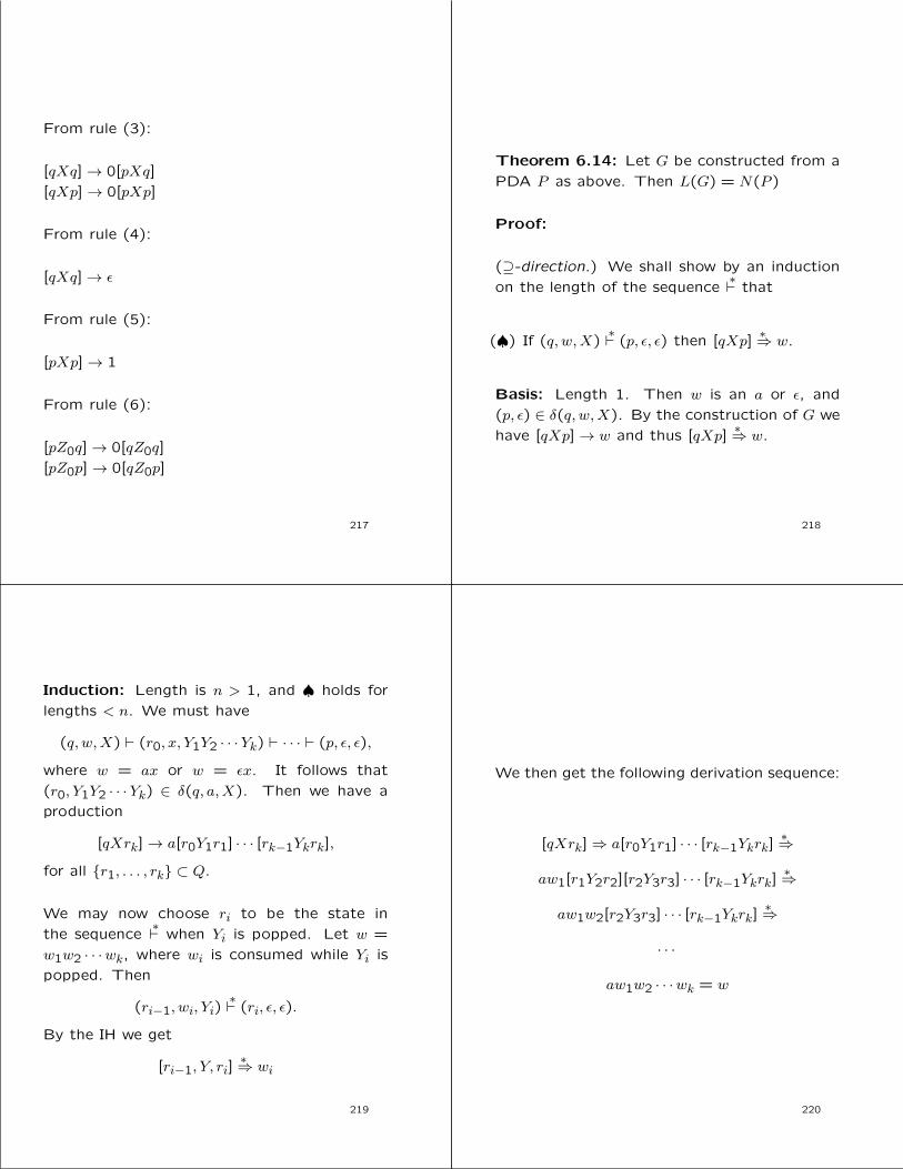
From rule (3):

[qXq]→ 0[pXq]

[qXp]→ 0[pXp]

From rule (4):

[qXq]→ ε

From rule (5):

[pXp]→ 1

From rule (6):

[pZ0q]→ 0[qZ0q]

[pZ0p]→ 0[qZ0p]

217

Theorem 6.14: Let G be constructed from a

PDA P as above. Then L(G) = N(P )

Proof:

(⊇-direction.) We shall show by an induction

on the length of the sequence∗

that

(♠) If (q, w,X)∗

(p, ε, ε) then [qXp]∗⇒ w.

Basis: Length 1. Then w is an a or ε, and

(p, ε) ∈ δ(q, w,X). By the construction of G we

have [qXp]→ w and thus [qXp]∗⇒ w.

218

Induction: Length is n > 1, and ♠ holds for

lengths < n. We must have

(q, w,X) ` (r0, x, Y1Y2 · · ·Yk) ` · · · ` (p, ε, ε),

where w = ax or w = εx. It follows that

(r0, Y1Y2 · · ·Yk) ∈ δ(q, a,X). Then we have a

production

[qXrk]→ a[r0Y1r1] · · · [rk−1Ykrk],

for all {r1, . . . , rk} ⊂ Q.

We may now choose ri to be the state in

the sequence∗

when Yi is popped. Let w =

w1w2 · · ·wk, where wi is consumed while Yi is

popped. Then

(ri−1, wi, Yi)∗

(ri, ε, ε).

By the IH we get

[ri−1, Y, ri]∗⇒ wi

219

We then get the following derivation sequence:

[qXrk]⇒ a[r0Y1r1] · · · [rk−1Ykrk]∗⇒

aw1[r1Y2r2][r2Y3r3] · · · [rk−1Ykrk]∗⇒

aw1w2[r2Y3r3] · · · [rk−1Ykrk]∗⇒

· · ·

aw1w2 · · ·wk = w

220

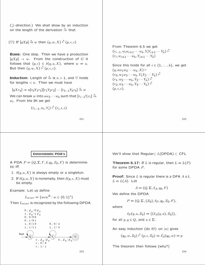
(⊇-direction.) We shall show by an induction

on the length of the derivation∗⇒ that

(♥) If [qXp]∗⇒ w then (q, w,X)

∗(p, ε, ε)

Basis: One step. Then we have a production

[qXp] → w. From the construction of G it

follows that (p, ε) ∈ δ(q, a,X), where w = a.

But then (q, w,X)∗

(p, ε, ε).

Induction: Length of∗⇒ is n > 1, and ♥ holds

for lengths < n. Then we must have

[qXrk]⇒ a[r0Y1r1][r1Y2r2] · · · [rk−1Ykrk]∗⇒ w

We can break w into aw2 · · ·wk such that [ri−1Yiri]∗⇒

wi. From the IH we get

(ri−1, wi, Yi)∗

(ri, ε, ε)

221

From Theorem 6.5 we get

(ri−1, wiwi+1 · · ·wk, YiYi+1 · · ·Yk)∗

(ri, wi+1 · · ·wk, Yi+1 · · ·Yk)

Since this holds for all i ∈ {1, . . . , k}, we get

(q, aw1w2 · · ·wk, X) `(r0, w1w2 · · ·wk, Y1Y2 · · ·Yk)

∗

(r1, w2 · · ·wk, Y2 · · ·Yk)∗

(r2, w3 · · ·wk, Y3 · · ·Yk)∗

(p, ε, ε).

222

Deterministic PDA’s

A PDA P = (Q,Σ,Γ, δ, q0, Z0, F ) is determinis-tic iff

1. δ(q, a,X) is always empty or a singleton.

2. If δ(q, a,X) is nonempty, then δ(q, ε,X) mustbe empty.

Example: Let us define

Lwcwr = {wcwR : w ∈ {0,1}∗}Then Lwcwr is recognized by the following DPDA

1 ,

Z 0 Z 0 Z 0 Z 0ε , /

1 , 0 / 1 00 , 1 / 0 10 , 0 / 0 0

Z 0 Z 01 ,0 , Z 0 Z 0/ 0

0 , 0 / ε

q q q0 1 2

1 / 1 1

/

Start

1 , 1 / ε

/ 1

,0 / 01 / 1,

,ccc

223

We’ll show that Regular⊂ L(DPDA) ⊂ CFL

Theorem 6.17: If L is regular, then L = L(P )

for some DPDA P .

Proof: Since L is regular there is a DFA A s.t.

L = L(A). Let

A = (Q,Σ, δA, q0, F )

We define the DPDA

P = (Q,Σ, {Z0}, δP , q0, Z0, F ),

where

δP (q, a, Z0) = {(δA(q, a), Z0)},for all p, q ∈ Q, and a ∈ Σ.

An easy induction (do it!) on |w| gives

(q0, w, Z0)∗

(p, ε, Z0)⇔ δA(q0, w) = p

The theorem then follows (why?)

224

What about DPDA’s that accept by null stack?

They can recognize only CFL’s with the prefix

property.

A language L has the prefix property if there

are no two distinct strings in L, such that one

is a prefix of the other.

Example: Lwcwr has the prefix property.

Example: {0}∗ does not have the prefix prop-

erty.

Theorem 6.19: L is N(P ) for some DPDA P

if and only if L has the prefix property and L

is L(P ′) for some DPDA P ′.

Proof: Homework

225

• We have seen that Regular⊆ L(DPDA).

• Lwcwr ∈ L(DPDA)\ Regular

• Are there languages in CFL\L(DPDA).

Yes, for example Lwwr.

• What about DPDA’s and Ambiguous Gram-mars?

Lwwr has unamb. grammar S → 0S0|1S1|εbut is not L(DPDA).

For the converse we have

Theorem 6.20: If L = N(P ) for some DPDAP , then L has an unambiguous CFG.

Proof: By inspecting the proof of Theorem6.14 we see that if the construction is appliedto a DPDA the result is a CFG with uniqueleftmost derivations.

226

Theorem 6.20 can actually be strengthen asfollows

Theorem 6.21: If L = L(P ) for some DPDAP , then L has an unambiguous CFG.

Proof: Let $ be a symbol outside the alphabetof L, and let L′ = L$.

It is easy to see that L′ has the prefix property.

By Theorem 6.19 we have L′ = N(P ′) for someDPDA P ′.By Theorem 6.20 N(P ′) can be generated byan unambiguous CFG G′

Modify G′ into G, s.t. L(G) = L, by adding theproduction

$→ ε

Since G′ has unique leftmost derivations, G′

also has unique lm’s, since the only new thingwe’re doing is adding derivations

w$⇒lmw

to the end.227

Properties of CFL’s

• Simplification of CFG’s. This makes life eas-

ier, since we can claim that if a language is CF,

then it has a grammar of a special form.

• Pumping Lemma for CFL’s. Similar to the

regular case.

• Closure properties. Some, but not all, of the

closure properties of regular languages carry

over to CFL’s.

• Decision properties. We can test for mem-

bership and emptiness, but for instance, equiv-

alence of CFL’s is undecidable.

228

Chomsky Normal Form

We want to show that every CFL (without ε)is generated by a CFG where all productionsare of the form

A→ BC, or A→ a

where A,B, and C are variables, and a is aterminal. This is called CNF, and to get therewe have to

1. Eliminate useless symbols, those that donot appear in any derivation S

∗⇒ w, forstart symbol S and terminal w.

2. Eliminate ε-productions, that is, produc-tions of the form A→ ε.

3. Eliminate unit productions, that is, produc-tions of the form A → B, where A and B

are variables.

229

Eliminating Useless Symbols

• A symbol X is useful for a grammar G =

(V, T, P, S), if there is a derivation

S∗⇒GαXβ

∗⇒Gw

for a teminal string w. Symbols that are not

useful are called useless.

• A symbol X is generating if X∗⇒Gw, for some

w ∈ T ∗

• A symbol X is reachable if S∗⇒G

αXβ, for

some {α, β} ⊆ (V ∪ T )∗

It turns out that if we eliminate non-generating

symbols first, and then non-reachable ones, we

will be left with only useful symbols.

230

Example: Let G be

S → AB|a, A→ b

S and A are generating, B is not. If we elimi-nate B we have to eliminate S → AB, leavingthe grammar

S → a, A→ b

Now only S is reachable. Eliminating A and bleaves us with

S → a

with language {a}.

OTH, if we eliminate non-reachable symbolsfirst, we find that all symbols are reachable.From

S → AB|a, A→ b

we then eliminate B as non-generating, andare left with

S → a, A→ b

that still contains useless symbols

231

Theorem 7.2: Let G = (V, T, P, S) be a CFG

such that L(G) 6= ∅. Let G1 = (V1, T1, P1, S)

be the grammar obtained by

1. Eliminating all nongenerating symbols and

the productions they occur in. Let the new

grammar be G2 = (V2, T2, P2, S).

2. Eliminate from G2 all nonreachable sym-

bols and the productions they occur in.

The G1 has no useless symbols, and

L(G1) = L(G).

232

Proof: We first prove that G1 has no uselesssymbols:

Let X remain in V1∪T1. Thus X∗⇒ w in G1, for

some w ∈ T ∗. Moreover, every symbol used inthis derivation is also generating. Thus X

∗⇒ win G2 also.

Since X was not eliminated in step 2, there areα and β, such that S

∗⇒ αXβ in G2. Further-more, every symbol used in this derivation isalso reachable, so S

∗⇒ αXβ in G1.

Now every symbol in αXβ is reachable and inV2∪T2 ⊇ V1∪T1, so each of them is generatingin G2.

The terminal derivation αXβ∗⇒ xwy in G2 in-

volves only symbols that are reachable from S,because they are reached by symbols in αXβ.Thus the terminal derivation is also a dervia-tion of G1, i.e.,

S∗⇒ αXβ

∗⇒ xwy

in G1.233

We then show that L(G1) = L(G).

Since P1 ⊆ P , we have L(G1) ⊆ L(G).

Then, let w ∈ L(G). Thus S∗⇒Gw. Each sym-

bol is this derivation is evidently both reach-

able and generating, so this is also a derivation

of G1.

Thus w ∈ L(G1).

234

We have to give algorithms to compute the

generating and reachable symbols of G = (V, T, P, S).

The generating symbols g(G) are computed by

the following closure algorithm:

Basis: g(G) == T

Induction: If α ∈ g(G) and X → α ∈ P , then

g(G) == g(G) ∪ {X}.

Example: Let G be S → AB|a, A→ b

Then first g(G) == {a, b}.

Since S → a we put S in g(G), and because

A→ b we add A also, and that’s it.

235

Theorem 7.4: At saturation, g(G) containsall and only the generating symbols of G.

Proof:

We’ll show in class on an induction on thestage in which a symbol X is added to g(G)that X is indeed generating.

Then, suppose that X is generating. ThusX∗⇒Gw, for some w ∈ T ∗. We prove by induc-

tion on this derivation that X ∈ g(G).

Basis: Zero Steps. Then X is added in thebasis of the closure algo.

Induction: The derivation takes n > 0 steps.Let the first production used be X → α. Then

X ⇒ α∗⇒ w

and α∗⇒ w in less than n steps and by the IH

α ∈ g(G). From the inductive part of the algoit follows that X ∈ g(G).

236

The set of reachable symbols r(G) of G =(V, T, P, S) is computed by the following clo-sure algorithm:

Basis: r(G) == {S}.

Induction: If variable A ∈ r(G) and A→ α ∈ Pthen add all symbols in α to r(G)

Example: Let G be S → AB|a, A→ b

Then first r(G) == {S}.

Based on the first production we add {A,B, a}to r(G).

Based on the second production we add {b} tor(G) and that’s it.

Theorem 7.6: At saturation, r(G) containsall and only the reachable symbols of G.

Proof: Homework.237

Eliminating ε-Productions

We shall prove that if L is CF, then L \ {ε} hasa grammar without ε-productions.

Variable A is said to be nullable if A∗⇒ ε.

Let A be nullable. We’ll then replace a rulelike

A→ BAD

with

A→ BAD, A→ BD

and delete any rules with body ε.

We’ll compute n(G), the set of nullable sym-bols of a grammar G = (V, T, P, S) as follows:

Basis: n(G) == {A : A→ ε ∈ P}

Induction: If {C1C2 · · ·Ck} ⊆ n(G) and A →C1C2 · · ·Ck ∈ P , then n(G) == n(G) ∪ {A}.

238

Theorem 7.7: At saturation, n(G) contains

all and only the nullable symbols of G.

Proof: Easy induction in both directions.

Once we know the nullable symbols, we can

transform G into G1 as follows:

• For each A → X1X2 · · ·Xk ∈ P with m ≤ k

nullable symbols, replace it by 2m rules, one

with each sublist of the nullable symbols ab-

sent.

Exeption: If m = k we don’t delete all m nul-

lable symbols.

• Delete all rules of the form A→ ε.

239

Example: Let G be

S → AB, A→ aAA|ε, B → bBB|ε

Now n(G) = {A,B, S}. The first rule will be-

come

S → AB|A|Bthe second

A→ aAA|aA|aA|athe third

B → bBB|bB|bB|bWe then delete rules with ε-bodies, and end up

with grammar G1 :

S → AB|A|B, A→ aAA|aA|a, B → bBB|bB|b

240

Theorem 7.9: L(G1) = L(G) \ {ε}.

Proof: We’ll prove the stronger statement:

(]) A∗⇒ w in G1 if and only if w 6= ε and A

∗⇒ w

in G.

⊆-direction: Suppose A∗⇒ w in G1. Then

clearly w 6= ε (Why?). We’ll show by and in-

duction on the length of the derivation that

A∗⇒ w in G also.

Basis: One step. Then there exists A → w

in G1. Form the construction of G1 it follows

that there exists A→ α in G, where α is w plus

some nullable variables interspersed. Then

A⇒ α∗⇒ w

in G.

241

Induction: Derivation takes n > 1 steps. Then

A⇒ X1X2 · · ·Xk∗⇒ w in G1

and the first derivation is based on a produc-

tion

A→ Y1Y2 · · ·Ymwhere m ≥ k, some Yi’s are Xj’s and the other

are nullable symbols of G.

Furhtermore, w = w1w2 · · ·wk, and Xi∗⇒ wi in

G1 in less than n steps. By the IH we have

Xi∗⇒ wi in G. Now we get

A⇒GY1Y2 · · ·Ym ∗⇒

GX1X2 · · ·Xk

∗⇒Gw1w2 · · ·wk = w

242

⊇-direction: Let A∗⇒Gw, and w 6= ε. We’ll show

by induction of the length of the derivation

that A∗⇒ w in G1.

Basis: Length is one. Then A → w is in G,

and since w 6= ε the rule is in G1 also.

Induction: Derivation takes n > 1 steps. Then

it looks like

A⇒GY1Y2 · · ·Ym ∗⇒

Gw

Now w = w1w2 · · ·wm, and Yi∗⇒Gwi in less than

n steps.

Let X1X2 · · ·Xk be those Yj’s in order, such

that wj 6= ε. Then A→ X1X2 · · ·Xk is a rule in

G1.

Now X1X2 · · ·Xk∗⇒Gw (Why?)

243

Each Xj/Yj∗⇒Gwj in less than n steps, so by

IH we have that if w 6= ε then Yj∗⇒ wj in G1.

Thus

A⇒ X1X2 · · ·Xk∗⇒ w in G1

The claim of the theorem now follows from

statement (]) on slide 238 by choosing A = S.

244

Eliminating Unit Productions

A→ B

is a unit production, whenever A and B are

variables.

Unit productions can be eliminated.

Let’s look at grammar

I → a | b | Ia | Ib | I0 | I1

F→ I | (E)

T → F | T ∗ FE→ T | E + T

It has unit productions E → T , T → F , and

F → I

245

We’ll expand rule E → T and get rules

E → F, E → T ∗ FWe then expand E → F and get

E → I|(E)|T ∗ FFinally we expand E → I and get

E → a | b | Ia | Ib | I0 | I1 | (E) | T ∗ F

The expansion method works as long as there

are no cycles in the rules, as e.g. in

A→ B, B → C, C → A

The following method based on unit pairs will

work for all grammars.

246

(A,B) is a unit pair if A∗⇒ B using unit pro-

ductions only.

Note: In A→ BC, C → ε we have A∗⇒ B, but

not using unit productions only.

To compute u(G), the set of all unit pairs of

G = (V, T, P, S) we use the following closure

algorithm

Basis: u(G) == {(A,A) : A ∈ V }

Induction: If (A,B) ∈ u(G) and B → C ∈ P

then add (A,C) to u(G).

Theorem: At saturation, u(G) contains all

and only the unit pair of G.

Proof: Easy.

247

Given G = (V, T, P, S) we can construct G1 =

(V, T, P1, S) that doesn’t have unit productions,

and such that L(G1) = L(G) by setting

P1 = {A→ α : α /∈ V,B → α ∈ P, (A,B) ∈ u(G)}

Example: Form the grammar of slide 242 we

get

Pair Productions

(E,E) E → E + T(E, T ) E → T ∗ F(E,F ) E → (E)(E, I) E → a | b | Ia | Ib | I0 | I1(T, T ) T → T ∗ F(T, F ) T → (E)(T, I) T → a | b | Ia | Ib | I0 | I1(F, F ) F → (E)(F, I) F → a | b | Ia | Ib | I0 | I1(I, I) I → a | b | Ia | Ib | I0 | I1

The resulting grammar is equivalent to the

original one (proof omitted).

248

Summary

To “clean up” a grammar we can

1. Eliminate ε-productions

2. Eliminate unit productions

3. Eliminate useless symbols

in this order.

249

Chomsky Normal Form, CNF

We shall show that every nonempty CFL with-

out ε has a grammar G without useless sym-

bols, and such that every production is of the

form

• A→ BC, where {A,B,C} ⊆ T , or

• A→ α, where A ∈ V , and α ∈ T .

To achieve this, start with any grammar for

the CFL, and

1. “Clean up” the grammar.

2. Arrange that all bodies of length 2 or more

consists of only variables.

3. Break bodies of length 3 or more into a

cascade of two-variable-bodied productions.

250

• For step 2, for every terminal a that appears

in a body of length ≥ 2, create a new variable,

say A, and replace a by A in all bodies.

Then add a new rule A→ a.

• For step 3, for each rule of the form

A→ B1B2 · · ·Bk,k ≥ 3, introduce new variables C1, C2, . . . Ck−2,

and replace the rule with

A → B1C1

C1 → B2C2

· · ·Ck−3 → Bk−2Ck−2

Ck−2 → Bk−1Bk

251

Illustration of the effect of step 3

B 1

B 2

B k-1 B k

B 1 B 2 B k

A

C

C

C k

1

2

-2

...

A

. . .

(a)

(b)

252

Example of CNF conversion

Let’s start with the grammar (step 1 alreadydone)

E → E + T | T ∗ F | (E) | a | b | Ia | Ib | I0 | I1T → T ∗ F | (E)a | b | Ia | Ib | I0 | I1F → (E) a | b | Ia | Ib | I0 | I1I → a | b | Ia | Ib | I0 | I1

For step 2, we need the rulesA→ a,B → b, Z → 0, O → 1P → +,M → ∗, L→ (, R→)and by replacing we get the grammar

E → EPT | TMF | LER | a | b | IA | IB | IZ | IOT → TMF | LER | a | b | IA | IB | IZ | IOF → LER | a | b | IA | IB | IZ | IOI → a | b | IA | IB | IZ | IOA→ a,B → b, Z → 0, O → 1P → +,M → ∗, L→ (, R→)

253

For step 3, we replace

E → EPT by E → EC1, C1 → PT

E → TMF, T → TMF by

E → TC2, T → TC2, C2 →MF

E → LER, T → LER,F → LER by

E → LC3, T → LC3, F → LC3, C3 → ER

The final CNF grammar is

E → EC1 | TC2 | LC3 | a | b | IA | IB | IZ | IOT → TC2 | LC3 | a | b | IA | IB | IZ | IOF → LC3 | a | b | IA | IB | IZ | IOI → a | b | IA | IB | IZ | IOC1 → PT,C2 →MF,C3 → ER

A→ a,B → b, Z → 0, O → 1

P → +,M → ∗, L→ (, R→)

254

The size of parse trees

Theorem: Suppose we have a parse tree ac-

cording to a CFG G in CNF, and let w be the

yield of the tree. If the longest path (no. of

edges) in the tree is n, then |w| ≤ 2n−1.

Proof: Induction on n.

Basis: n = 1. Then the tree consists of a root

and a leaf, and the production must be of the

form S → a. Thus |w| = |a| = 1 = 20 = 2n−1.

Induction: Let the longest path be n. Then

the root must use a production of the form

S → AB. No path in the subtrees rooted at

A and B can have a path longer than n − 1.

Thus the IH applies, and S ⇒ AB∗⇒ w = uv,

where where A∗⇒ u and B

∗⇒ v. By the IH we

have |u| ≤ 2n−2 and |v| ≤ 2n−2. Consequently

|w| = |u|+ |v| ≤ 2n−2 + 2n−2 = 2n−1.

255

The Pumping Lemma for CFL’s

Theorem: Let L be a CFL. Then there exists

a constant n such that for any z ∈ L, if |z| ≥ n,

then z can be written as uvwxy, where

1. |vwx| ≤ n.

2. vx 6= ε

3. uviwxiy ∈ L, for all i ≥ 0.

S

A =A

A

u v w x y

z

j

i j

256

Proof:

Let G be a CFG in CNF, such that L(G) =L \ {ε}, and let m be the number of variablesin G.

Choose n = 2m. Let w be a yield of a parsethree where the longest path is at most m. Bythe previous theorem |w| ≤ 2m−1 = n/2.

Since |z| ≥ n the parse tree for z must have apath of length k ≥ m+ 1.

A

A

A

A

a

k

0

1

2

.

.

.

257

Since G has only m variables, at least one vari-

able has to be repeated. Suppose Ai = Aj,

where k−m ≤ i < j ≤ k (choose Ai as close to

the bottom as possible).

S

A =A

A

u v w x y

z

j

i j

258

Then we can pump the tree in (a) as uv0wx0y

(tree (b)) or uv2wx2 (tree (c)), and in general

as uviwxiy, i ≥ 0.

Since the longest path in the subtree rooted

at Ai is at most m + 1, the previous theorem

gives us |vwx| ≤ 2m = n.

(a)

(b)

(c)

u v x y

u y

u v

v x

x y

w

w

w

S

S

S

A

A

A

A

A

A

259

Closure Properties of CFL’s

Consider a mapping

s : Σ→ 2∆∗

where Σ and ∆ are finite alphabets. Let w ∈ Σ∗,where w = a1a2 . . . an, and define

s(w) = s(a1).s(a2). · · · .s(an)

and, for L ⊆ Σ∗,

s(L) =⋃

w∈Ls(w).

Such a mapping s is called a substitution.

267

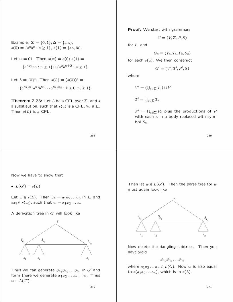
Example: Σ = {0,1},∆ = {a, b},s(0) = {anbn : n ≥ 1}, s(1) = {aa, bb}.

Let w = 01. Then s(w) = s(0).s(1) =

{anbnaa : n ≥ 1} ∪ {anbn+2 : n ≥ 1}.

Let L = {0}∗. Then s(L) = (s(0))∗ =

{an1bn1an2bn2 · · · ankbnk : k ≥ 0, ni ≥ 1}.

Theorem 7.23: Let L be a CFL over Σ, and s

a substitution, such that s(a) is a CFL, ∀a ∈ Σ.

Then s(L) is a CFL.

268

Proof: We start with grammars

G = (V,Σ, P, S)

for L, and

Ga = (Va, Ta, Pa, Sa)

for each s(a). We then construct

G′ = (V ′, T ′, P ′, S)

where

V ′ = (⋃a∈Σ Va) ∪ V

T ′ =⋃a∈Σ Ta

P ′ =⋃a∈Σ Pa plus the productions of P

with each a in a body replaced with sym-

bol Sa.

269

Now we have to show that

• L(G′) = s(L).

Let w ∈ s(L). Then ∃x = a1a2 . . . an in L, and

∃xi ∈ s(ai), such that w = x1x2 . . . xn.

A derivation tree in G′ will look like

S

S S

x x xn

Sa a a1 2 n

1 2

Thus we can generate Sa1Sa2 . . . San in G′ and

form there we generate x1x2 . . . xn = w. Thus

w ∈ L(G′).

270

Then let w ∈ L(G′). Then the parse tree for w

must again look like

S

S S

x x xn

Sa a a1 2 n

1 2

Now delete the dangling subtrees. Then you

have yield

Sa1Sa2 . . . San

where a1a2 . . . an ∈ L(G). Now w is also equal

to s(a1a2 . . . an), which is in s(L).

271

Applications of the Substitution Theorem

Theorem 7.24: The CFL’s are closed under(i) : union, (ii) : concatenation, (iii) : Kleeneclosure and positive closure +, and (iv) : ho-momorphism.

Proof: (i): Let L1 and L2 be CFL’s,let L = {1,2}, and s(1) = L1, s(2) = L2.Then L1 ∪ L2 = s(L).

(ii) : Here we choose L = {12} and s as before.Then L1.L2 = s(L).

(iii) : Suppose L1 is CF. Let L = {1}∗, s(1) =L1. Now L∗1 = s(L). Similar proof for +.

(iv) : Let L1 be a CFL over Σ, and h a homo-morphism on Σ. Define s by

a 7→ {h(a)}Then h(L) = s(L).

272

Theorem: If L is CF, then so in LR.

Proof: Suppose L is generated b G = (V, T, P, S).

Construct GR = (V, T, PR, S), where

PR = {A→ αR : A→ α ∈ P}Show at home by inductions on the lengths of

the derivations in G (for one direction) and in

GR (for the other direction) that (L(G))R =

L(GR).

273

CFL’s are not closed under ∩

Let L1 = {0n1n2i : n ≥ 1, i ≥ 1}. The L1 is CF

with grammar

S → AB

A→ 0A1|01

B → 2B|2

Also, L2 = {0i1n2n : n ≥ 1, i ≥ 1} is CF with

grammar

S → AB

A→ 0A|0B → 1B2|12

However, L1 ∩ L2 = {0n1n2n : n ≥ 1} which is

not CF, as we have proved using the pumping

lemma for CFL’s.

274

CF ∩ Regular = CF

Theorem 7.27: If L is CR, and R regular,

then L ∩R is CF.

Proof: Let L be accepted by PDA

P = (QP ,Σ,Γ, δP , qP , Z0, FP )

by final state, and let R be accepted by DFA

A = (QA,Σ, δA, qA, FA)

We’ll construct a PDA for L ∩ R according to

the picture

Accept/reject

Stack

AND

PDA

stateFA

state

Input

275

Formally, define

P ′ = (QP ×QA, ,Σ,Γ, δ, (qP , qA), Z0, FP × FA)

where

δ((q, p), a,X

)={(

(r, δA(p, a)), γ)

: (r, γ) ∈ δP (q, a,X)}

Prove at home by an induction∗, both for P

and for P ′ that

(qP , w, Z0)∗P

(q, ε, γ), and δ(qA, w) ∈ FA

if and only if((qP , qA), w, Z0

) ((q, δ(pA, w)), ε, γ

)

The claim then follows (Why?)

276

Theorem 7.29: Let L, L1, L2 be CFL’s and

R regular. Then

1. L \R is CF

2. L is not necessarily CF

3. L1 \ L2 is not necessarily CF

Proof:

1. R is regular, L ∩ R is regular, and L ∩ R =

L \R.

2. If L always were CF, it would follow that

L1 ∩ L2 = L1 ∪ L2

always would be CF.

3. Note that Σ∗ is CF, so if L1\L2 were always

CF, then so would Σ∗ \ L = L.

277

Inverse homomorphism

Let h : Σ→ Θ∗ be a homom. Let L ⊆ Θ∗, anddefine

h−1(L) = {w ∈ Σ∗ : h(w) ∈ L}Now we have

Theorem 7.30: Let L be a CFL, and h ahomomorphism. Then h−1(L) is a CFL.

Proof: The plan of the proof is

Accept/reject

Stack

statePDA

Buffer

Input hh(a)a

278

Let L be accepted by PDA

P = (Q,Θ,Γ, δ, q0, Z0, F )

We construct a new PDA

P ′ = (Q′,Σ,Γ, δ′, (q0, ε), Z0, F × {ε})where

• Q′ = {(q, x) : q ∈ Q, x ∈ suffix(h(a)), a ∈ Σ}

• δ′((q, ε), a,X) =

{((q, h(a)), X) : ε 6= a ∈ Σ, q ∈ Q, X ∈ Γ}

• δ′((q, bx), ε,X) = {((p, x), γ) :

(p, γ) ∈ δ(q, b,X), b ∈ T ∪ {ε}, q ∈ Q,X ∈ Γ}

Show at home by suitable inductions that

• (q0, h(w), Z0)∗

(p, ε, γ) in P if and only if

((q0, ε), w, Z0)∗

((p, ε), ε, γ) in P ′.

279

Decision Properties of CFL’s

We’ll look at the following:

• Complexity of converting among CFA’s and

PDAQ’s

• Converting a CFG to CNF

• Testing L(G) 6= ∅, for a given G

• Testing w ∈ L(G), for a given w and fixed G.

• Preview of undecidable CFL problems

280

Converting between CFA’s and PDA’s

• Input size is n.

• n is the total size of the input CFG or PDA.

The following work in time O(n)

1. Converting a CFG to a PDA (slide 203)

2. Converting a “final state” PDA

to a “null stack” PDA (slide 199)

3. Converting a “null stack” PDA

to a “final state” PDA (slide 195)

281

Avoidable exponential blow-up

For converting a PDA to a CFG we have

(slide 210)

At most n3 variables of the form [pXq]

If (r, Y1Y2 · · ·Yk) ∈ δ(q, a,X)}, we’ll have O(nn)

rules of the form

[qXrk]→ a[rY1r1] · · · [rk−1Ykrk]

• By introducing k−2 new states we can mod-

ify the PDA to push at most one symbol per

transition. Illustration on blackboard in class.

282

• Now, k will be ≤ 2 for all rules.

• Total length of all transitions is still O(n).

• Now, each transition generates at most n2

productions

• Total size (and time to calculate) the gram-

mar is therefore O(n3).

283

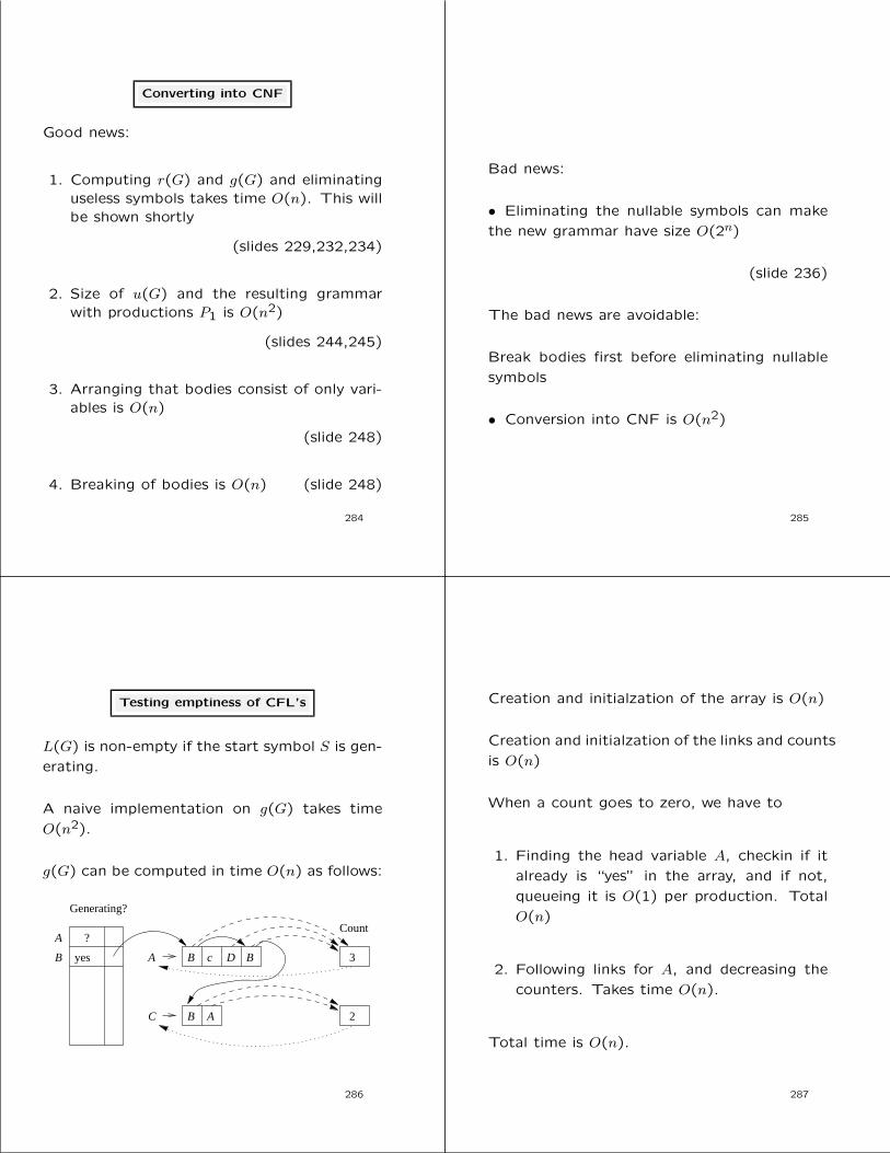
Converting into CNF

Good news:

1. Computing r(G) and g(G) and eliminatinguseless symbols takes time O(n). This willbe shown shortly

(slides 229,232,234)

2. Size of u(G) and the resulting grammarwith productions P1 is O(n2)

(slides 244,245)

3. Arranging that bodies consist of only vari-ables is O(n)

(slide 248)

4. Breaking of bodies is O(n) (slide 248)

284

Bad news:

• Eliminating the nullable symbols can make

the new grammar have size O(2n)

(slide 236)

The bad news are avoidable:

Break bodies first before eliminating nullable

symbols

• Conversion into CNF is O(n2)

285

Testing emptiness of CFL’s

L(G) is non-empty if the start symbol S is gen-

erating.

A naive implementation on g(G) takes time

O(n2).

g(G) can be computed in time O(n) as follows:

Count

Generating?

3

2

BA

C

c D B

B A

A

B

?

yes

286

Creation and initialzation of the array is O(n)

Creation and initialzation of the links and counts

is O(n)

When a count goes to zero, we have to

1. Finding the head variable A, checkin if it

already is “yes” in the array, and if not,

queueing it is O(1) per production. Total

O(n)

2. Following links for A, and decreasing the

counters. Takes time O(n).

Total time is O(n).

287

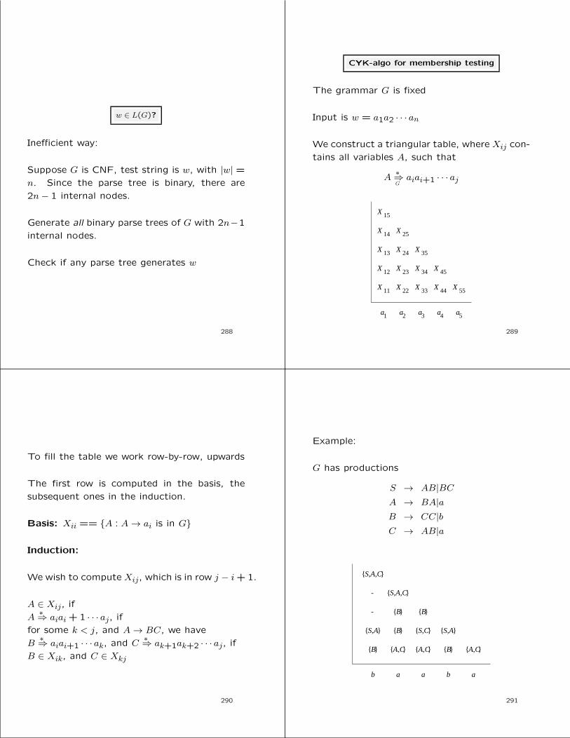
w ∈ L(G)?

Inefficient way:

Suppose G is CNF, test string is w, with |w| =n. Since the parse tree is binary, there are

2n− 1 internal nodes.

Generate all binary parse trees of G with 2n−1

internal nodes.

Check if any parse tree generates w

288

CYK-algo for membership testing

The grammar G is fixed

Input is w = a1a2 · · · an

We construct a triangular table, where Xij con-

tains all variables A, such that

A∗⇒Gaiai+1 · · · aj

a a a a a1 2 3 4 5

X X X X X

X X X X

X X X

X X

X

11 22 33 44 55

45342312

13 24 35

14 25

15

289

To fill the table we work row-by-row, upwards

The first row is computed in the basis, the

subsequent ones in the induction.

Basis: Xii == {A : A→ ai is in G}

Induction:

We wish to compute Xij, which is in row j − i+ 1.

A ∈ Xij, if

A∗⇒ aiai + 1 · · · aj, if

for some k < j, and A→ BC, we have

B∗⇒ aiai+1 · · · ak, and C

∗⇒ ak+1ak+2 · · · aj, if

B ∈ Xik, and C ∈ Xkj

290

Example:

G has productions

S → AB|BCA → BA|aB → CC|bC → AB|a

S,A,C

-

-

B

S,A B

BB

A,C

S,C

A,C

S,A

B A,C

{ }

{

{

S,A,C{

{

{

{

{

{

{

{

{ {

}

}

}

}

}

}

}

}

}

}

} }

b a a b a

291

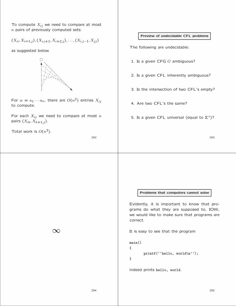
To compute Xij we need to compare at most

n pairs of previously computed sets:

(Xii, Xi=1,j), (Xi,i+1, Xi+2,j), . . . , (Xi,j−1, Xjj)

as suggested below

For w = a1 · · · an, there are O(n2) entries Xijto compute.

For each Xij we need to compare at most n

pairs (Xik, Xk+1,j).

Total work is O(n3).

292

Preview of undecidable CFL problems

The following are undecidable:

1. Is a given CFG G ambiguous?

2. Is a given CFL inherently ambiguous?

3. Is the intersection of two CFL’s empty?

4. Are two CFL’s the same?

5. Is a given CFL universal (equal to Σ∗)?

293

∞

294

Problems that computers cannot solve

Evidently, it is important to know that pro-

grams do what they are supposed to, IOW,

we would like to make sure that programs are

correct.

It is easy to see that the program

main()

{

printf(‘‘hello, world\n’’);

}

indeed prints hello, world.

295

What about the program in Fig. 8.2 in the

textbook?

It will print hello, world, for input n if and only

if the equation

xn + yn = zn

has a solution where x, y, and z are integers.

We now know that it will print hello, world,

for input n = 2, and loop forever for inputs

n > 2.

It took humanity 300+ years to prove this.

Can we hope to have a program that proves

the correctness of programs?

296

The hypothetical “Hello, world” tester H

Suppose the following program H exists.

Hello-worldtester

HP

I yes

no

Modify the no print statement of H to

hello, world. We get program H1

P

I

H1

yes

hello, world

297

Modify H1 so that it takes only P as input,

stores P and uses it both as P and I. We get

program H2.

H2Pyes

hello, world

Give H2 as input to H2.

H2H2

yes

hello, world

• If H2 prints yes it should have printed

hello, world.

• If H2 prints hello, world it should have

printed yes.

• Thus H2 cannot exist.

• Consequently H cannot exist either.

298

The Turing Machine (1936)

X 2 X i X nX 1

controlFinite

. . .BBB B. . .

A TM makes a move depending on its state,

and the symbol under the tape head.

In a move, a TM will

1. Change state

2. Write a tape symbol in the cell scanned

3. Move the tape head one cell left or right

299

A (deterministic) Turing Machine is a 7-tuple

M = (Q,Σ,Γ, δ, q0, B, F ),

where

• Q is a finite set of states,

• Σ is a finite set of input symbols,

• Γ is a finite set of tape symbols, Γ ⊃ Σ

• δ is a transition function from Q × Γ toQ× Γ× {L,R},

• q0 is the start state,

• B ∈ Γ \Σ is the blank symbol, and

• F ⊆ Q is the set of final states.

300

Instantaneous Description

A TM changes configuration after each move.

We use Instantaneous Descriptions, ID’s, to

describe configurations.

An ID is a string of the form

X1X2 · · ·Xi−1qXiXi+1 · · ·Xnwhere

1. q is the state of the TM.

2. X1X2 · · ·Xn is the non-blank portion of the

tape

3. The tape head is scanning the ith symbol

301

The moves and the language of a TM

We’ll useM

to indicate a move by M from aconfiguration to another.

• Suppose δ(q,Xi) = (p, Y, L). Then

X1X2 · · ·Xi−1qXiXi+1 · · ·Xn MX1X2 · · · pXi−1Y Xi+1 · · ·Xn

• If δ(q,Xi) = (p, Y,R), we have

X1X2 · · ·Xi−1qXiXi+1 · · ·Xn MX1X2 · · ·Xi−1Y pXi+1 · · ·Xn

We denote the reflexive-transitive closure ofM

with∗M

.

• A TM M = (Q,Σ,Γ, δ, q0, B, F ) accepts thelanguage

L(M) = {w ∈ Σ∗ : q0w∗Mαpβ, p ∈ F, α, β ∈ Γ∗}

302

A TM for {0n1n : n ≥ 1}

M = ({q0, q1, q2, q3, q4}, {0,1}, {0,1, X, Y,B}, δ, q0, B, {q4})where δ is given by the following table

0 1 X Y B

→ q0 (q1, X,R) (q3, Y, R)q1 (q1,0, R) (q2, Y, L) (q1, Y, R)q2 (q2,0, L) (q0, X,R) (q2, Y, L)q3 (q3, Y, R) (q4, B,R)?q4

We can represent M by the following transitiondiagram

/Y Y

/Y Y

/Y Y

0/0

X/0

/X X

/B B

/ Y1

/Y Y

0/0Start

q q q

q q

0 1 2

3 4

303

A TM with “output”

The following TM computes

m·− n = max(m− n,0)

0 1 B

→ q0 (q1, B,R) (q5, B,R)q1 (q1,0, R) (q2,1, R)q2 (q1,1, L) (q2,1, R) (q4, B, L)q3 (q3,0, L) (q3,1, L) (q0, B,R)q4 (q4,0, L) (q4, B, L) (q6,0, R)q5 (q5, B,R) (q5, B,R) (q6, B,R)?q6

The transition diagram is

/1 1/0 B

1 / B

1 / B

0/0

/1 1

/B B

/B B

0/0/0 B

1 / B

B / 0

0/0 /1 1

/B B

Startq q q

q q

0 1 2

q

q0 / 1

4

3

5 6

304

Programming Techniques for TM’s

Although TM’s seem very simple, they are as

powerful as any computer.

Lots of “features” can be simulated with a

“standard” machine.

• Storage in State

A TM M that “remembers” the first symbol.

M =(Q, {0,1}, {0,1, B}, δ, [q0, B], B, {[q1, B]}

)

where Q = {q0, q1} × {0,1, B}.δ 0 1 B

→ [q0, B] ([q1,0],0, R) ([q1,1],1, R)[q1,0] ([q1,0],1, R) ([q1, B], B,R)[q1,1] ([q1,0],1, R) ([q1, B], B,R)

?[q1, B]

L(M) = L(01∗+ 10∗).

305

• Multiple Tracks for {wcw : w ∈ {0,1}∗}

q

A B C

X

Y

Z

State

Storage

Track 1

Track 2

Track 3

M = (Q,Σ,Γ, δ, [q1, B], [B,B], {[q0, B]})where

Q = {q1, q2, . . . , q9} × {0,1, B}

Σ = {[B,0], [B,1], [B, c]}

Γ = {B, ∗} × {0,1, c, B}

306

• Subroutines

The TM computes 0m10n1 7→ 0m·n

Start

Copy

0/

0/0

1/1 0/0 1/1

0/0

0/0/

/

1/

0/

1/

B B

B

B

B

B

B B

q

q q q

q

q

qqq

0

6 1 5 q7 8

9

101112

Here is the “Copy” TM

Start 0/

1/1

1/1

/0

/

X B

X X

q q q

q q

1 2 3

4 5

0/01/1 1/1

0/0

/0X

307

Variations of the basic TM

• Multitape TM’s. Input on first tape.

. . . . . .

. . . . . .

. . . . . .

In one move the TM

1. Remains in the same state or enters a newstate.

2. For each tape, writes a new symbol in thecurrent cell.

3. Independently moves each head left or right.

308

Theorem: Every language accepted by a multi-tape TM M is RE

Proof idea: Simulate M by multitrack TM N

A A A i1 2 A j

B B B Bi21 j

X

X

1. 2k tracks for k tape simulation. Even tracks= tape content. Odd tracks = head posi-tion.

2. N has to visit k head markers to simulatea move of M . Store the number of headsvisited in state.

3. For each head N does what M does on thecorresponding tape.

4. N changes state acording to M .

309

• Nondeterministic TM’s

Theorem: For every nondeterministic TM MNthere is a deterministic TM MD such that

L(MN) = L(MD).

Proof idea: Suppose at each state MN has kchoiches for each symbol.

ID1 * * **ID2 ID3 ID4

Finitecontrol

Queueof ID’s

Scratchtape

x . . .

1. MD has transitions δ(q, a, k).

2. For each ID copy it to scratch tape. Foreach k create a new ID at the end of thequeue.

3. Unmark the current ID and go to next ID.

310

Undecidability

We want to prove undecidable Lu which is the

language of pairs (M,w) such that:

1. M is a TM (encoded in binary) with input

alphabet {0,1}.

2. w ∈ {0,1}∗.

3. M accepts w.

311

The landscape of languages (problems)

REbut

Not RE

L

L

.

.

recursivenot

Recursive

u

d

1. The recursive languages L:

There is a TM M that always halts andsuch that L(M) = L. IOW there is analgorithm that on input w answers “yes” ifw ∈ L, and answers “no” if w /∈ L.

2. The recursively enumerable languages L:

There is a TM M that halts and accepts ifw ∈ L, and might run forever otherwise.

3. The non-RE languages L:

There is no TM whatsoever for L.

312

Encoding TM’s

• Enumerate strings: w ∈ {0,1}∗ is treated asbinary integer 1w. The ith string is denoted wi.

ε = w1,0 = w2,1 = w3,00 = w4,01 = w5, . . .

To enccode M = (Q, {0,1},Γ, δ, q1, B, F )

- Assume Q = {q1, q2, . . . , qr}, F = {q2}.

- Assume Γ = {X1, X2, . . . , Xs}, whereX1 = 0, X2 = 1, and X3 = B.

- Encode L as D1 and R as D2.

- Encode δ(qi, Xj) = (qk, X`, Dm) as

0i10j10k10`10m

- Encode the entire TM as

C111C211 · · ·11cn−111Cn

where each Ci is the code of one transition.

313

Example:

M = ({q1, q2, q3}, {0,1}, {0,1, B}, δ, q1, B, {q2}),

whereδ 0 1 B

→ q1 (q3,0, R)?q2q3 (q1,1, R) (q2,0, R) (q3,1, L)

The code for transitions C1, C2, C3, C4:

0100100010100

0001010100100

00010010010100

0001000100010010

The code for the entire M :

01001000101001100010101001001100010010010100110001000100010010

314

The diagonalization language Ld

The ith TM Mi: The TM whose code is wi.

Write down a matrix where

(i, j) =

{1 if wj ∈ L(Mi),0 otherwise

.

.

.

.

.

.

.

.

.

.

.

.

.

.

.

1 2 3 4

1

2

3

4

0 1 1 0

1 1 0 0

10

0 1 0 1

0

Diagonal

. . .

. . .

. . .

. . .

. . .

..

.

i

j

1

Define Ld = {wi : wi /∈ L(Mi)}

If there is a TM for Ld it must be Mi for some i.If wi ∈ Ld then wi ∈ L(Mi) and thus wi /∈ LdIf wi /∈ Ld then wi /∈ L(Mi) and thus wi ∈ Ld

315

Theorem: If L is recursive, so is L.

Proof:

Accept

Reject Reject

AcceptMw

Theorem: If L is RE and L also is RE, then

L is recursive.

Proof:

Accept

Accept

Accept

Reject

M

M

w

1

2

316

The universal language Lu

Lu = {(enc(M), enc(w)) : w ∈ L(M)}

TM U where L(U) = Lu

Finitecontrol

Tape of

State of

0001000001010001

000

M w

M

M . . .

. . .

0BB . . .

Input

Scratch

317

Operation of U:

1. If enc(M) is not legitimate halt and reject

2. Write enc(w) on tape 2. Use the blank of

U for 1000

3. Write the start state 0 on tape 3. Place

head of tape 2 on first simulated cell

4. Search tape 1 for 0i10j10k10`10m, where

(a) 0i is the state on tape 3

(b) 0j is tape symbol of M that begins un-

der the head on 2

318

5. Make the move

(a) Change tape 3 to 0k

(b) Replace 0j on tape 2 by 0`

(c) Move head 2 left (if m = 1) or

right (if m = 2) to next 1

(d) If no 0i10j1 · · ·1 · · · is not found on

tape 1, then halt and reject

(e) If M enters its accepting state then

accept and halt

319

Theorem: Lu is RE but not recursive.

Proof: Lu is RE since L(U) = Lu.

Suppose Lu were recursive. Then Lu is also

recursive. Let M be an always halting TM

with L(M) = Lu.

We modify M to M ′, such that L(M ′) = Ld

Accept

w 111 wCopyw

RejectLM’

Reject

Accept

M L

algorithm

for

for

Hypothetical

u

d

• wi ∈ L(M ′)⇒ wi111wi ∈ Lu ⇒ wi /∈ L(Mi)⇒ wi ∈ Ld

• wi /∈ L(M ′)⇒ wi111wi ∈ Lu ⇒ wi ∈ L(Mi)⇒ wi /∈ Ld

320

Reductions for proving lower bounds

Find an algorithm that reduces a known hardproblem P1 to P2.

yes

no

yes

no

P P1 2

Theorem: If there is a reduction from P1 toP2, then

1. If P1 is undecidable, then so is P2

2. If P1 is non-RE, then so is P2.

Proof: by contradiction. If there were an al-gorithm for P2 you could also solve P1 by firstreducing P1 to P2 and then running the algo-rithm for P2.

321

A non-recursive and a non-RE language

Le = {enc(M) : L(M) = ∅}

Lne = {enc(M) : L(M) 6= ∅}

Theorem: Lne is recursively enumerable.

Proof: Non-deterministic TM for Lne

GuessedAcceptw

M U

Mi

Accept

for Lne

322

Theorem: Lne = {enc(M) : L(M) 6= ∅} is not

recursive.

Proof: by contradiction. Suppose ∃ TM M ,

such that L(M) = Lne. Transform instance

(M,w) of Lu into M ′ such that

w ∈ L(M)⇔ L(M ′) 6= ∅

w AcceptMx

M’

Accept

We have reduced Lu to Lne.

Suppose there is an algorithm for Lne.

Run the algorithm to see if L(M ′) 6= ∅.

Since Lu is not recursive, Lne cannot be recur-

sive either.

323

Theorem: Le = {enc(M) : L(M) = ∅} is

not RE

Proof: If Le were RE then Lne would be re-

cursive, since Le = Lne.

Other undecidable properties of TM’s

1. Lfin = {enc(M) : L(M) is finite}

2. Lreg = {enc(M) : L(M) is regular}

3. Lcfl = {enc(M) : L(M) is a CFL}

These follow from Rice’s Theorem.

324

Properties of the RE languages

Every nontrivial property of the RE languages

is undecidable.

Property of RE languages (example):

“the language is CF”

Formally: A nontrivial property is a nonempty

strict subset of all RE languages.

Let P be a nontrivial property of the RE lan-

guages.

LP = {enc(M) : L(M) ∈ P}.

Rice’s Theorem: LP is not recursive.

325

Proof of Rice’s Theorem:

Suppose first ∅ /∈ P.

Let L ∈ P and ML be a TM such that L(ML) = L.

Transform instance (M,w) of Lu into TM M ′such that

L(M ′) =

{L if w ∈ L(M),∅ if w /∈ L(M)

w

x

M

M

M’

Acceptstart Accept

L

Accept

We have reduced Lu to LP.

Suppose there is an algorithm for LP.

Run the algorithm to see if L(M ′) 6= ∅.

Since Lu is not recursive, LP cannot be recur-sive either.

326

Proof of Rice’s Theorem:

Suppose then that ∅ ∈ P

Consider P: the set of RE languages that do

not have property P. Based on the above P is

undecidable.

Since every TM accepts an RE language we

have

LP = LP

If LP were decidable then LP would also be

decidable.

327

Post’s Correspondence Problem

PCP is a problem about strings that isundecidable (RE)

Let A = w1, w2, . . . , wk and B = x1, x2, . . . , xk,where xi, yi ∈ Σ∗ for some alphabet Σ.

The instance (A,B) has a solution if there ex-ists indices i1, i2, . . . , im, such that

wi1wi2 · · ·wim = xi1xi2 · · ·xim

Example:List A List B

i wi xi1 1 1112 10111 103 10 0

Solution: i1 = 2, i2 = 1, i3 = 1, i4 = 3 gives

w2w1w1w3 = x2x1x1x3 = 101111110

Another solution: 2,1,1,3,2,1,1,3

328

Example:

List A List Bi wi xi1 10 1012 011 113 101 011

This PCP instance has no solution.

Suppose i1, i2, . . . , im is a solution:

If i1 = 2 we cannot matchw2x2=

01111

If i1 = 3 we cannot matchw3x3=

101011

Therefore i1 = 1 and a partial solution isw1x1=

10101

329

If i2 = 1 we cannot matchw1w1x1x1=

1010101101

If i2 = 2 we cannot matchw1w2x1x2=

1001110111

Only i2 = 3 is possible givingw1w3x1x3=

10101101011

Now we are back to “square one:”

Only i3 = 3 is possible givingw1w3x1x3=

10101101101011011

Only i4 = 3 is possible givingw1w3w3x1x3x3=

10101101101101011011011

Conclusion: The first list can never catch up

with the second

330

The Modified PCP:

Let A = w1, w2, . . . , wk and B = x1, x2, . . . , xk,

where xi, yi ∈ Σ∗ for some alphabet Σ.

The modifeid PCP A,B has a solution if there

exists indices i1, i2, . . . , im, such that

w1wi1, wi2, . . . , wim = x1xi1, xi2, . . . xim

Example:

List A List Bi wi xi1 1 1112 10111 103 10 0

Any solution would have to begin withw1x1=

1111

If i2 = 2 we cannot matchw1w2x1x2=

11011111110

If i2 = 3 we cannot matchw1w2x1x2=

1101110

If i2 = 1 we have to matchw1w2x1x2=

11111111

We are back to “square one.”

331

We reduce MPCP to PCP

Let MPCP be A = w1, w2, . . . , wk, B = x1, x2, . . . , xk

We construct PCP A′ = y0, y1, . . . , yk+1,

B′ = z0, z1, . . . , zk+1 as follows:

y0 = ∗y1 and z0 = z1

If wi = a1a2 . . . a` then yi = a1 ∗ a2 ∗ . . . a`∗

If xi = b1b2 . . . bp then zi = ∗b1 ∗ b2 . . . ∗ bp

yk+1 = $ and zk+1 = ∗$

Now (A,B) has a solution iff (A′, B′) has one.

332

Example:

Let MPCP be

List A List Bi wi xi1 1 1112 10111 103 10 0

Then we construct PCP

List A List Bi yi zi0 *1* *1*1*11 1* *1*1*12 1*0*1*1*1* *1*03 1*0* *4 $ *$

333

PCP is undecidable

Given an instance (M,w) of Lu we construct

instance (A,B) of MPCP such that w ∈ L(M)

iff (A,B) has a solution.

algorithman

algorithmanL u MPCP PCP

Partial solutions will consist of strings of the

form

#α1#α2#α3 · · ·where α1 is the initial configuartion of M on w,

and αi ` αi+1.

The string from list B will always be one ID

ahead of A until M accepts w and A can catch up.

334

Let M = (Q,Σ,Γ, δ, q0, B, F ) be the TM. WLOGassume that M never prints a blank, and nevermoves the head left of the initial position.

1. The initial pair

List A List B# #q0w#

2. For each X ∈ Γ

List A List BX X# #

3. ∀q ∈ Q \ F, ∀p ∈ Q, ∀X,Y, Z ∈ Γ

List A List BqX Y p if δ(q,X) = (p, Y,R)ZqX pZY if δ(q,X) = (p, Y, L), Z ∈ Γq# Y p# if δ(q,B) = (p, Y,R)Zq# pZY# if δ(q,B) = (p, Y, L), Z ∈ Γ

335

4. ∀q ∈ F, ∀X,Y ∈ Γ

List A List BXqY qXq qqY q

5. Final pair

List A List Bq## #

336

Example: Lu instance: (M,01)

M = ({q1, q2, q3}, {0,1}, {0,1, B}, δ, q1, B, {q3})δ 0 1 B

→ q1 (q2,1, R) q2,0, L) (q2,1, L)q2 (q3,0, L) (q1,0, R) (q2,0, R)?q3 - - -

The corresponding MPCP is:

Rule List A List B Source(1) # #q101(2) 0 0

1 1# #

(3) q10 1q2 from δ(q1,0) = (q2,1, R)0q11 q200 from δ(q1,1) = (q2,0, L)1q11 q210 from δ(q1,1) = (q2,0, L)0q1# q201# from δ(q1, B) = (q2,1, L)1q1# q211# from δ(q1, B) = (q2,1, L)0q20 q300 from δ(q2,0) = (q3,0, L)1q20 q310 from δ(q2,0) = (q3,0, L)q21 0q1 from δ(q2,1) = (q1,0, R)q2# 0q2# from δ(q2, B) = (q2,0, R)

(4) 0q30 q30q31 q31q30 q31q31 q30q3 q30q3 q31q3 q3q30 q3q31 q3

(5) q3## #

337