NBER WORKING PAPER SERIES FOUNDATIONS OF TECHNICAL ANALYSIS: COMPUTATIONAL ALGORITHMS, STATISTICAL INFERENCE, AND EMPIRICAL IMPLEMENTATION Andrew W. Lo Harry Mamaysky Jiang Wang Working Paper 7613 http://www.nber.org/papers/w7613 NATIONAL BUREAU OF ECONOMIC RESEARCH 1050 Massachusetts Avenue Cambridge, MA 02138 March 2000 This research was partially supported by the MIT laboratory for Financial Engineering, Merrill Lynch, and the National Science Foundation (Grant No. SBR-9709976). We thank Ralph Acampora, Franklin Allen, Susan Berger, Mike Epstein, Narasimhan Jegadeesh, Ed Kao, Doug Sanzone, Jeff Simonoff, Tom Stoker, and seminar participants at the Federal Reserve Bank of New York, NYU, and conference participants at the Columbia-JAFEE conference, the 1999 Joint Statistical Meetings, RISK 99, the 1999 Annual Meeting of the Society forComputational Economics, and the 2000 Annual Meeting of the American Finance Association for valuable comments and discussion. The views expressed herein are those of the authors and are notnecessarily those of the National Bureau of Economic Research. 2000 by Andrew W. Lo, Harry Mamaysky, and Jiang Wang. All rights reserved. Short sections of text, not to exceed two paragraphs, may be quoted without explicit permission provided that full credit, including notice, is given to the source.

Welcome message from author
This document is posted to help you gain knowledge. Please leave a comment to let me know what you think about it! Share it to your friends and learn new things together.
Transcript

NBER WORKING PAPER SERIES
FOUNDATIONS OF TECHNICAL ANALYSIS:COMPUTATIONAL ALGORITHMS, STATISTICAL
INFERENCE, AND EMPIRICAL IMPLEMENTATION
Andrew W. LoHarry Mamaysky
Jiang Wang
Working Paper 7613http://www.nber.org/papers/w7613
NATIONAL BUREAU OF ECONOMIC RESEARCH1050 Massachusetts Avenue
Cambridge, MA 02138March 2000
This research was partially supported by the MIT laboratory for Financial Engineering, Merrill Lynch, andthe National Science Foundation (Grant No. SBR-9709976). We thank Ralph Acampora, Franklin Allen,Susan Berger, Mike Epstein, Narasimhan Jegadeesh, Ed Kao, Doug Sanzone, Jeff Simonoff, Tom Stoker, andseminar participants at the Federal Reserve Bank of New York, NYU, and conference participants at theColumbia-JAFEE conference, the 1999 Joint Statistical Meetings, RISK 99, the 1999 Annual Meeting of theSociety forComputational Economics, and the 2000 Annual Meeting of the American Finance Association forvaluable comments and discussion. The views expressed herein are those of the authors and are notnecessarilythose of the National Bureau of Economic Research.
2000 by Andrew W. Lo, Harry Mamaysky, and Jiang Wang. All rights reserved. Short sections of text,not to exceed two paragraphs, may be quoted without explicit permission provided that full credit, including
notice, is given to the source.
Foundations of Technical Analysis: Computational Algorithms, Statistical Inference,and Empirical ImplementationAndrew W. Lo, Harry Mamaysky, and Jiang WangNBER Working Paper No. 7613March 2000
ABSTRACT
Technical analysis, also known as "charting," has been part of financial practice for many
decades, but this discipline has not received the same level of academic scrutiny and acceptance as
more traditional approaches such as fundamental analysis. One of the main obstacles is the highly
subjective nature of technical analysis—the presence of geometric shapes in historical !price charts is
often in the eyes of the beholder. In this paper, we propose a systematic and automatic approach to
technical pattern recognition using nonparametric kernel regression, and apply this method to a large
number of U.S. stocks from 1962 to 1996 to evaluate the effectiveness to technical analysis. By
comparing the unconditional empirical distribution of daily stock returns to the conditional
distribution—conditioned on specific technical indicators such as head-and-shoulders or double-
bottoms—we find that over the 31-year sample period, several technical indicators do provide
incremental information and may have some practical value.
Andrew W. Lo Harry MamayskySloan School of Management Sloan School of ManagementMIT Mn'50 Memorial Drive, E52-432 50 Memorial Drive, E52-458Cambridge, MA 02142 Cambridge, MA 02142and NBER [email protected]@mit.edu
Jiang WangSloan School of ManagementMIT50 Memorial Drive, E52-435Cambridge, MA 02142and NBERwangj @mit.edu

One of the greatest gulfs between academic finance and industry practice is the separation
that exists between technical analysts and their academic critics. In contrast to fundamental
analysis, which was quick to be adopted by the scholars of modern quantitative finance, tech-
nical analysis has been an orphan from the very start. It has been argued that the difference
between fundamental analysis and technical analysis is not unlike the difference between
astronomy and astrology. Among some circles, technical analysis is known as "voodoo fi-
nance." And in his influential book A Random Walk Down Wall Street, Burton Maildel
(1996) concludes that "[ujnder scientific scrutiny, chart-reading must share a pedestal with
alchemy."
However, several academic studies suggest that despite its jargon and methods, technical
analysis may well be an effective means for extracting useful information from market prices.
For example, in rejecting the Random Walk Hypothesis for weekly US stock indexes, Lo and
MacKinlay (1988, 1999) have shown that past prices may be used to forecast future returns to
some degree, a fact that all technical analysts take for granted. Studies by Tabell and Tabell
(1964), Treynor and Ferguson (1985), Brown and Jennings (1989), Jegadeesh and Titman
(1993), Blume, Easley, and O'Hara (1994), Chan, Jegadeesh, and Lakonishok (1996), Lo and
MacKinlay (1997), Grundy and Martin (1998), and Rouwenhorst (1998) have also provided
indirect support for technical analysis, and more direct support has been given by Pruitt
and White (1988), Neftci (1991), Broth, Lakonishok, and LeBaron (1992), Neely, Weber,
and Dittmar (1997), Neely and Weller (1998), Chang and Osler (1994), Osler and Chang
(1995), and Allen and Karjalainen (1999).
One explanation for this state of controversy and confusion is the unique and sometimes
impenetrable jargon used by technical analysts, some of which has developed into a standard
lexicon that can be translated. But there are many "homegrown" variations, each with its
own patois, which can often frustrate the uninitiated. Campbell, Lo, and MacKinlay (1997,
pp. 43—44) provide a striking example of the linguistic barriers between technical analysts
and academic finance by contrasting this statement:
The presence of clearly identified support and resistance levels, coupled with
a one-third retracement parameter when prices lie between them, suggests the
1

presence of strong buying and selling opportunities in the near-term.
with this one:
The magnitudes and decay pattern of the first twelve autocorrelations and the
statistical significance of the Box-Pierce Q-statistic suggest the presence of a
high-frequency predictable component in stock returns.
Despite the fact that both statements have the same meaning—that past prices contain
information for predicting future returns-—-most readers find one statement plausible and
the other puzzling, or worse, offensive.
These linguistic barriers underscore an important difference between technical analysis
and quantitative finance: technical analysis is primarily visual, while quantitative finance is
primarily algebraic and numerical. Therefore, technical analysis employs the tools of geom-
etry and pattern recognition, while quantitative finance employs the tools of mathematical
analysis and probability and statistics. In the wake of recent breakthroughs in financial en-
gineering, computer technology, and numerical algorithms, it is no wonder that quantitative
finance has overtaken technical analysis in popularity—the principles of portfolio optimiza-
tion are far easier to program into a computer than the basic tenets of technical analysis.
Nevertheless, technical analysis has survived through the years, perhaps because its visual
mode of analysis is more conducive to human cognition, and because pattern recognition is
one of the few repetitive activities for which computers do not have an absolute advantage
(yet).Indeed, it is difficult to dispute the potential value of price/volume charts when confronted
with the visual evidence. For example, compare the two hypothetical price charts given in
Figure 1. Despite the fact that the two price series are identical over the first half of the
sample, the volume patterns differ, and this seems to be informative. In particular, the lower
chart, which shows high volume accompanying a positive price trend, suggests that there
may be more information content in the trend, e.g., broader participation among investors.
The fact that the joint distribution of prices and volume contains important information is
hardly controversial among academics. Why, then, is the value of a visual depiction of that
joint distribution so hotly contested?
2

In this paper, we hope to bridge this gulf between technical analysis and quantitative
finance by developing a systematic aiid scientific approach to the practice of technical anal-
ysis, and by employing the now-standard methods of empirical analysis to gauge the efficacy
of technical indicators over time and across securities. In doing so, our goal is not only to
develop a lingua franca with which disciples of both disciplines can engage in productive
dialogue, but also to extend the reach of technical analysis by augmenting its tool kit with
some modem techniques in pattern recognition.
The general goal of technical analysis is to identify regularities in the time series of prices
by extracting nonlinear patterns from noisy data. Implicit in this goal is the recognition
that some price movements are significant—they contribute to the formation of a specific
pattern—and others are merely random fluctuations to be ignored. In many cases, the
human eye can perform this "signal extraction" quickly and accurately, and until recently,
computer algorithms could not. However, a class of statistical estimators, called smoothing
estimators, is ideally suited to this task because they extract nonlinear relations the) by
"averaging out" the noise. Therefore, we propose using these estimators to mimic, and in
some cases, sharpen the skills of a trained tec]mical analyst in identifying certain patterns
in historical price series.
In Section I, we provide a brief review of smoothing estimators and describe in detail the
specific smoothing estimator we use in our analysis: kernel regression. Our algorithm for
automating technical analysis is described in Section II. We apply this algorithm to the daily
returns of several hundred U.S. stocks from 1962 to 1996 and report the results in Section
III. To check the accuracy of our statistical inferences, we perform several Monte Carlo
simulation experiments and the results are given in Section IV. We conclude in Section V.
I. Smoothing Estimators and Kernel Regression
The starting point for any study of technical analysis is the recognition that prices evolve
in a nonlinear fashion over time and that the nonlinearities contain certain regularities or
patterns. To capture such regularities quantitatively, we begin by asserting that prices {P}
3
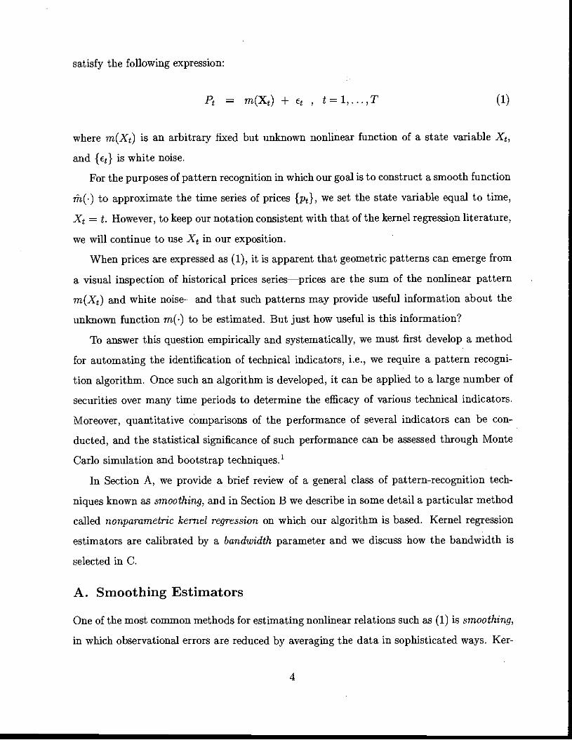
satisfy the following expression:
Pt = m(Xt) + c , t=1,...,T (1)
where m(X) is an arbitrary fixed but unknown nonlinear function of a state variable X,
and {e} is white noise.
For the purposes of pattern recognition in which our goal is to construct a smooth function
nze) to approximate the time series of prices {pt}, we set the state variable equal to time,
X = t. However, to keep our notation consistent with that of the kernel regression literature,
we will continue to use X, in our exposition.
When prices are expressed as (1), it is apparent that geometric patterns can emerge from
a visual inspection of historical prices series—prices are the sum of the nonlinear pattern
im(Xt) and white noise—and that such patterns may provide useful information about the
unknown function me) to be estimated. But just how useful is this information?
To answer this question empirically and systematically, we must first develop a method
for automating the identification of technical indicators, i.e., we require a pattern recogni
tion algorithm. Once such an algorithm is developed, it can be applied to a large number of
securities over many time periods to determine the efficacy of various technical indicators.
Moreover, quantitative comparisons of the performance of several indicators can be con-
ducted, and the statistical significance of such performance can be assessed through Monte
Carlo simulation and bootstrap techniques.'
In Section A, we provide a brief review of a general class of pattern-recognition tech-
niques known as smoothing, and in Section B we describe in some detail a particular method
called nonparametric kernel regression on which our algorithm is based. Kernel regression
estimators are calibrated by a bandwidth parameter and we discuss how the bandwidth is
selected in C.
A. Smoothing Estimators
One of the most common methods for estimating nonlinear relations such as (1) is smoothing,
in which observational errors are reduced by averaging the data in sophisticated ways. Ker-
4

nel regression, orthogonal series expansion, projection pursuit, nearest-neighbor estimators,
average derivative estimators, splines, and neural networks are all examples of smoothing
estimators. In addition to possessing certain statistical optirnality properties, smoothing
estimators are motivated by their close correspondence to the way human cognition extracts
regularities from noisy data.2 Therefore, they are ideal for our purposes.
To provide some intuition for how averaging can recover nonlinear relations such as
the function me) in (1), suppose we wish to estimate mC) at a particWar date to when
X0=x0. Now suppose that for this one observation, X0, we can obtain repeated independent
observations of the price P,0, say = Pi,-• . , = p, (note that these are ii independent
realizations of the price at the same date to, clearly an impossibility in practice, but let us
continue with this thought experiment for a few more steps). Then a natural estimator of
the function mC) at the point zo is
ñt(xo) = 1pi = 1[m(xo)+efl (2)ni=1
= m(xo) + —Ed, (3)
and by the Law of Large Numbers, the second term in (3) becomes negligible for large ii.
Of course, if {P} is a time series, we do not have the luxury of repeated observations
for a given X,. However, if we assume that the function mC) is sufficiently smooth, then
for time-series observations X near the value x0, the corresponding values of P should be
close to m(xo). In other words, if mC) is sufficiently smooth, then in a small neighborhood
around x0, m(xo) will be nearly constant and may be estimated by taking an average of the
Pr's that correspond to those Xe's near x0. The closer the Xi's are to the value x0, the closer
an average of corresponding Pt's will be to m(xo). This argues for a weighted average of the
Pt's, where the weights decline as the X,'s get farther away from x0. This weighted-average
or "local averaging" procedure of estimating m(x) is the essence of smoothing.
More formally, for any arbitrary x, a smoothing estimator of m(x) may be expressed as
lTrui(x) w(z)Pt (4)
t= 1
5
where the weights {wt(x)} are large for those Ps's paired with Xe's near x, and small for those
Pr's with Xe's far from x. To implement such a procedure, we must define what we mean by
"near" and "far." If we choose too large a neighborhood around x to compute the average,
the weighted average will be too smooth and will not exhibit the genuine nonlinearities of
mC). If we choose too small a neighborhood around x, the weighted average will be too
variable, reflecting noise as well as the variations in mC). Therefore, the weights {wt(x)}
must be chosen carefully to balance these two considerations.
B. Kernel Regression
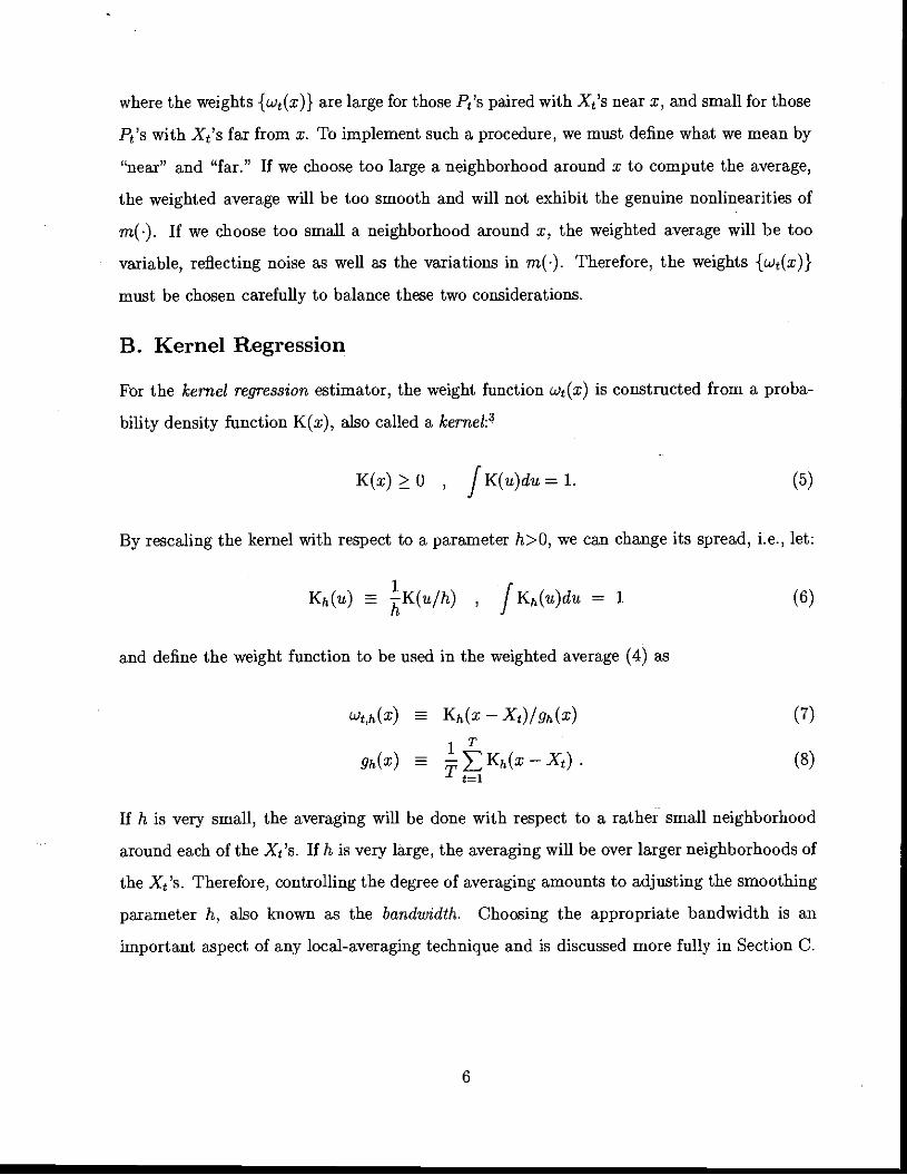
For the kernel regression estimator, the weight function Wt(x) is constructed from a proba-
bility density function K(x), also called a kernel:3
K(x) � 0 , fK(n)d'u= 1. (5)
By rescaling the kernel with respect to a parameter h>0, we can change its spread, i.e., let:
Kh(u) K(u/h) , fKh(u)du= 1 (6)
and define the weight function to be used in the weighted average (4) as
wt,h(x) — Xt)/gh(x) (7)
gh(x) fLKh(x—Xt). (8)
If h is very small, the averaging will be done with respect to a rather small neighborhood
around each of the Xe's. If h is very large, the averaging will be over larger neighborhoods of
the Xe's. Therefore, controlling the degree of averaging amounts to adjusting the smoothing
parameter Ii, also known as the bandwidth. Choosing the appropriate bandwidth is an
important aspect of any local-averaging technique and is discussed more fully in Section C.
6

Substituting (8) into (4) yields the Nadaraya- Watson kernel estimator 'thh(x) of m(x):
1 '" >i::1 Kh(x — X)Ymnh(x) = —EWt,h(X)Yt = T (9)T E=1 Khfr — X)
Under certain regularity conditions on the shape of the kernel K and the magnitudes and
behavior of the weights as the sample size grows, it may be shown, that ñth(x) converges to
ni(x) asymptotically in several ways (see Hãrdlle (1990) for further details). This convergence
property holds for a wide class of kernels, but for the remainder of this paper we shall use
the most popular choice of kernel, the Gaussian kernel:
Kh(x) = (10)
C. Selecting the Bandwidth
Selecting the appropriate bandwidth h in (9) is clearly central to the success of ñzhC) in
approximating mO—too little averaging yields a function that is too choppy, and too much
averaging yields a function that is too smooth. To illustrate these two extremes, Figure II
displays the Nadaraya-Watson kernel estimator applied to 500 datapoints generated from
the relation:
= Sin(Xt) + 0.5 c , c 'S-' N(0, 1) (11)
where X is evenly spaced in the interval [0, 2ir]. Panel 11(a) plots the raw data and the
function to be approximated.
Kernel estimators for three different bandwidths are plotted as solid lines in Panels 11(b)—
(c). The bandwidth in 11(b) is clearly too small; the function is too variable, fitting the
"noise" 0.5 t as well as the "signal" Sin(S). Increasing the bandwidth slightly yields a much
more accurate approximation to Sine) as Panel 11(c) illustrates. However, Panel 11(d) shows
that if the bandwidth is increased beyond some point, there is too much averaging and
information is lost.
There are several methods for automating the choice of bandwidth h in (9), but the most
7
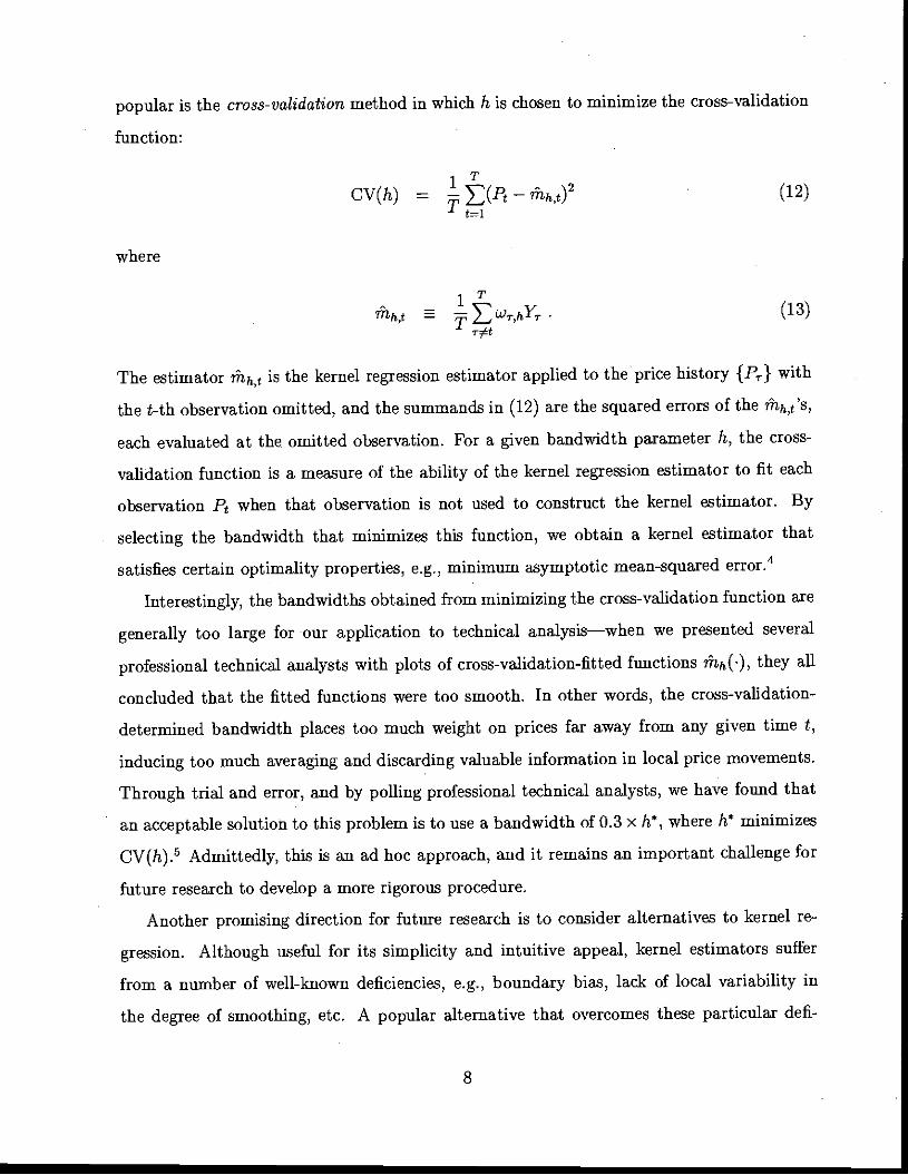
popular is the cross-validation method in which h is chosen to minimize the cross-validation
function:
CV(h) = (P - rnh,t)2 (12)
where
Tflh,t = >W,hYr (13)
The estimator iuih,t is the kernel regression estimator applied to the price history {P,-} with
the t-th observation omitted, and the summands in (12) are the squared errors of the ihh,t's,
each evaluated at the omitted observation. For a given bandwidth parameter It, the cross-
validation function is a measure of the ability of the kernel regression estimator to fit each
observation P when that observation is not used to construct the kernel estimator. By
selecting the bandwidth that minimizes this function, we obtain a kernel estimator that
satisfies certain optimality properties, e.g., minimum asymptotic mean-squared error.4
Interestingly, the bandwidths obtained from minimizing the cross-validation function are
generally too large for our application to technical analysis—when we presented several
professional technical analysts with plots of cross-validation-fitted functions ni4e), they all
concluded that the fitted functions were too smooth. In other words, the cross-validation-
determined bandwidth places too much weight on prices far away from any given time t,
inducing too much averaging and discarding valuable information in local price movements.
Through trial and error, and by polling professional technical analysts, we have found that
an acceptable solutioft to this problem is to use a bandwidth of 0.3 x h*, where h minimizes
CV(h).5 Admittedly, this is an ad hoc approach, and it remains an important challenge for
future research to develop a more rigorous procedure.
Another promising direction for future research is to consider alternatives to kernel re-
gression. Although useful for its simplicity and intuitive appeal, kernel estimators suffer
from a number of well-known deficiencies, e.g., boundary bias, lack of local variability in
the degree of smoothing, etc. A popular alternative that overcomes these particular defi-
8

ciencies is local polynomial regression in which local averaging of polynomials is performed
to obtain an estimator of tm(x) 6 Such alternatives may yield important improvements the
pattern-recognition algorithm described in Section II.
TI. Automating Technical Analysis
Armed with a mathematical representation the) of {P} with which geometric properties can
be characterized in an objective manner, we can now construct an algorithm for automating
the detection of technical patterns. Specifically, our algorithm contains three steps:
1. Define each technical pattern in terms of its geometric properties, e.g., local extrema
(maxima and minima).
2. Construct a kernel estimator thC) of a given time series of prices so that its extrema
can be determined numerically.
3. Analyze the) for occurrences of each technical pattern.
The last two steps are rather straightforward applications of kernel regression. The. first step
is likely to be the most controversial because it is here that the skills and judgment of a
professional technical analyst come into play. Although we will argue in Section A that most
technical indicators can be characterized by specific sequences of local extrema, technical
analysts may argue that these are poor approximations to the kinds of patterns that trained
human analysts can identify.
While pattern-recognition techniques have been successful in automating a number of
tasks previously considered to be uniquely human endeavors—fingerprint identification,
handwriting analysis, face recognition, and so on—nevertheless it is possible that no algo-
rithm can completely capture the skills of an experienced technical analyst. We acknowledge
that any automated procedure for pattern recognition may miss some of the more subtle nu-
ances that human cognition is capable of discerning, but whether an algorithm is a poor
approximation to human judgment can only be determined by investigating the approxima-
tion errors empirically. As long as an algorithm can provide a reasonable approximation to
9

some of the cognitive abilities of a human analyst, we can use such an algorithm to investi-
gate the empirical performance of those aspects of technical analysis for which the algorithm
is a good approximation. Moreover, if technical analysis is an art form that can be taught,
then surely its basic precepts can be quantified and automated to some degree. And as
increasingly sophisticated pattern-recognition techniques are developed, a larger fraction of
the art will become a science.
More importantly, from a practical perspective, there may be significant benefits to devel-
oping an algorithmic approach to technical analysis because of the leverage that technology
can provide. As with many other successful technologies, the automation of technical pat-
tern recognition may not replace the skills of a technical analyst, but can amplify them
considerably.
In Section A, we propose definitions of ten technical patterns based on their extrema. In
Section B, we describe a specific algorithm to identify technical patterns based on the local
extrema of kernel regression estimators, and provide specific examples of the algorithm at
work in Section C.
A. Definitions of Technical Patterns
We focus on five pairs of technical patterns that are among the most popular patterns of
traditional technical analysis (see, for example, Edwards and Magee (1966, Chapters VII—
X)): head-and-shoulders (HS) and inverse head-and-shoulders (IRS), broadening tops (BT)
and bottoms (BB), triangle tops (TT) and bottoms (TB), rectangle tops (RT) and bottoms
(RB), and double tops (DT) and bottoms (DB). There are many other technical indicators
that may be easier to detect algorithmically—moving averages, support and resistance levels,
and oscillators, for example—but because we wish to illustrate the power of smoothing
techniques in automating technical analysis, we focus on precisely those patterns that are
most difficult to quantify analytically.
Consider the systematic component me)ofa price history {P} and suppose we have iden-
tified ii local extrema, i.e., the local maxima and minima, of tm{';). Denote by E1, E2,. . . ,
the ii extrema and t, t,. . . , t the dates on which these extrema occur. Then we have the
following definitions:
10

Definition 1 (Head-and-Shoulders) Head-and-shoulders (HS) and inverted head-and-shoulders (IHS) patterns are characterized by a sequence of five consecutive local extremaE1,. . , P25 such that:
a maximum
IfS =—E1 and P25 within 1.5percent of their averageP22 and P24 within 1.5percent of their average
P21 a minimum
IHS =—F1 and F5 within 1.5percent of their averageF2 and F4 within l.5percent of their average
Observe that only five consecutive extrema are required to identify a head-and-shoulders
pattern. This follows from the formalization of the geometry of a head-and-shoulders pattern:
three peaks, with the midifie peak higher than the other two. Because consecutive extrema
must alternate between maxima and minima for smooth functions,7 the three-peaks pattern
corresponds to a sequence of five local extrema: maximum, minimum, highest maximum,
minimum, and maximum. The inverse head-and-shoulders is simply the mirror image of the
head-and-shoulders, with the initial local extrema a minimum.
Because broadening, rectangle, and triangle patterns can begin on either a local maximum
or minimum, we aUow for both of these possibilities in our definitions by distinguishing
between broadening tops and bottoms:
Definition 2 (Broadening) Broadening tops (BTOP) and bottoms (EBOT) are charac-terized by a sequence of five consecutive local extrema F1,.. . , F5 such that:
a maximum I F1 a minimumBTOP P21<E3<E5 , BBOT
1E2<P24
Definitions for triangle and rectangle patterns follow naturally:
Definition 3 (Triangle) Triangle tops (TTOF) and bottoms (TBOT) are characterized bya sequence of five consecutive local extrema Er,.. . ,E5 such that:
I E1 a maximum (F1 a minimumTTOP=— , TBOT=
L.E2<P24 IE2>E4
11
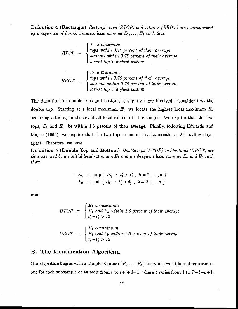
Definitign 4 (Rectangle) Rectangle tops (RTOP) and bottoms (RBOT) are characterizedby a sequence of five consecutive local extrema E1,. . . , E5 such that:
a maximum
RTOP = tops within 0. 75 percent of their average—
bottoms within 0.75 percent of their averagelowest top> highest bottom
a minimum
RBOT = tops within 0.75 percent of their average—
bottoms within 0.75 percent of their averagelowest top > highest bottom
The definition for double tops and bottoms is slightly more involved. Consider first the
double top. Starting at a local maximum E1, we locate the highest local maximum Ea
occurring after E1 in the set of all local extrema in the sample. We require that the two
tops, E1 and E, be within 1.5 percent of their average. Finally, following Edwards and
Magee (1966), we require that the two tops occur at least a month, or 22 trading days,
apart. Therefore, we have:
Definition 5 (Double Top and Bottom) Double tops (DTOP) and bottoms (DBO T) arecharacterized by an initial local extremum E1 and a subsequent local extrema E and Eb suchthat:
sup{Pç : t>t, k=2,...,n}inf{Pt : t>t , k=2,;..,n}
and
P21 a maximumDTOP Ej and E within 1.5 percent of their average
•
1t—t>22
E a minimumDBOT . P11 and Eb within 1.5 percent of their average
• 1t—t>22
B. The Identification Algorithm
Our algorithm begins with a sample of prices {P1,. .. Pr} for which we fit kernel regressions,
one for each subsample or window from t to t+l+d—1, where t varies from 1 to T—l—d+1,
12

and I and d are fixed parameters whose purpose is explained below. In the empirical analysis
of Section III, we set I =35 and d = 3, hence each window consists of 38 trading days.
The motivation for fitting kernel regressions to rolling windows of data is to narrow our
focus to patterns that are completed within the span of the window—i + d trading days in
our case. If we fit a single kernel regression to the entire dataset, many patterns of various
durations may emerge, and without imposing some additional structure on the nature of the
patterns, it is virtually impossible to distinguish signal from noise in this case. Therefore,
our algorithm fixes the length of the window at I+d, but kernel regressions are estimated on
a rolling basis and we search for patterns in each window.
Of course, for any fixed window, we can only find patterns that are completed within l+d
trading days. Without further structure on the systematic component of prices me), this is
a restriction that any empirical analysis must contend with.8 We choose a shorter window
length of 1 = 35 trading days to focus on short-horizon patterns that may be more relevant
for active equity traders, and leave the analysis of longer-horizon patterns to future research.
The parameter d controls for the fact that in practice we do not observe a realization of
a given pattern as soon as it has completed. Instead, we assume that there may be a lag
between the pattern completion and the time of pattern detection. To account for this lag,
we require that the final extremum that completes a pattern occurs on day t+l—1; hence d is
the number of days following the completion of a pattern that must pass before the pattern
is detected. This will become more important in Section III when we compute conditional
returns, conditioned on the realization of each pattern. In particular, we compute post-
pattern returns starting from the end of trading day t+l+d, i.e., one day after the pattern
has completed. For example, if we determine that a head-and-shoulder pattern has completed
on day t + 1— 1 (having used prices from time t through time t + 1 + d —1), we compute the
conditional one-day gross return as Yt+l+d+1/Yt÷l+d. Hence we do not use any forward
information in computing returns conditional on pattern completion. In other words, the
lag d ensures that we are computing our conditional returns completely out-of-sample and
without any "look-ahead" bias.
Within each window, we estimate a kernel regression using the prices in that window,
13
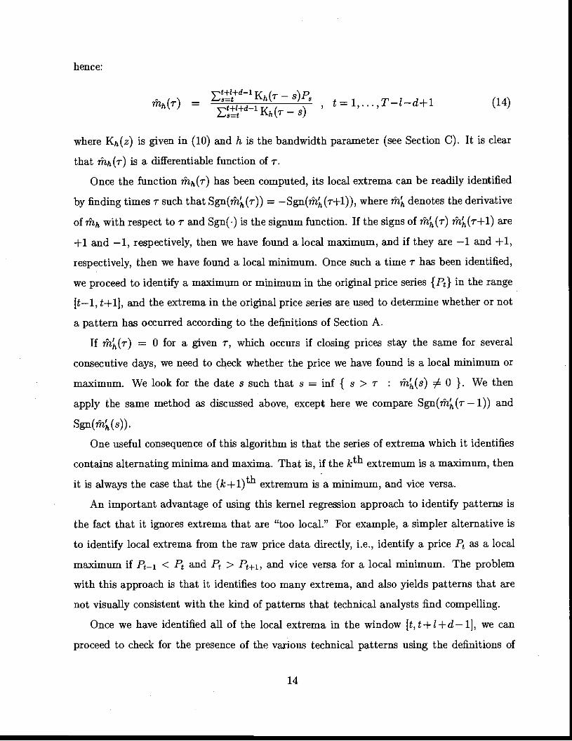
hence:
Et+l+d—1it I \ fl
I \ — s=t flhkr—S).I—, .mhkr) —
'c-'t+t+d—liy I ' — —
L.5=t IhkT — 8)
where Kh(z) is given in (10) and h is the bandwidth parameter (see Section C). It is clear
that ñih(r) is a differentiable function of r.
Once the function ñ'ih(r) has been computed, its local extrema can be readily identified
by finding times r such that Sgn(ñz(r)) = —Sgn(n4(r+1)), where ñz denotes the derivative
of flih with respect to r and Sgn(.) is the signum function. If the signs of ñ%(r) ñt(r+1) are
+1 and —1, respectively, then we have found a local maximum, and if they are —1 and +1,
respectively, then we have found a local minimum. Once such a time r has been identified,
we proceed to identify a maximum or minimum in the original price series {P} in the range
[t—i, t+iJ, and the extrema in the original price series are used to determine whether or not
a pattern has occurred according to the definitions of Section A.
If th(r) = 0 for a given i-, which occurs if closing prices stay the same for several
consecutive days, we need to check whether the price we have found is a local minimum or
maximum. We look for the date s such that s = inf { s > r : ñz(s) $ 0 }. We then
apply the same method as discussed above, except here we compare Sgn(i%(r —1)) and
Sgn(u14(s)).
One useful consequence of this algorithm is that the series of extrema which it identifies
contains alternating minima and maxima. That is, if the kth extremum is a maximum, then
it is always the case that the (k+l)th extremum is a minimum, and vice versa.
An important advantage of using this kernel regression approach to identify patterns is
the fact that it ignores extrema that are "too local." For example, a simpler alternative is
to identify local extrema from the raw price data directly, i.e., identify a price P as a local
maximum if P,1 C Pt and P, > P+1, and vice versa for a local minimum. The problem
with this approach is that it identifies too many extrema, and also yields patterns that are
not visually consistent with the kind of patterns that technical analysts find compelling.
Once we have identified all of the local extrema in the window [t, t + I + d — 1], we can
proceed to check for the presence of the various technical patterns using the definitions of
14

Section A. This procedure is then repeated for the next window [t+i, t+l+d] ,and continues
until the end of the sample is reached at the window [T —i —d+ 1, T].
C. Empirical Examples
To see how our algorithm performs in practice, we apply it to the daily returns of a single
security, CTX, during the five-year period from 1992 to 1996. Figures 111—Vu plot occur-
rences of the five pairs of patterns defined in Section A that were identified by our algorithm.
Note that there were no rectangle bottoms detected for CTX during this period, so for com-
pleteness we substituted a rectangle bottom for CDO stock which occurred during the same
period.
In each of these graphs, the solid lines are the raw prices, the dashed lines are the kernel
estimators mh(•), the circles indicate the local extrema, and the vertical line marks date
t+l —1, the day that the final extremum occurs to complete the pattern.
Casual inspection by several professional technical analysts seems to confirm the ability of
our automated procedure to match human judgment in identifying the five pairs of patterns
in Section A. Of course, this is merely anecdotal evidence and not meant to be conclusive—
we provide these• figures simply to illustrate the output of a technical pattern recognition
algorithm based on kernel regression.
III. Is Technical Analysis Informative?
Although there have been many tests of technical analysis over the years, most of these tests
have focused on the profitability of technical trading rules.9 While some of these studies do
find that technical indicators can generate statistically significant trading profits, they beg
the question of whether or not such profits are merely the equilibrium rents that accrue to
investors willing to bear the risks associated with such strategies. Without specifying a fully
articulated dynamic general equilibrium asset-pricing model, it is impossible to determine
the economic source of trading profits.
Instead, we propose a more fundamental test in this section, one that attempts to gauge
the information content in the technical patterns of Section A by comparing the unconditional
15

empirical distribution of returns with the coriesponding conditional empirical distribution,
conditioned on the occurrence of a technical pattern. If technical patterns are informative,
conditioning on them should alter the empirical distribution of returns; if the information
contained in such patterns has already been incorporated into returns, the conditional and
unconditional distribution of returns should be close. Although this is a weaker test of the
effectiveness of technical analysis—informativeness does not guarantee a profitable trading
strategy—it is, nevertheless, a natural first step in a quantitative assessment of technical
analysis.
To measure the distance between the two distributions, we propose two goodness-of-fit
measures in Section A. We apply these diagnostics to the daily returns of individual stocks
from 1962 to 1996 using a procedure described in Sections B to D, and the results are
reported in Sections E and F.
A. Goodness-of-Fit Tests
A simple diagnostic to test the informativeness of the ten technical patterns is to compare the
quantiles of the conditional returns with their unconditional counterparts. If conditioning on
these technical patterns provides no incremental information, the quantiles of the conditional
returns should be similar to those of unconditional returns. In particular, we compute the
deciles of unconditional returns and tabulate the relative frequency 5 of conditional returns
falling into decile j of the unconditional returns, j= 1,. . ., 10:
number of conditional returns in decile15
total number of conditional returns
Under the null hypothesis that the returns are independently and identically distributed and
the conditional and unconditional distributions are identical, the asymptotic distributions of
S and the corresponding goodness-of-fit test statistic Q are given by:
—0.10) Qi Af(0, 0.10(1—0.10)) (16)
Q (nj_0J0n)2 (17)
16
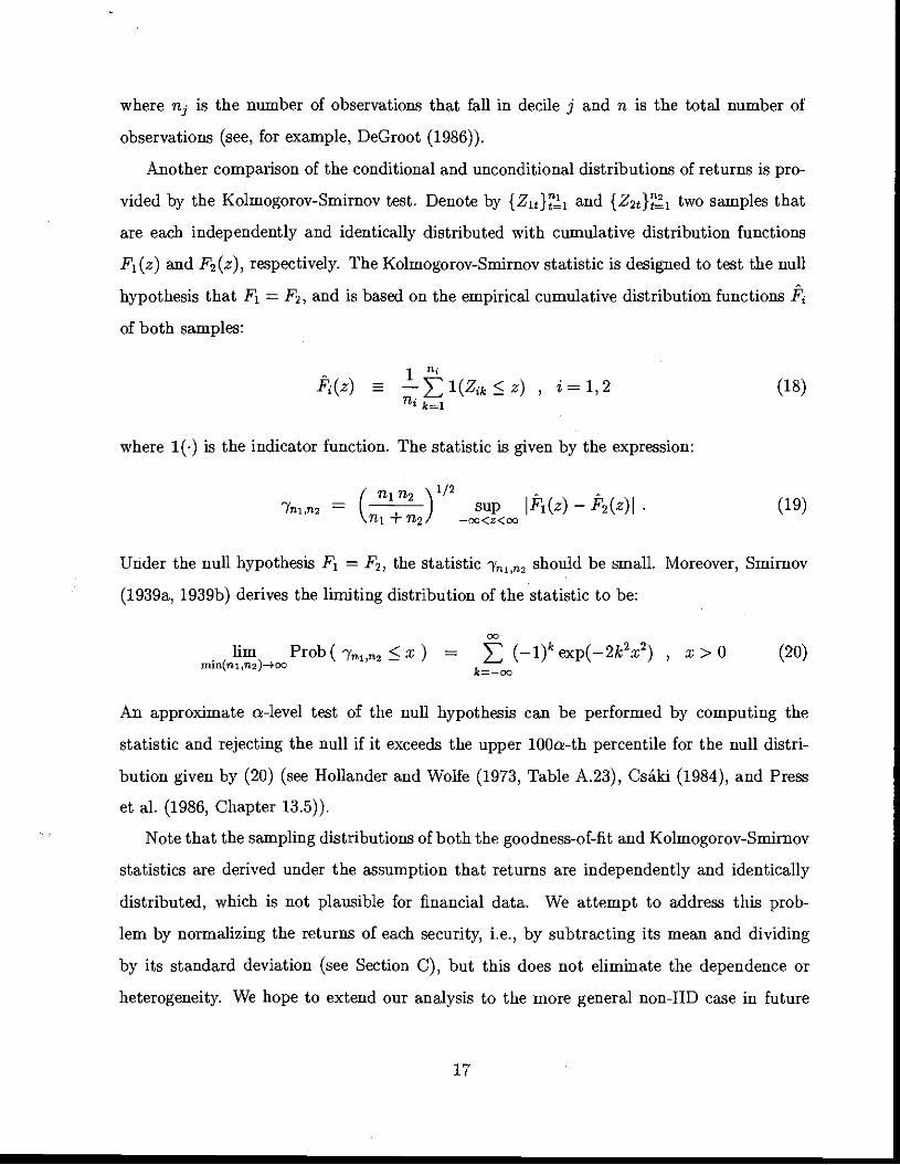
where nj is the number of observations that fall in decile j and n is the total number of
observations (see, for example, DeGroot (1986)).
Another comparison of the conditional and unconditional distributions of returns is pro-
vided by the Kolmogorov-Smirnov test. Denote by {Z1}1 and {Z2}1 two samples that
are each independently and identically distributed with cumulative distribution functions
Fi(z) and F2(z), respectively. The Kolmogorov-Smirnov statistic is designed to test the null
hypothesis that F1 = F2, and is based on the empirical cumulative distribution functions N
of both samples:
i=1,2 (18)k=i
where 1(.) is the indicator function. The statistic is given by the expression:
7m1,n2=
(n1n2
)1/2 sup Ei(z) —fr2(z)I . (19)Ti1 + n2
Under the null hypothesis F1 = F2, the statistic 'y,,22 should be small. Moreover, Smirnov
(1939a, 1939b) derives the limiting distribution of the statistic to be:
lim Prob( 'y1,2 x) = E (_1)k exp(—2k2x2) , x> 0 (20)mm(ni ,fl2)—*oC k=—oo
An approximate a-level test of the null hypothesis can be performed by computing the
statistic and rejecting the null if it exceeds the upper lOOa-th percentile for the null distri-
bution given by (20) (see Hollander and Wolfe (1973, Table A.23), Csáki (1984), and Press
et al. (1986, Chapter 13.5)).
Note that the sampling distributions of both the goodness-of-fit and Kolmogorov-Smirnov
statistics are derived under the assumption that returns are independently and identically
distributed, which is not plausible for financial data. We attempt to address this prob-
lem by normalizing the returns of each security, i.e., by subtracting its mean and dividing
by its standard deviation (see Section C), but this does not eliminate the dependence or
heterogeneity. We hope to extend our analysis to the more general non-lID case in future
17

research.
B. The Data and Sampling Procedure
We apply the goodness-of-fit and Kolmogorov-Smirnov tests to the daily returns of indi-
vidual NYSE/AMEX and Nasdaq stocks from 1962 to 1996 using data from the Center for
Research in Securities Prices (CRSP). To ameliorate the effects of nonstationarities induced
by changing market structure and institutions, we split the data into NYSE/AMEX stocks
and Nasdaq stocks and into seven five-year periods: 1962 to 1966, 1967 to 1971, and so on.
To obtain a broad cross-section of securities, in each five-year subperiod, we randomly select
ten stocks from each of five market-capitalization quintiles (using mean market-capitalization
over the subperiod), with the further restriction that at least 75 percent of the price obser-
vations must be non-missing during the subperiod.'° This procedure yields a sample of 50
stocks for each subperiod across seven subperiods (note that we sample wjth replacement,
hence there may be names in common across subp eriods).
As a check on the robustness of our inferences, we perform this sampling procedure twice
to construct two samples, and apply our empirical analysis to both. Although we report
results only from the first sample to conserve space, the results of the second sample are
qualitatively consistent with the first and are available upon request.
C. Computing Conditional Returns
For each stock in each subperiod, we apply the procedure outlined in Section II to identify
all occurrences of the ten patterns deBited in Section A. For each pattern detected, we com-
pute the one-day continuously compounded return d days after the pattern has completed.
Specifically, consider a window of prices {P} from t to t+l +d— 1, and suppose that the
identified pattern p is completed at t + I —1. Then we take the conditional return R' as
log(1 + R+1÷i). Therefore, for each stock, we have ten sets of such conditional returns,
each conditioned on one of the ten patterns of Section A.
For each stock, we construct a sample of unconditional continuously compounded returns
using non-overlapping intervals of length r, and we compare the empirical distribution func-
tion of these returns with those of the conditional returns. To facilitate such comparisons,
18
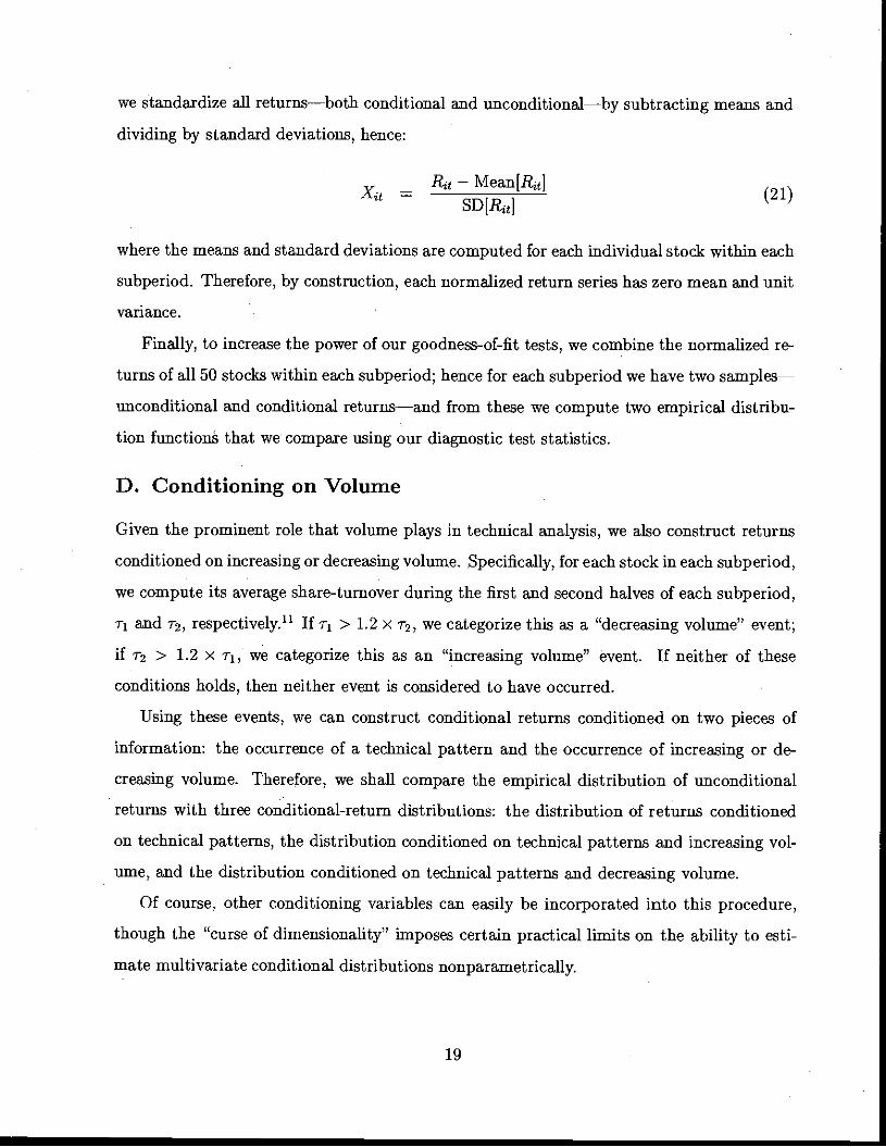
we standardize all returns—both conditional and unconditional—by subtracting means and
dividing by standard deviations, hence:
— — Mean[Rt]21it —
SD[Rj]'
where the means and standard deviations are computed for each individual stock within each
subperiod. Therefore, by construction, each normalized return series has zero mean and unit
variance.
Finally, to increase the power of our goodness-of-fit tests, we combine the normalized re-
turns of all 50 stocks within each subperiod; hence for each subperiod we have two samples—
unconditional and conditional returns—and from these we compute two empirical distribu-
tion functions that we compare using our diagnostic test statistics.
D. Conditioning on Volume
Given the prominent role that volume plays in technical analysis, we also construct returns
conditioned on increasing or decreasing volume. Specifically, for each stock in each subperiod,
we compute its average share-turnover during the first and second halves of each subperiod,
r1 and r2, respectively." If i-, > 1.2 x r2, we categorize this as a "decreasing volume" event;
if r2 > 1.2 x r1, we categorize this as an "increasing volume" event. If neither of these
conditions holds, then neither event is considered to have occurred.
Using these events, we can construct conditional returns conditioned on two pieces of
information: the occurrence of a technical pattern and the occurrence of increasing or de-
creasing volume. Therefore, we shall compare the empirical distribution of unconditional
returns with three conditional-return distributions: the distribution of returns conditioned
on technical patterns, the distribution conditioned on technical patterns and increasing vol-
ume, and the distribution conditioned on technical patterns and decreasing volume.
Of course, other conditioning variables can easily be incorporated into this procedure,
though the "curse of dimensionality" imposes certain practical limits on the ability to esti-
mate multivariate conditional distributions nonparametrically.
19

E. Summary Statistics
In Tables I and II, we report frequency counts for the number of patterns detected over the
entire 1962 to 1996 sample, and within each subperiod and each market-capitalization quin-
tile, for the ten patterns defined in Section A. Table I contains results for the NYSE/AMEX
stocks, and Table II contains corresponding results for Nasdaq stocks.
Table I shows that the most common patterns across all stocks and over the entire sam-
ple period are double tops and bottoms (see the row labelled "Entire"), with over 2,000
occurrences of each. The second most common patterns are the head-and-shoulders and
inverted head-and-shoulders, with over 1,600 occurrences of each. These total counts corre-
spond roughly to four to six occurrences of each of these patterns for each stock during each
five-year subperiod (divide the total number of occurrences by 7 x 50), not an unreasonable
frequency from the point of view of professional technical analysts. Table I shows that most
of the ten patterns are more frequent for larger stocks than for smaller ones, and that they
are relatively evenly distributed over the five-year subperiods. When volume trend is con-
sidered jointly with the occurrences of the ten patterns, Table I shows that the frequency
of patterns is not evenly distributed between increasing (the row labelled "r(,)") and de-
creasing (the row labelled "r(N)") volume-trend cases. For example, for the entire sample
of stocks over the 1962 to 1996 sample period, there are 143 occurrences of a broadening
top with decreasing volume trend, but 409 occurrences of a broadening top with increasing
volume trend.
For purposes of comparison, Table I also reports frequency counts for the number of pat-
terns detected in a sample of simulated geometric Brownian motion, calibrated to match the
mean and standard deviation of each stock in each five-year subperiod.12 The entries in the
row labelled "Sim. GBM" show that the random walk model yields very different implications
for the frequency counts of several technical patterns. For example, the simulated sample
has only 577 head-and-shoulders and 578 inverted-head-and-shoulders patterns, whereas the
actual data have considerably more, 1,611 and 1,654, respectively. On the other hand, for
broadening tops and bottoms, the simulated sample contains many more occurrences than
the actual data, 1,227 and 1,028 as compared to 725 and 748, respectively. The number of
20
triangles is roughly comparable across the two samples, but for rectangles and double tops
and bottoms, the differences are dramatic. Of course, the simulated sample is only one real-
ization of geometric Brownian motion, so it is difficult to draw general conclusions about the
relative frequencies. Nevertheless, these simulations point to important differences between
the data and independently and identically distributed lognormal returns.
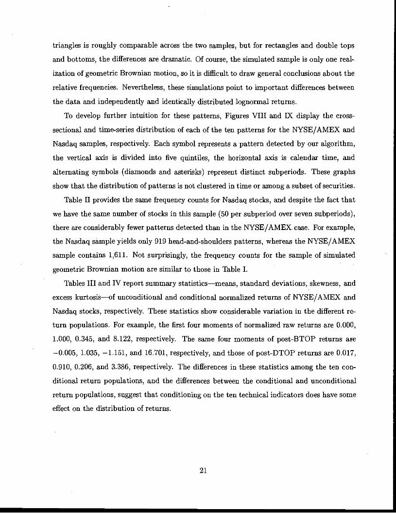
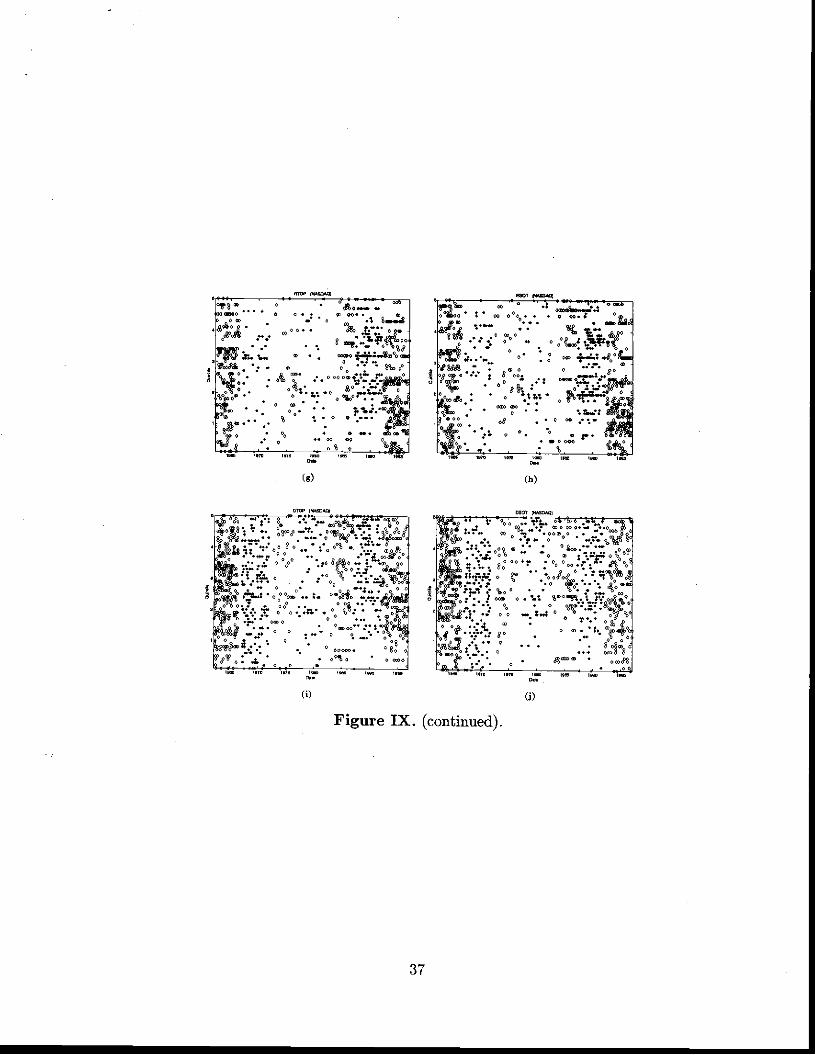
To develop further intuition for these patterns, Figures VIII and IX display the cross-
sectional and time-series distribution of each of the ten patterns for the NYSE/AMEX and
Nasdaq samples, respectively. Each symbol represents a pattern detected by our algorithm,
the vertical axis is divided into five quintiles, the horizontal axis is calendar time, and
alternating symbols (diamonds and asterisks) represent distinct subperiods. These graphs
show that the distribution of patterns is not clustered in time or among a subset of securities.
Table II provides the same frequency counts for Nasdaq stocks, and despite the fact that
we have the same number of stocks in this sample (50 per subperiod over seven subperiods),
there are considerably fewer patterns detected than in the NYSE/AMEX case. For example,
the Nasdaq sample yields only 919 head-and-shoulders patterns, whereas the NYSE/AMEX
sample contains 1,611. Not surprisingly, the frequency counts for the sample of simulated
geometric Brownian motion are similar to those in Table I.
Tables III and IV report suumiary statistics—means, standard deviations, skewness, and
excess kurtosis—of unconditional and conditional normalized returns of NYSE/AMEX and
Nasdaq stocks, respectively. These statistics show considerable variation in the different re-
turn populations. For example, the first four moments of normalized raw returns are 0.000,
1.000, 0.345, and 8.122, respectively. The same four moments of post-BTOP returns are
—0.005, 1.035, —1.151, and 16.701, respectively, and those of post-DTOP returns are 0.017,
0.910, 0.206, and 3.386, respectively. The differences in these statistics among the ten con-
ditional return populations, and the differences between the conditional and unconditional
return populations, suggest that conditioning on the ten technical indicators does have some
effect on the distribution of returns.
21

F. Empirical Results
Tables V and Vi reports the results of the goodness-of-fit test (16)—(l7) for our sample of
NYSE and AMEX (Table V) and Nasdaq (Table VI) stocks, respectively, from 1962 to 1996
for each of the ten technical patterns. Table V shows that in the NYSE/AMEX sample,
the relative frequencies of the conditional returns are significantly different from those of the
unconditional returns for seven of the ten patterns considered. The three exceptions are the
conditional returns from the BBOT, TTOP, and DBOT patterns, for which the p-values of
the test statistics Qare 5.1 percent, 21.2 percent, and 16.6 percent respectively. These results
yield mixed support for the overall efficacy of technical indicators. However, the results of
Table VI tell a different story: there is overwhelming significance for all ten indicators in the
Nasdaq sample, with p-values that are zero to three significant digits, and test statistics Q
that range from 34.12 to 92.09. In contrast, the test statistics inTable V range from 12.03
to 50.97.
One possible explanation for the difference between the NYSE/AMEX and Nasdaq
samples is a difference in the power of the test because of different sample sizes. If the
NYSE/AMEX sample contained fewer conditional returns, i.e., fewer patterns, the corre-
sponding test statistics might be subject to greater sampling variation and lower power.
However, this explanation can be ruled out from the frequency counts of Tables I and II—
the number of patterns in the NYSE/AMEX sample is considerably larger than those of the
Nasdaq sample for all ten patterns. Tables V and VI seem to suggest important differences
in the informativeness of technical indicators for NYSE/AMEX and Nasdaq stocks.
Table VII and VIII report the results of the Kolmogorov-Smirnov test (19) of the equality
of the conditional and unconditional return distributions for NYSE/AMEX (Table VII) and
Nasdaq (Table VIII) stocks, respectively, from 1962 to 1996, in five-year subperiods, and
in market-capitalization quintiles. Recall that conditional returns are defined as the one-
day return starting three days following the conclusion of an occurrence of a pattern. The
p-values are with respect to the asymptotic distribution of the Kolmogorov-Smirnov test
statistic given in (20).
Table VII shows that for NYSE/AMEX stocks, five of the ten patterns—HS, BBOT,
22

RTOP, RBOT, and DTOP—yield statistically significant test statistics, with p-values rang-
ing from 0.000 for RBOT to 0.021 for DTOP patterns. However, for the other five patterns,
the p-values range from 0.104 for IRS to 0.393 for DBOT, which implies an inability to
distinguish between the conditional and unconditional distributions of normalized returns.
When we condition on declining volume trend as well, the statistical significance declines
for most patterns, but increases the statistical significance of TBOT patterns. In contrast,
conditioning on increasing volume trend yields an increase in the statistical significance of
BTOP patterns. This difference may suggest an important role for volume trend in TBOT
and BTOP patterns. The difference between the increasing and decreasing volume-trend
conditional distributions is statistically insignificant for almost all the patterns (the sole
exception is the TBOT pattern). This drop in statistical significance may be due to a lack
of power of the K-S test given the relatively small sample sizes of these conditional returns
(see Table I for frequency counts).
Table VIII reports corresponding results for the Nasdaq sample and as in Table VI, in
contrast to the NYSE/AMEX results, here all the patterns are statistically significant at
the 5 percent level. This is especially significant because the the Nasdaq. sample exhibits far
fewer patterns than the NYSE/AMEX sample (see Tables I and II), hence the K-S test is
likely to have lower power in this case.
As with the NYSE/AMEX sample, volume trend seems to provide little incremental
information for the Nasdaq sample except in one case: increasing volume and BTOP. And
except for the TTOP pattern, the K-S test still cannot distinguish between the decreasing
and increasing volume-trend conditional distributions, as the last pair of rows of Table Viii's
first panel indicates.
IV. Monte Carlo Analysis
Tables IX and X contain bootstrap percentiles for the Kolmogorov-Smirnov test of the equal-
ity of conditional and unconditional one-day return distributions for NYSE/AMEX and Nas-
daq stocks, respectively, from 1962 to 1996, and for market-capitalization quintiles, under
the null hypothesis of equality, For each of the two sets of market data, two sample sizes,
23

in1 and in2, have been chosen to span the range of frequency counts of patterns reported
in Tables I and II. For each sample size m, we resample one-day normalized returns (with
replacement) to obtain a bootstrap sample of in1 observations, compute the Kolmogorov-
Smirnov test statistic (against the entire sample of one-day normalized returns), and repeat
this procedure 1,000 times. The percentiles of the asymptotic distribution are also reported
for comparison under the column "-y".
Tables IX and X show that for a broad range of sample sizes and across size quintiles,
subperiod, and exchanges, the bootstrap distribution of the Kohnogorov-Smirnov statistic
is well approximated by its asymptotic distribution (20).
V. Conclusion
In this paper, we have proposed a new approach to evaluating the efficacy of technical anal-
ysis. Based on smoothing techniques such as nonparametric kernel regression, our approach
incorporates the essehce of technical analysis: to identify regularities in the time series of
prices by extracting nonlinear patterns from noisy data. While human judgment is still
superior to most computational algorithms in the area of visual pattern recognition, recent
advances in statistical learning theory have had successful applications in fingerprint identi-
fication, handwriting analysis, and face recognition. Technical analysis may well be the next
frontier for such methods.
When applied to many stocks over many time periods, we find that certain technical
patterns do provide incremental information, especially for Nasdaq stocks. While this does
not necessarily imply that technical analysis can be used to generate "excess" trading profits,
it does raise the possibility that technical analysis can add value to the investment process.
Moreover, our methods suggest that technical analysis can be improved by using auto-
mated algorithms such as ours, and that traditional patterns such as head-and-shoulders and
rectangles, while sometimes effective, need not be optimal. In particular, it may be possible
to determine "optimal patterns" for detecting certain types of phenomena in financial time
series, e.g., an optimal shape for detecting stochastic volatility or changes in regime. More-
over, patterns that are optimal for detecting statistical anomalies need not be optimal for
24

trading profits, and vice versa. Such considerations may lead to an entirely new branch of
technical analysis, one based on selecting pattern recognition algorithms to optimize specific
objective functions. We hope to explore these issues more fully in future research.
25

Footnotes
1A similar approach has been proposed by Chang and Osler (1994) and Osler and Chang(1995) for the case of foreign-currency trading rules based on a head-and-shouiders pat-tern. They develop an algorithm for automatically detecting geometric patterns in price orexchange data by looking at properly defined local extrema.
2See, for example, Beymer and Poggio (1996), Poggio and Beymer (1996), and Riesenhu-ber and Poggio (1997).
3flespite the fact that K(x) is a probability density function, it plays no probabilisticrole in the subsequent analysis—it is merely a convenient method for computing a weightedaverage, and does not imply, for example, that X is distributed according to K(x) (whichwould be a parametric assumption).
4However, there are other bandwidth-selection methods that yield the same asymptoticoptimality properties but which have different implications for the finite-sample propertiesof kernel estimators. See Hãrdle (1990) for further discussion.
5Specifically, we produced fitted curves for various bandwidths and compared their ex-trema to the original price series visually to see if we were fitting more "noise" than "signal,"and asked several professional technical analysts to do the same. Through this informal pro-cess, we settled on the bandwidth of 0.3 x h and used it for the remainder of our analysis.This procedure was followed before we performed the statistical analysis of Section III, andwe made no revision to the choice of bandwidth afterwards.
6See Simonoff (1996) for a discussion of the problems with kernel estimators and alter-natives such as local polynomial regression.
TAfter all, for two consecutive maxima to be local maxima, there must be a local minimumin between, and vice versa for two consecutive minima.
81f we are willing to place additional restrictions on me),. e.g., linearity, we can obtainconsiderably more accurate inferences even for partially completed patterns in any fixedwindow.
9For example, Chang and Osler (1994) and Osler and Chang (1995) propose an algorithmfor automatically detecting head-and-shoulders patterns in foreign exchange data by lookingat properly defined local extrema. To assess the efficacy of a head-and-shoulders trading rule,they take a stand on a class of trading strategies and compute the profitability of these acrossa sample of exchange rates against the U.S. dollar. The null return distribution is computedby a bootstrap that samples returns randomly from the original data so as to induce temporalindependence in the bootstrapped time series. By comparing the actual returns from tradingstrategies to the bootstrapped distribution, the authors find that for two of the six currenciesin their sample (the yen and the Deutsche mark), trading strategies based on a head andshoulders pattern can lead to statistically significant profits. See, also, Neftci and Policano(1984), Pruitt and White (1988), and Brock, Lakonishok, and LeBaron (1992).
'°If the first price observation of a stock is missing, we set it equal to the first non-missingprice in the series. If the t-th price observation is missing, we set it equal to the firstnon-missing price prior to t.
11For the Nasdaq stocks, r1 is the average turnover over the first third of the sample, andr2. is the average turnover over the final third of the sample.
26
12[u particular, let the price process satisfy
dP(t) = jzP(t) dt + cP(t) dW(t) (22)
where W(t) is a standard Brownian motion. To generate simulated prices for a single securityin a given period, we estimate the security's drift and diffusion coefficients by maximumlikelihood and then simulate prices using the estimated parameter values. An independentprice series is simulated for each of the 350 securities in both the NYSE/AMEX and theNasdaq samples. Finally, we use our pattern recognition algorithm to detect the occurrenceof each of the ten patterns in the simulated price series.
27

References
Allen, Franklin and Risto Karjalainen, 1999, Using genetic algorithms to find technicaltrading rules, Journal of Financial Economics 51, 245—271.
Beymer, David and Tomaso Poggio, 1996, Image representation for visual learning, Science272, 1905—1909.
Blume, Lawrence, Easley, David and Maureen O'Hara, 1994, Market statistics and technicalanalysis: The role of volume, Journal of Finance 49, 153—181.
Brock, William, Lakonishok, Joseph and Blake LeBaron, 1992, Simple technical tradingrules and the stochastic properties of stock returns, Journal of Finance 47, 1731—1764.
Brown, David and Robert Jennings, 1989, On technical analysis, Review of Financial Stud-ies 2, 527—551.
Campbell, John, Lo, Andrew W. and A. Craig MacKinlay, 1997, The Econometrics ofFinancial Markets. Princeton, NJ: Princeton University Press.
Chan, Louis, Jegadeesh, Narasimhan and Joseph Lakonishok, 1996, Momentum strategies,Journal of Finance 51, 1681—1713.
Chang, Kevin and Carol Osler, 1994, Evaluating chart-based technical analysis: The head-and-shoulders pattern in foreign exchange markets, working paper, Federal ReserveBank of New York.
Csáki, E., 1984, Empirical distribution function, in P. Krislmaiah and P. Sen, eds., Handbookof Statistics, Volume.4 (Elsevier Science Publishers, Amsterdam, The Netherlands).
DeGroot, Morris, 1986, Probability and Statistics (Addison Wesley Publishing Company,Reading, MA).
Edwards, Robert and John Magee, 1966, Technical Analysis of Stock Trends, 5th Edition(John Magee Inc., Boston, MA).
Grundy, Bruce and S. Martin, 1998, Understanding the nature of the risks and the sourceof the rewards to momentum investing, unpublished working paper, Wharton School,University of Pennsylvania.
Hãrdle, Wolfgang, 1990, Applied Nonparametric Regression (Cambridge University Press,Cambridge, UK).
Hollander, Myles and Douglas Wolfe, 1973, Nonparametric Statistical Methods (John Wiley& Sons, New York, NY).
Jegadeesh, Narasimhan and Sheridan Titman, 1993, Returns to buying winners and sellinglosers: Implications for stock market efficiency, Journal of Finance 48, 65—91.
Lo, Andrew W. and A. Craig MacKinlay, 1988, Stock market prices do not follow randomwalks: Evidence from a simple specification test, Review of Financial Studies 1, 41—66.
Lo, Andrew W. and A. Craig MacKinlay, 1997, Maximizing predictability in the stock andbond markets, Macroeconomic Dynamics 1(1997), 102—134.
28
Lo, Andrew W. and A. Craig MacKinlay, 1999, A Non-Random Walk Down Wall Street(Princeton University Press, Princeton, NJ).
Malkiel, Burton, 1996, A Random Walk Down Wall Street: Including a Life-Cycle Guideto Personal Investing (W.W. Norton, New York, NY).
Neely, Christopher, Weller, Peter and Robert Dittmar, 1997, Is technical analysis in theforeign exchange market profitable? A genetic programming approach, Journal ofFinancial and Quantitative Analysis 32, 405—426.
Neely, Christopher and Peter Weller, 1998, Technical trading rules in the european mone-tary system, working paper, Federal Bank of St. Louis.
Neftci, Salih, 1991, Naive trading rules in financial markets and wiener-kolmogorov predic-tion theory: K study of technical analysis, Journal of Business 64, 549—571.
Neftci, Salih and Andrew Policano, 1984, Can chartists outperform the market? Marketefficiency tests for 'technical analyst' , Journal of Future Markets 4, 465—478.
Osler, Carol and Kevin Chang, 1995, Head and shoulders: Not just a flaky pattern, StaffReportNo. 4, Federal Reserve Bank of New York.
Poggio, Tomaso and David Beymer, 1996, Regularization networks for visual learning, inShree Nayar and Tomaso Poggio, eds., Early Visual Learning (Oxford University Press,Oxford, UK).
Press, William, Flannery, Brian, Teukolsky, Saul and William Vetterling, 1986, NumericalRecipes: The Art of Scientific Computing (Cambridge University Press, Cambridge,UK).
Pruitt, Stephen and Robert White, 1988, The CRISMA trading system: Who says technicalanalysis can't beat the market?. Journal of Portfolio Management 14, 55—58.
Riesenhuber, Maximilian and Tomaso Poggio, 1997, Common computational strategies inmachine and biological vision, in Proceedings of International Symposium on SystemLife. Tokyo, Japan, 67—75.
Rouwenhorst, Geert, 1998, International momentum strategies, Journal of Finance 53,26 7—284.
Simonoff, Jeffrey, 1996, Smoothing Methods in Statistics (Springer-Verlag, New York, NY):
Smirnov, N., 1939a, Sur les écarts de la courbe de distribution empirique, Eec. Math.(Mat. Sborn.) 6, 3—26.
Smirnov, N., 1939b, On the estimation of the discrepancy between empirical curves ofdistribution for two independent samples, Bulletin. Math. Univ. Moscow 2, 3—14.
Tabell, Anthony and Edward Tabell, 1964, The case for technical analysis, Financial Ana-lyst Journal 20, 67—76.
Treynor, Jack and Robert Ferguson, 1985, In defense of technical analysis, Journal ofFinance 40, 757—773.
29

Price
Volume
Volume
liii II' 11111 I iiiiHI''''
''liiiliiiiIiiil liii'liii
I
1111111
11M.J .IIId,ItI.IIIiIJS IJ,li.iiiiLIi idL1iii1l I
Price
I
' 'II'I'III
''Ill'
'.IIIIiIiII.I,IHiI,II iIII,11ii111 iiI I
Figure I. Two hypothetical price/volume charts.
30
Date
Date

n.no
Simulated DaIs V — Sin(K) + .5Z
1.57 3,14
(,)
Kernel E.limntn lnrY—SntK3+,5Z. I, —
.57 7.53 4.71
S
(c)
Kernel [eLimut. Car 1—01,7110* .5Z. 4—. In
.37 7.14 4.71 - 4,24
(b)
- Kanral F.ti.nutn nrVSir(3)+ ,SZ. h2.nn -
0.00 .57 3.14 4.71 1,20
0-
(a)
Figure II. Illustration of bandwidth selection for kernel regression.
551 . — .I
() HeaSand-Shonuldern (b) Inverse Head-and-Shouldern
Figure III. Head-and-shoulders and inverse head-and-shoulders.
31
-
—-' tcuc3.—.f. -
:-x.-• &
-ITE
H-
- -
Sr.-:

I;
/ !.— IIj\j I
.1
•
t\, r\J
TTt#4 ..?C.La) Broadening Top tIi) Hro&den,ng Bottom
Figure IV. Broadening tops and bottoms.
_____________ :..._..
flM j. f ¼
V
3) ,,•,I p
0 . • •
* i. aon
La' TTiangl. Ti p (II) triangle Rotton'
Figure V. Triangle tops and bottoms.
32

Figure VI. Rectaig1e tops and bottoms.
O..si, crc fQ%Glfl -344I r- II I-klr
I - I - I
0-
no
*9 I II
an- I /I
20 I;44 14
- - .
49
I a I Dot. hic Toj I Lj Don I I. 13. Ittfln
Figure VII. Double tops and bottoms.
(a) Rectangle Top (I,) Rectangle Bottom
33

Figure VIII. Distribution of patterns in NYSE/AMEX sample.
34
(a) (b)
o o
:°
00
v; %04* —000 0
000 0
0(c) (a)
(0)

Figure VIII. (continued).
35
(g) (h)
0(i) (j)

4
Figure IX. Distribution of patterns in NASDAQ sample.
36
C,) (b)
_gr —00
oco0%• o.°4t 0
00000 •t 0
08
0oc:
4 o o00
.0 •°_ — 0%0 00
(c) (dY
(0) (I)
m' —
37
Cs) (h)
(i) ci)
Figure IX. (continued).
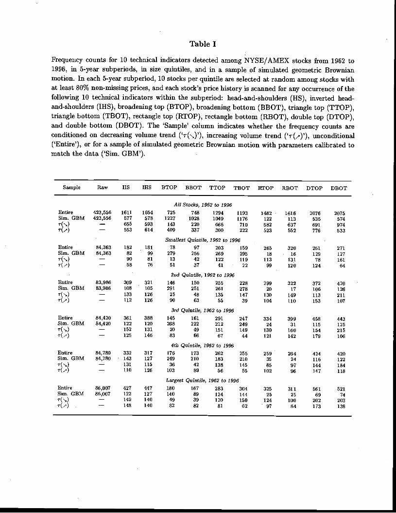
Table I
Frequency counts for 10 technical indicators detected among NYSE/AMEX stocks from 1962 to1996, in 5-year subperiods, in size quintiles, and in a sample of simulated geometric Brownianmotion. In each 5-year subperiod, 10 stocks per quintile are selected at random among stocks withat least 80% non-missing prices, and each stock's price history is scanned for any occurrence of thefollowing 10 technical indicators within the subperiod: head-and-shoulders (HS), inverted head-and-shoulders (IRS), broadening top (BTOP), broadening bottom (BBOT), triangle top (TTOP),triangle bottom (TBOT), rectangle top (RTOP), rectangle bottom (RBOT), double top (DTOP),and double bottom (DBOT). The 'Sample' column indicates whether the frequency counts areconditioned on decreasing volume trend ('r(\)'), increasing volume trend ("r(4'),unconditional('Entire'), or for a sample of simulated geometric Brownian motion with parameters calibrated tomatch the data ('Sim. GBM').
Sample Raw US IHS BTOP BBOT TTOP TBOT RTOP RUOT DTOP DBOT
All Stocks, 1962 to 1996Entire 423,556 1611 1654 725 748 1294 1193 1482 1616 2076 2075Sim. GEM 423,556 577 578 1227 1028 1049 1176 122 113 535 574r(N) — 655 593 143 220 666 710 582 637 691 974r(,') — 553 614 409 337 300 222 523 552 776 533
.
Smallest Quintile, 1962 to 1996 .
Entire 84,363 182 181 78 97 203 159 265 320 261 271Sim. GBM 84,363 82 99 279 256 269 295 18 16 129 127,-(.,.) — 90 Si 13 42 122 119 113 131 78 161r(i') — 58 76 51 37 41 22 99 120 124 64
. .2nd Quintile, 1962 to 1996
Entire 83,986 309 321 146 150 255 228 299 322 372 420Sim. GEM 83,986 108 105 291 251 261 278 20 17 106 126T(N) — 133 126 25 48 135 147 130 149 113 211,-(,) — 112 126 90 63 55 39 104 110 153 107
3rd Quiotile, 1962 to 1996Entire 84,420 361 388 145 161 291 247 334 399 458 443Sim. GEM 84,420 122 120 268 222 212 249 24 31 115 125r(N) — 152 131 20 49 151 149 130 160 154 215,-(,') — 125 146 83 66 67 44 121 142 179 106
4th Quintile, 1962 to 1996Entire 84,780 332 317 176 173 262 255 259 264 424 420Sim. GBM 84,780 143 127 249 210 183 210 35 24 116 122,.('.,) — 131 115 36 42 138 145 85 97 144 184r(,) — 110 126 103 89 56 55 102 96 147 118
Largest Quintile, 1962 to 1996Entire 86,007 427 447 180 167 283 304 325 311 561 521Sim. GEM 86,007 122 127 140 89 124 144 25 25 69 74t(N) — 149 140 49 39 120 150 124 100 202 203
.— 148 140 82 82 81 62 97 84 173 138
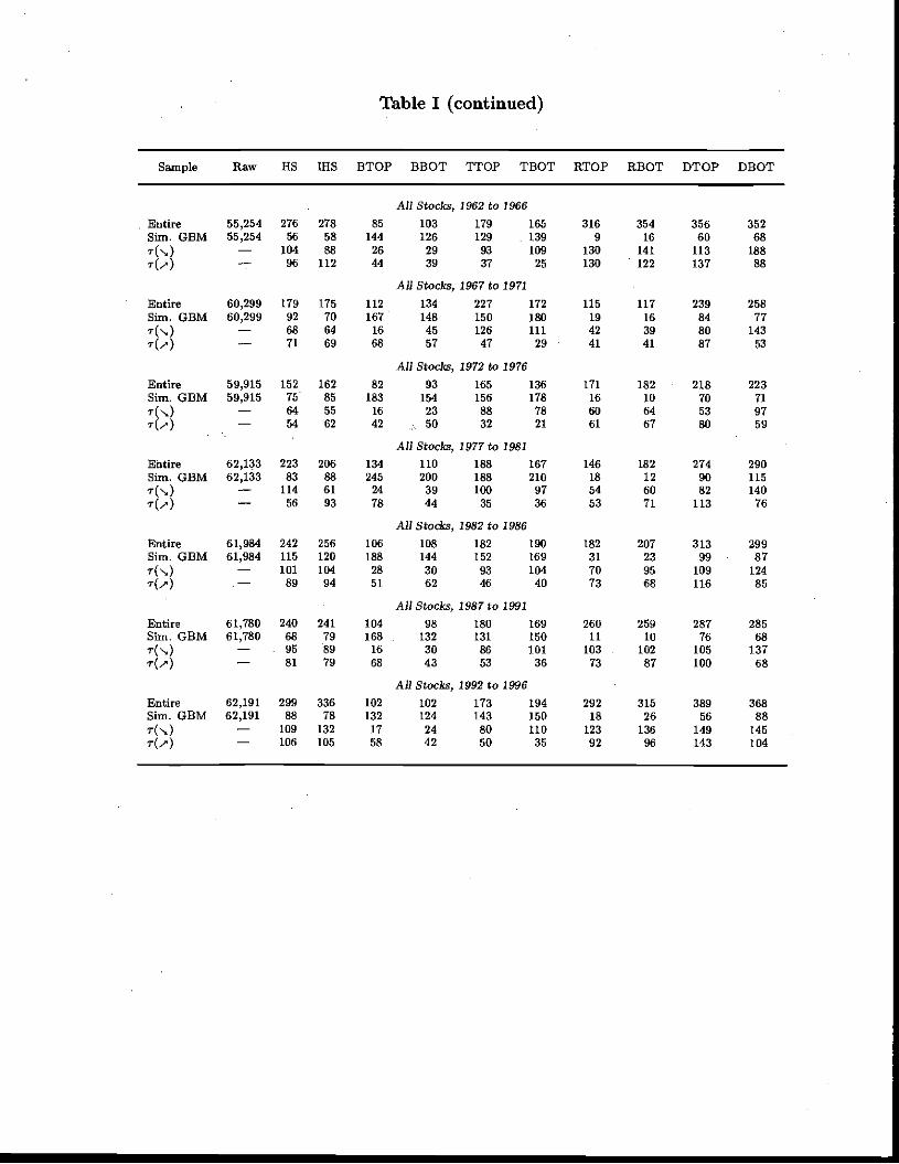
Table I (continued)
Sample Raw US IllS ETOP BBOT flOP TBOT aTOP RBOT DTOP DBOT
All Stocks, 1962 to 1966
• Entire 55,254 276 278Sim. GBM 55,254 56 58
7(N) — 104 8896 112
85 103 179 165144 126 129 13926 29 93 10944 39 37 25
316 354 356 3529 16 60 68
130 141 113 188130 122 137 88
All Stocks, 1967 to 1971
Entire 60,299 179 175Sim. GEM 60,299 92 70
7(N) — 68 64r(,) — 71 69
112 134 227 172 115 117 239 258167 148 150 180 19 16 84 7716 45 126 111 42 39 80 14368 57 47 29 41 41 87 53
All Stocks, 1972 to 1976
All Stocks, 1977 to 1981
— 101 104 28 30 93 104 70 95 109 124— 89 94 51 62 46 40 73 68 116 85
All Stocks, 1987 to 1991104 98168 13216 3068 43
All Stocks, 1992 to 1996Entire 62,191 299 336Sim. GEM 62,191 88 78
r(N) — 109 132— 106 105
102 102 173 194 292 315 389 368132 124 143 150 18 26 56 88
17 24 80 110 123 136 149 14558 42 50 35 92 96 143 104
Entire 59,915 152 162 82 93 165 136 171 182 218 223Sim. GEM 59,915 75 85 183 154 156 178 16 10 70 717(N) — 64 55 16 23 88 78 60 64 53 97r(,) — 54 62 42 :50 32 21 61 67 80 59
Entire 62,133 223 206 134 110 188 167 146 182 274 290Sun. GUM 62,133 83 88 245 200 188 210 18 12 90 115
— 114— 56
6193
2478
39 10044 35
9736
5453
6071
82113
14076
All Stocks, 1982 to 1986Entire 61,984 242 256 106 108 182 190 182 207 313 299Sim. GUM 61,984 115 120 188 144 152 169 31 23 99 87
Entire 61,780 240 241Sim. GEM 61,780 68 797(N) — 95 89r(,) — 81 79
180 169 260 259 287 285131 150 11 10 76 6886 101 103 • 102 105 13753 36 73 87 100 68

Table II
Frequency counts for 10 technical indicators detected among NASDAQ stocks from 1962 to 1996,in 5-year subperiods, in size quintiles, and in a sample of simulated geometric Brownian motion.In each 5-year subperiod, 10 stocks per quintile are selected at random among stocks with atleast 80% non-missing prices, and each stock's price history is scanned for any occurrence of thefollowing 10 technical indicators within the subperiod: head-and-shoulders (HS), inverted head-and-shoulders (IRS), broadening top (BTOP), broadening bottom (BBOT), triangle top (TTOP),triangle bottom (TBOT), rectangle top (RTOP), rectangle bottom (RBOT), double top (DTOP),and double bottom (DBOT). The 'Sample' column indicates whether the frequency counts areconditioned on decreasing volume trend ('r(N)'), increasing volume trend ('r(4'), unconditional('Entire'), or for a sample of simulated geometric Brownian motion with parameters calibrated tomatch the data ('Sim. GBM').
Sample Raw 115 1115 ETOP BBOT flop TBOT ETOP RBOT DTOP DBOT
All Stocks, 1962 to 1996Entire 411,010 919 817 414 508 850 789 1134 1320 1208 1147Sun. GBM 411,010 434 447 1297 1139 1169 1309 96 91 567 579r(N)
— 408 268 69 133 429 460 488 550 339 580r(.,) — 284 325 234 209 185 125 391 461 474 229
Smallest Quintie, 1962 to 1996Entire 81,754 84 64 41 73 111 93 165 218 113 125Shn. GEM 81,754 85 84 341 289 334 367 11 12 140 125
t(N) — 36 25 6 20 56 59 77 102 31 81r(,) — 31 23 31 30 24 15 59 85 46 17
2nd Quintile, 1962 to 1996Entire 81,336 191 138 68 88 161 148 242 305 219 176Sim. GBM 81,336 67 84 243 225 219 229 24 12 99 1247(N) — 94 51 11 28 86 109 111 131 69 101r(,')
— 66 57 46 38 45 22 85 120 90 42
3rd Quintile, 1962 to 1996
Entire 81,772 224 186 105 121 183 155 235 244 279 267Sim. GEM 81,772 69 86 227 210 214 239 15 14 105 100r(..)
— 108 66 23 35 87 91 90 84 78 145
r(i')— 71 79 56 49 39 29 84 86 122 58
4th Quintile, 1962 to 1996
Entire 82,727 212 214 92 116 187 179 296 303 289 297Sim. GBM 82,727 104 92 242 219 209 255 23 26 115 97r(,.)
— 88 68 12 26 101 101 127 141 77 143
r(,')— 62 83 57 56 34 22 104 93 118 66
Largest Quintile, 1962 to 1996
Entire 83,421 208 215 108 110 208 214 196 250 308 282Sim. GEM 83,421 109 101 244 196 193 219 23 27 108 1337(N) — 82 58 17 24 99 100 83 92 84 110i-(,) 54 83 44 36 43 37 59 77 98 46
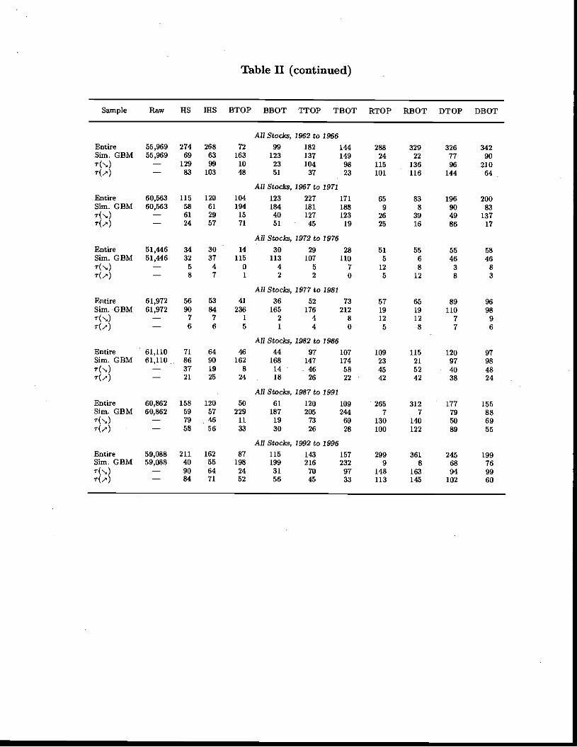
Table II (continued)
Sample Raw ES IHS BTOP BBOT flop TBOT RTOP RBOT DTOP DBOT
All Stocks, 1962 to 1966Entire 55,969 274 268Slim. GBM 55,969 69 63
— 129 99— 83 103
Entire 60,563 115 120Slut GBM 60,563 58 61'-(N) — 61 29T(/) — 24 57
Entire 61,972 56 53Sim. GBM 61,972 90 84
— 7 7— 6 6
Entire 61,110 71 64Sim. GEM 61,110 .. 86 90
T(N) — 37 19— 21 25
721631048
99 182 144 288 329 326 342123 137 149 24 22 77 9023 104 98 115 136 96 21051 37 23 101 116 144 64
All Stocks, 1967 to 1971104 123 227 171 65 83 196 200194 184 181 188 9 8 90 8315 40 127 123 26 39 49 13771 51 45 19 25 16 86 17
502291133
All Stocks, 1972 to 1976
All Stocks, 1987 to 1991
All Stocks, 1992 to 1996
155886955
Entire 59,088 211 162Sim. GEM 59,088 40 55'-(N) — 90 64— 84 71
87198
2452
Entire 51,446 34 30 14 30 29 28 51 55 55 58Sim. GBM 51,446 32 37 115 113 107 110 5 6 46 46'-(N) — 5 4 0 4 5 7 12 8 3 8'-(A) — 8 7 1 2 2 0 5 12 8 3
All Stocks, 1977 to 198141 36 52 73 57 65 89 96
236 165 176 212 19 19 110 981 2 4 8 12 12 7 95 1 4 0 5 8 7 6
All Stocks, 1982 to 1986
Entire 60,862 158 120Sim. GEM 60,862 59 57
— 79 46r(,) — 58 56
162 168 147 174 23 21 97 988 14 .46 58 45 52 40 4824. 18 26 22 42 42 38 24
61 120 109 265 312 177187 205 244 7 7 7919 73 69 130 140 5030 26 28 100 122 89
115 143 157 299 361 245 199199 216 232 9 8 68 7631 70 97 148 163 94 9956 45 33 113 145 102 60

Table III
Summary statistics (mean, standard deviation, skewness, and excess kurtosis) of raw and condi-tional 1-day normalized returns of NYSE/AMEX stocks from 1962 to 1996, in 5-year subperiods,and in size quintiles. Conditional returns are defined as the daily return three days followingthe conclusion of an occurrence of one of 10 technical indicators: head-and-shoulders (HS), in-verted head-and-shoulders (IllS), broadening top (BTOP), broadening bottom (BBOT), triangletop (TTOP), triangle bottom (TROT), rectangle top (RTOP), rectangle bottom (RBOT), doubletop (DTOP), and double bottom (DBOT). All returns have been normalized by subtraction oftheir means and division by theft standard deviations.
Moment Raw 115 IRS BTOP BBOT flop TBOT RTOP RBOT DTOP DEOT
An Stocks, 1962 to 1996MeanS.D.SkewKurt
—0.0001.0000.3458.122
—0.0380.8670.1352.428
0.0400.9370.6604.527
—0.005 —0.062 0.021 —0.0091.035 0.979 0.955 0.959
—1.151 0.090 0.137 0.64316.701 3.169 3.293 7.061
0.0090.865
—.0.4207.360
0.014 0.0170.883 0.9100.110 0.2064.194 3.386
0.0O10.9990.4607.374
Smallest Quintile, 1962 to 1996MeanS.D.SkewKurt
—0.0001.0000697
10.873
—0.014-0.8540.8023.870
0.0361.0021.3377.143
—0.093 —0.188 0.036 —0.0200.940 0.850 0.937 1.157
—1.771 —0.367 0.861 2.5926,701 0.575 4.185 12.532
0.0370.833
—0.1871.793
—0.093 0.0430.986 0.9500.445 0.5114.384 2.581
—0.0550.9620.0023.989
MeanS.D.SkewKurt
—0.0001.0000.3927.836
—0.0690.7720.2230.657
0.1441.0311.1286.734
2nd Qthntile, 1962 to 19960.061 —0.113 0.003 0.0351.278 1.004 0.913 0.965
—3.296 0.485 —0.529 0.16632.750 3.779 3.024 4.987
0.0180.979
—1.37517.040
0.019 0.0670.868 0.7760.452 0.3923.914 2.151
.
—0.011L0691.728
15.544
MeanS.D.SkewKurt
—0.0001.0000.2467.466
—0.0480.888
—0.4653.239
—0.0430.8560.1071.612
3rd QuintiIe, 1962 to 1996—0.076 —0.056 0.036 0.012
0.894 0.925 0.973 0.796—0.023 0.233 0.538 0.166
1.024 0.611 2.995 0.586
0.0750.7980.6783.010
0.028 —0.0390.892 0.956
—0.618 0.0134.769 .4.517
—0.0341.026
—0.2423.663
MeanS.D.SkewKurt
—0.0001.0000.2226.452
—0.0120.9640.0551.444
0.0220.9030.5921.745
4th Quintile, 1962 to 19960.115 0.028 0.022 —0.0140.990 1.093 0.986 0.9590.458 0.537 —0.217 —0.4561.251 2.168 4.237 8.324
—0.1130.854
—0.4154.311
0.065 0.0150.821 0.8580.820 0.550
. 3.632 1.719
—0.0060.992
—0.0624.691
Largest Quintile, 1962 to 1996MeanS.D.SkewKurt
—0.0001.0000.1747.992
—0.0380.8430.4382.621
0.0540.9270.1823.465
—0.081 —0.042 0.010 —0.0490.997 0.951 0.964 0.9650.470 —1.099 0.089 0.3573.275 6.603 2.107 2.509
0.0090.850
—0.1670.816
0.060 0.0180.820 0.971
—0.140 0.0113.179 3.498
0.0670.9410.5115.035

Table III (continued)
Moment Raw H5 IHS ETOP BBOT flOP TBOT RTOP IthOT DTOP DBOT
All Stocks, 1962 to 1966
—0.007 0.011 0.095 —0.114 —0.067 0.050 0.005 0.011 —0.0131.002 1.109 0,956 0.924 0.801 0.826 0.934 0.850 1.0260.441 0.372 —0.165 0.473 —1.249 0.231 0.467 0.528 0.8676.128 2.566 2.735 3.208 5.278 1.108 4.234 1.515 7.400
0.033 —0.091 —0.040 0.053 0.003 0.040 —0.020 —0.022 —00170.895 0.955 0.818 0.857 0.981 0.894 0.833 0.873 1.0520.272 0.108 0.231 0.165 —1.216 0.293 0.124 —1.184 —0.3684.395 2.247 1.469 4.422 9.586 1.646 3.973 4.808 4.297
0.069 —0.231 —0.272 0.122 0.041 0.082 0.011 0.102 —0.0161.021 1.406 1.187 0.953 1.078 0.814 0.996 0.960 1.0351.305 —3.988 —0.502 —0.190 2.460 —0.167 —0.129 —0.091 0.3796.684 27.022 3.947 1.235 12.883 0.506 6.399 1.507 3.358
0.090 0.159 0.079 —0.033 —0.039 —0.041 0.019 —0.071 —0.1000.925 0.825 1.085 1.068 1.011 0.961 0.814 0.859 0.9620.462 0.363 1.151 —0.158 1.264 —1.337 —0.341 —0.427 —0.8761.728 0.657 5.063 2.674 4.826 17.161 1.400 3.416 5.622
All Stocks, 1967 to 19710.079 —0.035 —0.056 0.025 0.057 —0.101 0.110 0.093 0.0790.944 0.793 0.850 0.885 0.886 0.831 0.863 1.083 0.8350.666 0.304 0.085 0.650 0.697 —1.393 0.395 1.360 0.7012.725 0.706 0.141 3.099 1.659 8.596 3.254 4.487 1.853
All Stocks, 1972 to 19760.043 0.101 —0.138 —0.045 —0.010 —0.025 —0.003 —0.051 —0.1080.810 0.985 0.918 0.945 0.922 0.870 0.754 0.914 0.9030.717 —0.699 0.272 —1.014 0.676 0.234 0.199 0.056 —0.3661.565 6.562 1.453 5.261 4.912 3.627 2.337 3.520 5.047
All Stocks, 1977 to 1981—0.040 0.076 —0.114 0.135 —0.050 —0.004 0.026 0.042 0.178
0.863 1.015 0.989 1.041 1.011 0.755 0.956 0.827 1.0950.052 1.599 —0.033 0.776 0.110 —0.084 0.534 0.761 2.2141.048 4.961 —0.125 2.964 0.989 1.870 2.184 2.369 15.290
All Stocks, 1982 to 1986
Mean —0.000 0.070S.D. 1.000 0.797Skew 0.563 0.159Kurt 9.161 0.612
Mean —0.000 —0.044S.D. 1.000 0.809Skew 0.342 0.754Kurt 5.810 3.684
Mean —0.000 —0.035S.D. 1.000 1.015Skew 0.316 —0.334Kurt 6.520 2.286
Mean —0.000 —0.138S.D. 1.000 0.786Skew 0.466 —0.304Kurt 6.419 1.132
Mean —0.000 —0.099S.D. 1.000 0.883Skew 0.460 0.464Kurt 6.799 2.280
Mean —0.000 —0.037S.D. 1.000 0.848Skew —0.018 —0.526Kurt 13.478 3.835
Mean —0.000 —0.014S.D. 1.000 0.935Skew 0.308 0.545Kurt 8.683 2.249
All Stocks, 1987 to 1991
All Stocks, 1992 to 1996

Table IV
Summary statistics (mean, standard deviation, skewness, and excess kurtosis) of raw and condi-tional 1-day normalized returns of NASDAQ stocks from 1962 to 1996, in 5-year subperiods, andin size quintiles. Conditional returns are defined as the daily return three days following the con-clusion of an occurrence of one of 10 technical indicators: head-and-shoulders (HS), inverted head-
and-shoulders (IHS), broadening top (BTOP), broadening bottom (BBOT), triangle top (TTOP),triangle bottom (TBOT), rectangle top (RTOP), rectangle bottom (RBOT), double top (DTOP),and double bottom (DBOT). All returns have been normalized by subtraction of their means anddivision by their standard deviations.
Moment Raw 115 IllS BTOP BBOT flOP TBOT ICOP REOT DTOP DROT
All Stocks, 1962 to 1996
MeanS.D.SkewKurt
0.0001.0000.608
12.728
—0.016 0.0420.907 0.994
—0.017 1.2903.039 8.774
—0.009 0.009 —0.020 0.0170.960 0.995 0.984 0.9320.397 0.586 0.895 0.7163.246 2.783 6.692 3.844
0.0520.9480.7105.173
0.0430.9290.7554.368
0.0030.9330.4054.150
—0.0350.880
—0.1042.052
MeanS.D.SkewKurt
—0.0001.0000.754
15.859
0.018 —0.0320.845 1.3190.325 1.7561.096 4.221
Smallest Quintile, 1962 to 19960.087 —0.153 0.059 0.1080.874 0.894 1.113 1.044
—0.239 —0.109 2.727 2.3001.490 0.571 14.270 10.594
0.1361.1871.7418.670
0.0130.9820.1991.918
0.0400.7730.1260.127
0.0430.906
—0.3580.730
MeanS.D.SkewKurt
—0.0001.0000.844
16.738
—0.064 0.0760.848 0.9910.406 1.8922,127 11.561
2nd Quintile, 1962 to 1996—0.109 —0.093 —0.085 —0.038
1.106 1.026 0.805 0.997—0.122 0.635 0.036 0.455
2.496 3.458 0.689 1.332
—0.0660.898
—0.579•2.699
—0.0150.8970.4163.871
0.0391.1191.1963.910
—0.0340.8210.1900.777
. 3rd Quintile, 1962 to 1996MeanS.D.SkewKurt
—0.0001.0000.698
12.161
0.033 0.0280.933 0.9060.223 0.5291.520 1.526
0.078 0.210 —0.030 0.0680.931 0.971 0.825 1.0020.656 0.326 0.539 0.4421.003 0.430 1.673 1.038
0.1170.9920.8852.908
0.2100.9700.8204.915
—0.1090.9970.1635.266
—0.0750.9730.1232.573
4th Quintile, 1962 to 1996MeanS.D.SkewKurt
0.0001.0000.655
11.043
—0.079 0.0370.911 0.957
—0.456 2.6712.525 19.593
—0.006 —0.044 —0.080 0.0070.992 0.975 1.076 0.824
—0.174 0.385 0.554 0.7172.163 1.601 7.723 3.930
0.0840.8900.2901.555
0.0440.8511.0342.982
0.0380.8570.1542.807
—0.0480.819
—0.1492.139
Largest Quintile, 1962 to 1996MeanS.D.SkewKurt
0.0001.0000.1007.976
0.026 0.0580.952 L002
—0.266 —0.1445.807 4.367
—0.070 0.031 0.052 —0.0130.895 1.060 1.076 0.8711.699 1.225 0.409 0.0258.371 5.778 1.970 2.696
0.0010.7940.1051.336
—0.0240.9581.3007.503
0.032.0.8440.3152.091
—0.0180.877
—0.3632.241

Table IV (continued)
Moment Raw HS 1115 BTOP BEOT TTOP TEOT RTOP RBOT DTOP DBOT
All Stocks, 1962 to 1966
0.089 —0.403 —0.034 —0.132 —0.422 —0.076 0-108 —0.004 —0.1630.908 0.569 0.803 0.618 0.830 0.886 0.910 0.924 0.5640.973 —1.176 0.046 —0.064 -'--1.503 —2.728 2.047 —0.551 —0.7911.828 0.077 0.587 —0.444 2.137 13.320 9.510 1.434 2.010
All Stocks, 1982 to 19860.204 —0.137 —0.001 —0.053 —0.022 —0.028 0.116 —0.224 —0.0521.442 0.804 1.040 0.982 1.158 0.910 0.830 0.868 1.0822.192 0.001 0.048 1.370 1.690 —0.120 0.048 0.001 —0.091
10.530 0,863 0.732 8.460 - 7.086 0.780 0.444 1.174 0.818
All Stocks, 1987 to 1991-
0.120 —0.080 —0.031 —0.052 0.038 0.098 0.049 —0.048 —0.122 -- 1.136 0.925 0.826 1.007 0.878 0.936 1.000 0.772 0.860
0.976 —0.342 0.234 —0.248 1.002 0.233 0.023 —0.105 —0.375.5.183 1.839 0.734 2.796 2.768 1.038. 2.350 0.313 2.598
All Stocks, 1992 to 1996—0.058 —0.033 —0.013 —0.078 0.086 —0.006 —0.011 0.003 —0.105
0.854 0.964 1.106 1.093 0.901 0.973 0.879 0.932 0.875—0.015 1.399 0.158 —0.127 0.150 0.283 0.236 0.039 —0.097—0.059 7.584 0.626 2.019 1.040 1.266 1.445 1.583 0.205
Mean —0.000 0.116S.D. 1.000 0.912Skew 0.575 0.711Kurt 6.555 1.538
Mean —0.000 —0.127S.D. 1.000 0.864Skew 0.734 —0.097Kurt 5.194 1.060
0.041 0.099 0.090 0.028 —0.066 0.100 0.010 0.096 0.0270.949 0.989 1.039 1.015 0.839 0.925 0.873 1.039 0.8401.794 0.252 L258 1,601 0.247 2.015 1.021 0.533 —0.3519.115 2.560 6.445 7.974 1.324 13.653 5.603 6.277 2.243
All Stocks, 1967 to 19710.114 0.121 0.016 0.045 0.077 0.154 0.136 —0.000 0.006osos 0.995 1.013 0.976 0.955 1.016 1.118 0.882 0.9301.080 0.574 0.843 1.607 0.545 0.810 1.925 0.465 0.4312.509 0.380 2.928 10.129 1.908 1.712 5.815 1.585 2.476
All Stocks, 1972 to 1976MeanS.D.SkewKurt
0.000 0.0141.000 0.5750,466 —0.281
17.228 2.194
Mean —0.000 0.025S.D. 1.000 0.769Skew 1.092 0.230Kurt 20.043 1.618
All Stocks, 1977 to 19-81—0.212 —0.112 —0.056 —0.110 0.086 0.055 0.177 0.081. 0.040
1.025 1.091 0.838 0.683 0.834 1.036 1.047 0.986 0.880—1.516 —0.731 0.368 0.430 0.249 2.391 2.571 L520 —0.291
4.397 3.766 0.460 0.962 4.722 9.137 10.961 7.127 3.682
MeanS.D.SkewKurt
Mean.S.D.SkewKurt
MeanS.D.SkewKurt
0.000 —0.1471.000 1.0731.267 —1.400
21.789 4.899
0.000 0.0121.000 0.9070.104 —0.326
12.688 3.922
0.000 —0.1191.000 0.926
—0.036 0.0795.377 2.818

Tab
le V
Goo
dnes
s-of
-fit
diag
nost
ics
for
the
cond
ition
al 1
-day
nor
mal
ized
ret
urns
, co
nditi
onal
on
10 te
chni
cal
indi
cato
rs,
for
a sa
mpl
e of
350
NY
SE/A
ME
X s
tock
s fr
om 1
962
to 1
996
(10
stoc
ks p
er s
ize-
quin
tile
with
at
leas
t 80%
non
-mis
sing
pri
ces
are
rand
omly
cho
sen
in e
ach
five
-yea
r su
bper
iod,
yie
ldin
g 50
sto
cks
per
subp
erio
d ov
er 7
sub
peri
ods)
. Fo
r ea
ch p
atte
rn, t
he p
erce
ntag
e of
con
ditio
nal r
etur
ns t
hat
fall
with
in e
ach
of th
e 10
unc
ondi
tiona
l-re
turn
dec
iles
is t
abul
ated
. If
cond
ition
ing
on th
e pa
ttern
pro
vide
s no
info
rmat
ion,
the
expe
cted
pe
rcen
tage
falli
ng in
eac
h de
cile
is 1
0%.
Asy
mpt
otic
t-st
atis
tics
for t
his
null
hypo
thes
is a
re r
epor
ted
in p
aren
thes
es, a
nd th
e x2
goo
dnes
s-
of-f
itnes
s te
st s
tatis
tic Q
is r
epor
ted
in th
e la
st c
olum
n w
ith th
e p-
valu
e in
par
enth
eses
bel
ow th
e st
atis
tic.
The
10
tech
nica
l ind
icat
ors
are:
he
ad-a
nd-s
houl
ders
(US)
, in
vert
ed h
ead-
and-
shou
lder
s (Il
lS),
bro
aden
ing
top
(BT
OP)
, br
oade
ning
bot
tom
(B
BO
T),
tri
angl
eS to
p (T
TO
P), t
rian
gle
botto
m (
TB
OT
), re
ctan
gle
top
(RT
OP)
, rec
tang
le b
otto
m (R
BO
T),
dou
ble t
op (
DT
OP)
, and
dou
ble b
otto
m (
DB
OT
).
Dec
iIe
Patte
rn
1 2
3 4
5 6
7 5
9 10
(p
-Val
ue)
HS
8.9
10.4
11
.2
11.7
12
.2
7.9
9-2
10.4
10
.8
7.1
39.3
1 (—
1.49
) (0
.56)
(1
.49)
(2
.16)
(2
.73)
(—
3.05
) (—
1.04
) (0
.48)
(1
.04)
(—
4.46
) (0
.000
) Il
ls
8.6
9.7
9.4
11.2
13
.7
7.7
9.1
11.1
9.
6 10
.0
40.9
5 (—
2.05
) (—
0.36
) (—
0.88
) (1
.60)
(4
,34)
(—
3.44
) (—
1.32
) (1
.38)
(—
0.62
) (—
0.03
) (0
.000
) E
TO
P 9.
4 10
.6
10.6
11
.9
8.7
6.6
9.2
13.7
9.
2 10
.1
23.4
0 (—
0.57
) (0
.54)
(0
.54)
(1
.55)
(—
1.25
) (—
3.66
) (—
0.71
) (2
.87)
(—
0.71
) (0
.06)
(0
.005
) B
BO
T
11.5
9.
9 13
.0
11.1
. 7.
8 9.
2 8.
3 9.
0 10
.7
9.6
16.8
7 (1
.28)
(—
0.10
) (2
.42)
(0
.95)
(—
2.30
) (—
0.73
) (—
1.70
) (—
1.00
) (0
.62)
(—
0.35
) (0
.051
) T
TO
P 7.
8 10
.4
10.9
11
.3
9.0
9.9
10.0
10
.7
10.5
9.
7 12
.03
(—2.
94)
(0.4
2)
(1.0
3)
(1.4
6)
(—1.
30)
(—0.
13)
(—0.
04)
(0.7
7)
(0.6
0)
(—0.
41)
(0.2
12)
TB
OT
8.
9 10
.6
10.9
12
.2
9.2
8.7
9.3
11.6
8.
7 9.
8 17
.12
(—1.
35)
(0.7
2)
(0.9
9)
(2.3
6)
(—0.
93)
(—1.
57)
(—0.
83)
(1.6
9)
(—1.
57)
(—0.
22)
(0.0
47)
RT
OP
8.4
9.9
9.2
10.5
12
.5
10.1
10
.0
10.0
11
.4
8.1
22.7
2 (—
2.27
) (—
0.10
) (—
1.10
) (0
.58)
(2
.89)
(0
.16)
(—
0.02
) (—
0.02
) (1
.70)
(—
2.69
) (0
.007
) R
BO
T
8.6
9.6
7.8
10.5
12
.9
10.8
11
.6
9.3
10.3
8.
7 33
.94
(—2.
01)
(—0.
56)
(—3.
30)
(0.6
0)
(3.4
5)
(1.0
7)
(1.9
8)
(—0.
99)
(0.4
4)
(—1.
91)
(0.0
00)
DT
OP
8.2
10.9
9.
6 12
.4
11.8
7.
5 8.
2 11
.3
10.3
9.
7 50
.97
(—2.
92)
(1.3
6)
(—0.
64)
(3.2
9)
(2.6
1)
(—4.
39)
(—2.
92)
(1.8
3)
(0.4
6)
(—0.
41)
(0.0
00)
DB
OT
9.
7 9.
9 10
.0
10.9
11
.4
8.5
9.2
10.0
10
.7
9.8
12.9
2
(—0.
48)
(—0.
18)
(—0.
04)
(1.3
7)
(1.9
7)
(—2.
40)
(—1.
33)
(0.0
4)
(0.9
6)
(—0.
33)
(0.1
66)

Tab
le V
T
Goo
dnes
s-of
-fit
diag
nost
ics
for
the
cond
ition
al 1
-day
nor
mal
ized
retu
rns,
con
ditio
nal
on 1
0 te
clm
ical
indi
cato
rs,
for
a sa
mpl
e of
350
NA
SDA
Q s
tock
s fr
om 1
962
to 1
996
(10
stoc
ks p
er s
ize-
quin
tile
with
at l
east
80%
non
-mis
sing
pri
ces
are
rand
omly
cho
sen
in e
ach
five
-
year
sub
peri
od, y
ield
ing
50 s
tock
s pe
r su
bper
iod
over
7 s
ubpe
riod
s).
For
each
pat
tern
, the
per
cent
age
of c
ondi
tiona
l ret
urns
tha
t fal
l w
ithin
eac
h of
the
10 u
ncon
ditio
nal-
retu
rn d
ecile
s is
tab
ulat
ed.
If c
ondi
tioni
ng o
n th
e pa
ttern
pro
vide
s no
inf
orm
atio
n, th
e ex
pect
ed
perc
enta
ge fa
lling
in e
ach
deci
le i
s 10
%.
Asy
mpt
otic
t-st
atis
tics
for t
his
null
hypo
thes
is a
re re
port
ed i
n pa
rent
hese
s, a
nd th
e x2
goo
dnes
s-
of-f
itnes
s te
st s
tatis
tic Q
is
repo
rted
in
the
last
col
umn
with
the
p-v
alue
in p
aren
thes
es b
elow
the
stat
istic
. T
he 1
0 te
chni
cal i
ndic
ator
s ar
e:
head
-and
-sho
ulde
rs (1
18),
inv
erte
d he
ad-a
nd-s
houl
ders
(Ills
), b
road
enin
g to
p (B
TO
P),
broa
deni
ng b
otto
m (
BB
OT
), t
rian
gle
top
(TT
OP)
, tr
iang
le b
otto
m (
TB
OT
), r
ecta
ngle
top
(RT
OP)
, rec
tang
le b
otto
m (
RB
OT
), d
oubl
e to
p (D
TO
P), a
nd d
oubl
e bo
ttom
(D
BO
T).
Dec
ile;
Patte
rn
.
1 2
3 4
5 6
7 8
10
(p-V
alue
)
HS
10.8
10
.8
13.7
8.
6 8.
5 6.
0 6.
0 12
.5
13.5
9.
7 64
.41
(0.7
6)
(0.7
6)
(3.2
7)
(—1.
52)
(—1.
65)
(—5.
13)
(—5.
13)
(2.3
0)
(3.1
0)
(—0.
32)
(0.0
00)
fl-IS
9.
4 14
.1
12.5
8.
0 7.
7 4.
8 6.
4 13
.5
12.5
11
.3
75.8
4 (—
0.56
) (3
.35)
(2
.15)
(—
2.16
) (—
2.45
) (—
7.01
) (—
4.26
) (2
.90)
(2
.15)
(1
.14)
(0
.000
) B
TO
P 11
.6
12.3
12
.8
7.7
8.2
6.8
4.3
13.3
12
.1
10.9
34
.12
(1.0
1)
(1.4
4)
(1.7
1)
(—1.
73)
(—1.
32)
(—2.
62)
(—5.
64)
(1.9
7)
(1.3
0)
(0.5
7)
(0.0
00)
BB
OT
11
.4
11.4
14
.8
5.9
6.7
9.6
5.7
11.4
9.
8 13
.2
43.2
6 (1
.00)
(1
.00)
(3
.03)
(—
3.91
) (—
2.98
) (—
0.27
) (—
4.17
) (1
.00)
(—
0.12
) (2
.12)
(0
.000
) T
TO
P 10
.7
12.1
16
.2
6.2
7.9
8.7
4.0
12.5
11
.4
10.2
92
.09
(0.6
7)
(1.8
9)
(4.9
3)
(—4.
54)
(—2.
29)
(—1.
34)
(—8.
93)
(2.1
8)
(1.2
9)
(0.2
3)
(0.0
00)
TB
OT
9.
9 11
.3
15.6
7.
9 7.
7 5.
7 5.
3 14
.6
12.0
10
.0
85.2
6 (—
0.11
) (1
.14)
(4
.33)
(—
2.24
) (—
2.39
) (—
5.20
) (—
5.85
) (3
.64)
(1
.76)
(0
.01)
(0
.000
) R
TO
P 11
,2
10.8
8.
8 8,
3 10
.2
7.1
7.7
9.3
15.3
11
.3
57.0
8 (1
.28)
(0
.92)
(—
1.40
) (—
2.09
) (0
.25)
(—
3.87
) (—
2.95
) (—
0.75
) (4
.92)
(1
.37)
(0
.000
) R
BO
T
8.9
12.3
8.
9 8.
9 11
.6
8.9
7.0
9.5
13.6
10
.3
45.7
9
(—1.
35)
(2.5
2)
(—1.
35)
(—1.
45)
(1.8
1)
(—1.
35)
(—4.
19)
(—0.
66)
(3.8
5)
(0.3
6)
(0.0
00)
DT
OP
11.0
12
.6
11.7
9.
0 9.
2 5.
5 5.
8 11
.6
12.3
11
.3
71.2
9
(1.1
2)
(2.7
1)
(1.8
1)
(—1.
18)
(—0.
98)
(—6.
76)
(—6.
26)
(1.7
3)
(2.3
9)
(1.4
7)
(0.0
00)
DB
OT
10
.9
11.5
13
.1
8.0
8.1
7.1
7.6
11.5
12
.8
9.3
51.2
3
(0.9
8)
(1.6
0)
(3.0
9)
(—2.
47)
(—2.
35)
(—3.
75)
(—3.
09)
(1.6
0)
(2.8
5)
(—0.
78)
(0.0
00)

Table VII
Kolmogorov-Smirnov test of the equality of conditional and unconditional 1-day return distributionsfor NYSE/AMEX stocks from 1962 to 1996, in 5-year subperiods, and in size quintiles. Conditionalreturns are defined as the daily return three days following the conclusion of an occurrence of one of10 technical indicators: head-and-shoulders (HS), inverted head-and-shoulders (1115), broadeningtop (BTOP), broadening bottom (BBOT), triangle top (PTOP), triangle bottom (TBOT), rect-angle top (RTOP), rectangle bottom (RBOT), double top (DTOP), and double bottom (DBOT).All returns have been normalized by subtraction of their means and division by their standarddeviations, p-values are with respect to the asymptotic distribution of the Kolmogorov-Smirnovtest statistic. The symbols 'r(x,j' and '-r(4' indicate that the conditional distribution is alsoconditioned on decreasing and increasing volume trend, respectively.
Statistic HS IllS BTOJ> BROT flOP TBOT aro RBOT DTOP DBOT
All Stocks, 1962 to 1996
p-value1,890.002
1.220.104
1.150.139
1.76 0.90 1.090.004 0.393 0.185
1.840.002
2.450.000
1.510.021
1.060.215
7 ,-('...)p-value
1.490.024
0.950.327
0.440.989
0.62 0.73 1.330.839 0.657 0.059
1.370.047
1.770.004
0.960.319
0.780.579
r(,)p-value
0.720.671
1.050.220
1.330.059
1.59 0.92 1.290.013 0.368 0.073
1.130.156
1.240.090
0.740.638
0.840.481
Duff.p-value
0.880.418
0.540.935
0.590.879
0.94 075 1.370.342 0.628 0.046
0.790.557
1.200.111
0.820.512
0.710.698

Table VII (continued)
Statistic HS IHS ETOP BBOT flOP TEOT RTOP REOT DTOP DBOT
1.82 L63 0.930.003 0.010 0.353
1.62 L03 0.880.010 0.242 0.427
1.06 1.63 0.960.213 0.010 0.317
0.78 0.94 1.040.576 0.334 0.228
0.83 1.56 1.000.502 0.016 0.266
0.95 0.94 0.660.326 0.346 0.775
1.05 1.43 0.930.223 0.033 0.350
1.02 1.14 0.450.246 0.148 0.986
0.72 0.61 1,290.683 0.852 0.0711.01 0.95 0.830.255 0.330 0.504
0.93 0.66 1.290.349 0.772 0.0721.10 0.97 0.640.175 0.301 0.804
Smallest Quintile, 1962 to 1996
0.59 1.19 0.720.872 0.116 0.679
0.67 0.80 1.160.765 0.540 0.136
0.43 0.95 0.670.994 0.325 0.756
0.52 0.48 1.140.951 0.974 0.151
1.200.114
0.690.723
1.030.236
0.680.741
0.980.290
1.000.271
0.470.981
0.480.976
1.430.033
1.460.0290.880.423
0.980,291
7p-value7p-value7p-value7 Duff.p-value
7p-value
p-value
77(4p-value7 Duff.p-value
7p-value7p-value
77(4p-value7 Duff.p-value
7p-value7p-value
77(4p-value7 Duff.p-value
7p-value
77(N)p-value7 7(1')p-value7 Duff.p-value
1.090.188
1.310.065
0,510.959
0.980.294
0.880.417
0.710.703
1.190.119
0.990.276
1.960.001
1.450.031
0.930.354
0.660.774
1.370.0481.340.056
0.640.810
0.640.806
2nd Quintile, 1962 to 1996
0.92 0.62 0.840.365 0.505 0.485
0.42 0.91 0.900.994 0.378 0.394
0.83 0.89 0.980.497 0.407 0.289
0.71 1.22 0.920.687 0.102 0.361
3rd Quintile, 1962 to 1996
1.28 0.57 1.030.074 0.903 0.243
0.76 0.61 0.820.613 0.854 0.520
1.14 0.63 0.800.147 0.826 0.544
0.48 0.50 0.890.974 0.964 0.413
4th Quintile, 1962 to 1996
0.84 0.61 0.840.479 0.855 0.480
0.96 0.78 0.840.311 0.585 0.487
0.96 1.16 0.690.316 0.137 0.731
1.16 1.31 0.780.138 0.065 0.571
Largest QuintiIe, 1962 to 1996
1.190.1200.940.339
0.930.356
0.790.552
1.290.0730.860.443
1.150.141
0.790.564
1.500.023
1.610.012
0.780.578
0.910.383
1.370.047
0.720.6801.160.136
0.920.363
1.760.004
0.870.44 2
0.870.432
1.11
0.840.485
1.120.165
0.940.342
1.160.133
1.460.029
1,500.022
0.960.317
1.180.126
1.550.0161.170.131
0.590.878
0.720.670
0.720.6820.620.841
0.690.7200.660.780
0.900.395
0.640.802
0.460.982
0.54
0.780.5830.730.6630.580.8920.620.840
0.840.478
0.970.298
0.990.2860.680.74 5
1.140.150
1,010.258
0.860.4501.150.143
0.530.943
1.010.2580.850.468
1.100.176
1.280.0771.200.114
0.880.4 18
0.79
1.25 1.16 0.980.088 0.136 0,287
1.12 0.90 0.570.164 0.386 0.906
0.81 0.93 0.830.522 0.350 0.495
0.71 0.54 0.590.699 0.934 0.874
0.480.977
0.780.580
0.610.854
0.64
0.500.964
0.640.806
0.690.729
0.76
0.80 0.940.544 0.346
1.17 0.910.127 0.379
0.81 0.730.532 0.661
1.21 0.850.800 0.607 0.110 0.467 0.170 0.929 0.552

Table VII (continued)
Statistic 115 IllS UTOP BBOT flop TBOT ItTOP RBC)T DTOP DBOT
1.29 1.67 1.07p-value 0.072 0.007 0.202
7 r('..) 0.83 1.01 1.04p-value 0.499 0.260 0.232
7 r(,) 1.13 1.13 0.84p-value 0.156 0.153 0.480
7 Duff. 0.65 0.71 0.75p-value 0.799 0.691 0.629
1,10 0.96 0.60p-value 0.177 0.317 0.867
7 i-(',) 1.02 0.80 0.53p-value 0.248 0.551 0.943
7 r(i') 1.08 0.86 0.68p-value 0.190 0.454 0.750
Duff. 1.36 0.51 0.53p-value 0.049 0.956 0.942
7 0.47 0.75 0.87p-value 0.980 0.620 0.441
7 r(') 0.80 0.40 0.50p-value 0.539 0.998 0.966
7 r(,) 0.49 0.78 0.94p-value 0.970 0.577 0.340
'y Duff. 0.55 0.56 0.51p-value 0.925 0.915 0.960
7 1.16 0.73 0.76p-value 0.138 0.665 0.617
7 T(\) 1.04 0.73 1.00p-value 0.228 0.654 0.274
7 t(,) 0.75 0.84 0.88p-value 0.623 0.476 0.426
7 Duff. 0.67 0.94 0.88p-value 0.767 0.335 0.423
0.72 0.75 1.320.671 0.634 0.062
1.200.112
1.530.018
2.040.001
1.730.005
0.80 0.63 1.800.539 0.826 0.003
0.660.771
1.840.002
1.030.244
1.540.017
0.84 0.58 1.400.475 0.894 0.040
1.120.163
0.830.492
1.090.183
1.160.135
0.76 0.60 1.900.615 0.863 0.001
0.680.741
1.350.052
0.730.657
0.830.503
All Stocks, 1967 to 1971
0.65 0.98 0.760.797 0.292 0.606
1.290.071
1.650.009
0.870.436
1.220.101
0.85 0.97 0.770.464 0.303 0.5900.91 1.11 0.820.373 0.169 0.508
0.710.7000.790.554
1.420.035
0.730.660
0.970.300
0.710.699
1.060.214
0.960.315
0.76 0.68 0.710.616 0.751 0.699
0.710.701
0.980.290
1.060.210
1.120.163
All Stocks, 1972 to 1976
1.56 1.21 0.750.015 0.106 0.627
0.870.441
0.940.341
1.640.009
1,200.113
1.24 1.21 0.650.093 0.106 0.794
1.260.084
0.630.821
0.700.718
1.390.041
1.21 1.12 1.030.108 0.159 0.244
0.810.521
0.950.331
0.840.485
0.700.7t9
0.95 0.81 1.110.333 0.525 0.170
1.150.141
0.620.836
0.670.767
1.310.065
All Stocks, 1977 to 1981
1.16 0.82 1.140.136 0.506 0.147
1.010.263
0.870.428
0.860.449
1.790.003
1.31 1.10 1.320.065 0.176 0.062
0.830.494
0.800.550
1.200.113
1.810.003
0.65 0.67 0.760.799 0.754 0.602
1.510.020.
1.410.037
0.860.450
0.990.280
0.70 0.65 0.700.708 0.785 0.716
1.110.172
1.290.073
1.160.137
0.700.713

Table VII (continued)
Statistic HS IRS . BTOP BBOT flop TROT RTOP RHOT DTOP DBOT
AU Stocks, 1982 to 1986
1.57 0.99 0.59 1.46 1.47 1.04 0.87 0.68 0.76 0.90p-value 0.015 0.276 0.883 0.029 0.027 0.232 0.431 0.742 0.617 0.387
'7 r(".) 1.17 0.68 0.44 1.30. 1.53 1.21 1.08 0.93 0.84 0.88p-value 0.129 0.741 0.991 0.070 0.018 0.106 0.190 0.356 0.478 0.421
'y i-(,) 0.81 1.03 0.74 0.62 0.83 1.23 0.77 0.79 0.63 0.81p-value 0.533 0.243 0.640 0.831 0.499 0.097 0.597 0.564 0.821 0.528
Duff. 0.51 0.79 0.70 0.81 0.74 1.21 0.73 0.75 0.93 0.74p-value 0.961 0.567 0.717 0.532 0.643 0.107 0.657 0.623 0.352 0.642
All Stocks, 1987 to 1991
1.36 1.53 1.05 0.67 0.75 0.86 0.60 1.09 1.20 0.67p-value 0.048 0.019 0.219 0.756 0.627 0.456 0.862 0.185 0.111 0.764
,-('-.,) 0.52 1.16 1.25 0.72 1.03 0.81 0.81 0.61 1.07 0.68p-value 0.953 0.135 0.087 0.673 0.235 0.522 0.527 0.848 0.201 0.751
'7 T(/) 1-72 1.03 0.64 137 0.74 1.10 1.04 1.20 1.02 1.32p-value 0.006 0.241 0.813 0.046 0.639 0.181 0.232 0.111 . 0.250 0.062
Duff. 1.11 1.29 1.07 1.06 0.67 0.93 0.89 0.74 0.84 1.17p-value 0.168 0.072 0.201 0.215 0.753 0.357 0.403 0.638 0.483 0.129
All Stocks, 1992 to 1996
1.50 1.31 1.05 1.89 1.27 0.94 1.23 0.66 1.72 1.54p-value 0.022 0.066 0.222 0.002 0.078 0.343 0.095 0.782 0.005 0.018
7 r(',) 0.87 1.05 0.60 0.89 1.11 1.03 0.90 0.65 0.99 1.12
p-value 0.443 0.218 0.858 0.404 0.174 0.242 0.390 0.787 0.2.83 0.165
7 r(t) 0.72 0.66 0.75 1.42 1.02 0.58 0.61 0.64 1.36 0.93p-value 0.670 0.778 0.624 0.036 0.246 0.895 0.854 0.813 0.048 0.357
7 Duff. 0.58 0.88 0.50 0.49 0.43 0.81 0.60 0.46 0.96 0.99p-value 0.887 0.422 0.966 0.971 0.993 0.528 0.858 0.984 0.314 0.282

TabLe VIII
Kolmogorov-Smirnov test of the equality of conditional and unconditional 1-day return distribu-tions for NASDAQ stocks from 1962 to 1996, in 5-year subperiods, and in size quintiles. Conditionalreturns are defined as the daily return three days following the conclusion of an occurrence of one of10 technical indicators: head-and-shoulders (HS), inverted head-and-shoulders (IHS), broadening
top (BTOP), broadening bottom (BBOT), triangle top (TTOP), triangle bottom (TBOT), rect-angle top (RTOP), rectangle bottom (RBOT), double top (DTOP), and double bottom (DBOT).All returns have been normalized by subtraction of their means and division by their standarddeviations, p-values are with respect to the asymptotic distribution of the Kolmogorov-Smirnovtest statistic. The symbols 'r(N)' and 'r(4' indicate that the conditional distribution is alsoconditioned on decreasing and increasing volume trend, respectively.
Statistic HS IRS DTOP BBOT flop TEOT RTOP REOT DTOP DEOT
••!All Stocks, 1962 to 1996
p-vatue2.310.000
2.680.000
1.600.012
184 2.81 2.340.002 0.000 0.000
2.690.000
1.900.001
2.290.000
2.060.000
'y r(s,)p-value
1.860.002
1.530.019
1.350.052
0.99 1.97 1.950.281 0.001 0.001
2.160.000
1.730.005
1.380.045
1.940.001
'y r(i.)p-value
1.590.013
2.100.000
1.820.003
1.59 1.89 1.180.013 0.002 0.126
1.570.014
1.220.102
2.150.000
1.460.028
' Duff.p-value
1.080.195
0.860.450
1.100.175
0.80 1.73 0.740.542 0.005 0.637
0.910.379
0.750.621
0.760.619
1.520.020

Table VIII (continued)
Statistic IIS IllS BTOP BBOT flop TEOT RTOP R.BOT DTOP DBOT
Smallest Quintile, 1962 to 1996
7p-value
77(N)p-value7 r(,')p-value7 Duff.p-value
7p-value
77(N)p-value7 r(,)p-value7 Duff.p-value
7p-value7p-value7 r(,)p-value7 Duff.p-value
1.51 2.16 1.720.021 0.000 0.006
1.16 1.30 0.850.139 0.070 0.463
0.85 1.73 1.610.462 0.005 0.012
1.04 0.95 0.830.227 0.334 0.493
1.55 1.46 0.940.016 0.029 0.341
1.11 1.13 1.080.173 0.157 0.192
1.37 0.87 0.730.048 0.439 0.665
1.23 0.62 0.970.095 0.535 0.309
1.25 1.72 0.820.087 0.005 0.510
0.93 1.08 0.540.348 0.194 0.930
0.59 1.14 0.970.873 0.146 0.309
0.61 0.89 0.580.852 0.405 0.890
1.04 0.82 1.200.233 0.510 0.111
0.81 0.54 0.570.528 0.935 0.897
0.97 1.04 1.290.306 0.229 0.0711.17 0.89 0.980.128 0.400 0.292
1.68 1.22 1.55 2,130.007 0.101 0.016 0.0001.14 1.25 1.62 1.430.150 0.089 0.010 0.0332.00 1.34 0.79 1.580.001 0.055 0.553 0.0141.44 1.39 0.72 0.950.031 0.042 0.574 0.326
2nd Quintile, 1962 to 1996
1.44 1.24 1.08 1.200.031 0.095 0.192 0.1130.92 1.23 0.79 1.340.371 0.097 0.557 0.0550.97 1.38 1.29 1.120.309 0.044 0.073 0.1620.69 1.02 1.05 1.090.733 0.248 0.224 0.183
3rd Quintile, 1962 to 1996
1.71 1.41 L52 1.250.006 0.038 0.020 0.0891.23 1.06 1.02 0.790.097 0.213 0.245 0.5601.37 0.75 1.01 1.130.047 0.633 0.262 0.1590.46 0.61 0.89 0.520.984 0.844 0.404 0.947
4th Quintile, 1962 to 1996
0.98 1.30 1.25 1.880.298 0.067 0.087 0.0021.05 0.92 1.06 1.230.217 0.367 0.215 0.0970.53 2.25 0.71 1.050.938 0.000 0.696 0.2190.97 1.86 0.62 0.930.301 0.002 0.843 0.352
0.77 1.20 0.970.589 0.114 0.3090.73 1.31 0.920.653 0.065 0.371
Largest Quintile, 1962 to 1996
1.08 1.01 1.030.190 0.255 0.242
1.03 0.54 0.930.237 0.931 0.356
1.18 1.39 0.500.123 0.041 0.967
0.94 1.25 0.730.342 0.090 0.668
0.66 0.92 0.68 0.850.778 0.360 0.742 0.4620.47 0.77 0.76 0.850.981 0.587 0.612 0.4680.93 0.88 1.25 0.770.358 0.415 0.089 0.5970.84 0.76 1.11 0.730.476 0.617 0.169 0.662
1.740.0051.080.19 1
1.470.0260.940.338
1.900.001
1.090.1851.120.165
0.580.894
1.860.002
1.380.044
1.370.047
0.600.864
1.980.001
1.950.001
1.200.115
1.090.184
1.270.078
1.610.011
0.940.3430.510.955
1.820.0030.880,4231.780.003
1.090.188
1.700.006
1.050.2 16
1.520.019
0.730.654
1.100.175
1.190.117
0.910,38 1
0.780.579
1.840.002
1.470.026
1.340.054
0.380.999
0.790.553
0.720.672
7p-value
77(N)p-vaLue
7 r(,)p-value7 flitp-value
0.94 0.660.341 0.7791.53 0.870.019 0.431
7p-value7p-value7p-value7 Duff.p-value
0.137 0.150 0.7560.620.840
0.850.465
1.140.149
1.130.156
0.980.292
1.120.160
0.860.457
0.860.454
0.770598

Table VIII (continued)
Statistic HS IHS BTOP BBOT flOP TEOT RTOP RBOT DTOP DBOT
All Stocks, 1962 to 1966
1.01 0.84 1.08 0.82 0.71 0.70 1.59 0.89 1.12 1.10p-value 0.261 0.481 0.193 0.508 0.697 0.718 0.013 0.411 0.166 0.115
7 T(\.) 0.95 0.65 0.41 1.05 0.51 1.13 0.79 0.93 0.93 1.21p-value 0.322 0.798 0.997 0.224 0.956 0.155 0.556 0.350 0.350 0.108
7 T(/') 0.77 0.96 0.83 0,73 1.35 0.49 1.17 0.62 1.18 1.15p-value 0.586 0.314 0.489 0.663 0.052 0.972 0.130 0.843 0.121 0.140
7 Duff. 1.10 0.67 0.32 0.69 1.29 0.58 0.80 0.75 0.98 1.06p-value 0.174 0.761 1.000 0.735 0.071 0.892 0.551 0.620 0.298 0.208
All Stocks, 1967 to 1971
0.75 1.10 1.00 0.74 1.27 1.35 1.16 0.74 0.74 1.21
p-value 0.636 0.175 0.273 0437 0.079 0.052 0.136 0.642 0.638 0.107
7 r("..) 1.03 0.52 0.70 0.87 1.24 1.33 1.29 0.83 0.72 1.45p-value 0.241 0.947 0.714 0.438 0.092 0.058 0.072 0.490 0.684 0.031
7 r(,s) 1.05 1.08 1.12 0.64 0.79 0.65 0.55 0.53 0.75 0.69p-value 0.217 0.192 0.165 0.810 0.566 0.797 0.923 0.941 0.631 0.723
Duff. 1.24 0.89 0.66 0.78 1.07 0.88 0.88 0.40 0.91 0.76p-value 0.093 0.413 0.770 0.585 0.203 0.418 0.423 0.997 0.385 0.602
All Stocks, 1972 to 1976
0.82 1.28 1.84 1.13 1.45 1.53 1.31 0.96 0.85 1.76p-value 0.509 0.077 0.002 0.156 0.029 0.019 0.064 0.314 0.464 0.004
7 r('.) 0.59 0.73 —99.00 0.91 1.39 0.73 1.37 0.98 1.22 0.94p-value 0.875 0.669 0.000 0.376 0.042 0.654 0.046 0.292 0.100 0.344
7 r(,') 0.65 0.73 —99.00 —99.00 —99.00 —99.00 0.59 0.76 0.78 0.65p-value 0.800 0.653 0.000 0.000 0.000 0.000 0.878 0.611 0.573 0.798
7 Duff. 0.48 0.57 —99.00 —99.00 —99.00 —99.00 0.63 0.55 0.92 0.37p-value 0.974 0.902 0.000 0.000 0.000 0.000 0.828 0.925 0.362 0.999
All Stocks, 1977 to 1981• 1.35 1.40 1.03 1.02 1.55 2.07 0.74 0.62 0.92 1.28
p-value 0.053 0.039 0.23t 0.249 0.016 0.000 0.636 0.842 0.369 0.077
'y ,j) 1.19 1.47 —99.00 —99.00 0.96 0.98 0.86 0.79 0.81 0.68p-value 0.117 0.027 0.000 0.000 0.317 0.290 0.453 0.554 0.522 0.748
,-(i') 0.69 0.94 0.80 —99.00 1.46 —99.00 0.56 0.82 1.06 094p-value 0.728 0.341 0.542 0.000 0.028 0.000 0.918 0.514 0.207 0.336
Diff. 0.73 0.90 —99.00 —9900 0.35 —99.00 0.44 0.37 0.80 0.53p-value 0.665 0.395 0.000 0.000 1.000 0.000 0.991 0.999 0.541 0.944
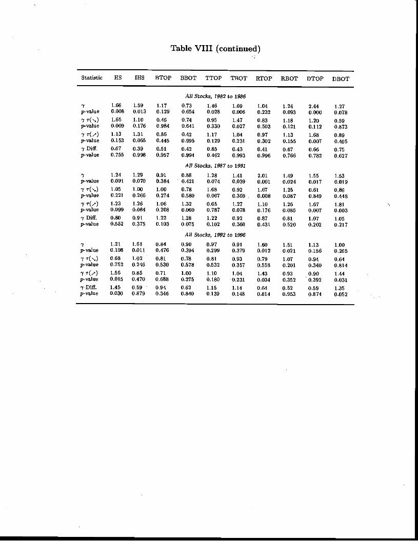
Table VIII (continued)
Statistic US IllS BTOP BBOT flop TBOT RTOP RBOT DTOP DBOT
All Stocks, 1982 to 1986
166 1.59 1.17 0.73 1.46 1.69 1.04 1.24 2.44 1.27p-value 0.008 0.013 0.129 0.654 0.028 0.006 0.232 0.093 0.000 0.078
7 ,-() 1.65 1.10 0.46 0.74 0.95 1.47 0.83 1.18 1.20 0.59p-value 0.009 0.176 0.984 0.641 0.330 0.027 0.503 0.121 0.112 0.873
7 T(/) 1.13 1.31 0.86 0.42 1.17 1.04 0.97 1.13 1.68 0.89p-value 0.153 0.065 0.445 0.995 0.129 0.231 0.302 0.155 0.007 0.4057 Duff. 0.67 0.39 0.51 0.42 0.85 0.43 0.41 0.67 0.66 0.75p-value 0.755 0.998 0.957 0.994 0.462 0.993 0.996 0.766 0.782 0.627
AU Stocks, 1987 to 1991
-y 1.24 1.29 0.91 0.88 1.28 1.41 2.01 1.49 1.55 1.53p-value 0.091 0.070 0.384 0.421 0.074 0.039 0.001 0.024 0.017 0.0197 r(',.) 1.05 1.00 1.00 0.78 1.68 0.92 1.67 1.25 0.61 0.86p-value 0.221 0.266 0.274 0.580 0.007 0.369 0.008 0.087 0.849 0.448
7 T(/) 1.23 1.26 1.06 1.32 0.65 1.27 1.10 1.26 1.67 1.81p-value 0.099 0.084 0.208 0.060 0.787 0.078 0.176 0.085 0.007 0.0037 Duff. 0.80 0.91 1.22 1,28 1.22 0.92 0.87 0.81 1.07 1.05p-value 0.552 0.375 0.103 0.075 0.102 0.360 0.431 0.520 0.202 0.217
All Stocks, 1992 to 1996
1.21 1.61 0.84 0.90 0.97 0.91 L60 1.51 1.13 LOUp-value 0.108 0.011 0.476 0.394 0.299 0.379 0.012 0.021 0.156 0.265
7 t('.) 0.68 L02 0.81 0.78 0.81 0.93 0.79 1.07 0.94 0.64p-value 0.752 0.246 0.530 0.578 0.532 0.357 0.558 0.201 0.340 0.8147 T(/) 1.56 0.85 0.71 L00 1.10 1.04 1.43 0.93 0.90 1.44p-value 0.015 0.470 0.688 0.275 0.180 0.231 0.034 0.352 0.392 0.031
yDiff. 1.45 0.59 0.94 0.62 1.15 1.14 0.64 0.52 0.59 1.35p-value 0.030 0.879 0.346 0.840 0.139 0.148 0.814 0,953 0.874 0.052
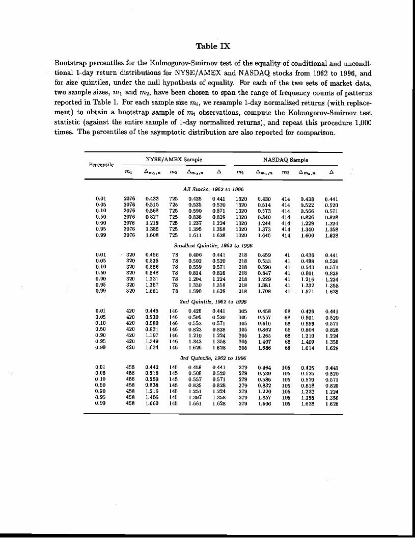
Table IX
Bootstrap percentiles for the Kolmogorov-Smirnov test of the equality of conditional and uncondi-tional 1-day return distributions for NYSE/AMEX and NASDAQ stocks from 1962 to 1996, andfor size quintiles, under the null hypothesis of equality. For each of the two sets of market data,two sample sizes, in1 and in2, have been chosen to span the range of frequency counts of patternsreported in Table 1. For each sample size mj, we resample 1-day normalized returns (with replace-ment) to obtain a bootstrap sample of mj observations, compute the Kohnogorov-Smirnov teststatistic (against the entire sample of 1-day normalized returns), and repeat this procedure 1,000times. The percentiles of the asymptotic distribution are also reported for comparison.
PercentileNYSE!AMEX Saznpe NASDAQ Sample
Ami,n '712 A Ami,n m2 . A
All Stocks, 1962 to 1996
0.010.050.100.500.900.950.99
2076207620762076207620762076
0.4330.5150.5680.8271.2191.3351.608
725 0.435 0.441 1320725 0.535 0.520 1320725 0.590 0.571 1320725 0.835 0.828 1320725 1.237 1.224 1320725 1.395 1.358 1320725 1.611 1.628 1320
0.4300.5140.5730.8401.2441.3731.645
414 0.438414 0.522414 0.566414 0.826414 1.229414 1.340414 1.600
0.4410.5200.5710.8281.2241.3581.628
Smallest Quintile, 1962 to 1996
0.010.050.100.500.900.950.99
320320320320320320320
0.4560.5350.5860.8481.2311.3571.661
78 0.406 0.441 21878 0.502 0.520 21878 0.559 0.571 21878 0.814 0.828 21878 1.204 1.224 21878 1.330 1.358 21878 1.590 1,628 218
0.4590.5330.5900.8471.2291.3811.708
41 0.43641 0.49841 0.54341 0.80141 1.21641 1.33241 1.571
0.4410.5200.5710.8281.2241.3581.628
. 2nd Quintile, 1962 to 1996
0.010.050.100.500.900.950.99
420420420420420420420
0.4450.5300.5800.831L1971.3491.634
146 0.428 0.441 305146 0.505 0.520- 305146 0.553 0.571 305146 0.823 0.828 305146 1.210 1.224 305146 1.343 1.358 305146 1.626 1.628 305
0.4580.5570.6100.8621.2651.4071.686
68 0.42668 0.50168 0,55968 0.80468 1.21068 1.40968 1.614
0.4410.5200.5710.8281.2241,3581.628
3rd Quintile, 1962 to 1996
0.010.050.100.500.900.950.99
458458458458458458458
0.4420.5160.5590.8331.2161.4061.660
145 0.458 0.441 279145 0.508 0.520 279145 0.557 0.571 279145 0.835 0.828 279145 1.251 1.224 279145 1.397 1.358 279145 1.661 1.628 279
0.4640.5390.5860.8321.2201.3571.606
105 0.425105 0.525105 0.570105 0.818105 1.233105 1.355105 1.638
0.4410.5200.5710.8281.2241.3581.628

Table IX (continued)
PercentileNYSE/AMEX Sample NASDAQ Sample
mj An,,, 7712 A tvij Ams,n Am,,n A
4th Qiiotile, 1962 to 1996
0.01 424 0.429 173 0.418 0.441 303 0.454 92 0.446 0,4410.05 424 0.506 173 0.516 0.520 303 0.526 92 0.506 0.5200.10 424 0.552 173 0.559 0.571 303 0.563 92 0.554 0.5710.50 424 0.823 173 0.815 0.828 303 0.840 92 0.818 0.8280.90 424 1.197 173 1,183 1.224 303 1.217 92 1.178 1.2240.95 424 1.336 173 1.313 1.358 303 1.350 92 1.327 1.3580.99 424 1.664 173 1.592 1.628 303 1.659 92 1.606 1.628
Largest Quintile, 1962 to 1996
0.01 561 0.421 167 0.425 0.441 308 0.441 108 0.429 0.4410.05 561 0.509 167 0.500 0.5W 308 0.520 108 0.508 0.5200.10 561 0.557 167 0.554 0.571 308 0.573 108 0.558 0.5710.50 561 0.830 157 0.817 0.828 308 0.842 108 0.816 0.8280.90 561 1.218 167 1.202 1.224 , 308 1.231 108 1.226 1.2240.95 561 1.369 167 1.308 1.358 308 1.408 108 1.357 1.3580.99 561 1.565 167 1.615 1.628 308 1.724 108 1.630 1.628

Table X (continued)
PercentileNYSE/AMEX Sample NASI)AQ Sample
.
mj Ami,,. 2 am,,,. a lThi a1,. 2 a,,.,,,. a
All Stocks, 1982 to 1986
0.01 313 0.462 106 0.437 0.441 120 0.448 44 0.417 0.4410.05 313 0.542 106 0.506 0.520 120 0.514 44 0.499 0.5200.10 313 0.585 106 0.559 0.571 120 0.579 44 0.555 0.5710.50 313 0.844 106 0.819 0.828 120 0.825 44 0.802 0.8280.90 313 1.266 106 1.220 1.224 120 1.253 44 1.197 1.224
• 0.95 313 1.397 106 1.369 1.358 120 1.366 44 1.337 1.3580.99 313 1.727 106 1.615 1.628 120 1.692 44 1.631 1.628
All Stocks, 1987 to 1991
0.01 287 0.443 98 0.449 0.441 312 0.455 50 0.432 0.4410.05 287 0.513 98 0.522 0.520 312 0.542 50 0.517 0.5200.10 287 0.565 98 0.566 0.571 312 0.610 50 0.563 0.5710.50 287 0.837 98 0.813 0.828 312 0.878 50 0.814 0.8280.90 287 1.200 98 1.217 1.224 312 1.319 50 1.216 1.2240.95 287 1.336 98 1.348 1.358 312 1.457 50 1.323 1.3580.99 287 1.626 98 1.563 1.628 312 1.701 50 1.648 1.628
All Stocks, 1992 to1996
0.01 389 0.438 102 0.432 0.441 361 0.447 87 0.428 0.4410.05 389 0.522 102 0.506 0.520 361 0.518 87 0.492 0.5200.10 389 0.567 102 0.558 0.571 361 0.559 87 0.550 0.5710.50 389 0.824 102 0.818 0.828 361 0.817 87 0.799 0.8280.90 389 1.220 102 1.213 1.224 361 1.226 87 1,216 1.2240.95 389 1.321 102 1.310 1.358 361 1.353 87 1.341 1.3580.99 389 1.580 102 1.616 1.628 361 1.617 87 1.572 1.628
Related Documents


