Formalization of Measure Theory and Lebesgue Integration for

13

Formalization of Measure Theory and Lebesgue Integration forProbabilistic Analysis in HOL

TAREK MHAMDI, OSMAN HASAN, and SOFIENE TAHAR, Concordia University

Dynamic systems that exhibit probabilistic behavior represent a large class of man-made systems such ascommunication networks, air traffic control, and other mission-critical systems. Evaluation of quantitativeissues like performance and dependability of these systems is of paramount importance. In this paper, wepropose a generalized methodology to formally reason about probabilistic systems within a theorem prover.We present a formalization of measure theory in the HOL theorem prover and use it to formalize basic con-cepts from the theory of probability. We also use the Lebesgue integration to formalize statistical propertiesof random variables. To illustrate the practical effectiveness of our methodology, we formally prove classicalresults from the theories of probability and information and use them in a data compression application inHOL.

Categories and Subject Descriptors: F.4.1 [Mathematical Logic and Formal Languages]: MathematicalLogic—Proof Theory

General Terms: Verification, Reliability

Additional Key Words and Phrases: Probabilistic systems, Lebesgue integration, measure theory, theoremproving, statistical properties, information theory

ACM Reference Format:Mhamdi, T., Hasan, O., and Tahar, S. 2013. Formalization of measure theory and Lebesgue Integrationfor probabilistic analysis in HOL. ACM Trans. Embed. Comput. Syst. 12, 1, Article 13 (January 2013), 23pages.DOI:http://dx.doi.org/10.1145/2406336.2406349

1. INTRODUCTION

Hardware and software systems usually exhibit some random or unpredictable ele-ments. Examples include failures due to environmental conditions or aging phenom-ena in hardware components and the execution of certain actions based on a proba-bilistic choice in randomized algorithms. Moreover, these systems act upon and withincomplex environments that themselves have certain elements of unpredictability, suchas noise effects in hardware components and the unpredictable traffic pattern in thecase of telecommunication protocols. Due to these random components, establishingthe correctness of a system under all circumstances usually becomes impractically ex-pensive. The engineering approach to analyze a system with these kind of unavoidableelements of randomness and uncertainty is to use probabilistic analysis. Even for hard-ware and software systems for which correctness may be unconditionally guaranteed,the study of system performance primarily relies on probabilistic analysis. In fact, theterm system performance commonly refers to the average time required by a systemto perform a given task, such as the average runtime of a computational algorithm

Author’s address: T. Mhamdi (corresponding author), Concordia University; email:[email protected] to make digital or hard copies of part or all of this work for personal or classroom use is grantedwithout fee provided that copies are not made or distributed for profit or commercial advantage and thatcopies show this notice on the first page or initial screen of a display along with the full citation. Copyrightsfor components of this work owned by others than ACM must be honored. Abstracting with credit is per-mitted. To copy otherwise, to republish, to post on servers, to redistribute to lists, or to use any componentof this work in other works requires prior specific permission and/or a fee. Permissions may be requestedfrom Publications Dept., ACM, Inc., 2 Penn Plaza, Suite 701, New York, NY 10121-0701 USA, fax +1 (212)869-0481, or [email protected]© 2013 ACM 1539-9087/2013/01-ART13 $15.00DOI:http://dx.doi.org/10.1145/2406336.2406349

ACM Transactions on Embedded Computing Systems, Vol. 12, No. 1, Article 13, Publication date: January 2013.

13:2 T. Mhamdi et al.

or the average message delay of a telecommunication protocol. These averages can becomputed, based on a probabilistic analysis approach, by using appropriate randomvariables to model inputs for the system model.

Traditionally, computer simulation techniques are used to perform probabilisticanalysis. However, they provide less accurate results and cannot handle large-scaleproblems due to their enormous computer processing time requirements. This unreli-able nature of the results poses a serious problem in safety-critical applications, suchas those in space travel, military, and medicine. A possible solution for overcoming theaccuracy problem of simulation is to conduct probabilistic analysis within the soundcore of a higher-order logic theorem prover. Higher-order logic [Gordon 1989] is a sys-tem of deduction with a precise semantics and is expressive enough to be used for thespecification of almost all classical mathematics theories. Due to its high expressive na-ture, higher-order logic can be utilized to precisely model the behavior of any system,while expressing its random or unpredictable elements in terms of formalized randomvariables, and any kind of system property, including the probabilistic and statisti-cal ones, as long as they can be expressed in a closed mathematical form. Interactivetheorem proving [Harrison 2009] is the field of computer science and mathematicallogic concerned with precise computer based formal proof tools that require some sortof human assistance. Due to its interactive nature, interactive theorem proving canbe utilized to reason about the correctness of probabilistic or statistical properties ofsystems, which are usually undecidable.

The foremost criteria for conducting a theorem proving based probabilistic analysisis to be able to formalize the underlying mathematical theories of measure [Bogachev2006], probability [Halmos 1944], and Lebesgue integration [Berberian 1998] inhigher-order logic. Using measure theory to formalize probability has the advantageof providing a mathematically rigorous treatment of probability and a unified frame-work for discrete and continuous probability measures. In this context, a probabilitymeasure is a measure function, an event is a measurable set and a random variableis a measurable function. The expectation of a random variable is its integral withrespect to the probability measure. Lebesgue integration is the natural choice fordeveloping statistical properties on random variables from measure theory and isused in most textbooks.

In the recent past, most of the above three fundamentals have been formalized inhigher-order logic. For instance, Hurd [2002] formalized some measure and probabil-ity theory in the HOL theorem prover [Gordon and Melham 1993]. Richter [2004] andCoble [2010] built upon Hurd’s formalization of measure theory to formalize Lebesgueintegration using the Isabelle/HOL [Paulson 1994] and HOL theorem provers, respec-tively. Lester [2007] also attempted the formalization of all the three fundamental con-cepts of measure, probability and Lebesgue integral in the PVS theorem prover [Owreet al. 1992]. But, unfortunately, none of these formalizations can be termed as completeand thus each approach has its own limitations. For example, the available formaliza-tions of measure theory do not allow the manipulation of random variables definedon arbitrary topological spaces, the probability theory formalizations do not not al-low us to work with the sum of random variables as a random variable itself, andfinally the Lebesgue integration formalizations have a very limited support for theBorel algebra [Bogachev 2006], which is a sigma algebra generated by the open sets.These deficiencies restrict the formal reasoning about some very useful probabilisticand statistical properties, which in turn limits the scope of theorem proving basedprobabilistic analysis of systems.

In this article, we present a generalized formalization of the measure and proba-bility theories and Lebesgue integration in order to exploit their full potential for theformal analysis of probabilistic systems. We extend the measure theory with a general


Measure Theory and Lebesgue Integration for Probabilistic Analysis in HOL 13:3

formalization of the Borel sigma algebra that can be used for any topological space. Weprove important properties of real-valued measurable functions and use them to definereal-valued random variables and prove their properties. We also formalize the conceptof independence of random variables in HOL and prove key properties of independentrandom variables. Additionally, we prove important properties of the Lebesgue inte-gral and use it to define statistical properties of random variables such as the expecta-tion and variance. To the best of our knowledge, the above capabilities are not sharedby any other existing formalization of measure, probability and Lebesgue integration.

Some of the possible applications of the proposed probability formalization includethe verification of security protocols and communication systems. In this article,we formalize the Shannon entropy in higher-order logic as a measure of how muchinformation was leaked [Smith 2009]. This result can be directly used to verifyproperties, such as the anonymity of classical security protocols like the dining cryp-tographers [Chaum 1988] and the crowds protocols [Reiter and Rubin 1998]. Similarly,our formalization can be used to verify properties of error-correcting codes. In order toillustrate the practical effectiveness of our work and its utilization to tackle such ap-plications, we present in this article a data compression application in which we provethe Asymptotic Equipartition Property [Cover and Thomas 1991], a fundamentalconcept in information theory, and use it to prove the Shannon source coding theoremthat establishes the limits of data compression [Cover and Thomas 1991]. The sourcecoding theorem states that it is possible to compress the data and get a code rate thatis arbitrarily close to the Shannon entropy without significant loss of information.Most of the infrastructure that we needed for this application, such as the properties ofreal valued measurable functions, properties of the expectation of arbitrary functions,variance, independence of random variables and the weak law of large numbers,was not available in the previous formalizations and thus the technical contribu-tions of this article paved the path for the verification of Asymptotic EquipartitionProperty.

We use the HOL theorem prover for the above mentioned formalization and verifica-tion tasks. The main motivation behind this choice was to build on existing formaliza-tions of measure [Hurd 2002] and Lebesgue integration [Coble 2010] theories in HOL

The rest of the article is organized as follows: Section 2 provides a review of relatedwork. In Section 3, we give an overview of the main definitions of the measure theoryand present our formalization of the Borel theory. Section 4 presents a formalization ofprobability spaces and random variables as well as independence of random variablesand related properties. In Section 5 we prove the main properties of the Lebesgueintegral that we use to define statistical properties of random variables. In this sec-tion we also prove important inequalities from the theory of probability as well as theWeak Law of Large Numbers. In Section 7, we illustrate the practical effectiveness ofour formalization by proving fundamental results in information theory and data com-pression. Finally, Section 8 concludes the article and provides hints to future work.

2. RELATED WORK

The early foundations of probabilistic analysis in a higher-order-logic theorem proverwere laid down by Nedzusiak [1989] and Bialas [1990] when they proposed a formal-ization of some measure and probability theories in higher-order logic. Hurd [2002]implemented their work and developed a formalization of measure theory in HOL,upon which he constructed definitions for probability spaces and functions on them.Despite important contributions, Hurd’s formalization did not include basic conceptssuch as the expectation of random variables. Besides, in Hurd’s formalization, a



measure space is the pair (A,μ); A is a set of subsets of X, called the set of measurablesets and μ is a measure function. Hence, the space is implicitly the universal set of theappropriate type. This approach does not allow to construct a measure space wherethe space is not the universal set. The only way to apply this approach for an arbitraryspace X is to define a new type for the elements of X, redefine operations on this setand prove properties of these operations. This requires considerable effort that needsto be done for every space of interest.

Based on the work of Hurd [2002], Richter [2004] formalized the measure theory inIsabelle/HOL, where he has the same restriction on the the measure spaces that can beconstructed. Richter [2004] defined the Borel sets as being generated by the intervals.In the formalization we propose in this article, the Borel sigma algebra is generatedby the open sets and is more general as it can be applied not only to the real numbersbut to any metric space such as complex numbers or Rn, the n-dimensional Euclideanspace. It provides a unified framework to prove the measurability theorems in thesespaces. Besides, our formalization allows us to prove that any continuous function ismeasurable, which is an important result to prove the measurability of a large class offunctions, in particular, trigonometric and exponential functions.

Coble [2010] generalized the measure theory formalization by Hurd [2002] and builton it to formalize the Lebesgue integration theory. He proved some properties of theLebesgue integral but only for the class of positive simple functions. Besides, multipletheorems in Coble’s work have the assumption that every set is measurable, whichis not correct in most cases of interest. We based our work on the formalization ofCoble [2010] where we define a measure space as a triplet (X,A,μ); the set X beingthe space. We prove the Lebesgue integral properties and convergence theorems forarbitrary functions by providing a formalization of the Borel sigma algebra, which hasalso been used to overcome the assumption of Cobles’s work.

Hasan built upon Hurd and Coble’s formalizations of measure, probability andLebesgue integration to verify the probabilistic and statistical properties of some com-monly used discrete [Hasan and Tahar 2007] and continuous [Hasan et al. 2009] ran-dom variables. The results were then utilized to formally reason about the correctnessof many real-world systems that exhibit probabilistic behavior. Some examples includethe analysis of the Coupon Collector’s problem [Hasan and Tahar 2009a], the Stop-and-Wait protocol [Hasan and Tahar 2009b] and the repairability condition of hardwarereconfigurable memory arrays in the presence of stuck-at and coupling faults [Hasanet al. 2009]. Hasan’s work demonstrates the practical usefulness of formal probabilis-tic analysis using theorem proving but inherits the above mentioned limitations ofHurd and Coble’s work. For example, separate frameworks for handling systems withdiscrete and continuous random variables are required and the inability to handlemultiple continuous random variables. We believe that the formalization, presented inthe current article, would allow us to utilize Hasan’s formalized random variables forthe analysis of a broader range of systems and properties.

In his work in topology on the PVS theorem prover, Lester [2007] provided formal-izations for measure and integration theories but did not prove the properties of theLebesgue integral nor its convergence theorems.

Based on the work of Coble [2010], we developed a formalization of the Lebesgueintegration and verified its key properties and Lebesgue convergence theorems usingthe HOL theorem prover [Mhamdi et al. 2010b]. In the current article, we utilized someparts of this formalization to achieve a generalized methodology for analyzing systemswith probabilistic behavior. The distinguishing features of the current article, whencompared to this previous work of ours, include the formalization of random variablesand their statistical properties as well as the formal proofs of classical results from thetheories of probability, information, and communications technologies.



Besides theorem proving, probabilistic model checking is the second most widelyused formal probabilistic analysis method [Baier et al. 2003; Rutten et al. 2004]. Liketraditional model checking [Baier and Katoen 2008], probabilistic model checkinginvolves the construction of a precise state-based mathematical model of the givenprobabilistic system, which is then subjected to exhaustive analysis to verify if itsatisfies a set of probabilistic properties formally expressed in some appropriate logic.Numerous probabilistic model checking algorithms and methodologies have beenproposed in the open literature, e.g., de Alfaro [1997] and Parker [2001], and based onthese algorithms, a number of tools have been developed, e.g., PRISM [Kwiatkowskaet al. 2005] and VESTA [Sen et al. 2005]. Besides the accuracy of the results, anotherpromising feature of probabilistic model checking is the ability to perform the analysisautomatically. On the other hand, probabilistic model checking is limited to systemsthat can only be expressed as probabilistic finite state machines or Markov chains.Another major limitation of the probabilistic model checking approach is state spaceexplosion [Baier and Katoen 2008]. Similarly, to the best of our knowledge, it hasnot been possible to precisely reason about statistical relations, such as expectationand variance, using probabilistic model checking so far. Higher-order-logic theoremproving, on the other hand, overcomes the limitations of probabilistic model checkingand thus allows conducting formal probabilistic analysis of algorithms but at the costof significant user interaction.

3. MEASURE THEORY

After the discovery of paradoxes in the naive set theory, various axiomatic systemswere proposed, the best known of which is the Zermelo-Fraenkel set theory [Fraenkelet al. 1973] with the famous Axiom of Choice (ZFC). This set theory is the most commonfoundation of mathematics down to the present day. The Axiom of Choice, however,implies the existence of counter-intuitive sets and gives rise to paradoxes of its own,in particular, the Banach-Tarski paradox [Wagon 1993], which says that it is possibleto decompose a solid unit ball into finitely many pieces and reassemble them into twocopies of the original ball, using only rotations and no scaling. This paradox shows thatthere is no way to define the volume in three dimensions in the context of the ZFC settheory and at the same time require that the rotation preserves the volume, and thatthe volume of two disjoint sets is the sum of their volumes. The solution to this is totag some sets as nonmeasurable and to assign a volume only to a measurable set. Thissolution was adopted in the measure theory by defining the measure only on a class ofsubsets called the measurable sets.

A measure is a way to assign a number to a set, interpreted as its size, a general-ization of the concepts of length, area, volume, etc. We define the measure on a classof subsets called the measurable sets. One important condition for a measure functionis countable additivity, meaning that the measure of a countable collection of disjointsets is the sum of their measures. This leads to the requirement that the measurablesets should form a sigma algebra.

Parts of the measure theory were formalized in Hurd [2002] and Coble [2010]. Wemake use of these formalizations in our development and extend it by formalizing theBorel sigma algebra and Borel measurable functions. This will allow us to define andmanipulate random variables defined on any topological space.

3.1. General Definitions

Definition 1 (Sigma Algebra). Let A be a collection of subsets (or subset class) of aspace X. A defines a sigma algebra on X iff A contains the empty set ∅, and is closedunder countable unions and complementation within the space X.



Definition 1 is formalized in HOL as

� ∀X A.sigma_algebra (X,A) =subset_class X A ∧ {} ∈ A ∧ (∀s. s ∈ A ⇒ X\s ∈ A) ∧∀c. countable c ∧ c ⊆ A ⇒

⋃c ∈ A,

where X\s denotes the complement of s within X,⋃

c the union of all elements of c andsubset_class is defined as

� ∀X A.subset_class X A = ∀s. s ∈ A ⇒ s ⊆ X.

A set S is countable if its elements can be counted one at a time, or in other words, ifevery element of the set can be associated with a natural number, i.e., there exists asurjective function f : N → S.

� ∀s. countable s = ∃f. ∀x. x ∈ s ⇒ ∃n. f n = x.

The smallest sigma algebra on a space X is A = {∅, X} and the largest is its powerset,P(X), the set of all subsets of X. The pair (X,A) is called a σ-field or a measurablespace, A is the set of measurable sets.We define the space and subsets functions such that

� ∀X A. space (X,A) = X� ∀X A. subsets (X,A) = A.

For any collection G of subsets of X we can construct σ(X, G), the smallest sigma alge-bra on X containing G. σ(X, G) is called the sigma algebra on X generated by G. Thereis at least one sigma algebra on X containing G, namely the power set of X. σ(X, G) isthe intersection of all those sigma algebras and it is formalized in HOL as

� ∀X G. sigma X G = (X,⋂{s | G ⊆ s ∧ sigma_algebra (X,s)}).

where⋂

c denotes the intersection of all elements of c.

Definition 2 (Measure Space). A triplet (X,A,μ) is a measure space iff (X,A) is ameasurable space and μ : A → R is a nonnegative and countably additive measurefunction.

� ∀X A mu.measure_space (X,A,mu) =sigma_algebra (X,A) ∧ positive (X,A,mu) ∧countably_additive (X,A,mu).

A measure function is countably additive when the measure of a countable union ofpairwise disjoint measurable sets is the sum of their respective measures.

� ∀X A mu.countably_additive (X,A,mu) =∀f. f ∈ (UNIV → A) ∧ (∀m n. m �= n ⇒ DISJOINT (f m) (f n)) ∧⋃

(IMAGE f UNIV) ∈ A ⇒ mu o f sums mu(⋃

(IMAGE f UNIV)).

Similarly, we define the functions m_space, measurable_sets and measure such that

� ∀X A mu. m_space (X,A,mu) = X� ∀X A mu. measurable_sets (X,A,mu) = A� ∀X A mu. measure (X,A,mu) = mu.



There is a special class of functions, called measurable functions, that are structurepreserving, in the sense that the inverse image of each measurable set is also mea-surable. This is analogous to continuous functions in metric spaces where the inverseimage of an open set is open.

Definition 3 (Measurable Functions). Let (X1,A1) and (X2,A2) be two measurablespaces. A function f : X1 → X2 is called measurable with respect to (A1,A2) (or (A1,A2)measurable) iff f –1(A) ∈ A1 for all A ∈ A2.

f –1(A) denotes the inverse image of A. The HOL formalization is the following.

� ∀a b f.f ∈ measurable a b =sigma_algebra a ∧ sigma_algebra b ∧ f ∈ (space a → space b) ∧∀s. s ∈ subsets b ⇒ PREIMAGE f s ∩ space a ∈ subsets a.

Notice that unlike Definition 3.1, the inverse image in the formalization(PREIMAGE f s) needs to be intersected with space a because the functions inHOL are total, meaning that they map every value of a certain HOL type (eventhose outside space a) to a value of an appropriate type that may or may not be inspace b. In other words, writing in HOL that f is a function from space a to space b(f ∈ (space a -> space b)), does not exclude values outside space a and hence theintersection is needed.

In this definition, we did not specify any structure on the measurable spaces. If weconsider a function f that takes its values on a metric space, most commonly the set ofreal numbers or complex numbers, then the Borel sigma algebra on that space is used.In the following, we present our formalization of the Borel sigma algebra in HOL.

3.2. Borel Sigma Algebra

Working with the Borel sigma algebra makes the set of measurable functions avector space. It also allows us to prove various properties of the measurable functionsnecessary for the formalization of the Lebesgue integral and its properties in HOL.

Definition 4 (Borel Sigma Algebra). The Borel sigma algebra on a space X is thesmallest sigma algebra generated by the open sets of X.

� borel X = sigma X (open_sets X).

An important example, especially in the theory of probability, is the Borel sigma alge-bra on R, denoted by B(R), which we simply call Borel in the sequel.

� Borel = sigma UNIV (open_sets UNIV).

where UNIV is the universal set of real numbers R. Details about our formalization ofthe open sets and other aspects of the Topology of the real line can be found in Mhamdiet al. [2010b].

We prove in HOL the following theorem, stating that B(R), which, by definition,is generated by the open sets of R, is also generated by the open intervals (]c, d[ forc, d ∈ R). This was actually used in many textbooks as a starting definition for theBorel sigma algebra on R. While we will prove that the two definitions are equivalentin the case of the real line, our formalization is vastly more general and can be usedfor any metric space such as the complex numbers or Rn, the n-dimensional Euclidianspace. We show that B(R) is also generated by any of the following classes of intervals:] – ∞, c[, [c, +∞[, ]c, +∞[, ] – ∞, c], [c, d[, ]c, d], [c, d], where c, d ∈ R.



THEOREM 1. B(R) is generated by the open intervals ]c, d[, where c, d ∈ R

� Borel = sigma UNIV (open_intervals_set),

where the open intervals set is formalized as

� open_intervals_set ={{x | a < x ∧ x < b} | a ∈ UNIV ∧ b ∈ UNIV}.

PROOF. The sigma algebra generated by the open intervals, σI, is by definition theintersection of all sigma algebras containing the open intervals. B(R) is one of thembecause the open intervals are open sets as proven in Mhamdi et al. [2010b]. Hence,σI ⊆ B(R). Conversely, B(R) is the intersection of all the sigma algebras containingthe open sets. σI is one of them because every open set on the real line is the union ofa countable collection of open intervals, a result we proved in [Mhamdi et al. 2010b].Consequently B(R) ⊆ σI and finally B(R) = σI.

To prove that B(R) is also generated by the other classes of intervals, it suffices toprove that any interval ]a, b[ is contained in the sigma algebra corresponding to eachclass. For the case of the intervals of type [c, d[, this follows from the following equation:

]a, b[ =⋃n

[a +12n , b[. (1)

For the open rays ] –∞, c [, the result follows from the fact that [a, b[ can be written asthe difference of two rays, [a, b[ = ] – ∞, b [ \ ] – ∞, a [.In a similar manner, we prove in HOL that all mentioned classes of intervals generatethe Borel sigma algebra on R.

Another useful result, asserts that the singleton sets are measurable sets of B(R).

THEOREM 2. ∀c ∈ R, {c} ∈ B(R)

� ∀c. {c} ∈ subsets Borel.

The proof of this theorem follows from the fact that a sigma algebra is closed undercountable intersection and the equation

∀c ∈ R {c} =⋂n

[c –12n , c +

12n [. (2)

Recall that in order to check if a function f is measurable with respect to (A1,A2), itis necessary to check that for any A ∈ A2, its inverse image f –1(A) ∈ A1. The followingtheorem states that, for real-valued functions, it suffices to perform the check on theopen rays (] – ∞, c[, c ∈ R).

THEOREM 3. Let (X,A) be a measurable space. A function f : X → R is measurablewith respect to (A,B(R)) iff ∀c ∈ R, f –1(] – ∞, c[) ∈ A.

� ∀f a.f ∈ measurable a Borel =sigma_algebra a ∧ f ∈ (space a → UNIV) ∧∀c. {x | f x < c} ∩ space a ∈ subsets a.

PROOF. We have shown above that ∀c ∈ R, ] – ∞, c[∈ B(R). If f is measurable withrespect to (A,B(R)) then f –1(] – ∞, c[) ∈ A. Now suppose that ∀c ∈ R, f –1(] – ∞, c[) ∈ A,we need to prove ∀A ∈ B(R), f –1(A) ∈ A. Since B(R) is generated by the open sets, itis sufficient to prove the result for an open set A. Any open set of R can be written as



a countable union of open intervals [Mhamdi et al. 2010b]. The result is then derivedfrom the equalities f –1(

⋃n∈N An) =

⋃n∈N f –1(An) and f –1(]–∞, c[) =

⋃n∈N f –1(]–n, c[).

In a similar manner, we prove in HOL that f is measurable with respect to (A,B(R))iff ∀ c, d ∈ R the inverse image of any of the following classes of intervals is an elementof A: ] – ∞, c[, [c, +∞[, ]c, +∞[, ] – ∞, c], [c, d[, ]c, d], [c, d].

Every constant real function on a space X is measurable. In fact, if ∀x ∈ X, f (x) = k,then if c ≤ k, f –1(] – ∞, c[) = ∅ ∈ A. Otherwise f –1(] – ∞, c[) = X ∈ A. The indicatorfunction on a set A is measurable iff A is measurable. In fact, I–1

A (] – ∞, c[) = ∅, X orX\A when c ≤ 0, c > 1 or 0 < c ≤ 1 respectively.

In the following, we prove in HOL various properties of the real-valued measurablefunctions.

THEOREM 4. If f and g are (A,B(R)) measurable and c ∈ R, then cf , |f |, f n, f + g, f*gand max(f , g) are (A,B(R)) measurable.

� ∀a f g h c.sigma_algebra a ∧ f ∈ measurable a Borel ∧g ∈ measurable a Borel ⇒((\x. c * f x) ∈ measurable a Borel) ∧((\x. abs(f x)) ∈ measurable a Borel) ∧((\x. f x pow n) ∈ measurable a Borel) ∧((\x. f x + g x) ∈ measurable a Borel) ∧((\x. f x * g x) ∈ measurable a Borel) ∧((\x. max (f x) (g x)) ∈ measurable a Borel).

The notation (\x. f x) is the lambda notation of f , used to represent the functionf : x �→ f (x).

THEOREM 5. If (fn) is a monotonically increasing sequence of real-valued measurablefunctions with respect to (A,B(R)), such that ∀n, x, fn(x) → f (x), then f is also (A,B(R))measurable.

� ∀a f fi.sigma_algebra a ∧ (∀i. fi i ∈ measurable a Borel) ∧(∀x. mono_increasing (\i. fi i x)) ∧(∀x. x ∈ m_space m ⇒ (\i. fi i x) –→ f x) ⇒f ∈ measurable a Borel.

THEOREM 6. Every continuous function g : R → R is (B(R),B(R)) measurable.

� ∀g. (∀x. g contl x) ⇒ g ∈ measurable Borel Borel

THEOREM 7. If g : R → R is continuous and f is (A,B(R)) measurable, then g ◦ f isalso (A,B(R)) measurable.

� ∀a f g.sigma_algebra a ∧ f ∈ measurable a Borel ∧(∀x. g contl x) ⇒ g o f ∈ measurable a Borel.

Theorem 6 is a direct result of the theorem stating that the inverse image of an openset by a continuous function is open [Mhamdi et al. 2010b]. Theorem 7 guarantees,for instance, that if f is measurable then exp(f ), Log(f ), cos(f ) are measurable. This isderived using Theorem 6 and the equality (g ◦ f )–1(A) = f –1(g–1(A)). We now show howto prove that the sum of two measurable functions is measurable.



PROOF. We need to prove that for any c ∈ R, (f + g)–1(] – ∞, c[) is a measurableset. One way to solve this is to write it as a countable union of measurable sets. Bydefinition of the inverse image, (f + g)–1(] – ∞, c[) = {x : f (x) + g(x) < c} = {x : f (x) <c – g(x)}. Using the density of Q in R [Mhamdi et al. 2010b] we prove that it is equalto

⋃r∈Q{x : f (x) < r and r < c – g(x)}. We deduce that (f + g)–1(] – ∞, c[) =

⋃r∈Q f –1(] –

∞, r[) ∩ g–1(] – ∞, c – r[). The right hand side is a measurable set as a countable unionof measurable sets because Q is countable [Mhamdi et al. 2010b] and f and g aremeasurable functions.

This concludes our formalization of the measure theory in HOL. This formalizationwill allow us to define random variables, events and probability measures in the nextsection.

4. PROBABILITY THEORY

Probability provides mathematical models for random phenomena and experiments.The purpose is to describe and predict relative frequencies (averages) of these experi-ments in terms of probabilities of events.

The classical approach to formalize probabilities, which was the prevailing defini-tion for many centuries, defines the probability of an event A as p(A) = NA

N , WhereNA is the number of outcomes favorable to the event A and N is the number of allpossible outcomes of the experiment. Problems with this approach include the as-sumption that all outcomes are equally likely (equiprobable), a concept of probabilityused to define probability itself, and hence this cannot be used as a basis for a math-ematical theory. Besides, for many random experiments the outcomes are not equallylikely. Finally the definition does not work when the number of possible outcomes isinfinite.

Kolmogorov later introduced the axiomatic definition of probability that provides amathematically consistent way for assigning and deducing probabilities of events. Thisapproach consists in defining a set of all possible outcomes, Ω, called the sample space,A set F of events that are subsets of Ω and a probability measure p such that (Ω, F, p)is a measure space with p(Ω) = 1.

Using measure theory to formalize probability has the advantage of providing amathematically rigorous treatment of probabilities and a unified framework for dis-crete and continuous probability measures. In this context, a probability measure is ameasure function, an event is a measurable set and a random variable is a measur-able function. The expectation of a random variable is its integral with respect to theprobability measure.

Basic definitions in the formalization of the probability theory in HOL are based onthe work of Coble [2010]. Our contributions consist in going beyond the definitionsto provide important theorems that will allow us to operate with the basic conceptssuch us random variables and their expected values. For instance, the formalizationof Coble [2010] does not allow us to work with the sum of random variables as arandom variable itself; we would have to add it as an assumption. Another importantshortcoming is the lack of the properties of the expected value of a random variablesuch as the linearity and monotonicity.

Definition 5 (Probability Space). (Ω, F, p) is a probability space iff it is a measurespace and p(Ω) = 1.

� ∀p. prob_space p = measure_space p ∧ (measure p (p_space p) = 1)



A probability measure is a measure function and an event is a measurable set.

� ∀p. p_space p = m_space p� ∀p. prob p = measure p� ∀p. events p = measurable_sets p.

Definition 6 (Independent Events). Two events A and B are independent iffp(A ∩ B) = p(A)p(B).

Here A ∩ B is the intersection of A and B, that is, it is the event that both events Aand B occur.� ∀p a b. indep p a b =

a ∈ events p ∧ b ∈ events p ∧(prob p (a ∩ b) = prob p a * prob p b).

Definition 7 (Random Variable). X : Ω → R is a random variable iff X is (F,B(R))measurable� ∀X p. random_variable X p Borel =

prob_space p ∧ X ∈ measurable (p_space p,events p) Borel.

where F denotes, as previously, the set of events. Here we focus on real-valued randomvariables but the definition can be adapted for random variables having values on anytopological space thanks to our general definition of the Borel sigma algebra.

� ∀X p s. random_variable X p s =prob_space p ∧ X ∈ measurable (p_space p,events p) s.

The properties we proved for measurable functions are obviously valid for real-valuedrandom variables.

THEOREM 8. If X and Y are random variables and c ∈ R, then the following functionsare also random variables: cX, |X|, Xn, X + Y, XY and max(X, Y).

� ∀X Y c n p.random_variable X p Borel ∧ random_variable Y p Borel ⇒random_variable (\x. c * X x) p Borel ∧random_variable (\x. abs (X x)) p Borel ∧random_variable (\x. (X x) pow n) p Borel ∧random_variable (\x. X x + Y x) p Borel ∧random_variable (\x. X x * Y x) p Borel ∧random_variable (\x. max (X x) (Y x)) p Borel.

THEOREM 9. If X is a random variable, then exp(X) is also a random variable.

� ∀X p. random_variable X p Borel ⇒random_variable (\x. exp (X x)) p Borel.

THEOREM 10. If X is a positive random variable, then so is Log(X).

� ∀X p. random_variable X p Borel ∧ (∀x. 0 < f x) ⇒random_variable (\x. ln (X x)) p Borel.

We prove the last two theorems by first proving that the functions (\x. exp(x)) and(\x. ln(x)) are continuous and then use Theorem 3.2.

Definition 8 (Independent Random Variables). Two random variables X and Y areindependent iff ∀A, B ∈ B(R), the events {X ∈ A} and {Y ∈ B} are independent.



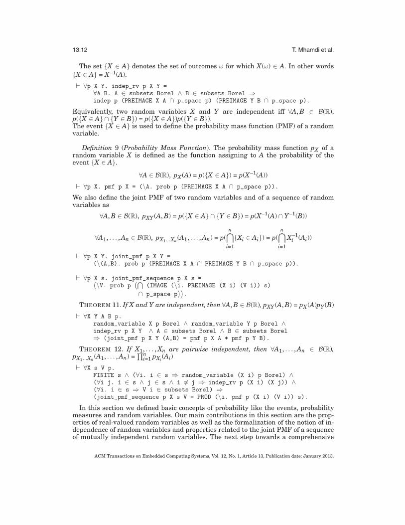
The set {X ∈ A} denotes the set of outcomes ω for which X(ω) ∈ A. In other words{X ∈ A} = X–1(A).

� ∀p X Y. indep_rv p X Y =∀A B. A ∈ subsets Borel ∧ B ∈ subsets Borel ⇒indep p (PREIMAGE X A ∩ p_space p) (PREIMAGE Y B ∩ p_space p).

Equivalently, two random variables X and Y are independent iff ∀A, B ∈ B(R),p({X ∈ A} ∩ {Y ∈ B}) = p({X ∈ A})p({Y ∈ B}).The event {X ∈ A} is used to define the probability mass function (PMF) of a randomvariable.

Definition 9 (Probability Mass Function). The probability mass function pX of arandom variable X is defined as the function assigning to A the probability of theevent {X ∈ A}.

∀A ∈ B(R), pX (A) = p({X ∈ A}) = p(X–1(A))

� ∀p X. pmf p X = (\A. prob p (PREIMAGE X A ∩ p_space p)).

We also define the joint PMF of two random variables and of a sequence of randomvariables as

∀A, B ∈ B(R), pXY (A, B) = p({X ∈ A} ∩ {Y ∈ B}) = p(X–1(A) ∩ Y–1(B))

∀A1, . . . , An ∈ B(R), pX1...Xn (A1, . . . , An) = p(n⋂

i=1

{Xi ∈ Ai}) = p(n⋂

i=1

X–1i (Ai))

� ∀p X Y. joint_pmf p X Y =(\(A,B). prob p (PREIMAGE X A ∩ PREIMAGE Y B ∩ p_space p)).

� ∀p X s. joint_pmf_sequence p X s =(\V. prob p

(⋂(IMAGE (\i. PREIMAGE (X i) (V i)) s)

∩ p_space p)).

THEOREM 11. If X and Y are independent, then ∀A, B ∈ B(R), pXY (A, B) = pX (A)pY (B)

� ∀X Y A B p.random_variable X p Borel ∧ random_variable Y p Borel ∧indep_rv p X Y ∧ A ∈ subsets Borel ∧ B ∈ subsets Borel⇒ (joint_pmf p X Y (A,B) = pmf p X A * pmf p Y B).

THEOREM 12. If X1, . . . , Xn are pairwise independent, then ∀A1, . . . , An ∈ B(R),pX1...Xn (A1, . . . , An) =

∏ni=1 pXi

(Ai)

� ∀X s V p.FINITE s ∧ (∀i. i ∈ s ⇒ random_variable (X i) p Borel) ∧(∀i j. i ∈ s ∧ j ∈ s ∧ i �= j ⇒ indep_rv p (X i) (X j)) ∧(∀i. i ∈ s ⇒ V i ∈ subsets Borel) ⇒(joint_pmf_sequence p X s V = PROD (\i. pmf p (X i) (V i)) s).

In this section we defined basic concepts of probability like the events, probabilitymeasures and random variables. Our main contributions in this section are the prop-erties of real-valued random variables as well as the formalization of the notion of in-dependence of random variables and properties related to the joint PMF of a sequenceof mutually independent random variables. The next step towards a comprehensive



formalization of probability in higher-order logic is the definition of main statisticalproperties of random variables, such as the expectation and the variance. The expec-tation of a random variable is its integral with respect to the probability measure.Lebesgue is the natural choice and will be discussed next.

5. LEBESGUE INTEGRAL

Similar to the way in which step functions are used in the development of the Riemannintegral, the Lebesgue integral makes use of a special class of functions called positivesimple functions. The Lebesgue integral is first defined for those functions then ex-tended to nonnegative functions and finally to arbitrary functions. A positive simplefunction g is a measurable function taking finitely many values. In other words, it canbe written as a finite linear combination of indicator functions of measurable sets (ai)that form a partition of X.

∀x ∈ X, g(x) =∑i∈s

αiIai (x) ci ≥ 0. (3)

Definition 10. Let (X,A,μ) be a measure space. The integral of the positive simplefunction g with respect to the measure μ is defined as∫

Xg dμ =

∑i∈s

αiμ(ai) (4)

� ∀m s a x. pos_simple_fn_integral m s a x =SIGMA (\i. x i * measure m (a i)) s.

The choice of ((αi), (ai), s) to represent g is not unique. However, the integral as definedabove is independent of that choice.Next, we define the Lebesgue integral of nonnegative measurable functions

Definition 11. Let (X,A,μ) be a measure space. The integral of a nonnegative mea-surable function f is defined as∫

Xf dμ = sup

{∫X

g dμ | g ≤ f and g positive simple function}

(5)

� ∀m f. pos_fn_integral m f =sup {r | ∃g. r ∈ psfis m g ∧ ∀x. g x ≤ f x},

where r ∈ psfis m g is equivalent to r = pos_simple_fn_integral m s a x and g isa positive simple function represented by (s,a,x).Finally, the integral for arbitrary measurable functions is given in the followingdefinition.

Definition 12. Let (X,A,μ) be a measure space. The integral of an arbitrary measur-able function f is defined as ∫

Xf dμ =

∫X

f + dμ –∫

Xf – dμ, (6)

where f + and f – are the nonnegative functions defined by f +(x) = max(f (x), 0) andf –(x) = max(–f (x), 0).

� ∀m f. fn_integral m f =pos_fn_integral m (\x. if 0 < f x then f x else 0) -pos_fn_integral m (\x. if f x < 0 then -f x else 0)



Various properties of the Lebesgue integral for positive simple functions have beenproven in HOL [Coble 2010]. We mention in particular that the above integral is well-defined and independent of the choice of (αi), (ai), s. Other properties include the lin-earity and monotonicity of the integral for positive simple functions. Another theoremthat was widely used in Coble [2010] has however a serious constraint, as was dis-cussed in the related work, where the author had to assume that every subset of thespace X is measurable, which is equivalent to assuming that every function defined onthat space is measurable.

Utilizing our formalization of the Borel sigma algebra and functions measurablewith respect to it, we have been able to prove that the functions used in the theoremare in fact measurable without having to assume that every function is measurable.For example we prove that a positive simple function is a measurable function as alinear combination of indicator functions on measurable sets. We also use Theorem 1to prove that the sets used in the theorem are in fact measurable sets. The newtheorem can be stated as follows.

THEOREM 13. Let (X,A,μ) be a measure space, f a nonnegative function measur-able with respect to (A,B(R)) and (fn) a monotonically increasing sequence of posi-tive simple functions, pointwise convergent to f such that ∀n, x, fn(x) ≤ f (x), then∫

Xf dμ = limn→∞∫

Xfn dμ.� ∀m f fi ri r.

measure_space m ∧f ∈ measurable (m_space m,measurable_sets m) Borel ∧(∀x. mono_increasing (\i. fi i x)) ∧(∀x. x ∈ m_space m ⇒ (\i. fi i x) → f x) ∧(∀i. ri i ∈ psfis m (fi i)) ∧ ri → r ∧(∀i x. fi i x <= f x) ⇒(pos_fn_integral m f = r),

where the notation xn –→ x means that the sequence xn converges to x.

5.1. Integrability

In this section, we provide the criteria of integrability of a measurable functionand prove the integrability theorem that will play an important role in proving theproperties of the Lebesgue integral.

Definition 13 (Integrable Functions). Let (X,A,μ) be a measure space, a measur-able function f is integrable iff

∫X |f |dμ < ∞ or equivalently iff

∫Xf + dμ < ∞ and∫

Xf – dμ < ∞� ∀m f. integrable m f =measure_space m ∧f ∈ measurable (m_space m,measurable_sets m) Borel ∧(∃z. ∀r.r ∈ {r | ∃g. r ∈ psfis m g ∧ ∀x. g x ≤ fn_plus f x} ⇒ r ≤ z) ∧

∃z. ∀r.r ∈ {r | ∃g. r ∈ psfis m g ∧ ∀x. g x ≤ fn_minus f x} ⇒ r ≤ z.

THEOREM 14. For any nonnegative integrable function f there exists a sequence ofpositive simple functions (fn) such that ∀n, x, fn(x) ≤ fn+1(x) ≤ f (x) and ∀ x, fn(x) → f (x).Besides ∫

Xf dμ = lim

n

∫X

fn dμ.



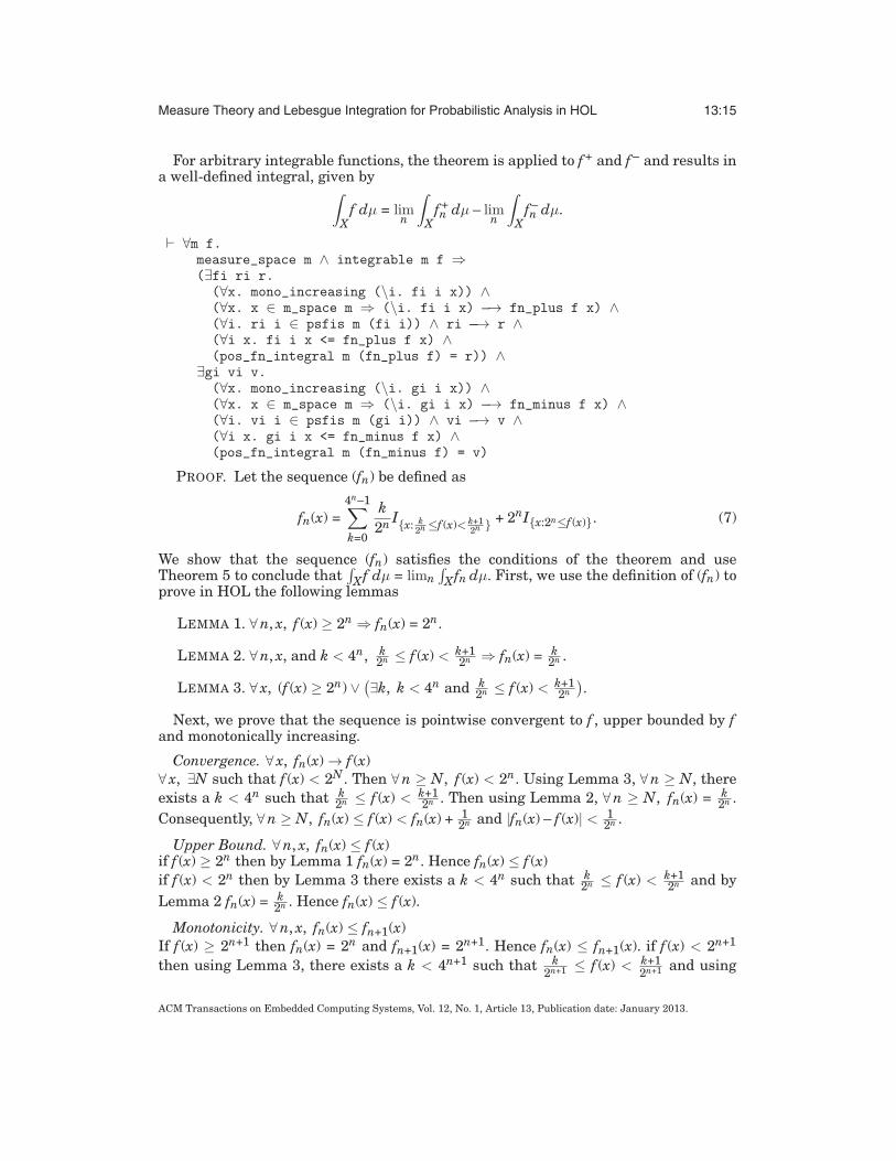
For arbitrary integrable functions, the theorem is applied to f + and f – and results ina well-defined integral, given by∫

Xf dμ = lim

n

∫X

f +n dμ – lim

n

∫X

f –n dμ.

� ∀m f.measure_space m ∧ integrable m f ⇒(∃fi ri r.(∀x. mono_increasing (\i. fi i x)) ∧(∀x. x ∈ m_space m ⇒ (\i. fi i x) –→ fn_plus f x) ∧(∀i. ri i ∈ psfis m (fi i)) ∧ ri –→ r ∧(∀i x. fi i x <= fn_plus f x) ∧(pos_fn_integral m (fn_plus f) = r)) ∧

∃gi vi v.(∀x. mono_increasing (\i. gi i x)) ∧(∀x. x ∈ m_space m ⇒ (\i. gi i x) –→ fn_minus f x) ∧(∀i. vi i ∈ psfis m (gi i)) ∧ vi –→ v ∧(∀i x. gi i x <= fn_minus f x) ∧(pos_fn_integral m (fn_minus f) = v)

PROOF. Let the sequence (fn) be defined as

fn(x) =4n–1∑k=0

k2n I{x: k

2n ≤f (x)< k+12n } + 2nI{x:2n≤f (x)}. (7)

We show that the sequence (fn) satisfies the conditions of the theorem and useTheorem 5 to conclude that

∫Xf dμ = limn

∫Xfn dμ. First, we use the definition of (fn) to

prove in HOL the following lemmas

LEMMA 1. ∀n, x, f (x) ≥ 2n ⇒ fn(x) = 2n.

LEMMA 2. ∀n, x, and k < 4n, k2n ≤ f (x) < k+1

2n ⇒ fn(x) = k2n .

LEMMA 3. ∀ x, (f (x) ≥ 2n) ∨(∃k, k < 4n and k

2n ≤ f (x) < k+12n

).

Next, we prove that the sequence is pointwise convergent to f , upper bounded by fand monotonically increasing.

Convergence. ∀ x, fn(x) → f (x)∀ x, ∃N such that f (x) < 2N . Then ∀n ≥ N, f (x) < 2n. Using Lemma 3, ∀n ≥ N, thereexists a k < 4n such that k

2n ≤ f (x) < k+12n . Then using Lemma 2, ∀n ≥ N, fn(x) = k

2n .Consequently, ∀n ≥ N, fn(x) ≤ f (x) < fn(x) + 1

2n and |fn(x) – f (x)| < 12n .

Upper Bound. ∀n, x, fn(x) ≤ f (x)if f (x) ≥ 2n then by Lemma 1 fn(x) = 2n. Hence fn(x) ≤ f (x)if f (x) < 2n then by Lemma 3 there exists a k < 4n such that k

2n ≤ f (x) < k+12n and by

Lemma 2 fn(x) = k2n . Hence fn(x) ≤ f (x).

Monotonicity. ∀n, x, fn(x) ≤ fn+1(x)If f (x) ≥ 2n+1 then fn(x) = 2n and fn+1(x) = 2n+1. Hence fn(x) ≤ fn+1(x). if f (x) < 2n+1

then using Lemma 3, there exists a k < 4n+1 such that k2n+1 ≤ f (x) < k+1

2n+1 and using



Lemma 2, fn+1(x) = k2n+1 . Now we need to determine fn(x) and compare it to fn+1(x).

k2n+1 ≤ f (x) <

k + 12n+1 ⇒

k2

2n ≤ f (x) <k+1

22n

— if k is even and k2 < 4n then fn(x) = k

2n+1 = fn+1(x)

— if k is even and k2 ≥ 4n then fn(x) = 2n and fn(x) ≤ fn+1(x)

— if k is odd and k–12 < 4n then fn(x) = k–1

2n+1 ≤ fn+1(x)

— if k is odd and k–12 ≥ 4n then fn(x) = 2n and fn(x) ≤ fn+1(x).

5.2. Lebesgue Integral Properties

We formally verified in the HOL theorem prover some key properties of the Lebesgueintegral, such as the monotonicity and linearity. Let f and g be integrable functionsand c ∈ R then

— ∀ x, 0 ≤ f (x) ⇒ 0 ≤∫

Xf dμ— ∀ x, f (x) ≤ g(x) ⇒

∫Xf dμ ≤

∫Xg dμ

—∫

Xcf dμ = c∫

Xf dμ—

∫Xf + g dμ =

∫Xf dμ +

∫Xg dμ

— A and B disjoint sets ⇒∫

A∪Bf dμ =∫

Af dμ +∫

Bf dμ

PROOF. We only show the proof for the linearity of the integral. We start by provingthe property for nonnegative functions. Using the integrability property, given inTheorem 14, there exists two sequences (fn) and (gn) that are pointwise convergent tof and g, respectively, such that

∫Xf dμ = limn

∫Xfn dμ and

∫Xg dμ = limn

∫Xgn dμ. Let

hn = fn + gn then the sequence hn is monotonically increasing, pointwise convergentto f + g and ∀ x hn(x) ≤ (f + g)(x) and using Theorem 13,

∫Xf + g dμ = limn

∫Xhn dμ.

Finally, using the linearity of the integral for positive simple functions and thelinearity of the limit,

∫Xf + g dμ = limn

∫Xfn dμ + limn

∫Xgn dμ =

∫Xf dμ +

∫Xg dμ. Now

we consider arbitrary integrable functions. We first prove in HOL the following lemma.

LEMMA 4. If f1 and f2 are positive integrable functions such that f = f1 – f2 then∫Xf dμ =

∫Xf1 dμ –

∫Xf2 dμ.

The definition of the integral is a special case of this lemma where f1 = f + and f2 = f –.Going back to our proof, let f1 = f + + g+ and f2 = f – + g– then f1 and f2 are nonnegativeintegrable functions satisfying f + g = f1 – f2. Using the lemma we conclude that∫

Xf + g dμ =∫

Xf1 dμ –∫

Xf2 dμ = (∫

Xf + dμ +∫

Xg+ dμ) – (∫

Xf + dμ +∫

Xg+ dμ) = (∫

Xf + dμ –∫Xf – dμ) + (

∫Xg+ dμ –

∫Xg– dμ) =

∫Xf dμ +

∫Xg dμ.

In this section we presented a formalization of the Lebesgue integration in HOL.We also provided the criteria of integrability of a measurable function and proved theintegrability theorem. We used this theorem to prove the properties of the Lebesgueintegral for arbitrary measurable functions compared to only positive simple functionsin the work of Coble [2010]. This formalization allows us to define the expectation andother statistical properties of random variables and prove their properties.

6. STATISTICAL PROPERTIES

We use our formalization of the Lebesgue integral to define the expected value of arandom variable and prove its properties.



6.1. Expected Value

The expected value of a random value X is defined as the integral of X with respect tothe probability measure.

Definition 14. E[X] =∫ΩX dp. � expectation = fn_integral.

The properties of the expectation are derived from the properties of the integral. Wefocus on random variables for which the expected value exists and prove, among otherproperties, the linearity and monotonicity of the expectation.

6.2. Variance

The variance and covariance of random variables are formalized as follow

� variance p X = expectation p (\x. (X x - expectation p X) pow 2)

� covariance p X Y = expectation p (\x. (X x - expectation p X) *(Y x - expectation p Y)).

Two random variable X and Y are uncorrelated iff Cov(X, Y) = 0.

� uncorrelated p X Y = (covariance p X Y = 0).

We prove the following properties in HOL.

— Var(X) = E[X2] – E[X]2— Cov(X, Y) = E[XY] – E[X]E[Y]— Var(X) ≥ 0— ∀a ∈ R, Var(aX) = a2Var(X)— Var(X + Y) = Var(X) + Var(Y) + 2Cov(X, Y)— if X, Y uncorrelated then Var(X + Y) = Var(X) + Var(Y)— if ∀i �= j, Xi, Xj uncorrelated, then Var

(∑Ni=1 Xi

)=∑N

i=1 Var(Xi)

Next, we use our formalization of the probability concepts in HOL to prove some im-portant properties, namely, the Chebyshev and Markov inequalities and the Weak Lawof Large Numbers [Papoulis 1984].

6.3. Chebyshev and Markov Inequalities

In probability theory, both the Chebyshev and Markov inequalities provide estimatesof tail probabilities. The Chebyshev inequality guarantees, for any probability distri-bution, that nearly all values are close to the mean and it plays a major role in thederivation of the laws of large numbers [Papoulis 1984]. The Markov inequality pro-vides loose yet useful bounds for the cumulative distribution function of a randomvariable.

Let X be a random variable with expected value m and finite variance σ2. TheChebyshev inequality states that for any real number k > 0,

P(|X – m| ≥ kσ) ≤ 1k2 . (8)

� ∀p X k.random_variable X p Borel ∧integrable p (\x. (X x - expectation p X) pow 2) ∧ 0 < k ⇒prob p {x | x ∈ p_space p ∧ k <= abs (X x - expectation p X)}<= variance p X / k pow 2.



The Markov inequality states that for any real number k > 0,

P(|X| ≥ k) ≤ E[X]k

, (9)

� ∀p X k.random_variable X p Borel ∧ 0 < k ⇒prob p {x | x ∈ p_space p ∧ k <= abs (X x)} <=expectation p X / k.

Instead of proving directly these inequalities, we provide a more general proof usingmeasure theory and Lebesgue integrals in HOL that can be used for both as well as fora number of similar inequalities. The probabilistic statement follows by considering aspace of measure 1.

THEOREM 15. Let (S,S,μ) be a measure space, and let f be a measurable functiondefined on S. Then for any nonnegative function g, nondecreasing on the range of f,

μ({x ∈ S : f (x) ≥ t}) ≤ 1g(t)

∫S

g ◦ f dμ .

� ∀m f g t.(let A = {x | x ∈ m_space m ∧ t <= f x} in

measure_space m ∧f ∈ measurable (m_space m,measurable_sets m) Borel ∧(∀x. 0 <= g x) ∧ (∀x y. x <= y ⇒ g x <= g y) ∧integrable m (\x. g (f x)) ⇒measure m A <= (1 / (g t)) * fn_integral m (\x. g (f x))).

The Chebyshev inequality is derived by letting t = kσ, f = |X – m| and g defined asg(t) = t2 if t ≥ 0 and 0 otherwise. The Markov inequality is derived by letting t = k,f = |X| and and g defined as g(t) = t2 if t ≥ 0 and 0 otherwise.

PROOF. Let A = {x ∈ S : t ≤ f (x)} and IA be the indicator function of A. Fromthe definition of A, ∀x 0 ≤ g(t)IA(x) and ∀x ∈ A t ≤ f (x). Since g is non-decreasing,∀x, g(t)IA(x) ≤ g(f (x))IA(x) ≤ g(f (x)). As a result, ∀x g(t)IA(x) ≤ g(f (x)). A is mea-surable because f is (S,B(R)) measurable. Using the monotonicity of the integral,∫

S g(t)IA(x)dμ ≤∫

S g(f (x))dμ. Finally from the linearity of the integral g(t)μ(A) ≤∫S g ◦ fdμ.

6.4. Weak Law of Large Numbers (WLLN)

The WLLN states that the average of a large number of independent measurementsof a random quantity converges in probability towards the theoretical average ofthat quantity. Interpreting this result, the WLLN states that for a sufficiently largesample, there will be a very high probability that the average will be close to theexpected value. This law is used in a multitude of fields. It is used, for instance, toprove the asymptotic equipartition property [Cover and Thomas 1991], a fundamentalconcept in the field of information theory.

THEOREM 16. Let X1, X2, ... be an infinite sequence of independent, identically dis-tributed random variables with finite expected value E[X1] = E[X2] = ... = m and letX = 1

n∑n

i=1 Xi then for any ε > 0,

limn→∞

P(|X – m| < ε) = 1. (10)



� ∀p X m v e.prob_space p ∧ 0 < e ∧(∀i j. i �= j ⇒ uncorrelated p (X i) (X j)) ∧(∀i. expectation p (X i) = m) ∧ (∀i. variance p (X i) = v) ⇒lim (\n. prob p {x | x ∈ p_space p ∧

abs ((\x. 1/n * SIGMA (\i. X i x) (count n))x-m) < e}) = 1.

PROOF. Using the linearity property of the Lebesgue integral as well as the proper-ties of the variance we prove thatE[X] = 1

n∑n

i=1 m = m and Var(X) = 1n2

∑ni=1 Var(Xi) = σ2

n .

Applying the Chebyshev inequality to X, we get P(|X – m| ≥ ε) ≤ σ2

nε2 .

Equivalently, 1 – σ2

nε2 ≤ P(|X – m| < ε) ≤ 1.It then follows that limn→∞ P(|X – m| < ε) = 1.Notice that in the proof we did not need to assume that the random variables are in-dependent and identically distributed. We simply assume that they are uncorrelatedand have the same expected value and variance.

To prove the results of this section in HOL we used the Lebesgue integral proper-ties, in particular, the monotonicity and the linearity, as well as the properties of real-valued measurable functions. All of these results are not available in the work of Coble[2010] because his formalization does not include the Borel sets so he cannot prove theLebesgue properties and the theorems of this section. The Markov and Chebyshev in-equalities were previously proven by Hasan and Tahar [2009a] but only for discreterandom variables. Our formalization allows us to provide a proof valid for both thediscrete and continuous cases. Richter’s formalization [Richter 2004] only allows ran-dom variables defined on the whole universe of a certain type. All of the mentionedformalizations do not include the definition of variance and proofs of its properties andhence cannot be used to verify the WLLN.

7. SHANNON SOURCE CODING THEOREM

The source coding theorem establishes the limits of data compression. It states that nindependent and identically distributed (iid) random variables with entropy H(X) canbe expressed on the average by nH(X) bits without significant risk of information loss,as n tends to infinity.

A proof of this result consists in proposing an encoding scheme for which the averagecodeword length can be made arbitrarily close to nH(X) with negligible probability ofloss. We start by proving the Asymptotic Equipartition Property (AEP) [Cover andThomas 1991] and use it to define the typical set that will be the basis of the encodingscheme.

7.1. Asymptotic Equipartition Property (AEP)

The Asymptotic Equipartition Property is the Information Theory analog of theWLLN. It states that for a stochastic source X, if its time series X1, X2, . . . is asequence of iid random variables with entropy H(X), then – 1

nlog(pX1...Xn ) converges in



probability to H(X).We define the entropy of a random source as H(X) = E[–log(pX )].

THEOREM 17. (AEP): if X1, X2, . . . are iid, then

–1n

log(pX1...Xn

)–→ H(X) in probability.

PROOF. Let X1, X2, . . . be iid random variables and let Yi = –log(pXi). Then

Y1, Y2, . . . are iid random variables and ∀i, E[Yi] = H(X). Using Theorem 16, we have

limn→∞

P(|1n

n∑i=1

Yi – H(X)| < ε)

= 1.

Furthermore,

1n

n∑i=1

Yi =1n

n∑i=1

–log(pXi

)= –

1n

log( n∏

i=1

pXi

).

Using Theorem 12, since X1, . . . , Xn are mutually independent,

–1n

log( n∏

i=1

pXi

)= –

1n

log(pX1...Xn

).

Consequently,

limn→∞

P(| –

1n

log(pX1...Xn

)– H(X)| < ε

)= 1. (11)

7.2. Typical Set

A consequence of the AEP is the fact that the set of observed sequences (x1, . . . , xn)which joint probabilities p(x1, x2, . . . , xn) are close to 2–nH(X) has a total probabilityequal to 1. This set is called the typical set and such sequences are called the typicalsequences. In other words, out of all possible sequences, only a small number ofsequences will actually be observed and those sequences are nearly equally probable.The AEP guarantees that any property that is proved for the typical sequences willthen be true with high probability and will determine the average behavior of a largesample.

Definition 15. The typical set Anε with respect to p(x) is the set of sequences

(x1, . . . , xn) satisfying

2–n(H(X)+ε) ≤ p(x1, . . . , xn) ≤ 2–n(H(X)–ε). (12)

We prove in HOL various properties of the typical set.

THEOREM 18. If (x1, . . . , xn) ∈ Anε , then

H(X) – ε ≤ –1n

log(p(x1, . . . , xn)) ≤ H(X) + ε (13)

This theorem is a direct consequence of Definition 15.

THEOREM 19. ∀ε > 0, ∃N, ∀n ≥ N, p(Anε ) > 1 – ε.



The proof of this theorem is derived from the formally verified AEP. The next twotheorems give upper and lower bounds for the number of typical sequences |An

ε |.

THEOREM 20. |Anε | ≤ 2n(H(X)+ε).

PROOF. Let x = (x1, . . . , xn), then∑

x∈Anε

p(x) ≤ 1. From Equation (12), ∀x ∈Anε , 2–n(H(X)+ε) ≤ p(x). Hence

∑x∈An

ε2–n(H(X)+ε) ≤

∑x∈An

εp(x) ≤ 1. Consequently,

2–n(H(X)+ε)|Anε | ≤ 1 proving the theorem.

THEOREM 21. ∀ε > 0, ∃N.∀n ≥ N, (1 – ε)2n(H(X)–ε) ≤ |Anε |.

PROOF. Let x = (x1, . . . , xn). From Theorem 19, ∃N.∀n ≥ N, 1 – ε <∑

x∈Anε

p(x).

From Equation 12, ∀x ∈ Anε , p(x) ≤ 2–n(H(X)–ε). Hence, ∃N.∀n ≥ N, 1– ε <

∑x∈An

εp(x) ≤∑

x∈Anε

2–n(H(X)–ε). Consequently, ∃N.∀n ≥ N, 1 – ε < 2–n(H(X)–ε)|Anε | proving the

theorem.

7.3. Shannon Source Coding Theorem

The main idea behind the proof of the source coding theorem is that the average code-word length for all sequences is close to the average codeword length considering onlythe typical sequences. This is true because according to Theorem 19, for a sufficientlylarge n, the typical set has a total probability close to 1. In other words, for any ε > 0,and sufficiently large n, the probability of observing a nontypical sequence is less thanε. Furthermore, according to Theorem 20, the number of typical sequences is smallerthan 2n(H(X)+ε) and hence no more than n(H(X) + ε) + 1 bits are needed to representall typical sequences. If we encode each typical sequence by simply enumerating itsposition within an ordered list of typical sequences and add 0 as a prefix, the totalnumber of bits needed is no more than n(H(X) + ε) + 2. We also encode each nontypicalsequence by enumerating its position within an ordered list of all possible sequencesand prefix it by 1. The total number of bits needed for the nontypical sequences is lessthan nlog(|Ω|) + 2. If we denote by Y the random variable defined over all the possiblesequences and returns the corresponding codeword length. The expectation of the Yis equal to the average codeword length L. Besides, ∀x ∈ An

ε , Y(x) ≤ n(H(X) + ε) + 2otherwise Y(x) ≤ nlog(|Ω|) + 2.

L = E[Y] =∑

x∈Anε

p(x)Y(x) +∑

x∈Anε

p(x)Y(x) (14)

L ≤ p(Anε )(n(H(X) + ε) + 2) + (1 – p(An

ε ))(nlog(|Ω|) + 2) (15)

L ≤ p(Anε )n(H(X) + ε) + (1 – p(An

ε ))nlog(|Ω|) + 2. (16)

Using Theorem 19, ∃N, ∀n ≥ N, p(Anε ) > 1 – ε. Hence,

L ≤ n(H(X) + ε) + εnlog(|Ω|) + 2 (17)

L ≤ n(H(X) + ε′), (18)

where ε′

= ε + εlog(|Ω|) + 2n .

Consequently, for any ε > 0 and n sufficiently large, the code rate Ln can be made as

close as needed to the entropy H(X) while maintaining a probability of error of theencoder that is bounded by ε.



The coding scheme we used is one-to-one, as the first bit in the codeword indicatesits length and the remaining bits determine its position in the corresponding orderedset. We formally verified that the average codeword length of this code can be madearbitrarily close to nH(X) without significant loss of information.

8. CONCLUSIONS

In this article we have presented a comprehensive methodology to reason about prob-abilistic systems in a theorem prover. We provided a formalization of the measuretheory including the Borel sigma algebra defined for any topological space. We then fo-cused on real-valued measurable functions and proved their key properties. Using thisformalization we defined a theory of probability in Higher-order logic. Main conceptsof probability in our formalization include random variables, probability mass func-tions (pmf), joint pmf, and independence of random variables. To formalize statisticalproperties of random variables, we presented a Lebesgue integration infrastructureincluding important properties such as the linearity and monotonicity of the Lebesgueintegral. We applied the Lebesgue integral properties to the expectation operator andused the whole formalization to prove classical results from the theory of probability,namely, the Chebyshev and Markov inequalities as well as the WLLN.

The proposed work paves the path for the usage of formal verification for analyzingprobabilistic aspects in many critical domains, such as security protocols, transporta-tion and communication systems. We illustrated the effectiveness of our formaliza-tion by proving a fundamental result in information theory, namely the AsymptoticEquipartition Property, which we used to prove the classical source coding theorem.The HOL codes corresponding to all the formalization and proofs, presented in this ar-ticle, are available in Mhamdi et al. [2010a] and can be built upon to formally analyzeother interesting applications.

Overall our formalization required more than 9000 lines of code. Only 700 lineswere required to verify the key properties of the application section. This shows thesignificance of our work in terms of simplifying the formal analysis of probabilisticsystems. The main difficulties encountered were the multidisciplinary nature of thiswork, requiring deep knowledge of measure and integration theories, topology, set the-ory, real analysis and probability and information theories. Some of the mathematicalproofs also posed challenges to be implemented in HOL. Our future plans include usingthe Lebesgue monotone convergence theorem and the Lebesgue integral properties toprove the Radon Nikodym theorem [Bogachev 2006], paving the way to defining theprobability density functions for continuous random variables as well as the Kullback-Leibler divergence [Cover and Thomas 1991], which is related to the mutual informa-tion, entropy and conditional entropy.

REFERENCES

Baier, C. and Katoen, J. 2008. Principles of Model Checking. MIT Press.Baier, C., Haverkort, B., Hermanns, H., and Katoen, J. 2003. Model checking algorithms for continuous

time Markov chains. IEEE Trans. Softw. Engin 29, 4, 524–541.Berberian, S. K. 1998. Fundamentals of Real Analysis. Springer.Bialas, J. 1990. The σ-additive measure theory. J. Formal. Math. 2.Bogachev, V. I. 2006. Measure Theory. Springer.Chaum, D. 1988. The dining cryptographers problem: Unconditional sender and recipient untraceability. J.

Cryptology 1, 1, 65–75.Coble, A. R. 2010. Anonymity, information, and machine-assisted proof. Ph.D. thesis, University of

Cambridge.Cover, T. M. and Thomas, J. A. 1991. Elements of Information Theory. Wiley-Interscience.de Alfaro, L. 1997. Ph.D. thesis, Stanford University.



Fraenkel, A., Bar-Hillel, Y., and Levy, A. 1973. Foundations of Set Theory. North Holland.Gordon, M. 1989. Mechanizing programming logics in higher-order logic. In Current Trends in Hardware

Verification and Automated Theorem Proving. Springer, 387–439.Gordon, M. and Melham, T. 1993. Introduction to HOL: A theorem proving environment for higher-order

logic. Cambridge University Press.Halmos, P. R. 1944. The foundations of probability. Amer. Math. Monthly 51, 9, 493–510.Harrison, J. 2009. Handbook of Practical Logic and Automated Reasoning. Cambridge University Press.Hasan, O. and Tahar, S. 2007. Verification of expectation properties for discrete random variables in HOL.

In Theorem Proving in Higher-Order Logics. Lecture Notes in Computer Science, vol. 4732. Springer,119–134.

Hasan, O. and Tahar, S. 2009a. Formal verification of tail distribution bounds in the HOL theorem prover.Math. Methods Appl. Sci. 32, 4 (March), 480–504.

Hasan, O. and Tahar, S. 2009b. Performance analysis and functional verification of the stop-and-waitprotocol in HOL. J. Autom. Reasoning 42, 1, 1–33.

Hasan, O., Abbasi, N., Akbarpour, B., Tahar, S., and Akbarpour, R. 2009. Formal reasoning about expec-tation properties for continuous random variables. In Proceedings of the 2nd World Congress on FormalMethods. Lecture Notes in Computer Science, vol. 5850. 435–450.

Hasan, O., Tahar, S., and Abbasi, N. 2009. Formal reliability analysis using theorem proving. Trans.Comput. 59, 579–592.

Hurd, J. 2002. Formal verifcation of probabilistic algorithms. Ph.D. thesis, University of Cambridge.Kwiatkowska, M., Norman, G., and Parker, D. 2005. Quantitative analysis with the probabilistic model

checker PRISM. Electron. Notes in Theor Comput Sci. 153, 2, 5–31. Elsevier.Lester, D. 2007. Topology in PVS: Continuous mathematics with applications. In Proceedings of the Workshop

on Automated Formal Methods. ACM, 11–20.Mhamdi, T., Hasan, O., and Tahar, S. 2010a. Formal analysis of systems with probabilistic behavior in

HOL. http://users.encs.concordia.ca/~mhamdi/hol/probability/.Mhamdi, T., Hasan, O., and Tahar, S. 2010b. On the formalization of the Lebesgue integration theory in

HOL. In Proceedings of the Conference on Interactive Theorem Proving. 387–402.Nedzusiak, A. 1989. σ-fields and Probability. J. Formal. Math. 1.Owre, S., Rushby, J. M., and Shankar, N. 1992. PVS: A prototype verification system. In Proceedings of the

11th International Conference on Automated Deduction. Lecture Notes in Computer Science, vol. 607.748–752.

Papoulis, A. 1984. Probability, Random Variables, and Stochastic Processes. Mc-Graw Hill.Parker, D. 2001. Ph.D. thesis, University of Birmingham, Birmingham, UK.Paulson, L. C. 1994. Isabelle: A Generic Theorem Prover. Springer.Reiter, M. K. and Rubin, A. D. 1998. Crowds: Anonymity for web transactions. ACM Trans. Inf. Syst.

Secur. 1, 1, 66–92.Richter, S. 2004. Formalizing integration theory with an application to probabilistic algorithms. In Proceed-

ings of the 17the International Conference on Theorem Proving in Higher Order Logics. Lecture Notesin Computer Science. vol. 3223. 271–286.

Rutten, J., Kwaiatkowska, M., Normal, G., and Parker, D. 2004. Mathematical Techniques for AnalyzingConcurrent and Probabilisitc Systems. CRM Monograph Series, vol. 23. American Mathematical Society.

Sen, K., Viswanathan, M., and Agha, G. 2005. VESTA: A statistical model-checker and analyzer for prob-abilistic systems. In Proceedings of the IEEE International Conference on the Quantitative Evaluationof Systems. 251–252.

Smith, G. 2009. On the foundations of quantitative information flow. In Proceedings of the Conference onFoundations of Software Science and Computational Structures. 288–302.

Wagon, S. 1993. The Banach-Tarski Paradox. Cambridge University Press.

Received March 2010; revised October 2010; accepted June 2011


Formalization of Measure Theory and Lebesgue Integration for

Documents