Formal Verification of Timed Properties of Randomized ...groups.csail.mit.edu/tds/papers/Segala/PS95.pdf · Formal Verification of Timed Properties of Randomized Distributed ... We

Formal Verification of Timed Properties of Randomized Distributed Algorithms*

Anna Pogosyants and Roberto Segala

Laboratory for Computer Science

Massachusettss Institute of Technology

Cambridge, MA 02139 USA

emaik anya, segala@theory. lcs. mit. edu

Abstract

In [11] a method for the analysis of the expected time com-

plexity of a randomized distributed algorithm is presented.

The method consists of proving auxiliary probabilistic time

bound statements of the form U ~ U’, which mean that

whenever the algorithm begins in ‘a state in set U, it will

reach a state in set U’ within time t with probability at

least p . However, [11] does not provide a formal method-

ology to prove the validity of a specific probabilistic time

bound statement from scratch: each statement is proved

by means of ad hoc operational arguments. Unfortunately,

operational reasoning is generally error-prone and difficult

to check. In this paper we overcome the problem by de-

veloping a new technique to prove probabilistic time bound

statements, which consists of reducing the analysis of a time

bound statement to the analysis of a statement that does not

involve probability. As a consequence, several existing tech-

niques for non-randomized algorithms can be applied, and

correctness proofs can be verified mechanically.

1 Introduction

Randomization is a useful tool for the solution of problems

in distributed computation (e.g., [3, 4, 9]), but even simple

randomized algorithms are sometimes hard to verify and

analyze. As a result, many randomized algorithms are pre-

sented with only informal proofs, and even when formal

proofs are presented, they are often ad hoc; mistakes are

common. Most of the mistakes come from considering to-

gether probabilistic and non-deterministic choices. Another

problem with informal and ad hoc arguments is that it is

hard to be convinced that all the possible cases are consid-

ered.

In this paper we provide a methodology that allows us

to verify timed properties of randomized algorithms, Our

methodology consists of the following steps.

“Research supported m part by the Advanced Research ProjectsAgency of the Department of Defense, monitored by the Office ofNaval Research under contracts NOO014-92-J-1795 and NOOO14-92-J-4033, by the National Science Foundation under grants 9115797-CCRand S915206-CCR, and by the Office of Naval Research under contractNOOO14-91-J-1O46.

Permission to make digital/hard copies of all or part of this materiai forpersonal or classr?orn use is granted without fee provided that the copiesare not made or dmtrlbuted for profit or commercial advantage, the copy-right notice, the title of the publication and its date appear, and notice isgiven that copyright is by permission of the ACM, Inc. To copy otherwise,to republish, to post on servers or to redistribute to lists, requires specific

1

2,

3.

Here

Decompose the timed properties of a randomized algo-

rithm into probabilistic time boztnd statements as sug-

gested in [1 1]. A probabilistic time bound statement

is an expression of the form U ~ U’, where U and

U’ are sets of states of the algo~ithm, p is a proba-

bility, and t is a positive real number. Its meaning is

that whenever an algorithm is started from a state of

U, then a state of U’ is reached within time t with

probability at least p.

Reduce each problem of checking whether a probabilis-

tic time bound statement U &. U’ is satisfied byP

a randomized algorithm to the problem of checking

whether the non-probabilistic time bound statement

U ~ U’ is satisfied by some specific non-randomized

algorithm. The non-randomized algorithm is derived

from the original randomized algorithm.

Prove each of the non-probabilistic time bound state-

ments using some of the existing techniques for ordi-

nary, non-randomized, distributed algorithms.

we focus on the second and third steps. We provide a

way of reducing a probabilistic system, de~oted b; A4, to a

non-probabilistic system, denoted by A, so that the validity

of U ~ U’ for A implies the validity of U L U’ for M.

We call the system A a generating automato;. Informally,

A is obtained from M by forcing some of the probabilistic

choices of M to give some specific outcomes, and by chang-

ing all the other probabilistic choices of J4 into nondeter-

ministic choices. The forced outcomes should be chosen so

that their probability in M is always greater than or equal

to p.

Once the reduction is carried out, since generating au-

tomata describe ordinary (non-randomized) algorithms, sev-

eral existing techniques can be used to prove the new time

bound =tatements. We present a technique based on progress

functions in the style of [10]. A progress function is a func-

tion that associates real numbers with some of the states

of a system; roughly speaking, a progress function gives an

upper bound on the time left until reaching a state of U’.The existence of a progress function is sufficient for prov-

ing a time bound statement. Moreover, proofs based on the

progress function method can be machine checked.

The main advantage of our methodology is that it sep-

arates completely probability from non-determinism, thus

pem-ission andlor fee.PODC 95 Ottawa Ontario CA e 1995 ACM 0-89791-710-3/95/08. .$3.50

174

eliminating the most common source of mistakes in cor-

rectness proofs. Moreover, our method eliminates ad hoc

arguments and allows for proofs to be carried out at dif-

ferent levels of details. A high level description of a proof

can be given by specifying the key parameters of our proof

method; then, some interesting cases can be considered in

more detail, and, if necessary, the most critical parts can

be checked mechanically by an automatic theorem prover.

Even for high level proofs the advantages of our methodol-

ogy are evident: it provides a systematic way of listing allpossible cases, thus reducing the possibility of not consider-

ing some cases. Moreover, a skeptical reader can always fill

in the details easily.

We applied the new technique for the formal verifica-

tion of the randomized Dining Philosophers algorithm of

Lehmann and Rabin [9](same example asin [11]). We used

the proof sketch from [11], and we reproved all main lem-

mas using generating automata and progress functions. We

carried out the proofs in full detail and automated the rou-

tine parts of the proofs using the Larch Prover [7]. The

complete proof (hand and automatic) can be found in [15].

We sketched the proof of correctness of the randomized al-

gorithm for consensus with stopping faults of Ben-Or [4],

and, based on the experience that we gained, we are confi-

dent that our methodology applies to most of the standard

randomized distributed algorithms as well.

Previous work on verification of randomized distributed

algorithms appears in [6,8, 11,14, 16]. The work of [14]

presents a technique, based on ranking functions defined

on states, for establishing liveness properties for random-

ized algorithms; the work of [16] extends UNITY [5] to han-

dle probability, and provides a completeness result for some

properties that hold with probability 1; the work of [6,8]

presents model checking techniques; the work of[11] presents

a technique based on probabilistic time bound statements,

where each statement is proved by means of ad hoc oper-

ational arguments. Our methodology, combined with the

extensive collection of verification techniques available on

ordinary non-randomized algorithms, overcomes several of

the limitations of [6,8, 11, 14, 16].

The rest of the paper is organized as follows. Section 2

presents the non-probabilistic model, introduces the time

bound statements, and describes the proof method based on

progress functions; Section 3 presents a simplified version of

the probabilistic models of [17], introduces the probabilis-

tic time bound statements, and shows how to prove them

through generating automata; Section 4 presents the algo-

rithm of Lehmann and Rabin and illustrates our technique

by giving some fragments of the correctness proofi Section 5

contains some concluding remarks.

2 The Non-probabilistic Framework

In this section we introduce the non-probabilistic framework.

We define semi-timed automata, which are a simplification

of the timed automata of [12], and we formalize the state-

ments U ~ U‘. Furthermore, we int reduce the verification

technique based on progress functions.

2.1 Semi-Timed Automata and Time Bound Statements

Definition 2.1 A semi-timed automaton A consists of four

components

●

●

●

●

a set States(A) of states;

a non-empty set Start(A) ~ States(A) of start states;

a timed action signature

Sig(A) = (int(A), ezt(A), time(A)),

where int(A), ext(A) and time(A) are disjoint sets:

int(A) is the set of internal actions, ezt(A) is the set

of external actions, and time(A) = {v(t) I t c R+} is

the set of time-passage actions;

a transition relation

Trans(A) G States(A) x Actzons(A) x States(A),

where Actions(A) denotes the set znt(A) U ezt(A) U

time(A). The elements of Trans(A) are called transi-

tions. ■

The main difference between a semi-timed automaton de-

fined here and a timed automaton of [12] is that a semi-timed

automaton is not required to satisfy the trajectory axioms,

which restrict the transition relation so that the actions of

time(A) model actual passage of time. The trajectory ax-

ioms do not play a fundamental role for the results of this

paper, and thus we omit them from the discussion.

An execution fragment of a semi-timed automaton A is

a sequence a of alternating states and actions of A start-

ing with a state, and, if a is finite, ending with a state,

a = seal sl az S2.,., such that for each z > 0 there exists a

transitions,, a,+l, S,+I) of A. Denote by fstate(cr) the first

state of w and, if a is finite, denote by ktate(a) the last state

of a; furthermore, denote by Mime(a) the sum of the reals in

the time passage actions of cr. Denote by frag” (A) the set of

finite execution fragments of A. An ezecution is an execu-

tion fragment whose first state is a start state. An execution

a of A is admissible if itime(w) = co. Denote by ezec” (A)

and exec(A) the sets of admissible and all executions of A,

respectively.

A state s of A is said to enable a transition if there is a

transition (s, a, s’) in Trans(A); an action a is said to be en-

abled from s if there is a transition (s, a, s’) in Z’rans(A); an

execution a is said to be complete in A iff either a is infinite

or a is finite and lstate(a) d?es not enable any transition. A

state s of A is reachable if there exists a finite execution of

A that ends in s. Denote by rstates(A) the set of reachable

states of A. A fimte execution fragment al = .Oal S1 . a~sn

of A and an execution fragment aZ = snan+l Sn+I of A

can be concatenated. The concatenation, written al m aZ,

is the execution fragment soalsl . . . a~s~a~+ls~+l . . . . An

execution fragment a 1 of A is a prejix of an execution frag-

ment az of A, written al < c22, iff either al = CY2 or al is

finite and there exists an execution fragment aj of A such

that crz = crl n aj. If a = a] n cw, then az is called a sufix

of a, and it is denoted alternatively by aoa].

In this paper we concentrate on the admissible executions

of a semi-timed automaton, since they are those executions

that represent realistic behaviors: no system can stop time,

and thus time grows unfoundedly. We can now define for-

mally a time bound statement.

Definition 2.2 Let A be a semi-timed automaton, U, U’ ~>0 Then u ~ u ~ denotes a predicate that

States(A), t E R- .

is true for A iff every admissible execution fragment a of Athat starts from a state of U has a finite prefix a’ such that

Mme(cr’) < t and /state(a’) c U’. 9

175

2.2 Proving Time Bound Statements

There are several techniques to prove properties of semi-

timed automata. Here we present a techniqne, based on

progress functions, which is useful to prove the validity of

time bound statements. The key idea of the technique is

based on the following theorem.

Theorem 2.3 Let A be a semi-timed automaton, U, U’ ~

States(A). Suppose that there exist two functions

p : States(A) + Bool, and

‘P : States(A) + l?~”,

such that the following hold:

1. Ijs E U then eitherp(s) A ‘P(s) < t or s c U’;

2, For ail transitions(s, a, s’) E Tkns(A) such that p(s)

(a) if a is a time-passage action v(At) then p(s’) A

(P(S) - At> p(S’));

(b) if a is not a time-passage action then either-p(s’)A

(P(s) ~ P(s’)) or s’ E u’.

Then U 2 U’ is true for A. ■

A pair (p, ‘P) satisfying the conditions of Theorem 2.3 defines

a partial function from states of A onto nonnegative real

numbers. The domain of the function consists of states of

A such that p(s) is true, and the values of the function are

given by ‘P(s). Informally, this partial function describes an

upper bound on the time left until reaching a state of U’.

Condition 1 guarantees that the upper bound for the states

of U is at most t;Conditions 2 (a, b) ensure that the upper

bound associated with each state is correct. We refer to the

pair (p, ‘P) as a progress function. The idea of a progress

function is borrowed from [10].

3 The Probabilistic Framework

In this section we present our methodology for proving prob-

abilistic time bound statements of tkibrm. U ~ U’. WeP

start by introducing the probabilistic semi-timed automaton

model, which is a simplification of the model of [17], and by

formalizing the statements U ~ U’ within this model.

Then we show how such statements can be verified formally

by reducing the problem to a new problem that does not

involve probability.

3.1 Probabilistic Semi-Timed Automata and Time BoundStatements

Definition 3.1 A probability space is a triplet (Q, 5, P)where tl is a set, also called the sample space, F is a col-

lection of subsets of Q that is closed under complement and

count able union and such that ~ c F, also called a u-field,

and P is a function from 3 to [0, 1] such that P[Q] = 1

and such that for any collection {C, }, of at most countably

many pairwise disjoint elements of 3, ~[uic,] = ~, P[C’].

A probability space (Q, F, P) is discrete if F = 2Q and

for each C ~ Q, P[C] = ~zGC P[{z}]. It is immediate

to verify that for every discrete probability space there are

at most countably many points with a positive probability

measure. For any arbitrary set X, let Probs(X) denote the

set of discrete probability distributions whose sample space

is a subset of X.

A probability space is called a Dirac distribution if its

sample space contains exactly one element. Denote by Dx

the Dirac space whose sample set is {z}. ■

Definition 3.2 A probabilistic semi-timed automaton M con-

sists of four components:

● a set States(M) of states;

● a non-empty set Start(M) ~ States(M) of start states;

● a timed action signature Sig(M);

● a transition relation

Trans(M) G

States(M) x Actions(M) x Probs(States(M)),

such that each transition with a time-passage action

leads to a Dirac distribution, i.e., if (s, v(t),(Q,7, P)) c

Trans(M), then Ifll = 1.

A probabilistic semi-timed automaton M is fully probabilis-

tic if M has exactly one start state and each state of M

enables at most one transition. ■

Execution fragments and executions are defined similarly to

the non-probabdistic case. An execution fragment of M is

a sequence a of alternating states and actions of M start-

ing with a state, and, if a is finite ending with a state,

a = so al S1a2s2..., such that for each i > 0 there exists

a transitions,, a,+l, (Q, F, P)) of M such–that s,+] E Q.

All the terminology that is used for executions in the non-

probabilistic case applies to the probabilistic case as well.

An execution fragment of M is the result of resolving

both the probabilistic and the nondeterministic choices of

M. If only the nondeterministic choices are resolved, then

we obtain a fully probabilistic semi-timed automaton, which

we call a probabilistic execution fragment of M. Probabilistic

execution fragments are the objects where the probabilistic

behavior of a probabilistic automaton can be studied. In-

formally, a probabilistic execution can be thought of as the

result of unfolding the transition relation of a probabilis-

tic automaton and then choosing at most one transition for

each state of the unfolding.

Definition 3.3 A probabilistic execution fragment H of a

probabilistic semi-timed automaton M is a fully probabilis-

tic semi-timed automaton, such that:

States(H) G /rag*(M); let q range over the states of

H;

Sig(lT) = Sig(M);

Start(H) ~ States(M);

for each transition(q, a, (Q, ~, P)) of H there exists a

transition(ktate (q), a, (0’, >’, P’)) of M such that 0 =

{qas I s E Q’} and P’[gas] = P[s] for all s c Q’;

all the states of H are reachable, i.e., for each state g

of H there is an execution of H that leads to q.

176

We say that a probabilistic execution fragment H starts with

a state s of M if Start(H) = {s}. A probabilistic esecutiorz

H of a probabilistic semi-timed automaton M is a proba-

bilistic execution fragment of M that starts with a state of

Start(M).

A probabilistic execution fragment Hof Missaid to be

m-knissiblei feveryc ompleteexecution of lf inadmissible. ■

Remark 3.1 Thedefinition ofaprobabilistic execution that

we have given here is simpler than the definition given in

[17]. The-main differences are the following: -

1.

2.

the start state of a probabilistic execution fragment

of [17] can be an arbitrary finite execution fragment

rather than just a state;

each transition that leaves from astateof arxobabilis-

tic execution fragment of [17] can lead to a ~robabilit y

distribution over pairs (action, state) plus a special

symbol 6 that models deadlock.

The first feature is necessary to prove what we are going

to state in Proposition 3.5; the second feature is necessary

if we want to be able to resolve the nondeterminism in a

probabilistic automaton using randomization. In this paper

we assume that randomization cannot be used to resolve the

nondeterminism; however, all the results that we prove here

carry over to the randomized case. ■

There is a strong correspondence between the executions of

a probabilistic semi-timed automaton and the executions of

one of its probabilistic executions. Specifically, if H is a

probabilistic execution fragment of M, then every execution

of H can be represented by an execution fragment of M.

Below we define two operations on execution fragments that

exploit the correspondence. Let go be the start state of H,

and let a = qoalgl a2g2 . . . be an execution of H. Denote by

cr~ the execution go A alistrate(ql )az Mate(q2) . . . . Note that,

from the definition of a probabilistic execution fragment, al

is an execution fragment of M. For each execution fragment

a’ of M starting with qO (a’ = qO m alslazsz... ), let c#lH

denote the sequence qOaI (goalsl)az(qoalslazsz). Then, it

is easy to show that for each execution fragment a of H,

(crJ)TH = cr.

We now define the probability space associated with a

probabilktic execution fragment, so that its probabilistic

behavior can be studied. Given a probabilistic execution

fragment H, the sample space is the set ~H = {al I cr is a

complete execution of H}. The a-field ~H is the smallest

a-field that contains the set of cones C~, consisting of the

executions of ~H having a as a prefixl. The probability

measure PH is the unique extension of the probability mea-

sure defined on cones as follows: PH [c~] is the product of

the probabilities of each transition of H generating a. In

[17] it is shown that there is a unique probability measure

having the property above, and thus (fl~, ~H, ~H) is a well

defined probability space.

An event E of H is a measurable subset of ~H, i.e., an

elament of ~H. However, events alone are not sufficient for

the analysis a probabilistic semi-timed automaton, since a

probabilktic semi-timed automaton may have seversJ prob-

abilistic execution fragments, and each probabilistic exe-

cution fragment is associated with a different probability

1Note that a cone Ca can be used to express the fact that thefimte execution a occurs

space. Thus, a more abstract structure is needed. An event

schema is a function that associates an event of ~H with

each probabilistic execution fragment of M.

We can now give the formal definition of a probabilistic

time bound statement.

Definition 3.4 Let M be a probabilistic semi-timed au-

tomaton, U, U’ ~ States(M), t c R~O. Then U L U’

denotes a predicate that is true for M iff for each admis-

sible probabilistic execution fragment H of M that starts

with a state of U, P~[eu,,J > p, where eu~,t(ll) is the set

of executions a of ~H such that a has a prefix a’ such that

ltirne(cr’) < t and ktate(cr’) c U’. ■

Some inference rules of [11] that can be used to derive new

probabilistic time bound statements from existing ones are

the following.

Proposition 3.5 Let M be a probabilistic semi-timed au-

tomaton, U, U’, U“, U’” G States(M). Then,

1.

.2.

3.

3.2

if U + U! and Uf + U“, then U % U“;W’

if U ~ U’, then U I-I U“ L U’ IJ U“;P P

u’ u u’”.

Proving Probabilistic Time Bound Statements

A technique to prove the validity of a probabilistic time

bound statement U & U’ for a probabilistic semi-timedP

automaton M, which is hinted at in [11], consists of the

following steps.

1.

2.

3.

Choose a set of random draws that may occur in a

probabilistic execution of M, and choose some of the

possible outcomes;

Show that starting from a state of U, no matter how

the nondeterminism is resolved, the chosen random

draws give the chosen outcomes with some minimum

probability p;

Show that whenever the chosen draws give the chosen

outcome, a state of U’ is reached withi~ time t.

This technique corresponds to the informal arguments of

correctness that appear in the literature. Usually the intu-

ition behind an algorithm is exactly that success is guaran-

teed whenever some specific random draws give some specific

results.

The first two steps can be reformulated in terms of the

set @ of admissible execution fragments of M that start in

a state of U and such that each of the chosen random draws

gives one of the chosen outcomes. Then the minimum prob-

ability requirement of the second step can be formulated

as follows: for every admissible probabilistic execution frag-

ment H of M that starts in a state of U, P[@ ~ OH] > p.

Once the first two steps are reformulated in terms of @,

the third step can be carryed out by showing that for any

execution fragment a of @ a state of U’ is reached within

time t. If we build a non-probabilistic automaton, called

177

a generating automaton, so that its admissible executions

contain @, and we show that each admissible execution of

the generating automaton leads to U’withintimet, then we

are done. To carry out this last step the progress function

of Section 2.2 or any other technique for non-probabilistic

automata can be applied. Given a set @, a generating au-

tomaton for @ with the properties described above can be

built as follows.

Definition 3.6 Let ill be a probabilistic semi-timed au-

tomaton, and let @ be a set of admissible execution frag-

ments of M. Define a semi-timed automaton A such that

1.

2.

3.

4.

Sig(A) = Sig(M);

States(A) = {a E -fr-ag*(M) I 3aZe@CV < a’}, i.e.,

States(A) is the set of finite prefixes of elements of

@. Denote a generic state of A by q;

Start(A) = {q G States(A) I Igl = O};

(g, a, g’) c Z’rarzs(A) iff q’ = gas, where s = Istcate(q’).

We call A the generating automaton for (9, and we denote

it by GM(@). 9

Lemma 3.7 Let M be a probabilistic semi-timed automat-

on, and let @ be a set of admissible execution fragments of

M. Then @ ~ execw(GM(@)). ■

We can now formulate the main theorem that justifies our

reduction.

Theorem 3.8 Let M be a probabilistic semi-timed automat-

on, and let U and U’ be sets of states of M. Let @ be

a set of admissible execution fragments of M such that the

following hold.

1. For every admissible probabilistic execution fragment

H of M starting with a state of U, PH[@ ~ flH] z p.

2. Start(G~(@)) ~ U;, where U; is the set of states q

of GM(@) such that L-tate(q) G U’.

Then U L U’ is valid for M. ■P

Theorem 3.8 states that by chosing a set @ that satisfies

Condition 1 we can reduce the proof of U ~ U’ for M (theP

probabilistic problem) to the proof of Start ( GM( @)) ~ U;

for GM ( 67) (a non-probabilistic problem). We can use any

standard technique for non-probabilistic automata to solve

the non-probabilistic problem. In particular, we can use the

technique based on progress functions of Section 2, which is

also machine checkable.

Remark 3.2 Although the problem is reduced to the anal-ysis of a non-probabilistic system, it is important to under-

stand that building a generating automaton is not trivial in

general. To build a generating automaton it is necessary to

identify the right set @ and make sure that El is express-

ible by an automaton. This process involves understanding

the main idea of a randomized algorithm, which is usually

the creative part of a correctness proof. Fortunately, the

designer of an algorithm usually has enough intuition about

why the algorithm works so that the task of building a gen-

erating automaton is simplified. ■

4 Example

In this section we use the randomized Dining Philosophers

algorithm of Lehmann and Rabin to illustrate our method.

The same problem was analized in [11]. Here we concentrate

more on a fragment of the proof of [11] and we show how it is

possible to use generating automata and progress functions

to prove the validity of a time bound statement. We start

by presenting the algorithm of Lehmann and Rabin; then we

consider a specific time bound statement and we define the

corresponding generating automaton and the corresponding

progress function; finally, we prove by structural induction

that indeed we have defined a progress function. The whole

analysis is carried out in a simplified model, called the prob-

abilistic MMT automaton model, where time-passage is con-

strained according to some specific restricted kinds of rules.

Since the details of the MMT model are necessary only to

prove that we have defined a progress function, we postpone

the presentation of the simplified model to the point where

it is necessary.

4.1 The Problem, the Protocol, and its Formalization

The problem consists of allocating n resources among n pro-

cesses arranged in a ring. The resources are interspersed

between the processes, and each process requires both its

adj scent resources to perform its task.

According to the Lehmann-Rabin algorithm, every pro-

cess that is trying to obtain its resources executes the follow-

ing protocol. It first flips a fair coin to choose between its left

and right resources. Then it waits for the chosen resource

to be free and takes it. After that, it attempts to access the

other resource: if the other resource is free, then the pro-

cess gets it an proceeds to its task; otherwise, the process

returns the first resource and starts the protocol again. The

algorithm ensures exclusive possession of resources and also

ensures that, with probability y 1, if some process is trying

to get its resources, then eventually some process (may be

different one) will proceed to its task.

To formalize the algorithm, we use the probabilistic MMT

automaton model, which is a useful special case of prob-

abilistic semi-timed automata. A probabilistic MMT au-

tomaton is an automaton whose actions are partitioned into

classes. Each class T is associated with an upper bound and

a lower bound, which give restrictions to the time at which

any action from T can occur (cf. Sections 4.5 and 4.6).

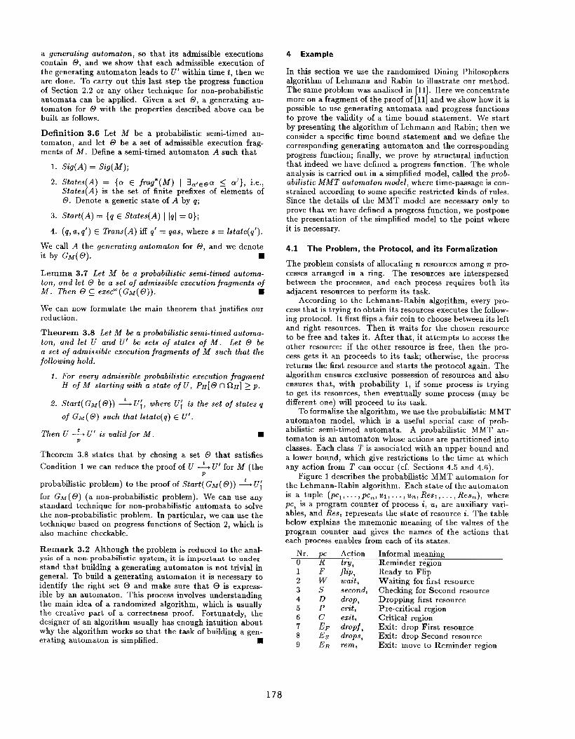
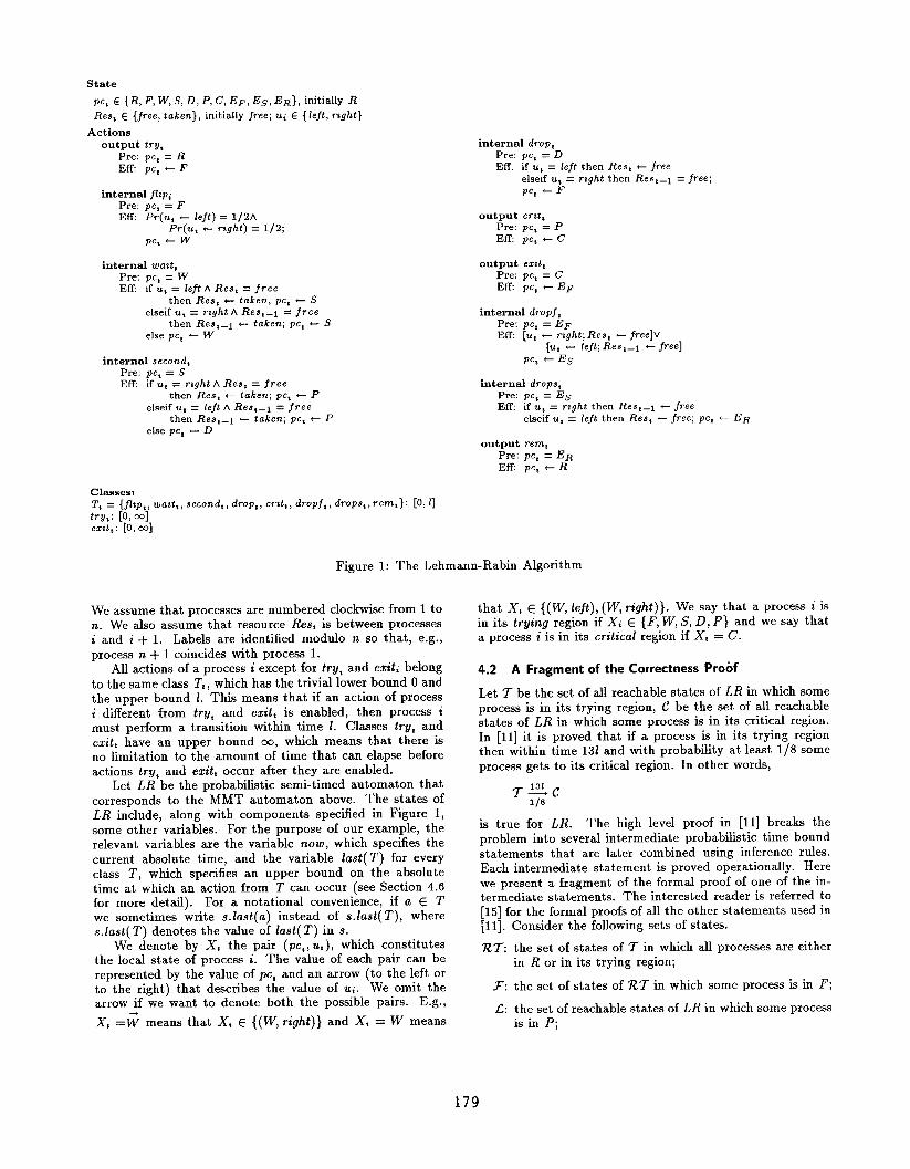
Figure 1 describes the probabilistic MMT automaton for

the Lehmann-Rabin algorithm. Each state of the automaton

is a tuple (pcl, . . ..pcn. ul, ..., %, Resl, . . . . Resn), where

pc, is a program counter of process 2, u, are auxiliary vari-

ables, and Res, represents the state of resource i. The table

below explains the mnemonic meaning of the values of the

program counter and gives the names of the actions that

each process enables from each of its states.

Nr. pc Action Informal meaning

OR try, Reminder region

IF

2W3s

4D.5P6C7 EF

8 ES

9 ER

f7i~,

wait,second,

drop,

crit,

exit,

dropf,

drops,

rem,

Ready to Fli~

Waiting for first resource

Checking for Second resource

Dropping first resource

Pre-critical region

Critical region

Exit: drop First resource

Exit: drop Second resource

Exit: move to Reminder region

178

State

PC, E {R, F, W, S, D, P, C, Ep, E.s, ER], initiallY R

Rest c {free, taken}, initially free; u; E {left, ~?g~t}

Actionsoutput try,

Pre: PC, = REff pC, - F

internal flzpaPre: PC, = FEff Pr(u, - left) = l/2A

Pr(u, + rzght) = 1/2;pc, t w

internal wait,Pre: pc, = WEff ]f u, = left A Rest = free

then Rest + taken, PC, + Selseif u, = rzght A Rest_l = free

then Res, -l + taken; PC, * Selse pc, + W

internal second~Pre: pc, = SEff if u, = r$ght A Rest = free

then Rest +- taken; PC, +- Pelseif u, = left A Res, _l = free

then Rest_l + taken; PC, + Pelse PC, + D

internal drop,Pre: PC, = DEff. if u, = left then Res, + free

elself ~1 = rtght then Rest—l = free;PC, + F

output Cr%t,Pre: pc, = PEff PC, - C

output eztttPre: pc, = CEff PC, - E~

internal dropfzPre: PC, = EFEff [u, t r%ght; Res, + .free]V

[u, +- left; Res,–1 + free]pet + ES

internal drops%Pre: PC, = ESER if u% = rtght then Res%_l + free

elseif w, = /eft then Rest + free; PC, +- ER

output remzPre: PC, = EREff pC, t-- R

Classes:z’, = {.fhpt, watt,, second,, drop,, crzt,, dropf,, drops,, rem,}: [0, ~1try,: [0, co]emtt, [0, co]

Figure 1: The Lehmann-Rabin Algorithm

We assume that processes are numbered clockwise from 1 to

n. We also assume that resource Rest is between processes

i and i + 1. Labels are identified modulo n so that, e.g.,

process n + 1 coincides with process 1.

All actions of a process i except for try, and e~it: belong

to the same class T,, which has the trivial lower bound O and

the upper bound 1. Thk means that if an action of process

i different from tr~,and ezit, is enabled, then process i

must perform a transition within time 1. Classes trg, and

ezit, have an upper bound co, which means that there is

no limitation to the amount of time that can elapse before

actions try,and esit, occur after they are enabled.

Let LR be the probabilistic semi-timed automaton that

corresponds to the MMT automaton above. The states ofLR include, along with components specified in Figure 1,

some other variables. For the purpose of our example, the

relevant variables are the variable now, which specifies the

current absolute time, and the variable Iast( T) for every

class T, which specifies an upper bound on the absolute

time at which an action from T can occur (see Section 4.6

for more detail). For a notational convenience, if a c T

we sometimes write s.kzst(a) instead of s. last( T), where

s.last( T) denotes the value of last(T) in s.

We denote by X, the pair (PC,, u, ), which constitutes

the local state of process i. The value of each pair can be

represented by the value of PC, and an arrow (to the left or

to the right) that describes the value of tii. We omit the

arrow if we want to denote both the possible pairs. E.g.,

X, =7 means that X, E {(W, right)} and X, = W means

that X, ~ {(W, left),

in its trying region i

W, right)

xi E {F,a process i is in its critical regi

. We say that a process i is

V, S, D, P} and we say that

m if X, = C.

4.2 A Fragment of the Correctness Proof

Let T be the set of all reachable states of LR in which some

process is in its trying region, C be the set of all reachable

states of LR in which some process is in its critical region.

In [11] it is proved that if a process is in its trying region

then within time 13/ and with probabtity at least 1/8 some

process gets to its critical region. In other words,

T~C

is true for LR. The high level proof in [11] breaks the

problem into several intermediate probabilistic time bound

stat ements that are later combined using inference rules.

Each intermediate statement is proved operationally. Here

we present a fragment of the formrd proof of one of the in-

termediate statements. The interested reader is referred to

[15] for the formal proofs of all the other statements used in

[11]. Consider the following sets of states.

‘RE

F:

/!2

the set of states of T in which all processes are either

in R or in its trying region;

the set of st ates of I?T in which some process is in F;

the set of reachable states of LR in which some process

is in P;

179

~: the set of states of ‘RT in which there is a process z

such that

The statement we want to analyze here is

F-&u L.

The meaning of this statement is that if some process is

ready to flip a coin, then within time 21 and with probabil-

ity at least 1/2 either some process is in P, which means that

this same process will go to C on the next transition, or ~ is

reached. Reaching ~ is a substantial progress towards reach-

ing C, since in each state of !7 there must exist two adj scent

processes that act asymmetrically. Asymmetric behavior is

a key element for reaching C.

Just for completeness of presentation, the other state-

ments that are shown in [11] are the following.

TL7Z7- UC,

wAF(J~uL,

In the rest of the paper we analyze only ~ ~ ~ UC.

4.3 Help in Building a Generating Automaton

Before proving the time bound statement above, we state

an auxiliary result, that can be used to discharge the first

condition of Theorem 3.8. Let M be a probabilistic semi-

timed automaton, S be a collection of pairs (a,, U,), 1< z’ <

k, consisting of an action a, of 34 and a set of states U, of

M. Assume that the actions a,’s are all distinct. Let us

restrict our attention to probabilistic execution fragments

that start from a state of U, and let first~(M,U) be the set

of admissible execution fragments a of &f such that the first

state of a is in U and such that either none of the a,’s occur

in a, or, if aj is the first of the ai’s that occur in a, the firstoccurrence of a~ in a leads to a state of UJ. The following

Lemma follows from results of [11].

Lemma 4.1 Let H be an admissible probabilistic execution

fragment of M staring with a state of U, P1, . . ..p~ be real

number-s between O and 1 such that for each 1 < j < n and

for each transitiova(s, aj, (Q, F, P)) the pr-obab~ity P[Uj ~

Q] > pj. Then PH~rst~(M, U) (l QH] > rnin(pl, . . ..p~).

■

Lemma 4.1 is called a coin lemma in [11] since in most of

the algorithms randomization is introduced by flipping fair

coins. Each action a, identifies one of the possible random

draws and the set U; identifies the outcomes that are al-

lowed. If each a, identifies the process of flipping a coin,

then Lemma 4.1 can be used to say that no matter how the

nondeterminism is resolved the probabihty that either no

coin is flipped or the first coin that is flipped gives head is

at least 1/2.

4.4 Building the Generating Automaton and the ProgressFunction

We now return to the proof of 7 % g U L for LR. The

main intuition is that if some process flips a coin, then one

of the two outcomes leads to a state where the symmetry

is broken. Since in F at least one process is ready to flip a

coin, within time 1 some process flips. Once a process has

flipped and the coin flipped has given the desired result, it

may be that another transition is necessary before reaching

~. For this reason the time bound associated with the time

bound statement that we are proving is 21.

Consider a state s of ~ and consider a number k such

that xk = F. We know that k exists from definition of X.

Let 71 be the set of states of> such that Xk-1 c {~ U ~

U D URU F}, FZ be the set of states of ~ such that Xk+l C

{~ U @ U j URUF}, and Fs be the set of states of X such

that X~.I C {~ U ~ U j} and Xk+l E {~ U fi U j}.The sets fl, %’z and 73 form a partition of 7. We prove a

probabtistic time bound statement for each of the three sets,

and later combine the statements using Proposition 3.5.

Proof. Denote by left, and right, the sets of states of

LR where u, is equal to left and right, respectively. Let

S = {(fli~k, ~efik), (fl~Pk-1, r@tk_l )}. we prove Lemma4.2 by showing that the set @I = fir-st~(LR, 71 ) satisfies

the conditions of Theorem 3.8 with t= 1and p = 1/2. From

Lemma 4.1, PH[ G n OH] > 1/2 for all admissible prob-

abilistic execution fragments H that start with a state of

F].

Let Al be the generating automaton for @I. It is left to

show that Star-t(Al) ~ Gt U .CT is true for A]. We do it

using the progress function method.

Let s be a state of AI. Let j7ippedk,k_1 (s) be a predi-

cate that is true iff either jlipk or flipk_l occur in S. For

shorthand we write s. X,, s./ast(T8 ) and s. now instead of

Mate(s). X,, Mate(s) .last(T,) and ktate(s). now respectively.

Define the predicate p on States(Al ), and the function

? : States(Al) ~ R~O as follows:

p(s) ~ s E restates A =flippedk,k-l(s)

As.xk = F A (S.XL1 E {E uf’ U R})

As G ~?_~ \ CT

P(s) = (rnin(s.last(jlipk), s.last(flipk_l)) – snow).

The complete proof that (p(s), p(s)) is a progress function

can be carried out by showing that the conditions of Theo-

rem 2.3 are satisfied. This can be done by standard struc-

tural induction, which considers the effect of all actions, one

at a time (cf. Section 4.7). The proof can be verified me-

chanically by a computer. The complete proof together with

its automation can be found in [15]. ■

Informally, p(s) says that s is a reachable state of Al such

that s @ ~t U Zt and the processes k and k – 1 did not flip

any coin yet. That is,

p(s) u s G restates A =j7ippedk,k_1 (s) As @ Gt u C?.

However, to carry out the inductive proof that (p(s), P(s))

is a progress function, we need to specify in more detail what

180

it means for s not to be in ~1 U Lt, and so we obtain the

additional clause s.xk = F A (9.~k_l c {5 UF U R}) that

appears in the proof of Lemma 4.2. This clause is presentalso in the operational argument of [1 I], but it is not stated

explicitly. Using our method we can check that this clause

is correct, since otherwise the verification that (p, P) is a

progress function would break.

The idea behind the definition of P(s) is that a state of

~T is reached for sure as soon as the first flip action of either

process k or k – 1 occurs. Thus, P(s) gives an upper bound

on the time left until either process k or k – 1 flips. By

carrying out the complete progress function proof we can

check that the informal reasoning is correct.

Lemma 4.3 YZ ~ G U L.

Proof. Symmetric to the proof of Lemma 4.2. ■

Lemma 4.4 FS ~ G u L.

Proof. If s 6 73 then from the fact that processes are

arranged in a ring we get that there exists a process j such

that

s.xy C{ti U; UjU~U~} As.xJ+, {ti U; Ub}.

Let S = {(flZPJ, ~~g~tj), (fl@j+l, leftj+l )}. We prove Lemma

4.4 by showing that the set Oz = jirst~(LR, F3) satisfies the

conditions of Theorem 3.8 with t = 21 and p = 1/2. We

know that PH( @3 n H) > 1/2 for all admissible H that start

with a state of 33 (Lemma 4.1).

Let A3 be the generating automaton for Os. It is left

to show Star-t(A3) 3 ~t U Ct for As. We do it using the

progress function method.

Let s be a state of As. Let jlippedj,, +l (s) Le a predicate

that is true iff either J7ipj or .fiz’p J+l occur in S.

Define the Dredicate ~ on States(As). and the function

P : Stotes(A3) + R20 as-follows: ‘ -‘’

p(s) @ s E r-states(As) A -tiippedj,J+l (s)

AS. XJE{ii U; U~URU~}

AS.XJ+I C {b uF} A s ● %?7T \ LT;

if XJ+I =D, then

‘P(s) = (.s.last(dropj+l) + 1) – snow;

otherwise,

P(s) = rnin(s.last(flip, ), s.last(flip,+l)) snow.

The complete proof that (p(s), P(s)) is a progress function

can be carried out by induction as in the proof of Lemma 4.2.

The complete proof together with its automation can be

found in [15]. ■

Informally, p(s) says that s is a reachable state of A3 such

that s @ ~T U CT and the processes j and j + 1 did not flip

any coin yet. That is,

p(s) @ s G restates A Tjlippedj,j+l (s) A s @ GT U Lt.

However, to carry out the inductive proof that (p(s), 7(s))is a progress function, we need to specify in more detail what

it means for s not to be in ~T U .Lt, and so we obtain the. . .

additional clause s.Xj E {W U S U D URU F} A S.X1+I E

{b U~} that appears in the proof of Lemma 4.4. The clause

is present in the operational argument of [1 I], but it is not

stated explicitly. Using our method we can verify that this

clause is correct, since otherwise the verification that (p, T)

is a progress function would break.

The idea behind the definition of ‘P(s) is that if s.X~+l =

F then G’t will be reached for sure after the first flip of

processes j or j + 1. This is expressed by the second clause

for ‘P(s). If S.X3+I =5 then we have to. wait for process

j + I to perform drop (at most last(dropj+l ) – now), and

then for one of the processes of j and j + 1 to perform a flip

(at most 1). This is expressed by the first clause for ‘P. By

carrying out the complete progress function proof we can

check that the informal reasoning is correct.

4.5 Probabilistic MMT Automata

We want to complete our example by showing how to verify

the correctness of a progress function. To do so, we need

to give a more precise definition of probabilistic MMT am

tomata. The model presented in this section is an extension

of the non-probabilistic MMT automaton model of [13].

A Probabilistic 1/0 Automaton M consists of the followi-

ng five components:

a set States(M) of states;

a nonempty set Start(M) Q States(M) of start states;

an action signature

Sig(M) = (in(M), out(M), int(kf)),

where in(M), out(kf) and int(lf) are three disjoint

sets of input, output and internal actions of M.

a transition relation

Trans(M) s

States(M) x Actions(M) x Prob. (States(M))

such that for every input action a and every state s

there is a transition (s, a, (Q,7, P)) in Trans(M).

a task ~artition Part(M), which ~artitions int(lil) U. .out(kfj into disjoint ~las~es (task;).

A class T c Part(M) is said to be enabled in a state s if at

least one of its actions is enabled in s.

Definition 4.5 Let M be a probabilistic 1/0 automaton

with finitely many tasks. A boundmap b for M is a pair

of mappings lower and upper, that give lower and upper

bounds for each class of M, such that for all classes T

O < lower-(T) < GO, O < upper(T) ~ co, and lower(Z’) <

upper( T). A pair (M, b) is called an MMT probabilistic au-tomaton. ❑

4.6 Probabilistic Semi-Timed 1/0 Automata

A probabilistic semi-timed 1/0 automaton is a probabilis-

tic semi-timed automaton M, augmented with an external

action signature Esig(M) = (in(M), out(A4)), which parti-

tions actions of ezt(Sig(M)) into input and output actions.

181

Z’r-cms(ill) is required to have a transitions, a, (Q, %, P)) for

every input action a and every state s.

In this section we describe how to incorporate the tim-

ing information of a probabilistic MMT automaton (M, b)

into the state yielding a probabilistic semi timed 1/0 au-

tomaton Time(M, b) of a special form. This construction is

an extension to the probabilistic case of the construction of

[10].

Each state s of Time (M, b) consists of the following com-

ponents:

basic E States(M), initially a start state of M;

now c R>, initially O;

for each class T c Part(Af),

fht(T) c R>, initially lower(T) if some action of T

is enabled in basic, otherwise O;

kt( T) E R+ U {co} initially upper(T) if some action

of T is enabled in basic, otherwise co.

The transition relation of Time(M, b) is defined as follows:

if a E Actions(M), then a transition (s, a, (0, ~, P)) is in

Trans( Time(M, b)) iff all the following conditions hold

1.

2.

3.

4.

Vs’ c Q (S’. now = Snow);

(s. basic, a, (Cl’, X’, P’)) is a transition of &f, where Q’ =

{s. basic I s c Q}, and P’[s.basic] = P[S] for all s E Q;

for each T in F’art(M),

(a) for all s’ c Cl such that T is not enabled in s’,

s’.first( 2’) = O and s’.last( T) = co;

(b) for all s’ c C? such that T is enabled in s’, if a c l“

or T is not enabled in s, then s’.fkrt = s. now +

lower(T) and s’.last( T) = snow+ upper( T); if

T is enabled in s and a # T, then s’.first( T) =

s.jrst( T) and s’.last( T) = s./ast(T);

if a is a time-passage action, say v(t),then (s, v(t), s’)

is in Trans ( Time (M, b)) iff all the following conditions

hold:

(a) s’.now = snow+ t;

(b) s’. basic = s. basic;

(c) for each T c Part(M),

i. s’. now s s.last( T),

ii. s’.first( T) = s.first( 2’), and

iii. s’.last( T) = s.last( T).

We often omit the . basic part of the selector while referring

to components of a state of III. We also write s.last(a),

where a is an action of ill instead of writing s. last ( T), where

T is a class of a in Par-t(M).Based on the definition of ‘l’am. (M, 6), it is easy to show

that the following invariants are satisfied.

Proposition 4.6 The following hold in any reachable state

s of Time(M, b) for any class T E Par-t(M):

● o < Snow;

● S.rlow < S.last( T);

● s.last(T) s s.raow + upper(T);

● first(T) < last( T). ■

The invariants that are true for Time (M, b) carry over to

some of the generating automata obtained from Time (M, b).

Proposition 4.7 Let U be a subset of reachable states of

M’, and let @ be a set of admissible execution fragments of

M’ starting in U. Then the following hold in any reachable

state q of G~,(@) for any class T c Part(M):

● O < ktate(g). now;

● Istate(q). now ~ ktate(q). iast( T);

● lstate(g).last( T) s lstate(q). now + rtpper( T);

● lstate(q).first( T) ~ ktate(q).last( T). ■

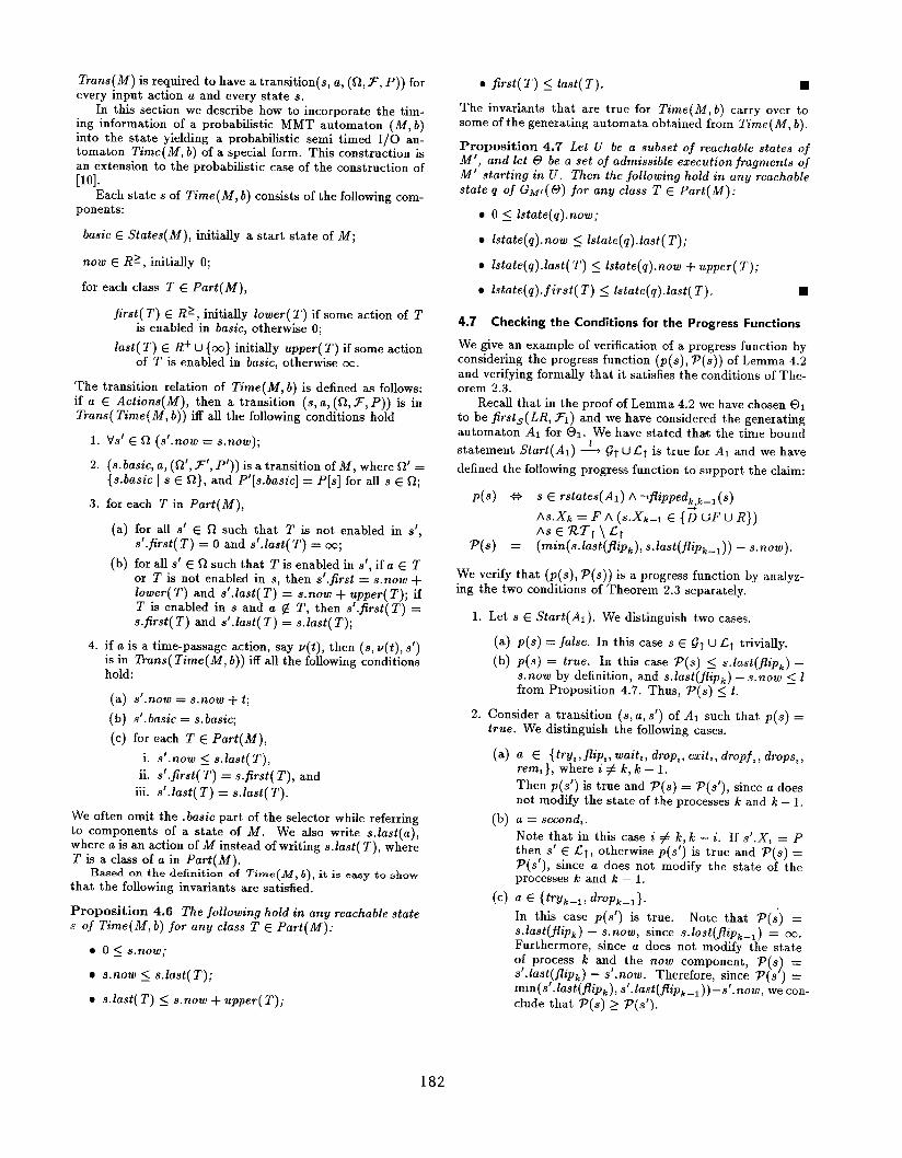
4.7 Checking the Conditions for the Progress Functions

We give an example of verification of a progress function by

considering the progress function (p(s), P(s)) of Lemma 4.2

and verifying formally that it satisfies the conditions of The-

orem 2.3.

Recall that in the proof of Lemma 4.2 we have chosen @l

to be first~( LR, F1 ) and we have considered the generating

automaton Al for 631. We have stated that the time bound

statement Start(Al) ~ ~t U CT is true for Al and we have

defined the following progress function to support the claim:

p(s) ~ s ● rstdes(Al) A ‘ffiPPedk,k-l (s)

/’w.~k = F A (S.xk-l G {5 UF U R})

As E R7T \ ~t

P(s) = (rnin(s.last(f7ip~), s.last(f?ipk_l)) – s.nozu).

We verify that (p(s), ‘P(s)) is a progress function by analyz-

ing the two conditions of Theorem 2.3 separately.

1. Let s c Start(Al ). We distinguish two cases.

(a) p(s) = false. In this case s c gt U CT trivially.

(b) p(s) = true. In this case ‘P(s) < s.last(flipk) -

snow by definition, and s.last(fl~pk) — snow <1

from Proposition 4.7. Thus, P(s) <1.

2. Consider a transition (s, a, s’) of Al such that p(s) =

true. We distinguish the following cases.

(a)

(b)

(c)

a G {try,, f7ipz, wait,, drop,, exit,, dropf,, drops,,rem,}, where i# k,k–1.

Then p(s’) is true and P(s) = P(s’), since a does

not modify the state of the processes k and k – 1.

a = secondi.

Note that in this case i # k, k – i. If s’.X, = P

then s’ ~ Cl, otherwise p(s’) is true and ‘P(s) =

~(s’), since a does not modify the state of theprocesses k and k – 1.

a ~ {try~–l, drop~–1 }.

In this case p(s’) is true. Note that ~(s) =

s.last(f7ipk) – snow, since s.iast(f3ipk_1) = w.

Furthermore, since a does not modify the state

of process k and the now component, P(s) =

s’, (ast(j%pk) – s’. now. Therefore, since P(s ) =

min(s’.last(flip ~),s’.1ast(f7ipk_1 ))-s’. now, we con-

clude that P(s) > P(s’).

182

(d)

(e)

(f)

(g)

a = flipk.

In this case S’.xk =fi As’.Xk_l & {B uFu R} A

s’ E l?’Tt \ CT, which implies s’ E Gt.

a = fiipk_l.

In this case S’.X~-I =$ As’.Xk = F, which im-

plies s’ C ~t.

a 6 {trt/k,WU2tk, tiropk, t?X2tk, droptkj dropsk,remk].

This case is not possible since if p(s) is true then

S.xk = F.

a = v(At).

In this case p(s’) is true. By substituting the

definition of ‘P(s) in P(s) – At we ontain P(s) –

At = min(s.last(f7ipk), ~.ia$t(fiipk_~)) – (s. n02U +

At). Observe that s’.last(f%pk) = s.kast(flipk),

that s’. iast(f@k_l) = s.iast(fiipk_~), and thatsnow + At = s’, now. Therefore,

~(s) – At = ?(S’).

The proof above consists of a very detailed and structured

cases analysis, where the effect of each action is considered.

Although the analysis is long and tedious, the cases st ruc-

ture and the reasoning for each case are simple and can be

automat ed using a theorem prover.

5 Conclusion

In this paper we have improved the results of [11] by intro-

ducing a stylized way of proving probabilistic time bound

statements. This allows us to eliminate the operational rea-

soning from correctness proofs, and therefore, it allows us

to produce proofs that are formal and easy to verify.

Our proof method separates the key insights of a cor-

rectness proof from the routine parts, and makes it possible

to structure a proof in several levels of detail. This allows

a designer to work out the specific details of a correctness

proof only where it is desired. Moreover, the routine parts

of the proof, which are the most tedious ones, are the parts

that can be verified automatically.

The method can be used to verify time bounded progress

of several randomized algorithms. We have carried out and

verified automatically the complete proof for the algorithm

of Lehmann and Rabin, and we have done some work in ap-

plying the method to prove the correctness of Ben Or’s ran-

domized agreement protocol [4]. We believe that the method

can be applied also to the randomized self-stabilizing span-

ning tree algorithm by Sudhanshu Aggarwal and Shay Kut-

ten [2]. In [1] the algorithm is verified using time bound

stat ements and inference rules, but the individual basic time

bound statements are justified by long operational argu-

ments, which can be eliminated using our method.

Further work involves the analysis of other existing algo-

rithms so that the full power of our method can be tested.

At the moment we do not know its limitations, and it is

likely that new features will be added to the method in the

future. However, we think that the main idea of reducing

the analysis of a probabilistic property to the analysis of a

non-probabilistic property is always applicable.

Acknowledgments We thank Nancy Lynch for helpful com-

ments and suggestions.

References

[1]

[2]

[3]

[4]

[5]

[6]

[7]

[8]

[9]

[10]

[11]

[12]

[13]

[14]

[15]

[16]

[17]

i

3. Aggarwal. Time optimal self-stabilizing spanning

tree algorithms. Technical Report MIT/LCS/TR-632,

MIT Laboratory for Computer Science, 1994.

3. Aggarwal and S. Kutten. Time optimal self stabiliz-

ing spanning tree algorithms. In R.K. Shyamasundar,

editor, I.?th International Conference on Foundations

of Software Technology and Theoretical Computer Sci-

ence, LNCS 761, 1993

J. Aspnes and M.P. Herlihy. Fast ~andomized con-

sensus using shared memory. Journal of Algorithms,

15(1):441–460, September 1990.

M. Ben-Or. Another advantage of free choice: com-

pletely asynchronous agreement protocols. In Proceed-

ings of the 2nd Annual ACM PODC, 1983

K.M. Chandi and J. Misra. Parallel Program Design:

A Foundation. Addison-Wesley, 1988.

L. Christoff and I. Christoff. Efficient algorithms for

verification of equivalences for probabilistic processes.

In Proceedings of the %d Workshop on Computer-Aided

Verification, 1991.

S.J. Garland and J.V. Guttag. A guide to LP, the Larch

Prover. Technical Report 82, DEC Systems Research

Center, December 1991.

H. Hansson. Time and Probability in Formal Design

of Distributed Systems, volume 1 of Real- Time Safety

Critical Systems. Elsevier, 1994.

D. Lehmann and M. Rabin. On the advantage of free

choice: a symmetric and fully distributed solution to

the dining philosophers problem. In Proceedings of the

8th Annuat ACM PODC, pages 133–138, January 1981.

N.A. Lynch and H. Attiya. Using mappings to prove

timing properties. Distributed Computing, 6:121-139,

1992.

N.A. Lynch, I. Saias, and R. Segala. Proving time

bounds for randomized distributed algorithms. In Pro-

ceedings of the 13*h Annual ACM PODC, 1994.

N.A. Lynch and F. W. Vaandrager. Forward and back-

ward simulations – part II: Timing-based systems.

Technical Report MIT/LCS/TM-487, MIT Laboratory

for Computer Science, September 1993.

M. Merritt, F. Modugno, and M. Tuttle. Time con-

strained automata. In J.C. M. Baeten and J.F. Groote,

editors, Proceedings of CONCUR 91, LNCS 527, 1991.

A. Pnueli and L. Zuck. Verification of multipro-

cess probabilistic protocols. Distributed Computing,

1(1):53–72, 1986.

A. Pogosyants and R. Segala. Automatic verification of

time properties of randomized distributed algorithms.

In progress, 1995.

J .R. Rae. Reasoning about probabilistic algorithms. In

Proceedings of the 9’h Annual ACM PODC, 1990.

R. Segala. Modeling and Verification of Randomwed

Distributed Real- Time Systems. PhD thesis, MIT,

Dept. of Electrical Eng. and Computer Science, 1995.

183