Formal Theory for Comparative Politics * Avidit Acharya † January 2013 I taught this material in the first half of a class called “Formal Modeling in Comparative Politics” to second year graduate students in the political science and economics departments at the University of Rochester. The second half of the class was mainly student presentations. * This material was taught to University of Rochester graduate students in political science and economics in the spring of 2013. † Assistant Professor of Political Science and Economics at the University of Rochester. 1

Welcome message from author
This document is posted to help you gain knowledge. Please leave a comment to let me know what you think about it! Share it to your friends and learn new things together.
Transcript

Formal Theory for Comparative Politics∗
Avidit Acharya†
January 2013
I taught this material in the first half of a class called “Formal Modeling in
Comparative Politics” to second year graduate students in the political science
and economics departments at the University of Rochester. The second half of
the class was mainly student presentations.
∗This material was taught to University of Rochester graduate students in political science and
economics in the spring of 2013.†Assistant Professor of Political Science and Economics at the University of Rochester.
1

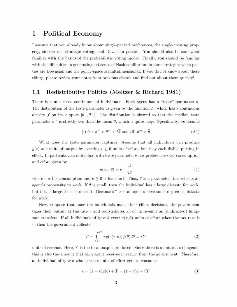
Contents
1 Political Economy 3
1.1 Redistributive Politics (Meltzer & Richard 1981) . . . . . . . . . . . . . . . 3
1.2 Non-distortionary Taxation . . . . . . . . . . . . . . . . . . . . . . . . . . . 6
1.3 Targetted Transfers (Lindbeck & Weibull 1987) . . . . . . . . . . . . . . . . 7
1.4 Corruption and Party Bias (Acharya, Roemer & Somanathan 2012) . . . . 9
1.5 Progressive Income Taxation (Roemer 1999) . . . . . . . . . . . . . . . . . . 11
1.6 Political Economy with Strategic Voting (Acharya 2012) . . . . . . . . . . . 15
1.7 Comparative Politics and Public Finance (Persson, Roland & Tabellini 2000) 19
2 Dynamic Methods, etc. 25
2.1 Infinite Horizon Dynamic Programming . . . . . . . . . . . . . . . . . . . . 25
2.2 Dynamic Game Theory . . . . . . . . . . . . . . . . . . . . . . . . . . . . . 27
2.3 Weak and Strong States (Acemoglu 2005) . . . . . . . . . . . . . . . . . . . 29
2.4 Political Transitions (Acemoglu & Robinson 2001) . . . . . . . . . . . . . . 32
2.5 Global Games (Carlsson & van Damme 1993) . . . . . . . . . . . . . . . . . 38
2.6 The Global Game of Revolution (Acharya 2009) . . . . . . . . . . . . . . . 39
2.7 Persistent Effects of Colonization in Africa (Nunn 2007) . . . . . . . . . . . 44
3 Behavioral Political Economy 49
3.1 Ideology (Benabou 2008) . . . . . . . . . . . . . . . . . . . . . . . . . . . . . 49
3.2 Social Identity Equilibrium (Shayo 2009) . . . . . . . . . . . . . . . . . . . . 52
2
1 Political Economy
I assume that you already know about single-peaked preferences, the single-crossing prop-
erty, sincere vs. strategic voting, and Downsian parties. You should also be somewhat
familiar with the basics of the probabilistic voting model. Finally, you should be familiar
with the difficulties in generating existence of Nash equilibrium in pure strategies when par-
ties are Downsian and the policy-space is multidimensional. If you do not know about these
things, please review your notes from previous classes and find out about them quickly!
1.1 Redistributive Politics (Meltzer & Richard 1981)
There is a unit mass continuum of individuals. Each agent has a “taste”-parameter θ.
The distribution of the taste parameter is given by the function F , which has a continuous
density f on its support [θ−, θ+]. The distribution is skewed so that the median taste
parameter θm is strictly less than the mean θ, which is quite large. Specifically, we assume
(i) 0 < θ− < θ+ < 2θ and (ii) θm < θ (A1)
What does the taste parameter capture? Assume that all individuals can produce
y(e) = e units of output by exerting e ≥ 0 units of effort, but they each dislike putting in
effort. In particular, an individual with taste parameter θ has preferences over consumption
and effort given by
u(c, e|θ) = c− e2
2θ(1)
where c is his consumption and e ≥ 0 is his effort. Thus, θ is a parameter that reflects an
agent’s propensity to work: If θ is small, then the individual has a large distaste for work,
but if it is large then he doesn’t. Because θ− > 0 all agents have some degree of distaste
for work.
Now, suppose that once the individuals make their effort decisions, the government
taxes their output at the rate τ and redistributes all of its revenue as (undirected) lump-
sum transfers. If all individuals of type θ exert e(τ, θ) units of effort when the tax rate is
τ , then the government collects
T =
∫ θ+
θ−τy(e(τ, θ))f(θ)dθ ≡ τY (2)
units of revenue. Here, Y is the total output produced. Since there is a unit mass of agents,
this is also the amount that each agent receives in return from the government. Therefore,
an individual of type θ who exerts e units of effort gets to consume
c = (1− τ)y(e) + T = (1− τ)e+ τY (3)
3

units of output. Note that because each agent is infinitesimal, he is negligible: the effort
decision e has no effect on T (or Y ).
How is the tax rate determined? We assume that prior to the agents exerting their
effort, there is a majoritarian election in which two Downsian political parties, A and B,
announce (and commit to) a tax rate τ ∈ [0, 1]. Thus, these parties compete over the issue
of fiscal policy. All voters vote sincerely for the party whose policy will give them a higher
utility. Voters who are indifferent toss a coin. If the election is tied, then each party comes
to power with probability 1/2. The party that comes to power implements its announced
policy.
So, the timing of events is as follows.
1. Parties announce τA and τB.
2. Voting takes place, and the winner is determined.
3. All agents exert effort and produce output.
4. The party in power implements the policy that it announced, so tax and redistribution
take place.
5. Consumption takes place.
A voter of type θ has preferences over tax and effort given by
(1− τ)e+ τY − e2
2θ(4)
This expression is strictly concave in effort, so we can find the optimal effort by solving the
first order condition. The solution is
e∗(τ, θ) = (1− τ)θ (5)
Here we have used the fact that the agent’s effort decision does not affect total output Y . We
can see that the agent’s optimal effort is increasing in his taste parameter θ and decreasing
in τ . The reason it is decreasing in τ is because taxes are distortionary: when agents get
to keep less of their output and their effort does not affect how much they get from the
government, they work less. We can now use the optimal effort decisions to compute total
output
Y ∗(τ) =
∫ θ+
θ−y(e∗(τ, θ))f(θ)dθ = (1− τ)θ (6)
This reflects the distortionary effect of taxation on the aggregate economy. As the tax rate
τ increases, total output decreases because agents exert less effort.
4

Figure 1: τ∗(θ)
Now let us substitute back the optimal effort e∗(τ, θ) and total output Y ∗(τ) into the
agent’s preferences in (4). This gives us the the agent’s preference over the tax rate τ :
v(τ |θ) =θ
2(1− τ)2 + τ(1− τ)θ (7)
By assumption A1(i), the above expression is strictly concave in τ for all agent types θ.
This means that we can find type θ’s most preferred tax rate τ∗(θ) by solving the first order
condition to the maximization of (7) subject to τ ∈ [0, 1]. The solution is
τ∗(θ) =
θ−θ2θ−θ if θ < θ
0 if θ ≥ θ(8)
One can see that by assumption A1(i), the optimal feasible tax rate satisfies τ∗(θ) < 1 for
all θ ∈ [θ−, θ+] and is positive only if θ < θ. By plotting τ∗(θ) one can see that the optimal
tax rate is decreasing in θ. (See Figure 1.)
Since voters’ preferences are single peaked in τ for all θ, you should immediately know
that both parties will announce the most preferred tax rate of a voter of type θm. Thus,
Downsian convergence takes place and the implemented tax rate is always
τ∗(θm) =θ − θm
2θ − θm> 0. (9)
The ratio of incomes of any two types θ and θ′ is simply y(e∗(τ, θ))/y(e∗(τ, θ′)) = θ/θ′, which
is invariant to the tax rate. Therefore, fiscal policy does not change the relative positions
of any two individuals. Then, observe that the equilibrium policy τ∗(θm) is decreasing
with the ratio of median to mean income θm/θ. Since this ratio is taken to be an inverse
5

measure of inequality, the model argues that inequality and redistribution covary, though
the relationship is not causal.
The equilibrium tax rate τ∗(θm) differs from the efficient tax rate
τ fb = 0 (10)
that maximizes total output Y ∗(τ). Thus, we have seen the first of many models that argue
that economic distortions have political causes. Here, the political cause is the class-conflict
between those who dislike to work (low θ agents) versus those who have a greater proclivity
to work (high θ agents).
Exercise. Consider the following modification to the model above. Suppose that now
tax revenue can be used for two things: to provide untargeted lump-sum transfers (as above)
and to finance a public good g that results in an additional payoff of H(g) = 1α(g)α for every
agent. Thus, agent θ’s preferences are now given by
v(c, e, g|θ) = u(c, e|θ) +H(g) (11)
where u(c, e|θ) is the function in (1). Parties compete over the linear tax rate τ and the
fraction z of total tax revenue T that is used to create the public good. Assume that g
units of the public good can be created using exactly g units of the tax revenue. Compute
the optimal z as a function of T for an agent of type θ, and show that it is independent
of θ. Then show that there exists a Nash equilibrium to the policy announcement game in
which both Downsian parties propose the same tax rate as in equation (9).
1.2 Non-distortionary Taxation
We could have, instead, started with an even simpler model in which taxes are non-
distortionary. Suppose that a unit continuum of agents are indexed by their income y which
is distributed by a function G with continuous density g on the support [y−, y+] ⊂ R+. The
mean income y is strictly greater than the median ym. Again, we have a government that
taxes at a linear rate τ and redistributes all proceeds as untargeted lump-sum transfers.
Note that tax revenues are
T =
∫ y+
y−τyg(y)dy = τy (12)
Thus an agent with income y has preferences over τ given by (1−τ)y+τy. These preferences
are single peaked in τ for every y. So, again, Downsian convergence holds and the optimal
tax rate of the median income earner is implemented. Because ym < y this optimal tax
rate is τ∗(ym) = 1.
6

The assumption that median income is lower than the mean income is one that is
empirically true for every country in the world. That we don’t observe linear tax rates
of 100% may be because of the distortionary effects of taxation that Meltzer and Richard
(1981) formalized using a model similar to that of the previous section. But many empirical
studies have estimated that the distortion must be enormous to explain why the tax rate is
as low as it is in many countries where the gap between mean and median income is very
large. (Think of Latin America.)
A large literature in political economy is concerned with explaining why more redistri-
bution does not take place. Indeed, some scholars consider it to be the most important
question in political economy.
1.3 Targetted Transfers (Lindbeck & Weibull 1987)
The Meltzer-Richard model assumes that transfers are lump-sum and untargeted. When
transfers are targeted across multiple, say three, groups then the policy space becomes
multidimensional. Here we outline a popular way to deal with the problem of existence
of pure strategy Nash equilibrium when the policy space is multidimensional: probabilistic
voting. We also assume that the two parties are maximizing vote share, which simplifies
the analysis but is not crucial to probabilistic voting models.
Assume that there is a continuum of unit mass citizens partitioned into three groups
j = 1, 2, 3, with population shares λj > 0. Two political parties must decide how to target
a resource of 1 unit across these groups. Every individual within a group receives the same
amount as every other individual in the group. Thus a policy is triple x = (x1, x2, x3) with
xj representing the amount that a member of group j receives. The parties propose (and
commit to) feasible policies xA and xB. A feasible policy x is a nonnegative vector that
satisfies the budget constraint ∑j
λjxj = 1 (BC)
Members of group j have the following preferences over policy
uj(xj) = (xj)1−α
where α ∈ (0, 1) is a parameter that reflects diminishing marginal utility. In addition a
voter from group j receives a preference shock ε in favor of party B. The shock is drawn
uniformly and independently across voters from the interval[− 1
2φj, 1
2φj
]. We will assume
that these intervals are quite large, in particular
φj <1
2∀j
7

So, a voter from group j votes for party A if and (essentially) only if
(xAj )1−α > (xBj )1−α + ε
or, ε < (xAj )1−α − (xBj )1−α ≡ ∆j(xAj , x
Bj )
Note that ∆j(xAj , x
Bj ) is strictly concave in xAj and strictly convex in xBj . Also, for all
feasible distributions xAj , xBj , the difference ∆j(xAj , x
Bj ) lies in the interval
[− 1
2φj, 1
2φj
]since ∆j(x
Aj , x
Bj ) ∈ [−1, 1] ⊂
[− 1
2φj, 1
2φj
]. So, the vote share of party A from group j is
1
2+ φj∆j(x
Aj , x
Bj )
This is because there is a continuum of voters in each group and voters are identical within
groups, so the probability that an individual voter votes for party A is also the vote share
of party A from that group. The total vote share for party A is then
V (xA, xB) =1
2+∑j
λjφj∆j(xAj , x
Bj )
which is strictly concave in each xAj since ∆j(xAj , x
Bj ) is strictly concave in xAj . The vote
share of party B is 1−V (xA, xB), which is strictly concave in each xBj . Therefore, the best
response of party A to a policy xB of party B can then be found by solving the first order
conditions of the maximization of V (xA, xB) with respect to xA, and subject to the budget
constraint (BC). These conditions are simply
λjφj(1− α)(xAj )−α = µλj , j = 1, 2, 3
where µ is the Lagrange multiplier associated with the budget constraint (BC). These
conditions imply that the ratios of distributions satisfy
xAixAj
=
(φiφj
)1/α
, i, j = 1, 2, 3
So, along with the budget constraint, we have three equations in three unknowns. There
are two ratio equations, above, since the others are redundant. (For example, the ratios
xA1 /xA2 and xA2 /x
A3 already define the ratio xA1 /x
A3 , and the reciprocal ratios.) And there is
the budget constraint (BC). Solving these three equations we find the unique best response
for party A
xAj =(φj)
1/α∑i λi(φi)
1/α, j = 1, 2, 3
which is independent of party B’s policy. By a symmetric argument, party B’s best response
is the same quantity. These mutual best responses give us the unique Nash equilibrium of
the electoral competition game between parties.
8
A few things to note about the equilibrium. Groups that are more responsive to policy
receive more from both parties. Group j is more responsive to policy when φj is higher, in
which case the preference shocks for that groups members are small and voting behavior is
mostly determined by the relative comparison of policy.
Exercise. The model above assumes that each voter in group j has a “bias” toward
party B if his realized ε is larger than 0, and a bias toward party A if the realized ε is
smaller than 0. But since there is a continuum of voters in each group, the average bias
across voters in any given group j is 0. This is because we assumed the distribution of
ε to be uniform on an interval[− 1
2φj, 1
2φj
]that is centered at 0. Suppose instead that
for a voter in group j, the bias ε is drawn uniformly from an interval[bj − 1
2φj, bj + 1
2φj
],
bj 6= 0. Now, on average, members of group j have a bias bj toward party B. Allow bj
to be positive or negative, so that they may in fact have a positive average bias towards
party A (when bj < 0). Show that there is still a unique (interior) Nash equilibrium in pure
strategies when the magnitudes of the average biases |bj | are not too large. Show that in
fact the equilibrium is the same for all small enough values of the biases bj , including the
benchmark case bj = 0 for all j. Conclude that there is policy convergence even when there
is aggregate party bias.
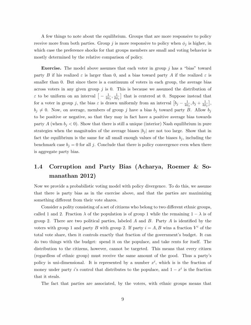
1.4 Corruption and Party Bias (Acharya, Roemer & So-
manathan 2012)
Now we provide a probabilistic voting model with policy divergence. To do this, we assume
that there is party bias as in the exercise above, and that the parties are maximizing
something different from their vote shares.
Consider a polity consisting of a set of citizens who belong to two different ethnic groups,
called 1 and 2. Fraction λ of the population is of group 1 while the remaining 1 − λ is of
group 2. There are two political parties, labeled A and B. Party A is identified by the
voters with group 1 and party B with group 2. If party i = A,B wins a fraction V i of the
total vote share, then it controls exactly that fraction of the government’s budget. It can
do two things with the budget: spend it on the populace, and take rents for itself. The
distribution to the citizens, however, cannot be targeted. This means that every citizen
(regardless of ethnic group) must receive the same amount of the good. Thus a party’s
policy is uni-dimensional. It is represented by a number xi, which is is the fraction of
money under party i’s control that distributes to the populace, and 1 − xi is the fraction
that it steals.
The fact that parties are associated, by the voters, with ethnic groups means that
9
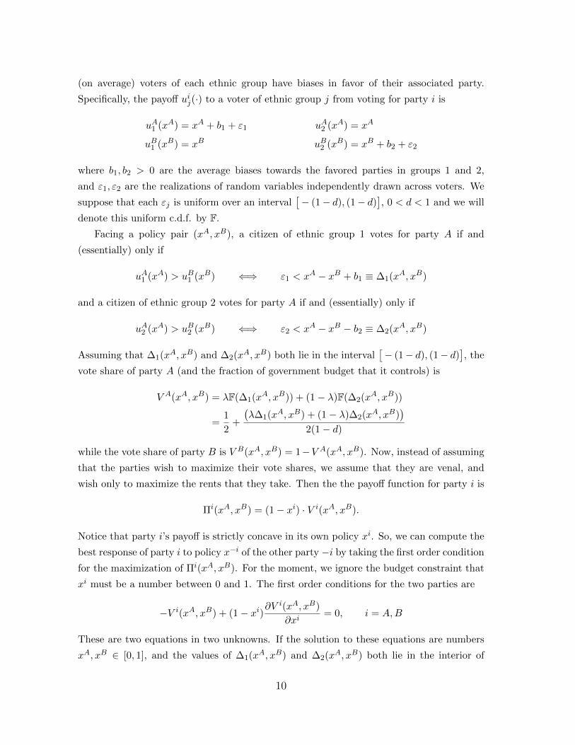
(on average) voters of each ethnic group have biases in favor of their associated party.
Specifically, the payoff uij(·) to a voter of ethnic group j from voting for party i is
uA1 (xA) = xA + b1 + ε1 uA2 (xA) = xA
uB1 (xB) = xB uB2 (xB) = xB + b2 + ε2
where b1, b2 > 0 are the average biases towards the favored parties in groups 1 and 2,
and ε1, ε2 are the realizations of random variables independently drawn across voters. We
suppose that each εj is uniform over an interval[− (1− d), (1− d)
], 0 < d < 1 and we will
denote this uniform c.d.f. by F.
Facing a policy pair (xA, xB), a citizen of ethnic group 1 votes for party A if and
(essentially) only if
uA1 (xA) > uB1 (xB) ⇐⇒ ε1 < xA − xB + b1 ≡ ∆1(xA, xB)
and a citizen of ethnic group 2 votes for party A if and (essentially) only if
uA2 (xA) > uB2 (xB) ⇐⇒ ε2 < xA − xB − b2 ≡ ∆2(xA, xB)
Assuming that ∆1(xA, xB) and ∆2(xA, xB) both lie in the interval[− (1− d), (1− d)
], the
vote share of party A (and the fraction of government budget that it controls) is
V A(xA, xB) = λF(∆1(xA, xB)) + (1− λ)F(∆2(xA, xB))
=1
2+
(λ∆1(xA, xB) + (1− λ)∆2(xA, xB)
)2(1− d)
while the vote share of party B is V B(xA, xB) = 1−V A(xA, xB). Now, instead of assuming
that the parties wish to maximize their vote shares, we assume that they are venal, and
wish only to maximize the rents that they take. Then the the payoff function for party i is
Πi(xA, xB) = (1− xi) · V i(xA, xB).
Notice that party i’s payoff is strictly concave in its own policy xi. So, we can compute the
best response of party i to policy x−i of the other party −i by taking the first order condition
for the maximization of Πi(xA, xB). For the moment, we ignore the budget constraint that
xi must be a number between 0 and 1. The first order conditions for the two parties are
−V i(xA, xB) + (1− xi)∂Vi(xA, xB)
∂xi= 0, i = A,B
These are two equations in two unknowns. If the solution to these equations are numbers
xA, xB ∈ [0, 1], and the values of ∆1(xA, xB) and ∆2(xA, xB) both lie in the interior of
10

[− (1 − d), (1 − d)
]at the solution, then we have found a local Nash equilibrium (LNE).1
The solutions are
xA = d− λb1 − (1− λ)b23
xB = d+λb1 − (1− λ)b2
3.
If b1 and b2 are small, then both of these numbers lie between 0 and 1 and ∆1(xA, xB) and
∆2(xA, xB) will lie inside[− (1− d), (1− d)
]. So, we have an LNE.
Notice that the equilibrium value of xA is decreasing in b1 and increasing in b2 while
xB is increasing in b1 and decreasing in b2. As the ethnic party bias grows for the members
of group j = 1, 2, the corruption level of their party increases while the corruption level of
the other party decreases.
Exercise. The model above assumes that the parties cannot target their distribution
to the two groups as in the model of the previous section. Assume now that the parties
can target their distribution. In particular, party i can give xij to each member of group j,
keeping 1−λxi1− (1−λ)xi2 for itself. Find conditions under which a local Nash equilibrium
exists with venal parties, and compute the equilibrium. Which features of the equilibrium
are noteworthy?
1.5 Progressive Income Taxation (Roemer 1999)
There is a continuum of voters of unit mass. Income is distributed among voters according
to a continuous (atomless) probability distribution F on the support [0, 1]. A tax policy is
a triple of real numbers (a, b, c). If this policy is implemented, then a voter with income
w receives after-tax income aw2 + bw + c. Taxes are purely redistributive, so the budget
balance condition is ∫(aw2 + bw + c)dF (w) =
∫wdF (w) ≡ µ.
This implies that
c = −aµ2 − bµ+ µ where µ2 ≡∫w2dF (w).
So the budget balance condition implies that a tax policy can be denoted simply (a, b) where
c is determined residually. The after-tax income (and utility) of a voter with income w at
tax policy (a, b) is
u(a, b, w) = a(w2 − µ2) + b(w − µ) + µ
1I could in fact make the equilibrium global by assuming that the payoff were instead φuij(·),where φ > 0 is a small number in comparison to d.
11

Figure 2: The triangle OUV
Thus, a voter with income w 6= µ is indifferent between two policies (a, b) and (a′, b′) iff
aφ(w) + b = a′φ(w) + b′, where
φ(w) =w2 − µ2
w − µSo, the indifference curves of a voter with income w 6= µ are straight lines in (a, b)-space of
slope −φ(w). The indifference curves of a voter with income µ are vertical straight lines. We
further restrict a tax-policy (a, b) to satisfy the following assumptions that are maintained
throughout.
(1.) a(w2 − µ2) + b(w − µ) + µ ≥ 0 for all w
(2.) 2aw + b ≥ 0 for all w
The first assumption says that no voter can be left with a negative income. The second
condition says that after-tax income must be a nondecreasing function of income. This is
an incentive compatibility constraint that says that no voter wants to burn money.
Exercise. First, show that the conditions (1.) and (2.) above imply that the set of
admissible tax policies (a, b) coincides with the triangle OUV in Figure 2. Second, define a
tax policy to be (weakly) progressive if after-tax income as a percent of income is a (weakly)
decreasing function of income. A (weakly) regressive policy is one in which after-tax income
as a percent of income is a (weakly) increasing function of income. A proportional (or linear)
tax is one in which after-tax income as a percent of income is constant in income. Show
that a tax policy (a, b) is weakly progressive iff it lies in the triangle OUT , weakly regressive
iff it lies in the triangle OV T , and proportional iff it lies on the segment OT . Note that the
12
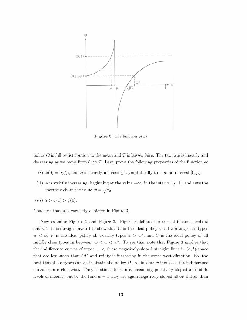
Figure 3: The function φ(w)
policy O is full redistribution to the mean and T is laissez faire. The tax rate is linearly and
decreasing as we move from O to T . Last, prove the following properties of the function φ:
(i) φ(0) = µ2/µ, and φ is strictly increasing asymptotically to +∞ on interval [0, µ).
(ii) φ is strictly increasing, beginning at the value −∞, in the interval (µ, 1], and cuts the
income axis at the value w =õ2.
(iii) 2 > φ(1) > φ(0).
Conclude that φ is correctly depicted in Figure 3.
Now examine Figures 2 and Figure 3. Figure 3 defines the critical income levels w
and w∗. It is straightforward to show that O is the ideal policy of all working class types
w < w, V is the ideal policy all wealthy types w > w∗, and U is the ideal policy of all
middle class types in between, w < w < w∗. To see this, note that Figure 3 implies that
the indifference curves of types w < w are negatively-sloped straight lines in (a, b)-space
that are less steep than OU and utility is increasing in the south-west direction. So, the
best that these types can do is obtain the policy O. As income w increases the indifference
curves rotate clockwise. They continue to rotate, becoming positively sloped at middle
levels of income, but by the time w = 1 they are again negatively sloped albeit flatter than
13

Figure 4: The triangle OUV with policies L and R
the segment OU since φ(1) < 2 (which is a fact depicted in Figure 3 and proven by you in
the Exercise above).
We suppose that there are two parties, called Left and Right, that propose policies
tL = (a, b) and tR = (a′, b′). Let Ω(tL, tR) be the set of voters that strictly prefer policy tL
to tR, and thus vote for the Left party. We assume that voters who are indifferent mix in
an arbitrary way, but as long as Left and Right propose different policies, this set of voters
is always measure zero so their behavior will not matter in determining vote shares. The
vote share of Left is thus
π(tL, tR) = F (Ω(tL, tR))
and the vote share of Right is 1 − π(tL, tR). Now, we assume that some members of each
party are policy-motivated. Specifically, some members of Left have the interest of a voter
of income wL < w in mind, whereas some members of Right have the interest of a voter of
income wR > w∗ in mind. We call such factions the Militants. The militants of party j want
to propose a policy tj that maximizes u(tj , wj). We also assume that some members of the
parties are purely office-motivated in that they care only about maximizing vote-share. We
call these fractions the Opportunists. The policy pair (tL, tR) is a Roemer-Nash equilibrium
(RNE) if it is admissible (i.e. each policy lies in the triangle OUV ) and
(L) there is no admissible policy t′L for Left such that π(t′L, tR) ≥ π(tL, tR) and u(t′L, wL) ≥u(tL, wL) with at least one inequality strict; and
(R) there is no admissible policy t′R for Right such that 1− π(tL, t′R) ≥ 1− π(tL, tR) and
u(t′R, wR) ≥ u(tR, wR) with at least one inequality strict.
14

These state that neither Left nor Right can find deviations that make their Militants better
off without making their Opportunists worse off, or make their Opportunists better off
without making their Militants worse off. We now have the following result.
Theorem 1: There exists an RNE. In particular, there is one such that Left and Right
propose distinct strictly progressive policies.
Proof: Pick a point L on the interior of segment OU and a point R on the interior of
segment UV such that the slope of LR is nearly −2, in particular pick L close to O. Look
at Figure 4 for a depiction. Suppose Left proposes the policy L and Right proposes the
policy R. Note that the set of types that vote for Left is precisely [0, w+ ε) for some small
ε. Next, since the income type wL is smaller than w, its indifference curve through the
point L is a straight line that is flatter in slope than OU . Moreover, utility is increasing in
the south-west direction. Therefore, the set of policies that make income type wL weakly
better off (than under policy L) are the policies that lie in the small shaded triangle LOQ.
But a deviation to any other policy in this triangle would strictly decrease Left’s vote share
since it would make the line LR less steep, reducing the set of types that vote for Left from
[0, w + ε) to [0, w) with w < w + ε. (Note that the triangle LOQ can really be made as
small as one wants by choosing L close enough to O.) Therefore, the equilibrium condition
(L) is satisfied. In fact, the only deviations that would increase Left’s vote share without
reducing wL’s utility, or increase wL’s utility without reducing Left’s vote share are in the
shaded cone below the point L in Figure 4; but these are not admissible deviations. A
similar argument establishes that the analogously “profitable” deviations for Right are in
the shaded cone above point R; but again these are not admissible. Hence the equilibrium
condition (R) is also satisfied, and (L,R) is and RNE. In addition, L and R are strictly
progressive policies and L 6= R.
Under some slightly stronger assumptions, and a weak refinement of RNE called strong
RNE, one can show that Left and Right propose weakly progressive policies in all strong
RNE. But the key point to highlight is that by modeling the fact of intra-party competi-
tion between Opportunist factions that care about winning and Militant factions that care
about “protecting the base,” one can generate existence of equilibrium in multidimensional
political competition while also enhancing a model’s realism.
1.6 Political Economy with Strategic Voting (Acharya 2012)
There are 2n+ 1 voters. With probability λ ∈ (0, 1/2) a voter is a high income earner, and
with probability 1−λ he is a low income earner. There are two periods and two policies. In
the first period, a status quo policy is in effect. Then, an election is held to decide whether
15
to continue with the status quo or to switch to a more redistributive policy. The policy
that wins the election is implemented in the second period. Under the more redistributive
policy, each high income voter receives a payoff yh while each low income voter receives a
payoff yl. Under the status quo policy, each high income voter has payoff yh, while each
low income voter has probability δ of receiving an opportunity to become a high income
voter. If a low income voter receives the opportunity to climb the economic ladder, and he
is talented, then he receives a payoff yh. If he is not talented, or if he does not receive the
opportunity, then his payoff is yl. Each low income voter has prior probability p ∈ (1/2, 1)
of being talented. If a voter becomes a high income earner in the first period, he remains a
high income earner in the second period. Voters who receive an opportunity to become high
income earners in the first period and are unsuccessful learn that they are untalented, and
would also be unsuccessful in the following period even if they got the opportunity again.
Voters who do not receive the opportunity in the first period do not learn whether or not
they are talented.
Voters do not directly observe δ, nor does any voter observe the consequences of the
first period policy for any other voter. Instead, voters believe that δ is a random variable
with continuous density f . Assume that there is a number ν > 0 for which
f(δ) > ν ∀δ ∈ [0, 1] (A2)
If the status quo policy is re-elected, then the value of δ in the second period is the same
as in the first. Let δ denote the expected value of δ according to f . Conditional on δ, the
expected payoff from the status quo policy for a low income voter is given by
y(δ) = (1− δp)yl + δpyh (13)
Therefore, the unconditional expected payoff to re-electing the status quo policy for a low
income voter who did not receive the economic opportunity is y(δ). His expected payoff to
electing the redistributive policy is simply yl. We will assume that
(i) yl < yl ≤ yh < yh and (ii) y(δ) < yl < y(1) (A3)
A strategy for a voter is the probability with with he votes to re-elect the status quo pol-
icy. The equilibrium concept is symmetric Bayes Nash equilibrium in weakly un-dominated
strategies. All voters are rational, so each voter casts his ballot as if he believes that his
vote will decide the election, i.e. he conditions his vote on the event that his vote is pivotal.
Call the set of voters that started off as high income earners H, the set of voters who got
the opportunity and climbed the socio-economic ladder (because they were talented) L+,
the set of voters who got the opportunity but failed to climb the socio-economic ladder
16
(because they were not talented) L− and the set of voters who did not get the opportunity
L0. The following observation is straightforward.
Lemma 1: In every equilibrium of the game, voters in H and L+ vote to re-elect the
status quo while voters in L− vote to switch to the more redistributive alternative.
Proof. Voters in H and L+ have a weakly dominant strategy to vote for the status quo,
while voters in L− have a weakly dominant strategy to vote for the more redistributive al-
ternative. Since the equilibrium concept rules out equilibria in weakly dominated strategies,
the result follows.
Let x denote the probability with which an L0 voter votes to re-elect the status quo.
Lemma 1 implies that equilibria can be identified by entirely by x. Given any symmetric
strategy x ∈ [0, 1], the unconditional probability of casting a vote for the status quo policy
(when H, L+ and L− voters play their symmetric equilibrium strategy) is
π(δ, x) = λ+ (1− λ)(δp+ (1− δ)x
)The probability that an L0 voter is pivotal is
φ(δ|x, n) =
(2n
n
)(π(δ, x))n(1− π(δ, x))n
The distribution of the state variable δ given that an L0 voter is pivotal (viewed as a function
of x and n) is
fpiv(δ|x, n) =φ(δ|x, n)(1− δ)f(δ)∫ 1
0 φ(ω|x, n)(1− ω)f(ω)dω
The expectation of δ for an L0 voter, conditional on pivotal, is
δpiv(x, n) =
∫ 1
0δfpiv(δ|x, n)dδ
Now, the next result is also straightforward.
Lemma 2: There exists a cutoff δ∗ ∈ (0, 1) such that the symmetric strategy x = 0
is part of an equilibrium iff δpiv(0, n) ≤ δ∗, the symmetric strategy x = 1 is part of an
equilibrium iff δpiv(1, n) ≥ δ∗, and the symmetric strategy x ∈ (0, 1) is part of an equilibrium
iff δpiv(x, n) = δ∗.
Proof. Follows immediately from (A2), (13), (A3)(ii) and Lemma 1.
Now note that for fixed values of x 6= p, the function π(δ, x) is a strictly monotone in δ on
the interval [0, 1]. Therefore, there is a unique number δ†(x) that minimizes |π(δ, x)− 1/2|.Now, the following mathematical result will be extremely useful.
17

Theorem 2: If x 6= p then for all ε > 0 there is N such that n ≥ N implies
|δpiv(x, n)− δ†(x)| ≤ ε
If x = p then δpiv(x, n) is a constant number between 0 and 1, for all n.
Proof. The proof of the x = p part is straightforward. For the first part, define the
function h : [0, 1]→ R by
h(π) = π(1− π)
Since π(δ, x) is continuous in its arguments, the composite function h(π(·, ·)) : [0, 1]2 → R is
continuous. Moreover, for all x 6= p, the function h(π(·, x)) : [0, 1]→ R is single peaked and
maximized by the value of δ ∈ [0, 1] that minimizes |π(δ, x) − 1/2|. Thus δ†(x) maximizes
h(π(·, x)).
Fix x 6= p and define
∆ε(x) = δ ∈ [0, 1] : |δ − δ†(x)| ≤ ε
to be an ε-neighborhood of δ†(x). Fix any ε. If ε is small enough, then ∆ε(x) 6= [0, 1]. In
this case, there exists a small number ηε ∈ (0, 1) such that
h(π(δ†(x), x))− ηε > supδ /∈∆ε(x)
h(π(δ, x))
Furthermore, define the set
Ωε(x) = ω ∈ ∆ε(x) : |h(π(δ†(x), x))− h(π(ω, x))| ≤ ηε/2
Note that the set Ωε(x) must contain a small interval I ⊂ [0, 1] that in turn contains the
number δ†(x). Let µ be the length of this interval.
We will prove that there is a number N large enough that for all n ≥ N we have∫δ∈∆ε(x)
fpiv(δ|x, n) > 1− ε.
To see this, note that if ∆ε(x) = [0, 1] then∫δ∈∆ε(x) f
piv(δ|x, n) = 1, so the above inequality
trivially holds. If ∆ε(x) 6= [0, 1] then∫δ /∈∆ε(x)
fpiv(δ|x, n)dδ =
∫δ /∈∆ε(x) φ(δ|x, n)(1− δ)f(δ)dδ∫ 1
0 φ(ω|x, n)(1− ω)f(ω)dω≤
∫δ /∈∆ε(x) φ(δ|x, n)(1− δ)f(δ)dδ∫ω∈Ωε(x) φ(ω|x, n)(1− ω)f(ω)dω
≤supδ /∈∆ε(x) φ(δ|x, n)
infω∈Ωε(x) φ(ω|x, n)
∫δ /∈∆ε(x)(1− δ)f(δ)dδ∫ω∈Ωε(x)(1− ω)f(ω)dω
≤(
supδ /∈∆ε(x) φ(δ|x, n)
infω∈Ωε(x) φ(ω|x, n)
)1
ν∫ω∈Ωε(x)(1− ω)dω
≤(
h(π(δ†(x), x))− ηεh(π(δ†(x), x))− ηε/2
)n1
12µ
2ν≤(
1− ηε1− ηε/2
)n 112µ
2ν.
18

So we can choose N large enough such that n ≥ N implies that the integral on the left
above is smaller than ε.
Finally, to prove the theorem, write
δpiv(x, n) =
∫δ /∈∆ε(x)
δfpiv(δ|x, n)dδ +
∫δ∈∆ε(x)
δfpiv(δ|x, n)dδ.
and observe that for n ≥ N , this quantity is bounded above by ε+ (δ†(x) + ε) = δ†(x) + 2ε
and bounded below by (δ†(x) − ε)(1 − ε) > δ†(x) − 2ε. Thus, the conditional expectation
δpiv(x, n) is within 2ε of δ†(x). But ε was arbitrary.
The following is an immediate corollary of Theorem 2.
Proposition 1: There exists N such that for all n ≥ N , it is (part of) an equilibrium
for all L0 voters to vote for the status quo policy with probability 1.
Proof. Suppose x = 1. Then δ†(1) = 1. So Theorem 2 implies that for n large enough
δpiv(x, n) is close to 1. So by Lemma 2, x = 1 is part of an equilibrium.
Exercise. Assume that n is large, and characterize all of the equilibria of the model.
Bonus Exercise. (Only to be done by those who took Sourav’s class last semester and
know what “information aggregation” means.) Which of the equilibria aggregate informa-
tion and which do not?
1.7 Comparative Politics and Public Finance (Persson, Roland
& Tabellini 2000)
The exposition follows that of Persson & Tabellini, Ch. 10, with some minor changes in
notation. There are three voters j = 1, 2, 3 residing in different districts. Each voter j is
represented by a legislator l = 1, 2, 3. Voter j has preferences given by
wj = y − τ + f j +H(g)
where y is his income, τ is the amount he pays in taxes, f j is the pork he receives and
H(g) is the value of a public good g, one unit of which can be produced by one unit of tax
revenue. H is a strictly concave function that you can assume to be
H(g) =z
1− α(g)1−α
19
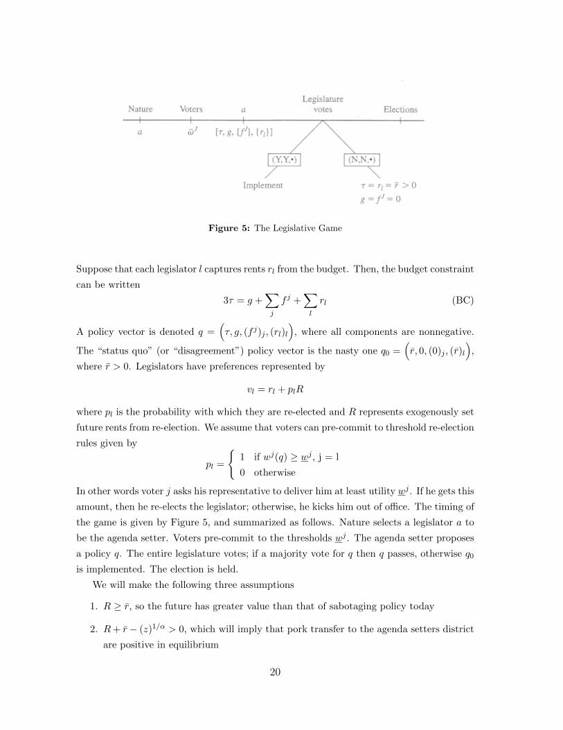
Figure 5: The Legislative Game
Suppose that each legislator l captures rents rl from the budget. Then, the budget constraint
can be written
3τ = g +∑j
f j +∑l
rl (BC)
A policy vector is denoted q =(τ, g, (f j)j , (rl)l
), where all components are nonnegative.
The “status quo” (or “disagreement”) policy vector is the nasty one q0 =(r, 0, (0)j , (r)l
),
where r > 0. Legislators have preferences represented by
vl = rl + plR
where pl is the probability with which they are re-elected and R represents exogenously set
future rents from re-election. We assume that voters can pre-commit to threshold re-election
rules given by
pl =
1 if wj(q) ≥ wj , j = l
0 otherwise
In other words voter j asks his representative to deliver him at least utility wj . If he gets this
amount, then he re-elects the legislator; otherwise, he kicks him out of office. The timing of
the game is given by Figure 5, and summarized as follows. Nature selects a legislator a to
be the agenda setter. Voters pre-commit to the thresholds wj . The agenda setter proposes
a policy q. The entire legislature votes; if a majority vote for q then q passes, otherwise q0
is implemented. The election is held.
We will make the following three assumptions
1. R ≥ r, so the future has greater value than that of sabotaging policy today
2. R+ r− (z)1/α > 0, which will imply that pork transfer to the agenda setters district
are positive in equilibrium
20

3. 3y −R− r > 0, so that there is lots of money in the economy
4. 3y > (3z)1/α, so the socially optimal level of the public good is affordable
We first characterize the socially optimum level of public goods from the perspective of
the voters. To do this, define the social welfare function (over policies) to be the sum of
only the voters’ utility
W (q) =∑j
wj = 3(y − τ) +∑j
f j + 3H(g)
The social planner maximizes this function.
Proposition 2: At the solution to the maximization of the planner’s objective function
W (q) subject to the budget constraint (BC), we have gsp = (3z)1/α and rspl = 0 for all l.
Taxes τ must be weakly greater than gsp, but otherwise taxes and transfers, f j , j = 1, 2, 3,
are indeterminate.
Proof. Substituting the budget constraint (BC) into W (q), we get
W (q) = 3y − g +∑l
rl + 3H(g)
Clearly rspl = 0 for all l. To find the optimal g, we solve the first order condition
3H ′(g) = 3z(g)−α = 1
which gives us gsp = (3z)1/α. This is called the Samuelson level of the public good, and by
Assumption 4 above, it is affordable with a tax rate τ sp = gsp/3. Note that taxes may be
higher so long as they are given back to the districts in the form of transfers. Consequently,
the level of taxes and transfers is indeterminate.
We can now compare the equilibrium level of the public good with the planner’s optimal
level. An equilibrium of the game is a subgame perfect equilibrium in which legislators use
weakly un-dominated voting strategies. Then, the equilibrium level of the public good is
characterized in the following proposition.
Proposition 3: On every equilibrium path we have the following
g∗ = (z)1/α τ∗ = y r∗a = 3y −R− r r∗l = 0, l 6= a
fa∗ = R+ r − g∗ f j∗ = 0, j 6= a wa∗ = H(g∗) + fa∗ wj∗ = H(g∗), j 6= a
21

Proof sketch. I will sketch the argument that these are sequentially optimal on the path
of play, and you will (in the Bonus Exercise below) close the argument by proving that there
are equilibria that support this path of play (and indeed all of them support this path of
play).
We work backwards. Note that because all legislators use weakly un-dominated voting
strategies, in every equilibrium all legislators vote to pass any proposal q that gives them
a payoff least r whenever it is the case that if the proposal fails, then they will not be
re-elected. So, suppose the agenda setter proposes q∗ =(τ∗, g∗, (f j∗)j , (r
∗l )l
)when voters
use the thresholds wj∗. Then all of the legislators must vote to pass the proposal. If the
proposal does not pass, then q0 is implemented and voters in all districts receive utility
H(0) = 0 < wj∗, all j. Moreover, both legislators l 6= a receives a payoff r instead of the
payoff he would receive from q∗ which is r∗l + R = R > r by Assumption 1. The legislator
a receives a payoff r instead of the payoff r∗a +R > r by Assumptions 1 and 3, which states
that r∗a > 0. So, all vote to pass the proposal q∗.
Now, we show that it is optimal for the agenda setter a to propose q∗ when the voters
use the thresholds wj∗. Suppose a proposes a policy that gives voter j = a a payoff lower
than wa∗. Then he forgoes re-election, receiving a payoff at most 3y − r. This is because
his best deviation from q∗ is the policy τ = 1, g = f j = 0, all j and ra = 3y − r, rb = r,
rc = 0, where b is either of the other two legislators and c is the third. But by proposing q∗
he gets exactly 3y −R− r +R = 3y − r, so he is indifferent. On the other hand, it cannot
be optimal for him to give voter j = a a payoff higher than wa∗, since this eats into his
own resources (and we will show below that g∗ and fa∗ have been chosen by voter j = a
optimally).
Finally, note that it is optimal for wb∗ = wc∗ = H(g∗). If either b or c ask for more,
then q∗ will pass anyway. Likewise, it does not make sense to ask for less. Finally, voter
j = a sets wj∗ according to the following problem
maxqwa∗ = y − τ + fa +H(g)
subject to (BC) and ra ≥ 3y −R− r
In other words, he maximizes his payoff subject to the budget constraint and the incentive
constraint that legislator a wants to propose a policy that gets him re-elected. The solutions
are given in the statement of the proposition. Pork transfers to district a are positive, and
the equilibrium level of the public good is affordable by Assumptions 2 and 4 respectively.
By Assumption 3, legislator a captures positive rents.
We immediately have the following corollary.
22

Figure 6: The Congressional Committees Game
Corollary 1: The equilibrium level of the public good is lower than the Samuelson
level (social planner’s optimum):
g∗ < gsp
Bonus Exercise. (This exercise is optional.) Complete the proof of Proposition 3, i.e.
show that all equilibria of the game are path-equivalent.
Exercise. (Congressional Committees) The congressional policy game is like the game
above, except that there are two different agenda setters aτ and ag, the finance committee
and the expenditure committee, that are selected by nature at the start of the game. Voters
set their utility cutoffs wj as before. aτ proposes the tax rate τ and an up or down vote is
held. If the proposal fails then an exogenous τ0 ∈ (0, r), r < y. Then ag proposes g, (f j)j
and (rl)l subject to the budget constraint (BC) where τ here is the tax proposal that passes
or τ0 if the proposal fails to pass. Then again a vote takes place on ag’s proposal. If the
proposal fails then g = 0, f j = τ − rl ≥ 0, all j, and rl = r, all l, is implemented. Finally,
elections are held. (See Figure 6.)
Maintain Assumptions 1-4 and characterize the equilibria of the Congressional Com-
mittees game, showing in particular that the equilibrium level of the public good is unique
and under-provided, as before. Specifically,
g∗ = (z)1/α
Exercise. (Parliamentary Regimes) Now consider a parliamentary model depicted in
Figure 7. Nature selects the expenditure and finance ministers, ag and aτ . Voters set their
reservation utilities wj as before. The finance minister, aτ , proposes τ . The expenditure
minister ag proposes(g, (f j)j , (rl)l
)subject to (BC) given the proposed tax rate τ . Either
23

Figure 7: The Parliamentary Game
member of government ag or aτ can veto the aggregate proposal q =(τ, g, (f j)j , (rl)l
).
If neither does, then the proposal passes, and elections are held. If one of them vetoes,
government collapses and a legislator is selected randomly (i.e. each with probability 1/3)
to form a caretaker government. Voters then set new reservation utilities wj . The caretaker
makes an entire budget proposal q′ =(τ ′, g′, (f ′j)j , (r
′l)l
)which passes or fails by simple
majority. If it fails then the following default policy is implemented:
τ0 = r g0 = 0 rl = r, ∀l f j = 0, ∀j
Maintain Assumptions 1-4 and show that there is an equilibrium in which the level of the
public good supplied is larger than the level supplied in the congressional committees regime,
but lower than the Samuelson level, the sum total of equilibrium rents in the parliamentary
regime is larger than the sum total of equilibrium rents in the congressional committees
regime, and taxes are higher under the parliamentary regime than under the congressional
committees regime.
24

2 Dynamic Methods, etc.
I assume that you have some familiarity with this material. If you do not, please consult a
good textbook, such as Mailath and Samuelson’s (2006) Repeated Games and Reputations
and Daron Acemoglu’s (2008) Modern Economic Growth.
2.1 Infinite Horizon Dynamic Programming
We consider an infinite horizon stationary discounted dynamic programming problem as
follows. Here, I simply state the main results of dynamic programming, leaving it to you
to discover the proofs if necessary.
Suppose time is discrete and indexed by t = 0, 1, 2...,∞. Let δ ∈ [0, 1) be a discount
factor. Let X ⊆ Rm be the set of control variables. Let G : X → 2X be a correspondence
from X to itself and u : X × X → R an instantaneous reward or payoff function. The
canonical stationary dynamic program is
maxxt∞t=0
U(xt∞t=0) ≡∞∑t=0
δtu(xt, xt+1)
subject to xt+1 ∈ G(xt) for all t ≥ 0 and x0 = x ∈ X (P)
A solution to this problem may or may not exist. If it exists, then label it x∗t ∞t=0 and let
U∗ be the value of U attained at this solution, i.e. U∗ = U(x∗t ∞t=0).
For any t ≥ 0, it will be useful to define the set of feasible “plans” starting with an
initial value xt ∈ X as
Φ(xt) = xs∞s=t : xs+1 ∈ G(xs), s = t, t+ 1, ...,∞
Now define a completely new function V : X → R such that
∀x ∈ X V (x) = maxy∈G(x)
u(x, y) + δV (y) (B)
Again, such a function may or may not exist. The equality in (B) is called a “Bellman
equation” and the function V is called a “value function.”
Consider the following assumption.
Assumption A: X is compact; G is continuous, nonempty-, convex-, and compact-
valued, and it is monotone in the sense that x ≤ x′ implies G(x) ⊂ G(x′); and u is
continuously differentiable on int X×X, strictly concave, and strictly increasing in its first
m arguments; and, for all x0 ∈ X and plans xt∞t=0 ∈ Φ(x0), the following limit exists and
is finite:
limn→∞
n∑t=0
δtu(xt, xt+1)
25
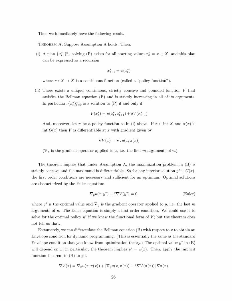
Then we immediately have the following result.
Theorem A: Suppose Assumption A holds. Then:
(i) A plan x∗t ∞t=0 solving (P) exists for all starting values x∗0 = x ∈ X, and this plan
can be expressed as a recursion
x∗t+1 = π(x∗t )
where π : X → X is a continuous function (called a “policy function”).
(ii) There exists a unique, continuous, strictly concave and bounded function V that
satisfies the Bellman equation (B) and is strictly increasing in all of its arguments.
In particular, x∗t ∞t=0 is a solution to (P) if and only if
V (x∗t ) = u(x∗t , x∗t+1) + δV (x∗t+1)
And, moreover, let π be a policy function as in (i) above. If x ∈ int X and π(x) ∈int G(x) then V is differentiable at x with gradient given by
∇V (x) = ∇xu(x, π(x))
(∇x is the gradient operator applied to x, i.e. the first m arguments of u.)
The theorem implies that under Assumption A, the maximization problem in (B) is
strictly concave and the maximand is differentiable. So for any interior solution y∗ ∈ G(x),
the first order conditions are necessary and sufficient for an optimum. Optimal solutions
are characterized by the Euler equation:
∇yu(x, y∗) + δ∇V (y∗) = 0 (Euler)
where y∗ is the optimal value and ∇y is the gradient operator applied to y, i.e. the last m
arguments of u. The Euler equation is simply a first order condition. We could use it to
solve for the optimal policy y∗ if we knew the functional form of V ; but the theorem does
not tell us that.
Fortunately, we can differentiate the Bellman equation (B) with respect to x to obtain an
Envelope condition for dynamic programming. (This is essentially the same as the standard
Envelope condition that you know from optimization theory.) The optimal value y∗ in (B)
will depend on x; in particular, the theorem implies y∗ = π(x). Then, apply the implicit
function theorem to (B) to get
∇V (x) = ∇xu(x, π(x)) + [∇yu(x, π(x)) + δ∇V (π(x))]∇π(x)
26
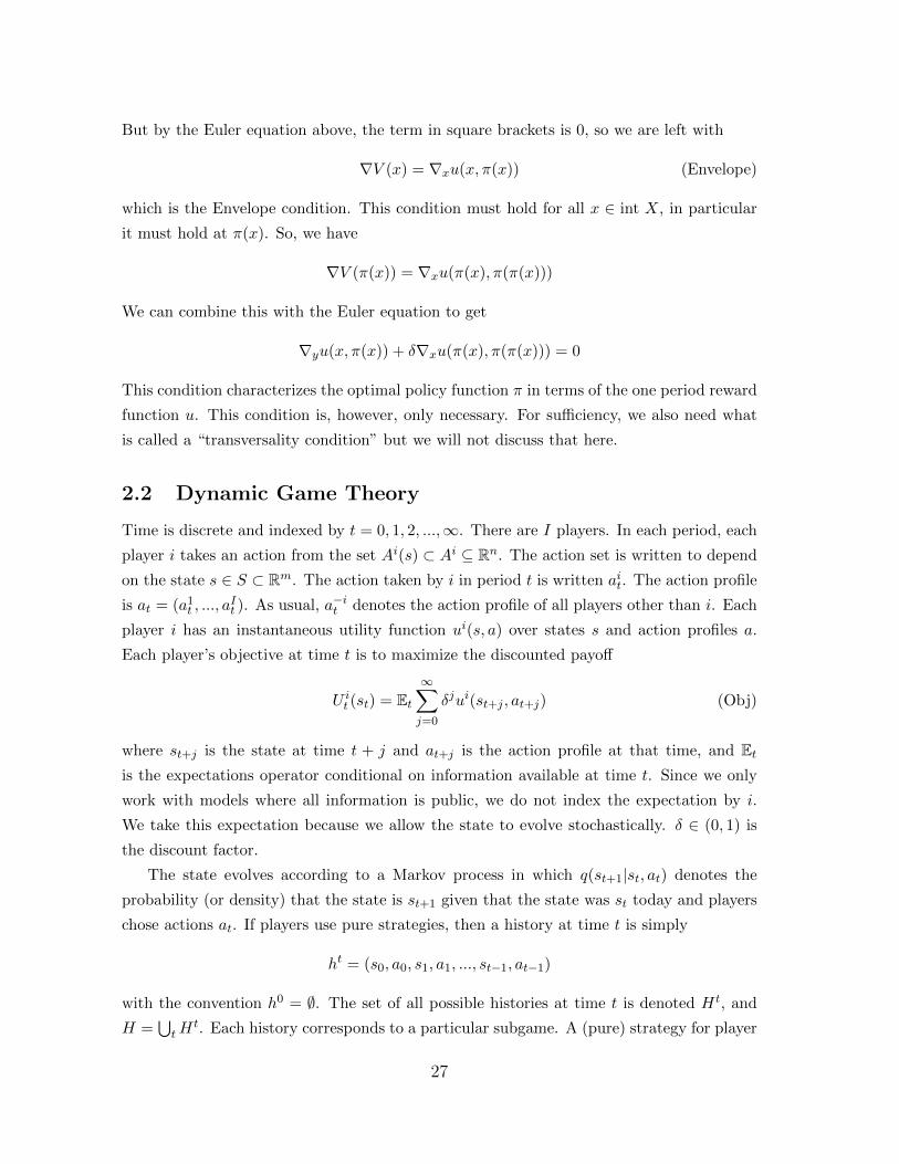
But by the Euler equation above, the term in square brackets is 0, so we are left with
∇V (x) = ∇xu(x, π(x)) (Envelope)
which is the Envelope condition. This condition must hold for all x ∈ int X, in particular
it must hold at π(x). So, we have
∇V (π(x)) = ∇xu(π(x), π(π(x)))
We can combine this with the Euler equation to get
∇yu(x, π(x)) + δ∇xu(π(x), π(π(x))) = 0
This condition characterizes the optimal policy function π in terms of the one period reward
function u. This condition is, however, only necessary. For sufficiency, we also need what
is called a “transversality condition” but we will not discuss that here.
2.2 Dynamic Game Theory
Time is discrete and indexed by t = 0, 1, 2, ...,∞. There are I players. In each period, each
player i takes an action from the set Ai(s) ⊂ Ai ⊆ Rn. The action set is written to depend
on the state s ∈ S ⊂ Rm. The action taken by i in period t is written ait. The action profile
is at = (a1t , ..., a
It ). As usual, a−it denotes the action profile of all players other than i. Each
player i has an instantaneous utility function ui(s, a) over states s and action profiles a.
Each player’s objective at time t is to maximize the discounted payoff
U it (st) = Et∞∑j=0
δjui(st+j , at+j) (Obj)
where st+j is the state at time t + j and at+j is the action profile at that time, and Etis the expectations operator conditional on information available at time t. Since we only
work with models where all information is public, we do not index the expectation by i.
We take this expectation because we allow the state to evolve stochastically. δ ∈ (0, 1) is
the discount factor.
The state evolves according to a Markov process in which q(st+1|st, at) denotes the
probability (or density) that the state is st+1 given that the state was st today and players
chose actions at. If players use pure strategies, then a history at time t is simply
ht = (s0, a0, s1, a1, ..., st−1, at−1)
with the convention h0 = ∅. The set of all possible histories at time t is denoted Ht, and
H =⋃tH
t. Each history corresponds to a particular subgame. A (pure) strategy for player
27

i is a function
αi : H × S → Ai s.t. αi(ht, s) ∈ Ai(s) ∀s ∈ S, ∀ht ∈ Ht, ∀t
Again, α−i has the usual interpretation. A best response correspondence at time t for player
i is simply
BR(α−i|ht, st) = αi : αi maximizes (Obj) given α−i, ht and st
So, a subgame perfect equilibrium (SPE) is a strategy profile α = (α1, ..., αI), such that
αi ∈ BR(α−i|ht, st) for all histories ht ∈ Ht, states s ∈ S, players i, and periods t. A
Markov perfect equilibrium (MPE) is an SPE in which
αi(ht, st) = αi(ht′ , st) ∀ht 6= ht′ , ∀i
Theorem B: If S and Ai are finite sets, then MPE exist.
Exercise. Suppose there are I + 1 <∞ players, each with payoffs
∞∑j=0
δj log(cit+j)
at time j, where δ ∈ (0, 1) is a discount factor and cit+j denotes consumption of individual
i at time t+ j. The society owns a resource of amount Rt, which satisfies
Rt+1 = QRt −∑i
cit
where Q > 0 and R0 is given and consumptions cit must be chosen so that Rt ≥ 0 every
period. At each date t all players simultaneously announce the amount they wish to consume
cit. If∑
i cit ≤ QRt, then each individual consumes cit. If
∑i cit > QRt then QRt is equally
divided among the I + 1 players.
1. Suppose that cit are chosen by a social planner that maximizes
I+1∑i=1
∞∑j=0
δj log(cit+j)
every period t. Show that the social planner’s value function V as a function of the
resource stock R is uniquely defined, continuous, concave, and differentiable. Also
show that the saving level of the resource is π(R) = δQR.
28

2. Show that there is a symmetric MPE in which the state is the resource stock R, all
players’ consumptions are continuous in the state, the aggregate savings level in the
economy is given by
π(R) =δQR
1 + I − δI
3. Show that under this MPE, the resource stock shrinks over time.
4. Characterize the set of δ such that there exist SPEs that implement the social plan-
ner’s solution.
2.3 Weak and Strong States (Acemoglu 2005)
There is ruler who rules over a continuum of citizens of unit mass. Each citizen has an
instantaneous payoff over consumption ct and effort et in each period t, given by
u(ct, et) = ct − et (1)
Each citizen has access to the Cobb-Douglas production technology
yt =1
1− αAαt (et)
1−α (2)
where A is the level of public good in the economy. A will be determined by the investment
of the ruler. The ruler sets a linear tax rate τt on individual income yt in period t. Each
citizen can decide to hide a fraction zit of his output, which is not taxable, but hiding is
costly and ρ units are lost in the process. So given τt, the consumption of agent i is
cit =[(1− τt)(1− zit) + (1− ρ)zit
]yit (3)
where revenues are
Tt = τt
∫(1− zit)yitdi (4)
If the ruler spends Gt on the public good then the following units of it are produced to be
used in the following period
At+1 =
[(1− α)φ
αGt
]1/φ
(5)
where φ > 1 is a parameter. A0 > 0 is given. The consumption of the ruler is what is left
over:
Tt −Gt (6)
The timing of events within each period t is
1. the economy inherits At from the ruler’s choice of Gt−1
29

2. citizens exert effort eit
3. the ruler sets τt, collects revenue and decides how much to spend Gt on next period’s
public good
4. citizens decide how much of their output to hide zit
All players share a discount factor δ ∈ (0, 1) and maximize the discounted sum of their
consumption net of effort. (The ruler exerts no effort.)
Exercise. Suppose a social planner chooses effort levels eit for everyone, hiding fractions
zit for everyone, taxes τt and the public good investments Gt in every period. Suppose the
planner chooses these quantities to maximize the sum of output net of effort. Suppose the
ruler is infinitesimal (since there is a continuum of citizens, he is just another massless dot
on the continuum). Show that for all t > 0, the planner’s choices result in:
At = δ1/(φ−1) eit = δ1/(φ−1) ∀i yit =1
1− αδ1/(φ−1) ∀i
Now, we characterize the MPE. An MPE for this model is simply a set of choices(eit, τt, zit, Gt
)that depend only on the payoff relevant state At of the game, and on
prior actions within the same period, but not on actions in previous periods. The convenient
feature of MPEs is that we can use backward induction within a period.
Since citizens are small and anonymous, they maximize their current income, so
zit =
1 if τt > ρ
x ∈ [0, 1] if τt = ρ
0 if τt < ρ
(7)
So the optimal tax rate for the ruler is
τt = ρ (8)
and the citizens hide nothing so zit = 0. Citizens will thus maximize (1) subject to (2), (3),
(8) and their hiding decision zit = 0. This results in
eit = (1− ρ)1/αAt (9)
This implies that revenues from taxes are
T (At) =(1− ρ)(1−α)/αρAt
1− α(10)
30
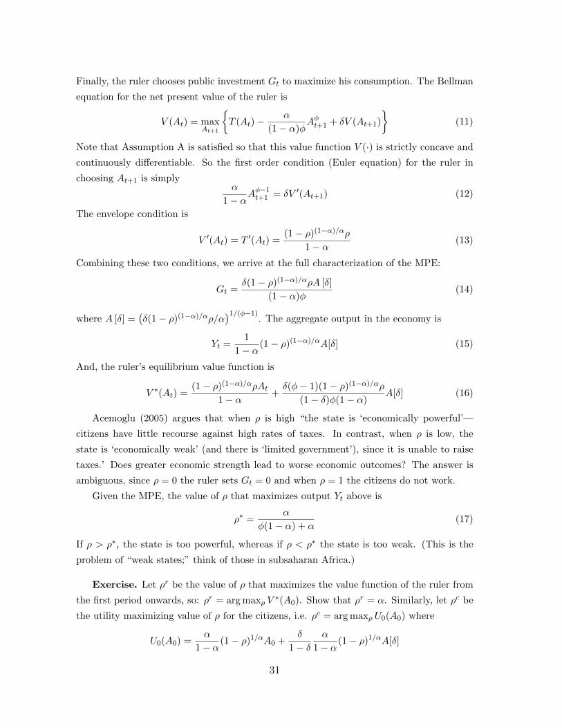
Finally, the ruler chooses public investment Gt to maximize his consumption. The Bellman
equation for the net present value of the ruler is
V (At) = maxAt+1
T (At)−
α
(1− α)φAφt+1 + δV (At+1)
(11)
Note that Assumption A is satisfied so that this value function V (·) is strictly concave and
continuously differentiable. So the first order condition (Euler equation) for the ruler in
choosing At+1 is simplyα
1− αAφ−1t+1 = δV ′(At+1) (12)
The envelope condition is
V ′(At) = T ′(At) =(1− ρ)(1−α)/αρ
1− α(13)
Combining these two conditions, we arrive at the full characterization of the MPE:
Gt =δ(1− ρ)(1−α)/αρA [δ]
(1− α)φ(14)
where A [δ] =(δ(1− ρ)(1−α)/αρ/α
)1/(φ−1). The aggregate output in the economy is
Yt =1
1− α(1− ρ)(1−α)/αA[δ] (15)
And, the ruler’s equilibrium value function is
V ∗(At) =(1− ρ)(1−α)/αρAt
1− α+δ(φ− 1)(1− ρ)(1−α)/αρ
(1− δ)φ(1− α)A[δ] (16)
Acemoglu (2005) argues that when ρ is high “the state is ‘economically powerful’—
citizens have little recourse against high rates of taxes. In contrast, when ρ is low, the
state is ‘economically weak’ (and there is ‘limited government’), since it is unable to raise
taxes.’ Does greater economic strength lead to worse economic outcomes? The answer is
ambiguous, since ρ = 0 the ruler sets Gt = 0 and when ρ = 1 the citizens do not work.
Given the MPE, the value of ρ that maximizes output Yt above is
ρ∗ =α
φ(1− α) + α(17)
If ρ > ρ∗, the state is too powerful, whereas if ρ < ρ∗ the state is too weak. (This is the
problem of “weak states;” think of those in subsaharan Africa.)
Exercise. Let ρr be the value of ρ that maximizes the value function of the ruler from
the first period onwards, so: ρr = arg maxρ V∗(A0). Show that ρr = α. Similarly, let ρc be
the utility maximizing value of ρ for the citizens, i.e. ρc = arg maxρ U0(A0) where
U0(A0) =α
1− α(1− ρ)1/αA0 +
δ
1− δα
1− α(1− ρ)1/αA[δ]
31

Show that ρc = α/φ. Finally, let ρwm be the value of ρ that the social planner in the above
exercise would choose in period 0. Show all of the following:
0 < ρc < ρ∗ < ρr < 1 0 < ρc < ρwm < ρr < 1
The exercise shows that the citizens want state capacity to be lower than socially opti-
mal, whereas the ruler wants state capacity to be higher than socially optimal. Excessively
weak and excessively strong states are both bad; there should be a balance of power between
citizens and the ruler.
2.4 Political Transitions (Acemoglu & Robinson 2001)
Nondemocratic Politics. Time is discrete and indexed by t = 0, 1, 2, ...,∞. There is a
continuum of citizens of unit mass partitioned into two classes: the (rich) elite and (poor)
citizens. Each elite person has income yr in each period, and each poor person has income
yp in each period. Fraction 1 − λ > 1/2 of the population is poor. Mean income is y. Let
θ be the share of total income accruing to the rich. So we have
yp =(1− θ)y
1− λyr =
θy
λ(1)
You can verify that the assumption θ > λ is equivalent to the only sensible ordering
yp < y < yr (2)
We will assume that in each period t, revolution takes place ρt = 1 or it does not take
place ρt = 0. If revolution has never taken place in the past, ρt′ = 0 for all t′ ≤ t, then a
linear tax rate τt is implemented and all government revenue is redistributed as un-targeted
lump sum transfers. The function c(τt)y measures the dead-weight loss due to taxation, so
government revenues in period t are given by
Tt = τt((1− λ)yp + λyr)− c(τt)y = (τt − c(τt))y (3)
You can take the rate of dead-weight loss to be the function
c(τ) =τ2
2γ(4)
where 0 < γ < 1. If δ is a common discount factor, then at each time t, a voter of type
i = p, r has utility
uit = (1− δ)[(1− ρt)
[(1− τt)yi + (τt − c(τt))
]y + ρty
iR
](5)
32

where yiR is the payoff to an individual of type i in any every period following a revolution.
The indicator ρt indicates that revolution has taken place at some time in the past t′ ≤ t.If a revolution is attempted at time t then fraction µt of everyone’s income in that period
is destroyed. We assume that µt is an economic state variable equal to either 1 or µ in each
period, where µ ∈ (0, 1). We assume that the state is i.i.d. across periods and in particular
µt = 1 with probability 1− q and µt = µ with probability q in each period. We assume that
ypR =(1− µs)y
1− λ(6)
and yrR = 0, where s indicates the period in which revolution took place. This is tantamount
to assuming that if revolution does take place in period s then total income is smaller by
a fraction µs in every period thereafter, and citizens fully expropriate the rich and divide
the money evenly amongst themselves.
Now, the timing of events within each period t is as follows:
1. The state µt is publicly revealed.
2. If revolution has occurred in the past ρt = 1, then each agent of type i = p, r receives
yiR and the period ends. If it has never occurred in the past ρt = 0, then:
(a) An elite person sets the tax rate τt = τNt .
(b) Each citizen decides whether or not to revolt.
(c) If at least ξp ∈ (0, 1) fraction of them revolt then revolution takes place ρt = 1
and payoffs yiR are received. If revolution does not take place ρt = 0 then the
tax rate τNt is implemented and each person receives his post-fisc payoff and the
period ends.
We characterize the Markov perfect equilibrium (MPE) of the game. In an MPE all
agents can condition their behavior on the current state µt and past actions chosen by them
and others within the same period, but not in previous periods.
Let V i(R,µs) be the value to each individual of type i = p, r if there is a revolution that
took place when the state was µs ∈ 1, µ. This value is thus
V p(R,µs) =(1− µs)y
1− λV r(R,µs) = 0 (7)
Now, let us characterize value functions for i = p, r in political states N where the elite
are in power. Clearly, no citizen would ever revolt when the state is µt = 1. Therefore, in
these states, the elite will set the tax rate τNt = 0. Thus, in states µt = 1, we have the
following Bellman equations for the values of the elite and citizens
V i(N, 1) = (1− δ)yi + δ[qV i(N, 1) + (1− q)V i(N,µ)
](8)
33
We need to characterize V i(N,µ), and then we can solve for V i(N, 1) using the above
Bellman equation. The Markovian structure of the game and equilibrium concept enables
us to conduct the following analysis. Let V i(N) denote the value that would apply to
i = p, r if revolution never took place when the state is µ and the elite set τt = 0 in such
states. Then we have V i(N) = yi. Say that the revolution constraint binds if the poor
prefer to revolt, i.e. if V p(R,µ) > V p(N), which plugging in values is equivalent to
θ > µ (9)
In other words, inequality should be sufficiently high for the revolution constraint to bind.
Now suppose that when the revolution constraint binds, the elite set a tax rate τ > 0
whenever the state is µ. Therefore, the value to i when elites set tax τ in states µ and
revolution is avoided is given by the Bellman equation
V i(N,µ, τ) = (1− δ)[yi +
(τ(y − yi)− c(τ)y
)]+ δ
[qV i(N,µ, τ) + (1− q)V i(N, 1)
](10)
Citizens would like to revolt if
V p(R,µ) > V p(N,µ, τ) (11)
The elite would like to avoid revolution at all costs, but the best they can do is give each
poor citizen his most preferred tax rate τp that solves
θ − λ1− λ
= c′(τp) (12)
=⇒ τp = γ
(θ − λ1− λ
)(13)
If V p(N,µ, τp) ≥ V p(R,µ) then a revolution can be averted, but not otherwise. To derive
an expression for V p(N,µ, τp), substitute V p(N,µ, τp) = V p(N,µ) into (8) and solve with
(10) to get
V p(N,µ, τp) = yp + (1− δ(1− q))(τp(y − yp)− c(τp)y) (14)
So, revolution can be averted only if
µ ≥ θ − (1− δ(1− q))(τp(θ − λ)− (1− λ)c(τp)) (15)
So, we can define a critical value of µ, call it µ∗, such that the above inequality holds as
equality. Clearly µ∗ < θ. (Why?) If µ ≥ µ∗ then revolution can be averted, but if µ < µ∗
then it cannot. In the case where revolution can be averted, we can define the optimal tax
rate for the elite, τ∗, that averts revolution to be the one that solves
µ = θ − (1− δ(1− q))(τ∗(θ − λ)− (1− λ)c(τ∗)) (16)
34

We now have the following result:
Result: The MPE predictions of the game are unique.
1. If θ ≤ µ, the elite never redistribute and the citizens never undertake revolution.
2. If θ > µ then
(a) if µ < µ∗, promises by the elite are insufficiently credible to avoid a revolution:
If µt = 1 then the elite do not redistribute, and no revolution takes place. If
µt = µ then revolution takes place whatever the tax the elite set.
(b) if µ ≥ µ∗ the elite do not redistribute when µt = 1, and they set the tax rate
equal to τ∗ when µt = µ, which is just enough to stop a revolution. The citizens
never revolt.
Democratization. We assume that the game is exactly as before, except now the elite
have three tools at their disposal to avert the threat of revolution. As before, they can offer
a one-period concessionary tax rate τ . Alternatively, they can repress the citizens, which
is costly but always averts revolution. Finally, they can relinquish power to the citizens
by creating democracy. Like revolution, democracy is an “absorbing” political state in this
section: once it is created, the median voter (who is a poor agent, since the poor are a
majority) sets his most preferred tax rate τp in every period after. The timing is now
1. The state µt is publicly revealed.
2. If revolution has occurred at any point in the past ρt = 1, then each agent of type
i = p, r receives yiR and the period ends. If democratization has ever occurred in the
past φt = 1, then the tax rate τp given in (13) is set by the median voter and the
period ends.
3. If neither democratization nor revolution have occurred in the past ρt = φt = 0, then
the elite decide whether to repress ω = 1 or not ω = 0. If repression takes place then
each agent i = p, r gets income (1− κ)yi and the period ends. If repression does not
take place, then the elite decide whether to democratize φt = 1 or not φt = 0. If they
democratize then τp gets set by the median voter and the period ends. If they do
not, then
(a) An elite person sets the tax rate τt = τNt .
(b) Each citizen decides whether or not to revolt.
35
(c) If at least ξp ∈ (0, 1) fraction of them revolt then revolution takes place ρt = 1
and payoffs yiR are received. If revolution does not take place ρt = 0 then the
tax rate τNt is implemented and each person receives his pos-fisc payoff and the
period ends.
So, the important states are (R,µs), (N,µt) and D. The first one (R,µs) means that
revolution happened when the state was µs; the second one (N,µt) means the elite are in
power and the state is µt; and the third D means that democracy was created at some point
in the past. We characterize MPE. Again, the values V i(R,µs) are given by (7).
In state (N, 1), the elite are in power and there is no threat of revolution, so φ = ω = 0
and τN = 0. So the Bellman equation for this state is again given by (8).
The revolution constraint in states (N,µ) is again given by (9). Suppose that the elite
set tax rate τ in states (N,µ) in the event that they don’t repress. Let V i(O,µ|κ) be the
value to agent i = p, r when elites use repression to avert revolution in states (N,µ). Then
the payoff to a citizen is
V p(N,µ) = ωV p(O,µ|κ)+
(1− ω) maxρ∈0,1
[ρV p(R,µ) + (1− ρ)(φV p(D) + (1− φ)V p(N,µ, τ)] (17)
Here V p(D) is the value of democracy to a poor citizen, and V p(N,µ, τ) is the value of
receiving the concessionary tax rate τ . If the elite choose to redistribute rather than de-
mocratize in states (N,µ) then citizens get the value in (10). Revolution is then avoided
via a concessionary tax rate τ∗ solving (16) only if µ ≥ µ∗. If µ < µ∗ then the elite must
either democratize or repress.
The returns from democracy are
V p(D) = yp + τp(y − yp)− c(τp)y V r(D) = yr + τp(y − yr)− c(τp)y (18)
Democratization would prevent revolution if V p(D) ≥ V p(R,µ). This is equivalent to
µ ≥ θ − (τp(θ − λ) + (1− λ)c(τp)) (19)
The value of µ, call it µ∗∗, that equalizes this inequality is smaller than µ∗. Note that the
elite always prefer to avoid revolution via the concessionary tax rate τ instead of democra-
tizing. (Why?) To determine whether they prefer to repress rather than democratize or use
the one-period concessionary tax rate τ , let us derive their value from repression. Indeed,
we have
V i(O,µ|κ) = (1− δ)(1− κ)yi + δ[qV i(O,µ|κ) + (1− q)V i(O, 1|κ)
](20)
V i(O, 1|κ) = (1− δ)yi + δ[qV i(O,µ|κ) + (1− q)V i(O, 1|κ)
](21)
36

which takes into account that the cost of repression κ will only be incurred in states where
the revolution threat is binding. These Bellman equations imply
V i(O,µ|κ) = yi − (1− δ(1− q))κyi (22)
To understand whether or not repression occurs we compare V r(O,µ|κ) to V r(D) when
µ < µ∗∗ and to V r(N,µ, τ∗) when µ ∈ [µ∗∗, µ∗). Note that the critical value of κ that
makes V r(O,µ|κ) = V r(N,µ, τ) is
κ∗ =1
θ(λc(τ)− τ(λ− θ)) (23)
The critical value of κ that makes V r(O,µ|κ) = V r(D) is
κ∗∗ =1
1− δ(1− q)(λc(τp)− τp(λ− θ)) (24)
We now have the following
Result: In MPE, we have the following
1. If θ ≤ µ, then the revolution constraint does not bind and the elite can stay in power
without repressing, redistributing or democratizing.
2. If θ > µ, then the revolution constraint binds, and
(a) if µ > µ∗ and κ ≥ κ∗, repression is costly and the elite redistribute income in
state µ at rate τ∗ to avoid revolution
(b) if µ < µ∗ and κ < κ∗∗, or µ < µ∗∗ and κ > κ∗, or if µ > µ∗ and κ < κ∗, then
the elite use repression in state µ
(c) if µ∗∗ < µ < µ∗ and κ ≥ κ∗∗ concessions are insufficient to avoid a revolution
and repression is relatively costly, so the elite democratize the first time the
state µ is reached.
We can draw a graph to depict this result.
Exercise (Political Transitions). The game is similar to that of the previous section,
except now democracy is no longer an absorbing state. Now, in a democracy, the median
voter sets the tax rate strategically considering the incentives of the elite to mount a coup.
In each period t, there is an additional state variable ψt ∈ ψ, 1 drawn i.i.d. like µt, with
a denoting the probability that ψt equals ψ. Assume that both q and a are smaller than
1/2. If a coup is mounted in period t then all agents lose fraction ψt of their income in that
period. The game begins in the political state N with the elite in power. The timing of
events is as follows.
37

1. The state (µt, ψt) is publicly revealed.
2. If the political state is democracy D, then the citizens set a tax rate τDt ; if the political
state is nondemocracy N then the elite set a tax rate τNt .
3. In a nondemocracy N , the elite decide whether or not to repress ω and whether or not
to democratize φ. In a democracy D, they decide whether to mount a coup ζ. If they
democratize or undertake a coup, the party that comes to power decides whether to
keep the tax rate set in step 2 or set a new tax rate.
4. If the political state is nondemocracy N and ω = 0 so the citizens have not been
repressed, then the citizens decide whether or not to initiate a revolution ρ. If there
is a revolution, agents get yiR. If there is no revolution, then the tax rate set in step
2 or 3 is implemented.
Characterize the MPE and show that for some parameter values, society is able to enter
into a “consolidated democracy” where democratization takes place the first time µt = µ,
and democracy survives forever after; for other parameter values society cycles back and
forth between democracy and nondemocracy, as a result of elite’s mounting coups and
democratizing in response to revolution threats; and for yet other parameter values society
never democratizes. When is repression used? How does inequality, as measured by θ, affect
society’s likelihood of being a permanent autocracy, a consolidated democracy or a semi-
consolidated democracy that flip-flops back and forth between democracy and dictatorship?
Draw a nice picture (like the one we drew in class) to illustrate your findings.
2.5 Global Games (Carlsson & van Damme 1993)
The issues underlying this digression are so important, you cannot afford to misunderstand
them.
Probably most games that you write down will have multiple equilibria. Why do games
have multiple equilibria? What does this mean for applied game theory? Let’s begin by
writing down a two-player binary action game with payoff.
A B
A 1, 1 0, θ
B θ, 0 θ, θ
If θ < 0 then A is strictly dominant, so the only equilibrium is (A,A); if θ > 1 then
B is strictly dominant, so the only equilibrium (B,B). But if θ ∈ [0, 1] then the game is
38

a coordination game with two pure strategy equilibria (A,A) and (B,B) and a very silly
mixed strategy equilibrium.
Suppose that players do not observe θ perfectly; instead they have a common prior
that θ was drawn uniformly from the interval [−a, 1 + b], where 0 < z < mina, b. Then,
each player i observes a noisy signal xi drawn uniformly from the interval [θ− z, θ+ z] and
independently from the observation of the other player −i. As z goes to 0, the agents almost
perfectly observe θ; and if θ ∈ (0, 1) then they are nearly certain that they are playing a
coordination game.
Note that E(θ|xi) = xi so long as xi ∈ [−a + z, 1 + b − z]. When xi < 0 the expected
payoff from choosing B is smaller than 0. But the expected payoff from choosing A is at
minimum 0. So when xi < 0, player i chooses A because it is strictly dominant. Because A
is strictly dominant, we say that it is uniquely rationalizable. Symmetrically, when xi > 1,
player i chooses B because it is uniquely rationalizable. Let
x = infxi| A is not uniquely rationalizable at xi
Note that A is not uniquely rationalizable at x. (Suppose it is. Let ν be the (absolute
value) of difference between the expected payoff to A and the expected payoff to B for a
player who observes x. For δ small enough, i.e. satisfying δ + δ2z < ν, the expected payoff
to A is greater than the payoff to B for all x ∈ [x, x+ δ), a contradiction.)
Since the game is symmetric, a player who receives signal x puts probability at least
1/2 on her opponent playing A. So the expected payoff for that player from playing A is at
least 1/2, regardless of what else he believes. The expected payoff from playing B is x. So
we must have x ≥ 1/2; otherwise, A is uniquely rationalizable at x. Symmetrically, we can
establish that for
x = supxi| B is not uniquely rationalizable at xi
we must have x ≤ 1/2. But then we must have x ≤ x; otherwise, there would be a nonempty
interval on which both A and B are uniquely rationalizable, which is absurd. This is only
consistent with x = x = 1/2.
So for arbitrarily precise signals (arbitrarily small z), players observe very close signals
and nearly always play the same actions. Moreover, the equilibrium is (essentially) unique:
if your signal is lower than 1/2 play B; otherwise play A.
2.6 The Global Game of Revolution (Acharya 2009)
A continuum of agents of unit mass are divided into two groups. Fraction λ form the elite
with income yr = θy/λ per agent, while the remaining 1 − λ make up the citizenry with
39

income yp = (1− θ)y/(1− λ) per individual. These are exactly the same incomes as in the
Acemoglu-Robinson model we just saw. θ is the fraction of income in the hands of the elite,
and y is the average (and total) income in society. Each citizen decides whether to revolt or
to stay at home. Assume throughout that a citizen who is indifferent chooses to not revolt.
An agent who revolts incurs a cost cy of participating.
A revolution, if it occurs, may or may not be successful. For simplicity of exposition,
assume that the probability that the revolution is successful is
φ(ξ) =
ξ if ξ ≥ ξp
zξ if ξ < ξp(1)
where ξp ∈ (0, 1) is a threshold and z < 1 satisfies the assumption
zθ/(1− λ) > c (A1)
If more than a fraction ξp of the citizens participate, then there is a critical mass of them
and their probability of success receives a discontinuous bump. If the revolution is successful
then a fraction 1−µ of the elite income is expropriated by the citizens, who divide it equally
among themselves. Thus, µ measures the capacity of the elite – their ability to hide their
money. If a revolution is not attempted, or is unsuccessful, then each citizen receives only
his initial income less the cost of participating in the event he revolted. So, the expected
payoff of participating is
yp +φ(ξ)
ξ
(1− µ)θ
1− λy − cy (2)
so long as ξ > 0. We assume this expected payoff is continuous at ξ = 0, so that handles
the ξ = 0 case.
Citizens who do not participate get yp. Since we are interested in analyzing a citizen’s
decision to participate, we will compare the payoff in (2) to the payoff from not participating.
Since the term yp is common in both the payoffs, this is equivalent to comparing
φ(ξ)
ξ
(1− µ)θ
1− λ− c (3)
to 0. In fact, from here on out we will take (3) to be the normalized expected payoff from
revolting, with the payoff from staying at home normalized to 0. The next Lemma is an
important step in applying the global games analysis to the revolution model. It states that
for the citizens, the game of perfect information is a coordination game with two dominance
regions, one for each strategy.
Lemma. Suppose that µ is common knowledge. There exist 0 < µ < µ < 1 such that
for µ > µ it is a dominant strategy to not revolt; for µ < µ it is a dominant strategy to
revolt, and for µ ∈ [µ, µ] there are multiple equilibria.
40

Exercise. Prove the above lemma.
The lemma captures the essential feature of revolutions: the coordination problem.
Agents will want to participate if they believe that others are likely to participate (recall
the critical mass ξp that is needed to boost the probability of a revolution succeeding). If
they can expropriate more of the elite income, then 1 − µ is high and revolting becomes
a dominant strategy: even if nobody participates and the probability that the revolution
succeeds is essentially zero, if it does succeed, then the agent that participates receives a
very large reward. If 1− µ is low, then it is a dominant strategy to not revolt.
Now, instead of assuming that µ is common knowledge, let us assume that all agents
have a common prior that µ is distributed uniformly on the unit interval, and before citizens
decide whether or not to revolt, each agent privately observes a signal
x ∼ U [µ− ε, µ+ ε] (4)
where ε < minµ, 1 − µ. All signals are drawn independently of each other. Note that
because agents do not observe µ, so it cannot be common knowledge. Let the aggregate
strategy of the citizens be denoted σ. In other words, σ(x) denotes denotes the density
of citizens who decide to revolt at for each signal x. Given the aggregate strategy σ, the
fraction of citizens who revolt is
ξ(µ, σ) =1
2ε
∫ µ+ε
µ−εσ(x)dx (5)
so long as µ ∈ [ε, 1− ε]. For µ outside this range, the limits of integration can be adjusted
accordingly. Now define the set
R(σ) = µ|ξ(µ, σ) ≥ ξp (6)
This is the set of states at which the critical mass of protestors ξp is reached when citizens
use aggregate strategy σ. The expected (normalized) payoff of participating in revolution
is
u(x, σ) =1
2ε
∫ x+ε
x−ε
φ(ξ)
ξ
(1− µ)θ
1− λdµ− c (7)
since E[µ|x] = x implies that participating guarantees at least z(1−x)θ/(1−λ) throughout
the posterior support of µ.
Now, it is useful to define an ordering on aggregate strategies. Let
σ σ′ iff σ(x) ≥ σ′(x) ∀x (8)
We can easily verify that the game has strategic complementary. Suppose σ σ′. Then
ξ(µ, σ) ≥ ξ(µ, σ′) for all µ. This implies R(σ′) ⊆ R(σ), whence u(x, σ) ≥ u(x, σ′). This
property will be useful in proving the theorem below.
41

Define a threshold strategy to be a strategy in which a citizen with signal x participates
in revolution if and only if x < x∗ for some x∗.
Theorem: The game has a unique equilibrium. This equilibrium is in symmetric
threshold strategies. As ε→ 0 the threshold is given by
0 < x∗ = 1− c(1− λ)
θ[1− ξp(1− z)]< 1
In a symmetric equilibrium in threshold strategies with threshold s, the aggregate strat-
egy is given by the step function
σs(x) =
1 if x < s
0 if x ≥ s(9)
We now prove the theorem in three steps.
Proof of Theorem 1.
Step 1. For all s, the quantity u(s, σs) is continuous and strictly decreasing in s.
The assumption that x takes a uniform distribution implies that for µ ∈ [s− ε, s+ ε] we
have
ξ(µ, σs) =1
2
[1− µ− s
ε
](10)
and in addition ξ(µσs) = 1 if µ < s− ε and ξ(µ, σs) = 0 if µ > s+ ε. (Draw it.) Therefore,
the value of µ at which ξ(µ, σs) crosses ξp is
µ = s+ ε(1− 2ξp) (11)
which we note is strictly greater than s− ε. Substituting in equation (7), we have
u(s, σs) =z(1− s)θ
1− λ+
1
2ε
∫ s+ε(1−2ξp)
s−ε
(1− z)(1− µ)θ
1− λdµ− c (12)
The first term is strictly decreasing in s and the integrand is strictly decreasing in µ, so
u(s, σs) is strictly decreasing in s. Continuity is immediate.
Step 2. We now prove that there is a unique equilibrium and it is in a symmetric
threshold strategy.
Step 1 implies that there is a unique number x∗ such that u(x∗, σx∗) = 0. To see this,
note that by the Lemma above, for s < µ− ε we must have u(s, σs) > 0 and for s > µ+ ε
we must have u(s, σs) < 0. Strict monotonicity from Step 2 and the intermediate value
theorem deliver the existence of the unique x∗.
42
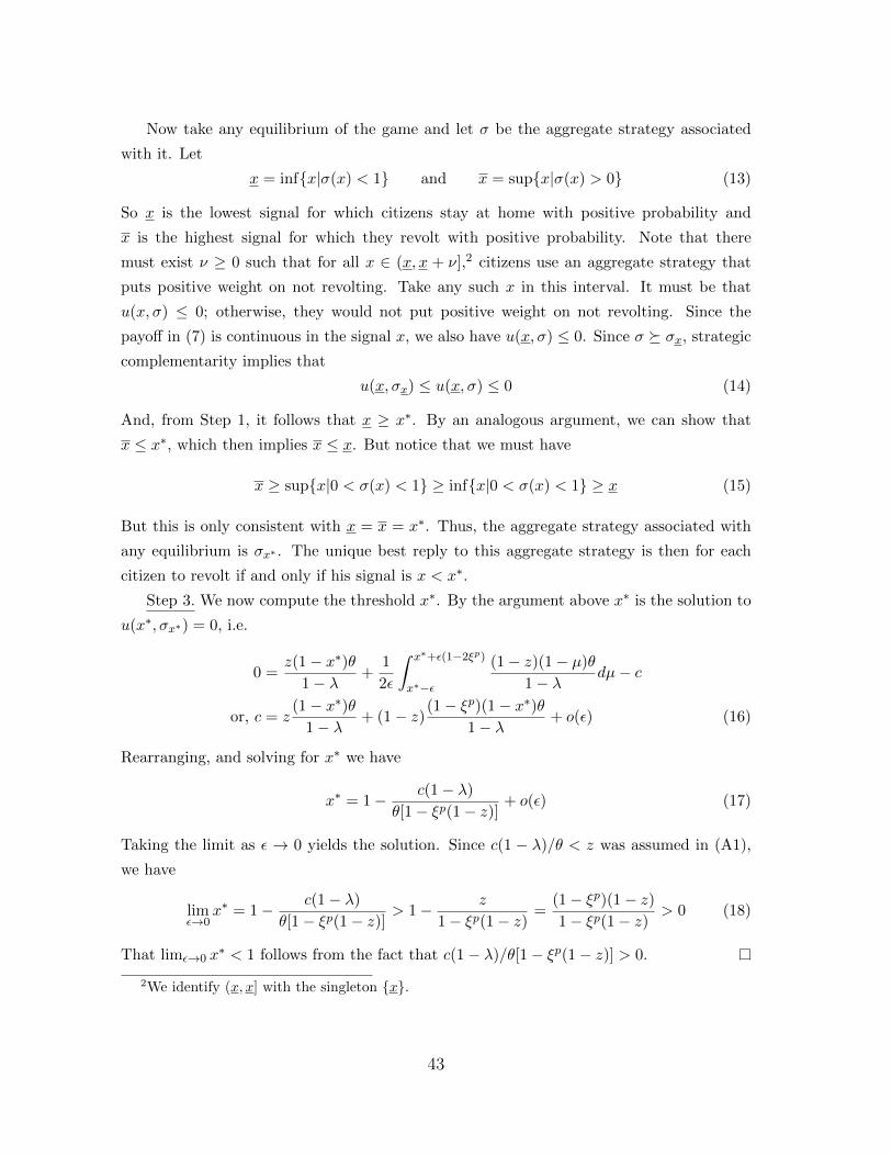
Now take any equilibrium of the game and let σ be the aggregate strategy associated
with it. Let
x = infx|σ(x) < 1 and x = supx|σ(x) > 0 (13)
So x is the lowest signal for which citizens stay at home with positive probability and
x is the highest signal for which they revolt with positive probability. Note that there
must exist ν ≥ 0 such that for all x ∈ (x, x + ν],2 citizens use an aggregate strategy that
puts positive weight on not revolting. Take any such x in this interval. It must be that
u(x, σ) ≤ 0; otherwise, they would not put positive weight on not revolting. Since the
payoff in (7) is continuous in the signal x, we also have u(x, σ) ≤ 0. Since σ σx, strategic
complementarity implies that
u(x, σx) ≤ u(x, σ) ≤ 0 (14)
And, from Step 1, it follows that x ≥ x∗. By an analogous argument, we can show that
x ≤ x∗, which then implies x ≤ x. But notice that we must have
x ≥ supx|0 < σ(x) < 1 ≥ infx|0 < σ(x) < 1 ≥ x (15)
But this is only consistent with x = x = x∗. Thus, the aggregate strategy associated with
any equilibrium is σx∗ . The unique best reply to this aggregate strategy is then for each
citizen to revolt if and only if his signal is x < x∗.
Step 3. We now compute the threshold x∗. By the argument above x∗ is the solution to
u(x∗, σx∗) = 0, i.e.
0 =z(1− x∗)θ
1− λ+
1
2ε
∫ x∗+ε(1−2ξp)
x∗−ε
(1− z)(1− µ)θ
1− λdµ− c
or, c = z(1− x∗)θ
1− λ+ (1− z)(1− ξp)(1− x∗)θ
1− λ+ o(ε) (16)
Rearranging, and solving for x∗ we have
x∗ = 1− c(1− λ)
θ[1− ξp(1− z)]+ o(ε) (17)
Taking the limit as ε → 0 yields the solution. Since c(1 − λ)/θ < z was assumed in (A1),
we have
limε→0
x∗ = 1− c(1− λ)
θ[1− ξp(1− z)]> 1− z
1− ξp(1− z)=
(1− ξp)(1− z)1− ξp(1− z)
> 0 (18)
That limε→0 x∗ < 1 follows from the fact that c(1− λ)/θ[1− ξp(1− z)] > 0.
2We identify (x, x] with the singleton x.
43
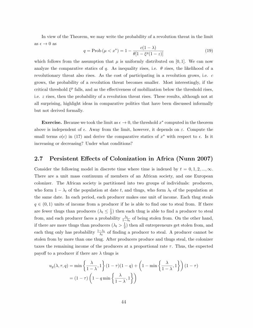
In view of the Theorem, we may write the probability of a revolution threat in the limit
as ε→ 0 as
q = Prob (µ < x∗) = 1− c(1− λ)
θ[1− ξp(1− z)](19)
which follows from the assumption that µ is uniformly distributed on [0, 1]. We can now
analyze the comparative statics of q. As inequality rises, i.e. θ rises, the likelihood of a
revolutionary threat also rises. As the cost of participating in a revolution grows, i.e. c
grows, the probability of a revolution threat becomes smaller. Most interestingly, if the
critical threshold ξp falls, and as the effectiveness of mobilization below the threshold rises,
i.e. z rises, then the probability of a revolution threat rises. These results, although not at
all surprising, highlight ideas in comparative politics that have been discussed informally
but not derived formally.
Exercise. Because we took the limit as ε→ 0, the threshold x∗ computed in the theorem
above is independent of ε. Away from the limit, however, it depends on ε. Compute the
small terms o(ε) in (17) and derive the comparative statics of x∗ with respect to ε. Is it
increasing or decreasing? Under what conditions?
2.7 Persistent Effects of Colonization in Africa (Nunn 2007)
Consider the following model in discrete time where time is indexed by t = 0, 1, 2, ...,∞.
There are a unit mass continuum of members of an African society, and one European
colonizer. The African society is partitioned into two groups of individuals: producers,
who form 1 − λt of the population at date t, and thugs, who form λt of the population at
the same date. In each period, each producer makes one unit of income. Each thug steals
q ∈ (0, 1) units of income from a producer if he is able to find one to steal from. If there
are fewer thugs than producers (λt ≤ 12) then each thug is able to find a producer to steal
from, and each producer faces a probability λt1−λt of being stolen from. On the other hand,
if there are more thugs than producers (λt >12) then all entrepreneurs get stolen from, and
each thug only has probability 1−λtλt
of finding a producer to steal. A producer cannot be
stolen from by more than one thug. After producers produce and thugs steal, the colonizer
taxes the remaining income of the producers at a proportional rate τ . Thus, the expected
payoff to a producer if there are λ thugs is
ug(λ, τ, q) = min
λ
1− λ, 1
(1− τ)(1− q) +
(1−min
λ
1− λ, 1
)(1− τ)
= (1− τ)
(1− qmin
λ
1− λ, 1
)
44
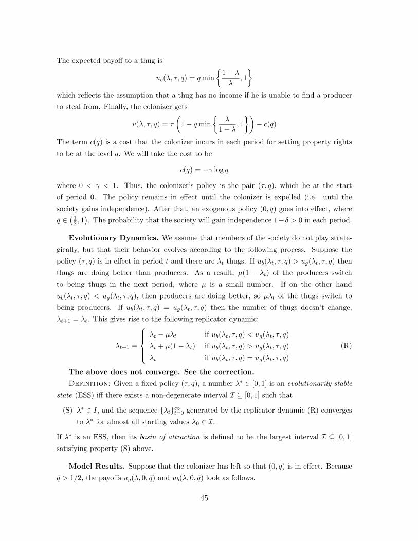
The expected payoff to a thug is
ub(λ, τ, q) = qmin
1− λλ
, 1
which reflects the assumption that a thug has no income if he is unable to find a producer
to steal from. Finally, the colonizer gets
v(λ, τ, q) = τ
(1− qmin
λ
1− λ, 1
)− c(q)
The term c(q) is a cost that the colonizer incurs in each period for setting property rights
to be at the level q. We will take the cost to be
c(q) = −γ log q
where 0 < γ < 1. Thus, the colonizer’s policy is the pair (τ, q), which he at the start
of period 0. The policy remains in effect until the colonizer is expelled (i.e. until the
society gains independence). After that, an exogenous policy (0, q) goes into effect, where
q ∈(
12 , 1). The probability that the society will gain independence 1−δ > 0 in each period.
Evolutionary Dynamics. We assume that members of the society do not play strate-
gically, but that their behavior evolves according to the following process. Suppose the
policy (τ, q) is in effect in period t and there are λt thugs. If ub(λt, τ, q) > ug(λt, τ, q) then
thugs are doing better than producers. As a result, µ(1 − λt) of the producers switch
to being thugs in the next period, where µ is a small number. If on the other hand
ub(λt, τ, q) < ug(λt, τ, q), then producers are doing better, so µλt of the thugs switch to
being producers. If ub(λt, τ, q) = ug(λt, τ, q) then the number of thugs doesn’t change,
λt+1 = λt. This gives rise to the following replicator dynamic:
λt+1 =
λt − µλt if ub(λt, τ, q) < ug(λt, τ, q)
λt + µ(1− λt) if ub(λt, τ, q) > ug(λt, τ, q)
λt if ub(λt, τ, q) = ug(λt, τ, q)
(R)
The above does not converge. See the correction.
Definition: Given a fixed policy (τ, q), a number λ∗ ∈ [0, 1] is an evolutionarily stable
state (ESS) iff there exists a non-degenerate interval I ⊆ [0, 1] such that
(S) λ∗ ∈ I, and the sequence λt∞t=0 generated by the replicator dynamic (R) converges
to λ∗ for almost all starting values λ0 ∈ I.
If λ∗ is an ESS, then its basin of attraction is defined to be the largest interval I ⊆ [0, 1]
satisfying property (S) above.
Model Results. Suppose that the colonizer has left so that (0, q) is in effect. Because
q > 1/2, the payoffs ug(λ, 0, q) and ub(λ, 0, q) look as follows.
45

0.0 0.2 0.4 0.6 0.8 1.0l
0.2
0.4
0.6
0.8
1.0Hug,ubL
Figure 1: ub is flat at first, then downward sloping; ug is downward sloping first and then flat.
Importantly, the payoffs cross at two points λ1 and λ2. The only candidates for ESS are
0, λ1 and λ2. But λ1 is not an ESS because there is no non-degenerate interval for which
property (S) is satisfied. On the other hand, 0 and λ2 are ESS with basins of attraction
[0, λ1) and (λ1, 1] respectively. To show this, note that on the interval [0, λ1) we have
ub(λt, τ, q) < ug(λt, τ, q) so
λt+1 = λt − µλt
Defining the function f(λ) = λ−µλ which is continuous, and note that λt+1 = f(λt). Then
the sequence of λt is strictly decreasing but contained in the unit interval, so it has a limit
λ∗. The limit must be a fixed point of the function f , for the following reason:
f(λ∗) = f( limt→∞
λt) = limt→∞
f(λt) = limt→∞
λt+1 = λ∗
But the only fixed point of f(λ), as you can verify, is λ = 0. Analogous arguments work on
the basin (λ1, 1].
Now consider the problem of the colonizer. Let us suppose that when the colonizer
arrived in period t = 0, he found society in relative harmony with (0, q) in effect and society
at the harmonious ESS, λ0 = 0. This assumption is consistent with the idea that although
much of Africa was “stateless” when the colonizer arrived in period 0 (q > 12), society was
nevertheless in social harmony (λ0 = 0).
The colonizer maximizes
V (τ, q) = (1− δ)∞∑t=0
δtv(λt, τ, q)
subject to λ0 = 0 and λt evolving according to (R) (C)
which implicitly assumes that once he is kicked out the colonizer gets 0 every period. This
is simply a normalization.
46
To solve this problem, let us first try to understand how the replicator works under an
arbitrary policy (τ, q). Note that if τ > 1− q then ug(0, τ, q) < ub(0, τ, q) as in the figure on
the left. On the other hand, if τ < 1− q then ug(0, τ, q) > ub(0, τ, q) as in the figure on the
right. If τ = 1− q then ug(0, τ, q) = ub(0, τ, q). In general, ug(λ, τ, q) is shifts downward as
τ increases, but ub(λ, τ, q) does not move in τ .
0.0 0.2 0.4 0.6 0.8 1.0l
0.2
0.4
0.6
0.8
1.0Hug,ubL
0.0 0.2 0.4 0.6 0.8 1.0l
0.2
0.4
0.6
0.8
1.0Hug,ubL
Figure 2: Again, ub is flat at first, then downward sloping; ug is downward sloping first and then
flat.
This observation implies that if the colonizer chooses a policy with τ ≤ 1−q then λt = 0
for all t. If τ < 1 − q the 0 is an ESS. If τ = 1 − q then 0 is not an ESS, but society will
(very delicately) stay at 0 forever. But this means that τ < 1− q cannot be optimal for the
colonizer. To see why, note that the colonizer’s payoff each period would be
τ − c(q)
which is increasing in τ . Indeed, at the solution to the colonizer’s maximization problem,
we need to have τ ≥ 1− q. Now, there are two kinds of strategies for the colonizer that are
possibly optimal:
(SR) (Short Run Strategy) τ > 1− q(LR) (Long Run Strategy) τ = 1− q
Proposition: There exists δ ∈ (0, 1) such that δ > δ implies that the colonizer uses
the LR strategy (τ, q) = (1− γ, γ); and if δ < δ he uses an SR strategy.
If the colonizer uses the LR strategy then we have society staying delicately at λt = 0
forever. If the colonizer uses an SR strategy then society converges as
λt → λ
If the colonizer exits early when λt < λ1 < 12 , then society will slowly revert back to the
harmonious ESS where λ∗ = 0. If, on the other hand, the colonizer stays a good while and
47

leaves only in a period t where λt > λ1 then society will converge to the unfortunate ESS
where λ∗ = λ2 > 12 . (This is the disruption of colonization.)
Instead of providing a formal proof, let me give you the basic intuition, and you can go
home and write a formal proof. Observe that for every LR strategy, there is an SR strategy
that yields strictly higher payoff in the first period. To see why, note that under an LR
strategy, we have λt = 0 for all t. So again, the colonizer’s first period payoff is τ − c(q),which is increasing in τ . This observation implies that if δ is sufficiently close to 0 then the
colonizer will use a short term strategy. (This is intuitive: if he expects to be kicked out
with high probability in each period, then he uses short term strategies.)
Likewise, there exists a period t large enough such that the LR strategy yields higher
payoffs in every period t ≥ t. To prove this, fix any SR strategy (τ, q). Over time, λt
converges to the point λ in Figure 2 above, such that λ > 12 . Consider a period t large
enough that λt ≥ 12 . The colonizer’s payoff in this period is
τ(1− q)(1− λt)− c(q)
But under an LR strategy (1− q′, q′) his payoff each period is
(1− q′)− c(q′)
The value of q′ that maximizes this payoff is q′ = γ, which characterizes the best LR
strategy. Then, we have the following result
v(0, 1− γ, γ) = (1− γ)− c(γ)
≥ (1− q)− c(q)
> τ(1− q)(1− λt)− c(q)
= v(λt, τ, q)
So for t large enough that λt ≥ 12 the LR strategy yields higher payoffs than any SR strategy.
This implies that if δ is sufficiently close to 1 the colonizer uses an LR strategy, in particular
the optimal one (1− γ, γ).
Exercise. We did not characterize the optimal SR strategy, which is really the only
thing left to do to prove the propoistion. Do it, and find an expression for δ.
48

3 Behavioral Political Economy
3.1 Ideology (Benabou 2008)
There are a continuum of individuals of unit mass indexed by i. The maximum feasible tax
rate that government can set is τ < 1. Taxes are linear so revenues from the tax rate τ are
simply τ . Taxes are non-distortionary and used entirely to fund a public good denoted h,
which provides individuals in society with some human capital (e.g. education or health).
There are three periods in the game, periods 0, 1 and 2. In period 0, the state H or L is
realized. The prior probability of state H is q. After states are realized, each agent obtains
a signal about the state. We assume that the signal is perfect, so that if the state is H
then all agents receive the signal H while if the state is L then all agents receive the signal
L. Unlike standard models of Bayesian updating however, we assume that each agent can
choose either to update (and learn perfectly the state) or he can choose to ignore his signal
and go with the prior. The choice is denote λ ∈ 0, 1, with λ = 0 meaning that the agent
has chosen ‘denial’ and λ = 1 meaning that he has chosen ‘realism.’ Choosing denial comes
at a cost of m > 0.
Once agents choose denial or realism, period 1 begins with society voting on the tax
rate τ . Once voting is over and the tax rate is set, each agent decides how much effort ei
to exert. Effort is a substitute to the government provision of the public good. Think, for
example, of government providing public education/healthcare or agents educating/taking
care of themselves. The amount of human capital that agent i obtains is given by the
technology
hi = minγei + τθj , E, j = H,L
which depends on the state. Thus, there is an upper limit E on how much human capital
an agent can amass. We will assume that
0 ≤ θL < γ < θH < E/τ (A1)
which states that government is less efficient than the market in state L, and more efficient
in state H, and government resources are always limited so some private investment has a
positive marginal return (τ θH < E).
Finally in period 2 agents receive their final payoffs which are
U i = 1− τ − ei + αhi + (1− α)h
where h is the population average human capital and 1−α determines the extent of exter-
nalities / public nature of human capital. When agents receive their period 2 payoff, they
49

have learned whether the state is H or L independent of their choice of denial or realism in
the first period.
The twist that I didn’t mention is that period 1 actually ends with agents obtaining
some ‘anticipatory’ utility, specifically
sEi1[U i] = sEi1[1− τ − ei + αhi + h]
Here s ≥ 0 captures the importance of ‘hope,’ ‘anxiety,’ ‘dread,’ and similar emotions. Note
that the expectations operator is indexed both by the period (1) and the agent (i). This
is because the agents’ choice of beliefs in period 0 implies that agents may have differing
expectations about the future depending on whether they chose denial or realism.
Therefore, given τ , agents choose ei in period 1 to maximize the expected sum of their
anticipatory and final utility, i.e.
sEi1[U i] + Ei1[U i]
So, if in period 1 an agent believes that the state is H with probability r(λ) ∈ 0, q, 1 then
the agent maximizes (s+ 1) times
1− τ − e+ α[r(λ) minγe+ θHτ, E+ (1− r(λ)) minγe+ θLτ, E]
(Since all agents are infinitesimal, they cannot control the average term h so it doesn’t
figure into this maximization problem.) It is straightforward to show that if
αγ > 1 > (1− q)αγ (A2)
then agents who did not choose denial will invest e = (E−τθj)/γ when the state is j = L,H,
but agents who chose denial will invest e = (E − τθH)/γ in both states.
In period 0, agents will choose either denial or realism (λ ∈ 0, 1) after they have
observed their signals, to maximize
−M + Ei0[sEi1[U i]] + Ei0[U i]
This is because they know that they will receive the anticipatory utility in period 1 and
the final utility in period 2, and they take expectations given with respect to the private
information they have in period 0. (The fact that information is private, however, does
not matter since the signals are perfectly informative.) In this payoff M = m if the agent
chooses denial (λ = 0) and M = 0 if he chooses realism (λ = 1).
When all agents choose realism (λi = 1∀i) everyone in society fully acknowledges what
government can and cannot deliver, and they invest e = (E − τθj)/γ when the state is θj ,
50

achieving hj = E in both cases. So a voter gets 1− τ − (E − τθj)/γ +E in state j = H,L.
So by assumption (A1), voters unanimously choose τ = 0 in state L and τ = τ in state H.
On the other hand, when λi = 0∀i agents discard their signals. So the posterior for every
agent is r(0) = q. If the realized state is L By (A2), they only invest ei = (E − τ θH)/γ
effort, which falls short of the optimal effort in state L by τ(θH − θL)/γ = τ∆θ/γ. The
expected utility of a voter is thus (1 + s) times
1− τ − (E − τθH)/γ + qE + (1− q)(E − τ∆θ)
The marginal value of taxation is positive if
θH/γ > 1 + (1− q)∆θ (A3)
Proposition: Under (A1), (A2) and (A3), if hope and anxiety are salient features of
the human condition, i.e. if the salience of anticipatory utility is large enough with
s ≥ m+ (α− 1/γ)τ∆θ
(q − α+ 1/γ)τ∆θ≡ s
then both realism (λi = 1∀i) and collective denial (λi = 0∀i) are equilibrium social cogni-
tions when the state is L. In the latter, agents believe in and vote for a large government in
spite of evidence that it is inefficient. If s < s only realism is an equilibrium social cognition.
Proof. What happens when an agent i deviates to censoring (λi = 0) when everyone
else is choosing realism (λ−i = 1)? In period 1, the winning tax rate τ = 0 or τ = τ fully
reveals to him the state, so denial does not enable him to savor the anticipatory utility.
Denial would just costs m > 0 but provide no benefit. So λi = 1∀i is always an equilibrium.
When society collectively chooses denial (λi = 0∀i) the policy no longer reveals the state
of the world to any individual. The policy is in fact always τ by assumption (A3). So, here,
it is feasible for a censoring agent to remain ignorant of a signal that was censored. But is it
optimal to censor? If an agent retains the bad news, he correctly invests ei = (E − τ θL)/γ
but lives knowing that taxes are unproductive and that everyone is under-investing due to
excessive faith in government. His expected utility in period 0 from choosing realism R is
thus
V R0 = (s+ 1)
[1− τ − (E − τ θL)/γ︸ ︷︷ ︸
optimal effort
+ αE︸︷︷︸personal part
+ (1− α)(E − τ∆θ)︸ ︷︷ ︸social part
]If he is in denial D like everyone else he incorrectly invests (E − τ θH)/γ and gets
V D0 = −m+ (s+ 1)× [1− τ − (E − τ θH)/γ]︸ ︷︷ ︸
part common to savoring and final payoffs
+ s [qE + (1− q)(E − τ∆θ)]︸ ︷︷ ︸extra part from savoring
+ [E − τ∆θ]︸ ︷︷ ︸extra part in final payoff
51
One can show that
V D0 − V R
0 = −m− (s+ 1)(α− 1/γ)τ∆θ︸ ︷︷ ︸direct and indirect cost of denial due to underinvesting
+ sqτ∆θ︸ ︷︷ ︸gain in savoring
One can show that V D0 − V R
0 ≥ 0 if and only if s ≥ s.
Benabou writes that “interacting with realists makes it more difficult to sustain delu-
sions; conversely, the more others avoid the truth, the easier it is for one to avoid it—if so
desired.” Note that it is infeasible to sustain individual denial in a world of realists. Ben-
abou writes that the model reflects a Mutually Assured Delusion (MAD) principle: “When
others’ denial of an unpleasant reality leads them to act in ways that further worsen an
agent’s prospects, this increases his own incentives to engage in wishful thinking, making
cognitive strategies complements. Conversely, when others’ ignorance of bad news is benefi-
cial, that news becomes easier to face and cognitive strategies are substitutes. The political
and economic interactions considered here clearly belong to the first case. Indeed, when an
ideological electorate votes for the wrong policy, each citizen suffers an expected loss (fiscal
channel). Moreover, if people’s distorted view of what the state or market will deliver leads
them to underinvest in their (or their children’s) education, undersave for their retirement,
and so on, there will be further collective losses to bear (interactions channel).”
Exercise. Consider a new parameter κ. Replace (A1), (A2) and (A3) with the following
assumptions
(A1′) 0 ≤ θL < γ < θH < E/κ
(A2′) αγ > 1 > qαγ
(A3′) θL/γ < 1− q∆θand suppose that now hi = minγei + θ(τ − κ), E. Let
s∗ =m+ (α− 1/γ)κ∆θ
(1− q − α+ 1/γ)κ∆θ
Show that under the new assumptions both λ = 0 and λ = 1 are equilibrium social cognitions
if s ≥ s∗. Explain when and how we might interpret the λ = 0 equilibrium as collective
denial of market failures in which agents distrust and vote against government provision in
spite of good evidence that it is necessary and effective. (What is the relevant assumption
about κ?)
3.2 Social Identity Equilibrium (Shayo 2009)
There are a continuum of agents of unit mass, partitioned into two groups, poor and rich.
Fraction λ > 12 are poor, while fraction 1 − λ are rich. Let P and R denote the sets of
52

poor and rich, and N the set of all agents (N for nation). Each poor agent p has the same
income, denoted yp, while each rich agent has the same income, denoted yr > yp. Mean
income is denoted y = λyp + (1− λ)yr.
Given a proportional tax rate τ , each agent i = p, r has post-fisc income πi(τ) =
(1− τ)yi + T where T =(τ − τ2
2
)y. This reflects the assumption of un-targeted lump-sum
transfers with quadratic deadweight losses to taxation that we have seen in Meltzer and
Richard (1981). As in that model, the median voter is poor, so if he cares only about his
material payoff, he sets the tax rate τ =(1− yp/y
). However, we will instead assume that
each agent i = p, r has the following utility function
ui(τ, j) = πi(τ)− β(dij)2
+ γSj(τ)
where β and γ are positive constants and diJ and SJ(τ) are nonmaterial components of an
agent’s objective that we describe next.
Let qpN = qrN = 1 and qiC be an indicator function taking value 1 if i = p and 0 otherwise.
Let qjN denote the mean value of qiN across all members i who “identify” with group j. (We
will make precise what we mean by “identify” later.) Similarly, let qjC denote the mean
value of qiC across all members i who identify with group j. And, let yj denote the mean
value of yi across all members i who identify with group j. For each i and each group
j = P,R,N , the “social distance” between individual i and group j is
dij =(wy(y
i − yj)2 + wN (qiN − qjN )2 + wC(qiC − q
jC)2)1/2
where wy, wN and wC are nonnegative weights that sum to 1. Now, let πP (τ) = πp(τ)
and πR = πr(τ) and πN (τ) = απp(τ) + (1 − α)πr(τ), 0 ≤ α ≤ 1. The “status” of group
j = P,R,N is then
Sj(τ) = µj + νj(πj(τ)− πr(j)(τ)
)where µj and νj are nonnegative constants and r(R) = P , r(P ) = R, and πr(N)(τ) is some
constant.
Let Gi be the set of groups to which agent i belongs. (So Gp = P,N and Gr =
R,N.) Each voter’s strategy is to announce a tax rate τ i and choose a group ji ∈ Gi to
identify with.
Social Identity Equilibrium (SIE): An SIE is a profile of tax rates and social
identities (τ i, ji)i∈N such that for all i ∈ N , we have τ i ∈ [0, 1], ji ∈ Gi, and
ui(τ i, ji) ≥ ui(τ i, ji) ∀τ i ∈ [0, 1] ∀ji ∈ Gi
We do not have to assume that the political process always implements the median
announced tax rate since it is implicitly assumed that in an SIE, voters “vote sincerely.”
53

Now look at the figure below. In both panels, the payoff πp(τ) is plotted against the
payoff πr(τ) as τ moves from 0 to 1. The dotted line on the left panel is an indifference
curve of an agent i = p who identifies with the poor, j = P , when all other poor agents
identify with P . Utility increases as the line moves southeast. Why isn’t the curve simply
a vertical line? Because the agent cares about the status SP (τ) of the poor relative to the
rich, so he internalizes the payoffs of others like him. This yields a higher optimal tax rate
that the arrow points to than the tax rate τ that maximizes individual material utility. Call
the tax rate that the arrow points to τ∗P .
Now look at the panel on the right. The dotted line is an indifference curve of an agent
i = p who identifies with the nation, j = N , when all other poor agents identify with the
nation N . Utility increases as the line moves to the northeast. The slope of this indifference
line is determined by α and νN . If νN = 0 then the line would be vertical, for example,
because he would not care about the status of his nation relative to other nations. The
best tax rate for this agent, conditional on identifying with the nation, is where the arrow
points. It is lower than the tax rate in the left panel. Call the tax rate that the arrow
points to τ∗N .
Now, let us focus on a symmetric SIE and try to determine when the poor identify with
the nation versus their class. The poor identify with the nation rather than with their class
if
γSN − β(dpN )2 > γSP − β(dpP )2
and they identify with their class if the reverse inequality holds. So the relevant comparison
here is SN −SP to βγ
((diN )2 − (dpP )2
). The difference SN −SP is always strictly decreasing
in tax rate τ on the interval [τ∗N , τ∗P ]. The reason is that a higher level of redistribution
diminishes the difference in material payoff between rich and poor, so it increases the status
54

of the poor. Furthermore, due to the efficiency loss of taxation, higher levels of taxation
reduce national status on the interval [τ∗N , τ∗P ].
In fact, the difference SN −SP looks as follows. In case I, only the poor identifying with
the nation and setting tax rate τ∗N is part of a symmetric SIE. In case II, only the poor
identifying with their class and setting tax rate τ∗P is part of a symmetric SIE. In case III,
there are multiple equilibria.
Exercise. State the conditions under which there is a unique symmetric SIE with taxes
τ∗N , there is a unique symmetric SIE with taxes τ∗P and there are multiple equilibria. What
are the comparative statics of these conditions with respect to the parameters?
Exercise. (Dangerous) Can you use a global-games type perturbation to eliminate the
multiplicity of equilibria in this model? If so, do it.
55
Related Documents