Formal Report UAL Usler Guide Nikolay Malitsky and IRichard ...

BNL : 71010-2003

Formal Report

UAL Usler Guide

Nikolay Malitsky and IRichard Talman (BNL)

December 20,2002

Collider Accelerator Development Department 5paIlation Neutron Project

Brookhaven National Laboratory Brookhaven 5ciance Associates

Upton, EJY 11973

Under Contract No. DE-AC02-98CH10886 with the

United 5 ta tes Department of Energy

DISCLAIMER

This report was prepared as an account of work sponsored by an agency o f t h e United S ta tes Government. Neither t h e United S ta tes Government nor any agency thereof, nor any employees, nor any of their contractors, subcontractors or their employees, makes any warranty, express o r implied, or assumes any legal liability or responsibility for t h e accuracy, completeness, or any third party’s use or t h e results o f such use o f any information, apparatus, product, or process disclosed, or represents t h a t i t s use would not infringe privately owned rights. Reference herein to any specific commercial product, process, or service by t rade name, trademark, manufscturer, or otherwise, does no t necessarily const i tu te or imply i t s endorsement, recommendation, or favoring by t h e United S ta tes Government or any agency thereof or i t s contractors or subcontractors. The views and opinions o f authors expressed herein do not necessarily s t a t e or reflect those o f t h e United S ta tes Government or any agency thereof.

UAL Us'er Guide

Nikolay Malitsky and IRichard Talman (BNL)

December 20,2002

Collider Accelerator Development Department 5pallation Neutron Project

Brookhaven National Laboratory Brookhaven 5ciance Associates

Upton, NY 11973

Under Contract No. DE-AC02-98CH10886 with the

United 5 ta tes Department of Energy

* This work wa5 performed under the auejpices of the U.5. Department of Energy.

UAL User Guide

Nikolay Malitsky and Richard Talman

Accelerator-Colllider Department Brookhaven National Laboratory

The Unified Accelerator Libraries (UAL) provide a modularized envi- ronment for applying diverse accelerator simulation codes. Development of UAL is strongly prejudiced toward1 importing existing codes rather than developing new ones. This guide pralvides instructions for using this envi- ronment. This includes instructions for acquiring and building the codes, then for launching and interpreting some of the examples included with the distribution. In some cases the examples are general enough to be applied to different accelerators by mimicking input files and input parameters. The intention is to provide just enough computer language discussion (C++ and Ped) to support the use and understanding of the examples and to help the reader gain a general understanding of the overall architecture. Otherwise the manual is “documentation by example.” Except for an appendix con- cerning maps, discussion of physics is limited to comments accompanying the numerous code examples. Importation of codes into UAL is an ongoing enterprise and when a code is said to have been Tmported it does not nec- essarily mean that all features are supported. Other than this, the original documentation remains applicable (a.nd is not duplicated here.)

i

.. 11

Table of Contents

. . . . . . . . . . . . . . . . . . . . . . . . . . . . . . . . . . . 1 1 . Introduction 1.1. General description of UAL . . . . . . . . . . . . . . . . . . . . . . . . 2

1.2. Modularity and object orientation 3 . . . . . . . . . . . . . . . . . . . . .

. . . . . . . . . . . . . . . . . . . . . . . . . . . . . 9 2 . The Architecture of UAL

3 . Code Checkout and Environment Variables . . . . . . . . . . . . . . . . . . . 12

4 . Perl as Interface Language . . . . . . . . . . . . . . . . . . . . . . . . . . . . 16

4.1. Elementary Perl . . . . . . . . . . . . . . . . . . . . . . . . . . . . . . 17 4.1.1. Variables and statements . . . . . . . . . . . . . . . . . . . . . . . 17 4.1.2. Subroutines . . . . . . . . . . . . . . . . . . . . . . . . . . . . . . 20 4.1.3. Modules, packages/name-spaces, scopes . . . . . . . . . . . . . . . 22 4.1.4. References . . . . . . . . . . . . . . . . . . . . . . . . . . . . . . . 24 4.1.5. Regular expressions . . . . . . . . . . . . . . . . . . . . . . . . . . 26

4.1.6. Printing out results . . . . . . . . . . . . . . . . . . . . . . . . . . 27 4.1.7. Issuing system commands . . . . . . . . . . . . . . . . . . . . . . . . 29

4.2. UAL file directory structure and packages . . . . . . . . . . . . . . . . . 30

4.3. Perl extensions . . . . . . . . . . . . . . . . . . . . . . . . . . . . . . . 30

5 . Online Documentation of Simulation Methods . . . . . . . . . . . . . . . . . . 32

6 . Annotated Examples . . . . . . . . . . . . . . . . . . . . . . . . . . . . . . . 33 6.1. Introduction . . . . . . . . . . . . . . . . . . . . . . . . . . . . . . . . 33

6.2. Basic example . . . . . . . . . . . . . . . . . . . . . . . . . . . . . . . . 35

6.3. Selective lattice function output . . . . . . . . . . . . . . . . . . . . . . 42

6.4. A personalized shell for code deve1o:prnent 6.5. Fringe field map . . . . . . . . . . . . . . . . . . . . . . . . . . . . . . 49

6.5.1. Map generation . . . . . . . . . . . . . . . . . . . . . . . . . . . . 50 6.5.2. Map application . . . . . . . . . . . . . . . . . . . . . . . . . . . . 54

6.6. SXF input to UAL . . . . . . . . . . . . . . . . . . . . . . . . . . . . . 54 6.6.1. SXF rationale . . . . . . . . . . . . . . . . . . . . . . . . . . . . . 54 6.6.2. RHIC example . . . . . . . . . . . . . . . . . . . . . . . . . . . . 55

6.7. FastTeapot . . . . . . . . . . . . . . . . . . . . . . . . . . . . . . . . . 58

. . . . . . . . . . . . . . . . . 44

7 . MPI Multiprocessor Support . . . . . . . . . . . . . . . . . . . . . . . . . . . 60 7.1. MPI installation . . . . . . . . . . . . . . . . . . . . . . . . . . . . . . 61

iii

7.2. Overview of MPI . . . . . . . . . . . . . . . . . . . . . . . . . . . . . . 63

7.3. MPI applied to UAL . . . . . . . . . . . . . . . . . . . . . . . . . . . . 64

Appendices . . . . . . . . . . . . . . . . . . . . . . . . . . . . . . . . . . . . .

A . Ancestry of UAL . . . . . . . . . . . . . . . . . . . . . . . . . . . . . . . . . 67

B . Glossary . . . . . . . . . . . . . . . . . . . . . . . . . . . . . . . . . . . . . 70

B.l. Acronyms . . . . . . . . . . . . . . . . . . . . . . . . . . . . . . . . . . 70

B.2. File name extensions . . . . . . . . . . . . . . . . . . . . . . . . . . . . 71

. . . . . . . . . . . . . . . . . . . . . . . . . . . . . . C . Accelerator Parameters 72

72 C.l. Global geometry and survey C.2. Local particle coordinates . . . . . . . . . . . . . . . . . . . . . . . . . 75

. . . . . . . . . . . . . . . . . . . . . . . .

D . The Evolution of Standard Machine Format (SMF) . . . . . . . . . . . . . . . D.1. The SMF object model . . . . . . . . . . . . . . . . . . . . . . . . . . . D.2. SMF/RHIC example . . . . . . . . . . . . . . . . . . . . . . . . . . . . 82

D . 3. ADXF: Accelerator Description Exchange Format . . . . . . . . . . . . 86

77

77

E . Truncated Power Series and Lie Maps . . . . . . . . . . . . . . . . . . . . . . 90

E.l. F’unction evolution . . . . . . . . . . . . . . . . . . . . . . . . . . . . . 90

E.2. Taylor series in more than one dimension and Lie maps

E.3. Symplecticity of Lie map . . . . . . . . . . . . . . . . . . . . . . . . . . E.4. Hamiltonian maps . . . . . . . . . . . . . . . . . . . . . . . . . . . . . 95

E.5. Discrete maps . . . . . . . . . . . . . . . . . . . . . . . . . . . . . . . 96

E.6. Computation time estimates . . . . . . . . . . . . . . . . . . . . . . . . 98 E.7. Future directions . . . . . . . . . . . . . . . . . . . . . . . . . . . . . . 102

E.7.1. Flexible FastTeapot implemenitations . . . . . . . . . . . . . . . . 102 E.7.2. Sector maps plus sextupole kiicks . . . . . . . . . . . . . . . . . . . E.7.3. Irwin factorization . . . . . . . . . . . . . . . . . . . . . . . . . . 104

. . . . . . . . . 92

94

103

References . . . . . . . . . . . . . . . . . . . . . . . . . . . . . . . . . . . . . . 105

Index . . . . . . . . . . . . . . . . . . . . . . . . . . . . . . . . . . . . . . . . . 108

Chapter 1. Introduction

This is supposed to be something of a “quick start” manual. The reader looking

for a quickest possible start should skip to Chapter 3, Code Checkout and Environment

Variables, and from there to Chapter 6, Annotated Examples.

If “pure physics” is the analysis of physical systems made possible by their ideal-

ization, then the pure physics of acceleratoi:~ reduces to a rather small package. Circu-

lar accelerators basically work, with proper ties matching the expectations of Lawrence,

Kerst-Serber, McMillen-Veksler, Courant-Snyder, and a few others. The rest of acceler-

ator physics amounts to understanding why accelerators don’t work very well, or rather,

to efforts to make them work better. The problem is that the actual performance of an

accelerator depends on features that violat e the idealization mentioned previously. At

the risk of exaggerating the point, one might therefore say that the bulk of accelerator

physics is an antithesis of pure physics, in that it amounts to analyzing non-ideal sys-

tems. Hamiltonian requirements are easily met only in a linearized approximation that

becomes progressively less valid as accelerators become larger. This has called for modest

extensions of the theoretical foundations, but far more essential difficulty comes from the

vastly increased number of influential degrees of freedom that enter as deviation from the

ideal needs to be described. This is nowhere more true than in accelerator physics, where

thousands of pieces of uncorrelated data are needed to describe a large accelerator. Since

the handling of complicated data is more nearly the subject of computer science than of

physics, it seems sensible to take advantage of advances that have been made in computer

science. This requires a certain amount of reorientation for those physicists who think of

themselves as having invented computer science.

Of the many contributors, some to TEAPOT, some to UAL, the following deserve

special mention: Chris Iselin (for establishing a standard to be emulated), Maury Tigner

(for suggesting the task), Lindsay Schachinger (for establishing the pattern and getting

the project off the ground), Alexander Reshatov (for contribution to the UAL conceptual

design), and George Bourianoff and Jie Wei (for enthusiastic support).

- 1. -

2 1.1 : Introduction: General descmption of UAL

1.1. General description of UAI,

The Unified Accelerator Libraries (UAL)1-’2 attempt to “manage the ~mplexity” of ac-

celerators by providing an environment’ for simulating a variety of properties of a variety

of accelerators using a variety of simulation codes and methods. The intended value of the

environment is to provide homogeneous access to these resources while masking their diver-

sity yet assuring their consistency. This allows different methods to be consistently applied

to the same accelerator and the same methods to be applied to different accelerators. An-

other potential benefit is the feasability and economy of “infrastructure” (shared resources)

such as postprocessors, plotting/histogramming/fitting, input and output translation, and

parallel processing.

At this time, the object-oriented programs included in UAL are: PAC (Platform for

Accelerator Codes) , ZLIB (Numerical Libra:ry for Differential Algebra), TEAPOT (Thin

Element Program for Optics and Tracking) , ACCSIM (Accumulator Simulation Code) , ORBIT (Objective Ring Beam Injection and Tracking Code). Modules that are partially

supported and are under active development are ICE (Incoherent and Coherent Effects),

AIM (Accelerator Insturnentation Module), SPINK (tracks polarized particles in circular

accelerator), and TIBETAN (longitudinal phase space tracking). The Application Pro-

gramming Interface (API), written in Perl, .provides a universal shell for integrating and

managing all project extensions.

Three UAL manuals are planned of which this is the first:

0 User Guide. A manual containing the bare minimum of information needed to

acquire and build the code and to run t:he examples. In many cases the example

codes should be close enough to a problem of interest to enable the user to perform

other simulations by mimicking external inputs and Perl scripts.

0 Physics Manual. This manual will describe and explain the physical methods

used in the various modules, in many cases giving annotated reference to external

manuals and documentation. This manual will also provide sufficient reference to

the Developer’s Manual and online documentation to support “looking under the

hood” to enable the user to perform code modifications and additions.

1.2 : Introduction: Modularity and object orientation 3

0 Developer’s Manual. This manual supplies full technical documentation. It consists

largely of online documentation, much of .which is available at h t t p : //www . ual . bnl . gov

The primary programming languages of UAL are C++, which provides fast, secure,

basic calculations and Perl, which provides .a flexible user interface. Both are object ori-

ented.

In this manual typewriter font is used to exhibit text that would be visible on a

computer monitor, either because the text is being viewed by a text editor or because a

program has generated it as output. Italic ,font is used when a term or program having

a narrow technical sense is first introduced ([often without even the pretense of immediate

definition) or f o r emphasis. “Quotation marks” indicate either that a term is actually

being defined or that it is being used loosely.

1.2. Modularity and object orientation

As has been stated already, the prime purpose of UAL is to “unify” diverse codes

and procedures. Diverse codes are to form “modules” in an evolving, unified, coherent

environment. Modularity is a challenging and universally-applauded attribute that all

computer codes strive for, and some achieve, at least in individually-developed, single-

purpose codes. Two such codes being applied to the same system would certainly be

modular, relative to each other, but they would be too modular if their representations of

the system were too different and too complicated. In this situation it is hard to assure

that the systems represented in the two codes are, in fact, the same. This consideration

makes the task of unifying multipurpose, multideveloper codes all the more challenging.

To facilitate such unification UAL has introduced an open architecture in which di-

verse accelerator codes are connected toget.her via common accelerator objects such as

Element, Bunch, Twiss, etc. In this architecture each accelerator code is implemented

as an object-oriented library of C++ classes. There is a very natural identification of

physical elements, such as magnets, with their representation by computer objects. UAL

supports considerable flexibility in the attributes of all objects-certainly enough that all

attributes of objects contained in modules included so far have been describable without

4 1.2 : Introduction: Modularity and object orientation

constraint. Such flexibility has made it practical to evaluate, compare, and integrate a

variety of design models and to build heterogeneous, project-specific applications. This

experience has motivated the development of the Element-Algorithm-Probe framework4

that will be a core part of the UAL release currently being completed. This framework

is intended to provide a uniform mechanism for combining diverse modules to simulate

complex combinations of physical effects and dynamic processes. t

One of the purposes of this manual is to make clear the way object orientation helps in

such unification, and thereby justify its adoption by UAL. Object-oriented methodology

affects code developers far more than it affects code users. It is not necessary for a user

of UAL to endorse object-orientation or even to understand exactly what constitutes an

object-oriented program. The single consideration that most distinguishes object-oriented

code from procedural code is the priority assigned to, on the one hand, data, and, on

the other hand, the procedures used to process data. (Procedures are always mathematics,

broadly defined.) The procedural program lavishes great care on the procedures and treats

data casually if not contemptuously-like a feudal lord managing his vassals. In object-

oriented code the data is pre-eminent and demands orderly management-like a democratic

people demanding to be governed by laws.

Since data is usually descriptive of the structure of stationary objects, and procedures

change data, it can be said that procedures represent behavior, a subject inherently more

complicated than structure. In this sense object-orientation should be expected to be

simpler than procedural-orientation. A system built around objects rather than around

functionality more closely corresponds to the humanly-comprehended world.

~

t The Element-Algorithm-Probe framework is not actually used in the Perl-based examples described in this manual. There is, however, a preliminary directory, $UAL/examples/FastTeapot (symbol $UAL is defined in Chapter 3) that contains code which applies the Element-Algorithm-Probe framework. The script rhic.pl in this directory applies standard, Perl-based, UAL analysis (as documented in this guide) to a RHIC lattice as it is defined by its SXF (Standard Exchange Format).This same lattice is used by the FastTeapot code contained in subdirectories of the 'same directory. The main incentive for speeding up the UAL simulation capability has been to improve its serviceability for online modeling. In order to be fast as well as control-system-embeddable, FastTeapot is written in C++. The C++ code is contained in the $UAL/examples/FastTeapot/src directory and the examples of its use for map generation and map-tracking are in $UAL/examples/FastTeapot/linux. Instruct ions for compiling the code and running the examples are given in a README file. Except for brief comments in section 6.7, FastTeapot is not otherwise documented in this guide, but understanding the material in this guide is something of a prerequisite to using FastTeapot.

1.2 : Introduction: Modularity and object orientation 5

Here is an example of encapsulation, which is one of the cornerstones of object-

orientation. Consider the distinction between file names in Unix and in Windows. The

filename of a Unix text file merely identifies the file, with no necessary implication what-

soever as to the intended use or treatment O F the data it contains. In the “8f3” file name

plus extension conventiont of Windows the data is organized in such a way as to be acces-

sible only by the collection of calculational procedures that is identified by the 3-character

extension of the file name.

The term encapsulation is perhaps not as descriptive of this feature of object-orientation

as the closely related term data hiding. Thl: organization of data into structure’s in pro-

cedural languages like C or Fortran might deserve to be called “encapsulation” in the

colloquial use of that term. But in those languages this does not imply any reduction in

accessability. Data hiding intentionally restricts access to data.

There would be no point in hiding data if there were no mechanism for accessing the

hidden data. So the term encapsulation also conveys the meaning that the calculational

procedures needed to access the hidden data, (they are always called methods in this con-

text) are linked to the data as part of the same encapsulation. These methods will

have been authenticated by the same developer whose job has been to organize the data.

This helps to make the access to, and processing of, data contained in complicated data

structures more reliable. Any spreadsheet usler will agree that is is more reliable to use the

spreadsheet’s methods than it would be to search for and find, and then process, the data

“hidden” in the spreadsheet file.

The distinction between object-orientation and procedural-orientation can be contin-

ued by comparing structures and functions, the procedural mechanisms supporting mod-

ularization, with objects, classes, and methods, the object-oriented mechanisms. As far as

the data it contains and its having a name, an object is the same thing as a structure. But,

by virtue of its belonging to a class, the attributes of an object are subject to manipulation

(including creation and destruction) exclusively by the methods of its class. “Method”

and “function” would be synonyms except that a method must “belong to” a class and a

function need not. Both attributes and methods are referred to as class members.

t The “8f3” file name plus extension file naming of Windows, though an abomination for most purposes, has undoubtedly helped Microsoft’s profits by billions of dollars.

6 1.2 : Introduction: Modularity and object orientation

Two other features that characterize object-oriention, overloading (also known as “poly-

morphism”) and inheritance, will be mentioned below when their application within UAL

is being explained.

Within UAL the object-orientation is “enforced” by C++ and, a priori, one might

expect no other computer language to be required. But, by now, it is universally agreed

that this approach is too inconvenient for users, and that it is necessary to produce a

consistent interface using a “control” language. For UAL (at this time) this language is

Perl. The interface is textual+ (not graphical) and, line-by-line, its instructions may look

to the user very much like the directives in a procedural code like MAD.5 This makes

it possible to “pay no attention to the man, behind the curtain” and treat the input as

an old-fashioned, procedural control file. The most important step in going beyond this

level is to acquire an understanding of the rnodularixation mechanism of the code, which

is based on the naming of directories, classes, modules, and so on. This puts the greatest

demands on Perl, as the interface, and on the user, trying to use and understand the code.

This discussion continues below in Section 4.

Even apart from the diversity of codes supported, there is inherent difficulty in doc-

umenting a modularized open environment.. Many or most of the users for whom the

UAL environment is potentially of greatest value are probably most familiar with a closed

code having strict input language, such as MAD. Such input languages capture relevant

“use cases” (computer science jargon) of accelerator applications and organize them as

a sequence of commands, starting from the lattice description, proceeding through “ac-

tions” (magnet field error distribution, tuning, etc.) and finally to results (lattice function

determination, etc.) This use-case-organized interface matches the expectations of most

Because the UAL command language is Perl, a graphical interface to Perl would serve as a graphical interface to UAL. Something approaching this is provided by a free utility called DDD which provides a graphical debugging interface to various languages, including Perl. DDD permits the user to proceed step- by-step through a Perl script, or to continue to the next user-inserted breakpoint. While the script is stopped variable values can be inspected, or even altered. Other typical debugging capabilities are also supported. This is an excellent facility for the user to gain familiarity with UAL’s example scripts. At this time DDD is restricted to the Perl level as it is not mature enough to “step” down into the Cff extensions UAL employs, or even to exhibit values in the Cf+ domain. Failure to respect this causes DDD to crash, so one has to learn to avoid making such requests. Fortunately the cost of crashing is not high as the same state can be recovered quickly with a few button clicks. Crashes can sometimes be avoided by setting multiple breakpoints and continuing from breakpoint to breakpoint rather i;han stepping from instruction to instruction. Perhaps a more powerful displaying debugger will come available in the future.

1.2 : Introduction: Modularity and object orientat ion 7

users. Such “sequentially-organized” codes proceed from start to finish with minimal

branching and it is natural for the documentation to be organized along the same lines.

An open environment, on the other hand, is “module-organized”, allowing the user to

pick and choose among various modules for building project-specific applications. If the

modules are well-designed, with clean interfaces, they tend to be “self-documenting” , as

the existence of modern “documentation engines” proves. UAL uses the utility dozygen

for automatic generation of on-line documentation. The existence of this documentation

helps to amortize the initial expenditure in (code development for the code developer and

in conceptual effort required of the code user. The clean interfaces make it practical for

a user to make controlled ad hoc changes to localized blocks of code without the need to

understand the rest of the code.

UAL strives to preserve the advantage13 of both use-case and module-oriented ap-

proaches, by encouraging a division of labor between code developer and code user. Work-

ing in an object-oriented “research environment” the goal of the developer is to supply a

“use case” view of the code which, ideally, allows the code user to be most productive. The

mechanism for accomplishing is known as a Shell (or Fugade) layer. This layer hides the

complexity of the numerous interfaces of the underlying UAL components and implements

a list of MAD-like Per1 commands that delegate user requests to appropriate modules.

Since this manual is intended primarily for the code user rather than for the code

developer, technical code features are discussed only to a depth judged appropriate to

provide the user with general orientation and critical appreciation of the fundamental

issues.

This manual therefore consists mainly of “documentation by example”. It is supposed

to supply a minimal set of intructions adequate to guide the user through meaningful

calculations while treating UAL as a traditional accelerator code. The variety of examples

is intended to carry the user part way along a path of acquiring confidence in the results

without requiring detailed understanding of the mechanisms by which they have been

obtained. To obtain fuller confidence the user is expected either to develop test examples

or to delve more deeply into the code, guided by other manuals and documentation.

It would be a formidable task to study thoroughly the various programming tools,

languages and systems on which UAL depends. References are given to literature that

8 1.2 : Introduction: Moddar i t y and object orientation

seem to us to be appropriately elementary arid useful. The instructions in this manual are

supposed to be mechanical enough that thesle references are inessential for first running of

the examples, but they may be useful in advancing past the beginning stage.

Chapter 2. The Architecture of UAL

PERIL API / H /Y /Y H /Y f l /Y /Y

a N 3

l+i /' / / / /

/ A Element-Algorithm-Probe Framework

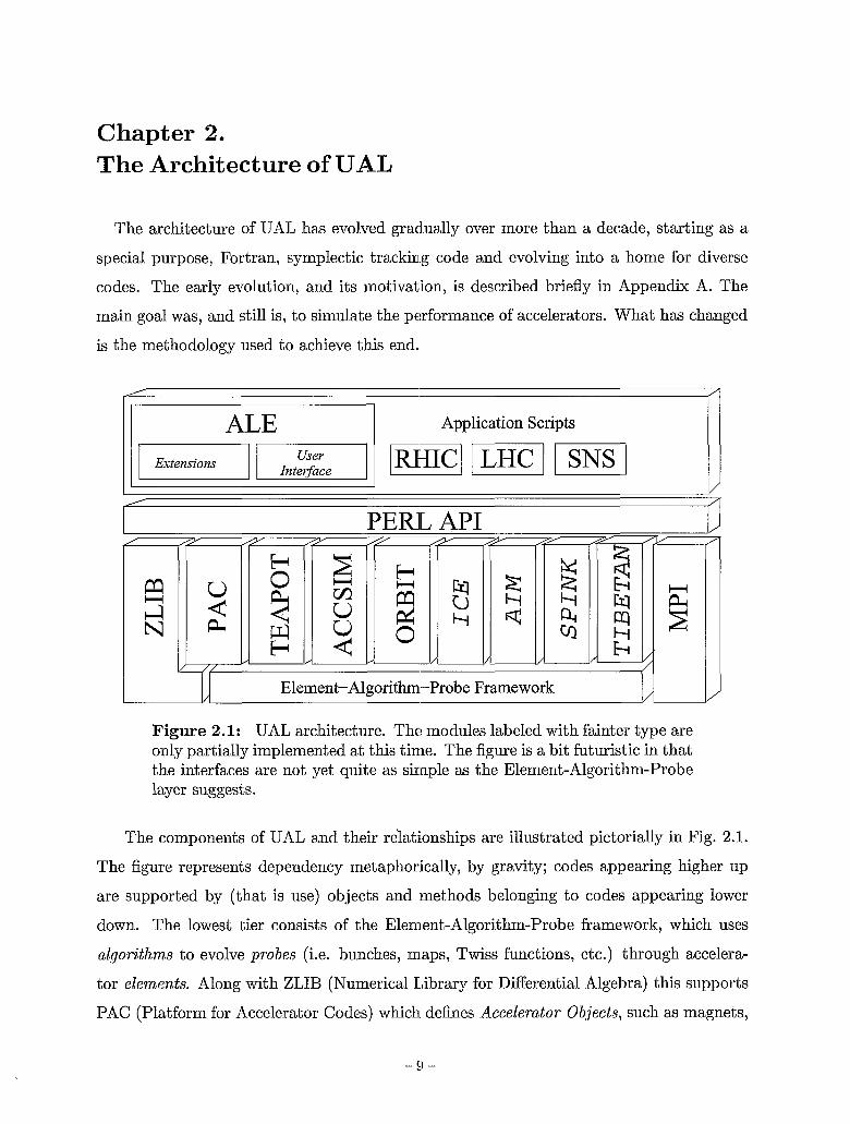
The architecture of UAL has evolved gradually over more than a decade, starting as a

special purpose, Fortran, symplectic trackin-g code and evolving into a home for diverse

codes. The early evolution, and its motivation, is described briefly in Appendix A. The

main goal was, and still is, to simulate the performance of accelerators. What has changed

is the methodology used to achieve this end.

ALE Application Scripts

I I

The components of UAL and their relationships are illustrated pictorially in Fig. 2.1.

The figure represents dependency metaphorically, by gravity; codes appearing higher up

are supported by (that is use) objects and methods belonging to codes appearing lower

down. The lowest tier consists of the Element-Algorithm-Probe framework, which uses

algorithms to evolve probes (i.e. bunches, maps, Twiss functions, etc.) through accelera-

tor elements. Along with ZLIB (Numerical Library for Differential Algebra) this supports

PAC (Platform for Accelerator Codes) which defines Accelerator Objects, such as magnets,

- SI -

10 2 : The Architecture of UAL

lattice, particles, bunch, etc. These components form the “model” part of a three part

simulation environment containing elements that are common to all modules, and there-

fore support connections between different imodules. They are the glue that holds UAL

together.

The second major part of the simulation environment consists of the boxes, TEAPOT,

ACCSIM, . . ., TIBETAN, which stand for accelerator simulation modules, coded in C f f .

In most cases these modules derive from earlier, procedural, Fortran codes, which have

been ported to Cff . They constitute the ‘cphysics” supported at this time; things like

tracking, analysis, optimization, correction a,lgorithms, etc. They form the “actions” part

of the organization. Each of these modules is a separate, self-contained library of C++

classes having its own internal organization and methods. For completeness the module

MPI (Message-Passing Interface)‘ which supports parallel processing is also shown.

The separation mentioned so far, into accelerator objects, on the one hand, and actions,

on the other, is very comparable to the similar separation in any procedural program

deriving its input from a file such as MAD.t

The upper levels of Fig. 2.1 contain the “controller” part of the environment. The

API (Application Program Interface), written in Perl, makes available to the user the

capabilities of the various modules while “hiding” as much as possible of their complexity.

Scripts appropriate to particular accelerators, RHIC, LHC, SNS, etc. are based on the

user-friendly facade or interface ALE (Accelerator Library Extension). However, most of

the examples documented in this guide use directly the more generic ALE shell that is not

specific to any particular accelerator.

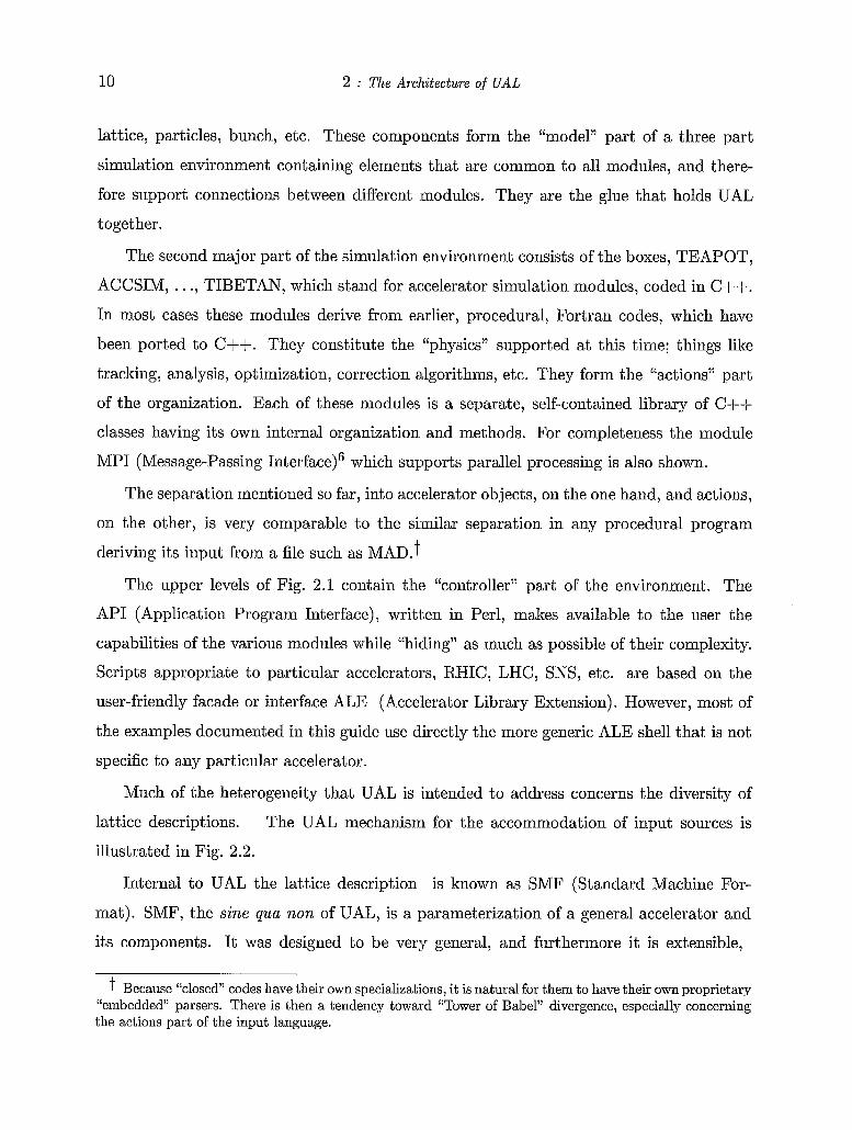
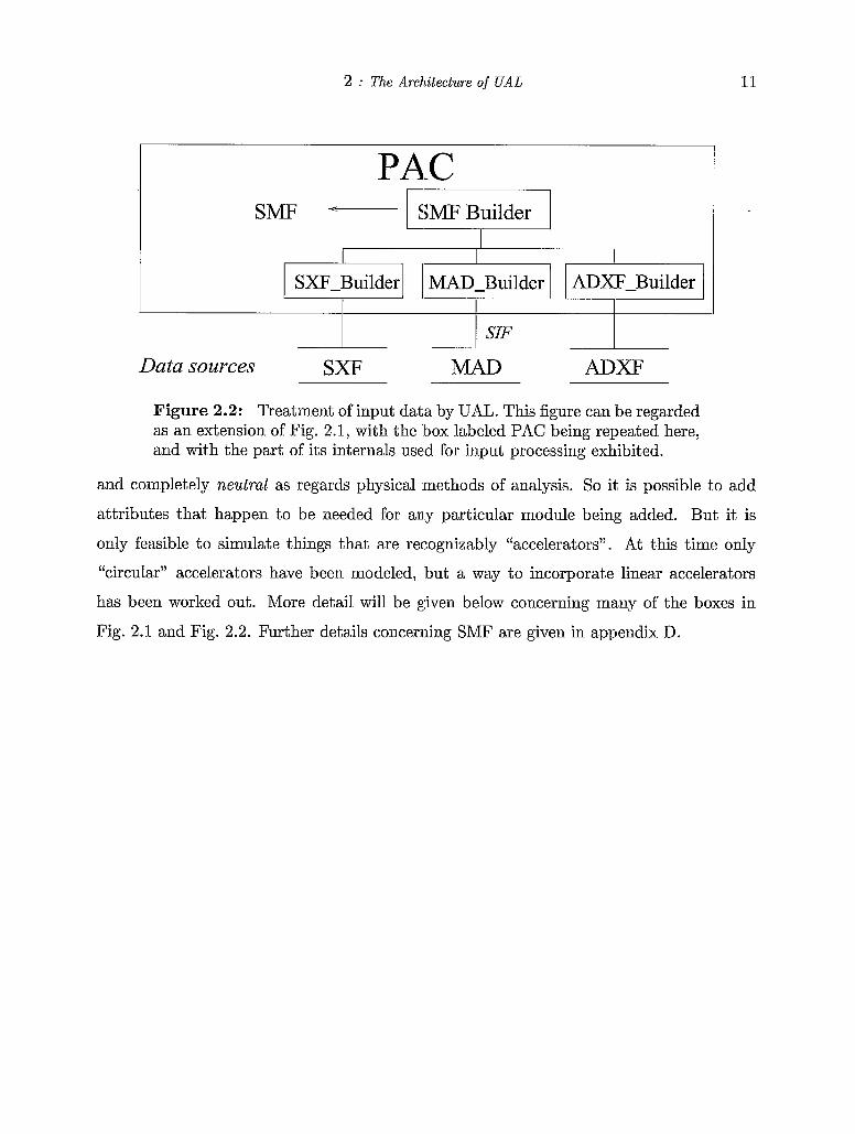
Much of the heterogeneity that UAL is intended to address concerns the diversity of

The UAL mechanism for the accommodation of input sources is lattice descriptions.

illustrated in Fig. 2.2.

Internal to UAL the lattice description is known as SMF (Standard Machine For-

mat). SMF, the sine qua non of UAL, is a parameterization of a general accelerator and

its components. It was designed to be very general, and furthermore it is extensible,

t Because “closed” codes have their own specializations, it is natural for them to have their own proprietary “embedded” parsers. There is then a tendency toward “Tower of Babel” divergence, especially concerning the actions part of the input language.

2 : The Architecture of UAL 11

PAC SMF 1 SMFBuilder I

‘ I I I I SXF-Builder I I MAD-Builder I I ADXF-Builder I “I I

I SIF

Data sources SXF MAD ADXF

Figure 2.2: Treatment of input data by UAL. This figure can be regarded as an extension of Fig. 2.1, with the ‘box labeled PAC being repeated here, and with the part of its internals used for input processing exhibited.

and completely neutrd as regards physical methods of analysis. So it is possible to add

attributes that happen to be needed for any particular module being added. But it is

only feasible to simulate things that are recognizably “accelerators”. At this time only

“circular” accelerators have been modeled, but a way to incorporate linear accelerators

has been worked out. More detail will be given below concerning many of the boxes in

Fig. 2.1 and Fig. 2.2. Further details concerning SMF are given in appendix D.

Chapter 3. Code Checkout and Environment Variables

As part of the object orientation of the code the various modules are referenced by sym-

bolic names. A helpful convention is that these names are consistently related to the names

of the code-containing directories, but these directory names may themselves be expressed

relative to symbolic environment variables. To use the UAL environment it is therefore

absolutely essential for all environment variables to be set correctly. One way of helping

to establish and preserve this state is to set up a dedicated account for a UAL user (called

ualusr in this manual) who performs nothing but UAL calculations and who has estab-

lished appropriate environment variables, most easily by using an appropriately-updated,

code-managed, login script that is part of the distribution. This avoids the unwitting al-

teration of the environment by other programs or shells or initialization routines. In this

manual we assume that ualusr is performing all the set-up, checking out of codes, and

calculations. The UAL user chooses a base directory, for example Nualusr, into which

the UAL simulation(s) is to be installed.

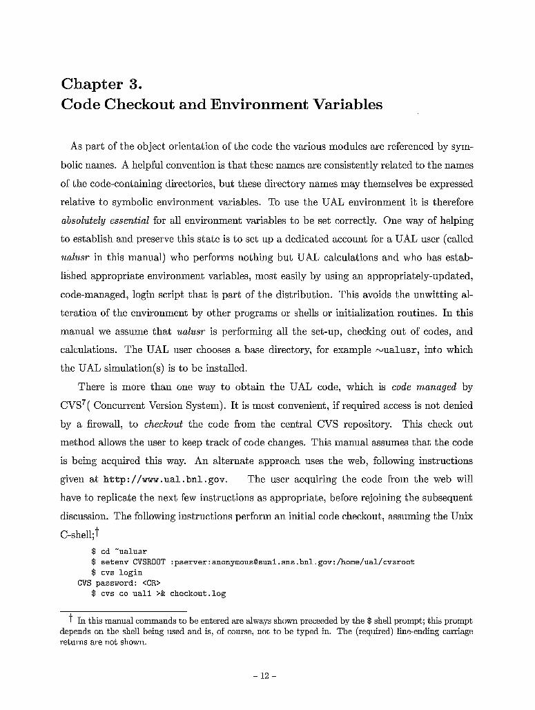
There is more than one way to obtain the UAL code, which is code managed by

CVS7( Concurrent Version System). It is most convenient, if required access is not denied

by a firewall, to checkout the code from the central CVS repository. This check out

method allows the user to keep track of code changes. This manual assumes that the code

is being acquired this way. An alternate approach uses the web, following instructions

given at http://www.ual.bnl.gov. The user acquiring the code from the web will

have to replicate the next few instructions as appropriate, before rejoining the subsequent

discussion. The following instructions perforin an initial code checkout , assuming the Unix

C-shell;t $ cd "ualusr $ setenv CVSROOT :pserver:anonymousQsunl..sns.bnl.gov:/home/ual/cvsroot $ cvs login

CVS password: <CR> $ cvs co ual l >& checkout.log

t In this manual commands to be entered are always shown preceeded by the $ shell prompt; this prompt depends on the shell being used and is, of course, not to be typed in. The (required) line-ending carriage returns are not shown.

- 12 -

3 : Code Checkout and Environment Variables 13

Here anonymousQsun1. sns . bnl . gov : /home/ual/cvsroot represents an anonymous

remote login (followed by user-supplied carriage return as response to the request for CVS

password) to the central CVS code repository applicable at this date-it may change-and

uall is the name of the particular version of the code being checked out. The steps per-

formed in the CVS checkout are logged into checkout. log. The code is extracted to the

subdirectory uall and to its subdirectories, along with supporting files and documentation.

This may take a few minutes.

Before continuing to compile and link i;he codes it is necessary to confirm that all

required environment variables have been set correctly. Appropriate setup scripts and

instructions are included in the code just checked out. An environment variable specifying

the local architecture (preferably Linux) will be set by the appropriate set-up script.*

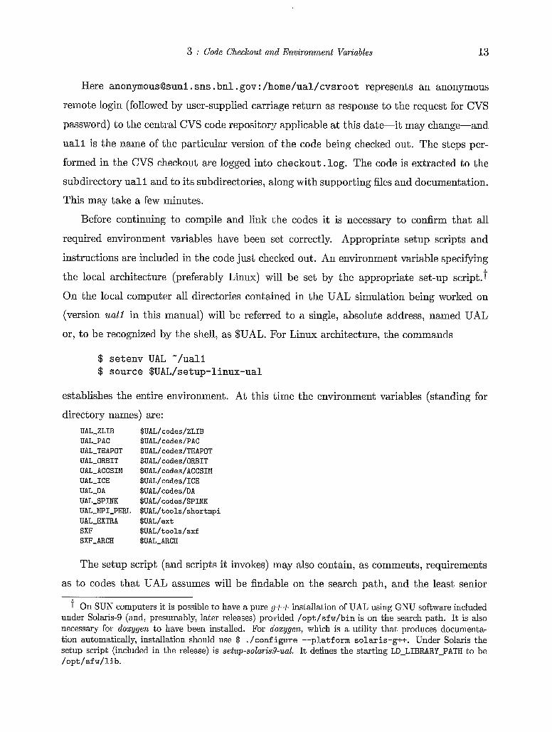
On the local computer all directories contained in the UAL simulation being worked on

(version uall in this manual) will be referred to a single, absolute address, named UAL

or, to be recognized by the shell, as $UAL. For Linux architecture, the commands

$ setenv UAL “/uall $ source $UAL/setup-linux-ual

establishes the entire environment. At this time the environment variables (standing for

directory names) are: UAL-ZLIB $UAL/codes/ZLIB UAL-P AC $UAL/codes/PAC UAL-TEAPOT $UAL/codes/TEAPOT UAL-ORBIT $UAL/codes/ORBIT UAL-ACCSIM $UAL/codes/ACCSIM UAL-ICE $UAL/codes/ICE UAL-DA $UAL/codes/DA UAL-SPINK $UAL/codes/SPINK UAL-MPI-PERL $UAL/tools/shortmpi UAL-EXTRA $UAL/ext SXF $UAL/tools/sxf SXF- ARCH $UAL-ARCH

The setup script (and scripts it invokes) may also contain, as comments, requirements

as to codes that UAL assumes will be finda,ble on the search path, and the least senior

On SUN computers it is possible to have a pure g++ installation of UAL using GNU software included under Solaris-9 (and, presumably, later releases) provided /opt/sfw/bin is on the search path. It is also necessary for doxygen to have been installed. For aloxygen, which is a utility that produces documenta- tion automatically, installation should use $ . /configure --platform solaris-g++. Under Solaris the setup script (included in the release) is setup-solaris:9-ual. It defines the starting LD-LIBRARY-PATH to be /opt/sf w/lib.

14 3 : Code Checkout and Environment Variables

version number that has been tested to be satisfactory. (An up-to-date Linux release,

such as Red Hat 7.3 or later, has essentially all required code.) Detailed specification

of required codes are given at h t t p : //www . ual . bnl . gov/vl/download. htm, along with

brief installation instructions. In a few cases public domain code may be included with

the UAL code checkout and build.

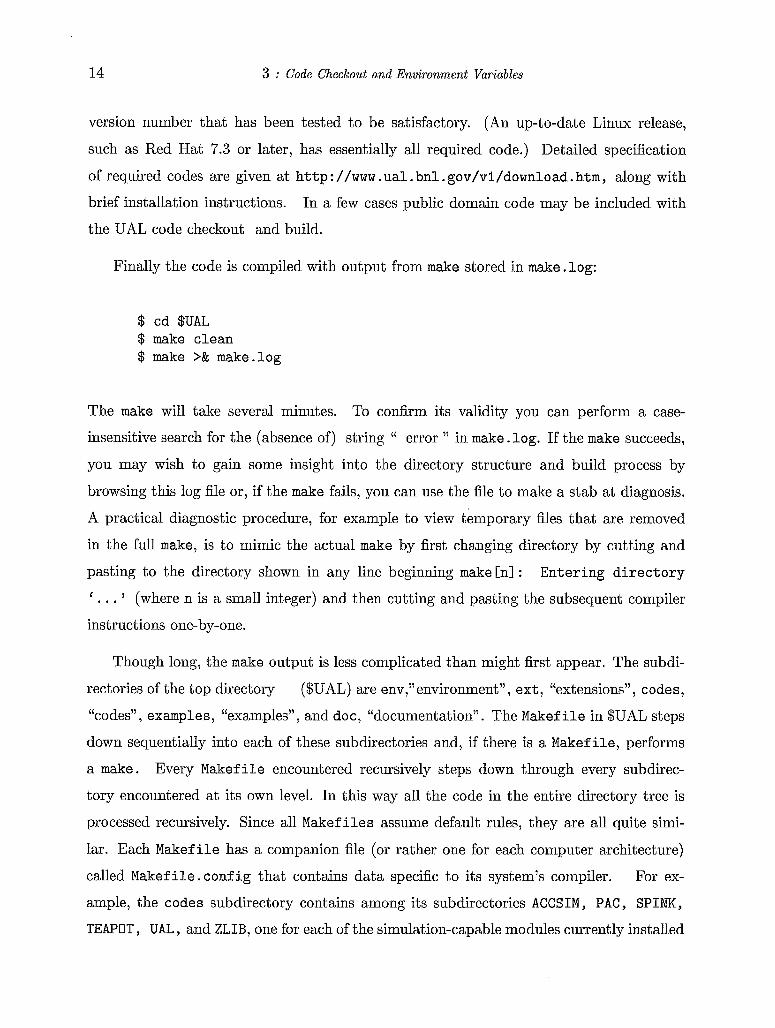
Finally the code is compiled with output from make stored in make. log:

$ cd $UAL $ make clean $ make >& make-log

The make will take several minutes. To confirm its validity you can perform a case-

insensitive search for the (absence of) string “ error ” in make. log. If the make succeeds,

you may wish to gain some insight into the directory structure and build process by

browsing this log file or, if the make fails, yoii can use the file to make a stab at diagnosis.

A practical diagnostic procedure, for example to view temporary files that are removed

in the full make, is to mimic the actual make by first changing directory by cutting and

pasting to the directory shown in any line beginning make Cnl : Entering d i rec tory

I . . . ’ (where n is a small integer) and then cutting and pasting the subsequent compiler

instructions one-by-one.

Though long, the make output is less complicated than might first appear. The subdi-

rectories of the top directory ($UAL) are env,”environment”, ext, “extensions”, codes,

“codes”, examples, “examples”, and doc, “dixumentation”. The Makef i l e in $UAL steps

down sequentially into each of these subdirectories and, if there is a Makefile, performs

a make. Every Makef i l e encountered recursively steps down through every subdirec-

tory encountered at its own level. In this way all the code in the entire directory tree is

processed recursively. Since all Makefiles assume default rules, they are all quite simi-

lar. Each Makefile has a companion file (or rather one for each computer architecture)

called Makefile.config that contains data specific to its system’s compiler. For ex-

ample, the codes subdirectory contains among its subdirectories ACCSIM PAC, SPINK,

TEAPOT, UAL and ZLIB, one for each of the simulation-capable modules currently installed

3 : Code Checkout an.d Environment Variables 15

in UAL.t The Makefile.config file specific to ACCSIM (running under Linux architec-

ture) is $UAL-ACCSIM/conf ig/linux/Makef ile . conf ig. Other configuration file names

are constructed by making obvious transcriptions in this pathname. The Makef ile . conf ig file accesses its own pathname using its mat'ching environment variable.

The general purposes for the codes in the various directories can largely by guessed

from the directory names (which match the corresponding environmental variables given

above.) Details will emerge in the sequel. The user wishing to browse a file referred to in a

script can locate the file by using these environment variables. For example, note how the

full pathname of the configuration file mentioned in the previous paragraph follows from

$UAL-ACCSIM. Paths to C++ and Per1 code specific to ACCSIM are derived similarly.

UAL also supports multiprocessor applications. Logically the instructions for installa-

tion of the environment supporting these applications would be contained in a continuation

of this section. But, because most users will use this environment only later, if at all, these

instructions are deferred until Chapter 7.

t The relationships among modules ACCSIM, PAC, SPINK, TEAPOT, UAL , and ZLIB is actually a bit more complicated than is suggested by this sentence.

Chapter 4. Perl as Interface Language

A user starting to use a specific accelerator simulation code probably expects to begin

by studying its proprietary input language, in order to learn how to use the language to

define the lattice and to specify the desired calculations. UAL handles lattice description

similarly, in the form of conventional ASCII files, either MAD (the lattice description part

only)? or SXF or ADXF. But there is no proprietary UAL command language. Instead,

the simulation to be performed is specified by the statements of a Perl script. Standard

references are Schwartz’ and Wall et the latter of which is the definitive Perl reference

which, however, makes it fairly dense reading;. For exploiting the “object oriented” aspects

Conway,lo is appropriate. The best reference dedicated to interfacing Perl with compiled

languages, especially C and C++ is by Jentness and Cozens.” The m a n pages perlxs,

per lxs tu t , and xsubpp are useful for the same purpose, as is Srinivasan.12

Detailed documentation can be obtained by using $ m a n per1 which mainly provides

a list of all the Perl m a n files. After identifying per lvar as the most promising source of

information concerning Perl variables, one uses $ m a n perlvar.

Fortunately, it is unnecessary for the beginning user (or the advanced user either) to

understand how Perl performs its control function. But the apparent effect of this control

is that everything “appears to be Perl” even if the code being executed is some other

language. For this reason the UAL user has t o become at least somewhat conversant

with Perl. Though this may cause some initial difficulty, it should soon have become

comforting to be working with a highly-supported modern computer language rather than

with a homemade, perhaps ambiguous, special-purpose input language. This power is

perhaps most impressive when it comes to controlling multiprocessor applications using

MPI.

5- Because the MAD input languages includes both lattice description and calculation directives it is useful to have a term that describes just the lattice diescription pa.rt. For this purpose we will use the term SIF (Standard Input Format) in spite of the fact that the MAD format has evolved substantially from its correspondance with the original SIF spe~ification.~‘ So, in this manual the term SIF is to be interpreted as the lattice description part of MAD, version 8.

- lfi -

4.1.1 : Perl as Interface Language: Elementary P e d : Variables and s tatements 17

4.1. Elementary Perl

This section contains a short description of the Perl language. It is too brief even t be

called a “tutorial” but is intended to at least mention every language ingredient appearing

in the examples appearing in subsequent sections. In the interest of making the UAL/Perl

interface as “clean” as possible, only a restricted set of valid Perl syntax is actually used

by UAL. In some cases usage that is deprecated (or at least not used) by UAL even though

used in other Perl sources. When this situation arises this guide shows the (UAL)-preferred

usage in the body of the text and includes alternative usage or clarification in a footnote.

Perl is a “scripting language’’ that can. be used either as a standalone procedural

programming language (such as C or Fortran) or as an object oriented languages (such as

C++). Its syntax is much like C, but with features drawn from other languages, especially

AWK. By practicing with Perl to perform si:mple Fortran-like calculations, the reader can

acquire a useful introduction to the language (and then the courage to later insert minor

postprocessing manipulations into the example scripts).

4.1.1. Variables and statements

Perl statements terminate with semi-colons ; and a single line is allowed to have more

than one statement. Comments begin with #I and continue to the end of the line.

The most visually striking notational aspect of Perl is that (single value) variable names

begin with $ signs, as in $variablename. (So a C program with $ signs inserted in front

of every variable name has a chance of being a valid Perl program.) Such a variable, called

a scalar in Perl jargon, can stand for a real number or for a string or for a reference to

something else, without the need for declaration as to which is intended. Some examples:

$aScalar=42; # an integer $aScalar=3.14; # a real number $aScalar=”perl” ; # a string

Perl implicitly interprets and converts $aScalar as it considers appropriate. Two multiple

data types are also supported: arrays and hashes, both one-dimensional.

18 4.1.1 : Perl as Interface Language: Elementary Perl: Variables and statements

Array. An array variable is a list of scalars that have been grouped together so they can

be manipulated as a single Perl variable. Array names are prefixed with the @ symbol, and

an array is defined, that is, entered literally, by a comma-separated listt 8 as in

@languages= ("perl" "f ortran" Itc++") ;

These scalars will commonly be homogeneoiis (as in this example) but they need not be.

For example some entries may point to othler things-that is the way more complicated

structures, such as two dimensional arrays, c,an be established. Array elements are indexed

by their sequential order (starting with 0, a8 in C). A particular value from the array is denoted by using its index enclosed in square brackets; so T

my $f irst-language=$languages [Ol ; $languages [Ol ="per1 6" ;

# assigns "perl" to $f irst-language # replaces "perl" by "per1 6"

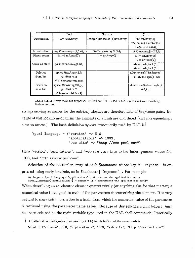
For understanding the UAL architecture it is useful to compare the support for one

dimensional, sequential data types in Perl, Cff, and Fortran. This is done in Table 4.1.1.

In C++ there are three one dimensional t:ypes: (fixed length) array, (variable length)

standard vector template and list. With seqyential elements, random access can be a very

fast operation. Some types are "dynamic" (meaning the number of elements can change)

as examples in the table show. In Perl there is only one urray type but, even so, all of the

C++ manipulations (and then some) are supported. But this comes at the cost of slower

access, because the structure is implemented by doubly-linked list. This (along with the

compiler/interpreter issue) is the sort of spleed/convenience compromise that drives the

use of Cff for compute bound computation and Perl for interface implementation.

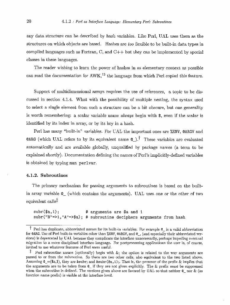
Hashes (also known as associative arrays, or dictionaries, or two-column tables) have

names beginning with % as in %hashname. Like lists, hashes contain multiple scalars, but

these scalars are referenced not by sequential integers but by symbolic k e y s (which are

t Perl documentation distinguishes between the term array and the term list even though both consist of sequences of scalars. This distinction should probably be ignored. The literal representation of a list may include an array or hash but, if so, the elements of the array are simply "flattened" (broken out and strung together, comma-separated) into the enclosing list-t he original grouping is forgotten.

In Perl documentation the phrase list context, is Idistinguished from the other possibility, namely scalar contezt. Here "context" means the type of the variable a function is expected to return. This is a kind of overloading in which a function & f m c can return either a scalar or list depending on context. For example $x = &func expects a scalar and @x = &func expects a list. This distinction should probably be ignored during casual browsing of code examples, but it may have to be understood when writing new code.

fT The scope-defining word my will be explained shortly.

4.1.1 : Perl as Interface Language: Elementary Perl: Variables and statements

Declaration Perl Fortran C++

my QanArray; Integer ,dimension(4) : :anArray int anArray[4]; vect or(int) aVect or (4) ;

anArray/2,3,4/ Direct access $il=$anArray[2]; i l = anArray(3)

list(int) aList(4); int QanArrayl=2,3,4;

i l = anArray[2];

19

4rray as stack

Deletion from list

Insertion into list

strings serving as names for the entries.) Hashes are therefore lists of key,/vuZue pairs. Be-

cause of this lookup mechanism the elements of a hash are unordered (and correspondingly

slow to access.) The hash definition syntax customarily used by UAL ist

i l = aVector[2]; push QanArray,(5,6); aList.push-back(5);

aList .push-back( 6) ; splice @anArray,2,3; aList.erase(aList .begin()

+2, aList . begin() +5);

aList .insert (aList . begin()

# offset is 2 # 3 elements removed

splice QanArray,2,0, (9);

# inserted list is (9) # offset is 2 +2,9 1;

%perl-language = ("version" => 5,. 6, "applications" => 1003, "web site" => "http: //www .perl. corn")

Here "version", "applications", and "web site", are keys to the heterogeneous va,ies 5.6,

1003, and "http://www.perl.com" . Selection of the particular entry of hash %hashname whose key is "keyname" is ex-

pressed using curly brackets, as in $hashname{" keyname" }. For example: my $apps = $perl-language{"applications"); # returns the application entry $perl-1anguageC"applications") = $apps + I; # increments the applications entry

When describing an accelerator element quantitatively (or anything else for that matter) a

numerical value is assigned to each of the parameters characterizing the element. It is very

natural to store this information in a hash, from which the numerical value of the parameter

is retrieved using the parameter name as key. Because of this self-describing feature, hush

has been selected as the main variable type used in the UAL shell commands. Practically

An alternative Perl synta.x (not used by UAL) fo'r definition of the same hash is

%hash = ("vers ion" , 5.6, " a p p l i c a t i o n s " , 1003, "web s i te" , "http://www.perl. corn")

20 4.1.2 : Perl as Interface Languiage: Elementary Perl: Subroutines

any data structure can be described by hash variables. Like Perl, UAL uses them as the

structures on which objects are based. Hashes are too flexible to be built-in data types in

compiled languages such as Fortran, C, and IC++ but they can be implemented by special

classes in these languages.

The reader wishing to learn the power ad hashes in as elementary context as possible

can read the documentation for AWK,13 the language from which Perl copied this feature.

Support of multidimensional arrays requires the use of references, a topic to be dis-

cussed in section 4.1.4. What with the possibility of multiple nesting, the syntax used

to select a single element from such a structure can be a bit obscure, but one generality

is worth remembering: a scalar variable name always begin with $, even if the scalar is

identified by its index in array, or by its key in a hash.

Perl has many "built-in" variables. For UAL the important ones are %ENV, @ARGV and

@ARG (which UAL refers to by its equivalent name @-).t These variables are evaluated

automatically and are available globally, unqualified by package names (a term to be

explained shortly). Documentation defining the names of Perl's implicitly-defined variables

is obtained by typing man perlvar.

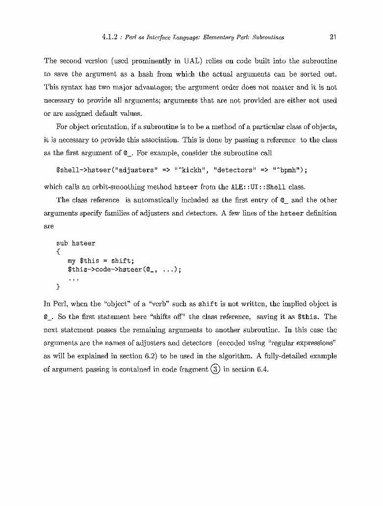
4.1.2. Subroutines

The primary mechanism for passing arguments to subroutines is based on the built-

in array variable @- (which contains the arguments). UAL uses one or the other of two

equivalent c a d

subr($a, 1) ; # arguments a r e $a and 1 subr("B"=>l, "A"=>$a) ; # subroutine deciphers arguments f r o m hash

t Perl has duplicate, abbreviated names for its built-in variables. For example 0- is a valid abbreviation for 0ARG. Use of Perl built-in variables other than %EN\[, QARGV, and 0-, (and especially their abbreviated ver- sions) is deprecated by UAL because they complicate the interface unnecessarily, perhaps impeding eventual migration to a more disciplined interface language. For postprocessing applications the user is, of course, invited to use whatever features of Perl seem useful.

Perl subroutine names (optionally) begin with &; the option is related to the way arguments are passed to or from the subroutine. So there are two other calls, also equivalent to the two listed above. Assuming @-=($a,l), they are &subr; and &subr ($a, 1);. That is, the presence of the prefix & implies that the arguments are to be taken from 0- if they are not given explicitly. The & prefix must be suppressed when the subroutine is defined. The versions given above are favored by UAL so that neither 0- nor & (as function name prefix) is visible at, the interface level.

4.1.2 : Perl as Interface Language: Elementary Perl: Subroutines 21

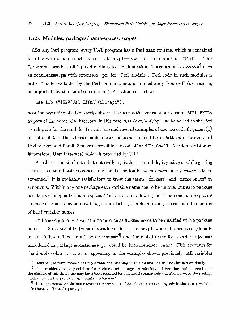
The second version (used prominently in UAL) relies on code built into the subroutine

to save the argument as a hash from which the actual arguments can be sorted out.

This syntax has two major advantages; the argument order does not matter and it is not

necessary to provide all arguments; argumeints that are not provided are either not used

or are assigned default values.

For object orientation, if a subroutine is to be a method of a particular class of objects,

it is necessary to provide this association. This is done by passing a reference to the class

as the first argument of @-. For example, consider the subroutine call

$shell->hsteer(t ladjusters” => “^ki.ckh”, ”detectors” => “^bpmh”) ;

which calls an orbit-smoothing method hsteer from the ALE: : U I : : Shell class.

The class reference is automatically included as the first entry of @- and the other

arguments specify families of adjusters and aietectors. A few lines of the hsteer definition

are

sub hsteer

my $this = shift; $this->code->hsteer (a_, . . . ; ...

In Perl, when the “object” of a “verb” such as shift is not written, the implied object is

@-. So the first statement here “shifts off” the class reference, saving it as $this. The

next statement passes the remaining arguments to another subroutine. In this case the

arguments are the names of adjusters and detectors (encoded using “regular expressions”

as will be explained in section 6.2) to be used in the algorithm. A fully-detailed example

of argument passing is contained in code fragment @ in section 6.4.

22 4.1.3 : Perl as Interface Language: Elementary Perl: Modules, packages/name-spaces, scopes

4.1.3. Modules, packages/name-spaces, scopes

Like any Perl program, every UAL progrxm has a Perl main routine, which is contained

in a file with a name such as simulation.pl-extension . p l stands for “Perl”. This

“program” provides all input directions to t,he simulation. There are also modulest such

as modulename.pm with extension .pm, for “Perl module”. Perl code in such modules is

either “made available” by the Perl command use, or immediately “sourced” (i.e. read in,

or imported) by the require command. A statement such as

us e l i b ( ‘I $ENV(UAL-EXTRA)/ ALE/api I ’ ) ;

near the beginning of a UAL script directs Ped to use the environment variable $UAL-EXTRA

as part of the name of a directory, in this case $UAL/ext/ALE/api, to be added to the Perl

search path for the module. For this line and several examples of use see code fragment @ in section 6.2. In those lines of code line #5 makes accessible F i l e : :Path from the standard

Perl release, and line #I2 makes accessible th.e code Ale : : UI : : Shel l (Accelerator Library

Extensions, User Interface) which is provided by UAL.

Another term, similar to, but not really equivalent to module, is package; while getting

started a certain fuzziness concerning the distinction between module and package is to be

expected.$ It is probably satisfactory to treat the terms “package” and “name space’’ as

synonyms. Within any one package each variable name has to be unique, but each package

has its own independent name space. The puirpose of allowing more than one name space is

to make it easier to avoid unwitting name claishes, thereby allowing the casual introduction

of brief variable names.

To be used globally a variable name such ,as $vname needs to be qualified with a package

name. So a variable $vname introduced in mainprog.pl would be accessed globally

by its “fully-qualified name” $main: :vname‘i and the global name for a variable $vname

introduced in package modulename. pm would. be $modulename : : vname. This accounts for

the double colon : : notation appearing in the examples shown previously. All variables

t Beware: the term module has more than one meaning in this manual, as will be cla.l-ified gradually. It is considered to be good form for modules and packages to coincide, but Perl does not enforce this-

the absence of this discipline may have been required for backward compatibility as Perl imposed the package mechanism on the pre-existing module mechanism?

Just one exception: the name $ m a i n : :vname can he abbreviated to $ : : vname, only in the case of variable introduced in the m a i n package.

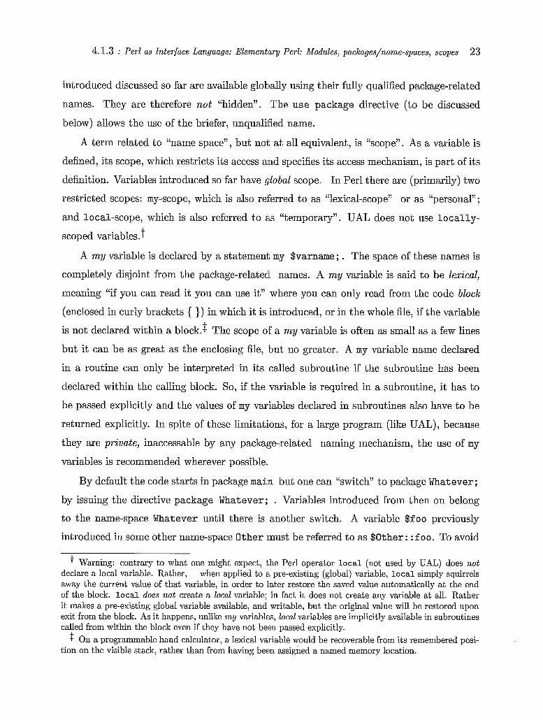
4.1.3 : Perl as Interface Language: E l e m e n t w y Perl: Modules, packages/name-spaces, scopes 23

introduced discussed so far are available globlally using their fully qualified package-related

names. They are therefore not “hidden”. The use package directive (to be discussed

below) allows the use of the briefer, unqualified name.

A term related to “name space”, but not; at all equivalent, is “scope”. As a variable is

defined, its scope, which restricts its access aiad specifies its access mechanism, is part of its

definition. Variables introduced so far have global scope. In Perl there are (primarily) two

restricted scopes: my-scope, which is also referred to as “lexical-scope” or as “personal” ;

and local-scope, which is also referred to ats “temporary”. UAL does not use locally-

scoped variables.?

A my variable is declared by a statement; my $varname; . The space of these names is

completely disjoint from the package-related! names. A my variable is said to be lexical,

meaning “if you can read it you can use it” where you can only read from the code block

(enclosed in curly brackets { }) in which it is introduced, or in the whole file, if the variable

is not declared within a block.$ The scope OF a my variable is often as small as a few lines

but it can be as great as the enclosing file, ‘but no greater. A my variable name declared

in a routine can only be interpreted in its called subroutine if the subroutine has been

declared within the calling block. So, if the variable is required in a subroutine, it has to

be passed explicitly and the values of my variables declared in subroutines also have to be

returned explicitly. In spite of these limitations, for a large program (like UAL), because

they are private, inaccessable by any package-related naming mechanism, the use of my

variables is recommended wherever possible.

By default the code starts in package main but one can “switch” to package Whatever;

by issuing the directive package Whatever; . Variables introduced from then on belong

to the name-space Whatever until there is another switch. A variable $foo previously

introduced in some other name-space Other must be referred to as $Other: : foo . To avoid

t Warning: contrary to what one might expect, the Perl operator l o c a l (not used by UAL) does n o t declare a local variable. Rather, when applied to at pre-existing (global) variable, l o c a l simply squirrels away the current value of that variable, in order to later restore the saved value automatically at the end of the block. l oca l does n o t create a local variable; in fact it does not create any variable at all. Rather it makes a pre-existing global variable available, and writable, but the original value will be restored upon exit from the block. As it happens, unlike m y variables, local variables are implicitly available in subroutines called from within the block even if they have not been passed explicitly.

On a programmable hand calculator, a lexical variable would be recoverable from its remembered posi- tion on the visible stack, rather than from having been assigned a named memory location.

24 4.1.4 : Perl as Interface Language: Elementary Perl: References

the need for qualification one can switch back and forth between packages while remaining

in the same file. For example, after directive package Other; the same variable could

be referenced just as $foo. It is probably best to avoid using this freedom however, as it

can be confusing, and hence prone to error. Because of possible ambiguity, Perl provides

the option of issuing the use strict; directive. After this directive all package variables

have to be fully qualified. For safety use strict; appears at the beginning of most UAL

modules. When making ad hoc changes to the code one may be tempted to introduce

a global variable, such as $myvariable, without declaring it to be a my. In the use

strict regime this would trigger the error message “Global symbol ‘ ‘ $myvariable j j

requires explicit package name”. Naming the variable $: :myvariable avoids this

error by explicitly assigning the global variable to the main package. Better yet is to avoid

introducing global variables for fear they will be forgotten and later cause trouble.

4.1.4. References

This sub-section is very much a continuation of subsection 4.1.1 as it expands the discus-

sion of variables. For elementary use of Perl as a procedural language, the new method of

specifying a variable might seem to be little ‘more than an optional syntax, which the user

could simply decline to employ. But for object-oriented application of Perl the notion of

reference is essential. UAL exploits the reference mechanism to allow user scripts to ig-

nore scope issues when addressing object variables and methods. When addressing object

variables and methods the UAL-provided shell uses references to allow the user to ignore

scope-of-variable considerations.

Within a Perl program a single scalar d.atum has at least three sorts of identity. It

has its actual value, say 3.14, it has its variable name, say $pi, and it has its location in

memory. For elementary purposes the user is shielded from the need to be aware of the

third of these identities. But to support object-orientation it turns out to be necessary

to name this location (thereby increasing th.e number of identities by one.) The storage

location is symbolized by \$pi, which is known as a reference, or sometimes as a hard

reference (in which case $pi is itself referred t,o as a soft reference.) The possible references

are

$rs = \$s; # reference to scalar $s

4.1.4 : Perl as Interface Language: Elementary P e r k References 25

$ra = \@a; $rh = \%h; $rf = \&f ;

# reference to array @a # reference to hash %kt # reference to subroutine &f

One can start to understand the role of references by considering an alternate Perl

notation for defining an array (frequently used in UAL but not previously mentioned in

this manual). An example of this syntax tak:en from code fragment @ in section 6.2 is

my $qSigB = C0.0, 0.0, -2.46, -0.76, -0.63, 0.00, 0.02, -0.631;

This defines an array (of multipole coefficients in this case) having the values shown. But

the name of the array is not $qSigB; rather $qSigB is a reference or pointer to the location

of the array which, in this case, is said to be “anonymous” or ‘(reference-identified”.t

This shows that “references” can identify multi-element structures. (In fact, they enable

dynamic memory allocation which is their main virtue.) When an array is to be populated

one element at a time it is convenient to start with an empty array using my $rarray =

[I;. To retrieve the data pointed to by referfence $rp it is necessary to “dereference” the

reference, by $$rp or by @$rp or by %$rp depending on whether it is a scalar, an array,

or a hash being retrieved. Without this distinguishing notation Perl would not be able to

determine the extent of the data to be retrieved.

There is a short-cut notation for selecting individual elements of reference-identified

arrays without the need for explicit dereferencing. An element can be selected from the

array defined two paragraphs back by $qSigB-> C21 which, in this case, would return the

value -2.46.

The notation for creating an anonymous hash uses braces instead of square brackets.

For example, an anonymous two-element hash is created and referenced by

The short-cut notation for selecting an element from such a reference-identified hash is

$rhash->“{k2}” which, in this case, would p:roduce “v2”. When a hash is to be populated

T One has to tolerate the inelegant syntax of Perl which (like C) fails to distinguish between a scalar variable name and a reference. Hence, for example, the statement $p=\$q makes sense; it assigns reference \$q to reference $p, both of which are therefore both x a l a r s and references. Perhaps this absence of explicit syntax for references is the reason that they are not referred to as pointers in Perl documentation?

26 4.1.5 : Perl as Interface Language:. Elementary Perl: Regular expressions

one element at a time it is convenient to start with an empty hash using my $rhash =

0; . To support object orientation there needs to be a mechanism for representing structures

more complicated than arrays or hashes. References can be used for this purpose. Without

going into detail, the Perl keyword bless associates a reference with the particular package

that is capable of digesting the contents of the structure that is referenced. An example is

given in the block of code below @ in section 6.2.

4.1.5. Regular expressions

It is often necessary to perform some action on only a subset of the elements in an

accelerator. Some examples of actions a simulation program performs on all elements of

such “families” are:

0 element subdivision 0 retrieval of parameter values 0 update of parameter values 0 establishment of detector families (such i3S BPM’s) 0 establishment of adjuster families (such i$S kickers) 0 print out of lattice parameters

In some simulation codes, provision for specifying such a family of elements is built into

the lattice description file by a flag assigned to elements in the particular family and to no

other elements. For example in SIF (Standard Input Format) the type=A flag is assigned

to all members of family A. In some cases such a family corresponds to actual hardware in

the accelerator (magnets on a single bus for example) but usually assignment to families is

best left to the tuning algorithms of the control system. In UAL philosophy it is therefore

inappropriate to burden the lattice description with “hard-wired” family assignment.

In UAL a family is specified by the “explicit” listing of the names of all the elements

that, for some immediate purpose, are useful1.y regarded as belonging to the same set. The

word “explicit” is placed in quotation mark:s because the so-called “regular expression”

mechanism is used to specify families and the element selection by regular expression

may not look all that explicit to a reader unfamiliar with regular expressions. A regular

expression is a highly-abbreviated shorthand ascii string that has been tailored (consistent

with well-defined rules) to match the names of all elements in a family and to fail to match

4.1.6 : Perl as Interface Language: Elementary Perk Printing out results 27

any other element name (of elements present in the ring.) By this time regular expressions

have come to be a powerful and indispensable part of most computer languages. In this

manual the mechanism will be clarified mainly by examples.

The consistent naming of lattice elements has always been an important consideration

in writing lattice description files. It is important for conveying the intended purposes for

the various elements in the original design ;and eventually every element needs a unique

“site-wide” name by which elements in external models are associated with elements in

the tunnel. The UAL mechanism for selecting families of elements makes naming-scheme

discipline all the more important. It would be convenient for all elements of a family to

have the same name; for example, all quad lcorrectors on a harmonic corrector bus could

have the name QDH. But this is too much to ask in general as it fails to allow for “overlap”

of the different sorts of family that need to bte defined. The regular expression mechanism

permits the efficient selection of elements even in the face of such type overlap, but the

mechanism is succinct only if a consistent naming scheme is carefully respected. As a

last resort a family can, in fact, be defined within UAL as a really explicit list of all of

its elements. An example of this will be given below. When first encountered the regular

expression approach may seem awkward to the user but it is a “feature”, not a “bug”, as

it solves a really hard simulation problem-how to specify families without the need for

ad hoc tampering with the lattice description language? Such tampering frequently leads

to errors and always erodes portability.

An example of the use of regular expressions for selecting a set of lattice elements is

code fragment @ in section 6.2. Because this example uses an actual SNS lattice file @ , further explanation of regular expressions will1 continue in connection with explaining that

code. The reader is encouraged to jump to that explanation and then return.

4.1.6. Printing out results

There are various mechanisms for outputting results. They can be printed to standard

output or to a file, either from Per1 or from C++. It is conventional for the Perl scripts

of UAL to issue progress reports announcing the commencement of major steps in the

simulation. These progress reports are generisted by lines like

p r i n t ”Create the ALE: :UI: :Shell instance (”, --LINE--, ‘l)\n”; ##E

28 4.1.6 : Perl as Interface Language: Elementary Perl: Printing out results

which is line #15 in listing @ in section 6.2 (the example script to be documented first

in this manual.) Incidentally this line shows how Perl-specific information (in this case

- LINE-, the line number in the script) can be output. Usually it will be a string or a

Perl variable, such as $aScalar, or a Perl built-in, such as $- that is output in this way.

(The symbol L I N E - is peculiar-looking blecause it relates to the script as a file rather

than to its execution as a Perl program.) (One convenience is the ability to interpolate

special variables into strings, as is illustrated by the following fragment of Perl code:

my $name = t t t e s t ' t ; p r in t "My name i s $nametl,"\n"; p r in t 'My name i s $name ,"\n";

which produces output

My name i s t e s t My name i s $name

-with double quotes the value of the variable $name is interpolated, with single quotes it is

not. To get printout under controlled-format the command pr in t f (which is equivalent to

p r i n t sp r in t f ) has to be used. These are identical to C-commands of the same names.

The opening and closing of files proceeds as in any other computer language. To write

from Perl to a file the file must first be opened with a statement such as?

open(OUTPUT, '>output/dat '> I I die 'Cannot create f i l e tloutput/dat". ' ;

which fails with an error message if the file cannot be created (for example because the

directory output does not exist or is not writeable.) Note that the access mode (read, write,

or append) begins the string containing the filename. Perl refers to the name "OUTPUT"

as a file handle. Variables $x and $y can then be written to the file with defined format

using a command such as

pr in t f OUTPUT ("%6.3f %6.3f I f y $x, $y>;

An example of a file handle being represented by a string with an interpolated variable is

line #I91 in code fragment @ of section 6.2. Note also the use of ".') (dot) as the string

t The symbol I I stands for or in Perl. As it happens o r can be used instead of I I in this context and is even preferred style, according to Perl documentation, because it has lower precedence (i.e. reduces the need for placing adjacent elements in brackets). The symbol for and is & or and.

4.1.7 : Perl as Interface Language: Elementary Perl: Issuing system commands 29

concatenating operator when filename . /ont / tes t / f o r t .8 is formed from ‘ ‘ . /out/

. $job-name . ‘ ‘ / f o r t .8 ’ ’. (The string ‘ ‘test’ ’ had been assigned to variable

$job-name earlier in line #4.) An example of formatted output appears a few lines later

(line #198) in the same code fragment.

A more fully spelled out example of saving results, which exhibits the output of lattice

parameters at specified lattice locations is given in section 6.3. Other than these brief

comments, the formatting of output is too complicated for useful discussion in this manual.

There are many samples to mimic in the examples.

Finally it can be mentioned that print t;tatements can also be introduced into Cff

code, for example for debugging purposes, or to obtain ad hoc access to an otherwise

inaccessable variable value. An example line of code is

cout << “desired chromaticit ies a r e It << mux << It << muy << ‘ ‘ \ny ;

which sends output to standard out. Many other examples are available in the UAL source

code. Of course the Cff code has to be recompiled for any added lines like this to effective.

4.1.7. Issuing system commands

There is another benefit coming from the use of a scripting language to control the

simulation-it is possible to issue system commands from within the script. An example

of this is code fragment 0 in section 6.2. The relevant lines of code are

my $job-name = “ t e s t ” ; use F i l e : :Path; &path( [ ‘ I . /out/” . $ j ob-name] 1 0755) ;

Here the variable $job-name contains a string ‘ ‘ tes ty that is concatenated (the dot

(.) operator) with the string ‘ ‘ . /out/ of a

directory which will be written to in a later command. The mkpath command (from

within the F i l e : :Path module) establishes the directory, with permissions specified by

the final argument.t Detailed documentation for F i le : :Path and mkpath (and all other

Perl routines) can be obtained from Perl documentation; for example with $ man perlmod

and $ man perlmodlib.

to form the pathname ‘ ‘ . /ou t / tes t

t If the mkpath command had not been included Perl would have issued the error message “can’t create ./out/test,/log at /export/home/ualusr/development~uall/ext/ALE/api/ALE/UI/Shell.pm line 32”, which is the first occurence of writing to that directory.

30 4.3 : P e d as Interface Language: Per1 extensions

4.2. UAL file directory structure and packages

Because there is a near one-to-one correspondance between packages and files there can

be (within UAL) a standard relation between filenames and package names. Examples of

this convention can be observed by the following instructions, which are followed by the

resulting output:

$ cd $UAL-ACCSIM $ find . -name ’*.pm’ -print I xargs grep “package Accsim”

./api/Accsim/Bunch.pm:package Accsim::Bunch;

./api/Accsim/Facade.pm:package Acc:sim::Facade;

./api/Accsim/Plot.pm:package Accsim::Plot;

./api/Accsim.pm:package Accsim;

./config/linux/Accsim/MakeMaker.pm.:package Accsim::MakeMaker;

./config/sun-gcc/Accsim/MakeMaker.pm:package Accsim::MakeMaker;

Note that package Accsim resides in file $UAL--ACCSIM and “sub-packages”t Accsim: :Bunch,

Accsim: :Facade, and Accsim: :Plot are in correspondingly-named directories. (Note also

that the Unix command used above can be modified to

$ find . -name ’*.someextension’ -print I xargs grep ”some text“

to search for “some text” in all files having extension “someextension”. Most of the filename

extensions appearing within the UAL environment are spelled out in Appendix B.2.)

4.3. Perl extensions

Even though all compute-bound UAL processing takes place using Cff code (archived

into libraries) overall control of any simulation is managed by Perl code. The codes required

to support calling C++ routines from Perl are known as P e d extensions. (The converse

operation, embedding Perl within C++, does not occur in UAL.) All data structures used

within the Cff code are declared in .h or .hh header files. Only some of the variables

declared in these files are used for input to or output from the C++ routines. But the

structures that are used as input or 0utpu.t need to be unambiguously related to the

corresponding structures within the Perl program. Apart from enabling the calling of

The reason “sub-packages’’ is in quotation marks is that, in Perl, this package naming convention is a bit artificial. It suggests that there is some kind of inheritance established automatically from, say, package Accsim to, say, package Accsim: :Bunch. In fact, if such inheritance is required, the programmer would have to set it up using the @ISA array. The packaging just restricts variable names.

4.3 : P e d as Interface Language: Perl extensions 31

C++ routines, the main task for the extension code is therefore to translate Perl outputs

into C++ inputs and then to translate C++ return variables into variables acceptable by

Perl. The data describing these required translations is contained in files with extension

. xs for external Subroutine. There are tools available to establish such data mechanically

for simple enough structures, but for more (complicated structures it has to be done “by

hand” and can be a formidable task.

Within the $UAL directory tree, all sujch .xs, files are contained in subdirectories

called ap i , which stands for Application Program Interface. These . xs files are converted

to C programs having . c extensions by a Perl utility called xsubpp.

This is the mechanism that gives an entire simulation the appearance of occuring within

a Perl script. Since the file interrelationships supporting this are complicated, it is not an

area in which casual recoding, or even browsing, is recommended. On the other hand,

modification of the Perl code should be rout-ine and (perhaps temporary) modification of

the C++ code should not be unduly feared.

Chapter 5. Online Documentation of Simulation Methods

Online documentation is available at h t t p : ,//www .ual . bnl . gov. Especially useful for the

reader of this guide is to follow the links, under UAL 1.x: Documentation, ALE : UI, then

Shell. This provides technical details for the basic user shell (or faqade) which accesses

the following UAL libraries and extensions: setMapAttributes (set dimensionality) readMAD (read in lattice) addsplit (segment element) addAperture (shape and size of vacuum chamber) addMap (for elements described by maps)

0 use (select lattice from input file) 0 writeFTPOT (produce file processable by Fortran version) 0 addFieldError (field imperfection)

addMisalignment (position imperfection) setBeamAttributes (adjust beam properties)

e analysis (perform complete linear lattice analysis) 0 map (produce truncated map)

survey (calculates and prints global geometry) twiss (calculates and prints all standard lattice fimctions) run (tracking)

Most of these methods will be exercised in the examples in Chapter 6.

Another link, Bunch, defines the attributes of the particles in a bunch (n;,p,, y, p,, et, dp, m, E )

and shows how they are set and retrieved.

Also appearing in the examples will be correction methods, that are not yet described

in the online documentation: hsteer (horizontal steering) vsteer (vertical steering) ftsteer (first turn steering) tunethin (tune adjustment)

0 chromfit (chromaticity adjustment) decouple (decoupling)

These are defined in $UAL/codes/TEAPOT/api/Teapot /Main. pm along with their support-

ing routines.

- 32 -

Chapter 6. Annotated Examples

6.1. Introduction

The simulation scripts for this manual are mainly contained in sub-directories of the

directory $UAL/examples. t Of these, the first, to be referred to as the “basic example”,

is the most important as it includes most of the commands that would be present in any

simulation. Routine steps that have been explained in this example will not be repeated

in subsequent examples. The first few examples are closely related, and represent an

evolution from using the code as delivered, through making minor changes, to establishing

a personalized, independent environment that can be used to reliably perform more extreme

surgery on the delivered code, and finally to incorporating maps for special elements. These

examples are all based on the same SNS lattice. The other examples illustrate some of

the special features of UAL, and introduce other accelerators. Since only code fragments

are exhibited in this manual there will inevitably be “loose ends” (apparently undefined

quantities for example) that the reader can only sort out up by bringing up the complete

code in a text editor.

Starting lattice files and other input information are in directories named data. For

SNS the starting file is $UAL/examples/UI/data/f f-sext-latnat .mad. There are also

RHIC and LHC examples based on SXF input; these are discussed in section 6.6.t

In using a computer code having any flexibility whatsoever a certain amount of detec-

tive work is required of the user. Apart from getting help from an expert or trial-and-error

running of the code-which one will always resort to eventually for confirmation-there

are two sources of information: the (often ambiguous or obscure, like the present guide)

f There are example scripts in directories other than $UAL/examples. They are available for browsing and testing, and they function correctly when run, but they may rely on specialized shell features that are considered to be obsolete.

Some scripts involving RHIC have complicated input descriptions that cannot be traced because they are derived using RHIC databases and dedicated and complicated “filters” not included in the UAL distribution. These descriptions, which are also Per1 scripts, have to be regarded as yet another (though archaic) input format. They are discussed further in section D.2 to illustrate the UAL lattice object model (SMF).

- 33 -

34 6.1 : Annotated Examples: Introduction

documentation or the source code (assuming; it is available). Even though the source code

is, by definition, accurate, most users are unwilling to follow the latter route.

Because UAL supports the flexibility of each of a multiplicity of codes the problem of

documentation is all the more acute. But UAL is structured in such a way that there is a

source of information intermediate between text documentation (such as this manual) and

Cff source code; it is the Perl code of the numerous examples included in the distribution.

Like source code, this source of information is, by definition, accurate. The serious user of

UAL has no real alternative to looking at this Perl code to figure out how the environment

is to be used. The annotation supplied with the following examples is intended to provide

help in this endeavor.

In an ideal world the UAL code would be architecturally and stylistically homoge-

neous, to improve its intelligibility. In fact, having evolved over quite a few years, the

organization of recently developed code may seem to be, and is, stylistically inconsistent

with modules developed earlier. For example most of the examples in this guide do not

need to rely on the Element-Algorithm-Probe framework mentioned in a lengthy footnote

to section 1.2 and in section 6.7. The prime purpose of this framework is to support ex-

tensions, which are typically quite specialized. It is expected that mastery of the material

in the present guide will help to make using these more advanced applications straightfor-

ward. The recently completed FastTeapot code, explained in section 6.7, is an example

of such an extension. Installation and checkout of another extension, MPI (Message Pass-

ing Interface,) is described in Chapter 7. Working accelerator simulation examples that

use multiple processors will be included in the distribution shortly, and a simulation of

injection “painting” will also be included.

The online C++ documentation is currently being mechanically upgraded using dozy-

gen and swig, software tools that are continually being improved.

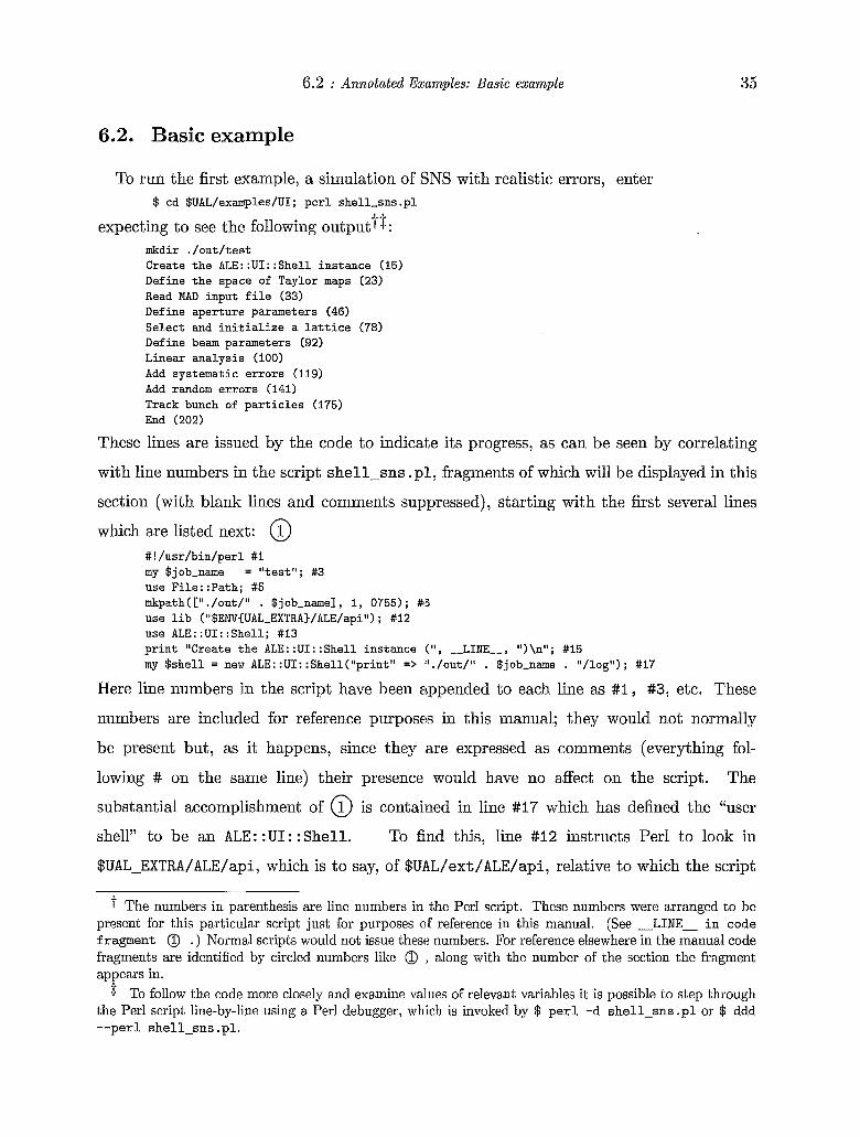
6.2 : Annotated Examples: Basic example 35

6.2. Basic example

To run the first example, a simulation of SNS with realistic errors, enter $ cd $UAL/examples/UI; per1 shel l -sns .pl

expecting to see the following outputt$: mkdir . /ou t / tes t Create t h e ALE: : U I : :Shel l instance (15) Define t h e space of Taylor maps (23) Read MAD input f i l e (33) Define aperture parameters (46) Se lec t and i n i t i a l i z e a l a t t i c e (78) Define beam parameters (92) Linear ana lys i s (100) Add systematic e r r o r s (119) Add random e r r o r s (141) Track bunch of p a r t i c l e s (175) End (202)

These lines are issued by the code to indicate its progress, as can be seen by correlating

with line numbers in the script shell-sns .p l , fragments of which will be displayed in this

section (with blank lines and comments suppressed), starting with the first several lines

which are listed next: @ #! /usr /bin/per l #l my $job-name = "test"; #3 use Fi le : :Path; #5 &path( [" . /out/ll . $ job-name] , I, 0755) ; #15 use l i b ("$ENV{UAL-EXTRA)/ALE/api") ; #12 use ALE::UI::Shell; #13 p r i n t "Create t h e ALE: : U I : :Shel l instance (", --LINE--, ")\n"; #15 my $ s h e l l = new ALE::UI::Shell("print" => 'l./out/ll . $job-name . "/log"); #17

Here line numbers in the script have been appended to each line as #1, #3, etc. These

numbers are included for reference purposes in this manual; they would not normally

be present but, as it happens, since they are expressed as comments (everything fol-

lowing # on the same line) their presence would have no affect on the script. The

substantial accomplishment of @ is contained in line #17 which has defined the "user

shell" to be an ALE: :UI: :Shell. To find this, line #I2 instructs Perl to look in

$UAL-EXTRA/ALE/api, which is to say, of $UAL/ext/ALE/api, relative to which the script

t The numbers in parenthesis are line numbers in the Perl script. These numbers were arranged to be present for this particular script just for purposes of reference in this manual. (See -LINE- in code fragment . ) Normal scripts would not issue these numbers. For reference elsewhere in the manual code fragments are identified by circled numbers like 0 , dong with the number of the section the fragment appears in.

To follow the code more closely and examine values of relevant variables it is possible to step through the Perl script line-by-line using a Perl debugger, which is invoked by $ per1 -d shell-sns . p l or $ ddd --per1 shell-sns . pl .

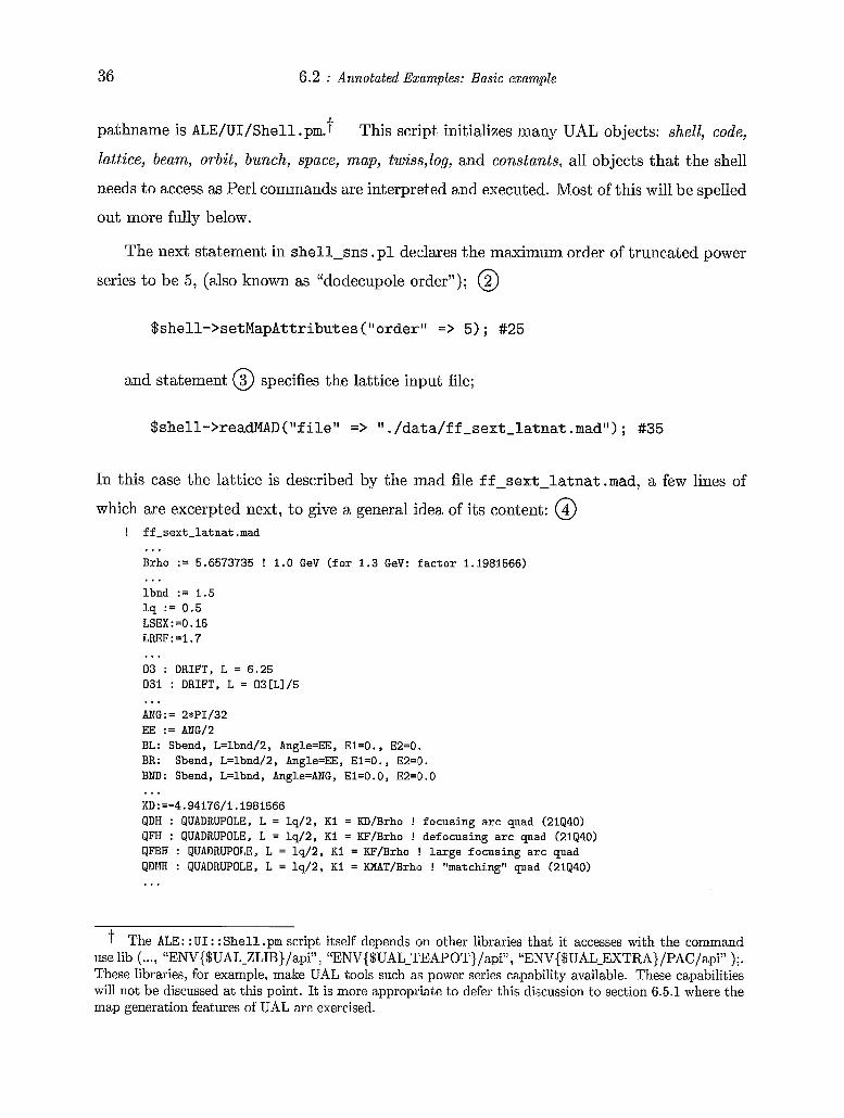
36 6.2 : Annotated Examples: Basic example

pathname is ALE/UI/Shell .pm.t This script initializes many UAL objects: shell, code,

lattice, beam, orbit, bunch, space, map, twiss,log, and constants, all objects that the shell

needs to access as Per1 commands are interprleted and executed. Most of this will be spelled

out more fully below.

The next statement in shell-sns . pl declares the maximum order of truncated power

series to be 5 , (also known as “dodecupole order”); @

$shell->setMapAttributes(”ordeP => 5); #25

and statement @ specifies the lattice input file;

$shell->readMAD(”f ile” => ‘ I . /da.ta/ff-sext-latnat .mad”) ; #35

In this case the lattice is described by the mad file ff-sext-latnat .mad, a few lines of

which are excerpted next, to give a general idea of its content: @ ! ff-sext-latnat .mad

... Brho := 5.6573735 ! 1.0 GeV (for 1.3 GeV: factor 1.1981566)

lbnd := 1.5 lq := 0.5 LSEX:=0.15 LREF: =l .7

03 : DRIFT, L = 6.25 031 : DRIFT, L = 03[L1/5

ANG:= 2*PI/32 EE := ANG/2 BL: Sbend, L=lbnd/2, Angle=EE, E1=0., E2=0. BR: BND: Sbend, L=lbnd, Angle=ANG, El=O.O, E2=0.O

KD:=-4.94176/1.1981566 QDH : QUADRUPOLE, L = lq/2, Kl = KD/Brho ! focusing arc quad (21Q40) QFH : QUADRUPOLE, L = lq/2, Kl = KF/Brho ! defocusing arc quad (21440) QFBH : QUADRUPOLE, L = lq/2, Kl = KF/Brho ! large focusing arc quad QDMH : IJUADRUPOLE, L = lq/2, Kl = KMAT/Brho ! “matching” quad (21Q40)

...

...

...

Sbend, L=lbnd/Z, Angle=EE, E1=0., E2=8.

...

...

t The ALE: :UI : :Shel l . pm script itself depends on other libraries that it accesses with the command use lib (..., “ENV{ $UAL-ZLIB}/api” , “EN\‘{ $UAL-TEAPOT}/api” , “ENV{$UAL-EXTRA}/PAC/api” );. These libraries, for example, make UAL tools such as power series capability available. These capabilities will not be discussed at this point. It is more appropriate to defer this discussion to section 6.5.1 where the map generation features of UAL are exercised.

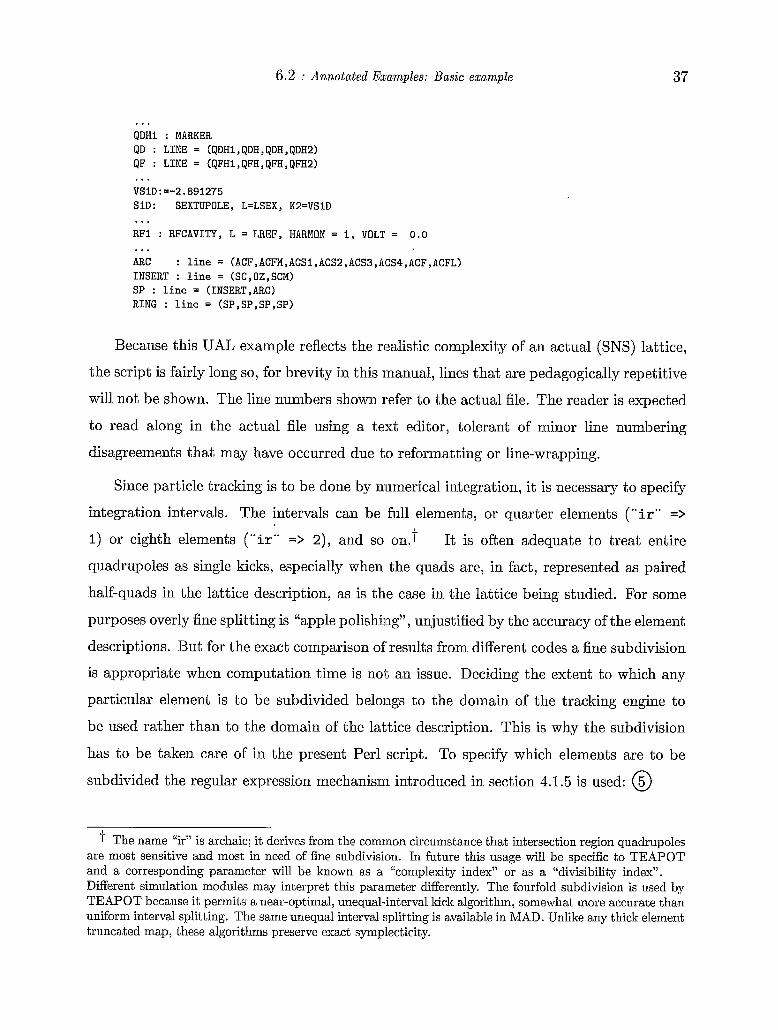
6.2 : Annotated Examples: Basic example 37

... QDHl : MARKER QD : LINE = (QDHl,QDH,QDH,QDH2) QF : LINE = (QFHl,QFH,QFH,QFH2) ... VSlD:=-2.891275 SlD: SEXTUPOLE, L=LSEX, K2=VSID

RFl : RFCAVITY, L = LREF, HARMON = 1, VOLT = 0.0

ARC : line = (ACF,ACFM,ACSl,ACS2,ACS3,ACS4,ACF,ACFL) INSERT : line = (SC,OZ,SCM) SP : line = (INSERT,ARC) RING : line = (SP,SP,SP,SP)

...

...

Because this UAL example reflects the realistic complexity of an actual (SNS) lattice,

the script is fairly long so, for brevity in this manual, lines that are pedagogically repetitive

will not be shown. The line numbers shown refer to the actual file. The reader is expected

to read along in the actual file using a text editor, tolerant of minor line numbering

disagreements that may have occurred due to reformatting or line-wrapping.

Since particle tracking is to be done by numerical integration, it is necessary to specify

integration intervals. The intervals can be full elements, or quarter elements ( O ‘ i r “ =>

1) or eighth elements (*‘ir“ => 2), and so on.? It is often adequate to treat entire

quadrupoles as single kicks, especially when the quads are, in fact, represented as paired

half-quads in the lattice description, as is the case in the lattice being studied. For some

purposes overly fine splitting is “apple polishiiag” , unjustified by the accuracy of the element

descriptions. But for the exact comparison of‘ results from different codes a fine subdivision

is appropriate when computation time is not an issue. Deciding the extent to which any

particular element is to be subdivided beloiags to the domain of the tracking engine to

be used rather than to the domain of the lattice description. This is why the subdivision

has to be taken care of in the present Per1 script. To specify which elements are to be

subdivided the regular expression mechanism introduced in section 4.1.5 is used: @

The name “ir” is archaic; it derives from the common circumstance that intersection region quadrupoles are most sensitive and most in need of fine subdivision. In future this usage will be specific to TEAPOT and a corresponding parameter will be known as a “complexity index” or as a “divisibility index”. Different simulation modules may interpret this parameter differently. The fourfold subdivision is used by TEAPOT because it permit,s a near-optimal, unequal-interval kick algorithm, somewhat more accurate than uniform interval splitting. The same unequal interval splitting is available in MAD. Unlike any thick element truncated map, these algorithms preserve exact symplecticity.

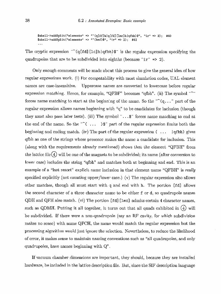
38 6.2 : Annotated Examples: Basic example

$sheLl->addSplit("elements" => "-(q[df]hlq[fdl [lmclhIqfbh)$", "ir" => 2) ; #40 $shell->addsplit ("elements" => "-(bnd)$", "ir" => 2) ; #42 ...

The cryptic expression ""(q[fd] [lcl h I qfbh) $" is the regular expression specifying the

quadrupoles that are to be subdivided into eighths (because "ir" => 2).

Only enough comments will be made about this process to give the general idea of how

regular expressions work. (i) For coinpatability with most simulation codes, UAL element

names are case-insensitive. Uppercase names are converted to lowercase before regular

expression matching. Hence, for example, "QFBF" becomes "qfbh" . (ii) The symbol

forces name matching to start at the beginning of the name. So the (9. . . '* part of the

regular expression allows names beginning with "q" to be candidates for inclusion (though

they must also pass later tests). (iii) The symbol ". . .$" forces name matching to end at

the end of the name. So the ""( . . . I$" part of the regular expression limits both the

beginning and ending match. (iv) The part cd the regular expression ( . . . I qfbh) gives

qfbh as one of the strings whose presence makes the name a candidate for inclusion. This

(along with the requirements already mentioned) shows that the element "QFBH" from

the lattice file@ will be one of the magnets to be subdivided; its name (after conversion to

lower case) includes the string "qfbh" and matches both at beginning and end. This is an

example of a "last resort" explicit name inclusion in that element name "QFBH" is really

specified explicitly (not counting upper/lower case.) (v) The regular expression also allows

other matches, though all must start with lq and end with h. The portion Cfdl allows

the second character of a three character name to be either f or d, so quadrupole names

QDH and QFH also match. (vi) The portion Cf dl Clmcl admits certain 4 character names,

such as QDMH. Putting it all together, it turns out that all quads exhibited in @ will

be subdivided. If there were a non-quadrupole (say an RF cavity, for which subdivision

makes no sense) with name QFCH, the name would match the regular expression but the

processing algorithm would just ignore the selection. Nevertheless, to reduce the likelihood

of error, it makes sense to maintain naming conventions such as "all quadrupoles, and only

quadrupoles, have names beginning with Q" .

..A

If vacuum chamber dimensions are important, they should, because they are installed

hardware, be included in the lattice descriptialn file. But, since the SIF description language

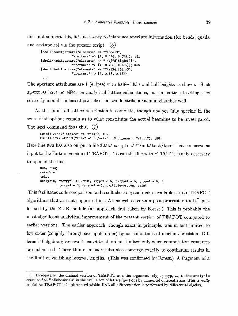
6.2 : Annotated Examples: Basic example 39

does not support this, it is necessary to introduce aperture information (for bends, quads,

and sextupoles) via the present script: @ $shell->addAperture ("elements" => (I^ (bnd) $Ir,

"aperture" => [I, 0.116, 0.0791); #51 $shell->addAperture ("elements" => @I^ (qCfd1 h I qdmh) $" ,

"aperture" => [I, 0.105, 0.1051); #56 $shell->addAperture ("elements" => It^ (s 1241 [fd] )$" ,

"aperture" => [I, 0.13, 0.131); ...

The aperture attributes are 1 (ellipse) with half-widths and half-heights as shown Such

apertures have no effect on analytical lattice calculations, but in particle tracking they

correctly model the loss of particles that would strike a vacuum chamber wall.

At this point all lattice description is complete, though not yet fully specific in the

sense that options remain as to what constitutes the actual beamline to be investigated.

The next command fixes this: @ $shell->use ("lattice" => "ring") ; #82 $shell->writeFTPOT("file" => I!. /out/" . $job-name . Il/tpot") ; #86

Here line #86 has also output a file $UAL/eximples/UI/out/test/tpot that can serve as

input to the Fortran version of TEAPOT. To run this file with FTPOT it is only necessary

to append the lines use, ring makethin twiss analysis, energy=l.93827231, xtyp=l.e-6, pxtyp4.e-6, ytyp=l.e-6, !L

pytyp'1.e-6, dptyp=l.e-6, particle=proton, print

This facilitates code comparison and result checking and makes available certain TEAPOT

algorithms that are not supported in UAL a,s well as certain post-processing tools.? per-

formed by the ZLIB module (an approach .Erst taken by Forest.) This is probably the

most significant analytical improvement of the present version of TEAPOT compared to

earlier versions. The earlier approach, though exact in principle, was in fact limited to

low order (roughly through sextupole order) by considerations of machine precision. Dif-

ferential algebra gives results exact to all orders, limited only when computation resources

are exhausted. These thin element results also converge exactly to continuum results in

the limit of vanishing interval lengths. (This was confirmed by Forest.) A fragment of a

T Incidentally, the original version of TEAPOT uses the arguments xtyp, pxtyp, ..., to the analysis command as "infinitesima.ls" in the evaluation of lattice functions by numerical differentiation. This is really crude! As TEAPOT is implemented within UAL all differentiation is performed by differential algebra

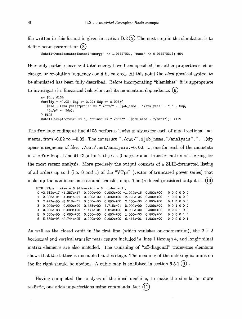
40 6.2 : Annotated Ezamples: Basic example

file written in this format is given in section D.2 @ The next step in the simulation is to

define beam parameters: @ $shell->setBeamAttributes ("energy" => 1.93827231, "mass" => 0.93827231) ; #94

Here only particle mass and total energy have been specified, but other properties such as

charge, or revolution frequency could be entered. At this point the ideal physical system to

be simulated has been fully described. Before incorporating "blemishes" it is appropriate

to investigate its linearized behavior and its momentum dependence: @ my $dp; #lo4 for($dp = -0.02; $dp <= 0.02; $dp += 0.005)C

$shell->analysis ("print" => ./out/'' . $job-name . "/analysis" . ".'I . $dp, "dp/p" => $dp);

3 #lo8 $shell->map("order" => 1, "print" => Il./out/" . $job-name . "/mapi") ; #112

The f o r loop ending at line #I08 performs Twiss analyses for each of nine fractional mo-

menta, from -0.02 to +0.02. The construct " . /out/". $ job-name . "/analysis". .'. " . $dp

opens a sequence of files, ./out/test/analysis.-0.02, ..., one for each of the momenta

in the € o r loop. Line #I12 outputs the 6 x 6 once-around transfer matrix of the ring for

the most recent analysis. More precisely the output consists of a ZLIB-formatted listing

of all orders up to 1 (i.e. 0 and 1) of the 'VTps" (vector of truncated power series) that

make up the nonlinear once-around transfer map. The (reduced-precision) output is: @ ZL1B::VTps : size = 6 (dimension = 6 order = 1 ) 0 -3.512e-17 -1.387e-17 0.000e+00 0.000e+00 -1.022e-15 0.000e+00 0 0 0 0 0 0 1 2.338e-01 -4.801e-01 0.000e+00 0.000e+OD -2.090e-05 0.000e+00 1 0 0 0 0 0 2 2.497e+00 -8.513e-01 0.000e+00 0.000e+00 2.000e-05 0.000e+00 0 1 0 0 0 0 3 0.000e+00 0.000ei-00 2.458e+00 4.715e-01 0.000e+00 0.000e+00 0 0 1 0 0 0 4 0.000e+00 0.000e+00 -1.17le+Ol -1.840e+00 0.000e+00 0.000e+00 0 0 0 1 0 0 5 0.000e+00 0.000e+00 0.000e+00 0.000e+00 l.OOOe+OO 0.000e+00 0 0 0 0 I O 6 5.689e-05 -2.744e-05 0.000e+00 0.000e+00 6.414e+Ol 1.000e+00 0 0 0 0 0 1

As well as the closed orbit in the first line (which vanishes on-momentum), the 2 x 2

horizontal and vertical transfer matrices are included in lines 1 through 4, and longitudinal

matrix elements are also included. The vanishing of "off-diagonal" transverse elements

shows that the lattice is uncoupled at this stage. The meaning of the indexing columns on

the far right should be obvious. A cubic map is exhibited in section 6.5.1 @ .

Having completed the analysis of the ideal machine, to make the simulation more

realistic, one adds imperfections using commands like: @

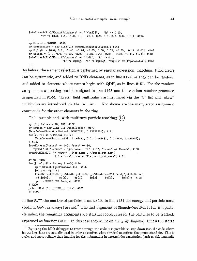
6.2 : Annotated Examples: Basic example 41

$shell->addFieldError("elements" => (bnd) $" , "R" => 0.13, "b" => cO.0, 0.1, 51.0, 0.5, -26.0, 0.2, 0.0, 0.0, 0.0, 0.01); #124

... my $heed = 973431; #143 my $rgenerator = new ALE::UI::RandomGenerator($iseed); #144 my $qSigB = 10.0, 0.0, -2.46, -0.76, -0.63, 0.00, 0.02, -0.63, 0.17, 0.001; #148 my $qSiqA = cO.0, 0.0, -2.50, -2.00, 1.29, 1.45, 0.25, 0.31, -0.11, 1.041; #149 $shell->addFieldError ("elements" => "-qdh", "R" => 0.1,

"b" => $qSigB, "a" => $ qSiqA, "engine" => $rgenerator) ; #157

As before, the element selection is performed by regular expression matching. Field errors

can be systematic, and added to BND elements, as in line #124, or they can be random,

and added to elements whose names begin with QDH, as in lines #157. For the random

assignments a starting seed is assigned in line #I43 and the random number generator

is specified in #144. "Erect" field multipoles are introduced via the "b" list and "skew"

multipoles are introduced via the "a" list. Not shown are the many error assignment

commands for the other elements in the ring;.

This example ends with multiturn particle tracking; 0 my ($i, $size) = (0, 10); #i77 my $bunch = new ALE::UI::Bunch($size); #179 $bunch->setBeamAttributes(l.93827231, 0.93827231); #181 for($i =O; $i < $size; $i++)C

) #185 $shell->run("turns" => 100, "step" => 10,

open(BUNCH-OUT, ">./out/" . $job-name . "/bunch-out-new") my ap; #193 for($i =O; $i < $size; $i++){ #194

$bunch->setPosition($i, 1.e-2*$i, 0.0, l.e-2*$i, 0.0, 0.0, i.e-3*$i);

"print" => "./out/" . $job-name . "/fort.8", "bunch" => $bunch) ; #188

I I die "can't create file (bunch-out-new) ; #191

@p = $bunch->getPosition($i); #195 $output= sprintf ("i=%5d x=%14.8e px=%14.8e y=%14.8e py=%l,4.8e ct=%l4.8e dp/p=%l4.8e \ntq, $is $p LO1 , $pC11, $p[21, $pC31, $pC41, $pC51); #198 print BUNCH-OUT $output; #I99

1 #200 print "End (", --LINE--, ")\n"; #202 1; #204

In line #I77 the number of particles is set to 10. In line #I81 the energy and particle mass

(both in GeV, as always) are set.t The first argument of $bunch->setPosition is a parti-

cle index; the remaining arguments are starting coordinates for the particles to be tracked,

expressed as functions of $i. In this case they all lie on a x, y, dp diagonal. Line #I88 starts

By using the DDD debugger to trace through the code it is possible to step down into the code where inputs like these are actually used in order to confirm what physical quantities the inputs stand for. This is easier a.nd more reliable than hunting for the information in external documentation (such a,s this manual).

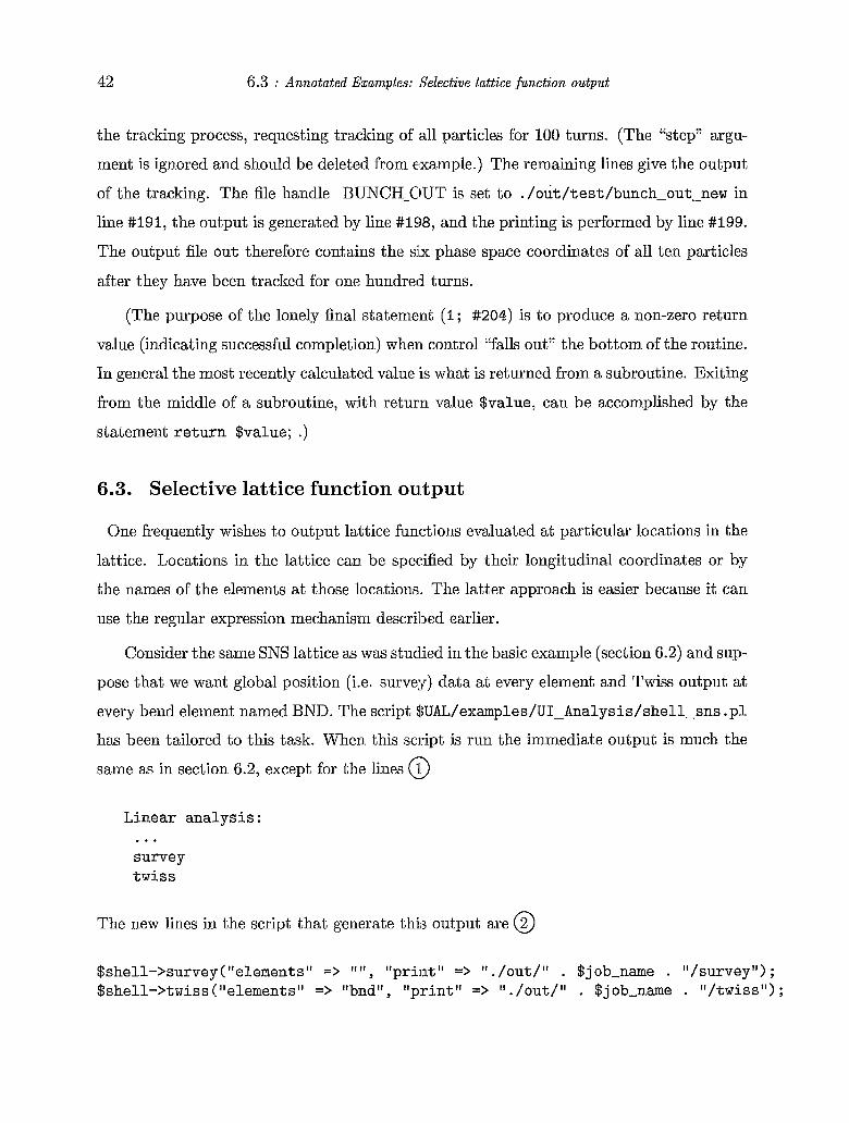
42 6.3 : Annotated Examples: Selective lattice func t ion output

the tracking process, requesting tracking of all particles for 100 turns. (The "step" argu-

ment is ignored and should be deleted from example.) The remaining lines give the output

of the tracking. The file handle BUNCH-OUT is set to ./out/test/bunch-out-new in

line #191, the output is generated by line #198, and the printing is performed by line #199.

The output file out therefore contains the sjx phase space coordinates of all ten particles

after they have been tracked for one hundred turns.

(The purpose of the lonely final statement (1; #204) is to produce a non-zero return

value (indicating successful completion) when control "falls 011t" the bottom of the routine.

In general the most recently calculated value is what is returned from a subroutine. Exiting

from the middle of a subroutine, with return value $value, can be accomplished by the

statement return $value; .)

6.3. Selective lattice function output

One frequently wishes to output lattice functions evaluated at particular locations in the

lattice. Locations in the lattice can be specified by their longitudinal coordinates or by

the names of the elements at those locations. The latter approach is easier because it can

use the regular expression mechanism described earlier.

Consider the same SNS lattice as was studied in the basic example (section 6.2) and sup-

pose that we want global position (i.e. survey) data at every element and Twiss output at

every bend element named BND. The script $UAL/examples/UI-Analysis/shell-sns . pl has been tailored to this task. When this script is run the immediate output is much the

same as in section 6.2, except for the lines G) Linear analysis: ... survey twiss

The new lines in the script that generate this output are @

$shell->survey("elements" => t l I 1 y "print" => I t . /out/" . $job-name . "/survey") ; $shell->twiss ("elements" => "bnd" "p:rint" => I t . /out/ll . $job-name . "/twiss") ;

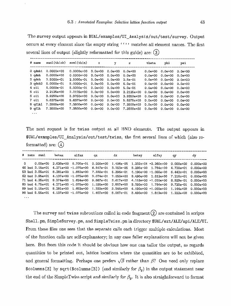
6.3 : Annotated Examples: Selective lattice func t ion output 43

The survey output appears in $UAL/exampl,es/UI-Analys is/out /t est /survey. Output

occurs at every element since the empty stri:ng ’ ’ matches all element names. The first

several lines of output (slightly reformatted for this guide) are: @ # name --- --- -_ 0 qdmhl 1 qdmh

3 qdmh2 2

4 011 5 oil 6 oil 7 Oil 8 qflhl 9 qflh ...

suml(thick)

0.0000e+00 0.0000e+00 2.5000e-01 5.0000e-01 5.0000e-01 2.2125e+00 3.9250e+00 5.6375e+00 7.3500e+00 7.3500e+00

suml(thin)

0.0000e+00 0.0000e+00 2.5000e-01 5.0000e-01 5.0000e-01 2.2125e+00 3.9250e+00 5.6375e+00 7.3500e+00 7.3500e+00

.--- -------- X

O.Oe+OO O.Oe+OO O.Oe+OO O.Oe+OO O.Oe+OO O.Oe+OO O.Oe+OO O.Oe+OO O.Oe+OO O.Oe+OO

Y

O.Oe+OO O.Oe+OO O.Oe+OO O.Oe+OO O.Oe+OO 0 . Oe+OO 0. Oe+OO O.Oe+OO 0. Oe+OO O.Oe+OO

z . -- -- ----- - -- O.Oe+OO O.Oe+OO 2.5e-0i 5.Oe-01 5.Oe-01 2.2125e+00 3.9250e+00 5.6375e+00 7.3500e+00 7.3500e+00

theta

O.Oe+OO O.Oe+OO O.Oe+OO O.Oe+OO O.Oe+OO O.Oe+OO O.Oe+OO O.Oe+OO O.Oe+OO O.Oe+OO

- -- ------ phi

O.Oe+OO O.Oe+OO O.Oe+OO O.Oe+OO O.Oe+OO O.Oe+OO O.Oe+OO O.Oe+OO O.Oe+OO O.Oe+OO

-- ------- psi

O.Oe+OO O.Oe+OO O.Oe+OO O.Oe+OO O.Oe+OO O.Oe+OO O.Oe+OO O.Oe+OO O.Oe+OO O.Oe+OO

-- ----

The next request is for twiss output at ,all BND elements. The output appears in

$UAL/examples/UI-Analysis/out/test/twiss, the first several lines of which (also re-

formatted) are: @

0 0.00e+00 46 bnd 3.15e+01 53 bnd 3.55e+01 62 bnd 3.95e+01 71 bnd 4.35e+01 80 bnd 4.75e+01 89 bnd 5.15e+Oi 98 bnd 5.55e+01 ...

...................... betax alf ax

...................... 2.626e+00 5.705e-01 4.271e+00 -1.075e+00 8.281et00 1.652e+00 4.137e+00 -1.075e+00 8.374e+00 1.624e+00 4.271e+00 -1.075e+00 8.281e+00 1.652e+00 4.137e+00 -1.075e+00

qx --- -- --- - - - O.OOOe+OO 6.547e-01 7.330e-01 9.074e-01 9.867e-01 1. 155e+00 I. 233e+00 I. 407e+00

-- --- - CPX

----- - 1 ,. 406e-05 3 253e-05 5 396e-01 2 050e+00 3 ,, 617e+00 2 ,. 857e+00 3 ,. 246e+00 8 ,, 067e-01

betay alf ay

1.232e+01 -2.260e+00 8.293e+00 1.764e+00 4.190e+00 -1.055e+00 8.490e+00 1.812e+00 4.116e+00 -1.020e+00 8.293e+00 1.764e+00 4.190e+00 -1.055e+00 8.490e+00 1.812e+00

qY

O.OOOe+OO 4.720e-01 6.442e-01 7.216e-01 8.929e-01 9.720e-01 1.144e+00 1.222e+00

The survey and twiss subroutines called in code fragment @ are contained in scripts

Shell. pm, SimpleSurvey . pm, and SimpleTwi.ss . pm in directory $UAL/ext/ALE/api/ALE/UI.

From these files one sees that the separate calls each trigger multiple calculations. Most

of the function calls are self-explanatory; in any case fuller explanations will not be given

here. But from this code it should be obvious how one can tailor the output, as regards

quantities to be printed out, lattice 1ocatio:ns where the quantities are to be exhibited,

and general formatting. Perhaps one prefers fl rather than ,B? One need only replace

$columns 131 by sqrt ($columns 131 1 (and similarly for ,By) in the output statement near

the end of the SimpleTwiss script and similarly for ,By. It is also straightforward to format

44 6.4 : Annotated Examples: A personalized shell for code development

the output file appropriately for graphing the lattice functions by a graphing program such

as gnuplot.

Most theoretical formulas in lattice physics involve integration (usually approximated

by summation) over all elements in the ring, of element parameters such as quadrupole gra-

dients, length-strength products, inverse focal lengths, sextupole strengths etc., weighted

by fractional powers or other functions of 1ati;ice functions (/Iz, /Iy, &,, dispersion, etc.) All

of the required lattice functions are available from $UAL/ext/ALE/api/ALE/UI/Shell. pm.

An example in section 6.4 will show how to gain access to the magnet strengths required.

Once this information is in hand one can usle Perl to evaluate the accelerator physics for-

mulas involving such summations (or even integrations if necessary). Though Perl may

not be as fast as a compiled language, it is plenty fast for typical postprocessing tasks.

6.4. A personalized shell for c0d.e development

The examples presented so far showed how to run canned UAL scripts. If these are

classified as “elementary UAL” we now advance to “intermediate level UAL” . A key pur-

pose of UAL is to be an environment in which an accelerator physicist’s attention can be

concentrated on a specialized problem without being overwhelmed by the complication of

“the rest of the system”. The reason this is important is that the detailed and correct

understanding of any subsystem requires that the rest of the accelerator perform more-

or-less as it is supposed to. A perfect simulation code would correctly model all systems

and be prepared to answer any question concerning the functioning of the accelerator, but

it is unrealistic even to strive for such a utclpian situation. Rather, individual physicists

strive to define and then answer sufficiently narrow, well-posed questions concerning the

performance of accelerator subsystems. The purpose of UAL is to support such activity.

The physicist zeroing in on some area of interest, and wishing to use the tools of

UAL, will often have to alter the existing (code in the area of concentration as well as

generating new code. In this sense “hacking into the code” is strongly encouraged. This

is fairly straightforward, especially when only Perl code is involved. What may be less

straightforward is keeping track of the changes in case it is necessary to “back them out”

or to cause the improved code to be integrated eventually into the distributed version of

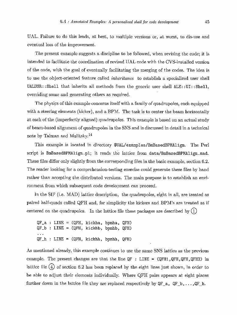
6.4 : Annotated Examples: A personalized shell for code development 45

UAL. Failure to do this leads, at best, to multiple versions or, at worst, to dis-use and

eventual loss of the improvement.

The present example suggests a discipline to be followed, when revising the code; it is

intended to facilitate the coordination of revjsed UAL code with the CVS-installed version

of the code, with the goal of eventually facilitating the merging of the codes. The idea is

to use the object-oriented feature called inheritance to establish a specialized user shell

UALUSR: : Shell that inherits all methods from the generic user shell ALE: : UI : : Shell,

overriding some and generating others as required.

The physics of this example concerns itself with a family of quadrupoles, each equipped

with a steering elements (kicker), and a BPNL The task is to center the beam horizontally

at each of the (imperfectly aligned) quadrupoles. This example is based on an actual study

of beam-based alignment of quadrupoles in the SNS and is discussed in detail in a technical

note by Talman and Ma1it~ky.I~

This example is located in directory $lJAL/examples/BmBasedBPMAlign. The Per1

script is BmBasedBPMAlign. pl; it reads the lattice from data/BmBasedBPMAlign .mad.

These files differ only slightly from the corresponding files in the basic example, section 6.2.

The reader looking for a comprehension-testing exercise could generate these files by hand

rather than accepting the distributed versions. The main purpose is to establish an envi-

ronment from which subsequent code deve1o:pment can proceed.

In the SIF (i.e. MAD) lattice description, the quadrupoles, eight in all, are treated as

paired half-quads called QFH and, for simplicity the kickers and BPM’s are treated as if

centered on the quadrupoles. In the lattice file these packages are described by 0 QF-a : LINE = (QFH, kickha, bpmha, QFH) QF-b : LINE = (QFH, kickhb, bpmhb, QFH)

QF-h : LINE = (QFH, kickhh, bpmhh, QFH) ...

As mentioned already, this example continues to use the same SNS lattice as the previous

example. The present changes are that the line QF : LINE = (QFHl,QFH,QFH,QFH2) in

lattice file @ of section 6.2 has been replaced by the eight lines just shown, in order to

be able to adjust their elements individually. Where QFH pairs appears at eight places

further down in the lattice file they are replaced respectively by QF-a, QF-by . . . ,QF-h.

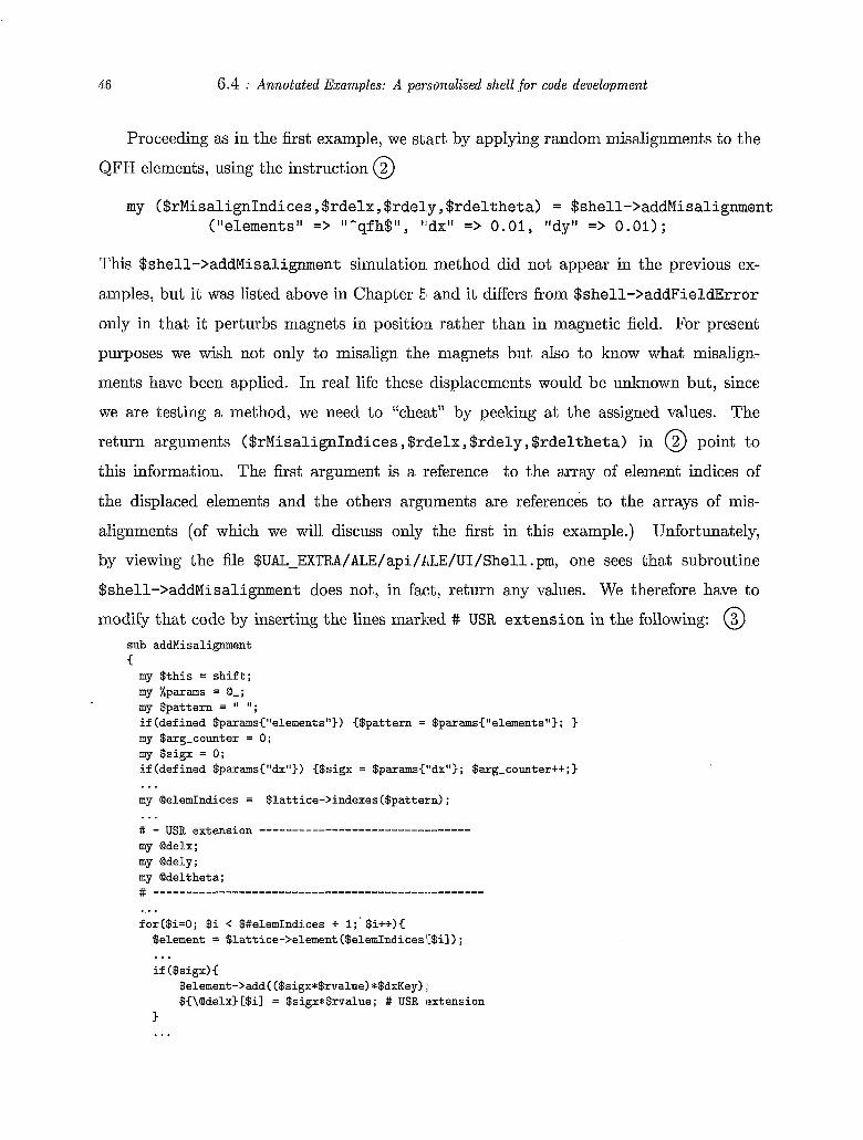
46 6.4 : Annotated Examples: A personalized shell for code development

Proceeding as in the first example, we start by applying random misalignments to the

QFH elements, using the instruction @ my ($rMisalignIndices, $rdelx , $rdel.y , $rdeltheta) = $shell->addMisalignment

("elements" => It^qfh$" , "dx" => 0.01 , "dy" => 0.01) ;

This $shell->addMisalignment simulation. method did not appear in the previous ex-

amples, but it was listed above in Chapter 51 and it differs from $shell->addFieldError

only in that it perturbs magnets in position rather than in magnetic field. For present

purposes we wish not only to misalign the magnets but also to know what misalign-

ments have been applied. Iii real life these displacements would be unknown but, since

we are testing a method, we need to "cheat" by peeking at the assigned values. The

return arguments ($rMisalignIndices , $rdelx, $rdely, $rdeltheta) in @ point to

this information. The first argument is a reference to the array of element indices of

the displaced elements and the others arguments are references to the arrays of mis-

alignments (of which we will discuss only the first in this example.) Unfortunately,

by viewing the file $UAL-EXTRA/ALE/api/ALE/UI/Shell . pm, one sees that subroutine

$shell->addMisalignment does not, in fact, return any values. We therefore have to

modify that code by inserting the lines marked # USR extension in the following: @ sub admisalignment c my $this = shift; my %params = Q-; my $pattern = "; if (def ined $params{llelernents")) €$pattern = $params{"elements") ; 1 my $arg-counter = 0; my $sigx = 0; if (def ined $params{ltdxtl)) {$sigx = $params{"dx"); $arg-counter++; )

my QelemIndices = $lattice->indexes($patteicn); ... ... # - USR extension my Qdelx; my QdeLy; my Qdeltheta; #

for($i=O; $i < $#elemIndices + 1; ' $i++){ $element = $lattice->element($elemIndicesJ~$il);

if ($sigx) I

...

... $element->add ( ($sigx*$rvalue) +$dxKey) ;; $C\Qdelx) [$il = $sigx*$rvalue; # USR extension

1 ...

6.4 : Annotated Examples: A personalized shell for code development 47

Too little detail has been given here to understand this code in every detail, but the

following things have been accomplished. The first seven lines decipher the input arguments

as was explained in section 4.1.2 and provide the example that was promised there. The

next line shown saves the indices of displaced elements in the array QelemIndices. So

far there has been no change but the following lines squirrel away information that is now

known will be needed later. Then (because dx was included in the argument list) $sigx

is true, so the misalignment values $sigx*!lrvalue are saved in the array @delx. The

last line returns the array reference.+ The other return values will be ignored.) We have

therefore modified code block @ to be consistent with the call in code block @ . A major virtue of CVS is that changes like these can be hacked into the code without

worrying about polluting the original version, since the original can always be retrieved.

But, once your revisions have been frozen, you will want to save them; so you may as well

plan for this from the start.

A new personalized "application interface" UALUSR: : Shell is needed. This is some-

thing that you would have to generate and save as the file api/Shell.pm. Here, since this

is an example, the script is supplied for you:f @ package UALUSR::Shell; use Carp; use strict; use vars qw(@ISA) ; use lib ("$ENVCUAL-EXTRA>/ALE/api") ; use ALE::UI::Shell; @ISA = qw(ALE: :UI: :Shell); sub new C my $type = shift; my %params = @-; my $this = new ALE: :UI: :Shell(%params) ;

return bless $this, $type; ...

t A quicker and dirtier approach to accessing the parameter changes would have been to make the saved arrays global variables so they would not have to be returned by reference. But this is the sort of slipshod practice that evolves inexorably into spaghetti code.

The line use Carp modifies error reporting and is therefore inconsequential. The curious Per1 construct q w ( x y z) is equivalent to placing quotation marks around the individual arguments; Le. equivalent to

z . The statement use strict prevents access to global variables and the statement use vars q w ( Q 1 S A ) restores access to just the Q I S A array. The Q I S A array array is used three lines further down to declare that the newly-defined shell will start with all methods defined in ALE: :UI: :Shell.

<< >> >1 >> >1 >> x y

48 6.4 : Annotated Examples: A personalized shell f o r code development

1 sub addMisalignment c

... return (\@elemIndices,\@klvalue);

1

c sub getErectMagnetStrengths

... return (\@elemIndices,\@delx,\@de I,'

1 If theta) ;

The subroutine addMisalignment listed here was spelled out above in @ . In this new

shell the inherited method addMisalignmerit has been over-ridden; also a new method

getErectMagnetStrengths has been defined (of which only one line is shown in @ .)

now begins with @ To make use of the new shell the UAL command script (call it BmE3asedBPMAlign.pl)

... use lib ( ' I . /api") ; use UALUSR::Shell; my $shell = new UALUSR: :Shell ("print" => ' I . /out/" . $ j ob-name . ''/log'') ; ...

which creates the new UALUSR shell instance. This replaces code fragment @ of sec-

tion 6.2. Following this will be the lattice (definition commands, for example fragments

from section 6.2: @ , @ , @ , @ , @ , and @ . Finally lines specific to the simulation

being developed are included, such as: @ ...

my ($rMisalignIndices ,$rdelx,$rdely, $rdelthetin) = $shell->addMisalignment

my $numMisaligns = $#c$rMisalignIndices); #19:2 my $numkicks = ($numMisaligns + 1)/2; #I93

$shell->hsteer ("adjusters" => "*kickh", "detectors" => ll-bp&ll) ; #204

my ($rErectIndices,$rkickhs) = $shell->getErei:tMagnetStrengths

("elementst' => "-qfh$", "dx" => 0.01) ; #I90

...

... ("elements" => "-kickhl', "multindex" => 0:) ; #208

...

Line #I90 is the revised command discussed. above as code fragment @ . Line #I92 il-

lustrates the Per1 syntax for obtaining the number of elements in an array and line #I93

accounts for the pairing of the quadrupoles (artificially present in the SIF lattice descrip-

tion.) Line #204 uses the hsteer algorithm to resteer the beam through quad centers

and line #208 uses the newly-defined method getErectMagnetStrengths to obtain the

6.5 : Annotated Examples: Fringe field map 49

strengths that have been determined by histeer. F’rom these strengths the quad mis-

alignments can be inferred and then compared to the (known by cheating) actual quad

misalignments. The calculations (not shown) required for this comparison are the sort of

postprocessing activity for which Per1 is ideal.

6.5. Fringe field map

Trajectory evolution through lattice sectors can be represented by maps. In this example

the end fields of quadrupoles in the SNS will be modeled. Just as the end fields of dipole

magnets are (predominantly) of quadrupole order, the end fields of quadrupoles are pre-

dominantly of octupole order-deflections are cubic functions of the transverse coordinates.

A theoretical discussion of maps is given in appendix E.

Especially for hadron accelerators, it is essential to preserve symplecticity to high

accuracy. No special treatment is required for dipole magnets with end fields modeled

by quadrupoles, since the end fields are linear and symplectic. Often the end fields of

quadrupoles can simply be ignored but, for i3 large aperture accelerator like the SNS, the

octupole end fields have significant effect-their leading effect is dependence of tune on

amplitude. To a good approximation an end field can be treated as if it acts impulsively at

a single plane. The relation between input-to and output-from coordinates for this plane

can be represented by a vector of truncated power series.

For extremely large amplitudes the convergence of such power series may simply be

too poor for the series to be applicable. But when the fields are weak, as here, this is not

expected to be an issue. The quad end deflections are approximated well by the cubic

terms in the power series of the map. Yet one cannot simply include cubic terms without

further investigation. Truncation causes nonsymplecticityt that can invalidate long term

tracking. A cubic map, even if symplectic “to cubic order”, is necessarily nonsymplectic

“to quartic order” or, in general, a truncated map can be symplectic to its own order, but

not to higher order.

To be able to investigate these issues it is valuable to have the capability of introducing

maps that are truncated to arbitrary order and that are symplectic at least to their order

There are techniques involving (nonlinear) transformation to new variables such that the exact map elements a.re actually polynomials rather than infinite series. No such procedure is being considered here.

50 6.5.1 : Annotated Examples: Fringe field map: M a p generation

of truncation. In this

approach the map element corresponding to each phase space coordinate is obtained by

appropriate differentiation of a polynomial “Hamiltonian” (sometimes known as a pseudo-

Hamiltonian). The actual differentation process is in fact a Poisson bracket evaluation,

an operation that is provided by ZLIB. What results, for each coordinate, is a power

series representing its output value as a power series of all input coordinates. In first

approximation the polynomial order of each of these series is one less than the order of the

Hamiltonian. But it is possible, by iterating, by keeping more terms in the exponential

series entering the Lie transform, and by truncating to higher order, for the resulting

map to be symplectic to higher order than t:he initially-truncated Hamiltonian. This does

not make the map “correct” to higher order, but it does make it symplectic to higher

order. Starting from an approximate map this process can therefore produce a map that

is symplectic to whatever order one is willing to evaluate the power series.

The so-called “Lie transform” formalism makes this possible.

These mapping capabilities of UAL are ithe subjects of this section. First the map or

maps have to be generated and then they have to be introduced into the simulation script.

These are the tasks of the next two sections.

6.5.1. Map generation

The code illustrating map generation is located in directory $UAL/examples/HardEdge.

The script f f . p l begins 0

use l i b ( I t $ENV(UAL_ZLIB) / api ‘I I t $ENV(UAL-DA) / api ” ; use Z1ib::Tps; use HardEdge; my $dimension = 6; my $maxOrder = 5; my $space = new Zlib::Space($dirnension, $maxOrder);

This example uses the truncated power series tools made available by the command use

Zlib : : Tps ; . This capability was already exhibited, with minimal explanation, in sec-

tion 6.2; a linear order, once-around, transfer map for the whole SNS ring was displayed

6.5.1 : Annotated Examples: Fringe field map: M a p generation 51

as @ . Here, as there, the full 6 x 6 phase space dimensionality is specified and the

maximum truncation order is set to 5.t Continuing with script ff .pl @) my $I = new Zlib: :VTps ($dimension) ;

# N - number of terms in the Lie transformation # K - MAD quad coefficient multiplied by +I (entrance) or -1 (exit) my $ff-integrator = new HardEdge("N" => 1, "K" => -4.35305u5.6575,

$I += 1.0;

;

an identity map $1 is defined, number of terms parameter N and strength parameter

K assigned and the routine HardEdge.pm for propagation through fringe field (from the

HardEdge package) declared. The header material of script HardEdge .pm isf : @

package HardEdge; use vars qw(@ISA) ; use Da: : Const qw($X- $PX- $Y- $PY-, $CT- $DE-) ; use Da::Lie::Integrator; @ISA = qw(Da: :Lie: :Integrator);

As well as associating map variables with physical coordinates this causes the script to in-

herit all the methods of the parent class Da: : Lie : : Integrator. The Da: : Const package

relies on the Per1 typeglob data type which is too technical and idiosynchratic to be ex-

plained here. The package defines and exports global references to read-only constants such

as particle rest energies or (in this case) the indices 0,1,2,3,4,5, as they correspond to the

variables x, p,, y, py, et, de. This has the seerningly cosmetic, self-documenting purpose of

permitting a variable value such as $PO->value (0) to be expressed as $PO->value ($X-)-

the actual purposes are: to support the overloading of coordinate representations by both

scalar value and power series; and to allow the truncated power series code to be math-

ematically general, absent of any particular identification of its variables with physical

quantities.

The instantiation code in the new integrator is @ sub new

my $type = shift;

t The order of a polynomial in UAL is dynamically determined as the power series is being evaluated. The order of any particular power series can therefore be less than t,he maximum order, but it cannot be greater.

Header material like this was explained in a footnote to section 6.4.

52 6.5.1 : Annotated Examples: Fringe field map: Map generation

my %params = @-; my $self = new Da: :Lie: :Integrator(@-) ; $self->(K> = 0.0 unless defined ( $self->(K) = $params(K) ); return bless $self, $type;

3

which receives K and N (not visible in the: code fragment shown because it is received

by Da: :Lie: :Integrator) as input arguments. The Lie integrator assumes propagation

through drift as default; this behavior has to be overridden (in HardEdge .pm) by introduc-

ing a Hamiltonian appropriate for propagation through the hard edge of a quadrupole;15

sub hamiltonian € my ($this, $p) = k; my $h = I.; if($p->size < $PXJ € return $h;) # Beam my $vObyc = $this->€vObyc>; my $charge = $this->€charge); my $PO = new Zlib: :VTps($p->size) ;

# Hamiltonian my $x2 = $PO->value ($XJ *$PO->value ($X-) ; my $y2 = $po->value($Y-)*$pO->value($Y-); $h = 3. *$xZ*$pO->value ($Ye) *$PO->value ($PY.-) ; $h -= 3, *$yZ*$pO->value ($X-) *$PO->value ($PX.-) ; $h += $y2*$po->value ($YJ *$PO->value ($PY.-) ; $h -= $x2*$pO->value ($X-) *$PO->value ($PX.-) : $h *= $this->€K)/lZ. ; return $h;

$PO += 1;

1

Note the line my $PO = new Zlib: :VTps($p->size); which has defined a new vector

of (initially vanishing) power series. The subsequent operations in the subroutine are

overloaded in the sense that all operations (such as =, - =, and *) are performed on

complete (truncated) power series.

Continuing with script ff .pl; @

my $ff-map = $I + 0.0; $ff-integrator->propagate($ff-map, $beam-att);

the map is instantiated and then propagated through the fringe region using a method

inherited from $UAL-DA/api/Da/Lie/Integrator . pm. This subroutine (with four incon-

sequential lines deleted) reads: @

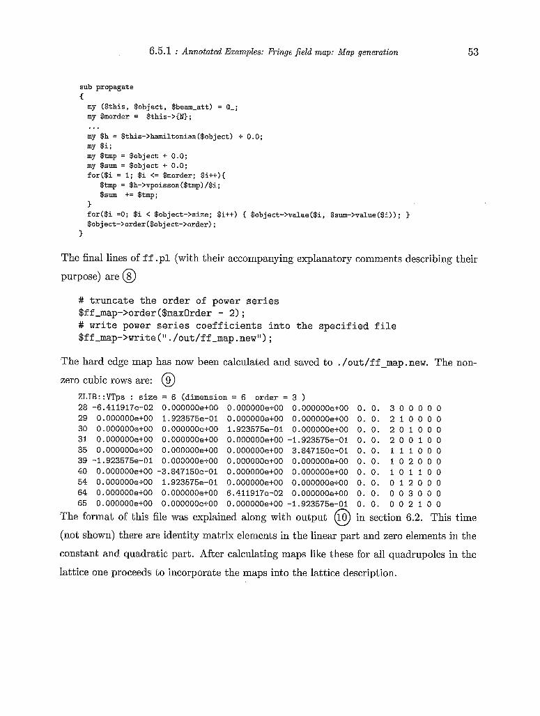
6.5.1 : Annotated Examples: Fringe field map: M a p generation 53

sub propagate c my ($this, $object, $beam-att) = tl-; my $morder = $this->IN);

my $h = $this->hamiltonian($object) + 0.0; my $i; my $tmp = $object + 0.0; my $sum = $object + 0.0; for($i = I; $i <= $morder; $i++){

...

$tmp = $h->vpoisson($tmp) /$i; $sum += $tmp;

1 for($i =O; $i < $object->size; $i++) $object->value($i, $sum->value($i)) ; > $object->order($object->order);

>

The final lines of ff .pl (with their accompanying explanatory comments describing their

purpose) are @ ## truncate the order of power series $ff-map->order($maxOrder - 2); # write power series coefficients into the specified file $ff-map->write("./out/ff-map.new") ;

The hard edge map has now been calculated and saved to ./out/ff-map.new. The non-

zero cubic rows are: @ ZL1B::VTps : size = 6 (dimension = 6 order = 3 ) 28 -6.411917e-02 0.000000e+00 O.OOOOOOe+OO 0.000000e+00 0. 0. 3 0 0 0 0 0 29 0.000000e+00 1.923575e-01 0.000000e+00 0.000000e+00 0. 0. 2 1 0 0 0 0 30 0.000000e+00 0.000000e+00 1.923575~:-01 0.000000e+00 0. 0. 2 0 I O 0 0 31 0.000000e+00 0.000000e+00 0.000000e+00 -1.923575e-01 0. 0. 2 0 0 1 0 0 35 0.000000e+00 0.000000e+00 0.000000e+00 3.847150e-01 0. 0. I 1 1 0 0 0 39 -1.923575e-01 0.000000e+00 O.OOOOOO~!+OO 0.000000e+00 0. 0. I 0 2 0 0 0 40 0.000000e+00 -3.847150e-01 0.000000e+00 0.000000e+00 0. 0. I O I 1 0 0 54 0.000000e+00 1.923575e-01 0.000000e+00 0.000000e+00 0. 0. 0 1 2 0 0 0 64 0.000000e+00 0.000000e+00 6.411917~:-02 0.000000e+00 0. 0. 0 0 3 0 0 0 65 0.000000e+00 0.000000e+00 0.000000e+00 -1.923575e-01 0. 0. 0 0 2 1 0 0

The format of this file was explained along with output @ in section 6.2. This time

(not shown) there are identity matrix elements in the linear part and zero elements in the

constant and quadratic part. After calculating maps like these for all quadrupoles in the

lattice one proceeds to incorporate the maps into the lattice description.

54 6.6.1 : Annotated Examples: SXF input t o UAL: SXF rationale

6.5.2. Map application

The code illustrating the inclusion of maps in lattice descriptions is located in directory

$UAL/examples/UI-FF. The starting lattice file is

$UAL/examples/UI-FF/dat a/f f -sext-l.atnat. mad

It is an SNS lattice much like the lattices in. previous examples. The end field maps for

its quads have been pre-calculated and reside in directory quadff. The first seventy or so

lines of the shell-sns-ff .pl script are much like the corresponding lines of the script in

section 6.2. Deviation begins with the lines (3 print "Define 3D fringe fields" , "\n" ; # We include ff only for quads because it was shown # that contribution from bends was negligible $shell->addMap("elements" => @I^ (qdhl) $" ,

$shell->addMap("elements" => I s ^ (qdh2) $ ' I ,

"map" => "./quadff/frlqd.zrnap") ;

"map" => "./quadff/fr2qd.zmap") ; ...

$she 11-> addMap ( "elements " => I t ^ ( qf bh2) $ , "map" => It. /quadf f /f r2qf. zmapt) ;

Because the deflections (and even displacements that male the orbit discontinuous) caused

by fringe fields occur at fixed longitudinal positions, their treatment by TEAPOT is just

like the treatment of deflections by thin multipole elements. Therefore, nothing more

needs to be done. The remaining lines of script shell-snsff .pl are identical to the

corresponding lines of shell-sns- . pl.

6.6. SXF input to UAL

6.6.1. SXF rationale

There has always been a need for a portable, fully-instantiated lattice description. When

parameter deviations are entered by a particular code from a measurement database or,

even more so, when errors are generated by Monte Carlo programs, it becomes difficult

to perform accurate result comparisons. Calmmonly one is forced to repeat calculations

already performed, using possibly-suspect code, just for the purpose of regenerating iden-

tical data. This limitation was felt strongly when the US-LHC collaboration was starting

to perform LHC simulations. The result was SXF (Standard exchange Format).22

6.6.2 : Annotated Examples: :iXF input t o UAL: RHIC example 55

By now an even more important use for SXF has been realized at RHIC. It is for

capturing “snapshots” of actual lattice conditions, encountered during operations, to be

used for offline simulations and “post mortem” analysis. Though it is straightforward,

sta.rting from an SIF input, to collect and apply all the field imperfections, misalignments,

apertures, operational procedures, etc. needed to instantiate all lattice elements, this is

very time consuming and hard to maintain. Furthermore (for better of for worse from the

point of view of database management) it is easier to output the current, fully-instantiated

lattice parameters, than to update the original data sources.

To understand some of the issues involved in reconstructing a lattice from an SXF

file some understanding of SMF (the UAL accelerator model) is useful; a brief description

is contained in Appendix D. For now the only point to be made is that each element in

the lattice has two names, a design/generic GenNume and a fully-instantiated LutNume;

sometimes known as a site-wide name. Within SXF the lattice is represented by a sequence

of LutNume’s, along with their attributes. Since one of these attributes (the tug attribute)

is the GenNume, it is easy to cross-reference one name to the other, even when only SXF

information is available. But, within the original SIF lattice design, there are hierarchical

features like sub-lines, symmetric sections, repetitions, and so on. None of this information

finds its way into the SXF file. Hence a simulation that depends on hierarchical information

(other than GenNume association) must either start from a SIF lattice description or

re-insert the required relationships post facto. So far this has turned out to be either

unnecessary or straightforward, so the absence of hierarchical information from SXF files

has proved not to be a serious impediment.

6.6.2. RHIC example

RHIC simulation documented in this guide will be based purely on the SXF lattice

description. t

Historically the RHIC lattice description, like the SNS description in the basic example of section 6.2, started from a MAD file. Both the lattice descriptions and the UAL scripts from that era a.re obsolete but, primarily for the benefit of RHIC workers, there are functioning scripts from that era residing in directory $UAL-SXF/examples/codes/ual. They have self-expanatory names, rhic2sxf . p l , sxf 21hc. pl, a,nd sxf 2rhic. pl, The README file in the same directory contains some information about the scripts. These examples assume that the appropriate SIF lattice description is available.

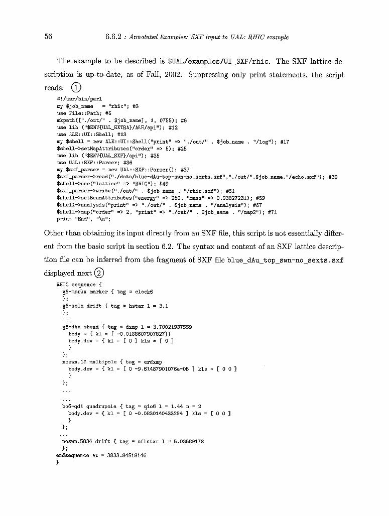
56 6.6.2 : Annotated Examples: ! X F inpu t t o UAL: RHIC example

The example to be described is $UAL/e:xamples/UI-SXF/rhic. The SXF lattice de-

scription is up-to-date, as of Fall, 2002. Suppressing only print statements, the script

reads; @ #!/usr/bin/perl my $job-name = "rhic"; #3 use File::Path; #5 mkpath(C"./out/" . $job-namel, 1, 0755); #6 use lib ("$ENV{UAL_EXTRA3/ALE/api") ; #12 use ALE::UI::Shell; #13 my $shell = new ALE::UI::Shell("print" => "./out/'' . $job-name . "/log"); #17 $shell->setMapAttributes("order" => 5); #25 use lib ("$ENV{UAL-SXF)/api") ; #35 use UAL::SXF::Parser; #36 my $sxf-parser = new UAL::SXF::Parser(); #37 $sxf -parser->read(". /data/blue-dAu-top-swn-no-sexts . sxf It, 'I. /out/ll. $job-name. "/echo. sxf ") ; #39 $shell->use ("lattice" => IIRHICII) ; $49 $sxf-parser->write("./out/" . $job-name . "/rhic. sxf ") ; #51 $shell->setBeamAttributes ("energy" => 250, "mass" => 0.93827231) ; #59 $shell->analysis ("print" => It. /out/" . $job-name . "/analysis") ; #67 $shell->map("order" => 2, "print" => 'I ./out/" . $job-name . "/map2") ; #71 print "End", "\n" ;

Other than obtaining its input directly from i%n SXF file, this script is not essentially differ-

ent from the basic script in section 6.2. The syntax and content of an SXF lattice descrip-

tion file can be inferred from the fragment of SXF file blue-dAu-top-swn-no-sexts . sxf

displayed next @ RHIC sequence { g6-markx marker { tag = clock6

g6-solx drift { tag = hstar 1 = 3.1 3;

3; ... g6-dhx sbend { tag = dxmp 1 = 3.70021937559 body = kl = C -0.018860790782713 body.dev = C kl = I: 0 1 kls = C 0 1 3

3; noswn.14 multipole { tag = erdmp body.dev = C kl = C 0 -9.61487901076e-05 1 kls = I: 0 0 1 3

3; . . ..

bo6-qdl quadrupole { tag = qlo6 1 = 1.44 n := 2 body.dev = C kl = C 0 -0.0830140433294 1 kls = C 0 0 1 3

3 ; ... noswn.5834 drift { tag = oflstar 1 = 5.0358!3178 3;

endsequence at = 3833.84518146 3

6.6.2 : Annotated Examples: SXF input t o UAL: RHIC example 57

A few of the lattice elements supported by SXF-marker, sbend, multipole, quadrupole-

are visible in this listing. A complete listing of supported elements is given in section D.3.

Also visible in @ are LatName’s such as g6-markx7 g6-solx, g6-dhx, noswn.14, and

noswn.5834, the final two of which show tlhe mechanism for making LatName’s unique

when the same the same GenName appears more than once in the design lattice. As men-

tioned above, the GenNume’s, i.e. design names, such as clock6 and hstar are retained

using the tag= syntax. The n=2 entry records a “complexity” index, which TEAPOT in-

terprets as ir=2. Element lengths are given lby 1= entries and their strengths by multipole

lists such as kl = C 0 -0.0830140433294 11. Browsing the simulation script 0 , the first few lines are routine. From line. #I7

one sees that this simulation is performed using the shell ALE: : U I : : Shell, the code of

which is $UAL-EXTRA/ALE/api/ALE/UI/She:L1. pm. (This pathname is constructed using

statement #I2 and the conventional file naming prescription.) By lines #35 through #37

the SXF parser code is $UAL-SXF/api/UAL/SXF/Parser .pm. Note that these scripts are

generic; i.e. they are not RHIC-specific. Line #39 reads in the SXF file, a fragment of

which was shown above under @ . After establishing beam attributes in line #59, this

script, in line #67, evaluates and prints out beginning and ending Twiss parameters to file

. /out/rhic/analysis and prints out the second order, once-around transfer map in line

. /out /rhi c /map2.

For completeness the elements and element attributes supported by SXF would be

documented here. But this guide (in section D.3) documents ADXF instead, correlating

its properties with the SMF lattice object model. Of course the elements described by

SXF and ADXF are essentially similar, differing, in the case of, say, RHIC, by RHIC-

specific features. The extensibility feature of ISMF is what makes the support of alternative

descriptions straightforward.

58 6.7 : Annotated Examples: FastTeapot

6.7. FastTeapot

As mentioned in the introduction, FastTeapot consists of recently developed C++ code

whose purpose is implied by its name. Since the present user guide primarily documents the

Per1 interface, as contrasted with the C++ code, it cannot properly document FastTeapot.

However, a few words can be said about the motivation behind examples

$UAL/examples/FastTeapot/linux/evolver, $UAL/examples/FastTeapot/linux/tracker,

both of which are C++ executables. (Compilation instructions are given in the README

file.) Their purpose is to exercise the Elemen$-Algorithm-Probe framework and to compare

computation times and results obtained using traditional element-by-element TEAPOT re-

sults with (matrix multiplication through sectors) FastTeapot results. Matrix multiplica-

tion is the most obvious speed-up mechanism. for mapping through sectors. An application

that came up recently requires tracking that needs to be fast while retaining a faithful

representation of chromatic effects; in particular the second order coefficients T116, T226,

T336, and T446 need to be accurate.

With canonical (x, p z ) variables, even transport through drifts brings in chromatic

effects which, being second order, are not accurately modeled by pure linear matrix mul-

tiplication. On the other hand drifts sections are linear when (z,x’ = dx/ds), (position,

slope) variables, are used instead of x,pz (and likewise for y,pg). In these coordinates,

even with no quadratic terms included, the desired chromatic effects are retained. So ma-

trix evolution through drifts retains the correct contribution of drifts to chromaticity. Of

course quadrupoles, sextupoles, and octupoles continue to need symplectic, TEAPOT kick

treatment. It is not claimed that this particular procedure is universally applicable, but it

does exercise the Element-Algorithm-Probe framework.

Program evolver calculates second order, once-around maps two ways: one uses

only traditional element-by-element TEAPOT kick-tracking; the other uses kick-tracking

through quadrupoles and nonlinear elements, but uses the non-canonical (x, d) coordi-

nates of the previous paragraph through other elements. Of the second order coefficients

determined, it is only T116, T226, T336, and T44, that are expected to agree in this compar-

ison. Program tracker is similarly motivated. It uses the same two evolution mechanisms

6.7 : Annotated Examples: FastTeapot 59

to perform multiparticle tracking of a bunch. of particles. The idea is that tunes obtained

by FFT processing of the outputs of program tracker can be used to extract, and hence

compare, off-momentum tune dependence.

Chapter 7. MPI Multiprocessor Suppolrt

Since tracking many particles for many turns through a long and complicated accelerator

lattice takes a long time, it is extremely useful to have access to a cluster of workstations

working simultaneously. Sometimes one wishes to run the same simulation for a variety of

parameter values. This leads to the “lowest tech” use of multiple processors-one simply

uses one computer for each of the parameter combinations. This requires no multipro-

cessing software. The next simplest case is that of Monte Carlo calculations, for example

to determine dynamic aperture, in which randomly selected particles are tracked through

multiple lattices having randomly assigned error fields and misalignments. In the past

calculations like this have often used multiple computers in the trivial way just mentioned.

But already in this case, which is known as “embarassingly parallelizable” because so lit-

tle interprocess communication is required, it is extremely useful to have special purpose

multiprocessor software. Without such software lengthy output files tend to exceed the

available storage space and the book-keeping becomes onerous. Multiprocessor software

permits one node-the term node is normally used instead of processor in this context-

both to do this bookkeeping and to take responsibility for assigning particles and/or lattices

to the remaining nodes. The MPI module of‘ UAL is ideal for this purpose.

The MPI module of UAL is also ideal for the next more complex type of calculation

in which there are multiple particles (prob,ably with a single lattice) and a large (but

“not overwhelming”) amount of interprocess communication is required. Here we have

in mind multiparticle simulations involving space charge or beam-beam interactions, for

which considerations of computation time make it all but obligatory to employ multiple

processors. Again it is natural to distribute equal numbers of particles to all but one of

the nodes. Then, since every particle is influenced by every other particle, the information

about a particle in one node has to be made available to all the other nodes. However

this information need not be ‘Loverwhelming”. The calculation can be performed in two

steps such that all-on-all intercommunication is avoided. Gathering data from each of the

tracking nodes, a managing node can work out a space charge field, which it redistributes

to all the tracking nodes. As long as this computation time is short compared to the

- 60 -

7.1 : M P I Multiprocessor Support: M P I installation 61

tracking times the overall computation rate can be almost proportional to the number of

nodes in the cluster.

The so-called “message-passing” model of parallel computing is just one of the ways

of harnessing the power of multiple computers. It is the one adopted by MPI (Message

Passing Interface). It seemed to be the best approach for the level of complexity of parallel

processing inost frequently encountered in accelerator simulation (though not necessarily

for all multiprocessing tasks.) An excellent reference is by Gropp, Lusk, and Skjellum.lG

MPI is a specification for libraries of subroutines written in Fortran, C, and C++. As

such MPI is not a “language” and there is no MPI compiler. Rather the subroutines

are compiled and linked by the appropriate Fortran, C, or Cff compiler. There can be

more than one implementation of the MPI standard. The one employed by UAL is known

as MPICH17 where the “CH” derives from ‘Chameleon” which apparently was the name

of an early version. When the letter combination “ch” appears, for example in device

type “chp4” they refer back to this early code. MPICH and its various utilities are public

domain software.

7.1. MPI installation

Instructions will be given here for download’ing, configuring, and testing the MPI software

on a single node. This is not to suggest that ithere is a great advantage to running multiple

processes on the same computer. Rather, the purpose is to get the software running in the

simplest possible environment. Configuration of multiple nodes is straightforward, but

specific to the number and types of nodes axailable; instructions are included as part of

the download in the file doc/mpichman-chp4 .pdf.

To start, one downloads file mpich. tar. g:z from http: //www .mcs . an1 . gov/mpi/mpich, saving it, for example, in dirctory Nualusr/tools/tmp. For documentation see

http://www-unix.mcs.anl.gov/mpi/mpich/docs/mpic~an-chp4.pdf

The code is unpacked (into a directory mpich-1.2.4, possibly with a later version number),

compiled, and installed using the instructions

$ cd “ualusr/tools/tmp $ gzip -d mpich.tar.gz $ tar xvf mpich.tar

62 7.1 : MPI Multiproceswr Support: MPI installation

$ cd mpich-1.2.4 $ . /configure --with-device=ch-.p$ --pref ix=/export/home/ualusr/tools/mpich

--enable-sharedlib > & configure . l og $ make > & make.log $ make install > & install.log

Since this example assumes a private version of MPI is being installed in the directory

wualusr/tools/mpich, root privilege is unnecessary to complete these steps.t

In the configuration step the device was specified to be --with-device=ch-p$ which is

the correct type for MPMD (multiple-processor, multiple-data) (possibly heterogeneous)

Unix clusters. The shared library flag --ena.ble-sharedlib is supported in systems (like

UAL) compiled using gcc. Other configuration flags are specified in section 4.1 of the

mpichman-chp4 documentation listed above. As the make finishes, near the bottom of

make. log, the following paragraph appears:

Completed build of MPI. Check the output for errors. Also try executing 'make testing' in examples/test (This relies on mpirun, which currently works for many but not all systems. networks, mpirun requires that you. first setup a "machines" file listing the machines available; this is covered in the installation manual. )

For workstation

Other than checking the output €or errors this test should be deferred as it tries to access

more than one node.

After MPICH has been built, appropriate environment variable and path have to be

set;

$ setenv MPIHOME "ualusr/tools/mpich $ set path = ($MPIHOME/bin $path) $ setenv LD-LIBRARY-PATH $MPIHOME/lib/shared/$LD-LIBRARY-PATH

Then one can test the set-up by

$ cd $MPIHOME/examples $ make $ mpirun -np 1 cpi

~ ~

f For later convenience in starting up multiple nodes on heterogeneous clusters the configuration looks for, and tests rsh and ssh. Depending on the local set-up, either of these can appear to hang the con- figuration process with the most recent line in configure. log saying, for example, checking whether /usr/kerberos/bin/rsh works. . . , but, after a seemingly interminable delay, the time-out(s) will end and the configuration will continue. If this problem occurs it need not fixed right away since it will not disable the examples given here as they function in a single computer.

7.2 : MPI Multiprocessor Support: Overview of MPI 63

This runs a toy program cpi that calculates 7r by the thoroughly impractical method of

evaluating numerically an integral whose valiie is known analytically to be 7r. The program

subdivides the range of integration and distributes the ranges to the available processors.

In this case the command line arguments -np 1 state that one processor is available.

The utility script . /mpirun detects what is needed from the environment-its defaults

correspond to the present installation-and then runs the program.

The program cpi is the compiled version of the C program cpi. c. This program is

thoroughly documented in reference16. The same calculation is performed by the Fortran

program pi3. f which is run identically, replacing cpi by pi3 in the listing above.

Using MPICH on multiple nodes requires that the available nodes are correctly con-

figured and described. The main requirement is that rsh, or an equivalent remote shell

access, function correctly. This is too specialized for further discussion in this manual.

What needs to be done is clearly explained in the the mpichman-chp4 .pdf documentation

mentioned above. Some access may require the intervention of the system administrator.

7.2. Overview of MPI

Just to skim the general ideas, this section extracts key points from Gropp et a1.16. For

any kind of detail this reference, and the others listed previously, should be referred to.

For the calculations being performed in multiple processors to be coordinated by mes-

sage passing there are certain minimal requirements that have to be met. Basically data

from the address space of one processor has to be written into the address space of another.

This process requires cooperation between the two participants. One process sends the

data, but the transaction is only complete when the other has received it. The minimal

message interface for these two actions is

send(address , length, destination, tag) receive (address , length, source , tag, actlen)

The send line specifies the location and length (in sequential bytes) of the data to be

transferred, and identifies the recipient. In MPI functioning on n processors, each process

has an identifier, known as its rank, an integer in the range from 0 to n - 1; destination

and source are so identified. The tag argument is the beginnings of a mechanism for

64 7.3 : M P I Multiprocessor Support: MPI applied to UAL

differentiating among a possible multiplicity of messages. Assuming a match of the tags,

the receive line identifies the sender, and specifies the address where the data is to be

placed and its expected length. The argument actlen, specifying the actual length of the

received data, provides the beginnings of an error flagging mechanism.

The MPI protocol goes well beyond this minimal specification of message transfer.

For one thing the data being transferred can be organized into far more complicated,

non-contiguous structures. Also a communicator object, identified by a comm argument,

supports communication. So the actual MPI: send/receive interface is

MPI-Send(address, count, datatype, destination, tag, comm) MPI-Recv(address, maxcount, datatype, source, tag, comm, status)

The more-complicated data structure location information is encoded into the address , count, and datatype arguments.

Before these operations can be used a certain amount of initialization is required, and

graceful termination of the multiprocessor program is also essential. Along with MPI-Send

and MPI-Recv, a minimal MPI version would therefore contain16

MPI -Init Initialize MPI MPI-Comm-size Find out how many processes there are MPI-Comm-rank Find out which process I am MPI-Finalize Terminate MPI

As mentioned previously, these and all other MPI routines need to be compiled into the

simulation programs running on the various machines, using the native compiler for the

computer language of the simulation being run.

7.3. MPI applied to UAL

One thing to be appreciated is that the UAL. user accesses MPI indirectly via Perl, and the

Perl interface does not necessarily make all MPI routines described in MPI documentation

directly accessable to the user-not even all the routines mentioned in the previous section.

Routines needed to establish and terminate multiprocessor computations are supported,

but arbitrary internode communication is not. The reason for this is that, because of its

interpreted rather than compiled nature, message passing via Perl is slow. To circumvent

this, message passing among nodes within TJAL occurs at the Cff level. The primary

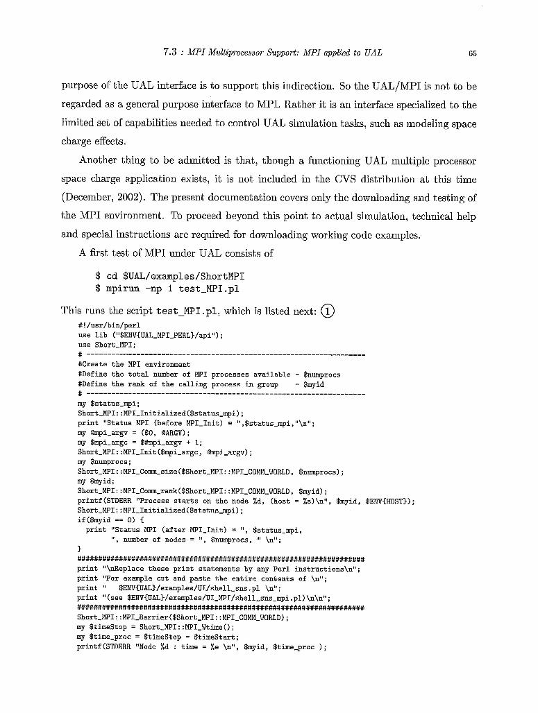
7.3 : MPI Multiprocessor Support: MPI applied t o UAL 65

purpose of the UAL interface is to support this indirection. So the UAL/MPI is not to be

regarded as a general purpose interface to MPI. Rather it is an interface specialized to the

limited set of capabilities needed to control TJAL simulation tasks, such as modeling space

charge effects.

Another thing to be admitted is that, though a functioning UAL multiple processor

space charge application exists, it is not included in the CVS distribution at this time

(December, 2002). The present documentation covers only the downloading and testing of

the MPI environment. To proceed beyond this point to actual simulation, technical help

and special instructions are required for downloading working code examples.

A first test of MPI under UAL consists of

$ cd $UAL/examples/ShortMPI $ mpirun -np 1 test-MPI.pl

This runs the script test-MPI . p l , which is llisted next: 0 #!/usr/bin/perl use lib ("$ENVIUAL-MPI-PERL)/api") ; use Short-MPI;

#Create the MPI environment #Define the total number of MPI processes available - $numprocs #Define the rank of the calling process in group - $myid

my $status-mpi; Short-MP1::MPI-Initialized($status-mpi); print "Status MPI (before MPI-Init) = ",$status-mpi,"\n"; my Qmpi-argv = ($0, QARGV) ; my $mpi-argc = $#mpi-argv + i; Short-MP1::MPI-Init($mpi-argc, Qmpi-argv); my $numprocs; Short-MPI::MPI-Comm-size($Short-MPI::MPI-COMM.~WORLD, $numprocs); my $myid; Short-MPI::MPI-Comm-rank($Short-MPI::MPI-COMM.~WORLD, $myid); printf(STDERR "Process starts on the node %d, (host = %s)\nll, $myid, $ENV{HOST)); Short-MPI: :MPI-Initialized($status-mpi) ; if($myid == 0 ) I print "Status MPI (after MPI-Init) = I(, $stiitus-mpi,

' I , number of nodes = #I, $numprocs, '\n"; 1 ...................................................................... print "\nReplace these print statements by any Per1 instructions\n"; print "For example cut and paste the entire contents of \n"; print print 'I (see $ENVIUAL~/examples/UI~MPI/shell~s~is~mpi .pl) \n\nll ; . . . . . . . . . . . . . . . . . . . . . . . . . . . . . . . . . . . . . . . . . . . . . . . . . . . . . . . . . . . . . . . . . . . . . . Short~MPI::MPI~Barrier($Short~MPI::MPI~COMM~W[lRLD); my $timestop = Short-MPI: :MPI-Wtime() ; my $time-proc = $timestop - $timestart; printf (STDERR "Node %d : time = %e \n9I, $myid,, $time-proc ) ;

$ENV~UAL)/examples/UI/shell-sns . pl '\n" ;

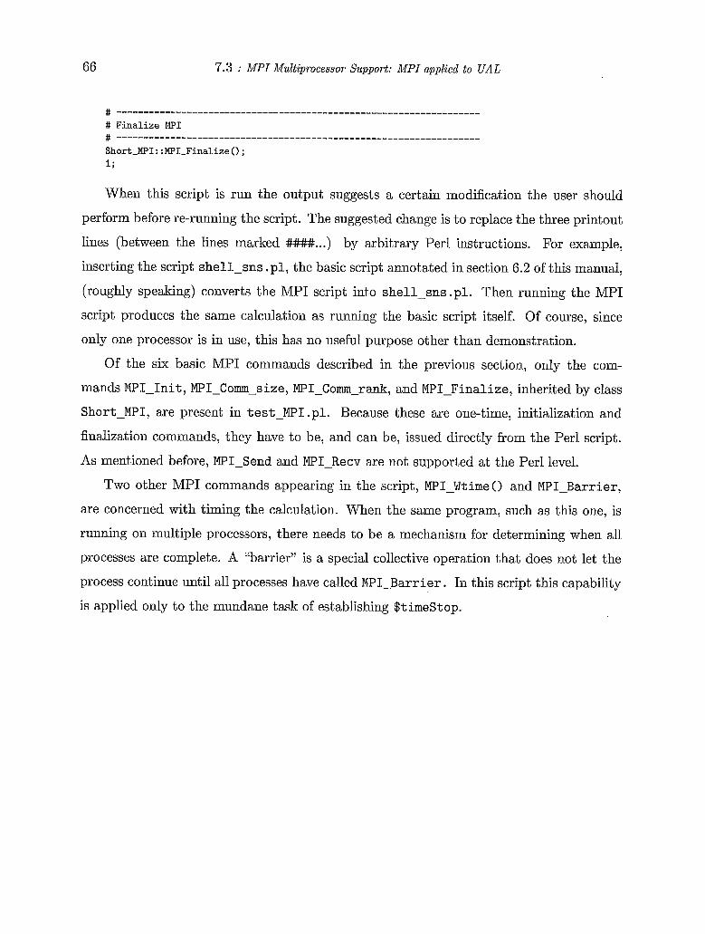
66 7.3 : MPI Multiprocessor Support: MPI applied t o UAL

When this script is run the output suggests a certain modification the user should

perform before re-running the script. The suggested change is to replace the three printout

lines (between the lines marked #### ...) by arbitrary Perl instructions. For example,

inserting the script shell-sns .pl, the basic script annotated in section 6.2 of this manual,

(roughly speaking) converts the MPI script into shell-sns.pl. Then running the MPI

script produces the same calculation as running the basic script itself. Of course, since

only one processor is in use, this has no useful purpose other than demonstration.

Of the six basic MPI commands described in the previous section, only the com-

mands MPI-Init, MPI-Corn-size, MPI-Corm-rank, and MPI-Finalize, inherited by class

Short-MPI, are present in test-MPI . pl. Because these are one-time, initialization and

finalization commands, they have to be, and can be, issued directly from the Perl script.

As mentioned before, MPI-Send and MPI-Recv are not supported at the Perl level.

Two other MPI commands appearing in. the script, MPI-WtimeO and MPIBarrier,

are concerned with timing the calculation. When the same program, such as this one, is

running on multiple processors, there needs to be a mechanism for determining when all

processes are complete. A “barrier” is a special collective operation that does not let the

process continue until all processes have called MPIBarrier . In this script this capability

is applied only to the mundane task of establishing $timestop.

Appendix A. Ancestry of UAL

The ancestry of UAL can be traced back as far as the early days of the SSC (Supercon-

ducting Supercollider) even before it had that name, when it was being designed at the

CDG (Central Design Group) in Berkeley.

As the SSC was being planned, it was realized that a design as conservative as the

Fermilab Tevatron might be unacceptably expensive. At the CDG plans were set in motion

to study this issue experimentally (Fermilab Experiment E778) and by computer simulation

and other theoretical studies.

The program TEAPOT18, was developed both to design and analyse experiment E778

and to anticipate performance of the SSC using computer simulation. At the same time,

and the same place, mapping techniques and. differential algebra were being developed to

put the numerical work on a firmer and more powerful theoretical foundation. After the

SSC project moved to Dallas a computational structure called PAC (Platform for Acceler-

ator corn put at ion^)^^-^^ was developed, with the purpose of permitting the integration of

diverse computer codes. PAC adopted the ‘,‘object oriented” approach (whose value was

just becoming universally appreciated at the time) to computer software. At Cornell, in

the period following the termination of the SEIC, this architecture was exploited to integrate

TEAPOT++ (upgraded from procedural Fortran and C to object oriented C++) along

with PAC and DA into UAL (Unified Accelerator Libraries.)’ For the first time in UAL,

this permitted element-by-element tracking to be integrated with analyses using maps of

arbitrary order. This satisfied the goal: “Special-purpose codes should be modular in ways

that permit them to be combined as parts od more general calculations.” (Aside: the re-

cently developed Element-Algorithm-Probe framework greatly expands this capability.)

The next code to be integrated (though only through adoption of input format) into this

environment was MAD (Methodical Aceelerator Design) which is the pre-eminent lattice

code for designing transfer lines and sectors of high energy lattices. Shortly thereafter,

responsive to “Call for a New Accelerator and driven by the need, within

the US-LHC collaboration, for a mechanism to share design information of the LHC, a

Standard Exchange Format (SXF)22 was developed and integrated into UAL, (as well,

- 6’7 -

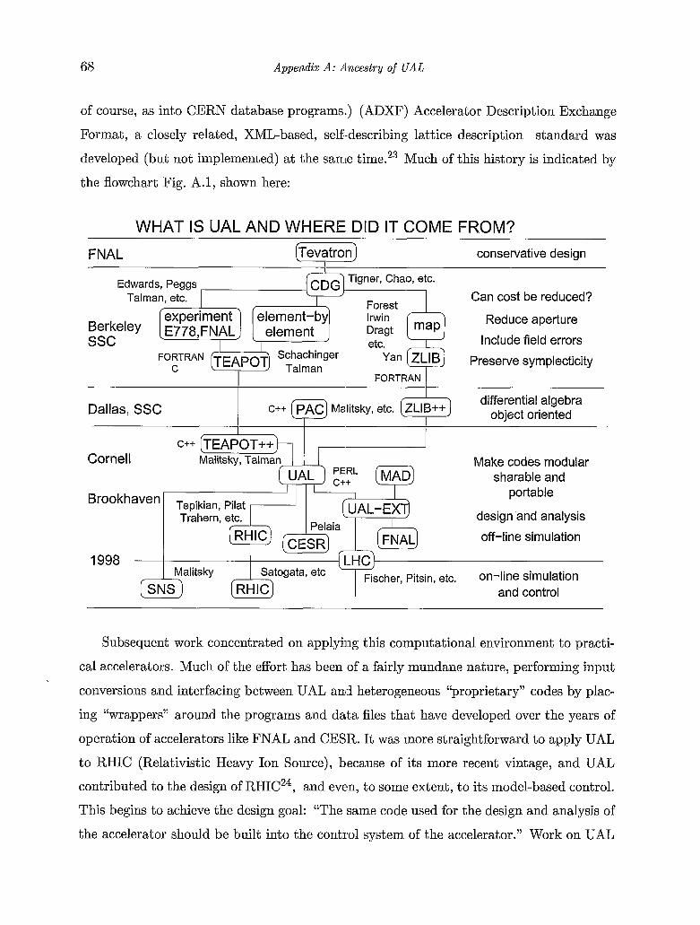
68 Appendix A: Ancestry of UAL

of course, as into CERN database programs.) (ADXF) Accelerator Description Exchange

Format, a closely related, XML-based, self-describing lattice description standard was

developed (but not implemented) at the same time.23 Much of this history is indicated by

the flowchart Fig. A.1, shown here:

WHAT IS UAL AND WHERE DID IT COME FROM? FNAL [Teva t ron) conservative design

I Tigner, Chao, etc. Edwards, Peggs

Talman, etc. Can cost be reduced?

Irwin Reduce aperture

Include field errors

Preserve symplecticity

experiment Berkeley E778,FNAL ssc

Schachinger C

Dallas, SSC differential algebra

object oriented 1 c++ @ Malitsky, etc.

Cornell Malitsky, Talman Make codes modular sharable and

portable

design and analysis

off-line simulation

sin, etc, on-line simulation and control

Brookhaven Tepikian, Pilat

1998

Subsequent work concentrated on applying this computational environment to practi-

cal accelerators. Much of the effort has been of a fairly mundane nature, performing input

conversions and interfacing between UAL and heterogeneous “proprietary” codes by plac-

ing “wrappers” around the programs and data files that have developed over the years of

operation of accelerators like FNAL and CESR. It was more straightforward to apply UAL

to RHIC (Relativistic Heavy Ion Source), because of its more recent vintage, and UAL

contributed to the design of RHIC24, and even, to some extent, to its model-based control.

This begins to achieve the design goal: “The same code used for the design and analysis of

the accelerator should be built into the control system of the accelerator.” Work on UAL

Appendix A: Ances t ry of U A L 69

continued after Malitsky went to the SNS in 1999.25-26 This has included the capability of

importing special purpose codes ACCSIM and ORBIT into the UAL environment. This

adds capabilities such as space charge analysis, radiation damage, and injection “painting”

into the simulation e n ~ i r o n m e n t . ~ ~ - ~ ~ Also progress was made toward integrating UAL

into the SNS control system. Currently FastTeapot is being incorporated into the RHIC

control system.

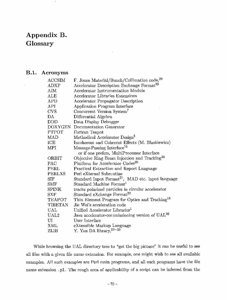
Appendix B. Glossary

B. 1. Acronyms ACCSIM F. Jones Material/Bunch/Collimation code,29 ADXF Accelerator Description Exchange Format23 AIM Accelerator Instrumentation Module ALE Accelerator Libraries Extensions APD Accelerator Propagator Description API Application Prograin Interface cvs Concurrent Version System7 DA Differential Algebra DDD Data Display Debugger DOXY GEN Document at ion Generator FTPOT MAD ICE MPI

ORBIT PAC PERL PERLXS SIF SMF SPINK SXF TEAPOT TIBETAN UAL UAL2 UI XML ZLIB

Fortran Teapot Methodical Accelerator Design5 Incoherent and Coherent Effects (M. Blaskiewicz) Message-Passing Interfacel6

or if one prefers, :MultiProcessor Interface Objective Ring Beam Injection and Tracking3’ Platform for Accelerator Codes20 Practical Extraction and Report Language Perl external Subroutine Standard Input For:mat31, MAD etc. input language Standard Machine Format’ tracks polarized particles in circular accelerator Standard exchange Format22 Thin Element Program for Optics and Tracking’* Jie Wei’s acceleration code Unified Accelerator Libraries’ Java accelerator-cornmissioning version of UAL26 User Interface extensible Markup Language Y. Yan DA l i b r a r ~ , ~ ~ - ~ ~

While browsing the UAL directory tree to “get the big picture” it can be useful to see

all files with a given file name extension. For example, one might wish to see all available

examples. All such examples are Perl main programs, and all such programs have the file

name extension . p l . The rough area of applicability of a script can be inferred from the

Appendix B: Glossary 71

name of the directory in which it is contained. Here is an instruction to list all examples,

followed by two lines of response:

% cd $UAL; find . -name * .pl" -print ... ./examples/ShortMPI/test-MP1.pl ./examples/UI/shell-sns.pl

As mentioned before, the scripts in directories other than . /examples, though out-dated,

can be browsed and, in most cases, run. Some may be useful for code test purposes.

B.2. File name extensions .bs, .xs, .xsc, .PL

.cc, .cpp

.hh, .h

.c

.css

.11, .YY

.PI

. cfg

.sxf

.pm

.map, .zmap

.so

Perl/C++ interface C source code C.f+ source code Cascading Style Sheet C++ /C header lex, yacc parser support Perl main program Perl Module DiaVTps map configuration data shared library SXF lattice description

Appendix C. Accelerator Parameters

T h e contents of this appendix will probably move t o the V A L Physics Manual” when that

document comes into existence.

C.l. Global geometry and survely

The global ( X , Y, 2) and local (2, y , s) coordinate systems used by UAL are identical to

those used by MAD5. The global survey code was ported from that source, as was much

of the discussion in this section. There is a strong prejudice towards having the reference orbit lie close to a plane perpendicular to the Z-axis. t

The survey command reconstructs the global coordinates of all elements in the lat-

tice. For this purpose all elements except RIBEND’S and SBEND’s are treated as drifts.

Elements like KICKER’S, which could, in practice, influence the closed orbit, are assumed

to have been set to zero. Similarly, QUAD’S etc., which would steer the beam centroid if

they were misaligned, are assumed not to be misaligned for purposes of first calculating

the ideal closed orbit. For the lattice to make sense as a storage ring the lattice should

“close”, but exact closure (or any degree of closure whatsoever) is not required. In mul-

titurn tracking every particle is displaced to take up any closure defect as its orbit passes

the origin. Though unphysical, this discontinuous translation is at least symplectic and is

unlikely to cause any harm to a simulation, provided it is not very large.

Unlike the survey command, the analysis command calculates the closed orbit in

.the presence of all steering perturbations ju.st mentioned, and also includes any vertical

steering due to RBEND and SBEND roll errors.

The global coordinates, both displacemeiits and angles relative to the global ( X , Y, 2)

frame, are exhibited in Fig. C.l.l, which is a revised (but not intentionally changed) version

t Within the TEAPOT module the prejudice toward the reference orbit lying in a single plane goes so far as to exclude non-horizontal RBEND and SBEN:D components. Out of plane reference orbits have to be modeled by KICK elements. This restriction could be, but has not been, lifted using the Element- Algorithm-Probe framework. In any case this restriction is orthogonal to the definition of both local and global coordinates.

- 7:2 -

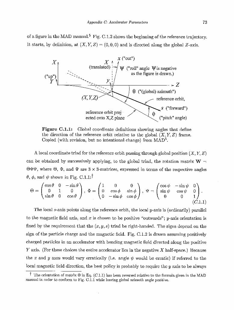
Appendix C: Accelerator Parameters 73

of a figure in the MAD m a n ~ a l . ~ Fig. (3.1.2 shows the beginning of the reference trajectory.

It starts, by definition, at ( X , Y, 2) = (0, 0,O) and is directed along the global Z-axis.

x ("out") X ? c

. (translated) bJ v (~lrol1~t angle v is negative as the figure is drawn.)

.. . .. . . 8 ("(global) azimuth")

reference orbit proj- ected onto X,Z plane

Figure C.l . l: Global coordinate lclefinitions showing angles that define the direction of the reference orbit relative to the global ( X , Y, 2) frame. Copied (with revision, but no intentional change) from MAD5.

A local coordinate triad for the reference orbit passing through global position ( X , Y, 2)

can be obtained by successively applying, to the global triad, the rotation matrix W =

0@Q, where 0, a, and Q are 3 x 3-matricel3, expressed in terms of the respective angles

0, $, and $ shown in Fig. C.1.1:t

cos0 0 -sin0 cos$ -sin$ 0

sin0 0 0 -sin$ cos$ (C. 1.1)

The local s-axis points along the referencle orbit, the local y-axis is (ordinarily) parallel

to the magnetic field axis, and x is chosen tal be positive "outwards"; y-axis orientation is

fixed by the requirement that the (x, y, s ) triad be right-handed. The signs depend on the

sign of the particle charge and the magnetic field. Fig. C.1.2 is drawn assuming positively

charged particles in an accelerator with bend.ing magnetic field directed along the positive

Y axis. (For these choices the entire accelerator lies in the negative X half-space.) Because

the x and y axes would vary erratically (i.e. angle $ would be erratic) if referred to the

local magnetic field direction, the best policy is probably to require the y axis to be always

T The orientation of matrix 0 in Eq. (C.l.l) has been reversed relative to the formula given in the MAD manual in order to conform to Fig. C.l . l while leaving global a.zimuth angle positive.

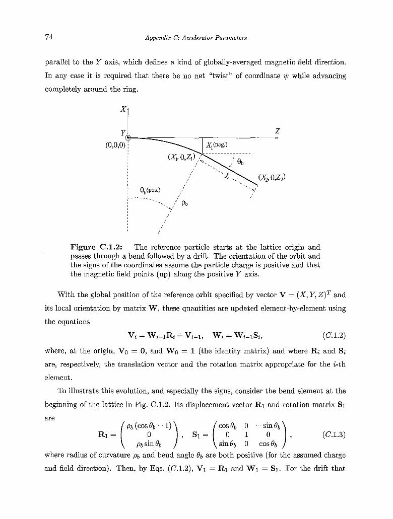
74 Appendix G: Accelerator Parameters

parallel to the Y axis, which defines a kind of globally-averaged magnetic field direction.

In any case it is required that there be no net “twist” of coordinate y5 while advancing

completely around the ring.

“1

Figure C.1.2: The reference particle starts at the lattice origin and passes through a bend followed by a drift. The orientation of the orbit and the signs of the coordinates assume the particle charge is positive and that the magnetic field points (up) along the positive Y axis.

With the global position of the reference orbit specified by vector V = (X, Y, Z)T and

its local orientation by matrix W, these quantities are updated element-by-element using

the equations

Vi = Wi-IRi f Vi-1, Wi = Wi-ISi, (C. 1.2)

where, at the origin, Vo = 0, and Wo = 1 (the identity matrix) and where Ri and Si are, respectively, the translation vector and the rotation matrix appropriate for the i-th

element.

To illustrate this evolution, and especially the signs, consider the bend element at the

beginning of the lattice in Fig. C.1.2. Its displacement vector R1 and rotation matrix S1

are cos& 0 -sin&

sin& 0 cosBb (C. 1.3)

where radius of curvature pb and’bend angle o b are both positive (for the assumed charge

and field direction). Then, by Eqs. (C.1.2), V1 = R1 and W1 = SI. For the drift that

R 1 = ( Pb (cos 0 Qb - 1) ) , S I = ( 0 1

Pb sin o b

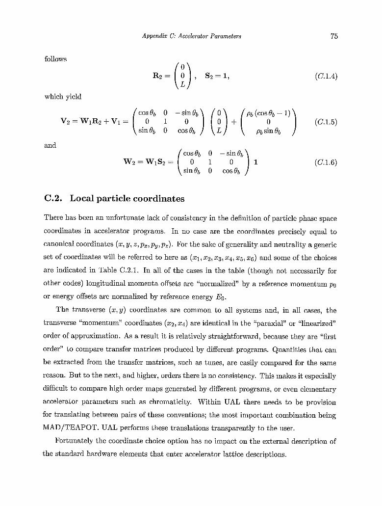
Appendix C: Accelerator Parameters 75

follows

R 2 = (!:), S 2 = 1 , (C. 1.4)

which yield

and

(C. 1.6)

C.2. Local particle coordinates

There has been an unfortunate lack of consistency in the definition of particle phase space

coordinates in accelerator programs. In no’ case are the coordinates precisely equal to

canonical coordinates (z, y, x , p x , p , , p z ) . For the sake of generality and neutrality a generic

set of coordinates will be referred to here as (21, 2 2 , z3, xq, x5, z g ) and some of the choices

are indicated in Table C.2.1. In all of the cases in the table (though not necessarily for

other codes) longitudinal momenta offsets are “normalized” by a reference momentum po

or energy offsets are normalized by reference energy Eo.

The transverse (x,y) coordinates are common to all systems and, in all cases, the

transverse “momentum” coordinates ( z 2 , 2 4 ) are identical in the “paraxial” or “linearized”

order of approximation. As a result it is relatively straightforward, because they are “first

order” to compare transfer matrices produced by different programs. Quantities that can

be extracted from the transfer matrices, such as tunes, are easily compared for the same

reason. But to the next, and higher, orders there is no consistency. This makes it especially

difficult to compare high order maps generated by different programs, or even elementary

accelerator parameters such as chromaticity. Within UAL there needs to be provision

for translating between pairs of these conventions; the most important combination being

MAD/TEAPOT. UAL performs these translations transparently to the user.

Fortunately the coordinate choice option has no impact on the external description of

the standard hardware elements that enter accelerator lattice descriptions.

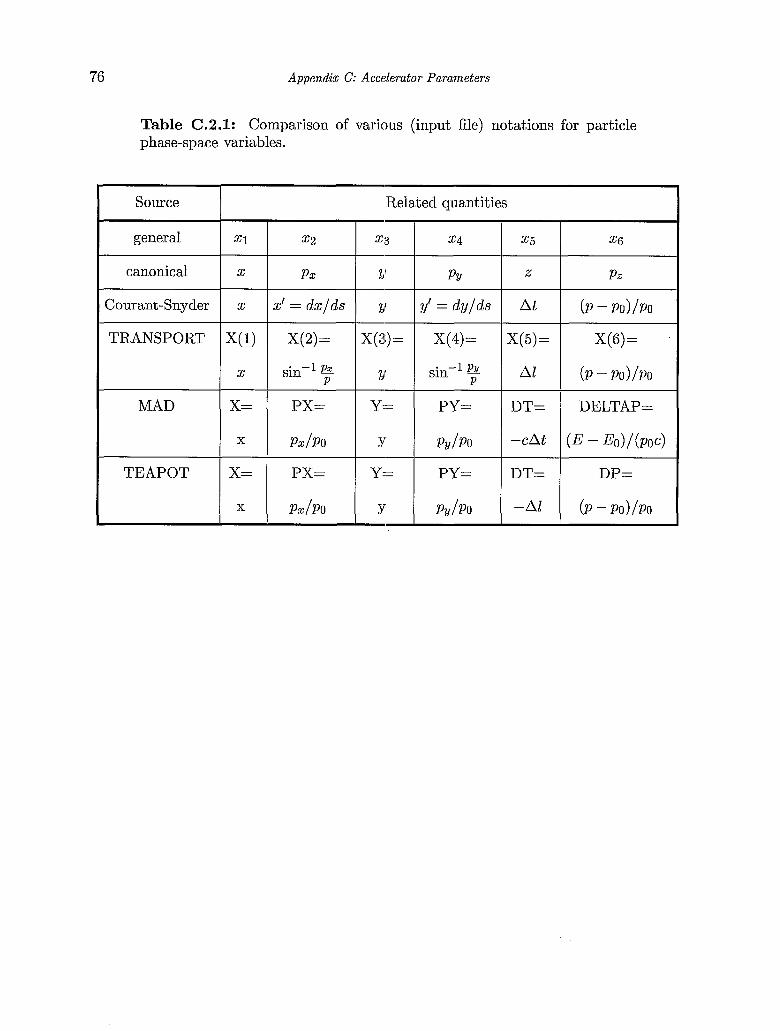
76 Appendix C: Accelerator Parameters

Table C.2.1: Comparison of various (input file) notations for particle phase-space variables.

Appendix D. The Evolution of Standard :Machine Format (SMF)

D.l . The SMF object model

The heart of UAL is SMF (Standard Machine Format). It is an abstract accelerator

object model capable of including all parameters of a lattice or lattices under study. It

is, in principle, capable of being realized in various forms, internal or external, human or

machine-readable. But, in this manual, the term SMF will mainly apply to the internal

(to UAL) classes containing all lattice parameters.

The organization of SMF is exhibited graphically in Fig. D.l.l; actually two separate

object models are shown in the same figure. The more detailed version, (a), exhibits

the original implementation. Version (b) exhibits a more succinct, pattern-based, model,

which represents the same data in an up-to-date implementation.

The historical evolution of lattice descriptions is briefly reviewed in Appendix A. The

first attempt at standardization was SIF (Standard Input Format)31 which has evolved

into MAD.5 These formats have been sufficiently general to support much accelerator

design and simulation. They are however “closed”, meaning they are non-extensible, or

rather, extensions can be made only unilaterally or by mutual agreement. Though the

former has been common, the latter, more satisfactory, approach has typically required a

degree of organization greater than the community has been able to muster. One attempt,

SXF22, a portable lattice description supporting fully-instantiated parameter values (Le.

including deviations), has had some acceptance.

SMF is an abstraction or generalization of formats such as these; the primary moti-

vation is to support extensibility. The default accelerator types and their attributes are

pretty much the same as in these formats, but the introduction in a disciplined way of

new types, and new attributes for existing types, is supported. Without this flexibility it

would not be possible to incorporate diverse modules.

Fig. D.l.l(a) shows the original SMF impliementation. One sees both a DESIGN lattice

and a FLAT lattice. The DESIGN lattice is based on generic elements GenElement’s and

- 77 -

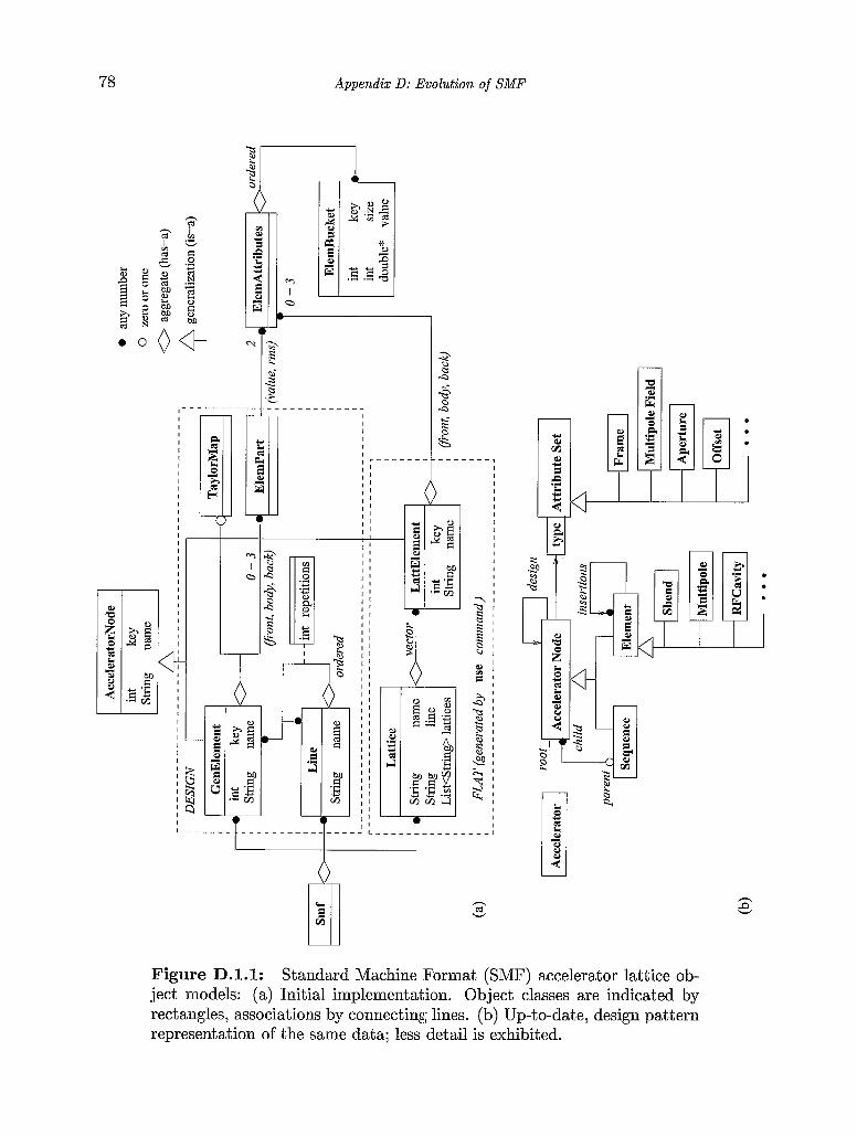
78 Appendix D: Evolution of SMF

c B 1 Ei

N,

I 0

]a I I I I I I I I I I I I I I I I I I I I I I

- 1

I I I I I I I I I I I I I I I I

I n-

$- Y

Figure D.l.l: Standard Machine Format (SMF) accelerator lattice ob- ject models: (a) Initial implementation. Object classes are indicated by rectangles, associations by connecting lines. (b) Up-to-date, design pattern representation of the same data; less detail is exhibited.

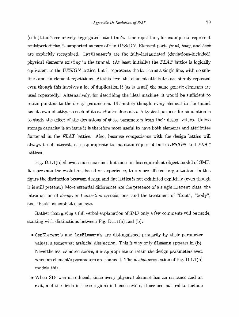
Appendix D: Evolution of SMF 79

(sub-)Line’s recursively aggregated into Line’s. Line repetition, for example to represent

multiperiodicity, is supported as part of the DESIGN. Element parts front , body, and back

are explicitly recognized. LatElement ’s arle the fully-instantiated (deviations-included)

physical elements existing in the tunnel. (At least initially) the PLAT lattice is logically

equivalent to the DESIGN lattice, but it represents the lattice as a single line, with no sub-

lines and no element repetitions. At this level the element attributes are simply repeated

even though this involves a lot of duplication if (as is usual) the same generic elements are

used repeatedly. Alternatively, for describing the ideal machine, it would be sufficient to

retain pointers to the design parameters. Ultimately though, every element in the tunnel

has its own identity, so each of its attributes does also. A typical purpose for simulation is

to study the effect of the deviations of these parameters from their design values. Unless

storage capacity is an issue it is therefore most useful to have both elements and attributes

flattened in the FLAT lattice. Also, because comparisons with the design lattice will

always be of interest, it is appropriate to maintain copies of both DESIGN and FLAT

lattices.

Fig. D.l.l(b) shows a more succinct but more-or-less equivalent object model of SMF.

It represents the evolution, based on experience, to a more efflcient organization. In this

figure the distinction between design and flat lattice is not exhibited explicitly (even though

it is still present.) More essential differences ,are the presence of a single Element class, the

introduction of design and insert ion associations, and the treatment of “front”, “body”,

and “back” as explicit elements.

Rather than giving a full verbal explanation of SMF only a few comments will be made,

starting with distinctions between Fig. D.l.l(a) and (b):

0 GenElement ’s and LatElement ’s are distinguished primarily by their parameter

values, a somewhat artificial distinction. This is why only Element appears in (b).

Nevertheless, as noted above, it is appropriate to retain the design parameters even

when an element’s parameters are changed. The design association of Fig. D.l.l(b)

models this.

0 When SIF was introduced, since every physical element has an entrance and an

exit, and the fields in these regions influence orbits, it seemed natural to include

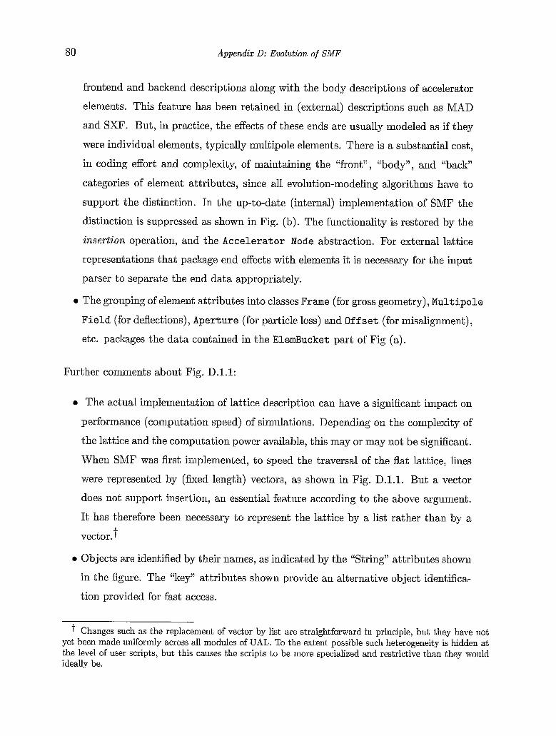
80 Appendix D: Evolution of SMF

frontend and backend descriptions along with the body descriptions of accelerator

elements. This feature has been retained in (external) descriptions such as MAD

and SXF. But, in practice, the effects of these ends are usually modeled as if they

were individual elements, typically multipole elements. There is a substantial cost,

in coding effort and complexity, of maintaining the “front”, “body”, and “back”

categories of element attributes, since a,ll evolution-modeling algorithms have to

support the distinction. In the up-to-da,te (internal) implementation of SMF the

distinction is suppressed as shown in Fig. (b). The functionality is restored by the

insertion operation, and the Accelerator Node abstraction. For external lattice

representations that package end effects .with elements it is necessary for the input

parser to separate the end data appropriately.

0 The grouping of element attributes into classes Frame (for gross geometry), Multipole

Field (for deflections), Aperture (for particle loss) and Off s e t (for misalignment),

etc. packages the data contained in the ElemBucket part of Fig (a).

Further comments about Fig. D.l.l:

0 The actual implementation of lattice description can have a significant impact on

performance (computation speed) of simulations. Depending on the complexity of

the lattice and the computation power available, this may or may not be significant.

When SMF was first implemented, to speed the traversal of the flat lattice, lines

were represented by ( h e d length) vectors, as shown in Fig. D.l.l. But a vector

does not support insertion, an essential feature according to the above argument.

It has therefore been necessary to represent the lattice by a list rather than by a

vector. t 0 Objects are identified by their names, as indicated by the ‘String” attributes shown

in the figure. The “ley” attributes shown provide an alternative object identifica-

tion provided for fast access.

t Changes such as the replacement of vector by list are straightforward in principle, but they have not yet been made uniformly across all modules of UAL. To the extent possible such heterogeneity is hidden at the level of user scripts, but this causes the scripts to be more specialized and restrictive than they would ideally be.

Appendix D: Evolution of SMF 81

0 One novel aspect of SMF is the inclusion of both value and rrns uncertainty for pa-

rameters of the design lattice. In Monte Carlo simulations the random assignment

of parameter deviations to actual elements can be based on the rms entries.

0 Another novel feature is the (optional) j.nclusion of a Taylor map to describe the

effect of the element on a particle or burich of particles.

0 It has sometimes been considered essential to preserve the hierarchical organization

of the DESIGN lattice even after the flattening process. Consider, for example,

structure resonances; they depend critic;slly on lattice symmetries which are only

apparent in a hierarchical description. Another example is families of elements

distributed around the ring, perhaps sharing the same bus because they form a

systematic correction circuit. We have found it easy to,model features such as these

even in the fully flattened description in which hierarchy has not been explicity

retained. This is is accomplished using families specified by regular expressions, as

has been explained previously. Several examples are given in this manual.

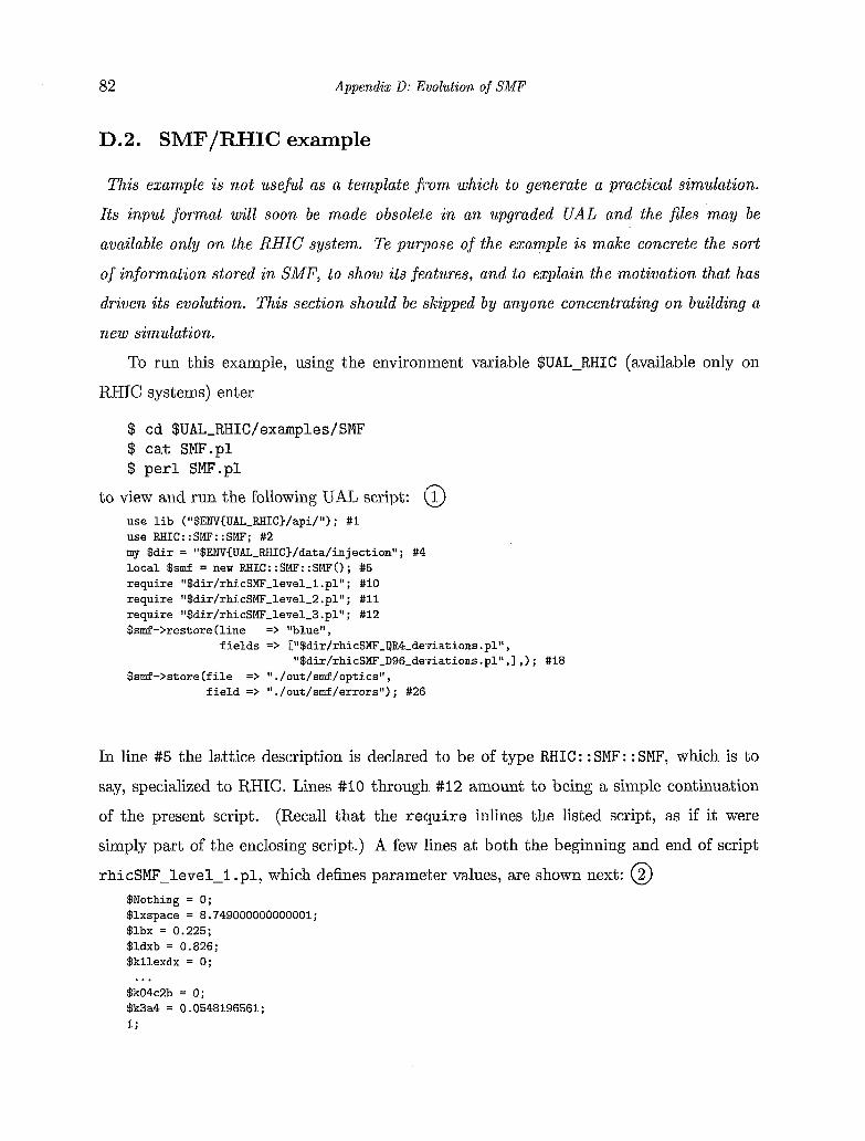
82 Appendix D: Evolution of SMF

D.2. SMF/RHIC example

This example i s no t useful as a template j?om, which to generate a practical simulation.

Its input f o rmat will soon be made obsolete in a n upgraded UAL and the files m a y be

available only o n the RHIC system. Te purpose of the example is make concrete the sort

of information stored in SMF, t o show i ts features, and to explain the motivat ion that has

driven i ts evolution. This section should be :skipped by anyone concentrating on building a

new simulation.

To run this example, using the environment variable $UAL-RHIC (available only on

RHIC systems) enter

$ cd $UAL-RHIC/examples/SMF $ cat SMF.pl $ per1 SMF.pl

to view and run the following UAL script: @ use lib (ll$ENV€UAL-RHIC)/api/ll) ; #l use RH1C::SMF::SMF; #2 my $dir = "$ENV{UAL-RHIC)/data/injection"; #4 local $smf = new RH1C::SMF::SMFO; #5 require "$dir/rhicSMF-level-l .pl" ; # l o require "$dir/rhicSMF-level-2 .pl" ; #ll require "$dir/rhicSMF-level-3 .pl"; #12 $smf->restore (line => "blue",

fields => ["$dir/rhicSMF_qRB-deviations .pl" , "$dir/rhicSMF-D96-deviations .pl" ,I ,) ; #18

$smf->store (f ile => #I. /out/smf/optics" , field => I' . /out/smf/errorsll) ; #26

In line #5 the lattice description is declared to be of type RHIC : : SMF: : SMF, which is to

say, specialized to RHIC. Lines #IO through. #I2 amount to being a simple continuation

of the present script. (Recall that the require inlines the listed script, as if it were

simply part of the enclosing script.) A few lines at both the beginning and end of script

rhicSMF-level-1 .pl, which defines parameter values, are shown next: @ $Nothing = 0; $lxspace = 8.749000000000001; $lbx = 0.225; $ldxb = 0.826; $kllexdx = 0;

$k04c2b = 0; $k3a4 = 0.0548196561; 1;

...

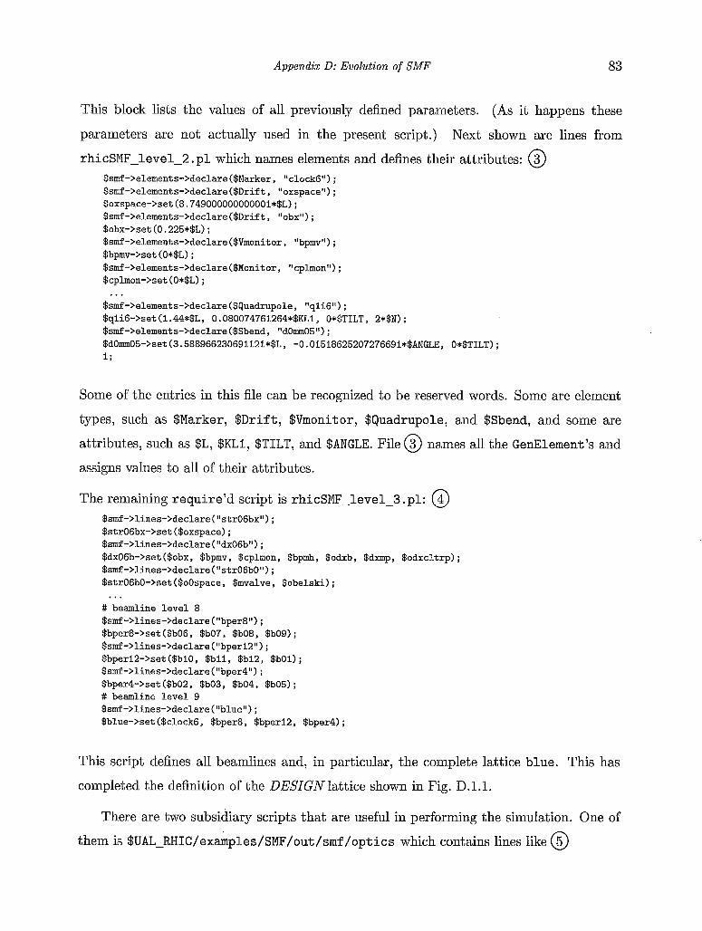
Appendix D: Evolution of SMF 83

This block lists the values of all previously defined parameters. (As it happens these

parameters are not actually used in the present script.) Next shown are lines from

rhicSMF-level-2. pl which names elements; and defines their attributes: @ $smf->elements->declare($Marker, "clock6"); $smf->elements->declare($Drift, "oxspace"); $oxspace->set (8.749000000000001*$L) ; $smf->elements->declare ($Drif t , "obx") ; $obx->set (0.225*$L) ; $smf->elements->declare ($Vmonitor , "bpmv") ; $bpmv->set (O*$L) ; $smf->elements->declare ($Monitor, "cplmon") ; $cplmon->set (O*$L) ;

$smf->element s->declare ($Quadrupole, Ilqli6l') ; $qli6->set (1.44*$L, O.O80074761264*$KLl, O*$TILT, 2*$N) ; $smf->elements->declare ($Sbend, "dOm05") ; $dOmm05->set(3.588966230691121*$L, -O.O1518625207276691*$ANGLE, O*$TILT);

...

Some of the entries in this file can be recogrdzed to be reserved words. Some are element

types, such as $Marker, $Drift, $Vmonitor, $Quadrupole, and $Sbend, and some are

attributes, such as $L, $KL1, $TILT, and $ANGLE. File @ names all the GenElement's and

assigns values to all of their attributes.

The remaining require'd script is rhicSMF--level-3. pl: @ $smf->lines->declare ("str06bx") ; $str06bx->set ($oxspace) ; $smf->lines->declare ("dx06b") ; $dx06b->set ($obx, $bpmv, $cplmon, $bpmh, $odx'b, $dxmp, $odxcltrp) ; $smf->lines->declare ("str06b0") ; $strO6bO->set($oOspace, $mvalve, $obelski);

# beamline level 8 $smf->lines->declare ("bper8") ; $bper8->set ($b06, $b07, $b08, $bog) ; $smf->lines->declare ("bper12") ; $bperlZ->set($blO, $bll, $biz, $bOi) ; $smf->lines->declare ("bper4") ; $bper4->set ($b02, $b03, $b04, $bo51 ; # beamline level 9 $smf->lines->declare ("blue") ; $blue->set ($clock6, $bper8, $bperl2, $bper4) ;

...

This script defines all beamlines and, in particular, the complete lattice blue. This has

completed the definition of the DESIGN lattice shown in Fig. D.l.l.

There are two subsidiary scripts that arc! useful in performing the simulation. One of

them is $UAL-RHIC/exiples/SMF/out/srnf /optics which contains lines like @

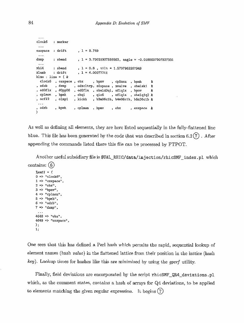
84 Appendix D: Evolution of SMF

... clock6 : marker

oxspace : dr i f t

dxmp : sbend

xki4 : sbend xlamb : dr i f t blue : l i n e = ( &

clock6 , oxspace , , odxb , dxmp , , odOflx , dOpp06 , , c p h o n , bpmh , , ocf l2 , olmpl ,

, odxb , bpmh , 1

...

...

...

...

, 1 = 8.749

, 1 = 3.70021937558562, angle = -0.0188607907827331

, 1 = 0.8 , tilt = 1.5707963267949 , 1 = 4.00072211

obx , bpmv , cplmon , bpmh & odxcl t rp , oOspace , mvalve , obelski & odOfla , obeldOq1, of lq lx , bpmv & obql , qio6 , o f l q l a , obelqlq2 & kickh , b3m06clb, b4m06clb, b5m06cib k

cplmon , bpmv , obx , oxspace &

As well as defining all elements, they are here listed sequentially in the fully-flattened line

blue. This file has been generated by the code that was described in section 6.2 @ . After

appending the commands listed there this fi1.e can be processed by FTPOT.

Another useful subsidiary file is $UAL-RHIC/data/in j ect ion/rhicSMF-index . p l which

contains: @ %smfI = ( 0 => "clock6", 1 => lIoxspace'l, 2 => "obx", 3 => "bpmv", 4 => "cplmon" , 5 => "bpmh", 6 => "odxb", 7 => "dxmp",

4648 => "obx", 4649 => "oxspace", 1; 1 ;

...

One sees that this has defined a Per1 hash which permits the rapid, sequential lookup of

element names (hash value) in the flattened 1.attice from their position in the lattice (hash

key). Lookup times for hashes like this are minimized by using the gperf utility.

Finally, field deviations are encorporated. by the script rhicSMF-QR4-deviations. p l

which, as the comment states, contains a hash of arrays for Q4 deviations, to be applied

to elements matching the given regular expression. It begins @

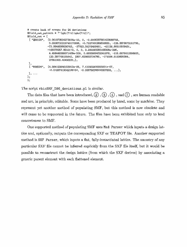
Appendix D: Evolution of SMF 85

# create hash of arrays for 94 deviations $field-set-pattern = "-(q4i(?!t) Iq4o(?!t))"; $field-set = [ [ '1qB412011, [3.061873504273504e-10, 0, -0.0006297661423589744,

0.0008720215740170938, -0.7227001269606835, -126.8879572151795, -73.9944598536752, -37022.31279458461, -41135.90310509401, -169279257.8510112, 0, 0, 3.294690580168208e-296, 4.458448388071409e-316, 0.6893869432341878, -118.6576412356923, 120.397765185641, 2307.623832724786, -171566.8153895384, 27651353.40430221,1,

1, [ "D96524", C4.564153846153912e-05, 7.410902400000001e-07,

-0.01897419042166154, -0.008756266220307693, ... 1, I, ...

1 ; 1;

The script rhicSMF_D96_deviations. p l is similar.

The data files that have been introduced, @ , @ , @ , and @ , are human readable

and are, in principle, editable. Some have been produced by hand, some by machine. They

represent yet another method of populating SMF, but this method is now obsolete and

will cease to be supported in the future. The files have been exhibited here only to lend

concreteness to SMF.

One supported method of populating SMF uses Mad Parser which inputs a design lat-

tice and, optionally, outputs the correspondiug SXF or TEAPOT file. Another supported

method is SXF Parser, which inputs a flat, fully-instantiated lattice. The ancestry of any

particular SXF file cannot be inferred explicitly from the SXF file itself, but it would be

possible to reconstruct the design lattice (from which the SXF derives) by associating a

generic parent element with each flattened element.

86 Appendix D: Evolution of SMF

D.3. ADXF: Accelerator Description Exchange Format

ADXF is an XML-based lattice description language.23 The schema for a matching

“Optics database”, patterned to some extenir; after the LAMBDA design of Peggs et

has been designed by M a l i t ~ k y . ~ ~ The variety of element attributes are shown in Ta-

ble D.3.1, grouped into “attribute sets” .t The supported accelerator elements are listed

in Table D.3.2 along with their applicable ahtribute sets. All elements have a length at-

tribute apart separate from any attribute set. As well as this length, magnetic elements

also have a magnetic length. As has been emphasized, both element types and attribute

list types are extensible.

t Internal to UAL “attribute sets” are referred to as “buckets”. The replacement has been made in external documentation since the term “bucket” has been said to be confusing.

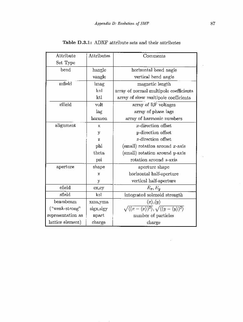
Appendix D: Evolution of SMF

Table D.3.1: ADXF attribute sets and their attributes

87

Attribute Set Type

bend

mfield

rffield

alignment

aperture

efield sfield

beambeam ( “weak-strong”

:epresentation as lattice element)

Attributes

hangle vangle lmag knl ktl volt

harmon 1%

X

Y

phi theta psi

Z

shape X

Y

ksl xma,yma sigx,sigy

npart charge

- Comments

horizontal bend angle vertical bend angle

magnetic length array of normal multipole coefficients a:rray of skew multipole coefficients

array of RF voltages array of phase lags

array of harmonic numbers x-direction offset y-direction offset z-direction offset

(small) rotation around z-axis (small) rotation around y-axis

rotation around s-axis ~

aperture shape horizontal half-aperture

vert ic a1 half- ap er t ure

Em E, -

integrated solenoid strength

number of particles charge -

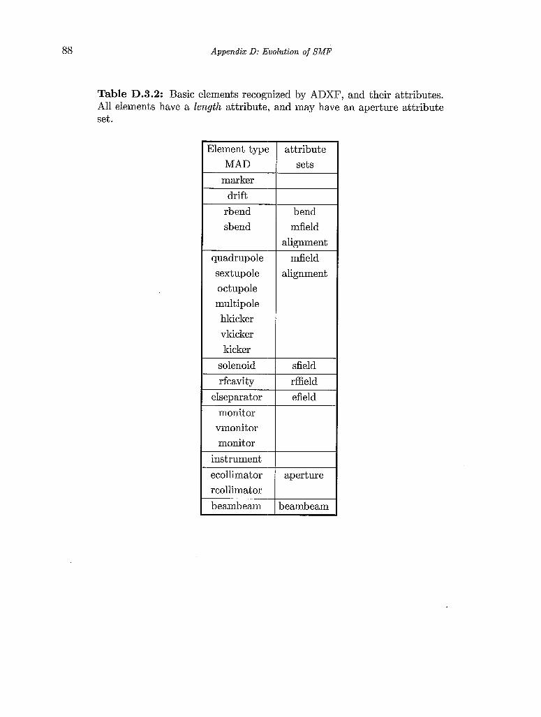
88 Appendix D: Euolution of SMF

Table D.3.2: Basic elements recog:nized by ADXF, and their attributes. All elements have a length attribute, and may have an aperture attribute set.

- marker -

-

sb end

sext up ole oct up ole multipole

I hlticker I vkicker

- kicker solenoid rfcavity

elseparat or monitor

vmonitor monitor

instrument ecollimat or rcollimator beambeam

- - -

-

-

-

attribute sets

bend mfield

alignment mfield

a 1 i g n m e n t

sfield rffield efield

aperture

3eambeam

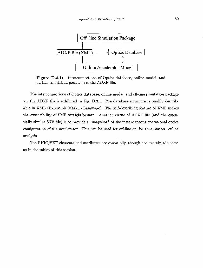
Appendix D: Evolution of SMF 89

1 Off-line Simulation Package 1 Q

J, I I

ADXF file (XML) 4 OpticsDatabase I 4 !

JI k c c e l e r a t o r Model I

Figure D.3.1: off-line simulation package via the ADXF file.

Interconnections of Optics database, online model, and

The interconnections of Optics database, online model, and off-line simulation package

via the ADXF file is exhibited in Fig. D.3.11. The database structure is readily describ-

able in XML (Extensible Markup Language). The self-describing feature of XML makes

the extensibility of SMF straightforward. Another virtue of ADXF file (and the essen-

tially similar SXF file) is to provide a “snapshot” of the instantaneous operational optics

configuration of the accelerator. This can be used for off-line or, for that matter, online

analysis.

The RHIC/SXF elements and attributes are essentially, though not exactly, the same

as in the tables of this section.

Appendix E. Truncated Power Series and Lie Maps

This section more properly belongs in the ‘VAL Physics Manual”. It is parked here until

that manual comes into existence.

E.l. Function evolution

Truncated power series play an important role in UAL. Their role is to approximate the

“maps” that express “output” particle coordinates (at some place in the ring) in terms of

“input” particle coordinates (at a different place in the ring). When truncated to linear

order these power series reduce to the elements of the traditional, Courant-Snyder, transfer

matrix description of the accelerator lattice. Historically, most of accelerator physics has

been (very successfully) based on analysis performed in this limit. But effects appearing

already at a “next order of approximation” such as chromaticity and amplitude-dependent

detuning, have ways of intruding, even in elementary contexts, and nonlinearity becomes

increasingly important as amplitudes are inerteased to achieve higher beam current. As soon

as any nonlinearity whatsoever is allowed to enter the description the issue of symplecticity,

or rather lack thereof, rears its head. Especially for hadron accelerators, for which there

is essentially no true damping, any anti-darnping artificially and erroneously introduced

through non-symplecticity can ruin an accelerator simulation program’s ability to predict

the long term future.

Symplectic maps (typically nonlinear) are also known as Lie maps. One therefore

seeks to describe particle trajectories in an a.ccelerator by a Lie map. As with all physics,

such a description can only be approximate. For one thing the idealized model of the

accelerator, on which the “idealized map” is based, is undoubtedly inaccurate and incom-

plete. Accepting this as inevitable, possible further inaccuracy results from the computer

program representation of the map. It is the latter source of inaccuracy that is the subject

of this appendix. Maps based on truncated power series can only approximate idealized

maps. For reasons explained in the previoiLzs paragraph, failure of symplecticity is ex-

pected to be more serious than other inaccuracy. An important goal of UAL is to preserve

symplecticity, or rather to keep the inevitable failure of symplecticity controllably small.

- 90 -

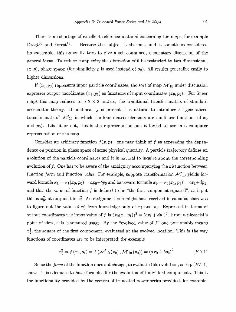
Appendix E: Truncated Power Series and L i e Maps 91

There is no shortage of excellent referenlce material concerning Lie maps; for example

Dragt36 and Forest15. Because the subject is abstract, and is sometimes considered

impenetrable, this appendix tries to give a self-contained, elementary discussion of the

general ideas. To reduce complexity the discussion will be restricted to two dimensional,

( z , p ) , phase space; (for simplicity p is used instead of p z ) . All results generalize easily to

higher dimensions.

If (z0,po) represents input particle coordinates, the sort of map M‘lo under discussion

expresses output coordinates ( z 1 , p l ) as functions of input coordinates (50 , PO). For linear

maps this map reduces to a 2 x 2 matrix, the traditional transfer matrix of standard

accelerator theory. If nonlinearity is present it is natural to introduce a “generalized

transfer matrix” M’lo in which the four m.atrix elements are nonlinear functions of 20

and PO) . Like it or not, this is the representation one is forced to use in a computer

representation of the map.

Consider an arbitrary function f(z,p)-one may think of f as expressing the depen-

dence on position in phase space of some physical quantity. A particle trajectory defines an

evolution of the particle coordinates and it is natural to inquire about the corresponding

evolution off . One has to be aware of the ambiguity accompanying the distinction between

function form and function value. For exarnlple, suppose transformation M’lo yields for-

ward formulaq = zl(zo,po) = upo+bpo and backward formulazo = xo(z1,pl) = c z l f d p l ,

and that the value of function f is defined t o be “the first component squared”; at input

this is xi, at output it is x?. An assignment one might have received in calculus class was

to figure out the value of xg from knowledge only of x1 and P I . Expressed in terms of

output coordinates the input value off is ( ~ o ( ~ : l , p 1 ) ) ~ = (ex1 + d p ~ ) ~ . From a physicist’s

point of view, this is tortured usage. By the “evolved value of f” one presumably means

xi, the square of the first component, evaluated at the evolved location. This is the way

functions of coordinates are to be interpreted; for example

x: = f ( m , ~ i ) = f (M’io (zo) , M‘io (PO)) = (azo + PO)^ ( E .1 .l)

Since the form of the function does not change, to evaluate this evolution, as Eq. (E.l.1)

shows, it is adequate to have formulas for the evolution of individual components. This is

the functionality provided by the vectors of truncated power series provided, for example,

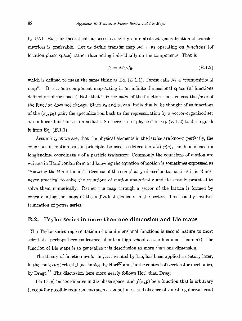
92 Appendix E: Tmncated Power Series and Lie Maps

by UAL. But, for theoretical purposes, a slightly more abstract generalization of transfer

matrices is preferable. Let us define transfer map Mlo as operating on functions (of

location phase space) rather than acting individually on the components. That is

which is defined to mean the same thing as Eq. (E.l.l). Forest calls M a “compositional

map”. It is a one-component map acting in an infinite dimensional space (of functions

defined on phase space.) Note that it is the value of the function that evolves; the form of

the function does not change. Since zo and po can, individually, be thought of as functions

of the (z0,po) pair, the specialization back to the representation by a vector-organized set

of nonlinear functions is immediate. So there is no “physics” in Eq. (E.1.2) to distinguish

it from Eq. (E.l.l).

Assuming, as we are, that the physical elements in the lattice are known perfectly, the

equations of motion can, in principle, be used to determine z ( s ) ,p ( s ) , the dependence on

longitudinal coordinate s of a particle trajectory. Commonly the equations of motion are

written in Hamiltonian form and knowing thcr equation of motion is sometimes expressed as

“knowing the Hamiltonian”. Because of the complexity of accelerator lattices it is almost

never practical to solve the equations of motion analytically and it is rarely practical to

solve them numerically. Rather the map through a sector of the lattice is formed by

concatenating the maps of the individual elements in the sector. This usually involves

truncation of power series.

E.2. Taylor series in more than one dimension and Lie maps

The Taylor series representation of one dimensional functions is second nature to most

scientists (perhaps because learned about in high school as the binomial theorem?) The

function of Lie maps is to generalize this description to more than one dimension.

The theory of function evolution, as invented by Lie, has been applied a century later,

in the context of celestial mechanics, by H ~ r i ~ ~ and, in the context of accelerator mechanics,

by Dragt.38 The discussion here more nearly follows Hori than Dragt.

Let ( z , p ) be coordinates in 2D phase space, and f ( z , p ) be a function that is arbitrary

(except for possible requirements such as smoothness and absence of vanishing derivatives.)

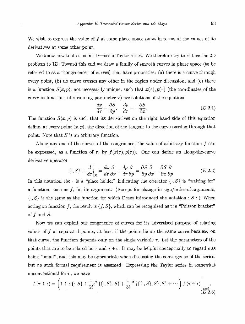
Appendix E: Dunca ted Power Series and L ie Maps 93

We wish to express the value of f at some phase space point in terms of the values of its

derivatives at some other point.

We know how to do this in 1D-use a Ta,ylor series. We therefore try to reduce the 2D

problem to 1D. Toward this end we draw a family of smooth curves in phase space (to be

referred to as a “congruence” of curves) that have properties: (a) there is a curve through

every point, (b) no curve crosses any other in the region under discussion, and (e) there

is a function S(x,p), not necessarily unique, such that x(T),p(r) (the coordinates of the

curve as functions of a running parameter r ) are solutions of the equations

( E .2.1) dx as dp - as

The function S(x,p) is such that its deriva1;ives on the right hand side of this equation

define, at every point (x, p), the direction of i;he tangent to the curve passing through that

point. Note that S is an arbitrary function.

- - - - d r a p ’ d r ax

Along any one of the curves of the congruence, the value of arbitrary function f can

be expressed, as a function of r, by f(x(~),p(r)). One can define an along-the-curve

derivative operator

(E.2.2)

In this notation the - is a “place holder” indicating the operator { . ,S} is “waiting for”

a function, such as f, for its argument. (Escept for change in sign/order-of-arguments,

{-, S } is the same as the function for which Dragt introduced the notation : S :.) When

acting on function f, the result is {f, S } , which can be recognized as the “Poisson bracket”

o f f and S.

{.,S}=-I d =--+ dx a dp a as a as a dr drax d d p a p a x a x a p ’

Now we can exploit our congruence of Icurves for its advertised purpose of relating

values of f at separated points, at least if the points lie on the same curve because, on

that curve, the function depends only on the! single variable r. Let the parameters of the

points that are to be related be r and r + E . It may be helpful conceptually to regard E as

being “small”, and this may be appropriate when discussing the convergence of the series,

but no such formal requirement is assumed,

unconventional form, we have

Expressing the Taylor series in somewhat

1 f (7 + €) = 1 + € { e , S } + -E2 {{*, S} , S } -t ( 2!

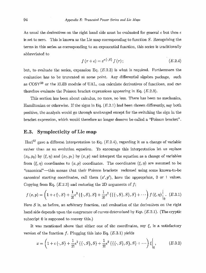
94 Appendix E: Truncated Power Series and Lie Maps

As usual the derivatives on the right hand side must be evaluated for general E but then E

is set to zero. This is h o w n as the Lie map corresponding to function S. Recognizing the

terms in this series as corresponding to an exponential function, this series is traditionally

abbreviated to

f (7- + €) = eE{.,S) f (7) ; (E. 2 A)

but, to evaluate the series, expansion Eq. (E.2.3) is what is required. F’urtherrnore the

evaluation has to be truncated at some point. Any differential algebra package, such

as COSY39 or the ZLIB module of UAL, can calculate derivatives of functions, and can

therefore evaluate the Poisson bracket expressions appearing in Eq. (E.2.3).

This section has been about calculus, no more, no less. There has been no mechanics,

Hamiltonian or otherwise. If the signs in Eq. (E.2.1) had been chosen differently, say both

positive, the analysis would go through unchanged except for the switching the sign in the

bracket expression, which would therefore no longer deserve be called a “Poisson bracket”.

E.3. Syrnplecticity of Lie map

H ~ r i ~ ~ gave a different interpretation to Eq. (E.2.4), regarding it as a change of variable

rather than as an evolution equation. To encourage this interpretation let us replace

( z 0 , p o ) by ( [ , T I ) and ( z 1 , p l ) by ( z , p ) and interpret the equation as a change of variables

from ( [ ,q ) coordinates to ( z , p ) coordinates. The coordinates ( J , q ) are assumed to be

LLcanonical”-this means that their Poisson brackets reckoned using some known-to-be

canonical starting coordinates, call them (:E’, p’), have the appropriate, 0 or 1 values.

Copying from Eq. (E.2.3) and restoring the ‘2D arguments of f;

Here S is, as before, an arbitrary function, and evaluation of the derivatives on the right

hand side depends upon the congruence of curves determined by Eqs. (E.2.1). (The cryptic

subscript 0 is supposed to convey this.)

It was mentioned above that either one of the coordinates, say E , is a satisfactory

version of the function f . Plugging this into Eq. (E.3.1) yields

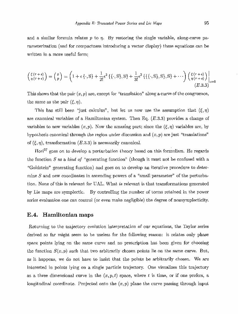
Appendix E: Truncated Power Series and L ie Maps 95

and a similar formula relates p to q. By restoring the single variable, along-curve pa-

rameterization (and for compactness introducing a vector display) these equations can be

written in a more useful form;

This shows that the pair (z, p ) are, except for “translation” along a curve of the congruence,

the same as the pair (t, 7).

This has still been “just calculus”, but let us now use the assumption that ( t , q )

are canonical variables of a Hamiltonian system. Then Eq. (E.3.3) provides a change of

variables to new variables ( z , p ) . Now the ainazfng part; since the ( E , q) variables are, by

hypothesis canonical through the region under discussion and (z, p ) are just “translations”

of ( E , q) , transformation (E.3.3) is necessarily canonical.

H ~ r i ~ ~ goes on to develop a perturbation theory based on this formulism. He regards

the function S as a kind of “generating function” (though it must not be confused with a

“Goldstein” generating function) and goes on to develop an iterative procedure to deter-

mine S and new coordinates in ascending powers of a “small parameter” of the perturba-

tion. None of this is relevant for UAL. What is relevant is that transformations generated

by Lie maps are symplectic. By controlling the number of terms retained in the power

series evaluation one can control (or even ma,ke negligible) the degree of nonsymplecticity.

E.4. Hamiltonian maps

Returning to the trajectory evolution interpretation of our equations, the Taylor series

derived so far might seem to be useless for the following reason: it relates only phase

space points lying on the same curve and :no prescription has been given for choosing

the function S(z ,p ) such that two arbitrarily chosen points lie on the same curve. But,

as it happens, we do not have to insist that the points be arbitrarily chosen. We are

interested in points lying on a single particle trajectory. One visualizes this trajectory

as a three dimensional curve in the (x,p,t) space, where t is time, or if one prefers, a

longitudinal coordinate. Projected onto the (z, p ) plane the curve passing through input

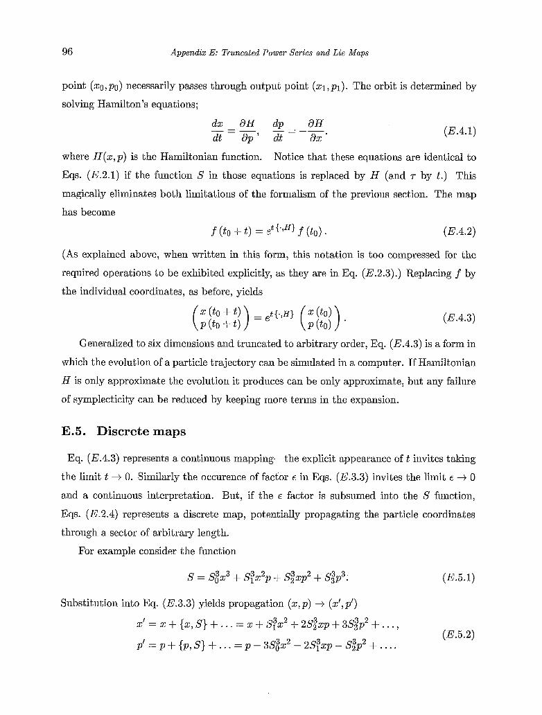
96 Appendix E: n u n c a t e d Power Series and L i e Maps

point ( X O , P O ) necessarily passes through output point (21, P I ) . The orbit is determined by

solving Hamilton’s equations;

(E.4.1)

where H(x,p) is the Hamiltonian function. Notice that these equations are identical to

Eqs. (E.2.1) if the function S in those equations is replaced by H (and r by t.) This

magically eliminates both limitations of the formalism of the previous section. The map

has become

f (to + t ) = ,e t{- ,H) f (to) . ( E .4.2)

(As explained above, when written in this form, this notation is too compressed for the

required operations to be exhibited explicitly, as they are in Eq. (E.2.3).) Replacing f by

the individual coordinates, as before, yields

(E.4.3)

Generalized to six dimensions and truncated to arbitrary order, Eq. (E.4.3) is a form in

which the evolution of a particle trajectory can be simulated in a computer. If Hamiltonian

H is only approximate the evolution it produces can be only approximate, but any failure

of symplecticity can be reduced by keeping rnore terms in the expansion.

E.5. Discrete maps

Eq. (E.4.3) represents a continuous mapping-the explicit appearance of t invites taking

the limit t + 0. Similarly the occurence of factor E in Eqs. (E.3.3) invites the limit E -+ 0

and a continuous interpretation. But, if the E factor is subsumed into the S function,

Eqs. (E.2.4) represents a discrete map, potentially propagating the particle coordinates

through a sector of arbitrary length.

For example consider the function

s = $ 2 3 + Sfx2p f s2 3 2 xp f s33p3. (E.5.1)

Substitution into Eq. (E.3.3) yields propagation (x,p) -+ (x’,p’)

X I = x + ( x , S ) + . . . = x + :gx2 f 2s;xp i- 3s33p2 + . . . , (E.5.2)

PI = P + { p , S ) + . . . = p - 3s:x2 - 2s;xp - s;p2 + . . . . \

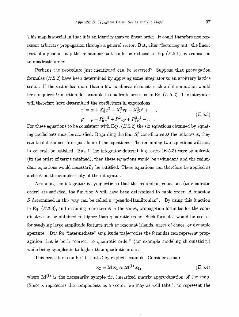
Appendix E: Truncated Power Series and Lie Maps 97

This map is special in that it is an identity map to linear order. It could therefore not rep-

resent arbitrary propagation through a general sector. But, after “factoring out” the linear

pa.rt of a general map the remaining part could be reduced to Eq. (E.5.1) by truncation

to quadratic order.

Perhaps the procedure just mentioned can be reversed? Suppose that propagation

formulas (E.5.2) have been determined by applying some integrator to an arbitrary lattice

sector. If the sector has more than a few nonlinear elements such a determination would

have required truncation, for example to quadratic order, as in Eq. (E.5.2). The integrator

will therefore have determined the coefficients in expansions x’ = x f xi92 + :r,2xp + x ; p 2 + . . . , p’ = p + P&l? + FFxp f P;p2 i- . . . .

(E. 5.3)

For these equations to be consistent with Eqs. (E.5.2) the six equations obtained by equat-

ing coefficients must be satisfied. Regarding the four Si3 coordinates as the unknowns, they

can be determined from just four of the equations. The remaining two equations will not,

in general, be satisfied. But, if the integrator determining series (E.5.3) were symplectic

(to the order of terms retained), then these equations would be redundant and the redun-

dant equations would necessarily be satisfied. These equations can therefore be applied as

a check on the symplecticity of the integrator.

Assuming the integrator is symplectic so that the redundant equations (to quadratic

order) are satisfied, the function S will have been determined to cubic order. A function

S determined in this way can be called a “pseudo-Hamiltonian” . By using this function

in Eq. (E.3.3), and retaining more terms in ithe series, propagation formulas for the coor-

dinates can be obtained to higher than quadratic order. Such formulas would be useless

for studying large amplitude features such as resonant islands, onset of chaos, or dynamic

aperture. But for “intermediate” amplitude trajectories the formulas can represent prop-

agation that is both “correct to quadratic order” (for example modeling chromaticity)

while being symplectic to higher than quadratic order.

This procedure can be illustrated by explicit example. Consider a map

~2 = Mxl x M(‘)xl, ( E . 5.4)

where M(l) is the necessarily symplectic, linearized matrix approximation of the map.

(Since x represents the components as a vector, we may as well take it to represent the

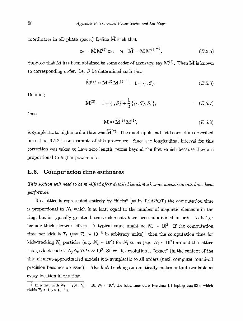
98 Appendix E: Truncated Power Series and Lie Maps

coordinates in 6D phase space.) Define G such that

Suppose that M has been obtained to some order of accuracy, say M(2). Then % is known

to corresponding order. Let S be determined such that

(E. 5.6)

Defining 1 N

M(3) = 1 + {.,Sl) + 5 {{ - ,S} ,S , } , (E. 5.7)

then

M x G:(3) M(l), ( E .5 -8)

is symplectic to higher order than was G(2). The quadrupole end field correction described

in section 6.5.2 is an example of this procedure. Since the longitudinal interval for this

correction was taken to have zero length, terms beyond the first vanish because they are

proportional to higher powers of E .

E.6. Computation time estimates

This section will need t o be modified af ter detailed benchmark t i m e measurements have been

performed.

If a lattice is represented entirely by “kicks” (as in TEAPOT) the computation time

is proportional to NI, which is at least equa’l to the number of magnetic elements in the

ring, but is typically greater because elements have been subdivided in order to better

include thick element effects. A typical value might be NI, - lo3. If the computation

time per kick is T k (say TI, N in arbitrary units)f then the computation time for

kick-tracking Np particles (e.g. Np - lo3) for Nt turns (e.g. Nt N lo3) around the lattice

using a kick code is N,N~N~TI, - lo3. Since kick evolution is “exact” (in the context of the

thin-element-approximated model) it is symplectic to all orders (until computer round-off

precision becomes an issue). Also kick-tracking automatically makes output available at

every location in the ring.

t In a test with Nk = 701, Np = 10, Nt = lo4, the total time on a Pentium I11 laptop was 93s, which yields Trc M 1.3 x s.

Appendix E: Truncated Power Series and L i e Maps 99

Instead of element-by-element tracking one can consider the use of nonlinear maps to

model particle orbits. Usually one is interested in particle positions at a limited set of

positions in the ring. For investigation of long term stability or determination of beam

distributions this set may reduce to a single point but, in general, one is interested in

particle positions at an appreciable number of selected points that is still far less than the

number of localized kicks in the ring. One therefore contemplates breaking the lattice into

sectors and using nonlinear maps to compute trajectory evolution sector by sector. The

hope would be that the map-tracking would be much faster than the kick-tracking.

For concentrating attention on a short segment of a lattice, perhaps representable only

by Runge Kutta numerical tracking or some other specialized method, one could model

“the rest of the lattice” by a nonlinear map. Since only a single nonlinear mapping is

required this application is sure to be “fast” even for a relatively high order map. But one

is also interested in intermediate cases where ithe lattice is subdivided into some appreciably

large number N, (e.g N, N 100) of sectors. For example sector boundaries could be taken

at every sextupole, in which case Nc9 would be the number of sextupoles.

Apart from the faithfulness of the simulation one wants to be sure that the time spent

in first determining the needed maps is smaller than the time spent in applying the maps

to the simulation task for which they are intended. This ratio depends on arbitrary factors

such as Nt and Np and the number of times each map can be usefully re-used. We will see

that, for typically large values of these numbers, the map-determination time is acceptably

small, at least for modest order of nonlinearity.

The sort of nonlinear effect one may wish to model correctly is tune dependence on am-

plitude. The dominant nonlinear elements in lattices are typically sextupoles, but a single

sextupole causes no tune shift in lowest order. A mapping procedure limited to “sextupole

order”, cannot, therefore, be expected to usefully model tune dependence on amplitudes.

Any octupoles present in the ring cause first order tune shift but, whether present inten-

tionally or not, such octupoles are normally “weak” compared to the intentionally-present

sextupoles. It is not uncommon for the tune shifts caused by octupoles in lowest order

to be comparable with the tune shifts caused by sextupoles in second order. A sensible

“lowest useful order of nonlinearity” might therefore be to perform calculations to octupole

100 Appendiz E: Truncated Power Series and Lie Maps

order-this would correctly include tune dependence due to sextupoles, would be symplec-

tic to one higher than sextupole order, and would include octupole effects symplectic to

their own order. This corresponds to determining to quartic order the polynomial S in-

troduced in the previous section. Let us adapt the proposition that, for any computation

going beyond simple matrix multiplication, it is appropriate to carry the computation to

this, one higher than sextupole, order. A table below shows that the generating function

for this mapping already has 210 terms, and the computer cost increases steeply as the

order is increased beyond this level.

To estimate the cost (in computer time) of performing map calculations it is useful to

know the number Nc of coefficients appearing in each of the truncated power series that

have to be calculated. The needed formula, given by Yan40, is

(17, + R)! N --_- n!R! ' c - (E.6.1)

where n is the phase space dimensionality and R is the polynomial order. Some numerical

examples are contained in Table E.6.1.

Since the map calculation time per sector is proportional to the number of elements

per sector, the time to obtain the needed maps should be more of less independent of the

number of sectors N,. The second last column of Table E.6.1 gives the once-around map

calculation time for the same 0.7 x 103-kick: lattice as mentioned in an earlier footnote.

Even for a fairly high order map the map calculation time for this lattice is much less than

the kick-tracking number ( lo3) calculated ablove. For multiparticle, multiturn tracking, it

seems therefore that the time for initial generation of the maps is likely to be acceptably

short. Certainly this will be true for the C1 = 3 option recommended here for general

purpose nonlinear tracking. One can note also that distributing the various lattice sectors

to multiple processors makes the task of map generation readily parallelizable.

It remains to compare computation times for map-tracking and kick-tracking. A crude

estimate of the time for each order=R map application, relative to the time per kick

application, is f2Nc(R)/Nc(l). This accountrs roughly for the number of multiplications

per power series evaluation. It underestimates the kick evaluation time, which is greater

than a linear matrix multiplication time. Accepting this estimate, the ratio of map-tracking

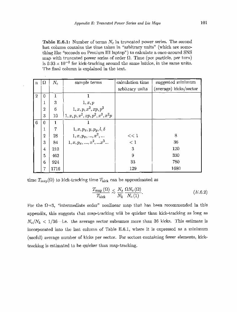
Appendix E: Truncated Power Series and Lie Maps 101

calculation time arbitrary units

Table E.6.1: Number of terms Nc in truncated power series. The second last column contains the tiine taken in “arbitrary units” (which are some- thing like “seconds on Pentium I11 laptop”) to calculate a once-around SNS map with truncated power series of order R. Time (per particle, per turn) is 0.93 x for kick-tracking around the same lattice, in the same units. The final column is explained in the text.

suggested minimum (average) kiclts/sector

n R

2 0

6 0

- N e

1 3 6 10

1 2 3

1 2 3 4 5 6 7

1 7 28 84 210 462 924 1716

2 l ,z,pz ) . “ ) x ,... 3 1, x,px, ’”) x2, ... x ...

<< 1 < 1

3 9 33 129

8 36 120 330 780 1680

time Tmap(R) to kick-tracking time Tki& can be approximated as

(E.6.2)

For the R=3, “intermediate order” nonlinear map that has been recommended in this

appendix, this suggests that map-tracking will be quicker than kick-tracking as long as

N,/Nk < 1/36-i.e. the average sector subsumes more than 36 kicks. This estimate is

incorporated into the last column of Table E.6.1, where it is expressed as a minimum

(useful) average number of kicks per sector. For sectors containing fewer elements, kick-

tracking is estimated to be quicker than map-tracking.

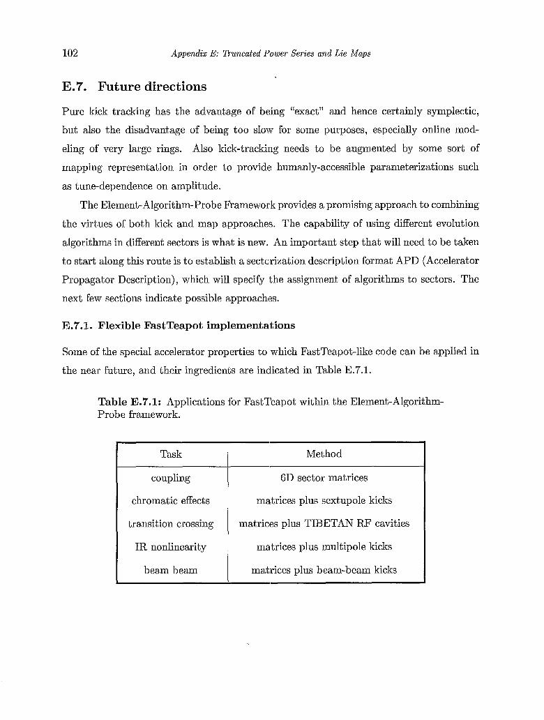
102 Appendix E: Truncated Power Series and Lie Maps

coupling

chromatic effects

transition crossing

E.7. Future directions

6D sector matrices

ma,trices plus sextupole kicks

matrioes plus TIBETAN RF cavities

Pure kick tracking has the advantage of being “exact” and hence certainly symplectic,

but also the disadvantage of being too slow for some purposes, especially online mod-

eling of very large rings. Also kick-tracki:ng needs to be augmented by some sort of

mapping representation in order to provide humanly-accessible parameterizations such

as tune-dependence on amplitude.

The Element- Algorithm-Probe Framework provides a promising approach to combining

the virtues of both kick and map approaches. The capability of using different evolution

algorithms in different sectors is what is new. An important step that will need to be taken

to start along this route is to establish a sectalrization description format APD (Accelerator

Propagator Description), which will specify the assignment of algorithms to sectors. The

next few sections indicate possible approaches.

E.7.1. Flexible FastTeapot implementations

Some of the special accelerator properties to which FastTeapot-like code can be applied in

the near future, and their ingredients are indicated in Table E.7.1.

Table E.7.1: Applications for FastTeapot within the Element-Algorithm- Probe framework.

Task I Method

I IR nonlinearity 1 ma,trices plus multipole kicks

I beam beam I matrices plus beam-beam kicks

Appendix E: Truncated Power Series and L i e Maps 103

E.7.2. Sector maps plus sextupole kicks

It would be highly desirable to have a latticle model robust enough and fast enough to be

applicable to all operational problems without any need for task-specific specialization.

The option of combining kick-tracking and map-tracking may meet this need, espe-

cially if there is a relatively small number of “strong” nonlinear elements (for example

chromaticity sextupoles) and a relatively large number of “weak” nonlinear elements (for

example magnetic field errors or quadrupole end fields). By treating the strong elements

as kicks their individual deflections as well as, the dependence of their kicks on other strong

kicks are accurately represented. Their resonant effects and tune dependences would there-

fore be accurately modeled. The modificatj.ons of these effects by weak elements would

then be handled accurately only to the order of the sector maps. We conjecture that the

choice R=3 for map-tracking through the sectors between chromaticity sextupoles, along

with explicit kicks at each of these sextupoles, will give tracking that is sufficiently accu-

rate for all short term effects and most long term effects, such as dynamic aperture. This

conjecture has not been tested however.

For RHIC, with 5300 elements and 144 sextupoles, accepting the entry 36 from the last

column of Table E.6.1, the ratio of computation time for map/kick mixed tracking to pure

kick tracking would be less than 5300/144/36 M 1-optimistically the kick-map tracking

would be two or three times faster than the pure kick tracking. But that is not the real

point, since other potential benefits accrue. For example, there would be no penalty for

finer subdivision, and hence more faithful, thick element and end field representations of

elements within the mapped sectors.

A more important benefit would be the adoption of the mapping approach. For current

day accelerator operation there are nominal beta functions at every lattice position, as well

as nominal phase advances and transfer matrices between different positions. Even though

it is no small achievement to have agreement at this level, the suggestion here is for

these matrices to be generalized to R = 3 m;%ps, which would be the basis for all machine

studies investigations. For large amplitude, large momentum offset, investigations these

maps would be used as described so far. For operational investigations concerning only

a small number of lattice positions, for example kicker and pickup in a transfer function

104 Appendix E: Truncated Power Series and Lie Maps

determination, it would be natural to concatenate the maps to obtain a speed up factor

close to one hundred, while retaining nearly exact contact with the nominal lattice model.

Another promising approach, not begun as yet, would be to reduce all the sector

maps to “normal form”. As well as making available the “physics” that this implies, it

would open the possiblility of “lightning fast” tracking using some form of normal form

representation of the sector maps combined with treating strong nonlinear elements as

kicks.

E.7.3. Irwin factorization

From the numerical estimates of the previoiis section it appears that the use of maps of

order higher than R = 3 will be impractical because of being too slow. Even so, the

kick-factorization scheme of Irwin41 could, in principle, make higher order maps practical

for online modeling. Irwin gives a formula for the number of kicks needed to faithfully

represent maps as a function of their order. For R = 2 , 3 , 4 , 5 , 6 , 7 , 8 , ... his formula gives

8,12,18,27,36,48,64, ... as the number of k.ck factors required. The fact that this series

increases far less rapidly with increasing R :than does N, (given in Table E.6.1) suggests

that high order maps should be represented by kick factorization. But for the sextupole-

to-sextupole sectorization example of the previous section, the number of kicks per sector

seems to be insufficiently greater than the Irwin factor to justify his kick factorization for

the R = 3 case.

References 105

References

1.

2.

3.

4.

5 .

6.

7.

8. 9.

10. 11.

12.

13.

14.

15.

16.

17. 18.

N. Malitsky and R. Talman, Unified Accelerator Libraries, AIP 391, Williamsburg, 1996. N. Malitsky and R. Talman, Status of Unified Accelerator Libraries, IEEE Particle Accelerator Conference, p. 2434, 1997. In high energy physics there is a facility called ROOT R. Brun et al., An Object- Oriented Data Analysis Framework, h t t p : / / roo t . cern. ch/root whose purpose is to unify data analysis of elementary particle physics experiments. Except for working on accelerators instead of experiments the UAL motivation and design principles are the same. We use the term “environaient” instead of “framework” only to reserve the latter term for a slightly more specialized sense below. N. Malitsky and R. Talman, The Framework of Unified Accelerator Libraries, ICAP98, Monterey, 1998. H. Grote and F. Iselin, The MAD Pro!gram (Methodical Accelerator Design), User’s Reference Manual, CERN/SL/SO-l3(A:P), 1990. N. Malitsky and A. Shishlo, A Parallel Extension of the UAL Environment, PAC, 2001. K. Fogel and M. Bar, Open Source Development with CVS, Coriolis Technology Press, Scottsdale, Arizona, 2001. R. Schwartz, Learning Perl, O’Reilly and Associates, Cambridge, U.S.A., 1994. L. Wall, T. Christansen, and R. Schwartz, Programming Perl, O’Reilly and Asso- ciates, Cambridge, U.S.A., 3nd Ed, 2000. D. Conway, Object Oriented Perl, Manning Publications, Grenwich, CT, 1999. T. Jenness and S. Cozens, Extending and Embedding Perl Manning Publications, Greenwich, CT, 2003. S. Srinivasan, Advanced Perl Programming, O’Reilly and Associates, Sebastopol, CA, 1997. A. Aho, B. Kernighan, and P. Weinberger, The AWK Programming Language, Addison- Wesley, 1988. R. Talman and N. Malitsky, Beam-Based BPM Alignment, BNL/SNS Technical Note No. 1 1 6, September 16, 2002. ht t p : //server. ags . bnl. gov/ bnlags/ bnlsns/ 1 1 6. pdf. E. Forest, Beam Dynamics, A New Attitude and Framework, Harwood Academic Publishers, Amsterdam, 1998, p. 390. Forest explains why the seemingly-unphysical discontinuity in particle trajectory occurring at a quadrupole edge is, in fact, a best approximation, at a .point, of an effect that actually accumulates over an extended longitudinal interval. W. Gropp et al., Using MPI: Portable Parallel Programming with the Message- Passing Interface, 2nd ed., MIT Press, 1999. MPICH , http: //www . mcs. anl. gov/mpi/’mpich. L. Schachinger and R. Talman, TEAPOT: A Thin Element Program for Optics and Tracking, Part. Accel. 22,35(1987).

106

19.

20.

21.

22.

23.

24.

25.

26.

27.

28.

29.

30.

31.

32. 33.

34. 35.

36.

37.

38.

39.

References

N. Malitsky, A. Reshetov, and G. Bourianoff, PAC++: Object-Oriented Platform for Accelerator Codes, SSCL-675, 1994. G. Bourianoff, A. Reshetov, and N. Malitsky, Object-Oriented Approach f o r the De- sign of the Simulation Facility of the SSC, SSCL-677, 1994. C. Iselin, E. Keil and R. Talman, Call For a New Accelerator Description Standard, Beam Dynamics, Newsletter 16, April, 1998. H. Grote, J. Holt, N. Malitsky, F. Pilat, R. Talman, C. Trahern, SXF: Definition, Syntax, Examples, RHIC/AP/155 (1998). N. Malitsky and R. Talman, Accelerator Description Exchange Format, ICAP98, Monterey, 1998. F. Pilat, C. Trahern, J. Wei, T. Satogata, and S. Tepikian, Modeling R H I C Using the Standard Machine Format Accelerator Description, PAC97, 1997. N. Malitsky, R. Casella, K. Lally, S. Peng, J. Smith, and D. Giird, Design of a Unified Control System API, Int. Conf. on Accelerator and Large Experimental Phys. Control Systems, Trieste, Italy, 1.999. N. Malitsky, J. Smith, and J. Wei, A Prototype of the U A L 2.0 Application Toolkit, 8th Int. Conf. on Accelerator and Large Experimental Phys. Control Systems, San Jose, CA, 2001. N. Malitsky, J. Smith, J. Wei, and R. Talman, UAL-Based Simulation Environment f o r Spallation Neutron Source Ring, p. 2713, Proc. 1999 PAC, New York. N. Malitsky, P. Cameron, A. Fedotov, J . Smith, J . Wei, Development and Applications of the UAL-based SNS Ring Simulation Environment, ICFA-HB 2002 Workshop. F. Jones, http://www.triuinf.ca/compserv/accsim.doc/refguide.ps, User’s Guide to Accsim, 1990. J. Galambos et al. O R B I T User Manual, Version 1.10, SNS/ORNL/AP Technical Note Number 011, Rev. 1. D. Carey and F. Iselin, Standard Input Language f o r Particle Beams, Snowmass, Colorado, 1984. Y. Yan and C-Y Yan, A Numerical Libi-ary f o r Diflerential Algebra, SSCL-300, 1990. N. Malitsky, A. Reshatov, and Y. Yan, ZLIB++: Object-Oriented Library f o r Difler- entia1 Algebra, SSCL-659, 1994. S . Peggs et al. L A M B D A Manual, RHIC/AP/13, 1993. N. Malitsky, A Prototype of the SNS Optics Database, BNL/SNS Technical Note No. 085, November, 2000. A. Dragt, in Lectures on Nonlinear Orhit Dynamics, American Institute of Physics, New York, 1981. G. Hori, Theory of General Perturbations with Unspecified Canonical Variables, Publ. Astro. SOC. Japan, Vol. 18, No. 4, 1966. A. Dragt, in Proceedings of the 1984 Study on the Design and Utilization of the SSC, ed. by R. Donaldson and J. Morphin, Am. Phys. Soc., Snowmass, 1985. M. Berz, Diflerential Algebraic Description of Beam Dynamics to Very High Orders, Particle Accelerators, 24, 109, 1989.

References 107

40.

41.

Y. Yan, Applications of Differential Algebra t o Single-Particle Dynamics in Storage Rings, SSCL-500, 1991. J. Irwin, Construction of High-order Maps for Large Hadron Colliders, Proc. IEEE Part. Accel. Conf., SanFrancisco, 1991.

108 Index

ACCSIM, 13 addAperture, 32 addFieldError, 32 addMap, 32 addMisalignment , 32 addsplit, 32 adjuster, 26, 45 adjusters, 21, 48

AIM, 2, 70

algorithm, 4, 9, 10, 21, 26, 37-39, 48, 80 analysis, 32, 42 anonymous

ADXF, 16, 68, 70, 86-89

ALE, 10, 22, 27, 29, 32, 35, 40, 41, 45-47, 56, 57

hash, 25 log-in, 12 reference, 25

aperture, 32, 39, 80 dynamic, 97, 103 shape, 39

attribute set,bucket, 86 AWK, 17,20

BPM, 26, 45 bucket,attribute set, 86 built-in, 20, 28

case (in)sensitivity, 38 checkout, 12-14, 34 chromfit, 32 class, 3, 5, 6, 10, 20, 78, 80 code checkout, 12-14,34 codes, UAL code directory, 14 command

absence of, in UAL, 16 basic, 33 Perl, 7, 22 shell, 19 system, 29 UAL, 32, 33 ualusr, 12, 13 Unix, 30 use case, 6

complexity index, 37, 57, 87 computation time, 18, 37, 98 configure, 13, 61, 63 CVS, 12, 13, 45, 47, 65, 70

DA, 13, 50-52,67, 70, 71 database, optics, 86 DDD, 6, 35,41 debug, 29, 35, 41 decouple, 32

detector, 26, 45 detectors, 21, 48 differential algebra, 39, 67, 94 divisibility index, 37, 87 doc, UAL documentation directory, 14 Doxygen, 7, 13 doxygen, 34

element, front, body, back, 80 Element-Algorithm-Probe fra.mework, 1

98 embedding Perl, 30 encapsulation, 5 env, UAL environment directory, 14

9, 67,

environment, i, 2, 3, 6, 7, 10, 12, 15, 30, 33, 34, 44, 45, 61-63, 65, 68, 69, 105

variables, 12, 13, 15, 22, 62, 82 erect multipole, 41 error, 27, 38

magnetic field, 6, 35, 41, 54, 60, 82, 103 message, 14, 24, 28, 29, 47, 62, 64 misalignment, 60, 82

examples, UAL examples directory, 14 ext, UAL extension directory, 14 extensible, 10, 77, 86 extension

file name, 5, 22 Perl, 30 UAL, 14

faqade, 32 family, 26

explicit enumeration, 26, 27, 38 reg. exp. definition, 26, 38

FastTeapot, 4, 56, 58, 69 file handle, 28, 42 fonts in this guide, 3 FORTRAN, 9, 10, 17, 20, 32, 39, 61, 63, 67, 70 frame length, 87 FTPOT, 32, 39, 70, 84 ftsteer, 32 function, 5

g++, 13 global

geometry, 72 MPI, 65 Perl scope, 22-24,47, 51 survey, 42

gnuplot, 44

hamiltonian, 1, 52, 92, 95, 96 hard edge, 52 hash, 18-21, 25, 26, 84

definition, 19 key, 18

Index 109

parameter assignment, 20 tutorial, 20 value, 18

hiding, 5, 10 hsteer, 21, 32, 48, 49 http, 3, 12, 14, 19, 32, 61, 70, 105

ICE, 2, 13 inheritance, 6, 30, 45 integrator, 51, 52

interface, 3, 6, 7, 9, 10, 16-18, 20, 58, 65, 71 simplectic, 97

MPI, 63-65 personalized, 47

complexity index, 38 ir

ir, complexity index, 37, 57

kicker, 26, 45

lattice description, 6, 10, 16, 26, 27, 37-39, 45, 48,

lattice function weighted sums, 44 LD-LIBRARYPATH , 13 lexical scope, 23 LHC, 10, 33, 54, 67 Lie

53-56, 68, 75, 77, 80, 82

integrator, 51, 52 map, 51, 90, 92, 94 transform, 50

Linux, 4, 13, 15, 30, 58 lists in C++,Perl,Fortran, 18 local, Perl scope, 23

77, 80 make, 14, 61, 62 Makefile, 14 makethin, 39 manual

MAD, 6, 7, 10, 16, 32, 35-37, 45, 51, 67, 70, 75,

developer, 3 physics, 2 quick start, 1

-kick track comparison, 58 application, 54 calculation time, 100 compositional, 92 cubic, 40, 49, 53 discrete, 96 fringe field, 49, 52, 54 generation, 4, 32, 36, 50 Hamiltonian, 95 identity, 51 Lie, 51, 90, 92, 94, 95 linear, 40, 91

map

number of terms, 100 once-around, 40, 57 order, 40, 56 polynomial, 49 pseudo-Hamiltonian, 96 recommended order, 103 sector, 58, 99 symplectic, 37, 49, 50, 90, 94, 95 Taylor, 35 tracking, 4, 32 transfer, 92 truncated, 37, 50, 90 UAL, 40

member, 5 method, 5, 9, 10, 19, 21 mkpath, Perl command, 29, 35, 56 module, 2-4, 6, 7, 9, 22

organized, 7 Perl, 22, 29 UAL, 2, 10, 12, 14, 24, 37, 80

coefficients, 25, 41 erect, 41 skew, 41

multipole

multiprocessor, 15, 16, 60, 64 my, Perl scope, 18, 19, 21, 23, 25

object orientation data hiding, 5 encapsulation, 5 inheritance, 30, 45 member, 5 modularity, 3 object, 5, 9 overloading, 5, 51 polymorphism, 5

object/procedural orientation, 4 online model, 89 optics database, 86, 89 ORBIT, 2, 13, 69, 70 order, of polynomial, 36 overloading, polymorphism, 5, 18, 52

PAC, 2, 9, 11, 13, 14, 36, 67, 70 package, Perl, 22, 23, 26, 30, 47 Perl, 16

array, 18 as interface language, 16 associative array, 18 debug, 6, 29, 35 dictionary, 18 documentation, 16, 20, 29 elementa.ry, 17 embedding, 30

110 Index

extension, 30 hash, 18 list context, 18 mkpath, 29, 35 package, 22, 23, 26, 30, 47 reference, 17, 20, 21, 24-26, 46 scalar, 17 statement, 17 typeglob, 51 variable, 17

Perl, mkpath, 56 perlvar, 20 Poisson bracket, 50, 93, 94 polymorphism, overloading, 5 post-processing, 44 print, 28

C++, 29 printf, 28 sprintf, 28

procedural/object orientation, 4 pseudo-haniiltonian, 50, 52, 95-97

qualified name, 20, 22, 24

readMAD, 32 reference

-identified, 25 class, 21, 26 hard, 24 Perl, 17, 20, 21, 24-26, 46 soft, 24

regular expression, 21, 26, 27, 37, 38,41, 42, 81, 84 require, Perl command, 22, 82, 83 RHIC, 4, 10, 33, 55-57, 68, 69, 71, 82-84

scope global, 22-24, 47, 51 lexical, 23 local, 23 my, 18, 19, 21, 23, 25

scripting language, 17, 29 self-describing, 89 sequentially organized, 7 setBeamAttributes, 32 setMapAttributes, 32 setup script, 13, 62 shell

c-, 12

UNIX, 12 user, 2, 10, 19, 21, 32, 35

shift, Perl statement, 21, 46, 47, 51 shift, tune-, 99 shortmpi, 13 SIF, 16, 26, 38, 45, 48, 55, 70, 77, 79 skew multipole, 41

SNS, 10, 33, 35, 37,42, 45, 49, 69 Solaris, SUN, 13 SPINK, 13 steer, 10, 21, 32, 48, 49 subdivision, element, 26, 37, 38 subroutines, 20 survey, 72 swig, 34 SXF, 4, 13, 16, 33, 54, 55, 67, 70, 71, 77, 80, 85

Taylor series, 2D, 92 TEAPOT, 2, 10, 13, 14, 32, 36, 37, 39, 54, 57, 67,

70, 75, 85, 98 TIBETAN, 2, 10, 70 tunethin, 32 Twiss, 36, 39 twiss output, 42 typeglob, 51

URL, 3, 12, 14, 19, 32, 61, 70, 105

use

SMF, 10, 33, 40, 55, 70, 77-85,89

US-LHC, 54, 67

Carp, Perl command, 47 lib, Perl command, 48, 50 Perl command, 22, 35, 36 shell comma.nd, 39 strict, Perl command, 24, 47 TEAPOT command, 39 UAL command, 32 vars, Perl comma.nd, 51

use case, 7

vsteer, 32

writeFTPOT, 32

XML, 68, 70,86, 89

ZLIB, 2, 9, 13, 14, 36, 39, 40, 49, 50, 53, 70, 94 maximum order, 36, 51