FOREST Unbiased Galactic plane Imaging survey with the ...

S50-1

Publ. Astron. Soc. Japan (2018) 70 (SP2), S50 (1–26)doi: 10.1093/pasj/psx137

Advance Access Publication Date: 2018 January 11

FOREST Unbiased Galactic plane Imaging

survey with the Nobeyama 45 m telescope

(FUGIN): Molecular clouds toward W 33;

possible evidence for a cloud–cloud collision

triggering O star formation

Mikito KOHNO,1,∗ Kazufumi TORII,2 Kengo TACHIHARA,1

Tomofumi UMEMOTO,2,3 Tetsuhiro MINAMIDANI,2,3 Atsushi NISHIMURA,1

Shinji FUJITA,1 Mitsuhiro MATSUO,2 Mitsuyoshi YAMAGISHI,4 Yuya TSUDA,5

Mika KURIKI,6 Nario KUNO,6,8 Akio OHAMA,1 Yusuke HATTORI,1

Hidetoshi SANO,1,7 Hiroaki YAMAMOTO,1 and Yasuo FUKUI1,7

1Department of Physics, Nagoya University, Furo-cho, Chikusa-ku, Nagoya, Aichi 464-8601, Japan2Nobeyama Radio Observatory, National Astronomical Observatory of Japan (NAOJ), National Institutesof Natural Sciences (NINS), 462-2 Nobeyama, Minamimaki, Minamisaku, Nagano 384-1305, Japan

3Department of Astronomical Science, School of Physical Science, SOKENDAI (The Graduate Universityfor Advanced Studies), 2-21-1 Osawa, Mitaka, Tokyo 181-8588, Japan

4Institute of Space and Astronautical Science, Japan Aerospace Exploration Agency, 3-1-1 Yoshinodai,Chuo-ku, Sagamihara, Kanagawa 252-5210, Japan

5Graduate School of Science and Engineering, Meisei University, 2-1-1 Hodokubo, Hino, Tokyo 191-0042,Japan

6Department of Physics, Graduate School of Pure and Applied Sciences, University of Tsukuba, 1-1-1Ten-nodai, Tsukuba, Ibaraki 305-8577, Japan

7Institute for Advanced Research, Nagoya University, Furo-cho, Chikusa-ku, Nagoya, Aichi 464-8601,Japan

8Tomonaga Center for the History of the Universe, University of Tsukuba, Tsukuba, Ibaraki 305-8571, Japan∗E-mail: [email protected]

Received 2017 July 10; Accepted 2017 October 25

Abstract

We observed molecular clouds in the W 33 high-mass star-forming region associatedwith compact and extended H II regions using the NANTEN2 telescope as well as theNobeyama 45 m telescope in the J = 1–0 transitions of 12CO, 13CO, and C18O as part ofthe FOREST Unbiased Galactic plane Imaging survey with the Nobeyama 45 m telescope(FUGIN) legacy survey. We detected three velocity components at 35 km s−1, 45 km s−1,and 58 km s−1. The 35 km s−1 and 58 km s−1 clouds are likely to be physically associatedwith W 33 because of the enhanced 12CO J = 3–2 to J = 1–0 intensity ratio as R3-2/1-0 > 1.0due to the ultraviolet irradiation by OB stars, and morphological correspondence betweenthe distributions of molecular gas and the infrared and radio continuum emissions excitedby high-mass stars. The two clouds show complementary distributions around W 33.The velocity separation is too large to be gravitationally bound, and yet not explained

C© The Author(s) 2018. Published by Oxford University Press on behalf of the Astronomical Society of Japan. All rights reserved.For Permissions, please email: [email protected]

Dow

nloaded from https://academ

ic.oup.com/pasj/article/70/SP2/S50/4801123 by guest on 30 M

ay 2022

mailto:[email protected]

mailto:[email protected]

Publications of the Astronomical Society of Japan (2018), Vol. 70, No. SP2 S50-2

by expanding motion by stellar feedback. Therefore, we discuss whether a cloud–cloudcollision scenario likely explains the high-mass star formation in W 33.

Key words: ISM: clouds — ISM: individual objects (W 33) — ISM: molecules — stars: formation

1 Introduction

1.1 High-mass star formation

High-mass stars have a huge influence on the interstellarmedium (ISM) and galactic evolution via stellar feed-back and supernova explosions. Feedback from high-mass stars is supposed to induce the formation of next-generation stars as a sequential star formation (Elmegreen& Lada 1977; Lada 1987). Supernova explosions scatterheavy elements in the ISM that drives chemical evolutionof galaxies. However, the formation mechanism of high-mass stars is not clearly understood because it is difficult toachieve high mass accretion rate (∼10−3 M� yr−1; Wolfire& Cassinelli 1987). It is, therefore, an important issue toinvestigate what the necessary condition is for high-massstar formation in astrophysics.

Based on theoretical studies, two scenarios for high-mass star formation are proposed: core accretion (mono-lithic collapse) and competitive accretion (see Zinnecker& Yorke 2007; Tan et al. 2014 for reviews). In the coreaccretion (monolithic collapse) model, high-mass stars areformed by the collapse of isolated gravitationally boundmassive cores. It is a similar process to low-mass starformation with more massive aggregation (e.g., Nakanoet al. 2000; Yorke & Sonnhalter 2002; McKee & Tan 2003;Krumholz et al. 2007, 2009; Hosokawa & Omukai 2009).On the other hand, for the competitive accretion model,high-mass stars are formed by growth of low-mass proto-stellar seeds by mass accretion from surrounding gas (e.g.,Bonnell et al. 1997, 2001, 2004). One of the differencesbetween the two models is the initial condition of the natalcloud. It is therefore important to observe high-mass star-forming regions at a very early stage of evolution whichholds the initial condition of high-mass star formation inorder to verify the theories; such a comparison between the-ories and observations has not been well made so far, andwe do not have compelling evidence for either theory (Tanet al. 2014). Difficulties lie in the rareness of high-mass star-forming regions in the solar neighborhood, and the shorttimescale of the feedback processes that are heavily mixedup with star formation processes.

1.2 Cloud–cloud collisions as a trigger ofhigh-mass star formation

During the past ten years, it has become increasingly prob-able that cloud–cloud collisions play an important role

in high-mass star formation. In observational studies, acloud–cloud collision was first reported in the star-formingregion NGC 1333 by Loren (1976). The Sagittarius B2star-forming region in the Galactic center was also sug-gested to have starburst triggered by a cloud–cloud colli-sion based on the complementary distributions between thecloud of two velocity components (Hasegawa et al. 1994;Sato et al. 2000). In 2009, molecular observations with theNANTEN2 telescope showed two molecular clouds withdifferent radial velocities toward a super star cluster West-erlund 2, and their distributions are interpreted as that thecluster formation was triggered by the collision of the twoclouds (Furukawa et al. 2009). Further evidence for thephysical association of the two molecular clouds with thecluster reinforced the interpretation (Ohama et al. 2010).Subsequently, three other super star clusters including 10–20 O stars were found to be associated with two molec-ular clouds with different velocities, and formation ofO stars triggered by a cloud–cloud collision is likely tobe a common process for clusters having more than 10O stars (NGC 3603: Fukui et al. 2014; RCW 38: Fukuiet al. 2016; DBS[2003]179: S. Kuwahara et al. in prepa-ration). Among the eight super star clusters listed in thereview article of Portegies Zwart, McMillan, and Gieles(2010), only three are known to be associated with local-ized nebulosities, indicating that the three are young andstill associated with the remnant of natal molecular gaswithout heavy ionization. Additional possible cases of mul-tiple O star formation triggered by a cloud–cloud colli-sion are reported for M 42 (Fukui et al. 2017a), NGC6334-NGC 6357 (Fukui et al. 2018a), M 17 (Nishimuraet al. 2018), W 49 A (Miyawaki et al. 1986, 2009; Buckley& Ward-Thompson 1996), W 51 (Okumura et al. 2001;Kang et al. 2010; Fujita et al. 2017), and R136 (Fukuiet al. 2017b). In addition to the above, many star-formingregions and dense clumps in the Milky Way have been sug-gested to be triggered by a cloud–cloud collision: LkHα198(Loren 1977); IRAS 19550+3248 (Koo et al. 1994); IRAS2306+1451 (Vallee 1995); M 20 (Torii et al. 2011, 2017a);RCW 120 (Torii et al. 2015); N37 (Baug et al. 2016);GM 24 (Fukui et al. 2018b); M 16 (Nishimura et al. 2017);RCW 34 (Hayashi et al. 2018); RCW 36 (Sano et al. 2018);RCW 166 (Ohama et al. 2018b); S116, S117, S118 (Fukuiet al. 2018c); RCW 79 (Ohama et al. 2018a); Sh2-48 (Toriiet al. 2017b); NGC 2024 (Ohama et al. 2017); NGC 2068,NGC 2071 (Tsutsumi et al. 2017); NGC 2359 (Sanoet al. 2017); S87 (Xue & Wu 2008); S87E, S88B, AFGL

Dow



ay 2022

S50-3 Publications of the Astronomical Society of Japan (2018), Vol. 70, No. SP2

5142, AFGL 5180 (Higuchi et al. 2010); G0.253+0.016(Higuchi et al. 2014); Circinus-E cloud (Shimoikura &Dobashi 2011); Sh2-252 (Shimoikura et al. 2013); L 1641-N (Nakamura et al. 2012); Serpens Main Cluster (Duarte-Cabral et al. 2011); Serpens South (Nakamura et al. 2014);L 1004E in the Cygnus OB 7 (Dobashi et al. 2014);G35.20−0.74 (Dewangan 2017); S235 (Dewangan &Ojha 2017); L 1188 (Gong et al. 2017); the GalacticCenter 50 km s−1 molecular cloud (Tsuboi et al. 2015);and N 159 West (Fukui et al. 2015) and N 159 East (Saigoet al. 2017) in the Large Magellanic Cloud.

In theoretical studies, hydrodynamical numerical sim-ulation of a cloud–cloud collision was first carried out byStone (1970a, 1970b). Habe and Ohta (1992) made numer-ical simulations of head-on collisions for two clouds ofdifferent sizes. They showed that gravitationally unstablecores are created by compression between the two clouds(see also Anathpindika 2010; Takahira et al. 2014, 2018;Shima et al. 2018). Balfour et al. (2015) and Balfour, Whit-worth, and Hubber (2017) also presented numerical simu-lation of head-on and non-head-on cloud–cloud collisions.In addition, magneto-hydrodynamical (MHD) simulationsof giant molecular cloud (GMC) collision were carried outby several authors (e.g., Wu et al. 2015, 2017a, 2017b;Christie et al. 2017; Bisbas et al. 2017; Li et al. 2018). Theyshowed that GMC collisions enhanced star formation rateand efficiency (Wu et al. 2017b). Inoue and Fukui (2013)studied the interface layer of colliding clouds in three-dimensional MHD simulations, and showed formation ofmassive molecular cores, which likely lead to forming high-mass protostars gaining high mass accretion rate helped byamplified turbulence and magnetic fields via supersonic col-lision (see also Inoue et al. 2018). Kobayashi et al. (2017,2018) discussed the evolution of GMC mass functionsincluding cloud–cloud collisions. In global scale numericalsimulations, cloud–cloud collisions are an important mech-anism of star formation in the Galaxy (e.g., Tan 2000;Tasker & Tan 2009; Fujimoto et al. 2014a, 2014b; Dobbset al. 2015; Li 2017).

These observational and theoretical studies suggest thata cloud–cloud collision is a promising mechanism for mas-sive star formation, whereas there still remain large num-bers of massive star-forming regions where cloud–cloud col-lisions have not been investigated well.

1.3 High-mass star-forming region W 33

W 33 is a high-mass star-forming region first catalogedby the 1390 MHz radio continuum survey (Wester-hout 1958), extending for 10 pc × 10 pc centered on (l,b) ∼ (12.◦8, −0.◦2). The parallactic distance of W 33 wasmeasured as 2.4 kpc based on water maser observations

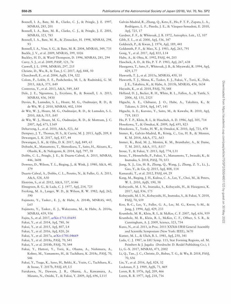
by Immer et al. (2013), indicating that W 33 is locatedin the Scutum spiral arm in the Milky Way. Figure 1shows a three-color composite image of the Spitzer spacetelescope observations (GLIMPSE: Benjamin et al. 2003;MIPSGAL: Carey et al. 2009), where blue, green, andred correspond to the 3.6 μm, 8 μm, and 24 μm emis-sions, respectively. The contours in figure 1 indicate theMAGPIS 90 cm radio continuum emission (Helfand et al.2006).

W 33 harbors many star-forming clumps, OB stars,and H II regions. There are six dust clumps (W 33 Main,W 33 A, W 33 B, W 33 Main1, W 33 A1, and W 33 B1) asshown in the pink contours in figure 1, obtained by theAtacama Pathfinder Experiment (APEX) Telescope LargeArea Survey of the GALaxy (ATLASGAL) 870 μm survey(Schuller et al. 2009; Contreras et al. 2013; Urquhartet al. 2014). The sizes and masses of the dust clumps arelisted, together with their physical properties, in table 1.These six dust clumps are suggested to be on differentevolutional stages, indicated by their spectral propertiesand associations with radio continuum sources (Immeret al. 2014). W 33 Main includes a (compact) H II regiondetected by radio continuum observations (Haschick &Ho 1983; Ho et al. 1986), while W 33 A and W 33 Bharbor hot cores by the chemical line survey. W 33 Main1,W 33 A1, and W 33 B1 are identified as high-mass pro-tostellar objects (Immer et al. 2014). Radio observationsby Haschick and Ho (1983) revealed the presence of anobscured (proto)cluster which includes a number of high-mass stars with spectral types from O7.5 to B1.5 byassuming a distance of 4 kpc. Associations of the masersources also support the nature of the young massive stellarobjects, i.e., water and methanol masers in W 33 Main,W 33 A, and W 33 B, and OH masers in W 33 A and W 33 B(Immer et al. 2013; Menten et al. 1986; Caswell 1998;Colom et al. 2015). The Submillimeter Array (SMA)high-resolution observations showed that W 33 Main har-bors multiple ultra-compact H II regions and three high-density clumps (W 33 Main-A, W 33 Main-B1, W 33 Main-B2) embedded in a dense gas envelope detected in C2H(Jiang et al. 2015). W 33 A has been studied based on obser-vations at various wavelengths (Gibb et al. 2000; Roueffet al. 2006; Davies et al. 2010; de Wit et al. 2007, 2010).Galvan-Madrid et al. (2010) detected high-velocity gasassociated with an outflow in the CO J = 2–1 transi-tion by SMA 230 GHz band observations in W 33 A. Theysuggested that star formation activity in W 33 A was trig-gered by filamentary convergent gas flows from two dif-ferent velocity components. Recently, Maud et al. (2017)carried out Atacama Large Millimeter/Submillimeter Array(ALMA) observations in Band 6 and Band 7 with500 au-scale resolution toward W 33 A, finding spiral and

Dow



ay 2022


Fig. 1. Three-color image of W 33 with blue, green, and red corresponding to Spitzer/IRAC 3.6 μm (Benjamin et al. 2003), Spitzer/IRAC 8 μm (Benjaminet al. 2003), and Spitzer/MIPS 24 μm (Carey et al. 2009) respectively. The large black crosses indicate the dust clumps (W 33 Main, W 33 A, W 33 B,W 33 Main1, W 33 A1, and W 33 B1) identified with APEX in 870 μm by Contreras et al. (2013) and Urquhart et al. (2014). The orange and white circlesindicate O- and B-type stars identified by Messineo et al. (2015). The white and pink contours show the VLA 90 cm and ATLASGAL 870 μm continuumimage. The white arrows show H II regions identified with the WISE satellite (Anderson et al. 2014, 2015).

filamentary structures around the central massive youngstellar object in W 33 A.

H II regions in W 33 are shown in the radio con-tinuum emissions shown in figure 1 as white con-tours, where the names of the H II regions cataloged bythe radio recombination line survey (G012.745−00.153:Downes et al. 1980; Lockman 1989) and Wide-FieldInfrared Survey Explorer (WISE) satellite (Andersonet al. 2014, 2015), G012.692−00.251, G012.820−00.238,G012.884−00.237, and G012.907−00.277, are labeled.

Messineo et al. (2015) identified many high-mass stars inW 33 based on the near-infrared K-band observations usingSpectrograph for INtegral Field Observations in the NearInfrared (SINFONI) on the Very Large Telescope (VLT).The positions of the OB stars identified by Messineo et al.(2015) are indicated as circles on the three-color image ofthe Spitzer observations in figure 1, where the circles coloredin orange indicate the O-type stars, while those in whiteindicate early B-type stars. Two O4-6 are distributed inG012.745−00.153, and Messineo et al. (2015) discussed

Dow



ay 2022


Table 1. Observational properties of dust clumps in W 33.∗

Source � b Size(1) Mass(1) Evolutional stage(2) VLSR,H2O(3) VLSR,H2CO

(4)

[◦] [◦] [pc] [M�] [km s−1] [km s−1]

W 33 Main 12.804 −0.200 0.25 4 × 103 (Compact) H II region 34 ∼35W 33 A 12.907 −0.259 0.15 3 × 103 Hot core 35 ∼35W 33 B 12.679 −0.182 0.1 2 × 103 Hot core 59 ∼60W 33 Main1 12.852 −0.225 0.1 5 × 102 High-mass protostellar object – –W 33 A1 12.857 −0.273 0.1 4 × 102 High-mass protostellar object – –W 33 B1 12.719 −0.217 0.1 2 × 102 High-mass protostellar object – –

∗References: (1) Immer et al. (2014); (2) Haschick and Ho (1983); Immer et al. (2014); (3) Immer et al. (2013); (4) Gardner and Whiteoak (1972).

Table 2. Observational properties of NANTEN2 and FUGIN datasets.

Telescope Line HPBW Effective Velocity RMS noisebeam size resolution level∗

NANTEN2 12CO J = 1–0 160′′ 180′′ 0.16 km s−1 ∼0.6 KNobeyama 45 m† 12CO J = 1–0 14′′ 20′′ 1.3 km s−1 ∼0.5 K

13CO J = 1–0 15′′ 21′′ 1.3 km s−1 ∼0.2 KC18O J = 1–0 15′′ 21′′ 1.3 km s−1 ∼0.2 K

∗The rms noise level value is after smoothing datasets.†Reference: Umemoto et al. (2017).

that the two O stars have evolved to be (super-)giant. Theauthors discussed the ages of these two O stars as less than6 Myr based on a stellar model by Ekstrom et al. (2012) or2–4 Myr by comparing the O4-6 supergiants in the Archescluster in the Galactic center (Martins et al. 2008), whichshow similar K-band spectra to the present two O starsin W 33.

CO rotational transition line observations at millimeterwavelengths covering the entire W 33 region were carriedout using the Five College Radio Observatory (FCRAO)14 m telescope and Millimeter Wave Observatory (MWO)5 m telescope by Goldsmith and Mao (1983), revealing thatW 33 has complicated velocity structures, whereas detailedspatial and velocity distributions of molecular gas remainedunclear. Observations of the H2CO absorption and radiorecombination lines indicate that W 33 Main has a velocityof ∼35 km s−1, while W 33 B’s is ∼60 km s−1 (Gardner &Whiteoak 1972; Bieging et al. 1978). Immer et al. (2013)detected water maser emission at a velocity of ∼35 km s−1

toward W 33 Main and W 33 A, and ∼60 km s−1 towardW 33 B, finding that these two velocity components are atthe same annual parallaxial distance of 2.4 kpc. The authorsconcluded that W 33 is a single star-forming region in spiteof the large velocity difference between the two velocitycomponents, ∼25 km s−1, although the origin of the twovelocity components is still ambiguous.

In order to reveal the detailed spatial and velocity distri-butions of the molecular gas in W 33, we carried out high-resolution observations in the J = 1–0 transition of 12CO,13CO, and C18O using the NANTEN2 and Nobeyama 45 m

telescopes. This paper is organized as follows: section 2describes the observations, section 3 gives the observa-tional results and comparison with archive datasets, andsection 4 discusses a cloud–cloud collision scenario forW 33. Section 5 concludes the paper.

2 Dataset

2.1 NANTEN2 12CO J = 1–0 observations

The NANTEN2 4 m millimeter/submillimeter telescopeof Nagoya University situated in Chile was used toobserve a large area of W 33 in 12CO J = 1–0 emis-sion with the on-the-fly (OTF) mode from 2012 May to2012 December. The half-power beam width (HPBW) is2.′7 at 115 GHz. This corresponds to 1.9 pc at the dis-tance of 2.4 kpc. A 4 K cooled superconductor–insulator–superconductor (SIS) mixer receiver provided a typicalsystem temperature of ∼250 K in double side band (DSB),and a 16384-channel digital spectrometer with a band-width and resolution of 1 GHz and 61 kHz respectively,which corresponds to 2600 km s−1 and 0.16 km s−1, respec-tively, at 115 GHz. We smoothed the obtained data toa velocity resolution of 1 km s−1 and angular resolu-tion of 200′′. The pointing accuracy was confirmed tobe better than 15′′ with daily observations of the Sunand IRC + 10216. We used the chopper wheel methodto calibrate the antenna temperature T∗

a (Penzias &Burrus 1973; Ulich & Haas 1976; Kutner & Ulich 1981).The absolute intensity fluctuation was calibrated by daily

Dow



ay 2022


observations of IRAS 16293−2422 [αJ2000.0 = 16h32m23.s3,

δJ2000.0 = −24◦28′39.′′2], and the intensity scale was con-verted into the Tmb scale by assuming its peak to beTmb = 18 K (Ridge et al. 2006). The intensity uncertaintyof NANTEN2 datasets is <20%. The typical root-mean-square (rms) noise level is ∼0.6 K with 200′′ smoothingdata and a velocity resolution of 1.0 km s−1.

2.2 Nobeyama 45 m telescope 12CO J = 1–0,13CO J = 1–0, C18O J = 1–0 observations

Detailed CO J = 1–0 data around W 33 were obtainedby using the Nobeyama 45 m telescope at the NobeyamaRadio Observatory (NRO). The HPBW is 14′′ at 115 GHz,and 15′′ at 110 GHz. This corresponds to 0.2 pc at thedistance of 2.4 kpc. We simultaneously observed in 12CO,13CO, and C18O as part of the FUGIN (FOREST UnbiasedGalactic plane Imaging survey with the Nobeyama 45 mtelescope; Minamidani et al. 2015; Umemoto et al. 2017)legacy survey with the OTF mode (Sawada et al. 2008)from 2014 March to 2015 May. FOREST (FOur-beamREceiver System on the 45 m Telescope) is a four-beam,dual-polarization, two-sideband (2SB) receiver providing atypical system temperature of ∼150 K in 13CO J = 1–0and ∼250 K in 12CO J = 1–0 (Minamidani et al. 2016).We used SAM45 (Spectral Analysis Machine for the 45 mtelescope: Kuno et al. 2011), an FX-type digital spectrom-eter the same as the ALMA ACA Correlator (Kamazakiet al. 2012). It has 4096 channels with a bandwidthand resolution of 1 GHz and 244.14 kHz respectively,which corresponds to 2600 km s−1 and 1.3 km s−1, respec-tively, at 115 GHz. We smoothed the obtained data to theangular resolution of 30′′. The typical pointing accuracywas confirmed to be better than 3′′ observing SiO masersources, such as V VX Sgr [αB1950 = 18h05m02.s959, δB1950 =−22◦13′55.′′58], for the observing run toward W 33 everyhour with the 40 GHz HEMT receiver named H40. Theintensity variation was calibrated with daily observationsof W51D [αB1950 = 19h21m22.s2, δB1950 = 14◦25′17.′′0]. Weused the chopper wheel method to convert the antenna tem-perature T∗

a (Penzias & Burrus 1973; Ulich & Haas 1976;Kutner & Ulich 1981). The data in the antenna tempera-ture (T∗

a ) scale was converted into main beam temperature(Tmb) by Tmb = T∗

a /ηmb, with a main beam efficiency (ηmb)of 0.43 for 12CO and 0.45 for 13CO and C18O (Minamidaniet al. 2016; Umemoto et al. 2017). The typical rms noiselevels after intensity calibration (Tmb scale) are ∼0.5 K,∼0.2 K, and ∼0.2 K for 12CO, 13CO, and C18O J = 1–0,respectively. The intensity variation of 12CO, 13CO, andC18O J = 1–0 are 10%–20%, 10%, and 10%, respectively.The FUGIN project overview paper gives more detailed

information (Umemoto et al. 2017). We summarize theobservational parameters of the NANTEN2 and Nobeyama45 m datasets in table 2.

2.3 Archive dataset

We use the 12CO J = 3–2 archival data of the CO HighResolution Survey (COHRS) obtained with JCMT (JamesClark Maxwell Telescope: Dempsey et al. 2013). The spa-tial and velocity resolutions are 1.0 km s−1 and 16′′, respec-tively. We smoothed the data to an angular resolutionof 30′′. The data in the antenna temperature (T∗

a ) scalewas converted into main beam temperature (Tmb) with theequation Tmb = T∗

a /ηmb, where the main beam efficiency(ηmb) of 0.61 was adopted by planet observations withan uncertainty of about 10%–15% (Dempsey et al. 2013;Buckle et al. 2009). The typical rms noise in the Tmb scalewas ∼0.2 K for 12CO J = 3–2.

We use the following datasets to compare withthe CO data: near- and mid-infrared data from theSpitzer space telescope (GLIMPSE in 3.6 μm and 8.0 μm:Benjamin et al. 2003; MIPSGAL in 24 μm: Careyet al. 2009); the 20 cm and 90 cm free–free radio con-tinuum data from MAGPIS (A Multi-Array Galactic PlaneImaging Survey: Helfand et al. 2006) observed with theVery Large Array (VLA); and the H I 21 cm emission datafrom SGPS II (Southern Galactic Plane Survey: McClure-Griffiths et al. 2005) observed with the Australia TelescopeCompact Array (ATCA) and the Parkes Radio Telescope.The angular resolution of the H I data is ∼ 3.′3, and theirspectrum resolution is 0.8 km s−1.

3 Results

3.1 Distribution and properties of molecular gas

Figure 2a shows the longitude–velocity diagram of theNANTEN2 12CO J = 1–0 data for a large area includingW 33. There are four distinct velocity components towardW 33, as depicted by arrows. Goldsmith and Mao (1983)mentioned with CO observations that association of the 5–25 km s−1 velocity component indicated with a black arrowwith W 33 is not clear, as it is likely to be located in the Sagit-tarius arms (Reid et al. 2016). In this study, we thereforefocus on the velocity components at 35 km s−1, 45 km s−1,and 58 km s−1 as candidate clouds associated with W 33.We hereafter refer to these three clouds as “the 35 km s−1

cloud,” “the 45 km s−1 cloud,” and “the 58 km s−1 cloud.”These three clouds appear to be connected with each otherin the velocity space (figure 2a). The 35 km s−1 cloud iscontinuously distributed along the Galactic longitude forthe present region, while the CO emissions in the other

Dow



ay 2022


Fig. 2. (a) Longitude–velocity diagram of the 12COJ = 1–0 emission with the NANTEN2 telescope. The arrows indicate the four velocity components:black arrow—10 km s−1; blue arrows—35 km s−1, 45 km s−1, and 58 km s−1. The dashed box indicates the W 33 region as the range of figure 2b.(b) Longitude–velocity diagram of the 12COJ = 1–0 emission with the Nobeyama 45 m telescope. The arrows indicate the three velocity components,35 km s−1, 45 km s−1, and 58 km s−1.

two clouds at higher velocities are especially enhancedtoward W 33 (dashed box in figure 2a). Figure 2b showsthe longitude–velocity diagram of the three velocity cloudsof W 33 using the FUGIN 12CO J = 1–0 data, which showsthe detailed velocity distribution of the gas at high spa-tial resolution. The three velocity clouds can be separatelyidentified at this spatial scale in figure 2b.

Figure 3 shows the spatial distributions of the threeclouds in the four CO lines. The left, center, and rightcolumns show the 30 km s−1, 45 km s−1, and 58 km s−1

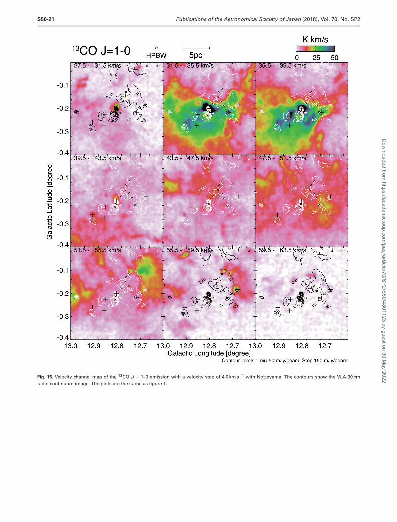
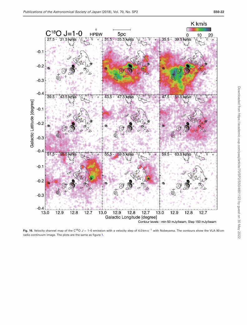
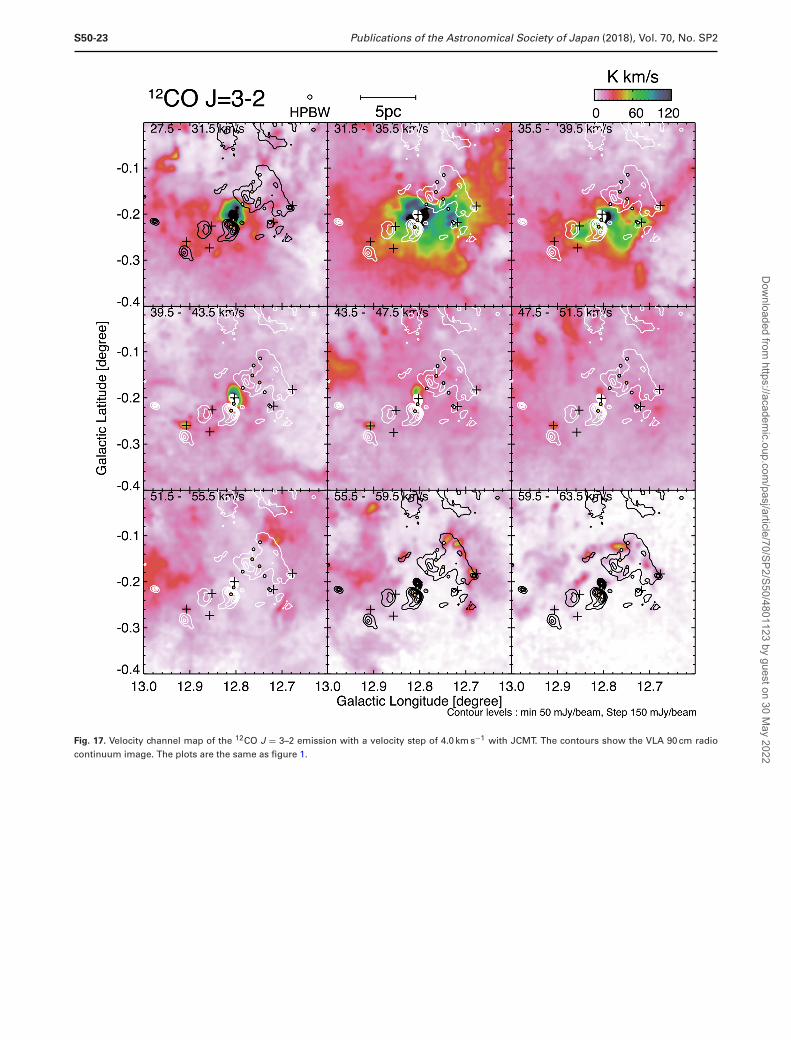
clouds, respectively, where the contours indicate theMAGPIS 90 cm radio continuum emission, and the posi-tions of the dust clumps and OB stars identified by Messineoet al. (2015) are depicted by crosses and circles, respectively.We also present the velocity channel maps of the four COtransitions obtained with Nobeyama 45 m and JCMT infigures 14–17 in the Appendix as supplements. The COemission in the 35 km s−1 cloud is enhanced at the corre-sponding region of W 33 in all the transitions. W 33 Mainshows the brightest CO emission in this region.

We found counterparts of W 33 A, W 33 Main, andW 33 B1 in the 35 km s−1 cloud in the C18O emis-sion (figure 3g). Figure 4 shows the C18O distributionsof each dust clump (the C18O molecular clump prop-erties are discussed in subsection 3.2.) Among thesesources, W 33 Main and W 33 A are associated with COmolecular outflows, as discussed in subsection 3.6. The35 km s−1 cloud also shows morphological anti-correlationswith the radio continuum emissions in H II regionsG012.745−00.153 and G012.820−00.238. The CO emis-sion in G012.745−00.153 is enhanced at the eastern

(l, b) = (12.78, −0.18) and southern rim (l, b) = (12.74,−0.18) of the H II region, showing a steep intensity gra-dient in the 12CO emissions, while G012.820−00.238 issurrounded by molecular gas, especially in the 13CO andC18O emissions. W 33 Main is sandwiched by these twoH II regions. The 45 km s−1 cloud has diffuse CO emis-sion extended over the present region. The compact emis-sions at W 33 Main and W 33 A correspond to the wingfeatures of the outflows (see subsection 3.6 for details),and are thus not related to the 45 km s−1 cloud. Moleculargas in the 58 km s−1 cloud is separated into the northernand southern components relative to W 33, and the cen-tral part corresponding to W 33 is weak in the CO emis-sion. There are several clumpy structures embedded at thenorthern rim of the southern component, which are clearlyseen in the 12CO emissions, and these clumps show spa-tial correlations with radio continuum emissions from theH II regions G012.745−00.153 and G012.692−00.251 aswell as W 33 B. In the C18O map in figure 3i and figure 4d,W 33 B is associated with the strong CO peak. There areseveral other clumpy molecular structures at the interspacebetween the northern and southern components of the58 km s−1 cloud, forming an arc-like molecular structurewhich looks to surround W 33. The size of the arc-likestructure is roughly estimated to be ∼7 pc. On the otherhand, clear associations of molecular clumps with W 33 A1and W 33 Main1 are not recognized.

We derived the column densities and masses of thethree velocity clouds using the 12CO integrated inten-sity maps shown in figures 3a–3c, where we definedthe individual clouds by drawing contours at 5 σ noise

Dow



ay 2022


Fig. 3. Integrated intensity distributions of the 35 km s−1 (left column), 45 km s−1 (center column), and 58 km s−1 clouds (right column). (a)–(c)12COJ = 1–0, (d)–(f) 13COJ = 1–0, and (g)–(i) C18OJ = 1–0 are obtained with Nobeyama. (j)–(l) 12COJ = 3–2 is obtained with JCMT. Contours showthe VLA 90 cm radio continuum image. Plots are same as figure 1.

Dow



ay 2022


Fig. 4. C18O J = 1–0 integrated intensity distributions of the molecular clumps by the Nobeyama 45 m telescope. The crosses indicate the dustclumps (W 33 Main, W 33 A, W 33 B, W 33 Main1, W 33 A1, W 33 B1) identified at APEX 870 μm by Contreras et al. (2013) and Urquhart et al. (2014). Thelowest contour is defined as half (W 33 Main, W 33 B) and 75% (W 33 A, W 33 B1, W 33 A1, W 33 Main1) of the level of the peak integrated intensity.The integrated velocity range shows in the lower left of the figures.

Dow



ay 2022


levels in the integrated intensity of 8 K km s−1 for thevelocity interval of 10 km s−1. By assuming an X(CO) factorof 2 × 1020 (K km s−1)−1 cm−2 (Strong et al. 1988), weestimated the mean column densities of the 35 km s−1,45 km s−1, and 58 km s−1 clouds as 1.7 × 1022 cm−2,1.7 × 1022 cm−2, and 6.2 × 1021 cm−2, respectively, withthe total molecular masses derived as 1.1 × 105 M�,1.0 × 105 M�, and 3.8 × 104 M�. The uncertainty of themass estimation using the X factor is about ±30% (Bolattoet al. 2013). Lin et al. (2016) derived the mean column den-sities as 2.5 × 1022 cm−2 using the infrared dust emissiondata obtained by Herschel, which is consistent with ourestimate.

3.2 C18O molecular clump properties

We define C18O molecular clumps using the followingprocedures in order to investigate the physical propertiesof dense molecular gas belonging to the 35 km s−1 and58 km s−1 clouds corresponding to the dust clumps.

(1) Search for a peak integrated intensity toward the six dustclumps.

(2) Define a clump boundary as the half level of its peakintegrated intensity.

(3) If the area enclosed by the boundary has multiple peaks,define the boundary as the contour of the 75% level ofits peak integrated intensity.

We identified four molecular clumps corresponding tothe dust clumps of W 33 Main, W 33 A, and W 33 B1 asso-ciated with the 35 km s−1 cloud (figures 4a, 4b, and 4c),and W 33 B associated with the 58 km s−1 cloud (figure 4d),while we could not define the boundary of the molecularclump toward W 33 Main1 and W 33 A1 because W 33 A1does not have an intensity peak toward the dust clump andW 33 Main1 cannot be separated from the extended feature(figures 4e and 4f).

Then, we derived the physical parameters assuming localthermal equilibrium (LTE) using the following procedures(Wilson et al. 2009).

(1) Derive the excitation temperature (Tex) assuming thatthe 12CO J = 1–0 transition line is optically thickand Tex is uniform throughout the molecular clump byfollowing the equation from the 12CO peak intensity(Tmb(12COpeak)) at the peak position of the clump:

Tex = 5.5/

ln[1 + 5.5

Tmb(12COpeak) + 0.82

]. (1)

(2) Estimate the optical depth of the C18O emission (τ 18) ateach pixel and velocity channel from the C18O brightness

temperature [Tmb(v)] at velocity v:

τ18(v) =− ln

⎧⎨⎩1 − Tmb(v)

5.3

[1

exp( 5.3Tex

) − 1− 0.17

]−1⎫⎬⎭ .

(2)

(3) Calculate the C18O column density [N(C18O)] at eachpixel, summing the quantities of all v channels whoseresolution is 1 km s−1:

N(C18O) = 2.4 × 1014 ×∑

v

Texτ18(v)�v

1 − exp(− 5.3

Tex

) . (3)

(4) N(C18O)) is converted into H2 column density (N(H2))assuming the following conversion formula derived fromthe Ophiuchus molecular cloud (Frerking et al. 1982):

N(H2) =[

N(C18O)1.7 × 1014

+ 3.9]

× 1021. (4)

(5) Estimate the size (r) of each clump assuming that clumpsare spherical shapes, using:

r =√

Sπ

=√

D2

π, (5)

where S is the area of the clump enclosed by theboundary contour, D is the distance to W 33, and

is the solid angle of the clump.(6) Calculate the mass of each clump:

M = μmH D2∑

N(H2), (6)

where μ is the mean molecular weight 2.8, mH is theproton mass, and the summation is performed over theeach clump within the boundary.

(7) The averaged number density of hydrogen molecules iscalculated as

n(H2) = 3M4πr3μmH

(7)

by assuming that the clumps have a uniform density.(8) The virial mass is estimated by

Mvir = 5r�v2

8(ln 2)G= 210

(r

[pc]

)(�Vcomp

[km s−1]

)2

(8)

from the virial theorem using the clump size (r) andthe full width at half maximum (FWHM) of the com-posite spectrum �Vcomp in the clump estimated by asingle Gaussian fitting.

Table 3 presents the physical properties of the molec-ular clumps. The typical values of the peak column den-sity, mean column density, mass, size, hydrogen molecule

Dow



ay 2022


Table 3. Physical parameters of the C18O molecular clumps in W 33.∗

Clump VLSR Tex τ18 N(H2)peak Size �Vcomp N(H2)mean Mclump n(H2) Mvir

[km s−1] [K] [cm−2] [pc] [km s−1] [cm−2] [M�] [cm−3] [M�](1) (2) (3) (4) (5) (6) (7) (8) (9) (10) (11)

W 33 Main 35.5 34 0.11 6.0 × 1023 0.60 5.5 5.1 × 1022 9.5 × 103 1.5 × 105 3.8 × 103

W 33 A† 36.5 18 0.15 2.6 × 1023 1.0 5.5 3.7 × 1022 1.4 × 104 4.8 × 104 6.4 × 103

W 33 B 56.5 17 0.096 1.9 × 1023 0.81 6.4 2.1 × 1022 5.1 × 103 3.3 × 104 6.9 × 103

W 33 Main1 36.5 19 0.096 2.0 × 1023 – – – – – –W 33 A1 36.5 18 0.12 2.1 × 1023 – – – – – –W 33 B1† 35.5 23 0.13 1.2 × 1023 0.41 3.1 1.3 × 1022 1.9 × 103 9.2 × 104 8.3 × 102

∗Columns: (1) Name. (2) C18O peak velocity. (3) Excitation temperature of 12CO J = 1–0 peak intensity. (4) Optical depth of peak position. (5) Peakcolumn density of the C18O clump. (6) Size of the C18O clump. (7) Line width of the composite profile obtained by averaging spectra in the C18Oclump. (8) Average column density of the C18O clump. (9) The molecular mass within the clump size with the assumption of LTE. (10) Density of theclump with the assumption of a sphere. (11) Virial mass of the clump. W 33 Main1 and W 33 A1 show only peak parameters because we could notdefine the size of clump.

†Defined by the 75%-level boundary.

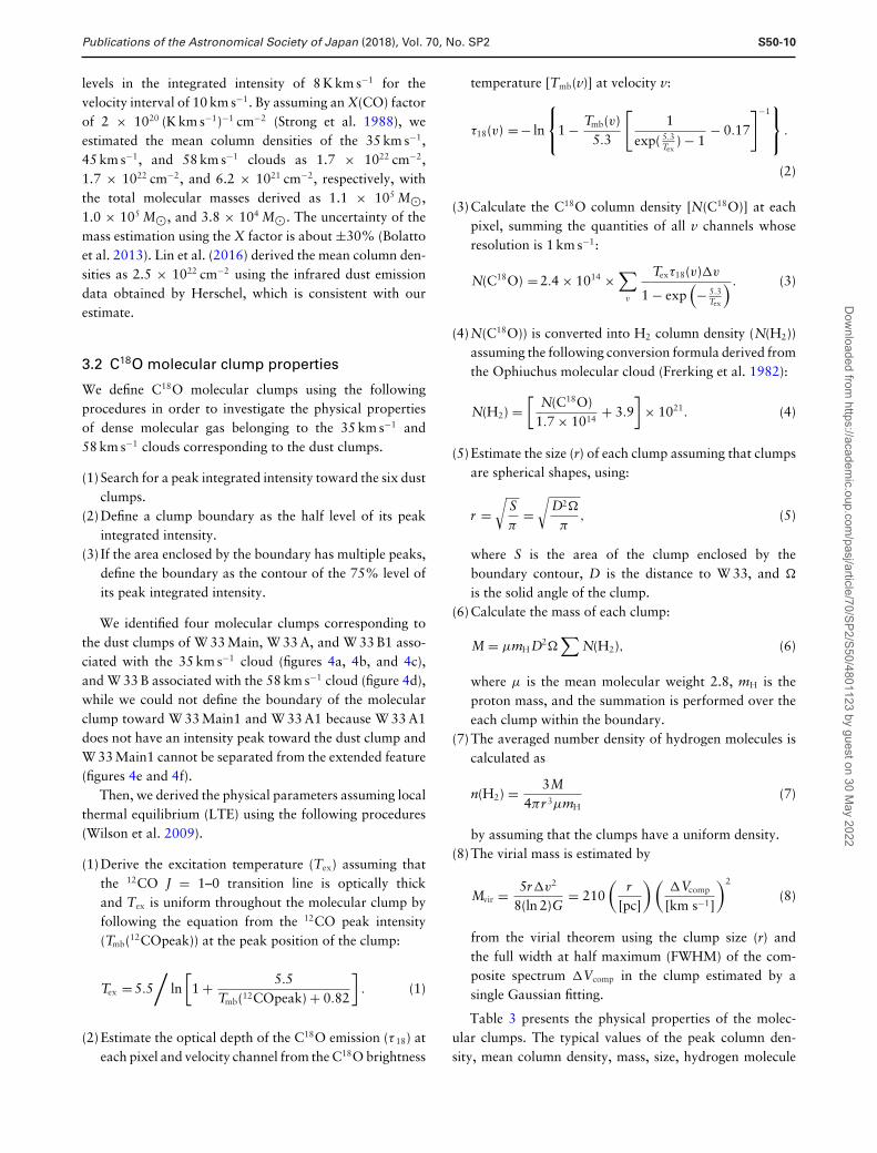
Fig. 5. R3–2/1–0 maps of the (a) 35 km s−1, (b) 45 km s−1, and (c) 58 km s−1 clouds are shown in the color image. The contours show the 12COJ = 3–2emission, which was spatially smoothed at 50′′. The plots are the same as figure 1. The clipping level is 8 σ .

number density, and virial mass are N(H2)peak ∼ 1023 cm−2,N(H2)mean ∼ 1022 cm−2, Mclump ∼ 103–104 M�, r ∼0.4–1 pc, n(H2) ∼ 104–105 cm−3, and Mvir ∼ 102–103 M�. Thepeak and mean column densities are roughly consistentwith those calculated from the dust continuum observa-tions (Immer et al. 2014).

3.3 CO J = 3–2 / J = 1–0 intensity ratio

Figure 5 shows distributions of the 12CO J = 3–2/J = 1–0 intensity ratio (R3-2/1-0) using 50′′ smoothing data (rms∼0.26 K) in the 35 km s−1, 45 km s−1, and 58 km s−1 clouds,respectively. We adopted the clipping level as 8 σ . Lineintensity ratios between different J levels of CO provideuseful diagnostics to investigate the physical association ofmolecular gas with high-mass stars, as these depend onthe gas kinematic temperature (Tk) and number density ofhydrogen [n(H2)] following the Large Velocity Gradient

(LVG) model (e.g., Goldreich & Kwan 1974). Figure 5ashows that the 35 km s−1 cloud has a high R3-2/1-0 of >1.0around the central part of W 33, which includes W 33 Main,W 33 Main1, and W 33 B1. The 45 km s−1 cloud showslower R3-2/1-0 of 0.4–0.5 except for the corresponding partsof W 33 Main and W 33 A, where R3-2/1-0 is locally ele-vated up to 0.8–1.2. As discussed in the next subsection,the high R3-2/1-0 in W 33 Main and W 33 A in the 45 km s−1

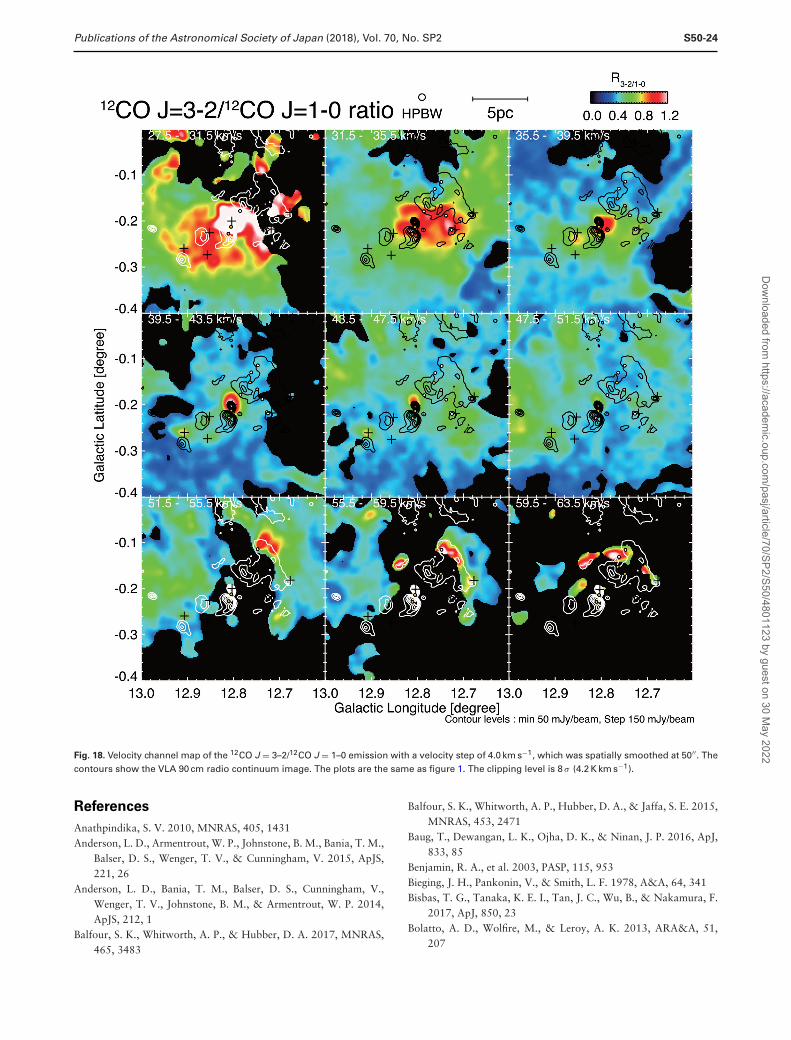
cloud are due to the outflows emitted from the protostarsembedded in the 35 km s−1 cloud. The 58 km s−1 cloud hashigh R3-2/1-0 of 1.2 in the arc-like structure which seems tosurround W 33, while the gas outside the arc-like structureshows low R3-2/1-0 of ∼0.4. We also present the velocitychannel map of R3-2/1-0 in figure 18 in the Appendix. Thecause of the high R3-2/1-0 of the gas in the 35 km s−1 and58 km s−1 clouds can be understood as heating by the high-mass stars in W 33. The high R3-2/1-0 of the molecular gasin the 35 km s−1 and 58 km s−1 clouds can be understood as

Dow



ay 2022


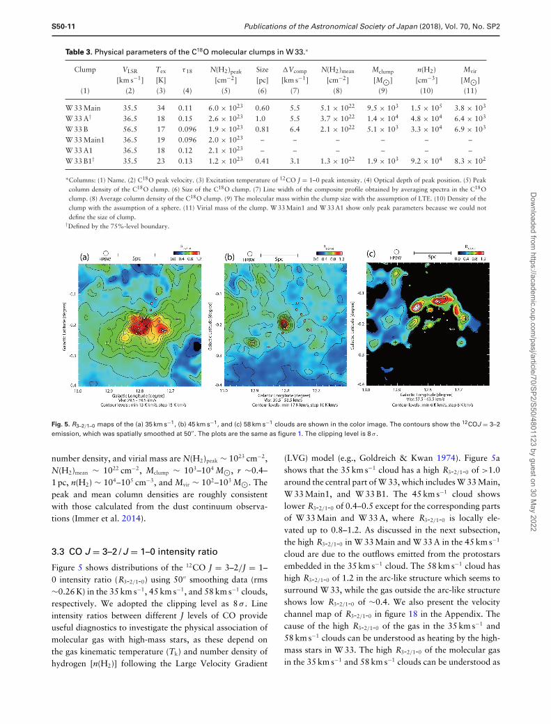
Fig. 6. Comparison of the 35 km s−1 (blue) and 58 km s−1 (red) clouds (12CO J = 3–2 contours) with (a) the Spitzer 8 μm and (b) 24 μm image(grayscale). The plots are the same as figure 1.

high kinematic temperature heated by the high-mass stars inW 33. Therefore, the 35 km s−1 and 58 km s−1 clouds indi-cate physical associations of W 33, whereas association ofthe 45 km s−1 is elusive.

3.4 Comparisons of the 35 km s−1 and 58 km s−1

clouds with infrared data

We focus here on the 35 km s−1 and 58 km s−1 clouds,as these are most likely associated with W 33. Figure 6demonstrates comparisons between the 12CO J = 3–2 andinfrared emissions, where the Spitzer 8 μm and 24 μm emis-sions are shown in grayscale in panels (a) and (b), respec-tively. The 8 μm emissions trace thermal emission fromhot dust plus emission from polycyclic aromatic hydrocar-bons (PAH), which are distributed in the photo-dissociationregion (PDR; e.g., Churchwell et al. 2004). The 24 μmemission also traces warm dust grains heated by brighthigh-mass stars in the H II region (e.g., Carey et al. 2009,Deharveng et al. 2010). The red and blue contours showthe 35 km s−1 and 58 km s−1 clouds, respectively. The arc-like structure in the 58 km s−1 cloud surrounds the strongemission part of the 35 km s−1 cloud, showing complemen-tary distributions between these two. The 8 μm emission,which is bright at the southeastern rim of the H II regionG012.745−00.153 (l, b) ∼ (12.75, −0.18), coincides withthe steep intensity gradient of the CO emission in the35 km s−1 cloud. This lends more credence to associationbetween the 35 km s−1 cloud and G012.745−00.153.

The 24 μm emission shown in figure 6b is attributedto the warm dust grains and thus can be used to probethe region where the heating by the high-mass stars inW 33 is efficient. The 24 μm emission in W 33 is enhancedat the dust clumps and the H II regions. In particular,G012.745−00.153 and G012.820−00.238, as well asW 33 Main, show bright 24 μm emissions. The arc-likestructure in the 58 km s−1 cloud overall traces the out-line of the 24 μm distribution. This suggests that thehigh R3-2/1-0 of the gas in the arc-like structure shownin figure 5c is due to interaction with the star-formingregions, which are spatially correlated with the arc-likestructure.

The morphological correlations of the 58 km s−1 cloudwith infrared emissions, as well as the high R3-2/1-0 of thegas in the 58 km s−1 cloud, strongly suggest that not onlythe 35 km s−1 cloud but also the 58 km s−1 cloud are phys-ically associated with W 33 despite the large velocity sep-aration between the two clouds, ∼23 km s−1. This is con-sistent with the previous studies by Gardner and Whiteoak(1972), Bieging, Pankonin, and Smith (1978), and Immeret al. (2013) based on observations of H2CO absorption,radio recombination line, and water masers; Immer et al.(2013) discussed that the two velocity components are atthe same annual parallax distance of 2.4 kpc.

On the other hand, association of the 45 km s−1 cloud atthe intermediate velocity range between the 35 km s−1 and58 km s−1 clouds with W 33 is not evident in the presentdataset.

Dow



ay 2022


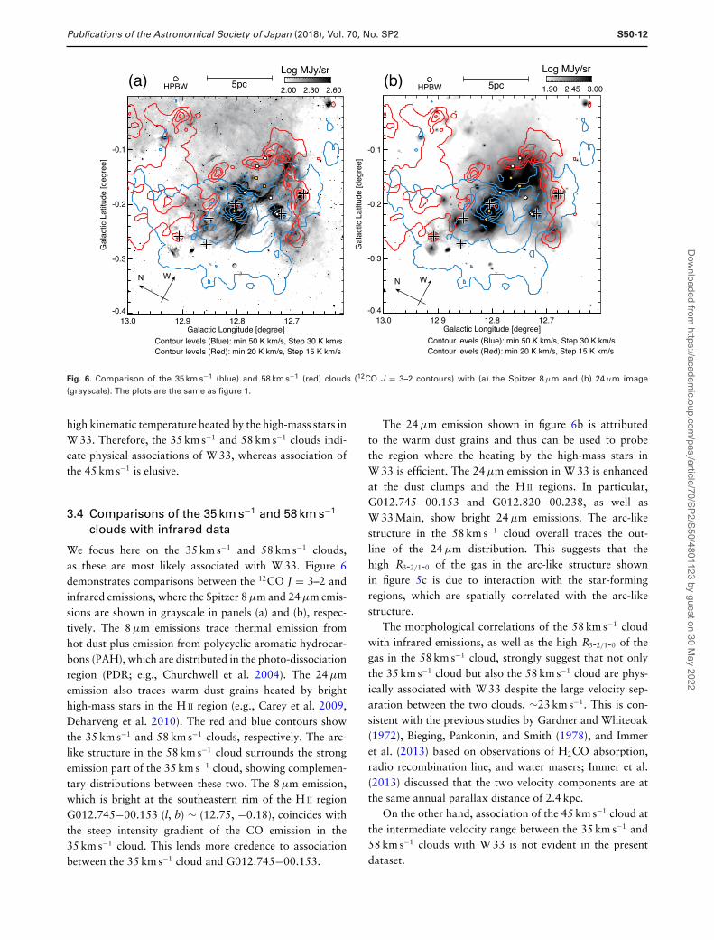
Fig. 7. Comparison of the H I 21 cm emission with velocity integration ranges of (a) 30–40 km s−1, (b) 45–50 km s−1, and (c) 55–58 km s−1, respectivelyand the VLA 20 cm continuum image (black contour). A, B, and C are the positions of spectra in figure 8 at (l, b) = (12.◦795,−0.◦202), (12.◦731, −0.◦154),and (12.◦710, −0.◦112), respectively. The plots are the same as figure 1.

Fig. 8. H I 21 cm and 12CO J = 1–0 spectrum of A, B, and C in figure 7 at (l, b) = (12.◦795,−0.◦202), (12.◦731, −0.◦154), and (12.◦710, −0.◦112), respectively.The gray areas show the absorption position of H I 21 cm emissions.

3.5 Comparison with the H I 21 cm line

We analyzed the H I 21 cm line data in W 33 using thearchival data obtained in the Southern Galactic PlaneSurvey (SGPS) project (McClure-Griffiths et al. 2005).Figure 7 shows the integrated intensity distributions of thethree velocity clouds of the H I data. The contours showthe MAGPIS 20 cm radio continuum emission, where theoriginal image was spatially smoothed to have the sameresolution as that of the SGPS H I data. In figure 7a theH I emission in the 35 km s−1 cloud shows strong inten-sity depression at W 33 Main where the 20 cm continuumemission is strong. The depression can be confirmed in theH I 21 cm spectra shown in figure 8a. The H I profile hasnegative intensities at the velocity range of the 35 km s−1

cloud, as indicated by the shading. This indicates absorp-tion against the background continuum source, implyingthat W 33 Main is distributed at the inside or at the rearside of the 35 km s−1 cloud. The H I maps of the 45 km s−1

and 58 km s−1 clouds in figures 7b and 7c show weak inten-sity depressions toward G012.745−00.153 and W 33 B,whereas it is not clear toward W 33 Main. The H I spectratoward G012.745−00.153 shown in figures 8b and 8c show

absorption features at the velocity ranges where the 12COemission appears, i.e., 40–50 km s−1 in figure 8b and at 50–60 km s−1 in figure 8c. We suggest that these absorptionsare unrelated foreground components overlapping on theline of sight.

3.6 Molecular outflows

We identified bipolar outflows in the CO emissions towardW 33 Main and W 33 A. Figures 9 and 10 show the COspectra and spatial distributions of the outflow lobes inW 33 Main and W 33 A, respectively. The outflows in bothW 33 Main and W 33 A have total velocity widths as largeas 40–50 km s−1. The systemic velocities of these outflowsare estimated to be ∼35 km s−1 using the optically thin C18OJ = 1–0 emission. W 33 A has been reported to be associ-ated with outflows (Davies et al. 2010; de Wit et al. 2010;Galvan-Madrid et al. 2010). As the blue and red lobes infigures 9 and 10 are not fully resolved in the present COdata due to the limitation of the spatial resolution, we esti-mate here the lengths of the outflow lobes to be 0.5 pc,defined by contours at half of the peak intensity level.

Dow



ay 2022


Fig. 9. (a), (b) CO spectra of the blue-shifted and the red-shifted lobes obtained at (l, b) = (12.◦800,−0.◦185) and (12.◦807, −0.◦197), respectively. The blueand red areas show integrated velocity ranges for the lobes. The dashed lines show systematic velocity. (c) 12COJ = 3–2 distributions of the molecularoutflows associated with W 33 Main, where the blue-shifted lobe is shown in blue contours and the red-shifted lobe is shown in red contours. Thebackground image is the Spitzer 8 μm emission. The cross indicates W 33 Main.

Fig. 10. (a), (b) CO spectra of the blue-shifted and the red-shifted lobes obtained at (l, b) = (12.◦906, −0.◦266) and (l, b) = (12.◦908, −0.◦261), respectively.The blue and red areas show integrated velocity ranges for the lobes. The dashed lines show systematic velocity. (c) 12COJ = 3–2 distributions ofthe molecular outflows associated with W 33 A, where the blue-shifted and red-shifted lobes are shown in blue and red respectively. The backgroundimage is the Spitzer 8 μm emission. The cross indicates W 33 A.

If we assume an inclination angle of 45◦, the dynamicaltimescales (tdyn) of W 33 Main and W 33 A are calculatedfrom the maximum velocity (Vmax ∼ 23 km s−1) and size (r)to be 0.5/23 × √

2 ∼ 3 × 104 yr, which is consistent withprevious JCMT 12CO and 13CO J = 3–2 observation results(Maud et al. 2015).

4 Discussion

The results of the present observations and analyses aresummarized as follows:

(1) We identified three molecular clouds toward W 33at ∼35 km s−1, ∼45 km s−1, and ∼58 km s−1 using

the NANTEN2, FUGIN CO J = 1–0, and JCMT12CO J = 3–2 data. The total molecular massesof each of the three clouds are derived as1.1 × 105 M�, 1.0 × 105 M�, and 3.8 × 104 M�,respectively.

(2) The 35 km s−1 cloud is spatially coincident withW 33. Our CO data revealed a spatial correlationof the 35 km s−1 cloud with the dust clumps ofW 33 Main, W 33 A, W 33 B1, and the H II regionsG012.745−00.153 and G012.820−00.238, havingR3-2/1-0 of higher than 1.0. A strong absorption featurein the H I 21 cm line is seen in the velocity range of the35 km s−1 cloud. Therefore, W 33 Main is located insideor behind the 35 km s−1 cloud.

Dow



ay 2022


(3) The 45 km s−1 cloud shows diffuse CO emissionextended for the present region, and its association withW 33 is not clear in terms of spatial correlation.

(4) In the 58 km s−1 cloud the present CO dataset revealedan arc-like structure having a size of ∼7 pc. It showscomplementary distributions with the 35 km s−1 cloudand the infrared images along the line of sight,having R3-2/1-0 of higher than 1.0. These observationalproperties suggest association of the arc-like struc-ture with the dust clump W 33 B and the H II regionsG012.745−00.153 and G012.692−00.251 distributedat the southern part of W 33.

(5) We identified two bipolar molecular outflows towardW 33 Main and W 33 A. The full velocity widths ofthe outflows are as large as 40–50 km s−1. The dynam-ical timescales of the outflows can be estimated to be∼3 × 104 yr.

In this section, we discuss the origin of the observedproperties of the multiple velocity clouds in W 33 over23 km s−1 and these relationships with the high-mass starformation in W 33.

4.1 Gravitational binding of the multiple velocityclouds

Based on the proper motion measurements, Immer et al.(2014) discussed whether W 33 A and W 33 B are gravita-tionally bound to W 33 Main, and the authors concludedthat W 33 A and W 33 B are not gravitationally bound toW 33 Main, as the total speeds of W 33 A and W 33 B arelarger than the derived escape velocity.

In addition to their calculations, we test here the dynam-ical binding of the 35 km s−1 and 58 km s−1 clouds, asthese contain the high-mass star-forming regions otherthan W 33 Main, W 33 A, and W 33 B. If we assume thatthe two clouds are separated by 10 pc in space, the sameorder as the cloud size as a rough order-of-magnitudeestimation, and by 23 km s−1 in velocity, the total massrequired to gravitationally bind these two clouds can becalculated as M = rv2

2G = 6 × 105 M�. This figure is a factorof four larger than the total molecular mass associatedwith W 33, 1.5 × 105 M�, calculated in subsection 3.1,indicating that the coexistence of the two velocity cloudsin W 33 cannot be interpreted as a gravitationally boundsystem.

4.2 Expanding motion driven by feedback fromhigh-mass stars

Another idea to interpret the multiple velocity clouds isexpanding motion driven by feedback from high-mass stars.

If we assume a spherical expansion of gas interactingwith feedback, it would display a ring-like velocity dis-tribution in both a spatial map and a position–velocitydiagram (e.g., see figure 8 of Torii et al. 2015). Theexpanding velocity (vexp) of an H II region is limited bythe sound speed of the ionized gas confined in the H II

region, which corresponds to vexp ∼ 12 km s−1 with anelectron temperature of 10000 K (e.g., Ward-Thompson &Whitworth 2011). For the present case in W 33, the arc-likestructure in the 58 km s−1 cloud and velocity separation of23 km s−1 look consistent with this assumption. However,the longitude–velocity diagram presented in figure 2 showsthat both the 35 km s−1 and 58 km s−1 clouds are separated,having uniform velocities for a large area including W 33.These velocity distributions in the position–velocity dia-gram are inconsistent with the prediction from the expan-sion assumption. Dale et al. (2013) discussed that the contri-bution of stellar wind to the expansion of a neutral mediumis relatively minor compared with the expansion of an H II

region at gas density ∼104 cm−1. We thus conclude thatthe co-location of the multiple velocity clouds in W 33 over23 km s−1 was not formed by the feedback from the high-mass stars in W 33.

4.3 The cloud–cloud collision model

We postulate here a cloud–cloud collision scenario as analternative idea to interpret the multiple velocity cloudsassociated with W 33. In a collision between two cloudswith different sizes (Habe & Ohta 1992), a smaller clouddrives into a larger cloud, forming a cavity in the largercloud, and a dense gas layer is formed at the interfaceof the collision, which corresponds to the bottom of thecavity, by strong compression of gas. High-mass stars areformed in this dense gas layer. In addition, a thin layerwith turbulent gas is formed at the interface between thelarger cloud and the dense layer, which has intermediatevelocities between the larger cloud and the dense layer.This thin, turbulent layer is observed as “broad bridge fea-tures” in a position–velocity diagram, which is the emissionbetween two velocity peaks with intermediate intensities(e.g., Haworth et al. 2015a, 2015b; Torii et al. 2017a). Theturbulent gas is replenished as long as the collisioncontinues.

Another observational signature of cloud–cloud colli-sions is “complementary distribution between two velocityclouds” (Fukui et al. 2017a; Torii et al. 2017a). For anobserver viewing angle parallel to the collisional axis sothat the two clouds are spatially coincident, the observercan see an anti-correlated or complementary distributionbetween the two clouds separated in velocity, as the larger

Dow



ay 2022


Fig. 11. Schematic of a collision between two dissimilar clouds and cartoon position–velocity diagrams, where the gas density in the smaller cloudis much smaller than that in the larger cloud. The different color components in the collision schematics correspond to the different colors on theposition–velocity diagrams.

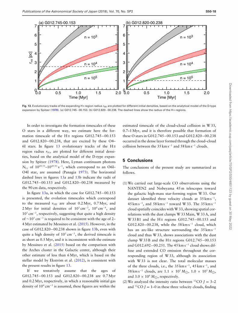
Fig. 12. As figure 11, but for the case that the gas density in the smaller cloud is much higher than that in the larger cloud.

cloud with a cavity displays a ring-like gas distributionon the sky. Fukui et al. (2017a) pointed out that, if theviewing angle has an inclination relative to the collidingaxis, the complementary distribution has a spatial offset,which is proportional to the projected travel distance of thecollision.

The gas distribution in the position–velocity diagramincluding the broad bridge feature depends on variousparameters such as the cloud shapes, the density contrast ofthe clouds, the initial relative velocity between the clouds,etc. In figures 11 and 12, we show schematics of twoextreme cases of a cloud–cloud collision and cartoons of

Dow



ay 2022


the corresponding position–velocity diagrams, based on thediscussions by Haworth et al. (2015a, 2015b), in which theauthors post-processed the model data of cloud–cloud col-lisions calculated by Takahira, Tasker, and Habe (2014).

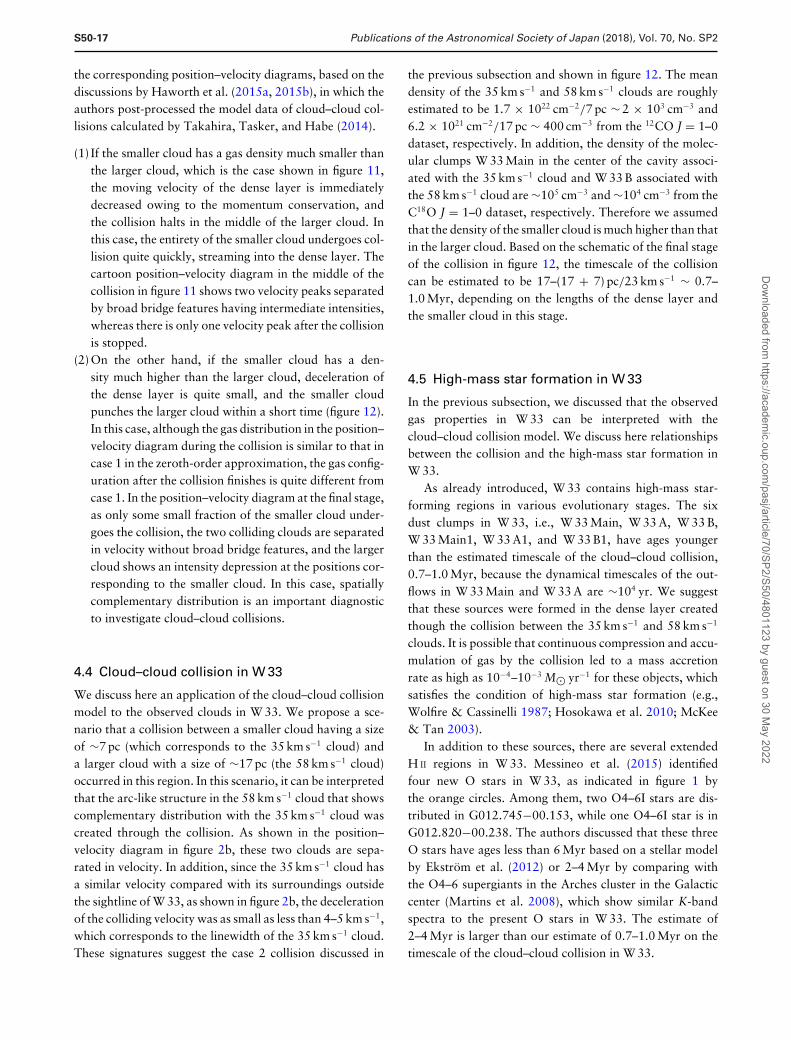
(1) If the smaller cloud has a gas density much smaller thanthe larger cloud, which is the case shown in figure 11,the moving velocity of the dense layer is immediatelydecreased owing to the momentum conservation, andthe collision halts in the middle of the larger cloud. Inthis case, the entirety of the smaller cloud undergoes col-lision quite quickly, streaming into the dense layer. Thecartoon position–velocity diagram in the middle of thecollision in figure 11 shows two velocity peaks separatedby broad bridge features having intermediate intensities,whereas there is only one velocity peak after the collisionis stopped.

(2) On the other hand, if the smaller cloud has a den-sity much higher than the larger cloud, deceleration ofthe dense layer is quite small, and the smaller cloudpunches the larger cloud within a short time (figure 12).In this case, although the gas distribution in the position–velocity diagram during the collision is similar to that incase 1 in the zeroth-order approximation, the gas config-uration after the collision finishes is quite different fromcase 1. In the position–velocity diagram at the final stage,as only some small fraction of the smaller cloud under-goes the collision, the two colliding clouds are separatedin velocity without broad bridge features, and the largercloud shows an intensity depression at the positions cor-responding to the smaller cloud. In this case, spatiallycomplementary distribution is an important diagnosticto investigate cloud–cloud collisions.

4.4 Cloud–cloud collision in W 33

We discuss here an application of the cloud–cloud collisionmodel to the observed clouds in W 33. We propose a sce-nario that a collision between a smaller cloud having a sizeof ∼7 pc (which corresponds to the 35 km s−1 cloud) anda larger cloud with a size of ∼17 pc (the 58 km s−1 cloud)occurred in this region. In this scenario, it can be interpretedthat the arc-like structure in the 58 km s−1 cloud that showscomplementary distribution with the 35 km s−1 cloud wascreated through the collision. As shown in the position–velocity diagram in figure 2b, these two clouds are sepa-rated in velocity. In addition, since the 35 km s−1 cloud hasa similar velocity compared with its surroundings outsidethe sightline of W 33, as shown in figure 2b, the decelerationof the colliding velocity was as small as less than 4–5 km s−1,which corresponds to the linewidth of the 35 km s−1 cloud.These signatures suggest the case 2 collision discussed in

the previous subsection and shown in figure 12. The meandensity of the 35 km s−1 and 58 km s−1 clouds are roughlyestimated to be 1.7 × 1022 cm−2/7 pc ∼ 2 × 103 cm−3 and6.2 × 1021 cm−2/17 pc ∼ 400 cm−3 from the 12CO J = 1–0dataset, respectively. In addition, the density of the molec-ular clumps W 33 Main in the center of the cavity associ-ated with the 35 km s−1 cloud and W 33 B associated withthe 58 km s−1 cloud are ∼105 cm−3 and ∼104 cm−3 from theC18O J = 1–0 dataset, respectively. Therefore we assumedthat the density of the smaller cloud is much higher than thatin the larger cloud. Based on the schematic of the final stageof the collision in figure 12, the timescale of the collisioncan be estimated to be 17–(17 + 7) pc/23 km s−1 ∼ 0.7–1.0 Myr, depending on the lengths of the dense layer andthe smaller cloud in this stage.

4.5 High-mass star formation in W 33

In the previous subsection, we discussed that the observedgas properties in W 33 can be interpreted with thecloud–cloud collision model. We discuss here relationshipsbetween the collision and the high-mass star formation inW 33.

As already introduced, W 33 contains high-mass star-forming regions in various evolutionary stages. The sixdust clumps in W 33, i.e., W 33 Main, W 33 A, W 33 B,W 33 Main1, W 33 A1, and W 33 B1, have ages youngerthan the estimated timescale of the cloud–cloud collision,0.7–1.0 Myr, because the dynamical timescales of the out-flows in W 33 Main and W 33 A are ∼104 yr. We suggestthat these sources were formed in the dense layer createdthough the collision between the 35 km s−1 and 58 km s−1

clouds. It is possible that continuous compression and accu-mulation of gas by the collision led to a mass accretionrate as high as 10−4–10−3 M� yr−1 for these objects, whichsatisfies the condition of high-mass star formation (e.g.,Wolfire & Cassinelli 1987; Hosokawa et al. 2010; McKee& Tan 2003).

In addition to these sources, there are several extendedH II regions in W 33. Messineo et al. (2015) identifiedfour new O stars in W 33, as indicated in figure 1 bythe orange circles. Among them, two O4–6I stars are dis-tributed in G012.745−00.153, while one O4–6I star is inG012.820−00.238. The authors discussed that these threeO stars have ages less than 6 Myr based on a stellar modelby Ekstrom et al. (2012) or 2–4 Myr by comparing withthe O4–6 supergiants in the Arches cluster in the Galacticcenter (Martins et al. 2008), which show similar K-bandspectra to the present O stars in W 33. The estimate of2–4 Myr is larger than our estimate of 0.7–1.0 Myr on thetimescale of the cloud–cloud collision in W 33.

Dow



ay 2022


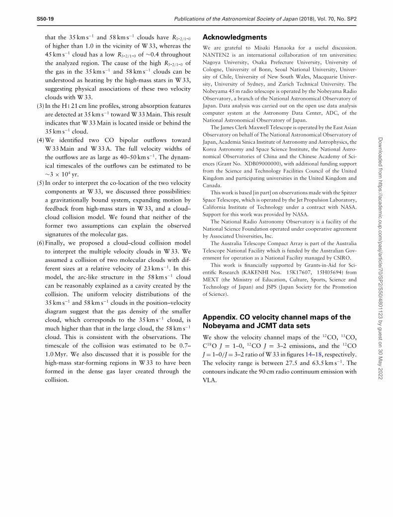
Fig. 13. Evolutionary tracks of the expanding H II region radius rHII are plotted for different initial densities, based on the analytical model of the D-typeexpansion by Spitzer (1978). (a) G012.745−00.153. (b) G012.820−00.238. The dashed lines show the radius of the H II regions.

In order to investigate the formation timescales of theseO stars in a different way, we estimate here the for-mation timescale of the H II regions G012.745−00.153and G012.820−00.238, that are excited by these O4–6I stars. In figure 13 evolutionary tracks of the H II

region radius rH II are plotted for different initial densi-ties, based on the analytical model of the D-type expan-sion by Spitzer (1978). Here, Lyman continuum photonsNLy of 1049.55–1049.93 s−1, which correspond to an O6I–O4I star, are assumed (Panagia 1973). The horizontaldashed lines in figures 13a and 13b indicate the radii ofG012.745−00.153 and G012.820−00.238 measured bythe 90 cm data, respectively.

In figure 13a, in which the case for G012.745−00.153is presented, the evolution timescales which correspondto the measured rHII are about 0.2 Myr, 0.7 Myr, and2 Myr for initial densities of 103 cm−3, 104 cm−4, and105 cm−3, respectively, suggesting that quite a high densityof ∼105 cm−3 is required to be consistent with the age of 2–4 Myr estimated by Messineo et al. (2015). However, in thecase of G012.820−00.238 shown in figure 13b, even withquite a high density of 105 cm−3, the derived timescale isas short as 0.5 Myr, and it is inconsistent with the estimateby Messineo et al. (2015) based on the comparison withthe Arches cluster in the Galactic center, although theirother estimate of less than 6 Myr, which is based on thestellar model by Ekstrom et al. (2012), is consistent withthe present results in figure 13.

If we tentatively assume that the ages ofG012.745−00.153 and G012.820−00.238 are 0.7 Myrand 0.2 Myr, respectively, in which a reasonable initial gasdensity of 104 cm−3 is assumed, these figures are within the

estimated timescale of the cloud–cloud collision in W 33,0.7–1 Myr, and it is therefore possible that formation ofthese O stars in G012.745−00.153 and G012.820−00.238occurred in the dense layer formed through the cloud–cloudcollision between the 35 km s−1 and 58 km s−1 clouds.

5 Conclusions

The conclusions of the present study are summarized asfollows.

(1) We carried out large-scale CO observations using theNANTEN2 and Nobeyama 45 m telescopes towardthe galactic high-mass star-forming region W 33. Ourdataset identified three velocity clouds at 35 km s−1,45 km s−1, and 58 km s−1 toward W 33. The 35 km s−1

cloud spatially coincides with W 33, showing spatial cor-relations with the dust clumps W 33 Main, W 33 A, andW 33 B1 and the H II regions G012.745−00.153 andG012.820−00.238, while the 58 km s−1 cloud, whichhas an arc-like structure surrounding the 35 km s−1

cloud and thus W 33, shows associations with the dustclump W 33 B and the H II regions G012.745−00.153and G012.692−00.251. The 45 km s−1 cloud shows dif-fuse and extended CO emission throughout the cor-responding region of W 33, although its associationwith W 33 is not clear. The total molecular massesof the three clouds, i.e., the 35 km s−1, 45 km s−1, and58 km s−1 clouds, are 1.1 × 105 M�, 1.0 × 105 M�,and 3.0 × 104 M�, respectively.

(2) We analyzed the intensity ratio between 12CO J = 3–2and 12CO J = 1–0 in these three velocity clouds, finding

Dow



ay 2022


that the 35 km s−1 and 58 km s−1 clouds have R3-2/1-0

of higher than 1.0 in the vicinity of W 33, whereas the45 km s−1 cloud has a low R3-2/1-0 of ∼0.4 throughoutthe analyzed region. The cause of the high R3-2/1-0 ofthe gas in the 35 km s−1 and 58 km s−1 clouds can beunderstood as heating by the high-mass stars in W 33,suggesting physical associations of these two velocityclouds with W 33.

(3) In the H I 21 cm line profiles, strong absorption featuresare detected at 35 km s−1 toward W 33 Main. This resultindicates that W 33 Main is located inside or behind the35 km s−1 cloud.

(4) We identified two CO bipolar outflows towardW 33 Main and W 33 A. The full velocity widths ofthe outflows are as large as 40–50 km s−1. The dynam-ical timescales of the outflows can be estimated to be∼3 × 104 yr.

(5) In order to interpret the co-location of the two velocitycomponents at W 33, we discussed three possibilities:a gravitationally bound system, expanding motion byfeedback from high-mass stars in W 33, and a cloud–cloud collision model. We found that neither of theformer two assumptions can explain the observedsignatures of the molecular gas.

(6) Finally, we proposed a cloud–cloud collision modelto interpret the multiple velocity clouds in W 33. Weassumed a collision of two molecular clouds with dif-ferent sizes at a relative velocity of 23 km s−1. In thismodel, the arc-like structure in the 58 km s−1 cloudcan be reasonably explained as a cavity created by thecollision. The uniform velocity distributions of the35 km s−1 and 58 km s−1 clouds in the position–velocitydiagram suggest that the gas density of the smallercloud, which corresponds to the 35 km s−1 cloud, ismuch higher than that in the large cloud, the 58 km s−1

cloud. This is consistent with the observations. Thetimescale of the collision was estimated to be 0.7–1.0 Myr. We also discussed that it is possible for thehigh-mass star-forming regions in W 33 to have beenformed in the dense gas layer created through thecollision.

Acknowledgments

We are grateful to Misaki Hanaoka for a useful discussion.NANTEN2 is an international collaboration of ten universities:Nagoya University, Osaka Prefecture University, University ofCologne, University of Bonn, Seoul National University, Univer-sity of Chile, University of New South Wales, Macquarie Univer-sity, University of Sydney, and Zurich Technical University. TheNobeyama 45 m radio telescope is operated by the Nobeyama RadioObservatory, a branch of the National Astronomical Observatory ofJapan. Data analysis was carried out on the open use data analysiscomputer system at the Astronomy Data Center, ADC, of theNational Astronomical Observatory of Japan.

The James Clerk Maxwell Telescope is operated by the East AsianObservatory on behalf of The National Astronomical Observatory ofJapan, Academia Sinica Institute of Astronomy and Astrophysics, theKorea Astronomy and Space Science Institute, the National Astro-nomical Observatories of China and the Chinese Academy of Sci-ences (Grant No. XDB09000000), with additional funding supportfrom the Science and Technology Facilities Council of the UnitedKingdom and participating universities in the United Kingdom andCanada.

This work is based [in part] on observations made with the SpitzerSpace Telescope, which is operated by the Jet Propulsion Laboratory,California Institute of Technology under a contract with NASA.Support for this work was provided by NASA.

The National Radio Astronomy Observatory is a facility of theNational Science Foundation operated under cooperative agreementby Associated Universities, Inc.

The Australia Telescope Compact Array is part of the AustraliaTelescope National Facility which is funded by the Australian Gov-ernment for operation as a National Facility managed by CSIRO.

This work is financially supported by Grants-in-Aid for Sci-entific Research (KAKENHI Nos. 15K17607, 15H05694) fromMEXT (the Ministry of Education, Culture, Sports, Science andTechnology of Japan) and JSPS (Japan Society for the Promotionof Science).

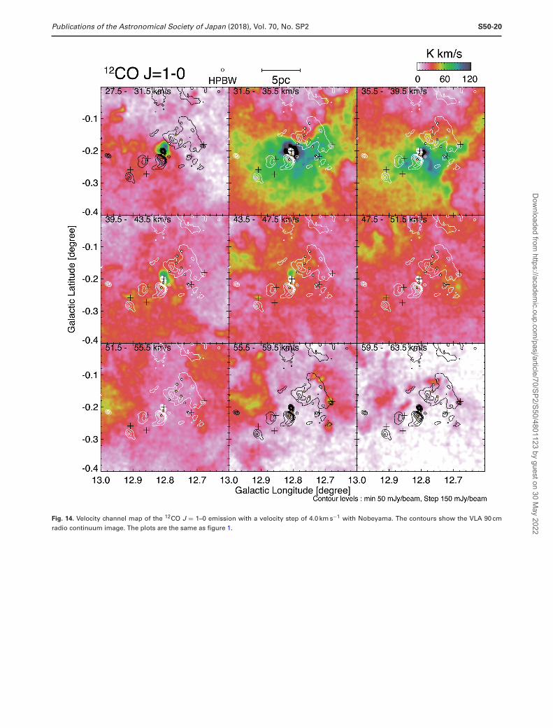
Appendix. CO velocity channel maps of the

Nobeyama and JCMT data sets

We show the velocity channel maps of the 12CO, 13CO,C18O J = 1–0, 12CO J = 3–2 emissions, and the 12COJ = 1–0/J = 3–2 ratio of W 33 in figures 14–18, respectively.The velocity range is between 27.5 and 63.5 km s−1. Thecontours indicate the 90 cm radio continuum emission withVLA.

Dow



ay 2022


Fig. 14. Velocity channel map of the 12CO J = 1–0 emission with a velocity step of 4.0 km s−1 with Nobeyama. The contours show the VLA 90 cmradio continuum image. The plots are the same as figure 1.

Dow



ay 2022


Fig. 15. Velocity channel map of the 13CO J = 1–0 emission with a velocity step of 4.0 km s−1 with Nobeyama. The contours show the VLA 90 cmradio continuum image. The plots are the same as figure 1.

Dow



ay 2022


Fig. 16. Velocity channel map of the C18O J = 1–0 emission with a velocity step of 4.0 km s−1 with Nobeyama. The contours show the VLA 90 cmradio continuum image. The plots are the same as figure 1.

Dow



ay 2022


Fig. 17. Velocity channel map of the 12CO J = 3–2 emission with a velocity step of 4.0 km s−1 with JCMT. The contours show the VLA 90 cm radiocontinuum image. The plots are the same as figure 1.

Dow



ay 2022


Fig. 18. Velocity channel map of the 12CO J = 3–2/12CO J = 1–0 emission with a velocity step of 4.0 km s−1, which was spatially smoothed at 50′′. Thecontours show the VLA 90 cm radio continuum image. The plots are the same as figure 1. The clipping level is 8 σ (4.2 K km s−1).

References

Anathpindika, S. V. 2010, MNRAS, 405, 1431Anderson, L. D., Armentrout, W. P., Johnstone, B. M., Bania, T. M.,

Balser, D. S., Wenger, T. V., & Cunningham, V. 2015, ApJS,221, 26

Anderson, L. D., Bania, T. M., Balser, D. S., Cunningham, V.,Wenger, T. V., Johnstone, B. M., & Armentrout, W. P. 2014,ApJS, 212, 1

Balfour, S. K., Whitworth, A. P., & Hubber, D. A. 2017, MNRAS,465, 3483

Balfour, S. K., Whitworth, A. P., Hubber, D. A., & Jaffa, S. E. 2015,MNRAS, 453, 2471

Baug, T., Dewangan, L. K., Ojha, D. K., & Ninan, J. P. 2016, ApJ,833, 85

Benjamin, R. A., et al. 2003, PASP, 115, 953Bieging, J. H., Pankonin, V., & Smith, L. F. 1978, A&A, 64, 341Bisbas, T. G., Tanaka, K. E. I., Tan, J. C., Wu, B., & Nakamura, F.

2017, ApJ, 850, 23Bolatto, A. D., Wolfire, M., & Leroy, A. K. 2013, ARA&A, 51,

207

Dow



ay 2022


Bonnell, I. A., Bate, M. R., Clarke, C. J., & Pringle, J. E. 1997,MNRAS, 285, 201

Bonnell, I. A., Bate, M. R., Clarke, C. J., & Pringle, J. E. 2001,MNRAS, 323, 785

Bonnell, I. A., Bate, M. R., & Zinnecker, H. 1998, MNRAS, 298,93

Bonnell, I. A., Vine, S. G., & Bate, M. R. 2004, MNRAS, 349, 735Buckle, J. V., et al. 2009, MNRAS, 399, 1026Buckley, H. D., & Ward-Thompson, D. 1996, MNRAS, 281, 294Carey, S. J., et al. 2009, PASP, 121, 76Caswell, J. L. 1998, MNRAS, 297, 215Christie, D., Wu, B., & Tan, J. C. 2017, ApJ, 848, 50Churchwell, E., et al. 2004, ApJS, 154, 322Colom, P., Lekht, E. E., Pashchenko, M. I., & Rudnitskij, G. M.

2015, A&A, 575, A49Contreras, Y., et al. 2013, A&A, 549, A45Dale, J. E., Ngoumou, J., Ercolano, B., & Bonnell, I. A. 2013,

MNRAS, 436, 3430Davies, B., Lumsden, S. L., Hoare, M. G., Oudmaijer, R. D., &

de Wit, W.-J. 2010, MNRAS, 402, 1504de Wit, W. J., Hoare, M. G., Oudmaijer, R. D., & Lumsden, S. L.

2010, A&A, 515, A45de Wit, W. J., Hoare, M. G., Oudmaijer, R. D., & Mottram, J. C.

2007, ApJ, 671, L169Deharveng, L., et al. 2010, A&A, 523, A6Dempsey, J. T., Thomas, H. S., & Currie, M. J. 2013, ApJS, 209, 8Dewangan, L. K. 2017, ApJ, 837, 44Dewangan, L. K., & Ojha, D. K. 2017, ApJ, 849, 65Dobashi, K., Matsumoto, T., Shimoikura, T., Saito, H., Akisato, K.,

Ohashi, K., & Nakagomi, K. 2014, ApJ, 797, 58Dobbs, C. L., Pringle, J. E., & Duarte-Cabral, A. 2015, MNRAS,

446, 3608Downes, D., Wilson, T. L., Bieging, J., & Wink, J. 1980, A&A, 40,

379Duarte-Cabral, A., Dobbs, C. L., Peretto, N., & Fuller, G. A. 2011,

A&A, 528, A50Ekstrom, S., et al. 2012, A&A, 537, A146Elmegreen, B. G., & Lada, C. J. 1977, ApJ, 214, 725Frerking, M. A., Langer, W. D., & Wilson, R. W. 1982, ApJ, 262,

590Fujimoto, Y., Tasker., E. J., & Habe, A. 2014b, MNRAS, 445,

L65Fujimoto, Y., Tasker., E. J., Wakayama, M., & Habe, A. 2014a,

MNRAS, 439, 936Fujita, S., et al. 2017, arXiv:1711.01695Fukui, Y., et al. 2014, ApJ, 780, 36Fukui, Y., et al. 2015, ApJ, 807, L4Fukui, Y., et al. 2016, ApJ, 820, 26Fukui, Y., et al. 2017a, arXiv:1701.04669Fukui, Y., et al. 2018a, PASJ, 70, S41Fukui, Y., et al. 2018b, PASJ, 70, S44Fukui, Y., Hattori, Y., Torii, K., Ohama, A., Nishimura, A.,

Kohno, M., Yamamoto, H., & Tachihara, K. 2018c, PASJ, 70,S46

Fukui, Y., Tsuge, K., Sano, H., Bekki, K., Yozin, C., Tachihara, K.,& Inoue, T. 2017b, PASJ, 69, L5

Furukawa, N., Dawson, J. R., Ohama, A., Kawamura, A.,Mizuno, N., Onishi, T., & Fukui, Y. 2009, ApJ, 696, L115

Galvan-Madrid, R., Zhang, Q., Keto, E., Ho, P. T. P., Zapata, L. A.,Rodrıguez, L. F., Pineda, J. E., & Vazquez-Semadeni, E. 2010,ApJ, 725, 17

Gardner, F. F., & Whiteoak, J. B. 1972, Astrophys. Lett., 12, 107Gibb, E. L., et al. 2000, ApJ, 536, 347Goldreich, P., & Kwan, J. 1974, ApJ, 189, 441Goldsmith, P. F., & Mao, X. J. 1983, ApJ, 265, 791Gong, Y., et al. 2017, ApJ, 835, L14Habe, A., & Ohta, K. 1992, PASJ, 44, 203Haschick, A. D., & Ho, P. T. P. 1983, ApJ, 267, 638Hasegawa, T., Sato, F., Whiteoak, J. B., & Miyawaki, R. 1994, ApJ,

429, L77Haworth, T. J., et al. 2015a, MNRAS, 450, 10Haworth, T. J., Shima, K., Tasker, E. J., Fukui, Y., Torii, K., Dale,

J. E., Takahira, K., & Habe, A. 2015b, MNRAS, 454, 1634Hayashi, K., et al. 2018, PASJ, 70, S48Helfand, D. J., Becker, R. H., White, R. L., Fallon, A., & Tuttle, S.

2006, AJ, 131, 2525Higuchi, A. E., Chibueze, J. O., Habe, A., Takahira, K., &

Takano, S. 2014, ApJ, 147, 141Higuchi, A. E., Kurono, Y., Saito, M., & Kawabe, R. 2010, ApJ,

719, 1813Ho, P. T. P., Klein, R. I., & Haschick, A. D. 1986, ApJ, 305, 714Hosokawa, T., & Omukai, K. 2009, ApJ, 691, 823Hosokawa, T., Yorke, H. W., & Omukai, K. 2010, ApJ, 721, 478Immer, K., Galvan-Madrid, R., Konig, C., Liu, H. B., & Menten,

K. M. 2014, A&A, 572, A63Immer, K., Reid, M. J., Menten, K. M., Brunthaler, A., & Dame,

T. M. 2013, A&A, 553, A117Inoue, T., & Fukui, Y. 2013, ApJ, 774, L31Inoue, T., Hennebelle, P., Fukui, Y., Matsumoto, T., Iwasaki, K., &

Inutsuka, S. 2018, PASJ, 70, S53Jiang, X. J., Liu, H. B., Zhang, Q., Wang, J., Zhang, Z. Y., Li, J.,

Gao, Y., & Gu, Q. 2015, ApJ, 808, 114Kamazaki, T., et al. 2012, PASJ, 64, 29Kang, M., Bieging, J. H., Kulesa, C. A., Lee, Y., Choi, M., & Peters,

W. L. 2010, ApJS, 190, 58Kobayashi, M. I. N., Inutsuka, S., Kobayashi, H., & Hasegawa, K.

2017, ApJ, 836, 175Kobayashi, M. I. N., Kobayashi, H., Inutsuka, S., & Fukui, Y. 2018,

PASJ, 70, S59Koo, B.-C., Lee, Y., Fuller, G. A., Lee, M. G., Kwon, S.-M., &

Jung, J. 1994, ApJ, 429, 233Krumholz, M. R., Klein, R. I., & McKee, C. F. 2007, ApJ, 656, 959Krumholz, M. R., Klein, R. I., McKee, C. F., Offner, S. S. R., &

Cunningham, A. J. 2009, Science, 323, 754Kuno, N., et al. 2011, in Proc. 2011 XXXth URSI General Assembly

and Scientific Symposium (New York: IEEE), 3670Kutner, M. L., & Ulich, B. L. 1981, ApJ, 250, 341Lada, C. J. 1987, in IAU Symp. 115, Star Forming Regions, ed. M.

Peimbert & J. Jugaku (Dordrecht: D. Reidel Publishing Co.), 1Li, G.-X. 2017, MNRAS, 471, 2002Li, Q., Tan., J. C., Christie, D., Bisbas, T. G., & Wu, B. 2018, PASJ,

70, S56Lin, Y., et al. 2016, ApJ, 828, 32Lockman, F. J. 1989, ApJS, 71, 469Loren, R. B. 1976, ApJ, 209, 466Loren, R. B. 1977, ApJ, 218, 716

Dow



ay 2022

http://arxiv.org/abs/1711.01695



McClure-Griffiths, N. M., Dickey, J. M., Gaensler, B. M., Green,A. J., Haverkorn, M., & Strasser, S. 2005, ApJS, 158, 178

McKee, C. F., & Tan, J. C. 2003, ApJ, 585, 850Martins, D., Hillier, D. J., Paumard, T., Eisenhauer, F., Ott, T., &

Genzel, R. 2008, A&A, 478, 219Maud, L. T., Hoare, M. G., Galvan-Madrid, R., Zhang, Q., de Wit,

W. J., Keto, E., Johnston, K. G., & Pineda, J. E. 2017, MNRAS,467, L120

Maud, L. T., Moore, T. J. T., Lumsden, S. L., Mottram, J. C.,Urquhart, J. S., & Hoare, M. G. 2015, MNRAS, 453, 645

Menten, K. M., Walmsley, C. M., Henkel, C., & Wilson, T. L. 1986,A&A, 157, 318

Messineo, M., et al. 2015, ApJ, 805, 110Minamidani, T., et al. 2015, in Conditions and Impact of Star For-

mation, ed. R. Simon et al., ESA SP-75 (Noordwijk: ESA), 193Minamidani, T., et al. 2016, Proc. SPIE, 9914, 99141ZMiyawaki, R., Hayashi, M., & Hasegawa, T. 1986, ApJ, 305, 353Miyawaki, R., Hayashi, M., & Hasegawa, T. 2009, PASJ, 61, 39Nakamura, F., et al. 2012, ApJ, 746, 25Nakamura, F., et al. 2014, ApJ, 791, L23Nakano, T., Hasegawa, T., Morino, J.-I., & Yamashita, T. 2000,

ApJ, 534, 976Nishimura, A., et al. 2017, PASJ, submitted (arXiv:1706.06002)Nishimura, A., et al. 2018, PASJ, 70, S42Ohama, A., et al. 2010, ApJ, 709, 975Ohama, A., et al. 2017, PASJ, submitted (arXiv:1706.05652)Ohama, A., et al. 2018a, PASJ, 70, S45Ohama, A., et al. 2018b, PASJ, 70, S47Okumura, S., Miyawaki, R., Sorai, K., Yamashita, T., & Hasegawa,

T. 2001, PASJ, 53, 793Panagia, N. 1973, AJ, 78, 929Penzias, A. A., & Burrus, C. A. 1973, ARA&A, 11, 51Portegies Zwart, S. F., McMillan, S. L. W., & Gieles, M. 2010,

ARA&A, 48, 431Reid, M. J., Dame, T. M., Menten, K. M., & Brunthaler, A. 2016,

ApJ, 823, 77Ridge, N. A., et al. 2006, AJ, 131, 2921Roueff., E., Dartois, E., Geballe, T. R., & Gerin, M. 2006, A&A,

447, 963Saigo, K., et al. 2017, ApJ, 835, 108Sano, H., et al. 2017, PASJ, submitted (arXiv:1708.08149)Sano, H., et al. 2018, PASJ, 70, S43Sato, F., Hasegawa, T., Whiteoak, J. B., & Miyawaki, R. 2000, ApJ,

535, 857

Sawada, T., et al. 2008, PASJ, 60, 445Schuller, F., et al. 2009, A&A, 504, 415Shima, K., Tasker, E. J., Federrath, C., & Habe, A. 2018, PASJ, 70,

S54Shimoikura, T., et al. 2013, ApJ, 768, 72Shimoikura, T., & Dobashi, K. 2011, ApJ, 731, 23Spitzer, L., Jr. 1978, Physical Processes in the Interstellar Medium

(New York: Wiley), 333Stone, M. E. 1970a, ApJ, 159, 277Stone, M. E. 1970b, ApJ, 159, 293Strong, A. W., et al. 1988, A&A, 207, 1Takahira, K., Shima, K., Habe, A., & Tasker, E. J. 2018, PASJ, 70,

S58Takahira, K., Tasker, E. J., & Habe, A. 2014, ApJ, 792, 63Tan, J. C. 2000, ApJ, 536, 173Tan, J. C., Beltran, M. T., Caselli, P., Fontani, F., Fuente, A.,

Krumholz, M. R., McKee, C. F., & Stolte, A. 2014, in Protostarsand Planets VI, ed. H. Beuther et al. (Tucson, AZ: University ofArizona Press), 149

Tasker, E. J., & Tan, J. C. 2009, ApJ, 700, 358Torii, K., et al. 2011, ApJ, 738, 46Torii, K., et al. 2015, ApJ, 806, 7Torii, K., et al. 2017a, ApJ, 835, 142Torii, K., et al. 2017b, PASJ, submitted (arXiv:1706.07164)Tsuboi, M., Miyazaki, A., & Uehara, K. 2015, PASJ, 67, 109Tsutsumi, D., et al. 2017, PASJ, submitted (arXiv:1706.05664)Ulich, B. L., & Haas, R. W. 1976, ApJS, 30, 247Umemoto, T., et al. 2017, PASJ, 69, 78Urquhart, J. S., et al. 2014, A&A, 568, A41Vallee, J. P. 1995, AJ, 110, 2256Ward-Thompson, D., & Whitworth, A. P. 2011, An Introduction to

Star Formation (Cambridge: Cambridge University Press)Westerhout, G. 1958, Bull. Astron. Inst. Netherlands, 14, 215Wilson, T. L., Rohlfs, K, & Huttemeister, S. 2009, Tools of Radio

Astronomy, 5th ed. (Berlin: Springer-Verlag)Wolfire, M. G., & Cassinelli, J. P. 1987, ApJ, 319, 850Wu, B., Tan, J. C., Christie, D., Nakamura, F., Van, L S., &

Collins, D. 2017b, ApJ, 841, 88Wu, B., Tan, J. C., Nakamura, F., Van, L. S., Christie, D., &

Collins, D. 2017a, ApJ, 835, 137Wu, B., Van Loo, S., Tan, J. C., & Bruderer, S. 2015, ApJ, 811, 56Xue, R., & Wu, Y. 2008, ApJ, 680, 446Yorke, H. W., & Sonnhalter, C. 2002, ApJ, 569, 846Zinnecker, H., & Yorke, H. W. 2007, ARA&A, 45, 481

Dow



ay 2022






FOREST Unbiased Galactic plane Imaging survey with the ...

Documents