The Pennsylvania State University The Graduate School Department of Industrial and Manufacturing Engineering FORECASTING TECHNICAL AND FUNCTIONAL OBSOLESCENCE FOR IMPROVED BUSINESS PROCESSES A Dissertation in Industrial and Manufacturing Engineering by Connor Jennings Ó 2018 Connor Jennings Submitted in Partial Fulfillment of the Requirements for the Degree of Doctor of Philosophy December 2018

Welcome message from author
This document is posted to help you gain knowledge. Please leave a comment to let me know what you think about it! Share it to your friends and learn new things together.
Transcript

The Pennsylvania State University
The Graduate School
Department of Industrial and Manufacturing Engineering
FORECASTING TECHNICAL AND FUNCTIONAL OBSOLESCENCE FOR
IMPROVED BUSINESS PROCESSES
A Dissertation in
Industrial and Manufacturing Engineering
by
Connor Jennings
Ó 2018 Connor Jennings
Submitted in Partial Fulfillment
of the Requirements
for the Degree of
Doctor of Philosophy
December 2018

ii
The dissertation of Connor Jennings was reviewed and approved by the following:
Janis Terpenny Peter and Angela Dal Pezzo Department Head and Professor Dissertation Advisor Chair of Committee
Soundar Kumara Allen E. Pearce and Allen M. Pearce Professor of Industrial Engineering
Timothy W. Simpson Paul Morrow Professor in Engineering Design and Manufacturing
Conrad Tucker Associate Professor in Engineering Design
Signatures on file in the Graduate School

iii
ABSTRACT
Any product can become obsolete. Products becoming obsolete causes increased costs to
organizations due to the interruption of the usual flow of business. These interruptions can be seen in
product and component shortages, stockpiling, and forced redesigns. To minimize the impact of product
obsolescence, businesses must integrate forecasting methods into business processes to allow for proactive
management. Proactive management enables organizations to maximize the time to make a decision and
increases the number of viable decisions. This dissertation seeks to demonstrate new obsolescence
forecasting methods and techniques, along with frameworks for applying these to business processes.
There are four main types of product obsolescence: (1) technical, (2) functional, (3) style, and (4)
legislative. In technical obsolescence, old products can no longer compete with the specifications of newer
products. In functional obsolescence, products can no longer perform their original task due to aging factors.
The third is style; many products no longer are appealing visually and become obsolete due to changes in
fashion (e.g., wood paneling on cars). The last is legislative; if a government passes laws that forbid certain
materials, components, chemicals in manufacturing process, or creates new requirements in a market, this
can often lead to many products and designs becoming obsolete. The focus in this research is on technical
and functional obsolescence. Technical obsolescence is especially prolific in highly competitive consumer
electronic markets such as cell phones and digital cameras. This work seeks to apply traditional machine
learning methods to predict obsolescence risk levels and assign a status of “discontinued” or “procurable”
depending on the availability in the market at a given time. After these models have been investigated, a
new framework is proposed to reduce the cost impact of mislabeled products in the forecasting process.
Current models pick a threshold between the “discontinued” and “procurable” status that minimizes the
number of errors rather than the error cost of the model. The new method proposes minimizing the average
error cost of status misclassifications in the forecasting process. The method looks at the cost to the
organization from false positives and false negatives; it varies the threshold between the statuses to reduce

iv
the number of more-costly errors by trading off less-costly errors using Receiver Operating Characteristic
(ROC) analysis. This technique draws from practices in disease detection to decide the tradeoff between
telling a healthy person they have a disease (false positive) and telling a sick person they do not have a
disease (false negative). Early work and a case study using this method have demonstrated an average
reduction of 6.46% in average misclassification cost in the cell phone market and a reduction of 20.27% in
the camera market.
Functional obsolescence management has grown with the increased connectivity of products,
equipment, and infrastructure. In the alternative energy industry, as solar farms and wind turbines transform
from emerging technologies to a fully developed one, these industries seek to better monitor the
performance of aging equipment. Similar techniques to forecasting technical obsolescence is applied to
predict whether equipment is functioning properly. A case study is used to predict functional obsolescence
of wind turbines.
Obsolescence forecasting models are quite useful when applied to aid business decisions. In
business, the classic tradeoff is between longer life cycles and lower costs. This research seeks to create a
generalized model to estimate the total life cycle cost of a component and the life cycle of a product before
it becomes obsolete. These models will aid designers and manufacturers in better understanding how
changes in usage and manufacturing factors shift the life cycle and total cost. A genetic optimization
algorithm is applied to find the minimal cost given a desired life cycle. An alternative model is developed
to find the maximum life cycle given a set cost level.

v
TABLE OF CONTENTS
LIST OF TABLES ................................................................................................... x
LIST OF EQUATIONS ........................................................................................... xii
ACKNOWLEDGEMENTS ..................................................................................... xiv
Chapter 1 Introduction ............................................................................................ 1
1.1 Background and Present Situation in Obsolescence Mitigation and Management… ........................................................................................... 1
1.2 Motivation ................................................................................................... 4 1.3 Research Purpose and Objective .................................................................. 4 1.4 Research Questions ..................................................................................... 5
1.4.1 Primary Research Question ................................................................ 5 1.4.2 Research Sub-Questions .................................................................... 6
1.5 Research Approach and Methods................................................................. 8 1.6 Research Contributions ............................................................................... 8 1.7 Document Outline ....................................................................................... 9
Chapter 2 Literature Review.................................................................................... 10 2.1 Forecasting Technical Obsolescence............................................................ 10
2.1.1 Life Cycle forecasting........................................................................ 12 2.1.2 Obsolescence Risk Forecasting .......................................................... 14 2.1.3 Technical Obsolescence Scalability ................................................... 15 2.1.4 Current Technical Obsolescence Forecasting Scalability .................... 17 2.1.5 Current State of Technical Obsolescence Forecasting in Industry ...... 19
2.2 Accounting for Asymmetric Error Cost in Forecasting ................................ 19 2.2.1 Technical Obsolescence Forecasting and Cost Avoidance.................. 20 2.2.2 Applications of Receiver Operating Characteristic Analysis .............. 21
2.3 Forecasting Functional Obsolescence for Gear Boxes .................................. 23 2.3.1 Temperature ...................................................................................... 23 2.3.2 Power Quality.................................................................................... 24 2.3.3 Oil and Debris Monitoring ................................................................. 24 2.3.4 Vibration and Acoustic Emissions ..................................................... 25
Chapter 3 Approach and Methodology .................................................................... 28 3.1 Forecasting Technical Obsolescence Framework ......................................... 29
3.1.1 Obsolescence Risk Forecasting using Machine Learning ................... 31 3.1.2 Life Cycle Forecasting using Machine Learning ................................ 33
3.2 Accounting for Asymmetric Error Cost in Forecasting ................................ 34 3.3 Forecasting Functional Obsolescence Framework........................................ 39 3.4 Life Cycle and Cost in Design and Manufacturing ....................................... 40
3.4.1 Life Cycle and Cost Tradeoff Framework .......................................... 40

vi
3.4.2 Life Cycle and Cost Optimization ...................................................... 43 3.4.3 Recommending Goal Manufacturing Attributes for Gear Repair ........ 47
Chapter 4 Forecasting Technical Obsolescence in Consumer Electronics Case Study……. ........................................................................................................ 49
4.1 Results of Obsolescence Risk Forecasting ................................................... 49 4.1.1 Cell Phone Market ............................................................................. 49 4.1.2 Digital Camera Market ...................................................................... 56 4.1.3 Digital Screen for Cell Phones and Cameras Market .......................... 59
4.2 Results of Life Cycle Forecasting ................................................................ 62 4.2.1 Cell Phone Market ............................................................................. 62
4.3 Accuracy Benchmarking and Additional Features of LCML and ORML ..... 66 4.3.1 Benchmarking Life Cycle Forecasting Methods ................................. 66 4.3.2 Benchmarking Obsolescence Risk Methods ....................................... 71 4.3.3 Converting Life Cycle to Obsolescence Risk Forecasting .................. 73
4.4 Machine Learning based Obsolescence Forecasting Scalability ................... 74 4.5 Machine Learning based Obsolescence Forecasting Limitation ................... 75
Chapter 5 Reducing the Cost Impact of Misclassification Errors in Obsolescence Risk Forecasting........................................................................................................ 77
5.1 Algorithm Selection using Area Under the ROC Curve (AUC) .................... 79 5.2 Assigning Costs and Calculating the Optimal Threshold .............................. 82 5.3 Misclassification Cost Sensitivity Analysis.................................................. 89
Chapter 6 Health Status Monitoring of Wind Turbine Gearboxes ............................ 93
6.1 Fast Fourier Transform ................................................................................ 95 6.2 Wavelet Transform ...................................................................................... 97
Chapter 7 Life Cycle and Cost Tradeoff Framework ............................................... 100
7.1 Information Flow Model ............................................................................. 100 7.2 Model Generation ........................................................................................ 102 7.3 Genetic Search Optimization Results ........................................................... 104
Chapter 8 Conclusions and Future Work ................................................................. 113
References ............................................................................................................... 119
Appendix A. Technical Obsolescence Forecasting Data and Code ........................... 128
Appendix B. Misclassification Error Cost Sensitivity Analysis ................................ 129

vii
LIST OF FIGURES
Figure 1-1: Atari 800 Advertisement from 1979 [6] ................................................. 2
Figure 2-1: Product life cycle model [2] ................................................................... 12
Figure 2-2: Life cycle forecast using Gaussian trend curve [7] ................................. 13
Figure 2-3: Wind Turbine Gearbox Failure Examples [59] ....................................... 25
Figure 3-1: Organizations of Methods and Case Studies ........................................... 29
Figure 3-2: Supervised Learning Process [25] .......................................................... 31
Figure 3-3: Output of ORML ................................................................................... 32
Figure 3-4: Creation of ROC Curves ........................................................................ 34
Figure 3-5: Pseudocode to Implement Brute Force Search to Solve Mathematical Model…. ........................................................................................................... 38
Figure 3-6: Life Cycle and Cost Tradeoff Information Flow ..................................... 41
Figure 3-7: Life Cycle and Cost Tradeoff Framework Software Implementation ...... 43
Figure 3-8: Genetic Search Algorithm Process ......................................................... 45
Figure 3-9: Repairing Gear Information Flow .......................................................... 48
Figure 4-1: Overall Average Evaluation Speed by Training Data Set Fraction for ORML…........................................................................................................... 54
Figure 4-2: Average Evaluation speed by Training Data Set Fraction for ORML in the Camera Market ................................................................................................. 58
Figure 4-3: Average Evaluation Speed by Training Data Set Fraction for ORML in the Screen Market ................................................................................................... 61
Figure 4-4: Actual vs. Predicted End of Life using Neural Networks and LCML ..... 63
Figure 4-5: Actual vs. Predicted End of Life using SVM and LCML........................ 64
Figure 4-6: Actual vs. Predicted End of Life using Random Forest and LCML ........ 64
Figure 4-7: Overall average evaluation speed by training data set fraction for LCML……. ...................................................................................................... 65
Figure 4-8: LCML Method [25] Predictions vs. Actual Results ................................ 68

viii
Figure 4-9: CALCE++ Method [8] Predictions vs. Actual Results ............................ 69
Figure 4-10: Time Series Method [23] Predictions vs. Actual Results ...................... 70
Figure 5-1: Digital Cameras ROC Curves ................................................................ 80
Figure 5-2: Cell Phone ROC Curves......................................................................... 81
Figure 5-3: Digital Screens ROC Curves .................................................................. 81
Figure 5-4: Obsolescence Risk Prediction at a Threshold of 0.331 for Cell phones ... 85
Figure 5-5 Obsolescence Risk Prediction at a Threshold of 0.277 for Digital Cameras…… .................................................................................................... 87
Figure 5-6: Obsolescence Risk Prediction at a Threshold of 0.369 for Digital Screens…… ...................................................................................................... 89
Figure 5-7: Cost Sensitivity Analysis for Optimal Threshold for Cell phones .......... 90
Figure 6-1: Location of Sensors on the Wind Turbine [86] ....................................... 93
Figure 6-2: Speed of Model creation and prediction for FFT .................................... 96
Figure 6-3: Prediction accuracy of different training set sizes for FFT ...................... 97
Figure 6-4: Speed of model creation and prediction for wavelet transform ............... 98
Figure 6-5: Prediction accuracy of different training set sizes for wavelet transform………. .............................................................................................. 99
Figure 7-1: Information Flow for Life cycle vs. Cost Tradeoff for the Gear Case Study….. ........................................................................................................... 101
Figure 7-2: Weibull Life Cycle Cumulative Distribution Function with Slope 100 and Scale 100 .......................................................................................................... 103
Figure 7-3: Life Cycle vs. Cost Tradeoff Optimizing for Minimum Cost with a Life Cycle of 20 ................................................................................................................. 107
Figure 7-4: Life Cycle vs. Cost Tradeoff Model Cost Convergence Over 150 Iterations of the Genetic Search to Minimize Cost ............................................................ 108
Figure 7-5: Life Cycle vs. Cost Tradeoff Model Life Cycle Convergence Over 150 Iterations of the Genetic Search to Minimize Cost ............................................. 109
ix
Figure 7-6: Life Cycle vs. Cost Tradeoff Optimizing for Maximum Life Cycle with a Cost of $80,000 ................................................................................................. 110
Figure 7-7: Life Cycle vs. Cost Tradeoff Model Cost Convergence Over 150 Iterations of the Genetic Search to Minimize Life Cycle ....................................................... 110
Figure 7-8: Life Cycle vs. Cost Tradeoff Model life cycle Convergence Over 150 Iterations of the Genetic Search to Minimize Life Cycle .................................... 111
Figure 7-9: Pareto Frontier of Solutions from Figure 7-3 and Figure 7-6 .................. 112
Figure B-1: Cost Sensitivity Analysis for Optimal Threshold for Cell phones .......... 129
Figure B-2: Cost Sensitivity Analysis for Optimal Threshold for Cameras ............... 131
Figure B-3: Cost Sensitivity Analysis for Optimal Threshold for Digital Screens ..... 133

x
LIST OF TABLES
Table 2-1: List of All Methodologies and Scalability Problems ................................ 18
Table 3-1: Genetic Search Algorithm Population with a Required Life of 20 ............ 46
Table 4-1: Neural Networks ORML Confusion Matrix for Cell Phones .................... 52
Table 4-2: Support Vector Machine ORML Confusion Matrix for Cell Phones ........ 52
Table 4-3: Random Forest ORML Confusion Matrix for Cell Phones....................... 53
Table 4-4: K Nearest Neighbor ORML Confusion Matrix for Cell Phones ............... 53
Table 4-5: Summary of Model Preference Ranking For ORML in the Cell Phone Market…........................................................................................................... 54
Table 4-6: Neural Networks ORML Confusion Matrix for Digital Cameras ............. 56
Table 4-7: Support Vector Machine ORML Confusion Matrix for Digital Cameras..57
Table 4-8: Random Forest ORML Confusion Matrix for Digital Cameras ................ 57
Table 4-9: K Nearest Neighbor ORML Confusion Matrix for Digital Cameras......... 57
Table 4-10: Summary of Model Preference Ranking For ORML in the Camera Market….. ......................................................................................................... 59
Table 4-11: Neural Networks ORML Confusion Matrix for Screens ........................ 59
Table 4-12: Support Vector Machine ORML Confusion Matrix for Screens ............ 60
Table 4-13: Random Forest ORML Confusion Matrix for Screens ........................... 60
Table 4-14: K Nearest Neighbor ORML Confusion Matrix for Screens .................... 60
Table 4-15: Summary of Model Preference Ranking For ORML in the Screen Market…... ........................................................................................................ 62
Table 4-16: Summary of Model Preference Ranking for LCML ............................... 65
Table 4-17: Accuracies Life Cycle Forecasting Methods in the Flash Memory Market…… ....................................................................................................... 71
Table 4-18: Monolithic Flash Memory Confusion Matrix for ORML ....................... 74
Table 5-1: Cell phone Confusion Matrix with Classic Threshold .............................. 84

xi
Table 5-2: Cell phone Confusion Matrix with ROC Threshold ................................. 84
Table 5-3: Digital Cameras Confusion Matrix with Classic Threshold ...................... 86
Table 5-4: Digital Cameras Confusion Matrix with ROC Threshold ......................... 86
Table 5-5: Digital Screens Confusion Matrix with Classic Threshold ....................... 88
Table 5-6: Digital Screens Confusion Matrix with ROC Threshold .......................... 88
Table 5-7: Optimal Thresholds in Cellphone Error Cost Sensitivity Analysis ........... 92
Table 6-1: Name, Description, Model Number, and Units of Sensors in Figure 6-1 [85]…. .............................................................................................................. 94
Table 7-1: Genetic Search Algorithm Population with a Required Life of 20 ............ 105
Table B-1: Optimal Thresholds in Cellphone Error Cost Sensitivity Analysis........... 130
Table B-2: Optimal Thresholds in Camera Error Cost Sensitivity Analysis .............. 132
Table B-3: Optimal Thresholds in Digital Screens Error Cost Sensitivity Analysis ... 134
xii
LIST OF EQUATIONS
Equation 1:
!"#:&'() *+(,-.
/
-01+&'3) *+(,-.
/
-01
4(1)
!+(,- ≥ 9:,- − <:,- !+3,- ≥ <:,- − 9:,- !9:,- ≥ 9=,- − >
1 ≥ 9=,- ≥ 0 1 ≥ > ≥ 0
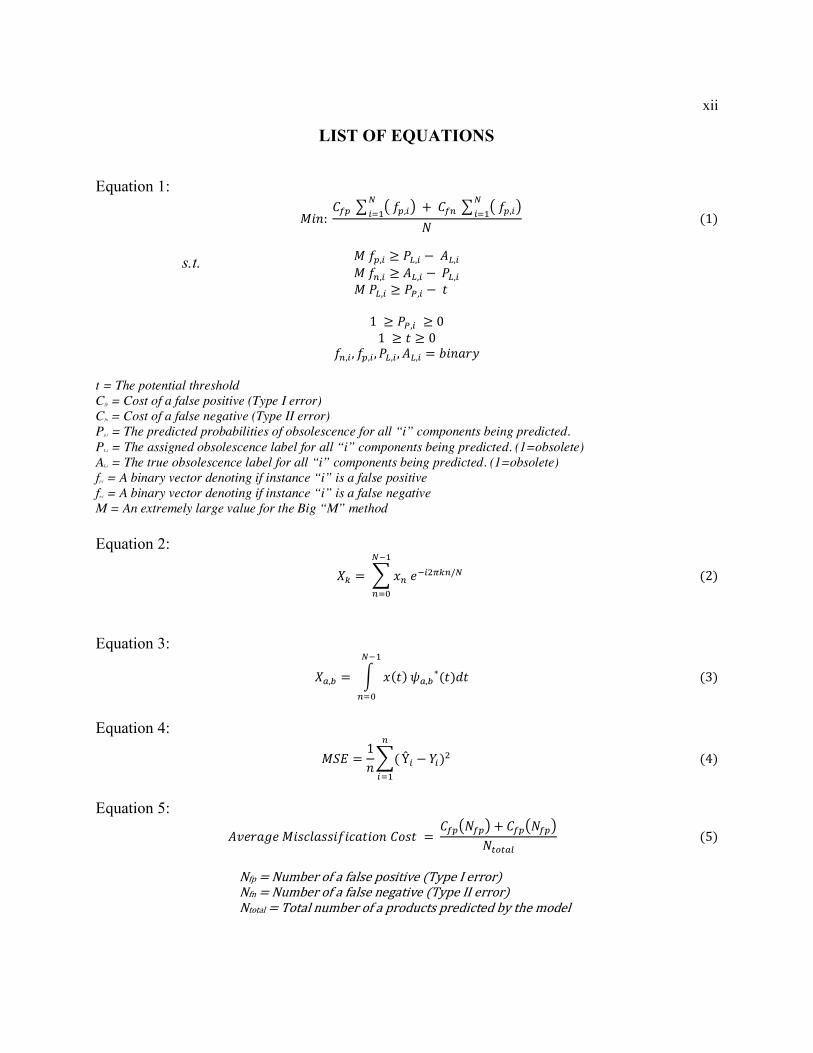
+3,-, +(,-, 9:,-, <:,- = A"#BCD t = The potential threshold Cfp = Cost of a false positive (Type I error) Cfn = Cost of a false negative (Type II error) Pp,i = The predicted probabilities of obsolescence for all “i” components being predicted. PL,i = The assigned obsolescence label for all “i” components being predicted. (1=obsolete) AL,i = The true obsolescence label for all “i” components being predicted. (1=obsolete) fp,i = A binary vector denoting if instance “i” is a false positive fn,i = A binary vector denoting if instance “i” is a false negative M = An extremely large value for the Big “M” method Equation 2:
EF = G H3IJ-KLF3///J1
30N
(2)
Equation 3:
EP,Q = R H(>)SP,Q∗(>)U>
/J1
30N
(3)
Equation 4:
!WX =1#G(
3
-01
Ŷ- − Z-)K(4)
Equation 5:
<\ICB]I!"^_`B^^"+"_B>"a#&a^> =&'(*4'(. + &'(*4'(.
4bcbPd(5)
Nfp=Numberofafalsepositive(TypeIerror)Nfn=Numberofafalsenegative(TypeIIerror)Ntotal=Totalnumberofaproductspredictedbythemodel
s.t.

xiii
Equation 6:
}I"A~``&�Ä = 1 −IJÅÇλÑÖ
(6)Where:
x = The life cycle prediction in time λ = The Weibull parameter scale k = The Weibull parameter shape

xiv
ACKNOWLEDGEMENTS
I must first start by thanking my family. Without them any achievement I make would be
empty because, above all else, I want to make them proud.
My parents, Kevin and Linda Jennings, have given me every advantage imaginable. If I
could rearrange the stars myself, I do not believe I could order them better than my parents have
for me. Any one of my achievements is only possible through them.
I would also like to thank my sisters, Kate and Lauren Jennings, for always being
supportive. Although I am the oldest sibling, your approval means so much to me.
I dedicate this dissertation to my parents and sisters.
In addition, my entire extended family has been tremendously supportive. Over the years,
they have nurtured my ego to be large enough that I believed I could finish a Ph.D. Thank you for
your support and for providing relaxing times on breaks away from school.
Before I even attended college, there were a few high school teachers at Homewood-
Flossmoor High School who continually challenged me to improve and grow.
First, I would like to thank two of my English teachers. I have been in and out of English
and reading classes my whole life. I have always regarded it as my biggest weakness. Joseph Upton
and Jake Vallicelli were my junior and senior year high school English teachers. Their classes are
the reason I had the confidence to believe I could write a dissertation.
Second, I would like to thank John Schmidt, my high school world history teacher. In his
class, we wrote a lengthy research paper. It seemed like an impossible task to a sophomore, but
Mr. Schmidt developed a workbook which broke down the paper systematically into very

xv
achievable, short-term goals. This workbook allowed students to work in small sections and not
procrastinate until the night before the paper was due. This concept has stuck with me and helped
me finish this dissertation (although I would be lying if I said much of this writing was not
accomplished because of an impending deadline).
I would also like to thank Paul Fasse. After a terrible start in Algebra 2/ Trigonometry, the
teacher told me that maybe I was not smart enough to be in the honors level course. I dropped from
honors level into Mr. Fasse’s regular level class. Mr. Fasse was an outstanding math teacher and
helped me rebuild my confidence in math. He took the time with me and even suggested I move
back up to honors level the following year. I did not want to but he talked me into it. The conditions
were that I would be in his honors section and, if the class covered something I had not learned
because I was in the regular level the year prior, Mr. Fasse would tutor me after class. I was
successful in honors level math for the remainder of high school. Although I never took Mr. Fasse
up on his offer to tutor me, it was the spark I needed to push myself back up to honors math.
Next, I would like to thank my high school economics teacher, Carl Coates. His excitement
for economics spurred that same excitement in me and caused me to pursue a second undergraduate
degree in economics. Although my primary focus in college was engineering, my solid background
in economics, which started with Mr. Coates, opened many doors for me and was crucial in the
chain of events that led me to graduate school and Penn State.
I would like to extend a special thanks to my high school Spanish teacher, Rodolfo Rios.
Mr. Rios was so encouraging in the subject, even though it was obvious I was not gifted in Spanish.
His kindness and patience taught me the value of having a champion when you are trying to
accomplish something, especially if it is not easy. I have tried to take this lesson into everything I
do and always give people an opportunity even if they do not excel at first.

xvi
While not technically a teacher, my lacrosse coach, Mark Thompson, taught me many
lessons about hard work and determination. Mr. Thompson created the lacrosse program at my
high school. Because I had been his neighbor, he asked me to play on the very first day. Over the
years, I watched Mr. Thompson grow the program from 10 kids on a field who did not know how
to pass and catch to a large program with a youth team and Freshman, JV, and Varsity teams. This
evolution showed me that with passion and determination, you can create a successful
organization.
I would also like to thank Brian McCarthy. Mr. McCarthy was my high school physics
teacher and my cross-country coach. Without my knowledge, Mr. Thompson signed me up for
cross country my freshman year. Mr. McCarthy showed up in my biology class and told me I had
practice after school. He told me it would be a light day and I would be running only three miles.
Since my running had consisted of a slow one-mile jog in gym class, three miles sounded like
going to Mars, but I showed up and started running. After the first mile, I had to walk. After a
month, I was running right behind everyone (unfortunately I would stay there most of my four
years of cross country). Running taught me to get up early and get ready to do something I was
not excited about. This has been invaluable because even when working toward accomplishing my
goal, some days I need to wake up early and complete tasks that I do not want to do.
Mr. McCarthy was also my AP Physics C teacher. This was my hardest class in high school
and on par with my most challenging college classes. I was able to earn a B in that class. Being
pushed to that level in high school was great preparation for college. (It also gave me wonderful
preparation for the sacred tradition in engineering school of complaining about the difficulty of
your classes.)

xvii
Last, I would like to thank my computer aided design (CAD) teacher, Nathan Beebe. Mr.
Beebe required all CAD students to complete a job shadow of an engineer or architect. I was
paired with sales engineers. For the first time I saw how engineering and people skills could be
combined into a career. This class project opened my mind to the possibility of pursuing an
education in engineering.
Again, I would like to thank my mother (she deserves a lot more thanks than are written
here, but I will not list every reason because the acknowledgements to my mom alone would be
longer than my dissertation) for Googling “sales engineering” and finding out Iowa State
University (ISU) was one of only two universities in the country to offer a sales engineering minor
program. This pushed Iowa State to the top of my list and I ultimately decided to attend ISU as an
undergraduate in industrial engineering.
Iowa State was another huge part of my life due, in part, to all of the wonderful people I
met there.
First, I would like to give thanks to the Iowa State lacrosse team for helping me adjust and
providing friendship when I first got to campus. Without them, it would be very likely that I would
have left Iowa State after my first year and none of the following would have happened.
My fraternity, the Epsilon chapter of Tau Kappa Epsilon, was integral in my development.
I met so many exceptional men in this fraternity. One of my greatest passions in college was
celebrating our many successes.
I also feel it is necessary to acknowledge the people in the chain of events that led me to
graduate school.
In my freshman year, I emailed Joydeep Bhattacharya, my intermediate macroeconomics
professor, about working as a TA for him. He was not hiring TAs but he found a position for me

xviii
in the economics help room. The economics help room was populated with so many exceptionally
smart and curious economics Ph.D. students. Two students specifically, T.J. Rakitan and Matt
Simpson, helped mentor me in economics, statistics, and math when there was no one else coming
in for economics help. These conversations sparked my interest in graduate school. For that, I must
thank Dr. Bhattacharya, T.J., and Matt.
One day I came into the economics help room and asked Matt about an article on a
professor visualizing sports scoring data. The professor was Gray Calhoun. Matt suggested I ask
to work with him for free. Dr. Calhoun took the meeting with me. After asking me if I knew any
programming other than VBA, he said I would need to learn to program in R or Python before
volunteering with him. Fortunately, Iowa State was offering a graduate “Introduction to R” class
that fall. I enrolled in the class taught by Heike Hofmann and quickly fell in love with manipulating
data in R. Dr. Hofmann said she and Di Cook would be co-teaching a more advanced version of
the R class in the spring. That class was fantastic. Both Dr. Hofmann and Dr. Cook are outstanding
educators and experts at understanding data. I have to thank Dr. Calhoun, Dr. Hofmann and Dr.
Cook for introducing me to R (Note: Chapters 4, 5, and 6 were all written using the R language).
ISU’s Industrial Engineering department had two fantastic undergraduate advisors, Devna
Popejoy-Sheriff and Kelsey Smyth. Devna knew I was developing an interest in programming and
that Dr. Terpenny was looking for an undergraduate research assistant to help do some
programming on a research project. I interviewed for the position and was hired two days later. I
have worked in Dr. Terpenny’s research lab now for five years, with Dr. Terpenny serving as my
master’s advisor at Iowa State and Ph.D. advisor at Penn State. I must thank Devna for suggesting
I apply to Dr. Terpenny’s job posting and to both Devna and Kelsey for being outstanding advisors
xix
with a phenomenal ability to listen to a student's dreams and help develop a plan to make it a
reality.
Additionally, the Iowa State Industrial Engineering department offered many outstanding
classes that have had a large impact on my life and the work in this dissertation. Dave Sly’s sales
engineering course was so universally useful. I rarely have a week where I do not use some of the
techniques discussed in that class. The manufacturing courses taught by Frank Peters and Matt
Frank were always exciting and hands on- a wonderful break from many of the purely theoretical
classes in engineering. Both Sigurdur Olafsson’s and Mingyi Hong’s data mining courses were
extremely insightful and served as a bridge between industrial engineering and the data mining
course in statistics. And lastly, John Jackman’s e-commerce course was a fantastic dive into web-
based programming for businesses.
Thank you to all the Iowa State professors who provided me with an outstanding education
and prepared me for my time at Penn State.
In the summer of 2015, Dr. Terpenny let me know she would be leaving Iowa State
University to become the Industrial Engineering Department Head at Penn State University. She
gave me the option to join her and I accepted. While it was difficult to leave my friends and mentors
in Iowa, going to Penn State gave me the chance to leave my comfort zone and expand my network
of friends and mentors.
As my advisor for the past five years, Dr. Terpenny has been the ultimate mentor. During
my journey from undergraduate researcher to a master’s student to a Ph.D. student in two different
schools, she has provided me with invaluable guidance. I have been fortunate to watch her lead
two outstanding departments. It is hard to describe the impact she has had on my life. As my
advisor, she has taught me how to conduct research. She has shown me how to assemble groups

xx
of people to solve hard problems. She has shown me the importance of interdisciplinary teams.
She has demonstrated to me how to lead people and change the culture of an organization for the
better. In watching her take on difficult problems over the years, I have learned so much about
leadership and the politics of people. I hope throughout my career that I am able to lead and
organize people to reach their full potential as well as Dr. Terpenny.
Through my Ph.D. at Penn State, my committee has helped guide me and polish my
research. I would like to thank my committee members for their comments and suggestions on this
work. In particular, I would like to say a special thanks to Tim Simpson for suggesting a
benchmarking study in Chapter 4 to compare against other algorithms. This greatly increases the
impact of this work. A special thanks also goes to Conrad Tucker for his suggested changes to the
language around the problems in scaling obsolescence forecasting models in industry. Also, a
thank you to Soundar Kumara for suggesting a sensitivity analysis for the error cost weights in
Chapter 5. Additionally, I would like to thank Peter Sandborn of the University of Maryland for
his feedback and suggestions on Chapter 5. Finally, I would like to thank my advisor, Dr.
Terpenny, for all the comments and suggestions over the years. I cannot even begin to describe all
the ways you have impacted this work for the better.
Penn State is filled with inspirational professors who have had an immense impact on my
education and my life as a whole.
Dr. Kumara’s data mining courses gave me a fundamental understanding of data mining,
search algorithms, and network analysis. These skills were critical in being hired as a data scientist
at Wells Fargo. I would like to thank Dr. Tucker for the conversations we have had that opened
my eyes to the intersection between professors and entrepreneurs. Although I am currently
pursuing work in the business world, these conversations linger with me and very well might draw

xxi
me back to academia in the future. The reflection learning essays in Dr. Simpson’s product family
course were fundamental in evaluating my learning style and how I can use different teaching
techniques and styles. The design of experiments class taught by Andris Freivalds was fantastic
and has been very useful in my data science career. Also, the creative examples from Hui Yang’s
stochastic processes class gave me an extraordinary understanding of Markov chains and the
underlying statistics. Thank you to all my professors at Penn State; I am so proud to be graduating
from Penn State because of you.
An additional special thanks to Dan Finke and Robert Voigt at Penn State. Dan Finke
helped me better convey my research to industry collaborators and helped organize letters of intent
for my first National Science Foundation grant. Thank you, Dan. These skills have moved my
career forward more than you know. And Dr. Voigt, as the department graduate program
coordinator, handles input and feedback from the graduate students and I provided more than my
fair share of input. I would like to thank Dr. Voigt for always listening and taking my input in
stride and using this feedback to mold the program into its best possible form.
Additional thanks to the National Science Foundation for supporting parts of this work
under Grant No. 1650527 and to the Digital Manufacturing and Design Innovation Institute
(DMDII) for supporting parts of this work under project number 15-05-03. The opinions stated in
this dissertation express the opinions of the author and do not reflect the opinions of the National
Science Foundation or the DMDII.
Also, a special thanks goes out to our industrial partners on this work: The Boeing
Company, Rolls-Royce Holdings, John Deere, and Sentient Science. The feedback and input from
these great companies has made a significant contribution to the findings in this dissertation.

xxii
The staff in the Industrial Engineering department and Center for eDesign have always
been wonderful and so helpful. The department is like a gearbox. The professors are like the gears
but the staff is the oil that keeps the gearbox running smoothly. Special thanks to Olga Covasa,
Terry Crust, Danielle Fritchman, Lisa Fuoss, Laurette Gonet, Paul Humphreys, Sue Kertis, Lisa
Petrine, Pam Wertz, and James Wyland for always putting up with my strange exceptions to
normal, everyday requests.
Thanks to my colleagues in the Smart Design and Manufacturing Systems Lab at Penn
State, particularly Dazhong Wu, Amol Kulkarni, Yupeng Wei, and Zvikomborero Matenga, who
provided crucial feedback on the research in this dissertation. I would also like to thank my
undergraduate researchers, Jiajun Chen and Carolyn Riegel, who helped clean and organize data
for some of this research. Special thanks goes to Dr. Wu who, as a postdoc for our lab, helped
mentor me and refine my research. Your guidance has not only improved this dissertation but has
made me a better researcher.
In all, I would like to thank the many friends I met in college, at both Iowa State and Penn
State, who helped me relax and de-stress from classes and exams. These breaks from work helped
me stay sane and allowed me to stay diligent over the long journey to complete this Ph.D.
And finally, I would like to thank Hong-En Chen. Without her love, support, and our
weekend writing sessions, finishing this dissertation would have been a much less enjoyable
process.
Although this acknowledgement is lengthy, it is still a small subset of all the people who
have had positive impacts in my life.
If I can leave you with one thing from this acknowledgement, it is that the smallest positive
impact on one person’s life can ripple for years. If Mr. Fasse had not taken the time to help me in

xxiii
math or Dr. Bhattacharya ignored my email about wanting to be a TA or Dr. Calhoun had not taken
a meeting with an unqualified kid and explained how to become qualified or Devna not suggested
to Dr. Terpenny that I would be a good fit for an undergrad research assistantship, I would have
absolutely never completed this dissertation.
So please be kind and, if you get a chance, please take the time to help someone else explore
their potential. You might be surprised where a little ripple can lead.

1
Chapter 1
Introduction
1.1 Background and Present Situation in Obsolescence Mitigation and Management
All products and systems are subject to obsolescence. There are four main types of product
obsolescence: (1) technical, (2) functional, (3) style, and (4) legislative. In technical obsolescence, old
products can no longer compete with the specifications of newer products [1], [2]. As needs and wants
change over time in a market, products and systems become obsolete. In functional obsolescence, products
can no longer perform their original task due to aging factors [1], [2]. The third type is style; many products
no longer are appealing visually and become obsolete due to changes in fashion (e.g., wood paneling on
cars) [2]. The last is legislative; if a government passes laws that forbid certain materials, components,
chemicals in manufacturing process, or creates new requirements in a market, this can often lead to many
products and designs becoming obsolete.
A product or a component becoming obsolete can have large implications throughout the
organization. For example, when a component becomes technically obsolete and is no longer manufactured
by suppliers, the lack of a component can cause stoppages of manufacturing lines and the overall supply
chain. The shortage of components forces organizations to take a number of possible actions. First,
organizations can stockpile components in last-time buys or life-time buys. Second, organizations can find
alternative sources for components such as aftermarket or used/refurbished components. Third, the part can
be emulated or a part replacement/substitution study can be conducted. Finally, when other alternatives
are not viable, a redesign must be undertaken [3]. These problems are exacerbated in industries with
qualification regulations. For instance, government and defense contractors are required to have parts and

2
products certified to certain specifications. If an alternative part or redesign is required, then this can trigger
a recertification process which can be lengthy.
One solution to these problems is to design products to be modular [4], [5]. With this approach, a
module can be more readily replaced, significantly extending the life and this holds obsolescence at bay.
An example of this was the Atari 800. Figure 1-1 shows an Atari 800 advertisement from 1979, which
reads, “The personal computer with expandable memory, advanced peripherals, and comprehensive
software so it will never become obsolete” [6]. Any 21st century observer of this 1979, Atari 800
advertisement would correctly assume the Atari 800 fell drastically short on the promise to “never become
obsolete”. In fact, the production of the computer started in 1979 and 6 years later, the production of the
personal computer which will “never become obsolete” was shutdown. By the end of 1991, Atari stopped
supporting any of the Atari 800 or its derivatives.
Figure 1-1: Atari 800 Advertisement from 1979 [6]

3
Even with modular designs and architectures, products and systems often fall victim to technical
obsolescence because innovation makes not only the underlining products obsolete, but also the overall
modular designs and architectures as well. This across-the-board risk of products becoming obsolete
requires organizations to have methods for assessing decisions around technical obsolescence. The methods
for assessing obsolescence mitigation strategies are dependent on the ability to reliably forecast when
products will become obsolete.
For this reason, one of the main areas of focus in this dissertation research is on how technical
obsolescence can be accurately forecasted in a market. These forecasting techniques will allow
organizations to continuously monitor the technical obsolescence status of both products and components,
and serve as a fundamental cornerstone for obsolescence mitigation strategies where organizations are
constantly balancing between two types of failures in obsolescence forecasting: (1) conducting unnecessary
stockpiling while (2) trying to never have a shortage, which can trigger a costly redesign.
Like technical obsolescence, organizations also must monitor functional obsolescence to avoid
catastrophic failures from wear out and help optimally use their products and machinery. Organizations that
monitor functional obsolescence are forced to tradeoff between two difficult alternatives: (1) conduct
premature maintenance and replace wearing components, which will lead to each component not being
used to its full potential, or (2) allow components to remain in service longer and risk a catastrophic failure
from an old worn out part. Like in technical obsolescence, making the best decisions requires that economic
impact be included in the functional obsolescence forecasting framework to minimize cost impact.
The goal in this research is to investigate methods for forecasting both technical and functional
obsolescence while minimizing errors of the models and minimizing the overall cost impact from
obsolescence.

4
1.2 Motivation
Over the last 20 years, the rate of innovation has become staggering, causing products to become
obsolete much faster[7], [8]. In response, there has been a rise in the number of methods and approaches
for estimating the true cost of obsolescence [2], [5]–[9]. However, many of these methods require
probability estimates or date ranges for when the products will become obsolete [2], [5]–[9]. Currently, the
literature has many methods of conducting economic analysis, but few methods for conducting the crucial
obsolescence forecasting needed to make these economic analysis methods viable. With obsolescence and
obsolescence mitigation costing the US government $10 billion annually, economic analysis methods are
fundamental in reducing this economic impact [10]. Development of obsolescence forecasting methods will
also allow models to predict obsolescence events further in advance and with greater accuracy. With greater
accuracy and increased prediction range, organizations will have longer time to react, more options
available, and increased confidence in decision making.
1.3 Research Purpose and Objective
The purpose in this research is to develop data-driven forecasting methods for forecasting both
technical and functional obsolescence. The goal of these forecasting models is to provide support for
decision making that will aid cost reductions. These forecasting models are combined with models to
estimate the cost of a product throughout its life cycle. The new combined model will conduct a what-if
analysis to understand the tradeoff between attempting to increase the product’s life, while trying to
decrease the cost of manufacturing and maintenance. Specifically, the following objectives will be achieved
in this research:
(1) to more accurately forecast when a product will no longer be technically competitive in a
marketplace,

5
(2) to account for differences in false positives and false negatives errors cost to minimize
average cost impact of mislabeled products (i.e., errors) in the obsolescence forecasting method,
(3) to more accurately forecast when a product will become worn out and no longer conduct
its functions properly, and
(4) to conduct tradeoff analyses between the length of the product’s life cycle versus the cost
to manufacture and maintain the product.
These objectives are addressed with generalizable frameworks so as to be robust and adaptable to
industry specific needs.
Based on the research purpose and objectives, primary research questions and research sub-
questions are defined in the following section. These primary research questions and sub-questions, provide
the basis and outline for the proposed work.
1.4 Research Questions
1.4.1 Primary Research Question
How can machine learning obsolescence forecasting methods be utilized to forecast technical and
functional obsolescence to help minimize costs associated with obsolescence mitigation?
Cell phone and digital camera markets provide cases for investigating technical obsolescence, and
gearbox wear provides the case for investigating functional obsolescence. These methods and case studies
lay the foundation for generalizable and comprehensive frameworks to aid organizations in implementing
obsolescence forecasting models and incorporating these models in business decisions.

6
1.4.2 Research Sub-Questions
(1) Questions on Technical Obsolescence Forecasting
Q1.1. How can large-scale technical obsolescence forecasting be conducted faster and for lower
cost?
H1.1. A machine learning based framework utilizing existing commercial parts databases would
lower cost and increase speed by saving on manual human filtering and predictions, while eliminating the
need for additional data collection (e.g., monthly sales data).
Q1.2. What level of accuracy can be achieved for consumer electronics to be classified as still
procurable or discontinued at scale using only technical specifications?
H1.2. The predictions from models using technical specifications to estimate availability in the
market will be accurate enough to be used reliably in business decisions.
(2) Questions on Minimizing Error Cost for Obsolescence Forecasting
Q2.1. What is the effect on expected error cost, when obsolescence forecasting models are
optimized to minimize the cost impact of errors instead of minimizing errors?
H2.1. Minimizing the cost impact of errors will have a much greater effect on lowering the expected
error cost compared to minimizing standard error cost because accuracy is only a proxy for cost savings.
Q2.2. How can cost impact of errors be minimized using the standard probability outputs from
obsolescence risk models?
H2.2. A mathematical model, with an objective function with the goal to minimize expected error
cost and has the threshold between the obsolescence classifications as the decision variable, would be
capable of calculating an optimal cutoff threshold to reduce the cost impact of obsolescence.
(3) Questions on Functional Obsolescence Forecasting
Q3.1. Which signal processing method (Fourier or wavelet) develops more accurate models for
predicting functional obsolescence?

7
H3.1. Since wavelet records frequency and location, while Fourier only records frequency, wavelet
is assumed to be the preferred signal processing method.
(4) Questions on Tradeoff Between Life Cycle Cost and Life Cycle Length
Q4.1. How can early stage design information be compiled to estimate the life cycle and cost of a
product?
H4.1. Individual models, such as life cycle forecasting, life cycle cost forecasting, and
manufacturing process models, can be chained together to define how information flows through an
organization to estimate the life cycle and cost of a product.
Q4.2. How can a generalizable machine learning framework be created to estimate the life cycle
and cost of a product given usage, material properties and general cost information?
H4.2. Each of the individual models outlined in H4.1 could be approximated by using data mining
techniques to develop a relationship between the inputs and outputs. These inputs and outputs could feed
into each other and develop a generalizable machine learning framework to estimate the life cycle and cost
of a product.
Q4.3. What is required in order to optimize the general machine learning framework presented in
Q4.2?
H4.3. A genetic optimization algorithm could search the complex search space and can be
designed to minimize cost while maintaining a desired life or maximize the life cycle while maintaining a
desired cost.

8
1.5 Research Approach and Methods
Five main aspects of this research are investigated. First, a technical obsolescence forecasting
framework using web scraping and machine learning is proposed. The framework is tested by forecasting
technical obsolescence in the consumer electronics fields, specifically cell phones and digital cameras.
Second, a functional obsolescence forecasting method using Fourier and wavelet transforms is proposed
and tested using sensor information from a gear box. Third, the argument is made that maximizing model
accuracy is merely a proxy for minimizing the cost impact to the organization. A mathematical model for
tuning models for minimizing costs, rather than maximizing accuracy, is presented. Fourth, a framework
for functional obsolescence forecasting methods and economics analysis is presented. The framework uses
gearbox data from a gear simulation company, Sentient Science, and cost information from Boeing to
conduct “What-if” analysis based on manufacturing properties, usage data, and cost information. Fifth, a
genetic optimization approach is developed and presented to find the optimal settings given a set of
requirements (e.g., maximize life given a desire cost or minimize cost given a desired life).
1.6 Research Contributions
The obsolescence forecasting techniques with overall economic optimization frameworks will not
only help organizations in the industries explored in the case studies in this research, but also assist in the
following:
a) Help organizations conduct more accurate economic analyses for different obsolescence mitigation
decisions.
b) Decrease the impact of obsolescence forecasting errors by optimizing the forecasting models for
cost avoidance rather than just standard error avoidance.
c) Allow organizations to better understand the information flow of parts throughout its life cycle.

9
d) Enhance the quality and reduce the cost of products by allowing designers tools to find optimal
product specifications and requirements in order to reach target life cycle and cost.
1.7 Document Outline
The first chapter has provided an introduction to life cycle management and the problems in the
field this research addresses. The second chapter provides a review of the literature related to technical and
functional obsolescence forecasting methods and economic analysis for life cycle management. Chapter 3
presents the methodologies proposed to solve the problems outlined in Chapter 1. The fourth chapter
contains case studies assessing the accuracy of the proposed obsolescence risk and life cycle forecasting
models in the cell phone, digital camera, and screen component markets. The fifth chapter applies an error
cost minimization framework to further lower the cost impact of errors in the obsolescence forecasting
process. Chapter 6 contains a comparative case study to find the best combination of sensor signal
transformation (i.e., Fourier and wavelet transforms) and machine learning algorithms to predict the health
status of a wind turbine engine. Chapter 7 is a case study to apply a life cycle verse cost tradeoff model
using the example of designing a gear for a gearbox. The last chapter, Chapter 8, discusses the contributions
and results of the research conducted in the previous chapters. The chapter then proposes future directions
for research based on the contributions of this dissertation.

10
Chapter 2
Literature Review
The review of the literature focuses first on work related to forecasting technical obsolescence. This
is followed by a discussion of how the forecasting methods used to predict technical obsolescence events
can be tuned to more effectively help organizations avoid cost from technical obsolescence. Finally, a
review of methods for predicting functional obsolescence is provided.
Here, technical obsolescence refers to products no longer being technically competitive in a market.
For example, technical obsolescence occurs when newer products with superior specifications are
introduced that render the older models obsolete. This often causes organizations to cease production of
older products in favor for new more competitive ones. By definition, functional obsolescence occurs when
a product can no longer perform its original purpose. Section 2.3 focuses on literature around forecasting
functional obsolescence in gear boxes. This example was chosen since gear boxes are frequently used in
many industries as well as the numerous types of failures that can occur.
2.1 Forecasting Technical Obsolescence
Technical obsolescence can have an immensely negative effect on many industries; the
ramifications of which have generated a large body of research around obsolescence related decision
making and more generally, around studying products through the product’s life cycle. To address the
economic aspect of obsolescence, cost minimization models are presented for both the product design side
and the supply chain management side of obsolescence management [9]–[11]. Extensive work has also
been conducted on the organization of obsolescence information [12]–[14]. The organization of information
allows one to make more accurate decisions during the design phase of a product life cycle.

11
Obsolescence management and decision-making methods have three groups: (1) short-term
reactive, (2) long-term reactive, and (3) proactive. The most common short term reactive obsolescence
resolution strategies include lifetime buy, last-time buy, aftermarket sources, identification of alternative or
substitute parts, emulated parts, and salvaged parts [15], [16]. However, these strategies are only temporary
and can fail if the organization runs out of ways to procure the required parts. More sustainable long-term
alternatives are design-refresh and redesign. These alternatives usually require large design projects and
can carry costly budgets. In a 2006 report, the U.S. Department of Defense (DoD) estimated cost of
obsolescence and obsolescence mitigation for the government to be $10 billion annually for the U.S.
government [17]. The estimates in the private sector could be higher because smaller firms cannot afford
the systems DoD uses to track and forecast obsolescence.
Obsolescence forecasting can be categorized according to two groups: (1) obsolescence risk
forecasting and (2) life cycle forecasting. Obsolescence risk forecasting generates a probability that a part
or other element may fall victim to obsolescence [18]–[21]. Life cycle forecasting estimates the time from
creation to obsolescence of the part or element [1], [2], [8]. Using the creation date and life cycle forecast,
analysts can predict a date range for when a part or element will become obsolete [1], [2], [8].
Obsolescence forecasting is important in both the design phase of the product and the
manufacturing life cycle of the product. It is estimated that 60-80% of cost during a product’s life cycle are
caused by decisions made in the design phase [22]. Understanding the risk level for each component in
proposed bills of materials developed in the design phase can help designers determine designs that have
lower risk of component obsolescence and therefore reduce the life time cost impact. Additionally,
obsolescence forecasting can be used throughout a product’s life cycle to analyze predicted component
obsolescence dates and find the optimal time to administer a product redesign that will remove the
maximum number of obsolete or high obsolescence risk parts.
12
2.1.1 Life Cycle forecasting
The key benefit of life cycle forecasting is that it allows analysts to predict a range of dates when
the part will become obsolete [7]. These dates enable project managers to set timeframes for the completion
of obsolescence mitigation projects, aid designers in determining when redesigns are needed, and enable
managers to more effectively manage inventory. All of these effects of life cycle forecasting reduce the
impacts of obsolescence [7].
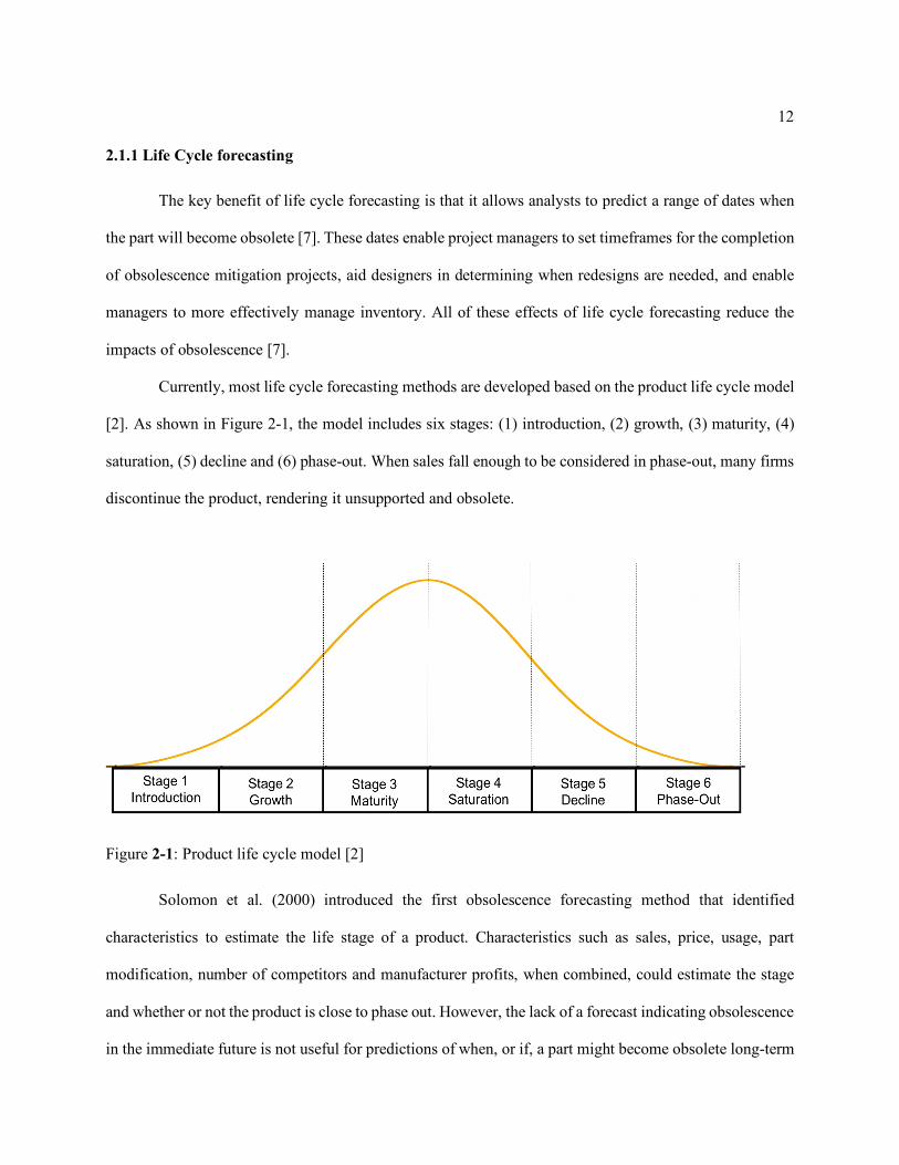
Currently, most life cycle forecasting methods are developed based on the product life cycle model
[2]. As shown in Figure 2-1, the model includes six stages: (1) introduction, (2) growth, (3) maturity, (4)
saturation, (5) decline and (6) phase-out. When sales fall enough to be considered in phase-out, many firms
discontinue the product, rendering it unsupported and obsolete.
Solomon et al. (2000) introduced the first obsolescence forecasting method that identified
characteristics to estimate the life stage of a product. Characteristics such as sales, price, usage, part
modification, number of competitors and manufacturer profits, when combined, could estimate the stage
and whether or not the product is close to phase out. However, the lack of a forecast indicating obsolescence
in the immediate future is not useful for predictions of when, or if, a part might become obsolete long-term
Figure 2-1: Product life cycle model [2]
13
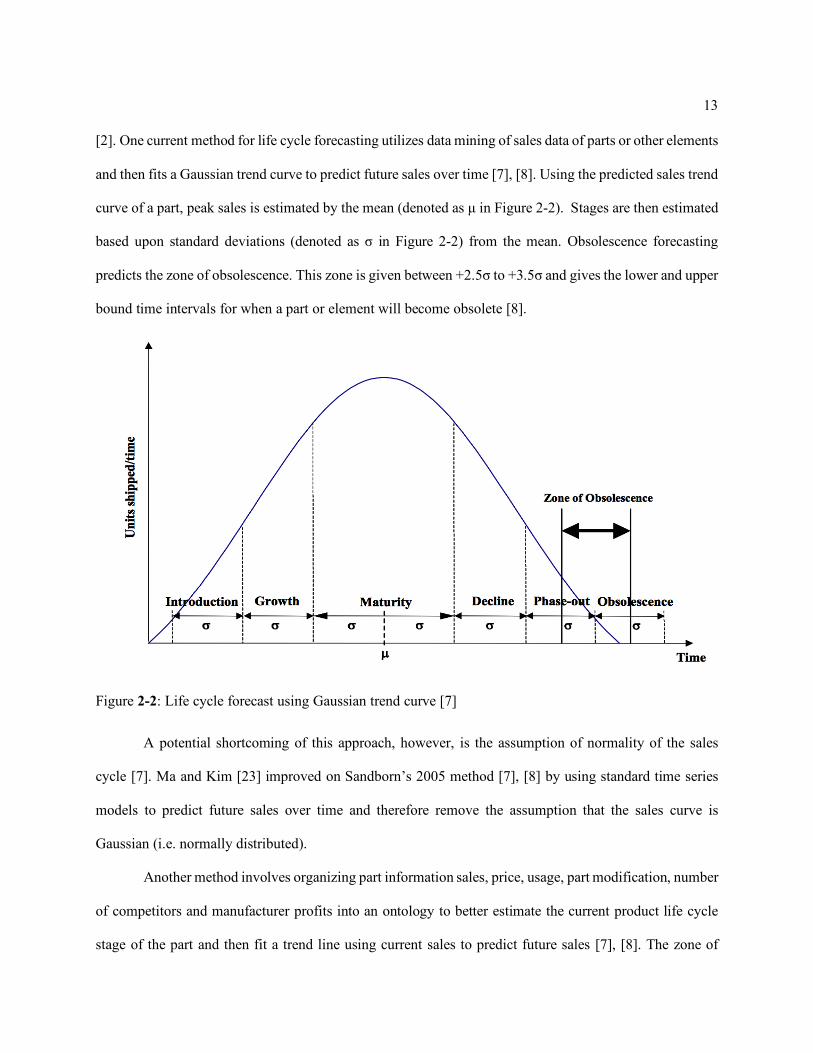
[2]. One current method for life cycle forecasting utilizes data mining of sales data of parts or other elements
and then fits a Gaussian trend curve to predict future sales over time [7], [8]. Using the predicted sales trend
curve of a part, peak sales is estimated by the mean (denoted as µ in Figure 2-2). Stages are then estimated
based upon standard deviations (denoted as σ in Figure 2-2) from the mean. Obsolescence forecasting
predicts the zone of obsolescence. This zone is given between +2.5σ to +3.5σ and gives the lower and upper
bound time intervals for when a part or element will become obsolete [8].
A potential shortcoming of this approach, however, is the assumption of normality of the sales
cycle [7]. Ma and Kim [23] improved on Sandborn’s 2005 method [7], [8] by using standard time series
models to predict future sales over time and therefore remove the assumption that the sales curve is
Gaussian (i.e. normally distributed).
Another method involves organizing part information sales, price, usage, part modification, number
of competitors and manufacturer profits into an ontology to better estimate the current product life cycle
stage of the part and then fit a trend line using current sales to predict future sales [7], [8]. The zone of
Figure 2-2: Life cycle forecast using Gaussian trend curve [7]

14
obsolescence is estimated using the predicted future sales, but it does not assume normality since the factors
utilized in the Gaussian trend curve are used to estimate the stage, not the curve shape.
Currently, most life cycle forecasting methods in the literature are built upon the concept of product
life cycle model. This method involves data mining parts information databases for introduction dates and
procurement lifetimes to create a function with the input being the introduction date and the output being
the estimated life cycle [16]. The advantage of this method is the lack of reliance on sales data, the ability
to create confidence limits on predictions and the simplicity of a model with one input and one output [16].
However, this does not take into account the specifications of each individual part. As a result, the model
could be skewed. For example, two manufacturers with two different design styles both make similar
products. The first manufacturer creates a well-designed product and predicts that the specifications will
hold in the market for five years. The second manufacturer does not conduct market research and introduces
a new product every year to keep specifications up to market standards. Over the next five years, the first
company will have one long life data point, and the second company will have five short life data points;
this will skew the model into predicting the approximate life cycle is shorter than it actually is because the
model does not take into account changes in specifications.
2.1.2 Obsolescence Risk Forecasting
Another common method used for predicting obsolescence is obsolescence risk forecasting.
Obsolescence risk forecasting involves creating a scale to indicate the levels of the chance of a part or
element becoming obsolete. The most common of these scales is to use probability of obsolescence [18]–
[21]. These scales, like product life cycle stage prediction, use a combination of key characteristics to
identify where the part falls on a scale.
Currently, two simple models exist for obsolescence risk forecasting; both use high, medium, and
low ratings for key obsolescence factors that can identify the risk level of a part becoming obsolete [18],

15
[19], [21]. Rojo et al. [21] conducted a survey of current obsolescence analysts and created an obsolescence
risk forecasting best practice that looks at the number of manufacturers, years to end of life, stock available
versus consumption rate, and operational impact criticality as key indicators for potential parts with high
obsolescence risk. Josias and Terpenny also created a risk index to measure obsolescence risk [18]. The
key metrics identified in their technique are manufacturers’ market share, number of manufacturers, life
cycle stage, and company’s risk level [18]. The weights for each metric can be altered based on changes
from industry to industry. However, this output metric is not a percentage but rather a scale from zero to
three (zero being no risk of obsolescence and three being high risk).
Another approach introduced by van Jaarsveld uses demand data to estimate the risk of
obsolescence. The method manually groups similar parts and watches the demand over time [20]. A formula
is given to measure how a drop in demand increases the risk of obsolescence [20]. However, this method
cannot predict very far into the future because it does not attempt to forecast demand, which causes the
obsolescence risk to be reactive.
2.1.3 Technical Obsolescence Scalability
For a method to be scalable, it must have the ability to adjust the capacity of predictions with
minimal cost in minimal time over a large capacity range [24]. To achieve scalability in industry,
obsolescence forecasting methods must meet the following requirements:
(1). Do not require frequent (quarterly or more often) collection of data for all parts.
The reason for this requirement is that many methods involve tracking sales data of products to estimate
where the product is in the sales cycle [2], [7], [8], [23]. A relatively small bill of material with 1000
parts would require a worker to find quarterly sales for 1000 parts and input the sales numbers every
quarter (or even more frequently). Companies have built web scrapers to aggregate this data

16
automatically, like specifications and product change notifications, but many manufacturers do not
publish individual component sales publicly on the web. Large commercial parts databases have
contracts with manufacturers and distributors to gain access to sales data, but many companies not
solely dedicated to aggregating component information have difficulty obtaining this information. The
lack of ability for most companies to gather sales data makes forecasting methods requiring sales of
individual parts extremely difficult to scale.
(2). Remove human opinion about market
Asking humans to input opinions on every part leads to methods that are impractical for industry.
Additionally, finding and interviewing subject matter experts for long periods of time can be costly.
Also, there may exist biases inherent for subject matter experts when estimating obsolescence risk
within their field of expertise. These biases are largely due to experts being so ingrained in the traditions
of their field that new products or skills can seem inferior when in fact the new techniques may
supersede the expert’s traditional preferences. The requirement of human opinion creates additional
variance in the resulting predictions and makes repeatability hard. For example, two experts within the
same organization can use the same prediction method and come to different results because their
perceptions of the market are different. Whereas if two experts use a mathematical model-based
approach that is generated from sales or specification data, both experts will always come to the same
result as long as the method and underlying data is the same. For these reasons, obsolescence
forecasting models must try to remove human opinion as much as possible in the model development
and implementation stage. Obviously, all models will require humans to make decisions during the
development of the model on which variables to include and which to not include, but removing human
opinion as an input to a model in favor of more quantitative metrics like specifications, sales numbers,
and market size will increase repeatability of predictions and minimize human bias.

17
(3). Account for multi-feature products in the obsolescence forecasting methodology
Methods have been developed to predict obsolescence of single feature products [7], [8], for example
flash drives. The flash drive may vary slightly in size and color but only has one key feature, memory.
When a flash drive does not have sufficient memory to compete in the flash drive market, companies
phase out that memory size in preference for ones with larger memory. Creating models for single-
feature products like memory is straightforward because the part has only one variable that only causes
one type of obsolescence, namely technical. However, multi-feature products, for example a car, can
have many causes for becoming obsolete and this makes it much more challenging to model. Some
examples might include (1) style obsolescence that comes from changes such as eliminating cigarette
lighters, ashtrays and the removal of wood paneling from the sides of cars, (2) the functional
obsolescence of cassettes, and now even CD players for MP3 ports or Bluetooth, and (3) the technical
obsolescence of drum brakes giving way to safer and longer running disc brakes. With these multiple
obsolescence factors, many of the current forecasting models fall apart.
Any obsolescence forecasting method that does not meet these three requirements will most likely
develop problems when trying to scale to meet the needs of industry.
2.1.4 Current Technical Obsolescence Forecasting Scalability
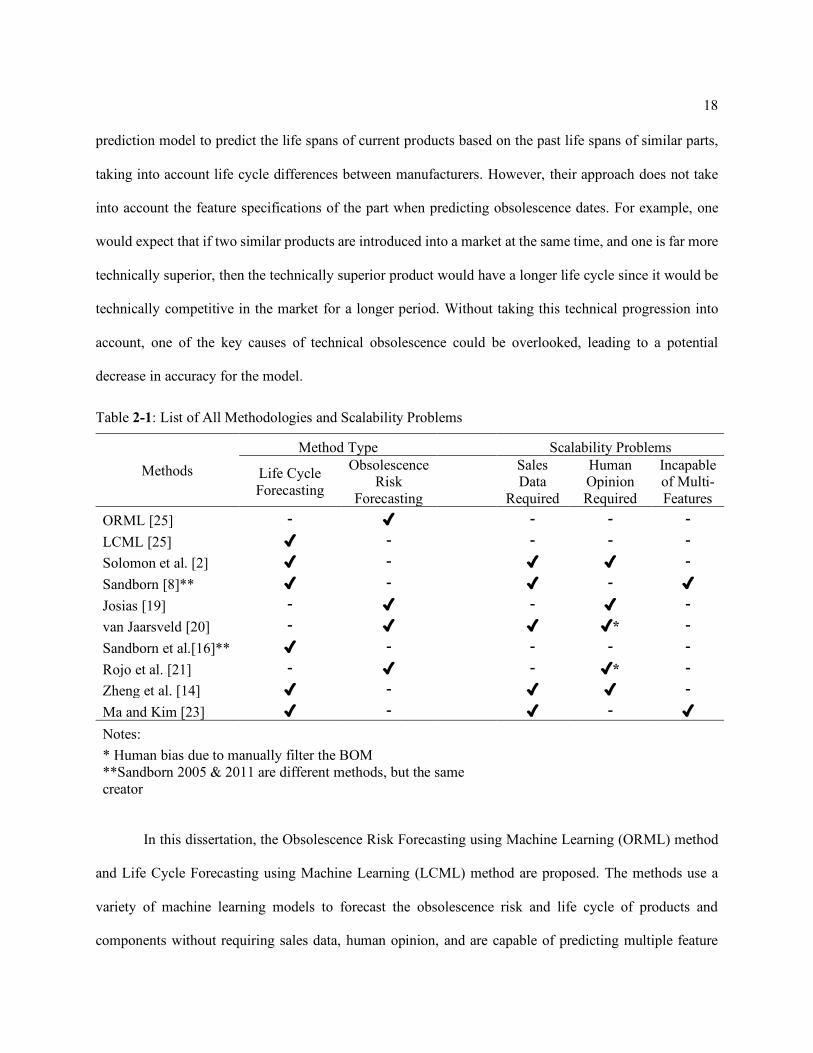
Table 2-1 provides an overview of obsolescence forecasting methods that have been published in
the last 15 years. Each method is characterized according to type of obsolescence forecasting and whether
it meets each of the scalability factors. Ideally, methods that do not require sales data or human opinion but
should be capable of forecasting obsolescence for multi-feature products. These characteristics are also
indicated in Table 2-1 for each method. As shown, Sandborn et al. [16] is currently the only method that
does not require sales data or human opinion, but it does consider multi-feature products. They create a
18
prediction model to predict the life spans of current products based on the past life spans of similar parts,
taking into account life cycle differences between manufacturers. However, their approach does not take
into account the feature specifications of the part when predicting obsolescence dates. For example, one
would expect that if two similar products are introduced into a market at the same time, and one is far more
technically superior, then the technically superior product would have a longer life cycle since it would be
technically competitive in the market for a longer period. Without taking this technical progression into
account, one of the key causes of technical obsolescence could be overlooked, leading to a potential
decrease in accuracy for the model.
Table 2-1: List of All Methodologies and Scalability Problems
Methods Method Type Scalability Problems
Life Cycle Forecasting
Obsolescence Risk
Forecasting
Sales Data
Required
Human Opinion Required
Incapable of Multi-Features
ORML [25] - ✓ - - - LCML [25] ✓ - - - - Solomon et al. [2] ✓ - ✓ ✓ - Sandborn [8]** ✓ - ✓ - ✓ Josias [19] - ✓ - ✓ - van Jaarsveld [20] - ✓ ✓ ✓* - Sandborn et al.[16]** ✓ - - - - Rojo et al. [21] - ✓ - ✓* - Zheng et al. [14] ✓ - ✓ ✓ - Ma and Kim [23] ✓ - ✓ - ✓ Notes: * Human bias due to manually filter the BOM **Sandborn 2005 & 2011 are different methods, but the same creator
In this dissertation, the Obsolescence Risk Forecasting using Machine Learning (ORML) method
and Life Cycle Forecasting using Machine Learning (LCML) method are proposed. The methods use a
variety of machine learning models to forecast the obsolescence risk and life cycle of products and
components without requiring sales data, human opinion, and are capable of predicting multiple feature

19
components. As a result, the ability to scale obsolescence forecasting models, a long-time limitation of
existing methods, has been addressed.
2.1.5 Current State of Technical Obsolescence Forecasting in Industry
Because obsolescence forecasting can realize enormous cost savings for organizations, there are
several companies that have emerged in recent years, offering obsolescence forecasting and management
as a service. Currently, some of the leading obsolescence forecasting and management companies include
SiliconExpert, IHS, Total Parts Plus, AVCOM and QTEC Solutions [26]–[29]. These companies focus on
electronic components because of the high rate of obsolescence and have databases with information on
millions of electronic parts such as, part ID, specifications and certification standards. The commercial
forecasting services can be sorted into life cycle and obsolescence risk. Currently SiliconExpert, Total Parts
Plus, AVCOM and QTEC Solutions offer life cycle forecasts and IHS offers an obsolescence risk
forecasting solution. However, none of these services offer both obsolescence risk and life cycle
forecasting.
2.2 Accounting for Asymmetric Error Cost in Forecasting
The ultimate goal of obsolescence mitigation and management is to help organizations avoid
unnecessary costs when it comes to products becoming obsolete. Currently obsolescence forecasting
techniques focus on accuracy in the hopes that higher accuracy will lead to more cost avoidance. However,
maximum model accuracy is a proxy for maximum cost avoidance. This section discusses how
organizations can tune obsolescence forecasting models to maximize cost avoidance rather than to
maximize accuracy in the hopes of achieving maximum cost avoidance.

20
2.2.1 Technical Obsolescence Forecasting and Cost Avoidance
For electronic components, extensive commercial databases containing both life cycle forecasts
and obsolescence status of components are available; however, in many other industries, no commercial
components databases are available or the databases that exist only address a subset of the components.
When the obsolescence status of a component cannot be found in a commercial database, risk forecasting
methods can be utilized to estimate the obsolescence risk forecast. When predicting an obsolescence risk
level, the obsolescence risk corresponds to the risk that the component will be obsolete at a given time. The
time is determined by the data used to develop the models. If the model uses the current status of
components, then the risk will represent the current probability the component is obsolete compared to its
peers in the market. If some information is available about when component manufacturers will no longer
offer other components in the same market, then a future time can be selected. For example, one month
could be selected, and then followed with gathering all the expected statuses. Organizations with expected
obsolescence statuses in a month for a few products in the market can develop models using products with
known statuses to predict the expected obsolescence statuses and risks in a month for other products in the
market where the status is currently not available. These models can allow industries without robust
commercial component databases to predict the obsolescence risk and statuses for all products in a market.
Although this method is not ideal, it increases the organization’s obsolescence knowledge about
components with no obsolescence status report from the manufacturer.
Currently, many organizations do not use risk levels directly, but rather they translate the risk levels
into statuses of procurable or discontinued. These statuses are then used by decision-makers to make
actionable obsolescence management decisions. Many organizations will use a default status threshold of
50% probability. Products with risk levels above 50% are assigned a status of discontinued; below a 50%
risk levels are assigned procurable. However, using a cut off of 50%, assumes equal costs of Type I (false
positive) and Type II (false negative) errors. In obsolescence management, predicting that a procurable

21
component as discontinued may trigger a stockpiling of the component or a redesign. If a discontinued
component is predicted to be still procurable, then this can starve production systems and even lead to a
shutdown. Each of these outcomes has a corresponding cost, and the costs are rarely equal. In this
dissertation, Receiver Operating Characteristic (ROC) analysis [30] is applied to obsolescence risk
forecasting to control for these asymmetrical error costs. ROC analysis calculates the optimal obsolescence
risk cut-off threshold by analyzing the trade-off of decreasing the accuracy for less costly outcomes while
increasing the accuracy for costlier outcomes. This will lead to reduced negative cost impacts when
compared to the standard methods described earlier in this section because current methods seek to
minimize error without accounting for the cost implications of predictions. By accounting for the cost of
the different types of errors for the forecasting model, the organization can reduce the average cost impact
of an error from their preexisting obsolescence risk models. The cost can be incorporated after a risk level
is predicted but before a status of procurable or discontinued is assigned by varying the cutoff threshold
used to assign statuses.
2.2.2 Applications of Receiver Operating Characteristic Analysis
Receiver Operating Characteristic (ROC) analysis is a statistical method that accounts for
asymmetrical error costs in classification models [30]. The analysis has two phases: (1) understanding the
classification model’s ability to separate each status and (2) selecting an optimal cut off threshold between
statuses based on some certain criteria. ROC curves are closely related to Gini Indexes in decision trees
because of their ability to quantify the separation between classes in a classification problem [31]. This
quantification of separability allows for the comparison of classification models; like comparing model
accuracies. However, Cortes and Mohri [30] argue comparing models using ROC analysis is superior to
standard accuracies due to the more holistic approach of ROC analysis. An example of this would be a
classification model to predict whether or not a patient has a rare disease. A model could achieve a high
degree of accuracy by predicting all patients are negative, and the few positive patients would become the

22
error. Although the model has a high accuracy, it is completely useless to predict the disease. ROC analyzes
the classification rate for each class to ensure both positive and negative classes are being classified
correctly.
For this reason, ROC analysis has become an integral tool in disease detection in the medical field.
Ridker [32] improved the accuracy of cardiovascular risk prediction by pairing classification models with
ROC curves. Nagel et al. [33] applied ROC curves to improve noninvasive detection of coronary artery
disease with an 89% accuracy. Metz [34] proposed an objective evaluation using ROC curves of medical
images for disease detection. These objective methods prevent any tendency for doctors to “under-read” or
“over-read” images. ROC curves are also used in early stage ovarian cancer, prostate cancer, breast cancer,
lung cancer, Parkinson’s, liver disease, and even early detection of disease outbreaks [35]–[41]. Another
application area of ROC analysis is for identification of fault detection. Specifically, fault detection on large
systems where each type of fault may have only a few occurrences and the majority class label would be a
status of “normal”. For example, Kumar et al. [42] use ROC curves to evaluate classifiers for fault detention
in cloud-based manufacturing systems. Dellomo [43] employs ROC to detect faults in a helicopter gearbox
using acoustic vibration data. Sawitri et al. [44] apply ROC analysis to identify failures in the electric power
grid. Oberweger et al. [45] apply ROC to a combination of computer vision and fault detection for
noninvasive power line insulation flaw inspection.
In summary, ROC curves, and overall ROC analysis, are a powerful and robust statistical tool to
select optimal predictive models. The previous section summarized works in obsolescence forecasting and
the focus of prediction accuracy. Section 3.2 explores the potential application of ROC curves to analyze
the costs incurred by misclassification in obsolescence risk forecasting.

23
2.3 Forecasting Functional Obsolescence for Gear Boxes
Health monitoring is any technique or method to predict if the wind turbine gearbox is running
correctly and not becoming functionally obsolete. The goal of health monitoring is to minimize downtimes,
operation and maintenance costs, and maximize output [46]–[49]. This section will discuss how health
monitoring is conducted in industrial gearboxes. The methods can be broken down into a few key areas:
temperature, power quality, oil/debris, vibrations, and acoustics emissions [50]–[52]. The rest of this section
discusses the different methods to detect abnormal operating conditions.
2.3.1 Temperature
Monitoring temperature is one of the most common methods of health status monitoring for
gearboxes [51]. Temperature change can indicate excess load on a gear or bearing. Although other factors
can change the temperature, the majority of the time the gears and bearings will remain at relatively constant
temperatures in a healthy turbine. Therefore, the change in temperature can often indicate a change in load
which can be caused by wearing and failing components within the gearbox. The temperature change can
also be caused by low oil or other fluid levels. The lack of oil can cause increased friction between
components [53], [54]. However, temperature changes are slow and only will happen if there is a large
change in the gearbox, otherwise many small faults and wears may not be detected [51].
Even though temperature is not a perfect indicator of gearbox health many researchers have had
success using temperature to predict faults. Kusiak and Verma [55] generated models using neural networks
to predict future bearing and gear temperatures. The temperatures are then compared against manufacturer’s
acceptable operating condition intervals and if the predicted temperature is outside the interval, the gear or
bearing is predicted to have a fault. Astolfi et al., [56] use a graphing technique to visualize changes from
normal operating conditions. This method plots percentage of rated power versus temperature of historical

24
and current operations. If the current is well outside the historical norm, then the turbine is detected as
abnormal.
2.3.2 Power Quality
The next prediction method is power quality. Power quality looks at the power output from the
turbine and compares it to the theoretical expected output from a turbine in similar operating conditions.
The output can be measured by the mechanical power of the drive shaft or the electrical output from the
overall turbine.
Uluyol et al. [57] developed a performance analytic to indicate when a wind turbine is
underperforming given the manufacturer’s expected power output for a given wind speed and air density.
Kim et al. [58] developed a neural network to predict expected power output using more than 150 signals.
The predicted power output was compared to the actual output, and if a difference existed, then the turbine
was given an abnormal status [58].
2.3.3 Oil and Debris Monitoring
Oil and debris monitoring seeks to track the changes in the oil throughout a gearbox’s life in an
attempt to predict wear. Splinters and debris can often end up in the oil of the gearbox if gears and bearings
are deteriorating [51] (see Figure 2-3 for an example of a gear that would produce debris). This is often
reliable because it is a direct relationship with the bearings but can be one of the most expensive attributes
to monitor on a wind turbine [50].

25
Wu et al. [60] reviewed trends in oil monitoring and found many applications involve thresholds
where the percent of debris in the oil becomes too high and the gearbox needs attention. These researchers
also found few organizations in industry adopt this technology due to the high cost of sensors [60]. To
address the cost of sensors, Dupuis [59] developed a method to monitor all of the gears and bearings using
only one debris monitoring sensor. This method looks at debris size overtime and found debris larger than
200 µm was an indicator of extreme gear and bearing wear [59].
2.3.4 Vibration and Acoustic Emissions
The last method considered in this research involves monitoring the waves of vibration and/or
acoustic emissions from the gearbox. Vibration monitoring involves accelerometer sensors measuring the
oscillations or shaking of the machine. Acoustic emission records the resulting waves from energy released
due to microstructural changes from stress [61]. Although vibrations and acoustic emissions measure
different attributes of a gear box, both are waves with similar techniques for developing models. The models
can be broken into three main types: (1) Time domain, (2) Fast Fourier transform (FFT), and (3) Wavelet
transform [46].
Figure 2-3: Wind Turbine Gearbox Failure Examples [59]

26
Time Domain
Time domain models deal with inputs that are time series or chronological measurement over time at a
consistent interval. These models tend to be more intuitive than FFT and Wavelet based models because
there is not a transformation involved. However, these simpler models often have trouble capturing the
complex relationships between inputs and outputs.
Futter [62] established a method to predict wind turbine gearbox health by averaging the vibration
sensors in the time domain. McFadden [63] improved this method by using harmonic mesh smoothing
to reduce noise in the signal and more accurately predict faults from standard noise. Caselitz and
Giebhardt [64] developed statistical models using variables such as rotational speed of shafts, power,
generator temperature, vibrations etc. The mean and standard deviation of the above attributes are taken
and weights are assigned using a statistical model to classify healthy and unhealthy gearboxes [64].
Fast Fourier Transform
Fourier transform takes data from the time domain and transforms it into the frequency domain. The
frequency domain represents how the time series is distributed within each frequency band for a given
range of frequencies.
Unala et al. [65] develop neural networks using envelope analysis accompanied by Hilbert transform
and Fast Fourier transform. Miao et al. [66] used a modified Fourier transform called “interpolated
discrete Fourier transform” (IpDFT). IpDFT resulted in frequency resolution in signal parameter
estimation when characteristic frequencies are very close [66]. Shakya et al. [67] developed a mixed

27
Fourier and Wavelet model. The model takes vibration data and conducts both transformations to
develop inputs for the classification model.
Wavelet Transform
Wavelet transform is another transform, similar to Fourier, but the Wavelet not only includes
frequencies, but also the scale of each frequency [68]. For example, if the amplitude of a signal changes
in time, the Fourier transform will not indicate when this occurred.
Suh et al. [69] developed a neural network using wavelet transform. The authors argue wavelet
transforms are a more appropriate approach to process signals then compared to Fourier transform. This
is due to Wavelet transform being able to decompose a signal into different frequencies with different
resolutions while conserving time and frequency domain information [69]. Roulias [70] applies
Wavelet transform to de-noise the vibration sensor information. This resulted in more accurate
remaining useful life predictions [70]. Kumar [71] developed a neural network classifier to predict
bearing failures. The bearing had three statuses (normal, defect on inner face, and defect on outer face).
The neural network used wavelet data to classify the status of the bearing.
Although, there have been many significant contributions to the field of wind turbine health
monitoring, specifically using vibration and acoustic emissions, there has not been benchmarking between
different signal processing techniques. Also, most data mining-based approaches use neural networks with
very little exploration into other data mining approaches. Chapter 6 seeks to explore these gaps in the
literature by using both Fast Fourier Transform and Wavelet Transform with four different data mining
algorithms then comparing the speed and accuracy of each.

28
Chapter 3
Approach and Methodology
This chapter presents the approach and methodology that is subsequently demonstrated through
case studies in Chapters 4 to 7. Figure 3-1 shows the relationship between the sections of this chapter to the
following chapters. The first section of this chapter describes a new technical obsolescence forecasting
method that is scalable for industrial applications. This method is capable of predicting both obsolescence
risk level and life cycle with case studies being found in Sections 4.1 and 4.2. Section 3.2 makes the
argument for optimizing technical obsolescence forecasting models to minimize cost rather than minimize
error, Section 3.2 presents a mathematical model to accomplish this task. The third section discusses how
to predict functional obsolescence in wind turbine gear boxes using acoustic emission sensors. The section
compares two of the most popular signal processing methods, namely, Fourier transforms and Wavelet
transforms. The two signal processing methods are compared and contrasted in the case study in Chapter
6. Section 3.4 describes a framework for the Life Cycle & Cost Tradeoff model. The framework allows
designers and engineers the ability to see how usage and material properties of a product will affect the
length of its life and the overall cost. The framework is first shown conceptually as an information
flowchart, and then a software architecture is presented to implement the framework. Chapter 7 then shows
a case study of predicting the life cycle and cost of a gear in a gearbox.

29
3.1 Forecasting Technical Obsolescence Framework
In this section, two separate, technical obsolescence forecasting methodologies and frameworks are
introduced. Both approaches apply machine learning to improve accuracy and maintainability over other
existing methods. The two approaches are differentiated by the two major outputs of the model. The first
outputs the risk level that a product or component will become obsolete. This is termed Obsolescence Risk
forecasting using Machine Learning (ORML). The second method outputs an estimation of the date the
product or component will become obsolete and is termed Life Cycle forecasting using Machine Learning
(LCML).
Machine learning has gained popularity in many application fields because it can process large data
sets with many variables. The applications of machine learning range from creating better recommendation
systems on Netflix to facial recognition in pictures to cancer prediction and prognosis [45], [72].
Figure 3-1: Organizations of Methods and Case Studies

30
Specifically, in the field of design, machine learning has been used to gather information and develop
conclusions from previously underutilized sources. For example, public online customer reviews of
products are mined to better understand how customers feel about individual product features [73], [74].
The results of these analyses can be used to improve products during redesign and in new product
development by understanding customers’ preferences in products. Another example of data mining and
machine learning in design is the analysis of social media for feedback on products. Current work has
shown that by using social media data, machine learning can predict sales of product and levels of market
adoption [73]. Understanding the market adoption of features can indicate if the feature is a passing or a
permanent trend.
Both ORML and LCML use a subset of machine learning called supervised learning [25].
Supervised learning creates predictive models based on data with known labels. These predictive models
are used to predict labels of new and unknown data. A common introduction problem in supervised learning
is to create a model to predict whether an individual will go outside or stay inside based on the weather.
Two data sets are presented and follow the process shown in Figure 3-2. The first data set contains the
temperature, humidity, and sunniness for each day and whether the subject stayed inside or went outside.
This data set is the training data set because a predictive model with output, stay inside or go outside, is
trained using this data. The training data set is fed into a machine-learning algorithm, which creates a
predictive model that will most accurately classify the known label based on the known weather
information. The new model can also be fed weather information where the label is unknown. The model
predicts the label with the highest likelihood of occurring. The unknown data set is also called the test set
because it is used to test the accuracy of the predictive model. For the stay inside or go outside prediction
model and all supervised learning models, the more data with known labels submitted to the machine
learning algorithm the more effective the predictive model. This means supervised machine learning is a
strong fit for any problem where data continually flows in and can make the predictions more accurate.
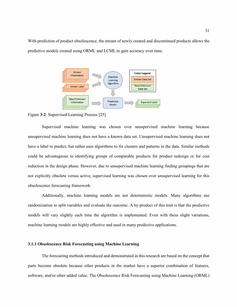
31
With prediction of product obsolescence, the stream of newly created and discontinued products allows the
predictive models created using ORML and LCML to gain accuracy over time.
Supervised machine learning was chosen over unsupervised machine learning because
unsupervised machine learning does not have a known data set. Unsupervised machine learning does not
have a label to predict, but rather uses algorithms to fix clusters and patterns in the data. Similar methods
could be advantageous to identifying groups of comparable products for product redesign or for cost
reduction in the design phase. However, due to unsupervised machine learning finding groupings that are
not explicitly obsolete versus active, supervised learning was chosen over unsupervised learning for this
obsolescence forecasting framework.
Additionally, machine learning models are not deterministic models. Many algorithms use
randomization to split variables and evaluate the outcome. A by-product of this trait is that the predictive
models will vary slightly each time the algorithm is implemented. Even with these slight variations,
machine learning models are highly effective and used in many predictive applications.
3.1.1 Obsolescence Risk Forecasting using Machine Learning
The forecasting methods introduced and demonstrated in this research are based on the concept that
parts become obsolete because other products in the market have a superior combination of features,
software, and/or other added value. The Obsolescence Risk Forecasting using Machine Learning (ORML)
Figure 3-2: Supervised Learning Process [25]

32
framework, like the weather example, is shown information and attempts to classify the part with the correct
label. However, instead of weather information, the technical specifications of current active and obsolete
parts are fed into algorithms to create the predictive models. In Figure 3-2, after the predictive model is
created, the technical specifications of parts with unknown obsolescence statuses are structured in the same
way as the known parts and input into the predictive model. The model then outputs the probability that the
part is classified with the label active or obsolete. The probability the part is obsolete can be used to show
the obsolescence risk level.
Figure 3-3 shows the output from the ORML method. Product A shows a product with a 100%
chance of the part being active. Product B demonstrates a mixed prediction with between a 60% chance of
being active and a 40% chance of being obsolete. Product C shows the prediction of a product with a 100%
chance of being obsolete.
One application of this output is to predict the obsolescence risk level for every component in two
competing designs or subassemblies and then create a composite obsolescence risk level for each design
using a combination of the components’ risks. The new composite risk level could be used as an attribute
in the process for selecting a final design.
Figure 3-3: Output of ORML

33
3.1.2 Life Cycle Forecasting using Machine Learning
The LCML framework is built on the same principle that parts become obsolete because other
products in the market have a superior combination of features, software, and/or other added value; the
difference lies in what the frameworks are predicting. Where ORML predicts the status as either actively
in production or obsolete, LCML uses regression to predict a numeric value of when the product/component
will stop being manufactured.
LCML’s ability to estimate a date of obsolescence is a highly useful metric. LCML will give
designers and supply chain professionals a more effective way of predicting the length of time to complete
redesign or find a substitute supplier or component. Understanding when each component on a bill of
materials will become obsolete will allow designers not only the ability to provide time constraints on
projects, but more effectively time redesign projects to maximize the number of high risk components
removed from the assembly.
The combinations of the ORML and LCML outputs into analyses have numerous applications in
business decision making processes. Current commercial obsolescence forecasting methods and those in
the literature only predict obsolescence risk or product life cycle. Since the ORML and LCML models both
use product specifications as input and the same machine learning algorithms to build the model, the only
additional work needed to switch between predicting risk versus life cycle is changing the output in the
training data. This is just one of the reasons a machine learning-based obsolescence forecasting method is
superior to previous obsolescence forecasting methods because of the ease of transferring between outputs
(Section 4.3.2 discusses this point further). Currently, it is the only method that readily provides both
obsolescence risk and product life cycle, essential to improved accuracy.

34
3.2 Accounting for Asymmetric Error Cost in Forecasting
This section introduces obsolescence risk forecasting optimization using ROC curves and the basics
of ROC analysis. First, the creation of ROC and interpretation of ROC curves is discussed. Then, the
process for calculating an optimal cut-off threshold is presented.
ROC curves are generated by changing the classification threshold of a single binary classifier and
plotting the corresponding true positive and false positive rate. The threshold is the probability cutoff point
between each classification status. The left plot of Figure 3-4 shows the distributions of prediction for each
status in a classification model with status positive and negative. Each vertical line corresponds to a
different potential threshold. Line B represents a threshold of 0.25 in the left plot, and the Point B in the
right plot represents the relationship between false positives rate and true positive rate when the threshold
is at Line B. The negative distribution above the 0.25 threshold represents false positives (Type I errors),
and the positive area under Line B represents false negatives (Type II error). The true positive rate (TPR)
and false positive rate (FPR) are plotted on the right plot in Figure 3-4 and labeled with the corresponding
threshold. TPR is the correctly classified positive classes out of the total number of positives, and FPR is
the number of incorrectly classified negative classes over the total number of negative classes.
Figure 3-4: Creation of ROC Curves

35
Since both TPR and FPR are probabilities, a TPR of 1 and FPR of 0 would be optimal. This would
correspond to Point F in Figure 3-4, which represents a perfect classification with zero percent false positive
rate or “false alarms” and 100% true positive rate. Any point on the dashed line, such as Point G, is equal
to a random guess. Points below the dashed line are worse than a random guess. Point C is closest to optimal
Point F; therefore, it would be the best choice out of thresholds options A through E.
However, Point C is only optimal when the cost of misclassification for positive and negative
instances are the same. If the costs are different, then a mathematical programming model can be utilized
to find the optimal threshold. The following mathematical model, Equation 1, does this by minimizing the
total misclassification cost for all instance in the data set. It does this by using the vector of predicted
probability (PP,i) of a positive event from each instance that is returned from the machine learning model.
The model then converts the vector of probabilities (PP,i) to a binary prediction (PL,i) using the decision
variable of the threshold (t). The new binary prediction vector (PL,i) is compared to the actual obsolescence
status (AL,i) and vectors of false positives (fp,i) and false negatives (fn,i) were created. The vectors of false
positives (fp,i) and false negatives (fn,i) are summed and multiplied by their respective costs. The threshold
is then changed and these steps are repeated until an optimal threshold is found.

36
!"#:áàâG *'â,ä.
ã
äåçéáàèG *'â,ä.
ã
äåç
/(1)
!+(,- ≥ 9:,- −<:,- !+3,- ≥ <:,- − 9:,- !9:,- ≥ 9=,- − >
1 ≥ 9=,- ≥ 0 1 ≥ > ≥ 0
+3,- , +(,- , 9:,- , <:,- = A"#BCD t = The potential threshold Cfp = Cost of a false positive (Type I error) Cfn = Cost of a false negative (Type II error) Pp,i = The predicted probabilities of obsolescence for all “i” components being predicted. PL,i = The assigned obsolescence label for all “i” components being predicted. (1=obsolete) AL,i = The true obsolescence label for all “i” components being predicted. (1=obsolete) fp,i = A binary vector denoting if instance “i” is a false positive fn,i = A binary vector denoting if instance “i” is a false negative M = An extremely large value for the Big “M” method
The M is a significantly large value, many magnitudes bigger than the other values used in this
mathematical model. The large M works as an on/off switch for the variable multiplied by it. If P P,I - t is
greater than zero, the predicted probability (PP,i ) is above the threshold value (t) and this means the label
should be obsolete or “1” in the binary. To solve the third constraint, since M is a large constant and is
greater than zero, the obsolescence label (PL,i ) is forced to be “1”. If the predicted probability (PP,i) is below
the threshold value (t) then the obsolescence label (PL,i ) is able to be “0”. This method allows for the
threshold to convert values into a binary above or below the given threshold. This method is repeated in
finding Type 1 and Type 2 errors in constraints 1 and 2.
The cost of a false positive (Cfp) and cost of a false negative (Cfn) represent the expected system-
wide cost implications for one component’s incorrect prediction. Some examples of costs an organization
can incur include premature stockpiling of components, early and unnecessary redesigns, and the cost of
the production line shutting down due to the lack of available components. There are two methods for
calculating the cost of a false positive (Cfp) and cost of a false negative (Cfn). The first is a standard economic
s.t.

37
analysis. An economic analysis would involve developing cost models for each possible event that could
be triggered and weighting the costs by the probability the cost will be incurred to create the average cost
value for when a false positive or false negative occurs. The second is using the unique attribute of a linear
objective function that the magnitudes of the weights do not change the optimal value as long as the ratio
of the weights remain the same. For example, if Cfp and Cfn are $100,000 and $200,000, respectfully, or 5
and 10, then the same optimal value will be calculated because the ratio remains 1:2 (This is further explored
in Section 5.3). This feature means organizations only need to know the ratio between the cost of a false
positive and cost of a false negative and not the actual values of the costs. The method borrows from Multi-
Attribute Utility Theory (MAUT), a structured technique for finding weights of criteria for multiple-criteria
decision making [75]. The method is adapted to find the ratio of the two cost values for the mathematical
program. The first step involves listing all the potential effects of a procurable component being predicted
discontinued and a discontinued component being predicted as procurable. Second, the potential effects are
ranked and reordered from highest cost impact to lowest cost impact. Third, the first effect in the new
reordered list (the effect with the highest cost) is assigned a cost of 100%. Then we would go down the list
asking, “How costly is this effect as a percentage of the first effect’s cost?”. For example, if the second
effect on the list would cost the business 70% of what the first effect would cost the business, then we
would assign this effect a cost of 70%. These comparisons are repeated until all the effects are assigned a
percentage of the first effect. The next step is to split the list of effects into two lists: (1) potential effects
of a Type I error and (2) potential effects of a Type II error. The last step is to go through each of these lists
and ask “If this type of error occurred, what is the probability of this effect and cost happening?”. Then
multiply each probability by the cost assigned in the previous step and sum for each type of error. The
resulting sum for each list will be at the same ratio as the true costs between Type I error and Type II error.
A brute force search method is used to solve the mathematical model in Equation 1. Brute force,
also known as exhaustive search, looks at all possible combinations in the feasible region and takes the
maximum or minimum from all the possible combinations. Traditionally brute force search is not used

38
because of the computational overhead. However, in this model, the only decision variable is the threshold,
and the threshold is bounded between 0 and 1, which greatly reduces the complexity of the search space
and makes brute force search a suitable method for solving this problem because it evaluates every option
which removes the chance of returning a solution that is a local minimum or maximum. When starting the
search for this problem, a step size must be specified. The step size is the size of the difference between
each potential solution. For example, the step size for the case studies presented in this document is 0.00001.
Figure 3-5 presents pseudocode showing how the programs steps through possible thresholds and finds the
optimal threshold.
Additionally, this methodology can be used for more than just obsolescence forecasting. Any binary
classifier with a probability the instance is in either class and has differences in error cost (e.g. fraud
detection, disease detection, fault detection, and obsolescence forecasting) could use this method to
minimize the cost impact of errors resulting from the binary classifier. This represents a much more
fundamental contribution to not only obsolescence forecasting, but machine learning as a whole.
Define a step size (for the case study in Chapter 5, the step size is 0.00001) For i = 0 to 1 by step size
- Threshold = i - Convert obsolescence risk prediction to labels using threshold (e.g., risk prediction of
0.80 and a threshold of 0.60 would result in a status of "discontinued") - Compare predicted label vs. actual label and count number of false positives and false
negatives. - Find the “total error cost” by multiplying number of errors by the respective cost. - If “total error cost” <= “minimal total error cost” then
o “optimal threshold” = Threshold o “minimal total error cost” = “total error cost”
Next i Return (“optimal threshold”)
Figure 3-5: Pseudocode to Implement Brute Force Search to Solve Mathematical Model

39
3.3 Forecasting Functional Obsolescence Framework
In this section, two signal processing methods, Fast Fourier Transform (FFT) and Wavelet
transform, are explained, and the machine learning algorithms used in the functional obsolescence case
study are discussed. Fast Fourier Transform returns the discrete Fourier Transform using the Cooley–Tukey
algorithm [76]. The Cooley–Tukey algorithm finds discrete frequency components in N-periodic sequence
from signal x. It does this by decomposing the signal into each frequency within the range and then
identifying the strength of that frequency. This strength can be found by solving the following equation:
EF = ∑ H3IJ-KLF3//
/J130N (2)
The Wavelet transform outputs a matrix defined by scale and translation and not a vector of
frequency like the FFT [69], [77], [78]. Translation is the shifting of wavelet across the signal, and scale
represents the flattening and amplifying of the wavelets in the signal. The following equation can be used
to find the wavelet with x representing the signal, a representing scale, and b representing the translation.
EP,Q = ∫ H(>)SP,Q
∗(>)U>/J130N (3)
These two signal processing methods are evaluated by using different machine learning algorithms:
Random Forest, Support Vector Machine (SVM), K-Nearest Neighbor (KNN), single-layer Neural
Networks, and multi-layer Neural Networks [79]–[82]. Random Forest works by constructing multiple
decisions trees and then aggregating the prediction to predict a more reliable estimate then one decision tree
alone [79]. The decision trees are randomized by only evaluating a different randomized subset of variables
for every split node of the decision tree.

40
SVM is an algorithm designed to calculate an optimal boarded between the classes being predicted.
Commonly used with straight lines, the case study in Chapter 6 implements SVM with a Gaussian kernel
and therefore has highly non-linear borders between classes [81].
KNN works by finding the k closes example with known health statuses [82] and then the most
common health status from the k closest instances is taken and assigned to make the prediction. Because
this model is relatively simple and largely based on distance, KNN has difficultly with high dimensional
data due to the reduced effectiveness of Euclidian distance [82]. It was included because it does better with
fewer variables and therefore may work better with a signal processing method like FFT when compared
to Wavelet because of the reduced number of input data.
Neural networks tend to be the standard algorithm for modeling the health status of wind turbines
[65], [69], [71]. For this reason, the case study in Chapter 6 includes both single and two-layer neural
networks. Neural networks work by creating a network of nodes that fire based in a certain input criterion
is met [80]. As these networks grow in complexity by adding layers, the models are able to represent more
complex and high-nonlinear relationships. However, these additional layers add a computational time. By
using both a single and double layer, the pros and cons of each can be better assessed.
3.4 Life Cycle and Cost in Design and Manufacturing
This section outlines the Life Cycle and Cost Tradeoff Model and how obsolescence and other life
cycle information can be used, by designers, to improve products.
3.4.1 Life Cycle and Cost Tradeoff Framework
The Life Cycle and Cost Tradeoff Framework seeks to help solve one of the most prolific problems
faced by designers: How do we design products which will last as long as possible, while reducing cost?
The framework presented in this section is generalizable and could be applied in different areas (e.g.,

41
selecting manufacturing and usage requirements in early stage design and finding the desired manufacturing
attributes for redesigns). The goal of the framework is to show to designers how changes in usage and
manufacturing properties change impact life cycle and cost. The designers will be able to use the framework
to quickly predict how changes in these requirements will affect the quality and cost of the product.
The Life Cycle and Cost Tradeoff Framework uses many smaller models to predict key variables
in determining the life cycle and the total cost through the product’s entire life cycle. The smaller models
are linked together to create a flow of information. This flow of information can be seen in Figure 3-6. Each
rectangle represents a model, while the arrows represent the information going into or coming from the user
or other models. The two green rectangles at the top are both cost models. The “Manufacturing Cost Model”
estimates the per unit cost to manufacture the product. The “Manufacturing and Repair Cost Model”
estimates not only the manufacturing cost, but also the repair and replace costs for the product in the
framework. This is referred to as total cost.
The “Life Cycle Estimation Model” estimates the life of the product or how long the product will
continue to run until a failure. Although still predicting functional obsolescence, this is different from
Section 3.4 because the model in Section 3.4 is based on continuous process monitoring while this is a
general estimate over all products. For this reason, the model often can be used to predict a distribution
Figure 3-6: Life Cycle and Cost Tradeoff Information Flow

42
rather than a single point, such as an average. For instance, the model could predict a Weibull distribution
and have scale and slope be the output variables.
The manufacturing process model is a repository of manufacturing capability. This includes
different sequences of manufacturing processes and the resulting manufacturing attributes. This will allow
the user to select desired manufacturing attributes and tell the user if the process is feasible.
Since the framework is to be generalizable between industries, the models are developed using a
number of approaches. The first approach is a standard mathematical model. These often are industry
defined standard equations and are well known. The second is a simulation model. These often take a Monte
Carlo approach and use the inputs to sample many possible outcomes and return the results as distributions.
The last model creation method is a data driven or machine learning based approach. These approaches can
utilize simulated data or field data to develop complex models to try and approximate the relationships
between inputs and outputs. These methods are often quicker at making predictions than simulations but
slower than standard mathematical models. However, many industries do not have standard mathematical
models; so, data-driven models are the best option.
To implement all of these models and store the information to support them, a software architecture
must be developed. Figure 3-7 shows one proposed approach of implementing the models in the framework.
The web-based user interface is on the left side in yellow, the server is in gray in the middle column, and
the database is on the right column in light blue. The user specifies how the product will be used and the
manufacturing requirements. The application then calls the server using the manufacturing model from the
application programming interface (API). An API is a set of programming functions placed on a server for
accessibility. The manufacturing model is able to check the manufacturing database to ensure that there are
manufacturing process that can meet the desired manufacturing requirements. The manufacturing attributes
from the selected manufacturing process is returned and passed to the life cycle model in the API. The life
cycle model calls the server, which returns the life span distribution given the manufacturing attributes and
usage over the product’s life. The unit cost from the manufacturing function and the life prediction from
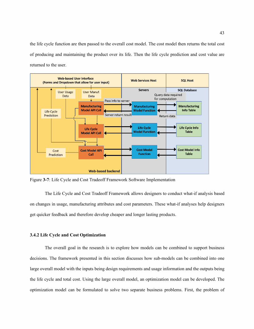
43
the life cycle function are then passed to the overall cost model. The cost model then returns the total cost
of producing and maintaining the product over its life. Then the life cycle prediction and cost value are
returned to the user.
The Life Cycle and Cost Tradeoff Framework allows designers to conduct what-if analysis based
on changes in usage, manufacturing attributes and cost parameters. These what-if analyses help designers
get quicker feedback and therefore develop cheaper and longer lasting products.
3.4.2 Life Cycle and Cost Optimization
The overall goal in the research is to explore how models can be combined to support business
decisions. The framework presented in this section discusses how sub-models can be combined into one
large overall model with the inputs being design requirements and usage information and the outputs being
the life cycle and total cost. Using the large overall model, an optimization model can be developed. The
optimization model can be formulated to solve two separate business problems. First, the problem of
Figure 3-7: Life Cycle and Cost Tradeoff Framework Software Implementation

44
minimizing cost while maintaining a desired life cycle and second, the problem of maximizing the life cycle
while maintaining a desired cost.
In this optimization tradeoff problem, the relationships of the underlining constraints are extremely
complex and difficult to define mathematically. This is because the relationships between the
manufacturing properties are extremely complex. For example, a given residual stress may be impossible
at a given surface roughness from a manufacturing perspective. The relationship between feasible and
infeasible combinations of surface roughness and residual stress is too complex of a relationship to easily
model it in a mathematical constraint. When this complexity is scaled to the interactions between all the
inputs for the Life-Cycle Tradeoff model, the modeling of constraints would be almost impossible. For this
reason, the Life-Cycle Tradeoff model does not seek to model any of these relationships and does not
account for these constraints. A genetic search algorithm was chosen to address this element of the problem
because most search algorithms attempt to find the absolute single best solution to a given mathematical
model, but genetic search uses a population that eventually converge around the best alternatives. The final
generation has a number of solutions and by allowing the users of the Life-Cycle Tradeoff model to define
the number of solutions that will be returned, the method lowers the chance that all returned solutions are
infeasible combinations of inputs, such as residual stress and surface roughness. For this reason, the Life-
Cycle Tradeoff model is not a traditional optimization model, but rather generates many top solutions and
allows the users to select the best option from the list of solutions.
The process of genetic search can be seen in Figure 3-8. First a population of options is generated.
Then all the option which were generated are evaluated based on some criteria (e.g., life cycle and cost)
and then the best options are selected. The best options are then randomly combined together to generate
new options for the next generation of the genetic search. Sometimes, the next generation has small
mutations to help prevent local minima or maxima in the search. The new generation is then evaluated, and
the best options are selected again. This process continues until the desired goals are reached or a sufficient
number of generations have passed.

45
The genetic search algorithm for the life cycle and cost tradeoff model works by generating many
random inputs (surface roughness, stress, speed, etc.) within the boundaries of each input which is set by
the user. Each random guess is put through the framework to assess the life and cost of the option. The life
and cost are outputted and compared to the desired requirements. For example, Table 3-1 demonstrate some
randomly generated options. The goal of the optimization problem for Table 3-1 is to minimize cost while
maintaining a life of at least 20. No option with a life prediction below 20 will be selected for the next
generation of the genetic search. The options with life above 20 will be selected as parents of the future
generation at a higher rate if their cost is lower (this can be seen in the percentage column Table 3-1).
Figure 3-8: Genetic Search Algorithm Process

46
Then two options with life greater than 20 will be randomly selected. These two options will serve
as the parents of an option in the next generation. A new option is generated by randomly selecting inputs
from either of the parents. The new option with the random combination of inputs from the parents serves
as one option for the next population, and this process is repeated until the number of options in the next
generation is equal to the population of the previous generation.
After the next generation is created, each option is evaluated again by the framework to estimate a
life and cost. As the generations grow, lower cost options that meet the minimum life of 20 will parent more
options because of the lower cost and higher cost options will have fewer children. This will cause the
genetic search algorithm to converge to lower cost options while maintaining the desired life.
Table 3-1: Genetic Search Algorithm Population with a Required Life of 20

47
3.4.3 Recommending Goal Manufacturing Attributes for Gear Repair
The last section focused on the manufacturing of a part; this section focuses on how a similar framework
can be created for repair and maintenance of a part. Often, when a part is showing signs of wear or is not
functioning to the optimal output, the part will be recommended for repair. If a repair occurs, then the part
can be remanufactured to improve performance. This section presents a framework to estimate the
remaining useful life of a part then determine the manufacturing attributes required to achieve a given life.
Figure 3-9 shows the flow of the Repairing Gear Framework. The blue area on the top of the figure
represents information or questions exchanged between the models and the user. This is unlike the Life
Cycle and Cost Tradeoff Framework because the framework does not simply take inputs and then give an
output. Users will need to respond to predictions and then input desired results based on the predictions.
The framework starts by the user inputting the current manufacturing attributes of the product (e.g., surface
roughness, residual stress, etc.). Then the manufacturing attributes and information on how the product will
be used for the remainder of its life are input into the life cycle estimation model. This is the same model
used in the Life Cycle and Cost Tradeoff Framework. The predicted remaining useful life of the product is
returned to the user. If the user wishes to lengthen the life of the product, then the user can input a desired
life and a percentile (e.g., L10 or L50). This information along with the usage information is input into the
inverse life cycle estimation model.
The inverse life cycle estimation model is a machine learning model that is generated from the same data
to create the life cycle estimation model. However, for this model, life is switched from the output to an
input, and the manufacturing attributes are switched from inputs to the output. This creates a model that
can be fed a desired life and usage information and return the required manufacturing attributes to achieve
the given life. Although the data underlying the model can be from simulations or empirical data, this
method of reversing inputs and outputs and using a machine learning model to approximate the relationship
is advantageous when compared to other methods. For example, if a physics-based simulation tried to find
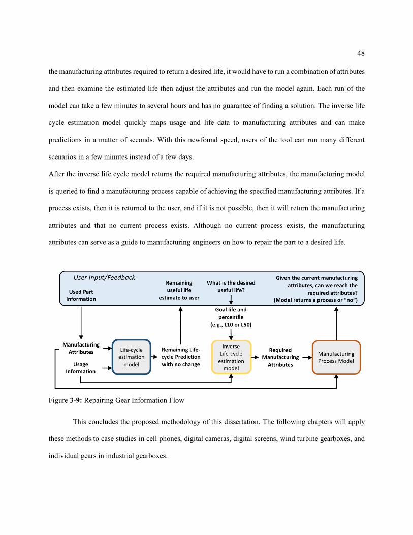
48
the manufacturing attributes required to return a desired life, it would have to run a combination of attributes
and then examine the estimated life then adjust the attributes and run the model again. Each run of the
model can take a few minutes to several hours and has no guarantee of finding a solution. The inverse life
cycle estimation model quickly maps usage and life data to manufacturing attributes and can make
predictions in a matter of seconds. With this newfound speed, users of the tool can run many different
scenarios in a few minutes instead of a few days.
After the inverse life cycle model returns the required manufacturing attributes, the manufacturing model
is queried to find a manufacturing process capable of achieving the specified manufacturing attributes. If a
process exists, then it is returned to the user, and if it is not possible, then it will return the manufacturing
attributes and that no current process exists. Although no current process exists, the manufacturing
attributes can serve as a guide to manufacturing engineers on how to repair the part to a desired life.
Figure 3-9: Repairing Gear Information Flow
This concludes the proposed methodology of this dissertation. The following chapters will apply
these methods to case studies in cell phones, digital cameras, digital screens, wind turbine gearboxes, and
individual gears in industrial gearboxes.

49
Chapter 4
Forecasting Technical Obsolescence in Consumer Electronics Case Study
The following case studies serve to demonstrate the accuracy and scalability of ORML and LCML
as methods to forecast obsolescence. The first section of this chapter contains case studies applying the
ORML method in the cell phone, digital camera, and screen component markets. The next section includes
a case study to apply LCML to the cell phone market. The third section contains a benchmarking case study
to compare the accuracies between LCML, Sandborn 2005 [8], and Ma and Kim 2017 [23] methods and
discusses additional benefits of the ORML and LCML over other methods. The final section of this chapter
discusses limitations to the proposed machine learning-based obsolescence forecasting.
4.1 Results of Obsolescence Risk Forecasting
4.1.1 Cell Phone Market
The cell phone market was chosen for the case study due to availability of data and the ease it
provides for understanding the product and specifications. Although the case study is a consumer product,
the ORML and LCML prediction frameworks can be utilized to predict component obsolescence found in
larger complex systems. The case data contains over 7000 unique models of cellular phones with known
procurable or discontinued status, release year and quarter, and other technical specifications. The
specifications include weight (g.), screen size (inch.), screen resolution (pixels), talk time on one battery
(min.), primary and secondary camera size (MP), type of web browser, and if the phone has the following:
3.5 mm headphone jack, Bluetooth, email, push email, radio, SMS, MMS, thread text messaging, GPS,
vibration alerts, or a physical keyboard. The data set included 4030 procurable and 3021 discontinued
phones. However, the data set only included 38 obsolescence dates. This means the ORML portion of the

50
case study had 7051 unique cell phone models while the LCML had 38. Although the data sets differ in
size, each data set is suitable in size to demonstrate the ORML and LCML frameworks.
The data was collected from one of the most popular cell phone forums, GSMArena.com using a
web scraper (Accessed: 17-5-2015). The original data set, and the code for the web scraper, and machine
learning models created in this case study can be downloaded at connorj.github.io/research. GSM Arena is
an online forum that provides detailed and accurate information about mobile phones and associated
features. For this reason, the data set can have missing values and even miss reported information. Despite
these shortfalls with their data set is typical of data collected in industry and demonstrates the robustness
of the ORML and LCML frameworks.
After formatting the data, the data set was split into two random groups. The first group represents
⅔ of the data set and is called the training data set, which is used to create the prediction model. The second
is the test set and represents the other ⅓. Although all the data sets are known in this case study, the test set
will be evaluated with the predictive model, and accuracy will be determined by comparing actual
obsolescence statues and obsolescence dates verses the values predicted by the model. This practice is
known as validation and is a best practice for model creation and evaluation because the data used to create
a prediction model is never used to validate its accuracy [35]. Currently, the majority of the obsolescence
forecasting models in the literature estimate model accuracy by using the same data used to create the
model. The data set was split into a ⅓ test set and a ⅔ training set for an initial analysis for accuracy using
confusion matrixes.
The next step in the case study was to run the training data set through a machine-learning algorithm
to create a predictive model. Machine learning has many algorithms and infinitely more if counting all the
slight variations that can be done to increase accuracy. Four machine learning algorithms, artificial neural
networks (NNET), support vector machines (SVM), k nearest neighbor (KNN), and random forest (RF) are
applied for this case study [37-39]. Decision trees and support vector machines were ranked first and third,
respectfully on the list of the “Top 10 Algorithms in Data Mining” [40]. However, standard decision trees

51
are often inaccurate and over-fit data sets [42]. Random forest, an aggregation of many decision trees,
averages the trees with the intention of lowering the variance of the prediction [42]. For this reason, random
forest was selected over standard decision trees. The algorithm listed second, K-means, is an unsupervised
clustering method and would group similar products together rather than forecast an output. For this reason,
K-means is not a possible alternative for algorithm to be used for either ORML and LCML and therefore
was not included in this case study. K nearest neighbors was 8th on the list and was selected. K nearest
neighbors takes the average vote on the most common status of the K number closest data points. Although
artificial neural networks were not on this Top 10 list, they were selected based on wide usage in deep
learning, a subset of machine learning. Deep learning looks at the complex relationships between inputs in
an effort to have a greater understanding of combined relationships with the output [42]. In the final step,
once the algorithm constructs a predictive model, each part or element from the “unknown” data set is run
through the model and receives a predicted label.
The accuracy of the ORML model is represented in a confusion matrix. The confusion matrix (See
Tables 4-1, 4-2, 4-3, and 4-4) shows how many cell phones were classified correctly versus incorrectly.
Numbers in the (available, available) and (discontinued, discontinued) cells are correctly classified and all
other cells are misclassified.
The first algorithm used was NNET. The neural networks classification was done in R 3.0.2 using
the package “caret” [41]. All the NNET in this study were constructed with 2 hidden layers. The probability
of each part being available or discontinued was output, and the highest probability label of available or
discontinued was assigned. The actual statuses were compared to the predicted values, and a confusion
matrix was developed in Table 4-1. The model correctly predicted 91.66% of cell phones with the correct
label in the test data set.

52
Table 4-1: Neural Networks ORML Confusion Matrix for Cell Phones
Actual Available Discontinued Total
Prediction Available 1295 129 Discontinued 67 860 Total 1362 (95.08%) 989 (13.04%) 2351 (91.66%)
The next algorithm applied was SVM. The support vector machine utilized the SVM classification
function from the package “e1071” [42] in R 3.0.2, and a radial basis kernel was selected. The algorithm
was implemented on the training data set that contained 66.6% of the total data. The prediction model then
classified the remaining 33.3% of phones not used in the model creation. The actual statuses and the
predicted statuses were compared and the confusion matrix in Table 4-2 was created. The SVM model has
a model accuracy of 92.41%.
Table 4-2: Support Vector Machine ORML Confusion Matrix for Cell Phones
Actual Available Discontinued Total
Prediction Available 1218 92 Discontinued 76 827 Total 1294 (94.13%) 919 (10.01%) 2213 (92.41%)
The next algorithm applied was RF. The model was implemented in R 3.0.2, using the package
“randomForest” [43]. The randomForest function was set to have 500 trees for all RF in this case study.
The model was trained with a 66.6% training set and was tested with 33.3%. The predicted test set and the
actual statuses were compared in Table 4-3. The model received an accuracy of 92.56%.

53
Table 4-3: Random Forest ORML Confusion Matrix for Cell Phones
Actual Available Discontinued Total
Prediction Available 1243 98 Discontinued 72 873 Total 1315 (94.52%) 971 (10.09%) 2286 (92.56%)
The last algorithm tested was K nearest neighbors. For this algorithm, k was set to five, meaning
products in the testing set are assigned a status label based on the five closest products in the training set.
The model was able to correctly predict the status of the label 90.91% of the time in the testing set.
Table 4-4: K Nearest Neighbor ORML Confusion Matrix for Cell Phones
Actual Available Discontinued Total
Prediction Available 1279 113 Discontinued 105 901 Total 1384 (92.41%) 1014 (11.14%) 2398 (90.91%)
Ten predictive models were created for each training size, and the average time was plotted in
Figure 4-1. All the algorithms increased in time at a near constant rate, except for KNN. This is due to KNN
being based entirely on distance and requiring a distance matrix between the training and test sets. The
number of distance calculations is maximized when the training and test sets are equal in size because the
distance matrix is square. When the training and test sets sizes are less equal, the distance matrix is more
rectangular and requires less combinations of products that need distance calculations. For this reason, as
the training set grows in size the model generation speed grows until a size of 50% then decreases after for
KNN. Besides KKN, NNET is the fastest algorithm, followed by SVM, which is followed by RF.

54
Figure 4-1: Overall Average Evaluation Speed by Training Data Set Fraction for ORML
Although the speed of creating these predictive models are relatively small (< 1 minute per model),
it is important to remember this case study is only creating prediction models for one product type. If ORML
was scaled to create a prediction model for each component on a 10,000-component bill of materials, these
relatively small differences in times would compound rapidly.
Table 4-5: Summary of Model Preference Ranking For ORML in the Cell Phone Market
RF SVM NNET KNN
Performance based characteristics Accuracy 1st 2nd 3rd 4th Evaluation Speed 4th 3rd 2nd 1st Non-Performance based characteristics Interpretability 1st 3rd 4th 2nd Maintainability 1st 2nd 2nd 2nd
Four characteristics, identified in Zhang & Bivens 2007 [83], were measured to rank the algorithms.
The first two characteristics were performance based: (1) accuracy and (2) evaluation speed. The rankings
of the algorithms in Table 4-5 for the first two attributes was determined by best model accuracy and by
average time to complete the ten simulations of each of the six different training set sizes. The second two
characteristics were usability based: (3) interpretability and (4) maintainability/flexibility. Interpretability

55
is defined as the ability for analysts to comprehend the model and analyze the output.
Maintainability/flexibility represents the model’s ability to adapt over time and how much work is required
to keep the model running.
Random Forest was ranked best (first) in interpretability due to the visual nature of decision trees
and the ability for analysts to follow the flow of the tree to understand the steps in the classification model.
K nearest neighbors was ranked second in interpretability because of the easy ability to find the 5 closest
products in the training set to understand the prediction. Support Vector Machine was ranked third because,
while the concept of creating a plane to separate the available and discontinued groups is easy to understand,
due to the high dimensionality of the data, there is no obvious visual representation of this model. Lastly,
neural networks were ranked fourth out of the four because of the complexity of the trained network and
the ‘black box’ nature of this classification method.
Maintaining machine-learning models requires regular inputs of data to maintain the accuracy of
the model because k nearest neighbors, neural networks, and support vector machines require only numeric
variables, all variables must be converted to numeric. Creating numeric indexes can be time consuming and
will slow down the data entry process. For this reason, random forest was ranked number one and k nearest
neighbors, neural networks, and support vector machines were tied for second.
Overall, random forest was ranked first in all attributes besides speed where it was ranked fourth.
However, the difference in speed from random forest and the fastest algorithm was under 4 seconds. For
these reasons, random forest is the most appropriate algorithm for ORML in the cell phone market.

56
4.1.2 Digital Camera Market
The next case study applies the ORML method to predict obsolescence in the digital camera market
and assess the resulting accuracy. The data was gathered from product review forums, DPReview.com. The
data was aggregated by a web scraper coded in the programming language R and using the package ‘rvest’
[34]. The digital camera data set contains 2214 unique models and 50 specification variables including body
type, dimensions, battery type and life, headphone port, microphone, speakers, wireless technology (WiFi,
Bluetooth, etc.), built-in flash or modular flash, flash range, digital zoom, megapixels, screen size and
resolution, USB adaptor type, minimum and maximum aperture, manual vs. digital zoom, picture ratios,
image stabilization technology, uncompressed file format, built-in memory, and a few other specifications.
The data set contains 985 procurable and 1229 discontinued models.
Like the previous section, the data is split into training and testing sets at a ratio of 2 to 1,
respectfully. A model is then generated using the training set and the accuracy is assessed using the test set.
The first algorithm used to develop an ORML model was neural networks. The results are displayed in the
confusion matrix shown in on Table 4-6. The neural network has two layers with 20 nodes in each layer.
The neural network achieved an accuracy of 92.43%.
Table 4-6: Neural Networks ORML Confusion Matrix for Digital Cameras
Actual Available Discontinued Total
Prediction Available 312 31 Discontinued 26 384 Total 338 (92.31%) 415 (7.47%) 753 (92.43%)
The next algorithm applied to the camera data set is support vector machines (SVM). The SVM
model used a Gaussian kernel to allow the resulting separating surface to be nonlinear. As shown in Table
4-7, the support vector machine was able to correctly classify the obsolescence status 93.89% of the time.

57
Table 4-7: Support Vector Machine ORML Confusion Matrix for Digital Cameras
Actual Available Discontinued Total
Prediction Available 319 27 Discontinued 19 388 Total 338 (94.38%) 415 (6.51%) 753 (93.89%)
Random forest was the third algorithm tested. The algorithm was generated using 500 randomly
generated decision trees and by using Gini values as the splitting criteria. As shown in Table 4-8 the
algorithm achieved an accuracy of 93.63%.
Table 4-8: Random Forest ORML Confusion Matrix for Digital Cameras
Actual Available Discontinued Total
Prediction Available 316 26 Discontinued 22 389 Total 338 (93.49%) 415 (6.27%) 753 (93.63%)
The last algorithm tested was K nearest neighbors. The k was set to 5 for this algorithm, and
calculated distance used the standard Euclidean distance. The data was scaled to be between zero and one
to minimize the size of each metric. As shown in Table 4-9, the resulting model achieved a 93.23%
accuracy.
Table 4-9: K Nearest Neighbor ORML Confusion Matrix for Digital Cameras
Actual Available Discontinued Total
Prediction Available 304 17 Discontinued 34 398 Total 338 (89.94%) 415 (4.1%) 753 (93.23%)

58
The speed was then assessed by varying the training set size from 10% to 100% of the data and
recording how long each algorithm took to generate a model. Each combination of algorithm and training
set size was run 10 times. The average was plotted in Figure 4-2. As shown, the neural network was the
slowest followed by random forest then support vector machines, with K nearest neighbors running the
fastest.
Figure 4-2: Average Evaluation speed by Training Data Set Fraction for ORML in the Camera Market
Using the metrics identified in Zhang and Bivens 2007 [83], two performance-based characteristics
and two non-performance-based characteristics were ranked and recorded in Table 4-10. The algorithms
from most accurate to least accurate are support vector machine, random forest, k nearest neighbors, and
neural networks. The speed was ranked fastest to slowest: k nearest neighbor, support vector machine with
random forest and neural networks tied. The rankings of the non-performance based characteristics are the
same as Section 4.1.1 because the algorithms suffer from the same interpretability and maintainability
problems. Although, it did not have the best non-performance based characteristics, SVM was shown to be
first in accuracy and second in speed, making it the best algorithm to apply ORML to the digital camera
market.
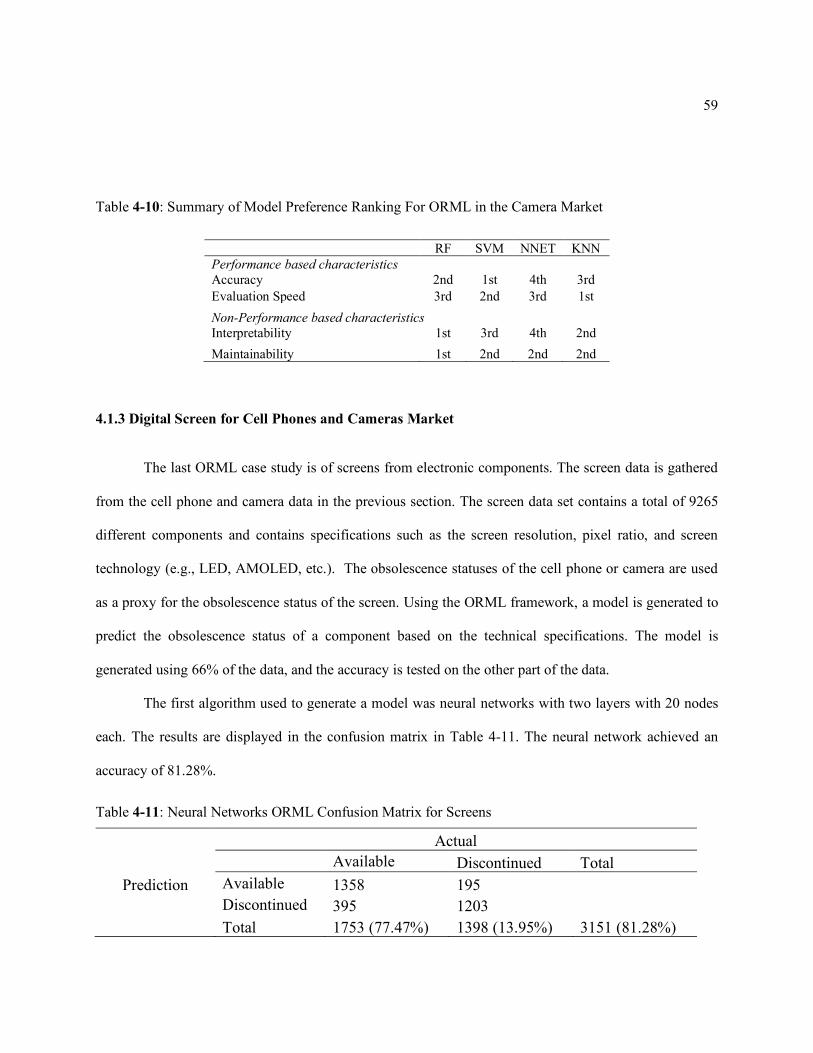
59
Table 4-10: Summary of Model Preference Ranking For ORML in the Camera Market
RF SVM NNET KNN Performance based characteristics Accuracy 2nd 1st 4th 3rd Evaluation Speed 3rd 2nd 3rd 1st Non-Performance based characteristics Interpretability 1st 3rd 4th 2nd Maintainability 1st 2nd 2nd 2nd
4.1.3 Digital Screen for Cell Phones and Cameras Market
The last ORML case study is of screens from electronic components. The screen data is gathered
from the cell phone and camera data in the previous section. The screen data set contains a total of 9265
different components and contains specifications such as the screen resolution, pixel ratio, and screen
technology (e.g., LED, AMOLED, etc.). The obsolescence statuses of the cell phone or camera are used
as a proxy for the obsolescence status of the screen. Using the ORML framework, a model is generated to
predict the obsolescence status of a component based on the technical specifications. The model is
generated using 66% of the data, and the accuracy is tested on the other part of the data.
The first algorithm used to generate a model was neural networks with two layers with 20 nodes
each. The results are displayed in the confusion matrix in Table 4-11. The neural network achieved an
accuracy of 81.28%.
Table 4-11: Neural Networks ORML Confusion Matrix for Screens
Actual Available Discontinued Total
Prediction Available 1358 195 Discontinued 395 1203 Total 1753 (77.47%) 1398 (13.95%) 3151 (81.28%)
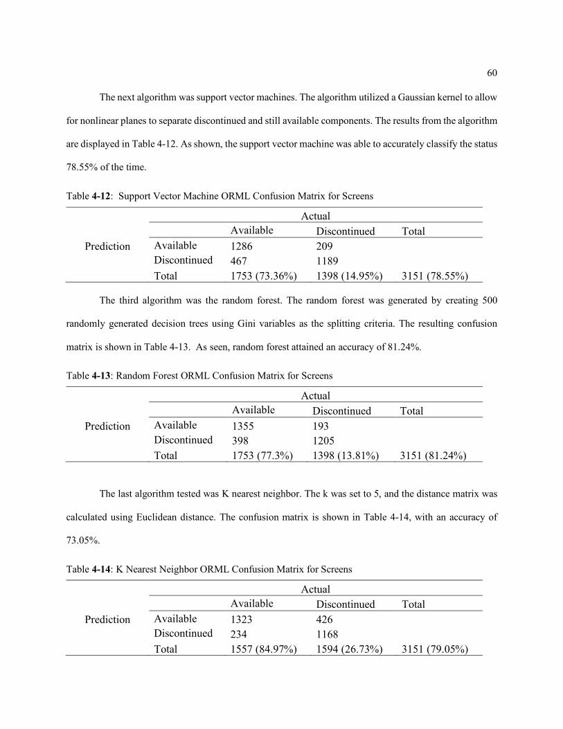
60
The next algorithm was support vector machines. The algorithm utilized a Gaussian kernel to allow
for nonlinear planes to separate discontinued and still available components. The results from the algorithm
are displayed in Table 4-12. As shown, the support vector machine was able to accurately classify the status
78.55% of the time.
Table 4-12: Support Vector Machine ORML Confusion Matrix for Screens
Actual Available Discontinued Total
Prediction Available 1286 209 Discontinued 467 1189 Total 1753 (73.36%) 1398 (14.95%) 3151 (78.55%)
The third algorithm was the random forest. The random forest was generated by creating 500
randomly generated decision trees using Gini variables as the splitting criteria. The resulting confusion
matrix is shown in Table 4-13. As seen, random forest attained an accuracy of 81.24%.
Table 4-13: Random Forest ORML Confusion Matrix for Screens
Actual Available Discontinued Total
Prediction Available 1355 193 Discontinued 398 1205 Total 1753 (77.3%) 1398 (13.81%) 3151 (81.24%)
The last algorithm tested was K nearest neighbor. The k was set to 5, and the distance matrix was
calculated using Euclidean distance. The confusion matrix is shown in Table 4-14, with an accuracy of
73.05%.
Table 4-14: K Nearest Neighbor ORML Confusion Matrix for Screens
Actual Available Discontinued Total
Prediction Available 1323 426 Discontinued 234 1168 Total 1557 (84.97%) 1594 (26.73%) 3151 (79.05%)

61
After the accuracies were recorded, the model generation speed was compiled. The training set size
was varied from 10% to 100% of the data, and ten models were generated for each algorithm at each training
set size. The average speed of the ten models were recorded and presented in Figure 4-3. As shown, support
vector machines, random forest, and neural networks all increased at linear speed. While K nearest neighbor
increased to 50% then decreased after (an explanation of this relationship is given in Section 4.1.1). The
algorithms from fastest to slowest are k nearest neighbor, neural network, random forest, and support vector
machines.
Figure 4-3: Average Evaluation Speed by Training Data Set Fraction for ORML in the Screen Market
Like the previous three cases, two performance-based characteristics and two non-performance-
based characteristics were ranked and recorded for each algorithm in Table 4-15. The algorithms from most
accurate to least accurate are neural networks, random forest, k nearest neighbors, and support vector
machine. The speed was ranked fastest to slowest k nearest neighbor, neural network, random forest, and
support vector machines. The rankings of the non-performance based characteristics are the same as Section
4.1.1 and Section 4.1.2 because the algorithms suffer from the same interpretability and maintainability
problems. Although it came in third for speed and an extremely close second for accuracy, random forest
is the easiest to implement because it can handle categorical variables and is the easiest to interpret because

62
of its tree nature. For these reasons, random forest is the best algorithm for implementing ORML in the
digital screen market.
Table 4-15: Summary of Model Preference Ranking For ORML in the Screen Market
RF SVM NNET KNN Performance based characteristics Accuracy 2nd 4th 1st 3rd Evaluation Speed 3rd 4th 2nd 1st Non-Performance based characteristics Interpretability 1st 3rd 4th 2nd Maintainability 1st 2nd 2nd 2nd
4.2 Results of Life Cycle Forecasting
4.2.1 Cell Phone Market
The following section contains the results of the cell phone case study to forecast obsolescence by
using the LCML framework. First, the results of the ⅔ training set and ⅓ test set are shown and discussed.
Similar to the ORML section, the model accuracy is examined as the training size changes and the speed
of each algorithm is accessed. Finally, each algorithm is ranked based on the four characteristics: accuracy,
evaluation speed, interpretability, and maintainability/flexibility.
The LCML framework predicts the date the product/component will become obsolete. Since the
output is a numeric rather than a binary classifier, the results cannot be easily presented in a confusion
matrix. For this reason, the actual obsolescence dates versus the predicted obsolescence dates were plotted
to visually represent the accuracy of each model. A dashed line at 45 degrees was plotted to show a prefect
1-to-1 prediction rate. Unlike ORML, to access the model accuracy, the percentage correct cannot be used
to gauge model success. For the LCML framework, mean square error (MSE) is used to determine accuracy
as follows:

63
!WX =1#G(
3
-01
Ŷ- − Z-)K(4)
where n is the number of predictions made, Ŷ is the predicted obsolescence date, and Y is the actual
obsolescence date. Since MSE is a measure of error, then a lower MSE means the model has a higher degree
of accuracy.
One large challenge of the LCML section of the case study was the lack of obsolescence dates
available through the web scraping data source. Users of the cell phone web forum commonly updated cell
phone specifications and whether the phone was procurable or discontinued, but rarely listed an explicit
date of obsolescence. For this reason, substantially less data was available for the LCML case study.
The first algorithm tested with the LCML framework was NNET. The neural networks require a
large amount of data to create accurate prediction models. Since the LCML data set was smaller, the neural
network was unable to create a model. If no model is created, then the algorithm defaults to taking an
average of the training set and always applying the average for all predictions. The results of this method
are shown in Figure 4-4. The prediction model received an MSE of 4.77. The square root of the MSE
determines the average prediction error. For neural networks, the average prediction had an error of 2.18
years. An error that large would not be useful in the cell phone market when the average life span of the
product is only 1-2 years.
Figure 4-4: Actual vs. Predicted End of Life using Neural Networks and LCML
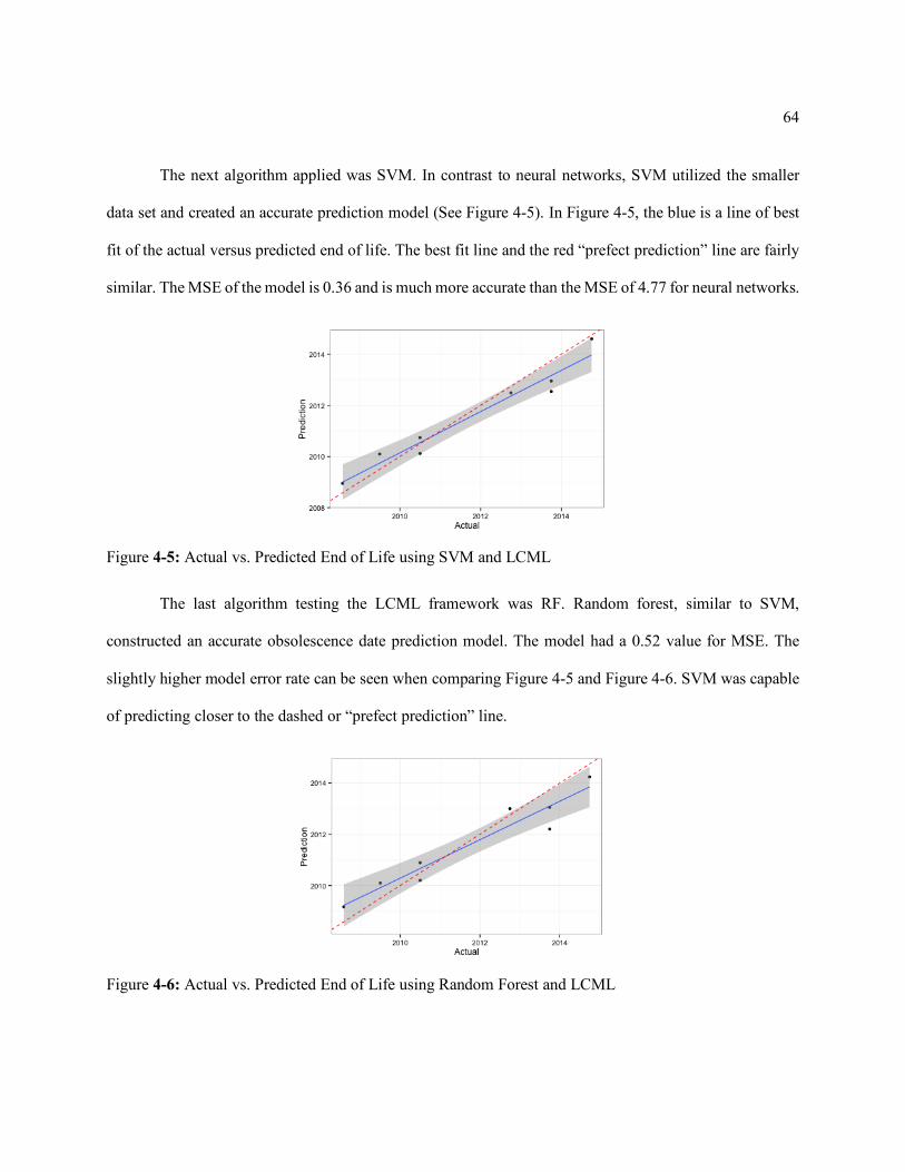
64
The next algorithm applied was SVM. In contrast to neural networks, SVM utilized the smaller
data set and created an accurate prediction model (See Figure 4-5). In Figure 4-5, the blue is a line of best
fit of the actual versus predicted end of life. The best fit line and the red “prefect prediction” line are fairly
similar. The MSE of the model is 0.36 and is much more accurate than the MSE of 4.77 for neural networks.
Figure 4-5: Actual vs. Predicted End of Life using SVM and LCML
The last algorithm testing the LCML framework was RF. Random forest, similar to SVM,
constructed an accurate obsolescence date prediction model. The model had a 0.52 value for MSE. The
slightly higher model error rate can be seen when comparing Figure 4-5 and Figure 4-6. SVM was capable
of predicting closer to the dashed or “prefect prediction” line.
Figure 4-6: Actual vs. Predicted End of Life using Random Forest and LCML
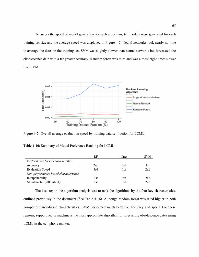
65
To assess the speed of model generation for each algorithm, ten models were generated for each
training set size and the average speed was displayed in Figure 4-7. Neural networks took nearly no time
to average the dates in the training set. SVM was slightly slower than neural networks but forecasted the
obsolescence date with a far greater accuracy. Random forest was third and was almost eight times slower
than SVM.
Figure 4-7: Overall average evaluation speed by training data set fraction for LCML
Table 4-16: Summary of Model Preference Ranking for LCML
RF Nnet SVM Performance based characteristics Accuracy 2nd 3rd 1st Evaluation Speed 3rd 1st 2nd Non-performance based characteristics Interpretability 1st 3rd 2nd Maintainability/flexibility 1st 3rd 2nd
The last step in the algorithm analysis was to rank the algorithms by the four key characteristics,
outlined previously in the document (See Table 4-16). Although random forest was rated higher in both
non-performance-based characteristics, SVM performed much better on accuracy and speed. For these
reasons, support vector machine is the most appropriate algorithm for forecasting obsolescence dates using
LCML in the cell phone market.

66
4.3 Accuracy Benchmarking and Additional Features of LCML and ORML
The following section presents a benchmarking study (comparison) of the LCML method and
other life cycle forecasting methods, discusses the difficulties of benchmarking the ORML method versus
other obsolescence risk methods, and then demonstrates how the LCML method can be easily converted
into the ORML method with a switch of the target output.
4.3.1 Benchmarking Life Cycle Forecasting Methods
First, the LCML method is compared with the CALCE ++ method introduced by Sandborn (2005)
[8] and with the Times Series method introduced by Ma and Kim (2017) [23]. For all three methods, the
same data set is utilized to facilitate the assessment of the resulting life cycle predictions.
The data set utilized in this benchmarking study was introduced in Sandborn 2005 [8] when the
CALCE ++ method was first introduced. The data set is comprised of monolithic flash memory components
from 1997 to 2004. The data contains 362 different components varying in memory sizes from 128K to
32MB. The components are manufactured by 7 different vendors, such as AMD and Intel. The data contains
the model number, obsolescence date, memory size, time for peak sales, and variance of sales.
The mean square error (MSE) was chosen to compare the accuracies of the life cycle forecasting
methods. The formulation for computing MSE is shown in Equation 4. The variable n denotes the number
of predictions made using the forecasting method, and ŷi is a vector of length n that contains the predicted
values. The variable yi represents the true obsolescence date for component i.
The computed results can be seen in Figures 4-8, 4-9, and 4-10, visualized using the same technique
from Sandborn 2005 [8]. The x-axis is the actual data the component became obsolete, and the y-axis is the
predicted range of when the component will become obsolete. The black diagonal line represents a correct
prediction. If the red life cycle prediction band intersects the black line, then the method correctly predicted

67
the obsolescence date within the range. If the red range appears below the black diagonal line, then the
prediction underestimated the obsolescence date, and if the red range appears above the black diagonal line,
then the prediction overestimated the obsolescence date. Similar to how the results of obsolescence risk
forecasting can be interpreted in a variety of ways, these two types of errors can have different effects on
the business. However, in life cycle forecasting, underestimating the obsolescence date is often preferred
because it will allow additional time to manage the obsolescence reaction plan. Over estimating the date a
component will become obsolete will often cause organizations to employ costly reactionary strategies to
mitigate the effect of obsolescence. For this reason, if a prediction does not intercept the black line, then it
is better to be below the black line than be over it.
The first algorithm tested was the Life Cycle Forecasting using Machine Learning (LCML) method.
It was able to achieve a mean squared error of 1.237 or an average error of 1.112 years. As can be seen in
Figure 4-8, many of the predictions fall near the diagonal line which represents a prefect prediction. The
model was not able to accurately predict the obsolescence date for monolithic flash memory before 1999
because there were very few components within this data set with obsolescence dates before 1999.

68
Figure 4-8: LCML Method [25] Predictions vs. Actual Results
The next method was the CALCE++ method from Sandborn 2005 [8]. Figure 4-9 shows the
predicted obsolescence dates versus the actual dates. CALCE++ has a mean squared error of 2.212 or an
average error of 1.487 years. Although many of the prediction ranges intercept the black diagonal line,
CALCE++ obtained a lower accuracy than the LCML method. Additionally, like the LCML method, the
method overestimated the values before 1999 and was much more accurate after 1999.
1996
1998
2000
2002
2004
2006
2008
2010
1997 1999 2001 2003 2005
Pred
icte
d O
bsol
esce
nce
Dat
e
Actual Obsolescence Date
LCML
LCML

69
Figure 4-9: CALCE++ Method [8] Predictions vs. Actual Results
The last method benchmarked in this study was the Time Series method proposed by Ma and Kim
2017. The time series method is an improvement on the CALCE++ method because it does not assume the
sales cycle is perfectly normal and uses more powerful time series statistical modeling. In Ma and Kim
2017, the authors predict obsolescence dates for monolithic flash memory, but the authors use the sales data
for the entire market for each memory size (e.g., 2GBs, 8GBs, 256MBs, etc.) to predict the obsolescence
range and not the sales data for individual components. For this benchmarking study, the ability to predict
the obsolescence dates of individual components is being assessed. Unfortunately, sales data for individual
components is not available for this method. The individual sales data by components was scrubbed to only
contain the information needed for the CALCE++ method, such as sales variance and peak, and does not
contain monthly sales numbers. Therefore, the predictions from the larger markets are used as the
1996
1998
2000
2002
2004
2006
2008
2010
1997 1999 2001 2003 2005
Pred
icte
d O
bsol
esce
nce
Dat
e
Actual Obsolescence Date
CALCE ++
CALCE ++

70
predictions for individual components (i.e., if the 2GBs market will sell its last unit in 2001, then any 2GB
flash memory component in this data set will receive a prediction of 2001). For this reason, the comparison
of the time series method to the LCML and CALCE++ methods are not a perfect one-to-one comparison.
However, this will serve as a rough estimate of the accuracy of the model.
The time series model was able to achieve a mean squared error of 15.490, and the results can be
seen in Figure 4-10. The majority of predictions overestimated the obsolescence date, but this can be
expected due to using the obsolescence date of the total market rather than the individual component. This
is because the obsolescence date of a total market will always be the maximum of all the components within
the market and therefore overestimation is not unexpected.
Figure 4-10: Time Series Method [23] Predictions vs. Actual Results
1996
1998
2000
2002
2004
2006
2008
2010
1997 1999 2001 2003 2005
Pred
icte
d O
bsol
esce
nce
Dat
e
Actual Obsolescence Date
Time SeriesTimeSeries

71
Table 4-17 shows the resulting MSE and average error of each method. LCML was the most
accurate followed closely by CALCE++ and then last was the Time Series method. LCML was the most
accurate model while only requiring the component specifications (i.e., memory) and the obsolescence date,
while the other methods required the component specifications, the obsolescence date and sales data.
Because LCML requires less data, it would be easier to implement into an obsolescence management
strategy for an organization.
Table 4-17: Accuracies Life Cycle Forecasting Methods in the Flash Memory Market
Method MSE Mean Error (Years)
LCML 1.237 1.112 CALCE 2.212 1.487
Time Series 15.490 3.936
4.3.2 Benchmarking Obsolescence Risk Methods
A quantitative analysis comparing the different approaches to obsolescence risk forecasting would
be fraught with many problems, limiting accuracy and meaningful conclusions. This is due to many of the
obsolescence risk forecasting methods requiring expert opinion on the market or expert curation of a bill of
materials. With any familiarity of specific case studies, conducting an unbiased comparison of forecasting
methods without potentially contaminating the results is not possible. An alternative would be to have
individuals unfamiliar with specific data sets perform the obsolescence risk predictions using each method
and then compare the results to the ORML method. However, since the knowledge of the market will vary
depending on the individual selected, multiple individuals would need to conduct the method and then those
results could more accurately convey the strength of the method. Additionally, any obsolescence case study
could only be done by individuals who are making obsolescence predictions in the future because if the
experts are retroactively making predictions on pass markets, obsolescence methods with human input will

72
have an unfair advantage because of expert’s knowledge of the future of the market versus models using
only data from the past, such as ORML. For example, many people in 2012 would have assumed the trend
of cell phones continuing to get smaller or at the very least stay the same size. However, due to increase
bandwidth and the ability to stream video on cell phones, Apple, and many other phone manufacturers,
increased the size of their cell phone models (e.g. both the iPhone 6 and 6+ are bigger than the iPhone 5).
As an observer looking back at the 2012 market, modern observers are aware of this trend and would have
unfair knowledge of the market to make obsolescence predictions.
For the above reasons, an obsolescence risk method benchmarking study would require numerous
experts to make predictions using each method in the current market and then wait a year or two for the
predictions to be validated or invalidated. Unfortunately, such a study is not feasible for this research.
Recognition of these requirements for basic benchmarking studies highlights one of the problems with the
current state of obsolescence risk methods. Unlike life cycle forecasting, the current obsolescence risk
methods require qualitative inputs, such as market health and life cycle stage, rather than quantitative inputs,
such as product sales or specification data [25]. The ORML method addresses this problem, as it is
dependent on specification methods and does not require subjective or qualitative inputs. For this reason,
experts using the same data will always come to the same obsolescence risk level using ORML but are not
guaranteed to come to the same result with other obsolescence risk methods because of the subjective nature
of the inputs and the differences between the experts.
Because the inputs for both the LCML and ORML methods are product specifications, one of the
other benefits of the LCML and ORML methods is the ability to easily change between the two by changing
the output of the model and keeping the input data the same. The following section demonstrates how the
benchmarking study in Section 4.4.1 can be readily converted to predicting obsolescence risk with a few
additional steps.

73
4.3.3 Converting Life Cycle to Obsolescence Risk Forecasting
The case study presented in this section simulates an organization subscribing to a commercial
obsolescence part database, similar to the commercial databases discussed in Section 2.1.2. The
organization would use the data available in the database to generate an obsolescence risk model to predict
the obsolescence risk of components not available in the database. For this case study, the same data is used
from Section 4.3.1. The 362 monolithic flash memory components are split into two groups, testing and
training. The first 181 components are used to train the obsolescence risk model. This data can be thought
of as a commercial obsolescence database.
The obsolescence database is used to generate a LCML model as demonstrated in the benchmarking
case study in Section 4.3.1. Additionally, this same database information and LCML model is readily
converted into an ORML by varying the desired output of the model. The first step was turning the
obsolescence date into a binary label of “procurable” or “discontinued”. For this study, the assumption is
the current date is February 1999; therefore, components with obsolescence dates after February 1999 are
labeled procurable and before are labeled discontinued. Once the new labels were assigned, the LCML
method is performed again with a switch of the output of the model being trained from the obsolescence
date to the obsolescence status label.
The resulting model is used to make predictions on the 181 components with known obsolescence
statuses that are not currently in the obsolescence database. Table 4-18 compares the actual versus predicted
obsolescence status of the monolithic flash memory components. As shown, the model was able to
accurately predict the obsolescence status of components 83.76% of the time. Further, with this accuracy,
commercial component obsolescence databases could be used to generate both ORML and LCML models
allowing for the extrapolation and ability to make predictions for obsolescence risk and life cycle for
components not contained in the database.

74
Table 4-18: Monolithic Flash Memory Confusion Matrix for ORML
Actual Available Discontinued Total
Prediction Available 83 15 Discontinued 17 82 Total 100 (83%) 97 (15.46%) 197 (83.76%)
4.4 Machine Learning based Obsolescence Forecasting Scalability
Both the ORML and LCML methodologies for forecasting obsolescence have shown high degrees
of accuracy in a variety of case studies. The goal of introducing the ORML and LCML methods was to
maintain an accurate model while addressing the problems previously proposed obsolescence forecasting
models had when trying to scale to industry needs. The three scalability problems outlined in Section 2.1.3
are (1) the requirement of frequent data collection for all parts, (2) requirement of human opinions, and (3)
forecasting only one key product specification (e.g. memory). The machine learning based approach to
obsolescence forecasting outlined in this dissertation was able to address these scalability problems to
varying degrees.
First, any empirical forecasting model requires data and therefore requires data collection.
However, different types of data needs updating at different intervals. For instance, a model which requires
sales data to make a prediction and has 100 products will require new sales data every month, quarter, etc.
for each product. While a model based on specifications will need the product’s specifications when the
product is added to the modeling data set. This slight difference can be many hours of data collection
because the specification-based model only requires data input for a product one time and a sales-based
model will require data input for all products every time the sales data is updated. For this reason, the
ORML and LCML improve over traditional sales data base obsolescence forecasting models, but still
requires some specification-based data collection.

75
Second, the ORML and LCML model requires no human opinion. Although a person may be
needed to set up the model or input specifications, an individual’s opinion is not explicitly required as a
variable in the model. This greatly helps with the speed predictions can be made because there is no waiting
for human input and for this reason, the ORML and LCML methods could generate a model and make
predictions on thousands of products in a few seconds. Additionally, the removal of human opinion in a
model helps maintain repeatability. If two supply chain managers predict the obsolescence risk of a product
and both input the correct specifications, the managers will always receive the same result. If the managers
were required to input their opinion, they may come to different results. This standardization and increased
speed greatly help with ORML and LCML’s ability to scale to industries’ needs.
Third, both ORML and LCML use product specifications as inputs and are not limited to one key
specification. Because of this, the ORML and LCML methods are able to make predictions in more complex
industries which are not easily defined by one specification (e.g. memory).
For these three reasons, ORML and LCML significantly improved upon the scalability of
obsolescence forecasting when compared to current models.
4.5 Machine Learning based Obsolescence Forecasting Limitation
Like other obsolescence forecasting frameworks, LCML and ORML have limitations and problems
that may compromise the validity of the estimations. This section addresses these problems and limitations
and provides greater insight into the frameworks.
The first problems can arise from the start, during data collection. The data must be both fairly
reliable and up-to-date. As demonstrated in the case study, the data does not need to be complete, but the
more complete the data is, the more accurate the prediction. Another important part of the data formatting
process is variable selection and creation. The correct variables can easily capture the change in the market
and can indicate when parts or elements are becoming obsolete. However, these variables might not always

76
be a simple measure of memory, screen resolutions or another metric. For example, a variable may need to
be created to denote the highest, medium, and lowest memory levels of a phone. Apple, Inc. usually ends
production of the highest and medium versions of a phone, but still produces the lowest memory version of
the prior model phone to capture the market of people looking for a “cheap” iPhone. The size of memory
in the lowest memory version of the iPhone has changed over time and using only phone memory would
not capture this trend in the predictive model.
With the diversity of industry where obsolescence is present and these frameworks can be used,
there will be no uniform indicator between industries. A good metric to measure obsolescence for flash
drives is probably memory; however, for cell phones the features like thread text messaging and screen
resolution are more useful than memory. Furthermore, good metrics can change over time. When cell
phones were first invented, connectivity was one of the most important factors and little emphasis was on
features. Now connectivity is a given, and other features determine phone obsolescence.
Another problem with obsolescence forecasting frameworks is finding acceptable prediction
accuracies from industry to industry. An industry like transistors, with exponential change such as described
by Moore’s Law, would likely be predicted more accurately than the cell phone market due to the
complexity of the products and different marketing and pricing aspects.
The last problem is one that plagues all machine learning and statistical models. If the data used to
build the model does not represent the current real world, then the model will not be accurate. In
obsolescence, there is an extremely high chance of this occurring due to rapid innovation or invention.
When Apple released the first iPhone, it was the first in many categories, and because of that, it accelerated
the obsolescence of many of the phones in the current market. A machine learning or statistical
obsolescence model at the time built with past obsolescence data would not predict the jump in technology
that this innovation caused. This means the obsolescence forecasting frameworks introduced in this research
and all current obsolescence models cannot predict large jumps in innovation but are better suited to track
steady improvements in an industry.

77
Chapter 5
Reducing the Cost Impact of Misclassification Errors in Obsolescence Risk Forecasting
The case studies provided predict obsolescence risk in two common consumer electronic markets:
cell phones and digital cameras. Then the specifications of the screens from both the cell phones and digital
cameras are combined to create a third data set, which contains obsolescence information about screens as
components to other electronics.
The case studies apply ROC analysis to an obsolescence risk forecasting method to find an optimal
threshold that minimizes the average cost impact of misclassified components. The obsolescence risk
forecasting using machine learning (ORML) method [8] was selected for this example. However, the ROC
analysis method for calculating thresholds can be utilized by any obsolescence risk prediction method that
converts a probability into a label. The digital camera data set was selected to show the obsolescence
prediction of a particular component within a product. In the design of drones and other devices that ship
with or connect modularly with cameras, understanding the obsolescence risk of camera models is
necessary to ensure that the product that uses the digital camera will last within its market. Camera
obsolescence information is crucial in the design phase to select the camera models that systems or products
like the ones described above will depend on throughout their life cycle. This information can go beyond
the design phase to impact decisions on when to add technical support for new camera models and remove
support for others.
The second dataset chosen was from the cell phone market. Traditionally, cell phones are seen as
a final product and is not a component into another product. Therefore, the standard obsolescence problem
of a component becoming obsolete and then potentially starving a manufacturing line would not apply.
However, as cell phones evolve from simple phones into small computers, cell phones have become
components within other more complex products and systems. For example, with the growth of virtual

78
reality, businesses have attempted to lower the price of VR headsets. Many companies now offer headsets
that allow the users to use their cell phone as the screen. Companies designing these virtual reality cell
phone mounts must monitor the current cell phone market because it has become a critical component of
their virtual reality system. As cell phones continue to grow into non-traditional markets, the monitoring
of the obsolescence status of individual models will become more important than ever.
Additionally, as traditionally nonelectronic components continue to become digitized, the need for
digital screen components for a variety of products is growing in importance. The third case study in this
section will apply the ROC method to the screen components, specifically screens from cell phones and
cameras. The screen specifications are gathered by combining the cell phone and camera data sets in the
first two case studies.
The cell phone and digital camera data were gathered from product review forums, GSMArena.com
(Accessed: 17-5-2015) and DPReview.com (Accessed: 26-3-2016), respectfully. The data was aggregated
by a web scraper coded in the programming language R and using the package ‘rvest’ [34]. The digital
camera data set contains 2214 unique models and 50 specification variables including body type,
dimensions, battery type and life, headphone port, microphone, speakers, wireless technology (WiFi,
Bluetooth, etc.), built-in flash or modular flash, flash range, digital zoom, megapixels, screen size and
resolution, USB adaptor type, minimum and maximum aperture, manual vs digital zoom, picture ratios,
image stabilization technology, uncompressed file format, built-in memory, and a few other specifications.
The data set contains 985 procurable and 1229 discontinued models. The cell phone data set contains 7051
unique cell phone models and 70 specification variables. Some of the specifications included in this data
are weight, screen size, screen resolution, talk time on one battery, primary and secondary camera size, type
of web browser, and whether the phone has the following: 3.5-mm headphone jack, Bluetooth, e-mail, push
e-mail, radio, SMS, MMS, thread text messaging, GPS, vibration alerts, or a physical keyboard. The data
set contains 4030 procurable and 3021 discontinued models. The screen data set contains a total of 9265
different components and contains specifications such as the screen resolution, pixel ratio, and screen

79
technology (e.g., LED, AMOLED, etc.). The obsolescence statuses of the cell phone or camera the screen
comes from is used as a proxy for the obsolescence status of the screen.
Some of the algorithms in the case study can only allow numerical inputs as opposed to categorical
variables. To handle this, each categorical variable was turned into many binary variables. For example,
web browser type could be HTML5, HTMLx, i-mode, WAP, or WAP 2.0. The variable of web browser
type would be transformed into 5 binary variables denoting whether the model does have the browser type
or not. For algorithms that can handle categorical variables, the data was left in the standard format. All
data and code in this case study can be downloaded at connorj.github.io/research. Throughout the entire
case study, the data sets were broken into a training set, making up 66.6% of the data and a test set making
up the other 33.3%. The training set is used in the model creation phase and the test set is used to evaluate
the model. This is a best practice in model validation and prevents over fitting of models to a data set [35].
5.1 Algorithm Selection using Area Under the ROC Curve (AUC)
The first step in the ROC analysis is selecting the best algorithm or other method for predicting the
obsolescence risk level of products for a given industry. For all three markets, four machine learning
algorithms: Random Forest (RF), Support Vector Machines (SVM), Neural Networks (NN), K-Nearest
Neighbors (KNN) are applied and the accuracy is assessed [36]-[38]. RF is based on decision trees and
generates many random decision trees and aggregates their predictions for the status of each component to
create a more effective classification method. SVM creates a plane in high dimensional space to try and
find separability between the statuses. NN was inspired by biological neural networks and develops a
network to find complex relationships between inputs and outputs. KNN takes the majority class of the “k”
closest known instances. These four algorithms were chosen because of their wide spread usage in machine
learning and other data mining applications. For this study, the RF, SVM, NN, and KNN algorithms are
used to create the predictive models. RF was set to have 500 unique trees and used the Gini coefficient
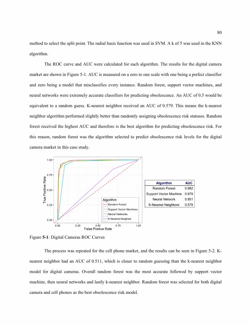
80
method to select the split point. The radial basis function was used in SVM. A k of 5 was used in the KNN
algorithm.
The ROC curve and AUC were calculated for each algorithm. The results for the digital camera
market are shown in Figure 5-1. AUC is measured on a zero to one scale with one being a perfect classifier
and zero being a model that misclassifies every instance. Random forest, support vector machines, and
neural networks were extremely accurate classifiers for predicting obsolescence. An AUC of 0.5 would be
equivalent to a random guess. K-nearest neighbor received an AUC of 0.579. This means the k-nearest
neighbor algorithm performed slightly better than randomly assigning obsolescence risk statuses. Random
forest received the highest AUC and therefore is the best algorithm for predicting obsolescence risk. For
this reason, random forest was the algorithm selected to predict obsolescence risk levels for the digital
camera market in this case study.
The process was repeated for the cell phone market, and the results can be seen in Figure 5-2. K-
nearest neighbor had an AUC of 0.511, which is closer to random guessing than the k-nearest neighbor
model for digital cameras. Overall random forest was the most accurate followed by support vector
machine, then neural networks and lastly k-nearest neighbor. Random forest was selected for both digital
camera and cell phones as the best obsolescence risk model.
Figure 5-1: Digital Cameras ROC Curves

81
The final data set combines screen specifications from the cell phones and digital cameras data to
create a third data set. The resulting AUCs for the ORML method are shown in Figure 5-3. Similar to the
previous two case studies, k-nearest neighbor has the lowest AUC. The top AUC was neural networks with
both random forest and support vector machine following within 0.003.
Figure 5-2: Cell Phone ROC Curves
Figure 5-3: Digital Screens ROC Curves

82
5.2 Assigning Costs and Calculating the Optimal Threshold
After the best algorithm was selected for predicting the obsolescence status of a component, the
mathematical model from Section 3.3 is used to find the optimal threshold value. The model takes the
predicted obsolescence risk, the true obsolescence status, and the cost of a Type I and Type II error (Cfp and
Cfn) as inputs then uses a brute force searching algorithm with a risk threshold step size of 0.00001 to solve
Equation 1 in Section 3.2. The predicted obsolescence risk levels are taken as the output from the algorithm
selected in the previous section. The costs are found by conducting an economic analysis. The assumed
excepted cost incurred by a company if one discontinued component is classified as procurable (Cfn) for
this case study is $200,000. This can be found by taking the cost of a production shutdown event,
$1,000,000, and multiplying the cost by the probability that the event will occur due to the misclassification
of a discontinued component as still procurable (20%). Alternatively, the excepted cost incurred by an
organization if a procurable component is classified as discontinued (Cfp) for this case study is taken as
$100,000. Again, the events, triggered by this instance of component misclassification, are compiled and
the average cost and probability of each event are estimated. Two events that could occur if a false positive
(Type I error) occurs are (1) component stockpiling and (2) a premature redesign. The stockpiling assumes
a cost $50,000 and has a 100% chance of occurring. The premature redesign costs $500,000 but has only a
10% chance of occurring. Summing the product of the cost and probabilities returns $100,000 or the average
cost of a procurable component if classified as discontinued (Cfp). These calculations are simplified for the
purposes of this research. In practice, a complete economic analysis should be conducted to estimate these
costs; however, the focus here is how to account for and minimize the average misclassification cost impact
from predictions and not how to calculate the cost.
When these costs are used in the mathematical model, the search algorithm found an obsolescence
risk level cut-off of 0.331 for the cell phone market. This threshold means all cell phone models with higher
risk levels would be classified as discontinued, and those with lower risk levels are assigned the status

83
procurable. The new threshold will classify more components as discontinued and less as procurable
compared to the original 0.5 threshold. The increase in components classified as discontinued increases the
number of Type I errors (procurable phone predicted as discontinued) to hedge against the number of
costlier Type II errors (discontinued phone predicted as procurable).
Using the new optimal threshold, the new statuses were assigned based on predicted risk levels.
The results can be seen in the confusion matrix in Table 5-1. Table 5-1 shows how the statuses were
assigned using the standard 0.50 threshold, and Table 5-2 shows the results using the new optimal threshold.
Between the two methods, the overall traditional accuracy fell from 93.37% to 91.87%. TP rate increased
from 89.74% to 94.97% while FP rate increased from 3.97% to 10.4%. Overall, the objective function
output dropped from $26.3 million to $24.6 million.
To evaluate this drop in the objective function, the metric of average misclassification cost is used
to understand how this metric translates into an organization’s cost savings. Average misclassification cost
is the excepted cost impact from misclassification for one prediction for one product. When an organization
uses a model, there is a risk that the model will be incorrect, and “average misclassification cost” creates
an economic impact of that risk. For example, if a market has a cost of a false positive of $100,000 and cost
of a false negative of $200,000 and the models used in this market has 300 products to predict. Out of the
300 products, the model predicts 80 false positives, 20 false negatives, and the other 200 products are
correctly classified. The 200 products classified correctly have a misclassification cost impact of zero
dollars. Now the average value is calculated with the Equation 5, and an average misclassification cost of
$40,000 per prediction is found. This means that each prediction has a potential additional cost of $40,000
worth of unnecessary action triggered by an incorrect prediction.
<\ICB]I!"^_`B^^"+"_B>"a#&a^> = &'(*4'(. + &'(*4'(.
4bcbPd(5)
Nfp = Number of a false positive (Type I error) Nfn = Number of a false negative (Type II error) Ntotal = Total number of a products predicted by the model

84
Using this metric, the new threshold caused an overall drop in the average misclassification cost
from $10,967.50 to $10,258.50 (see the following calculations). Although, the change in average
misclassification cost in absolute dollars is not large, this represents a 6.5% reduction in the average
misclassification cost for each predicted instance within the system.
MisclassificationCostusingStandardAccuracy =$100,000(55) + $200,000(104)
2398= $10,967.50
MisclassificationCostusingOptimalThreshold = $100,000(144) + $200,000(51)
2398= $10,258.50
Table 5-1: Cell phone Confusion Matrix with Classic Threshold
Actual Available Discontinued Total
Prediction Available 910 55 Discontinued 104 1329 Total 1014 (89.74%) 1384 (3.97%) 2398 (93.37%)
Table 5-2: Cell phone Confusion Matrix with ROC Threshold
Actual Available Discontinued Total
Prediction Available 963 144 Discontinued 51 1240 Total 1014 (94.97%) 1384 (10.4%) 2398 (91.87%)
The Vogler method [85] is used to visualize the results for the ROC confusion matrix. The actual
statuses are plotted against their obsolescence risk levels in the top half of Figure 5-4. The red line represents
the optimal threshold, and the blue lines represent mirrored density distributions for discontinued and
procurable cell phones. The purple and blue dots represent true positives and true negatives, respectfully.
These are correctly classified cell phone models. The red and green dots denote false negatives and false
positives, respectfully. In Figure 5-4, all the points to the right of the red threshold line and below the 0.5
obsolescence risk line would be assigned different statuses under the ROC analysis method and the

85
traditional method. These new statuses show the tradeoff between more correctly classified positive classes
(discontinued) and the decrease in correctly classified negative classes (procurable).
The bottom chart in Figure 5-4 shows the result of the objective function from Equation 1. The
graph shows the threshold represents the lowest expected error cost per prediction.
In the digital camera market, an optimal threshold of 0.277 was calculated. The new statuses were
assigned using the new threshold and the results are displayed in Table 5-3 and Table 5-4. Again, the total
accuracy decreased but the ability to identify costlier discontinued models was improved by almost 5%.
This translated into an overall reduction in the objective function from $7,400,000 to $5,900,000. The new
threshold caused an overall drop in the average misclassification cost from $9,827.40 to $7,835.32 (see the
Figure 5-4: Obsolescence Risk Prediction at a Threshold of 0.331 for Cell phones
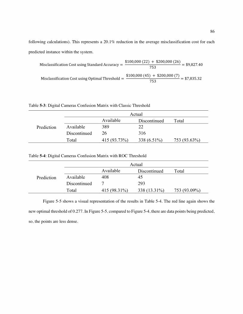
86
following calculations). This represents a 20.1% reduction in the average misclassification cost for each
predicted instance within the system.
MisclassificationCostusingStandardAccuracy = $100,000(22)+ $200,000(26)
753= $9,827.40
MisclassificationCostusingOptimalThreshold = $100,000(45) + $200,000(7)
753= $7,835.32
Table 5-3: Digital Cameras Confusion Matrix with Classic Threshold
Actual Available Discontinued Total
Prediction Available 389 22 Discontinued 26 316 Total 415 (93.73%) 338 (6.51%) 753 (93.63%)
Table 5-4: Digital Cameras Confusion Matrix with ROC Threshold
Actual Available Discontinued Total
Prediction Available 408 45 Discontinued 7 293 Total 415 (98.31%) 338 (13.31%) 753 (93.09%)
Figure 5-5 shows a visual representation of the results in Table 5-4. The red line again shows the
new optimal threshold of 0.277. In Figure 5-5, compared to Figure 5-4, there are data points being predicted,
so, the points are less dense.

87
An optimal threshold of 0.369 was calculated in the digital screen market. The new statuses were
assigned using the new threshold, and the results are displayed in Table 5-5 and Table 5-6. However, the
reduction in total accuracy was only 0.12%, and the accuracy of correctly classifying more costly
discontinued components increased from 87.53% to 88.6%. The new threshold caused an overall drop in
the average misclassification cost from $24,880.99 to $24,309.74 (see calculations that follow). This
equates to a 2.295% reduction in average misclassification cost for each predicted instance within the
market. Although this percentage is smaller than the cell phone or camera market examples, this could lead
to much higher savings because the screen market is much larger than the cell phone and camera market.
Therefore, even a small percentage cost saving in a much larger market can have a larger effect than a large
percentage cost saving of a small market.
Figure 5-5 Obsolescence Risk Prediction at a Threshold of 0.277 for Digital Cameras

88
MisclassificationCostusingStandardAccuracy = $100,000(398) + $200,000(193)
3151= $24,880.99
MisclassificationCostusingOptimalThreshold =$100,000(424) + $200,000(171)
753= $24,309.74
Table 5-5: Digital Screens Confusion Matrix with Classic Threshold
Actual Available Discontinued Total
Prediction Available 1355 398 Discontinued 193 1205 Total 1548 (87.53%) 1603 (24.83%) 3151 (81.24%)
Table 5-6: Digital Screens Confusion Matrix with ROC Threshold
Actual Available Discontinued Total
Prediction Available 1329 424 Discontinued 171 1227 Total 1500 (88.6%) 1651 (25.68%) 3151 (81.12%)
Figure 5-6 shows a graphical representation of Table 5-5 and Table 5-6. However, unlike the
previous two figures, the results of the optimization function are not smooth. This is due to the predicted
obsolescence risk levels being less uniformly distributed than the previous two examples, and therefore
when the threshold crosses one of these large groups, it has a large jump in the objective value of Equation
1.

89
5.3 Misclassification Cost Sensitivity Analysis
This section presents the results of sensitivity analysis that was conducted to better understand the
relationship between the misclassification cost values and the resulting optimal threshold using the method
proposed in Section 3.2. The data used in the sensitivity analysis presented in this section will only be from
the cell phone case study. The results of the sensitivity analysis on the other two data sets can be found in
the Appendix B.
The sensitivity analysis was conducted by varying the obsolescence misclassification costs for both
Type I and Type II errors. The error cost was varied between one and four. Figure 5-7 shows the resulting
Figure 5-6: Obsolescence Risk Prediction at a Threshold of 0.369 for Digital Screens

90
threshold from the different combinations of error cost. Figure 5-7 is a 4 x 4 matrix with the rows
representing the weight for Type 1 errors and the columns represent the weights for Type 2 errors. For
example, row one and column two represents a ratio of 1:2 and this is the same as the case study in Section
5.2, which used cost weights of $100,000 and $200,000, respectfully. In the case study in Section 5.2, the
weights of $100,000 and $200,000 found an optimal threshold of 0.311 and using costs of 1 and 2, again,
0.311 was found as the optimal threshold for that ratio. Additionally, since only the ratio of the costs defines
the threshold and not the magnitude of the costs, all cells of the matrix with the same ratio will have the
same resulting threshold. For instance, the diagonal from top left to bottom right all have a ratio of 1:1 and
therefore, have the same resulting threshold. Additionally, row one and column two have the same ratio as
row two column four (1:2). Both of these cells of the matrix have the same resulting threshold as well.
Conversely, 2:1 and 4:2 have the same threshold due to having the same underlining ratio).
Figure 5-7: Cost Sensitivity Analysis for Optimal Threshold for Cell phones

91
One interpretation of the ratios is the tradeoff cost or additional marginal cost of an error. For
example, a ratio of 1 to 4 (false negatives cost $1 and false positives cost $4) would mean an organization
would allow up to 4 false negatives to happen to avoid 1 false positive. This concept can visually explain
why certain thresholds are selected. For example, if a threshold could move lower and prevent 1 false
positive, while only incurring 3 false positives, the threshold will be lowered. Figure 5-7 seeks to explain
this graphically. As shown, this is most evident with the ratios of 1 to 4 and 4 to 1. For the ratio of 1 to 4,
as the threshold moves down from its default position of 0.5, the occurrence of Type I errors happens at a
rate lower than 4 times that of Type II errors. However, once the threshold meets the optimal threshold, any
lower would cause the occurrence of Type I errors to be more than 4 times that of Type II errors. This can
be seen from the high density of blue points which would become misclassified and the low density of
green which would become correctly classified in the upper right graph of Figure 5-6. For this reason, the
threshold does not go lower than the four times level because it does not make economic sense. Similar
results can be seen in the ratio of 4 to 1 in the bottom left corner graph of Figure 5-6. Since a red point is 4
times as costly as a green point, the threshold rises above its default position of 0.5 until the ratio of
converting misclassified red points to blue points is four times the rate of correctly classified purple points
being converted to green points. A threshold any lower than the optimal could save money by converting
three Type I errors at a cost of 1 per each for one Type II error at a cost saving of 4 and a threshold any
higher than optimal would be trading five Type I errors at a cost of 1 per each for one Type II error at a cost
saving of 4. This means any threshold lower than the optimal would move up and any threshold higher
would move down. Therefore, the threshold stops when the ratio of points above and below the threshold
are equal to the inverse of the weight thresholds.
Table 5-7 shows the resulting threshold values from Figure 5-7. As can be observed from Figure
5-7, the diagonal from top left to bottom right all have cost ratios are 1 to 1 and therefore all optimal cutoff
thresholds are 0.466. The ratio of 1 to 2 and 2 to 4 have a threshold of 0.331 (same as the case studying
Section 5.2); while the ratio of both 2 to 1 and 4 to 2 have a threshold of 0.565.

92
Table 5-7: Optimal Thresholds in Cell phone Error Cost Sensitivity Analysis
Type II Misclassification Cost 1 2 3 4
Type I Misclassification
Cost
1 0.466 0.331 0.266 0.219 2 0.565 0.466 0.344 0.331 3 0.596 0.565 0.466 0.353 4 0.730 0.565 0.565 0.466
In summary, this section explores the relationships between varying error costs and the resulting
cut off threshold in obsolescence forecasting. Additionally, versions of Figure 5-7 and Table 5-7 for both
the digital camera and screen components data set can be found in Appendix B. These follow the same
methodology as above by varying the cost from one to four for both error costs. As can be seen, similar
results were observed.
The next section will shift focus from technical obsolescence forecasting to function obsolescence
forecasting. Specifically, it will focus on predicting the health status of gearboxes of wind turbines.

93
Chapter 6
Health Status Monitoring of Wind Turbine Gearboxes
With this substantial growth and the distributed nature of wind turbines, effective maintenance
plans and remote monitoring has become more important than ever. The following case study is used to test
and validate the prediction models that were developed to predict the health status of a wind turbine from
attached sensors accessed remotely. This will allow organizations to better allocate the time of repair teams
and reduce the need for manual inspection.
The data for the case study is provided by the Department of Energy – National Renewable Energy
Laboratory and consists of instances of healthy running turbines and ones that have had a catastrophic loss
of oil event [86]. The data set contains information on ten healthy and ten unhealthy turbines. The data has
eight acoustic emission sensors collecting information at 40 kHz per channel and one speed sensor
measuring rpm of the blades. Each sensor has about 876,000 data points for each of the 10 sensors for every
instance. The location of the acoustic emission sensors can be found in the diagram in Figure 6-1.
Figure 6-1: Location of Sensors on the Wind Turbine [86]

94
Table 6-1 shows the models and units of all the sensors and the table is supplied by the Department
of Energy – National Renewable Energy Laboratory [86]. Both AN3 and AN4 use the same model IMI
622B02 sensor, while all the other acoustic emission sensors use model IMI 622B01. The speed sensor uses
an IMI 611b02 to measure rpm.
Table 6-1: Name, Description, Model Number, and Units of Sensors in Figure 6-1 [86]
The analysis was conducted using the R programming language (version 3.3.2). The signal
processing and model creation was developed using prewritten functions available from popular packages.
Specifically, the FFT was created using the fft function available in base R. The FFT was set to return
frequencies from 1 to 500 and thus created 500 variables for each sensor. The wavelet transform was
conducted using the dwt function from the package ‘wavelet’ [36]. The function uses a Haar filter and
periodic boundaries to generate the transform.
For the data mining algorithms, Random forest was set to have 500 random decision trees and use
Gini coefficients as the splitting criteria and was generated by using the package ‘randomForest’ [37]. SVM
was implemented using a Gaussian kernel and the package “e1071” [38]. KNN has a k of 5 and was
generated using the “class” package [39]. The neural network was implemented with 50 nodes for each
layer. One neural network had one hidden layer of 50 nodes, and the other has two hidden layers of 50
nodes each. The networks were generated with the “neuralnet” package [40].
The case study uses two key metrics, speed and accuracy. Speed is measured by the time it takes
for a model to be created using the model and the training data, then how long the model takes make a

95
prediction on the test data set. The reason for including both model creation and model prediction in this
metric is the KNN. KNN does not create a model, but rather uses the training set to make a prediction on
the test set; therefore the decision was made to measure time from data to model to predict over just model
creation. The second metric is accuracy. Accuracy is measured by the percentage of correctly classified
status over the total number of predicted statuses in the test set.
To assess the true model accuracy, the data set is split into a training and test set. The training size
is varied from 10% to 100% of the available data by steps of 10%. The testing data is whatever is not
included in the training data set. For each percentage threshold, 10 randomly generated training sets are
generated with the given percentage of data. This separating of data into testing and training allows for
models to be assessed using data the model has never seen. To increase the number of samples, the 10
healthy and 10 unhealthy instances were split into 10 smaller instances. This results in 200 total instances
for this case study.
6.1 Fast Fourier Transform
The signal was processed first by using Fast Fourier Transform. The signal was feed into machine
learning algorithms, and the speed and accuracy was recorded. Figure 6-2 shows the speed of the algorithm
as the percentage of the available data is switched from testing to training the model. The algorithms go
from slowest to fastest: multi-layer neural network, single-layer neural network, Random Forest, SVM, and
KNN. However, when assessing accuracy, the opposite is true. Multi-layer neural network preforms the
best while KNN is only slightly better than a random guess.

96
KNN has extremely high accuracy in the training set and a low accuracy in the test set. This is
because in the training set, it will always find the exact point it is predicting and therefore at least one of
the 5 k’s will have the correct status. This makes predicting the correct status of the training set likely, but
this does not transfer well to unknown data like in the test set. Also, the multi-layer neural network has
extremely high training accuracy. This is due to the highly complex model’s ability to find optimal weights
for the networks. Although highly complex neural networks can be partial to overfitting, in this case, the
neural networks are not overfit because the same high-level accuracy is seen in both the training and the
testing data sets and an overfit model would only have high accuracy in the training set and low accuracy
in the test set.
Figure 6-2: Speed of Model creation and prediction for FFT
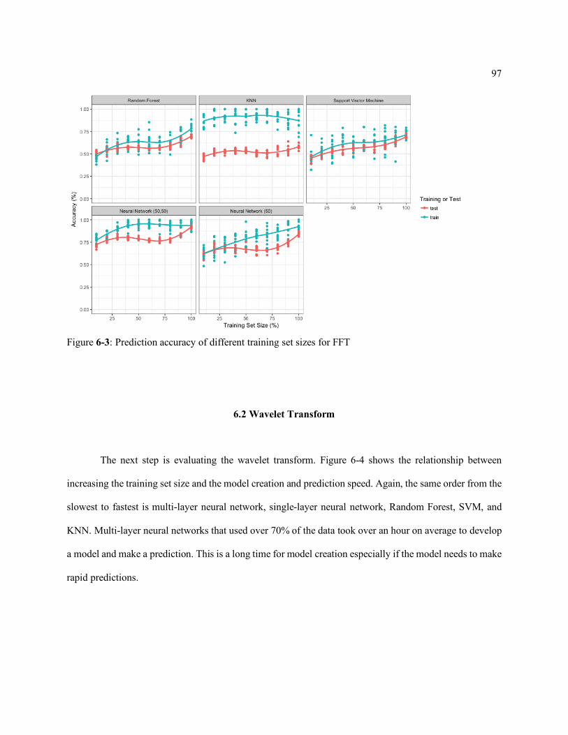
97
6.2 Wavelet Transform
The next step is evaluating the wavelet transform. Figure 6-4 shows the relationship between
increasing the training set size and the model creation and prediction speed. Again, the same order from the
slowest to fastest is multi-layer neural network, single-layer neural network, Random Forest, SVM, and
KNN. Multi-layer neural networks that used over 70% of the data took over an hour on average to develop
a model and make a prediction. This is a long time for model creation especially if the model needs to make
rapid predictions.
Figure 6-3: Prediction accuracy of different training set sizes for FFT

98
Figure 6-5 shows the accuracy of predicting the status of wind turbines in both the training and
testing set. Random Forest was a dramatic improvement from Fourier transform with a 20% increase in
accuracy. The same KNN and SVM accuracy trends were common between Fourier and Wavelet. Both
neural networks improved over their Fourier counterparts. The most accurate model was still multi-layer
neural network then the single layer neural network closely followed by the Random Forest.
Figure 6-4: Speed of model creation and prediction for wavelet transform

99
Using the data from the Department of Energy – National Renewable Energy Laboratory,
algorithms which used Wavelet transform as their signal processing method were more accurate than
algorithms which used Fourier transform. This supports other similar research findings and the common
usage of Wavelet transforms over Fourier in gearbox health prediction research. The next section will
switch from focusing on health prediction in functional obsolescence to life cycle prediction in functional
obsolescence. The case study in Chapter 7 will introduce the life-cycle and cost tradeoff framework and
seeks to apply it to a gear in an industrial gearbox.
Figure 6-5: Prediction accuracy of different training set sizes for wavelet transform

100
Chapter 7
Life Cycle and Cost Tradeoff Framework
In this chapter, the life cycle and cost tradeoff framework is applied to a case study of a gear. This
chapter outlines the information flow diagram and then shows how the required machine learning models
are generated from preexisting models commonly found in many organizations. The results of the case
study are also presented and discussed.
The case study makes use of an industrial gear within a gear box found in agricultural machinery.
As requested by an industry partner, the data in this chapter has been randomized to conceal proprietary
industry knowledge, while still allowing for real data to be used for the analysis.
The machine learning models and overall application programming interface (API) for the case
study is implemented using the architecture outlined in Figure 3-7 using the programming language Python
3.3.7 and Amazon Web Services EC2 t2.micro server instance [87], [88].
7.1 Information Flow Model
The first step in the life cycle and cost tradeoff framework is mapping the information flow needed
to run all of the required models. A list of all the required outputs from each model needed to conduct the
life cycle and cost tradeoff is generated. The first step is to define the models needed to predict these values.
Often these models already exist in organizations, but not in a form that is friendly to genetic search
optimization. Next, the required inputs for each of these models need to be defined. Once this is completed,
a flowchart of the information is created. For the gear case study, the flowchart of information is shown in
Figure 7-1.

101
As shown in Figure 7-1, the inputs for the life cycle estimation model are categorized into three
groups: (1) manufacturing attributes, (2) usage attributes, and (3) life prediction. The manufacturing
attributes are surface roughness and residual stress. The usage metrics are speed of rotation, torque,
misalignment from other gears, center distance from other gears, and axial offset from other gears. For the
cost model, the following variables are required: manufactured unit cost, operational and spare units
produced, spare units produced, usage hours per month, replacement time, shop visit cost, and cost
escalation rate per year.
During the information flow planning phase, if there are too many input variables, then variable
reduction techniques can be borrowed from statistics and machine learning to reduce input variables to
those that have statistically significant effects on the outputs. The following section discusses how the
machine learning models are generated from traditional industry models.
Figure 7-1: Information Flow for Life cycle vs. Cost Tradeoff for the Gear Case Study

102
7.2 Model Generation
Many traditional prediction models are simulations that take many minutes to run. Due to the high
rate of predictions each of these models will be required to conduct in the genetic search algorithm,
traditional industry models (Monte Carlo Excel spreadsheets and other computer simulations) will not have
the prediction speed required to make thousands of predictions for hundreds of generations. Machine
learning models are well suited as approximations of the traditional industry models because the prediction
speed is much faster. Another reason machine learning approximation models are more appropriate than
the traditional models is the relative ease of putting the machine learning model on a cloud-based server for
an API. The ability to quickly develop the machine learning model into an open API increases the ability
to create cloud-based dashboards and other real-time predictions.
The first model is the life cycle model. The life cycle model is a physics-based simulation that
simulates the gear usage and estimates when cracks will develop in the gear. After many simulations, rather
than predict a single point like most regression models, the life cycle model outputs a distribution. The
distribution is a Weibull distribution, which is common in life cycle predictions because of its similarities
to a Normal distribution, but, unlike Normal distributions, never allowing an output below zero (this is
optimal for predicting time, which cannot be negative). The Weibull distribution is defined by two
parameters: (1) scale and (2) slope. Using the physics-based simulations, many instances can be run (each
of these instances takes between 5-20 hours). The model inputs and the resulting Weibull parameters are
recorded. This data becomes the training set for the machine learning approximation model. The machine
learning approximation model is generated by first fitting a single regression model to predict the scale in
the Weibull distribution and then fitting a second model with the output of the slope in the Weibull. For
the gear case study, a neural network with two outputs could have achieved a similar result, but for
simplicity, this was done with two independent models.
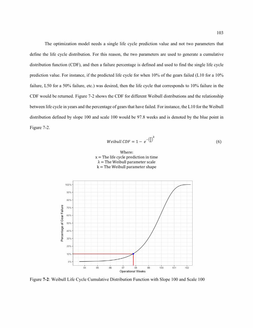
103
The optimization model needs a single life cycle prediction value and not two parameters that
define the life cycle distribution. For this reason, the two parameters are used to generate a cumulative
distribution function (CDF), and then a failure percentage is defined and used to find the single life cycle
prediction value. For instance, if the predicted life cycle for when 10% of the gears failed (L10 for a 10%
failure, L50 for a 50% failure, etc.) was desired, then the life cycle that corresponds to 10% failure in the
CDF would be returned. Figure 7-2 shows the CDF for different Weibull distributions and the relationship
between life cycle in years and the percentage of gears that have failed. For instance, the L10 for the Weibull
distribution defined by slope 100 and scale 100 would be 97.8 weeks and is denoted by the blue point in
Figure 7-2.
}I"A~``&�Ä = 1 −IJÅÇλÑÖ
(6)
Where:x=Thelifecyclepredictionintimeλ=TheWeibullparameterscalek=TheWeibullparametershape
Figure 7-2: Weibull Life Cycle Cumulative Distribution Function with Slope 100 and Scale 100

104
These two prediction models were paired together in a single programable function that took
surface roughness, residual stress, speed of rotation, torque, misalignment from other gears, center distance
from other gears, and axial offset from other gears, and the failure percentage (L10, L50, etc.) as inputs and
then output a single life cycle prediction for when X percentage of gears have failed.
The second model is the cost model. This model is a complex Monte Carlo Excel spreadsheet.
Since the model runs in Excel, it is takes about 10-20 minutes to run the cost analysis. It can easily call the
genetic search algorithm. Many different scenarios were run in the Excel cost model and the input settings
and resulting outputs were recorded. A machine learning model was then trained to predict the output of
total cost of ownership for 15 years using the life cycle inputs defined in Figure 7-1.
The resulting life cycle model was input into a function and placed on a server where users could
send different input parameters and receive a life cycle prediction estimate. Both the life cycle and cost
functions had a prediction speed under 0.1 seconds. This is a large improvement over the prediction times
of 5-20 hours and 10-20 minutes of the original life cycle and cost functions, respectfully.
7.3 Genetic Search Optimization Results
After the prediction functions were generated, validated for accuracy, and placed on a server, the
next step was integrating the functions into the genetic search algorithm. For this tradeoff framework, there
are two potential ways of setting up the optimization problem. The first is to minimize cost while
maintaining a given life, and the second is to maximize life while maintaining a given cost. An example of
the first approach to setting up the problem can be seen in Table 7-1. The user defines the rank limits for
all numeric inputs and categories for all categorical variables. Then, a number is randomly generated within
the range or a category is selected from the list of categories. This is repeated until an entire population of

105
guesses are generated to form a first-generation population for the genetic search algorithm for this case
study. For this case study, each generation has 5,000 guesses.
All the randomly generated inputs were run through both functions, and the life cycle and cost
estimations are returned. Table 7-1 shows the numbered guesses with randomly generated inputs and
outputs (life and cost) in the right columns. All resulting life cycle predictions under the desired life of 20
are removed and were not be used to produce the second generation. The remaining guesses with life cycles
greater or equal to 20 were then used to weight the probability the guess will be used in the next generation.
This weight is generated by giving the lowest cost guess having the highest weight or highest probability
to reproduce for the next generation. The weight for optimizing life is generated by taking a percentage of
the life prediction of the sum of the life predictions. This gives guesses with longer life predictions a greater
weight and therefore a greater chance of being selected to parent the second generation.
Table 7-1: Genetic Search Algorithm Population with a Required Life of 20

106
The next generation was generated by including the top 100 lowest cost guesses with life cycle
greater than or equal to 20. Then, by randomly selecting two guesses from the previous generation using
the weight probabilities and randomly picking between each guess attribute, a new guess is created (e.g.,
select one guess surface roughness and then another’s residual stress). This is repeated until 2900 guesses
are generated. Then to keep the population for each generation at 5000, 2000 additional guess were
randomly generated using the limit method of the first generation. This was repeated for 150 generations.
The population after 150 generations can be seen in Figure 7-3. Figure 7-3 compares the
relationship between cost and life cycle. The vertical dashed line represents the constraint requirement for
a life cycle of 20 with the red points not meeting this requirement. It can be seen that as the life cycle
increases, the price largely remains constant between $50,000 to $100,000, but after a life cycle of 24, the
cost begins to grow rapidly, with even one solution having a life cycle of over 28 and a cost over $450,000.
This relationship shows how as organizations reach for longer life products with “higher-quality”, the cost
also increases.
Also, because not all randomly generated guesses are possible due to manufacturing constraints
and other real-world business factors, the top 25 guesses are returned. This is to prevent the possibility of a
single optimal solution being infeasible and gives the users more options from which to choose. The blue
points in Figure 7-3 show the 25 best guesses in terms of meeting the life requirement and minimizing costs.
The average cost of the returned guesses is $24,438.79 and an average life cycle of 21.4. The average cost
of all guesses that meet the requirement of life cycle bigger than 20 is $78,253.58 and an average life cycle
of 22.5. This means the returned results are on average 68.8% less than the rest of the population that meets
the life cycle constraint. This can correspond to large cost savings for organizations.
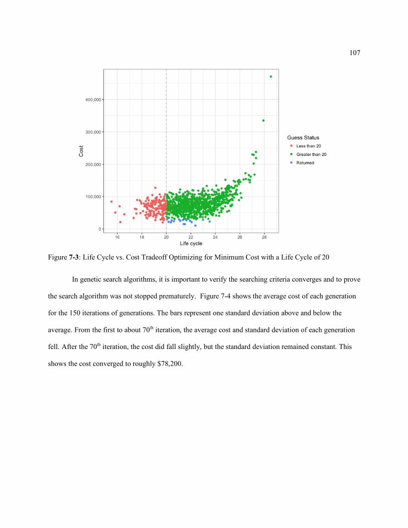
107
In genetic search algorithms, it is important to verify the searching criteria converges and to prove
the search algorithm was not stopped prematurely. Figure 7-4 shows the average cost of each generation
for the 150 iterations of generations. The bars represent one standard deviation above and below the
average. From the first to about 70th iteration, the average cost and standard deviation of each generation
fell. After the 70th iteration, the cost did fall slightly, but the standard deviation remained constant. This
shows the cost converged to roughly $78,200.
Figure 7-3: Life Cycle vs. Cost Tradeoff Optimizing for Minimum Cost with a Life Cycle of 20

108
The second variable of interest is the life cycle over these iterations. Figure 7-5 shows the average
life cycle and standard deviation changes for each of the 150 generation iterations. Again, at around the
60-70th iteration, the average life cycle per generation stopped changing at around 22. It makes sense both
the cost and life cycle stop changing around the same iteration because the algorithm found an area that
gave optimal solutions to this problem. Since options with better costs could not be found, the options did
not change, and therefore the life cycle of the optimal cost options did not change. For this reason, both
life cycle and cost stopped improving and reached convergence at the same iteration.
Figure 7-4: Life Cycle vs. Cost Tradeoff Model Cost Convergence Over 150 Iterations of the Genetic Search to Minimize Cost

109
The second way to set up the problem is to maximize life cycle while maintaining a given cost. For
this case study, the desired cost is $80,000. After 150 generations, Figure 7-6 shows the results. Again, the
dashed gray line presents the constraint requirement of a minimum cost of $80,000. Like Figure 7-3, the
green and the blue points are the feasible points because these points meet the requirements. The top 25
guesses are returned to the user. The returned values have an average life cycle of 24.72 and average cost
$67,394.75, while all the guesses that meet the desired cost have an average life cycle of 21.6 and average
cost of $61,193.55. The returned values have a 14.4% higher life cycle than the other guess that meets the
cost constraint with only a 10% average increase in cost. These results would allow the organization to
increase the life of the products with a smaller increase in cost.
Figure 7-5: Life Cycle vs. Cost Tradeoff Model Life Cycle Convergence Over 150 Iterations of the Genetic Search to Minimize Cost

110
Figure 7-6: Life Cycle vs. Cost Tradeoff Optimizing for Maximum Life Cycle with a Cost of $80,000
Figure 7-7: Life Cycle vs. Cost Tradeoff Model Cost Convergence Over 150 Iterations of the Genetic Search to Minimize Life Cycle
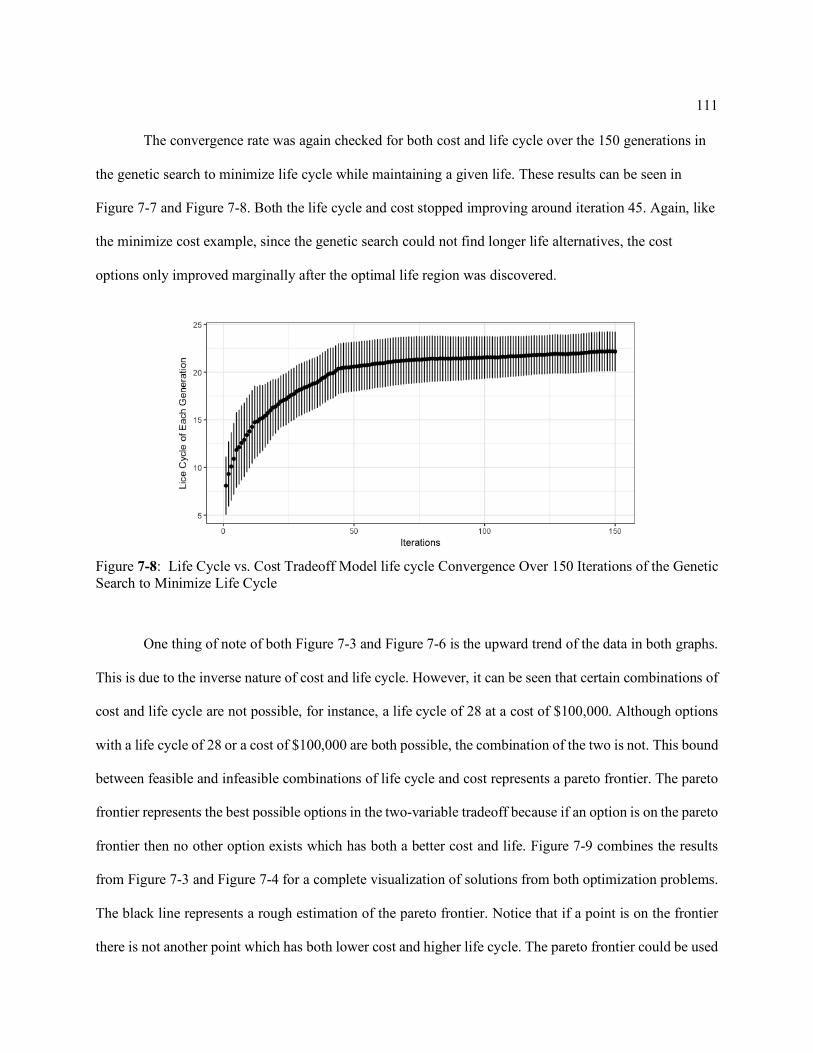
111
The convergence rate was again checked for both cost and life cycle over the 150 generations in
the genetic search to minimize life cycle while maintaining a given life. These results can be seen in
Figure 7-7 and Figure 7-8. Both the life cycle and cost stopped improving around iteration 45. Again, like
the minimize cost example, since the genetic search could not find longer life alternatives, the cost
options only improved marginally after the optimal life region was discovered.
One thing of note of both Figure 7-3 and Figure 7-6 is the upward trend of the data in both graphs.
This is due to the inverse nature of cost and life cycle. However, it can be seen that certain combinations of
cost and life cycle are not possible, for instance, a life cycle of 28 at a cost of $100,000. Although options
with a life cycle of 28 or a cost of $100,000 are both possible, the combination of the two is not. This bound
between feasible and infeasible combinations of life cycle and cost represents a pareto frontier. The pareto
frontier represents the best possible options in the two-variable tradeoff because if an option is on the pareto
frontier then no other option exists which has both a better cost and life. Figure 7-9 combines the results
from Figure 7-3 and Figure 7-4 for a complete visualization of solutions from both optimization problems.
The black line represents a rough estimation of the pareto frontier. Notice that if a point is on the frontier
there is not another point which has both lower cost and higher life cycle. The pareto frontier could be used
Figure 7-8: Life Cycle vs. Cost Tradeoff Model life cycle Convergence Over 150 Iterations of the Genetic Search to Minimize Life Cycle

112
to find the optimal solutions to the life cycle and cost tradeoff and users could select the optimal solution
from the frontier that fits the requirements. Future research should be done to explore the possible pareto
frontier of this case and future Life Cycle vs. Cost Tradeoff model case studies.
With 5000 guesses in each generation and 150 generations, the genetic search algorithms evaluate
hundreds of thousands of possible configurations for the gear and returns a list of best possible results.
The entire search takes between 5-15 minutes. This would be impossible for a human to reproduce
manually. The machine learning approximation models also allow the knowledge from more complex
simulation-based models (such as physics-based simulations and Excel Monte Carlo simulations) to be
encoded into faster and easier to use models. For this reason, hundreds of thousands of scenarios are able
to be evaluated in minutes while the traditional models took 5-20 hours and 10-20 minutes for a single
evaluation.
Figure 7-9: Pareto Frontier of Solutions from Figure 7-3 and Figure 7-6

113
Chapter 8
Conclusions and Future Work
The goal in this dissertation is to explore how machine learning-based obsolescence forecasting
can be utilized to forecast both technical and functional obsolescence to help minimize costs associated
with obsolescence mitigation. Technical obsolescence is defined as a product no longer being competitive
based on its specifications and often occurs when newer models are introduced to the market. Functional
obsolescence occurs when a product no longer can perform its intended function. The motivation to improve
obsolescence forecasting methods is based on the need for accurate time and risk predictions in economic
analyses. This section discusses how this dissertation improves these forecasting methods and discusses
how these improvements can be utilized in future work.
Three limitations for why technical obsolescence forecasting models are not more widely used in
industry were presented in Section 2.1.4: (1) requirement of monthly sales data, (2) requiring manual human
input or expert opinion, and (3) only being capable of modeling the changes of one specification (e.g.,
memory or transistors per square inch). Currently, technical obsolescence forecasting models often are
hindered by one or more of these limitations, making industry adoption limited. Both of the technical
obsolescence forecasting methods presented in this dissertation, the Obsolescence Risk Forecasting using
Machine Learning (ORML) and Life Cycle Forecasting using Machine Learning (LCML), improve on the
previous limitations by:
1) Requiring no sales data but instead data mining relationships from specification changes
from older and newer products in a market.
2) Requiring no manual human input or expert opinion by only relying on technical
specifications of products as inputs to machine learning algorithms, thereby increasing the repeatability of
obsolescence predictions.
3) Capable of modeling the changes of more than one specification over time.

114
These advances greatly increase the usability of the ORML and LCML frameworks and increase
the chance of industrial adoption of technical obsolescence forecasting methods.
The ORML was applied in three industrial markets, including case studies based on cell phones,
digital cameras, and digital screens for handheld electronics. Each of the three case studies used
specifications from the products in the market and the current market availability (if the product is currently
being manufactured) as inputs into a machine learning algorithm to generate a model to predict the
obsolescence status (i.e., market availability). In the case studies, four machine learning algorithms were
tested: (1) random forest, (2) neural networks, (3) support vector machines, and (4) k nearest neighbors.
For the cell phone case study random forest was the most accurate and was able to correctly predict if the
product would be available in the market with 92.56% accuracy. For the digital camera case study, support
vector machine was the most accurate and was able to correctly predict if the product would be available
in the market with 93.49% accuracy. For the digital screen case study, neural networks were the most
accurate and was able to correctly predict if the product would be available in the market with 76.96%
accuracy.
Additionally, a case study was conducted in the cell phone market to predict the accuracy of the
LCML method. Three machine learning algorithms were used: (1) random forest, (2) neural networks, and
(3) support vector machines. The most accurate was support vector machine, which achieved a mean
squared error of 0.36. The LCML method was then benchmarked against two of the most prominent life
cycle forecasting methods (Sandborn 2005 [8] and Ma and Kim 2017 [23]) using the standard data set of
flash memory. The results demonstrated that LCML had the best accuracy out of the three methods with a
mean error of 1.112 years.
Although many machine learning algorithms were applied to both ORML and LCML, no single
algorithm was markedly better than all others. All algorithms were able to make fast and accurate
predictions, even when comparing the best algorithm to the worst algorithm for a given case study. For this
reason, it is difficult to say one algorithm will produce a faster or more accurate output and the small

115
difference between algorithms was largely noise and did not signal a supreme algorithm. However, during
the data cleaning and preprocessing, one algorithm did stand out. Random Forest was able to handle both
categorical variables and numeric variables and therefore required very little data processing. While neural
networks, support vector machines, and k nearest neighbors required categorical variables be converted into
numeric/binary dummy variables. This took additional preparation time over Random Forest and for this
reason, the recommendation from this dissertation would be to first model ORML or LCML using random
forest because it is the fastest model to get working from a data preprocessing perspective.
When converting an obsolescence risk level into an obsolescence status of discontinued or still
manufactured, false positives and false negatives often have differing cost implications for organizations.
For this reason, Section 3.2 presented a mathematical model to control for the differences in these costs.
The model adjusts the risk cutoff threshold between the discontinued or still manufactured statuses to
increase the likelihood of less costly errors while decreasing the rate of more costly errors. This tradeoff
allows for the lowering of the average expected error cost per prediction. In Chapter 5, the mathematical
model is applied in three markets: cell phones, digital cameras, and digital screens for handheld electronics.
The cell phone case study found a 6.5% drop in the expected error cost of a prediction with only a 1.5%
drop in accuracy. The digital camera case study found a 20.1% drop in the expected error cost of a prediction
with only a 0.54% drop in accuracy. The digital screen case study found a 2.295% drop in the expected
error cost of a prediction with only a 0.12% drop in accuracy.
The mathematical model outlined in Section 3.2 and applied in Chapter 5 is not only a contribution
to the field of obsolescence forecasting, but machine learning as a whole. This is because any binary
classifier which outputs a probability instance is in either class and that has different costs for Type 1 and
Type 2 errors could use this mathematical model to find an optimal cut off threshold to minimize the
expected cost impact of misclassified instances. This could be used in most applications which use ROC
curves (e.g. fraud detection, disease detection, fault detection, and obsolescence forecasting). Additionally,
the observation that the ratio of the misclassification costs and not the individual magnitude of the

116
misclassification costs is the driving factor in determining the optimal cut off threshold between classes is
a large theoretical contribution to the field because it allows practitioners to estimate the ratio of the cost
rather than conduct a full economic analysis estimate. The ratio estimation method is outlined in Section
3.2.
The other type of obsolescence forecasting investigated in this research was functional
obsolescence. A case study on predicting the health of status wind turbine engines using acoustic emission
sensors was conducted to compare machine learning algorithms and Fourier and Wavelet transforms as
sensor processing methods. Neural network, random forest, K nearest neighbors, and support vector
machines were all tested as possible algorithms. Neural networks were the most accurate algorithm closely
followed by random forest. Wavelet transform always outperformed Fourier transform as a sensor
preprocessing method.
The last contribution of this dissertation is the combining of an obsolescence model with a cost
model to develop a decision support method for life cycle verse cost tradeoffs. The first iteration of the
framework presented a flow of information and data from sub-models, such as manufacturing models, life
cycle models, and cost models. The chaining of the input and outputs of these models created a framework
where users could specify manufacturing requirements and usage information, and the estimated life cycle
and cost throughout the product’s life would be returned. After the framework of standardized inputs and
outputs was created, a genetic optimization algorithm was proposed because of the feature of genetic
optimization to compute a set of optimal approximations rather than one global optimal. The framework
allowed users to define a target life cycle and then minimize the cost or define a desired cost and maximize
the life cycle of a given product. The genetic algorithm returns the top few numbers of possible attributes
to the user and the user (design engineers, manufacturing engineering, etc.) could select the most viable
option. A potential improvement on this method and area for additional research would be to apply a
stochastic optimization approach that could account for the distributions outputted from the models and not
just a single number.

117
Future work should be done to integrate obsolescence risk forecasting techniques into commercial
component databases (see Section 2.1.5 for discussion of current state of commercial databases). Currently
these databases have massive amounts of components with data and estimated obsolescence date supplied
by manufacturers. These databases could be leveraged to help predict the obsolescence date of products
where the manufacturer either refuses to supply a date or when a prediction has not yet been requested. In
both of these cases, the companies maintaining commercial component databases could greatly expand
capabilities by integrating the methods discussed in this dissertation.
Currently much of the technical obsolescence forecasting is focused on forecasting the
obsolescence of components within products to help minimize scarcity of suppliers and reduce production
and supply chain problems. However, this is approaching obsolescence from a purchaser’s perspective. If
obsolescence forecasting was applied from the seller’s perspective, obsolescence forecasting could be used
as a market research tool. It could be used to filter different future product designs to see how long each
will stay technically competitive in the market and even to reverse engineer the models to find which
specifications are most important in determining life cycle and obsolescence risk. These key specifications
could be fed to designers to help improve designs, similar to market research or benchmarking.
In this dissertation, the algorithms selected for obsolescence forecasting were standard machine
learning methods. Future work should be done to test the possibility of using ensemble learning algorithms
to generate the forecasting models. Ensemble learning combines multiple machine learning algorithms and
takes the output of each then combines these into one single output. Since the ensemble model is made up
of many different modeling types, the disadvantages of each individual algorithm can be minimized because
each model has different errors over the same data set. The resulting average output is a combination of
each modeling type and because of this ensemble learning can often result in more accurate and robust
models. For this reason, future work should be conducted to benchmark ensemble learning methods against
the methods described in this dissertation.

118
During the analysis of the results from the Life Cycle vs. Cost Tradeoff model case study, a Pareto
Frontier is observed. The frontier represents the outer most limit to tradeoff between life cycle and cost.
Future research should be conducted to investigate this phenomenon in the gear case study, but also other
case studies of the Life Cycle vs. Cost Tradeoff model. The Pareto Frontier could be used by organization
to verify a chosen solution is on the frontier and therefore an optimal combination. Additionally, a Pareto
Frontier would allow other optimization methods, other than a genetic search algorithm, to be applied to
the Life Cycle vs. Cost Tradeoff model.
Finally, the ideas of this dissertation were born out of a need for more robust obsolescence
forecasting techniques to help conduct economic analysis. Future work should be conducted to combine
the obsolescence forecasting techniques presented in this dissertation with obsolescence cost models and
other economic analysis research that are currently hindered from being applied in industry due to a lack of
reliable and scalable obsolescence forecasting models.

119
References
[1] P. A. Sandborn, “Software obsolescence - Complicating the part and technology obsolescence
management problem,” IEEE Trans. Components Packag. Technol., vol. 30, no. 4, pp. 886–888,
2007.
[2] R. Solomon, P. Sandborn, and M. Pecht, “Electronic Part Life Cycle Concepts and Obsolescence
Forecasting,” IEEE Trans. Components Packag. Technol., vol. 23, no. 1, pp. 190–192, 2000.
[3] P. Singh and P. Sandborn, “Obsolescence Driven Design Refresh Planning For Sustainment-
Dominated Systems,” The Engineering Economist, vol. 51, no. 2, pp. 1–16, 2006.
[4] K. Ishii, B. H. Lee, and Eubanks, “Design for product retirement and modularity based on
technology life-cycle,” Manuf. Sci. Eng., vol. Vol 42, no. 1, pp. 695–706, 1995.
[5] K. Ishii, “Product Modularity: a Key Concept in Life-Cycle Design,” in Frontiers of Engineering:
Reports on Leading Edge Engineering from the 1996 NAE Synposium on Frontiers of
Engineering, pp. 17–35.
[6] “Atari 800 Advertisement from 1979,” Merchandising, vol. 4, no. 1, 1979. pp. 55.
[7] P. Sandborn, F. Mauro, and R. Knox, “A data mining based approach to electronic part
obsolescence forecasting,” IEEE Trans. Components Packag. Technol., vol. 30, no. 3, pp. 397–
401, 2007.
[8] P. Sandborn, F. Mauro, and R. Knox, “A data mining based approach to electronic part
obsolescence forecasting,” Proc. 2005 Diminishing manufacturing sources and material shortages
(DMSMS) Conference, pp. 397-401.
[9] E. Menipaz, “An Inventory Model with Product Obsolescence and its Implications for High
Technology Industry,” IEEE Trans. Reliab., vol. 35, no. 2, pp. 185–187, 1986.

120
[10] V. J. Prabhakar and P. Sandborn, “A Part Total Cost of Ownership Model for Long Life Cycle
Electronic Systems,” Int. J. Comput. Integr. Manuf., vol. 25, no. 5, pp. 384–397, 2012.
[11] A. Kleyner and P. Sandborn, “Minimizing life cycle cost by managing product reliability via
validation plan and warranty return cost,” International Journal of Production Economics, vol.
112, no. 2, pp. 796–807, 2008.
[12] C. Jennings and J. P. Terpenny, “Taxonomy of Factors for Lifetime Buy,” in Proceedings of the
2015 Industrial and Systems Engineering Research Conference, 2015, pp. 430-436.
[13] L. Zheng and J. Terpenny, “A hybrid ontology approach for integration of obsolescence
information,” Comput. Ind. Eng., vol. 65, no. 3, pp. 485–499, 2013.
[14] L. Zheng, J. Terpenny, R. Nelson III, and P. Sandborn, “Ontology-Based Knowledge
Representation for Product Life Cycle Concepts and Obsolescence Forecasting,” IIE Annu. Conf.
Proc., vol. 13, March 2013, pp. 1–8.
[15] R. C. Stogdill, “Dealing with obsolete parts,” IEEE Des. Test. Comput., vol. 16, no. 2, pp. 17–25,
1999.
[16] P. Sandborn, V. Prabhakar, and O. Ahmad, “Forecasting electronic part procurement lifetimes to
enable the management of DMSMS obsolescence,” Microelectron. Reliab., vol. 51, no. 2, pp.
392–399, 2011.
[17] E. Payne, “DoD Diminishing manufacturing sources and material shortages (DMSMS)
Conference,” Keynote address, in DMSMS Conference, 2006.
[18] C. Josias, J. P. Terpenny, and K. J. McLean, “Component obsolescence risk assessment,” Proc.
2004 Ind. Eng. Res. Conf., vol. 15, pp. 2–7, 2004.
[19] C. L. Josias, “Hedging future uncertainty: A framework for obsolescence prediction, proactive
mitigation and management,” ProQuest Disertation & Theses - University of Massachusetts -
Amherst, February 2009.
[20] W. Van Jaarsveld and R. Dekker, “Estimating obsolescence risk from demand data to enhance

121
inventory control - A case study,” Int. J. Prod. Econ., vol. 133, no. 1, pp. 423–431, 2011.
[21] F. J. Romero Rojo, R. Roy, and E. Shehab, “Obsolescence management for long-life contracts:
State of the art and future trends,” Int. J. Adv. Manuf. Technol., vol. 49, no. 9–12, pp. 1235–1250,
2010.
[22] J. W. H. Custers, “Cost Analysis of Electronic Systems: Chapter 1,” World Scientific Series in
Advanced Integration and Packaging – Vol. 4 pp. 1–12, 2001.
[23] J. Ma and N. Kim, “Electronic part obsolescence forecasting based on time series modeling,” Int.
J. Precis. Eng. Manuf., vol. 18, no. 5, pp. 771–777, 2017.
[24] P. Spicer, Y. Koren, M. Shpitalni, and D. Yip-Hoi, “Design principles for machining system
configurations,” CIRP Ann.-Manuf. Technol., vol. 51, no. 1, pp. 275–280, 2002.
[25] C. Jennings, D. Wu, and J. Terpenny, “Forecasting obsolescence risk and product life cycle with
machine learning,” IEEE Transactions on Components, Packaging and Manufacturing
Technology, vol. 6, no. 9, 2016, pp. 1428-1439.
[26] “IHS CAPS Universe,” IHS.com, Accessed 1/22/2016.
[27] “Parts Plus,” Home.TotalPartsPlus.com, Accessed 1/22/2016.
[28] “Home,” Avcom-DMSMS.com, Accessed 1/23/2016.
[29] “QTEC Solutions: Q-Star,” QTEC.us, Accessed 1/22/2016.
[30] C. Cortes and M. Mohri, “AUC Optimization vs. Error Rate Minimization.,” NIPS 2003
Proceedings of the 16th International Conference on Neural Information Processing Systems, pp.
313–320.
[31] L. Breiman, J. H. Friedman, R. A. Olshen, and C. J. Stone, Classification and Regression Trees,
1st Edition 1984, pp. 250-254.
[32] P. M. Ridker, “Clinical application of C-reactive protein for cardiovascular disease detection and
prevention,” Circulation, vol. 107, no. 3, pp. 363–369, 2003.
[33] E. Nagel, C. Klein, I. Paetsch, S.Hettwer, B. Schnackenburg, K. Wegscheider, and E. Fleck,

122
“Magnetic resonance perfusion measurements for the noninvasive detection of coronary artery
disease,” Circulation, vol. 108, no. 4, pp. 432–437, 2003.
[34] C. E. Metz, “ROC Methodology in Radiologic Imaging,” Invest. Radiol., vol. 21, no. 9, pp. 720–
733, 1986.
[35] W. J. Catalona, A. W. Partin, K. M. Slawin, M. K. Brawer, R. C. Flanigan, A. Patel, J. P. Richie, J.
B. deKernion, P. C. Walsh, P. T. Scardino, P. H. Lange, E. N. Subong, R. E. Parson, G. H. Gasior,
K. G.Loveland, and P. C. Southwick. “Use of the percentage of free prostate-specific antigen to
enhance differentiation of prostate cancer from benign prostatic disease: a prospective multicenter
clinical trial,” The Journal of the American Medical Association, vol. 279, no. 19, pp. 1542–1547,
1998.
[36] J. Havrilesky, C. M. Whitehead, J. M. Rubatt, R. L. Cheek, J. Groelke, Q. He, D. P. Malinowski,
T. J. Fischer, and A. Berchuck.“Evaluation of biomarker panels for early stage ovarian cancer
detection and monitoring for disease recurrence,” Gynecol. Oncol., vol. 110, no. 3, pp. 374–382,
2008.
[37] N. Houssami, S. Ciatto, P. Macaskill, S. J. Lord, R. M. Warren, J. M. Dixon, and L.
Irwig,“Accuracy and surgical impact of magnetic resonance imaging in breast cancer staging:
Systematic review and meta-analysis in detection of multifocal and multicentric cancer,” J. Clin.
Oncol., vol. 26, no. 19, pp. 3248–3258, 2008.
[38] M. Boeri, C. Verri, D. Conte, L. Roz, P. Modena, F. Facchinetti, E. Calabrò, C. M. Croce, U.
Pastorino, and G. Sozzia, “MicroRNA signatures in tissues and plasma predict development and
prognosis of computed tomography detected lung cancer,” Proc. Natl. Acad. Sci. U. S. A., vol.
108, no. 9, 2011, pp 3713-3718.
[39] T. Tokuda, M. M. Qureshi, M. T. Ardah, S. Varghese, S. A. Shehab, T. Kasai, N. Ishigami, A.
Tamaoka, M. Nakagawa, and O. M. El-Agnaf, “Detection of elevated levels of α-synuclein
oligomers in CSF from patients with Parkinson disease,” Neurology, vol. 75, no. 20, pp. 1766–

123
1772, 2010.
[40] B. S. Garra, M. F. Insana, T. H. Shawker, R. F. Wagner, M. Bradford, and M. Russell,
“Quantitative Ultrasonic Detection and Classification of Diffuse Liver Disease: Comparison with
Human Observer Performance,” Invest. Radiol., vol. 24,no. 3, 1989 pp 196-203.
[41] M. M. Wagner, F.C. Tsui, J.U. Espino, V.M. Dato, D.F. Sittig, R.A. Caruana, L.F. McGinnis,
D.W. Deerfield, M.J. Druzdzel, and D.B. Fridsma, “The Emerging Science of Very Early
Detection of Disease Outbreaks,” J. Public Heal. Manag. Pract., vol. 7, no. 6, 2001, pp. 51-59.
[42] A. Kumar, R. Shankar, A. Choudhary, and L. S. Thakur, “A big data MapReduce framework for
fault diagnosis in cloud-based manufacturing,” Int. J. Prod. Res., vol. 54, no. 23, pp. 7060–7073,
2016.
[43] M. Dellomo, “Helicopter gearbox fault detection: a neural network based approach,” J. Vib.
Acoust., vol. 121, no. July 1999, pp. 265–272, 1999.
[44] D. R. Sawitri, A. Muntasa, K. E. Purnama, M. Ashari, and M. H.Purnomo, “Data Mining Based
Receiver Operating Characteristic (ROC) for Fault Detection and Diagnosis in Radial Distribution
System,” IPTEK Journal for Technology and Science, vol. 20, no. 4, 2009, pp. 155-161.
[45] M. Oberweger, A. Wendel, and H. Bischof, “Visual Recognition and Fault Detection for Power
Line Insulators,” Comput. Vis. Winter Work., 2014.
[46] F. P. García Márquez, A. M. Tobias, J. M. Pinar Pérez, and M. Papaelias, “Condition monitoring
of wind turbines: Techniques and methods,” Renew. Energy, vol. 46, pp. 169–178, 2012.
[47] S. Sharma and D. Mahto, “Condition Monitoring of Wind Turbines: A Review,” Int. J. Sci. Eng.
Res., vol. 4, no. 8, pp. 35–50, 2013.
[48] T. Verbruggen, “Condition Monitoring: Theory and Practice,” Wind Turbine Condition
Monitoring Workshop. Brooming, CO., 2009, pp. 1 -21.
[49] W. Yang, P.J. Tavner, C.J. Crabtree, and M. Wilkinson “Cost Effective Condition Monitoring For
Wind Turbines,” IEEE Trans. Ind. Electron., vol 57 no. 1, 2010, pp. 263-271.

124
[50] B. Lu, Y. Li, X. Wu, and Z. Yang, “A review of recent advances in wind turbine condition
monitoring and fault diagnosis,” Electron. Mach. Wind, vol. 6 no.24, pp. 1–7, 2009.
[51] H. D. M. de Azevedo, A. M. Araújo, and N. Bouchonneau, “A review of wind turbine bearing
condition monitoring: State of the art and challenges,” Renew. Sustain. Energy Rev. vol. 56 April
2016, pp. 368-379.
[52] Z. Hameed, Y. S. Hong, Y. M. Cho, S. H. Ahn, and C. K. Song, “Condition monitoring and fault
detection of wind turbines and related algorithms: A review,” Renew. Sustain. Energy Rev., vol.
13, no. 1, pp. 1–39, 2009.
[53] P. Tchakoua, R. Wamkeue, M. Ouhrouche, F. Slaoui-Hasnaoui, T. A. Tameghe, and G. Ekemb,
“Wind turbine condition monitoring: State-of-the-art review, new trends, and future challenges,”
Energies, vol. 7, no. 4, pp. 2595–2630, 2014.
[54] J. Urbanek, T. Barszcz, and J. Antoni, “Integrated modulation intensity distribution as a practical
tool for condition monitoring.,” Condition Monitoring of Machinery in Non-Stationary
Operations., 1st edition, 2012, pp. 365-373
[55] A. Kusiak and A. Verma, “Analyzing bearing faults in wind turbines: A data-mining approach,”
Renew. Energy, vol. 48, pp. 110–116, 2012.
[56] D. Astolfi, F. Castelliani, and L. Terzi, “Fault prevention and diagnosis through scada temperature
data analysis of an onshore wind farm,” Diagnostyka, vol. 15, no. 2, pp. 71–78, 2014.
[57] O. Uluyol, G. Parthasarathy, W. Foslien, and K. Kim, “Power Curve Analytic for Wind Turbine
Performance Monitoring and Prognostics,” Annu. Conf. Progn. Heal. Manag. Soc., no. August, pp.
1–8, 2011.
[58] S. Kim, I. Ra, and S. Kim, “Design of wind turbine fault detection system based on performance
curve,” The 6th International Conference on Soft Computing and Intelligent Systems, and The
13th International Symposium on Advanced Intelligence Systems, 2012, pp. 20–24.
[59] R. Dupuis, “Application of Oil Debris Monitoring For Wind Turbine Gearbox Prognostics and

125
Health Management,” Annu. Conf. Progn. Heal. Manag. Soc., vol 10, 2010, pp. 45 -53 .
[60] T. Wu, H. Wu, Y. Du, and Z. Peng, “Progress and trend of sensor technology for on-line oil
monitoring,” Sci. China Technol. Sci., vol. 56, no. 12, pp. 2914–2926, 2013.
[61] M. Wevers, “Listening to the sound of materials: Acoustic emission for the analysis of material
behaviour,” Independent Nondestructive Testing and Evaluation., vol. 30, no. 2, pp. 99–106, 1997.
[62] D. Futter, “Vibration monitoring of industrial gearboxes using time domain averaging,”
Proceedings of the Second International Conference on Gearbox Noise, Vibration, and
Diagnostics, ImechE Conference Transaction, 1995, pp. 35-47.
[63] P. D. McFadden, “Examination of a technique for the early detection of failure in gears by signal
processing of the time domain average of the meshing vibration,” Mech. Syst. Signal Process., vol.
1, no. 2, pp. 173–183, 1987.
[64] P. Caselitz and J. Giebhardt, “Fault prediction techniques for offshore wind farm maintenance and
repair strategies,” Proc. EWEC, 2003.
[65] M. Unala, M. Onatb, M. Demetgulc, and H. Kucukc, “Fault diagnosis of rolling bearings using a
genetic algorithm optimized neural network,” Measurement, vol. 58, 2014, pp. 187-196.
[66] Q. Miao, L. Cong, and M. Pecht, “Identification of multiple characteristic components with high
accuracy and resolution using the zoom interpolated discrete Fourier transform,” Meas. Sci.
Technol., vol. 22, no. 5, 2011 pp. 1-12.
[67] P. Shakya, A. K. Darpe, and M. S. Kulkarni, “Bearing damage classification using instantaneous
energy density,” J. Vib. Control, vol. 23, no. 16, 2017 ,pp. 1-41.
[68] Val, “Difference between Fourier transform and Wavelets,”
https://math.stackexchange.com/q/303706. Access 4/20/2018 .
[69] J. H. Suh, S. R. Kumara, and S. P. Mysore, “Machinery fault diagnosis and prognosis: application
of advanced signal processing techniques,” CIRP Ann. Technol., vol. 48, no. 1, pp. 317–320, 1999.
[70] D. Roulias, T. Loutas, and V. Kostopoulos, “A statistical feature utilising wavelet denoising and

126
neighblock method for improved condition monitoring of rolling bearings,” Chem. Eng. Trans.,
vol. 33, no. 1, pp. 1045–1050, 2013.
[71] H. S. Kumar, P. Srinivasa Pai, N. S. Sriram, and G. S. Vijay, “ANN based evaluation of
performance of wavelet transform for condition monitoring of rolling element bearing,” Procedia
Eng., vol. 64, pp. 805–814, 2013.
[72] K. Kourou, T. P. Exarchos, K. P. Exarchos, M. V. Karamouzis, and D. I. Fotiadis, “Machine
learning applications in cancer prognosis and prediction,” Comput. Struct. Biotechnol. J., vol. 13,
pp. 8–17, 2015.
[73] C. S. Tucker, “Fad or here to stay: Predicting product market adoption and longevity using large
scale, social media data,” ASME 2013 International Design Engineering Technical Conferences,
pp. 1–13, 2013.
[74] C. Tucker and H. Kim, “Predicting emerging product design trend by mining publicly available
customer review data,” Proceedings of the 18th International Conference on Engineering Design
(ICED 11), Impacting Society through Engineering Design, Vol. 6: Design Information and
Knowledge, Lyngby/Copenhagen, Denmark, Vol. 6 August, 2011.
[75] R. L. Keeney and H. Raiffa, “Decisions with Multiple Objectives: Preferences and Value Trade-
Offs,” IEEE Trans. Syst. Man Cybern., vol. 9, no. 7, pp. 403-405, 1979.
[76] J. W. Cooley and J. W. Tukey, “An Algorithm for the Machine Calculation of Complex Fourier
Series Author ( s ): James W . Cooley and John W . Tukey Published by : American Mathematical
Society Stable URL : http://www.jstor.org/stable/2003354 REFERENCES Linked references are
available o,” Math. Comput., vol. 19, no. 90, pp. 297–301, 1964.
[77] S. T. S. Bukkapatnam, S. R. T. Kumara, and A. Lakhtakia, “Analysis of acoustic emission signals
in machining,” J. Manuf. Sci. Eng. Trans. ASME, vol. 121, no. 4, pp. 568–575, 1999.
[78] S. V. Kamarthi, S. R. T. Kumara, and P. H. Cohen, “Flank Wear Estimation in Turning Through
Wavelet Representation of Acoustic Emission Signals,” J. Manuf. Sci. Eng., vol 122 no. 1, 1996.

127
[79] L. Breiman, “Random Forest,” Machine Learning, pp. 1–33, 2001.
[80] W. S. McCulloch and W. Pitts, “A logical calculus of the ideas immanent in nervous activity,”
Bull. Math. Biophys., vol. 5, no. 4, pp. 115–133, 1943.
[81] C. Cortes and V. Vapnik, “Support-Vector Networks,” Mach. Learn., vol. 20, no. 3, pp. 273–297,
1995.
[82] J. L. Fix, E., Hodges, “Discriminatory analysis, nonparametric discrimination: Consistency
properties,” in USAF School of Aviation Medicine, Vol. 21 No. 49 1951, pp. 1–10.
[83] R. Zhang and A. Bivens, "Comparing the use of Bayesian networks and neural networks in
response time modeling for service-oriented systems". Proceedings of the workshop on service-
oriented computing performance (pp. 67–74). Monterey, 2007.
[84] U. Sag l̆am, " A two-stage data envelopment analysis model for efficiency assessments of 39
state’s wind power in the United States" Energy Conversion and Management Vol. 146, 2017 pp.
52-67.
[85] R. Vogler, "Illustrated Guide to ROC and AUC" Joy of Data, www.joyofdata.de/blog/illustrated-
guide-to-roc-and-auc/ Accessed 5/13/2016.
[86] S. Sheng, "Wind Turbine Gearbox Vibration Condition Monitoring Benchmarking Datasets"
Department of Energy – National Renewable Energy Laboratory, www.nrel.gov/wind. Accessed
6/18/2017.
[87] Python Softare Foundation, “Python Releases,” Python.org, 2018. Acceseed 2/9/2018.
[88] Amazon Web Services, “Amazon EC2 Instance Types,” Amazon.com, 2018. Acceseed 3/3/2018.

128
Appendix A.
Technical Obsolescence Forecasting Data and Code
For all code and data please go to connorj.github.io/research

129
Appendix B.
Misclassification Error Cost Sensitivity Analysis
Figure B-1: Cost Sensitivity Analysis for Optimal Threshold for Cell phones

130
Table B-1: Optimal Thresholds in Cell phone Error Cost Sensitivity Analysis
Type II Misclassification Cost 1 2 3 4
Type I Misclassification
Cost
1 0.466 0.331 0.266 0.219 2 0.565 0.466 0.344 0.331 3 0.596 0.565 0.466 0.353 4 0.730 0.565 0.565 0.466

131
Figure B-2: Cost Sensitivity Analysis for Optimal Threshold for Cameras

132
Table B-2: Optimal Thresholds in Camera Error Cost Sensitivity Analysis
Type II Misclassification Cost 1 2 3 4
Type I Misclassification
Cost
1 0.433 0.277 0.277 0.197 2 0.487 0.433 0.433 0.277 3 0.864 0.487 0.433 0.433 4 0.864 0.487 0.437 0.433
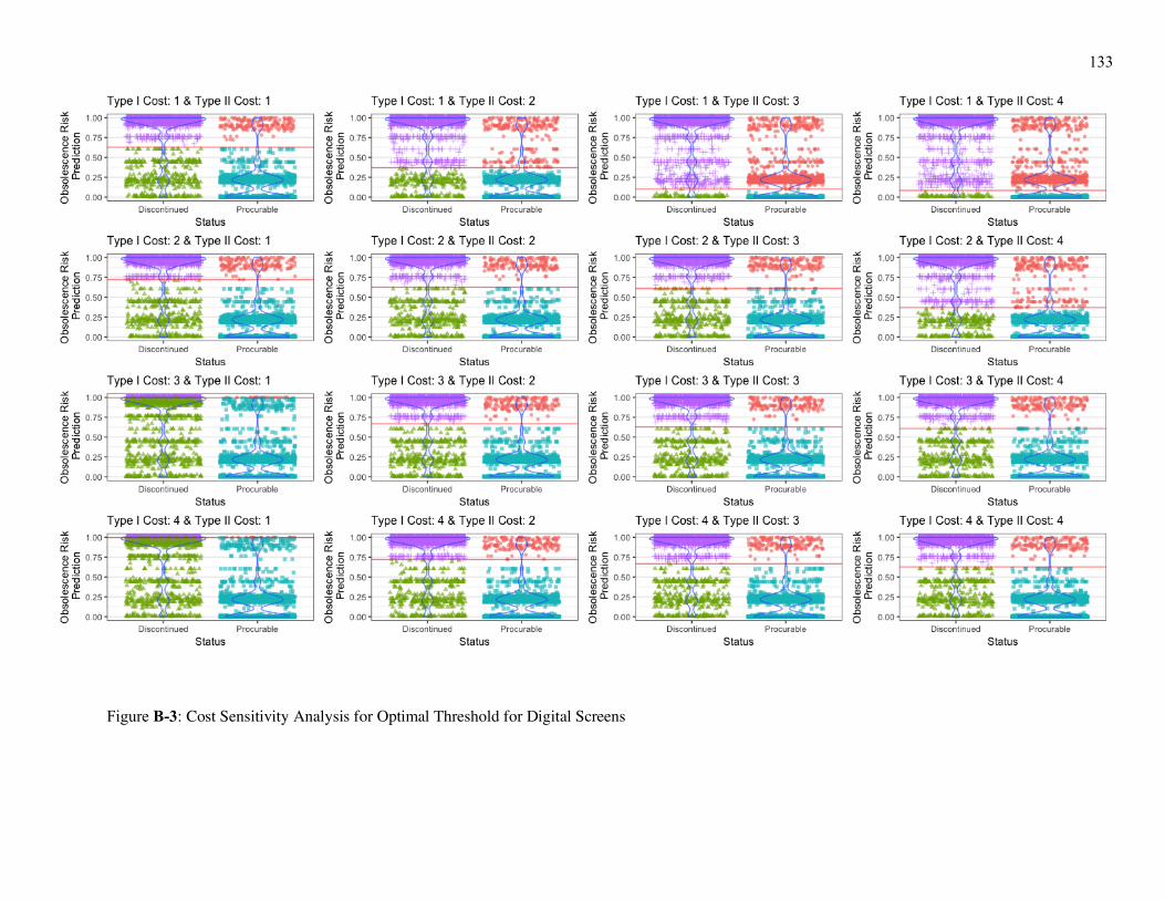
133
Figure B-3: Cost Sensitivity Analysis for Optimal Threshold for Digital Screens

134
Table B-3: Optimal Thresholds in Digital Screens Error Cost Sensitivity Analysis
Type II Misclassification Cost 1 2 3 4
Type I Misclassification
Cost
1 0.628 0.369 0.100 0.084 2 0.721 0.628 0.608 0.369 3 0.997 0.667 0.628 0.608 4 0.997 0.721 0.667 0.628

Connor P. Jennings Leonhard 107 State College, PA • 815-546-6989 • [email protected]
Education 2016 – 2018 The Pennsylvania State University State College, PA
Ph.D. Industrial and Manufacturing Engineering '18 2011 – 2015 Iowa State University of Science and Technology Ames, IA
M.S. Industrial Engineering '15 B.S. Economics '14, B.S. Industrial and Manufacturing Systems Engineering '14
2013-2014 Abu Dhabi Department of Economic Development Abu Dhabi, UAE Study Abroad – Studied the UAE economy and the diversification efforts
Work Experience Wells Fargo & Company – Artificial Intelligence and Machine Learning Group Des Moines, IA Data Scientist 2018-Present
• Developed 7-day cash flow forecasting model for small businesses using machine learning and other ad hoc modeling methods. • Organize and standardize data scientist onboarding procedures to minimize startup time.
Digital Manufacturing and Design Innovation Institute (DMDII) Chicago, IL Visiting Scholar 2018
• Wrote and acquired funding for a National Science Foundation grant to study the flow of research from academia to industry. • Helped further develop government collaboration strategy for the DMDII by identifying and analyzing potential government programs.
The National Science Foundation Center for E-Design State College, PA Graduate Researcher 2013-2018
• Developed Python API using Amazon Web Services to estimate component lifecycle and cost and to find the optimal tradeoff using a combination of genetic search algorithms and machine learning models (e.g. Random Forest and Neural Networks).
• Led Penn State portion of a project with Rolls Royce, John Deere, Boeing, and Sentient Science to analyze the total cost impact of decisions made during the product design and manufacturing planning stages.
• Supported business decision processes by modeling cost projections and other outcomes utilizing Monte Carlo simulation designed and implemented as an Excel add-on.
• Served as a reviewer for the IEEE Transactions on Components, Packaging, Manufacturing Technology and The Journal of Manufacturing Science and Engineering.
Katalyst Surgical, LLC Chesterfield, MO VBA Consultant 2015
• Designed VBA macros to automate sales reports in Excel and allow the company to track individual sales people more effectively. • Reduced preparation time of a weekly report from 2 hours to 15 seconds.
Hy-Vee Inc. West Des Moines, IA Supply Chain Analyst (Senior Design Project) 2014
• Developed a metric for the analysis of inventory levels and included lead-time variations. The metric exposed $1.6 million worth of excess inventory, or 18% of the value the warehouse.
• The reduction in inventory prevented the building of an additional warehouse. NewLink Genetics Ames, IA Financial Planning and Analysis Intern 2014
• Assessed value of products’ pre-market launch by building hybrid models for in-house review. • Supported executive business intelligence distribution using VBA reporting tools to auto-update with email reports.
Amcor Rigid Plastics Ames, IA Student Statistical Analyst 2014
• Developed a method to quantify the precision added in an additional step when measuring thin invisible glass filings on bottle. • Statistically proved the additional step added no precision in the process and saved them more than $50,000.
Selected Publications (for a complete list of publications https://scholar.google.com/citations?user=pmr22ikAAAAJ) (1) Wu, D., Jennings, C., Terpenny, J., Gao R. X., and Soundar Kumara S. “A Comparative Study on Machine Learning Algorithms for
Smart Manufacturing: Tool Wear Prediction Using Random Forests,” Journal of Manufacturing Science and Eng. Vol. 139 No. 7 2017 (2) Jennings, C., Wu, D. and Terpenny, J., “Forecasting Obsolescence Risk and Product Lifecycle with Machine Learning,” IEEE
Transactions on Components, Packaging, Manufacturing Technology. Vol. 6 No. 9, 2016 (3) Jennings, C., Wu, D. and Terpenny, J., “Obsolescence Risk Forecasting using Machine Learning,” 2016 ASME International
Manufacturing Science and Engineering Conference (MSEC) 2016. (4) Jennings, C. and Terpenny, J., “Taxonomy of Factors for Lifetime Buy,” 2015 Industrial and Systems Engineering Research Conference
(ISERC), Nashville, Tennessee, May 30-June 2, 2015 (Invited). Awards and Honors
• DMDII DMC Hackathon – 2nd Place Award (2016) • Alpha Pi Mu – Industrial Engineering Honor Society (2014) • IMSE Senior Design Competition – 2nd Place Award • Capital One SmallBizDev Hackathon NY – Top 20 Finalist (2014)
• CyHack - Iowa State Hackathon – Top 6 Finalist (2014) • Excellence in Statistical Quality – 1st Place Award (2014) • McIlrath Emerging Leadership Scholar (2013) • Elmer Kaser Sophomore Award (2013)
Related Documents