Forecasting Malaysia Bulk Latex Prices Using Autoregressive ...

70

Fu and Suhaila | Malaysian Journal of Fundamental and Applied Sciences, Vol. 18 (2022) 70-81

RESEARCH ARTICLE

Forecasting Malaysia Bulk Latex Prices Using Autoregressive Integrated Moving Average (ARIMA) and Exponential Smoothing Mong Cheong Fua, Jamaludin Suhailaa,b,* a Department of Mathematical Sciences, Faculty of Science, Universiti Teknologi Malaysia, 81310 Johor Bahru, Malaysia; b UTM-Centre for Industrial and Applied Mathematics, Ibnu Sina Institute for Scientific and Industrial Research, Universiti Teknologi Malaysia, 81310 Johor Bahru, Malaysia

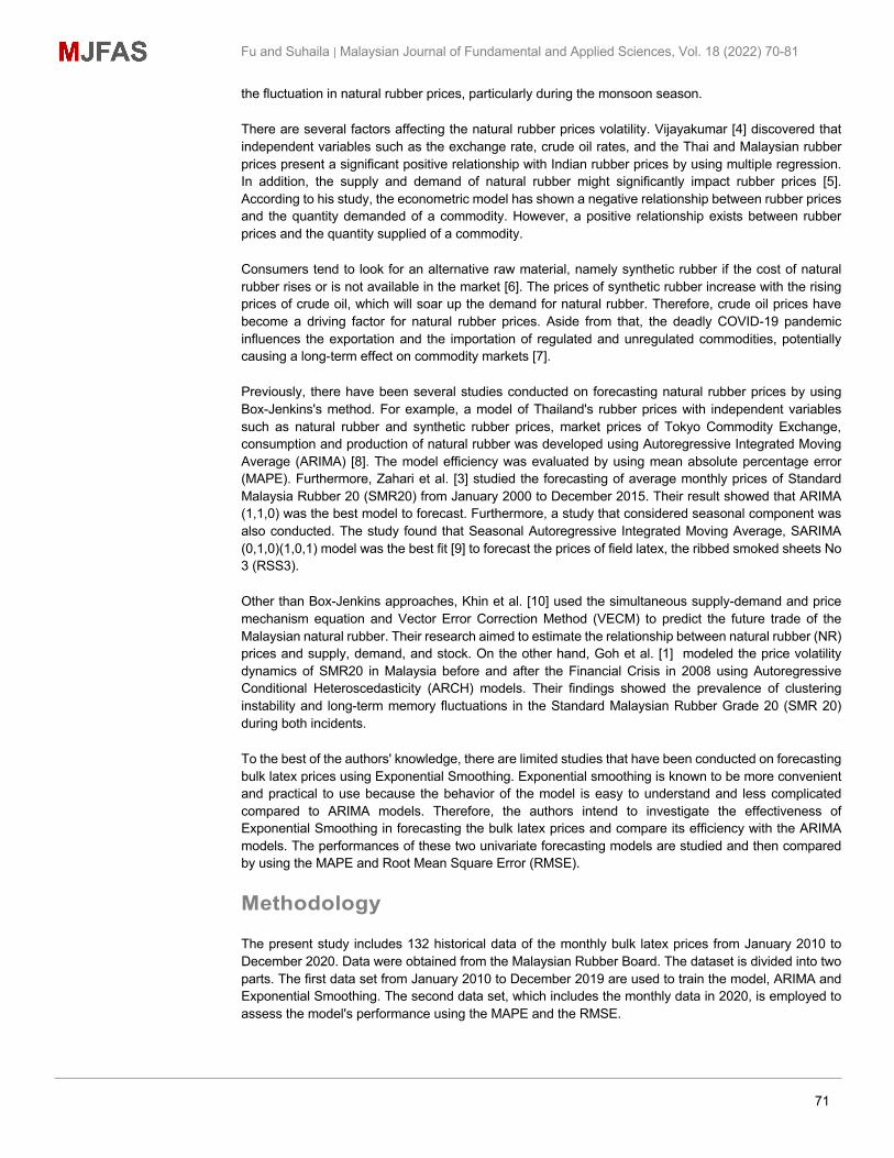
Abstract Natural rubber is a crucial component of many developed countries' socioeconomic structures since it is often used to manufacture essential consumer goods such as tires and latex gloves. The natural rubber industry is heavily affected by the volatility and unpredictability of the natural bulk latex markets. Therefore, forecasting natural rubber prices is critical for the rubber industry in procurement decisions and marketing strategies. This study aims to model monthly bulk latex prices in Malaysia using Autoregressive Integrated Moving Averages (ARIMA) and Exponential Smoothing. The models' performance is measured using the Mean Absolute Percentage Error (MAPE) and Root Mean Square Error (RMSE). The Malaysian Rubber Board has 132 historical prices for latex in Malaysia from January 2010 to December 2020. They are used for training and testing in determining forecasting accuracy. The findings show that ARIMA (1,1,0) provides the most accurate prediction. The model is considered as the best and highly accurate, with a lower MAPE of 8.59 percent and RMSE of 69.78 sen per kilogram. Keywords: natural rubber, time series, forecasting, ARIMA; exponential smoothing.

Introduction Natural rubber (NR) is an important agricultural product used to create various items, including tires and latex gloves. Goh et al. [1] stated that the volatility of natural rubber prices was a major challenge for manufacturers, merchants, customers, and those involved in the natural rubber industry. In circumstances of considerable complexity and high risk, prices forecasting is required to support the purchasing or marketing decision-making. Due to the high uncertainty of natural rubber prices, it is recommended that accurate statistical methods could be used to forecast future natural rubber prices. The high accuracy of prices forecasts was particularly important to facilitate the decision-makers to make strategic decisions since there was a significant time gap between the investment decision and the actual supply of the commodity in the market [2,3]. Volatility and instability of natural bulk latex prices are the main concerns in the natural rubber industry. Numerous influencing factors may have a significant impact on the volatility of natural prices. Therefore, the future trading of agricultural commodities exists. The policy may help the seller of natural rubber to cover their risk by selling their material in future contracts. The prediction of bulk latex prices will aid decision-makers in the natural rubber industry buy or sell their raw material at the best moment. Furthermore, the impact of climate change affects the yield of natural rubber in Malaysia, which caused

*For correspondence: [email protected]

Received: 6 Sep 2021 Accepted: 18 Feb 2022

© Copyright Fu and Suhaila. This article is distributed under the terms of the Creative Commons Attribution License, which permits unrestricted use and redistribution provided that the original author and source are credited.

71


the fluctuation in natural rubber prices, particularly during the monsoon season.

There are several factors affecting the natural rubber prices volatility. Vijayakumar [4] discovered that independent variables such as the exchange rate, crude oil rates, and the Thai and Malaysian rubber prices present a significant positive relationship with Indian rubber prices by using multiple regression. In addition, the supply and demand of natural rubber might significantly impact rubber prices [5]. According to his study, the econometric model has shown a negative relationship between rubber prices and the quantity demanded of a commodity. However, a positive relationship exists between rubber prices and the quantity supplied of a commodity. Consumers tend to look for an alternative raw material, namely synthetic rubber if the cost of natural rubber rises or is not available in the market [6]. The prices of synthetic rubber increase with the rising prices of crude oil, which will soar up the demand for natural rubber. Therefore, crude oil prices have become a driving factor for natural rubber prices. Aside from that, the deadly COVID-19 pandemic influences the exportation and the importation of regulated and unregulated commodities, potentially causing a long-term effect on commodity markets [7]. Previously, there have been several studies conducted on forecasting natural rubber prices by using Box-Jenkins's method. For example, a model of Thailand's rubber prices with independent variables such as natural rubber and synthetic rubber prices, market prices of Tokyo Commodity Exchange, consumption and production of natural rubber was developed using Autoregressive Integrated Moving Average (ARIMA) [8]. The model efficiency was evaluated by using mean absolute percentage error (MAPE). Furthermore, Zahari et al. [3] studied the forecasting of average monthly prices of Standard Malaysia Rubber 20 (SMR20) from January 2000 to December 2015. Their result showed that ARIMA (1,1,0) was the best model to forecast. Furthermore, a study that considered seasonal component was also conducted. The study found that Seasonal Autoregressive Integrated Moving Average, SARIMA (0,1,0)(1,0,1) model was the best fit [9] to forecast the prices of field latex, the ribbed smoked sheets No 3 (RSS3). Other than Box-Jenkins approaches, Khin et al. [10] used the simultaneous supply-demand and price mechanism equation and Vector Error Correction Method (VECM) to predict the future trade of the Malaysian natural rubber. Their research aimed to estimate the relationship between natural rubber (NR) prices and supply, demand, and stock. On the other hand, Goh et al. [1] modeled the price volatility dynamics of SMR20 in Malaysia before and after the Financial Crisis in 2008 using Autoregressive Conditional Heteroscedasticity (ARCH) models. Their findings showed the prevalence of clustering instability and long-term memory fluctuations in the Standard Malaysian Rubber Grade 20 (SMR 20) during both incidents. To the best of the authors' knowledge, there are limited studies that have been conducted on forecasting bulk latex prices using Exponential Smoothing. Exponential smoothing is known to be more convenient and practical to use because the behavior of the model is easy to understand and less complicated compared to ARIMA models. Therefore, the authors intend to investigate the effectiveness of Exponential Smoothing in forecasting the bulk latex prices and compare its efficiency with the ARIMA models. The performances of these two univariate forecasting models are studied and then compared by using the MAPE and Root Mean Square Error (RMSE).

Methodology The present study includes 132 historical data of the monthly bulk latex prices from January 2010 to December 2020. Data were obtained from the Malaysian Rubber Board. The dataset is divided into two parts. The first data set from January 2010 to December 2019 are used to train the model, ARIMA and Exponential Smoothing. The second data set, which includes the monthly data in 2020, is employed to assess the model's performance using the MAPE and the RMSE.

72


Exponential Smoothing Exponential Smoothing is forecasts of weighted averages of past observation [11]. There are three types of models in this method: Simple Exponential Smoothing, Holt's Exponential Smoothing, and Holt-Winter's Exponential Smoothing. Simple Exponential Smoothing is suitable for predicting data without consistent trends or seasonal components. The general formula for this model is expressed as

𝑦"#$% = 𝛼𝑦# + (1 − 𝛼)𝑦#- (1)

where 𝛼 is the smoothing parameter, 𝑦"# is the predicted value and 𝑦# is the observed value. Besides, if the dataset is presented with a trend, it is advised to forecast using Double Exponential Smoothing, the extension of Simple Exponential Smoothing. The general formula of this model can be written as

𝑦"#$. = ℓ# + ℎ𝑏# (2)

ℓ# = 𝛼𝑦# + (1 − 𝛼)(ℓ#2% + 𝑏#2%),0 ≤ 𝛼 ≤ 1

𝑏# = 𝛽(ℓ# − ℓ#2%) + (1 − 𝛽)𝑏#2%,0 ≤ 𝛽 ≤ 1 where 𝑦"#$.is the predicted value and 𝑦# is the actual value. The symbols of 𝛼and𝛽are thesmoothing parameters for level (ℓ8) and trend (𝑏#) component respectively, while ℎ is the number of periods to be forecast. Box-Jenkins Method The Box-Jenkins methods were developed by George Box and Gwilym Jenkins in 1976 [12]; both of them used the ARMA family to forecast the optimal fit of time series prediction. The ARIMA model is a conventional forecasting model in time series analysis. ARIMA model is a combination of Autoregression (AR) and Moving Average (MA). Data Pre-processing Data normalization such as the Box-cox power transformation is used to convert the non-normal data to stabilize the variance for obeying the normality. The transformation parameter 𝜆 is selected automatically by the Guerrero method, which minimizes the coefficient of variation for subseries of data [13], This transformation can be defined as

𝑦# = :𝑙𝑜𝑔 𝑦# , 𝜆 = 0>?@2%A, 𝜆 ≠ 0

. (3)

The time series must be stationary in order to use the ARIMA model. The time series is stationary when the mean, variance, and auto-covariance do not vary over time. The Augmented Dicker Fuller (ADF) test can be used to determine if the time series is stationary. The null hypothesis, 𝐻D denotes that the time series is not stationary. The commonly used 𝑡-statistic, 𝑇 under 𝐻D is

𝑇 = G-HI(G-)

(4)

where 𝛾" is the unit root and 𝑆𝐸(𝛾") is the squared error of unit root. Reject 𝐻D if |𝑇| > O𝜏Q,RO for 𝑁 sample size and critical value, 𝜏Q,R. Besides, the 𝐻D can be rejected if p-value less than 𝛼significance level to conclude the time series is stationary. The differencing process will then be applied to the non-stationary time series to achieve stationary. Differencing is the computation of differences between consecutive observations to reduce or eliminate the trend and seasonality presented in the data which is given as

𝑦#T = 𝑦# − 𝑦#2% (5)

73


where 𝑦# is the observation from the time series at time 𝑡. ARIMA Model Identification and Selection The Autocorrelation Function (ACF) and Autocorrelation Function (PACF) plots are used to determine the order of ARIMA. The properties of ACF and PACF for ARIMA [14] is shown in Table 1.

Table 1. Properties of ACF and PACF for ARIMA. The Akaike Information Criterion (AIC) can be used to assess the best model selection for the Box-Jenkins model. AIC is an estimator of out-sample prediction error for the datasets. As a result, a good model with the least prediction errors should comprise the least value of AIC. The formula of 𝐴𝐼𝐶 and corrected 𝐴𝐼𝐶 (𝐴𝐼𝐶X) are given as:

𝐴𝐼𝐶 = 𝑁ln(𝑆𝑆𝐸) + 2𝑘 (6)

𝐴𝐼𝐶X = 𝐴𝐼𝐶 + ](^$%)(^$])R2^2%

(7)

where 𝑘 is the number of parameters, 𝑁 is the sample size, 𝑆𝑆𝐸 is the sum square of errors. ARIMA Diagnostic Checking Residual analysis is used to ensure the adequacy of the model in this procedure. An adequate ARIMA model should comprise residuals with properties of zero mean, constant variance, non-autocorrelated, independence, and normality. The randomness of the residual can be verified by using the plot of the standardized residuals. A good predictive model should comprise the residuals with zero mean and exhibit a random plot pattern. Besides, the independence of residuals is then tested by using the ACF plot of residuals. If most of the ACF of residuals fall within the 95% confidence interval, then the model's residuals are independent. The ACF at lag 𝑘 and the 95% confidence interval (𝐶𝐼) with 𝑁 sample size is computed as

𝑟 = ∑ (a?2b?cdef a̅)(a?ed2a̅)

∑ (a?2b?cf a̅)h

(8)

𝐶𝐼 = ± %.kl√R (9)

where 𝑟 is the autocorrelation at lag 𝑘 and 𝑥# is the input data at time 𝑡. In addition, the Ljung-Box test is used to test the autocorrelation of the residuals from the chosen model. The null hypothesis, 𝐻D of Ljung-Box test is that the residuals are not autocorrelated. The model is considered inadequate if the association with the Q statistic is small (p-value < 𝛼) [3]. The 𝑄-statistic for the Ljung-Box is given as:

𝑄 = 𝑁(𝑁 + 2)∑ p̂dh

R2^r^s% (10)

where 𝑁 is the sample size, 𝑟- is the sample autocorrelation at lag 𝑘, and 𝐾 is the number of lags being tested. Reject 𝐻D if 𝑄 > 𝜒^2v] where 𝑣 = 𝑝 + 𝑞, where 𝑝 is the order of autoregression and 𝑞 is the order

Properties 𝐴𝑅(𝑝) 𝑀𝐴(𝑞) 𝐴𝑅𝑀𝐴(𝑝, 𝑞)ACF Decay Cuts after the 𝑞 lag Decay

PACF Cuts after the 𝑝 lag Decay Decay

74


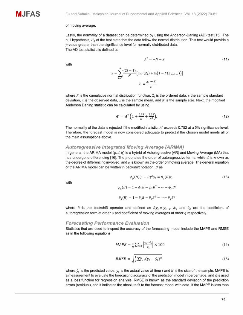
of moving average. Lastly, the normality of a dataset can be determined by using the Anderson-Darling (AD) test [15]. The null hypothesis, 𝐻D of the test state that the data follow the normal distribution. This test would provide a 𝑝-value greater than the significance level for normally distributed data. The AD test statistic is defined as:

𝐴] = −𝑁 − 𝑆 (11) with

𝑆 =|(2𝑖 − 1)

𝑁

R

~s%

�ln𝐹(𝑍~) + ln�1 − 𝐹(𝑍�$%2~)��

𝑍~ =𝑥~ − �̅�𝑠

where 𝐹 is the cumulative normal distribution function, 𝑍~ is the ordered data, 𝑠 the sample standard deviation, 𝑥 is the observed data, �̅� is the sample mean, and 𝑁 is the sample size. Next, the modified Anderson Darling statistic can be calculated by using

𝐴∗ = 𝐴] �1 + D.��R+ ].]�

Rh�. (12)

The normality of the data is rejected if the modified statistic, 𝐴∗ exceeds 0.752 at a 5% significance level. Therefore, the forecast model is now considered adequate to predict if the chosen model meets all of the main assumptions above. Autoregressive Integrated Moving Average (ARIMA) In general, the ARIMA model (𝑝, 𝑑, 𝑞) is a hybrid of Autoregressive (AR) and Moving Average (MA) that has undergone differencing [16]. The 𝑝 donates the order of autoregressive terms, while 𝑑 is known as the degree of differencing involved, and 𝑞 is known as the order of moving average. The general equation of the ARIMA model can be written in backshift notation, 𝐵 as

𝜙�(𝐵)(1 − 𝐵)�𝑦# = 𝜃�(𝐵)𝜀# (13) with

𝜙�(𝐵) = 1 − 𝜙%𝐵 − 𝜙]𝐵] −⋯−𝜙�𝐵�

𝜃�(𝐵) = 1 − 𝜃%𝐵 − 𝜃]𝐵] −⋯− 𝜃�𝐵� where 𝐵 is the backshift operator and defined as 𝐵𝑦# = 𝑦#2%. 𝜙� and 𝜃� are the coefficient of autoregression term at order 𝑝 and coefficient of moving averages at order 𝑞 respectively. Forecasting Performance Evaluation Statistics that are used to inspect the accuracy of the forecasting model include the MAPE and RMSE as in the following equations

𝑀𝐴𝑃𝐸 = %R∑ �>?2>"?

>?� × 100R

#s% (14)

𝑅𝑀𝑆𝐸 = �%R∑ (𝑦# − 𝑦"#)]R#s% (15)

where 𝑦"# is the predicted value, 𝑦# is the actual value at time 𝑡and𝑁 is the size of the sample. MAPE is a measurement to evaluate the forecasting accuracy of the prediction model in percentage, and it is used as a loss function for regression analysis. RMSE is known as the standard deviation of the prediction errors (residual), and it indicates the absolute fit to the forecast model with data. If the MAPE is less than

75


10%, it can be considered a highly accurate forecast [17]. An outperformed model should comprise the lowest MAPE and RMSE.

Results and Discussions In this section, the time series analysis, the employment of the forecasting model using Exponential Smoothing and ARIMA and the model's performance will be discussed. Time Series Analysis The results and discussion may be presented separately, or in one combined section, and may optionally be divided into headed subsections.

Figure 1. Time Series and ACF of Malaysia bulk latex prices from 2010 to 2019.

Figure 2. Detrended Time Series and ACF plot.

The time series as in Figure 1 shows the latex price has an inconsistent trend changing over time and it was not fluctuating around the mean. Moreover, the ACF plot indicates that ACF decays in slower rate.

76


Thus, this indicates that the time series is non-stationary. Besides, the ADF test of this series resulting a p-value of 0.4076 > 0.05. This indicates that 𝐻D is not rejected at 5% significance level, the data is not stationary.

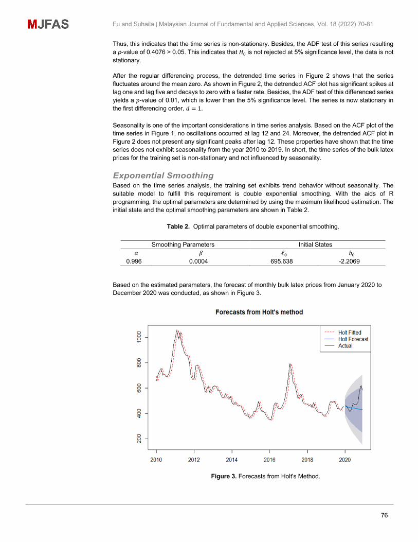
After the regular differencing process, the detrended time series in Figure 2 shows that the series fluctuates around the mean zero. As shown in Figure 2, the detrended ACF plot has significant spikes at lag one and lag five and decays to zero with a faster rate. Besides, the ADF test of this differenced series yields a 𝑝-value of 0.01, which is lower than the 5% significance level. The series is now stationary in the first differencing order, 𝑑 = 1. Seasonality is one of the important considerations in time series analysis. Based on the ACF plot of the time series in Figure 1, no oscillations occurred at lag 12 and 24. Moreover, the detrended ACF plot in Figure 2 does not present any significant peaks after lag 12. These properties have shown that the time series does not exhibit seasonality from the year 2010 to 2019. In short, the time series of the bulk latex prices for the training set is non-stationary and not influenced by seasonality. Exponential Smoothing Based on the time series analysis, the training set exhibits trend behavior without seasonality. The suitable model to fulfill this requirement is double exponential smoothing. With the aids of R programming, the optimal parameters are determined by using the maximum likelihood estimation. The initial state and the optimal smoothing parameters are shown in Table 2.

Table 2. Optimal parameters of double exponential smoothing.

Based on the estimated parameters, the forecast of monthly bulk latex prices from January 2020 to December 2020 was conducted, as shown in Figure 3.

Figure 3. Forecasts from Holt's Method.

Smoothing Parameters Initial States𝛼 𝛽 ℓD 𝑏D

0.996 0.0004 695.638 -2.2069

77


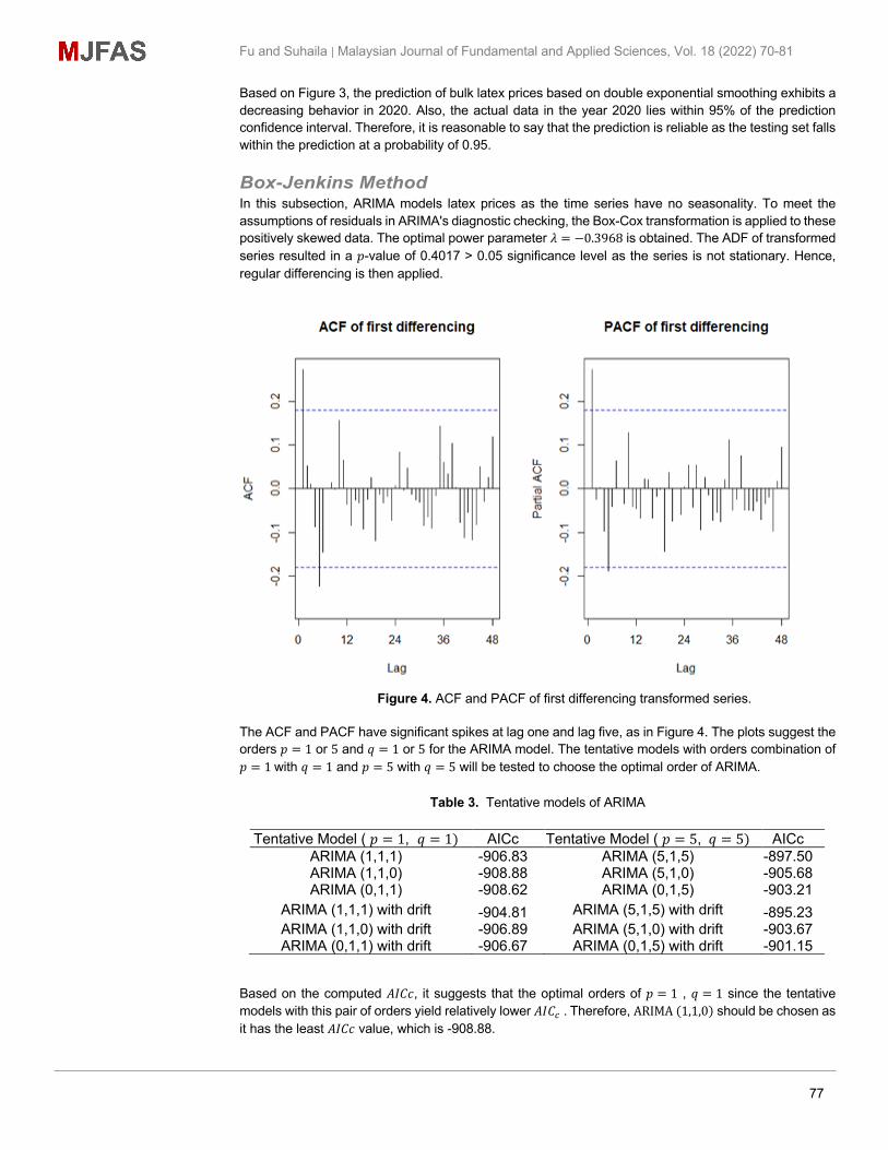
Based on Figure 3, the prediction of bulk latex prices based on double exponential smoothing exhibits a decreasing behavior in 2020. Also, the actual data in the year 2020 lies within 95% of the prediction confidence interval. Therefore, it is reasonable to say that the prediction is reliable as the testing set falls within the prediction at a probability of 0.95. Box-Jenkins Method In this subsection, ARIMA models latex prices as the time series have no seasonality. To meet the assumptions of residuals in ARIMA's diagnostic checking, the Box-Cox transformation is applied to these positively skewed data. The optimal power parameter 𝜆 = −0.3968 is obtained. The ADF of transformed series resulted in a 𝑝-value of 0.4017 > 0.05 significance level as the series is not stationary. Hence, regular differencing is then applied.

Figure 4. ACF and PACF of first differencing transformed series.

The ACF and PACF have significant spikes at lag one and lag five, as in Figure 4. The plots suggest the orders 𝑝 = 1 or 5 and 𝑞 = 1 or 5 for the ARIMA model. The tentative models with orders combination of 𝑝 = 1with 𝑞 = 1 and 𝑝 = 5 with 𝑞 = 5 will be tested to choose the optimal order of ARIMA.

Table 3. Tentative models of ARIMA

Tentative Model ( 𝑝 = 1, 𝑞 = 1) AICc Tentative Model ( 𝑝 = 5, 𝑞 = 5) AICc ARIMA (1,1,1) -906.83 ARIMA (5,1,5) -897.50 ARIMA (1,1,0) -908.88 ARIMA (5,1,0) -905.68 ARIMA (0,1,1) -908.62 ARIMA (0,1,5) -903.21

ARIMA (1,1,1) with drift -904.81 ARIMA (5,1,5) with drift -895.23 ARIMA (1,1,0) with drift -906.89 ARIMA (5,1,0) with drift -903.67 ARIMA (0,1,1) with drift -906.67 ARIMA (0,1,5) with drift -901.15

Based on the computed 𝐴𝐼𝐶𝑐, it suggests that the optimal orders of 𝑝 = 1 , 𝑞 = 1 since the tentative models with this pair of orders yield relatively lower 𝐴𝐼𝐶X .Therefore, ARIMA(1,1,0) should be chosen as it has the least 𝐴𝐼𝐶𝑐 value, which is -908.88.

78


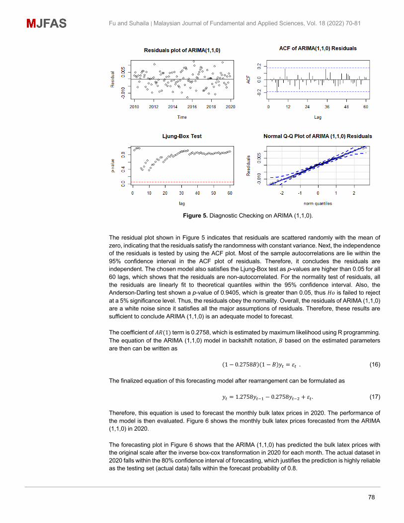
Figure 5. Diagnostic Checking on ARIMA (1,1,0).

The residual plot shown in Figure 5 indicates that residuals are scattered randomly with the mean of zero, indicating that the residuals satisfy the randomness with constant variance. Next, the independence of the residuals is tested by using the ACF plot. Most of the sample autocorrelations are lie within the 95% confidence interval in the ACF plot of residuals. Therefore, it concludes the residuals are independent. The chosen model also satisfies the Ljung-Box test as p-values are higher than 0.05 for all 60 lags, which shows that the residuals are non-autocorrelated. For the normality test of residuals, all the residuals are linearly fit to theoretical quantiles within the 95% confidence interval. Also, the Anderson-Darling test shown a p-value of 0.9405, which is greater than 0.05, thus 𝐻𝑜 is failed to reject at a 5% significance level. Thus, the residuals obey the normality. Overall, the residuals of ARIMA (1,1,0) are a white noise since it satisfies all the major assumptions of residuals. Therefore, these results are sufficient to conclude ARIMA (1,1,0) is an adequate model to forecast. The coefficient of 𝐴𝑅(1) term is 0.2758, which is estimated by maximum likelihood using R programming. The equation of the ARIMA (1,1,0) model in backshift notation,𝐵 based on the estimated parameters are then can be written as

(1 − 0.2758𝐵)(1 − 𝐵)𝑦# = 𝜀#. (16) The finalized equation of this forecasting model after rearrangement can be formulated as

𝑦# = 1.2758𝑦#2% − 0.2758𝑦#2] + 𝜀#. (17) Therefore, this equation is used to forecast the monthly bulk latex prices in 2020. The performance of the model is then evaluated. Figure 6 shows the monthly bulk latex prices forecasted from the ARIMA (1,1,0) in 2020. The forecasting plot in Figure 6 shows that the ARIMA (1,1,0) has predicted the bulk latex prices with the original scale after the inverse box-cox transformation in 2020 for each month. The actual dataset in 2020 falls within the 80% confidence interval of forecasting, which justifies the prediction is highly reliable as the testing set (actual data) falls within the forecast probability of 0.8.

79


Figure 6. Forecasted values using ARIMA (1,1,0). Forecasting Performance Evaluation The performances of the forecasting models were evaluated by using the MAPE and RMSE as in Table 4. To ensure the consistency of the outcomes, the evaluation of forecast accuracy is based on testing set only to select the best model. Based on Table 4, the best forecasting model is ARIMA (1,1,0), as it has the least MAPE and RMSE in forecasting accuracy. This model is also considered a highly accurate forecast as it yields the MAPE lower than 10%.

Table 4. Tentative models of ARIMA.

Model Modelling Forecasting MAPE RMSE MAPE RMSE

Holt Trend 5.338 40.568 10.734 85.308 ARIMA 5.089 38.762 8.594 69.779

Figure 7 shows the testing sample from January to December in 2020 with their forecasted values. The actual data of the latex prices for 2020 shows a fluctuation starting from September. It raised to 620.76 sen per kg in November 2020. The uptrend of bulk latex prices from September to November 2020 was driven by COVID-19 vaccine optimism, solid economic growth and NR demand from China, and tightened NR supply due to the rainy season [18]. Therefore, the employed univariate forecasting models cannot predict as expected to reach the actual data for September to December 2020. It is because the univariate models do not consider the influencing factors to the bulk latex prices.

80


Figure 7. Actual and Forecast of Bulk Latex Prices in 2020.

Conclusions and Recommendations Forecasting in bulk latex prices in Malaysia is extremely important in the rubber industry and related parties for decision-making in sourcing and procurement, and resource allocation planning. Based on the time series analysis, the bulk latex prices in Malaysia from January 2010 to December 2019 presents the trend without seasonality. As a result, the ARIMA is the most appropriate model in forecasting the bulk latex prices with non-linear behaviors in this study. The results in this study are consistent with Zahari et al. [3], which used ARIMA (1,1,0) as the best forecasting model of rubber, namely SMR20. However, due to the COVID-19 outbreak and surging demand for latex products, some predictions are not forecasted as expected as in actual data. Therefore, the hybrid models may help to improve the results. The hybrid model is the combination of two methods used to overcome the drawbacks of the individual techniques. It is suggested that several influential factors should be considered in forecasting the pricing of raw materials, namely supply and demand of raw material, weather conditions, foreign exchange currency, productions, and consumption of the raw material. Future studies should include an exogenous model such as ARIMAX to gain better accuracy.

Data Availability

The data have been used in this research are monthly average prices of bulk latex in Malaysia, from January 2010 to December 2020. The data are acquired from the websites of Malaysian Rubber Board, retrieved from https://www.lgm.gov.my/webv2/sidenav/(mreDetails:mreprice).

Conflicts of Interest

The authors declare that there is no conflict of interest regarding the publication of this paper.

81


Acknowledgments

The authors would like to express their gratitude to the Ministry of Higher Education (MOHE) for the funding given under the Fundamental Research Grant Scheme (FRGS/1/2020/STG06/UTM/02/3) under vote 5F311. We are also grateful to Universiti Teknologi Malaysia for supporting this project with Research University Grant (QJ130000.3854.19J58).

References [1] Goh, H. H., Tan, K. L., Khor, C. Y., & Ng, S. L. "Volatility and Market Risk of Rubber Price in Malaysia: Pre-

and Post-Global Financial Crisis," Journal of Quantitative Economics, 14(2), pp. 323–344, 2016. [2] Ismai, Z., Abu, N., & Sufahani, S. "New product forecasting with limited or no data,". AIP Conference

Proceedings, 1782, 2016. [3] Zahari, F. Z., Khalid, K., Roslan, R., Sufahani, S., Mohamad, M., Rusiman, M. S., & Ali, M. "Forecasting

Natural Rubber Price in Malaysia Using Arima," Journal of Physics: Conference Series, 995(1), pp. 0–7, 2018. [4] Vijayakumar, A.N. "International Determinants on Indian Rubber Prices," SJCC Management Research

Review. Vol. 9, 2019. [5] Chawananon, C. "Factors affecting the Thai Natural rubber market Equilibrium: demand and supply response

analysis using two stage least squares approach'" 2014. [6] Ramli, N., Md Noor, A. H. S., Sarmidi, T., Said, F. F., & Azam, A. H. M. "Modelling the volatility of rubber

prices in ASEAN-3," International Journal of Business and Society, 20(1), pp.1–18. 2019. [7] Rajput, H., Changotra, R., Rajput, P., Gautam, S., Gollakota, A. R. K., & Arora, A. S. "A shock like no other:

coronavirus rattles commodity markets," Environment, Development and Sustainability. 2020. [8] Cherdchoongam, S., & Rungreunganun, V. "Forecasting the Price of Natural Rubber in Thailand Using the

ARIMA Model," King Mongkut's University of Technology North Bangkok International Journal of Applied Science and Technology, 9(4), pp. 271–277, 2016.

[9] Udomraksasakul, C., & Rungreunganun, V. "Forecasting the Price of Field Latex in the Area of Southeast Coast of Thailand Using the ARIMA Model," 13(1), 550–556, 2018.

[10] Khin, A. A., Thambiah, S., & Teng, K. L. L. "Short-term and long-term price forecasting models for the future exchange of Malaysian natural rubber market," International Journal of Agricultural Resources, Governance and Ecology, 13(1), 21–42, 2017.

[11] Winters, P. R. "Forecasting Sales by Exponentially Weighted Moving Averages," Management Science, 6(3), pp. 324–342, 1960.

[12] Hammad, M. A., Jereb, B., Rosi, B., & Dragan, D. "Methods and Models for Electric Load Forecasting: A Comprehensive Review," Logistics & Sustainable Transport, 11(1), 51–76, 2020.

[13] Petropoulos, F., Hyndman, R. J., & Bergmeir, C. "Exploring the sources of uncertainty: Why does bagging for time series forecasting work?," European Journal of Operational Research, 268(2), pp. 545–554, 2018.

[14] Bandyopadhyay, G., & Guha, B. "Gold Price Forecasting Using ARIMA Model," Journal of Advanced Management Science, 4(2), pp. 117–121, 2016.

[15] Anderson, T. W., & Darling, D. A. "A Test of Goodness of Fit," Journal of the American Statistical Association, 49(268), pp. 765–769, 1954.

[16] Karia, A. A., & Bujang, I. "Progress accuracy of CPO price prediction: Evidence from ARMA family and artificial neural network approach," International Research Journal of Finance and Economics, 64(64), pp. 66–79, 2011.

[17] Lewis, C. D. "Industrial and business forecasting methods: a practical guide to exponential smoothing and curve fitting," Butterworth Scientific, 1982.

[18] "Natural Rubber Market Review". Lembaga Getah Malaysia, November. http://www3.lgm.gov.my/digest/ digest/digest-11-2020.pdf, 2020.

Forecasting Malaysia Bulk Latex Prices Using Autoregressive ...

Documents