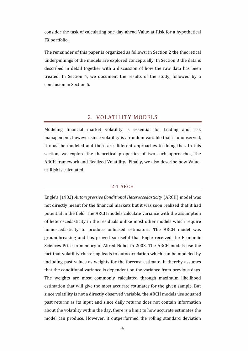
1 UPPSALA UNIVERSITY Jan 31, 2010 Department of Statistics Uppsala Bachelor’s Thesis Fall Term 2010 Advisor: Lars Forsberg FORECASTING FOREIGN EXCHANGE VOLATILITY FOR VALUE AT RISK CAN REALIZED VOLATILITY OUTPERFORM GARCH PREDICTIONS? David Fallman 1 & Jens Wirf 2 ABSTRACT In this paper we use model-free estimates of daily exchange rate volatilities employing high-frequency intraday data, known as Realized Volatility, which is then forecasted with ARMA-models and used to produce one-day-ahead Value- at-Risk predictions. The forecasting accuracy of the method is contrasted against the more widely used ARCH-models based on daily squared returns. Our results indicate that the ARCH-models tend to underestimate the Value-at- Risk in foreign exchange markets compared to models using Realized Volatility. KEYWORDS: Realized volatility, volatility forecasting, exchange rates, high- frequency data, value-at-risk. 1 [email protected] 2 [email protected]

Welcome message from author
This document is posted to help you gain knowledge. Please leave a comment to let me know what you think about it! Share it to your friends and learn new things together.
Transcript

1
UPPSALA UNIVERSITY Jan 31, 2010 Department of Statistics Uppsala
Bachelor’s Thesis Fall Term 2010 Advisor: Lars Forsberg
F O R E C A S T I N G F O R E I GN E X CHA N G E VO L A T I L I T Y F O R
V A L U E A T R I S K
CAN REALIZED VOLATILITY OUTPERFORM GARCH PREDICTIONS?
David Fallman1 & Jens Wirf2
ABSTRACT
In this paper we use model-free estimates of daily exchange rate volatilities employing high-frequency intraday data, known as Realized Volatility, which is then forecasted with ARMA-models and used to produce one-day-ahead Value-at-Risk predictions. The forecasting accuracy of the method is contrasted against the more widely used ARCH-models based on daily squared returns. Our results indicate that the ARCH-models tend to underestimate the Value-at-Risk in foreign exchange markets compared to models using Realized Volatility.
KEYWORDS: Realized volatility, volatility forecasting, exchange rates, high-frequency data, value-at-risk.
2
CONTENT
1. Introduction ................................................................................................................................. 3
2. Volatility Models ........................................................................................................................ 4
2.1 ARCH ......................................................................................................................................... 4
2.2 Realized Volatility ............................................................................................................... 5
2.3 ARMA ........................................................................................................................................ 6
2.4 Value-at-Risk ......................................................................................................................... 7
3. Data .................................................................................................................................................. 8
3.1 Data Construction ............................................................................................................... 8
3.2 Data Description .................................................................................................................. 9
4. Results ......................................................................................................................................... 13
4.1 In-Sample Fit ...................................................................................................................... 13
4.2 Out-of-Sample Forecast Evaluation .......................................................................... 15
4.3 Value-at-Risk: Practical Application ......................................................................... 18
5. Conclusion ................................................................................................................................. 20
6. References ................................................................................................................................. 22
Appendix .......................................................................................................................................... 23

3
1. INTRODUCTION
It is widely acknowledged in academic literature that financial asset prices are
difficult, if not impossible, to predict, much due to their seemingly random
nature. However, ever since Engle’s seminal contribution of the Autoregressive
Conditional Heteroskedasticity framework in 1982, much progress has been
made in modeling the dynamics of the conditional volatility. This modeling has
spurred significant interest among academics and financial market
practitioners alike as volatility is a core measure of the risk associated with
holding a financial asset. Accurately predicting volatility is instrumental to
making informed risk management decisions and bears implications for
numerous areas in financial economics.
Although unobserved and inherently time-varying, financial asset volatility is
well documented to display serial dependence [volatility clustering], which
means it has predictable features. The prevailing methodology for modeling and
forecasting asset volatility stems from Engle’s (1982) ARCH framework and the
plethora of variants that have since followed. Notably the Generalized ARCH
(GARCH) by Bollerslev (1986) has become standard practice in many financial
institutions.
A more recent and competing approach to modeling volatility is Realized
Volatility, popularized by among others Talyor & Xu (1992) and Andersen,
Bollerslev, Diebold & Labys (1999). Following the increasing availability of
high-frequency data, RV has become an increasingly popular method. It is a
model-free methodology which harnesses the information contained in higher
frequency data, i.e. intraday data such as five or ten minute returns. It has the
advantage that it can be modeled with parsimonious standard time series
models rather than the arguably more complex ARCH-family of models.
In this paper, we consider the practical task of forecasting one-day-ahead
foreign exchange volatility and compare the predictive ability of a number of
GARCH and RV based models. The objective is to determine whether RV can
outperform standard practice in forecasting procedures and so assess whether
there is real merit to using computer intensive high-frequency data. To this aim
we analyze four major exchange spot rates, namely the Euro versus the U.S.
Dollar, Japanese Yen, Great British Pound and Swedish Krona over the period
Jan 2009 to Oct 2010. As a practical application of volatility forecasting we also
4
consider the task of calculating one-day-ahead Value-at-Risk for a hypothetical
FX portfolio.
The remainder of this paper is organized as follows; in Section 2 the theoretical
underpinnings of the models are explored conceptually, In Section 3 the data is
described in detail together with a discussion of how the raw data has been
treated. In Section 4, we document the results of the study, followed by a
conclusion in Section 5.
2. VOLATILITY MODELS
Modeling financial market volatility is essential for trading and risk
management, however since volatility is a random variable that is unobserved,
it must be modeled and there are different approaches to doing that. In this
section, we explore the theoretical properties of two such approaches, the
ARCH-framework and Realized Volatility. Finally, we also describe how Value-
at-Risk is calculated.
2.1 ARCH
Engle’s (1982) Autoregressive Conditional Heteroscedasticity (ARCH) model was
not directly meant for the financial markets but it was soon realized that it had
potential in the field. The ARCH models calculate variance with the assumption
of heteroscedasticity in the residuals unlike most other models which require
homoscedasticity to produce unbiased estimators. The ARCH model was
groundbreaking and has proved so useful that Engle received the Economic
Sciences Price in memory of Alfred Nobel in 2003. The ARCH models use the
fact that volatility clustering leads to autocorrelation which can be modeled by
including past values as weights for the forecast estimate. It thereby assumes
that the conditional variance is dependent on the variance from previous days.
The weights are most commonly calculated through maximum likelihood
estimation that will give the most accurate estimates for the given sample. But
since volatility is not a directly observed variable, the ARCH models use squared
past returns as its input and since daily returns does not contain information
about the volatility within the day, there is a limit to how accurate estimates the
model can produce. However, it outperformed the rolling standard deviation
5
model which was the regularly used method before Engle discovered the ARCH
application for financial data.
The Generalized Autoregressive Conditional Heteroscedasticity (GARCH) model
introduced by Bollerslev (1986) is by far the most used application of the ARCH
model. Formally denoted as GARCH(p,q) where q are the ARCH-term which
refers to how many autoregressive lags the model are using and the p refers to
the GARCH-term i.e. the number moving average lags that the model will
include.
The conditional variance ( can be modeled using previous day’s variance and
return ( as follows with a GARCH(1,1) process
. (1)
The unconditional variance can be found by rearranging the model to
(2)
with the restriction that .The GARCH model with its long memory
through declining weights that never reach zero has proven so successful that it
has replaced the ARCH as the standard practice model.
The exponential GARCH model is further extensions by Nelson (1991) which
avoids the non-negative restrictions on the weights of the GARCH by modeling
instead of . In addition the volatility can react asymmetrically. EGARCH is
a logarithmic variation of the GARCH model where
∑
∑
(3)
where is defined as | | | | which allows to have
asymmetric effect on the volatility, where
if
2.2 REALIZED VOLATILITY
As previously mentioned, the most common method is to use statistical models
from the ARCH family, but there exists also an alternative model-free approach
which is called Realized Volatility.
Summing up high frequency squared realizations will result in a good estimate
for the variance of a random i.i.d variable (Merton, 1980). Realized volatility is

6
an extension of this where squared intraday returns is used to construct a time
series of the variance. Realized volatility is defined as
[∑ ]
(4)
This can also be written as
[∑
] { [ ]
[ ] (5)
where ri,t is the returns for each observation which is calculated as
( ) ( ) . (6)
If the assumptions above are fulfilled and if the returns are distributed with
fixed and even intervals each day will make RV(t) an consistent and unbiased
estimator of the daily variance (Andersen et al. 2000a), A higher frequency of
returns would normally be ideal but can introduce unwanted effect due micro
market effects such as bid-ask bounces etc. To determine the appropriate
frequency can be tricky as where a too high frequency will introduce bias and
while a too low frequency loses much of the information you normally would
want to model. When determining this, the stocks and currency’s volume of
trading should be taken in consideration as a higher trading volume results in
that a higher interval frequency can be chosen.
2.3 ARMA
Since RV is a consistent measure of volatility we can treat it as “observed”. As
such, it can be modeled and forecasted using standard time series techniques.
The Autoregressive Moving Average (ARMA) model, which we have opted to
use, is applied to stationary and autocorrelated time series data. The model
contains two parts, the autoregressive (AR) part and the moving average (MA).
Part. Both parts can be modeled by themselves to describe time series of data.
The AR(p) model is defined as:
∑ (7)
Where is a observed time series and are the parameters which have
restrictions for the model to be stationary, for example of | | , in the case
7
of an AR(1). Each observation is made of a random error shock that is a linear
combination of prior observations. The MA(q) model is defined as
∑ (8)
where are the MA parameters and is a constant. Each observation here is
made up of a random error shock that is a linear combination of prior random
shocks. ARMA(p,q) refers to the merger of the two models and has the same
assumptions and conditions. The ARMA process is modeled as
∑ ∑
(9)
2.4 VALUE-AT-RISK
Value-at-Risk is an intuitive and easily understood measure of risk. Take for
example, a 5% VaR on a portfolio of assets. Value-of-risk states the least amount
of money the portfolio is expected to lose in the worst 5% of the trading days.
Risk management has gone through a revolution since the introduction of
Value-at-Risk (VaR) in the early 1990s. VaR is now used to control, manage and
measure market risk. The most common use of VaR is to calculate 1% or 5%
probabilities for a given portfolio of assets. VaR can be calculated in a few
different ways depending on if it uses daily volatility or average volatility. One
way of defining VAR is
(10)
where loss is denoted L and c is the confidence level. We will mainly be focusing
on the one day ahead VaR for this essay and for that specification to be valid do
we need to identify the quantile’s distribution and estimate the volatility for
.
The one day ahead VaR is defined as
size. (11)
The VaR adjusted for given time horizon is defined as
√ ⁄ (12)
The financial asset return distributions quantile is an important part of Value-
at-Risk model. A big problem today is that the Gaussian distribution is often
8
used even though daily returns often tend to be more leptokurtic relative to the
Gaussian distribution. This will inevitably lead to inaccurate risk management.
One approach to mitigating the problem is standardizing the returns with the
conditional standard deviation estimate derived from Realized Volatility or
from another model such as GARCH. Returns can theoretically be decomposed
as:
(13)
Assuming that returns are uncorrelated with the conditional variance and that
. However since is not a directly observable variable we have to
use to the next best thing, our Realized Volatility estimate. Standardizing the
returns can be done by simple rearranging the former decomposition to:
(14)
This should in theory result in a Gaussian distribution but due to noise in the ,
the tails may sometimes be fatter. Student-t is normally the distribution that is
used to handle a fat-tailed distribution, but if you have a large number of
observations, this will reduce the noise in which allows the Normal
distribution to be used anyway.
3. DATA
In this section we document how the raw data has been manipulated and the
series of interest constructed. Last in this section, some key data is plotted in
graphs.
3.1 DATA CONSTRUCTION
As previous mentioned, the empirical analysis is focused around four FOREX
spot rate series, namely the Euro versus the Swedish Krona, Great British
Pound, U.S. Dollar and the Japanese Yen. The data3 spans over the period
3 The data provider is Forex Rate at forexrate.co.uk.
9
January 1st 2009 through October 29th 2010, which is a total of 476 active
trading days. We have opted for two sampling frequencies, daily and ten minute
evenly spaced intervals. This means there is one low and one high frequency
sampling for use in comparing the modeling frameworks.
Regarding the high-frequency sampling intervals, there is an inherent tradeoff
between choosing ultra-high frequencies such as tick or second data and semi-
high frequencies such as 20, 30, 60 minutes data. The problem is essentially that
ultra-high frequencies has microstructure bid/ask frictions which distorts the
data, and while lower frequencies avoids this problem, more and more
information is lost with the longer sampling intervals. In this paper, we rely on a
10 min interval, as previously mentioned, which seems a reasonable tradeoff.
The raw data are global 24-hour trading day quotes. To achieve continuity in
the sampling and avoid irregularities in the number of observations per day
around weekends, we follow Bollerslev (2002) and let a five-day trading week
span from Sunday to Friday, where each trading day runs from 21:00 GMT to
21:00 GMT the next day. This gives around 68’300 observations in the higher
frequency series. To then transform the spot rates into returns we calculate the
first difference of the logarithm of the close-to-close prices.4
3.2 DATA DESCRIPTION
Graph 3.1 depicts the raw price series of the different exchange rates. At a first
glance, it seems that three of the series lack a clear trend, whereas the SEK has
an downward trend in the sample period. Notably, there is a fair bit of
fluctuation in all four series over the 15 months we have sampled.
4 The dataset can be obtained by sending a request to [email protected].

10
GRAPH 3.1 – PLOT OF PRICE DATA
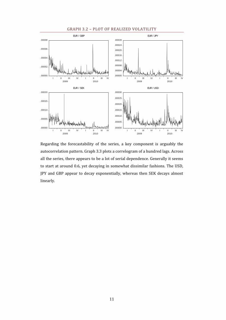
The volatility of the exchange rate series becomes more observable when we
look at the constructed RV series in Graph 3.2, recalling that this operation
visualizes volatility. The four series have a similar pattern in the first half of
2009 where they all seem to display a decreasing volatility level. From the mid
of 2009 through the mid 2010 there is relatively stable period with a lower
level of activity. For three of the series, the GBP, JPY and USD, this is followed by
a major spike in volatility in the summer of 2010. The SEK only shows a slight
tendency of this event, in an otherwise exceptionally low volatility period.
.80
.84
.88
.92
.96
I II III IV I II III IV
2009 2010
EUR / GBP
100
110
120
130
140
I II III IV I II III IV
2009 2010
EUR / JPY
9.0
9.5
10.0
10.5
11.0
11.5
12.0
I II III IV I II III IV
2009 2010
EUR / SEK
1.1
1.2
1.3
1.4
1.5
1.6
I II III IV I II III IV
2009 2010
EUR / USD
11
GRAPH 3.2 – PLOT OF REALIZED VOLATILITY
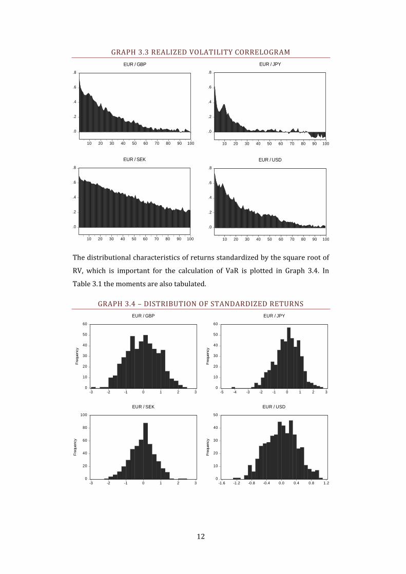
Regarding the forecastability of the series, a key component is arguably the
autocorrelation pattern. Graph 3.3 plots a correlogram of a hundred lags. Across
all the series, there appears to be a lot of serial dependence. Generally it seems
to start at around 0.6, yet decaying in somewhat dissimilar fashions. The USD,
JPY and GBP appear to decay exponentially, whereas then SEK decays almost
linearly.
.00000
.00002
.00004
.00006
.00008
I II III IV I II III IV
2009 2010
EUR / GBP
.00000
.00004
.00008
.00012
.00016
.00020
.00024
.00028
I II III IV I II III IV
2009 2010
EUR / JPY
.00000
.00005
.00010
.00015
.00020
I II III IV I II III IV
2009 2010
EUR / SEK
.00000
.00005
.00010
.00015
.00020
.00025
.00030
I II III IV I II III IV
2009 2010
EUR / USD
12
GRAPH 3.3 REALIZED VOLATILITY CORRELOGRAM
The distributional characteristics of returns standardized by the square root of
RV, which is important for the calculation of VaR is plotted in Graph 3.4. In
Table 3.1 the moments are also tabulated.
GRAPH 3.4 – DISTRIBUTION OF STANDARDIZED RETURNS
.0
.2
.4
.6
.8
10 20 30 40 50 60 70 80 90 100
EUR / USD
.0
.2
.4
.6
.8
10 20 30 40 50 60 70 80 90 100
EUR / JPY
.0
.2
.4
.6
.8
10 20 30 40 50 60 70 80 90 100
EUR / SEK
.0
.2
.4
.6
.8
10 20 30 40 50 60 70 80 90 100
EUR / GBP
0
10
20
30
40
50
60
-3 -2 -1 0 1 2 3
Fre
quency
EUR / GBP
0
10
20
30
40
50
60
-5 -4 -3 -2 -1 0 1 2 3
Fre
quency
EUR / JPY
0
20
40
60
80
100
-3 -2 -1 0 1 2 3
Fre
quency
EUR / SEK
0
10
20
30
40
50
-1.6 -1.2 -0.8 -0.4 0.0 0.4 0.8 1.2
Fre
quency
EUR / USD

13
TABLE 3.1 – DISTRIBUTION OF STANDARDIZED RETURNS
Returns standardized by √ as estimate of σ
EUR/BGP EUR/SEK EUR/USD EUR/JPY
Mean -0.03606 -0.05715 -0.00315 -0.01624
Skewness -0.00377 -0.04603 -0.05969 -0.33878
Kurtosis 2.45123 3.18318 2.64013 3.34074
Jarque-Bera 5.97387 0.83368 2.85117 11.4085
Probability
0.05044 0.65912 0.24036 0.00333
4. RESULTS
In the first part of the empirical results we focus on the in-sample model
estimation, specifically the model parameters and how well the models fit the
data in question. In the second part, we turn to the actual forecasting of
volatility and compare the models predictive abilities.
4.1 IN-SAMPLE FIT
As a first step in our analysis we examine the RV data set for each of the four
exchange rate series. The idea is to fit a number of standard parametric time
series models to this data, in order capture the serial dependence described in
the data section. To this aim, we employ number of ARMA-type models, namely
one autoregressive, one moving average and one mixed model. These models
are also applied to the logarithm and square root of RV. Since we use a rolling
one-year in-sample window for forecasting, explained in detail in the section,
there are a total of 216 forecasts per series. This of course involves 216
regression estimation results per series and per model, totaling around 7’700
estimations for the RV dataset alone. Naturally, the results of this quantity of
estimations are difficult to portray in any comprehensible way. Which is why
we have only summarized some schematic aspects of the estimations, seen in
Table 4.1. The statistics reported show the range of coefficients as well as the
stability of the parameters. Furthermore we consider the fit of the models by
looking at both the adjusted R-Squared and the Breusch-Godfrey Portmanteau
test for residual autocorrelation. Whether or not there is any serial dependence
left in the residual is of course a key indicator of whether the model has
successfully captured the information contained the series.

14
What is seen in Table 4.1 is that all the AR-models generally leave a lot of
residual autocorrelation as is indicated by the Breusch-Godfrey test. This also
applies to the MA-models which seem to leave serial dependence almost all the
time. The most successful models are the ARMA models which have the highest
R-squared values and least residual autocorrelation. The most successful
transformation alternates between the logarithm and square root. It however
also seems that the coefficients in the ARMA models vary a lot more than the
single models as the window rolls.
TABLE 4.1 - IN-SAMPLE RV ESTIMATION DIAGNOSTICS
√ AR MA ARMA AR MA ARMA AR MA ARMA
EUR/SEK
Coef * 0.53 0.40 0.97 -0.81 0.78 0.59 0.98 -0.66 0.69 0.51 0.98 -0.75
(StDev) 0.21 0.18 0.11 0.21 0.12 0.12 0.02 0.18 0.13 0.14 0.01 0.17
Adj-R2 ** 0.32 0.21 0.47 0.62 0.40 0.70 0.50 0.32 0.62
B-G ***
1.00 1.00 0.32 1.00 1.00 0.14 1.00 1.00 0.26
EUR/GBP Coef * 0.47 0.33 0.56 -0.26 0.46 0.34 0.93 -0.74 0.49 0.37 0.82 -0.54 (StDev) 0.12 0.19 0.31 0.39 0.10 0.06 0.04 0.11 0.11 0.07 0.13 0.28
Adj-R2 ** 0.24 0.16 0.27 0.22 0.15 0.30 0.25 0.18 0.31
B-G ***
0.37 1.00 0.17 0.93 0.99 0.00 0.41 1.00 0.00
EUR/JPY Coef * 0.52 0.41 0.76 -0.32 0.70 0.54 0.86 -0.34 0.65 0.51 0.80 -0.26 (StDev) 0.20 0.16 0.16 0.48 0.05 0.05 0.03 0.08 0.11 0.11 0.07 0.27
Adj-R2 ** 0.31 0.23 0.34 0.49 0.34 0.51 0.43 0.31 0.46
B-G ***
0.69 1.00 0.01 0.80 1.00 0.03 0.44 1.00 0.10
EUR/USD
Coef * 0.65 0.51 0.84 -0.39 0.60 0.42 0.91 -0.59 0.65 0.48 0.88 -0.49 (StDev) 0.07 0.07 0.11 0.33 0.06 0.04 0.05 0.14 0.06 0.05 0.07 0.22
Adj-R2 ** 0.43 0.29 0.49 0.37 0.23 0.43 0.42 0.28 0.48
B-G ***
0.96 1.00 0.65 1.00 1.00 0.29 0.98 1.00 0.55
*Statistic reported: Mean, Standard Devivation of coefficients. **Mean adjusted R-squared. ***Percentage of cases where a null hypothesis of ‘no residual autocorrelation’ is rejected at 5% significance, lag length=5. Bold font indicates highest R-Squared and Italic font is the lowest B-G result.
The second set of models is the ARCH-type models. Note here that these models
use the daily return data and not the higher frequency RV data. We have opted
to fit three different ARCH-model specifications, namely the ARCH(1), the
GARCH(1,1) as well as the EGARCH(1,1). As with the previous set of data we
evaluate to what extent these models are able to capture the information
contained within the in-sample period. Again, the shear amount estimation
outputs associated with the models means we need summarize the results. We
15
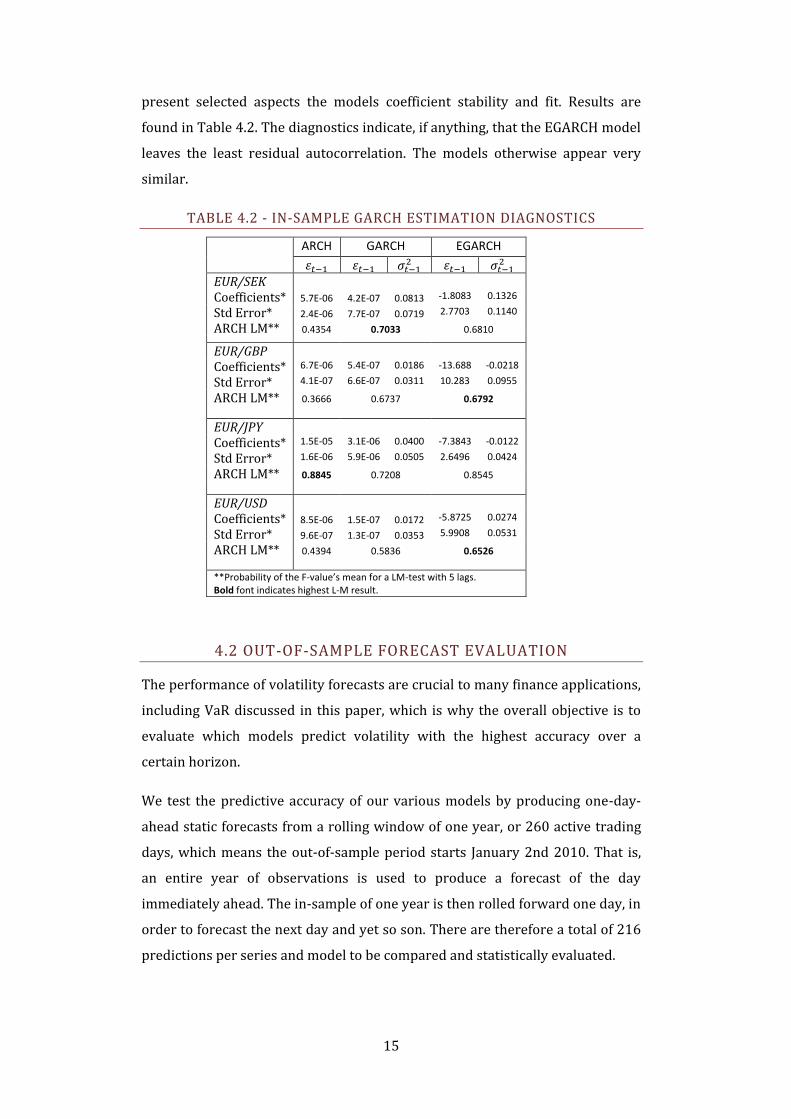
present selected aspects the models coefficient stability and fit. Results are
found in Table 4.2. The diagnostics indicate, if anything, that the EGARCH model
leaves the least residual autocorrelation. The models otherwise appear very
similar.
TABLE 4.2 - IN-SAMPLE GARCH ESTIMATION DIAGNOSTICS
ARCH GARCH EGARCH
EUR/SEK Coefficients* 5.7E-06 4.2E-07 0.0813 -1.8083 0.1326
Std Error* 2.4E-06 7.7E-07 0.0719 2.7703 0.1140
ARCH LM** 0.4354 0.7033 0.6810
EUR/GBP
Coefficients* 6.7E-06 5.4E-07 0.0186 -13.688 -0.0218
Std Error* 4.1E-07 6.6E-07 0.0311 10.283 0.0955
ARCH LM** 0.3666 0.6737 0.6792
EUR/JPY
Coefficients* 1.5E-05 3.1E-06 0.0400 -7.3843 -0.0122
Std Error* 1.6E-06 5.9E-06 0.0505 2.6496 0.0424
ARCH LM** 0.8845 0.7208 0.8545
EUR/USD
Coefficients* 8.5E-06 1.5E-07 0.0172 -5.8725 0.0274
Std Error* 9.6E-07 1.3E-07 0.0353 5.9908 0.0531
ARCH LM** 0.4394 0.5836 0.6526
**Probability of the F-value’s mean for a LM-test with 5 lags. Bold font indicates highest L-M result.
4.2 OUT-OF-SAMPLE FORECAST EVALUATION
The performance of volatility forecasts are crucial to many finance applications,
including VaR discussed in this paper, which is why the overall objective is to
evaluate which models predict volatility with the highest accuracy over a
certain horizon.
We test the predictive accuracy of our various models by producing one-day-
ahead static forecasts from a rolling window of one year, or 260 active trading
days, which means the out-of-sample period starts January 2nd 2010. That is,
an entire year of observations is used to produce a forecast of the day
immediately ahead. The in-sample of one year is then rolled forward one day, in
order to forecast the next day and yet so son. There are therefore a total of 216
predictions per series and model to be compared and statistically evaluated.

16
The idea is to compare the models both within respective classes i.e. ARCH-
types and the RV based, as well as contrast them against each other.
In comparing the forecasts we use three standard forecast error measurements,
namely MAE, MAPE and RMSE5. Note that, to calculate the forecast error, we
contrast the forecast with actual RV, as is customary. This also applies to the
ARCH-models. These loss functions are widely used and seem a good base for
discussion of performance. Although, assessing the quality of out-of-sample
forecasts is not entirely straightforward since numerical indications such these
may be misleading. It may be the case, if there for example are extreme outliers
in the series that some models get a disproportionate large mean error which
fails to describe forecasting performance in the absence of extreme outliers.
What this means is that these measures should only be interpreted in company
with the forecast graph.
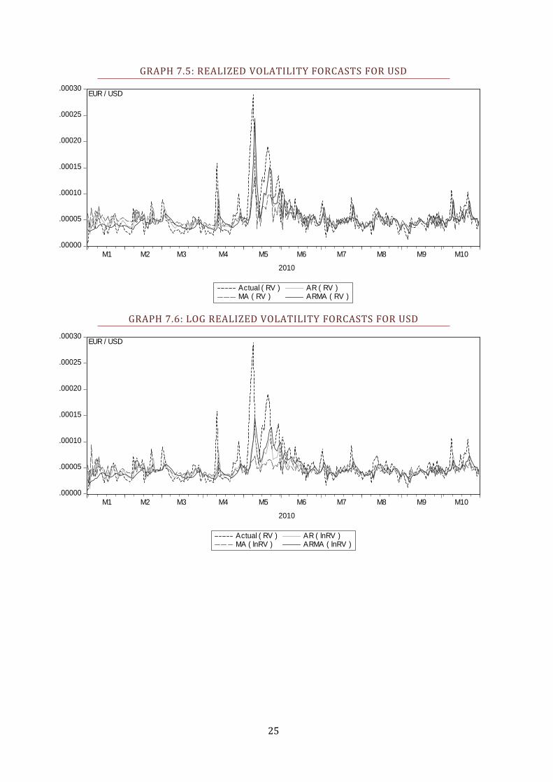
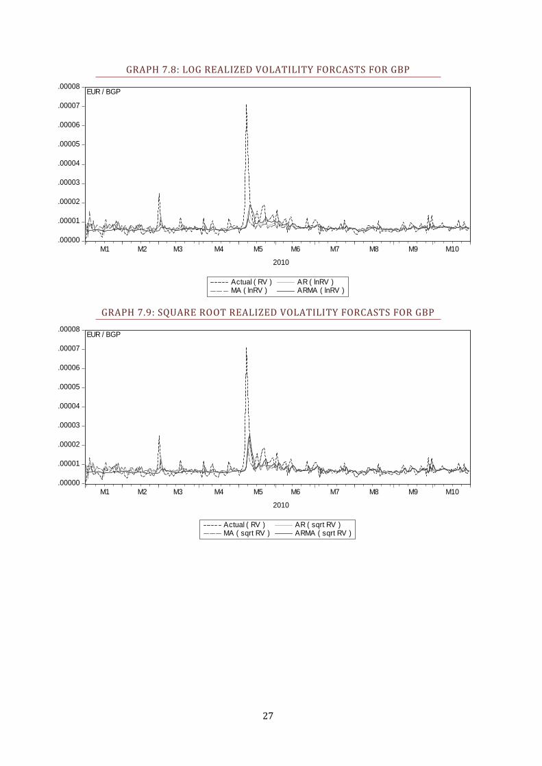
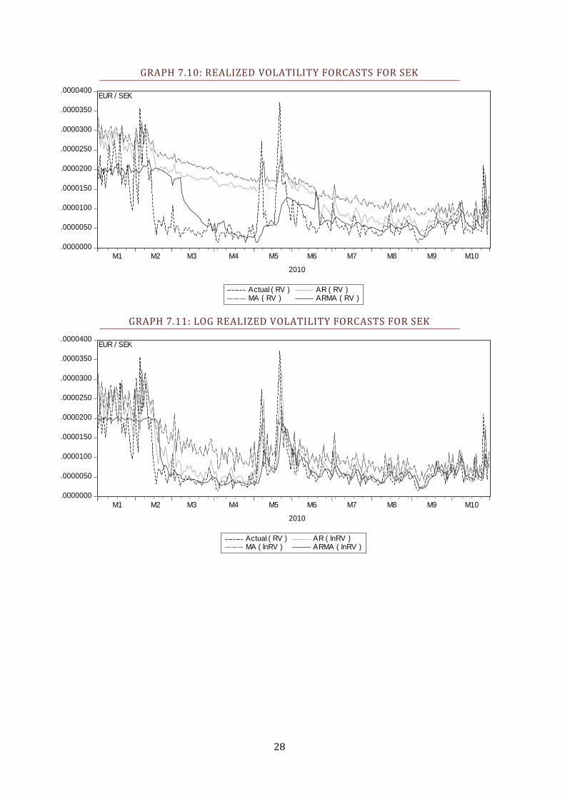
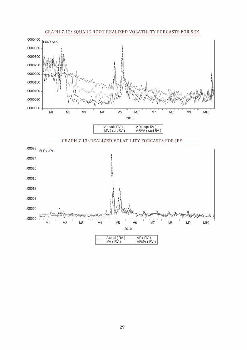
First, we look at how the total of nine RV models performs in the one-day-ahead
forecasts, results seen in Table 4.3. Notably, it seems one particular model, the
ARMA based on the logarithm of RV, quite consistently give the superior
forecasts. The ARMA on the square root of RV also performs admirably.
TABLE 4.3 - RV FORECAST EVALUATION
√ AR MA ARMA AR MA ARMA AR MA ARMA
EUR/SEK
MAE 7.0E-06 9.3E-06 3.8E-06 3.1E-06 5.3E-06 2.6E-06 4.2E-06 7.0E-06 2.3E-06
MAPE 1.4203 1.8938 0.6154 0.4548 0.9917 0.3459 0.7205 1.3832 0.4105
RMSE 8.6E-06 1.0E-05 6.0E-06 4.7E-06 6.6E-06 4.5E-06 5.6E-06 8.2E-06 4.9E-06
** *
EUR/JPY
MAE 8.7E-06 9.8E-06 8.4E-06 8.3E-06 9.7E-06 8.2E-06 8.2E-06 9.3E-06 8.1E-06
MAPE 0.4737 0.5594 0.4108 0.3742 0.4297 0.3532 0.3961 0.4648 0.3749
RMSE 2.0E-05 2.2E-05 2.1E-05 2.1E-05 2.4E-05 2.1E-05 2.0E-05 2.3E-05 2.0E-05
* * *
EUR/GBP
MAE 2.5E-06 2.9E-06 2.4E-06 2.5E-06 2.7E-06 2.3E-06 2.5E-06 2.7E-06 2.4E-06
MAPE 0.3616 0.4285 0.3359 0.3168 0.3518 0.2866 0.3338 0.3784 0.3031
RMSE 5.2E-06 5.9E-06 5.3E-06 5.5E-06 5.7E-06 5.5E-06 5.3E-06 5.6E-06 5.3E-06
* **
EUR/USD
MAE 1.8E-05 2.0E-05 1.8E-05 1.8E-05 2.0E-05 1.7E-05 1.8E-05 1.9E-05 1.8E-05
MAPE 0.3751 0.4267 0.3515 0.3371 0.3756 0.3169 0.3542 0.3944 0.3320
RMSE 2.7E-05 3.0E-05 2.8E-05 2.9E-05 3.4E-05 2.9E-05 2.8E-05 3.2E-05 2.8E-05
* **
MAE: Mean Absolute Error, MAPE: Mean Absolute Percentage Error, RMSE: Root Mean Squared Error Bold font indicates lowest error. Note that the logged and square rooted series are anti-logged and squared respectively prior to evaluation.
5 Mean Absolute Error, Mean Absolute Percentage Error and Root Mean Squared Error

17
Next, we have a look at the corresponding results for the ARCH-type models,
Table 4.4. It is clear to see that the GARCH specification most often give the top
forecasts, although the ARCH model is not far behind.
TABLE 4.4 – GARCH FORECAST EVALUATION
ARCH GARCH EGARCH NAIVE
EUR/SEK MAE 3.9E-06 4.5E-06 4.7E-06 1.1E-07
MAPE 0.4844 0.4053 0.4446 0.3506
RMSE 6.2E-06 7.9E-06 8.0E-06 4.9E-06
** *
EUR/JPY
MAE 1.1E-05 1.0E-05 1.2E-05 -3.2E-08
MAPE 0.5383 0.4470 0.5050 0.4210
RMSE 2.5E-05 2.6E-05 2.5E-05 2.0E-05
* **
EUR/GBP
MAE 2.9E-06 2.5E-06 3.3E-06 -3.3E-10
MAPE 0.3648 0.2751 0.3954 0.3788
RMSE 6.2E-06 5.9E-06 6.4E-06 5.7E-06
***
EUR/USD
MAE 4.5E-05 4.5E-05 4.6E-05 -2.2E-08
MAPE 0.7913 0.7954 0.8118 0.3837
RMSE 5.7E-05 5.6E-05 5.7E-05 2.9E-05
* ** MAE: Mean Absolute Error, MAPE: Mean Absolute Percentage Error, RMSE: Root Mean Squared Error. Bold font indicates lowest error.
We now turn our attention to comparing the alternative forecasting
frameworks. Recall that the GARCH(1,1) is widely used as the standard for
many financial practitioners and it is hence the benchmark against which the
competing models should measure up. In Table 4.5 we have documented the
improvement in forecasting errors for a selection of the top models against the
GARCH(1,1).
TABLE 4.5 – MODEL COMPARSION AGAINST GARCH
ARCH EGARCH AR-RV LOG-ARMA SQ-ARMA
EUR/SEK 13% -4% -55% 42% 49%
EUR/JPY -10% -20% 13% 18% 19%
EUR/GBP -16% -32% 0% 8% 4%
EUR/USD 0% -2% 60% 62% 60%
Statistics reported: Percentage improvement in RMSE (i.e. lower forecast error) over the benchmark GARCH(1,1) result. Bold font indicates highest improvement for respective series.
18
4.3 VALUE-AT-RISK: PRACTICAL APPLICATION
We now turn to the practical application of the results attained in the paper.
Take, for instance, a portfolio with 100’000 Euro invested in each of the four
currencies. The following information is necessary to calculate the desirable
VaR:
Portfolio size, which in this case is 100’000 Euro for each currency.
Volatility forecast for given day (e.g. √ from a Log-ARMA(1,1)
which we recognized as the ideal model (see Table 4.3) for one day
ahead forecasts).
Confidence level which in this case is 99% since we will be calculating
the standard VaR (1%).
Time period of trading (we will be using one day ahead).
The distribution for each exchange rate series (see Table 3.1).
As seen in Table 3.1 all currencies pass as normally distributed except the
Japanese Yen series. Since the Yen series was not normal we proceeded with a
robustness check in the form of a Monte Carlo simulation6. However, it is
noteworthy that only the left tail of the distribution matters in VaR calculations.
Therefore, it is only necessary for the Monte Carlo values on that particular side
that need to correspond to the Gaussian distribution if you want use it. The
conclusion from the simulation is that the critical value taken from the Monte
Carlo simulation is only marginally different to the Gaussian’s 1 percent
quantile (2.33).When comparing VaR(1%) calculated with the Gaussian
distribution, the student-t distribution and with the results of a Monte Carlo
simulation we get what is seen in Graph 4.1.
6 Monte Carlo simulation is a method which calculates distributions with information from the sample. As this did not change our results we will not dwell on it, but the interested reader is referred to Jackel, P. (2002), Monte Carlo – Methods in finance, John Wiley & Sons, 1st edition, Somerset, NJ, USA.

19
GRAPH 4.1 – VAR DISTRIBUTION SIMUALTION COMPARISON
We can now calculate one day ahead VAR (1%) for each series with a rolling in-
sample with one trading years observation with volatility forecasts taken from
the log-ARMA(1,1) model.
GRAPH 4.2 – 1% VAR WITH 100’000 EURO PORTFOLIO
400
800
1,200
1,600
2,000
2,400
2,800
M1 M2 M3 M4 M5 M6 M7 M8 M9 M10
2010
Monte Carlo
Gaussian distribution
T distribution with 10 d.f
EUR / JPY
1% VAR with 100 00 Euro portfolio with different distribution assumtions:
1,000
1,500
2,000
2,500
3,000
3,500
M1 M2 M3 M4 M5 M6 M7 M8 M9 M10
2010
EUR / USD
400
600
800
1,000
1,200
1,400
M1 M2 M3 M4 M5 M6 M7 M8 M9 M10
2010
EUR / SEK
400
800
1,200
1,600
2,000
2,400
M1 M2 M3 M4 M5 M6 M7 M8 M9 M10
2010
EUR / JPY
500
600
700
800
900
1,000
1,100
M1 M2 M3 M4 M5 M6 M7 M8 M9 M10
2010
EUR / BGP
1% VAR with 100 000 EUR portfolio
20
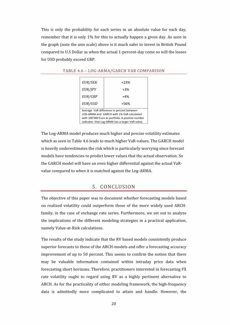
This is only the probability for each series in an absolute value for each day,
remember that it is only 1% for this to actually happen a given day. As seen in
the graph (note the axis scale) above is it much safer to invest in British Pound
compared to U.S Dollar as when the actual 1-percent-day come so will the losses
for USD probably exceed GBP.
TABLE 4.6 – LOG-ARMA/GARCH VAR COMPARISON
The Log-ARMA model produces much higher and precise volatility estimates
which as seen in Table 4.6 leads to much higher VaR-values. The GARCH model
is heavily underestimates the risk which is particularly worrying since forecast
models have tendencies to predict lower values that the actual observation. So
the GARCH model will have an even higher differential against the actual VaR-
value compared to when it is matched against the Log-ARMA.
5. CONCLUSION
The objective of this paper was to document whether forecasting models based
on realized volatility could outperform those of the more widely used ARCH-
family, in the case of exchange rate series. Furthermore, we set out to analyze
the implications of the different modeling strategies in a practical application,
namely Value-at-Risk calculations.
The results of the study indicate that the RV based models consistently produce
superior forecasts to those of the ARCH-models and offer a forecasting accuracy
improvement of up to 50 percent. This seems to confirm the notion that there
may be valuable information contained within intraday price data when
forecasting short horizons. Therefore, practitioners interested in forecasting FX
rate volatility ought to regard using RV as a highly pertinent alternative to
ARCH. As for the practicality of either modeling framework, the high-frequency
data is admittedly more complicated to attain and handle. However, the
EUR/SEK +23%
EUR/JPY +3%
EUR/GBP +4%
EUR/USD +56%
Average VaR difference in percent between LOG-ARMA and GARCH with 1% VaR calculated with 100’000 Euro as portfolio. A positive number indicates that Log-ARMA has a larger VaR-value.
21
convenience of using standard time series ARMA methodology should not be
overlooked. It is of course also possible that the potential gains in forecasting
precision afforded by the RV methodology alone can outweigh the cost and
inconvenience of using intraday data.
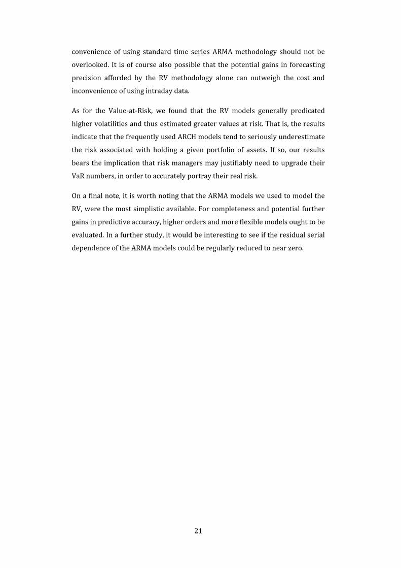
As for the Value-at-Risk, we found that the RV models generally predicated
higher volatilities and thus estimated greater values at risk. That is, the results
indicate that the frequently used ARCH models tend to seriously underestimate
the risk associated with holding a given portfolio of assets. If so, our results
bears the implication that risk managers may justifiably need to upgrade their
VaR numbers, in order to accurately portray their real risk.
On a final note, it is worth noting that the ARMA models we used to model the
RV, were the most simplistic available. For completeness and potential further
gains in predictive accuracy, higher orders and more flexible models ought to be
evaluated. In a further study, it would be interesting to see if the residual serial
dependence of the ARMA models could be regularly reduced to near zero.
22
6. REFERENCES
Articles:
Andersen, T.G. & Bollerslev, T. & Diebold F.X. & Labys, P. (2001), ”The
Distribution of Realized Exchange Rate Volatility”, Journal of the American
Statistical Association, No. 96, pp. 42-55.
Andersen, T.G. & Bollerslev, T. & Diebold F.X. & Labys, P. (2000), ”Exchange rate
returns standardized by Realized Volatility are (nearly) Gaussian”,
Multinational Finance Journal, No. 4, pp. 159-179.
Andersen, T.G. & Bollerslev, T. & Diebold F.X. & Labys, P. (2002), ”Modeling and
forecasting Realized Volatility”, Econometrica, No. 71, pp. 529-626.
Frinjs, B. & Margaritis, D. (2008), “Forecasting daily volatility with intraday
data”, The European Journal of Finance, Vol. 14, No. 6, pp. 523-540.
Gardner, Jr. E.S. (2006), “Exponential smoothing: The state of Art – Part ll”,
International Journal of Forecasting, vol. 22, issue 4, pp. 637-666.
Teräsvirta, T. (2006), “An Introduction to Univariate GARCH models”, SSE/EFI
Working Papers in Economics and Finance, No. 646.
Books:
Alexander, C. (2008), Practical Financial Econometrics, 1st ed., John Wiley &
Sons Inc, Hoboken, USA.
Jäckel, P. (2002), Monte Carlo – Methods in finance, 1st ed., John Wiley & Sons
Inc, Hoboken, USA.
Philippe, J. (2007), Value At Risk: The New Benchmark for Managing Financial
Risk, 3rd ed., The McGraw-Hill Companies Inc, NY, USA.
23
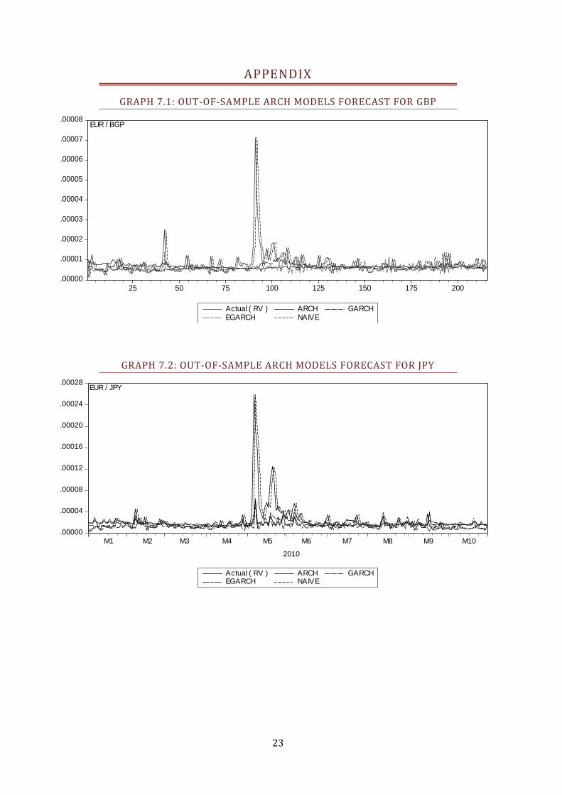
APPENDIX
GRAPH 7.1: OUT-OF-SAMPLE ARCH MODELS FORECAST FOR GBP
GRAPH 7.2: OUT-OF-SAMPLE ARCH MODELS FORECAST FOR JPY
.00000
.00001
.00002
.00003
.00004
.00005
.00006
.00007
.00008
25 50 75 100 125 150 175 200
Actual ( RV ) ARCH GARCHEGARCH NAIVE
EUR / BGP
.00000
.00004
.00008
.00012
.00016
.00020
.00024
.00028
M1 M2 M3 M4 M5 M6 M7 M8 M9 M10
2010
Actual ( RV ) ARCH GARCHEGARCH NAIVE
EUR / JPY
24
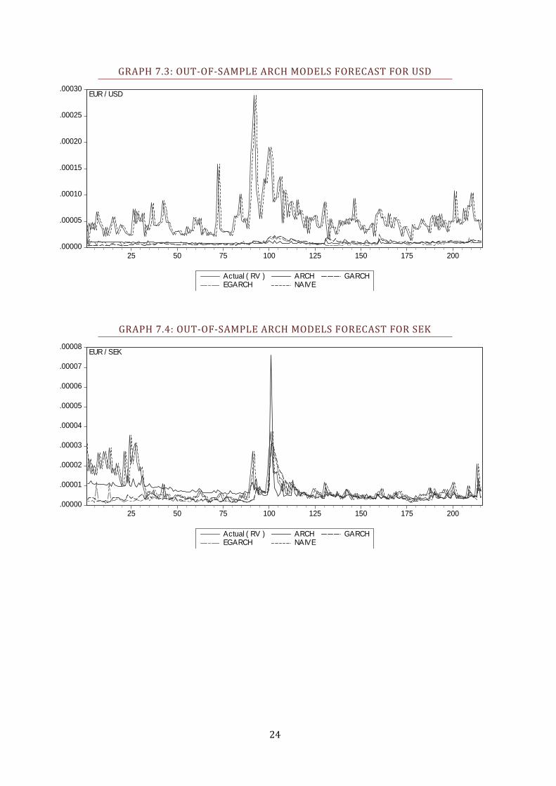
GRAPH 7.3: OUT-OF-SAMPLE ARCH MODELS FORECAST FOR USD
GRAPH 7.4: OUT-OF-SAMPLE ARCH MODELS FORECAST FOR SEK
.00000
.00005
.00010
.00015
.00020
.00025
.00030
25 50 75 100 125 150 175 200
Actual ( RV ) ARCH GARCHEGARCH NAIVE
EUR / USD
.00000
.00001
.00002
.00003
.00004
.00005
.00006
.00007
.00008
25 50 75 100 125 150 175 200
Actual ( RV ) ARCH GARCHEGARCH NAIVE
EUR / SEK
25
GRAPH 7.5: REALIZED VOLATILITY FORCASTS FOR USD
GRAPH 7.6: LOG REALIZED VOLATILITY FORCASTS FOR USD
.00000
.00005
.00010
.00015
.00020
.00025
.00030
M1 M2 M3 M4 M5 M6 M7 M8 M9 M10
2010
Actual ( RV ) AR ( RV )MA ( RV ) ARMA ( RV )
EUR / USD
.00000
.00005
.00010
.00015
.00020
.00025
.00030
M1 M2 M3 M4 M5 M6 M7 M8 M9 M10
2010
Actual ( RV ) AR ( lnRV )MA ( lnRV ) ARMA ( lnRV )
EUR / USD

26
GRAPH 7.6: SQUARE ROOT REALIZED VOLATILITY FORCASTS FOR USD
GRAPH 7.7: REALIZED VOLATILITY FORCASTS FOR GBP
.00000
.00005
.00010
.00015
.00020
.00025
.00030
M1 M2 M3 M4 M5 M6 M7 M8 M9 M10
2010
Actual ( RV ) AR ( sqrt RV )MA ( sqrt RV ) ARMA ( sqrt RV )
EUR / USD
.00000
.00001
.00002
.00003
.00004
.00005
.00006
.00007
.00008
M1 M2 M3 M4 M5 M6 M7 M8 M9 M10
2010
Actual ( RV ) AR ( RV )MA ( RV) ARMA ( RV )
EUR / BGP
27
GRAPH 7.8: LOG REALIZED VOLATILITY FORCASTS FOR GBP
GRAPH 7.9: SQUARE ROOT REALIZED VOLATILITY FORCASTS FOR GBP
.00000
.00001
.00002
.00003
.00004
.00005
.00006
.00007
.00008
M1 M2 M3 M4 M5 M6 M7 M8 M9 M10
2010
Actual ( RV ) AR ( lnRV )MA ( lnRV ) ARMA ( lnRV )
EUR / BGP
.00000
.00001
.00002
.00003
.00004
.00005
.00006
.00007
.00008
M1 M2 M3 M4 M5 M6 M7 M8 M9 M10
2010
Actual ( RV ) AR ( sqrt RV )MA ( sqrt RV ) ARMA ( sqrt RV )
EUR / BGP
28
GRAPH 7.10: REALIZED VOLATILITY FORCASTS FOR SEK
GRAPH 7.11: LOG REALIZED VOLATILITY FORCASTS FOR SEK
.0000000
.0000050
.0000100
.0000150
.0000200
.0000250
.0000300
.0000350
.0000400
M1 M2 M3 M4 M5 M6 M7 M8 M9 M10
2010
Actual ( RV ) AR ( RV )MA ( RV ) ARMA ( RV )
EUR / SEK
.0000000
.0000050
.0000100
.0000150
.0000200
.0000250
.0000300
.0000350
.0000400
M1 M2 M3 M4 M5 M6 M7 M8 M9 M10
2010
Actual ( RV ) AR ( lnRV )MA ( lnRV ) ARMA ( lnRV )
EUR / SEK
29
GRAPH 7.12: SQUARE ROOT REALIZED VOLATILITY FORCASTS FOR SEK
GRAPH 7.13: REALIZED VOLATILITY FORCASTS FOR JPY
.0000000
.0000050
.0000100
.0000150
.0000200
.0000250
.0000300
.0000350
.0000400
M1 M2 M3 M4 M5 M6 M7 M8 M9 M10
2010
Actual ( RV ) AR ( sqrt RV )MA ( sqrt RV ) ARMA ( sqrt RV )
EUR / SEK
.00000
.00004
.00008
.00012
.00016
.00020
.00024
.00028
M1 M2 M3 M4 M5 M6 M7 M8 M9 M10
2010
Actual ( RV ) AR ( RV )MA ( RV ) ARMA ( RV )
EUR / JPY
30
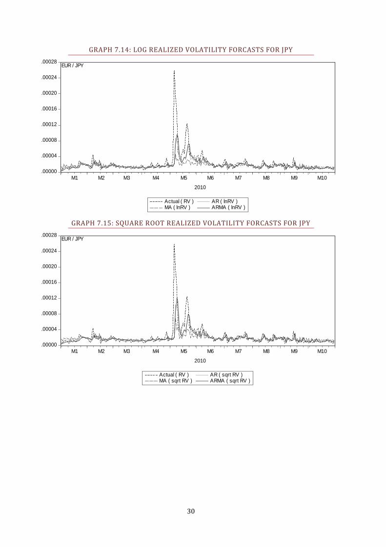
GRAPH 7.14: LOG REALIZED VOLATILITY FORCASTS FOR JPY
GRAPH 7.15: SQUARE ROOT REALIZED VOLATILITY FORCASTS FOR JPY
.00000
.00004
.00008
.00012
.00016
.00020
.00024
.00028
M1 M2 M3 M4 M5 M6 M7 M8 M9 M10
2010
Actual ( RV ) AR ( lnRV )MA ( lnRV ) ARMA ( lnRV )
EUR / JPY
.00000
.00004
.00008
.00012
.00016
.00020
.00024
.00028
M1 M2 M3 M4 M5 M6 M7 M8 M9 M10
2010
Actual ( RV ) AR ( sqrt RV )MA ( sqrt RV ) ARMA ( sqrt RV )
EUR / JPY
Related Documents