Journal of Sports Analytics 7 (2021) 77–97 DOI 10.3233/JSA-200462 IOS Press 77 Forecasting football matches by predicting match statistics Edward Wheatcroft ∗ London School of Economics and Political Science, Houghton Street, London, United Kingdom, WC2A 2AE Abstract. This paper considers the use of observed and predicted match statistics as inputs to forecasts for the outcomes of football matches. It is shown that, were it possible to know the match statistics in advance, highly informative forecasts of the match outcome could be made. Whilst, in practice, match statistics are clearly never available prior to the match, this leads to a simple philosophy. If match statistics can be predicted pre-match, and if those predictions are accurate enough, it follows that informative match forecasts can be made. Two approaches to the prediction of match statistics are demonstrated: Generalised Attacking Performance (GAP) ratings and a set of ratings based on the Bivariate Poisson model which are named Bivariate Attacking (BA) ratings. It is shown that both approaches provide a suitable methodology for predicting match statistics in advance and that they are informative enough to provide information beyond that reflected in the odds. A long term and robust gambling profit is demonstrated when the forecasts are combined with two betting strategies. Keywords: Probability forecasting, sports forecasting, football forecasting, football predictions, soccer predictions 1. Introduction Quantitative analysis of sports is a rapidly grow- ing discipline with participants, coaches, owners, as well as gamblers, increasingly recognising its poten- tial in gaining an edge over their opponents. This has naturally led to a demand for information that might allow better decisions to be made. Associa- tion football (hereafter football) is the most popular sport globally and, although, historically, the use of quantitative analysis has lagged behind that of US sports, this is slowly changing. Gambling on football matches has also grown significantly in popularity in recent decades and this has contributed to an increased demand for informative quantitative anal- ysis. Today, in the most popular football leagues glob- ally, a great deal of match data are collected. Data on the location and outcome of every match event can be purchased, whilst free data are available including ∗ Corresponding author: Edward Wheatcroft, London School of Economics and Political Science, Houghton Street, London, United Kingdom, WC2A 2AE. E-mail: [email protected]. match statistics such as the numbers of shots, corners and fouls by each team. This creates huge potential for those able to process the data in an informative way. This paper focuses on probabilistic prediction of the outcomes of football matches, i.e. whether the match ends with a home win, a draw or an away win. A prob- abilistic forecast of such an event simply consists of estimated probabilities placed on each of the three possible outcomes. Statistical models can be used to incorporate information into probabilistic forecasts. The basic philosophy of this paper is as follows. Suppose, somehow, that certain match statistics, such as the number of shots or corners achieved by each team, were available in advance of kickoff. In such a case, it would be reasonable to expect to be able to use this information to create informative forecasts and it is shown that this is the case. Obviously, in reality, this information would never be available in advance. However, if one can use statistics from past matches to predict the match statistics before the match begins, and those predictions are accurate enough, they can be used to create informative forecasts of the match outcome. The quality of the forecast is then dependent ISSN 2215-020X © 2021 – The authors. Published by IOS Press. This is an Open Access article distributed under the terms of the Creative Commons Attribution-NonCommercial License (CC BY-NC 4.0).

Welcome message from author
This document is posted to help you gain knowledge. Please leave a comment to let me know what you think about it! Share it to your friends and learn new things together.
Transcript
Journal of Sports Analytics 7 (2021) 77–97DOI 10.3233/JSA-200462IOS Press
77
Forecasting football matches by predictingmatch statistics
Edward Wheatcroft∗London School of Economics and Political Science, Houghton Street, London, United Kingdom, WC2A 2AE
Abstract. This paper considers the use of observed and predicted match statistics as inputs to forecasts for the outcomes offootball matches. It is shown that, were it possible to know the match statistics in advance, highly informative forecasts of thematch outcome could be made. Whilst, in practice, match statistics are clearly never available prior to the match, this leads to asimple philosophy. If match statistics can be predicted pre-match, and if those predictions are accurate enough, it follows thatinformative match forecasts can be made. Two approaches to the prediction of match statistics are demonstrated: GeneralisedAttacking Performance (GAP) ratings and a set of ratings based on the Bivariate Poisson model which are named BivariateAttacking (BA) ratings. It is shown that both approaches provide a suitable methodology for predicting match statistics inadvance and that they are informative enough to provide information beyond that reflected in the odds. A long term androbust gambling profit is demonstrated when the forecasts are combined with two betting strategies.
Keywords: Probability forecasting, sports forecasting, football forecasting, football predictions, soccer predictions
1. Introduction
Quantitative analysis of sports is a rapidly grow-ing discipline with participants, coaches, owners, aswell as gamblers, increasingly recognising its poten-tial in gaining an edge over their opponents. Thishas naturally led to a demand for information thatmight allow better decisions to be made. Associa-tion football (hereafter football) is the most popularsport globally and, although, historically, the use ofquantitative analysis has lagged behind that of USsports, this is slowly changing. Gambling on footballmatches has also grown significantly in popularityin recent decades and this has contributed to anincreased demand for informative quantitative anal-ysis.
Today, in the most popular football leagues glob-ally, a great deal of match data are collected. Data onthe location and outcome of every match event canbe purchased, whilst free data are available including
∗Corresponding author: Edward Wheatcroft, London Schoolof Economics and Political Science, Houghton Street, London,United Kingdom, WC2A 2AE. E-mail: [email protected].
match statistics such as the numbers of shots, cornersand fouls by each team. This creates huge potential forthose able to process the data in an informative way.This paper focuses on probabilistic prediction of theoutcomes of football matches, i.e. whether the matchends with a home win, a draw or an away win. A prob-abilistic forecast of such an event simply consists ofestimated probabilities placed on each of the threepossible outcomes. Statistical models can be used toincorporate information into probabilistic forecasts.
The basic philosophy of this paper is as follows.Suppose, somehow, that certain match statistics, suchas the number of shots or corners achieved by eachteam, were available in advance of kickoff. In such acase, it would be reasonable to expect to be able to usethis information to create informative forecasts andit is shown that this is the case. Obviously, in reality,this information would never be available in advance.However, if one can use statistics from past matches topredict the match statistics before the match begins,and those predictions are accurate enough, they canbe used to create informative forecasts of the matchoutcome. The quality of the forecast is then dependent
ISSN 2215-020X © 2021 – The authors. Published by IOS Press. This is an Open Access article distributed under the termsof the Creative Commons Attribution-NonCommercial License (CC BY-NC 4.0).
78 E. Wheatcroft / Forecasting football matches by predicting match statistics
both on the importance of the match statistic itselfand the accuracy of the pre-match prediction of thatstatistic.
In this paper, observed and predicted match statis-tics are used as inputs to a simple statistical model toconstruct probabilistic forecasts of match outcomes.First, observed match statistics in the form of thenumber of shots on target, shots off target and cor-ners, are used to build forecasts and are shown to beinformative. The observed match statistics are thenreplaced with predicted statistics calculated using(i) Generalised Attacking Performance (GAP) Rat-ings, a system which uses past data to estimatethe number of defined measures of attacking per-formance a team can be expected to achieve in agiven match (Wheatcroft, 2020), and (ii) BivariateAttacking (BA) ratings which are introduced hereand are a slightly modified version of the BivariatePoisson model which has demonstrated favourableresults in comparison to other parametric approaches(Ley et al. 2019). Whilst, unsurprisingly, it is foundthat predicted match statistics are less informativethan observed statistics, they can still provide usefulinformation for the construction of the forecasts. It isshown that a robust profit can be made by construct-ing forecasts based on predicted match statistics andusing them alongside two different betting strategies.
For much of the history of sports prediction, ratingsystems in a similar vein to the GAP rating systemused in this paper have played a key role. Probablythe most well known is the Elo rating system whichwas originally designed to produce rankings for chessplayers but has a long history in other sports (Elo, etal. 1978). The Elo system assigns a rating to eachplayer or team which, in combination with the ratingof the opposition, is used to estimate the probability ofeach possible outcome. The ratings are updated aftereach game in which a player or team is involved. Aweakness of the original Elo rating system is that itdoes not estimate the probability of a draw. As such, insports such as football, in which draws are common,some additional methodology is required to estimatethat probability.
Elo ratings are in widespread use in football andhave been demonstrated to perform favourably withrespect to other rating systems (Hvattum and Arntzen,2010). Since 2018, Fifa has used an Elo rating systemto produce its international football world rankings(Fifa, 2018). Elo ratings have also been appliedto a wide range of other sports including, amongothers, Rugby League (Carbone et al., 2016) andvideo games (Suznjevic et al., 2015). The website
fivethirtyeight.com produces probabilities for NFL(FiveThirtyEight, 2020a) and NBA (FiveThirtyEight,2020b) based on Elo ratings. A limitation of the Elorating system is that it does not account for the size ofa win. This means that a team’s ranking after a matchwould be the same after either a narrow or convinc-ing victory. Some authors have adapted the system toaccount for the margin of victory (see, for example,Lasek et al. (2013) and Sullivan and Cronin (2016)).
The original Elo rating system assigns a single rat-ing to each participating team or player, reflectingits overall ability. This does not directly allow fora distinction between the performance of a team inits home or away matches. Typically, some adjust-ment to the estimated probabilities is made to accountfor home advantage. Other rating systems distinguishbetween home and away performances. One sys-tem that does this is the pi-rating system in whicha separate home and away rating is assigned to eachteam (Constantinou and Fenton, 2013). The pi-ratingsystem also takes into account the winning mar-gin of each team, but this is tapered such that theimpact of additional goals on top of already largewinning margins is lower than that of goals in closematches.
The GAP rating system, introduced in Wheatcroft(2020) and used in this paper, differs from both theElo rating and the pi-rating systems in that, rather thanproducing a single rating, each team is assigned a sep-arate attacking and defensive rating both for its homeand away matches. This results in a total of 4 ratingsper team. The approach of assigning attacking anddefensive ratings has been taken by a large numberof authors. An early example is Maher (1982) whoassigned fixed ratings to each team and combinedthem with a Poisson model to estimate the number ofgoals scored. They did not use their ratings to estimatematch probabilities but Dixon and Coles (1997) didso using a similar approach. Combined with a valuebetting strategy, they were able to demonstrate a sig-nificant profit for matches with a large discrepancybetween the estimated probabilities and the proba-bilities implied by the odds. Dixon and Pope (2004)modified the Dixon and Coles model and were ableto demonstrate a profit using a wider range of pub-lished bookmaker odds. Rue and Salvesen (2000)defined a Bayesian model for attacking and defen-sive ratings, allowing them to vary over time. Otherexamples of systems that use attacking and defensiveratings can be found in Karlis and Ntzoufras (2003),Lee (1997) and Baker and McHale (2015). Ley etal. (2019) compared ten different parametric models
E. Wheatcroft / Forecasting football matches by predicting match statistics 79
(with the parameters estimated using maximum like-lihood) and found the Bivariate Poisson model to givethe most favourable results. Koopman and Lit (2015)used a Bivariate Poisson model alongside a Bayesianapproach to demonstrate a profitable betting strategy.
The use of rating systems naturally leads to thequestion of how to translate them into probabilisticforecasts. One of two approaches is generally taken.The first is to model the number of goals scoredby each team using Poisson or Negative Binomialregression with the ratings of each team used aspredictor variables. These are then used to estimatematch probabilities. The second approach is to pre-dict the probability of each match outcome directlyusing methods such as logistic regression. There islittle evidence to suggest a major difference in theperformance of the two approaches (Goddard, 2005).In this paper, the latter approach is taken, specificallyin the form of ordinal logistic regression.
The idea that match statistics might be moreinformative than goals in terms of making match pre-dictions has become more widespread in recent years.The rationale behind this view is that, since it is diffi-cult to score a goal and luck often plays an importantrole, the number of goals scored by each team mightbe a poor indicator of the events of the match. It wasshown by Wheatcroft (2020) that, in the over/under2.5 goals market, the number of shots and corners pro-vide a better basis for probabilistic forecasting thangoals themselves. Related to this is the concept of‘expected goals’ which is playing a more and moreimportant role in football analysis. The idea is thatthe quality of a shot can be measured in terms ofits likelihood of success. The expected goals from aparticular shot corresponds to the number of goalsone would ‘expect’ to score by taking that shot. Thenumber of expected goals by each team in a matchthen gives an indication of how the match played outin terms of efforts at goal. Several academic papershave focused on the construction of expected goalsmodels that take into account the location and natureof a shot (Eggels, 2016; Rathke, 2017).
This paper is organised as follows. In section 2,background information is given on betting oddsand the data set used in this paper. The BivariatePoisson model, which is used for comparison pur-poses in the results section and forms the basis ofthe Bivariate Attacking (BA) rating system is alsodescribed. In section 3, the GAP and BA rating sys-tems are described along with the approach usedfor constructing forecasts of match outcomes. Thetwo betting strategies used in the results section
are also described. In section 4, the accuracy ofpredicted match statistics in terms of how closethey get to observed statistics under the GAP andBA rating systems is compared. Match forecastsformed using different combinations of observedand predicted statistics are then compared usingmodel selection techniques. Next, the performanceof forecasts formed using combinations of predictedstatistics is compared. Finally, the profitability oftwo betting strategies is compared when used along-side forecasts formed using different combinationsof predicted match statistics. Section 6 is used fordiscussion.
2. Background
2.1. Betting odds
In this paper, betting odds are used both as poten-tial inputs to models and as a tool with which todemonstrate profit making opportunities. Decimal,or ‘European Style’, betting odds are consideredthroughout. Decimal odds simply represent the num-ber by which the gambler’s stake is multiplied in theevent of success. For example, if the decimal odds are2, a £ 10 bet on said event would result in a return of2 × £10 = £20.
Another useful concept is that of the ‘odds implied’probability. Let the odds for the i-th outcome of anevent be Oi. The odds implied probability is sim-ply defined as the multiplicative inverse, i.e. ri = 1
Oi.
For example, if the odds on two possible outcomesof an event (e.g. home or away win) are O1 = 3and O2 = 1.4, the odds implied probabilities arer1 = 1
3 ≈ 0.33 and R2 = 11.4 ≈ 0.71. Note how, in
this case, r1 and r2 add to more than one. This isbecause, whilst, conventionally, probabilities over aset of exhaustive events should add to one, this neednot be the case for odds implied probabilities. In fact,usually, the sum of odds implied probabilities foran event will exceed one. The excess represents thebookmaker’s profit margin or the ‘overround’ whichis formally defined as
π =(
m∑i=1
1
Oi
)− 1. (1)
Generally, the larger the overround, the more difficultit is for a gambler to make a profit since the returnfrom a winning bet is reduced.
80 E. Wheatcroft / Forecasting football matches by predicting match statistics
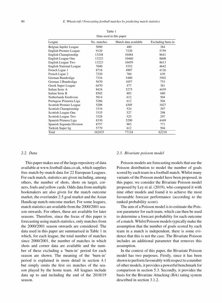
Table 1
Data used in this paper
League No. matches Match data available Excluding burn-in
Belgian Jupiler League 5090 480 384English Premier League 9120 7220 5759English Championship 13248 10484 8641English League One 13223 10460 8608English League Two 13223 10459 8613English National League 7040 5352 4642French Ligue 1 8718 4907 4126French Ligue 2 7220 760 639German Bundesliga 7316 5480 3502German 2.Bundesliga 5670 1057 753Greek Super League 6470 477 381Italian Serie A 8424 5275 4439Italian Serie B 8502 803 680Netherlands Eredivisie 5814 612 504Portugese Primeira Liga 5286 612 504Scottish Premier League 5208 4305 3427Scottish Championship 3334 524 297Scottish League One 3335 527 298Scottish League Two 3328 525 297Spanish Primera Liga 8330 5290 4449Spanish Segunda Division 8757 903 771Turkish Super lig 5779 612 504Total 162435 77124 62218
2.2. Data
This paper makes use of the large repository of dataavailable at www.football-data.co.uk, which suppliesfree match-by-match data for 22 European Leagues.For each match, statistics are given including, amongothers, the number of shots, shots on target, cor-ners, fouls and yellow cards. Odds data from multiplebookmakers are also given for the match outcomemarket, the over/under 2.5 goal market and the AsianHandicap match outcome market. For some leagues,match statistics are available from the 2000/2001 sea-son onwards. For others, these are available for laterseasons. Therefore, since the focus of this paper isforecasting using match statistics, only matches fromthe 2000/2001 season onwards are considered. Thedata used in this paper are summarised in Table 1 inwhich, for each league, the total number of matchessince 2000/2001, the number of matches in whichshots and corner data are available and the num-ber of these excluding a ‘burn-in’ period for eachseason are shown. The meaning of the ‘burn-in’period is explained in more detail in section 4.1but simply omits the first six matches of the sea-son played by the home team. All leagues includedata up to and including the end of the 2018/19season.
2.3. Bivariate poisson model
Poisson models are forecasting models that use thePoisson distribution to model the number of goalsscored by each team in a football match. Whilst manyvariants of the Poisson model have been proposed, inthis paper, we consider the Bivariate Poisson modelproposed by Ley et al. (2019), who compared it withnine other models and found it to achieve the mostfavourable forecast performance (according to theranked probability score).
The aim of a Poisson model is to estimate the Pois-son parameter for each team, which can then be usedto determine a forecast probability for each outcomeof a match. Whilst Poisson models typically make theassumption that the number of goals scored by eachteam in a match is independent, there is some evi-dence that this is not the case. The Bivariate Poissonincludes an additional parameter that removes thisassumption.
In the context of this paper, the Bivariate Poissonmodel has two purposes. Firstly, since it has beenshown to perform favourably with respect to a numberof other models, it provides a powerful benchmark forcomparison in section 5.3. Secondly, it provides thebasis for the Bivariate Attacking (BA) rating systemdescribed in section 3.1.2.
E. Wheatcroft / Forecasting football matches by predicting match statistics 81
Let Gi,m and Gj,m be random variables for thenumber of goals scored in the m-th match by teamsi and j, respectively, where team i is at home andteam j is away. In a match between the two teams, aPoisson model can be written as
P(Gi,m = α, Gj,m = β)
= λαi,mexp(−λi,m)
α!.λ
βj,mexp(−λj,m)
β!, (2)
where λi,m and λj,m are the means of Gi,m and Gj,m,respectively.
The Bivariate Poisson model is an extension ofanother model, also described by Ley et al. (2019),called the Independent Poisson model and it is usefulto define this first. The Independent Poisson Modelparametrises the Poisson parameters for a home teami against an away team j as λi,m = exp(c + (ri +h) − rj) and λj,m = exp(c + rj − (ri + h)), respec-tively, where c is a constant parameter, h is ahome advantage parameter and r1, ..., rT are strengthparameters for each team.
The Bivariate Poisson model closely resembles theindependent model but introduces an extra parame-ter to account for potential dependency between thenumber of goals scored by each team. Under theBivariate Poisson model, the joint distribution forthe number of goals in a match between teams i andj is given by
P(Gi,m = α, Gj,m = β)
= λαi,mλ
βj,m
α!β!exp(−(λi,m + λj,m + λc))
min(x,y)∑k=0
(x
k
)(y
k
)k!
(λc
λi,mλj,m
)(3)
where λc is a parameter that introduces a dependencyin the number of goals scored by each team and λi,m
and λj,m are parametrised in the same way as theIndependent Poisson model. For the Bivariate Pois-son model, the Poisson parameter for the home andaway team is λc + λi,m and λc + λj,m, respectively.
Both the Independent and Bivariate Poisson mod-els are parametric models in which the parametersare estimated using maximum likelihood. However,in both cases, a slight adjustment is made to the likeli-hood function such that matches that happened morerecently are given more weight than those that hap-pened longer ago. To do this, the weight placed on
match m is given by
wtime,m(xm) =(
1
2
) xmH
, (4)
where xm is the number of days since the match wasplayed and H is the half life (e.g. if the half life is twoyears, a match played two years ago receives halfthe weight of a match played today). The adjustedlikelihood to be maximised is then given by
L =M∏
m=1
P(Ghm,m = αm, Gam,m = βm)wtime,m(xm)
(5)where, for the m-th match, αm denotes the number ofgoals scored by the home team hm, and β the numberscored by the away team am.
Performing maximum likelihood estimation witha large number of parameters is, in general, difficultand there is a risk of falling into local optima. Wefollow the approach used by Ley et al. (2019) whouse the Broyden-Fletcher-Goldfarb-Shanno (BFGS)algorithm, a quasi-Newton method known for itsrobust properties, implemented with the ‘fmincon’function in Matlab. Strictly positive parameters areinitialised at one and each of the other parametersis initialised at zero. The sum of the team ratingsr1, ..., rT is constrained to zero.
A convenient property of the Poisson model isthat the difference between two Poisson distributionsfollows a Skellam distribution and therefore matchoutcome probabilities can be estimated from the Pois-son parameters for each team. For more details, seeKarlis and Ntzoufras (2009).
3. Methodology
3.1. Ratings systems
In this paper, two different approaches are used toproduce predictions for the number of goals, shotson target, shots off target and corners achieved byeach team in a given football match. Each approachis described below.
3.1.1. GAP ratingsThe Generalised Attacking Performance (GAP)
rating system, introduced by Wheatcroft (2020), isa rating system for assessing the attacking and defen-sive strength of a sports team with relation to a
82 E. Wheatcroft / Forecasting football matches by predicting match statistics
particular measure of attacking performance such asthe number of shots or corners in football. For a par-ticular given measure of attacking performance, eachteam in a league is given an attacking and a defen-sive rating, both for its home and away matches. Anattacking GAP rating can be interpreted as an esti-mate of the number of defined attacking plays theteam can be expected to achieve against an averageteam in the league, whilst its defensive rating can beinterpreted as an estimate of the number of attackingplays it can be expected to concede against an averageteam. The ratings for each team are updated each timeit plays a match. The GAP ratings of the i-th team ina league who have played k matches are denoted asfollows:
�
Hai,k - Home attacking GAP rating of the i-th
team in a league after k matches.�
Hdi,k - Home defensive GAP rating of the i-th
team in a league after k matches.�
Aai,k - Away attacking GAP rating of the i-th
team in a league after k matches.�
Adi,k - Away defensive GAP rating of the i-th
team in a league after k matches.
The ratings are updated as follows. Consider a matchin which the i-th team in the league is at home tothe j-th team. The i-th team have played k1 previ-ous matches and the j-th team k2. Let Si,k1 and Sj,k2
be the number of defined attacking plays by teams i
and j in the match (note in many cases, both teamswill have played the same number of matches and k1and k2 will be equal). The GAP ratings for the i-thteam (the home team) are updated in the followingwayHa
i,k1+1 = max(Hai,k1
+ λφ1(Si,k1 − (Hai,k1
+ Adj,k2
)/2), 0),
Aai,k1+1 = max(Aa
i,k1+ λ(1 − φ1)(Si,k1 − (Ha
i,k1+ Ad
j,k2)/2), 0),
Hdi,k1+1 = max(Hd
i,k1+ λφ1(Sj,k2 − (Aa
j,k2+ Hd
i,k1)/2), 0),
Adi,k1+1 = max(Ad
i,k1+ λ(1 − φ1)(Sj,k2 − (Aa
j,k2+ Hd
i,k1)/2), 0).
(6)
The GAP ratings for the j-th team (the away team)are updated as follows:
Aaj,k2+1 = max(Aa
j,k2+ λφ2(Sj,k2 − (Aa
j + Hdi )/2), 0),
Haj,k2+1 = max(Ha
j,k2+ λ(1 − φ2)(Sj,k2 − (Aa
j + Hdi )/2), 0),
Adj,k2+1 = max(Ad
j,k2+ λφ2(Si,k1 − (Ha
i + Adj )/2), 0),
Hdj,k2+1 = max(Hd
j,k2+ λ(1 − φ2)(Si,k1 − (Ha
i + Adj )/2), 0),
(7)where λ > 0, 0 < φ1 < 1 and 0 < φ2 < 1 are param-eters to be estimated. Here, λ determines the overall
influence of a match on the ratings of each team. Theparameter φ1 governs how the adjustments are spreadover the home and away ratings of the i-th team (thehome team), whilst φ2 governs how the adjustmentsare spread over the home and away ratings of the j-thteam (the away team). After any given match, a hometeam is said to have outperformed expectations in anattacking sense if its attacking performance is higherthan the mean of its attacking rating and the opposi-tion’s defensive rating. In this case, its home attackingrating is increased (or decreased, if its attacking per-formance is lower than expected). If the parameterφ1 > 0, a team’s away ratings will be impacted bya home match, whilst a team’s home ratings will beimpacted by an away match if φ2 > 0.
In this paper, GAP ratings are used to estimate theattacking performance of each team. For a matchinvolving the i-th team at home to the j-th team,where the teams have played k1 and k2 previousmatches in that season, respectively, the predictednumbers of defined attacking plays for the home andaway teams are given by
Sh = Hai,k1 + Ad
j,k2
2Sa = Aa
j,k2 + Hdi,k1
2. (8)
The predicted number of attacking plays by thehome team is therefore the average of the hometeam’s home attacking rating and the away team’saway defensive rating whilst the predicted number ofattacking plays by the away team is given by the aver-age of the away team’s away attacking rating and thehome team’s home defensive rating. The predicteddifference in the number of defined attacking playsmade by the two teams is given by Sh − Sa and it isthis quantity that is of interest in the match predictionmodel later in this paper.
GAP ratings are determined by three parameterswhich are estimated by minimising the mean abso-lute error between the estimated number of attackingplays and the observed number. The function to beminimised is therefore
f (λ, φ1, φ2)= 1
N
N∑m=1
|Sh,m−Sh,m| + |Sa,m − Sa,m|(9)
where, for the m-th match, Sh,m and Sa,m are theobserved numbers of attacking plays for the homeand away team, respectively, and Sh,m and Sa,m
are the predicted numbers from the GAP ratingsystem.
In this paper, optimisation is performed using thefminsearch function in Matlab which implements the
E. Wheatcroft / Forecasting football matches by predicting match statistics 83
Nelder-Mead simplex algorithm. The small numberof parameters required to be optimised makes the riskof falling into local minima small.
Note that the approach to parameter estimation inthis paper, in which the parameters are based purelyon the prediction accuracy of the GAP ratings withrelation to the observed match statistics, differs fromthe approach taken in Wheatcroft (2020), in whichthe parameters are optimised with respect to the per-formance of the probabilistic forecasts for which theratings are predictor variables (in that paper, the fore-casts predict the probability that the total numberof goals will exceed 2.5). Whilst a similar approachcould be taken here, our chosen approach is selectedto simplify the forecasting process and allow us to useas predictor variables GAP ratings based on multi-ple measures of attacking performance. For example,this allows for both predicted shots on target andpredicted corners to be used as predictor variableswithout requiring simultaneous optimisation of theGAP rating parameters.
3.1.2. Bivariate attacking ratingsWe present an alternative approach to the GAP rat-
ing system for predicting match statistics which wecall the Bivariate Attacking (BA) rating system. Theapproach is similar to the Bivariate Poisson modeldescribed in section 2.3 but differs in a number ofways. Firstly, whilst the Bivariate Poisson model istypically used to model the number of goals scored byeach team, it is just as straightforward to extend thisto match statistics of attacking performance such asshots and corners and this is the approach taken here.The second adjustment is the cost function used toselect the parameters. Whilst the Bivariate Poissonmodel defined by Ley et al. (2019) uses maximumlikelihood estimation, here we aim to minimise themean absolute error (MAE) between the estimatednumber of defined match statistics and the observednumber. This is done because the predicted number ofshots or corners cannot directly be used to model thematch outcome. The aim is therefore to make deter-ministic predictions of a chosen match statistic anduse this as an input to a statistical model of the matchoutcome. The MAE loss function also has the addedadvantage that it is relatively robust with respect tooutliers.
Similarly to the Bivariate Poisson model, let c bea constant parameter, h a home advantage parameter,r1, ..., rT strength parameters for each team and λc
a parameter that determines the dependency betweenthe number of defined attacking plays by each team.
For a match in which team i is at home against teamj, the estimated number of defined attacking playsfor the home team in match m is given by Sh,m =λc + exp(c + (ri + h) − rj) and for the away teamSa,m = λc + exp(c + rj − (ri + h)). The function tobe minimised is
MAE = 1
M
M∑m=1
wtime,m(xm)(|Sh,m − Sh,m| + |Sa,m − Sa,m|),
(10)
where M is the number of matches over which theparameters are optimised, Sh,m and Sh,m are theobserved and predicted numbers of attacking playsfor the home team in the m-th match and Sa,m andSa,m are the same but for the away team. The inclu-sion of wtime,m(xm), defined in equation (4), meansthat more weight is placed on more recent matches.As for the Bivariate Poisson model, the half life isdetermined by the chosen value of H and xm is thenumber of days between match m and the present day.
It is useful to note that, whilst the above approachis based on the Bivariate Poisson model, the switchfrom maximum likelihood estimation to the minimi-sation of the mean absolute error removes the use ofthe Poisson distribution entirely since, here, we areinterested in single valued point predictions ratherthan probability distributions.
Similarly to the Bivariate Poisson model, parame-ter estimation for BA ratings is somewhat difficult asthere are a large number of parameters and thereforethe risk of falling into local optima is high. In theresults section, we consider a large number of pastmatches and several different values of the half lifeparameter and we therefore need an algorithm that isboth accurate and fast. Here, we use the ‘fmincon’function in Matlab, selecting the ‘active-set’ algo-rithm which provides a compromise between speedand accuracy. To initialise the optimisation algorithmat the beginning of the season, each team’s ratings areset to zero. Under this initialisation, the algorithmrequires a large number of iterations and is thereforerelatively slow to converge. Therefore, subsequently(i.e. once the first match of the season has beenplayed), the optimisation algorithm is initialised withthe optimised parameter values from the previous run.This speeds up the process considerably because ateam’s previous ratings are expected to be similarto its new ratings, reducing the required number ofiterations for convergence. The sum of r1, ..., rT isconstrained to zero whilst all other parameters areinitialised at zero.
84 E. Wheatcroft / Forecasting football matches by predicting match statistics
3.2. Constructing probabilistic forecasts
The nature of football matches is that the threepossible outcomes can be considered to be ‘ordered’.Clearly, a home win is ‘closer’ to a draw than it isto an away win. As such, an appropriate model forpredicting the probability of each outcome is ordinallogistic regression and this is the approach taken here.
Define an event with J ordered potential out-comes 1, .., J . Let Y be a random variable such thatp(Y = i) = pi and
∑Ji=1 pi = 1 The ordinal logistic
regression model is parametrised as
log
(p(Y ≥ i)
p(Y < i)
)= αi +
K∑j=1
βjVj + ε (11)
where V1, ..., VK are predictor variables and α andβ1, ..., βK are parameters to be selected. In footballmatches, since, in some sense, a home win is ‘greater’than a draw which is ‘greater’ than an away win, fromequation (11), the model can be parameterised as
log
(ph
pd + pa
)= α1 +
K∑j=1
βjVj + ε, (12)
and
log
(ph + pd
pa
)= α2 +
K∑j=1
βjVj + ε (13)
where ph, pd and pa are the probabilities of a homewin, a draw and an away win respectively. Theseare easily estimated by solving with respect to equa-tions 12 and 13. Throughout this paper, least squaresparameter estimates are used to select the regressionparameters α1, α2 and β1, ..., βk.
Combinations of the following predictor variablesare used:
� The home team’s odds-implied probability ofwinning.
� Observed differences in the number of shots ontarget, shots off target and corners achieved byeach team.
� Differences in the predicted number of shotson target, shots off target, corners and goals foreach team.
The home team’s odds-implied probability isincluded in order to assess the importance of matchstatistics both individually and when used alongsidethe other information reflected in the odds.
3.3. Betting strategies
Following Wheatcroft (2020), in this paper, fore-casts are constructed and used alongside two bettingstrategies: a simple level stakes value betting strategyand a strategy based on the Kelly Criterion. These areboth described below.
Under the Level stakes betting strategy, a unit bet isplaced on the i-th outcome of an event when pi > ri,where pi and ri are the predicted probability and theodds-implied probability, respectively. The simpleidea here is that, if the true probability is higher thanthe odds-implied probability, the bet offers ‘value’,that is the statistical expectation of the net return fromthe bet is positive. The idea is to use the forecast prob-abilities to try and find these value bets. Of course, thesuccess of the strategy depends on the performanceof the forecast probabilities in terms of uncoveringsuch opportunities.
The Kelly strategy is based on the Kelly Criterion(Kelly Jr, 1956) and has been used in, for exam-ple, Wheatcroft (2020) and Boshnakov et al. (2017).Under this approach, the amount staked on a betis dependent on the difference between the forecastprobability and the odds implied probability. Whenthe discrepancy between the forecast probability andthe odds-implied probability is high, a greater amountof money is staked. Under the Kelly Criterion, betsare placed as a proportion of one’s wealth. For a par-ticular outcome, the proportion of wealth staked isgiven by
fi = max
(ri + pi − 1
ri − 1, 0
)(14)
where pi is the estimated probability of the outcomeand ri represents the decimal odds on offer. Under theKelly strategy used in this paper, we take a slightlydifferent approach in that the stake does not depend onthe bank but is given by si = kfi where k is a normal-ising constant set such that 1
m
∑mi=1 kfi = 1, where
fi is calculated from equation (14) and m is the totalnumber of bets placed. The normalising constant isincluded purely so that the average stake is 1 mak-ing the profit/loss from the Kelly Strategy directlycomparable with that of the Level Stakes strategy.
Both the Level Stakes and Kelly betting strategiesfocus on the concept of ‘value’ in which bets areonly taken if the forecast implies a positive expectedreturn. It should be noted, however, that the twostrategies are only guaranteed to find bets with valueif the estimated probability and the true probability
E. Wheatcroft / Forecasting football matches by predicting match statistics 85
coincide. In practice, due to model error in the fore-casts, this can never be expected to be the case andthe performance of the strategies must therefore beassessed empirically.
4. Results
4.1. Calculation of ratings
In the following experiment, we assess the per-formance of differences in observed and predictednumbers of shots on target, shots off target, cor-ners and goals as potential predictor variables forthe outcomes of football matches. Different combi-nations of observed and predicted match statistics arethen assessed both with and without the odds-impliedprobability of the home team (calculated using themaximum odds over all bookmakers) included as anextra predictor variable.
The experiment aims to assess the performanceof observed and predicted match statistics in theforecasting of match outcomes. This is done in thecontext of (i) traditional variable selection (usingmodel selection techniques), (ii) assessment of fore-cast performance, and (iii) betting performance. Incases (i) and (ii), observed and predicted match statis-tics are used as inputs to an ordinal regression modelwhilst, in (iii), only predicted statistics are consid-ered. Whilst extra details of the experiment are givenunder the following headings, here we describe theprocess of producing sets of predicted match statisticsusing GAP and BA ratings.
We look to test forecast performance over as largea number of matches as possible. However, since weplan to use match statistics to build our forecasts andwe look to assess betting performance, we are limitedto those matches in which both match statistics andbetting odds are available. In addition, whilst we useall matches that have this information available for thecalculation of ratings, we exclude from the analysisall matches within a ‘burn-in’ period in which thehome team has played six or fewer matches so farin that season to give the ratings sufficient time to‘learn’ about the relative strengths of the teams.
For the GAP rating system, parameter estimationis performed simultaneously over all leagues andtakes place between seasons such that, at the begin-ning of each season, optimisation is performed overall previous seasons in which the relevant statisticsare available. Those parameters are then used forthe entirety of the season. The first season in which
match statistics are available for any of the consid-ered leagues (2000/2001) is used only to optimisethe GAP rating parameters for the following seasons,and therefore is not considered in the assessment ofthe performance of the forecasts or in variable selec-tion. A team’s GAP ratings are updated each time itplays a match. However, this leaves open the ques-tion of how to initialise the ratings for each team.Whilst there are a number of approaches that couldbe taken, in the first season in which match statisticsare available in a particular league, all GAP ratings areinitialised at zero. For subsequent seasons, a team’sratings are retained from one season to the next ifthey remain in the same league. Teams relegated to aleague are assigned the average ratings of those teamsthat were promoted in the previous season and teamsthat are promoted are assigned the average ratingsof those teams that were relegated in the previousseason (note that promoted teams tend to outperformrelegated teams. In the English Premier League, pro-moted teams have been found to achieve an averageof around 8 more points than the teams they replaced(Constantinou and Fenton, 2017)). Despite this, weconsider our approach to be reasonable whilst notingthat more sophisticated approaches might be moreeffective.
For Bivariate Attacking ratings, optimisation isperformed on each day in which at least one matchoccurs in a given league and the ratings are used forall matches on that day.
4.2. Evaluating predicted match statistics
Before assessing the performance of probabilisticmatch forecasts, we assess the performance of thepredicted match statistics in terms of how well theypredict the observed statistics.
To provide a benchmark for the performance ofthe forecasts, a very simple alternative prediction foreach match statistic is given by the sample mean ofthat statistic over all matches played by all teams inthe data set previous to the day on which the matchoccurs. For the j-th match, this is given for the homeand away team, respectively, by
fh,j = 1
Nprev
Nprev∑i=1
Sh,i, (15)
and
fa,j = 1
Nprev
Nprev∑i=1
Sa,i, (16)
86 E. Wheatcroft / Forecasting football matches by predicting match statistics
where Sh,i and Sa,i are the number of defined attack-ing plays in the i-th match by the home and awayteams, respectively, and Nprev is the number ofmatches played prior to the present day and in whichthat match statistic is available. We refer to thisapproach as the mean-benchmark model.
To assess the performance of the predicted matchstatistics as predictors of observed statistics, we com-pare the mean absolute error with that achieved withthe mean-benchmark model. The mean absolute errorover N forecasts (predicted match statistics) and out-comes (observed match statistics) is given by
MAE = 1
N
N∑i=1
|Sh,i − ˆSh,i| + |Sa,i − ˆSa,i|. (17)
The ratio of the MAE for each approach is given by
R = MAEm
MAEb
(18)
where MAEm and MAEb are the mean absoluteerror for the predicted statistics and for the mean-benchmark model, respectively. When R < 1, themodel produces forecasts closer to the true value thanthe mean benchmark model.
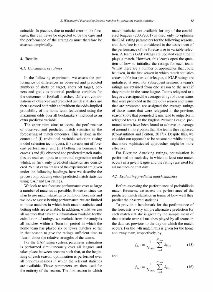
The performance of the two approaches (GAP rat-ings and BA Ratings) in terms of the prediction ofmatch statistics is assessed by comparing the valueof R. The values of R for both GAP and BA ratingsare shown in Fig. 1 for each of the four measures ofattacking performance (goals, corners, shots on targetand shots off target). For BA ratings, R is shown as afunction of the chosen ‘half life’. In all cases, the GAPratings are able to outperform the mean-benchmarkmodel and this is generally also the case for BA rat-ings. Note that, due to high computational intensity, Ris not shown for values of the half life longer than 135days. However, as described in the next section, weare primarily interested in relatively short values ofthe half life that reflect a team’s recent performancesand are able to augment the information contained inthe match odds. We therefore find that the half lifethat maximises the performance of forecasts of thematch outcome is relatively short compared with thatwhich minimises R.
There is a notably high degree of variation in theperformance of the predicted statistics. Under theGAP rating system, the value of R is smallest for shotsoff target, whilst for goals and corners, R is not muchsmaller than 1. This is likely explained by the factthat there are typically a larger number of shots offtarget in a game than the other statistics and therefore
Fig. 1. Values of R for GAP ratings (straight lines) and BA ratings(curves with open circles) for each match statistic. The latter isshown as a function of half life.
there is more information on which to base the fore-casts. BA ratings do not outperform GAP ratings formatch statistics other than goals for any tested halflife.
5. Variable selection
Our next focus is on variable selection and theaim is to find the combination of (i) observed and(ii) predicted match statistics that explain the matchoutcomes most effectively. Variable selection is per-formed using Akaike’s Information Criterion (AIC),which weighs up the fit of the model to the data withthe number of parameters selected in-sample (seeappendix A for details). As required for the calcu-lation of information criteria, the ordinal regressionparameters are selected in-sample and therefore, inorder to calculate the likelihood, a single set of param-eters is selected over all available matches.
To provide further context to the calculated AICvalues, we make use of the confidence set approachdescribed by Anderson and Burnham (2004). Here,the Akaike weights for each model (which can bethought of as the probability that each one repre-sents the best approximating model) are calculatedand sorted from largest to smallest. Models are thenadded to the confidence set in order of their Akaikeweights (largest first) until the sum of the weightsexceeds 0.95. The confidence set then represents theset in which the best approximating model falls withat least 95 percent probability.
E. Wheatcroft / Forecasting football matches by predicting match statistics 87
Table 2
AIC of each combination of observed match statistics with and without the home odds-implied probability included as a predictor variable.Variables that are included are denoted with a star and, in each case, AIC is given with that of model A0 subtracted. The combination ofvariables with the lowest AIC is highlighted in bold and each one that falls into the 95 percent confidence set is highlighted in italic (which
is only combination A1 in this case)
Combination of Shots on Shots off Corners AIC w/o odds AIC w. oddsvariables Target Target
A1 ∗ ∗ ∗ −15125.4 −19473.6A3 ∗ ∗ −14804.3 −18572.7A2 ∗ ∗ −13530.9 −17124.8A4 ∗ −12239.9 −14643.5A5 ∗ ∗ −18.5 −9150.4A6 ∗ −18.3 −8658.7A7 ∗ −9.2 −8598.3A0 0 −5619.1
5.1. Variable selection: observed match statistics
The results of variable selection when usingobserved match statistics are shown in Table 2. Here,the AIC for different combinations of statistics isshown both with and without the home odds-impliedprobability included as an additional predictor vari-able. Note that the AIC in each case is expressedwith that of model A0 (fitted without the odds-implied probability) subtracted such that negativevalues imply better support for a particular combi-nation of predictor variables than that of the modelfitted without any predictor variables. The lower theAIC, the more support for that particular combinationof variables.
The results yield a number of conclusions. Thebest AIC is achieved when the model includes allthree observed match statistics both when the homeodds-implied probability is included as an additionalpredictor variable and when it is not. That the numberof shots on target should have an impact on the matchresult should not come as a surprise, since all goalsother than own goals and highly unusual events (suchas the ball deflecting off the referee or, in one casein 2009, a beachball) result from a shot on target.Interestingly, however, the inclusion of the numberof corners and shots off target, which don’t usuallydirectly result in goals, improves the model even onceshots on target are considered.
It is also interesting to compare the effects ofeach observed match statistic as an individual pre-dictor variable. Unsurprisingly, the number of shotson target provides the most information, followed bycorners and shots off target. Interestingly, shots offtarget and corners do not provide much informationwhen considered individually but add a great deal ofinformation when combined with the number of shots
on target and/or the home odds-implied probability.It is a property of generalised linear models that somepredictor variables are only informative in combina-tion with other predictor variables and this appears tobe the case here.
Finally, all three match statistics add informationeven when the odds-implied probability is included inthe model. This is perhaps not surprising since matchstatistics give an indication of how the match actuallywent.
In practice, of course, observed statistics are neveravailable pre-match. Despite this, the results shownhere have important implications. Match statistics canbe predicted and, if those predictions are informativeenough, it stands to reason that informative forecastsof the outcome of the match can be made.
5.2. Variable selection: predicted matchstatistics
In section 4.2, the results of predicting match statis-tics using GAP and BA ratings were presented. It wasshown that, in the latter case, the choice of half life hasan important impact on the MAE of the predictions.Although, typically, longer half lives tend to providebetter predictions for the match statistics, it may notbe the case that they provide a more useful input forprobabilistic forecasts of the match outcome. This isbecause a consistently strong team like, say, Manch-ester United will be expected to take a larger numberof shots and corners than a weaker side over a longperiod of time and this will be reflected in the ratings.However, we are looking for information that is notreflected in the odds and thus to augment the informa-tion the odds provide. For example, if a team’s recentresults have not reflected their performances, we lookto identify that this is the case from their match
88 E. Wheatcroft / Forecasting football matches by predicting match statistics
Fig. 2. AIC as a function of half life for forecasts produced using different combinations of (i) BA ratings (lines with points) and (ii) GAPratings (straight horizontal lines). In both cases, the home odds-implied probability is used as an additional predictor variable.
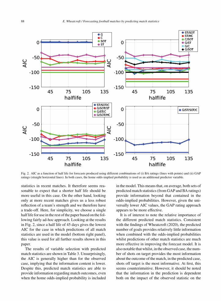
statistics in recent matches. It therefore seems rea-sonable to expect that a shorter half life should bemore useful in this case. On the other hand, lookingonly at more recent matches gives us a less robustreflection of a team’s strength and we therefore havea trade-off. Here, for simplicity, we choose a singlehalf life for use in the rest of the paper based on the fol-lowing fairly ad-hoc approach. Looking at the resultsin Fig. 2, since a half life of 45 days gives the lowestAIC for the case in which predictions of all matchstatistics are used in the model (bottom right panel),this value is used for all further results shown in thispaper.
The results of variable selection with predictedmatch statistics are shown in Table 3. Unsurprisingly,the AIC is generally higher than for the observedcase, implying that the information content is lower.Despite this, predicted match statistics are able toprovide information regarding match outcomes, evenwhen the home odds-implied probability is included
in the model. This means that, on average, both sets ofpredicted match statistics (from GAP and BA ratings)provide information beyond that contained in theodds-implied probabilities. However, given the uni-versally lower AIC values, the GAP rating approachappears to be more effective.
It is of interest to note the relative importance ofthe different predicted match statistics. Consistentwith the findings of Wheatcroft (2020), the predictednumber of goals provides relatively little informationwhen combined with the odds-implied probabilitieswhilst predictions of other match statistics are muchmore effective in improving the forecast model. It isalso notable that whilst, in the observed case, the num-ber of shots on target provides the most informationabout the outcome of the match, in the predicted case,shots off target is the most informative. At first, thisseems counterintuitive. However, it should be notedthat the information in the prediction is dependentboth on the impact of the observed statistic on the
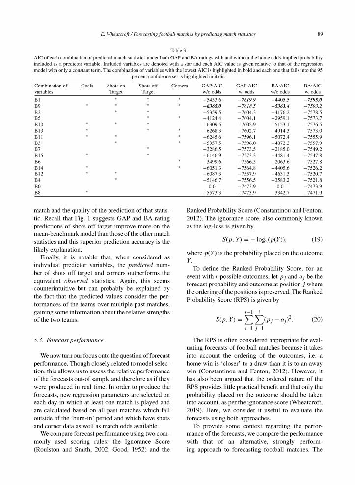
E. Wheatcroft / Forecasting football matches by predicting match statistics 89
Table 3
AIC of each combination of predicted match statistics under both GAP and BA ratings with and without the home odds-implied probabilityincluded as a predictor variable. Included variables are denoted with a star and each AIC value is given relative to that of the regressionmodel with only a constant term. The combination of variables with the lowest AIC is highlighted in bold and each one that falls into the 95
percent confidence set is highlighted in italic
Combination of Goals Shots on Shots off Corners GAP:AIC GAP:AIC BA:AIC BA:AICvariables Target Target w/o odds w. odds w/o odds w. odds
B1 ∗ ∗ ∗ −5453.6 −7619.9 −4405.5 −7595.0B9 ∗ ∗ ∗ ∗ −6365.0 −7618.5 −5363.4 −7593.2B2 ∗ ∗ −5359.5 −7604.3 −4176.2 −7578.5B5 ∗ ∗ −4124.4 −7604.1 −2959.1 −7573.7B10 ∗ ∗ ∗ −6309.5 −7602.9 −5153.1 −7576.5B13 ∗ ∗ ∗ −6268.3 −7602.7 −4914.3 −7573.0B11 ∗ ∗ ∗ −6245.6 −7596.1 −5072.4 −7555.9B3 ∗ ∗ −5357.5 −7596.0 −4072.2 −7557.9B7 ∗ −3286.5 −7573.5 −2185.0 −7549.2B15 ∗ ∗ −6146.9 −7573.3 −4481.4 −7547.8B6 ∗ −3499.6 −7566.5 −2063.6 −7527.8B14 ∗ ∗ −6051.3 −7564.8 −4405.6 −7526.2B12 ∗ ∗ −6087.3 −7557.9 −4631.3 −7520.7B4 ∗ −5146.7 −7556.5 −3583.2 −7521.8B0 0.0 −7473.9 0.0 −7473.9B8 ∗ −5573.3 −7473.9 −3342.7 −7471.9
match and the quality of the prediction of that statis-tic. Recall that Fig. 1 suggests GAP and BA ratingpredictions of shots off target improve more on themean-benchmark model than those of the other matchstatistics and this superior prediction accuracy is thelikely explanation.
Finally, it is notable that, when considered asindividual predictor variables, the predicted num-ber of shots off target and corners outperforms theequivalent observed statistics. Again, this seemscounterintuitive but can probably be explained bythe fact that the predicted values consider the per-formances of the teams over multiple past matches,gaining some information about the relative strengthsof the two teams.
5.3. Forecast performance
We now turn our focus onto the question of forecastperformance. Though closely related to model selec-tion, this allows us to assess the relative performanceof the forecasts out-of sample and therefore as if theywere produced in real time. In order to produce theforecasts, new regression parameters are selected oneach day in which at least one match is played andare calculated based on all past matches which falloutside of the ‘burn-in’ period and which have shotsand corner data as well as match odds available.
We compare forecast performance using two com-monly used scoring rules: the Ignorance Score(Roulston and Smith, 2002; Good, 1952) and the
Ranked Probability Score (Constantinou and Fenton,2012). The ignorance score, also commonly knownas the log-loss is given by
S(p, Y ) = − log2(p(Y )), (19)
where p(Y ) is the probability placed on the outcomeY .
To define the Ranked Probability Score, for anevent with r possible outcomes, let pj and oj be theforecast probability and outcome at position j wherethe ordering of the positions is preserved. The RankedProbability Score (RPS) is given by
S(p, Y ) =r−1∑i=1
i∑j=1
(pj − oj)2. (20)
The RPS is often considered appropriate for eval-uating forecasts of football matches because it takesinto account the ordering of the outcomes, i.e. ahome win is ‘closer’ to a draw than it is to an awaywin (Constantinou and Fenton, 2012). However, ithas also been argued that the ordered nature of theRPS provides little practical benefit and that only theprobability placed on the outcome should be takeninto account, as per the ignorance score (Wheatcroft,2019). Here, we consider it useful to evaluate theforecasts using both approaches.
To provide some context regarding the perfor-mance of the forecasts, we compare the performancewith that of an alternative, strongly perform-ing approach to forecasting football matches. The
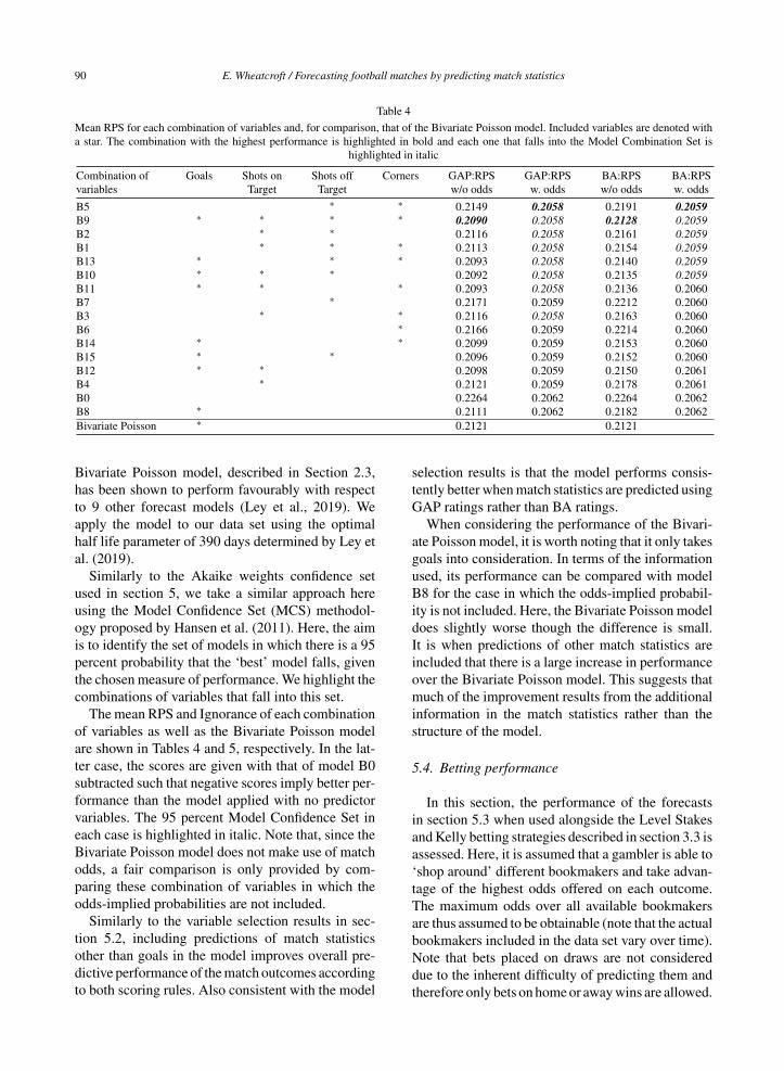
90 E. Wheatcroft / Forecasting football matches by predicting match statistics
Table 4
Mean RPS for each combination of variables and, for comparison, that of the Bivariate Poisson model. Included variables are denoted witha star. The combination with the highest performance is highlighted in bold and each one that falls into the Model Combination Set is
highlighted in italic
Combination of Goals Shots on Shots off Corners GAP:RPS GAP:RPS BA:RPS BA:RPSvariables Target Target w/o odds w. odds w/o odds w. odds
B5 ∗ ∗ 0.2149 0.2058 0.2191 0.2059B9 ∗ ∗ ∗ ∗ 0.2090 0.2058 0.2128 0.2059B2 ∗ ∗ 0.2116 0.2058 0.2161 0.2059B1 ∗ ∗ ∗ 0.2113 0.2058 0.2154 0.2059B13 ∗ ∗ ∗ 0.2093 0.2058 0.2140 0.2059B10 ∗ ∗ ∗ 0.2092 0.2058 0.2135 0.2059B11 ∗ ∗ ∗ 0.2093 0.2058 0.2136 0.2060B7 ∗ 0.2171 0.2059 0.2212 0.2060B3 ∗ ∗ 0.2116 0.2058 0.2163 0.2060B6 ∗ 0.2166 0.2059 0.2214 0.2060B14 ∗ ∗ 0.2099 0.2059 0.2153 0.2060B15 ∗ ∗ 0.2096 0.2059 0.2152 0.2060B12 ∗ ∗ 0.2098 0.2059 0.2150 0.2061B4 ∗ 0.2121 0.2059 0.2178 0.2061B0 0.2264 0.2062 0.2264 0.2062B8 ∗ 0.2111 0.2062 0.2182 0.2062Bivariate Poisson ∗ 0.2121 0.2121
Bivariate Poisson model, described in Section 2.3,has been shown to perform favourably with respectto 9 other forecast models (Ley et al., 2019). Weapply the model to our data set using the optimalhalf life parameter of 390 days determined by Ley etal. (2019).
Similarly to the Akaike weights confidence setused in section 5, we take a similar approach hereusing the Model Confidence Set (MCS) methodol-ogy proposed by Hansen et al. (2011). Here, the aimis to identify the set of models in which there is a 95percent probability that the ‘best’ model falls, giventhe chosen measure of performance. We highlight thecombinations of variables that fall into this set.
The mean RPS and Ignorance of each combinationof variables as well as the Bivariate Poisson modelare shown in Tables 4 and 5, respectively. In the lat-ter case, the scores are given with that of model B0subtracted such that negative scores imply better per-formance than the model applied with no predictorvariables. The 95 percent Model Confidence Set ineach case is highlighted in italic. Note that, since theBivariate Poisson model does not make use of matchodds, a fair comparison is only provided by com-paring these combination of variables in which theodds-implied probabilities are not included.
Similarly to the variable selection results in sec-tion 5.2, including predictions of match statisticsother than goals in the model improves overall pre-dictive performance of the match outcomes accordingto both scoring rules. Also consistent with the model
selection results is that the model performs consis-tently better when match statistics are predicted usingGAP ratings rather than BA ratings.
When considering the performance of the Bivari-ate Poisson model, it is worth noting that it only takesgoals into consideration. In terms of the informationused, its performance can be compared with modelB8 for the case in which the odds-implied probabil-ity is not included. Here, the Bivariate Poisson modeldoes slightly worse though the difference is small.It is when predictions of other match statistics areincluded that there is a large increase in performanceover the Bivariate Poisson model. This suggests thatmuch of the improvement results from the additionalinformation in the match statistics rather than thestructure of the model.
5.4. Betting performance
In this section, the performance of the forecastsin section 5.3 when used alongside the Level Stakesand Kelly betting strategies described in section 3.3 isassessed. Here, it is assumed that a gambler is able to‘shop around’ different bookmakers and take advan-tage of the highest odds offered on each outcome.The maximum odds over all available bookmakersare thus assumed to be obtainable (note that the actualbookmakers included in the data set vary over time).Note that bets placed on draws are not considereddue to the inherent difficulty of predicting them andtherefore only bets on home or away wins are allowed.
E. Wheatcroft / Forecasting football matches by predicting match statistics 91
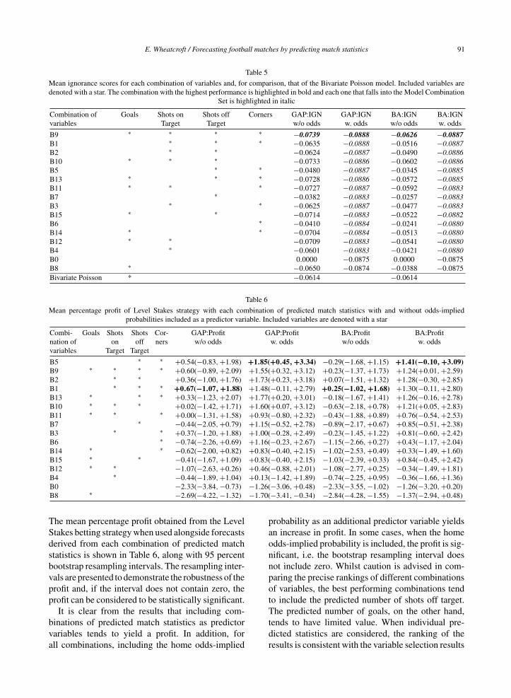
Table 5
Mean ignorance scores for each combination of variables and, for comparison, that of the Bivariate Poisson model. Included variables aredenoted with a star. The combination with the highest performance is highlighted in bold and each one that falls into the Model Combination
Set is highlighted in italic
Combination of Goals Shots on Shots off Corners GAP:IGN GAP:IGN BA:IGN BA:IGNvariables Target Target w/o odds w. odds w/o odds w. odds
B9 ∗ ∗ ∗ ∗ −0.0739 −0.0888 −0.0626 −0.0887B1 ∗ ∗ ∗ −0.0635 −0.0888 −0.0516 −0.0887B2 ∗ ∗ −0.0624 −0.0887 −0.0490 −0.0886B10 ∗ ∗ ∗ −0.0733 −0.0886 −0.0602 −0.0886B5 ∗ ∗ −0.0480 −0.0887 −0.0345 −0.0885B13 ∗ ∗ ∗ −0.0728 −0.0886 −0.0572 −0.0885B11 ∗ ∗ ∗ −0.0727 −0.0887 −0.0592 −0.0883B7 ∗ −0.0382 −0.0883 −0.0257 −0.0883B3 ∗ ∗ −0.0625 −0.0887 −0.0477 −0.0883B15 ∗ ∗ −0.0714 −0.0883 −0.0522 −0.0882B6 ∗ −0.0410 −0.0884 −0.0241 −0.0880B14 ∗ ∗ −0.0704 −0.0884 −0.0513 −0.0880B12 ∗ ∗ −0.0709 −0.0883 −0.0541 −0.0880B4 ∗ −0.0601 −0.0883 −0.0421 −0.0880B0 0.0000 −0.0875 0.0000 −0.0875B8 ∗ −0.0650 −0.0874 −0.0388 −0.0875Bivariate Poisson * −0.0614 −0.0614
Table 6
Mean percentage profit of Level Stakes strategy with each combination of predicted match statistics with and without odds-impliedprobabilities included as a predictor variable. Included variables are denoted with a star
Combi- Goals Shots Shots Cor- GAP:Profit GAP:Profit BA:Profit BA:Profitnation of on off ners w/o odds w. odds w/o odds w. oddsvariables Target Target
B5 ∗ ∗ +0.54(−0.83, +1.98) +1.85(+0.45, +3.34) −0.29(−1.68, +1.15) +1.41(−0.10, +3.09)B9 ∗ ∗ ∗ ∗ +0.60(−0.89, +2.09) +1.55(+0.32, +3.12) +0.23(−1.37, +1.73) +1.24(+0.01, +2.59)B2 ∗ ∗ +0.36(−1.00, +1.76) +1.73(+0.23, +3.18) +0.07(−1.51, +1.32) +1.28(−0.30, +2.85)B1 ∗ ∗ ∗ +0.67(−1.07, +1.88) +1.48(−0.11, +2.79) +0.25(−1.02, +1.68) +1.30(−0.11, +2.80)B13 ∗ ∗ ∗ +0.33(−1.23, +2.07) +1.77(+0.20, +3.01) −0.18(−1.67, +1.41) +1.26(−0.16, +2.78)B10 ∗ ∗ ∗ +0.02(−1.42, +1.71) +1.60(+0.07, +3.12) −0.63(−2.18, +0.78) +1.21(+0.05, +2.83)B11 ∗ ∗ ∗ +0.00(−1.31, +1.58) +0.93(−0.80, +2.32) −0.43(−1.88, +0.89) +0.76(−0.54, +2.53)B7 ∗ −0.44(−2.05, +0.79) +1.15(−0.52, +2.78) −0.89(−2.17, +0.67) +0.85(−0.51, +2.38)B3 ∗ ∗ +0.37(−1.20, +1.88) +1.00(−0.28, +2.49) −0.23(−1.45, +1.22) +0.81(−0.60, +2.42)B6 ∗ −0.74(−2.26, +0.69) +1.16(−0.23, +2.67) −1.15(−2.66, +0.27) +0.43(−1.17, +2.04)B14 ∗ ∗ −0.62(−2.00, +0.82) +0.83(−0.40, +2.15) −1.02(−2.53, +0.49) +0.33(−1.49, +1.60)B15 ∗ ∗ −0.41(−1.67, +1.09) +0.83(−0.40, +2.15) −1.03(−2.39, +0.33) +0.84(−0.45, +2.42)B12 ∗ ∗ −1.07(−2.63, +0.26) +0.46(−0.88, +2.01) −1.08(−2.77, +0.25) −0.34(−1.49, +1.81)B4 ∗ −0.44(−1.89, +1.04) +0.13(−1.42, +1.89) −0.74(−2.25, +0.95) −0.36(−1.66, +1.36)B0 −2.33(−3.84, −0.73) −1.26(−3.06, +0.48) −2.33(−3.55, −1.02) −1.26(−3.20,+0.20)B8 ∗ −2.69(−4.22, −1.32) −1.70(−3.41, −0.34) −2.84(−4.28, −1.55) −1.37(−2.94, +0.48)
The mean percentage profit obtained from the LevelStakes betting strategy when used alongside forecastsderived from each combination of predicted matchstatistics is shown in Table 6, along with 95 percentbootstrap resampling intervals. The resampling inter-vals are presented to demonstrate the robustness of theprofit and, if the interval does not contain zero, theprofit can be considered to be statistically significant.
It is clear from the results that including com-binations of predicted match statistics as predictorvariables tends to yield a profit. In addition, forall combinations, including the home odds-implied
probability as an additional predictor variable yieldsan increase in profit. In some cases, when the homeodds-implied probability is included, the profit is sig-nificant, i.e. the bootstrap resampling interval doesnot include zero. Whilst caution is advised in com-paring the precise rankings of different combinationsof variables, the best performing combinations tendto include the predicted number of shots off target.The predicted number of goals, on the other hand,tends to have limited value. When individual pre-dicted statistics are considered, the ranking of theresults is consistent with the variable selection results
92 E. Wheatcroft / Forecasting football matches by predicting match statistics
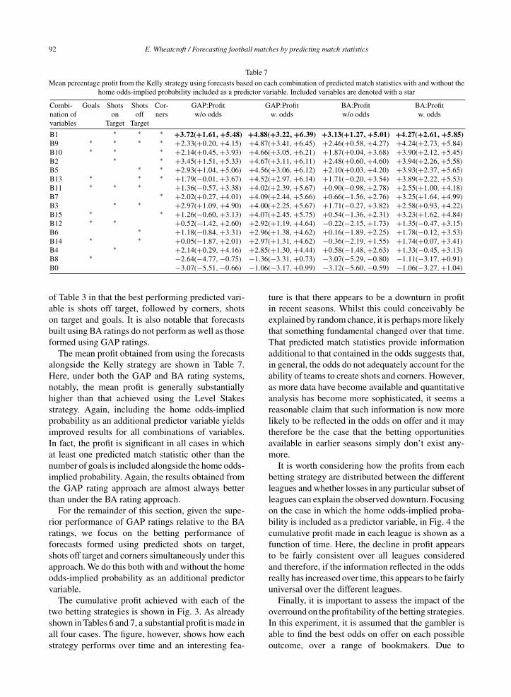
Table 7
Mean percentage profit from the Kelly strategy using forecasts based on each combination of predicted match statistics with and without thehome odds-implied probability included as a predictor variable. Included variables are denoted with a star
Combi- Goals Shots Shots Cor- GAP:Profit GAP:Profit BA:Profit BA:Profitnation of on off ners w/o odds w. odds w/o odds w. oddsvariables Target Target
B1 ∗ ∗ ∗ +3.72(+1.61, +5.48) +4.88(+3.22, +6.39) +3.13(+1.27, +5.01) +4.27(+2.61, +5.85)B9 ∗ ∗ ∗ ∗ +2.33(+0.20, +4.15) +4.87(+3.41, +6.45) +2.46(+0.58, +4.27) +4.24(+2.73, +5.84)B10 ∗ ∗ ∗ +2.14(+0.45, +3.93) +4.66(+3.05, +6.21) +1.87(+0.04, +3.68) +3.90(+2.12, +5.45)B2 ∗ ∗ +3.45(+1.51, +5.33) +4.67(+3.11, +6.11) +2.48(+0.60, +4.60) +3.94(+2.26, +5.58)B5 ∗ ∗ +2.93(+1.04, +5.06) +4.56(+3.06, +6.12) +2.10(+0.03, +4.20) +3.93(+2.37, +5.65)B13 ∗ ∗ ∗ +1.79(−0.01, +3.67) +4.52(+2.97, +6.14) +1.71(−0.20, +3.54) +3.89(+2.22, +5.53)B11 ∗ ∗ ∗ +1.36(−0.57, +3.38) +4.02(+2.39, +5.67) +0.90(−0.98, +2.78) +2.55(+1.00, +4.18)B7 ∗ +2.02(+0.27, +4.01) +4.09(+2.44, +5.66) +0.66(−1.56, +2.76) +3.25(+1.64, +4.99)B3 ∗ ∗ +2.97(+1.09, +4.90) +4.00(+2.25, +5.67) +1.71(−0.27, +3.82) +2.58(+0.93, +4.22)B15 ∗ ∗ +1.26(−0.60, +3.13) +4.07(+2.45, +5.75) +0.54(−1.36, +2.31) +3.23(+1.62, +4.84)B12 ∗ ∗ +0.52(−1.42, +2.60) +2.92(+1.19, +4.64) −0.22(−2.15, +1.73) +1.35(−0.47, +3.15)B6 ∗ +1.18(−0.84, +3.31) +2.96(+1.38, +4.62) +0.16(−1.89, +2.25) +1.78(−0.12, +3.53)B14 ∗ ∗ +0.05(−1.87, +2.01) +2.97(+1.31, +4.62) −0.36(−2.19, +1.55) +1.74(+0.07, +3.41)B4 ∗ +2.14(+0.29, +4.16) +2.85(+1.30, +4.44) +0.58(−1.48, +2.63) +1.33(−0.45, +3.13)B8 ∗ −2.64(−4.77, −0.75) −1.36(−3.31, +0.73) −3.07(−5.29, −0.80) −1.11(−3.17, +0.91)B0 −3.07(−5.51, −0.66) −1.06(−3.17, +0.99) −3.12(−5.60, −0.59) −1.06(−3.27,+1.04)
of Table 3 in that the best performing predicted vari-able is shots off target, followed by corners, shotson target and goals. It is also notable that forecastsbuilt using BA ratings do not perform as well as thoseformed using GAP ratings.
The mean profit obtained from using the forecastsalongside the Kelly strategy are shown in Table 7.Here, under both the GAP and BA rating systems,notably, the mean profit is generally substantiallyhigher than that achieved using the Level Stakesstrategy. Again, including the home odds-impliedprobability as an additional predictor variable yieldsimproved results for all combinations of variables.In fact, the profit is significant in all cases in whichat least one predicted match statistic other than thenumber of goals is included alongside the home odds-implied probability. Again, the results obtained fromthe GAP rating approach are almost always betterthan under the BA rating approach.
For the remainder of this section, given the supe-rior performance of GAP ratings relative to the BAratings, we focus on the betting performance offorecasts formed using predicted shots on target,shots off target and corners simultaneously under thisapproach. We do this both with and without the homeodds-implied probability as an additional predictorvariable.
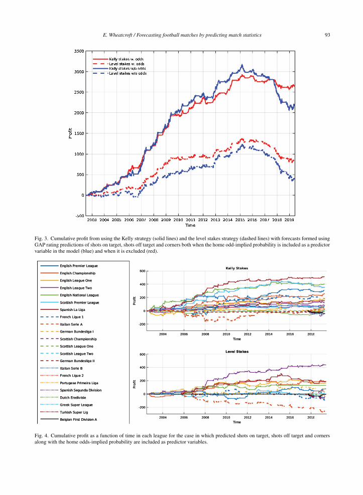
The cumulative profit achieved with each of thetwo betting strategies is shown in Fig. 3. As alreadyshown in Tables 6 and 7, a substantial profit is made inall four cases. The figure, however, shows how eachstrategy performs over time and an interesting fea-
ture is that there appears to be a downturn in profitin recent seasons. Whilst this could conceivably beexplained by random chance, it is perhaps more likelythat something fundamental changed over that time.That predicted match statistics provide informationadditional to that contained in the odds suggests that,in general, the odds do not adequately account for theability of teams to create shots and corners. However,as more data have become available and quantitativeanalysis has become more sophisticated, it seems areasonable claim that such information is now morelikely to be reflected in the odds on offer and it maytherefore be the case that the betting opportunitiesavailable in earlier seasons simply don’t exist any-more.
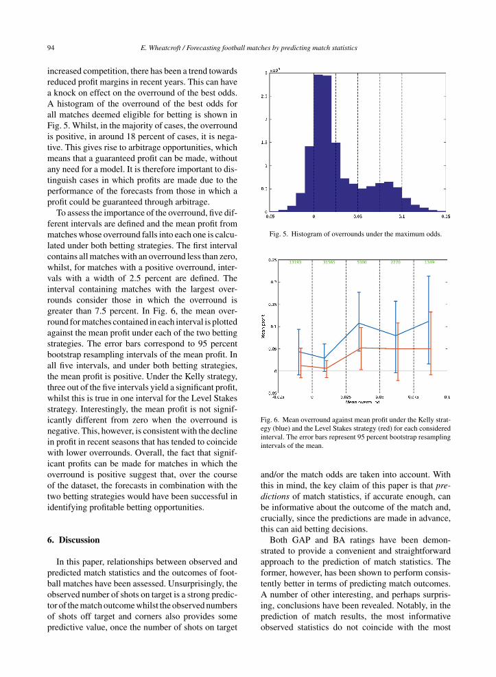
It is worth considering how the profits from eachbetting strategy are distributed between the differentleagues and whether losses in any particular subset ofleagues can explain the observed downturn. Focusingon the case in which the home odds-implied proba-bility is included as a predictor variable, in Fig. 4 thecumulative profit made in each league is shown as afunction of time. Here, the decline in profit appearsto be fairly consistent over all leagues consideredand therefore, if the information reflected in the oddsreally has increased over time, this appears to be fairlyuniversal over the different leagues.
Finally, it is important to assess the impact of theoverround on the profitability of the betting strategies.In this experiment, it is assumed that the gambler isable to find the best odds on offer on each possibleoutcome, over a range of bookmakers. Due to
E. Wheatcroft / Forecasting football matches by predicting match statistics 93
Fig. 3. Cumulative profit from using the Kelly strategy (solid lines) and the level stakes strategy (dashed lines) with forecasts formed usingGAP rating predictions of shots on target, shots off target and corners both when the home odd-implied probability is included as a predictorvariable in the model (blue) and when it is excluded (red).
Fig. 4. Cumulative profit as a function of time in each league for the case in which predicted shots on target, shots off target and cornersalong with the home odds-implied probability are included as predictor variables.
94 E. Wheatcroft / Forecasting football matches by predicting match statistics
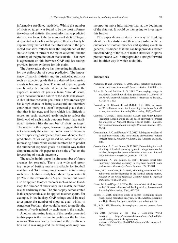
increased competition, there has been a trend towardsreduced profit margins in recent years. This can havea knock on effect on the overround of the best odds.A histogram of the overround of the best odds forall matches deemed eligible for betting is shown inFig. 5. Whilst, in the majority of cases, the overroundis positive, in around 18 percent of cases, it is nega-tive. This gives rise to arbitrage opportunities, whichmeans that a guaranteed profit can be made, withoutany need for a model. It is therefore important to dis-tinguish cases in which profits are made due to theperformance of the forecasts from those in which aprofit could be guaranteed through arbitrage.
To assess the importance of the overround, five dif-ferent intervals are defined and the mean profit frommatches whose overround falls into each one is calcu-lated under both betting strategies. The first intervalcontains all matches with an overround less than zero,whilst, for matches with a positive overround, inter-vals with a width of 2.5 percent are defined. Theinterval containing matches with the largest over-rounds consider those in which the overround isgreater than 7.5 percent. In Fig. 6, the mean over-round for matches contained in each interval is plottedagainst the mean profit under each of the two bettingstrategies. The error bars correspond to 95 percentbootstrap resampling intervals of the mean profit. Inall five intervals, and under both betting strategies,the mean profit is positive. Under the Kelly strategy,three out of the five intervals yield a significant profit,whilst this is true in one interval for the Level Stakesstrategy. Interestingly, the mean profit is not signif-icantly different from zero when the overround isnegative. This, however, is consistent with the declinein profit in recent seasons that has tended to coincidewith lower overrounds. Overall, the fact that signif-icant profits can be made for matches in which theoverround is positive suggest that, over the courseof the dataset, the forecasts in combination with thetwo betting strategies would have been successful inidentifying profitable betting opportunities.
6. Discussion
In this paper, relationships between observed andpredicted match statistics and the outcomes of foot-ball matches have been assessed. Unsurprisingly, theobserved number of shots on target is a strong predic-tor of the match outcome whilst the observed numbersof shots off target and corners also provides somepredictive value, once the number of shots on target
Fig. 5. Histogram of overrounds under the maximum odds.
Fig. 6. Mean overround against mean profit under the Kelly strat-egy (blue) and the Level Stakes strategy (red) for each consideredinterval. The error bars represent 95 percent bootstrap resamplingintervals of the mean.
and/or the match odds are taken into account. Withthis in mind, the key claim of this paper is that pre-dictions of match statistics, if accurate enough, canbe informative about the outcome of the match and,crucially, since the predictions are made in advance,this can aid betting decisions.
Both GAP and BA ratings have been demon-strated to provide a convenient and straightforwardapproach to the prediction of match statistics. Theformer, however, has been shown to perform consis-tently better in terms of predicting match outcomes.A number of other interesting, and perhaps surpris-ing, conclusions have been revealed. Notably, in theprediction of match results, the most informativeobserved statistics do not coincide with the most
E. Wheatcroft / Forecasting football matches by predicting match statistics 95
informative predicted statistics. Whilst the numberof shots on target was found to be the most informa-tive observed statistic, the most informative predictedstatistic was found to be the number of shots off target.As pointed out earlier in the paper, this can likely beexplained by the fact that the information in the pre-dicted statistics reflects both the importance of thestatistic itself, in terms of the match outcome, and theaccuracy of the prediction of that statistic. That thereis agreement on this between GAP and BA ratingsprovides further evidence for this claim.
The observation above has interesting implicationsfor the philosophy of sports prediction. The impor-tance of match statistics and, in particular, statisticssuch as expected goals that are derived from matchevents is becoming clear. The aim of expected goalscan broadly be considered to be to estimate theexpected number of goals a team ‘should’ score,given the location and nature of the shots it has taken.A shot taken close to the goal and at a favourable anglehas a high chance of being successful and thereforecontributes more to a team’s expected goals than ashot that is far away and from which it is difficult toscore. As such, expected goals ought to reflect thelikelihood of each match outcome better than tradi-tional statistics like the number of shots on target.The results in this paper, however, suggest that it isnot necessarily the case that predictions of the num-ber of expected goals by each team would outperformpredictions of, or ratings based on, other statistics.Interesting future work would therefore be to predictthe number of expected goals in a similar way to thatdemonstrated in this paper to assess the effect on theforecasting of match outcomes.
The results in this paper inspire a number of futureavenues for research. There is a wide and grow-ing range of betting markets available for footballmatches and GAP ratings may be useful in informingsuch bets. This has already been shown by Wheatcroft(2020) in the over/under 2.5 goal market but couldalso be applied to other markets such as Asian Hand-icap, the number of shots taken in a match, half timeresults and many more. The philosophy demonstratedin this paper could also be applied to other sports. Forexample, in ice hockey, GAP ratings could be usedto estimate the number of shots at goal, whilst, inAmerican Football, they could be used to predict thenumber of yards gained by each team in the match.
Another interesting feature of the results presentedin this paper is the decline in profit over the last fewseasons. This was briefly discussed in the results sec-tion and it was suggested that betting odds may now
incorporate more information than at the beginningof the data set. It would be interesting to investigatethis further.
This paper demonstrates a new way of thinkingabout match statistics and their relationship with theoutcomes of football matches and sporting events ingeneral. It is hoped that this can help provide a betterunderstanding of the role of match statistics in sportsprediction and GAP ratings provide a straightforwardand intuitive way in which to do this.
References
Anderson, D. and Burnham, K. 2004, Model selection and multi-model inference, Second. NY: Springer-Verlag, 63(2020), 10.
Baker, R. D. and McHale, I. G. 2015, Time varying ratings inassociation football: the all-time greatest team is.., Journal ofthe Royal Statistical Society: Series A (Statistics in Society),178(2), 481-492.
Boshnakov, G., Kharrat, T. and McHale, I. G. 2017, A bivari-ate Weibull count model for forecasting association footballscores, International Journal of Forecasting, 33(2), 458-466.
Carbone, J., Corke, T. and Moisiadis, F. 2016, The Rugby LeaguePrediction Model: Using an Elo-based approach to predictthe outcome of National Rugby League (NRL) matches,International Educational Scientific Research Journal, 2(5),26-30.
Constantinou, A. C. and Fenton, N. E. 2012, Solving the problem ofin-adequate scoring rules for assessing probabilistic footballforecast models, Journal of Quantitative Analysis in Sports,8(1).
Constantinou, A. C. and Fenton, N. E. 2013, Determining the levelof ability of football teams by dynamic ratings based on therelative discrepancies in scores between adversaries, Journalof Quantitative Analysis in Sports, 9(1), 37-50.
Constantinou, A. and Fenton, N. 2017, Towards smart-data:Improving predictive accuracy in long-term football teamperformance, Knowledge-Based Systems, 124, 93-104.
Dixon, M. J. and Coles, S. G. 1997, Modelling association foot-ball scores and inefficiencies in the football betting market,Journal of the Royal Statistical Society: Series C (AppliedStatistics), 46(2), 265-280.
Dixon, M. J. and Pope, P. F. 2004, The value of statistical forecastsin the UK association football betting market, InternationalJournal of Forecasting, 20(4), 697-711.
Eggels, H. 2016, Expected goals in soccer: Explaining matchresults using predictive analytics, in The Machine Learningand Data Mining for Sports Analytics workshop, pp. 16.
Elo, A. E. 1978, The rating of chessplayers, past and present, ArcoPub.
Fifa 2018, Revision of the FIFA / Coca-Cola WorldRanking, https://resources.fifa.com/image/upload/fifa-world-ranking-technical-explanation-revision.pdf?cloudid=edbm045h0udbwkqew35a. Accessed:27/04/2019.
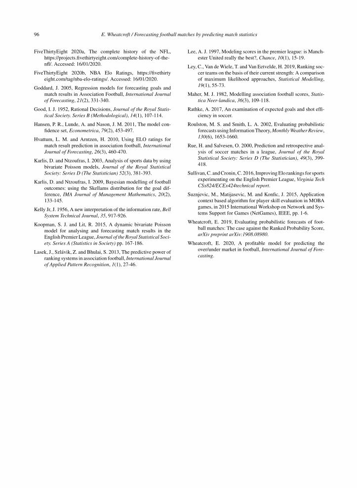
96 E. Wheatcroft / Forecasting football matches by predicting match statistics
FiveThirtyEight 2020a, The complete history of the NFL,https://projects.fivethirtyeight.com/complete-history-of-the-nfl/. Accessed: 16/01/2020.
FiveThirtyEight 2020b, NBA Elo Ratings, https://fivethirtyeight.com/tag/nba-elo-ratings/. Accessed: 16/01/2020.
Goddard, J. 2005, Regression models for forecasting goals andmatch results in Association Football, International Journalof Forecasting, 21(2), 331-340.
Good, I. J. 1952, Rational Decisions, Journal of the Royal Statis-tical Society. Series B (Methodological), 14(1), 107-114.
Hansen, P. R., Lunde, A. and Nason, J. M. 2011, The model con-fidence set, Econometrica, 79(2), 453-497.
Hvattum, L. M. and Arntzen, H. 2010, Using ELO ratings formatch result prediction in association football, InternationalJournal of Forecasting, 26(3), 460-470.
Karlis, D. and Ntzoufras, I. 2003, Analysis of sports data by usingbivariate Poisson models, Journal of the Royal StatisticalSociety: Series D (The Statistician) 52(3), 381-393.
Karlis, D. and Ntzoufras, I. 2009, Bayesian modelling of footballoutcomes: using the Skellams distribution for the goal dif-ference, IMA Journal of Management Mathematics, 20(2),133-145.
Kelly Jr, J. 1956, A new interpretation of the information rate, BellSystem Technical Journal, 35, 917-926.
Koopman, S. J. and Lit, R. 2015, A dynamic bivariate Poissonmodel for analysing and forecasting match results in theEnglish Premier League, Journal of the Royal Statistical Soci-ety. Series A (Statistics in Society) pp. 167-186.
Lasek, J., Szlavik, Z. and Bhulai, S. 2013, The predictive power ofranking systems in association football, International Journalof Applied Pattern Recognition, 1(1), 27-46.
Lee, A. J. 1997, Modeling scores in the premier league: is Manch-ester United really the best?, Chance, 10(1), 15-19.
Ley, C., Van de Wiele, T. and Van Eetvelde, H. 2019, Ranking soc-cer teams on the basis of their current strength: A comparisonof maximum likelihood approaches, Statistical Modelling,19(1), 55-73.
Maher, M. J. 1982, Modelling association football scores, Statis-tica Neer-landica, 36(3), 109-118.
Rathke, A. 2017, An examination of expected goals and shot effi-ciency in soccer.
Roulston, M. S. and Smith, L. A. 2002, Evaluating probabilisticforecasts using Information Theory, Monthly Weather Review,130(6), 1653-1660.
Rue, H. and Salvesen, O. 2000, Prediction and retrospective anal-ysis of soccer matches in a league, Journal of the RoyalStatistical Society: Series D (The Statistician), 49(3), 399-418.
Sullivan, C. and Cronin, C. 2016, Improving Elo rankings for sportsexperimenting on the English Premier League, Virginia TechCSx824/ECEx424technical report.
Suznjevic, M., Matijasevic, M. and Konfic, J. 2015, Applicationcontext based algorithm for player skill evaluation in MOBAgames, in 2015 International Workshop on Network and Sys-tems Support for Games (NetGames), IEEE, pp. 1-6.
Wheatcroft, E. 2019, Evaluating probabilistic forecasts of foot-ball matches: The case against the Ranked Probability Score,arXiv preprint arXiv:1908.08980.
Wheatcroft, E. 2020, A profitable model for predicting theover/under market in football, International Journal of Fore-casting.

E. Wheatcroft / Forecasting football matches by predicting match statistics 97
A Akaike’s Information Criterion (AIC)
Akaike’s Information Criterion (AIC) weighs upthe likelihood of a model with the number of esti-mated parameters to provide an indication of the fit ofthe model out-of-sample. In the context of predictingfootball match outcomes, AIC is given by
AIC = −2 log(L) + 2k (21)
where k is the number of estimated parameters and L
is the maximised log-likelihood given by
L =n∏i
pi(Yi) (22)
where pi(Yi) is the probability placed on the outcomeYi in game i.
Related Documents