Forecasting Financial Time Seriesusers.cecs.anu.edu.au/~trumpf/LSslides/Manfred_Deistler.pdf · Introduction Factor Models An Example ForecastingFinancialTimeSeries: ProblemsandApproaches

IntroductionFactor Models

An Example

Forecasting Financial Time Series

Manfred Deistler and Christiane Zinner

Canberra, February, 2007

Manfred Deistler and Christiane Zinner Forecasting Financial Time Series


An Example

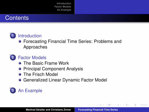
Contents

1 IntroductionForecasting Financial Time Series: Problems andApproaches

2 Factor ModelsThe Basic Frame WorkPrincipal Component AnalysisThe Frisch ModelGeneralized Linear Dynamic Factor Model

3 An Example



An ExampleForecasting Financial Time Series: Problems and Approaches

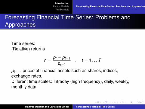
Forecasting Financial Time Series: Problems andApproaches

Time series:(Relative) returns

rt =pt − pt−1

pt−1, t = 1 . . . T

pt . . . prices of financial assets such as shares, indices,exchange rates.Different time scales: Intraday (high frequency), daily, weekly,monthly data.




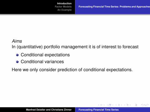
AimsIn (quantitative) portfolio management it is of interest to forecast

Conditional expectationsConditional variances

Here we only consider prediction of conditional expectations.




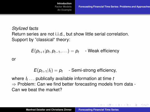
Stylized factsReturn series are not i.i.d., but show little serial correlation.Support by ”classical“ theory:

E(pt+1|pt , pt−1, . . .) = pt - Weak efficiency

or

E(pt+1|It) = pt - Semi-strong efficiency,

where It . . . publically available information at time t⇒ Problem: Can we find better forecasting models from data -Can we beat the market?




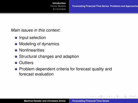
Main issues in this context:

Input selectionModeling of dynamicsNonlinearitiesStructural changes and adaptionOutliersProblem dependent criteria for forecast quality andforecast evaluation




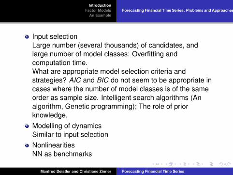
Input selectionLarge number (several thousands) of candidates, andlarge number of model classes: Overfitting andcomputation time.What are appropriate model selection criteria andstrategies? AIC and BIC do not seem to be appropriate incases where the number of model classes is of the sameorder as sample size. Intelligent search algorithms (Analgorithm, Genetic programming); The role of priorknowledge.Modelling of dynamicsSimilar to input selectionNonlinearitiesNN as benchmarks




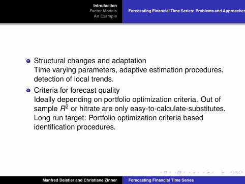
Structural changes and adaptationTime varying parameters, adaptive estimation procedures,detection of local trends.Criteria for forecast qualityIdeally depending on portfolio optimization criteria. Out ofsample R2 or hitrate are only easy-to-calculate-substitutes.Long run target: Portfolio optimization criteria basedidentification procedures.



An Example

The Basic Frame WorkPrincipal Component AnalysisThe Frisch ModelGeneralized Linear Dynamic Factor Model

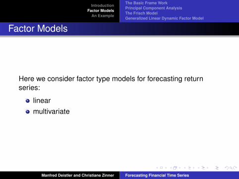
Factor Models

Here we consider factor type models for forecasting returnseries:

linearmultivariate



An Example


The Basic Frame Work

Factor models are used to condense high dimensional dataconsisting of many variables into a much smaller number offactors. The factors represent the comovement between thesingle time series or underlying nonobserved variablesinfluencing the observations. Here we consider (static anddynamic)

Principal component modelsFrisch or idiosyncratic noise modelsGeneralized linear factor models

for forecasting return series.



An Example


The modelThe basic, common equation for all different kinds of factormodels considered here is of the form

yt = Λ(z)ξt + ut , (1)

whereyt . . . observations (n-dim).ξt . . . factors (unobserved)

(r << n-dim).Λ(z) =

∑∞j=−∞ Λjz j , Λj ∈ Rn×r . . . factor loadings

yt = Λ(z)ξt . . . latent variablesΛ = Λ0 . . . (quasi-)static case.



An Example


AssumptionsThroughout we assume the following:

Eξt = 0, Eut = 0 for all t ∈ Z.Eξtu′s = 0 for all s, t ∈ Z.(ξt) and (ut) are wide sense stationary and (linearly)regular with covariances γξ(s) = Eξtξ

′t+s and

γu(s) = Eutu′t+s satisfying

∞∑s=−∞

|s|‖γξ(s)‖ < ∞,

∞∑s=−∞

|s|‖γu(s)‖ < ∞ (2)

The spectral density fy of yt has rank r for all λ ∈ [−π, π].



An Example


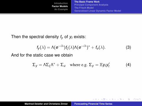
Then the spectral density fy of yt exists:

fy (λ) = Λ(e−iλ)fξ(λ)Λ(e−iλ)∗ + fu(λ). (3)

And for the static case we obtain

Σy = ΛΣξΛ∗ + Σu where e.g. Σy = Eyty ′t (4)



An Example


We will be concerned with the following questions.

Identifiability questions:Identifiability of fy = ΛfξΛ∗ and fuIdentifiability of Λ and fξ

Estimation of integers and real-valued parameters:Estimation of rEstimation of the free parameters in Λ, fξ, fuEstimation of ξt

Forecasting



An Example


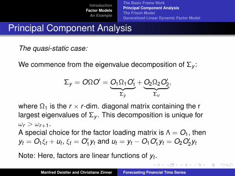
Principal Component Analysis

The quasi-static case:

We commence from the eigenvalue decomposition of Σy :

Σy = OΩO′ = O1Ω1O′1︸︷︷︸

Σy

+ O2Ω2O′2︸︷︷︸

Σu

,

where Ω1 is the r × r -dim. diagonal matrix containing the rlargest eigenvalues of Σy . This decomposition is unique forωr > ωr+1.A special choice for the factor loading matrix is Λ = O1, thenyt = O1ξt + ut , ξt = O′

1yt and ut = yt −O1O′1yt = O2O′

2yt

Note: Here, factors are linear functions of yt .



An Example


Estimation:

Determine r from ω1, . . . , ωnEstimate Λ,Σξ,Σu, ξt from the eigenvalue decomposition ofΣy = 1

T∑T

t=1 yty ′t



An Example


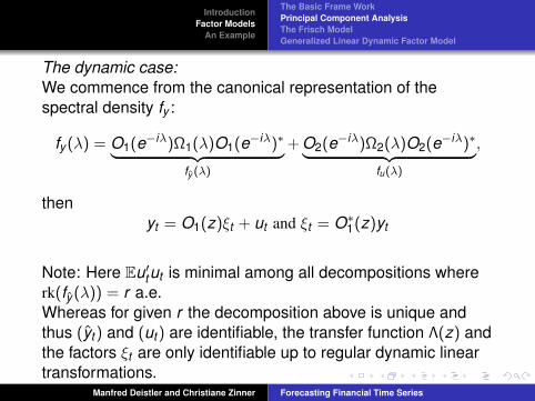
The dynamic case:We commence from the canonical representation of thespectral density fy :

fy (λ) = O1(e−iλ)Ω1(λ)O1(e−iλ)∗︸︷︷︸fy (λ)

+ O2(e−iλ)Ω2(λ)O2(e−iλ)∗︸︷︷︸fu(λ)

,

thenyt = O1(z)ξt + ut and ξt = O∗

1(z)yt

Note: Here Eu′tut is minimal among all decompositions whererk(fy (λ)) = r a.e.Whereas for given r the decomposition above is unique andthus (yt) and (ut) are identifiable, the transfer function Λ(z) andthe factors ξt are only identifiable up to regular dynamic lineartransformations.



An Example


Again ξt = O∗1(z)yt , i.e. factors are linear transformations of (yt)

Problem: In general, the filter O∗1(z) will be non-causal and

non-rational. Thus, naive forecasting may lead to infeasibleforecasts for yt . Restriction to causal filters is required.In estimation, we commence from a spectral estimate.



An Example


The Frisch Model

Here the additional assumption fu is diagonal is imposed in (1).Interpretation: Factors describe the common effects, the noiseut takes into account the individual effects, e.g. factors describemarkets and sector specific movements and the noise the firmspecific movements of stock returns.For given yt the components of yt are conditionallyuncorrelated.



An Example


The quasi-static case:

Identifiability: More demanding compared to PCA

Σy = ΛΣξΛ′︸︷︷︸

Σy

+Σu, (Σu) diagonal (5)

Identifiability of Σy : Uniqueness of solution of (5)for given n and r, the number of equations (i.e. the number offree elements in Σy ) is n(n+1)

2 . The number of free parameterson the r.h.s. is nr − r(r−1)

2 + n.



An Example


Now let

B(r) =n(n + 1)

2− (nr − r(r − 1)

2+ n) =

12((n − r)2 − n − r)

then the following cases may occur:

B(r) < 0 : In this case we might expect non-uniqueness ofthe decompositionB(r) ≥ 0 : In this case we might expect uniqueness of thedecomposition

The argument can be made more precise, in particular, forB(r) > 0 generic uniqueness can be shown. Given Σy , ifΣξ = Ir is assumed, then Λ is unique up to postmultiplication byorthogonal matrices (rotation).Note that, as opposed to PCA, here the factors ξt , in general,cannot be obtained as a function of the observations yt . Thus,the factors have to be approximated by a linear function of yt .



An Example


Estimation:If ξt and ut were Gaussian white noise, then the (negativelogarithm of the) likelihood function has the form

LT (Λ,Σu) =12

T log(det(ΛΛ′ + Σu)) +12

T∑t=1

y ′t (ΛΛ′ + Σu)−1yt =

=12

T log(det(ΛΛ′ + Σu)) +12

T tr((ΛΛ′ + Σu)−1Σy ).(6)



An Example


The dynamic case:Here Equation (1) together with the assumption

fu is diagonal.

is considered. Again ut represents the individual influences andξt the comovements. The only difference to the previoussection is that Λ is now a dynamic filter and the components ofut are orthogonal to each other for all leads and lags.There are still many unsolved problems.



An Example


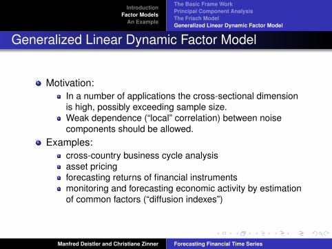
Generalized Linear Dynamic Factor Model

Motivation:In a number of applications the cross-sectional dimensionis high, possibly exceeding sample size.Weak dependence (“local” correlation) between noisecomponents should be allowed.

Examples:cross-country business cycle analysisasset pricingforecasting returns of financial instrumentsmonitoring and forecasting economic activity by estimationof common factors (“diffusion indexes”)



An Example


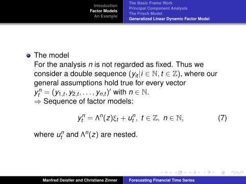
The modelFor the analysis n is not regarded as fixed. Thus weconsider a double sequence (yit |i ∈ N, t ∈ Z), where ourgeneral assumptions hold true for every vectoryn

t = (y1,t , y2,t , . . . , yn,t)′ with n ∈ N.

⇒ Sequence of factor models:

ynt = Λn(z)ξt + un

t , t ∈ Z, n ∈ N, (7)

where unt and Λn(z) are nested.



An Example


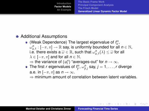
Additional Assumptions(Weak Dependence) The largest eigenvalue of f n

u ,ωn

u,1 : [−π, π] → R say, is uniformly bounded for all n ∈ N,i.e. there exists a ω ∈ R, such that ωn

u,1(λ) ≤ ω for allλ ∈ [−π, π] and for all n ∈ N.⇒ the variance of (un

t ) “averages-out” for n →∞.The first r eigenvalues of f n

y , ωny,j say, j = 1, . . . , r diverge

a.e. in [−π, π] as n →∞.⇒ minimum amount of correlation between latent variables.



An Example


Representation, Forni and Lippi, 2001The double sequence yit |i ∈ N, t ∈ Z can be represented by ageneralized dynamic factor model, if and only if,

1 the first r eigenvalues of f ny , ωn

y ,j say, j = 1, . . . , r , divergea.e. in [−π, π] as n →∞, whereas

2 the (r + 1)-th eigenvalue of f ny , ωn

y ,r+1 say, is uniformlybounded for all λ ∈ [−π, π] and for all n ∈ N .

The last result indicates that the spectral densities of yt and utare asymptotically (for n →∞) identified by dynamic PCA, i.e.the canonical representation of f n

y , decomposed as

f ny (λ) = On

1(e−iλ)Ωn1(λ)On

1(e−iλ)∗ + On2(e−iλ)Ωn

2(λ)On2(e−iλ)∗,

(8)



An Example


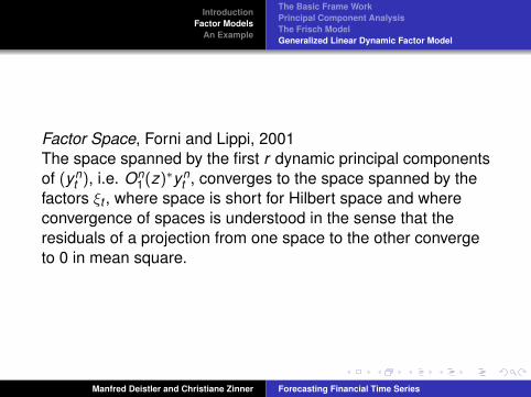
Factor Space, Forni and Lippi, 2001The space spanned by the first r dynamic principal componentsof (yn

t ), i.e. On1(z)∗yn

t , converges to the space spanned by thefactors ξt , where space is short for Hilbert space and whereconvergence of spaces is understood in the sense that theresiduals of a projection from one space to the other convergeto 0 in mean square.



An Example


Latent variables, Forni et al., 2000The latent variables from the PCA-model converge to thecorresponding generalized dynamic factor model variables asn →∞. Let yn

it = On1,i(z)On

1(z)∗ynt denote the projection of yn

itonto On

1(z)∗ynt , i.e. the i-th element of the latent variable of the

corresponding PCA-model at t , then

limn→∞

ynit = yit , for all i ∈ N and for all t ∈ Z, (9)

where yit denotes the i-th element of Λn(z)ξt (for n ≥ i), hencethe corresponding “true” latent variable.



An Example


IdentifiabilityConcerning identifiability, the results from dynamic PCA areadopted asymptotically, i.e. asymptotically (as n tends toinfinity) the latent variables as well as the idiosyncraticcomponents are identifiable, whereas the transfer function Λ(z)and the factors ξt are only identifiable up to regular dynamiclinear transformations. If the factors are assumed to be whitenoise with Eξtξ

′t = Ir , which is no further restriction, since our

assumptions always allow this transformation, they areidentifiable up to static rotations.



An Example


For estimation the dynamic PCA estimators are employed, thuse.g. ˆyn

t =[On

1(z)On1(z)∗

]tyn

t , where On1(e−iλ) denotes the

matrix consisting of the first r eigenvectors of a consistentestimator of f n

y (λ), f nx (λ) say.

The filter On1(z)On

1(z)∗ is in general two-sided and of infiniteorder and has to be truncated at lag t − 1 and lead T − t as fort ≤ 0 and t > T yn

t is not available. As a consequence of thistruncation convergence of the estimators of yt and ut , as n andT tend to infinity, can only be granted for a “central” part of theobserved series, whereas for fixed t the estimators are neverconsistent.



An Example


Determination of rSo far the number of factors r was considered fixed and known,whereas in practice it has to be determined from the data. Theabove discussion indicates that the eigenvalues of f n

x could beused for determining the number of factors and Forni et al.propose a heuristic rule, but indeed, no formal testingprocedure has been developed yet.



An Example


One-sided modelThe fact that the filters occurring in dynamic PCA are in generaltwo-sided and thus non causal yields infeasible forecasts. Oneway to overcome this problem is to assume that

Λn(z) is of the form Λn(z) =∑p

j=0 Λnj z j

and that(ξt) is of the form ξt = A(z)−1εt , A(z) = I − A1z − . . . Aszs

with Aj ∈ Rr×r , det A(z) 6= 0 for |z| ≤ 1, s ≤ p + 1 and theinnovations εt are r -dimensional white noise with Eεtε

′t = I

(and are orthogonal to ut at any leads and lags.)



An Example


The model then can be written in a quasi static form, on thecost of higher dimensional factors,

yt = ΛFt + ut = yt + ut , t ∈ Z, (10)

where Ft = (ξ′t , . . . , ξ′t−p)′ is the q = r(p + 1)-dimensional vector

of stacked factors and Λn = (Λn0, . . . ,Λ

np) is the

(n × q)-dimensional static factor loading matrix. – Note that(yn

t ),Λn, (ynt ), (un

t ) and their variances and spectra still dependon n, but for simplicity we will drop the superscript from now.Under the assumptions imposed Ft and ut remain orthogonal atany leads and lags and thus fy is of the form

fy (λ) = ΛfF (λ)Λ∗ + fu(λ) (11)

.



An Example


For estimation, Stock and Watson propose the static PCAprocedure with q factors and they prove consistency for thefactor estimates (i.e. the first q sample principal components ofyt ) up to premultiplication with a nonsingular matrix as n and Ttend to infinity. In other words, the space spanned by the trueGDFM-factors can be consistently estimated.



An Example


An alternative two-stage “generalized PCA” estimation methodhas been proposed by Forni et al. It differs from classical PCAin two respects: firstly in the determination of the covarianceand secondly in the determination of the weighting scheme.While classical PCA is based on the sample covariance Σy of(yt), this approach commences from the estimated spectraldensity fy decomposed according to the dynamic model. Thenthe covariance matrices Σy and Σu of the common componentand the noise respectively are estimated as

Σy =

∫ −π

πfy (λ)dλ and (12)

Σu =

∫ −π

πfu(λ)dλ. (13)



An Example


In the second step, the factors are estimated as Ft = C′yt ,where the (n × q)-dimensional weighting matrix C isdetermined as the first q generalized eigenvectors of thematrices (Σy , Σu), i.e. ΣyC = ΣuCΩ1, where Ω1 denotes thediagonal matrix containing the q largest generalizedeigenvalues. C is then the matrix that maximizes

C′ΣyC

s.t. C′ΣuC = Iq, (14)

(whereas in static PCA the corresponding weights C maximizeC′ΣyC, s.t. C′C = Iq).



An Example


The matrix Λ is then estimated by projecting yt onto C′yt , i.e.Λ = ΣyC(C′ΣyC)−1. The common component estimator ˆytdefined this way can be shown to be consistent (for n and Ttending to infinity). The argument for this procedure is thatvariables with higher noise variance or lower commoncomponent variance respectively get smaller weights and viceversa, thus the common-to-idiosyncratic variance ratio in theresulting latent variables is maximized, which could possiblyimprove efficiency upon static PCA.



An Example


Boivin and Ng propose a third estimation method called“weighted PCA” which is related to classical PCA asgeneralized least squares (GLS) is related to ordinary leastsquares (OLS) in the regression context. Remember, that, if theregression residuals are non-spherical, but their variancematrix is known, GLS weights the residuals with the inverse ofthe square root of their variance matrix and yields efficientestimators. Assume for a moment that the noise variance Σuwere known, then the same principle could be applied to PCAby transforming the least squares problem min Eu′tut into thegeneralized least squares problem min Eu′tΣ

−1u ut .

Since the residual matrix of the unweighted PCA-model issingular, it cannot be used. A feasible alternative is e.g. theestimator resulting ¿from dynamic PCA. Again the factor spaceis consistently estimated as n and T tend to infinity.



An Example


ForecastingConcerning forecasting, at least two different approaches havebeen proposed.

First, as suggested by Forni et al., the problem offorecasting yi,t say can be split into forecasting thecommon component yi,t and forecasting the idiosyncraticui,t separately. To forecast the common component, yi,t+his projected onto the space spanned by the factorestimates Ft :

yi,t+h|t = proj(yi,t+h|Ft) = proj(yi,t+h|Ft).

The idiosyncratic ui,t may be forecast by a univariateAR-process.



An Example


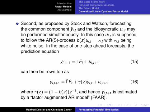
Second, as proposed by Stock and Watson, forecastingthe common component yi,t and the idiosyncratic ui,t maybe performed simultaneously. In this case ui,t is supposedto follow the AR(S)-process b(z)ui,t = νi,t with νi,t beingwhite noise. In the case of one-step ahead forecasts, theprediction equation

yi,t+1 = ΓFt + ui,t+1 (15)

can then be rewritten as

yi,t+1 = ΓFt + γ(z)yi,t + νi,t+1, (16)

where γ(z) = (1− b(z))z−1, and hence yi,t+1 is estimatedby a “factor augmented AR model” (FAAR).



An Example

Forecasting stock index returns

Data and sample periodTargets (i.e. time series to be forecast)Weekly returns of 5 investable stock indices: Euro STOXX50, Nikkei 225, S&P 500, Nasdaq and FTSE (data:Monday close prices)Additional informationadditionally used to estimate the factor space: relativedifferences (weekly) of sector indices of Euro STOXX 50,Nikkei 225 and S&P 500

⇒ 54 time series with 421 observations from 01/04/1999 until01/22/2007.



An Example

50

10

01

50

20

02

50

4Jan99 27Nov2000 28Oct2002 27Sep2004 22Jan2007

Targets

STOXX50NIKKEINASDAQS&PFTSE

−0

.15

−0

.10

−0

.05

0.0

00

.05

0.1

00

.15

0.2

0

4Jan99 27Nov2000 28Oct2002 27Sep2004 22Jan2007

Target returns

STOXX50

NIKKEI

NASDAQ

S&P

FTSE

Figure: Target time series: absolute prices (indexed) and returns.



An Example

Estimation detailsWe calculate 1-week ahead forecasts recursively based on arolling 250-weeks estimation window.⇒ out of sample forecasting period: 171 weeks (10/20/2003 -01/22/2007)

Two benchmarks

Univariate AR(p)-models (lag selection: recurs. computedAIC, BIC with 0 ≤ p ≤ 15Univariate full ARX-models : all 54 time series are used asregressors (with lag 1), the target time series may enterwith more lags (selection as for AR(p)-models).



An Example

Estimation details

Generalized dynamic factor models

FAAR : simultaneous selection of q (no. of static factors)and p (AR-lags) by rec. computed AIC, BIC applied to the(univariate) forecasting equation.PCA : selection of q by rec. computed AIC, BIC andmodified AIC, BIC (as proposed by Bai, Ng, 2002) appliedto the (multivariate) factor model equation of the targets.(idiosyncratic model, see AR(p)-model)GPCA (Generalized PCA) : selection of r (no. of dynamicfactors) based on dynamic eigenvalues, selection of q andp: see PCA.



An Example

−0.0

3−0

.02

−0.0

10.

000.

010.

020.

03

11Sep2006 13Nov2006 18Dec2006 22Jan2007

Target returns and forecasts

3800

3900

4000

4100

4200

11Sep2006 13Nov2006 18Dec2006 22Jan2007

Target (abs.) and forecasts

Target

AR

ARX

PCA

FAAR

GPCA

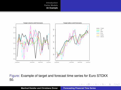
Figure: Example of target and forecast time series for Euro STOXX50.



An Example

Results - Forecasting qualityWith respect to o.o.s. R2 and hitrate the GDFM-methodsdominate the 2 benchmarks across different series andselection methods; in the case of forecasting root mean squareerror (RMSE) this does not hold true.Average o.o.s. statistics over all target time series:

AR ARX FAAR PCA GPCARMSE 0.0248 0.0302 0.0247 0.0255 0.0258

R2 0.0018 0.0034 0.0080 0.0054 0.0041Hitrate 0.51 0.51 0.52 0.53 0.53



An Example

Portfolio simulationsWe will consider

One asset long/short portfolios : according to the forecast’sdirection the whole capital is invested either long or shortinto the asset.Equally weighted long short portfolios : according to theforecast’s direction a constant proportion of the capital isinvested either long or short into each asset (hence theweights can only be 0.2 or -0.2, as we have 5 assets to betraded).

For these portfolios we can compare returns, volatilities,Sharpe-ratios.



An Example

Portfolio simulationsPortfolio statistics for one-asset long/short strategy (averageacross series):

AR ARX FAAR PCA GPCAReturn p.a. 0.0383 0.0137 0.0228 0.1404 0.0665

Volatility p.a. 0.1390 0.1394 0.1391 0.1379 0.1389Sharpe-R. p.a. 0.2814 0.0940 0.1959 1.0188 0.5291

The two GDFM-methods that split the forecasting problem into2 separated problems for the latent component and the noise,PCA and GPCA, clearly outperform all other models;FAAR-forecasts are very similar to AR-forecasts but slightlyworse, and ARX-forecasts (without input selection!) performworst not generating any significant return.



An Example

100

150

200

13.10.2003 20.09.2004 05.09.2005 22.01.2007

One asset portfolios for PCA−forecasts

STOXX50NIKKEINASDAQS&PFTSE

Figure: Example for one-asset portfolios according to PCA-forecasts.



An Example

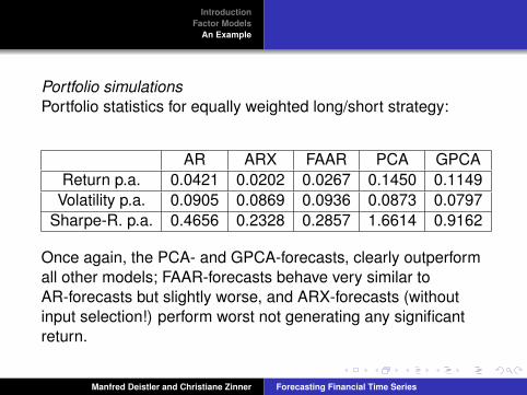
Portfolio simulationsPortfolio statistics for equally weighted long/short strategy:

AR ARX FAAR PCA GPCAReturn p.a. 0.0421 0.0202 0.0267 0.1450 0.1149

Volatility p.a. 0.0905 0.0869 0.0936 0.0873 0.0797Sharpe-R. p.a. 0.4656 0.2328 0.2857 1.6614 0.9162

Once again, the PCA- and GPCA-forecasts, clearly outperformall other models; FAAR-forecasts behave very similar toAR-forecasts but slightly worse, and ARX-forecasts (withoutinput selection!) perform worst not generating any significantreturn.



An Example

9010

011

012

013

014

015

0

13.10.2003 20.09.2004 05.09.2005 22.01.2007

Portfolios (equ. weighted)

AR

ARX

PCA

FAAR

GPCA

Figure: Equally weighted long short portfolios according to differentforecasting models.



An Example

Conclusions

Obviously, forecasting financial time series is a verydifficult problem.A large number of candidate inputs and model classeshighly increases the risk of overfitting.Forecasting models for high-dimensional time series areneeded.Factor models solve, at least in part, the input selectionproblem as they condense the information contained in thedata into a small number of factors. They allow formodelling dynamics and for forecasting high-dimensionaltime series.However, in this area there is still a substantial number ofunsolved problems.


Forecasting Financial Time Seriesusers.cecs.anu.edu.au/~trumpf/LSslides/Manfred_Deistler.pdf · Introduction Factor Models An Example ForecastingFinancialTimeSeries: ProblemsandApproaches

Documents