Forecasting Bike Sharing Demand - Semantic Scholar€¦ · Jayant Malani, Neha Sinha, Nivedita Prasad, Vikas Lokesh, {jmalani, nesinha, n1prasad, vlokesh}@eng.ucsd.edu ABSTRACT Bike

Forecasting Bike Sharing Demand Jayant Malani, Neha Sinha, Nivedita Prasad, Vikas Lokesh,

{jmalani, nesinha, n1prasad, vlokesh}@eng.ucsd.edu

ABSTRACT Bike sharing systems consist of a fleet of bikes placed in a network of docking stations. These bikes are rented and returned to any docking station after usage. Predicting the hourly bike demand at locations will help in designing and expanding bike sharing system as well as maintaining adequate number of bikes at working stations. We predicted hourly demand of bike in each neighbourhood, defined as a census tract, of Washington DC area. We integrated weather and temporal statistics and population/housing data as covariates for predicting bike demands and designed the model for predictions. Keywords Bike Sharing, Washington DC, Random Forest Regressor, XGBoost, Gradient Boost, Time Series Analysis, Random Forest INTRODUCTION Bike sharing system is a service in which fleet of bicycles are available to individuals for shared use, allowing individuals to rent a bike from “Point x” and return to “Point y”. This system began in Europe and is currently available in more than 50 countries including 712 cities with 806,200 bicycles operating at some 37,500 stations. Predicting ride sharing demand in general has become common problem to address, with emerging car sharing services in transport network companies such as Uber and Lyft. In United States, the bike sharing program was built on project insights from European and Canadian counterparts, with some differences in technology and operations like, short transit. An interest in bike share has been incited by success in several US cities, including Washington, DC, New York, Chicago, Denver and Minneapolis, where bike share has gained popularity as accepted transportation option. The heavy traffic in cities and desire for environment friendly medium of transportation are primarily cause of success. The data generated by these systems such as duration of travel, departure location, arrival location, and time elapsed motivated us to study mobility in city by combining historical usage patterns with weather data to forecast bike rental demand in the Capital Bikeshare program in Washington, D.C. In past, various studies have analyzed several factors that affect bike usage and flow. Alexander R. et al (1) investigates and analyzed the impact of demographic and environment built characteristics and suggests that population density critically affects the bike usage. Buck and Ralph et at (2), analysis finds a significant correlation between the presence of bicycle lanes and Capital Bikeshare usage, and highlights the importance of population density. Etienne and Latifa et al (3), used model based clustering to explore the usage of bike sharing systems. In our effort to predict bike rental demand in each neighbourhood on hourly basis, we have combined the demand for all the stations that would fall within one census tract area. We tried various regression models with covariates like weather, population and time. DATA For the task, we obtained the bike sharing usage data from Capital Bikeshare et al (4) located in Washington DC. The data comprises of quarterly usage of bike across all bike stations located in Washington DC. We used data from January 2011 to December 2012. This dataset provided information as shown in Table 1. Total number of rides in dataset is 3,288,891. Total number of casual rides are 619,779 and registered rides are 2,669,112. There were total 204 bike stations. 52 stations are located in Arlington and 152 stations are located in Washington DC. Additionally, we inserted the population and housing metric to the dataset. We collected population and housing data of each census tract in Washington DC from Planning DC website et al (6). In order to map this data to bike station we obtained the geographic location of bike station from Capital BikeShare website et al (4) and used web service (www.data.fcc.gov/api/block/) to get exact census tract for bike station location thus integrating the information with the actual dataset. To further strengthen the model we further integrated hourly weather data from 2011 to 2012 obtained from UCI bike sharing dataset (kaggle competition et al (5)). For this we preprocess the current data to give hourly count of bike rental per station. We also generated the count with respect to registered as well as casual user. We then mapped the weather data from UCI dataset according to hour and location. For stations outside Washington DC like Arlington Virginia we gathered weather statistics from Weather Ground website et at (7). The weather data was preprocessed to match the

1

format of UCI dataset and then was integrated with actual dataset according to time and location. After preprocessing total data points reduced to 665,387. The dataset and variables in the data set obtained from the website of Capital Bikeshare are shown below in the table.

Table 1. Dataset Variable and Type

Variate Format Duration in hour, minute and second format Start Date & Time of Bike rental Timestamp End Date & Time of Bike rental Timestamp Start Station name String Start Station Id Number End Station name String End Station Id Number Bike Id Number Member Type Casual or Registered

Thus, the final dataset after combining the weather data, housing, population data and preprocessing to get the hourly

rental demand of each neighbourhood contains the following features: 1. Census tract ID: There are 100 tract in total which contains bike stations. We mapped the census tract id’s got

from population data to ID’s ranging is given from 0 to 99 2. DateTime: Timestamp that indicates date and time information 3. Casual count: Demand for bikes by casual users 4. Registered count: Demand for bikes by registered users 5. Temperature: normalized temperature in Celsius 6. Atemp: normalized temperature felt in Celsius 7. Season (1:spring, 2:summer, 3:fall, 4:winter) 8. Holiday : Boolean variable that indicates if it is a government holiday 9. Weekday : Boolean variable indicating if it a weekday or weekend 10. Humidity: normalized humidity;the values are divided to 100 (max) 11. Wind speed: Normalized wind speed. The values are divided to 67 (max) 12. Weather:

a. Clear, Few clouds, Partly cloudy, Partly cloudy b. Mist + Cloudy, Mist + Broken clouds, Mist + Few clouds, Mist c. Light Snow, Light Rain + Thunderstorm + Scattered clouds, Light Rain d. Heavy Rain + Ice Pallets + Thunderstorm + Mist, Snow + Fog

13. Population: population count of census tract 14. Housing: housing count of census tract

DATASET EXPLORATION To understand the numerical distribution of variables we plotted the histogram of covariates.

Figure 1. histogram of duration of bike rental Figure 2. histogram of log of bike Count/rental per station

2

Figure1 shows the histogram of bike rental duration. We can see that 97% of the rides were of short durations, less than 20 min. There were very few rides that were greater than 100 minutes. In order to validate our prediction task, we checked that indeed the bike rentals for each station is different. We can see from Figure 2 that the bike rentals considerably vary for each station. The same can be seen from the heat map Figure 3 of Washington DC where the colored dots represent the stations and size of the colored dot resembles the relative total demand of bikes from that station. It is interesting to observe that the maximum bike rentals are from stations located in the central Washington DC area whereas areas like Arlington and South East Washington have minimum bike rentals compared to other stations. Another interesting finding when observing the pairwise station demand is that more than 10k bike rides were from Eastern Market Metro Station to Lincoln Park in the mornings and an equal number of rides on the opposite direction in the evenings suggesting that people often use the bikes for commuting to and fro work.

Figure 3. Normalized Heat Map of Washington DC showing the relative demand per station

From Figure 4 , we observe that most number of data points have clear weather, followed by light mist, followed by light rain and negligible data points have heavy rain/snow. It indicates people prefer taking bikes in clear weather. From Figure 5 , we observe that we have a uniform distribution of datapoints across all four seasons: spring, summer, fall and winter.

Figure 4. Distribution of data points over weather Figure 5. Distribution of data points over season

3

Figure 6,7,8,9 shows that temperature, temperature felt, humidity and windspeed looks naturally distributed. One interesting finding is that in Figure 9 it can be seen that values 1-7 mph are not present. This could be attributed to malfunctioning of the instrument or range of the instrument doesn’t allow it to capture those values or some kind of data transformation have truncated those values.

Figure 6. Distribution of data points over temperature Figure 7. Distribution of data points over temperature felt

Figure 8. Distribution of data points over normalized humidity

Figure 9. Distribution of data points over normalized wind speed

Figure 10 gives the distribution of bike rentals according to hour of the day. This plot also shows that the registered users count follows a similar trend as the total count whereas, casual users follow a different trend with the maximum demand being in the evenings. Also there are two peaks in total count as well as registered count during morning and evening time which suggests that most of the registered users are working people. Thus, we can conclude that ‘hour’ is significant variable which distinguishes registered user count prediction from the casual users count prediction. We can also see outliers in the below Figure 10 . They seems to be natural outliers and we will use logarithmic scale to reduce their effect as explained in Models Section. The bike rentals can be segregated into three categories:

1. High : 8:00-10:00 and 17:00-20:00 2. Average : 10:00-16:00 3. Low : 0:00-6:00 and 20:00-24:00

4

Figure 10. Boxplot of distribution of bike rentals according to hour of the day vs Total, Registered Count & Casual Count

Figure 11 shows the distribution of bike rentals over the days of the week. We observe a stark difference between the trend of registered users and casual users. Registered users use bikes more on the weekdays as compared to the weekends maybe because they use bikes to commute to their workplace whereas casual users use bikes mostly on the weekends maybe because casual users use bikes for recreational purposes.

Figure 11. Boxplot of distribution of bike rentals according to Weekday vs Total Count, Registered Count & Casual Count Figure 12 shows the distribution of bike rentals over the days of the months. We observe that the distribution of bike rentals for both casual users and registered users are more or less uniform across all days of the month.

Figure 12. Line Plot of distribution of bike rentals according to day of Month vs Total Count, Registered Count & Casual Count Figure 13 shows the correlation matrix for continuous variables like temperature, temperature felt, humidity and windspeed with the total count, registred users count and casual users count.

5

Some of the observations obtained from the correlation matrix(Figure 13) are: ● Temperature is positively correlated with the total users count. Temperature has a higher degree of positive

correlation with casual bike rental count as compared to registered bike rental count. That means people prefer to ride a bike at cool to medium temperatures than cold temperatures in Washington DC.

● Temperature felt (atemp) is very highly correlated with the actual temperature and hence it would be best to consider the only the temperature felt.

● Humidity is negatively correlated with the total users count. Humidity has a higher degree of negative correlation with casual users count as compared to registered users count. This suggests that high humidity days like rainy season attracts less riders.

● Wind Speed is positively correlated with bike rental count but the correlation is low.

Figure 13. Correlation matrix for wind speed, humidity, temperature and temperature felt with registered and casual users

count

Figure 14 shows the correlation matrix for population and housing with respect to the registered bike rental and casual bike rental count. It is observed that the population and housing have a higher degree of positive correlation with the registered count as compared to casual count suggesting that the registered users use bikes for commute and that most of the casual users are tourists or they ride bike just as a hobby.

Figure 14. Correlation Matrix for Population, Housing with registered, casual and total user count

Another interesting finding was that there was high correlation between start and end station. People who usually starts their journey from one station to another tends to take the same but reverse journey while returning back. Thus the demand between two stations is highly correlated. This behavior is much more observed among registered user than casual user.

6

The exploratory analysis has some interesting trends which we will try to capture in the prediction model. The correlation between weather, population and time statistics with the bike rental motivates us to develop a predictive model for bike rental prediction. PREDICTIVE TASK Our predictive task is to forecast bike rental demand of Bike sharing program in Washington, D.C based on historical usage patterns in relation with weather, time, population and housing. We have combined the demand for all the stations that fall within one census tract and we are trying to forecast the demand for each census tract on an hourly basis.

EVALUATION OF MODEL We will be evaluating our model on the basis of Root Mean Square Log Error (RMSLE). RMSLE is calculated as:

ε = √(1/n) (log(p ) log(a ))∑n

i=1i + 1 − i + 1 2

Where, pi is the predicted value, ai is the actual value and n is the total number of samples. RMSLE is suitable for our problem because RMSLE penalises an underprediction more than an over prediction. The bike sharing company would lose revenue if the number of bikes will be less than the demand for the bikes.

BASELINE We have considered three different types of baseline predictors. We will be evaluating our models against these three baselines.

● Baseline 1 - We calculated the mean hourly demand for bikes using the response values in the train set. For each observation in the test data, if we predict the demand as the mean value, the RMSLE on the test data is 0.60296.

● Baseline 2 - We calculated the average demand for each hour .i.e 12am, 1am, 2am, ..etc using all the points in the train set. For each observation in the test data, if we predict the demand using the average value for that particular hour, the RMSLE on the test data is 0.57589.

● Baseline 3 - We calculated the average demand for each area for each hour using all the datapoints in training set. For each observation, if we predict the demand as the average value for that particular area for that particular hour, the RMSLE on the test data is 0.570283. Since this baseline gives the lowest RMSLE, we will be evaluating our model against this baseline.

VALIDATION We will be validating our model and tuning the hyperparameters using a 10 fold cross validation. We randomly shuffled our data set and used ⅓ of the data points as test set. We partitioned the remaining data set into 10 splits. In each of the 10 iterations we trained our model on 9 splits and calculated the RMSLE on the remaining split. On the basis of the average of 10 RMSLEs, we tuned our hyper parameters. After tuning the hyperparameters, we trained the model on the complete data set and evaluated the model on the test set. Thus, 10 fold cross validation was used to prevent overfitting. PREPROCESSING The data points were aggregated as per the station’s census tract. The aggregated dataset now contained the census tract ID instead of station name and the count of users per hour were added together if two or more stations fall under the same census tract. The data points maintained the demand by registered users per hour and the demand by casual users per hour separately since we will be using separate models for predicting the demand by registered users and casual users. The dataset was then shuffled and divided into three splits: 2/3 for training and validation set and 1/3 for test set. FEATURE ENGINEERING AND FEATURE SELECTION Based on the data exploration we decided to use the Independent Features mentioned below. Tract number: There are 100 census tracts in our dataset, so tract number ranges from 0 to 99. Temperature Felt: In the original dataset we had temperature and temperature felt as two different features. But since the correlation between temperature felt and temperature is too high, we hypothesised that dropping one feature would not affect the

7

error. We experimented by having temperature as feature, temperature felt as a feature and both temperature and temperature felt as feature. Although there is a negligible difference in the error, we decided to keep just the temperature felt as having less number of features reduces the complexity of models. Weather : We used one-hot encoding to represent the weather: clear weather, misty weather, light snow/rain weather and heavy snow/rain weather. Day of week: Using the datetime stamp in our data set, we calculated the day of the week. We used one-hot encoding to represent the day of the week from Sunday through Saturday. Date: We extracted the date from the datetime stamp in the dataset. We used the day of the month as a feature. Month: We extracted the month from the date timestamp. We used one-hot encoding to represent the months between January and December. Working day: This is a boolean value, 1 for weekdays and 0 for weekends Season: We used one-hot encoding to represent the four seasons: winter, spring, summer and fall. Holiday: This is a boolean value, 1 if it is a government holiday. Population and Housing: We had a hypothesis that the tracts which have higher population and number of houses, will have more demand for the bikes. We experimented by putting population and housing as a feature and observed that the RMSLE increased on validation set with a very small value ~0.0004. One possible explanation for this behaviour could be that the tracts which have higher population and houses in general will have higher demand, but this information gets encoded in the weights assigned to the ‘Tract ID’ by the models even in absence of population and housing data. So in our final model we did not use these features. Hour: Hour is also extracted from the timestamp value present in the data set. We used one-hot encoding to represent the hour of the day. Year: As seen in the data exploration section, 2012 had much higher overall bike demand as compared to 2011. We used one-hot encoding to represent the year: 0 for 2011 and 1 for 2012. Apart from the above independent features, we did some feature engineering to improve our model : BINS FOR HOUR DECISION TREE Apart from having ‘Hour’ as a feature, we also experimented with having an ‘Hour bin’ as an additional feature. During the data exploration Figure 10 , we have seen that the trend for bike demand over hours is different for registered users and casual users. We broadly classified hour into 3 bins corresponding to the high, medium and low demand. Further, we experimented by increasing the number of bins to improve our error. We used decision tree algorithm to find the bins that would give lowest error on the validation set. To create the decision tree, we aggregated the demand at each station to find the total demand of bikes at each hour. We used Sklearn’s decision tree to generate the decision tree. We created separate decision trees for registered users and casual users. We varied the ‘number of leaf nodes’(which is equal to number of bins to be created) from 1 to 24 and calculated the validation error. The lowest validation error was found when the number of hour bins for registered count was 7 and number of hour bins for casual count was 5. We saw an improvement of around ~0.001 in our RMSLE on our validation set. The Figure 12,13 shows the final decision tree used

8

for creating the bin.

Table 2. Hour range for each of the bins using demand by registered user

Hour Bin Hour Range 1 Less than 6.5 2 Greater than 20.5 3 18.5 - 20.5 4 16.5 – 18.5 5 8.5 – 16.5 6 6.5 – 7.5 7 7.5 – 8.5

Figure 15. Decision tree for demand by registered users

Table 3. Hour range for each of the bins created using demand by casual users

Hour Bin Hour Value 1 Less than 7.5 2 7.5 – 9.5 3 Greater than 9.5 4 7.5 – 10.5 5 10 – 19.5

9

Figure 16. Decision tree for demand by casual users

BINS FOR TEMPERATURE DATA BASED ON DECISION TREE: In the data exploration Figure 14 , we saw that there is a very high correlation between ‘temperature’ and ‘temperature felt’ variables in the dataset. So we dropped the temperature and just used ‘temperature felt’ as it is natural that the riders would like to rent bikes based on the temperature felt. Apart from using ‘temperature felt’ as a feature, we also created temperature bin and added it as a feature. The RMSLE on the validation set improved by ~0.0008. The decision tree created for binning the temperature for both registered and casual users is shown in Figure 14,15.

Figure 17. Temperature bins for registered users demand

Table 4. Temperature range for each of the bins created using demand by registered users

Temperature Bins Temperature Values 1 Less than 18.5600 2 18.5600 – 30.6825 3 30.6825 - 35.9850 4 Greater than 35.9850

10

Figure 18. Temperature bins for casual users demand

Table 5. [Temperature range for each of the bins created using demand by registered users]

Temperature Bins Temperature Values 1 Less than 14.7725 2 14.7725 – 29.9250 3 29.9250 - 35.2275 4 Greater than 35.2275

MODELS In the data exploration Figure 10 & 11 we have seen that the trend for the bike demand by casual users and registered users are very different. So we decided to train two different models, one for predicting the hourly demand by casual users in each area and another for predicting the hourly demand for registered users in each area. We did try running a single model to predict the total demand ( demand by registered users and and demand by casual users), the RMSLE in this case was 0.54812. Also, in the data exploration we have seen that there are natural outliers while plotting the demand vs Hour Figure 10 . To take care of these outliers, without actually eliminating it, we converted the demand to logarithmic scale. Using the models, we then predicted the demand by casual users and registered users in logarithmic scale and convert it back to find the predicted demand. We also tried to predict the demand without converting it into logarithmic scale. In this case, the RMSLE was 0.61238, which is even worse than our baselines. We explored different types of parametric models based on the features mentioned above. Since this is a regression problem, we have to chose a regressor that can efficiently train our model, while taking into account that we have a large number of data points in our training set 443,591 and around 45 features (46 features for demand by casual users and 48 features for demand by registered users). LINEAR REGRESSION We used the ridge regressor provided by the Sklearn library. This model solves a regression model where the loss function is the linear least squares function and regularization is given by the l2-norm. We experimented with different values of regularization coefficient: alpha [0.001, 0.01, 0.1, 1, 5, 10, 100, 1000]. We got the lowest value of RMSLE of 0.54675 on the validation set (10 fold cross validation error) at lambda(regularization parameter) = 1000 which is better than our baseline by 4.1266%. SVR This model works similar to SVM’s as described in class, but is adapted to handle regression. It attempts to approximate the value of a continuous variable by using a loss function that is insensitive to the error. We tried to use the sklearn’s SVR library. One challenge in using the SVR is that it is very slow. So ran SVR for RBF kernel with penalty parameter =

11

1e0.3 and gamma = 0.1. The RMSLE on the validation set (formed by randomly selecting ⅓ data points from the train data) was found to be 0.64425. Since, it took one day to run SVR on our laptops, it was not possible for us to tune the hyper parameters and improve our results. GRADIENT BOOSTING TREE REGRESSOR Gradient Boosting regressor builds an additive model in a forward stage-wise fashion. In each stage a regression tree is fit on the negative gradient of the given loss function. The model greedily adds base learners from a select hypothesis class, and attempts to find a weighted combination of them that minimizes the training error. We tried Gradient Boosting trees provided by Sklearn for different values of n_estimators (number of trees) [50, 100, 200, 300], max_depth = [20, 30] and gamma = [.01, 1]. The lowest 10 fold cross validation RMSLE on the validation set was 0.48213 was obtained with n_estimators = 300, max_depth = 30 and gamma = 0.1. Sklearn’s gradient boosting takes a lot of time to train a model. It took around 3 hours to train a model with one set of hyper parameters. This is because gradient boosting trees build the trees(weak regressors) sequentially and not parallely like random forest. we might have been able to improve our error, but due to the very slow computation we could not try more hyper parameters and decided to use XGBoost which is computationally much faster than Sklearn’s Gradient boosting trees. We also tried running PCA on our training data and reduce the dimensions of the feature vector to 30. It still took more than two hours to train a model and we got an error of 0.49435. XGBOOST REGRESSOR eXtreme Gradient Boosting regressor is an implementation for Gradient Boosting specifically designed to optimize speed and performance. Using the XGBoost python library, we were able to train a model in 30 minutes. we ran XGBoost regressor for different values of n_estimators(number of trees) = [50, 75,100, 125] and max_depth(maximum depth of each trees) = [6,9,12,15] and learning rate = [0.01, 0.1]. The lowest value for 10 fold cross validation RMSLE of 0.4035 was found with n_estimators = 125, max_depth = 12. XGBoost Regressor outperformed all the other regressors that we have experimented with. RANDOM FOREST A random forest is a meta estimator that fits a number of classifying decision trees on various sub-samples of the dataset. To improve the predictive accuracy and control over-fitting, averaging is used. We trained our model using Sklearn random forest library for different values of n_estimators (number of trees in the forest) = [20,30,40,50,60,70,100,110,120,130,150,160] and max_depth (maximum depth of each tree in the forest) = [10,15,20,25,30,35,40,45,50] and max_features (number of features to consider while looking at the split) = [sqrt of the total number of features, all the features]. We found the lowest 10 fold cross validation RMSLE of 0.41891 with n_estimator = 100, max_depth = 25 and Max_features = All the features. EXTRATREE REGRESSOR This class implements a meta estimator that fits a number of randomized decision trees (a.k.a. extra-trees) on various sub-samples of the dataset and use averaging to improve the predictive accuracy and control over-fitting. We trained our model for n_estimators (number of trees in the forest) = [50, 70, 100, 120, 150] and max_depth (maximum depth of each tree in the forest) = [10, 20,25,30]. The 10 fold cross validation RMSLE was found to be 0.42712. Extratree Regressor are known to be computationally faster than Random Forest. In our case, we observed the training time to be 20 minutes which was less than time taken by Random Forest(~35 minutes), when ran on the same machine. But, the RMSLE went up by 0.00822, which may be due to presence of noisy features. BAGGING REGRESSOR A Bagging regressor is a meta-estimator that fits base regressors each on random subsets of the original dataset and then aggregate their individual predictions (either by voting or by averaging) to form a final prediction. We used Sklearn’s Bagging regressor to train our model. We used different values of n_estimators = [20,30,40,50,60,70,80,90,100,120,150] and Bootstrap = True. We got the lowest 10 fold validation RMSLE of 0.41627 with n_estimators = 120 and Bootstrap = True. Thus the bagging regressor outperforms the random forest by 0.0072. ENSEMBLE OF REGRESSORS We also experimented by averaging the predictions of the three different predictors. To do this, first we trained three different models, Random Forest, XGBoost, and Bagging regressors (with the hyperparameters mentioned above) on the training set. We then created a new train data set. For each data point in the original training data set there will be a point in this new data set. Each data point in this new data set has three features which are the predicted values for the corresponding data points in the original data set using the three regressors mentioned above. Similarly, the new test set is also created. Now we run linear regression with X_train as the newly created data set, y_train as the actual values of the count. We trained two different linear regressors to predict demand by casual users and demand by registered users.

12

The main intuition behind this model was to take advantage of the two types of ensembles method, averaging methods like Random Forest and Bagging regressor which reduces the variances of the base estimators and boosting methods like XGBoost which reduces the bias of the base estimators. However, the 10 fold cross validation RMSLE on the test data turned out to 0.41092 which is not better than the performance of XGBoost. TIME SERIES

We tried using time-series analysis for our prediction where we use the bike demand of the recent past of a station in order to predict the current bike demand in that station. We can observe the time-series plot of the overall bike demand from Jan 2011 to December 2012.

Figure 19. Time series graph showing bike demands from Jan 2011 to Dec 2012

However, we noted that using the previous day’s demand will not yield good results since the demand significantly varies with the day of the week. Hence, we used the bike demand at that station on the same day of the previous week. For example, in order to predict the bike demand at 11am Saturday at Station A, we used the feature vectors as well as count of bike rentals at 11am on the 1st, 2nd & 3rd previous Saturdays at Station A in addition to other features we are currently using. With the new feature vector we tried running XGBoost and Random Forest. However, we observed a RMSLE value of 0.46831 which is higher than that of Random Forest Regressor, Bagging Regressor, XGBoost regressor. This may be due to the absence of trend and seasonality in the demand pattern or due to overfitting. However, there are more complex models which can be used for time-series analysis and has been mentioned in the Future Work section. LITERATURE SURVEY People have earlier studied Bike Rental Demand Prediction for many cities across US. There also has been Kaggle Competition on predicting Bike Demand, but the prediction was not based on any geographical location or neighbourhood but for entire Washington DC. A few of the papers worth mentioning are given below: STATION-LEVEL FORECASTING OF BIKE SHARING RIDERSHIP:STATION NETWORK EFFECTS IN THREE U.S. SYSTEMS BY R. ALEXANDER RIXEY: This study investigates the effects of demographic and built environment characteristics near bike sharing stations on bikesharing ridership across Capital Bikeshare, Denver B-Cycle, and Nice Ride MN. Their project expands on previous studies by including the network effects of the size and spatial distribution of the bike sharing station network that contributes to a more robust regression model for predicting station ridership. They have also identified through regression analysis a number of statistically significant correlation variables: population density, retail job density, median income levels, the share of alternative commuters, days of precipitation (negative association), non-white population(negative association) and proximity to a network of other bike sharing stations that are critical factors in estimating bikesharing ridership. According to authors Bike sharing system planners should consider the importance of a comprehensive network of potential destinations within biking proximity of each other when determining the extent and spatial distribution of bike sharing stations as it exhibits a strong positive correlation with ridership in a variety of model specifications. PREDICTING BIKE USAGE FOR NEW YORK’S BIKE SHARING SYSTEM, 2015 BY SINGHVIS, FRAZIER, HENDERSON, MAHONY, SHMOYS AND WOODYARD: The paper addresses predicting pairwise bike demand for New York city. Their focus is mainly on morning

13

rush hours between 7:00 AM to 11 AM during weekdays.One interesting covariate they have considered is use of taxi besides other weather,temporal,demographic variables in order to predict bike demand using linear regression model. They first performed analysis using linear regression model at the station pair level by fitting a linear regression model using log-transformations of taxi trips, population, and housing units. However, it did not yield the desired level of accuracy in predictions for the test set, as the model consistently underpredicts log(1+bike trips) relative to actual values, leading to substantial amount of unpredicted variation. They then fit a regression model to predict pairwise bike demand between neighborhoods. This outperformed the individual station model with RMSE of approximately 0.42 on logarithmic scale. FORECASTING BIKE RENTAL DEMAND BY JIMMY DU, ROLLAND HE, ZHIVKP ZHECHEV: The authors of this paper describes predicting the number of bike rentals for city bikeshare system in Washington D.C. Their noticeable observation is prediction based on "hours" which lead to significant improvement in performance of the predictor. The authors suggest weather variable covariates have less dominance in contributing to accurate prediction. Two of the three tree based models,namely CTree with RMSLE of 0.460 and RF with RMSLE 0.503, outperformed other models they used to predict with most accuracy. The reason being the tree based models were able to capture the subtle nonlinear interaction effects between variables, in which they are equipped. They also performed separate regression on registered and non registered users and summed up the individual result together which did not perform better than regression on total count or combined users owing to introduction of more noise and variance because of separate regression on each component. They concluded that decision tree model, CTree could best capture the relationship between the data. Our predictive task is slightly different from above mentioned work where people have either predicted bike demand for entirety of area or are predicting pairwise prediction. The features used were also different among the papers as well as our model. We chose to use census tract as geographic bounding for prediction because it gave better visualization of overall bike demand according to geographic location which is an important parameter. Thus a direct comparison of the performance of our model with their models is difficult. RESULTS We tested the performance of our regressors on the test set. The XGBoost regressor outperformed all other regressors. The table below summarizes the performance of all the models that we tried.

Table 6. Result

Model Average root mean square log error for 10 fold cross validation

Root mean square log error on test set

Baseline (mentioned as baseline3) 0.57812 0.57028 Linear regressor 0.54675 0.55623

Gradient Boosting Regressor 0.48213 0.48327 XGBoost Regressor 0.40350 0.40505

Random Forest 0.41891 0.42144 ExtraTree Regressor 0.42712 0.43176 Bagging Regressor 0.41627 0.41433

Ensemble of Regressors 0.41092 0.41003 Time series 0.46831 0.48124

From the above results we see that the ensemble methods works better than the linear regression. Few of the reason why these methods worked better are:

● Decision trees are the base regressor for all the ensembles methods used. Using decision trees we are able to model the complex nonlinear interaction between the features.

● With decision trees, if two features are strongly correlated, one of the features is arbitrarily chosen for a split and the other feature has no further effect on the model. Whereas the linear regression shows low performance when the features are correlated.

● Linear regressor is not good at handling outliers, whereas the ensemble of decision trees are not affected much by the presence of outliers.

● Though a single decision tree tends to overfit on the train data, ensemble of trees are better at preventing overfitting. To improve the performance of decision tree we used ensemble methods that reduces the bias and/or

14

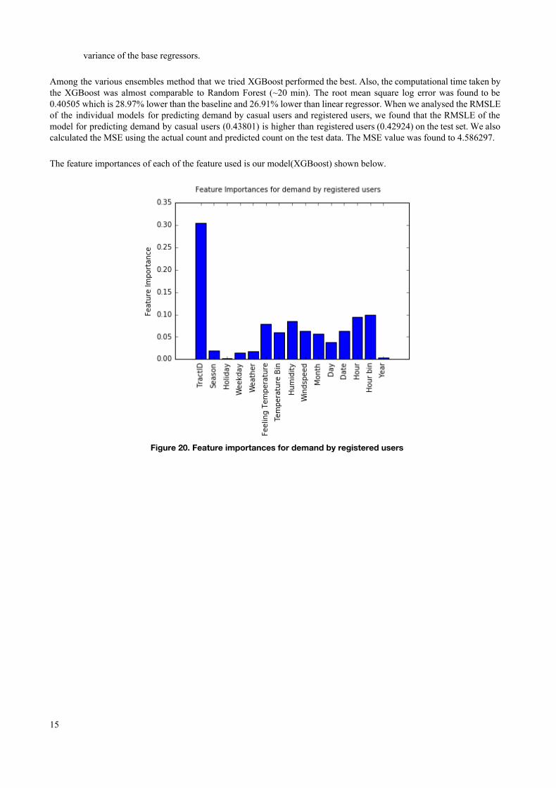
variance of the base regressors. Among the various ensembles method that we tried XGBoost performed the best. Also, the computational time taken by the XGBoost was almost comparable to Random Forest (~20 min). The root mean square log error was found to be 0.40505 which is 28.97% lower than the baseline and 26.91% lower than linear regressor. When we analysed the RMSLE of the individual models for predicting demand by casual users and registered users, we found that the RMSLE of the model for predicting demand by casual users (0.43801) is higher than registered users (0.42924) on the test set. We also calculated the MSE using the actual count and predicted count on the test data. The MSE value was found to 4.586297. The feature importances of each of the feature used is our model(XGBoost) shown below.

Figure 20. Feature importances for demand by registered users

15

Figure 21. Feature importances for demand by casual users

From Figure 20 and Figure 21 , we can see that for both demands by casual users and registered users, tract ID is the most important feature, the feature importance has higher value in case of registered users . We also observe that weekday and holiday has more importance for predicting demands by casual users than registered users. In the data exploration section also we have seen that the demand by casual users is much more on weekends and holidays whereas the demand by registered users varies by small value over the different days of the week. Also, wind speed has higher importance in case of demand by casual users. CONCLUSION We established significant relationship between several independent variables and Bikesharing ridership. We developed a regression model that can be applied directly to bike station business to predict hourly demand. We also found that the usage of bike rental is far more high for registered users as compared to casual user and the demand is maximum during morning and evening travel hours. Also weather has significant effect on bike ridership. A clear and sunny weather invites more riders as compared to rainy and snow weather. We trained various different models and performed featurization and found that XGBoost was best to capture the variance and non linearity of the dataset. It gave an RMSLE of 0.40505 on test set. The ensemble of regressors didn’t worked as expected. One possible explanation could be absence of trend and seasonality in the bike demand pattern. We can thus conclude that the developed model can be used to predict the bike demand in urban environment. The model can be used by the Bike sharing company to strategically place the bikes at different stations depending on the forecast. They can also change their revenue model to introduce price surge during peak hours based on the forecast of demand.

FUTURE WORK

In future work we would like to add some more covariates and improve the predictions. We can also do hourly predictions between each pair of stations. This prediction task may further help the Bike sharing company to do strategic management at more granular level. Some of the covariates that we could think of integrating in future are:

● Taxi and subway data. We suspect that there could be a positive correlation between demand for short taxi rides within an area and demand for bikes in that area. The presence of subway station near a bike station may also increase the demand for bikes at that particular station.

● Restaurant and retail shop data. If there are a lot of restaurants and retail shop in an area, the number of customers visiting these places may have

16

a positive correlation with the bike demand in the same area. ● Data related to High Schools/Universities/Office Timings.

If there are High Schools, universities or offices in an area, the working hours may have an influence on the bike demand.

Some of the different models that could be tried in future are:

● Time series analysis using models such as autoregressive integrated moving average (ARIMA), Multivariate GARCH model, Microsoft’s time series algorithm, ARXTP (autoregressive tree-models with cross prediction).

● Neural network algorithms like LSTM, MLP regression.

REFERENCES 1. R. Alexander Rixey, 2012, Station-Level Forecasting of Bike Sharing Ridership: Station Network Effects in

Three U.S. Systems, TRB 2013 Annual Meeting. 2. Buck, D., and Buehler, R. 2012. Bike lanes and other determinants of capital bikeshare trips. In 91st

Transportation Research Board Annual Meeting . 3. Etinne, C., and Latifa, O. 2012. Model-based count series clustering for bike-sharing system usage mining, a

case study with the velib’system of paris. 4. Capital Bike Sharing - https://www.capitalbikeshare.com/system-data 5. Bike Sharing Demand - https://www.kaggle.com/c/bike-sharing-demand 6. Planning DC Website - https://planning.dc.gov/page/census-tracts

17