USA FA-TR-80-17 04I FORCE ACADEMY 0 eAERONAUTICS DIGEST - SPRING/SUMMER 1980 0 C .. . . . .. _______. ,0 4.00 OCTOBER 1980 FINAL REPORT -2. oeo , :00. 0 *0 aJ APPROVED FOR PUBLIC RELEASE: DISTRIBUTION UNLIMITED DEPARTMENT OF AERONAUTICS DEAN OF THE FACULTY UNITED STATES AIR FORCE ACADEMY COLORADO 80840 -- - ,J 4 ( , ;I : ..-.-. . , _-. _,-; -. , ,_ _ _ __. " .. - - - .: , .: .. "- -- ' '- " '

Welcome message from author
This document is posted to help you gain knowledge. Please leave a comment to let me know what you think about it! Share it to your friends and learn new things together.
Transcript
USA FA-TR-80-17
04I FORCE ACADEMY0eAERONAUTICS DIGEST - SPRING/SUMMER 1980
0
C .. . . . .._______. ,0
4.00
OCTOBER 1980
FINAL REPORT
-2. oeo , :00. 0*0 aJ
APPROVED FOR PUBLIC RELEASE: DISTRIBUTION UNLIMITED
DEPARTMENT OF AERONAUTICS
DEAN OF THE FACULTY
UNITED STATES AIR FORCE ACADEMYCOLORADO 80840
-- - ,J 4 ( , ;I
: ..-.-. . , _-. _,-; -., ,_ _ _ __. " .. - - - .: , .: .. "- -- ' '- " '

r1
Fi
COVER:
Capt Clynn Sisson and 2nd !.t Richard Crandall, DFAN, produced this USAFA-Computer-Graptics-System plot of a three-dimensional surface representing the total pressure field behinda cnnard-configured, wind-tunnel model. If you are interested in details on the instru-mentation used to collect the total pressure data, consult the paper in this Digest en-titled "Measurement of Very Large Flow Angles with Non-Nulling Seven-Hole Probes."
Editorial Review by Capt James M. Kempf, Department of EnglishUSAF Academy, Colorado 80840
F:
This document is presented as a compilation of monographs worthy of publication.The United States Air Force Academy vouches for the quality of research, withoiut neces-sarily endursing the opioi,.ns and conclusions of the authors.
11is digest has been cleared for open publication and/or public release by the ap-optLl iine O-fice of i-i[or1iZLioin in accordance with AFR i90-i7 and DODD )23U.. There
is no objection to unlimited distribution of this digest to the public at large, or byDDC to the National Technical Information Service.
This digest has been rev iewed and is approved for publication.
M. . BACON, Colonel, USAFjDirector of Research andContinuing Education
... ,+ ,. : i. • . ; , :;,,,, ' ,':..i2 Ar

UN LASSIFPKMSECURtTYr CLASSIFICATION OF THIS PAGE fW%*es, Dmw.Entorod)
REPORT DOCUMENTATION PAGE READ INSTRUCTIONSREPORTDOCUMENTATIONPAGE_ BEFORE COMPLETING FORM
1. RE ....... VT ACCESIONNo.3RE PIENVS CATALOG NUo"Ef,
UeAir Force Academy Aeronauace Digest>
/- A__
E. .uper R.. Gregory ~t
9 PERFORMING OROANIZATION NAME AND ADDRESS S. PROGRAM ELEMENT. PROJECT. TASKAREA III WORK UN IT HUMIoERS
Department of AeronauticsUnited States Air Forc- Academy, CO 80840
II CONTROLLING OFFICE NAME AND ADDRESS
I 3-WOMBEIR OF PGI
I1. MONITORING AGENCY NAiE A AOFlighdtipIt Ican.Co pu10olsin O nc*) I. SECURITY CLA! , -l0t1IS 19por"
IS. ECL ASSIFICATION'OWNGRADINGSCHEDULE
16. DISTRIBUTION STATEMENT (of this Report
17. DISTRIBUTION STATEMENT (.1 th. ab.ut e nf-.51c* h, 81-k 20. It difl-sI trm ROOCf)
II. SUPPLEMENTARY NOTES
,It EY WORDIS (Continu on ,.vero* side It necesay ad identify by Woek ftmbw)
Aerodynamics, Flight Mechanics, Propulsion, Thermodynamics, HeatTransfer, Hind Tunnel, Aeronautical Instrumentation, AeronauticalHistory
20. BSTRACT (Co -ino , tavoreo side It niosie.. .d Idmity, blW k i.6oc)
This digest covers unclassified research in aeronautics performed atthe United States Air Force Academy during the six months ending15 July 1980. This report includes technical papers in the specificareas of aerodynamics, flight mechanics, propulsion, experimentalinstrumientation, thermodynamics and heat transfer, and aeronauticalhistory.
DD I AN7 1473 EDITION oF I NOV 45 Is OSSOLILTE UNCLAkSSIFIEDSECURITY CLASSIFICATION OF THIS PAGE (111144 Do#& Vnierd)
4.m/

SECUNi?'v CLAWPICAT@W" OF THIS PAEm eDa bbe.4
UNCLASSIFIED24CURITY CLAWPICAT10% OF ' PAGC(WhI Doi* Zate.Oj
~U,,FA-TZ-80- 17
PREFACE
This report is the fifth issue of the Air Force Academy Aeronautics Digest.* Our
policy is to print articles which represent recent scholarly work by students and faculty
of the Department of Aeronautics, members of other departments of the Academy and the
Frank J. Seiler Research Laboratory, researchers directly or indirectly involved with
USAFA-sponsored projects, and authors in fields of interest to the USAFA.
In addition to complete papers, the Digest also includes, when appropriate, abstracts
of lengthier reports and articles published in other formats. The editors will consider
for publication contributions in the general field of Aeronautics, including
Aeronautical Engineering
Flight Mechanics
PropulsionStructuresInstrumentation
-Fluid Mechanics-Thermodynamics and Heat Transfer-Engineering Education-Aeronautical History
Papers on other topics will be considered on an individual basis. Contributions
should be sent to:
Editor, Aeronautics DigestDFANUS Air Force Academy, CO 80840
The Aeronautics Digest is presently edited by Capt A. M. Higgins, PhD, Maj E. J.
Jumper, PhD, and Capt J. M. Kempf (Department of English), who provided the final editorial
review. Our thanks also to our Associate Editor, Barbara J. gregorv, of Contract Technical
Services, Inc.
rWe would like to correct an oversight in a previous Digest. We failed to mention
that Mr. Dick Dobbek of the Air Force Flight Dynamics Laboratory furnished tLe article
on the first United States aircraft accident wrirten by F. P. Lahm. This report appeared
in the Aeronautical History section of the Aeronautics Digest - Fall 1979.
The first three issues of the Digest can be ordered from the Detense Documentation
Center (DDC), Cameron Station, Alexandria, VA 22314. Use the following AD numbers:Aeronautics Digest - Spring 1978, AfDA060207; Aeronautics Df; est - Fall 1978, ADA069044;and Aeronautics Digest - Spring 1979, ADA075419.
ii
l l [ I I I - I I I I I I I I I I

USAFA-Th- -0-17/
Section
I. AERODYNAMICS 1
- AERODYNAMIC EFFECTS f SANWISE GROOVES A SYMMETRICAL AIRFOIL' 2
C. Y. Chow, E. 3. Juzaper, T.A. Gay, M. Al Hoffman, and S. Suhr
II. FLIGHT MECHANICS 13
- C9PARISON J +IM-DEPENDENT ROTATION MATRIX TRANSFORMATION METHODS, 14
--- J. E. Justn and P. F. To~rey V_ - ./
III. PROPULSION 22
- 1 URTHER VYALUATION OF14( GLUHAREFF PRESSbRE JET;
-- . .Brilliant, M. f Fortson', D. S. Hess, and A. J. Torosiin
' IV. THERMODYNAMICS AND HEAT TRANSFER 30
-A LOW-COST POINT-FOCUSING DISTRIBUTED SOLAR CONCENTRATOR - '" " 314 -A-R. C. Ofiver
I -- V. INSTRUMTATION AND HARDWARE 59
: "-AS N , VERY LARGE FLOW ANGLES WITH NON-NULLING SEVErN-HOLE 60
-: 'a- -R. W. Gallington.
VI. AERONAUTICAL HISTORY 89
COMMENT BY A SERVING AIRMAN 9o--- B. Poe II
ACCS~iflFor
ES GRA&I
DTIC TAB --
U -Y
Av i;.ab2tY t Code5# i -Avail Unalor
Dist!
I. ..; .. ,._. ..
I I I I I I I I I

USAFk-TR-80- 17
SECTION II
AERODYNAMI CS
OPP.
USAFA-T-80-17
AERODYNAMIC EFFECTS OF SPANWISE GROOVESON A SYMMETRICAL AIRFOIL
C. Y. Chow, E. J. Jumper,T. C. Gay, M. A. Hoffman, S. Suhr
Abstract
This paper discusses the results of a wind tunnel study of a grooved NACA 0015airfoil. The effect on lift, drag and moment are discussed, and wind tunnel data forselected groove geometries are presented. Recommendations for further study aresuggested.
I. Introduction
When a boundary-layer flow on a rigid surface goes through a region of adverse pres-
sure gradient, fluid particles are decelerated by a net pressure force which is in the
direction opposite to that of the motion. If the adverse pressure gradient persists
for a long distance, the slower particles may not have enough momentum to go through the
entire length, so that at a certain station the direction of motion near the body surface
becomes reversed and the boundary layer becomes separated from the body. This is what
happens to the flow on the upper surface of a stalled airfoil. The onset of stall is
characterized by a sudden loss of lift and a drastic increase in drag as the angle of
attack increases, both of which are undesirable on an aircraft wing.
To delay separation, the basic principle is to increase the downstream momentum
of the boundary-layer flow on the u.per surface of the wing. The additional kinetic
energy enables the flow to better resist the action of an adverse pressure gradient.
The improvement is commonly accomplished by injecting high speed air into the boundary
layer in the downstream direction or by making the boundary layer turbulent ahead of
the separation point.
Even without an adverse pressure gradient, there is another retarding effect on
the boundary layer resulting from the no-slip condition on a stationary body. Since the
fluid velocity varies from zero at the body surface to its inviscid value at a very short
distance above, there exists a sLrong speed gradient which causes shear stress to slow
down the boundary-layer flow. From this point of view a different approach might be
taken to delay separation. Our idea was to remove the no-slip condition on part of the
surface, so that the kinetic energy thus saved could be used for the flow to go through
a longc distahice against the adverse pressure gradient before it separates.
We proposed that spanwise grooves be cut through the upper surface of a wing as
shown in Figure 1. If constructed properly, a line vortex would be trapped WiLhin each
*Distinguish. d Visiting Professor, DFAN**Major, USAF. Associate Professor of Aeronautics, DFAN
***Cadet, USAF Academy
2

USAFA-TR-80-17
.7/Z
Figure 1. Grooved Airfoil
groove so the air flowirg over it would gain a downstream velocity instead of the orig-
inal z. ro velocity implied by the no-slip condition. By varying the pattern of the
grooves, we hoped to find the variation which improved the stall characteristics.
It must bc pointed out that energy is continuously dissipated in the cavity by vis-
cosity. In steady state the vortex is sustained by drawing energy trom the boundaly
layer above. Thus, if separation could be delayed by using this technique, it might
be achieved at the expense of an additional drag on the wing. This ruditional drag would
occur if the energy being dissipated by the vortex exceeds that which would be present
if the flaw separated causing pressure drag.
II. Model Design
To examine our idea for delaying separation, a grooved wing of constant chord was
constructed, and we tested it in the Air Force Academy 2 x 3 subsonic wind tunnel. ThiG
wing model required that the number of 'rooves and their locations be variable, the
spaces between adjacent grooves be adjustable, and the groove dimensions facilitate the
trapping of line vortices in the grooves.
The wing, machined out of a piece of solid aluminum, is shown in Figure 2. Except
the midspan portion which contained a cylindrical hole for mounting the model on a force
balance in the wind tunnel, a part of the upper surface was removed from both left and
right sides of the wing and was replaced by six tight-fitting aluminum slats on each
side. With all six slats installed, the cross se:tion of the wing closely approximated
the symmetrical NACA 0015 airfoil whose maximum thickness was 15 percent of chord. A
groove was formed by removing a symmetric pair of slats on both sides of the wing al-
though the groove was blocked at the midspan. Aluminum plates were attached on both
ends of the wing to eliminate tip effects, so the flow past the wing was approximately
two-dimensional. The slats were secured in position by screws through both the wing
and end plates as indicated in Figure 2. Figure 3 is a photograph showing the mounted
3
. . . . . . ...-- _," . . .. .. "

USAA-TR-80- 17
SLArIW
Figue 2. TheWindTunel M~d0
0IENDPLAT
Figure 3, Photograph of Tunnel Model
4
USAFA-TR-80- 17
model in the wi-d tunnel with the first and sixth slats removed.
We determined the slat dimensions from the following considerations. In studying flow
over rectangular cavities, Pan and Acrivos (Ref. 1) and O'Brien (Ref. 2) found numerical-
ly that the numbei of vortices formed in a cavity ,oas determined by the Reynold@ number
as well as by the depth-to-width rati, of the cavity. Shallow cavities could hardly
hold the vortex, whereas the deep cavities caused higher drag forces. It seemed that
the square cavity would trap a single vortex in a stable manner and yet would not yield
too large a drag. To approximately obtain this configuration, a portion of the upper
wing surface was cut out above the chord line, with the forward edge of the cut at a
distance of 25 percent chord measured from the leading edge of the wing. The space was
then refilled with six slats of equal width, the first of which had an approximately
square cross section. Because of the curved contour of the NACA 0015 airfoil, all six
slats were different with their height decreasing toward the trailing edge.
Table 1 gives the essential dimensions of the model.
Table I
WING DIMENSIONS
Wing Span 17.7 inches
Maximum Thickness 0.9 inches
Average Chord 5.85 inches
Size of First Slat 3/8 x 3/8 x 8 inches
Size of End Plates 4 x 8 x 1/4 inches
III. Experimental Proc dures
With six slats we could have up to three unconnected square grooves on the wing.
There was a total of nineteen different ways of arranging the grooves. We tested each
of the nineteen configurations and compared the aerodynamic characteristics with those
of the ungrooved wing.
After a desired groove arrangement had been made on the wing, screw slots were
filled with wax, and the model was then mounted on a 0.75-inch Mark II balance manufac-
tured by the Task Corporation. During testing, the balance converted lift, drag, and
moment data of the wing into voltage signals whicI were fed into a PDP 11/45 digital
computer for storage and manipulation.
The experiment was carried out in the subsonic wind tunnel in the Aeronautics Labor-
atory of the United States Air Force Academy. The tunnel had a 2 x 3 foot test section
and was capable of producing air speeds up to 400 ft/sec. All experimental data were
taken under a steady air speed of 135 ft/sec at whic the Mach number was approximately
0.12 and the Reynolds number based on chord was approximately 5 x 10s.
The experimental unit was equipped to automatically position the model in the-4Mnd
tunnel at different angles of attack for data gathering. Thirty-three data values were
5

t.
USAFA-TR-80-17
recorded in a single run for lift, drag, and moment about the aerodynamic center when
the angle of attack varied from -4 degrees to 28 degrees at one-degree Llcrements.
IV Results
The measured aerodynamic characteristics were nondimensionallzed in the conventional
manner to obtain lift, drag, and moment coefficients denoted by CL, CD. and CH , respec-
tively. For each groove configuration, the experimental results were presented in three
plots, respectively CL versus angle of attack a, CD versus CL , and CM versus a, and com-
pared with the results obtained for the ungrooved wing.
Let us designate the slat closest to the leading edge of the wing as slat 1, the
slat adjacent to dlat 1 as slat 2, and so forth. Without slat 1, stall was delayed,
although only by one degree as revealed in Figure 4. However, the groove causes a
slight reduction in lift at all angles of attack away from the stall region, and also
causes a 10 percent decrease in CLmax. Intuitively, the drop in lift is probably the
result of a virtual decrease in the camber of rhe airfoil in the presence of a groove
on the upper surface.
Figure 5 sholws that frr the se-e groev rnfitguratlon, the grooved wing generally
has a higher drag than the original wing having the same lift. On the other hand, if
we examine the d.ta points for these two wings at the some angle of attack, we can see
that although the grooved wing always gives a smaller lift, its drag can be either great-
er or smaller than the drag of the ungrooved one. An explanation may be as follows:
the vertical walls of a cavity cause a pressure drag on the wing, but the skin friction
becomes less after the removal of the no-slip condition on the top surface. The net
contribution of the groove to the drag of the wing can thus be either positive or nega-
tive depending upon on local flow conditions.
rhe 3roove causes an increase in pitching moment about the aerodynamic center, as
shown in Figure 6. According to the linearized aerodynamic theory, the aerodynamic cen-
ter of a symmetric airfoil is at the quarter chord behind the leading edge and the moment
about it is always zero independent of the angle of attack. The negative slope of the
curve for the ungrooved wing indicates that moment was measured about a station ahead
of the true aerodynamic center. Nevertheless, the effect of groove on moment would re-
main the same as previously statee even if the experimental error was corrected.
All other groove arrangements with slat 1 removed give similar aerodynamic charac-
teristics, but the delay in stall is not as effective as having only slat I removed.
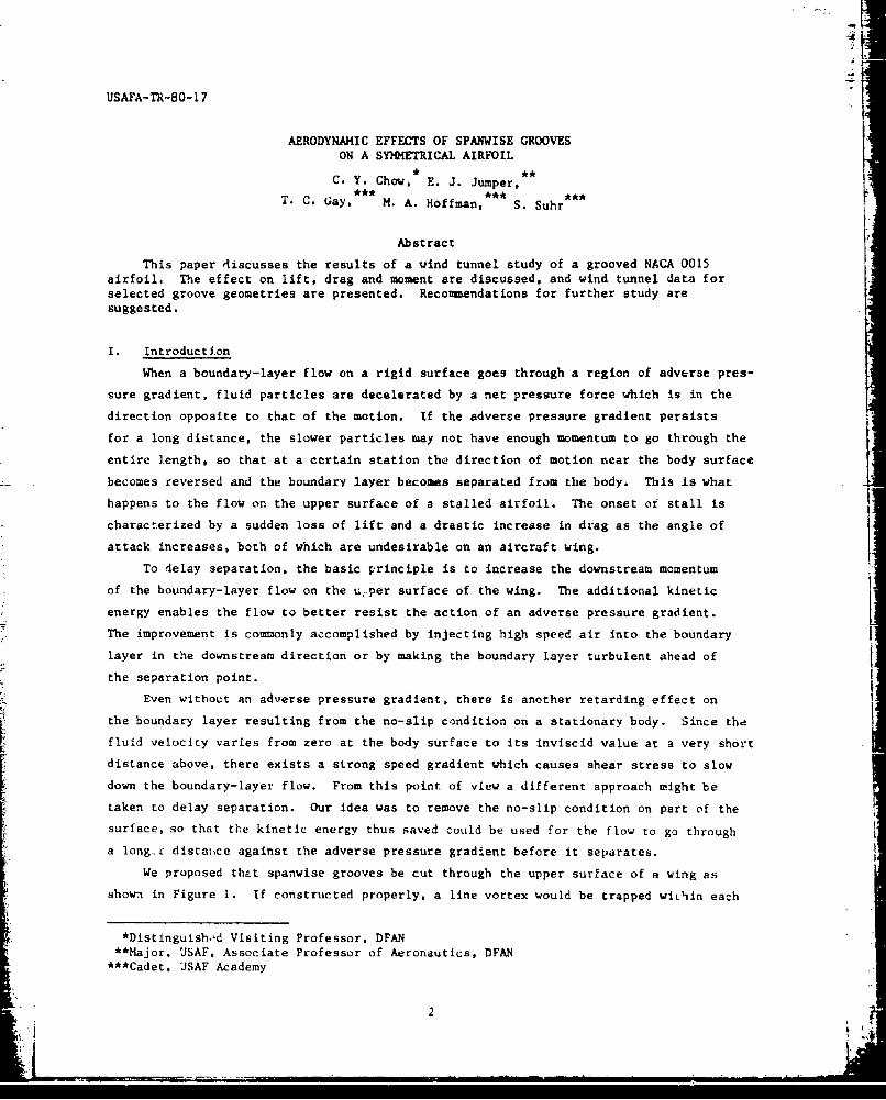
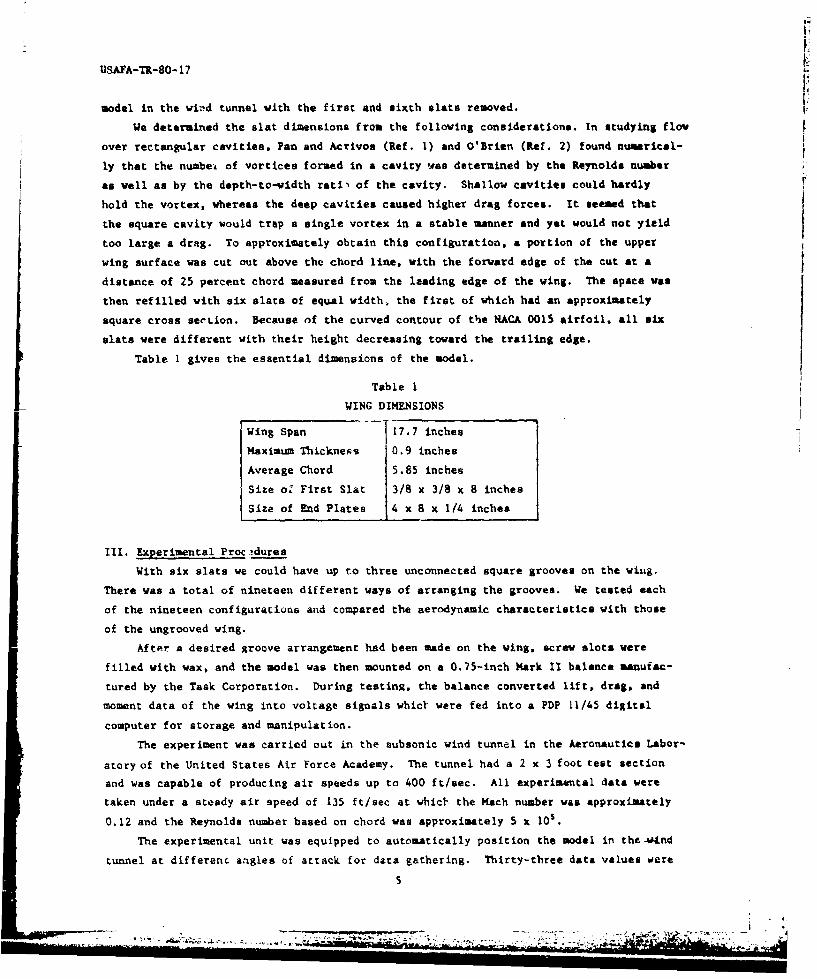
A detrimental effect on stall is found by removing slat 6. Figure 7 reveals that
with a single groove at that position, the stall Angle of the wing drops from 18.5
degrees to 13.5 degrees. Such a result is totally unexpected. The lift-drag variation
and the effect on moment are plotted in Figures 8 and ? respectively. The latter shows
that the increase in moment is less than that caused by the groove located at slat 1.
We are not sure why the last groove causes a tremendous opposite effect on stall.
6

7I
USAFA-'t-80-17
1.5-
0 NO SLATS REMOVED
00 0 *SLAT 1 REMOVED
-05- , , , , , , .-5 0 5 10 15 20 25 30
Figure 4. Coefficient of lift versus angle of attackwith no slats removed and vith elat I removed.
1.5
1.01
CL 0.5
o NO SLATS REMOVED0.0 *SLAT I REMOVED
-0.5 1 , i i / i , i i , 1 , i 1 i i 1 i , l ' 1
0.0 0.1 0.2 0.3 0.4 0.5
CL)Figure 5. Coefficient of lift versus coefficient of drag
-ith no slats reuoved and vith slat I removed.
*1 7

V4
USAYA-Th-BO-17f
0.1-
0 NO SLATS RE MOVED
*SLAT I REMOVED --0.1
CM
-0.2:
-0 .3 - _ _ _ _ _ _ _ _ _ _ _ _ _ _ _ _ _
-5 0 5 10 15 20 25 30
Figure 6. Coefficient of moment versus angle of attackwith, no slats removed and with slat I removed.
1.0-
CL 0.5
0 NO SLATS REMOVED
* SLAT 6 REMOVED0.0
/051111 l-5 0 5 10 15 20 25 30
O.Figure 7. Coefficient of lift versus augle of attack
with no slat-, removed and with slat 6 removed.
USAPA-TR-80-17
1.5
1.0
CL 0.5
0 MO SLATS REMOD
0.0 * SLAT 6 MA0YED
-,50.0 0.J 0.2 0.3 0.4 0.5
CDFigure S. Coefficient of lift versus coefficient of drag
vith n2 slats rmved and with slat6 removed.
0.1-
0.0- o NO SLATS REMOVED0 SLAT 6 REMOVED
-0.1
-0.3
-5 0 5 10 15 20 25 30
aFigure 9. Coefficient of asest versus an81. of attack
with no slats removed and vith slat 6 removtd.

dSAFA-TR-80-17
One of the possible explanations could be the shape of the groove. Because of the way
the slats were made, the depth-to-width ratio of the last groove is approximately 0.7.
We suspect that a cavity of this geometry may not be able to confine a line vortex in
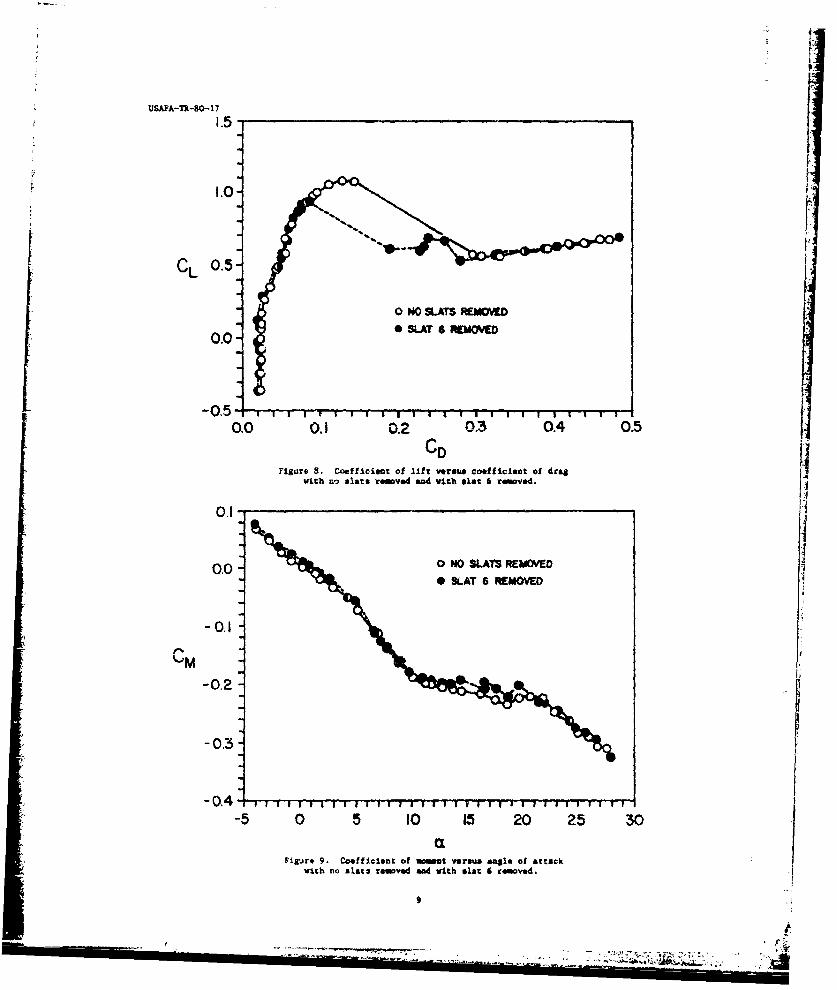
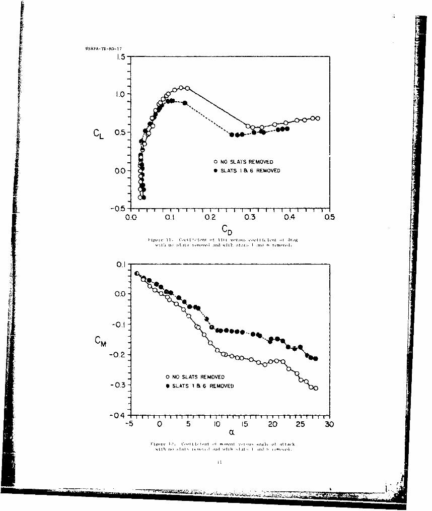
a stable manner. Experimental data show that the same behavior that stall exhibits in
the CL versus a plot for all groove combinations is enhanced as long as slat 6 is out,
with 'ie exception of one case in which slats 1 and 6 are both removed (results are plot-
ted in Figures 10, 11, and 12). These plots show that the one-deg-" - delay of stall
is regained by using groove 1, but the decrease in lift and increase in moment are pro-
longed more than those having only one of the two grooves open.
The effects of grooves between the first and the sixth are not as significant, and
are therefore not discussed here.
V. Conclusions and Recommendations
Laboratory testing seems to imply that the addition of spanwise grooves to the upper
surface of a wing, if properly arranged, can delay stall. Accompanying a delay in stall
of about one degree in angle of attack is a reduced overall lift and CL as well as
an increased drag at the same lift. If these results are typical of all grooved config-
15.
I0
CL 0.5
0 NO SLATS REMOVED0.0 * SLATS I a 6 REMOVED
-5 0 5 10 15 20 25 30
Figure 10. Coefficient of lift versus angle of attackwith no slats removed and with slats I and 6 removed.
10,_______
CL L50 NO SLATS REMOVED
0.0 0 SLATS I&a6 REMOVED
-0.5-0.0 01 0.2 0.3 0.4 0.5
cD
0.1~
0.0-
-0.2-
0 NO SLATS REMOVED
-0.3- 0 SLATS I & 6 REMOVED
-0,4- 5 1 1 1 1 1 1 1 i ~ l 1 1 5 1 1 1
-5 0 5 10 15 20 25 30
I'vltl 1 . -' I i ,t 11 - ,il ,-I :I0.i
w~~~~ ~ ~ ~ i ,1 a dI
NEEM--7

USAFA-TR-80-17
urations, it seems that the grooved-wing idea can have little use in practical applica-
tions.
As far as the groove location is concerned, the first groove is most effective in
delaying stall within the geometric limitation imposed on our wing model. The detrimen-
tel effect of the sixth groove might be caused by either its location or its cross-
sectional shape; a conclusion cannot be made unless further experiments are performed.
In order to fully understand the observed phenomena, we recommend that grooves clo-
ser to the leading edge be tested to see if further improvement can be achieved and if
a square cross section can be constructed for the sixth groove to determine the cause of
the peculiar behavior at that location.
References
1. Pan, F. and A. Acrivos. "Steady Flows in Rectangular Cavities." Journal of Fluid
Mechanics, Vol. 28, Part 4 (June 1967), 643-655.
2. O'Brien, V. "Closed Streamlines Associated with Channel Flow Over a Cavity." Phy-
sics of Fluids, Vol. 15 (December 1972), 2089-2097.
12

SECTION 11
LI FLIGHT MEcI CS
13

USAFA-TR-80-17
COMPARISON OFTIME-DEPENDENT ROTATION MATRIX TRANSFORMATION METHODS
J. E. Justin and P. F. Torrey
Abstract
This paper reviews three methods for computation of coordinate trame transformationsbased on time-varying body rotations. The three methods are Euler angles, directioncosines, and quaternions. A suggested quaternion methodology is highlighted.
I. Introduction: Euler Angles
Engineers familiar with Euler angles might ask: "Why use anything else when three
Euler angles will suffice?" There are three reasons. First, Euler angles exhibit a
discontinuity. As shown in Figure 1, with (aircraft) Euler angles there is a disconti-
nuity when the body frame rotates with respect to an inertial frame such that the body-
axis is either straight up or straight down. In either of these orientations, two of
the Euler rotation axes (the azimuth rotation axis and the body roll axis) are then
aligned. This situation implies that Lwo of the Euler rvtaLiuis are abouL the Same
axis, and therefore, yaw cannot be distinguished from roll. Second, the accuracy of
the transformation matrix which results from Euler angles tends to degrade near the two
discontinuity positions. Finally, and most significant, the calculation of a time-
dependent transformation matrix by integrating Euler angles involves more calculations
with numerous time-consuming series expansions of sine-cosine terms. Fcrtunately, there
are other methods available that have no discontinuities or singularities, maintain ex-
cellent accuracy, and involve only simple algebraic parameters that lend themselves
to solution by digital computer programs.
II. Direction Cosine
Direction cosine method -- the classical and easiest to understand solut ion -- uses
the body rates to find the time rate of -han.v% of fl- trav-1frm;1tin matrtx elements.
If you assume pure rotation motion, the principal equation is
h T it t f t [TeB/I n s (1)
where IT]B/I is the transformation matrix from inertial to body, and Is the skew sym-
metric matrix of angular rotation rates of the body witi respect to inertial space. The
matrix wB is given as
" 0 -p rad/sec , (2)
*Captain, USAF, Assistant Professor of Aronautics, DFACS**Major, USAF, Assistant Professor of Aeronautics, DFACS
14

USAPA-T-80-17
where p is the roll rate about the x-axis. q is the pitch rate about the y-axis, and
r is the yaw rate about the z-.axis.
The principal equation leads to nine first-order differential equations which you
can solve using numerical integration techniques. You can see the sensitivity of the
integration method by considering the Taylor Series expansion of a transformation matrix:
d 1 d2[T (t + At)] - IT (t)] +( fT t)] At + M dt I fT (t)] at 2 + (3)
The first-order integration uses the first two terms in the expansion. Therefore, the
higher-order terms would represent error. In particular, you can write the third term
x-axis aircraft nose
XNO'qTH
IyEAST
DOWN
Figure 1. Euler Angles with Body Pointed Straight Up
15 Sif
F
USAFA-TR-80-17
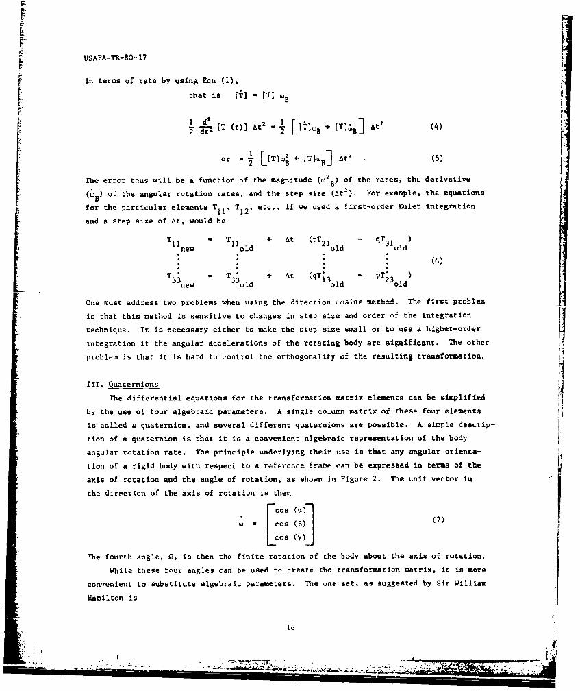
in terms of rate by using Eqn (1),
I that is [I] - (T) B
1 2 rt. &t2&t- IT (t)+ t2 - LT]wa + [Ti 3 At2 (4)
or - [[T].2 + [Tiwij At 2 .(5)
The error thus will be a function of the magnitude (w25 ) of the rates. the derivative
( ) of the angular rotation rates, and the step size (At2 ). For example, the equations
for the particular elements T11 , T12, etc.. if we used a first-order Euler integration
and a step size of At, would be-1 Tl + At C1 1 - q 3
Tlnew old (rT21old qT31old
(6)
T3 + At (qT 3 - pT3 )33new 33old old old
One must address two problems when using the direction cosine method. The first problem
is that this method is sensitive to changes in step size and order of the integration
technique. It is necessary either to make the step size small or to use a higher-order
integration if the angular accelerations of the rotating body are significant. The other
problem is that it is hard to control the orthogonality of the resulting transformation.
III. Quaternion0
The differential equations for the transformation matrix elements can be simplified
by the use of four algebraic parameters. A single column matrix of these four elements
is called a quaternion, and several different quaternions are possible. A simple descrip-tion of a quaternion is that it is a convenient algebraic representation of the bodyangular rotation rate. The principle underlying their use is that any angular orienta-
tion of a rigid body with respect to a reference frame can be expressed in terms of the
axis of rotation and the angle of rotation, as shown in Figure 2. The unit vector in
the direction of the axis of rotation is then
cos (a)-
W- cos (8) (7)LCos ()jThe fourth angle, Q, is then the finite rotation of the body about the axis of rotation.
While these four angles can be used to create the transformation matrix, it is more
convenient to substitute algebraic parameters. The one set, as suggested by Sir William
Hamilton is
16
*-- - - - -.--L -_ - -.. . . . _ . , . . [

USAFA-TR-80-17
W I Cos (SI/2)
W 2 coo Wc) sin (Q/2)w -E (8)
W3 Cos (0) sin (f/2)
W4 coo (y) sin (0/2)4L
This quaternion can now be used to create a transformation matrix. First find the ini-
tial values of the quaternion from Euler angles by using the following set of equations:
OAjUT an( t aii1.,,I IDTH l ro tation? XL an t t ii)f I
LX ...r._'4 i,/F
loo ) with Yroll to the EAST
left
orientationangles
IiIFigure 2. Quaternion Description of a Rigid Body
17
• : "~ "" ". . '7:r-'-;7. -. . ,' : " . 'rI. " - ' -- ,;, ",", - -- U
:1USAFA-TR-80-17
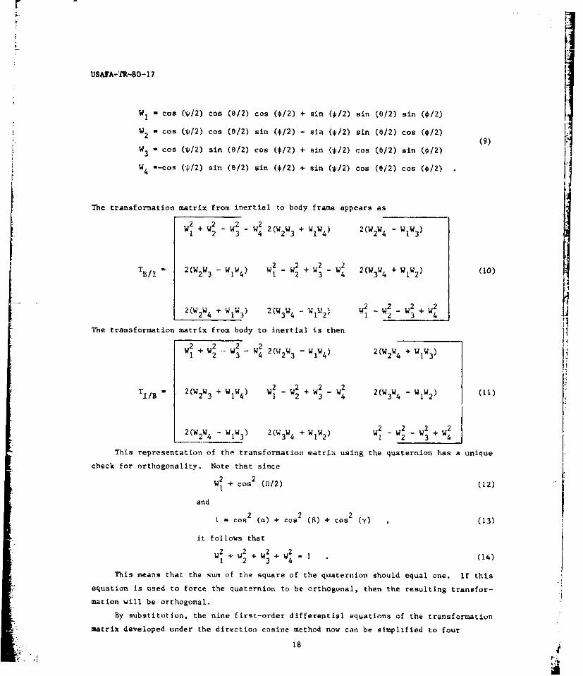
W1 = cos (02) cos (8/2) cos (0/2) + sin (4j/2) sin (6/2) sin (0/2)
W - cos (4/2) cos (6/2) sin ($/2) - sin ($/2) sin (0/2) cos (€/2)(9)
W3 - cos ( /2) sin (6/2) cos ($/2) + sin (*/2) cos (e/2) s ($12)
W4 -cos (p/2) sin (e/2) sin ($/2) + sin (i12) cos (e/2) cos ($/2)
The transformation matrix from inertial o body frame appears as
W 2 2 2 2 W + 2(WW 1 +W2 -W 3 W4 2IW 4) -
T = - 2 2 + 2 2 2(W3W40)B/I 2(WW 3 WW4 ) WI - 2 3 4 W W4 + WIW 2) (1o)
W2 _W2 _W2 + 2
2(W2W4 + WIW3 ) 2(W3W4 - WIW2) W1 - - W3+ 4h
The transformation matrix from body to inertial is then fi2 2 2 22W2322W+ I )
W + W2 "- W - W - WW4)1 2 3 4 112 3 1 W 4) 2 2 4 1 ~ 3)
T = + 2 2 2 2I/B 2(W2W3 WW 4) W - + W3 W4 (W3W4 - WIW2 )
2(W 2 W4 - WW) 2(WW + W2W WI - W2 - W2 + W22 3 4 1 2)1 2 3 4
This representation of the transformation matrix using the quaternion has a unique
check for orthogonality. Note that since
2 + cos2 (Q/2) (12)
and
I1 cos (a) + cos 2 (8) + cos 2 (y) , (13)
it follows that
W 2 +W 2 +W2 + = (14)
1 2 3 4
This means that the sum of the square of the quaternion should equal one. If this
equation is used to force the quaternion to be orthogonal, then the resulting transfor-
mation will be orthogonal.
By substitution, the nine first-order differential equations of the transformation
matrix developed under the direction cosine method now can be simplified to four
18

USAFA-TR-80-17
equations t (_W " - W "wq W r2 2 3f
w2 C WlP + W 3r - W4q)
W - ( W - r + W4 P)
W ( Wr + W q - WP
where p, q. and r are aaain the body rates.
The significance of these derivatives is that if the initial values of W1, W2, W3,
and W4 are known at time t - told' then the value of the W's (and therefore the trans-
formation matrix) can be calculated at time tnew - tol d + AT by any integration method,
the simplest of which is We - V + Wnew AT. (16)nw old new
Integrating to the next time step, you will find that the possibility exists of
the quaternion's departing from the orthogonal condition. To preclude this, you can
renormalize the paramEters to 1.0 after each integration as
Wi Wi
W= 2 2 W2 (17)3W + +W4 or1 W2 + W2+W 2+W 2
WI 3 41 2 3 4 iwhere i - 1. 2. 3, and 4.
There may be some instances where it is unnecessary to orient the inertial frame
in a particular manner. You may be concerned only with keeping track of "some" inertial J
frame. In this case, you can omit the initial conditions and arbitrarily set the W's
to some convenient combination such that the orthogonality equation is satisfiel. For
example,= -,
0
which corresponds to the Euler angles' all being zero. The transformation matrix, re-
sulting from thin initialization, then represents rotation from this arbitrary initial
attitude.
In summary, to obtain a coordinate transformation matrix from the inertial frame
to the body frame that changes with time as the body frame rotates, you proceed as fol-
lows:
1. Calculate W's from the new body rates.
2. Integrate to find the new W's.
3. Renormalize the new W's.
4. Finally, calculate the transformation matrix.
19
* -.l.C~a --- -

7lAAT 8- Ii
IV. ConclusionThe calculation of a time-dependent transformation matrix can be accomplished by
Euler angles, direction cosines, and quaternions. The Euler angle method is easy to
understand but is not an efficient method for digital computers. The direction cosine
method is simple in principle but inefficient if one desires acceptable accuracy. The
method using the quaternion is abstract in concept but I Ives simple algebraic equa-
tions that lend themselves to fast and accurate solution by digital computer progsral.
Symbo'.
p roll rate about thL x-axie 1sq pitch rate about the y-axis
r yaw rate about the z-axis
t time
TB/I transformation matrix from inertial to body reference frame
TI/B transforwaLiota "atrix fr= bod, to inertiel rpferonce frameIA
TiJ T3 /I element where i - 1, 2. 3 and j w 1, 2 3
W quaternion
W quaternion element where 1. 1, 2, 3, 4
x body rolls axis
X fixed x-axis
y body pitch axis [Y fixed y-axis
z body azimuth rotation axis
Z fixred -Axisa
a angle between x and w
B angle between y and w
y angle between z and W
AT step size of time
6 Euler pitch angle
* Euler roll angle
, Euler azimuth angle
20
7, _ _'

USAFA-TR-80-17
t unit vector in the direction of the axis of rotation
B matrix of angular rotation rates of the body with respect to inertial1 finite angle of rotation
Superscript time rate of change
Subscriptnew next value
old initial value
tA
Refferences
1. Broxmeyer, C. Inertial Navigation Systems. New York: McGraw-Hill Book Company, 1964.
2. Justin, 3. E. Guidance and Dynamics. Textbook published by the USAF Academy, De-
partment of Astronautics and Computer Science, August 1979.
Ii
-21
JI

USAFA-TR-80-17
SECTION III
[ PROPULSION
22
IUSAFA-TR-80-17
FURTHER EVALUATION OF A GLUHAREFF PRESSURE JET
H.M. Brilliant,* M.L. Fortson,** D.S. Hess,** and A.J. Torosian**
Abstract
In an earlier issue of the Aeronautics Digest one of the authors presented initialwork oa the evaluation of a Gluhareff pressure jet engine. This paper discusses furtherevaluation of that engine. We also describe measurements of the noise levels produced
*by the engine and further design improvements and tests conducted.sIA
I. Introduction
In the early 1970's Mr. Eugene M. Gluhareff began development of a lightweight, in-
expensive jet engine which he called a p-essure jet. In 1977 the United States Air Force
Academy bought the G8-2-15 version of his engine. This version, the smallest in a series,
weighs only 5.5 lbf excluding the fuel system and is rated for 20 lbf of thrust at sea
level. The purpose of the project was to evaluate the engine and its components. Early
studies of the engine appeared in a previous edition of the Aeronautics Digest (Ref. 1).
This paper is a continued progress report of work performed since then and describes
some test resulLs and suggestions for future work.
II. Description of Engine Operation
The Gluhareff pressure jet is basically an ejector ramjet which runs on propane fuel.
Figure 1 shows a schematic of the engine. The basic parts of the engine are the fuel
tank, throttle, heat exchanger coil, supercharger system, combustion chamber with an
ignition system, and the exit nozzle.
The fuel tank houses the propane and feeds the fuel to the engine. Because propane
has a vapor pressure of approximately 125 psia at room temperature, the tank is self-
pressurizing; therefore, the engine is simplified by not requiring a fuel pump. For
this reason, Mr. Gluhareff calls the engine a "pressure jet." The tank is designed so
that the propane leaves as a liquid alleviating the problem of rapid tank depressuriza-
tion.
From the fuel tank the propane flows through a needle valve throttle which controls
the flow rate to the heat exchanger coil. The coil is housed in the combustion chamber
so that, when the engine is operating stably, the propane vaporizes and heats to approx-
imately 1000 degrees F (Ref. 2).
This high-temperature, high-pressure propane then goes to the supercharger system
cooling to 600 degrees F by the time it arrives. The supercharger system is basically
an ejector, an item common in ramjets to supplement ram co-'pression allowing the en-
gine to operate statically. The fuel entering the supercharger is accelerated to
*Captain, USAF, Associate Professor of Aeronautics**Cadet, USAFA; Presently 2nd Lt, USAF
23
... ......... .. ... T q ' ..... .. . . . .....
- - ai .. .. . . . ..

USAFA-TR-B0-17
EXIT NOZZLE .23000V HIGH VOLTAGE WIREHEAT EXCHANGER COIL
COMBUST ION CHAMBER tNflSP1ARK PLUG 9 VOLT BATTERY
THIRD '-FUEL-LINE -6.NNECTION FITTING
SUPERCHARGER& ENGINE MOUNTING PLATES FUELDIFFUSIER TANK
SECOND / VAPORIZED :UEL r3H
FIRST SUPERCHARGERSUPERSONIC FUEL VALVE
INJECTION NOZZLEL
INJECTOR COWLING -
TEMERATUR ) ,.E
INJECTOR N• "PRESSURE
GAUGE *-~NEEDLE VALVE(THRIOTTLE)
Figure 1. Schematic Diagram of the Gluhareif Pressure Jet
supersonic speed through a ccnvergent-divergent (CD) nozzle. At this speed the static
pressure of the fuel flow is lower than the atmospheric pressure and entrains air into
the stream. Theoretically, the three stages of supercharging are designed to produce
a near-stoichiometric fuel-air mixture in the combustor. The major difference between
this supercharged pressure jet and an ejector ramjet is that the inlet in the pressure
jet is designed to let in air from the side so that there will never be ram compression
even when the engine is moving. This supercharger system also :Umplifies :he engine
design.
From the supercharger the fuel-air mixture flows into the combustor. here the side-"[
mounted intake design provides a low-veiocity recirculation aone in the dome located
next to the fuel-air inlet to the combustor (Figure 2). This design functions to stabil-
ize the flame in the combustor. Locating the inlet in front rather than to the side
would require a more complicated means of flame stabilization. The fuel is ignited by
the ignition system, a si tple spark ignitor fed by a 23,000 volt supply. Once the mix-
ture is burning the ignitor is not needed to maintain combustion unless the flame is
inadvertently blown out.
From the combustor the products of combustion go through a convergent nozzle.
Gluhaceff recommends that the end of the nozzle be V-notched as shown in Figure 1. The
function of this notch is to reduce the noise level by about one half and increase thrust
by 3 lbf (Ref. 3), a claim we have not investigated.
.:- 24

USAFA-TR-80-17 I
I
FLAMEHOLDING REGION(THE DOME)
I&
AIR
Figure 2. Flameholding in the Combustor
111. Lfrovements to the Test Set-Up
We made major improvements to the test set-up for the newest tests. The improve-
ments included measurement of noise levels produced by the engine, revision of the
load cell for thrust measurement, and additional pressure and temperature measurements.
We measured noise levels at various places around the engine at different thrust levels.
As indicated in the earlier report (Ref. 1), the load cell was non-linear and had
some hysteresis and zero shift. Installing a new system eliminated all three problems.
We performed calibrations prior to and after each engine run and noticed no changes,
and we set full scale deflection of the load cell at 20 lb to allow for the maximumthrust expected from the engine.
In these tests we also installed an additional pressure gauge and thermocouple on
the engine just upstream of the supersonic fuel injection nozzle whereas the previously
measured nozzle total pressure location was ahead of the heat exchanger coil as shown
in Figure 1. We attempted to take into account heat addition and friction losses by
using a constant loss factor of 5 percent.
IV. Results
As indicated in Figure 3. the new injection nozzle total pressure (called simply
the injector pressure) was about 10 percent below the "old" nozzle pressure at the lower
pressures and about 15 percent below at the higher pressures. The thermocouple measured
- ,the total temperature of the fuel entering the injection nozzle, Previously we assumed
that this temperature was 1060 degrees R based on the studies performed by Gluhareff (Ref.
2). Figure 4 shows the results of measuring fuel temperatures at the injector. The decrease
in temperature with run number is related to the depletion of fuel in the tank. As fuel is
25

L
USAFA-TR-80-17
120-*4 -ps .9O Pn
Z ,8i Pr
I
80<
Suj 60
LU40
U'20/LW
Z0 I I -
0 20 40 60 s0 100 120
NOZZLE PRESSURE (PSIA) -"OLD"
Figure 3. Comparison of Pressure MeasurementsTaken at "Old" and "New" Locations
used at the beginning of a run, the flow takes longer to stabilize ard the propane enters
the heat exchanger coil at a lower temperature.
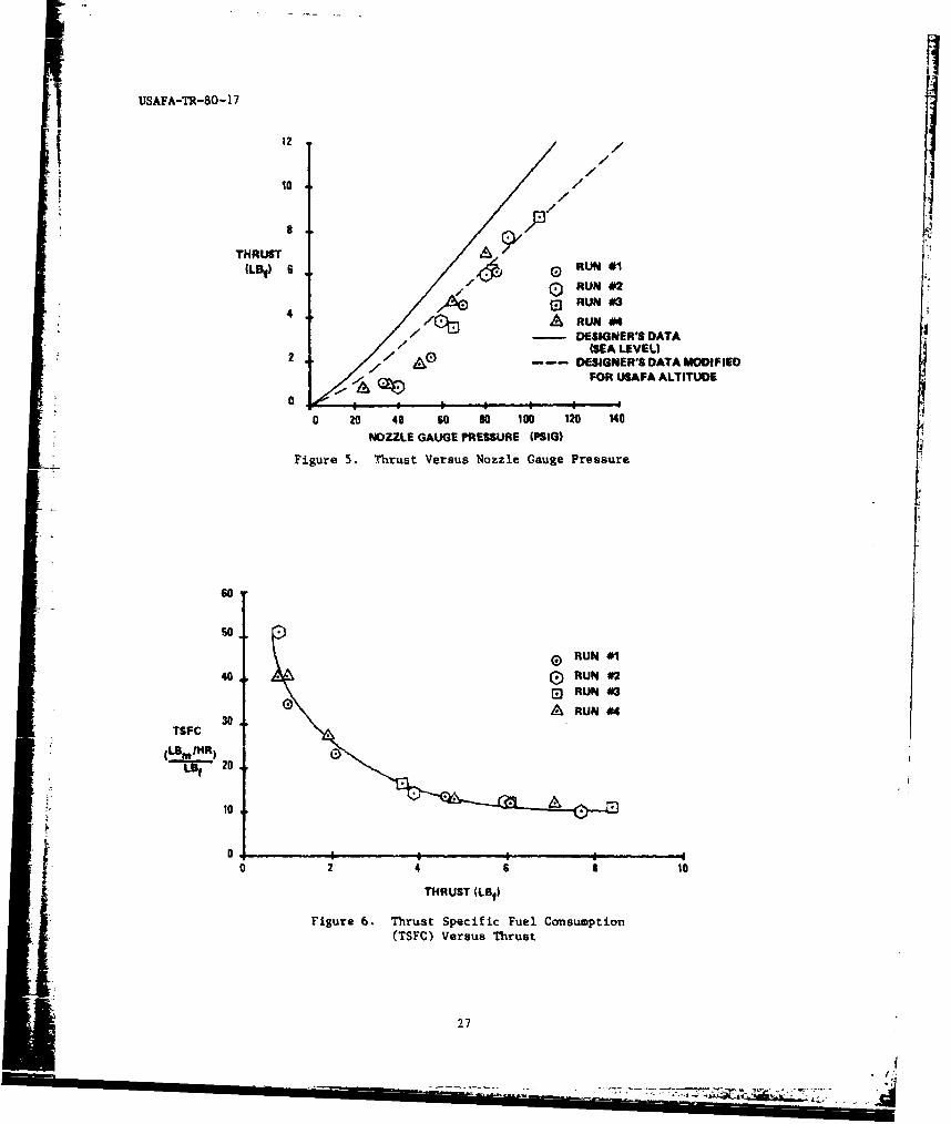
Thrust measurements appeared similar to previous data as shown in Figure 5. At the
low nozzle pressures the thrust was lower than the designer's data (Ref. 2) corrected for
altitud,. At the higher nozzle pressures the data agree with the corrected designer's
data. Maximum thrust was less than that previously obtained. The engine would not oper-
ate stably over 104 psig. The cause of this unstable performance is not known but may
be related to the movement of the second supercharger in its support.
Thc thrust sh-.wed only one level of performance in these tests. In the previous
report we noted two levels of performance. This was due to air temperature differences.
1400
w ( )RUN *1''u. 1200 PREVIOUSLY
cr C) RUN *2S'ASSUMEDl RUN 3
< j VALUE ---- .--- A RUN *3,,,- 1000 ,,./ J/ RUN *'4
* 0I
.1I-Ugo =)Z
20 40 60 s0 100 120
INJECTOR PRESSURE (PSIA)
Figure 4. Temperaturc of Fuel Entering the Injector
2t
USAFA-TR-80-17
12 /
I/10/
~/ 8 ,Jj. 3
THRUST /(Lf) B ( RUN #1
0Z) RUN #2E4 RUN 03
4~ RUN *6qDESIGNER'S DATA(SEA LEVEL)
2 A 0 DESIGNER'S DATA MODIFIED
- o FOR USAFA ALTITUDE
Co
a 20 40 so s0 100 120 140
NOZZLE GAUGE PRESSURE (PSIG)
Figure 5. Thrust Versus Nozzle Gauge Pressure
so
so
4 RUN #1
i RUN *30 A RUN #4
30TSFC
(LBm/MR)
10
2 46 va1
THRUST (LOf)
Figure 6. Thrust Specific Fuel Consumption(TSFC) Versus Thrust
27

USAFA-TR-80-17
Temperatures below approximately 45 degrees F appear to strongly reduce engine performance.
In the latest tests the air temperature was always above 54 degrees F.
Figure 6 shows the thrust specific fuel consumption (TSFC). It follows the same
trend as previous data and agrees closely with previous values. Slight differences are
due to more accurate propane flow measurements in this experiment.
Figure 7 shows noise measurements. The readins indicate that noise increases as
thrust increases and is fairly uniform in all directions. The noise levels are comparableto those produced by a turbojet but at a much higher thrust level (Ref. 4). Note that
data was taken at less than half power. Above this power level no data was taken, but
the operators did notice some ear discomfort even with ear protection.
We found that the "fuel leak" noted previously was not a fuel leak at all. Rather,
it was water that had condensed from the air caused by the low temperature of the fuel
REAR(1) 104 do
M2 IIIdB
(3) 121 dIS
OPERATOR POITION JIRL(1) 111dB 11) 113 dB(2) 117dB ,I 3IFTr (2) Ill dB
(31133 dB (3 130 dl
READING THRUST
NUMSER LEVEL I.t(1) U
0n (2) 1.5(3) 4.6
FRONT(1) 106 dB
(2) 110 o(3) 121 dB
Figure 7. Noise Level Heasurements
28
.';.. - - .. .

USAFA-TR-80-17
as it evaporated prior to arriving at the heat exchanger coil. The condensation rate
was such that the liquid appeared to have the flow rate of a liquid escaping through
a small crack in the tubing.
We further established that the engine is not easy to operate. Fast advancement
of the throttle usually resulted in flameout, and the throttle lever position required
constant operator attention or it would change due to test stand vibration. A new throt-
tle is desirable since, with the current throttle, small changes in throttle position
result in large changes in injector pressure.
At the beginning of a test run it took several minutes to achieve stable engine
operation. Further, the operator had to keep the nozzle pressure from 70 to 80 psig
during this time; less pressure would cause the combustor section to overheat. Note
on Figure 4 that below this pressure the propane leaving the heat exchange coil is at
its highest temperature. The engine also required a long time after a run to cool down.
V. Conclusions and Recommendations
If this engine is to be tested further, we recommend a few changes. First, the
current throttle should be replaced with a less sensitive one. Other than this change,
future experimenters should obLain additional perfarmance dete on the engine at higher
air temperatures and include additional noise measurements prior to making further design
changes. After collecting data on the unmodified engine, a V-notch to the tailpipe
should be machined and the tests repeated. It will be interesting to examine the design-
er's claims for thrust improvement and noise reduction. We recommend separate parametric
studies of t'ae supercharger system to determine the effect of moving the second stage.
Data collection for this series should include measuring total pressure profiles at the
end of each stage to determine the effect on stage performance.
While we continue to be reluctant to recommend this engine for the use suggested
by its designer (Ref. 5), the engine is ideal as a tool for teaching alternative pro-
pulsion systems. It could also be used as a vehicle to demonstrate problems of measure-
ment in high-temperature environments.
References
1. Brilliant, H. M. "Evaluation of a Gluhareff Pressure Jet." Aeronautics Digest -
Spring 1979. USAFA-TR-79-7, USAF Academy, Colorado, July 1979.
2. EMG Engineering Co. G8-2 Gluhareff Pressure Jet Engine Technical Handbook. Gardena,
CA: EKG Engineering Co., date unknown.
3. Thomas, Wayne. "A Jet You Can Build in Your Own Shop." Mechanics Illustrated,
Vol. 71 (January 1975), 28-29,
4. Treager, I. Aircraft Gas Turbine Engine Technoloy. 2nd ed. New York: McGraw-Hill,
1979.
5. EMG Engineering Co. Uses of G8-2 Jet. Gardena, CA: EG Engineering Co., date unknown.
29

USA?A-TR-80-17
SECTION IV
THERMODYNAICS AND HEAT TRANSFER
30
i. ..

USAFA-TR-80-17
A LOW-COST POINT-FOCUSING
DISTRIBUTED SOLAR CONCENTRATORR.C. Oliver*
Abstract
Recent investigations of small-scale solar Rankine cycle applications have shownthe need for a cost-effective solar collection system. This paper describes and analyzesa design using flat plate mirrors to collect and concentrate solar energy, and it discussesthe performance of the collector design. The combination of an inexpensive collector andcurrent Rankine cycle technology appears to provide a system which could supply or supple- Iment the energy requirements of activities conducted in remote sites or of typical house-
hold or community needs. Although this solar collection design has been combined with aRankine cycle system, the collector itself is independent of the conversion system.
I. Introduction
The Rankine cycle is a technique for converting heat energy to mechanical work which
is currently used most often as a method for converting the stored energy in fossil fuels
to mechanical and electrical power. The energy is in the form of heat provided by the
burning of fossil fuels. Recent reports indicate that the energy input to the Rankine
-I cycle could be provided by a solar collector cystem and that adequate Rankine cycle tech-
nology exists for this application. Unfortunately, the cost of the resulting solar Ran-
kine system output energy is not presently cost competitive with energy available from
commercial power sources. Since a previous paper described the basic functioning of the
T Rankine cycle (Ref.l), this raper will not attempt to explain the cycle itself or a choice
*of working fluids to be used in the system.
Barber has shown that two-thirds of the cost of a solar Rankine cycle system is at-
tributable to the cost of the solar collector (Ref. 2). Working from his figures Barber
also concluded that a two- or three-fold increase in the cost of conventional energy would
be required to make this system cost-competitive. At a 12 percent inflation rate (a level
which seems destined to persist for some time), current costs will double in less than six
years, and the increased costs of petroleum due to the OPEC cartel may drive the cost of
energy derived from conventional fuel sources up even faster than the inflation rate. Con-
sidering this situation, price conditions may exist in the near future that make Barber's
system feasible.
Barber's study concluded that a tracking collector/concentrator design was the best ap-
proach for building a solar collector system, since it showed the Rankine cycle system con-
verting 10 percent of the incident energy into electrical output energy. In the design re-
ported on in a previous paper (Ref. 1), the authors proposed a boom-mounted collector which
would significantly reduce the cost. However, the size of this type of collector is limited
to about 600 ft2 . Although this restriction may be satisfactory in many applications, a
"r design which provides a greater collector area is more desirable. Such a design is the
*Mjor, USAF, Associate Professor of Aeronautics, DFAN
31
F
USAFA-TR-80-17
the subject of this paper.
I. Collector Costs
If we could halve the system cost as reported by Barber, a solar Rankine cycle would
be almost economically feasible today. Halving the system cost by reducing the collector
cost would require a reduction in the cost of the collector to one-fourth that reported
by Barber. Current available tracking collectors cost $215/m with an estimated produc-
tion cost of $135/m 2 including installation (Ref. 2). This would mean that to achieve
economic feasibility, a new collector would need a production cost of under $35/m 2 . The
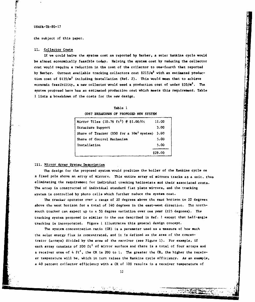
system proposed here has an estimated production cost which meets this requirement. Table
1 lists a breakdown of the costs for the new design.
Table I
COST BREAKDOWN OF PROPOSED NEW SYSTEM
Mirror Tiles (10.76 ft2 ) @ $1.00/ft 11.00
Structure Support 3.00
Share of Tracker ($50 for a lOm2 system) 5.00
Share of Control Mechanism 5.00
Installation 5.00
$29.00
III. Mirror Array Systew Description
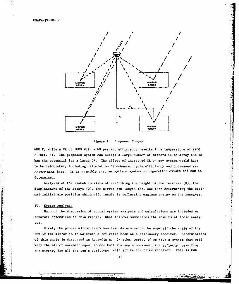
The design for the proposed system would position the boiler of the Rankine cycle on
a fixed pole above an array of mirrors. This entire array of mirrors tracks as a unit, thus
eliminating the requirement for individual tracking heliostats and their associated costs.
The array is constructed of individual standard flat plate mirrors, and the tracking
system is controlled by photo cells which further reduce the system cost.
The tracker operates over a range of 20 degrees above the east horizon to 20 degrees
above the west horizon for a total of 140 degrees in the east-west direction. The north-
south tracker can expect up to a 50 degree variation over one year (t25 degrees). The
tracking system proposed is similar to the one described in Ref. 1 except that half-angle
tracking is incorporated. Figure I illustrates this general design concept.
The system concentration ratio (CR) Is a parameter used as a measure of how much
the solar energy flux is concentrated, and it is defined as the area of the concen-
trator (arrays) divided by the area of the receiver (see Figure 1). For example, if
each array consists of 200 ft2 of mirror surface and there is a total of four arrays and
a receiver area of 4 ft2 , the CR is 200 to 1. The greater the CR, the higher the receiv-
er temperature will be, which in turn raises the Rankine cycle efficiency. As an example,
a 40 percent collector efficiency with a CR of 100 results in a receiver temperature of
32
..... ,. .... -.- x : ,:, ?, .. .. .
USAFA-TR-80-17 "
/ / /
/ // I
/ -/ / .-I
-, "-,,/./ /%
MIRROR MIROA/
,/ ' /
/ I
ARIRAY ARRAY
Figure 1. Proposed Concept
600 F, while a CR of 1000 with a 60 percent efficiency results in a temperature of 2200
F (Ref. 3). The proposed system can accept a large number of mirrors in an array and so
has the potential for a large C.. The effect of increased CR on any system would ha e ito be calculated, including calculation of enhanced cycle efficiency and increased re-
ceiver heat loss. It is possible that an optimum system configuration exists and can be
determined.
Analysis of the system consists of describing the height of the receiver (H), the
displacement of the arrays (D), the mirror arm length (R), and then determining the opti-
mal initial arm position which will result in reflecting maximum energy on the receiver.
IV. System Analysis
Huch of the discussion of actual system analysis and calculations are included as
separate appendices to this report. What follows summarizes the results of those analy-
ses.
First, the proper mirror track has been determined to be one-half the angle of the
sun if the mirror is to waintain a reflected beam on a stationary receiver. Determination
of this angle is discussed in Apendix A. In other words, if we have a system that will
keep the mirror movement equal to one half the sun's movement, the reflected beam from
the mirror, for all the sun's positions, will strike the fixed receiver. This is t'ae
33
" ... ';. " "" -- '" .... ' " .,: .... . .. ......... ......- :.L :.:_,..." :

! ii
USAFA-TR-80- 17
basis of the proposed system. A half-angle tracker can be constructed as a simple modi-
fication to the tracker described in Ref. 1.
In the proposed system all the mirrors of an array will be rotated from a single
pivot position. Therefore, each mirror is considered to be on a rigid arm. Appendix
B shows that the angular movement of a mirror on an arm is the same as the movement of
the mirror itself.
Appendix C describes and discusses the "reflected bean offset error" which occurs
for all mirrors in a rotating array (except mirrors located at the pivot point). This
error is a function of the system geometry and the mirror'u initial and fi al orientation.
For any given system geometry we can determine the error as a function of a selected
initial position. The iritial position of all mirrors is selected when the sun is at
its zenith and results in all reflected beams from the array striking the receiver. As
the array "tracks," each mirror will incur the error described above.
Appendix D contains a computer program which is used to calculate the error associ-
ated with each initial mirror position as a result of subsequent tracking movements.
7or each =bteqent "_1rion "THETA." this error is calculated as "ERROR" in the computer
program. The errors are summed to provide a relative measurement of the error associated
with each initial angle. This sum is shown as "CUM ERR" in the computer program. In
addition, the beam shift on the receiver is calculated in the program as "XERR." This
is a direct measurement which can be used in conjunction with the receiver and reflected
beam size to determine the amounL of energy missing the receiver. It specifies the shift
of the beam from the center of the receiver. [1
Two additional factors are described and formulated in Appendix E. First, the inci-
dent energy is a function of the sun's angle and increases as the sun approaches its izenith. Additionally, the angle between the mirror face and the incom-ing rays of the
sun changes as the mirror roratev from its initial position. The projected area there-
fore changes as the array rotates. These two factors are quantified and described in hAppendix E. The resulting program then includes all known physical effects and can be
used to compare various system geometries and initial mirror positio- by calculating
the amount of energy striking the receiver for each.
V. Results
Using the methods for calculating the various parameters described in the previous
section, the optimum configuration for a distributed solar concentrator can be determined
for any given system parameters. To demonstrate the effect of the various configuration
parameters on a typical solar Rankine cycle system, a baseline case was considered using
the height (H) of the receiver tower, the distance (D) from the base of the receiver
tower to the pivot point of the array, and the distance (R) from the pivot point to the
outside mirror. The ratio of these distances was determined as H:D;R - 20:10:5. That
Is, th. distance from the tower to the pivot is twice the radius to the outside mirror4 : I 34
I * I I I I I -

US AFA-TR-80-17
and half the tower or pole height. The program computed an optimum initial angle of 38
degrees for this particular configuration. Using the optimum initial angle, each of
the parameters (H,D,R) for the baseline case was then varied ±60 percent, and the change
in the error function was calculated. The results indicated an increase in error due
to a non-optimum ccrfiguration.
Figure 2 illustrates the effect of a clhange in tower heigbt. Slight increases abo 'e
the design uint have little effect, but a decrease caused a marked increase in the
error.
100-BASELINE OATA0, '33'-W R - 20/10/5
.. =,.
S40-
20-
0ECN ADw 04 .3 * [CHANGEHEIGHT
Figure 2. Change in Error as a Function ofChange in Height from Design PoinL
Figure 3 indicates a more symmetric effect on the error due to a variation in the
displacement of the array from the design point. Although the effect is less than a
height charge, it is worth noting.
Figure 4 shows the effect of radius changes on error. As expected, the shorter the
radi.s to the mirror, the less the error. In the Limit a single mirror has no error (no
lever ar-, similar to tppendic A).
These results demonstrate the impor:ance of choosing a proper design point. If the
parameters are estimated rather than calculated, the performance of the solar collector
could be significantly less than an optimum case.
The effect of the configuration parameters on the initial mirror angle is shcin ini
Figures 5 through 10. The optimum angle Is plotted using the simple measure of performance
(position error only) as e1 opt and incorporating the sun; error and projected area as
6 opt. Figures 5. 6, and 7 show tle results for the closest side of the array to Lhe
receiver tower, and Figures 8. 9, and 10 show the results for the far side (see Figure
35
i 1 i :1 [ '1 .... 1 .. .. i.......T " ...... i ......... i... ... j

USAFA-TR-80-17
BASELINE DATA
HIDIR - Z0410,
5I -
E+10
PERCENT 2 0 20CHANGEIo0 2
DISPLACEMENT
DIH .2 3 .4 .b .6 7
Figure 3. Change in Error as a Function of
Change in Displacemant from Desgn Point
II.
C 40 -
~BASE LINE D'ATAV. - $8'
I ~ ~PERCENT'C H A N G E F . .. 1.04 U; 0 -2 0 -4 0 .6 0
RAIS
W.K,., . . .40 .35, .3 .26, .20 If, AD !l
ai
Figure 4. Chanve in Error as a Function of
Chang i i io Arm
II 3b

USAFA-TR-80-17 11
fi~ BASELINE DATA210 KID/R - 2XVl1A
DMVARIED q
0 1
17-1W
I170~ I "" I IA .7 .1
DIN4
Figure 5. Optimum Initial Angle as a Functionof D/H (near side)
20 BA$ LINE DATA
KIDO ; 2W1015
RIH -VARIED
200
IN -
FF
'ap
.10 IS .20 .30 .35 .AG
RIM
Figure 6. Optimum initial Angle as a Function
of R/H (near side)
37

USAI. i
C-4 for the receiver/mirror geometry). The figures indicate how the optimum initial
angle varies with the configuration parameters. In both cases (near and far sides), the
optimum angle increased with an increase in D/H and R/H and decreased with an increase
in it. The optimum angle varies with the parameters, and as shown in Figures 2, 3, and
4, any deviation from the optimum angle leads to marked increases in error.
It is also interesting to note the absolute value of the error. Appendix E includes
a portion of a print-out which gives the error in the horizontal direction at the receiv-
er. This error, "XERR" in the computer program, for the case of H:D:R - 20:10:5 and
an initial angle of 30 degrees, ranges from 0.44 in one direction to 1.74 in the other
(units would be the same as H, D, and R). Thus, a beam shifted 1.74 units from its ini-
tial position is the worst case for this configuration. The initial position does not
205- PASLINEOATA
IfDk- 25/10MR/N -VARIESD/H - VAR4IES(W IS VARIED)
130-
I I
* 12 6 24 23 32
Figure 7. Optimum Initial Angle as a Functionof Height (near side)
have to be located at the center of the receiver. If the beaLa position at the initial
angle is selected so that it is C.44 units from the center of the receiver area, then
as the sun rises the arm angle would be 65 degrees and the beam would be located near
the center of the receiver. As the sur approaches overhead, the beam woull move to
the position selected for the initial angle. The beam would then reverse its direction
of travel and proceed to the other edge as the sun sets. If the receiver area was equal
in length in the appropriate direction to the longest XERR, all of the reflected energy
would strike it.
Designing the receiver area to the appropriate size dictated by calculations of error
38

USAFA-TR-80- 17
tN!.0
46
[9
S40
35
BASELINE DATAHfD/R - M0160Kim -VARIES
30
25 i I 4
.10 .15 .20 .is .30 35 .40
Figure 8. Optimum Initial Angle as a Functionof D/H (far side)
JJ
46-
40-
SASEL0J DATA
30 DA4-VARIES
265
20. . l i
..2 A A . .6.7
Figure 9. Optimum Initial Angle as a Functionof R/H (far side)
39

USAFA-TR-80-17
so BASELINE DATAH/D/R -2/1O/D/R - VARIESH R - VARIES
9D (H IS VARIED)
0 2 Is 20 24 28 32
Figure 10. Optimum Initial Angle as a Function
of H{eight (far side)
is not an unreasonable requirement. For the demonstration system, a beam capture area
(allowing for mirrors completely around the receiver) of only 1.74 units in radius would
allow the capture of all reflected radiation - that is, none would miss the receiver!
Considered from this perspective, the error function becomes a measure of the minimum
receiver size required to intercept all the reflected energy for a given system design.
VI. Applications of the Proposed System
If the proposed sygtem was constructed to supply heat to a Rankine cycle system,
a net 10 percent of the incident solar energy could be converted to electrical power.
If four such arrays were used, 10 by 10 feet each, an incident flux of 120,000 BTU/hr
could be expected as seen in Figure 1. Theoretically, this equates to 35 KwHr input
with an expected output of 3.5 KwHr (using the solar constant on the surface of the
earth which is higher than normally encountered). Considering a more practical case,
a location of 35 degrees latitude (like Albuquerque, NM) where the annual beam radiation
(including cloudiness with no diffuse radiation) is 8.38 x 10⁶ KJ/m?(Ref. 4), we could
expect a net energy output of 8653.5 KwHr per year. Based on a current average cost
. of $.055 per KwHr, the cost benefit of the system would be $476 per year if the systemL.. is amortized over a ten-year period. While thif- figure does not include maintenance costs,
li the simplicity of the system would require little annual operating and maintenance ex-
pense.40
N~ 7iFigue 10 OpimumIniial ngleas Funtio
of Height' (far side). . , . . ...; o,." , .-.. , =,,o-;:- . .:.-..:.•:- ..',
isnta nraoal reqiremn. For.. th demonstraio sytm a bea catr rea1 II
USAFA-TR-aO- 17
Reference.
1. Oliver, R. C. and G. A. DuFresne. "The Solar Rankine Cycle and The Energy Crisis."
Aeronautics Digest - Fall 1979, USAFA-TR-80-7, USAF Academy, Colorado, April 1980.
2. Barber, R. E. "Current Costs of Solar Powered Organic Rankine Cycle Engines."
Solar EnergY, Vol. 20 (1978), 1-6.
3. Duffie, J. A. and W. A. Beckman. Solar Energy Thermal Processes, Wiley, 1974, p.187.
4. Ibid., Duffie, p. 58.
4
Li
USAFA-TR-80-17
Appendix A
MATHEMATICAL DEMONSTRATION OF THE FACT THAT THE MIRROR ANGLE MOVEMENTREQUIRED TO KEEP A REFLECTED BEAM ON A FIXED RECEIVER
MUST BE EQUAL TO ONE-HALF THE SUN'S MOVEMENT
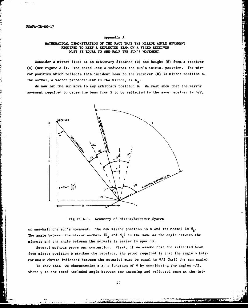
Consider a mirror fixed at an arbitrary distance (D) and height (H) from a receiver
(R) (see Figure A-i). The solid line A indicates the sun's initial position. The mir-
ror position which reflects this incident beam to the receiver (R) is mirror position a.
The normal, a vector perpendicular to the mirror, is Na .
We now let the sun move to any arbitrary position B. We must show that the mirror
movement required to cause the beam from B to be reflected to the same receiver is 0/2,
ECIEIVeR
H
_ _ H
Figure A-I. Geometry of Mirror/Receiver System
or one-half the sun's movement. The new mirror position is b and its normal is Nb *
The angle between the mirror normals (N and Nb ) is the same as the angle between the[ a
mirrors and the angle between the normals is easier to specify.Several methods prove our contention. First, if we assume that the reflected beam
from mirror position b strikes the receiver, the proof required is that the angle a (mir-
ror angle chrnve indicated between the normals) must be equal to 8/2 (half the sun angle).
To show this we characterize a ar. a function of e by considering the angles y/2,
where y is the total included angle between the incoming and reflected beam at the ini-
42

USAFA-TR-80-17
tial position A. Writing Y/2 In terms of e, we have for the angle to the right of Na.
I e - 4t+A(l2 2 (Al)
Here 6 is the total included angle between the incident and reflected beam for the new
sun position B. We use the fact that the incident and reflected angle are equal allow-
ing description of y/2 and 0/2. For the angle to the left of N we can write:a
B a + (A2)2
Equating (Al) and (A2), and solving for a, we have:i 8 B
or
which proves that to maintain the reflected beam on the receiver, the mirror must move
through one-half the angle of the sun's movement.
We can also show that if we arbitrarily move the mirror through an angle equal to
0/2, the reflection will strike the receiver. Given that a - 012, we need to show that
B + 6 = € or that the included angle B plus the angle between the incident and a con-
structed normal (N ) is equal to the angle 4 which results in the reflection striking
the receiver. Piom observation we see that 4 = S + B. This again proves the same point:
the angle created by the mirror's movement is equal to one-half the sun's angle of move-
By using this information we know that if we have a system which moves the mirror
angle one-half the angle of the movement of the sun, the reflected beam from a single
arbitrarily placed mitror will remain on a fixed receiver.
43
Z.

USAA-TR-80-17
Appendix B
OBSERVATIONS CONCERNING THE ROTATION OF A MIRRORFIXED ON A RIGID ARM
Appendix A illustrated that the angle of a mirror's movement must be equal to one-
half the angle of the movement of the sun to keep the reflected beam on a fixed receiver.
Consider the possibility of providing this rotation by placing the mirror on an extended
arm and rotating the arm. This is important in that we would like to place a number
of mirrors (perhaps an array) on a rigid arm and rotate all of them simultaneously by
moving the arm. We will consider a single mirror as shown in Figure B-I.
6Je- 61
Figure B-1. Geometry of Mirror Rotating on Rigid Arm
he nt ia mirror posiion is at A and isdsrbdb~ n R. The mirror is
fie ta eti abtayangle relative to thear().Athamrote fram
poiinA to position B, we want to show that the change in the mirror angle is the
suam as the rotation angle (ell + e 2 ).
If we let the angle between the mirror at position A and the positive x-axis be 41,
we have
e(B)
44
Figure ~~~~~ ~~ ~ ~ .B-AGoe9 irrRttngo ii r

?U
USAyA-TR-80-17
Similarly,
2= 0 2 +c (B2)
where 02 is the angle between the mirror at position B and the positive x-axs. The angle
of mirror rotation from A to B can then be represented as 42 - 41. Subtracting equation rj
V (Bl) from (B2) yields:
42 - 01 -82 + " -- 8 ) - e2 + 1
(3)
The rotation of the mirrors is exactly equal to the rotation of the arm. This can also
be verified by letting the angle a be equal to zero. The mirror then lies along the
arm, and its change in angle is exactly equal to the change in angle of the arm.
45
i 45

USAFA-TR-80-17
Appendix C
EVALUATION OF THE FOCUSING ERROR DUE TO ROTATING THE TRACKING MIRRORS
ON AN ARM RATHER THAN ROTATING EACH ONE INDEPENDENTLY
In Appendix A it was shown that a tracking mirror would need to rotate at an angle
equal to one-half the angle of the sun's movement in order to maintain the reflected
beam on a fixed receiver. Appendix B illustrated that this rotation could be obtained
by placing the mirror on a fixed arm and rotating the arm one-half the sun's movement
angle. In this situation the mirror angle was shown to be correct but an error is pro-
duced. This error arises as a result of the movement of the mirror out of its initial
plane. For example, Figure C-1 illustrates the lateral displacement, 6, associated with
the rotation of a point on a fixed arm. In some situations this movement is desirable,
but for our analysis it will lead to a beam displacement.
I .-- COS#I . R ,.co5,)
Figure C-I. Movement Associated with a Fixed Arm Rotation
To understand how this beam displacement affects the collection problem, consider
the mirror array of Figure C-2. We show only two mirror positions here - the mirror
at the pivot point and the last mirror located on t e arm. Ain actual array would, of
course, have more mirror elements along the illustrated arm as well as a series of other
mirror elements parallel to those illustrated. The initial mirror positions are selected
when the sun is at its zenith and result in all reflected energy being directed
to the receiver. As the sun moves 50 degrees from its zenith, the arm rotates 25 degrees
to attempt to keep the reflected beams on the receiver as demonstrated in Figure C-2.
The reflected energy from the pivot mirror still strikes squarely on the receiver. The
energy from Lte end airror however partially misses the recelver due tn the mirror dis-
46

USAFA-TR-80-17
(A) SUN AT ZENITH (1) SUN 50 DEGERES FROM ZENITHMIRRORS AT INITIAL POSITIONS MIR*ORS ROTATW 2$ D1G0EES
FROM INITIAL POSITION
RECEIVER RECEIVU
INCOMING I INCOMING
RAYS \ \ AO
RAY\ \ R
RRAIATOON \ DIATION
FROM END MIkROR , END MIRRORILADLATION REFLECTED
REFLECTED FROM -,-.. RADIATION FROM ._
PIVOT MIRROR PIVOT MIRROR V"-\ \\ \
PIVOTPOINT i I
ARM I RMIROR ELEMENT
ELEMENT AT tN0 Of A M
AT PIVOTPOINT
Figure C-2. Effect of Arm Rotation on a Reflected Energy Beam
placement from its initial plane. This is the effect that is quantified in this appendix.
For the development of the describing equations in the remainder of this appendix, the
reflecting mirrors are considered to be point reflectors.
flow we must quantify the effect of this lateral movement on the reflected beam.
If the tracking mirror is rotated one-half the angle of the sun's movement, the only
error will be one of displacement. This error cannot be specified unless we specify
the receiver location relative to the mirror and the initial arm position. By considering
these factors, we can determine the location or the line along which there will be no
reflected beam deviation trom the receiver.
Consider the receiver mirror orientation of Figure C-3. If the mirror is Initially
located at (R, 80), the line connecting the mirror (center) with the receiver (center)
will be the no error line (NEL). Anywhere along that line a mirror rotation of one-half
the sun's angle of movement will keep the reflection exactly on the receiver. However,
as we rotate our mirror by use of the arm, we will introduce a displacement error. Two
locations indicate this error. As 0 is increased counter-clockwise from B0 to point
A, the mirror fixed on the arm follows the arc and deviates from the NEL. The displace-
ment error is also indicated as the angle is rotated clockwise from 80 to point B. We
again have an error but less than the one associated with point A. The movement c' the
mirror position (arc) about the NEL between the initial point and point B illustrles
t : -7

USAFA-TR-80- 17
\ '
\ ,tI,
\
9HR9
Figure C-3. Mirror Displacement Due ToRotation from Initial Position
the importance of the initial mirror position in limiting error. This point will be
more fully 4iseCested. Also note that the error is a displacement error only with all
reflected rays being parallel to the NEL.
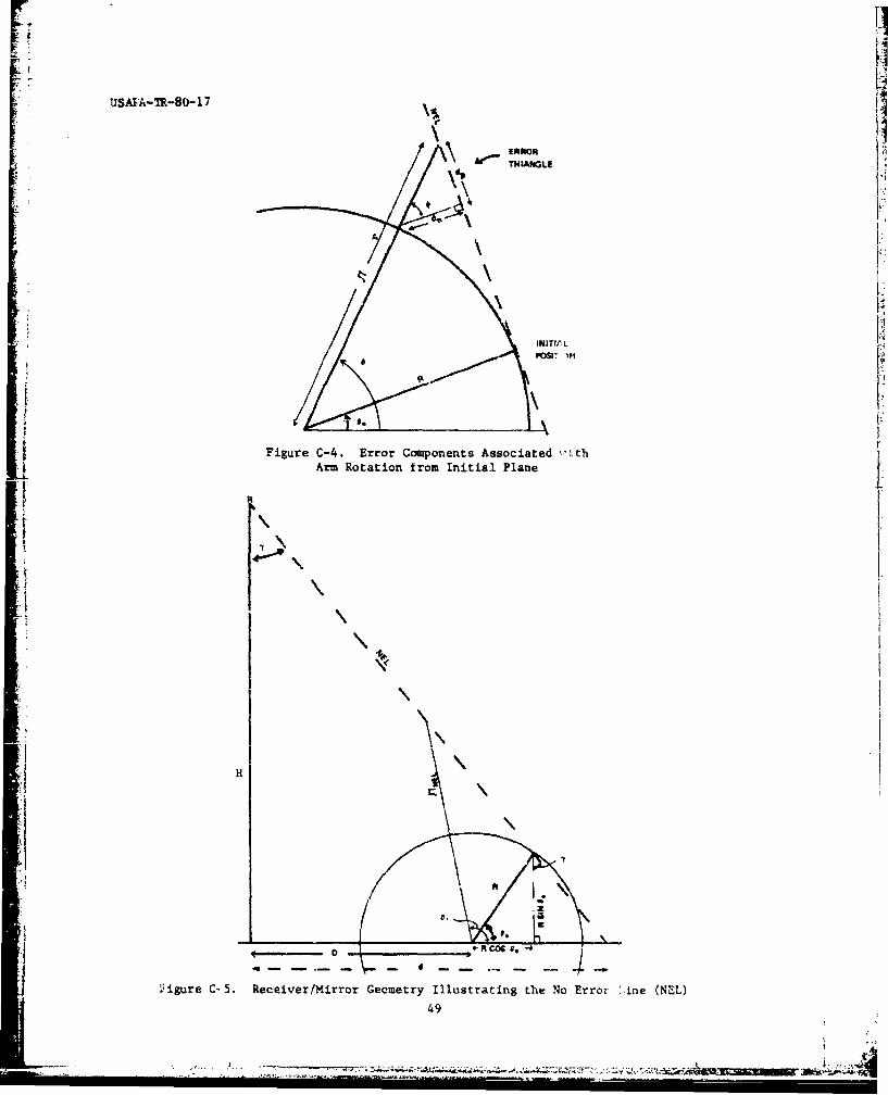
As we consider the displacement error in more detail (Figure C-4), note that the
displacement from the NEL can be described as a displacement normal to (dn) and a dis-
placement parallel to or along (dp) the NEL. The displacement parallel to or along the
NEL causes no error. It just moves the mirror closer to or further from the receiver.
The normal component, however, results in displacement of the reflected beam as indicated.
The angle * would, of course, be equal to the absolute angular difference between the
initial position and subsequent position A.
If we know the exact geometry and initial mirror position, we can describe the NEL
as a function of the geometry. For any given initial and present poEition, we can then
calculate the normal displacement error. Figure C-5 includes the overall geometry and
describes the NEL. 7lie distarce d is the x-intercepr of the line betwceen the recciver
48
USA1ZATR-80-1 7
INITI. L
POSIT W*i
Figure C-4. Error Components Associated -tthArm Rotation from In~itial Plane
I H
j iigure C-5. Receiver/Mirror Geemetry Illustrating the No Error :.ine (NEwL)
49

USAFA-TR-80- 17
and the initial mirror position. L is the displacement of the mirror arm center pivot
from the pe;pendicular to the re~eiver:
d -D + R Cos 80 + R Sin 6o Tan y (Cl)
but
y- Tan (d/H) (C2)
so
d D + R Cos 6 0 + R Sin e0 Tan (tan- 1 d/H) (C3)
ordD+R Cos O0 + R sin . (C4)
HFurther redu)cing this equation and solving for d, we have:
d- D + R Los O (CS)
1 -R - sin 0oH
Having defined d in terms of the initial geometry and posicion, we can now develop
an equation for the NEL. The NEL is the line connecting the receiver and cae initial
mirror position.
If we use the coordinate axis at the base of the receiver, the equation for the
NEL is:
Hy x 4 h (C6)
However, we will need this equation based on the R, 0 axis, which is displaced D. In
that reference frame, the y-intercept c, i be found:
H (- D -.- H - H (I (C7)
The NEL equation in this new frame then becomes:
H DY - - x + H (i - .(C
dd
Expre:sing Lhis in polar coordinates for any value of theta (ror example, O6 in Figure
(C-5) gives:
H D(i)r sin e=-ir cosO+ HO( --- )
d d
Solving for the distance to the NEL as a function of any arbitrary mirror arm angle, 0.
yields:r H (I - D/d) C)
r (sin + H/d cos )(ClO)
This value is the distance from the r, 0 origin (mirror axis) to the NEL. Referring to
50
I " " I . .. I. . .. . .. . . .. . . . .
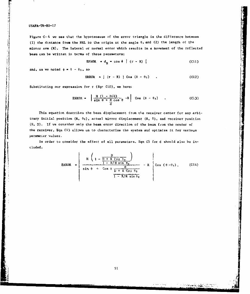
'a
USAFA-TR-80- 17
Figure C- 4 we see that the hypoteneuse of the error triangle is the difference between
(1) the distance from the NEL to the origin at the angle e, and (2) the length of the
mirror arm (R). The lateral or normal error which zesults in a movement of the reflected
beam can be written in terms of these parameters:
EPRkOR d N - cos (r - R) (Cil)
and, as we noted 6 = 6 - 6o, so
ERROR- (r- R) Cos (O- ) (C12)
Substituting our expression for r (Eqr C1O), we have:
ERROR- s 8 -D/d) -R I Cos (6 00) (C13)
This equation describes the beam displacement from the receiver center for any arbi-
trary initial position (R, 6O), actual mirror displacement (R, 0), and receiver position
(He D). If we consider only the beam error direction of the beam from the center of
In order to consider the effect of all parameters, Eqn C5 for d should also be in-
( DH 1 -D + R Cos 81
ERROR = 1 - R/H sin % - R Cos (6-00) (C14)sin 6 + Cos + R Cos 9
1 - R/H sin c
i.c
51
----------------------------------------- .
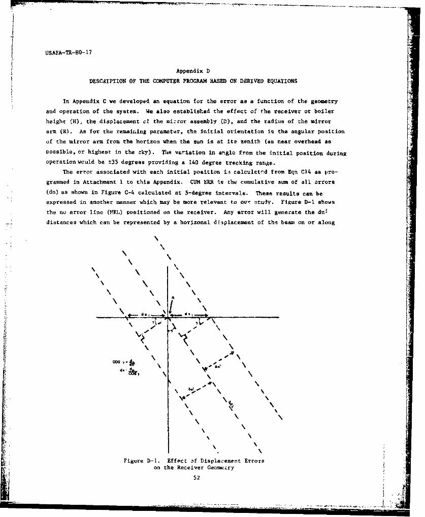
UsAFA-TR-80-17
Appendix D
DESCRIPTION OF THE COMPUTER PROGRAM BASED ON DERIVED EQUATIONS
In Appendix C we developed an equation for the error as a function of the geometry
and operation of the system. We also established the effect of the receiver or boiler
height (H), the displacement ct the mi:ror assembly (D), and the radius of the mirror
arm (R). As for the remaining parameter, the initial orientation is the angular position
of the mirror arm from the horizon when the sun is at its zenith (as near overhead as
Possible, or highest in the cky). The v&riation in anogle from the initial position during
operation wculd be ±35 degrees providing a 140 degree tracking range.
The error associated with each initial position ii calculatnd from Eqn C14 as pro-
grammed in Attachment 1 to this Appendix. CUM ERR is the cumulative sum of all errors
(dn) as shown in Figure C-4 calculated at 5-degree intervals. These results can be
expressed in another manner which may be more relevant to our itudy. Figure D-1 shows
the no error line (VEL) positioned on the receiver. Any error will generate the dni
distances which can be represented by a horlzonal displacement of the beam on or along
ZU
%V.
Figure D-.Effect afDisplacement Errorson theRecei eoemetry
\ \5\
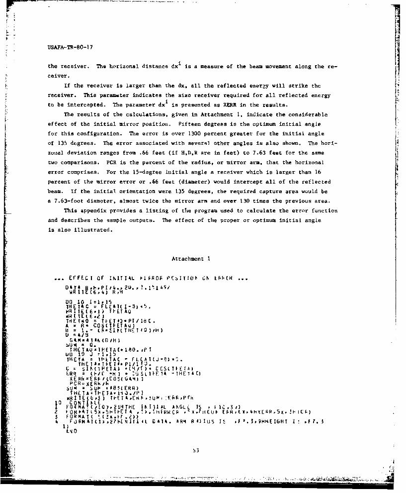
USAFA-TR-80-1 7
the receiver. The horizonal distance dx is a measure of the beam movement along the re-
ceiver.
If the receiver is larger than the dx, all the reflected energy will strike the
receiver. This parameter indicates the size receiver required for all reflected energy
to be intercepted. The parameter dxi is presented as XERR in the results.
The results of the calculations, given in Attachment 1, indicate the considerable
effect of the initial mirror position. Fifteen degrees is the optimum initial angle
for this configuration. The error is over 1300 percent greater for the initial angle
of 135 degrees. The error associated with several other angles is also shown. The hori-
zonal deviation ranges from .66 feet (if H,D,R are in feet) to 7.63 feet for the same
two comparisons. PCR is the percent of the radius, or mirror arm, that the horizonal
error comprises. For the 15-degree initial angle a receiver which is larger than 16
percent of the mirror error or .66 feet (diameter) would intercept all of the reflected
beam. If the initial orientation were 135 degrees, the required capture area would be
a 7.63-foot diameter, almost twice the mirror arm and over 130 times the previous area.
This appendix provides a listing of the program used to calculate the error function
and describes the sample outputs. The effect of the proper or optimum initial angle
is also illustrated.
Attachment 1
EFFECI OF IN ITI AL PIFROF I'tbIT[O Ch L fd(H.
OAT ,h,PI4./ 24 . , l 14lW 1 6 (6 ) R; A2 .p'" tl s
00 10 [=1.15THET FL A1(I-5},5oboRITkE(E,I) TIETAQWR I TE ( E ,? )THET0 = TiET0)*P1/i1b.A Re C OSCMiETAU)
U =A/iGA M± Al AN (Dill )s UM C .THETAUz1V[TAC*180. uP I
THETA a ItILTA¢ FL A1 -e *5.TlE IL:Ti-El '.PI/I 3.(J "
C = Si-(1HETA) *(4/1), CCS(T ETAJERR (if -) * jSlIA -IHETAC)XERR=E P1(t0S(OG4 )PCR= XERk/ j:iU' 1 = ,U?, iWB(ERR)tHE.TA=TPETA-140.fPI
m TT INlIAL AKGL 1S f 1l.3t)2 f OR T4TI( .5HTI{T4 ,!,iiHHCRp , HL.tiiUt. EFRX,4HxEQR,5K,!I-IhF.)3 FORMAT( .(!Xf?.2))4 FJFtMAT(1Xo2?NIritL cgi. AR4 R)ILj 1S ,F .3,HNEIGHT I ,F 1. 1
5NO

USAp-T-80-1 7
INITIAL DATA. ARP RA) IUS IS 4.OOChIEIGHT IS *?0.COC
THlE INIIIAL ANGLE IS -35.COC
THEIA EgJ jjF 0 FR FCR
0.9 ;.5 E. 0.2'4
0.1) 0.92 C.23-15.00 0.E2 !.65 G.E3 0.21
-25:04 !2 4.t( 0:53 01
-09C.35 -o~e'
S: 1 _.2 -o .
-70-00 -?.!S Z!! -1.E3 -1.51
THE IIpIfI4L ANGLE IS -3o.tco
THE14 ERtFCR CLIO FR XEFR FCR5.00 -0.21 -0.22 -0.C5
-CD c3-0.15 -0.c3
:15. 00 &- 6 58 0. G
200 E 0 , .C2
30.03 c.CO C.83 -C.00 -C.co
- - -35.00 -C .14 (.8 0. 1 0(
-45.00 -0.77 1.-0.76 -C.19
60.0 -. E -3.73 -G.S3
-6.13 -6.2
THE IKITIAL ANGLE IS 10.coc
THET ERRER CL~lf Xr FCIR5.' -c.78 E.18ll -C.flb" -0.2C
40.0' -0.55 14i3 -0.iE -0.14
.70 -0.04
25.0 -0.11 2.C3 -0.11 -C.C3
:20:0 *0.34 ic? -. 4 0c
15.0) ;c .ci :0 B4 - -c .C20 2- ~ 00
-5.00 (;.Ca lo -. 2 2c
0) 0 2.C 2.!2CIC
15.00 .!2~ ~ e 00'000 -C.42 .J
25.00 -G.!2 .%I -0.!3 -03
45.00 -&CE C-c? -O.CE -C.QO
-20.00 5CC -C0
-10-00-:0.6
54
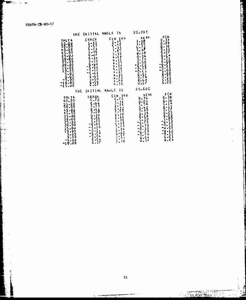
USAFA-Th80 1 7
THE INITIAL ANGLE IS 20.0c
TH Atil8 k ERR XEFr FCR
L eI05 0.2b
45.00 0.11 8140.00 Q.:46
:1350Cc? il52')2 C.C7
3 .0 3) 0.1 4 0.14 0 125.00 0.05 0.1 1.
-4.1125.00 L.11C2 '6.0 Cl
210. L :C1 Q.C
03 :C 4 1E 0.7 0.1810 ~~C G Lb4C0
L3 1.5 4."s 0 4
3t0 C.S ?.Co 0.C 0uE.CZ25. 03 *.C .00 0.00
15.00 -(.1 '.I-01
C.C' 0 IILkiE1 r.C4 .C
TH TAO..700C7 0.7.1
H g-4-8:j
'4111 41S
35.00 0 19 C55
NE -.
68 £-% 'C,-

USAFA-TR-80-17
Appendix E
ADDITIONAL FACTORS INCLUDED TO COMPLETE ANALYSIS:EFFECT OF SUN ANGLE AND MIRROR PROJECTED AREA
The factor we wish to maximize is the energy available at the receiver. In addi-
tion to the parameters previously described, we should also include several other factors
which will incorporate actual effects.
First, the amount of available insolation is a function of the sui angle which
is maximum when the sun is at its zenith. The insolation decreases as the sun nears
the horizon, approaching 73 percent of the zenith flux at 20 degrees above the horizon.
This factor, identified as SOL, is included in the program and iE illustrated in Attach-
ment 1.
Additionally, the mirror area "1seen" by the sun or the projected mirror area should
be considered. If the mirror was "on edge" to the sun, no energy would be reflected.
In the cases we considered, the angle is nowhere near this extreme and we can easily
include this effect. Referring to Figure E-1, it is obvious that the projected area
\ I
\,/ -
PAWIECTEO AREA .ARA COG(.W)
Figure F-1. Projected M'irror Area
56
- , . I/-\ , .

HI
USAPA-TL-80-17
is equal to the actual mirror area times cos *, where
-I-Y + 2 1 (El)2
The figure illustrates this relationship, whicb also holds if the initial orienta-
tiLon is greater than 180 degrees.
The energy shifted due to the error which results from the configuration and initial
angle now also includes the effect of the sun's angle and the mirror projected area. This
i i incorporated in the calculation and is printed out as CUM E (see Attachment I to this
A4pendix). When this factor is used in place of the noncorrected error (CUM ERR), it
results in a slightly different optimum angle. This is discussed in greater detail in
the main text, and the results can be seen by comparing e' opt (uncorrected) to 6 opt
(including sun angle and projected area) in Figures 5 through 10.
Attachment 1
)iMEN-iOh 5 Li 5)C ... "FEC OF ZNI[i&. IFRJR POSITION OK tiMCI
DATA tOtLl) -1,5 )1.7 S ,ad,9e. .. 97.9 g 9 '1.vOTATi H*CR ,2t.,1O..5.
- ' .15~IITE( 46 ) ,,
010 I 1= 3C17ETAC = FLGAT(I-8):.4?5. I-TiET4C = FLCAT(I -8) .1.415.
1 T( P, ) TAO
SUM = 0.0 0 l~J ZI15i r4 2 IHETA " FL (AT (J-) *5.
TH 0UIi P1 /1 1Pli = IHLT A-THET 40
A:v 0 . FaCOS(THETAD)e= 1-(sI) * s~lc WE1AC)C:" iEs - (I.- OHC)Fz -LN(TikEl) ,o LOS(IHE) HiC)ER? 5E ( FI -4)- CO5 (4 Tk -iTHETAG)I =R°E /F( R =ERR i(CO UGAm) )
Sr. SL (J) *[At7 &RE CU S(fSIt
=RXERR ia1U v SUM 9N iUf.tR)fl'T [iT l' E 10* IS O./P I
IRd .3 ) THILTi-,FUPXERF.,PCiIaOL(J),E$,1,g!"1) ? Nl! l o 2 I"HJ1~1L8
J PJ pAr(.),5HIErA 4 2Xv.HFRKP! HCUP X, vX H1'K.5HSULP, H;S,,X,5H(UP Ev5X,4HFERP )
3 4 k IMA1(T1 WMIdt It. D14. AR14 R ) U S 1S -F ? .3 P HI EIGH T 1 7 73I#-5HD SCF I oF' .3)
57 - _ - - - - .

USAFA-TR-80-17
THE INlIlAL ANGLE IS 30.CO(
TiE[, ER RCR C ERR xPF 0.9 ES CM E
6C.00 C .9 I
4 *90 C.(4 (. e0 .(4 0: € . r 64 0 . 1
40.05 C.C6 C' ( c. C.9, .06 c.6r55 .0 C5 (. 1. €l 0C.99 *05 0.72
. U99 0.20 0.89 .2 2046
0.0 1.9 '. 1. , is 0.2 .8 .T2 3.-5.00 1.!5 *toG 174 0.35 C.r .T5 3.53
51
58

USAFA-TR-80-17
SECTION V
INSTRUMENTATION AND HARDWARE
I
I:
USAFA-TR-80-17
MEASUREMENT OF VERY LARGE FLOW ANGLESWITH NON-NIILLING SEVEN-HOLE PROBES
R.W. Gallington*
Abstract
This paper describes a method for meas-rxng local direction and total and staticpressures of a flow by means of a fixed probe, provided that the local air flow doesnot make an angle of more than 80 degrees with the axis of the probe. Rapid surveysof the wakes formed behind variously-configured lifting body models durin; wind tunneltesting require such a probe. The probe is easily manufactured from standard-sized tub-ing materials. The power series calibration method used with the probe results in expli-cit polynomial expressions for the desired aerodynamic properties. The calibration methodis easily programmed on a data acquisition system. This paper includes an e,;amplc- c'a complete incompressible calibration and discusses a logical method for extending thecalibration technique to compressible flows.
I. Introduction
When testing aerodynamic shapes in the wind tunnel, researchers are oftea interested
in obtaining information about the flow field created by these shapes. To this end,
numerous techniques have been devised to make the flow patterns visible. These techniques
are helpful in visualizing the flow, but actual quantitative intormation about the sizc
and direction of the velocity field ultimately depend on a direct flow measurement.
One of the oldest known quantitative techniques involves the use of a pressure probe.
The earliest of these probes was developed by Henri Pitot in the 1700's. Over the years
Pitot tubes have been made extremely small so as not to disturb the flow field with
the intruding probe. Additionally, the old ideas of measuring stagnation pressure direct-
ly, requir'ing near perfect alignment of the probe with the flow direction (that is,
extremely small flow angles), have given way to small probes with multiple ports and
a relaxation of the near-zero flow angle requirciant.
In a previous paper we discussed the calibrat. n of one such small multiple-hole
probe, the five-hole probe (Ref. 1). As we reported in Ref. 1, and as Wuest reported
earlier (Ref. 2), the probes could not be calibrated to give UsefUl flow information
beyond flow angles of 30 degrees measured from the flow 'Irecticn to the probe axis.
a limitation shared with triaxial, hot wire probes (Ref. 3). Unfortunately, many inter-
esting flows such as wing wakes involve flow fields containing concentrated vortices.
In these wakes 'qrger flow angles occur (ReV. 4) which until now co-.ild only be measured
by means of elaborate mechanical devices such as nulling probes or the laser doppler
velocimeter. These too have limitations; the laser doppler velocimeter, for example, has
geometrical limitations when the required optical paths are considered (Ref. 5).
Practical methods for calibrating pressure probes are rapidly improving as experience
with automited data acqtIsition systems increases. Some very general method,, of calibra-
*Lt Col, USAF, Tenure Associate Professor of Aeronautics, DFAN
60

USAFA-TR-80-17
tion described only conceptually a few years ago (Ref. 6) can now be conveniently applied
because of the use of automated data systems. These calibration methods effectively
remove the requirement for the probe to directly measure certain fluid pressures (such
as total and static pressures) or to generate simple coefficients which vary almost
in a linear relation to changes in the probe's angle of attack or angle of sideslip
measured from the flow direction to the probe axis. The requirement to compensate for
these nonlinear effects is factored into the calibration procedure. Thus, the design
of the probe and the technique of manufacturing them becomes primarily governed oy consider-
ations such as ease of manufacture and the need to provide adequate flow areas in the
probe holes to enhance pneumatic response of sensors connected by tubing to the probe
holes.
This paper describes a unique probe design, manufacturing process, and calibration
procedure which in combination permit the accurate measurement of the total pressure
of the flow, the static pressure of the flow, and all three components of fluid flow
velocity all at the probe location and through total flow angles of 80 degrees measured
from the flow direction to the probe axis. Further, this method is relatively fast
in mcaturing she characteristics.
In order to approach this subject in an orderly manner, the paper first describes
the reason for building a seven-hole probe by examining the pressure coefficients for
T a five-hole probe and comparing them to those for a seven-hole probe. Then, the desired
*orm of these calibration equations which makes use of these variable pressure coefficients
is described. The method we use for computing the numerous constant calibration coef'i-
cients of the power series in the variable pressure coefficients Js also described.
Next we describe the manufacturing procedure for a seven-hole probe and other necessary
apparatus and the procedures necessary to calibrate a probe. The final section of the
paper describes the results when the probe and computation method are applied to a probe
calibrated for measuring incompressible fluid flows.
II. Rationale for a Seven-Hole Probe
To describe why the seven-hole probe is a desirable design uhoice for measurijng
flow when the probe is positioned at high angles of attack and sideslip, one must first
understand why the more commonly used five-hole probe fails at high flow angles.
A. Five-Hole Probes at High Flow Angles
Refer to Figure 1. One can see that at high angles of attack one of the side
ports in the five-hole probe becomes almost a stagnation port while the opposite portmeasures the pressure in the separated wake.. Neither of these pressures is sensitive
to small changes in angle of attack. Specifically (still referring to Figuze 1), the
coumonly used pressure coefficient, C , which will yield the angle of attack the probe
makes to the flow whert the pressure coefficient is inserted into the appropriate calibra-
6-

USAFA-TR-80-17
SEUARATED FLCVi
STAGNiATION FPdNI
Figure 1. Flow Pattern Over Five-lHole Probe
at High Angle of Attack
tion equation, is given by Eqn. (1):
P3 - P1C =
a _ PI +
P" +
P3 +
P4 l
4
This pressure coefficient, however, becomes independent of the angle of attack at high
flow angles. Similarly, C., the coefficient Inteuded to yield sideslip tnformaton. be-
comes independent of thu angle it is intended to measure at large angles of sideslip.
In fact, at high flow angles it is the center port pressure which is the most uepend-
ent on flow angle in contrast to low flow angle situations where the center port pressure
Is nearly independent of flow atxgle (that is, in the usual case the center port mea.ures
stagnation pressure). Thierefore, a coefficient which is sensitive to flow angle ait
high flow angles might be C. which includes the pressure difference between the new
stagnation port and the center port. Thl is mathematically expressed by this equation:
C P1 - P5C, 4 : (2)
- 2
As long as the fluid velocity is generallv upward across thv probe, this oefficient c'ould
give us flow angle information. (Other coo'ffic Lent s could bo defined for othLer quadrant .)
To determine the azimuthal angle ,,f fhe velocity VeL tor, one might consider the pressure
coefficient C given by the following equation:
C = -I - P
However, this pressure coeff citnt will be insensit iv- to the azimuthal po it io, .
the probe if thL. f,)w in the -ross flow plano i:s att ichod bevotid port 2 anl 4 a
in ideal air low around a cylinder. Certainly th. flow will not he, rii abiy a1t t .ilvd
62
....-.---- - .-.- _--

USAFA-TR-8- [I7or separated over these ports for the whole range of desiren measurement angles, tlhereby
introducing uncertainties into any measurement that might be made at a particular instant
or point. In general, past experience has shown that it is preferable to use only pres-
sure ports under attached flows. Thus, separateo air flow reduces the number of ports
which can be applied to a given measurement situation and since at least one of the
four peripheral ports will always be in separated flow, the five-hole probe is a bad
cheice for measuring high flow angles.
B. Seven-Hole Probe at High Angles
With the seven-hole probe illustrated in Figure 2, the problem of finding a
C) G4
Figure 2. Flow Pattern Over Seven-Hole Probe
at High Angle of Attack Iroll-angle-sensitive pressure coefficient is solved by using the pressure coefficients
obtained directly from measured pressures insert .,I into the following equations:
P P7 C P 3 - P5
P4. - , + - 3 P (4)
2 2
which apply for the case when tlh,e v.locit vector is in an .it-shaped sector contaiing l.
the 60-dr.gree region directly beneath the -obe. Note hcre that we are assured that lthe pressure ports we are ir.tcrested in wil alw'ays , in an attached flow region. Ii
To determine the flow ang'is in sectors where the oncoming xelocity is other than
:rectlv below the pr be, additi- in! coefficiont; are ni-tded. The reouired set of pres-
sure coefficients are as follows:
PC - P7 P - P 2
P- P + .- P +
~2
63
z.4
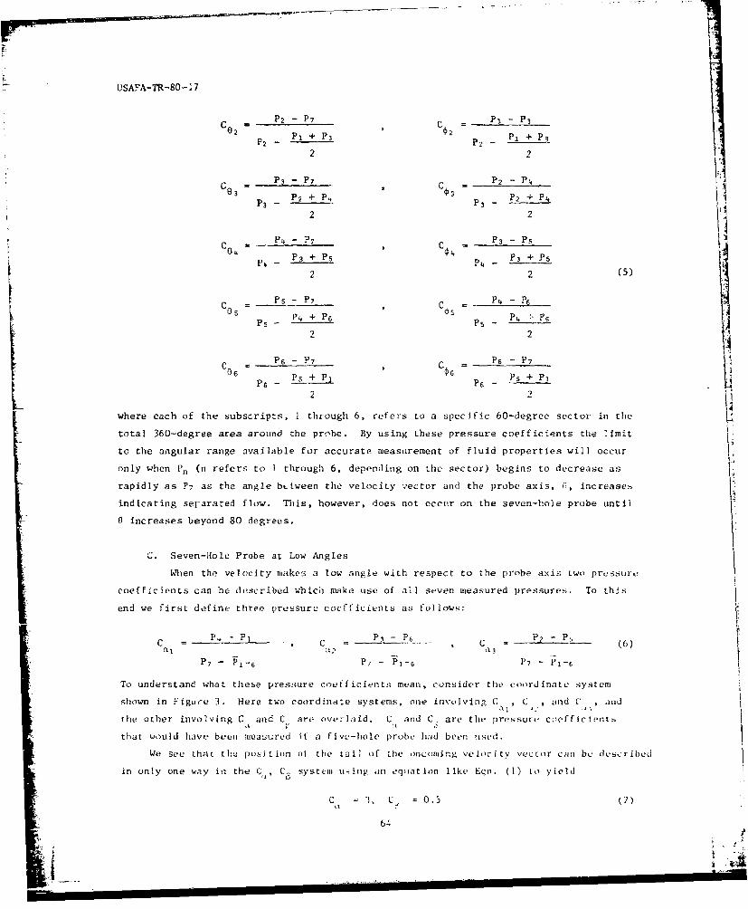
USAFA-TR-80-17
P2 -P7 = PI - P3
PI + P3 C 2 P2 + P3P2 P2
2 2
- P3 - PC P2 - P4 _P33 - P2 + P4 C 3 P2 + P4
P3 P P2+-
2 2
PC - P7 P3 -P
P4-P3 + P5 4 P3 + PSP..- P.,
2 2 (5)
C 5 PS - P7 C S P4 - P6
P5-P4 + P6 P ' 4 . PS
2 2
o P6 - P7 = P6 - P7C0F S + PI C PS + PI
P6 P6-
2 2
where each of the subscripts, I through 6, refers to a specific 60-degree sector in the
total 360-degree area around the probe. By using these pressure coefficients the limit
to the angular range available for accurate measurement of fluid properties will occur
only when Pn (n refers to I through 6, depending on the sector) begins to decrease as
rapidly as P7 as the angle bttween the velocity ,ector and the probe axis, 0, increases
indicating seyarated flow. This, however, does not occur on the seven-hole probe until
0 increases beyond 80 degrees.
C. Seven-Hole Probe at Low Angles
When the velocity makes a low angle with respect to the probe axis two pressure
coefficients can be described which make use of all seven measured pressures. To this
end we first dfine three pressure coefficients as follows:
P4.- P1 - P6 P2 - PC - , C =, C (6)
P 7 - P- P 7 - e 1 -s I'7 - l-16
To understand what these pressure coe fficients mean, consider the coordinate system
shown in Figure 3. Here two coordinate systems, one involving C , C . and C , and
the other involving C and C are overlaid. C and C. are the pressure coefficients
that would have been measured if a five-hole probe hajd been uised.
We see that thy posit ion of the tail of the oncoming velocity vector can be described
in only one way in the C , CL system using an equation like Eqn. (1) to yield
C I , C =0.5 (7)
64i i • : 4
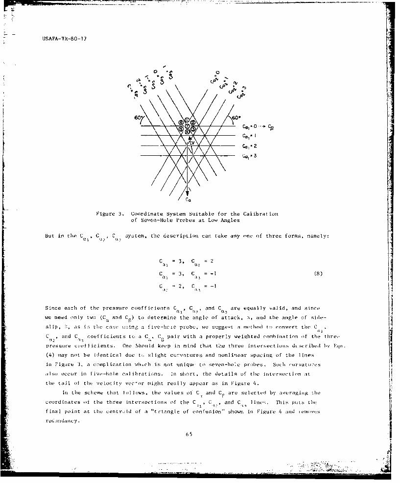
USAFA-TR-80-17
0 C4 lop.C
Cal' I
VV /\
/Ca
Figure 3. Coordinate System Suitable for the Calibrationof Se'en-Hole Probes at Low Angles
But in the C , C, C system, the description can take any one of three forms, namely:U?
C =3, C =2a1, a1?
C , C =-l (8)
C =2, C =-1
Since each of the pressure coefficients C , C, and C are equally valid, and since
we need only two (Ca and CP) to determine the angle of attack, a, and the angle of side-
slip, , as L; the ca;c -::ing a five-hce probe, we suggest a method to convert the C .
C ', and C coefficients to a C , C. pair with a properly weighted combination of the thre.'113
pressure coefficients. One Should keep in mind that the three intersections dt 5cribed 1wy Eqn.
(4) may not be identical due t, slight curvatures and nonlinear spacing of tie lines
in Figure 3, a complication whch is not uniqut to seven-hole probes. Such curvatures
also occur in five-hoie calibrations. In short, the details of the intersection at
the tail ot the. vel.ocitv vector might really appear as in Figure 4.
In the scheme that fol lows, the values of C and C, are selected by averaging the
coordinates ,f the three intersections of the C , C , and C lines. This puts the
final point at the centroid of a "triangle of confusion" shown in Figure 4 and temov,s
ruC(tnidancy.
65

USAFA-TR-9i0-17
Ca 3 -I =.5CO CC,= Ii
Figure 4. DqtaiJs of Intersection
The equations of tht C , C C, and Ca3 lines ar2 given respectively by:
C =C
C
C -C tan 60 ,-a sin 30' (9)
CC CB can 600 - X3
sin 30'
Eqns. (9) are three equations In the two unknowns C and CP. so three equally valid
solutions are possible, each corresponding o an apex of the triangle shown in Figure 4.
oJ
I tan 600 CC
a bin 30'
0 CQ (
i-tan 607 i
I.. - tan 60 C- -
66

USaFA-TR-80-17
Eqns. (10) are solved for the Ca's and C6 1 Lu terms of Ci, Ca , and C The values
of C and C are determined from the average of the three pairs:
C a C C + C
C= a ab ble (C)
3 3
The final result of the indicated algebraic operations is:
C -C
C _ (C + C) C C + C 2 C (12)/3 2
In summary, the process for getting a C and CB from the seven measured pressures
of the seven-hole probe is to first substitute the pressures measured from the probe
into Eqns. (6) to find C a, L,2, and C3 , then substitute these pressure coefficients
into Eqns. (12) to find Ca and C From this point on a determination of the angles
would proceed exactly as in the case for the five-hole probes measuring at low flow angles(Ref. 1).
D. Division of Angular Space
If one follows the methods described above, the only remaining questions
concern the determination of when to use the equations for low flow angles and when
to use the equations for high flow angles. Associated with these questions is the task
of specifying the dividing lines for each of the six 60-degree sectors when using the
high flow angle equations. Initially, because of the experience with the five-hole
probes, one is tempted to specify a 30-degree cone around the nose of the probe as the
cut-off point for using the low flow angle equations. To do this, however, is naive since
data taken during a survey of a known flow field (done for the purpose of calibrating
Lhu probe) may suggest a better cut-off angle and this will only be apparent after cali-
bration. Further, arbitrarily locating the sector division lines might also prove naive
after examining calibration drta. Therefore, we suggest the plan shown schematically
in Figure 5, which describes the decision network for deciding which angle pressure
coefficient pair to use in determining the flow angles a and a.
There are se-veral commonly used reference systems for measuring the flow angle
with respect to a probe axis at low flow angles. To select the angle description ref-
erence system that could best be adapted to a power series curve fit, we used the argu-
ment that the angle pressure coefficients C and C should be unaffected by velocity
components that are perpendicular tc the plane in vhich the angles a and 8 are measured.
That is, the pressure coefficient C which would be roughly proportional to a in
the chosen reference system would be nearly independent of B and vice versa. This argu-
67

USAFA-TIL-80-17
ment leads to the selection of the tangent reference system which yieldu the angles aT
and T shown in Figure 6.
For measuring at high flow angles, no conventional reference system is appropriate
because they all have indeterminate angles and singularities at very high total flow
angles. Therefore, for the high flow angles, we use the 0, * method described earlier,which has a ingular determination only when the velocity vector is aligned with the
probe. This singularity is eliminated by switching to the low flow angle coordinate
system.
P LARGEST _PP
Figure 5. Division of Angular Space i
Based on Measured Pressures i
Tdeally, of course, the lines of constant C , Co, and C,1 in Figure 7 would be i
equally spaced and parallel to the lines of constant 07. %T, 8 and * respectively. In
reality, for a host of reasons, this is not exactly true. That is, the nomnally constant-(
calibration coefficients are not really constant and are m.ore complicated than a siplei
linear relation. This complication is the topic of the following sections. L
III. Seven-Hole Probe Calibration Theory
At the beginning of the paper we mentioned that we wanted a method of measuring
fluid flow properties that would yield the desired output quantities explicitly. Ad-
ditionally. we insisted that the procedures necessary to perform a calibration of theI
probe to provide power series coefficients must be amenable to our available mechanical
.68 - -
ii i ....... ... .. .. .... .. T

* USAFA-TR-80-17
v
I CONVENTIONAL POLAR TANGENT
UK V Cos cz ossB u-V cose rtn-T u
v -V sin$8 v - VsinG sin ~ =ac
v - V sina cosB w - V sinO cost
Figure 6. Flow Angle Definitions
Ar cI,
CalCo.
Figure 7, Idealized Coordinate Systems
69

T ~USAPA-TR-80-17 F
apparatus and should not require the development of extensive special-purpose computer
software. We also wanted our calibration scheme to be capable of being extended to com-
pressible flow situations. This section of the paper describes the mathmatical structure
and calibration of a power series determination method which meets all these requirements.
By using this method we obtain a statistically correct estimate of the accuracy with
which each measurement can be made.
A. Form of the Desired Flow Property Determination Method
In each of the seven regions of the flow around the probe (which are illustrated
in Figure 5) the desired output quantities are represented by a power series in the pair
of pressure coefficients most sensitive to the flow angles to be measured. Although
there is some arbitrariness in specifying the form of the defining equations, we have
found the following form can accurately reproduce the experimental data. For the inner
sector (low flow angle) we define a B' and C0 and C by these equntions:
CL a a,.
a - 1 +K2 C + K 0, 4T o-KKi + K .c a c+ ......... 0(4) h
S a ........ H
On Kl+KC + nI
fn - K " + K2C + KC + 0(4)10 (13)
C K2C C + KCs +......... 0(4)
For each outer region 6 's and 0 's, C s and C 's are given by these equationst
n On Rn
n a K n + K2nCOn + K3cn + ......... ( 0(4)
C On ,+KO n + 3On ....... 0(4) (14
R n qn n
The K's are calibration coefficients. T7hese are constant and unique to the particu-
lar probe. Assuming the K's are kiuuwrn, when taking data one uses the pressures measured
on the probe to first determine which sector is appropriate (see Figure 5) and then to
calculate the pair of angle pressure coefficients (CC and CS or COn and C4n ) appropriateto that sector by using Eqns. (13) or (14). We then have the two flow angles and the
pressure coefficients C and C or C and C . Note that this Information requires
no iteration; we obtain it explicitly. The local dynamic pressure is then easily and ex-
plicitly obtained from C or C and the measured pressures. Further, the total pressure
can be explicitly obtained from C or C and the measured pressures, as for exampleo o
in the inner sector calculation shown below:
P " P7 - C (P7 - P1-6) (15)
70
-V
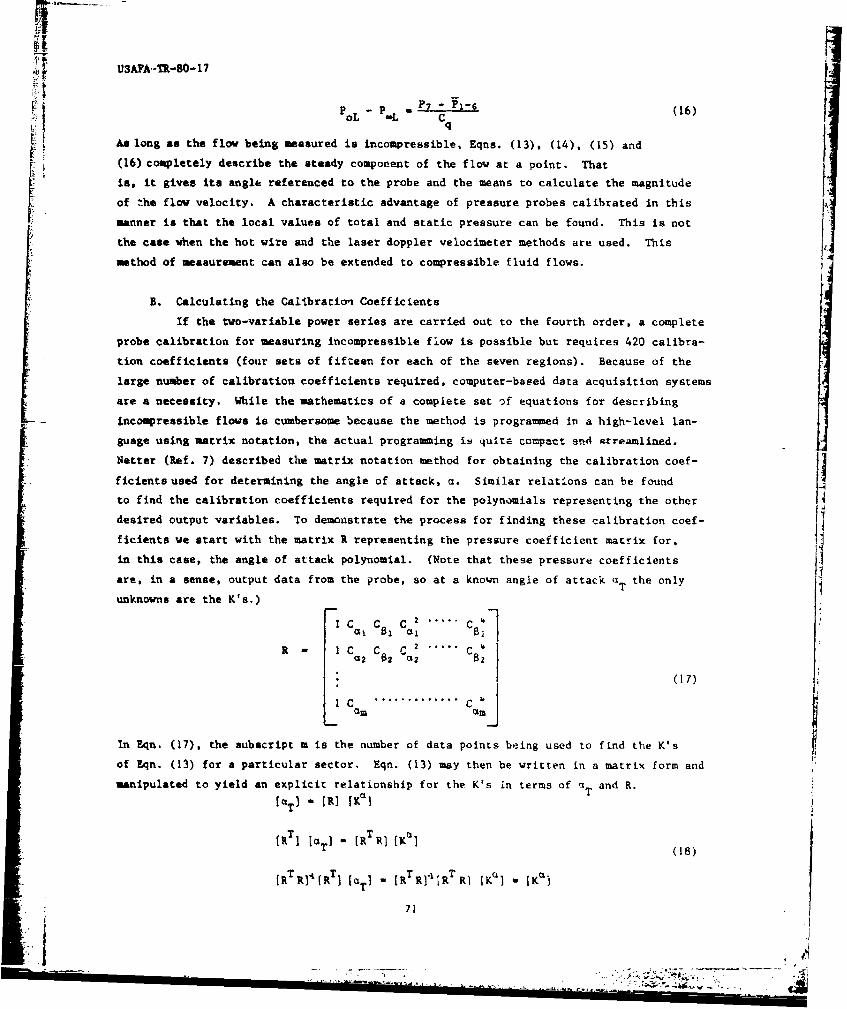
Po- P-L 7 (16)oL Cq
As long as the flow being measured is incompressible, Eqns. (13), (14). (15) and
(16) completely describe the steady component of the flow at a point. That
is, it gives its angle referenced to the probe and the means to calculate the magnitude
of the flow velocity. A characteristic advantage of pressure probes calibrated in this
manner is that the local values of total and static pressure can be found. This is not
the case when the hot wire and the laser doppler velocimeter methods are used. This
method of measurement can also be extended to compressible fluid flows.
B. Calculating the Calibration Coefficients
If the two-variable power series are carried out to the fourth order, a complete
probe calibration for measuring incompressible flow is possible but requires 420 calibra-
tion coefficients (four sets of fifteen for each of the seven regions). Because of the
large number of calibration coefficients required, computer-based data acquisition systems
are a necessity. While the mathematics of a complete set of equations for describing
incompressible flows is cumbersome because the method is programmed in a high-level lan-
guage using matrix notation, the actual programming is quite compact end ntreamlined.
Netter (Ref. 7) described the matrix notation method for obtaining the calibration coef-
ficients used for determining the angle of attack, a. Similar relations can be found
to find the calibration coefficients required for the polynomials representing the other
desired output variables. To demonstrate the process for finding these calibration coef-
ficients we start with the matrix R representing the pressure coefficient matrix for,
in this case, the angle of attack polynomial. (Note that these pressure coefficients Iare, in a sense, output data from the probe, so at a known angle of attack aT the only
unknowns are the K's.)
c C C 2 C "]
R- IC C C I * ..
L Ca.............. j 7)
In Eqn. (17), the subscript m is the number of data points being used to find the K's
of Eqn. (13) for a particular sector. Eqn. (13) may then be written in a matrix form and
manipulated to yield an explicit relationship for the K's in terms of aT and R.
TaT) - I]1 10(8
IRT T [RT) T [aR] [R -T K) [Ka)
.- 71

USAFA-TR-80-17
The values of the K's result in a polynomial that best fits the data set in a least
squares sense. Also, having found the K's, it is a simple matter to calculate an output
quantity, say a , corresponding to each of the pairs of coefficients, say Ca and C., used
in the computation of the K's and to compare these calculated output values to the exper-
imental values. A global estimate of the accuracy of the curve fit (that is, the poly-
nomial expression for each of the desired output quantities) can be obtained by computing
the standard deviation of the difference between the experimental points aud those pre-
dicted by the calibration polynomials. This standard deviation, O(aT, is given by Eqn.
(19):
... (19)X l OY
a (a T) (19)
The discussion above applies to a probe angle of attack which falls in the inner sector
(low flow angle) only. The same reasoning applies to the other three output variables
obtained in the inner sector (S, Co , C q) and to the four output variables obtained in
each outer sector (high flow angles).
While the ,standard deviations in the angles aT and 8- are representative of the
accuracy with which these angles are calculated by the polynomials, the standard devia-
tion in C and C are not representative of the accuracy of the obtained total pressureo qand dynamic pressure. The correct expressions for the standard deviation of these two
la t te r c o e f f ic i en t s a r e )(q ) ( Y( 0
________= '(20)PoL " -L Cq
a (oL (C~q~oCO) z+ (C0 a C q) )2 ) (21)
These expressions can be derived by the proper application of small perturbation analysis
or by taking partial de.-vativcu of the defining equations and subsequent application
of the method ot Kline and McClintock (Ref. 8).
C. Extension to Compressible Flow
To understand how to extend these ideas to permit measurement of compressible
fluid flows, first realize that the total and static pressure can be extracted from the
method already described and thus the Mach number can be calculated by means of the fol-
lowing equation:
O 7 -1(22)P ol-
C (P PPoL P P7 T1-6
72
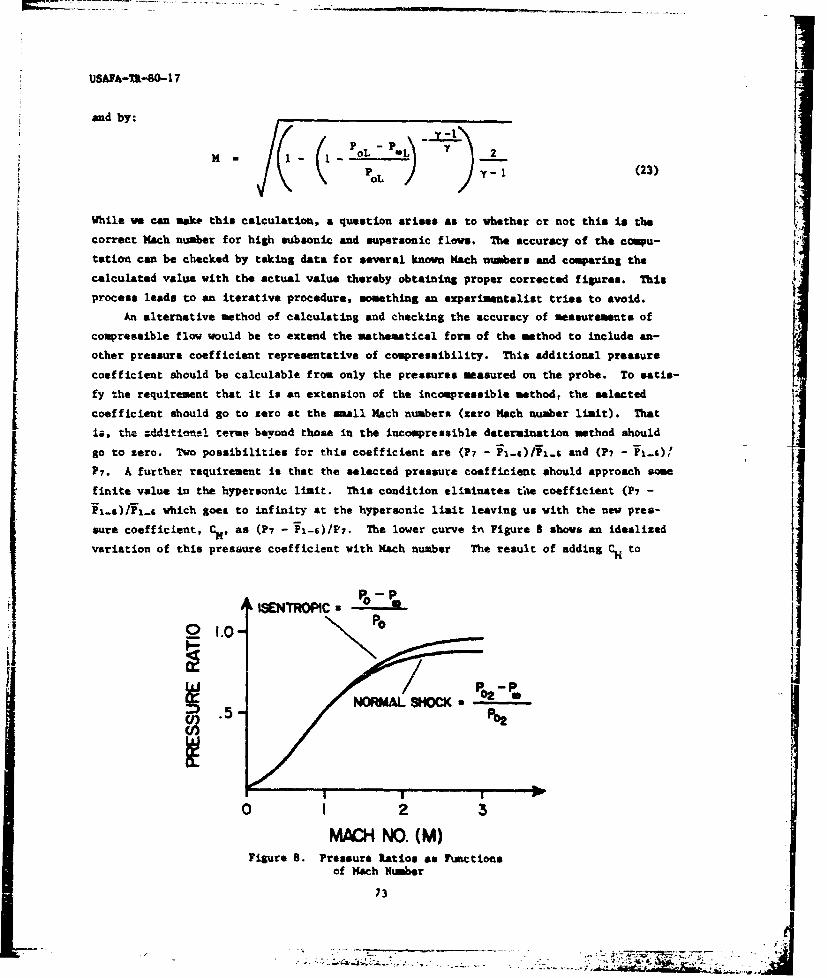
USAFA-7I-80-17
and by:
P H o L P oo 2
POt Yh- 1 (23)
While we can ske this calculation, a question arises as to whether or not this is thecorrect Mach number for high subsonic and supersonic flows. The accuracy of the compu-tation can be checked by taking data for several known Mach numbers and comparing thecalculated value with the actual value thereby obtaining proper corrected figures. Thisprocess leads to an iterative procedure, something an experimentalist tries to avoid.
An alternative method of calculating and checking the accuracy of measurements ofcompressible flow would be to extend the mtheomatical form of the method to include an-other pressure coefficient representative of compressibility. This additional pressure
coefficient should be calculable from only the pressures measured on the probe. To satis-fy the requirement that it is an extension of the incompressible method, the selectedcoefficient should go to zero at the small Mach numbers (zero Mach number limit). Thatis, the additional term# beyond those in the incompressible determInation method shouldgo to zero. Two possibilities for this coefficient are (P7 - PFI-)1F1 ... and (P, - FX-01
P7. A further requirement is that the selected pressure coefficient should approach smefinite value in the hypersonic limit. This condition eliminates tite coefficient (P7 -
Pi-..)!Pj.g which goes to infinity at the hypersonic limit leaving us with the new pres-sure coefficient, CM, as (P7 - P-s)/P,. The lower curve in Figure 8 shows an idealizedvariation of this pressure coefficient with Mach number The result of adding CH to
ISENTROPIC
MA~i NO. (M)Figure 8. Pressure Ratios as Functions
of Mach Nber
73
.. . . ..- " ; J . .. .: ; "-"-a'- .. . . . . ' '

USAFA-TR-80-17
the determination scheme is Eqn. (24):
a - K + K C + K C 2 + K C +0a a 2 3 z B &M
(24)
KC C + KCCM + KCBCM + .....
In the application of these calibrations we use the isentropic Eqn. (25)
___- ~__i 2_P° - PL fi1_1_YIM2 -oL 2 (25)
to calculate the Mach number when it is less than one (subsonic) corresponding to the
pressure ratio
oL. 'L < .472Po
0
And we use the Rayleigh-Pitot formula below
PoL - PL _ ( . Y )Y
to calculate the Mash number if the flow is supersonic corresponding to the pressure
ratio
PL -PoL o > .472
Po
The total pressure, PoL' n Eqn. (26) is the total pressure behind a normal shock wave
Here, for supersonic flows, the total pressure incated by the determination scheme will be
very nearly the total pressure behind a normal shock wave. The static pressure indicated by
by the probe determination method will be near the free stream static pressure in both subsonic
and supersonic flow. Also, (PoL - P )/P is approximated by (P7 - P- 6 )/P7 and at aol L at,minimum we would expect them to be nearly linear functions of each other. Therefore, the
polynomials are not required to fit the compressible flow relations of Eqns. (25) and
(26). Because of the unpredictable nature of transonic flow, this scheme may not yield
good data near the speed of sound but should yield good results at all other Mach numbers.
As the hypersonic limit is approached, the Mach number becomes irrelevant and cannot
be calculated by any pressure probe method.
A complete compressible calibration of a probe in this manner requires that a range
of Mach numbers be tested. However. as in the case of angle of attack and angle of
74

USAFA-TR-80-17
sideslip variations, it is not necessary to take complete sets of data at each specific
Mach number. Instead, one simply has to insure that the entire parameter space (angle
of attack, angle of sideslip, and Mach number) is roughly uniformly overed by a data
set that has a number of points that exceeds t*e number of calibration coefficients (K's)
to be found in each series by about 20 to allow an accurate calculation of a standard
deviation.
IV. Apparatus and Procedures for Calibration
This section describes how we make our probes, the various stings and holders used
in calibration, the sequential calibration procedure, and the associated software.
A. Probe Manufacture
The manufacturing technique used for building the seven-hole probe is quite
similar to the one used for the five-hole probes (Ref. 9). The seven-hole probe is some-
what simpler because the seven properly-sized tubes can only be packed into the outer
tube in a unique way as shown in Figure 9. This design eliminates the need to find properly-
STAINLESS TUBING
3CC SOLDER
i'4
0.0)IN. i
DIA.M. 4 000 i[CROSS -SECT ION
Figure 9. Probe Tip (eometry
sized spacers which are required in the manufacture of five-hole probes (Ref. 9). Aother
refinement is that we now machine the conical surface of the probe with a very sharp tool
that has generous relief angles. This technique permits smooth cutting through the alter-
nately hard and soft materials which form the probe. Otherwise the technique is the same
75
L "'........................................-'.,. ..

rL
USAA-JJ-80-17
as that described for the five-hole probes. That is, in the end the seven-hole probe re-
tains the advantage of large flay areas in a probe of given diameter.
Z. Mechanical Set-Up for Calibration
For total flow angles of lese than 30 degrees, we mount the probe on a conven-
tional wind tunnel sting holder. The same mechanim that is used for changing the angle
of attack of sting-mounted models is used to sweep the probe through an angle of attack
range of -30 to +30 degrees. By rolling the probe in its holder, ye can repeat the
weep to obtain sideslip angles. An important feature of the calibration sche is that
the data does not have to be taken along lines of constant angle of attack or lines of
constant angle of sideslip. Consequently, the probe is set at a constant roll angle
and total angle sweep@ are used.
For total flow angles betveen 30 and 90 degrees, ye use the bent sting arrangement
shoa in Figure 10. Again, roll angles are set by rolling the probe about its ova
-300 POD ANGLE+ 300 PROBE ANGLE
BENT STING
777'f777777777777777f=
+ 300 PRO ANGLE
Figure 10. bent Sting Geometry
axis and sweeping the angle of attack.
Frequently,. for some of the data taken on the straight sting, one of the outer pres-
sures will be greater than the pressure at hole number seven. When this situation cccurs
it signals that the probe has entered a high flow angle region and the data is properly
sorted into the correct sector by our computer program. The program also provides for
the case where some of the data taken on the bent ating should properly fall into the
low angle region. Figute 11 shows a simplified schematic and v'iring diagram of the exper-
Imental set-up for running calibration tests. The sequence of operations and the func-
tions of the various sot t're packages is described below.
76
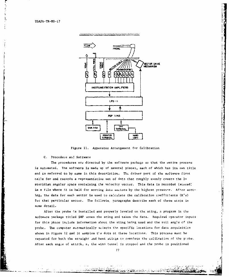
L
USAFA-TR-80- 17
CL: " EcIOR FAiVE
_ lll~lllll~/ /i l ll f//
2 .... ,1
MECK46NISM
L INSTRUMENIATION AMPLIFERS
,Ii ..F/l 1]~~LPS -11
ttFigure I. Apparatus Arrangement for Calibration
C. Procedu-fe arn2 Software
The procedures are directed by the software package so that the entire process
is automated. The software is made up of several pieces, each of which has its own title
and is referred to by name in this description. The driver part of the software first
calls for and records a representative set of data that roughly evenly covers the 2V,
steridian angular space containing the velocity vector. This data is recorded (stored'
in a file where I.t is held for sorting itnLu sectors by the highest pressu,e. After sort-
ing, ttia data for each sector is used to calculate the calibration coefficients (K's)
for that particular sector. The followin. paragraphs describe each of these steps in
some detail.
After the probe is installed and properly leveled on the sting, a program in the
software package titled SHP soves the sting and takes the data. Required operator inputs
for this phase include information about the sting being used and the roll angle of the
probe. The computer automatically sclects the specific locations for data acquisiticn
shown in Figure 12 and it samples tle data at these locations. This process must be
repeatad for both the straight and bent stings to comnlete the calitration of the p:obe.
After each angie of atteck, a, the wind tunnel is stopped and the probe is positioned
77t

USAFA-TR-80- 17
a. Inner Sector b. Typical Outer Sector (Sector 1) L
L50
105
t \45
I"30
Figure 12. Distribution of Points Over Angular Space
to a new roll angle. Currently, only the roll angles showi in Figure 12 can be used
since the computer program decides which angles to stop at based on these input roll
angles. For each data point, this program stores the absolute pressure at each port,
the roll angle, the total angle of attack, the tunnel total and static pressures, and
the tunnel temperature.
The next program, titled SORT, sorts the data into sectors based on the highest
pressure. There is no way of knowing how many data points will fall in each sector.
One must verify that enough points have fallen in each sector to proviie a reasonable
calibration. Also, to perform the subsequently required matrix operations, the exact
number of points in each sector must be known to properly descrLbe the size of the R ma-
trix to be used. To accomplish this matrix operation we currently have to modify another
computer program, although there is no reason that this task could not be avoided by
using a more capable system in the computer for handling matrices. Our current program
also calculates the pressure coefficients C, C8 or Co, C.The ibrotion coefficients (K's) are then calculated for each sector in tutn by
programs called Kl through K7 using the matrix equations already described. The nmber
of data points in each sector is tequired to write dimension statements for each of these
programs. Additionally, this program substitutes the actual pressures into the calibra-
tion polynomials at each data point and determines the output variable that would have
been calculated by the polynomial for that point. The difference between this and the actual
output variable is an error in the calibration curve. The computer program sums the squares
of these errors and divides the sum by the number of data points in that sector and takes the
square root to find the standard deviation of the data set. This standard deviation
provides an excellent assessment of the curve fit and the overall accuracy achieved.
Four standard deviations are computed fir each of the seven sectors, one for each of
the two angles, one for the total pressure coefficient, and one for the dynamic pressure
I.l78

r1*
USAFA-TR-8S0-1 7
coefficient.
This completes the calibration of a probe for measuring incompressible flows.
V. Examples
We have calibrated two probes so far, each with a slightly different nose shape.
The resulcs were quite similar and few conclusions can be drawn from the differences
in calibrations. Therefore, in this section we will discuss the common features of both
calibrations which seem to be characteristic of this type of probe.
The probe geometry tested is shown in Figure 9. The only difference between the
two shapes is the conical angle: 25 degrees for one and 30 degrees for the other.
The general features of the low angle calibration are shown in Figures 13, 14 and
15. Figure 13 depicts lines of censtant Ca and constant C8 . If these coefficients were
linearly dependent on their respective angles, and independent of the other angle, this
figure would appear as evenly-spaced horizontal and vertical lines. The relative lack
of orthogonality and any uneveness in spacing indicates deviation from this ideal behav-
ior. Manufacturing assymmetries or fluid mechanical effects overlooked in our simplified
model of flow around the probe are included in the curve fit. In any case, the fit is
very good as indicated by the standard deviations of the actual angle data away from
the calibration curves in the inner sectors tabulated in Table 1.
The lines of constant C and constant C shown in Figures 14 and 15 generally behave0 q
as one would expect. First, we see that the total pressure is not properly measured
by hole number seven at the higher angles. Specifically, the pressure measured at hole
number seven is less than the true total at significant angles. However, the calibration
I0 0" .4 N O,1
t0,0201
CP .-.6
-20 -10 0 1C 20
a, (deg)
Figure 13. Ca and C versus a T and ST for Low Angles
79.

II..
USAFA-TR-80-17
Table 1
STANDARD DEVIATIONS
AVERAGE OF TWO INNER SECTORS AVERAGE OF 12 OUTER SECTORS
Variable Std. Dev. Variable Std. Dev.
aT 0.42" 8 0.840
8T 0.36* 0 1. 17*
C 1.0% C 1.1%0 On
C 0.6% C 2.4%q qn
(P oL) 0.62 (P oL) 1.2%
PoL -PL PoL " PL
CF _q 2.4%
-l PLP ol. -LoL - L o -P_ _ _ _
,.o
co -.05
1.5-.5.
-1.0
-,.5 -1.0 -.5 0 5 1.0 1.5
CC.Figure 14. Coefficient C. versus Ca ar.d Ca for Typical
Inner Sector (30-Degree Nose Angle. Sector #7)
80
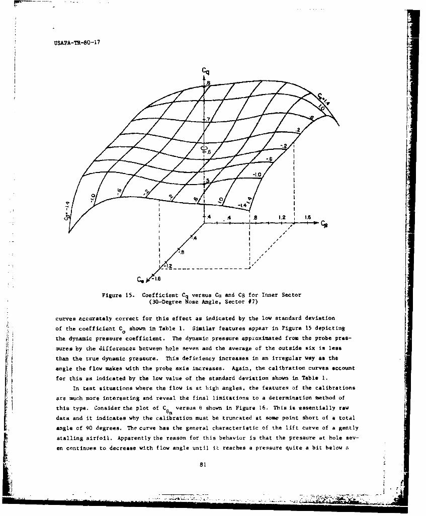
UsAPA-TR-80-17
f ! f
I I
I 4
Figure 15. Coefficient Cq versus Ca ard Cg for Inner Sector
(30-Degree Nose Angle, Sector #7)
curves accurately correct for this effect as indicated by the low standard deviation
of the coefficient C shown in Table 1. Similar features appear in Figure 15 depicting0
the dynamic pressure coefficient. The dynamic pressure approximated from the probe pres-
sures by the differences between hole seven and the average of the outside six is less
than the true dynamic pressure. This deficiency increases in an irregular way as the
angle the flow makes with the probe axis increases. Again, the calibration curves account
for this as indicated by the low value of the standard deviation shown in Table 1.
In test situations where the flow is at high angles, the features of the calibrations
are much more interesting and reveal the final limitations to a determination method of
this type. Consider the plot of Cn versus 6 shown in Figure 16. This is essentially raw
data and it indicates why the calibration must be truncated at some point short of a total
angle of 90 degrees. The curve has the general characteristic of the lift curve of a gently
stalling airfoil. Apparently the reason for this behavior is that the pressure at hole sev-
en continues to decrease with flow angle until It reaches a pressure quite a bit below a
81
j
__W&_
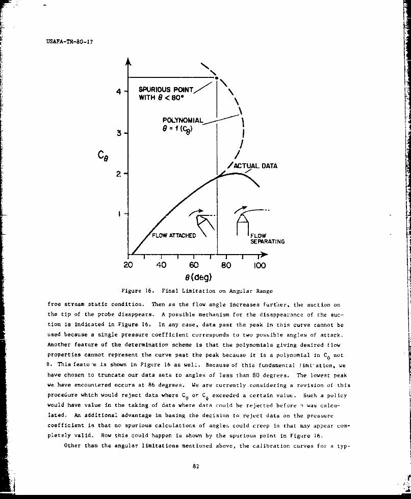
II
USAFA-TR-80-l171
4 SPURIOUS POINT,,I--WITHG< 800 -
POLYNOMIAL
3 J/Ce /
/ACTUAL DATA2
FLOW ATTCHED FLOISEPARATING
20 40 60 80 100
8 (deg)Figure 16. Final Limitation on Angular Range
free stream static condition. Then as the flow angle increases further, the suction on
the tip of the probe disappears. A possible mechanism for the disappeazance of the suc-
tion is indicated in Figure 16. In any case, data past the peak in this curve cannot be
used because a single pressure coefficient corresponds to two possible angles of attack.
Another feature of the determination scheme is that the polynomials giving desired flow
properties cannot represent the curve past the peak because it is a polynomial in C0 not
0. This feature is shown in Figure 16 as welL. Because of this fundamental limi. ation, we
have chosen to truncate our data sets to angles of less than 80 degrees. The lowest peak
we have encountered occurs at 86 degrees. We are currently considering a revision of this
procedure which would reject data where C or C exceeded a certain value. Such a policy
would have value in the taking of data where data could be rejected before 1i was calcu-
laced. An additional advantage in basing the decision to reject data on the pressure
coefficient is that no spurious calculations of angle. could creep in that may appear com-
pletely valid. How this could happen is shown by the spurious point in Figure 16.
Other than the angular limitations mentioned above, the calibration curves for a typ-
82
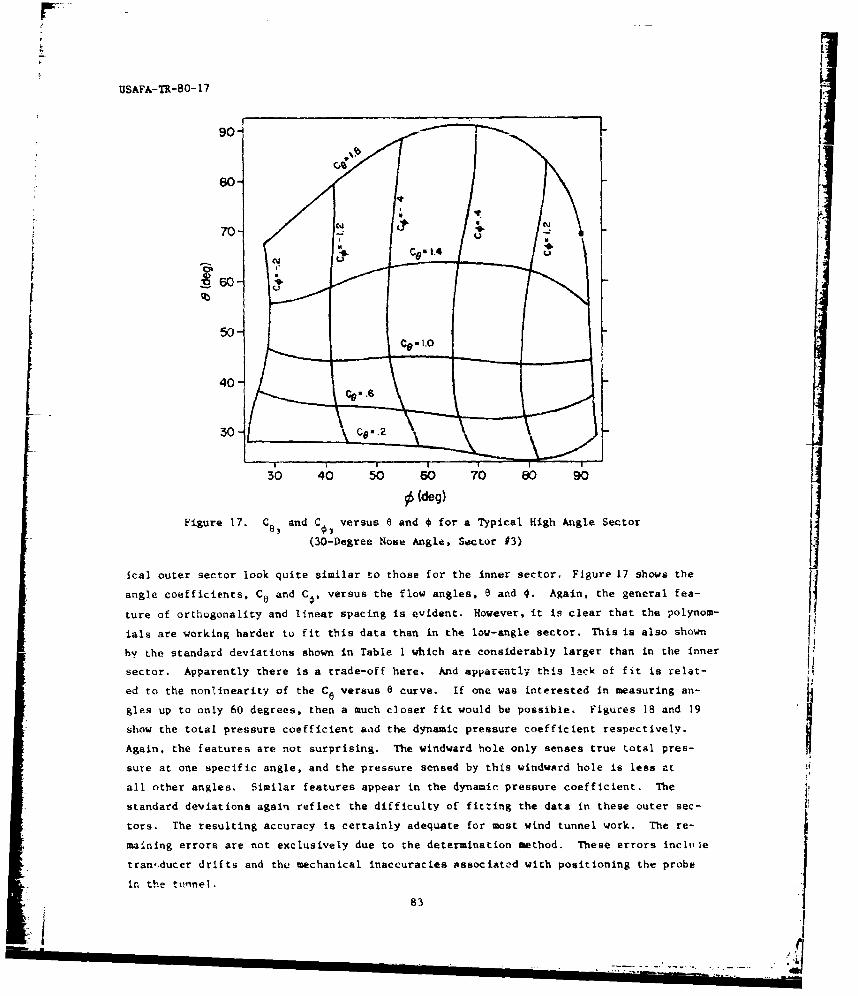
r;
IJsAFA-TR-80- 17
90 I707
50-C .
40-
30-
30 40 50 M0 7 810 90
0 (deg)
Figure 17. C83 and C versus 6 and 0 for a Typical High Angle Sector3e(30-Degree Nose Angle, Sector #3)
ical outer sector look quite similar to those for the inner sector. Figure 17 shows theangle coefficients, C. and C€, versus the flow angles, 0 and 4. Again, the general fea-
ture of orthogonality and linear spacing is evident. However, it is clear that the polynom-
ials are working harder to fit this data than in the low-angle sector. This is also shown
by the standard deviations shown in Table I which are considerably larger than in the inner
sector. Apparently there is a trade-off here. And apparently this lack of fit is relat-
ed to the nonlinearity of the C8 versus 8 curve. If one was interested in measuring an-
gles up to only 60 degrees, then a much closer fit would be possible. Figures 18 and 19
show the total pressure coefficient and the dynamic pressure coefficient respectively.
Again, the features are not surprising. The windward hole only senses true total pres-
sure at one specific angle, and the pressure sensed by this windwArd hole is less at
all other angles. Similar features appear in the dynamic pressure coefficient. The
standard deviations again reflect the difficulty of fitting the data in these outer sec-
tors. The resulting accuracy is certainly adequate for most wind tunnel work. The re-
maining errors are not exclusively due to the determination method, These errors incile
tran',ducer drifts and the mechanical inaccuracies associated with positioning the probe=:. In the tunnel.
83
*1

rL~~20 USIT40-1
c.0 .
-2.0'
Ce
Figure 18. Coefficient Co vergae C 6 and C. for a Typical outer Sector
(30-tDegree Nose Angle, Sector *2)
1.4'
first* 19. Coefficient Cz warmus C atad C #2for a Typical 0-,ter Soctor(30-Uegrou No"e Angle, Sector t7)
84I
I -
USAFA-TR-80-17
V1. Conclusions
We have described the manufacture, calibration, and use of a unique seven-hole probe
that permits the accurate measurement of all steady flow properties provided that the
local flow makes an angle of no more than 80 degrees with respect to the probe axis.
This large angle capability exceeds, by at least a factor of two, the performance of
the beat probes of other designs. The determination method is comprised of explicit
polynomial relations for all the desired output quantities in terms of pressures measured
on the probe. This method is easily programmed in matrix notation on a modern and capable
data acquisition system and does not require that the probe be tested at constant angles
of sideslip or constant angles of attack as required by some other determination methods.
Flexibility in the calibration procedure mean, that quite simple mechanical apparatus
may be used in the calibration process. Once the calibration coefficients are determined
by the calibration process, the determination method can be reapplied to the calibration
data to obtain a statistical estimate of the enpected error in the variables determined
from the polynomials of the determination method. Thlis expected error includes error
from all possible sources.
We have also presented a method for exLeud",g thC -alt rtin to compressible flowsboth below and above the speed of sound, although no examples of such a calibration have I
yet been completed. Representative flow angle errors are .4 degrees at low flow angles
and 1 degree at high flow angles. Expected errors in dynamic pressure are 1.0 percent
at low flow angles and 2 percent at high flow angles.
VII. AcknowledementFj
The design of this pressure probe measurir:g technique is the result of the coordi-
nated efforts of a number of people. It depended on expert skills in mechanical design
and manufacture, computer-experiment interface design, instrumentation, wind tunnel ope--
ation, and expert computer programming. Mr. Claude HIollenbaugh carefully constructed
many of the smell probes and the holding and indexing apparatus. Lt Ken Barker initially
wrotemuch of the prograuesing for calibrati.on ot the five-hole probe. This programming was
later extended to the seven-hole probe design by Capt Tom Bolick. Two Air Force Academy
student groups exercised the software on two, diff-rcnt probes to assure that -It the
software worked properly. Additionally, Capt Bolick awsisted the two cadet groups by
troubleshooting the programs during each calibration to refine it to its present well-
documented and efficient form. Mr. Charles Meadows operated the wind tunnel and the
data acquisition system to acquire and reduce the massive amount of data needed to do
a complete probe calibration.
NASA's Ames Research Center supported the effort as a step toward the goal of de-
scribing the flow around canard-configure-d aircraft at high angles of attack.
,- "

USAFA-TR-80-17
C 0ol apparent total pressure coefficient forP7 - low angles
Pn PoL 1-6
on - n-* + Pn-n apparent total pressure coefficients forn+1P1+--6 high angles*
2
P7 - Pi-sC q apparent dynamic pressure coefficient for
oL *L low angles
Pn (Pn~ + P - ) 12 n 1--
n n+ nIn-+I---P6 apparent dynamic pressure coefficient foraqnL P P n-l ---6 high angles*PoL " PL n-1-1 --- 6
Ca angle of attack pressure coefficient forlow angles
C angle of sideslip pressure coefficient forlow angles
COn total angle coefficient for high angles
CIO roll angle coefficient for high angles
K coefficient in power series (Superscriptindicates variable being expanded. First
digit of subscript indicates position inseries. Second digit of subscript indicatesone of six high angle sectors.)
Pn' n I --- 7 pressure at port "n"
average of pressures I through 6
PoL local total pressure
P. local static pressure
o 04total pressure of free stream
n 1 indicates the next hole clockwise from the n hole and n - 1 indicates the nexthole comanterclockwise from the n hole as viewed from the front o the probe
86
" S r-I

USAFA-TR-80-17
static pressure of free stream
U,V,W local velocity components with respect toprobe
CT angle between probe axis and velocity vector
projected on vertical plane through probe
axis
8 T angle between probe axis and velocity vectorprojected on horizontal plane through probeaxis
e total angle between velocity vector and r".obeaxis
1P angle between a plane containing the velocity
vector and probe axis and a vertical plane
through the probe axis measured positiveclockvine from .,rt number four as viewedfrom the front
a (CT standard deviation of experimental values ofT a away from those calculated from the cali-
blation expressions
a (BT) standard deviation of angle of sideslip
o(q) standard deviation of dynamic pressure
0 standard deviation of coefficient C(q) q
0(C )standard deviation of coefficient C
(po ) standard deviation of total pressure
11
87
la"- - ..."- . I
USAFA-TR-80-17
Rferences
1. Barker, K., R. W. Gallington, and S. Minster. "Calibration of Five-Hole Probes for
On-line Data Reduction." Aeronautics Digest - Spring 1979, USAFA-TR-79-7, USAF Academy,
Colorado, July 1979.
2. Wuest, W. "Measurement of Flow Speed and Flow Direction by Aerodynamic Probes and
Vanes." Paper presented at the 30th Flight Mechanics Panel Meeting, Montreal, Canada,
1967.
3. Huffman, G. D. "Calibration of Tri-Axial Hot Wire Probes Using a Numerical Search
Algorithm." Aeronautics Digest - Fall 1979, USAFA-TR-80-7, USAF Academy, Colorado, April
1980.
4. Sforza, P. M. and M. J. Smorto. "Streamwise Development of the Flow Over a Delta
Wing." AIAA Paper 80-0200, January 1980.
5. Reed, T. D., T. C. Pope, and J. M. Cooksey. "Calibration of Transonic and Supersonic
Wind Tunnels." NASA Contractor Report 2920, Appendix II, November 1977.
6. Breyer. D. W. and R. C. Pankhurst. "Pressure-Probe Methods for Determining Wind
Speed and Direction." London: Her Majesty's Stationery Office, 1971.
7. Netter, J. and W. Wasserman. Applied Linear Statistical Models. Homewood, IL:
Richard D. Irwin, Inc., 1974.
8. Kline, S. J. and F. A. McClintock. "Describing Uncertainties in Single-Sample Exper-
iments." Mechanical Engineering, January 1953.
9. Gallington, R. W. and C. F. Hollenbaugh. "A Fast Method for Accitrate Manufacture
of Small Five-Hole Probes." Aeronautics Digest - Spring 1979, USAFA-TR-79-7, USAF Academy,
Colorado, July 1979.
88
K.2
usAFA-TR-80-17I
SECTION VII- AERONAUTICAL HI STORY
- 89

USAFA-TR-80-17
COMMENT BY A SERVING AIRMAN
B. Poe 11*
Editor's Note
Colonel Alfred Hurley, Department of History, suggested this article for inclusionin the Digest. The article is reprinted from Air Power and Warfare, The Proceedings ofthe 8th Military History Symposium. I think you will enjoy this look at the impact oftechnology from the user's point of view.
I am happy to be here. I'm obviously not here as a historian. Rather, I've been
asked to give a participant's view of the "other side of technology." I fePl rather
strongly about that -- probably because, and I'm very proud of the facr, in my thirty-
plus years I have been a commander at every rank except Second Lieutenant and Brigadier
General. This experience gives one a different look at technology than one might have
in other circumstances. When we discuss technology and its role in the evolution of
air power, we should remember that technology is the application of science -- not the
knnw)Pdge itself so much as the use to which we can apply it. To somebody who has the
kind of responsibilities most of us in the Air' Force have, technological improvements
have little charm until they're shaken down into reliable, maintainable, and, most of
all, available systems that will put bombs on the target.
A stereotype persists that military professionals have usually been conservative
about change. Sometimes this stereotype has worked to the great advantage of those mili-
tary forces willing to press on with new technology and thereby gain an edge over their
opponents. Often, however, the real worth of a new technical system has had to wait
on improvements that have brought it to a practical, useful state. You can go back as
far as you want. I'm sure there were iron weapons around for a thousand years before
Scipio Africanus gave his legions chat short .,word of Spanish iron; but, as Carthage
found out, that sword made an awful lot of difference to the legionnaire as he went to
war and had something he could sharpen, a weapon that wouldn't. bend and wouldn't twist.
Perhaps the flintlock should hnve replaced immediately its clumsy predecessors; but,
if one goes through the museums of Europe, you will find that some of those flintlocks
also had an old matchlock on the iame barrel because some soldier, perhaps the logistics
commander of the day, said, "I want to be sure the thing works because it's not yet weath-
erproof " Before the Marlboroughs get to use the Brown Bess, there are people in between
who try to see that it works.
When you look at technological change influencing warfare, you can go as far back
as the introduction of the stirrup in 600 AD or as far forward as today. The laser is a
scientific achievement. To me, responsible for logistics, laser communications and laser-
SGeneral, USAF, Comnander, Air Force Logistics Command
90.Lii

USAFA-TR-80-17
a iguided bombs are technical applications that have evolved from that scientific achieve-[ iment, and I want to see to it that they work. I am irresponsible if I don't see to it
that they work. The problem we participants face, in other words, is not so mch one
of advancing -echnology as one of keeping abreast of that technology with weapons that
will accomplish the mission.
I would like to look for a few minutes at technology from other perspectives: our
dependence on it, the problems it creates, how the public who pays for both the technol-
ogy and the problems reacts to it, and a few examples of some of the lessons we've
learned in dealing with technology. Clearly, we can't afford Alvin Toffler's symptoms
of maladaptation to changing technology -- be they denial, specialization, reversion,
or over-simplification. We in the Air Force or, for that matter, anybody in the mili-
tary, not only have to search for and develop the latest technologies, but we must be
open to all aspects of their workings -- open to new ways of dealing with them -- and
we must be aware that they represent a complex and not easily assimilated progression.
The other day, a friend sent me a 1927 aircraft yearbook for the Air Force Museum.
Before I passed it to the Director of the Museum, Colonel Uppstrou, I looked through
it; and I noticed with some jealousy that a pursuit plane, of which the Air Corps bought
fifty in 1927, cost just over $33,000. The F-15, an integral part of our force both
here and in Europe, has a current price tag of about eleven million dollars. By the
time we get it ready to be mare than a static display, the price is about seventeen mil-
lion dollars. Even when you take into account the tremendous inflation over those fifty
years, the F-15 costs some seventy times the pursuit plane of the 1920's. The point
is that those 1927 aircraft were technologically simpler, easier to build, and easier
to maintain than anything we fly today, and, consequently, much cheaper.
A similar example comes from the notes of General Benjamin Foulois, Chief of the
Army Air Corps from 1931 to 1935. In 1909, Lieutenant Foulois prepared for flying train-
ing with Orville and Wilbur Wright by reading the few published works on aeronautical
theory. With this "limited" knowledge, he began pestering the Wrights with theoretical
questions. One day, while the airplane -- the only one they had -- was undergoing minor
repairs, and after Wilbur Wright's patience had worn thin, the inventor pointed to the
airplane and spoke one sentence to Foulois: "Throw your books away and go get your hands
dirty on that machine." Foulois ended up with a suit of overalls, a pair of pliers,
a screwdriver, a handful cf cotton waste, and a bar of soap; and he was probably a bet-
ter piiot as a result. The technology of the Wrights was such that one could understand
it by getting one's hands dirty, and Fouiois certainly did that.
Today, we are far beyond "dirty hands" -- although not so far as some think. Even
during the days in 1946 and 1947 when I was on the air show circuit with the "new" F-80,
I could keep that airplane's engine going for a week or ten days and a dozen sorties
with a six-inch crescent wrench with which I took out the top spark plug to clean it.
There were two spark plugs: the bottom one was too hacd to get to, but I didn't mind the
91

USAPA-TR-80-17
rumble in the engine caused by starting just with the top one.
What can an F-15 pilot do today if we sent him on a similar series of flights'( He
certainly cannot be expected to know in any real detail the workings of those black
boxes and delicately-tuned instruments he uses to perform his mission. The hand-held
bomb once dropped from biplanes is now a "smart" bomb. guided by television or laser
to a target several miles away. With cruise missiles, those miles become many miles.
We've also come a long way from the staple of the 1927 Air Corps, the Liberty Engine.
The F-100 engine (which confuses some people because it is what we put in the F-15 and
F-16) is designed in five parts or modules; we can remove, service, and replace each
module without disassembling the entire engine. We use one F-100 engine on the F-16,
two in the F-15. They have ninety-two components which permit us to maintain the engine
without having to break it down for maintenance overhauls as often as in the past.
You don't get something for nothing with this technological improvement, however.
To give you an example of the scale of management we are dealing with: United, the larg-
est airline in the free world, manages 1,600 engines; we manage 44.000 jet engines.
Now, instead of managing one engine, we're managing five modules per engine; and we
really should, if we could get the automatic data processing (AD') aquip-e t to do fit
manage all twenty-two life-limited components. Speaking of modules, incidently, the
F-16 aircraft itself is built the same way. Its five air frame modules ske it an Ossier
aircraft to get into and to fix. Most of its technology is current state of the art.An area that perhaps overlaps all the technology of modern air powereis automatic
data processing, ADP. In a world that some say contains 200,000 digital computers, we
are in the middle of a data processing revolution. The pr~gress has been astounding.
Dr. Carl Sagan has pointed out that the first large electronic digital computer, ENIAC,
constructed in 1946, had 18,000 vacuum tubes and occupied a large room. The same compu-
tational ability resides today in a silicon chip microcomputer the size of one's small
finger joint. Today, we have microprocessors costing about $20.00 that can compute as
much as a large Lomputer that cost one million dollars twenty years ago. In my command
alone, we have over 330 compuLet systems at work; when you include the work we do with
the other services and the Defense Logistics Agency, the number grows to about 430. We
got those first computers in 1954, and by the mid-sixties we had some 375 data systems
processing on about one hundred second-generation computers. Today we are down to around
eighty-three, but it is impossible really to count the computers embedded in the equip-
ment we support.
We could not have kept going without that technology, because we went from about
181,000 people in my comumand in 1961, the year we began to get IBM 7080 computers, to
91,000 today -- cut in half in a period when we've gotten much more complex and difficult
weapons systems to operate. The ADP took up a lot of technological slack, but thoseI
90.000 people we lost represent technological expertise that is gone forever. Now we
are running into a situation in which the 7080 computer is so old that IBM tells me that
£ .92
USAFA-TR-80-17
in a year they will no longer support it. It is so old that I have difficulty finding
people who know the AUTOCODER language on it and who can move it to the high-order lan-
guage of today. We have to look into the retired community to find people to come back
and help us make that transfer into the higher-order language.
Testing is another function by and large dominated by technology. We have about
3,300 automatic testing equipment systems, with 400 more coming in the next two years --
the cost: about a billion dollars. And, of course, we have automatic testing equipment
that tests automatic testing equipment.
If the surge in ADP has been a technological escalation, the growth in embedded
computers has been even more phenomenal. Today, when the pilot pulls the trigger on
his F-16, the impulse runs through about six computers before the missile comes off the
wing. By the early sixties, we had miniaturized th- computer and made it tough enough
to use La airborne and spaceborne systems. Today, most aircraft carry little black boxes
that help navigate, locate targets, fire missile and gun systems, rnd detect enemy fire
and radar. Consequently, we have shifted our approach in aircraft design. Where once
one ceptral computer controlled action, we now use a federated computer with each major
sensor controlled by its own computer, which must communicate wiih all the resL of Liew
to perform the mission. One good message I can bring you is that this month for the
first time, and I think this would interest General Weyland and General LeMay, the cost
and time to repair avionics is going down. We have a radio that does a thousand hours
without repair and a TACAN system that goes 1,800 hours. At the same time, however,
the cost of software is going up like a rocket.
What all this technological surge has caused for us, the participants, is the prob-
lem of how to maintain it, how to keep it running within reasonable costs -- in terms
of both money and manpower. The single most pressing problem we face as a result of
the shift from quantitative to qualitative emphasis is in our aircraft. Back in 1964,
when the B-52s were relatively new and the F-4 was the pride of the TAC fleet, only about
34 percent of our total inventory was nine years old or older. In fact, the age of the
active inventory then was seven and three-quarters years. Today, over two-thirds of
the airplanes I support are nine years old or older. The average age is just over eleven
years. The problem with that statistic, as with technology in general, is the basic
rule of mechanics that the older mechanical things get the more liable they are to break
and the more expensive they are to fix. We face an added problem. When an airplane
comes in for an update of its avionics systems, we can't treat it as routine maintenance.
Technology has decreed that the package for that fighter or bomber must be removed and
reprogrammd our maintenance time for software, consequently, is governea by how long
we must take to reprogram the black boxes. And the problem is going to get more compli-
cated. I cm told that the cost of software development will likely run ten times more
than hardware in the years ahead.
In other areas, we sometimes let technology confuse our sense of priorities, and
93

USAPA-TR-80-17
here I shift back into the commander role. It Is difficult to swallow the argument that
money is not available for mundane things like hardening avionics buildings in the for-
ward area or providing absolutely reliable command and control when somebody comes up
with an exotic system to provide a warm fog dispersal system that will not recover a
single strike aircraft, because it is intended to support airlift in the forward area,
anC that will use in one hour enough fuel for a hundred A-7 sorties. Once in a while
we have got to get away from the charm of doing something technical because we can do
it and pay attention to the ftvndamentals. We killed that fog thing temporarily, in USAFE
(United States Air Force in Europe) at least. I'm sure we broke some people's hearts,
but we put the money in the kind of things we can use to put the bombs down. The Air
Force, incidently, is still studying the concept.
Another side of technological innovation has been to lure us with the promise of
things to come to tne point that, as my Soviet counterpart sometimes says, "the better
is the enemy of the good." In Europe, in 1974, we had to pound the table and fight and
make trips to Washington to get laser pods for the F-4s. General Vogt, CINCUSAFE, and
I, as Vice CINC, felt we needed tem desperately. The reason we had to fight so hard
to get them was that we were continually told that the Precision Emitter Location Strike
System (PELSS) was "Just around the corner."* The tantalizing technological promise of
PELSS is that it can pinpoint a guided strike force to an emitting target even if trans-
mission stops after you launch the strike force. Now, don't get me wrong, I still sup-
port PELSS. I've got my command behind PELSS, but it is not here. And the pods that
we wanted, crude as they were, had done the Job in North Vietnam. We eventually got
the pods in Europe, and maybe we did so because I told some people the story about the
Frenchman. I said I'm sort of like the Frenchman who lost his mistress and is weeping
and waiting at the churchyard, and his friends at the funeral say: "Look, my friend,
we know it's a sad time for you; but you're a young man, you'll meet another girl."
And he says: "Yes, but what about tonight?" That's my responsibility: tonight. And
I can't forget it. If I do, I am not responsible.
Perhaps the most challenging test of technology is at the very core of technology
itself, and that is what is used to power it -- energy. We in the Air Force use about
half of the Department of Defense's 2 percent of the nation's energy. Seventy-seven
percent of Air Force energy is in the form of petroleum, of which we use 66 percent to
fly. In the last ten years, the cost has gone from $100 a flying hour to $490 a flying
hour; as a result, we're flying much less. So we call upon technology to do the mundane
again: to save us ten million gallons by reducing drag through putting vertical winglets
on KC-135s or by putting on or removing vortex generators, depending on the kind of air-
craft. This is not the exciting kind of work some of the technology people are interested
in, but it will keep us over the target with the forces we need to accomplish the mission.
The task of coping with technological change in the employment of sir power, of
course, always revolves around money, and .hus, since we're taxfunded, the public. Al-
94
-Tr USAFA-TR-80-1 ?
though public support has varied, it has been traditionally conservative. Remember the
famous quote of 1911: '"hy all this fuss about airplanes for the Army; I thol&ght we
already had one." Of course, five years later public support was completely behind Army
aviation on the eve of war. That sine wave of support has been consistent: World War
I, World War II. Korea. Sputnik, Vietnam. Even if the military explains that the conse-
quences of inadequate support might be a decline in our technological parity with pro-
spective enemies and we're given the money, an essential truth remains: you cannot con-
fuse money and lead time. Whatever we do in the Air Force, whatever technological ad-
vances we order with that money, we must plan for lead time or we may get only a pretty
static display. In most instances, the support equipment takes much longer to turn out
than the airframe or the missile. Let me cite some examples to prove my point.
[In 1970, Air Force planners asked industry to examine the possibilities of a highly
maneuverable lightweight fighter. In 1971, we Legan to seek interested contractors.
In April 1972, after we chose two of the five companies that offered proposals. GeneralIDynamics and Northrop began to build two YF-16s and YF-17s, respectively. In January
1975, we selected the YF-16 as our air combat fighter. The first models were completed
in 1976, and the first production aircraft will be delixered to a United States Air Force
combat organization at Hill Air Force Base In January cf 1979. Eight yars from techno-
logical idea to the actual system. Now I can't be too hard on the people involved with
the technology in this case because some of that delay was due to "stretch-out" of the
money, a factor our budgetary system always requires us to take into account. Eight
years are what it took for that fighter; and it will take more than that, probably,
for the next one.
Another example: electronic countermeasure pods are particularly susceptible to
the problem of lead time. For two years now, we have realized that the ALQ-119 does
not cover all the threats it must, and we have begun a program to improve its capability.
The ALQ-131 pod is our latest system. It was conceived in 1972, and now, in late 1978,
we have received less than three dozen, all of which are in testing. We designed this
pod with a reprogrammable software system, and yet we will probably encounter still an-
other threat outside its ability. This doesn't mean we cannot get to the target, but
it means that we have to look closely at the promises of technology.
One of the ways we in Logistics Command try to counter both the rising surge of
technology-related problems and their rising cost is through a new outfit call the Air
Force Acquisition Logistics Division. Its objective is to make sure lessons learned
from operational units are written into production contracts, the only places we can
ever improve performance. We walk the flight line, and we talk to the mechanic; we take
that knowledge back to the design engineer and say, for example, "Don't put another ra-
dio under the seat like in the F-4." We have spent $250,000 a month to remove and re-
place ejection seats in the F-4 when there is nothing wrong with the ejection seat, but
rather with the radio. We do learn. I flew into a rage awhile back when I found sey-
95

USAFA-TR-80-17
eral things under the seat of the F-16, but t contract had been written this time to
require General Dynamics to figure out a way to lean the seat forward to allow us to
&et under it to change those items.
A third example: after World War I, the Air Force used mostly lightweight, light-
gaugai aluminum alloy skins. It was highly corrosion-resistant and required minimum
protection. In the early sixties, technology made rapid advances in developing higher
strength aluminum alloys used primarily for structural applications because of their
strength-to-weight ratio. They were tough, relatively cheap, easy to work with, and
the engineers loved them. What we did not suspect was that the heavy gauge aluminum
might be less resistant to corrosion than the light. That neglect turned out to be a
costly mistake. Catastrophic stress corrosion failures occurred. We were forced to
put the entire F-4 fleet on restricted flight after the Navy determined an F-4J crashed
because of a stress-corrosion crack. The potential for failure of the nose landing gear
outer cylinder on the F-ill was so great that we replaced every one of them at a cost
of 3.5 million dollars. But the cost is not the point. The point is we had a whole
fleet of inoperable F-Ills which could deter no one and could not carry out their mis-sLon.
Finally, a lesson learned that may have significant technological impact on the
way we design and 'build aircraft: fuel leaks have always been a major problem for us.
For example, on the C-130 the major cost of keeping the aircraft flying is fixing fuel
leaks .- about $5.00 a flying hour. The situation is the same for many other aircraft,
except two. When we surveyed the inventL Y, we found two old airplanes (the F-102 and
F-106) that just didn't leak. We looked a little further and found that, instead of
using sealant, they used a thermosetting film adhesive sealing process commonly referred
to as "scotch-weld bonding." In November 1977, we completed fabricating a C-130 with
the process and began testing it last December. So far it has compieted 384 flight hours
with no leaks related to that process.
So, you see, technology for me and my people in Logistics Command is a bit more
involved than merely a new development in flight dynamics or an increase in look-down
capability in a radar. Each technological development must bring with it some equiva-
lent advance in logistic technology, or the advances in air power capabilities are mean-
ingless. They're only good as long as we can use them in combat. Secretary of Defense
Brown summd up the problem of technology and warfare when he called for us to be
more modest in performance goals, recognizing that a system with less advancedtechnology that works, is far more militarily useful than a system with moreadvanced technology that doesn't work.
People tell me that this year we will go over fourteen billion dollars in the money
we manage. If those were sales, that would replace ITT as number 11 on the Fortune 500.
We take that responsibility very seriously and the cost Is not going to decrease. But
the money can be more sensibly spent through equal emphasis on the "other side of tech-
96

USA.A-TR-80-17
nology." This "other side" may be mundane, dull, and unglamrous; but I hope that you
historians will now understand my reactions to the developers who. in the past. may have
kept aircreow alive by always giving us an extra ten knots, an extra thousand feet of
altitude, and an extra thousand pounds of payload. When those developers com in as
happy as they can be with a new advance, I may say. "Vhy don't we go with what we planned;
and let me turn down the wick on the engine a little bit. so as to use fewer maintenance
people and, above all, so that we can give the commander sore aircraft to put more bombs
on the target?"
*U. S. CMNWNhT PRIU~w. COFICE IUs 777451/1"3 R"e. *97
4i
Related Documents