For Peer Review - crd-legacy.lbl.govcrd-legacy.lbl.gov/~xiaoye/KTNihei_GJI.pdf · Frequency response modeling of seismic waves using f inite difference time ... and the integration

For Peer ReviewFrequency response modeling of seismic waves using finite difference

time domain with phase sensitive detection (TD-PSD)

Journal: Geophysical Journal International Manuscript ID: GJI-05-0367.R2

Manuscript Type: Research Paper Date Submitted by the

Author: n/a

Complete List of Authors: Nihei, Kurt; Chevron ETC, Seismic Analysis & Property Estimation Li, Xiaoye; Lawrence Berkeley National Laboratory, Computational Research Division

Keywords: Finite-difference methods, Numerical techniques, Seismic modeling

Geophysical Journal International

For Peer Review

1

Frequency response modeling of seismic waves using finite difference time domain with phase sensitive detection (TD-PSD)

Kurt T. Nihei1 and Xiaoye Li2

1Earth Sciences Division, Lawrence Berkeley National Laboratory; now at Chevron ETC, 6001 Bollinger

Canyon Rd., San Ramon, CA 94583 USA. E-mail: [email protected]

2Computational Research Division, Lawrence Berkeley National Laboratory, 1 Cyclotron Rd., MS 50F-

1650, Berkeley, CA 94720 USA. E-mail: [email protected]

xxxxxxxxxxxxxxxxxxxxx

SUMMARY

This paper describes an efficient approach for computing the frequency response of seismic waves

propagating in 2D and 3D earth models within which the magnitude and phase are required at many

locations. The approach consists of running an explicit finite difference time domain (TD) code with a

time harmonic source out to steady state. The magnitudes and phases at locations in the model are

computed using phase sensitive detection (PSD). Phase sensitive detection does not require storage of

time series (unlike an FFT), reducing its memory requirements. Additionally, the response from multiple

sources can be obtained from a single finite difference run by encoding each source with a different

frequency. For 2D models with many sources, this time domain phase sensitive detection (TD-PSD)

approach has a higher arithmetic complexity than direct solution of the finite difference frequency domain

(FD) equations using nested dissection re-ordering (FD-ND). The storage requirements for 2D finite

difference TD-PSD are lower than FD-ND. For 3D finite difference models, TD-PSD has significantly

lower arithmetic complexity and storage requirements than FD-ND, and, therefore, may prove useful for

computing the frequency response of large 3D earth models.

Key words: finite-difference methods, seismic modeling, numerical techniques.

Page 1 of 33 Geophysical Journal International

123456789101112131415161718192021222324252627282930313233343536373839404142434445464748495051525354555657585960

For Peer Review

2

1 INTRODUCTION

Computation of the frequency response (phase and magnitude) of seismic waves propagating in

heterogeneous, anisotropic, viscoelastic media is required for a number of scientific and engineering

endeavors, including frequency domain full-waveform inversion, earthquake site response modeling, and

structural vibration studies. When the frequency response is required at a limited number of locations, it

can be computed efficiently with a finite difference time domain (TD) code by storing the time series at

specified receiver locations and computing the magnitude and phase with a fast Fourier transform (FFT).

However, when the frequency response is required at many or all grid locations in the model, as in

frequency domain full-waveform inversion (e.g., Pratt et al. 1998), the memory requirements for storing

the waveforms at many model locations (for subsequent FFT analysis) make this approach prohibitive.

An alternative approach is to compute the frequency response by reformulating the finite difference

equations in the frequency domain (FD) (Marfurt 1984; Štekl & Pratt 1998; Hustedt et al. 2004). The

resulting linear system has the form Ku=f. For fourth order accuracy spatial differencing on a 2D elastic

n×n finite difference grid, the system of implicit equations for u (the unknown particle velocities and

stresses) at the finite difference cell locations is a large, complex, banded (band-diagonal with 8 sub-

bands), sparse, non-Hermitian system matrix K with O(n2) non-zero entries. Direct solution of the 2D

matrix using LU-factorization with nested dissection (ND) re-ordering requires O(n2log2n) storage and

O(n3) operations (arithmetic complexity), and, for an n×n×n 3D problem, O(n4) storage and O(n6)

operations (George & Liu 1981). An attractive feature of direct solution is its ability to provide solutions

for additional sources f via a low cost backsubstitution. For typical 2D seismic exploration models (e.g.,

10,000×2,500, K of O(108)) with several hundred sources, high performance sparse direct solution of the

frequency domain system via nested dissection (FD-ND) (Li & Demmel 2003) is an efficient approach

for computing of the entire-model frequency response. For large 3D problems, however, direct solution

requires a prohibitive O(n6) operations. A viable alterative is to solve Ku=f with an iterative method,

recognizing that a separate iterative solution is now required for each source. For 3D problems, a simple

Page 2 of 33Geophysical Journal International

123456789101112131415161718192021222324252627282930313233343536373839404142434445464748495051525354555657585960

For Peer Review

3

Krylov iterative solver without preconditioning and blocking requires O(n3) storage and a sparse matrix-

vector multiplication requiring O(n3) operations per iteration. To speed up convergence, Krylov methods

require a preconditioner (Barrett et al. 1994). For 2D acoustic wave propagation, Plessix & Mulder

(2003) show that a separation-of-variables preconditioner and a bi-conjugate gradient (BICGSTAB)

Krylov iterative solver yield acceptable convergence for smooth models and low frequencies.

Unfortunately, poor convergence was observed as the frequency of the wave and the roughness of the

model increase to values typically encountered in seismic exploration problems.

In the following sections, we examine an alternative approach for computing the frequency response

of a heterogeneous, anisotropic, viscoelastic medium. The approach consists of running an explicit finite

difference time domain (TD) code with a harmonic wave source out to steady-state, and then extracting

the magnitude and phase from the transient data via phase sensitive detection (PSD). The PSD algorithm

requires integration over a single cycle of the waveform to obtain accurate phase and magnitude

estimates. Because this integration is performed by a summation over time, it is not necessary to store

waveforms at all the grid locations, as would be required if a fast Fourier transform was employed. We

also demonstrate that the response of multiple sources at different spatial locations can be obtained in a

single finite difference run by encoding each source with a different frequency and extracting the phase

and magnitude fields for each source (i.e., each frequency) via the PSD algorithm.

2 ENTIRE-MODEL FREQUENCY RESPONSE MODELING WITH FINITE DIFFERENCE

TIME DOMAIN AND PHASE SENSITIVE DETECTION (TD-PSD)

In principle, the phase and magnitude fields can be computed from a finite difference time domain code

by recording the time series at all locations in the model that are generated by a broadband source. For a

2D n×n model, this approach requires storage of n2 time series of length N (i.e., 2( )O n N⋅ storage) and n2

fast Fourier transforms (i.e., 22( log )O n N N⋅ operations; Press et al. 1992). For a 3D n×n×n model, this


123456789101112131415161718192021222324252627282930313233343536373839404142434445464748495051525354555657585960

For Peer Review

4

approach requires 3( )O n N⋅ storage and 32( log )O n N N⋅ operations. The large storage requirements

make this approach intractable for large 2D and modest size 3D models.

2.1 Phase sensitive detection (PSD)

Here, we describe an alternative approach that can recover the magnitude and phase fields at a single

frequency from finite difference time domain (TD) simulations performed with a time harmonic source.

The approach, which is commonly employed in digital lock-in amplifiers to recover the magnitude and

phase of very small AC signals with exceptionally high accuracy (e.g., Stanford Research Systems 1999),

is referred to as phase sensitive detection (PSD). The PSD algorithm uses a reference waveform and a

90º phase shifted version of this reference waveform to compute the magnitude Esig and phase θsig of the

recorded signal εsig

0

90

cos( ) signal ,

cos( ) reference (in-phase) ,

cos( 90 ) reference (out-of -phase) .

sig sig sig

ref refref

ref refref

E t

E t

E t

ε ω θ

ε ω θ

ε ω θ

= +

= +

= + +

o

o

o

(1)

The cross-correlation of the recorded signal εsig with the reference εref 0º over an integer number of

periods mT gives the in-phase component of the signal X

0

1.

S

S

t mT

sig reft

X dtmT

ε ε+

= ⋅ ∫ o (2)

The cross-correlation of the recorded signal εsig with the 90º phase shifted reference εref 90º over an

integer number of periods mT gives the out-of-phase component of the signal Y

90

1.

S

S

t mT

sig reft

Y dtmT

ε ε+

= ⋅ ∫ o (3)

The magnitude and phase of the signal are computed from the in-phase and out-of-phase components

2 2sig ref

1sig ref

E 2 X Y E

tan (Y / X) ,θ θ−

= +

= + (4)


123456789101112131415161718192021222324252627282930313233343536373839404142434445464748495051525354555657585960

For Peer Review

5

which can be verified by substitution of eqs (1)-(3) into eq. (4).

Practical implementation of the PSD approach in a finite difference TD code requires two pieces of

information: (1) a starting time tS at which the integration should commence, and (2) the number of

periods mT required for an accurate estimate of the magnitude and phase. For the former, a simple

criterion based on the travel time of the slowest shear waves in the model is used (Appendix A). For the

latter, experience with the TD-PSD approach has demonstrated that a single period (i.e., m=1) of

integration is sufficient to obtain accurate phase and magnitude estimates.

Because the PSD approach requires a simple integration over time, the magnitude and phase

computations do not require the storage of time series. This significantly reduces the storage

requirements over the fast Fourier transform approach in applications that require the computation of the

magnitude and phase at many locations in the finite difference model, such as frequency domain full-

waveform inversion (Pratt et al. 1998; Sirgue & Pratt 2004). It should be noted that, taken collectively,

the PSD eqs (1)-(3) have the form of a discrete Fourier transform (DFT) for the specific case where the

signal is a harmonic wave, the reference wave has a magnitude of 1 and a phase of zero (i.e., Eref = 1 and

θref = 0), and the integration is over integer multiples of the wave period T. The application of a DFT,

which like PSD, is also a running sum over time calculation, to extract the frequency response of finite

difference time domain electromagnetic wave propagation simulations is described by Furse (2000).

2.2 Accuracy test

The accuracy of the TD-PSD approach for computing the phase and magnitude fields is established for a

2D isotropic elastic inclusion model through a comparison with a frequency domain boundary element

method (BEM) solution (Nihei 2005). Because the BEM solution is constructed from the analytic

Green’s function for elastic waves, experience has shown that it can be very accurate when the numerical

integration is performed at ~8-10 points per shear wavelength. However, the computational expense of

forming and solving the implicit system of complex, non-sparse BEM equations limits its applicability to

simplistic earth models.


123456789101112131415161718192021222324252627282930313233343536373839404142434445464748495051525354555657585960

For Peer Review

6

For the BEM−finite difference TD-PSD comparison, the model consists of a square region containing

higher P- and S-wave velocities (Fig. 1). A vertical body force source driven at 30 Hz excites both P- and

S-waves that superimpose in space and time to form simple harmonic particle motion at every point in the

model (Fig. 1).

The finite difference TD modeling was carried out using an elastic staggered grid code with O(2) time

and O(4) space differencing accuracies (Levander 1988). The magnitude and phase fields are computed

via the PSD approach (i.e., eqs (1)−(4)). The integrations in eqs (2) and (3) are started at tS = 0.4 s. A

comparison of the recorded particle velocity at a location x = 200 m, z = -600 m and that reconstructed

from the PSD computed magnitude and phase is displayed in Fig. 2. At this particular receiver location,

simple harmonic motion (i.e., a steady-state) is achieved by 0.4 s. Accurate PSD estimates of the particle

velocity are evident at integer multiples of the wave period T = 1/(30 Hz), where the autocorrelations in

eqs (2) and (3) “lock-in” to the correct magnitude and phase.

A comparison of the BEM and finite difference TD-PSD computed magnitude and phase fields are

shown in Fig. 3 for the vertical particle velocity. The finite difference TD-PSD computed magnitude and

phase fields show very good agreement in the region interior to the absorbing boundaries (indicated by

the dashed box).

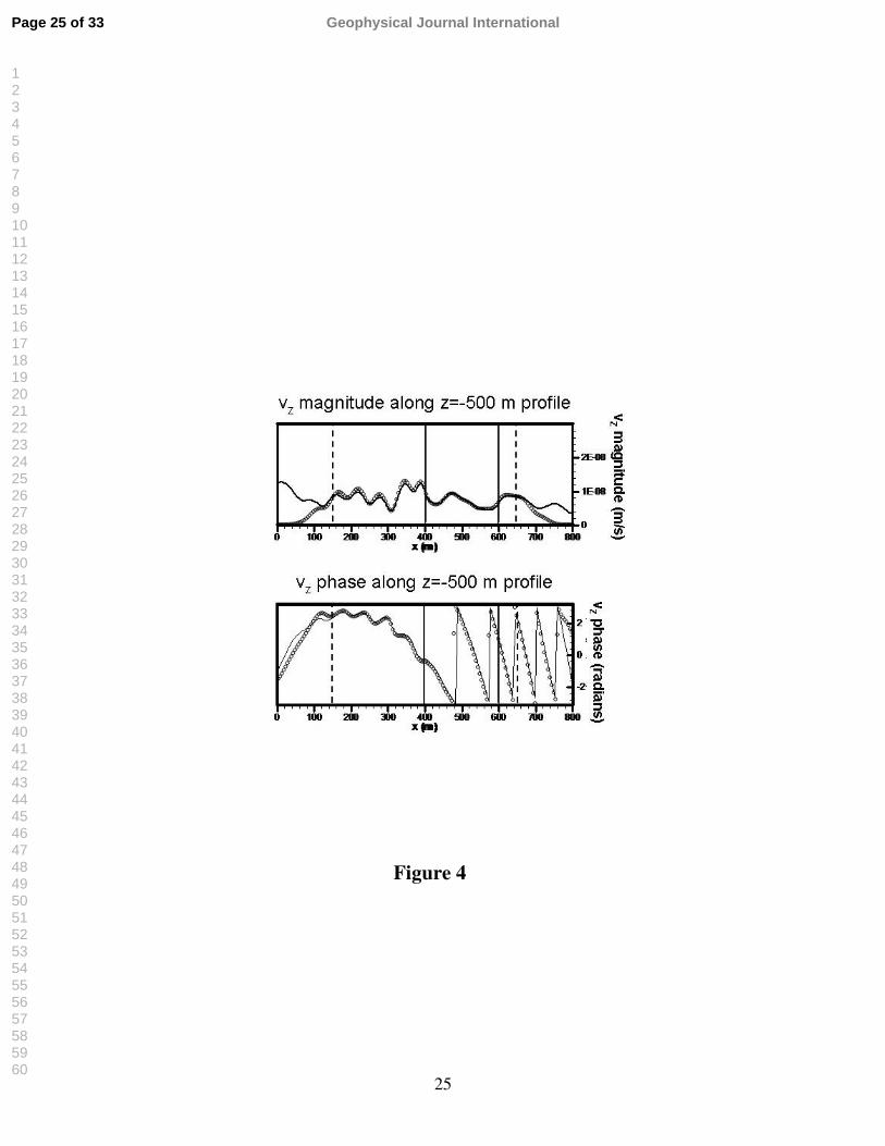
Detailed comparisons of the magnitude and phase along the profile at z = -500 m are displayed in Fig.

4. The agreement between the BEM and finite difference TD-PSD magnitudes and phases is very good in

the region interior to the absorbing boundaries of the finite difference model.

2.3 SEG/EAGE salt model example

The subsurface can exhibit a range of complexities for elastic waves, including multi-scale

heterogeneities, anisotropy, and attenuation. To be of practical value, the TD-PSD approach must be

capable of computing the frequency response in earth models with realistic complexity. In this section,

TD-PSD is used to extract the frequency response of elastic waves propagating in the 2D SEG/EAGE salt

model (Aminzadeh et al. 1994).


123456789101112131415161718192021222324252627282930313233343536373839404142434445464748495051525354555657585960

For Peer Review

7

The 2D SEG/EAGE salt model contains a high velocity salt body embedded in faulted and variable

thickness sediments typical of the Gulf of Mexico (Fig. 5). The model is isotropic with a constant density

(2450 kg/m3) and a constant Poisson’s ratio (ν = 0.25). The 16.2×3.7 km finite difference model was

discretized into 12.2×12.2 m cells to form a 1324×300 mesh. A stress-free boundary condition was set at

the top of the model to represent the surface of the ocean. A 30 Hz cosine wave (tapered on its leading

edge) was injected 3.7 m below the ocean surface at location x = 3.7 km. The finite difference

simulations on this model were carried out to 41 s with a time step of 1.5 ms using an O(2,4) viscoelastic

staggered grid finite difference TD code (Robertsson et al. 1994).

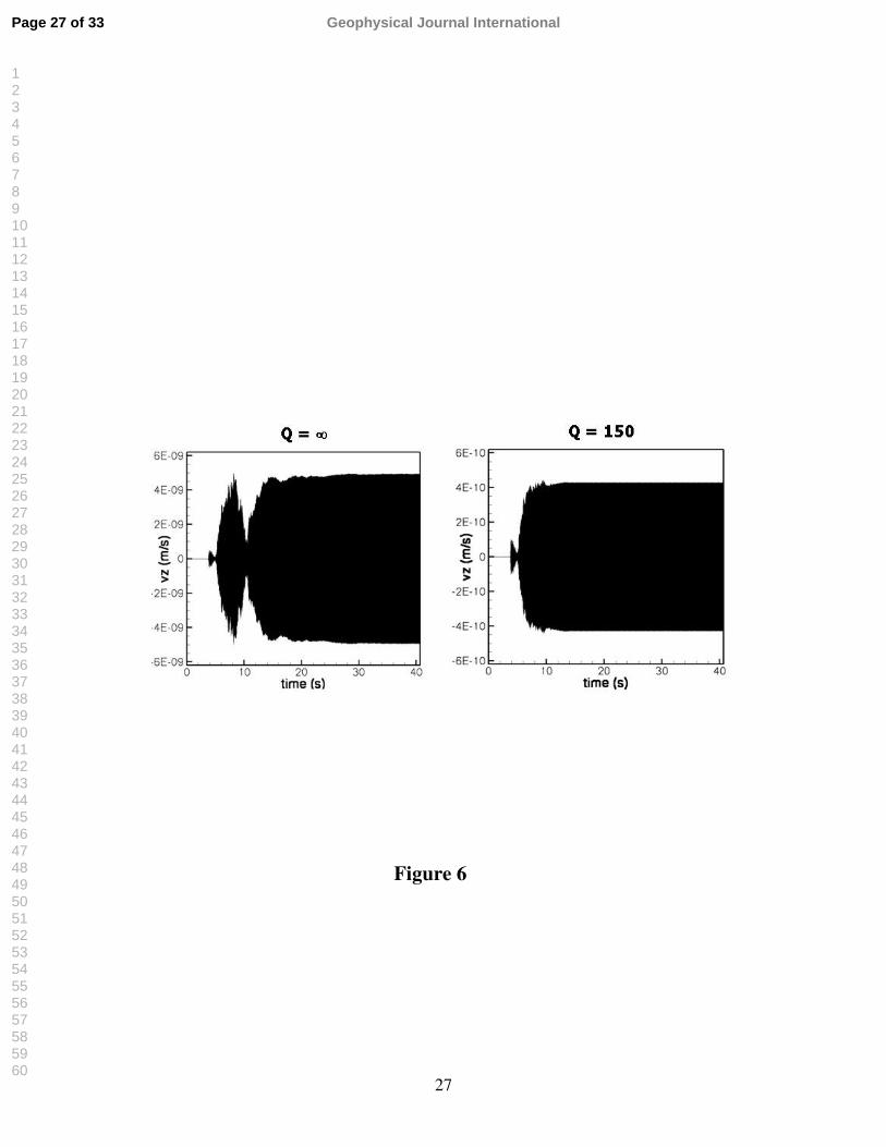
Traces for a receiver located in the bottom right-hand corner of the model (x = 15.1 km, z = 3.1 km)

are displayed in Fig. 6 for two values of attenuation: Q = ∞ (zero attenuation) and Q = 150 (considered

near the upper bound of Q values for Gulf of Mexico sediments). This result demonstrates the long times

required to achieve steady-state (i.e., simple harmonic motion) in a purely elastic model. In fact, the

traces in Fig. 6 show that a steady-state condition is not achieved in the 41 s simulation time for the Q = ∞

model, while it is achieved at ~15 s in the Q = 150 model. Thus, incorporating realistic Q values in the

model can significantly reduce the number of time steps required to achieve steady-state conditions.

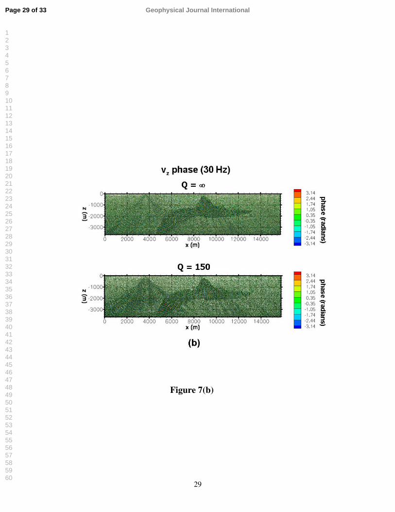
The magnitude and phase of the vertical particle velocity were computed at every cell in the finite

difference model, and are displayed in Fig. 7 for the two Q values. As expected, attenuation has a strong

effect on the spatial decay of the magnitude away from the source, while the corresponding phase changes

are more subtle.

3 MULTI-SOURCE MODELING USING TD-PSD WITH FREQUENCY-ENCODED SOURCES

Frequency response measurements by a lock-in detector are made possible by the PSD’s ability to

accurately isolate the frequency response at the specified frequency while rejecting contributions from

other frequencies (Stanford Research Systems 1999). This feature can be exploited in finite difference

TD-PSD modeling to compute the frequency response at multiple frequencies from a single run by

superimposing multiple frequencies at the source or to compute the frequency response for multiple


123456789101112131415161718192021222324252627282930313233343536373839404142434445464748495051525354555657585960

For Peer Review

8

sources by encoding each with a slightly different frequency. Multi-frequency PSD is described in further

detail below.

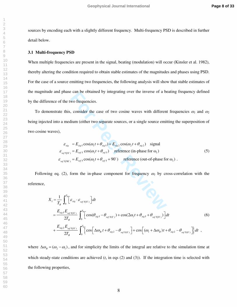
3.1 Multi-frequency PSD

When multiple frequencies are present in the signal, beating (modulation) will occur (Kinsler et al. 1982),

thereby altering the condition required to obtain stable estimates of the magnitudes and phases using PSD.

For the case of a source emitting two frequencies, the following analysis will show that stable estimates of

the magnitude and phase can be obtained by integrating over the inverse of a beating frequency defined

by the difference of the two frequencies.

To demonstrate this, consider the case of two cosine waves with different frequencies ω1 and ω2

being injected into a medium (either two separate sources, or a single source emitting the superposition of

two cosine waves),

1 2 2 2

1 10 )

1 190 )

cos( ) cos( ) signal

cos( ) reference (in-phase for ω )

cos( 90 ) reference (out-of-phase for ω ) .

sig sig sig sig sig

ref refref

ref refref

E t E t

E t

E t

ε ω θ ω θ

ε ω θ

ε ω θ

= + + +

= +

= + +

o

o

o

1 1

1 11(

1 11(

(5)

Following eq. (2), form the in-phase component for frequency ω1 by cross-correlation with the

reference,

{ }

1 0 )0

0 )1(0 ) 0 )

0

2 0 )2 1 2(0 ) (0 )

0

1

cos( ) cos(2 )2

cos cos ( ) ,2

B

B

B

T

sig refB

Tsig ref

sig sigref refB

Tsig ref

B sig B sigref refB

X dtT

E Et dt

T

E Et t dt

T

ε ε

θ θ ω θ θ

ω θ θ ω ω θ θ

= ⋅

= − + + +

+ ∆ + − + + ∆ + −

∫

∫

∫

o

o

o o

o

o o

1(

1 1(1 11 1(

1(

1 1

(6)

where 2 1( )Bω ω ω∆ = − , and for simplicity the limits of the integral are relative to the simulation time at

which steady-state conditions are achieved (ts in eqs (2) and (3)). If the integration time is selected with

the following properties,


123456789101112131415161718192021222324252627282930313233343536373839404142434445464748495051525354555657585960

For Peer Review

9

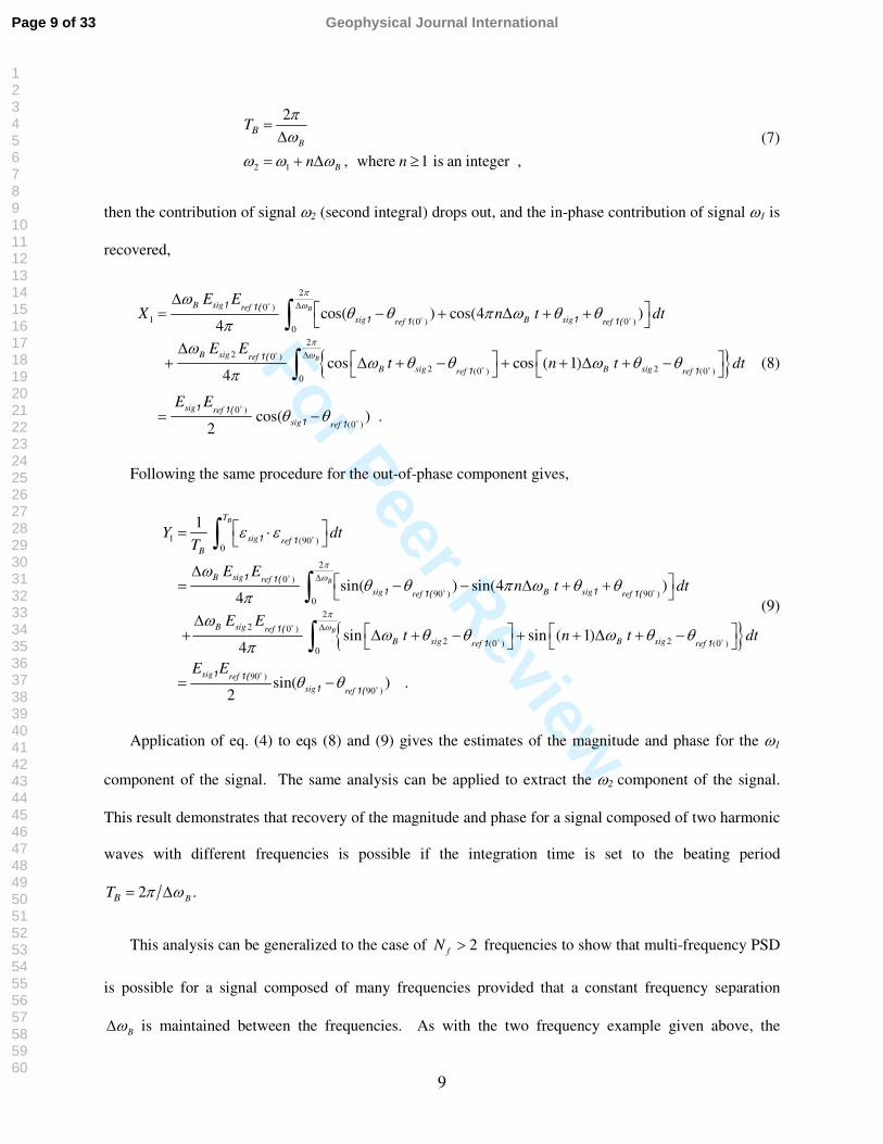
2 1

2

, where 1 is an integer ,B

B

BT

n n

πω

ω ω ω

=∆

= + ∆ ≥ (7)

then the contribution of signal ω2 (second integral) drops out, and the in-phase contribution of signal ω1 is

recovered,

{ }

2

0 )1 (0 ) 0 )

02

2 0 )2 2(0 ) (0 )

0

0 )

cos( ) cos(4 )4

cos cos ( 1)4

cos(2

B

B

B sig refsig B sigref ref

B sig refB sig B sigref ref

sig refsig

E EX n t dt

E Et n t dt

E E

πω

πω

ωθ θ π ω θ θ

πω

ω θ θ ω θ θπ

θ θ

∆

∆

∆ = − + ∆ + +

∆ + ∆ + − + + ∆ + −

= −

∫

∫

o

o o

o

o o

o

1 1(1 11 1(

1(

1 1

1 1(1 (0 )

) .ref o1

(8)

Following the same procedure for the out-of-phase component gives,

{ }

1 (90 )0

2

0 )

90 ) 90 )0

22 0 )

2 2(0 ) (0 )0

1

sin( ) sin(4 )4

sin sin ( 1)4

B

B

T

sig refB

B sig refsig B sigref ref

B sig refB sig B sigref ref

Y dtT

E En t dt

E Et n t

πω

π

ε ε

ωθ θ π ω θ θ

πω

ω θ θ ω θ θπ

∆

∆

= ⋅

∆ = − − ∆ + +

∆ + ∆ + − + + ∆ + −

∫

∫

o

o

o o

o

o o

1 1

1 1(1 11( 1(

1(

1 1

90 )

90 )sin( ) .

2

B

sig refsig ref

dt

E E

ω

θ θ= −

∫o

o

1 1(1 1(

(9)

Application of eq. (4) to eqs (8) and (9) gives the estimates of the magnitude and phase for the ω1

component of the signal. The same analysis can be applied to extract the ω2 component of the signal.

This result demonstrates that recovery of the magnitude and phase for a signal composed of two harmonic

waves with different frequencies is possible if the integration time is set to the beating period

2 BBT π ω= ∆ .

This analysis can be generalized to the case of 2fN > frequencies to show that multi-frequency PSD

is possible for a signal composed of many frequencies provided that a constant frequency separation

Bω∆ is maintained between the frequencies. As with the two frequency example given above, the


123456789101112131415161718192021222324252627282930313233343536373839404142434445464748495051525354555657585960

For Peer Review

10

constant frequency separation for the 2fN > case allows the PSD integration over 2B BT π ω= ∆ to

accurately recover the magnitudes and phases for each frequency component contained in the signal.

3.2 Frequency-encoded sources

Recent work on finite difference frequency domain migration and full-waveform inversion (Mulder &

Plessix 2004; Sirgue & Pratt 2004) demonstrate that subsurface imaging of structure and properties is

possible with far-fewer frequencies ( 10fN < ) than prescribed by Nyquist theorem. This work has also

demonstrated that a scale approach to frequency domain inversion in which the inversion is progressed

from low frequency to high better ensures convergence to the global solution. Because seismic reflection

surveys can have hundreds (2D) to thousands (3D) of spatially-distributed sources and in order to

preserve the scale approach, it is desirable to have a frequency response seismic modeling engine that can

efficiently model many sources around a narrow frequency band.

The multi-frequency PSD described in 3.1 offers the possibility of obtaining the frequency response

from many sources in a single finite difference TD simulation by encoding each source with a different

frequency. As discussed in the previous section, for more than two frequencies, each frequency should be

separated by a constant Bf∆ in order for the PSD integration to accurately recover the magnitude and

phase.

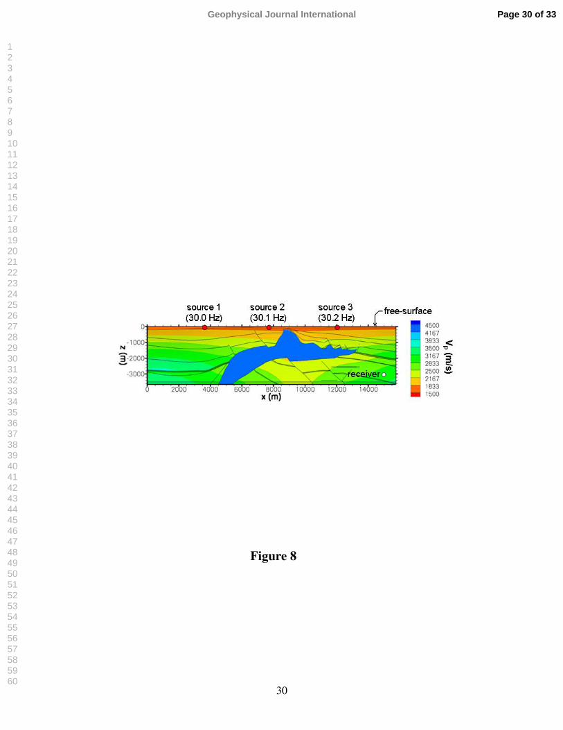
Fig. 8 shows the layout for three frequency-encoded sources propagating in the SEG/EAGE salt

model (Q = 150). In this model, the sources have frequencies 30Hz Bf n f= + ∆ , where 0,1,2n = and

0.1 HzBf∆ = . Fig. 9 shows the trace recorded at the receiver located in the bottom right corner of the

model (Fig. 8). Comparison of Fig. 9 with the trace from the single source simulation (Fig. 6) shows the

1 10sB BT f= ∆ = beating resulting from the superposition of the three frequencies. The magnitude and

phase of the vertical particle velocity were computed at every grid location in the finite difference model.

These values were then used to reconstruct a snapshot of the time-harmonic wavefield (Fig. 10) using eq.


123456789101112131415161718192021222324252627282930313233343536373839404142434445464748495051525354555657585960

For Peer Review

11

(1). Clear separation of the wavefields for each source can be seen, indicating that the PSD is capable of

extracting the wavefield from each source, with negligible contributions from the other sources.

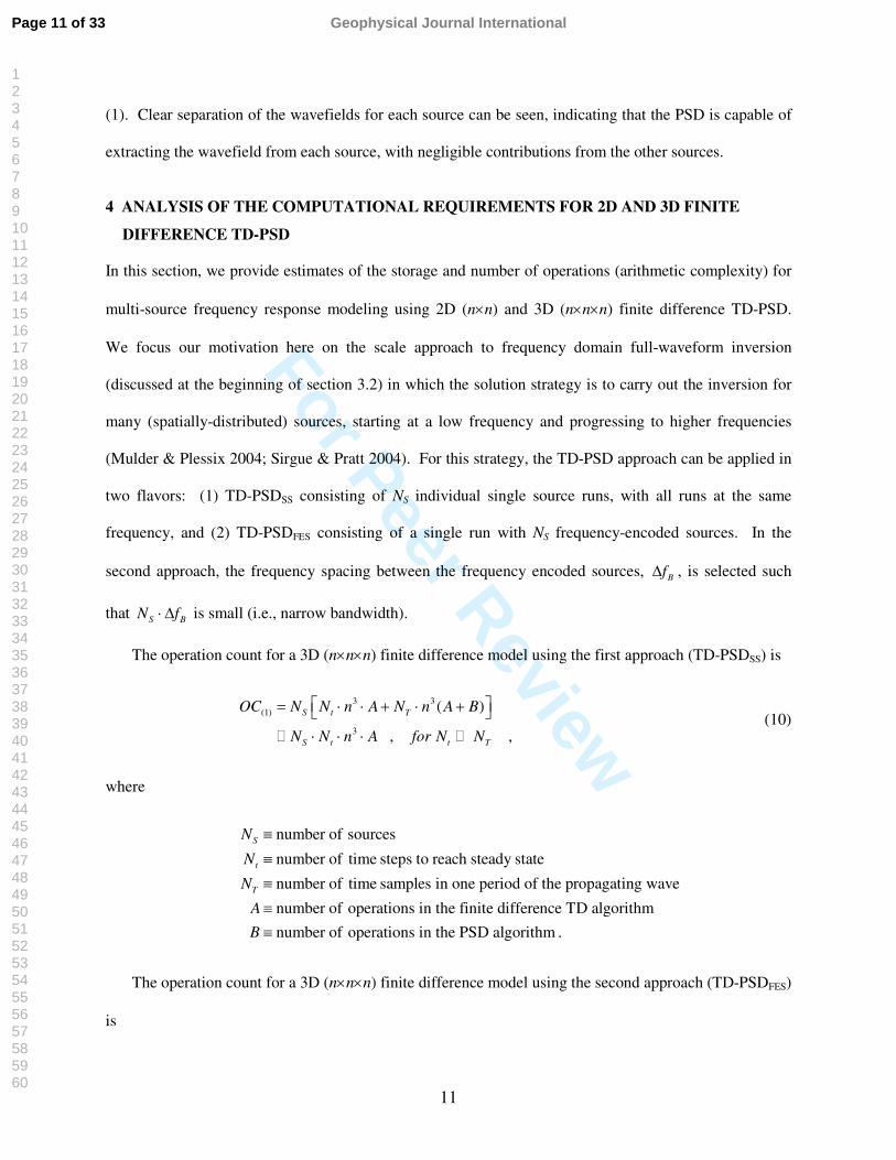
4 ANALYSIS OF THE COMPUTATIONAL REQUIREMENTS FOR 2D AND 3D FINITE

DIFFERENCE TD-PSD

In this section, we provide estimates of the storage and number of operations (arithmetic complexity) for

multi-source frequency response modeling using 2D (n×n) and 3D (n×n×n) finite difference TD-PSD.

We focus our motivation here on the scale approach to frequency domain full-waveform inversion

(discussed at the beginning of section 3.2) in which the solution strategy is to carry out the inversion for

many (spatially-distributed) sources, starting at a low frequency and progressing to higher frequencies

(Mulder & Plessix 2004; Sirgue & Pratt 2004). For this strategy, the TD-PSD approach can be applied in

two flavors: (1) TD-PSDSS consisting of NS individual single source runs, with all runs at the same

frequency, and (2) TD-PSDFES consisting of a single run with NS frequency-encoded sources. In the

second approach, the frequency spacing between the frequency encoded sources, Bf∆ , is selected such

that S BN f⋅ ∆ is small (i.e., narrow bandwidth).

The operation count for a 3D (n×n×n) finite difference model using the first approach (TD-PSDSS) is

3 3(1)

3

( )

, ,

S t T

S t t T

OC N N n A N n A B

N N n A for N N

= ⋅ ⋅ + ⋅ + ⋅ ⋅ ⋅� �

(10)

where

number of sources

number of time steps to reach steady state

number of time samples in one period of the propagating wave

number of operations in the finite difference TD algorithm

number of operations in th

S

t

T

N

N

N

A

B

≡

≡≡≡≡ e PSD algorithm .

The operation count for a 3D (n×n×n) finite difference model using the second approach (TD-PSDFES)

is


123456789101112131415161718192021222324252627282930313233343536373839404142434445464748495051525354555657585960

For Peer Review

12

3 3(2)

3

( )

1 1 ,

t T S

T

t St

B

B

OC N n A N n A N B

N BN n A N

N A

= ⋅ ⋅ + ⋅ + ⋅

= ⋅ ⋅ + +

(11)

where TB BN T t= ∆ is the number of time steps in one beat cycle.

The ratio between eqs (10) and (11) has the form

(1)

(2) 1 1

.1

1 1

S

T

St

S

SB t

B

OC NR

NOC BN

N A

N

BN

f t N A

= + +

+ + ∆ ∆

�

�

(12)

When eq. (12) is plotted as a function of the number of sources SN and the product S BN f∆ (i.e., the

frequency bandwidth occupied by the SN sources each separated by Bf∆ ), a trade-off curve results (Fig.

11). This curve illustrates that if it is desirable to keep the frequency spread between the first and last

source in the simulation to a minimum (i.e., a small value of S BN f∆ ), as in the strategy for frequency

domain full-waveform inversion discussed at the beginning of section 3.2, then there is an optimum

number of sources that can be used in TD-PSDFES to achieve the maximum speed-up over TD-PSDSS. For

an assumed ratio of ( / ) 1/10B A = and an upper bound of 5 HzS BN f∆ = , the TD-PSDFES speed-up is

~10× when 15-40 sources are used. Because the model size has dropped out of the ratio eq. (12), this

result also holds for 2D TD-PSDFES.

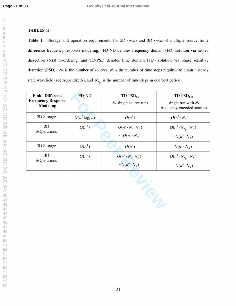
Table 1 gives the computational efficiency (big-O) estimates for both flavors of TD-PSD for the

multiple source problem. Note that these order of magnitude estimates do not reflect the smaller gains

described in eq. (12), i.e., both flavors of TD-PSD have the same operation counts. Also note that for

problems with many sources, TD-PSDFES requires SN more storage for the additional magnitude and

phase fields for each source.


123456789101112131415161718192021222324252627282930313233343536373839404142434445464748495051525354555657585960

For Peer Review

13

Also shown in Table 1 for reference are the estimates of storage and number of operations for direct

solution of the finite difference frequency domain equations by LU-factorization with the nested

dissection reordering method (FD-ND; George & Liu 1981). For 2D problems with many sources, FD-

ND is an effective solution strategy: both TD-PSDSS and TD-PSDFES require a factor NS more operations

than FD-ND, but TD-PSDSS has lower storage requirements. For 3D problems, both TD-PSD approaches

have significantly lower number of operations than FD-ND. TD-PSDSS is superior to both TD-PSDFES

and FD-ND in storage requirements.

The storage and operation count estimates in Table 1 suggest that for most 2D frequency

response modeling problems (many sources, ample memory), FD-ND is the method of choice.

For large, memory-limited 3D problems (e.g., 10,000×2,500×2,500) typical in seismic

exploration, multi-source frequency response modeling is best addressed with TD-PSDSS, i.e., by

running NS single source TD-PSD runs.

5 SUMMARY

This paper presents an approach for computing the frequency response of realistic earth models using an

explicit finite difference time domain (TD) code and a phase sensitive detection (PSD) algorithm. In the

TD-PSD approach, the frequency response of seismic waves is computed by running the finite difference

TD code with a harmonic wave source out to steady-state, and then extracting the magnitude and phase

from the transient data via a cross-correlation with in-phase and out-of-phase reference cosine waves.

The PSD algorithm requires integration over a single cycle of the waveform to obtain accurate phase and

magnitude estimates. Because this integration is performed by a running summation over time, it is not

necessary to store waveforms at the grid locations, as would be the case if an FFT was used.

Comparisons of the finite difference TD-PSD approach with a frequency domain boundary element

method (BEM) solution demonstrate the accuracy of this approach. Simulations in the SEG/EAGE salt

model demonstrate the importance of including (realistic) attenuation in the model to reduce the time


123456789101112131415161718192021222324252627282930313233343536373839404142434445464748495051525354555657585960

For Peer Review

14

required to achieve steady state conditions (simple harmonic motion). It was demonstrated that the TD-

PSD approach can be used to obtain the frequency response of multiple sources in a single finite

difference TD run by encoding each source with a different frequency (TD-PSDFES). The presence of

multiple sources gives rise to beating, and analysis of the multi-frequency PSD demonstrates that the PSD

integration must be made over the beat period of the interfering waves to accurately recover the

magnitude and phase.

Analysis of the operation counts suggests that significant speed-ups can be achieved with the

frequency-encoded source approach TD-PSDFES relative to the more conventional TD-PSDSS approach

where separate single source runs are performed. Analysis of the storage for TD-PSDFES, however,

indicates that this approach requires significantly more memory to store the magnitude and phase fields

for all the sources. For large 3D problems, this additional storage may render the TD-PSDFES approach

intractable. The analysis shows that the straightforward TD-PSDSS approach of running separate finite

difference models for each source is the best approach for 3D frequency response modeling, with

significantly lower storage and operations than a direct solution of the finite difference frequency domain

equations using nested dissection re-ordering (FD-ND). Further work is required to examine the

performance of TD-PSD in realistic 3D earth models, and to investigate potential avenues for increasing

its computation efficiency.

ACKNOWLEDGMENTS

This work was supported by the Director, Office of Science, Office of Basic Energy Sciences, Division of

Chemical Sciences, Geosciences, and Biosciences of the U.S. Department of Energy under Contract No.

DE-AC03-76SF00098. We thank Jonathan Ajo-Franklin, Valeri Korneev, and Joe Stefani for insightful

discussions on monochromatic waves, and the reviewers for improving the content and readability of the

paper.


123456789101112131415161718192021222324252627282930313233343536373839404142434445464748495051525354555657585960

For Peer Review

15

REFERENCES

Aminzadeh, F., Burkhard, N., Nicoletis, L., Rocca, F. & Wyatt, K., 1994. SEG/EAGE 3-D modeling

project: 2nd update, The Leading Edge, 13, 949-952.

Barrett, R., Michael, B., Chan, T.F., Demmel, J., Donato, J., Dongarra, J., Eijkhout, V., Pozo, R., Romine,

C. & van der Vorst, H., 1994. Templates for the Solution of Linear Systems: Building Blocks for

Iterative Methods, SIAM, Philadelphia.

Furse, C.M., 2000. Faster than Fourier-ultra-efficient time-to-frequency domain conversions for FDTD

simulations, Antennas & Propagation Mag., 42, 24-34.

George, J.A. & Liu, J.W.H., 1981. Computer Solution of Large Sparse Positive Definite Systems,

Prentice-Hall, New Jersey.

Hustedt, B., Operto, S. & Virieux, J., 2004. Mixed-grid and staggered-grid finite-difference methods for

frequency-domain acoustic wave modelling, Geophys. J. Int., 157, 1269-1296.

Kinsler, L.E., Frey, A.R., Coppens, A.B. & Sanders, J.V., 1982. Fundamentals of Acoustics, 3rd edn, pp.

20-23, John Wiley & Sons, New York.

Levander, A.R., 1988. Fourth-order finite-difference P-SV seismograms, Geophysics, 53, 1425-1436.

Li, X.S. & Demmel, J., 2003. SuperLU_DIST: A scalable distributed-memory sparse direct solver for

unsymmetric linear systems, ACM Trans. on Mathematical Software, 29, 110-140.

http://crd.lbl.gov/~xiaoye/SuperLU/

Marfurt, K.J., 1984, Accuracy of finite difference and finite element modeling of the scalar and elastic

wave equations, Geophysics, 49, 533-549.

Mulder, W.A. & Plessix, R.-E., 2004. How to choose a subset of frequencies in frequency-domain finite-

difference migration, Geophys. J. Int., 158, 801-812.


123456789101112131415161718192021222324252627282930313233343536373839404142434445464748495051525354555657585960

http://crd.lbl.gov/%7Exiaoye/SuperLU/

For Peer Review

16

Nihei, K.T., 2005. BE2D: A 2D Boundary Element Code for Computing the Frequency Response of

Elastic Waves in Heterogeneous Media with Imperfect Interfaces, Lawrence Berkeley National

Laboratory Report, LBNL-58685, Berkeley.

Plessix, R.E. & Mulder, W.A., 2003. Separation-of-variables as a preconditioner for an iterative

Helmholtz solver, Applied Numerical Mathematics, 44, 385-400.

Pratt, R.G., Shin, C. & Hicks, G.J., 1998. Gauss-Newton and full Newton methods in frequency space

seismic waveform inversion, Geophys. J. Int., 133, 341-362.

Press, W.H., Teukolsky, S.A., Vetterling, W.T. & Flannery, B.P., 1992. Numerical Recipes in C, 2nd edn,

pp. 504, Cambridge University Press, Cambridge.

Robertsson, J.O.A, Blanch, J.O. & Symes, W.W., 1994. Viscoelastic finite-difference modeling,

Geophysics., 59, 1444-1456.

Sirgue, L. & Pratt, R.G., 2004. Efficient waveform inversion and imaging: A strategy for selecting

temporal frequencies, Geophysics, 69, 231-248.

Stanford Research Systems, 1999. DSP Lock-In Amplifier Model 850, Rev. 1.4.

http://www.thinksrs.com/downloads/PDFs/Manuals/SR830m.pdf

Štekl, I. & Pratt, R.G., 1998. Accurate viscoelastic modeling by frequency-domain finite differences using

rotated operators, Geophysics, 63, 1779-1794.

APPENDIX A: Demonstration that Nt ~ O(n)

Let the number of time steps that a 2D (n×n) or 3D (n×n×n) finite difference TD code must be run to in

order to attain steady-state wavefields (i.e., simple harmonic motion) be defined as

St

tN

t=∆

. (A1)


123456789101112131415161718192021222324252627282930313233343536373839404142434445464748495051525354555657585960

http://www.thinksrs.com/downloads/PDFs/Manuals/SR830m.pdf

For Peer Review

17

In eq. (A1), St is selected large enough to include the slowest arrivals coming from the most distant parts

of the model. As a conservative estimate, we take this to be the travel time it takes a shear wave to

propagate across five lengths 5L of the largest model dimension at the slowest shear velocity cSmin

contained in the model

min min

5 5S

S S

L n lt

c c

∆= = , (A2)

where l∆ is the grid size. We will see at the end of this analysis that doubling or tripling this distance

estimate will not alter the final result. The time step t∆ is prescribed by the stability condition for a

fourth order spatial differencing scheme (Levander 1988)

max

max0,1

0.6061 /2

P

P ii

lt l c

c c=

∆∆ ≤ = ∆

∑ , (A3)

where c0= 9/8 and c1= -1/24 are the inner and outer coefficients of the fourth order approximation to the

first derivative.

Substituting eqs (A2) and (A3) into eq. (A1) gives

min max

5

0.6061( / )tS P

nN

c c= ~ O(n) . (A4)

Because “big-O” notation operation estimates are essentially proportionality estimates for large inputs

(i.e., large n), it is clear that the relation (A4) still holds even if we had used a larger estimate of the

maximum propagation path.


123456789101112131415161718192021222324252627282930313233343536373839404142434445464748495051525354555657585960

For Peer Review

18

FIGURE LEGENDS (11)

Figure 1. Snapshots of the vertical particle velocity taken at ωt=π: (left) BEM, and (right) reconstructed

from the TD-PSD computed magnitudes and phases. The model consists of a higher velocity 200×200 m

square inclusion (VP = 4000 m/s, VS = 2406 m/s, ρ = 2200 kg/m3) embedded in an infinite space (VP =

3300 m/s, VS = 1700 m/s, ρ = 2350 kg/m3). The source is a vertical body force driven at 30 Hz. The

results show very close agreement except in the outer 150 m of the finite difference time domain model

(region outside the dashed lines) where absorbing boundaries are applied.

Figure 2. Finite difference time domain particle velocity (vertical component) at a location x = 200 m, z

= -600 m: (solid) recorded, and (dotted) reconstructed from the TD-PSD computed magnitude and phase.

The arrows indicate integral multiples of the wave period T where the PSD integration “locks-in” to the

correct particle velocity magnitude and phase.

Figure 3. Comparison of the magnitude and phase fields of the vertical particle velocity computed by:

(left column) BEM, and (right column) TD-PSD. The magnitude fields are displayed in the upper row,

and the phase fields in the lower row. The dashed box in the TD-PSD figures indicates the location of the

absorbing boundaries. The solid horizontal line is the profile along which the fields are compared in Fig.

4.

Figure 4. Detailed comparison of the magnitude and phase of the vertical particle velocity along the

profile z= -500 m computed by: (solid line) BEM, and (circles) TD-PSD. The vertical dashed lines show

the location of the absorbing boundaries in the finite difference model, and the vertical solid lines show

the location of the high velocity inclusion.


123456789101112131415161718192021222324252627282930313233343536373839404142434445464748495051525354555657585960

For Peer Review

19

Figure 5. SEG/EAGE salt model used to test the finite difference TD-PSD approach for estimating the

frequency response. A 30 Hz source is located near the free-surface, and a monitor receiver is embedded

in the bottom-right corner of the model.

Figure 6. The traces recorded at the monitor receiver (Fig. 5). Note that the effect of adding attenuation

to the model (Q = 150) is to significantly reduce the time at which steady-state (simple harmonic motion)

is achieved.

Figure 7. The magnitude (a) and phase (b) fields of the vertical particle velocity computed with finite

difference TD-PSD for two Q values.

Figure 8. SEG/EAGE salt model with the locations of the three sources used in the multi-source test of

TD-PSDFES. The source frequencies used were 30.0, 30.1, and 30.2 Hz.

Figure 9. The trace recorded at the monitor receiver for the frequency-encoded three source example

(Fig. 8). The frequency difference between each of the three sources, 0.1 Hzf∆ = , gives rise to beating

with a period of 10 s.

Figure 10. Vertical particle velocity transient fields at 40 s constructed for each of the three sources from

the TD-PSDFES computed magnitudes and phases. The computed wavefields show a clean separation of

wave motion coming from each source.

Figure 11. Trade-off plot of the speed-up that can be obtained for multiple source frequency response

modeling using frequency encoded sources (TD-PSDFES) relative to the more conventional approach in

which each source is modeled in a separate finite difference run (TD-PSDSS). The trade-off is between


123456789101112131415161718192021222324252627282930313233343536373839404142434445464748495051525354555657585960

For Peer Review

20

the number of frequency-encoded sources and the frequency spread (between the first and last source)

that can be tolerated. The boxed region highlights the range of speed-ups possible with TD-PSDFES for

15-40 sources and a frequency bandwidth of 1-5 Hz.


123456789101112131415161718192021222324252627282930313233343536373839404142434445464748495051525354555657585960

For Peer Review

21

TABLES (1)

Table 1. Storage and operation requirements for 2D (n×n) and 3D (n×n×n) multiple source finite

difference frequency response modeling: FD-ND denotes frequency domain (FD) solution via nested

dissection (ND) re-ordering, and TD-PSD denotes time domain (TD) solution via phase sensitive

detection (PSD). NS is the number of sources, Nt is the number of time steps required to attain a steady

state wavefield (see Appendix A), and TBN is the number of time steps in one beat period.

Finite DifferenceFrequency Response

Modeling

FD-ND TD-PSDSS

NS single source runs

TD-PSDFES

single run with NS

frequency-encoded sources

2D Storage 22( log )O n n 2( )O n 2( )SO n N⋅

2D #Operations

3( )O n 2( )t SO n N N⋅ ⋅

~ 3( )SO n N⋅

2( )T SBO n N N⋅ ⋅

~ 3( )SO n N⋅

3D Storage 4( )O n 3( )O n 3( )SO n N⋅

3D #Operations

6( )O n 3( )t SO n N N⋅ ⋅

~ 4( )SO n N⋅

3( )T SBO n N N⋅ ⋅

~ 4( )SO n N⋅


123456789101112131415161718192021222324252627282930313233343536373839404142434445464748495051525354555657585960

For Peer Review

22

FIGURES (11)

Figure 1


123456789101112131415161718192021222324252627282930313233343536373839404142434445464748495051525354555657585960

For Peer Review

23

Figure 2


123456789101112131415161718192021222324252627282930313233343536373839404142434445464748495051525354555657585960

For Peer Review

24

Figure 3


123456789101112131415161718192021222324252627282930313233343536373839404142434445464748495051525354555657585960

For Peer Review

25

Figure 4


123456789101112131415161718192021222324252627282930313233343536373839404142434445464748495051525354555657585960

For Peer Review

26

Figure 5


123456789101112131415161718192021222324252627282930313233343536373839404142434445464748495051525354555657585960

For Peer Review

27

Figure 6


123456789101112131415161718192021222324252627282930313233343536373839404142434445464748495051525354555657585960

For Peer Review

28

Figure 7(a)


123456789101112131415161718192021222324252627282930313233343536373839404142434445464748495051525354555657585960

For Peer Review

29

Figure 7(b)


123456789101112131415161718192021222324252627282930313233343536373839404142434445464748495051525354555657585960

For Peer Review

30

Figure 8


123456789101112131415161718192021222324252627282930313233343536373839404142434445464748495051525354555657585960

For Peer Review

31

Figure 9


123456789101112131415161718192021222324252627282930313233343536373839404142434445464748495051525354555657585960

For Peer Review

32

Figure 10


123456789101112131415161718192021222324252627282930313233343536373839404142434445464748495051525354555657585960

For Peer Review

33

Figure 11


123456789101112131415161718192021222324252627282930313233343536373839404142434445464748495051525354555657585960

For Peer Review - crd-legacy.lbl.govcrd-legacy.lbl.gov/~xiaoye/KTNihei_GJI.pdf · Frequency response modeling of seismic waves using f inite difference time ... and the integration

Documents