Bergische Universität Wuppertal Faculty of Mathematics and Natural Sciences Department of Food Chemistry _________________________________________________________________________ Food matrices – Impact on odorant partition coefficients and flavour perception Manuela Rusu from Iasi, Romania Inaugural - Thesis for obtaining the Degree of Doctor in Natural Sciences (Dr.rer.nat.) at the Bergische Universität Wuppertal The present work arose on suggestion and under the guidance of Mr. Prof. Dr. Helmut Guth Wuppertal 2006

Welcome message from author
This document is posted to help you gain knowledge. Please leave a comment to let me know what you think about it! Share it to your friends and learn new things together.
Transcript
Bergische Universität Wuppertal
Faculty of Mathematics and Natural Sciences
Department of Food Chemistry
_________________________________________________________________________
Food matrices – Impact on odorant partition coefficients
and flavour perception
Manuela Rusu
from Iasi, Romania
Inaugural - Thesis for obtaining the Degree of Doctor in Natural Sciences (Dr.rer.nat.)
at the Bergische Universität Wuppertal
The present work arose on suggestion and under the guidance of
Mr. Prof. Dr. Helmut Guth
Wuppertal 2006

Die Dissertation kann wie folgt zitiert werden:
urn:nbn:de:hbz:468-20070067[http://nbn-resolving.de/urn/resolver.pl?urn=urn%3Anbn%3Ade%3Ahbz%3A468-20070067]

The work described in this thesis was carried out in the Department of Food Chemistry,
Bergische Universität Wuppertal, under the scient ific supervision of Prof. Dr. Helmut Guth,
during the period of January, 2001-November, 2006.
Referee: Prof. Dr. Helmut Guth
Co-referee: Prof. Dr. Walter Reineke

sotului meu, Vasile
si
fiicei noastre, Delia
ACKNOWLEDGMENTS
No work is ever the making of one single person. Hereby I would like to thank all the persons
who have contributed directly or indirectly to my work and to this thesis.
First, I would like to thank my supervisor, Prof. Dr. Helmut Guth for offering me the PhD
position in his group and for his guidance, and supporting me during all these years, making
this study possible. I would like to express my gratitude for his patience, understanding and
constructively critical eye; all these have always helped me find my way through the critical
moments of my research.
I am very grateful to Prof. Dr. Walter Reineke for agreeing to take the time to evaluate this
thesis as a co-referee.
Completing a PhD is truly a marathon event, and I would not have been able to complete this
journey without the aid and support of my former and present colleagues over the past five
years. I would like to thank them for their help and friendship, and for the pleasant work
atmosphere.
I thank always Mrs. Henny Usmawati for some data she put me at disposal from her research
project, accomplished in the framework of Cost Action 921.
A special thanks goes to families Hauser and Schulz who accepted me in their house. They
have been beside me every time I need them, making me easier this period, here, in
Wuppertal.
I would also like to thank my entire family for the support they provided, from the distance,
through my period here, and for being spiritually always near by me.
My final, but not least, and most heartfelt acknowledgment must go to my daughter Delia and
my husband Vasile, for their support and patience, during these years. We have endured our
separation and I would not be at this point without their encouragement and understanding.
ABSTRACT
Foods are complex multi-component systems which are composed of volatile and non-volatile
substances. The flavour profile of a food is an important criterion for the selection of our
foodstuffs.
The main objective of this study was the clarification of the complex relationships of the
flavour release as a function of the composition of the food matrix at molecular level.
Therefore the influence of matrix effects onto the partition coefficients, odour activity values
and sensory properties of selected flavour compounds, in model and in real food systems were
investigated. Different matrices were selected to measure their influence onto the partition
coefficients of odorants: water, water-ethanol-mixtures, matrices containing lipids and more
complex samples, such as mixtures of water, oil, proteins and polysaccharides.
The studies included a series of lactones, esters and alcohols (γ-octalactone, γ-nonalactone, γ-
decalactone, δ-octalactone, δ -nonalactone, δ -decalactone, ethyl hexanoate and ethyl
octanoate, 3-methyl-1-butanol and 2-phenylethanol).
The vapour pressures and partition coefficients were determined using static headspace gas
chromatography (HS-GC) techniques. The influence of the model systems on the adsorptions
of the odorants at the gas-tight syringes were taken into account. The results obtained, showed
that the vapour pressures of the flavour compounds are decreasing with the increasing of the
molecular weight of the compounds. The comparison of water/air partition coefficients
(logPW/A) with miglyol/air partition coefficients of selected odorants (logPM/A) showed that
for miglyol system, the logPM/A are higher than the logPW/A for all flavour compounds studied.
The measurement of the partition coefficients of selected aroma compounds in water-oil
matrices (emulsions) revealed that the fat content of emulsions influence significantly the
partition coefficients of odorants. The highest partition coefficients were obtained in
emulsions where the portion between water/miglyol/emulsifier was: 47.5 + 47.5 + 5, w/w/w.
In the present study the flavour release of different aroma compounds (ethyl hexanoate and S-
(-)-limonene) in carbohydrate-water solutions was examined. The static headspace method
allows the measurement of the released odour components that interact with β -cyclodextrin.
The HS-GC analysis of β -cyclodextrin-water/odorant mixtures showed a reduction of the
odorant in presence of the carbohydrate.
The influence of the various matrices on the human biological response of odorants was
investigated by an olfactometer (e.g. determination of the threshold values of odorants in air
and in the presence of ethanol) and the headspace odour activity values (HOAV’s) were
calculated. The results showed that the threshold values in air in absence of ethanol were
lower than the values in presence of ethanol, which means the presence of ethanol in the
matrix increase the threshold value of the odorant.
The studies also included the influence of wine matrix onto the partition coefficients of
important wine flavour compounds. The quantification of the aroma compounds in white
wine samples was achieved by isotope dilution analyses and standard addition method.
Odorants in the headspace above wines were analysed by HS-GC techniques and the partition
coefficients (wine/air) calculated. The results pointed out that the presence of ethanol in wine
matrix does not influence the partition coefficients of selected aroma compounds. The highest
partition coefficients in wines were found for the two alcohols: 2-phenylethanol and 3-
methyl-1-butanol.
Concerning COST Action 921 custard samples were investigated as real foodstuff and the
aroma compounds were quantified in the matrix and in the headspace above the food. The
research data indicated that the partition coefficients custard/air are located between the
partition coefficients water/air and partition coefficients miglyol/air, but closer to the
miglyol/air values. Furthermore the mass transfer rates of selected odorants were investigated
in custard- and milk powder/water samples. The values of the mass transfer rate were found
higher in milk powder/water systems than in custard model. Nevertheless the results indicated
that the viscosity of the matrix did not significantly influence the values of mass transfer rate
of selected flavour compounds.
Molecular Modelling methods have been used for the prediction of solvation free energies of
the flavour compounds studied in different model solutions, e.g. water and water-oil systems.
The results showed that the predicted values (Mopac 97) for γ-decalactone, γ-nonalactone and
2-phenylethanol in water are in good agreement with experimentally solvation free energies.

ABBREVIATIONS AEDA Aroma Extract Dilution Analysis
API-MS Atmospheric Pressure Ionisation Mass Spectrometry
CI Chemical Ionization
DHS Dynamic Headspace
EPICS Equilibrium Partitioning in Closed Systems
FID Flame Ionization Detector
GC Gas Chromatography
GLC Gas Liquid Chromatography
GCO Gas Chromatography Olfactometry
GCMS Gas Chromatography-Mass Spectrometry
HLB Hydrophilic-Lipophilic Balance
HOAV Headspace Odour Activity Values
HP Hewlett Packard
HS Headspace
HSGC Headspace Gas Chromatography
HS-SPME Headspace Solid Phase Micro Extraction
IDA Isotope Dilution Analysis
MC Monte Carlo
MD Molecular Dynamics
MEP Molecular Electrostatic Potential
MSD Mass Spectrometry Detector
MST Miertus-Scrocco-Tomasi
MS (CI) Mass Spectrometry / Chemical Ionization
MW Molecular Weight
OAV Odour Activity Values
PRV Phase Ratio Variation
QM Quantum Mechanical
QSAR Quantitative Structure-Activity Relationships
PTI Purge and Trap Injector
SCRF Self-Consistent Reaction Field
SFI Solid Fat Index
SIDA Stable Isotope Dilution Assays

SHA Static Headspace Analyse
SPME Solid Phase Micro Extraction
SHA-O Static Headspace Analysis-Olfactometry
SHS Static Headspace
TCT Thermal Desorption Cold Trap Injector
VPC Vapor Phase Calibration
VOC Volatile Organic Compound

I
CONTENTS ________________________________________________________________________
1. INTRODUCTION……………………………………………………………1
1.1. Effect of food matrices on flavour release and perception…………………………....1
1.2. State of the art…………………………………………………………………………5
1.2.1. Methods for the determination of flavour release and partition
coefficients (LogP)…………………………………………….…………….…5
1.2.2. Studies on the physico-chemical parameters of flavour
compounds in model systems and in real food-models of flavour
release………………………………........………………………….....….. 12
1.2.3. Studies on vapour pressure...............................................................................20
1.2.4. Studies on partition coefficients........................................................................23
1.2.5. Odor activity values (OAV)…………………………………………………..29
1.2.6. Matrix effects - β -cyclodextrin / wine containing models and wine
samples…………………………………...............................................……..31
1.2.7. Molecular modelling studies on the prediction of solvation
free energies of flavour compounds in different model
systems..……………........................................................................................38
1.3. Aims of the work…………………………………………………………………….43
2. EXPERIMENTAL PART…………………………………………………45
2.1. Materials and methods.................................................................................................45
2.1.1. Reference substances........................................................................................45
2.1.2. Instrumentation.................................................................................................48
2.1.2.1. Instrumentation for the preparation of emulsions......................................48
2.1.2.2. Static Headspace Gas Chromatography (SHS-GC)...................................48
2.1.2.3. Instrumentation for the determination of odorant headspace
concentrations in wine samples..................................................................50
2.1.2.4. Mass-spectrometry (MS)............................................................................51
2.1.2.5. Olfactometer...............................................................................................52
2.1.2.6. Software packages......................................................................................53

II
2.2. Determination of physico-chemical parameters of selected aroma
compounds (lactones, esters and alcohols) with static headspace-gas
chromatography (SHS-GC)………………………………….………………………53
2.2.1. Determination of vapour pressure……………………………………………53
2.2.2. Determination of partition coefficients in different matrices………………...55
2.2.2.1. Water / air……………………………………………………….………..55
2.2.2.2. Water-ethanol mixtures / air……………………………………………..55
2.2.2.3. Miglyol/air.................................................................................................56
2.2.2.4. Emulsions (Miglyol-Water-Emulsifier) / air…………………………….56
2.3. Interaction of odorants with β -cyclodextrin………………………………………...57
2.3.1. Condition for the determination of flavour release of ethyl hexanoate in
the presence of β -cyclodextrin.........................................................................57
2.3.2. Condition for the determination of flavour release of S-(-) limonene in
the presence of β -cyclodextrin..........................................................................58
2.4. Determination of partition coefficients of selected flavour compounds
(alcohols and esters) in real food matrix………………………………………….58
2.4.1. Wine matrix……......…………………………..……………………………….58
2.4.2. Custard sample…….....…………………………………..........……………….62
2.5. Determination of odorant threshold values (esters and alcohols) in air and in
presence of ethanol using an Olfactometer……………………….................…….64
3. RESULTS AND DISCUSSION………………………………………….66
3.1. Determination of the adsorption effects of odorants at the gas-tight
syringe……………………………………………………………………………..66
3.2. Determination of the vapour pressures of selected aroma compounds
and comparison with literature data………………………………………………68
3.3. The influence of the matrix effects onto the partition coefficients
of selected aroma compounds (model systems: water, water-ethanol,
miglyol, and miglyol-water emulsions)……………………………………………69
3.4. The influence of β -cyclodextrin onto the headspace concentration of
aroma compounds selected (ethyl hexanoate and S-(-) limonene)………………..83
3.5. The influence of the food matrix onto the partition coefficients of
selected flavour compounds……………………………………………………….86
3.5.1. Wine matrix…………………………………………………………………86

III
3.5.1.1.Influence of ethanol on the partition coefficients………………………90
3.5.2. Custard sample……………………………………………………………..91
3.5.2.1.Determination of mass transfer coefficients of some
flavour compounds studied, in custard- and milk
powder/water samples…………………………………………………100
3.6. The influence of the matrix effects onto the odour activity values of
selected flavour compounds………………………………………………………106
3.6.1. Calculation of the headspace odour activity values (HOAV’s)……………107
3.7. Molecular modelling studies for the determination of the free energy of solvation
in different model systems........................................................................................108
3.7.1. In water systems……………………………………………......……………109
3.7.2. In water-oil systems…………………………………………………………109
3.8. Comparison of the solvation free energy calculated by molecular modelling
studies and experimentally values............................................................................ 110
4. CONCLUSIONS………………………………………………………… 113 5. REFERENCES…………………………………………………………... 115
1
1. INTRODUCTION
1.1. Effect of food matrices on flavour release and perception
Foods are complex multi-component systems which are composed of volatile and non-volatile
substances. Flavour is one of the major organoleptic characteristics of food; it depends only
on the nature and quantity of aroma compounds involved.
As Bakker et al. (1996) reported, it is considered that the sensory perception of flavour of a
food forms an important aspect of the enjoyment people get from eating, and hence influences
consumers’ acceptability.
Buck et al. (1991) explained that the flavour sensation is caused by flavour molecules released
into the vapour phase during eating and subsequently transported to the olfactory epithelium.
To perceive an aroma, the flavour compounds need to achieve a sufficiently high
concentration in the vapour phase to stimulate the olfactory receptors.
As Taylor et al. (2000) showed, flavour perception can be defined as:
Flavour perception = aroma + taste + mouth feel + texture + pain/irritation
He mentioned also that’s ideally, to characterise a flavour, it is necessary to measure all these
parameters.
A food’s characteristic flavour and aroma are the result of a complex construct of hundreds of
individual constituent compounds interacting to produce a recognizable taste and aroma.
Milicevic et al. (2002) defined aroma as one of the sensory food characteristics provoked by
physiological phenomena. According to the British Standards Institution definition, aroma is
a combination of taste and odour caused by the experience of pain, heat, cold and sense.
Therefore aroma is a complete and unique experience generated from not only the taste and
odour stimula but from other sensorial receptors too.
Thus, if one or more flavour constituents are altered or diminished, food quality may be
reduced. A reduction in food quality may result from the oxidation of aroma components due
to the ingress of oxygen, or it may be the result of the loss of specific aroma compounds to the
packaging material or environment. Aroma compounds are little molecules with a molecular
weight generally lower than 400 g mol-1 (Souchon et al., 2004). They are characterised by two
main properties: their hydrophobicity and their volatility.
2
The flavour of a food will be characterized by volatiles, the so-called odorants, which were
perceived by the human nose (nasal) and in the mouth-nose space (retro nasal), respectively.
The flavour profile of a food is an important criterion for the selection of our foodstuffs.
The structure of our food, in particular the presence of macromolecules as for example
proteins, fats and polysaccharides, influence the mouth feeling and the extend of the flavour
release.
As Taylor et al. (2004) predicted, there are four levels of interaction that must be taken into
account when analyzing flavour:
• chemical interactions occurring in the food matrix, that may directly affect flavour
perception; physicochemical interactions can change flavour intensity or even
generate new flavours;
• mechanical/structural interactions of the food and mastication with the release of
compounds;
• peripheral physiological interactions; and
• cognitive interactions among tastes, odours and somato-sensations perceived
together.
Kolb et al. (1997) showed that in headspace analysis, the use of the term “matrix” express the
bulk of the sample that contains the volatile compounds to be measured. Usually the matrix is
not a pure compound, but a complex mixture of compounds, some of which may be non-
volatile.
The interaction of the matrix components with the analyte influences its solubility and
partition coefficient. This is called the matrix effect.
If the matrix is a mixture of two (or more) compounds, the distribution of the analyte between
the two phases will depend on the quantitative composition of the matrix, which plays an
important role in controlling flavour release at each step of food product separation and
consumption.
The chemical composition of a food matrix will influence perceived flavour, whether the food
is primarily lipid, protein, carbohydrate or aqueous will affect release of flavour-active
compounds from the matrix (Taylor et al., 2004). Flavours may be dissolved, adsorbed,
bound, entrapped, encapsulated or diffusion limited by food components. Oil interacts with
flavours, changing the concentration of free flavour in the solution and consequently
increasing or decreasing the amount of adsorption.
3
Because many food products are emulsions of fat and water, such as milk and milk products,
the fat content is an important variable in the food matrix.
Davidek et al. (1992) mentioned, that lipids, particularly fats and oils, are the only main
components of foodstuffs which are not water-soluble.
Lipids often interact with water-soluble substances forming unstable products in which the
lipids are bound to non- lipidic moieties mainly or exclusively by physical forces, such as
hydrogen bonds with the polar groups of lipids or hydrophobic forces between non-polar
groups of non- lipidic substances and hydrocarbon chains of lipids.
Lipids interact not only with proteins, but also with other hydrophilic biomacromolecules, for
instance with carbohydrates, and particularly with starch.
The fat/oil content is often reduced in order to increase calorific intake to make food healthier.
Removal or reduction of lipids can lead to an imbalanced flavour, often with a much higher
intensity than the original full fat food (Widder et al., 1996; Ingham et al., 1996).
In fact, lipids adsorb and solubilize lipophilic flavour compounds and reduce their vapour
pressures (Buttery et al., 1971; Buttery et al., 1973). This effect was confirmed by
mathematical models (Harrison et al., 1997), headspace analysis (Schirle et al., 1994), and
sensory analysis (Ebeler et al., 1988; Guyot et al.).
Extensive reviews of the effects of lipids (Hatchwell, 1994; de Roos, 1997; Plug et al., 1993)
on the rate and amount of aroma released have been previously published.
De Roos (1997) reported that in products containing aqueous and lipids phases, a flavour
compound is distributed over three phases: fat (or oil), water and air. Flavour release depends
on oil content, which affects the partition of aroma compounds during the different emulsion
phases (lipid, aqueous, and vapour). Flavour release from the oil/fat phase of a food
proceeded at a lower rate than from the aqueous phase. This was attributed, first to the higher
resistance to mass transfer in fat and oil than in water and, second to the fact that in oil/water
emulsions flavour compounds had initially to be released from the fat into the aqueous phase
before they could be released from the aqueous phase to the headspace.
In the case of emulsions the structure itself has been shown to affect the release rate of flavour
(Overbosch et al., 1991; Salvador et al., 1994).
Overbosch et al. (1991) showed in their model that diffusion from a single phase system and
release is independent of the emulsion type. Their data, using diacetyl at two levels (10 mg/kg
and 20 mg/kg), indicated that the flavour release was twice as fast from oil- in-water
emulsions than from water- in-oil emulsions, which they suggested was a consequence of
using a different emulsifier for each system. In the oil-water emulsion, sodium dodecyl
4
sulphate was used, while in the water-oil emulsion, mono acyl glycerol, and lecithin were
used.
In the investigations of Salvador et al. (1994), the emulsions were made from the same
emulsifier (sugar ester emulsifier S-370, HLB =3) and diacetyl as a model flavour, because it
is a common volatile in high-fat foods. In their experiments, with diacetyl at an initial
concentration of 2 g/litre, the rate of release from the oil- in-water emulsion was 1.5 times
greater than from the water- in-oil emulsion. This difference was due to the emulsifier.
The effects of the primary structural and compositional properties of emulsions on the release
of aroma have been both systematically investigated (van Ruth et al., 2002; Miettinen et al.,
2002).
Van Ruth et al. (2002) examined the influence of compositional and structural properties of
oil- in-water emulsions on aroma release under mouth and equilibrium conditions. The impact
of the lipid fraction, emulsifier fraction, and mean particle diameter on release was
determined for 20 aroma compounds, included alcohols, ketones, esters, aldehydes, a terpene
and a sulphur compound. The selection of the 20 compounds was based on the
physicochemical and odor properties of the compounds. As emulsifier, Tween 20
(polyoxyethylene sorbitan monolaurate) was used. All the influences were evaluated
statistically for the complete data set as well as for the individual compounds by MANOVA
(multivariate analysis of variance). The results obtained showed that the decrease in lipid
fraction and emulsifier fraction, as well as increase in particle diameter, increased aroma
release under mouth conditions.
Miettinen et al. (2002) investigated the effects of oil- in-water emulsion structure (droplet size)
and composition of the matrix (oil volume fraction and the type of the emulsifier) on the
release of two chemical different aroma compounds: linalool (non-polar) and diacetyl (polar).
Modified potato starch (starch sodium octenylsuccinate, E 1450) and sucrose stearate (E 473)
were chosen as emulsifiers (1% w/w) because of their ability to form stable emulsions over a
wide range of oil volume fraction. The results showed that the fat content strongly affected
the release of linalool, but it was not as critical a factor in the release of the more polar
compound, diacetyl. A slight effect of the emulsifier type on the release of aromas was
observed with sensory and gas chromatographic methods. The reduced droplet size, resulting
from higher homogenization pressure, enhanced the release of linalool but had no effect on
diacetyl.

5
Flavour release depends on the ability of the aroma compounds to be in the vapour phase and
therefore on their affinity for the product, which participates in their rate of transfer (Voilley
et al., 2000).
Kinsella (1989) reported that several mechanisms might be involved in the interaction of
flavour compounds with food components, mechanisms respons ible for the release of volatile
components from food:
• Diffusion phenomena influence the viscosity;
• Specific and unspecific binding of aroma compounds to macromolecules influence
the intermolecular interactions.
In lipid systems, solubilization and rates of partitioning control the rates of release.
Polysaccharides can interact with flavour compounds mostly by non-specific adsorption and
formation of inclusion compounds.
In protein systems, adsorption, specific binding, entrapment, encapsulation and cova lent
binding may account for the retention of flavours.
Oil/fat has a major influence on flavour compounds (perception, intensity, volatility, etc.) and
on the properties of packaging material.
An entire understanding of the matrix with its influence on the binding of the most different
odour materials leads to a differentiated application of the suitable ingredients in the food
industry.
1.2. State of the art 1.2.1. Methods for the determination of flavour release and partition coefficients (LogP) Widder et al. (1996) showed that the binding of flavour and flavour release can be studied by
different methods:
• On the one hand sensory methods, such as descriptive sensory analysis are used to
describe and quantify the influence of the food composition on specific flavour
attributes leading to flavour profiles;
• On the other hand flavour release can be investigated by analysing the volatiles in the
gaseous headspace above the food sample.

6
Stevenson et al. (1996) showed that various techniques are used to separate and isolate
mixtures of volatile flavour compounds from sample matrices.
These include:
• headspace sampling (static and dynamic);
• distillation followed by liquid- liquid extraction;
• simultaneous distillation-extraction;
• solid-phase extraction and;
• new methods of extraction such as solid-phase micro extraction and
membrane-based systems.
Also, the authors specified that mass spectrometry coupled with gas chromatography is a
major method used to identify volatile flavour compounds.
Atmospheric Pressure Ionisation Mass Spectrometry (API-MS)
The technique of Atmospheric Pressure Ionisation Mass Spectrometry (API-MS) is now
commercially available for the trace analysis of volatile compounds and is fast and sensitive
enough to measure breath-by-breath release of a wide range of aroma compounds (Taylor et
al., 2000). It can detect volatile compounds at concentrations in the ppb to ppt (by volume)
range, providing sensitivity to measure about 80% of volatiles at their odor threshold.
The collection of expired air involves resting one nostril on a small plastic tube, through
which expired air passes, and from which a portion of air is continuously sampled into the
API-MS (Figure 1.1.).
API
MS (High vacuum)
Breath by breath trace for up to 20 volatiles
Fig.1.1. Schematic diagram of API-MS and breath collection
7
This technique has been used to follow release from strawberries (Grab et al., 2000) and from
model confectionery gels (Linforth et al., 1999) as well as from yoghurt (Brauss et al., 1999),
biscuits (Brauss et al., 2000).
In the modelling area, both model system release (Marin et al., 1999; Malone et al., 2000;
Marin et al., 2000) and release from people eating foods (Linforth et al., 2000) has benefited
from the availability of real data with which to validate the models.
The API-MS technique and other emerging techniques will be increasingly deployed to
provide data to compare with the theoretical models and with which the effect of food matrix
on flavour release can be determined.
Headspace-Gas Chromatography
Generalities
The term headspace gas chromatography (HS-GC) is applied for various gas extraction
techniques, where volatile sample constituents are first transferred into a gas with subsequent
analysis by gas chromatography (Kolb, 1999).
Headspace gas chromatography has been shown to be a mostly objective analytical, suitable
and easy method for investigating food flavours (Bohnenstengel et al., 1993).
The same author remarked, after the experiments carried out, that there are strong interactions
between substances in the headspace and between the volatiles and the sample matrix. Even
small changes in the sample composition can cause drastic changes in the resulting headspace
composition. Other influencing factors, such as the vo latility and polarity of the analytes, their
solubility in the sample matrix, are also difficult to estimate, especially in HS-GC with large
sample volumes of complex samples.
The HS technique involves the equilibration of volatile analytes between a liquid phase and a
gaseous phase; with only the gaseous phase sampled (Seto, 1994).
HS analysis involves a special sampling technique. The sample is placed in a vial, which is
sealed vapour-tight with a septum cap. The vial is thermostated, and when equilibrium
between the sample and the vapour in the headspace has been reached, a portion of the vapour
is withdrawn and injected onto the analytical column.
The gas chromatographic headspace technique is therefore suitable for the analysis of
components of relatively high vapour pressure in the presence of matrix components.
8
In this way, headspace analysis is a particularly useful analytical tool. It finds important
applications in: clinical chemistry; in the quality control of foods and drinks; in industrial
hygiene; in water analysis. In fact, anywhere trace volatile components or contaminants are to
be determined.
The HS-GC technique can be divided into the two following categories:
• Static (equilibrium) HS and
• Dynamic (non-equilibrium) HS, also referred to the “purge and trap” method
(Seto, 1994).
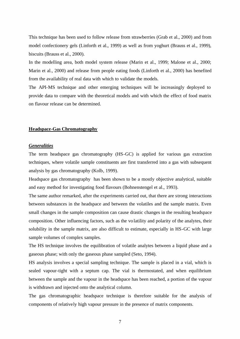
The static headspace method (SHS) involves the equilibration of volatile analyte within the
sample with the vapour phase at a defined temperature. The vapour phase containing the
analyte is then injected into the GC column.
SHS analysis is based on the theory that an equilibrium between a condensed phase and a
gaseous phase can be established for the analytes of interest and that the gaseous phase
containing the analytes can be sampled (Meyers, 2000).
Advantages:
• Simple;
• Minimizes the number of artifacts during analysis ;
• Can provide precise quantification;
• Can effectively measure volatile substances with relatively low water
solubility.
The method is useful for the analysis of highly volatile compounds.
Disadvantages:
• Low sensitivity
Fig. 1.2. Schematic diagram of static headspace gas chromatography

9
where: CL and CG represent the concentrations in the liquid and headspace, respectively, after
equilibrium, CL0 represents the analyte concentration in the liquid phase prioir to HS
equilibrium and VL and VG represent the volumes of the liquid and headspace. As illustrated
in Figure 1.2. the following equation is valid:
GGLLLL VCVCVC +=0 (1-1)
The partition coefficient (k) and phase ratio (? ) are defined as CL / CG and VG / VL,
respectively. Equation (1-1) can be transformed as follows:
)(0 ??? kCC LG (1-2)
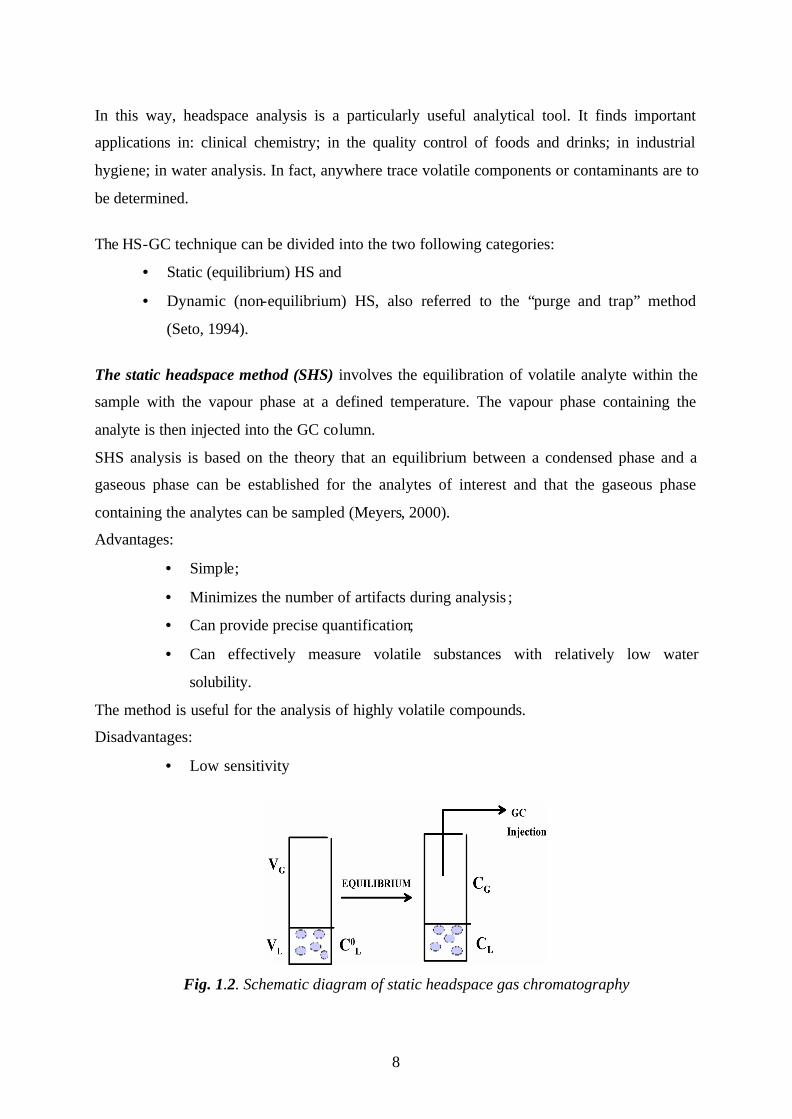
The dynamic headspace method (DHS) involves passing a carrier gas over the sample for a
specified period of time and trapping the analyte in a cryogenic or adsorbent trap. The
concentrated analyte is then introduced using pulsed heating.
In general, the DHS method is effective for the measurement of volatile substances of
moderate to high water solubility. In addition, this method offers increased sensitivity when
compared with SHS, direct aqueous injection (DAI) and solvent extraction (SE) methods
owing to the concentration after trapping of the volatile analyte (Seto, 1994).
Water sample
Glass frit
Purge
Trapping column
Heating
Cooling N2
GCTemperature controller
Cryofocusing
Fig. 1.3. Scheme of purge-and-trap technique
ß
ß
ß+=
10
The dynamic headspace extraction is represented in Figure 1.4.
Water sample
Thermostat
GC
Trapping
Purge
Fig. 1.4. Scheme of dynamic headspace extraction
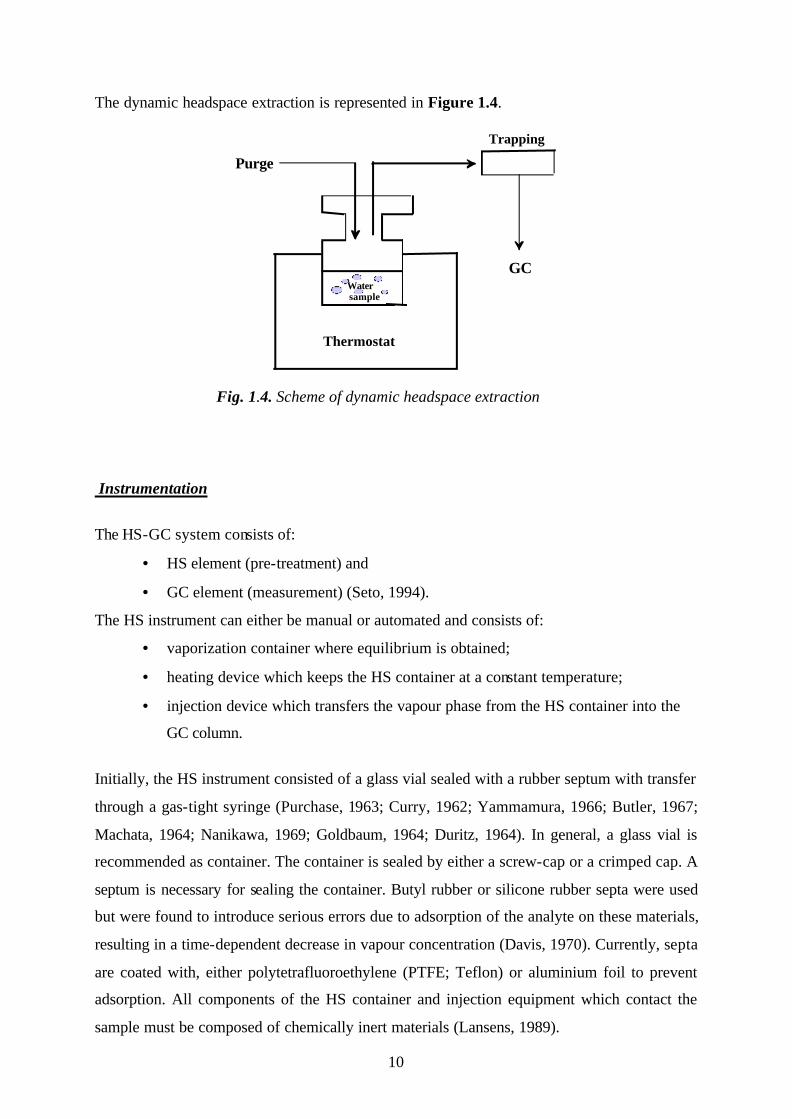
Instrumentation
The HS-GC system consists of:
• HS element (pre-treatment) and
• GC element (measurement) (Seto, 1994).
The HS instrument can either be manual or automated and consists of:
• vaporization container where equilibrium is obtained;
• heating device which keeps the HS container at a constant temperature;
• injection device which transfers the vapour phase from the HS container into the
GC column.
Initially, the HS instrument consisted of a glass vial sealed with a rubber septum with transfer
through a gas-tight syringe (Purchase, 1963; Curry, 1962; Yammamura, 1966; Butler, 1967;
Machata, 1964; Nanikawa, 1969; Goldbaum, 1964; Duritz, 1964). In general, a glass vial is
recommended as container. The container is sealed by either a screw-cap or a crimped cap. A
septum is necessary for sealing the container. Butyl rubber or silicone rubber septa were used
but were found to introduce serious errors due to adsorption of the analyte on these materials,
resulting in a time-dependent decrease in vapour concentration (Davis, 1970). Currently, septa
are coated with, either polytetrafluoroethylene (PTFE; Teflon) or aluminium foil to prevent
adsorption. All components of the HS container and injection equipment which contact the
sample must be composed of chemically inert materials (Lansens, 1989).

11
The most popular device for headspace sampling is a gas syringe. Besides the risk of sample
carry-over and significant memory effects there is the inherent problem that the internal
pressure in the vial extends into the barrel of the syringe and after withdrawal from the vial,
the headspace gas then expands through the open needle to the atmosphere. Part of the
headspace gas will thus be lost. This drawback may be avoided by using a gas-tight syringe
equipped with a valve. Such syringes may be adequate for manual sampling, but are hard to
automate (Kolb, 1999).
Manual injection with gas-tight syringes (Figure 1.5.) is the transfer method of choice. Unless
special pressure corrections are employed (Seto, 1993), the use of pressure-lock-type syringes
is recommended to prevent the loss of sample vapour.
Fig. 1.5. Scheme of gas-tight syringe (Guth and Sies, 2001)
Contamination of the syringes is a major concern as it can lead to non-quantitative results
(Bassette, 1968). It is possible to minimize contamination by cleaning the syringe with hot
water and drying with hot air at high temperature between analyses.
The following procedure was applied: appropriate carrier gas flows and temperature zones are
established. Additional carrier gas flow is initiated to sweep the lines, sample loop, and
needle. A sample in a sealed vial is allowed to equilibrate at an elevated temperature for a
specified length of time. The sealed sample vial is raised onto a needle that punctures a
septum and pressurization gas fills the vial to a predetermined level. The vial is allowed to
equilibrate for a relatively short time to ensure complete diffusion of the pressurization gas
with the sealed sample vial’s atmosphere. A vent valve is opened and the pressurized contents
Gas-tight syringe
12
of the sealed sample vial exit the system through a thermally controlled sample loop of
previously selected volume, usually = 1 mL. The vent valve is then closed and the contents of
the loop allowed equilibrating for a specified time. Next a multiple port valve is activated,
placing the sample loop in the carrier gas stream. The carrier gas then sweeps the contents of
the loop through the heated transfer line and into the GC. Usually upon initiation of sample
transfer to the GC, instrumentation software is employed to automatically begin the
chromatographic separation and data collection (Meyers, 2000).
A peculiar problem in static HS-GC is the internal pressure in the headspace vial generated
during thermostated by the sum of partial vapour pressures from all volatile sample
constituents, from which in general the humidity of the sample is predominant (Kolb, 1999).
Thus, the vapour pressure of water contributes mostly to the internal pressure. Moreover,
some sampling techniques pressurize the vial prior to sample transfer with the inert carrier
gas. For these reasons it is necessary to close the vial pressure tight by a septum (preferably
PTFE-lined) and to crimp-cap it by an aluminium cap.
HS-GC can be performed with both packed and capillary columns.
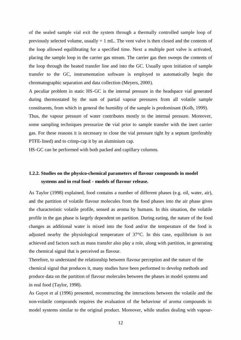
1.2.2. Studies on the physico-chemical parameters of flavour compounds in model
systems and in real food - models of flavour release. As Taylor (1998) explained, food contains a number of different phases (e.g. oil, water, air),
and the partition of volatile flavour molecules from the food phases into the air phase gives
the characteristic volatile profile, sensed as aroma by humans. In this situation, the volatile
profile in the gas phase is largely dependent on partition. During eating, the nature of the food
changes as additional water is mixed into the food and/or the temperature of the food is
adjusted nearby the physiological temperature of 37°C. In this case, equilibrium is not
achieved and factors such as mass transfer also play a role, along with partition, in generating
the chemical signal that is perceived as flavour.
Therefore, to understand the relationship between flavour perception and the nature of the
chemical signal that produces it, many studies have been performed to develop methods and
produce data on the partition of flavour molecules between the phases in model systems and
in real food (Taylor, 1998).
As Guyot et al (1996) presented, reconstructing the interactions between the volatile and the
non-volatile compounds requires the evaluation of the behaviour of aroma compounds in
model systems similar to the original product. Moreover, while studies dealing with vapour-
13
liquid partition phenomena may have reported the effects of medium composition on the
headspace concentrations at equilibrium, they have not connected the physical properties with
sensory scores by model equations (Van Boekel et al, 1992; Land, 1979).
With complex foodstuffs, it is useful to have some model systems to relate to. Studies of these
model systems can at least give an approximation of the behaviour we might expect in the
actual practical system (Buttery et al., 1973).
Various models for predicting flavour release have been proposed, based either on partition
(De Roos & Wolswinkel, 1994) or on an understanding of the physical processes involved in
the mouth during eating (Harrison & Hills, 1997).
Three types of model systems are mentioned in the literature:
• First model system: pure water (e.g. Buttery et al., 1969, 1971);
• Second model system: vegetable oil (Buttery et al., 1973);
• Third model system: water-vegetable oil mixtures (Buttery et al., 1973).
Several reviews of flavour release studies (Overbosch et al., 1991; Bakker) emphasized the
need for a better understanding of food-flavour interactions and under more complex food
consumption conditions.
Most detailed studies on flavour release have been made on simple liquid systems, and little
research has been done on the release from solid or semi-solid foods, having different
structures (Bakker et al., 1996).
The same authors mentioned that the perceived quality and intensity of the flavour of a food is
related to the concentration of volatile components released into the airspace of the mouth
while eating. It was assumed that the concentration of a flavour released into the airspace is
quantitatively and qualitatively related to the sensory perception.
Models of flavour release A review of the literature on flavour release (Overbosch et al., 1991; Plug et al., 1993) reveals
two main mechanisms for release which are then adapted for the particular food matrix under
investigation.
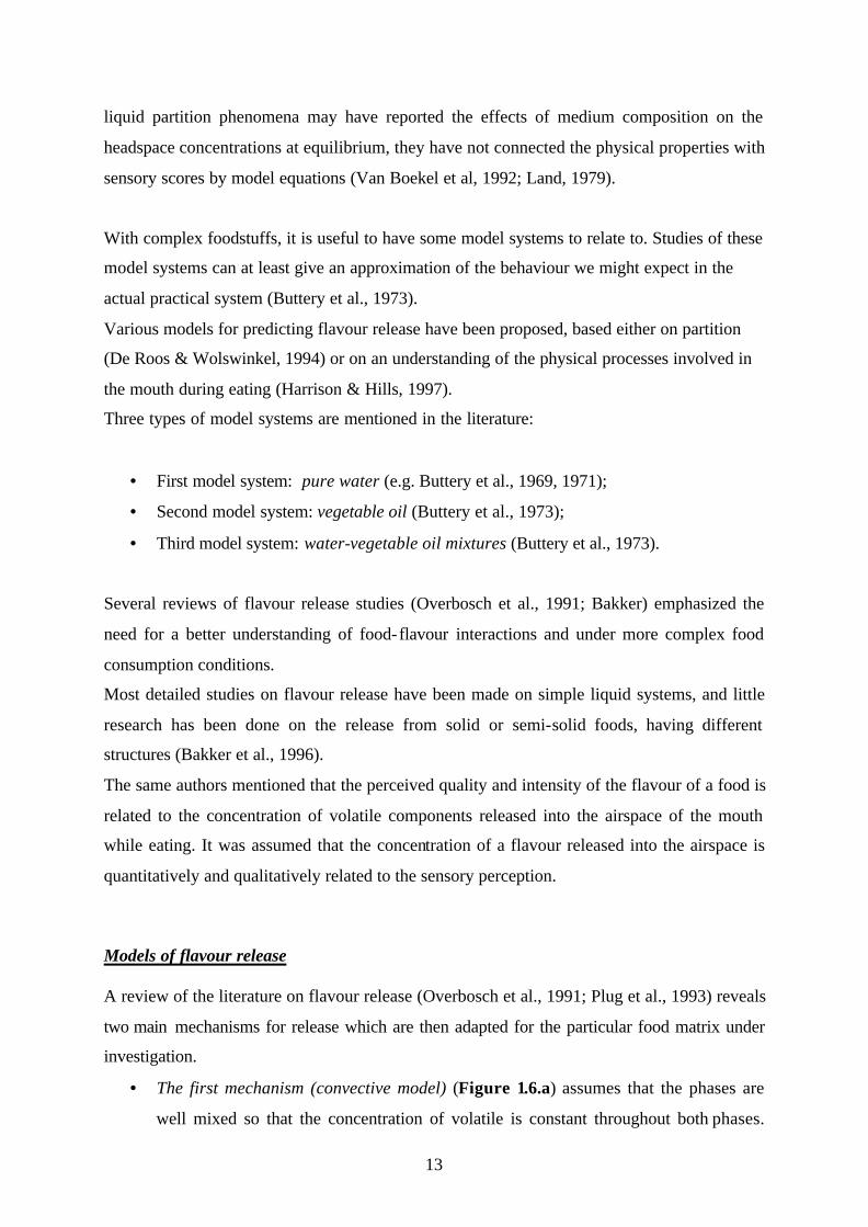
• The first mechanism (convective model) (Figure 1.6.a) assumes that the phases are
well mixed so that the concentration of volatile is constant throughout both phases.
14
Mass transport across the interface occurs by diffusion in very thin layers (the
boundary or interfacial layers) either side of the interface.
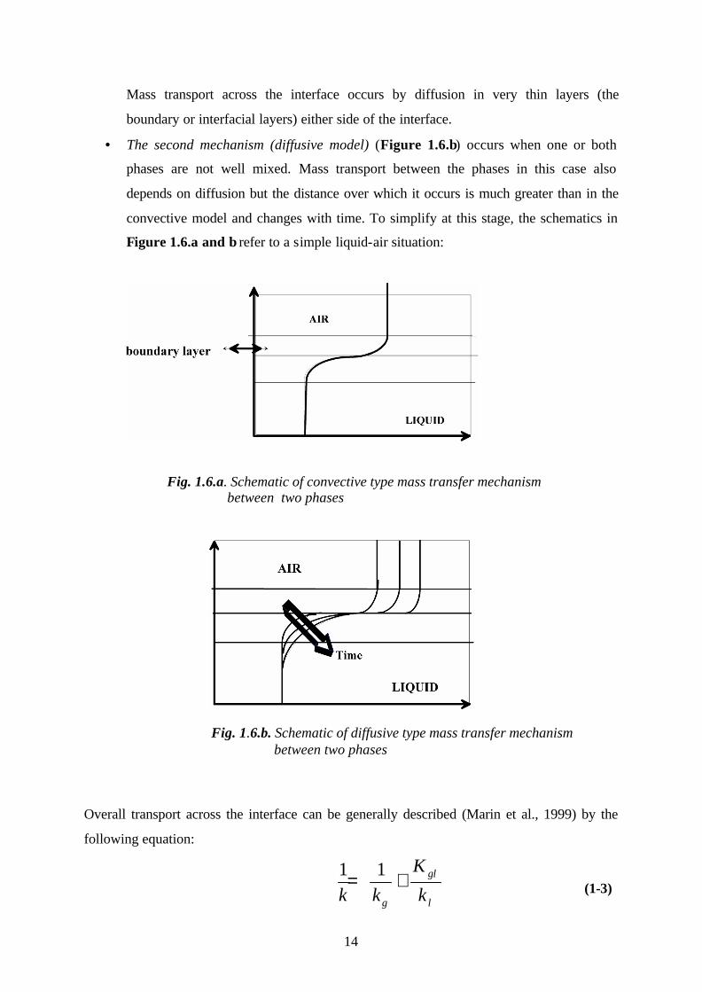
• The second mechanism (diffusive model) (Figure 1.6.b) occurs when one or both
phases are not well mixed. Mass transport between the phases in this case also
depends on diffusion but the distance over which it occurs is much greater than in the
convective model and changes with time. To simplify at this stage, the schematics in
Figure 1.6.a and b refer to a simple liquid-air situation:
Fig. 1.6.a. Schematic of convective type mass transfer mechanism between two phases
Fig. 1.6.b. Schematic of diffusive type mass transfer mechanism between two phases
Overall transport across the interface can be generally described (Marin et al., 1999) by the
following equation:
l
gl
g k
K
kk+= 11
(1-3)

15
where: k is the overall mass transport across the phases;
kg and kl refer to mass transport in the gas and liquid boundary layers,
respectively;
Kgl is the partition coefficient between the gas and liquid phases.
Because k depends on the mass transfer in the liquid and gas phases, plus a contribution from
the air-water partition coefficient (1-3), the values for these parameters and the effects of flow
rate on these parameters (when appropriate) were determined (Marin et al., 1999).
In the model proposed by Marin et al.(1999) (an air-water system at equilibrium, for which
the air-water partition coefficient (Kaw) and temperature are the determining factors for
volatile release) the authors reported that release depended almost entirely on the air-water
partition coefficient for values of Kaw less than 10-3. When Kaw was greater than 10-3, the
model predicted that the conditions in the gas phase (exemplified by the Reynolds number),
would become significant. The Reynolds’ number (a dimensionless parameter) is the ratio of
inertial to viscous forces and determines the type of flow (Roberts et al., 2000).
The Reynolds’ number is given by:
???l
?Re (1-4)
where: ? = fluid density [kg/m3];
? = fluid velocity [m/s];
l = some typical dimension [m];
? = fluid viscosity [kg/ms].
Oil water partition models
Models for oil-water/air partition were published from McNulty and Karel, (1973c); McNulty
and Karel, (1973b) and McNulty and Karel, (1973c) and summarized more recently
(McNulty, 1987). The models are based on oil-water/air partitioning.
Using these models, release of volatile flavours from emulsions, representing the extremes of
the oil fraction, were tested. Oil fraction (f) is the percentage of oil in the system (f = 1
corresponds to 100% of oil) and the examples used by McNulty and Karel (McNulty, 1987)
were milk (f = 0.035) and mayonnaise (f = 0.80).
By modelling these two systems, they predicted that flavour release on dilution would depend
entirely on the oil-water partition coefficient (Ko/w). They assumed that Cowi = 100 ppm (Cowi
= initial emulsion flavour concentration), DFem = 2 (i.e. a 1:1 dilution) (DFem = emulsion
= pv
v
p
h
h
16
dilution factor) and Vowi = 10 ml (Vowi = initial emulsion volume), and then evaluated the
flavour concentrations in the aqueous phases of milk and mayonnaise after dilution with
saliva. The results obtained showed that, with increasing of Ko/w, the potential extent of
flavour release increases slightly for milk and appreciably for mayonnaise. Ko/w was given by:
we
oewo C
CK ?/ (1-5)
where : Ko/w = oil-water partition coefficient;
Coe, Cwe = flavour concentrations in the oil and aqueous phase at
equilibrium, respectively [? g/ml].
McNulty and Karel summarized the experimental evidence to validate their model in their
1987 review (McNulty, 1987). Some experiments were carried out with a simple oil-water
system, others with an oil-water-surfactant (Tween 60) system. The effect of fat melting point
on the oil-water partition was then studied.
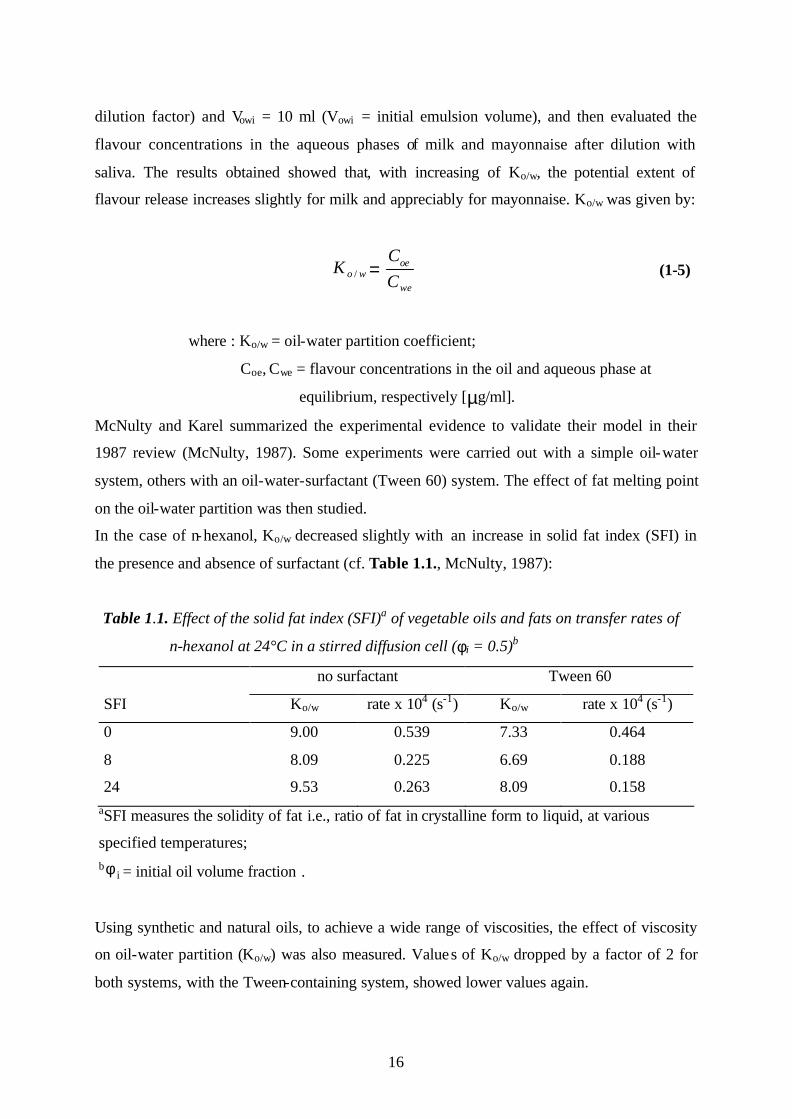
In the case of n-hexanol, Ko/w decreased slightly with an increase in solid fat index (SFI) in
the presence and absence of surfactant (cf. Table 1.1., McNulty, 1987):
Table 1.1. Effect of the solid fat index (SFI)a of vegetable oils and fats on transfer rates of
n-hexanol at 24°C in a stirred diffusion cell (? i = 0.5)b
no surfactant Tween 60
SFI Ko/w rate x 104 (s-1) Ko/w rate x 104 (s-1)
0 9.00 0.539 7.33 0.464
8 8.09 0.225 6.69 0.188
24 9.53 0.263 8.09 0.158
aSFI measures the solidity of fat i.e., ratio of fat in crystalline form to liquid, at various
specified temperatures;
b ? i = initial oil volume fraction .
Using synthetic and natural oils, to achieve a wide range of viscosities, the effect of viscosity
on oil-water partition (Ko/w) was also measured. Values of Ko/w dropped by a factor of 2 for
both systems, with the Tween-containing system, showed lower values again.
=
µ
φ
φ
17
The influence of proteins, polysaccharides, and droplet size on flavour release of an oil- in-
water emulsion was determined using aroma compounds with different hydrophobic
characteristics (Charles et al., 2000). Flavour release of lipophilic compounds (ethyl
hexanoate and allyl isothiocyanate) was influenced by three factors: the structure of the
emulsion; the nature of the protein used as emulsifier, and the presence of polysaccharides.
Emulsions
There are many other published reports on flavour release from a variety of emulsion system
(Dickinson, 1992; Salvador et al., 1994; Guyot et al., 1996; McClements, 1998; Charles et al.,
2000; van Ruth and Roozen, 2000). Release has been measured using both sensory and
instrumental methods and the effect of oil fraction on flavour release has been verified. The
majority of work describes theoretical models with little experimental validation.
Flavour release from model emulsions has been followed in vitro using Atmospheric Pressure
Ionisation Mass Spectrometry (API-MS) monitoring which allows real time measurement of
gas phase concentrations at levels around 10 ppb (volatile per litre air). Using dynamic
headspace dilution and following the release with time it was possible to compare actual
release data with theoretical convective and diffusive models.
Overbosch et al. (1991) pointed out that the time course of release from the convective and
diffusive models was different and this could affect flavour perception. If both systems are
allowed to come to equilibrium and the headspace is then diluted, the diffusive model predicts
an exponential release, while the convective model will show an initial decrease, followed by
a steady state, followed by a further decline as the volatile flavour in the liquid phase becomes
depleted.
Emulsion systems contained various lipids, water and dilute solutions of the emulsion (up to
1.92% oil) were used to minimize any viscosity effect.
For the emulsions, Malone et al. (2000) pointed out that the “Harrison models” were
developed for simple model systems (water systems). Harrison et al. (1997) propose a
mathematical model for the release of flavour (one hydrophilic: diacetyl and the other
hydrophobic: heptan-2-one) from a liquid emulsion based on the assumption that the rate-
limiting step was the resistance to mass transfer across the emulsion-gas interface and that this
could be described by penetration theory. The authors assumed that partitioning of flavour
molecules between oil and aqueous phase was extremely rapid compared to the transport of
flavour across the emulsion-gas interface. They took also into account the dependence of
mass transfer coefficients on viscosity, oil fraction and droplet size. The results showed that

18
the mass transfer coefficient was expected to increase with decreasing oil fraction, leading to
faster flavour release in low fat systems. However, partitioning can also influence the flavour
release rate, depending on physical/chemical properties of the flavour. Experimental data for
heptan-2-one agreed reasonably well with theoretical predictions, suggesting that the rate
limiting step for flavour release was the mass transport across the emulsion-gas interface.
To apply this model to the situation that occurs when a sample of emulsion is placed in
mouth, masticated, and swallowed, required some estimate of other factors, like the degree of
mixing in mouth, as well as the extent of dilution with saliva and air.
In vivo release mesurements of butanone, heptan-2-one and ethyl hexanoate were studied to
cover a range of compounds with differing lipophilicity. Butanone represented a relatively
hydrophilic molecule and its release was largely unaffected by the oil fraction of the emulsion
used. For heptan-2-one and ethyl hexanoate (relatively lipophilic compounds), oil fraction
affected both the maximum intensity of release as well as the duration of release, which is in
agreement with theory (Taylor, 2002).
Malone et al. (2000) pointed out that the overall release of the three volatiles in vivo was
related to their partitioning behaviour in static model systems.
Van Ruth et al. (1999) concluded that the pH of emulsions influences the aroma profiles of
emulsions through effects on aroma generation and aroma release.
Real food systems
While all the models described in the previous chapter relate to well-defined model systems,
flavour release from a system closer to a real food product, namely composite dairy gels, has
been modelled (Moore, 2000).
The gel contained protein, fat and water, as the main constituents, but the gel also contained
structural elements in the form of composite particles, composed of an inner layer of fat with
an outer coating of protein.
The model proposed by Harrison and Hills (1997) was used with minor modifications and
using direct numerical solutions. The mathematical model was compared with experimental
data obtained by sensory time intensity measurements of flavour release. Good agreement
between the model and the experimental data was obtained when the model contained
appropriate terms for flavour removal by swallowing and breathing. The model predicted
correctly that flavour diffusivity and fat particle size had little effect on perceived intensity of
flavour, nor on the timing of maximum intensity. The prediction, that perceived flavour

19
intensity depended on flavour concentration in the gel, was also found to be valid, although
the relationship between the two parameters was not exactly as predicted.
The theoretical models to predict the effect of food matrix on flavour delivery have not been
validated to any great extent (Taylor, 2002). The suitable analytical methods are available to
measure dynamic flavour release in vivo and in vitro.
Dynamic flavour release methods have been developed over the last 10 years and have been
reviewed recently (Taylor et al., 2000).
The model proposed by Nahon and Roozen (2000) described the dynamic flavour release for
five volatile compounds (ethyl acetate, methyl butanoate, ethyl butanoate, hexanal and
octanal) from aqueous sucrose solutions. By determination of the viscosities and the partition
coefficients, the model provided an acceptable fit to the experimental data obtained with
instrumental analysis. The model description revealed that at low sucrose concentrations the
partition coefficient primarily controls the flavour release, whereas at higher sucrose
concentrations the mass transfer coefficient has more influence.
Banavara and Berger (2002) developed a mathematical model, derived from the convective
mass transfer theory, to predict dynamic flavour release from water. The model was based on
physicochemical constants of flavour compounds and on some parameters of an apparatus
used for validation. The model predicted a linear pattern of release kinetics during the first
30 s, and large differences of absolute release, for individual compounds.
Rabe et al. (2002) measured dynamic flavour release from liquid food matrices using a fully
computer-controlled apparatus. The concept of the apparatus presented was developed from
the idea to represent an idealized situation of food consumption. Flavour compounds from
different chemical classes were dissolved in water to achieve concentrations typically present
in food (µ g-mg/L). Most of the compounds showed constant release rates. The entire method
of measurement including sample preparation, release, sampling, trapping, thermodesorption,
and GC analysis, showed good sensitivity and reproducibility (mean standard deviation =
7.2%).
Analogous methods for following non-volatile release in-mouth are also available (Davidson
et al., 2000).
20
1.2.3. Studies on Vapour Pressure The saturated vapour pressure is one of the most important physico-chemical properties of
pure compounds (Boublik et al., 1973).
The vapour pressure of a liquid or solid is the pressure of the gas in equilibrium with the
liquid or solid at a given temperature (Verschueren, 1983). The same author explained that
vapour pressure values provide indications of the tendency of pure substances to vaporize in
an unperturbed situation, and thus provide a method for ranking the relative volatilities of
chemicals.
Vapour pressures are expressed, either in mm Hg (abbreviated mm), or in atmospheres (atm.).
The thermodynamic expression of phase equilibrium for a pure substance is given by the
Clapeyron equation:
VTH
dTdP
??=
0
(1-6)
where: P0 denotes the vapour pressure [Pa], T the absolute temperature [°K], ∆ H [J/mol K],
the heat absorbed at constant temperature in transferring one mole from phase (‘) to phase (“)
in equilibrium and ∆ V the volume change per mole transferred [m3] (Boublik et al., 1973).
This equation is applicable only over narrower temperature ranges in which the enthalpy of
vaporization is relatively constant (Mackay et al., 1981).
A whole series of semiempirical equations (correlation equations) has been proposed. One
suitable equation, published by Antoine (Antoine, 1888), has the following form:
? ?CtBAP ?−=0log (1-7)
where P0 is the vapour pressure [Pa], t the temperature [°C], and A, B, C are constants
characteristic of the substance and the given temperature range.
The Antoine Equation (1-7) represents well the behaviour of most substances over large
temperature intervals (Willingham et al. (1945)). The authors did measurements of vapour
pressures for 52 purified hydrocarbons over the range 47 to 780 mm Hg at 12°C.
As de Roos (2000) described, vapour pressures in the product medium can be influenced by
many factors, such as:
• Temperature;
• Composition of the aqueous phase;
∆∆
( )+
21
• Flavour binding / Complex formation;
• Acid-Base equilibria;
• Phase partitioning between aqueous and lipid phase;
• Sorption to suspended particles;
• Crystallization.
As Widder et al. (1996) showed, the fat content is an important variable in a food matrix.
One important point is that fat is a good solvent of flavour compounds and influences the
vapour pressure of the volatiles, thereby affecting the perceivable aroma profile. Hence, good
fat based flavourings tend to become unbalanced or even off- flavoured in aqueous or reduced
fat systems (Hatchwell, 1994; Plug et al., 1993).
Vapour pressure measurements can be made directly through the use of a pressure gauge (e.g.,
a diaphragm gauge), or by indirect methods based on evaporation rate measurements or
chromatographic retention times (Bambord et al., 1998).
Mackay et al. (1981) explained that accurate measurements of vapour pressure have been
possible for many years using standard isoteniscopic techniques which are applicable down to
approximately 1 mm Hg or 100 Pa. The authors noted that it is difficult to estimate the
accuracy of much published data since the values reported are usually the fitted data or the
regression constants.
The preferred experimental technique for determination of low vapour pressures is similar in
principle to that of the “generator column” solubility technique except that a gas stream is
saturated with solute (Mackay et al., 1981). Methods have been described by Spencer and
Cliath (1968), Sinke (1974), and Macknick and Prausnitz (1979), in which a standard error
better than 3% is attainable.
In the method described by Spencer and Cliath (1968) to determinate the vapour density of
dieldrin, the apparent vapour pressures were calculated from the vapour density, W / V (W =
the weight of the given volume of gas [g], V = volume of gas [m3]), with the equation:
( )( )MRTVW P = (1-8)
where: R is the molar gas constant [8.314 J/mol K], T the absolute temperature [K], and M the
molecular weight [g/mol] of dieldrin assuming a monomer gaseous species.

22
Macknick and Prausnitz (1979) used the same method to obtain experimental data at near-
ambient temperature for selected high-molecular-weight hydrocarbons.
Buttery et al. (1969) determined the vapour pressures for nonanal, undecan-2-one, and methyl
octanoate using gas-chromatography method. These values at 25°C were determined in the
following way. The pure compound (10 ml) was placed in a dry Teflon bottle and equilibrated
in a 25° C water bath for 30 minutes. Vapor samples were introduced into the GLC apparatus
by connecting an 18- inch length of Teflon capillary tube (0. 04- inch I.D.) from the GLC gas
sampling valve to the Teflon bottle and then transferring the sample to the valve by squeezing
the flexible bottle.
The concentration of the compound in the vapour was determined by comparing the vapour
GLC peaks to those obtained by injecting a standard solution of the compound in hexane.
Le Thanh et al. (1993) determined the vapour pressures for six aroma compounds (ethyl
acetate, ethyl butanoate, ethyl isobutanoate, ethyl hexanoate, 2,5-dimethyl pyrazine, octen-1-
ol-3) using a static measurement.This method is adapted for measuring the vapour pressure
and consists of measure the pressure above the product for which the thermodynamic
equilibrium is attended.
A smoothing of the experimental points was made with the semi-empirique equation of
Antoine, which links up the vapour pressure with the temperature T (in K):
( ) 273log
− +−=
TC B
AP s (1-9)
where: Ps = the vapour pressure of a pure compound [mm Hg];
T = absolute temperature [K].
The three coefficients A, B, and C from this equation were calculated for all the compounds.
Van Boekel et al (1992) reported that most flavour compounds have a lower vapour pressure
(and higher odour thresholds) in oil than in aqueous solutions.

23
1.2.4. Studies on Partition Coefficients Since partition is a fundamental parameter describing the distribution of a volatile flavour
compound between two phases at equilibrium, it has been widely studied (Taylor, 2002).
The work presented by Land & Reynolds (1981) emphasized the importance of the partition
coefficient as this is the underlying principle governing the release of flavours from the food
matrix into the gas phase (the so-called headspace).
Andriot et al. (2000) and van Ruth et al. (2002) explained that the influence of specific
physicochemical properties (composition, structure, concentration) of a food matrix on the
volatility of an aroma compound can be observed using static headspace analysis and
quantified in terms of the air-to-matrix partition coefficient for that compound.
The flavour volatiles partition between the phases depending on their relative affinity for the
phases. Unfortunately, the theory of partition can be applied only to relatively simple systems
and, as Land (1996) pointed out, the physical laws which describe the processes of diffusion
and the equilibration concentration ratios are understood for simple single-phase bulk systems
such as water or oil, although there is much less data for many of the solid materials which are
present in foods.
Partition coefficients describe the thermodynamic component and the extent of aroma release
under equilibrium conditions.
Partition coefficients are based on many parameters, e.g., polarity, volatility and molecular
mass. In general, partition coefficients of volatile substances in water increase with increasing
water solubility and therefore the following order among chemical classes is observed:
aromatics > cycloalkanes > alkenes > alkanes (Seto, 1994). Within each chemical class, a
decrease in partition coefficient occurs as the molecular mass increases (Buttery et al., 1969).
Verschueren (1983) gave a definition for the partition coefficient and said that the partition
coefficient P is defined as the ratio of the equilibrium concentration C of a dissolved
substance in a two-phase system consisting of two largely immiscible solvents, for example
n-octanol and water:
water
oloc
CC
P tan= (1-10)
In addition to the above, the partition coefficient is ideally dependent only upon temperature
and pressure. It is a constant without dimensions. It is usually given in the form of its
24
logarithm to base ten (logP). LogP values are indicator variables for lipophilicity (Buhr et al.,
2001).
Taylor (1998) pointed out that if a single volatile is dissolved in a solvent (the binary system),
the relationship between the concentration of volatile compound in the liquid phase and in the
air phase can be expressed by Henry’s law. This states that “the mass of vapour dissolved in a
certain volume of solvent is directly proportional to the partial pressure of the vapour that is in
equilibrium with the solution” (Morris, 1968).
The same author found when the concentrations in the water and gas phases are plotted
against each other a linear relationship signifies that Henry’s law is applicable for data in this
range.
Land (1996) stated that “most published data at realistically low concentrations show that
such (model) systems do obey Henry’s Law”.
As Hansen et al. (1993) remarked, an innovative static headspace method referred to as
equilibrium partitioning in closed systems (EPICS) has been used frequently to measure the
Henry’s law constants of volatile organic compounds. The EPICS method is based on a
comparison of the headspace concentration of a volatile compound in two systems at
equilibrium which are identical in the mass of the compound but not identical in the volumes
of the gas and liquid phases.
Robbins et al. (1993) presented a new method for determining Henry’s law constants,
applicable to the static headspace method. Experimentally, this method involves measur ing by
gas chromatography the equilibrium headspace peak areas of one or more compounds from
aliquots of the same solution in three separate enclosed vials having different headspace-to-
liquid volume ratios. A plot of the reciprocal of the peak areas versus headspace-to-liquid
volume ratios gives a straight line. The slope of that line divided by its y- intercept, as
determined by linear regression, gives a value for the dimensionless Henry’s law constant:
erceptyslopeH i int−= (1-11)
A similar headspace gas chromatographic method for the determination of liquid/gas partition
coefficients of gases and volatile substances of low and intermediate solubility was described
by Vitenberg et al. (1975) ; Guitart et al. (1989).
25
Taylor (1998) remarked that water is frequently used as the solvent, but the same principles
can be applied to other solvents, provided that they are pure solvents. In studying food, the
partition between oil and air is also of interest, with each solvent having a different partition
coefficient depending on the relative affinity of the volatile for the solvent.
The relationship between concentration in the aqueous phase and the gas phase is no longer a
simple linear relationship but can still be described mathematically (Taylor, 1998). A special
case of non- ideality was reported by Buttery et al. (1971) for volatiles that had a high affinity
for the solvent. The activity coefficients for non-polar volatiles in lipid and for hydroxyl-
containing volatiles in water were less than 1, demonstrating interactions between these
volatile solutes and the solvents.
As Leo et al. (1971) showed, the most extensive and useful partition coefficient data were
obtained by simply shaking a solute with two immiscible solvents and then analyzing the
solute concentration in one or both phases.
To determine the air-water partition coefficient many workers have used simple sealed vessels
(normally a glass bottle) containing a solution of the compound, which is allowed to
equilibrate with the air phase at a defined temperature. Samples of the gas phase are then
taken and analysed by GC (Taylor, 1998).
Chaintreau et al. (1995) described a convenient experimental method in which the phases
were equilibrated in a glass syringe and portions of the air phase were then injected onto a GC
by moving the syringe plunger to determine the gas-phase concentration. The method
developed by him is based on a combination of static headspace sampling and dynamic
headspace traps. This method has the following advantages:
• determination of the partition coefficients does not require calibration;
• quantification is achieved without adding a standard;
• combination of static headspace with traps allows components with low vapour phase
concentrations to be analyzed;
• small changes in the aroma profile due to nonvolatile constituents can be investigated.
Amoore and Buttery (1978) determined the air/water partition coefficients of many odorants
from available data on their vapour pressures and solubilities at 25°C. They specified that if a
liquid odorant is added to water, and shaken with air in a closed vessel, the odorant dissolves
and evaporates, distributing itself between the air and water in a constant ratio (at a given
pressure):
26
W
AAW c
cK = (1-12)
The constant KAW is the air / water partition coefficient; cA: the concentration of the odorant in
the air phase (grams of odorant per litre of air); cW: the concentration of the odorant in water
phase (grams of odorant per litre of water).
Buttery et al. (1969) evaluated this constant for a series of lower aliphatic aldehydes, by
measuring their concentrations in samples, drawn from the air and water phases, injected into
a gas chromatograph.
Also Mackay et al. (1981) determined the Henry’s law constants (air/water partition
coefficients) from vapour pressures and solubility data for chemicals of environmental
interest, and Fendinger et al. (1989) measured experimentally the Henry’s law constants of
several pesticides, that have been reported in environmental samples, using a wetted-wall
column and a fog chamber.
As a conclusion described by Gossett (1987), Robbins et al. (1993), and Poddar et al. (1996)
in their papers, there are three basic methods cited by Mackay and Shiu (1981) for measuring
Henry’s law constants:
• use of vapour pressure and solubility data;
• direct measurement of air and aqueous concentrations in a system at equilibrium;
• measurement of relative changes in concentration within one phase, while
effecting a near-equilibrium exchange with the other phase (batch air stripping).
Ramachandran et al. (1996) remarked that reliable H data are crucial in quantitative
investigations in diverse areas as:
• the estimation of the flux of VOCs from surface waters to air (Fendinger et al.,
1989);
• design of air-stripping towers (Hansen et al., 1993);
• partitioning of gas-phase atmospheric species into cloud and fog droplets (Kames
et al., 1992);
• transfer of chlorinated organic solvents from tap water to indoor air (Tancrede et
al., 1990) and;
• transfer of inhaled anesthetic gases to the brain (Lockhart et al., 1990).
27
Henry’s law constant is a strong function of temperature (Poddar et al., 1996). The author
specified that at a constant pressure, the temperature dependence of Henry’s law constant can
be expressed by (Robbins et al., 1993):
???
??? −= Hi
Hii A
TB
H exp (1-13)
where: T is the absolute temperature [K] and AHi and BHi are constants which depend on the
solvent-solute combination and need to be obtained from the experimental data.
The partition coefficient for a volatile compound between headspace and water (K HS/water) can
be related to its hydrophobicity, volatility, and solubility, and the presence of nonvolatile
constituents in solution can subsequently change the thermodynamic behaviour of the volatile
compound (Jung et al., 2003).
Buttery et al. (1968) determined air to solution partition coefficient using the following
equation:
s
aas c
cK = (1-14)
where: Kas = the partition coefficient; ca = solute concentration in air; cs = solute
concentration in solution.
Since many flavours are hydrophobic, fat as a food ingredient is an excellent solvent of many
food flavours and even the addition of a small amount of fat to a flavour solution has a
considerable effect on the food-air partition coefficient. Binding of flavours to food
ingredients (proteins and also carbohydrates) can also lessen the concentration of free flavour,
and hence will affect partitioning of flavour (Bakker et al., 1996).
( )

28
Behaviour of the odorous compounds Guyot et al (1996) studied the relationships between odorous intensity and partition
coefficients in model emulsions for some aroma compounds, among them being
δ-decalactone.
He observed that the δ -decalactone has a very strong hydrophobic behaviour that makes not
possible to measure vapour-liquid partition coefficients in media containing paraffin oil.
Because δ -decalactone is highly retained by the oily phase, its concentration in the gaseous
phase decreases and leads to weaker odour intensities.
Guyot also remarked that, unlike δ -decalactone has a higher affinity for the aqueous phase,
when the oil content increases, the concentration in the gaseous phase increases and leads to
higher odour intensities and vapour- liquid partition coefficients.
Partition in real foods Although partition coefficients can be defined and measured, their relevance to real food
systems has often been questioned (Taylor, 1998). The argument is that partition values
measured at equilibrium do no t reflect the situation in real foods where equilibrium is rarely
achieved. The same author remarked that in many instances, foods are undergoing a dynamic
process, where the gas phase is not constrained and equilibrium between the food and the gas
phase is never attained. This is the situation for the majority of foods, where flavour volatiles
are lost from the food into the surrounding gas phase. When food is eaten, the situation is
even more complex and equilibrium is not achieved, since both aqueous and gas phases are
undergoing dilution, due to saliva flow and breathing, respectively. To model this behaviour,
partition coefficients need to be combined with other factors such as mass transfer and
dilution (Taylor, 1998).
The rate at which equilibrium can be achieved is determined by the mass transfer coefficient
(kinetic component). The mass transfer coefficient k is a measure for the velocity at which the
solute diffuses through the phase (De Roos, 2000).
Mass transfer is always described as a succession of diffusion steps from the aqueous
boundary layer, through the stripping phase filled membrane pores, to the stripping phase
boundary layer (Souchon et al., 2004).
When phase equilibria are disturbed, mass transport will take place resulting in concentration
gradients in the product and vapour phases, as is presented in Figure 1. 7. (de Roos, 2000).

29
E-1
E-1
E-1
E-1
E-1
E-1
E-1
E-1
E-1
E-1
E-1
E-1E-1E-1
E-1
E-1
E-1
E-1E-1
E-1 E-1
E-1E-1
E-1
E-1
E-1
E-1
E-1
CG? CG
? CL
CLi
CL
PGL ?G
?L
LIQUID
AIR
LOW CONCENTRATION HIGH
Fig.1.7. Schematic diagram of flavour concentrations at the liquid-gas interface
during release from the liquid phase (CL: concentration in the liquid phase; CG: concentration in the headspace; PGL: gas-liquid partition
coefficient; ? G: the thickness of the gas layer; ? L: the thickness of the liquid layer)
1.2.5. Odor activity values (OAV)
Generalities
Odor consists of many kinds of compounds which are present in low concentration that the
applicability of chemical analysis is limited. Therefore, a method based on the usage of
human nose as a sensor, is developed.
Olfactometer is one of the techniques used to deliver odorants to panelists.
With the olfactometer, can be measured:
• Odor threshold (odour concentration);
• Odor intensity;
• Hedonic quality.
Odor intensity and odor concentration are the two most important properties of an odor
(Zhang et al., 2002).
DD
d
d
d d
30
Measurement procedure
The human nose smells odor only when a certain number of molecules is present in the air.
A human nose can detect odor at concentrations well below the sensitivity levels of chemical
analytical methods.
An olfactometer is an instrument that dilutes sample (odor) air with fresh air and presents the
diluted sample to a sniffing port.
The concentration, at which an odorous substance can be smelled by the human nose, is
called as odor threshold. In this case, the difference between an odorous and an odourless air
can be detected.
As the sensitivity of different human noses differs greatly among the people, every sample is
tested by a number of fixed persons at the same time.
In the olfactometer, the gas samples are diluted and are smelled by the testers. The testers
smell different samples of odourless air and odorous air without any information about the
type of the sample air. At the beginning, odorous air is diluted with odourless air so that the
testers notice no difference between the odorous and clean air (concentration below the odor
threshold). With the decrease in dilution step by step, the concentration of the odorous air
increases. Independent from each other, the testers give signals when they smell any odor .
The dilution threshold is established when 50% of the panellists have correctly identified the
odorous sample from the odor free samples (Feddes et al., 2001). This dilution threshold is
equivalent to the odor concentration described as odor units. A sample diluted by a factor of
100 at the detection threshold has an odor concentration of 100 odor units (Feddes et al.,
2001).
In 1963, Rothe and Thomas proposed the Odor Unit (concentration in food / odor threshold)
to quantify the potency of odorants in a flavor system, i.e., beverages, foods, fragrances, and
other natural products. This relationship has been used to distinguish constituents that may
contribute to aroma (potent odorants) from the vast majority of volatiles in natural products
that are at concentrations below their odor threshold (Grosch et al., 1990; Grosch, 1993;
Schieberle, 1995; Audouin et al., 2001; Mistry et al., 1997; Munch et al., 1997).
Among the techniques used to deliver odorants to panelists are also food models, GCO, and
water, as predicted Huyer (1917); Chaplet (1936); Dravnieks (1974); Lawless (1998); Ong et
al. (1999); Gygax et al. (2001). The use of gas chromatography olfactometry (GCO) to
correlate variation in the human olfactory response in both quantitative and qualitative terms
can clarify the relationship between patterns of odorant mixtures and the perceptions they
invoke (Acree et al., 2004).

31
Quantification and calculation of odor activity values (OAV) As Grosch (2001) described, due to the complexity of the volatile fraction and the large
differences in concentration, volatility and reactivity of the odorants, it is not possible in most
cases to quantify the odorants precisely by using conventional methods (Grosch, 1993;
Schieberle, 1995). Precise quantitative measurements of the odorants can be performed by the
use of stable isotopomers of the analytes as internal standards in the so-called: stable isotope
dilution assays (SIDA). As Grosch (2001) explained, each assay consists of the following
steps: after the food sample or its extract has been spiked by the addition of known amounts
of the corresponding labelled odorants, the volatile fraction is distilled off; the volatiles are
then enriched by column chromatography; finally, the subfractions containing the mixture of
the unlabelled analytes and their isotopomers are analysed by capillary GC in combination
with MS. The precision of SIDA has been confirmed in model experiments (Guth and Grosch,
1990). To approach the situation in food, OAV’s of the odorants were calculated.
1.2.6. Matrix effects - ? -cyclodextrin / wine containing models and wine samples ? -Cyclodextrin Cyclodextrins are macrocyclic carbohydrate compounds, obtained from the enzymatic
degradation of starch. They represent one of the simplest encapsulant systems (Kant et al.,
2004).
First of all, amylase from starch decomposed in maltodextrins. Then with the help of an
enzyme, cyclodextrin glycosyl transferase (CGT), from Bacillus macerans, the suitable
cyclodextrins are produced. Besides, under splitting, the enzyme transfers an α -1, 4-binding
glycosyl moiety to the non-reducing end of maltodextrins, under formation of cyclic
glycosides, with 6-12 glucopyranose units.
There are three naturally occurring forms:α , β and γ, which have 6, 7 and 8 glucose units
respectively.
b
b

32
β –Cyclodextrin (oligosaccharide), the principal product, is a cyclic heptamer
composed of seven glucose units joined “head-to-tail” by α -1,4 links. The chemical
structure of β –cyclodextrin is shown below:
Fig. 1.8. Chemical structure of ? -cyclodextrin
b
33
The molecular weight of β –cyclodextrin is 1135 Da.
The molecule is a cylinder which is limited on one side by a crown primary (C6) and on other
side of a crown secondary hydroxyl groups (C2, C3), while the superficial surfaces, composed
of pyranose rings, are hydrophob.
The hydroxyl units on the top of the cyclodextrin are chirally positioned and have different
interactions with solute enantiomers when they are included into the cyclodextrin cavities.
The hydroxyl groups can be chemically derivatised to give a range of neutral and ionic
derivatives which give different chiral separations and are more water soluble that the
naturally occurring forms.
From the hydrophob hollow cavity the hydrate water is lost out very lightly from the sterisch
suitable apolar compounds (e.g., to aroma compounds) which are disguised (masked) in this
way.
Therefore, β -cyclodextrin is used in the food processing to the stabilization by vitamins and
aromatic compounds as well as to the neutralization of bitter taste of the substances
introduced.
As a result of its cyclic structure, β –cyclodextrin has the ability to form inclusion compounds
with a range of molecules, generally of molecular mass of less than 250.
Micro encapsulation is a process by which a substance or a mixture is coated or entrapped in
another material (Goubet et al., 2001). It is widely used in the food industry to protect flavour
compounds and to control their release.
Matsui et al. (1994) have previously determined the spatial conformation of β -cyclodextrin
complexes obtained with ethyl hexanoate. The authors used NMR studies for analysis of the
β -cyclodextrin – ethyl hexanoate inclusion complex.
They proved that only one molecule of ethyl hexanoate can be included in each cavity. The
maximal retention of 0.91 mole of aroma per mole of carrier observed in the case of ethyl
hexanoate can also be explained by the fact that this aroma compound is retained in the cavity
of β-cyclodextrin, whereas molecules initially present in excess are removed during freeze
drying.
Figure 1.9. illustrates retention of ethyl hexanoate, hexanal, hexanol and hexanoic acid, after
dehydration of a mixture in which increasing amounts of an equimolar mixture of these four
compounds were initially added (Goubet et al., 1999).
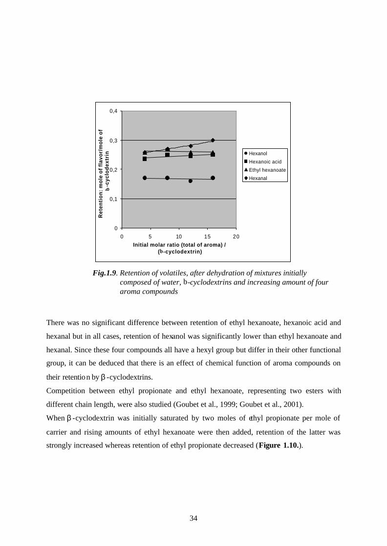
34
0
0,1
0,2
0,3
0,4
0 5 10 15 20Initial molar ratio (total of aroma) /
(β -cyclodextrin)
Ret
enti
on
: m
ole
of
flav
or/
mo
le o
f β
-cyc
lod
extr
in Hexanol
Hexanoic acid
Ethyl hexanoate
Hexanal
Fig.1.9. Retention of volatiles, after dehydration of mixtures initially composed of water, ? -cyclodextrins and increasing amount of four aroma compounds
There was no significant difference between retention of ethyl hexanoate, hexanoic acid and
hexanal but in all cases, retention of hexanol was significantly lower than ethyl hexanoate and
hexanal. Since these four compounds all have a hexyl group but differ in their other functional
group, it can be deduced that there is an effect of chemical function of aroma compounds on
their retention by β -cyclodextrins.
Competition between ethyl propionate and ethyl hexanoate, representing two esters with
different chain length, were also studied (Goubet et al., 1999; Goubet et al., 2001).
When β -cyclodextrin was initially saturated by two moles of ethyl propionate per mole of
carrier and rising amounts of ethyl hexanoate were then added, retention of the latter was
strongly increased whereas retention of ethyl propionate decreased (Figure 1.10.).
b
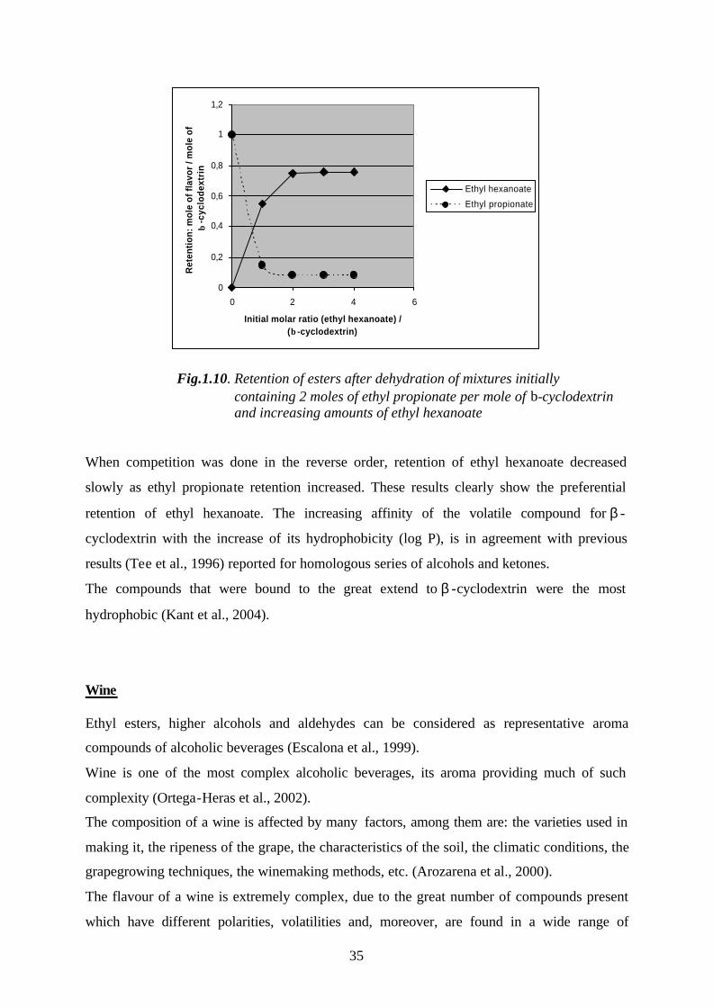
35
0
0,2
0,4
0,6
0,8
1
1,2
0 2 4 6
Initial molar ratio (ethyl hexanoate) / (β -cyclodextrin)
Ret
enti
on: m
ole
of fl
avor
/ m
ole
of
β-c
yclo
dext
rin
Ethyl hexanoate
Ethyl propionate
Fig.1.10. Retention of esters after dehydration of mixtures initially containing 2 moles of ethyl propionate per mole of ? -cyclodextrin and increasing amounts of ethyl hexanoate
When competition was done in the reverse order, retention of ethyl hexanoate decreased
slowly as ethyl propionate retention increased. These results clearly show the preferential
retention of ethyl hexanoate. The increasing affinity of the volatile compound for β -
cyclodextrin with the increase of its hydrophobicity (log P), is in agreement with previous
results (Tee et al., 1996) reported for homologous series of alcohols and ketones.
The compounds that were bound to the great extend to β -cyclodextrin were the most
hydrophobic (Kant et al., 2004).
Wine Ethyl esters, higher alcohols and aldehydes can be considered as representative aroma
compounds of alcoholic beverages (Escalona et al., 1999).
Wine is one of the most complex alcoholic beverages, its aroma providing much of such
complexity (Ortega-Heras et al., 2002).
The composition of a wine is affected by many factors, among them are: the varieties used in
making it, the ripeness of the grape, the characteristics of the soil, the climatic conditions, the
grapegrowing techniques, the winemaking methods, etc. (Arozarena et al., 2000).
The flavour of a wine is extremely complex, due to the great number of compounds present
which have different polarities, volatilities and, moreover, are found in a wide range of
b

36
concentrations (Hernanz Vila et al., 1999). The authors specified that from this reason, sample
preparation, especially extraction and concentration of aroma compounds remains one of the
critical areas in aroma volatiles analysis.
More than 800 compounds have been identified in the volatile fraction of wine (Ortega-Heras
et al., 2002; Guth, 1997). An important number of the volatile components in wine can only
be found at very low concentration ( µ g ml-1). The most studied and known compounds
present in wines are the esters, alcohols, acids, terpenes, lactines, volatile phenols and
aldehydes (Ortega-Heras et al., 2002; Hernanz Vila et al., 1999). Many of the aromatic
components are unstable.
One of the main problems that appear when studying the compounds responsible for wine
aroma is the choice of a suitable extraction procedure to qualitatively and quantitatively
represent the wine original aroma. As Cies (1999) described, many aroma compounds of a
wine are lost during processing of the wine, making it less pleasurable. Wine makers have
been looking for ways to try and keep these compounds in the wine during periods such as
fermentation, distillation, and processing. The same author remarked that wine makers have
looked into many extraction processes to try and avoid loosing precious aroma compounds.
Some include steam distillation, air stripping, and the spinning cone column.
The screening experiments by aroma extract dilution analysis (AEDA) and static headspace
analysis-olfactometry (SHA-O), followed by quantification and calculation of odour activity
values (OAV’s) and reconstitution experiments are suitable tools to investigate wine flavour
(Guth et al. ; Escudero et al., 2000).
Another used method for the quantification of the volatiles in wines is stable isotope dilution
assays (SIDA) (Schieberle et al., 1987; Guth et al., 1990; Sen et al., 1991; Guth, 1997).
Headspace solid phase microextraction (HS-SPME) was investigated as a solvent-free
alternative method for the extraction and determination of some volatile compounds in red
wine by capillary gas chromatography with flame ionization detector (FID) (Monje et al.,
2002).
The static headspace (SHS) technique is a suitable tool for the analysis and quantification of
most of the volatile compounds in wine because the preparation of the sample is very simple

37
and the extraction and analysis is completely automated (Ortega-Heras et al., 2002; Noble,
1978).
Concentrations of volatiles in the headspace influence the aroma character of alcoholic drinks.
(Conner et al., 1998; Escalona et al., 1999).
The partition coefficients wine/air for the volatile compounds, using SHS, were determined
(Clarke et al., 2004). From the experiments was observed that the volatile organic compounds
with high boiling points, but low solubility in water (or wine) have very high partition
coefficients. In contrast, compounds with low boiling points and high water solubility have
low values. The authors pointed out that this phenomenon is a consequence of the inherent
hydrophobicity of the volatile compound, reflected in the ratio of the number and size of non-
polar to polar groups, and their positioning in the particular molecule.
They noticed also that in any homologous series, for example aliphatic esters, alcohols,
ketones, etc., partition coefficients will be at their lowest for compounds at the bottom of the
series, with the lowest molecular weights. Partition coefficients will rapidly increase with
increasing molecular weight.
One of the advantages of the SHS method versus for example the liquid- liquid extraction is
that the analytes are extracted from the sample matrix without the use of an organic solvent,
so in the chromatogram the solvent peak does not appear. However, the method is only
sensitive for detection of highly volatile components or medium volatile ones present in high
concentrations, such as 2-phenyl-1-ethanol (Ortega-Heras et al., 2002).
The ability to link analytical and sensory information has been advanced through application
of numerous multivariate statistical analyses.
The impact of these advances on the understanding of wine flavour has recently been
reviewed (Ebeler, 1999; Ebeler, 2001; Ebeler et al., 2000; Noble et al., 2002).
Ebeler (2004) showed, that most food and beverage flavors are extremely complex and arise
from the combination of a number of chemical components. For example, the distinctive
varietal flavor of most wines is not due to a single impact compound but to the combination
of several components, most of which are not unique to a single grape variety.
In similar studies, Fischer et. al., 1999 have shown that sensory properties of Riesling wines
can vary significantly, even within the same vineyard designation. Heymann and Noble, 1987
and Guinard and Cliff, 1987 have shown that judges can distinguish among wines of different
geographic origin on the basis of their aroma properties.
38
The quality of alcoholic beverages is significantly determined by the content of hundreds of
volatile substances (Nykänen et al., 1983). Most of them are produced by fermentation
processes.
Ethanol is the most abundant compound, affecting only moderately the smell and taste of all
alcoholic beverages. Ethanol influences the volatility of aroma compounds in wines, it leads
to modification in macromolecule conformation such as protein, which changes the binding
capacity of the macromolecule (Voilley et al., 1999).
1.2.7. Molecular modelling studies on the prediction of solvation free energies of
flavour compounds in different model systems
The solvation free energy is defined according to the following thermodynamic equation:
PRTG l n-=∆ (1-15)
where: ∆ G – energy of solvation: kcal / mol;
R – universal gas constant: 8.314 Jmol-1K-1 = 1.98 10-3 kcal / mol K;
T – temperature: 298.15 K;
P – partition coefficient.
As it can be seen from the Equation (1-15), the solvation free energy is correlated with
partition coefficient.
Molecular modelling appears to be concerned with ways to mimic the behaviour of molecules
and molecular systems (Leach, 2001).
Molecular modelling investigations are important for the consideration and prediction of
complex chemical processes that take place at molecular level. From molecular modelling
studies one can understand representation and treatment of real three-dimensional molecule
structures and their physical-chemical properties.
Bakker et al. (1996) mentioned that using mathematical modelling to describe the various
aspects of flavour release gives a fundamental understanding of the mechanism of flavour
release.
39
Mathematical models are used to describe in physical terms the events leading to flavour
release, and allow predictions regarding the factors of importance for flavour release from
defined food structures.
As Bachs et al. (1994) presented, the theoretical simulation of chemical processes in solution
is difficult due to the large number of solvent molecules to be considered. This impedes a pure
quantum mechanical (QM) approach to the study of solvated systems and makes necessary
the use of simplified methods. The authors said also that among these methods, the most
popular are:
• classical (force-field-derived) models;
• the hybrid QM-classical models, and
• self-consistent reaction field (SCRF) methods.
Classical models (Jorgensen, 1991) represent both solute and solvent by means of classical
Hamiltonians (force field), which permit a fast calculation of solvation free energies using
molecular dynamics (MD) or Monte Carlo (MC) techniques.
QM- classical models (Singh et al., 1976; Weiner et al., 1989; Field et al., 1990; Luzhkov et
al., 1992; Gao, 1992; Floris et al., 1997) describe the solute at the QM level (usually using a
semi empirical Hamiltonian), whereas the solvent is treated at the classical level.
They observed that to build up the effective Hamiltonian and to solve the corresponding
Schrödinger equation one has to introduce a cavity in the continuum solvent distribution,
where the solute is accommodated. The need of using a cavity to solve the Schrödinger
equation leads to a definition of the basic energetic quantity in a form also containing a
contribution corresponding to the energy spent to form the cavity. This basic energy quantity
has the status of a free energy.
Finally, SCRF methods (Tapia, 1992) use a QM description of the solute (either at the ab
initio or semi empirical levels) and a “quasi” continuum representation of the solvent.
Bachs et al. (1994) explained that SCRF methods are based on the theory of electrostatic
interactions in fluids.
SCRF methods provide a fast representation of solvent effects and allow one to consider
explicitly polarization effects, which are neglected or only partially considered in classical
and QM-classical calculations.

40
MST/SCRF Method
Miertus, Scrocco, and Tomasi developed a rigorous SCRF model (MST) (Tomasi et al.,
1994; Miertus et al., 1981 ; Miertus et al., 1982). The MST model relies on the continuum
model (known as polarizable continuum model).
This method makes a precise description of the perturbation operator in terms of the
molecular electrostatic potential (MEP) (Scrocco et al., 1973), thus avoiding the use of
truncated expansions of the solute charge distribution.
Bachs et al. (1994) described that the accuracy of the results obtained in MST calculations
will depend in practice on several factors:
• the quality of the basis set in the SCF procedure;
• the cavity use to simulate the solute / solvent interface; and
• the reliability of the method used to represent steric effects (cavitations and van
der Waals interactions).
Unfortunately, the criteria for the selection of the cavity size and for the calculation of steric
contributions are not so clear. Particularly, the proper selection of the cavity size is crucial in
MST-SCRF calculations: A cavity that is too large will underestimate the solvent effect,
whereas a cavity that is too small will overestimate such an effect (Bachs et al., 1994).
The free energy of solvation in the MST model is expressed as the sum of three contributions
(Equation 1-16): cavitations ( ∆ Gcav), van der Waals ( ∆ GvW), and electrostatic (Gele)
(Curutchet et al., 2001):
vWcavelesol GGGG (1-16)
As Luque et al. (1996) presented, the transfer of a given solute from the gas phase into
solution can be partitioned into three steps: (i) creation of the solute cavity inside bulk
solvent; (ii) generation of the van der Waals particle inside the cavity, and (iii) generation of
the solute charge distribution in solution. If changes in the internal degrees of freedom of the
solute are neglected, ∆ Gsol can be expressed as in Equation (1-15).
Monte Carlo (MC) calculations were performed to help in determining the best solute /
solvent interface for the electrostatic component of the free energy of solvation (Curutchet et
al., 2001).
∆+∆+∆=∆

41
Also, Duffy and Jorgensen (2000) used Monte Carlo (MC) statistical mechanics to predict the
free energies of solvation in hexadecane, octanol, and water for more than 200 organic
solutes, including 125 drugs and related heterocycles. The study provided links between
statistical mechanics simulations for solutes in solutions, traditional physical-organic
analyses, quantitative structure-property relationships (QSPR), and linear response
approaches for estimating free energies of solvation.
Luque et al., 1996 explained that the three main differences between the SCRF methods are:
(i) the shape of the solute/solvent interface; (ii) the definition of the solvent reaction field, and
(iii) the evaluation of nonelectrostatic contributions to the free energy of solvation, ∆ Gsol.
A computational method to introduce solvent effects in the description of molecular systems
in the ground state has been proposed few years ago (Pascual-Ahuir et al., 1987), and later on
extended to systems subjected to a change of electronic state (Bonaccorsi et al., 1983).
Most chemistry and biochemistry occur in condensed media, in particular, aqueous solutions.
Thus, the proper simulation of these processes has to take into account the solvent effects
(Hernandes et al., 2002).
There are basically three models (Dillet et al., 1994; Cappelli et al., 2000) to describe the
solvent, namely:
• the continuum or dielectric model;
• the discrete or super molecule model; and
• the discrete-continuum model, which attempts to combine the two previous ones.
The continuum model treats the solvent as a structureless dielectric medium and the solute is
inserted in a cavity.
Hernandes et al. (2002) also specified that the continuum models are not able to describe
specific solute-solvent interactions, in particular, hydrogen bonds. In addition, the definition
of the solute cavity and the dielectric constant are arbitrary.
Cappelli et al. (2000) explained that continuum solvation models are generally focused on
purely electrostatic effects; the solvent is modelled as a homogeneous continuous medium,
usually isotropic, whose response is determined by its dielectric constant, ε? . Electrostatic
effects usually constitute the dominating part of the solute-solvent interaction but in some
cases explicit solute-solvent interactions should be taken into account to reach a reliable and
accurate estimate of the phenomenon.

42
The standard-state free energy of solvation is the free energy difference associated with the
transfer of a solute X from the gas-phase to a given solvent Y (Ben-Naim, 1987), and it is a
fundamental quantity that describes the interactions between a solute molecule and the solvent
in which it is dissolved (Ben-Naim, 1987; Tomasi et al., 1994; Cramer et al., 1999).
The free energy of solvation in two solvents provides enough information to calculate the
partition coefficient of a solute between the two solvents (Thompson et al., 2004).
The standard –state free energy of solvation, ∆ G0S of a solute in a liquid solvent is written in
SM5.43R continuum solvation model proposed by Thompson et al. (2004) as:
concCDSPS GGGEG 00 (1-17)
where: G P is the electronic polarization energy from mutual polarization of the solute and the
solvent; ∆ E is the change in the solute’s internal electronic energy when the solute is placed in
the solvent; GCDS is a semiempirical term that accounts for all interactions except bulk
electrostatics, and ∆ G0conc accounts for the concentration change between the gas-phase and
the liquid-phase standard states.
The discrete model treats the solvent as individual molecules, which interact with the solute
via a parametric potential (Allen et al., 1987) (classical models) or an instantaneous
Coulombic interaction between the electrons and the nuclei of the solute and the solvent
molecules (quantum models).
As Dillet et al. (1994) specified, in the case of a molecule interacting with a solvent, such an
approach becomes inoperating because one would have to apply statistical mechanics to a
system made of a large number of atoms or molecules and the computation of the electron
properties of each of the many configurations to be considered is out of reach of the most
powerful modern computers.
The same authors explained that this is the reason why one currently uses simplified models.
One of simplest possible models consists of considering the solvent as a macroscopic
continuum and the solute as filling a cavity created in this continuous medium.
=∆ +∆ + + ∆
43
1.3. Aims of the work
The effect of food matrix composition on flavour release and partition coefficient should be
investigated and discussed through complementary studies carried out by thermodynamic or
kinetic approaches.The basic research in this area should make a contribution to the
optimization of economic processes in the industrial food production.
The present studies are part of a research project (COST Action 921) at EU level with the
following title: “Food matrices: structural organisation from nano to macro scale and impact
on flavour release and perception”. Essential impulses and efficiency for the treatment of the
research subject arise from the involvement and bundling of experiences and research
methods on this task by the European institutions. COST Action 921 is an international
project in the framework of the European Union, whose main objective is to understand the
impact of structural organisation of food matrices, and their changes during mastication, on
perception and flavour release.
Further objectives are as follows:
• To understand the perception of flavour and texture as a function of composition,
structure and physiology;
• To develop appropriate methods to follow the aroma release and perception
during oral processing;
• To extrapolate results obtained with simple model systems to food- like models;
• To develop mathematical models which predict the relationship between the structural
organisation of food matrices at molecular and meso-structure level, rheology and
transport phenomena, flavour release and sensory perception.
An aim of the present research work should be the clarification of the complex relationships
of the flavour release as a function of the composition of the food matrix, at molecular level,
especially the clarification of the influence of matrix effects onto the partition coefficients,
odour activity values and sensory properties of selected flavour compounds, in model and in
real food systems.
Further aims of the research work are the determination of physico-chemical parameters of
selected flavour compounds, such as vapour pressures and partition coefficients.
Different matrices should be investigated to measure their influence onto the partition
coefficients of odorants: water, water-ethanol-mixtures, matrices containing lipids and more
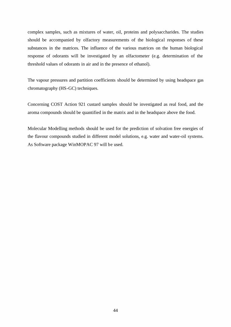
44
complex samples, such as mixtures of water, oil, proteins and polysaccharides. The studies
should be accompanied by olfactory measurements of the biological responses of these
substances in the matrices. The influence of the various matrices on the human biological
response of odorants will be investigated by an olfactometer (e.g. determination of the
threshold values of odorants in air and in the presence of ethanol).
The vapour pressures and partition coefficients should be determined by using headspace gas
chromatography (HS-GC) techniques.
Concerning COST Action 921 custard samples should be investigated as real food, and the
aroma compounds should be quantified in the matrix and in the headspace above the food.
Molecular Modelling methods should be used for the prediction of solvation free energies of
the flavour compounds studied in different model solutions, e.g. water and water-oil systems.
As Software package WinMOPAC 97 will be used.
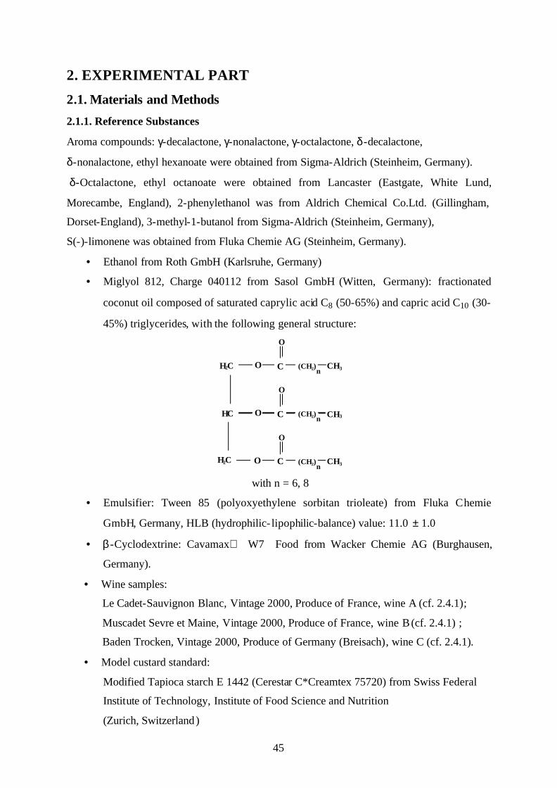
45
2. EXPERIMENTAL PART
2.1. Materials and Methods
2.1.1. Reference Substances
Aroma compounds: γ-decalactone, γ-nonalactone, γ-octalactone, δ -decalactone,
δ-nonalactone, ethyl hexanoate were obtained from Sigma-Aldrich (Steinheim, Germany).
δ-Octalactone, ethyl octanoate were obtained from Lancaster (Eastgate, White Lund,
Morecambe, England), 2-phenylethanol was from Aldrich Chemical Co.Ltd. (Gillingham,
Dorset-England), 3-methyl-1-butanol from Sigma-Aldrich (Steinheim, Germany),
S(-)-limonene was obtained from Fluka Chemie AG (Steinheim, Germany).
• Ethanol from Roth GmbH (Karlsruhe, Germany)
• Miglyol 812, Charge 040112 from Sasol GmbH (Witten, Germany): fractionated
coconut oil composed of saturated caprylic acid C8 (50-65%) and capric acid C10 (30-
45%) triglycerides, with the following general structure:
H2C O C (CH2) CH3n
O
HC O C (CH2) CH3n
O
H2C O C (CH2) CH3n
O
with n = 6, 8
• Emulsifier: Tween 85 (polyoxyethylene sorbitan trioleate) from Fluka Chemie
GmbH, Germany, HLB (hydrophilic- lipophilic-balance) value: 11.0 ± 1.0
• β -Cyclodextrine: Cavamax W7 Food from Wacker Chemie AG (Burghausen,
Germany).
• Wine samples:
Le Cadet-Sauvignon Blanc, Vintage 2000, Produce of France, wine A (cf. 2.4.1);
Muscadet Sevre et Maine, Vintage 2000, Produce of France, wine B (cf. 2.4.1) ;
Baden Trocken, Vintage 2000, Produce of Germany (Breisach), wine C (cf. 2.4.1).
• Model custard standard:
Modified Tapioca starch E 1442 (Cerestar C*Creamtex 75720) from Swiss Federal
Institute of Technology, Institute of Food Science and Nutrition
(Zurich, Switzerland)
46
Full Fat Milk Powder (26% fat) from Friesland Coberco Dairy Foods (Corporate
Research, Deventer, Netherland)
Strawberry aroma from Givaudan Schweiz AG (Dubendorf, Switzerland)
κ-Carrageenan (MeyproTM Lact HMF, Gelymar Lot 114, Production January 2004)
from Swiss Federal Institute of Technology, Institute of Food Science and
Nutrition (Zurich, Switzerland)
Sucrose from Sigma-Aldrich Chemie GmbH (Steinheim, Germany)
The composition of the strawberry aroma is listed in Table 2.1.
Table 2.1. Composition of the strawberry aroma
Aroma compound Amount (mg / g)
Furaneol 5
Vanilin 5
Methyl cinnamate 24
Ethyl hexanoate 20
Ethyl butyrate 90
Benzyl acetate 2
Styrallyl acetate 1
Gamma-decalactone 20
Methyl anthranilate 1
Ethyl iso-pentanoate 10
Hexanal 1
cis-3-Hexenyl acetate 5
cis-3-Hexenol 15
Methyl dihydrojasmonate 5
Beta- ionone 1
Triacetin (solvent) 795
The custard was produced with the following ingredients: water, sugar (sucrose), milk
powder, flavour, modified tapioca starch and carrageenan (thickener).
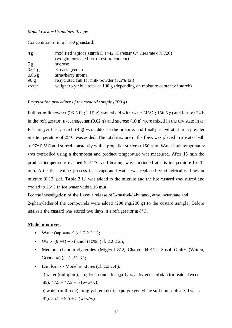
47
Model Custard Standard Recipe Concentrations in g / 100 g custard: 4 g modified tapioca starch E 1442 (Cerestar C* Creamtex 75720) (weight corrected for moisture content) 5 g sucrose 0.01 g κ-carrageenan 0.06 g strawberry aroma 90 g rehydrated full fat milk powder (3.5% fat) water weight to yield a total of 100 g (depending on moisture content of starch) Preparation procedure of the custard sample (200 g) Full fat milk powder (26% fat; 23.5 g) was mixed with water (45°C; 156.5 g) and left for 24 h
in the refrigerator. κ-carrageenan (0.02 g) and sucrose (10 g) were mixed in the dry state in an
Erlenmeyer flask, starch (8 g) was added to the mixture, and finally rehydrated milk powder
at a temperature of 25°C was added. The total mixture in the flask was placed in a water bath
at 97±0.5°C and stirred constantly with a propeller stirrer at 150 rpm. Water bath temperature
was controlled using a thermostat and product temperature was measured. After 15 min the
product temperature reached 94±1°C and heating was continued at this temperature for 15
min. After the heating process the evaporated water was replaced gravimetrically. Flavour
mixture (0.12 g cf. Table 2.1.) was added to the mixture and the hot custard was stirred and
cooled to 25°C in ice water within 15 min.
For the investigation of the flavour release of 3-methyl-1-butanol, ethyl octanoate and
2-phenylethanol the compounds were added (200 mg/200 g) to the custard sample. Before
analysis the custard was stored two days in a refrigerator at 8°C.
Model mixtures:
• Water (tap water) (cf. 2.2.2.1.);
• Water (90%) + Ethanol (10%) (cf. 2.2.2.2.);
• Medium chain triglycerides (Miglyol 812, Charge 040112, Sasol GmbH (Witten,
Germany) (cf. 2.2.2.3.);
• Emulsions - Model mixtures (cf. 2.2.2.4.):
a) water (millipore), miglyol, emulsifier (polyoxyethylene sorbitan trioleate, Tween
85): 47.5 + 47.5 + 5 (w/w/w);
b) water (millipore), miglyol, emulsifier (polyoxyethylene sorbitan trioleate, Tween
85): 85.5 + 9.5 + 5 (w/w/w);

48
c) water (millipore), miglyol, emulsifier (polyoxyethylene sorbitan trioleate, Tween
85): 90.25 + 4.75 + 5 (w/w/w).
2.1.2. Instrumentation
2.1.2.1. Instrumentation for the preparation of emulsions For the preparation of the emulsions the following two instruments were used:
a) Ultra-Turrax homogenizer: Typ T 18/10, Janke&Kunkel GmbH & Co. KG, Germany, IKA
LABORTECHNIK, operating range (up to 200 mP s):10-500 ml; shaft tube-∅ mm:18; stator -
∅ mm: 18; rotor - ∅ mm: 12.7; maximum circumferential (m/s): 15.9; maximum depth of
immersion (mm): 225.
b) Ultrasound – disintegrator (Cell disruptor) Branson sonifier B – 15: Branson Sonic Power
Co. A SmithKline Com. Gerhard Henemann Labor-Ansrüstungen (Schwäbisch Gmünd,
Germany).
Technical Data – SONIFIER B-15: Generator, FTZ –shielded; network connection: 220 V /
50 Hz; 2.5 A; output: 150 Watt; work frequency:20 kHz; dimensions: 360x365x135 mm
(BxTxH). Convertor: oscillator: lead-zirconate-titanate; dimensions: 178x64 mm φ .
2.1.2.2. Static Headspace Gas Chromatography (SHS-GC) Static headspace analysis (SHA) was performed at a Chrompack CP 4010 gas chromatograph
connected to the TCT/PTI 4001 (Varian-Chrompack, Darmstadt; Germany) headspace
injector (Figure 2.1.) (TCT– Thermal Desorption Cold Trap injector; PTI – Purge and Trap
injector).
Pure substances and model mixtures (cf. 2.1.) were put into a thermostated vessel (250 ml)
(30°C), sealed with a septum, and equilibrated for 3 hours. Headspace gas was drawn by a gas
tight syringe (1-5 ml, velocity of injection: 10 ml/min) and then analysed by GC-FID
(Hewlett-Packard 5890 Series II) (FID – Flame Ionization Detector).
The TCT/PTI 4001 system operated in the desorption mode for 15 min at a temperature of
200°C and a flow rate of 20 ml helium (desorption purge). The fused silica trap (30 cm x
0.53 mm, coated with CP-Sil5CB, film thickness 5 µ m) was cooled with liquid nitrogen at

49
–110°C and after 15 min the trap was heated up to 200°C and this temperature was held for 1
min. The trapped compounds were flushed by the helium flow into the GC onto the capillaries
detailed in conditions of SHS.
Fig.2.1: Schematic presentation of the method for the determination of partition coefficients (water/air, water-ethanol-mixtures/air, miglyol/air, emulsions/air) and odorant adsorptions to the gas-tight syringe. A: Headspace sampling. B: Coupling of syringe 1 and 2, transfer of a defined volume gas from syringe 1 to syringe 2. C: Injection with syringe 2. D: Direct injection with syringe 1.
Gas-tight syringe 1
Gas-tight
syringe 2
A
B
C
Gas-tight syringe 1
Injection
Gas-tight
syringe 2
Injection Gas-tight syringe 1
D

50
Conditions of SHS:
• Carrier gas: He, 30 kPa (20 ml/min);
• Backflush: 50 ml/min;
• Temperature program of the GC oven:
35°C (1 min) ° min/ 40 C
60°C (1 min) 8 °C/min 240°C (20 min);
• Column: 30 m x 0.32 mm ; 0.25 µ m film thickness DB-FFAP (Free Fatty Acid Phase),
Phase: Nitroterephtalic acid modified polyethylene glycol, from J&W Scientific
(Agilent Böblingen,Germany);
• Syringes used: 1ml and 5 ml syringes with valve (from SGE Germany);
• Equilibration time of samples: 3 h at 30°C;
• Vials volume: 250 ml.
Quantification of the odorants in the headspace was achieved by external calibration
(concentration range of the standard solution:18-20 ng / 1 µ l).
Adsorption measurements by static headspace gas chromatography
Adsorptions of the odorants at the gas-tight syringe were checked by the method detailed in
Figure 2.1. (Guth and Sies, 2001). The calculation of the adsorption was made from five
replicates (standard deviation: ± 10%).
Adsorption (%) = ( ?)
121
100syringeconodorant
syringeconodorantsyringeconodorant −× (2-1)
2.1.2.3. Instrumentation for the determination of odorant headspace concentrations in wine
samples For the determination of the headspace concentration of selected aroma compounds in wine
samples the gas-chromatograph CP-3380 with Combi Pal SHS-Autosampler was used.
Gas-chromatograph CP-3380
• Varian GmbH (Darmstadt, Deutschland)
• Injector: Split / Splitless – Injector, Varian 1079
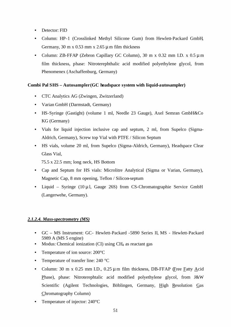
51
• Detector: FID
• Column: HP-1 (Crosslinked Methyl Silicone Gum) from Hewlett-Packard GmbH,
Germany, 30 m x 0.53 mm x 2.65 µ m film thickness
• Column: ZB-FFAP (Zebron Capillary GC Column), 30 m x 0.32 mm I.D. x 0.5 µ m
film thickness, phase: Nitroterephthalic acid modified polyethylene glycol, from
Phenomenex (Aschaffenburg, Germany)
Combi Pal SHS – Autosampler (GC headspace system with liquid-autosampler)
• CTC Analytics AG (Zwingen, Zwitzerland)
• Varian GmbH (Darmstadt, Germany)
• HS-Syringe (Gastight) (volume 1 ml, Needle 23 Gauge), Axel Semran GmbH&Co
KG (Germany)
• Vials for liquid injection inclusive cap and septum, 2 ml, from Supelco (Sigma-
Aldrich, Germany), Screw top Vial with PTFE / Silicon Septum
• HS vials, volume 20 ml, from Supelco (Sigma-Aldrich, Germany), Headspace Clear
Glass Vial,
75.5 x 22.5 mm; long neck, HS Bottom
• Cap and Septum for HS vials: Microlitre Analytical (Sigma or Varian, Germany),
Magnetic Cap, 8 mm opening, Teflon / Silicon-septum
• Liquid – Syringe (10 µ l, Gauge 26S) from CS-Chromatographie Service GmbH
(Langerwehe, Germany).
2.1.2.4. Mass-spectrometry (MS)
• GC – MS Instrument: GC- Hewlett-Packard -5890 Series II, MS - Hewlett-Packard
5989 A (MS 5 engine) • Modus: Chemical ionization (CI) using CH4 as reactant gas
• Temperature of ion source: 200°C
• Temperature of transfer line: 240 °C
• Column: 30 m x 0.25 mm I.D., 0.25 µ m film thickness, DB-FFAP (Free Fatty Acid
Phase), phase: Nitroterephtalic acid modified polyethylene glycol, from J&W
Scientific (Agilent Technologies, Böblingen, Germany, High Resolution Gas
Chromatography Column)
• Temperature of injector: 240°C
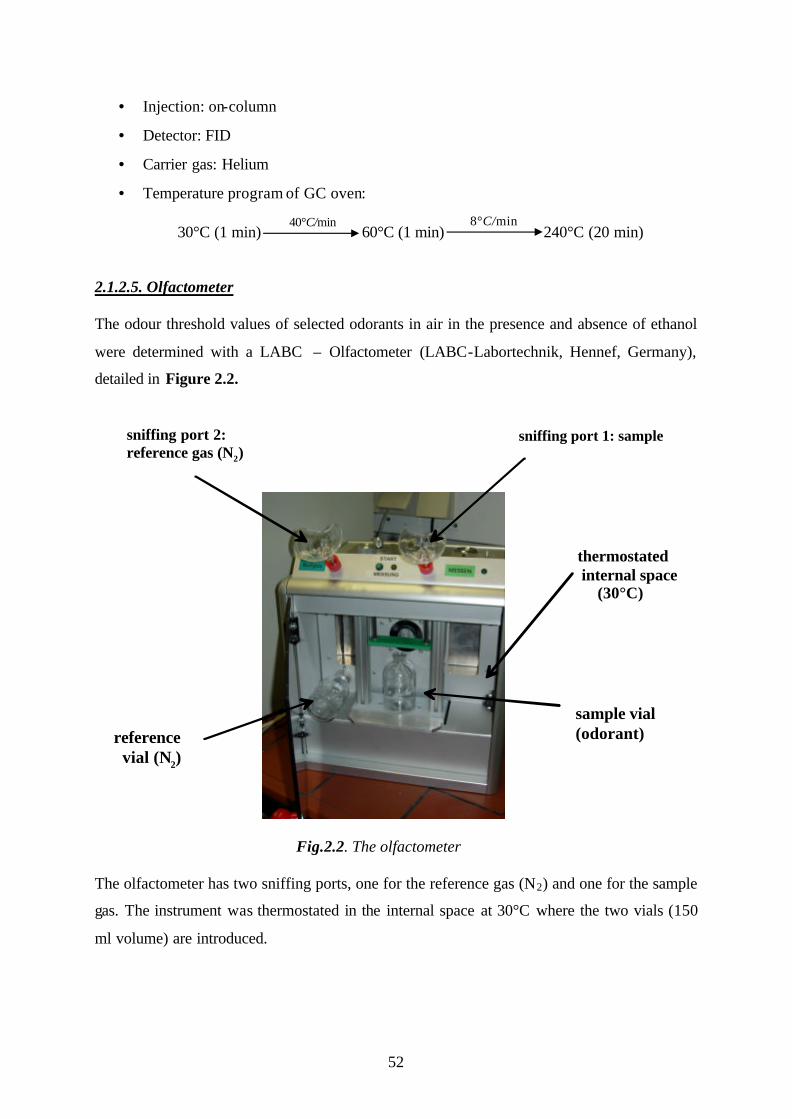
52
• Injection: on-column
• Detector: FID
• Carrier gas: Helium
• Temperature program of GC oven:
30°C (1 min) 40°C/min
60°C (1 min) 8°C/min
240°C (20 min)
2.1.2.5. Olfactometer The odour threshold values of selected odorants in air in the presence and absence of ethanol
were determined with a LABC – Olfactometer (LABC-Labortechnik, Hennef, Germany),
detailed in Figure 2.2.
reference vial (N2)
sample vial(odorant)
thermostated internal space (30°C)
sniffing port 1: samplesniffing port 2: reference gas (N2)
Fig.2.2. The olfactometer The olfactometer has two sniffing ports, one for the reference gas (N2) and one for the sample
gas. The instrument was thermostated in the internal space at 30°C where the two vials (150
ml volume) are introduced.
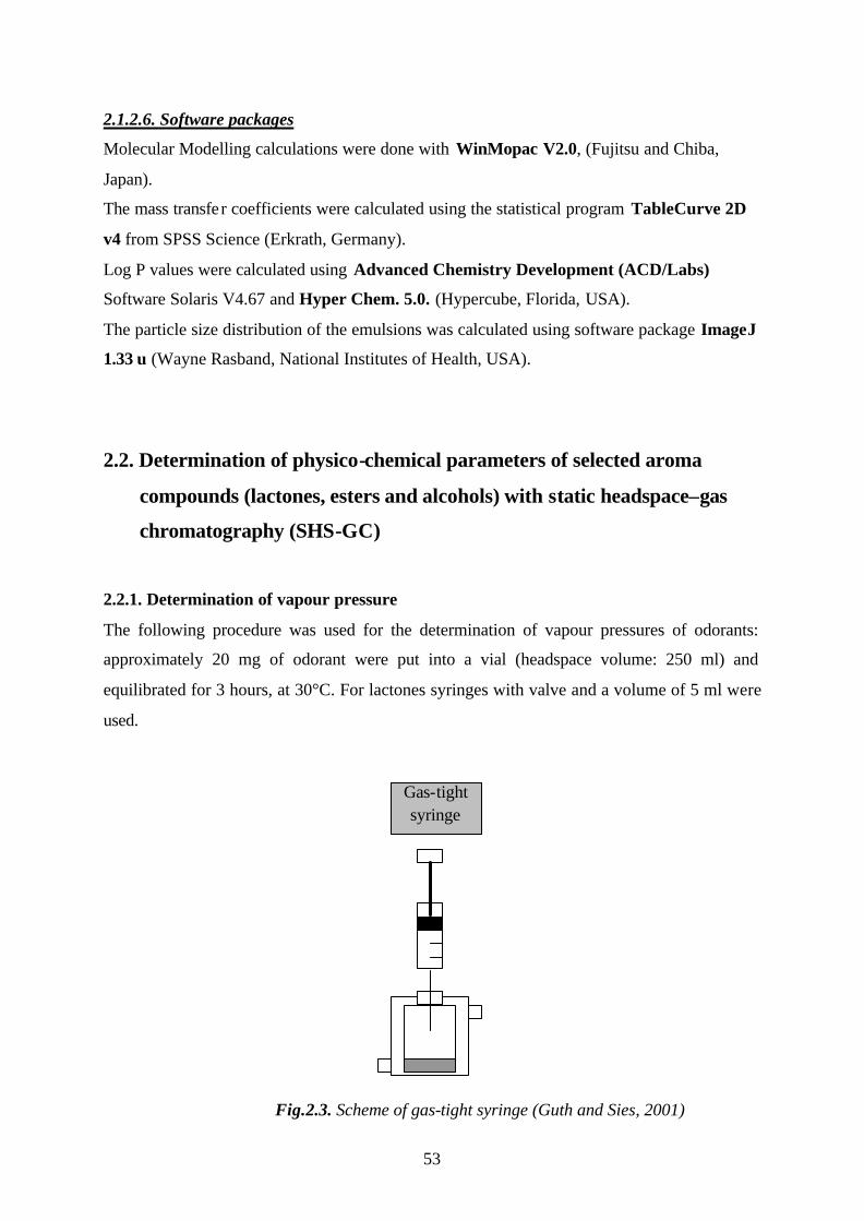
53
2.1.2.6. Software packages
Molecular Modelling calculations were done with WinMopac V2.0, (Fujitsu and Chiba,
Japan).
The mass transfer coefficients were calculated using the statistical program TableCurve 2D
v4 from SPSS Science (Erkrath, Germany).
Log P values were calculated using Advanced Chemistry Development (ACD/Labs)
Software Solaris V4.67 and Hyper Chem. 5.0. (Hypercube, Florida, USA).
The particle size distribution of the emulsions was calculated using software package ImageJ
1.33 u (Wayne Rasband, National Institutes of Health, USA).
2.2. Determination of physico-chemical parameters of selected aroma
compounds (lactones, esters and alcohols) with static headspace–gas
chromatography (SHS-GC)
2.2.1. Determination of vapour pressure
The following procedure was used for the determination of vapour pressures of odorants:
approximately 20 mg of odorant were put into a vial (headspace volume: 250 ml) and
equilibrated for 3 hours, at 30°C. For lactones syringes with valve and a volume of 5 ml were
used.
Fig.2.3. Scheme of gas-tight syringe (Guth and Sies, 2001)
Gas-tight syringe

54
For esters and alcohols, syringes with a volume of 5 ml and 1 ml, respectively, were used.
Adsorptions of odorants were measured according to the following procedure:
For the IInd syringe injection (cf. Figure 2.1.), the two syringes (I + II) were coupled together.
A fixed amount of headspace sample (lactones: 1, 3, 5 ml, depending on lactone
concentration; esters: 0.1 and 0.2 ml; alcohols: 1 and 0.1 ml) was taken from the vial,
transferred into the syringe II and injected into the TCT-system. The syringes are equipped
with a valve, which is closed after transferring of the vapour sample into the syringe, to
prevent the loss of the volatile compound.
For the Ist syringe injection a fixed amount of gas sample was taken from the vial and injected
directly into the TCT system.
Between two injections, a blank run was made, and before each injection the syringes were
washed with hot water and dried.
From the chromatograms the areas of the compounds (Ist syringe and IInd syringe) were
obtained. From these areas the adsorption effect on the syringe was calculated according to
the Equation (2-1). For the same odorant, between 2 and 5 injections have been done, and an
adsorption average was calculated.
The concentration of the compound in the headspace was determined by comparison the area
of headspace sample to the area obtained by injecting a standard solution of the compound in
diethyl ether.The standard solution of specified compound (standard solution prepared in
diethyl ether with a known concentration) was injected (1 µ l) and the area was recorded. Also
from all the standard injections an average was made (5 injections). The concentration
average of the compound in the gas phase (ng/ml) was calculated according to the following
equation:
gist
DIa Va
ac
×= (2-2)
ca: concentration average (ng/ml); aDI: average area of the direct injection; ast : average area for
1 ng from the standard injection; Vgi: volume of gas injected (ml).
The vapour pressure for the selected pure compound, taking into account the adsorption effect
was calculated according to the following equation:
V
nRTpnRTpV =⇒= (2-3)

55
p: vapour pressure (Pa); n: number of moles of odorant; R: gas constant (8.314 J K-1 mol-1); T:
absolute temperature (K); V: volume of gas (ml).
2.2.2. Determination of partition coefficients in different matrices
For the calculation of partition coefficients of selected aroma compounds in different matrices
(water, water-ethanol mixtures, miglyol, emulsions) the procedure of work was similar as
described for the vapour pressures. The syringes used for the injections were 1 ml and 5 ml
syringes with valve. Partition coefficient (logP) for each compound was calculated as ratio of
the odorant concentration in the matrix to the concentration in the headspace above the
matrix.
2.2.2.1. Water / air partition coefficients of lactones, esters and alcohols
Solutions of selected lactones (γ-decalactone, γ-nonalactone, γ-octalactone and δ-decalactone,
δ-nonalactone, δ -octalactone), alcohols (3-methyl-1-butanol, 2-phenylethanol) and esters
(ethyl hexanoate and ethyl octanoate) in water were prepared with known concentrations
(approximately 20 mg/100 ml and 100 mg/100 ml, respectively), depending on the solubility
of selected compound in water. 10 ml of samples were put in vials (headspace volume: 250
ml) for equilibration. After equilibration (3 hours, 30°C) a defined headspace volume was
injected into the TCT system according to the procedure described in 2.2.1.
The standard solution of each compound (standard solution prepared in diethyl ether with a
known concentration) was injected (1 µ l) and the area of the compound was obtained.
An adsorption and concentration average of specified odorant in the headspace (ng/ml) was
calculated from five replicates (standard deviation: ± 10%).
2.2.2.2. Water-ethanol mixtures / air partition coefficients of lactones, esters and alcohols
Solutions of selected lactones (γ-decalactone), alcohols (3-methyl-1-butanol, 2-phenylethanol)
and esters (ethyl hexanoate and ethyl octanoate) in water (90%) + ethanol (10%), v/v, were
prepared with known concentrations (approximately 20 mg/50 ml, 20 mg/100 ml and 100
mg/100 ml, respectively).
The conditions of work and the injection procedure were similar as for the selected
compounds in water solution (cf. 2.2.2.1.). Quantification of the odorants in the headspace
was achieved by external calibration.

56
2.2.2.3. Miglyol / air partition coefficients of lactones, esters and alcohols
Solutions of selected lactones (γ-decalactone, γ-nonalactone, γ-octalactone and δ-decalactone,
δ-nonalactone, δ-octalactone), alcohols (3-methyl-1-butanol, 2-phenylethanol) and esters
(ethyl hexanoate and ethyl octanoate) in miglyol were prepared with known concentrations
(approximately 1 g/50 ml, 10 mg/50 ml, 50 mg/50 ml and 100 mg/50 ml, respectively),
depending on the solubility of selected compound in miglyol.
The conditions of work and the injection procedure was conforming those described in
2.2.2.1. Quantification of the odorants in the headspace was achieved by external calibration.
2.2.2.4. Emulsions (Miglyol-Water-Emulsifier) / air partition coefficients of lactones, esters
and alcohols
The emulsions were prepared in glasses, by mixing calculated amounts of oil (miglyol) with
water (Millipore water) and emulsifier, Tween 85 (polyoxyethylene sorbitan trioleate). An
Ultra turrax homogenizer TP 18/10 (IKA-Labortechnik, Germany) was used (cf.2.1.2.1.), for
homogenization 3 minutes at rotation speed indicator 4 (scale 1-10) and afterwards a Cell-
disrupter disintegrator (continuous modus, 4 minutes, output control 7, on a scale:1-10)
(cf.2.1.2.1.) for obtaining a better homogenization and a stable emulsion.
Three types of emulsions were prepared. The proportions between water, miglyol and
emulsifier were the following ones:
• Emulsion I: Water / Miglyol / Emulsifier Tween 85: (47.5 + 47.5 + 5, w/w/w)
• Emulsion II: Water / Miglyol / Emulsifier Tween 85: (85.5 + 9.5 + 5, w/w/w)
• Emulsion III: Water / Miglyol / Emulsifier Tween 85: (90.25 + 4.75 + 5, w/w/w)
The syringes used were 1 ml and 5 ml syringes with valve. The headspace injection volume:
1 ml, 3 ml and 5ml, respectively, depending of the compound.
The quantities of water, miglyol and emulsifier were weighted at the analytical balance. First,
water and emulsifier and then, during mixing with the Ultra-turax, was added slowly the
weighted quantity of miglyol. The mixture was homogenized with the Ultra-turax. To obtain a
stable emulsion a cell-disruptor disintegrator was used for homogenizing.
The emulsion stayed then approximately 1 hour at room temperature to stabilize. A known
quantity of odorant (approximately 200 mg/10 ml, 10 mg/50 ml, 20 mg/25 ml, 25 mg/25 ml,
40 mg/20 ml, respectively) was weighted, depending on the solubility of the compound in
emulsion. 10 ml from the emulsion were taken and put in vials (250 ml) for equilibration.
After equilibration (1 hour, 30°C) the samples were injected into the TCT system (cf. 2.2.1.).
57
The standard solution of specified odorant (standard solution prepared in diethyl ether with a
known concentration) was injected (1 µ l ) and the area of the compound was obtained. An
adsorption and concentration average of selected compound in the headspace (ng/ml) was
calculated from five replicates (standard deviation: ± 5%).
2.3. Interaction of odorants with ? -cyclodextrin The flavour release of ethyl hexanoate in the presence of β –cyclodextrin, respectively S-(-)-
limonene in the presence of β –cyclodextrin, at different dilution stages were studied.
For the determination of the reduction of the odour compounds ethyl hexanoate and S-(-)-
limonene in presence of β -cyclodextrin, a standard solution of aroma compound (solvent: tap
water, pH 7.6) was prepared. A defined aliquot was taken and transferred into a headspace
vial and filled up (10 ml) with water. The concentration of oligosaccharides was 10 mg/ml
and for every measurement was weighted directly in the headspace vials.
For the calculation of the reduction of the esters in the headspace, a solution was prepared,
which contained only the aroma compound in water. The solutions were stirred at ambient
temperature (22°C) for one hour before analysis.
2.3.1. Condition for the determination of flavour release of ethyl hexanoate in the
presence of ? -cyclodextrin
Materials: ethyl hexanoate water solution: 24 mg / 100 ml;
cyclodextrin: approximately 10 mg (weighted) in headspace vials (20 ml);
1 ml syringes with valve ;
volume of injection: from 1 to 0.1 ml, depending on the dilution;
50 ml flasks for dilutions;
standard solution: ethyl hexanoate in pentane: 22.6 ng/ 1 µ l;
volume injected: 1 µ l.
Conditions of work: equilibration time for each vial: 1 hour (stirring) at room temperature;
10 ml solution in vial (cyclodextrin + ethyl hexanoate or only ethyl hexanoate).
b
b
58
2.3.2. Condition for the determination of flavour release of S-(-)-limonene in the
presence of ? -cyclodextrin
Materials: S-(-)-Limonene water solution: 10.6 mg / 1 L;
cyclodextrin: approximately 10 mg (weighted) in headspace vials (20 ml);
1 ml syringes with valve ;
volume of injection: from 1 to 0.5 ml depending on the dilution;
50 ml flasks for dilutions;
standard solution: S-(-)-limonene in pentane: 12.1 ng/1 µ l;
volume injected: 1 µ l.
Conditions of work: equilibration time for each vial: 1 hour (stirring) at room temperature;
10 ml solution in vial (cyclodextrin + S-(-)-limonene or only S-(-)-limonene).
2.4. Determination of partition coefficients of selected flavour compounds
(alcohols and esters) in real food matrix
2.4.1. Wine matrix
Determination of the concentration of alcohols and esters in white wine samples The wine samples used for the measurements were as follows: Le Cadet Sauvignon, Baden
Trocken and Muscadet Sevre (cf.2.1.1.).
Standard addition method
The concentrations of 3-methyl-1-butanol, ethyl hexanoate and ethyl octanoate were
determinate by standard addition method, using headspace-gas chromatography (HS-GC).
The standard addition method is used to prepare a calibration plot in cases where the
composition of the sample matrix is variable or unknown so that a reagent / sample matrix
blank response cannot be reliably subtracted from each standard to arrive at the analyte
b

59
response alone as with calibration plots. In these cases, the sample is spiked with increasing
amounts of analyte.
The solutions were prepared according to the following procedure:
3-methyl-1-butanol: c = 11 mg/100 ml; ethyl hexanoate: c = 0,04 mg/100 ml; ethyl octanoate:
c = 0,042 mg/100 ml.
For the determination of the concentration through addition procedure, method HS-GC with
autosampler was used.
• HS – Autosampler (HP 1 column)
• Temperature program :
35°C (1 min) C
60°C (0 min)
240°C (10 min)
• Injection: 500 µ l
• Temperature of incubation : 30°C
• Equilibration time: 1 h
• 9.5 ml sample in headspace vials (20 ml)
• Sample delivery : splitless
Isotope dilution analysis (IDA) In the case of 2-phenylethanol, the concentration in wines could not be determined through
standard addition method. The concentration of 2-phenylethanol was determined by isotope
dilution analysis. As standard, 2-phenylethanol labelled compound (2[H]2 –phenylethanol)
was used. 2H2-Phenylethanol was synthesized according to:
CH2 COOH + LiAlD4 CH2 CD2 OH
CH2 C OH
D
D Fig.2.4. Structure of 2[H]2 –phenylethanol
where: D = deuterium
The instrument used for the determination of the concentration of 2-phenylethanol in wine
samples was GC – MS (cf. 2.1.2.4.).
40°C / min 8°C / min

60
Determination of the concentration of 2[H]2 –phenylethanol Methyl octanoate in diethyl ether of known concentration was mixed together with a solution
of 2[H]2 –phenylethanol standard (~ 40 mg/100 ml), each 1 µ l of the obtained mixture was
injected into the GC. The peak areas were recorded by FID detection. The concentration of 2[H]2 –phenylethanol was calculated from five replicates.
Determination of mass spectrometer correction factor of 2[H]2 –phenylethanol For the determination of the correction factor (f), 2-phenylethanol and 2[H]2 –phenylethanol
with known concentrations were mixed together and 1 µ l from the mixture was injected into
the GC-MS (CI modus). The correction factor (f) was calculated according to the following
equation:
f = Area 2[H]2 –phenylethanol ´ Concentration of 2-phenylethanol Area 2-phenylethanol
× Concentration of 2[H]2 –phenylethanol (2-4)
The correction value was calculated from three replicates (f = 1.3). The GC correction factor
of 2[H]2 –phenylethanol was taken from Guth H. (Habilitation work, 1997) and the value
was 1.02.
Determination of the concentration of 2-Phenylethanol in wine samples Three samples, one for each wine, were prepared conform the following schematic procedure:
1ml wine + 100 µ l 2[H]2 –phenylethanol ⇓ Addition of sodium chloride (100 mg) ⇓ Addition of Pentane / Diethyl ether (1:1, v/v) ⇓ Extraction ⇓ Addition of sodium sulphate to the organic phase ⇓ Injection of 1µ l organic phase into the mass spectrometer

61
1 µ l from solvent extract was injected in GC-MS running in CI modus with CH4 as reactant
gas (cf.2.1.2.3.). The m/z for the two compounds, 2-phenylethanol and 2H2-phenylethanol are:
105; 107, respectively.
Determination of the concentration of alcohols and esters in headspace above wines The concentrations of alcohols and esters in headspace above wines were determined using
headspace-gas chromatography method, with GC Varian with autosampler Combi Pal.
GC-HS conditions:
• GC Varian with HS Autosampler (HP 1 column)
• Temperature program :
35°C (1 min) ??? ?? ° min/40 C 60°C (0 min) ??? ?? ° min/8 C
240°C (10 min)
• Injection: 500 µ l
• Temperature of incubation : 30°C
• Equilibration time: 1 h
• 5 ml wine in headspace vials (20 ml)
• Sample injection : splitless
• Standard injection: 1 µ l, with 5 µ l syringe, manual injection after finishing the
headspace injection of the 3 pure samples of wines. The sample delivery was:
splitless, after 2 min with split. The standard solution contains all the compounds
studied solved in diethyl ether at a known concentration. The areas from the standard
injection were recorded.
The concentrations of each compound in the headspace above wine could be calculated from
the areas of the compounds from the sample injection and the areas of the compounds from
standard injection.
The partition coefficients of all compounds (esters and alcohols) in wine samples was
calculated as ratio between the concentrations of the compounds in wines and the
concentrations of the compounds in the headspace above wines.

62
2.4.2. Custard sample Determination of odorant partition coefficients in custard samples For the headspace injection custard sample (5 g) were weighted in the headspace vials (20 ml)
and 0.5 ml air above the custard was drawn by a gas-tight syringe and injected into the GC
instrument (GC-Varian CP-3380, cf. 2.1.2.3.).
Conditions of work:
• Injection volume: 500 µl, headspace
• Syringe temperature: 30°C
• Incubation temperature : 30°C
• Program temperature:
35°C (2 min) 60°C (1 min)
240°C (10-20 min)
From the analysis the chromatograms were obtained and the peak areas for each compound
were recorded.
The standard was injected (1 µ l) and the peak areas for each compound in the standard
mixture were determined.
The concentration of each aroma compound in 0.5 ml air was calculated knowing the
concentration of each aroma compound in the standard, the peak areas from the standard
injection and the peak areas from the headspace injection.
To calculate the concentration of each compound in custard the standard addition method was
used.
Quantity of aroma compound added in 5 g custard is given in the following table: Table 2.2. Aroma compound added using standard addition method
Aroma compound mg / 5g custard
10% addition
mg / 5g custard
20% addition
mg / 5g custard
30% addition
3-Methyl-1-butanol 0.62 1.23 1.85
Ethyl hexanoate 0.06 0.11 0.17
2-Phenylethanol 0.54 1.09 1.63
Ethyl octanoate 0.54 1.08 1.62
Then the concentration of each aroma compound added function of peak area was graphically
represented and the results obtained are summarized in the part Results and Discussion. From
8°C / min 40°C / min

63
the graphics the concentration of aroma compounds in custard were determined. After that,
the partition coefficients custard / air of odorants were calculated.
Investigation of the aroma release as a function of matrix components
The following custards were prepared, under similar conditions and using the same
concentration of the aroma compounds added:
1. Original Custard: κ-Carrageenan, Milk, modified Starch and Sucrose
2. Modified Custard: κ-Carrageenan, modified Starch and Sucrose
3. Modified Custard: κ-Carrageenan, Milk, native Starch and Sucrose
4. Modified Custard: Milk, modified Starch and Sucrose
5. Modified Custard: only with Milk and Water
6. Modified Custard: only with modified Starch and Water
7. Modified Custard: only with native Starch and Water
Then the aroma release as a function of matrix components for each compound was studied.
The aroma compounds were analyzed and graphically represented (cf. Chapter 3).
Investigation of the time influence to the aroma release With this attempt, the length of the incubation time of the original custard and milk was
varied, to investigate their influence. The concentration and the conditions remained the same.
The analyses for each compound have been done. To investigate the dependence, the data
were graphically represented.
Calculation of LogP-value (octanol / water) LogP values were calculated using Advanced Chemistry Development (ACD/Labs )
Software Solaris V4.67 and Hyper Chem. 5.0.
Viscosity determination The viscosity of the custard was experimentally measured using falling ball viscosimetry and
the value was compared with the viscosity value for glycerine, taken as a model. For milk, the
viscosity value was taken from the literature.
64
Custard (400 g custard prepared according to 2.1.1.)
The viscosity determination has been done in the following way:
ball (m = 2.09 g). Conditions of work: temperature = 22°C; ball diameter = 8 mm, r = 0.4
cm; berzelius glass: 400 ml, diameter = 90 mm, R = 4.5 cm; L = 7 cm (the length of the
way the ball is falling); t med = 4 s (the time the ball falls); v = L / t med = 7/4 = 1.75 cm/s
ρ ball = m / V = m / (4π r 3/3) = 7.8 g/cm3
ρ custard = 1.07 g/cm3
The value for the custard was compared with the value for glycerine (as model) (cf. 3.5.2.1).
Glycerine ball (m = 2.09 g). Conditions of work: temperature = 23°C; ball diameter = 8 mm, r = 0.4
cm; cylinder: 500 ml, diameter = 52 mm, R = 2.6 cm; L = 17 cm (the length of the way the
ball is falling); t med = 1.5 s (the time the ball falls); v = L / t med = 17/1.5 = 11.33 cm/s
ρ ball = m / V = m / (4π r 3/3) = 7.8 g/cm3
ρ glycerine = 1.262 g/cm3
2.5. Determination of odorant threshold values (esters and alcohols) in air
and in presence of ethanol using an Olfactometer The threshold values in air and in presence of ethanol for three esters (ethyl butanoate, ethyl
hexanoate and ethyl octanoate) and for an alcohol: 3- methyl-1-butanol were determined.
The instrument used for these determinations was a LABC – Olfactometer (LABC-
Labortechnik, Hennef, Germany). The vials used: 150 ml vials.
The operation mode: automatically, the reference gas was nitrogen and the steps of dilution
were recorded at the instrument.
Before the headspace vials (volume 150 ml) were introduced in the LABC-Olfactometer, a
sample (2 µ l of a water solution of the aroma compound, approximately 10-200 mg / L) by
means of a micro litre syringe was injected inside the vial and 1 h at room temperature
equilibrated. Subsequent, the pressure in the headspace vials was raised with nitrogen at 1 bar
and after 1 minute, the aroma compound was released in a nose mask. The process was
repeated (dilution steps) until no odour could be detected at the nose mask.
For the determination of the thresholds values in presence of ethanol, the sample volume

65
(2 µ l) and ethanol (4.2 µ l, calculated from the concentration of ethanol determined in the
headspace) were injected, using a micro litre syringe, into the headspace vial. The vial was
left 1 h, to equilibrate, at room temperature. Then the pressure was increasing at 1 bar and
after 1 minute the aroma compounds were released as shown before.
The determination of the threshold value of the substance took place through the dilution
series (1+1, w/w) of the aroma compound in water, after introducing of the headspace vials
(150 ml) in the olfactometer, in the same conditions described above.
This value was obtained dividing the concentration of aroma compound in the headspace vial
by the value written at the dilution step where no more aroma compound was detected by the
nose.
Determination of the headspace odour activity values (HOAV’s) Headspace odour activity values (HOAV’s) were calculated from aroma concentration in the
headspace with and without ethanol divided by the threshold values of the odorant.
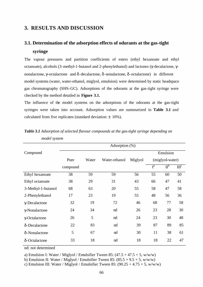
66
3. RESULTS AND DISCUSSION
3.1. Determination of the adsorption effects of odorants at the gas-tight
syringe
The vapour pressures and partition coefficients of esters (ethyl hexanoate and ethyl
octanoate), alcohols (3-methyl-1-butanol and 2-phenylethanol) and lactones (γ-decalactone, γ-
nonalactone, γ-octalactone and δ -decalactone, δ -nonalactone, δ -octalactone) in different
model systems (water, water-ethanol, miglyol, emulsion) were determined by static headspace
gas chromatography (SHS-GC). Adsorptions of the odorants at the gas-tight syringe were
checked by the method detailed in Figure 3.1.
The influence of the model systems on the adsorptions of the odorants at the gas-tight
syringes were taken into account. Adsorption values are summarized in Table 3.1 and
calculated from five replicates (standard deviation: ± 10%).
Table 3.1 Adsorption of selected flavour compounds at the gas-tight syringe depending on
model system
Adsorption (%)
Emulsion
(miglyol-water)
Compound
Pure
compound
Water
Water-ethanol
Miglyol
Ia IIb IIIc
Ethyl hexanoate 38 59 59 56 55 60 50
Ethyl octanoate 38 29 31 43 66 47 41
3-Methyl-1-butanol 68 63 20 55 58 47 58
2-Phenylethanol 17 23 19 55 48 56 36
γ-Decalactone 32 19 72 46 68 77 58
γ-Nonalactone 24 34 nd 26 23 28 30
γ-Octalactone 26 5 nd 24 23 30 48
δ-Decalactone 22 83 nd 39 87 89 85
δ-Nonalactone 5 67 nd 30 11 38 61
δ-Octalactone 33 18 nd 18 18 22 47
nd: not determined
a) Emulsion I: Water / Miglyol / Emulsifier Tween 85: (47.5 + 47.5 + 5, w/w/w) b) Emulsion II: Water / Miglyol / Emulsifier Tween 85: (85.5 + 9.5 + 5, w/w/w) c) Emulsion III: Water / Miglyol / Emulsifier Tween 85: (90.25 + 4.75 + 5, w/w/w)
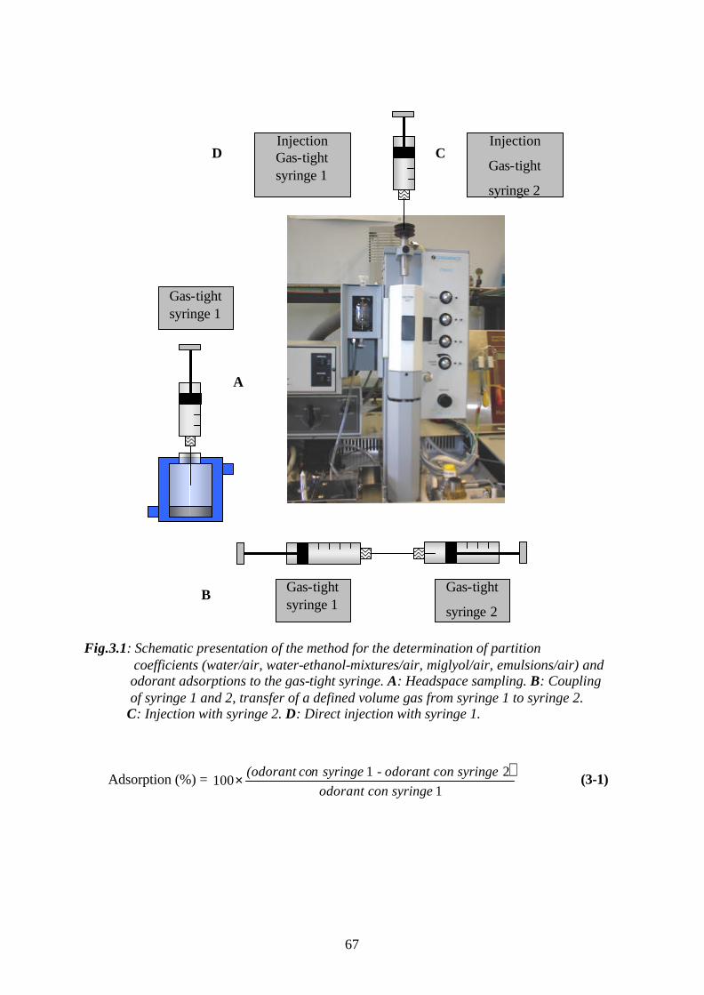
67
Fig.3.1: Schematic presentation of the method for the determination of partition coefficients (water/air, water-ethanol-mixtures/air, miglyol/air, emulsions/air) and odorant adsorptions to the gas-tight syringe. A: Headspace sampling. B: Coupling of syringe 1 and 2, transfer of a defined volume gas from syringe 1 to syringe 2. C: Injection with syringe 2. D: Direct injection with syringe 1.
Adsorption (%) = ? )1
21100
syringeconodorantsyringeconodorantsyringeco (odorant n - × (3-1)
Gas-tight syringe 1
Gas-tight
syringe 2
A
B
C
Gas-tight syringe 1
Injection
Gas-tight
syringe 2
Injection Gas-tight syringe 1
D
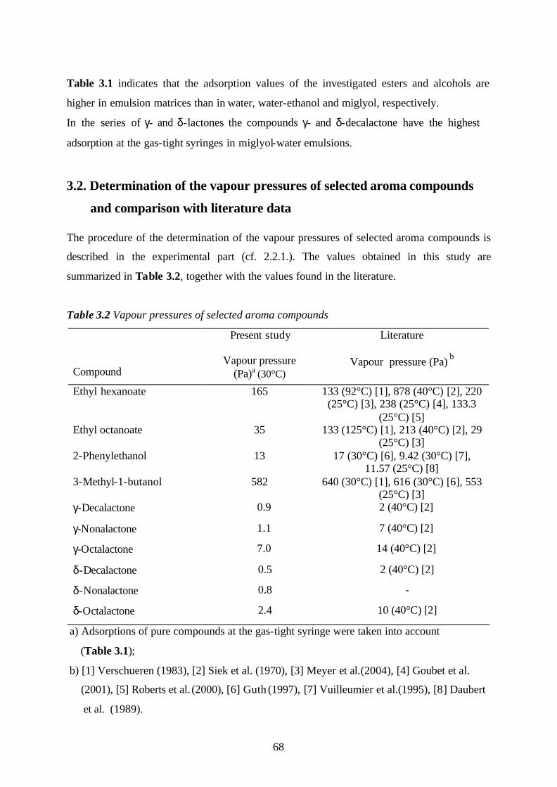
68
Table 3.1 indicates that the adsorption values of the investigated esters and alcohols are
higher in emulsion matrices than in water, water-ethanol and miglyol, respectively.
In the series of γ- and δ-lactones the compounds γ- and δ-decalactone have the highest
adsorption at the gas-tight syringes in miglyol-water emulsions.
3.2. Determination of the vapour pressures of selected aroma compounds
and comparison with literature data The procedure of the determination of the vapour pressures of selected aroma compounds is
described in the experimental part (cf. 2.2.1.). The values obtained in this study are
summarized in Table 3.2, together with the values found in the literature.
Table 3.2 Vapour pressures of selected aroma compounds
Compound
Present study
Vapour pressure (Pa)a (30°C)
Literature
Vapour pressure (Pa) b
Ethyl hexanoate 165 133 (92°C) [1], 878 (40°C) [2], 220 (25°C) [3], 238 (25°C) [4], 133.3
(25°C) [5] Ethyl octanoate 35 133 (125°C) [1], 213 (40°C) [2], 29
(25°C) [3] 2-Phenylethanol 13 17 (30°C) [6], 9.42 (30°C) [7],
11.57 (25°C) [8] 3-Methyl-1-butanol 582 640 (30°C) [1], 616 (30°C) [6], 553
(25°C) [3] γ-Decalactone 0.9 2 (40°C) [2]
γ-Nonalactone 1.1 7 (40°C) [2]
γ-Octalactone 7.0 14 (40°C) [2]
δ-Decalactone 0.5 2 (40°C) [2]
δ-Nonalactone 0.8 -
δ-Octalactone 2.4 10 (40°C) [2]
a) Adsorptions of pure compounds at the gas-tight syringe were taken into account
(Table 3.1);
b) [1] Verschueren (1983), [2] Siek et al. (1970), [3] Meyer et al.(2004), [4] Goubet et al.
(2001), [5] Roberts et al. (2000), [6] Guth (1997), [7] Vuilleumier et al.(1995), [8] Daubert
et al. (1989).
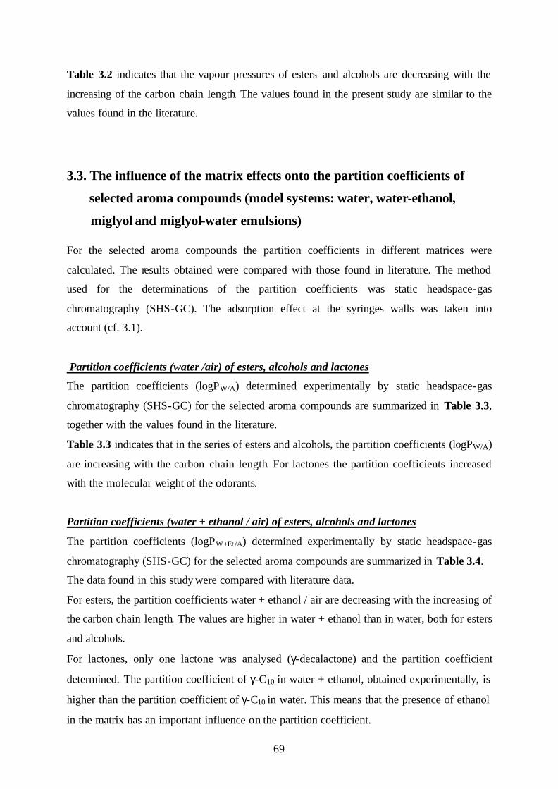
69
Table 3.2 indicates that the vapour pressures of esters and alcohols are decreasing with the
increasing of the carbon chain length. The values found in the present study are similar to the
values found in the literature.
3.3. The influence of the matrix effects onto the partition coefficients of
selected aroma compounds (model systems: water, water-ethanol,
miglyol and miglyol-water emulsions) For the selected aroma compounds the partition coefficients in different matrices were
calculated. The results obtained were compared with those found in literature. The method
used for the determinations of the partition coefficients was static headspace-gas
chromatography (SHS-GC). The adsorption effect at the syringes walls was taken into
account (cf. 3.1).
Partition coefficients (water /air) of esters, alcohols and lactones
The partition coefficients (logPW/A) determined experimentally by static headspace-gas
chromatography (SHS-GC) for the selected aroma compounds are summarized in Table 3.3,
together with the values found in the literature.
Table 3.3 indicates that in the series of esters and alcohols, the partition coefficients (logPW/A)
are increasing with the carbon chain length. For lactones the partition coefficients increased
with the molecular weight of the odorants.
Partition coefficients (water + ethanol / air) of esters, alcohols and lactones
The partition coefficients (logPW+Et /A) determined experimentally by static headspace-gas
chromatography (SHS-GC) for the selected aroma compounds are summarized in Table 3.4.
The data found in this study were compared with literature data.
For esters, the partition coefficients water + ethanol / air are decreasing with the increasing of
the carbon chain length. The values are higher in water + ethanol than in water, both for esters
and alcohols.
For lactones, only one lactone was analysed (γ-decalactone) and the partition coefficient
determined. The partition coefficient of γ-C10 in water + ethanol, obtained experimentally, is
higher than the partition coefficient of γ-C10 in water. This means that the presence of ethanol
in the matrix has an important influence on the partition coefficient.

70
The values found in the literature for some of the compounds are comparable with those
found experimentally. The determination of the partition coefficients in water-ethanol models
was important for further investigations of the partition coefficients in wines.
Table 3.3 Partition coefficients (water/air) of selected aroma compounds
Compound
Present study
Partition coefficients water / air (logPW/A)a
(30°C)
∆ Gc (kcal/mol)
Literature
Partition coefficients water / air (logPW/A) b
Ethyl hexanoate 2.2 -3.1 1.2 [1]; 1.53 (25°C) [2]
Ethyl octanoate 2.56 -3.5 0.72 [1]
2-Phenylethanol 5.23 -3.4 4.63 [3]
3-Methyl-1-butanol 2.52 -7.2 2.88 [1]; 3.17 [3]
γ-Decalactone 3.9 -5.3 -
γ-Nonalactone 4.25 -5.8 -
γ-Octalactone 4.82 -6.6 -
δ-Decalactone 4.62 -6.3 -
δ-Nonalactone 5.25 -7.2 -
δ-Octalactone 5.68 -7.8 -
a) Adsorptions of pure compounds at the gas-tight syringe were taken into account
(Table 3.1);
b) [1] Meyer et al. (2004), [2] Roberts et al. (2000) [3] Guth et al. (2001) c) Solvation free energy: ∆ G = - RT lnPW/A
Table 3.4 Partition coefficients (water + ethanol / air) of selected aroma compounds
Compound
Present study
Partition coefficients water + ethanol / air (logPW+Et/A)a (30°C)
Literature values
Partition coefficients water + ethanol / air
(logPW+Et/A) b Ethyl hexanoate 2.9 -
Ethyl octanoate 2.53 -
2-Phenylethanol 5.37 4.65 [1]
3-Methyl-1-butanol 3 3.32 [1]
γ-Decalactone 4.16 -
a) Adsorptions of pure compounds at the gas-tight syringe: taken into account (Table 3.1);
b) [1] Guth et al. (2001)
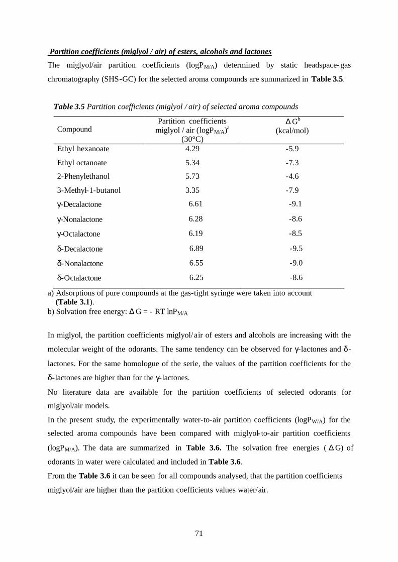
71
Partition coefficients (miglyol / air) of esters, alcohols and lactones
The miglyol/air partition coefficients (logPM/A) determined by static headspace-gas
chromatography (SHS-GC) for the selected aroma compounds are summarized in Table 3.5.
Table 3.5 Partition coefficients (miglyol / air) of selected aroma compounds
Compound Partition coefficients
miglyol / air (logPM/A)a (30°C)
∆ Gb (kcal/mol)
Ethyl hexanoate 4.29 -5.9
Ethyl octanoate 5.34 -7.3
2-Phenylethanol 5.73 -4.6
3-Methyl-1-butanol 3.35 -7.9
γ-Decalactone 6.61 -9.1
γ-Nonalactone 6.28 -8.6
γ-Octalactone 6.19 -8.5
δ-Decalactone 6.89 -9.5
δ-Nonalactone 6.55 -9.0
δ-Octalactone 6.25 -8.6
a) Adsorptions of pure compounds at the gas-tight syringe were taken into account (Table 3.1). b) Solvation free energy: ∆ G = - RT lnPM/A
In miglyol, the partition coefficients miglyol/ air of esters and alcohols are increasing with the
molecular weight of the odorants. The same tendency can be observed for γ-lactones and δ -
lactones. For the same homologue of the serie, the values of the partition coefficients for the
δ-lactones are higher than for the γ-lactones.
No literature data are available for the partition coefficients of selected odorants for
miglyol/air models.
In the present study, the experimentally water-to-air partition coefficients (logPW/A) for the
selected aroma compounds have been compared with miglyol- to-air partition coefficients
(logPM/A). The data are summarized in Table 3.6. The solvation free energies ( ∆ G) of
odorants in water were calculated and included in Table 3.6.
From the Table 3.6 it can be seen for all compounds analysed, that the partition coefficients
miglyol/air are higher than the partition coefficients values water/air.
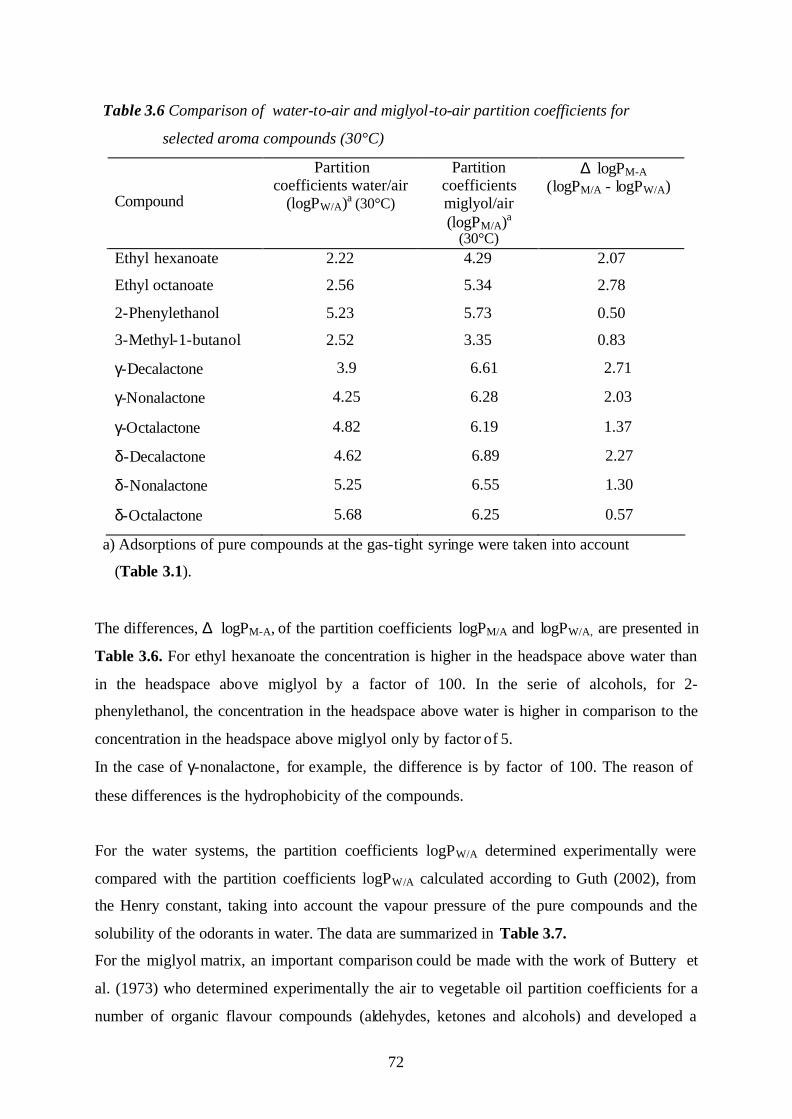
72
Table 3.6 Comparison of water-to-air and miglyol-to-air partition coefficients for
selected aroma compounds (30°C)
Compound
Partition coefficients water/air
(logPW/A)a (30°C)
Partition coefficients miglyol/air (logPM/A)a
(30°C)
∆ logPM-A (logPM/A - logPW/A)
Ethyl hexanoate 2.22 4.29 2.07
Ethyl octanoate 2.56 5.34 2.78
2-Phenylethanol 5.23 5.73 0.50
3-Methyl-1-butanol 2.52 3.35 0.83
γ-Decalactone 3.9 6.61 2.71
γ-Nonalactone 4.25 6.28 2.03
γ-Octalactone 4.82 6.19 1.37
δ-Decalactone 4.62 6.89 2.27
δ-Nonalactone 5.25 6.55 1.30
δ-Octalactone 5.68 6.25 0.57
a) Adsorptions of pure compounds at the gas-tight syringe were taken into account
(Table 3.1).
The differences, ∆ logPM-A, of the partition coefficients logPM/A and logPW/A, are presented in
Table 3.6. For ethyl hexanoate the concentration is higher in the headspace above water than
in the headspace above miglyol by a factor of 100. In the serie of alcohols, for 2-
phenylethanol, the concentration in the headspace above water is higher in comparison to the
concentration in the headspace above miglyol only by factor of 5.
In the case of γ-nonalactone, for example, the difference is by factor of 100. The reason of
these differences is the hydrophobicity of the compounds.
For the water systems, the partition coefficients logPW/A determined experimentally were
compared with the partition coefficients logPW/A calculated according to Guth (2002), from
the Henry constant, taking into account the vapour pressure of the pure compounds and the
solubility of the odorants in water. The data are summarized in Table 3.7.
For the miglyol matrix, an important comparison could be made with the work of Buttery et
al. (1973) who determined experimentally the air to vegetable oil partition coefficients for a
number of organic flavour compounds (aldehydes, ketones and alcohols) and developed a

73
model for the prediction of air/vegetable partition coefficients. The author proposed an
equation for the determination of air/vegetable partition coefficients.
For our study, the equation given by Βuttery for the partition coefficient can be re-written as
follows:
Psa = (solute concentration in solution) (solute concentration in air) (3-2)
)(
1factorconversionsolventC
Psa ×= (3-3)
The solvent conversion factor is a simple number which involves conversion of pressure
units to mass units. This factor is dependent on the molecular weight of the solvent but is
independent of the solute molecular weight which cancels out in the calculation of this
factor.
As Buttery et al. (1971) outlined, from solution volatility theory:
?xpC 0= (3-4)
=CsN
xp1
0 (3-5)
where p0 is the vapour pressure of the pure compound, γ is the activity coefficient in that
solvent and Ns is the solubility of the compound in that solvent in mole fraction terms. For
the low solubility compounds Ns = 1, that means C = p0. Then, Equation (3-2) becomes:
)(
1
0 factorconversionsolventpPsa ××
=?
(3-6)
For vegetable oil the conversion factor determined by Buttery et al. (1973) is 5.2 x 10⁻⁵.
Taking into account this value from Buttery and the activity coefficient generally approaches
1, the Psa values (cf. Equation 3-6) for the compounds selected in the present study were
determined. The data are summarized in Table 3.7.
γ
γ
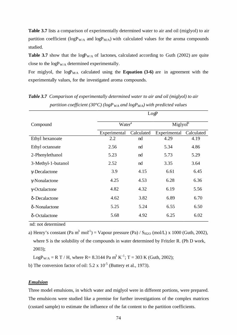
74
Table 3.7 lists a comparison of experimentally determined water to air and oil (miglyol) to air
partition coefficient (logPW/A and logPM/A) with calculated values for the aroma compounds
studied.
Table 3.7 show that the logPW/A of lactones, calculated according to Guth (2002) are quite
close to the logPW/A determined experimentally.
For miglyol, the logPM/A calculated using the Equation (3-6) are in agreement with the
experimentally values, for the investigated aroma compounds.
Table 3.7 Comparison of experimentally determined water to air and oil (miglyol) to air
partition coefficient (30°C) (logPW/A and logPM/A) with predicted values
LogP
Compound Watera Miglyolb
Experimental Calculated Experimental Calculated Ethyl hexanoate 2.2 nd 4.29 4.19
Ethyl octanoate 2.56 nd 5.34 4.86
2-Phenylethanol 5.23 nd 5.73 5.29
3-Methyl-1-butanol 2.52 nd 3.35 3.64
γ-Decalactone 3.9 4.15 6.61 6.45
γ-Nonalactone 4.25 4.53 6.28 6.36
γ-Octalactone 4.82 4.32 6.19 5.56
δ-Decalactone 4.62 3.82 6.89 6.70
δ-Nonalactone 5.25 5.24 6.55 6.50
δ-Octalactone 5.68 4.92 6.25 6.02
nd: not determined
a) Henry’s constant (Pa m3 mol-1) = Vapour pressure (Pa) / SH2O (mol/L) x 1000 (Guth, 2002),
where S is the solubility of the compounds in water determined by Fritzler R. (Ph D work,
2003);
LogPW/A = R T / H, where R= 8.3144 Pa m3 K-1; T = 303 K (Guth, 2002);
b) The conversion factor of oil: 5.2 x 10⁻⁵ (Buttery et al., 1973).
Emulsion
Three model emulsions, in which water and miglyol were in different portions, were prepared.
The emulsions were studied like a premise for further investigations of the complex matrices
(custard sample) to estimate the influence of the fat content to the partition coefficients.

75
The emulsions were microscopically analyzed at the firm Sasol Germany GmbH. The analysis
indicated that the three emulsions are from type oil in water (o/w). From the microscopic
pictures (Figures 3.2-3.4) one can observe that, with decreasing of the concentration of the oil
phase, the particle distribution becomes higher. Emulsion I (Figure 3.2.) showed very small
particles in contrast to emulsion II (Figure 3.3.) and emulsion III (Figure 3.4.).
Fig.3.2. Emulsion I: Water / Miglyol / Emulsifier Tween 85: (47.5 + 47.5 + 5, w/w/w)
Fig. 3.3. Emulsion II: Water / Miglyol / Emulsifier Tween 85: (8.5 + 9.5 + 5, w/w/w)

76
Fig. 3.4. Emulsion III: Water / Miglyol / Emulsifier Tween 85: (90.25 + 4.75 + 5, w/w/w)
For each emulsion (I-III), the particles were analyzed using software ImageJ. Determination
of particle size distribution has been done, first by scaling the image (set scale, threshold
images), and then by the command “analyze particles”. The software counts and measures
objects in the binary or threshold images.
A portion of the threshold image for the emulsion I, used for the calculation, is given in
Figure 3.5. The dark parts represent the oil particles.
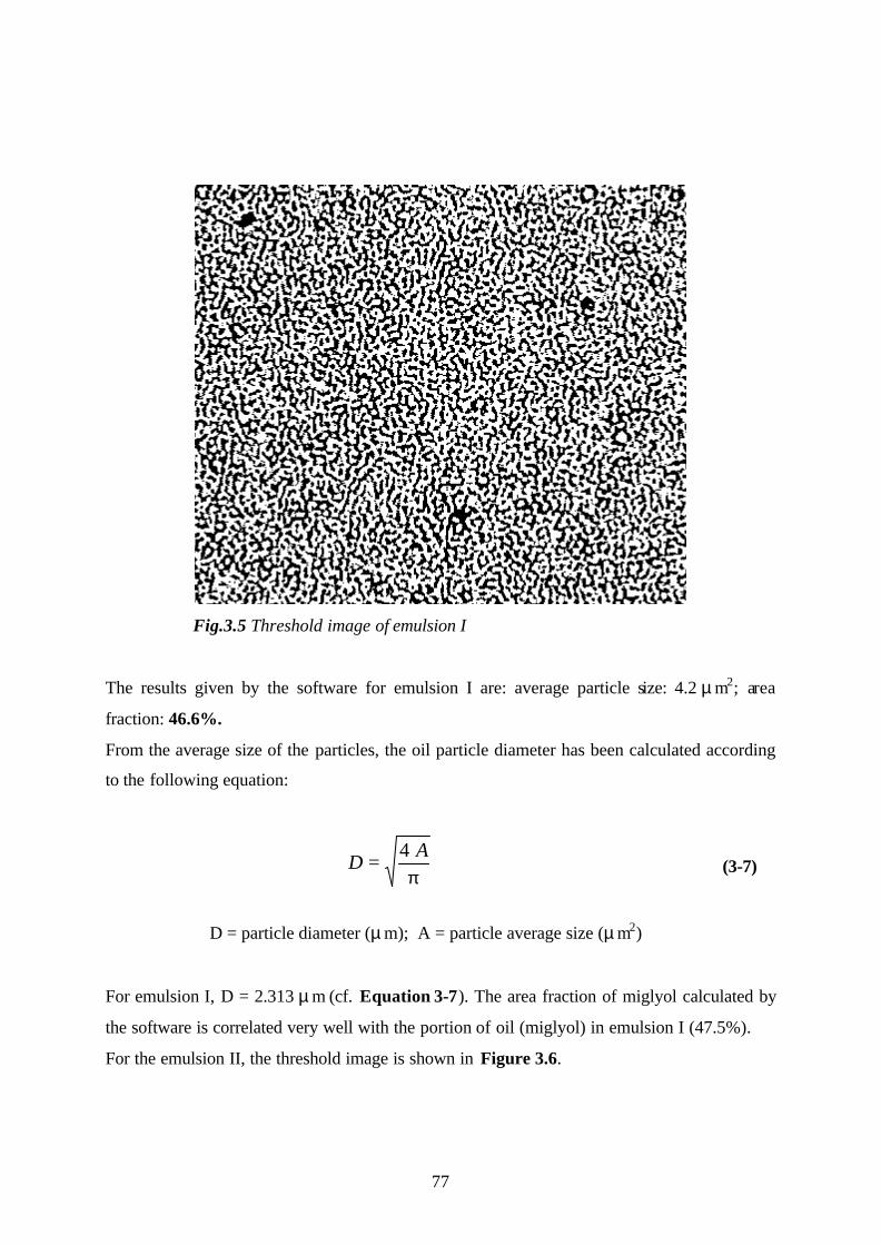
77
Fig.3.5 Threshold image of emulsion I
The results given by the software for emulsion I are: average particle size: 4.2 µ m2; area
fraction: 46.6%.
From the average size of the particles, the oil particle diameter has been calculated according
to the following equation:
?AD 4= (3-7)
D = particle diameter (µ m); A = particle average size (µ m2)
For emulsion I, D = 2.313 µ m (cf. Equation 3-7). The area fraction of miglyol calculated by
the software is correlated very well with the portion of oil (miglyol) in emulsion I (47.5%).
For the emulsion II, the threshold image is shown in Figure 3.6.
π
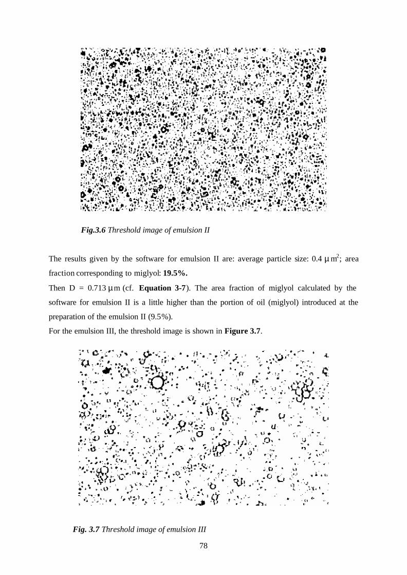
78
Fig.3.6 Threshold image of emulsion II
The results given by the software for emulsion II are: average particle size: 0.4 µ m2; area
fraction corresponding to miglyol: 19.5%.
Then D = 0.713 µm (cf. Equation 3-7). The area fraction of miglyol calculated by the
software for emulsion II is a little higher than the portion of oil (miglyol) introduced at the
preparation of the emulsion II (9.5%).
For the emulsion III, the threshold image is shown in Figure 3.7.
Fig. 3.7 Threshold image of emulsion III

79
The results given by the software for emulsion III are: average particle size: 0.4 µ m 2; area
fraction corresponding to miglyol: 8.6%.
Then D = 0.713 µm (cf. Equation 3-7). The area fraction of miglyol calculated by the
software for emulsion III almost corresponds to the portion of oil (miglyol) introduced at the
preparation of the emulsion (4.75%).
Partition coefficients (emulsions/air) (LogPE/A) of esters, alcohols and lactones The partition coefficients emulsions/air for the selected aroma compounds were determined.
The experimentally values obtained are summarized in Table 3.8.
Table 3.8 Partition coefficients (emulsions/air) of selected aroma compounds
Compound Partition coefficients
emulsion I / air (logPEI/A)a (30°C)
Partition coefficients emulsion II / air
(logPEII/A)a (30°C)
Partition coefficients emulsion III / air (logPEIII/A)a (30°C)
Ethyl hexanoate
4.25
3.39
3.34
Ethyl octanoate
5.06
4.75
4.59
2-Phenylethanol
5.75
5.48
5.44
3-Methyl-1-butanol
3.59
3.39
3.23
γ-Decalactone
6.50
5.95
5.91
γ-Nonalactone
6.33
5.91
5.88
γ-Octalactone
6
5.75
5.47
δ-Decalactone
6.56
5.87
6
δ-Nonalactone
6.83
6.35
6
δ-Octalactone
6.30
6.13
5.77
a) Adsorptions of pure compounds at the gas-tight syringe were taken into account
(Table 3.1).
For the esters and alcohols in emulsion I, the partition coefficients emulsion I/air are
increasing with the increasing of the carbon number. In the series of γ- and δ -lactones, it can
be seen the same behaviour, exception is δ -nonalactone.

80
In emulsion II, the partition coefficients emulsion II/air for all aroma compounds selected are
also increasing with the carbon number, except δ -decalactone.
In emulsion III, the partition coefficients values emulsion III/air is following the same
behaviour as for emulsion I and II.
For the emulsions a comparison could be made with the work of Buttery et al. (1973) who
determined experimentally vegetable oil-water mixtures/air partition coefficients for a number
of organic flavour compounds (aldehydes, ketones and alcohols) and developed a model for
the prediction of vegetable oil-water mixtures/air partition coefficients. The equation
proposed by Buttery for the determination of oil-water mixtures/air partition coefficients can
be re-written for our study as follows:
Pma = (solute concentration in the mixture) (solute concentration in the air) (3-8)
Equation (3-8) can be simplified to:
oilaoilwawma PFPFP ×××= (3-9)
where: Pwa = water/air partition coefficient;
Poila = oil (miglyol)/air partition coefficient;
Fw = fraction of water in the mixture (%);
Foil = fraction of oil (miglyol) in the mixture (%).
The total volume, Fw + Foil is equal to 1.
Using Equation (3-9), it is possible to calculate miglyol-water/air partition coefficients for
emulsion I, II and III. The results obtained are presented in Table 3.9, in comparison with the
experimentally values.
Table 3.9 indicates that the logP values calculated according to Equation (3-9.) proposed by
Buttery et al. (1973) are correlated with the experimentally determined values, in agreement
with the results obtained by Buttery, where for the case of 1% and 10% vegetable oil-water
mixtures, the experimentally and calculated vegetable oil-water mixture/air partition
coefficients (logP) agree quite closely.
As example, the experimentally value of octanal, given by Buttery for the 10% vegetable oil-
water mixture was logPoil-water/air = 3.46 and the calculated value was LogP oil-water/air = 3.40.
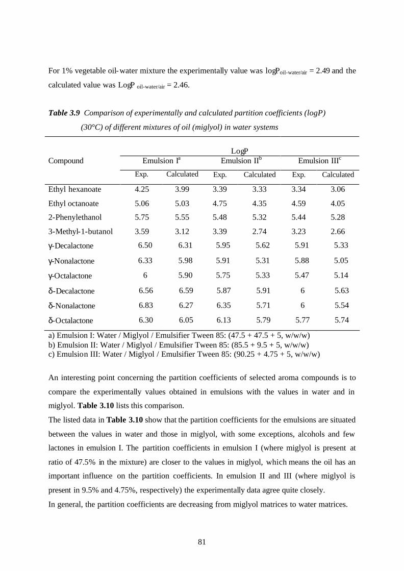
81
For 1% vegetable oil-water mixture the experimentally value was logPoil-water/air = 2.49 and the
calculated value was LogP oil-water/air = 2.46.
Table 3.9 Comparison of experimentally and calculated partition coefficients (logP)
(30°C) of different mixtures of oil (miglyol) in water systems
LogP
Compound Emulsion Ia Emulsion IIb Emulsion IIIc
Exp. Calculated Exp. Calculated Exp. Calculated
Ethyl hexanoate 4.25 3.99 3.39 3.33 3.34 3.06
Ethyl octanoate 5.06 5.03 4.75 4.35 4.59 4.05
2-Phenylethanol 5.75 5.55 5.48 5.32 5.44 5.28
3-Methyl-1-butanol 3.59 3.12 3.39 2.74 3.23 2.66
γ-Decalactone 6.50 6.31 5.95 5.62 5.91 5.33
γ-Nonalactone 6.33 5.98 5.91 5.31 5.88 5.05
γ-Octalactone 6 5.90 5.75 5.33 5.47 5.14
δ-Decalactone 6.56 6.59 5.87 5.91 6 5.63
δ-Nonalactone 6.83 6.27 6.35 5.71 6 5.54
δ-Octalactone 6.30 6.05 6.13 5.79 5.77 5.74
a) Emulsion I: Water / Miglyol / Emulsifier Tween 85: (47.5 + 47.5 + 5, w/w/w) b) Emulsion II: Water / Miglyol / Emulsifier Tween 85: (85.5 + 9.5 + 5, w/w/w) c) Emulsion III: Water / Miglyol / Emulsifier Tween 85: (90.25 + 4.75 + 5, w/w/w)
An interesting point concerning the partition coefficients of selected aroma compounds is to
compare the experimentally values obtained in emulsions with the values in water and in
miglyol. Table 3.10 lists this comparison.
The listed data in Table 3.10 show that the partition coefficients for the emulsions are situated
between the values in water and those in miglyol, with some exceptions, alcohols and few
lactones in emulsion I. The partition coefficients in emulsion I (where miglyol is present at
ratio of 47.5% in the mixture) are closer to the values in miglyol, which means the oil has an
important influence on the partition coefficients. In emulsion II and III (where miglyol is
present in 9.5% and 4.75%, respectively) the experimentally data agree quite closely.
In general, the partition coefficients are decreasing from miglyol matrices to water matrices.
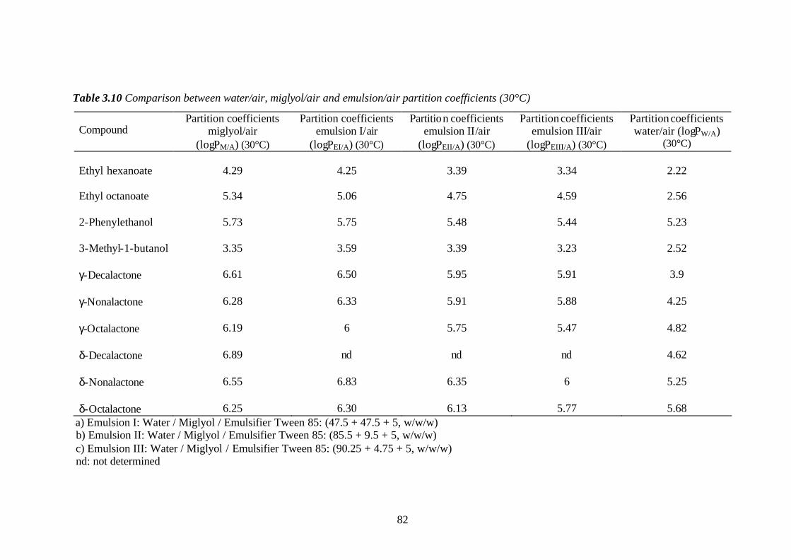
82
Table 3.10 Comparison between water/air, miglyol/air and emulsion/air partition coefficients (30°C)
Compound Partition coefficients
miglyol/air (logPM/A) (30°C)
Partition coefficients emulsion I/air
(logPEI/A) (30°C)
Partition coefficients emulsion II/air
(logPEII/A) (30°C)
Partition coefficients emulsion III/air
(logPEIII/A) (30°C)
Partition coefficients water/air (logPW/A)
(30°C) Ethyl hexanoate
4.29
4.25
3.39
3.34
2.22
Ethyl octanoate
5.34
5.06
4.75
4.59
2.56
2-Phenylethanol
5.73
5.75
5.48
5.44
5.23
3-Methyl-1-butanol
3.35
3.59
3.39
3.23
2.52
γ-Decalactone
6.61
6.50
5.95
5.91
3.9
γ-Nonalactone
6.28
6.33
5.91
5.88
4.25
γ-Octalactone
6.19
6
5.75
5.47
4.82
δ-Decalactone
6.89
nd
nd
nd
4.62
δ-Nonalactone
6.55
6.83
6.35
6
5.25
δ-Octalactone
6.25
6.30
6.13
5.77
5.68
a) Emulsion I: Water / Miglyol / Emulsifier Tween 85: (47.5 + 47.5 + 5, w/w/w) b) Emulsion II: Water / Miglyol / Emulsifier Tween 85: (85.5 + 9.5 + 5, w/w/w) c) Emulsion III: Water / Miglyol / Emulsifier Tween 85: (90.25 + 4.75 + 5, w/w/w) nd: not determined
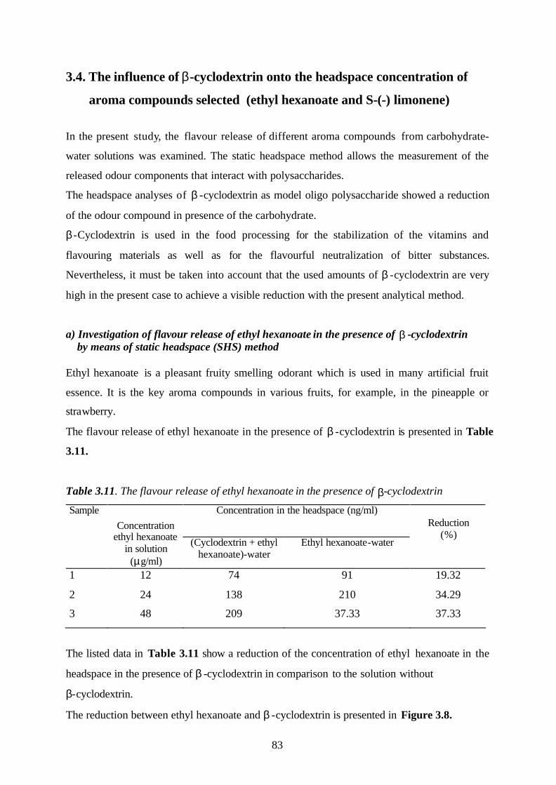
83
3.4. The influence of ? -cyclodextrin onto the headspace concentration of
aroma compounds selected (ethyl hexanoate and S-(-) limonene)
In the present study, the flavour release of different aroma compounds from carbohydrate-
water solutions was examined. The static headspace method allows the measurement of the
released odour components that interact with polysaccharides.
The headspace analyses of β -cyclodextrin as model oligo polysaccharide showed a reduction
of the odour compound in presence of the carbohydrate.
β -Cyclodextrin is used in the food processing for the stabilization of the vitamins and
flavouring materials as well as for the flavourful neutralization of bitter substances.
Nevertheless, it must be taken into account that the used amounts of β -cyclodextrin are very
high in the present case to achieve a visible reduction with the present analytical method.
a) Investigation of flavour release of ethyl hexanoate in the presence of ? -cyclodextrin by means of static headspace (SHS) method
Ethyl hexanoate is a pleasant fruity smelling odorant which is used in many artificial fruit
essence. It is the key aroma compounds in various fruits, for example, in the pineapple or
strawberry.
The flavour release of ethyl hexanoate in the presence of β -cyclodextrin is presented in Table
3.11.
Table 3.11. The flavour release of ethyl hexanoate in the presence of ? -cyclodextrin
Concentration in the headspace (ng/ml) Sample Concentration
ethyl hexanoate in solution
(µg/ml) (Cyclodextrin + ethyl
hexanoate)-water Ethyl hexanoate-water
Reduction
(%)
1 12 74 91 19.32
2 24 138 210 34.29
3 48 209 37.33 37.33
The listed data in Table 3.11 show a reduction of the concentration of ethyl hexanoate in the
headspace in the presence of β -cyclodextrin in comparison to the solution without
β-cyclodextrin.
The reduction between ethyl hexanoate and β -cyclodextrin is presented in Figure 3.8.
β
β
β

84
Fig.3.8 The reduction of ethyl hexanoate in presence of ? -cyclodextrin
b) Investigation of flavour release of S-(-) limonene in the presence of ? -cyclodextrin by means of static headspace (SHS) method Limonene belongs chemically to the group of terpene. Most components of the oils of a lot of
plants belong to the class of terpene. These ethereal oils can be obtained by steam distillation
of the plants. The oils which are separated in the distillate have mostly characteristically
smells which are typical for the used plants.
S-(-)-Limonene
Fig. 3.9 The structure of S-(-)-limonene
S-(-) limonene is a chirale molecule. Both enantiomers differ substantially in flavour.
0 5
10 15 20 25 30 35 40 The reduction
[%]
1 2 3 Sample number
The reduction of ethyl hexanoate in presence of ? -Cyclodextrin
Concentration of ethyl hexanoate
Sample 3: 48 mg/ml
Sample 1: 12 mg/ml Sample 2: 24 mg/ml
β
β
β

85
The S-(-) limonene is found in american peppermint oil and owns a minty flavour.
D-(+) limonene is forming in the nature, 90% in sour orange oil, in the Caraway oil, or in the
citrus oil, the perceived flavour is associated with oranges.
Furthermore, it is also known that (+/-) limonene is found, e.g., in the pine-needle oil,
camphoric oil or nutmeg oil. Limonene is used in the dye and varnish industries.
The flavour release of S-(-) limonene in the presence of β -cyclodextrin is presented in Table
3.12.
Table 3.12 The flavour release of S-(-) limonene in the presence of ? -cyclodextrin
Concentration in the headspace (ng/ml) Sample Concentration S-(-) limonene
in solution (µg/ml)
(Cyclodextrin + S-(-) limonene)-water
S-(-) limonene-water
Reduction
(%)
1 0.106 0.9 1 21
2 1.06 9 13 31
3 2.12 10 16 39
From the Table 3.12 it can be seen a reduction of the concentration of S-(-)-limonene in the
gase phase in the presence of β -cyclodextrin in comparison to the solution in absence of
β -cyclodextrin. The reduction between S-(-)-limonene and β-cyclodextrin is presented in
Figure 3.10.
Fig.3.10 The reduction of S-(-)-limonene in presence of ? -cyclodextrin
0 5
10 15 20 25 30
35 40 Reduction [%]
1 2 3 Sample number
Reduction of S-(-)-Limonene in presence of ? -Cyclodextrin
Concentration of S - ( - ) - Limonene
η
sample 2 : 10,6 µ g/10 ml sample 3: 21,2 µ g/10 ml
sample 1: 1.06 µ g/10 ml .
β
β
β

86
The present investigations by means of HS-GC showed that the concentrations of the
carbohydrate were relatively high; however, the analytical results revealed that β -cyclodextrin
with its hydrophobic hollow cavity can bind very well aroma compounds.
3.5. The influence of the food matrix onto the partition coefficients of
selected flavour compounds
3.5.1. Wine matrix
To determine the partition coefficients in wines it is necessary to know the concentrations of
alcohols and esters in wines (in white wines) and in the headspace above wines and then
making a ratio between the odorant concentration in the wine matrix to the concentration in
the headspace above wine, was possible to calculate the partition coefficients wines / air.
The concentrations of 3-methyl-1-butanol, ethyl hexanoate and ethyl octanoate in wines were
determined by standard addition method, using headspace-gas chromatography (HS-GC), and
by mass spectrometry, MS (CI method) for 2-phenylethanol (cf. 2.4.1.).
Standard addition method The graphics for the determination of the concentration of 3-methyl-1-butanol, ethyl
hexanoate and ethyl octanoate in wines are presented in Figures 3.11-3.13.
3-Methyl-1-butanol in "Le Cadet Sauvignon"
y = 106042x + 77557R2 = 0,999
0
20000
40000
60000
80000
100000
0 0,05 0,1 0,15 0,2
3-methyl-1-butanol added (mg)
Pea
k A
reas
Figure 3.11 Determination of the concentration of 3-methyl-1-butanol
in “Le Cadet Sauvignon”

87
Ethyl hexanoate in "Baden Trocken"
y = 3E+06x + 3032,7R2 = 0,9981
01000
20003000
4000
50006000
0 0,0001 0,0002 0,0003 0,0004 0,0005 0,0006 0,0007
Ethyl hexanoate added (mg)
Pea
k A
reas
Figure 3.12 Determination of the concentration of ethyl hexanoate
in “Baden Trocken”
Ethyl octanoate in "Baden Trocken"
y = 6E+06x + 4469,5R2 = 0,9963
0
2000
4000
6000
8000
10000
0 0,0001 0,0002 0,0003 0,0004 0,0005 0,0006 0,0007
Ethyl octanoate added (mg)
Pea
k A
reas
Figure 3.13 Determination of the concentration of ethyl octanoate in “Baden Trocken”
Isotope dilution analysis (IDA) For 2-phenylethanol, the concentration in wines was determined by IDA using MS (CI)
(cf.2.4.1.).
The wine sample contains 2[H]2 –phenylethanol standard, with known concentration.
CH2 C OH
D
D Fig.3.14 The structure of 2[H]2 –phenylethanol
where: D = deuterium

88
1 µ l from the wine sample was injected in MS by CI modus and the spectrum for both
compounds in wine (2-phenylethanol and 2[H]2 –phenylethanol standard) was obtained. The
concentration of 2-phenylethanol in wine was calculated from the peak areas of both
compounds and the known concentration of 2[H]2 –phenylethanol, taking into account the
correction factor, f.
The mass trace for the two compounds, the 2[H]2 –phenylethanol standard and 2-
phenylethanol are shown in Figure 3.15 a and 3.15 b.
10.00 11.00 12.00 13.00 14.00 15.00 16.00 17.00 18.00 19.000
5000
10000
15000
20000
25000
30000
35000
40000
45000
50000
Time-->
AbundanceIon 107.00 (106.70 to 107.70): 50211#1.D
17.00
Fig. 3.15 a Mass trace of 2[H]2 –phenylethanol standard
10.00 11.00 12.00 13.00 14.00 15.00 16.00 17.00 18.00 19.000
5000
10000
15000
20000
25000
30000
35000
Time-->
AbundanceIon 105.00 (104.70 to 105.70): 50211#1.D
17.04
Fig. 3.15 b Mass trace of 2-phenylethanol

89
The concentration of the compounds in wines is given in Table 3.13. For each wine, the
concentrations were calculated from four replicates (standard deviation: ± 10%).
Table 3.13 Concentrations of selected odorants in white wines Compound Concentration in
wine A (µ g / L)
Concentration in
wine B (µ g / L)
Concentration in
wine C (µ g / L)
3-Methyl-1-butanol a) 145000 131000 231000
Ethyl hexanoate a) 444 200 315
Ethyl octanoate a) 515 246 272
2-Phenylethanol b) 73602 63008 103370
a) The concentrations were determined through standard addition method using HS-GC (cf. 2.4.1.); b) The concentration was determined by isotope dilution analysis (IDA) using MS (CI) (cf. 2.4.1).
For the determination of the concentration of alcohols and esters in headspace above wines,
the headspace-gas chromatography (HS-GC) method was used.
The concentrations of the compounds in headspace above wines are given in the Table 3.14
and calculated from two replicates (standard deviation: ± 5%).
Table 3.14 The concentrations of selected aroma compounds in headspace above wines
Compound Concentration in
wine A (ng / L)
Concentration in
wine B (ng / L)
Concentration in
wine C (ng / L)
3-Methyl-1-butanol 76835 104890 117775
Ethyl hexanoate 4870 2660 3295
2-Phenylethanol 1540 2590 1110
Ethyl octanoate 7925 7920 5245
After the determination of the concentration of each compound in wines and in the headspace
above wines, the partition coefficient of compounds in wines was calculated.
The partition coefficients were calculated from 2-5 replicates (standard deviation: ± 3%). The
results are summarized in Table 3.15.
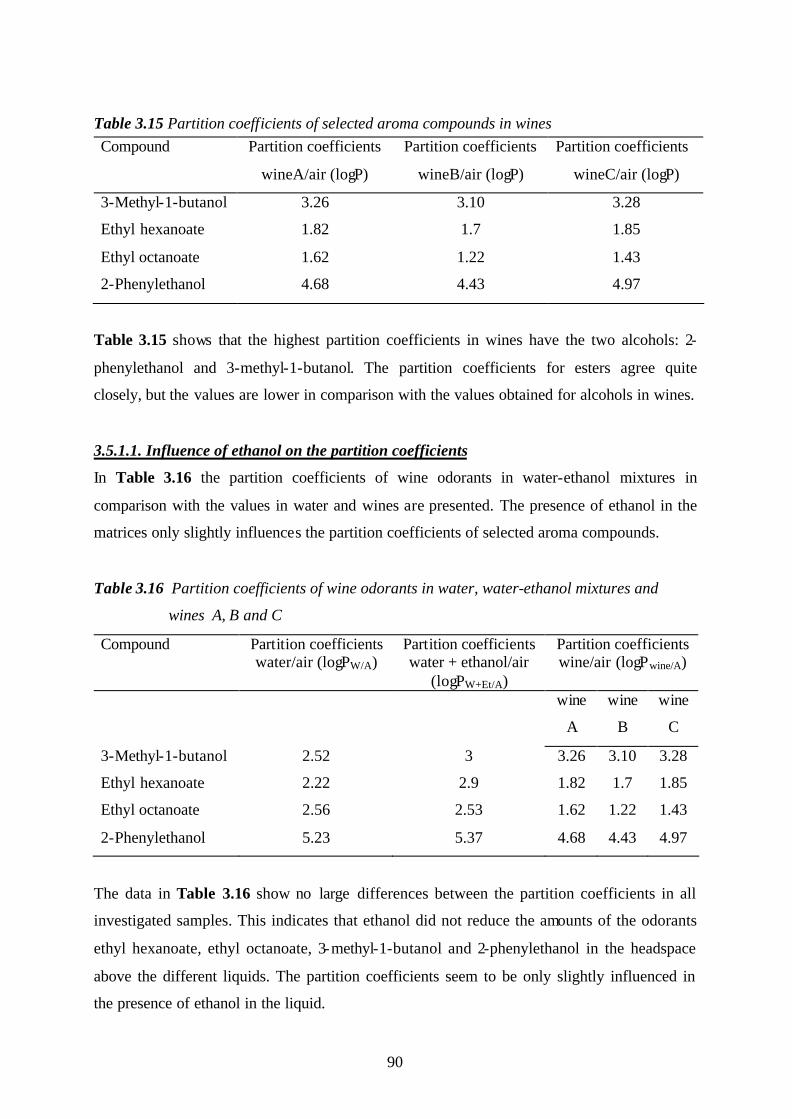
90
Table 3.15 Partition coefficients of selected aroma compounds in wines Compound Partition coefficients
wineA/air (logP) Partition coefficients
wineB/air (logP)
Partition coefficients
wineC/air (logP)
3-Methyl-1-butanol 3.26 3.10 3.28
Ethyl hexanoate 1.82 1.7 1.85
Ethyl octanoate 1.62 1.22 1.43
2-Phenylethanol 4.68 4.43 4.97
Table 3.15 shows that the highest partition coefficients in wines have the two alcohols: 2-
phenylethanol and 3-methyl-1-butanol. The partition coefficients for esters agree quite
closely, but the values are lower in comparison with the values obtained for alcohols in wines.
3.5.1.1. Influence of ethanol on the partition coefficients
In Table 3.16 the partition coefficients of wine odorants in water-ethanol mixtures in
comparison with the values in water and wines are presented. The presence of ethanol in the
matrices only slightly influences the partition coefficients of selected aroma compounds.
Table 3.16 Partition coefficients of wine odorants in water, water-ethanol mixtures and
wines A, B and C
Compound Partition coefficients water/air (logPW/A)
Partition coefficients water + ethanol/air
(logPW+Et/A)
Partition coefficients wine/air (logPwine/A)
wine
A
wine
B
wine
C
3-Methyl-1-butanol 2.52 3 3.26 3.10 3.28
Ethyl hexanoate 2.22 2.9 1.82 1.7 1.85
Ethyl octanoate 2.56 2.53 1.62 1.22 1.43
2-Phenylethanol 5.23 5.37 4.68 4.43 4.97
The data in Table 3.16 show no large differences between the partition coefficients in all
investigated samples. This indicates that ethanol did not reduce the amounts of the odorants
ethyl hexanoate, ethyl octanoate, 3-methyl-1-butanol and 2-phenylethanol in the headspace
above the different liquids. The partition coefficients seem to be only slightly influenced in
the presence of ethanol in the liquid.
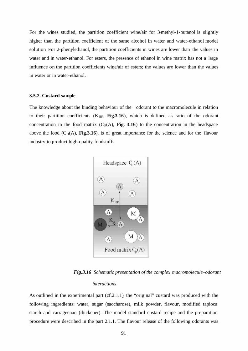
91
For the wines studied, the partition coefficient wine/air for 3-methyl-1-butanol is slightly
higher than the partition coefficient of the same alcohol in water and water-ethanol model
solution. For 2-phenylethanol, the partition coefficients in wines are lower than the values in
water and in water-ethanol. For esters, the presence of ethanol in wine matrix has not a large
influence on the partition coefficients wine/air of esters; the values are lower than the values
in water or in water-ethanol.
3.5.2. Custard sample
The knowledge about the binding behaviour of the odorant to the macromolecule in relation
to their partition coefficients (KHF, Fig.3.16), which is defined as ratio of the odorant
concentration in the food matrix (CF(A), Fig. 3.16) to the concentration in the headspace
above the food (CH(A), Fig.3.16), is of great importance for the science and for the flavour
industry to product high-quality foodstuffs.
Fig.3.16 Schematic presentation of the complex macromolecule–odorant
interactions
As outlined in the experimental part (cf.2.1.1), the “original” custard was produced with the
following ingredients: water, sugar (saccharose), milk powder, flavour, modified tapioca
starch and carrageenan (thickener). The model standard custard recipe and the preparation
procedure were described in the part 2.1.1. The flavour release of the following odorants was

92
investigated in the custard samples: 3-methyl-1-butanol, ethyl octanoate, ethyl hexanoate, 2-
phenylethanol.
The main goal was the determination of the following subjects in custard:
Ø Investigation of the aroma release as a function of matrix components;
Ø Investigation of the time influence to the aroma release;
Ø Comparison of custard/air – and octanol/water partition coefficients (logP);
Ø Comparison of custard/air -, water/air - and emulsion/air partition coefficients (LogP).
Determination of partition coefficients in custard sample
The results concerning the influence of the matrix onto the partition coefficients of selected
aroma compounds are presented.
As described in the experimental part, 5 g custard was weighted in the headspace vials
(volume: 20 ml) and 0.5 ml air above the custard was injected into the gas chromatograph.
Table 3.17 lists the headspace concentrations above the custard obtained (ng/ml).
Table 3.17 Headspace concentrations obtained for the selected flavour compounds above
the original custard sample
Aroma compound Concentration (ng/ml air)
3-Methyl-1-butanol 264
Ethyl hexanoate 58.3
2-Phenylethanol 5.4
Ethyl octanoate 39.4
Determination of the concentrations of odorants in the custard samples For the determination of the losses of odorants during the preparation of the custard the
standard addition method was used (Figure 3.17).

93
3-Methylbutanol
y = 192530x + 555972 R 2 = 0,9846
0 100000 200000 300000 400000 500000 600000 700000 800000 900000
1000000
0 0,2 0,4 0,6 0,8 1 1,2 1,4 1,6 1,8 2 Aroma added [mg]
Pea
k ar
eas
Ethyl octanoate
y = 42247x + 109758 R 2 = 0,9995
0 20000 40000 60000 80000
100000 120000 140000
160000 180000 200000
0 0,2 0,4 0,6 0,8 1 1,2 1,4 1,6 1,8 Aroma added (mg)
Pea
k ar
eas
Ethyl hexanoate
y = 250232x + 138860 R 2 = 0,9936
0 20000 40000 60000 80000
100000 120000 140000 160000 180000 200000
0 0,02 0,04 0,06 0,08 0,1 0,12 0,14 0,16 0,18 Aroma added (mg)
Pea
k A
reas
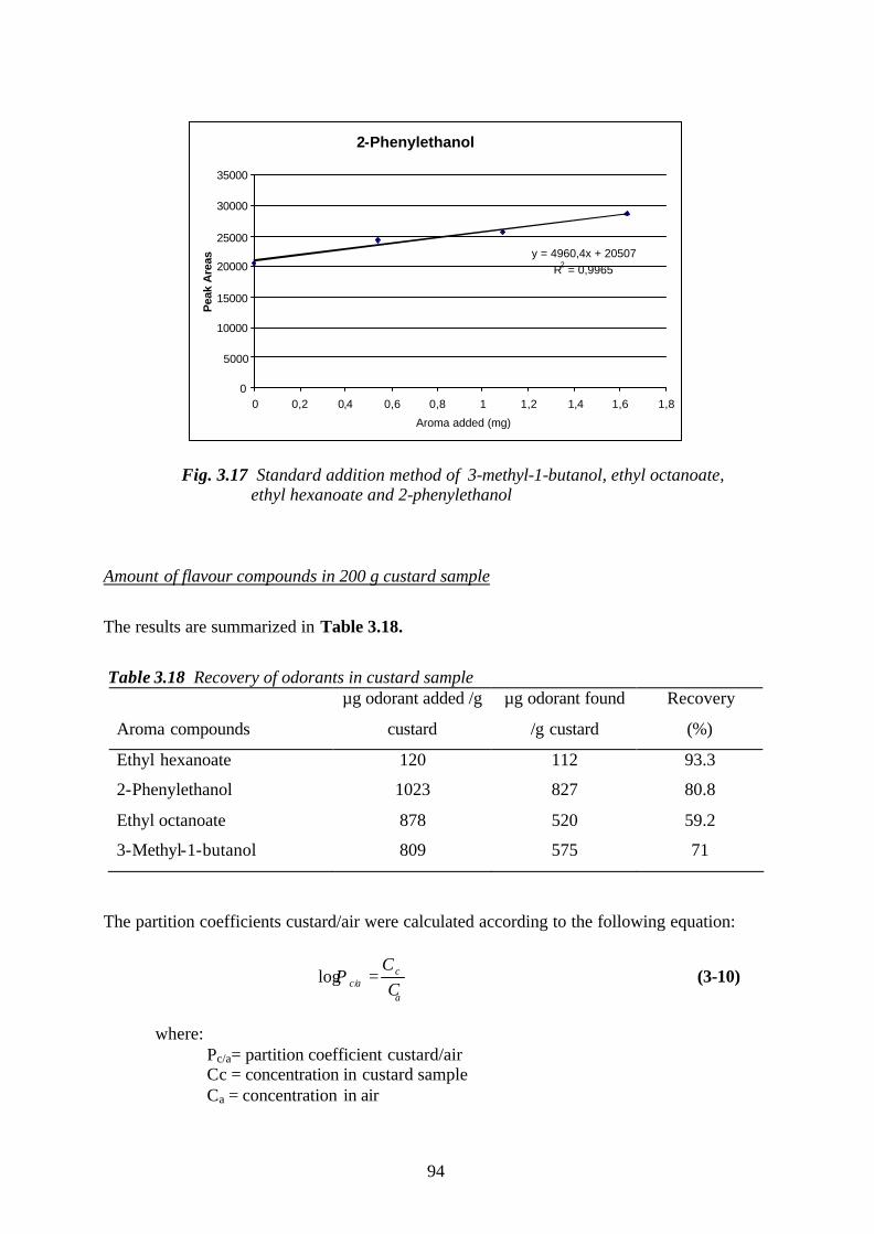
94
2-Phenylethanol
y = 4960,4x + 20507 R 2 = 0,9965
0
5000
10000
15000
20000
25000
30000
35000
0 0,2 0,4 0,6 0,8 1 1,2 1,4 1,6 1,8 Aroma added (mg)
Pea
k A
reas
Fig. 3.17 Standard addition method of 3-methyl-1-butanol, ethyl octanoate, ethyl hexanoate and 2-phenylethanol
Amount of flavour compounds in 200 g custard sample
The results are summarized in Table 3.18.
Table 3.18 Recovery of odorants in custard sample
Aroma compounds
µg odorant added /g
custard
µg odorant found
/g custard
Recovery
(%)
Ethyl hexanoate 120 112 93.3
2-Phenylethanol 1023 827 80.8
Ethyl octanoate 878 520 59.2
3-Methyl-1-butanol 809 575 71
The partition coefficients custard/air were calculated according to the following equation:
a
ca c C
CP =/log (3-10)
where:
Pc/a= partition coefficient custard/air Cc = concentration in custard sample Ca = concentration in air

95
The partition coefficients custard/air (logPc/a) for the selected aroma compounds calculated
(cf. Equation 3-10) are summarized in Table 3.19..
Table 3.19 Partition coefficients custard/air of aroma compounds
Aroma compounds
ng odorant /ml
custarda
ng odorant /ml air
Partition
coefficient,
custard/air (logPc/a)
Ethyl hexanoate 120000 58.38 3.31
2-Phenylethanol 885000 5.4 5.21
Ethyl octanoate 556000 39.4 4.15
3-Methyl-1-butanol 615000 280 3.34
a) Density of the custard: 1.07 g/ml. The density was gravimetrically determined. Analysis of the aroma release as a function of matrix components The influence of the matrix components (κ-carrageenan, modified- and native tapioca starch
and milk powder, used for the preparation of the custard samples) on the headspace
concentrations of odorants were investigated.
For this purpose, model mixtures containing one of the before mentioned high molecular
matrix component (sample 1-3), water and selected odorants were prepared. Furthermore, the
original custard sample (sample 4) was investigated by leaving out one of the above
mentioned components (5-7).
For 3-methyl-1-butanol (Figure 3.18), the lowest concentration in the headspace was found in
the model mixture containing modified tapioca starch and water (sample 2, 222 ng/ml) and
the highest concentration was found in the model mixture containing milk powder and water
(sample 1, 390 ng/ml).
In model mixtures containing neither native tapioca starch nor modified tapioca starch there
are small differences in the concentration of 3-methyl-1-butanol in the headspace. This means
that native and modified tapioca starch have similar effect on the flavour release.
The highest headspace concentration of 3-methyl-1-butanol (103 ng/ml) was found in the
model mixture containing only milk powder (sample 1). This means that milk has a large
influence to the flavour release. 3-Methyl-1-butanol is a polar compound; the presence of
milk (fat) has a positive effect to its release.
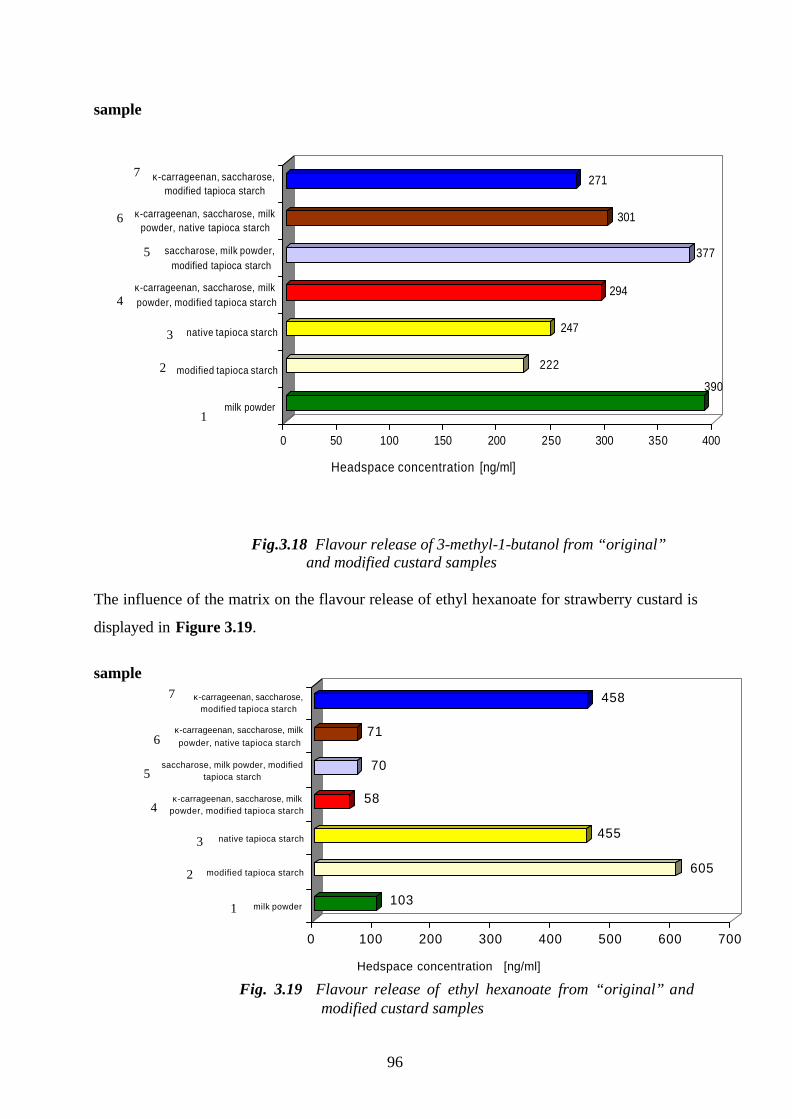
96
390
222
247
294
377
301
271
0 50 100 150 200 250 300 350 400
[ng/ml]
milk powder
modified tapioca starch
native tapioca starch
κ-carrageenan, saccharose, milkpowder, modified tapioca starch
saccharose, milk powder,modified tapioca starch
κ-carrageenan, saccharose, milkpowder, native tapioca starch
κ-carrageenan, saccharose,modified tapioca starch
Headspace concentration
103
605
455
58
70
71
458
0 100 200 300 400 500 600 700
[ng/ml]
milk powder
modified tapioca starch
native tapioca starch
κ-carrageenan, saccharose, milkpowder, modified tapioca starch
saccharose, milk powder, modifiedtapioca starch
κ-carrageenan, saccharose, milkpowder, native tapioca starch
κ-carrageenan, saccharose,modified tapioca starch
Hedspace concentration
sample
7 6
5 4 3 2
1
Fig.3.18 Flavour release of 3-methyl-1-butanol from “original” and modified custard samples
The influence of the matrix on the flavour release of ethyl hexanoate for strawberry custard is
displayed in Figure 3.19.
sample 7 6
5 4
3 2
1
Fig. 3.19 Flavour release of ethyl hexanoate from “original” and modified custard samples

97
97
966
776
40
45
50
618
0 100 200 300 400 500 600 700 800 900 1000
(ng/ml]
milk powder
modified tapioca starch
native tapioca starch
κ-carrageenan, saccharose, milkpowder, modified tapioca starch
saccharose, milk powder,modified tapioca starch
κ-carrageenan, saccharose, milkpowder, native tapioca starch
κ-carrageenan, saccharose,modified tapioca starch
Headspace concentration
The highest headspace concentration of ethyl hexanoate (sample 2, 605 ng/ml air) was found
above sample containing only water and modified starch. The lowest headspace concentration
of the odorant (sample 4, 58 ng/ml air) was measured above the original custard sample. The
headspace concentration of ethyl hexanoate increased slightly (70 ng/ml air) in the sample
without κ-carrageenan (sample 5), compared to the original custard (sample 4, 58 ng/ml air).
In contrast to the sample containing no milk powder a drastically effect on the headspace
concentration of ethyl hexanoate was observed; the concentration was higher by a factor of
eight (sample 3, 457 ng/ml air) compared to the original custard. These results showed that
the constituents of the milk (proteins and fats) are responsible for the reduction of ethyl
hexanoate in the headspace above the food. In most cases a change of the food matrix leads to
a change in flavour release. Caused by these changes the consumer’s acceptance can go back
for a food or be promoted. The strength of the interaction of an odorant with a macromolecule
should be considered closer for the proteins and lipids in milk.
• Milk has a large influence to the aroma release
• Native starches and modified starches have different influence to the aroma release
sample 7 6
5 4
3
2
1
Fig.3.20 Flavour release of ethyl octanoate from “original” and
modified custard samples

98
The highest headspace concentration of ethyl octanoate was found in the model mixture
containing modified tapioca starch and water (sample 2, 966 ng/ml) and the lowest
concentration in the original custard sample (sample 4, 40 ng/ml). Between modified samples
without κ-carrageenan and the sample where modified tapioca starch was replaced by native
tapioca starch there were not large differences in the concentrations of ethyl octanoate found
in the headspace to the original custard sample (sample 4). In contrast, in the sample
containing no milk powder, a drastically effect on the headspace concentration of ethyl
octanoate was observed. The concentration was higher by a factor of 15 compared to original
custard. The concentration of ethyl octanoate found in the headspace in model mixtures
containing native tapioca starch and water (sample 3) and modified tapioca starch and water
(sample 2), respectively, was higher but almost similar between both of them, which mean the
effect on aroma release is similar.
sample 7 6 5
4 3 2 1
Fig.3.21. Flavour release of 2-phenylethanol from “original” and modified
custard samples
7.8
12.2
7.9
8
8.6
7.2
16
0 2 4 6 8 10 12 14 16
milk powder
modified tapioca starch
native tapioca starch
κ-carrageenan, saccharose, milkpowder, modified tapioca starch
saccharose, milk powder,modified tapioca starch
κ-carrageenan, saccharose, milkpowder, native tapioca starch
κ-carrageenan, saccharose,modified tapioca starch
Headspace concentrationn (ng/ml)
)
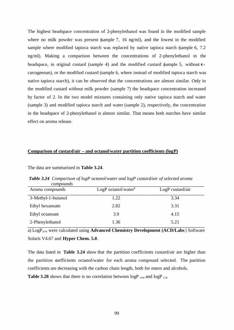
99
The highest headspace concentration of 2-phenylethanol was found in the modified sample
where no milk powder was present (sample 7, 16 ng/ml), and the lowest in the modified
sample where modified tapioca starch was replaced by native tapioca starch (sample 6, 7.2
ng/ml). Making a comparison between the concentrations of 2-phenylethanol in the
headspace, in original custard (sample 4) and the modified custard (sample 5, without κ-
carrageenan), or the modified custard (sample 6, where instead of modified tapioca starch was
native tapioca starch), it can be observed that the concentrations are almost similar. Only in
the modified custard without milk powder (sample 7) the headspace concentration increased
by factor of 2. In the two model mixtures containing only native tapioca starch and water
(sample 3) and modified tapioca starch and water (sample 2), respectively, the concentration
in the headspace of 2-phenylethanol is almost similar. That means both starches have similar
effect on aroma release.
Comparison of custard/air – and octanol/water partition coefficients (logP)
The data are summarized in Table 3.24. Table 3.24 Comparison of logP octanol/water and logP custard/air of selected aroma compounds Aroma compounds LogP octanol/watera LogP custard/air
3-Methyl-1-butanol 1.22 3.34
Ethyl hexanoate 2.82 3.31
Ethyl octanoate 3.9 4.15
2-Phenylethanol 1.36 5.21
a) LogPo/w were calculated using Advanced Chemistry Development (ACD/Labs ) Software
Solaris V4.67 and Hyper Chem. 5.0.
The data listed in Table 3.24 show that the partition coefficients custard/air are higher than
the partition coefficients octanol/water for each aroma compound selected. The partition
coefficients are decreasing with the carbon chain length, both for esters and alcohols.
Table 3.28 shows that there is no correlation between logP o/w and logP c/a.

100
Comparison of custard/air -, water/air - and emulsion/air partition coefficients (LogP) The data are summarized in Table 3.25.
Table 3.25 shows that the LogP custard/air is situated between logP water/air and LogP
emulsion/air for the aroma compounds selected, but closer to the logP emulsion/air. The LogP
values octanol/water for esters is between logP water/air and LogP emulsion/air. For alcohols,
the LogP octanol/water is lower than the logP water/air and LogP emulsion/air.
Table 3.25 Comparison of custard/air -, water/air - and emulsion/air partition coefficients of
selected aroma compounds Aroma compounds LogP
custard/air
LogP
water/air
LogP emulsion
(miglyol + water,
90,25 + 4,75 w/w)/air
LogP
octanol/water
Ethyl hexanoate 3.31 2.22 3.34 2.82
3-Methyl-1-butanol 3.34 2.52 3.23 1.22
Ethyl octanoate 4.15 2.56 4.59 3.9
δ-Decalactone 4.90 3.9 5.91 -
2-Phenylethanol 5.21 5.23 5.44 1.36
3.5.2.1. Determination of mass transfer coefficients of some flavour compounds studied, in
custard- and milk powder / water samples
In physical terms, the mass transfer of flavour compounds between two phases is the main
mechanism of flavour release (Marin et al., 2000).
The mass transfer coefficients between the liquid phase (custard and milk, respectively) and
the headspace were determined for some flavour compounds studied and the viscosity
measurements of the custard and milk samples were correlated with mass transfer data.
Viscosity determination
The viscosity of the custard was experimentally measured (cf. 2.4.2) using falling ball
viscosimetry and the value was compared with the viscosity value for glycerine, taken as a
model. For milk, the viscosity values were taken from the literature.
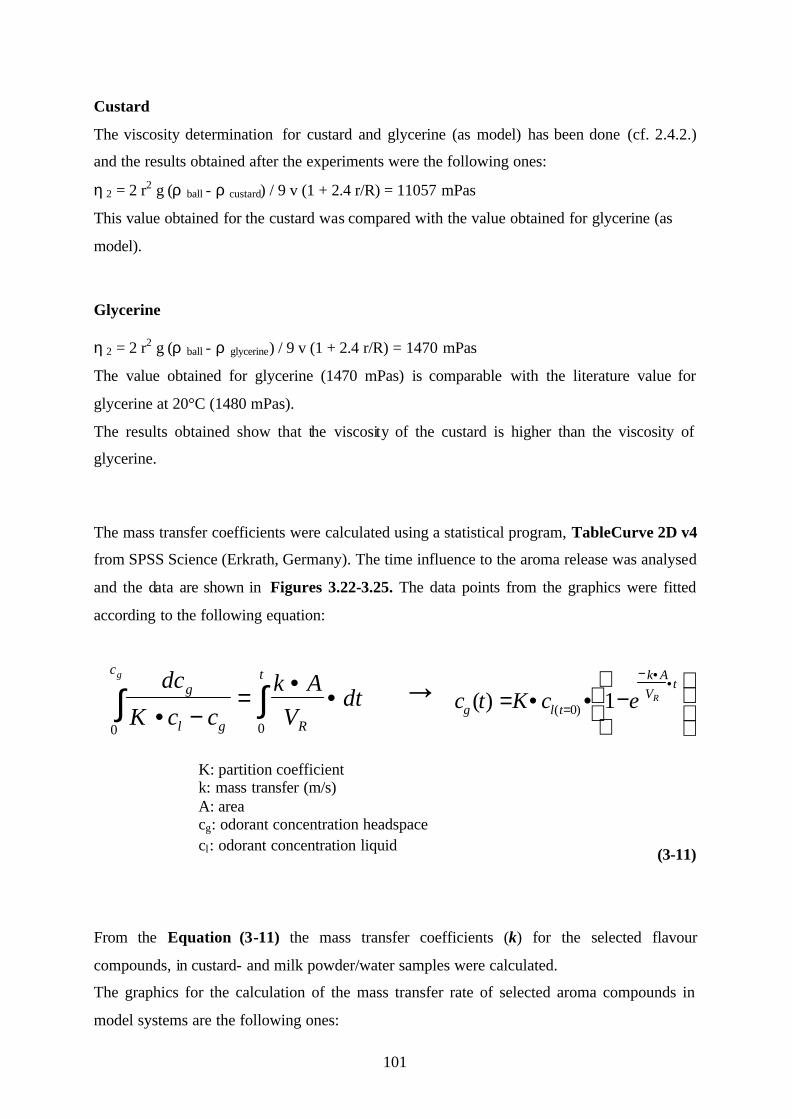
101
Custard
The viscosity determination for custard and glycerine (as model) has been done (cf. 2.4.2.)
and the results obtained after the experiments were the following ones:
η 2 = 2 r2 g (ρ ball - ρ custard) / 9 v (1 + 2.4 r/R) = 11057 mPas
This value obtained for the custard was compared with the value obtained for glycerine (as
model).
Glycerine η 2 = 2 r2 g (ρ ball - ρ glycerine) / 9 v (1 + 2.4 r/R) = 1470 mPas
The value obtained for glycerine (1470 mPas) is comparable with the literature value for
glycerine at 20°C (1480 mPas).
The results obtained show that the viscosity of the custard is higher than the viscosity of
glycerine.
The mass transfer coefficients were calculated using a statistical program, TableCurve 2D v4
from SPSS Science (Erkrath, Germany). The time influence to the aroma release was analysed
and the data are shown in Figures 3.22-3.25. The data points from the graphics were fitted
according to the following equation:
(3-11)
From the Equation (3-11) the mass transfer coefficients (k) for the selected flavour
compounds, in custard- and milk powder/water samples were calculated.
The graphics for the calculation of the mass transfer rate of selected aroma compounds in
model systems are the following ones:
→
K: partition coefficient k: mass transfer (m/s) A: area cg: odorant concentration headspace cl: odorant concentration liquid
dtV
AkccK
dc t
R
c
gl
gg
••=−• ∫∫
00
−••=
••−
=
tV
Ak
tlgRecKtc 1)( )0(
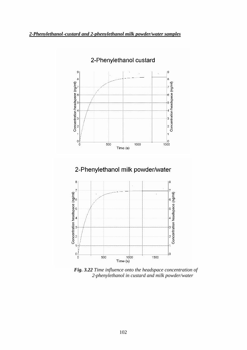
102
2-Phenylethanol -custard and 2-phenylethanol milk powder/water samples
Fig. 3.22 Time influence onto the headspace concentration of
2-phenylethanol in custard and milk powder/water
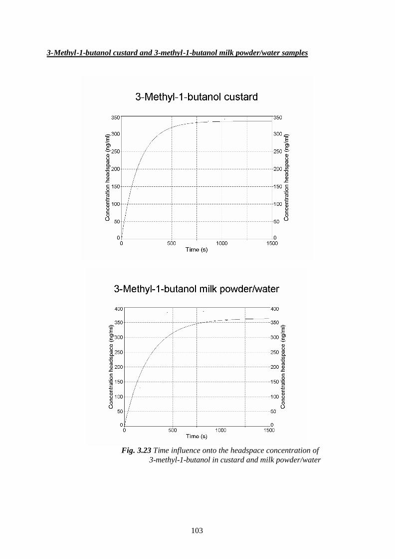
103
3-Methyl-1-butanol custard and 3-methyl-1-butanol milk powder/water samples
Fig. 3.23 Time influence onto the headspace concentration of 3-methyl-1-butanol in custard and milk powder/water
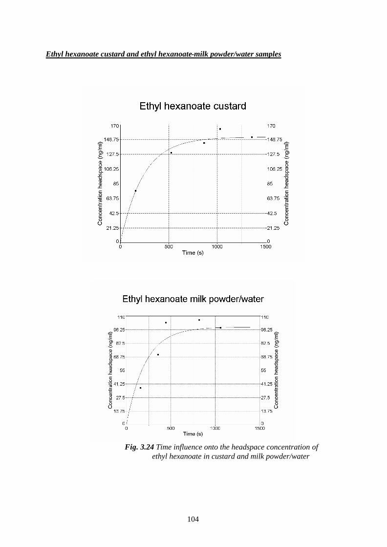
104
Ethyl hexanoate custard and ethyl hexanoate-milk powder/water samples
Fig. 3.24 Time influence onto the headspace concentration of ethyl hexanoate in custard and milk powder/water
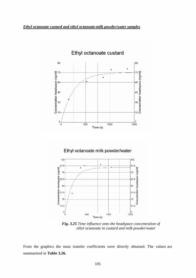
105
Ethyl octanoate custard and ethyl octanoate-milk powder/water samples
Fig. 3.25 Time influence onto the headspace concentration of
ethyl octanoate in custard and milk powder/water
From the graphics the mass transfer coefficients were directly obtained. The values are
summarized in Table 3.26.

106
Table 3.26 Mass transfer coefficients of aroma compounds selected in model systems
Model systems Mass transfer coefficients (m/s)
2-Phenylethanol custarda 2.2 x 10⁻⁴
2-Phenylethanol milk powder/waterb 2.4 x 10⁻⁴
3-Methyl-1-butanol custard 2.6 x 10⁻⁴
3-Methyl-1-butanol milk powder/water 1.8 x 10⁻⁴
Ethyl hexanoate custard 1.9 x 10⁻⁴
Ethyl hexanoate milk powder/water 2.0 x 10⁻⁴
Ethyl octanoate custard 1.7 x 10⁻⁴
Ethyl octanoate milk powder/water 2.5 x 10⁻⁴
a) The viscosity of the custard was experimentally determined and the value found was:
11057 mPas;
b) Viscosity of the milk: 2.4 mPas.
The data in Table 3.26 indicated that the viscosity of the matrix did not significantly
influence the values of mass transfer rate of selected aroma compounds.
From the Table 3.26, the values of the mass transfer rate are higher in milk powder/water
systems than in custard model, for all the compounds investigated, except 3-methyl-1-butanol.
3.6. The influence of the matrix effects onto the odour activity values of
selected flavour compounds
The matrix has an important contribution to the determination of the threshold values and
odour activity values of selected aroma compounds.
The threshold values for three esters and an alcohol were determined in air in the presence
and absence of ethanol, using a LABC – Olfactometer (cf. 2.1.2.5).
The procedure of work was in experimental part explained (cf. 2.5.).
The results are summarized in Table 3.27 and the values obtained experimentally were
compared with those found in the literature.
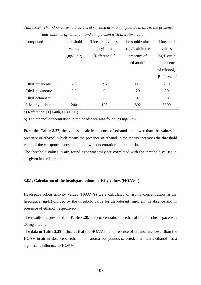
107
Table 3.27 The odour threshold values of selected aroma compounds in air, in the presence
and absence of ethanol, and comparison with literature data
Compound Threshold
values
(ng/L air)
Threshold values
(ng/L air)
[Reference] a
Threshold values
(ng/L air in the
presence of
ethanol) b
Threshold
values
(ng/L air in
the presence
of ethanol)
[Reference]a
Ethyl butanoate 2.9 2.5 11.7 200
Ethyl hexanoate 2.5 9 20 90
Ethyl octanoate 5.5 6 87 63
3-Methyl-1-butanol 200 125 802 6300
a) Reference: [1] Guth, H. (1997)
b) The ethanol concentration in the headspace was found 28 mg/L air.
From the Table 3.27, the values in air in absence of ethanol are lower than the values in
presence of ethanol, which means the presence of ethanol in the matrix increases the threshold
value of the component present in a known concentration in the matrix.
The threshold values in air, found experimentally are correlated with the threshold values in
air given in the literature.
3.6.1. Calculation of the headspace odour activity values (HOAV’s)
Headspace odour activity values (HOAV’s) were calculated of aroma concentration in the
headspace (ng/L) divided by the threshold value for the odorant (ng/L air) in absence and in
presence of ethanol, respectively.
The results are presented in Table 3.28. The concentration of ethanol found in headspace was
28 mg / L air.
The data in Table 3.28 indicates that the HOAV in the presence of ethanol are lower than the
HOAV in air in absence of ethanol, for aroma compounds selected, that means ethanol has a
significant influence to HOAV.

108
Table 3.28 Headspace odour activity values (HOAV’s) of selected odour compounds Compound Headspace
concentration
(µ g/L)
Threshold
values in air
in absence
of ethanol
(ng/L)
HOAV
in absence
of ethanol
Threshold
values in air
in presence of
ethanol (ng/L)
HOAV
in
presence
of
ethanol
Ethyl hexanoate 123.13 2.5 49252 20 6157
Ethyl octanoate 61.45 5.5 11173 87 706
3-Methyl-1-butanol 2753.91 200 13770 802 3434
3.7. Molecular modelling studies for the determination of the free energy of
solvation in different model systems The Molecular modelling methods have been used for the prediction of solvation free energies
of the flavour compounds studied in different model solutions, e.g. water and water-oil
systems. As Software package WinMOPAC 97 has been used.
Within MOPAC 97 there are two continuum models. One is the so-called Tomasi model and
the other is COSMO.
For the water systems the Tomasi model is given and the free energy of solvation was
possible to be calculated and then the experimentally data correlated with the model.
The solvation energy is defined accordance to the following thermodynamic equation:
PRTG ln-=∆ , (3-12)
where: ∆ G – energy of solvation: J mol-1
R – universal gas constant: 8.314 J mol-1 K-1;
T – temperature: 298.15 K;
P – partition coefficient.
The free energy of solvation is expressed as the sum of three contributions: cavitation-
(∆ Gcav), van der Waals- (∆ GvW) and electrostatic energies (∆ Gele):
vWcavele GGGGsol ∆+∆ +∆ = ∆ (3-13)
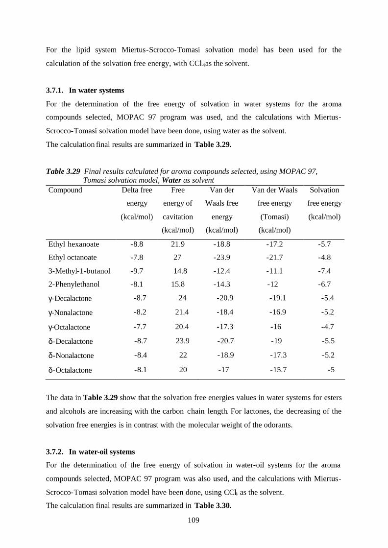
109
For the lipid system Miertus-Scrocco-Tomasi solvation model has been used for the
calculation of the solvation free energy, with CCl4 as the solvent.
3.7.1. In water systems
For the determination of the free energy of solvation in water systems for the aroma
compounds selected, MOPAC 97 program was used, and the calculations with Miertus-
Scrocco-Tomasi solvation model have been done, using water as the solvent.
The calculation final results are summarized in Table 3.29.
Table 3.29 Final results calculated for aroma compounds selected, using MOPAC 97, Tomasi solvation model, Water as solvent Compound Delta free
energy
(kcal/mol)
Free
energy of
cavitation
(kcal/mol)
Van der
Waals free
energy
(kcal/mol)
Van der Waals
free energy
(Tomasi)
(kcal/mol)
Solvation
free energy
(kcal/mol)
Ethyl hexanoate -8.8 21.9 -18.8 -17.2 -5.7
Ethyl octanoate -7.8 27 -23.9 -21.7 -4.8
3-Methyl-1-butanol -9.7 14.8 -12.4 -11.1 -7.4
2-Phenylethanol -8.1 15.8 -14.3 -12 -6.7
γ-Decalactone -8.7 24 -20.9 -19.1 -5.4
γ-Nonalactone -8.2 21.4 -18.4 -16.9 -5.2
γ-Octalactone -7.7 20.4 -17.3 -16 -4.7
δ-Decalactone -8.7 23.9 -20.7 -19 -5.5
δ-Nonalactone -8.4 22 -18.9 -17.3 -5.2
δ-Octalactone -8.1 20 -17 -15.7 -5
The data in Table 3.29 show that the solvation free energies values in water systems for esters
and alcohols are increasing with the carbon chain length. For lactones, the decreasing of the
solvation free energies is in contrast with the molecular weight of the odorants.
3.7.2. In water-oil systems
For the determination of the free energy of solvation in water-oil systems for the aroma
compounds selected, MOPAC 97 program was also used, and the calculations with Miertus-
Scrocco-Tomasi solvation model have been done, using CCl4 as the solvent.
The calculation final results are summarized in Table 3.30.

110
Table 3.30 Final results calculated for aroma compounds selected, using MOPAC 97, Tomasi solvation model, CCl4 as solvent Compound Delta free
energy
(kcal/mol)
Free
energy of
cavitation
(kcal/mol)
Van der
Waals free
energy
(kcal/mol)
Van der Waals
free energy
(Tomasi)
(kcal/mol)
Solvation
free energy
(kcal/mol)
Ethyl hexanoate -0.9 19.8 -26.5 -24.2 -7.6
Ethyl octanoate -0.5 23.6 -31.6 -29.4 -8.6
3-Methyl-1-butanol 0 14.1 -18.5 -16.5 -4.4
2-Phenylethanol -0.7 15 -20.7 -17.6 -6.4
γ-Decalactone -0.9 21.2 -28.7 -26.2 -8.3
γ-Nonalactone -0.8 19.3 -26.1 -23.5 -7.6
γ-Octalactone -0.7 18.4 -24.6 -22.3 -7
δ-Decalactone -0.8 21.1 -28.3 -26 -8
δ-Nonalactone -0.8 19.6 -26.1 -24 -7.4
δ-Octalactone -0.8 18.1 -24 -22 -6.7
In water-oil systems (Table 3.30), the increasing of the solvation free energies values for
aroma compounds selected is in contrast with the carbon chain length. For lactones, the
behaviour is similar as for the water systems.
The data in Table 3.29 and Table 3.30 indicate that the solvation free energies are lower in
water-oil systems than the values in water systems for the aroma compounds selected.
3.8. Comparison of the solvation free energy calculated by molecular
modelling studies and experimentally values
The solvation free energy was experimentally calculated (in water and miglyol) (cf. 3.3) for
all aroma compounds selected, according to the following thermodynamic equation:
PRTG ln-=∆ (3-14)

111
where: ∆ G – energy of solvation: kcal mol-1
R – universal gas constant: 8.314 J mol-1 K-1;
T – temperature: 303 K;
P – partition coefficients, experimentally values
(in water and miglyol).
The correlations of the free energy of solvation of the model with the free energy of solvation
calculated experimentally are given in Table 3.31.
Table 3.31 Comparison between solvation free energies (in water and miglyol) calculated
and solvation free energy found experimentally for aroma compounds selected
Solvation free energy (kcal/mol)
Compound Water Miglyol
Calculated Experimental Calculated Experimental
Ethyl hexanoate -5.7 -3.1 -7.6 -5.9
Ethyl octanoate -4.8 -3.5 -8.6 -7.3
3-Methyl-1-butanol -7.4 -3.4 -4.4 -4.6
2-Phenylethanol -6.7 -7.2 -6.4 -7.9
γ-Decalactone -5.4 -5.3 -8.3 -9.1
γ-Nonalactone -5.2 -5.8 -7.6 -8.6
γ-Octalactone -4.7 -6.6 -7 -8.5
δ-Decalactone -5.5 -6.3 -8 -9.5
δ-Nonalactone -5.2 -7.2 -7.4 -9.0
δ-Octalactone -5 -7.8 -6.7 -8.6
Table 3.31 shows that the increasing of the solvation free energies found experimentally for
esters and alcohols in water systems is in contrast with the carbon chain length. For lactones,
the solvation free energies found experimentally for the water systems are decreasing with the
molecular weight of the odorants.

112
In water-oil systems, the experimentally values of esters and alcohols are following the same
behaviour as for the water systems. But for lactones, in water-oil systems, the increasing of
the solvation free energies found experimentally is in contrast with the carbon chain length.
Making a correlation between the experimentally values found for the solvation free energies
in the two model systems studied: water and oil-water system, it can be observed that the
experimentally values found for the water system are higher than the experimentally values
found for the oil-water system for the aroma compounds selected., which means that the oil
has a influence to the solvation free energy, reducing the value.
The experimentally values found for the solvation free energies in water systems are higher
for esters and alcohols (except 2-phenylethanol) than the solvation free energies of the model.
For lactones, the experimentally values found for the solvation free energies are lower (except
γ-decalactone) than the solvation free energies of the model.
In water-oil systems, the experimentally values found for the solvation free energies are
higher for esters than the solvation free energies of the model, and for alcohols and lactones,
the experimentally values found for the solvation free energies are lower than the solvation
free energies of the model.

113
4. CONCLUSIONS Foods are complex multi-component systems which are composed of volatile and non-volatile
substances. The flavour profile of a food is an important criterion for the selection of our
foodstuffs. The structure of our food, in particular the presence of macromolecules as for
example proteins, fats and polysaccharides, influence the mouth feeling and the extent of the
flavour release. The effect of food matrix composition and structure on flavour release was
presented and discussed through complementary studies carried out by thermodynamic or
kinetic approaches.
The main objective of this study was the clarification of the complex relationships of the
flavour release as a function of the composition of the food matrix at molecular level.
Therefore the influence of matrix effects onto the partition coefficients, odour activity values
and sensory properties of selected flavour compounds, in model and in real food systems were
investigated. Different matrices were selected to measure their influence onto the partition
coefficients of odorants: water, water-ethanol-mixtures, matrices containing lipids and more
complex samples, such as mixtures of water, oil, proteins and polysaccharides. The studies
included a series of lactones, esters and alcohols (γ-octalactone, γ-nonalactone, γ-decalactone,
δ-octalactone, δ -nonalactone, δ -decalactone, ethyl hexanoate and ethyl octanoate, 3-methyl-1-
butanol and 2-phenylethanol).
The vapour pressures and partition coefficients were determined using static headspace gas
chromatography (HS-GC) techniques. The influence of the model systems on the adsorptions
of the odorants at the gas-tight syringes were taken into account. The results obtained showed
that the vapour pressures of the flavour compounds are decreasing with the increasing of the
molecular weight of the compounds. The comparison of water/air partition coefficients
(logPW/A) with miglyol/air partition coefficients of selected odorants (logPM/A) showed that for
miglyol system, the logPM/A are higher than the logPW/A for all flavour compounds studied.
The measurement of the partition coefficients of selected aroma compounds in water-oil
matrices (emulsions) revealed that the fat content of emulsions influence significantly the
partition coefficients of odorants. The highest partition coefficients were obtained in
emulsions where the portion between water/miglyol/emulsifier was: 47.5 + 47.5 + 5, w/w/w.
In the present study the flavour release of different aroma compounds (ethyl hexanoate and S-
(-)-limonene) in carbohydrate-water solutions was examined. The static headspace method
114
allows the measurement of the released odour components that interact with β -cyclodextrin.
The HS-GC analysis of β -cyclodextrin-water/odorant mixtures showed a reduction of the
odorant in presence of the carbohydrate.
The influence of the various matrices on the human biological response of odorants was
investigated by an olfactometer (e.g. determination of the threshold values of odorants in air
and in the presence of ethanol) and the headspace odour activity values (HOAV’s) were
calculated. The results showed that the threshold values in air in absence of ethanol were
lower than the values in presence of ethanol, which means the presence of ethanol in the
matrix increase the threshold value of the odorant.
The studies also included the influence of wine matrix onto the partition coefficients of
important wine flavour compounds. The quantification of the aroma compounds in white wine
samples was achieved by isotope dilution analyses and standard addition method. Odorants in
the headspace above wines were analysed by HS-GC techniques and the partition coefficients
(wine/air) calculated. The results pointed out that the presence of ethanol in wine matrix does
not influence the partition coefficients of selected aroma compounds. The highest partition
coefficients in wines were found for the two alcohols: 2-phenylethanol and 3-methyl-1-
butanol.
Concerning COST Action 921 custard samples were investigated as real foodstuff and the
aroma compounds were quantified in the matrix and in the headspace above the food. The
research data indicated that the partition coefficients custard/air are located between the
partition coefficients water/air and partition coefficients miglyol/air, but closer to the
miglyol/air values. Furthermore the mass transfer rates of selected odorants were investigated
in custard- and milk powder/water samples. The values of the mass transfer rate were found
higher in milk powder/water systems than in custard model. Nevertheless the results indicated
that the viscosity of the matrix did not significantly influence the values of mass transfer rate
of selected flavour compounds.
Molecular Modelling methods have been used for the prediction of solvation free energies of
the flavour compounds studied in different model solutions, e.g. water and water-oil systems.
The results showed that the predicted values (Mopac 97) for γ-decalactone, γ−nonalactone and
2-phenylethanol in water are in good agreement with experimentally solvation free energies.

115
5. REFERENCES
Acree, T.E., Deibler, K.D., Kittel, K.M., Similarity and diversity in flavour perception.
Handbook of flavour characterization, 2004: p. 83-91.
Allen, M.P., Tildesley, D.J., Computer Simulation of Liquids, 1987.
Allen, R.R., Volatile flavour constituents in coconut oil. Chem Ind, 1965. 36: p. 1560.
Amoore, J.E., Buttery, R.G., Partition coefficients and comparative olfactometry.
Chemical Senses and Flavour, 1978. 3(1): p. 57-71.
Andriot, I., Harrison, M., Fournier, N., Guichard, E., Interactions between methyl
ketones and beta-lactoglobulin: Sensory analysis, headspace analysis, and
mathematical modeling. Journal of Agricultural and Food Chemistry, 2000. 48(9): p.
4246-4251.
Antoine, C., C.R. Acad. Sci., 1888: p. 107, 681, 836, 1143.
Arozarena, I., Casp, A., Marin, R., Navarro, M., Multivariate differentiation of
Spanish red wines according to region and variety. Journal of the Science of Food and
Agriculture, 2000. 80(13): p. 1909-1917.
Audouin, V., Bonnet, F., Vickers, Z.M., Reineccius, G.A., Limitations in the use of
odor activity values to determine important odorants in foods. Gas Chromatography-
Olfactometry, 2001: p. 156-171.
Bachs, M., Luque, F.J., Orozco, M., Optimization of Solute Cavities and Van-Der-
Waals Parameters in Ab-Initio Mst-Scrf Calculations of Neutral Molecules. Journal of
Computational Chemistry, 1994. 15(4): p. 446-454.
Bakker, J., Brown, W., Hills, B., Boudaud, N., Wilson, C., Harrison, M., Effect of the
food matrix on flavour release and perception. Flavour Science, Recent
Developments, 1996: p. 369-372.

116
Bakker, J., Flavour interactions with the food matrix and their effects on perception.
p. 411.
Bakker, J., Ingredient Interactions - Effects on Food Quality. 1995: p. 411.
Bamford, H.A., Baker, J.E., Poster, D.L., Review of Methods and Measurements of
selected hydrophobic organic contaminant aqueous solubilities, vapor pressures, and
air-water partition coefficients. NIST Special Publication 928, 1998.
Banat, F.A., Abu Al-Rub, F.A., Simandl, J., Analysis of vapor-liquid equlibrium of
ethanol-water system via headspace gas chromatography: effect of molecular sieves.
Separation and Purification Technology, 2000. 18: p. 111-118.
Banavara, D.S., Rabe, S., Krings, U., Berger, R. G., Modeling dynamic flavor
release from water. J Agric Food Chem, 2002. 50(22): p. 6448-6452.
Bassette, R., Glendenn.Bl, Analysis of Blood Alcohol by Direct Head Space Gas
Sampling and Gas Chromatography. Microchemical Journal, 1968. 13(3): p. 374-&.
Becher, P., Emulsions, Theory and Practice. 1966: p. 233.
Becher, P., Physical Properties of Emulsions: Theory and Prcatice, 2nd Ed., 1994: p.
49-94.
Ben-Naim, A., Solvation Thermodynamics, 1987.
Binks, B.P., Dyab, A.K. and Fletcher, P.D., Novel emulsions of ionic liquids stabilised
solely by silica nanoparticles. Chem Commun (Camb), 2003(20): p. 2540-1.
Bohnenstengel, F., Soltani, N., Baltes, W., Headspace analysis with large sample
volumes. Influence of sampling device volume, analyte concentration and sample
matrix. Journal of Chromatography A, 1993. 655: p. 249-255.
117
Bonaccorsi, R., Cimiraglia, R. and Tomasi, J., Abinitio Evaluation of Absorption and
Emission Transitions for Molecular Solutes, Including Separate Consideration of
Orientational and Inductive Solvent Effects. Journal of Computational Chemistry,
1983. 4(4): p. 567-577.
Boublik, T., Fried, V., Hala, E., The vapour pressures of pure substances. Elsevier
Scientific Publishing Company, 1973.
Brauss, M.S., Linforth, R.S.T., Cayeux, I., Harvey, B., Taylor, A.J., Altering the fat
content affects flavour release in a model yogurt system. J. Agric. Food Chem., 1999.
47: p. 2055-2059.
Brauss, M.S., Linforth, R.S.T., Balders, B., Avison, S., Taylor, A.J., Fat content,
baking time, hydration and temperature affect flavour release from biscuits in model
and real systems. Flav. Frag. J., 2000. 14: p. 351-357.
Brossard, C., Rousseau, F. and Dumont, J.P., Oil-water partition coefficient of
odorants: reliable index for smell but deceptive for odor rating! Food Quality and
Preference, 2002. 13(2): p. 65-72.
Buck, L., Axel, R., Cell, 1991. 65: p. 175.
Buhr, K., Fritzler, R., Guth, H., Structure -odour relationships of gama- and delta-
lactones. Flavour 2000, 2001.
Burkhard, L.P., Armstrong, D.E., Andren, A.W., Henry's Law Constants for the
Polychlorinated Biphenyls. Environ. Sci. Technol., 1985. 19: p. 590-596.
Burnett, M.G., Determination of Partition Coefficients at Infinite Dilution by the Gas
Chromatographic Analysis of the Vapor above Dilute Solutions. Analytical Chemistry,
1963. 35(11).
Butler, R.A., Kelly, A.B., Zapp, J., Anesthesiology, 1967. 28: p. 760.
118
Buttery, R.G., Ling, L.C., Guadagni, D.G., Volatilities of Aldehydes, Ketones and
Esters in Dilute Water Solutions. J. Agric. Food Chem., 1969. 17: p. 385.
Buttery, R.G., Guadagni, D.G., Ling, L.C., Flavor compounds: Volatilities in
vegetable oil and oil-in-water mixtures: Estimation of odor thresholds. J. Agric. Food
Chem., 1973. 21(2): p. 198-201.
Buttery, R.G., Bomben, J.L., Guadagni, D.G., Ling, L.C., Some considerations of the
volatiles of organic flavor compounds in foods. J Agric Food Chem, 1971. 19: p.
1045-1048.
Büttner, A., Hoch, U., Schieberle, P., Studies on correlations between odor activity
values, headspace concentrations and odor intensities in defined aroma model
solutions.
Cappelli, C., Mennucci, B., da Silva, C.O., Tomasi, J., Refinements on solvation
continuum models: Hydrogen-bond effects on the OH stretch in liquid water and
methanol. Journal of Chemical Physics, 2000. 112(12): p. 5382-5392.
Cayot, N., Taisant, C. and Voilley, A., Release and perception of isoamyl acetate from
a starch-based food matrix. Journal of Agricultural and Food Chemistry, 1998. 46(8):
p. 3201-3206.
Chaintreau, A., Grade, A. and Munozbox, R., Determination of Partition-Coefficients
and Quantitation of Headspace Volatile Compounds. Analytical Chemistry, 1995.
67(18): p. 3300-3304.
Chaplet, A., Olfactometers and olfactometry. Parfumerie Moderne, 1936. 30: p. 3-13.
Charalambous, G., Analysis of foods and beverages. Headspace techniques. 1978.
Charles, M., Lambert, S., Brondeur, P., Courthaudon, J.L., Guichard, E., Influence of
Formulation and Structure of an Oil-in-Water Emulsion on Flavor Release. Flavour
Release, 2000: p. 342-354.
119
Cies, J.J., 1999.
Clarke, R.J., Bakker, J., Wine Flavour Chemistry. 2004.
Clemons, J.M., Chromatography in Process Analysis. Encyclopedia of Analytical
Chemistry. 9.
Conner, J.M., Birkmyre, L., Paterson, A., Piggott, J.R., Headspace Concentrations of
Ethyl Esters at Different Alcoholic Strengths. J Sci Food Agric., 1998. 77: p. 121-126.
Cramer, C.J. and Truhlar, D.G., Implicit Solvation Models: Equilibria, Structure,
Spectra, and Dynamics. Chem Rev, 1999. 99(8): p. 2161-2200.
Crooks, G.E. and Chandler, D., Gaussian statistics of the hard-sphere fluid. Physical
Review E, 1997. 56(4): p. 4217-4221.
Curry, A.S., Hurst, G., Kent, N.R., Powell, H., Rapid screening of blood samples for
volatile poisons by gas chromatography. Nature, 1962. 195: p. 603-4.
Curutchet, C., Orozco, M. and Luque, F.J., Solvation in octanol: Parametrization of
the continuum MST model. Journal of Computational Chemistry, 2001. 22(11): p.
1180-1193.
D'Appolonia, B.L., Gilles, K.A., Osman, E.M., Pomeranz, Y., Wheat-Chemistry and
Technology, 1978: p. 301.
Daubert, T.E., Danner, R.P., MPBPVP EPI Suite, 1989. 2000 b.
Davidek, J., Velisek, J., Pokorny, J., Chemical Changes during Food Processing.
1990. 21.
Davidson, J.M., Linforth, R.S.T., Hollowood, T.A., Taylor, A.J., Release of non-
volatile flavour components in vivo. Flavour Release: Linking experiments, theory and
reality, 2000: p. 99-111.
120
Davies, J.T., Proc. Int. Congr. Surface Activ., 2nd, 1957. 1: p. 476.
Davis, P.L., J. Chromatogr. Sci., 1970. 8: p. 423.
De Roos, K.B., How lipids influence food flavour. Food Technology, 1997. 51: p. 60-
62.
De Roos, K.B., Wolswinkel, K., Non-equilibrium partition models for predicting
flavour release in the mouth. Trends in Flavour Research, 1994: p. 15-32.
De Roos, K.B., Physicochemical Models of Flavour Release from Foods. Flavour
Release, 2000: p. 126-141.
Deibler, K.D., Delwiche, J., Handbook of Flavour Characterization. Sensory analysis,
chemistry and physiology. 2004.
Dickinson, E., Interfacial Interactions and the Stability of Oil-in-Water Emulsions.
Pure and Applied Chemistry, 1992. 64(11): p. 1721-1724.
Dickinson, E., Stainsby, G., Colloids in Food. Applied Science Publishers, 1982.
Dillet, V., Rinaldi, D. and Rivail, J.L., Liquid-State Quantum-Chemistry - an
Improved Cavity Model. Journal of Physical Chemistry, 1994. 98(19): p. 5034-5039.
Dimick, P.S., Patton, S., Kinsella, J.E., Walker, N.J., The prevalence of aliphatic
delta-lactones or their precursors in animal fats. Lipids, 1966. 1: p. 387.
Dravniek.A, Measuring Industrial Odors. Chemical Engineering, 1974. 81(22): p. 91-
95.
Duffy, E.M., Jorgensen, W.L., Prediction of Properties from Simulations: Free
Energies of Solvation in Hexadecane, Octanol, and Water. J. Am. Chem. Soc.,
2000(122): p. 2878-2888.
121
Duritz, G. and Truitt, E.B.Jr., A Rapid Method For The Simultaneous Determination
Of Acetaldehyde And Ethanol In Blood Using Gas Chromatography. Q J Stud
Alcohol, 1964. 25: p. 498-510.
Ebeler, S.E., Linking flavour chemistry to sensory analysis of wine. Flavour
Chemistry: 30 years of Progress, 1999: p. 409-421.
Ebeler, S.E., Analytical Chemistry: Unlocking the secrets of wine flavour. Food Rev
Int, 2001. 17(1): p. 45-64.
Ebeler, S.E., Noble, A.C., Past and the future: Bucket flavour chemistry to
sensochemistry. Am J Enol Viticult, 2000. 51(5): p. 205-208.
Ebeler, S.E., Sensory analysis and analytical flavor chemistry: missing links.
Handbook of flavor characterization. Sensory analysis, chemistry, and physiology,
2004: p. 41-50.
Ebeler, S.E., Pangborn, R.M., Jennings, W.G., Influence of dispersion medium on
aroma intensity and headspace concentration of methone and isoamyle acetate. J
Agric Food Chem, 1988. 36: p. 791-796.
Ellis, R. and Wong, N.P., Lactones in butter, butteroil, and margarine-1. J Am Oil
Chem Soc, 1975. 52(7): p. 252-5.
Escalona, H., Piggott, J.R., Conner, J.M., Paterson, A., Effect of ethanol strength on
the volatility of higher alcohols and aldehydes. Italian Journal of Food Science, 1999.
11(3): p. 241-248.
Escher, F.E., Nuessli, J., Conde-Petit, B., Interactions of Flavor Compounds with
Starch in Food Processing. Flavour Release, 2000: p. 230-245.
Escudero, A., Cacho, J. and Ferreira, V., Isolation and identification of odorants
generated in wine during its oxidation: a gas chromatography-olfactometric study.
European Food Research and Technology, 2000. 211(2): p. 105-110.
122
Esquena, J., Solans, C., Study of low energy emulsification methods for the
preparation of narrow size distribution W/O emulsions. Prog. Colloid. Polym. Sci.,
1998. 110: p. 235-239.
Fabre, M., Aubry, V., Hugi, A., Guichard, E., Correlation between sensory time-
intensity and SPME analysis of fruity flavor in model food emulsions. Abstracts of
Papers of the American Chemical Society, 2002. 224: p. U65-U65.
Fama, L., Rojas, A.M., Goyanes, S., Gerschenson, L., Mechanical properties of
tapioca-starch edible films containing sorbates. LWT, 2004. 38: p. 631-639.
Feddes, J.J.R., qu, G., Ouellette, C.A., Leonard, J.J., Development of an eight-panelist
single port, forced-choice, dynamic dilution olfactometer. Canadian Biosystems
Engineering, 2001. 43.
Fendinger, N.J., Glotfelty, D.E., Freeman, H.P., Comparison of Two Experimental
Techniques for Determining Air/Water Henry's Law Constants. Environ. Sci.
Technol., 1989. 23(12): p. 1528-1531.
Fennema, O.R., Food Chemistry. 1996. Third Edition.
Field, M.J., Bash, P.A., Karplus, M., J. Comp. Chem., 1990. 11: p. 700.
Fioriti, J.A., Krampl, V. and Sims, R.J., Lactones in autoxidized vegetable oils. J Am
Oil Chem Soc, 1967. 44(9): p. 534-8.
Fischer, U., Roth, D. and Chr istmann, M., The impact of geographic origin, vintage
and wine estate on sensory properties of Vitis vinifera cv. Riesling wines. Food
Quality and Preference, 1999. 10(4-5): p. 281-288.
Floris, F.M., Selmi, M., Tani, A., Tomasi, J., Free energy and entropy for inserting
cavities in water: comparison of Monte Carlo simulation and scaled particle theory
results. J.Chem. Phys., 1997. 107(16).

123
Forss, D.A., J. Agric. Food Chem., 1969. 17: p. 681.
Forster, T., Principles of Emulsion Formation, Surfactants in Cosmetics. Surfactant
Science Series, 1997. 68: p. 105-125.
Fox, P.F., Developments in Dairy Chemistry. 1983. II.
Fritzler,R., Bindungsverhaltenvon Geruchstoffen an makromolekulare
Lebensmittelinhaltstoffe, Ph D work, 2003.
Gao, J., J. Phys. Chem., 1992. 96: p. 537.
Geary, M.D., van Ruth, S.M., Delahunty, C.M., Lavin, E.H., Acree, T.E., Effects of
oral physiological characteristics on the release of aroma compounds from oil-in-
water emulsions using two mouth simulator systems. Handbook of flavor
characterization. Sensory analysis, chemistry, and physiology, 2004: p. 345-361.
Goldbaum, L.R., Domanski, T.J. and Schloegel, E.L., Analysis Of Biological
Specimenes For Volatile Compounds By Gas Chromatography. J Forensic Sci, 1964.
67: p. 63-71.
Gomez-Nieto, M., Thodos, G., Generalized Vapour Pressure Equation for Nonpolar
Substances. Ind. Eng. Chem. Fundam., 1978. 17(1): p. 45-51.
Gossett, J.M., Measurement of Henry's law constants for C1 and C2 chlorinated
hydrocarbons. Environ.Sci.Technol., 1987. 21(2): p. 202-208.
Goubet, I., Dahout, C., Semon, E., Guichard, E., Le Quere, J.L., Voilley, A.,
Competitive binding of aroma compounds by beta-cyclodextrin. J Agric Food Chem,
2001. 49(12): p. 5916-22.
Goubet, I., Le Quere, J.L., Semon, E., Seuvre A.M., Voilley, A., Competition between
aroma for the binding on &B-cyclodextrins: Study of the nature of interactions.
Abstracts of Papers of the American Chemical Society, 1999. 218: p. U54-U54.
124
Grab, W., Gfeller, H., Flavourspace - a technology for the measurement of fast
dynamic changes of flavour release during eating. Flavour Release: Linking
experiments, theory and reality, 2000: p. 33-43.
Greenwood, C.T., Advances in Cereal Science and Technology, 1976: p. 119.
Grosch, W., Evaluation of the key odorants of foods by dilution experiments, aroma
models and omission. Chemical Senses, 2001. 26(5): p. 533-545.
Grosch, W., Sen, A., Guth, H., Zeiler-Hilgart, G., Quantification of aroma compounds
using a stable isotope dilution assay. Flavour Science Technology, 6th Edition, 1990:
p. 191-194.
Grosch, W., Detection of Potent Odorants in Foods by Aroma Extract Dilution
Analysis. Trends in Food Science & Technology, 1993. 4(3): p. 68-73.
Guinard, J.X. and Cliff, M., Descriptive Analysis of Pinot-Noir Wines from Carneros,
Napa, and Sonoma. American Journal of Enology and Viticulture, 1987. 38(3): p. 211-
215.
Guitart, R., Puigdemont, A. and Arboix, M., Rapid Headspace Gas-Chromatographic
Method for the Determination of Liquid Gas Partition-Coefficients. Journal of
Chromatography-Biomedical Applications, 1989. 491(2): p. 271-280.
Guth, H., Sies, A., Flavour of wines: towards an understanding by reconstitution
experiments and an analysis of ethanol's effect on odour activity of key compounds.
Eleventh Australian Wine Industry Technical Conference, Adelaide, South Australia,
2001. p. 128-139.
Guth, H., Quantitation and sensory studies of character impact odorants of different
white wine varieties. Journal of Agricultural and Food Chemistry, 1997. 45(8): p.
3027-3032.
125
Guth, H., Identification of character impact odorants of different white wine varieties.
Journal of Agricultural and Food Chemistry, 1997. 45(8): p. 3022-3026.
Guth, H., Comparison of different white wine varieties in odor profiles by
instrumental analysis and sensory studies. Abstracts of Papers of the American
Chemical Society, 1997. 213: p. 111-AGFD.
Guth, H., Objektivierung von Weissweinaromen: Habilitation Work, 1997.
Guth, H., Forschungsbericht zum DFG-Vorhaben GU 515/1-1, 2002.
Guth, H. and Fritzler, R., Binding studies and computer-aided modelling of
macromolecule/odorant interactions. Chemistry & Biodiversity, 2004. 1(12): p. 2001-
2023.
Guth, H. and Grosch, W., Evaluation of important odorants in foods by dilution
techniques. Abstracts of Papers of the American Chemical Society, 1998. 216: p. U61-
U61.
Guth, H. and Grosch, W., Deterioration of Soybean Oil - Quantification of Primary
Flavor Compounds Using a Stable Isotope-Dilution Assay. Food Science and
Technology-Lebensmittel-Wissenschaft & Technologie, 1990. 23(6): p. 513-522.
Guyot, C., Bonnafont, C., Lesschaeve, I., Issanchou, S., Voilley, A., Spinnler, H.E.,
Relationships between odorous intensity and partition coefficients of ? -decalactone,
diacetyl and butyric acid in model emulsions. Flavour Science, Recent Developments,
1996: p. 380-385.
Gygax, H. and Koch, H., The measurement of odours. Chimia, 2001. 55(5): p. 401-
405.
Hanaoka, K., Sieffermann, J.M. and Giampaoli, P., Effects of the sniffing port air
makeup in gas chromatography-olfactometry. J Agric Food Chem, 2000. 48(6): p.
2368-71.
δ
126
Hansen, K.C., Zhou, Z., Yaws, C.L., Aminabhavi, T.M., Determination of Henry's
Law Constants of Organics in Dilute Aqueous Solutions. J. Chem. Eng. Data, 1993.
38: p. 546-550.
Harrison, A.G., Chemical ionization mass spectrometry. CRC Press, 1992. 2nd
Edition.
Harrison, M., Hills, B.P., Bakker, J., Clothier, T., Mathematical models of flavor
release from liquid emulsions. Journal of Food Science, 1997. 62(4): p. 653-664.
Hatchwell, L.C., Overcoming flavor challenges in low-fat frozen desserts. Food
Technolog., 1994. 48: p. 98-102.
Hernandes, M.Z., da Silva, J.B.P., Longo, R.L., AGOA: A hydration procedure and its
application to the 1-Phenyl-? -carboline molecule. J.Braz. Chem. Soc., 2002. 13(1): p.
36-42.
Heymann, H. and Noble, A.C., Descriptive Analysis of Commercial Cabernet-
Sauvignon Wines from California. American Journal of Enology and Viticulture,
1987. 38(1): p. 41-44.
Hinshaw, J.V., Measuring flow. LC-GC INT., 1995. 8.
Huyer, C., Olfactology of aniline and its homologs. 1917.
Ingham, K.E., Taylor, A.J., Chevance, F.F.V., Farmer, L.J., Effect of fat content on
volatile release from foods. Flavour Science, Recent Developments, 1996: p. 386-
391.
Jalbert, J.J., Gilbert, R., Conference Record of the 1994 IEEE International
Dymposium on Electrical Insulation, Pittsburgh, PA. 1994: p. 123-129.
Jorgensen, W.L., Chemtracts-Organ. Chem., 1991. 4: p. 91.
β

127
Jung, D.M. and Ebeler, S.E., Headspace solid-phase microextraction method for the
study of the volatility of selected flavor compounds. J Agric Food Chem, 2003. 51(1):
p. 200-5.
Kames, J. and Schurath, U., Alkyl Nitrates and Bifunctional Nitrates of Atmospheric
Interest - Henry Law Constants and Their Temperature Dependencies. Journal of
Atmospheric Chemistry, 1992. 15(1): p. 79-95.
Kant, A., Linforth, R.S., Hort, J., Taylor, A.J., Effect of beta-cyclodextrin on aroma
release and flavor perception. J Agric Food Chem, 2004. 52(7): p. 2028-35.
Keeney, P.G. and Patton, S., The Coconut-Like Flavor Defect of Milk Fat.1. Isolation
of the Flavor Compound from Butter Oil and Its Identification as Delta-Decalactone.
Journal of Dairy Science, 1956. 39(8): p. 1104-1113.
Kinsella, J.E., Flavor perception and binding to food components. Flavour Chemistry
of lipid foods, 1989: p. 376-403.
Kinsella, J.E., Food Technol., 1975. 5: p. 82.
Kinsella, J.E., Patton, S. and Dimick, P.S., Flavor Potential of Milk Fat - a Review of
Its Chemical Nature and Biochemical Origin. Journal of the American Oil Chemists
Society, 1967. 44(7): p. 449-&.
Kitson, F.G., Larsen, B.S., McEwen, C.N., Gas Chromatography and Mass
Spectrometry. A Practical Guide. 1997.
Kolb, B., Headspace sampling with capillary columns. Journal of Chromatography A,
1999. 842(1-2): p. 163-205.
Kolb, B., Etre, L.S., Static headspace-gas chromatography. Theory and Practice.
1997.

128
Kolb, B., Application of an Automated Head-Space Procedure for Trace Analysis by
Gas-Chromatography. Journal of Chromatography, 1976. 122(Jul7): p. 553-568.
Kolb, B., Labor-Praxis, 1982. 3: p. 156.
Kolb, B., Pospisil, P. and Auer, M., Quantitative Headspace Analysis of Solid Samples
- a Classification of Various Sample Types. Chromatographia, 1984. 19: p. 113-122.
Kolb, B., Welter, C. and Bichler, C., Determination of Partition-Coefficients by
Automatic Equilibrium Headspace Gas-Chromatography by Vapor-Phase
Calibration. Chromatographia, 1992. 34(5-8): p. 235-240.
Kostiainen, O., Gas Chromatography in Screening of Chemicals Related to the
Chemical Weapons Convention. Encyclopedia of Analytical Chemistry. 2.
Land, D.G., Progress in Flavour Research, eds. D.G. Land and H.E. Nurstens, 1979: p.
53.
Land, D.G., Perspective on the effects of interactions on flavour perception: an
overview. Flavour-Food Interactions, 1996: p. 2-11.
Land, D.G., Reynolds, J., The influence of food components on the volatility of
diacetyl. Flavour '81, 1981: p. 701-705.
Lansens, P., Baeyens, W. and Termonia, M., Modification of the Perkin-Elmer Hs-6
Headspace Sampler for the Determination of Organomercury Compounds. Hrc-
Journal of High Resolution Chromatography, 1989. 12(3): p. 132-133.
Lawless, H.T., Theoretical note: tests of synergy in sweetener mixtures. Chem Senses,
1998. 23(4): p. 447-51.
Le Thanh, M., Lamer, T., Voilley, A., Jose, J., Determination of Vapor-Liquid
Partition and Activity-Coefficients of Aroma Compounds from Their Physicochemical

129
Characteristics. Journal De Chimie Physique Et De Physico-Chimie Biologique,
1993. 90(3): p. 545-560.
Leach, A.R., Molecular Modelling. Principles and applications. 2001. Second
Edition.
Leo, A., Hansch, C. and Elkins, D., Partition Coefficients and Their Uses. Chemical
Reviews, 1971. 71(6): p. 525-+.
Linforth, R.S.T., Baek, I., Taylor, A.J., Simultaneous instrumental and sensory
analysis of volatile release from gelatine and pectin/gelatine gels. Food Chem., 1999.
65: p. 77-83.
Linforth, R.S.T., Friel, E. N., Taylor, A.J., Modeling flavour release from foods using
physico-chemical parameters. Flavour Release: Linking experiments, theory and
reality, 2000: p. 166-178.
Lockhart, S.H. and Eger, E.I., 2nd, Absence of abundant saturable binding sites for
halothane or isoflurane in rabbit brain: inhaled anesthetics obey Henry's law. Anesth
Analg, 1990. 71(1): p. 70-2.
Luque, F.J., Zhang, Y., Aleman, C., Bachs, M., Gao, J., Orozco, M., Solvent effects in
chloroform solution: parametrization of the MST/SCRF Continuum Model.
J.Phys.Chem., 1996(100): p. 4269-4276.
Luque, F.J., Bachs, M., Optimization of solute cavities and van der Waals parameters
in Ab Initio MST-SCRF calculations of neutral molecules. Journal of Computational
Chemistry, 1994. 15(4): p. 446-454.
Luque, F.J., Bachs, M., Aleman, C., Orozco, M., Extension of MST/SCRF method to
organic solvents: Ab initio and semiempirical parametrization for neutral solutes in
CCl4. Journal of Computational Chemistry, 1996. 17(7): p. 806-820.
130
Luzhkov, V. and Warshel, A., Microscopic Models for Quantum-Mechanical
Calculations of Chemical Processes in Solutions - Ld/Ampac and Scaas/Ampac
Calculations of Solvation Energies. Journal of Computational Chemistry, 1992. 13(2):
p. 199-213.
Machata, G., Uber Die Gaschromatographische Blutalkoholbestimmung Analyse Der
Dampfphase. Mikrochimica Et Ichnoanalytica Acta, 1964(2-4): p. 262-&.
Mackay, D., Shiu, W.Y., A Critical Review of Henry's Law Constants for Chemicals
of Environmental Interest. J. Phys. Chem. Ref. Data, 1981. 10(4): p. 1175-1199.
Macknick, A.B., Prausnitz, J.M., Vapour Pressures of High-Molecular-Weight
Hydrocarbons. J.Chem. Eng. Data, 1979. 24: p. 175-178.
Maga, J.A., Lactones in Foods. 1976.
Malone, M.E., Appelqvist, A.M., Goff, T.C., Homan, J.E., Wilkins, J.P.G., A Novel
Approach to the Selective Control of Liphophilic Flavor Release in Low Fat Foods.
Flavour Release, 2000: p. 213-227.
Manners, D.J., Cereal Foods World, 1985. 30: p. 461.
Marin, M., Baek, I., Taylor, A.J., Flavour Release as a Unit Operation: A Mass
Transfer Approach based on a Dynamic Headspace Dilution Method. Flavour
Release, 2000: p. 153-165.
Marin, M., Baek, I. and Taylor, A.J., Volatile release from aqueous solutions under
dynamic headspace dilution conditions. Journal of Agricultural and Food Chemistry,
1999. 47(11): p. 4750-4755.
Matsui, T., Iwasaki, H., Matsumoto, K., Osajima, Y., Nmr-Studies of Cyclodextrin
Inclusion Complex with Ethyl Hexanoate in Ethanol Solution. Bioscience
Biotechnology and Biochemistry, 1994. 58(6): p. 1102-1106.

131
Mayer, S.W., A molecular parameter relationship between surface tension and liquid
compressibility. J. Phys. Chem., 1963. 67: p. 2160-2164.
McClements, D.J., Food emulsions. Principles, practice, and techniques.
McClements, D.J., Analysis of Food Emulsions. 1998: p. 571-585.
McNulty, P.B., Flavor Release - elusive and dynamic. Food Structure and Behaviour,
1987: p. 245-248.
McNulty, P.B.K., M., Factors affecting flavour release and uptake in O/W emulsions.
I. Release and uptake models. J. Food Technol., 1973a. 8: p. 309-318.
McNulty, P.B.K., M., Factors affecting flavour release and uptake in O/W emulsions.
II. stirred cell studies. J. Food Technol., 1973b. 8: p. 319-331.
McNulty, P.B.K., M., Factors affecting flavor release and uptake in O/W emulsions.
III. Scale-up model and emulsion studies. J. Food Technol., 1973c. 8: p. 415-427.
Mellon, F.A., Self, R., Startin, J.R., Mass Spectrometry of Natural Substances in
Foods. Royal Society of Chemistry, 2000.
Meyer, A.S., Bylaite, E., Ilgunaite, Z., Adler-Nissen, J., Influence of ? -Carrageenan
on the Release of Systematic Series of Volatile Flavor Compounds from Viscous Food
Model Systems. J. Agric. Food Chem., 2004.52: p. 3542-3549.
Meyers, R.A., Gas Chromatography: Introduction. Encyclopedia of Analytical
Chemistry. 2000.12.
Meyers, R.A., Encyclopedia of Analytical Chemistry.2000. 5.
Miertus, S., Scrocco, E. and Tomasi, J., Electrostatic Interaction of a Solute with a
Continuum - a Direct Utilization of Abinitio Molecular Potentials for the Prevision of
Solvent Effects. Chemical Physics, 1981. 55(1): p. 117-129.
λ
132
Miertus, S. and Tomasi, J., Approximate Evaluations of the Electrostatic Free-Energy
and Internal Energy Changes in Solution Processes. Chemical Physics, 1982. 65(2): p.
239-245.
Miettinen, S.M., Tuorila, H., Piironen, V., Vehkalahti, K., Hyvonen, L., Effect of
emulsion characteristics on the release of aroma as detected by sensory evaluation,
static headspace gas chromatography, and electronic nose. Journal of Agricultural
and Food Chemistry, 2002. 50(15): p. 4232-4239.
Milicevic, B., Banovic, M., Kovacevic-Ganic, K., Gracin, L., Impact of grape
varieties on wine distillates flavour. Food Technology and Biotechnology, 2002.
40(3): p. 227-232.
Mistry, B.S., Reineccius, T., Olson, L.K., Gas chromatography olfactometry for the
determination of key odorants in foods. Techniques for Analyzing food aroma, 1997:
p. 265-292.
Monje, M.C., Privat, C., Gastine, V., Nepveu, F., Determination of ethylphenol
compounds in wine by headspace solid-phase microextraction in conjunction with gas
chromatography and flame ionization detection. Analytica Chimica Acta, 2002.
458(1): p. 111-117.
Moore, I., Flavour release from composite dairy gels: a comparison between model
predictions and time intensity experimental studies. Flavour Release: Linking
experiments, theory and reality, 2000: p. 381-394.
Morris, J.G., A Biologist's Physical Chemistry. 1968.
Munch, P., Hofmann, T. and Schieberle, P., Comparison of key odorants generated by
thermal treatment of commercial and self-prepared yeast extracts: Influence of the
amino acid composition on odorant formation. Journal of Agricultural and Food
Chemistry, 1997. 45(4): p. 1338-1344.
Nahon, D.F., Harrison M., and Roozen J.P., Modeling flavor release from aqueous
133
sucrose solutions, using mass transfer and partition coefficients. J Agric Food Chem,
2000. 48(4): p. 1278-1284.
Nanikawa, R., Kotoku, S., Jpn. J. Stud. Alcohol., 1969. 4: p. 27.
Nielsen, S.S., Food Analysis. Second Edition. An Aspen Publication, 1998.
Noble, A.C., Ebeler, S.E., Use of multivariate statistics in understanding wine flavour.
Food Rev Int, 2002. 18(1): p. 1-20.
Nykänen, L., Suomalainen, H., Aroma of Beer, Wine and Distilled Alcoholic
Beverages. 1983.
O'Brien, R.D., Farr, W.E., Wan, P.J., Introduction to fats and oils technology. AOCS
Press, 2000. Second Edition.
Ong, P.K. and Acree, T.E., Similarities in the aroma chemistry of Gewurztraminer
variety wines and lychee (Litchi chinesis sonn.) fruit. J Agric Food Chem, 1999. 47(2):
p. 665-70.
Ortega-Heras, M., Gonzalez-SanJose, M.L. and Beltran, S., Aroma composition of
wine studied by different extraction methods. Analytica Chimica Acta, 2002. 458(1):
p. 85-93.
Overbosch, P., Afterof, W.G.M., Haring, P.M.G., Flavour release in the mouth. Food
Rev Intl., 1991. 7(2): p. 137-184.
Pascualahuir, J.L., Silla, E., Tomasi, J., Bonaccorsi, R., Electrostatic Interaction of a
Solute with a Continuum - Improved Description of the Cavity and of the Surface
Cavity Bound Charge-Distribution. Journal of Computational Chemistry, 1987. 8(6):
p. 778-787.
Pierotti, R.A., A scaled particle theory of aqueous and nonaqueous solutions.
Chemical Reviews, 1976. 76(6).
134
Plug, H., Haring, P., The role of ingredient-flavour interactions in the development of
fat-free foods. Trends Food Sci. Technol., 1993. 4: p. 150-152.
Poddar, T.K., Sirkar, K.K., Henry's Law Constant for Selected Volatile Organic
Compounds in High-Boiling Oils. J.Chem. Eng. Data, 1996. 41: p. 1329-1332.
Pollnitz, A.P., Jones, G.P. and Sefton, M.A., Determination of oak lactones in barrel-
aged wines and in oak extracts by stable isotope dilution analysis. J Chromatogr A,
1999. 857(1-2): p. 239-46.
Postel, W., Drawert, F., Adam, L., Chem Mikrobiol. Technol. Lebensm., 1972. 1: p.
224.
Potter, A.L., Hassid, W.Z., J. Am. Chem. Soc., 1948. 70: p. 3774.
Purchase, I.F., Estimation of halothane tensions in blood by gas chromatography.
Nature, 1963. 198: p. 895-6.
Rabe, S., Krings, U., Banavara, D. S., Berger, R. G., Computerized apparatus for
measuring dynamic flavor release from liquid food matrices. J Agric Food Chem,
2002. 50(22): p. 6440-6447.
Ramachandran, B., Allen, J.M., Halpern, A.M., The importance of weighted
regression analysis in the determination of Henry's law constants by static headspace
gas chromatography. Analytical Chemistry, 1996. 68: p. 281-286.
Reineccius, G.A., Gas Chromatography. 1998: p. 527-547.
Robbins, G.A., Wang, S., Stuart, J.D., Using the Static Headspace Method to
Determine Henry's Law Constants. Analytical Chemistry, 1993. 65: p. 3113-3118.
Roberts, D.D., Taylor, A.J., Flavour Release. ACS Symposium Series, 2000.
135
Rothe, M., Thomas, B., Aroma of bread: Evaluation of chemical taste analyses with
the aid of threshold value. Z. Lebensm. Untersuch. Forsch 119:302, 1963.
Rouseff, R. and Cadwallader, K., Headspace techniques in foods, fragrances and
flavors - An overview. Headspace Analysis of Foods and Flavors. Theory and Practice,
1998. 488: p. 1-8.
Salvador, D., Bakker, J., Langley, K.R., Potjewijd, R., Martin, A., Elmore, J.S.,
Flavour release of diacetyl from water, sunflower oil and emulsions in model systems.
J. Food Qua. Pref., 1994. 5: p. 103-107.
Sangster, J., Octanol-Water Partition Coefficients: Fundamentals and Physical
Chemistry. 1997. 2.
Schieberle, P., New developments in methods for analysis of volatile flavour
compounds and their precursors. 1995: p. 403-431.
Schieberle, P. and Grosch, W., Quantitative-Analysis of Aroma Compounds in Wheat
and Rye Bread Crusts Using a Stable Isotope-Dilution Assay. Journal of Agricultural
and Food Chemistry, 1987. 35(2): p. 252-257.
Schinz, H., Seidel, C.F., Aromatic Materials I. Raspberry aromatic materials. Helv.
Chim. Acta, 1957. 40: p. 1839.
Schirle-Keller, J.P., Reineccius, G.A., Hatchwell, L.C., Flavor interactions with fat
replacers: Effect of oil level. J Food Sci, 1994. 59: p. 813-815.
Scott Smith, J., Thakur, R.A., Mass Spectrometry. 1998: p. 443-454.
Scrocco, E., Tomasi, J., Top. Curr. Chem., 1973. 42: p. 95.
Sen, A., Laskawy, G., Schieberle, P., Grosch, W., Quantitative-Determination of Beta-
Damascenone in Foods Using a Stable Isotope-Dilution Assay. Journal of Agricultural
and Food Chemistry, 1991. 39(4): p. 757-759.

136
Seto, Y., Determination of Volatile Substances in Biological Samples by Headspace
Gas-Chromatography. Journal of Chromatography A, 1994. 674(1-2): p. 25-62.
Seto, Y., Tsunoda, N., Ohta, H., Shinohara, T., Determination of chloroform levels in
blood using a headspace capillary gas chromatographic method. J Anal Toxicol,
1993. 17(7): p. 415-420.
Seto, Y., Tsunoda, N., Ohta, H., Shinohara, T., Determination of Blood Cyanide by
Headspace Gas-Chromatography with Nitrogen Phosphorus Detection and Using a
Megabore Capillary Column. Analytica Chimica Acta, 1993. 276(2): p. 247-259.
Siek, T.J., Albin, I.A., Sather, L.A., Lindsay, R.C., Comparison of Flavor Thresholds
of Aliphatic lactones with Those of Fatty Acids, Esters, Aldehydes, Alcohols and
Ketones. Research Papers, 1970.
Singh, U.C., Kollman, P.A., J. Comp. Chem., 1976. 7: p. 718.
Smyth, W.F., Analytical Chemistry of Complex Matrices. John Wiley & Sons and
B.G. Teubner, 1996.
Souchon, I., Athes, V., Pierre, F.X., Marin, M., Liquid-liquid extraction and air
stripping in membrane contactor: application to aroma compounds recovery.
Desalination, 2004. 163(1-3): p. 39-46.
Spanier, A.M., Shahidi, F., Parliment, T.H., Mussinan, C., Ho, C.T., Contis, E.T.,
Food flavours and chemistry. Advances of the new millennium. Royal Society of
Chemistry, 2001.
Spencer, W.F., Shoup, T.D., Cliath, M.M., Farmer, W.J., Haque, R., Vapour Pressures
and Relative Volatility of Ethyl and Methyl Parathion. J. Agr. Food Chem., 1979.
27(2): p. 273-278.
Spencer, W.F., Cliath, M.M., Vapour Density of Dieldrin. Environmental Science and
Technology, 1968. 3: p. 670-674.
137
Stevenson, R.J., Chen, X.D., Mills, O.E., Modern analyses and binding studies of
flavour volatiles with particular reference to dairy protein products. Food Research
International, 1996. 29(3-4): p. 265-290.
Sun, L.X., Danzer, K., Thiel, G., Classification of wine samples by means of artificial
neural networks and discrimination analytical methods. J.Anal. Chem., 1997. 359: p.
143-149.
Takeoka, G.R., Güntert, M., Engel, K.H., Aroma Active Compounds in Foods.
Chemistry and Sensory Properties, 2001.
Tancrede, M.V. and Yanagisawa, Y., An analytical method to determine Henry's law
constant for selected volatile organic compounds at concentrations and temperatures
corresponding to tap water use. J Air Waste Manage Assoc, 1990. 40(12): p. 1658-
1663.
Tang, C.S., Jennings, W.G., Lactonic compounds of apricot. J. Agr. food Chem.,
1968. 16: p. 252.
Tapia, O., Solvent Effect Theories - Quantum and Classical Formalisms and Their
Applications in Chemistry and Biochemistry. Journal of Mathematical Chemistry,
1992. 10(1-4): p. 139-181.
Taylor, A.J., Roberts, D.D., Flavour Perception. Blackwell Publishing Ltd., 2004.
Taylor, A.J., Linforth, R. S.T., Baek, I., Brauss, M., Davidson, J., Gray, D.A., Flavor
Release and Flavor Perception. Flavor Chemistry, 2000: p. 151-165.
Taylor, A.J., Release and Transport of Flavours In Vivo: Physicochemical,
Physiological, and Perceptual Considerations. Comprehensive Reviews in Food
Science and Food Safety, 2002. 1: p. 45-55.
Taylor, A.J., Physical chemistry of flavour. International Journal of Food Science and
Technology, 1998(33): p. 53-62.

138
Tee, O.S., Fedortchenko, A.A., Loncke, P.G., Gadosy, T., J. Chem. Soc., Perkin
Trans. 2, 1996. 2: p. 1243-1249.
Thompson, J., Cramer, J., Truhlar, D.G., New Universal Solvation Model and
Comparison of the accuracy of the SM5.42R, SM5.43R, C-PCM, D-PCM, and IEF-
PCM Continuum Solvation Models for Aqueous and Organic solvation free energies
and for Vapor Pressures. J.Phys.Chem. A, 2004.
Tomasi, J., Cammi, R. and Mennucci, B., Medium effects on the properties of
chemical systems: An overview of recent formulations in the polarizable continuum
model (PCM). International Journal of Quantum Chemistry, 1999. 75(4-5): p. 783-
803.
Tomasi, J. and Persico, M., Molecular-Interactions in Solution - an Overview of
Methods Based on Continuous Distributions of the Solvent. Chemical Reviews, 1994.
94(7): p. 2027-2094.
Van Boekel, M.A.J.S., Lindsay, R.C., Neth.Milk Dairy J., 1992. 46: p. 197.
Van Ruth, S.M., de Vries, G., Geary, M.D., Giannouli, P., Delahunty, C.M., Influence
of composition and structure of oil-in-water emulsions on retention of aroma
compounds. J Sci Food Agric, 2002. 82: p. 1028-1035.
Van Ruth, S.M., King, C. and Giannouli, P., Influence of lipid fraction, emulsifier
fraction, and mean particle diameter of oil-in-water emulsions on the release of 20
aroma compounds. J Agric Food Chem, 2002. 50(8): p. 2365-2371.
Van Ruth, S.M., Roozen, J.P., Posthumus, M.A., Jansen, F.J., Volatile composition of
sunflower oil-in-water emulsions during initial lipid oxidation: influence of pH. J
Agric Food Chem, 1999. 47(10): p. 4365-4369.
Van Ruth, S.M., Roozen, J.P., Aroma compounds of oxidised sunflower oil and its oil-
in-water emulsion: volatility and release under mouth conditions. Eur Food Res
Technol, 2000. 210: p. 258-262.

139
Verschueren, K., Handbook of environmental data on organic chemicals. Second
Edition, 1983. UNR 2077(2): p. 330-333, 764.
Vila hernanz, D., Mira, F.C., Lucena, R.B., Recamales, M.A., optimization of an
extraction method of aroma compounds in white wine using ultrasound. Talanta, 1999.
50.
Vitenberg, A.G., Ioffe, B.V., Dimitrova, Z. St., Butaeva, I.L., Determination of gas-
liquid partition coefficients. Chromatography, 1975. 112.
Voilley, A., Espinoza Diaz, M.A., Druaux, C., Landy, P., Flavor Release from
Emulsions and Complex Media. Flavour Release, 2000.
Voilley, A. and Lubbers, S., Flavor - Matrix interactions in wine. Abstracts of Papers
of the American Chemical Society, 1997. 213: p. 165-AGFD.
Vuilleumier, C., Flament, I., Sauvegrain, P., Headspace analysis study of evaporation
rate of perfume ingredients applied to skin. International Journal of Cosmetic Science,
1995. 17: p. 61-76.
Warisnoicharoen, W., Lansley, A.B. and Lawrence, M.J., Light-scattering
investigations on dilute nonionic oil-in-water microemulsions. Aaps Pharmsci, 2000.
2(2): p. art. no.-12.
Waterhouse, A.L., Ebeler, S.E., Chemistry of Wine Flavour. ACS Symposium Series,
1999.
Weiner, S.J., Seibel, G.L. and Kollman, P.A., The nature of enzyme catalysis in
trypsin. Proc Natl Acad Sci U S A, 1986. 83(3): p. 649-653.
Weurman, C., Food Technolog., 1961. 15: p. 531.
140
Widder, S., Fischer, N., Measurement of the influence of food ingredients on flavour
release by headspace gas chromatography-olfactometry. Flavour Science, 1996: p.
405-412.
Willingham, C.B., Taylor, W.J., Pignocco, J.M., Rossini, F.D., Vapour pressures and
boiling points of some paraffin, alkylcyclopentane, alkylcyclohexane, and
alkylbenzene hydrocarbons. Journal of Research of the National Bureau of Standards,
1945. 35: p. 219-244.
Wyatt, J.C., Pereira, R.L., Day, E.A., Lactone precursor in fresh milk fat. Isolation
and characterization of the precursor. J. Dairy Sci., 1967. 50: p. 1760.
Yamamura, H., Wakasugi, B., Sato, S., Takebe, Y., Gas chromatographic analysis of
inhalation anesthetics in whole blood by an equilibration method. Anesthesiology,
1966. 27(3): p. 311-31 7.
Zhang, Q., Feddes, J.J.R., Edeogu, I.K., Zhou, X.J., Correlation between odour
intensity assessed by human assessors and odour concentration measured with
olfactometers. Canadian Biosystems Engineering, 2002. 44.

141
Related Documents