I S P R D 1987 Indian Society of Pulses Research and Development ICAR-Indian Institute of Pulses Research Kanpur, India Volume 30 of Journal Food Legumes April-June, 2017 www.isprd.in Number 2

Welcome message from author
This document is posted to help you gain knowledge. Please leave a comment to let me know what you think about it! Share it to your friends and learn new things together.
Transcript
I SPRD1987
Indian Society of Pulses Research and DevelopmentICAR-Indian Institute of Pulses Research
Kanpur, India
Volume 30
of
Journal
Food Legumes
April-June, 2017
www.isprd.in
Number 2
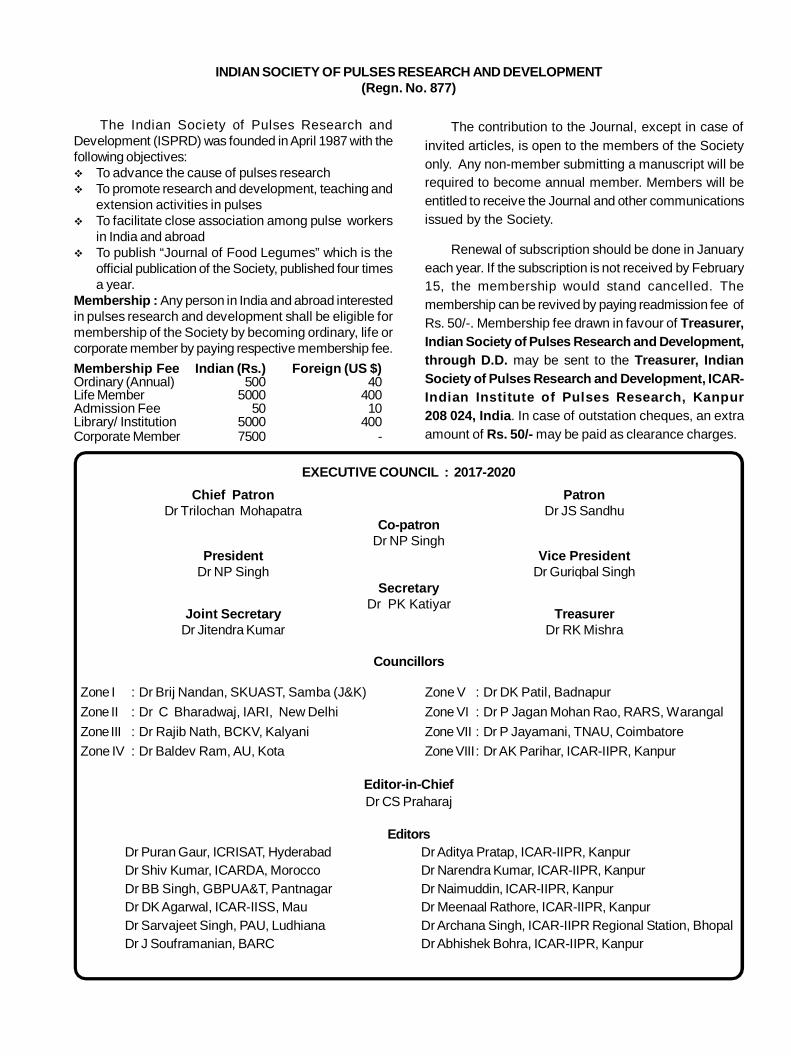
EXECUTIVE COUNCIL : 2017-2020
Zone I : Dr Brij Nandan, SKUAST, Samba (J&K)Zone II : Dr C Bharadwaj, IARI, New DelhiZone III : Dr Rajib Nath, BCKV, KalyaniZone IV : Dr Baldev Ram, AU, Kota
Councillors
Dr Puran Gaur, ICRISAT, HyderabadDr Shiv Kumar, ICARDA, MoroccoDr BB Singh, GBPUA&T, PantnagarDr DK Agarwal, ICAR-IISS, MauDr Sarvajeet Singh, PAU, LudhianaDr J Souframanian, BARC
Chief PatronDr Trilochan Mohapatra
PatronDr JS Sandhu
Co-patronDr NP Singh
Zone V : Dr DK Patil, BadnapurZone VI : Dr P Jagan Mohan Rao, RARS, WarangalZone VII : Dr P Jayamani, TNAU, CoimbatoreZone VIII: Dr AK Parihar, ICAR-IIPR, Kanpur
PresidentDr NP Singh
SecretaryDr PK Katiyar
Joint SecretaryDr Jitendra Kumar
TreasurerDr RK Mishra
Vice PresidentDr Guriqbal Singh
Editors
Editor-in-ChiefDr CS Praharaj
The Indian Society of Pulses Research andDevelopment (ISPRD) was founded in April 1987 with thefollowing objectives: To advance the cause of pulses research To promote research and development, teaching and
extension activities in pulses To facilitate close association among pulse workers
in India and abroad To publish “Journal of Food Legumes” which is the
official publication of the Society, published four timesa year.
Membership : Any person in India and abroad interestedin pulses research and development shall be eligible formembership of the Society by becoming ordinary, life orcorporate member by paying respective membership fee.Membership Fee Indian (Rs.) Foreign (US $)Ordinary (Annual) 500 40Life Member 5000 400Admission Fee 50 10Library/ Institution 5000 400Corporate Member 7500 -
INDIAN SOCIETY OF PULSES RESEARCH AND DEVELOPMENT(Regn. No. 877)
The contribution to the Journal, except in case ofinvited articles, is open to the members of the Societyonly. Any non-member submitting a manuscript will berequired to become annual member. Members will beentitled to receive the Journal and other communicationsissued by the Society.
Renewal of subscription should be done in Januaryeach year. If the subscription is not received by February15, the membership would stand cancelled. Themembership can be revived by paying readmission fee ofRs. 50/-. Membership fee drawn in favour of Treasurer,Indian Society of Pulses Research and Development,through D.D. may be sent to the Treasurer, IndianSociety of Pulses Research and Development, ICAR-Indian Institute of Pulses Research, Kanpur208 024, India. In case of outstation cheques, an extraamount of Rs. 50/- may be paid as clearance charges.
Dr Aditya Pratap, ICAR-IIPR, KanpurDr Narendra Kumar, ICAR-IIPR, KanpurDr Naimuddin, ICAR-IIPR, KanpurDr Meenaal Rathore, ICAR-IIPR, KanpurDr Archana Singh, ICAR-IIPR Regional Station, BhopalDr Abhishek Bohra, ICAR-IIPR, Kanpur

Journal of Food Legumes(Formerly Indian Journal of Pulses Research)
Vol. 30 (2) April-June 2017
CONTENTSRESEARCH PAPERS
1. SSR polymorphism and distinctiveness, uniformity and stability (DUS) features in selected genotypes of blackgram(Vigna mungo L. Hepper) 1
V Bindu Prathyusha, Y Koteswara Rao, GMV Prasada Rao, L Prasanthi, Y Hari1, G Mallikarjuna and JS Bentur
2. Heterosis in relation to molecular diversity in pigeonpea [Cajanus cajan (L.) Millsp.] 9
Bharathi Mudaraddi and KB Saxena
3. Genetic diversity for seed yield traits and micronutrient content in recombinant inbred lines of mungbean [Vigna radiata(L.) Wilczek] 14
Kritika, Rajesh Yadav and Ravika
4. Evaluation of pigeonpea [Cajanus cajan (L.) Millsp] germplasm for phosphorus use efficiency based on rootarchitecture 21
Sukhpreet Kaur Sidhu, Jagmeet Kaur and Inderjit Singh
5. Genetic variability and association analysis for yield, physiological and quality traits in drought tolerant groundnutgenotypes 27
A Lokeshwar Reddy, T Srinivas, A Prasanna Rajesh and P Umamaheswari
6. Assessment of induced genetic variability in blackgram [Vigna mungo (L.) Hepper] 31
RK Gill, Ashok Kumar, Inderjit Singh and Vikrant Tyagi
7. Effect of fertilizer use with different seed sizes on nodulation, yield and yield components of chickpea (Cicer arietinumL.) 35
Irfan Erdemct, Medeni Yasar and Murut Koc
8. Nitrogen sources manipulation for higher productivity, profitability and its use efficiency in rajmash (Phaseolus vulgarisL.) in cold desert region of North-Western Himalaya 40
J Singh
9. Principal component analysis for quantitative traits and powdery mildew resistance in pea (Pisum sativum L.) 43
Chinmayee Mohapatra, Ramesh Chand, Anil Kumar Singh and GP Dixit
10. Role of biophysical factors imparting resistance in inter-specific chickpea genotypes against Helicoverpa armigera(Hübner) 48
Uma Devi Ngangom and Ravinder Singh
11. Biorational management of aphid [Acyrthosiphon pisum (harris)] and leaf miner [Chromatomyia horticola (goureau)]infesting pea 55
PS Singh and SK Singh
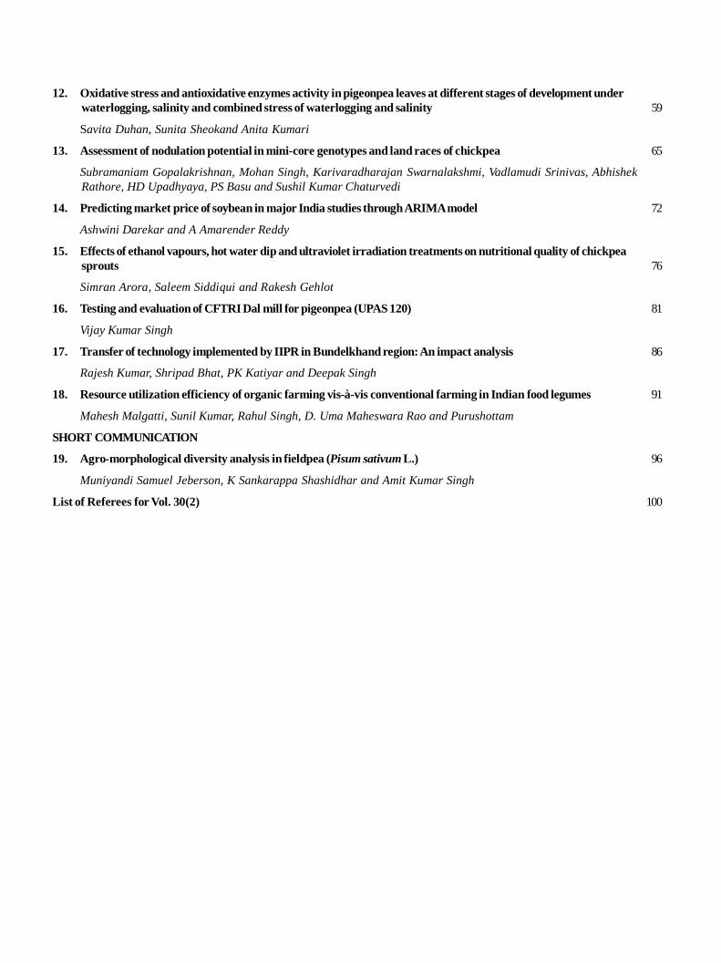
12. Oxidative stress and antioxidative enzymes activity in pigeonpea leaves at different stages of development underwaterlogging, salinity and combined stress of waterlogging and salinity 59
Savita Duhan, Sunita Sheokand Anita Kumari
13. Assessment of nodulation potential in mini-core genotypes and land races of chickpea 65
Subramaniam Gopalakrishnan, Mohan Singh, Karivaradharajan Swarnalakshmi, Vadlamudi Srinivas, AbhishekRathore, HD Upadhyaya, PS Basu and Sushil Kumar Chaturvedi
14. Predicting market price of soybean in major India studies through ARIMA model 72
Ashwini Darekar and A Amarender Reddy
15. Effects of ethanol vapours, hot water dip and ultraviolet irradiation treatments on nutritional quality of chickpeasprouts 76
Simran Arora, Saleem Siddiqui and Rakesh Gehlot
16. Testing and evaluation of CFTRI Dal mill for pigeonpea (UPAS 120) 81
Vijay Kumar Singh
17. Transfer of technology implemented by IIPR in Bundelkhand region: An impact analysis 86
Rajesh Kumar, Shripad Bhat, PK Katiyar and Deepak Singh
18. Resource utilization efficiency of organic farming vis-à-vis conventional farming in Indian food legumes 91
Mahesh Malgatti, Sunil Kumar, Rahul Singh, D. Uma Maheswara Rao and Purushottam
SHORT COMMUNICATION
19. Agro-morphological diversity analysis in fieldpea (Pisum sativum L.) 96
Muniyandi Samuel Jeberson, K Sankarappa Shashidhar and Amit Kumar Singh
List of Referees for Vol. 30(2) 100
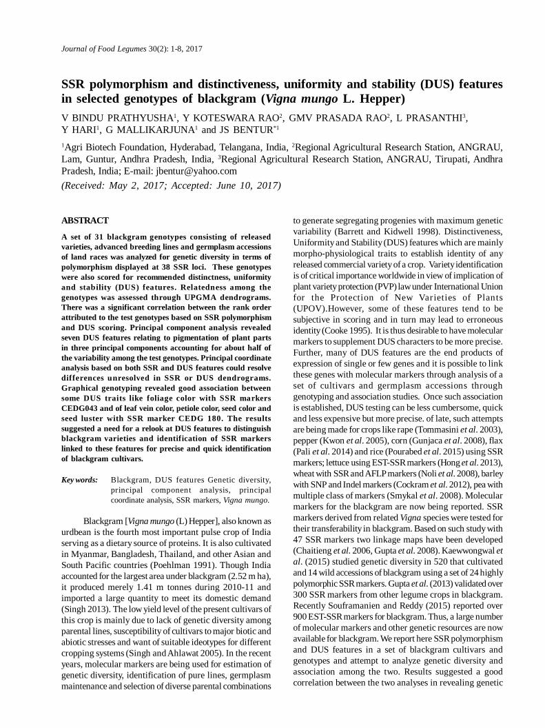
Journal of Food Legumes 30(2): 1-8, 2017
SSR polymorphism and distinctiveness, uniformity and stability (DUS) featuresin selected genotypes of blackgram (Vigna mungo L. Hepper)V BINDU PRATHYUSHA1, Y KOTESWARA RAO2, GMV PRASADA RAO2, L PRASANTHI3,Y HARI1, G MALLIKARJUNA1 and JS BENTUR*1
1Agri Biotech Foundation, Hyderabad, Telangana, India, 2Regional Agricultural Research Station, ANGRAU,Lam, Guntur, Andhra Pradesh, India, 3Regional Agricultural Research Station, ANGRAU, Tirupati, AndhraPradesh, India; E-mail: [email protected](Received: May 2, 2017; Accepted: June 10, 2017)
ABSTRACT
A set of 31 blackgram genotypes consisting of releasedvarieties, advanced breeding lines and germplasm accessionsof land races was analyzed for genetic diversity in terms ofpolymorphism displayed at 38 SSR loci. These genotypeswere also scored for recommended distinctness, uniformityand stability (DUS) features. Relatedness among thegenotypes was assessed through UPGMA dendrograms.There was a significant correlation between the rank orderattributed to the test genotypes based on SSR polymorphismand DUS scoring. Principal component analysis revealedseven DUS features relating to pigmentation of plant partsin three principal components accounting for about half ofthe variability among the test genotypes. Principal coordinateanalysis based on both SSR and DUS features could resolvedifferences unresolved in SSR or DUS dendrograms.Graphical genotyping revealed good association betweensome DUS traits like foliage color with SSR markersCEDG043 and of leaf vein color, petiole color, seed color andseed luster with SSR marker CEDG 180. The resultssuggested a need for a relook at DUS features to distinguishblackgram varieties and identification of SSR markerslinked to these features for precise and quick identificationof blackgram cultivars.
Key words: Blackgram, DUS features Genetic diversity,principal component analysis, principalcoordinate analysis, SSR markers, Vigna mungo.
Blackgram [Vigna mungo (L) Hepper], also known asurdbean is the fourth most important pulse crop of Indiaserving as a dietary source of proteins. It is also cultivatedin Myanmar, Bangladesh, Thailand, and other Asian andSouth Pacific countries (Poehlman 1991). Though Indiaaccounted for the largest area under blackgram (2.52 m ha),it produced merely 1.41 m tonnes during 2010-11 andimported a large quantity to meet its domestic demand(Singh 2013). The low yield level of the present cultivars ofthis crop is mainly due to lack of genetic diversity amongparental lines, susceptibility of cultivars to major biotic andabiotic stresses and want of suitable ideotypes for differentcropping systems (Singh and Ahlawat 2005). In the recentyears, molecular markers are being used for estimation ofgenetic diversity, identification of pure lines, germplasmmaintenance and selection of diverse parental combinations
to generate segregating progenies with maximum geneticvariability (Barrett and Kidwell 1998). Distinctiveness,Uniformity and Stability (DUS) features which are mainlymorpho-physiological traits to establish identity of anyreleased commercial variety of a crop. Variety identificationis of critical importance worldwide in view of implication ofplant variety protection (PVP) law under International Unionfor the Protection of New Varieties of Plants(UPOV).However, some of these features tend to besubjective in scoring and in turn may lead to erroneousidentity (Cooke 1995). It is thus desirable to have molecularmarkers to supplement DUS characters to be more precise.Further, many of DUS features are the end products ofexpression of single or few genes and it is possible to linkthese genes with molecular markers through analysis of aset of cultivars and germplasm accessions throughgenotyping and association studies. Once such associationis established, DUS testing can be less cumbersome, quickand less expensive but more precise. of late, such attemptsare being made for crops like rape (Tommasini et al. 2003),pepper (Kwon et al. 2005), corn (Gunjaca et al. 2008), flax(Pali et al. 2014) and rice (Pourabed et al. 2015) using SSRmarkers; lettuce using EST-SSR markers (Hong et al. 2013),wheat with SSR and AFLP markers (Noli et al. 2008), barleywith SNP and Indel markers (Cockram et al. 2012), pea withmultiple class of markers (Smykal et al. 2008). Molecularmarkers for the blackgram are now being reported. SSRmarkers derived from related Vigna species were tested fortheir transferability in blackgram. Based on such study with47 SSR markers two linkage maps have been developed(Chaitieng et al. 2006, Gupta et al. 2008). Kaewwongwal etal. (2015) studied genetic diversity in 520 that cultivatedand 14 wild accessions of blackgram using a set of 24 highlypolymorphic SSR markers. Gupta et al. (2013) validated over300 SSR markers from other legume crops in blackgram.Recently Souframanien and Reddy (2015) reported over900 EST-SSR markers for blackgram. Thus, a large numberof molecular markers and other genetic resources are nowavailable for blackgram. We report here SSR polymorphismand DUS features in a set of blackgram cultivars andgenotypes and attempt to analyze genetic diversity andassociation among the two. Results suggested a goodcorrelation between the two analyses in revealing genetic
2 Journal of Food Legumes 30(2), 2017
diversity and some markers appeared to be linked to DUSfeatures like foliage color, leaf vein color, petiole color, seedcolor and seed luster.
MATERIALS AND METHODS
Plant Material: Thirty one blackgram genotypes wereobtained from ICAR-Indian Institute of Pulse Research(IIPR), Kanpur; Regional Agricultural Research Station(RARS), Tirupati (TPT) and RARS, Lam farm Guntur (LAM).This set (Table 1) consisted of 11 released varieties, tenadvanced breeding lines and ten germplasm accessions ofland races. Three entries were represented by two sourcesof seeds each. Five pairs of sister lines derived from thesame cross with distinct trait differences were also includedin this set. Seeds were sown and plants raised atAgribiotech Foundation during kharif (wet season) 2014and 2015 to record DUS characteristics and collected leafsamples for isolation of DNA. Results were reconfirmedduring kharif2016.DNA extraction: Genomic DNA was extracted from leavesof 20 day old plants using C-TAB protocol described bySaghai–Maroof et al. (1984) with slight modifications. Thequality and quantity of DNA were checked through 1%
agarose gel electrophoresis and Nanodrop ®spectrophotometer (GE Healthcare Life sciences, USA). Theworking DNA was diluted to a standard concentration of50-100ng/µl.SSR marker amplification: In all 90 SSR markers reportedearlier (Chaitieng et al. 2006; Gupta et al. 2013) were initiallyused in the present study. Based on polymorphism dataand polymorphism information content (PIC) value, 38markers (Table 2) were considered for analysis. PCRamplification was carried out in 10 µl reaction mixturecontaining50-100 ng genomic DNA, 5 pmol of each forwardand reverse primer, 10x PCR buffer (Jonaki, India), 1U ofTaq DNA polymerase (Jonaki, India), 2mM dNTP mix(Thermo Scientific, USA)with 2.5mM MgCl2 (Jonaki, India).The PCR profile was programmed for an initial denaturationof 94OC for 4 min followed by 35 cycles of 94OC for 1 min,annealing for 1min at 55-60OC, extension for 2 min at 72OCand final extension at 72OC for 7 min. The amplified productswere resolved on 4.5% agarose gel and photographed usingGel Documentation System. A 100bp ladder was used forapproximate sizing of the bands. Polymorphic markers weredistinguished on the basis of differences in allele size orpresence or absence of marker allele visible on the gel.
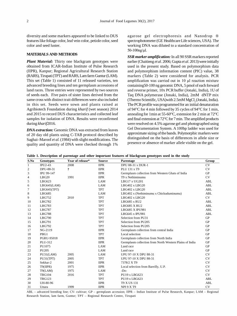
Table 1. Description of parentage and other important features of blackgram genotypes used in the study
ABL – advanced breeding line; CV- cultivar; GP – germplasm accession; IIPR – Indian Institute of Pulse Research, Kanpur; LAM – RegionalResearch Station, lam farm, Guntur; TPT – Regional Research Centre, Tirupati
S.No Genotypes Year of release* Source Parentage Group 1 IPU2-43 2008 IIPR DPU 88-31 x DUR-1 CV 2 DPU-88-31 ? IIPR PLU 131 x T9 CV 3 IPU 99-147 IIPR Germplasm collection from Western Ghats of India GP 4 LBG20 1991 IIPR T9 x Nethiminumu CV 5 LBG623 LAM LBG17 x UG201 ABL 6 LBG645(LAM) LAM LBG402 x LBG20 ABL 7 LBG645(TPT) TPT LBG402 x LBG20 ABL 8 LBG685 LAM LBG402 x (Nethiminumu x Chickuduminumu) ABL 9 LBG752 2010 TPT LBG402 x LBG20 CV 10 LBG782 TPT LBG685 x RU2 ABL 11 LBG783 TPT LBG685 X RU2 ABL 12 LBG787 TPT LBG685 X IPU981 ABL 13 LBG788 TPT LBG645 x IPU981 ABL 14 LBG790 TPT Selection from PU31 GP 15 LBG791 TPT Selection from PU205 GP 16 LBG792 TPT Selection from PU205 GP 17 NG-2119 IIPR Germplasm collection from central India GP 18 PBG1 TPT Local selection GP 19 PGRU-95018 IIPR Germplasm collection from North India GP 20 PLU-312 IIPR Germplasm collection from North Western Plains of India GP 21 PU1075 LAM Land race GP 22 PU205 LAM Land race GP 23 PU31(LAM) 2005 LAM UPU 97-10 X DPU 88-31 CV 24 PU31(TPT) 2005 TPT UPU 97-10 X DPU 88-31 CV 25 Sekhar-2 2001 IIPR 7378/2 X T9 CV 26 T9(IIPR) 1975 IIPR Local selection from Bareilly, U.P. CV 27 T9(LAM) 1975 LAM -Do- CV 28 TBG104 2016 TPT PU19 x LBG623 CV 29 TBG123 TPT PU19 x LBG623 ABL 30 UH-80-96 IIPR T9 X US 131 ABL 31 Uttara 1999 IIPR NPI 9 X T9 CV
Prathyusha et al. : SSR polymorphism in blackgram 3
DUS characterization: Thirty one test genotypes ofblackgram were planted in two rows composed of 20individuals per genotype. A total of 21 DUS features wasnoted and scored as per the guidelines of Protection ofPlant Varieties and Farmers’ Rights Authority (PPVFR), Indiamanual (Anonymous 2007). Each trait was scored basedon the alternative forms (alleles) as per the list (Table 3).Three randomly selected plants from each genotype werescored for consistency. Four of the features with novariability among the test genotypes were not consideredfor further analysis.Data collection and Analysis: SSR marker polymorphismamong the test genotype was scored based on the ampliconsize relative to the ladder fragments, sequentially from thesmallest to the largest-sized bands. Only clear andunambiguous bands were scored. Alleles were designatedin ascending order of their sizes.PIC was calculated(Anderson et al. 1993) for all the 38 SSR markers. Genetic
diversity among the test genotypes as revealed by SSRmarker polymorphism was assessed through a dendrogramgenerated based on Jaccard’s similarity coefficient (withunweighted pair group method and arithmetic mean -UPGMA using the NTSYS-pc version 2.02, (Rohlf 1998).
Test genotypes were similarly analysed for diversitybased on DUS characters using scores for the alternativeoptions. A dendrogram was generated based on Jaccard’ssimilarity as mentioned above. Test genotypes were rankedbased on distance from closest to farthest based on SSRpolymorphism and DUS polymorphism. These two rankorders were plotted one against the other to computecorrelation coefficient. Principal Component Analysis ofDUS features polymorphism and Principal CoordinateAnalysis of combined SSR and DUS data were done usingXL-STAT add-on on MS Excel. Association of SSR markerswith DUS characters was done through graphicalgenotyping.
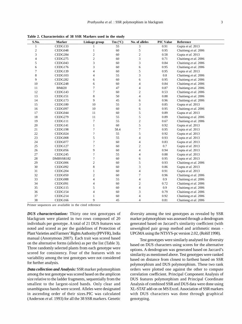
Table 2. Characteristics of 38 SSR Markers used in the study
Primer sequences are available in the cited reference
S.No. Marker Linkage group Tm (°C) No. of alleles PIC Value Reference 1 CEDG133 1 55 3 0.91 Gupta et al. 2013 2 CEDG048 1 60 5 0.95 Chaitieng et al. 2006 3 CEDG284 2 60 2 0.58 Gupta et al. 2013 4 CEDG275 2 60 3 0.71 Chaitieng et al. 2006 5 CEDG043 3 60 3 0.84 Chaitieng et al. 2006 6 CEDG176 3 60 6 0.95 Chaitieng et al. 2006 7 CEDG139 4 60 5 0.95 Gupta et al. 2013 8 CEDG103 4 55 3 0.8 Chaitieng et al. 2006 9 CEDG282 6 60 6 0.95 Chaitieng et al. 2006 10 CEDG248 6 60 4 0.84 Chaitieng et al. 2006 11 BMd20 7 47 4 0.87 Chaitieng et al. 2006 12 CEDG143 7 60 2 0.53 Chaitieng et al. 2006 13 CEDG151 8 50 4 0.88 Chaitieng et al. 2006 14 CEDG173 9 45 6 0.96 Chaitieng et al. 2006 15 CEDG180 10 55 3 0.85 Gupta et al. 2013 16 CEDG097 10 60 6 0.95 Chaitieng et al. 2006 17 CEDG044 11 60 5 0.89 Gupta et al. 2013 18 CEDG279 11 55 5 0.89 Chaitieng et al. 2006 19 CEDG111 7 55 2 0.67 Chaitieng et al. 2006 20 CEDG141 1 60 5 0.92 Gupta et al. 2013 21 CEDG198 ? 58.4 7 0.95 Gupta et al. 2013 22 CEDG024 ? 55 5 0.92 Gupta et al. 2013 23 CEDG008 5 55 4 0.93 Gupta et al. 2013 24 CEDG077 ? 60 4 0.83 Gupta et al. 2013 25 CEDG127 ? 60 2 0.7 Gupta et al. 2013 26 CEDG056 9 60 4 0.94 Gupta et al. 2013 27 CEDG245 ? 55 4 0.88 Gupta et al. 2013 28 DMBSSR182 ? 60 6 0.95 Gupta et al. 2013 29 CEDG006 2 60 5 0.93 Chaitieng et al. 2006 30 CEDG092 8 60 3 0.86 Gupta et al. 2013 31 CEDG204 1 60 4 0.91 Gupta et al. 2013 32 CEDG050 2 60 7 0.96 Chaitieng et al. 2006 33 CEDG088 4 55 4 0.9 Chaitieng et al. 2006 34 CEDG091 4 60 2 0.72 Chaitieng et al. 2006 35 CEDG115 5 60 4 0.9 Chaitieng et al. 2006 36 CEDG154 4 60 3 0.79 Chaitieng et al. 2006 37 CEDG214 1 60 4 0.92 Chaitieng et al. 2006 38 CEDG166 9 45 4 0.81 Chaitieng et al. 2006
4 Journal of Food Legumes 30(2), 2017
RESULTS
Genetic relationships based on SSR polymorphism: Theset of 38 polymorphic SSR markers used in the studyrepresented all the 11 linkage groups. These markersgenerated 158 alleles. Number of alleles per marker rangedfrom 1 to 7 with an average of 4.15 alleles per primer. PIC forthese markers ranged from 0.53 to 0.96 (Table 2). Usingpolymorphism data of 38 SSR markers, the geneticrelationship among the blackgram genotypes was estimated(Fig. 1). Highest similarity coefficient (0.79) was observedbetween a released variety (IPU2-43) and a land race (NG-2119). No distinct groups among test lines were discernible.Three of the test lines with two separate seed sourcesdisplayed genetic similarity ranging from 0.44 (LBG645),0.45 (PU31) to 0.47 (T9). Five pairs of sister-lines derived
from the same cross revealed similarity ranging from 0.32(LBG782/LBG783) to 0.7 (TBG104/TBG123) (Table 4).Similarity relationships based on DUS featurepolymorphism: Test genotypes were scored for all the 21DUS features which revealed polymorphism among the testgenotypes. The number of alleles (alternative phenotypictrait forms) ranged from1 to 4 which generated a total of 55alleles with an average of 2.62 alleles per trait. Four of thefeatures showing no polymorphism among the testgenotypes were not considered for further analysis. Usingthis data, the similarity relationship between the blackgramgenotypes was estimated and the dendrogram wasgenerated (Fig. 1). Thirty one genotypes could be groupedinto two clusters: one with 13 genotypes sharing>0.74similarity coefficients (sc) while the other with 18 more
Table 3. Morpho-physiological traits of blackgram genotypes evaluated for distinctiveness, uniformity and stability (DUS)features†
†Anonymous, 2007 * - No polymorphism seen among the test genotypes
DUS# DUS Characters State (score/allele) Number of alleles D1 Hypocotyl: anthocyanin production Absent (1) Present (2) 2 D2 Time of flowering Early (<40 days) (1), Medium (40-50 days)(2), Late(>50 days) (3) 3 D3 Plant: growth habit Erect (1),Semi-erect (2),Spreading (3) 3
D4* Plant: habit Determinate (1),Indeterminate (2) 2 D5 Stem color Green (1),Green with purple splashes (2), Purple with green
splashes (3), Purple (4) 4
D6* Stem pubescence Absent (1) Present (2) 2 D7 Leaflet(terminal): shape Deltoid (1),Ovate (2),Lanceolate (3),Cuneate (4) 4 D8 Foliage color Green (1),Dark green (2), Light green (3) 3 D9 Leaf vein color Green (1), Purple (2) 2
D10 Leaf pubescence* Absent (1) Present (2) 2 D11 Petiole color Green (1),Green with purple splashes (2), Purple (3), Purple with
Green splashes(4) 4
D12 Pod: intensity of green color in premature pods
green (1), yellowish green (2), dark green (3) 3
D13 Pod pubescence Absent (1) Present (2) 2 D14 Peduncle length Short(<5cms) (1), Medium (5-10cms) (2), long (>10cms) (3) 3 D15 Pod length Small(<5cms) (1), Medium (5-7cms) (2), long (>7cms) (3) 2 D16 Pod: color of matured pod* Buff(off white) (1), Brown (2), Black (3) 3 D17 Plant height Short(<45cms) (1), Medium (45-60cms) (2), long (>60cms) (3) 2 D18 Seed color Green (1), greenish brown (2), Brown (3), Black (4), Mottled (5) 5 D19 Seed luster Shiny (1) , Dull (2) 2 D20 Seed shape Globose (1), Oval (2), Drum shaped (3) 3 D21 Seed size(weight of 100 seeds) Small(<3gms) (1), Medium (3-5gms) (2), large (>5gms) (3) 3
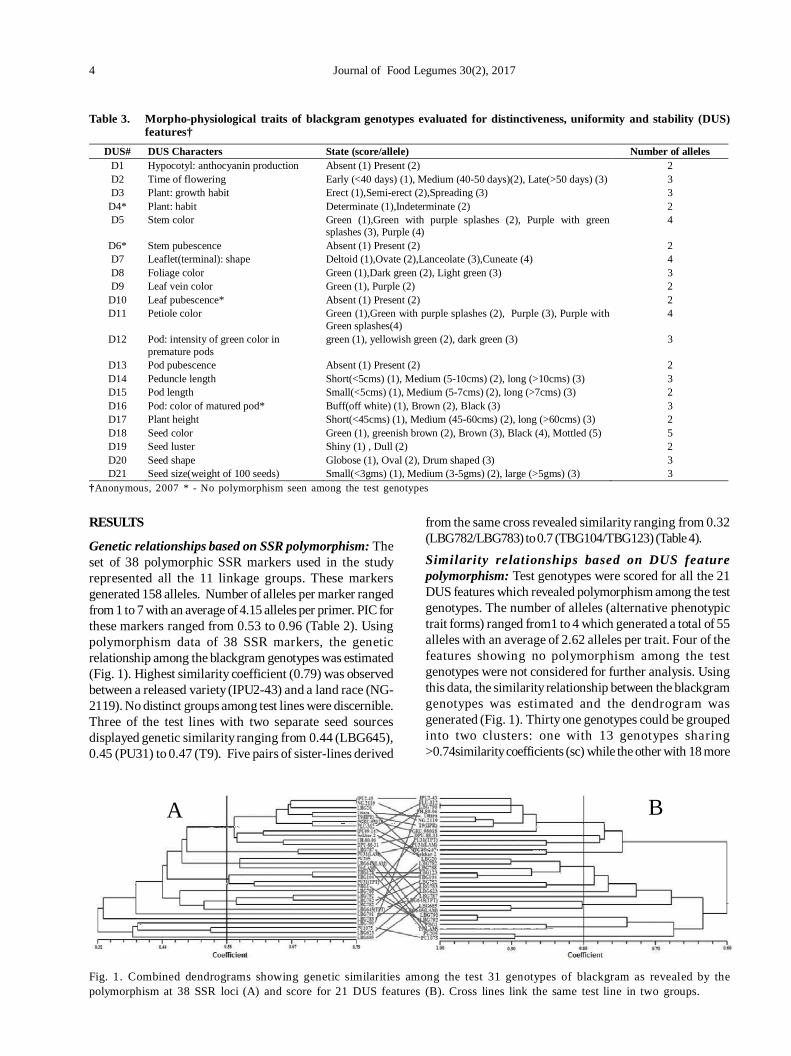
Fig. 1. Combined dendrograms showing genetic similarities among the test 31 genotypes of blackgram as revealed by thepolymorphism at 38 SSR loci (A) and score for 21 DUS features (B). Cross lines link the same test line in two groups.
A B
Prathyusha et al. : SSR polymorphism in blackgram 5
divergent genotypes with a sc>0.53.Within the first clustertwo entries viz., PLU-312 and LBG790 showed no diversity.Among the three test lines with two different seed sources,similarity coefficient ranged from 0.5 (T9), 0.8 (LBG645) to0.85 (PU31). Five pairs of sister-lines derived from the samecross revealed similarity ranging from 0.78 (LBG782/LBG783)to 0.95 (TBG104/TBG123, LBG791/LBG792) (Table 4).
Principal component analysis of DUS polymorphismrevealed that the first three components accounted forcumulative variance of 48.5% among the genotypes.Loadings of scored DUS features on three components(Table 5) revealed four DUS features under factor one, threeunder factor two and two features under factor three bearingsignificant influence on diversity of the test genotypes.Correlation coefficients among these nine DUS features(Table 6) revealed significant positive correlation amongthe features within each of the three principal components.Most of these features related to pigmentation like purplepetiole, leaf vein or leaf colour like light green of dark green.
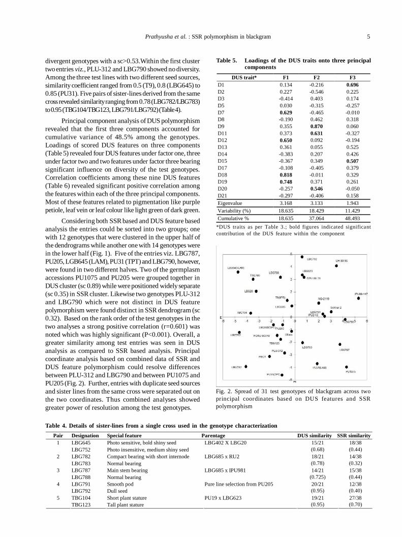
Considering both SSR based and DUS feature basedanalysis the entries could be sorted into two groups; onewith 12 genotypes that were clustered in the upper half ofthe dendrograms while another one with 14 genotypes werein the lower half (Fig. 1). Five of the entries viz. LBG787,PU205, LGB645 (LAM), PU31 (TPT) and LBG790, however,were found in two different halves. Two of the germplasmaccessions PU1075 and PU205 were grouped together inDUS cluster (sc 0.89) while were positioned widely separate(sc 0.35) in SSR cluster. Likewise two genotypes PLU-312and LBG790 which were not distinct in DUS featurepolymorphism were found distinct in SSR dendrogram (sc0.32). Based on the rank order of the test genotypes in thetwo analyses a strong positive correlation (r=0.601) wasnoted which was highly significant (P<0.001). Overall, agreater similarity among test entries was seen in DUSanalysis as compared to SSR based analysis. Principalcoordinate analysis based on combined data of SSR andDUS feature polymorphism could resolve differencesbetween PLU-312 and LBG790 and between PU1075 andPU205 (Fig. 2). Further, entries with duplicate seed sourcesand sister lines from the same cross were separated out onthe two coordinates. Thus combined analyses showedgreater power of resolution among the test genotypes.
Table 4. Details of sister-lines from a single cross used in the genotype characterizationPair Designation Special feature Parentage DUS similarity SSR similarity
LBG645 Photo sensitive, bold shiny seed 1 LBG752 Photo insensitive, medium shiny seed
LBG402 X LBG20 15/21 (0.68)
18/38 (0.44)
LBG782 Compact bearing with short internode 2 LBG783 Normal bearing
LBG685 x RU2 18/21 (0.78)
14/38 (0.32)
LBG787 Main stem bearing 3 LBG788 Normal bearing
LBG685 x IPU981 14/21 (0.725)
15/38 (0.44)
LBG791 Smooth pod 4 LBG792 Dull seed
Pure line selection from PU205 20/21 (0.95)
12/38 (0.40)
TBG104 Short plant stature 5 TBG123 Tall plant stature
PU19 x LBG623 19/21 (0.95)
27/38 (0.70)
Table 5. Loadings of the DUS traits onto three principalcomponents
*DUS traits as per Table 3.; bold figures indicated significantcontribution of the DUS feature within the component
DUS trait* F1 F2 F3 D1 0.134 -0.216 0.696 D2 0.227 -0.546 0.225 D3 -0.414 0.403 0.174 D5 0.030 -0.315 -0.257 D7 0.629 -0.465 -0.010 D8 -0.190 0.462 0.318 D9 0.355 0.870 0.060 D11 0.373 0.631 -0.327 D12 0.650 0.092 -0.194 D13 0.361 0.055 0.525 D14 -0.383 0.207 0.426 D15 -0.367 0.349 0.507 D17 -0.108 -0.405 0.379 D18 0.818 -0.011 0.329 D19 0.748 0.371 0.261 D20 -0.257 0.546 -0.050 D21 -0.297 -0.406 0.158 Eigenvalue 3.168 3.133 1.943 Variability (%) 18.635 18.429 11.429 Cumulative % 18.635 37.064 48.493
Fig. 2. Spread of 31 test genotypes of blackgram across twoprincipal coordinates based on DUS features and SSRpolymorphism
6 Journal of Food Legumes 30(2), 2017
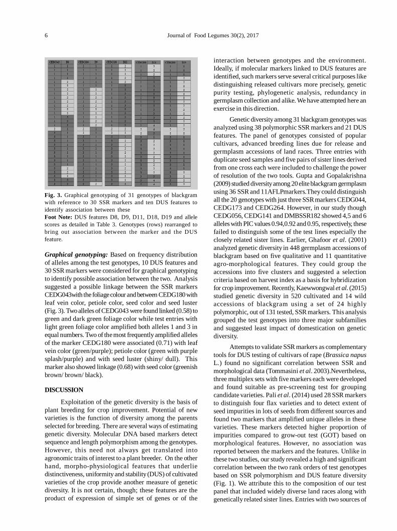
Graphical genotyping: Based on frequency distributionof alleles among the test genotypes, 10 DUS features and30 SSR markers were considered for graphical genotypingto identify possible association between the two. Analysissuggested a possible linkage between the SSR markersCEDG043with the foliage colour and between CEDG180 withleaf vein color, petiole color, seed color and seed luster(Fig. 3). Two alleles of CEDG043 were found linked (0.58) togreen and dark green foliage color while test entries withlight green foliage color amplified both alleles 1 and 3 inequal numbers. Two of the most frequently amplified allelesof the marker CEDG180 were associated (0.71) with leafvein color (green/purple); petiole color (green with purplesplash/purple) and with seed luster (shiny/ dull). Thismarker also showed linkage (0.68) with seed color (greenishbrown/ brown/ black).
DISCUSSION
Exploitation of the genetic diversity is the basis ofplant breeding for crop improvement. Potential of newvarieties is the function of diversity among the parentsselected for breeding. There are several ways of estimatinggenetic diversity. Molecular DNA based markers detectsequence and length polymorphism among the genotypes.However, this need not always get translated intoagronomic traits of interest to a plant breeder. On the otherhand, morpho-physiological features that underliedistinctiveness, uniformity and stability (DUS) of cultivatedvarieties of the crop provide another measure of geneticdiversity. It is not certain, though; these features are theproduct of expression of simple set of genes or of the
interaction between genotypes and the environment.Ideally, if molecular markers linked to DUS features areidentified, such markers serve several critical purposes likedistinguishing released cultivars more precisely, geneticpurity testing, phylogenetic analysis, redundancy ingermplasm collection and alike. We have attempted here anexercise in this direction.
Genetic diversity among 31 blackgram genotypes wasanalyzed using 38 polymorphic SSR markers and 21 DUSfeatures. The panel of genotypes consisted of popularcultivars, advanced breeding lines due for release andgermplasm accessions of land races. Three entries withduplicate seed samples and five pairs of sister lines derivedfrom one cross each were included to challenge the powerof resolution of the two tools. Gupta and Gopalakrishna(2009) studied diversity among 20 elite blackgram germplasmusing 36 SSR and 11AFLPmarkers.They could distinguishall the 20 genotypes with just three SSR markers CEDG044,CEDG173 and CEDG264. However, in our study thoughCEDG056, CEDG141 and DMBSSR182 showed 4,5 and 6alleles with PIC values 0.94,0.92 and 0.95, respectively, thesefailed to distinguish some of the test lines especially theclosely related sister lines. Earlier, Ghafoor et al. (2001)analyzed genetic diversity in 448 germplasm accessions ofblackgram based on five qualitative and 11 quantitativeagro-morphological features. They could group theaccessions into five clusters and suggested a selectioncriteria based on harvest index as a basis for hybridizationfor crop improvement. Recently, Kaewwongwal et al. (2015)studied genetic diversity in 520 cultivated and 14 wildaccessions of blackgram using a set of 24 highlypolymorphic, out of 131 tested, SSR markers. This analysisgrouped the test genotypes into three major subfamiliesand suggested least impact of domestication on geneticdiversity.
Attempts to validate SSR markers as complementarytools for DUS testing of cultivars of rape (Brassica napusL.) found no significant correlation between SSR andmorphological data (Tommasini et al. 2003).Nevertheless,three multiplex sets with five markers each were developedand found suitable as pre-screening test for groupingcandidate varieties. Pali et al. (2014) used 28 SSR markersto distinguish four flax varieties and to detect extent ofseed impurities in lots of seeds from different sources andfound two markers that amplified unique alleles in thesevarieties. These markers detected higher proportion ofimpurities compared to grow-out test (GOT) based onmorphological features. However, no association wasreported between the markers and the features. Unlike inthese two studies, our study revealed a high and significantcorrelation between the two rank orders of test genotypesbased on SSR polymorphism and DUS feature diversity(Fig. 1). We attribute this to the composition of our testpanel that included widely diverse land races along withgenetically related sister lines. Entries with two sources of
Fig. 3. Graphical genotyping of 31 genotypes of blackgramwith reference to 30 SSR markers and ten DUS features toidentify association between theseFoot Note: DUS features D8, D9, D11, D18, D19 and allelescores as detailed in Table 3. Genotypes (rows) rearranged tobring out association between the marker and the DUSfeature.
Prathyusha et al. : SSR polymorphism in blackgram 7
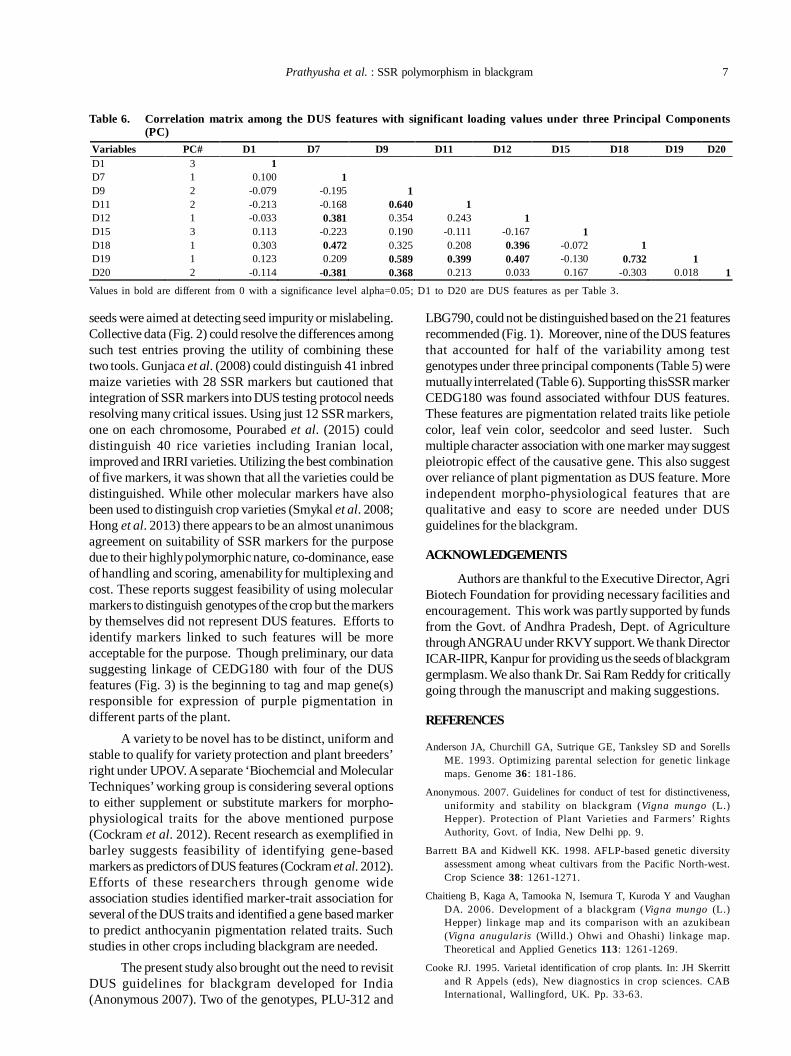
Table 6. Correlation matrix among the DUS features with significant loading values under three Principal Components(PC)
Values in bold are different from 0 with a significance level alpha=0.05; D1 to D20 are DUS features as per Table 3.
Variables PC# D1 D7 D9 D11 D12 D15 D18 D19 D20 D1 3 1 D7 1 0.100 1 D9 2 -0.079 -0.195 1 D11 2 -0.213 -0.168 0.640 1 D12 1 -0.033 0.381 0.354 0.243 1 D15 3 0.113 -0.223 0.190 -0.111 -0.167 1 D18 1 0.303 0.472 0.325 0.208 0.396 -0.072 1 D19 1 0.123 0.209 0.589 0.399 0.407 -0.130 0.732 1 D20 2 -0.114 -0.381 0.368 0.213 0.033 0.167 -0.303 0.018 1
seeds were aimed at detecting seed impurity or mislabeling.Collective data (Fig. 2) could resolve the differences amongsuch test entries proving the utility of combining thesetwo tools. Gunjaca et al. (2008) could distinguish 41 inbredmaize varieties with 28 SSR markers but cautioned thatintegration of SSR markers into DUS testing protocol needsresolving many critical issues. Using just 12 SSR markers,one on each chromosome, Pourabed et al. (2015) coulddistinguish 40 rice varieties including Iranian local,improved and IRRI varieties. Utilizing the best combinationof five markers, it was shown that all the varieties could bedistinguished. While other molecular markers have alsobeen used to distinguish crop varieties (Smykal et al. 2008;Hong et al. 2013) there appears to be an almost unanimousagreement on suitability of SSR markers for the purposedue to their highly polymorphic nature, co-dominance, easeof handling and scoring, amenability for multiplexing andcost. These reports suggest feasibility of using molecularmarkers to distinguish genotypes of the crop but the markersby themselves did not represent DUS features. Efforts toidentify markers linked to such features will be moreacceptable for the purpose. Though preliminary, our datasuggesting linkage of CEDG180 with four of the DUSfeatures (Fig. 3) is the beginning to tag and map gene(s)responsible for expression of purple pigmentation indifferent parts of the plant.
A variety to be novel has to be distinct, uniform andstable to qualify for variety protection and plant breeders’right under UPOV. A separate ‘Biochemcial and MolecularTechniques’ working group is considering several optionsto either supplement or substitute markers for morpho-physiological traits for the above mentioned purpose(Cockram et al. 2012). Recent research as exemplified inbarley suggests feasibility of identifying gene-basedmarkers as predictors of DUS features (Cockram et al. 2012).Efforts of these researchers through genome wideassociation studies identified marker-trait association forseveral of the DUS traits and identified a gene based markerto predict anthocyanin pigmentation related traits. Suchstudies in other crops including blackgram are needed.
The present study also brought out the need to revisitDUS guidelines for blackgram developed for India(Anonymous 2007). Two of the genotypes, PLU-312 and
LBG790, could not be distinguished based on the 21 featuresrecommended (Fig. 1). Moreover, nine of the DUS featuresthat accounted for half of the variability among testgenotypes under three principal components (Table 5) weremutually interrelated (Table 6). Supporting thisSSR markerCEDG180 was found associated withfour DUS features.These features are pigmentation related traits like petiolecolor, leaf vein color, seedcolor and seed luster. Suchmultiple character association with one marker may suggestpleiotropic effect of the causative gene. This also suggestover reliance of plant pigmentation as DUS feature. Moreindependent morpho-physiological features that arequalitative and easy to score are needed under DUSguidelines for the blackgram.
ACKNOWLEDGEMENTS
Authors are thankful to the Executive Director, AgriBiotech Foundation for providing necessary facilities andencouragement. This work was partly supported by fundsfrom the Govt. of Andhra Pradesh, Dept. of Agriculturethrough ANGRAU under RKVY support. We thank DirectorICAR-IIPR, Kanpur for providing us the seeds of blackgramgermplasm. We also thank Dr. Sai Ram Reddy for criticallygoing through the manuscript and making suggestions.
REFERENCES
Anderson JA, Churchill GA, Sutrique GE, Tanksley SD and SorellsME. 1993. Optimizing parental selection for genetic linkagemaps. Genome 36: 181-186.
Anonymous. 2007. Guidelines for conduct of test for distinctiveness,uniformity and stability on blackgram (Vigna mungo (L.)Hepper). Protection of Plant Varieties and Farmers’ RightsAuthority, Govt. of India, New Delhi pp. 9.
Barrett BA and Kidwell KK. 1998. AFLP-based genetic diversityassessment among wheat cultivars from the Pacific North-west.Crop Science 38: 1261-1271.
Chaitieng B, Kaga A, Tamooka N, Isemura T, Kuroda Y and VaughanDA. 2006. Development of a blackgram (Vigna mungo (L.)Hepper) linkage map and its comparison with an azukibean(Vigna anugularis (Willd.) Ohwi and Ohashi) linkage map.Theoretical and Applied Genetics 113: 1261-1269.
Cooke RJ. 1995. Varietal identification of crop plants. In: JH Skerrittand R Appels (eds), New diagnostics in crop sciences. CABInternational, Wallingford, UK. Pp. 33-63.
8 Journal of Food Legumes 30(2), 2017
Ghafoor A, Sharif A, Ahmed Z, Zahid MA and Rabbani MA. 2001.Genetic diversity in blackgram (Vigna mungo L. Hepper). FieldCrops Research 69: 183-190.
Gunjaca J, Buhinicek I and Jukicetal M. 2008. Discriminating maizeinbred lines using molecular and DUS data. Euphytica 161: 165-172.
Gupta S, Gupta DS, Anjum TK, Pratap A and Kumar J. 2013.Inheritance and molecular tagging of MYMIV resistance genein blackgram (Vigna mungo L. Hepper). Euphytica 193: 27-37.
Gupta SK and Gopalakrishna T. 2009. Genetic diversity analysis inblackgram (Vigna mungo (L.) Hepper) using AFLP andtransferable micro satellite markers from azuki bean (Vignaangularis) (willd.) Ohwi & Ohashi.). Genome 52: 120-128.
Gupta SK, Souframanien J and Gopalakrishna T. 2008. Constructionof a genetic linkage map of blackgram based on molecular markersand comparative studies. Genome 51: 628-637.
Hong JH, Kwon YS, Choi KJ, Mishra RK and Kim DH. 2013.Identification of lettuce germplasms and commercial cultivarsusing SSR markers developed from EST. Korean Journal ofHorticultural Science and Technology 31: 772-781.
James C, Jones H, Norris C and Sullivan DM. 2012. Evaluation ofdiagnostic molecular markers for DUS phenotypic assessmentin the cereal crop, barley (Hordeum vulgare spp. vulgareL.). Theoretical and Applied Genetics 125 (8): 1735-1749.
Kaewwongwal A, Kongjaimun A, Somta P, Chankaew S, Yimram Tand Srinives P. 2015. Genetic diversity of the blackgram (Vignamungo (L.) Hepper) gene pool as revealed by SSR markers.Breeding science 65: 127-137.
Kwon YS, Lee JM, Yi GB, Yi Sl, Kim KM, Soh EH, Bae KM, ParkEK, Song IH and Kim BD. 2005. Use of SSR markers tocomplement tests of distinctiveness, uniformity, and stability(DUS) of pepper (Capsicum annuum L.) varieties. Moleculesand Cells 19 (3): 428-435.
Noli E, Teriaca MS, Sanguineti MC and Conti S. 2008. Utilization ofSSR and AFLP markers for the assessment of distinctness indurum wheat. Molecular Breeding 22: 301-303.
Pali V, Verma SK, Xalxo MS, Saxena RR, Mehta N and Verulkar SB.2014. Identification of microsatellite markers for fingerprinting
popular Indian flax (Linum usitatissimum L.) cultivars and theirutilization in seed genetic purity assessments. Australian Journalof Crop Science 8: 119-126.
Poehlman JM. 1991. History, description, classification and origin.In: Poehlman JM (ed). The Mungbean. West View, Boulder. Pp:6-21.
Pourabed E, Noushabadi MRJ, Jamali SH, Alipour NM, Zareyan Aand Sadeghi L. 2015. Identification and DUS Testing of RiceVarieties through Microsatellite Markers. International journalof plant genomics. doi: 10.1155/2015/965073.
Rohlf M. 1998. NTSYSpc. Numerical Taxonomy and MultivariateAnalysis System. Version 2.02i. Department of Ecology andEvolution. State University of New York.
Saghai-Maroof MA, Soliman KM, Jorgensen RA and Allard RW.1984. Ribosomal spacer length in barley: mendelian inheritance,chromosomal location and population dynamics. Proceedingsof National Academy of Sciences 81: 8104-8118.
Singh DP and Ahlawat IPS. 2005. Greengram (Vigna radiata) andblackgram (V.mungo) improvement in India: past, present andfuture prospects. Indian Journal of Agricultural Science 75: 243-50.
Singh RP. 2013. Status paper on pulses. Government of India Ministryof Agriculture, Department of agriculture and cooperation,Directorate of Pulses Development, Vidyanchal Bhavan, Bhopal.
Smykal P, Horacek J, Dostalova R and Hybl M. 2008. Varietydiscrimination in pea (Pisum sativum L.) by molecular,biochemical and morphological markers. Journal of AppliedGenetics 49: 155-66.
Souframanien J and Reddy KS. 2015. De novo assembly,characterization of immature seed transcriptome anddevelopment of genic–SSR markers in blackgram (Vigna mungo(L.) Hepper). PLoS ONE 10(6): 128-748.
Tommasini L, Batley J, Arnold GM, Cooke RJ, Donini P, Lee D,Law JR, Lowe C, Moule C, Trick M and Edwards KJ. 2003. Thedevelopment of multiplex simple sequence repeats (SSR) markersto complement distinctness, uniformity and stability testing ofrape (Brassica napus L.) varieties. Theoretical and AppliedGenetics 106: 1091–1101.
Journal of Food Legumes 30(2): 9-13, 2017
(Received: April 4, 2017; Accepted: June 4, 2017)
ABSTRACT
Pigeonpea is the only grain legume crop where hybrid vigourhas been exploited commercially. For sustaining thistechnology, it is imperative that information about thegenetic nature of hybrid vigour is generated and new high-yielding hybrids are bred at regular intervals. In this context,a set of genetic materials, consisting 19 hybrids, their parentsand F2 bulks was studied. Only four hybrids expressedsignificant heterosis over mid-parent; and of these, two werefound to be significantly superior to their respective betterparent also. The hybrid between ICPA 2209 and ICPL 20108was the best with respect to heterobeltiosis (55.9%**) andrelative heterosis (60.5%**). The studies also showed thatboth additive as well as non-additive genetic variation playeda key role in the manifestation of hybrid vigour. Based onthe molecular diversity of the parents, two heterotic groupswere formed in A-lines, while three heterotic groups wereformed in the R-lines. The results showed that in thismaterial high heterosis was not necessarily related to theirmolecular diversity.
Key words: Gene action, Hybrid vigour, Inbreeding depression,Molecular diversity, Pigeonpea
In self-pollinated crops, breeding of inbred cultivarsis the most popular approach to develop new cultivars,which primarily involves accumulation of useful alleles fromthe two parents in a single genotype. This approach,however, has a limitation of the availability of differentfavorable alleles and therefore, may lead to plateauing ofproductivity. To overcome this constraint, Shull (1908)proposed the concept of exploiting hybrid vigour. Thistechnology could only be applied to the crops where large-scale production of F1 hybrid seed was easy andeconomically viable; and for this reason, legumes couldnot be benefited from this genetic phenomenon due to theirhighly self-pollinated nature. In some legumes such as fababean, soybean, and pigeonpea, however, some degree ofnatural out-crossing exists and attempts were made in thepast to breed hybrids; but the success was achieved onlyin pigeonpea. In this pulse crop three commercial hybridswith 25-40% yield advantages, were released in India(Saxena 2015, Saxena et al. 2017). For the success of thistechnology, it is important that genetic information relatedto the manifestation of hybrid vigour is generated and newhybrids are bred at regular intervals. In this context, the
Heterosis in relation to molecular diversity in pigeonpea [Cajanus cajan (L.)Millsp.]BHARATHI MUDARADDI and KB SAXENA
International Crops Research Institute for the Semi-Arid Tropics (ICRISAT), Patancheru, 502324, Telangana,India; E-mail: [email protected]
present study was conducted to get some insight into geneaction involved in the expression of hybrid vigour for seedyield and other important traits. Besides this, the levels ofhybrid vigour and their relationship with molecular diversitywere also studied.
MATERIALS AND METHODS
In the present investigation, 19 pigeonpea hybrids,their parents, and F2s were studied for estimating the extentsof hybrid vigour over both mid-parent (relative heterosis)as well as the better parent (heterobeltiosis). Besides this,depression in performance of the hybrids due to theirinbreeding was also estimated. Six CMS lines and 11 knownfertility restorers were identified from ICRISAT’s PigeonpeaBreeding Programme. These included five CMS lines (ICPA2043, ICPA 2047, ICPA 2048, ICPA 2078, and ICPA 2092]with A4 (Cajanus cajanifolius) cytoplasm; while ICPA 2209carried the cytoplasm of Cajanus lineatus, designated asA6. The fertility restoring (R-) lines were ICPLs 87119, 20093,20096, 20106, 20108, 20129, 20177, 20343, 20346, 20347, and20349. A total of 19 hybrid (A- x R-) combinations weredeveloped by hand pollinating the male sterile plants in2010 rainy season. The hybrid seeds were grown in 2011and to advance the generation, the plants were self-pollinated using muslin cloth bags of 100 x 60 cm size.
The evaluation of the test materials was carried outin two separate trials; one for studying hybrid vigour andanother for estimating inbreeding depression during 2012rainy season in Vertisols at ICRISAT Campus, Patancheru.Since one of the parents used for the production of hybridswas male-sterile, their respective maintainer (B-) lines wereused in the trails to collect information on various traits.Both the trials were sown in randomized complete blockdesign with three replications at the on-set of rainy season.Each entry was sown in four meter long rows, spaced 75 cmapart. The intra row spacing was kept at 30 cm. In the hybridtrial, the test entries were sown in four row plots. In theinbreeding trial, the F1 hybrids and their parents were sownin four-row plots, whereas the F2 populations were evaluatedin eight-row plots. The crop received four irrigations in thepost rainy season. The weeds were controlled by handweeding at early seedling and pre-flowering stages. Tocontrol the pod borers, three sprays of insecticide‘Spinosad’ were applied during flowering and poddingstages. In the hybrid trial, five competitive plants wereselected randomly in each plot for recording observations.
1 0 Journal of Food Legumes 30(2), 2017
Similarly, in the inbreeding trial also, five plants were sampledwithin the each plot of hybrid and its parents; while in theF2 plot, 200 competitive plants were sampled randomly. Inboth the trials, observations were recorded on individualplants for plant height (cm), number of primary branches,number of pods, 100-seed weight (g), seeds/ pod, and seedyield (g). Data on days to flower and bulk yield (kg/ha)were recorded on plot basis.Hybrid vigour was estimatedas percent advantage of the hybrid over mid-parent or betterparent. Similarly, the inbreeding depression was estimatedas percent increase or decrease of F2 over F1 generation.
RESULTS
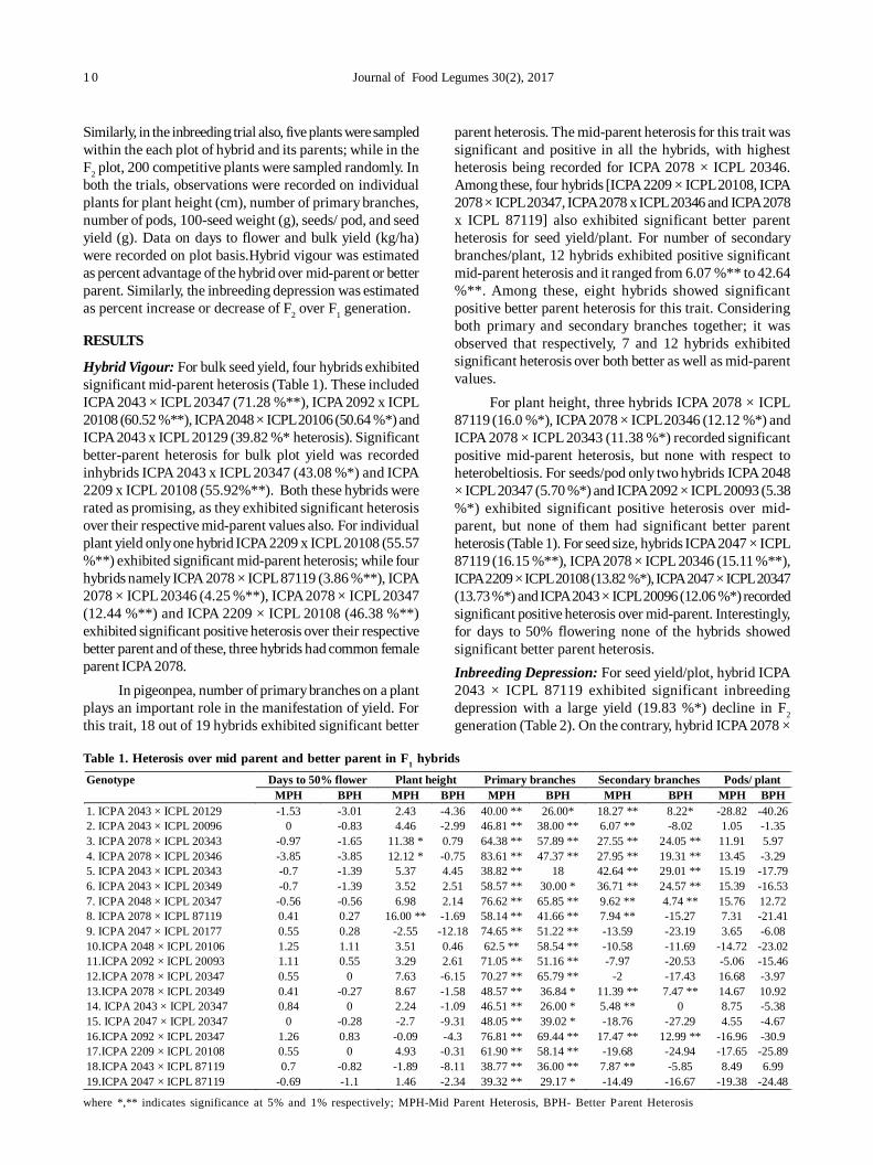
Hybrid Vigour: For bulk seed yield, four hybrids exhibitedsignificant mid-parent heterosis (Table 1). These includedICPA 2043 × ICPL 20347 (71.28 %**), ICPA 2092 x ICPL20108 (60.52 %**), ICPA 2048 × ICPL 20106 (50.64 %*) andICPA 2043 x ICPL 20129 (39.82 %* heterosis). Significantbetter-parent heterosis for bulk plot yield was recordedinhybrids ICPA 2043 x ICPL 20347 (43.08 %*) and ICPA2209 x ICPL 20108 (55.92%**). Both these hybrids wererated as promising, as they exhibited significant heterosisover their respective mid-parent values also. For individualplant yield only one hybrid ICPA 2209 x ICPL 20108 (55.57%**) exhibited significant mid-parent heterosis; while fourhybrids namely ICPA 2078 × ICPL 87119 (3.86 %**), ICPA2078 × ICPL 20346 (4.25 %**), ICPA 2078 × ICPL 20347(12.44 %**) and ICPA 2209 × ICPL 20108 (46.38 %**)exhibited significant positive heterosis over their respectivebetter parent and of these, three hybrids had common femaleparent ICPA 2078.
In pigeonpea, number of primary branches on a plantplays an important role in the manifestation of yield. Forthis trait, 18 out of 19 hybrids exhibited significant better
parent heterosis. The mid-parent heterosis for this trait wassignificant and positive in all the hybrids, with highestheterosis being recorded for ICPA 2078 × ICPL 20346.Among these, four hybrids [ICPA 2209 × ICPL 20108, ICPA2078 × ICPL 20347, ICPA 2078 x ICPL 20346 and ICPA 2078x ICPL 87119] also exhibited significant better parentheterosis for seed yield/plant. For number of secondarybranches/plant, 12 hybrids exhibited positive significantmid-parent heterosis and it ranged from 6.07 %** to 42.64%**. Among these, eight hybrids showed significantpositive better parent heterosis for this trait. Consideringboth primary and secondary branches together; it wasobserved that respectively, 7 and 12 hybrids exhibitedsignificant heterosis over both better as well as mid-parentvalues.
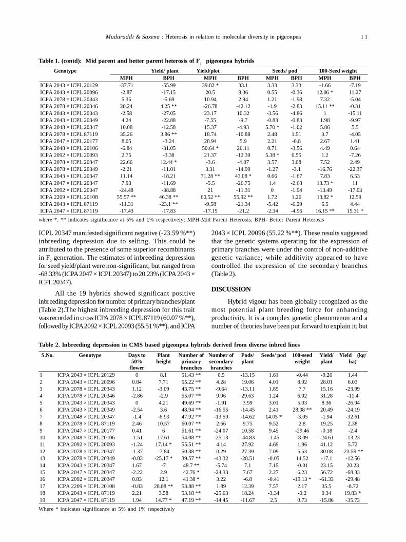
For plant height, three hybrids ICPA 2078 × ICPL87119 (16.0 %*), ICPA 2078 × ICPL 20346 (12.12 %*) andICPA 2078 × ICPL 20343 (11.38 %*) recorded significantpositive mid-parent heterosis, but none with respect toheterobeltiosis. For seeds/pod only two hybrids ICPA 2048× ICPL 20347 (5.70 %*) and ICPA 2092 × ICPL 20093 (5.38%*) exhibited significant positive heterosis over mid-parent, but none of them had significant better parentheterosis (Table 1). For seed size, hybrids ICPA 2047 × ICPL87119 (16.15 %**), ICPA 2078 × ICPL 20346 (15.11 %**),ICPA 2209 × ICPL 20108 (13.82 %*), ICPA 2047 × ICPL 20347(13.73 %*) and ICPA 2043 × ICPL 20096 (12.06 %*) recordedsignificant positive heterosis over mid-parent. Interestingly,for days to 50% flowering none of the hybrids showedsignificant better parent heterosis.Inbreeding Depression: For seed yield/plot, hybrid ICPA2043 × ICPL 87119 exhibited significant inbreedingdepression with a large yield (19.83 %*) decline in F2generation (Table 2). On the contrary, hybrid ICPA 2078 ×
Table 1. Heterosis over mid parent and better parent in F1 hybrids
where *,** indicates significance at 5% and 1% respectively; MPH-Mid Parent Heterosis, BPH- Better Parent Heterosis
Days to 50% flower Plant height Primary branches Secondary branches Pods/ plant Genotype MPH BPH MPH BPH MPH BPH MPH BPH MPH BPH
1. ICPA 2043 × ICPL 20129 -1.53 -3.01 2.43 -4.36 40.00 ** 26.00* 18.27 ** 8.22* -28.82 -40.26 2. ICPA 2043 × ICPL 20096 0 -0.83 4.46 -2.99 46.81 ** 38.00 ** 6.07 ** -8.02 1.05 -1.35 3. ICPA 2078 × ICPL 20343 -0.97 -1.65 11.38 * 0.79 64.38 ** 57.89 ** 27.55 ** 24.05 ** 11.91 5.97 4. ICPA 2078 × ICPL 20346 -3.85 -3.85 12.12 * -0.75 83.61 ** 47.37 ** 27.95 ** 19.31 ** 13.45 -3.29 5. ICPA 2043 × ICPL 20343 -0.7 -1.39 5.37 4.45 38.82 ** 18 42.64 ** 29.01 ** 15.19 -17.79 6. ICPA 2043 × ICPL 20349 -0.7 -1.39 3.52 2.51 58.57 ** 30.00 * 36.71 ** 24.57 ** 15.39 -16.53 7. ICPA 2048 × ICPL 20347 -0.56 -0.56 6.98 2.14 76.62 ** 65.85 ** 9.62 ** 4.74 ** 15.76 12.72 8. ICPA 2078 × ICPL 87119 0.41 0.27 16.00 ** -1.69 58.14 ** 41.66 ** 7.94 ** -15.27 7.31 -21.41 9. ICPA 2047 × ICPL 20177 0.55 0.28 -2.55 -12.18 74.65 ** 51.22 ** -13.59 -23.19 3.65 -6.08 10.ICPA 2048 × ICPL 20106 1.25 1.11 3.51 0.46 62.5 ** 58.54 ** -10.58 -11.69 -14.72 -23.02 11.ICPA 2092 × ICPL 20093 1.11 0.55 3.29 2.61 71.05 ** 51.16 ** -7.97 -20.53 -5.06 -15.46 12.ICPA 2078 × ICPL 20347 0.55 0 7.63 -6.15 70.27 ** 65.79 ** -2 -17.43 16.68 -3.97 13.ICPA 2078 × ICPL 20349 0.41 -0.27 8.67 -1.58 48.57 ** 36.84 * 11.39 ** 7.47 ** 14.67 10.92 14. ICPA 2043 × ICPL 20347 0.84 0 2.24 -1.09 46.51 ** 26.00 * 5.48 ** 0 8.75 -5.38 15. ICPA 2047 × ICPL 20347 0 -0.28 -2.7 -9.31 48.05 ** 39.02 * -18.76 -27.29 4.55 -4.67 16.ICPA 2092 × ICPL 20347 1.26 0.83 -0.09 -4.3 76.81 ** 69.44 ** 17.47 ** 12.99 ** -16.96 -30.9 17.ICPA 2209 × ICPL 20108 0.55 0 4.93 -0.31 61.90 ** 58.14 ** -19.68 -24.94 -17.65 -25.89 18.ICPA 2043 × ICPL 87119 0.7 -0.82 -1.89 -8.11 38.77 ** 36.00 ** 7.87 ** -5.85 8.49 6.99 19.ICPA 2047 × ICPL 87119 -0.69 -1.1 1.46 -2.34 39.32 ** 29.17 * -14.49 -16.67 -19.38 -24.48
Mudaraddi & Saxena : Heterosis in relation to molecular diversity in pigeonpea 1 1
ICPL 20347 manifested significant negative (-23.59 %**)inbreeding depression due to selfing. This could beattributed to the presence of some superior recombinantsin F2 generation. The estimates of inbreeding depressionfor seed yield/plant were non-significant; but ranged from-68.33% (ICPA 2047 × ICPL 20347) to 20.23% (ICPA 2043 ×ICPL 20347).
All the 19 hybrids showed significant positiveinbreeding depression for number of primary branches/plant(Table 2).The highest inbreeding depression for this traitwas recorded in cross ICPA 2078 × ICPL 87119 (60.07 %**),followed by ICPA 2092 × ICPL 20093 (55.51 %**), and ICPA
2043 × ICPL 20096 (55.22 %**). These results suggestedthat the genetic systems operating for the expression ofprimary branches were under the control of non-additivegenetic variance; while additivity appeared to havecontrolled the expression of the secondary branches(Table 2).
DISCUSSION
Hybrid vigour has been globally recognized as themost potential plant breeding force for enhancingproductivity. It is a complex genetic phenomenon and anumber of theories have been put forward to explain it; but
Yield/ plant Yield/plot Seeds/ pod 100-Seed weight Genotype MPH BPH MPH BPH MPH BPH MPH BPH
ICPA 2043 × ICPL 20129 -37.71 -55.99 39.82 * 33.1 3.33 3.33 -1.66 -7.19 ICPA 2043 × ICPL 20096 -2.87 -17.15 20.5 8.36 0.55 -0.36 12.06 * 11.27 ICPA 2078 × ICPL 20343 5.35 -5.69 10.94 2.94 1.21 -1.98 7.32 -5.04 ICPA 2078 × ICPL 20346 20.24 4.25 ** -26.78 -42.12 -1.9 -2.83 15.11 ** -0.31 ICPA 2043 × ICPL 20343 -2.58 -27.05 23.17 10.32 -3.56 -4.86 1 -15.11 ICPA 2043 × ICPL 20349 4.24 -22.88 -7.55 -9.7 -0.83 -0.83 1.98 -9.97 ICPA 2048 × ICPL 20347 10.08 -12.58 15.37 -4.93 5.70 * -1.02 5.86 5.5 ICPA 2078 × ICPL 87119 35.26 3.86 ** 18.74 -10.88 2.48 1.51 3.7 -4.05 ICPA 2047 × ICPL 20177 8.05 -3.24 28.94 5.9 2.21 -0.8 2.67 1.41 ICPA 2048 × ICPL 20106 -6.84 -31.05 50.64 * 26.11 0.71 -3.56 4.49 0.64 ICPA 2092 × ICPL 20093 2.75 -3.38 21.37 -12.39 5.38 * 0.55 1.2 -7.26 ICPA 2078 × ICPL 20347 22.66 12.44 * -3.6 -4.07 3.57 3.08 7.52 2.49 ICPA 2078 × ICPL 20349 -2.21 -11.01 3.31 -14.99 -1.27 -3.1 -16.76 -22.37 ICPA 2043 × ICPL 20347 11.14 -18.21 71.28 ** 43.08 * 0.66 -1.67 7.83 6.53 ICPA 2047 × ICPL 20347 7.93 -11.69 -5.5 -26.75 1.4 -2.68 13.73 * 11 ICPA 2092 × ICPL 20347 -24.48 -38.88 21 -11.31 0 -1.94 -13.49 -17.03 ICPA 2209 × ICPL 20108 55.57 ** 46.38 ** 60.52 ** 55.92 ** 1.72 1.26 13.82 * 12.59 ICPA 2043 × ICPL 87119 -11.31 -23.1 ** -9.58 -21.34 -5.42 -6.29 6.5 4.44 ICPA 2047 × ICPL 87119 -17.43 -17.83 -17.15 -21.2 -2.34 -4.96 16.15 ** 15.31 *
Table 1. (contd): Mid parent and better parent heterosis of F1 pigeonpea hybrids
where *, ** indicates significance at 5% and 1% respectively; MPH-Mid Parent Heterosis, BPH- Better Parent Heterosis
Table 2. Inbreeding depression in CMS based pigeonpea hybrids derived from diverse inbred lines
Where * indicates significance at 5% and 1% respectively
S.No. Genotype Days to 50%
flower
Plant height
Number of primary branches
Number of secondary branches
Pods/ plant
Seeds/ pod 100-seed weight
Yield/ plant
Yield (kg/ ha)
1 ICPA 2043 × ICPL 20129 0 8.1 51.43 ** 0.5 -13.15 1.61 -0.44 -9.26 1.44 2 ICPA 2043 × ICPL 20096 0.84 7.71 55.22 ** 4.28 19.06 4.01 8.92 28.01 6.03 3 ICPA 2078 × ICPL 20343 1.12 -3.09 43.75 ** -9.64 -13.11 1.85 7.7 15.16 -23.99 4 ICPA 2078 × ICPL 20346 -2.86 -2.9 55.07 ** 9.96 29.63 1.24 6.92 31.28 -11.4 5 ICPA 2043 × ICPL 20343 0 4.21 49.69 ** -1.91 3.99 3.01 5.03 8.36 -26.94 6 ICPA 2043 × ICPL 20349 -2.54 3.6 48.94 ** -16.55 -14.45 2.41 28.08 ** 20.49 -24.19 7 ICPA 2048 × ICPL 20347 -1.4 -6.93 47.92 ** -13.59 -14.62 14.05 * -3.05 -1.94 -32.61 8 ICPA 2078 × ICPL 87119 2.46 10.57 60.07 ** 2.66 9.75 9.52 2.8 19.25 2.38 9 ICPA 2047 × ICPL 20177 0.41 6 51.61 ** -24.07 10.58 9.45 -29.46 -0.18 -2.4 10 ICPA 2048 × ICPL 20106 -1.51 17.61 54.08 ** -25.13 -44.83 -1.45 -8.09 -24.61 -13.23 11 ICPA 2092 × ICPL 20093 -1.24 17.14 * 55.51 ** 4.14 27.92 4.69 1.96 41.12 5.72 12 ICPA 2078 × ICPL 20347 -1.37 -7.84 50.38 ** 0.29 27.39 7.09 5.53 30.08 -23.59 ** 13 ICPA 2078 × ICPL 20349 -0.83 -25.17 * 39.57 ** -43.32 -28.51 -0.05 14.52 -17.1 -12.56 14 ICPA 2043 × ICPL 20347 1.67 -7 48.7 ** -5.74 7.1 7.15 -0.01 23.15 20.23 15 ICPA 2047 × ICPL 20347 -2.22 2.9 42.76 * -24.33 7.67 2.27 6.23 56.72 -68.33 16 ICPA 2092 × ICPL 20347 0.83 12.1 41.38 * 3.22 -6.8 -0.41 -19.13 * -61.33 -29.48 17 ICPA 2209 × ICPL 20108 -0.83 28.88 ** 53.88 ** 1.89 12.39 7.57 2.17 35.5 -8.72 18 ICPA 2043 × ICPL 87119 2.21 3.58 53.18 ** -25.63 18.24 -3.34 -0.2 0.34 19.83 * 19 ICPA 2047 × ICPL 87119 1.94 14.77 * 47.19 ** -14.45 -11.67 2.5 0.73 -15.86 -35.73
1 2 Journal of Food Legumes 30(2), 2017
its reality is still under natural wraps. The evolution ofhybrid technology in pigeonpea (Saxena 2015) has createda sort of revolution in breeding of this pulse crop with 25-40% on-farm yield advantage.
In the present investigation, hybrid ICPA 2209 x ICPL20108 exhibited the highest (55.92 %**) better parentheterosis for plot yield. Kandalkar (2007), Saxena andNadarajan (2010), Wanjari and Rathod (2012) and Pandeyet al. (2013) also reported significant positive heterosis forgrain yield in some CMS-based hybrids of pigeonpea. Theabsence of inbreeding depression in this cross gave anindication for the additive genetic control of yield. Further,it can be assumed that the genes controlling yield withadditive effects came together from both the parents andexpressed in the hybrid to produce heterotic effect. Thishybrid can also be subjected to pedigree selection to derivehigh yielding inbred lines. In contrast, hybrid ICPA 2043 xICPL 87119 exhibited non-significant heterosis but theinbreeding depression was highly significant. This situationmay arise due to the presence of genes, predominantlywith non-additive affects, which upon selfing, producedunproductive F2 segregants and poor yield.
For yield/plant, four hybrids expressed significantheterosis over their respective better parent and all of themalso had highly significant inbreeding depression for yieldand number of primary branches. It appears that the numberof primary branches that is controlled by non-additive geneaction at most loci, directly contributed to hybrid vigourfor seed yield. A perusal of overall data further indicatedthat inbreeding depression for seed yield was theconsequence of significant inbreeding depression for yieldcontributing trait such as number of primary branches.Studies on component analysis in pigeonpea also revealedthat number of primary branches played the most importantrole in determining yield (Saxena and Sharma 1990, Phad2003, Yadav and Singh 2004, Phad et al. 2009 andChandirakala et al. 2010).
The differences observed between per plant yieldand bulk plot yield data with respect to heterosis andinbreeding depression, observed in some hybridcombinations, could be attributed to the influence ofunequal competition between the individual plant andenvironment on the expression of these traits. Green et al.(1981) and Saxena and Sharma (1983) reported highlysignificant intra-population variability for individual plantyield even within highly inbred lines in pigeonpea. Theypostulated that such situation can arise under the field-grown trials because the pigeonpea plants are highlysensitive to changes in the micro-environment. They alsoconcluded that the individual pigeonpea plants are highlycompetitive with respect to space, sunlight, moisture etc.
In the present study, some fertility restoring lineswere derived from inter-specific crosses and these had verylow productivity and it may be the consequence of
undesirable linkage drag in the progenies. In pigeonpea,significant negative heterosis for flowering (earliness) wasreported by Shoba and Balan (2010) and Sameerkumaret al. (2012), but none of the hybrids showed significantinbreeding depression. This suggested that the floweringtime was predominantly controlled by additive genes.Similar conclusions were also made by Kandalkar (2007)and Sarode et al. (2009).Heterosis in Relation to Molecular Diversity of Parents:Mudaraddi and Saxena (2015) assessed the moleculardiversity of among hybrid parents including 20 A-lines and135 R-lines using 24 simple sequence repeat (SSR) markers.In this study the number of alleles amplified ranged from 3to 41 at an average of 14.5 alleles per marker with meanpolymorphic information content (PIC) value of 0.64. Basedon this information, they constructed two heterotic groups(HG) for A-lines and three HGs for R-lines. The informationgenerated in this study was used to study the relationshipof hybrid vigour with molecular diversity of the hybridparents (Table 3).
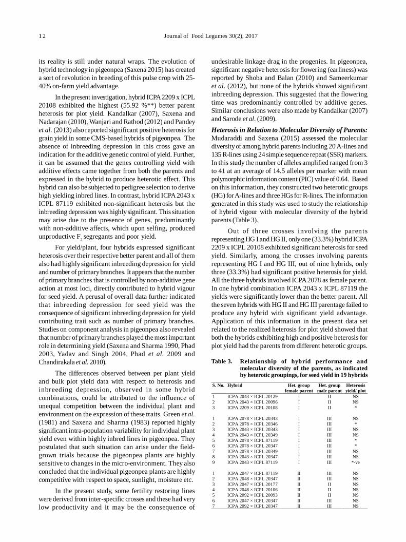
Out of three crosses involving the parentsrepresenting HG I and HG II, only one (33.3%) hybrid ICPA2209 x ICPL 20108 exhibited significant heterosis for seedyield. Similarly, among the crosses involving parentsrepresenting HG I and HG III, out of nine hybrids, onlythree (33.3%) had significant positive heterosis for yield.All the three hybrids involved ICPA 2078 as female parent.In one hybrid combination ICPA 2043 x ICPL 87119 theyields were significantly lower than the better parent. Allthe seven hybrids with HG II and HG III parentage failed toproduce any hybrid with significant yield advantage.Application of this information in the present data setrelated to the realized heterosis for plot yield showed thatboth the hybrids exhibiting high and positive heterosis forplot yield had the parents from different heterotic groups.
Table 3. Relationship of hybrid performance andmolecular diversity of the parents, as indicatedby heterotic groupings, for seed yield in 19 hybrids
S. No. Hybrid Het. group female parent
Het. group male parent
Heterosis yield/ plot
1 ICPA 2043 × ICPL 20129 I II NS 2 ICPA 2043 × ICPL 20096 I II NS 3 ICPA 2209 × ICPL 20108 I II * 1 ICPA 2078 × ICPL 20343 I III NS 2 ICPA 2078 × ICPL 20346 I III * 3 ICPA 2043 × ICPL 20343 I III NS 4 ICPA 2043 × ICPL 20349 I III NS 5 ICPA 2078 × ICPL 87119 I III * 6 ICPA 2078 × ICPL 20347 I III * 7 ICPA 2078 × ICPL 20349 I III NS 8 ICPA 2043 × ICPL 20347 I III NS 9 ICPA 2043 × ICPL 87119 I III *-ve 1 ICPA 2047 × ICPL 87119 II III NS 2 ICPA 2048 × ICPL 20347 II III NS 3 ICPA 2047 × ICPL 20177 II II NS 4 ICPA 2048 × ICPL 20106 II II NS 5 ICPA 2092 × ICPL 20093 II II NS 6 ICPA 2047 × ICPL 20347 II III NS 7 ICPA 2092 × ICPL 20347 II III NS
Mudaraddi & Saxena : Heterosis in relation to molecular diversity in pigeonpea 1 3
For example, in hybrid ICPA 2043 x ICPL 20347 the femaleand male parents, respectively, represented heteroticgroups I and III. Similarly, the other hybrid ICPA 2092 xICPL 20108 had the parents belonging to the heterotic groupII and III. But, all the parents from diverse heterotic groupsdid not produce heterotic hybrids. The present studiesshowed that even though the hybrids were produced usingdiverse parents, the frequency of heterotic hybrids waslow; this may be due to their poor per se performance andcombining ability.
CONCLUSIONS
Considering the observations on heterosis andinbreeding depression together, it was concluded that inpigeonpea both additive and non-additive genetic variationplayed a significant role in the manifestation of seed yield.However, their relative importance varied from cross tocross. Among the 19 hybrids tested, ICPA 2209 x ICPL 20108was adjudged the best for productivity, because it exhibitedsignificant positive hybrid vigour for both per plant andper plot yields. Besides this, the inbreeding depression inthis cross was also non-significant; suggesting that in thisheterotic combination the expression of high yield was theconsequence of combining the genes with additive effects.Hence besides exploiting its hybridity, this cross can alsobe used to breed inbred cultivars with more number ofadditive genes. Such inbreds can also be used as parentallines to breed second generation of high yieldinghybrids.The results also showed that molecular diversityinthis set of hybrid parents was limited and it was foundrelated to high hybrid vigour only in a few hybridcombinations.
REFERENCES
Bharathi M and Saxena KB. 2015. Molecular diversity based heteroticgroups in pigeonpea [Cajanus cajan (L.) Millsp.]. Indian Journalof Genetics and Plant Breeding 75(1): 57-61.
Chandirakala R, Subbaraman N and Hameed A. 2010. Heterosis foryield in pigeonpea (Cajanus cajan L. Mill sp.). Electronic Journalof Plant Breeding 1(2): 205-208.
Green JM, Sharma D, Reddy LJ, Saxena KB, Gupta SC, Jain KC,Reddy BV and Rao MR. 1981. Methodology and Progress in theICRISAT Pigeonpea Breeding Program. In: Proceedings of theInternational Workshop on Pigeonpeas, ICRISAT Center,Patancheru, India 1: 437-449.
Kandalkar VS. 2007. Evaluation of standard heterosis in advancedCMS based hybrids for grain yield, harvest index and theirattributes in pigeonpea. In: Proceeding of 7 th InternationalConference on Sustainable Agriculture for Food, Bio-energy andLivelihood Security. 14-16 February 2007, Jabalpur, MadhyaPradesh, India pp 195.
Pandey P, Pandey VR, Yadav S, Tiwari D and Kumar R. 2015.Relationship between heterosis and genetic diversity in Indianpigeonpea [Cajanus cajan (L.) Millsp.] accessions usingmultivariate cluster analysis and heterotic grouping. AustralianJournal of Crop Science 9: 494-503.
Phad DS. 2003. Heterosis, Combining ability and stability analysisin pigeonpea Cajanus cajan (L.) Millsp. Ph.D thesis submittedto Marathwada Agricultural University, Parbhani, India
Phad DS, Madrap IA and Dalvi VA. 2009. Heterosis in relation tocombining ability effects and phenotypic stability in pigeonpea.Journal of Food Legumes 22(1): 59-61.
Sameer kumar CV, Sreelakshmi CH and Shivani D. 2012. Gene effects,heterosis and inbreeding depression in Pigeonpea, Cajanus cajanL. Electronic Journal of Plant Breeding 3(1): 682- 685.
Sarode SB, Singh MN and Singh UP. 2009. Heterosis in long durationpigeonpea [Cajanus cajan(L.) Millsp.]. International Journalof Plant Sciences 4(1): 106 –108.
Saxena KB. 2015. From concept to field: evolution of hybridpigeonpea technology in India. Indian Journal of Genetics andPlant Breeding 75(3): 279-293.
Saxena KB and Nadarajan N. 2010. Prospects of pigeonpea hybridsin Indian agriculture. Electronic Journal of Plant Breeding 1(4):1107-1117.
Saxena KB and Sharma D. 1983. Early generation in pigeonpea(Cajanus cajan (L.) Millsp.). Tropical Plant Science Research1(4): 309-313.
Saxena KB and Sharma D.1990. Pigeonpea: genetics. In: Nene Y.L.,S.D. Hall, and V. K. Sheila, (eds.). The Pigeonpea 137-158.CAB International, Wallingford.
Saxena KB, Sharma D and Vales MI. 2017. Development andcommercialization of CMS pigeonpea hybrid. Plant BreedingReviews Volume 41: (in press)
Shoba D and Balan A. 2010. Heterosis in CMS/GMS based pigeonpea[Cajanus cajan (L.) Millsp.] hybrids. Agriculture Science Digest30(1): 32-36.
Shull GH. 1908. The composition of a field of maize. AmericanBreeders Association Reports 4: 296-301.
Wanjari KB and Rathod ST. 2012. Exploitation of heterosis throughF1 hybrid in pigeonpea (Cajanus cajan L.). The status andprospects.Indian Journal of Genetics and Plant Breeding 72(3):257-263.
Yadav SS and Singh DP. 2004. Heterosis in pigeonpea.Indian Journalof Pulses Research 17(2): 179-180.
Journal of Food Legumes 30(2): 14-20, 2017
ABSTRACT
Micronutrient malnutrition is recognized as a massive andrapidly growing health issue as major emphasis was laidupon crop productivity improvement with little concern tonutritional value. Considering the diverse growing conditionsof mungbean, its varied food products and their ease indigestion, emphasis on development of new mungbeanvarieties with high zinc and iron content will be on afternote option to improve the nutritional status of vegetarianpopulation. Seventy mungbean Recombinant Inbred Linesdeveloped from two diverse genotypes i.e. MH 2-15 (low Znand Fe) and ML 776 (high Zn and Fe content) were grownalong with their both parents and three popular checks (MH1-25, MH 421 and MH 318) in untreated and treated with (Znand Fe) environments to study genetic divergence amongthese. Genotypes performed significantly better under treatedenvironment than the untreated condition for traits viz.,plant height, number of branches plant-1, 100-seed weight,seed yield plot-1, biological yield plot-1 and zinc and ironcontent in seeds. Thirteen variables were reduced to fourprincipal factors through principal factor analysis explaining77.48 and 74.33 per cent variability, in untreated and treatedenvironments respectively. The first principal factor (PF)showed high loadings for six yield variables and PF 3 ascribedfor Zn and Fe content in seeds. Eight clusters containingone to 30 and three to 23 genotypes under untreated andtreated environments, respectively were formed usinghierarchical cluster analysis. Inter-cluster distance wasobserved maximum between clusters VII and VIII in boththe environments.
Key words: Cluster, Diversity, Micronutrients, Mungbean,Principal component
Green gram [Vigna radiata (L.) Wilczek] commonlyknown as mungbean, is a widely cultivated pulse crop oftropics and sub-tropics which is used extensively for humanconsumption as well as animal feed. It enables soil to restoreits fertility through nitrogen fixation and is relatively droughttolerant and well adapted to a range of soil conditions.Moreover, it is well suited for various crop rotations andcrop mixtures. Till now, major emphasis has been laid toimprove the crop productivity with little concern tonutritional value. Micronutrient malnutrition is recognizedas a massive and rapidly growing public health issueespecially among poor people that causes several diseasesand the affected people are more prone to infection by acomplex of diseases resulting in further deterioration in
Genetic diversity for seed yield traits and micronutrient content in recombinantinbred lines of mungbean [Vigna radiata (L.) Wilczek]KRITIKA, RAJESH YADAV and RAVIKA
CCS Haryana Agricultural University, Hisar-125 004, Haryana, India; E-mail: [email protected](Received: February 10, 2017; Accepted: May 22, 2017)
quality of life (Welch 2002). Zinc and iron are importantmicronutrients which are required to maintain metabolicregulation and organ function. Zinc is an essentialcomponent of more than 300 enzymes that are needed torepair wounds, maintain fertility, synthesize protein, boostsimmunity and plays thus, a central role in cellular growthand differentiation. Iron is an important component ofvarious enzyme systems such as the cytochromes, ferritinand haemosider in stored in the liver and human bodyrequires iron for synthesis of the oxygen, transport proteins,haemoglobin, myoglobin and other iron containing enzymeswhich are important for energy production, immune defenceand thyroid function. Both zinc and iron are, therefore,essential to human well being (Singh et al. 2013).
Numerous strategies have been employed for this.However, ‘Biofortification’ has come up as a new strategyto cope up with micronutrient malnutrition (Welch andGraham 2004) as it has the potential to provide coveragefor remote rural population. Thus, breeding crop plants forhigher micronutrient concentration has become an activegoal in the developing world. Considering the diversegrowing conditions of mungbean, its varied food productsand their ease in digestion, emphasis should be laid ondeveloping new high yielding varieties with high zinc andiron content which can improve the nutritional status ofvegetarian population. Creation of variability and selectionof superior recombinants among the variants are majorobjective of any plant breeding programme. Geneticdiversity is the basic requirement of any programme aimedat genetic amelioration of any trait. Effective hybridizationprogramme between genetically diverse parents will leadto considerable amount of heterotic response and broadenthe spectrum of variability in segregating generations.Although considerable amount of knowledge has beengenerated during past few decades, yet very few studieshave been conducted to access the micronutrientsvariability and diversity in mungbean. One of theconstraints listed for lack of breakthrough in mungbeanproduction has been the lack of genetic variability andtherefore, recombinant inbred lines (RILs) would be a goodoption. Taunk et al. (2012) and Aneja et al. (2013) identifiedSattya (MH 2-15) and ML 776 as ideal parents for makingRILs, as both of these are genetically diverse withcontrasting zinc and iron content. Considering all these astudy was conducted to work out the genetic divergencein mungbean RILs.
Kritika et al. : Genetic diversity in mungbean RILs 1 5
MATERIALS AND METHODS
The experimental material comprised of 70 mungbeanRILs in F6 generation, their two parents (ML 776 and MH 2-15) and three popular cultivated varieties of mungbean asyield checks (MH 1-25, MH 421 and MH 318). GenotypeML 776 has high zinc and iron content in seeds while MH2-15 is a high yielding MYMV resistant released variety ofmungbean with low zinc and iron content. This fieldexperiment was carried out in kharif 2015 at CCS HaryanaAgricultural University, Hisar in two sets, one (untreated)with recommended doses of fertilizer (RDF) only and theother one treated with RDF+25 kg/ha ZnSO4 as basal doseand 0.5% solution of FeSO4 as foliar spray at floweringstage. Both the sets of the experiments were laid out inrandomized block design with three replications. All thegenotypes were grown in a plot size of 4m2 (2m rows × 2mlength). The row-to-row distance was kept at 30 cm andplant to plant distance at 10 cm.
The observations were recorded as the means fromfive randomly selected plants from each genotype in eachreplication for plant height, number of branches plant-1,number of pods plant-1 and number of seeds pod-1.Othertraits viz., days to 50% flowering, days to maturity, 100-seed weight, seed yield plot-1, biological yield plot-1, harvestindex, reaction to Mungbean Yellow Mosaic Virus (MYMV)were determined on plot basis. For recording the incidenceof MYMV, 1 to 9 scales was used. Atomic AbsorptionSpectrophotometer (AAS) analysis of Benton-Jones (1989)based on nitric/perchloric acid digestion was followed toestimate the zinc and iron concentration in mungbean seeds.The data collected for each quantitative trait were subjectedto Hierarchical Cluster and Principal Factor analysis usingSPSS software (Version 20). Un weighted pair group methodusing arithmetic averages (UPGMA) with City Blockdistance was used for clustering the genotypes. Principalcomponent method of factor extraction was used forextraction of factors. As the initial factor loading wereinadequate and not clearly interpretable, the factor axeswere rotated using Varimax rotation (Kaiser 1958). Principalfactor scores were determined. The genotypes were plottedusing their individual factor scores taking different principalfactors as axes.
RESULTS AND DISCUSSION
The mean squares due to genotypes were foundsignificant for all the characters studied revealingconsiderable variability among the genotypes for all the
characters except for harvest index. All the traits studiedwere compared for their expression under untreated andtreated environments using Independent t-test whichindicated that plant height, number of branches plant-1,100-seed weight, seed yield plot-1, biological yield plot-1,zinc and iron content in seeds increased by the applicationof Zn and Fe. However, the quantum of increase variedfrom genotype to genotype. Studies of Samreen et al. (2013)and Singh et al. (2013) are in partial corroboration to ourfindings.
Principal factor analysis was carried out as eachobserved variable is expressed linearly in terms of a commonfactor and a unique factor. The common factor accountsfor the correlation among the variables, while each uniquefactor accounts for the remaining variance of that variable.Further in principal component analysis, the total variationcontained in a set of variables is considered, whereas infactor analysis interest centers on that part of variancewhich is shared by the common factors. Initially the datawere analyzed without any rotation to derive a picture ofinteraction of variables among themselves and with theprincipal factors. However, it failed to provide muchinformation regarding the correlation between the variablesand the principal factors hence analysis with Varimaxrotation was applied to draw sensible conclusions. Thefirst four principal components exhibited eigen values morethan one in both the environments and together explained77.42 and 74.33 % cumulative variability in untreated andtreated environments, respectively (Table 1). The firstprincipal component absorbed and accounted for maximumproportion of total variability and remaining componentsaccounted for progressively lesser and lesser amount ofvariation. Similar trend was observed by Yimram et al. (2009),Pandiyan et al.(2012), Divyaramakrishnan and Savithramma(2014) and Ghanbari et al. (2015) in mungbean.
In both untreated and treated environments, all thethirteen variables showed high loading on different principalfactors and grouped the similar type of variables by loadingthem together on a common principal factor in both theenvironments (Table 2 and 3). The first PF showed highloadings for six seed yield related variables i.e.seed yieldplot-1, biological yield plot-1, number of branches plant-1,number of pods plant-1, number of seeds pod-1and reactionto MYMV and thus, can easily be designated as seed yieldfactor. The PF 2 ascribed for four variables viz., plant height,days to 50% flowering, days to maturity and 100-seedweight. PF 3 was clearly loaded with Zn and Fe content and
Table 1. Total variance explained by different principal components
Principal Component
Rotation Sums of Squared Loadings- Untreated Rotation Sums of Squared Loadings- Treated Eigen value % of Variance Cumulative % Eigen value % of Variance Cumulative %
1 4.926 37.891 37.891 4.61 35.465 35.465 2 2.39 18.381 56.272 2.277 17.512 52.977 3 1.55 11.922 68.194 1.634 12.57 65.547 4 1.199 9.225 77.418 1.142 8.782 74.328
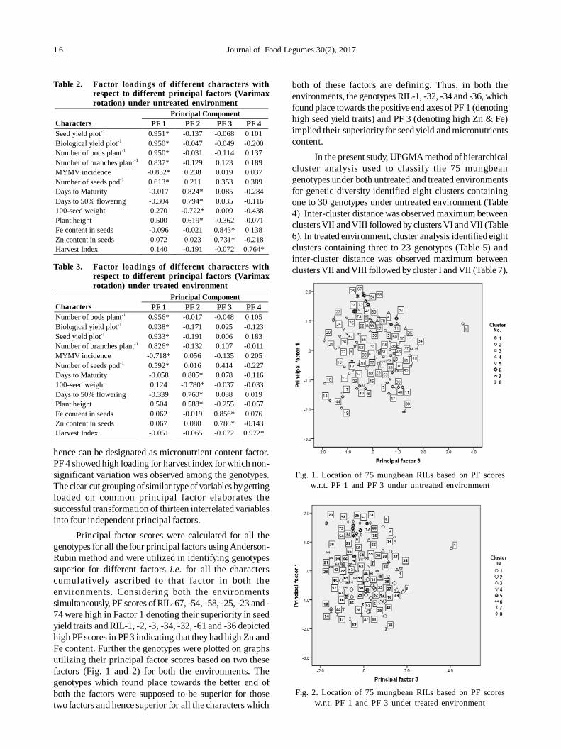
1 6 Journal of Food Legumes 30(2), 2017
hence can be designated as micronutrient content factor.PF 4 showed high loading for harvest index for which non-significant variation was observed among the genotypes.The clear cut grouping of similar type of variables by gettingloaded on common principal factor elaborates thesuccessful transformation of thirteen interrelated variablesinto four independent principal factors.
Principal factor scores were calculated for all thegenotypes for all the four principal factors using Anderson-Rubin method and were utilized in identifying genotypessuperior for different factors i.e. for all the characterscumulatively ascribed to that factor in both theenvironments. Considering both the environmentssimultaneously, PF scores of RIL-67, -54, -58, -25, -23 and -74 were high in Factor 1 denoting their superiority in seedyield traits and RIL-1, -2, -3, -34, -32, -61 and -36 depictedhigh PF scores in PF 3 indicating that they had high Zn andFe content. Further the genotypes were plotted on graphsutilizing their principal factor scores based on two thesefactors (Fig. 1 and 2) for both the environments. Thegenotypes which found place towards the better end ofboth the factors were supposed to be superior for thosetwo factors and hence superior for all the characters which
both of these factors are defining. Thus, in both theenvironments, the genotypes RIL-1, -32, -34 and -36, whichfound place towards the positive end axes of PF 1 (denotinghigh seed yield traits) and PF 3 (denoting high Zn & Fe)implied their superiority for seed yield and micronutrientscontent.
In the present study, UPGMA method of hierarchicalcluster analysis used to classify the 75 mungbeangenotypes under both untreated and treated environmentsfor genetic diversity identified eight clusters containingone to 30 genotypes under untreated environment (Table4). Inter-cluster distance was observed maximum betweenclusters VII and VIII followed by clusters VI and VII (Table6). In treated environment, cluster analysis identified eightclusters containing three to 23 genotypes (Table 5) andinter-cluster distance was observed maximum betweenclusters VII and VIII followed by cluster I and VII (Table 7).Table 3. Factor loadings of different characters with
respect to different principal factors (Varimaxrotation) under treated environment
Principal Component Characters PF 1 PF 2 PF 3 PF 4 Number of pods plant-1 0.956* -0.017 -0.048 0.105 Biological yield plot-1 0.938* -0.171 0.025 -0.123 Seed yield plot-1 0.933* -0.191 0.006 0.183 Number of branches plant-1 0.826* -0.132 0.107 -0.011 MYMV incidence -0.718* 0.056 -0.135 0.205 Number of seeds pod-1 0.592* 0.016 0.414 -0.227 Days to Maturity -0.058 0.805* 0.078 -0.116 100-seed weight 0.124 -0.780* -0.037 -0.033 Days to 50% flowering -0.339 0.760* 0.038 0.019 Plant height 0.504 0.588* -0.255 -0.057 Fe content in seeds 0.062 -0.019 0.856* 0.076 Zn content in seeds 0.067 0.080 0.786* -0.143 Harvest Index -0.051 -0.065 -0.072 0.972*
Table 2. Factor loadings of different characters withrespect to different principal factors (Varimaxrotation) under untreated environment
Principal Component Characters PF 1 PF 2 PF 3 PF 4 Seed yield plot-1 0.951* -0.137 -0.068 0.101 Biological yield plot-1 0.950* -0.047 -0.049 -0.200 Number of pods plant-1 0.950* -0.031 -0.114 0.137 Number of branches plant-1 0.837* -0.129 0.123 0.189 MYMV incidence -0.832* 0.238 0.019 0.037 Number of seeds pod-1 0.613* 0.211 0.353 0.389 Days to Maturity -0.017 0.824* 0.085 -0.284 Days to 50% flowering -0.304 0.794* 0.035 -0.116 100-seed weight 0.270 -0.722* 0.009 -0.438 Plant height 0.500 0.619* -0.362 -0.071 Fe content in seeds -0.096 -0.021 0.843* 0.138 Zn content in seeds 0.072 0.023 0.731* -0.218 Harvest Index 0.140 -0.191 -0.072 0.764*
Fig. 1. Location of 75 mungbean RILs based on PF scoresw.r.t. PF 1 and PF 3 under untreated environment
Fig. 2. Location of 75 mungbean RILs based on PF scoresw.r.t. PF 1 and PF 3 under treated environment
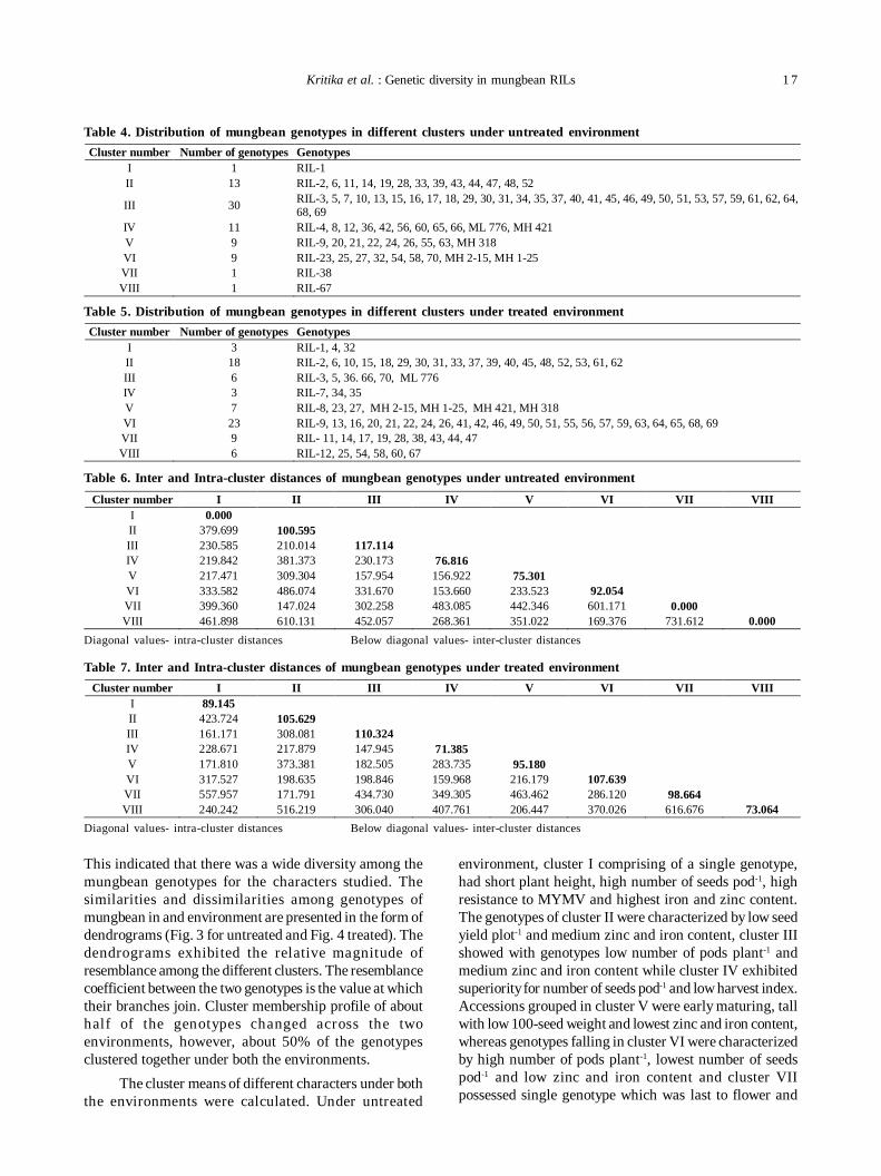
Kritika et al. : Genetic diversity in mungbean RILs 1 7
This indicated that there was a wide diversity among themungbean genotypes for the characters studied. Thesimilarities and dissimilarities among genotypes ofmungbean in and environment are presented in the form ofdendrograms (Fig. 3 for untreated and Fig. 4 treated). Thedendrograms exhibited the relative magnitude ofresemblance among the different clusters. The resemblancecoefficient between the two genotypes is the value at whichtheir branches join. Cluster membership profile of abouthalf of the genotypes changed across the twoenvironments, however, about 50% of the genotypesclustered together under both the environments.
The cluster means of different characters under boththe environments were calculated. Under untreated
environment, cluster I comprising of a single genotype,had short plant height, high number of seeds pod-1, highresistance to MYMV and highest iron and zinc content.The genotypes of cluster II were characterized by low seedyield plot-1 and medium zinc and iron content, cluster IIIshowed with genotypes low number of pods plant-1 andmedium zinc and iron content while cluster IV exhibitedsuperiority for number of seeds pod-1 and low harvest index.Accessions grouped in cluster V were early maturing, tallwith low 100-seed weight and lowest zinc and iron content,whereas genotypes falling in cluster VI were characterizedby high number of pods plant-1, lowest number of seedspod-1 and low zinc and iron content and cluster VIIpossessed single genotype which was last to flower and
Table 4. Distribution of mungbean genotypes in different clusters under untreated environmentCluster number Number of genotypes Genotypes
I 1 RIL-1 II 13 RIL-2, 6, 11, 14, 19, 28, 33, 39, 43, 44, 47, 48, 52
III 30 RIL-3, 5, 7, 10, 13, 15, 16, 17, 18, 29, 30, 31, 34, 35, 37, 40, 41, 45, 46, 49, 50, 51, 53, 57, 59, 61, 62, 64, 68, 69
IV 11 RIL-4, 8, 12, 36, 42, 56, 60, 65, 66, ML 776, MH 421 V 9 RIL-9, 20, 21, 22, 24, 26, 55, 63, MH 318 VI 9 RIL-23, 25, 27, 32, 54, 58, 70, MH 2-15, MH 1-25 VII 1 RIL-38 VIII 1 RIL-67
Table 5. Distribution of mungbean genotypes in different clusters under treated environmentCluster number Number of genotypes Genotypes
I 3 RIL-1, 4, 32 II 18 RIL-2, 6, 10, 15, 18, 29, 30, 31, 33, 37, 39, 40, 45, 48, 52, 53, 61, 62 III 6 RIL-3, 5, 36. 66, 70, ML 776 IV 3 RIL-7, 34, 35 V 7 RIL-8, 23, 27, MH 2-15, MH 1-25, MH 421, MH 318 VI 23 RIL-9, 13, 16, 20, 21, 22, 24, 26, 41, 42, 46, 49, 50, 51, 55, 56, 57, 59, 63, 64, 65, 68, 69 VII 9 RIL- 11, 14, 17, 19, 28, 38, 43, 44, 47 VIII 6 RIL-12, 25, 54, 58, 60, 67
Table 6. Inter and Intra-cluster distances of mungbean genotypes under untreated environment
Diagonal values- intra-cluster distances Below diagonal values- inter-cluster distances
Cluster number I II III IV V VI VII VIII I 0.000 II 379.699 100.595 III 230.585 210.014 117.114 IV 219.842 381.373 230.173 76.816 V 217.471 309.304 157.954 156.922 75.301 VI 333.582 486.074 331.670 153.660 233.523 92.054 VII 399.360 147.024 302.258 483.085 442.346 601.171 0.000 VIII 461.898 610.131 452.057 268.361 351.022 169.376 731.612 0.000
Table 7. Inter and Intra-cluster distances of mungbean genotypes under treated environment
Diagonal values- intra-cluster distances Below diagonal values- inter-cluster distances
Cluster number I II III IV V VI VII VIII I 89.145 II 423.724 105.629 III 161.171 308.081 110.324 IV 228.671 217.879 147.945 71.385 V 171.810 373.381 182.505 283.735 95.180 VI 317.527 198.635 198.846 159.968 216.179 107.639 VII 557.957 171.791 434.730 349.305 463.462 286.120 98.664 VIII 240.242 516.219 306.040 407.761 206.447 370.026 616.676 73.064
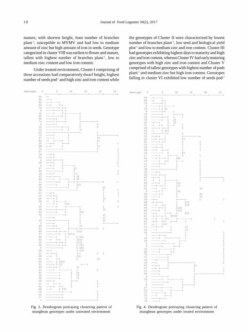
1 8 Journal of Food Legumes 30(2), 2017
mature, with shortest height, least number of branchesplant-1, susceptible to MYMV and had low to mediumamount of zinc but high amount of iron in seeds. Genotypecategorized in cluster VIII was earliest to flower and mature,tallest with highest number of branches plant-1, low tomedium zinc content and low iron content.
Under treated environment, Cluster I comprising ofthree accessions had comparatively dwarf height, highestnumber of seeds pod-1 and high zinc and iron content while
the genotypes of Cluster II were characterized by lowestnumber of branches plant-1, low seed and biological yieldplot-1 and low to medium zinc and iron content. Cluster IIIhad genotypes exhibiting highest days to maturity and highzinc and iron content, whereas Cluster IV had early maturinggenotypes with high zinc and iron content and Cluster Vcomprised of tallest genotypes with highest number of podsplant-1 and medium zinc but high iron content. Genotypesfalling in cluster VI exhibited low number of seeds pod-1
Fig. 3. Dendrogram portraying clustering pattern ofmungbean genotypes under untreated environment
Genotype 0 5 10 15 20 25 +---------+---------+---------+---------+---------+ 65 -+ 66 -+-+ 42 -+ +-----+ 56 ---+ +-+ 74 ---------+ +-+ 8 -----+-----+ I 12 -----+ I +---------+ 60 -----------+ I I 36 -----+-+ I I 71 -----+ +-----+ +-----------+ 4 -------+ I I 32 -----------+---+ I I 70 -----------+ I II 23 -----+---------+-------+ I 73 -----+ I +-------------+ 27 -+---+ I II 54 -+ +-----+ I II 25 ---+-+ +---+ I I 58 ---+ I II 72 -----------+ I I 67 -----------------------------------+ I 39 ---+-+ I 52 ---+ I I 2 -+-+ +-----+ I 48 -+ +-+ I I 6 ---+ I +-------+ I 47 -----+ I II 33 -----------+ I I 14 ---+-+ +-+ I 43 ---+ +---+ I II 44 -----+ +-----+ I II 11 -------+-+ +---+ +-----------------+ I 28 -------+ I III 19 ---------------+ I II 38 ---------------------+ I I 21 ---+-+ I I 22 ---+ +-+ I I 20 -+---+ I II 24 -+ I +-----+ I I 9 -----+ I III 55 -------+ +---------+ I I 26 -------+-----+ I II 63 -------+ I III 75 -------------+ I II 7 -----+ I II 10 -----+---------+ I II 3 -----+ I I +---------+ 49 -----+-+ I II 53 -----+ +-+ +-----+ +-----------+ I 40 -------+ +---+ I IIII 37 ---------+ I IIIII 46 ---+---+ +-+ I III 50 ---+ +-+ I IIII 35 -------+ +-+ I IIII 34 ---------+ +-+ I III 5 -----------+ I III 29 -+-+ I III 51 -+ +---+ +-+ I I 69 ---+ I III 41 -+ +-+ I II 64 -+-+ I IIII 31 -+ +-+ I II +---+ 59 ---+ +-+ I II 13 -----+ +-------+ I I 61 ---------+ I II 16 ---------+ I II 30 ---------+ I II 45 -+---+ +---+ I 57 -+ +---+ I I 62 ---+-+ +-+ I I 68 ---+ I III 18 ---------+ +-----+ I 15 -----------+ I 17 -----------+ I 1 -----------------------------------+
Fig. 4. Dendrogram portraying clustering pattern ofmungbean genotypes under treated environment
Genotype 0 5 10 15 20 25 +---------+---------+---------+---------+---------+ 39 -+-----+ 48 -+ +-+ 10 -------+ I
2 -----+-+ +-----+ 33 -----+ I II 6 -------+-+ I 37 -------+ +-----+ 18 -------+---+ I I 30 -------+ I II 29 -+---+ I II 31 -+ +-+ +---+ I 40 -+---+ +-+ I I 45 -+ I III 53 -------+ +-+ I 52 ---+-+ I +-----------+ 62 ---+ +-+ I II 61 -----+ +-+ I I
15 -------+ I I 28 ---+---+ I I 44 ---+ +---+ I I 14 -------+ I II 17 ---+-+ +-----+ I I 43 ---+ +---+ I III 19 -----+ +-+ +---+ I 11 -----+---+ I I 47 -----+ I I 38 -----------------+ I 56 ---+-+ I 64 ---+ +---+ I 20 -+---+ I +---------------+ 21 -+ I +-------+ I I 65 -----+ I III 59 ---+---+ I III 63 ---+ +-+ I II 9 ---+-+ I III 42 ---+ +-+ I II 26 -----+ I II 46 -+-+ +-----+ I I 68 -+ +---+ I III 49 ---+ +-+ I III 50 -----+-+ I IIII 69 -----+ I IIII 22 -+-+ +---+ I III 41 -+ +---+ I IIIII 24 ---+ I III +---------+ I 51 -+-+ +-+ +---+ I I 57 -+ I IIII 13 ---+---+ I II 16 ---+ I II 55 -------------+ I I 7 -----+---+ I I 34 -----+ +---------+ I I 35 ---------+ +---+ I 3 -------+-------+ I I 5 -------+ +---+ I 36 -----+-------+ I I 66 -----+ +-+ I 70 -----------+-+ I 71 -----------+ I 25 ---+-------+ I 54 ---+ +-----------------+ I 60 ---+-+ I II 67 ---+ +-----+ I I 12 -----+ I I 58 -----+ +-------------------+ 4 -------+---+ I 32 -------+ +---------+ I 1 -----------+ I I 8 -------+ +-------+ 27 -------+-----+ I 23 -------+ +-------+ 73 ---+-----+ I 75 ---+ +---+ 72 -----+---+ 74 -----+
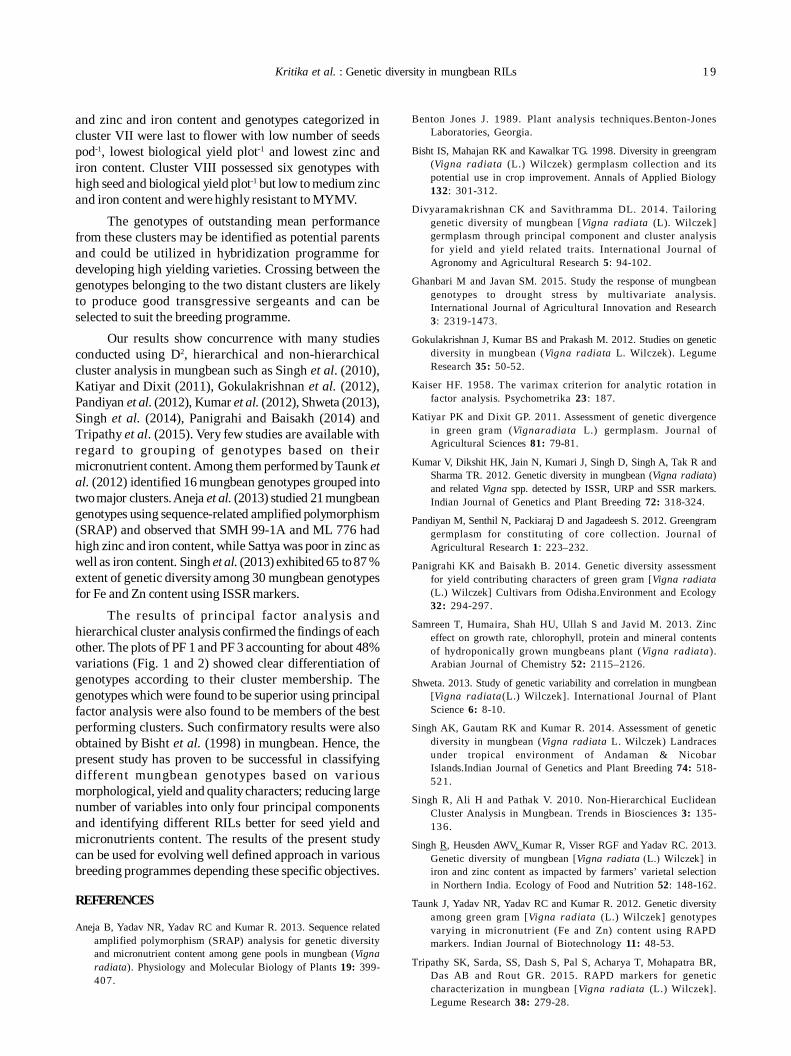
Kritika et al. : Genetic diversity in mungbean RILs 1 9
and zinc and iron content and genotypes categorized incluster VII were last to flower with low number of seedspod-1, lowest biological yield plot-1 and lowest zinc andiron content. Cluster VIII possessed six genotypes withhigh seed and biological yield plot-1 but low to medium zincand iron content and were highly resistant to MYMV.
The genotypes of outstanding mean performancefrom these clusters may be identified as potential parentsand could be utilized in hybridization programme fordeveloping high yielding varieties. Crossing between thegenotypes belonging to the two distant clusters are likelyto produce good transgressive sergeants and can beselected to suit the breeding programme.
Our results show concurrence with many studiesconducted using D2, hierarchical and non-hierarchicalcluster analysis in mungbean such as Singh et al. (2010),Katiyar and Dixit (2011), Gokulakrishnan et al. (2012),Pandiyan et al. (2012), Kumar et al. (2012), Shweta (2013),Singh et al. (2014), Panigrahi and Baisakh (2014) andTripathy et al. (2015). Very few studies are available withregard to grouping of genotypes based on theirmicronutrient content. Among them performed by Taunk etal. (2012) identified 16 mungbean genotypes grouped intotwo major clusters. Aneja et al. (2013) studied 21 mungbeangenotypes using sequence-related amplified polymorphism(SRAP) and observed that SMH 99-1A and ML 776 hadhigh zinc and iron content, while Sattya was poor in zinc aswell as iron content. Singh et al. (2013) exhibited 65 to 87 %extent of genetic diversity among 30 mungbean genotypesfor Fe and Zn content using ISSR markers.
The results of principal factor analysis andhierarchical cluster analysis confirmed the findings of eachother. The plots of PF 1 and PF 3 accounting for about 48%variations (Fig. 1 and 2) showed clear differentiation ofgenotypes according to their cluster membership. Thegenotypes which were found to be superior using principalfactor analysis were also found to be members of the bestperforming clusters. Such confirmatory results were alsoobtained by Bisht et al. (1998) in mungbean. Hence, thepresent study has proven to be successful in classifyingdifferent mungbean genotypes based on variousmorphological, yield and quality characters; reducing largenumber of variables into only four principal componentsand identifying different RILs better for seed yield andmicronutrients content. The results of the present studycan be used for evolving well defined approach in variousbreeding programmes depending these specific objectives.
REFERENCES
Aneja B, Yadav NR, Yadav RC and Kumar R. 2013. Sequence relatedamplified polymorphism (SRAP) analysis for genetic diversityand micronutrient content among gene pools in mungbean (Vignaradiata). Physiology and Molecular Biology of Plants 19: 399-407.
Benton Jones J. 1989. Plant analysis techniques.Benton-JonesLaboratories, Georgia.
Bisht IS, Mahajan RK and Kawalkar TG. 1998. Diversity in greengram(Vigna radiata (L.) Wilczek) germplasm collection and itspotential use in crop improvement. Annals of Applied Biology132: 301-312.
Divyaramakrishnan CK and Savithramma DL. 2014. Tailoringgenetic diversity of mungbean [Vigna radiata (L). Wilczek]germplasm through principal component and cluster analysisfor yield and yield related traits. International Journal ofAgronomy and Agricultural Research 5: 94-102.
Ghanbari M and Javan SM. 2015. Study the response of mungbeangenotypes to drought stress by multivariate analysis.International Journal of Agricultural Innovation and Research3: 2319-1473.
Gokulakrishnan J, Kumar BS and Prakash M. 2012. Studies on geneticdiversity in mungbean (Vigna radiata L. Wilczek). LegumeResearch 35: 50-52.
Kaiser HF. 1958. The varimax criterion for analytic rotation infactor analysis. Psychometrika 23: 187.
Katiyar PK and Dixit GP. 2011. Assessment of genetic divergencein green gram (Vignaradiata L.) germplasm. Journal ofAgricultural Sciences 81: 79-81.
Kumar V, Dikshit HK, Jain N, Kumari J, Singh D, Singh A, Tak R andSharma TR. 2012. Genetic diversity in mungbean (Vigna radiata)and related Vigna spp. detected by ISSR, URP and SSR markers.Indian Journal of Genetics and Plant Breeding 72: 318-324.
Pandiyan M, Senthil N, Packiaraj D and Jagadeesh S. 2012. Greengramgermplasm for constituting of core collection. Journal ofAgricultural Research 1: 223–232.
Panigrahi KK and Baisakh B. 2014. Genetic diversity assessmentfor yield contributing characters of green gram [Vigna radiata(L.) Wilczek] Cultivars from Odisha.Environment and Ecology32: 294-297.
Samreen T, Humaira, Shah HU, Ullah S and Javid M. 2013. Zinceffect on growth rate, chlorophyll, protein and mineral contentsof hydroponically grown mungbeans plant (Vigna radiata).Arabian Journal of Chemistry 52: 2115–2126.
Shweta. 2013. Study of genetic variability and correlation in mungbean[Vigna radiata(L.) Wilczek]. International Journal of PlantScience 6: 8-10.
Singh AK, Gautam RK and Kumar R. 2014. Assessment of geneticdiversity in mungbean (Vigna radiata L. Wilczek) Landracesunder tropical environment of Andaman & NicobarIslands.Indian Journal of Genetics and Plant Breeding 74: 518-521.
Singh R, Ali H and Pathak V. 2010. Non-Hierarchical EuclideanCluster Analysis in Mungbean. Trends in Biosciences 3: 135-136.
Singh R, Heusden AWV, Kumar R, Visser RGF and Yadav RC. 2013.Genetic diversity of mungbean [Vigna radiata (L.) Wilczek] iniron and zinc content as impacted by farmers’ varietal selectionin Northern India. Ecology of Food and Nutrition 52: 148-162.
Taunk J, Yadav NR, Yadav RC and Kumar R. 2012. Genetic diversityamong green gram [Vigna radiata (L.) Wilczek] genotypesvarying in micronutrient (Fe and Zn) content using RAPDmarkers. Indian Journal of Biotechnology 11: 48-53.
Tripathy SK, Sarda, SS, Dash S, Pal S, Acharya T, Mohapatra BR,Das AB and Rout GR. 2015. RAPD markers for geneticcharacterization in mungbean [Vigna radiata (L.) Wilczek].Legume Research 38: 279-28.

2 0 Journal of Food Legumes 30(2), 2017
Welch RM. 2002. Breeding strategies for biofortified staple plantfoods to reduce micronutrient malnutrition globally. Journal ofNutrition 132: 495S–499S.
Welch RM and Graham RD. 2004.Breeding for micronutrients instaple food crops from a human nutrition perspective. Journalof Experimental Botany 55: 353-364.
Yimram T, Somta P and Srinives P. 2009. Genetic variation incultivated mungbean germplasm and its implication in breedingfor high yield. Field Crops Research 112: 260-266.
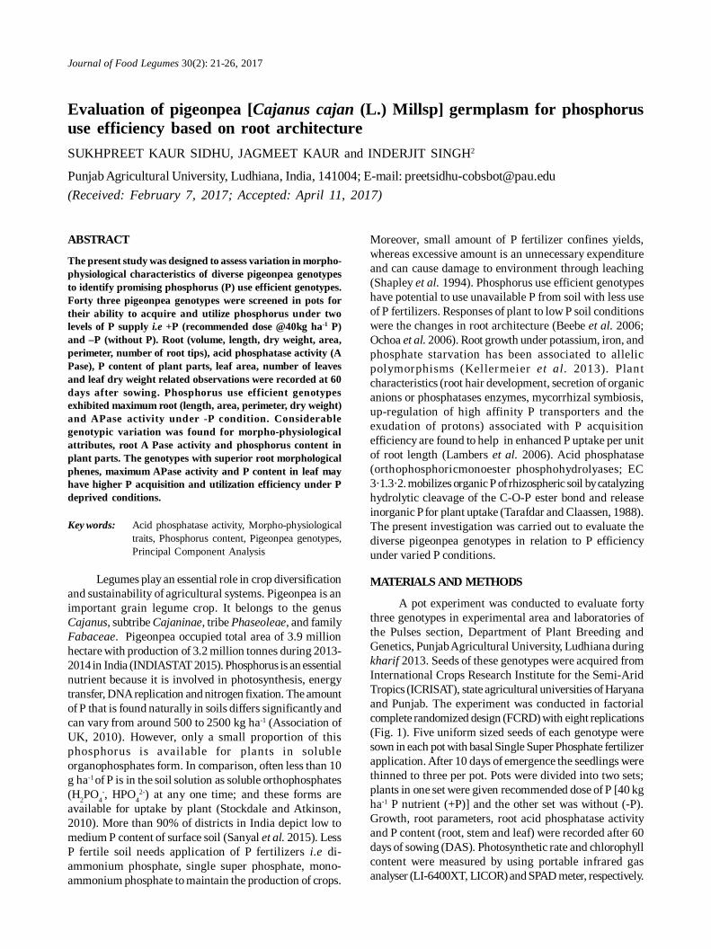
Journal of Food Legumes 30(2): 21-26, 2017
Evaluation of pigeonpea [Cajanus cajan (L.) Millsp] germplasm for phosphorususe efficiency based on root architectureSUKHPREET KAUR SIDHU, JAGMEET KAUR and INDERJIT SINGH2
Punjab Agricultural University, Ludhiana, India, 141004; E-mail: [email protected](Received: February 7, 2017; Accepted: April 11, 2017)
ABSTRACT
The present study was designed to assess variation in morpho-physiological characteristics of diverse pigeonpea genotypesto identify promising phosphorus (P) use efficient genotypes.Forty three pigeonpea genotypes were screened in pots fortheir ability to acquire and utilize phosphorus under twolevels of P supply i.e +P (recommended dose @40kg ha-1 P)and –P (without P). Root (volume, length, dry weight, area,perimeter, number of root tips), acid phosphatase activity (APase), P content of plant parts, leaf area, number of leavesand leaf dry weight related observations were recorded at 60days after sowing. Phosphorus use efficient genotypesexhibited maximum root (length, area, perimeter, dry weight)and APase activity under -P condition. Considerablegenotypic variation was found for morpho-physiologicalattributes, root A Pase activity and phosphorus content inplant parts. The genotypes with superior root morphologicalphenes, maximum APase activity and P content in leaf mayhave higher P acquisition and utilization efficiency under Pdeprived conditions.
Key words: Acid phosphatase activity, Morpho-physiologicaltraits, Phosphorus content, Pigeonpea genotypes,Principal Component Analysis
Legumes play an essential role in crop diversificationand sustainability of agricultural systems. Pigeonpea is animportant grain legume crop. It belongs to the genusCajanus, subtribe Cajaninae, tribe Phaseoleae, and familyFabaceae. Pigeonpea occupied total area of 3.9 millionhectare with production of 3.2 million tonnes during 2013-2014 in India (INDIASTAT 2015). Phosphorus is an essentialnutrient because it is involved in photosynthesis, energytransfer, DNA replication and nitrogen fixation. The amountof P that is found naturally in soils differs significantly andcan vary from around 500 to 2500 kg ha-1 (Association ofUK, 2010). However, only a small proportion of thisphosphorus is available for plants in solubleorganophosphates form. In comparison, often less than 10g ha-1 of P is in the soil solution as soluble orthophosphates(H2PO4
-, HPO42-) at any one time; and these forms are
available for uptake by plant (Stockdale and Atkinson,2010). More than 90% of districts in India depict low tomedium P content of surface soil (Sanyal et al. 2015). LessP fertile soil needs application of P fertilizers i.e di-ammonium phosphate, single super phosphate, mono-ammonium phosphate to maintain the production of crops.
Moreover, small amount of P fertilizer confines yields,whereas excessive amount is an unnecessary expenditureand can cause damage to environment through leaching(Shapley et al. 1994). Phosphorus use efficient genotypeshave potential to use unavailable P from soil with less useof P fertilizers. Responses of plant to low P soil conditionswere the changes in root architecture (Beebe et al. 2006;Ochoa et al. 2006). Root growth under potassium, iron, andphosphate starvation has been associated to allelicpolymorphisms (Kellermeier et al. 2013). Plantcharacteristics (root hair development, secretion of organicanions or phosphatases enzymes, mycorrhizal symbiosis,up-regulation of high affinity P transporters and theexudation of protons) associated with P acquisitionefficiency are found to help in enhanced P uptake per unitof root length (Lambers et al. 2006). Acid phosphatase(orthophosphoricmonoester phosphohydrolyases; EC3·1.3·2. mobilizes organic P of rhizospheric soil by catalyzinghydrolytic cleavage of the C-O-P ester bond and releaseinorganic P for plant uptake (Tarafdar and Claassen, 1988).The present investigation was carried out to evaluate thediverse pigeonpea genotypes in relation to P efficiencyunder varied P conditions.
MATERIALS AND METHODS
A pot experiment was conducted to evaluate fortythree genotypes in experimental area and laboratories ofthe Pulses section, Department of Plant Breeding andGenetics, Punjab Agricultural University, Ludhiana duringkharif 2013. Seeds of these genotypes were acquired fromInternational Crops Research Institute for the Semi-AridTropics (ICRISAT), state agricultural universities of Haryanaand Punjab. The experiment was conducted in factorialcomplete randomized design (FCRD) with eight replications(Fig. 1). Five uniform sized seeds of each genotype weresown in each pot with basal Single Super Phosphate fertilizerapplication. After 10 days of emergence the seedlings werethinned to three per pot. Pots were divided into two sets;plants in one set were given recommended dose of P [40 kgha-1 P nutrient (+P)] and the other set was without (-P).Growth, root parameters, root acid phosphatase activityand P content (root, stem and leaf) were recorded after 60days of sowing (DAS). Photosynthetic rate and chlorophyllcontent were measured by using portable infrared gasanalyser (LI-6400XT, LICOR) and SPAD meter, respectively.
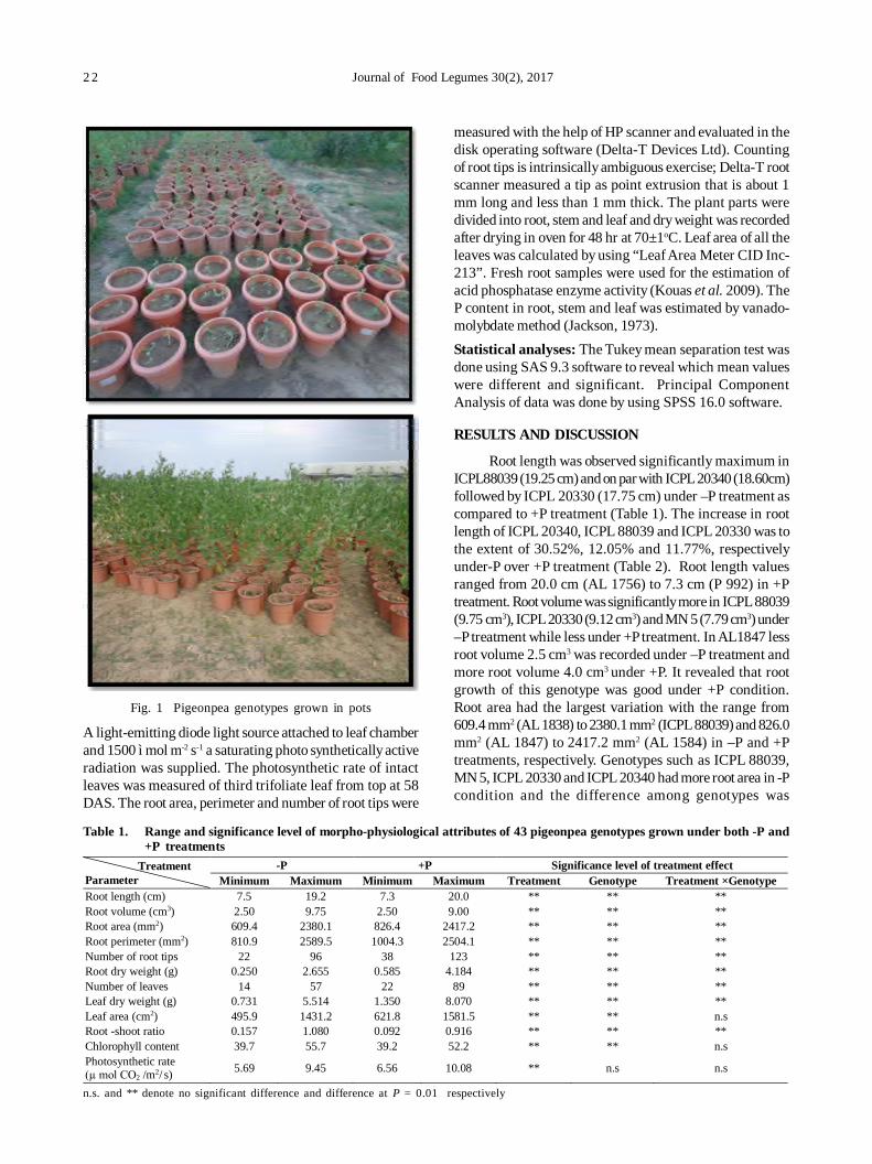
2 2 Journal of Food Legumes 30(2), 2017
measured with the help of HP scanner and evaluated in thedisk operating software (Delta-T Devices Ltd). Countingof root tips is intrinsically ambiguous exercise; Delta-T rootscanner measured a tip as point extrusion that is about 1mm long and less than 1 mm thick. The plant parts weredivided into root, stem and leaf and dry weight was recordedafter drying in oven for 48 hr at 70±1oC. Leaf area of all theleaves was calculated by using “Leaf Area Meter CID Inc-213”. Fresh root samples were used for the estimation ofacid phosphatase enzyme activity (Kouas et al. 2009). TheP content in root, stem and leaf was estimated by vanado-molybdate method (Jackson, 1973).Statistical analyses: The Tukey mean separation test wasdone using SAS 9.3 software to reveal which mean valueswere different and significant. Principal ComponentAnalysis of data was done by using SPSS 16.0 software.
RESULTS AND DISCUSSION
Root length was observed significantly maximum inICPL88039 (19.25 cm) and on par with ICPL 20340 (18.60cm)followed by ICPL 20330 (17.75 cm) under –P treatment ascompared to +P treatment (Table 1). The increase in rootlength of ICPL 20340, ICPL 88039 and ICPL 20330 was tothe extent of 30.52%, 12.05% and 11.77%, respectivelyunder-P over +P treatment (Table 2). Root length valuesranged from 20.0 cm (AL 1756) to 7.3 cm (P 992) in +Ptreatment. Root volume was significantly more in ICPL 88039(9.75 cm3), ICPL 20330 (9.12 cm3) and MN 5 (7.79 cm3) under–P treatment while less under +P treatment. In AL1847 lessroot volume 2.5 cm3 was recorded under –P treatment andmore root volume 4.0 cm3 under +P. It revealed that rootgrowth of this genotype was good under +P condition.Root area had the largest variation with the range from609.4 mm2 (AL 1838) to 2380.1 mm2 (ICPL 88039) and 826.0mm2 (AL 1847) to 2417.2 mm2 (AL 1584) in –P and +Ptreatments, respectively. Genotypes such as ICPL 88039,MN 5, ICPL 20330 and ICPL 20340 had more root area in -Pcondition and the difference among genotypes was
Table 1. Range and significance level of morpho-physiological attributes of 43 pigeonpea genotypes grown under both -P and+P treatments
n.s. and ** denote no significant difference and difference at P = 0.01 respectively
Fig. 1 Pigeonpea genotypes grown in pots
A light-emitting diode light source attached to leaf chamberand 1500 ì mol m-2 s-1 a saturating photo synthetically activeradiation was supplied. The photosynthetic rate of intactleaves was measured of third trifoliate leaf from top at 58DAS. The root area, perimeter and number of root tips were
Treatment Parameter
-P +P Significance level of treatment effect Minimum Maximum Minimum Maximum Treatment Genotype Treatment ×Genotype
Root length (cm) 7.5 19.2 7.3 20.0 ** ** ** Root volume (cm3) 2.50 9.75 2.50 9.00 ** ** ** Root area (mm2) 609.4 2380.1 826.4 2417.2 ** ** ** Root perimeter (mm2) 810.9 2589.5 1004.3 2504.1 ** ** ** Number of root tips 22 96 38 123 ** ** ** Root dry weight (g) 0.250 2.655 0.585 4.184 ** ** ** Number of leaves 14 57 22 89 ** ** ** Leaf dry weight (g) 0.731 5.514 1.350 8.070 ** ** ** Leaf area (cm2) 495.9 1431.2 621.8 1581.5 ** ** n.s Root -shoot ratio 0.157 1.080 0.092 0.916 ** ** ** Chlorophyll content 39.7 55.7 39.2 52.2 ** ** n.s Photosynthetic rate (µ mol CO2 /m2/ s) 5.69 9.45 6.56 10.08 ** n.s n.s
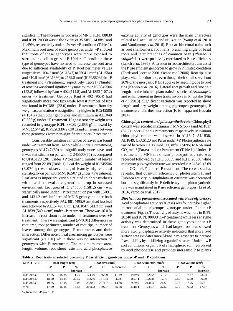
Sindhu et al. : Evaluation of pigeonpea germplasm for phosphorus use efficiency 2 3
significant. The increase in root area of MN 5, ICPL 88039and ICPL 20330 was to the extent of 35.58%, 14.88% and11.49%, respectively under –P over +P condition (Table 2).Maximum root area of some genotypes under –P showedthat roots of these genotypes were more exposed tosurrounding soil to get soil P. Under +P condition thesetype of genotypes have no need to increase the root areadue to sufficient availability of P. Root perimeter valuesranged from 1004.3 mm2 (AL1847) to 2504.1 mm2 (AL1584)and 810.9 mm2 (AL1836) to 2589.5 mm2 (ICPL88039) in –Ptreatment and +P treatment, respectively (Table1). Numberof root tips was found significantly maximum in IC 5045506(123.8) followed by Pant A 402 (114.8) and AL1853 (107.2)under +P treatment. Genotype Pant A 402 (96.4) hadsignificantly more root tips while lowest number of tipswas found in PAU881 (22.0) under –P treatment. Root dryweight accumulation was significantly higher in IC 245506(4.184 g) than other genotypes and minimum in AL1849(0.585 g) under +P treatment. Highest root dry weight wasrecorded in genotype ICPL 88039 (2.655 g) followed byMN5 (2.644 g), ICPL 20330 (2.630 g) and difference betweenthese genotypes were non-significant under–P treatment.
Considerable variation in number of leaves was foundunder –P treatment from 14 to 57 while under +P treatment,genotypes AL1747 (89) had significantly more leaves andit was statistically on par with IC 245506 (75) as comparedto UPAS120 (20). Under +P treatment, number of leavesranged from 22-89 (Table 1). Leaf dry weight of IC 245506(8.070 g) was observed significantly highest andstatistically on par with MN5 (6.507 g) under +P treatment.Leaf area is important variable related to photosynthesiswhich aids to evaluate growth of crop in stressedenvironment. Leaf area of IC 245506 (1581.5 cm2) wasstatistically more under + P treatment, on par with 1509.1and 1431.2 cm2 leaf area of MN 5 genotype under bothtreatments, respectively. PAU 881 (495.9 cm2) had less leafarea followed by AL15 (496.8 cm2), AL1847 (511.3 cm2) andAL1839 (549.4 cm2) under –P treatment. There was 16.0 %increase in root shoot ratio under –P treatment over +Ptreatment. There were significant (P<0.01) differences inroot area, root perimeter, number of root tips, number ofleaves among the genotypes, P treatments and theirinteraction. Difference of leaf area among genotypes weresignificant (P<0.01) while there was no interaction ofgenotypes with P treatments. The maximum root area,length, volume, root shoot ratio and acid phosphatase
enzyme activity of genotypes were the main charactersrelated to P acquisition and utilization (Wang et al. 2010and Vandamme et al. 2016). Root architectural traits suchas root shallowness, root hairs, branching angle of basalroots and later branches of common bean (Phaseolusvulgaris L.) were positively correlated to P use efficiency(Lynch et al. 1995). Alteration in root architecture can assistthe P use efficient genotypes to grow in P limited condition(Forde and Lorenzo 2001, Ochoa et al. 2006). Root tips alsoplay a vital function and, even though their small size, about20% of the inorganic P (Pi) uptake by seedling due to roottips (Kanno et al. 2016). Lateral root growth and root hairlength are the inherent plant traits in species of Arabidopsisand enhancement in these traits involve in Pi uptake (Niuet al. 2013). Significant variation was reported in shootlength and dry weight among pigeonpea genotypes, Ptreatments and in their interaction (Krishnappa and Hussain2014).Chlorophyll content and photosynthetic rate: Chlorophyllcontent was recorded maximum in MN 5 (55.7) and AL1817(52.2) under –P and +P treatments, respectively. Minimumchlorophyll content was observed in AL1847, AL1838,AL1849, UPAS120 and Paras under +P. Photosynthetic ratevaried between 10.08 ìmol CO2 m
-2s-1 (MN5) to 6.56 ìmolCO2 m
-2s-1 (Paras) under +P treatment (Table 1 ). Under –Ptreatment in MN5 maximum photosynthetic rate wasrecorded followed by ICPL 88039 and ICPL 20330 whileminimum photosynthetic rate was recorded in AL1849 (5.69ìmol CO2 m
-2s-1) under –P treatment. The recent studiesrevealed that quantum efficiency of photosystem II andRubisco activity in Amphidinium carterae was decreasedbut not significantly in P deficiency and photosyntheticrate was maintained in P use efficient genotypes (Li et al.2016, Veronica et al. 2017).Biochemical parameters associated with P use efficiency:Acid phosphatase activity (APase) was found to be higherin roots of all the pigeonpea genotypes under –P than +Ptreatment (Fig. 2). The activity of enzyme was more in ICPL20340 and ICPL 88039 in–P treatment while less enzymeactivity was determined in these genotypes under +Ptreatment. Genotypes which had largest root area showedmore acid phosphatase activity indicated that more rootsurface area exudates more APase in rhizosphere to increaseP availability by mobilizing organic P sources. Under low Psoil conditions, organic P of rhizospheric soil hydrolyzedby acid phosphatase and provides inorganic P to plants
Table 2. Root traits of selected promising P use efficient genotypes under -P and +P conditions.
% Increase: -P over +P
GENOTYPE Root length (cm) Root area (mm2) Root perimeter (mm2) Root volume (cm3) -P +P %
Increase -P +P % Increase -P +P %
Increase -P +P %
Increase ICPL20330 17.75 15.88 11.77 1743.6 1563.9 11.49 1949.9 1820.2 7.12 9.12 7.37 23.74 ICPL20340 18.60 14.25 30.52 1582.6 1510.4 4.78 1827.4 1620.8 12.75 7.50 5.00 50.00 ICPL88039 19.25 17.18 12.05 2380.1 2071.7 14.88 2589.5 2131.4 21.50 9.75 7.75 25.81 MN5 17.69 15.18 16.53 2166.2 1597.7 35.58 2318.4 1749.7 32.50 7.79 6.62 17.67
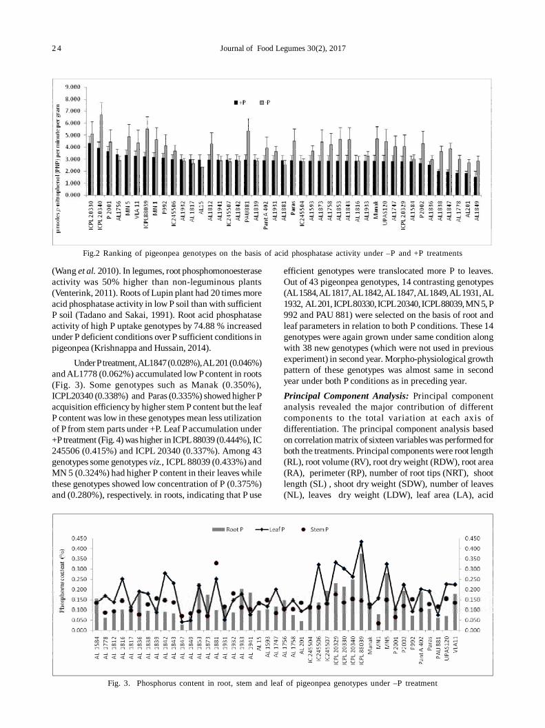
2 4 Journal of Food Legumes 30(2), 2017
(Wang et al. 2010). In legumes, root phosphomonoesteraseactivity was 50% higher than non-leguminous plants(Venterink, 2011). Roots of Lupin plant had 20 times moreacid phosphatase activity in low P soil than with sufficientP soil (Tadano and Sakai, 1991). Root acid phosphataseactivity of high P uptake genotypes by 74.88 % increasedunder P deficient conditions over P sufficient conditions inpigeonpea (Krishnappa and Hussain, 2014).
Under P treatment, AL1847 (0.028%), AL 201 (0.046%)and AL1778 (0.062%) accumulated low P content in roots(Fig. 3). Some genotypes such as Manak (0.350%),ICPL20340 (0.338%) and Paras (0.335%) showed higher Pacquisition efficiency by higher stem P content but the leafP content was low in these genotypes mean less utilizationof P from stem parts under +P. Leaf P accumulation under+P treatment (Fig. 4) was higher in ICPL 88039 (0.444%), IC245506 (0.415%) and ICPL 20340 (0.337%). Among 43genotypes some genotypes viz., ICPL 88039 (0.433%) andMN 5 (0.324%) had higher P content in their leaves whilethese genotypes showed low concentration of P (0.375%)and (0.280%), respectively. in roots, indicating that P use
efficient genotypes were translocated more P to leaves.Out of 43 pigeonpea genotypes, 14 contrasting genotypes(AL 1584, AL 1817, AL 1842, AL 1847, AL 1849, AL 1931, AL1932, AL 201, ICPL 80330, ICPL 20340, ICPL 88039, MN 5, P992 and PAU 881) were selected on the basis of root andleaf parameters in relation to both P conditions. These 14genotypes were again grown under same condition alongwith 38 new genotypes (which were not used in previousexperiment) in second year. Morpho-physiological growthpattern of these genotypes was almost same in secondyear under both P conditions as in preceding year.Principal Component Analysis: Principal componentanalysis revealed the major contribution of differentcomponents to the total variation at each axis ofdifferentiation. The principal component analysis basedon correlation matrix of sixteen variables was performed forboth the treatments. Principal components were root length(RL), root volume (RV), root dry weight (RDW), root area(RA), perimeter (RP), number of root tips (NRT), shootlength (SL) , shoot dry weight (SDW), number of leaves(NL), leaves dry weight (LDW), leaf area (LA), acid
Fig.2 Ranking of pigeonpea genotypes on the basis of acid phosphatase activity under –P and +P treatments
Fig. 3. Phosphorus content in root, stem and leaf of pigeonpea genotypes under –P treatment
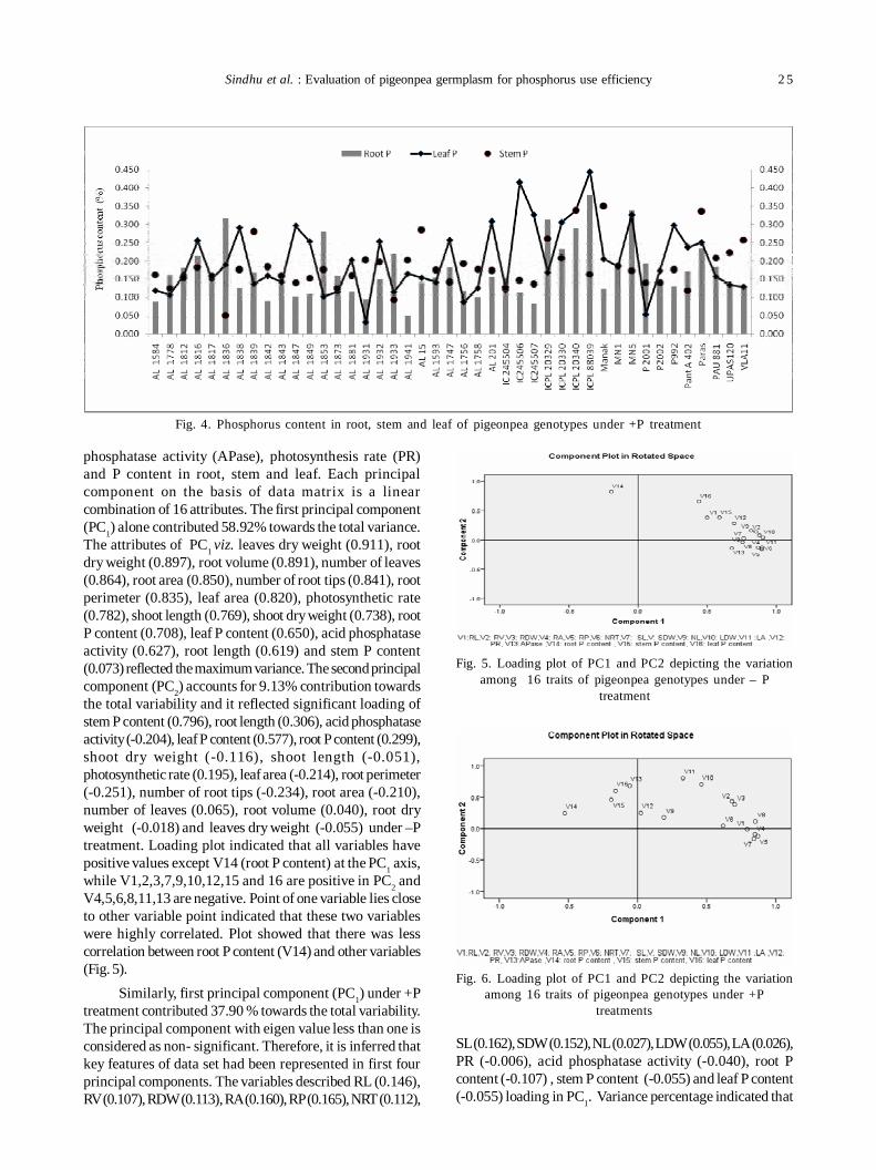
Sindhu et al. : Evaluation of pigeonpea germplasm for phosphorus use efficiency 2 5
phosphatase activity (APase), photosynthesis rate (PR)and P content in root, stem and leaf. Each principalcomponent on the basis of data matrix is a linearcombination of 16 attributes. The first principal component(PC1) alone contributed 58.92% towards the total variance.The attributes of PC1 viz. leaves dry weight (0.911), rootdry weight (0.897), root volume (0.891), number of leaves(0.864), root area (0.850), number of root tips (0.841), rootperimeter (0.835), leaf area (0.820), photosynthetic rate(0.782), shoot length (0.769), shoot dry weight (0.738), rootP content (0.708), leaf P content (0.650), acid phosphataseactivity (0.627), root length (0.619) and stem P content(0.073) reflected the maximum variance. The second principalcomponent (PC2) accounts for 9.13% contribution towardsthe total variability and it reflected significant loading ofstem P content (0.796), root length (0.306), acid phosphataseactivity (-0.204), leaf P content (0.577), root P content (0.299),shoot dry weight (-0.116), shoot length (-0.051),photosynthetic rate (0.195), leaf area (-0.214), root perimeter(-0.251), number of root tips (-0.234), root area (-0.210),number of leaves (0.065), root volume (0.040), root dryweight (-0.018) and leaves dry weight (-0.055) under –Ptreatment. Loading plot indicated that all variables havepositive values except V14 (root P content) at the PC1 axis,while V1,2,3,7,9,10,12,15 and 16 are positive in PC2 andV4,5,6,8,11,13 are negative. Point of one variable lies closeto other variable point indicated that these two variableswere highly correlated. Plot showed that there was lesscorrelation between root P content (V14) and other variables(Fig. 5).
Similarly, first principal component (PC1) under +Ptreatment contributed 37.90 % towards the total variability.The principal component with eigen value less than one isconsidered as non- significant. Therefore, it is inferred thatkey features of data set had been represented in first fourprincipal components. The variables described RL (0.146),RV (0.107), RDW (0.113), RA (0.160), RP (0.165), NRT (0.112),
SL (0.162), SDW (0.152), NL (0.027), LDW (0.055), LA (0.026),PR (-0.006), acid phosphatase activity (-0.040), root Pcontent (-0.107) , stem P content (-0.055) and leaf P content(-0.055) loading in PC1. Variance percentage indicated that
Fig. 4. Phosphorus content in root, stem and leaf of pigeonpea genotypes under +P treatment
Fig. 5. Loading plot of PC1 and PC2 depicting the variationamong 16 traits of pigeonpea genotypes under – P
treatment
Fig. 6. Loading plot of PC1 and PC2 depicting the variationamong 16 traits of pigeonpea genotypes under +P
treatments
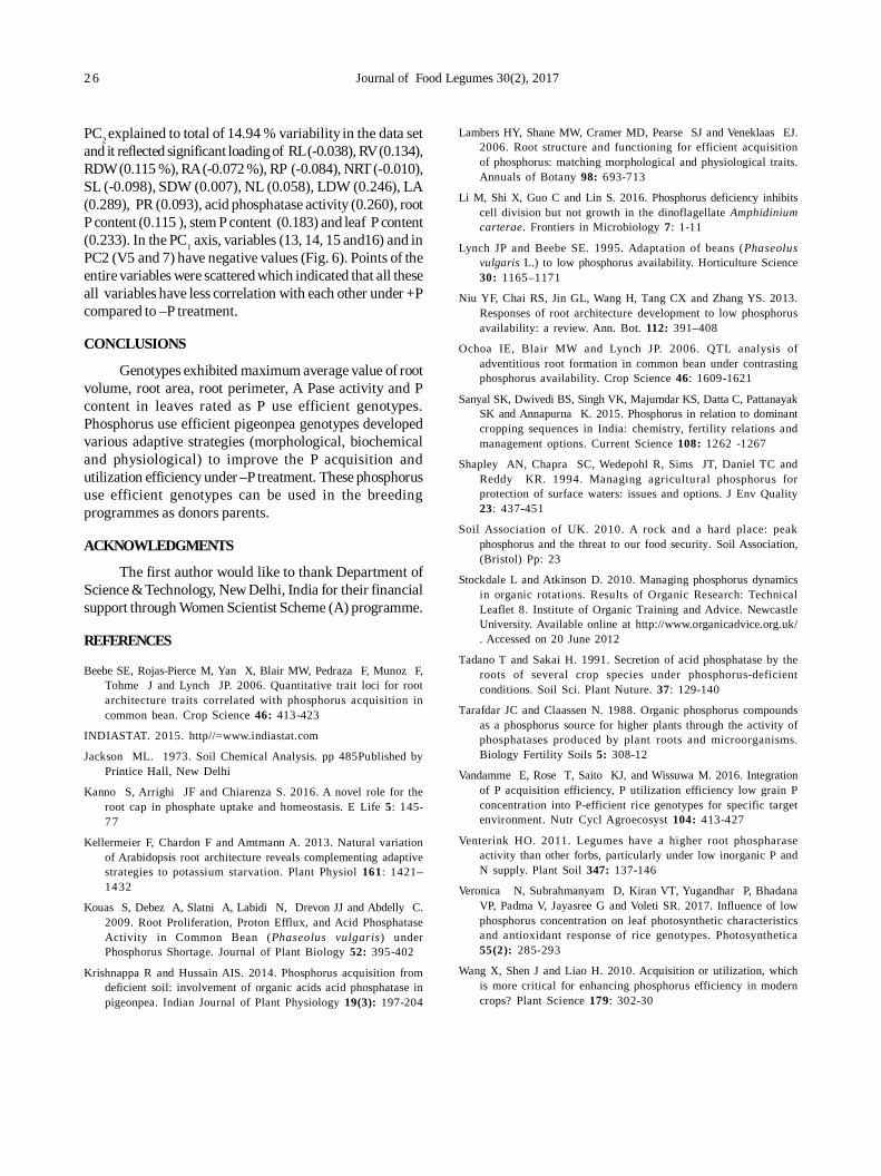
2 6 Journal of Food Legumes 30(2), 2017
PC2 explained to total of 14.94 % variability in the data setand it reflected significant loading of RL (-0.038), RV (0.134),RDW (0.115 %), RA (-0.072 %), RP (-0.084), NRT (-0.010),SL (-0.098), SDW (0.007), NL (0.058), LDW (0.246), LA(0.289), PR (0.093), acid phosphatase activity (0.260), rootP content (0.115 ), stem P content (0.183) and leaf P content(0.233). In the PC1 axis, variables (13, 14, 15 and16) and inPC2 (V5 and 7) have negative values (Fig. 6). Points of theentire variables were scattered which indicated that all theseall variables have less correlation with each other under +Pcompared to –P treatment.
CONCLUSIONS
Genotypes exhibited maximum average value of rootvolume, root area, root perimeter, A Pase activity and Pcontent in leaves rated as P use efficient genotypes.Phosphorus use efficient pigeonpea genotypes developedvarious adaptive strategies (morphological, biochemicaland physiological) to improve the P acquisition andutilization efficiency under –P treatment. These phosphorususe efficient genotypes can be used in the breedingprogrammes as donors parents.
ACKNOWLEDGMENTS
The first author would like to thank Department ofScience & Technology, New Delhi, India for their financialsupport through Women Scientist Scheme (A) programme.
REFERENCES
Beebe SE, Rojas-Pierce M, Yan X, Blair MW, Pedraza F, Munoz F,Tohme J and Lynch JP. 2006. Quantitative trait loci for rootarchitecture traits correlated with phosphorus acquisition incommon bean. Crop Science 46: 413-423
INDIASTAT. 2015. http//=www.indiastat.com
Jackson ML. 1973. Soil Chemical Analysis. pp 485Published byPrintice Hall, New Delhi
Kanno S, Arrighi JF and Chiarenza S. 2016. A novel role for theroot cap in phosphate uptake and homeostasis. E Life 5: 145-7 7
Kellermeier F, Chardon F and Amtmann A. 2013. Natural variationof Arabidopsis root architecture reveals complementing adaptivestrategies to potassium starvation. Plant Physiol 161: 1421–1432
Kouas S, Debez A, Slatni A, Labidi N, Drevon JJ and Abdelly C.2009. Root Proliferation, Proton Efflux, and Acid PhosphataseActivity in Common Bean (Phaseolus vulgaris) underPhosphorus Shortage. Journal of Plant Biology 52: 395-402
Krishnappa R and Hussain AIS. 2014. Phosphorus acquisition fromdeficient soil: involvement of organic acids acid phosphatase inpigeonpea. Indian Journal of Plant Physiology 19(3): 197-204
Lambers HY, Shane MW, Cramer MD, Pearse SJ and Veneklaas EJ.2006. Root structure and functioning for efficient acquisitionof phosphorus: matching morphological and physiological traits.Annuals of Botany 98: 693-713
Li M, Shi X, Guo C and Lin S. 2016. Phosphorus deficiency inhibitscell division but not growth in the dinoflagellate Amphidiniumcarterae. Frontiers in Microbiology 7: 1-11
Lynch JP and Beebe SE. 1995. Adaptation of beans (Phaseolusvulgaris L.) to low phosphorus availability. Horticulture Science30: 1165–1171
Niu YF, Chai RS, Jin GL, Wang H, Tang CX and Zhang YS. 2013.Responses of root architecture development to low phosphorusavailability: a review. Ann. Bot. 112: 391–408
Ochoa IE, Blair MW and Lynch JP. 2006. QTL analysis ofadventitious root formation in common bean under contrastingphosphorus availability. Crop Science 46: 1609-1621
Sanyal SK, Dwivedi BS, Singh VK, Majumdar KS, Datta C, PattanayakSK and Annapurna K. 2015. Phosphorus in relation to dominantcropping sequences in India: chemistry, fertility relations andmanagement options. Current Science 108: 1262 -1267
Shapley AN, Chapra SC, Wedepohl R, Sims JT, Daniel TC andReddy KR. 1994. Managing agricultural phosphorus forprotection of surface waters: issues and options. J Env Quality23: 437-451
Soil Association of UK. 2010. A rock and a hard place: peakphosphorus and the threat to our food security. Soil Association,(Bristol) Pp: 23
Stockdale L and Atkinson D. 2010. Managing phosphorus dynamicsin organic rotations. Results of Organic Research: TechnicalLeaflet 8. Institute of Organic Training and Advice. NewcastleUniversity. Available online at http://www.organicadvice.org.uk/. Accessed on 20 June 2012
Tadano T and Sakai H. 1991. Secretion of acid phosphatase by theroots of several crop species under phosphorus-deficientconditions. Soil Sci. Plant Nuture. 37: 129-140
Tarafdar JC and Claassen N. 1988. Organic phosphorus compoundsas a phosphorus source for higher plants through the activity ofphosphatases produced by plant roots and microorganisms.Biology Fertility Soils 5: 308-12
Vandamme E, Rose T, Saito KJ, and Wissuwa M. 2016. Integrationof P acquisition efficiency, P utilization efficiency low grain Pconcentration into P-efficient rice genotypes for specific targetenvironment. Nutr Cycl Agroecosyst 104: 413-427
Venterink HO. 2011. Legumes have a higher root phospharaseactivity than other forbs, particularly under low inorganic P andN supply. Plant Soil 347: 137-146
Veronica N, Subrahmanyam D, Kiran VT, Yugandhar P, BhadanaVP, Padma V, Jayasree G and Voleti SR. 2017. Influence of lowphosphorus concentration on leaf photosynthetic characteristicsand antioxidant response of rice genotypes. Photosynthetica55(2): 285-293
Wang X, Shen J and Liao H. 2010. Acquisition or utilization, whichis more critical for enhancing phosphorus efficiency in moderncrops? Plant Science 179: 302-30
Journal of Food Legumes 30(2): 27-30, 2017
Genetic variability and association analysis for yield, physiological and qualitytraits in drought tolerant groundnut genotypesA LOKESHWAR REDDY, T SRINIVAS, A PRASANNA RAJESH and P UMAMAHESWARI
Department of Genetics and Plant Breeding, Agricultural College, Mahanandi - 518 502, Andhra Pradesh, India;E-mail:[email protected](Received: July 1, 2016; Accepted: March 4, 2017)
ABSTRACT
Thirty drought tolerant groundnut genotypes developed atAgricultural Research Station, Kadiri of Anantapur District,Andhra Pradesh were evaluated for their variability withregards to yield, physiological and quality traits. Estimatesof heritability, genetic advance and genetic advance as percent mean were also obtained for the above traits. The resultsrevealed high to moderate GCV and PCV in addition to highheritability and high genetic advance as per cent mean forhaulm yield per plant and free proline content. Further,pods per plant, pod yield per plant, and 100 kernel weightswere observed with high positive direct effects and strongpositive associations with kernel yield per plant.Consequently, these attributes are identified as effectiveselection criteria for kernel yield improvement ingroundnut.
Key words: Correlation, Genetic advance, Groundnut,Heritability, Path analysis, Variability, Yield
India ranks first in groundnut cultivated area butoccupies second place in production. The productivity ofgroundnut in India is also low, primarily due to cultivationof the crop mostly under rainfed conditions with frequentdry spells. Therefore, there is an urgent need fordevelopment of high yielding drought tolerant varieties ingroundnut. Kernel yield in groundnut however is influencedby different yield components, physiological and qualitytraits, which makes direct selection for kernel yieldineffective, owing to its complex nature of inheritance. Inthis context, information on variability of the experimentalmaterial, heritability of the traits conditioning kernel yieldand their genetic advance, the nature and extent ofassociation between the yield component traits and theirassociation with kernel yields are pre-requisites forplanning of effective crop improvement programmes.Information on the direct and indirect effects of thesecomponent traits on kernel yield also aids in targetedselections and superior crop improvement. The presentinvestigation was undertaken in this context to study thevariability, heritability, genetic advance, characterassociations and path effects of yield components,physiological and quality traits on kernel yield with a viewto identify suitable selection criteria for higher kernel yieldin drought tolerant groundnut.
MATERIALS AND METHODS
Experimental material for the present investigationcomprised of 30 drought tolerant groundnut genotypesdeveloped at Agricultural Research Station, Kadiri ofAcharya N.G. Ranga Agricultural University. Thesegenotypes were sown during kharif 2015 at AgriculturalResearch Station, Kadiri of Ananthapuram District in AndhraPradesh state. Each genotype was sown in continuous tworow plots of 5m row length at spacing of 30cm betweenrows and 10cm between plants within the row in aRandomized Block Design with two replications. The cropwas raised under rainfed conditions and all recommendedpractices were followed to raise a healthy crop.Observations were recorded on yield and physiologicaland quality traits, such as days to 50 per cent flowering,pods per plant, pod yield per plant mature kernel per cent,kernel yield per plant, 100 kernel weight, SPAD chlorophyllmeter reading (SCMR), specific leaf area (SLA), oil, proteinand free proline content in seed. The observations wererecorded from five randomly selected plants for eachgenotype in each replication, while observations on daysto 50 per cent flowering, oil, protein and free proline contentin seeds were recorded on plot basis. The data collectedwas subjected to standard statistical procedures.Genotypic, phenotypic and environment co-efficient ofvariation, in addition to broad sense heritability and geneticadvance as per cent mean were calculated and categorizedas per standard procedures. Genotypic and phenotypiccorrelation coefficients in addition to the direct and indirecteffects of different yield attributes were also estimated andcategorized.
RESULTS AND DISCUSSION
The analysis of variance revealed highly significantmean squares due to genotypes for all traits, indicating theexistence of sufficient variation among the genotypes foryield, physiological and quality characters studied in thepresent investigation. Leading in a scope for their effectiveselection. Information on mean, range, phenotypiccoefficient of variation (PCV), genotypic coefficient ofvariation (GCV), environmental coefficient of variation(ECV), heritability, genetic advance and genetic advanceas per cent mean for yield, physiological and quality traits
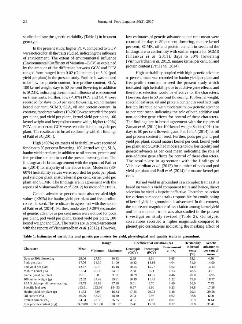
2 8 Journal of Food Legumes 30(2), 2017
studied indicate the genetic variability (Table 1) in frequentgenotype.
In the present study, higher PCV, compared to GCVwere noticed for all the traits studied, indicating the influenceof environment. The extent of environmental influence(Environmental Coefficient of Variation – ECV) as explainedby the amount of the difference between GCV and PCVranged from ranged from 0.02 (Oil content) to 5.02 (podyield per plant) in the present study. Further, it was noticedto be low for protein content, free proline content, SLA,100 kernel weight, days to 50 per cent flowering in additionto SCMR, indicating the minimal influence of environmenton these traits. Further, low (<10%) PCV and GCV wererecorded for days to 50 per cent flowering, sound maturekernel per cent, SCMR, SLA, oil and protein content. Incontrast, moderate values (10-20%) were recorded for podsper plant, pod yield per plant, kernel yield per plant, 100kernel weight and free proline content while, higher (>20%)PCV and moderate GCV were recorded for haulm yield perplant. The results are in broad conformity with the findingsof Patil et al. (2014).
High (>60%) estimates of heritability were recordedfor days to 50 per cent flowering, 100-kernel weight, SLA,haulm yield per plant, in addition to oil content, protein andfree proline content in seed the present investigation. Thefindings are in broad agreement with the reports of Patil etal. (2014) for majority of the above traits. Moderate (30-60%) heritability values were recorded for pods per plant,pod yield per plant, mature kernel per cent, kernel yield perplant and SCMR. The findings are in agreement with thereports of Vishnuvardhan et al. (2012) for most of the traits.
Genetic advance as per cent mean also revealed highvalues (>20%) for haulm yield per plant and free prolinecontent in seed. The results are in agreement with the reportsof Patil et al. (2014). Further, moderate (10-20%) estimatesof genetic advance as per cent mean were noticed for podsper plant, pod yield per plant, kernel yield per plant, 100kernel weight and SLA. The results are in broad agreementwith the reports of Vishnuvardhan et al. (2012). However,
low estimates of genetic advance as per cent mean wererecorded for days to 50 per cent flowering, mature kernelper cent, SCMR, oil and protein content in seed and thefindings are in conformity with earlier reports for SCMR(Thankur et al. 2011), days to 50% flowering(Vishnuvardhan et al. 2012), mature kernel per cent, oil andprotein content (Patil et al. 2014).
High heritability coupled with high genetic advanceas percent mean was recorded for haulm yield per plant andfree proline content in seed the present study whichindicated high heritability due to additive gene effects; andtherefore, selection would be effective for the characters.However, days to 50 per cent flowering, 100 kernel weight,specific leaf area, oil and protein content in seed had highheritability coupled with moderate to low genetic advanceas per cent mean indicating the role of both additive andnon-additive gene effects for control of these characters.The findings are in broad agreement with the reports ofZaman et al. (2011) for 100 kernel weight Satish (2014) fordays to 50 per cent flowering and Patil et al. (2014) for oiland protein content in seed. Further, pods per plant, podyield per plant, sound mature kernel per cent, kernel yieldper plant and SCMR had moderate to low heritability andgenetic advance as per cent mean indicating the role ofnon-additive gene effects for control of these characters.The results are in agreement with the findings ofVishnuvardhan et al. (2012) for number of pods and podyield per plant and Patil et al. (2014) for mature kernel percent.
Kernel yield in groundnut is a complex trait as it isbased on various yield component traits and hence, directselection for yield is largely ineffective. Therefore, selectionfor various component traits responsible for conditioningof kernel yield in groundnut is advocated. In this context,the nature and magnitude of association among kernel yieldand its component traits was also studied in the presentinvestigation study revised (Table 2). Genotypiccorrelations recorded a higher magnitude compared tophenotypic correlations indicating the masking effect of
Table 1. Estimates of variability and genetic parameters for yield, physiological and quality traits in groundnut.
Character Mean
Range Coefficient of variation (%) Heritability in broad
sense (%)
Genetic advance as per cent of
mean Minimum Maximum Genotypic
(GCV) Phenotypic
(PCV) Environment
(ECV)
Days to 50% flowering 29.06 27.50 30.33 2.69 3.34 0.65 65.1 4.50 Pods per plant 17.76 14.30 21.90 10.12 14.16 4.04 51.0 14.90 Pod yield per plant 12.87 9.73 15.48 10.25 15.27 5.02 44.9 14.15 Mature kernel (%) 81.54 76.33 84.67 2.58 3.71 1.13 48.5 3.71 Kernel yield per plant 8.16 5.05 9.52 10.39 14.85 4.46 49.0 14.95 100 kernel weight (g) 32.02 27.42 39.91 10.19 11.41 1.22 79.9 18.77 SPAD chlorophyll meter reading 43.73 38.88 47.38 5.01 6.70 1.69 56.0 7.73 Specific leaf area 163.61 132.66 184.53 8.67 8.90 0.23 94.8 17.38 Haulm yield per plant (g) 11.33 7.93 16.33 17.25 20.73 3.48 69.3 29.58 Oil content (%) 46.29 43.22 48.40 2.93 2.95 0.02 98.8 6.00 Protein content (%) 24.34 22.33 26.25 4.01 4.08 0.07 96.9 8.14 Free proline content (mg) 2419.80 1661.00 3080.17 15.41 15.58 0.17 97.8 31.41
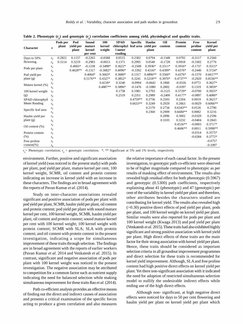
Reddy et al. : Variability, character association and path studies in groundnut 2 9
environment. Further, positive and significant associationof kernel yield (was noticed in the present study) with podsper plant, pod yield per plant, mature kernel per cent, 100kernel weight, SCMR, oil content and protein contentindicating an increase in kernel yield with an increase inthese characters. The findings are in broad agreement withthe reports of Pavan Kumar et al. (2014).
Study on inter-character associations revealedsignificant and positive association of pods per plant withpod yield per plant, SCMR, haulm yield per plant, oil contentand protein content; pod yield per plant with sound maturekernel per cent, 100 kernel weight, SCMR, haulm yield perplant, oil content and protein content; sound mature kernelper cent with 100 kernel weight; 100 kernel weight withprotein content; SCMR with SLA; SLA with proteincontent; and oil content with protein content in the presentinvestigation, indicating a scope for simultaneousimprovement of these traits through selection. The findingsare in broad agreement with the reports of earlier workers(Pavan Kumar et al. 2014 and Venkatesh et al. 2015). Incontrast, significant and negative association of pods perplant with 100 kernel weight was noticed in the presentinvestigation. The negative association may be attributedto competition for a common factor such as nutrient supplyindicating the need for balanced selection while makingsimultaneous improvement for these traits Rao et al. (2014).
Path co-efficient analysis provides an effective meansof finding out the direct and indirect causes of associationand presents a critical examination of the specific forcesacting to produce a given correlation and also measures
the relative importance of each causal factor. In the presentinvestigation, to genotypic path co-efficient were observedto be of higher magnitude compared to phenotypic as perresults of masking effect of environment. The results alsorevealed high residual effect for both phenotypic (0.5967)and genotypic (0.5300) path coefficients, respectivelyexplaining about 41 (phenotypic) and 47 (genotypic) percent of the variability in kernel yield per plant and therefore,other attributes besides the characters studied arecontributing for kernel yield. The results also revealed high(>0.30) positive direct effects of pod yield per plant, podsper plant, and 100 kernel weight on kernel yield per plant.Similar results were also reported for pods per plant and100 kernel weight (Kwaga 2013) and pod yield per plant(Venkatesh et al. 2015). These traits had also exhibited highlysignificant and strong positive association with kernel yieldper plant. High direct effects of these traits are the mainfactor for their strong association with kernel yield per plant.Hence, these traits should be considered as importantselection criteria in all groundnut improvement programmesand direct selection for these traits is recommended forkernel yield improvement. Although, SLA and free prolinecontent had high positive direct effects on kernel yield perplant. Yet there non-significant association with it indicatedthe need for adoption of restricted simultaneous selectionmodel to nullify the undesirable indirect effects whileending use of the high direct effects.
Although non- significant, at high negative directeffects were noticed for days to 50 per cent flowering andhaulm yield per plant on kernel yield per plant which
Table 2. Phenotypic (rp) and genotypic (rg) correlation coefficients among yield, physiological and quality traits.
rp= Phenotypic correlation; rg = genotypic correlation; *, ** Significant at 5% and 1% levels, respectively
Character r
Pods per plant
Pod yield per
plant
Sound mature kernel
per cent
100 kernel weight
SPAD chlorophyl
l meter reading
Specific leaf area
Haulm yield per
plant
Oil content
Protein content
Free proline content
Kernel yield per
plant
Days to 50% flowering
rp 0.2822 0.1157 -0.2263 -0.0588 0.0515 0.2302 0.0794 -0.1348 0.0792 -0.3117 0.2560
rg 0.3114 0.3219 -0.2983 -0.0653 0.1371 0.2995 0.0540 -0.1728 0.0918 -0.3302 0.2776
Pods per plant rp 0.4065* -0.1238 -0.3498* 0.3622* -0.2508 0.3936* 0.3511* 0.3916* -0.1737 0.3515*
rg 0.4628** -0.1317 -0.3682* 0.4096* -0.3392 0.4316* 0.4399* 0.4376* -0.2446 0.3724*
Pod yield per plant (g)
rp 0.4064* 0.3663* 0.3680* 0.1317 0.4896** 0.3560* 0.4376* -0.1570 0.6617**
rg 0.5176** 0.4327* 0.3852* 0.3241 0.5218** 0.3970* 0.4737** -0.2929 0.8336**
Mature kernel (%) rp 0.4218* 0.3240 -0.0994 -0.0642 0.1860 -0.0326 0.0772 0.3627*
rg 0.4887** 0.3896* -0.1476 -0.1080 0.2802 -0.0397 0.1319 0.3859*
100 kernel weight (g)
rp 0.1758 0.1981 0.2793 -0.2125 0.3729* -0.0700 0.3925*
rg 0.2519 0.2351 0.2989 -0.2400 0.4177* -0.0897 0.4080*
SPAD chlorophyll Meter Reading
rp 0.4759** 0.2736 0.2503 0.2204 0.0019 0.3621*
rg 0.6633** 0.3249 0.2929 0.2663 -0.0029 0.6066**
Specific leaf area rp 0.2170 0.2734 0.6343** 0.0126 0.2790
rg 0.2360 0.2909 0.6684** 0.0082 0.3216
Haulm yield per plant (g)
rp 0.2896 0.3002 -0.0329 0.2596
rg 0.3103 0.3232 -0.0404 0.2843
Oil content (%) rp 0.4516** -0.0003 0.3717*
rg 0.4606** 0.0011 0.5998**
Protein content (%)
rp -0.0314 0.3575*
rg -0.0284 0.3772*
Free proline content(%)
rp -0.0757 rg -0.1097
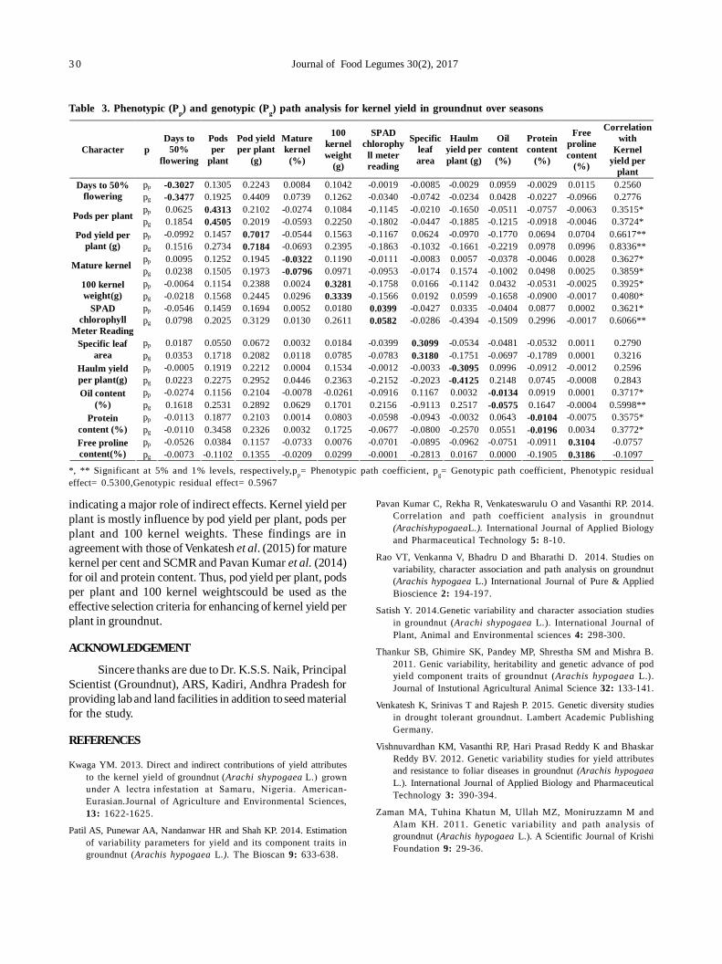
3 0 Journal of Food Legumes 30(2), 2017
indicating a major role of indirect effects. Kernel yield perplant is mostly influence by pod yield per plant, pods perplant and 100 kernel weights. These findings are inagreement with those of Venkatesh et al. (2015) for maturekernel per cent and SCMR and Pavan Kumar et al. (2014)for oil and protein content. Thus, pod yield per plant, podsper plant and 100 kernel weightscould be used as theeffective selection criteria for enhancing of kernel yield perplant in groundnut.
ACKNOWLEDGEMENT
Sincere thanks are due to Dr. K.S.S. Naik, PrincipalScientist (Groundnut), ARS, Kadiri, Andhra Pradesh forproviding lab and land facilities in addition to seed materialfor the study.
REFERENCES
Kwaga YM. 2013. Direct and indirect contributions of yield attributesto the kernel yield of groundnut (Arachi shypogaea L.) grownunder A lectra infestation at Samaru, Nigeria. American-Eurasian.Journal of Agriculture and Environmental Sciences,13: 1622-1625.
Patil AS, Punewar AA, Nandanwar HR and Shah KP. 2014. Estimationof variability parameters for yield and its component traits ingroundnut (Arachis hypogaea L.). The Bioscan 9: 633-638.
Pavan Kumar C, Rekha R, Venkateswarulu O and Vasanthi RP. 2014.Correlation and path coefficient analysis in groundnut(ArachishypogaeaL.). International Journal of Applied Biologyand Pharmaceutical Technology 5: 8-10.
Rao VT, Venkanna V, Bhadru D and Bharathi D. 2014. Studies onvariability, character association and path analysis on groundnut(Arachis hypogaea L.) International Journal of Pure & AppliedBioscience 2: 194-197.
Satish Y. 2014.Genetic variability and character association studiesin groundnut (Arachi shypogaea L.). International Journal ofPlant, Animal and Environmental sciences 4: 298-300.
Thankur SB, Ghimire SK, Pandey MP, Shrestha SM and Mishra B.2011. Genic variability, heritability and genetic advance of podyield component traits of groundnut (Arachis hypogaea L.).Journal of Instutional Agricultural Animal Science 32: 133-141.
Venkatesh K, Srinivas T and Rajesh P. 2015. Genetic diversity studiesin drought tolerant groundnut. Lambert Academic PublishingGermany.
Vishnuvardhan KM, Vasanthi RP, Hari Prasad Reddy K and BhaskarReddy BV. 2012. Genetic variability studies for yield attributesand resistance to foliar diseases in groundnut (Arachis hypogaeaL.). International Journal of Applied Biology and PharmaceuticalTechnology 3: 390-394.
Zaman MA, Tuhina Khatun M, Ullah MZ, Moniruzzamn M andAlam KH. 2011. Genetic variability and path analysis ofgroundnut (Arachis hypogaea L.). A Scientific Journal of KrishiFoundation 9: 29-36.
Table 3. Phenotypic (Pp) and genotypic (Pg) path analysis for kernel yield in groundnut over seasons
*, ** Significant at 5% and 1% levels, respectively,pp= Phenotypic path coefficient, pg= Genotypic path coefficient, Phenotypic residualeffect= 0.5300,Genotypic residual effect= 0.5967
Character p Days to
50% flowering
Pods per
plant
Pod yield per plant
(g)
Mature kernel
(%)
100 kernel weight
(g)
SPAD chlorophy
ll meter reading
Specific leaf area
Haulm yield per plant (g)
Oil content
(%)
Protein content
(%)
Free proline content
(%)
Correlation with
Kernel yield per
plant pp -0.3027 0.1305 0.2243 0.0084 0.1042 -0.0019 -0.0085 -0.0029 0.0959 -0.0029 0.0115 0.2560 Days to 50%
flowering pg -0.3477 0.1925 0.4409 0.0739 0.1262 -0.0340 -0.0742 -0.0234 0.0428 -0.0227 -0.0966 0.2776
pp 0.0625 0.4313 0.2102 -0.0274 0.1084 -0.1145 -0.0210 -0.1650 -0.0511 -0.0757 -0.0063 0.3515*
Pods per plant pg 0.1854 0.4505 0.2019 -0.0593 0.2250 -0.1802 -0.0447 -0.1885 -0.1215 -0.0918 -0.0046 0.3724*
pp -0.0992 0.1457 0.7017 -0.0544 0.1563 -0.1167 0.0624 -0.0970 -0.1770 0.0694 0.0704 0.6617** Pod yield per plant (g) pg 0.1516 0.2734 0.7184 -0.0693 0.2395 -0.1863 -0.1032 -0.1661 -0.2219 0.0978 0.0996 0.8336**
pp 0.0095 0.1252 0.1945 -0.0322 0.1190 -0.0111 -0.0083 0.0057 -0.0378 -0.0046 0.0028 0.3627*
Mature kernel pg 0.0238 0.1505 0.1973 -0.0796 0.0971 -0.0953 -0.0174 0.1574 -0.1002 0.0498 0.0025 0.3859*
pp -0.0064 0.1154 0.2388 0.0024 0.3281 -0.1758 0.0166 -0.1142 0.0432 -0.0531 -0.0025 0.3925* 100 kernel weight(g) pg -0.0218 0.1568 0.2445 0.0296 0.3339 -0.1566 0.0192 0.0599 -0.1658 -0.0900 -0.0017 0.4080*
pp -0.0546 0.1459 0.1694 0.0052 0.0180 0.0399 -0.0427 0.0335 -0.0404 0.0877 0.0002 0.3621* SPAD chlorophyll
Meter Reading pg 0.0798 0.2025 0.3129 0.0130 0.2611 0.0582 -0.0286 -0.4394 -0.1509 0.2996 -0.0017 0.6066**
pp 0.0187 0.0550 0.0672 0.0032 0.0184 -0.0399 0.3099 -0.0534 -0.0481 -0.0532 0.0011 0.2790 Specific leaf area pg 0.0353 0.1718 0.2082 0.0118 0.0785 -0.0783 0.3180 -0.1751 -0.0697 -0.1789 0.0001 0.3216
pp -0.0005 0.1919 0.2212 0.0004 0.1534 -0.0012 -0.0033 -0.3095 0.0996 -0.0912 -0.0012 0.2596 Haulm yield per plant(g) pg 0.0223 0.2275 0.2952 0.0446 0.2363 -0.2152 -0.2023 -0.4125 0.2148 0.0745 -0.0008 0.2843
pp -0.0274 0.1156 0.2104 -0.0078 -0.0261 -0.0916 0.1167 0.0032 -0.0134 0.0919 0.0001 0.3717* Oil content (%) pg 0.1618 0.2531 0.2892 0.0629 0.1701 0.2156 -0.9113 0.2517 -0.0575 0.1647 -0.0004 0.5998**
pp -0.0113 0.1877 0.2103 0.0014 0.0803 -0.0598 -0.0943 -0.0032 0.0643 -0.0104 -0.0075 0.3575* Protein content (%) pg -0.0110 0.3458 0.2326 0.0032 0.1725 -0.0677 -0.0800 -0.2570 0.0551 -0.0196 0.0034 0.3772*
pp -0.0526 0.0384 0.1157 -0.0733 0.0076 -0.0701 -0.0895 -0.0962 -0.0751 -0.0911 0.3104 -0.0757 Free proline content(%) pg -0.0073 -0.1102 0.1355 -0.0209 0.0299 -0.0001 -0.2813 0.0167 0.0000 -0.1905 0.3186 -0.1097
Journal of Food Legumes 30(2): 31-34, 2017
ABSTRACT
The present study was carried out to analyse induced geneticvariability in forty five advanced mutant lines of black gram(vigna mungo L. Hepper). These lines were developedthrough irradiation of seeds of urdbean Mash 1008’ withthree doses of gamma rays (45 KR, 55KR & 65 KR) followedby selection from M2 to M5 generation. These advancedmutant lines (M6) were evaluated for nine quantitative traitsat two locations viz., Punjab Agricultural University (PAU),Ludhiana and Regional Research Station (RRS), Gurdaspur.Pooled analysis of variance showed significant differencesamong the lines for all the traits under study with theexception of plant height. The phenotypic coefficient ofvariation (PCV) was highest for grain yield per plot followedby number of pods per plant and branches per plant.Heritability estimates with high genetic advance wereobserved for number of branches per plant and pod length.Phenotypic correlation coefficients over the twoenvironments showed that grain yield per plot exhibitedsignificant positive correlation with pods per plant, 100-seedweight, branches per plant and days to maturity. Path analysisrevealed maximum direct effect of pods per plant (followedby 100-seed weight and branches per plant) on grain yieldper plot.
Keywords: Black gram, Correlation, Gamma rays, Heritability,Path analysis.
Blackgram [Vigna mungo (L.) Hepper] commonlyknown as urdbean or mash is an important legume crop ofIndia. It belongs to family Leguminosae and sub-familyPapilionaceae with Indian sub-continent as the centre oforigin. It is considered to be domesticated from its wildprogeny of Vigna mungo var. silvestris. It is an excellentsource of high quality dietary protein with gooddigestibility. It also contributes a major portion of lysine invegetarian diets of most of Asian population. India is largestproducer of urdbean with 70 percent of world’s production(Singh et al. 2014). However, the productivity of blackgram is very low in Indian sub-continent due to narrowgenetic base of existing cultivars. The genetic architectureof grain yield can be better resolved through componenttraits than yield per se as yield is end product of interactionsbetween various component traits. Progress in plant-breeding depends upon the extent of genetic variabilitypresent in a breeding population. Induced mutagenesis isan important tool in the hands of plant breeder to createvariation in breeding material of a particular crop. Studies
Assessment of induced genetic variability in blackgram [Vigna mungo (L.)Hepper]RK GILL, ASHOK KUMAR, INDERJIT SINGH and VIKRANT TYAGI
Punjab Agricultural University, Ludhiana, India, E-mail: [email protected](Received: March 15, 2017; Accepted: May 26, 2017)
on genetic variability, heritability and genetic advance ofgrain yield and components traits in urdbean indicate thescope of improvement through selection (Baisakh etal.2014). Significant genetic variability for quantitative traitshas been induced through gamma rays and EMS inmungbean and 40 KR dose of gamma rays was found to bemost effective (Singh 2009). Induced mutations were alsofound effective in creating genetic variability forquantitative traits like plant height and number of pods perplant in urdbean (Meshram et al. 2013 and Usharani andKumar 2015). Therefore the present investigation wascarried out to assess genetic variability and studyassociation among various quantitative traits in advancedmutant lines of urdbean sown under two environmental
MATERIALS AND METHODS
In the present study, thousand seeds each of summerurdbean variety Mash 1008 were treated with three dosesof gamma rays (45 KR, 55KR and 65 KR). The M1 generationwas grown at Punjab Agricultural University, (PAU)Ludhiana during Kharif 2012. All the M1 plants were bulkharvested and three M2 populations were raised in summer2013. Vigorous single plants with profuse pod bearing wereharvested and their M3 progenies were evaluated in kharif2013. Thus, 45 M5 mutant lines were developed in kharif2015 through selection for higher grain yield by applyingselection from M2 to M4 generation. These lines are alsoresistant to yellow mosaic virus (YMV) as Ludhiana is hotspot for screening of YMV disease during kharif season.
These mutant lines were bulked in M5 generationand evaluated alongwith untreated control pulses farm areaof both at PAU, Ludhiana and Regional Research Station(RRS),Gurdaspur during summer 2016. The experiment wasconducted in randomized block design with tworeplications in four meter long paired rows sowing spacingof 22.5 x 10 cm recommended packages of practices werefollowed to raise healthy crop. Observations were recordedon five randomly seduces plants with respect to plant height(cm), number of branches per plant, number of pods perplant, number of seeds per pod, pod length (cm) and 100-seed weight (g). Observations on days to 50% flowering,days to maturity and grain yield (g) were recorded on perplot basis. The data collected was analysis for amongstandard statistical procedures as per Singh and Choudhary(1985) using SAS Software (SAS 1996).
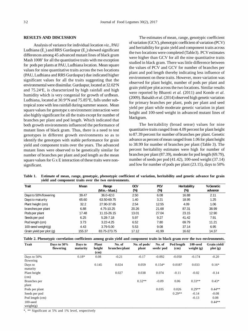
3 2 Journal of Food Legumes 30(2), 2017
RESULTS AND DISCUSSION
Analysis of variance for individual location viz., PAULudhiana (E1) and RRS Gurdaspur (E2) showed significantdifferences among 45 advanced mutant lines of black gramMash 1008’ for all the quantitative traits with me exceptionfor pods per plants at PAU, Ludhiana location. Mean squarevalues for nine quantitative traits across the two locations(PAU, Ludhiana and RRS Gurdaspur) due indicated highersignificant values for all the traits suggesting that theenvironmental were dissimilar. Gurdaspur, located at 32.02oNand 75.24oE, is characterized by high rainfall and highhumidity which is very congenial for growth of urdbean.Ludhiana, located at 30.9°N and 75.85°E, falls under sub-tropical zone with less rainfall during summer season. Meansquare values for genotype x environment interaction werealso highly significant for all the traits except for number ofbranches per plant and pod length. Which indicated thatboth growth environments influenced the performance ofmutant lines of black gram. Thus, there is a need to testgenotypes in different growth environments so as toidentify the genotypes with stable performance for grainyield and component traits over the years. The advancedmutant lines were observed to be genetically similar fornumber of branches per plant and pod length as the meansquare values for G x E interaction of these traits were non-significant.
The estimates of mean, range, genotypic coefficientof variation (GCV), phenotypic coefficient of variation (PCV)and heritability for grain yield and component traits acrossthe two locations were completed (Table3). PCV estimateswere higher than GCV for all the nine quantitative traitsstudied in black gram. There was little difference betweenthe values of PCV and GCV for number of branches perplant and pod length thereby indicating less influence ofenvironment on these traits. However, more variation wasobserved for plant height, number of pods per plant andgrain yield per plot across the two locations. Similar resultswere reported by Bhareti et al. (2011) and Konde et al.(2009). Baisakh et al. (2014) observed high genetic variationfor primary branches per plant, pods per plant and seedyield per plant while moderate genetic variation in plantheight and 100-seed weight in advanced mutant lines ofblackgram.
The heritability (broad sense) values for ninequantitative traits ranged from 4.09 percent for plant heightto 87.39 percent for number of branches per plant. Geneticadvance as percent of mean ranged from 1.06 for plant heightto 38.99 for number of branches per plant (Table 3). Thepercent heritability estimates were high for number ofbranches per plant (87.39), moderate for pod length (69.79),number of seeds per pod (41.42), 100-seed weight (37.14)and low for number of pods per plant (23.15), days to 50%
Table 1. Estimate of mean, range, genotypic, phenotypic coefficient of variation, heritability and genetic advance for grainyield and component traits over the two environments.
Trait Mean Range (Min.– Maxi.)
GCV (%)
PCV (%)
Heritability (%)
% Genetic advance
Days to 50% flowering 39.47 36.0-42.0 2.50 6.08 16.88 2.11 Days to maturity 65.60 63.50-69.75 1.40 3.21 18.95 1.25 Plant height (cm) 32.2 27.90-37.65 2.54 12.55 4.09 1.06 branches per plant 6.88 4.75-10.25 20.26 21.68 87.31 38.99 Pods per plant 17.48 11.15-26.15 13.01 27.04 23.15 12.90 Seeds per pod 6.25 5.28-7.18 5.97 9.27 41.42 7.91 Pod length (cm) 3.73 3.22-4.25 6.52 7.80 69.79 11.21 100-seed weight(g) 4.43 3.79-5.00 5.53 9.08 37.14 6.95 Grain yield per plot (g) 155.37 83.75-273.75 17.12 41.99 16.62 14.37
Table 2. Phenotypic correlation coefficients among grain yield and component traits in black gram over the two environments.
*, ** Significant at 5% and 1% level, respectively
Trait Days to 50% flowering
Days to maturity
Plant height (cm)
No. of branches/plant
No. of pods/ plant
No. of seeds/ pod
Pod length (cm)
100-seed weight (g)
Grain yield/ plot (g)
Days to 50% flowering
0.18* 0.08 -0.21 -0.17 -0.092 -0.050 -0.174 -0.20
Days to maturity
0.145 0.024 0.059 0.154* 0.0187 0.033 0.16*
Plant height (cm)
0.027 0.038 0.074 -0.11 -0.02 -0.14
Branches per plant
0.32** -0.09 0.06 0.33** 0.43*
Pods per plant 0.035 0.026 0.29** 0.44** Seeds per pod 0.29** -0.14 -0.08 Pod length (cm) -0.13 0.08 100-seed weight(g)
0.44**
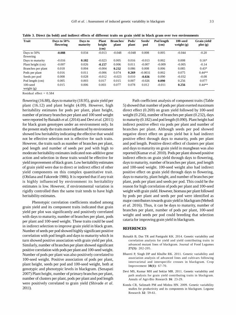
Gill et al. : Assessment of induced genetic variability in blackgram 3 3
flowering (16.88), days to maturity (18.95), grain yield perplant (16.12) and plant height (4.09). However, highheritability estimates for pods per plant, plant height,number of primary branches per plant and 100 seed weightwere reported by Baisakh et al. (2014) and Devi et al. (2011)for black gram genotypes under an environment only. Inthe present study the traits more influenced by environmentshowed low heritability indicating the effective that wouldnot be effective selection not is effective for such traits.However, the traits such as number of branches per plant,pod length and number of seeds per pod with high tomoderate heritability estimates indicated non-additive geneaction and selection in these traits would be effective foryield improvement of black gram. Low heritability estimatesof grain yield were due to direct or indirect effect of otheryield components on this complex quantitative trait.(Obilana and Fakorede 1986). It is reported that if any traitis highly influenced by environment its heritabilityestimates is low. However, if environmental variation isrigidly controlled then the same trait tends to have highheritability estimates.
Phenotypic correlation coefficients studied amonggrain yield and its component traits indicated that grainyield per plot was significantly and positively correlatedwith days to maturity, number of branches per plant, podsper plant and 100-seed weight. These traits could be usedin indirect selection to improve grain yield in black gram.Number of seeds per pod showed highly significant positivecorrelation with pod length and days to maturity which inturn showed positive association with grain yield per plot.Similarly, number of branches per plant showed significantpositive correlation with pods per plant and 100-seed weight.Number of pods per plant was also positively correlated to100-seed weight. Positive association of pods per plant,plant height, seeds per pod and 100-seed weight, both atgenotypic and phenotypic levels in blackgram. (Senapati2007) Plant height, number of primary branches per plant,number of clusters per plant, pods per plant and pod lengthwere positively correlated to grain yield (Shivade et al.2011).
Path coefficient analysis of component traits (Table5) showed that number of pods per plant exerted maximumdirect effect (0.269) on gram yield followed by 100-seedweight (0.256), number of branches per plant (0.232), daysto maturity (0.182) and pod length (0.090). Plant height hadindirect positive effect via pods per plant and number ofbranches per plant. Although seeds per pod showednegative direct effect on grain yield but it had indirectpositive effect through days to maturity, pods per plantand pod length. Positive direct effect of clusters per plantand days to maturity on grain yield in mungbean was alsoreported (Kumar et al. 2010). Pods per plant showed positiveindirect effects on grain yield through days to flowering,days to maturity, number of branches per plant, pod lengthand 100-seed weight. 100-seed weight also had indirectpositive effect on grain yield through days to flowering,days to maturity, plant height, and number of branches perplant, pods per plant and seeds per pod. This could be thereason for high correlation of pods per plant and 100-seedweight with grain yield. However, biomass per plant followedby pods per plant and seeds per pod were identified asmajor contributors towards grain yield in blackgram (Mehediet al. 2016). Thus, it can be days to maturity, number ofbranches per plant, number of pods per plant, 100-seedweight and seeds per pod could breeding that selectioncataria for improving grain yield in blackgram.
REFERENCES
Baisakh B, Das TR and Panigrahi KK. 2014. Genetic variability andcorrelation analysis for yield and yield contributing traits inadvanced mutant lines of blackgram. Journal of Food Legumes27(3): 202-205.
Bhareti P, Singh DP and Khulbe RK. 2011. Genetic variability andassociation analysis of advanced lines and cultivars followingintervarietal and interspecific crosses in blackgram. CropImprovement 38(1): 67-70.
Devi MS, Kumar MH and Seklar MR. 2011. Genetic variability andpath analysis for grain yield contributing traits in blackgram.Annals of Agri-Bio Research 16: 23-29.
Konda CR, Salimath PM and Mishra HN. 2009. Genetic variabilitystudies for productivity and its components in blackgram. LegumeResearch 32: 59-61.
Table 3. Direct (in bold) and indirect effects of different traits on grain yield in black gram over two environments
Residual effect = 0.584
Trait Days to 50% flowering
Days to maturity
Plant height (cm)
Branches/ plant
Pods/ plant
Seeds/ pod
Pod length (cm)
100-seed weight (g)
Grain yield/ plot (g)
Days to 50% flowering
-0.088 0.034 -0.013 -0.048 -0.048 0.008 0.005 -0.044 -0.20
Days to maturity -0.016 0.182 -0.023 0.005 0.016 -0.013 0.002 0.008 0.16* Plant height (cm) -0.007 0.026 -0.157 0.006 0.011 -0.007 -0.009 -0.005 -0.14 Branches per plant 0.018 0.004 -0.004 0.232 0.086 0.008 0.006 0.085 0.43* Pods per plant 0.016 0.011 -0.006 0.074 0.269 -0.0031 0.002 0.075 0.44** Seeds per pod 0.008 0.028 -0.012 -0.023 0.010 -0.026 0.090 -0.032 -0.08 Pod length (cm) 0.005 0.003 0.017 0.015 0.007 -0.026 0.090 0.256 0.077 100-seed weight (g)
0.015 0.006 0.003 0.077 0.078 0.012 -0.011 0.256 0.44**
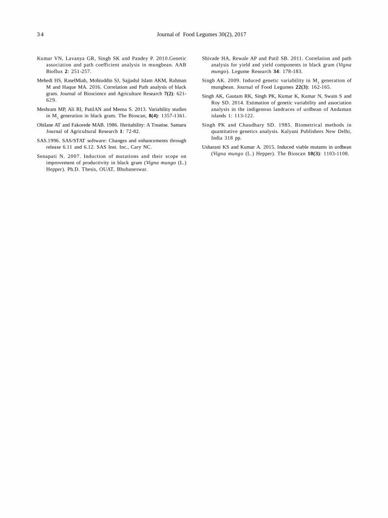
3 4 Journal of Food Legumes 30(2), 2017
Kumar VN, Lavanya GR, Singh SK and Pandey P. 2010.Geneticassociation and path coefficient analysis in mungbean. AABBioflux 2: 251-257.
Mehedi HS, RaselMiah, Mohiuddin SJ, Sajjadul Islam AKM, RahmanM and Haque MA. 2016. Correlation and Path analysis of blackgram. Journal of Bioscience and Agriculture Research 7(2): 621-629.
Meshram MP, Ali RI, PatilAN and Meena S. 2013. Variability studiesin M3 generation in black gram. The Bioscan, 8(4): 1357-1361.
Obilane AT and Fakorede MAB. 1986. Heritability: A Treatise. SamaruJournal of Agricultural Research 1: 72-82.
SAS.1996. SAS/STAT software: Changes and enhancements throughrelease 6.11 and 6.12. SAS Inst. Inc., Cary NC.
Senapati N. 2007. Induction of mutations and their scope onimprovement of productivity in black gram (Vigna mungo (L.)Hepper). Ph.D. Thesis, OUAT, Bhubaneswar.
Shivade HA, Rewale AP and Patil SB. 2011. Correlation and pathanalysis for yield and yield components in black gram (Vignamungo). Legume Research 34: 178-183.
Singh AK. 2009. Induced genetic variability in M3 generation ofmungbean. Journal of Food Legumes 22(3): 162-165.
Singh AK, Gautam RK, Singh PK, Kumar K, Kumar N, Swain S andRoy SD. 2014. Estimation of genetic variability and associationanalysis in the indigenous landraces of urdbean of Andamanislands 1: 113-122.
Singh PK and Chaudhary SD. 1985. Biometrical methods inquantitative genetics analysis. Kalyani Publishers New Delhi,India 318 pp.
Usharani KS and Kumar A. 2015. Induced viable mutants in urdbean(Vigna mungo (L.) Hepper). The Bioscan 10(3): 1103-1108.
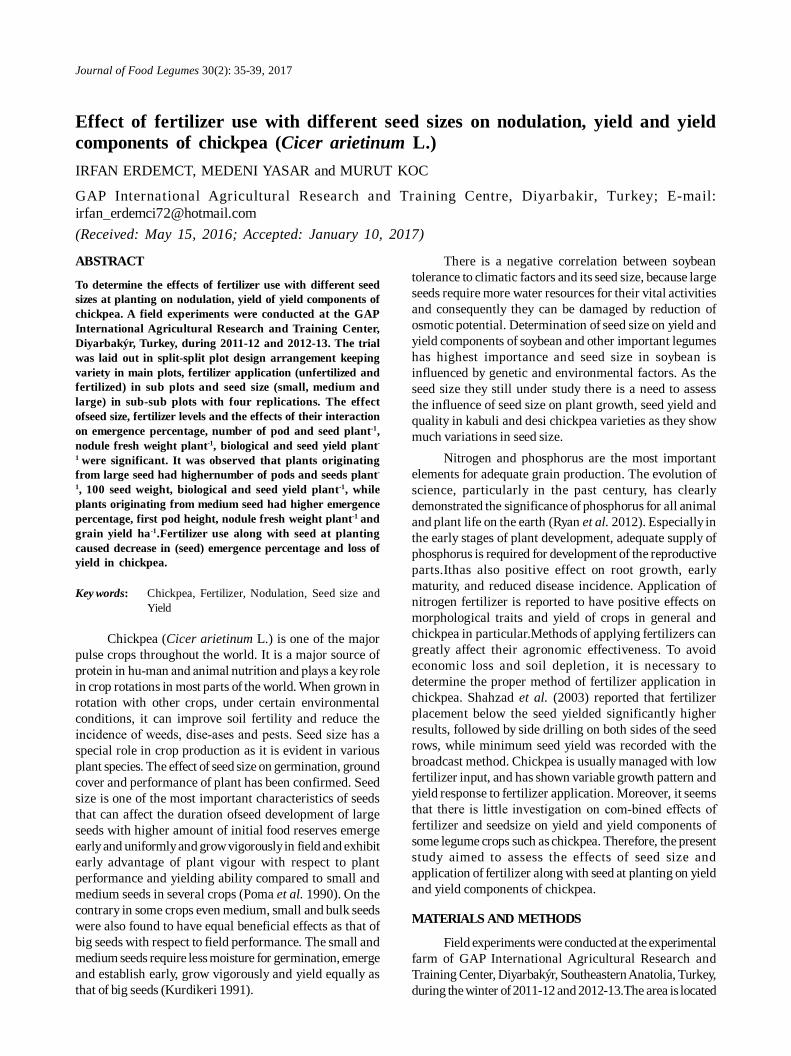
Journal of Food Legumes 30(2): 35-39, 2017
ABSTRACT
To determine the effects of fertilizer use with different seedsizes at planting on nodulation, yield of yield components ofchickpea. A field experiments were conducted at the GAPInternational Agricultural Research and Training Center,Diyarbakýr, Turkey, during 2011-12 and 2012-13. The trialwas laid out in split-split plot design arrangement keepingvariety in main plots, fertilizer application (unfertilized andfertilized) in sub plots and seed size (small, medium andlarge) in sub-sub plots with four replications. The effectofseed size, fertilizer levels and the effects of their interactionon emergence percentage, number of pod and seed plant-1,nodule fresh weight plant-1, biological and seed yield plant-
1 were significant. It was observed that plants originatingfrom large seed had highernumber of pods and seeds plant-
1, 100 seed weight, biological and seed yield plant-1, whileplants originating from medium seed had higher emergencepercentage, first pod height, nodule fresh weight plant-1 andgrain yield ha-1.Fertilizer use along with seed at plantingcaused decrease in (seed) emergence percentage and loss ofyield in chickpea.
Key words: Chickpea, Fertilizer, Nodulation, Seed size andYield
Chickpea (Cicer arietinum L.) is one of the majorpulse crops throughout the world. It is a major source ofprotein in human and animal nutrition and plays a key rolein crop rotations in most parts of the world. When grown inrotation with other crops, under certain environmentalconditions, it can improve soil fertility and reduce theincidence of weeds, diseases and pests. Seed size has aspecial role in crop production as it is evident in variousplant species. The effect of seed size on germination, groundcover and performance of plant has been confirmed. Seedsize is one of the most important characteristics of seedsthat can affect the duration ofseed development of largeseeds with higher amount of initial food reserves emergeearly and uniformly and grow vigorously in field and exhibitearly advantage of plant vigour with respect to plantperformance and yielding ability compared to small andmedium seeds in several crops (Poma et al. 1990). On thecontrary in some crops even medium, small and bulk seedswere also found to have equal beneficial effects as that ofbig seeds with respect to field performance. The small andmedium seeds require less moisture for germination, emergeand establish early, grow vigorously and yield equally asthat of big seeds (Kurdikeri 1991).
Effect of fertilizer use with different seed sizes on nodulation, yield and yieldcomponents of chickpea (Cicer arietinum L.)IRFAN ERDEMCT, MEDENI YASAR and MURUT KOC
GAP International Agricultural Research and Training Centre, Diyarbakir, Turkey; E-mail:[email protected](Received: May 15, 2016; Accepted: January 10, 2017)
There is a negative correlation between soybeantolerance to climatic factors and its seed size, because largeseeds require more water resources for their vital activitiesand consequently they can be damaged by reduction ofosmotic potential. Determination of seed size on yield andyield components of soybean and other important legumeshas highest importance and seed size in soybean isinfluenced by genetic and environmental factors. As theseed size they still under study there is a need to assessthe influence of seed size on plant growth, seed yield andquality in kabuli and desi chickpea varieties as they showmuch variations in seed size.
Nitrogen and phosphorus are the most importantelements for adequate grain production. The evolution ofscience, particularly in the past century, has clearlydemonstrated the significance of phosphorus for all animaland plant life on the earth (Ryan et al. 2012). Especially inthe early stages of plant development, adequate supply ofphosphorus is required for development of the reproductiveparts.Ithas also positive effect on root growth, earlymaturity, and reduced disease incidence. Application ofnitrogen fertilizer is reported to have positive effects onmorphological traits and yield of crops in general andchickpea in particular.Methods of applying fertilizers cangreatly affect their agronomic effectiveness. To avoideconomic loss and soil depletion, it is necessary todetermine the proper method of fertilizer application inchickpea. Shahzad et al. (2003) reported that fertilizerplacement below the seed yielded significantly higherresults, followed by side drilling on both sides of the seedrows, while minimum seed yield was recorded with thebroadcast method. Chickpea is usually managed with lowfertilizer input, and has shown variable growth pattern andyield response to fertilizer application. Moreover, it seemsthat there is little investigation on combined effects offertilizer and seedsize on yield and yield components ofsome legume crops such as chickpea. Therefore, the presentstudy aimed to assess the effects of seed size andapplication of fertilizer along with seed at planting on yieldand yield components of chickpea.
MATERIALS AND METHODS
Field experiments were conducted at the experimentalfarm of GAP International Agricultural Research andTraining Center, Diyarbakýr, Southeastern Anatolia, Turkey,during the winter of 2011-12 and 2012-13.The area is located
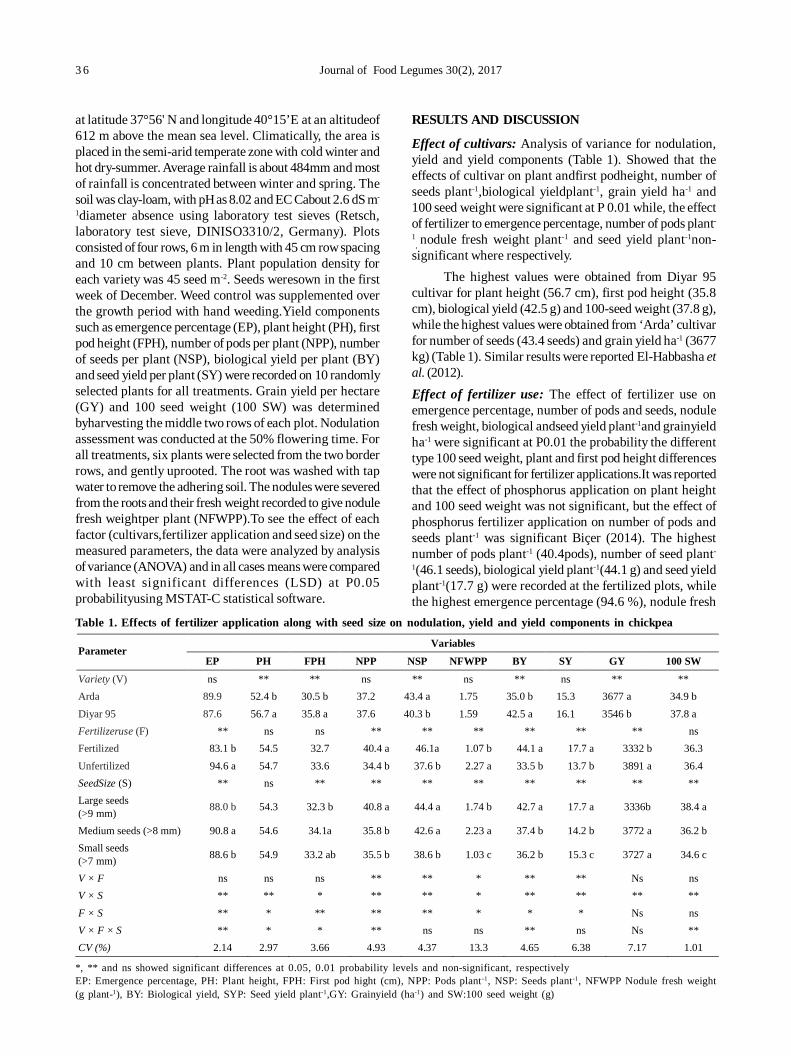
3 6 Journal of Food Legumes 30(2), 2017
at latitude 37°56' N and longitude 40°15’E at an altitudeof612 m above the mean sea level. Climatically, the area isplaced in the semi-arid temperate zone with cold winter andhot dry-summer. Average rainfall is about 484mm and mostof rainfall is concentrated between winter and spring. Thesoil was clay-loam, with pH as 8.02 and EC Cabout 2.6 dS m-
1diameter absence using laboratory test sieves (Retsch,laboratory test sieve, DINISO3310/2, Germany). Plotsconsisted of four rows, 6 m in length with 45 cm row spacingand 10 cm between plants. Plant population density foreach variety was 45 seed m-2. Seeds weresown in the firstweek of December. Weed control was supplemented overthe growth period with hand weeding.Yield componentssuch as emergence percentage (EP), plant height (PH), firstpod height (FPH), number of pods per plant (NPP), numberof seeds per plant (NSP), biological yield per plant (BY)and seed yield per plant (SY) were recorded on 10 randomlyselected plants for all treatments. Grain yield per hectare(GY) and 100 seed weight (100 SW) was determinedbyharvesting the middle two rows of each plot. Nodulationassessment was conducted at the 50% flowering time. Forall treatments, six plants were selected from the two borderrows, and gently uprooted. The root was washed with tapwater to remove the adhering soil. The nodules were severedfrom the roots and their fresh weight recorded to give nodulefresh weightper plant (NFWPP).To see the effect of eachfactor (cultivars,fertilizer application and seed size) on themeasured parameters, the data were analyzed by analysisof variance (ANOVA) and in all cases means were comparedwith least significant differences (LSD) at P0.05probabilityusing MSTAT-C statistical software.
RESULTS AND DISCUSSION
Effect of cultivars: Analysis of variance for nodulation,yield and yield components (Table 1). Showed that theeffects of cultivar on plant andfirst podheight, number ofseeds plant-1,biological yieldplant-1, grain yield ha-1 and100 seed weight were significant at P 0.01 while, the effectof fertilizer to emergence percentage, number of pods plant-
1, nodule fresh weight plant-1 and seed yield plant-1non-
significant where respectively.The highest values were obtained from Diyar 95
cultivar for plant height (56.7 cm), first pod height (35.8cm), biological yield (42.5 g) and 100-seed weight (37.8 g),while the highest values were obtained from ‘Arda’ cultivarfor number of seeds (43.4 seeds) and grain yield ha-1 (3677kg) (Table 1). Similar results were reported El-Habbasha etal. (2012).Effect of fertilizer use: The effect of fertilizer use onemergence percentage, number of pods and seeds, nodulefresh weight, biological andseed yield plant-1and grainyieldha-1 were significant at P0.01 the probability the differenttype 100 seed weight, plant and first pod height differenceswere not significant for fertilizer applications.It was reportedthat the effect of phosphorus application on plant heightand 100 seed weight was not significant, but the effect ofphosphorus fertilizer application on number of pods andseeds plant-1 was significant Biçer (2014). The highestnumber of pods plant-1 (40.4pods), number of seed plant-
1(46.1 seeds), biological yield plant-1(44.1 g) and seed yieldplant-1(17.7 g) were recorded at the fertilized plots, whilethe highest emergence percentage (94.6 %), nodule fresh
Table 1. Effects of fertilizer application along with seed size on nodulation, yield and yield components in chickpea
*, ** and ns showed significant differences at 0.05, 0.01 probability levels and non-significant, respectivelyEP: Emergence percentage, PH: Plant height, FPH: First pod hight (cm), NPP: Pods plant -1, NSP: Seeds plant-1, NFWPP Nodule fresh weight(g plant-1), BY: Biological yield, SYP: Seed yield plant-1,GY: Grainyield (ha-1) and SW:100 seed weight (g)
Variables Parameter
EP PH FPH NPP NSP NFWPP BY SY GY 100 SW
Variety (V) ns ** ** ns ** ns ** ns ** ** Arda 89.9 52.4 b 30.5 b 37.2 43.4 a 1.75 35.0 b 15.3 3677 a 34.9 b Diyar 95 87.6 56.7 a 35.8 a 37.6 40.3 b 1.59 42.5 a 16.1 3546 b 37.8 a Fertilizeruse (F) ** ns ns ** ** ** ** ** ** ns Fertilized 83.1 b 54.5 32.7 40.4 a 46.1a 1.07 b 44.1 a 17.7 a 3332 b 36.3 Unfertilized 94.6 a 54.7 33.6 34.4 b 37.6 b 2.27 a 33.5 b 13.7 b 3891 a 36.4 SeedSize (S) ** ns ** ** ** ** ** ** ** ** Large seeds (>9 mm) 88.0 b 54.3 32.3 b 40.8 a 44.4 a 1.74 b 42.7 a 17.7 a 3336b 38.4 a
Medium seeds (>8 mm) 90.8 a 54.6 34.1a 35.8 b 42.6 a 2.23 a 37.4 b 14.2 b 3772 a 36.2 b Small seeds (>7 mm) 88.6 b 54.9 33.2 ab 35.5 b 38.6 b 1.03 c 36.2 b 15.3 c 3727 a 34.6 c
V × F ns ns ns ** ** * ** ** Ns ns V × S ** ** * ** ** * ** ** ** ** F × S ** * ** ** ** * * * Ns ns V × F × S ** * * ** ns ns ** ns Ns ** CV (%) 2.14 2.97 3.66 4.93 4.37 13.3 4.65 6.38 7.17 1.01
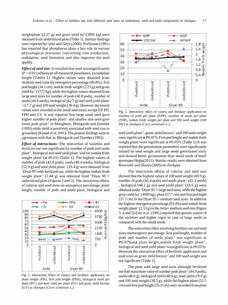
Erdemct et al. : Effect of fertilizer use with different seed sizes on nodulation, yield and yield components of chickpea 3 7
weightplant-1(2.27 g) and grain yield ha-1(3891 kg) wereobtained from unfertilized plots (Table 1). Similar findingswere reported by ªahin and Geçit (2006). Pochiman (1991)has reported that phosphorus plays a key role in variousphysiological processes concerning root production,nodulation, seed formation and also improves the seedquality.Effect of seed size: It revealed that seed sizessignificantly(P < 0.01) influenced all measured parameters, exceptplantheight (Tables 1). Highest values were obtained frommedium seed sizes for emergence percentage (90.8%), firstpod height (34.1 cm), nodule fresh weight (2.23 g) and grainyield ha-1 (3772 kg), while the highest values obtained fromlarge seed sizes for number of pods (40.8 pods), number ofseeds (44.4 seeds), biological (42.7 g) and seed yield plant-
1 (17.7 g) and 100 seed weight (38.4 g). However the lowestvalues were recorded at the small seed sizes, except EP, PH,FPH and GY. It was reported that large sized seed gavehigher number of pods plant-1 and smaller size seed gavelower pods plant-1 in Mungbean, Bhingarde and Dumbre(1993) while yield is positively associated with seed size ingroundnut (Kamal et al.2001). The present findings were inagreement with that as Bhingarde and Dumbre (1993).Effect of interactions: The interaction of varieties andfertilizer use was significant for number of pods and seedsplant-1, biological and seed yield plant-1and for nodule freshweight plant-1(at P0.01) (Table 1). The highest values ofnumber of pods (43.8 pods), seeds (48.4 seeds), biological(52.0 g) and seed yield plant-1 (19.4 g) were obtained from‘Diyar 95’with fertilized use, while the highest nodule freshweight plant-1 (2.44 g) was obtained from ‘Diyar 95’×unfertilized plots (Figures 1 and 2). The interaction effectsof cultivar and seed sizes on emergence percentage, plantheight, number of pods and seeds plant, biological and
seed yield plant-1, grain yield hectare-1 and 100 seed weightwere significant at P0.01%.First pod height and nodule freshweight plant-1were significant at P0.05% (Table 1).It wasreported that the germination parameters were significantlyrelated by seed weight and large seeds germinated earlyand showed better germination than small seeds of lentilgenotypes Hojjat(2011). Similar results were obtained fromRoozrokh and Shams (2005) on chickpea.
The interaction effects of cultivar and seed sizeshowed that the highest values of 100 seed weight (40.9 g),number of pods (45.4 pods) and seeds plant-1 (45.3 seeds), biological (48.2 g) and seed yield plant-1 (18.6 g) wereobtained under ‘Diyar 95’× large seed sizes, while the highestgrain yield ha-1 (4000 kg), plant (57.7 cm) and first pod hight(37.7 cm) in the Diyar 95 × medium seed sizes. In additionthe highest emergence percentage (93.4%) and nodule freshweight plant-1 (2.53 g) in the Arda× medium seed size (Figure3, 4 and 5).Eser et al. (1991) reported that genetic nature ofthe varieties and higher vigor in case of large seeds ascompared with the small seeds.
The interaction effect involving fertilizer use and seedsizes onemergence percentage, first pod height, number ofpods and number of seeds plant-1 was significant atP0.01%and plant height,nodule fresh weight plant -1,biological and seed yield plant-1wassignificant at P0.05%.However the interaction effect of fertilizer application andseed sizes on grain yield hectare-1 and 100 seed weight wasnot significant (Table 1).
The plots with large seed sizes although fertilizeduse had maximum value of number pods plant-1 (44.9 pods),seeds (48.6 g), biological yield (48.6 g), seed yield (19.6 g)and 100 seed weight (38.5 g), while the highest plant (55.5cm) and first pod height (35.0 cm) were recorded from plots
Fig. 1. Interaction effect of variety and fertilizer application onplant height (PH), first pod height (FPH), biological yield perplant (BY) and seed yield per plant (SY) and grain yield hectare(GY) in chickpea (Cicer arietinum L.)
Fig. 2. Interaction effect of variety and fertilizer application onnumber of pods per plant (NPP), number of seeds per plant(NSP), nodule fresh weight per plant and 100 seed weight (100SW) in chickpea (Cicer arietinum L.)
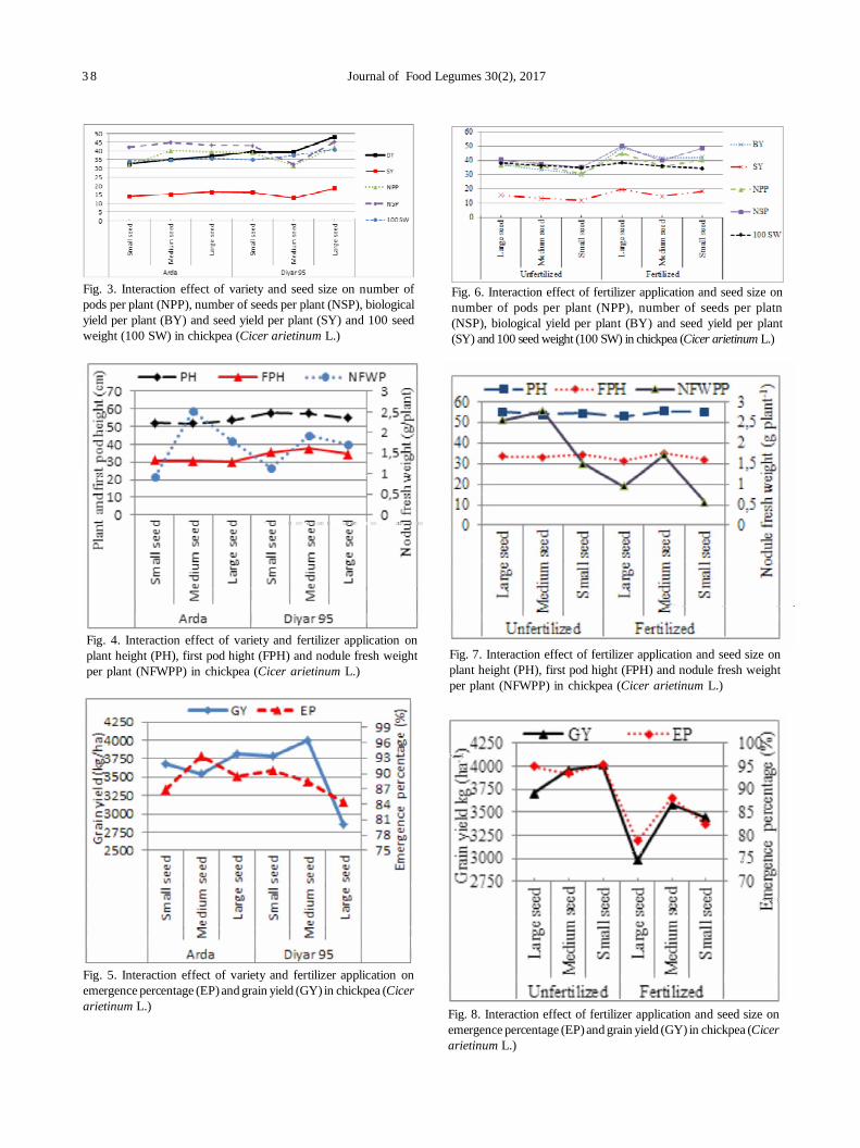
3 8 Journal of Food Legumes 30(2), 2017
Fig. 5. Interaction effect of variety and fertilizer application onemergence percentage (EP) and grain yield (GY) in chickpea (Cicerarietinum L.)
Fig. 3. Interaction effect of variety and seed size on number ofpods per plant (NPP), number of seeds per plant (NSP), biologicalyield per plant (BY) and seed yield per plant (SY) and 100 seedweight (100 SW) in chickpea (Cicer arietinum L.)
Fig. 4. Interaction effect of variety and fertilizer application onplant height (PH), first pod hight (FPH) and nodule fresh weightper plant (NFWPP) in chickpea (Cicer arietinum L.)
Fig. 7. Interaction effect of fertilizer application and seed size onplant height (PH), first pod hight (FPH) and nodule fresh weightper plant (NFWPP) in chickpea (Cicer arietinum L.)
Fig. 6. Interaction effect of fertilizer application and seed size onnumber of pods per plant (NPP), number of seeds per platn(NSP), biological yield per plant (BY) and seed yield per plant(SY) and 100 seed weight (100 SW) in chickpea (Cicer arietinum L.)
Fig. 8. Interaction effect of fertilizer application and seed size onemergence percentage (EP) and grain yield (GY) in chickpea (Cicerarietinum L.)
Erdemct et al. : Effect of fertilizer use with different seed sizes on nodulation, yield and yield components of chickpea 3 9
REFERENCES
Bhingarde MT and Dumbre AD. 1993. Effect of seed size on growthand yield components in greengram (Vigna radiata L. Wilczek)under summer conditions. Seed Research 21: 104-106.
Biçer BT. 2014. Some Agronomic studies in Chickpea (Cicerarietinum L.) and Lentil (Lens culinaris Medik). Türk TarýmveDoða Bilimleri Dergisi 1(1): 42–51.
El-Habbasha SF, Amal GA and Magda HM. 2012. Response of somechickpea varieties to compound foliar fertilizer under sandy soilconditions.Journal of Applied Sciences Research 8(10): 5177-5183.
Eser D, Ukur A and Adak MS. 1991. Effect of seed size on yield andyield components in chickpea. International ChickpeaNewsletter 25: 13-15.
Hojjat SS. 2011. Effect of seed size on germination and seedlinggrowth of some lentil genotypes.International Journal ofAgriculture and Crop Sciences 3: 1-5.
Kamal MM, Hosain MA and Khan MSA. 2001. Ýnfluence of seedsize on growth, yield and seed quality of groundnut. BangladeshJournal of Agricultural Research 26: 589-599.
Kurdikeri MB. 1991. Studies on seed quality in hybrid maize (Zeamays L.). Ph.D Thesis, University of Agricultural Science,Bangalore (India).
Pochiman JM. 1991. The Mungbean, Oxford and IBH PublishingCo.pvt.ltd.New Delhi, Ýndia Pp. 62.
Poma I, Sarno R, Noto F and Zora D. 1990. Effect of sowing date onyield and quality characteristics of chickpeas Informatore Agrario46: 53-55.
Roozrokh MK and Shams M. 2005. Effects of seed size and seedlingdepth on seed vigor of chiek pea, First National Legume Congress.Mashhad Ferdowsi. University, Mashhad, Iran.
Ryan J, Ibrikci H, Delgado A, Torrent J, Sommer R and Rashid A.2012. Significance of phosphorus for agriculture and theenvironment in the West Asia and North Africaregion. Advancesin Agronomy 114: 91-153.
Shahzad MA, Hussain SH and Nazar MS. 2003. Growth and yieldresponse of Brassica cultivars to fertilizer application methodsunder saline field conditions. Journal of Agricultural Research41: 131-140.
Sahin N and Geçit HH. 2006. Farklý Gübreleme Yöntemlerinin Nohut(Cicer arietinum L.)’ ta Verimve Verim Öðeleri Üzerine Etkiler.Tarým Bilimleri Dergisi 12: 252-258.
with fertilize use×medium seed size treatment (Figure 6 and7). The highest emergence percentage (95.7%) and grainyield (4010.2 kg ha-1) were determined from unfertilized ×small seed size treatment. Generally emergence percentageand grain yield in unfertilized treatment was higher thanfertilized treatment (Figure 8). This is related to direct fertilizerapplication below the sown seed. This application leads toincrease the risk of burning the roots of the sown seeds,especially during dry conditions. Thus the percentage ofseed emergence was influenced by the used fertilizerplacement and consequently, the yield per unit areadecreased.
The study indicated that the effect of fertilizer usealong with seed planting was significant for other examinedcharacteristics, except plant height, first pod height and100-grain weight. This effect was not significance onemergence percentage, grain yield and fresh nodule weight.Seed size affected all studied features of chickpea, exceptplant height. In general, plants originating from large seedhad higher number of pods and number of seeds plant-
1,100 seed weight, biological and seed yield plant-1, whileplants originating from medium seed had higher emergencepercentage, first pod height, nodule fresh weight plant-1
andgrain yield ha-1.However, these effects tend to decreasein chickpea varieties having medium seed weight (37g 100seeds-1) of ‘Arda’. The increase in grain yield was associatedwith emergence percentage. Furthermore, variety × seedsize and fertilizer use× seed size interaction had avoidedthrough tapered side bird merged frequency inheritance ofsignificant on yield and its components. Consequently useof fertilizer along with seed at planting coved decreaseemergence percentage of the seeds leading in yield loss.Intense, let fertilizer contact with seed is avoided with
Journal of Food Legumes 30(2): 40-42, 2017
Nitrogen sources manipulation for higher productivity, profitability and its useefficiency in rajmash (Phaseolus vulgaris L.) in cold desert region of North-Western HimalayaJ SINGH
CSKHPKV Highland Agricultural Research and Extension Centre, Kukumseri, Lahaul & Spiti, Himachal Pradesh,India; E-mail: [email protected](Received: August 20, 2016; Accepted: March 9, 2017)
ABSTRACT
A field experiment was conducted sandy loam and acidic soilat Highland Agricultural Research and Extension Centre,Kukumseri in Himanchal Pradesh (India) to study the effectof levels and methods of nitrogen application on growth,yield, economics and nitrogen use efficiency in rajmash.The experiment was laid out in a randomized block designwith treatments involving for leaves and two methods andrespected there growth and yield significantly increased withnitrogen application. Taller plants were recorded infects N60followed by N40. Significantly higher dry matter production(6430 kg/ha) was observed with N60 followed by N40.Maximum dry matter efficiency (0.49%/day), unit areaefficiency (2.96 g/m2/day), pod dry weight (3.1g) andproductivity (29.63kg/ha/day) was due recorded with N60. Thehighest seed yield (3200 kg/ha) was observed with N60 whichwas 68 and 20 percent higher over N0 and N20, respectively.Maximum nitrogen use efficiency (37.5 kg seed/kg N) wasrecorded with N20 while minimum was at N60. Howevermaximum gross returns (¹ 3, 32,920/ha), net returns (¹2,57,537/ha), B:C 6CR (4.42) and profitability (¹2385/ha/day)were also recorded at N60. Basal application of nitrogen wasfound beneficial than split application. Basal application of60 kg N/ha as based requested in higher productivity andprofitability of rajmash in cold desert region.
Key words: Nitrogen, Nitrogen use efficiency, Productivity,Profitability, Rajmash
The cold desert region of North-western Himalayaconstitutes 79,278 sq. kms of area spread over HimachalPradesh, Jammu & Kashmir, Sikkim and Uttarakhand, wherethe region in Himanchal Pradesh alone creating about 42per cent of its total geographical area. The climate isextremely cold and heavy snowfall occurs during winter.Single cropping season prevails in the region which startsfrom April to October. The population of the region is entirelyrural and economically backward (Singh and Chaudhary2016, Singh et al. 2015, Kumar et al. 2015). Phaseolusvulgaris is known as frenchbean, common bean, snap beanand green bean in the form of vegetable whereas in theform of pulse, it is known as rajmash, haricot bean, drybean and navy bean (Singh et al. 2014). It is a short durationnon-traditional grain legume and is inefficient in symbioticnitrogen fixation as it lacks nodulation due to absence of anodulation gene regulator. It is the only grain legume grown
in cold desert region of the state. It is a very nutritive cropcontaining 20.69 to 25.81% crude protein, 1.72% fats and72.42% carbohydrates (Sood et al. 2003) and is also rich indietary fiber, potassium, selenium, molybdenum, thiamine,vitamin B6 and folic acid (Turuko and Mohammed 2014).Rajmash is a main source of protein and also a major sourceof income for the tribal people as there is a great demand ofrajmash in different parts of the country due to its betterquality and taste.
Imbalanced application of fertilizers is one of majorproblems resulting in deterioration of crop productivity inthe region. Nitrogen is also applied as top dressing by thefarmers for enhancing its yield. There a need in study therequirement of on base per se and its method so as enhanceits productivity performance and over in cold desert regionof North-Western Himalaya.
MATERIALS AND METHODS
A field experiment was conducted during summerseason of 2013 at the Research Farm, Highland AgriculturalResearch and Extension Centre, CSK Himachal PradeshKrishi Vishvavidyalaya, Kukumseri (32° 44‘ 55" N latitudeand 76° 41‘ 23" E longitude, and 2672 m above the mean sealevel), Lahaul & Spiti, Himachal Pradesh. The soil of theexperimental site was sandy loam in texture and acidic inreaction with 10.5 g organic carbon/kg soil, 280 kg availableN/ha, 31 kg available P/ha and 300 kg available K/ha. Duringcropping season, the minimum and maximum temperaturesrange from 12°C to 24°C. Average annual rainfall of theregion is 250 mm. The experiment was laid out in arandomized block design with six treatment combinationsinvolving of four N levels (0, 20, 40 and 60 kg/ha) and twomethods (basal and split application) of nitrogenapplication. The treatment combinations were N0 (control),N20 (basal), N40 (basal), N20+20 (split), N60 (basal) and N30+30(split). The treatments were replicated thrice and allocatedrandomly in the different experimental plots using randomtable. Rajmash HPR 35 (Kanchan) having short and bushystature, early maturity and bold seeded with light pink colourwas used as test crop. Nitrogen was applied as basal andinto two splits (½ N as basal and ½ N as top dressing at 30days after sowing) as per treatments. Phosphorus andpotassium were applied @ 60 kg and 30 kg/ha, respectivelyas basal application in all the experimental plots. N, P and K
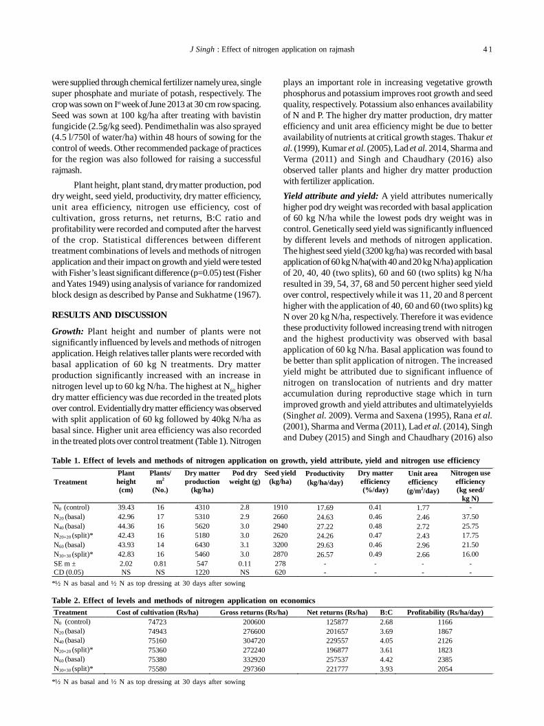
J Singh : Effect of nitrogen application on rajmash 4 1
were supplied through chemical fertilizer namely urea, singlesuper phosphate and muriate of potash, respectively. Thecrop was sown on Ist week of June 2013 at 30 cm row spacing.Seed was sown at 100 kg/ha after treating with bavistinfungicide (2.5g/kg seed). Pendimethalin was also sprayed(4.5 l/750l of water/ha) within 48 hours of sowing for thecontrol of weeds. Other recommended package of practicesfor the region was also followed for raising a successfulrajmash.
Plant height, plant stand, dry matter production, poddry weight, seed yield, productivity, dry matter efficiency,unit area efficiency, nitrogen use efficiency, cost ofcultivation, gross returns, net returns, B:C ratio andprofitability were recorded and computed after the harvestof the crop. Statistical differences between differenttreatment combinations of levels and methods of nitrogenapplication and their impact on growth and yield were testedwith Fisher’s least significant difference (p=0.05) test (Fisherand Yates 1949) using analysis of variance for randomizedblock design as described by Panse and Sukhatme (1967).
RESULTS AND DISCUSSION
Growth: Plant height and number of plants were notsignificantly influenced by levels and methods of nitrogenapplication. Heigh relatives taller plants were recorded withbasal application of 60 kg N treatments. Dry matterproduction significantly increased with an increase innitrogen level up to 60 kg N/ha. The highest at N60 higherdry matter efficiency was due recorded in the treated plotsover control. Evidentially dry matter efficiency was observedwith split application of 60 kg followed by 40kg N/ha asbasal since. Higher unit area efficiency was also recordedin the treated plots over control treatment (Table 1). Nitrogen
plays an important role in increasing vegetative growthphosphorus and potassium improves root growth and seedquality, respectively. Potassium also enhances availabilityof N and P. The higher dry matter production, dry matterefficiency and unit area efficiency might be due to betteravailability of nutrients at critical growth stages. Thakur etal. (1999), Kumar et al. (2005), Lad et al. 2014, Sharma andVerma (2011) and Singh and Chaudhary (2016) alsoobserved taller plants and higher dry matter productionwith fertilizer application.Yield attribute and yield: A yield attributes numericallyhigher pod dry weight was recorded with basal applicationof 60 kg N/ha while the lowest pods dry weight was incontrol. Genetically seed yield was significantly influencedby different levels and methods of nitrogen application.The highest seed yield (3200 kg/ha) was recorded with basalapplication of 60 kg N/ha(with 40 and 20 kg N/ha) applicationof 20, 40, 40 (two splits), 60 and 60 (two splits) kg N/haresulted in 39, 54, 37, 68 and 50 percent higher seed yieldover control, respectively while it was 11, 20 and 8 percenthigher with the application of 40, 60 and 60 (two splits) kgN over 20 kg N/ha, respectively. Therefore it was evidencethese productivity followed increasing trend with nitrogenand the highest productivity was observed with basalapplication of 60 kg N/ha. Basal application was found tobe better than split application of nitrogen. The increasedyield might be attributed due to significant influence ofnitrogen on translocation of nutrients and dry matteraccumulation during reproductive stage which in turnimproved growth and yield attributes and ultimatelyyields(Singhet al. 2009). Verma and Saxena (1995), Rana et al.(2001), Sharma and Verma (2011), Lad et al. (2014), Singhand Dubey (2015) and Singh and Chaudhary (2016) also
Table 1. Effect of levels and methods of nitrogen application on growth, yield attribute, yield and nitrogen use efficiency
*½ N as basal and ½ N as top dressing at 30 days after sowing
Treatment
Plant height (cm)
Plants/ m2
(No.)
Dry matter production
(kg/ha)
Pod dry weight (g)
Seed yield (kg/ha)
Productivity (kg/ha/day)
Dry matter efficiency (%/day)
Unit area efficiency (g/m2/day)
Nitrogen use efficiency (kg seed/
kg N) N0 (control) 39.43 16 4310 2.8 1910 17.69 0.41 1.77 - N20 (basal) 42.96 17 5310 2.9 2660 24.63 0.46 2.46 37.50 N40 (basal) 44.36 16 5620 3.0 2940 27.22 0.48 2.72 25.75 N20+20 (split)* 42.43 16 5180 3.0 2620 24.26 0.47 2.43 17.75 N60 (basal) 43.93 14 6430 3.1 3200 29.63 0.46 2.96 21.50 N30+30 (split)* 42.83 16 5460 3.0 2870 26.57 0.49 2.66 16.00 SE m ± 2.02 0.81 547 0.11 278 - - - - CD (0.05) NS NS 1220 NS 620 - - - - Table 2. Effect of levels and methods of nitrogen application on economics
*½ N as basal and ½ N as top dressing at 30 days after sowing
Treatment Cost of cultivation (Rs/ha) Gross returns (Rs/ha) Net returns (Rs/ha) B:C Profitability (Rs/ha/day) N0 (control) 74723 200600 125877 2.68 1166 N20 (basal) 74943 276600 201657 3.69 1867 N40 (basal) 75160 304720 229557 4.05 2126 N20+20 (split)* 75360 272240 196877 3.61 1823 N60 (basal) 75380 332920 257537 4.42 2385 N30+30 (split)* 75580 297360 221777 3.93 2054
4 2 Journal of Food Legumes 30(2), 2017
reported significant response of common bean to chemicalfertilizers.Nitrogen use efficiency: Nitrogen use efficiency indicatesincrement in seed yield per kg nitrogen applied in the field.There was a decreasing trend within an increase in N level.The highest value of was with basal application of 20 kg N/ha while the lowest was at N60 (split application). Nitrogenuse efficiency observed in split application remained inferiorto basal application of nitrogen (Table 1).Economics: Maximum gross returns, net returns, B:C ratioand profitability was recorded with basal application of 60kgN/ha. Application of 20, 40, 40 (two splits), 60 and 60(two splits) kg N/ha resulted in 60,82,56,105 and 76 percenthigher net returns over control while it was 14, 28 and 10per cent higher with the application of 40, 60 and 60 (twosplits) kg over 20 kg N/ha (Table 2). Higher gross returns,net returns, benefit cost ratio and profitability could beattributed to increased yield with application of fertilizers(Rana et al. 2001, Singh et al. 2009, Lad et al. 2014, Singhand Chaudhary, 2016).
On the basis of above it was concluded that basalapplication of 60kgN/ha will be helpful in getting higherproductivity and profitability of rajmashin cold desertregion of North-western Himalaya.
REFERENCES
Fisher RA and Yates F. 1949. Statistical Tables for Biological,Agricultural and Medical Research.Oliver and Boyd, EdinburghPp 112.
Kumar A, Manuja S, Singh J, Chaudhary, DR and Sharma, SK.2015.Intensification of cropping through introduction of secondcrop after peas in Lahaul valley of Himachal Pradesh. HimachalJournal of Agricultural Research 41(2): 122-125.
Kumar P, Verma TS, Bindra AD and Rana MC. 2005. Response ofrajmash to integrated nutrient management in dry temperateregion of Himachal Pradesh.Himachal Journal of AgriculturalResearch 31(2): 15-19.
Lad NG, Patange MJ and Dhage SJ. 2014. Effect of nitrogen andphosphorus levels on growth, yield attributing characters, yieldand economics of frenchbean. International Journal of CurrentMicrobiology and Applied Sciences 3(12): 822-827.
Panse VG and Sukhatme PV. 1967. Statistical methods for agriculturalworkers, ICAR, New Delhi Pp 38.
Rana RS, Rana SS, Chahota RK, Sharma GD and Mankato B. 2001.Influence of row spacing and fertility levels on the productivityand economics of rajmash in dry temperate region of H.P.Himachal Journal of Agricultural Research 27(1&2): 11-18.
Sharma R and Verma ML. 2011. Effect of Rhizobium, FYM andchemical fertilizers on sustainable production and profitabilityof rajmash (Phaseolus vulgaris L.) and soil fertility in drytemperate region of North-Western Himalayas. LegumeResearch 34(4): 251-258.
Singh J, Chaudhary DR and Kumar S. 2015. Effect of post emergenceherbicides on productivity and profitability of graden pea inLahaul valley of Himachal Pradesh. Himachal Journal ofAgricultural Research 41(2): 172-176.
Singh J and Chaudhary DR. 2016. Productivity and profitability offrenchbean as influenced by nutrient management in cold desertregion of North-western Himalaya.Indian Journal of Agronomy61(1): 53-57.
Singh SR, Bhat MI, Wani JA and Najar GR. 2009. Role of Rhizobiumand VAM fungi improvement in fertility and yield of greengram under temperate conditions. Journal of Indian Society ofSoil Science 57(3): 345-52.
Singh VK, Singh GR and Dubey SK. 2014. Effect of agronomicpractices on growth, dry matter and yield of rajmash (Phaseolusvulgaris L.). African Journal of Agricultural Research 9(51):3711-3719.
Singh, R and Dubey YP. 2015. Effect of organic and inorganicnutrients on yield of rajmash in dry temperate zone of HimachalPradesh. Universal Journal of Agricultural Research 3(1): 1-3.
Sood S, Awasthi CP and Singh N. 2003. Biochemical evaluation ofpromising rajmash genotypes of Himachal Pradesh. HimachalJournal of Agricultural Research 29(1&2): 65-69.
Thakur RN, Arya PS and Thakur SK. 1999. Response of frenchbean(Phaseolus vulgaris L.). varieties to fertilizer levels, Rhizobiuminoculatum and their residual effect on onion in midhills ofnorth-western Himalayas. Indian Journal of Agricultural Sciences69(6): 416-418.
Turuko M and Mohammed A. 2014. Effect of different phosphorusfertilizer rates on growth, dry matter, yield and yield componentsof common bean (Phaseolus vulgaris L.). World Journal ofAgricultural Research 2(3): 88-92.
Verma VS and Saxena KK. 1995. Response of frenchbean (Phaseolusvulgaris L.) to graded dose of nitrogen, phosphorus and potassiumin silty soil of central Uttar Pradesh. Indian Journal of Agronomy40(1): 67-71.
Journal of Food Legumes 30(2): 43-47, 2017
ABSTRACT
Powdery mildew (PM) caused by Erysiph episi is an importantfungal disease of pea. Resistance to PM is known to begoverned by two independent recessive genes e1 and er2 incultivated peas and by a dominant gene Er3 in wild peas(Pisum fulvum L.). Identification of new resistance sourcesand introgression of these gene(s) into varietal developmentis one of the most effective methods to control the disease.In the present study, 50 pea genotypes comprising vegetableand field peas were screened in the field during crop seasons2012-13 and 2013-14 for seven quantitative charactersincluding, days to 50% flowering, days to pod formation,plant height (cm), number of pods per plant, number of seedsper pod, 100-seed weight (g) and disease severity (%).Estimates of correlation coefficients indicated highlysignificant but negative associations between AUDPC withdays to flowering (r = -0.448, p < 0.001) and 100-seed weight(r = -0.622, p < 0.001).Days to pod formation was significantlyassociated with days to 50% flowering (r = 0.79, p< 0.0001).Multivariate and regression analysis found, 100-seed weightand days to 50% flowering were the most reliable traits forselection of resistant genotypes. Some potent Indian PMresistant vegetable (VRPMR-9, VRPMR-10, VRPMR-11 andArka Ajeet) and field (HUDP-5, JP-4, PMR-45 II and VRP-343) pea genotypes have been identified in the present study,that would be used in PM resistance breeding programs.
Keywords: AUDPC, field pea, stepwise regression, traitassociation, vegetable pea
Pea powdery mildew (PM) caused by Erysiph episiis a major fungal disease causing upto 50% reduction inyield by affecting quantity and quality of green pods anddry seeds (Ek et al. 2005). It is an obligate parasite invadingepidermal cells and it is unique as its haustoria are restrictedonly to the epidermal cells devoid of chloroplasts and thedevelopment of the pathogen solely depends on thephotosynthetic activity of the underlying mesophyll cells(Carver and Jones 1988). PM is mainly prevalent in tropicaland sub tropical regions characterized by warm humidweather conditions. The disease is more prevalent atflowering and pod formation stage (Ghafoor et al. 2012).The initial symptoms appear as white powdery mycelia andspores on leaf and stem surfaces. With the advancement ofthe disease, entire aerial portion of the pea plant are coveredwith white floury patches. Although disease is reported to
Principal component analysis for quantitative traits and powdery mildewresistance in pea (Pisum sativum L.)CHINMAYEE MOHAPATRA1, RAMESH CHAND1, ANIL KUMAR SINGH2 and GP DIXIT3
1Department of Mycology and Plant Pathology, Institute of Agricultural Sciences, Banaras Hindu University,Varanasi, India- 221 005; 2College of Agriculture and Research Station, IGKVV 497 335, Chhattisgarh, India;3Indian Institute of Pulses Research, Kanpur, India; Email : [email protected](Received: May 12, 2017; Accepted: June 17, 2017)
be controlled by chemical (Rajappan and Yesuraja 2000),but genetic resistance is the most effective, economic andenvironment friendly method to control powdery mildewdisease (Cao et al. 2011). Identification of resistance sourcesand their incorporation into modern cultivars remains themost effective method of controlling the disease (Katochet al. 2010).
Since, most of the available resistant sources showedvariable reaction therefore there is a need to identify/reaffirm some potent PM resistant genotypes throughstringent selection criterion. Keeping in view, the presentstudy was undertaken to quantify the variability for PMresistance in field and vegetable peas, so that theinformation generated could be used in selection ofgenotypes with high level of resistance and theresubsequent use in pea PM resistance breeding programs.
MATERIALS AND METHODS
Plant material: Fifty pea genotypes (Table 1) werescreened under field conditions in a randomized blockdesign with three replications during the cropping seasonof 2012-13 and 2013-14 at the Agricultural Research Farm,Banaras Hindu University, Varanasi, India. Each genotypewas grown in a two meter long row with inter and intra-rowspacing of 30 and 10 cm, respectively. One row of PM highlysusceptible pea genotype ‘PG-3’ was planted after everyfive rows of test genotypes. Five plants were randomlychosen from test genotype in each replication andobservations were recorded on seven quantitativecharacters viz., days to 50% flowering (days), days to podformation (days), plant height (cm), number of pods perplant, number of seeds per pod, 100-seed weight (g) anddisease severity (%).Assessment of powdery mildew severity: Fifty peagenotypes were inoculated at the flowering stage with thepathogen causing powdery mildew of pea (E. pisi) bytapping the conidia from the leaves on the young diseasefree leaves of pea plant during evening time (Lim1973).Severity of disease was scored visually on individual plantsusing a 0 to 9 scale based on percent of foliage coveredwith hyphae (Warkentin et al.1995), when PM severity onthe susceptible genotype PG-3 reached to 20%.Warkentinet al. (1995) suggested that scores of 0-40 AUDPC (0-4
4 4 Journal of Food Legumes 30(2), 2017
disease severity score) are considered resistant and thosehaving 50-90 AUDPC (5-9 disease severity score areconsidered as susceptible ones. Five plants from each rowwere tagged before the expected appearance of disease.Powdery mildew severity was recorded at seven differentdates at an interval of two days. These values were thenused to calculate the AUDPC as per the formula given byShaner and Finney (1977):
AUDPC = Ó [(Yi + Yi+1)/2] (ti+1 “ ti)Where, Yi is the disease level at time tiand(ti+1 “ ti) is time (days) between two disease scores.
Data analysis: Analysis of variance (ANOVA) for differentparameters was performed using PROC GLM of SAS(version 9.2; SAS Institute Inc. Cary NC 2010). Correlationcoefficients among different parameters were calculatedusing PROC CORR function of SAS. Principal componentanalysis was performed by PROC PRIN COMP of SAS. Inaddition, stepwise multiple regression analysis wasconducted using AUDPC as response variable and the othersix quantitative traits i.e., day to flowering, days to podformation, plant height, number of pods per plants, numberof seeds per pod, 100-seed weight, as predictor variables.
RESULTS AND DISCUSSION
In India, pea powdery mildew usually appears duringJanuary to the end of February when the crop is in theflowering or pod formation stage when coincides with awarmer and humid weather, which favors growth,reproduction and spread of the powdery mildew pathogen.The losses caused by powdery mildew in pea are morewhen the crop is grown for seed purpose as it reduces boththe number and size of seeds (Mert- Turk et al. 2008)because disease severity level increases towards maturity(Ahmad et al. 2001).Variability of different phenotypic traits: In the presentstudy, a considerable range of variations was found forAUDPC and other quantitative traits among the fifty peagenotypes (Table 1). The days to 50% flowering wasshortest in VRP 130 (50.25) and was longest in EC 313635-II (80.50) whereas days to pod formation ranged between60.75 (VRP 249; a PM susceptible genotype) to 88.00 (KPMR536; a PM resistant genotype). Plant height of thegenotypes ranged from 25.50 (PMR 44) to 111 cm (EC 324108II). The mean number of pods per plant ranged from 2.25 inthe case of PM susceptible genotype VRP 249 to 26.00 in aPM resistant genotype EC 328747, whereas the number ofseeds per pod ranged from 2.15 (EC 322748 I; PM susceptiblegenotype) to 7.67 (EC 341753 II; PM moderately susceptiblegenotype). The 100-seed weight varied from 11.32 g insusceptible genotype EC- 341753 -I to 23.00 g in resistantgenotype KPMR- 642. The AUDPC varied from 88.97 insusceptible genotype (AP-1) to 2.45 in resistant genotype(HUDP-5). Kujur et al. (2014) performed multivariate analysis
among 191 pea genotypes for yield traits and reported thata mean pods per plant 17.92 varies from 10 to 26.67 whereas,100-seed weight varied from 14.32 to 26.69g with an overallmean of 19.59g.
In the present study, wide variation among the peagenotypes for PM resistance suggested genetic makeupof genotypes owing to different resistance alleles (Banyalet al. 2005, Fondevilla et al. 2007; Ghafoor et al. 2012).Among 50 genotypes evaluated in the present experiment,22 were powdery mildew resistance (d”40 AUDPC), whereas28 were powdery mildew susceptible (>60 AUDPC). AUDPCvalues of 50 pea genotypes showed wide range of variation(6.70 to 88.80) and clearly separated the pea genotypeswith high level of resistance. AUDPC has been usedsuccessfully to evaluate the progress of disease on differentcrops (Jeger et al. 2001, Skelsey et al. 2014). In general, thegenotypes with higher AUDPC (more susceptible) hadlower 100-seed weight(HSW)e.g., AP-1 (AUDPC 88.97 andHSW 16.0 g), EC-32874 II (AUDPC 86.67 and HSW 12.57 g),EC-322745 (AUDPC 84.40 and HSW 12.12 g) and vice-versai.e., genotypes with lower AUDPC (more resistant) showedhigher 100-seed weight e.g., KPMR-642 (AUDPC 11 andHSW 23 g), JP-4 (5.5 AUDPC and HSW 20.10 g) and PMR-38 (AUDPC 21.5 and HSW 21.17 g when the 100 seed weightof susceptible genotypes were compared with resistantgenotypes, 21.55 % of reduction in seed weight wasobserved in case of susceptible genotypes on mean basis.Interrelationships and multiple regression analysis:Estimates of correlation coefficients among sevenquantitative traits are presented in Table 2. Days to podformation was significantly associated with days to 50%flowering (r = 0.79, p< 0.0001). Number of pods per plantwas significantly associated with 100-seed weight (r = 0.35,p < 0.01). Similarly, number of seeds per pod was negativelyassociated with two yield attributes namely, days toflowering (r = -0.31, p < 0.01) and days to pod formation (r =-0.30, p < 0.01). However, negative but highly significantassociations were found between AUDPC with days toflowering (r = -0.448, p < 0.001) and test weight (r = -0.622, p< 0.001). Kujur et al. (2014) also reported a significantpositive correlation of pods per plant with plant height and100-seed weight.
Stepwise regression of AUDPC with other sixquantitative characters contributing to yield was estimatedin 50 pea genotypes considering AUDPC as dependentvariable and other six characters as estimator variables.Days to 50% flowering (DTF) alone explained approximately39% (R2 = 0.386) of variation in AUDPC, while days to 50%flowering (DTF) and 100-seed weight (HSW) togetherexplained 55% (R2 = 0.547) of variation for predictingAUDPC. Analysis indicated that DTF and HSW playsignificant role in deciding AUDPC in pea as predictorvariables. The model fitted for AUDPC in this study is asfollows:
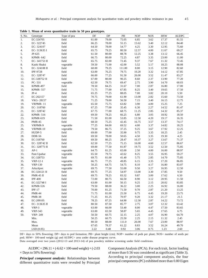
Mohapatra et al. : Principal component analysis for quantitative traits and powdery mildew resistance in pea 4 5
Table 1. Mean of seven quantitative traits in 50 pea genotypes.
DF= days to 50% flowering; DP= days to pod formation; PH= plant height (cm); NOP= number of pods per plant; NOS= number of seeds perpod; HSW= 100-seed weight (g) and AUDPC= area under disease progress curve.Data averaged over two years (2012-13 and 2013-14) of pea powdery mildew screening under field conditions.
S. No. Genotype Type of pea DF DP PH NOP NOS HSW AUDPC 1. EC-324705 field 61.00 79.00 75.05 6.85 3.62 17.37 81.55 2. EC- 322745 field 66.25 78.00 55.15 15.62 3.40 12.12 84.40 3. EC- 324107 field 64.50 78.00 54.77 4.25 3.30 12.95 75.60 4. EC- 313635 I field 65.75 79.25 80.50 12.57 4.00 11.67 69.27 5. JP-625 field 61.50 80.00 88.78 12.25 3.38 13.12 66.45 6. KPMR- 642 field 66.75 80.00 72.25 4.87 3.35 23.00 11.00 7. EC- 341753 II field 65.75 82.00 72.45 9.37 7.67 11.32 72.45 8. Kashi Shakti vegetable 59.50 71.00 42.00 5.52 5.17 18.25 88.08 9. EC- 324108 II field 60.00 79.25 111.00 8.00 3.15 12.90 82.60 10. IPF-9728 field 63.00 76.25 79.75 10.20 3.32 14.12 67.85 11. EC- 328747 field 66.00 77.25 91.50 26.00 3.52 11.47 83.27 12. EC-328752 II field 67.00 80.00 90.25 8.60 2.37 13.90 77.20 13. PC- 531 vegetable 62.50 79.75 69.47 2.75 3.90 14.70 60.03 14. KPMR-497 field 78.50 84.25 31.67 7.00 2.87 16.80 17.00 15. KPMR- 557 field 71.75 77.00 67.85 8.25 3.40 19.65 17.50 16. JP-4 field 65.25 77.25 88.05 7.00 3.82 20.10 5.50 17. EC-262157 field 70.75 79.00 61.90 13.00 2.82 15.60 73.50 18. VKG- 28157 field 71.25 79.00 56.50 7.15 3.40 16.15 12.75 19. VRPMR- 11 vegetable 65.50 75.75 63.82 3.90 4.00 15.25 7.25 20. EC- 318760 field 67.25 77.00 35.45 6.30 2.27 14.52 81.47 21. EC- 328742 field 67.75 77.00 68.75 11.25 2.85 14.32 85.37 22. KPMR- 516 field 69.50 78.25 66.25 6.80 3.05 18.92 18.50 23. KPMR-619 field 71.50 81.00 53.85 12.50 4.20 19.17 16.35 24. PMR-45 field 68.50 75.25 42.45 16.75 3.57 13.37 74.17 25. VRPMR-9 vegetable 77.25 84.00 69.52 4.00 3.37 14.82 18.25 26. VRPMR-10 vegetable 79.50 86.75 37.25 9.25 3.67 17.92 12.25 27. HUDP-5 field 69.00 77.00 35.90 9.75 3.35 18.25 2.45 28. DDR-56 field 69.50 78.00 50.65 4.50 3.35 19.30 4.25 29. EC-318760 field 69.50 80.25 28.47 10.37 3.27 13.67 71.37 30. EC- 328742 II field 62.50 77.25 75.15 16.00 4.60 12.57 86.67 31. EC- 328773 II field 69.00 77.50 81.87 19.75 3.52 12.50 75.85 32. AP-1 vegetable 64.75 81.25 65.00 2.50 4.00 16.00 88.97 33. Pant Upahar vegetable 65.50 79.75 42.62 8.25 3.55 16.95 59.27 34. EC-328753 field 69.75 81.00 41.40 5.75 2.85 14.70 75.85 35. VRP-12-1 vegetable 66.75 77.25 49.85 6.15 3.35 17.20 86.85 36. VRP-130 vegetable 50.25 64.75 54.75 8.10 4.17 16.80 83.07 37. ArkaAjeet vegetable 69.75 77.50 55.00 9.50 3.27 16.95 12.50 38. EC-324121 II field 69.75 77.25 54.97 13.00 3.30 17.85 9.50 39. PMR-45 II field 69.75 78.25 83.32 9.87 3.00 17.62 6.50 40. IPF-400 field 72.00 80.75 66.50 8.90 3.12 20.95 11.50 41. EC-322748 I field 63.00 81.00 50.15 9.25 2.15 20.02 83.85 42. KPMR-526 field 79.50 88.00 36.22 3.00 2.25 16.92 16.00 43. IPF-17 field 70.00 81.25 71.50 9.70 2.87 21.20 13.25 44. PMR-44 field 71.75 81.00 25.50 6.75 4.45 19.20 23.75 45. PMR-38 field 71.25 81.25 70.97 9.20 3.32 21.17 21.5 46. EC-209105 field 78.25 87.25 64.90 12.50 2.87 14.22 73.72 47. EC- 313635 II field 80.50 87.50 85.77 2.75 3.07 12.32 63.42 48. VRP-3 vegetable 63.00 66.00 53.40 8.00 4.47 17.50 83.65 49. VRP-343 vegetable 63.00 65.50 58.87 5.65 4.45 17.65 6.75 50. VRP- 249 vegetable 50.50 60.75 32.15 2.25 4.07 16.90 64.70 Min. 50.25 60.75 25.50 2.25 2.15 11.32 2.45 Max. 80.50 88.00 111.0 26.00 7.67 23.00 88.97 Mean 67.65 78.37 61.22 8.83 3.52 16.24 49.70 LSD (0.05) 2.22 0.48 0.92 3.06 0.75 1.23 2.60
AUDPC = 296.11 + (-6.62 × 100-seed weight) + (-2.03× Days to 50% flowering)Principal component analysis: Relationships betweendifferent quantitative traits were revealed by Principal
Component Analysis (PCA). For each trait, factor loadingof more than 0.56 was considered as significant (Table 3).According to principal component analysis, the fourprincipal components (PC) exhibited more than 0.80 Eigen
4 6 Journal of Food Legumes 30(2), 2017
value and explained about 83.42% of total variation, andhence were taken into consideration. First principalcomponent (PC1) was the most important and explainedabout 32.98% of total variance. Important loading factorsfor PC1 were days to 50% flowering, days to pod formationand AUDPC with loading value of 0.80, 0.63 and -0.74,respectively. PC1 was positively influenced by days to 50%flowering and days to pod formation whereas, negativelyinfluenced by AUDPC. The second PC contributed 25.57% of the variation among the genotypes. PC2 was positivelydefined by number of pods per plant and negativelyinfluenced by 100-seed weight. The third principalcomponent (PC3) accounted for 12.94% of total varianceand was positively influenced by plant height (loadingvalue 0.71). The fourth principal component (PC4)accounted for 12.02% of total variation explained andpositively defined by number of seeds per pod. A numberof workers have been done PCA in peas and other relatedlegumes for yield and component traits (Jha et al. 2012;Parihar et al. 2013; 2014, Kujur et al. 2014). Parihar et al.(2014) revealed significant variation among traits studiedwhere seven major principal components explained about90% of total variation in field peas. Similarly, Kujuret al.(2014) reported that three principal components (PCs)explaining 67.88% of the total variation for seven quantitativetraits (plant height, pods per plant, test weight, yield perplant, lodging score, stem diameter and linear stem density)in 191 diverse pea germplasm.
CONCLUSION
On the basis of principal component analysis ofquantitative traits and powdery mildew resistance in pea,the present study identified a number of field (e.g., HUDP-
5, JP 4, PMR 45 II and VRP 343) and vegetable pea (e.g.,VRPMR 9, VRPMR 10, VRPMR 11 and Arka Ajeet)genotypes which are resistant to PM as well as potent inother yield attributing traits and thus, would be used in PMresistance breeding programs
ACKNOWLEDGEMENT
First author is gratefully acknowledged the financialassistance provided by University Grants Commission,India in form of fellowship during Ph.D. program. Authorsare also thankful to Dr. Satish Sanwal, Senior Scientist, IndianInstitute of Vegetable Research, Varanasi, India forproviding vegetable pea genotypes used in the presentstudy.
REFERENCES
Ahmad Z, Ghafoor A and Iqbal SM. 2001. Yield potential of localand exotic germplasm with special reference to powdery mildewdisease in peas Pisum sativum (L.). Pakistan Journal of Botany33: 251-255.
Banyal DK, Singh A and Tyagi PD. 2005. Pathogenic variability inErysiph episi causing pea powdery mildew. Himachal Journal ofAgricultural Research 32: 87-92.
Cao A, Xing L, Wang X, Yang X, Wang W, Sun Y, Qian C, Ni J, ChenY, Liu D, Wang X and Chen P. 2011. Serine/threonine kinasegene Stpk-V, a key member of powdery mildew resistance genePm21, confers powdery mildew resistance in wheat. PNAS 108:7727-7732.
Carver TLW and Jones SW. 1988. Colony development byErysiphegraminis f.Sp. hordei on isolated epidermis of barleycoleoptile incubated under continuous light or short-dayconditions. Transact. British Mycological Society 90: 114-116.
Ek M, Eklund M, Von Post R, Dayteg C, Henriksson T, Weibull P,Ceplitis A, Isaac P and Tuvesson S. 2005. Microsatellite markers
Table 2. Correlation coefficient among seven quantitative traits in 50 pea genotypes.
***significant at p < 0.0001; **significant at p < 0.001; *significant at p < 0.01.DF= days to 50% flowering; DP= days to pod formation; PH= plant height (cm); NOP= number of pods per plant; NOS= number of seeds perpod; HSW= 100-seed weight (g) and AUDPC= area under disease progress curve.
Trait DF DP PH NOP NOS HSW DP 0.79*** PH -0.10 0.11 NOP 0.03 0.01 0.25 NOS -0.31* -0.30* 0.01 0.01 HSW 0.08 -0.07 -0.26 0.35* -0.14 AUDPC -0.44** -0.17 0.12 0.24 0.09 -0.62***
Table 3. Eigen value, cumulative variance and scores of the four major factors obtained from the PCA of seven quantitativetraits performed on 50 pea genotypes.
**Significant at p < 0.001 (Significant factor loading was observed above 0.56).
Variable PC1 PC2 PC3 PC4 Eigen value 2.30 1.79 0.89 0.84 % cumulative variance 32.98 58.55 71.40 83.42 Days to 50% flowering 0.80** 0.46 -0.07 0.25 Days to pod formation 0.63** 0.44 -0.07 0.19 Plant height -0.26 0.48 0.71** -0.21 Number of pods per plant -0.31 0.58** 0.21 -0.02 Number of seeds per pod -0.46 -0.27 0.24 0.79** 100-seed weight 0.56 -0.64** 0.27 -0.20 AUDPC -0.74** 0.32 -0.43 -0.11
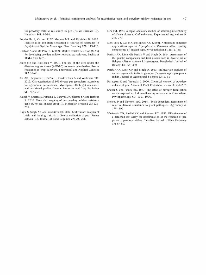
Mohapatra et al. : Principal component analysis for quantitative traits and powdery mildew resistance in pea 4 7
for powdery mildew resistance in pea (Pisum sativum L.).Hereditas 142: 86-91.
Fondevilla S, Carver TLW, Moreno MT and Rubiales D. 2007.Identification and characterisation of sources of resistance toErysiphepisi Syd. In Pisum spp. Plant Breeding 126: 113-119.
Ghafoor A and Mc Phee K. (2012). Marker assisted selection (MAS)for developing powdery mildew resistant pea cultivars, Euphytica186L: 593–607.
Jeger MJ and Rollinsen V. 2001. The use of the area under thedisease-progress curve (AUDPC) to assess quantitative diseaseresistance in crop cultivars. Theoretical and Applied Genetics102:32-40.
Jha AB, Arganosa G, Tar’an B, Diederichsen A and Warkentin TD.2012. Characterization of 169 diverse pea germplasm accessionsfor agronomic performance, Mycosphaerella blight resistanceand nutritional profile. Genetic Resources and Crop Evolution60: 747-761.
Katoch V, Sharma S, Pathania S, Banayal DK, Sharma SK and RathourR. 2010. Molecular mapping of pea powdery mildew resistancegene er2 to pea linkage group III. Molecular Breeding 25: 229-237.
Kujur S, Singh AK and Srivastava CP. 2014. Multivariate analysis ofyield and lodging traits in a diverse collection of pea (Pisumsativum L.). Journal of Food Legumes 27: 293-296.
Lim TM. 1973. A rapid laboratory method of assessing susceptibilityof Hevea clones to Oidiumheveae. Experimental Agriculture 9:275-279.
Mert-Turk F, Gul MK and Egesel, CO (2008). Nitrogenand fungicideapplications against Erysiphe cruciferarum affect qualitycomponents of oilseed rape. Mycopathologia 165: 27-35.
Parihar AK, Dixit GP, Pathak V and Singh D. 2014. Assessment ofthe genetic components and trait associations in diverse set offieldpea (Pisum sativum L.) genotypes. Bangladesh Journal ofBotany 43: 323-330
Parihar AK, Dixit GP and Singh D. 2013. Multivariate analysis ofvarious agronomic traits in grasspea (Lathyrus spp.) germplasm.Indian Journal of Agricultural Sciences 83: 570-5
Rajappan K and Yesuraja I. 2000. Chemical control of powderymildew of pea. Annals of Plant Protection Science 8: 266-267.
Shaner G and Finney RE. 1977. The effect of nitrogen fertilizationon the expression of slow-mildewing resistance in Knox wheat.Phytopathology 67: 1051-1056.
Skelsey P and Newton AC. 2014. Scale-dependent assessment ofrelative disease resistance to plant pathogens. Agronomy 4:178- 190
Warkentin TD, Rashid KY and Zimmer RC. 1995. Effectiveness ofa detached leaf assay for determination of the reaction of peaplants to powdery mildew. Canadian Journal of Plant Pathology17: 87-89.
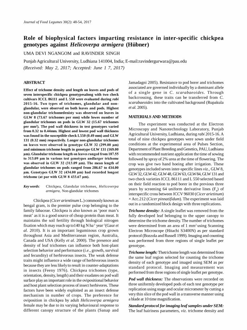
Journal of Food Legumes 30(2): 48-54, 2017
ABSTRACT
Effect of trichome density and length on leaves and pods ofseven interspecific chickpea genotypesalong with two checkcultivars ICCL 86111 and L 550 were evaluated during rabi2015-16. Two types of trichomes, glandular and non-glandular, were observed on both leaves and pods. Highestnon-glandular trichomedenisty was observed on leaves inGLW 8 (73.67 trichomes per mm) while lowes number ofglandular trichomes on pods in GLW 32 (15.67 trichomesper mm2). The pod wall thickness in test genotypes variedfrom 0.32 to 0.44mm. Highest and lowest pod wall thicknesswas found in the susceptible check L550 (0.49 mm) and GLW131 (0.32 mm) respactivily. Longer non-glandular trichomeson leaves were observed in genotype GLW 32 (299.00 µm)and minimum trichome length in genotype GLW 131 (169.00µm). Glandular trichome length on leaves ranged from 187.55to 313.09 µm in various test genotypes andlarger trichomewas observed in GLW 32 (313.09 µm). The mean length ofglandular trichomes on pods ranged from 286.67 to 434.00µm. Genotypes GLW 32 (434.00 µm) had recorded longesttrichome (at par with GLW 8 433.67 µm).
Key words: Chickpea, Glandular trichomes, Helicoverpaarmigera, Non-glandular trichomes
Chickpea (Cicer arientinum L.) commonly known asbengal gram, is the premier pulse crop belonging to thefamily fabaceae. Chickpea is also known as ‘poor man’smeat’ as it is a good source of cheap protein than meat. Itmaintains the soil fertility through biological nitrogenfixation which may reach up to140 kg N ha-1 year-1(Gaur etal. 2010). It is an important leguminous crop grownthroughout Asia and Mediterranean region, Australia,Canada and USA (Kelly et al. 2000). The presence anddensity of leaf trichomes can influence both host-plantselection behavior and performance (i.e., growth, survivaland fecundity) of herbivorous insects. The weak defensetraits might influence a wide range of herbivorous insectsbecause they are less likely to result in counter-adaptationsin insects (Feeny 1976). Chickpea trichomes (type,orientation, density, length) and their exudates on pod wallsurface play an important role in the ovipositional behaviorand host plant selection process of insect herbivores. Thesefactors have been widely exploited as an insect defensemechanism in number of crops. The preference foroviposition in chickpea by adult Helicoverpa armigerafemale may be due to its varying behavioural response todifferent canopy structure of the plants (Sanap and
Role of biophysical factors imparting resistance in inter-specific chickpeagenotypes against Helicoverpa armigera (Hübner)UMA DEVI NGANGOM and RAVINDER SINGH
Punjab Agricultural University, Ludhiana 141004, India; E-mail:[email protected](Received: May 2, 2017; Accepted: June 1 7, 2017)
Jamadagni 2005). Resistance to pod borer and trichomesassociated are governed individually by a dominant alleleof a single gene in C. scarabaeoides. Throughbackcrossing, these traits can be transferred from C.scarabaeoides into the cultivated background (Rupakulaet al. 2005).
MATERIALS AND METHODS
The experiment was conducted at the ElectronMicroscopy and Nanotechnology Laboratory, PunjabAgricultural University, Ludhiana, during rabi 2015-16. Atotal of nine chickpea genotypes were sown under fieldconditions at the experimental area of Pulses Section,Department of Plant Breeding and Genetics, PAU, Ludhianawith recommended nutrient application the time of sowingfollowed by spray of 2% urea at the time of flowering. Thecrop was give two hand hoeing after irrigation. Thesegenotypes included seven inter-specific lines viz., GLW 8,GLW 32, GLW 42, GLW 48, GLW 63, GLW 84, GLW 131 andtwo check varieties ICCL 86111 and L 550 selected basedon their field reaction to pod borer in the previous threeyears by screening 64 uniform derivative lines (F9) ofinterspecific cross between ICCV 96030 (Cicer arietinum)× Acc.212 (Cicer pinnatifidum). The experiment was laidout in a randomized block design with three replications.Trichome density: A single leaflet was removed from thefully developed leaf belonging to the upper canopy todetermine the trichome density. The number of trichomeswere determined from an area of 1 mm2 using ScanningElectron Microscope (Hitachi S3400N) as per standardprotocol (Bozzola and Russell 1999). Imaging and countingwas performed from three regions of single leaflet pergenotype.Trichome length: Thetrichome length was determined fromthe same leaf region selected for counting the trichomedensity of each genotype and imaged using SEM as perstandard protocol. Imaging and measurement wasperformed from three regions of single leaflet per genotype.Pod wall thickness: The observations were recorded onthree uniformly developed pods of each test genotype perreplication using stage and ocular micrometer by cutting avery thin slice of the pod wall in a transverse manner usinga blade at 10 time magnification.Standard protocol for imaging leaf samples under SEM:The leaf hairiness parameters, viz. trichome density and
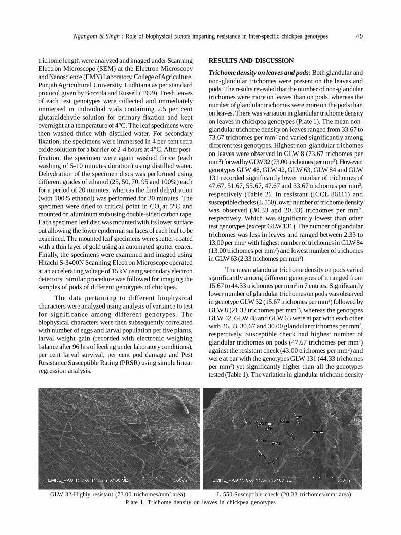
Ngangom & Singh : Role of biophysical factors imparting resistance in inter-specific chickpea genotypes 4 9
trichome length were analyzed and imaged under ScanningElectron Microscope (SEM) at the Electron Microscopyand Nanoscience (EMN) Laboratory, College of Agriculture,Punjab Agricultural University, Ludhiana as per standardprotocol given by Bozzola and Russell (1999). Fresh leavesof each test genotypes were collected and immediatelyimmersed in individual vials containing 2.5 per centglutaraldehyde solution for primary fixation and keptovernight at a temperature of 4°C. The leaf specimens werethen washed thrice with distilled water. For secondaryfixation, the specimens were immersed in 4 per cent tetraoxide solution for a barrier of 2-4 hours at 4°C. After post-fixation, the specimen were again washed thrice (eachwashing of 5-10 minutes duration) using distilled water.Dehydration of the specimen discs was performed usingdifferent grades of ethanol (25, 50, 70, 95 and 100%) eachfor a period of 20 minutes, whereas the final dehydration(with 100% ethanol) was performed for 30 minutes. Thespecimen were dried to critical point in CO2 at 5°C andmounted on aluminum stub using double-sided carbon tape.Each specimen leaf disc was mounted with its lower surfaceout allowing the lower epidermal surfaces of each leaf to beexamined. The mounted leaf specimens were sputter-coatedwith a thin layer of gold using an automated sputter coater.Finally, the specimens were examined and imaged usingHitachi S-3400N Scanning Electron Microscope operatedat an accelerating voltage of 15 kV using secondary electrondetectors. Similar procedure was followed for imaging thesamples of pods of different genotypes of chickpea.
The data pertaining to different biophysicalcharacters were analyzed using analysis of variance to testfor significance among different genotypes. Thebiophysical characters were then subsequently correlatedwith number of eggs and larval population per five plants,larval weight gain (recorded with electronic weighingbalance after 96 hrs of feeding under laboratory conditions),per cent larval survival, per cent pod damage and PestResistance Susceptible Rating (PRSR) using simple linearregression analysis.
RESULTS AND DISCUSSION
Trichome density on leaves and pods: Both glandular andnon-glandular trichomes were present on the leaves andpods. The results revealed that the number of non-glandulartrichomes were more on leaves than on pods, whereas thenumber of glandular trichomes were more on the pods thanon leaves. There was variation in glandular trichome densityon leaves in chickpea genotypes (Plate 1). The mean non-glandular trichome density on leaves ranged from 33.67 to73.67 trichomes per mm2 and varied significantly amongdifferent test genotypes. Highest non-glandular trichomeson leaves were observed in GLW 8 (73.67 trichomes permm2) forwed by GLW 32 (73.00 trichomes per mm2). However,genotypes GLW 48, GLW 42, GLW 63, GLW 84 and GLW131 recorded significantly lower number of trichomes of47.67, 51.67, 55.67, 47.67 and 33.67 trichomes per mm2,respectively (Table 2). In resistant (ICCL 86111) andsusceptible checks (L 550) lower number of trichome densitywas observed (30.33 and 20.33) trichomes per mm2,respectively. Which was significantly lowest than othertest genotypes (except GLW 131). The number of glandulartrichomes was less in leaves and ranged between 2.33 to13.00 per mm2 with highest number of trichomes in GLW 84(13.00 trichomes per mm2) and lowest number of trichomesin GLW 63 (2.33 trichomes per mm2).
The mean glandular trichome density on pods variedsignificantly among different genotypes of it ranged from15.67 to 44.33 trichomes per mm2 in 7 entries. Significantlylower number of glandular trichomes on pods was observedin genotype GLW 32 (15.67 trichomes per mm2) followed byGLW 8 (21.33 trichomes per mm2), whereas the genotypesGLW 42, GLW 48 and GLW 63 were at par with each otherwith 26.33, 30.67 and 30.00 glandular trichomes per mm2,respectively. Susceptible check had highest number ofglandular trichomes on pods (47.67 trichomes per mm2)against the resistant check (43.00 trichomes per mm2) andwere at par with the genotypes GLW 131 (44.33 trichomesper mm2) yet significantly higher than all the genotypestested (Table 1). The variation in glandular trichome density
GLW 32-Highly resistant (73.00 trichomes/mm2 area) L 550-Susceptible check (20.33 trichomes/mm2 area)Plate 1. Trichome density on leaves in chickpea genotypes
5 0 Journal of Food Legumes 30(2), 2017
on pods in chickpea genotypes my also enteral (Plate 3).Non-glandular trichome density on pods did not play anyrole in genotype resistance and ranged 0.67 (GLW 63) to7.67 trichomes per mm2 (GLW 42 and GLW 48) respectively.Pod wall thickness: The pod wall thickness of all thegenotypes varied from 0.32 to 0.44 mm. Higher pod wallthickness was found in the susceptible check an kabuligenotype L 550 (0.49 mm) was followed by GLW 8, GLW 48,GLW 63 and GLW 84 with 0.44, 0.40, 0.42 and 0.40 mmrespectively. On biophysical basis, the best genotype viz.,GLW 32 and GLW 42 had the thickness of 0.36 and 0.37 mm,respectively (at par with each other). Lower pod wallthickness was recorded in genotype GLW 131 (0.32 mm)floured 5mm resistant check ICCL 86111 (0.36 mm). Therewas no role of pod wall thickness in interspecific chickpeagenotypes for resistance against Helicoverpa armigera.Thus, pod wall thickness and pod borer damage werenegatively correlated. Hossain et al. (2008), Girija et al.(2008) however a contrast results showed that thicker podhusks exhibited less per cent pod damage.Trichome length on leaves and pods: Length of non-glandular trichomes in case of leaves. Ranged from 169.00
to 299.00 µm. Minimum non-glandular trichome length wasobserved in genotype GLW 131 (169.00 µm). Maximum non-glandular trichome length was observed in genotype GLW32 (299.00 µm) Forwed by GLW 8, GLW42, GLW 48, GLW 63and GLW 84 with trichome length of 274.67, 297.33, 265.67,243.33 and 264.00 µm, respectively. Susceptible check L550 had trichome length of 235.67 µm against the resistantcheck ICCL 86111 of 212.67 µm (which was at par with GLW131mm 169.00 µm). Glandular trichome length on leavesranged from 187.55 to 313.09 µm. Highest trichome lengthwas observed in GLW 32 (313.09 µm) Forwered by GLW 8,GLW 42, GLW 48, GLW 63 and GLW 84 with trichome lengthof 289.89, 250.66, 268.89, 267.99 and 263.99 µm, respectively(Table 2). Susceptible check genotype L 550 had recordedtrichome length of 239.33 µm against the resistant genotypeICCL 86111 (223.99mm) which was at par with GLW 131(187.55).
The mean glandular trichome length on pods variedsignificantly among different test genotypes. As it rangedfrom 286.67 to 434.00 µm. Genotypes GLW 32 (434.00 µm)had significantly longer trichome length which was at parwith GLW 8 (433.67 µm), whereas genotypes GLW 42, GLW
GLW 32-Highly resistant (299.00 µm) L 550-Susceptible check (235.67 µm)Plate 2. Trichome length on leaves in chickpea genotypes
GLW 32-Highly resistant (15.67 trichomes/mm2 area) L 550-Susceptible check (47.67 trichomes/mm2 area)Plate 3. Trichome density on pods in chickpea genotypes
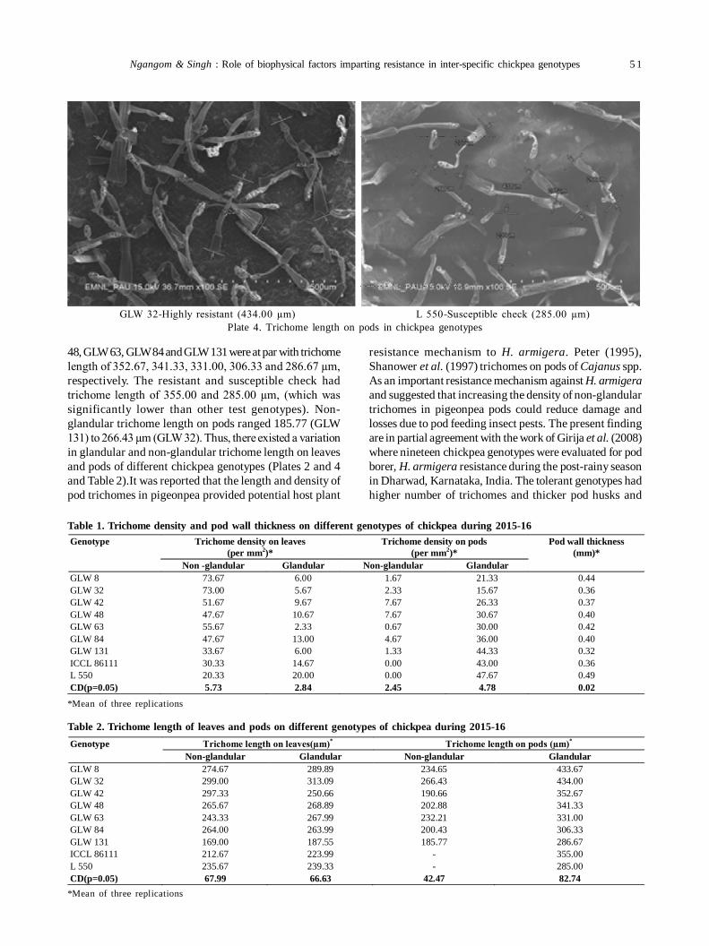
Ngangom & Singh : Role of biophysical factors imparting resistance in inter-specific chickpea genotypes 5 1
48, GLW 63, GLW 84 and GLW 131 were at par with trichomelength of 352.67, 341.33, 331.00, 306.33 and 286.67 µm,respectively. The resistant and susceptible check hadtrichome length of 355.00 and 285.00 µm, (which wassignificantly lower than other test genotypes). Non-glandular trichome length on pods ranged 185.77 (GLW131) to 266.43 µm (GLW 32). Thus, there existed a variationin glandular and non-glandular trichome length on leavesand pods of different chickpea genotypes (Plates 2 and 4and Table 2).It was reported that the length and density ofpod trichomes in pigeonpea provided potential host plant
resistance mechanism to H. armigera. Peter (1995),Shanower et al. (1997) trichomes on pods of Cajanus spp.As an important resistance mechanism against H. armigeraand suggested that increasing the density of non-glandulartrichomes in pigeonpea pods could reduce damage andlosses due to pod feeding insect pests. The present findingare in partial agreement with the work of Girija et al. (2008)where nineteen chickpea genotypes were evaluated for podborer, H. armigera resistance during the post-rainy seasonin Dharwad, Karnataka, India. The tolerant genotypes hadhigher number of trichomes and thicker pod husks and
GLW 32-Highly resistant (434.00 µm) L 550-Susceptible check (285.00 µm)Plate 4. Trichome length on pods in chickpea genotypes
Table 1. Trichome density and pod wall thickness on different genotypes of chickpea during 2015-16
*Mean of three replications
Genotype Trichome density on leaves (per mm2)*
Trichome density on pods (per mm2)*
Pod wall thickness (mm)*
Non -glandular Glandular Non-glandular Glandular GLW 8 73.67 6.00 1.67 21.33 0.44 GLW 32 73.00 5.67 2.33 15.67 0.36 GLW 42 51.67 9.67 7.67 26.33 0.37 GLW 48 47.67 10.67 7.67 30.67 0.40 GLW 63 55.67 2.33 0.67 30.00 0.42 GLW 84 47.67 13.00 4.67 36.00 0.40 GLW 131 33.67 6.00 1.33 44.33 0.32 ICCL 86111 30.33 14.67 0.00 43.00 0.36 L 550 20.33 20.00 0.00 47.67 0.49 CD(p=0.05) 5.73 2.84 2.45 4.78 0.02
Table 2. Trichome length of leaves and pods on different genotypes of chickpea during 2015-16
*Mean of three replications
Genotype Trichome length on leaves(µm)* Trichome length on pods (µm)* Non-glandular Glandular Non-glandular Glandular
GLW 8 274.67 289.89 234.65 433.67 GLW 32 299.00 313.09 266.43 434.00 GLW 42 297.33 250.66 190.66 352.67 GLW 48 265.67 268.89 202.88 341.33 GLW 63 243.33 267.99 232.21 331.00 GLW 84 264.00 263.99 200.43 306.33 GLW 131 169.00 187.55 185.77 286.67 ICCL 86111 212.67 223.99 - 355.00 L 550 235.67 239.33 - 285.00 CD(p=0.05) 67.99 66.63 42.47 82.74
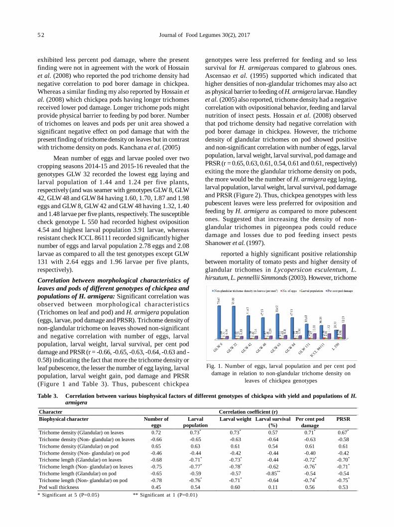
5 2 Journal of Food Legumes 30(2), 2017
exhibited less percent pod damage, where the presentfinding were not in agreement with the work of Hossainet al. (2008) who reported the pod trichome density hadnegative correlation to pod borer damage in chickpea.Whereas a similar finding my also reported by Hossain etal. (2008) which chickpea pods having longer trichomesreceived lower pod damage. Longer trichome pods mightprovide physical barrier to feeding by pod borer. Numberof trichomes on leaves and pods per unit area showed asignificant negative effect on pod damage that with thepresent finding of trichome density on leaves but in contrastwith trichome density on pods. Kanchana et al. (2005)
Mean number of eggs and larvae pooled over twocropping seasons 2014-15 and 2015-16 revealed that thegenotypes GLW 32 recorded the lowest egg laying andlarval population of 1.44 and 1.24 per five plants,respectively (and was seamer with genotypes GLW 8, GLW42, GLW 48 and GLW 84 having 1.60, 1.70, 1.87 and 1.98eggs and GLW 8, GLW 42 and GLW 48 having 1.32, 1.40and 1.48 larvae per five plants, respectively. The susceptiblecheck genotype L 550 had recorded highest oviposition4.54 and highest larval population 3.91 larvae, whereasresistant check ICCL 86111 recorded significantly highernumber of eggs and larval population 2.78 eggs and 2.08larvae as compared to all the test genotypes except GLW131 with 2.64 eggs and 1.96 larvae per five plants,respectively).Correlation between morphological characteristics ofleaves and pods of different genotypes of chickpea andpopulations of H. armigera: Significant correlation wasobserved between morphological characteristics(Trichomes on leaf and pod) and H. armigera population(eggs, larvae, pod damage and PRSR). Trichome density ofnon-glandular trichome on leaves showed non-significantand negative correlation with number of eggs, larvalpopulation, larval weight, larval survival, per cent poddamage and PRSR (r = -0.66, -0.65, -0.63, -0.64, -0.63 and -0.58) indicating the fact that more the trichome density orleaf pubescence, the lesser the number of egg laying, larvalpopulation, larval weight gain, pod damage and PRSR(Figure 1 and Table 3). Thus, pubescent chickpea
genotypes were less preferred for feeding and so lesssurvival for H. armigeraas compared to glabrous ones.Ascensao et al. (1995) supported which indicated thathigher densities of non-glandular trichomes may also actas physical barrier to feeding of H. armigera larvae. Handleyet al. (2005) also reported, trichome density had a negativecorrelation with ovipositional behavior, feeding and larvalnutrition of insect pests. Hossain et al. (2008) observedthat pod trichome density had negative correlation withpod borer damage in chickpea. However, the trichomedensity of glandular trichomes on pod showed positiveand non-significant correlation with number of eggs, larvalpopulation, larval weight, larval survival, pod damage andPRSR (r = 0.65, 0.63, 0.61, 0.54, 0.61 and 0.61, respectively)exiting the more the glandular trichome density on pods,the more would be the number of H. armigera egg laying,larval population, larval weight, larval survival, pod damageand PRSR (Figure 2). Thus, chickpea genotypes with lesspubescent leaves were less preferred for oviposition andfeeding by H. armigera as compared to more pubescentones. Suggested that increasing the density of non-glandular trichomes in pigeonpea pods could reducedamage and losses due to pod feeding insect pestsShanower et al. (1997).
reported a highly significant positive relationshipbetween mortality of tomato pests and higher density ofglandular trichomes in Lycopersicon esculentum, L.hirsutum, L. pennellii Simmonds (2003). However, trichome
Table 3. Correlation between various biophysical factors of different genotypes of chickpea with yield and populations of H.armigera
* Significant at 5 (P=0.05) ** Significant at 1 (P=0.01)
Character Correlation coefficient (r) Biophysical character Number of
eggs Larval
population Larval weight Larval survival
(%) Per cent pod
damage PRSR
Trichome density (Glandular) on leaves 0.72 0.73* 0.73* 0.57 0.71* 0.67* Trichome density (Non- glandular) on leaves -0.66 -0.65 -0.63 -0.64 -0.63 -0.58 Trichome density (Glandular) on pod 0.65 0.63 0.61 0.54 0.61 0.61 Trichome density (Non- glandular) on pod -0.46 -0.44 -0.42 -0.44 -0.40 -0.42 Trichome length (Glandular) on leaves -0.68 -0.71* -0.73* -0.44 -0.72* -0.70* Trichome length (Non- glandular) on leaves -0.75 -0.77* -0.78* -0.62 -0.76* -0.71* Trichome length (Glandular) on pod -0.65 -0.59 -0.57 -0.85** -0.54 -0.54 Trichome length (Non- glandular) on pod -0.78 -0.76* -0.71* -0.64 -0.74* -0.75* Pod wall thickness 0.45 0.54 0.60 0.11 0.56 0.53
Fig. 1. Number of eggs, larval population and per cent poddamage in relation to non-glandular trichome density on
leaves of chickpea genotypes
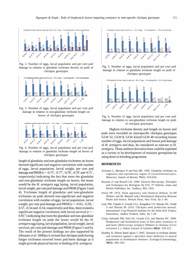
Ngangom & Singh : Role of biophysical factors imparting resistance in inter-specific chickpea genotypes 5 3
Highest trichome density and length on leaves andpods were recorded on interspecific chickpea genotypesGLW 32, GLW 8, GLW 42and GLW 48 recording lowestnumber of eggs, larval population and lowest pod damageof H. armigera and thus, be considered as tolerant to H.armigera. These uniform derivative lines could be exploitedas a variety or by development of resistant germplasm byusing them in breeding programme.
REFERENCES
Ascensao L, Marques N and Pais MS. 1995. Glandular trichomes onvegetative and reproductive organs of Leonotisleonurus(La-Maiacez). Annals of Botany 75(6): 619-626.
Bozzola JJ and Russell LD. 1999. Electron Microscopy: Principlesand Techniques for Biologists Pp 670. 2nd Edition, Jones andBarlett Publishers, Inc. Sudbury, MA, USA.
Feeny PP. 1976. Plant apparency and chemical defense. In:JMWallace and RL Mansell (eds.) Biochemical Interaction BetweenPlants and Insects. Plenum Press, New York, Pp 1–40.
Gaur PM, Tripathi S, Gowda CLL, RangaRao GV, Sharma HC, PandeS and Sharma M. 2010. Chickpea seed production manual.International Crop Research Institute for the Semi-Arid Tropics,Patancheru, Andhra Pradesh, India. Pp 1-28.
Girija, Salimath PM, Patil SA, Gowda CLL and Sharma HC. 2008.Biophysical and biochemical basis of host plant resistance topod borer (Helicoverpa armigera Hübner) in chickpea (Cicerarietinum L.). Indian Journal of Genetics 68(3): 320-323.
Handley R, Ekbom Band Agren J. 2005. Variation in trichome densityand resistance against a specialist insect herbivore in naturalpopulations of Arabidopsis thaliana. Ecological Entomology,30(3): 284–292.
Fig. 3. Number of eggs, larval population and per cent poddamage in relation to non-glandular trichome length on
leaves of chickpea genotypes
Fig. 4. Number of eggs, larval population and per cent poddamage in relation to glandular trichome length on leaves of
chickpea genotypes
Fig. 5. Number of eggs, larval population and per cent poddamage in relation to glandular trichome length on pods of
chickpea genotypes
Fig. 6. Number of eggs, larval population and per cent poddamage in relation to non-glandular trichome length on pods
of chickpea genotypes
Fig. 2. Number of eggs, larval population and per cent poddamage in relation to glandular trichome density on pods of
chickpea genotypes
length of glandular and non-glandular trichomes on leavesshowed significant and negative correlation with numberof eggs, larval population, larval weight, per cent poddamage and PRSR (r = -0.75*, -0.77*, -0.78*, -0.76* and -0.71*,respectively) indicating the fact that more the glandularand non-glandular trichome length on leaves, the lesserwould be the H. armigera egg laying, larval population,larval weight, per cent pod damage and PRSR (Figure 3 and4). Trichome length of glandular and non-glandulartrichomes on pods showed non-significant and negativecorrelation with number of eggs, larval population, larvalweight, per cent pod damage and PRSR (r = -0.65, -0.59, -0.57, -0.54 and -0.54, respectively) and thus, there existed asignificant negative correlation with larval survival (r = -0.85**) indicating that more the glandular and non-glandulartrichome length on pods the lesser would be the H.armigera egg laying, larval population, larval weight, larvalsurvival, per cent pod damage and PRSR (Figure 5 and 6).The result of the present findings are also supported by(Hossain et al. 2008)as it revised that chickpea pods havinglonger trichomes received lower pod borer damage as itmight provide physical barrier to feeding of H. armigera.
5 4 Journal of Food Legumes 30(2), 2017
Hossain Altaf, Haque Azizul and Prodhan MZH. 2008. Effect ofpods characteristics on pod borer, Helicoverpa armigera(Hübner), investigation in chickpea. SAARC Journal ofAgriculture 6(1): 51-60.
Kanchana R, Lakshmi KV and Sekhar PR. 2005. Morphological andbiochemical bases of host plant resistance to Helicoverpaarmigera (Hübner) in chickpea. Journal of Plant Protectionand Environment 2(1): 12-17.
Kelly TG, ParthasarathyRao P and Grisko-Kelly H. 2000. The pulseeconomy in the mid 1990. In: Knight R (ed.) Linking Researchand Marketing Opportunities for Pulses in the 21 st century,Kluwer, Dordrecht Pp 1-29.
Peter AJ. 1995. Pigeonpea trichomes: a promising source for podborer resistance. IPM and IRM Newsletter for Legume Crops inAsia 2: 5-6.
Rupakula A, Rao DM, Reddy LJ, Upadhyaya HD and Sharma HC.2005. Inheritance of trichomes and resistance to pod borer(Helicoverpa armigera) and their association in inter specificcrosses between cultivated pigeonpea (Cajanus cajan) and itswild relative (C. scarabaeoides).Euphytica 145: 247-257.
Sanap MM and Jamadagni BM. 2005. Screening of chickpea forresistance to pod borer Helicoverpa armigera (Hübner) at Rahuri,Maharashtra, India. ICPN 12: 37-39.
Shanower TG, Yoshida M and Peter AJ. 1997. Survival, growth,fecundity and behaviour of Helicoverpa armigera (Lepidoptera:Noctuidae) on pigeonpea and two wild Cajanus species. Journalof Economic Entomology 90: 837-841.
Simmonds MSJ. 2003. Flavonoid-insect interactions: recent advancesin our knowledge. Phytochemical 64: 21-30.
Journal of Food Legumes 30(2): 55-58, 2017
Biorational management of aphid [Acyrthosiphon pisum (harris)] and leaf miner[Chromatomyia horticola (goureau)] infesting peaPS SINGH and SK SINGH
Department of Entomology and Agricultural Zoology, Institute of Agricultural Sciences, Banaras Hindu University,Varanasi, Uttar Pradesh, India; E-mail: [email protected](Received: February 16, 2016; Accepted: December 6, 2016)
ABSTRACT
Field experiment was undertaken to evaluate the efficacy ofinsecticides & botanicals in managing aphid & leaf minorin pea. Among the various treatments, imidacloprid 50g a.i./ha was found superior in reducing the aphid population &leaf minor damage during both the seasons (Rabi 2012 &13). The botanicals were found to be least effective incontrolling the both pests. The maximum per field wasrecorded from plots treated with imidacloprid. Imidacloprid50g a.i./ha was found most effective in both the years againstpea aphid and leaf miner and also produced maximum yield.
Keywords: Acyrthosiphon pisum, Botanicals Chromatomyiahorticola, Insecticides, Pea
Field pea (Pisum sativum L.) is one of the mostimportant legume crops of India. Which is cultivated forthe fresh green seeds, tender green pods, dried seeds andfoliage (Duke, 1981). It is a highly nutritious vegetable withprotein concentration ranging from 15.5-39.7 per cent(Davies et al. 1985, Bressani and Elias 1988). Its intensivecultivation steadily increased acreage and production. Peacrop is infested by number of insect pests throughout itsvegetative and production phases viz., pea stem fly(Ophiomyia phaseoli), pea leaf miner (Chromatomyiahorticola), pea aphid (Acyrthosiphon pisum), pod borer(Etiella zinckenella), (Helicoverpa armigera) and thrips(Thrips tabaci) (Singh and Mishra 2013). Pea leaf miner isa serious, polyphagous and pest of regular occurrenceworldwide (Darshan et al. 1991). The larvae construct minesin leaves, consume leaf tissues and eventually disruptphotosynthesis (Fathi 2011). Which is also known totransmit plant diseases (Parrella et al. 1985, Parrella 1987).The severe infestation by pea leaf minor can cause cropdamage up to 90 per cent by restricting its flowering andpod formation (Atwal et al. 1969, Mavi and Singh 1988 andTariq et al. 1991). Keeping in view the importance of peacrop, the present study was conducted to test the relativeefficacy of some insecticides and botanicals against peaaphid (Acyrthosiphon pisum) and leaf miner(Chromatomyia horticola) in pea.
MATERIALS AND METHODS
The present study was conducted at AgriculturalResearch Farm of Banaras Hindu University, Varanasi during
Rabi 2012 and 2013 for efficacy of some botanicals andinsecticides against pea aphid, Acyrthosiphon pisum andleaf miner, Chromatomyia horticola. Experiment was laidout in a RBD with 7 treatments (NSKE 5 %, Nimbecidine1500ppm, Imidacloprid 50g a.i./ha, Triazophos 750g a.i./ha,Fipronil 100g a.i./ha, Thiamethoxam 30g a.i./ha and Control)which were replicated thrice with 4×210 cm plot size and25×10 cm plant spacing. The recommended dose of fertilizerswere applied under normal irrigated conditions eachtreatment were sprayed with a knapsack high volumesprayer by ensuring uniform coverage at 50 % floweringstage.
Aphid infestation was recorded by counting numberof aphids per 10 cm upper stem per plant at one day beforeand 3rd, 7th and 10th days after spray. The per cent leafdamage by leaf miner was recorded at one day before and3rd, 7th and 10th days after spray. The cumulative per centleaf infestation was worked out on the basis of total numberof leaves from all the observation as given below:
At the time of maturity grain yield data were alsorecorded. The percentage reduction of the aphid populationover untreated check in different treatments was calculatedusing Henderson and Tilton‘s (1955) formula.
Per cent efficacy =Where,
Ta = Population in the treated plot after spray.
Tb = Population in the treated plot before spray.
Ca = Population in the control plot after spray.
Cb = Population in the control plot before spray.
The data obtained were analyzed statistically tocompare the treatment effects (Panse and Sukhatme 1961).
RESULTS AND DISCUSSION
Efficacy of insecticides and botanicals on pea aphid: It isevident that the aphid population before spraying was non-significantly varied from 11.20 to 13.60 aphids per 10 cmupper stem per plant during Rabi 2012 (Table 1). All the
Per cent leaf infestation =Total No. of infested leaves
Total No. of leaves× 100
1001
a
b
b
a
CC
TT
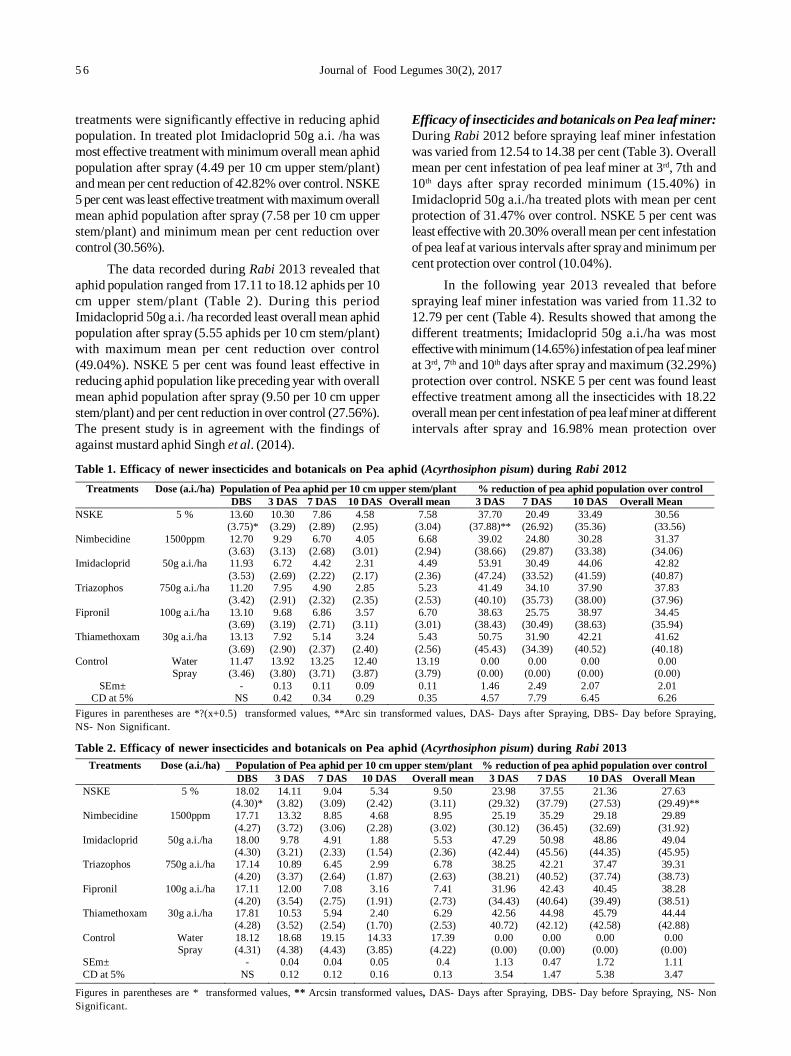
5 6 Journal of Food Legumes 30(2), 2017
treatments were significantly effective in reducing aphidpopulation. In treated plot Imidacloprid 50g a.i. /ha wasmost effective treatment with minimum overall mean aphidpopulation after spray (4.49 per 10 cm upper stem/plant)and mean per cent reduction of 42.82% over control. NSKE5 per cent was least effective treatment with maximum overallmean aphid population after spray (7.58 per 10 cm upperstem/plant) and minimum mean per cent reduction overcontrol (30.56%).
The data recorded during Rabi 2013 revealed thataphid population ranged from 17.11 to 18.12 aphids per 10cm upper stem/plant (Table 2). During this periodImidacloprid 50g a.i. /ha recorded least overall mean aphidpopulation after spray (5.55 aphids per 10 cm stem/plant)with maximum mean per cent reduction over control(49.04%). NSKE 5 per cent was found least effective inreducing aphid population like preceding year with overallmean aphid population after spray (9.50 per 10 cm upperstem/plant) and per cent reduction in over control (27.56%).The present study is in agreement with the findings ofagainst mustard aphid Singh et al. (2014).
Efficacy of insecticides and botanicals on Pea leaf miner:During Rabi 2012 before spraying leaf miner infestationwas varied from 12.54 to 14.38 per cent (Table 3). Overallmean per cent infestation of pea leaf miner at 3rd, 7th and10th days after spray recorded minimum (15.40%) inImidacloprid 50g a.i./ha treated plots with mean per centprotection of 31.47% over control. NSKE 5 per cent wasleast effective with 20.30% overall mean per cent infestationof pea leaf at various intervals after spray and minimum percent protection over control (10.04%).
In the following year 2013 revealed that beforespraying leaf miner infestation was varied from 11.32 to12.79 per cent (Table 4). Results showed that among thedifferent treatments; Imidacloprid 50g a.i./ha was mosteffective with minimum (14.65%) infestation of pea leaf minerat 3rd, 7th and 10th days after spray and maximum (32.29%)protection over control. NSKE 5 per cent was found leasteffective treatment among all the insecticides with 18.22overall mean per cent infestation of pea leaf miner at differentintervals after spray and 16.98% mean protection over
Table 1. Efficacy of newer insecticides and botanicals on Pea aphid (Acyrthosiphon pisum) during Rabi 2012Treatments Dose (a.i./ha) Population of Pea aphid per 10 cm upper stem/plant % reduction of pea aphid population over control
DBS 3 DAS 7 DAS 10 DAS Overall mean 3 DAS 7 DAS 10 DAS Overall Mean NSKE 5 % 13.60
(3.75)* 10.30 (3.29)
7.86 (2.89)
4.58 (2.95)
7.58 (3.04)
37.70 (37.88)**
20.49 (26.92)
33.49 (35.36)
30.56 (33.56)
Nimbecidine 1500ppm 12.70 (3.63)
9.29 (3.13)
6.70 (2.68)
4.05 (3.01)
6.68 (2.94)
39.02 (38.66)
24.80 (29.87)
30.28 (33.38)
31.37 (34.06)
Imidacloprid
50g a.i./ha 11.93 (3.53)
6.72 (2.69)
4.42 (2.22)
2.31 (2.17)
4.49 (2.36)
53.91 (47.24)
30.49 (33.52)
44.06 (41.59)
42.82 (40.87)
Triazophos
750g a.i./ha 11.20 (3.42)
7.95 (2.91)
4.90 (2.32)
2.85 (2.35)
5.23 (2.53)
41.49 (40.10)
34.10 (35.73)
37.90 (38.00)
37.83 (37.96)
Fipronil
100g a.i./ha 13.10 (3.69)
9.68 (3.19)
6.86 (2.71)
3.57 (3.11)
6.70 (3.01)
38.63 (38.43)
25.75 (30.49)
38.97 (38.63)
34.45 (35.94)
Thiamethoxam
30g a.i./ha 13.13 (3.69)
7.92 (2.90)
5.14 (2.37)
3.24 (2.40)
5.43 (2.56)
50.75 (45.43)
31.90 (34.39)
42.21 (40.52)
41.62 (40.18)
Control Water Spray
11.47 (3.46)
13.92 (3.80)
13.25 (3.71)
12.40 (3.87)
13.19 (3.79)
0.00 (0.00)
0.00 (0.00)
0.00 (0.00)
0.00 (0.00)
SEm± CD at 5%
- NS
0.13 0.42
0.11 0.34
0.09 0.29
0.11 0.35
1.46 4.57
2.49 7.79
2.07 6.45
2.01 6.26
Figures in parentheses are *?(x+0.5) transformed values, **Arc sin transformed values, DAS- Days after Spraying, DBS- Day before Spraying,NS- Non Significant.
Table 2. Efficacy of newer insecticides and botanicals on Pea aphid (Acyrthosiphon pisum) during Rabi 2013
Figures in parentheses are * transformed values, ** Arcsin transformed values, DAS- Days after Spraying, DBS- Day before Spraying, NS- NonSignificant.
Treatments Dose (a.i./ha) Population of Pea aphid per 10 cm upper stem/plant % reduction of pea aphid population over control DBS 3 DAS 7 DAS 10 DAS Overall mean 3 DAS 7 DAS 10 DAS Overall Mean
NSKE 5 % 18.02 (4.30)*
14.11 (3.82)
9.04 (3.09)
5.34 (2.42)
9.50 (3.11)
23.98 (29.32)
37.55 (37.79)
21.36 (27.53)
27.63 (29.49)**
Nimbecidine 1500ppm 17.71 (4.27)
13.32 (3.72)
8.85 (3.06)
4.68 (2.28)
8.95 (3.02)
25.19 (30.12)
35.29 (36.45)
29.18 (32.69)
29.89 (31.92)
Imidacloprid
50g a.i./ha 18.00 (4.30)
9.78 (3.21)
4.91 (2.33)
1.88 (1.54)
5.53 (2.36)
47.29 (42.44)
50.98 (45.56)
48.86 (44.35)
49.04 (45.95)
Triazophos
750g a.i./ha 17.14 (4.20)
10.89 (3.37)
6.45 (2.64)
2.99 (1.87)
6.78 (2.63)
38.25 (38.21)
42.21 (40.52)
37.47 (37.74)
39.31 (38.73)
Fipronil
100g a.i./ha 17.11 (4.20)
12.00 (3.54)
7.08 (2.75)
3.16 (1.91)
7.41 (2.73)
31.96 (34.43)
42.43 (40.64)
40.45 (39.49)
38.28 (38.51)
Thiamethoxam
30g a.i./ha 17.81 (4.28)
10.53 (3.52)
5.94 (2.54)
2.40 (1.70)
6.29 (2.53)
42.56 40.72)
44.98 (42.12)
45.79 (42.58)
44.44 (42.88)
Control Water Spray
18.12 (4.31)
18.68 (4.38)
19.15 (4.43)
14.33 (3.85)
17.39 (4.22)
0.00 (0.00)
0.00 (0.00)
0.00 (0.00)
0.00 (0.00)
SEm± CD at 5%
- NS
0.04 0.12
0.04 0.12
0.05 0.16
0.4 0.13
1.13 3.54
0.47 1.47
1.72 5.38
1.11 3.47
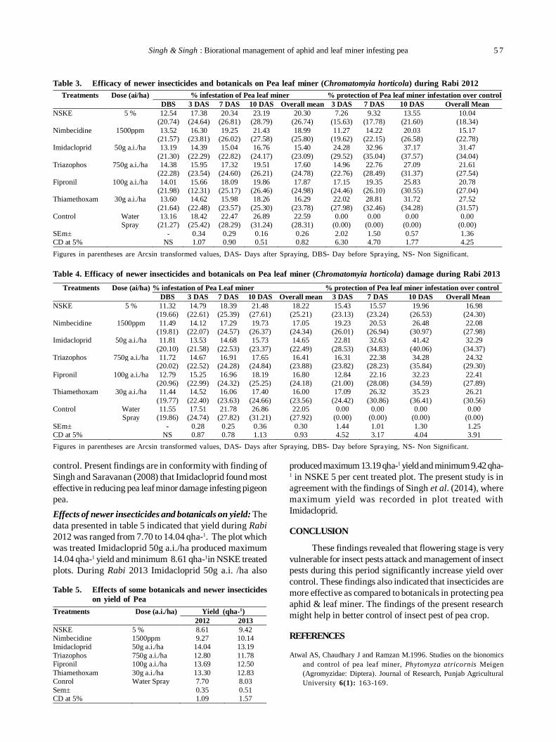
Singh & Singh : Biorational management of aphid and leaf miner infesting pea 5 7
Table 3. Efficacy of newer insecticides and botanicals on Pea leaf miner (Chromatomyia horticola) during Rabi 2012
Figures in parentheses are Arcsin transformed values, DAS- Days after Spraying, DBS- Day before Spraying, NS- Non Significant.
Treatments Dose (ai/ha) % infestation of Pea leaf miner % protection of Pea leaf miner infestation over control DBS 3 DAS 7 DAS 10 DAS Overall mean 3 DAS 7 DAS 10 DAS Overall Mean
NSKE 5 % 12.54 (20.74)
17.38 (24.64)
20.34 (26.81)
23.19 (28.79)
20.30 (26.74)
7.26 (15.63)
9.32 (17.78)
13.55 (21.60)
10.04 (18.34)
Nimbecidine 1500ppm 13.52 (21.57)
16.30 (23.81)
19.25 (26.02)
21.43 (27.58)
18.99 (25.80)
11.27 (19.62)
14.22 (22.15)
20.03 (26.58)
15.17 (22.78)
Imidacloprid
50g a.i./ha 13.19 (21.30)
14.39 (22.29)
15.04 (22.82)
16.76 (24.17)
15.40 (23.09)
24.28 (29.52)
32.96 (35.04)
37.17 (37.57)
31.47 (34.04)
Triazophos
750g a.i./ha 14.38 (22.28)
15.95 (23.54)
17.32 (24.60)
19.51 (26.21)
17.60 (24.78)
14.96 (22.76)
22.76 (28.49)
27.09 (31.37)
21.61 (27.54)
Fipronil
100g a.i./ha 14.01 (21.98)
15.66 (12.31)
18.09 (25.17)
19.86 (26.46)
17.87 (24.98)
17.15 (24.46)
19.35 (26.10)
25.83 (30.55)
20.78 (27.04)
Thiamethoxam
30g a.i./ha 13.60 (21.64)
14.62 (22.48)
15.98 (23.57)
18.26 (25.30)
16.29 (23.78)
22.02 (27.98)
28.81 (32.46)
31.72 (34.28)
27.52 (31.57)
Control Water Spray
13.16 (21.27)
18.42 (25.42)
22.47 (28.29)
26.89 (31.24)
22.59 (28.31)
0.00 (0.00)
0.00 (0.00)
0.00 (0.00)
0.00 (0.00)
SEm± CD at 5%
- NS
0.34 1.07
0.29 0.90
0.16 0.51
0.26 0.82
2.02 6.30
1.50 4.70
0.57 1.77
1.36 4.25
Figures in parentheses are Arcsin transformed values, DAS- Days after Spraying, DBS- Day before Spraying, NS- Non Significant.
Table 4. Efficacy of newer insecticides and botanicals on Pea leaf miner (Chromatomyia horticola) damage during Rabi 2013Treatments Dose (ai/ha) % infestation of Pea Leaf miner % protection of Pea leaf miner infestation over control
DBS 3 DAS 7 DAS 10 DAS Overall mean 3 DAS 7 DAS 10 DAS Overall Mean NSKE 5 % 11.32
(19.66) 14.79
(22.61) 18.39
(25.39) 21.48
(27.61) 18.22
(25.21) 15.43
(23.13) 15.57
(23.24) 19.96
(26.53) 16.98
(24.30) Nimbecidine 1500ppm 11.49
(19.81) 14.12
(22.07) 17.29
(24.57) 19.73
(26.37) 17.05
(24.34) 19.23
(26.01) 20.53
(26.94) 26.48
(30.97) 22.08
(27.98) Imidacloprid
50g a.i./ha 11.81 (20.10)
13.53 (21.58)
14.68 (22.53)
15.73 (23.37)
14.65 (22.49)
22.81 (28.53)
32.63 (34.83)
41.42 (40.06)
32.29 (34.37)
Triazophos
750g a.i./ha 11.72 (20.02)
14.67 (22.52)
16.91 (24.28)
17.65 (24.84)
16.41 (23.88)
16.31 (23.82)
22.38 (28.23)
34.28 (35.84)
24.32 (29.30)
Fipronil
100g a.i./ha 12.79 (20.96)
15.25 (22.99)
16.96 (24.32)
18.19 (25.25)
16.80 (24.18)
12.84 (21.00)
22.16 (28.08)
32.23 (34.59)
22.41 (27.89)
Thiamethoxam
30g a.i./ha 11.44 (19.77)
14.52 (22.40)
16.06 (23.63)
17.40 (24.66)
16.00 (23.56)
17.09 (24.42)
26.32 (30.86)
35.23 (36.41)
26.21 (30.56)
Control Water Spray
11.55 (19.86)
17.51 (24.74)
21.78 (27.82)
26.86 (31.21)
22.05 (27.92)
0.00 (0.00)
0.00 (0.00)
0.00 (0.00)
0.00 (0.00)
SEm± CD at 5%
- NS
0.28 0.87
0.25 0.78
0.36 1.13
0.30 0.93
1.44 4.52
1.01 3.17
1.30 4.04
1.25 3.91
control. Present findings are in conformity with finding ofSingh and Saravanan (2008) that Imidacloprid found mosteffective in reducing pea leaf minor damage infesting pigeonpea.Effects of newer insecticides and botanicals on yield: Thedata presented in table 5 indicated that yield during Rabi2012 was ranged from 7.70 to 14.04 qha-1. The plot whichwas treated Imidacloprid 50g a.i./ha produced maximum14.04 qha-1 yield and minimum 8.61 qha-1in NSKE treatedplots. During Rabi 2013 Imidacloprid 50g a.i. /ha also
produced maximum 13.19 qha-1 yield and minimum 9.42 qha-1 in NSKE 5 per cent treated plot. The present study is inagreement with the findings of Singh et al. (2014), wheremaximum yield was recorded in plot treated withImidacloprid.
CONCLUSION
These findings revealed that flowering stage is veryvulnerable for insect pests attack and management of insectpests during this period significantly increase yield overcontrol. These findings also indicated that insecticides aremore effective as compared to botanicals in protecting peaaphid & leaf miner. The findings of the present researchmight help in better control of insect pest of pea crop.
REFERENCES
Atwal AS, Chaudhary J and Ramzan M.1996. Studies on the bionomicsand control of pea leaf miner, Phytomyza atricornis Meigen(Agromyzidae: Diptera). Journal of Research, Punjab AgriculturalUniversity 6(1): 163-169.
Table 5. Effects of some botanicals and newer insecticideson yield of Pea
Treatments Dose (a.i./ha) Yield (qha-1) 2012 2013
NSKE 5 % 8.61 9.42 Nimbecidine 1500ppm 9.27 10.14 Imidacloprid 50g a.i./ha 14.04 13.19 Triazophos 750g a.i./ha 12.80 11.78 Fipronil 100g a.i./ha 13.69 12.50 Thiamethoxam 30g a.i./ha 13.30 12.83 Conrol Water Spray 7.70 8.03 Sem± CD at 5%
0.35 1.09
0.51 1.57
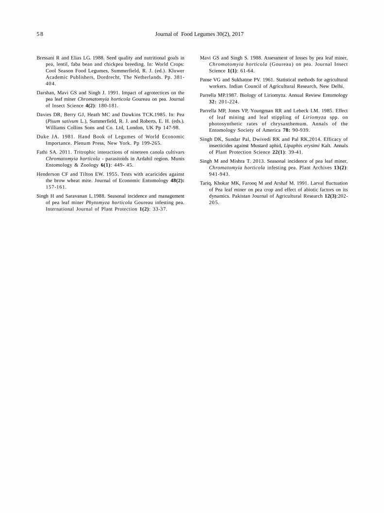
5 8 Journal of Food Legumes 30(2), 2017
Bressani R and Elias LG. 1988. Seed quality and nutritional goals inpea, lentil, faba bean and chickpea breeding. In: World Crops:Cool Season Food Legumes, Summerfield, R. J. (ed.). KluwerAcademic Publishers, Dordrecht, The Netherlands. Pp. 381-404.
Darshan, Mavi GS and Singh J. 1991. Impact of agrotectices on thepea leaf miner Chromatomyia horticola Goureau on pea. Journalof Insect Science 4(2): 180-181.
Davies DR, Berry GJ, Heath MC and Dawkins TCK.1985. In: Pea(Pisum sativum L.), Summerfield, R. J. and Roberts, E. H. (eds.).Williams Collins Sons and Co. Ltd, London, UK Pp 147-98.
Duke JA. 1981. Hand Book of Legumes of World EconomicImportance. Plenum Press, New York. Pp 199-265.
Fathi SA. 2011. Tritrophic interactions of nineteen canola cultivarsChromatomyia horticola - parasitoids in Ardabil region. MunisEntomology & Zoology 6(1): 449- 45.
Henderson CF and Tilton EW. 1955. Tests with acaricides againstthe brow wheat mite. Journal of Economic Entomology 48(2):157-161.
Singh H and Saravanan L.1988. Seasonal incidence and managementof pea leaf miner Phytomyza horticola Goureau infesting pea.International Journal of Plant Protection 1(2): 33-37.
Mavi GS and Singh S. 1988. Assessment of losses by pea leaf miner,Chromotomyia horticola (Goureau) on pea. Journal InsectScience 1(1): 61-64.
Panse VG and Sukhatme PV. 1961. Statistical methods for agriculturalworkers. Indian Council of Agricultural Research, New Delhi.
Parrella MP.1987. Biology of Liriomyza. Annual Review Entomology32: 201-224.
Parrella MP, Jones VP, Youngman RR and Lebeck LM. 1985. Effectof leaf mining and leaf stippling of Liriomyza spp. onphotosynthetic rates of chrysanthemum. Annals of theEntomology Society of America 78: 90-939.
Singh DK, Sundar Pal, Dwivedi RK and Pal RK.2014. Efficacy ofinsecticides against Mustard aphid, Lipaphis erysimi Kalt. Annalsof Plant Protection Science 22(1): 39-41.
Singh M and Mishra T. 2013. Seasonal incidence of pea leaf miner,Chromatomyia horticola infesting pea. Plant Archives 13(2):941-943.
Tariq, Khokar MK, Farooq M and Arshaf M. 1991. Larval fluctuationof Pea leaf miner on pea crop and effect of abiotic factors on itsdynamics. Pakistan Journal of Agricultural Research 12(3):202-205.
Journal of Food Legumes 30(2): 59-64, 2017
ABSTRACT
Four pigeonpea genotypes (ICPH 2431, PARAS, UPAS 120and H09 33) were raised in polythene bags filled with halfkg soil + FYM manure mixture. Water logging, salinity andwaterlogging + salinity treatments were given for 8 daysand observations were recorded at initial stage 1st day andsubsequently after 8 days of treatment (20 and 40 day oldplant leaves). A significant increase in superoxide radicalcontent was observed with all the three treatments both 1and 8 days after removal from treatment. However increasewas comparatively less 8 day after removal from treatment.Among all the treatment salinity alone was found leastdeleterious and combined waterlogging and salinity wasfound more deleterious. Increase in antioxidative enzymeactivity and antioxidative metabolite content was alsoobserved in all the treatments. Maximum increase wasobserved in ICPH 2431 followed by PARAS, HO 933andminimum was observed in UPAS 120.
Key words: Antioxidative enzymes, Waterlogging, Salinity,Oxidative stress, Pigeonpea
Cajanus cajan, commonly known as pigeon pea, is adrought-resistant crop grown in semi-arid low rainfall areas.Pigeonpea contains high protein content and important Bgroup vitamins and therefore is important for people livingon subsistence diets. In India, where most of world’spigeonpea is produced, a large acre of land is affected bywaterlogging and salinity (CSSRI, 2016). It is well knownthat waterlogging and salinity inhibit the plant growth anddevelopmental processes. Tayyab et al. 2016 reported asignificant decline in chlorophyll content, carotenoids,sugar, proteins and yield of pigeonpea under salinity stress.Under waterlogging stress, decreased chlorophyll andstarch content and increased membrane injury in pigeonpeahas been reported (Bansal and Srivastava. 2015).Waterlogged plants are subjected to anoxia (completeabsence of oxygen) (Setter et al. 2009) which results in theproduction of ROS perturbing several cellular metabolicprocesses of plants (Ashraf et al. 2010). Lethal reactiveoxygen species (ROS) include superoxide (O2
"), hydrogenperoxide (H2O2) and the hydroxyl radical (OH-). Singletoxygen generated due to the reaction of oxygen with excitedchlorophyll, is also considered as potential ROS (Ashrafand Akram 2009). These ROS are extremely reactive and
Oxidative stress and antioxidative enzymes activity in pigeonpea leaves at differentstages of development under waterlogging, salinity and combined stress ofwaterlogging and salinitySAVITA DUHAN, SUNITA SHEOKAND ANITA KUMARI
Department of Botany and Plant Physiology, CCS HAU, Hisar. 125004, Haryana, India; E-mail:[email protected](Received: March 6, 2017; Accepted: May 24, 2017)
induce damage to a number of cellular molecules andmetabolites such as proteins, lipids, pigments, DNA etc.(Ashraf 2009, Ashraf. 2012). ROS are also produced undernormal conditions but their concentration is very low.However, when plants are facing some environmentalstresses, the concentration of ROS is elevated to a levelthat is damaging for several cellular metabolic reactions ofplants such as photosynthesis, efficiency of PS II etc(Ashraf 2009). For example, elevated cellular levels ofhydrogen peroxide result in inhibition of calvin cycle (Ashrafand Akram, 2009). All the plants have the ability to detoxifythe adverse effects of ROS by producing different types ofantioxidants. Generally, antioxidants are categorized intoenzymatic and non-enzymatic antioxidants. Enzymaticantioxidants include ascorbate peroxidase (APX),superoxide dismutase (SOD), peroxidase (POD), catalase(CAT), glutathione reductase (GR), whereas, ascorbic acid,glutathione, tocopherols and carotenoids are included innon-enzymatic antioxidants (Gupta et al. 2005). Increase inthe activities of different enzymatic antioxidants wasrecorded in maize seedlings when subjected to varyingdegree of waterlogging stress (Tang et al. 2010). Similarincrease in ROS and antioxidative enzymes was alsoobserved under salinity stress in several plants likeHordeum vulgare (Unal et al. 2014), Zea mays (Rios andPinto 2014), Nicotiana tabacum (Celik and Atak 2012). Inrecent years, an impressive amount of knowledge hasaccumulated on plant physiological and molecularresponses to salinity or waterlogging stresses. However,studies dealing with the combined effects of these twostresses are much rarer and often controversial (Barrett-Lennard 2003). Nonetheless, the occurrence of combinedsalinity and waterlogging stress is increasing throughoutthe world. This is due to intensive irrigation in agriculturalproduction systems (Smedema and Shiati 2002) rise of salinewater tables (Hatton et al. 2003) and seawater intrusion incoastal environments (Carter et al. 2006). When combinedwith waterlogging, salinity can cause even greater damageto plants, so having a major impact on agriculturalproduction (Barrett-Lennard 2003). Only a very few cropspecies can tolerate the combination of salinity andwaterlogging (Bennett et al. 2009) and the physiologicaland molecular mechanisms conferring this tolerance remainelusive. However very little has been done on the interactive
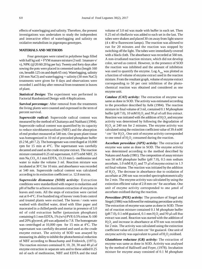
6 0 Journal of Food Legumes 30(2), 2017
effects of waterlogging and salinity. Therefore, the presentinvestigations was undertaken to study the independentand interactive effect of waterlogging and salinity onoxidative metabolism in pigeonpea genotypes.
MATERIALS AND METHODS
Four genotypes were raised in polythene bags filledwith half kg soil + FYM manure mixture (3 soil: 1manure v/v), NPK (@20:60:20 kg per ha). Twenty and forty days aftersowing the pots were placed in cemented tanks (length 160cm, breadth 125 cm and depth 65 cm). Waterlogging, salinity(30 mm NaCl) and waterlogging + salinity (30 mm NaCl)treatments were given for 8 days and observations wererecorded 1 and 8 day after removal from treatment in leavesof plant.Statistical Design: The experiment was performed inFactorial Randomized Design with 4 Replications.Survival percentage: After removal from the treatmentsthe living plants were counted and expressed in the term ofpercent survival.Superoxide radical: Superoxide radical content wasmeasured by the method of Chaitanya and Naithani (1994).Superoxide radical content was quantified by its capacityto reduce nitrobluetetrazolium (NBT) and the absorptionof end product measured at 540 nm. One gram plant tissuewas homogenized in 10 ml of precooled phosphate buffer(0.2 M, pH 7.2). The homogenate was centrifuged at 10,000rpm for 15 min at 4°C. The supernatant was carefullydecanted and used as the crude enzyme extract. The reactionmixture contained 0.25 ml supernatant, 0.075 mM NBT, 25mm Na2CO3, 0.1 mm EDTA, 13.33 mm L- methionine andwater to make the volume 3 ml. Reaction mixture wasincubated at 30 ºC for 10 min. and absorbance was recordedat 540 nm. Superoxide radical content was calculatedaccording to its extinction coefficient i.e. 12.8 mm/cm.Superoxide dismutase (SOD) activity: Extractionconditions were standardized with respect to molarities andpH of buffer to achieve maximum extraction of enzyme inleaves and roots. All the steps of extraction were carriedout at 0-4°C. Five hundred mg of leaves/ roots from controland treated plants were excised. The leaves / roots werewashed with distilled water, dried with filter paper andmacerated in a chilled pestle and mortar in presence of 3.0ml of cold extraction buffer (potassium phosphate)containing 0.1 mm EDTA, 1% (w/v) PVP, 0.5% triton X-100and 20% glycerol, pH was adjusted to 7.8. The homogenatewas centrifuged at 10,000 rpm for 15 min at 4°C. Thesupernatant was carefully decanted and used as the crudeenzyme extract. The activity of SOD was assayed bymeasuring its ability to inhibit the photochemical reductionof NBT according to Beauchamp and Fridovich, (1971).The reaction mixture contained 0, 10, 20, 30 and 40 µl ofenzyme extraction in separate sets and to these added 0.25ml of each of methionine, NBT and EDTA and the total
volume of 3.0 ml was made with buffer in each set. Then0.25 ml of riboflavin was added to each set in the last. Thetubes were shaken and placed 30 cm away from light source(4 x 40 w fluorescent lamps). The reaction was allowed torun for 20 minutes and the reaction was stopped byswitching off the light. The tubes were immediately coveredwith a black cloth. The absorbance was recorded at 560 nm.A non-irradiated reaction mixture, which did not developcolor, served as control. However, in the presence of SODthe reaction was inhibited and the amount of inhibitionwas used to quantify the enzyme. Log A560 was plotted asa function of volume of enzyme extract used in the reactionmixture. From the resultant graph, volume of enzyme extractcorresponding to 50 per cent inhibition of the photo-chemical reaction was obtained and considered as oneenzyme unit.Catalase (CAT) activity: The extraction of enzyme wassame as done in SOD. The activity was estimated accordingto the procedure described by Aebi (1984). The reactionmixture in final volume of 3 ml, contained 0.1 M phosphatebuffer (pH 7.0), 10 mM H2O2 and 50 µl of cell free extract.Reaction was initiated with the addition of H2O2 and enzymeactivity was determined by following the degradation ofH2O2 at 240 nm for 2 minutes. The enzyme activity wascalculated using the extinction coefficient value of 39.4 mM-
1 cm-1 for H2O2. One unit of enzyme activity correspondedto one nmol of H2O2 consumed during the reaction.Ascorbate peroxidase (APX) activity: The extraction ofenzyme was same as done in SOD. The enzyme activitywas determined according to the method described byNakano and Asada (1981). The composition of assay mixturewas 50 mM phosphate buffer (pH 7.0), 0.5 mm sodiumascorbate, 1.0 mM H2O2 and 75 µl of enzyme extract in 1.5ml final volume. The reaction was initiated by the additionof H2O2. The decrease in absorbance due to oxidation ofascorbate at 290 nm was recorded spectrophotometricallyfor 2 min. The enzyme activity was calculated by using theextinction efficient value of 2.8 mm cm-1 for ascorbate. Oneunit of enzyme activity corresponded to one µmol ofascorbate oxidised during the reaction.Peroxidase (POX) activity: The procedure of Siegel andSiegel (1986) was followed for estimating peroxidase activity.The extraction of enzyme was same as done in SOD. Threeml of reaction mixture contained 0.1 M phosphate buffer(pH 7.0), 0.1 mM guaiacol, 0.1 mm H2O2 and 50 µl cell freeextract was used. Reaction was started with the addition ofH2O2 and increase in absorbance at 470 nm was recordedfor 2 min. The activity was calculated using the extinctioncoefficient value of 22.6 mm cm-1 for guaiacol. One unit ofenzyme activity was equivalent to µmol of H2O2 oxidised.Glutathione reductase (GR) activity: The extraction ofenzyme was same as done in SOD. Activity was analysedby the method of Halliwell and Foyer, (1978). Incubationmixture for enzyme assay consisted of 0.1 M phosphate
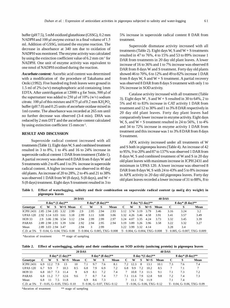
Duhan et al. : Expression of antioxidant activities in pigeonpea subjected to salinity and water-logging 6 1
buffer (pH 7.5), 5 mM oxidized glutathione (GSSG), 0.2 mmNADPH and 100 µl enzyme extract in a final volume of 1.5ml. Addition of GSSG, initiated the enzyme reaction. Thedecrease in absorbance at 340 nm due to oxidation ofNADPH was monitored. The enzyme activity was calculatedby using the extinction coefficient value of 6.2 mm cm-1 forNADPH. One unit of enzyme activity was equivalent toone nmol of NADPH oxidised during the reaction.Ascorbate content: Ascorbic acid content was determinedwith a modification of the procedure of Takahama andOniki (1992). Five hundred mg fresh leaves were ground in1.5 ml of 2% (w/v) metaphosphoric acid containing 1mmEDTA. After centrifugation at 12000 x g for 5min, 500 µl ofthe supernatant was added to 250 µl of 10% (w/v) sodiumcitrate. 100 µl of this mixture and 875 µl of 0.2 mm KH2PO4buffer (pH 7.0) and 0.25 units of ascorbate oxidase mixed in1ml cuvette. The absorbance was recorded at 265 nm untilno further decrease was observed (3-4 min). DHA wasreduced by 2 mm DTT and the ascorbate content calculatedby using extinction coefficient 15 mm cm-1.
RESULT AND DISCUSSION
Superoxide radical content increased with alltreatments (Table 1). Eight days W, S and combined treatmentresulted in 3 to 8%, 1 to 4% and 16 to 24% increase insuperoxide radical content 1 DAR from treatment (Table 1).A partial recovery was observed 8 DAR from 8 days W andS treatments with 2 to 4% and 1 to 3% increase in superoxideradical content. A higher increase was observed in 40 dayold plants. An increase of 20 to 28%, 2 to 4% and 21 to 38%was observed 1 DAR from W (8 days), S (8 days), and W +S (8 days) treatment. Eight days S treatment resulted in 3 to
5% increase in superoxide radical content 8 DAR fromtreatment.
Superoxide dismutase activity increased with alltreatments (Table 2). Eight days W, S and W + S treatmentsresulted in 47 to 76%, 4 to 15% and 53 to 89% increase 1DAR from treatments in 20 day old plant leaves. A lowerincrease of 16 to 36% and 1 to 7% increase was observed 8DAR from 8 days W and S treatment. Forty day old plantsshowed 46 to 70%, 6 to 12% and 49 to 82% increase 1 DARfrom 8 days W, S and W + S treatment. A partial recoverywas observed 8 DAR from 8 days S treatment with only 1 to5% increase in SOD activity.
Catalase activity increased with all treatment (Table3). Eight days W , S and W + S resulted in 30 to 64%, 2 to5% and 41 to 83% increase in CAT activity 1 DAR fromtreatment and 12 to 30% and 1 to 3% 8 DAR respectively in20 day old plant leaves. Forty day plant leaves hadcomparatively lower increase in enzyme activity. Eight daysW, S, and W + S treatment resulted in 24 to 56%, 1 to 4%and 34 to 72% increase in enzyme activity 1 DAR fromtreatment and this increase was 1 to 3% 8 DAR from 8 daysS treatment.
APX activity increased under all treatments of Wand S both in pigeonpea leaves (Table 4). An increase of 42to 95%, 9 to 20% and 87 to 137% was observed 1 DAR from8 days W, S and combined treatment of W and S in 20 dayold plant leaves with maximum increase in ICPH 2431 andminimum in UPAS 120. A lower increase was observed 8DAR from 8 days W, S with 24 to 43% and 5 to 8% increasein APX activity in 20 day old pigeonpea leaves. Forty dayold plant leaves recorded a lower increase of 31 to 88%, 8 to
Table 2. Effect of waterlogging, salinity and their combination on SOD activity (units/mg protein) in pigeonpea leaves
*duration of treatment ** stage of sampling
Table 1. Effect of waterlogging, salinity and their combination on superoxide radical content (µ mol/g dry weight) inpigeonpea leaves
*duration of treatment ** stage of sampling
20 DAS 40 DAS 8 day* (1 day)** 8 day* (8 day)** 8 day *(1 day)** 8 day* (8 day)** Genotype C W S W+S Mean C W S Mean C W S W+S Mean C S Mean ICPH 2431 2.85 2.94 2.85 3.32 2.99 2.9 2.95 2.94 2.93 3.12 3.74 3.19 3.79 3.46 3.16 3.24 3.2 UPAS 120 2.92 3.14 3.03 3.61 3.18 2.99 3.11 3.08 3.06 3.32 4.26 3.46 4.58 3.91 3.41 3.57 3.49 HO9 33 2.9 3.06 2.96 3.54 3.12 2.94 2.99 2.99 2.97 3.24 4.07 3.35 4.24 3.73 3.32 3.45 3.39 PARAS 2.89 2.98 2.91 3.39 3.04 2.92 2.94 2.95 2.94 3.19 3.89 3.26 3.96 3.58 3.22 3.32 3.27 Mean 2.89 3.03 2.94 3.47 2.94 3 2.99 3.22 3.99 3.32 4.14 3.28 3.4 C.D. at 5% T- 0.04, G- 0.04, TXG- 0.08 T- 0.004, G- 0.005, TXG- 0.008 T- 0.004, G- 0.004, TXG- 0.008 T- 0.005, G- 0.007, TXG- 0.009
20 DAS 40 DAS 8 day* (1 day)** 8 day* (8 day)** 8 day *(1 day)** 8 day* (8 day)** Genotype C W S W+S Mean C W S Mean C W S W+S Mean C S Mean ICPH 2431 6.9 12.2 7.9 13 10 7.1 9.7 7.6 8.1 7.2 12.3 8 13.1 10.1 7.3 7.6 7.4 UPAS 120 6.7 9.9 7 10.3 8.5 6.8 7.9 6.9 7.2 6.8 9.9 7.2 10.2 8.5 7 7.1 7 HO9 33 6.8 10.7 7.3 11.4 9 6.9 8.1 7.2 7.4 7 10.8 7.3 11.5 9.1 7.1 7.3 7.2 PARAS 6.8 11.2 7.7 12.6 9.6 7 8.7 7.4 7.7 7.1 11.6 7.9 12.8 9.8 7.2 7.4 7.3 Mean 6.8 11 7.5 11.8 6.9 8.6 7.3 7 11.1 7.6 11.9 7.1 7.4 C.D. at 5% T - 0.05, G- 0.05, TXG- 0.10 T- 0.06, G- 0.07, TXG- 0.12 T - 0.06, G- 0.06, TXG- 0.12 T- 0.04, G- 0.06, TXG- 0.09
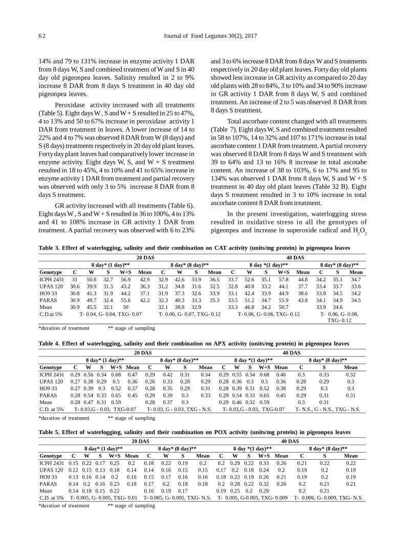
6 2 Journal of Food Legumes 30(2), 2017
14% and 79 to 131% increase in enzyme activity 1 DARfrom 8 days W, S and combined treatment of W and S in 40day old pigeonpea leaves. Salinity resulted in 2 to 9%increase 8 DAR from 8 days S treatment in 40 day oldpigeonpea leaves.
Peroxidase activity increased with all treatments(Table 5). Eight days W , S and W + S resulted in 25 to 47%,4 to 13% and 50 to 67% increase in peroxidase activity 1DAR from treatment in leaves. A lower increase of 14 to22% and 4 to 7% was observed 8 DAR from W (8 days) andS (8 days) treatments respectively in 20 day old plant leaves.Forty day plant leaves had comparatively lower increase inenzyme activity. Eight days W, S, and W + S treatmentresulted in 18 to 45%, 4 to 10% and 41 to 65% increase inenzyme activity 1 DAR from treatment and partial recoverywas observed with only 3 to 5% increase 8 DAR from 8days S treatment.
GR activity increased with all treatments (Table 6).Eight days W , S and W + S resulted in 36 to 100%, 4 to 13%and 41 to 108% increase in GR activity 1 DAR fromtreatment. A partial recovery was observed with 6 to 23%
and 3 to 6% increase 8 DAR from 8 days W and S treatmentsrespectively in 20 day old plant leaves. Forty day old plantsshowed less increase in GR activity as compared to 20 dayold plants with 28 to 84%, 3 to 10% and 34 to 90% increasein GR activity 1 DAR from 8 days W, S and combinedtreatment. An increase of 2 to 5 was observed 8 DAR from8 days S treatment.
Total ascorbate content changed with all treatments(Table 7). Eight days W, S and combined treatment resultedin 58 to 107%, 14 to 32% and 107 to 171% increase in totalascorbate content 1 DAR from treatment. A partial recoverywas observed 8 DAR from 8 days W and S treatment with39 to 64% and 13 to 16% 8 increase in total ascotabecontent. An increase of 38 to 103%, 6 to 17% and 95 to134% was observed 1 DAR from 8 days W, S and W + Streatment in 40 day old plant leaves (Table 32 B). Eightdays S treatment resulted in 3 to 10% increase in totalascorbate content 8 DAR from treatment.
In the present investigation, waterlogging stressresulted in oxidative stress in all the genotypes ofpigeonpea and increase in superoxide radical and H2O2
Table 3. Effect of waterlogging, salinity and their combination on CAT activity (units/mg protein) in pigeonpea leaves
*duration of treatment ** stage of sampling
Table 4. Effect of waterlogging, salinity and their combination on APX activity (units/mg protein) in pigeonpea leaves
*duration of treatment ** stage of sampling
Table 5. Effect of waterlogging, salinity and their combination on POX activity (units/mg protein) in pigeonpea leaves
*duration of treatment ** stage of sampling
20 DAS 40 DAS 8 day* (1 day)** 8 day* (8 day)** 8 day *(1 day)** 8 day* (8 day)** Genotype C W S W+S Mean C W S Mean C W S W+S Mean C S Mean ICPH 2431 31 50.8 32.7 56.9 42.9 32.9 42.6 33.9 36.5 33.7 52.6 35.1 57.8 44.8 34.2 35.1 34.7 UPAS 120 30.6 39.9 31.3 43.2 36.3 31.2 34.8 31.6 32.5 32.8 40.8 33.2 44.1 37.7 33.4 33.7 33.6 HO9 33 30.8 41.3 31.9 44.2 37.1 31.9 37.3 32.6 33.9 33.1 42.4 33.9 44.9 38.6 33.8 34.5 34.2 PARAS 30.9 49.7 32.4 55.6 42.2 32.3 40.3 33.3 35.3 33.5 51.2 34.7 55.9 43.8 34.1 34.9 34.5 Mean 30.9 45.5 32.1 50 32.1 38.8 32.9 33.3 46.8 34.2 50.7 33.9 34.6 C.D.at 5% T- 0.04, G- 0.04, TXG- 0.07 T- 0.06, G- 0.07, TXG- 0.12 T- 0.06, G- 0.06, TXG- 0.12 T- 0.06, G- 0.08,
TXG- 0.12
20 DAS 40 DAS 8 day* (1 day)** 8 day* (8 day)** 8 day *(1 day)** 8 day* (8 day)** Genotype C W S W+S Mean C W S Mean C W S W+S Mean C S Mean ICPH 2431 0.29 0.56 0.34 0.68 0.47 0.29 0.42 0.31 0.34 0.29 0.55 0.34 0.68 0.46 0.3 0.33 0.32 UPAS 120 0.27 0.38 0.29 0.5 0.36 0.26 0.33 0.28 0.29 0.28 0.36 0.3 0.5 0.36 0.28 0.29 0.3 HO9 33 0.27 0.39 0.3 0.52 0.37 0.28 0.35 0.29 0.31 0.28 0.39 0.31 0.52 0.38 0.29 0.3 0.3 PARAS 0.28 0.54 0.33 0.65 0.45 0.29 0.39 0.3 0.33 0.29 0.54 0.33 0.65 0.45 0.29 0.31 0.31 Mean 0.28 0.47 0.31 0.59 0.28 0.37 0.3 0.29 0.46 0.32 0.59 0.3 0.31 C.D. at 5% T- 0.03,G - 0.03, TXG-0.07 T- 0.03, G - 0.03, TXG - N.S. T- 0.03,G - 0.03, TXG-0.07 T- N.S., G - N.S., TXG - N.S.
20 DAS 40 DAS 8 day* (1 day)** 8 day* (8 day)** 8 day *(1 day)** 8 day* (8 day)** Genotype C W S W+S Mean C W S Mean C W S W+S Mean C S Mean ICPH 2431 0.15 0.22 0.17 0.25 0.2 0.18 0.22 0.19 0.2 0.2 0.29 0.22 0.33 0.26 0.21 0.22 0.22 UPAS 120 0.12 0.15 0.13 0.18 0.14 0.14 0.16 0.15 0.15 0.17 0.2 0.18 0.24 0.2 0.19 0.2 0.19 HO9 33 0.13 0.16 0.14 0.2 0.16 0.15 0.17 0.16 0.16 0.18 0.22 0.19 0.26 0.21 0.19 0.2 0.19 PARAS 0.14 0.2 0.16 0.23 0.18 0.17 0.2 0.18 0.18 0.2 0.28 0.22 0.32 0.26 0.2 0.21 0.21 Mean 0.14 0.18 0.15 0.22 0.16 0.19 0.17 0.19 0.25 0.2 0.29 0.2 0.21 C.D. at 5% T- 0.005, G- 0.005, TXG- 0.01 T- 0.005, G- 0.005, TXG- N.S. T- 0.005, G-0.005, TXG- 0.009 T- 0.006, G- 0.009, TXG- N.S.
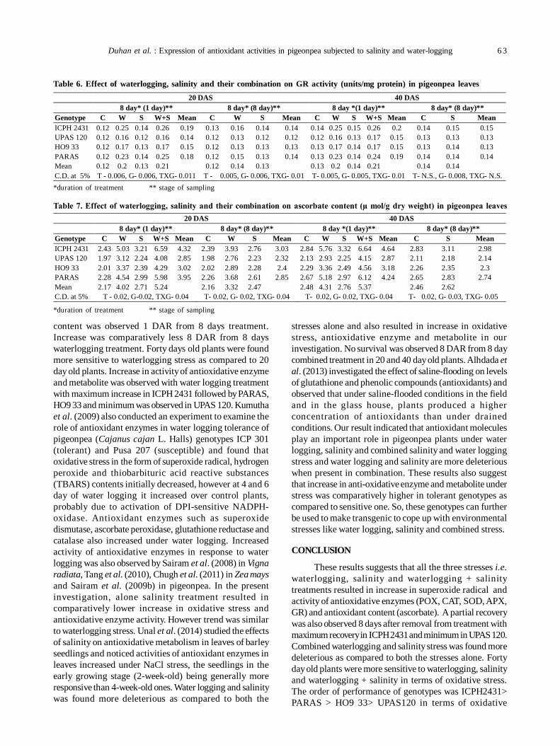
Duhan et al. : Expression of antioxidant activities in pigeonpea subjected to salinity and water-logging 6 3
content was observed 1 DAR from 8 days treatment.Increase was comparatively less 8 DAR from 8 dayswaterlogging treatment. Forty days old plants were foundmore sensitive to waterlogging stress as compared to 20day old plants. Increase in activity of antioxidative enzymeand metabolite was observed with water logging treatmentwith maximum increase in ICPH 2431 followed by PARAS,HO9 33 and minimum was observed in UPAS 120. Kumuthaet al. (2009) also conducted an experiment to examine therole of antioxidant enzymes in water logging tolerance ofpigeonpea (Cajanus cajan L. Halls) genotypes ICP 301(tolerant) and Pusa 207 (susceptible) and found thatoxidative stress in the form of superoxide radical, hydrogenperoxide and thiobarbituric acid reactive substances(TBARS) contents initially decreased, however at 4 and 6day of water logging it increased over control plants,probably due to activation of DPI-sensitive NADPH-oxidase. Antioxidant enzymes such as superoxidedismutase, ascorbate peroxidase, glutathione reductase andcatalase also increased under water logging. Increasedactivity of antioxidative enzymes in response to waterlogging was also observed by Sairam et al. (2008) in Vignaradiata, Tang et al. (2010), Chugh et al. (2011) in Zea maysand Sairam et al. (2009b) in pigeonpea. In the presentinvestigation, alone salinity treatment resulted incomparatively lower increase in oxidative stress andantioxidative enzyme activity. However trend was similarto waterlogging stress. Unal et al. (2014) studied the effectsof salinity on antioxidative metabolism in leaves of barleyseedlings and noticed activities of antioxidant enzymes inleaves increased under NaCl stress, the seedlings in theearly growing stage (2-week-old) being generally moreresponsive than 4-week-old ones. Water logging and salinitywas found more deleterious as compared to both the
stresses alone and also resulted in increase in oxidativestress, antioxidative enzyme and metabolite in ourinvestigation. No survival was observed 8 DAR from 8 daycombined treatment in 20 and 40 day old plants. Alhdada etal. (2013) investigated the effect of saline-flooding on levelsof glutathione and phenolic compounds (antioxidants) andobserved that under saline-flooded conditions in the fieldand in the glass house, plants produced a higherconcentration of antioxidants than under drainedconditions. Our result indicated that antioxidant moleculesplay an important role in pigeonpea plants under waterlogging, salinity and combined salinity and water loggingstress and water logging and salinity are more deleteriouswhen present in combination. These results also suggestthat increase in anti-oxidative enzyme and metabolite understress was comparatively higher in tolerant genotypes ascompared to sensitive one. So, these genotypes can furtherbe used to make transgenic to cope up with environmentalstresses like water logging, salinity and combined stress.
CONCLUSION
These results suggests that all the three stresses i.e.waterlogging, salinity and waterlogging + salinitytreatments resulted in increase in superoxide radical andactivity of antioxidative enzymes (POX, CAT, SOD, APX,GR) and antioxidant content (ascorbate). A partial recoverywas also observed 8 days after removal from treatment withmaximum recovery in ICPH 2431 and minimum in UPAS 120.Combined waterlogging and salinity stress was found moredeleterious as compared to both the stresses alone. Fortyday old plants were more sensitive to waterlogging, salinityand waterlogging + salinity in terms of oxidative stress.The order of performance of genotypes was ICPH2431>PARAS > HO9 33> UPAS120 in terms of oxidative
Table 6. Effect of waterlogging, salinity and their combination on GR activity (units/mg protein) in pigeonpea leaves
*duration of treatment ** stage of sampling
Table 7. Effect of waterlogging, salinity and their combination on ascorbate content (µ mol/g dry weight) in pigeonpea leaves
*duration of treatment ** stage of sampling
20 DAS 40 DAS 8 day* (1 day)** 8 day* (8 day)** 8 day *(1 day)** 8 day* (8 day)** Genotype C W S W+S Mean C W S Mean C W S W+S Mean C S Mean ICPH 2431 0.12 0.25 0.14 0.26 0.19 0.13 0.16 0.14 0.14 0.14 0.25 0.15 0.26 0.2 0.14 0.15 0.15 UPAS 120 0.12 0.16 0.12 0.16 0.14 0.12 0.13 0.12 0.12 0.12 0.16 0.13 0.17 0.15 0.13 0.13 0.13 HO9 33 0.12 0.17 0.13 0.17 0.15 0.12 0.13 0.13 0.13 0.13 0.17 0.14 0.17 0.15 0.13 0.14 0.13 PARAS 0.12 0.23 0.14 0.25 0.18 0.12 0.15 0.13 0.14 0.13 0.23 0.14 0.24 0.19 0.14 0.14 0.14 Mean 0.12 0.2 0.13 0.21 0.12 0.14 0.13 0.13 0.2 0.14 0.21 0.14 0.14 C.D. at 5% T - 0.006, G- 0.006, TXG- 0.011 T - 0.005, G- 0.006, TXG- 0.01 T- 0.005, G- 0.005, TXG- 0.01 T- N.S., G- 0.008, TXG- N.S.
20 DAS 40 DAS 8 day* (1 day)** 8 day* (8 day)** 8 day *(1 day)** 8 day* (8 day)** Genotype C W S W+S Mean C W S Mean C W S W+S Mean C S Mean ICPH 2431 2.43 5.03 3.21 6.59 4.32 2.39 3.93 2.76 3.03 2.84 5.76 3.32 6.64 4.64 2.83 3.11 2.98 UPAS 120 1.97 3.12 2.24 4.08 2.85 1.98 2.76 2.23 2.32 2.13 2.93 2.25 4.15 2.87 2.11 2.18 2.14 HO9 33 2.01 3.37 2.39 4.29 3.02 2.02 2.89 2.28 2.4 2.29 3.36 2.49 4.56 3.18 2.26 2.35 2.3 PARAS 2.28 4.54 2.99 5.98 3.95 2.26 3.68 2.61 2.85 2.67 5.18 2.97 6.12 4.24 2.65 2.83 2.74 Mean 2.17 4.02 2.71 5.24 2.16 3.32 2.47 2.48 4.31 2.76 5.37 2.46 2.62 C.D. at 5% T - 0.02, G-0.02, TXG- 0.04 T- 0.02, G- 0.02, TXG- 0.04 T- 0.02, G- 0.02, TXG- 0.04 T- 0.02, G- 0.03, TXG- 0.05
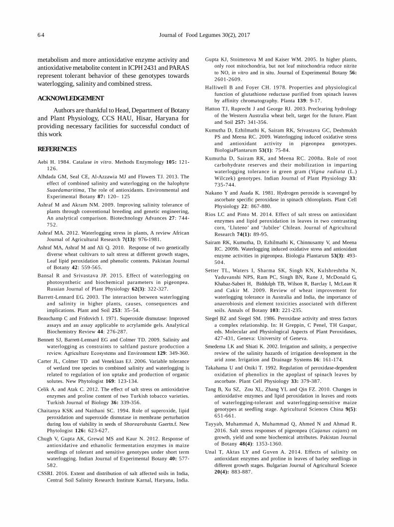
6 4 Journal of Food Legumes 30(2), 2017
metabolism and more antioxidative enzyme activity andantioxidative metabolite content in ICPH 2431 and PARASrepresent tolerant behavior of these genotypes towardswaterlogging, salinity and combined stress.
ACKNOWLEDGEMENT
Authors are thankful to Head, Department of Botanyand Plant Physiology, CCS HAU, Hisar, Haryana forproviding necessary facilities for successful conduct ofthis work
REFERENCES
Aebi H. 1984. Catalase in vitro. Methods Enzymology 105: 121-126.
Alhdada GM, Seal CE, Al-Azzawia MJ and Flowers TJ. 2013. Theeffect of combined salinity and waterlogging on the halophyteSuaedamaritima, The role of antioxidants. Environmental andExperimental Botany 87: 120– 125
Ashraf M and Akram NM. 2009. Improving salinity tolerance ofplants through conventional breeding and genetic engineering,An analytical comparison. Biotechnology Advances 27: 744-752.
Ashraf MA. 2012. Waterlogging stress in plants, A review AfricanJournal of Agricultural Research 7(13): 976-1981.
Ashraf MA, Ashraf M and Ali Q. 2010. Response of two geneticallydiverse wheat cultivars to salt stress at different growth stages,Leaf lipid peroxidation and phenolic contents. Pakistan Journalof Botany 42: 559-565.
Bansal R and Srivastava JP. 2015. Effect of waterlogging onphotosynthetic and biochemical parameters in pigeonpea.Russian Journal of Plant Physiology 62(3): 322-327.
Barrett-Lennard EG. 2003. The interaction between waterloggingand salinity in higher plants, causes, consequences andimplications. Plant and Soil 253: 35–54.
Beauchamp C and Fridovich I. 1971. Superoxide dismutase: Improvedassays and an assay applicable to acrylamide gels. AnalyticalBiochemistry Review 44: 276-287.
Bennett SJ, Barrett-Lennard EG and Colmer TD. 2009. Salinity andwaterlogging as constraints to saltland pasture production areview. Agriculture Ecosystems and Environment 129: 349-360.
Carter JL, Colmer TD and Veneklaas EJ. 2006. Variable toleranceof wetland tree species to combined salinity and waterlogging isrelated to regulation of ion uptake and production of organicsolutes. New Phytologist 169: 123-134.
Celik A. and Atak C. 2012. The effect of salt stress on antioxidativeenzymes and proline content of two Turkish tobacco varieties.Turkish Journal of Biology 36: 339-356.
Chaitanya KSK and Naithani SC. 1994. Role of superoxide, lipidperoxidation and superoxide dismutase in membrane perturbationduring loss of viability in seeds of Shorearobusta Gaertn.f. NewPhytologist 126: 623-627.
Chugh V, Gupta AK, Grewal MS and Kaur N. 2012. Response ofantioxidative and ethanolic fermentation enzymes in maizeseedlings of tolerant and sensitive genotypes under short termwaterlogging. Indian Journal of Experimental Botany 40: 577-582.
CSSRI. 2016. Extent and distribution of salt affected soils in India,Central Soil Salinity Research Institute Karnal, Haryana, India.
Gupta KJ, Stoimenova M and Kaiser WM. 2005. In higher plants,only root mitochondria, but not leaf mitochondria reduce nitriteto NO, in vitro and in situ. Journal of Experimental Botany 56:2601-2609.
Halliwell B and Foyer CH. 1978. Properties and physiologicalfunction of glutathione reductase purified from spinach leavesby affinity chromatography. Planta 139: 9-17.
Hatton TJ, Ruprecht J and George RJ. 2003. Preclearing hydrologyof the Western Australia wheat belt, target for the future. Plantand Soil 257: 341-356.
Kumutha D, Ezhilmathi K, Sairam RK, Srivastava GC, DeshmukhPS and Meena RC. 2009. Waterlogging induced oxidative stressand antioxidant activity in pigeonpea genotypes.BiologiaPlantarum 53(1): 75-84.
Kumutha D, Sairam RK, and Meena RC. 2008a. Role of rootcarbohydrate reserves and their mobilization in impartingwaterlogging tolerance in green gram (Vigna radiata (L.)Wilczek) genotypes. Indian Journal of Plant Physiology 33:735-744.
Nakano Y and Asada K. 1981. Hydrogen peroxide is scavenged byascorbate specific peroxidase in spinach chloroplasts. Plant CellPhysiology 22: 867-880.
Rios LC and Pinto M. 2014. Effect of salt stress on antioxidantenzymes and lipid peroxidation in leaves in two contrastingcorn, ‘Lluteno’ and ‘Jubilee’ Chilean. Journal of AgriculturalResearch 74(1): 89-95.
Sairam RK, Kumutha, D, Ezhilmathi K, Chinnusamy V, and MeenaRC. 2009b. Waterlogging induced oxidative stress and antioxidantenzyme activities in pigeonpea. Biologia Plantarum 53(3): 493-504.
Setter TL, Waters I, Sharma SK, Singh KN, Kulshreshtha N,Yaduvanshi NPS, Ram PC, Singh BN, Rane J, McDonald G,Khabaz-Saberi H, Biddulph TB, Wilson R, Barclay I, McLean Rand Cakir M. 2009. Review of wheat improvement forwaterlogging tolerance in Australia and India, the importance ofanaerobiosis and element toxicities associated with differentsoils. Annals of Botany 103: 221-235.
Siegel BZ and Siegel SM. 1986. Peroxidase activity and stress factorsa complex relationship. In: H Greppin, C Penel, TH Gaspar,eds. Molecular and Physiological Aspects of Plant Peroxidases,427-431, Geneva: University of Geneva.
Smedema LK and Shiati K. 2002. Irrigation and salinity, a perspectivereview of the salinity hazards of irrigation development in thearid zone. Irrigation and Drainage Systems 16: 161-174.
Takahama U and Oniki T. 1992. Regulation of peroxidase-dependentoxidation of phenolics in the apoplast of spinach leaves byascorbate. Plant Cell Physiology 33: 379-387.
Tang B, Xu SZ, Zou XL, Zhang YL and Qin FZ. 2010. Changes inantioxidative enzymes and lipid peroxidation in leaves and rootsof waterlogging-tolerant and waterlogging-sensitive maizegenotypes at seedling stage. Agricultural Sciences China 9(5):651-661.
Tayyab, Muhammad A, Muhammad Q, Ahmed N and Ahmad R.2016. Salt stress responses of pigeonpea (Cajanus cajans) ongrowth, yield and some biochemical attributes. Pakistan Journalof Botany 48(4): 1353-1360.
Unal T, Aktas LY and Guven A. 2014. Effects of salinity onantioxidant enzymes and proline in leaves of barley seedlings indifferent growth stages. Bulgarian Journal of Agricultural Science20(4): 883-887.
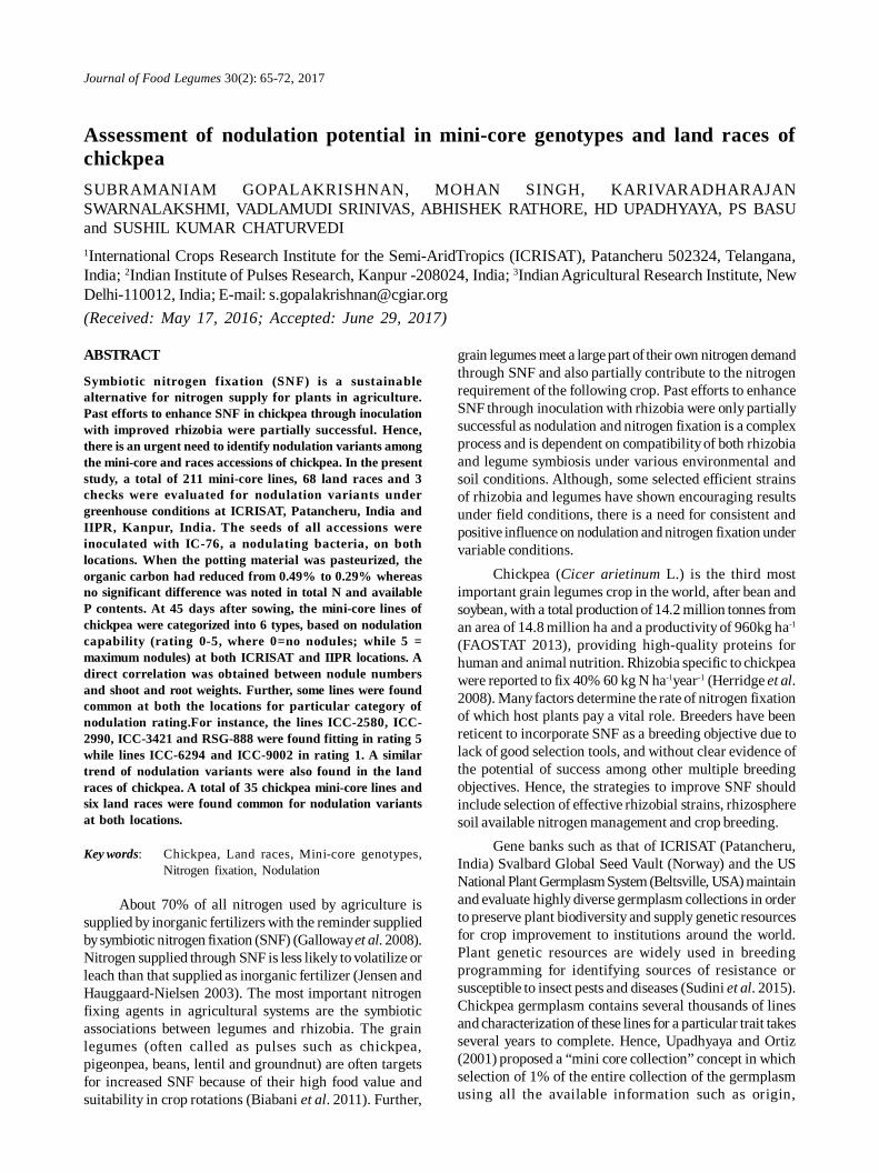
Journal of Food Legumes 30(2): 65-72, 2017
Assessment of nodulation potential in mini-core genotypes and land races ofchickpeaSUBRAMANIAM GOPALAKRISHNAN, MOHAN SINGH, KARIVARADHARAJANSWARNALAKSHMI, VADLAMUDI SRINIVAS, ABHISHEK RATHORE, HD UPADHYAYA, PS BASUand SUSHIL KUMAR CHATURVEDI1International Crops Research Institute for the Semi-AridTropics (ICRISAT), Patancheru 502324, Telangana,India; 2Indian Institute of Pulses Research, Kanpur -208024, India; 3Indian Agricultural Research Institute, NewDelhi-110012, India; E-mail: [email protected](Received: May 17, 2016; Accepted: June 29, 2017)
ABSTRACT
Symbiotic nitrogen fixation (SNF) is a sustainablealternative for nitrogen supply for plants in agriculture.Past efforts to enhance SNF in chickpea through inoculationwith improved rhizobia were partially successful. Hence,there is an urgent need to identify nodulation variants amongthe mini-core and races accessions of chickpea. In the presentstudy, a total of 211 mini-core lines, 68 land races and 3checks were evaluated for nodulation variants undergreenhouse conditions at ICRISAT, Patancheru, India andIIPR, Kanpur, India. The seeds of all accessions wereinoculated with IC-76, a nodulating bacteria, on bothlocations. When the potting material was pasteurized, theorganic carbon had reduced from 0.49% to 0.29% whereasno significant difference was noted in total N and availableP contents. At 45 days after sowing, the mini-core lines ofchickpea were categorized into 6 types, based on nodulationcapability (rating 0-5, where 0=no nodules; while 5 =maximum nodules) at both ICRISAT and IIPR locations. Adirect correlation was obtained between nodule numbersand shoot and root weights. Further, some lines were foundcommon at both the locations for particular category ofnodulation rating.For instance, the lines ICC-2580, ICC-2990, ICC-3421 and RSG-888 were found fitting in rating 5while lines ICC-6294 and ICC-9002 in rating 1. A similartrend of nodulation variants were also found in the landraces of chickpea. A total of 35 chickpea mini-core lines andsix land races were found common for nodulation variantsat both locations.
Key words: Chickpea, Land races, Mini-core genotypes,Nitrogen fixation, Nodulation
About 70% of all nitrogen used by agriculture issupplied by inorganic fertilizers with the reminder suppliedby symbiotic nitrogen fixation (SNF) (Galloway et al. 2008).Nitrogen supplied through SNF is less likely to volatilize orleach than that supplied as inorganic fertilizer (Jensen andHauggaard-Nielsen 2003). The most important nitrogenfixing agents in agricultural systems are the symbioticassociations between legumes and rhizobia. The grainlegumes (often called as pulses such as chickpea,pigeonpea, beans, lentil and groundnut) are often targetsfor increased SNF because of their high food value andsuitability in crop rotations (Biabani et al. 2011). Further,
grain legumes meet a large part of their own nitrogen demandthrough SNF and also partially contribute to the nitrogenrequirement of the following crop. Past efforts to enhanceSNF through inoculation with rhizobia were only partiallysuccessful as nodulation and nitrogen fixation is a complexprocess and is dependent on compatibility of both rhizobiaand legume symbiosis under various environmental andsoil conditions. Although, some selected efficient strainsof rhizobia and legumes have shown encouraging resultsunder field conditions, there is a need for consistent andpositive influence on nodulation and nitrogen fixation undervariable conditions.
Chickpea (Cicer arietinum L.) is the third mostimportant grain legumes crop in the world, after bean andsoybean, with a total production of 14.2 million tonnes froman area of 14.8 million ha and a productivity of 960kg ha-1
(FAOSTAT 2013), providing high-quality proteins forhuman and animal nutrition. Rhizobia specific to chickpeawere reported to fix 40% 60 kg N ha-1year-1 (Herridge et al.2008). Many factors determine the rate of nitrogen fixationof which host plants pay a vital role. Breeders have beenreticent to incorporate SNF as a breeding objective due tolack of good selection tools, and without clear evidence ofthe potential of success among other multiple breedingobjectives. Hence, the strategies to improve SNF shouldinclude selection of effective rhizobial strains, rhizospheresoil available nitrogen management and crop breeding.
Gene banks such as that of ICRISAT (Patancheru,India) Svalbard Global Seed Vault (Norway) and the USNational Plant Germplasm System (Beltsville, USA) maintainand evaluate highly diverse germplasm collections in orderto preserve plant biodiversity and supply genetic resourcesfor crop improvement to institutions around the world.Plant genetic resources are widely used in breedingprogramming for identifying sources of resistance orsusceptible to insect pests and diseases (Sudini et al. 2015).Chickpea germplasm contains several thousands of linesand characterization of these lines for a particular trait takesseveral years to complete. Hence, Upadhyaya and Ortiz(2001) proposed a “mini core collection” concept in whichselection of 1% of the entire collection of the germplasmusing all the available information such as origin,
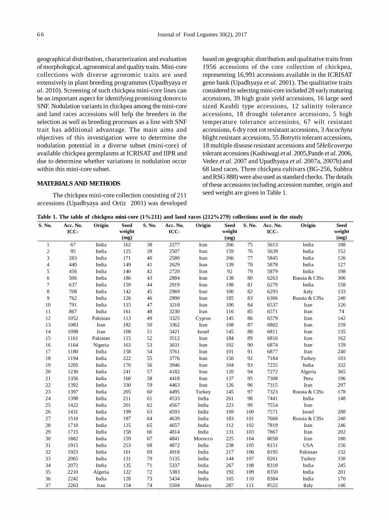
6 6 Journal of Food Legumes 30(2), 2017
geographical distribution, characterization and evaluationof morphological, agronomical and quality traits. Mini-corecollections with diverse agronomic traits are usedextensively in plant breeding programmes (Upadhyaya etal. 2010). Screening of such chickpea mini-core lines canbe an important aspect for identifying promising donors toSNF. Nodulation variants in chickpea among the mini-coreand land races accessions will help the breeders in theselection as well as breeding processes as a line with SNFtrait has additional advantage. The main aims andobjectives of this investigation were to determine thenodulation potential in a diverse subset (mini-core) ofavailable chickpea germplasms at ICRISAT and IIPR anddue to determine whether variations in nodulation occurwithin this mini-core subset.
MATERIALS AND METHODS
The chickpea mini-core collection consisting of 211accessions (Upadhyaya and Ortiz 2001) was developed
based on geographic distribution and qualitative traits from1956 accessions of the core collection of chickpea,representing 16,991 accessions available in the ICRISATgene bank (Upadhyaya et al. 2001). The qualitative traitsconsidered in selecting mini-core included 28 early maturingaccessions, 39 high grain yield accessions, 16 large seedsized Kaubli type accessions, 12 salinity toleranceaccessions, 18 drought tolerance accessions, 5 hightemperature tolerance accessions, 67 wilt resistantaccessions, 6 dry root rot resistant accessions, 3 Ascochytablight resistant accessions, 55 Botrytis tolerant accessions,18 multiple disease resistant accessions and 5Helicoverpatolerant accessions (Kashiwagi et al. 2005,Pande et al. 2006,Vedez et al. 2007 and Upadhyaya et al. 2007a, 2007b) and68 land races. Three chickpea cultivars (BG-256, Subhraand RSG 888) were also used as standard checks. The detailsof these accessions including accession number, origin andseed weight are given in Table 1.
Table 1. The table of chickpea mini-core (1%211) and land races (212%279) collections used in the studyS. No. Acc. No.
ICC- Origin Seed
weight (mg)
S. No. Acc. No. ICC-
Origin Seed weight (mg)
S. No. Acc. No. ICC-
Origin Seed weight (mg)
1 67 India 162 38 2277 Iran 266 75 5613 India 188 2 95 India 125 39 2507 Iran 159 76 5639 India 152 3 283 India 171 40 2580 Iran 266 77 5845 India 126 4 440 India 149 41 2629 Iran 139 78 5878 India 127 5 456 India 140 42 2720 Iran 92 79 5879 India 198 6 506 India 186 43 2884 Iran 138 80 6263 Russia & CISs 306 7 637 India 159 44 2919 Iran 198 81 6279 India 158 8 708 India 142 45 2969 Iran 100 82 6293 Italy 133 9 762 India 126 46 2990 Iran 185 83 6306 Russia & CISs 240
10 791 India 115 47 3218 Iran 100 84 6537 Iran 126 11 867 India 161 48 3230 Iran 116 85 6571 Iran 74 12 1052 Pakistan 113 49 3325 Cyprus 145 86 6579 Iran 142 13 1083 Iran 182 50 3362 Iran 108 87 6802 Iran 159 14 1098 Iran 108 51 3421 Israel 145 88 6811 Iran 135 15 1161 Pakistan 115 52 3512 Iran 184 89 6816 Iran 162 16 1164 Nigeria 163 53 3631 Iran 102 90 6874 Iran 159 17 1180 India 158 54 3761 Iran 101 91 6877 Iran 240 18 1194 India 222 55 3776 Iran 150 92 7184 Turkey 103 19 1205 India 170 56 3946 Iran 104 93 7255 India 332 20 1230 India 241 57 4182 Iran 120 94 7272 Algeria 365 21 1356 India 160 58 4418 Iran 137 95 7308 Peru 196 22 1392 India 330 59 4463 Iran 126 96 7315 Iran 297 23 1397 India 205 60 4495 Turkey 145 97 7323 Russia & CISs 178 24 1398 India 211 61 4533 India 261 98 7441 India 148 25 1422 India 201 62 4567 India 223 99 7554 Iran 26 1431 India 199 63 4593 India 169 100 7571 Israel 288 27 1510 India 187 64 4639 India 183 101 7668 Russia & CISs 240 28 1710 India 125 65 4657 India 112 102 7819 Iran 246 29 1715 India 158 66 4814 India 131 103 7867 Iran 202 30 1882 India 159 67 4841 Morocco 225 104 8058 Iran 180 31 1915 India 253 68 4872 India 238 105 8151 USA 156 32 1923 India 101 69 4918 India 217 106 8195 Pakistan 132 33 2065 India 131 70 5135 India 144 107 8261 Turkey 330 34 2072 India 135 71 5337 India 267 108 8318 India 245 35 2210 Algeria 122 72 5383 India 192 109 8350 India 201 36 2242 India 128 73 5434 India 165 110 8384 India 170 37 2263 Iran 154 74 5504 Mexico 287 111 8522 Italy 146
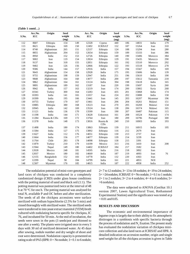
Gopalakrishnan et al. : Assessment of nodulation potential in mini-core genotypes and land races of chickpea 6 7
(Table 1 contd…)
S.No. Acc.No.
ICC Origin Seed
weight (mg)
S.No.
Acc. No. ICC
Origin Seed weight (mg)
S.No.
Acc.No. ICC
Origin Seed weight (mg)
112 8607 Ethiopia 154 149 12328 Cyprus 440 186 14831 India 179 113 8621 Ethiopia 169 150 12492 ICRISAT 152 187 15264 Iran 310 114 8740 Afghanistan 265 151 12537 Ethiopia 124 188 15294 Iran 280 115 8855 Afghanistan 204 152 12654 Ethiopia 159 189 15333 Iran 386 116 8950 India 152 153 12726 Ethiopia 140 190 15406 Morocco 384 117 9002 Iran 119 154 12824 Ethiopia 129 191 15435 Morocco 290 118 9137 Iran 318 155 12851 Ethiopia 161 192 15510 Morocco 292 119 9402 Iran 126 156 12866 Ethiopia 122 193 15518 Morocco 278 120 9586 India 144 157 12916 India 157 194 15567 India 169 121 9643 Afghanistan 154 158 12928 India 175 195 15606 India 139 122 9755 Afghanistan 198 159 12947 India 251 196 15610 India 190 123 9848 Afghanistan 164 160 13077 India 200 197 15612 Tanzania 218 124 9862 Afghanistan 164 161 13124 India 394 198 15618 India 165 125 9895 Afghanistan 189 162 13187 Iran 220 199 15697 Syria 260 126 9942 India 157 163 13219 Iran 174 200 15802 Syria 268 127 10341 Turkey 300 164 13283 Iran 435 201 15868 India 174 128 10393 India 141 165 13357 Iran 224 202 15888 India 158 129 10399 India 195 166 13441 Iran 145 203 16207 Myanmar 196 130 10755 Turkey 170 167 13461 Iran 206 204 16261 Malawi 151 131 10885 Ethiopia 380 168 13523 Iran 270 205 16269 Malawi 134 132 10945 India 142 169 13524 Iran 138 206 16374 Malawi 165 133 11121 India 136 170 13599 Iran 190 207 16487 Pakistan 115 134 11198 India 144 171 13628 Unknown 161 208 16524 Pakistan 174 135 11284 Russia & CISs 169 172 13764 Iran 180 209 16796 Portugal 300 136 11378 India 148 173 13816 Russia &
CISs 240 210 16903 India 193
137 11498 India 180 174 13863 Ethiopia 139 211 16915 India 195 138 11584 India 127 175 13892 Ethiopia 116 212 2679 Iran 139 11627 India 112 176 14051 Ethiopia 130 213 2737 Iran 140 11664 India 156 177 14077 Ethiopia 139 214 3239 Iran 141 11764 Chile 283 178 14098 Ethiopia 158 215 3391 Iran 142 11879 Turkey 210 179 14199 Mexico 313 216 3410 Iran 208 143 11944 Nepal 149 180 14402 ICRISAT 184 217 3582 Iran 144 12028 Mexico 248 181 14595 India 216 218 3892 Iran 145 12037 Mexico 180 182 14669 India 187 219 4093 Iran 76 146 12155 Bangladesh 152 183 14778 India 132 220 4363 Iran 147 12299 Nepal 90 184 14799 India 161 221 4853 NOI 148 12307 Myanmar 176 185 14815 India 187 222 4958 India 252
The nodulation potential of mini-core genotypes and
land races of chickpea was conducted in a completelyrandomized design (CRD) under glass house conditionswith the potting material of sand and black soil (1:1). Thepotting material was pasteurized twice at the interval of 48h at 70 °C for one h. The potting material was analysed fortotal N, available P and OC before and after sterilization.The seeds of all the chickpea accessions were surfacesterilized with sodium hypochlorite (2.5% for 5 min) andrinsed thoroughly with sterilized water. The sterilized seedswere transferred to into yeast extract mannitol (YEM) brothcultured with nodulating bacteria specific for chickpea, IC76, and incubated for 50 min. At the end of incubation, theseeds were sown in the pots (3 seeds/pot and thinned toone after a week). The plants were irrigated once in every 3days with 30 ml of sterilized deionised water. At 45 daysafter sowing, nodule number and dry weight of shoot androot were determined. Nodulation capacity is presented onrating scale of 0%5 (IIPR: 0 = No nodule; 1= 0.1 to 6 nodule;
2= 7 to 12 nodules; 3= 13 to 18 nodules; 4= 19 to 24 nodules;5= >24 nodules; ICRISAT: 0 = No nodule; 1= 0.1 to 1 nodule;2= 1 to 2 nodules; 3= 2 to 4 nodules; 4= 4 to 6 nodules; 5=>6 nodules).
The data were subjected to ANOVA (GenStat 10.1version 2007, Lawes Agricultural Trust, RothamstedExperimental Station) and the significance was tested at p< 0.01 and 0.05.
RESULTS AND DISCUSSION
The economic and environmental importance oflegume crops is largely due to their ability to fix atmosphericdinitrogen in a symbiosis with specific bacteria throughthe process of nodulation and N2 fixation.The present studyhas evaluated the nodulation variation of chickpea mini-core collection and also land races at ICRISAT and IIPR. Adetailed indication on accession number, origin and singleseed weight for all the chickpea accession is given in Table
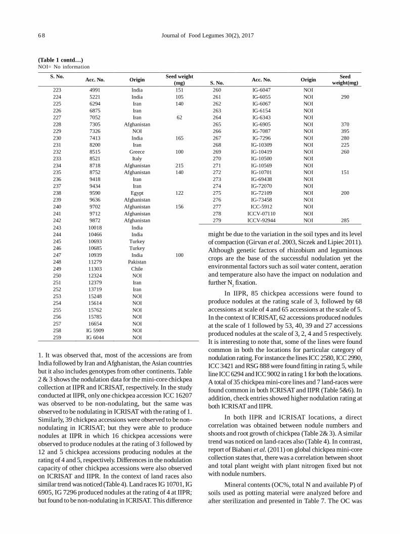
6 8 Journal of Food Legumes 30(2), 2017
(Table 1 contd…)NOI= No information
1. It was observed that, most of the accessions are fromIndia followed by Iran and Afghanistan, the Asian countriesbut it also includes genotypes from other continents. Table2 & 3 shows the nodulation data for the mini-core chickpeacollection at IIPR and ICRISAT, respectively. In the studyconducted at IIPR, only one chickpea accession ICC 16207was observed to be non-nodulating, but the same wasobserved to be nodulating in ICRISAT with the rating of 1.Similarly, 39 chickpea accessions were observed to be non-nodulating in ICRISAT; but they were able to producenodules at IIPR in which 16 chickpea accessions wereobserved to produce nodules at the rating of 3 followed by12 and 5 chickpea accessions producing nodules at therating of 4 and 5, respectively. Differences in the nodulationcapacity of other chickpea accessions were also observedon ICRISAT and IIPR. In the context of land races alsosimilar trend was noticed (Table 4). Land races IG 10701, IG6905, IG 7296 produced nodules at the rating of 4 at IIPR;but found to be non-nodulating in ICRISAT. This difference
might be due to the variation in the soil types and its levelof compaction (Girvan et al. 2003, Siczek and Lipiec 2011).Although genetic factors of rhizobium and leguminouscrops are the base of the successful nodulation yet theenvironmental factors such as soil water content, aerationand temperature also have the impact on nodulation andfurther N2 fixation.
In IIPR, 85 chickpea accessions were found toproduce nodules at the rating scale of 3, followed by 68accessions at scale of 4 and 65 accessions at the scale of 5.In the context of ICRISAT, 62 accessions produced nodulesat the scale of 1 followed by 53, 40, 39 and 27 accessionsproduced nodules at the scale of 3, 2, 4 and 5 respectively.It is interesting to note that, some of the lines were foundcommon in both the locations for particular category ofnodulation rating. For instance the lines ICC 2580, ICC 2990,ICC 3421 and RSG 888 were found fitting in rating 5, whileline ICC 6294 and ICC 9002 in rating 1 for both the locations.A total of 35 chickpea mini-core lines and 7 land-races werefound common in both ICRISAT and IIPR (Table 5&6). Inaddition, check entries showed higher nodulation rating atboth ICRISAT and IIPR.
In both IIPR and ICRISAT locations, a directcorrelation was obtained between nodule numbers andshoots and root growth of chickpea (Table 2& 3). A similartrend was noticed on land-races also (Table 4). In contrast,report of Biabani et al. (2011) on global chickpea mini-corecollection states that, there was a correlation between shootand total plant weight with plant nitrogen fixed but notwith nodule numbers.
Mineral contents (OC%, total N and available P) ofsoils used as potting material were analyzed before andafter sterilization and presented in Table 7. The OC was
S. No. Acc. No. Origin Seed weight (mg)
S. No. Acc. No. Origin Seed
weight(mg) 223 4991 India 151 260 IG-6047 NOI 224 5221 India 105 261 IG-6055 NOI 290 225 6294 Iran 140 262 IG-6067 NOI 226 6875 Iran 263 IG-6154 NOI 227 7052 Iran 62 264 IG-6343 NOI 228 7305 Afghanistan 265 IG-6905 NOI 370 229 7326 NOI 266 IG-7087 NOI 395 230 7413 India 165 267 IG-7296 NOI 280 231 8200 Iran 268 IG-10309 NOI 225 232 8515 Greece 100 269 IG-10419 NOI 260 233 8521 Italy 270 IG-10500 NOI 234 8718 Afghanistan 215 271 IG-10569 NOI 235 8752 Afghanistan 140 272 IG-10701 NOI 151 236 9418 Iran 273 IG-69438 NOI 237 9434 Iran 274 IG-72070 NOI 238 9590 Egypt 122 275 IG-72109 NOI 200 239 9636 Afghanistan 276 IG-73458 NOI 240 9702 Afghanistan 156 277 ICC-5912 NOI 241 9712 Afghanistan 278 ICCV-07110 NOI 242 9872 Afghanistan 279 ICCV-92944 NOI 285 243 10018 India 244 10466 India 245 10693 Turkey 246 10685 Turkey 247 10939 India 100 248 11279 Pakistan 249 11303 Chile 250 12324 NOI 251 12379 Iran 252 13719 Iran 253 15248 NOI 254 15614 NOI 255 15762 NOI 256 15785 NOI 257 16654 NOI 258 IG 5909 NOI 259 IG 6044 NOI
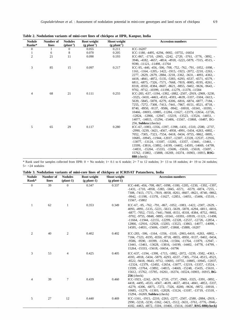
Gopalakrishnan et al. : Assessment of nodulation potential in mini-core genotypes and land races of chickpea 6 9
* Rank used for samples collected from IIPR: 0 = No nodule; 1= 0.1 to 6 nodule; 2= 7 to 12 nodules; 3= 13 to 18 nodules; 4= 19 to 24 nodules;5= >24 nodules
Table 2. Nodulation variants of mini-core lines of chickpea at IIPR, Kanpur, IndiaNodule Ranke*
Number of lines
Nodules (plant-1)
Root weight (g plant-1)
Shoot weight (g plant-1)
Accession numbers
0 1 0 0.055 0.211 ICC-16207 1 6 8 0.070 0.205 ICC-1180, -4495, -6294, -9002, -10755, -16654 2 21 11 0.090 0.193 ICC-867, -1710, -2065, -2242, -2720, -3761, -3776, -3892, -
3946, -4182, -4657, -4814, -4918, -5221,-5879, -7315, -8515, -9590, -11121, -11498, -11764
3 85 15 0.097 0.217 ICC-95, -440, -456, -506, -708, -752, -762, -791, -1052, -1098, -1161, -1164, -1205,- 1422, -1915, -1923, -2072, -2210, -2263, -2277, -2629, -2679, -2884, -3218, -3362, -3631, - 4093, -4363, -4418, -4841, -4872, -5135, -5383, -6293, -6537, -6571, -6579, -6811, -6875, -7326, -7571, -7668, -7819, -8085, -8195, -8261, -8318, -8350, -8384, -8607, -8621, -8855, -9402, -9636, -9643, -9702, -9712, -10399, -11198, -11279, -11378, -11584
4 68 21 0.111 0.255 ICC-283, -637, -1194, -1392, -1882, -2507, -2919, -2969, -3230, -3325, -3410, -4463, -4533, -4593, -4639, -5337, -5504, -5613, -5639, -5845, -5878, -6279, -6306, -6816, -6874, -6877, -7184, -7255, -7272, -7308, -7413, -7441, -7867, -8151, -8521, -8718, -8740, -8950, -9137, -9586, -9942, -10018, -10341, -10393, -10466, -10693, -10885, -11284, -11627, -12379, -12654, -12726, -12824, -12866, -12947, -13219, -13523, -13524, -14051, -14077, -14815, -15294, -15406, -15567, -15868, -16487, BG-256, Subhra (checks)
5 65 29 0.117 0.280 ICC-67, -1083, -1356, -1397, -1398, -1431, -1510, -2580, -2737, -2990, -3239, -3421, -4567, -4958, -4991, -5434, -6263, -6802, -7052, -7305, -7323, -7554, -9418, -9434, -9755, -9862, -9895, -10685, -10945, -11944, -12037, -12307, -12328, -12537, -12916, -13077, -13124, -13187, -13283, -13357, -13441, -13461, -13599, -13816, -13892, -14199, -14402, -14595, -14669, -14799, -14831, -15264, -15333, -15606, -15610, -15618, -15697, -15762, -15802, -15888, -16269, -16374, -16903, -16915, RSG-888 (check)
Nodule Rank*
Number of lines
Nodules (plant-1)
Root weight (g plant-1)
Shoot weight (g plant-1)
Accession numbers
0 39 0 0.347 0.337 ICC-440, -456, -708, -867, -1098, -1180, -1205, -1230, -1392, -1397, -1431, -1710, -4958, -5383, -5845, -6571, -6579, -6874, -7255, -7308, -7413, -7571, -7819, -8058, -8261, -8607, -8621, -8740, -9862, -9942, -11198, -11378, -11627, -12851, -14051, -15406, -15510, -15567, -15802
1 62 1 0.353 0.349 ICC-67, -95, -762, -791, -867, -1052, -1083, -1422, -2307, -2629, -4093, -4991, -5135, -5221, -5613, -5639, -5878, -6294, -6811, -6816, -6877, -7052, -7315, -7441,-7668, -8151, -8318, -8384, -8752, -9002, -9702, -9755, -9848, -9895, -10341, -10393, -10939, -11121, -11498, -11664, -11944, -12155, -12299, -12328, -12537, -12726, -12854, -12866, -12916, -12928, -13283, -13523, -13863, -14077, -14098, -14595, -14831, -15606, -15697, -15868, -15888, -16207
2 40 2 0.402 0.402 ICC-283, -506, -1164, -1356, -1510, -2065,-6410, -6263, -6802, -7184, -7323, -8195, -8350, -8718, -8855, -8950, -9137, -9402, -9434, -9586, -9590, -10399, -11284, -11584, -11764, -11879, -12947, -13441, -13461, -13628, -13816, -14199, -14402, -14778, -14799, -15264, -15333, -15618, -16654, -16796
3 53 4 0.425 0.405 ICC-637, -1194, -1398, -1715, -1882, -2072, -3239, -3582, -4363, -4593, -4918, -5434, -5879, -6293, -6537, -7305, -7554, -8515, -8521, -8522, -9418, -9643, -9712, -10693, -10755, -10885, -10945, -12037, -12324, -12379, -12492, -12654, -13077, -13219, -13357, -13524, -13599, -13764, -13892, -14815, -14669, -15248, -15435, -15610, -15612, -15762, -15785, -16261, -16374, -16524,-16903, -16915, BG-256 (check)
4 39 7 0.439 0.460 ICC-1923, -2242, -2679, -2720, -2737, -2969, -3325, -3391, -3892, -4418, -4495, -4533, -4567, -4639, -4657, -4814, -4841, -4853, -5337, -6279, -6306, -6875, -7272, -7326, -8200, -9636, -9872, -10018, -10685, -11279, -11303, -12028, -13124, -13187, -13719, -15518, -15294, -16269, Subhra (check)
5 27 12 0.440 0.469 ICC-1161, -1915, -2210, -2263, -2277, -2507, -2580, -2884, -2919, -2990, -3218, -3230, -3362, -3421, -3512, -3631, -3761, -3776, -3946,-4182, -4463, -4872, -5504, -10466, -15614, -16487, RSG-888(check)
Table 3. Nodulation variants of mini-core lines of chickpea at ICRISAT Patancheru, India
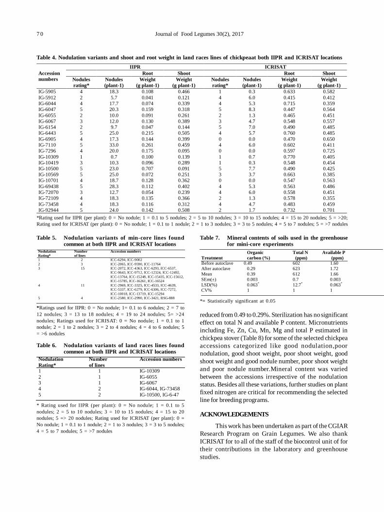
7 0 Journal of Food Legumes 30(2), 2017
Table 4. Nodulation variants and shoot and root weight in land races lines of chickpeaat both IIPR and ICRISAT locations
*Rating used for IIPR (per plant): 0 = No nodule; 1 = 0.1 to 5 nodules; 2 = 5 to 10 nodules; 3 = 10 to 15 nodules; 4 = 15 to 20 nodules; 5 = >20;Rating used for ICRISAT (per plant): 0 = No nodule; 1 = 0.1 to 1 nodule; 2 = 1 to 3 nodules; 3 = 3 to 5 nodules; 4 = 5 to 7 nodules; 5 = >7 nodules
IIPR ICRISAT Accession numbers
Root Shoot Root Shoot Nodules rating*
Nodules (plant-1)
Weight (g plant-1)
Weight (g plant-1)
Nodules rating*
Nodules (plant-1)
Weight (g plant-1)
Weight (g plant-1)
IG-5905 4 18.3 0.108 0.466 1 0.3 0.633 0.582 IG-5912 2 5.7 0.041 0.121 4 6.0 0.415 0.412 IG-6044 4 17.7 0.074 0.339 4 5.3 0.715 0.359 IG-6047 5 20.3 0.159 0.318 5 8.3 0.447 0.564 IG-6055 2 10.0 0.091 0.261 2 1.3 0.465 0.451 IG-6067 3 12.0 0.130 0.389 3 4.7 0.548 0.557 IG-6154 2 9.7 0.047 0.144 5 7.0 0.490 0.485 IG-6443 5 25.0 0.215 0.505 4 5.7 0.760 0.485 IG-6905 4 17.3 0.144 0.399 0 0.0 0.470 0.650 IG-7110 5 33.0 0.261 0.459 4 6.0 0.602 0.411 IG-7296 4 20.0 0.175 0.095 0 0.0 0.597 0.725 IG-10309 1 0.7 0.100 0.139 1 0.7 0.770 0.405 IG-10419 3 10.3 0.096 0.289 1 0.3 0.548 0.454 IG-10500 5 23.0 0.707 0.091 5 7.7 0.490 0.425 IG-10569 5 25.0 0.072 0.251 3 3.7 0.663 0.385 IG-10701 4 18.7 0.128 0.362 0 0.0 0.547 0.563 IG-69438 5 28.3 0.112 0.402 4 5.3 0.563 0.486 IG-72070 3 12.7 0.054 0.239 4 6.0 0.558 0.451 IG-72109 4 18.3 0.135 0.366 2 1.3 0.578 0.355 IG-73458 4 18.3 0.116 0.312 4 4.7 0.483 0.459 IG-92944 5 24.0 0.142 0.508 2 1.7 0.732 0.701
Table 5. Nodulation variants of min-core lines foundcommon at both IIPR and ICRISAT locations
*Ratings used for IIPR: 0 = No nodule; 1= 0.1 to 6 nodules; 2 = 7 to12 nodules; 3 = 13 to 18 nodules; 4 = 19 to 24 nodules; 5= >24nodules; Ratings used for ICRISAT: 0 = No nodule; 1 = 0.1 to 1nodule; 2 = 1 to 2 nodules; 3 = 2 to 4 nodules; 4 = 4 to 6 nodules; 5= >6 nodules
Nodulation Number Accession numbers Rating* of lines 1 2 ICC-6294, ICC-9002 2 3 ICC-2065, ICC-9590, ICC-11764 3 15 ICC-2072, ICC-4363, ICC-6293, ICC-6537, ICC-9643, ICC-9712, ICC-12324, ICC-12492, ICC-13764, ICC-15248, ICC-15435, ICC-15612, ICC-15785, ICC-16261, ICC-16524 4 11 ICC-2969, ICC-3325, ICC-4533, ICC-4639, ICC-5337, ICC-6279, ICC-6306, ICC-7272, ICC-10018, ICC-13719, ICC-15294 5 4 ICC-2580, ICC-2990, ICC-3421, RSG-888
Table 6. Nodulation variants of land races lines foundcommon at both IIPR and ICRISAT locations
* Rating used for IIPR (per plant): 0 = No nodule; 1 = 0.1 to 5nodules; 2 = 5 to 10 nodules; 3 = 10 to 15 nodules; 4 = 15 to 20nodules; 5 => 20 nodules; Rating used for ICRISAT (per plant): 0 =No nodule; 1 = 0.1 to 1 nodule; 2 = 1 to 3 nodules; 3 = 3 to 5 nodules;4 = 5 to 7 nodules; 5 = >7 nodules
Nodulation Number Accession numbers Rating* of lines 1 1 IG-10309 2 1 IG-6055 3 1 IG-6067 4 2 IG-6044, IG-73458 5 2 IG-10500, IG-6-47
Table 7. Mineral contents of soils used in the greenhousefor mini-core experiments
*= Statistically significant at 0.05
Organic Total N Available P Treatment carbon (%) (ppm) (ppm) Before autoclave 0.49 602 1.60 After autoclave 0.29 623 1.72 Mean 0.39 612 1.66 SEm(±) 0.003 0.7 0.003 LSD(%) 0.063* 12.7* 0.063* CV% 1 1 1
reduced from 0.49 to 0.29%. Sterilization has no significanteffect on total N and available P content. Micronutrientsincluding Fe, Zn, Cu, Mn, Mg and total P estimated inchickpea stover (Table 8) for some of the selected chickpeaaccessions categorized like good nodulation,poornodulation, good shoot weight, poor shoot weight, goodshoot weight and good nodule number, poor shoot weightand poor nodule number.Mineral content was variedbetween the accessions irrespective of the nodulationstatus. Besides all these variations, further studies on plantfixed nitrogen are critical for recommending the selectedline for breeding programs.
ACKNOWLEDGEMENTS
This work has been undertaken as part of the CGIARResearch Program on Grain Legumes. We also thankICRISAT for to all of the staff of the biocontrol unit of fortheir contributions in the laboratory and greenhousestudies.
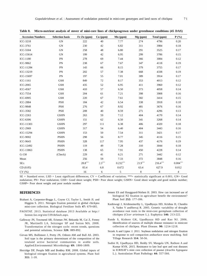
Gopalakrishnan et al. : Assessment of nodulation potential in mini-core genotypes and land races of chickpea 7 1
Table 8. Micro-nutrient analysis of stover of mini-core lines of chickpeagrown under greenhouse conditions (45 DAS)
SE = Standard error; LSD = Least significant differences; CV = Coefficient of variation; ***= statistically significant at 0.001; GN= Goodnodulation; PN= Poor nodulation; GSH= Good shoot weight; PSH= Poor shoot weight; GSHN= Good shoot weight and good nodule number;GSHP= Poor shoot weight and poor nodule number
REFERENCES
Biabani A, Carpenter-Boggs L, Coyne CJ, Taylor L, Smith JL andHiggins S. 2011. Nitrogen fixation potential in global chickpeamini-core collection. Biological Fertilizer Soils 47: 679-685.
FAOSTAT. 2013. Statistical database 2013 Available at http://faostat.fao.org/site/339/default.aspx.
Galloway JN, Townsend AR, Erisman JW, Bekunda M, Cai Z, FreneyJR, Martinelli LA, Seitzinger SP and Sutton MA. 2008.Transformation of the nitrogen cycle: recent trends, questionsand potential solutions, Science 320: 889-892.
Girvan MS, Bullimore J, Pretty JN, Osborn AM and Ball AS. 2003.Soil type is the primary determinant of the composition of thetotaland active bacterial communities in arable soils.Applied.Environmental Microbiology 69: 1800-1809.
Herridge DF, People MB and Boddey RM. 2008. Global inputs ofbiological nitrogen fixation in agricultural systems. Plant Soil311: 1-18.
Jensen ES and Hauggaard-Nielsen H. 2003. How can increased use ofbiological N2 fixation in agriculture benefit the environment?Plant Soil 252: 177-186.
Kashiwagi J, Krishnamurthy L, Upadhyaya HD, Krishna H, ChandraS, Vadez V andSerraj R. 2005. Genetic variability of droughtavoidance root traits in the mini-core germplasm collection ofchickpea (Cicer arietinum L.). Euphytica 146: 213-222.
Pande S, Kishore GK, Upadhyaya HD and Rao NJ. 2006.Identification of sources of multiple disease resistance in minicorecollection of chickpea. Plant Disease. 90: 1214-1218.
Siczek A and Lipiec J. 2011. Soybean nodulation and nitrogen fixationin response to soil compaction andsurface straw mulching. SoilTillage Research 114: 50-56.
Sudini H, Upadhyaya HD, Reddy SV, Mangala UN, Rathore A andKumar KVK. 2015. Resistance to late leaf spot and rust diseasesin ICRISAT’s mini core collection of peanut (Arachis hypogaeaL.). Australasian Plant Pathology 44: 557-566.
Accession Numbers Selection basis Fe Zn (ppm) Cu (ppm) Mn (ppm) Mg (ppm) Total (ppm) P (%) ICC-3218 GN 222 40 7.77 274 4796 0.20 ICC-3761 GN 230 42 6.82 311 3984 0.18 ICC-5504 GN 258 48 6.80 291 3525 0.17 ICC-15614 GN 199 42 6.95 299 3786 0.15 ICC-1180 PN 278 69 7.44 366 3084 0.12 ICC-9862 PN 238 67 7.67 347 4118 0.19 ICC-11284 PN 143 66 8.15 379 3755 0.17 ICC-13219 PN 202 57 7.38 668 4338 0.19 ICC-15697 PN 197 55 7.01 389 3914 0.17 ICC-1161 GSH 849 72 8.17 353 4013 0.12 ICC-2065 GSH 435 52 6.95 411 3960 0.12 ICC-4567 GSH 410 57 6.50 373 4058 0.14 ICC-7554 GSH 204 61 7.21 398 3908 0.16 ICC-6905 GSH 220 67 7.61 582 3414 0.15 ICC-2884 PSH 184 42 6.54 338 3918 0.18 ICC-9848 PSH 276 67 8.92 481 3676 0.16 ICC-3582 PSH 208 40 8.59 271 4296 0.13 ICC-2263 GSHN 263 59 7.12 404 4170 0.14 ICC-6306 GSHN 151 62 6.50 341 3268 0.14 ICC-11303 GSHN 297 111 6.38 406 4320 0.18 ICC-2969 GSHN 317 54 6.40 404 3443 0.16 ICC-15294 GSHN 153 50 7.54 311 3421 0.17 ICC-9002 PSHN 298 56 8.77 345 4116 0.15 ICC-9643 PSHN 328 117 7.95 437 4176 0.19 ICC-12492 PSHN 119 49 7.28 310 3044 0.18 ICC-13863 PSHN 138 65 7.91 450 4228 0.14 G-130 (Check) 229 41 6.21 271 3442 0.12 Mean 256 59 7.33 372 3848 0.16 SE± 28.8*** 2.3*** 0.232*** 21.9*** 216.4*** 0.004*** CD (0.05) 83.4 6.8 0.672 63.4 627.9 0.012 CV (%) 16 6 5 8 8 4
7 2 Journal of Food Legumes 30(2), 2017
Upadhyaya HD, Bramel PJ and Singh S. 2001. Development ofchickpea core subset using geographic distribution and qualitativetraits. Crop Science 41: 206-210.
Upadhyaya HD and Ortiz R. 2001. A min core subset for capturingdiversity and promoting utilization of chickpea genetic resourcesin crop improvement.Theoritical Applied Genetics 102: 1292-1298.
Upadhyaya HD, Dwivedi SL, Gowda CLL and Singh S. 2007a.Identification of diverse germplasm lines for agronomic traitsin a chickpea (Cicer arietinum L.) core collection for use incrop improvement. Field Crops Research 100: 320-326.
Upadhyaya HD, Salimath PM, Gowda CLL and Singh S. 2007b. Newearly-maturing germplasm lines for utilization in chickpeaimprovement. Euphytica 157: 195-208.
Upadhyaya HD, Yadav D, Dronavalli N, Gowda CLL and Singh S.2010.Minicore germplasm collections for infusing geneticdiversity in plant breeding programs. Electron Journal of PlantBreeding 1: 1294-1309.
Vadez V, Krishnamurthy L, Gaur PM, Upadhyaya HD, HoisingtonDA, Varshney RK, Turner NC and Siddique KHM. 2007. Largevariation in salinity tolerance is explained by differences in thesensitivity of reproductive stages in chickpea. Field CropsResearch 104: 123-129.
Journal of Food Legumes 30(2): 73-76, 2017
ABSTRACT
Soybean (Glycine max) is as an oilseed crop with inadvertentimportance. It is a good source of protein both for the humanbeings and livestock including pieces. The production anddemand for soybean have been many traits increased in Indiaduring the last decade resolving in its winder adoption amongfarmers in Madhya Pradesh, Maharashtra, Rajasthan,Karnataka and Gujarat. This necessitates the need forreliable information on futures prices for soybean.Therefore, the present study was undertaken by collectingmonthly prices of soybean in major soybean states of Indiafor a period of 11 years (January 2006 to December 2016) byusing ARIMA (Box-Jenkins model) so as to predict the futureprices of soybean.The performance of fitted model wasexamined by computing various measures of goodness of fitviz., AIC, SBC and MAPE. ARIMA was the most representativemodel for the price forecast of soybean among states and thecountry as a while. The developed model can be used as apolicy instrument for the farmers, processors and traders.The harvest of crop during September to October. Theproduction and market prices of soybean, would be ruling inthe range of INR 2,6000-3,6000 per tonne in kharif harvestingseason, 2017-18. Average price of soybean ruled at INR 2,6930 per tonne, compared to its MSP at INR 2,7750 per tonneduring the last year. INR may recover for the coming kharifseason. Since India is the largest importer of edible oils,there in a need to encourage soybean cultivation where everclimate is suitable for its cultivation.
Key words: ARIMA, Additional market price, Soybean
India is the fourth largest oilseed producing countryin the world, next only to USA, China and Brazil, harvestingabout 32 million tonnes of oilseeds against the worldproduction of 250 million tonnes per annum. Since 1995,India’s share in world production of oilseeds has beenaround 10 percent. Although, India is a major producer ofoilseeds, per capita oil consumption in India is only 10.6kg/year in compassion to 12.5 kg/year in China, 20.8 kg/year in Japan, 21.3 kg/year in Brazil and 48.0 kg/ year inUSA. The major oilseeds from in India included soybean,cottonseed, groundnut, sunflower, rapeseed, sesame seed,copra, linseed, castor seed and palm kernels.
India being the world’s largest producer of oilseedsaccounts for about 7-8 per cent of global vegetable oilproduction. However, the growth in domestic productionhas not kept pace with the growth in demand. The countrynow imports more than half of its oilseed for domesticconsumption resulting in substantial drain foreign
Predicting market price of soybean in major India studies through ARIMA modelASHWINI DAREKAR and A AMARENDER REDDY
National Institute of Agricultural Extension Management (MANAGE), Hyderabad, India;E-mail: [email protected](Received: March 2, 2017; Accepted: June 30, 2017)
exchange. Given the competing demands on agriculturalland from various crops and enterprises, the production ofoilseeds can be increased only if their productivities areimproved significantly and farmers receive remunerativeprices and have assured market access. Total productionof kharif oilseeds in the country is estimated at 23.36 milliontonnes 2016-17, which is significantly higher than theproduction of 16.59 million tonnes during 2015-16. Currentyear production of kharif oilseeds is also higher by 2.33million tonnes over the average production of realizing incomparison to last five years.
Soybean (Glycine max) is the world’s most importantseed legume contributing to 25% of the global edible oiland about two-thirds of the world’s protein concentrate forlivestock feeding. The contribution of India in the worldsoybean area is 10%, but the contribution to total worldsoybean grain is only 4% indicating productivity of thecrop in India (1.1 t/ha) as compared to world averageproductivity (2.2 t/ha). The Soybean is in the states ofMadhya Pradesh, Maharashtra, Rajasthan, Chhattisgarh,Andhra Pradesh, Telangana and Karnataka (country the98% of production in the country). It contributes nearly50% of the area and production followed by Maharashtra32 and 34 percent in report in the last decade which challengethe reliability of supply, stock levels, and reasonablepricing.(Reddy, 2012: Reddy and Reddy, 2011).
The time series approach to forecasting is one suchapproach which relies on the past pattern in a time series toforecast prices in the future (De Gooijer and Hyndman 2006,Taylor 2003). One of the most simple and bench mark methodis that of Box and Jenkins which is popularly known asrelying ARIMA methodology on the past pattern in a timeseries to forecast prices in the future. Burark and Sharma(2012) confirmed the suitability of Box-Jenkins univariateARIMA models in agricultural price forecasting. Time seriesmethod of forecasting has been used by Paul and Das (2010)for forecasting fish production in India while Darekaret al.(2016a and 2016b) validated onion prices in Kolhapur andYeola markets respectively. Manasa (2010) analyzed marketdynamics and price.
There was a need to assess the necessity offorecasting of soybean prices to the farmers, traders,speculators and the commodity exchanges. It is concludedthat the absolute forecasted prices, would ensure the marketreality and reduce price distortions and chances ofspeculation. This will help the farmers as well as the traders
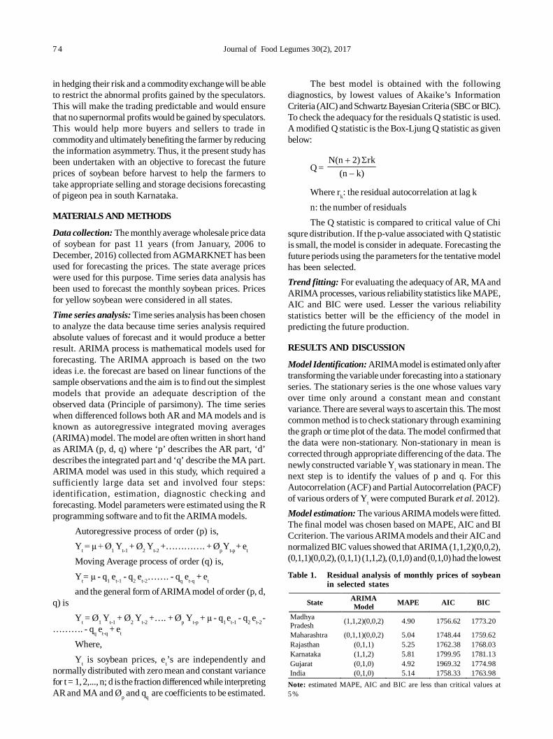
7 4 Journal of Food Legumes 30(2), 2017
in hedging their risk and a commodity exchange will be ableto restrict the abnormal profits gained by the speculators.This will make the trading predictable and would ensurethat no supernormal profits would be gained by speculators.This would help more buyers and sellers to trade incommodity and ultimately benefiting the farmer by reducingthe information asymmetry. Thus, it the present study hasbeen undertaken with an objective to forecast the futureprices of soybean before harvest to help the farmers totake appropriate selling and storage decisions forecastingof pigeon pea in south Karnataka.
MATERIALS AND METHODS
Data collection: The monthly average wholesale price dataof soybean for past 11 years (from January, 2006 toDecember, 2016) collected from AGMARKNET has beenused for forecasting the prices. The state average priceswere used for this purpose. Time series data analysis hasbeen used to forecast the monthly soybean prices. Pricesfor yellow soybean were considered in all states.Time series analysis: Time series analysis has been chosento analyze the data because time series analysis requiredabsolute values of forecast and it would produce a betterresult. ARIMA process is mathematical models used forforecasting. The ARIMA approach is based on the twoideas i.e. the forecast are based on linear functions of thesample observations and the aim is to find out the simplestmodels that provide an adequate description of theobserved data (Principle of parsimony). The time serieswhen differenced follows both AR and MA models and isknown as autoregressive integrated moving averages(ARIMA) model. The model are often written in short handas ARIMA (p, d, q) where ‘p’ describes the AR part, ‘d’describes the integrated part and ‘q’ describe the MA part.ARIMA model was used in this study, which required asufficiently large data set and involved four steps:identification, estimation, diagnostic checking andforecasting. Model parameters were estimated using the Rprogramming software and to fit the ARIMA models.
Autoregressive process of order (p) is,Yt = µ + Ø1 Yt-1 + Ø2 Yt-2 +…………. + Øp Yt-p + et
Moving Average process of order (q) is,Yt= µ - q1 et-1 - q2 et-2……. - qq et-q + et
and the general form of ARIMA model of order (p, d,q) is
Yt = Ø1 Yt-1 + Ø2 Yt-2 +…. + Øp Yt-p + µ - q1 et-1 - q2 et-2 -………. - qq et-q + et
Where,Yt is soybean prices, et’s are independently and
normally distributed with zero mean and constant variancefor t = 1, 2,..., n; d is the fraction differenced while interpretingAR and MA and Øp and qq are coefficients to be estimated.
The best model is obtained with the followingdiagnostics, by lowest values of Akaike’s InformationCriteria (AIC) and Schwartz Bayesian Criteria (SBC or BIC).To check the adequacy for the residuals Q statistic is used.A modified Q statistic is the Box-Ljung Q statistic as givenbelow:
Q = k)– (n rk 2) N(n
Where rk: the residual autocorrelation at lag kn: the number of residualsThe Q statistic is compared to critical value of Chi
squre distribution. If the p-value associated with Q statisticis small, the model is consider in adequate. Forecasting thefuture periods using the parameters for the tentative modelhas been selected.Trend fitting: For evaluating the adequacy of AR, MA andARIMA processes, various reliability statistics like MAPE,AIC and BIC were used. Lesser the various reliabilitystatistics better will be the efficiency of the model inpredicting the future production.
RESULTS AND DISCUSSION
Model Identification: ARIMA model is estimated only aftertransforming the variable under forecasting into a stationaryseries. The stationary series is the one whose values varyover time only around a constant mean and constantvariance. There are several ways to ascertain this. The mostcommon method is to check stationary through examiningthe graph or time plot of the data. The model confirmed thatthe data were non-stationary. Non-stationary in mean iscorrected through appropriate differencing of the data. Thenewly constructed variable Yt was stationary in mean. Thenext step is to identify the values of p and q. For thisAutocorrelation (ACF) and Partial Autocorrelation (PACF)of various orders of Yt were computed Burark et al. 2012).Model estimation: The various ARIMA models were fitted.The final model was chosen based on MAPE, AIC and BICcriterion. The various ARIMA models and their AIC andnormalized BIC values showed that ARIMA (1,1,2)(0,0,2),(0,1,1)(0,0,2), (0,1,1) (1,1,2), (0,1,0) and (0,1,0) had the lowest
State ARIMA Model MAPE AIC BIC
Madhya Pradesh (1,1,2)(0,0,2) 4.90 1756.62 1773.20
Maharashtra (0,1,1)(0,0,2) 5.04 1748.44 1759.62 Rajasthan (0,1,1) 5.25 1762.38 1768.03 Karnataka (1,1,2) 5.81 1799.95 1781.13 Gujarat (0,1,0) 4.92 1969.32 1774.98 India (0,1,0) 5.14 1758.33 1763.98
Table 1. Residual analysis of monthly prices of soybeanin selected states
Note: estimated MAPE, AIC and BIC are less than critical values at5%
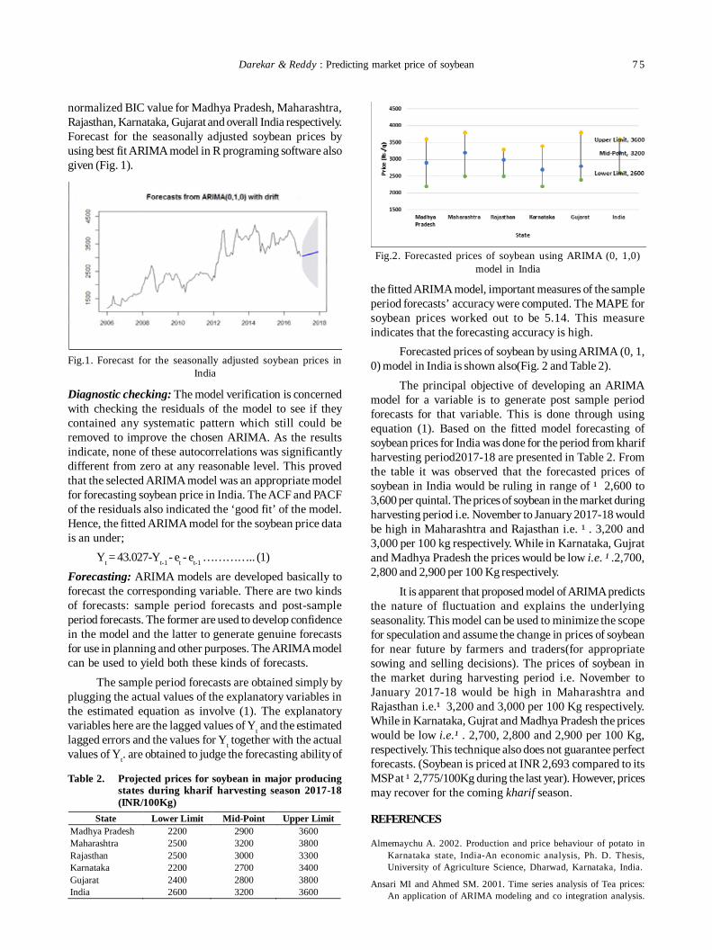
Darekar & Reddy : Predicting market price of soybean 7 5
normalized BIC value for Madhya Pradesh, Maharashtra,Rajasthan, Karnataka, Gujarat and overall India respectively.Forecast for the seasonally adjusted soybean prices byusing best fit ARIMA model in R programing software alsogiven (Fig. 1).
the fitted ARIMA model, important measures of the sampleperiod forecasts’ accuracy were computed. The MAPE forsoybean prices worked out to be 5.14. This measureindicates that the forecasting accuracy is high.
Forecasted prices of soybean by using ARIMA (0, 1,0) model in India is shown also(Fig. 2 and Table 2).
The principal objective of developing an ARIMAmodel for a variable is to generate post sample periodforecasts for that variable. This is done through usingequation (1). Based on the fitted model forecasting ofsoybean prices for India was done for the period from kharifharvesting period2017-18 are presented in Table 2. Fromthe table it was observed that the forecasted prices ofsoybean in India would be ruling in range of ¹ 2,600 to3,600 per quintal. The prices of soybean in the market duringharvesting period i.e. November to January 2017-18 wouldbe high in Maharashtra and Rajasthan i.e. ¹ . 3,200 and3,000 per 100 kg respectively. While in Karnataka, Gujratand Madhya Pradesh the prices would be low i.e. ¹ .2,700,2,800 and 2,900 per 100 Kg respectively.
It is apparent that proposed model of ARIMA predictsthe nature of fluctuation and explains the underlyingseasonality. This model can be used to minimize the scopefor speculation and assume the change in prices of soybeanfor near future by farmers and traders(for appropriatesowing and selling decisions). The prices of soybean inthe market during harvesting period i.e. November toJanuary 2017-18 would be high in Maharashtra andRajasthan i.e.¹ 3,200 and 3,000 per 100 Kg respectively.While in Karnataka, Gujrat and Madhya Pradesh the priceswould be low i.e.¹ . 2,700, 2,800 and 2,900 per 100 Kg,respectively. This technique also does not guarantee perfectforecasts. (Soybean is priced at INR 2,693 compared to itsMSP at ¹ 2,775/100Kg during the last year). However, pricesmay recover for the coming kharif season.
REFERENCES
Almemaychu A. 2002. Production and price behaviour of potato inKarnataka state, India-An economic analysis, Ph. D. Thesis,University of Agriculture Science, Dharwad, Karnataka, India.
Ansari MI and Ahmed SM. 2001. Time series analysis of Tea prices:An application of ARIMA modeling and co integration analysis.
Diagnostic checking: The model verification is concernedwith checking the residuals of the model to see if theycontained any systematic pattern which still could beremoved to improve the chosen ARIMA. As the resultsindicate, none of these autocorrelations was significantlydifferent from zero at any reasonable level. This provedthat the selected ARIMA model was an appropriate modelfor forecasting soybean price in India. The ACF and PACFof the residuals also indicated the ‘good fit’ of the model.Hence, the fitted ARIMA model for the soybean price datais an under;
Yt = 43.027-Yt-1 - et - et-1 ………….. (1)Forecasting: ARIMA models are developed basically toforecast the corresponding variable. There are two kindsof forecasts: sample period forecasts and post-sampleperiod forecasts. The former are used to develop confidencein the model and the latter to generate genuine forecastsfor use in planning and other purposes. The ARIMA modelcan be used to yield both these kinds of forecasts.
The sample period forecasts are obtained simply byplugging the actual values of the explanatory variables inthe estimated equation as involve (1). The explanatoryvariables here are the lagged values of Yt and the estimatedlagged errors and the values for Yt together with the actualvalues of Yt. are obtained to judge the forecasting ability of
Fig.1. Forecast for the seasonally adjusted soybean prices inIndia
State Lower Limit Mid-Point Upper Limit Madhya Pradesh 2200 2900 3600 Maharashtra 2500 3200 3800 Rajasthan 2500 3000 3300 Karnataka 2200 2700 3400 Gujarat 2400 2800 3800 India 2600 3200 3600
Table 2. Projected prices for soybean in major producingstates during kharif harvesting season 2017-18(INR/100Kg)
Fig.2. Forecasted prices of soybean using ARIMA (0, 1,0)model in India
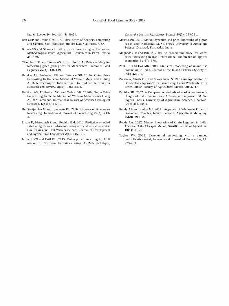
7 6 Journal of Food Legumes 30(2), 2017
Indian Economics Journal 48: 49-54.
Box GEP and Jenkin GM. 1976. Time Series of Analysis, Forecastingand Control, Sam Franscico, Holden-Day, California. USA.
Burark SS and Sharma H. 2012. Price Forecasting of Coriander:Methodological Issues. Agricultural Economics Research Review25: 530.
Chaudhari DJ and Tingre AS. 2014. Use of ARIMA modeling forforecasting green gram prices for Maharashtra. Journal of FoodLegumes 27(2): 136-139.
Darekar AS, Pokharkar VG and Datarkar SB. 2016a. Onion PriceForecasting In Kolhapur Market of Western Maharashtra UsingARIMA Technique. International Journal of InformationResearch and Review. 3(12): 3364-3368.
Darekar AS, Pokharkar VG and Yadav DB. 2016b. Onion PriceForecasting In Yeola Market of Western Maharashtra UsingARIMA Technique. International Journal of Advanced BiologicalResearch. 6(4): 551-552.
De Gooijer Jan G and Hyndman RJ. 2006. 25 years of time seriesforecasting. International Journal of Forecasting 22(3): 443-473.
Elham K, Masoumeh Z and Ebrahim BM. 2010. Prediction of addedvalue of agricultural subsections using artificial neural networks:Box-Jenkins and Holt-Winters methods. Journal of Developmentand Agricultural Economics 2(4): 115-121.
Jalikatti VN and Patil BL. 2015. Onion price forecasting in Hublimarket of Northern Karnataka using ARIMA technique,
Karnataka Journal Agriculture Science 28(2): 228-231.
Manasa PB. 2010. Market dynamics and price forecasting of pigeonpea in south Karnataka. M. Sc. Thesis, University of AgricultureScience, Dharwad, Karnataka, India.
Moghaddsi R and Bita R. 2008. An econometric model for wheatprice forecasting in Iran. International conference on appliedeconomics Pp 671-678.
Paul RK and Das MK. 2010. Statistical modelling of inland fishproduction in India. Journal of the Inland Fisheries Society ofIndia 42: 1-7.
Pravin A, Singh DR and Sivaramane N. 2005.An Application ofBox-Jenkins Approach for Forecasting Copra Wholesale PriceSeries. Indian Society of Agricultural Statists 59: 32-47.
Punitha SB. 2007. A Comparative analysis of market performanceof agricultural commodities - An economic approach. M. Sc.(Agri.) Thesis, University of Agriculture Science, Dharwad,Karnataka, India.
Reddy AA and Reddy GP. 2011 Integration of Wholesale Prices ofGroundnut Complex, Indian Journal of Agricultural Marketing.25(2): 89-108.
Reddy AA. 2012. Market Integration of Grain Legumes in India:The case of the Chickpea Market, SAARC Journal of Agriculture,10(1): 11-29.
Taylor JW. 2003. Exponential smoothing with a dampedmultiplicative trend, International Journal of Forecasting 19:273-289.
Journal of Food Legumes 30(2): 77-82, 2017
ABSTRACT
The present investigation was conducted to study effects ofvarious treatments on ascorbic acid, antioxidant activity,phytic acid, polyphenols and organoleptic quality of chickpeasprouts. Chickpea seeds were washed, soaked and allowedto sprout. The sprouts were subjected to various treatmentsviz., ethanol vapour (30 min), hot water dip (500 C for 2 min)and UV-Irradiation (10 kJm-2 for 1 h). The chickpea sproutswere then packed in disposable glasses, wrapped withperforated cling films and stored at room (25±30 C) and low(7±0.50 C) temperature. The sprouts were analyzed at 24 hinterval until the spoilage. Ascorbic acid and antioxidantactivity of chickpea sprouts first showed the elevation andthen reduced, however, polyphenols and phytic acid decreasedprogressively with storage period. Ascorbic acid andantioxidant activity of chickpea sprouts were highest inethanol vapours treatment whereas maximum reduction ofantinutritional factor was observed with UV- irradiationtreatment. The sprouts showed acceptability upto 48 h atroom temperature and 120 h at low temperature storageconditions.
Keywords: Antioxidant activity, ascorbic acid, chickpeasprouts, ethanol vapours, hot water dip, phyticacid, UV-irradiation.
Legumes contain complex carbohydrates, vitamins,proteins, minerals and worldwide known for its nutritionalquality (Wang et al. 2010). Sprouting has proven to be anefficient method for improving the nutritional quality oflegumes (Khattak et al . 2008) and reducing theantinutritional factors (Ghavidel and Prakash, 2007). It alsoincreases the vitamin concentrations and bioavailability ofminerals (El-Adawy, 2002).
There is a developing interest for chickpea (Cicerarietinum L.) because of its nutritional content. Chickpeaseed contains elevated amount of carbohydrate (59.09%)and protein (17.80%). It contains (9%) moisture, (6.48%)fibre and (5.80%) fat (Masood et al. 2014). Sprouts ofchickpea are gaining popularity due to its nutritional quality.The shelf life of sprouts is shorter due to the presence ofhigh moisture content and high metabolic activity whichdiverts the need to enhance its shelf life during storageperiod. It is reported that pre-treatment of UV-C irradiationto fresh cut mango results in maintaining its nutritionalcontent, preventing decay and extending shelf life upto 15days (George, 2015).
Effects of ethanol vapours, hot water dip and ultraviolet irradiation treatmentson nutritional quality of chickpea sproutsSIMRAN ARORA, SALEEM SIDDIQUI and RAKESH GEHLOT
Centre of Food Science and Technology, CCS HAU, Hisar, 125 004, Haryana, India; E-mail:[email protected](Received: April 25, 2017; Accepted: June 19, 2017)
Goyal and Siddiqui, 2014 reported that nutritional andkeeping quality of mung bean sprouts was enhanced byethanol vapour and hot water dip treatment. The shelf lifeof germinated beans is restricted to two days due to itsperishable nature. Generally regarded as safe (GRAS) pre-treatments, low temperature storage conditions, modifiedatmosphere packaging enhanced the keeping quality ofsprouts (Day 1990 and Goyal et al. 2014).
Keeping in view the dietetic importance of chickpeaand its sprouts, the investigation was undertaken to studythe effect of various pre-treatments on nutritional qualityof chickpea sprouts during storage.
MATERIALS AND METHODS
Seeds were procured from local market, CCS HAU,Hisar, Haryana, India. Chickpea seeds were cleaned, washedin hypochlorite solution and soaked in 4–5 volumes of waterfor 10 h under ambient laboratory conditions. After soaking,seed were allowed to germinate in sprout maker (NovellePlast, Delhi) for 24 h at 30±10C.Treatment and storage conditions: Sprouted chickpeawere divided into 4 lots of equal amount and subjected tovarious treatments viz., hot water dip (HWD) (50° C for 2min), ethanol vapours (in a glass chamber saturated withethanol vapours) for 30 min., and UV irradiation (10 kJm-2
for 1 h in laminar flow chamber). Untreated sprouts wereused as control. The sprouts from each treatment were filledin disposable plastic glasses (~200 ml volume) and wrappedwith (2%) perforated cling films. Wet white filter paper wasplaced along the inner sides of plastic glasses to maintainhigh humidity inside the disposable glasses. There was~100 g sprouts per pack and the packs were stored in darkat room (30±30 C) and low (7±0.50 C) temperature conditionsmaintained in B.O.D. incubator. The sampling for variousparameters was done regularly at 24 h interval until thespoilage.
Chemical analysis
Ascorbic acid: It was assessed by titration method asdescribed by AOAC (1995). Extraction of sample was doneby macerating 2 g of sprouts with (3%) metaphosphoricacid and final volume was made up to 10 ml withmetaphosphoric acid. The extract was filtered with whatmanno. 1 filter paper and 10 ml of aliquot was titrated with 2,6-
7 8 Journal of Food Legumes 30(2), 2017
dichloroindophenol dye till the end point (pink colour).The results were expressed in terms of mg ascorbic acid per100 g sprouts.Antioxidant activity: It was analyzed using free radical 2,2-diphenyl-1-picrylhydrazyl (DPPH) dye as per theprocedure suggested by Shimada et al. (1992). Extractionof sample was done by macerating 500 mg of sprouts in 10ml of methanol, centrifuged at 4000 rpm and filtered withwhatman no.1 filter paper. 100 µl of supernatant was addedto 3 ml of dye and incubated for 30 min at 25-300 C. Theinhibition percentage of DPPH solution at 517 nm withsample was calculated using the following equation:
Antioxidant activity (% scavenging of DPPH) =(Abst=0 min - Abst=30 min) × 100/Abst=0 min
(Where, Abs: Absorbance)
Antinutritional Factor
Phytic acid: It was determined by the method of Haug andLantzsch (1983). Finely ground (one gram) sample wasextracted with 0.2 N HCl for 3 h with continuous shakingand filtered through Whatmann No.1 filter paper. 500 µl ofextract was added to the tube containing 1.0 ml of ferricammonium sulphate solution and the tube was heated in aboiling water bath for 30 min. The contents of the tubewere then mixed and centrifuged for 30 min. at 3000 rpm.One ml supernatant was transferred to another test tubeand 1.5 ml bipyridine solution was added. Phytic acidconcentration at 519 nm was calculated from the standardcurve prepared using graded concentrations of sodiumphytate.
Polyphenols: It was estimated by the method of Swain andHills (1959). Defatted sample (500 mg) was refluxed withmethanol containing (1%) HCl for 3h. The extract wasconcentrated by evaporating methanol on a boiling waterbath and its volume was made to 25 ml with methanolic-HCl. To the 1.5 ml of the extract 8.5 ml of water and 0.5 mlFolin-Denis reagent was added. After three minutes, oneml saturated sodium carbonate solution was added withvigorous shaking. After one hour, the absorbance was readat 725 nm using methanolic- HCl as blank. Thecorresponding concentration of polyphenols was calculatedfrom the standard curve prepared using gradedconcentrations of tannic acid.Overall acceptability: Sensory evaluation of treatedsprouts and control samples was carried out using 9-pointhedonic scale. A trained panel of 10 judges checked thevariation present in samples for various organolepticqualities and acceptability of samples was decided on thebasis of that.Statistical analysis: There were three replicates for eachtreatment and the data was subjected to analysis of variance(ANOVA) technique and analyzed according to two factorialcompletely randomized designs (CRD) at 5% level ofsignificance.
RESULTS AND DISCUSSION
Ascorbic acid: Data regarding the ascorbic acid content ofchickpea sprouts at low and room temperature storage ispresented in Table 1. Initial value of ascorbic acid ofchickpea sprout was 14.7 mg/100 g which significantlyincreased to 29.6 mg/100 g after 48 h and thereafter decreased
Table 1. Effect of different treatments on ascorbic acid (mg/100g) of chickpea sprouts during storage
HWD= Hot water dip; Observation were not recorded due to spoilage of samples
Treatments Period of storage (h) 0 24 48 72 96 120 Mean
Room Temperature Control 17.2 20.0 23.2 20.6 - - 20.2 HWD 14.7 25.5 27.2 23.7 - - 22.8 Ethanol 15.4 27.2 29.6 26.2 - - 24.6 UV 16.9 24.0 26.6 22.2 - - 22.4 Mean 16.1 24.2 26.6 23.2 - - C.D. at 5% Treatments (T) = 0.44 ; Storage (S) = 0.44 ; TxS = 0.88 Low Temperature Control 18.4 19.3 21.7 23.4 24.3 21.9 21.5 HWD 15.8 23.0 26.4 29.4 28.1 24.8 24.6 Ethanol 16.7 23.3 28.1 31.5 28.5 26.4 25.8 UV 17.9 20.9 23.0 24.3 25.6 22.6 22.4 Mean 17.2 21.7 24.8 27.2 26.6 23.9 C.D. at 5% Treatments (T) = 0.29 ; Storage (S) = 0.35 ; TxS = 0.70
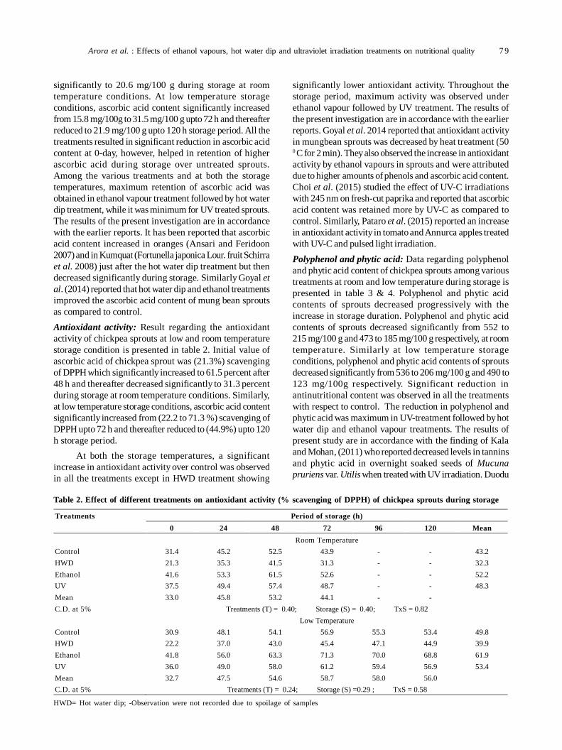
Arora et al. : Effects of ethanol vapours, hot water dip and ultraviolet irradiation treatments on nutritional quality 7 9
significantly to 20.6 mg/100 g during storage at roomtemperature conditions. At low temperature storageconditions, ascorbic acid content significantly increasedfrom 15.8 mg/100g to 31.5 mg/100 g upto 72 h and thereafterreduced to 21.9 mg/100 g upto 120 h storage period. All thetreatments resulted in significant reduction in ascorbic acidcontent at 0-day, however, helped in retention of higherascorbic acid during storage over untreated sprouts.Among the various treatments and at both the storagetemperatures, maximum retention of ascorbic acid wasobtained in ethanol vapour treatment followed by hot waterdip treatment, while it was minimum for UV treated sprouts.The results of the present investigation are in accordancewith the earlier reports. It has been reported that ascorbicacid content increased in oranges (Ansari and Feridoon2007) and in Kumquat (Fortunella japonica Lour. fruit Schirraet al. 2008) just after the hot water dip treatment but thendecreased significantly during storage. Similarly Goyal etal. (2014) reported that hot water dip and ethanol treatmentsimproved the ascorbic acid content of mung bean sproutsas compared to control.Antioxidant activity: Result regarding the antioxidantactivity of chickpea sprouts at low and room temperaturestorage condition is presented in table 2. Initial value ofascorbic acid of chickpea sprout was (21.3%) scavengingof DPPH which significantly increased to 61.5 percent after48 h and thereafter decreased significantly to 31.3 percentduring storage at room temperature conditions. Similarly,at low temperature storage conditions, ascorbic acid contentsignificantly increased from (22.2 to 71.3 %) scavenging ofDPPH upto 72 h and thereafter reduced to (44.9%) upto 120h storage period.
At both the storage temperatures, a significantincrease in antioxidant activity over control was observedin all the treatments except in HWD treatment showing
significantly lower antioxidant activity. Throughout thestorage period, maximum activity was observed underethanol vapour followed by UV treatment. The results ofthe present investigation are in accordance with the earlierreports. Goyal et al. 2014 reported that antioxidant activityin mungbean sprouts was decreased by heat treatment (500 C for 2 min). They also observed the increase in antioxidantactivity by ethanol vapours in sprouts and were attributeddue to higher amounts of phenols and ascorbic acid content.Choi et al. (2015) studied the effect of UV-C irradiationswith 245 nm on fresh-cut paprika and reported that ascorbicacid content was retained more by UV-C as compared tocontrol. Similarly, Pataro et al. (2015) reported an increasein antioxidant activity in tomato and Annurca apples treatedwith UV-C and pulsed light irradiation.Polyphenol and phytic acid: Data regarding polyphenoland phytic acid content of chickpea sprouts among varioustreatments at room and low temperature during storage ispresented in table 3 & 4. Polyphenol and phytic acidcontents of sprouts decreased progressively with theincrease in storage duration. Polyphenol and phytic acidcontents of sprouts decreased significantly from 552 to215 mg/100 g and 473 to 185 mg/100 g respectively, at roomtemperature. Similarly at low temperature storageconditions, polyphenol and phytic acid contents of sproutsdecreased significantly from 536 to 206 mg/100 g and 490 to123 mg/100g respectively. Significant reduction inantinutritional content was observed in all the treatmentswith respect to control. The reduction in polyphenol andphytic acid was maximum in UV-treatment followed by hotwater dip and ethanol vapour treatments. The results ofpresent study are in accordance with the finding of Kalaand Mohan, (2011) who reported decreased levels in tanninsand phytic acid in overnight soaked seeds of Mucunapruriens var. Utilis when treated with UV irradiation. Duodu
Table 2. Effect of different treatments on antioxidant activity (% scavenging of DPPH) of chickpea sprouts during storage
HWD= Hot water dip; -Observation were not recorded due to spoilage of samples
Treatments Period of storage (h) 0 24 48 72 96 120 Mean
Room Temperature Control 31.4 45.2 52.5 43.9 - - 43.2 HWD 21.3 35.3 41.5 31.3 - - 32.3 Ethanol 41.6 53.3 61.5 52.6 - - 52.2 UV 37.5 49.4 57.4 48.7 - - 48.3 Mean 33.0 45.8 53.2 44.1 - - C.D. at 5% Treatments (T) = 0.40; Storage (S) = 0.40; TxS = 0.82 Low Temperature Control 30.9 48.1 54.1 56.9 55.3 53.4 49.8 HWD 22.2 37.0 43.0 45.4 47.1 44.9 39.9 Ethanol 41.8 56.0 63.3 71.3 70.0 68.8 61.9 UV 36.0 49.0 58.0 61.2 59.4 56.9 53.4 Mean 32.7 47.5 54.6 58.7 58.0 56.0 C.D. at 5% Treatments (T) = 0.24; Storage (S) =0.29 ; TxS = 0.58
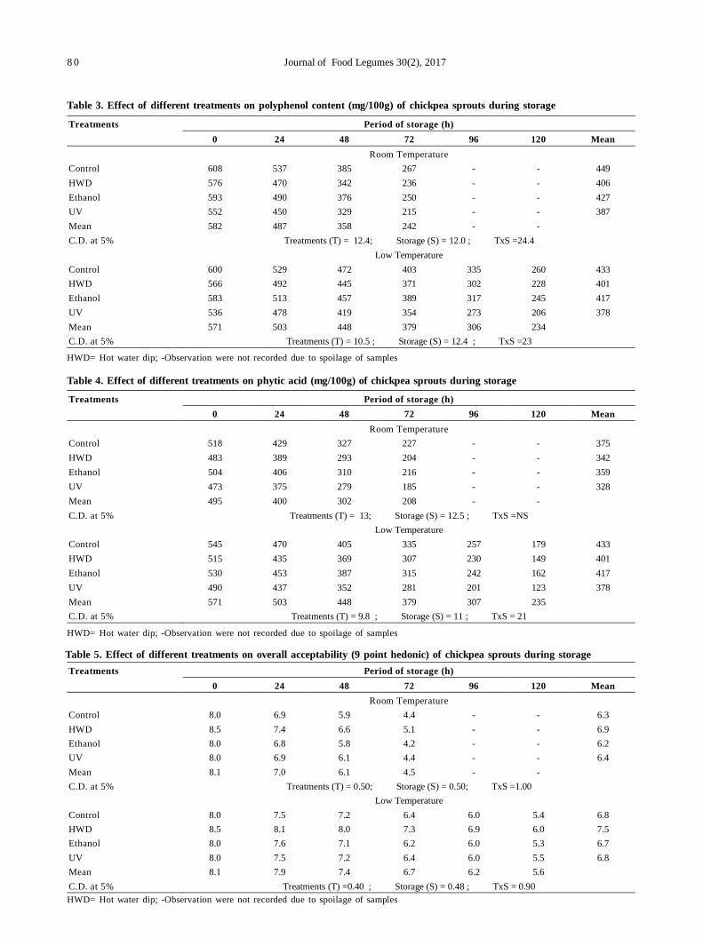
8 0 Journal of Food Legumes 30(2), 2017
Table 3. Effect of different treatments on polyphenol content (mg/100g) of chickpea sprouts during storage
HWD= Hot water dip; -Observation were not recorded due to spoilage of samples
Treatments Period of storage (h) 0 24 48 72 96 120 Mean
Room Temperature Control 608 537 385 267 - - 449 HWD 576 470 342 236 - - 406 Ethanol 593 490 376 250 - - 427 UV 552 450 329 215 - - 387 Mean 582 487 358 242 - - C.D. at 5% Treatments (T) = 12.4; Storage (S) = 12.0 ; TxS =24.4 Low Temperature Control 600 529 472 403 335 260 433 HWD 566 492 445 371 302 228 401 Ethanol 583 513 457 389 317 245 417 UV 536 478 419 354 273 206 378 Mean 571 503 448 379 306 234 C.D. at 5% Treatments (T) = 10.5 ; Storage (S) = 12.4 ; TxS =23
Table 4. Effect of different treatments on phytic acid (mg/100g) of chickpea sprouts during storage
HWD= Hot water dip; -Observation were not recorded due to spoilage of samples
Treatments Period of storage (h) 0 24 48 72 96 120 Mean
Room Temperature Control 518 429 327 227 - - 375 HWD 483 389 293 204 - - 342 Ethanol 504 406 310 216 - - 359 UV 473 375 279 185 - - 328 Mean 495 400 302 208 - - C.D. at 5% Treatments (T) = 13; Storage (S) = 12.5 ; TxS =NS Low Temperature Control 545 470 405 335 257 179 433 HWD 515 435 369 307 230 149 401 Ethanol 530 453 387 315 242 162 417 UV 490 437 352 281 201 123 378 Mean 571 503 448 379 307 235 C.D. at 5% Treatments (T) = 9.8 ; Storage (S) = 11 ; TxS = 21
Table 5. Effect of different treatments on overall acceptability (9 point hedonic) of chickpea sprouts during storage
HWD= Hot water dip; -Observation were not recorded due to spoilage of samples
Treatments Period of storage (h) 0 24 48 72 96 120 Mean
Room Temperature Control 8.0 6.9 5.9 4.4 - - 6.3 HWD 8.5 7.4 6.6 5.1 - - 6.9 Ethanol 8.0 6.8 5.8 4.2 - - 6.2 UV 8.0 6.9 6.1 4.4 - - 6.4 Mean 8.1 7.0 6.1 4.5 - - C.D. at 5% Treatments (T) = 0.50; Storage (S) = 0.50; TxS =1.00 Low Temperature Control 8.0 7.5 7.2 6.4 6.0 5.4 6.8 HWD 8.5 8.1 8.0 7.3 6.9 6.0 7.5 Ethanol 8.0 7.6 7.1 6.2 6.0 5.3 6.7 UV 8.0 7.5 7.2 6.4 6.0 5.5 6.8 Mean 8.1 7.9 7.4 6.7 6.2 5.6 C.D. at 5% Treatments (T) =0.40 ; Storage (S) = 0.48 ; TxS = 0.90
Arora et al. : Effects of ethanol vapours, hot water dip and ultraviolet irradiation treatments on nutritional quality 8 1
et al. (1999) suggested that degradation of phytic acid byradiation is due to cleavage of phytic acid itself.Organoleptic score: Data regarding on organoleptic scoreof chickpea sprouts among various treatments at room andlow temperature during storage is presented in table 5. Therewas a decrease in overall acceptability score with theadvancement in storage period and became unacceptabilityat 72 h of storage at room temperature and 120 h of storageat low temperature. There was no significant effect ofvarious treatments on the sprouting. However, under boththe storage temperatures, overall acceptability of chickpeasprouts significantly increased by HWD and ethanoltreatment, while it was decreased significantly by UVirradiation treatment. The results of present study are inaccordance with the findings of Goyal and Siddiqui (2014),who reported that mung bean sprouts remained acceptableupto 48 h and 120 h at room and low temperature storageconditions, respectively. They studied that keeping qualityof mung bean sprouts was enhanced by ethanol vapourand HWD treatments, both at room and low temperaturestorage conditions. Similarly, Bai et al.( 2004) and Hu et al.(2010) studied that the shelf life heat pre-treated apple slicesand fresh cut eggplant respectively, were improved byethanol vapour treatment.
CONCLUSION
Based on these results, it can be concluded thatdifferent treatments resulted in significant improvement ofnutritional quality of chickpea sprouts during storage. Theascorbic acid content and antioxidant activity were highestin ethanol vapours treated sprouts. Polyphenols and phyticacid content of sprouts decreased progressively with theincrease in storage period and maximum reduction wasobserved in UV treated sprouts. Ethanol vapoursignificantly improved the ascorbic acid content andantioxidant activity of chickpea sprouts and UV radiationresulted significance reduction of antinutritional compound.Keeping quality of chickpea sprouts can be maintainedwell upto 48 h at room temperature and 120 h at lowtemperature as against 24 and 96 h under control conditionsby subjecting the sprouts to hot water dip treatment of 500
C for 2 min. This treatment could also represent a promisingalternative to conventional methods for fruits andvegetables also.
ACKNOWLEDGMENTS
I acknowledge CFST-CCSHAU for providing all otherfacilities to accomplish this work.
REFERENCES
Ansari NA and Feridoon H. 2007. Postharvest application of hotwater, fungicide and waxing on the shelf life of Valencia andlocal oranges of siavarz. Asian Journal of Plant Science 6(2):314–319.
AOAC. 1995. Official methods of analysis. Association of OfficialAnalytical Chemists, Washington DC.
Bai J, Baldwin EA, Fortuny RCS, Mattheis JP, Stanley R, Perera Cand Brecth JK. 2004. Effect of pretreatment of intact ‘Gala’apple with ethanol vapor, heat, or 1-methylcyclopropene onquality and shelf life of fresh cut slices. Journal of AmericanSociety of Horticultural Sciences 129(4): 583-593.
Choi I, Yoo TJ and Kang H. 2015. UV-C treatments enhanceantioxidant activity; retain quality and microbial safety of fresh-cut paprika in MA storage. Horticulture EnvironmentBiotechnology 56(3): 324-329.
Day BPF. 1990. Modified atmosphere packaging of selected preparedfruits and vegetables. In: Proc COST 91 Final Seminar ElsevierScience Publishers, Amsterdam. pp. 3230-3232.
EL-Adway T. 2002. Nutritional composition and antinutritionalfactors of chickpeas (Cicer arietinum L.) undergoing differentcooking methods and germination. Plant Foods Human Nutrition57: 83–97.
George DS, Razali Z, Santhirasegaram V and Somasundram C. 2015.Effect of postharvest ultraviolet-C treatment on the proteomechanges in fresh cut mango (Mangifera indica L. cv. Chokanan).Journal of the Science of Food and Agriculture 96: 2851-2860.
Ghavidel RA and Prakash J. 2007. The impact of germination anddehulling on nutrients, antinutrients, in vitro iron and digestibilityof some legume seeds. Legume and Wheat Technology 40: 1292-1299.
Goyal A and Siddiqui S. 2014. Effects of ultraviolet irradiation, pulsedelectric field, hot water dip and ethanol vapours treatment onkeeping and sensory quality of mung bean (Vigna radiata L.Wilczek.) sprouts. Journal of Food Science and Technology51(10): 2664–2670.
Goyal, A, Siddiqui S, Upadhyay N and Soni J. 2014. Effects ofultraviolet irradiation, pulsed electric field, hot water and ethanolvapours treatment on functional properties of mung bean sprouts.Journal of Food Science and Technology 51(4): 708-714.
Haug W and Lantzsch H. 1983. Sensitive method for rapiddetermination of phytates in cereals and cereal products. Journalof Science of Food and Agriculture 34(12): 1423-1426.
Hu W, Jiang A, Tian M, Liu C and Wang Y. 2010. Effect of ethanoltreatment on physiological and quality attributes of fresh- cuteggplant. Journal of Science of Food and Agriculture 90(8):1323-1326.
Kala BK and Mohan VR. 2011. Effect of UV treatment onantinutritional factors of two accessions of valvet bean, Mucunapruriens(L.) DC var. Utilis (Wall.ex Wight) Bak.exBurck.Tropical and Subtropical Agro-ecosystems 15: 131-141.
Khattak AB, Zeb A, Bibi N and Khattak MS. 2008. Effect ofgermination time and type of illumination on proximatecomposition of chickpea seed (Cicer arietinum L.). AmericanJournal of Food Technology 3(1): 24-32.
Masood T, Shah HU and Zeb A. 2014. Effect of sprouting time onproximate composition and ascorbic acid level of mung bean(Vigna radiate L.) and chickpea (Cicer arietinum l.) seeds. TheJournal of Animal & Plant Sciences 24(3): 850-859.
8 2 Journal of Food Legumes 30(2), 2017
Pataro G, Donsi G and Ferrari G. 2015. Post-harvest UV-C and PLIrradiation of Fruits and Vegetables. Chemical Engineering 44:31-36.
Schirra M, Palma A, Aquina S, Angioni A, Minello EV, Melis M andCabras P. 2008. Influence of postharvest hot water treatmenton nutritional and functional properties of kumquat (Fortunellajaponica Lour. Swingle Cv. Ovale) fruit. Journal of Agriculturaland Food Chemistry 56: 455-460.
Shimada K, Fujikawa K, Yahara K and Nakamura T. 1992.Antioxidative properties of xanthan on the antioxidation ofsoybean oil in cyclodextrin emulsion. Journal of Agriculturaland Food Chemistry 40: 945-948.
Swain J and Hills WE. 1959. The phenolic constituents ofPramusdomestica I.The quantitative analysis of phenolicconstituent. Journal of the science of Food and Agriculture 10:63-68.
Wang N, Hatcher DW, Tyler RT, Toews R and Gawalko EJ. 2010.Effect of cooking on the composition of bean (Phaseolusvulgaris L.) and chickpea (Cicer arietinum L.). Food ResearchInternational 43: 589-594.
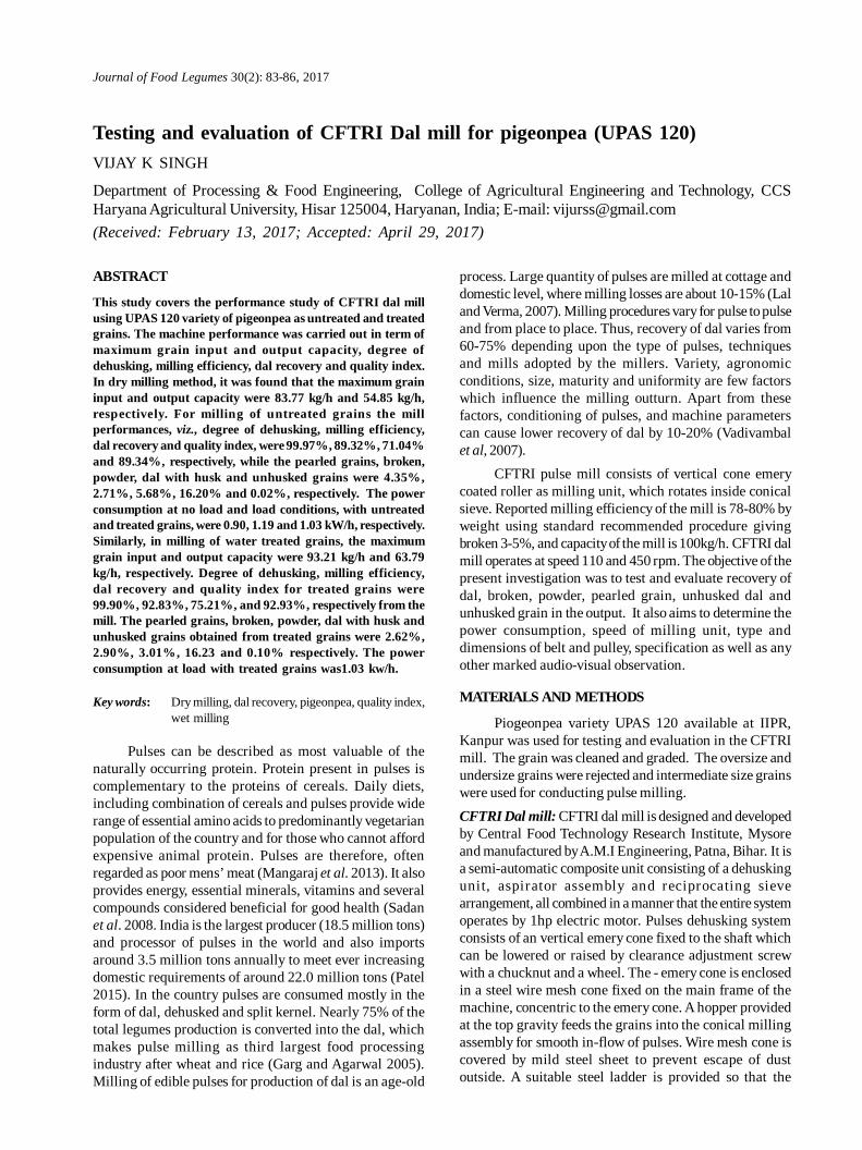
Journal of Food Legumes 30(2): 83-86, 2017
ABSTRACT
This study covers the performance study of CFTRI dal millusing UPAS 120 variety of pigeonpea as untreated and treatedgrains. The machine performance was carried out in term ofmaximum grain input and output capacity, degree ofdehusking, milling efficiency, dal recovery and quality index.In dry milling method, it was found that the maximum graininput and output capacity were 83.77 kg/h and 54.85 kg/h,respectively. For milling of untreated grains the millperformances, viz., degree of dehusking, milling efficiency,dal recovery and quality index, were 99.97%, 89.32%, 71.04%and 89.34%, respectively, while the pearled grains, broken,powder, dal with husk and unhusked grains were 4.35%,2.71%, 5.68%, 16.20% and 0.02%, respectively. The powerconsumption at no load and load conditions, with untreatedand treated grains, were 0.90, 1.19 and 1.03 kW/h, respectively.Similarly, in milling of water treated grains, the maximumgrain input and output capacity were 93.21 kg/h and 63.79kg/h, respectively. Degree of dehusking, milling efficiency,dal recovery and quality index for treated grains were99.90%, 92.83%, 75.21%, and 92.93%, respectively from themill. The pearled grains, broken, powder, dal with husk andunhusked grains obtained from treated grains were 2.62%,2.90%, 3.01%, 16.23 and 0.10% respectively. The powerconsumption at load with treated grains was1.03 kw/h.
Key words: Dry milling, dal recovery, pigeonpea, quality index,wet milling
Pulses can be described as most valuable of thenaturally occurring protein. Protein present in pulses iscomplementary to the proteins of cereals. Daily diets,including combination of cereals and pulses provide widerange of essential amino acids to predominantly vegetarianpopulation of the country and for those who cannot affordexpensive animal protein. Pulses are therefore, oftenregarded as poor mens’ meat (Mangaraj et al. 2013). It alsoprovides energy, essential minerals, vitamins and severalcompounds considered beneficial for good health (Sadanet al. 2008. India is the largest producer (18.5 million tons)and processor of pulses in the world and also importsaround 3.5 million tons annually to meet ever increasingdomestic requirements of around 22.0 million tons (Patel2015). In the country pulses are consumed mostly in theform of dal, dehusked and split kernel. Nearly 75% of thetotal legumes production is converted into the dal, whichmakes pulse milling as third largest food processingindustry after wheat and rice (Garg and Agarwal 2005).Milling of edible pulses for production of dal is an age-old
Testing and evaluation of CFTRI Dal mill for pigeonpea (UPAS 120)VIJAY K SINGH
Department of Processing & Food Engineering, College of Agricultural Engineering and Technology, CCSHaryana Agricultural University, Hisar 125004, Haryanan, India; E-mail: [email protected](Received: February 13, 2017; Accepted: April 29, 2017)
process. Large quantity of pulses are milled at cottage anddomestic level, where milling losses are about 10-15% (Laland Verma, 2007). Milling procedures vary for pulse to pulseand from place to place. Thus, recovery of dal varies from60-75% depending upon the type of pulses, techniquesand mills adopted by the millers. Variety, agronomicconditions, size, maturity and uniformity are few factorswhich influence the milling outturn. Apart from thesefactors, conditioning of pulses, and machine parameterscan cause lower recovery of dal by 10-20% (Vadivambalet al, 2007).
CFTRI pulse mill consists of vertical cone emerycoated roller as milling unit, which rotates inside conicalsieve. Reported milling efficiency of the mill is 78-80% byweight using standard recommended procedure givingbroken 3-5%, and capacity of the mill is 100kg/h. CFTRI dalmill operates at speed 110 and 450 rpm. The objective of thepresent investigation was to test and evaluate recovery ofdal, broken, powder, pearled grain, unhusked dal andunhusked grain in the output. It also aims to determine thepower consumption, speed of milling unit, type anddimensions of belt and pulley, specification as well as anyother marked audio-visual observation.
MATERIALS AND METHODS
Piogeonpea variety UPAS 120 available at IIPR,Kanpur was used for testing and evaluation in the CFTRImill. The grain was cleaned and graded. The oversize andundersize grains were rejected and intermediate size grainswere used for conducting pulse milling.CFTRI Dal mill: CFTRI dal mill is designed and developedby Central Food Technology Research Institute, Mysoreand manufactured by A.M.I Engineering, Patna, Bihar. It isa semi-automatic composite unit consisting of a dehuskingunit, aspirator assembly and reciprocating sievearrangement, all combined in a manner that the entire systemoperates by 1hp electric motor. Pulses dehusking systemconsists of an vertical emery cone fixed to the shaft whichcan be lowered or raised by clearance adjustment screwwith a chucknut and a wheel. The - emery cone is enclosedin a steel wire mesh cone fixed on the main frame of themachine, concentric to the emery cone. A hopper providedat the top gravity feeds the grains into the conical millingassembly for smooth in-flow of pulses. Wire mesh cone iscovered by mild steel sheet to prevent escape of dustoutside. A suitable steel ladder is provided so that the
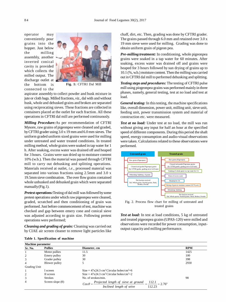
8 4 Journal of Food Legumes 30(2), 2017
operator mayconveniently pourgrains into thehopper. Just belowthe millingassembly, anotherinverted conicalcavity is providedwhich collects themilled output. Thedischarge outlet atthe bottom isconnected to theaspirator assembly to collect powder and husk mixture injute or cloth bags. Milled fractions, viz., dal with and withouthusk, whole and dehusked grains and broken are separatedusing reciprocating sieves. These fractions are collected incontainers placed at the outlet for each fraction. All theseoperations in CFTRI dal mill are performed continuously.Milling Procedure:As per recommendation of CFTRIMysore, raw grains of pigeonpea were cleaned and graded,by CFTRI grader using 3.0 x 19 mm and 6.0 mm sieves. Theuniform graded uniform sized grains were used for millingunder untreated and water treated conditions. In treatedmilling method, whole grains were soaked in tap water for 1h. After soaking, excess water was drained off and heapedfor 3 hours. Grains were sun dried up to moisture content10% (w.b.). Then the material was passed through CFTRImill to carry out dehusking and splitting operations.Materials received at outlet, i.e., processed material wasseparated into various fractions using 2.5mm and 3.0 x19.5mm sieve combination. The over flow grains containedwhole unhusked and dehusked grain which were separatedmanually (Fig.1).Pretest operations:Testing of dal mill was followed by somepretest operations under which raw pigeonpea were cleaned,graded, scratched and then conditioning of grain wasperformed. Just before commencement of test, machine waschecked and gap between emery cone and conical sievewas adjusted according to grain size. Following pretestoperations were performed;Cleaning and grading of grain: Cleaning was carried outby CIAE air screen cleaner to remove light particles like
chaff, dirt, etc. Then, grading was done by CFTRI grader.The grains passed through 6.0 mm and retained over 3.0 x19 mm sieve were used for milling. Grading was done toobtain uniform grain of pigeon pea.Pre-milling treatment: In conditioning, whole pigeonpeagrains were soaked in a tap water for 60 minutes. Aftersoaking, excess water was drained off and grains wereheaped for 3 hours followed by sun drying of grains up to10.1 (%, w.b.) moisture content. Then the milling was carriedout in CFTRI dal mill to performed dehusking and splitting.Testing steps and procedures: The testing of CFTRI pulsemill using piogeonpea grains was performed mainly in threephases, namely, general testing, test at no load and test atload.General testing: In this testing, the machine specificationslike, overall dimension, power unit, milling unit, sieve unit,feeding unit, power transmission system and material ofconstruction etc. were measured.Test at no load: Under test at no load, the mill was runwithout giving any input for half an hour at the specifiedspeed of different components. During this period the shaftspeed, energy consumption and audio-visual observationswere taken. Calculations related to these observations wereperformed.
Table 1. Specification of machine
Fig. 2. Process flow chart for milling of untreated andtreated grains
Untreated grain
Raw grains (Pigeonpea)
Cleaned and graded Pigeonpea grains (by CFTRI grader, grading sieve-3x19 mm)
Dehusking /Splitting of grains
Net fraction received Dal, Whole grains, Pearled grains, Husk,
Broken, Powder
Treated grain
Raw grains (Pigeonpea)
Cleaned and graded Pigeonpea grains (by CFTRI grader, grading sieve-3x19 mm)
Soaking of whole grain in a tap water for 1 h
Drain of excess water
Heaping for 3 h
Drying of grain to moisture content (10.7%,w.b.)
Dehusking/ Splitting
Net fraction received Dal, Whole grains, Pearled grains, Husk, Broken, Powder
Machine parameter Sr. No. Pullies Diameter, cm RPM 1 Motor pullies 11.5 1425 2 Emery pulley 30 100 3 Grader pulley 30 398 4 Blower pulley 5 2930 Grading Unit 1 I screen Size = 47x24.3 cm2 Circular holes/cm2=6 2 II screen Size = 47x24.3 cm2 Circular holes/cm2=2 3 Strokes No. of strokes/min. 98 4 Screen slope ()
76.223.1121.112
seiveoflengthInclinedgroundatsieveoflengthjectedProCos
Fig. 1: CFTRI Dal Mill
Test at load: In test at load conditions, 5 kg of untreatedand treated pigeonpea grains (UPAS-120) were milled andobservations were recorded for power consumption, input-output capacity and milling performance.
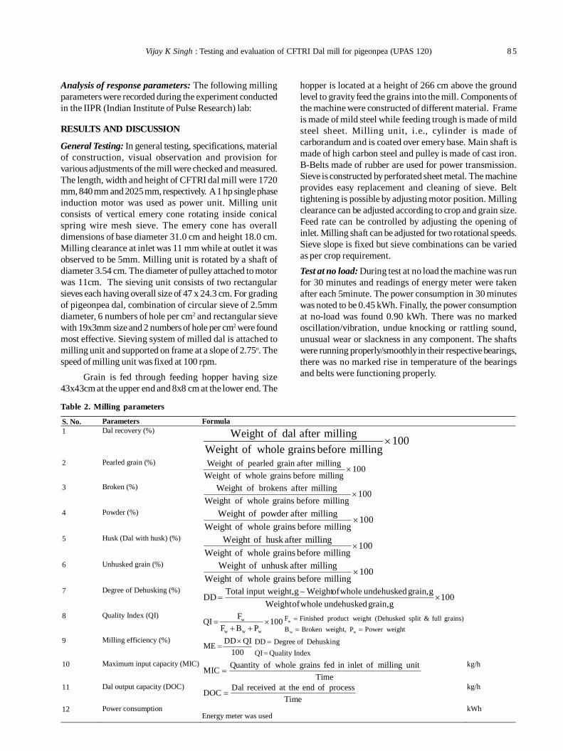
Vijay K Singh : Testing and evaluation of CFTRI Dal mill for pigeonpea (UPAS 120) 8 5
Analysis of response parameters: The following millingparameters were recorded during the experiment conductedin the IIPR (Indian Institute of Pulse Research) lab:
RESULTS AND DISCUSSION
General Testing: In general testing, specifications, materialof construction, visual observation and provision forvarious adjustments of the mill were checked and measured.The length, width and height of CFTRI dal mill were 1720mm, 840 mm and 2025 mm, respectively. A 1 hp single phaseinduction motor was used as power unit. Milling unitconsists of vertical emery cone rotating inside conicalspring wire mesh sieve. The emery cone has overalldimensions of base diameter 31.0 cm and height 18.0 cm.Milling clearance at inlet was 11 mm while at outlet it wasobserved to be 5mm. Milling unit is rotated by a shaft ofdiameter 3.54 cm. The diameter of pulley attached to motorwas 11cm. The sieving unit consists of two rectangularsieves each having overall size of 47 x 24.3 cm. For gradingof pigeonpea dal, combination of circular sieve of 2.5mmdiameter, 6 numbers of hole per cm2 and rectangular sievewith 19x3mm size and 2 numbers of hole per cm2 were foundmost effective. Sieving system of milled dal is attached tomilling unit and supported on frame at a slope of 2.75o. Thespeed of milling unit was fixed at 100 rpm.
Grain is fed through feeding hopper having size43x43cm at the upper end and 8x8 cm at the lower end. The
hopper is located at a height of 266 cm above the groundlevel to gravity feed the grains into the mill. Components ofthe machine were constructed of different material. Frameis made of mild steel while feeding trough is made of mildsteel sheet. Milling unit, i.e., cylinder is made ofcarborandum and is coated over emery base. Main shaft ismade of high carbon steel and pulley is made of cast iron.B-Belts made of rubber are used for power transmission.Sieve is constructed by perforated sheet metal. The machineprovides easy replacement and cleaning of sieve. Belttightening is possible by adjusting motor position. Millingclearance can be adjusted according to crop and grain size.Feed rate can be controlled by adjusting the opening ofinlet. Milling shaft can be adjusted for two rotational speeds.Sieve slope is fixed but sieve combinations can be variedas per crop requirement.Test at no load: During test at no load the machine was runfor 30 minutes and readings of energy meter were takenafter each 5minute. The power consumption in 30 minuteswas noted to be 0.45 kWh. Finally, the power consumptionat no-load was found 0.90 kWh. There was no markedoscillation/vibration, undue knocking or rattling sound,unusual wear or slackness in any component. The shaftswere running properly/smoothly in their respective bearings,there was no marked rise in temperature of the bearingsand belts were functioning properly.
Table 2. Milling parameters
S. No. Parameters Formula 1 Dal recovery (%)
100millingbeforegrainswholeofWeight
millingafterdalofWeight
2 Pearled grain (%) 100
millingbeforegrainswholeofWeightmillingaftergrainpearledofWeight
3 Broken (%) 100
millingbeforegrainswholeofWeightmillingafterbrokensofWeight
4 Powder (%) 100
millingbeforegrainswholeofWeightmillingafterpowderofWeight
5 Husk (Dal with husk) (%) 100
millingbeforegrainswholeofWeightmillingafterhuskofWeight
6 Unhusked grain (%) 100
millingbeforegrainswholeofWeightmillingafterunhuskofWeight
7 Degree of Dehusking (%) 100
ggrain,undehuskedwholeofWeightggrain,undehuskedwholeofWeightgweight,inputTotal
DD
8 Quality Index (QI) 100
PBFFQI
www
w
weightPowerPweight,BrokenB
grains)full&split(DehuskedweightproductFinishedF
ww
w
9 Milling efficiency (%)
100QIDDME
IndexQualityQI
DehuskingofDegreeDD
10 Maximum input capacity (MIC)
TimeunitmillingofinletinfedgrainswholeofQuantityMIC kg/h
11 Dal output capacity (DOC)
TimeprocessofendtheatreceivedDalDOC kg/h
12 Power consumption Energy meter was used
kWh
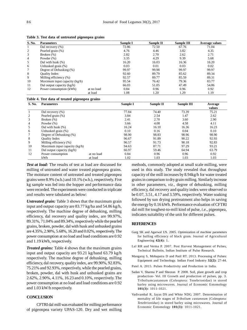
8 6 Journal of Food Legumes 30(2), 2017
Test at load: The results of test at load are discussed formilling of untreated and water treated pigeonpea grains.The moisture content of untreated and treated pigeonpeagrains were 8.9% (w.b.) and 10.1% (w.b.), respectively. Fivekg sample was fed into the hopper and performance datawere recorded. The experiments were conducted in triplicateand results were tabulated as below:Untreated grain: Table 3 shows that the maximum graininput and output capacity are 83.77 kg/ha and 54.86 kg/h,respectively. The machine degree of dehusking, millingefficiency, dal recovery and quality index, are 99.97%,89.31%, 71.04% and 89.34%, respectively while the pearledgrains, broken, powder, dal with husk and unhusked grainsare 4.35%, 2.90%, 5.68%, 16.20 and 0.02%, respectively. Thepower consumption at no load and load conditions are 0.92and 1.19 kWh, respectively.Treated grains: Table 4 shows that the maximum grainsinput and output capacity are 93.21 kg/hand 63.79 kg/hrespectively. The machine degree of dehusking, millingefficiency, dal recovery, quality index, are 99.90%, 92.83%,75.21% and 92.93%, respectively, while the pearled grains,broken, powder, dal with husk and unhusked grains are2.62%, 2.90%, 4.11%, 16.23 and 0.10%, respectively. Thepower consumption at no load and load conditions are 0.92and 1.03 kW/h respectively.
CONCLUSION
CFTRI dal mill was evaluated for milling performanceof pigeonpea variety UPAS-120. Dry and wet milling
methods, commonly adopted at small scale milling, wereused in this study. The study revealed that throughputcapacity of the mill increases by 8.94kg/h for water treatedgrains in comparison to dry grain milling. Similarly increasein other parameters, viz., degree of dehusking, millingefficiency, dal recovery and quality index were observed tobe 0.07, 3.51, 4.17 and 3.59%, respectively. Water soakingfollowed by sun drying pretreatment also helps in savingthe energy by 0.16 kWh. Performance evaluation of CFTRIdal mill for toughest-to-mill kind of pulse, i.e., pigeonpea,indicates suitability of the unit for different pulses.
REFERENCES
Garg SK and Agarwal US. 2005. Optimization of machine parametersfor hulling efficiency of black gram. Journal of AgriculturalEngineering 42(4): 1.
Lal RR and Verma P. 2007. Post Harvest Management of Pulses,Technical Bulletin, Indian Institute of Pulse Research.
Mangaraj S, Mohapatra D and Patil RT. 2013. Processing of Pulses:Equipment and Technology. Indian Food Industry 32(2): 27-44.
Patel A. 2015. Pulses Productivity and Production in India.
Sadan V, Sharma P and Sheoran P. 2008. Soil, plant growth and cropproduction- Vol. III Growth and production of pulses, pp. 3.Triboliumcastaneum (Coleoptera: Tenebrionidae) in storedbarley using microwaves. Journal of Economic Entomology101(3): 1011-1021.
Vadivambal R, Jayas DS and White NDG. 2007. Determination ofmortality of life stages of Tribolium castaneum (Coleoptera:Tenebrionidae) in stored barley using microwaves. Journal ofEconomic Entomology 101(3): 1011-1021.
Table 3. Test data of untreated pigeonpea grains
Table 4. Test data of treated pigeonpea grains
S. No. Parameters Sample I Sample II Sample III Average values 1 Dal recovery (%) 72.86 72.50 67.76 71.04 2 Pearled grain (%) 4.76 4.46 3.82 4.35 3 Broken (%) 2.82 2.70 2.62 2.71 4 Powder (%) 3.35 4.29 9.39 5.68 5 Dal with husk (%) 16.20 16.03 16.36 16.20 6 Unhusked grain (%) 0.03 0.01 0.03 0.02 7 Degree of Dehusking (%) 99.97 99.98 99.97 99.97 8 Quality Index 92.60 89.79 85.62 89.34 9 Milling efficiency (%) 92.57 89.77 85.59 89.31 10 Maximum input capacity (kg/h) 95.54 76.42 79.36 83.77 11 Dal output capacity (kg/h) 66.03 51.05 47.49 54.86 12 Power consumption (kWh) at no load 0.84 0.96 0.96 0.92
at load 1.08 1.20 1.29 1.19
S. No. Parameters Sample I Sample II Sample III Average
values 1 Dal recovery (%) 77.84 74.40 73.39 75.21 2 Pearled grain (%) 3.84 2.54 1.47 2.62 3 Broken (%) 2.41 2.70 3.60 2.90 4 Powder (%) 3.66 4.08 4.58 4.11 5 Dal with husk (%) 16.24 16.10 16.36 16.23 6 Unhusked grain (%) 0.10 0.16 0.04 0.10 7 Degree of Dehusking (%) 98.90 98.83 98.96 98.90 8 Quality Index 96.67 91.89 90.22 92.93 9 Milling efficiency (%) 96.57 91.73 90.18 92.83 10 Maximum input capacity (kg/h) 94.63 87.71 97.29 93.21 11 Dal output capacity (kg/h) 66.97 59.46 64.94 63.79 12 Power consumption
kWh at no load 0.84 0.96 0.96 0.92 at load 1.02 1.03 1.03 1.03
Journal of Food Legumes 30(2): 87-90, 2017
Transfer of technology implemented by IIPR in Bundelkhand region: An impactanalysisRAJESH KUMAR, SHRIPAD BHAT, PK KATIYAR AND DEEPAK SINGH
ICAR-Indian Institute of Pulses Research, Kanpur-208024, Uttar Pradesh, India; E-mail: [email protected](Received: June 16, 2016; Accepted: January 7, 2017)
ABSTRACT
Bundelkhand region is a major pulse producing belt of UttarPradesh. TAR-IVLP project was implemented in Hamirpurdistrict to create awareness and to provide critical inputs forenhancing the production of pulses and cereal crops during2000 to 2005. To assess the impact of this project, data werecollected from 50 farmers each from adopted village(Vidokhar village, Bharuwa Sumerpur Block) and non-adopted villages viz., Artara, Patanpur and Pipraunda(Maudaha Block) using interview, observation and discussionmethods. Major crops grown were in the study area werelentil, field pea, linseed, wheat, mustard, urdbean, mungbeanand pigeonpea. Results indicated that farmers in adoptedvillages under the IVLP project were benefited. Majority offarmers (60%) procured quality seed from the IIPR, NSC,and Bij Nigam. The non-adopted farmers were gettingapproximately 25-30% lesser yield than the adopted farmers.The average annual income was ø 1,42,198 in case of adoptedfarmers, while it was Rs. 77,850 in case of non-adoptedfarmers which was statistically significant which indicatesthe improved economic condition of adopted farmers.However, there is a need to improve the irrigationinfrastructures in Bundelkhand region along with emphasison weed management and improved weather forecastingservices for providing weather information in time to protectthe crops from adverse weather conditions.
Key words: Impact analysis, IVLP, Transfer of technology
Uttar Pradesh is one of the leading states in pulseproduction. Pulses are grown in an area of 2.35 millionhectares, producing 1.44 million tonnes with a productivitylevel of 612 Kg/ha in Uttar Pradesh (2014-15). Bundelkhandregion is a major pulse producing belt of Uttar Pradesh.During 2000 to 2005, TAR-IVLP project was implemented inHamirpur district of this region to create awareness and toprovide critical inputs for enhancing the production ofpulses and cereal crops. Different interventions related tocereal and pulses crops were introduced with specialemphasis of seed production of pulses. Varioustechnologies were transferred under this project by usingdifferent approaches and methodologies. Participatoryapproach was used to identify the problems and toimplement the programme. The interventions implementedwere need based and location specific. Keeping in view,this study was undertaken to estimate the technologicalimpact of this project along with identification of reasonsfor continuing the technologies introduced under thisproject.
MATERIALS AND METHODS
The present study was undertaken in Hamirpurdistrict of Uttar Pradesh during the year 2015-16 where TAR-Institution Village Linkage Programme was implemented.Two blocks, one as adopted block Bharuwa Sumerpur underIVLP project and another block Maudaha as non- adoptedwere selected for the study.Table 1. Sample villages in Hamirpur District of Uttar
Pradesh Adopted Non-adopted
Block Bharuwa Sumerpur Maudaha Villages Vidokhar Artara, Patanpur and
Pipraunda Sample Farmers 50 50
Data were collected from villages viz., Vidokhar fromSumerpur Block, Artara, Patanpur and Pipraunda fromMaudaha Block by using interview, observation anddiscussion methods from a total of 100 farmers. Data werecollected to estimate the impact of this project on farmer’sincome in both adopted villages and non-adopted villages.The ex-post facto research design and purposive randomsampling was used for selection of farmers. Data weretabulated and analysed by using statistical techniques offrequency, percentage, t test and students test for logicalconclusion.
Two-sample t-test analysis was carried out to findout is there any significant differences in the mean incomeof the adopted and non-adopted farmers. The t statistic iscalculated using the following equation (1).
21p
21
n1
n1 *s
X– X t
…………. (1)
Where 1X is the mean income of adopted farmers
2X is the mean income of non-adopted farmers
n1 = n2 = 50sp is the estimator of the pooled standard deviation
RESULTS AND DISCUSSION
Socio economic profile of adopted and non-adoptedfarmers under IVLP project: It is evident from the table 2
8 8 Journal of Food Legumes 30(2), 2017
that 72% of the farmers in adopted villages and 54% of thefarmers in non-adopted villages belonged to old category.This also indicated that young and middle aged groups aremoving away from farming in both adopted and non-adopted villages. It can be noticed that 82% of the farmersin adopted villages and 58% of the farmers in non-adoptedvillages were having a land holding of five acres or more.Tube well and canal were the major source of irrigation inboth adopted and non-adopted areas
It is indicate that food habit and sources of proteinof the sample farmers. It can be observed that around 88%of the farmers in adopted area and 68% of the farmers innon-adopted area were vegetarians. Pulses were the majorsource of protein in both these areas followed by egg (42%)and meat (18%) (Table 3).
It is indicate that consumption pattern of pulses in
the study area. This can be observed that the pigeonpea isused majorly as dal and no other products were preparedout of pigeonpea for consumption. In case of chickpea,many products such as dal, sattu, pakaura, besan wereprepared from it in both adopted and non-adopted area.Dal and namkeen were prepared from lentil as well (Table 4).Impact analysis of IVLP project: It is observed that 70%farmers have pulse based farming system in IVLP adoptedvillages followed by cereal based farming system (30%)whereas in non-adopted village 80% of farmers have pulsebased farming system followed by cereal based farmingsystem (20%) (Table 5).Changes occurred in cropping system afterimplementation of IVLP project: After implementation ofIVLP project, in case of adopted villages around 36% offarmers started crop rotation to maintain the productivity
Table 2. Socio economic profile of adopted and non-adopted farmers under IVLP project
Table 3. Food habit and sources of protein of farmers
Table 4. Consumption pattern of different pulses
Particulars S. No. Variables Adopted village Non-adopted villages Frequency Percentage Frequency Percentage
Age 1 Young (up to 30) 6 12.00 02 04.00 2 Middle (31-49) 8 64.00 21 42.00 3 Old (50 & above) 36 72.00 27 54.00
Land holding size (acre)
1 Small (2) 1 2.00 11 22.00 2 Medium (3-5) 8 16.00 10 20.00 3 Large (5 & above) 41 82.00 29 58.00
Ownership of land 1 Owned 50 100.00 50 100.00 2 Leased in 00 0.00 3 6.00 3 Leased out 00 0.00 0 0.00
Source of irrigation 1 Tube well 50 100.00 32 64 2 Canal 16 32 .00 30 60
Particulars S. No. Variables Adopted village Non-adopted villages
Frequency Percentage Frequency Percentage
Food habit 1 Vegetarian 44 88.00 34 68.00 2 Non-vegetarian 6 12.00 16 32.00
Protein sources 1 Pulses 43 86.00 32 64.00 2 Egg 21 42.00 27 54.00 3 Meat 9 18.00 24 48.00
S.No. Variables Products
Adopted Non-adopted
Frequency Percentage Frequency Percentage
1 Pigeon pea Dal 50 100.00 50 100.00 Any other product 0 0.00 0 0.00
2 Chickpea
Dal 11 22.00 16 32.00 Sattu 20 40.00 25 50.00 Pakaura 34 68.00 15 30.00 Besan 50 100.00 40 80.00 Fried 20 40.00 05 10.00 Boiled 12 24.00 10 20.00
3. Lentil Dal 50 100.00 50 100.00 Namkeen 6 12.00 7 14.00
4. Field pea Dal 12 24.00 15 30.00 Boiled 8 16.00 14 28.00
5 Mungbean Dal 50 100.00 50 100.00 Badi 0 0.00 12 24.00
6. Urdbean Dal 50 100.00 50 100.00 Haluwa 0 0.00 7 14.00
Kumar et al. : Transfer of Technology project (IVLP) implemented by IIPR in Bundelkhand region- An Impact analysis 8 9
Table 5. Changes occurred in farming system after implementation of IVLP project
Table 6. Changes occurred in cropping system after implementation of IVLP project
Table 7. Source of seed in adopted and non-adopted villages
S. No. Variables Adopted village Non-adopted villages Frequency Percentage Frequency Percentage
1 Pulses based 35 70.00 40 80.00 2 Cereals based 15 30.00 10 20.00 3 Animal based 0 0.00 0 0.00
S. No. Variables Adopted village Non-adopted villages
Frequency Percentage Frequency Percentage 1 Crop rotation 18 36.00 10 20.00 2 Mixed cropping 12 24.00 10 20.00 3 Monocropping 5 10.00 12 24.00 4 Intercropping 15 30.00 18 36.00
S. No. Variables Adopted village Non-adopted villages
Frequency Percentage Frequency Percentage 1 CSAUA&T 3 6.00 0 0.00 2 IIPR 33 66.00 0 0.00 3 Agril. department 2 4.00 0 0.00 4 Private agencies 7 14.00 2 4.00 5 Own seed 5 10.00 44 88.00 6 Relatives 0 0.00 4 8.00
of soil while 10 per cent of the farmers were followingmonocropping. In non-adopted villages, 24 % of the farmerswere practising the traditional monocropping system whileonly 20 % of the farmers were following crop rotation.Source of seed: Majority of farmers (66%) purchased seedfrom the IIPR in adopted village whereas in non-adoptedvillages, majority of the farmers (88%) used their own seed.There is a need to create awareness among of non-adoptedvillage farmers regarding use of quality seed from the reliablesources for enhancing productivity (Table 7).Shift in crops grown by farmers after implementation ofIVLP project: Crops grown during 2000-2005 and the cropsgrown at present in adopted and non-adopted villages.Around 80% of the farmers were growing chickpea during2000-2005, however, at present, only 10 % of the farmers inadopted area and 20% of the farmers in non-adopted areacultivate chickpea majorly due to non-remunerative prices.After completion of IVLP project, lentil became mostpreferred pulse crop by all the farmers because of higherprice followed by fieldpea and urdbean.Working hours, women’s participation and workloadduring cropping season: Majority of farmers worked forabout 10 hours in adopted village (50%) and for about 12hours in non-adopted villages (60%). Women’sparticipation in pulse production was low in adopted invillages and medium in case of non-adopted villages. Mostof the farmers opined that workload after implementationof IVLP project (Table 9).Reasons for continuing the technology introduced underthe IVLP project: It is evident from the table 10 that higherprofitability, timely availability of seed and other inputs,
collaboration with other agencies like NSC, Beej Nigam,guidance and linkages with IIPR were the major reasons forcontinuing the technology introduced under the IVLPproject.
Results of the Two-Sample t-Test analysis assumingequal variance indicated that there was a significantdifference in the mean incomes across adopted and non-adopted farmers (Table 11). For adopted farmers, the meanannual income was Rs. 1,42,198 while it as Rs. 77,850 fornon-adopted farmers. As indicated by the significant tstatistic, the mean annual income of adopted farmers wassignificantly higher than that of non-adopted farmers. Thisshowed that there was an improvement in the economiccondition of the farmers because of implementation of IVLPproject.
Annual income across adopted and non-adoptedfarmers have been depicted in the form of box plots (Fig. 1).Graph depicts higher income in case of adopted farmerswhen compared to non-adopted farmers.
CONCLUSION
Results have indicated that IVLP project has playedan important role in enhancing the production of pulsesand cereals by introducing of improved technologies.Project also improved the net income of farmerssignificantly thereby enhancing the economic condition ofadopted farmers. Farmers are now self-sufficient in qualityseeds of pulses and wheat. There is a need to improve theirrigation infrastructures in Bundelkhand region along withemphasis on weed management and improved weatherforecasting services for providing weather information intime to protect the crops from adverse weather conditions.
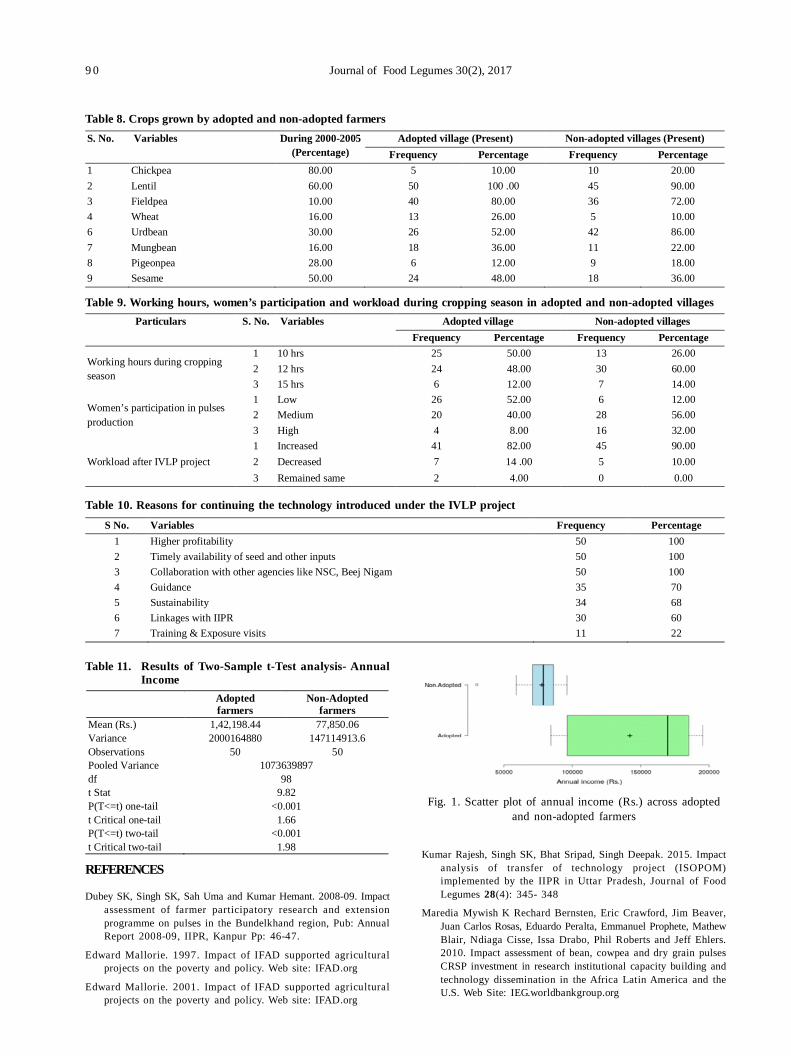
9 0 Journal of Food Legumes 30(2), 2017
Table 8. Crops grown by adopted and non-adopted farmers
Table 9. Working hours, women’s participation and workload during cropping season in adopted and non-adopted villages
Table 10. Reasons for continuing the technology introduced under the IVLP project
Table 11. Results of Two-Sample t-Test analysis- AnnualIncome
Adopted farmers
Non-Adopted farmers
Mean (Rs.) 1,42,198.44 77,850.06 Variance 2000164880 147114913.6 Observations 50 50 Pooled Variance 1073639897 df 98 t Stat 9.82 P(T<=t) one-tail <0.001 t Critical one-tail 1.66 P(T<=t) two-tail <0.001 t Critical two-tail 1.98
Fig. 1. Scatter plot of annual income (Rs.) across adoptedand non-adopted farmers
S. No. Variables During 2000-2005 (Percentage)
Adopted village (Present) Non-adopted villages (Present) Frequency Percentage Frequency Percentage
1 Chickpea 80.00 5 10.00 10 20.00 2 Lentil 60.00 50 100 .00 45 90.00 3 Fieldpea 10.00 40 80.00 36 72.00 4 Wheat 16.00 13 26.00 5 10.00 6 Urdbean 30.00 26 52.00 42 86.00 7 Mungbean 16.00 18 36.00 11 22.00 8 Pigeonpea 28.00 6 12.00 9 18.00 9 Sesame 50.00 24 48.00 18 36.00
Particulars S. No. Variables Adopted village Non-adopted villages Frequency Percentage Frequency Percentage
Working hours during cropping season
1 10 hrs 25 50.00 13 26.00 2 12 hrs 24 48.00 30 60.00 3 15 hrs 6 12.00 7 14.00
Women’s participation in pulses production
1 Low 26 52.00 6 12.00 2 Medium 20 40.00 28 56.00 3 High 4 8.00 16 32.00
Workload after IVLP project 1 Increased 41 82.00 45 90.00 2 Decreased 7 14 .00 5 10.00 3 Remained same 2 4.00 0 0.00
S No. Variables Frequency Percentage 1 Higher profitability 50 100 2 Timely availability of seed and other inputs 50 100 3 Collaboration with other agencies like NSC, Beej Nigam 50 100 4 Guidance 35 70 5 Sustainability 34 68 6 Linkages with IIPR 30 60 7 Training & Exposure visits 11 22
REFERENCES
Dubey SK, Singh SK, Sah Uma and Kumar Hemant. 2008-09. Impactassessment of farmer participatory research and extensionprogramme on pulses in the Bundelkhand region, Pub: AnnualReport 2008-09, IIPR, Kanpur Pp: 46-47.
Edward Mallorie. 1997. Impact of IFAD supported agriculturalprojects on the poverty and policy. Web site: IFAD.org
Edward Mallorie. 2001. Impact of IFAD supported agriculturalprojects on the poverty and policy. Web site: IFAD.org
Kumar Rajesh, Singh SK, Bhat Sripad, Singh Deepak. 2015. Impactanalysis of transfer of technology project (ISOPOM)implemented by the IIPR in Uttar Pradesh, Journal of FoodLegumes 28(4): 345- 348
Maredia Mywish K Rechard Bernsten, Eric Crawford, Jim Beaver,Juan Carlos Rosas, Eduardo Peralta, Emmanuel Prophete, MathewBlair, Ndiaga Cisse, Issa Drabo, Phil Roberts and Jeff Ehlers.2010. Impact assessment of bean, cowpea and dry grain pulsesCRSP investment in research institutional capacity building andtechnology dissemination in the Africa Latin America and theU.S. Web Site: IEG.worldbankgroup.org
Journal of Food Legumes 30(2): 91-95, 2017
ABSTRACT
In a study conducted among organic and conventionalpigeonpea growers of Gulberga district of Karnataka, anattempt was made to assess the resource use efficiency ofpigeonpea cultivation in three pigeonpea based croppingsystems. The results revealed that human labour, land, seeds,plant protection measures have contributed significantly tothe production elasticities. The co-efficients of multipledetermination for all three production functions fitted rangedbetween 0.96 and 0.98 indicating that the production functionfitted was sound and could help explain the variation ingross returns in pigeonpea based cropping systems. Thereturns to scale in all the pigeonpea based cropping systemswere superior in organic farming compared to conventionalfarming.
Key words: Black Gram, Cobb Douglas Production Function,Green Gram, Organic farming, Pigeon pea,Resource utilization efficiency
India is an agricultural country. In a country wheresizable proportion of the population is dependent onagriculture, the development of agricultural sector becomesa prerequisite. The agriculture sector has a direct impact onthe level of farm income as well as national income of thecountry. If farmers can increase their production, they shallimprove the national economy as well as their owneconomy. Therefore, it has become an urgent need toincrease agricultural production.
There are two feasible options available for increasingthe agricultural production in a country. The first option is:through extension of area under cultivation by reclamationof wastelands and by external land augmentation withoutshrinking of the area and productivity of any activity. Thesecond one is: increasing the productivity of land bycultivating normal soils through optimal allocation ofavailable resources and utilizing the full potential of existingtechnology. The adoption of new agricultural technologyis necessary for the development of agricultural sector,which depends on the availability of various inputs andresources in the region.
The agricultural growth is affected by the variousresources such as seeds, manures, fertilizers, irrigationfacilities, labour, bullock labour, working capital, farmimplements, machinery, crop protection inputs, etc. Therationality in the allocation of resources by the farmers is a
Resource utilization efficiency of organic farming vis-à-vis conventional farmingin indian food legumesMAHESH MALGATTI1, SUNIL KUMAR1, RAHUL SINGH1, D. UMA MAHESWARA RAO1 andPURUSHOTTAM2
1ICAR-Indian Agricultural Research Institute, New Delhi,2ICAR-Indian Institute of Pulse Research, Kanpur;E-mail: [email protected](Received: December 22, 2016; Accepted: March 16, 2017)
crucial issue in agricultural production. Here the focus needto be on the resource use efficiency. The farm income isdetermined by the efficiency with which all farmers are ableto utilize the resources at their own command. If farmers areefficient in the use of scarce resources, then farmers cansurely increase agricultural production and their income.
The optimum allocation of available resources isnecessary for the growth of agricultural production. Thecrux of the problem of increasing agricultural production inany area is: how to increase the output per unit of an input.In general, agricultural production continues to be at lowerlevel despite the use of critical inputs. Sometimes, the crucialinputs are either under-utilized or over-utilized in the cropproduction. Resource use inefficiency exists on the farms.If resource use is inefficient, production can be increasedby making adjustment in the use of factors of production inthe optimal direction.
The cost of agricultural resources is increasing byquantum jumps, thereby making agriculture a losingproposition. Increasing costs of cultivation has madeagriculture vulnerable and exposed to greater risks, thusmaking it an unviable option of one’s livelihood. Efficientresource use is the only option available now. Hence, it isnecessary that the available resources should be usedeconomically and efficiently.
To drive home this crucial issue, many researchershave worked on assessing the resource use efficiency invarious crops: paddy (Suresh and Reddy 2006), onion(Sankhayan and Sirohi 1971, Naik et al. 1998, Verma 2002),mesta (Sunanda and Narender 2003), redgram basedcropping systems (Biradar and Rajkumar 2007) and croppingsystems and farming systems (Ganesh 2000, Wadear 2003,Rajeshwari 2004, Saikumar 2005). Mixed cropping systems:potato and maize (Sankhayan and Sirohi 1971), maize-sunflower (Nagraj et al. 1996).
Resource use efficiency was measured in terms ofpartial ‘b’ coefficients contributing to the significantvariation in production function. The contribution of landand human labour was positive (Muralidharan 1987) andthat of land and farm yard manure was positive (Naik et al.1998). The ratio of Marginal value product (MVP) toMarginal factor cost (MFC) of land was greater than one,and MVP of labour was less than one. It was negative forseeds, fertilizers and pesticides in conventional farms. In
9 2 Journal of Food Legumes 30(2), 2017
case of farm practicing IPM, this ratio was greater than onefor land, labour, and seeds, but negative for fertilizers.(Vishweshwar 1994).
Hence, it has been attempted in this study to assessand compare resource use efficiency of organic andconventional farming in three pigeonpea based croppingsystems, with an objective of comparing organic farmingand conventional farming in pigeonpea based croppingsystems.
MATERIALS AND METHODS
Gulberga district is considered the pulse bowl ofIndia. Pigeonpea is predominantly grown in Aland andGulbarga taluks. So, district and taluks were purposivelyselected and two villages from each taluk were randomlyselected for the study. Accordingly the study wasconducted in the four villages of Gulbarga district inKarnataka state and survey approach was used for thepresent study. Sixty farmers who were actively involved inorganic farming and sixty conventional farmers formed arandom sample of one hundred and twenty respondents.The data were collected through personal interviews fromboth organic and conventional farmers with the help of aspecially designed semi-structured schedule.
Data on resource use were collected from fortyfarmers (20 organic farmers and 20 conventional farmers)form each group of cropping system: (i) sole crop ofpigeonpea, (ii) intercropping of pigeonpea with black gramand (iii) intercropping of pigeonpea with green gram. Aspecially designed semi-structured schedule was used.
Cobb-Douglas production function is used toestimate resource use efficiency and returns to scale inpigeonpea and pigeonpea based cropping system. Theresource factors like land, human labour, manures andfertilizers, seeds and plant protection measures were usedin both organic and conventional farming and hence theyare considered in the present study. The operationaldefinition of resource factors chosen in the study are asfollows:Output: The output has been defined as the sum of grossvalue output of the crops (pigeonpea, black gram and greengram) evaluated at the prevailing market price during theyear 2010-11, irrespective of being consumed, sold ormaintained in the stock.Land: In the present study, the actual area for the particularcrop (pigeonpea, black gram and green gram) wasconsidered as the land resource. The land was taken inhectares.Human Labour: The labour force on a farm consists offarmer’s labour and hired labour.Family Labour: Family labour is one of the most importantfactors in the growth of economic factor. Family labourconsidered with the actual work carried out by family
members for crop production was evaluated at the prevailingwage rates for hired labour.Hired Labour: It included the hired labour employed forcrop production. The hired labour was evaluated at actualamount paid in cash. Human labour was also divided intomale and female labour with varying wage rates. The workturn out of a male or female adult for a period of 8 hours istaken in to consideration.Manures and Fertilizers: Manures made from the wastesof plant materials and animals are used as sources of plantnutrients. Farm produced manures (farm yard manure, vermi-compost) were charged at prevailing local rates. Chemicalfertilizers and other manures purchased were charged atthe rates actually paid.Seeds: For the production own seeds or market seeds havebeen used in the farm. The farm produced seed was chargedat the market price and purchased seed was charged at therates actually paid.Plant protection measures: Labour costs incurred inmechanical measures and cultural measures were computed.The purchased pesticides for the use of plant protectionwere evaluated at the actual price paid in market and thevalue of bio-pesticides/insecticides produced in bio-digesters on the farm were evaluated as per costs incurredin making them.
Cobb-Douglas Function
The functional model adopted is of the followingform,
y = a. x1b1. x2
b2. x3b3. x4
b4. x5b5. u
y = Value of output (in rupees)x1 = Land area (in hectares)x2 = Value of human labour used (in rupees)x3 = Value of Manures and Fertilizers (in rupees.)x4= Value of seeds (in rupees)x5= Value of Plant Protection (in rupees)u = Error termb1 to b5 are production elasticities of factors x1 to x5
respectively and ‘a’ is the intercept. The above equationcan be transformed into log form as follows:
Log y = Log a + b1Log x1+ b2Log x2+ b3Log x3+ b4Logx4+ b5Log x5+Log u
In the present study, the above function was fitted inlog term with output (y) as dependent variable and fiveinputs as independent variables.
RESULTS AND DISCUSSION
The collected data was subjected to statistical dataanalysis using the Cobb Douglas production function. Theresults of the analysis: coefficients of production elasticities
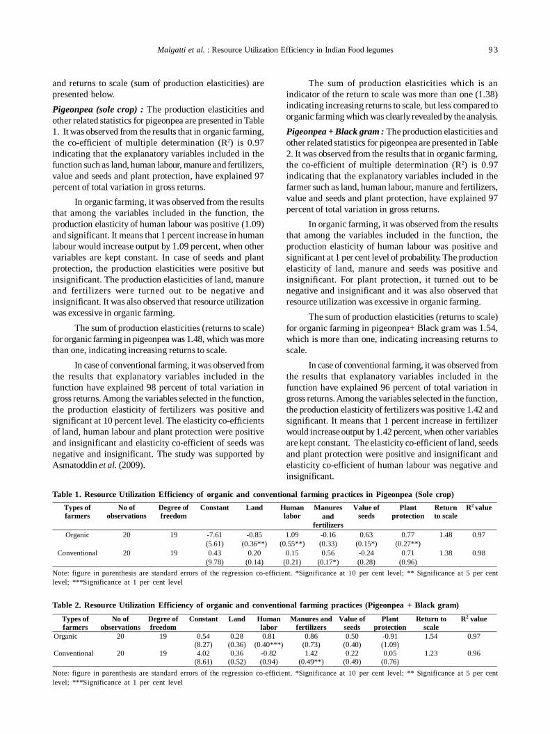
Malgatti et al. : Resource Utilization Efficiency in Indian Food legumes 9 3
and returns to scale (sum of production elasticities) arepresented below.Pigeonpea (sole crop) : The production elasticities andother related statistics for pigeonpea are presented in Table1. It was observed from the results that in organic farming,the co-efficient of multiple determination (R2) is 0.97indicating that the explanatory variables included in thefunction such as land, human labour, manure and fertilizers,value and seeds and plant protection, have explained 97percent of total variation in gross returns.
In organic farming, it was observed from the resultsthat among the variables included in the function, theproduction elasticity of human labour was positive (1.09)and significant. It means that 1 percent increase in humanlabour would increase output by 1.09 percent, when othervariables are kept constant. In case of seeds and plantprotection, the production elasticities were positive butinsignificant. The production elasticities of land, manureand fertilizers were turned out to be negative andinsignificant. It was also observed that resource utilizationwas excessive in organic farming.
The sum of production elasticities (returns to scale)for organic farming in pigeonpea was 1.48, which was morethan one, indicating increasing returns to scale.
In case of conventional farming, it was observed fromthe results that explanatory variables included in thefunction have explained 98 percent of total variation ingross returns. Among the variables selected in the function,the production elasticity of fertilizers was positive andsignificant at 10 percent level. The elasticity co-efficientsof land, human labour and plant protection were positiveand insignificant and elasticity co-efficient of seeds wasnegative and insignificant. The study was supported byAsmatoddin et al. (2009).
The sum of production elasticities which is anindicator of the return to scale was more than one (1.38)indicating increasing returns to scale, but less compared toorganic farming which was clearly revealed by the analysis.Pigeonpea + Black gram : The production elasticities andother related statistics for pigeonpea are presented in Table2. It was observed from the results that in organic farming,the co-efficient of multiple determination (R2) is 0.97indicating that the explanatory variables included in thefarmer such as land, human labour, manure and fertilizers,value and seeds and plant protection, have explained 97percent of total variation in gross returns.
In organic farming, it was observed from the resultsthat among the variables included in the function, theproduction elasticity of human labour was positive andsignificant at 1 per cent level of probability. The productionelasticity of land, manure and seeds was positive andinsignificant. For plant protection, it turned out to benegative and insignificant and it was also observed thatresource utilization was excessive in organic farming.
The sum of production elasticities (returns to scale)for organic farming in pigeonpea+ Black gram was 1.54,which is more than one, indicating increasing returns toscale.
In case of conventional farming, it was observed fromthe results that explanatory variables included in thefunction have explained 96 percent of total variation ingross returns. Among the variables selected in the function,the production elasticity of fertilizers was positive 1.42 andsignificant. It means that 1 percent increase in fertilizerwould increase output by 1.42 percent, when other variablesare kept constant. The elasticity co-efficient of land, seedsand plant protection were positive and insignificant andelasticity co-efficient of human labour was negative andinsignificant.
Table 1. Resource Utilization Efficiency of organic and conventional farming practices in Pigeonpea (Sole crop)
Note: figure in parenthesis are standard errors of the regression co-efficient. *Significance at 10 per cent level; ** Significance at 5 per centlevel; ***Significance at 1 per cent level
Table 2. Resource Utilization Efficiency of organic and conventional farming practices (Pigeonpea + Black gram)
Note: figure in parenthesis are standard errors of the regression co-efficient. *Significance at 10 per cent level; ** Significance at 5 per centlevel; ***Significance at 1 per cent level
Types of farmers
No of observations
Degree of freedom
Constant Land Human labor
Manures and
fertilizers
Value of seeds
Plant protection
Return to scale
R2 value
Organic 20 19 -7.61 (5.61)
-0.85 (0.36**)
1.09 (0.55**)
-0.16 (0.33)
0.63 (0.15*)
0.77 (0.27**)
1.48 0.97
Conventional 20 19 0.43 (9.78)
0.20 (0.14)
0.15 (0.21)
0.56 (0.17*)
-0.24 (0.28)
0.71 (0.96)
1.38 0.98
Types of farmers
No of observations
Degree of freedom
Constant Land Human labor
Manures and fertilizers
Value of seeds
Plant protection
Return to scale
R2 value
Organic 20 19 0.54 (8.27)
0.28 (0.36)
0.81 (0.40***)
0.86 (0.73)
0.50 (0.40)
-0.91 (1.09)
1.54 0.97
Conventional 20 19 4.02 (8.61)
0.36 (0.52)
-0.82 (0.94)
1.42 (0.49**)
0.22 (0.49)
0.05 (0.76)
1.23 0.96
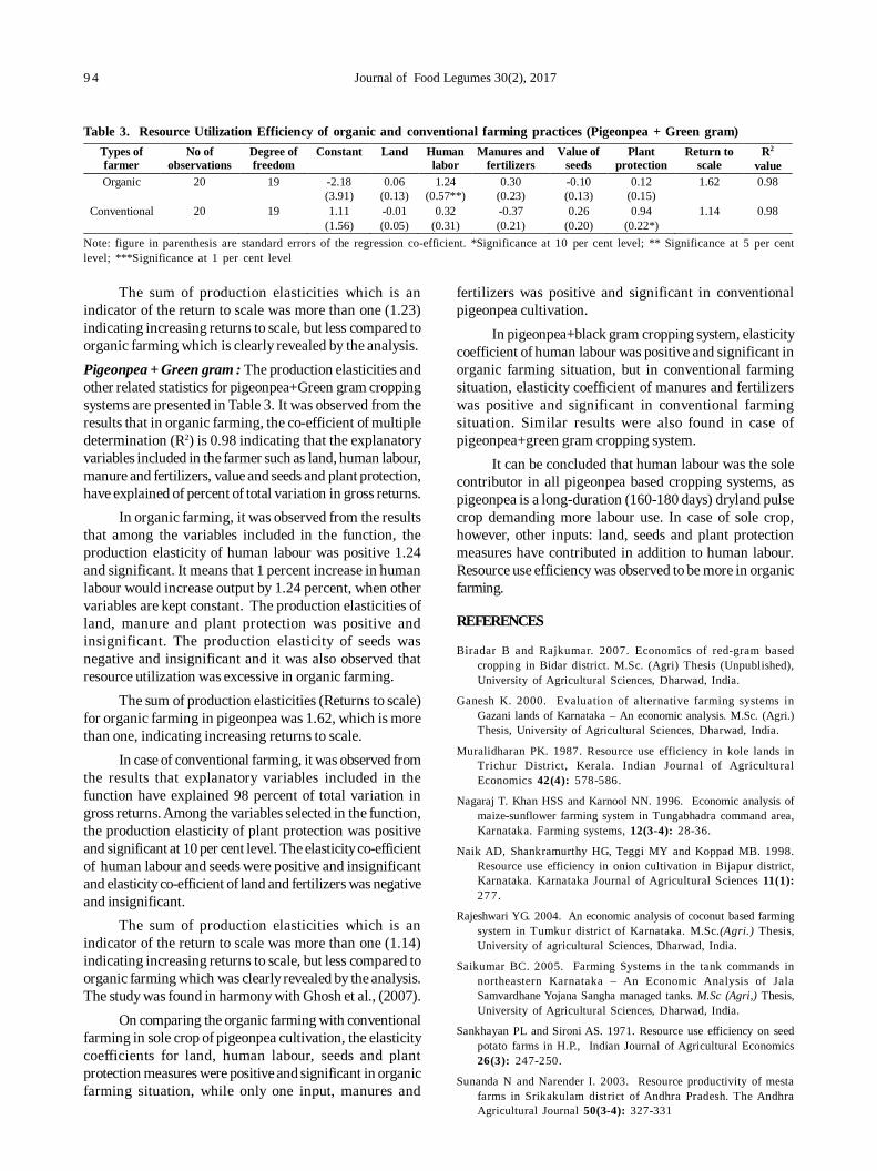
9 4 Journal of Food Legumes 30(2), 2017
The sum of production elasticities which is anindicator of the return to scale was more than one (1.23)indicating increasing returns to scale, but less compared toorganic farming which is clearly revealed by the analysis.Pigeonpea + Green gram : The production elasticities andother related statistics for pigeonpea+Green gram croppingsystems are presented in Table 3. It was observed from theresults that in organic farming, the co-efficient of multipledetermination (R2) is 0.98 indicating that the explanatoryvariables included in the farmer such as land, human labour,manure and fertilizers, value and seeds and plant protection,have explained of percent of total variation in gross returns.
In organic farming, it was observed from the resultsthat among the variables included in the function, theproduction elasticity of human labour was positive 1.24and significant. It means that 1 percent increase in humanlabour would increase output by 1.24 percent, when othervariables are kept constant. The production elasticities ofland, manure and plant protection was positive andinsignificant. The production elasticity of seeds wasnegative and insignificant and it was also observed thatresource utilization was excessive in organic farming.
The sum of production elasticities (Returns to scale)for organic farming in pigeonpea was 1.62, which is morethan one, indicating increasing returns to scale.
In case of conventional farming, it was observed fromthe results that explanatory variables included in thefunction have explained 98 percent of total variation ingross returns. Among the variables selected in the function,the production elasticity of plant protection was positiveand significant at 10 per cent level. The elasticity co-efficientof human labour and seeds were positive and insignificantand elasticity co-efficient of land and fertilizers was negativeand insignificant.
The sum of production elasticities which is anindicator of the return to scale was more than one (1.14)indicating increasing returns to scale, but less compared toorganic farming which was clearly revealed by the analysis.The study was found in harmony with Ghosh et al., (2007).
On comparing the organic farming with conventionalfarming in sole crop of pigeonpea cultivation, the elasticitycoefficients for land, human labour, seeds and plantprotection measures were positive and significant in organicfarming situation, while only one input, manures and
fertilizers was positive and significant in conventionalpigeonpea cultivation.
In pigeonpea+black gram cropping system, elasticitycoefficient of human labour was positive and significant inorganic farming situation, but in conventional farmingsituation, elasticity coefficient of manures and fertilizerswas positive and significant in conventional farmingsituation. Similar results were also found in case ofpigeonpea+green gram cropping system.
It can be concluded that human labour was the solecontributor in all pigeonpea based cropping systems, aspigeonpea is a long-duration (160-180 days) dryland pulsecrop demanding more labour use. In case of sole crop,however, other inputs: land, seeds and plant protectionmeasures have contributed in addition to human labour.Resource use efficiency was observed to be more in organicfarming.
REFERENCES
Biradar B and Rajkumar. 2007. Economics of red-gram basedcropping in Bidar district. M.Sc. (Agri) Thesis (Unpublished),University of Agricultural Sciences, Dharwad, India.
Ganesh K. 2000. Evaluation of alternative farming systems inGazani lands of Karnataka – An economic analysis. M.Sc. (Agri.)Thesis, University of Agricultural Sciences, Dharwad, India.
Muralidharan PK. 1987. Resource use efficiency in kole lands inTrichur District, Kerala. Indian Journal of AgriculturalEconomics 42(4): 578-586.
Nagaraj T. Khan HSS and Karnool NN. 1996. Economic analysis ofmaize-sunflower farming system in Tungabhadra command area,Karnataka. Farming systems, 12(3-4): 28-36.
Naik AD, Shankramurthy HG, Teggi MY and Koppad MB. 1998.Resource use efficiency in onion cultivation in Bijapur district,Karnataka. Karnataka Journal of Agricultural Sciences 11(1):277.
Rajeshwari YG. 2004. An economic analysis of coconut based farmingsystem in Tumkur district of Karnataka. M.Sc.(Agri.) Thesis,University of agricultural Sciences, Dharwad, India.
Saikumar BC. 2005. Farming Systems in the tank commands innortheastern Karnataka – An Economic Analysis of JalaSamvardhane Yojana Sangha managed tanks. M.Sc (Agri,) Thesis,University of Agricultural Sciences, Dharwad, India.
Sankhayan PL and Sironi AS. 1971. Resource use efficiency on seedpotato farms in H.P., Indian Journal of Agricultural Economics26(3): 247-250.
Sunanda N and Narender I. 2003. Resource productivity of mestafarms in Srikakulam district of Andhra Pradesh. The AndhraAgricultural Journal 50(3-4): 327-331
Table 3. Resource Utilization Efficiency of organic and conventional farming practices (Pigeonpea + Green gram)
Note: figure in parenthesis are standard errors of the regression co-efficient. *Significance at 10 per cent level; ** Significance at 5 per centlevel; ***Significance at 1 per cent level
Types of farmer
No of observations
Degree of freedom
Constant Land Human labor
Manures and fertilizers
Value of seeds
Plant protection
Return to scale
R2
value Organic 20 19 -2.18
(3.91) 0.06
(0.13) 1.24
(0.57**) 0.30
(0.23) -0.10 (0.13)
0.12 (0.15)
1.62 0.98
Conventional 20 19 1.11 (1.56)
-0.01 (0.05)
0.32 (0.31)
-0.37 (0.21)
0.26 (0.20)
0.94 (0.22*)
1.14 0.98
Malgatti et al. : Resource Utilization Efficiency in Indian Food legumes 9 5
Suresh A and Reddy TRK. 2006. Resource use efficiency of paddycultivation in Peechi command area of Thrissur district of Kerala:An economic analysis, Agricultural Economics Research Review19(1-6): 159-171.
Verma AR. 2002. Economics of production, resource use efficiencyand constraints-A case study of onion in Shajapur district ofMadhya Pradesh. The Bihar Journal of Agricultural Marketing10(4): 429-439.
Vishweshwar SP. 1994. Economics of hybrid cotton with specialreference to pest management in Malaprabha Command Area.M.Sc. (Agri.) Thesis, University of Agricultural Sciences,Dharwad, India.
Wadear PR. 2003. Animal based farming systems for long-termsustainability in northern Karnataka-A socio-economicassessment. Ph.D Thesis, University of Agricultural Sciences,Dharwad, India.
Ghosh PK, Bandyopadhyay KK, Wanjari RH, Manna MC, MisraAK, Mohanty M and Rao AS. 2007. Legume effect for enhancingproductivity and nutrient use-efficiency in major croppingsystems–an Indian perspective: a review. Journal of SustainableAgriculture 30(1): 59-86.
Asmatoddin MOHD, Jawale SV, Ghulghule JN and Tawale JB. 2009.Resource productivity and resource use efficiency in pulsesproduction on medium farm in Marathwada. InternationalJournal of Agricultural Sciences 5(2): 359-362.
Journal of Food Legumes 30(2): 96-99, 2017
ABSTRACT
The investigation was undertaken to understand the geneticvariability present in the 17 fieldpea genotypes grown underprotected irrigation at the marginal soils of foothills ofManipur. The significant variability was recorded for traitsstudied except days to attain 50% flowering. In PrincipleComponent Analysis, there are two Eigen values greaterthan 1 which determined the choice of the two principalcomponents (PCs), and the first and second component had60% and 18% of the total variance, respectively. The 1st
component was strongly influenced by characters such asplant height, days to 50% flowering and maturity pods/plant,whereas 2nd component was largely influenced by thecharacters such as seed yield and 100 seed weight. Genotype‘HFP 9426’ was positively characterized by both thecomponents (PC1 and PC2). The genotypes arranged inbipolar plane clearly exhibited that pods/plant, days to 50%flowering and maturity were with greatest length anddirectly helped to determine the level of Agro-morphologicaldiversity. The genotypes of fieldpea studied using clusteranalysis had formed three different groups.
Key words: Correlation, Cluster analysis, Fieldpea, GeneticVariability, Principal component analysis
Globally, Pea (Pisum sativum L. 2n = 14, Fabaceae) isone of the most important food legume crops grown inwinter season. It covers 6.27 million ha of acreage andproduces 11.16 million tonnes of food grains (FAOSTAT2015). In India, it is grown in an area of 3.05 lakh ha with aproduction of 1.9 million tonnes has of food grains. InManipur, it is grown in area of 28 thousand tonnes ofproduction with a productivity of 937 kg/ha only. Fieldpeagrains are primarily used for human consumption or aslivestock feed. The grains are nutritionally rich in proteins,carbohydrates, vitamins and essential minerals, etc.
Unfortunately, the productivity of fieldpea is verylow in India compared to the world’s productivity of 1.7tons/ha due to the narrow genetic base and limitedvariability used to improve the local varieties (Kumar et al.2004). Therefore, path-breaking breeding approaches arerequired not only to improve the quality but also to increasethe production of fieldpea by doubling the productivityusing diverse and foreign sources. Improvement of cropgreatly depends on the accessibility of diverse materialsand their efficient utilization. Therefore, present
Agro-morphological diversity analysis in fieldpea (Pisum sativum L.)MUNIYANDI SAMUEL JEBERSON, K SANKARAPPA SHASHIDHAR and AMIT KUMAR SINGH
Central Agricultural University, Imphal, Manipur; E-mail: [email protected](Received: April 5, 2017; Accepted: June 4, 2017)
investigation was formulated to evaluate the geneticdiversity and characteristic associations in different set offieldpea genotypes for their location specific utilization incrop improvement programs.
Therefore, the current field study was undertaken atResearch Farm of Central Agricultural University Imphal,Manipur during 2014-15. Experimental units situated at 94°0.03463 E longitude 24° 0.45893 N latitude with an altitudeof 875.0 meter above sea level and falls under the EasternHimalayan Region (II) and the agro climatic zone of Sub-Tropical Zone (NEH-4). A brief detail of experimental unit isbeing presented in Table-1.
The experiment was laid out in thrice replicatedrandomized complete block design (RCBD) with 17 fieldpeagenotypes collected from across the India. The experimentalfield prepared to obtain desired tilth and compact seedbedfor good and uniform germination, optimum growth & betterdevelopment of crop through tillage operations. Later on,desired plots having size of 7.2 m2 (1.8 m x 4.0 m) were made.Subsequently, sowing was done at a seed rate of 70 kgseed/ha at 30 cm rows at a depth of 4-5 cm only.Recommended package of practices were adapted is asuccessful crop.
Five randomly selected plants from each plot weremarked and used to estimate yield components such asnumber of days to 50% flowering and days to maturity,plant height, pods/plant, 100-seed weight, pod length andseed yield. However, all the data pertaining to the presentinvestigation were subjected to statistical analysis by SASversion-9.3. Analysis of variance (ANOVA) for bothprincipal component analysis (PCA) and cluster analysiswas computed out to assess the response of treatmentvariables.
A high degree of variability was observed (Table-2)for all the morphological characters except days taken toattain 50% flowering (Khan et al. 2013, Wani et al. 2013,Gixhari et al. 2014, Ouafi et al. 2016 and Georgieva et al.2016). Simple correlation matrix showed that the days to50% flowering was positively influencing the days tomaturity, plant height and pods/plant (Table-3). Similarly,days to maturity were significantly influencing the plantheight and pods/plant and plant height also influenced thepods/plant. All the first four characters were negativelyinfluenced 100-seed weight. The seed yield was not
Short Communication
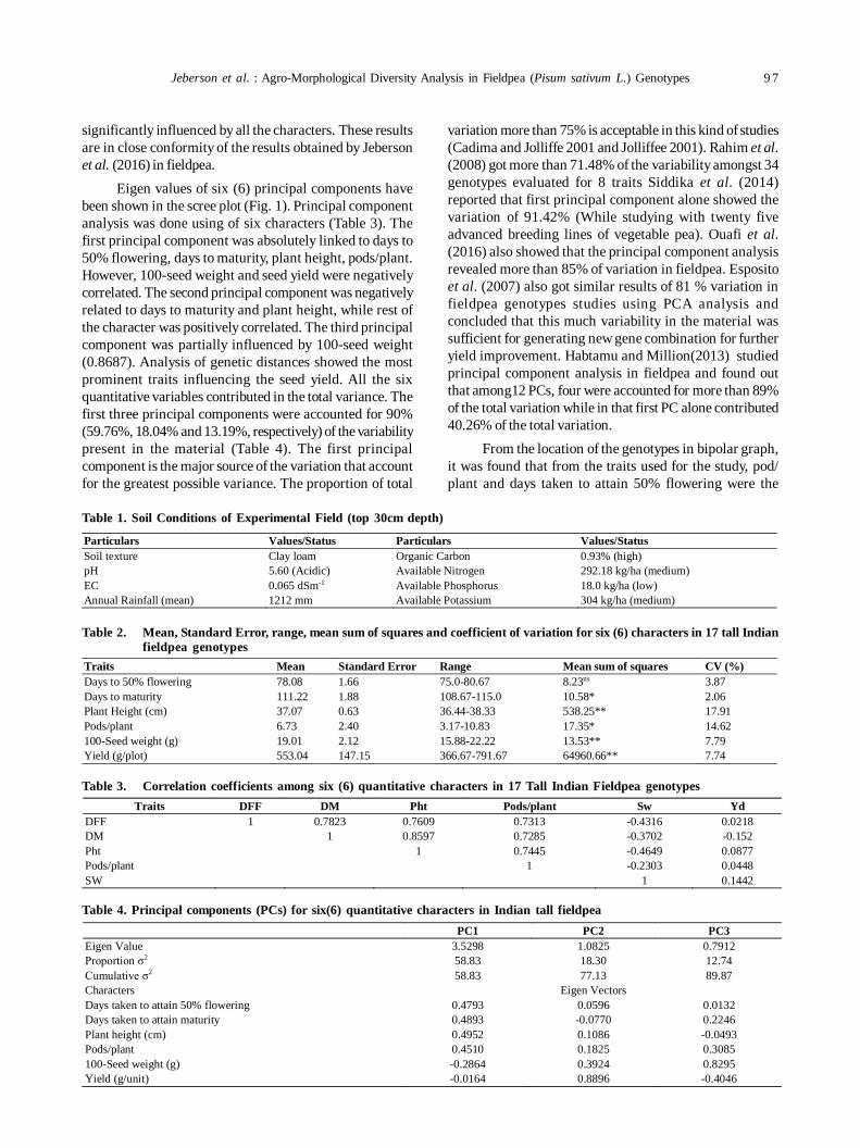
Jeberson et al. : Agro-Morphological Diversity Analysis in Fieldpea (Pisum sativum L.) Genotypes 9 7
significantly influenced by all the characters. These resultsare in close conformity of the results obtained by Jebersonet al. (2016) in fieldpea.
Eigen values of six (6) principal components havebeen shown in the scree plot (Fig. 1). Principal componentanalysis was done using of six characters (Table 3). Thefirst principal component was absolutely linked to days to50% flowering, days to maturity, plant height, pods/plant.However, 100-seed weight and seed yield were negativelycorrelated. The second principal component was negativelyrelated to days to maturity and plant height, while rest ofthe character was positively correlated. The third principalcomponent was partially influenced by 100-seed weight(0.8687). Analysis of genetic distances showed the mostprominent traits influencing the seed yield. All the sixquantitative variables contributed in the total variance. Thefirst three principal components were accounted for 90%(59.76%, 18.04% and 13.19%, respectively) of the variabilitypresent in the material (Table 4). The first principalcomponent is the major source of the variation that accountfor the greatest possible variance. The proportion of total
variation more than 75% is acceptable in this kind of studies(Cadima and Jolliffe 2001 and Jolliffee 2001). Rahim et al.(2008) got more than 71.48% of the variability amongst 34genotypes evaluated for 8 traits Siddika et al. (2014)reported that first principal component alone showed thevariation of 91.42% (While studying with twenty fiveadvanced breeding lines of vegetable pea). Ouafi et al.(2016) also showed that the principal component analysisrevealed more than 85% of variation in fieldpea. Espositoet al. (2007) also got similar results of 81 % variation infieldpea genotypes studies using PCA analysis andconcluded that this much variability in the material wassufficient for generating new gene combination for furtheryield improvement. Habtamu and Million(2013) studiedprincipal component analysis in fieldpea and found outthat among12 PCs, four were accounted for more than 89%of the total variation while in that first PC alone contributed40.26% of the total variation.
From the location of the genotypes in bipolar graph,it was found that from the traits used for the study, pod/plant and days taken to attain 50% flowering were the
Table 1. Soil Conditions of Experimental Field (top 30cm depth)
Table 2. Mean, Standard Error, range, mean sum of squares and coefficient of variation for six (6) characters in 17 tall Indianfieldpea genotypes
Table 3. Correlation coefficients among six (6) quantitative characters in 17 Tall Indian Fieldpea genotypesTraits DFF DM Pht Pods/plant Sw Yd
DFF 1 0.7823 0.7609 0.7313 -0.4316 0.0218 DM 1 0.8597 0.7285 -0.3702 -0.152 Pht 1 0.7445 -0.4649 0.0877 Pods/plant 1 -0.2303 0.0448 SW 1 0.1442
Table 4. Principal components (PCs) for six(6) quantitative characters in Indian tall fieldpea PC1 PC2 PC3 Eigen Value 3.5298 1.0825 0.7912 Proportion σ2 58.83 18.30 12.74 Cumulative σ2 58.83 77.13 89.87 Characters Eigen Vectors Days taken to attain 50% flowering 0.4793 0.0596 0.0132 Days taken to attain maturity 0.4893 -0.0770 0.2246 Plant height (cm) 0.4952 0.1086 -0.0493 Pods/plant 0.4510 0.1825 0.3085 100-Seed weight (g) -0.2864 0.3924 0.8295 Yield (g/unit) -0.0164 0.8896 -0.4046
Particulars Values/Status Particulars Values/Status Soil texture Clay loam Organic Carbon 0.93% (high) pH 5.60 (Acidic) Available Nitrogen 292.18 kg/ha (medium) EC 0.065 dSm-1 Available Phosphorus 18.0 kg/ha (low) Annual Rainfall (mean) 1212 mm Available Potassium 304 kg/ha (medium)
Traits Mean Standard Error Range Mean sum of squares CV (%) Days to 50% flowering 78.08 1.66 75.0-80.67 8.23ns 3.87 Days to maturity 111.22 1.88 108.67-115.0 10.58* 2.06 Plant Height (cm) 37.07 0.63 36.44-38.33 538.25** 17.91 Pods/plant 6.73 2.40 3.17-10.83 17.35* 14.62 100-Seed weight (g) 19.01 2.12 15.88-22.22 13.53** 7.79 Yield (g/plot) 553.04 147.15 366.67-791.67 64960.66** 7.74
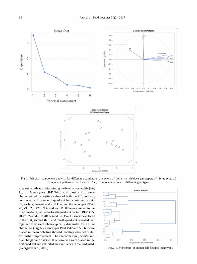
9 8 Journal of Food Legumes 30(2), 2017
greatest length and determining the level of variability (Fig1b, c.) Genotypes HFP 9426 and pant P 286 werecharacterized by positive values of both the PC1 and PC2components. The second quadrant had contained RFPG85, Rachna, Prakash and RFP 11-2, and the genotypes RFPG78, VL 62, KPMR 939 and Pant P 302 were situated in thethird quadrant, while the fourth quadrant contain RFPG 95,HFP 1024 and RFP 2011-3 and IPF 15-21. Genotypes placedin the first, second, third and fourth quadrant revealed thattogether they were phenotypically dissimilar for all thecharacters (Fig 1c). Genotypes Pant P 42 and VL 63 wereplaced in the middle line showed that they were not usefulfor further improvement. The characters viz., pods/plant,plant height and days to 50% flowering were placed in thefirst quadrant and exhibited their influence in the seed yield.(Georgieva et al, 2016).
Fig 1. Principal component analysis for different quantitative characters of Indian tall fieldpea genotypes; a.) Scree plot, b.)component pattern of PC1 and PC2 c.) component scores of different genotypes
Fig.2. Dendrogram of Indian tall fieldpea genotypes
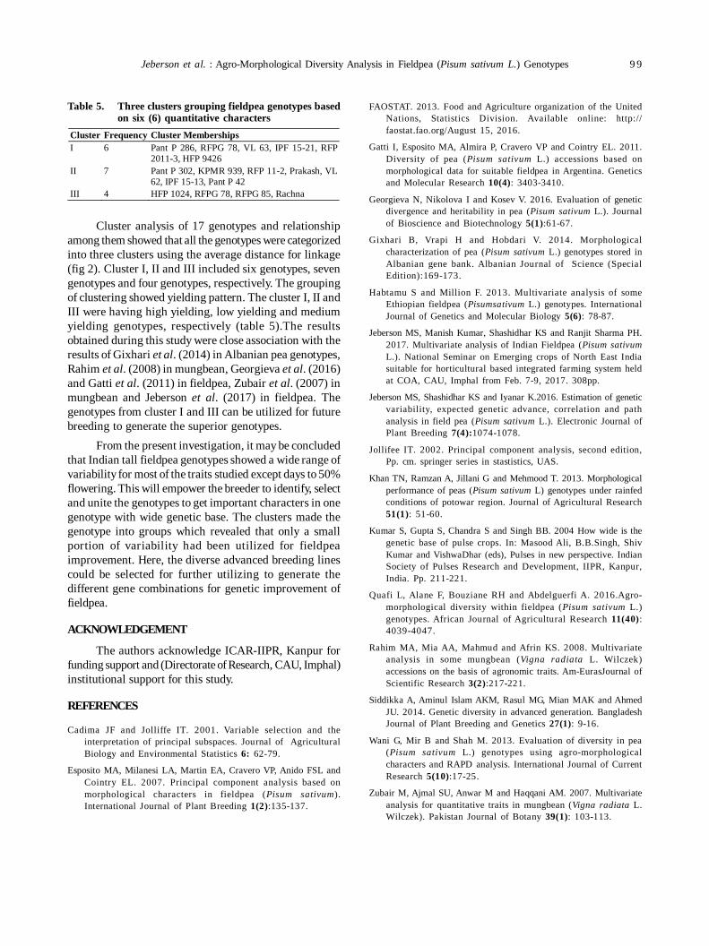
Jeberson et al. : Agro-Morphological Diversity Analysis in Fieldpea (Pisum sativum L.) Genotypes 9 9
Cluster analysis of 17 genotypes and relationshipamong them showed that all the genotypes were categorizedinto three clusters using the average distance for linkage(fig 2). Cluster I, II and III included six genotypes, sevengenotypes and four genotypes, respectively. The groupingof clustering showed yielding pattern. The cluster I, II andIII were having high yielding, low yielding and mediumyielding genotypes, respectively (table 5).The resultsobtained during this study were close association with theresults of Gixhari et al. (2014) in Albanian pea genotypes,Rahim et al. (2008) in mungbean, Georgieva et al. (2016)and Gatti et al. (2011) in fieldpea, Zubair et al. (2007) inmungbean and Jeberson et al. (2017) in fieldpea. Thegenotypes from cluster I and III can be utilized for futurebreeding to generate the superior genotypes.
From the present investigation, it may be concludedthat Indian tall fieldpea genotypes showed a wide range ofvariability for most of the traits studied except days to 50%flowering. This will empower the breeder to identify, selectand unite the genotypes to get important characters in onegenotype with wide genetic base. The clusters made thegenotype into groups which revealed that only a smallportion of variability had been utilized for fieldpeaimprovement. Here, the diverse advanced breeding linescould be selected for further utilizing to generate thedifferent gene combinations for genetic improvement offieldpea.
ACKNOWLEDGEMENT
The authors acknowledge ICAR-IIPR, Kanpur forfunding support and (Directorate of Research, CAU, Imphal)institutional support for this study.
REFERENCES
Cadima JF and Jolliffe IT. 2001. Variable selection and theinterpretation of principal subspaces. Journal of AgriculturalBiology and Environmental Statistics 6: 62-79.
Esposito MA, Milanesi LA, Martin EA, Cravero VP, Anido FSL andCointry EL. 2007. Principal component analysis based onmorphological characters in fieldpea (Pisum sativum).International Journal of Plant Breeding 1(2):135-137.
FAOSTAT. 2013. Food and Agriculture organization of the UnitedNations, Statistics Division. Available online: http://faostat.fao.org/August 15, 2016.
Gatti I, Esposito MA, Almira P, Cravero VP and Cointry EL. 2011.Diversity of pea (Pisum sativum L.) accessions based onmorphological data for suitable fieldpea in Argentina. Geneticsand Molecular Research 10(4): 3403-3410.
Georgieva N, Nikolova I and Kosev V. 2016. Evaluation of geneticdivergence and heritability in pea (Pisum sativum L.). Journalof Bioscience and Biotechnology 5(1):61-67.
Gixhari B, Vrapi H and Hobdari V. 2014. Morphologicalcharacterization of pea (Pisum sativum L.) genotypes stored inAlbanian gene bank. Albanian Journal of Science (SpecialEdition):169-173.
Habtamu S and Million F. 2013. Multivariate analysis of someEthiopian fieldpea (Pisumsativum L.) genotypes. InternationalJournal of Genetics and Molecular Biology 5(6): 78-87.
Jeberson MS, Manish Kumar, Shashidhar KS and Ranjit Sharma PH.2017. Multivariate analysis of Indian Fieldpea (Pisum sativumL.). National Seminar on Emerging crops of North East Indiasuitable for horticultural based integrated farming system heldat COA, CAU, Imphal from Feb. 7-9, 2017. 308pp.
Jeberson MS, Shashidhar KS and Iyanar K.2016. Estimation of geneticvariability, expected genetic advance, correlation and pathanalysis in field pea (Pisum sativum L.). Electronic Journal ofPlant Breeding 7(4):1074-1078.
Jollifee IT. 2002. Principal component analysis, second edition,Pp. cm. springer series in stastistics, UAS.
Khan TN, Ramzan A, Jillani G and Mehmood T. 2013. Morphologicalperformance of peas (Pisum sativum L) genotypes under rainfedconditions of potowar region. Journal of Agricultural Research51(1): 51-60.
Kumar S, Gupta S, Chandra S and Singh BB. 2004 How wide is thegenetic base of pulse crops. In: Masood Ali, B.B.Singh, ShivKumar and VishwaDhar (eds), Pulses in new perspective. IndianSociety of Pulses Research and Development, IIPR, Kanpur,India. Pp. 211-221.
Quafi L, Alane F, Bouziane RH and Abdelguerfi A. 2016.Agro-morphological diversity within fieldpea (Pisum sativum L.)genotypes. African Journal of Agricultural Research 11(40):4039-4047.
Rahim MA, Mia AA, Mahmud and Afrin KS. 2008. Multivariateanalysis in some mungbean (Vigna radiata L. Wilczek)accessions on the basis of agronomic traits. Am-EurasJournal ofScientific Research 3(2):217-221.
Siddikka A, Aminul Islam AKM, Rasul MG, Mian MAK and AhmedJU. 2014. Genetic diversity in advanced generation. BangladeshJournal of Plant Breeding and Genetics 27(1): 9-16.
Wani G, Mir B and Shah M. 2013. Evaluation of diversity in pea(Pisum sativum L.) genotypes using agro-morphologicalcharacters and RAPD analysis. International Journal of CurrentResearch 5(10):17-25.
Zubair M, Ajmal SU, Anwar M and Haqqani AM. 2007. Multivariateanalysis for quantitative traits in mungbean (Vigna radiata L.Wilczek). Pakistan Journal of Botany 39(1): 103-113.
Table 5. Three clusters grouping fieldpea genotypes basedon six (6) quantitative characters
Cluster Frequency Cluster Memberships I 6 Pant P 286, RFPG 78, VL 63, IPF 15-21, RFP
2011-3, HFP 9426 II 7 Pant P 302, KPMR 939, RFP 11-2, Prakash, VL
62, IPF 15-13, Pant P 42 III 4 HFP 1024, RFPG 78, RFPG 85, Rachna
100 Journal of Food Legumes 30(2), 2017
Dr. P. S. Basu, ICAR-IIPR, Kanpur
Dr. Guriqbal Singh, PAU, Ludhiyana
Dr. C. S. Praharaj, ICAR-IIPR, Kanpur
Dr. Poonam Singh, CAUA&T, Kanpur
Dr. S. S. Singh, ATARI, Kolkata
Dr. I. P. Singh, ICAR-IIPR, Kanpur
Dr. G.P. Dixit, ICAR-IIPR, Kanpur
Dr. Aditya Pratap, ICAR-IIPR, Kanpur
Dr. Abhishek Bohra, ICAR-IIPR, Kanpur
Dr. Ashok Chavan, MPKV, Rahuri
Dr. Purushottam, ICAR-IIPR, Kanpur
Dr. J. Soufamamian, BARC
Dr. Prasoon Verma, ICAR-IIPR, Kanpur
Dr. Anita Babber, JNKVV, Jabalpur
Dr. Hemant Kumar, ICAR-IIPR, Kanpur
Dr. R. P. Katiyar, CSAUA&T, Kanpur
Dr. Jitendra Kumar, ICAR-IIPR, Kanpur
Dr. D. K. Agarwal, ICAR-IISS, Mau
Dr. R. K. Mishra, ICAR-IIPR, Kanpur
List of Refrees for Vol. 30(2)
The Editorial Board gratefully acknowledges the help rendered by following referees in reviewing manuscripts for theVol. 30(2), 2017.
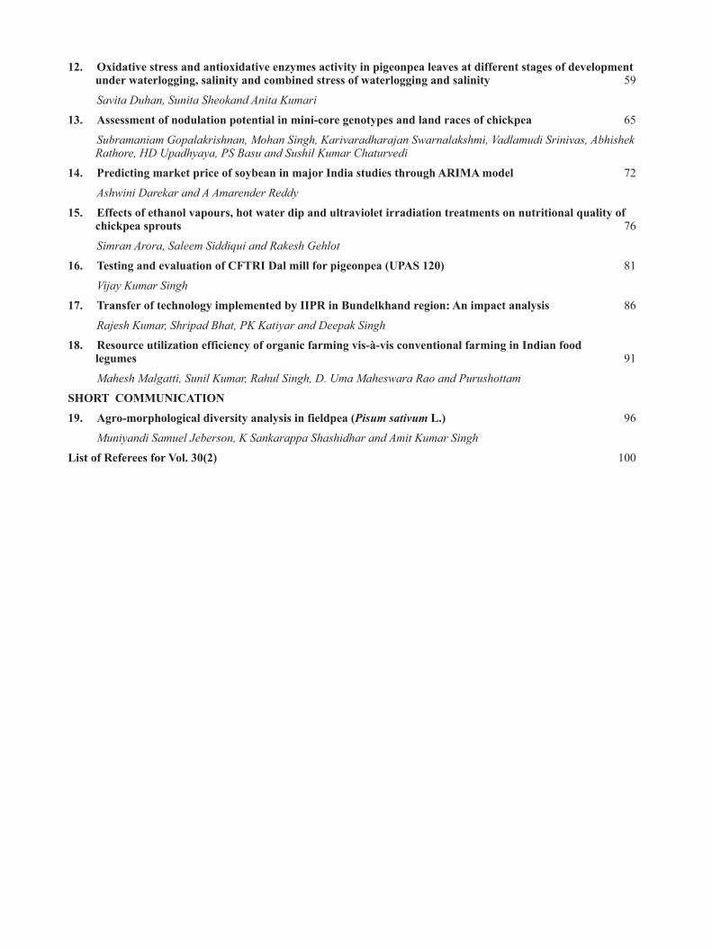
12. Oxidative stress and antioxidative enzymes activity in pigeonpea leaves at different stages of development under waterlogging, salinity and combined stress of waterlogging and salinity 59
Savita Duhan, Sunita Sheokand Anita Kumari
13. Assessment of nodulation potential in mini-core genotypes and land races of chickpea 65
Subramaniam Gopalakrishnan, Mohan Singh, Karivaradharajan Swarnalakshmi, Vadlamudi Srinivas, Abhishek Rathore, HD Upadhyaya, PS Basu and Sushil Kumar Chaturvedi
14. Predicting market price of soybean in major India studies through ARIMA model 72
Ashwini Darekar and A Amarender Reddy
15. Effects of ethanol vapours, hot water dip and ultraviolet irradiation treatments on nutritional quality of chickpea sprouts 76
Simran Arora, Saleem Siddiqui and Rakesh Gehlot
16. Testing and evaluation of CFTRI Dal mill for pigeonpea (UPAS 120) 81
Vijay Kumar Singh
17. Transfer of technology implemented by IIPR in Bundelkhand region: An impact analysis 86
Rajesh Kumar, Shripad Bhat, PK Katiyar and Deepak Singh
18. Resource utilization efficiency of organic farming vis-à-vis conventional farming in Indian foodlegumes 91
Mahesh Malgatti, Sunil Kumar, Rahul Singh, D. Uma Maheswara Rao and Purushottam
SHORT COMMUNICATION
19. Agro-morphological diversity analysis in fieldpea (Pisum sativum L.) 96
Muniyandi Samuel Jeberson, K Sankarappa Shashidhar and Amit Kumar Singh
List of Referees for Vol. 30(2) 100
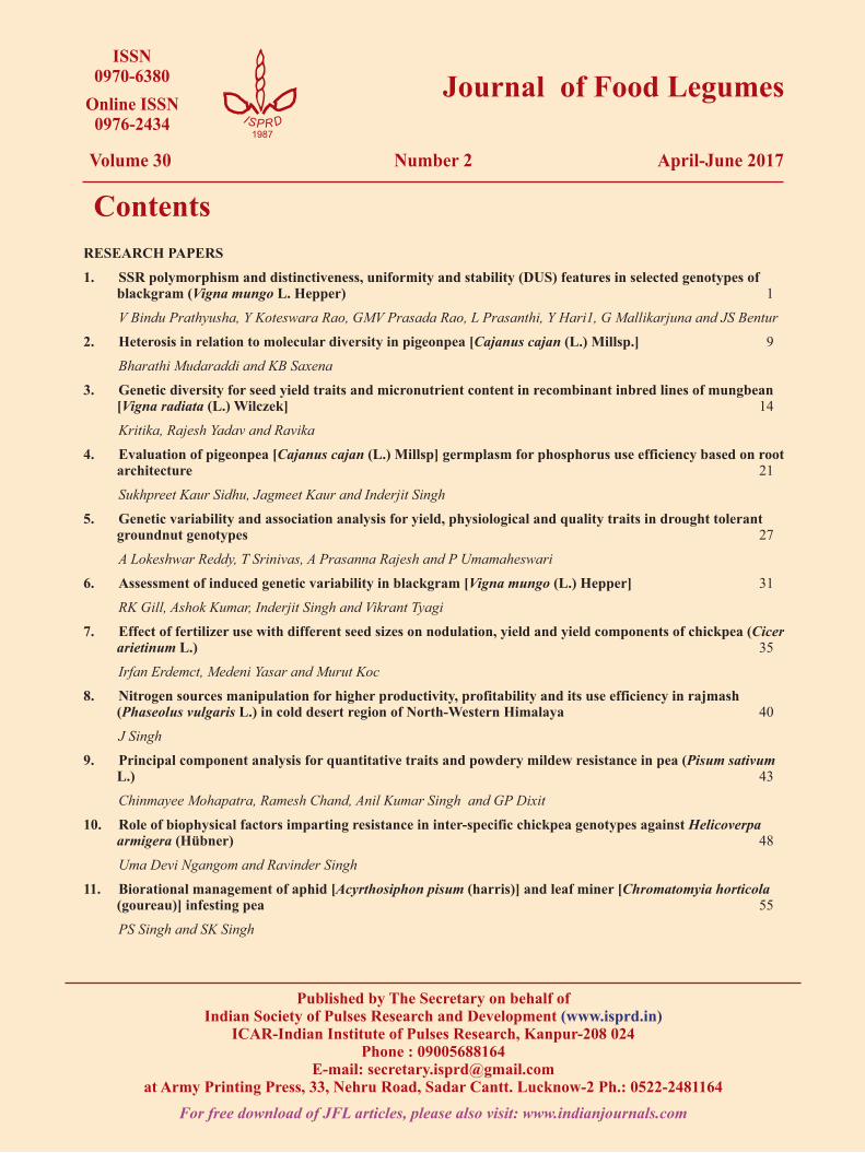
Published by The Secretary on behalf of Indian Society of Pulses Research and Development (www.isprd.in)
ICAR-Indian Institute of Pulses Research, Kanpur-208 024Phone : 09005688164
E-mail: [email protected] Army Printing Press, 33, Nehru Road, Sadar Cantt. Lucknow-2 Ph.: 0522-2481164
For free download of JFL articles, please also visit: www.indianjournals.com
Journal of Food LegumesISSN
0970-6380
Online ISSN0976-2434
Volume 30 Number 2 April-June 2017
Contents
I SPRD1987
RESEARCH PAPERS
1. SSR polymorphism and distinctiveness, uniformity and stability (DUS) features in selected genotypes of blackgram (Vigna mungo L. Hepper) 1
V Bindu Prathyusha, Y Koteswara Rao, GMV Prasada Rao, L Prasanthi, Y Hari1, G Mallikarjuna and JS Bentur
2. Heterosis in relation to molecular diversity in pigeonpea [Cajanus cajan (L.) Millsp.] 9
Bharathi Mudaraddi and KB Saxena
3. Genetic diversity for seed yield traits and micronutrient content in recombinant inbred lines of mungbean [Vigna radiata (L.) Wilczek] 14
Kritika, Rajesh Yadav and Ravika
4. Evaluation of pigeonpea [Cajanus cajan (L.) Millsp] germplasm for phosphorus use efficiency based on root architecture 21
Sukhpreet Kaur Sidhu, Jagmeet Kaur and Inderjit Singh
5. Genetic variability and association analysis for yield, physiological and quality traits in drought tolerant groundnut genotypes 27
A Lokeshwar Reddy, T Srinivas, A Prasanna Rajesh and P Umamaheswari
6. Assessment of induced genetic variability in blackgram [Vigna mungo (L.) Hepper] 31
RK Gill, Ashok Kumar, Inderjit Singh and Vikrant Tyagi
7. Effect of fertilizer use with different seed sizes on nodulation, yield and yield components of chickpea (Cicer arietinum L.) 35
Irfan Erdemct, Medeni Yasar and Murut Koc
8. Nitrogen sources manipulation for higher productivity, profitability and its use efficiency in rajmash (Phaseolus vulgaris L.) in cold desert region of North-Western Himalaya 40
J Singh
9. Principal component analysis for quantitative traits and powdery mildew resistance in pea (Pisum sativum L.) 43
Chinmayee Mohapatra, Ramesh Chand, Anil Kumar Singh and GP Dixit
10. Role of biophysical factors imparting resistance in inter-specific chickpea genotypes against Helicoverpa armigera (Hübner) 48
Uma Devi Ngangom and Ravinder Singh
11. Biorational management of aphid [Acyrthosiphon pisum (harris)] and leaf miner [Chromatomyia horticola (goureau)] infesting pea 55
PS Singh and SK Singh
Related Documents


![Advances in Food Legumes Research at ICRISAToar.icrisat.org/11055/1/11-57.pdf · [1] Advances in Food Legumes Research at ICRISAT Pooran M Gaur 1, Rajeev K Varshney , HD Upadhyaya](https://static.cupdf.com/doc/110x72/5f0d5de37e708231d439ffc7/advances-in-food-legumes-research-at-1-advances-in-food-legumes-research-at-icrisat.jpg)