Fokker–Planck equation with fractional coordinate derivatives

arX

iv:0

805.

0606

v1 [

phys

ics.

clas

s-ph

] 5

May

200

8

Fokker-Planck equation with fractional coordinate

derivatives

Vasily E. Tarasov1,2 and George M. Zaslavsky1,3

1) Courant Institute of Mathematical Sciences, New York University

251 Mercer St., New York, NY 10012, USA, and

2) Skobeltsyn Institute of Nuclear Physics,

Moscow State University, Moscow 119991, Russia

3) Department of Physics, New York University,

2-4 Washington Place, New York, NY 10003, USA

Abstract

Using the generalized Kolmogorov-Feller equation with long-range interaction,

we obtain kinetic equations with fractional derivatives with respect to coordinates.

The method of successive approximations with the averaging with respect to fast

variable is used. The main assumption is that the correlator of probability densities

of particles to make a step has a power-law dependence. As a result, we obtain

Fokker-Planck equation with fractional coordinate derivative of order 1 < α < 2.

1

1 Introduction

In studying of the processes with fractal time and long-term memory a generalized kinetic

equation was proposed in [1]. While the equation was of the master-type, its main property

was the presence of the power-type kernel for a probability density to make a step. This

type of equation was compared to the Kolmogorov-Feller equation in [2]. In this paper,

we would like to go farther and to show the conditions under which one can obtain the

fractional generalization of the Fokker-Planck equation from the Fokker-Planck equation.

Fractional calculus [3, 4, 5] has found many applications in recent studies in mechanics

and physics, and the interest in fractional equations has been growing continually during

the last years. Fractional Fokker-Planck equations with coordinate and time derivatives

of non-integer order has been suggested in [6]. The solutions and properties of these

equations are described in Refs. [2, 7]. The Fokker-Planck equation with fractional

coordinate derivatives was also considered in [8, 9, 10, 11, 12].

The Kolmogorov-Feller equation is integro-differential one and it belongs to the type

of master equations broadly used in different physical applications. It is well-known that

the Kolmogorov-Feller equation can lead us to the Fokker-Planck equation [13] under

some conditions. In this paper, we use the method of successive approximations with the

averaging with respect to the fast variable [14]. The main assumption is that the correlator

of probability densities of particle to make a step has power-law dependence. As a result,

we obtain Fokker-Planck equations with fractional derivatives of order 1 < α < 2.

In Sec. 2, the Kolmogorov-Feller equation for one-dimensional case is considered. In

Sec. 3, we present a generalization of the Kolmogorov-Feller equation for two-dimensional

case. The method of successive approximations is used for this generalized equation in

Sec. 4. In Sec. 5, we use averaging with respect to the fast variable to derive fractional

Fokker-Planck equations. Finally, a short conclusion is given in Sec. 6.

2

2 Kolmogorov-Feller equation for one-dimensional case

2.1 Operator representation of the KF-equation

Let P (t, x) be a probability density to find a particle at x at time instant t. The normal-

ization condition for P (t, x) is∫

+∞

−∞

dxP (t, x) = 1 (t > 0).

The Kolmogorov-Feller (KF) equation has the form

∂P (t, x)

∂t=

∫

+∞

−∞

dx′ w(x′)[P (t, x − x′) − P (t, x)], P (0, x) = δ(x), (1)

where w(x′) is probability density of particle to make a step of the length x′, and∫

+∞

−∞

dx′ w(x′) = 1. (2)

Let us introduce the operator representation of the KF-equation. We define the trans-

lation operator

Tx′ = exp{−x′∂x}, (3)

such that

Tx′P (t, x) = P (t, x − x′), (4)

and the finite difference operator

∆x′ = I − Tx′ , (5)

where I is an identity operator. Then the Kolmogorov-Feller equation (1) can be presented

as∂P (t, x)

∂t= L(∆) P (t, x). (6)

Here we use the integro-differential operator

L(∆) = −

∫

+∞

−∞

dx′ w(x′) ∆x′. (7)

The operator (7) will be called the Kolmogorov-Feller operator.

3

2.2 KF-equation with fractional coordinate derivative

The well-known fractional Caputo derivative [4] of order α is defined by

CDαxP (x) =

1

Γ(1 − α)

∫ x

−∞

dz

(x − z)α

∂P (z)

∂z, (0 < α < 1). (8)

The fractional Marchaud derivative [4] of order α is defined by

DαxP (x) =

1

Γ(−α)

∫ x

−∞

[P (z) − P (x)]dz

(x − z)α+1, (0 < α < 1). (9)

Using x′ = x − z, equation (9) has the form

DαxP (x) =

1

Γ(−α)

∫

∞

0

dx′

(x′)α+1[P (x − x′) − P (x)].

If the function w(x′) in KF-equation (1) is the exponential function

w(x′) =a

x′α+1H(x′), (10)

where H(x′) is a Heaviside step function, then Eq. (1) can be presented through the

fractional coordinate derivative

∂P (t, x)

∂t= aDα

xP (t, x), P (0, x) = δ(x), (0 < α < 1). (11)

This is the Kolmogorov-Feller equation with fractional coordinate derivatives of order

0 < α < 1. Note that the function w(x) is a probability density and it should sat-

isfy the normalization condition (2). Then equation (10) can be considered only as an

approximation for large x′.

2.3 Generalized KF-equation

In the general case, we can suppose that probability density of particle to make a step of

the length x′ depends on the time instant t and the coordinate x. Then we should replace

w(x′) by w(t, x|x′) in KF-equation (1). As a result, we can consider the equation

∂P (t, x)

∂t= ε

∫

+∞

−∞

dx′ w(t, x|x′)[P (t, x − x′) − P (t, x)], P (0, x) = δ(x), (12)

4

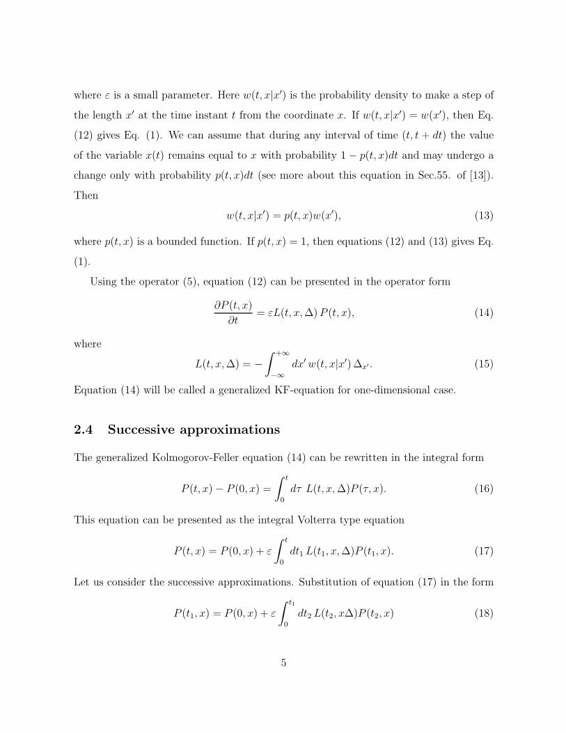
where ε is a small parameter. Here w(t, x|x′) is the probability density to make a step of

the length x′ at the time instant t from the coordinate x. If w(t, x|x′) = w(x′), then Eq.

(12) gives Eq. (1). We can assume that during any interval of time (t, t + dt) the value

of the variable x(t) remains equal to x with probability 1 − p(t, x)dt and may undergo a

change only with probability p(t, x)dt (see more about this equation in Sec.55. of [13]).

Then

w(t, x|x′) = p(t, x)w(x′), (13)

where p(t, x) is a bounded function. If p(t, x) = 1, then equations (12) and (13) gives Eq.

(1).

Using the operator (5), equation (12) can be presented in the operator form

∂P (t, x)

∂t= εL(t, x, ∆) P (t, x), (14)

where

L(t, x, ∆) = −

∫

+∞

−∞

dx′ w(t, x|x′) ∆x′. (15)

Equation (14) will be called a generalized KF-equation for one-dimensional case.

2.4 Successive approximations

The generalized Kolmogorov-Feller equation (14) can be rewritten in the integral form

P (t, x) − P (0, x) =

∫ t

0

dτ L(t, x, ∆)P (τ, x). (16)

This equation can be presented as the integral Volterra type equation

P (t, x) = P (0, x) + ε

∫ t

0

dt1 L(t1, x, ∆)P (t1, x). (17)

Let us consider the successive approximations. Substitution of equation (17) in the form

P (t1, x) = P (0, x) + ε

∫ t1

0

dt2 L(t2, x∆)P (t2, x) (18)

5

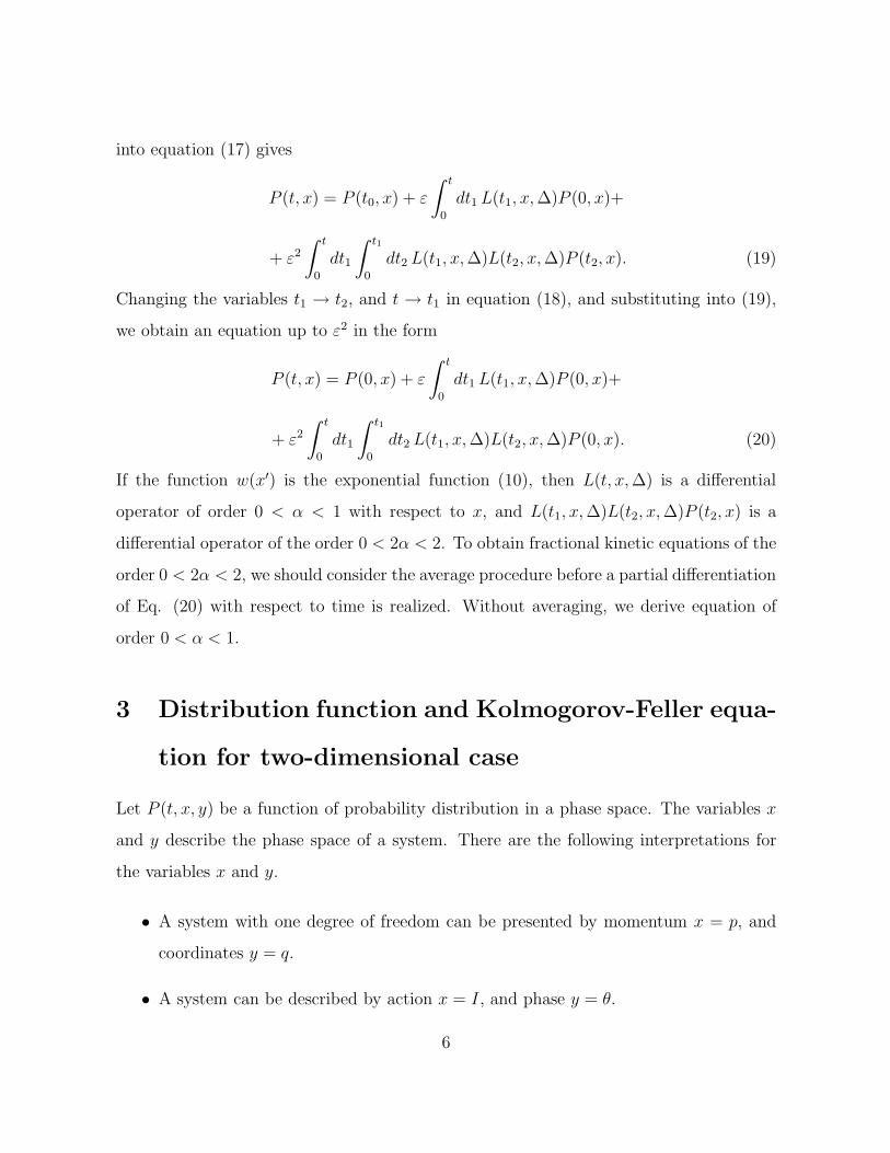
into equation (17) gives

P (t, x) = P (t0, x) + ε

∫ t

0

dt1 L(t1, x, ∆)P (0, x)+

+ ε2

∫ t

0

dt1

∫ t1

0

dt2 L(t1, x, ∆)L(t2, x, ∆)P (t2, x). (19)

Changing the variables t1 → t2, and t → t1 in equation (18), and substituting into (19),

we obtain an equation up to ε2 in the form

P (t, x) = P (0, x) + ε

∫ t

0

dt1 L(t1, x, ∆)P (0, x)+

+ ε2

∫ t

0

dt1

∫ t1

0

dt2 L(t1, x, ∆)L(t2, x, ∆)P (0, x). (20)

If the function w(x′) is the exponential function (10), then L(t, x, ∆) is a differential

operator of order 0 < α < 1 with respect to x, and L(t1, x, ∆)L(t2, x, ∆)P (t2, x) is a

differential operator of the order 0 < 2α < 2. To obtain fractional kinetic equations of the

order 0 < 2α < 2, we should consider the average procedure before a partial differentiation

of Eq. (20) with respect to time is realized. Without averaging, we derive equation of

order 0 < α < 1.

3 Distribution function and Kolmogorov-Feller equa-

tion for two-dimensional case

Let P (t, x, y) be a function of probability distribution in a phase space. The variables x

and y describe the phase space of a system. There are the following interpretations for

the variables x and y.

• A system with one degree of freedom can be presented by momentum x = p, and

coordinates y = q.

• A system can be described by action x = I, and phase y = θ.

6

• n-particle system can be defined by x = (q1, p1) and y = (q2, p2, ..., qn, pn), or x = q1,

and y = (p1, q2, p2, ..., qn, pn).

• The variables x describe a system, and y describes an environment of this system.

We plan to use the reduced distribution and average values with respect to y, where

y will be considered as a fast variable.

3.1 Generalized KF-equation for two-dimensional case

We assume that x ∈ X ⊂ R and y ∈ Y ⊂ R, then r = (x, y) ∈ X × Y ⊂ R2. We plan to

consider x is a slow variable and y will be considered as fast variable. The distribution

function P (t, r) in the region X × Y satisfies the generalized Kolmogorov-Feller equation

∂P (t, r)

∂t= ε

∫

X×Y

d2r1 w(t, r|r1)[P (t, r− r1) − P (t, r)], (21)

where d2r1 = dx1dy1, and ε is a small parameter. Here w(t, r|r1) is the probability density

to make a step on the vector r1 at the time instant t from the point r.

Equation (21) can be presented in the form

∂

∂tP (t, r) = εL(t, r, ∆)P (t, r), (22)

where L(t, r, ∆) is a Kolmogorov-Feller operator

L(t, r, ∆) = −

∫

X×Y

d2r1 w(t, r|r1) ∆r1

, (23)

Here ∆r1

is a finite difference operator

∆r1

= I − Tr1

,

where Tr1

is a translation operator in X × Y that is defined by

Tr1

= exp{−r1∇} = exp{−x1∂x − y1∂y}.

7

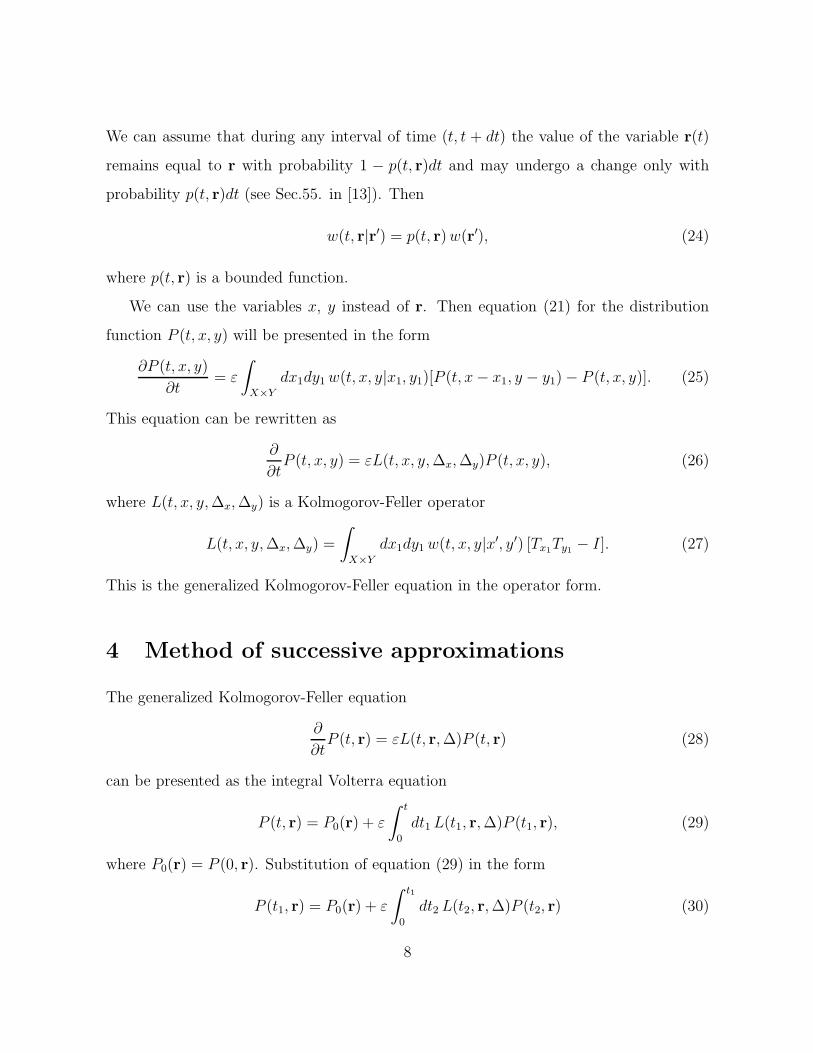
We can assume that during any interval of time (t, t + dt) the value of the variable r(t)

remains equal to r with probability 1 − p(t, r)dt and may undergo a change only with

probability p(t, r)dt (see Sec.55. in [13]). Then

w(t, r|r′) = p(t, r) w(r′), (24)

where p(t, r) is a bounded function.

We can use the variables x, y instead of r. Then equation (21) for the distribution

function P (t, x, y) will be presented in the form

∂P (t, x, y)

∂t= ε

∫

X×Y

dx1dy1 w(t, x, y|x1, y1)[P (t, x − x1, y − y1) − P (t, x, y)]. (25)

This equation can be rewritten as

∂

∂tP (t, x, y) = εL(t, x, y, ∆x, ∆y)P (t, x, y), (26)

where L(t, x, y, ∆x, ∆y) is a Kolmogorov-Feller operator

L(t, x, y, ∆x, ∆y) =

∫

X×Y

dx1dy1 w(t, x, y|x′, y′) [Tx1Ty1

− I]. (27)

This is the generalized Kolmogorov-Feller equation in the operator form.

4 Method of successive approximations

The generalized Kolmogorov-Feller equation

∂

∂tP (t, r) = εL(t, r, ∆)P (t, r) (28)

can be presented as the integral Volterra equation

P (t, r) = P0(r) + ε

∫ t

0

dt1 L(t1, r, ∆)P (t1, r), (29)

where P0(r) = P (0, r). Substitution of equation (29) in the form

P (t1, r) = P0(r) + ε

∫ t1

0

dt2 L(t2, r, ∆)P (t2, r) (30)

8

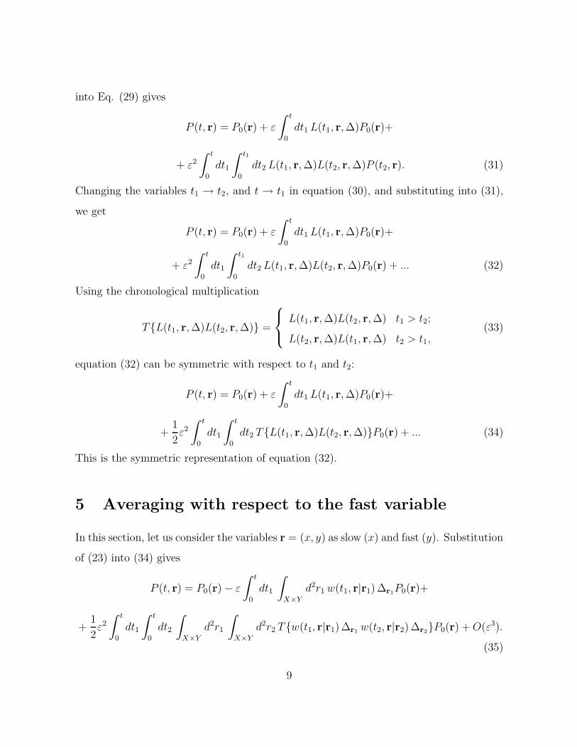
into Eq. (29) gives

P (t, r) = P0(r) + ε

∫ t

0

dt1 L(t1, r, ∆)P0(r)+

+ ε2

∫ t

0

dt1

∫ t1

0

dt2 L(t1, r, ∆)L(t2, r, ∆)P (t2, r). (31)

Changing the variables t1 → t2, and t → t1 in equation (30), and substituting into (31),

we get

P (t, r) = P0(r) + ε

∫ t

0

dt1 L(t1, r, ∆)P0(r)+

+ ε2

∫ t

0

dt1

∫ t1

0

dt2 L(t1, r, ∆)L(t2, r, ∆)P0(r) + ... (32)

Using the chronological multiplication

T{L(t1, r, ∆)L(t2, r, ∆)} =

L(t1, r, ∆)L(t2, r, ∆) t1 > t2;

L(t2, r, ∆)L(t1, r, ∆) t2 > t1,(33)

equation (32) can be symmetric with respect to t1 and t2:

P (t, r) = P0(r) + ε

∫ t

0

dt1 L(t1, r, ∆)P0(r)+

+1

2ε2

∫ t

0

dt1

∫ t

0

dt2 T{L(t1, r, ∆)L(t2, r, ∆)}P0(r) + ... (34)

This is the symmetric representation of equation (32).

5 Averaging with respect to the fast variable

In this section, let us consider the variables r = (x, y) as slow (x) and fast (y). Substitution

of (23) into (34) gives

P (t, r) = P0(r) − ε

∫ t

0

dt1

∫

X×Y

d2r1 w(t1, r|r1) ∆r1

P0(r)+

+1

2ε2

∫ t

0

dt1

∫ t

0

dt2

∫

X×Y

d2r1

∫

X×Y

d2r2 T{w(t1, r|r1) ∆r1

w(t2, r|r2) ∆r2}P0(r) + O(ε3).

(35)

9

The function w(t, r|r1) is the probability density to make a step of the vector r1 at

the time instant t from the point r. The first assumption is that this probability density

has a weak dependence (up to terms of order O(ε)) on the point r, i.e.,

w(t, r + r1|r2) = w(t, r|r2) + O(ε). (36)

Then

∆r1

w(t2, r|r2) = 0,

and

w(t1, r|r1) ∆r1

w(t2, r|r2) ∆r2

= w(t1, r|r1) w(t2, r|r2) ∆r1

∆r2

.

As a result, equation (35) has the form

P (t, r) = P0(r) − ε

∫ t

0

dt1

∫

X×Y

d2r1 w(t1, r|r1) ∆r1

P0(r)+

+1

2ε2

∫ t

0

dt1

∫ t

0

dt2

∫

X×Y

d2r1

∫

X×Y

d2r2 T{w(t1, r|r1) w(t2, r|r2)}∆r1

∆r2

P0(r) + O(ε3).

The second assumption states that P0(r) = P0(x, y) does not depend on the fast

variable y up to ε-terms such that

P0(r) = P0(x, y) = ρ0(x) + O(ε). (37)

Then, we have

∆r1

∆r2

P0(r) = ∆x1∆x2

ρ0(x) + O(ε). (38)

Averaging over the variable y will be denoted by < >y. We also use the notations

ρ(t, x) =< P (t, r) >y, (39)

and ρ(0, x) = ρ0(x).

Averaging of equation (35) with respect to the fast variable y, we obtain

ρ(t, x) = ρ0(x) − ε

∫ t

0

dt1

∫

X

dx1 A(t1, x|x1) ∆x1ρ0(x)+

10

+1

2ε2

∫ t

0

dt1

∫

X

dx1

∫

X

dx2 B(t1, x|x1, x2) ∆x1∆x2

ρ0(x) + O(ε3), (40)

where we introduce the functions

A(t1, x|x1) =

∫

Y

dy1 < w(t1, r|r1) >y, (41)

B(t1, x|x1, x2) =

∫ t

0

dt2

∫

Y

dy1

∫

Y

dy2 < T{w(t1, r|r1) w(t2, r|r2)} >y . (42)

Using r = (x, y), these functions can be presented by

A(t1, x|x1) =

∫

Y

dy1 < w(t1, x, y|x1, y1) >y, (43)

B(t1, x|x1, x2) =

∫ t

0

dt2

∫

Y

dy1

∫

Y

dy2 < T{w(t1, x, y|x1, y1) w(t2, x, y|x2, y2)} >y . (44)

The third assumption is that the function B(t1, x|x1, x2) is diagonal with respect to

variables x1 and x2 up to ε-term, i.e.,

B(t1, x|x1, x2) = B(t1, x|x1)δ(x1 − x2) + O(ε). (45)

Then the operator ∆x1∆x2

will be the finite difference operator ∆2x1

of second order.

This allows us to have fractional derivative for the exponential function B(t, x|x1) since

Marchaud and Riesz fractional derivatives [3] are defined through the finite difference

operator.

The fourth assumption is that the functions A(t1, x|x1) and B(t1, x|x1) are exponential

functions up to ε such that

A(t, x|x1) = a(t)1

κ(α1, 1)

1

|x1|α1+1H(x1) + O(ε), (0 < α1 < 1), (46)

B(t, x|x1) = b(t, x)1

κ(α2, 2)

1

|x1|α2

H(x1) + O(ε), (1 < α2 < 2), (47)

where H(x) is the Heaviside step function, and

κ(α, n) = −Γ(α)An(α), An(α) =n

∑

k=0

(−1)k−1n!

k!(n − k)!kα, (48)

11

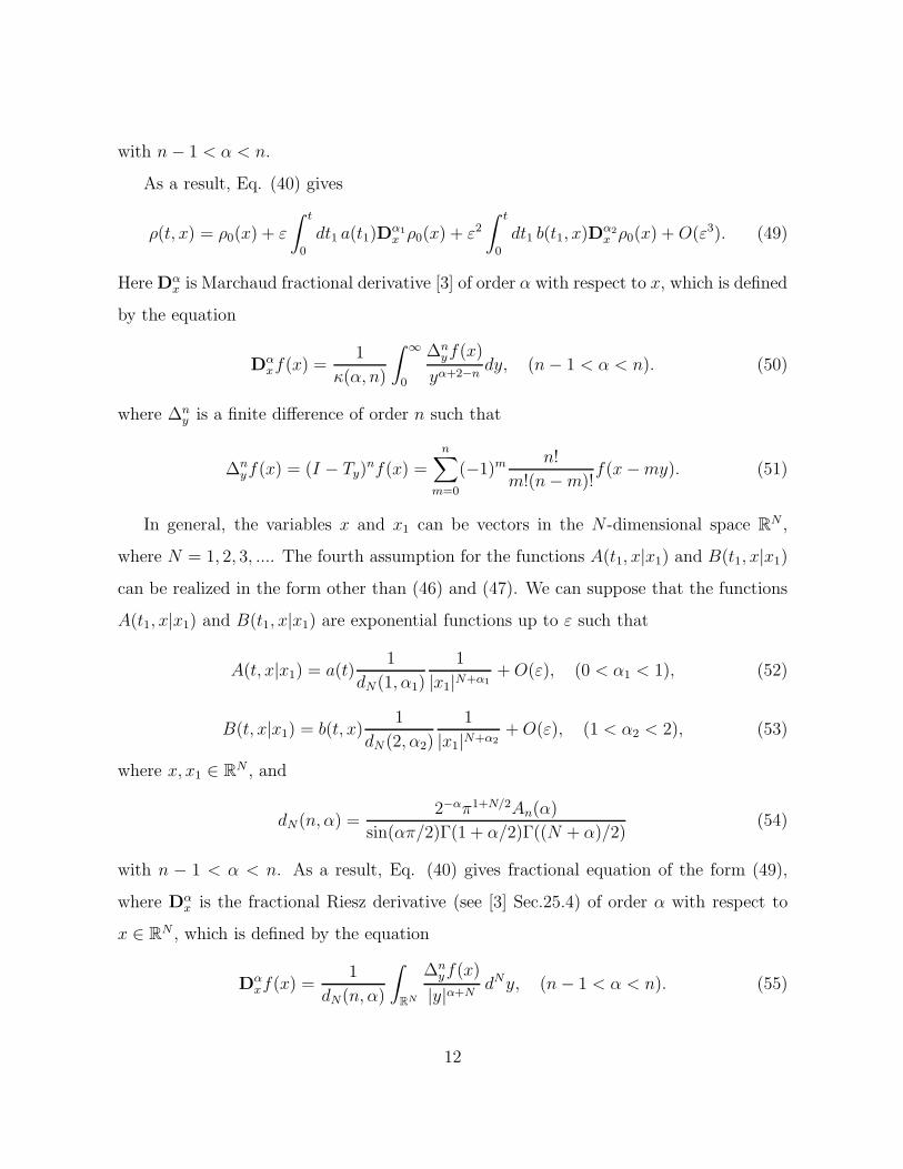
with n − 1 < α < n.

As a result, Eq. (40) gives

ρ(t, x) = ρ0(x) + ε

∫ t

0

dt1 a(t1)Dα1

x ρ0(x) + ε2

∫ t

0

dt1 b(t1, x)Dα2

x ρ0(x) + O(ε3). (49)

Here Dαx is Marchaud fractional derivative [3] of order α with respect to x, which is defined

by the equation

Dαxf(x) =

1

κ(α, n)

∫

∞

0

∆nyf(x)

yα+2−ndy, (n − 1 < α < n). (50)

where ∆ny is a finite difference of order n such that

∆nyf(x) = (I − Ty)

nf(x) =

n∑

m=0

(−1)m n!

m!(n − m)!f(x − my). (51)

In general, the variables x and x1 can be vectors in the N -dimensional space RN ,

where N = 1, 2, 3, .... The fourth assumption for the functions A(t1, x|x1) and B(t1, x|x1)

can be realized in the form other than (46) and (47). We can suppose that the functions

A(t1, x|x1) and B(t1, x|x1) are exponential functions up to ε such that

A(t, x|x1) = a(t)1

dN(1, α1)

1

|x1|N+α1

+ O(ε), (0 < α1 < 1), (52)

B(t, x|x1) = b(t, x)1

dN (2, α2)

1

|x1|N+α2

+ O(ε), (1 < α2 < 2), (53)

where x, x1 ∈ RN , and

dN(n, α) =2−απ1+N/2An(α)

sin(απ/2)Γ(1 + α/2)Γ((N + α)/2)(54)

with n − 1 < α < n. As a result, Eq. (40) gives fractional equation of the form (49),

where Dαx is the fractional Riesz derivative (see [3] Sec.25.4) of order α with respect to

x ∈ RN , which is defined by the equation

Dαxf(x) =

1

dN(n, α)

∫

RN

∆nyf(x)

|y|α+NdNy, (n − 1 < α < n). (55)

12

To denote Riesz fractional derivative (55) is also used the notation (−∆)α/2. Note that

the Fourier transform F of this derivative (see Property 2.34 of [4]) is defined by(

F{Dαxf(x)}

)

(k) = |k|α(

{Ff(x)})

(k).

The representation of the assumption in the form (52) and (53) allows us to obtain

fractional kinetic equation for arbitrary N -dimensional space (for example, in the 3-

dimensional Euclidean space).

The partial time differentiation of equation (49) gives

∂

∂tρ(t, x) = εa(t)Dα1

x ρ0(x) + ε2b(t, x)Dα2

x ρ0(x) + O(ε3). (56)

Substitution of equation (49) in the form

ρ0(x) = ρ(t, x) − ε

∫ t

0

dt1 a(t1)Dα1

x ρ0(x) + O(ε2) (57)

into equation (56) gives

∂

∂tρ(t, x) = εa(t)Dα1

x ρ(t, x) + ε2

(

b(t, x)Dα2

x − c(t)D2α1

x

)

ρ(t, x) + O(ε3), (58)

where

c(t) = a(t)

∫ t

0

dt1 a(t1).

Equation (58) up to O(ε3) has the form

∂

∂tρ(t, x) = εa(t)Dα1

x ρ(t, x) + ε2

(

b(t, x)Dα2

x − c(t)D2α1

x

)

ρ(t, x). (59)

This is the fractional kinetic equation with noninteger derivatives of the order 1 < α2 < 2

and 0 < 2α1 < 2 with respect to coordinate x.

If a(t) = 0, i.e.. A(t, x|x1) = 0, then we have the fractional equation of order 1 < α2 <

2 with respect to x such that

∂

∂tρ(t, x) = ε2b(t, x)Dα2

x ρ(t, x). (60)

This is the fractional Fokker-Planck equation that is suggested in [6] to describe fractional

kinetics. The solutions and properties of these equations are described in Refs. [2, 7].

The Fokker-Planck equation with fractional coordinate derivatives are also considered in

[8, 9, 10, 11, 12].

13

6 Conclusion

In this paper, the Fokker-Planck equations with coordinate derivatives of non-integer order

1 < α < 2 are derived by using Kolmogorov-Feller equation. The method of successive

approximations and the averaging with respect to a fast variable are used. The main

assumption in the paper is that the correlator of two probability densities of particle

to make a step has the form of exponential function. As a result, the Fokker-Planck

equations can have derivatives of order 1 < α < 2.

References

[1] E.W. Montroll, M.F. Shlesinger, ”On the wonderful world of random walks” in:

J. Lebowitz and E.W. Montroll, Editors, Studies in Statistical Mechanics, Vol. 11,

North-Holland, Amsterdam (1984), p.1.

[2] A.I. Saichev, G.M. Zaslavsky, ”Fractional kinetic equations: solutions and applica-

tions” Chaos 7(4) (1997) 753-764.

[3] S.G. Samko, A.A. Kilbas, O.I. Marichev, Fractional Integrals and Derivatives Theory

and Applications (Gordon and Breach, New York, 1993).

[4] A.A. Kilbas, H.M. Srivastava, J.J. Trujillo, Theory and Application of Fractional

Differential Equations (Elsevier, Amsterdam, 2006)

[5] I. Podlubny, Fractional Differential Equations, (Academic Press, San Diego, 1999).

[6] G.M. Zaslavsky, ”Fractional kinetic equation for Hamiltonian chaos” Physica D 76

(1994) 110-122.

[7] G.M. Zaslavsky, ”Chaos, fractional kinetics, and anomalous transport” Phys. Rep.

371 (2002) 461-580.

[8] G.M. Zaslavsky, ”Renormalization group theory of anomalous transport in systems

with Hamiltonian chaos” Chaos 4 (1994) 25-33.

14

[9] A.V. Milovanov, ”Stochastic dynamics from the fractional Fokker-Planck-

Kolmogorov equation: Large-scale behavior of the turbulent transport coefficient”

Phys. Rev. E 63 (2001) 047301.

[10] V.V. Yanovsky, A.V. Chechkin, D. Schertzer, A.V. Tur, ”Levy anomalous diffusion

and fractional Fokker-Planck equation” Physica A 282 (2000) 13-34.

[11] V.E. Tarasov, ”Fractional Fokker-Planck equation for fractal media” Chaos 15 (2005)

023102.

[12] V.N. Kolokoltsov, ”Generalized continuous-time random walks (CTRW), subordina-

tion by hitting times and fractional dynamics” E-print arXiv:0706.1928.

[13] B.V. Gnedenko, The Theory of Probability (Chelsea, New York, 1962).

[14] G.M. Zaslavsky, Chaos in Dynamic Systems, (Harwood Academic Publishers, New

York, 1985)

15