FOCUS ON EUROPEAN ECONOMIC INTEGRATION Stability and Security. Q1/ 19

Welcome message from author
This document is posted to help you gain knowledge. Please leave a comment to let me know what you think about it! Share it to your friends and learn new things together.
Transcript

FOCUS ON EUROPEANECONOMIC INTEGRATION
Stability and Security. Q1/ 19

This publication presents economic analyses and outlooks as well as analytical studies on macroeconomic and macro financial issues with a regional focus on Central, Eastern and Southeastern Europe.
Please visit http://www.oenb.at/feei.
Publisher and editor Oesterreichische NationalbankOtto-Wagner-Platz 3, 1090 ViennaPO Box 61, 1011 Vienna, [email protected] (+43-1) 40420-6666Fax (+43-1) 40420-046698
Editors in chief Doris Ritzberger-Grünwald, Helene Schuberth
General coordinator Peter Backé
Scientific coordinators Markus Eller, Julia Wörz
Editing Dagmar Dichtl, Jennifer Gredler, Ingrid Haussteiner, Lisa Madl
Layout and typesetting Sylvia Dalcher, Melanie Schuhmacher, Michael Thüringer
Design Information Management and Services Division
Printing and production Oesterreichische Nationalbank, 1090 Vienna
DVR 0031577
ISSN 2310-5291 (online)
© Oesterreichische Nationalbank, 2019. All rights reserved.
May be reproduced for noncommercial, educational and scientific purposes provided that the source is acknowledged.
Printed according to the Austrian Ecolabel guideline for printed matter.
REG.NO. AT- 000311
Please collect used paper for recycling. EU Ecolabel: AT/028/024
FOCUS ON EUROPEAN ECONOMIC INTEGRATION Q1/19 3
Contents
Call for applications: Klaus Liebscher Economic Research Scholarship 4
StudiesHousehold debt in CESEE economies: a joint look at macro- and micro-level data 6
Aleksandra Riedl
How useful are time-varying parameter models for forecasting economic growth in CESEE? 29
Martin Feldkircher, Nico Hauzenberger
Migration intentions in CESEE: sociodemographic profiles of prospective emigrants and their motives for moving 49
Anna Katharina Raggl
Event wrap-ups and miscellaneousConference on European Economic Integration 2018: How to finance cohesion in Europe? 70
Compiled by Antje Hildebrandt
“Connecting Europe and Asia” – conference summary 80
Compiled by Andrea Hofer, Carmencita Nader-Uher and Franz Nauschnigg
Referees for Focus on European Economic Integration 2016−2018 84
Opinions expressed by the authors of studies do not necessarily reflect the official viewpoint of the Oesterreichische Nationalbank or of the Eurosystem.
4 OESTERREICHISCHE NATIONALBANK
Call for applications: Klaus Liebscher Economic Research Scholarship
The Oesterreichische Nationalbank (OeNB) invites applications for the newly established “Klaus Liebscher Economic Research Scholarship.” This scholarship program gives out-standing researchers the opportunity to contribute their expertise to the research activities of the OeNB’s Economic Analysis and Research Department. This contribution will take the form of remunerated consultancy services.
The scholarship program targets Austrian and international experts with a proven research record in economics, finance or financial market stability. Applicants need to be in active employment and should be interested in broadening their research experience and expanding their personal research networks. Given the OeNB’s strategic research focus on Central, Eastern and Southeastern Europe, the analysis of economic developments in this region will be a key field of research in this context.
The OeNB offers a stimulating and professional research environment in close proximity to the policymaking process. The selected scholarship recipients will be expected to collaborate with the OeNB’s research staff on a prespecified topic and are invited to participate actively in the department’s internal seminars and other research activities. Their research output may be published in one of the department’s publication outlets or as an OeNB Working Paper. As a rule, the consultancy services under the scholar-ship will be provided over a period of two to three months. As far as possible, an adequate accommodation for the stay in Vienna will be provided.
Applicants must provide the following documents and information:• a letter of motivation, including an indication of the time period envisaged for the
consultancy• a detailed consultancy proposal• a description of current research topics and activities• an academic curriculum vitae• an up-to-date list of publications (or an extract therefrom)• the names of two references that the OeNB may contact to obtain further information
about the applicant• evidence of basic income during the term of the scholarship (employment contract
with the applicant’s home institution)• written confirmation by the home institution that the provision of consultancy services
by the applicant is not in violation of the applicant’s employment contract with the home institution
Applications should be e-mailed to [email protected] by April 1, 2019.Applicants will be notified of the jury’s decision by mid-May. The following round of applications will close on October 1, 2019.

Studies
6 OESTERREICHISCHE NATIONALBANK
The European debt crisis reminded policymakers about the potential threats to macroeconomic and financial stability stemming from household debt. While, in the long term, higher private sector credit can support economic growth (Beck et al., 2000), the relationship between household debt and long-term growth is not that clear-cut (Beck et al., 2012). Even if long-term effects were positive, the global financial crisis has highlighted that high levels of household indebtedness can lead to prolonged recessions (Mian and Sufi, 2011).
Yet, strong credit growth before the crisis had not only led to unsustainable levels in some advanced but also in some emerging European countries, where household debt levels were comparably low (Chmeler, 2013; André, 2016). However, the still relatively low levels of debt in Central, Eastern and Southeastern European (CESEE) countries do not necessarily imply that credit risks are less pronounced. In fact, Voinea et al. (2016), who empirically analyze the impact of debt on economic growth in Eastern Europe, find that household debt can become a threat to macroeconomic stability already at quite low levels, namely at credit-to-GDP ratios exceeding a threshold of 30%. Moreover, they show that the probability of a recession event increases more rapidly with a rise in household debt than it does when other debt categories are considered. Hence, compared to other sectors, like the public and the corporate sector, developments in the household sector need to be monitored with particular care and require a swift policy response when there is any indication of unsustainable debt increases.
So far, there have been relatively few studies analyzing household debt in Eastern Europe in the context of macrofinancial vulnerabilities (e.g. Fessler et al., 2017; Lahnsteiner, 2012; Beckmann et al., 2012).2 Some of these studies look at household
1 Oesterreichische Nationalbank, Foreign Research Division, [email protected]. Opinions expressed by the authors of studies do not necessarily reflect the official viewpoint of the Oesterreichische Nationalbank (OeNB) or of the Eurosystem. The author would like to thank Zoltan Walko, Mathias Lahnsteiner and Josef Schreiner (all OeNB) for their help and support and two anonymous referees for valuable comments.
2 Note that there are far more studies assessing credit developments in CESEE that do not distinguish between household and corporate debt (e.g. Comunale et al., 2018).
Household debt in CESEE economies: a joint look at macro- and micro-level data
Aleksandra Riedl1
JEL classification: E43, E44, G01Keywords: bank loans, DSTI, macrofinancial risk, household vulnerabilities, emerging Europe
Household debt can constitute a major risk to macrofinancial stability. This paper presents an overview of potential vulnerabilities stemming from household debt in ten Central, Eastern and Southeastern European (CESEE) economies, using the most recently available data. Unlike other papers that only evaluate macrofinancial risks, we take a complementary view on household debt. First, we provide several indicators based on macro-level data that are frequently used to assess macrofinancial risks. Second, we employ unique and newly available data from the OeNB Euro Survey conducted in fall 2017 to arrive at several vulnerability indicators that have not been available for most of the CESEE economies so far. Our analysis does not aim to provide a final risk assessment by evaluating all indicators within an elaborated analytical framework but to highlight the advantages of jointly looking at macro- and microlevel indicators when assessing macrofinancial risks.
Household debt in CESEE economies: a joint look at macro- and micro-level data
FOCUS ON EUROPEAN ECONOMIC INTEGRATION Q1/19 7
debt from the borrower perspective by using microdata, while others consider macrodata to explore credit developments in the household sector. In this paper, we take a combined look at the most recent macro- and micro-level data to provide a more complete picture of the potential vulnerabilities stemming from household debt in ten CESEE countries (CESEE-10).3 While we do not aim to argue in favor of either of the two approaches, we want to stress that both data sources together may enrich the assessment of potential risks stemming from households’ indebtedness in CESEE countries.
We will start by presenting indicators based on macro-level data that are often used in policy papers to assess macrofinancial risk, like debt-to-GDP ratios, credit growth and the composition of household debt with respect to the currency and interest rate structure (IMF, 2017; Zabai, 2017; Fiorante, 2011; various financial stability reports4). We will look at all indicators separately and highlight cross-country differences (section 1).
In the second part of the paper, we will employ unique micro-level data obtained from the OeNB Euro Survey5 conducted in fall 2017, which contains new information on household indebtedness. Survey data can be very useful to complement analysis based on macroeconomic data, as they make it possible to look at the distribution of debt across households. If two countries show the same debt characteristics in terms of all available macrodata indicators, the implications for macrofinancial stability can still be very different depending – among others – on (1) the share of households that are indebted in each country, (2) how the share of indebted house-holds varies across the wealth and income distribution6 and (3) the share of indebted households that are potentially vulnerable (i.e. have a higher default probability). We will assess the implied country risks across these three dimen-sions in the sections to follow.
In section 2, we will estimate the share of households that hold debt (as well as their net income) based on microdata and relate this information to the amount of outstand-ing debt available from macrodata. This makes it possible to compare debt levels across countries based on units that better reflect the debt-servicing capacity of a country (as opposed to GDP for example). In section 3, we will solely look at microdata to gain information on the characteristics of households that participate in the debt market and to explore the relationship between indebtedness and income (or wealth). In section 4, we will concentrate on those households that hold debt and try to assess the share of borrowers that are potentially vulnerable. Among others, we will present consistent information on the distribution of the debt service-to-income ratio (DSTI), which is a frequently used indicator of financial vulnerability in the literature (Fessler et al., 2017; Albacete and Lindner, 2013; Costa and Farinha, 2012). While the literature exploring microdata is increasing, the presented estimates are a novelty for most of the CESEE
3 The group includes only countries that have not introduced the euro, among them are the six EU Member States Bulgaria, the Czech Republic, Croatia, Hungary, Poland and Romania, as well as the four Western Balkan countries Albania, Bosnia and Herzegovina, the Former Yugoslav Republic of Macedonia (FYR Macedonia) and the Republic of Serbia.
4 See for example the financial stability reports (FSRs) by the central banks of Serbia (2017), FYR Macedonia (2016) or Bosnia and Herzegovina (2017).
5 For detailed information on the OeNB Euro Survey, see https://www.oenb.at/en/Monetary-Policy/Surveys/OeNB-Euro-Survey.html .
6 A higher share of indebted households in higher income categories would be regarded as more favorable (all else being equal).
Household debt in CESEE economies: a joint look at macro- and micro-level data
8 OESTERREICHISCHE NATIONALBANK
countries. Especially for the Western Balkan countries, but also for Bulgaria and Croatia, evidence based on these indicators has been absent so far.
Finally, in the last section we present a short summary of our results, highlighting that some countries that ranked high according to macro-level indicators did not feature prominently when vulnerability measures were considered based on micro-data, and vice versa. This strongly suggests looking both ways when analyzing potential risks stemming from households’ indebtedness in CESEE countries.
1 Some stylized facts from macro-level data
To compare household debt levels across the CESEE-10 countries we use data on bank loans granted to households and nonprofit institutions serving households (NPISH)7, relying on data provided by the countries’ central banks. While it certainly would be more advantageous to use financial accounts data (as provided by Eurostat), which contain information on all loans and securities provided to households, we must restrict ourselves to bank loans as non-European countries are not included in the aforementioned database.8
1.1 Levels and trends in household debt
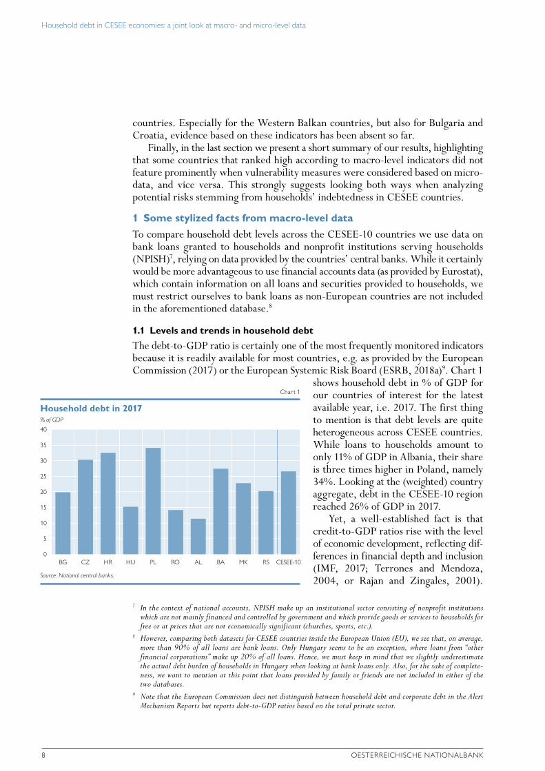
The debt-to-GDP ratio is certainly one of the most frequently monitored indicators because it is readily available for most countries, e.g. as provided by the European Commission (2017) or the European Systemic Risk Board (ESRB, 2018a)9. Chart 1
shows household debt in % of GDP for our countries of interest for the latest available year, i.e. 2017. The first thing to mention is that debt levels are quite heterogeneous across CESEE countries. While loans to households amount to only 11% of GDP in Albania, their share is three times higher in Poland, namely 34%. Looking at the (weighted) country aggregate, debt in the CESEE-10 region reached 26% of GDP in 2017.
Yet, a well-established fact is that credit-to-GDP ratios rise with the level of economic development, reflecting dif-ferences in financial depth and inclusion (IMF, 2017; Terrones and Mendoza, 2004, or Rajan and Zingales, 2001).
7 In the context of national accounts, NPISH make up an institutional sector consisting of nonprofit institutions which are not mainly financed and controlled by government and which provide goods or services to households for free or at prices that are not economically significant (churches, sports, etc.).
8 However, comparing both datasets for CESEE countries inside the European Union (EU), we see that, on average, more than 90% of all loans are bank loans. Only Hungary seems to be an exception, where loans from “other financial corporations” make up 20% of all loans. Hence, we must keep in mind that we slightly underestimate the actual debt burden of households in Hungary when looking at bank loans only. Also, for the sake of complete-ness, we want to mention at this point that loans provided by family or friends are not included in either of the two databases.
9 Note that the European Commission does not distinguish between household debt and corporate debt in the Alert Mechanism Reports but reports debt-to-GDP ratios based on the total private sector.
% of GDP
40
35
30
25
20
15
10
5
0BG CZ HR HU PL RO AL BA MK RS CESEE-10
Household debt in 2017
Chart 1
Source: National central banks.
Household debt in CESEE economies: a joint look at macro- and micro-level data
FOCUS ON EUROPEAN ECONOMIC INTEGRATION Q1/19 9
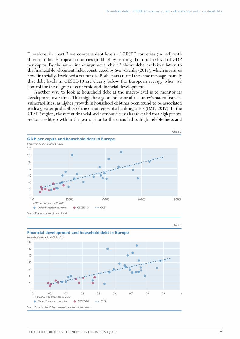
Therefore, in chart 2 we compare debt levels of CESEE countries (in red) with those of other European countries (in blue) by relating them to the level of GDP per capita. By the same line of argument, chart 3 shows debt levels in relation to the financial development index constructed by Svirydzenka (2016), which measures how financially developed a country is. Both charts reveal the same message, namely that debt levels in CESEE-10 are clearly below the European average when we control for the degree of economic and financial development.
Another way to look at household debt at the macro-level is to monitor its development over time. This might be a good indicator of a country’s macrofinancial vulnerabilities, as higher growth in household debt has been found to be associated with a greater probability of the occurrence of a banking crisis (IMF, 2017). In the CESEE region, the recent financial and economic crisis has revealed that high private sector credit growth in the years prior to the crisis led to high indebtedness and
Household debt in % of GDP, 2016
140
120
100
80
60
40
20
0
GDP per capita and household debt in Europe
Chart 2
Source: Eurostat, national central banks.
0 20,000 40,000 60,000 80,000GDP per capita in EUR, 2016
Other European countries CESEE-10 OLS
Household debt in % of GDP, 2016
140
120
100
80
60
40
20
0
Financial development and household debt in Europe
Chart 3
Source: Svirydzenka (2016), Eurostat, national central banks.
Financial Development Index, 2013
Other European countries CESEE-10 OLS
0.1 0.2 0.3 0.4 0.5 0.6 0.7 0.8 0.9 1
Household debt in CESEE economies: a joint look at macro- and micro-level data
10 OESTERREICHISCHE NATIONALBANK
Change in households’ debt-to-GDP ratio in percentage points
20
15
10
5
0
–5
–10
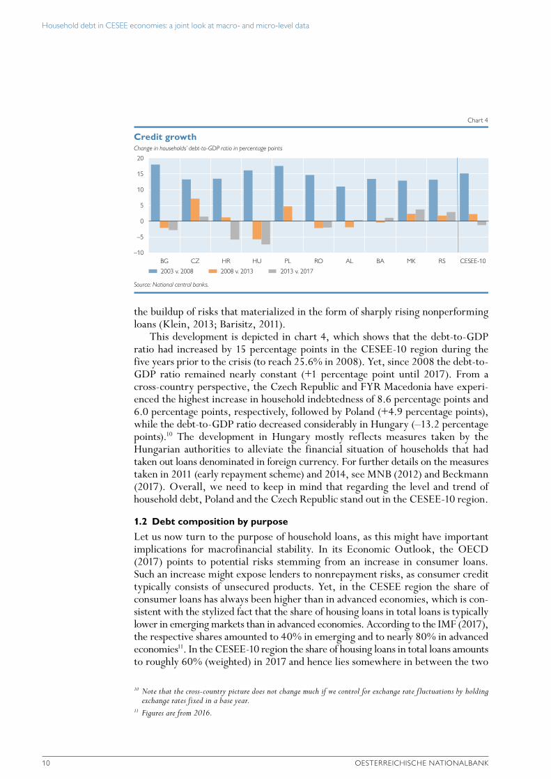
Credit growth
Chart 4
Source: National central banks.
2013 v. 20172003 v. 2008
BG CZ HR HU PL RO AL BA MK RS CESEE-10
2008 v. 2013
the buildup of risks that materialized in the form of sharply rising nonperforming loans (Klein, 2013; Barisitz, 2011).
This development is depicted in chart 4, which shows that the debt-to-GDP ratio had increased by 15 percentage points in the CESEE-10 region during the five years prior to the crisis (to reach 25.6% in 2008). Yet, since 2008 the debt-to-GDP ratio remained nearly constant (+1 percentage point until 2017). From a cross-country perspective, the Czech Republic and FYR Macedonia have experi-enced the highest increase in household indebtedness of 8.6 percentage points and 6.0 percentage points, respectively, followed by Poland (+4.9 percentage points), while the debt-to-GDP ratio decreased considerably in Hungary (–13.2 percentage points).10 The development in Hungary mostly reflects measures taken by the Hungarian authorities to alleviate the financial situation of households that had taken out loans denominated in foreign currency. For further details on the measures taken in 2011 (early repayment scheme) and 2014, see MNB (2012) and Beckmann (2017). Overall, we need to keep in mind that regarding the level and trend of household debt, Poland and the Czech Republic stand out in the CESEE-10 region.
1.2 Debt composition by purpose
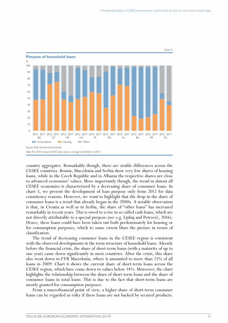
Let us now turn to the purpose of household loans, as this might have important implications for macrofinancial stability. In its Economic Outlook, the OECD (2017) points to potential risks stemming from an increase in consumer loans. Such an increase might expose lenders to nonrepayment risks, as consumer credit typically consists of unsecured products. Yet, in the CESEE region the share of consumer loans has always been higher than in advanced economies, which is con-sistent with the stylized fact that the share of housing loans in total loans is typically lower in emerging markets than in advanced economies. According to the IMF (2017), the respective shares amounted to 40% in emerging and to nearly 80% in advanced economies11. In the CESEE-10 region the share of housing loans in total loans amounts to roughly 60% (weighted) in 2017 and hence lies somewhere in between the two
10 Note that the cross-country picture does not change much if we control for exchange rate fluctuations by holding exchange rates fixed in a base year.
11 Figures are from 2016.
Household debt in CESEE economies: a joint look at macro- and micro-level data
FOCUS ON EUROPEAN ECONOMIC INTEGRATION Q1/19 11
country aggregates. Remarkably though, there are sizable differences across the CESEE countries. Bosnia, Macedonia and Serbia show very low shares of housing loans, while in the Czech Republic and in Albania the respective shares are close to advanced economies’ values. More importantly though, the trend in almost all CESEE economies is characterized by a decreasing share of consumer loans. In chart 5, we present the development of loan purpose only from 2012 for data consistency reasons. However, we want to highlight that the drop in the share of consumer loans is a trend that already began in the 2000s. A notable observation is that, in Croatia as well as in Serbia, the share of “other loans” has increased remarkably in recent years. This is owed to a rise in so called cash loans, which are not directly attributable to a special purpose (see e.g. Ljubaj and Petrovic, 2016). Hence, these loans could have been taken out both predominately for housing or for consumption purposes, which to some extent blurs the picture in terms of classification.
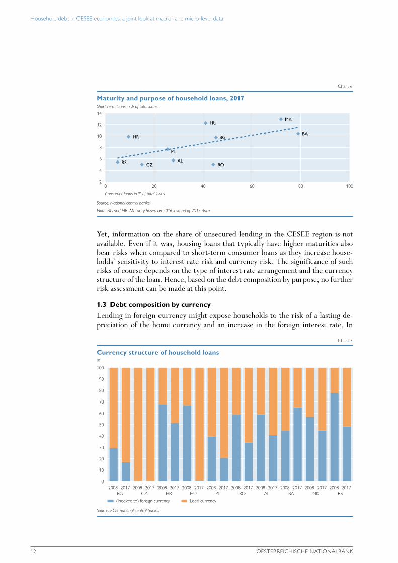
The trend of decreasing consumer loans in the CESEE region is consistent with the observed developments in the term structure of household loans. Already before the financial crisis, the share of short-term loans (with a maturity of up to one year) came down significantly in most countries. After the crisis, this share also went down in FYR Macedonia, where it amounted to more than 25% of all loans in 2009. Chart 6 shows the current share of short-term loans across the CESEE region, which have come down to values below 14%. Moreover, the chart highlights the relationship between the share of short-term loans and the share of consumer loans in total loans. This is due to the fact that short-term loans are mostly granted for consumption purposes.
From a macrofinancial point of view, a higher share of short-term consumer loans can be regarded as risky if these loans are not backed by secured products.
%
100
90
80
70
60
50
40
30
20
10
0
Purpose of household loans
Chart 5
Source: ECB, national central banks.
Note: RS: 2014 instead of 2012 data due to a change in definition in 2013.
OtherConsumption
BG2012 2017 2012 2017 2012 2017 2012 2017 2012 2017 2012 2017 2012 2017 2012 2017 2012 2017 2012 2017
CZ HR HU PL RO AL BA MK RS
Housing
Household debt in CESEE economies: a joint look at macro- and micro-level data
12 OESTERREICHISCHE NATIONALBANK
Yet, information on the share of unsecured lending in the CESEE region is not available. Even if it was, housing loans that typically have higher maturities also bear risks when compared to short-term consumer loans as they increase house-holds’ sensitivity to interest rate risk and currency risk. The significance of such risks of course depends on the type of interest rate arrangement and the currency structure of the loan. Hence, based on the debt composition by purpose, no further risk assessment can be made at this point.
1.3 Debt composition by currency
Lending in foreign currency might expose households to the risk of a lasting de-preciation of the home currency and an increase in the foreign interest rate. In
Short-term loans in % of total loans
14
12
10
8
6
4
2
Maturity and purpose of household loans, 2017
Chart 6
Source: National central banks.
Note: BG and HR: Maturity based on 2016 instead of 2017 data.
Consumer loans in % of total loans
BGHR
PL
ROCZ
HU
AL
BA
MK
RS
0 20 40 60 80 100
%
100
90
80
70
60
50
40
30
20
10
0
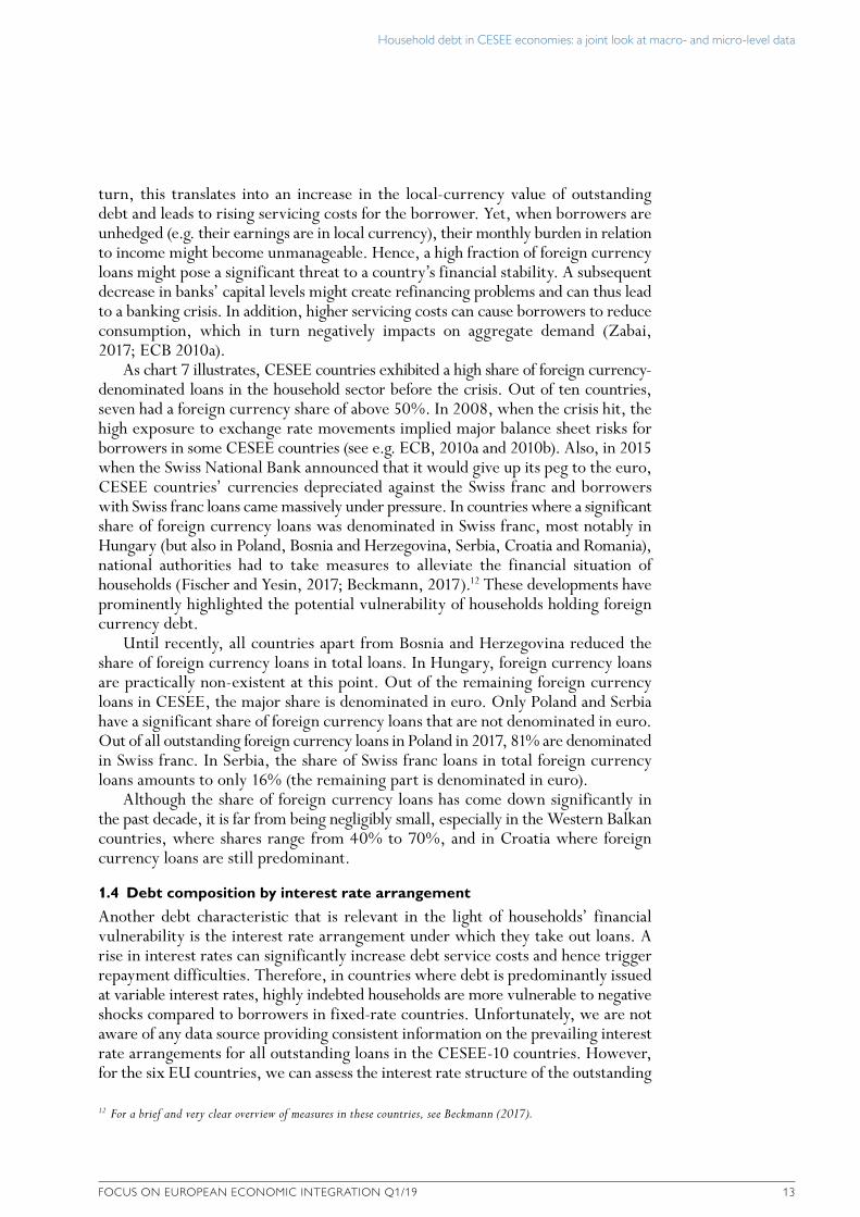
Currency structure of household loans
Chart 7
Source: ECB, national central banks.
(Indexed to) foreign currency
BG2008 2017 2008 2017 2008 2017 2008 2017 2008 2017 2008 2017 2008 2017 2008 2017 2008 2017 2008 2017
CZ HR HU PL RO AL BA MK RS
Local currency
Household debt in CESEE economies: a joint look at macro- and micro-level data
FOCUS ON EUROPEAN ECONOMIC INTEGRATION Q1/19 13
turn, this translates into an increase in the local-currency value of outstanding debt and leads to rising servicing costs for the borrower. Yet, when borrowers are unhedged (e.g. their earnings are in local currency), their monthly burden in relation to income might become unmanageable. Hence, a high fraction of foreign currency loans might pose a significant threat to a country’s financial stability. A subsequent decrease in banks’ capital levels might create refinancing problems and can thus lead to a banking crisis. In addition, higher servicing costs can cause borrowers to reduce consumption, which in turn negatively impacts on aggregate demand (Zabai, 2017; ECB 2010a).
As chart 7 illustrates, CESEE countries exhibited a high share of foreign currency- denominated loans in the household sector before the crisis. Out of ten countries, seven had a foreign currency share of above 50%. In 2008, when the crisis hit, the high exposure to exchange rate movements implied major balance sheet risks for borrowers in some CESEE countries (see e.g. ECB, 2010a and 2010b). Also, in 2015 when the Swiss National Bank announced that it would give up its peg to the euro, CESEE countries’ currencies depreciated against the Swiss franc and borrowers with Swiss franc loans came massively under pressure. In countries where a significant share of foreign currency loans was denominated in Swiss franc, most notably in Hungary (but also in Poland, Bosnia and Herzegovina, Serbia, Croatia and Romania), national authorities had to take measures to alleviate the financial situation of households (Fischer and Yesin, 2017; Beckmann, 2017).12 These developments have prominently highlighted the potential vulnerability of households holding foreign currency debt.
Until recently, all countries apart from Bosnia and Herzegovina reduced the share of foreign currency loans in total loans. In Hungary, foreign currency loans are practically non-existent at this point. Out of the remaining foreign currency loans in CESEE, the major share is denominated in euro. Only Poland and Serbia have a significant share of foreign currency loans that are not denominated in euro. Out of all outstanding foreign currency loans in Poland in 2017, 81% are denominated in Swiss franc. In Serbia, the share of Swiss franc loans in total foreign currency loans amounts to only 16% (the remaining part is denominated in euro).
Although the share of foreign currency loans has come down significantly in the past decade, it is far from being negligibly small, especially in the Western Balkan countries, where shares range from 40% to 70%, and in Croatia where foreign currency loans are still predominant.
1.4 Debt composition by interest rate arrangement
Another debt characteristic that is relevant in the light of households’ financial vulnerability is the interest rate arrangement under which they take out loans. A rise in interest rates can significantly increase debt service costs and hence trigger repayment difficulties. Therefore, in countries where debt is predominantly issued at variable interest rates, highly indebted households are more vulnerable to negative shocks compared to borrowers in fixed-rate countries. Unfortunately, we are not aware of any data source providing consistent information on the prevailing interest rate arrangements for all outstanding loans in the CESEE-10 countries. However, for the six EU countries, we can assess the interest rate structure of the outstanding
12 For a brief and very clear overview of measures in these countries, see Beckmann (2017).
Household debt in CESEE economies: a joint look at macro- and micro-level data
14 OESTERREICHISCHE NATIONALBANK
stock by looking at the interest rate type for newly granted loans to house-holds since 2007 (ECB Data Ware-house)13. Moreover, for Bosnia and Herzegovina and FYR Macedonia, this kind of information is available from 2012 onward, i.e. from the financial stability reports provided by these countries’ central banks (National Bank of the Republic of Macedonia, 2017; Central Bank of Bosnia and Herzegovina, 2018).
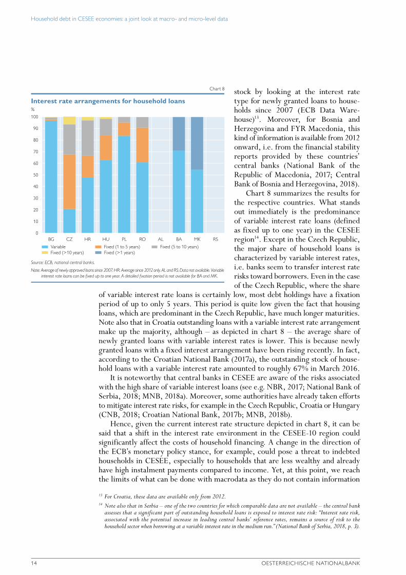
Chart 8 summarizes the results for the respective countries. What stands out immediately is the predominance of variable interest rate loans (defined as fixed up to one year) in the CESEE region14. Except in the Czech Republic, the major share of household loans is characterized by variable interest rates, i.e. banks seem to transfer interest rate risks toward borrowers. Even in the case of the Czech Republic, where the share
of variable interest rate loans is certainly low, most debt holdings have a fixation period of up to only 5 years. This period is quite low given the fact that housing loans, which are predominant in the Czech Republic, have much longer maturities. Note also that in Croatia outstanding loans with a variable interest rate arrangement make up the majority, although – as depicted in chart 8 – the average share of newly granted loans with variable interest rates is lower. This is because newly granted loans with a fixed interest arrangement have been rising recently. In fact, according to the Croatian National Bank (2017a), the outstanding stock of house-hold loans with a variable interest rate amounted to roughly 67% in March 2016.
It is noteworthy that central banks in CESEE are aware of the risks associated with the high share of variable interest loans (see e.g. NBR, 2017; National Bank of Serbia, 2018; MNB, 2018a). Moreover, some authorities have already taken efforts to mitigate interest rate risks, for example in the Czech Republic, Croatia or Hungary (CNB, 2018; Croatian National Bank, 2017b; MNB, 2018b).
Hence, given the current interest rate structure depicted in chart 8, it can be said that a shift in the interest rate environment in the CESEE-10 region could significantly affect the costs of household financing. A change in the direction of the ECB’s monetary policy stance, for example, could pose a threat to indebted households in CESEE, especially to households that are less wealthy and already have high instalment payments compared to income. Yet, at this point, we reach the limits of what can be done with macrodata as they do not contain information
13 For Croatia, these data are available only from 2012.14 Note also that in Serbia – one of the two countries for which comparable data are not available – the central bank
assesses that a significant part of outstanding household loans is exposed to interest rate risk: “Interest rate risk, associated with the potential increase in leading central banks’ reference rates, remains a source of risk to the household sector when borrowing at a variable interest rate in the medium run.” (National Bank of Serbia, 2018, p. 3).
%
100
90
80
70
60
50
40
30
20
10
0
Interest rate arrangements for household loans
Chart 8
Source: ECB, national central banks.
Note: Average of newly approved loans since 2007. HR: Average since 2012 only. AL and RS: Data not available. Variable interest rate loans can be fixed up to one year. A detailed fixation period is not available for BA and MK.
Variable
BG CZ HR HU PL RO AL BA MK RS
Fixed (1 to 5 years) Fixed (5 to 10 years)Fixed (>10 years) Fixed (>1 years)
Household debt in CESEE economies: a joint look at macro- and micro-level data
FOCUS ON EUROPEAN ECONOMIC INTEGRATION Q1/19 15
on the distribution of debt across e.g. wealth or income. Hence, in the next two sections we will rely on micro-based evidence to shed some more light on the dis-tribution of household debt in order to assess more accurately the potential risks inherent in households’ indebtedness across CESEE-10 countries.
2 The share of indebted households – a synthesis of macro- and microdata
In this section, we will use microdata to estimate the share of households that hold debt and relate these estimates to the amount of outstanding debt available from macrodata. Hence, by combining macro- with microdata we can assess debt levels per indebted household in each country. Following the same logic, we will also relate debt amounts to the average net income of indebted households. The resulting indicators will be expressed in units that better reflect the debt-servicing capacity of a country (as opposed to GDP for example).
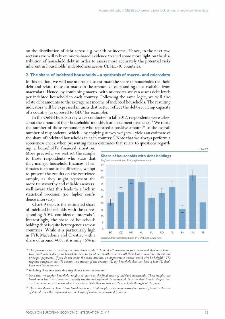
In the OeNB Euro Survey wave conducted in fall 2017, respondents were asked about the amount of their households’ monthly loan instalment payments.15 We relate the number of those respondents who reported a positive amount16 to the overall number of respondents, which – by applying survey weights – yields an estimate of the share of indebted households in each country17. Note that we always perform a robustness check when presenting mean estimates that relate to questions regard-ing a household’s financial situation. More precisely, we restrict the sample to those respondents who state that they manage household finances. If es-timates turn out to be different, we opt to present the results on the restricted sample, as they might represent the more trustworthy and reliable answers, well aware that this leads to a lack in statistical precision (i.e. higher confi-dence intervals).
Chart 9 depicts the estimated share of indebted households with the corre-sponding 90% confidence intervals18. Interestingly, the share of households holding debt is quite heterogenous across countries. While it is particularly high in FYR Macedonia and Croatia, with a share of around 40%, it is only 15% in
15 The questions that is asked by the interviewer reads: “Think of all members in your household that have loans. How much money does your household have to spend per month to service all these loans including interest and principal payments? If you do not know the exact amount, an approximate answer would also be helpful.” The response categories are: (1) amount in currency of the country, (2) my household does not have a loan (3) don’t know and (4) no answer.
16 Including those that state that they do not know the amount.17 Note that we employ household weights to arrive at the final share of indebted households. These weights are
based on at least two dimensions, namely the size and region of the household the respondent lives in. Proportions are in accordance with national statistics data. Note that we will use these weights throughout the paper.
18 The values shown in chart 10 are based on the restricted sample, as estimates turned out to be different in the case of Poland when the respondent was in charge of managing household finances.
% of total households and 90% confidence intervals
50
45
40
35
30
25
20
15
10
5
0
Share of households with debt holdings
Chart 9
Source: Author’s calculation based on OeNB Euro Survey data.
BG CZ HR HU PL RO AL BA MK RS
Household debt in CESEE economies: a joint look at macro- and micro-level data
16 OESTERREICHISCHE NATIONALBANK
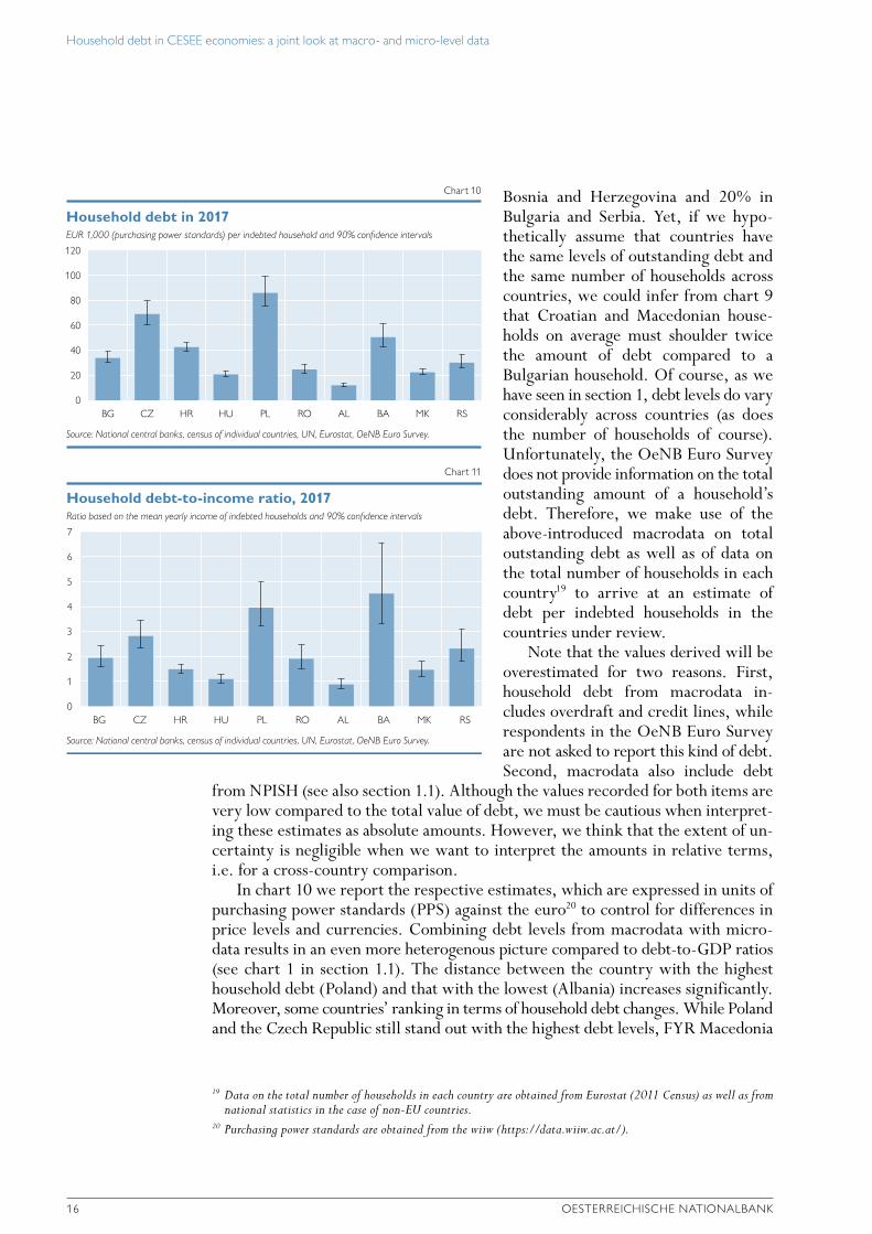
Bosnia and Herzegovina and 20% in Bulgaria and Serbia. Yet, if we hypo-thetically assume that countries have the same levels of outstanding debt and the same number of households across countries, we could infer from chart 9 that Croatian and Macedonian house-holds on average must shoulder twice the amount of debt compared to a Bulgarian household. Of course, as we have seen in section 1, debt levels do vary considerably across countries (as does the number of households of course). Unfortunately, the OeNB Euro Survey does not provide information on the total outstanding amount of a household’s debt. Therefore, we make use of the above-introduced macrodata on total outstanding debt as well as of data on the total number of households in each country19 to arrive at an estimate of debt per indebted households in the countries under review.
Note that the values derived will be overestimated for two reasons. First, household debt from macrodata in-cludes overdraft and credit lines, while respondents in the OeNB Euro Survey are not asked to report this kind of debt. Second, macrodata also include debt
from NPISH (see also section 1.1). Although the values recorded for both items are very low compared to the total value of debt, we must be cautious when interpret-ing these estimates as absolute amounts. However, we think that the extent of un-certainty is negligible when we want to interpret the amounts in relative terms, i.e. for a cross-country comparison.
In chart 10 we report the respective estimates, which are expressed in units of purchasing power standards (PPS) against the euro20 to control for differences in price levels and currencies. Combining debt levels from macrodata with micro-data results in an even more heterogenous picture compared to debt-to-GDP ratios (see chart 1 in section 1.1). The distance between the country with the highest household debt (Poland) and that with the lowest (Albania) increases significantly. Moreover, some countries’ ranking in terms of household debt changes. While Poland and the Czech Republic still stand out with the highest debt levels, FYR Macedonia
19 Data on the total number of households in each country are obtained from Eurostat (2011 Census) as well as from national statistics in the case of non-EU countries.
20 Purchasing power standards are obtained from the wiiw (https://data.wiiw.ac.at/).
EUR 1,000 (purchasing power standards) per indebted household and 90% confidence intervals
120
100
80
60
40
20
0
Household debt in 2017
Chart 10
Source: National central banks, census of individual countries, UN, Eurostat, OeNB Euro Survey.
BG CZ HR HU PL RO AL BA MK RS
Ratio based on the mean yearly income of indebted households and 90% confidence intervals
7
6
5
4
3
2
1
0
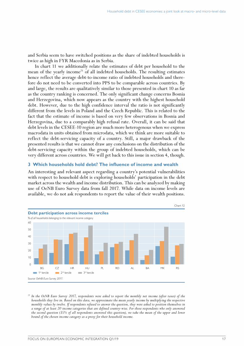
Household debt-to-income ratio, 2017
Chart 11
Source: National central banks, census of individual countries, UN, Eurostat, OeNB Euro Survey.
BG CZ HR HU PL RO AL BA MK RS
Household debt in CESEE economies: a joint look at macro- and micro-level data
FOCUS ON EUROPEAN ECONOMIC INTEGRATION Q1/19 17
and Serbia seem to have switched positions as the share of indebted households is twice as high in FYR Macedonia as in Serbia.
In chart 11 we additionally relate the estimates of debt per household to the mean of the yearly income21 of all indebted households. The resulting estimates hence reflect the average debt-to-income ratio of indebted households and there-fore do not need to be converted into PPS to be comparable across countries. By and large, the results are qualitatively similar to those presented in chart 10 as far as the country ranking is concerned. The only significant change concerns Bosnia and Herzegovina, which now appears as the country with the highest household debt. However, due to the high confidence interval the ratio is not significantly different from the levels in Poland and the Czech Republic. This is related to the fact that the estimate of income is based on very few observations in Bosnia and Herzegovina, due to a comparably high refusal rate. Overall, it can be said that debt levels in the CESEE-10 region are much more heterogenous when we express macrodata in units obtained from microdata, which we think are more suitable to reflect the debt-servicing capacity of a country. Still, a major drawback of the presented results is that we cannot draw any conclusions on the distribution of the debt-servicing capacity within the group of indebted households, which can be very different across countries. We will get back to this issue in section 4, though.
3 Which households hold debt? The influence of income and wealth
An interesting and relevant aspect regarding a country’s potential vulnerabilities with respect to household debt is exploring households’ participation in the debt market across the wealth and income distribution. This can be analyzed by making use of OeNB Euro Survey data from fall 2017. While data on income levels are available, we do not ask respondents to report the value of their wealth positions.
21 In the OeNB Euro Survey 2017, respondents were asked to report the monthly net income (after taxes) of the households they live in. Based on this data, we approximate the mean yearly income by multiplying the respective monthly values by twelve. If respondents refused to answer the question, they were asked to position themselves in a range of at least 20 income categories that are defined country-wise. For those respondents who only answered the second question (35% of all respondents answered this question), we take the mean of the upper and lower bound of the chosen income category as a proxy for their household income.
% of all households belonging to the relevant income category
60
50
40
30
20
10
0
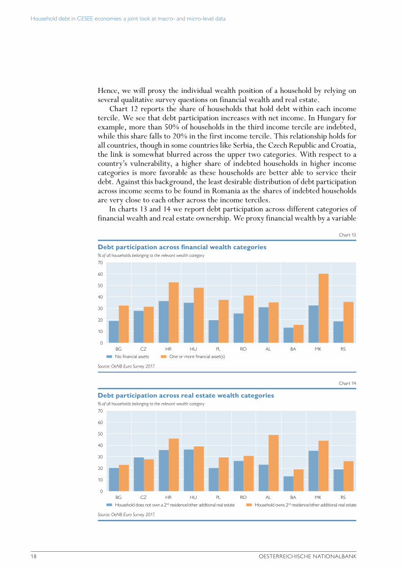
Debt participation across income terciles
Chart 12
Source: OeNB Euro Survey 2017.
1st tercile
BG CZ HR HU PL RO AL BA MK RS
2nd tercile 3rd tercile
Household debt in CESEE economies: a joint look at macro- and micro-level data
18 OESTERREICHISCHE NATIONALBANK
Hence, we will proxy the individual wealth position of a household by relying on several qualitative survey questions on financial wealth and real estate.
Chart 12 reports the share of households that hold debt within each income tercile. We see that debt participation increases with net income. In Hungary for example, more than 50% of households in the third income tercile are indebted, while this share falls to 20% in the first income tercile. This relationship holds for all countries, though in some countries like Serbia, the Czech Republic and Croatia, the link is somewhat blurred across the upper two categories. With respect to a country’s vulnerability, a higher share of indebted households in higher income categories is more favorable as these households are better able to service their debt. Against this background, the least desirable distribution of debt participation across income seems to be found in Romania as the shares of indebted households are very close to each other across the income terciles.
In charts 13 and 14 we report debt participation across different categories of financial wealth and real estate ownership. We proxy financial wealth by a variable
% of all households belonging to the relevant wealth category
70
60
50
40
30
20
10
0
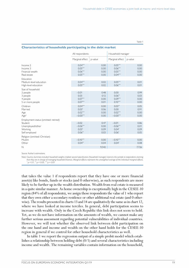
Debt participation across financial wealth categories
Chart 13
Source: OeNB Euro Survey 2017.
No financial assets
BG CZ HR HU PL RO AL BA MK RS
One or more financial asset(s)
% of all households belonging to the relevant wealth category
70
60
50
40
30
20
10
0
Debt participation across real estate wealth categories
Chart 14
Source: OeNB Euro Survey 2017.
Household does not own a 2nd residence/other additional real estate
BG CZ HR HU PL RO AL BA MK RS
Household owns 2nd residence/other additional real estate
Household debt in CESEE economies: a joint look at macro- and micro-level data
FOCUS ON EUROPEAN ECONOMIC INTEGRATION Q1/19 19
that takes the value 1 if respondents report that they have one or more financial asset(s) like bonds, funds or stocks (and 0 otherwise), as such respondents are more likely to be further up in the wealth distribution. Wealth from real estate is measured in a quite similar manner. As home ownership is exceptionally high in the CESEE-10 region (84% of all respondents), we assign those respondents the value of 1 who report that they own either a secondary residence or other additional real estate (and 0 other-wise). The results presented in charts 13 and 14 are qualitatively the same as in chart 12, where we have looked at income terciles. In general, debt participation seems to increase with wealth. Only in the Czech Republic this link does not seem to hold. Yet, as we do not have information on the amounts of wealth, we cannot make any further serious assessment regarding potential vulnerabilities of individual countries. However, we will test whether the observed link between debt participation on the one hand and income and wealth on the other hand holds for the CESEE-10 region in general if we control for other household characteristics as well.
In table 1 we report the regression output of a simple probit model which estab-lishes a relationship between holding debt (0/1) and several characteristics including income and wealth. The remaining variables contain information on the household,
Table 1
Characteristics of households participating in the debt market
All respondents Household manager
Marginal effect p-value Marginal effect p-value
Income 2 0.04*** 0.00 0.05*** 0.00Income 3 0.05*** 0.00 0.06*** 0.00Financial wealth 0.06*** 0.00 0.05*** 0.00Real estate 0.05*** 0.00 0.04*** 0.00
EducationMedium-level education 0.04*** 0.02 0.05*** 0.01High-level education 0.05*** 0.02 0.06*** 0.01
Size of household2 people –0.01 0.48 0.00 0.993 people 0.03 0.12 0.06** 0.034 people 0.07*** 0.00 0.09*** 0.005 or more people 0.07*** 0.01 0.10*** 0.00
Children 0.04*** 0.00 0.03** 0.05Married 0.03* 0.06 0.00 0.91Age 0.02*** 0.00 0.02*** 0.00Age2 –0.00*** 0.00 –0.00*** 0.00
Employment status (omitted: retired)Student –0.02 0.47 –0.01 0.86Unemployed/other –0.06*** 0.00 –0.06*** 0.01Working 0.03* 0.09 0.04* 0.09Self-employed 0.06** 0.03 0.06* 0.05
Religion (omitted: Christian)Muslim –0.10*** 0.00 –0.10*** 0.00Other 0.04** 0.04 0.04* 0.08
N 9,542 7,726
Source: Author’s estimations.
Note: Country dummies included; household weights implied; second specification (household manager) restricts the sample to respondents claiming that they are in charge of managing household finances. Marginal effects represent the unweighted average of the individual marginal effects. * p < 0.1, ** p < 0.05, *** p < 0.01
Household debt in CESEE economies: a joint look at macro- and micro-level data
20 OESTERREICHISCHE NATIONALBANK
like the number of household members and whether there are children in the house-hold. Also, we include individual respondent characteristics that might potentially interact with household debt, like education, age, employment status and religion (Costa and Farinha, 2012). We also consider country dummies to control for the individual debt participation levels across the region. At the top of the list in table 1, we report marginal effects of the second and the third income tercile. The results strongly support the positive link we have seen in chart 12. This is also true for both wealth proxies (financial wealth and real estate), which are highly significant as well. Hence, we can conclude that debt participation in CESEE-10 countries increases with a household’s income and wealth position.
4 Potentially vulnerable households
In the previous section we saw that debt participation increases with income and wealth, which is in itself a favorable outcome, as wealthier households might be regarded as less vulnerable in terms of their repayment capacities. So far, we have looked at the group of all households in the different economies to explore the dis-tribution of debt participation across income and wealth. In this section, we will solely focus on the group of indebted households and will try to assess the share of those households that are potentially vulnerable.
4.1 Indebted households with “bad” characteristics
Financial stability risks originating from indebted households materialize in the form of nonperforming loans, i.e. the inability of a significant group of households to meet its loan obligations. Hence, one way to identify potentially vulnerable households is to look at those characteristics of borrowers that increase their prob-ability of getting into repayment difficulties. This is exactly the approach taken in this subsection. More specifically, based on OeNB Euro Survey data from fall 2017, we will assess the share of vulnerable households in each of the ten CESEE economies by classifying indebted households according to specific characteristics. In doing so, we rely on the findings by Beckmann et al. (2012), who empirically identify two important sociodemographic factors that determine the probability of being in loan arrears. In particular, they find that households in the CESEE region are more likely to be in arrears on loan repayments when their income is lower and when the respondent exhibits a comparably low level of educational attainment. Another interesting finding worth highlighting is that households that experienced an income shock during the previous 12 months are much more likely to get into repayment difficulties. Here, we make use of these findings and report estimates of the share of households exhibiting those characteristics.
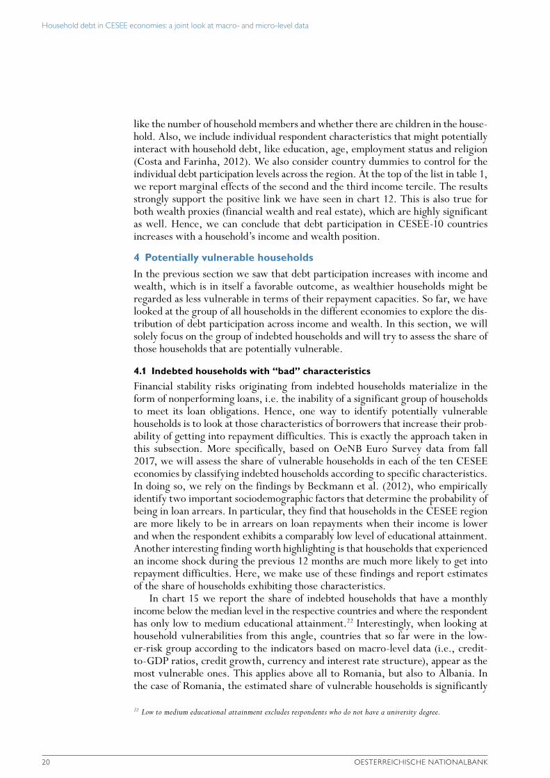
In chart 15 we report the share of indebted households that have a monthly income below the median level in the respective countries and where the respondent has only low to medium educational attainment.22 Interestingly, when looking at household vulnerabilities from this angle, countries that so far were in the low-er-risk group according to the indicators based on macro-level data (i.e., credit-to-GDP ratios, credit growth, currency and interest rate structure), appear as the most vulnerable ones. This applies above all to Romania, but also to Albania. In the case of Romania, the estimated share of vulnerable households is significantly
22 Low to medium educational attainment excludes respondents who do not have a university degree.
Household debt in CESEE economies: a joint look at macro- and micro-level data
FOCUS ON EUROPEAN ECONOMIC INTEGRATION Q1/19 21
higher compared to the regional average (unweighted). In contrast Bosnia and Herzegovina, Bulgaria and Hungary show significantly lower shares.
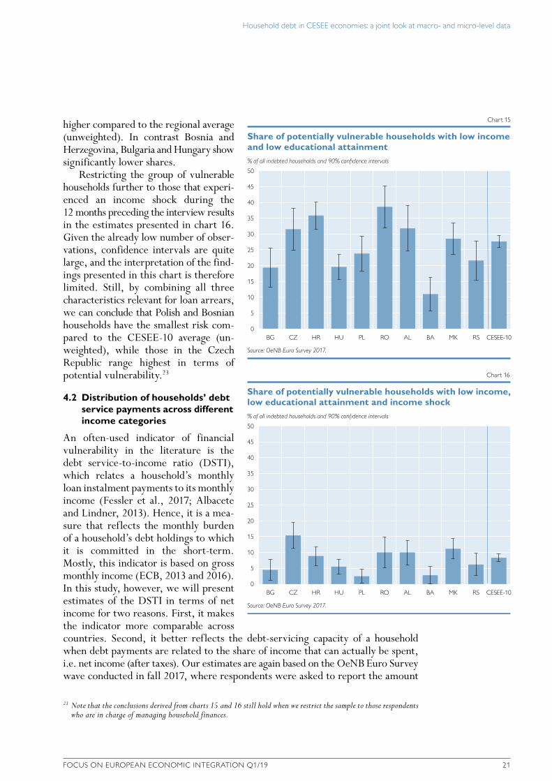
Restricting the group of vulnerable households further to those that experi-enced an income shock during the 12 months preceding the interview results in the estimates presented in chart 16. Given the already low number of obser-vations, confidence intervals are quite large, and the interpretation of the find-ings presented in this chart is therefore limited. Still, by combining all three characteristics relevant for loan arrears, we can conclude that Polish and Bosnian households have the smallest risk com-pared to the CESEE-10 average (un-weighted), while those in the Czech Republic range highest in terms of potential vulnerability.23
4.2 Distribution of households’ debt service payments across different income categories
An often-used indicator of financial vulnerability in the literature is the debt service-to-income ratio (DSTI), which relates a household’s monthly loan instalment payments to its monthly income (Fessler et al., 2017; Albacete and Lindner, 2013). Hence, it is a mea-sure that reflects the monthly burden of a household’s debt holdings to which it is committed in the short-term. Mostly, this indicator is based on gross monthly income (ECB, 2013 and 2016). In this study, however, we will present estimates of the DSTI in terms of net income for two reasons. First, it makes the indicator more comparable across countries. Second, it better reflects the debt-servicing capacity of a household when debt payments are related to the share of income that can actually be spent, i.e. net income (after taxes). Our estimates are again based on the OeNB Euro Survey wave conducted in fall 2017, where respondents were asked to report the amount
23 Note that the conclusions derived from charts 15 and 16 still hold when we restrict the sample to those respondents who are in charge of managing household finances.
% of all indebted households and 90% confidence intervals
50
45
40
35
30
25
20
15
10
5
0
Share of potentially vulnerable households with low income and low educational attainment
Chart 15
Source: OeNB Euro Survey 2017.
BG CZ HR HU PL RO AL BA MK RS CESEE-10
% of all indebted households and 90% confidence intervals
50
45
40
35
30
25
20
15
10
5
0
Share of potentially vulnerable households with low income, low educational attainment and income shock
Chart 16
Source: OeNB Euro Survey 2017.
BG CZ HR HU PL RO AL BA MK RS CESEE-10
Household debt in CESEE economies: a joint look at macro- and micro-level data
22 OESTERREICHISCHE NATIONALBANK
spent per month to service all loans held by household members (including interest and principal payments)24. We relate these payments to the household’s monthly net income also reported by the respondent to calculate the ratio.
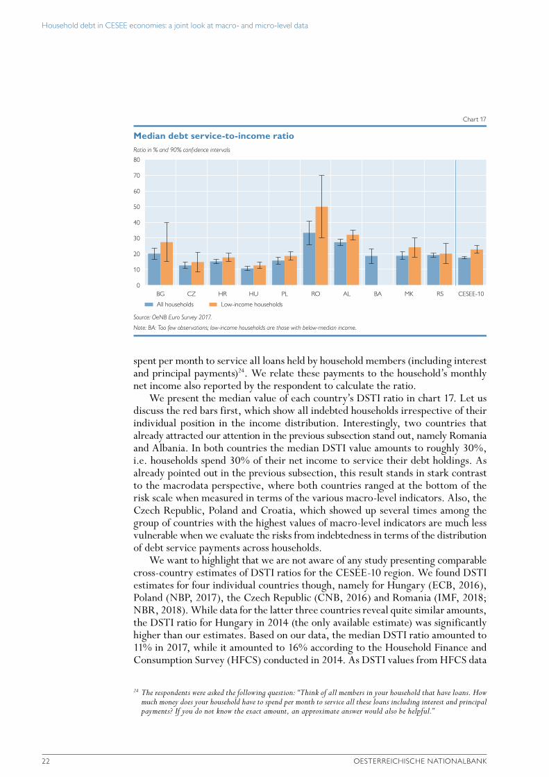
We present the median value of each country’s DSTI ratio in chart 17. Let us discuss the red bars first, which show all indebted households irrespective of their individual position in the income distribution. Interestingly, two countries that already attracted our attention in the previous subsection stand out, namely Romania and Albania. In both countries the median DSTI value amounts to roughly 30%, i.e. households spend 30% of their net income to service their debt holdings. As already pointed out in the previous subsection, this result stands in stark contrast to the macrodata perspective, where both countries ranged at the bottom of the risk scale when measured in terms of the various macro-level indicators. Also, the Czech Republic, Poland and Croatia, which showed up several times among the group of countries with the highest values of macro-level indicators are much less vulnerable when we evaluate the risks from indebtedness in terms of the distribution of debt service payments across households.
We want to highlight that we are not aware of any study presenting comparable cross-country estimates of DSTI ratios for the CESEE-10 region. We found DSTI estimates for four individual countries though, namely for Hungary (ECB, 2016), Poland (NBP, 2017), the Czech Republic (CNB, 2016) and Romania (IMF, 2018; NBR, 2018). While data for the latter three countries reveal quite similar amounts, the DSTI ratio for Hungary in 2014 (the only available estimate) was significantly higher than our estimates. Based on our data, the median DSTI ratio amounted to 11% in 2017, while it amounted to 16% according to the Household Finance and Consumption Survey (HFCS) conducted in 2014. As DSTI values from HFCS data
24 The respondents were asked the following question: “Think of all members in your household that have loans. How much money does your household have to spend per month to service all these loans including interest and principal payments? If you do not know the exact amount, an approximate answer would also be helpful.”
Ratio in % and 90% confidence intervals
80
70
60
50
40
30
20
10
0
Median debt service-to-income ratio
Chart 17
Source: OeNB Euro Survey 2017.
Note: BA: Too few observations; low-income households are those with below-median income.
BG CZ HR HU PL RO AL BA MK RS CESEE-10
All households Low-income households
Household debt in CESEE economies: a joint look at macro- and micro-level data
FOCUS ON EUROPEAN ECONOMIC INTEGRATION Q1/19 23
are based on gross income, the difference is even larger as it seems to be at the first glance (i.e. at least 10 percentage points). The significant decrease in the median DSTI seems to reflect the debt restructuring measures taken by the central bank of Hungary at the beginning of 2015 to address the issue of the high share of non-performing loans and the associated risks to financial stability back then. These measures were aimed at reducing repayment instalments for debt holders. According to estimates by the central bank of Hungary, the measures taken reduced borrowers’ loan instalment payments by 25% to 30% and by 16% in the case of nonperforming debtors (MNB, 2015). Hence, DSTI estimates based on the OeNB Euro Survey wave conducted in fall 2017 point to the fact that these measures had a lasting impact on the debt-servicing capacity of households.
One of the main conclusions drawn by the IMF in its special issue chapter on household debt in 2017 (IMF, 2017) was that lower-income households typically have higher DSTI ratios, which makes them more vulnerable to adverse shocks than higher-income households. In order to see whether this is true for the CESEE countries under review, we have estimated the median DSTI ratios for the low-income group of indebted households (i.e. below-median income), which are depicted by the blue bars in chart 17.25 According to our estimates, DSTI ratios are indeed higher for the lower-income group of households. The differences are not statistically significant though, which might certainly be related to the low number of observations. In the case of Bosnia and Herzegovina, we have even too few observations to compute reliable estimates for this subgroup. However, if we look at the whole region (unweighted CESEE-10), our estimates support the findings by the IMF that low-income house-holds are more vulnerable. This conclusion even holds, when we control for other household characteristics.
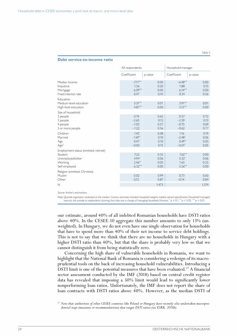
In table 2 we report estimates from a quantile regression of DSTI ratios (evaluated at the median) on a variable that indicates whether the household’s position in the income distribution is below or above the relevant country’s median income. We perform the regression on the overall CESEE sample including country dummies to control for the heterogenous DSTI levels across the region. The estimates reveal that the median DSTI ratio is 7 percentage points higher for low-income households. Another interesting finding is that DSTI ratios are higher for mortgage loans than for consumer loans. This result is also observed in the euro area, where the DSTI ratio for all loans amounted to 13.5% and that for mortgages to 15.8% in 2014 (ECB, 2016).26
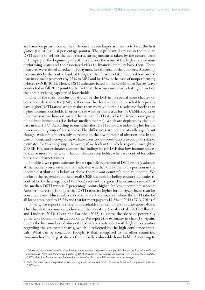
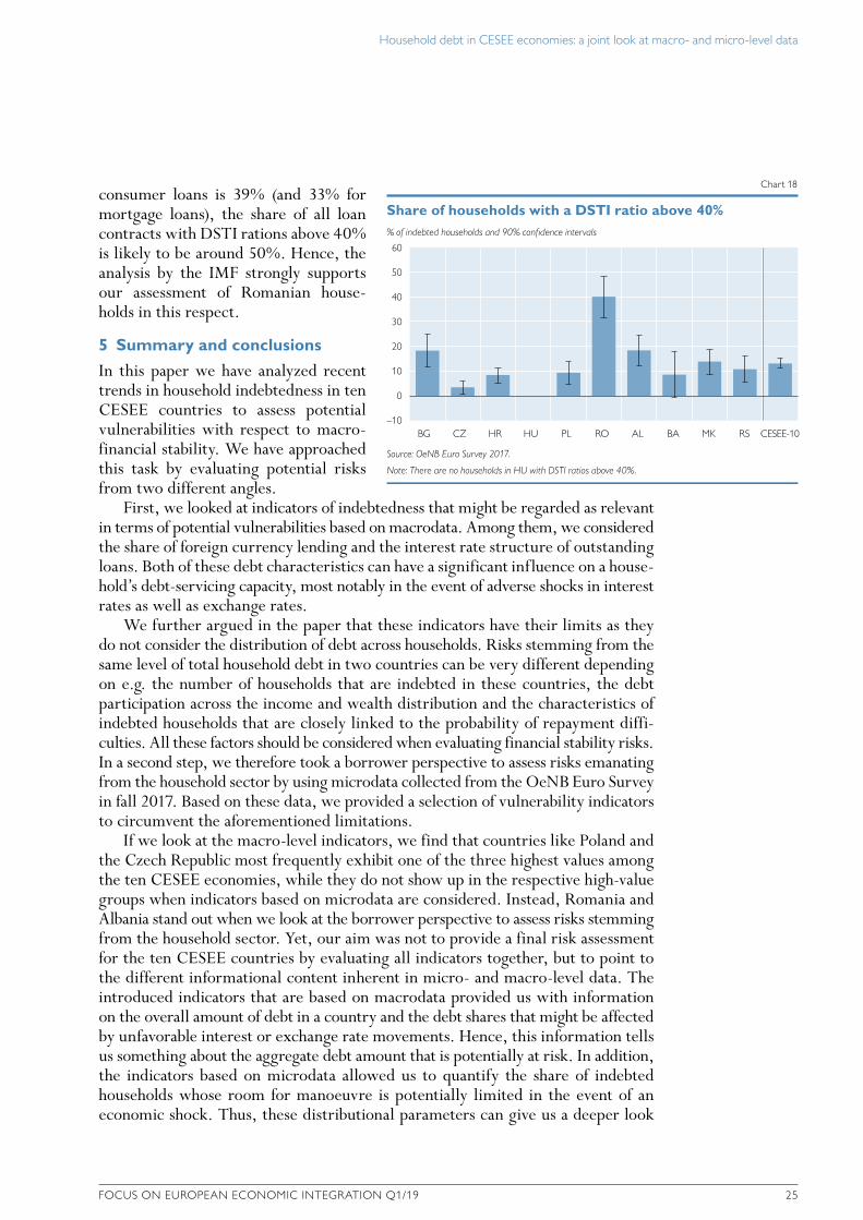
Finally, we report the share of households that exhibit DSTI ratios above 40%. This threshold is commonly chosen in the literature (Fessler et al., 2017; Albacete and Lindner, 2013; Costa and Farinha, 2012) to assess the share of potentially vulnerable households in an economy. We report the estimates in chart 18. Again, due to the low number of observations we are confronted with high uncertainties regarding the estimated shares, which is reflected by the high confidence inter-vals. What can be concluded though, is that, compared to the other countries, Romania has the largest share of potentially vulnerable households. According to
25 Unfortunately, a more detailed distribution across income categories is not feasible due to the limited number of observations. Note that the average number of DSTI observations per country amounts to 195. Hence, the calculated DSTI values for the low-income households are based on less than 100 observations on average.
26 Note that this value is reported on the basis of gross income (ECB, 2016) and is hence not comparable with our DSTI levels.
Household debt in CESEE economies: a joint look at macro- and micro-level data
24 OESTERREICHISCHE NATIONALBANK
our estimate, around 40% of all indebted Romanian households have DSTI ratios above 40%. In the CESEE-10 aggregate this number amounts to only 13% (un-weighted). In Hungary, we do not even have one single observation for households that have to spend more than 40% of their net income to service debt holdings. This is not to say that we think that there are no households in Hungary with a higher DSTI ratio than 40%, but that the share is probably very low so that we cannot distinguish it from being statistically zero.
Concerning the high share of vulnerable households in Romania, we want to highlight that the National Bank of Romania is considering a redesign of its macro-prudential tools on the back of increasing household vulnerabilities. Introducing a DSTI limit is one of the potential measures that have been evaluated.27 A financial sector assessment conducted by the IMF (2018) based on central credit register data has revealed that imposing a 50% limit would lead to significantly lower nonperforming loan ratios. Unfortunately, the IMF does not report the share of loan contracts with DSTI ratios above 40%. However, as the median DSTI of
27 Note that authorities of other CESEE countries like Poland or Hungary have recently also undertaken macropru-dential steps (measures or recommendations) that target DSTI ratios (see ESRB, 2018b).
Table 2
Debt service-to-income ratio
All respondents Household manager
Coefficient p-value Coefficient p-value
Median income –7.17*** 0.00 –6.48*** 0.00Impulsive 1.56 0.20 1.88 0.15Mortgage 6.09*** 0.00 6.14*** 0.00Fixed interest rate 0.47 0.43 0.34 0.56
EducationMedium-level education 3.51*** 0.01 3.91*** 0.01High-level education 4.87*** 0.00 5.13*** 0.00
Size of household2 people 0.74 0.65 0.57 0.723 people –2.65 0.12 –2.59 0.134 people –1.03 0.57 –0.75 0.695 or more people –1.22 0.56 –0.62 0.77
Children 1.42* 0.08 1.16 0.19Married –1.87* 0.10 –2.48* 0.06Age 0.41* 0.10 0.49** 0.03Age2 –0.00 0.15 –0.01* 0.05
Employment status (omitted: retired)Student 7.22 0.53 7.62*** 0.00Unemployed/other 4.94* 0.06 5.32* 0.06Working 2.46** 0.05 1.65 0.25Self-employed 6.32*** 0.00 5.56*** 0.00
Religion (omitted: Christian)Muslim 0.02 0.99 0.73 0.60Other 0.12 0.87 –0.14 0.84
N 1,473 1,374
Source: Author’s estimations.
Note: Quantile regression, evaluated at the median. Country dummies included; household weights implied; second specification (household manager) restricts the sample to respondents claiming that they are in charge of managing household finances. * p < 0.1, ** p < 0.05, *** p < 0.01
Household debt in CESEE economies: a joint look at macro- and micro-level data
FOCUS ON EUROPEAN ECONOMIC INTEGRATION Q1/19 25
consumer loans is 39% (and 33% for mortgage loans), the share of all loan contracts with DSTI rations above 40% is likely to be around 50%. Hence, the analysis by the IMF strongly supports our assessment of Romanian house-holds in this respect.
5 Summary and conclusions
In this paper we have analyzed recent trends in household indebtedness in ten CESEE countries to assess potential vulnerabilities with respect to macro-financial stability. We have approached this task by evaluating potential risks from two different angles.
First, we looked at indicators of indebtedness that might be regarded as relevant in terms of potential vulnerabilities based on macrodata. Among them, we considered the share of foreign currency lending and the interest rate structure of outstanding loans. Both of these debt characteristics can have a significant influence on a house-hold’s debt-servicing capacity, most notably in the event of adverse shocks in interest rates as well as exchange rates.
We further argued in the paper that these indicators have their limits as they do not consider the distribution of debt across households. Risks stemming from the same level of total household debt in two countries can be very different depending on e.g. the number of households that are indebted in these countries, the debt participation across the income and wealth distribution and the characteristics of indebted households that are closely linked to the probability of repayment diffi-culties. All these factors should be considered when evaluating financial stability risks. In a second step, we therefore took a borrower perspective to assess risks emanating from the household sector by using microdata collected from the OeNB Euro Survey in fall 2017. Based on these data, we provided a selection of vulnerability indicators to circumvent the aforementioned limitations.
If we look at the macro-level indicators, we find that countries like Poland and the Czech Republic most frequently exhibit one of the three highest values among the ten CESEE economies, while they do not show up in the respective high-value groups when indicators based on microdata are considered. Instead, Romania and Albania stand out when we look at the borrower perspective to assess risks stemming from the household sector. Yet, our aim was not to provide a final risk assessment for the ten CESEE countries by evaluating all indicators together, but to point to the different informational content inherent in micro- and macro-level data. The introduced indicators that are based on macrodata provided us with information on the overall amount of debt in a country and the debt shares that might be affected by unfavorable interest or exchange rate movements. Hence, this information tells us something about the aggregate debt amount that is potentially at risk. In addition, the indicators based on microdata allowed us to quantify the share of indebted households whose room for manoeuvre is potentially limited in the event of an economic shock. Thus, these distributional parameters can give us a deeper look
% of indebted households and 90% confidence intervals
60
50
40
30
20
10
0
–10
Share of households with a DSTI ratio above 40%
Chart 18
Source: OeNB Euro Survey 2017.
Note: There are no households in HU with DSTI ratios above 40%.
BG CZ HR HU PL RO AL BA MK RS CESEE-10
Household debt in CESEE economies: a joint look at macro- and micro-level data
26 OESTERREICHISCHE NATIONALBANK
into the likelihood of default. Summing up, if we were to highlight the most interesting and general conclusion of this paper, we would need to stress that the assessment of macroprudential vulnerabilities across countries can be very diverse depending on the angle of view. While we do not argue in favor of one particular view, we certainly want to emphasize the importance of looking in both directions as each of the two approaches has its merits.
Our analysis of macrofinancial risks was purely descriptive. Hence, a potential avenue for future research would be to combine the presented indicators from both data sources in a more advanced and analytical framework to evaluate potential risks from household indebtedness. This is certainly a challenge as survey data are often compiled at relatively long intervals resulting in a mismatch of frequencies between indicators from macro- and micro-level data. Yet, as the OeNB Euro Survey is conducted on a yearly basis it might be possible to use future surveys to overcome this shortcoming.
References
Albacete, N. and P. Lindner. 2013. Household Vulnerability in Austria – A Microeconomic Analysis Based on the Household Finance and Consumption Survey. In: OeNB. Financial Stability Report 25. 57–73.
André, C. 2016. Household Debt in OECD Countries: Stylised Facts and Policy Issues. In: OECD Economics Department Working Papers 1277.
Barisitz, S. 2011. Nonperforming Loans in CESEE – What Do They Comprise? In: OeNB. Focus on European Economic Integration Q4/11. 46–68.
Beck, T., R. Levine and N. Loayza. 2000. Finance and sources of growth. In: Journal of Financial Economics 58 (1–2). 261–300.
Beck, T., B. Büyüükkarabacak, F. Rioja and N. Valev. 2012. Who Gets the Credit? And Does It Matter? Household vs. Firm Lending Across Countries. In: The B.E. Journal of Macro-economics 12 (1). 1-46.
Beckmann, E. 2017. How does foreign currency debt relief affect households’ loan demand? Evidence from the OeNB Euro Survey in CESEE. In: OeNB. Focus on European Economic Inte-gration Q1/17. 8–32.
Beckmann, E., J. Fidrmuc and H. Stix. 2012. Foreign Currency Loans and Loan Arrears of Households in Central and Eastern Europe. In: OeNB Working Paper 181.
Central Bank of Bosnia and Herzegovina. 2018. Financial Stability Report 2017.Chmeler, A. 2013. Household Debt and the European Crisis. In: ECRI Research Report 13.CNB. 2016. Financial Stability Report 2015/2016.CNB. 2018. Financial Stability Report 2017/2018.Comunale, M., M. Eller and M. Lahnsteiner. 2018. Has private sector credit in CESEE
approached levels justified by fundamentals? A post-crisis assessment. In: OeNB. Focus on Euro-pean Economic Integration Q3/18. 141–154.
Costa, S. and L. Farinha. 2012. Households’ indebtedness: A microeconomic analysis based in the results of the households’ financial and consumption survey. In: Banco de Portugal. Financial Stability Report. 133–157.
Croatian National Bank. 2017a. Financial Stability No. 18.Croatian National Bank. 2017b. Analytical annex to Recommendation to mitigate interest rate
and interest rate-induced credit risk in long-term consumer loans. Hrvatska Narodna Banka, September 2017.
Household debt in CESEE economies: a joint look at macro- and micro-level data
FOCUS ON EUROPEAN ECONOMIC INTEGRATION Q1/19 27
ECB. 2010a. Addressing risks associated with foreign currency lending in EU Member States. In: Financial Stability Review June 2010 (IV). 161–169.
ECB. 2010b. The impact of the financial crisis on the Central and Eastern European Countries. ECB Monthly Bulletin. July 2010.
ECB. 2013. The Eurosystem Household Finance and Consumption Survey: results from the first wave. In: Statistics Paper Series No. 2.
ECB. 2016. The Household Finance and Consumption Survey: results from the second wave. In: Statistics Paper Series No. 18.
European Commission. 2017. Alert Mechanism Report 2018. https://ec.europa.eu/info/publi-cations/2018-european-semester-alert-mechanism-report_en
ESRB. 2018a. Annual Report 2017. https://www.esrb.europa.eu/pub/pdf/ar/2018/esrb.ar2017.en.pdfESRB. 2018b. A Review of Macroprudential Policy in the EU in 2017. April 2018.Fessler, P., E. List and T. Messner. 2017. How financially vulnerable are CESEE households?
An Austrian perspective on its neighbors. In: OeNB. Focus on European Economic Integration Q2/17. 58–79.
Fiorante, A. 2011. Foreign currency indebtedness: a potential systemic risk in emerging Europe. In: ECRI Commentary No. 8.
Fischer, A. and P. Yesin. 2017. Loan conversions and currency mismatches: Undoing Swiss franc mortgage loans in Eastern Europe (first draft). www.pinaryesin.com
IMF. 2017. Household debt and financial stability. In: Global Financial Stability Report: Is growth at risk? 53–89.
IMF. 2018. Romania – Financial Sector Assessment Program (Technical note – calibration of a DSTI limit in Romania – evidence from microdata). In: IMF Country Report No. 18/161.
Klein, N. 2013. Non-Performing Loans in CESEE: Determinants and Impact on Macroeconomic Performance. IMF Working Paper 13/72.
Lahnsteiner, M. 2012. Private Sector Debt in CESEE EU Member States. In: OeNB. Focus on European Economic Integration Q3/12. 30–47.
Ljubaj, I. and S. Petrović. 2016. A Note on Kuna Lending. In: Croatian National Bank. Surveys S-21. Mian, A. and A. Sufi. 2011. House Prices, Home Equity-Based Borrowing, and the U.S. House-
hold Leverage Crisis. In: American Economic Review 101 (5). 2132–2156.MNB. 2012. Report on Financial Stability. November 2012. Magyar Nemzeti Bank, Budapest.MNB. 2015. Comprehensive analysis of the nonperforming household mortgage portfolio using
micro-level data, MNB occasional papers, OP special issue. Magyar Nemzeti Bank, Budapest.MNB. 2018a. Financial Stability Report 2018. May. Magyar Nemzeti Bank, Budapest.MNB. 2018b. The amendment of the debt cap rules has been published. Press release by Magyar
Nemzeti Bank, Budapest. https://www.mnb.hu/en/pressroom/press-releases/press-releases-2018/the-amendment-of-the-debt-cap-rules-has-been-published
National Bank of Serbia. 2018. Annual Financial Stability Report 2017.National Bank of the Republic of Macedonia. 2017. Financial stability report for the Republic
of Macedonia in 2016. NBP. 2017. Household Wealth and Debt in Poland – Report of 2016 survey of the National Bank
of Poland. NBR. 2017. Financial Stability Report. December 2017. National Bank of Romania, Bucharest.NBR. 2018. Financial Stability Report. June 2018. National Bank of Romania, Bucharest.OECD. 2017. Resilience in a time of high debt. In: OECD Economic Outlook 2017 (2). 55–96.Rajan, R. and L. Zingales. 2001. Financial Systems, Industrial Structures, and Growth. In:
Oxford Review of Economic Policy 17(4). 467–482.
Household debt in CESEE economies: a joint look at macro- and micro-level data
28 OESTERREICHISCHE NATIONALBANK
Svirydzenka, K. 2016. Introducing a New Broad-based Index of Financial Development. In: IMF Working Paper 16/5.
Terrones, M. and E. Mendoza. 2004. Are Credit Booms in Emerging Markets a Concern? In: International Monetary Fund. World Economic Outlook, Chapter IV. Washington.
Voinea, L., A. Alupoaiei, F. Dragu and F. Neagu. 2016. Adjustments in the balance sheets – is it normal, this “new normal”? In: National Bank of Romania Occasional Papers (24).
Zabai, A. 2017. Household debt: recent developments and challenges. In: BIS Quarterly Review. 39–54.
FOCUS ON EUROPEAN ECONOMIC INTEGRATION Q1/19 29
How useful are time-varying parameter models for forecasting economic growth in CESEE?
Martin Feldkircher, Nico Hauzenberger1
Empirical evidence has shown that a prerequisite for generating reliable macroeconomic fore-casts is either the inclusion of a large information set or modeling time variation in the models’ parameters and volatilities. In this paper we examine these claims in a comparative manner, forecasting GDP growth for six CESEE economies. We use Bayesian techniques and evaluate the models based on both the accuracy of their point forecasts as well as the degree of uncer-tainty surrounding these predictions. Our results indicate that forecasts from a fully-fledged time-varying parameter model tend to outperform those from its constant parameter competitors. Adding more information, e.g. from other countries, by contrast, does not improve forecast performance significantly for most of the countries under study. Last, we analyze whether it pays to forecast GDP growth indirectly by summing up forecasts of GDP components. This approach yields competitive forecasts, yet it preserves an economic interpretation of the underlying drivers for the economic growth forecasts, which is of crucial importance from a practitioner’s view.
JEL classification: C11, C32, C53, E17Keywords: forecasting, CESEE, time-varying parameter, aggregate GDP forecast
“Those who have knowledge, don’t predict. Those who predict, don’t have knowledge.”Lao Tzu
Forecasting economic growth for Central, Eastern and Southeastern European (CESEE) countries is of key interest to individuals, firms and banks that have a stake in these economies. Also, due to the forward-looking element of monetary policy, macroeconomic forecasting has always been a core research field for central bankers. Today, a great number of forecasting models are applied at central banks on a regular basis. They range from large-scale models (e.g. the models used in the Banca d’Italia) and dynamic stochastic general equilibrium models (DSGE, e.g. used in the Bank of England) to structural or semi-structural time series models, such as the OeNB’s FORCEE model to forecast economic growth in CESEE econ-omies, with the latter yielding reliable forecasts as has been demonstrated in Crespo Cuaresma et al. (2009) and Slačík et al. (2014). However, in the aftermath of the global financial crisis, most quantitative models used by central banks came in for heavy criticisms (Hendry and Muellbauer, 2018). Since then, policymakers have been seeking flexible, yet economically consistent, forecasting models. These models should be able to adapt quickly to changes in the economic environment, which sometimes happen more gradually, sometimes abruptly. The challenge for a researcher is that flexibility can be achieved in different ways (Carriero et al., 2016). One way to ensure the model is capable of adapting quickly is to include a rich information set. Given that most CESEE economies use an export-driven
1 Oesterreichische Nationalbank, Foreign Research Division, [email protected], and Vienna University of Economics and Business, [email protected]. Opinions expressed by the authors of studies do not necessarily reflect the official viewpoint of the Oesterreichische Nationalbank (OeNB) or of the Eurosystem. The authors would like to thank Peter Backé, Florian Huber, Julia Wörz, Michael Pfarrhofer and two anonymous referees for helpful comments and valuable suggestions.
How useful are time-varying parameter models for forecasting economic growth in CESEE?
30 OESTERREICHISCHE NATIONALBANK
growth model, a more complete modeling of the external sector could prove partic-ularly useful. Another way of introducing flexibility is to use econometrically more sophisticated models that allow parameters to drift over time.
In this paper we examine forecasts derived from a range of Bayesian vector- autoregressive (BVAR) models for six non-euro area EU Member States from the CESEE region: Bulgaria, Croatia, the Czech Republic, Hungary, Poland and Romania. BVARs seem to be particularly suited for forecasting GDP growth for CESEE economies since the time series available for these economies are rather short (Brázdik and Franta, 2017). The models we examine vary in the degree to which they can adapt to changes in economic conditions and in the amount of information on foreign economic conditions they include. Our main research question is whether time-varying parameter models can improve forecast performance over more simple, linear-in-parameters models for the CESEE region. Since these economies underwent boom-bust cycles and structural breaks during the estimation period, time-varying parameter models might prove especially useful for forecasting CESEE growth, which so far has not been investigated systematically for the region. Following Crespo Cuaresma et al. (2009), we model the components of GDP jointly and compute forecasts either directly or by aggregating forecasts of GDP components. For the latter we propose two approaches: first, simply summing up GDP components’ forecasts accounting for their relative shares in overall GDP and second, optimizing the shares/weights of the components based on how well the model can predict them. For all models we compute predictive densities to evaluate their forecasting performance. By this we ensure that models that yield both an accurate point forecast and a small degree of uncertainty surrounding the prediction are rewarded.
Our results are as follows: First we find evidence for forecast improvements achieved by the proposed time-varying parameter model over constant parameter models and univariate benchmark models. However, the specification of the time-varying parameter model is such that time variation in the parameters is kept relatively tight. Our results show that setting the respective prior too loose results in overfitting and in turn poor forecast performance. Second, including a large information set – namely variables from all countries in the region – does not improve forecast performance. An exception to this is Hungary, for which this “region-wide” model yields the best forecast at both the one-quarter and four-quarters forecast horizon. Last, weighted forecasts of GDP components are competitive with direct time-series forecasts of GDP growth. This finding is important since it shows that not only does the proposed forecast method yield sound predictions but it can also be used in an institutional forecasting process, e.g. in a central bank, where the focus is not only on the point forecast but also on growth drivers.
The rest of the paper is structured as follows: The next section reviews the literature, and section 3 introduces the data. Section 4 describes the econometric framework, and section 5 discusses different ways of forecast aggregation. In section 6 we discuss the results, and section 7 concludes the paper.
1 Review of the literature In the aftermath of the global financial crisis, the economic profession started to develop new models that should yield more reliable forecasts. The consensus of this literature is that forecasting with vector-autoregressive (VAR) models can be improved
How useful are time-varying parameter models for forecasting economic growth in CESEE?
FOCUS ON EUROPEAN ECONOMIC INTEGRATION Q1/19 31
by exploiting large information sets and accounting for changes in the relationships of the macroeconomic variables by modeling time variation in their volatilities (Carriero et al., 2016). The first claim – the more information included, the better the forecast – has been empirically verified by several studies using different econo-metric techniques and data sets (see, among others, Bańbura, et al., 2010; Carriero et al., 2011; Koop, 2013; Carriero et al., 2015). Also, for CESEE forecasting, it has proven useful to include a large information set. For example, Franta et al. (2016) show that including a rich set of high-frequency information in a mixed-frequency vector autoregression outperforms official CNB inflation forecasts. Other applica-tions that use large information sets cover the area of nowcasting. Kunovac and Špalat (2014) use over 40, and Armeanu et al. (2017) use 80 high-frequency indi-cators to successfully nowcast Romanian and Croatian GDP, respectively. For an excellent review of this literature, consider Riedl and Wörz (2018).
The second key feature of a useful forecasting model – namely accounting for time variation using more sophisticated models – can be technically implemented in different ways. In its simplest form, time variation can be captured by allowing the volatility of the residual part of the model to vary over time (stochastic volatility). Such a model would yield precise inference during times in which volatility is low (i.e., the part of variation that is left unexplained by the model), while credible intervals are inflated during turbulent times. The bounds surrounding the forecast would thus vary over time, which allows gauging the reliability of a current forecast at hand – a feature that is absent in a purely linear model. In fact, the literature has shown that accounting for time variation in variances significantly improves fore-casts (Cogley and Sargent, 2005; Clark and Ravazzolo, 2015; Carriero et al., 2016; Chan and Eisenstat, 2018).
In a fully-fledged time-varying parameter model, not only residual variances but also the parameters that reflect the economic relationships would be allowed to vary over time. Such a model could be particularly useful when dealing with macroeconomic data of economies that have undergone structural changes or pro-nounced boom-bust phases, e.g., CESEE economies. Here, the claim that more information and accounting for time-variation improves forecasting should be modified. Huber et al. (2018) indicate a trade-off between the size of the informa-tion set and the flexibility of the model: time-varying parameter models are partic-ularly useful for small-scale models, where moving coefficients can account for missing information, while in a richer data information environment it suffices to account for stochastic volatility. In general, the numerosity of parameters to esti-mate in time-varying parameter models is huge, and these models usually suffer from issues related to overfitting. This holds also true for small-scale applications. Hence, it is crucial to put some regularization/shrinkage on the coefficients when estimating time-varying parameter models (Bitto and Frühwirth-Schnatter, 2018; Belmonte et al., 2014; Eisenstat et al., 2016). Can these models then improve fore-casting? There is a lot of empirical evidence that demonstrates the usefulness of time-varying parameter models, albeit most studies use U.S. data (Cogley and Sargent, 2005; Primiceri, 2005; D’Agostino et al., 2013; Aastveit et al., 2017). For CESEE economies, only Ravnik (2014) examines the usefulness of time-varying parameter VAR models. He shows that short-term forecasts for Croatian GDP can be significantly improved using a Bayesian time-varying parameter VAR relative to simple benchmark models as well as fixed parameter VARs.
How useful are time-varying parameter models for forecasting economic growth in CESEE?
32 OESTERREICHISCHE NATIONALBANK
2 Data
In this section we briefly describe the data we use to forecast GDP growth for Bulgaria, Croatia, the Czech Republic, Hungary, Poland and Romania. Following Crespo Cuaresma et al. (2009), we collect quarterly data on real GDP (gdp), its components (i.e., gross fixed capital formation (inv), private consumption (c), public consumption (g), imports (m) and exports (x)), nominal exchange rates vis-à-vis the euro (e), consumer prices (π), short-term interest rates (i), wages (wg) and private credit (pc). National data are augmented by euro area data on short-term interest rates (iEA) and GDP (gdpEA). All data except interest rates are in logarithms, seasonally adjusted and transformed to satisfy stationarity by first differencing. Note that by first differencing, long-run relationships are not taken into account, which could lead to more imprecise forecasts over the longer term. The forecasting gains from accounting for cointegration are, however, modest (Carriero et al., 2015), and time-varying parameter models are typically estimated with stationary data. Exchange rates are not included in the models for Croatia and Bulgaria since both countries – to a different extent – pursue a fixed exchange rate regime with the euro as the anchor currency.
Depending on the country, data are either available for the period from Q1 1995 to Q3 2017 (Czech Republic, Hungary, Poland and Romania) or from Q1 2000 to Q3 2017 (Bulgaria and Croatia).
3 Econometric frameworkIn this section we describe the setting we use to forecast output growth. For a typical country c, we estimate variants of the following VAR model:
(1)
We jointly model GDP growth, its components and additional key macroeconomic variables, such as wage growth, consumer price inflation, short-term interest rates, private credit growth and changes in the exchange rate vis-à-vis the euro. The exogenous euro area variables are internal projections from the ECB and hence do not have to be predicted endogenously within the model. These data are avail-able over the forecast horizon, assuming exogenous variables are given a priori.2
2 More precisely, we use confidential quarterly forecasts of the ECB’s Broad Macroeconomic Projection Exercise (BMPE) conducted by Eurosystem staff. The forecasts are available twice a year, in March and September, which coincides with the timing of the OeNB’ forecast exercise for the CESEE economies. For this study, rather than using forecast vintages, we have used forecasts from September 2018 for the whole estimation and forecast evaluation period. This is consistent with the macro data, which also stem from the last available vintage.
(
𝑔𝑔𝑔𝑔𝑔𝑔𝑐𝑐𝑐𝑐𝑐𝑐𝑐𝑐𝑐𝑐𝑖𝑖𝑖𝑖𝑖𝑖𝑐𝑐𝑐𝑐𝑔𝑔𝑐𝑐𝑐𝑐𝑥𝑥𝑐𝑐𝑐𝑐𝑚𝑚𝑐𝑐𝑐𝑐𝑤𝑤𝑔𝑔𝑐𝑐𝑐𝑐𝜋𝜋𝑐𝑐𝑐𝑐𝑖𝑖𝑐𝑐𝑐𝑐𝑔𝑔𝑐𝑐𝑐𝑐𝑐𝑐𝑒𝑒𝑐𝑐𝑐𝑐 )
= 𝐴𝐴c1,t
(
𝑔𝑔𝑔𝑔𝑔𝑔𝑐𝑐,𝑐𝑐−1𝑐𝑐𝑐𝑐,𝑐𝑐−1𝑖𝑖𝑖𝑖𝑖𝑖𝑐𝑐,𝑐𝑐−1𝑔𝑔𝑐𝑐,𝑐𝑐−1𝑥𝑥𝑐𝑐,𝑐𝑐−1𝑚𝑚𝑐𝑐,𝑐𝑐−1𝑤𝑤𝑔𝑔𝑐𝑐,𝑐𝑐−1𝜋𝜋𝑐𝑐,𝑐𝑐−1𝑖𝑖𝑐𝑐,𝑐𝑐−1𝑔𝑔𝑐𝑐𝑐𝑐,𝑐𝑐−1𝑒𝑒𝑐𝑐,𝑐𝑐−1 )
+⋯+ 𝐴𝐴𝑐𝑐𝑐𝑐,𝑐𝑐
(
𝑔𝑔𝑔𝑔𝑔𝑔𝑐𝑐,𝑐𝑐−𝑐𝑐𝑐𝑐𝑐𝑐,𝑐𝑐−𝑐𝑐𝑖𝑖𝑖𝑖𝑖𝑖𝑐𝑐,𝑐𝑐−𝑐𝑐𝑔𝑔𝑐𝑐,𝑐𝑐−𝑐𝑐𝑥𝑥𝑐𝑐,𝑐𝑐−𝑐𝑐𝑚𝑚𝑐𝑐,𝑐𝑐−𝑐𝑐𝑤𝑤𝑔𝑔𝑐𝑐,𝑐𝑐−𝑐𝑐𝜋𝜋𝑐𝑐,𝑐𝑐−𝑐𝑐𝑖𝑖𝑐𝑐,𝑐𝑐−𝑐𝑐𝑔𝑔𝑐𝑐𝑐𝑐,𝑐𝑐−𝑐𝑐𝑒𝑒𝑐𝑐,𝑐𝑐−𝑐𝑐 )
+ 𝐵𝐵𝑐𝑐𝑐𝑐
(
𝑔𝑔𝑔𝑔𝑔𝑔𝐸𝐸𝐸𝐸𝑐𝑐𝑖𝑖𝐸𝐸𝐸𝐸𝑐𝑐
..
.𝑔𝑔𝑔𝑔𝑔𝑔𝐸𝐸𝐸𝐸,𝑐𝑐−𝑐𝑐+1𝑖𝑖𝐸𝐸𝐸𝐸,𝑐𝑐−𝑐𝑐+1
1 )
+ 𝜀𝜀𝑐𝑐𝑐𝑐 . (1)
How useful are time-varying parameter models for forecasting economic growth in CESEE?
FOCUS ON EUROPEAN ECONOMIC INTEGRATION Q1/19 33
Jointly modeling GDP components and overall GDP can aggravate multicollinearity issues that typically plague VAR models. Since we do not cover stock changes and statistical discrepancy, our model is not perfectly collinear, though. Remaining collinearity will be treated by using shrinkage priors and focusing on density fore-casts that punish models that suffer from forecast uncertainty caused by overfitting.
More compactly, the model for t=1,...,T can be written in matrix form as follows:
(2)
with yct denoting the M-dimensional vector of endogenous variables, Xct the N-dimensional vector of exogenous regressors, Acj,t (j=1,...,p) denote M x M potentially time-varying coefficient matrices, Bct a M x N potentially time-varying coefficient matrix corresponding to exogenous variables, including an intercept term as well. The constant parameter VAR model arises as a special case of equation (2) with Acj,t = Acj (j=1,...,p) and Bct = Bc for all t.
For both variants, constant and time-varying parameter models, we assume that the errors Ɛct are multivariate Gaussian with zero mean and a variance-covariance matrix Σct that can be factorized as
(3)
Here Lc is an M x M lower triangular matrix with ones on the diagonal and Hct denotes an M-dimensional diagonal matrix with time-varying elements ehic,t, for i=1,...,M (Cogley and Sargent, 2005; Huber and Feldkircher, 2017). As emphasized in the introduction, stochastic volatility is an important feature of a successful fore-casting model. The time-varying (logarithm of) volatilities, hic,t, are assumed to follow an AR-(1) process (Jacquier et al., 1994; Kim et al., 1998; Kastner and Frühwirth-Schnatter, 2014). Specifically,
(4)
with μic denoting the unconditional mean of the log volatility, φic the persistence parameter with |φic|<1 and ϵic,t the error term, which is Gaussian with mean zero and variance ω2
ic.
3.1 Threshold time-varying parameter BVAR with stochastic volatility (TTVP-SV)
Using the set-up described above, we examine the predictive performance of three multivariate model classes and two univariate benchmark models. To begin with, we introduce the most flexible specification, which is the threshold time-varying parameter model with stochastic volatility. For that purpose, it proves to be convenient to collect all coefficient matrices Acj,t, ( j=1,...,p) and Bct in a matrix Cct and in addition define cct = vec(Cct). In the following, the ith element of the full coefficient vector cct evolves according to a random walk,
(5)
Restrictive, public after publication
Page 6 of 22
We jointly model GDP growth, its components and additional key macroeconomic variables,
such as wage growth, consumer price inflation, short-term interest rates, private credit growth
and changes in the exchange rate vis-à-vis the euro. The exogenous euro area variables are
internal projections from the ECB and hence do not have to be predicted endogenously within
the model. These data are available over the forecast horizon, assuming exogenous variables
are given a priori.2 Jointly modeling GDP components and overall GDP can aggravate
multicollinearity issues that typically plague VAR models. Since we do not cover stock changes
and statistical discrepancy, our model is not perfectly collinear, though. Remaining collinearity
will be treated by using shrinkage priors and focusing on density forecasts that punish models
that suffer from forecast uncertainty caused by overfitting.
More compactly, the model for 𝑡𝑡 = 1,⋯ ,𝑇𝑇 can be written in matrix form as follows:
𝑦𝑦𝑐𝑐𝑡𝑡 = 𝐴𝐴𝑐𝑐1,𝑡𝑡𝑦𝑦𝑐𝑐,𝑡𝑡−1 +⋯+𝐴𝐴𝑐𝑐𝑐𝑐,𝑡𝑡𝑦𝑦𝑐𝑐,𝑡𝑡−𝑐𝑐 + 𝐵𝐵𝑐𝑐𝑡𝑡𝑋𝑋𝑐𝑐𝑡𝑡 + 𝜀𝜀𝑐𝑐𝑡𝑡, (2)
with 𝑦𝑦𝑐𝑐𝑐𝑐 denoting the M-dimensional vector of endogenous variables, 𝑋𝑋𝑐𝑐𝑐𝑐 the N-dimensional
vector of exogenous regressors, Acj,t(j = 1,⋯ , p) denote M x M potentially time-varying
coefficient matrices, 𝐵𝐵𝑐𝑐𝑐𝑐 a M x N potentially time-varying coefficient matrix corresponding to
exogenous variables, including an intercept term as well. The constant parameter VAR model
arises as a special case of Eq. (2) with Acj,t = Acj(j = 1,⋯ , p) and 𝐵𝐵𝑐𝑐𝑐𝑐 = 𝐵𝐵𝑐𝑐 for all 𝑡𝑡.
For both variants, constant and time-varying parameter models, we assume that the errors 𝜀𝜀𝑐𝑐𝑐𝑐 are multivariate Gaussian with zero mean and a variance-covariance matrix 𝛴𝛴𝑐𝑐𝑐𝑐 that can be
factorized as
𝛴𝛴𝑐𝑐𝑐𝑐 = 𝐿𝐿𝑐𝑐𝐻𝐻𝑐𝑐𝑐𝑐𝐿𝐿𝑐𝑐′. (3)
Here 𝐿𝐿𝑐𝑐 is an M x M lower triangular matrix with ones on the diagonal, and 𝐻𝐻𝑐𝑐𝑐𝑐 denotes an M-
dimensional diagonal matrix with time-varying elements 𝑒𝑒ℎ𝑖𝑖𝑖𝑖,𝑡𝑡 , for i = 1,⋯ , M (Cogley and
Sargent, 2005; Huber and Feldkircher, 2017). As emphasized in the introduction, stochastic
volatility is an important feature of a successful forecasting model. The time-varying (logarithm
2 More precisely, we use confidential quarterly forecasts of the ECB’s Broad Macroeconomic Projection Exercise (BMPE) conducted by Eurosystem staff. The forecasts are available twice a year, in March and September, which coincides with the timing of the OeNB’ forecast exercise for the CESEE economies. For this study, rather than using forecast vintages, we have used forecasts from September 2018 for the whole estimation and forecast evaluation period. This is consistent with the macro data, which also stem from the last available vintage.
Restrictive, public after publication
Page 7 of 22
of) volatilities, ℎ𝑖𝑖𝑖𝑖,𝑡𝑡, are assumed to follow an AR-(1) process (Jacquier et al., 1994; Kim et al.,
1998; Kastner and Frühwirth-Schnatter, 2014). Specifically,
ℎ𝑖𝑖𝑖𝑖,𝑡𝑡 = 𝜇𝜇𝑖𝑖𝑖𝑖 + 𝜑𝜑𝑖𝑖𝑖𝑖(ℎ𝑖𝑖𝑖𝑖,𝑡𝑡−1 − 𝜇𝜇𝑖𝑖𝑖𝑖) + 𝜖𝜖𝑖𝑖𝑖𝑖,𝑡𝑡, (4)
with 𝜇𝜇𝑖𝑖𝑖𝑖 denoting the unconditional mean of the log volatility, 𝜑𝜑𝑖𝑖𝑖𝑖 the persistence parameter
with |𝜑𝜑𝑖𝑖𝑖𝑖| < 1, and 𝜖𝜖𝑖𝑖𝑖𝑖,𝑡𝑡 the error term, which is Gaussian with mean zero and variance 𝜔𝜔𝑖𝑖𝑖𝑖2 .
3.1 Threshold time-varying parameter BVAR with stochastic volatility (TTVP-SV)
Using the set-up described above, we examine the predictive performance of three multivariate
model classes and two univariate benchmark models. To begin with, we introduce the most
flexible specification, which is the threshold time-varying parameter model with stochastic
volatility. For that purpose, it proves to be convenient to collect all coefficient matrices
𝐴𝐴𝑖𝑖𝑐𝑐,𝑡𝑡, (𝑗𝑗 = 1,⋯ ,𝑝𝑝), and 𝐵𝐵𝑖𝑖𝑡𝑡 in a matrix 𝐶𝐶𝑖𝑖𝑡𝑡 and in addition define 𝑐𝑐𝑖𝑖𝑡𝑡 = vec(𝐶𝐶𝑖𝑖𝑡𝑡). In the
following, the 𝑖𝑖th element of the full coefficient vector 𝑐𝑐𝑖𝑖𝑡𝑡 evolves according to a random walk,
𝑐𝑐𝑖𝑖𝑐𝑐,𝑡𝑡 = 𝑐𝑐𝑖𝑖𝑐𝑐,𝑡𝑡−1 + 𝜂𝜂𝑖𝑖𝑐𝑐,𝑡𝑡. (5)
The way the model handles time variation in the coefficients deserves some explanation.
Huber et al. (2018) propose letting parameters drift depending on the size of previous
coefficient movements. More precisely, for each coefficient of the model, a threshold 𝛾𝛾𝑖𝑖𝑖𝑖 is
estimated. In case an estimated coefficient movement at time 𝑡𝑡, gauged by the absolute change
between period 𝑡𝑡 and 𝑡𝑡 − 1, is sufficiently large (i.e. surpasses the estimated threshold), the
coefficient is deemed moving. In case the threshold is not surpassed, the coefficient is pushed
toward the value for period 𝑡𝑡 − 1. Formally, this is achieved by specifying the shocks to
coefficients as a mixture of two Gaussians:
𝜂𝜂𝑖𝑖𝑖𝑖,𝑡𝑡 ~ δ𝑖𝑖𝑖𝑖,𝑡𝑡𝑁𝑁(0,𝜎𝜎𝑖𝑖𝑖𝑖,12 ) + (1 − δ𝑖𝑖𝑖𝑖,𝑡𝑡)𝑁𝑁(0,𝜎𝜎𝑖𝑖𝑖𝑖,0
2 ) (6)
with 𝜎𝜎𝑖𝑖𝑖𝑖,12 ≫ 𝜎𝜎𝑖𝑖𝑖𝑖,0
2 . δ𝑖𝑖 denotes a binary indicator being one, if the absolute change of the
coefficient is larger than the estimated threshold value 𝛾𝛾𝑖𝑖𝑖𝑖, and zero otherwise (Huber et al.,
2018). The high variance state (𝜎𝜎𝑖𝑖𝑖𝑖,12 ) translates into time-variation of coefficients without an
additional constraint, whereas the low variance state (𝜎𝜎𝑖𝑖𝑖𝑖,02 ) implies that the coefficient in
period 𝑡𝑡 is tightly centered on the coefficient of the previous period 𝑡𝑡 − 1 and thus
approximately held constant over time. Therefore, a crucial hyperparameter specified by the
researcher a priori is 𝜎𝜎𝑖𝑖𝑖𝑖,02 = ξ, with ξ being a scaling factor that governs the minimum level
of time variation on coefficient movements.3 We examine five variations of the TTVP-
3 See Huber et al. (2018) for more details.
How useful are time-varying parameter models for forecasting economic growth in CESEE?
34 OESTERREICHISCHE NATIONALBANK
The way the model handles time variation in the coefficients deserves some expla-nation. Huber et al. (2018) propose letting parameters drift depending on the size of previous coefficient movements. More precisely, for each coefficient of the model, a threshold γic is estimated. In case an estimated coefficient movement at time t, gauged by the absolute change between period t and t–1, is sufficiently large (i.e. surpasses the estimated threshold), the coefficient is deemed moving. In case the threshold is not surpassed, the coefficient is pushed toward the value for period t–1. Formally, this is achieved by specifying the shocks to coefficients as a mixture of two Gaussians:
(6)
with σ2ic,1 >>σ2
ic,0. δi denotes a binary indicator being one if the absolute change of the coefficient is larger than the estimated threshold value γic, and zero otherwise (Huber et al., 2018). The high variance state (σ2
ic,1) translates into time-variation of coefficients without an additional constraint, whereas the low variance state (σ2
ic,0) implies that the coefficient in period t is tightly centered on the coefficient of the previous period t–1 and thus approximately held constant over time. Therefore, a crucial hyperparameter specified by the researcher a priori is σ2
ic,0 = ξ, with ξ being a scaling factor that governs the minimum level of time variation on coefficient movements.3 We examine five variations of the TTVP-SV model, ranging from a very loose prior (TTVP-SV ξ=1e-04) to a very tight prior (TTVP-SV ξ=1e-08).
3.2 Constant parameter BVAR
Next, we consider constant parameter Bayesian VAR models with stochastic volatility that allow handling large information sets (see, for example, Banbura et al., 2010; Carriero et al., 2011; Koop, 2013; Carriero et al., 2015). The specifications we examine cover the well-known Minnesota prior put forth by Doan et al. (1984) and Litterman (1986). We include two versions, one with stochastic volatility (Minnesota-SV) and one assuming homoscedastic variances (Minnesota). As a workhorse of central banks’ forecasters, the Minnesota prior assumes a random walk a priori for log-transformed time series and a white noise process for log-differenced endogenous variables. In a classic deterministic fashion, shrinkage is introduced by downweighting more distant lags and lags of other endogenous variables more heavily, compared to own lags. In particular, the first own lags are expected to be essential drivers of a persistent economic time series. We also use a prior that is particularly useful for handling large data sets, namely the normal gamma (NG-SV) generalized to the VAR case by Huber and Feldkircher (2017).4 This prior belongs to the family of global-local shrinkage priors and proves partic-ularly useful when pushing coefficients strongly toward zero, which is necessary to handle large-scale models. The advantage of the normal-gamma prior arises since the prior distribution is characterized by heavier tails, which ensures that coeffi-cients are allowed to be non-zero when supported by the data, although the overall degree of shrinkage is high (Griffin and Brown, 2010).
3 See Huber et al. (2018) for more details.4 For the TTVP-SV, model variable selection is addressed by using a normal-gamma prior on the initial state of
coefficients at t = 0.
Restrictive, public after publication
Page 7 of 22
of) volatilities, ℎ𝑖𝑖𝑖𝑖,𝑡𝑡, are assumed to follow an AR-(1) process (Jacquier et al., 1994; Kim et al.,
1998; Kastner and Frühwirth-Schnatter, 2014). Specifically,
ℎ𝑖𝑖𝑖𝑖,𝑡𝑡 = 𝜇𝜇𝑖𝑖𝑖𝑖 + 𝜑𝜑𝑖𝑖𝑖𝑖(ℎ𝑖𝑖𝑖𝑖,𝑡𝑡−1 − 𝜇𝜇𝑖𝑖𝑖𝑖) + 𝜖𝜖𝑖𝑖𝑖𝑖,𝑡𝑡, (4)
with 𝜇𝜇𝑖𝑖𝑖𝑖 denoting the unconditional mean of the log volatility, 𝜑𝜑𝑖𝑖𝑖𝑖 the persistence parameter
with |𝜑𝜑𝑖𝑖𝑖𝑖| < 1, and 𝜖𝜖𝑖𝑖𝑖𝑖,𝑡𝑡 the error term, which is Gaussian with mean zero and variance 𝜔𝜔𝑖𝑖𝑖𝑖2 .
3.1 Threshold time-varying parameter BVAR with stochastic volatility (TTVP-SV)
Using the set-up described above, we examine the predictive performance of three multivariate
model classes and two univariate benchmark models. To begin with, we introduce the most
flexible specification, which is the threshold time-varying parameter model with stochastic
volatility. For that purpose, it proves to be convenient to collect all coefficient matrices
𝐴𝐴𝑖𝑖𝑐𝑐,𝑡𝑡, (𝑗𝑗 = 1,⋯ ,𝑝𝑝), and 𝐵𝐵𝑖𝑖𝑡𝑡 in a matrix 𝐶𝐶𝑖𝑖𝑡𝑡 and in addition define 𝑐𝑐𝑖𝑖𝑡𝑡 = vec(𝐶𝐶𝑖𝑖𝑡𝑡). In the
following, the 𝑖𝑖th element of the full coefficient vector 𝑐𝑐𝑖𝑖𝑡𝑡 evolves according to a random walk,
𝑐𝑐𝑖𝑖𝑐𝑐,𝑡𝑡 = 𝑐𝑐𝑖𝑖𝑐𝑐,𝑡𝑡−1 + 𝜂𝜂𝑖𝑖𝑐𝑐,𝑡𝑡. (5)
The way the model handles time variation in the coefficients deserves some explanation.
Huber et al. (2018) propose letting parameters drift depending on the size of previous
coefficient movements. More precisely, for each coefficient of the model, a threshold 𝛾𝛾𝑖𝑖𝑖𝑖 is
estimated. In case an estimated coefficient movement at time 𝑡𝑡, gauged by the absolute change
between period 𝑡𝑡 and 𝑡𝑡 − 1, is sufficiently large (i.e. surpasses the estimated threshold), the
coefficient is deemed moving. In case the threshold is not surpassed, the coefficient is pushed
toward the value for period 𝑡𝑡 − 1. Formally, this is achieved by specifying the shocks to
coefficients as a mixture of two Gaussians:
𝜂𝜂𝑖𝑖𝑖𝑖,𝑡𝑡 ~ δ𝑖𝑖𝑖𝑖,𝑡𝑡𝑁𝑁(0,𝜎𝜎𝑖𝑖𝑖𝑖,12 ) + (1 − δ𝑖𝑖𝑖𝑖,𝑡𝑡)𝑁𝑁(0,𝜎𝜎𝑖𝑖𝑖𝑖,0
2 ) (6)
with 𝜎𝜎𝑖𝑖𝑖𝑖,12 ≫ 𝜎𝜎𝑖𝑖𝑖𝑖,0
2 . δ𝑖𝑖 denotes a binary indicator being one, if the absolute change of the
coefficient is larger than the estimated threshold value 𝛾𝛾𝑖𝑖𝑖𝑖, and zero otherwise (Huber et al.,
2018). The high variance state (𝜎𝜎𝑖𝑖𝑖𝑖,12 ) translates into time-variation of coefficients without an
additional constraint, whereas the low variance state (𝜎𝜎𝑖𝑖𝑖𝑖,02 ) implies that the coefficient in
period 𝑡𝑡 is tightly centered on the coefficient of the previous period 𝑡𝑡 − 1 and thus
approximately held constant over time. Therefore, a crucial hyperparameter specified by the
researcher a priori is 𝜎𝜎𝑖𝑖𝑖𝑖,02 = ξ, with ξ being a scaling factor that governs the minimum level
of time variation on coefficient movements.3 We examine five variations of the TTVP-
3 See Huber et al. (2018) for more details.
How useful are time-varying parameter models for forecasting economic growth in CESEE?
FOCUS ON EUROPEAN ECONOMIC INTEGRATION Q1/19 35
3.2.1 Multi-country BVAR
Last, we modify equation (1) by stacking all country-specific VARs to yield a constant parameter multi-country model with stochastic volatility. This “regional” set-up constitutes a (very) large-scale VAR model and is estimated in order to investigate whether modeling cross-country spillovers pays off. Here we opt for estimating all countries jointly, which is in contrast to other multi-country models, such as global VARs (see, for example, Crespo Cuaresma et al., 2016). These estimate separate country models, which are linked in a second step by a measure of economic connectivity, such as the extent of bilateral trade. Estimating all countries jointly assesses cross-country dependencies empirically without the help of further assumptions/measures of connectivity. Since the model constitutes a large VAR, we opt for the normal-gamma prior with a specification that implies a high degree of shrinkage (Multi-NG-SV).
3.3 Univariate competitors
The set of competing models is completed by two univariate models: an autore-gressive model of order 1 (AR1-SV) and a random walk (RW-SV). Moreover, the AR1-SV model is linear in parameters. In order to obtain legitimate benchmark models, we also allow for stochastic volatility, since this feature commonly yields large gains for density forecasts. The prior distribution for the autoregressive coefficient is weakly informative. For both univariate specifications we also impose time-varying variances. That is, the logarithm of volatilities is defined as AR-(1) process as in equation (4).5 For all models we use Bayesian estimation methods. We employ a Markov chain Monte Carlo (MCMC) algorithm for all proposed models enabling inference of the joint posterior distribution. We use 5,000 draws for obtaining the predictive densities after a burn-in phase of 3,000 draws. For the estimation of time-varying volatilities, we exploit the R package stochvol (Kastner, 2016).
4 Forecast aggregation Once we have found a promising forecasting model, the question arises how to conduct the forecast. In theory, given the forecasting model fits the data well, aggregating forecasts from sub-components should boost forecast performance. In a recent contribution and in the context of inflation forecasts, Bermingham and D’Agostino (2014) indeed find that aggregating forecasts from CPI subcomponents can improve forecast performance. In practice, there is a range of pitfalls for fore-cast aggregation of output or inflation, though, since the predictive accuracy depends on two (potentially countervailing) effects, namely the predictive accuracy of all components and the cancel-out effects of components’ forecast errors. Moreover, Lütkepohl (2011a) and Lütkepohl (2011b) highlight potential problems when aggre-gating time series with time-varying weights. It is therefore not surprising that some studies such as Hubrich (2005), Hendry and Hubrich (2006) and Hendry and Hubrich (2011) point to mixed evidence regarding the superiority of forecast aggregation over using direct forecasts.
In the following, we use two approaches to yield GDP growth forecasts from subcomponents. The first one is a simple weighted aggregation of GDP components’
5 For further details on prior specifications, see the appendix.
How useful are time-varying parameter models for forecasting economic growth in CESEE?
36 OESTERREICHISCHE NATIONALBANK
forecasts, where the weights correspond to realized components’ shares in overall GDP. For the second approach, weights are optimized based on their historical forecast performance (Geweke and Amisano, 2011).
We first focus on simple aggregation based on realized GDP shares. Here the h-step ahead forecast conditional on information in period t can be decomposed as follows:
(7)
with wt+h = (wC,t+h, wI,t+h, wG,t+h, wX,t+h, – wM,t+h) being the vector of weights assigned to the components vector Zt+h|t = (ct+h|t , it+h|t, gt+h|t, xt+h|t, mt+h|t ) . ϑt+h accounts for inventory investments and statistical discrepancies (see, for example, Marcellino et al., 2003; Ravazzolo and Vahey, 2014). We treat ϑt+h as an unfore-castable white noise process, centered on zero. The simple “bottom-up” approach boils down to weighting each component’s fore-cast by its share in overall output in the current period t. That is,
(8)
where upper-case letters denote the corresponding levels of the variables and GDPt = Ct + It + Gt + Xt – Mt. In this case, we keep the corresponding weights fixed over the h-step ahead periods to the value of period t, which is assumed to be known. Note that this approach yields an economically consistent forecast, in the sense that GDP components’ realized contributions sum up to overall growth. However, as noted by Lütkepohl (2011a) and Brüggemann and Lütkepohl (2013), actual figures of output and components may not be available contemporaneously and are, more generally, subject to revisions.
As a second approach to forecast aggregation we propose considering components’ forecasts as a portfolio of predictions, which must be optimally weighted with respect to a loss function (Timmermann, 2006; Geweke and Amisano, 2011; Ravazzolo and Vahey, 2014). Geweke and Amisano (2011) provide a framework that maximizes the historical forecast performance to yield optimized weights. These weights are then used to sum up the predictive densities of the GDP compo-nents’ forecasts. In other words, this procedure ensures that inaccurate forecasts of components are down-weighted and those that can be predicted more successfully are up-weighted. Berg and Henzel (2015) successfully apply these methods for a set with different models when forecasting euro area output and inflation. Ravazzolo and Vahey (2014) combine forecasts of disaggregate time series to forecast U.S. personal consumption expenditures.
Here, we follow Geweke and Amisano (2011) and evaluate the historical log predictive score of aggregate output growth obtained via combining expendi-ture-side forecasts. That is, we maximize forecast weights for the components based on their respective historical performance, which is evaluated for the com-bined GDP growth forecast. This is in contrast to Geweke and Amisano (2011), who choose weights maximizing historical performance for each component.6
6 The difference to the approach of Geweke and Amisano (2011) is that we do not combine forecasts of different models for a single quantity of interest but combine forecasts of components for an aggregate (see, for example, Timmermann, 2006; Ravazzolo and Vahey, 2014).
Restrictive, public after publication
Page 10 of 22
weights are optimized based on their historical forecast performance (Geweke and Amisano,
2011).
We first focus on simple aggregation based on realized GDP shares. Here the h-step ahead
forecast conditional on information in period 𝑡𝑡 can be decomposed as follows,
𝑔𝑔𝑔𝑔𝑔𝑔𝑡𝑡+ℎ|𝑡𝑡 = 𝑤𝑤𝑡𝑡+ℎ𝑍𝑍𝑡𝑡+ℎ|𝑡𝑡+ 𝜗𝜗𝑡𝑡+ℎ, (7)
with 𝑤𝑤𝑡𝑡+ℎ = (𝑤𝑤𝐶𝐶,𝑡𝑡+ℎ, 𝑤𝑤𝐼𝐼,𝑡𝑡+ℎ, 𝑤𝑤𝐺𝐺,𝑡𝑡+ℎ, 𝑤𝑤𝑋𝑋,𝑡𝑡+ℎ, −𝑤𝑤𝑀𝑀,𝑡𝑡+ℎ) being the vector of weights assigned to
the components vector 𝑍𝑍𝑡𝑡+ℎ|𝑡𝑡 = (𝑐𝑐𝑡𝑡+ℎ|𝑡𝑡 , 𝑖𝑖𝑡𝑡+ℎ|𝑡𝑡, 𝑔𝑔𝑡𝑡+ℎ|𝑡𝑡, 𝑥𝑥𝑡𝑡+ℎ|𝑡𝑡, 𝑚𝑚𝑡𝑡+ℎ|𝑡𝑡)′. 𝜗𝜗𝑡𝑡+ℎ accounts for
inventory investments and statistical discrepancies (see, for example, Marcellino et al., 2003;
Ravazzolo and Vahey, 2014). We treat 𝜗𝜗𝑡𝑡+ℎ as an unforecastable white noise process, centered
on zero.
The simple “bottom-up” approach boils down to weighting each component’s forecast by its
share in overall output in the current period t. That is,
𝑤𝑤𝑧𝑧,𝑡𝑡+ℎ = 𝑧𝑧𝑡𝑡𝐺𝐺𝐺𝐺𝐺𝐺𝑡𝑡
𝑓𝑓𝑓𝑓𝑓𝑓 z𝑡𝑡 = {𝐶𝐶𝑡𝑡, 𝐼𝐼𝑡𝑡, 𝐺𝐺𝑡𝑡,𝑋𝑋𝑡𝑡,𝑀𝑀𝑡𝑡} (8)
where upper-case letters denote the corresponding levels of the variables and
𝐺𝐺𝐺𝐺𝐺𝐺𝑡𝑡 = 𝐶𝐶𝑡𝑡 + 𝐼𝐼𝑡𝑡 + 𝐺𝐺𝑡𝑡 + 𝑋𝑋𝑡𝑡 − 𝑀𝑀𝑡𝑡. In this case, we keep the corresponding weights fixed over
the h-step ahead periods to the value of period 𝑡𝑡, which is assumed to be known. Note that this
approach yields an economically consistent forecast, in the sense that GDP components’
realized contributions sum up to overall growth. However, as noted by Lütkepohl (2011a) and
Brüggemann and Lütkepohl (2013), actual figures of output and components may not be
available contemporaneously and are, more generally, subject to revisions.
As a second approach to forecast aggregation we propose considering components’ forecasts
as a portfolio of predictions, which must be optimally weighted with respect to a loss function
(Timmermann, 2006; Geweke and Amisano, 2011; Ravazzolo and Vahey, 2014). Geweke and
Amisano (2011) provide a framework that maximizes the historical forecast performance to
yield optimized weights. These weights are then used to sum up the predictive densities of the
GDP components’ forecasts. In other words, this procedure ensures that inaccurate forecasts of
components are down-weighted and those that can be predicted more successfully are up-
weighted. Berg and Henzel (2015) successfully apply these methods for a set with different
models when forecasting euro area output and inflation. Ravazzolo and Vahey (2014) combine
forecasts of disaggregate time series to forecast U.S. personal consumption expenditures.
Restrictive, public after publication
Page 10 of 22
weights are optimized based on their historical forecast performance (Geweke and Amisano,
2011).
We first focus on simple aggregation based on realized GDP shares. Here the h-step ahead
forecast conditional on information in period 𝑡𝑡 can be decomposed as follows,
𝑔𝑔𝑑𝑑𝑝𝑝𝑡𝑡+ℎ|𝑡𝑡 = 𝑤𝑤𝑡𝑡+ℎ𝑍𝑍𝑡𝑡+ℎ|𝑡𝑡+ 𝜗𝜗𝑡𝑡+ℎ, (7)
with 𝑤𝑤𝑡𝑡+ℎ = (𝑤𝑤𝐶𝐶,𝑡𝑡+ℎ, 𝑤𝑤𝐼𝐼,𝑡𝑡+ℎ, 𝑤𝑤𝐺𝐺,𝑡𝑡+ℎ, 𝑤𝑤𝑋𝑋,𝑡𝑡+ℎ, −𝑤𝑤𝑀𝑀,𝑡𝑡+ℎ) being the vector of weights assigned to
the components vector 𝑍𝑍𝑡𝑡+ℎ|𝑡𝑡 = (𝑐𝑐𝑡𝑡+ℎ|𝑡𝑡 , 𝑖𝑖𝑡𝑡+ℎ|𝑡𝑡, 𝑔𝑔𝑡𝑡+ℎ|𝑡𝑡, 𝑥𝑥𝑡𝑡+ℎ|𝑡𝑡, 𝑚𝑚𝑡𝑡+ℎ|𝑡𝑡)′. 𝜗𝜗𝑡𝑡+ℎ accounts for
inventory investments and statistical discrepancies (see, for example, Marcellino et al., 2003;
Ravazzolo and Vahey, 2014). We treat 𝜗𝜗𝑡𝑡+ℎ as an unforecastable white noise process, centered
on zero.
The simple “bottom-up” approach boils down to weighting each component’s forecast by its
share in overall output in the current period t. That is,
𝑤𝑤𝑧𝑧,𝑡𝑡+ℎ = 𝑧𝑧𝑡𝑡𝐺𝐺𝐺𝐺𝐺𝐺𝑡𝑡
𝑓𝑓𝑓𝑓𝑓𝑓 z𝑡𝑡 = {𝐶𝐶𝑡𝑡, 𝐼𝐼𝑡𝑡, 𝐺𝐺𝑡𝑡,𝑋𝑋𝑡𝑡,𝑀𝑀𝑡𝑡} (8)
where upper-case letters denote the corresponding levels of the variables and
𝐺𝐺𝐺𝐺𝐺𝐺𝑡𝑡 = 𝐶𝐶𝑡𝑡 + 𝐼𝐼𝑡𝑡 + 𝐺𝐺𝑡𝑡 + 𝑋𝑋𝑡𝑡 − 𝑀𝑀𝑡𝑡. In this case, we keep the corresponding weights fixed over
the h-step ahead periods to the value of period 𝑡𝑡, which is assumed to be known. Note that this
approach yields an economically consistent forecast, in the sense that GDP components’
realized contributions sum up to overall growth. However, as noted by Lütkepohl (2011a) and
Brüggemann and Lütkepohl (2013), actual figures of output and components may not be
available contemporaneously and are, more generally, subject to revisions.
As a second approach to forecast aggregation we propose considering components’ forecasts
as a portfolio of predictions, which must be optimally weighted with respect to a loss function
(Timmermann, 2006; Geweke and Amisano, 2011; Ravazzolo and Vahey, 2014). Geweke and
Amisano (2011) provide a framework that maximizes the historical forecast performance to
yield optimized weights. These weights are then used to sum up the predictive densities of the
GDP components’ forecasts. In other words, this procedure ensures that inaccurate forecasts of
components are down-weighted and those that can be predicted more successfully are up-
weighted. Berg and Henzel (2015) successfully apply these methods for a set with different
models when forecasting euro area output and inflation. Ravazzolo and Vahey (2014) combine
forecasts of disaggregate time series to forecast U.S. personal consumption expenditures.
How useful are time-varying parameter models for forecasting economic growth in CESEE?
FOCUS ON EUROPEAN ECONOMIC INTEGRATION Q1/19 37
Therefore, the optimal weights vector is chosen according to
(9)
with Iτ–1 denoting the historical information set containing all parameters and latent quantities estimated for this period. The superscript e.p. denotes the ex post (realized) value of output growth and T0 indicates the start of the hold-out sample. Optimization is carried out over a grid of possible weights, where we define the bounds of the grid based on the ex ante (at period t) realized value of a components’ GDP share. That is, we restrict the possible optimized weights to a neighborhood of the historically realized weights. Note that while simple aggregation ensures that the overall GDP growth forecast is consistent in an economic sense, by optimizing weights we lose this property but probably yield more accurate forecasts overall.
5 ResultsThe merits of the proposed models are evaluated with a pseudo out-of-sample fore-casting exercise by comparing log predictive likelihood scores (Geweke and Amisano, 2010). We also provide a detailed analysis of the components’ point fore-cast to identify the main sources of forecast errors and potential canceling-out effects when combining forecasts.
For the evaluation of one-step and four-step ahead predictions we keep a hold-out sample of size H from Q1 2010 to Q4 2017 for all countries, except Hungary. For Hungary, we start from Q1 2011 since for the early part of the hold-out sample, forecasts of most models showed an explosive behavior.7
Moreover, we use the first out-of-sample period Q1 2010 (or Q1 2011) for the initial optimization of weights. For all models with time-varying parameters and/or stochastic volatility, coefficient estimates are kept constant at the value corre-sponding to the last observation in the estimation sample when constructing the forecast.
In the following, we plug in the realized values of the hold-out sample in the predictive density for calculating the log predictive likelihood. Hence larger values indicate a better forecasting performance. Note that LPS scores have to be inter-preted relative to a benchmark model, which we choose as a simple random walk model with stochastic volatility (RW-SV). Hence a direct comparison of LPS scores across countries is not meaningful.
In table 1 we report cumulative “pseudo” log predictive scores over the hold-out sample.8 For both the one-step and four-steps ahead forecast horizon, we evaluate the predictive performance of the direct forecast for GDP growth (GDP direct), the composite forecast (GDP w(t-1)) and the composite forecast using optimized weights of the GDP’s components (GDP w(opt.dir)). Predictive densities for the aggregate forecasts are evaluated using realized GDP growth. For completeness, we evaluate the joint predictive density of output growth and the expenditure
7 This might be related to the comparatively strong downturn in economic growth in 2009 in Hungary. 8 See, for example, Kastner (2018), showing that the name pseudo arises from the fact that we approximate the pre-
dictive densities with a Gaussian distribution. From a practitioner’s point of view, this strategy makes it easy to calculate both the joint predictive likelihood and marginal predictive likelihood for a subset of variables of inter-est (in this case, output growth and the expenditure components).
Restrictive, public after publication
Page 11 of 22
Here, we follow Geweke and Amisano (2011) and evaluate the historical log predictive score
of aggregate output growth obtained via combining expenditure-side forecasts. That is, we
maximize forecast weights for the components based on their respective historical performance,
which is evaluated for the combined GDP growth forecast. This is in contrast to Geweke and
Amisano (2011), who choose weights maximizing historical performance for each component.6
Therefore, the optimal weights vector is chosen according to
𝑤𝑤𝑡𝑡+ℎ∗ = max
𝑤𝑤𝑡𝑡+ℎ
1𝑡𝑡 − (𝑇𝑇0 + 1) ∑ 𝑙𝑙𝑙𝑙𝑙𝑙
𝑡𝑡
𝜏𝜏=𝑇𝑇0+1𝑝𝑝(𝑙𝑙𝑔𝑔𝑝𝑝𝜏𝜏𝑒𝑒.𝑝𝑝.|𝐼𝐼𝜏𝜏−1,𝑤𝑤𝑡𝑡+ℎ) (9)
with 𝐼𝐼𝜏𝜏−1denoting the historical information set containing all parameters and latent quantities
estimated for this period. The superscript 𝑒𝑒.𝑝𝑝. denotes the ex post (realized) value of output
growth and 𝑇𝑇0 indicates the start of the hold-out sample. Optimization is carried out over a
grid of possible weights, where we define the bounds of the grid based on the ex ante (at period
𝑡𝑡) realized value of a components’ GDP share. That is, we restrict the possible optimized
weights to a neighborhood of the historically realized weights. Note that while simple
aggregation ensures that the overall GDP growth forecast is consistent in an economic sense,
by optimizing weights we lose this property but probably yield overall more accurate forecasts.
5 Results The merits of the proposed models are evaluated with a pseudo out-of-sample forecasting
exercise by comparing log predictive likelihood scores (Geweke and Amisano, 2010). We also
provide a detailed analysis of the components’ point forecast to identify the main sources of
forecast errors and potential canceling-out effects when combining forecasts.
For the evaluation of one-step and four-step ahead predictions we keep a hold-out sample of
size H from Q1 2010 to Q4 2017 for all countries, except Hungary. For Hungary, we start from
Q1 2011 since for the early part of the hold-out sample, forecasts of most models showed an
explosive behavior.7
Moreover, we use the first out-of-sample period Q1 2010 (or Q1 2011) for the initial
optimization of weights. For all models with time-varying parameters and/or stochastic
6 The difference to the approach of Geweke and Amisano (2011) is that we do not combine forecasts of different models for a single quantity of interest but combine forecasts of components for an aggregate (see, for example, Timmerman, 2006; Ravazzolo and Vahey, 2014). 7 This might be related to the comparatively strong downturn in economic growth in 2009 in Hungary.
How useful are time-varying parameter models for forecasting economic growth in CESEE?
38 OESTERREICHISCHE NATIONALBANK
components of GDP (joint). This serves as an overall measure of forecast perfor-mance for the variables of interest.9 The figures for the best performing model in each column are in bold.
First, we want to answer the question whether GDP growth forecasts can be improved using a time-varying parameter model. The simplest form to capture time variation is by allowing error variances to vary over time, and its importance for forecasting has been demonstrated in a range of recent empirical contributions. Our results corroborate these findings, which can be seen by the inferior perfor-mance of the Minnesota prior with homoscedastic variance (Minnesota). Forecasts from this model are frequently outperformed even by simple univariate benchmark models with stochastic volatility. More interestingly, looking at models that accom-modate time variation also in drifting parameters, we find variants of the threshold model outperforming constant parameter BVARs in Bulgaria, Croatia and mostly so in the Czech Republic. This holds true for both forecast horizons and regardless of whether the direct or composite forecasts are considered. In the Czech Republic and considering four-steps ahead forecasts, a BVAR that is linear in parameters and using optimized weights to aggregate the forecast yields a nearly identical perfor-mance though. For the remaining countries it turns out that the TTVP-SV model yields superior composite GDP forecasts for both forecast horizons and regardless of how the single component forecasts are aggregated. Constant parameter BVARs, however, excel when forecast performance is assessed using the direct GDP growth forecast. Also, in these instances, improvements over the TTVP-SV forecasts are modest. As a special case, Hungary is the only country where the regional model (Multi-NG-SV) shows a competitive forecast performance. Looking at direct GDP growth forecasts for the one- and four-steps ahead forecast horizon, this model even outperforms its competitors, indicating that cross-country linkages play an important role for forecasting Hungarian GDP growth.
Second, we draw attention to the question whether an aggregation of GDP components’ forecasts can improve forecast performance compared to directly forecasting the GDP series. For most economies and at the one-step ahead forecast horizon, direct forecasts are slightly more accurate in terms of LPS scores. A reason for this could be that the predictive uncertainty of the components’ forecasts aggre-gates when summing up the forecasts. Another reason could be that we do not model stock changes implicitly, assuming that their contribution is zero over the forecasting horizon. The finding that direct forecasts outperform aggregate fore-casts is, however, not a general pattern. More specifically, composite forecasts in Croatia, the Czech Republic and Poland yield higher LPS scores than direct fore-casts at the four-steps ahead forecast horizon. Only in Bulgaria do we find evidence that direct forecasts excel at both forecast horizons and by a great margin. An explanation for this could be the historically high contribution of statistical discrep-ancy in overall GDP growth, which is not captured by the components.
Third, our results allow us to examine the usefulness of specifying a regional multi-country model that takes into account the degree of economic integration among the countries under review. For most of the economies, the foreign sector plays a crucial role, and attempts have been made to better model the external sector
9 The LPS score of the joint predictive density is typically not identical to summing up the LPS scores of the mar-ginal distributions of each variable of interest, since the latter would neglect cross-variable dependence.
Table 1
Cumulative log predictive scores
One-step ahead Four-steps ahead
GDP direct
GDP w(t–1)
GDP w (opt. dir.)
Joint GDP direct
GDP w(t–1)
GDP w (opt. dir.)
Joint
BG
TTVP-SV BVARξ=1e-04 137.90 127.33 135.30 708.07 99.30 93.17 98.79 512.99ξ=1e-05 149.88 118.43 129.06 699.91 109.00 95.38 102.30 512.59ξ=1e-06 163.65 118.72 129.04 720.21 114.54 97.36 104.49 519.43ξ=1e-07 158.54 118.60 128.94 715.22 112.52 97.33 103.87 517.40ξ=1e-08 157.05 118.20 127.91 713.53 110.59 96.75 102.90 514.41
Constant parameter BVAR with SVMinesota-SV 163.05 112.25 124.69 724.86 111.99 85.98 94.46 531.78NG-SV 162.09 116.64 126.14 711.48 108.62 92.63 97.17 508.61Multi-NG-SV 147.90 110.91 122.52 689.87 107.60 84.89 93.40 501.19
Constant parameter BVAR no SVMinnesota 99.34 75.56 85.02 499.50 78.50 54.91 63.30 369.66
Univariate competitors with SVAR1-SV 136.78 94.03 105.31 660.71 103.15 64.49 74.35 484.44RW-SV 137.83 101.51 113.28 668.07 101.26 70.17 80.73 468.01
CZ
TTVP-SV BVARξ=1e-04 129.63 118.64 127.31 732.19 81.80 75.24 81.98 459.89ξ=1e-05 145.95 133.04 141.76 814.19 100.97 98.98 102.68 587.15ξ=1e-06 148.49 138.04 147.37 828.05 96.86 108.96 111.64 598.33ξ=1e-07 150.26 137.90 146.74 830.47 107.20 109.09 111.66 614.77ξ=1e-08 151.28 138.39 146.14 829.71 110.13 109.06 111.28 618.99
Constant parameter BVAR with SVMinnesota-SV 146.73 131.21 140.88 831.48 102.49 96.75 103.02 605.86NG-SV 149.63 135.66 144.57 829.07 107.22 106.83 111.68 601.16Multi-NG-SV 146.97 121.62 134.33 789.78 100.47 86.15 95.66 543.35
Constant parameter BVAR no SVMinnesota 103.99 81.89 92.45 559.65 80.43 62.03 70.88 429.88
Univariate competitors with SVAR1-SV 138.78 92.57 104.03 707.71 104.26 67.39 77.17 523.32RW-SV 141.13 106.93 119.74 743.91 99.23 74.83 85.61 519.78
HR
TTVP-SV BVARξ=1e-04 129.12 128.99 132.93 727.89 91.1 90.74 94.18 517.57ξ=1e-05 145.12 136.79 141.83 777.24 106.82 106.01 107.69 600.36ξ=1e-06 145.04 138.38 141.25 783.45 105.43 107.03 109.25 610.58ξ=1e-07 143.15 138.72 139.84 780.19 105.82 108.06 109.04 615.62ξ=1e-08 143.13 138.72 140.53 781.51 107.1 109.41 109.25 620.25
Constant parameter BVAR with SVMinnesota-SV 142.91 123.5 131.69 772.58 103.7 95.67 99.78 596.95NG-SV 142.84 131.2 136.82 770.73 106.92 105.39 106.97 594.25Multi-NG-SV 137.16 124.08 131.23 746.43 99.85 94.39 99.07 549.82
Constant parameter BVAR no SVMinnesota 96.65 79.58 86.85 507.22 73.94 60.59 66.71 378.22
Univariate competitors with SVAR1-SV 138.91 109.44 116.62 714.29 103.75 80.03 86.03 526.82RW-SV 141.54 117.98 125.58 729.11 103.96 85.62 92.67 525.11
Source: Authors’ calculations.
Note: Log predictive scores, cumulative over the hold-out sample. The left-hand part of the table refers to the one-step ahead forecast horizon, the right-hand part of the table refers to the four-steps ahead forecast horizon. “GDP direct” refers to a model’s direct GDP growth forecast, “GDP w(t-1)” and “GDP w(opt.dir)” refers to GDP forecasts obtained by aggregating forecasts of GDP components as described in the main text. “Joint” refers to LPS of the joint predictive density for the variables of interest, namely GDP growth and growth of its expenditure components. The figures that refer to the best model are in bold.
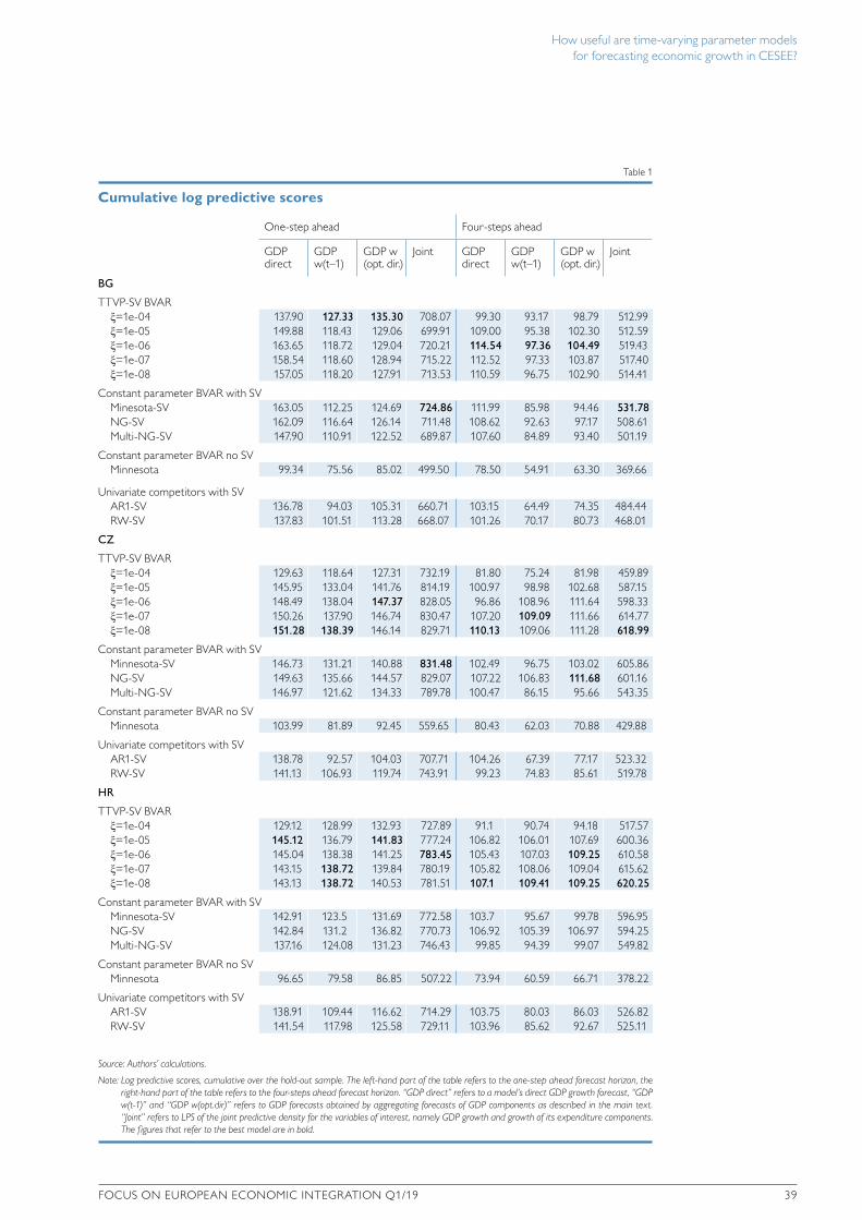
How useful are time-varying parameter models for forecasting economic growth in CESEE?
FOCUS ON EUROPEAN ECONOMIC INTEGRATION Q1/19 39
components of GDP (joint). This serves as an overall measure of forecast perfor-mance for the variables of interest.9 The figures for the best performing model in each column are in bold.
First, we want to answer the question whether GDP growth forecasts can be improved using a time-varying parameter model. The simplest form to capture time variation is by allowing error variances to vary over time, and its importance for forecasting has been demonstrated in a range of recent empirical contributions. Our results corroborate these findings, which can be seen by the inferior perfor-mance of the Minnesota prior with homoscedastic variance (Minnesota). Forecasts from this model are frequently outperformed even by simple univariate benchmark models with stochastic volatility. More interestingly, looking at models that accom-modate time variation also in drifting parameters, we find variants of the threshold model outperforming constant parameter BVARs in Bulgaria, Croatia and mostly so in the Czech Republic. This holds true for both forecast horizons and regardless of whether the direct or composite forecasts are considered. In the Czech Republic and considering four-steps ahead forecasts, a BVAR that is linear in parameters and using optimized weights to aggregate the forecast yields a nearly identical perfor-mance though. For the remaining countries it turns out that the TTVP-SV model yields superior composite GDP forecasts for both forecast horizons and regardless of how the single component forecasts are aggregated. Constant parameter BVARs, however, excel when forecast performance is assessed using the direct GDP growth forecast. Also, in these instances, improvements over the TTVP-SV forecasts are modest. As a special case, Hungary is the only country where the regional model (Multi-NG-SV) shows a competitive forecast performance. Looking at direct GDP growth forecasts for the one- and four-steps ahead forecast horizon, this model even outperforms its competitors, indicating that cross-country linkages play an important role for forecasting Hungarian GDP growth.
Second, we draw attention to the question whether an aggregation of GDP components’ forecasts can improve forecast performance compared to directly forecasting the GDP series. For most economies and at the one-step ahead forecast horizon, direct forecasts are slightly more accurate in terms of LPS scores. A reason for this could be that the predictive uncertainty of the components’ forecasts aggre-gates when summing up the forecasts. Another reason could be that we do not model stock changes implicitly, assuming that their contribution is zero over the forecasting horizon. The finding that direct forecasts outperform aggregate fore-casts is, however, not a general pattern. More specifically, composite forecasts in Croatia, the Czech Republic and Poland yield higher LPS scores than direct fore-casts at the four-steps ahead forecast horizon. Only in Bulgaria do we find evidence that direct forecasts excel at both forecast horizons and by a great margin. An explanation for this could be the historically high contribution of statistical discrep-ancy in overall GDP growth, which is not captured by the components.
Third, our results allow us to examine the usefulness of specifying a regional multi-country model that takes into account the degree of economic integration among the countries under review. For most of the economies, the foreign sector plays a crucial role, and attempts have been made to better model the external sector
9 The LPS score of the joint predictive density is typically not identical to summing up the LPS scores of the mar-ginal distributions of each variable of interest, since the latter would neglect cross-variable dependence.
Table 1
Cumulative log predictive scores
One-step ahead Four-steps ahead
GDP direct
GDP w(t–1)
GDP w (opt. dir.)
Joint GDP direct
GDP w(t–1)
GDP w (opt. dir.)
Joint
BG
TTVP-SV BVARξ=1e-04 137.90 127.33 135.30 708.07 99.30 93.17 98.79 512.99ξ=1e-05 149.88 118.43 129.06 699.91 109.00 95.38 102.30 512.59ξ=1e-06 163.65 118.72 129.04 720.21 114.54 97.36 104.49 519.43ξ=1e-07 158.54 118.60 128.94 715.22 112.52 97.33 103.87 517.40ξ=1e-08 157.05 118.20 127.91 713.53 110.59 96.75 102.90 514.41
Constant parameter BVAR with SVMinesota-SV 163.05 112.25 124.69 724.86 111.99 85.98 94.46 531.78NG-SV 162.09 116.64 126.14 711.48 108.62 92.63 97.17 508.61Multi-NG-SV 147.90 110.91 122.52 689.87 107.60 84.89 93.40 501.19
Constant parameter BVAR no SVMinnesota 99.34 75.56 85.02 499.50 78.50 54.91 63.30 369.66
Univariate competitors with SVAR1-SV 136.78 94.03 105.31 660.71 103.15 64.49 74.35 484.44RW-SV 137.83 101.51 113.28 668.07 101.26 70.17 80.73 468.01
CZ
TTVP-SV BVARξ=1e-04 129.63 118.64 127.31 732.19 81.80 75.24 81.98 459.89ξ=1e-05 145.95 133.04 141.76 814.19 100.97 98.98 102.68 587.15ξ=1e-06 148.49 138.04 147.37 828.05 96.86 108.96 111.64 598.33ξ=1e-07 150.26 137.90 146.74 830.47 107.20 109.09 111.66 614.77ξ=1e-08 151.28 138.39 146.14 829.71 110.13 109.06 111.28 618.99
Constant parameter BVAR with SVMinnesota-SV 146.73 131.21 140.88 831.48 102.49 96.75 103.02 605.86NG-SV 149.63 135.66 144.57 829.07 107.22 106.83 111.68 601.16Multi-NG-SV 146.97 121.62 134.33 789.78 100.47 86.15 95.66 543.35
Constant parameter BVAR no SVMinnesota 103.99 81.89 92.45 559.65 80.43 62.03 70.88 429.88
Univariate competitors with SVAR1-SV 138.78 92.57 104.03 707.71 104.26 67.39 77.17 523.32RW-SV 141.13 106.93 119.74 743.91 99.23 74.83 85.61 519.78
HR
TTVP-SV BVARξ=1e-04 129.12 128.99 132.93 727.89 91.1 90.74 94.18 517.57ξ=1e-05 145.12 136.79 141.83 777.24 106.82 106.01 107.69 600.36ξ=1e-06 145.04 138.38 141.25 783.45 105.43 107.03 109.25 610.58ξ=1e-07 143.15 138.72 139.84 780.19 105.82 108.06 109.04 615.62ξ=1e-08 143.13 138.72 140.53 781.51 107.1 109.41 109.25 620.25
Constant parameter BVAR with SVMinnesota-SV 142.91 123.5 131.69 772.58 103.7 95.67 99.78 596.95NG-SV 142.84 131.2 136.82 770.73 106.92 105.39 106.97 594.25Multi-NG-SV 137.16 124.08 131.23 746.43 99.85 94.39 99.07 549.82
Constant parameter BVAR no SVMinnesota 96.65 79.58 86.85 507.22 73.94 60.59 66.71 378.22
Univariate competitors with SVAR1-SV 138.91 109.44 116.62 714.29 103.75 80.03 86.03 526.82RW-SV 141.54 117.98 125.58 729.11 103.96 85.62 92.67 525.11
Source: Authors’ calculations.
Note: Log predictive scores, cumulative over the hold-out sample. The left-hand part of the table refers to the one-step ahead forecast horizon, the right-hand part of the table refers to the four-steps ahead forecast horizon. “GDP direct” refers to a model’s direct GDP growth forecast, “GDP w(t-1)” and “GDP w(opt.dir)” refers to GDP forecasts obtained by aggregating forecasts of GDP components as described in the main text. “Joint” refers to LPS of the joint predictive density for the variables of interest, namely GDP growth and growth of its expenditure components. The figures that refer to the best model are in bold.
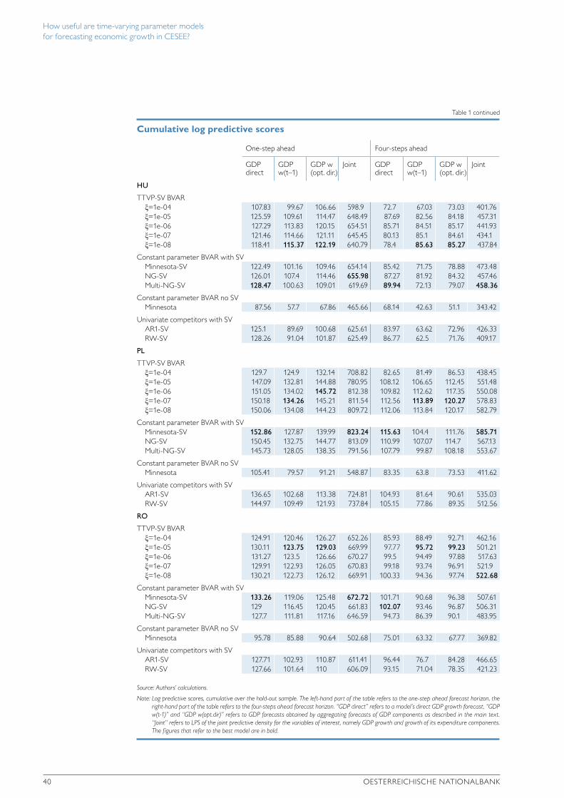
How useful are time-varying parameter models for forecasting economic growth in CESEE?
40 OESTERREICHISCHE NATIONALBANK
Table 1 continued
Cumulative log predictive scores
One-step ahead Four-steps ahead
GDP direct
GDP w(t–1)
GDP w (opt. dir.)
Joint GDP direct
GDP w(t–1)
GDP w (opt. dir.)
Joint
HU
TTVP-SV BVARξ=1e-04 107.83 99.67 106.66 598.9 72.7 67.03 73.03 401.76ξ=1e-05 125.59 109.61 114.47 648.49 87.69 82.56 84.18 457.31ξ=1e-06 127.29 113.83 120.15 654.51 85.71 84.51 85.17 441.93ξ=1e-07 121.46 114.66 121.11 645.45 80.13 85.1 84.61 434.1ξ=1e-08 118.41 115.37 122.19 640.79 78.4 85.63 85.27 437.84
Constant parameter BVAR with SVMinnesota-SV 122.49 101.16 109.46 654.14 85.42 71.75 78.88 473.48NG-SV 126.01 107.4 114.46 655.98 87.27 81.92 84.32 457.46Multi-NG-SV 128.47 100.63 109.01 619.69 89.94 72.13 79.07 458.36
Constant parameter BVAR no SVMinnesota 87.56 57.7 67.86 465.66 68.14 42.63 51.1 343.42
Univariate competitors with SVAR1-SV 125.1 89.69 100.68 625.61 83.97 63.62 72.96 426.33RW-SV 128.26 91.04 101.87 625.49 86.77 62.5 71.76 409.17
PL
TTVP-SV BVARξ=1e-04 129.7 124.9 132.14 708.82 82.65 81.49 86.53 438.45ξ=1e-05 147.09 132.81 144.88 780.95 108.12 106.65 112.45 551.48ξ=1e-06 151.05 134.02 145.72 812.38 109.82 112.62 117.35 550.08ξ=1e-07 150.18 134.26 145.21 811.54 112.56 113.89 120.27 578.83ξ=1e-08 150.06 134.08 144.23 809.72 112.06 113.84 120.17 582.79
Constant parameter BVAR with SVMinnesota-SV 152.86 127.87 139.99 823.24 115.63 104.4 111.76 585.71NG-SV 150.45 132.75 144.77 813.09 110.99 107.07 114.7 567.13Multi-NG-SV 145.73 128.05 138.35 791.56 107.79 99.87 108.18 553.67
Constant parameter BVAR no SVMinnesota 105.41 79.57 91.21 548.87 83.35 63.8 73.53 411.62
Univariate competitors with SVAR1-SV 136.65 102.68 113.38 724.81 104.93 81.64 90.61 535.03RW-SV 144.97 109.49 121.93 737.84 105.15 77.86 89.35 512.56
RO
TTVP-SV BVARξ=1e-04 124.91 120.46 126.27 652.26 85.93 88.49 92.71 462.16ξ=1e-05 130.11 123.75 129.03 669.99 97.77 95.72 99.23 501.21ξ=1e-06 131.27 123.5 126.66 670.27 99.5 94.49 97.88 517.63ξ=1e-07 129.91 122.93 126.05 670.83 99.18 93.74 96.91 521.9ξ=1e-08 130.21 122.73 126.12 669.91 100.33 94.36 97.74 522.68
Constant parameter BVAR with SVMinnesota-SV 133.26 119.06 125.48 672.72 101.71 90.68 96.38 507.61NG-SV 129 116.45 120.45 661.83 102.07 93.46 96.87 506.31Multi-NG-SV 127.7 111.81 117.16 646.59 94.73 86.39 90.1 483.95
Constant parameter BVAR no SVMinnesota 95.78 85.88 90.64 502.68 75.01 63.32 67.77 369.82
Univariate competitors with SVAR1-SV 127.71 102.93 110.87 611.41 96.44 76.7 84.28 466.65RW-SV 127.66 101.64 110 606.09 93.15 71.04 78.35 421.23
Source: Authors’ calculations.
Note: Log predictive scores, cumulative over the hold-out sample. The left-hand part of the table refers to the one-step ahead forecast horizon, the right-hand part of the table refers to the four-steps ahead forecast horizon. “GDP direct” refers to a model’s direct GDP growth forecast, “GDP w(t-1)” and “GDP w(opt.dir)” refers to GDP forecasts obtained by aggregating forecasts of GDP components as described in the main text. “Joint” refers to LPS of the joint predictive density for the variables of interest, namely GDP growth and growth of its expenditure components. The figures that refer to the best model are in bold.
How useful are time-varying parameter models for forecasting economic growth in CESEE?
FOCUS ON EUROPEAN ECONOMIC INTEGRATION Q1/19 41
(see e.g. Stoevsky, 2009, for Bulgaria, or Kolasa and Rubaszek, 2018, in the context of a DSGE framework). Note that by including euro area variables, the baseline models already control for developments in the most important export markets for the six economies. Slacík et al. (2014), however, take into account trade and eco-nomic links among the CESEE countries by including trade-weighted GDP in addition to euro area variables and show that this can further improve forecast performance. We go beyond the specification proposed in Slacík et al. (2014) by modeling all variables from all economies jointly, controling for euro area develop-ments by including euro area GDP and interest rates as additional exogeneous regressors. Looking at the results, we do not find compelling evidence that forecasts improve if we directly take into account economic linkages among the countries. An exception to this is Hungary, for which a regional specification yields the best forecast at both forecast horizons.
So far, the evaluation of forecasts was based on the overall performance over the hold-out sample. It could be argued that certain models/model classes perform better during volatile times, while others perform better during normal times. In the extreme case, the excellent predictive performance of the TTVP-SV models could stem from a few data points such as turning points which models linear in parameters are not able to capture appropriately. To examine this in more detail, we have examined in a robustness exercise the performance of the different models for each time point in the hold-out sample. The results are available from the authors upon request. Briefly, we do not find evidence of time-specific swings in perfor-mance. In other words, the models that had a superior track record over the whole hold-out sample tend to perform equally well over the hold-out sample. This holds true for both forecast horizons, the joint density of the GDP compo-nents and the marginal GDP forecasts.
Summing up, we find that for most economies the TTVP-SV model tends to excel at both the one-step and four-steps ahead forecast horizon. Our specification of the Minnesota prior, however, turns out to be a tough competitor, and the fore-cast performance of both model classes is relatively close. Hence it is not surprising that from the different specifications of the TTVP-SV model, the one that uses a tight prior (ξ=10-8) on coefficient movements tends to do a good job for all countries. For some countries, forecasts from multivariate models are competitive only at the end of the hold-out sample. These tend to be countries with shorter time series. For the remaining economies, the models that perform well do so equally over the hold-out sample, not showing any large swings in performance.
5.1 Sources of forecast error
In this section we delve deeper to analyze sources of forecast performance for the aggregate GDP growth forecasts. For that purpose, we focus on the TTVP-SV model with a tight prior (ξ=10–8) that showed a reasonable performance for all countries.
To assess forecast performance of the aggregate forecast in more detail, we focus on two measures of forecast performance: the average mean forecast error (MFE) and the average root mean of weighted square forecast error (RMWSFE). The MFE serves to gauge which components are over- or underestimated, indicates how much the predictions vary around the realizations and considers already the components’ share/weight in total GDP (Júlio and Esperanca, 2012).
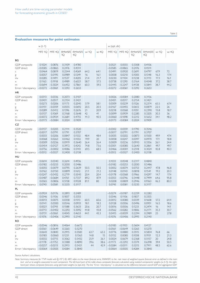
How useful are time-varying parameter models for forecasting economic growth in CESEE?
42 OESTERREICHISCHE NATIONALBANK
Table 2
Evaluation measures for point estimates
w (t–1) w (opt. dir)
MFE 1Q MFE 4Q RMWSFE 1Q
RMWSFE 4Q
wi 1Q wi 4Q MFE 1Q MFE 4Q RMWSFE 1Q
RMWSFE 4Q
wi 1Q wi 4Q
BG
GDP composite 0.1024 0.0876 0.3109 0.4780 0.0521 0.0555 0.3308 0.4106GDP direct –0.0585 –0.0865 0.2476 0.4514 –0.0585 –0.0865 0.2476 0.4514c 0.0464 0.0819 0.2544 0.4269 64.2 64.1 0.0491 0.0920 0.2691 0.4797 67.9 72g 0.0057 0.0195 0.0989 0.1249 16 16.1 0.0058 0.0210 0.1005 0.1348 16.3 17.4inv 0.0285 0.1491 0.1537 0.4205 21.4 21.7 0.0230 0.1104 0.1238 0.3113 17.3 16.1x 0.1163 0.1918 0.4989 0.6021 58.7 57.5 0.0738 0.1290 0.3164 0.4048 37.2 38.7m –0.0694 –0.3024 0.6452 0.7861 60.3 59.5 –0.0445 –0.2247 0.4138 0.5841 38.7 44.2Error / discrepancy –0.0272 –0.0061 0.3292 0.2653 –0.0272 –0.0061 0.3292 0.2653
HR
GDP composite 0.0313 0.0336 0.2073 0.3107 0.0026 –0.0584 0.2080 0.3156GDP direct 0.0431 0.0517 0.2154 0.3421 0.0431 0.0517 0.2154 0.3421c 0.0273 0.0206 0.1173 0.2045 57.9 58.1 0.0309 0.0239 0.1326 0.2374 65.5 67.4g –0.0151 –0.0359 0.0555 0.0692 20.5 20.5 –0.0167 –0.0455 0.0612 0.0879 22.5 26inv 0.0289 0.0412 0.1396 0.2676 21 20.9 0.0218 0.0368 0.1051 0.2390 15.8 18.7x 0.0137 0.1069 0.3168 0.3648 42 41 0.0099 0.0939 0.2285 0.3205 30.3 36m –0.0072 –0.0924 0.2681 0.4755 41.3 40.5 –0.0060 –0.1098 0.2212 0.5652 34.1 48.2Error / discrepancy –0.0173 –0.0084 0.2024 0.1909 –0.0173 –0.0084 0.2024 0.1909
CZ
GDP composite –0.0137 0.0205 0.2114 0.3520 –0.0302 0.0359 0.1790 0.3546GDP direct –0.0017 0.0791 0.1791 0.3707 –0.0017 0.0791 0.1791 0.3707c 0.0033 0.0206 0.0847 0.1532 48.4 48.4 0.0035 0.0202 0.0873 0.1500 49.9 47.4g 0.0068 0.0263 0.0462 0.1032 19.9 20 0.0058 0.0247 0.0397 0.0970 17.1 18.8inv 0.0009 0.0256 0.0919 0.3640 26.4 26.4 0.0009 0.0236 0.0910 0.3356 26.1 24.4x –0.0454 –0.0127 0.3972 0.4242 74.8 73.6 –0.0301 –0.0085 0.2640 0.2861 49.7 49.7m 0.0756 –0.0002 0.4086 0.5143 69.5 68.5 0.0466 –0.0001 0.2518 0.3024 42.8 40.3Error / discrepancy –0.0512 –0.0327 0.2400 0.2138 –0.0512 –0.0327 0.2400 0.2138
HU
GDP composite 0.0614 0.0340 0.2614 0.4936 0.1033 0.0548 0.2317 0.4840GDP direct –0.0182 –0.0253 0.2030 0.5486 –0.0182 –0.0253 0.2030 0.5486c 0.0055 –0.0079 0.0795 0.2639 50.5 50.5 0.0052 –0.0074 0.0753 0.2447 47.8 46.8g 0.0162 0.0150 0.0899 0.1612 21.1 21.2 0.0148 0.0143 0.0818 0.1541 19.2 20.3inv –0.0247 –0.0432 0.2719 0.5043 20.4 20.4 –0.0178 –0.0368 0.1966 0.4297 14.7 17.4x –0.0487 –0.0684 0.4761 0.7337 89.2 87.9 –0.0353 –0.0746 0.3448 0.7999 64.6 95.8m 0.0365 0.0806 0.5158 0.9328 81.1 80 0.0208 0.0809 0.2946 0.9363 46.3 80.3Error / discrepancy 0.0743 0.0581 0.3235 0.3117 0.0743 0.0581 0.3235 0.3117
PL
GDP composite –0.0924 0.0176 0.2893 0.2489 –0.0274 –0.0187 0.2259 0.2282GDP direct 0.0346 0.1106 0.1837 0.3355 0.0346 0.1106 0.1837 0.3355c –0.0013 0.0075 0.0358 0.1513 60.5 60.6 –0.0012 0.0080 0.0339 0.1608 57.2 64.4g 0.0141 0.0300 0.0546 0.0933 18.1 18.2 0.0128 0.0306 0.0496 0.0951 16.5 18.6inv 0.0021 0.0743 0.1588 0.3633 20.6 20.7 0.0016 0.0506 0.1233 0.2474 16 14.1x –0.0713 –0.0402 0.2292 0.3092 44.8 43.8 –0.0562 –0.0282 0.1806 0.2171 35.3 30.7m 0.0731 –0.0061 0.4045 0.4653 44.1 43.3 0.0415 –0.0039 0.2294 0.2989 25 27.8Error / discrepancy –0.1076 –0.0406 0.2993 0.2140 –0.1076 –0.0406 0.2993 0.2140
RO
GDP composite –0.0546 –0.0816 0.4064 0.6672 –0.0183 –0.1933 0.3604 0.4127GDP direct –0.0561 –0.0649 0.3265 0.5270 –0.0561 –0.0649 0.3265 0.5270c 0.0643 0.0843 0.2915 0.5583 63.7 63.2 0.0776 0.0880 0.3515 0.5834 76.8 66g 0.0183 0.0060 0.1251 0.1363 14.8 15 0.0152 0.0085 0.1038 0.1931 12.3 21.3inv 0.0032 0.0715 0.3062 0.5432 25.9 26.1 0.0024 0.0679 0.2368 0.5157 20 24.8x –0.1178 –0.1752 0.3388 0.4890 39.6 38.6 –0.1173 –0.2292 0.3374 0.6398 39.4 50.5m –0.0257 –0.0213 0.2913 0.5421 44 42.9 –0.0284 –0.0311 0.3215 0.7911 48.5 62.6Error / discrepancy –0.0064 –0.0505 0.4284 0.3840 –0.0064 –0.0505 0.4284 0.3840
Source: Authors’ calculations.
Note: Summary measures for TTVP model with ξ=10^(-8). MFE refers to the mean forecast error, RMWSFE to the root mean of weighted square forecast error as defined in the main text and wi to weights associated to each component. The left-hand part of the table shows composite forecasts calculated using realized components’ weights (w (t-1)), the right-hand part shows composite forecasts using optimized weights (w (opt.dir)). The line “Error / discrepancy” is calculated as the difference between overall GDP and aggregated GDP.
How useful are time-varying parameter models for forecasting economic growth in CESEE?
FOCUS ON EUROPEAN ECONOMIC INTEGRATION Q1/19 43
We define the forecast error ft+h|h for aggregate output growth and the forecast error vector of the components ftz+h|h as
Following Marcellino et al. (2003) and Júlio and Esperanca (2012), the RMWSFE and MFE for composite output growth are given by MFE = H–1ΣtϵH ft+h|t and R MSFE =
Restrictive, public after publication
Page 15 of 22
5.1 Sources of forecast error
In this section we delve deeper to analyze sources of forecast performance for the aggregate
GDP growth forecasts. For that purpose, we focus on the TTVP-SV model with a tight prior
(𝜉𝜉 = 10−8) that showed a reasonable performance for all countries.
To assess forecast performance of the aggregate forecast in more detail, we focus on two
measures of forecast performance: the average mean forecast error (MFE) and the average root
mean of weighted square forecast error (RMWSFE). The MFE serves to gauge which
components are over- or underestimated, indicates how much the predictions vary around the
realizations and considers already the components’ share/weight in total GDP (Júlio and
Esperanca, 2012).
We define the forecast error 𝑓𝑓𝑡𝑡+ℎ|ℎ for aggregate output growth and the forecast error vector of
the components 𝑓𝑓𝑡𝑡+ℎ|ℎ𝑧𝑧 as
𝑓𝑓𝑡𝑡+ℎ|ℎ = (𝑔𝑔𝑔𝑔𝑔𝑔𝑡𝑡+ℎ|ℎ − 𝑔𝑔𝑔𝑔𝑔𝑔𝑡𝑡+ℎ|ℎ𝑒𝑒.𝑝𝑝. ) and
𝑓𝑓𝑡𝑡+ℎ𝑧𝑧 =
(
𝑐𝑐𝑡𝑡+ℎ|𝑡𝑡 − 𝑐𝑐𝑡𝑡+ℎ𝑒𝑒.𝑝𝑝.
𝑖𝑖𝑖𝑖𝑖𝑖𝑡𝑡+ℎ|𝑡𝑡 − 𝑖𝑖𝑖𝑖𝑖𝑖𝑡𝑡+ℎ𝑒𝑒.𝑝𝑝.
𝑔𝑔𝑡𝑡+ℎ|𝑡𝑡 − 𝑔𝑔𝑡𝑡+ℎ𝑒𝑒.𝑝𝑝.
𝑥𝑥𝑡𝑡+ℎ|𝑡𝑡 − 𝑥𝑥𝑡𝑡+ℎ𝑒𝑒.𝑝𝑝.
−(𝑚𝑚𝑡𝑡+ℎ|𝑡𝑡 − 𝑚𝑚𝑡𝑡+ℎ𝑒𝑒.𝑝𝑝. ))
, (8)
Following Marcellino et al. (2003) and Júlio and Esperanca (2012) the RMWSFE and MFE for
composite output growth are given by 𝑀𝑀𝑀𝑀𝑀𝑀 = 𝐻𝐻−1 ∑ 𝑓𝑓𝑡𝑡+ℎ|𝑡𝑡𝑡𝑡 ∈ 𝐻𝐻 and 𝑅𝑅𝑀𝑀𝑅𝑅𝑀𝑀𝑀𝑀 =
√𝐻𝐻−1 ∑ 𝑓𝑓𝑡𝑡+ℎ|𝑡𝑡2
𝑡𝑡 ∈ 𝐻𝐻 and analogously for the components 𝑀𝑀𝑀𝑀𝑀𝑀𝑀𝑀𝑧𝑧 = ��𝑤𝑧𝑧,𝑡𝑡+ℎ 𝐻𝐻−1 ∑ 𝑓𝑓𝑧𝑧,𝑡𝑡+ℎ|𝑡𝑡𝑡𝑡 ∈ 𝐻𝐻
and 𝑅𝑅𝑀𝑀𝑀𝑀𝑅𝑅𝑀𝑀𝑀𝑀𝑧𝑧 = ��𝑤𝑧𝑧,𝑡𝑡+ℎ√𝐻𝐻−1 ∑ 𝑓𝑓𝑧𝑧,𝑡𝑡+ℎ|𝑡𝑡2
𝑡𝑡 ∈ 𝐻𝐻 with ��𝑤𝑧𝑧,𝑡𝑡+ℎ = 𝐻𝐻−1 ∑ 𝑤𝑤𝑧𝑧,𝑡𝑡+ℎ|𝑡𝑡𝑡𝑡 ∈ 𝐻𝐻 .
In table 2, we summarize forecast errors for the different GDP components.
[TABLE 2 ABOUT HERE]
The left-hand part of the table contains results using historical weights and the right-hand part
optimized weights.
a nd a na logously for t he component s MWFEz=
Restrictive, public after publication
Page 15 of 22
5.1 Sources of forecast error
In this section we delve deeper to analyze sources of forecast performance for the aggregate
GDP growth forecasts. For that purpose, we focus on the TTVP-SV model with a tight prior
(𝜉𝜉 = 10−8) that showed a reasonable performance for all countries.
To assess forecast performance of the aggregate forecast in more detail, we focus on two
measures of forecast performance: the average mean forecast error (MFE) and the average root
mean of weighted square forecast error (RMWSFE). The MFE serves to gauge which
components are over- or underestimated, indicates how much the predictions vary around the
realizations and considers already the components’ share/weight in total GDP (Júlio and
Esperanca, 2012).
We define the forecast error 𝑓𝑓𝑡𝑡+ℎ|ℎ for aggregate output growth and the forecast error vector of
the components 𝑓𝑓𝑡𝑡+ℎ|ℎ𝑧𝑧 as
𝑓𝑓𝑡𝑡+ℎ|ℎ = (𝑔𝑔𝑔𝑔𝑔𝑔𝑡𝑡+ℎ|ℎ − 𝑔𝑔𝑔𝑔𝑔𝑔𝑡𝑡+ℎ|ℎ𝑒𝑒.𝑝𝑝. ) and
𝑓𝑓𝑡𝑡+ℎ𝑧𝑧 =
(
𝑐𝑐𝑡𝑡+ℎ|𝑡𝑡 − 𝑐𝑐𝑡𝑡+ℎ𝑒𝑒.𝑝𝑝.
𝑖𝑖𝑖𝑖𝑖𝑖𝑡𝑡+ℎ|𝑡𝑡 − 𝑖𝑖𝑖𝑖𝑖𝑖𝑡𝑡+ℎ𝑒𝑒.𝑝𝑝.
𝑔𝑔𝑡𝑡+ℎ|𝑡𝑡 − 𝑔𝑔𝑡𝑡+ℎ𝑒𝑒.𝑝𝑝.
𝑥𝑥𝑡𝑡+ℎ|𝑡𝑡 − 𝑥𝑥𝑡𝑡+ℎ𝑒𝑒.𝑝𝑝.
−(𝑚𝑚𝑡𝑡+ℎ|𝑡𝑡 − 𝑚𝑚𝑡𝑡+ℎ𝑒𝑒.𝑝𝑝. ))
, (8)
Following Marcellino et al. (2003) and Júlio and Esperanca (2012) the RMWSFE and MFE for
composite output growth are given by 𝑀𝑀𝑀𝑀𝑀𝑀 = 𝐻𝐻−1 ∑ 𝑓𝑓𝑡𝑡+ℎ|𝑡𝑡𝑡𝑡 ∈ 𝐻𝐻 and 𝑅𝑅𝑀𝑀𝑅𝑅𝑀𝑀𝑀𝑀 =
√𝐻𝐻−1 ∑ 𝑓𝑓𝑡𝑡+ℎ|𝑡𝑡2
𝑡𝑡 ∈ 𝐻𝐻 and analogously for the components 𝑀𝑀𝑀𝑀𝑀𝑀𝑀𝑀𝑧𝑧 = ��𝑤𝑧𝑧,𝑡𝑡+ℎ 𝐻𝐻−1 ∑ 𝑓𝑓𝑧𝑧,𝑡𝑡+ℎ|𝑡𝑡𝑡𝑡 ∈ 𝐻𝐻
and 𝑅𝑅𝑀𝑀𝑀𝑀𝑅𝑅𝑀𝑀𝑀𝑀𝑧𝑧 = ��𝑤𝑧𝑧,𝑡𝑡+ℎ√𝐻𝐻−1 ∑ 𝑓𝑓𝑧𝑧,𝑡𝑡+ℎ|𝑡𝑡2
𝑡𝑡 ∈ 𝐻𝐻 with ��𝑤𝑧𝑧,𝑡𝑡+ℎ = 𝐻𝐻−1 ∑ 𝑤𝑤𝑧𝑧,𝑡𝑡+ℎ|𝑡𝑡𝑡𝑡 ∈ 𝐻𝐻 .
In table 2, we summarize forecast errors for the different GDP components.
[TABLE 2 ABOUT HERE]
The left-hand part of the table contains results using historical weights and the right-hand part
optimized weights.
and R MWSFEz =
Restrictive, public after publication
Page 15 of 22
5.1 Sources of forecast error
In this section we delve deeper to analyze sources of forecast performance for the aggregate
GDP growth forecasts. For that purpose, we focus on the TTVP-SV model with a tight prior
(𝜉𝜉 = 10−8) that showed a reasonable performance for all countries.
To assess forecast performance of the aggregate forecast in more detail, we focus on two
measures of forecast performance: the average mean forecast error (MFE) and the average root
mean of weighted square forecast error (RMWSFE). The MFE serves to gauge which
components are over- or underestimated, indicates how much the predictions vary around the
realizations and considers already the components’ share/weight in total GDP (Júlio and
Esperanca, 2012).
We define the forecast error 𝑓𝑓𝑡𝑡+ℎ|ℎ for aggregate output growth and the forecast error vector of
the components 𝑓𝑓𝑡𝑡+ℎ|ℎ𝑧𝑧 as
𝑓𝑓𝑡𝑡+ℎ|ℎ = (𝑔𝑔𝑔𝑔𝑔𝑔𝑡𝑡+ℎ|ℎ − 𝑔𝑔𝑔𝑔𝑔𝑔𝑡𝑡+ℎ|ℎ𝑒𝑒.𝑝𝑝. ) and
𝑓𝑓𝑡𝑡+ℎ𝑧𝑧 =
(
𝑐𝑐𝑡𝑡+ℎ|𝑡𝑡 − 𝑐𝑐𝑡𝑡+ℎ𝑒𝑒.𝑝𝑝.
𝑖𝑖𝑖𝑖𝑖𝑖𝑡𝑡+ℎ|𝑡𝑡 − 𝑖𝑖𝑖𝑖𝑖𝑖𝑡𝑡+ℎ𝑒𝑒.𝑝𝑝.
𝑔𝑔𝑡𝑡+ℎ|𝑡𝑡 − 𝑔𝑔𝑡𝑡+ℎ𝑒𝑒.𝑝𝑝.
𝑥𝑥𝑡𝑡+ℎ|𝑡𝑡 − 𝑥𝑥𝑡𝑡+ℎ𝑒𝑒.𝑝𝑝.
−(𝑚𝑚𝑡𝑡+ℎ|𝑡𝑡 − 𝑚𝑚𝑡𝑡+ℎ𝑒𝑒.𝑝𝑝. ))
, (8)
Following Marcellino et al. (2003) and Júlio and Esperanca (2012) the RMWSFE and MFE for
composite output growth are given by 𝑀𝑀𝑀𝑀𝑀𝑀 = 𝐻𝐻−1 ∑ 𝑓𝑓𝑡𝑡+ℎ|𝑡𝑡𝑡𝑡 ∈ 𝐻𝐻 and 𝑅𝑅𝑀𝑀𝑅𝑅𝑀𝑀𝑀𝑀 =
√𝐻𝐻−1 ∑ 𝑓𝑓𝑡𝑡+ℎ|𝑡𝑡2
𝑡𝑡 ∈ 𝐻𝐻 and analogously for the components 𝑀𝑀𝑀𝑀𝑀𝑀𝑀𝑀𝑧𝑧 = ��𝑤𝑧𝑧,𝑡𝑡+ℎ 𝐻𝐻−1 ∑ 𝑓𝑓𝑧𝑧,𝑡𝑡+ℎ|𝑡𝑡𝑡𝑡 ∈ 𝐻𝐻
and 𝑅𝑅𝑀𝑀𝑀𝑀𝑅𝑅𝑀𝑀𝑀𝑀𝑧𝑧 = ��𝑤𝑧𝑧,𝑡𝑡+ℎ√𝐻𝐻−1 ∑ 𝑓𝑓𝑧𝑧,𝑡𝑡+ℎ|𝑡𝑡2
𝑡𝑡 ∈ 𝐻𝐻 with ��𝑤𝑧𝑧,𝑡𝑡+ℎ = 𝐻𝐻−1 ∑ 𝑤𝑤𝑧𝑧,𝑡𝑡+ℎ|𝑡𝑡𝑡𝑡 ∈ 𝐻𝐻 .
In table 2, we summarize forecast errors for the different GDP components.
[TABLE 2 ABOUT HERE]
The left-hand part of the table contains results using historical weights and the right-hand part
optimized weights.
w it h
Restrictive, public after publication
Page 15 of 22
5.1 Sources of forecast error
In this section we delve deeper to analyze sources of forecast performance for the aggregate
GDP growth forecasts. For that purpose, we focus on the TTVP-SV model with a tight prior
(𝜉𝜉 = 10−8) that showed a reasonable performance for all countries.
To assess forecast performance of the aggregate forecast in more detail, we focus on two
measures of forecast performance: the average mean forecast error (MFE) and the average root
mean of weighted square forecast error (RMWSFE). The MFE serves to gauge which
components are over- or underestimated, indicates how much the predictions vary around the
realizations and considers already the components’ share/weight in total GDP (Júlio and
Esperanca, 2012).
We define the forecast error 𝑓𝑓𝑡𝑡+ℎ|ℎ for aggregate output growth and the forecast error vector of
the components 𝑓𝑓𝑡𝑡+ℎ|ℎ𝑧𝑧 as
𝑓𝑓𝑡𝑡+ℎ|ℎ = (𝑔𝑔𝑔𝑔𝑔𝑔𝑡𝑡+ℎ|ℎ − 𝑔𝑔𝑔𝑔𝑔𝑔𝑡𝑡+ℎ|ℎ𝑒𝑒.𝑝𝑝. ) and
𝑓𝑓𝑡𝑡+ℎ𝑧𝑧 =
(
𝑐𝑐𝑡𝑡+ℎ|𝑡𝑡 − 𝑐𝑐𝑡𝑡+ℎ𝑒𝑒.𝑝𝑝.
𝑖𝑖𝑖𝑖𝑖𝑖𝑡𝑡+ℎ|𝑡𝑡 − 𝑖𝑖𝑖𝑖𝑖𝑖𝑡𝑡+ℎ𝑒𝑒.𝑝𝑝.
𝑔𝑔𝑡𝑡+ℎ|𝑡𝑡 − 𝑔𝑔𝑡𝑡+ℎ𝑒𝑒.𝑝𝑝.
𝑥𝑥𝑡𝑡+ℎ|𝑡𝑡 − 𝑥𝑥𝑡𝑡+ℎ𝑒𝑒.𝑝𝑝.
−(𝑚𝑚𝑡𝑡+ℎ|𝑡𝑡 − 𝑚𝑚𝑡𝑡+ℎ𝑒𝑒.𝑝𝑝. ))
, (8)
Following Marcellino et al. (2003) and Júlio and Esperanca (2012) the RMWSFE and MFE for
composite output growth are given by 𝑀𝑀𝑀𝑀𝑀𝑀 = 𝐻𝐻−1 ∑ 𝑓𝑓𝑡𝑡+ℎ|𝑡𝑡𝑡𝑡 ∈ 𝐻𝐻 and 𝑅𝑅𝑀𝑀𝑅𝑅𝑀𝑀𝑀𝑀 =
√𝐻𝐻−1 ∑ 𝑓𝑓𝑡𝑡+ℎ|𝑡𝑡2
𝑡𝑡 ∈ 𝐻𝐻 and analogously for the components 𝑀𝑀𝑀𝑀𝑀𝑀𝑀𝑀𝑧𝑧 = ��𝑤𝑧𝑧,𝑡𝑡+ℎ 𝐻𝐻−1 ∑ 𝑓𝑓𝑧𝑧,𝑡𝑡+ℎ|𝑡𝑡𝑡𝑡 ∈ 𝐻𝐻
and 𝑅𝑅𝑀𝑀𝑀𝑀𝑅𝑅𝑀𝑀𝑀𝑀𝑧𝑧 = ��𝑤𝑧𝑧,𝑡𝑡+ℎ√𝐻𝐻−1 ∑ 𝑓𝑓𝑧𝑧,𝑡𝑡+ℎ|𝑡𝑡2
𝑡𝑡 ∈ 𝐻𝐻 with ��𝑤𝑧𝑧,𝑡𝑡+ℎ = 𝐻𝐻−1 ∑ 𝑤𝑤𝑧𝑧,𝑡𝑡+ℎ|𝑡𝑡𝑡𝑡 ∈ 𝐻𝐻 .
In table 2, we summarize forecast errors for the different GDP components.
[TABLE 2 ABOUT HERE]
The left-hand part of the table contains results using historical weights and the right-hand part
optimized weights.
. In table 2, we summarize forecast errors for the different GDP components.
The left-hand part of the table contains results using historical weights and the right-hand part optimized weights.
A few general patterns emerge from the data. First, for Bulgaria and Hungary, aggregating forecasts with historical weights leads to an overprediction, while the direct forecast tends to underestimate GDP growth for both horizons. The oppo-site is true for Poland. For Romania, both the direct and aggregate forecasts under-predict real GDP growth. Second, looking at the predictive accuracy of the com-ponents, we find that the forecasts of export and import growth are most inaccurate for all countries. Both components are driven to a large extent by macroeconomic conditions abroad, which are apparently not easily captured within the modelling framework. For Romania and Bulgaria, two countries whose growth model is strongly underpinned by domestic consumption, private consumption forecasts also tend to be relatively inaccurate. These observations hold true for both one-quarter and four-quarters ahead forecasts. While short-term predictions for investment growth tend to be quite accurate, in the longer term, these predictions get more inaccurate for half of the countries. Last, looking at the optimized weights, we can see that these mostly follow actual shares of GDP components. The relative predictive inaccuracy for export and import growth is mirrored in smaller, relative shares of these two components, though. This holds true for most economies.
6 ConclusionsIn this paper we forecast CESEE GDP growth using a range of Bayesian vector autoregressive time series models that are either suitable to handle large information sets or are flexible enough to handle gradual as well as abrupt changes in parameters. In accordance with the FORCEE model, the prevalent forecasting model of the OeNB for forecasting GDP growth in CESEE economies (Crespo Cuaresma et al., 2009), we condition on external developments by augmenting the models with euro area variables and using external assumptions on their development over the
Restrictive, public after publication
Page 15 of 22
5.1 Sources of forecast error
In this section we delve deeper to analyze sources of forecast performance for the aggregate
GDP growth forecasts. For that purpose, we focus on the TTVP-SV model with a tight prior
(𝜉𝜉 = 10−8) that showed a reasonable performance for all countries.
To assess forecast performance of the aggregate forecast in more detail, we focus on two
measures of forecast performance: the average mean forecast error (MFE) and the average root
mean of weighted square forecast error (RMWSFE). The MFE serves to gauge which
components are over- or underestimated, indicates how much the predictions vary around the
realizations and considers already the components’ share/weight in total GDP (Júlio and
Esperanca, 2012).
We define the forecast error 𝑓𝑓𝑡𝑡+ℎ|ℎ for aggregate output growth and the forecast error vector of
the components 𝑓𝑓𝑡𝑡+ℎ|ℎ𝑧𝑧 as
𝑓𝑓𝑡𝑡+ℎ|ℎ = (𝑔𝑔𝑔𝑔𝑔𝑔𝑡𝑡+ℎ|ℎ − 𝑔𝑔𝑔𝑔𝑔𝑔𝑡𝑡+ℎ|ℎ𝑒𝑒.𝑝𝑝. ) and
𝑓𝑓𝑡𝑡+ℎ𝑧𝑧 =
(
𝑐𝑐𝑡𝑡+ℎ|𝑡𝑡 − 𝑐𝑐𝑡𝑡+ℎ𝑒𝑒.𝑝𝑝.
𝑖𝑖𝑖𝑖𝑖𝑖𝑡𝑡+ℎ|𝑡𝑡 − 𝑖𝑖𝑖𝑖𝑖𝑖𝑡𝑡+ℎ𝑒𝑒.𝑝𝑝.
𝑔𝑔𝑡𝑡+ℎ|𝑡𝑡 − 𝑔𝑔𝑡𝑡+ℎ𝑒𝑒.𝑝𝑝.
𝑥𝑥𝑡𝑡+ℎ|𝑡𝑡 − 𝑥𝑥𝑡𝑡+ℎ𝑒𝑒.𝑝𝑝.
−(𝑚𝑚𝑡𝑡+ℎ|𝑡𝑡 − 𝑚𝑚𝑡𝑡+ℎ𝑒𝑒.𝑝𝑝. ))
, (10)
Following Marcellino et al. (2003) and Júlio and Esperanca (2012) the RMWSFE and MFE for
composite output growth are given by 𝑀𝑀𝑀𝑀𝑀𝑀 = 𝐻𝐻−1 ∑ 𝑓𝑓𝑡𝑡+ℎ|𝑡𝑡𝑡𝑡 ∈ 𝐻𝐻 and 𝑅𝑅𝑀𝑀𝑅𝑅𝑀𝑀𝑀𝑀 =
√𝐻𝐻−1 ∑ 𝑓𝑓𝑡𝑡+ℎ|𝑡𝑡2
𝑡𝑡 ∈ 𝐻𝐻 and analogously for the components 𝑀𝑀𝑀𝑀𝑀𝑀𝑀𝑀𝑧𝑧 = ��𝑤𝑧𝑧,𝑡𝑡+ℎ 𝐻𝐻−1 ∑ 𝑓𝑓𝑧𝑧,𝑡𝑡+ℎ|𝑡𝑡𝑡𝑡 ∈ 𝐻𝐻
and 𝑅𝑅𝑀𝑀𝑀𝑀𝑅𝑅𝑀𝑀𝑀𝑀𝑧𝑧 = ��𝑤𝑧𝑧,𝑡𝑡+ℎ√𝐻𝐻−1 ∑ 𝑓𝑓𝑧𝑧,𝑡𝑡+ℎ|𝑡𝑡2
𝑡𝑡 ∈ 𝐻𝐻 with ��𝑤𝑧𝑧,𝑡𝑡+ℎ = 𝐻𝐻−1 ∑ 𝑤𝑤𝑧𝑧,𝑡𝑡+ℎ|𝑡𝑡𝑡𝑡 ∈ 𝐻𝐻 .
In table 2, we summarize forecast errors for the different GDP components.
[TABLE 2 ABOUT HERE]
The left-hand part of the table contains results using historical weights and the right-hand part
optimized weights.
How useful are time-varying parameter models for forecasting economic growth in CESEE?
44 OESTERREICHISCHE NATIONALBANK
forecast horizon. Opting for a Bayesian approach, we compute predictive densities to assess uncertainty surrounding forecasts in a statistically coherent way.
First and foremost, we ask whether a forecasting framework that can accom-modate structural changes in the economic environment improves forecast quality. Our results show that it is of central importance to allow residual variances to change over time – a finding that is in line with the recent literature (see e.g. Clark and Ravazzolo, 2015). We then examine the forecasting performance of a fully-fledged time-varying parameter model with both residual variances and parameters changing over time. Our findings indicate that it is indeed this most flexible specification that tends to best forecast CESEE growth. There is one caveat, though: the prior that governs parameter time variation has to be set very tight. In other words, allowing for a bit of time variation improves forecast performance, but allowing for too much leads to overfitting and poor forecasts. This is also corroborated by looking at results of constant parameter BVARs that turn out to be strong competitors.
Second, we investigate whether it is better to forecast GDP growth directly or to construct forecasts of its components and then sum these component forecasts. We propose two ways to aggregate forecasts, one which uses historical (realized) shares of GDP components in overall GDP and one where weights are optimized based on historical forecast performance. Our results show that direct forecasts tend to yield the best forecast performance but not by a great margin. A researcher that needs to conduct an economically consistent forecast might thus still success-fully use the models tested in this study. Looking at forecast accuracy of single GDP components, we find that investment growth in the longer term and export and import growth seem to be particularly hard to forecast throughout the region. This is against the background that the multivariate models we tested already con-trol for developments in the euro area, the most important trading partner for CESEE economies. Estimating a “regional” model for all CESEE economies to-gether turns out to be no viable option since this model yields – with the exception of Hungary – inferior forecasts.
Our study sets the path for further research relevant for central bank forecasting. For example, we did not cover the issue of how to bring expert judgment – infor-mation that is not contained in the data – into the forecasting process. This could be achieved by “tilting” the predictive density forecasts of growth components of interest to a future path that matches expectations of an informed country expert. Alternatively, it would be possible to combine density forecasts with survey expec-tations, a framework that has been proposed by Kociecki et al. (2011). Finally, in order to improve overall forecast accuracy, a more accurate modeling of export, import and investment growth is essential. This could be achieved by a more precise account of global economic conditions or by the inclusion of forward-looking measures of uncertainty or soft data on the business climate.
How useful are time-varying parameter models for forecasting economic growth in CESEE?
FOCUS ON EUROPEAN ECONOMIC INTEGRATION Q1/19 45
References
Aastveit, K. A., A. Carriero, T. E. Clark and M. Marcellino. 2017. Have standard VARs remained stable since the crisis? In: Journal of Applied Econometrics 32(5). 931–951.
Armeanu, D., J. V. Andrei, L. Lache and M. Panait. 2017. A multifactor approach to fore-casting Romanian gross domestic product (GDP) in the short run. In: PLoS ONE 12(7): e0181379.
Banbura, M., D. Giannone and L. Reichlin. 2010. Large Bayesian vector auto regressions. In: Journal of Applied Econometrics 25(1). 71–92.
Belmonte, M. A., G. Koop and D. Korobilis. 2014. Hierarchical shrinkage in time‐varying parameter models. In: Journal of Forecasting 33(1). 80–94.
Berg, T. O. and S. R. Henzel. 2015. Point and density forecasts for the euro area using Bayesian VARs. In: International Journal of Forecasting. Vol. 31 Issue 4. 1067–1095.
Bermingham, C. and A. D’Agostino. 2014. Understanding and forecasting aggregate and disaggregate price dynamics. In: Empirical Economics 46(2). 765–788.
Bitto, A. and S. Frühwirth-Schnatter. 2018. Achieving shrinkage in a time-varying parameter model framework. In: Journal of Econometrics. Forthcoming. arXiv preprint arXiv:1611.01310.
Brázdik, F. and M. Franta. 2017. A BVAR model for forecasting of Czech inflation. CNB Work-ing Paper No. 7/2017.
Brüggemann, R. and H. Lütkepohl. 2013. Forecasting contemporaneous aggregates with stochastic aggregation weights. In: International Journal of Forecasting 29(1). 60–68.
Carriero, A., T. E. Clark and M. Marcellino. 2015. Bayesian VARs: specification choices and forecast accuracy. In: Journal of Applied Econometrics 30(1). 46–73.
Carriero, A., T. E. Clark and M. Marcellino. 2016. Common drifting volatility in large Bayes-ian VARs. In: Journal of Business & Economic Statistics 34(3). 375–390.
Carriero, A., G. Kapetanios and M. Marcellino. 2011. Forecasting large datasets with Bayesian reduced rank multivariate models. In: Journal of Applied Econometrics 26(5). 735–761.
Chan, J. C. and E. Eisenstat. 2018. Bayesian model comparison for time‐varying parameter VARs with stochastic volatility. In: Journal of Applied Econometrics 33(4). 509–532.
Clark, T. E. and F. Ravazzolo. 2015. Macroeconomic forecasting performance under alternative specifications of time‐varying volatility. In: Journal of Applied Econometrics 30(4). 551–575.
Cogley, T. and T. J. Sargent. 2005. Drifts and volatilities: monetary policies and outcomes in the post WWII US. In: Review of Economic Dynamics 8(2). 262–302.
Crespo Cuaresma, J., M. Feldkircher and F. Huber. 2016. Forecasting with global vector autoregressive models: a Bayesian approach. In: Journal of Applied Econometrics 31(7). 1371–1391.
Crespo Cuaresma, J., M. Feldkircher, T. Slačík and J. Wörz. 2009. Simple but effective: the OeNB’s forecasting model for selected CESEE countries. In: Focus on European Economic Integration Q4/09. Vienna: OeNB. 84–95.
D’Agostino, A., L. Gambetti and D. Giannone. 2013. Macroeconomic forecasting and structural change. In: Journal of Applied Econometrics 28(1). 82–101.
Doan, T., R. B. Litterman and C. Sims. 1984. Forecasting and conditional projection using realistic prior distributions. In: Econometric Reviews 3(1). 1–100.
Eisenstat, E., J. C. Chan and R. W. Strachan. 2016. Stochastic model specification search for time-varying parameter VARs. In: Econometric Reviews 35(8-10). 1638–1665.
Franta, M., D. Havrlant and M. Rusnák. 2016. Forecasting Czech GDP using mixed-frequency data models. In: Journal of Business Cycle Research 12 (2). 165–185.
Geweke, J. and G. Amisano. 2010. Comparing and evaluating Bayesian predictive distributions of asset returns. In: International Journal of Forecasting 26 (2). 216–230
Geweke, J. and G. Amisano. 2011. Optimal prediction pools. In: Journal of Econometrics 164(1). 130–141.
How useful are time-varying parameter models for forecasting economic growth in CESEE?
46 OESTERREICHISCHE NATIONALBANK
Griffin, J. E. and P. J. Brown. 2010. Inference with normal-gamma prior distributions in regression problems. In: Bayesian Analysis 5(1). 171–188.
Hendry, D. F. and K. Hubrich. 2006. Forecasting economic aggregates by disaggregates. ECB Working Paper No. 589.
Hendry, D. F. and K. Hubrich. 2011. Combining disaggregate forecasts or combining disaggregate information to forecast an aggregate. In: Journal of Business & Economic Statistics 29(2). 216–227.
Hendry, D. F. and J. Muellbauer. 2018. The future of macroeconomics: macro theory and models at the Bank of England. In: Oxford Review of Economic Policy 34(1-2). 2g87–328.
Huber, F. and M. Feldkircher. 2017. Adaptive shrinkage in Bayesian vector autoregressive models. In: Journal of Business & Economic Statistics. 1–13.
Huber, F., G. Kastner and M. Feldkircher. 2018. Should I stay or should I go? A latent threshold approach to large-scale mixture innovation models. In: Journal of Applied Econometrics. Forthcoming.
Hubrich, K. 2005. Forecasting euro area inflation: Does aggregating forecasts by HICP compo-nent improve forecast accuracy? In: International Journal of Forecasting. Vol. 21. Issue 1. 119–136.
Jacquier, E., N. G. Polson and P. Rossi. 1994. Bayesian Analysis of Stochastic Volatility Models. In: Journal of Business & Economic Statistics 12(4). 371–89.
Júlio, P. and P. Esperanca. 2012. Evaluating the forecast quality of GDP components: An application to G7. GEE Papers 47.
Kastner, G. 2016. Dealing with stochastic volatility in time series using the R package stochvol. In: Journal of Statistical Software 69(5). 1–30.
Kastner, G. 2018. Sparse Bayesian time-varying covariance estimation in many dimensions. In: Journal of Econometrics. Forthcoming. arXiv preprint arXiv:1608.08468.
Kastner, G. and S. Frühwirth-Schnatter. 2014. Ancillarity-sufficiency interweaving strategy (ASIS) for boosting MCMC estimation of stochastic volatility models. In: Computational Statistics & Data Analysis 76. 408–423.
Kim, S., N. Shephard and S. Chib. 1998. Stochastic volatility: likelihood inference and comparison with ARCH models. In: The Review of Economic Studies 65(3). 361–393.
Kociecki, A., M. Kolasa and M. Rubaszek, 2011. Predictivistic Bayesian Forecasting System. National Bank of Poland Working Papers 87/2011.
Kolasa, M. and M. Rubaszek. 2018. Does the foreign sector help forecast domestic variables in DSGE models? National Bank of Poland Working Papers 282/2018.
Koop, G. 2013. Forecasting with medium and large Bayesian VARs. In: Journal of Applied Econo-metrics 28(2). 177–203.
Kunovac, D. and B. Špalat. 2014. Nowcasting GDP using available monthly indicators. Croatian National Bank Working Papers W-39 (October).
Litterman, R. B. 1986. Forecasting with Bayesian vector autoregressions – five years of experience. In: Journal of Business & Economic Statistics 4(1). 25–38.
Lütkepohl, H. 2011a. Forecasting aggregated time series variables. In: OECD Journal: Journal of Business Cycle Measurement and Analysis 2010(2). 1–26.
Lütkepohl, H. 2011b. Forecasting nonlinear aggregates and aggregates with time-varying weights. In: Jahrbücher für Nationalökonomie und Statistik 231(1). 107–133.
Marcellino, M., J. H. Stock and M. W. Watson. 2003. Macroeconomic forecasting in the euro area: Country specific versus area-wide information. In: European Economic Review 47(1). 1–18.
Primiceri, G. E. 2005. Time varying structural vector autoregressions and monetary policy. In: The Review of Economic Studies 72(3). 821–852.
Ravazzolo, F. and S. Vahey. 2014. Forecast densities for economic aggregates from disaggregate ensembles. In: Studies in Nonlinear Dynamics & Econometrics 18(4). 367–381.
How useful are time-varying parameter models for forecasting economic growth in CESEE?
FOCUS ON EUROPEAN ECONOMIC INTEGRATION Q1/19 47
Ravnik, R. 2014. Short-term forecasting of GDP under structural changes. Croatian National Bank, Working Papers W-40/2014.
Riedl, A. and J. Wörz. 2018. A simple approach to nowcasting GDP growth in CESEE economies. In: Focus on European Economic Integration Q4/18. Vienna: OeNB.
Sims, C. and T. Zha. 1998. Bayesian methods for dynamic multivariate models. In: International Economic Review 39(4). 949–968.
Slacík, T., K. Steiner and J. Wörz. 2014. Can trade partners help better FORCEE the future? Impact of trade linkages on economic growth forecasts in selected CESEE countries. In: Focus on European Economic Integration Q1/14. Vienna: OeNB. 36–56.
Stoevsky, G. 2009. Econometric forecasting of Bulgaria’s export and import flows. Bulgarian National Bank Discussion Papers DP/77/2009.
Timmermann, A. 2006. Forecast combinations. In: Handbook of economic forecasting 1. 135–196.
AppendixPrior distributions
Since we employ Bayesian estimation methods, we need to impose suitable prior distributions on all parameters. As the majority of proposed models feature stochastic volatility, we follow Kastner and Frühwirth-Schnatter (2014) for the prior specification on parameters of equation (4). For the TTVP-SV model, we use an inverse gamma prior for σ2
ic,1,
with θic,0 = θic,1 = 0.01 (Huber et al., 2018).Moreover, we use shrinkage priors on the coefficients to avoid overfitting issues and improve forecasts of medium-scale (time-varying parameter) VAR. In constant parameter BVARs we impose either a normal-gamma shrinkage prior as put forward by Griffin and Brown (2010) and extended for VAR models by Huber and Feldkircher (2017) or a hierarchical Minnesota prior on the VAR coefficients. In TTVP-SV models we employ a normal-gamma prior on the time-invariant part of the coefficients.10
Following Sims and Zha (1998) and Feldkircher and Huber (2017), we specify a fully Bayesian Minnesota prior, integrating out the hyperparameters generally set by the researcher. The hierarchical priors already allow a great amount of flexibility, avoiding excessive shrinkage. We therefore integrate out three hyperparameters controlling the degree of shrinkage of a) own lags of endogenous variables, b) lags of other variables and c) the intercept and exogenous variables. When specifying a gamma prior on the two hyperparameters of a) and b), we obtain the marginal likelihood by specifying a Metropolis Hastings algorithm (Huber and Feldkircher, 2017). Moreover, when the hierarchical Minnesota prior is used, the elements of the lower triangular matrix Lc are centered on a Gaussian prior with relatively little information.
Following Huber and Feldkircher (2017), we specify a lag-wise normal-gamma prior on the coefficient matrices, imitating the Minnesota prior (Doan et al., 1984;
10 Note that a model linear in parameters is nested in the TTVP-SV specification, if the model is fully shrunk toward a constant parameter model.
Restrictive, public after publication
Page 21 of 22
Slačík, T., K. Steiner and J. Wörz. 2014. Can trade partners help better FORCEE the future? Impact
of trade linkages on economic growth forecasts in selected CESEE countries. In: Focus on European
Economic Integration Q1/14. Vienna: OeNB. 36–56.
Stoevsky, G. 2009. Econometric forecasting of Bulgaria's export and import flows. Bulgarian National
Bank Discussion Papers DP/77/2009.
Timmermann, A. 2006. Forecast combinations. In: Handbook of economic forecasting 1. 135–196.
Appendix 6.1 Prior distributions
Since we employ Bayesian estimation methods, we need to impose suitable prior distributions
on all parameters. As the majority of proposed models feature stochastic volatility, we follow
Kastner and Frühwirth-Schnatter (2014) for the prior specification on parameters of equation
(4). For the TTVP-SV model, we use an inverse gamma prior for 𝜎𝜎𝑖𝑖𝑖𝑖,12 ,
𝜎𝜎𝑖𝑖𝑖𝑖,12 ~ 𝐼𝐼𝐼𝐼(𝜃𝜃𝑖𝑖𝑖𝑖,0,𝜃𝜃𝑖𝑖𝑖𝑖,1),
with 𝜃𝜃𝑖𝑖𝑖𝑖,0 = 𝜃𝜃𝑖𝑖𝑖𝑖,1 = 0.01 (Huber et al., 2018).
Moreover, we use shrinkage priors on the coefficients to avoid overfitting issues and improve
forecasts of medium-scale (time-varying parameter) VAR. In constant parameter BVARs we
impose either a normal-gamma shrinkage prior as put forward by Griffin and Brown (2010) and
extended for VAR models by Huber and Feldkircher (2016) or a hierarchical Minnesota prior
on the VAR coefficients. In TTVP-SV models we employ a normal-gamma prior on the time-
invariant part of the coefficients.10
Following Sims and Zha (1998) and Feldkircher and Huber (2017), we specify a fully Bayesian
Minnesota prior, integrating out the hyperparameters generally set by the researcher. The
hierarchical priors already allow a great amount of flexibility, avoiding excessive shrinkage.
We therefore integrate out three hyperparameters controlling the degree of shrinkage of a) own
lags of endogenous variables, b) lags of other variables and c) the intercept and exogenous
variables. When specifying a gamma prior on the two hyperparameters of a) and b), we obtain
10 Note that a model linear in parameters is nested in the TTVP-SV specification, if the model is fully shrunk toward a constant parameter model.
How useful are time-varying parameter models for forecasting economic growth in CESEE?
48 OESTERREICHISCHE NATIONALBANK
Litterman, 1986), implying increasing lag orders are shrunk toward zero to a higher degree. Additionally, we take advantage of the triangularization algorithms to treat the elements of Lc similar to VAR coefficients and thus also place a normal-gamma prior on these parameters, but with less shrinkage (Huber and Feldkircher, 2017).
FOCUS ON EUROPEAN ECONOMIC INTEGRATION Q1/19 49
Migration intentions in CESEE: sociodemographic profiles of prospective emigrants and their motives for moving1
Anna Katharina Raggl2
What are the characteristics of prospective emigrants from Central, Eastern and Southeastern Europe (CESEE)? How many people intend to move? We use data from the 2017 wave of the OeNB Euro Survey to study migration intentions among individuals in CESEE. Our descriptive findings suggest that 8.3% of individuals aged 25 to 64 have the intention to move abroad within the next year. Migration intentions are considerably more common among young people and men. In most of the countries, we do not find significant differences related to educational attainment. The prevalence of migration intentions varies considerably across countries: In non-EU CESEE countries migration intentions are more widespread on average than in CESEE EU countries. Probit estimations confirm our descriptive findings. They further highlight that individual unemployment is a robust predictor of migration intentions in CESEE, while house-hold income is not significantly related to migration intentions. The level of regional development plays a key role in shaping migration intentions, and so do (direct and indirect) networks and trust in institutions. Finally, we find that the level of regional economic development also influences the magnitude of the push effect of individual unemployment. For individuals living in depressed regions, the positive correlation between unemployment and migration intentions is higher.
JEL classification: J61, F22, O52Keywords: migration intentions, individual-level data, probit, principal component analysis, CESEE
Central, Eastern and Southeastern Europe (CESEE)3 has seen considerable out-migration in the past few decades. With the exception of the Czech Republic and Hungary, all ten countries covered in this study experienced negative net migration through the 1990s up until now. Recently, net migration rates have moderated in CESEE EU countries, but in the non-EU countries, negative net migration is still sizeable.4 Together with unfavorable demographic developments, this adds up to strong declines in the working age population in these countries that are projected to further increase in the future (IMF, 2016; IMF, 2017; Atoyan et al., 2016). Recent opinion polls also reveal that brain drain and emigration are increasingly perceived as a major challenge in the Southeastern European countries (Regional Cooperation Council, 2018). A recent report (World Bank and wiiw, 2018) highlights that in spite of this issue’s importance for the region, data are sparse, and there are large knowledge gaps, especially regarding the motives and characteristics of migrants.
This study is an effort to contribute to a better understanding of the character-istics of individuals that want to emigrate from CESEE. We use individual-level
1 A brief summary of this study was published in the EBRD Transition Report 2018-19 (EBRD, 2018).2 Oesterreichische Nationalbank, Foreign Research Division, [email protected]. Opinions expressed by the
authors of studies do not necessarily reflect the official viewpoint of the Oesterreichische Nationalbank (OeNB) or of the Eurosystem. The author would like to thank Peter Backé, Markus Eller, Doris Ritzberger-Grünwald (all OeNB), two anonymous referees, and the participants of the 10th DialogForum at the Danube University Krems and the 16th ESCB Emerging Markets Workshop in Rome for helpful comments and valuable suggestions.
3 Six EU countries (Bulgaria, Croatia, the Czech Republic, Hungary, Poland and Romania) and four non-EU countries (Albania, Bosnia and Herzegovina, the former Yugoslav Republic (FYR) Macedonia and Serbia) are covered in this study.
4 Data on net migration are taken from the UN World Population Prospects (United Nations, 2017).
Migration intentions in CESEE: sociodemographic profiles of prospective emigrants and their motives for moving
50 OESTERREICHISCHE NATIONALBANK
data from the OeNB Euro Survey to study the characteristics of these individuals. The most recent survey wave was carried out in fall 2017, and with the collected data we are able to assess the prevalence of migration intentions but also the sociodemographic profiles of prospective emigrants. In a first descriptive analysis, we follow Raggl (2017), who uses OeNB Euro Survey data from the year 2014 to identify gender, age and education profiles of prospective migrants. With descriptive tools, we find, for the year 2017, that 8.3% of the working age population (aged 25 to 64) in an average CESEE country intend to emigrate. Among the young working age population (aged 25 to 39), the share is higher: 13.3% state that they intend to leave their country within the next year.
The core part of the analysis is an econometric assessment of individual and regional characteristics that are related to migration intentions. We consider a large set of possible influential factors commonly referred to in the literature and categorize them into five groups: sociodemographic characteristics, (individual) economic factors, regional development, network effects, and trust in institutions. Using (polychoric) principal component analysis, (P)PCA, we reduce the dimen-sionality of the dataset before running probit regressions to identify the effects.
This paper is structured as follows: Section 1 discusses the relevant literature and section 2 focuses on the usage of intentions data. Sections 3 and 4 explain the data used and sketch the setting of the empirical analysis, before the results are discussed in section 5. Section 6 concludes.
1 LiteratureTraditionally, the human capital model is used to model migration decisions. The expected costs and the benefits of migration are compared, and given a positive outcome, a person decides to migrate. Early analytical assessments were carried out by Sjaastad (1962) and Becker (1964).5 In his seminal work, Borjas (1987) developed a model that links the selection of migrants to the skill premium and wage dispersion in the migrants’ countries of origin. He argued that selection is positive, i.e. migrants are relatively better educated than those who stay, if income inequality in the origin country is low, and selection is negative if inequality is high.
Chiswick (1999) reasons that a positive selection of migrants is more likely: For more able individuals it is easier to bear the out-of-pocket costs of migration; they presumably migrate more “efficiently,” i.e. they have lower forgone earnings. The positive selectivity even intensifies if the relative wage gains in the destination country is higher for highly skilled individuals.6 Chiquiar and Hanson (2005) provide further evidence on a positive selectivity of migration, as do Liebig and Sousa-Poza (2004) in their study of migration intentions. Arguing that intentions are less prone to selection based on host country specifics, they use data on intentions from survey data spanning 23 countries, among them many typical immigration countries, for 1995. They find that one can generally expect a positive selection of migrants, even if income inequality is high in the country of origin, thereby contrasting with Borjas (1987). In addition, they confirm that income inequality
5 Another influential work is the study by Harris and Todaro (1970), who used a two sector-model to explain migration behavior by regional disparities.
6 In this theoretical framework, negative selection can only be possible, if the relative wage gains are considerably higher for low-skilled individuals than for highly skilled individuals. These wage gains of the low-skilled must offset the (positive) selectivity coming from out-of-pocket costs and from the higher efficiency of migration for the highly skilled.
Migration intentions in CESEE: sociodemographic profiles of prospective emigrants and their motives for moving
FOCUS ON EUROPEAN ECONOMIC INTEGRATION Q1/19 51
in the country of origin reduces positive selection. The data they use, however, date back to 1995.
Besides this important link between migration (intentions) and human capital, several other factors can be related to migration. One strand of the literature high-lights that migration may occur even if economic improvement upon migration is negligible (see e.g. Stark, 2003). Otrachshenko and Popova (2014) use Eurobaro-meter data from 27 Eastern and Western European countries collected in 2008 to relate life satisfaction measures – summarizing non-observable factors that go beyond economic factors such as tastes, cultures, or the feeling of deserving a better life – to individual migration intentions. Their findings suggest that in Central and Eastern European countries, among them five of the CESEE EU countries covered in the OeNB Euro Survey, individuals that are dissatisfied with life have more pronounced migration intentions. Similarly, Van Dahlen and Henkens (2013) show for the Netherlands that discontent with the quality of the public domain (mentality, crowded spaces, nature, pollution, crime, etc.) constitutes the most important group of factors explaining migration intentions. In a recent study, Williams et al. (2018) use data on nine European countries – among them Romania as the only country also covered in our analysis – and find that although socioeconomic factors have a strong explanatory power, also nonpecuniary factors play a nonnegligible role. Going beyond absolute income measures, Hyll and Schneider (2014) use data from Germany to show that the individual aversion to relative deprivation plays an important role in shaping migration preferences.
Migration has to be related to the receipt of remittances as well. Piracha and Saraogi (2017) use a large household survey from Moldova and find a causal link between receiving remittances and having the intention to emigrate. Apart from reducing credit constraints, remittances also signal previous emigrants’ success in the host countries and thus increase the desire to emigrate.
Manchin and Orazbayev (2016) concentrate on network effects using individual-level data for more than 150 countries. Distinguishing between close and broad social networks both at home and abroad, they find that networks abroad are important determinants of migration intentions, and strong networks at home reduce migration intentions (see also Docquier et al., 2014). A similar analysis with the same dataset is presented in the recent Transition Report of the EBRD (2018). The results show that, between 2010 and 2015, intentions to emigrate became more widespread. The report further found that nonmonetary factors play an important role, especially the quality of life and the quality of amenities in the home country.
Migration intentions have also been related to risk aversion (see for example Dustmann et al., 2017; Huber and Nowotny, 2018), to political values (Sandu and de Jong, 1996, for Romania), to concerns about the future welfare of one’s children (Dustmann, 2003), among others.
We use previous findings in the literature to define a set of possible covariates and relate them to individual migration intentions in ten CESEE countries in 2017. As common in the empirical literature on this topic, we use probit estimators to explain migration intentions to account for the fact that we have a binary depen-dent variable.
Migration intentions in CESEE: sociodemographic profiles of prospective emigrants and their motives for moving
52 OESTERREICHISCHE NATIONALBANK
2 Data on intentions vs. actual behavior
Most studies that assess the characteristics of migrants rely on data from the host countries, using data on revealed preferences on migration – or actual migration outcomes. As the migration outcomes are likely to depend on specific characteristics inherent to the host countries (immigration policies, network effects, geographic proximity, historical links), this approach can lead to problematic results. If, for instance, a host country has migration policies that favor highly skilled migrants, immigrants to this country constitute a positively selected group. Using data on migration intentions – or stated preferences – can help overcome these limitations, because they are much less likely to suffer from this selection bias (Liebig and Sousa -Poza, 2004). A drawback of using data on intentions is that they are likely to overestimate true migration flows (see box 1 below). Zaiceva and Zimmermann (2008) argue that while the magnitude of (future) emigration may indeed be over-estimated when building on migration intentions, studying the determinants of migration with data on intentions leads to results that are less prone to bias. Finally, it is worth highlighting that studying migration intentions is interesting and important in its own right. Being aware of the scope of migration intentions in populations and understanding their determinants is important for effective policymaking (Fouarge and Ester, 2007 and 2008).
Box 1
In how far are migration intentions reflected in actual behavior?
Not everybody that reports migration intentions will actually emigrate. Migration decisions are complex decisions and reasons for deviating from intentions are manifold.7 Empirical studies show, however, that migration intentions are strong predictors for subsequent behavior: Gordon and Molho (1995) use data from 1980 to show that 90% of people who expressed intentions of leaving Great Britain actually did so within five years. Working on the same country, Böheim and Taylor (2003) find that among individuals who have a preference for migration, actual relocation is three times more likely. Dustmann (2003) studies return migration from Germany. Approximately, 25% of those who intended to, actually did move, and 85% of those who moved had previously indicated their intentions. Van Dahlen and Henkens (2008) find, for the Netherlands, that 24% of individuals with migration intentions in 2004 and 2005 actually moved in the subsequent two years. In a more recent study, the same authors (2013) show that 34% of those with migration intentions in 2005 emigrated within five years. Furthermore, they find only few differences in observable characteristics between “movers” and “dreamers,” i.e. between those who emigrated and those who did not in spite of having migration inten-tions. Merely people’s health status appears to explain why individuals deviate from their in-tentions. In a similar vein, Creighton (2013) shows, for Mexico, that aspiring to move to the U.S.A. predicts subsequent migration to the U.S.A., and the same holds for intermunicipal and interstate migration.
While data on migration intentions cannot be used interchangeably with data on actual migration outcomes and do not predict actual behavior perfectly (Manski, 1990), empirical evidence shows that they have predictive value for actual behavior. This result, together with the advantage of lower selection effects when using source country data, explains the extensive literature that uses intentions data in this context.
7 See the theory of reasoned action developed by Fishbein and Ajzen (1975) for a relationship between intentions and actual behavior.
Migration intentions in CESEE: sociodemographic profiles of prospective emigrants and their motives for moving
FOCUS ON EUROPEAN ECONOMIC INTEGRATION Q1/19 53
3 Empirical setting
Methodologically, we use probit estimations to assess the determinants of individual migration intentions. As discussed in the literature section, a large set of possible covariates can influence a person’s intention to migrate – many of them being covered by the OeNB Euro Survey. We assign all possibly relevant explanatory variables to one of the following categories: sociodemographic characteristics, economic factors, regional development, network effects and trust in institutions (see table A1 in the annex). In many cases, the variables within one group are highly correlated, and including all variables in a regression analysis can lead to multicollinearity issues – high standard errors and imprecise estimation. Omitting some of the variables, however, may cause us to leave out potentially important information. We use principal component analysis (PCA) to reduce the dimensionality of the data while keeping the informational content at a high level.
3.1 (Polychoric) principal component analysis
This method was developed independently by Pearson (1901) and Hotelling (1933) and it is often used in economics to reduce the dimensionality of a dataset. A PCA finds the linear combination of variables that accounts for the greatest variance in the data. The first principal component is the linear combination of the variables that exhibits the largest variation. It is calculated as a weighted sum of the original variables and it includes most information contained in the original variables. The weights are commonly referred to as factor loadings. The second component is orthogonal to the first component and accounts for as much of the remaining variation as possible, etc. The analysis reports as many components as there are variables, each of them being orthogonal to the others. If all principal components were included in a regression, nothing would be gained vis-à-vis the inclusion of all original variables, so a subset of the components is used. There is no definite rule on how to decide how many components should be used. The decision is usually taken based on the eigenvalues of the components, where an eigenvalue greater than 1 indicates an inclusion of that component (Kaiser rule, scree test)8.
As many of our variables are discrete (binary or measured on a Likert-type scale) and PCA requires normality, we use polychoric principal component analysis (PPCA) if the underlying variables are discrete. PPCA is an extension of PCA developed by Kolenikov and Angeles (2004) that accommodates these types of variables. PPCA works for binary and ordinal data while it is not suitable for categorical variables that have no natural ordering. If the underlying variables are categorical, we use PCA.
The choice of variables that enter a PCA should be based on the criterion that all variables describe a common phenomenon. For groups of variables that fulfill this we perform (P)PCAs and use the most relevant components (eigenvalues greater than 1) in the probit regressions (see the annex for a detailed list of explan-atory variables). Box 2 outlines the procedure for variables related to regional eco-nomic development.9
8 All eigenvalues add up to the number of variables. An eigenvalue of e.g. 2 means that this component explains as much variation as two of the original variables. If a component has an eigenvalue smaller than 1, this implies that it explains less variation than an original variable (and one would be better off including an original variable).
9 Detailed results of the (P)PCAs for the other variable groups cannot be included due to space limitations but they are made available in the online appendix.
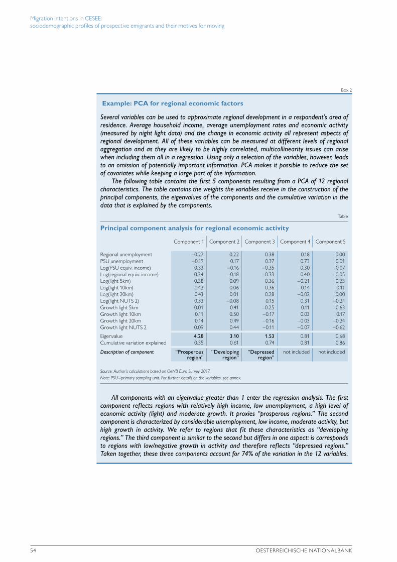
Migration intentions in CESEE: sociodemographic profiles of prospective emigrants and their motives for moving
54 OESTERREICHISCHE NATIONALBANK
Box 2
Example: PCA for regional economic factors
Several variables can be used to approximate regional development in a respondent’s area of residence. Average household income, average unemployment rates and economic activity (measured by night light data) and the change in economic activity all represent aspects of regional development. All of these variables can be measured at different levels of regional aggregation and as they are likely to be highly correlated, multicollinearity issues can arise when including them all in a regression. Using only a selection of the variables, however, leads to an omission of potentially important information. PCA makes it possible to reduce the set of covariates while keeping a large part of the information.
The following table contains the first 5 components resulting from a PCA of 12 regional characteristics. The table contains the weights the variables receive in the construction of the principal components, the eigenvalues of the components and the cumulative variation in the data that is explained by the components.
All components with an eigenvalue greater than 1 enter the regression analysis. The first component reflects regions with relatively high income, low unemployment, a high level of economic activity (light) and moderate growth. It proxies “prosperous regions.” The second component is characterized by considerable unemployment, low income, moderate activity, but high growth in activity. We refer to regions that f it these characteristics as “developing regions.” The third component is similar to the second but differs in one aspect: is corresponds to regions with low/negative growth in activity and therefore reflects “depressed regions.” Taken together, these three components account for 74% of the variation in the 12 variables.
Table
Principal component analysis for regional economic activity
Component 1 Component 2 Component 3 Component 4 Component 5
Regional unemployment –0.27 0.22 0.38 0.18 0.00PSU unemployment –0.19 0.17 0.37 0.73 0.01Log(PSU equiv. income) 0.33 –0.16 –0.35 0.30 0.07Log(regional equiv. income) 0.34 –0.18 –0.33 0.40 –0.05Log(light 5km) 0.38 0.09 0.36 –0.21 0.23Log(light 10km) 0.42 0.06 0.36 –0.14 0.11Log(light 20km) 0.43 0.01 0.28 –0.02 0.00Log(light NUTS 2) 0.33 –0.08 0.15 0.31 –0.24Growth light 5km 0.01 0.41 –0.25 0.11 0.63Growth light 10km 0.11 0.50 –0.17 0.03 0.17Growth light 20km 0.14 0.49 –0.16 –0.03 –0.24Growth light NUTS 2 0.09 0.44 –0.11 –0.07 –0.62
Eigenvalue 4.28 3.10 1.53 0.81 0.68Cumulative variation explained 0.35 0.61 0.74 0.81 0.86
Description of component “Prosperous region”
“Developing region”
“Depressed region”
not included not included
Source: Author’s calculations based on OeNB Euro Survey 2017. Note: PSU=primary sampling unit. For further details on the variables, see annex.
Migration intentions in CESEE: sociodemographic profiles of prospective emigrants and their motives for moving
FOCUS ON EUROPEAN ECONOMIC INTEGRATION Q1/19 55
3.2 Empirical specification
Based on the constructed variables and the results of the (P)PCA, we estimate the following empirical specification by simple probit regressions:
where mi is a binary variable that takes a value of 1 if an individual has the intention to emigrate to another country, Xj
S are J variables that belong to the group of socio-demographic characteristics, Xk
E represents the group of K economic factors, XlR the
L regional characteristics, XmN the M variables capturing network effects and Xp
T are P variables capturing trust in institutions. In addition, a constant and a full set of country dummies, denoted in the equation by a country-specific constant αr, is included in all specifications. The country dummies control for all factors that are common to all individuals in a country, such as institutional characteristics, the political environment, historic ties to other countries, geographic location, and similar. ϵi is a random error term. Standard errors are clustered at the regional level.
In the probit model, the estimated coefficients are not partial effects of the independent variables on the (likelihood of having) migration intentions, but the degree at which the z-score changes as a response to changes in the independent variables. We compute and report marginal effects in order to get a meaningful estimate of the magnitudes of the effects.
3.3 Caveats and limitations
Individuals’ migration intentions can depend on and be influenced by a large number of factors, and controlling for all of them is not possible. We cannot rule out that some of our estimates suffer from endogeneity, which can bias the estimated coefficients. First, the coefficient of the education variable might be overestimated. Individuals might acquire more education because they intend to emigrate (brain gain effect, see for example Beine et al., 2001 and 2011). It might seem that highly skilled people often develop migration intentions while, in fact, individuals might be highly skilled because they have migration intentions. This reversed causality might lead to an overestimation of the true effect of education.10 Second, the effect of networks might be overestimated. If the situation in migrants’ home regions is not attractive and has not been attractive in the past, migrants of the past might have left for (unobservable) reasons that are similar to those prospective migrants are currently considering. Manchin and Orazbayev (2016) use satisfaction with life in the region as an instrumental variable for networks, while controlling for an individual’s own life satisfaction in the main equation. The current wave of the OeNB Euro Survey, i.e. the 2017 fall wave, does not include a variable that would make it possible to approximate satisfaction with life in the region. Third, the effect of trust in institutions cannot be causally estimated in this setting. The causality could work in either way – from trust to migration intentions but also
10 Our results do not suggest that highly skilled individuals more frequently harbor migration intentions than individuals with lower skill levels. If the coefficient is upward-biased, the true effect of education is even lower. Beine et al. (2011) find no significant incentive mechanisms for prospective migration in middle (and high) income countries, i.e. no evidence for the brain gain effect. This can add to an explanation of our findings for the CESEE region.
8
growth. It proxies prosperous regions. The second component is characterized by considerable
unemployment, low income, moderate activity, but high growth in activity. We refer to regions that fit these
characteristics as developing regions. The third component is similar to the second but differs in one aspect:
is corresponds to regions with low/negative growth in activity and therefore reflects depressed regions. Taken
together, these three components account for 74% of the variation in the 12 variables.
3.2 Empirical specification Based on the constructed variables and the results of the (P)PCA, we estimate the following
empirical specification by simple probit regressions:
𝑚𝑚" = 𝛼𝛼% + 𝑋𝑋()𝛽𝛽()+
(,-
+ 𝑋𝑋./𝛽𝛽./0
.,-
+ 𝑋𝑋12𝛽𝛽123
1,-
+ 𝑋𝑋45𝛽𝛽456
4,-
+ 𝑋𝑋78𝛽𝛽789
7,-
+ 𝜖𝜖"
where 𝑚𝑚" is a binary variable that takes a value of 1 if an individual has the intention to emigrate
to another country, 𝑋𝑋() are 𝐽𝐽 variables that belong to the group of sociodemographic
characteristics, 𝑋𝑋./ represents the group of 𝐾𝐾 economic factors, 𝑋𝑋12 the 𝐿𝐿 regional characteristics,
𝑋𝑋45 the 𝑀𝑀 variables capturing network effects and 𝑋𝑋78 are 𝑃𝑃 variables capturing trust in
institutions. In addition, a constant and a full set of country dummies, denoted in the equation by
a country-specific constant 𝛼𝛼%, is included in all specifications. The country dummies control for
all factors that are common to all individuals in a country, such as institutional characteristics, the
political environment, historic ties to other countries, geographic location, and similar.𝜖𝜖" is a
random error term. Standard errors are clustered at the regional level.
In the probit model, the estimated coefficients are not partial effects of the independent variables
on the (likelihood of having) migration intentions, but the degree at which the z-score changes as
a response to changes in the independent variables. We compute and report marginal effects in
order to get a meaningful estimate of the magnitudes of the effects.
3.3 Caveats and limitations Individuals’ migration intentions can depend on and be influenced by a large number of factors
and controlling for all of them is not possible. We cannot rule out that some of our estimates
suffer from endogeneity, which can bias the estimated coefficients. First, the coefficient of the
education variable might be overestimated. Individuals might acquire more education because
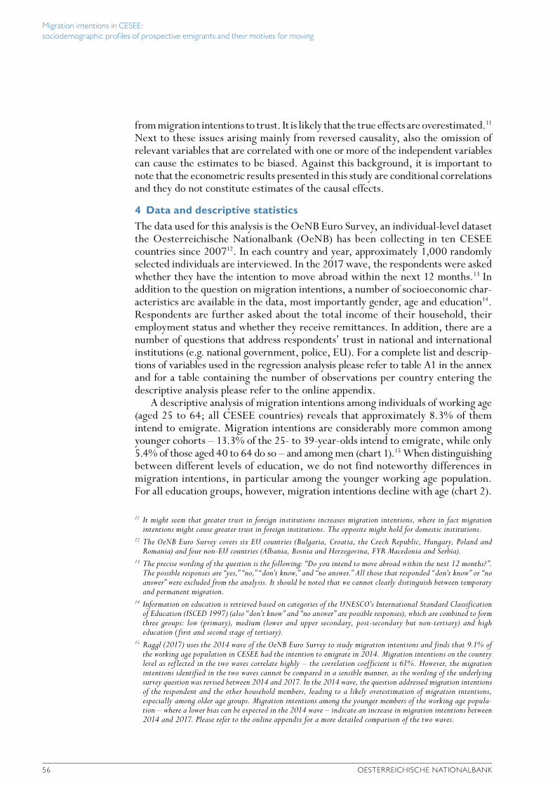
Migration intentions in CESEE: sociodemographic profiles of prospective emigrants and their motives for moving
56 OESTERREICHISCHE NATIONALBANK
from migration intentions to trust. It is likely that the true effects are overestimated.11 Next to these issues arising mainly from reversed causality, also the omission of relevant variables that are correlated with one or more of the independent variables can cause the estimates to be biased. Against this background, it is important to note that the econometric results presented in this study are conditional correlations and they do not constitute estimates of the causal effects.
4 Data and descriptive statisticsThe data used for this analysis is the OeNB Euro Survey, an individual-level dataset the Oesterreichische Nationalbank (OeNB) has been collecting in ten CESEE countries since 200712. In each country and year, approximately 1,000 randomly selected individuals are interviewed. In the 2017 wave, the respondents were asked whether they have the intention to move abroad within the next 12 months.13 In addition to the question on migration intentions, a number of socioeconomic char-acteristics are available in the data, most importantly gender, age and education14. Respondents are further asked about the total income of their household, their employment status and whether they receive remittances. In addition, there are a number of questions that address respondents’ trust in national and international institutions (e.g. national government, police, EU). For a complete list and descrip-tions of variables used in the regression analysis please refer to table A1 in the annex and for a table containing the number of observations per country entering the descriptive analysis please refer to the online appendix.
A descriptive analysis of migration intentions among individuals of working age (aged 25 to 64; all CESEE countries) reveals that approximately 8.3% of them intend to emigrate. Migration intentions are considerably more common among younger cohorts – 13.3% of the 25- to 39-year-olds intend to emigrate, while only 5.4% of those aged 40 to 64 do so – and among men (chart 1).15 When distinguishing between different levels of education, we do not find noteworthy differences in migration intentions, in particular among the younger working age population. For all education groups, however, migration intentions decline with age (chart 2).
11 It might seem that greater trust in foreign institutions increases migration intentions, where in fact migration intentions might cause greater trust in foreign institutions. The opposite might hold for domestic institutions.
12 The OeNB Euro Survey covers six EU countries (Bulgaria, Croatia, the Czech Republic, Hungary, Poland and Romania) and four non-EU countries (Albania, Bosnia and Herzegovina, FYR Macedonia and Serbia).
13 The precise wording of the question is the following: “Do you intend to move abroad within the next 12 months?”. The possible responses are “yes,” “no,” “don’t know,” and “no answer.” All those that responded “don’t know” or “no answer” were excluded from the analysis. It should be noted that we cannot clearly distinguish between temporary and permanent migration.
14 Information on education is retrieved based on categories of the UNESCO’s International Standard Classification of Education (ISCED 1997) (also “don’t know” and “no answer” are possible responses), which are combined to form three groups: low (primary), medium (lower and upper secondary, post-secondary but non-tertiary) and high education ( first and second stage of tertiary).
15 Raggl (2017) uses the 2014 wave of the OeNB Euro Survey to study migration intentions and finds that 9.1% of the working age population in CESEE had the intention to emigrate in 2014. Migration intentions on the country level as reflected in the two waves correlate highly – the correlation coefficient is 61%. However, the migration intentions identified in the two waves cannot be compared in a sensible manner, as the wording of the underlying survey question was revised between 2014 and 2017. In the 2014 wave, the question addressed migration intentions of the respondent and the other household members, leading to a likely overestimation of migration intentions, especially among older age groups. Migration intentions among the younger members of the working age popula-tion – where a lower bias can be expected in the 2014 wave – indicate an increase in migration intentions between 2014 and 2017. Please refer to the online appendix for a more detailed comparison of the two waves.
Share of individuals with migration intentions (%)
25
20
15
10
5
0
Migration intentions broken down by age and gender – CESEE average
Chart 1
Source: OeNB Euro Survey 2017.
All Men Women
20–24 25–29 30–34 35–39 40–44 45–49 50–54 55–59 60–64 65–69 70–74 75–79 80–84
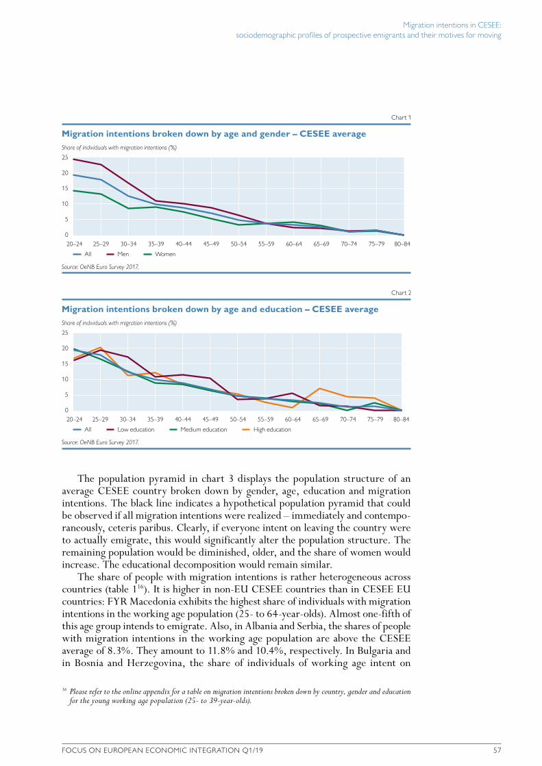
Migration intentions in CESEE: sociodemographic profiles of prospective emigrants and their motives for moving
FOCUS ON EUROPEAN ECONOMIC INTEGRATION Q1/19 57
The population pyramid in chart 3 displays the population structure of an average CESEE country broken down by gender, age, education and migration intentions. The black line indicates a hypothetical population pyramid that could be observed if all migration intentions were realized – immediately and contempo-raneously, ceteris paribus. Clearly, if everyone intent on leaving the country were to actually emigrate, this would significantly alter the population structure. The remaining population would be diminished, older, and the share of women would increase. The educational decomposition would remain similar.
The share of people with migration intentions is rather heterogeneous across countries (table 116). It is higher in non-EU CESEE countries than in CESEE EU countries: FYR Macedonia exhibits the highest share of individuals with migration intentions in the working age population (25- to 64-year-olds). Almost one-fifth of this age group intends to emigrate. Also, in Albania and Serbia, the shares of people with migration intentions in the working age population are above the CESEE average of 8.3%. They amount to 11.8% and 10.4%, respectively. In Bulgaria and in Bosnia and Herzegovina, the share of individuals of working age intent on
16 Please refer to the online appendix for a table on migration intentions broken down by country, gender and education for the young working age population (25- to 39-year-olds).
from migration intentions to trust. It is likely that the true effects are overestimated.11 Next to these issues arising mainly from reversed causality, also the omission of relevant variables that are correlated with one or more of the independent variables can cause the estimates to be biased. Against this background, it is important to note that the econometric results presented in this study are conditional correlations and they do not constitute estimates of the causal effects.
4 Data and descriptive statisticsThe data used for this analysis is the OeNB Euro Survey, an individual-level dataset the Oesterreichische Nationalbank (OeNB) has been collecting in ten CESEE countries since 200712. In each country and year, approximately 1,000 randomly selected individuals are interviewed. In the 2017 wave, the respondents were asked whether they have the intention to move abroad within the next 12 months.13 In addition to the question on migration intentions, a number of socioeconomic char-acteristics are available in the data, most importantly gender, age and education14. Respondents are further asked about the total income of their household, their employment status and whether they receive remittances. In addition, there are a number of questions that address respondents’ trust in national and international institutions (e.g. national government, police, EU). For a complete list and descrip-tions of variables used in the regression analysis please refer to table A1 in the annex and for a table containing the number of observations per country entering the descriptive analysis please refer to the online appendix.
A descriptive analysis of migration intentions among individuals of working age (aged 25 to 64; all CESEE countries) reveals that approximately 8.3% of them intend to emigrate. Migration intentions are considerably more common among younger cohorts – 13.3% of the 25- to 39-year-olds intend to emigrate, while only 5.4% of those aged 40 to 64 do so – and among men (chart 1).15 When distinguishing between different levels of education, we do not find noteworthy differences in migration intentions, in particular among the younger working age population. For all education groups, however, migration intentions decline with age (chart 2).
11 It might seem that greater trust in foreign institutions increases migration intentions, where in fact migration intentions might cause greater trust in foreign institutions. The opposite might hold for domestic institutions.
12 The OeNB Euro Survey covers six EU countries (Bulgaria, Croatia, the Czech Republic, Hungary, Poland and Romania) and four non-EU countries (Albania, Bosnia and Herzegovina, FYR Macedonia and Serbia).
13 The precise wording of the question is the following: “Do you intend to move abroad within the next 12 months?”. The possible responses are “yes,” “no,” “don’t know,” and “no answer.” All those that responded “don’t know” or “no answer” were excluded from the analysis. It should be noted that we cannot clearly distinguish between temporary and permanent migration.
14 Information on education is retrieved based on categories of the UNESCO’s International Standard Classification of Education (ISCED 1997) (also “don’t know” and “no answer” are possible responses), which are combined to form three groups: low (primary), medium (lower and upper secondary, post-secondary but non-tertiary) and high education ( first and second stage of tertiary).
15 Raggl (2017) uses the 2014 wave of the OeNB Euro Survey to study migration intentions and finds that 9.1% of the working age population in CESEE had the intention to emigrate in 2014. Migration intentions on the country level as reflected in the two waves correlate highly – the correlation coefficient is 61%. However, the migration intentions identified in the two waves cannot be compared in a sensible manner, as the wording of the underlying survey question was revised between 2014 and 2017. In the 2014 wave, the question addressed migration intentions of the respondent and the other household members, leading to a likely overestimation of migration intentions, especially among older age groups. Migration intentions among the younger members of the working age popula-tion – where a lower bias can be expected in the 2014 wave – indicate an increase in migration intentions between 2014 and 2017. Please refer to the online appendix for a more detailed comparison of the two waves.
Share of individuals with migration intentions (%)
25
20
15
10
5
0
Migration intentions broken down by age and gender – CESEE average
Chart 1
Source: OeNB Euro Survey 2017.
All Men Women
20–24 25–29 30–34 35–39 40–44 45–49 50–54 55–59 60–64 65–69 70–74 75–79 80–84
Share of individuals with migration intentions (%)
25
20
15
10
5
0
Migration intentions broken down by age and education – CESEE average
Chart 2
Source: OeNB Euro Survey 2017.
All Low education Medium education High education
20–24 25–29 30–34 35–39 40–44 45–49 50–54 55–59 60–64 65–69 70–74 75–79 80–84
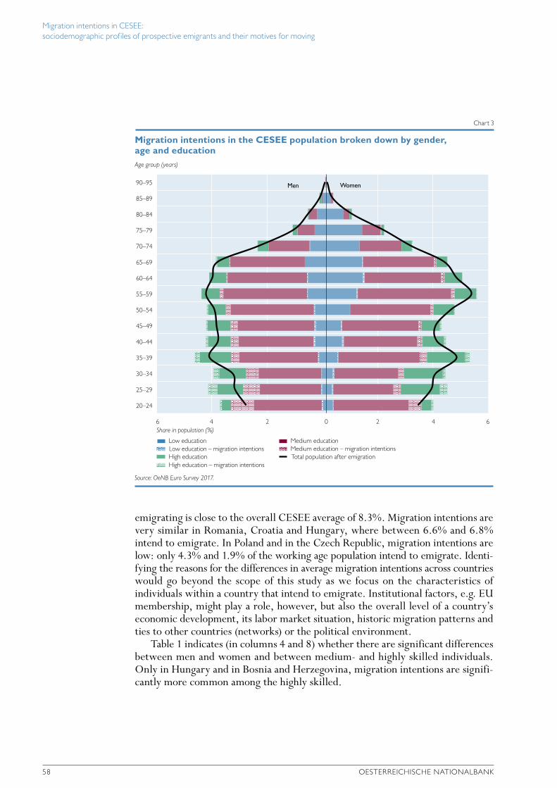
Migration intentions in CESEE: sociodemographic profiles of prospective emigrants and their motives for moving
58 OESTERREICHISCHE NATIONALBANK
emigrating is close to the overall CESEE average of 8.3%. Migration intentions are very similar in Romania, Croatia and Hungary, where between 6.6% and 6.8% intend to emigrate. In Poland and in the Czech Republic, migration intentions are low: only 4.3% and 1.9% of the working age population intend to emigrate. Identi-fying the reasons for the differences in average migration intentions across countries would go beyond the scope of this study as we focus on the characteristics of individuals within a country that intend to emigrate. Institutional factors, e.g. EU membership, might play a role, however, but also the overall level of a country’s economic development, its labor market situation, historic migration patterns and ties to other countries (networks) or the political environment.
Table 1 indicates (in columns 4 and 8) whether there are significant differences between men and women and between medium- and highly skilled individuals. Only in Hungary and in Bosnia and Herzegovina, migration intentions are signifi-cantly more common among the highly skilled.
Age group (years)
90–95
85–89
80–84
75–79
70–74
65–69
60–64
55–59
50–54
45–49
40–44
35–39
30–34
25–29
20–24
Migration intentions in the CESEE population broken down by gender, age and education
Chart 3
Source: OeNB Euro Survey 2017.
Low education Medium education
High education Total population after emigrationHigh education – migration intentions
Low education – migration intentions Medium education – migration intentions
6 4 2 0 2 4 6
Men Women
Share in population (%)
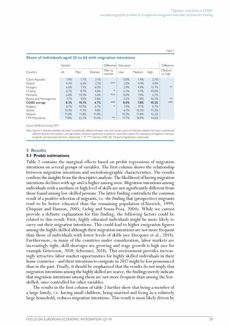
Migration intentions in CESEE: sociodemographic profiles of prospective emigrants and their motives for moving
FOCUS ON EUROPEAN ECONOMIC INTEGRATION Q1/19 59
5 Results5.1 Probit estimations
Table 2 contains the marginal effects based on probit regressions of migration intentions on several groups of variables. The first column shows the relationship between migration intentions and sociodemographic characteristics. The results confirm the insights from the descriptive analysis: The likelihood of having migration intentions declines with age and is higher among men. Migration intentions among individuals with a medium or high level of skills are not significantly different from those found among low-skilled persons. The latter finding contradicts the common result of a positive selection of migrants, i.e. the finding that (prospective) migrants tend to be better educated than the remaining population (Chiswick, 1999; Chiquiar and Hanson, 2005; Liebig and Sousa-Poza, 2004). While we cannot provide a definite explanation for this finding, the following factors could be related to this result: First, highly educated individuals might be more likely to carry out their migration intentions. This could lead to higher emigration figures among the highly skilled although their migration intentions are not more frequent than those of individuals with lower levels of skills (see Docquier et al., 2014). Furthermore, in many of the countries under consideration, labor markets are increasingly tight, skill shortages are growing and wage growth is high (see for example Grieveson, 2018; Schreiner, 2018). This environment provides increas-ingly attractive labor market opportunities for highly skilled individuals in their home countries – and their intentions to emigrate in 2017 might be less pronounced than in the past. Finally, it should be emphasized that the results do not imply that migration intentions among the highly skilled are scarce, the findings merely indicate that migration intentions among them are not more frequent than among the low-skilled, once controlled for other variables.
The results in the first column of table 2 further show that being a member of a large family, i.e. having small children, being married and living in a relatively large household, reduces migration intentions. This result is most likely driven by
Table 1
Share of individuals aged 25 to 64 with migration intentions
Gender Difference Education Difference
Country All Men Women Men vs. women Low Medium High Medium
vs. high
Czech Republic 1.9% 1.7% 2.1% 0.0% 1.9% 2.7%Poland 4.3% 6.6% 2.1% *** 3.0% 4.4% 4.9%Hungary 6.6% 7.3% 6.0% 2.4% 4.8% 13.1% **Croatia 6.7% 8.7% 4.8% * 6.5% 5.9% 10.0%Romania 6.8% 10.5% 3.6% *** 0.0% 7.0% 6.7%Bosnia and Herzegovina 7.7% 9.9% 5.8% 3.2% 7.8% 16.5% **CESEE average 8.3% 10.1% 6.7% *** 8.0% 7.8% 10.2% ***Bulgaria 8.7% 10.9% 6.7% * 7.4% 9.7% 6.7%Serbia 10.4% 11.1% 9.8% 6.7% 10.5% 13.2%Albania 11.8% 11.8% 11.8% 10.5% 11.8% 12.2%FYR Macedonia 17.8% 22.3% 13.4% ** 17.7% 18.9% 14.6%
Source: OeNB Euro Survey 2017.
Note: Column 4 indicates whether the mean is statistically different between men and women, column 8 indicates whether the mean is statistically different between the medium- and high-skilled. Statistical signif icance is based on t-tests from robust OLS regressions of migration intentions on gender and education dummies, respectively. *, **, *** indicate a 10%, 5%, 1% level of signif icance, respectively.
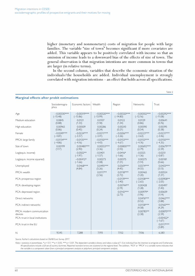
Migration intentions in CESEE: sociodemographic profiles of prospective emigrants and their motives for moving
60 OESTERREICHISCHE NATIONALBANK
higher (monetary and nonmonetary) costs of migration for people with large families. The variable “size of town” becomes significant if more covariates are added. This variable appears to be positively correlated with income so that an omission of income leads to a downward bias of the effects of size of town. The general observation is that migration intentions are more common in towns that are larger (in relative terms).
In the second column, variables that describe the economic situation of the individuals/the households are added. Individual unemployment is strongly correlated with migration intentions – an effect that holds across all specifications.
Table 2
Marginal effects after probit estimations
Sociodemogra-phics
Economic factors Wealth Region Networks Trust
Age –0.00330***(–15.48)
–0.00319***(–13.86)
–0.00320***(–13.99)
–0.00320***(–14.80)
–0.00302***(–12.16)
–0.00292***(–11.08)
Medium education 0.0845(0.88)
0.0121(1.33)
0.0107(1.18)
0.0122(1.34)
0.0129(0.86)
0.00641(0.76)
High education 0.00965(0.86)
0.00509(0.45)
0.00286(0.24)
0.00243(0.21)
0.00590(0.54)
0.00395(0.38)
Female –0.0249***(–4.81)
–0.0224***(–3.57)
–0.0211***(–3.41)
–0.0206***(–3.26)
–0.0223***(–3.63)
–0.0231***(–3.46)
PPCA: large family –0.0134***(–4.86)
–0.0135***(–4.16)
–0.0150***(–4.43)
–0.0153***(–4.67)
–0.0153***(–4.76)
–0.0150***(–4.35)
Size of town 0.00199(1.17)
0.00480***(2.90)
0.00553***(3.36)
0.00800***(3.10)
0.00692***(2.79)
0.00679***(2.59)
Log(equiv. income) –0.0502**(–1.97)
–0.0401(–1.57)
–0.0416*(–1.66)
–0.0325(–1.36)
–0.0251(–0.87)
Log(equiv. income squared) –0.00412*(–1.66)
0.00273(1.08)
0.00375(1.51)
0.00275(1.14)
0.00181(0.66)
Unemployed 0.0468***(4.84)
0.0495***(5.26)
0.0369***(4.45)
0.0374***(4.55)
0.0403***(5.13)
PPCA: wealth 0.0117**(2.56)
0.0118***(2.72)
0.00465(1.20)
0.00554(1.37)
PCA: prosperous region –0.0139***(–3.40)
–0.0108***(–2.65)
–0.00908**(–2.05)
PCA: developing region 0.00744**(2.19)
0.00428(1.28)
0.00497(1.40)
PCA: depressed region 0.0142***(2.73)
0.00979*(1.96)
0.00659(1.14)
Direct networks 0.0476***(4.52)
0.0462***(3.88)
PCA: indirect networks 0.0158***(4.58)
0.0160***(4.29)
PPCA: modern communication devices
0.00783**(2.38)
0.00870***(2.59)
PCA: trust in local institutions –0.00422*(–1.67)
PCA: trust in the EU 0.0117***(3.89)
N 9,545 7,288 7,193 7,152 7,106 6,583
Source: Author’s calculations based on OeNB Euro Survey 2017.
Note: t statistics in parentheses. * p < 0.1, ** p < 0.05, *** p < 0.01. The dependent variable is binary and takes a value of 1 if an individual has the intention to emigrate and 0 otherwise. All specif ications include a full set of country dummies. Reported standard errors are clustered at the regional level. The addition, “PCA” or “PPCA” in a variable name indicates that the variable is a component taken from a principal component analysis or polychoric principal component analysis.
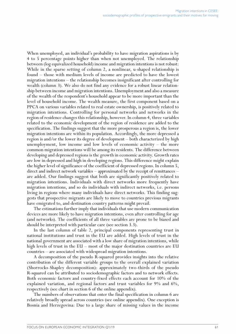
Migration intentions in CESEE: sociodemographic profiles of prospective emigrants and their motives for moving
FOCUS ON EUROPEAN ECONOMIC INTEGRATION Q1/19 61
When unemployed, an individual’s probability to have migration aspirations is by 4 to 5 percentage points higher than when not unemployed. The relationship between (log equivalized household) income and migration intentions is not robust: While in the sparse setting of column 2, a nonlinear, u-shaped relationship is found – those with medium levels of income are predicted to have the lowest migration intentions – the relationship becomes insignificant after controlling for wealth (column 3). We also do not find any evidence for a robust linear relation-ship between income and migration intentions. Unemployment and also a measure of the wealth of the respondent’s household appear to be more important than the level of household income. The wealth measure, the first component based on a PPCA on various variables related to real estate ownership, is positively related to migration intentions. Controlling for personal networks and networks in the region of residence changes this relationship, however. In column 4, three variables related to the economic development of the region of residence are added to the specification. The findings suggest that the more prosperous a region is, the lower migration intentions are within its population. Accordingly, the more depressed a region is and/or the lower its degree of development – both characterized by high unemployment, low income and low levels of economic activity – the more common migration intentions will be among its residents. The difference between developing and depressed regions is the growth in economic activity. Growth rates are low in depressed and high in developing regions. This difference might explain the higher level of significance of the coefficient of depressed regions. In column 5, direct and indirect network variables – approximated by the receipt of remittances – are added. Our findings suggest that both are significantly positively related to migration intentions. Individuals with direct networks more frequently have migration intentions, and so do individuals with indirect networks, i.e. persons living in regions where many individuals have direct networks. This finding sug-gests that prospective migrants are likely to move to countries previous migrants have emigrated to, and destination country patterns might prevail.
The estimations further imply that individuals that use modern communication devices are more likely to have migration intentions, even after controlling for age (and networks). The coefficients of all three variables are prone to be biased and should be interpreted with particular care (see section 3.3).
In the last column of table 2, principal components representing trust in national institutions and trust in the EU are added. High levels of trust in the national government are associated with a low share of migration intentions, while high levels of trust in the EU – most of the major destination countries are EU countries – are associated with widespread migration intentions.
A decomposition of the pseudo R-squared provides insights into the relative contribution of the different variable groups to the overall explained variation (Shorrocks-Shapley decomposition): approximately two-thirds of the pseudo R-squared can be attributed to sociodemographic factors and to network effects. Both economic factors and country-fixed effects each account for 10% of the explained variation, and regional factors and trust variables for 9% and 6%, respectively (see chart in section 6 of the online appendix).
The numbers of observations that enter the final specification in column 6 are relatively broadly spread across countries (see online appendix). One exception is Bosnia and Herzegovina: Due to a large share of missing values in the income
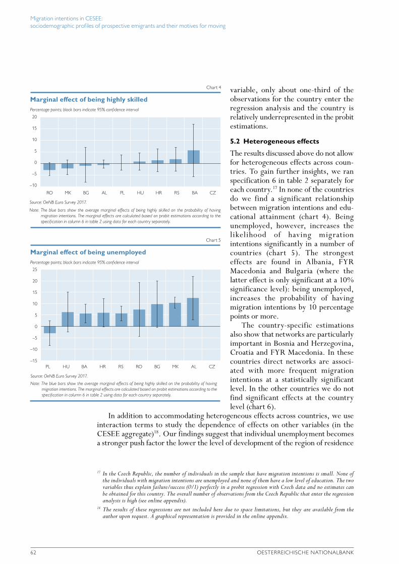
Migration intentions in CESEE: sociodemographic profiles of prospective emigrants and their motives for moving
62 OESTERREICHISCHE NATIONALBANK
variable, only about one-third of the observations for the country enter the regression analysis and the country is relatively underrepresented in the probit estimations.
5.2 Heterogeneous effects
The results discussed above do not allow for heterogeneous effects across coun-tries. To gain further insights, we ran specification 6 in table 2 separately for each country.17 In none of the countries do we find a significant relationship between migration intentions and edu-cational attainment (chart 4). Being unemployed, however, increases the likelihood of having migration intentions significantly in a number of countries (chart 5). The strongest effects are found in Albania, FYR Macedonia and Bulgaria (where the latter effect is only significant at a 10% significance level): being unemployed, increases the probability of having migration intentions by 10 percentage points or more.
The country-specific estimations also show that networks are particularly important in Bosnia and Herzegovina, Croatia and FYR Macedonia. In these countries direct networks are associ-ated with more frequent migration intentions at a statistically significant level. In the other countries we do not find significant effects at the country level (chart 6).
In addition to accommodating heterogeneous effects across countries, we use interaction terms to study the dependence of effects on other variables (in the CESEE aggregate)18. Our findings suggest that individual unemployment becomes a stronger push factor the lower the level of development of the region of residence
17 In the Czech Republic, the number of individuals in the sample that have migration intentions is small. None of the individuals with migration intentions are unemployed and none of them have a low level of education. The two variables thus explain failure/success (0/1) perfectly in a probit regression with Czech data and no estimates can be obtained for this country. The overall number of observations from the Czech Republic that enter the regression analysis is high (see online appendix).
18 The results of these regressions are not included here due to space limitations, but they are available from the author upon request. A graphical representation is provided in the online appendix.
Percentage points; black bars indicate 95% confidence interval
20
15
10
5
0
–5
–10
Marginal effect of being highly skilled
Chart 4
Source: OeNB Euro Survey 2017.
RO MK BG AL PL HU HR RS BA CZ
Note: The blue bars show the average marginal effects of being highly skilled on the probability of having migration intentions. The marginal effects are calculated based on probit estimations according to the specification in column 6 in table 2 using data for each country separately.
Percentage points; black bars indicate 95% confidence interval
25
20
15
10
5
0
–5
–10
–15
Marginal effect of being unemployed
Chart 5
Source: OeNB Euro Survey 2017.
PL HU BA HR RS RO BG MK AL CZ
Note: The blue bars show the average marginal effects of being highly skilled on the probability of having migration intentions. The marginal effects are calculated based on probit estimations according to the specification in column 6 in table 2 using data for each country separately.
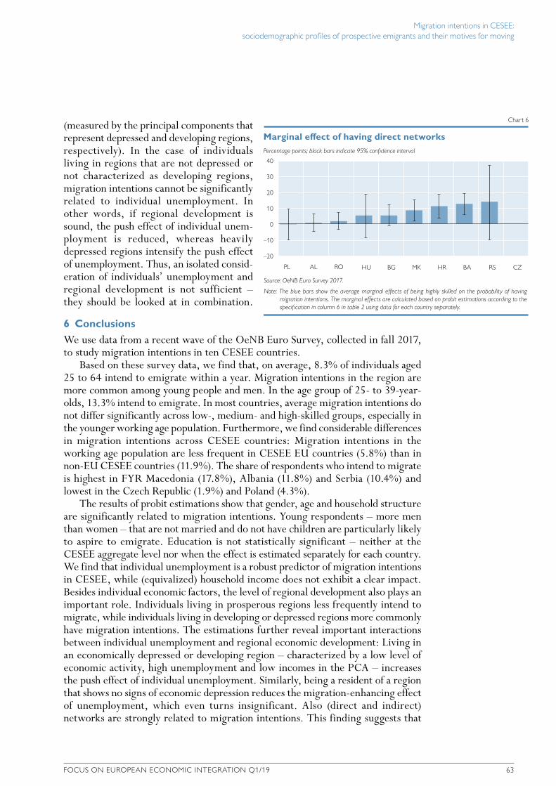
Migration intentions in CESEE: sociodemographic profiles of prospective emigrants and their motives for moving
FOCUS ON EUROPEAN ECONOMIC INTEGRATION Q1/19 63
(measured by the principal components that represent depressed and developing regions, respectively). In the case of individuals living in regions that are not depressed or not characterized as developing regions, migration intentions cannot be significantly related to individual unemployment. In other words, if regional development is sound, the push effect of individual unem-ployment is reduced, whereas heavily depressed regions intensify the push effect of unemployment. Thus, an isolated consid-eration of individuals’ unemployment and regional development is not sufficient – they should be looked at in combination.
6 ConclusionsWe use data from a recent wave of the OeNB Euro Survey, collected in fall 2017, to study migration intentions in ten CESEE countries.
Based on these survey data, we find that, on average, 8.3% of individuals aged 25 to 64 intend to emigrate within a year. Migration intentions in the region are more common among young people and men. In the age group of 25- to 39-year-olds, 13.3% intend to emigrate. In most countries, average migration intentions do not differ significantly across low-, medium- and high-skilled groups, especially in the younger working age population. Furthermore, we find considerable differences in migration intentions across CESEE countries: Migration intentions in the working age population are less frequent in CESEE EU countries (5.8%) than in non-EU CESEE countries (11.9%). The share of respondents who intend to migrate is highest in FYR Macedonia (17.8%), Albania (11.8%) and Serbia (10.4%) and lowest in the Czech Republic (1.9%) and Poland (4.3%).
The results of probit estimations show that gender, age and household structure are significantly related to migration intentions. Young respondents – more men than women – that are not married and do not have children are particularly likely to aspire to emigrate. Education is not statistically significant – neither at the CESEE aggregate level nor when the effect is estimated separately for each country. We find that individual unemployment is a robust predictor of migration intentions in CESEE, while (equivalized) household income does not exhibit a clear impact. Besides individual economic factors, the level of regional development also plays an important role. Individuals living in prosperous regions less frequently intend to migrate, while individuals living in developing or depressed regions more commonly have migration intentions. The estimations further reveal important interactions between individual unemployment and regional economic development: Living in an economically depressed or developing region – characterized by a low level of economic activity, high unemployment and low incomes in the PCA – increases the push effect of individual unemployment. Similarly, being a resident of a region that shows no signs of economic depression reduces the migration-enhancing effect of unemployment, which even turns insignificant. Also (direct and indirect) networks are strongly related to migration intentions. This finding suggests that
Percentage points; black bars indicate 95% confidence interval
40
30
20
10
0
–10
–20
Marginal effect of having direct networks
Chart 6
Source: OeNB Euro Survey 2017.
ALPL RO HU BG MK HR BA RS CZ
Note: The blue bars show the average marginal effects of being highly skilled on the probability of having migration intentions. The marginal effects are calculated based on probit estimations according to the specification in column 6 in table 2 using data for each country separately.
Migration intentions in CESEE: sociodemographic profiles of prospective emigrants and their motives for moving
64 OESTERREICHISCHE NATIONALBANK
the historic destination country patterns are likely to persist: networks abroad, approximated by the receipt of remittances, reduce the cost of migration and thus prospective migrants are likely to emigrate to a country previous emigrants from their country have moved to. Finally, variables that measure trust in institutions suggest that trust in national institutions is associated with relatively rare, trust in the EU with relatively widespread, migration intentions.
The analysis provides a recent picture of migration aspirations in CESEE countries and the characteristics of prospective emigrants. Due to a lack of appropriate instrumental variables, however, we are not able to establish causality between individual characteristics (most importantly education, networks and trust in institutions) and migration intentions. Our estimates merely constitute conditional correlations, and more research in this field is needed to establish causal links.
ReferencesAtoyan R., L. Christiansen, A. Dizioli, C. Ebeke, N. Ilahi, A. Ilyina, G. Mehrez, H. Qu,
F. Raei, A. Rhee and D. Zakharova. 2016. Emigration and Its Economic Impact on Eastern Europe. IMF Staff Discussion Note SDN/16/07.
Becker, G. S. 1964. Human Capital. A theoretical and empirical analysis, with special reference to education. National Bureau of Economic Research. New York.
Beine, M., F. Docquier and C. Oden-Defoort. 2011. A Panel Data Analysis of the Brain Gain. In: World Development 39(4). 523−532.
Beine, M., F. Docquier and H. Rapoport. 2001. Brain drain and economic growth: theory and evidence. In: Journal of Development Economics 64(1). 275−289.
Böheim, R. and M. P. Taylor. 2003. Tied Down Or Room To Move? Investigating The Relation-ships Between Housing Tenure, Employment Status And Residential Mobility In Britain. In: Scottish Journal of Political Economy 49(4). 369−392.
Borjas, G. 1987. Self-Selection and the Earnings of Immigrants. In: America Economic Review 77(4). 531−553.
Chiquiar, D. and G. H. Hanson. 2005. International Migration, Self-Selection, and the Distribu-tion of Wages: Evidence from Mexico and the United States. In: Journal of Political Economy 113(2). 239−281.
Chiswick, B. 1999. Are Immigrants Favorably Self-Selected? In: American Economic Review 89(2). 181−185.
Creighton, M. J. 2013. The role of aspirations in domestic and international migration. In: The Social Science Journal 50(1). 79−88.
Docquier, F., G. Peri and I. Ruyssen. 2014. The Cross-country Determinants of Potential and Actual Migration. In: International Migration Review 48(s1). 37−99.
Dustmann, C. 2003. Children and Return Migration. In: Journal of Population Economics 16(4). 815−830.
Dustmann, C., F. Fasani, X. Meng and L. Minale. 2017. Risk Attitudes and Household Migration Decisions. IZA Discussion Papers 10603. IZA Institute of Labor Economics.
EBRD. 2018. Work in Transition. Transition Report 2018-19. European Bank for Reconstruction and Development.
Fishbein, M. and I. Ajzen. 1975. Belief, attitudes, intention and behavior. An introduction to theory and research. Reading, MA. Addison-Wesley Publishing Company.
Migration intentions in CESEE: sociodemographic profiles of prospective emigrants and their motives for moving
FOCUS ON EUROPEAN ECONOMIC INTEGRATION Q1/19 65
Fouarge, D. and P. Ester. 2007. Factors Determining International and Regional Migration in Europe. European Foundation for the Improvement of Living and Working Conditions. Dublin.
Fouarge, D. and P. Ester. 2008. How Willing are Europeans to Migrate? A Comparison of Migration Intentions in Western and Eastern Europe. In: Ester, P., R. Muffels, J. Schippers and T. Wilthagen (eds.). Innovating European Labour Markets. Dynamics and Perspectives. Edward Elgar Publishing.
Gordon, I. and I. Molho. 1995. Duration Dependence in Migration Behaviour. Cumulative Iner-tia versus Stochastic Change. In: Environment and Planning A: Economy and Space 27(12). 1961−1975.
Grieveson, R. 2018. Demographic decline does not necessarily condemn CESEE EU countries to a low growth future. In: OeNB. Focus on European Economic Integration Q3/2018. 122−130.
Harris, J. R. and M. P. Todaro. 1970. Migration, Unemployment and Development: A Two-Sector Analysis. In: American Economic Review 60(1). 126−142.
Hotelling, H. 1933. Analysis of a complex of statistical variables into principal components. In: Journal of Educational Psychology 24(6) and (7). 417–441 and 498–520.
Huber, P. and K. Nowotny. 2018. Risk Aversion and the Willingness to Migrate in 30 Countries. WIFO Working Papers No. 569. Austrian Institute of Economic Research.
Hyll, W. and L. Schneider. 2014. Relative deprivation and migration preference. In: Economics Letters 122(2). 334−337.
IMF. 2016. Central, Eastern, and Southeastern Europe. How to Get Back on the Fast Track. Regional Economic Issues May 2016.
IMF. 2017. Central, Eastern, and Southeastern Europe. A Broadening Recovery. Regional Economic Issues May 2017.
Kolenikov, S. and G. Angeles. 2004. The Use of Discrete Data in PCA: Theory, Simulations, and Applications to Socioeconomic Indices. CPC/MEASURE Working paper No. WP-04-85.
Liebig, T. and A. Sousa-Poza. 2004. Migration, Self-Selection and Income Inequality: An International Analysis. In: Kyklos 57(1). 125−146.
Manski, C. F. 1990. The Use of Intentions Data to Predict Behavior: A Best-Case Analysis. In: Journal of the American Statistical Association 85(412). 934−940.
Manchin, M. and S. Orazbayev. 2016. Social networks and the intention to migrate. Develop-ment Studies Working Paper No. 409. Centro Study Luca D’Agliano.
Otrachshenko, V. and O. Popova. 2014. Life (dis)satisfaction and the intention to migrate: Evidence from Central and Eastern Europe. In: The Journal of Socio-Economics 48. 40−49.
Pearson, K. 1901. On lines and planes of closest fit to systems of points in space. In: Philosophical Magazine 2. 559−572.
Piracha, M. and A. Saraogi. 2017. Remittances and migration intentions of the left-behind. In: Migration and Development 6(1). 102−122.
Raggl, A. 2017. Migration intentions in CESEE – a descriptive analysis. In: OeNB. Focus on European Economic Integration Q4/17. 52−69.
Regional Cooperation Council. 2018. Balkan Barometer 2018: Public Opinion Survey. IV (4). Roy, A. 1951. Some Thoughts on the Distribution of Earnings. In: Oxford Economic Papers 3.
135−146.Sandu, D. and G. F. De Jong. 1996. Migration in market and democracy transition: Migration
intentions and behaviour in Romania. In: Population Research and Policy Review 15. 437−457.Schreiner, J. 2018. Developments in selected CESEE countries. In: OeNB. Focus on European
Economic Integration Q4/18.Sjaastad, L. A. 1962. The Costs and Returns of Human Migration. In: Journal of the Political
Economy 70(4). 80−93.
Migration intentions in CESEE: sociodemographic profiles of prospective emigrants and their motives for moving
66 OESTERREICHISCHE NATIONALBANK
Stark, O. 2003. Tales of Migration without Wage Differentials: Individual, Family, and Community Contexts. ZEF discussion papers on development policy No. 73. University of Bonn, Centre for Development Research (ZEF).
United Nations. 2017. World Population Prospects: The 2017 Revision. Department of Economic and Social Affairs, Population Division.
Van Dalen, H. P. and K. Henkens. 2008. Emigration Intentions: Mere Words or True Plans? Explaining International Migration Intentions and Behavior. Discussion Paper No. 2008-60. Tilburg University.
Van Dalen, H. P. and K. Henkens. 2013. Explaining Emigration Intentions and Behaviour in the Netherlands, 2005-10. In: Population Studies 67(2). 225−241.
Williams, A. M., C. Jephcote, H. Janta and G. Li. 2018. The migration intentions of young adults in Europe: A comparative, multilevel analysis. In: Population, Space and Place 24(1). 1−16.
World Bank and wiiw. 2018. Western Balkans. Labor Market Trends 2018. World Bank Group and The Vienna Institute for International Economic Studies.
Zaiceva, A. and K. F. Zimmermann. 2008. Scale, diversity, and determinants of labour migration in Europe. In: Oxford Review of Economic Policy 24(3). 427−451.
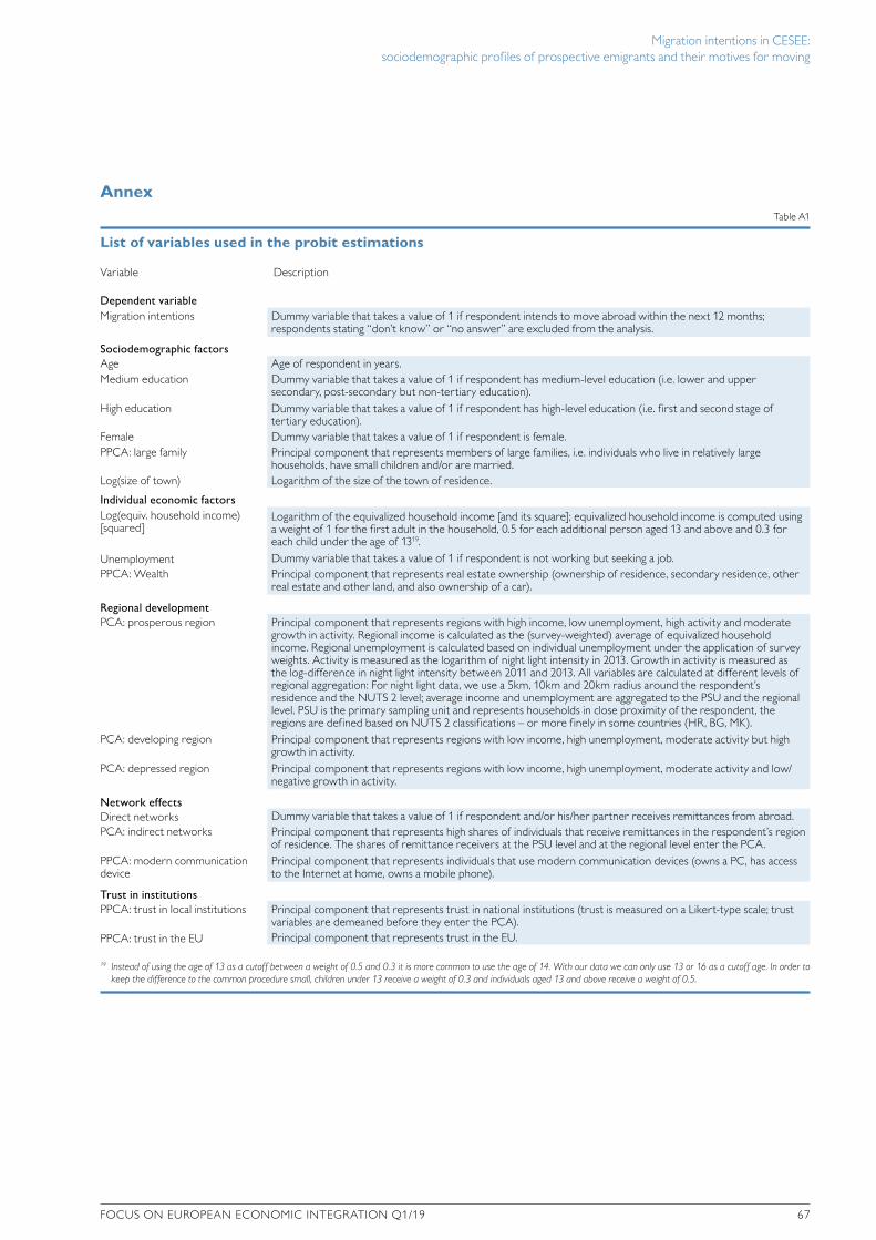
Migration intentions in CESEE: sociodemographic profiles of prospective emigrants and their motives for moving
FOCUS ON EUROPEAN ECONOMIC INTEGRATION Q1/19 67
AnnexTable A1
List of variables used in the probit estimations
Variable Description
Dependent variableMigration intentions Dummy variable that takes a value of 1 if respondent intends to move abroad within the next 12 months;
respondents stating “don’t know” or “no answer” are excluded from the analysis.
Sociodemographic factorsAge Age of respondent in years.Medium education Dummy variable that takes a value of 1 if respondent has medium-level education (i.e. lower and upper
secondary, post-secondary but non-tertiary education).High education Dummy variable that takes a value of 1 if respondent has high-level education (i.e. first and second stage of
tertiary education).Female Dummy variable that takes a value of 1 if respondent is female.PPCA: large family Principal component that represents members of large families, i.e. individuals who live in relatively large
households, have small children and/or are married.Log(size of town) Logarithm of the size of the town of residence.
Individual economic factorsLog(equiv. household income) [squared]
Logarithm of the equivalized household income [and its square]; equivalized household income is computed using a weight of 1 for the first adult in the household, 0.5 for each additional person aged 13 and above and 0.3 for each child under the age of 1319.
Unemployment Dummy variable that takes a value of 1 if respondent is not working but seeking a job.PPCA: Wealth Principal component that represents real estate ownership (ownership of residence, secondary residence, other
real estate and other land, and also ownership of a car).
Regional developmentPCA: prosperous region Principal component that represents regions with high income, low unemployment, high activity and moderate
growth in activity. Regional income is calculated as the (survey-weighted) average of equivalized household income. Regional unemployment is calculated based on individual unemployment under the application of survey weights. Activity is measured as the logarithm of night light intensity in 2013. Growth in activity is measured as the log-difference in night light intensity between 2011 and 2013. All variables are calculated at different levels of regional aggregation: For night light data, we use a 5km, 10km and 20km radius around the respondent’s residence and the NUTS 2 level; average income and unemployment are aggregated to the PSU and the regional level. PSU is the primary sampling unit and represents households in close proximity of the respondent, the regions are defined based on NUTS 2 classifications – or more finely in some countries (HR, BG, MK).
PCA: developing region Principal component that represents regions with low income, high unemployment, moderate activity but high growth in activity.
PCA: depressed region Principal component that represents regions with low income, high unemployment, moderate activity and low/negative growth in activity.
Network effectsDirect networks Dummy variable that takes a value of 1 if respondent and/or his/her partner receives remittances from abroad.PCA: indirect networks Principal component that represents high shares of individuals that receive remittances in the respondent’s region
of residence. The shares of remittance receivers at the PSU level and at the regional level enter the PCA.PPCA: modern communication device
Principal component that represents individuals that use modern communication devices (owns a PC, has access to the Internet at home, owns a mobile phone).
Trust in institutionsPPCA: trust in local institutions Principal component that represents trust in national institutions (trust is measured on a Likert-type scale; trust
variables are demeaned before they enter the PCA).PPCA: trust in the EU Principal component that represents trust in the EU.
19 Instead of using the age of 13 as a cutoff between a weight of 0.5 and 0.3 it is more common to use the age of 14. With our data we can only use 13 or 16 as a cutoff age. In order to keep the difference to the common procedure small, children under 13 receive a weight of 0.3 and individuals aged 13 and above receive a weight of 0.5.

Event wrap-ups and miscellaneous
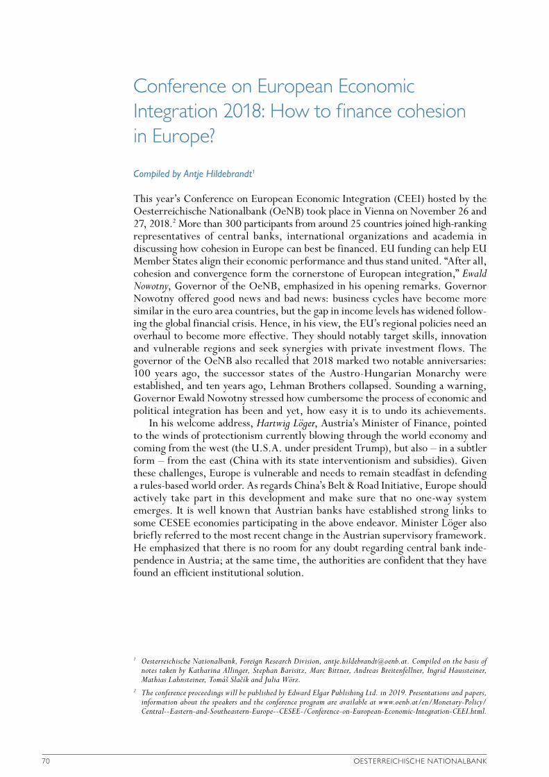
70 OESTERREICHISCHE NATIONALBANK
Conference on European Economic Integration 2018: How to finance cohesion in Europe?
Compiled by Antje Hildebrandt1
This year’s Conference on European Economic Integration (CEEI) hosted by the Oesterreichische Nationalbank (OeNB) took place in Vienna on November 26 and 27, 2018.2 More than 300 participants from around 25 countries joined high-ranking representatives of central banks, international organizations and academia in discussing how cohesion in Europe can best be financed. EU funding can help EU Member States align their economic performance and thus stand united. “After all, cohesion and convergence form the cornerstone of European integration,” Ewald Nowotny, Governor of the OeNB, emphasized in his opening remarks. Governor Nowotny offered good news and bad news: business cycles have become more similar in the euro area countries, but the gap in income levels has widened follow-ing the global financial crisis. Hence, in his view, the EU’s regional policies need an overhaul to become more effective. They should notably target skills, innovation and vulnerable regions and seek synergies with private investment flows. The governor of the OeNB also recalled that 2018 marked two notable anniversaries: 100 years ago, the successor states of the Austro-Hungarian Monarchy were established, and ten years ago, Lehman Brothers collapsed. Sounding a warning, Governor Ewald Nowotny stressed how cumbersome the process of economic and political integration has been and yet, how easy it is to undo its achievements.
In his welcome address, Hartwig Löger, Austria’s Minister of Finance, pointed to the winds of protectionism currently blowing through the world economy and coming from the west (the U.S.A. under president Trump), but also – in a subtler form – from the east (China with its state interventionism and subsidies). Given these challenges, Europe is vulnerable and needs to remain steadfast in defending a rules-based world order. As regards China’s Belt & Road Initiative, Europe should actively take part in this development and make sure that no one-way system emerges. It is well known that Austrian banks have established strong links to some CESEE economies participating in the above endeavor. Minister Löger also briefly referred to the most recent change in the Austrian supervisory framework. He emphasized that there is no room for any doubt regarding central bank inde-pendence in Austria; at the same time, the authorities are confident that they have found an efficient institutional solution.
1 Oesterreichische Nationalbank, Foreign Research Division, [email protected]. Compiled on the basis of notes taken by Katharina Allinger, Stephan Barisitz, Marc Bittner, Andreas Breitenfellner, Ingrid Haussteiner, Mathias Lahnsteiner, Tomáš Slacík and Julia Wörz.
2 The conference proceedings will be published by Edward Elgar Publishing Ltd. in 2019. Presentations and papers, information about the speakers and the conference program are available at www.oenb.at/en/Monetary-Policy/Central--Eastern-and-Southeastern-Europe--CESEE-/Conference-on-European-Economic-Integration-CEEI.html.
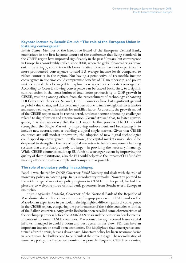
Conference on European Economic Integration 2018: How to finance cohesion in Europe?
FOCUS ON EUROPEAN ECONOMIC INTEGRATION Q1/19 71
Keynote lecture by Benoît Cœuré: “The role of the European Union in fostering convergence”Benoît Cœuré, Member of the Executive Board of the European Central Bank, emphasized in the first keynote lecture of the conference that living standards in the CESEE region have improved significantly in the past 30 years, but convergence in Europe has considerably stalled since 2008, when the global financial crisis broke out. Interestingly, countries with lower relative incomes have not experienced a more pronounced convergence toward EU average income levels compared to richer countries in the region. Not having a perspective of reasonable income convergence in due time could compromise benefits of EU membership, and policy makers should thus be urged to explore new ways to accelerate convergence. According to Cœuré, slowing convergence can be traced back, first, to a signifi-cant reduction in the contribution of total factor productivity to GDP growth in CESEE, resulting among others from the retrenchment of technology-enhancing FDI flows since the crisis. Second, CESEE countries have lost significant ground in global value chains, and this trend may persist due to increased global uncertainties and narrowed wage differentials for unskilled labor. As a result, the growth model of the CESEE region must be reconsidered, not least because of pending challenges related to digitalization and automatization. Cœuré stressed that, to foster conver-gence, it is also necessary that the EU supports this process. The EU should strengthen the Single Market by improving enforcement and broadening it to include new sectors, such as building a digital single market. Given that CESEE countries are still modest innovators, the adoption of new digital technologies could speed up convergence. Furthermore, the capital markets union should be deepened to strengthen the role of capital markets – to better complement banking systems that are probably already too large – in providing the necessary financing. While CESEE countries could tap EU funds to a stronger extent by improving the quality of their institutions, also the EU could help raise the impact of EU funds by making allocation rules as simple and transparent as possible.
The role of monetary policy in catching-up Panel 1 was chaired by OeNB Governor Ewald Nowotny and dealt with the role of monetary policy in catching-up. In his introductory remarks, Nowotny pointed to the wide range of monetary policy regimes in CESEE. In this panel, he had the pleasure to welcome three central bank governors from Southeastern European countries.
Anita Angelovska Bezhoska, Governor of the National Bank of the Republic of Macedonia, shared her views on the catching-up process in CESEE and on the Macedonian experience in particular. She highlighted different paths of convergence in the CESEE region, comparing the performances of the Baltic countries with that of the Balkan countries. Angelovska Bezhoska then recalled some characteristics of the catching-up process before the 2008/2009 crisis and the post-crisis developments. In contrast to some CESEE countries, Macedonia, having received lesser capital inflows, managed to avoid a boom and bust cycle. In her view, FDI can have an important impact on small open economies. She highlighted that convergence con-tinued after the crisis, but at a slower pace. Monetary policy has been accommodative in recent years, but buffers need to be rebuilt at the current stage. The normalization of monetary policy in advanced economies may pose challenges to CESEE economies.
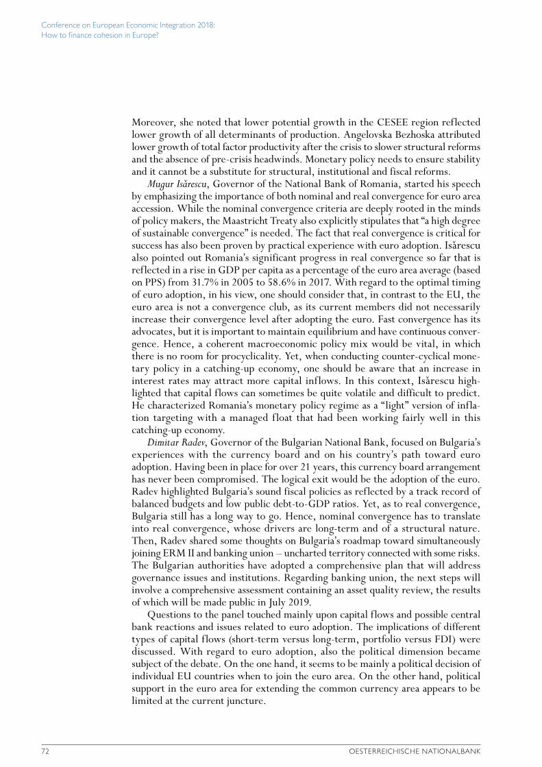
Conference on European Economic Integration 2018: How to finance cohesion in Europe?
72 OESTERREICHISCHE NATIONALBANK
Moreover, she noted that lower potential growth in the CESEE region reflected lower growth of all determinants of production. Angelovska Bezhoska attributed lower growth of total factor productivity after the crisis to slower structural reforms and the absence of pre-crisis headwinds. Monetary policy needs to ensure stability and it cannot be a substitute for structural, institutional and fiscal reforms.
Mugur Isarescu, Governor of the National Bank of Romania, started his speech by emphasizing the importance of both nominal and real convergence for euro area accession. While the nominal convergence criteria are deeply rooted in the minds of policy makers, the Maastricht Treaty also explicitly stipulates that “a high degree of sustainable convergence” is needed. The fact that real convergence is critical for success has also been proven by practical experience with euro adoption. Isarescu also pointed out Romania’s significant progress in real convergence so far that is reflected in a rise in GDP per capita as a percentage of the euro area average (based on PPS) from 31.7% in 2005 to 58.6% in 2017. With regard to the optimal timing of euro adoption, in his view, one should consider that, in contrast to the EU, the euro area is not a convergence club, as its current members did not necessarily increase their convergence level after adopting the euro. Fast convergence has its advocates, but it is important to maintain equilibrium and have continuous conver-gence. Hence, a coherent macroeconomic policy mix would be vital, in which there is no room for procyclicality. Yet, when conducting counter-cyclical mone-tary policy in a catching-up economy, one should be aware that an increase in interest rates may attract more capital inflows. In this context, Isarescu high-lighted that capital flows can sometimes be quite volatile and difficult to predict. He characterized Romania’s monetary policy regime as a “light” version of infla-tion targeting with a managed float that had been working fairly well in this catching-up economy.
Dimitar Radev, Governor of the Bulgarian National Bank, focused on Bulgaria’s experiences with the currency board and on his country’s path toward euro adoption. Having been in place for over 21 years, this currency board arrangement has never been compromised. The logical exit would be the adoption of the euro. Radev highlighted Bulgaria’s sound fiscal policies as reflected by a track record of balanced budgets and low public debt-to-GDP ratios. Yet, as to real convergence, Bulgaria still has a long way to go. Hence, nominal convergence has to translate into real convergence, whose drivers are long-term and of a structural nature. Then, Radev shared some thoughts on Bulgaria’s roadmap toward simultaneously joining ERM II and banking union – uncharted territory connected with some risks. The Bulgarian authorities have adopted a comprehensive plan that will address governance issues and institutions. Regarding banking union, the next steps will involve a comprehensive assessment containing an asset quality review, the results of which will be made public in July 2019.
Questions to the panel touched mainly upon capital flows and possible central bank reactions and issues related to euro adoption. The implications of different types of capital flows (short-term versus long-term, portfolio versus FDI) were discussed. With regard to euro adoption, also the political dimension became subject of the debate. On the one hand, it seems to be mainly a political decision of individual EU countries when to join the euro area. On the other hand, political support in the euro area for extending the common currency area appears to be limited at the current juncture.
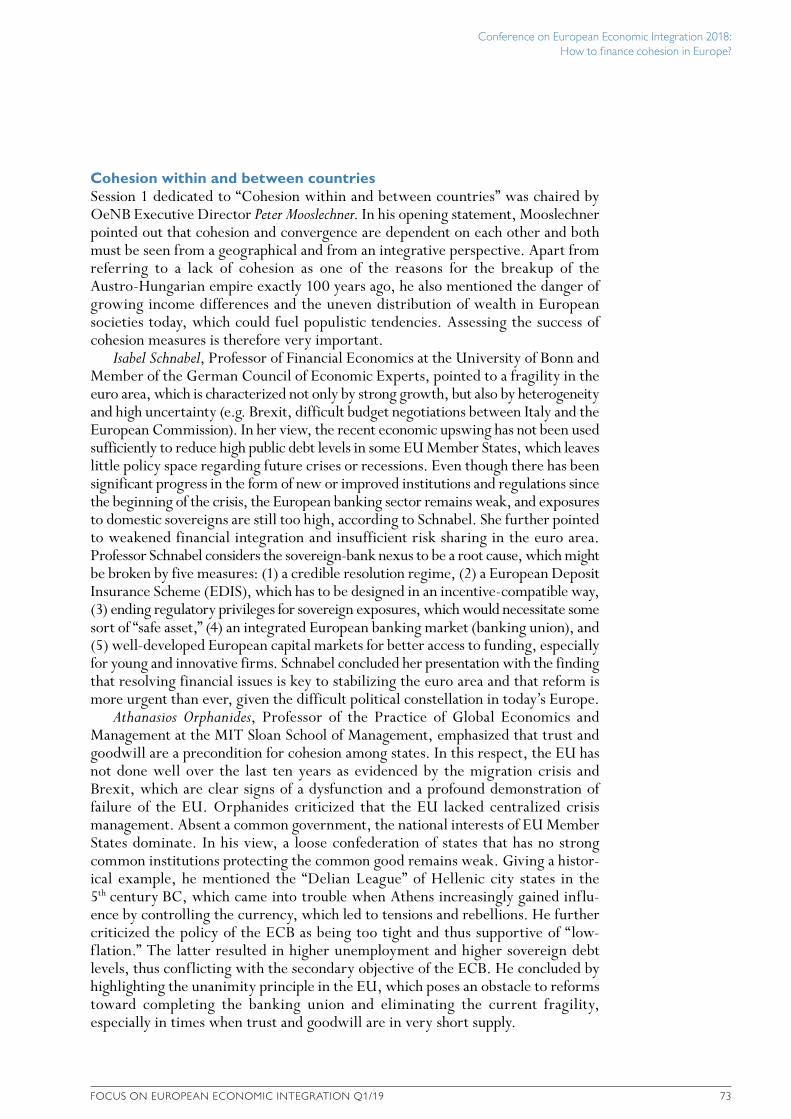
Conference on European Economic Integration 2018: How to finance cohesion in Europe?
FOCUS ON EUROPEAN ECONOMIC INTEGRATION Q1/19 73
Cohesion within and between countriesSession 1 dedicated to “Cohesion within and between countries” was chaired by OeNB Executive Director Peter Mooslechner. In his opening statement, Mooslechner pointed out that cohesion and convergence are dependent on each other and both must be seen from a geographical and from an integrative perspective. Apart from referring to a lack of cohesion as one of the reasons for the breakup of the Austro-Hungarian empire exactly 100 years ago, he also mentioned the danger of growing income differences and the uneven distribution of wealth in European societies today, which could fuel populistic tendencies. Assessing the success of cohesion measures is therefore very important.
Isabel Schnabel, Professor of Financial Economics at the University of Bonn and Member of the German Council of Economic Experts, pointed to a fragility in the euro area, which is characterized not only by strong growth, but also by heterogeneity and high uncertainty (e.g. Brexit, difficult budget negotiations between Italy and the European Commission). In her view, the recent economic upswing has not been used sufficiently to reduce high public debt levels in some EU Member States, which leaves little policy space regarding future crises or recessions. Even though there has been significant progress in the form of new or improved institutions and regulations since the beginning of the crisis, the European banking sector remains weak, and exposures to domestic sovereigns are still too high, according to Schnabel. She further pointed to weakened financial integration and insufficient risk sharing in the euro area. Professor Schnabel considers the sovereign-bank nexus to be a root cause, which might be broken by five measures: (1) a credible resolution regime, (2) a European Deposit Insurance Scheme (EDIS), which has to be designed in an incentive-compatible way, (3) ending regulatory privileges for sovereign exposures, which would necessitate some sort of “safe asset,” (4) an integrated European banking market (banking union), and (5) well-developed European capital markets for better access to funding, especially for young and innovative firms. Schnabel concluded her presentation with the finding that resolving financial issues is key to stabilizing the euro area and that reform is more urgent than ever, given the difficult political constellation in today’s Europe.
Athanasios Orphanides, Professor of the Practice of Global Economics and Management at the MIT Sloan School of Management, emphasized that trust and goodwill are a precondition for cohesion among states. In this respect, the EU has not done well over the last ten years as evidenced by the migration crisis and Brexit, which are clear signs of a dysfunction and a profound demonstration of failure of the EU. Orphanides criticized that the EU lacked centralized crisis management. Absent a common government, the national interests of EU Member States dominate. In his view, a loose confederation of states that has no strong common institutions protecting the common good remains weak. Giving a histor-ical example, he mentioned the “Delian League” of Hellenic city states in the 5th century BC, which came into trouble when Athens increasingly gained influ-ence by controlling the currency, which led to tensions and rebellions. He further criticized the policy of the ECB as being too tight and thus supportive of “low-flation.” The latter resulted in higher unemployment and higher sovereign debt levels, thus conflicting with the secondary objective of the ECB. He concluded by highlighting the unanimity principle in the EU, which poses an obstacle to reforms toward completing the banking union and eliminating the current fragility, especially in times when trust and goodwill are in very short supply.
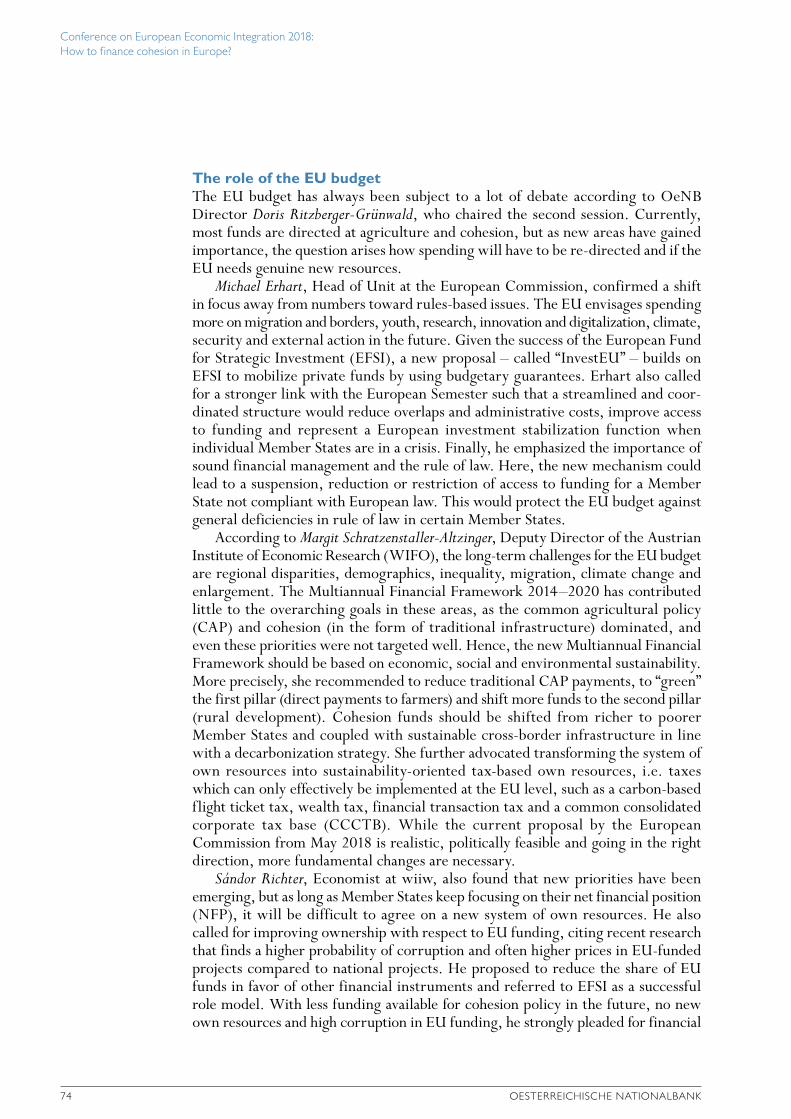
Conference on European Economic Integration 2018: How to finance cohesion in Europe?
74 OESTERREICHISCHE NATIONALBANK
The role of the EU budget The EU budget has always been subject to a lot of debate according to OeNB Director Doris Ritzberger-Grünwald, who chaired the second session. Currently, most funds are directed at agriculture and cohesion, but as new areas have gained importance, the question arises how spending will have to be re-directed and if the EU needs genuine new resources.
Michael Erhart, Head of Unit at the European Commission, confirmed a shift in focus away from numbers toward rules-based issues. The EU envisages spending more on migration and borders, youth, research, innovation and digitalization, climate, security and external action in the future. Given the success of the European Fund for Strategic Investment (EFSI), a new proposal – called “InvestEU” – builds on EFSI to mobilize private funds by using budgetary guarantees. Erhart also called for a stronger link with the European Semester such that a streamlined and coor-dinated structure would reduce overlaps and administrative costs, improve access to funding and represent a European investment stabilization function when individual Member States are in a crisis. Finally, he emphasized the importance of sound financial management and the rule of law. Here, the new mechanism could lead to a suspension, reduction or restriction of access to funding for a Member State not compliant with European law. This would protect the EU budget against general deficiencies in rule of law in certain Member States.
According to Margit Schratzenstaller-Altzinger, Deputy Director of the Austrian Institute of Economic Research (WIFO), the long-term challenges for the EU budget are regional disparities, demographics, inequality, migration, climate change and enlargement. The Multiannual Financial Framework 2014–2020 has contributed little to the overarching goals in these areas, as the common agricultural policy (CAP) and cohesion (in the form of traditional infrastructure) dominated, and even these priorities were not targeted well. Hence, the new Multiannual Financial Framework should be based on economic, social and environmental sustainability. More precisely, she recommended to reduce traditional CAP payments, to “green” the first pillar (direct payments to farmers) and shift more funds to the second pillar (rural development). Cohesion funds should be shifted from richer to poorer Member States and coupled with sustainable cross-border infrastructure in line with a decarbonization strategy. She further advocated transforming the system of own resources into sustainability-oriented tax-based own resources, i.e. taxes which can only effectively be implemented at the EU level, such as a carbon-based flight ticket tax, wealth tax, financial transaction tax and a common consolidated corporate tax base (CCCTB). While the current proposal by the European Commission from May 2018 is realistic, politically feasible and going in the right direction, more fundamental changes are necessary.
Sándor Richter, Economist at wiiw, also found that new priorities have been emerging, but as long as Member States keep focusing on their net financial position (NFP), it will be difficult to agree on a new system of own resources. He also called for improving ownership with respect to EU funding, citing recent research that finds a higher probability of corruption and often higher prices in EU-funded projects compared to national projects. He proposed to reduce the share of EU funds in favor of other financial instruments and referred to EFSI as a successful role model. With less funding available for cohesion policy in the future, no new own resources and high corruption in EU funding, he strongly pleaded for financial
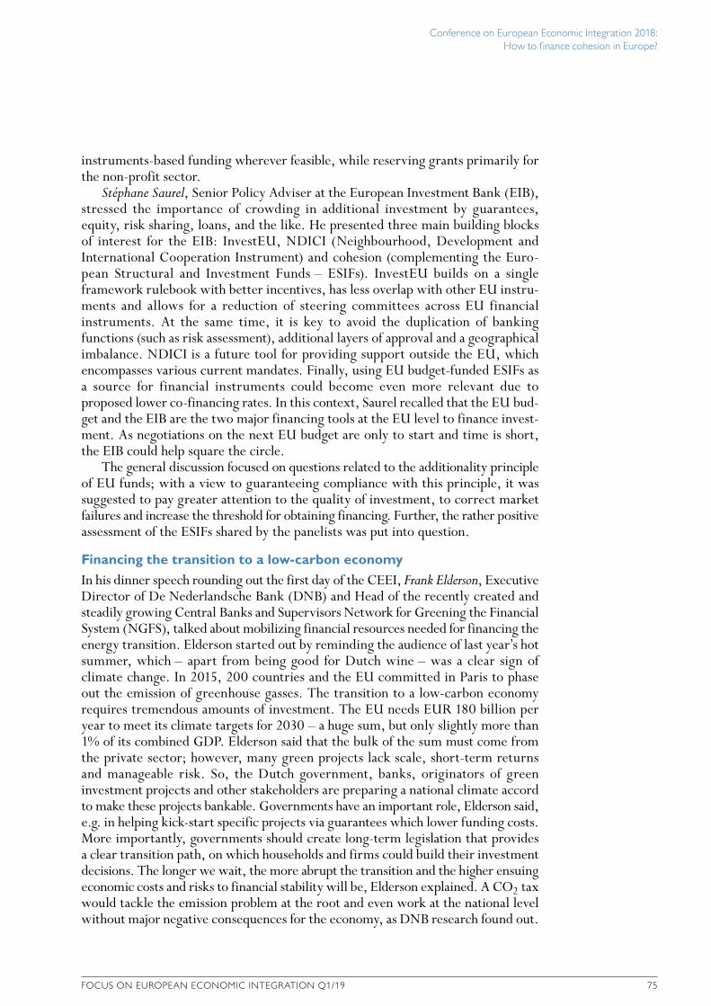
Conference on European Economic Integration 2018: How to finance cohesion in Europe?
FOCUS ON EUROPEAN ECONOMIC INTEGRATION Q1/19 75
instruments-based funding wherever feasible, while reserving grants primarily for the non-profit sector.
Stéphane Saurel, Senior Policy Adviser at the European Investment Bank (EIB), stressed the importance of crowding in additional investment by guarantees, equity, risk sharing, loans, and the like. He presented three main building blocks of interest for the EIB: InvestEU, NDICI (Neighbourhood, Development and International Cooperation Instrument) and cohesion (complementing the Euro-pean Structural and Investment Funds – ESIFs). InvestEU builds on a single framework rulebook with better incentives, has less overlap with other EU instru-ments and allows for a reduction of steering committees across EU financial instruments. At the same time, it is key to avoid the duplication of banking functions (such as risk assessment), additional layers of approval and a geographical imbalance. NDICI is a future tool for providing support outside the EU, which encompasses various current mandates. Finally, using EU budget-funded ESIFs as a source for financial instruments could become even more relevant due to proposed lower co-financing rates. In this context, Saurel recalled that the EU bud-get and the EIB are the two major financing tools at the EU level to finance invest-ment. As negotiations on the next EU budget are only to start and time is short, the EIB could help square the circle.
The general discussion focused on questions related to the additionality principle of EU funds; with a view to guaranteeing compliance with this principle, it was suggested to pay greater attention to the quality of investment, to correct market failures and increase the threshold for obtaining financing. Further, the rather positive assessment of the ESIFs shared by the panelists was put into question.
Financing the transition to a low-carbon economy In his dinner speech rounding out the first day of the CEEI, Frank Elderson, Executive Director of De Nederlandsche Bank (DNB) and Head of the recently created and steadily growing Central Banks and Supervisors Network for Greening the Financial System (NGFS), talked about mobilizing financial resources needed for financing the energy transition. Elderson started out by reminding the audience of last year’s hot summer, which – apart from being good for Dutch wine – was a clear sign of climate change. In 2015, 200 countries and the EU committed in Paris to phase out the emission of greenhouse gasses. The transition to a low-carbon economy requires tremendous amounts of investment. The EU needs EUR 180 billion per year to meet its climate targets for 2030 – a huge sum, but only slightly more than 1% of its combined GDP. Elderson said that the bulk of the sum must come from the private sector; however, many green projects lack scale, short-term returns and manageable risk. So, the Dutch government, banks, originators of green investment projects and other stakeholders are preparing a national climate accord to make these projects bankable. Governments have an important role, Elderson said, e.g. in helping kick-start specific projects via guarantees which lower funding costs. More importantly, governments should create long-term legislation that provides a clear transition path, on which households and firms could build their investment decisions. The longer we wait, the more abrupt the transition and the higher ensuing economic costs and risks to financial stability will be, Elderson explained. A CO2 tax would tackle the emission problem at the root and even work at the national level without major negative consequences for the economy, as DNB research found out.
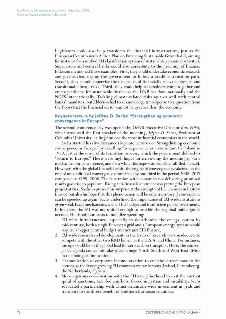
Conference on European Economic Integration 2018: How to finance cohesion in Europe?
76 OESTERREICHISCHE NATIONALBANK
Legislators could also help transform the financial infrastructure, just as the European Commission’s Action Plan on Financing Sustainable Growth did, aiming for instance for a unified EU classification system of sustainable economic activities. Supervisors and central banks could also contribute to the greening of finance. Elderson mentioned three examples: First, they could undertake economic research and give advice, urging the government to follow a credible transition path. Second, they should supervise the disclosure of financially relevant physical and transitional climate risks. Third, they could help stakeholders come together and create platforms for sustainable finance as the DNB has done nationally and the NGFS internationally. Tackling climate-related risks squares well with central banks’ mandates, but Elderson had to acknowledge (in response to a question from the floor) that the financial sector cannot be greener than the economy.
Keynote lecture by Jeffrey D. Sachs: “Strengthening economic convergence in Europe”
The second conference day was opened by OeNB Executive Director Kurt Pribil, who introduced the first speaker of the morning, Jeffrey D. Sachs, Professor at Columbia University, calling him one the most influential economists in the world.
Sachs started his (live streamed) keynote lecture on “Strengthening economic convergence in Europe” by recalling his experience as a consultant to Poland in 1989, just at the onset of its transition process, which the government dubbed its “return to Europe.” There were high hopes for narrowing the income gap via a mechanism for convergence, and for a while this hope was probably fulfilled, he said. However, with the global financial crisis, the engine of convergence weakened, as the rate of unconditional convergence diminished by one-third in the period 2008–2017 compared to 1995–2008. The frustration with economics not delivering promised results gave rise to populism. Rising anti-Brussels sentiment was putting the European project at risk. Sachs expressed his surprise at the strength of EU enemies in Eastern Europe but also his hope that this phenomenon will be only transitory if convergence can be speeded up again. Sachs underlined the importance of EU-wide institutions given weak fiscal mechanisms, a small EU budget and insufficient public investments. In his view, the EU was not united enough to provide the regional public goods needed. He listed four areas to mobilize spending: 1. EU-wide infrastructure, especially to decarbonize the energy system by
mid-century; both a single European grid and a European energy system would require a bigger central budget and not just EIB finance.
2. EU-wide research and development, as the levels of research were inadequate to compete with the other two R&D hubs, i.e. the U.S.A. and China. For instance, Europe could be in the global lead for zero carbon transport. Here, the conver-gence agenda comes into play given a huge North-South and West-East divide in technological innovation.
3. Harmonization of corporate income taxation to end the current race to the bottom, as the fastest growing EU countries are tax heavens (Ireland, Luxembourg, the Netherlands, Cyprus).
4. More vigorous coordination with the EU’s neighborhood to exit the current spiral of sanctions, U.S.-led conflicts, forced migration and instability. Sachs advocated a partnership with China on Eurasia-wide investment in grids and transport to the direct benefit of Southern European countries.
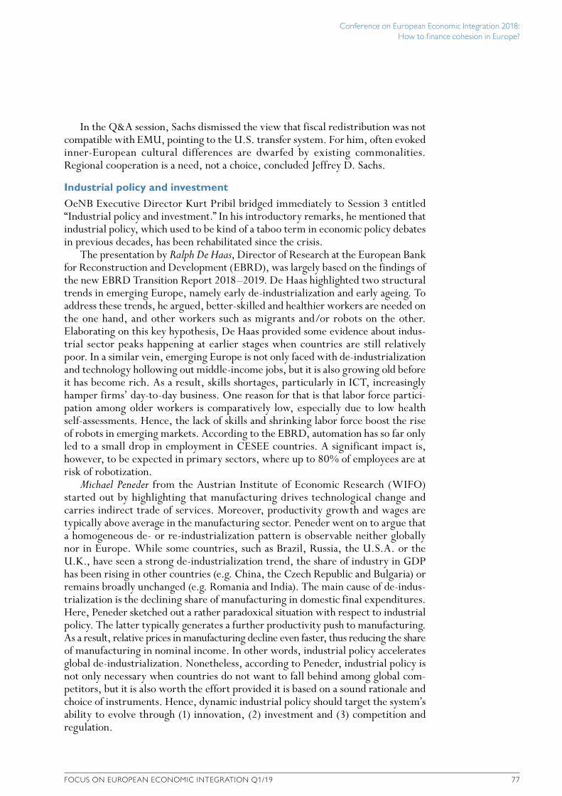
Conference on European Economic Integration 2018: How to finance cohesion in Europe?
FOCUS ON EUROPEAN ECONOMIC INTEGRATION Q1/19 77
In the Q&A session, Sachs dismissed the view that fiscal redistribution was not compatible with EMU, pointing to the U.S. transfer system. For him, often evoked inner-European cultural differences are dwarfed by existing commonalities. Regional cooperation is a need, not a choice, concluded Jeffrey D. Sachs.
Industrial policy and investment OeNB Executive Director Kurt Pribil bridged immediately to Session 3 entitled “Industrial policy and investment.” In his introductory remarks, he mentioned that industrial policy, which used to be kind of a taboo term in economic policy debates in previous decades, has been rehabilitated since the crisis.
The presentation by Ralph De Haas, Director of Research at the European Bank for Reconstruction and Development (EBRD), was largely based on the findings of the new EBRD Transition Report 2018–2019. De Haas highlighted two structural trends in emerging Europe, namely early de-industrialization and early ageing. To address these trends, he argued, better-skilled and healthier workers are needed on the one hand, and other workers such as migrants and/or robots on the other. Elaborating on this key hypothesis, De Haas provided some evidence about indus-trial sector peaks happening at earlier stages when countries are still relatively poor. In a similar vein, emerging Europe is not only faced with de-industrialization and technology hollowing out middle-income jobs, but it is also growing old before it has become rich. As a result, skills shortages, particularly in ICT, increasingly hamper firms’ day-to-day business. One reason for that is that labor force partici-pation among older workers is comparatively low, especially due to low health self-assessments. Hence, the lack of skills and shrinking labor force boost the rise of robots in emerging markets. According to the EBRD, automation has so far only led to a small drop in employment in CESEE countries. A significant impact is, however, to be expected in primary sectors, where up to 80% of employees are at risk of robotization.
Michael Peneder from the Austrian Institute of Economic Research (WIFO) started out by highlighting that manufacturing drives technological change and carries indirect trade of services. Moreover, productivity growth and wages are typically above average in the manufacturing sector. Peneder went on to argue that a homogeneous de- or re-industrialization pattern is observable neither globally nor in Europe. While some countries, such as Brazil, Russia, the U.S.A. or the U.K., have seen a strong de-industrialization trend, the share of industry in GDP has been rising in other countries (e.g. China, the Czech Republic and Bulgaria) or remains broadly unchanged (e.g. Romania and India). The main cause of de-indus-trialization is the declining share of manufacturing in domestic final expenditures. Here, Peneder sketched out a rather paradoxical situation with respect to industrial policy. The latter typically generates a further productivity push to manufacturing. As a result, relative prices in manufacturing decline even faster, thus reducing the share of manufacturing in nominal income. In other words, industrial policy accelerates global de-industrialization. Nonetheless, according to Peneder, industrial policy is not only necessary when countries do not want to fall behind among global com-petitors, but it is also worth the effort provided it is based on a sound rationale and choice of instruments. Hence, dynamic industrial policy should target the system’s ability to evolve through (1) innovation, (2) investment and (3) competition and regulation.
Conference on European Economic Integration 2018: How to finance cohesion in Europe?
78 OESTERREICHISCHE NATIONALBANK
Tomáš Slacík from the OeNB concluded the session by presenting joint work with colleagues from the European Investment Bank (EIB) on structural invest-ment needs in CESEE and the use of EU funds. He set the stage by showing that while it is quite a challenging task to determine the investment gap in quantitative terms, there is tangible evidence suggesting significant structural and qualitative investment needs. Using a large set of structural indicators, he shed some light on the qualitative investment gaps and their evolution in CESEE during the last EU budget period. His analysis suggests that convergence of the quality of capital toward the EU average has been negligible. Subsequently, he contrasted the identified structural investment needs with the flows of the European Structural and Investment Funds (ESIFs) in the 2007–2013 EU budget period. It turned out that, contrary to expecta-tions, higher ESIF amounts were not positively correlated neither with the largest structural needs nor with more significant improvements in capital quality. Slacík’s findings thus may suggest the policy conclusion that the link between allocated resources and structural reforms should be strengthened – which is exactly what the European Commission envisages for the next Multiannual Financial Framework.
Improving host countries’ investment environment Helene Schuberth, Head of Division at the OeNB chaired session 4 that dealt with the question how the environment of host countries can be improved. Linda van Gelder, country director for the Western Balkan region at the World Bank, argued that the Western Balkans face many challenges to secure faster, more inclusive, and sustainable growth. Boosting economic growth and creating more integrated and inclusive societies largely depends on a country’s investment environment. She pointed out three areas which are decisive for improving the investment climate: (1) macroeconomic stability, (2) the creation of markets by deepening economic integration and, increasingly important for the Western Balkans, (3) investment in human capital. The Western Balkans are characterized by very low employment ratios, with many people migrating in search of better job opportunities. In this regard, polices need to prioritize investment in education even if it only pays off in the future. The second presenter in this session was Irmfried Schwimann, Deputy Director-General at the European Commission. She focused on the EU Investment Plan, EFSI, and public procurement. EFSI has enabled financing of investments in key sectors and regions, and Schwimann emphasized that the cooperation with National Promotional Banks is one of the most effective EFSI tools. Furthermore, the Investment Advisory Hub operated by the EIB provides essential advisory and technical services that are important for the realization of good projects. Schwimann moreover pointed out the importance of transparent public procure-ment to create a stronger business environment and to boost investments. Finally, Andrew Watt, Deputy Director at the Macroeconomic Policy Institute, made a case for considering additional factors to explain weak investment growth. In his presentation, he referred – among other factors – to the impact of the crisis, the role of expected demand in driving private investment, fiscal constraints and possible perverse effects of some liberalization polices. Watt proposed various measures to tackle the problem of low investment activity. Transnational strategic investments, for instance, are needed to make use of economies of scale and to deal with the climate change. Furthermore, economic governance reforms and the EU Investment Plan would be conducive to investment growth.
Conference on European Economic Integration 2018: How to finance cohesion in Europe?
FOCUS ON EUROPEAN ECONOMIC INTEGRATION Q1/19 79
Corporate investment across EuropePanel 2 on corporate investment across EU borders was chaired by OeNB Vice- Governor Andreas Ittner, with Andrea Diamanti (UniCredit S.p.A.), Franz Hiesinger (Mayr-Melnhof Karton AG), Birgit Reiter-Braunwieser (Austrian Business Agency) and Lukas Stühlinger (oekostrom AG) as panelists. According to Diamanti, corporate bond and equity markets as well as the investor base were still underdeveloped in most of the CESEE region. There was overall agreement in the discussion that banks’ local know-how was very valuable when expanding to new markets. Moreover, access to finance for cross-border investments is not an issue, according to the panelists, even though new regulations, particularly in the field of Anti-Money Laundering (AML) have added to the complexity of obtaining finance. Regarding the attractiveness of the region, Hiesinger pointed out that CESEE continued to be an attractive market due to its comparative stability, but also to labor costs, which were still considerably below the euro area averages. He emphasized that, within the Mayr-Melnhof Group, he does not observe differences in productivity that could explain the wage differences. Stühlinger added that, in the renewable energy segment, investment security and legal certainty are particularly important and that these two preconditions are still not fully guaranteed in CESEE. Both Hiesinger and Stühlinger agreed that political uncertainty and turbulence factor into investment decisions but are only two of many factors. Reiter-Braunwieser noted that, in the past years, the Austrian Business Agency has seen a pickup in cross-border investments from CESEE to Austria – mostly in the form of sales offices and service companies, yet also including highly competitive “local heroes,” e.g. in the ICT sector.
80 OESTERREICHISCHE NATIONALBANK
“Connecting Europe and Asia” – conference summary
Compiled by Andrea Hofer, Carmencita Nader-Uher and Franz Nauschnigg1
On December 14, 2018, the Oesterreichische Nationalbank (OeNB) and the Reinventing Bretton Woods Committee (RBWC) hosted the conference “Connecting Europe and Asia.” Experts from academia, business and politics discussed ways to improve cooperation between, and to better connect, Europe and Asia to the benefit of both sides. The special value added of the conference was the balanced mixture of macroeconomic and microeconomic aspects of connectivity. Speakers and participants looked at big international trends and showed practical examples of how individual companies facilitate connectivity between Europe and Asia as part of their daily business.
Ewald Nowotny, Governor of the OeNB, pointed out that the topic of the conference is not just relevant for Austria but for the whole of Europe, including Central and Eastern Europe. He stated that we must be aware that Asia will very soon become the most important economic power center of the world. Some people see Asia’s economic rise as a challenge. However, according to Nowotny this is a mistake because foreign trade is not a zero-sum game. If China and Asia in general get richer this is not a problem for the rest of the world, but an opportunity. If one country becomes richer, the rest of the world also profits economically. “We will all win.” This is one lesson from the worldwide success story seen after World War II. Nowotny reminded the audience that when the United States of America helped Europe, also the U.S.A. profited.
Of course, for welfare, not total GDP is relevant, but it is GDP per capita that matters. For this reason, Nowotny stated, many consider Europe the best place in the world to live. Hopefully, it will stay the best place. It has economic strength and social structures that are attractive. Nowotny also stressed the importance of connections and mode of transport in our world. Connectivity is especially important for landlocked countries like Austria.
Marc Uzan, Executive Director of the RBWC, emphasized the importance of the economic ties of the two continents. Asian markets account for one-third of all exports from the EU, and almost half of all goods and services imported by the EU come from Asian countries. Together, Europe and Asia account for almost 70% of the world population and over 60% of world GDP. Economic relationships need to be able to rely on effective, functioning and sustainable connectivity, in other words on the physical and nonphysical infrastructure through which goods, services and ideas can flow.
In September 2018, the EU approved a new strategy for connectivity between Europe and Asia. Connectivity is a central element of the EU as a political project based on market integration. The EU can offer its regulatory experience, technical expertise and funding opportunities, which benefits project interoperability and convergence, and promotes fiscal and sound growth.
Uzan emphasized that China has made a remarkable rise in Central Asia over the last 15 years and is now the main donor and investor. The cause of this rise was
1 Oesterreichische Nationalbank, European Affairs and International Financial Organizations Division, [email protected], [email protected] and [email protected].
“Connecting Europe and Asia” – conference summary
FOCUS ON EUROPEAN ECONOMIC INTEGRATION Q1/19 81
the announcement by Chinese President Xi Jinping of his “Silk Road Economic Belt” plan during his visit in Astana (Kazakhstan) in 2013. The “One Belt, One Road” initiative is clearly a major investment expanding transport and energy corridors, connectivity and establishing new transport links between Asia and Europe. Both, China and the EU, have recently positioned themselves in Central Asia as leading players. However, so far their endeavors in Central Asia have been separate. This may be an opportune time to reshape the EU’s relations with China to contribute to the sustainable development of Central Asia. Some analysts have suggested that China should focus on hard infrastructure while the EU focuses on soft infrastructure, which could offer a powerful base of cooperation for development in the region. At the same time, there are clearly substantial challenges for a possible cooperation between the EU and China.
Panel 1: Integration in Europe: European Union (EU) and EurasiaFranz Nauschnigg, OeNB, stated that closer economic integration especially between the EU and the Eurasian Economic Union (EAEU) would be beneficial for both sides but for this to happen political obstacles need to be overcome.
Elena Rovenskaya, International Institute for Applied Systems Analysis (IIASA), gave an overview of the IIASA’s work on challenges and opportunities for economic integration in the wider European and Eurasian space, which would benefit all.
William Tompson, OECD, referred to the fact that infrastructure investments must be accompanied by a better business environment and human capital formation if their full benefits are to materialize. Distance remains a key factor; multilateralism would be helpful but is hampered by rising sovereignty sensibilities. The Chinese “One Belt, One Road” (OBOR) initiative has become a brand name, encompassing much more than originally planned.
Petros Sourmelis, European Commission, gave an overview of EU relations with countries in Central, Eastern and Southeastern Europe (CESEE). EAEU-internal trade barriers sometimes hamper the EU’s trade with the EAEU.
Tatyana Valovaya, Eurasian Economic Commission, offered an EAEU perspective, underlining that a substantial degree of integration has been achieved in a very short time span but that much still needs to be done. She argued that closer EU-EAEU cooperation would benefit both sides.
Panel 2: Connecting Europe and Asia: the land dimensionRudolf Schicker, Coordinator of the Danube Region, emphasized that connectivity plays an important role in the Danube Region as well as in the Eurasian region.
David Gould, World Bank, stressed the different dimensions of connectivity – trade, FDI, transport and migration. He diagnosed that progress in lowering barriers has stalled.
Jonas Grätz, OSCE, explained the work of the OSCE, shedding light on different dimensions, i.e. security-related, economic and humanitarian aspects. He pointed out that around 40% of inland transport time is lost at borders.
Mario Holzner, The Vienna Institute for International Economic Studies (wiiw), stressed the lack of infrastructure in the CESEE region. China finances infrastructure investments mainly via loans, while the EU provides grants. He underlined that it is important to enhance the connections of railways and roads with ports.
“Connecting Europe and Asia” – conference summary
82 OESTERREICHISCHE NATIONALBANK
Alexey Grom, United Transport and Logistics Company (UTLC), stressed the rapid growth in rail transports between China and the EU carried out by UTLC. He expects that further improvements in transport time and volumes will improve rail transport’s market share in EU-China trade.
Osman Erol, Rail Cargo Logistics Austria, explained that his company, which is the second biggest rail transport provider in the EU after Deutsche Bahn, is active in EU-China transports, seeking to develop the southern route. The company is also considering new liquefied natural gas (LNG) locomotives, which are more environmentally friendly than those powered by diesel. According to Erol, it has not yet been decided where a possible rail terminal might be located.
Panel 3: Connecting Europe and Asia: the maritime dimensionErnst Schmied, Danube Macro Region, stressed the importance of supply chain logistics.
Massimo Deandreis, SRM Economic Research Centre related to Intesa Sanpaolo Bank, emphasized that the Mediterranean ports are gaining in competitiveness. In his view, rail and ship are not competitors, but simply two different means of connectivity: one for intra-European development and the other for connecting Europe and China.
Igor Hribar, DB Cargo AG, pointed out that the competitiveness of ports heavily depends on hinterland logistics (rail and road) and container logistics.
Wojciech Szymulewicz, Adriatic Gate Container Terminal (Rijeka port), added how important it is to integrate all modes of transport to improve the process and increase efficiency. Containerization creates very high productivity gains.
Zeno D’Agostino, Trieste Port Authority, stressed that connectivity is improved by creating competitive advantages for ports, e.g. by integrating ports and dry ports, logistical platforms (intermodality) and “free zones” (areas for logistics and manufacturing). Trieste has 18m deep water for easy access by ships, excellent road and rail links and proximity to markets. To conclude, he proposed that Europe should also create logistics infrastructures for Africa.
Stephan Barisitz, OeNB, offered insights into the history of the Old Silk Road and highlighted the three dimensions of the New Silk Road: (1) Overland Silk Road (Silk Road Economic Belt – SREB): rail transports account for 3% to 8% of all Eurasian transports; (2) Maritime Silk Road (MSR): ship transports account for 80% to 90%; (3) air transports account for 6% to 12%.
Panel 4: Europe and Asia: financial connectivity, risks, challenges and opportunities
Ousmène Jacques Mandeng, Accenture and London School of Economics, stated that blockchain technology might contribute to connecting Europe and Asia and proposed that one currency could become the clearing currency of the OBOR corridor.
Giorgi Kvirikashvili, Former Prime Minister of Georgia, distinguished between two main concepts of connectivity between Europe and Asia, i.e. the EU strategy and the OBOR initiative. The EU is working on five dimensions of Eurasian con-nectivity (transport, customs, energy, digital, financial) while OBOR is seen as a call for international engagement to close huge infrastructure gaps in the regional neighborhood of China. In the discussion, Kvirikashvili pointed out that, as long as the Chinese currency does not fulfill certain criteria like transparency, convert-ibility etc., Georgia will remain unwilling to build up FX reserves in renminbi.
“Connecting Europe and Asia” – conference summary
FOCUS ON EUROPEAN ECONOMIC INTEGRATION Q1/19 83
Baurzhan Bektemirov, Astana International Financial Centre (AIFC), identified two dimensions of financial connectivity, i.e. trade (within existing infrastructure) and investment (into building new infrastructure), both of which use several underlying currencies (USD, EUR, SDR, RMB, CHF). For investment purposes, capital markets need to be developed.
Mattia Romani, European Bank for Reconstruction and Development (EBRD), stated that financial connectivity between Europe and Asia does not yet exist, and that even the EBRD fails to invest because there is a systemic lack of bankable projects in the region that meet the EBRD’s standards. Since 2013, China has invested an annual average of USD 100 billion in the core region of the Belt and Road Initiative (BRI), while international financial investors invest only USD 10 billion per year. China heavily invests in fossil fuels abroad while pursuing the opposite policy at home.
Naoyuki Yoshino, Asian Development Bank Institute (ADBI) stated that Asia could learn a lot from Europe in terms of (1) infrastructure and public capital, (2) SMEs and start-up businesses, (3) human capital, (4) state-owned enterprises and (5) sovereign debt and household debt. As there are positive externalities in infrastructure investment, governments should subsidize it.
Summing up, the great majority of speakers and participants shared the opinion that, for geographic, historic, cultural and economic reasons, connecting Europe and Asia would be beneficial for both sides – a win-win game.

84 OESTERREICHISCHE NATIONALBANK
Most of the research papers published in Focus on European Economic Integration (FEEI) are subject to a double-blind peer review process to ensure a high level of scientific quality. The FEEI’s editors in chief wish to thank the following researchers for their work and diligence in reviewing studies published in Focus on European Economic Integration in the period from 2016 to 2018:
Referees for Focus on European Economic Integration 2016−2018
Amat Adarov Reimo Juks
Vasily Astrov Vincent Labhard
Sergey Aleksashenko Marco Lombardi
Fritz Florian Bachmair Mikko Mäkinen
Bas Bakker Aaron Mehrotra
Mazur Błażej Stefano Neri
Serkan Çiçek Thomas Nitschka
Andrej Cupák Harald Oberhofer
Marek Dabrowski Alexander Plekhanov
Maria Davalos Éva Katalin Polgár
Xavier Debrun Dennis Reinhardt
Rumen Dobrinsky Gerhard Rünstler
Ettore Dorrucci Martin Sokol
Ludmila Fadejeva Martin Suster
Georg Fischer Goran Svilanovic
Louise Funch Sørensen Cédric Tille
Zuzana Fungáčová Neven Valev
Adam Geršl Isabel Vansteenkiste
Benjamin Guin Paul Wachtel
Josef Hollmayr Pinar Yesin
Anna Ilyina Nathaniel Young
Roel Janssens Fabrizio Zampolli
Related Documents