Focal plane metrology for the LSST camera

Work supported in part by the US Department of Energy contract DE-AC02-76SF00515

Focal plane metrology for the LSST camera

Andrew P. Rasmussena, Layton Haleb, Peter Kima, Eric Leea, Martin Perla, Rafe Schindlera,Peter Takacsc, Timothy Thurstona and the LSST Camera Team

aStanford Linear Accelerator Center, 2575 Sand Hill Road, Menlo Park, CA 94025, U.S.A.;

bInnovative Machine Solutions, 11501 Dublin Blvd. Suite 200, Dublin, CA 94568, U.S.A.;

cBrookhaven National Laboratory, P.O. Box 500, Upton, NY, 11973, U.S.A.

ABSTRACT

Meeting the science goals for the Large Synoptic Survey Telescope (LSST) translates into a demanding set ofimaging performance requirements for the optical system over a wide (3.5) field of view. In turn, meeting thoseimaging requirements necessitates maintaining precise control of the focal plane surface (10 µm P-V) over theentire field of view (640 mm diameter) at the operating temperature (T ∼ -100C) and over the operationalelevation angle range. We briefly describe the heirarchical design approach for the LSST Camera focal plane andthe baseline design for assembling the flat focal plane at room temperature. Preliminary results of gravity loadand thermal distortion calculations are provided, and early metrological verification of candidate materials undercold thermal conditions are presented. A detailed, generalized method for stitching together sparse metrologydata originating from differential, non-contact metrological data acquisition spanning multiple (non-continuous)sensor surfaces making up the focal plane, is described and demonstrated. Finally, we describe some in situalignment verification alternatives, some of which may be integrated into the camera’s focal plane.

Keywords: Telescopes, LSST, Wide Field Imaging, Sensor Array, Focal Plane, Flatness, Metrology, FiniteElement Metrology, Stitching Algorithms

1. INTRODUCTION

The Large Synoptic Survey Telescope (LSST) will perform high observing efficiency, seeing-limited imagery, withan exceptionally large etendue (AΩ ∼ 300 m2deg2) in several spectral bands. LSST’s science requirements1, 2

are derived from a set of performance parameters needed to meet the divers science objectives outlined for themission.3 Among these, perhaps the most challenging is the imaging performance required for studying DarkEnergy via weak lensing of galaxies. This demands an imaging point spread function with very little uncalibratedinstrumental signature down to the individual pixel (0.2

′′) scale over the full 3.5 field of view (FOV).

LSST’s strategy to maintain this imaging quality across the camera’s focal plane will be provided by twoenabling features: active optical compensation and a well defined focal plane. The active optics requires moni-toring the image formation wavefront at multiple field positions distributed over the FOV,4 while the focal planedefinition and stability will be achieved by adopting precision engineering principles and precision assembly tech-niques.5 The focal plane is required to be flat under well defined operational conditions (T∼-100C, elevationangle >45), but is constructed out of a large number (∼200) of individual imaging sensors, assembled in aheirarchical fashion.

In this paper we describe plans and procedures for performing the metrology necessary for ensuring fabricationand operation of the LSST focal plane that will permit realization of the broad science goals of the LSST. Wediscuss our metrological approaches for the relevant entries in the Science Requirements Document (SRD) anddescribe how we intend to meet those goals.

Further author information: (Send correspondence and color electronic version requests to A.P.R.)A.P.R.: E-mail: [email protected], Telephone: 1 650 926 2794

SLAC-PUB-12290

Contributed to Astronomical Telescopes and Instrumentation 2006, 05/24/2006--5/31/2006, Orlando, Florida

2. REQUIREMENTS

An enabling feature of the telescope’s large etendue is a fast beam (F/1.25) that converges at points acrossthe large field of view (FOV). The focal plane is flat and ∼640 mm in diameter, and is positioned after threecorrector lenses and one (selectable) wide-band color filter, all of which are housed in the camera,5 while threemirrors of the telescope’s main optical system provide the converging beam. Because of the annular geometryof the primary mirror, the depth of field of the system more closely resembles that of a significantly faster beam(F/1.0) in the case of a filled aperture. Consequently, any defocus of the system will appear to degrade theimage by a proportional amount (2/3) of the defocus distance. A small degree of non-flatness in the focal plane,therefore, can impart a local defocus to the system and a consequential blur associated with that defocus. Othercontributions that can degrade imaging performance, notably distortions to the optics due to changing gravityand thermal load, and probable active optical compensation limitations and are discussed in greater detail incompanion papers in these proceedings,4, 6 and are considered to be of comparable magnitude. Throughout thispaper, by “non-flat” we mean any deviation of the sensor light entrance surface from the ideal system planedefined by the ideally co-aligned optical elements in the system optical chain.

2.1. Flatness

An extensive error budget has been assembled for LSST’s baseline imaging performance. Among the variousterms, blur due to focal plane non-flatness has a small, but significant, contribution. The corresponding maximumpermissible focal plane non-flatness there is 10µm (P-V) over the entire focal plane area (∼3200 cm2). This is ingeneral a daunting task: As compared to the production of the WFI camera mounted to the MPG/ESO 2.2mtelescope,7 the LSST focal plane is approximately 25 times the surface area and requires 4 times tighter tolerancesthan their measured, as built (warm) focal plane configuration. Any way of arriving within specifications forthe LSST focal plane would be acceptable in principle. However, because of the large number of sensors thatare ganged together in a heirarchical fashion,5 we adopted a breakdown of the non-flatness requirement on thecomponent and subsystem levels. This is summarized in Table 1. To estimate contribution from a distributedmass, focal plane integrating structure or optical bench, we performed finite element analysis computations fora strawman structure design together with different choices of material. These are summarized in Figure 2 andTable 2. An allocation for contribution by the operational environment of the focal plane is based on scalingthe largest FEA derived deviations by a factor of a few, and loosens the non-flatness specification from 8 to10 µm (P-V) between the as built and operational allocations tabulated. In turn, the as built allocation of 8 µm(P-V) is based on precise assembly of ∼20 rafts that individually meet a tighter allocation of 6.5 µm (P-V),each of which are precisely assembled using packaged sensors that individually meet allocations of 5 µm (P-V).Preparation, alignment and metrology of these raft units is described in greater detail in a separate paper inthese proceedings.8

Table 1. Outline of the budget allocation for focal plane non-flatness.

Description Budget Term Specifications Comments

FP max. permissible 10 µm (P-V) LSST SRD Top Level Requirementnon-flatness

Sensor level 5 µm (P-V) operating, cold, 0-45 tilt as packaged, ready to mount onto raft

Raft level 6.5 µm (P-V) operating, cold, 0-45 tilt as packaged, ready to mount into IS9 sensors assembled onto raft

FP assembly level 8 µm (P-V) cold cables and thermal straps attached21 rafts assembled onto IS

FP operational level 10 µm (P-V) operating, cold, 0-45 tilt Meets top level requirementgravity load & thermo-mechanics

Proc. of SPIE Vol. 6273 62732U-2

Displacement Z 2 004e 04

Original Model 3.500e 24

Man Disp +4.5293E—D4

LoadSetoZ2 lODe 042.002e 04

502e—O4

1. 000e—04

.000e 0

Dgrov SiC CoorsTek" — FPA SiC Cooratek — StaticS

Wide band filter Focal plane —Li Corrector

Figure 1. Cut-away schematic of the LSST camera. The lens labeled “L3” is also the vacuum barrier of the cryostat.The focal plane sits directly behind L3.

Figure 2. A finite element analysis prediction of out-of-plane height distortion, a difference map between horizontal andvertical orientation of an LSST focal plane strawman. This map shows a 0.25 µm P-V distortion in the case of SiCmaterial choice tabulated in Table 2. There are 3 assumed mounting points, located at the center top and the two lowercorners of the focal plane integrating structure.


Table 2. Integrating structure (IS) material comparison matrix. Finite element analysis calculations were performed fora strawman design, whose results are tabulated here. A three point mounting constraint was assumed, and deflectionsdue to changing gravitational load were calculated for different material choices. Probable internal stresses and theirassociated distortions were not calculated. While the silicon carbide (SiC) material choice appears to have superioroverall characteristics (high stiffness to density ratio, high thermal conductivity to thermal expansion coefficient ratio),we baselined an operational contribution to focal plane non-flatness that was several times worse than the contributionexpected for the metal materials (cf. Table 1).

Property Unit Alum. Invar 36 SiC

Total mass with rafts (25 kg) kg 100 246 112

P-V gravity sag over aperture

0-90 elevation µm 1.350 1.400 0.250

30-90 elevation µm 0.675 0.700 0.125

45-90 elevation µm 0.395 0.410 0.073

60-90 elevation µm 0.181 0.188 0.033

Mode shape and frequency

Mode 1, torsion/twist Hz 205 184 463

Mode 2, X translation Hz 241 217 546

Mode 3, Y translation Hz 339 321 775

Mode 4, Z translation Hz 366 346 846

Elastic modulus/density SI 25.56 17.67 130.16

Thermal conductivity/CTE SI 10.00 8.08 75.00

Flatness assurance of the LSST focal plane will be achieved, therefore, by requiring strict adherence toallocations permitted at the various levels summarized in Table 1, and also by incorporating an in situ meansby which to verify focal plane geometry. Specifically, in regards to the assembly aspect, we concentrate on theallocation for assembly of the specification compliant sensor rafts (6.5 µm P-V) into the specification compliantfocal plane assembly (8 µm P-V). These are the main subjects of this paper. In the case of this focal plane, themetrology and assembly are intimately connected, and describing one of these aspects without the other rapidlyloses value.

Metrology of the 2-dimensional pixel registration across all focal plane sensor devices, combined with wellunderstood charge transport (either tight fidelity or precise characterization) is an additional science requirementfor LSST’s astrometric performance. This aspect of focal plane metrology is beyond the scope of this paper andis not discussed at all here.

3. ASSEMBLY

A natural decision point in planning the design for the LSST camera comes in adopting either of two distinctapproaches for establishing flatness of the focal plane. These approaches include dynamic actuation compensationof the sub-assemblies and thermo-mechanical build compensation. The first approach would be one whereindividual components (e.g. packaged sensors) and/or individual sub-assemblies (e.g. assembled rafts) arepistoned and tilted relative to their kinematic mounts to establish co-planarity simultaneously between focalplane constituent surfaces and with the defined system focal plane. Three actuators per sub-assembly (withadequate travel per actuator) would be sufficient to align sub-assemblies to the nominal focal plane surface.This approach would resemble working examples of active optical compensators on segmented primary mirrorassemblies, such as those of the Magellan Telescopes9 or that planned for the Thirty Meter Telescope.10


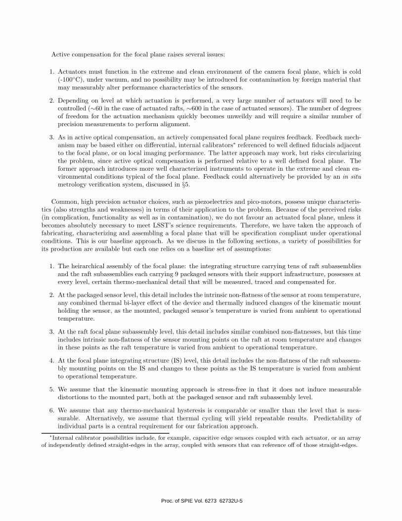
Active compensation for the focal plane raises several issues:

1. Actuators must function in the extreme and clean environment of the camera focal plane, which is cold(-100C), under vacuum, and no possibility may be introduced for contamination by foreign material thatmay measurably alter performance characteristics of the sensors.

2. Depending on level at which actuation is performed, a very large number of actuators will need to becontrolled (∼60 in the case of actuated rafts, ∼600 in the case of actuated sensors). The number of degreesof freedom for the actuation mechanism quickly becomes unweildy and will require a similar number ofprecision measurements to perform alignment.

3. As in active optical compensation, an actively compensated focal plane requires feedback. Feedback mech-anism may be based either on differential, internal calibrators∗ referenced to well defined fiducials adjacentto the focal plane, or on local imaging performance. The latter approach may work, but risks circularizingthe problem, since active optical compensation is performed relative to a well defined focal plane. Theformer approach introduces more well characterized instruments to operate in the extreme and clean en-vironmental conditions typical of the focal plane. Feedback could alternatively be provided by an in situmetrology verification system, discussed in §5.

Common, high precision actuator choices, such as piezoelectrics and pico-motors, possess unique characteris-tics (also strengths and weaknesses) in terms of their application to the problem. Because of the perceived risks(in complication, functionality as well as in contamination), we do not favour an actuated focal plane, unless itbecomes absolutely necessary to meet LSST’s science requirements. Therefore, we have taken the approach offabricating, characterizing and assembling a focal plane that will be specification compliant under operationalconditions. This is our baseline approach. As we discuss in the following sections, a variety of possibilities forits production are available but each one relies on a baseline set of assumptions:

1. The heirarchical assembly of the focal plane: the integrating structure carrying tens of raft subassembliesand the raft subassemblies each carrying 9 packaged sensors with their support infrastructure, possesses atevery level, certain thermo-mechanical detail that will be measured, traced and compensated for.

2. At the packaged sensor level, this detail includes the intrinsic non-flatness of the sensor at room temperature,any combined thermal bi-layer effect of the device and thermally induced changes of the kinematic mountholding the sensor, as the mounted, packaged sensor’s temperature is varied from ambient to operationaltemperature.

3. At the raft focal plane subassembly level, this detail includes similar combined non-flatnesses, but this timeincludes intrinsic non-flatness of the sensor mounting points on the raft at room temperature and changesin these points as the raft temperature is varied from ambient to operational temperature.

4. At the focal plane integrating structure (IS) level, this detail includes the non-flatness of the raft subassem-bly mounting points on the IS and changes to these points as the IS temperature is varied from ambientto operational temperature.

5. We assume that the kinematic mounting approach is stress-free in that it does not induce measurabledistortions to the mounted part, both at the packaged sensor and raft subassembly level.

6. We assume that any thermo-mechanical hysteresis is comparable or smaller than the level that is mea-surable. Alternatively, we assume that thermal cycling will yield repeatable results. Predictability ofindividual parts is a central requirement for our fabrication approach.

∗Internal calibrator possibilities include, for example, capacitive edge sensors coupled with each actuator, or an arrayof independently defined straight-edges in the array, coupled with sensors that can reference off of those straight-edges.


Figure 3. A schematic for a spring loaded kinematic mount that would hold each sensor in a raft subassembly to theraft. A similar concept applies to fixing the raft subassemblies to the focal plane IS.

Due to the various risks posed (e.g., ESD and contamination), handling of assembled focal plane subassemblyrafts will be strictly limited to essential operations. However, because of the geographically distributed propertyof the LSST project, metrology of specification compliant raft focal plane subassemblies will naturally be checkedat the time of receipt, but only at ambient temperature, as this will provide adequate verification of metrologyperformed at the time of assembly.

In the following, we outline a straightforward scheme of measurements and geometric calculations that pro-vides a basis by which we plan to achieve flatness of the LSST focal plane within specification. It includes highprecision measurements of at least one standard fixture used in receipt verification metrology of the raft sub-assemblies, precision measurements of each specification compliant focal plane subassembly raft when mountedto the standard fixture(s), and also precision measurements of the integrating structure under various physi-cal conditions. One important requirement of this approach is for the mounting interface to be identical (aspossible) across sub-assemblies, with only piston (z) adjustment available on one side at each contact point.Figure 3 depicts an example of the mating kinematic mount that we envision between mounted sensors and theraft subassembly.8 A spring load will assure minimal stress and uniform pressure at each contact point andalso an exactly constrained configuration for the mounted object. Similar kinematic mounts are considered forjoining each raft subassembly to the integrating structure. The available piston adjustment refered to above isdepicted here as a differential screw but may be in the form of a precision post or standoff that is longitudinallycompressed by the local spring-induced load.

By taking these essential metrological and (measured) thermo-mechanical details of constituent parts intoaccount, the focal plane will be assembled so that it will meet the flatness specifications when operational. Thismeans that the sensor surfaces may be significantly out of spec at the time of assembly, but specifically withinspec under operational conditions. The metrological bookkeeping required to arrive at the desired focal planefigure when assembled and operational listed here, in top-down order.

1. As-built non-planarity of mounting surfaces of the IS.

2. Thermally induced shape variation in the IS. We expect these to be due to variations in internal stress andpossible bi-layer effects where brazes or welds were performed.

3. Gravity load induced shape variation in the IS. Finite element calculations were performed to predict themagnitude of these variations, as described in Fig. 2 and Table 2. With proper material choice, these


Displacement I

sensors (up & downlooking)

Reference surface XY carriage

H

Bottom viewshows partialbuildupof focalplane11

Camera focal/ plane assembly

harness

Dual sensor XY carriage

Figure 4. A cartoon representation for performing assembly and alignment verification after attachment of each deliveredraft subassembly. In this, two independent non-contact displacement sensors are used to measure the distance betweena reference surface (bottom) and a portion of the assembled focal plane (top). Such measurements would be combinedaccording to the general stitching approach described and demonstrated in §4.3. A more straightforward, perhaps lessflexible approach would incorporate a large, polished granite surface and an actuated (X-Y) air bearing carriage for asingle displacement sensor (cf. §4.2).

variations can be limited to values well below our error budget allocation.

4. The figure signature of each individual raft, measured at room temperature. As-fabricated sensor non-flatness, combined with thermally induced variations in sensor figure is required to be bounded by theerror budget allocation. Typical as-built non-flatness and thermal distortions will be studied using deadsilicon, packaged identically to the science sensor packaging.

5. Thermally induced changes to the kinematic mounts that join individual raft subassemblies to the IS.

Table 3 summarizes the list of metrology data required for the constituent subassemblies, how these datawill be acquired, and how the data will be used to build the focal plane sensor array. A linear combinationof these measurements, and their measured changes due to thermal changes, will be combined to form a roomtemperature, as built figure map according to which the raft subassemblies will be aligned to and assembled onthe focal plane IS.

4. METROLOGY CONSTRAINTS

4.1. Tools

Because of the risks associated with handling the LSST sensors, we consider only non-contact metrology probesto provide metrological data. Furthermore, because of the number of individual sensor surfaces making up thefocal plane, we cannot rely on only normal-incidence, Fizeau interferometry with long coherence lengths: Thefigure height ambiguity that exists across focal plane discontinuities are too great. Frequency scanning inter-ferometry, white light interferometry and oblique illumination interferometry are possible methods for partiallyremoving figure height ambiguities, but also potentially provide far greater figure accuracy than required. Theseinterferometric methods each require capture of multiple interferograms, so additional sources of systematics(due to room air structure variations) would need to be contained. Furthermore, the sensor level flatness re-quirement is ambiguous enough so that very high fringe densities may exist (and potential frustration in figurecomputation), even for parts meeting specifications.


Table 3. Metrological data required for assemblying the LSST Focal Plane.

Symbol/Measurement Description Comments

ζMF(xh, yh) surface sample for raft metrologyfixture mounting point h

mapping is performed at ambienttemperature.

ρi(xk, yk) datum sample k acquired duringmetrology of raft i

“ “ ” ”

ζi(xj , yj) sensor array surface sample j forraft i

mapping is performed at ambientand at operational temperature.

ρi(xk, yk) datum sample k acquired duringmetrology of raft i

“ “ ” ”

∆ζi(xj , yj|Tcold, Twarm) thermal distortion function sam-ple j for raft i

map of datum-plane subtracteddifference between cold (-100C)and ambient (20C)

ζIS(xm, ym) surface sample for IS raft mount-ing point m

sampling is performed at ambientand at operational temperature

ρIS(xn, yn) IS datum sample n acquired dur-ing measurement for raft mount-ing point m

“ “ ” ”

∆ζIS(xm, ym|Tcold, Twarm) thermal distortion function sam-ple for raft mounting point m

map of datum-plane subtracteddifference in mounting point be-tween cold (-100C) and ambient(20C)

We therefore consider using other non-contact dispacement sensors, such as those used by other groups thathave built multiple CCD focal planes.7, 11 A number of sensors types, including laser triangulation displacementsensors, chromatic and non-chromatic confocal displacement sensors, have been considered. Each sensor typegenerally possess unique strengths and weaknesses, as well as more or less fixed ratios between measurementranges and linearity measures. For purposes of ongoing R&D work, we have decided to use three different modelsof laser triangulation displacement sensors provided by Keyence. These, mounted on ganged translation stages(X-Y; X-Y-Z), will permit non-contact metrology measurements with typical accuracies required.

4.2. Measurments

We plan to perform such non-contact metrology under various environments, ranging from pre-assembly partsmetrology (room temperature; under vacuum; under vacuum and cold) to assembly time alignment verification to(gravity) load induced sag verification. We have verified, using raytracing, that some of the non-contact sensorsselected can be used to verify focal plane flatness changes even while peering through the L3 corrector optic(which also serves as a vacuum barrier), although measurements will have better fidelity if the vacuum barrierthickness is minimized. There are a number of possibilities for choice of the reference surface (with respect towhich the focal plane figure height will be measured). Using a monolithic, polished granite block that exceedsboth focal plane flatness requirements and focal plane size is one possibility: An X-Y actuated air bearing chuckwould be used to carry the non-contact sensor and the entire focal plane surface could be mapped relative to theair bearing carriage surface. Use of the air bearing approach would probably be limited to horizontal orientationof the focal plane.

Another approach is also under consideration, which involves differential measurements between the focalplane and a much smaller reference surface (such as an optical flat), which can be translated independentlyof the displacement sensor assembly. This configuration is depicted as a cartoon representation in Figure 4.According to this method, sub-samples of the focal plane figure height would be measured rapidly (modulo anarbitrary plane introduced by translation of the reference surface. The rapid measurement of a finite area may


Mca.urtmmit Gñd Dcflnltlon __________1 Menstiriiwnt & Motion Control SlwdulinM

Reference Grid Definition P' Measurement MatrixL I I'crturni or Simulate Measuretttetirs

Overlap finition

I Sparse Darn CubeEompeOrdered Bootstrap Path

ultiple paths from reference, 1

ultiple_sanwles_per location ___________________________Regress

Path List

! Overlap ion Analysis

Path Specific Coation Fundion Figc Reconstruction.JStatistics Based

Stitched Image(finite element metrology) —

Figure 5. A flowchart representation of the generalized stitching algorithm demonstrated in this contribution. Shadowcolors indicate the approximate dimensionality of each operation or intermediate data set. We plan to re-define thealgorithm to include two new features. First, the Overlap Definition will be made from contents of the Sparse DataCube instead of from the Measurement Matrix; Second, Outlier (bootstrapped) measurements will be used to identifyproblematic reference locations. Figure 7 represent the computed error distributions prior to the Statistics Based FigureReconstruction step; Figure 8 represents Finally, Figure 9 is a test comparison of the final, Stitched Image produced usingfinite element metrology, against the figure input.

Figure 6. Two possible reference spacing grids considered for the demonstration of the stitching algorithm here. Thereference spacing is 2/

√3 × Rref , on the left, whereas it is 1.50 × Rref on the right.

prove to be a useful feature, since accurate measurements can be frustrated by time dependent effects routinelyobserved wherever sub-micron scale metrology is performed over larger areas. The method naturally requires ahigh fidelity figure height stitching operation, in which adjacent measurements are combined together to form afull figure height map. Such an operation is described briefly and demonstrated by simulation here.


Figure 7. A graphic comparison of the measured error distributions, sorted by the number of hops in the various bootstrappaths. Hop counts range from zero (sampling the input error distribution with no intermediate reference locations; lowestamplitude histograms) to 5 (4 intermediate reference locations and 10 bootstrap planar regression operations; highestamplitude histograms). The four plots represent four separate realizations of measuring a perfectly flat surface using a100 mm radius optical flat as a reference in differential mode. Two different measurement grids were used (5 mm grid, lefthand plots; 10 mm grid, right hand plots) and two different reference spacings were used (2/

√3×RRef reference spacing,

top plots; 1.50 × RRef reference spacing, bottom plots). Pictorial representations of the two reference grids are givenin Figure 6, and resulting, error distribution width parameters of the bootstrapping averages are displayed in Figure 8.Degradation of the multi-hop bootstrapped height estimates are at least in part compensated for by the larger number ofbootstrapping paths available.

4.3. Large Aperture Figure Height Synthesis

The general approach envisioned is outlined in the flowchart shown in Figure 5. This describes how the mea-surement is planned and executed, and how on-the-fly decisions to perform planar regression on sub-samples ofthe reference aperture are made. The bootstrapping algorithm provides hundreds of estimators for each mea-surement point on the focal plane. Figure 6 provides representations for two separate reference spacing grids, inunits of the reference radius. These reference spacing grids are referred to in the following figures. Figure 7 isa comparison of the sampling distribution generated for four separate realizations of measuring a known figureheight function. The degradation induced by the stitching algorithm depends on the number of “hops”, orintermediate reference positions, but also on the measurement and reference spacing grids. The input, assumedmeasurement distribution is also shown there for comparison. The large number of sample estimators (basedon different bootstrap paths) provide several ways to compute a single figure height for each location on themeasurement grid. In this demonstration, only mean values of all available data (using uniform weighting) werecalculated, although median calculations would also provide robust estimators. The distribution of these meanvalues are represented in Figure 8, where 50 and 90% width measures are plotted as a function of focal planeradius, for different measurement and reference spacing grid realizations. We note that only moderate degrada-tion of the input error distribution occurs when (1) the reference spacing grid is close to the spacing describedby drg ∼ 2/

√3× Rref (ensuring ∼ 30% overlap between adjacent measurements), and (2) the measurement grid

remains small (ensuring at least 1200 samples per reference location). Finally, Figure 9 provides an exampleof comparing a stitched, synthetic measurement of a test input figure (a cubic term along a single axis) andretrieval of the shape coefficient.


Figure 8. Resulting error distribution width measures derived from various realizations of the measurement matrix,reference spacing grid, input sampling error full-width, et cetera. The width parameters are based on the distribution oferrors, this time each location in the measurement grid is represented by a single number (the mean of all possible bootstrappaths with uniform weighting). Reduction of either the measurement grid sampling density or (more importantly) thereference spacing grid density, results in a loss of measurement fidelity. Maintaining the densities of each samplinggrid above some critical value appears to ensure high fidelity stitching of the figure to values comparable to the inputmeasurement error distribution.

5. IN SITU METROLOGY

Finally, several methods for providing in situ metrology verification are under consideration for possibly incorpo-ration into the focal plane assembly. These would provide independent estimates for changes in the focal planefigure height function. Such internal alignment feedback systems would be crucial in the case of an activelycompensated focal plane, but less so if there are no internal actuators for adjustments. Three chief approachesare being considered, and they are only briefly mentioned here.

5.1. Laser StraightedgeRelative movement of the sensor raft subassemblies can be measured by incorporating a laser straightedge system,in which ten separate beams are set up to pass beneath the focal plane sensors. Each of 21 rafts then has accessto two fiducial beams, nearly orthogonal to one another. Each of the two beams is sensed at two locations inthe raft, providing enough data to constrain changes in the plane of the raft with respect to the fiducial beams.Low reflectivity, high transmission pellicles would be used as pick-off mirrors to divert a fraction of the incidentbeam onto small, video format sensors, permitting the beams to pass on to the next raft. Four variable unknownparameters for each beam (20) and three unknown parameters per raft (63) combine to form 83 unknowns, wouldbe almost exactly constrained by the 4 measurements data points per raft (84). Additional beam sensors can beinstalled to over-constrain the fit, or permit partial failure of some of the beam sensors.

Sub-micron centroiding capability of such beams using video format cameras, together with camera operationand pellicle deformation at low temperature, and implications of more electronics located inside of the focal planecryostat are being studied.

5.2. Capacitive Edge SensingDifferential motion between adjacent rafts can be measured accurately and repeatably using capacitive edgesensors. Four sensors (and readout electronics) would be installed per raft edge facing a neighboring raft (128 edge


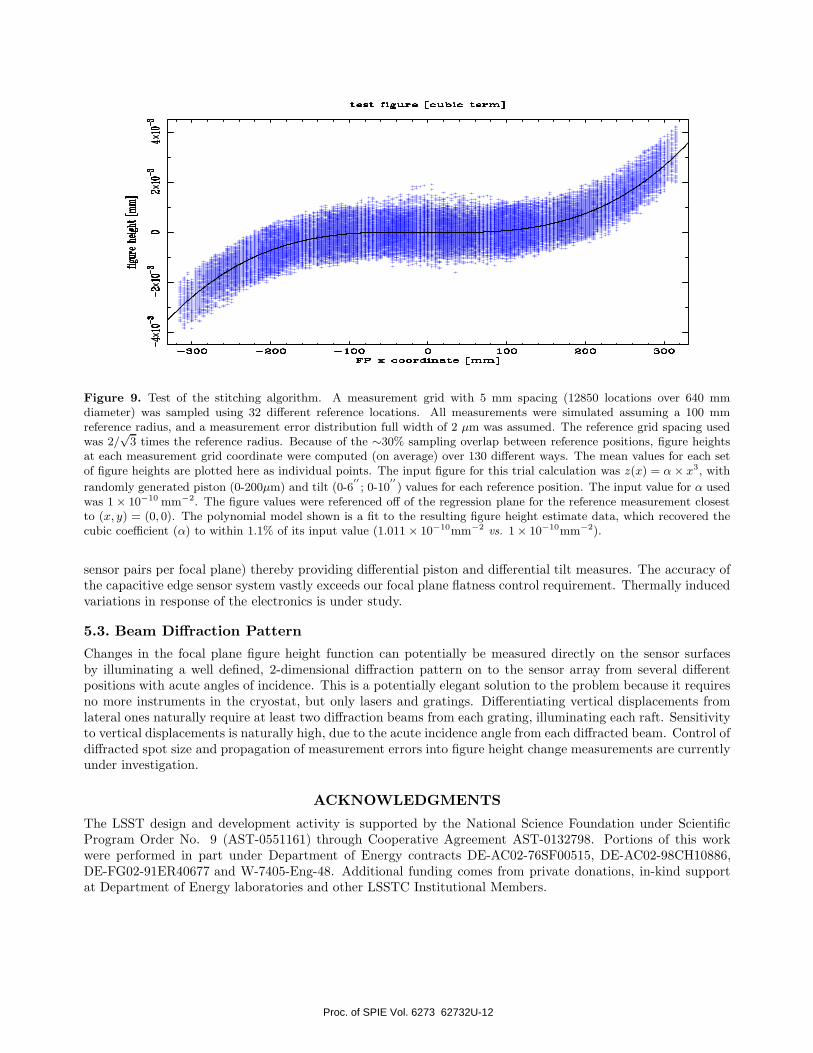
Figure 9. Test of the stitching algorithm. A measurement grid with 5 mm spacing (12850 locations over 640 mmdiameter) was sampled using 32 different reference locations. All measurements were simulated assuming a 100 mmreference radius, and a measurement error distribution full width of 2 µm was assumed. The reference grid spacing usedwas 2/

√3 times the reference radius. Because of the ∼30% sampling overlap between reference positions, figure heights

at each measurement grid coordinate were computed (on average) over 130 different ways. The mean values for each setof figure heights are plotted here as individual points. The input figure for this trial calculation was z(x) = α × x3, with

randomly generated piston (0-200µm) and tilt (0-6′′; 0-10

′′) values for each reference position. The input value for α used

was 1 × 10−10 mm−2. The figure values were referenced off of the regression plane for the reference measurement closestto (x, y) = (0, 0). The polynomial model shown is a fit to the resulting figure height estimate data, which recovered thecubic coefficient (α) to within 1.1% of its input value (1.011 × 10−10mm−2 vs. 1 × 10−10mm−2).

sensor pairs per focal plane) thereby providing differential piston and differential tilt measures. The accuracy ofthe capacitive edge sensor system vastly exceeds our focal plane flatness control requirement. Thermally inducedvariations in response of the electronics is under study.

5.3. Beam Diffraction Pattern

Changes in the focal plane figure height function can potentially be measured directly on the sensor surfacesby illuminating a well defined, 2-dimensional diffraction pattern on to the sensor array from several differentpositions with acute angles of incidence. This is a potentially elegant solution to the problem because it requiresno more instruments in the cryostat, but only lasers and gratings. Differentiating vertical displacements fromlateral ones naturally require at least two diffraction beams from each grating, illuminating each raft. Sensitivityto vertical displacements is naturally high, due to the acute incidence angle from each diffracted beam. Control ofdiffracted spot size and propagation of measurement errors into figure height change measurements are currentlyunder investigation.

ACKNOWLEDGMENTS

The LSST design and development activity is supported by the National Science Foundation under ScientificProgram Order No. 9 (AST-0551161) through Cooperative Agreement AST-0132798. Portions of this workwere performed in part under Department of Energy contracts DE-AC02-76SF00515, DE-AC02-98CH10886,DE-FG02-91ER40677 and W-7405-Eng-48. Additional funding comes from private donations, in-kind supportat Department of Energy laboratories and other LSSTC Institutional Members.


REFERENCES1. S. M. Kahn and LSST Camera Team, “Science Requirements for the Design of the LSST Camera,” American

Astronomical Society Meeting Abstracts 207, pp. –+, Dec. 2005.2. D. K. Gilmore, S. M. Kahn, M. Nordby, D. L. Burke, P. O’Connor, J. Olivier, V. Radeka, T. Schalk,

and R. Schindler, “LSST camera system overview,” in Ground-based and Airborne Instrumentation forAstronomy, Iye and McLean, eds., Proc. SPIE 6269, 2006.

3. J. A. Tyson, Z. Ivezic, S. Kahn, M. Strauss, C. Stubbs, D. Sweeney, and LSST Collaboration, “ScienceOpportunities with LSST,” American Astronomical Society Meeting Abstracts 207, pp. –+, Dec. 2005.

4. C. F. Claver, W. J. Gressler, V. L. Krabbendam, S. S. Olivier, D. L. Phillion, L. G. Seppala, and R. S.Upton, “LSST wavefront sensing and alignment system,” in Opto-Mechanical Technologies for Astronomy,Antebi, Atad-Ettedgui, and Lemke, eds., Proc. SPIE 6273, 2006.

5. M. Nordby, L. Hale, and LSST Camera Team, “The Mechanical Design of the LSST Camera,” AmericanAstronomical Society Meeting Abstracts 207, pp. –+, Dec. 2005.

6. S. S. Olivier, L. G. Seppala, D. K. Gilmore, L. C. Hale, and W. T. Whistler, “LSST camera optics,” inOpto-Mechanical Technologies for Astronomy, Antebi, Atad-Ettedgui, and Lemke, eds., Proc. SPIE 6273,2006.

7. D. Baade, K. Meisenheimer, O. Iwert, J. Alonso, T. Augusteijn, J. Beletic, H. Bellemann, W. Benesch,A. Boehm, H. Boehnhardt, J. Brewer, S. Deiries, B. Delabre, R. Donaldson, C. Dupuy, P. Franke, R. Gerdes,A. Gilliotte, B. Grimm, N. Haddad, G. Hess, G. Ihle, R. Klein, R. Lenzen, J.-L. Lizon, D. Mancini,N. Muench, A. Pizarro, P. Prado, G. Rahmer, J. Reyes, F. Richardson, E. Robledo, F. Sanchez, A. Silber,P. Sinclaire, R. Wackermann, and S. Zaggia, “The Wide Field Imager at the 2.2-m MPG/ESO telescope:first views with a 67-million-facette eye.,” The Messenger 95, pp. 15–16, 1999.

8. P. Z. Takacs, P. O’Connor, V. Radeka, G. Mahler, and J. C. Geary, “LSST detector module and raftassembly metrology concepts,” in Opto-Mechanical Technologies for Astronomy, Antebi, Atad-Ettedgui,and Lemke, eds., Proc. SPIE 6273, 2006.

9. H. M. Martin, R. G. Allen, B. Cuerden, S. T. DeRigne, L. R. Dettmann, D. A. Ketelsen, S. M. Miller,G. Parodi, and S. Warner, “Primary mirror system for the first Magellan telescope,” in Proc. SPIE Vol.4003, p. 2-13, Optical Design, Materials, Fabrication, and Maintenance, P. Dierickx, ed., pp. 2–13, July 2000.

10. A. Segurson and G. Z. Angeli, “Computationally efficient performance simulations for a thirty-meter tele-scope (TMT) point design,” in Optimizing Scientific Return for Astronomy through Information Technolo-gies, S. C. Craig and M. J. Cullum, eds., Proc. SPIE 5497, pp. 329–337, Sept. 2004.

11. Y. Komiyama, S. Miyazaki, M. Yagi, N. Yasuda, S. Okamura, M. Sekiguchi, M. Doi, K. Shimasaku,F. Nakata, H. Furusawa, M. Kimura, M. Ouchi, M. Hamabe, and H. Nakaya, “Suprime-Cam: Subaruprime focus camera,” in Instrument Design and Performance for Optical/Infrared Ground-based Telescopes,M. Iye and A. F. M. Moorwood, eds., Proc. SPIE 4841, pp. 152–159, Mar. 2003.


Focal plane metrology for the LSST camera

Documents