FNCE4030 Fall 2012 Ch06 Handout

INVESTMENTS | BODIE, KANE, MARCUS

Copyright © 2011 by The McGraw-Hill Companies, Inc. All rights reserved. McGraw-Hill/Irwin

CHAPTER 6

Risk Aversion and Capital

Allocation to Risky Assets


6-2

Allocation to Risky Assets

• Investors will avoid risk unless there

is a reward.

• The utility model allows optimal

allocation between a risky portfolio

and a risk-free asset.


6-3

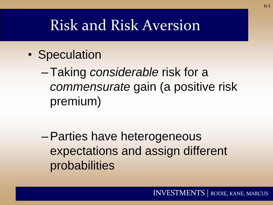
Risk and Risk Aversion

• Speculation

– Taking considerable risk for a

commensurate gain (a positive risk

premium)

– Parties have heterogeneous

expectations and assign different

probabilities


6-4

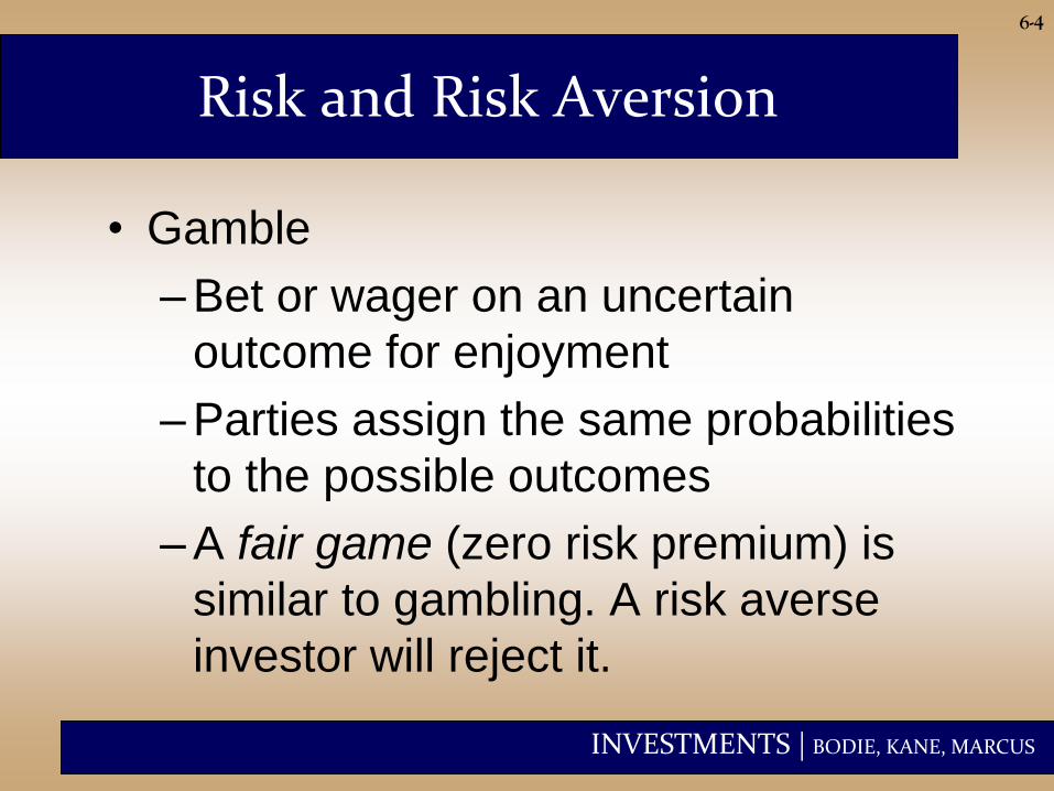
Risk and Risk Aversion

• Gamble

– Bet or wager on an uncertain

outcome for enjoyment

– Parties assign the same probabilities

to the possible outcomes

– A fair game (zero risk premium) is

similar to gambling. A risk averse

investor will reject it.


6-5

Risk Aversion and Utility Values

• Investors are willing to consider:

– risk-free assets

– speculative positions with positive risk premia

• Investors will reject fair games or worse

• Portfolio attractiveness increases with

expected return and decreases with risk.

• What happens when return increases with

risk?


6-6

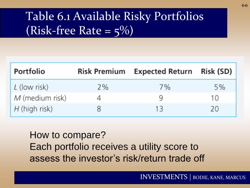
Table 6.1 Available Risky Portfolios (Risk-free Rate = 5%)

How to compare?

Each portfolio receives a utility score to

assess the investor’s risk/return trade off


6-7

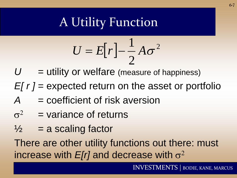
A Utility Function

U = utility or welfare (measure of happiness)

E[ r ] = expected return on the asset or portfolio

A = coefficient of risk aversion

s2 = variance of returns

½ = a scaling factor

There are other utility functions out there: must

increase with E[r] and decrease with s2

2

2

1sArEU


6-8

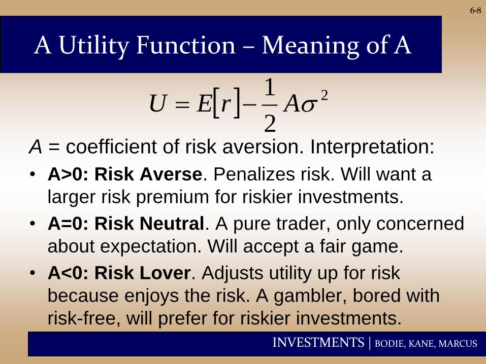
A Utility Function – Meaning of A

A = coefficient of risk aversion. Interpretation:

• A>0: Risk Averse. Penalizes risk. Will want a

larger risk premium for riskier investments.

• A=0: Risk Neutral. A pure trader, only concerned

about expectation. Will accept a fair game.

• A<0: Risk Lover. Adjusts utility up for risk

because enjoys the risk. A gambler, bored with

risk-free, will prefer for riskier investments.

2

2

1sArEU


6-9

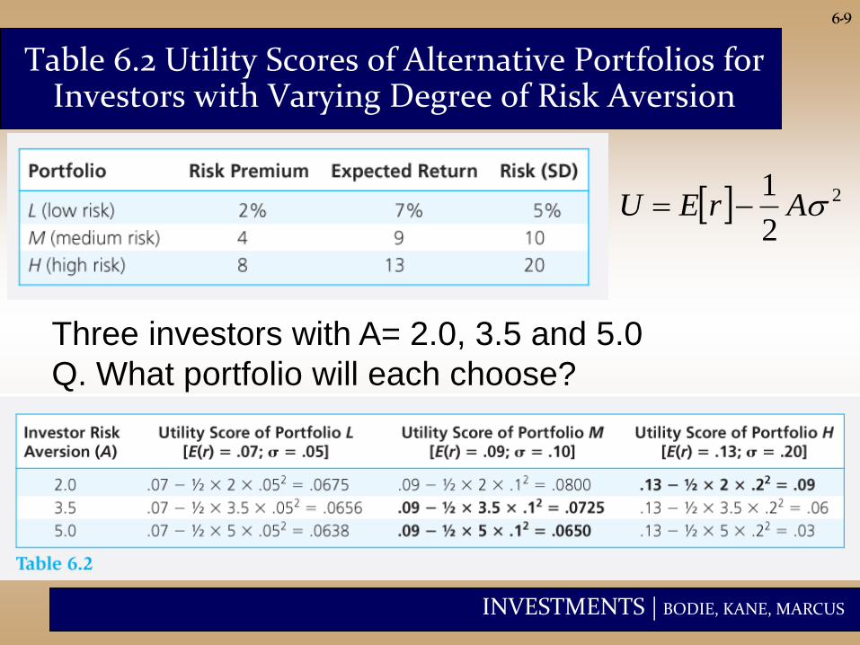
Table 6.2 Utility Scores of Alternative Portfolios for Investors with Varying Degree of Risk Aversion

Three investors with A= 2.0, 3.5 and 5.0

Q. What portfolio will each choose?

2

2

1sArEU


Let’s play a game

• I will toss a coin and pay you some money

X if heads and nothing if tails

• How much are you willing to pay to play

this game?

– For X=$0

– For X=$1

– For X=$10

– For larger X?

6-10


Let’s flip the game

• I will toss a coin and you pay me some

money X if heads and nothing if tails

• How much are you asking me to play this

game?

– For X=$0

– For X=$1

– For X=$10

– For larger X?

6-11


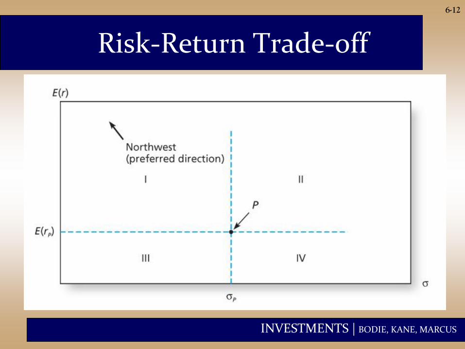
Risk-Return Trade-off

6-12


6-13

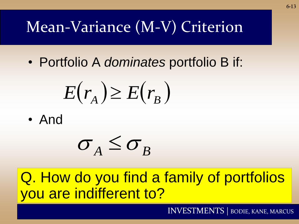
Mean-Variance (M-V) Criterion

• Portfolio A dominates portfolio B if:

• And

BA rErE

BA ss

Q. How do you find a family of portfolios you are indifferent to?


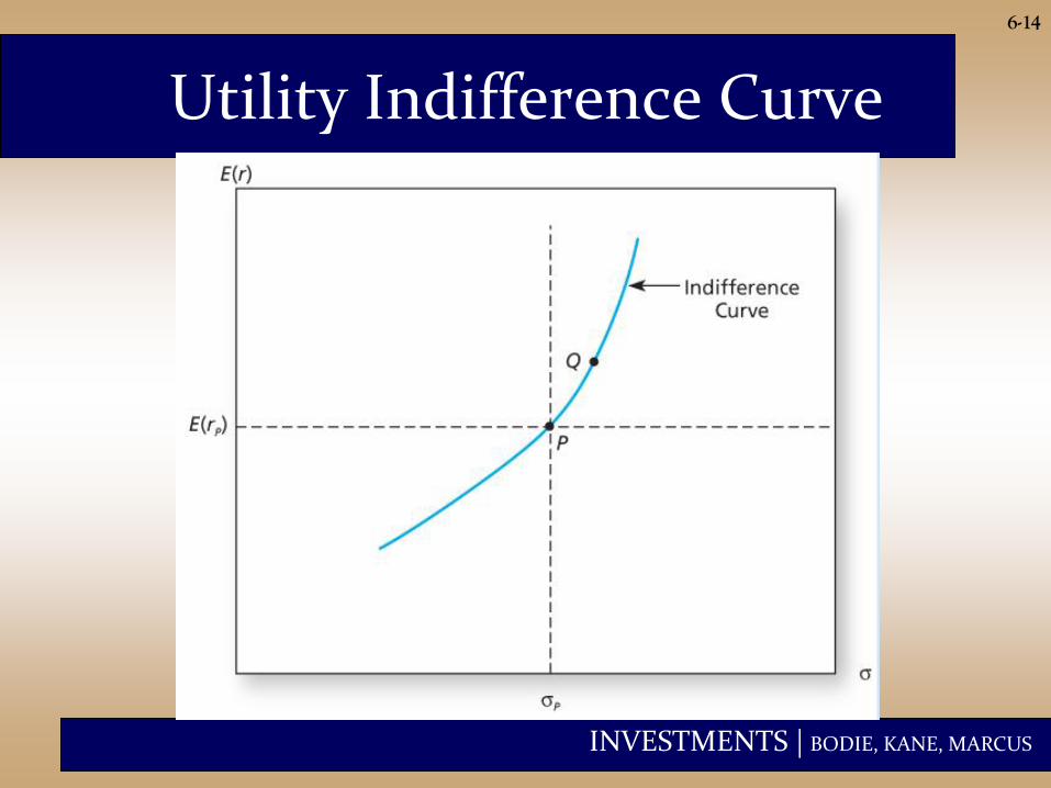
Utility Indifference Curve

6-14


6-15

How Do You Estimate Risk Aversion?

• Use questionnaires

• Observe individuals’ decisions when

confronted with risk

• Observe how much people are willing

to pay to avoid risk

• Use common sense


6-16

Capital Allocation Across Risky and Risk-Free Portfolios

Asset Allocation:

• Is a very important

part of portfolio

construction.

• Refers to the choice

among broad asset

classes.

Controlling Risk:

• Simplest way:

Manipulate the

fraction of the

portfolio invested in

risk-free assets

versus the portion

invested in the risky

assets


6-17

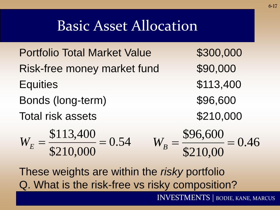
Basic Asset Allocation

Portfolio Total Market Value $300,000

Risk-free money market fund $90,000

Equities $113,400

Bonds (long-term) $96,600

Total risk assets $210,000

54.0000,210$

400,113$EW 46.0

00,210$

600,96$BW

These weights are within the risky portfolio

Q. What is the risk-free vs risky composition?


6-18

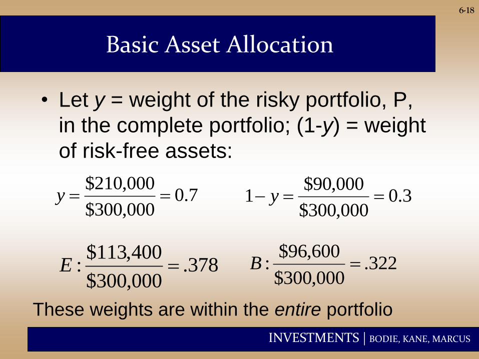
Basic Asset Allocation

• Let y = weight of the risky portfolio, P,

in the complete portfolio; (1-y) = weight

of risk-free assets:

7.0000,300$

000,210$y 3.0

000,300$

000,90$1 y

378.000,300$

400,113$: E 322.

000,300$

600,96$: B

These weights are within the entire portfolio


6-19

The Risk-Free Asset

• Only the government can issue

default-free bonds (caveats).

– Risk-free in real terms only if price

indexed and maturity equal to investor’s

holding period.

• T-bills viewed as “the” risk-free asset

• Money market funds also considered

risk-free in practice

(caveat, remember fall 2008?)


6-20

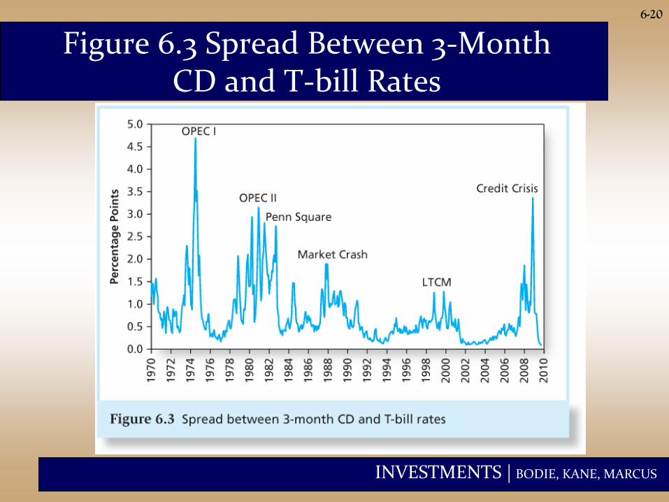
Figure 6.3 Spread Between 3-Month CD and T-bill Rates


6-21

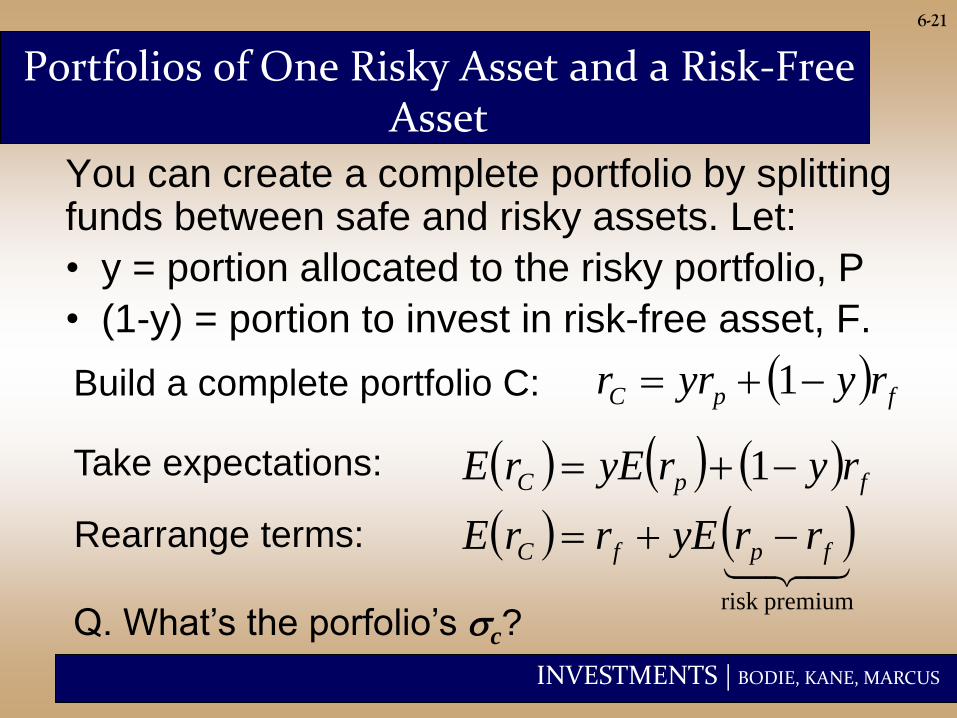
You can create a complete portfolio by splitting funds between safe and risky assets. Let:

• y = portion allocated to the risky portfolio, P

• (1-y) = portion to invest in risk-free asset, F.

Portfolios of One Risky Asset and a Risk-Free Asset

fpC ryyrr 1

fpC ryryErE 1Take expectations:

premiumrisk

fpfC rryErrE Rearrange terms:

Build a complete portfolio C:

Q. What’s the porfolio’s sc?


6-22

Risk-free

rf = 7%

srf = 0%

Risky

E(rp) = 15%

sp = 22%

y = % in p (1-y) = % in rf

Example Using Chapter 6.4 Numbers


6-23

Example (Ctd.)

The expected

return on the

complete

portfolio is the

risk-free rate plus

the weight of P

times the risk

premium of P

7157 yrE c

premiumrisk

fpfC rryErrE


6-24

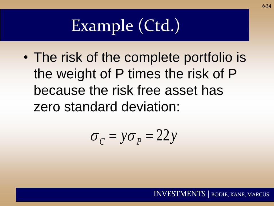
Example (Ctd.)

• The risk of the complete portfolio is

the weight of P times the risk of P

because the risk free asset has

zero standard deviation:

yy PC 22 ss


6-25

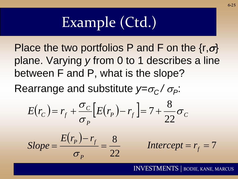
Example (Ctd.)

Place the two portfolios P and F on the {r,s}

plane. Varying y from 0 to 1 describes a line

between F and P, what is the slope?

Rearrange and substitute y=sC / sP:

CfP

P

CfC rrErrE s

s

s

22

87

22

8

P

fP rrESlope

s7 frIntercept


6-26

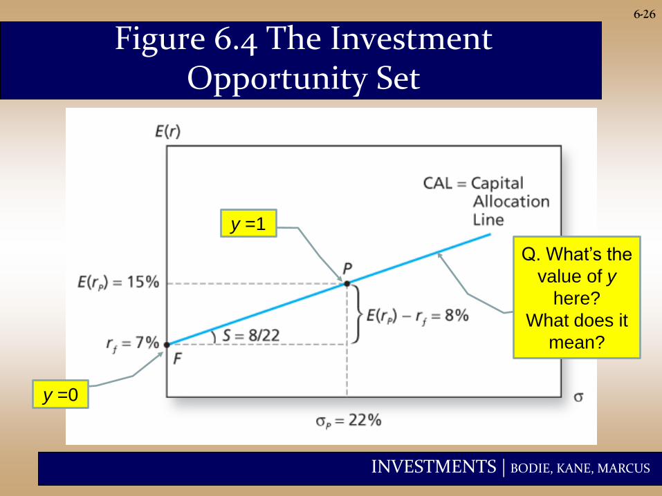
Figure 6.4 The Investment Opportunity Set

Q. What’s the

value of y

here?

What does it

mean?

y =0

y =1


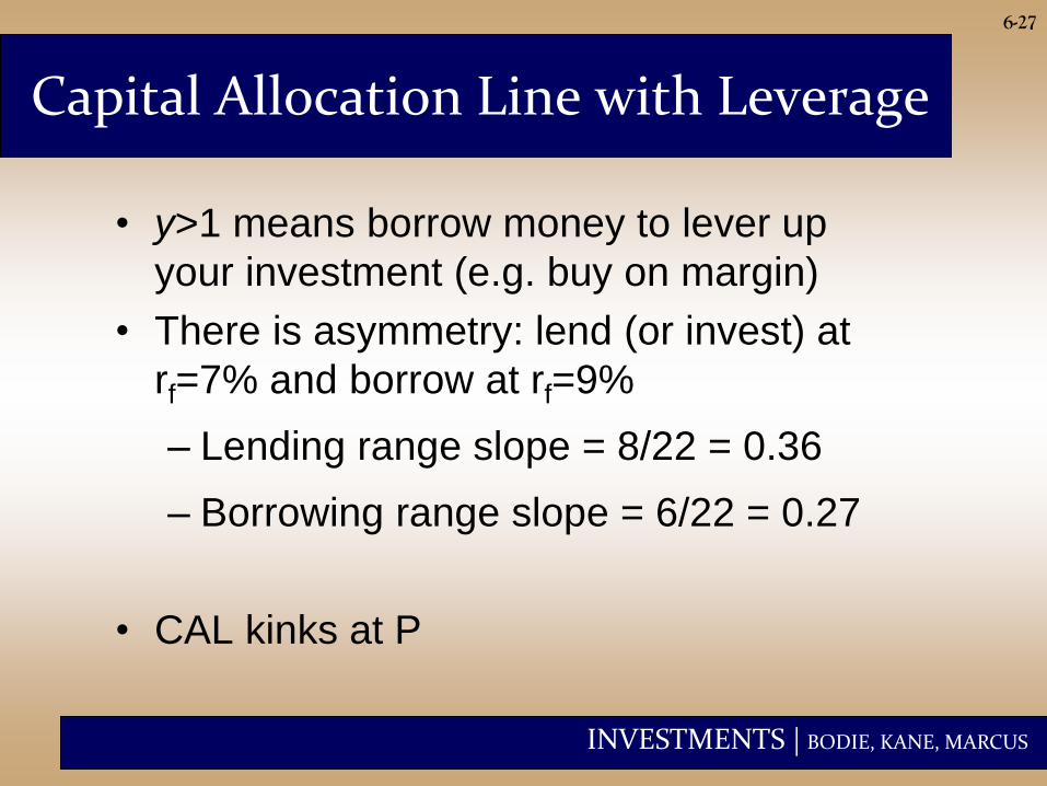
6-27

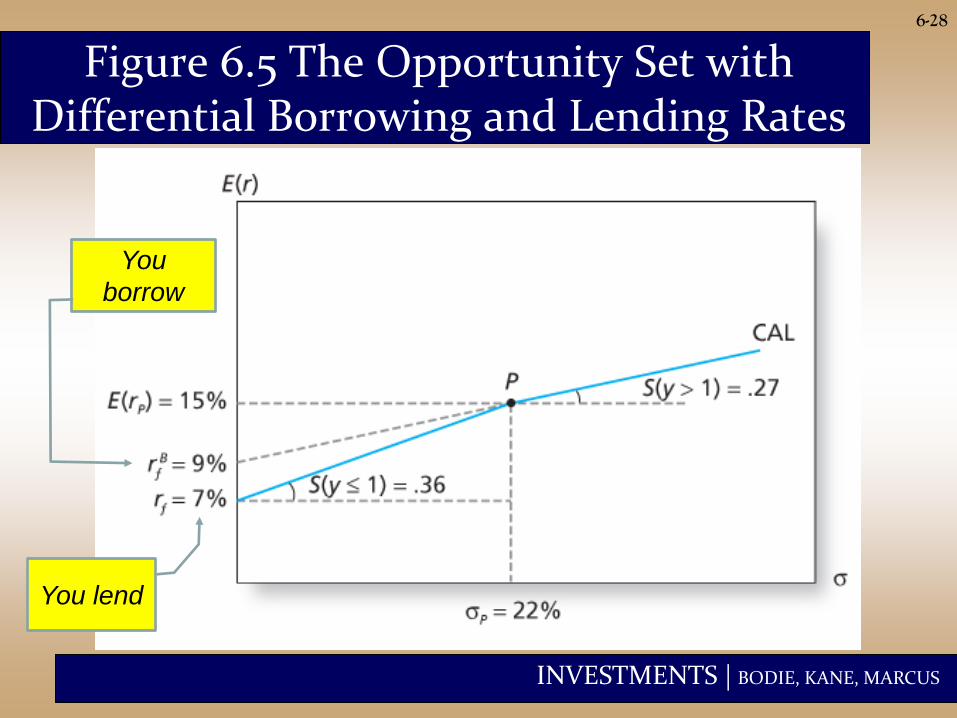
• y>1 means borrow money to lever up

your investment (e.g. buy on margin)

• There is asymmetry: lend (or invest) at

rf=7% and borrow at rf=9%

– Lending range slope = 8/22 = 0.36

– Borrowing range slope = 6/22 = 0.27

• CAL kinks at P

Capital Allocation Line with Leverage


6-28

Figure 6.5 The Opportunity Set with Differential Borrowing and Lending Rates

You lend

You

borrow


6-29

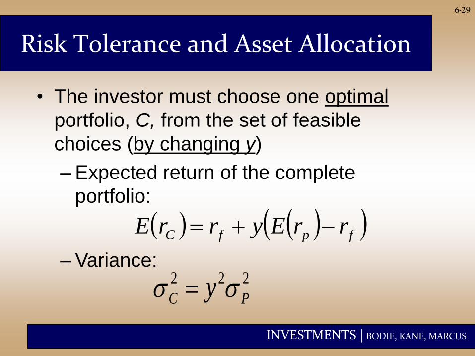
Risk Tolerance and Asset Allocation

• The investor must choose one optimal

portfolio, C, from the set of feasible

choices (by changing y)

– Expected return of the complete

portfolio:

fpfC rrEyrrE

222

PC y ss – Variance:


Utility Function depending on y

• Express U as a function of y

6-30

22

2

2

1

2

1

Pfpf

CC

yArrEyrU

ArEU

s

s

• U is a quadratic function of y

cybayU 2


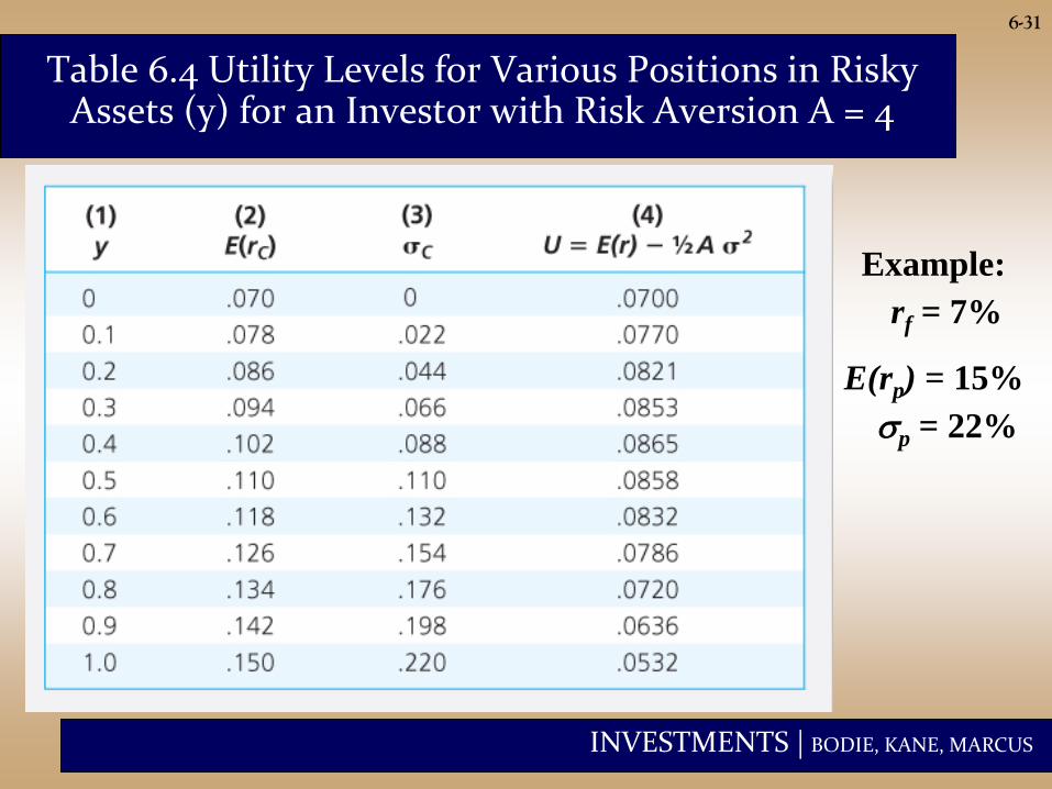
6-31

Table 6.4 Utility Levels for Various Positions in Risky Assets (y) for an Investor with Risk Aversion A = 4

rf = 7%

E(rp) = 15%

sp = 22%

Example:


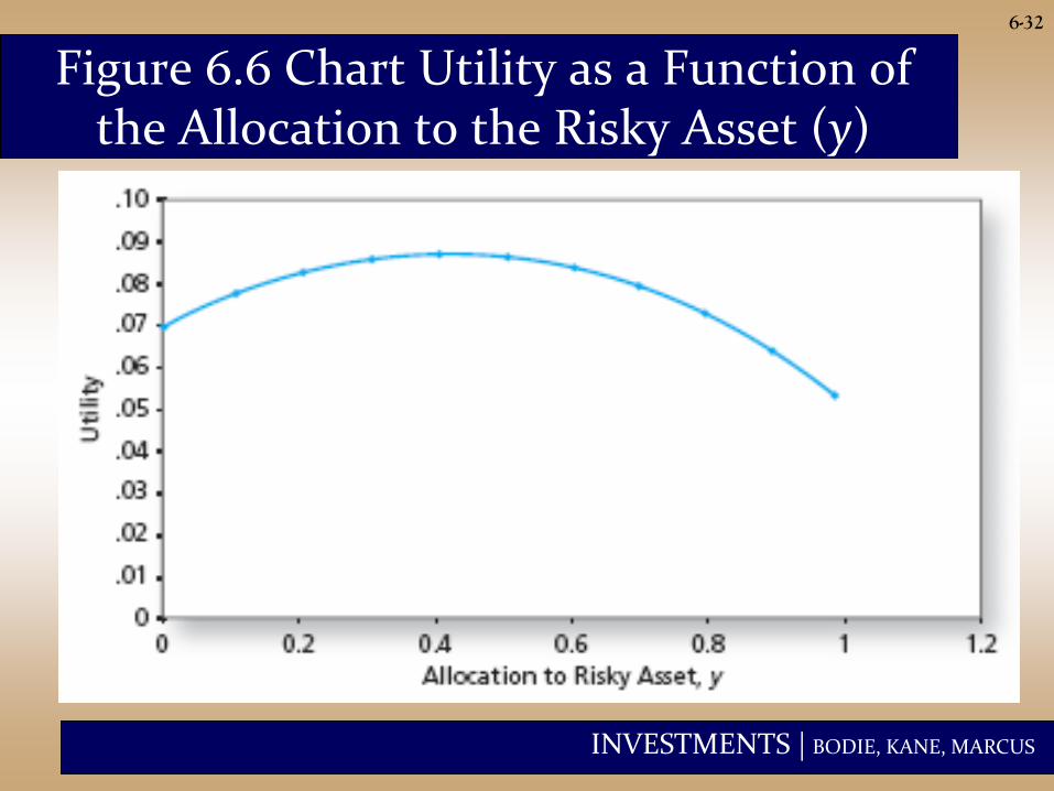
6-32

Figure 6.6 Chart Utility as a Function of the Allocation to the Risky Asset (y)


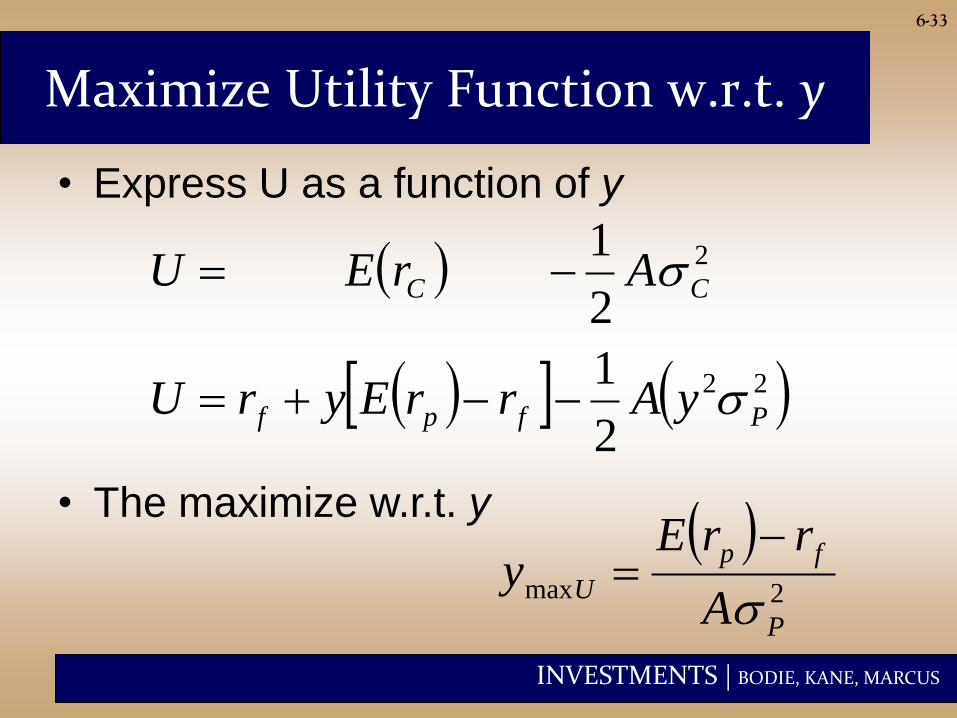
Maximize Utility Function w.r.t. y

• Express U as a function of y

6-33

22

2

2

1

2

1

Pfpf

CC

yArrEyrU

ArEU

s

s

• The maximize w.r.t. y 2max

P

fp

UA

rrEy

s


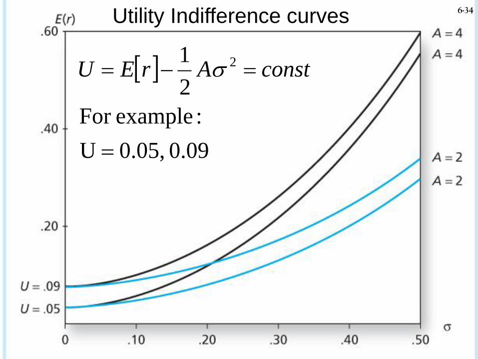
Utility Indifference Levels

6-34 Utility Indifference curves

90.0 0.05,U

:exampleFor

2

1 2

constArEU s


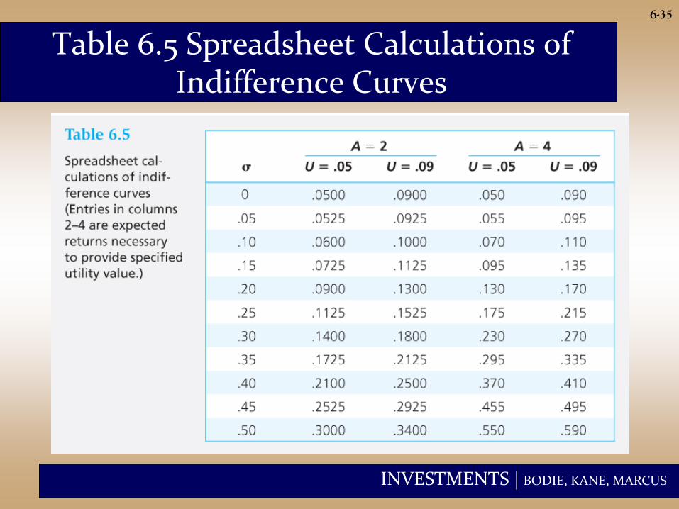
6-35

Table 6.5 Spreadsheet Calculations of Indifference Curves


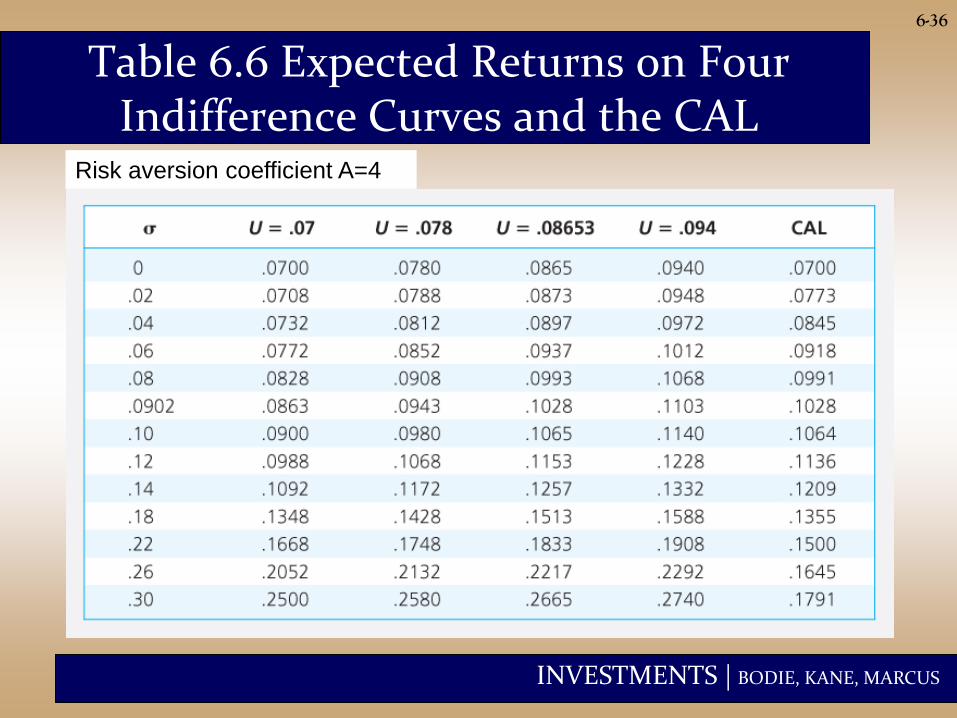
6-36

Table 6.6 Expected Returns on Four Indifference Curves and the CAL

Risk aversion coefficient A=4


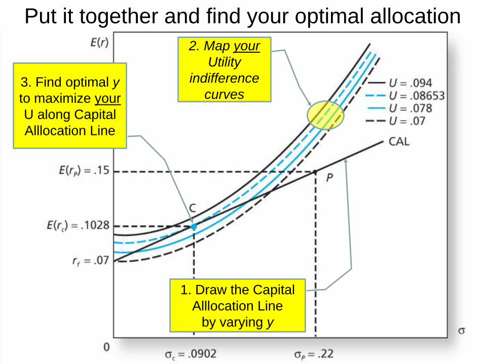
6-37

3. Find optimal y

to maximize your

U along Capital

Alllocation Line

2. Map your

Utility

indifference

curves

1. Draw the Capital

Alllocation Line

by varying y

Put it together and find your optimal allocation


6-38

Passive Strategies: The Capital Market Line

• The passive strategy avoids any direct or

indirect security analysis

• Supply and demand forces may make such

a strategy a reasonable choice for many

investors


6-39


• A natural candidate for a passively held

risky asset would be a well-diversified

portfolio of common stocks such as the

S&P 500.

• The capital market line (CML) is the capital

allocation line formed from 1-month T-bills

and a broad index of common stocks (e.g.

the S&P 500).


6-40


• The CML is given by a strategy that

involves investment in two passive

portfolios:

1. a virtually risk-free portfolio of short-

term T-bills (or a money market fund)

2. a fund of common stocks that mimics

a broad market index.


6-41


• From 1926 to 2009, the passive risky

portfolio offered an average risk premium

of 7.9% with a standard deviation of

20.8%, resulting in a reward-to-volatility

ratio of .38.

FNCE4030 Fall 2012 Ch06 Handout

Documents