fma.ny.presentation

Understanding rankings of financial analysts

Artur Aiguzhinov1 Carlos Soares1 Ana Paula Serra2

1LIAAD-INESC Porto LA & Faculdade de Economia da Universidade do Porto

2Faculdade de Economia da Universidade do Porto & CEFUP - Centro de Economia e Financasda Universidade do Porto

October 23rd, 2010FMA Annual Meeting, New York

1 of 23

Motivation: the value of the recommendations

� Efficient Market Hypothesis (Fama, 1970);

� High information costs provide possibilities for abnormal returns(Grossman & Stiglitz, 1980);

� On average, recommendations bring value to investors (Womack, 1996);

� Analysts’ accuracy in forecasts is valuable (Brown & Mohammad, 2003);

2 of 23

Motivation: rankings of the analysts

� StarMine R© issues annual analyst rankings:� Ranks the analysts based on recommendation performance and EPS

forecast accuracy;

� Why not to predict stock prices directly?� Analysts’ relative performance (rankings) is more predictable than the stock

prices.

� Is it possible to predict these rankings?:� If yes, can we use those predictions in profitable strategy?;

3 of 23

The Goals of the Research

� Accurately predict the rankings of financial analysts;

4 of 23

Research contributions

� Interdisciplinary approach to an interesting research topic;

� Financial Economics contributions:� analysis of the financial analysts based on state variables concerning market

conditions and stock characteristics;� first methodology to predict the rankings;� verify if there is a ranking consistency over time;� identify variables that discriminate the rankings;

5 of 23

Research design: an overview

� Initial rankings of the analysts (target rankings):� Analysts evaluation models (Clement, 1999; Brown, 2001; Creamer &

Stolfo, 2009);

� Predict rankings of the analysts (label ranking):

� Evaluate the ranking accuracy;

� Identify discriminative independent variables;

6 of 23

Database to use

� ThomsonOne I/B/E/S Detailed History:� Quarterly EPS forecasts (1989Q1-2009Q4);

� ThomsonOne DataStream:� Accounting data;� Market data;

7 of 23

Description of the data

Table: Summary of the data

Sector # analysts # stocks mean forecasts mean stocksper stock per quarter per analysts per quarter

Energy 135 34 7.57 1.91Industrials 208 66 3.66 1.05Materials 147 30 5.14 1.16

IT 301 106 7.85 2.76

Total 791 236 6.06 1.72

8 of 23

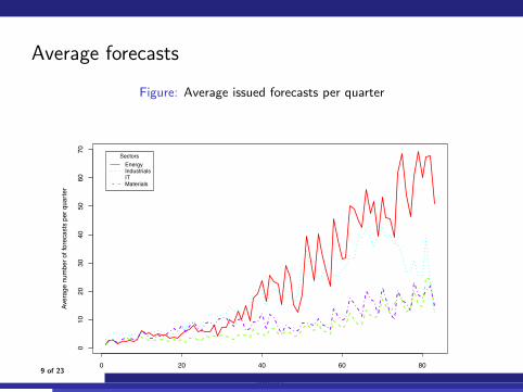
Average forecasts

Figure: Average issued forecasts per quarter

0 20 40 60 80

010

2030

4050

6070

Quarters

Aver

age

num

ber o

f for

ecas

ts p

er q

uarte

r

SectorsEnergyIndustrialsITMaterials

9 of 23

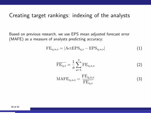
Creating target rankings: indexing of the analysts

Based on previous research, we use EPS mean adjusted forecast error(MAFE) as a measure of analysts predicting accuracy:

FEq,a,s = |ActEPSq,s − EPSq,a,s| (1)

FEq,s =1

n

n∑a=1

FEq,a,s (2)

MAFEq,a,s =FEq,a,s

FEq,s

(3)

10 of 23

Context characterization: state variables

Variables that describe market conditions and stock characteristics(Jegadeesh, Kim, Krische, & Lee, 2004):

� Analysts variables:� Lagged forecasting error;� Change in consensus;

� Earnings momentum:� Standardized Unexpected Earnings;

� Growth indicators:� Sales growth;

� Fundamentals:� Total accruals to total assets ratio;

� Valuation multiples:� Earnings-to-price ratio;

� Market volatility;

11 of 23

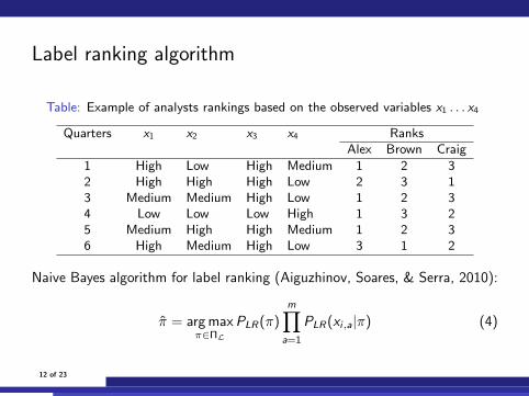
Label ranking algorithm

Table: Example of analysts rankings based on the observed variables x1 . . . x4

Quarters x1 x2 x3 x4 RanksAlex Brown Craig

1 High Low High Medium 1 2 32 High High High Low 2 3 13 Medium Medium High Low 1 2 34 Low Low Low High 1 3 25 Medium High High Medium 1 2 36 High Medium High Low 3 1 2

Naive Bayes algorithm for label ranking (Aiguzhinov, Soares, & Serra, 2010):

π = arg maxπ∈ΠL

PLR(π)m∏

a=1

PLR(xi,a|π) (4)

12 of 23

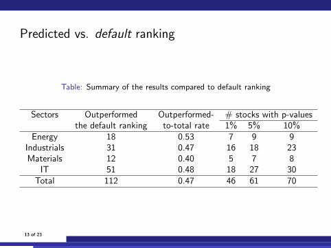
Predicted vs. default ranking

Table: Summary of the results compared to default ranking

Sectors Outperformed Outperformed- # stocks with p-valuesthe default ranking to-total rate 1% 5% 10%

Energy 18 0.53 7 9 9Industrials 31 0.47 16 18 23Materials 12 0.40 5 7 8

IT 51 0.48 18 27 30Total 112 0.47 46 61 70

13 of 23

Predicted vs naive ranking

Table: Summary of the results compared to naive ranking

Sectors Outperformed Outperformed- # stocks with p-valuesthe naive ranking to-total rate 1% 5% 10%

Energy 11 0.32 5 7 7Industrials 27 0.41 5 6 7Materials 11 0.37 0 0 1

IT 36 0.34 1 1 1Total 85 0.36 11 14 16

14 of 23

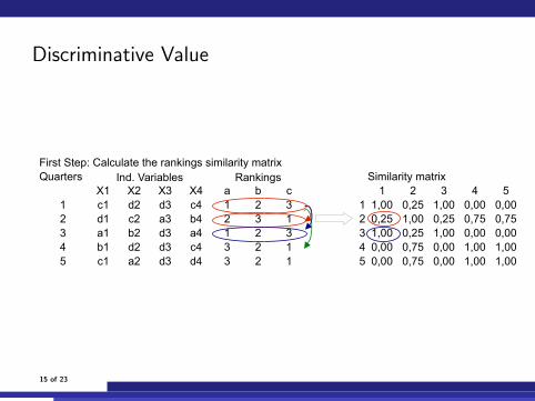
Discriminative Value

Лист1

Страница 1

First Step: Calculate the rankings similarity matrixQuarters Ind. Variables Rankings Similarity matrix

X1 X2 X3 X4 a b c 1 2 3 4 51 c1 d2 d3 c4 1 2 3 1 1,00 0,25 1,00 0,00 0,002 d1 c2 a3 b4 2 3 1 2 0,25 1,00 0,25 0,75 0,753 a1 b2 d3 a4 1 2 3 3 1,00 0,25 1,00 0,00 0,004 b1 d2 d3 c4 3 2 1 4 0,00 0,75 0,00 1,00 1,005 c1 a2 d3 d4 3 2 1 5 0,00 0,75 0,00 1,00 1,00

15 of 23

Discriminative Value

Лист1

Страница 1

Second step:X1=(a1,b1,c1,d1)a1 vs b1

X1 1 2 3 4 51 c1 1 2 3 1 1,00 0,25 1,00 0,00 0,002 d1 2 3 1 2 0,25 1,00 0,25 0,75 0,753 a1 1 2 3 3 1,00 0,25 1,00 0,00 0,004 b1 3 2 1 4 0,00 0,75 0,00 1,00 1,005 c1 3 2 1 5 0,00 0,75 0,00 1,00 1,00

mean(a1 vs b1) = (0)/1=0

16 of 23

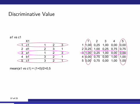
Discriminative Value

Лист1

Страница 1

a1 vs c1X1 1 2 3 4 5

1 c1 1 2 3 1 1,00 0,25 1,00 0,00 0,002 d1 2 3 1 2 0,25 1,00 0,25 0,75 0,753 a1 1 2 3 3 1,00 0,25 1,00 0,00 0,004 b1 3 2 1 4 0,00 0,75 0,00 1,00 1,005 c1 3 2 1 5 0,00 0,75 0,00 1,00 1,00

mean(a1 vs c1) = (1+0)/2=0,5

17 of 23

Discriminative Value

Лист1

Страница 1

a1 vs d11 2 3 4 5

1 1,00 0,25 1,00 0,00 0,002 0,25 1,00 0,25 0,75 0,753 1,00 0,25 1,00 0,00 0,004 0,00 0,75 0,00 1,00 1,005 0,00 0,75 0,00 1,00 1,00

mean(a1 vs d1) = (0,25)/1=0,25

18 of 23

Discriminative Value

X1 average Weights Weighted averagea1 vs. b1 0.00 1 0.00a1 vs. c1 0.50 2 1.00a1 vs. d1 0.25 3 0.75b1 vs. c1 0.50 1 0.50b1 vs. d1 0.75 2 1.50c1 vs. d1 0.50 1 0.50

0.708

Discriminative Power : 1-0.708=0.292 The higher the discriminative power,the more different are the rankings

19 of 23

Discriminative power

Table: Discriminative power of independent variables

Sectors FELAG SUE consensus EP SG TA MKTEnergy 0.235 0.211 0.234 0.208 0.194 0.341 0.148

Industrials 0.248 0.230 0.279 0.233 0.263 0.282 0.089Materials 0.180 0.197 0.278 0.232 0.156 0.378 0.051

IT 0.213 0.238 0.243 0.230 0.185 0.298 0.155Total 0.219 0.219 0.258 0.226 0.199 0.325 0.111

20 of 23

References (1)

Aiguzhinov, A., Soares, C., & Serra, A. P. (2010). A similarity-basedadaptation of naive bayes for label ranking: Application to themetalearning problem of algorithm recommendation. In B. Pfahringer,G. Holmes, & A. Hoffmann (Eds.), Discovery science (Vol. 6332, pp.16–26). Springer.

Black, F., & Litterman, R. (1992). Global portfolio optimization. FinancialAnalysts Journal, 48(5), 28–43.

Brazdil, P., Soares, C., & Costa, J. (2003). Ranking Learning Algorithms:Using IBL and Meta-Learning on Accuracy and Time Results.Machine Learning, 50(3), 251–277.

Brown, L. (2001). How Important is Past Analyst Earnings ForecastAccuracy? Financial Analysts Journal, 57(6), 44–49.

Brown, L., & Mohammad, E. (2003). The Predictive Value of AnalystCharacteristics. Journal of Accounting, Auditing and Finance, 18(4).

21 of 23

References (2)

Clement, M. (1999). Analyst forecast accuracy: Do ability, resources, andportfolio complexity matter? Journal of Accounting and Economics,27(3), 285–303.

Creamer, G., & Stolfo, S. (2009). A link mining algorithm for earningsforecast and trading. Data Mining and Knowledge Discovery, 18(3),419–445.

Fama, E. (1970). Efficient Capital Markets: A Review of Empirical Work.The Journal of Finance, 25, 383–417.

Grauer, R. (2008). Benchmarking measures of investment performance withperfect-foresight and bankrupt asset allocation strategies. The Journalof Portfolio Management, 34(4), 43–57.

Grossman, S., & Stiglitz, J. (1980). On the Impossibility of InformationallyEfficient Prices. American Economic Review, 70, 393–408.

Hullermeier, E., Furnkranz, J., Cheng, W., & Brinker, K. (2008). Labelranking by learning pairwise preferences. Artificial Intelligence,172(2008), 1897–1916.

22 of 23

References (3)

Jegadeesh, N., Kim, J., Krische, S., & Lee, C. (2004). Analyzing theAnalysts: When Do Recommendations Add Value? The Journal ofFinance, 59(3), 1083–1124.

Ljungqvist, A., Malloy, C., & Marston, F. (2009). Rewriting history. TheJournal of Finance, 64(4), 1935–1960.

Vembu, S., & Gartner, T. (2010, October). Preference learning. Springer.Vogt, M., Godden, J., & Bajorath, J. (2007). Bayesian interpretation of a

distance function for navigating high-dimensional descriptor spaces.Journal of chemical information and modeling, 47(1), 39-46.

Womack, K. (1996). Do Brokerage Analysts’ Recommendations HaveInvestment Value? The Journal of Finance, 51, 137–168.

23 of 23

Similarity-based Naive Bayes for Label Ranking: Priorprobability of label ranking

Table: Demonstration of the prior probability for label ranking

Quarters x1 x2 x3 x4 RanksAlex Brown Craig

1 High Low High Medium 1 2 32 High High High Low 2 3 13 Medium Medium High Low 1 2 34 Low Low Low High 1 3 2...

......

......

......

...14 Medium High High Medium 1 2 315 High Medium High Low 3 1 2

Maximizing the likelihood is equivalent to minimizing the distance (i.e.,maximizing the similarity) in a Euclidean space (Vogt, Godden, & Bajorath,2007)

Label ranking: formalization

� Instance: X ⊆ {V1, . . . ,Vm}� Labels: L = {λ1, . . . , λk}� Output: Y = ΠL� Training set: T = {xi , yi}i∈{1,...,n} ⊆ X × Y

Learn a mapping h : X → Y such that a loss function ` is minimized:

` =

∑ni=1 ρ(πi , πi )

n(5)

with ρ being a Spearman correlation coefficient:

ρ(π, π) = 1−6∑k

j=1(πj − πj)2

k3 − k(6)

where π and π are, respectively, the target and predicted rankings for agiven instance.

Posterior probability of label ranking

Proir probability of label ranking:

PLR(π) =

∑ni=1 ρ(π, πi )

n(7)

Conditional probability of label ranking:

PLR(va,i |π) =

∑i :xi,a=va,i

ρ(π, πi )

|{i : xi,a = va,i}|(8)

Estimated ranking:

π = arg maxπ∈ΠL

PLR(π)m∏

a=1

PLR(xi,a|π) (9)