Flux

THE USE OF FLUX LOOPS FORCALIBRATION OF MAGNETIC REPRODUCERS

BY

Alastair M. HeaslettAmpex Corporation

INTRODUCTION

In any system involving magnetic tape and ring core magnetic heads, a basic needexists for standardization of recorded flux versus frequency characteristics topermit interchange of recorded material. Thus, when setting up a recording andreproducing system, it is necessary to perform a series of measurements and ad-justments to align the system.

The result of this alignment must be a system which when reproducing other tapesmade to the same standard, or when recording tapes to this standard, will re-produce the recording with an appropriately flat frequency response, and converselyproduce a recording, which when reproduced ideally, is also flat.

From a practical standpoint, it is fortunate that the standards established forrecorded tape interchange in audio effectively demand a specific relationship betweenflux and frequency on the recorded material.

It is outside the scope of this paper to discuss the reasons why any one standard isas it is, except to comment that in some instances standards laid down many yearsago are becoming slightly outmoded and in some senses restrictive.

SYSTEM STANDARDIZATION

In all the currently used audio standards for magnetic tape systems, the equalizationrequired to correct for tape (and head losses) is divided into two parts, post andpreemphasis.

This is just an elegant way of saying that some of the losses are corrected duringrecording and some during playback. The division of the quantities of equalizationused between recording and playback should not be an arbitrary one, basically itdepends on whether you want good high level high frequency response, or good highfrequency noise. The two are unfortunately, in the limit, exclusive.

The recording standard will always specify how the remanent flux versus frequencyrecorded on the recorded tape should be.

Thus, if such a tape were reproduced by an ideal reproducer a flat system output,voltage (or current), versus frequency would result.

1

Today anyone can purchase such a tape, play it on their reproducer and adjustthat reproducer for a flat response.

Subsequently, when recording, the recording equalization and bias is adjustedso that the output from the reproducer is again flat.

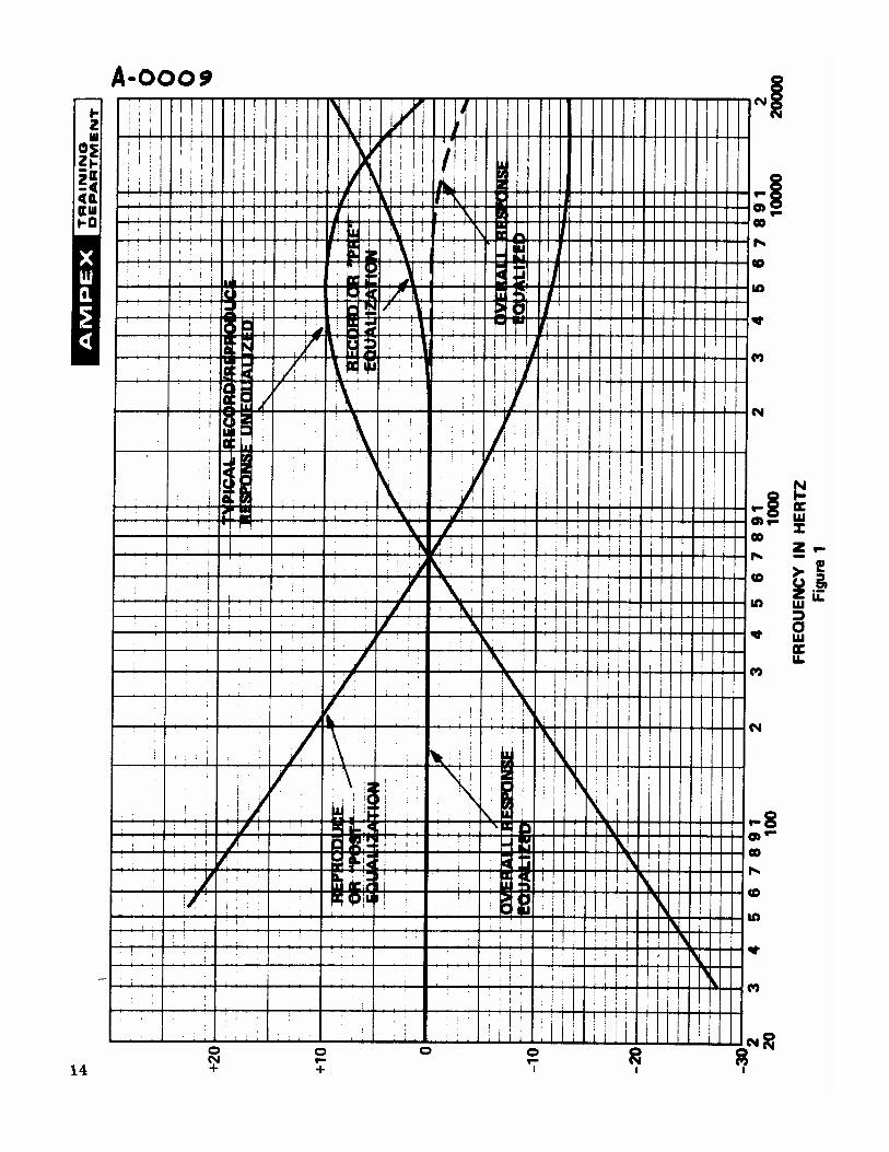
This process ensures that the flux/frequency response of the recorded tape isidentical to the standard. (See Figure 1)

Clearly, a standard tape is a very important link in the system since it duplicatesthe “ideal” tape and hence verifies the reproducing systems right from the re-produce head gap to the output terminals.

However, there may be some times when the standard tape does not give enoughinformation or doesn’t supply it for long enough. (As one who has had theprivilege of aligning all channels of a 24 channel machine from scratch can attest.)

In addition, there may come a time when, despite your efforts, the reproduceequalization cannot be set correctly. This might indicate a problem with theelectronics, or with the head, or with both, or it may be that the alignment tapehas come to the end of its useful life or even been damaged. This is where theflux loop appears as a diagnostic aide and useful tool in general maintenance.

THE FLUX LOOP

Essentially a flux loop is a means of generating flux and applying it to a magnetichead in such a way as to induce a field in the magnetic head which closelyapproximates the field from a moving length of tape. (See Figure 2)

Flux loops take many shapes, but the most common is simply a few turns of finewire wound closely together on a non-ferrous rectangular former. One straightedge of the winding is brought close to the front gap of the head under test withthe length of the coil aligned with the gap. The length of the winding broughtagainst the head should be greater than the track width of the head being checked,it may indeed extend over several tracks simultaneously. The other dimensionsof the loop are not overly important except that they should be somewhat longerthan the head dimensions.

The principle which makes the loop work is quite simple. If a current is passedthrough the winding, each wire generates a magnetic field directly proportionalto the current. The flux generated is concentric to the wire axis. The field fromseveral wires will add evenly at any given point in space around the bundle of conductors;i.e. the total field produced is virtually multiplied by the number of conductors. Thisis strictly only true at a point whose distance from the bundle is many times thewire bundle diameter.

The direction of the flux depends upon the direction of current flow in the wires.Thus if sinusoidal current flows in the wires, a sinusoidally varying field will result.

2

When the coil is brought close to a highly permeable object such as a magneticreproducing head, some of the flux from the coil will tend to travel in the mag-netic head core instead of the air. This flux will thus couple the turns of wirewound on the head cores.

In fact, the flux from the flux loop will be doing exactly what the flux from apiece of tape would do. It is not a very efficient process, but nonetheless, aconsiderable amount of flux is induced into the head.

Thus, if the current in the loop is held constant and the frequency varied, thefull flux field versus frequency response of the magnetic head and reproducingamplifier can be measured.

Note that only those sides of the flux loop parallel to the magnetic head gap caninduce flux in the head. (Those not in parallel do induce some because thebundle of conductors is not infinitely thin, nor is the head totally insensitive toflux coming from directions other than perpendicular to its gap line.) However,the remote end of the loop is producing flux in opposition to the end in contactwith the head. This is the reason for separating the two by some respectabledistance. Otherwise, the remote field will tend to cancel that from the side ofthe loop closest to the head.

LIMITATIONS

Useful though the flux loop is, it has some fundamental limitations which shouldbe understood.

a. The flux loop does not show the effect of head gap loss. This, if necessary, must be evaluated separately.

b. The flux loop does not make any allowance for head to tape separation.

c. There are slight errors at very high frequencies with multi-turn loops due to skin effect. These errors however are less than 0.1db to at least 20 kHz and are therefore negligible in the audio band.

d. The flux loop does not give any indication of the long wavelength, “pole contour” ripple which all magnetic reproducing heads are cursed with.

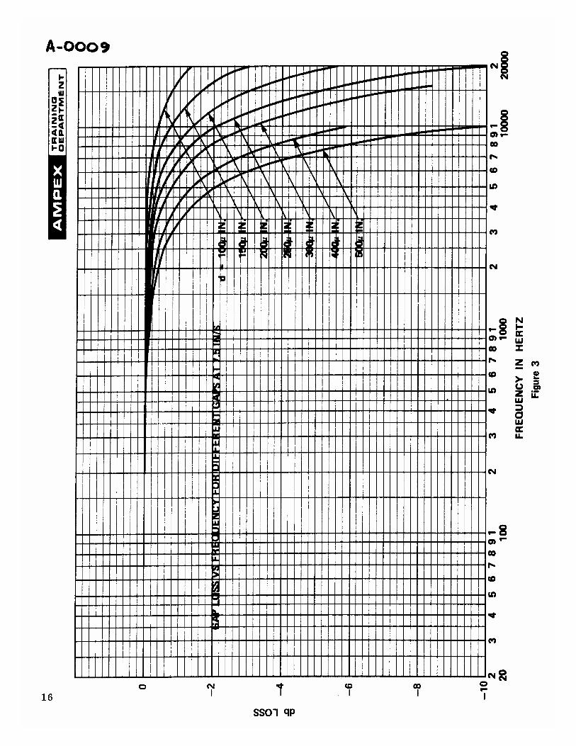
Of the four listed errors the most significant for normal studio tape speeds(15 in/s 7 1/2 in/s) is that due to gap loss. A graph showing gap loss againstfrequency for typical gaps is shown in Figure 3. for 7 1/2 ins/sec: For15 ins/s double all the frequencies, for 3.75 in/sec halve all frequencies (andpro rata for other speeds).

NOTE: The actual off tape flux response is obtained by measuring the freefield flux response and then correcting this response with the gap losscorrection for the head being tested.

3

PRACTICAL FLUX LOOPS

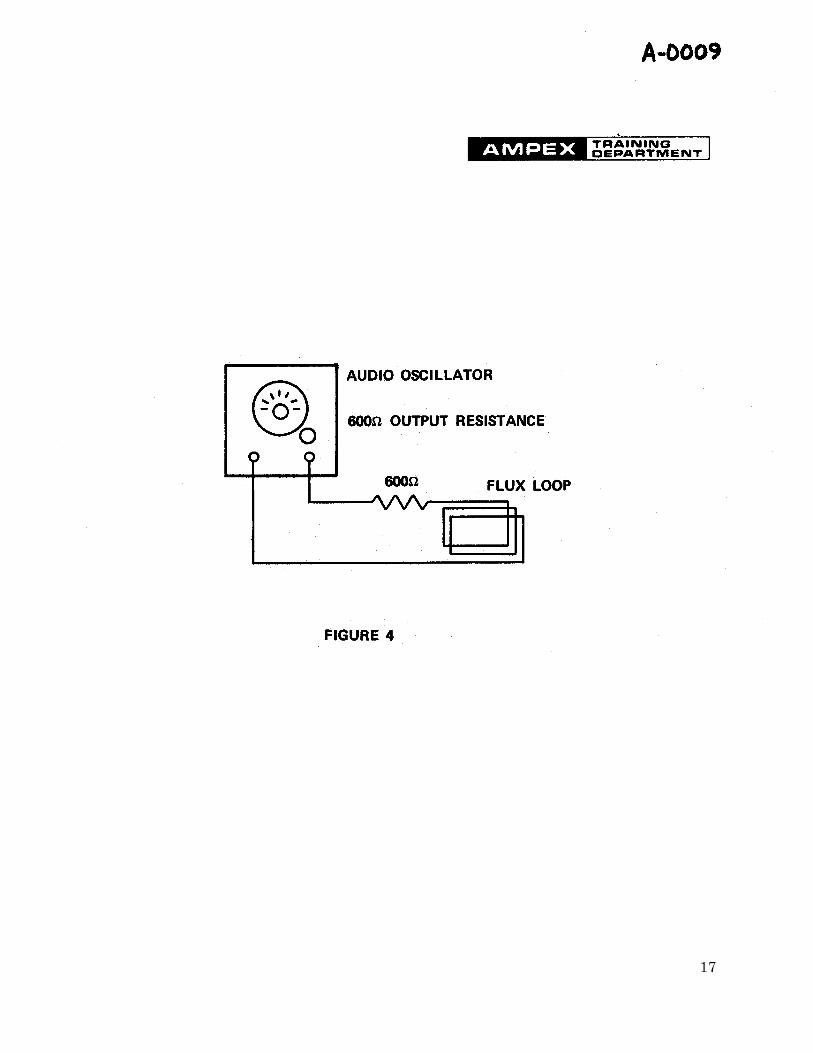
One of the requirements for making the flux loop useful is a means of keepingthe current in the loop constant with frequency. Since the loop is an inductance,its impedance will rise with frequency. However, its impedance up to quitehigh frequencies is very small, and placing a 600 ohm resistor in series withthe coil and connecting the whole thing to an audio oscillator will normally bemore than adequate. Obviously, the oscillator must have a constant output withfrequency, or must be adjusted to constant amplitude for each frequency output.(See Figure 4)

The current in the loop will stay constant in this case simply because the 600 ohmresistor is many times the impedance of the coil.

A typical multi-turn loop will have from 5 to 15 turns of 40 A.W.G wire. This willgive flux levels of around 60 to l80nWb/m when driven with 2V RMS through a600 ohm resistor. If more turns, or finer wire, are used, the coil impedance,or resistance, may tend to become significant.

Two typical flux loops are shown in Figures 5A & 5B. Figure 5B, known as the“super loop” is large enough to cover all the tracks on a 2” head stack.

A third loop, shown in Figure 6, was made to use on consumer cassette heads whenin situ.

If the flux loops illustrated seem a little inelegant, the author has used maskingtape and five turns of loose wire in an emergency!

USING THE FLUX LOOP

The flux loop shown in Figure 7 has been clipped to a reproduce head stack. Theloop is connected to a standard 600 ohm output impedance audio frequency oscillator.The loop is terminating the oscillator directly and the oscillator has a constantoutput voltage with frequency.

What now does one expect to see in the way of a frequency response from thereproduce amplifier output terminals?

For initial simplicity let us assume that the gap loss can be ignored, then let usassume that the reproduce amplifier and head are set up exactly to conform to theNAB standard.

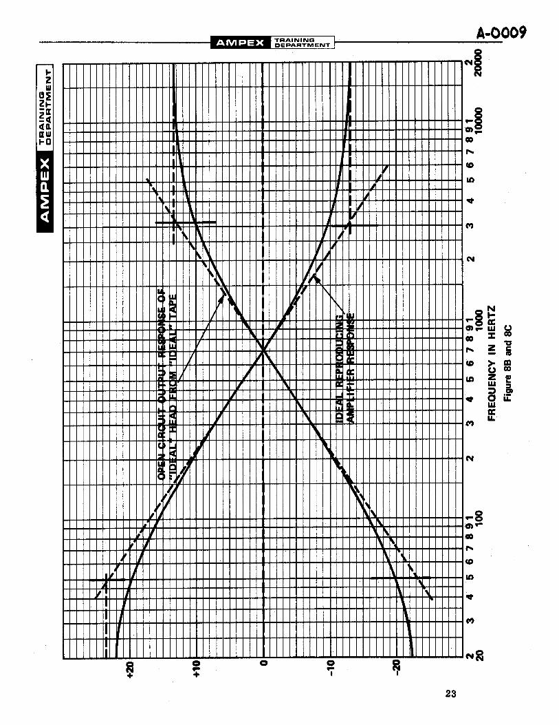
Figure 8a shows the required flux/frequency response of the tape (the curve is shownwith its ideal asymptotes). This flux/frequency response would produce the head outputvoltage shown in Figure 8b. This curve shows the characteristic rising response at lowfrequencies and levels out high frequencies. This is because the head output voltage

4

is proportional to rate of change of flux. Thus in the frequency range where theflux on the tape has constant amplitude, the head output rises at 6db/octave. Whenthe frequency reaches a point where the flux falls at 6 db/octave on the tape, thehead output stays constant.

Now the voltage/frequency response of the reproduce amplifier is normally theinverse of Figure 8b as shown in Figure 8c. The result overall, if the reproduceamplifier truly mirrors the head output, is a flat frequency response.

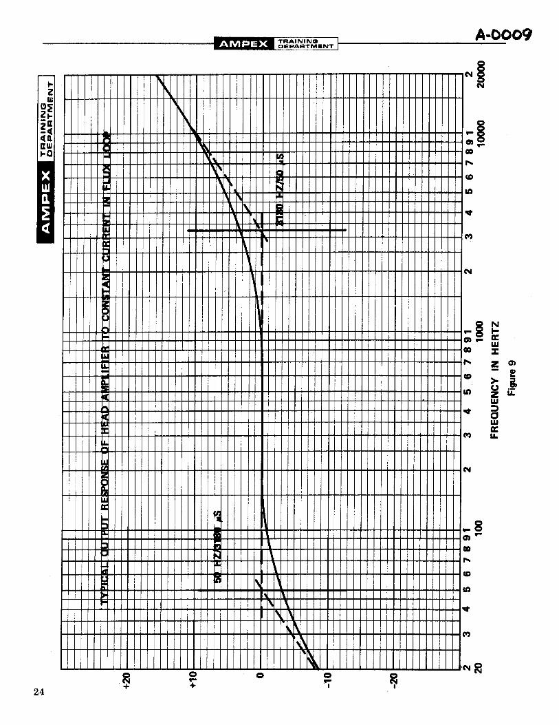
However, the flux loop will induce a constant flux/frequency in the head; this willthus not produce a flat output response with frequency. Rather, the reproduce amplifieroutput voltage will rise at 6 db/octave at high frequencies and be flat at medium fre-quencies, and fall off at 6 db/octave at low frequencies (see Figure 9).

Obviously if the precise curve which ought to be measured is known, and the gaploss is known, or can be estimated, then the reproduce amplifier can be adjustedfor minimum departure from the ideal curve. This applies at least at high fre-quencies; at low frequencies where pole contour effects would be occurring, thereproduce amplifier and head can only be set to the low frequency portions of thecurve and the equalization readjusted using an alignment tape, or during overallrecord reproduce.

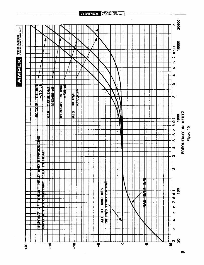
The precise curves which should result (which assume no pole coutour ripple,no gap loss and no head/tape spacing loss, are shown in Table 1 for all the majorequalization standards. Appendix 1 shows how to calculate these curves forequalization standards whose transition frequencies are known.

The most important curves, NAB 50 µs/3180µs, (15 and 7 1/2 in/s).

IEC/CCIR 35 µs / ∞ (15 in/s)

IEC/CCR 70 µs/ ∞ (7 1/2 in/s)

and AES/17.5 µs/ ∞ (30 ips) are also shown plotted in Figure 10. Notethat all the curves have been normalized to the flat midband asymptote.

PRACTICAL MEASUREMENTS

In use, the value obtained from the system must be compared to that from thetables or curves and due allowance made for any significant gap loss.

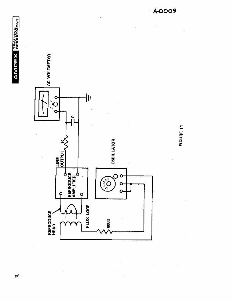
This process sounds easy enough, and certainly familiarity with the requiredcurve for a particular equalization and speed will make life easier. However,there are two ways to make the assessment of errors much easier. The first,which assumes the use of an AC voltmeter external to the reproduce amplifier,as does the classic method, simply involves placing a network between theamplifier and voltmeter, which provides the inverse of the expected ideal fre-quency response (Figure 11 ).

5

This method works satisfactorily for one channel at a time, but becomes verytedious for more than one channel.

The advantage is that instead of having a rising curve to match, the overallresponse should appear flat with frequency.

The second method, just as simple, leads itself to multiple channel use and alsopermits using the internal VU meters on the machine.

Both methods however, can compensate easily only for the high frequency rise.Any low frequency boost, such as is used in the NAB equalization, can only beprovided with an active circuit to any degree of accuracy.

Figure 12 shows the basic idea for the second method. The oscillator shouldhave a resistive output impedance. In this case, the oscillator shown has astandard 600 ohms output resistance.

If a capacitor is shunted across the oscillator terminals when the oscillator isalso loaded by a flux loop; which we have arranged to look like 600 ohms, thenat low frequencies where the impedance of the capacitor is large compared to the600 ohm source and load, the current in the flux loop will be constant with frequency,

As the frequency is increased, the capacitor impedance eventually provides analternate path for current and hence the current in the loop is reduced.

In fact the current in the loop will eventually fall at 6 db/octave, in exactly thesame way as the flux on a normally recorded tape will fall at 6 db/octave.

Thus at high frequencies at least, with the appropriate capacitor value, theoutput expected from the reproduce amplifier is constant with frequency. Thisis a lot easier to see, and any error or deviations from ideal easier to see, thanfollowing a rising curve.

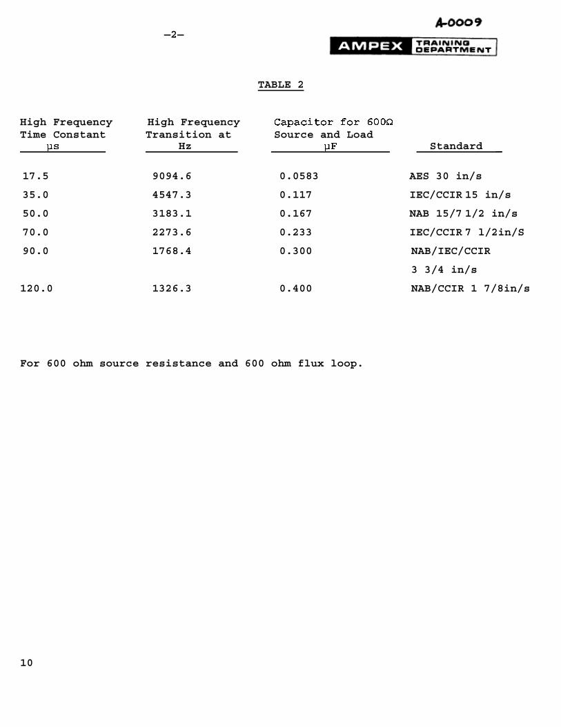
The values of capacitor needed for the various equalizations are shown in Table 2,which assumes a true 600 ohm oscillator output resistance and flux loop input resistance.If the oscillator output resistance is not 600 ohms, Appendix 2 shows how to calculate theexact value of capacitor.

However, in practice, the easiest way to check the capacitor value is to monitor thevoltage across the flux loop and capacitor.

Set the oscillator frequency to one tenth of the high frequency turnover required(see Table 1 for these frequencies). Adjust the oscillator level to give someconvenient reference level and then increase the oscillator frequency to ten timesthe turnover frequency. The voltage measured should have dropped to one tenthof its reference value, or 20 db down. (Purists will be able to calculate that itshould be 20.06 db).

6

If the attenuation seen is too great, the capacitor is too big; if the attenuation isinsufficient, the capacitor is too small.

Intermediate points may be checked, if desired, by referring to Table 1, i.e. at 10 kHz for the NAB 50/3180 µs equalization, the level in the table is 10.3 dbabove reference. The meter across the flux loop should thus read 10.3dbbelow the reference.

The ultimate in luxury would be a small switch box with the different capacitorsselected with a switch.

Since this process only flattens out the high frequency end of the response for yourinspection, the low frequency response will still fall off, ideally as shown in theTable when a low frequency rolloff is called for in the standard.

In a practical situation, the reproduce amplifier and reproduce head will notproduce a perfectly flat response. For example, the high frequency resonanceof the head may have been deliberately tailored to offset gap loss. The fluxlooped response will not be subjected to the gap loss and hence the high fre-quency response may still rise. In some consumer cassette machines, in factthe high frequency response can only be achieved by resonating the head at14 to 15 kHz to offset the gap loss. Very narrow gaps tend to be costly and alsoreduce the head efficiency.

Ideally the machine should be set up with a reproduce alignment tape and thenthe flux response taken. This will give some record of the response of headand amplifier with both test tape and head gap in normal condition. This maythen be referred to when either or both are in doubt.

The technique makes preliminary adjustment more accurate, and for multi-channel machines considerably decreases the time required for alignment.

CONCLUSIONS

The technique of using a flux loop can provide considerable reduction of errorsdue to defective or wornout heads and can provide a reasonable cross check ofthe useful life of an alignment tape. It cannot provide a substitute for analignment tape except under very well controlled laboratory conditions where allthe errors due to gap loss and head tape contact loss can be accurately determined.This technique is in fact the one most often used to calibrate a reproducingsystem when making alignment tapes.

It does not show long wavelength “ripples” due to pole contour effects, these canonly be seen accurately during an overall record/reproduce response check.

Specific frequencies may, of course, be checked using an accurate ReproduceTest Tape.

The method of “equalizing” the flux loop has been shown to provide easier inter-pretation of frequency response and is capable of being easily set up to give goodaccuracy.

7

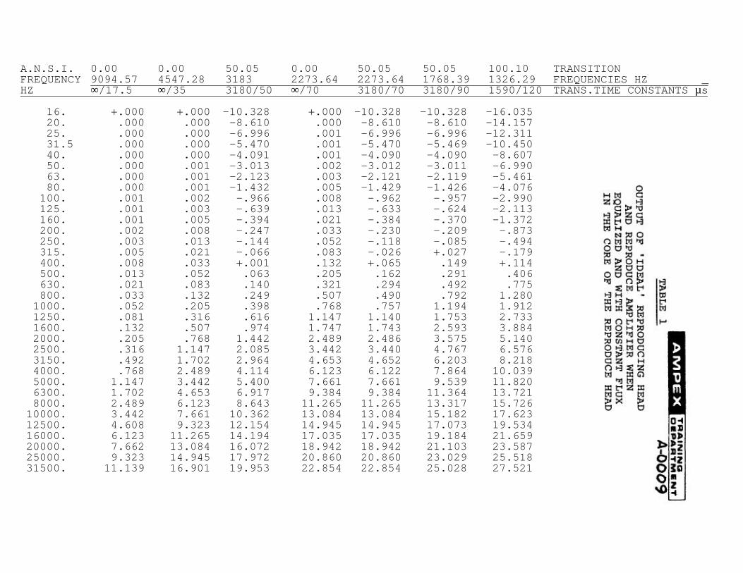
�A.N.S.I. 0.00 0.00 50.05 0.00 50.05 50.05 100.10 TRANSITIONFREQUENCY 9094.57 4547.28 3183 2273.64 2273.64 1768.39 1326.29 FREQUENCIES HZ _HZ ∞/17.5 ∞/35 3180/50 ∞/70 3180/70 3180/90 1590/120 TRANS.TIME CONSTANTS µs

16. +.000 +.000 —10.328 +.000 —10.328 —10.328 —16.03520. .000 .000 —8.610 .000 —8.610 —8.610 —14.15725. .000 .000 —6.996 .001 —6.996 —6.996 —12.31131.5 .000 .000 —5.470 .001 —5.470 —5.469 —10.45040. .000 .000 —4.091 .001 —4.090 —4.090 —8.60750. .000 .001 —3.013 .002 —3.012 —3.011 —6.99063. .000 .001 —2.123 .003 —2.121 —2.119 —5.46180. .000 .001 —1.432 .005 —1.429 —1.426 —4.076100. .001 .002 —.966 .008 —.962 —.957 —2.990125. .001 .003 —.639 .013 —.633 —.624 —2.113160. .001 .005 —.394 .021 —.384 —.370 —1.372200. .002 .008 —.247 .033 —.230 —.209 —.873250. .003 .013 —.144 .052 —.118 —.085 —.494315. .005 .021 —.066 .083 —.026 +.027 —.179400. .008 .033 +.001 .132 +.065 .149 +.114500. .013 .052 .063 .205 .162 .291 .406630. .021 .083 .140 .321 .294 .492 .775800. .033 .132 .249 .507 .490 .792 1.280

1000. .052 .205 .398 .768 .757 1.194 1.9121250. .081 .316 .616 1.147 1.140 1.753 2.7331600. .132 .507 .974 1.747 1.743 2.593 3.8842000. .205 .768 1.442 2.489 2.486 3.575 5.1402500. .316 1.147 2.085 3.442 3.440 4.767 6.5763150. .492 1.702 2.964 4.653 4.652 6.203 8.2184000. .768 2.489 4.114 6.123 6.122 7.864 10.0395000. 1.147 3.442 5.400 7.661 7.661 9.539 11.8206300. 1.702 4.653 6.917 9.384 9.384 11.364 13.7218000. 2.489 6.123 8.643 11.265 11.265 13.317 15.72610000. 3.442 7.661 10.362 13.084 13.084 15.182 17.62312500. 4.608 9.323 12.154 14.945 14.945 17.073 19.53416000. 6.123 11.265 14.194 17.035 17.035 19.184 21.65920000. 7.662 13.084 16.072 18.942 18.942 21.103 23.58725000. 9.323 14.945 17.972 20.860 20.860 23.029 25.51831500. 11.139 16.901 19.953 22.854 22.854 25.028 27.521

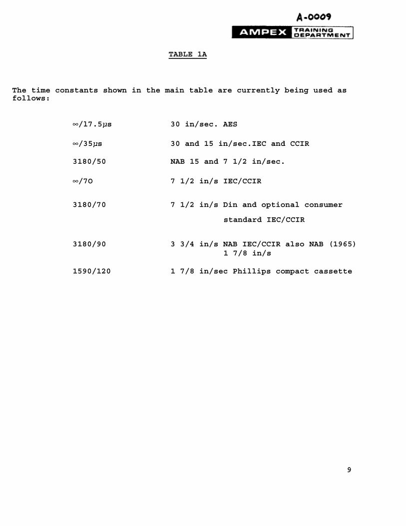
TABLE 1A

The time constants shown in the main table are currently being used asfollows:

∞/l7.5�s 30 in/sec. AES

∞/35�s 30 and 15 in/sec.IEC and CCIR

3180/50 NAB 15 and 7 1/2 in/sec.

∞/7O 7 1/2 in/s IEC/CCIR

3180/70 7 1/2 in/s Din and optional consumer

standard IEC/CCIR

3180/90 3 3/4 in/s NAB IEC/CCIR also NAB (1965)1 7/8 in/s

1590/120 1 7/8 in/sec Phillips compact cassette

9

—2—

TABLE 2

High Frequency High Frequency &DSDFLWRU IRU ���

Time Constant Transition at Source and Load�V Hz �) Standard _

17.5 9094.6 0.0583 AES 30 in/s

35.0 4547.3 0.117 IEC/CCIR 15 in/s

50.0 3183.1 0.167 NAB 15/7 1/2 in/s

70.0 2273.6 0.233 IEC/CCIR 7 l/2in/S

90.0 1768.4 0.300 NAB/IEC/CCIR

3 3/4 in/s

120.0 1326.3 0.400 NAB/CCIR 1 7/8in/s

For 600 ohm source resistance and 600 ohm flux loop.

10

Appendix I

Most standards quote the required transition time constants. The time

constant is related to the transition frequency by

HJ� D WUDQVLWLRQ WLPH FRQVWDQW RI ���V FRUUHVSRQGV WR ������ +]

transition frequency.

For a network whose transfer response has Bode asymptotes as shown in

Figure 13 with both high and low frequency transitions fhi and flo.

Then the response at any frequency f, relative to the midband flat

asymptote is,

Or if the answer is required in db relative to the midband asymptote,

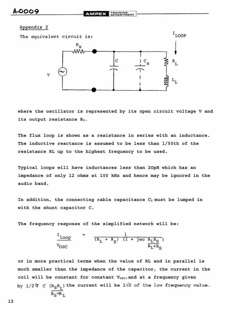
where the oscillator is represented by its open circuit voltage V and

its output resistance R5.

The flux loop is shown as a resistance in series with an inductance.

The inductive reactance is assumed to be less than 1/50th of the

resistance RL up to the highest frequency to be used.

Typical loops will have inductances less than 2OpH which has an

impedance of only 12 ohms at 100 kHz and hence may be ignored in the

audio band.

In addition, the connecting cable capacitance C5 must be lumped in

with the shunt capacitor C.

The frequency response of the simplified network will be:

or in more practical terms when the value of RL and in parallel is

much smaller than the impedance of the capacitor, the current in the

coil will be constant for constant VOSC,and at a frequency given

the current will be 1¥� RI WKH ORZ IUHTXHQF\ YDOXH�

12

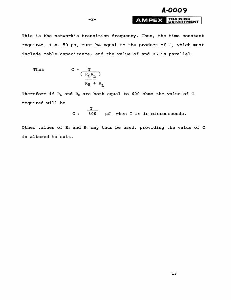
This is the network’s transition frequency. Thus, the time constant

UHTXLUHG� L�H� �� �V� PXVW EH HTXDO WR WKH SURGXFW RI &� ZKLFK PXVW

include cable capacitance, and the value of and RL is parallel.

Therefore if RL and RS are both equal to 600 ohms the value of C

required will be T _

C = 300 �I� ZKHQ 7 LV LQ PLFURVeconds.

Other values of RS and RL may thus be used, providing the value of C

is altered to suit.

13

17

Figure 5A

18

Figure 5B

19

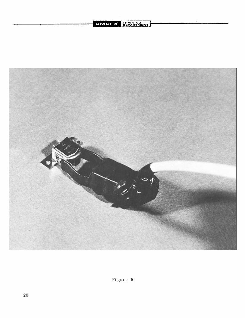
Figure 6

20

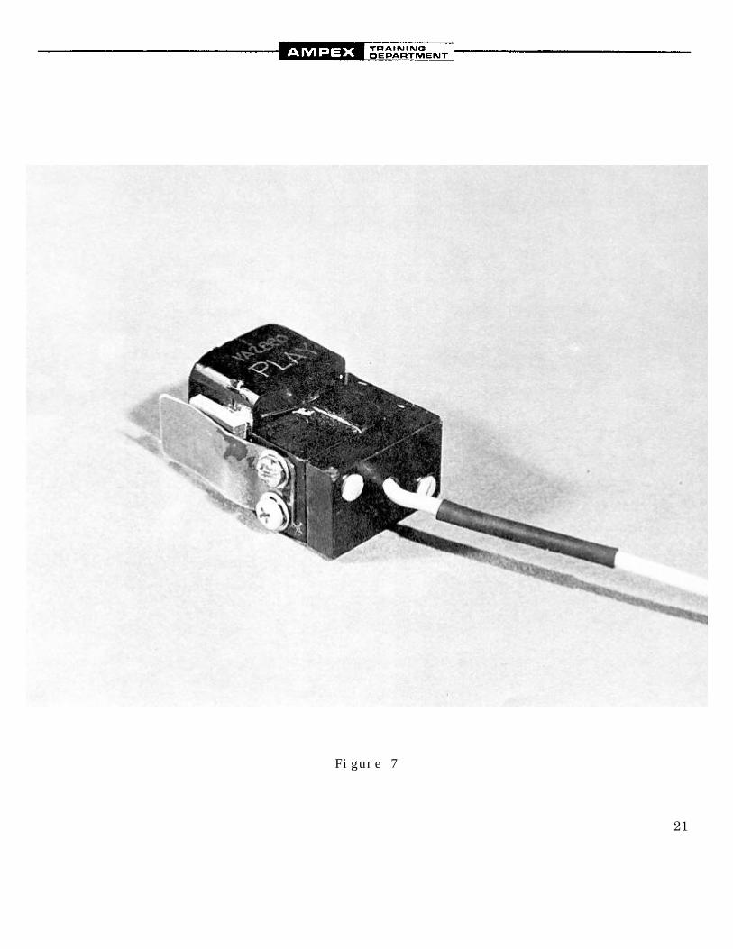
Figure 7

21